Characterizing Heat Transfer in sCO2 Cycle Coolers Utilizing ...

Characterizing Heat Transfer in sCO2 Cycle Coolers Utilizing the Wilson Plot Technique

5 October 2021

Office of Fossil Energy

DOE/NETL-2021/2657

Disclaimer

This project was funded by the United States Department of Energy, National Energy Technology Laboratory, in part, through a site support contract. Neither the United States Government nor any agency thereof, nor any of their employees, nor the support contractor, nor any of their employees, makes any warranty,

express or implied, or assumes any legal liability or responsibility for the accuracy, completeness, or usefulness of any information, apparatus, product, or process disclosed, or represents that its use would not infringe privately owned rights. Reference herein to any specific commercial product, process, or service

by trade name, trademark, manufacturer, or otherwise does not necessarily constitute or imply its endorsement, recommendation, or favoring by the United States Government or any agency thereof. The views and opinions of authors expressed herein do not necessarily state or reflect those of the United States

Government or any agency thereof.

Cover Illustration: The cover photo shows the U.S. Department of Energy’s (DOE) National Energy Technology Laboratory’s (NETL) Heat Exchange and Experimental

Testing (HEET) Rig which was utilized to perform the experiments in this study.

Suggested Citation: Searle, M.; Ramesh, S.; Straub, D. Characterizing Heat Transfer in sCO2 Cycle Coolers Utilizing the Wilson Plot Technique; DOE.NETL-2021.2657; NETL

Technical Report Series; U.S. Department of Energy, National Energy Technology Laboratory: Morgantown, WV, 2021; p 28. DOI: 10.2172/1824140.

Characterizing Heat Transfer in sCO2 Cycle Coolers Utilizing the Wilson Plot

Technique

Matthew Searle1,2, Sridharan Ramesh1,2, Doug Straub1

1U.S. Department of Energy, National Energy Technology Laboratory,

3610 Collins Ferry Road, Morgantown, WV 26507

2NETL Support Contractor, 3610 Collins Ferry Road, Morgantown, WV 26507

DOE/NETL-2021/2657

5 October 2021

NETL Contacts:

Doug Straub, Principal Investigator

Pete Strakey, Technical Portfolio Lead

Bryan Morreale, Executive Director, Research & Innovation Center

This page intentionally left blank.


i

Table of Contents ABSTRACT........................................................................................................................... 1 1. INTRODUCTION.......................................................................................................... 2 2. EXPERIMENTAL APPROACH ................................................................................... 6

2.1 TEST FACILITY ..................................................................................................... 6 2.2 TEST CONFIGURATION ....................................................................................... 7 2.3 WILSON PLOT TECHNIQUE AND UNCERTAINTY ANALYSIS......................... 8

3. RESULTS AND DISCUSSION.................................................................................... 10

3.1 EFFECT OF 𝑸"/𝑮 ................................................................................................. 13 3.2 EFFECT OF ORIENTATION................................................................................. 13

3.3 EFFECT OF PRESSURE ....................................................................................... 13 4. CONCLUSIONS .......................................................................................................... 15 5. FURTHER WORK ...................................................................................................... 16 6. REFERENCES ............................................................................................................ 17

APPENDIX ........................................................................................................................ A-1


ii

List of Figures Figure 1: Indirect recompression sCO2 power cycle. ................................................................. 3 Figure 2: Thermophysical properties plotted as a function of temperature at 8 MPa (a) and 8.7

MPa (b). .......................................................................................................................... 4

Figure 3: Diagram of the HEET rig. ......................................................................................... 6 Figure 4: Shell-and-tube vertical and horizontal configurations. ................................................ 7 Figure 5: Wilson plot data. ..................................................................................................... 11

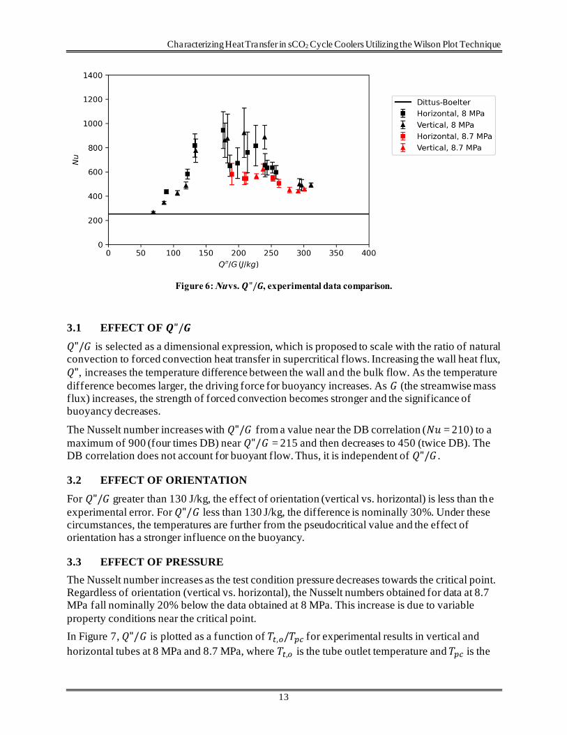
Figure 6: Nu vs. 𝑸"/𝑮, experimental data comparison............................................................. 13

Figure 7: 𝑸"/𝑮 plotted as a function of 𝑻𝒕, 𝒐/𝑻𝒑𝒄. ................................................................. 14

List of Tables Table 1: sCO2 Cooler Conditions Reported in Literature ........................................................... 3

Table 2: Test Heat Exchanger Dimensions ............................................................................... 8 Table 3: Experimental Test Conditions ..................................................................................... 8 Table 4: Uncertainty in Measured Variables ............................................................................. 9 Table 5: Experimental Matrix ................................................................................................ 10

Table 6: Summary of Test Condition Ranges .......................................................................... 12


iii

Acronyms, Abbreviations, and Symbols Term Description

CFD Computational fluid dynamics

DOE U.S. Department of Energy

DB Dittus-Boelter heat transfer correlation

H Horizontal

HEET Heat Exchange and Experimental Testing

HTR High temperature recuperator

LTR Low temperature recuperator

NETL National Energy Technology Laboratory

NIST National Institute of Standards and Technology

PID Proportional-integral-derivative

RANS Reynolds-averaged Navier-Stokes

REFPROP Reference Fluid Thermodynamic and Transport Properties

RIC Research and Innovation Center

RTD Resistance temperature detectors

sCO2 Supercritical carbon dioxide

V Vertical

Symbols

𝐴 Tube internal surface area

𝐷 Tube inner diameter

𝑓 Friction factor

𝑔 Gravitational acceleration

𝐺 Mass flux, Tube Side

𝐺𝑟 Grashoff number, 𝐺𝑟 = 𝑔(𝜌𝑏 − 𝜌𝑤)𝐷3/(𝜌𝑤𝜈𝑏2)

ℎ Heat transfer coefficient

ℎ̅ Average heat transfer coefficient

�̇� Mass flow rate

𝑁𝑢 Nusselt number

𝑃 Pressure

𝑃𝑟 Prandtl number

𝑄" Tube wall heat flux

𝑅 Thermal resistance


iv

Acronyms, Abbreviations, Symbols (cont.)

Term Description

Symbols

𝑅𝑒 Reynolds number

𝑅𝑖 Richardson number, 𝑅𝑖 = 𝐺𝑟/𝑅𝑒2

𝑇 Temperature

𝑢𝑁𝑢 Nusselt number uncertainty

𝑢𝑓 Friction factor uncertainty

𝛥𝑃 Pressure Drop

𝜈 Kinematic viscosity

𝜌 Density

𝑅𝑖 Richardson number, 𝑅𝑖 = 𝐺𝑟/𝑅𝑒2

𝑇 Temperature

𝑢𝑁𝑢 Nusselt number uncertainty

𝑢𝑓 Friction factor uncertainty

𝛥𝑃 Pressure Drop

𝜈 Kinematic viscosity

𝜌 Density

Subscripts

0 Smooth tube, or calculated with Gnielinski correlation

𝒃 Bulk flow

𝑖 Inlet

𝑜 Outlet

𝑜𝑣 Overall

𝑝𝑐 Pseudo-critical

𝑠 Shell

𝑡 Tube

𝑤 Wall


v

Acknowledgments This work was performed in support of the U.S. Department of Energy’s (DOE) Fossil Energy Supercritical CO2 Power Cycles Technology Crosscutting Technology Research Program. The research was executed through the U.S. DOE’s National Energy Technology Laboratory’s

(NETL) Research and Innovation Center’s Supercritical CO2 Field Work Proposal.

The authors would like to acknowledge the significant contributions and guidance provided by Jim

Black who recently retired from NETL. This research was supported in part by an appointment to the U.S. DOE Internship Program at NETL administered by the Oak Ridge Institute for Science and Education. The authors wish to acknowledge the contributions of site operations staff, particularly: Jeff Riley, Rich Eddie, Dave Reese, and Dennis Lynch.


vi



1

ABSTRACT

Effective design of coolers can decrease the capital expense of supercritical carbon dioxide (sCO2) power plants. Improved datasets reporting heat transfer from the CO2 in the cycle cooler

allow design engineers to calculate the required length of heat exchanger streams more accurately, thus reducing cooler material and heat exchanger cost. This study considered a shell-and-tube heat exchanger with non-condensing CO2 on the tube side and water flow on the shell side. The average Nusselt number on the tube side was measured employing the Wilson plot

technique for a flow at a Reynolds number, Re, equal to 1×105 and for a heat flux to mass flux ratio, Q"/G, ranging from 50 to 350 J/kg. The results indicate that the Nusselt number, Nu, increases as the CO2 pressure decreases towards the critical point. The results also indicate that Nu increases to maximum at Q"/G = 215 J/kg and then decreases with further increases in Q"/G.

The difference in Nu measured between the horizontal and vertical heat exchanger with downward flowing CO2 is less than the experimental error.


2

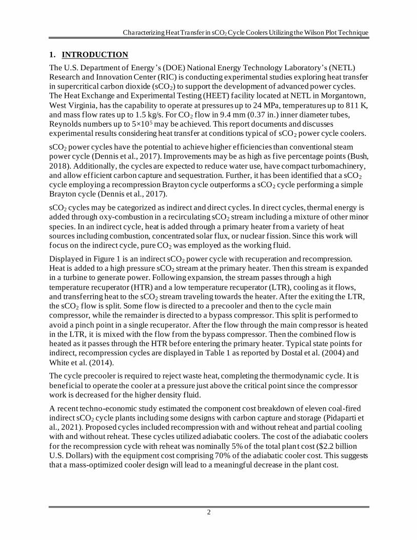
1. INTRODUCTION

The U.S. Department of Energy’s (DOE) National Energy Technology Laboratory’s (NETL) Research and Innovation Center (RIC) is conducting experimental studies exploring heat transfer in supercritical carbon dioxide (sCO2) to support the development of advanced power cycles. The Heat Exchange and Experimental Testing (HEET) facility located at NETL in Morgantown,

West Virginia, has the capability to operate at pressures up to 24 MPa, temperatures up to 811 K, and mass flow rates up to 1.5 kg/s. For CO2 flow in 9.4 mm (0.37 in.) inner diameter tubes, Reynolds numbers up to 5×105 may be achieved. This report documents and discusses experimental results considering heat transfer at conditions typical of sCO2 power cycle coolers.

sCO2 power cycles have the potential to achieve higher efficiencies than conventional steam power cycle (Dennis et al., 2017). Improvements may be as high as five percentage points (Bush,

2018). Additionally, the cycles are expected to reduce water use, have compact turbomachinery, and allow efficient carbon capture and sequestration. Further, it has been identified that a sCO2 cycle employing a recompression Brayton cycle outperforms a sCO2 cycle performing a simple Brayton cycle (Dennis et al., 2017).

sCO2 cycles may be categorized as indirect and direct cycles. In direct cycles, thermal energy is added through oxy-combustion in a recirculating sCO2 stream including a mixture of other minor

species. In an indirect cycle, heat is added through a primary heater from a variety of heat sources including combustion, concentrated solar flux, or nuclear fission. Since this work will focus on the indirect cycle, pure CO2 was employed as the working fluid.

Displayed in Figure 1 is an indirect sCO2 power cycle with recuperation and recompression. Heat is added to a high pressure sCO2 stream at the primary heater. Then this stream is expanded in a turbine to generate power. Following expansion, the stream passes through a high

temperature recuperator (HTR) and a low temperature recuperator (LTR), cooling as it flows, and transferring heat to the sCO2 stream traveling towards the heater. After the exiting the LTR, the sCO2 flow is split. Some flow is directed to a precooler and then to the cycle main compressor, while the remainder is directed to a bypass compressor. This split is performed to

avoid a pinch point in a single recuperator. After the flow through the main compressor is heated in the LTR, it is mixed with the flow from the bypass compressor. Then the combined flow is heated as it passes through the HTR before entering the primary heater. Typical state points for indirect, recompression cycles are displayed in Table 1 as reported by Dostal et al. (2004) and

White et al. (2014).

The cycle precooler is required to reject waste heat, completing the thermodynamic cycle. It is

beneficial to operate the cooler at a pressure just above the critical point since the compressor work is decreased for the higher density fluid.

A recent techno-economic study estimated the component cost breakdown of eleven coal-fired indirect sCO2 cycle plants including some designs with carbon capture and storage (Pidaparti et al., 2021). Proposed cycles included recompression with and without reheat and partial cooling with and without reheat. These cycles utilized adiabatic coolers. The cost of the adiabatic coolers

for the recompression cycle with reheat was nominally 5% of the total plan t cost ($2.2 billion U.S. Dollars) with the equipment cost comprising 70% of the adiabatic cooler cost. This suggests that a mass-optimized cooler design will lead to a meaningful decrease in the plant cost.


3

Figure 1: Indirect recompression sCO2 power cycle.

Table 1: sCO2 Cooler Conditions Reported in Literature

Parameter Dostal et al. (2004) White et al. (2014)

Working Fluid CO2 CO2

Cycle Indirect, Recompression Indirect, Recompression

Application Nuclear Generic

Inlet Pressure, MPa (psia) 7.7 (1,117) 8.69 (1,260)

Outlet Pressure, MPa (psia) 7.62 (1,105) 8.55 (1,240)

Inlet Temperature, K (°F) 344 (159.8) 361 (190.4)

Outlet Temperature, K (°F) 305 (89.6) 308 (95)

Predicting heat transfer in sCO2near the critical point is important to the design of effective sCO2 power cycle coolers. Higher accuracy in heat transfer correlations allows optimal (compact) cooler designs to be designed and built reducing component material costs. These predictions are

complicated by variations in thermophysical properties near the critical point.

The variation of the thermophysical properties—thermal conductivity, viscosity, density, and

specific heat—with temperature and pressure can have significant impacts on the heat transfer near the critical point and may lead to buoyant flow or flow acceleration (Jackson, 2017). In Figure 2, plots of these properties, as a function of temperature, are shown at 8 MPa (a) and 8.7 MPa (b). The property data has been scaled so that it may be shown on the same plot. The

scaling values are shown on the figure legends. In general, viscosity and density decrease


4

monotonically with temperature at both pressures. Thermal conductivity decreases before rising to a peak at the pseudocritical temperature and then decreasing as the temperature increases further. The specific heat rises to a peak near this temperature as well and then begins to decrease

again. Additionally, the pseudocritical temperature, the temperature at which the specific heat is maximized, increases as the pressure increases.

(a) (b)

Figure 2: Thermophysical properties plotted as a function of temperature at 8 MPa (a) and

8.7 MPa (b).

A literature review and preliminary computational fluid dynamics (CFD) simulation were

performed previously for heat transfer in sCO2 flowing through horizontal tubes (Ramesh et al., 2021). The study compared seven correlations for supercritical heat transfer coefficients to a

steady Reynolds-averaged Navier Stokes (RANS). CFD model applying SST k-𝜔 for turbulence closure. Cooling in these scenarios was applied by uniform heat flux.

It was proposed that the ratio of the wall heat flux to the channel mass flux could be correlated to buoyancy effects of the flow. Results were presented at Reynolds numbers of 1.0 × 10 4, 5.0 × 104, and 1.0 × 105. Since the experimental results of the present study were at 1.0 × 10 5, the present discussion focuses on prior results at this Reynolds number.

One important result of the study was that the Nusselt number at the top wall of the simulated horizontal tube was nominally twice that of the Nusselt number at the bottom wall. Further,

many of the correlations predicted that a different Nusselt number would occur at the top and bottom wall.

Both the trends and the magnitude of the correlations deviated from the CFD results, with some correlations deviating from the CFD by as much as 300%. Further, not all the correlations

captured the increase in the Nusselt number as a function of |𝑄"/𝐺|. The disagreement between the correlations increased at larger |𝑄"/𝐺|.

Standard mixed convection analysis employs the Richardson number, 𝑅𝑖, to determine the importance of natural convection relative to forced convection in the flow (Incroprera et al.,

2006). This analysis indicates that buoyant forces will be insignificant if 𝑅𝑖 ≪ 1. 𝑅𝑖 is defined as


5

the ratio of the Grashoff number, 𝐺𝑟, to the Reynolds number squared, 𝑅𝑖 = 𝐺𝑟/𝑅𝑒2. Here,

𝐺𝑟 = 𝑔(𝜌𝑏 − 𝜌𝑤 )𝐷3/(𝜌𝑤 𝜈𝑏2) where 𝑔 is the gravitational acceleration, 𝜌𝑏, is the bulk fluid

density, 𝜌𝑤, is the bulk fluid density at the wall surface, and 𝜈𝑏 is the bulk fluid kinematic viscosity. Several investigators have proposed refinements to this approach. Screening parameters were derived to rule out buoyancy and flow acceleration by Jackson (2017). Parameters were also utilized by Pidaparti et al. (2019) in which a reduced-order heat transfer model was experimentally validated and then utilized to design high-performance sCO2 heat

exchangers.

It is important to note that calculating 𝐺𝑟 requires measurement of the tube wall temperature. Due to operational constraints resulting from the present high-pressure tests, the tube wall temperature is not measured. As described in the experimental results section, the Wilson plot technique is employed to measure the CO2 side heat transfer coefficient. To perform the

calculation, the stream inlet and outlet temperatures of both streams are measured while the flow rate of the CO2 stream varies and while the flow rate of the water stream is held constant. Since non-dimensional parameters are not available, Nusselt number results are reported as a function of |𝑄"/𝐺|.

The present effort is novel in that it applies the Wilson plot approach to measure average heat transfer coefficients occurring in sCO2 coolers. This approach is beneficial to heat exchanger designers since internal measurement of the wall temperatures is often not feasible in high-pressure sCO2 coolers.


6

2. EXPERIMENTAL APPROACH

This section introduces the experimental approach, describes the NETL test facility, and displays the horizontal and vertical heat exchanger configurations. The following tables report heat exchanger dimensions and nominal test conditions. A discussion introduces the Wilson plot technique and an accompanying uncertainty analysis for reducing the data.

2.1 TEST FACILITY

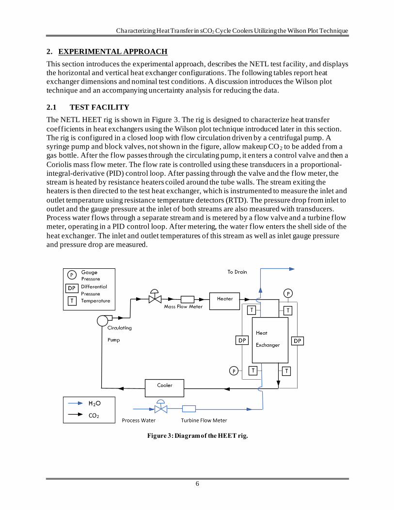
The NETL HEET rig is shown in Figure 3. The rig is designed to characterize heat transfer

coefficients in heat exchangers using the Wilson plot technique introduced later in this section. The rig is configured in a closed loop with flow circulation driven by a centrifugal pump. A syringe pump and block valves, not shown in the figure, allow makeup CO2 to be added from a gas bottle. After the flow passes through the circulating pump, it enters a control valve and then a

Coriolis mass flow meter. The flow rate is controlled using these transducers in a proportional-integral-derivative (PID) control loop. After passing through the valve and the flow meter, the stream is heated by resistance heaters coiled around the tube walls. The stream exiting the heaters is then directed to the test heat exchanger, which is instrumented to measure the inlet and

outlet temperature using resistance temperature detectors (RTD). The pressure drop from inlet to outlet and the gauge pressure at the inlet of both streams are also measured with transducers. Process water flows through a separate stream and is metered by a flow valve and a turbine flow meter, operating in a PID control loop. After metering, the water flow enters the shell side of the

heat exchanger. The inlet and outlet temperatures of this stream as well as inlet gauge pressure and pressure drop are measured.

Figure 3: Diagram of the HEET rig.


7

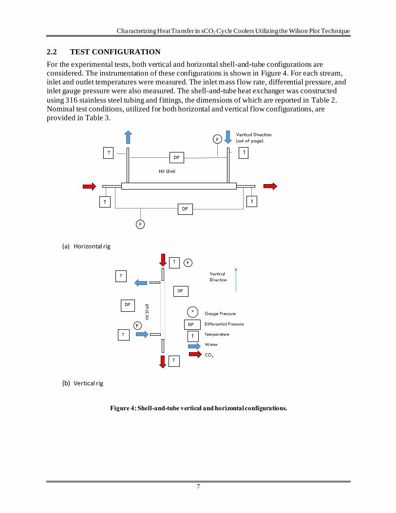
2.2 TEST CONFIGURATION

For the experimental tests, both vertical and horizontal shell-and-tube configurations are considered. The instrumentation of these configurations is shown in Figure 4. For each stream, inlet and outlet temperatures were measured. The inlet mass flow rate, differential pressure, and inlet gauge pressure were also measured. The shell-and-tube heat exchanger was constructed

using 316 stainless steel tubing and fittings, the dimensions of which are reported in Table 2. Nominal test conditions, utilized for both horizontal and vertical flow configurations, are provided in Table 3.

(a) Horizontal rig

(b) Vertical rig

Figure 4: Shell-and-tube vertical and horizontal configurations.


8

Table 2: Test Heat Exchanger Dimensions

Parameter SI English

Shell OD 19.05 mm 0.75 in.

Shell wall 2.41 mm 0.095 in.

Tube OD 9.53 mm 0.375 in.

Tube wall 1.24 mm 0.049 in.

HX length 1.04 m 41 in.

Table 3: Experimental Test Conditions

Shell Side

Fluid H2O

Mass Flow (kg/hr) 227 to 3,032

Inlet Temperature (K) 283

Inlet Pressure (MPa) 0.101

Tube Side

Fluid CO2

Mass Flow (kg/hr) 31.8 to 54.5

Inlet Temperature (K) 349.7

Inlet Pressure (MPa) 20.7

Reynolds Number 8 × 104 to 1.3 × 105

2.3 WILSON PLOT TECHNIQUE AND UNCERTAINTY ANALYSIS

The Wilson plot technique and uncertainty analysis employed in the present work have been

previously reported (Searle et al., 2020, 2021). In the Wilson plot approach, the overall heat exchanger resistance, calculated from measured inlet and outlet temperatures and mass flow rates, is plotted as a function of the calculated tube side resistance using the Dittus-Boelter (DB) correlation. Thermophysical properties are calculated for each stream at the average of the inlet

and outlet temperature using the National Institute of Standards and Technology (NIST) Reference Fluid Thermodynamic and Transport Properties (REFPROP) database 10.0, which implements the Span-Wagner equation of state for CO2 (Lemmon et al., 2018; Span and Wagner, 1996). The HEET rig is operated at seven different tube mass flow rates to vary the tube-side

resistance, while the shell-side resistance is controlled by keeping a constant shell side mass flow rate and average temperature. A least squares linear fit is performed to the resulting scatter plot. The tube side resistance is calculated from the slope of this line. Since the tube-side area is known, the average Nusselt number may be obtained from the tube-side resistance.

The uncertainty analysis employs both the Kline and McClintock approach (1953) and sequential perturbation (Moffat, 1985) to propagate uncertainty from the measured values to the calculated


9

results. Sequential perturbation, which is equivalent to the analytical Kline and McClintock approach, is employed to calculate the uncertainty in the Nusselt number using a data reduction script. The approach first evaluates the script. Then it repeats the calculation with each input to

the script perturbed by its plus or minus error. The differences of each result from the unperturbed case are then calculated. The overall uncertainty is the root sum of squares of all differences. Uncertainty in the measured variables is shown in Table 4. Uncertainties are reported at a 95% confidence interval using error bars on the data points.

Table 4: Uncertainty in Measured Variables

Measurement Uncertainty

Temperature (°C) ± (0.15 + 0.002T)

Pressure ±0.2% measured value

Differential Pressure ±0.2% measured value

Mass Flow Rate ±0.25% measured value

Tube Length ±6.35 mm (0.25 in.)

Tube Diameter ±0.25 mm (0.01 in.)


10

3. RESULTS AND DISCUSSION

This section presents and discusses experimental results. To introduce the range of results, an experimental matrix is displayed in Table 5. The columns indicate orientation, pressure, and pressure label. Some nomenclature is introduced. “H” indicates a horizontal orientation and “V” indicates a vertical orientation. The label “1” indicates a pressure of 8 MPa and “2” indicates a

pressure of 8.7 MPa. The rows indicate the flow label (a letter) and the water flow rate. A cell filled with the test condition label indicates that one or more experimental points were successfully obtained at the test condition. Ranges of test conditions are presented in Table 6.

Wilson plots for all data points are presented in Figure 5 and labeled as indicated in Table 5. Results are shown for both horizontal (H) and vertical (V) configurations across the range of water flow rates (52–3,032 kg/hr) considered and at pressures of 8 MPa and 8.7 MPa, labeled

“1” and “2”, respectively. In each plot, the overall resistance is plotted as a function of the tube side resistance calculated using the DB correlation.

Table 5: Experimental Matrix

Orientation H H V V

Pressure [MPa] 8 8.7 8 8.7

Pressure Label 1 2 1 2

Flow Label

Water [kg/hr]

A 52 AV1

B 97 BH1 BV1

C 141 CV1

D 184 DH1 DV1

E 227 EH1 EH2 EV1

F 341 FH1 FH2 FV1 FV2

G 455 GH1 GH2 GV1 GV2

H 909 HH1 HH2 HV1 HV2

I 1,136 IV1

J 1,364 JH1 JH2 JV1 JV2

K 2,273 KH1

L 2,500 LV1 LV2

M 3,032 MH1

The resistance plot for the horizontal test article at 8 MPa was divided into two plots (A) and (E)

since two groupings are observed with distinctly different values of 𝑅𝑜𝑣. This division was also applied to the data for the vertical test article at 8 MPa yielding panels (C) and (F).


11

Horizontal, 8 MPa Horizontal, 8.7 MPa

Vertical, 8 MPa Vertical, 8.7 MPa

Horizontal, 8 MPa Vertical, 8 MPa

Figure 5: Wilson plot data.


12

In the Wilson plots, 𝑅𝑜𝑣 is plotted versus 𝑅𝑡0, where 𝑅𝑡0 is calculated using the DB correlation. 𝑅𝑜𝑣 increases with 𝑅𝑡0 since total resistance to heat transfer is increasing as the resistance to heat transfer on the tube side is increasing.

At this point, it is important to recall that the slope of the Wilson plots is equal to

𝐴0𝑁𝑢0/(𝐴𝑁𝑢), where 𝐴 is the internal area and the subscript “0” indicates a smooth tube. The heat transfer coefficient for the smooth tube is calculated using the Gnielinski correlation. In the

present work, 𝐴 = 𝐴0, thus the slope is the inverse of the Nusselt number enhancement, 𝑁𝑢/𝑁𝑢0. Conditions yielding Wilson plots with lower slopes will have higher heat transfer than conditions yielding Wilson plots with higher slopes.

In these plots, it is observed that the y-intercept decreases with increasing water flow. The y-intercept is the sum of the convective resistance on the water (shell) side and the wall resistance. An increase in the water convective resistance occurs as the water flow rate decreases due to the

increasing resistance to heat transfer on the water side.

The current data reduction approach uses properties evaluated at the average of the inlet and

outlet temperatures to obtain the average heat transfer coefficient. The linearity observed in 𝑅𝑜𝑣

vs. 𝑅𝑡0, despite the change in properties, indicates that the approximation is appropriate across the range of the mass flows considered for each Wilson plot.

Table 6: Summary of Test Condition Ranges

Parameter Value

CO2 Inlet Temperature, K (°F) 350 (170)

CO2 Inlet Pressure, MPa (psia) 8 (1,160)

CO2 Mass Flow Range kg/hr (lbm/hr) 31.8–58.5 (70–117)

CO2 Reynolds Number Range (-) 7.9 × 104–1.33 × 105

Water Flow Rate Range kg/hr (lbm/hr) 227–3,032 (499–6,670)

The slopes measured using the Wilson plots are utilized to calculate the CO2 (tube) side heat

transfer rate. Shown in Figure 6 are results for the Nusselt number, 𝑁𝑢, as a function of 𝑄"/𝐺 . Results for the tube in the H and V orientations are shown both at 8 MPa and 8.7 MPa. Error bars are displayed indicating a 95% confidence interval. The error is greater over the range 120 to 240

𝑄"/𝐺 due to the increasing effect of enhanced heat transfer near the pseudocritical temperature. To facilitate comparison with conventional smooth tube flow, results for the DB correlation are

displayed. The effects of 𝑄"/𝐺 , orientation, and pressure on 𝑁𝑢 are discussed in the next section.


13

Figure 6: Nu vs. 𝑸"/𝑮, experimental data comparison.

3.1 EFFECT OF 𝑸"/𝑮

𝑄"/𝐺 is selected as a dimensional expression, which is proposed to scale with the ratio of natural convection to forced convection heat transfer in supercritical flows. Increasing the wall heat flux,

𝑄", increases the temperature difference between the wall and the bulk flow. As the temperature

difference becomes larger, the driving force for buoyancy increases. As 𝐺 (the streamwise mass flux) increases, the strength of forced convection becomes stronger and the significance of buoyancy decreases.

The Nusselt number increases with 𝑄"/𝐺 from a value near the DB correlation (𝑁𝑢 = 210) to a

maximum of 900 (four times DB) near 𝑄"/𝐺 = 215 and then decreases to 450 (twice DB). The DB correlation does not account for buoyant flow. Thus, it is independent of 𝑄"/𝐺 .

3.2 EFFECT OF ORIENTATION

For 𝑄"/𝐺 greater than 130 J/kg, the effect of orientation (vertical vs. horizontal) is less than the

experimental error. For 𝑄"/𝐺 less than 130 J/kg, the difference is nominally 30%. Under these circumstances, the temperatures are further from the pseudocritical value and the effect of orientation has a stronger influence on the buoyancy.

3.3 EFFECT OF PRESSURE

The Nusselt number increases as the test condition pressure decreases towards the critical point. Regardless of orientation (vertical vs. horizontal), the Nusselt numbers obtained for data at 8.7 MPa fall nominally 20% below the data obtained at 8 MPa. This increase is due to variable

property conditions near the critical point.

In Figure 7, 𝑄"/𝐺 is plotted as a function of 𝑇𝑡,𝑜/𝑇𝑝𝑐 for experimental results in vertical and

horizontal tubes at 8 MPa and 8.7 MPa, where 𝑇𝑡,𝑜 is the tube outlet temperature and 𝑇𝑝𝑐 is the


14

pseudocritical temperature. 𝑄"/𝐺 decreases as 𝑇𝑡,𝑜/𝑇𝑝𝑐 increases, with an inflection in the rate of

decrease occurring at 𝑇𝑡,𝑜/𝑇𝑝𝑐 = 1. Before the inflection, the rate of decrease becomes larger as

𝑇𝑡,𝑜 /𝑇𝑝𝑐 increases. Following the inflection, the rate of decrease becomes smaller. In general,

results for the various experimental cases collapse to the same trend. However, there is up to a

9% increase in 𝑄"/𝐺 as the pressure increases from 8 MPa to 8.7 MPa in the vertical oriented tube for 𝑇𝑏 /𝑇𝑝𝑐 < 1. The increase in heat flux is attributed to the increase in the heat transfer

coefficient as the pressure approaches the critical pressure while the temperature is held within a small tolerance of the pseudocritical line.

Figure 7: 𝑸"/𝑮 plotted as a function of 𝑻𝒕,𝒐/𝑻𝒑𝒄.


15

4. CONCLUSIONS

Experiments utilizing the Wilson plot technique were performed to consider heat transfer in a shell-and-tube heat exchanger at conditions typical of a cooler in a non-condensing, indirect sCO2 power cycle.

From the experimental results, it was found that

• 𝑁𝑢 increases as the heat exchanger operating pressure decreases towards the critical

point (nominally 17% higher at 8 MPa than 8.67 MPa).

• As 𝑄"/𝐺 increases, 𝑁𝑢 increases until a local maximum is approached at 𝑄”/𝐺 = 215

J/kg. Additional increases in 𝑄”/𝐺 yield a decrease in 𝑁𝑢.

• The variation in 𝑁𝑢 due changing from a horizontal to a vertical orientation is less

than the experimental error except when 𝑄"/𝐺 < 130 𝐽/𝑘𝑔, where a small difference,

greater than the experimental error, arises.


16

5. FURTHER WORK

Future experimental work could explore an appropriate non-dimensionalization for 𝑄”/𝐺.


17

6. REFERENCES

Bush, V. GTI STEP forward on sCO2 Power. In sCO2 Power Cycle Symposium; Pittsburgh, PA, 2018.

Dennis, R. A.; Musgrove, G.; Rochau, G; Fleming, D.; Carlson, M.; Pasch, J. Introduction and Background. In Fundamentals and Applications of Supercritical Carbon Dioxide (sCO2) Based Power Cycles; Woodhead Publishing, 2017; pp. xx–xxviii.

Dostal, V.; Driscoll, M. J.; Hejzlar, P.; A Supercritical Carbon Dioxide Cycle for Next Generation Nuclear Reactors. Dissertation. MIT, Cambridge, 2004.

Incroprera, F. P.; Dewitt, D. P.; Bergman, T. L.; Lavine, A. S. Fundamentals of Heat and Mass Transfer; John Wiley & Sons:New York, 2006.

Jackson, J. D. Models of Heat Transfer to Fluids at Supercritical Pressure with Influences of Bouyancy and Acceleration. Applied Thermal Engineering 2017, 124, 1481–1491.

Kline, S.; McClintock, F. Describing Uncertainties in Single-Sample Experiments. Mechanical Engineering 1953, 3–8.

Lemmon, E. W.; Bell, I. H.; Huber, M. L. NIST Standard Reference Database 23: Reference Fluid Thermodynamic and Transport Properties-REFPROP, NIST, 2018.

Moffat, R. J. Using Uncertainty Analysis in the Planning of an Experiment. Journal of Fluids Engineering 1985, 107, 173–178.

Pidaparti, S. R. Heat Transfer and Fluid Flow Characteristics of Supercritical Carbon Dioxide Flow. Dissertation. Georgia Institute of Technology, 2019.

Pidaparti, S. R.; White, C. W.; Weiland, N. T.; Optimized Performance and Cost Potential for Indirect Supercritical CO2 Coal Fired Power Plants. In Turbomachinery Technical Conference and Exposition, Virtual, Online, 2021.

Ramesh, S.; Straub, D.; Black, J.; Robey, E. Heat Transfer Analysis for Recompression Based sCO2 Power Cycles; NETL, Morgantown, WV. Unpublished Manuscript. In press.

Pending publication, 2021.

Searle, M.; Black, J.; Straub, D.; Robey, E.; Yip, J.; Ramesh, S.; Roy, A.; Sabau, A. S.; Mollot, D. Heat transfer coefficients of additively manufactured tubes with internal pin fins for supercritical carbon dioxide cycle recuperators. Applied Thermal Engineering 2020, 181, 116030.

Searle, M.; Roy, A.; Black, J.; Straub, D.; Ramesh, S.Investigating Gas Turbine Internal Cooling Using Supercritical CO2 at High Reynolds Numbers for Direct Fired Cycle Applications. In Turbomachinery Technical Conference and Exhibition , Virtual, Online, 2021.

Span, R.; Wagner, W. A New Equation of State for Carbon Dioxide Covering the Fluid Region from the Triple-Point Temperature to 1100 K at Pressure up to 800 MPa. J. Phys. Chem.

Ref. Data 1996, 25, 1509–1596.

White, C.; Shelton, W.; Dennis, R. An Assessment of Supercritical CO2 Power Cycles with Generic Heat Sources. In 4th International Symposium - Supercritical CO2 Power Cycles, Pittsburgh, PA, 2014.


18



A-1

APPENDIX

The data collected in the present experiment is reported in Table A1.

Table A1: Experimental Data

Test Condition 𝑻𝒔,𝒊 [K]

�̇�𝒔 [kg/s] 𝑻𝒕,𝒊 [K] 𝑻𝒕,𝒐 [K]

𝑷𝒕,𝒊

[MPa] �̇�𝒕

[kg/s] 𝜟𝑷𝒕 [Pa] 𝑮

[kg/m2-s] 𝑸"/𝑮 [J/kg 𝑹𝒆 [-] 𝑵𝒖 [-] 𝒖𝑵𝒖 [-] 𝒇 [-] 𝒖𝒇 [-]

GH1 289.29 0.12630 349.77 308.27 7.97 0.01114 629.73 286.43 213.80 1.00E+05 760.85 334.60 0.0218 0.0045

GH1 288.18 0.12633 350.03 308.05 7.98 0.01103 682.59 283.68 226.21 9.92E+04 816.18 335.10 0.0254 0.0051

HH1 288.71 0.25266 350.03 307.53 7.98 0.01112 656.19 286.12 257.47 1.00E+05 597.07 55.47 0.0235 0.0048

KH1 293.08 0.63127 349.42 307.73 7.98 0.01111 620.53 285.68 243.77 9.98E+04 633.91 61.41 0.0217 0.0045

FH1 290.87 0.09407 349.76 309.35 7.98 0.01113 620.53 286.37 186.64 1.00E+05 650.09 176.21 0.0212 0.0044

JH1 290.64 0.37892 349.41 307.63 7.99 0.01117 620.53 287.33 251.75 1.00E+05 635.28 45.10 0.0214 0.0044

GH1 291.05 0.12626 349.93 308.88 7.99 0.01133 620.53 291.44 198.39 1.02E+05 672.31 253.65 0.0202 0.0042

MH1 294.19 0.84188 350.91 307.89 7.99 0.01116 620.53 287.01 240.63 1.00E+05 654.52 95.80 0.0212 0.0044

GH1 293.45 0.12617 349.76 309.97 7.99 0.01112 1038.82 286.06 176.50 1.00E+05 944.71 304.09 0.0435 0.0082

DH1 293.46 0.05110 349.81 315.88 7.99 0.01109 1081.77 285.31 121.54 1.00E+05 582.33 40.83 0.0441 0.0083

EH1 293.35 0.06309 349.78 314.20 7.99 0.01109 1060.37 285.29 132.82 1.00E+05 817.44 95.82 0.0435 0.0082

BH1 295.21 0.02694 349.81 322.09 8.00 0.01108 1105.47 285.11 89.35 1.00E+05 436.00 17.00 0.0435 0.0082

JH2 291.67 0.37876 349.51 310.57 8.66 0.01140 639.55 293.32 252.78 9.74E+04 546.71 22.75 0.0255 0.0051

GH2 291.43 0.12625 349.07 312.11 8.67 0.01143 620.53 294.07 211.27 9.78E+04 545.48 43.64 0.0239 0.0048

FH2 289.34 0.09453 350.12 312.39 8.68 0.01144 620.53 294.15 208.68 9.80E+04 545.34 50.41 0.0237 0.0048

EH2 289.35 0.06323 350.17 313.28 8.68 0.01146 627.43 294.67 189.56 9.83E+04 581.27 88.99 0.0237 0.0048

HH2 287.85 0.25269 349.93 310.31 8.69 0.01141 645.00 293.41 261.82 9.73E+04 504.87 33.28 0.0259 0.0052


A-2

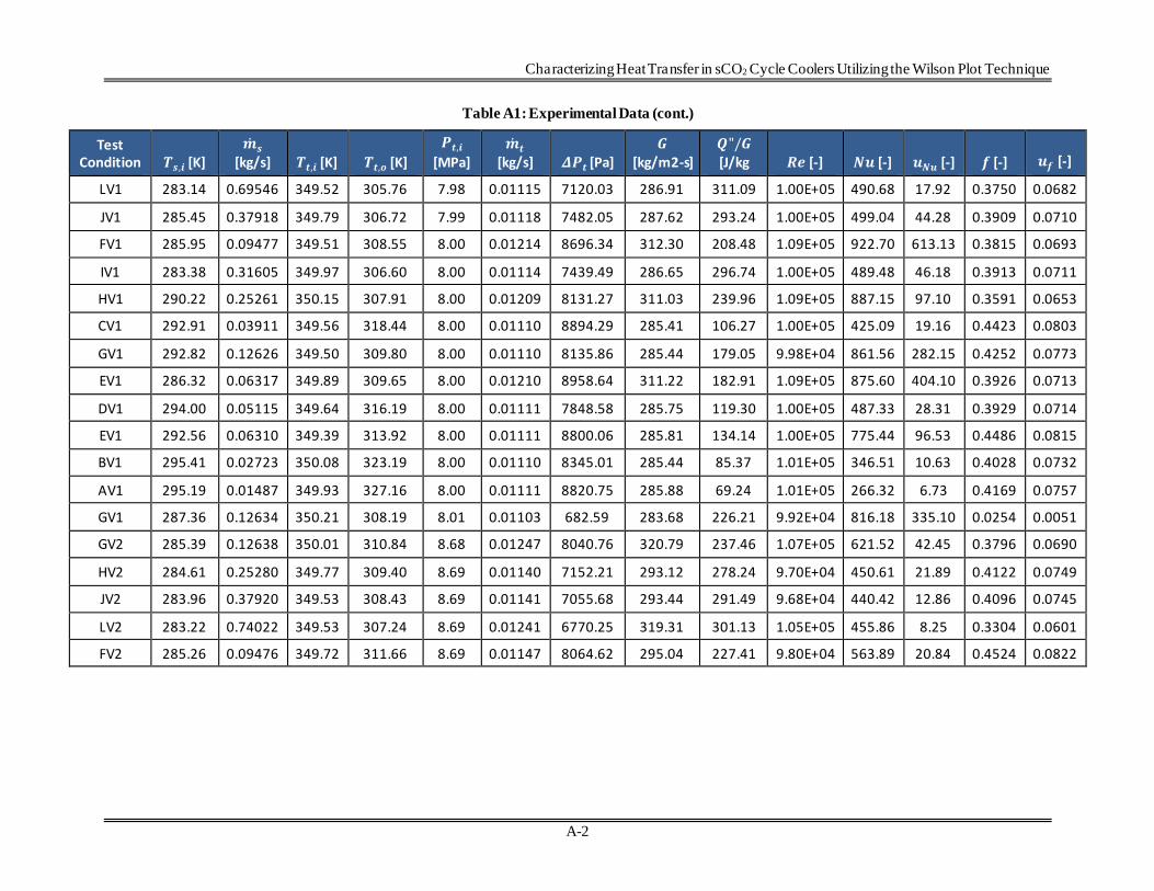
Table A1: Experimental Data (cont.)

Test Condition 𝑻𝒔,𝒊 [K]

�̇�𝒔 [kg/s] 𝑻𝒕,𝒊 [K] 𝑻𝒕,𝒐 [K]

𝑷𝒕,𝒊

[MPa] �̇�𝒕

[kg/s] 𝜟𝑷𝒕 [Pa] 𝑮

[kg/m2-s] 𝑸"/𝑮 [J/kg 𝑹𝒆 [-] 𝑵𝒖 [-] 𝒖𝑵𝒖 [-] 𝒇 [-] 𝒖𝒇 [-]

LV1 283.14 0.69546 349.52 305.76 7.98 0.01115 7120.03 286.91 311.09 1.00E+05 490.68 17.92 0.3750 0.0682

JV1 285.45 0.37918 349.79 306.72 7.99 0.01118 7482.05 287.62 293.24 1.00E+05 499.04 44.28 0.3909 0.0710

FV1 285.95 0.09477 349.51 308.55 8.00 0.01214 8696.34 312.30 208.48 1.09E+05 922.70 613.13 0.3815 0.0693

IV1 283.38 0.31605 349.97 306.60 8.00 0.01114 7439.49 286.65 296.74 1.00E+05 489.48 46.18 0.3913 0.0711

HV1 290.22 0.25261 350.15 307.91 8.00 0.01209 8131.27 311.03 239.96 1.09E+05 887.15 97.10 0.3591 0.0653

CV1 292.91 0.03911 349.56 318.44 8.00 0.01110 8894.29 285.41 106.27 1.00E+05 425.09 19.16 0.4423 0.0803

GV1 292.82 0.12626 349.50 309.80 8.00 0.01110 8135.86 285.44 179.05 9.98E+04 861.56 282.15 0.4252 0.0773

EV1 286.32 0.06317 349.89 309.65 8.00 0.01210 8958.64 311.22 182.91 1.09E+05 875.60 404.10 0.3926 0.0713

DV1 294.00 0.05115 349.64 316.19 8.00 0.01111 7848.58 285.75 119.30 1.00E+05 487.33 28.31 0.3929 0.0714

EV1 292.56 0.06310 349.39 313.92 8.00 0.01111 8800.06 285.81 134.14 1.00E+05 775.44 96.53 0.4486 0.0815

BV1 295.41 0.02723 350.08 323.19 8.00 0.01110 8345.01 285.44 85.37 1.01E+05 346.51 10.63 0.4028 0.0732

AV1 295.19 0.01487 349.93 327.16 8.00 0.01111 8820.75 285.88 69.24 1.01E+05 266.32 6.73 0.4169 0.0757

GV1 287.36 0.12634 350.21 308.19 8.01 0.01103 682.59 283.68 226.21 9.92E+04 816.18 335.10 0.0254 0.0051

GV2 285.39 0.12638 350.01 310.84 8.68 0.01247 8040.76 320.79 237.46 1.07E+05 621.52 42.45 0.3796 0.0690

HV2 284.61 0.25280 349.77 309.40 8.69 0.01140 7152.21 293.12 278.24 9.70E+04 450.61 21.89 0.4122 0.0749

JV2 283.96 0.37920 349.53 308.43 8.69 0.01141 7055.68 293.44 291.49 9.68E+04 440.42 12.86 0.4096 0.0745

LV2 283.22 0.74022 349.53 307.24 8.69 0.01241 6770.25 319.31 301.13 1.05E+05 455.86 8.25 0.3304 0.0601

FV2 285.26 0.09476 349.72 311.66 8.69 0.01147 8064.62 295.04 227.41 9.80E+04 563.89 20.84 0.4524 0.0822

NETL Technical Report Series

Brian J. Anderson

Director

National Energy Technology Laboratory

U.S. Department of Energy

John Wimer

Associate Director

Strategic Planning

Science & Technology Strategic Plans & Programs

National Energy Technology Laboratory

U.S. Department of Energy

Bryan Morreale

Executive Director

Research and Innovation Center

National Energy Technology Laboratory U.S. Department of Energy

Characterizing Heat Transfer in sCO2 Cycle Coolers Utilizing ...

Documents

Transcript of Characterizing Heat Transfer in sCO2 Cycle Coolers Utilizing ...