Chapter 3: Repair and rewind of induction motor

Design and

Implementation of a grid-

connected variable-speed

PM WECS

By: Stefan Thomas Sager

Thesis submitted to the Department of Electrical Engineering, University of Cape

Town, in complete fulfilment of the requirements for the degree of Master of Science

in Electrical Engineering

31st of March 2010

i

Declaration

This thesis is submitted to the Department of Electrical Engineering, University

of Cape Town, in complete fulfilment of the requirements for the degree of Master of

Science in Electrical Engineering. It has not been submitted before for any degree or

examination at this or any other university.

“I know the meaning of plagiarism and declare that all the work in the document,

save for that which is properly acknowledged, is my own.”

--------------------------------------

S.T. Sager

31st of March 2010

ii

Acknowledgments

I would like to thank my family for their continuous support throughout my time at

UCT. They have been more than generous in their support and encouragement.

My sincere thanks go to my supervisor Dr. M.A Khan and my co-supervisor, Dr. P.

Barendse. They have been great mentors and supported me with their guidance

throughout this project.

To my fellow members of the AMES group, you have been very good colleagues and

hopefully will remain so in the future.

Special thanks go to Chris Wozniak and Phillip Titus, who have been extremely

helpful during the long hours in the laboratory and without whom I could not have

completed this work.

The financial support provided by the University of Cape Town, the AMES group and

the Centre for Renewable Energy Studies is gratefully acknowledged.

Finally, to all my friends, who have been there for me over the past six years, I am

very grateful and privileged to have shared this part of my life with you. May this only

be the beginning of many more years to come.

iii

Abstract

As renewable energy (RE) sources are increasingly becoming an integral part of the

world’s power generation capacity, they are becoming more sophisticated and

provide a solid platform for power generation today. Wind Energy is the fastest

growing RE source. The correct understanding of issues associated with this

technology and how to address them is integral in furthering this RE source.

A turbine emulator has been developed and implemented in the laboratory to

effectively test the developed system in a controlled environment. This has been

achieved through use of a torque controlled DC-machine which emulates the

behaviour of a turbine.

The main objective of the work presented in this thesis is the full understanding and

implementation of a PM Wind Turbine System. Focus is on a grid-tied Surface

Mounted PM Wind Generator, which operates at variable speed without making use

of pitch control. The operating conditions of the machine are fully controlled through

power electronic converters which also provide the grid connection. Both power

converters, on the machine-side and the grid-side are controlled through Space

Vector Modulation (SVM).

The control of the PM generator is implemented and investigated in simulation and

experimentally. Maximising the energy output under different wind conditions is

investigated. Maximum Power Point Tracking (MPPT) is implemented to extract

maximum power from the incident wind. Three different control strategies for the

operation of the generator are investigated and their impact on generator efficiency

investigated.

The grid-connection is provided through a LCL-type grid-filter between the power

converter and a step-down transformer to reduce the grid voltage.

A thorough review of work done on this WECS topology has been carried out and the

different approaches have been simulated and implemented experimentally in the

laboratory.

iv

Certain limitations were encountered which are discussed and addressed in the

thesis.

v

Contents

List of Figures.......................................................................................................... viii

List of Tables ........................................................................................................... xiii

List of Abbreviations ................................................................................................ xiv

List of Symbols ......................................................................................................... xv

1. Introduction ...................................................................................................... 1

1.1. Background ................................................................................................... 1

1.2. Literature Review ........................................................................................... 2

1.3. Research Questions ...................................................................................... 5

1.4. Objectives ...................................................................................................... 5

1.5. Scope and Limitations .................................................................................... 6

1.6. Structure ........................................................................................................ 6

2. The Theory and Basic Principles of a WECS ................................................. 7

2.1. Overview ........................................................................................................ 7

2.2. Wind Power ................................................................................................... 7

2.3. Maximum Power Point Tracking..................................................................... 8

2.4. Other factors impacting the power obtained from the wind ........................... 10

2.4.1. Tower shadowing ................................................................................... 10

2.4.2. Furling .................................................................................................... 11

2.4.3. Turbine and Generator Inertia ................................................................ 12

2.5. Emulating the behaviour of a wind turbine ................................................... 12

2.6. WECS Topologies ....................................................................................... 14

2.7. PMSG Wind Energy System Topologies ...................................................... 16

2.8. Converter Topologies ................................................................................... 19

2.8.1. Passive/Diode Rectifier .......................................................................... 19

2.8.2. Active Rectifier ....................................................................................... 20

2.9. Controlling a Permanent Magnet Synchronous Generator ........................... 21

2.9.1. Maximum Torque per Current Control (id=0) of a PMSG ........................ 22

2.9.2. Unity Power Factor Control .................................................................... 23

2.9.3. Maximum Efficiency Control ................................................................... 24

2.10. Grid-Side Converter and Control Theory .................................................... 31

2.10.1. Control Strategies of a Grid-tied Inverter .............................................. 31

2.10.2. Grid Filter ............................................................................................. 33

2.11. Conclusions ............................................................................................... 33

3. A grid-tied Permanent Magnet Synchronous Generator WECS .................. 35

3.1. Introduction .................................................................................................. 35

vi

3.2. Components used in the implementation of a variable-speed PMSG-based WECS ................................................................................................................. 35

3.3. Machine-Side Converter and Control ........................................................... 36

3.4. Grid-Side Converter and Control .................................................................. 39

3.4.1. Grid-Filter Design ................................................................................... 41

3.4.2. Simplified Design Method ....................................................................... 43

3.5. Applied Control Strategies ........................................................................... 45

3.5.1. Maximum Torque per Current Control .................................................... 45

3.5.2. Maximum Power Factor Control ............................................................. 45

3.5.3. Maximum Efficiency Control ................................................................... 46

3.6. Conclusions ................................................................................................. 48

4. Analytical Results .......................................................................................... 49

4.1. Introduction .................................................................................................. 49

4.2. Projected power extracted from the incident wind ........................................ 50

4.3. Projected Generator Performance under different control strategies ............ 51

4.4. Conclusions ................................................................................................. 57

5. Simulation of a variable-speed PM WECS .................................................... 58

5.1. Introduction .................................................................................................. 58

5.2. Simulation Overview .................................................................................... 58

5.3. Turbine Emulator ......................................................................................... 59

5.4. Controlling the Machine-Side Converter ....................................................... 60

5.4.1. Current Control Mode ............................................................................. 60

5.4.2. Speed control mode for the implementation of MPPT ............................. 63

5.5. Grid-Side Converter ..................................................................................... 66

5.5.1. Current Control ....................................................................................... 67

5.5.2. DC-Link Control ...................................................................................... 69

5.6. Complete System Simulation ....................................................................... 72

5.6.1. Complete System Response to a Step in Wind Speed ........................... 72

5.6.2. Steady-State Performance of the complete System ............................... 75

5.7. Conclusions ................................................................................................. 77

6. Experimental Setup – hardware & software implementation ...................... 78

6.1. Introduction .................................................................................................. 78

6.2. Overview of Laboratory Setup and Components .......................................... 79

6.3. Generator Parameter Estimation.................................................................. 80

6.3.1. Estimating Core Losses as a function of Speed and Loading ................. 83

6.4. Wind Turbine Emulator ................................................................................ 87

6.5. Machine-Side Controller Implementation ..................................................... 90

6.6. Grid-Side Controller Implementation ............................................................ 92

6.7. Experimental Implementation of the complete system ................................. 95

6.8. Conclusions ................................................................................................. 98

vii

7. Experimental Results and Discussion .......................................................... 99

7.1. Introduction .................................................................................................. 99

7.2. Motor Mode Operation ................................................................................. 99

7.2.1. Open-Loop Operation ............................................................................. 99

7.2.2. Speed Control Mode ............................................................................ 100

7.3. Generator Mode Operation ........................................................................ 101

7.3.1. Current Control Mode ........................................................................... 101

7.4. Complete System Operation of the WECS ................................................. 103

7.4.1. Experimental Results at a wind speed of 7m/s ..................................... 103

7.4.2. Complete System Response to a Step in Wind Speed ......................... 109

7.4.3. Experimental Evaluation of different generator control strategies and their impact on power production ........................................................................... 112

7.5. Conclusions ............................................................................................... 116

8. Conclusion and Recommendations ............................................................ 117

8.1. Conclusions ............................................................................................... 117

8.2. Recommendations ..................................................................................... 119

References ............................................................................................................ 120

Appendix A: Analytical Results .............................................................................. 123

Appendix B: Tabulated Simulation Results ............................................................ 125

Appendix C: Tabulated Experimental Results........................................................ 126

Appendix D: Simulink Models ................................................................................ 128

viii

List of Figures Figure 2.1: Power Coefficient vs. TSR ....................................................................... 9

Figure 2.2: Impact of Tower Shadowing on the wind flow ........................................ 10

Figure 2.3: Impact of Furling on the effective wind speed experienced by the wind turbine ..................................................................................................................... 11

Figure 2.4: Fixed Speed Grid-tied IG WECS ........................................................... 14

Figure 2.5: Variable-Speed Grid-tied Doubly-Fed IG WECS .................................... 15

Figure 2.6: Variable-Speed IG WECS with back-to-back grid converter .................. 16

Figure 2.7: Stand-alone PMSG with Diode Rectifier and DC/DC converter ............. 17

Figure 2.8: Grid-tied PMSG with Diode Rectifier and intermediate DC/DC converter17

Figure 2.9: Grid-tied PMSG with full back-to-back VSC's ........................................ 18

Figure 2.10: Stand-Alone PMSG with fully controlled Rectifier ................................ 18

Figure 2.11: d-q axis equivalent circuits of the PMSG [4] ........................................ 27

Figure 2.12: d-q equivalent circuit [9] ....................................................................... 28

Figure 2.13: (a) d-axis and (b) q-axis equivalent circuit [7]....................................... 29

Figure 3.1: Schematic Overview of the Variable Speed WECS ............................... 36

Figure 3.2: Schematic of the Current Control Loops ................................................ 37

Figure 3.3: Schematic of the Speed-Control Loop ................................................... 37

Figure 3.4: Machine-side control scheme ................................................................ 38

Figure 3.5: Schematic Overview of the Grid-Side Current Controller Loops ............ 40

Figure 3.6: Schematic Overview of the DC-Link Control Loop ................................. 40

Figure 3.7: Grid-side control scheme ....................................................................... 41

Figure 3.8: id Reference for Loss Minimisation ........................................................ 48

Figure 4.1: Ideal Turbine Speed for MPPT as a function of Wind Speed ................. 50

Figure 4.2: Maximum Turbine Power as a function of Wind Speed .......................... 50

Figure 4.3: Ideal Generator quadrature current as a function of Wind Speed .......... 51

Figure 4.4: Direct current reference as a function of wind speed ............................. 52

ix

Figure 4.5: Analytical Power Flow diagram .............................................................. 53

Figure 4.6: Calculated Generator Output Power as a function of wind speed .......... 53

Figure 4.7: Generator Efficiency as a function of wind speed .................................. 54

Figure 4.8: Increased Kc vs. Generator Speed ........................................................ 55

Figure 4.9: Direct current reference vs. wind speed ................................................ 55

Figure 4.10: Projected generator output power vs. wind speed ............................... 56

Figure 4.11: Projected Generator Efficiency vs. Wind Speed .................................. 56

Figure 4.12: Generator Efficiency Improvement under LMA control compared to max. torque per current control ........................................................................................ 56

Figure 5.1: Turbine Emulator Scheme ..................................................................... 59

Figure 5.2: Wind Turbine Emulator Simulation ........................................................ 59

Figure 5.3: Generator Current Response at rated speed (a) and half rated speed (b) ................................................................................................................................ 60

Figure 5.4: DC-Link Currents (filtered) at rated speed (a) and half rated speed (b) . 61

Figure 5.5: DC-Link Voltage at rated speed (a) and half rated speed (b) ................. 62

Figure 5.6: Shaft Power developed at (a) rated speed and (b) half rated speed (b) . 63

Figure 5.7: Principle speed control scheme ............................................................. 64

Figure 5.8: Simulated Speed Response .................................................................. 65

Figure 5.9: Simulated Generator Torques ............................................................... 65

Figure 5.10: Mechanical Shaft Torque applied ........................................................ 65

Figure 5.11: Torque difference and Generator Speed ............................................. 66

Figure 5.12: DC-Current Difference and Link Voltage .............................................. 66

Figure 5.13: Gird-side current control scheme ......................................................... 67

Figure 5.14: dq-axis current response ..................................................................... 68

Figure 5.15: Power transferred to the Grid .............................................................. 68

Figure 5.16: Grid-side DC-link control scheme ........................................................ 69

Figure 5.17: Input Current to the DC-Link ................................................................ 69

Figure 5.18: DC-Link Voltage .................................................................................. 70

Figure 5.19: direct current component ..................................................................... 70

x

Figure 5.20: quadrature current component ............................................................ 70

Figure 5.21: Power into DC-Link.............................................................................. 71

Figure 5.22: Reactive and Real Power transferred to the Grid ................................. 71

Figure 5.23: Grid and DC-Link Power ...................................................................... 72

Figure 5.24: Wind speed step Input ......................................................................... 72

Figure 5.25: Generator current response to a step in wind speed............................ 73

Figure 5.26: Generator speed response to a step in wind speed ............................. 73

Figure 5.27: Turbine power coefficient response to a step in wind speed ................ 73

Figure 5.28: DC-link voltage .................................................................................... 74

Figure 5.29: Grid current components ..................................................................... 74

Figure 5.30: Grid power components ...................................................................... 74

Figure 5.31: Real Grid Power as a function of wind speed ...................................... 75

Figure 5.32: Real Grid Power as a function of wind speed (6.5m/s - 7m/s) .............. 75

Figure 5.33: Simulated System Efficiency as a function of wind speed .................... 76

Figure 6.1: Schematic of the overall experimental setup ......................................... 79

Figure 6.2: Experimental Setup in the laboratory ..................................................... 80

Figure 6.3: Generator Open Terminal Voltage vs. Speed ........................................ 81

Figure 6.4: Rotor alignment with d-axis (a) and q-axis (b) ....................................... 81

Figure 6.5: Current Response to a Voltage Step across the d and q axis ................ 82

Figure 6.6: DC-machine losses at No-Load ............................................................. 84

Figure 6.7: Rotational Losses in the PMSG under no-load ...................................... 85

Figure 6.8: Core Loss Constant vs. Machine Speed ................................................ 86

Figure 6.9: Turbine Emulator (Diagram) .................................................................. 87

Figure 6.10: DC-thyristor drive ................................................................................ 88

Figure 6.11: Torque vs. Reference Voltage ............................................................. 89

Figure 6.12: Mechanical Shaft Power ...................................................................... 89

Figure 6.13: Cp vs. TSR (Lab Results and Original curve) ...................................... 90

Figure 6.14: PMSG and the incremental encoder in the laboratory .......................... 91

xi

Figure 6.15: Generator-Side Current-control Scheme ............................................. 92

Figure 6.16: Grid-Side Converter Schematic ........................................................... 93

Figure 6.17: Power Converter in the laboratory ....................................................... 94

Figure 6.18: LCL-type grid filter and step-down transformer .................................... 95

Figure 6.19: Complete schematic of the experimental setup ................................... 95

Figure 6.20: Current LEM module with RC-filter ...................................................... 96

Figure 6.21: Common ground and earth bar ............................................................ 97

Figure 7.1: Speed vs. Quadrature voltage ............................................................. 100

Figure 7.2: Response to a step in speed reference (motor-mode) ......................... 100

Figure 7.3: Machine dq-current response to a Speed-Step (motor mode) ............. 101

Figure 7.4: Generator Current Response .............................................................. 102

Figure 7.5: DC-Link Voltage .................................................................................. 102

Figure 7.6: Measured q-axis current components under different control strategies .............................................................................................................................. 104

Figure 7.7: Measured d-axis current components under different control strategies .............................................................................................................................. 104

Figure 7.8: Generator Phase A Current (Max. Torque per current control) ............ 105

Figure 7.9: Generator Phase A Current (UPF control) ........................................... 105

Figure 7.10: Generator Phase A Current (LMA control) ......................................... 106

Figure 7.11: DC-Link Voltage ................................................................................ 106

Figure 7.12: Grid-side d-axis current component under different control strategies 107

Figure 7.13: Captured grid currents (Generator in Max. Torque Control) ............... 107

Figure 7.14: Captured grid currents in dq-frame (Generator in Max. Torque Control) .............................................................................................................................. 108

Figure 7.15: Captured grid voltages ...................................................................... 108

Figure 7.16: Captured grid voltages in the dq-reference frame .............................. 108

Figure 7.17: Wind Speed Step .............................................................................. 109

Figure 7.18: Generator Current Response to a step in wind speed ....................... 109

Figure 7.19: Generator Power components ........................................................... 110

Figure 7.20: Generator Speed Response to a step in wind speed ......................... 110

xii

Figure 7.21: Turbine Torque Response to a step in wind speed ............................ 110

Figure 7.22: Turbine Power Coefficient Response to a step in wind speed ........... 110

Figure 7.23: Developed Turbine Power Response to a step in wind speed ........... 111

Figure 7.24: DC-Link Voltage ................................................................................ 111

Figure 7.25: Grid Currents ..................................................................................... 111

Figure 7.26: Real and Reactive Power transferred to the grid ............................... 112

Figure 7.27: Real generator power under steady-state conditions vs. Wind speed 113

Figure 7.28: Generator Efficiency under Steady-State Conditions vs. Wind Speeds .............................................................................................................................. 114

Figure 7.29: Real Grid Power under steady-state conditions vs. Wind speed ........ 115

Figure 7.30: System Efficiency under Steady-State Conditions vs. Wind speed .... 116

Figure D.1: Simulink Model of the Generator Side Current Control Simulations .... 128

Figure D.2: Simulink Model used in the complete system simulations ................... 129

xiii

List of Tables

Table 3.1: Controller Gains...................................................................................... 38

Table 4.1: : PMSG parameters as obtained experimentally ..................................... 49

Table 4.2: Formulas to obtain direct current component .......................................... 52

Table 4.3: Increased Stator Impedance ................................................................... 55

Table 6.1: DC-machine parameters ......................................................................... 83

Table A.1: Theoretical Generator Output Power as a function of wind speed for the

machine used in this project .................................................................................. 123


modified machine .................................................................................................. 124

Table B.1: Simulated Grid Power vs. Wind Speed ................................................. 125

Table C.1: Real Generator power under Steady-State Conditions ......................... 126

Table C.2: Real Grid Power under Steady-State Conditions .................................. 127

xiv

List of Abbreviations ADC - Analogue to Digital Converter

DAC - Digital to Analgoue Converter

d-axis - Direct axis (rotor pole axis)

DFIG - Doubly-fed Induction Generator

EMF - Electromotive force

HCC - Hysteresis Current Control

IG - Induction Generator

IPMSG - Interior Permanent Magnet Synchronous Generator

LEM - Line Entrance Module

LMA - Loss Minimisation Algorithm

LP - Low-pass

MPP - Maximum power point

MPPT - Maximum power point tracking

PLL - Phase-lock loop

PM - Permanent magnet

PMs - Permanent magnets

PMSG - Permaneng Magnet Synchronous Generator

PMSGs - Permaneng Magnet Synchronous Generators

PMSM - Permaneng Magnet Synchronous Machine

PWM - Pulse-Width Modulation

q-axis - quadrature axis (rotor inter-pole axis)

RMS - Root mean square

SV - Space-Vector

SVM - Space-Vector-Modulation

TSR - Tip-speed-ratio

UPF - Unity power factor

WECS - Wind Energy Conversion System

WRSG - Wound-Rotor Synchronous Generator

xv

List of Symbols

Symbol Unit Definition

𝐴 𝑚2 Area

𝐵𝑚𝑎𝑥𝑛 T Peak flux density

𝐶𝑏 F Base capacitance

𝐶𝑓 F Filter capacitance

𝐶𝑝 Power Coefficient

𝑓𝑔𝑟𝑖𝑑 Hz Grid frequency

𝑓𝑟𝑒𝑠 Hz Resonant frequency

𝑓𝑠𝑤 Hz Switching frequency

𝑖𝑑 A d- axis current component

𝑖𝑑∗ A d-axis reference current component

𝐼𝐷𝐶 A DC-link current

𝑖𝑑𝑔 A d-axis component of grid current

𝑖𝑑𝑠 A d-axis component of stator current

𝐼𝑚 A Mean current

𝑖𝑜𝑑 A d-axis current component

𝑖𝑜𝑞 A q-axis current component

𝐼𝑃𝑕 ,𝑅𝑀𝑆 A Phase RMS current

𝑖𝑞 A q-axis current component

𝑖𝑞𝑠 A q-axis component of stator

𝐼𝑟𝑎𝑡𝑒𝑑 A rated current

𝑖𝑟𝑖𝑝𝑚 A Mean value of ripple current

𝐽𝑔𝑒𝑛𝑒𝑟𝑎𝑡𝑜𝑟 𝑘𝑔𝑚2 Generator inertia

𝐽𝑡𝑢𝑟𝑏𝑖𝑛𝑒 𝑘𝑔𝑚2 Turbine inertia

𝐾𝑐 𝑊/𝑊𝑏𝑡𝑢𝑟𝑛𝑠2 Core loss constant

𝐾𝑛 Polynomial coefficient

𝐿𝑏 H Base inductance

𝐿𝑑 H d-axis inductance

𝐿𝑔 H Grid inductance

𝐿𝑔𝑒𝑛 H Generator side inductance

𝐿𝑔𝑟𝑖𝑑 H Grid side inductance

xvi


𝐿𝑖𝑛𝑣 H Inverter side inductance

𝐿𝑞 H q-axis inductance

𝐿𝑠 H Stator inductance

𝑚𝑎 Modulation ratio

𝑃𝐶𝑢 W Copper losses

𝑃𝐷𝐶 W DC Power

𝑃𝐹𝑒 W Iron losses

𝑃𝐺𝑒𝑛 W Real generator power

𝑃𝑔𝑟𝑖𝑑 W Real grid power

𝑃𝑙𝑜𝑠𝑠 W Losses

𝑃𝑚𝑒𝑐 W Mechanical power

𝑝𝑛 Pole number

𝑃𝑟𝑒𝑐𝑡𝑖𝑓𝑖𝑒𝑟 W Rectifier losses

𝑃𝑅𝑒𝑠 W Resistive losses

𝑃𝑠𝑕𝑎𝑓𝑡 W Shaft power

𝑃𝑡𝑢𝑟𝑏𝑖𝑛𝑒 W Turbine power

𝑅𝑎 Ω Armature resistance

𝑅𝐶 Ω Core loss resistance

𝑅𝑠 Ω Stator resistance

𝑟𝑠 Ω Stator resistance

𝑆𝑛 W Rated absolute power

𝑇𝑒𝑚 Nm Electromagnetic torque

𝑇𝑓𝑟𝑖𝑐𝑡𝑖𝑜𝑛 ,𝑤𝑖𝑛𝑑𝑎𝑔𝑒 Nm Friction and windage torque

𝑇𝑔 Nm Generator torque

𝑇𝑔𝑒𝑛𝑒𝑟𝑎𝑡𝑜𝑟 Nm Generator torque

𝑇𝑚 Nm Mechanical torque

𝑇𝑠𝑕𝑎𝑓𝑡 Nm Shaft torque

𝑇𝑡𝑜𝑤𝑒𝑟 Nm Tower torque

𝑇𝑡𝑢𝑟𝑏𝑖𝑛𝑒 Nm Turbine torque

𝑈𝐷𝐶 V DC-voltage

𝑈𝑛 V Rated RMS voltage

𝑣𝑑 V d-axis voltage component

𝑉𝐷𝐶 V DC-voltage

xvii


𝑣𝑑𝑔 V d-axis voltage component of grid

𝑣𝑞 V q-axis voltage component

𝑣𝑤𝑖𝑛𝑑 m/s Wind speed

𝑊𝑐 W Core losses

𝑊𝑐𝑜𝑟𝑒 W Core losses

𝑊𝑐𝑢 W Copper losses

𝑊𝐹𝑒 W Iron losses

𝑊𝑙𝑜𝑠𝑠 W Total losses

𝑋𝑆 Ω Stator reactance

𝑍𝑏 Ω Base impedance

𝜂𝐺𝑒𝑛 % Generator Efficiency

𝜂𝑠𝑦𝑠𝑡𝑒𝑚 % System Efficiency

𝜃𝑒 rad electrical phase angle

𝜃𝑚 rad mechanical angle

𝜆𝑑 Wb-turns d-axis flux linkage

𝜆𝑜𝑝𝑡 Wb-turns optimum tip-speed ratio

𝜆𝑝𝑚 Wb-turns Permanent magnet excitation

𝜆𝑞 Wb-turns q-axis flux linkage

𝜆𝑠 Wb-turns stator flux linkage

𝜉𝑙𝑖𝑚 demagnetising coefficient

𝜏𝑑 s d-axis time constant

𝜏𝑞 s q-axis time constant

𝜓𝑆 Wb-turns Stator flux linkage

𝜔𝑏 rad/s Base speed

𝜔𝑒 rad/s Electrical frequency

𝜔𝑔𝑒𝑛 rad/s Generator speed

𝜔𝑜𝑝𝑡 rad/s Optimum turbine speed

𝜔𝑅𝑒𝑓 ,𝑀𝑃𝑃𝑇 rad/s MPPT reference speed

𝜔𝑠𝑕𝑎𝑓𝑡 rad/s Shaft Speed

𝜔 𝑡𝑢𝑟𝑏𝑖𝑛𝑒 rad/s2 Turbine acceleration

1

Chapter 1

1. Introduction

1.1. Background

Wind power has been captured and used for hundreds of years in various ways. Its

applications include water pumping, milling grain and various other applications

which make use of the kinetic energy present in the wind.

The first wind turbine used to generate electricity was built in Scotland in 1887. From

that moment on wind turbine technology has evolved steadily. Initial projects focused

on rural applications where an independent source of electricity was required, but the

first Megawatt Turbine was built in 1941 in Vermont, USA. In spite of the long history

of technological development, wind energy and renewable energy sources in general

have only really been developed on a large commercial scale over the past 30 years,

since the oil crisis in 1970. Wind energy has since developed into a main-stream

business sector and is currently the world’s fastest growing renewable energy

source. The main reason for this is the fast depletion of the world’s fossil fuel

resources and the growing awareness of the environmental impact of fossil fuels.

Many countries are now investing in and subsidising the development of renewable

energy sources in order to reduce their dependence on fossil fuels.

One of the most important aspects associated with development of renewable energy

sources is to make them economically competitive. Numerous factors have to be

considered to achieve this. Non-technical factors include policy framework and

financial support from the responsible bodies such as the government. Improving the

efficiency of WECS is an important area which requires attentions. Especially in

2

areas with low wind speeds any efficiency improvements contribute to making wind

energy systems more viable and strengthen their competitiveness. This is the

motivation behind the work presented in this thesis.

1.2. Literature Review

A variety of different Wind Energy Conversion System (WECS) Topologies are

proposed in the literature. These systems use different types of generators, drive-

trains and power electronic converters, and can be configured as stand-alone or grid-

tied systems. Furthermore, there are constant, semi-constant as well as variable

speed systems. The focus of this work is on the variable-sped grid-tied permanent

magnet synchronous wind turbine system. A review of literature on such systems is

presented here while a more in depth analysis is presented in chapter 2 and 3.

Variable-Speed Permanent Magnet Synchronous WECSs are connected to the grid

by means of a converter which has a machine-side rectifier and a grid-side inverter.

There are two main converter topologies available which include an active rectifier

plus full-bridge inverter or a diode-bridge rectifier plus full-bridge inverter. All systems

found in literature need to make use of a full-bridge inverter with vector control on the

grid-side in order to synchronise the output and control the power flow to the grid.

In systems which use a passive diode-bridge rectifier only the active power drawn

from the machine can be controlled and hence the operating speed. This allows for

Maximum Power Point Tracking (MPPT) to obtain maximum aerodynamic power

from the turbine, but does not allow for more efficient control of the generator itself.

Such configurations are used in smaller WECSs, where the power loss due to

uncontrollable operating variables of the generator are low and therefore does not

justify the additional cost of a full active machine-side converter. Power Factor and

Machine Efficiency cannot be controlled directly as is the case in systems with an

active machine-side converter.

A 25kW WECS employing a diode-bridge rectifier in conjunction with a DC/DC boost

converter and a VSI to connect the system to the grid is discussed in [1]. The author

discusses the relationship between 𝑖𝑑 and 𝑖𝑞 and argues that under steady-state

conditions and ignoring the diode rectifier’s commutation phenomena, the power

factor is constantly equal to unity. This imposes a maximum values on the developed

3

torque which is decreased by the leakage inductance of the machine. This can be

considerably large when using a surface-mounted generator. A similar system is

presented and analysed in [2], where a diode-bridge rectifier and a DC boost chopper

is supplying a DC-Link.

In both the aforementioned works, the generator speed is controlled by controlling

the DC/DC converter’s duty cycle and therefore the power flow from the generator.

This controls the current in the machine, thereby controlling the developed torque. By

controlling the developed torque the machine’s speed can be controlled and the

maximum power point (MPP) is tracked.

For systems in which the generator is controlled by an active rectifier there are

several control approaches. Such systems usually make use of a back-to-back

converter configuration. This allows for independent control of the generator’s d- and

q-axis current components. In Surface Mounted PM machines the d-axis current

component has traditionally been set to zero in order to minimise the current required

at a desired torque level. Furthermore this technique reduces the demagnetising

effect on the magnets due to the magnetising (d-axis) current component. Due to

improvement in modern magnets the magnetising current can be adjusted more

freely to improve machine efficiency.

Numerous strategies are found in literature, which aim at maximising the efficiency of

PM machine drives, both in motor and generator mode. These can be categorised

into two main approaches, which include the use of a “search algorithm” [3]. The

“search algorithm” changes the machine operating variable (in this case 𝑖𝑑 ) and

observes the impact on the output, namely the active power and thus finding the

ideal operating point. In [3] the “search algorithm” has been implemented for a

Surface Mounted PM machine operating in motor-mode aiming at minimising the

input power to the drive. Applying the same principle to a machine operating as a

generator means that the maximum output power will be tracked instead. The

advantage of such a strategy is that it works on machines without the knowledge of

its exact parameters. One drawback however is that the search algorithm can

introduce oscillations into the system which may require additional control to stabilise

[4].

The second approach is based on exact knowledge of the equivalent circuit and its

parameters. The governing equations of the machine can then be used to determine

the ideal operating conditions that result in minimum losses. Much work has been

4

carried out on this type of loss minimisation and an overview of relevant work for this

project is given here.

In [5] and [6] the author presents three control strategies which aim at minimising

different losses in the machine. By setting the d-axis current reference to zero the

copper losses are minimised. This represents the most common control technique for

a PM machine. The second approach aims to maintain a maximum power factor,

which results in minimum stator voltage, therefore minimising the core losses in the

machine. Finally, the author proposes a loss minimisation algorithm (LMA) which

aims at minimising the overall losses in the machine. This is achieved by defining the

controllable losses, namely copper and core losses, as a function of the d-axis

current component, and minimising this expression. Since in a surface mounted

machine only the quadrature current component affects the torque produced, which

is dictated by the MPPT algorithm to operate at the desired speed, the d-axis current

component is derived as a function of quadrature current component and operating

speed to minimise the overall losses. In a variable speed wind turbine the

relationship between the machine’s torque and hence qudrature current and the

machine speed is dictated by characteristics of the turbine. The direct current

component can therefore be computed as a function of speed or qudrature current.

The author compares the traditional maximum torque strategy (id=0) with the

proposed maximum efficiency control experimentally for a 3kW WECS at two

different wind sites. It was found that an efficiency improvement of between 0.9% and

1.4% respectively was achieved, when using the LMA, compared to the maximum

torque strategy.

Similar work is presented in [7], [8] and [9], where the author applies similar

arguments to an IPMSG. Based on an equivalent circuit of the IPMSG and the known

characteristics of the turbine, the author derives reference values for the d- and q-

axis current components as a function of generator speed. No comparison to the

traditional approach of zero direct current is given in [8], but the combination of

MPPT and efficiency maximisation is proven successful based on accurate models of

the machine and turbine. In [7], the author argues that the due to the considerable

increase in iron losses at high speed, the loss minimisation control yields a higher

efficiency improvement at higher speeds, which is confirmed by the results

presented.

5

The impact of maximum efficiency control on a Surface-Mounted PM Machine is

investigated through simulation in [4]. The controllable losses in the machine under

consideration are copper and iron losses. Assuming the torque and speed of the

machine being dictated by the MPPT algorithm, these losses can be minimised

according to the same principles. In simulating and comparing this approach with the

traditional maximum torque per current control (𝑖𝑑 = 0), the author determines an

efficiency improvement of up to 5% at rated speed and torque and close to 10% at

rated speed and 140% of its rated torque. This shows that the LMA becomes more

effective at higher speeds and loading as was found in the literature discussed in this

chapter.

1.3. Research Questions

The research presented in this thesis focuses on the full understanding and

implementation, both in simulations and experimentally of a Permanent Magnet

Synchronous Generator (PMSG) Wind Turbine System. Special attention is given to

the different control strategies used to operate the system at its highest efficiency.

To achieve this, several research questions have been formulated:

How can a wind turbine be emulated in the laboratory?

Which system topologies are available for the development of a PMSG

WECS?

How can the PMSG be controlled?

What options are available to connect the WECS to the grid?

How can the losses in the machine be estimated and minimised?

Which control strategies can be utilised to maximise the energy production of

the system?

1.4. Objectives

The objectives of the work carried out are to:

Implement a wind turbine emulator in the laboratory for the research project.

6

Develop and implement the control of the PMSG in simulations and

experimentally.

Investigate and identify the appropriate control for the power electronic

converter, which provides the grid connection.

Implement the WECS experimentally in the laboratory by combining the

individual components.

Validate the operation of the WECS through simulations and experimentally.

Compare and assess the control strategies and compare their effects on the

operation of the WECS

1.5. Scope and Limitations

The simulation and experimental work was limited to a 6kW PM wind turbine system

that was available for this project. The operating range of the system was limited to

2.5kW due to the restrictions of the hardware available. This translates into a

maximum wind speed of about 7m/s which was below the rated speed of 12m/s for

the turbine used. Furthermore the absence of a torque transducer in the experimental

setup presented a significant challenge to predict the performance of the PM

generator accurately.

1.6. Structure

An overview of the most commonly used WECS system topologies and the various

components available to construct such a system is presented in chapter 2. In

chapter 3, a more specific analysis of the PMSG system and its development is

presented together with the control strategies used to maximise its output. An

analysis based on the governing equations has is discussed in chapter 4. The

simulated system is developed and implemented in chapter 5. Chapter 6 discusses

the implementation of the system in the laboratory. The analysis of the results and

comparisons between established and expected outcomes are presented in chapter

7. Conclusions and findings are finally presented in chapter 8.

7

Chapter 2

2. The Theory and Basic

Principles of a WECS

2.1. Overview

The fundamental principles which determine the amount of energy absorbed by a

Wind Energy Conversion System (WECS) are presented in this chapter.

Furthermore, the dominant system topologies are discussed briefly. A more detailed

discussion of the Permanent Magnet Synchronous Generator Wind System is

provided together with the different control strategies available for this system.

Finally, the theory and control associated with the transfer of power to the grid is

presented along with the design of an appropriate grid-filter to minimise current

distortions.

2.2. Wind Power

The power obtained from the wind is dependent on several factors, which include:

the wind speed, the shaft speed and the turbine characteristics.

The amount of power extracted from the incident wind varies with wind and turbine

speed. The power coefficient (𝐶𝑝) of the turbine describes the ratio of the captured

turbine power to the absolute power available from the incident wind. The power

coefficient is a function of the Tip Speed Ratio (TSR), which is the ratio of the blade

tip speed to the wind speed [10] [11].

8

The theoretical maximum of the value of 𝐶𝑝 λ is 0.593, which is based on Betz’s

Law [12]. The value of 𝐶𝑝 is a function of wind speed, turbine speed and pitch angle.

For a fixed-blade turbine as used in many small wind power applications, the pitch

angle is constant and assumed not to affect 𝐶𝑝 . The TSR is calculated according to

equation (2.1).

λ =ω∙R

ν (2.1)

where 𝜔 is the shaft speed, R the radius of the turbine blades and 𝑣 the wind speed.

The power captured by the turbine is given as:

𝑃𝑡𝑢𝑟𝑏𝑖𝑛𝑒 = 12 𝜌𝐴𝑣3𝐶𝑝 (2.2)

where 𝐴 is the area swept by the turbine’s blades and 𝜌 is the density of air [13],[14].

The torque developed by the turbine is calculated as a function of wind speed and

turbine speed according to equation (2.3).

Tturbine =Pturbine

ω (2.3)

From these formulae, it emerges that for each wind speed there is exactly one

turbine speed at which maximum power can be extracted from the incident wind if the

blades are fixed. In order to maximize the energy captured of the wind turbine, the

system is required to track this maximum power point (MPP) as closely as possible,

whilst accounting for other limitations such as rated values and safety limits of the

machine and turbine.

2.3. Maximum Power Point Tracking

When dealing with variable-speed wind turbines, the operating speed should be

adjusted with wind speed to ensure that maximum power is extracted by the turbine

and delivered to the generator. One important differentiation can be made between

9

systems which employ wind speed sensors and sensor less control approaches. If a

wind sensor is available the ideal operating speed of the turbine can be calculated

according to the turbine’s properties. This type of Maximum Power Point Tracking

(MPPT) requires detailed knowledge of the turbine and it’s Power vs. Operating

Speed curves at different wind speeds and pitch angles. This project deals with a

fixed-pitch wind turbine, therefore each wind speed has only one curve relating the

power coefficient to the operating speed. The relationship between wind speed,

turbine speed and power coefficient is defined through the tip-speed-ratio of the

turbine (TSR) [5],[9]. The TSR is defined as the ratio of blade tip-speed to the wind

velocity and can be expressed as:

𝜆 =𝜔∙𝑅

𝑣𝑤𝑖𝑛𝑑 (2.4)

And the power coefficient (CP) is then given as a function of the TSR (λ).

𝐶𝑝 = 𝑓(𝜆) (2.5)

The relationship between CP and λ which was used in this project is shown in figure

2.1.

Figure 2.1: Power Coefficient vs. TSR

The ideal rotor speed at which the maximum power is extracted from the incident

wind can then be calculated according to the following equation:

𝜔𝑅𝑒𝑓 ,𝑀𝑃𝑃𝑇 =𝜆𝑜𝑝𝑡 ∙𝑣𝑤𝑖𝑛 𝑑

𝑅 (2.6)

This provides the speed reference for the machine, which will ensure that the

maximum power is extracted from the wind.

10

2.4. Other factors impacting the power obtained from the wind

In addition to the basic aerodynamic laws which govern the power captured from the

wind, there are other issues which affect the extraction of this power. These are

described conceptually in this section and include: tower shadowing, furling, etc.

2.4.1. Tower shadowing

Any horizontal-axis turbine has to be mounted onto a structure, usually a tower,

which inevitably has an impact on the wind flow experienced by the turbine. The

tower or any other obstruction to the wind will cause the wind speed to decrease in

front of such a structure as shown in figure 2.2. Every time a turbine blade passes in

front of the tower it experiences a reduced wind speed which results in an overall

reduced torque exerted on the shaft of the turbine. This tower shadowing effect

results in a ripple in the torque and power of the turbine. This ripple occurs at a

frequency determined by the product of the turbine speed and the number of blades.

The amplitude of the torque ripple depends on the physical dimensions of the tower

as well as the blades [13].

Figure 2.2: Impact of Tower Shadowing on the wind flow

Averaging the torque ripple over one turbine results in equation (2.7) for the turbine

torque:

𝑇𝑡𝑢𝑟𝑏𝑖𝑛𝑒 =1

2 𝜌𝐴𝑣3𝐶𝑝

𝜔− 𝑇𝑡𝑜𝑤𝑒𝑟 (2.7)

11

The torque ripple due to the tower shadowing effect can be incorporated in any

simulated and emulated behaviour of a turbine.

2.4.2. Furling

Furling can be used to limit the power absorbed from the wind at high wind speeds in

order to protect the turbine and generator from damage. The turbine is turned around

either its vertical or horizontal axis in order to decrease the angle of attack from the

wind.

Figure 2.3: Impact of Furling on the effective wind speed experienced by the wind

turbine

To account for this effect, only the component of the wind speed perpendicular to the

plane of rotation of the blades is considered. Measuring the angle as 𝜃 and

substituting it into equation (2.2) yields a new, more complete formula for the wind

power extracted. This is expressed as equation (2.8).

Pturbine = 12 ρA(vcosθ)3Cp (2.8)

Consequentially, the torque from the wind turbine becomes:

𝑇𝑡𝑢𝑟𝑏𝑖𝑛𝑒 =𝑃𝑡𝑢𝑟𝑏𝑖𝑛𝑒

𝜔=

12 𝜌𝐴(𝑣𝑐𝑜𝑠𝜃 )3𝐶𝑝

𝜔 (2.9)

The effects of tower shadowing and furling can be combined to write an expression

of the net turbine torque. This can be expressed as in equation (2.10).

12

𝑇𝑡𝑢𝑟𝑏𝑖𝑛𝑒 =1

2 𝜌𝐴(𝑣𝑐𝑜𝑠𝜃 )3𝐶𝑝

𝜔− 𝑇𝑡𝑜𝑤𝑒𝑟 (2.10)

2.4.3. Turbine and Generator Inertia

All mechanical parts of the wind turbine drive train have inertia which will limit the

acceleration during transient changes in wind speed.

The change in turbine speed will be limited according to the following equation (2.11).

𝜔 𝑡𝑢𝑟𝑏𝑖𝑛𝑒 =𝑇𝑡𝑢𝑟𝑏𝑖𝑛𝑒 −𝑇𝑔𝑒𝑛𝑒𝑟𝑎𝑡𝑜𝑟

𝐽 𝑡𝑢𝑟𝑏𝑖𝑛𝑒 +𝐽𝑔𝑒𝑛𝑒𝑟𝑎𝑡𝑜𝑟 (2.11)

This formula assumes that the wind turbine and the generator are coupled directly

without a gearbox. Furthermore, friction in the bearings of the machine and turbine

will reduce the effective torque further and can be included in the equation above.

Incorporating all the factors discussed in this section will result in a more accurate

model of the aerodynamics of a wind turbine. This becomes especially important

when analysing the transient behaviour of the system. Since the main focus of the

work presented in this thesis was on the steady-state behaviour the system, the

inertia of the drive train was not considered.

2.5. Emulating the behaviour of a wind turbine

The behaviour of a wind turbine can be implemented in simulation with relative ease.

However, to test the proposed system experimentally in a laboratory, a wind turbine

emulator is required. An emulator provides a better way of testing a wind generator

system under controlled but realistic conditions in a laboratory [15]. An overview of

the different options available to implement such a system is discussed in this

section. The governing equations which determine the behaviour of a wind turbine

were presented in section 2.2. These equations provide the basis for the work

discussed here.

An approach to emulate a wind turbine by means of a DC motor driven by a

commercial DC drive is presented in [15]. The system measures the rotational speed

of the turbine by means of a dSPACE control board and then calculates the

applicable torque based on the governing equations of the turbine and depends on

13

the wind speed and blade pitch angle. This reference torque is converted into the

applicable reference voltage of the DC drive. Since the DC drive is operated in torque

control mode the reference voltage will result in the same torque regardless of the

speed it is operating at [15]. The emulator developed is able to emulate a turbine with

fixed or variable-pitch blades. In addition, it allows for the implementation of effects

such as tower shadowing and furling, which are a mere reduction in torque applied

and therefore simple to implement.

A similar approach is presented by Battaiotto in [16]. Similar to [15], the author uses

a DC motor which is supplied from an AC/DC converter with current feedback in

order to operate in torque control mode. The current reference is supplied by a dual-

DSP microprocessor system that calculates the applicable torque based on operating

speed, wind velocity and the turbine characteristics. To experimentally confirm the

systems viability it was programmed with the characteristics of a fixed-pitch, variable-

speed wind turbine and used to drive a grid-connected six-pole induction generator.

The system was then fed with a wind profile consisting of numerous step-changes.

Both systems presented in the afore-mentioned literature exhibit the expected

behaviour as shown in the experimental results.

Neammanee [17] argues, in his work on a wind turbine simulator, for the use of a

squirrel-cage induction motor rather than a DC motor. This is due to a number of

factors, which include the relatively large-sized DC motor required to meet the torque

requirements and the high cost and maintenance requirements associated with this.

The proposed system uses a 4kW induction motor which is fed from an inverter and

operated in torque control mode. The reference torque signal is generated based on

the turbine characteristics in a digital signal control board. In addition to the tower

effect which produces a torque ripple, the author also emulates the rotor inertia in his

system which limits the rate of acceleration by means of reducing the effective torque

acting on the generator [17]. The results presented show a comparison of the

calculated power with the actual measured power in the wind turbine as a function of

wind speed and turbine speed under varying wind conditions. These results show a

close correlation between the calculated and experimental results.

14

2.6. WECS Topologies

Several WECS topologies are currently used for various applications. These

topologies can be classified, depending on whether it is a fixed- or variable-speed

system and also the type of generator used. The most common generators are the

squirrel-cage induction generator, doubly-fed induction generators, synchronous

generators and PMSGs. The various WECS configurations are briefly discussed

here.

Fixed-speed WECSs have been popular in the past due to their simple design and

low-maintenance. These systems generally have an induction generator, and are

directly connected to the grid. This results in almost constant speed operation, limited

to the operating slip range of the generator. Induction generators are mechanically

simple and have relatively high efficiency, whilst requiring low maintenance. This

makes the induction generator popular in fixed-speed WECS applications. The

relatively low power factor which is a result of the machines inherent reactive power

consumption is a major drawback [18].

A fixed-speed WECS is usually designed to be most efficient at a particular wind

speed. This can be overcome by using a generator with 2 sets of windings and a

turbine with variable-pitch blades. This will result in more efficient operation at a

range of wind speeds. A typical fixed-speed WECS setup with an induction generator

is shown in figure 2.4.

Figure 2.4: Fixed Speed Grid-tied IG WECS

Variable-speed WECS on the other hand have become the preferred topology in

recent times. This is largely due to technological advances in power converter

technology which decouple the generator from the grid [18]. The ability to change the

15

rotational speed as desired allows the system to operate at high aerodynamic

efficiency as described in section 2.2.

Doubly-fed induction generators (DFIGs) play a major role in variable-speed WECS.

Their stators are usually connected directly to the grid while their rotors are excited

through power electronic converters, usually a back-to-back AC-AC converter as

shown in figure 2.5. This allows for operation over a wide speed range as well as

independent control of active and reactive power which renders the DFIG a highly

controllable WECS configuration.

Figure 2.5: Variable-Speed Grid-tied Doubly-Fed IG WECS

In addition to the DFIG, a variable-speed WECS can be based around a squirrel-

cage induction generator or synchronous generator. The synchronous generator can

either be a wound rotor type (WRSG), also known as a separately excited

synchronous generator or a permanent magnet synchronous generator (PMSG). In

order to achieve variable speed operation, these generators have to be connected

through a back-to-back power converter as shown in figure 2.6.

16

Figure 2.6: Variable-Speed IG WECS with back-to-back grid converter

In order to limit the power at winds above rated speed, a WECS can either make use

of stall-control, pitch-control or furling. Larger systems usually have pitch-controlled

blades, while smaller systems either make use of blades designed to stall at high

wind speeds or furling. Furling and stalling are cheaper to implement, which makes

them more popular in smaller systems.

Variable speed WECSs based on PMSGs are discussed in the next section as this

forms the basis for the system developed in this project.

2.7. PMSG Wind Energy System Topologies

The focus of this project is on the use of a PMSG in a variable speed WECS. There

are several power converter topologies which can be used with the PMSG. The most

prominent ones are presented here, although there are several uncommon

topologies which are not discussed.

WECSs which make use of PMSGs can either used in be stand-alone systems or

grid-connected applications.

Stand-alone systems typically need an energy storage element due to the erratic

nature of wind which determines the available energy. The storage element can be a

battery or any other form of energy storage. Figure 2.7 shows a typical stand-alone

WECS. A diode-bridge rectifier is used to convert the AC output of the machine into

DC.

17

Figure 2.7: Stand-alone PMSG with Diode Rectifier and DC/DC converter

A diode-bridge rectifier only allows for the control of the machine’s active power flow.

This is achieved by means of controlling the rectifier current through a DC/DC

converter. This topology is applicable for small systems where the additional cost of a

back-to-back converter is not justifiable. The DC-DC converter can be a boost, buck

or buck-boost type and is ultimately responsible for controlling the PMSG’s speed. An

alternative to storing the produced energy is a grid-tied converter as shown in figure

2.8.

Figure 2.8: Grid-tied PMSG with Diode Rectifier and intermediate DC/DC converter

If more sophisticated control of the machine is required, a controllable converter

needs to be used on the machine side. The back-to-back configuration is the most

common topology for medium to large PMSG systems, which are primarily grid-

connected. This is shown in figure 2.9. Here a full rated converter is required as

compared to the 1 3 rating in the DFIG systems.

This represents one of the main drawbacks of PMSGs for large WECSs. However

the perceived drawback of the full converter is offset by the absence of a gearbox in

large direct-drive PMSG WECSs. The maintenance requirements and unreliability of

the gearbox is therefore eliminated in a direct-drive WECS.

18

Figure 2.9: Grid-tied PMSG with full back-to-back VSC's

Depending on the generator used and the turbine characteristics the use of a

gearbox can improve the systems performance. This depends on several factors,

including maintenance, cost, performance, etc. However this is not required in

modern direct-drive WECSs.

Another topology for stand-alone WECSs is shown in figure 2.10. Here a fully-flexed

converter is used to convert the produced AC into DC and supply an energy storage

element. This topology allows for full control of the machine. However, stand-alone

WECSs which supply an energy storage element are usually too small. This topology

is therefore not popular.

Figure 2.10: Stand-Alone PMSG with fully controlled Rectifier

Energy Storage can be realised in a wide variety of ways, ranging from simple

battery banks to pump storage systems. These systems are not discussed here since

the focus of the project is on grid-tied systems

19

A grid-tied system does not require such storage, since all available energy is

transferred to the grid. A more detailed comparison between the converter topologies

and their respective features is presented in the next section.

2.8. Converter Topologies

Power electronic converters are used to connect a wind turbine to the grid or a

standalone network. Throughout literature, numerous topologies are found which

depend on the system design and its application. The focus in this project is on grid-

connected wind turbine systems with PMSGs, which operate at variable speeds.

WECSs operating at variable speeds require power electronic converters to connect

the WECS to the grid or load. Three main categories of rectifier systems are found in

literature, namely passive rectifiers, passive rectifiers in conjunction with a DC/DC

converter and active controllable rectifiers.

Most systems feature an intermediate storage element in the DC link. This can be

either a capacitor or an inductor depending on the type of system [19]. The DC-Link

decouples the generator from the grid which is necessary when operating at variable

speed and hence frequency. This is in contrast to systems which are directly

connected to the grid, such as induction generators. These systems are usually

operated at fixed speed or a narrow speed range due to the fixed frequency of the

grid [20].

2.8.1. Passive/Diode Rectifier

The use of diode rectifiers has been discussed and investigated by various authors

throughout literature. In [21], Tan connects a PMSG to the grid by means of an

uncontrolled diode rectifier which feeds into a current-controlled inverter. A current-

controlled inverter allows for a wide range of DC-voltages which is necessary in order

to operate the machine at variable speed. It must be noted that in this topology the

inverter controls the power drawn from the generator which can result in slow

responses depending on the time constant of the control system as well as the DC-

Link storage element. [19]

20

In [22] a diode rectifier is used in conjunction with a boost DC/DC converter to supply

the required voltage for a grid-connected inverter. This topology allows for two

separate control loops, the DC/DC converter controls the generator power while the

inverter control loop maintains the desired DC-voltage while transferring the excess

power to the grid.

It should be noted that a passive rectifier does not allow for the control of reactive

power drawn from the generator, thus making this system configuration unsuitable for

optimising the generator efficiency.

2.8.2. Active Rectifier

Using an active or controllable rectifier results in certain advantages compared to the

passive alternative.

In [23], Zhang describes a system which uses two back-to-back PWM converters.

The generator side converter controls the generator under the desired conditions

while the grid side inverter maintains the DC-Link voltage and transfers the power to

the grid. The afore-mentioned generator side converter operates as an active

rectifier, which can control the active and reactive power drawn from the generator

independently. This can be achieved by manipulating the direct and quadrature

current components of the generator as discussed in section 2.8.

In [5], Chinchilla proposes the use of Space-Vector-Modulation to control both

converters. Using active power converters allows her to impose various different

control strategies on the generator which can lead to improved efficiencies. This is

discussed in more detail in chapter 3.7.

Morimoto discusses a similar approach in [8] and [7]. He also uses vector controlled

converters to control the generator. Although he does not describe the actual

converter topology it is implied that an active rectifier is utilised in order to achieve full

vector control of the generator currents.

21

2.9. Controlling a Permanent Magnet Synchronous Generator

The basic control principles of a PMSG are discussed in this section. Furthermore,

the different control strategies used to implement variable speed operation of a

PMSG are discussed, together with their effect on generator performance. Since this

project focuses on fixed-pitch wind turbines, the control of variable-pitch turbines is

omitted and attention is given to control by means of active back-to-back power

converters.

To achieve better control of the generator is modelled in the dq-reference frame

according to the following equations:

𝑣𝑑 = −𝑅𝑠𝑖𝑑 − 𝐿𝑠𝑑𝑖𝑑

𝑑𝑡+ 𝐿𝑠𝜔𝑒 𝑖𝑞 (2.12)

𝑣𝑞 = −𝑅𝑠𝑖𝑞 − 𝐿𝑠𝑑𝑖𝑞

𝑑𝑡− 𝐿𝑠𝜔𝑒 𝑖𝑑 + 𝜔𝑒𝜆𝑝𝑚 (2.13)

𝑇𝑒𝑚 = 32 𝑝 ∙ 𝜆𝑝𝑚 𝑖𝑞 − 𝐿𝑑 − 𝐿𝑞 𝑖𝑑 𝑖𝑞 (2.14)

𝑃 = 32 𝑣𝑑 𝑖𝑑 + 𝑣𝑞 𝑖𝑞 (2.15)

𝑄 = 32 𝑣𝑞 𝑖𝑑 − 𝑣𝑑 𝑖𝑞 (2.16)

𝜆𝑠 = 𝜆𝑞2 + 𝜆𝑑

2 = 𝜆𝑝𝑚 − 𝐿𝑠𝑖𝑑 2

+ −𝐿𝑠𝑖𝑞 2 (2.17)

The cross-coupling effect between the d- and q-axis is evident from equations (2.12)

and (2.13). In order to control the direct and quadrature current components

independently the control has to compensate for the voltage components induced by

currents in the other axis as well as the permanent magnet flux linkage component in

the quadrature axis. The components added to the d- and q-axis control

implementations respectively, are:

∆𝑣𝑑 ,𝑑𝑒𝑐𝑜𝑢𝑝𝑙𝑖𝑛𝑔 = −𝐿𝑠𝜔𝑒 𝑖𝑞 (2.18)

∆𝑣𝑞 ,𝑑𝑒𝑐𝑜𝑢𝑝𝑙𝑖𝑛𝑔 = −𝐿𝑠𝜔𝑒 𝑖𝑑 + 𝜔𝑒𝜆𝑝𝑚 (2.19)

22

The speed of the machine is controlled by adjusting the torque producing component

of the stator current (ie. quadrature current) and thereby the developed torque which

in turn results in an acceleration or deceleration of the machine. The implementation

of this control is presented in chapter 3 while an analytical study is carried out in

chapter 4. The simulated and experimental results are presented in chapter 5 and 6

respectively.

2.9.1. Maximum Torque per Current Control (id=0) of a PMSG

The most popular approach to controlling a PMSG is to maximise the torque output

per ampere of current applied. This approach found in literature ensures that

minimum stator current is drawn in order to develop the required torque. When

dealing with a surface mounted machine the torque equation is simplified due to the

absence of saliency in its magnetic circuit. The generalised expression for torque,

presented in equation (2.14) reduces to equation (2.20) since 𝐿𝑑 = 𝐿𝑞 .

𝑇𝑒𝑚 =3

2∙ 𝑝 ∙ 𝜆𝑝𝑚 𝑖𝑞 (2.20)

As evident in equation (2.20), the direct current component has no impact on the

developed torque and is therefore set to 0 in order to minimise the total stator current

in the machine. This in turn minimises the resistive losses which are a function of the

total stator current, governed by the relationship in equation (2.21).

𝑊𝑐𝑢 = 3 ∙ 𝑅𝑠 ∙ (𝑖𝑑2 + 𝑖𝑞

2) (2.21)

Reducing the direct current component to zero clearly minimises this expression and

hence the copper losses. However, this does not minimise other losses in the

machine, such as core and stray losses.

23

2.9.2. Unity Power Factor Control

Maximising the power factor at which the machine is operating minimises the

incurred core losses in the machine and minimises the overall stator voltage. It must

be noted that minimising the core losses by maximising the power factor does not

take other losses into account and can in fact result in increased overall losses. The

additional non-zero d-axis current component will increase the total stator current and

may thereby increase the total losses, depending on the machine parameters.

To achieve unity power factor for the machine the phase angle of the stator current

should equal the phase angle of the stator voltages [24]. The voltage and current

phase angles in the machine are defined as equations (2.22) and (2.23) respectively.

𝜃𝑣 = tan−1 𝑣𝑞

𝑣𝑑 (2.22)

𝜃𝑖 = tan−1 𝑖𝑞

𝑖𝑑 (2.23)

In order for the two phase angles two be equal, it is necessary that:

𝑖𝑞𝑠

𝑖𝑑𝑠=

𝑣𝑞𝑠

𝑣𝑑𝑠 (2.24)

Hence the reference value for the d-axis (magnetising current) component is given by

equation (2.25).

𝑖𝑑 = 𝑖𝑞𝑣𝑑

𝑣𝑞 (2.25)

Another approach to obtain the direct current component which results in unity power

factor is based on the reactive power in the machine. By reducing the reactive power

to zero, the power factor will become maximised. In a PMSG the reactive power is

calculated according to equation (2.16).

To attain unity power factor the reactive power must be zero, therefore:

0 =3

2∙ 𝑣𝑑 𝑖𝑑 − 𝑣𝑞 𝑖𝑞 (2.26)

24

𝑣𝑑 𝑖𝑑 = 𝑣𝑞 𝑖𝑞 (2.27)

Substituting the governing machine equations (2.12) and (2.13) into equation (2.27)

results in the expression in equation (2.28).

𝑖𝑑 𝑖𝑞𝑟𝑠 − 𝜔𝐿𝑞 𝑖𝑞2 = 𝑖𝑑 𝑖𝑞𝑟𝑠 + 𝜔𝜆𝑝𝑚 𝑖𝑑 + 𝜔𝐿𝑞 𝑖𝑞

2 (2.28)

And hence:

−2𝜔𝐿𝑞 𝑖𝑞2 = 𝜔𝜆𝑝𝑚 𝑖𝑑 (2.29)

Solving equation (2.29) for 𝑖𝑑 results in the expression shown in equation (2.30).

𝑖𝑑 =−2𝐿𝑞 𝑖𝑞

2

𝜆𝑝𝑚 (2.30)

Equation (2.30) can be used to produce the reference d-axis current (𝑖𝑑 ) as a

function of machine parameters and q-axis current reference (𝑖𝑞 ). This forms the

basis of the Unity Power Factor control strategy applied in this project.

2.9.3. Maximum Efficiency Control

In order to maximize the overall system efficiency, the power extracted from the wind

turbine and the generator must be maximised simultaneously. This is required since

the generator efficiency varies with loading and speed. Furthermore the total losses

in the machine should be considered to maximise its output electrical power. This

type of control is only possible with a fully controllable generator side converter,

which can impose the desired direct and quadrature current components on the

machine. Prior research presented in the literature provides meaningful discussions

on how the system’s overall efficiency can be improved through sophisticated control

of the machine side converter. Furthermore, there are different approaches and

conclusions on how best to address this problem.

All approaches discussed in the literature fit into one of the two following categories:

They are either based on a search algorithm or a Loss Minimisation Algorithm (LMA)

derived from a loss model.

25

In a surface-mounted PM machine the electromagnetic torque is governed by

equation (2.20), and only depends on the q-axis current component. This allows for

the d-axis current component to be adjusted in a manner that will improve generator

efficiency, although there are limiting factors such as the maximum permissible stator

current.

The traditional approach has been to minimise resistive losses in the machine by

minimising the stator current. This is achieved by setting the d-axis current

component of the stator current to 0 (𝑖𝑑 = 0) [5], as discussed in the section on

maximum torque per current control. Resistive losses in a PM machine only occur in

the stator windings of the machine due to the absence of rotor windings. The copper

losses can be calculated according to equation (2.21). This clearly illustrates how a

zero d-axis current component will result in minimum resistive losses. Usually this

technique is suitable for high torque and low speed operation since the total stator

current consists of only the torque-producing q-axis current component [5].

Minimising the resistive losses in the generator does not take into account the core

losses or mechanical losses. Mechanical losses are a function of generator speed

and friction and windage in the system which are uncontrollable [7],[5]. However,

core losses are a function of frequency and the magnetic flux present in the machine,

which in turn depends on the stator voltage. By setting the d-axis current component

such that the generator operates at unity power factor, the stator voltage is minimised

and so are the core losses [5]. In Chinchillas work [5], she expresses the core losses

as a function of speed as well as stator current according to equation (2.31).

𝑃𝐹𝑒 = 𝐾𝑐(Ω) 𝜆𝑝𝑚 − 𝐿𝑠𝑖𝑑 2

+ −𝐿𝑠𝑖𝑞 2 (2.31)

From here she concludes that minimum core loses are obtained by minimising this

equation. Since the q-axis current component is dictated by the required torque, the

equation is minimised for the following condition:

𝜆𝑝𝑚 − 𝐿𝑠𝑖𝑑 = 0 (2.32)

Hence:

𝑖𝑑 =𝜆𝑝𝑚

𝐿𝑠 (2.33)

26

Chinchilla argues that minimising the core losses can result in very high stator

currents under high loading and speed, which increases copper losses and possibly

exceeds the rated current of the machine. She therefore suggests minimising the

sum of both losses as long as current ratings are not exceeded [5]. This is explored

in the third control strategy discussed in her work. To achieve this, the author

differentiates the sum of all controllable losses as a function of the direct current

component, as follows:

𝑑

𝑑𝑖𝑑 𝑃𝑐𝑢 + 𝑃𝑐𝑜𝑟𝑒 = 0 (2.34)

𝑑

𝑑𝑖𝑑 3 ∙ 𝑅𝑠 ∙ 𝑖𝑑

2 + 𝑖𝑞2 + 𝐾𝑐(Ω) 𝜆𝑝𝑚 − 𝐿𝑠𝑖𝑑

2+ −𝐿𝑠𝑖𝑞

2 = 0 (2.35)

Solving equation (2.35) for 𝑖𝑑 results in the following expression:

𝑖𝑑∗ =

𝑃𝐹𝑒 ,0(Ω)𝐿𝑠𝜆𝑝𝑚

3𝑅𝑠𝜆𝑝𝑚2+𝑃𝐹𝑒 ,0(Ω)𝐿𝑠

2 (2.36)

According to [5] the d-axis current component must be limited to:

𝑖𝑑 𝑙𝑖𝑚 = 𝜉𝑙𝑖𝑚𝜆𝑝𝑚

𝐿𝑠𝑝 (2.37)

,where 𝜉𝑙𝑖𝑚 is the demagnetising coefficient which depends on the magnet properties

and the machine design and 𝑝 is the pole number. This limit is imposed to prevent

permanent demagnetisation of the PMs.

However, Chinchilla states that the rated current will always be lower than this limit

which means the actual d-axis current limit is given as:

𝑖𝑑 ,𝑙𝑖𝑚 = 𝑖𝑠,𝑟𝑎𝑡𝑒𝑑2 − 𝑖𝑞

2 (2.38)

In her work, Chinchilla compares the maximum efficiency direct current control with

the traditional maximum torque per current control method at two different wind

conditions. Under both wind conditions (average wind speeds of 7.5 and 6m/s) the

maximum efficiency control proves to be more efficient than the maximum torque per

current control. The efficiency improvement is higher at lower wind speeds. For an

27

average wind speed of 6m/s, Chinchilla found the improvement to be 1.4% compared

to approximately 0.9% at the higher wind speed [5].

In [8] it was found that variable speed wind generator systems have to employ

different control strategies under varying operating conditions. When the system is

operating below rated conditions, maximum power needs to be extracted and the

generator should be operated at maximum efficiency.

In [4] a dynamic dq-model of the PMSG is developed in order to estimate the losses

at various operating conditions. The model developed is shown in figure 2.11 below.

Figure 2.11: d-q axis equivalent circuits of the PMSG [4]

In [4], Di Tommaso develops an expression for the copper and iron losses due to the

fundamental components of the stator currents as a function of the operating speed

and the d- and q-axis components of the stator current. This can be expressed as:

𝑊𝑐 𝑖𝑜𝑑 , 𝑖𝑜𝑞 , 𝜔 = 𝑊𝐶𝑢 + 𝑊𝐹𝑒 (2.39)

Differentiating this equation with respect to the d-axis current component allows the

ideal value for 𝑖𝑜𝑑 to be determined, which results in minimum losses for fixed values

of the other two variables (𝑖𝑜𝑞 , 𝜔) which are dictated by the MPPT algorithm. The

author simulates the machine losses at various loading conditions and compares the

resulting losses using this Loss Minimisation Algorithm (LMA) [4] to the traditional

approach of maximum torque per current, which only minimise resistive losses. Di

Tommaso’s simulations show an efficiency improvement of up to 10% at low speed

and high torque (138.9% loading), and an improvement of approximately 3% at rated

conditions [4].

28

A similar approach to Output Maximization is presented by Morimoto in [9]. Using the

equivalent circuits, shown in figure 2.12, he derives formulae for the core and copper

losses in the machine. This is expressed as:

𝑊𝑙𝑜𝑠𝑠 = 𝑊𝐶𝑢 + 𝑊𝑐𝑜𝑟𝑒 = 𝑅𝑆 𝑖𝑑2 + 𝑖𝑞

2 +𝜔2 𝐿𝑑 𝑖𝑜𝑑 +𝜆𝑝𝑚

2+ 𝐿𝑞 𝑖𝑜𝑞

2

𝑅𝐶 (2.40)

𝝎𝝀𝒑𝒎

Figure 2.12: d-q equivalent circuit [9]

Furthermore, Morimoto suggests different control strategies depending on the

operating conditions. At operating speeds below the base speed, MPPT is applied

together with the LMA, which results in the highest possible efficiency. Due to the

complexity of the calculations involved in obtaining the ideal reference values for the

direct and quadrature current components as a function of torque and generator

speed, the author suggests a way of calculating the current components as a third-

order polynomial, as a function of speed only. To achieve this he uses the fact that

the MPPT conditioning relates each operating speed to exactly one torque value

which enables the cancellation of the torque variable from the current reference

calculations [9]. This results in the maximum aerodynamic power being obtained from

the turbine while the generator losses are minimised.

Morimoto proposes a change in control strategy once the base speed is reached and

voltage and current values reach their maximum. To remain within the applicable

voltage and current boundaries at speeds above base speed the quadrature current

component is reduced while the direct current component increases further according

to the formulae shown below [9]:

𝑖𝑑 =

𝜆𝑝𝑚 𝐿𝑑− 𝜆𝑝𝑚 𝐿𝑑 2

+ 𝐿𝑞2 −𝐿𝑑

2 𝐿𝑑 𝐼𝑎𝑚 2− 𝑉𝑜𝑚𝜔

2

𝐿𝑞2 −𝐿𝑑

2 (2.41)

𝑖𝑞 = − 𝐼𝑎𝑚2 − 𝑖𝑑

2 (2.42)

29

where 𝐼𝑎𝑚 and 𝑉𝑜𝑚 are the maximum values of the armature current and induced

voltage.

Morimoto proposes a system in which the current references are solely a function of

generator speed. These values are calculated in advance and then recorded which

means only the speed needs to be measured to obtain the applicable reference

values. The author verifies the developed theory through experiments. He uses an

AC servomotor to emulate the wind turbine in the laboratory instead of an actual wind

turbine [9]. Using the calculated reference currents for the direct and quadrature

current components and imposing them onto the generator depending on the

operating speeds, the system achieves an overall efficiency of close to 80% at

medium to high operating speeds. The generator efficiency exceeds 80% at lower

speeds around 40% of rated speed (1800rpm) [9]. Morimoto does not offer any

comparison to a system operating the generator at maximum torque per current

control (i.e. 𝑖𝑑 = 0) and he acknowledges that the low generator rating could impact

negatively on the generator efficiency, as efficiency generally improves with power

rating [9].

In [7] the author addresses the same issue of loss minimisation control in a slightly

different approach. Using the equivalent circuits shown in figure 2.13, he derives the

ideal values for direct and quadrature axis current components.

𝝎𝝀𝒑𝒎

Figure 2.13: (a) d-axis and (b) q-axis equivalent circuit [7]

The author derives the ideal value for 𝑖𝑜𝑑 as:

𝑖𝑜𝑑 =𝜔2𝐿𝑑 (𝑅𝑎+𝑅𝑐)𝜆𝑝𝑚

𝑅𝑎𝑅𝑐2+𝜔2𝐿𝑑

2 (𝑅𝑎+𝑅𝑐) (2.43)

30

As the machine has no saliency, the developed torque is independent of the direct

current component, which is used to minimise the generator losses, just as in [9] and

[8]. The current components which can be controlled are 𝑖𝑑 and 𝑖𝑞 which are

calculated according to:

𝑖𝑜𝑑 = 𝑖𝑑 − 𝑖𝑐𝑑 (2.44)

𝑖𝑜𝑞 = 𝑖𝑞 − 𝑖𝑐𝑞 (2.45)

where

𝑖𝑐𝑑 = −𝜔𝜌𝐿𝑑 𝑖𝑜𝑞

𝑅𝑐 (2.46)

𝑖𝑐𝑞 =(𝜆𝑝𝑚 +𝐿𝑑 𝑖𝑜𝑑 )

𝑅𝑐 (2.47)

Using the same principle as in [9] Morimoto suggest an approximation of the LMA in

the form of a polynomial which relates the value of 𝑖𝑑 to the q-axis current component

(𝑖𝑞 ) as follows:

𝑖𝑑 = 𝐾0 + 𝐾1𝑖𝑞 + 𝐾2𝑖𝑞2 (2.48)

The constants 𝐾0 ,𝐾1 and 𝐾2 depend on the operating speed and have to be

calculated accordingly. Morimoto compares this LMA in simulation to the traditional

approach of maximum torque per current (𝑖𝑑 = 0) at rated torque, while varying the

speed. His results show a definite improvement in the efficiency of approximately

10%. He points out that this large increase in efficiency is mainly due to the increase

in reluctance torque which results in lower armature current and hence reduced

copper losses. The second reason for the improvement is due to the reduced flux-

linkage, which results in a reduced armature voltage, thereby leading to a decrease

in iron losses. In a non-salient machine the direct current component does not

contribute to the torque produced and hence the efficiency improvements are

expected to be lower [7].

Throughout the works discussed, one fundamental method to minimise generator

losses can be extracted, which all authors address in their respective works, the

fundamental principle of the LMA. Depending on the type of machine used, salient or

31

non-salient, the equations differ, but the principle remains the same. Expressing the

controllable losses as a function of the controlled variable and minimising this

expression as a function of the relevant operating conditions results in minimum

losses. For a non-salient machine the only variable which can be changed is the d-

axis current component (𝑖𝑑 ). Therefore the basic principle of the LMA is to derive an

expression for the controllable losses as a function of 𝑖𝑑 and then minimising the

expression. This forms the basis of the LMA derived for the PMSG in this thesis and

is presented in chapter 3.3.3.

It also stands out that machines with saliency are likely to profit more from the LMA

than their non-salient counterparts [7], [9].

2.10. Grid-Side Converter and Control Theory

The WECS considered for this project is connected to the grid by means of an

inverter and a grid filter. An inverter is required to convert the DC-Link Voltage to the

three-phase AC of the utility grid. There are different approaches to control the

inverter, each with their respective advantages and disadvantages. These are briefly

outlined in this section.

2.10.1. Control Strategies of a Grid-tied Inverter

In [25], Wang and Chang compare two prominent control strategies for the control of

a PWM inverters and evaluate their performance. These are Hysteresis Current (HC)

Control as well as Space-Vector Control.

The principle of HC control is simple. A reference current band is defined and used to

compare with the actual current. If the actual current crosses either boundary of the

reference band the switching state of the applicable inverter-leg is inverted, which will

drive the current in the opposite direction. The narrower the reference band, the

smoother the output current waveform will be. However, there is a limit to how narrow

the reference band can be made, which is dictated by the maximum switching

frequency of the semiconductors used, and the operating and sampling speed of the

control system. The narrower the reference band, the more frequent the boundaries

will be breached, which increases the switching frequency [25]. A fast and easily

implementable current control is the strong point of this control type, whereas the

32

demand for fast ADCs and fast and precise current detection can make it relatively

expensive.

The Space-Vector Control has become more prominent in recent years and is widely

used as an alternative to Sinusoidal PWM. The use of SV-PWM as compared to

Sinusoidal PWM results in lower harmonic distortion and up to 15% better utilisation

of the DC bus voltage. The improved utilisation of the DC bus allows for a lower DC-

Link voltage in grid-tied applications, as the grid-side converter will be able to supply

sufficient voltage levels at a DC-Link voltage of 15% lower than that required with

Sinusoidal PWM. More recent work on variable speed systems use back-to-back

converters and Space Vector control strategy on both converters, as it provides more

sophisticated control of the machine and grid-side converter.

The governing equations of the grid-side converter are:

𝑣𝑑 = 𝑅𝑖𝑑 + 𝐿𝑑𝑖𝑑

𝑑𝑡+ 𝜔𝑔𝑟𝑖𝑑 𝐿𝑖𝑞 + 𝑢𝑑 (2.49)

𝑣𝑞 = 𝑅𝑖𝑞 + 𝐿𝑑𝑖𝑞

𝑑𝑡+ 𝜔𝑔𝑟𝑖𝑑 𝐿𝑖𝑑 + 𝑢𝑞 (2.50)

Where 𝑣𝑑 and 𝑣𝑞 are the converter voltages while 𝑢𝑑 and 𝑢𝑞 are the grid voltages in

the dq-reference frame. The resistance 𝑅 and inductance 𝐿 are the total values of the

impedances, and include grid impedances as well as filter impedances.

The real and reactive power components are calculated according to the equations

presented below:

𝑃𝑔𝑟𝑖𝑑 =3

2𝑣𝑑 𝑖𝑑 (2.51)

𝑄𝑔𝑟𝑖𝑑 =3

2𝑣𝑞 𝑖𝑞 (2.52)

33

2.10.2. Grid Filter

Another important aspect of grid-tied variable speed wind turbine systems is the

actual connection to the grid.

In [26], [27] the authors discuss the design of a LCL-filter while comparing it to the

simpler L- and LC-filter. The advantage of the LCL-filter over a L- or LC-filter is

discussed further. The L-filter consists of a single inductance, in between the

converter and grid, has a slow response time. This results in poor system dynamics,

especially under fast changing conditions [26]. Furthermore the L-filter has a low

attenuation (20dB/decade) which necessitates high switching frequencies in order to

obtain sufficient attenuation of the resulting harmonics [27]. The LC-filter allows for a

lower inductor value due to the additional capacitance, which consequently reduces

losses and cost [26]. However, a LC-filter results in a varying resonant frequency as

the grid impedance changes, which makes this filter undesirable for grid-connected

applications [27].

In [27] and [26] the authors propose the use of a LCL-type grid filters to achieve low

grid current distortion, reactive power production and better attenuation of harmonics

(60dB/decade) at frequencies above the resonant frequency. The resonant frequency

associated with this filter can be expressed as:

𝑓𝑟𝑒𝑠 =1

2𝜋

𝐿1+𝐿2

𝐿1𝐿2𝐶 (2.53)

Where 𝐿1 and 𝐿2 are the converter and grid-side inductor values respectively, while 𝐶

is the capacitor value [27]. From this equation it is clear that the resonant frequency

only depends on the filter components values chosen. This yields another advantage

of the LCL-filter as it allows for relatively low switching frequencies, while achieving

good harmonic attenuation [27].

2.11. Conclusions The theory and governing equations which determine the performance of a wind

turbine have been presented here, as well as the principles of MPPT. Furthermore

the various topologies available to construct a WECS have been presented and

34

discussed. Special attention has been given to a variable-speed PMSG WECS which

is the focus in this thesis. The available power converter topologies and their

respective advantages and disadvantages have been presented as well as the

options available to connect a WECS to the grid. Based on the presented model of a

PMSG the available control strategies have been presented and their applications in

existing projects discussed.

35

Chapter 3

3. A grid-tied Permanent

Magnet Synchronous

Generator WECS

3.1. Introduction The system topology implemented in this thesis is presented here. This includes the

development of a turbine emulator as well as the control of the machine and grid-side

converters. Applicable system parameters, such as the grid-filter components, have

been derived, based on the literature and theory discussed in the previous chapter.

The previously discussed control strategies have been adopted for the system under

consideration.

3.2. Components used in the implementation of a variable-

speed PMSG-based WECS

A surface-mounted permanent magnet synchronous generator with 12 pole pairs and

a rated speed of 240rpm is connected to the grid through a full back-to-back

converter. The converter makes use of space-vector modulation to control the flow of

active and reactive power between the machine and the DC-Link, as well as between

36

the DC-Link and the grid. The generator is assumed to be coupled directly to a fixed-

pitch turbine and the converters are connected to the grid through a LCL-type filter.

To facilitate the laboratory-based implementation of the system, the actual wind

turbine is emulated by means of a DC-motor operated in torque control mode and

coupled to the generator through a 6:1 gearbox. The gearbox is treated as part of the

turbine and is required to match the rated speed of the DC-machine (1500rpm) to the

rated speed of the generator (240rpm). Similarly, the grid voltage is stepped down via

a transformer from 380V to 220V for safety and isolation. The transformer is

considered as part of the grid and its impact on the operation of the system is

neglected. The grid- and machine-side controls are independent and implemented

using two dSAPCE DS1104 kits, which are connected to PCs which provide the user-

interface. All control loops and signal feedback are implemented and processed in

MATLAB/Simulink and the dSPACE Control Desk. A schematic overview of the

system is provided below.

Figure 3.1: Schematic Overview of the Variable Speed WECS

Certain limitations that were encountered in the laboratory implementation of the

system were implemented in simulation to allow for meaningful comparison between

theory, simulations and experimental results. The DC-machine used to emulate the

turbine’s behaviour was rated at 3hp (2.24kW) which limits the maximum power and

hence wind speed that can be emulated. However, the concept was proven at lower

wind speeds of up to 7m/s.

3.3. Machine-Side Converter and Control

The machine-side converter consists of a standard 3-leg IGBT inverter stack. The

control makes use of two fast current control loops, which are the inner control loops

37

of the system, and an outer control loop for speed control. All controllers are of the

PI-type.

A schematic overview of the current control loops is shown in figure 3.2 below.

PI*

di

PI*

qi

di

qi

+

-

+

-

dv+

-

qL

qL

qv++

pm

+

Figure 3.2: Schematic of the Current Control Loops

The speed control of the machine is implemented as an outer control loop which

determines the reference value for the quadrature current and hence the applied

torque. The d-axis current component can be adjusted independently depending on

the control strategy implemented. A schematic overview of this control is provided in

figure 3.3.

*

di

PI*

+

-

Current Controller

*

di

*

qi

dv

qv

Figure 3.3: Schematic of the Speed-Control Loop

The gains of the PI controllers associated with the control of the machine-side

converter are listed in the table below.

38

Table 3.1: Controller Gains

d-axis current

controller

d-axis current

controller

Speed controller

Proportional Gain kP 5 5 0.2

Integral Gain kI 10 10 0.15

The complete machine-side control is shown as a schematic in figure 3.4.

PI*

di

PI

+

-

+

-

dv+

-

qv+

+

dq

αβ

qe

de

SVM

PWM

generator

PMSG

dq

abc

di

qi

DCV

Encoder

PI+

-

*

gen

rotor rotor

rotor

Figure 3.4: Machine-side control scheme

The d- and q-axis reference voltage components determined from the current control

loops are converted into the stationary αβ-reference frame components according to

the following equations, known as the inverse Parke transform:

𝑣𝛼

𝑣𝛽 =

cos(𝜃) − sin(𝜃)sin(𝜃) cos(𝜃)

𝑣𝑑

𝑣𝑞 (3.1)

where θ is the angle between the rotating dq-reference frame and the stationary αβ-

reference frame. Aligning the d-axis with the axis of phase A of the generator means

that θ is the angle between the axis of phase A and the rotor.

The resulting αβ-components of the stator voltage phasor are then fed to the SVM-

block which calculates the switching times for each of the converter switches.

39

The measured currents at the generator terminal are converted into the dq-frame.

This is done in two steps. First their αβ-components are computed according to the

Clarke transform:

𝑖𝛼𝑖𝛽

=2

3 1 −

1

2−

1

2

0 3

2−

3

2

𝑖𝑎𝑖𝑏𝑖𝑐

(3.2)

The dq-components are obtained by transforming the αβ-components into the dq-

frame according to the Parke transform:

𝑖𝑑𝑖𝑞

= cos(𝜃) sin(𝜃)− sin(𝜃) cos(𝜃)

𝑖𝛼𝑖𝛽

(3.3)

These dq-current components are compared with the reference current values and

the resulting errors are fed into PI controllers.

3.4. Grid-Side Converter and Control

The purpose of the grid-side converter is to maintain a fixed DC-Link voltage by

transferring power delivered to the DC-Link by the generator, to the grid.

The grid-side converter is synchronised to the grid voltages by means of a Phase-

Lock-Loop (PLL). The grid voltage phasor is chosen to coincide with the d-axis.

In addition to the transfer of real power into the grid, reactive power can be supplied

independently as required. This is achieved by decoupling the control of the d- and q-

axis current components. The principle is similar to the decoupling of the d- and q-

axis current components on the machine-side which has been discussed in chapter

2.8. A schematic overview of this control is shown in figure 3.5.

40

PI*

di

PI*

qi

di

qi

+

-

+

-

converterdv ,+

-

qL

qL

++

+

Griddv ,

Gridqv ,

+

converterqv ,

Figure 3.5: Schematic Overview of the Grid-Side Current Controller Loops

As presented in chapter 2, the real power is directly proportional to the d-axis current,

since the grid voltage is constant. The DC-Link regulation is therefore implemented

by controlling the reference value for 𝑖𝑑 as required. This is done by means of an

outer control loop as shown in figures 3.6 and 3.7. Notice that the Reference value

for the DC-Link Voltage is subtracted from the actual measured value. This is due to

the orientation of the reference frame which defines a current flowing into the grid as

positive. When the DC-Link Voltage rises above its desired value the reference for 𝑖𝑑

is increased by the PI controller and more power is transferred from the DC-Link into

the grid.

PI*

dcV

dcV

+

-

Current Controller

*

di

*

qi

dv

qv*

qi

Figure 3.6: Schematic Overview of the DC-Link Control Loop

The complete grid-side control scheme is presented in figure 3.7. It uses the same

inverse Parke, Parke, and Clarke transforms as presented in formulae 3.1, 3.2 and

3.3 respectively.

41

PI

PI

+

-

+

-

dv+

-

qv+

+

dq

αβ

qe

de

SVM

PWM

generator

Grid

dq

abc

di

qi

DCV

PI

+-*

DCV

*

qi

DCV grid PLL

grid

Figure 3.7: Grid-side control scheme

The reference angle for the two stationary reference frames is defined as the phase

angle of the grid’s phase A voltage. This angle is obtained by means of a Phase-

Lock-Loop (PLL).

3.4.1. Grid-Filter Design

The filter connecting the grid-side converter to the grid is a LCL-type filter. This

section presents the design process through which the filter component values are

derived. To determine the appropriate values for the LCL-type filter, certain

parameters need to be known. These are the rated power of the filter (𝑆𝑛 ), the line-to-

line voltage of the grid (𝑈𝑛 ) and the switching frequency of the grid-side converter

(𝑓𝑠𝑤 ).

According to [28], the base impedance is defined by equation (3.4).

𝑍𝑏 =𝑈𝑛

2

𝑆𝑛 (3.4)

The base values for the inductance and capacitance are defined as:

𝐿𝑏 =𝑍𝑏

𝜔𝑏 (3.5)

𝐶𝑏 =1

𝜔𝑏𝑍𝑏 (3.6)

The ratings of the grid-filter in this project are as follows:

42

Power: 𝑆𝑛 = 2𝑘𝑉𝑎

Phase Voltage: 𝑈𝑛 = 220𝑉𝑟𝑚𝑠

Base frequency: 𝜔𝑏 = 2𝜋 ∙ 𝑓𝑔𝑟𝑖𝑑 = 314.159 𝑟𝑎𝑑 𝑠

DC-Link Voltage: 𝑉𝐷𝐶 = 400𝑉

Rated Phase Current: 𝐼𝑃𝑕 ,𝑅𝑀𝑆 =5.25A

Hence, the base impedance is found to be 𝑍𝑏 = 24.2Ω and the base inductance and

capacitance to be 𝐿𝑏 = 0.077𝐻 and 𝐶𝑏 = 0.1315𝑚𝐹 respectively.

According to [29] the total inductance of the filter 𝐿𝑇 should be within the following

range:

𝑉𝐷𝐶

4 3∙𝑖𝑟𝑖𝑝 ,𝑝𝑒𝑎𝑘 𝑓𝑠𝑤≤ 𝐿𝑇 ≤

𝑉𝐷𝐶2

3−𝑈𝑛

2

𝜔𝐼𝑚 (3.7)

Allowing the peak ripple current (𝑖𝑟𝑖𝑝 ,𝑝𝑒𝑎𝑘 ) to be 15% of the peak value of the

fundamental (𝐼𝑚 ), the total inductance should lie within the range defined by equation

(3.8).

400𝑉

4 3∙1.114𝐴∙10𝑘𝐻𝑧≤ 𝐿𝑇 ≤

400𝑉 2

3− 2200𝑉 2

2∙𝜋∙50𝐻𝑧∙5.25𝐴 (3.8)

5.15𝑚𝐻 ≤ 𝐿𝑇 ≤ 42.6𝑚𝐻 (3.9)

During the design of the filter, the available inductor and capacitor values had to be

considered to allow for implementation in the laboratory. The available capacitor

values are 10𝜇𝐹, 15𝜇𝐹 and 50𝜇𝐹. In order to minimise the reactive power contribution

of the filter, a low capacitance value should be chosen. By connecting two capacitors

in series the effective capacitance can be reduced to 5𝜇𝐹.

Throughout literature the upper limit for the resonance frequency is given as half the

switching frequency [29],[30]. The switching frequency used in this project is 10kHz.

The maximum resonance frequency should therefore be lower than 5kHz.

43

Formulae (3.4) to (3.9) define the boundary values of acceptable filter component

values. A simplified design method is used to obtain the values for the filter

components. These are then compared to the boundary conditions defined in this

section to ensure they are within the permissible limits.

3.4.2. Simplified Design Method

In [29], a simplified design method for grid-tied LCL filters is discussed which was

used to derive the values for the grid-filter, while adhering to the derived range for

inductance and capacitance as discussed in section 3.4.1. After calculating the

relevant parameters they were compared to the limits discussed in the previous

section to ensure their compliance for the laboratory implementation.

From [29] the ideal grid-side inductance is defined by equation (3.10).

𝐿𝑔 =𝑈𝑛

2∙ 6∙𝑖𝑟𝑖𝑝𝑚 ∙𝑓𝑠𝑤=

220𝑉

2∙ 6∙0.15∙ 2∙5.25𝐴∙5000𝐻𝑧= 8.06𝑚𝐻 (3.10)

To obtain a good filter effect the inverter-side inductance should be half the grid-side

inductance.

𝐿𝑔 = 2𝐿𝑖𝑛𝑣 (3.11)

Hence

𝐿𝑖𝑛𝑣 = 4.03𝑚𝐻

The filter capacitance is obtained according to equation (3.12).

𝐶𝑓 =𝐿𝑖𝑛𝑣 +𝐿𝑔

𝐿𝑖𝑛𝑣 ∙𝐿𝑔 ∙(2𝜋∙𝑓𝑟𝑒𝑠 )2 =0.00403 +0.00806

0.00403 ∙0.00806 ∙(2𝜋∙5000)2 = 0.38𝑢𝐹 (3.12)

Finally the capacitor value should be less than 15% of the base capacitance

calculated.

𝐶𝑓 < 0.15 ∙ 𝐶𝑏 (3.13)

44

𝐶𝑓 < 19.72𝑢𝐹

The condition in equation (3.13) is satisfied by the derived value of 0.38𝑢𝐹.

However, the smallest capacitance value available for the implementation in the

laboratory was found to be 5𝑢𝐹. This value considers considerably from the ideal

value derived in equation (3.12). However the upper limit imposed by equation (3.13)

is not exceeded and therefore the available capacitance of 5𝑢𝐹 is used. The

available inductor values were found to be closer to the ideal values. The final

component values used in the laboratory implementation are:

𝐶𝑓 = 5𝑢𝐹

𝐿𝑔𝑒𝑛 = 7𝑚𝐻

𝐿𝑔𝑟𝑖𝑑 = 2.7𝑚𝐹

Calculating the resulting resonance frequency yields.

𝑓𝑟𝑒𝑠 =1

2𝜋

𝐿𝑔𝑒𝑛 +𝐿𝑔𝑟𝑖𝑑

𝐿𝑔𝑒𝑛 ∙𝐿𝑔𝑟𝑖𝑑 𝐶=

1

2𝜋

0.007𝐻+0.0027𝐻

0.007𝐻∙0.0027𝐻∙0.000005𝐹= 1026𝐻𝑧 (3.14)

This is well above the fundamental frequency of 50Hz and below, 5kHz, the upper

limit for the resonance frequency derived in chapter 3.2.1. Furthermore the total

inductance as well as capacitance falls within the applicable limits.

5.15𝑚𝐻 ≤ 𝐿𝑇 ≤ 42.6𝑚𝐻

𝐶𝑓 = 5𝑢𝐹 < 19.72𝑢𝐹

The derived filter parameters therefore fulfil the requirements for a grid-tied LCL filter

as found in literature while making use of the components available, although the

large capacitance might decrease the power factor on the grid side by introducing a

reactive power component.

45

3.5. Applied Control Strategies

The theory behind the control of a WECS, which maximises its power output, was

developed in chapter 2. Three control strategies were analysed and implemented in

simulation and experimentally.

3.5.1. Maximum Torque per Current Control

As mentioned previously, this is the most common and established method of

controlling a PMSG. The direct reference current component is maintained at zero to

minimise the armature current at any given moment. The control strategy aims to

minimise the copper losses in the machine under any operating conditions. It does

not consider any other losses, such as core or stray losses.

𝑖𝑑∗ = 0 (3.15)

This control strategy also provides the simplest reference for the d-axis current

component as evident from expression (3.15).

3.5.2. Maximum Power Factor Control

In chapter 2.9.2, the unity power factor control has been discussed. Two approached

have been discussed, by which a reference value for the d-axis current component

leading to UPF, which are expressed in equations (2.25) and (2.30). Equation (2.25)

defines the d-axis reference current component as a function of three variables

(𝑣𝑑 ,𝑣𝑞 , 𝑖𝑞 ), all of which keep changing and are interrelated. In equation (2.30) the d-

axis reference current component only depends on the q-axis current component as

well as two machine parameters which are constant. For this reason the d-axis

reference current component is calculated according to equation (3.16). This is the

same equation as (2.30).

𝑖𝑑∗ =

−2𝐿𝑞 𝑖𝑞2

𝜆𝑝𝑚 (3.16)

46

3.5.3. Maximum Efficiency Control

To maximise efficiency, both core and copper losses need to be minimised. This

control strategy focuses on minimising the sum of these 2 loss components, thus

attempting to maximise efficiency as discussed in section 2.9.3.

The core losses as a function of speed and current are given as:

𝑃𝑐𝑜𝑟𝑒 = 𝑘𝑕𝑓𝐵𝑚𝑎𝑥𝑛 + 𝑘𝑒𝑓

2𝐵𝑚𝑎𝑥2 (3.17)

The core losses can be approximated by the product of a frequency dependent

function 𝐾𝑐(𝑓) and the stator flux (𝜆𝑠), which allows for the simplification of equation

(3.17) to [31]:

𝑃𝑐𝑜𝑟𝑒 ≈ 𝐾𝑐(𝑓)𝜆𝑠2 (3.18)

Based on the tests carried out in chapter 6, the following relationship was established

for the core and copper losses in the machine under consideration:

𝑃𝑐𝑜𝑟𝑒 𝜔, 𝑖𝑑 , 𝑖𝑞 ≈

(0.00141 ∙ 𝜔2 + 0.166 ∙ 𝜔) ∙ 𝜆𝑝𝑚 − 𝐿𝑠𝑖𝑑 2

+ −𝐿𝑠𝑖𝑞 2 (3.19)

Where

𝐾𝑐 𝑓 = (0.00141 ∙ 𝜔2 + 0.166 ∙ 𝜔)

𝜆𝑠 is defined in equation (2.17)

𝑃𝑐𝑢 = 3 ∙ 𝑖𝑠2 ∙ 𝑅𝑠 = 3 ∙ (𝑖𝑑

2 + 𝑖𝑞2) ∙ 𝑅𝑠 (3.20)

This results in an expression for the total controllable losses in the machine as a

function of speed and stator current as follows:

𝑃𝑐𝑜𝑛𝑡𝑟 .𝑙𝑜𝑠𝑠𝑒𝑠 𝜔, 𝑖𝑑 , 𝑖𝑞 =

𝐾𝑐 𝑓 ∙ 𝜆𝑝𝑚 − 𝐿𝑠𝑖𝑑 2

+ −𝐿𝑠𝑖𝑞 2 + 3 ∙ (𝑖𝑑

2 + 𝑖𝑞2) ∙ 𝑅𝑠 (3.21)

47

By differentiating this equation with respect to 𝑖𝑑 the loss minimisation condition can

be established and the ideal direct current component calculated.

Thus,

𝑑

𝑑𝑖𝑑 𝑃𝑐𝑜𝑛𝑡𝑟 .𝑙𝑜𝑠𝑠𝑒𝑠 𝜔, 𝑖𝑑 , 𝑖𝑞 = −2𝐿𝑠𝜆𝑝𝑚𝐾𝑐 𝑓 + 2𝐿𝑠

2𝑖𝑑𝐾𝑐 𝑓 + 6𝑅𝑠𝑖𝑑 (3.22)

Setting

𝑑

𝑑𝑖𝑑 𝑃𝑐𝑜𝑛𝑡𝑟 .𝑙𝑜𝑠𝑠𝑒𝑠 𝜔, 𝑖𝑑 , 𝑖𝑞 = 0 (3.23)

yields the following condition for minimum losses in the machine.

𝑖𝑑 =−𝐾𝑐(𝑓)𝐿𝑠𝜆𝑝𝑚

𝐾𝑐 𝑓 𝐿𝑠2+3𝑅𝑠

(3.24)

Applying this to the machine, results in.

𝑖𝑑∗ =

− 0.00141 ∙𝜔2+0.166∙𝜔 ∙0.0065𝐻∙0.74𝑊𝑏

0.00141 ∙𝜔2+0.166∙𝜔 ∙(0.0065𝐻)2+3∙0.76Ω (3.25)

Plotting equation (3.25) as a function of speed over the applicable range and

approximating it as a quadratic function results in equation (3.26).

𝑖𝑑∗ 𝑛 = −0.000003094 ∙ 𝑛2 − 0.0003682 ∙ 𝑛 (3.26)

, where 𝑛 is the generator speed in rpm.

From the analysis above, it is evident that the ideal direct current component is only a

function of speed. This is expected since the quadrature current component is

treated as a constant and is dictated by the MPPT algorithm. As discussed in the

literature throughout chapter 1 and 2, this makes both current components a function

of speed, since the q-axis current component is required to maintain the desired

speed. The ideal d-axis current as a function of speed is shown below.

48

Figure 3.8: id Reference for Loss Minimisation

3.6. Conclusions This chapter has presented the theory behind and the development of the specific

WECS in this thesis. An overview of the components which make up the system is

given. The control theory of the individual components, the turbine emulator,

generator side converter and grid side converter has been developed and presented

here. The adoption of the three control strategies to the specific parameters of the

PMSG used in the WECS has been shown and the necessary formulae have been

developed.

49

Chapter 4

4. Analytical Results

4.1. Introduction This chapter analyses the WECS’s performance theoretically and predicts the

expected power production. Machine parameters are obtained from the laboratory as

presented in chapter 6. These include stator winding impedance, mechanical losses

as a function of speed and core losses as a function of speed and loading. The

applicable parameters are listed in table 4.1. Perfect tracking of the reference speed

has been assumed throughout the analysis and thus the maximum power is

extracted from the wind. The performance of the machine is predicted analytically

based on the formulae for the loss components and machine torque presented

earlier. The analysis is carried out for the specific WECS in this thesis as well as a

modified model to highlight the impact of specific generator parameters on the

performance of the different control strategies.

Table 4.1: PMSG parameters as obtained experimentally

Stator Resistance 0.76Ω

d-axis stator inductance (𝐿𝑑) 6.5mH

q-axis stator inductance (𝐿𝑞) 6.5mH

PM excitation (𝜆𝑝𝑚 ) 0.74Wb

Core Loss Constant (𝐾𝑐(𝑓)) 𝐾𝑐 𝑓 = 0.01346 ∙ 𝜔2 + 1.585 ∙ 𝜔

Rotational Losses 𝑃𝑟𝑜𝑡𝑎𝑡𝑖𝑜𝑛𝑎𝑙 𝜔 = 0.03314 ∙ 𝜔2 + 13.75 ∙ 𝜔 − 23.5𝑊

50

4.2. Projected power extracted from the incident wind

The range of wind speeds investigated is 4m/s up to 9m/s in steps of 0.2m/s. Based

on the curve relating power coefficient to TSR, the maximum power coefficient is

maintained for all wind speeds. From equation (2.1) the ideal turbine speed is a

function of wind speed according to.

𝜔𝑜𝑝𝑡 =𝑣𝑤𝑖𝑛𝑑 ∙𝜆𝑜𝑝𝑡

𝑅 (4.1)

Based on equation (4.1) the turbine speed reference for MPPT is obtained as a

function of wind speed. This is shown in figure 4.1.

Figure 4.1: Ideal Turbine Speed for MPPT as a function of Wind Speed

The maximum aerodynamic power extracted from the incident wind is calculated

according to equation (2.2), as shown in figure 4.2.

Figure 4.2: Maximum Turbine Power as a function of Wind Speed

The aerodynamic turbine power as a function of wind speed, shown in figure 4.2,

assumes that the turbine is operated at its ideal TSR and therefore maximum power

coefficient (𝐶𝑝).

51

4.3. Projected Generator Performance under different control

strategies

From the speed and power values, the applicable turbine torque is obtained which in

turn yields the required quadrature current for the generator to maintain that ideal

speed according to equation (4.2).

𝑖𝑞 =2∙𝑇𝑒𝑚

3∙𝑝∙𝜆𝑝𝑚=

2∙(𝑇𝑠𝑕𝑎𝑓𝑡 −𝑇𝑓𝑟𝑖𝑐𝑡𝑖𝑜𝑛 ,𝑤𝑖𝑛𝑑𝑎𝑔𝑒 )

3∙𝑝∙𝜆𝑝𝑚 (4.2)

The required electromagnetic torque is the difference between the developed shaft

torque and the torque experienced by the machine due to friction and windage. This

is obtained experimentally in the laboratory as described in chapter 6.

The required quadrature current is the same regardless of the control strategy

applied, due to the non-saliency in the machine. From equation (4.2) the required

quadrature current component is calculated, as shown in figure 4.3 below.

Figure 4.3: Ideal Generator quadrature current as a function of Wind Speed

From the machine speed and loading, the respective direct current component for

each of the control strategies are calculated according to the formulae derived in

section 2.9.2, 2.9.3 and 2.9.4. The formulae are shown in table 4.2 below.

52

Table 4.2: Formulas to obtain direct current component

Control Strategy id Reference:

Max. Torque per Current 𝑖𝑑 = 0

Unity Power Factor 𝑖𝑑 =−2𝐿𝑞 𝑖𝑞

2

𝜆𝑝𝑚

Loss Minimisation Algorithm 𝑖𝑑 =−𝐾𝑐(𝑓)𝐿𝑠𝜆𝑝𝑚

𝐾𝑐 𝑓 𝐿𝑠2 + 3𝑅𝑠

The resulting trajectories of the direct current components are shown as functions of

wind speed in figure 4.4.

Figure 4.4: Direct current reference as a function of wind speed

From figure 4.4 it can be seen that the d-axis current component obtained from the

LMA control differs only slightly from the maximum torque per current control, where

it is maintained at zero. Based on this, the performance of the two control strategies

is expected to be very similar. The UPF control results in an exponential trajectory for

its d-axis reference current component. This implies that the copper losses will

increase in a similar manner with wind speed.

The expected generator output power under different control strategies is derived by

subtracting the predicted copper losses, core losses as well as friction and windage

losses from the calculated shaft power as shown in the power flow diagram in figure

4.5.

53

Shaft

Power

Electrical

Power +

Controllable

Losses

Friction and

Windage LossesCore Losses

Electrical

Output

Power

Copper

Losses

Figure 4.5: Analytical Power Flow diagram

Mathematically this is expressed by equation (4.3)

𝑃𝑒𝑙𝑒𝑐 . = 𝑃𝑠𝑕𝑎𝑓𝑡 − 𝑃𝑐𝑢 − 𝑃𝑐𝑜𝑟𝑒 − 𝑃𝑓𝑟𝑖𝑐𝑖𝑡𝑜𝑛 ,𝑤𝑖𝑛𝑑𝑎𝑔𝑒 (4.3)

Figure 4.6: Calculated Generator Output Power as a function of wind speed

As shown in figure 4.6, there is very little difference between the theoretical generator

output power produced under maximum torque per current control (𝑖𝑑 = 0) and the

LMA control. This is expected from the almost identical trajectory of their respective

d-axis current components. They both perform better than the Unity Power Factor

approach although the difference is marginal. The wind speed range extends beyond

the range investigated in simulations and experimentally. The difference between

UPF Control and the two other control strategies becomes more evident when

plotting the projected generator efficiency as a function of wind speed as shown in

figure 4.7. The generator efficiency has been calculated according to:

𝜂𝑔𝑒𝑛 =𝑃𝑒𝑙𝑒𝑐 .

𝑃𝑠𝑕𝑎𝑓𝑡 (4.4)

54

Figure 4.7: Generator Efficiency as a function of wind speed

As expected from figure 4.6, the UPF control becomes less viable at higher wind

speeds which translate to higher loading. The resulting increase in stator current

makes this approach the least efficient due to the increased copper losses while the

maximum torque per current control produces an identical result to the Loss

Minimisation Control. Three factors can be cited as reasons for this. Firstly, the

estimated core loss contribution to the overall losses in the machine is very small

compared to the copper losses which results in the two control principles giving very

similar reference values for the d-axis current component as shown in figure 4.4. The

second reason for the similar results of the two afore-mentioned control strategies is

the low stator impedance of the machine, especially the low inductance. A low stator

inductance means that the change in total stator flux due to an applied direct current

component is small, as can be seen from the expression for the core losses, shown

in equation (3.19). Hence the incurred core losses are only marginally reduced.

Increasing the direct current component further decreases the core losses but leads

to an even larger increase in copper losses. Finally, the non-saliency of the machine

considered means that no reluctance torque component is produced by the d-axis

current component as opposed to a machine with saliency. In a machine with

saliency the d-axis current component contributed to the developed torque through

the reluctance torque which decreases the total stator current and therefore reduces

copper losses. This has been discussed in literature in [7] and [9].

To validate the principle of the LMA as well as to verify the argument that the low

stator impedance does prohibit the LMA to improve the efficiency of the machine

under consideration, the same analysis was carried out with an increased stator

impedance as listed in table 4.3. In this analysis the core loss constant as a function

of frequency was modified as well to emphasise the core losses compared to the

copper losses. The modified core loss constant is shown in figure 4.8.

55

Table 4.3: Increased Stator Impedance

Stator Resistance Stator Inductance

2.4Ω 51mH

Figure 4.8: Increased Kc vs. Generator Speed

Due to the increased stator current under Unity Power Factor Control, this is not an

optimal approach for a machine with high impedance. This is evident from equation

(3.16) where the d-axis current reference for UPF control is a square function of

inductance. Furthermore, equation (2.21) shows the quadratic relationship between

copper losses and stator current. The resulting copper losses under UPF would

make this control strategy extremely inefficient. Hence only the maximum torque per

current and LMA control have been compared here.

Based on the formulae listed in table 4.2 the applicable reference values for the d-

axis current components are plotted as a function of wind speed in figure 4.9. The

huge value for id under UPF control is shown which makes this control unsuitable as

stated.

Figure 4.9: Direct current reference vs. wind speed

Taking into account the applicable losses, by including friction and windage, copper

and core losses, the projected output power as a function of wind speed was

obtained and is shown in figure 4.10.

56

Figure 4.10: Projected generator output power vs. wind speed

With the same turbine characteristics the mechanical power which is extracted from

the wind remains the same as shown in figure 4.2. The generator efficiency is

calculated as the ratio of output electrical power to the power extracted from the

wind, according to equation (4.4). This is shown in figure 4.11.

Figure 4.11: Projected Generator Efficiency vs. Wind Speed

A relatively small improvement in efficiency is obtained from the LMA and is

compared to the maximum torque per current control. The improvement in efficiency


Figure 4.12: Generator Efficiency Improvement under LMA control compared to max.

torque per current control

57

The graph in figure 4.12 shows a slight improvement in generator efficiency which

becomes more evident at higher speeds and loading. This is consistent with the

findings discussed in literature. However the improvements are very small. It shows

that the machine parameters do impact on the performance of the LMA, although this

seems to only contribute a small portion. The machines considered in literature which

show a more significant efficiency improvement all have saliency. This is the more

significant contribution to the efficiency improvement discussed in [4], [7] and [9].

4.4. Conclusions The performance of the generator under three control strategies has been predicted

analytically. Based on the parameters obtained experimentally for the machine in this

thesis it was found that the LMA does not improve machine performance, due to the

nature of the machine, mainly the absence of reluctance torque component in a

surface-mounted machine. A modified version of the PMSG used has been analysed,

which shows a slight efficiency improvement under LMA control compared to the

maximum torque per current control. The improvement is very slight, nevertheless

showing that the LMA can be used to improve machine efficiency. However it is clear

that only certain machine types will show a significant improvement.

58

Chapter 5

5. Simulation of a

variable-speed PM

WECS

5.1. Introduction

The implementation of the PM WECS in MATLAB/Simulink is discussed in this

chapter. The main parts of the WECS are simulated individually, where after the

complete system is simulated. The results obtained from these simulations are

presented and discussed here.

5.2. Simulation Overview

The purpose of simulating a system is to provide quick and affordable way of

validating the performance of a system implementing it experimentally. As mentioned

in the previous chapter, the system was tested at wind speed well below rated wind

speed (12m/s) in order to accommodate the smaller DC-machine. The wind range

investigated was from 4m/s to 7m/s.

59

5.3. Turbine Emulator

The turbine emulator was implemented in Simulink. A block diagram of the emulator


pwindTurbine CAvP 3

21

shaft

turbineturbine

PT

windv

R

Speed Feedback

PMSG

Turbine Emulator

pC

)(fCp

windv

shaft

Wind Speed

Figure 5.1: Turbine Emulator Scheme

The emulator has two input signals, the wind speed and the machine speed. Based

on the on the data supplied by the turbine manufacturer the power curves were

implemented in the form of a look-up table. The applied shat torque is then calculated

as a function of the wind speed and the instantaneous shaft speed according to

equations (2.2) and (2.3). The relationship between shaft speed and the resulting

shaft power at different wind speeds is shown below.

Figure 5.2: Wind Turbine Emulator Simulation

The turbine emulator is operating as expected with no variation between the

expected outcome and the simulation. Additional factors which affect the behaviour

of the turbine emulator were discussed in chapter 2.3 and include: tower shadowing,

60

furling as well as the impact of inertia and mechanical losses. These factors have not

been included in the simulations or the experimental setup in chapter 6.

5.4. Controlling the Machine-Side Converter To validate the control principles of the generator side converter, it is simulated alone

without the grid-side converter, thus removing any possible external impact on the

machine side converter.

5.4.1. Current Control Mode

The machine is controlled by two inner current control loops for the direct and

quadrature axis components of the stator current, respectively. To validate the

correct operation of the two current control loops, the machine is simulated without

the outer speed control loop. The machine speed is simulated to be constant, while

the q-axis reference current is stepped and the resulting output observed. The d-axis

current component is maintained at zero throughout. A passive impedance

resistance of 600Ω is connected across the DC-Link to dissipate the generated

power. Initially, the machines speed is set to its rated speed of 240rpm and then

stepped down to half its rated value, i.e. 120rpm. Figure 5.3 below shows the current

response to a step input in quadrature current reference at both operating speeds.

(a)

(b)

Figure 5.3: Generator Current Response at rated speed (a) and half rated speed (b)

61

As shown in figures 5.3 (a) and (b) the direct current component is maintained at

zero while the quadrature current is stepped from -3A to -5A and -2A to -2.5A at

speeds of 120rpm and 240 rpm respectively. Due to the low impedance of the

machine, the current ripple is relatively high.

When the current drawn from the generator is increased, the DC-Link Voltage rises

until the current dissipated in the resistor matches the current fed into the DC-Link

from the machine. This is illustrated in figures 5.4 and 5.5, which shows the currents

flowing in and out of the DC-Link capacitor and the accompanying change in DC-Link

Voltage. The current shown have been filtered to remove the current ripple caused

by the PWM switching.

(a)

(b)

Figure 5.4: DC-Link Currents (filtered) at rated speed (a) and half rated speed (b)

(a)

62

(b)

Figure 5.5: DC-Link Voltage at rated speed (a) and half rated speed (b)

According to equation (2.15) the generated power is proportional to the equadrature

current component in the generator. Stepping up the q-axis current component

therefore equalt a step increase in power produced. The power dissipated in the

resistive load is given as:

𝑃𝑅𝑒𝑠 =𝑉2

𝑅 (5.1)

Since the resistance is constant, an increase in DC-Link voltage is expected. This is

evident as shown in figure 5.5.

In a surface mounted PM machine the current is directly proportional to the

quadrature current component as discussed in chapter 2 and expressed by equation

(2.20).

The mechanical power developed is calculated according to:

𝑃𝑠𝑕𝑎𝑓𝑡 = 𝑇𝑒𝑚 ∙ 𝜔𝑠𝑕𝑎𝑓𝑡 (5.2)

𝑃𝑠𝑕𝑎𝑓𝑡 = 32 ∙ 𝑝 ∙ 𝜆𝑝𝑚 ∙ 𝑖𝑞 ∙ 𝜔𝑠𝑕𝑎𝑓𝑡 (5.3)

Figure 5.6 shows the shaft power developed during the step tests.

63

(a)

(b)

Figure 5.6: Shaft Power developed at (a) rated speed and (b) half rated speed (b)

The Simulink Model used in these simulations is shown in figure 1 of Appendix D.

5.4.2. Speed control mode for the implementation of MPPT

As discussed in chapter 2.2 the amount of power captured from the wind depends on

the turbine and hence generator speed. Good speed control is essential to achieve

successful maximum power point tracking. The tracking of a speed set-point is

investigated through simulations in this section. This is done by removing the turbine

emulator as well as grid-side converter. The shaft torque is therefore manually set to

a certain value. Figure 5.7 shows a schematic of the simulation in this section.

64

id*

SV-PWM

w*

PMSG

abc-to-dq

Transfor

mation

dq-to-αβ

Transformation

Machine-

Side

Converter

Manual

Torque

Input

Machine-Side

Controller

rotor

GENqGENd uu ,, ,

Vdc

GENqGENd ii ,, ,

Figure 5.7: Principle speed control scheme

The input signals to the system are the applied shaft torque and the speed set point.

Both signals were stepped at different times to investigate the systems dynamic

response. During these tests, the direct current reference is maintained at zero since

it has no influence on the machines torque and hence does not influence the speed

control.

The relationship between applied torque and resulting quadrature current to maintain

the desired speed can be observed in figures 5.8, 5.9, and 5.10. At t=1.5 seconds,

the speed is stepped from 12rad/s up to 15rad/s, the current controller steps down

the quadrature current to allow the generator to accelerate to the desired speed. The

response shown is relatively short (0.5seconds) with little overshoot. The applied

shaft torque is then increased at t=3 seconds. There is a slight change in generator

speed while the quadrature current component is increased proportionally to the

increase in torque. Similar behaviour can be observed at t= 7 seconds, when the

torque is reduced to 35Nm. This causes a small dip in speed before the quadrature

current compensates to achieve the desired speed.

65

At t= 5 seconds the speed reference is increased while the applied torque is kept

constant. In order to increase the generator speed the quadrature current component

is reduced until the speed has increased to its reference value.

Figure 5.8: Simulated Speed Response

Figure 5.9: Simulated Generator Torques

Figure 5.10: Mechanical Shaft Torque applied

The difference between electromagnetic torque developed and the mechanical

torque applied determines the acceleration of the machine. The model ignores

friction and windage for simplicity.

Hence:

𝑑

𝑑𝑡𝜔𝑔𝑒𝑛 =

1

𝐽(𝑇𝑒𝑚 − 𝑇𝑚 ) (5.4)

66

This can be observed when the torque difference and the machine speed are

overlaid as shown in figure 5.11 below.

Figure 5.11: Torque difference and Generator Speed

Increasing or decreasing the generator currents results in a proportional change in

current flowing into the DC-Link Capacitor. The difference between this current and

the current dissipated in the resistor causes a change in DC-Link Voltage as shown

in figure 5.12.

Figure 5.12: DC-Current Difference and Link Voltage

Based on the simulations carried out and the results presented, it can be concluded

that the generator-side converter was proven to work as required.

5.5. Grid-Side Converter

The purpose of the grid-tied converter is to transfer energy from the DC-Link to the

grid and maintain a stable DC-Link voltage. In a similar manner to the machine-side

converter, the control is based around two inner current control loops which regulate

the direct and quadrature current components independently. An outer control loop

regulates the DC-Link voltage by modifying the direct current reference component

67

while the quadrature current can be used to regulate the reactive power transferred

to the grid.

5.5.1. Current Control

The aforementioned current control loops are simulated by supplying the DC-Link

from a constant DC-voltage source. The principle control scheme is shown in figure

5.13.

PI

PI

+

-

+

-

dv+

-

qv+

+

dq

αβ

qe

de

SVM

PWM

generator

Grid

dq

abc

di

qi

*

di

*

qi

grid PLL

grid

DC

-

vo

lta

ge

So

urc

eDCV

Figure 5.13: Gird-side current control scheme

Throughout the work carried out the quadrature current component is maintained at

zero to minimise the reactive power transferred to the grid. A step input was applied

to the direct current component and the resultant current flow to the grid measured. A

plot of the dq-current responses is shown below.

68

Figure 5.14: dq-axis current response

The response to a step input is very fast and shows little overshoot with some

oscillation. This can be attributed to the PI-controller gains used, which were

ascertained manually.

The resulting power transfer to the grid is shown in figure 5.15 below. From the graph

is can be concluded that the real and reactive power can be controlled

independently. No change in reactive power is observed when the real power is

stepped up or down.

Figure 5.15: Power transferred to the Grid

The filter used in these simulations is a LCL-type filter and its parameters are the

same as in the laboratory implementation discussed later on. The actual filter

components were derived in chapter 3.4.

69

5.5.2. DC-Link Control

The purpose of the outer control loop is to regulate the DC-Link voltage, which varies

due to the fluctuating current fed into the DC-Link from the generator. The grid-side

converter measures the DC-voltage and the error between measured and reference

DC-voltage, and determines d-axis current reference to the current controller, in

order to vary the real power delivered to the grid, thereby regulating the DC-voltage.

A schematic of the simulation is shown in figure 5.16.

PI

PI

+

-

+

-

dv+

-

qv+

+

dq

αβ

qe

de

SVM

PWM

generator

Grid

dq

abc

di

qi

DCV

PI

+-*

DCV

*

qi

DCV grid PLL

grid

DC-

current

source

DCI

Figure 5.16: Grid-side DC-link control scheme

A programmable current source was placed as the input to the DC-Link and the

voltage reference set to 750V. A step-change in DC-Link current represents the worst

case scenario, as this does not occur in the final system. The applied DC-Link

current is shown in figure 5.17 below.

Figure 5.17: Input Current to the DC-Link

70

Figure 5.18: DC-Link Voltage

The simulation clearly shows how an increase in DC-Link Current on the Generator-

Side results in an initial rise in DC-Voltage as illustrated in figure 5.18, at t=0 seconds

and again at t=0.6 seconds. The outer control loop brings the DC-Link voltage back

to its reference value by increasing the direct current component which is shown in

figure 5.19. At t=1.2 seconds the input current to the DC-Link is reduced to 0.3A. A

corresponding dip in DC-voltage is observed in figure 5.18. To counteract this, the d-

axis current is reduced, shown in figure 5.19, thereby stabilising the DC-voltage. The

quadrature reference current component is maintained at zero throughout, although a

small change can be observed during the transient period, as shown in figure 5.20.

Figure 5.19: direct current component

Figure 5.20: quadrature current component

71

The power transferred to the grid should be equal to the power in the DC-Link minus

the losses incurred in the converter and filter. The DC-Power was calculated

according to equation (5.5) and is shown in figure 5.21.

𝑃𝐷𝐶 = 𝑉𝐷𝐶 ∙ 𝐼𝐷𝐶 (5.5)

Figure 5.21: Power into DC-Link

The real and reactive power delivered to the grid is then calculated according to

equation (5.6) and (5.7).

𝑃 =3

2∙ 𝑣𝑑𝑔 ∙ 𝑖𝑑𝑔 (5.6)

𝑄 =3

2∙ 𝑣𝑞𝑔 ∙ 𝑖𝑞𝑔 (5.7)

Figure 5.22: Reactive and Real Power transferred to the Grid

A graph of Real and Reactive Power transferred to the grid is shown in figure 5.22.

The current ripple is caused by the PWM switching. In figure 5.23, the DC-Link power

is overlaid with the real and reactive power transferred to the grid. The waveforms

have been filtered to allow for a better comparison between real and reactive power

transferred to the grid and DC-Link power.

72

Figure 5.23: Grid and DC-Link Power

As expected, the DC-link power and Real Power transferred to the grid differ during

the grid current transient periods, however they settle to the same value once steady-

state has been reached.

5.6. Complete System Simulation

Once the individual components were simulated and shown to be working correctly

the complete system, consisting of the wind turbine emulator, the generator as well

as the power converters and their control were simulated. The sole input to the

system is the wind speed in meters per second.

5.6.1. Complete System Response to a Step in Wind Speed

The system response to a step change in wind speed has been simulated and

analysed in this section. The wind speed is stepped from 3.5m/s to 4m/s as shown in

figure 5.24.

Figure 5.24: Wind speed step Input

In order to track the MPP, the controller adjusts the generator and therefore turbine

speed accordingly. This is achieved by reducing the q-axis current component at

73

t=2.5seconds as shown in figure 5.25, thereby allowing the generator to accelerate to

its desired speed.

Figure 5.25: Generator current response to a step in wind speed

Figure 5.26 shows the speed response of the system. As expected the machine

accelerates to the new MPP at t=2.5seconds. The acceleration appears instant due

to the absence of inertia in the simulated system. There is some overshoot in the

response and some settling time until the steady-state speed is reached.

Figure 5.26: Generator speed response to a step in wind speed

Based on the wind speed and the turbine shaft speed, the power coefficient is

calculated, as shown in figure 5.27 below.

Figure 5.27: Turbine power coefficient response to a step in wind speed

During the transient period the power coefficient dips until the new optimum speed is

reached. This is in accordance with equation (2.5), which describes the relationship

between power coefficient and the optimum TSR. During the transient period the

turbine speed differs from the MPP which results in a lower power coefficient.

74

The grid-side converter maintains the DC-link voltage by adjusting the d-axis

component of the grid current, as shown in figure 5.28 below.

Figure 5.28: DC-link voltage

A small rise in DC-voltage, as shown in figure 5.28, occurs during the transient period

before the grid-side controller compensates by increasing the d-axis current

components. The corresponding grid current components are shown in figure 5.29

below.

Figure 5.29: Grid current components

Based on equations (2.51) and (2.52), the real and reactive components of the power

transferred to the grid are calculated as shown in figure 5.30.

Figure 5.30: Grid power components

From the simulated system response as presented in this section it is concluded that

the system has been simulated correctly. The absence of inertia and friction result in

very fast response times. This needs to be considered when comparing the

simulated results to values obtained experimentally.

75

5.6.2. Steady-State Performance of the complete System

The complete system was simulated over a time period of 5 seconds, while

maintaining a constant wind speed. This demonstrated the performance of the

system under steady-state conditions. In all simulations carried out the mechanical

losses, namely friction and windage losses, have been ignored. However, the model

of the friction and windage losses derived in section 6.1.2 was computed as a

function of speed and subtracted from the simulated results. Under all three control

strategies the system is simulated at wind speeds ranging from 4m/s to 7m/s at

intervals of 0.5m/s while the relevant parameters were recorded.

In figure 5.31 and 5.32 the real power transferred to the grid at different wind speeds

is shown.

Figure 5.31: Real Grid Power as a function of wind speed

Figure 5.32: Real Grid Power as a function of wind speed (6.5m/s - 7m/s)

The real power transferred to the grid is nearly the same under all three control

strategies as displayed in figure 5.31. However when the generator is operated at

76

maximum power factor (UPF control) the real power is less than under the maximum

torque per current and LMA control, especially at higher wind speeds as shown in the

enlarged graph, shown in figure 5.32. This is in accordance with the analytical results

obtained in the previous chapter.

The overall efficiency of the system is calculated according to:

𝜂𝑠𝑦𝑠𝑡𝑒𝑚 =𝑃𝑔𝑟𝑖𝑑

𝑃𝑡𝑢𝑟𝑏𝑖𝑛𝑒∙ 100% (5.8)

The wind turbine output under MPPT only depends on the turbine speed and the

wind speed, and is therefore the same in all three control modes. The calculated

system efficiency is shown in figure 5.33.

Figure 5.33: Simulated System Efficiency as a function of wind speed

The performance of the UPF control can be seen to deteriorate as the wind speed

increases. Although the difference is small, it is evidently increasing with wind speed.

The LMA and maximum torque per current control methods do not differ in the wind

speed range investigated.

The exact numerical values obtained through the simulations are listed in Appendix

B.

77

5.7. Conclusions A thorough analysis was conducted in simulation of the 2 main sections of the

system, the machine- and grid-side converter, independently. The complete system

was integrated and simulated. From the simulated results it can be concluded that

the system control was implemented correctly and that the system behaved as

expected.

78

Chapter 6

6. Experimental Setup –

hardware & software

implementation

6.1. Introduction

In this chapter, the experimental implementation of the system in the laboratory is

discussed. Furthermore, the process of obtaining relevant parameters of the various

components is presented. Certain problems and limitations were encountered during

the laboratory implementation. These are discussed together with the manner in

which they were addressed and their impact on the results obtained.

79

6.2. Overview of Laboratory Setup and Components

A schematic overview of the experimental setup is provided in figure 6.1.

Generator Side dSPACE

Interface BoxGrid Side dSPACE

Interface Box

DC-

Machine

+ GearboxPMSG

380V

Grid

LCL-filter

DC-drive

Incr

emen

tal

Enc

oder

.,genabci

Encoder

Pulses

DCVTorque

Reference

gridabc

gridabc

v

i

,

,

Switching

Signals

DS 1104

Controller CardDS 1104

Controller Card

PC with

Control Desk

User Interface

PC with

Control Desk

User Interface

Figure 6.1: Schematic of the overall experimental setup

The system is implemented in the laboratory using a 6kW Scirocco E5.6-6 PMSG

Generator. All control algorithms are implemented in MATALB/Simulink while two

dSPACE kits provide the required real-time interfaces. Currents and voltages are

measured through LEM modules, which reduce high voltages and currents to

acceptable voltage. These signals are fed into the ADCs on the respective dSPACE

kits. User-Interfaces are implemented in Control Desk on two PCs which are

connected to the dSPACE interface through a DS1104 Controller Card. An

incremental encoder is mounted on the generator shaft which provides the position

and speed feedback. The back-to-back converter used is a 20kVA Semikron

converter with a built-in DC-Link. The DC-Link capacitance is 4700uF. The turbine is

emulated through a DC-motor operating in torque control mode, which is coupled to

the generator through a 6:1 gearbox. The DC-motor is driven by a thyristor drive

which receives its control signal from a DAC channel on the dSPACE kit. The

complete setup in the laboratory is shown in figure 6.2 below.

80

Figure 6.2: Experimental Setup in the laboratory

6.3. Generator Parameter Estimation

The control of the machine requires knowledge of the relevant machine parameters,

both for the DC-machine as well as the PMSG. How the relevant parameters were

obtained and their values are presented in this section.

The permanent magnet excitation is established from the open terminal voltage of

the generator. Under open-terminal condition no currents are flowing and the

governing equations (2.12) and (2.13) are reduced to:

𝑣𝑑 = 0 (6.1)

𝑣𝑞 = 𝜔𝑒𝜆𝑝𝑚 (6.2)

Running the generator under these conditions and measuring the voltage is then

used to obtain the permanent magnet excitation (𝜆𝑝𝑚 ) according to:

𝜆𝑝𝑚 =𝑣𝑞

𝜔𝑒=

𝑣𝑞

𝑝∙𝜔𝑚 (6.3)

Figure 6.3 shows the recorded values for 𝑣𝑞 at different speeds.

81

Figure 6.3: Generator Open Terminal Voltage vs. Speed

Substituting the linear approximation of 𝑣𝑞 as a function of machine speed into

equation (6.3) results in permanent magnet flux value of:

𝜆𝑝𝑚 = 0.74𝑊𝑏

The stator d-axis and q-axis inductance of the PMSG are obtained according to the

method described in [32]. Aligning the rotor with the relevant axis as shown in figure

6.4 (a) and (b) and then applying a voltage step while observing the current response

yields two results, the stator resistance and time constant along the respective axis.

a) b)

Figure 6.4: Rotor alignment with d-axis (a) and q-axis (b)

The time constants 𝜏𝑑 and 𝜏𝑞 are the time it takes for the current to rise to 63% of its

final value. By plotting the current response as a function of time, these values were

obtained experimentally from the plots shown below.

82

Figure 6.5: Current Response to a Voltage Step across the d and q axis

The stator resistance is calculated according to equation (6.4).

𝑟𝑠 =𝑣𝑑 ,𝑓𝑖𝑛𝑎𝑙

𝑖𝑑 ,𝑓𝑖𝑛𝑎𝑙 (6.4)

Where 𝑣𝑑 =2

3𝑉𝐷𝐶 and 𝑖𝑑 = 𝐼𝐷𝐶

The stator resistance was found to be 𝑟𝑠 = 0.76Ω.

From the current responses in figure 6.5 the time constants are found.

𝜏𝑑 = 8.8𝑚𝑠 and 𝜏𝑞 = 8.8𝑚𝑠

The stator inductances are calculated according to equation (6.5) and (6.6) below.

𝐿𝑑 = 𝑟𝑠 ∙ 𝜏𝑑 (6.5)

𝐿𝑞 = 𝑟𝑠 ∙ 𝜏𝑞 (6.6)

From equations above, the respective inductance values along the d-axis and q-axis

are obtained.

𝐿𝑑 = 6.5𝑚𝐻 and 𝐿𝑞 = 6.5𝑚𝐻

These results are expected since the machine is a surface-mounted permanent

magnet machine which implies that the d- and q-axis inductance should be equal.

83

6.3.1. Estimating Core Losses as a function of Speed and Loading

For the loss minimisation control to effectively minimise the overall machine losses a

model of the core losses as a function of generator speed and loading is required.

Separating the core losses from friction and windage losses is difficult due to the

presence of core losses under no-load conditions in a PM machine. The absence of

a torque transducer further complicates this task as the mechanical shaft power had

to be estimated based on the input to the DC-machine used for the turbine emulator.

The losses in the DC-machine were estimated as described here. It should be noted

that the gear-box was treated as part of the DC-machine and its mechanical losses

are included in the friction losses of the DC-machine. The DC-machine was

decoupled from the generator and run under no-load conditions. It’s no-load losses,

which include friction, windage, copper and core losses were then measured as input

power. All no-load losses were considered to be a function of speed.

The DC-machine used in the turbine emulator has the flowing parameters.

Table 6.1: DC-machine parameters

Rated Speed Rated Power Rated Voltage Armature

Resistance

1500rpm 3hp 220V 1.3Ω

The armature resistance is measured directly after running the machine under load to

bring it up to operating temperature. As the machine is separately excited the copper

losses in the field winding can be ignored.

The different loss components under no-load conditions are shown in figure 6.6.

84

Figure 6.6: DC-machine losses at No-Load

By subtracting the copper losses under no-load conditions from the total losses the

friction, windage and core losses were determined. Assuming the core losses to

remain constant under loaded conditions, the friction and windage losses are

extracted as a function of speed. From the recorded results a best-fit curve was

found which is described by equation (6.7).

𝑃𝑟𝑜𝑡𝑎𝑡𝑖𝑜𝑛𝑎𝑙 𝜔 = 0.03314 ∙ 𝜔2 + 13.75 ∙ 𝜔 − 23.5𝑊 (6.7)

The derived polynomial for rotational losses as a function of speed does not comply

with the theory of machines since it yields negative values at low speed. Theoretically

the formula should not include any constant and be a purely quadratic function of

speed. The losses were only investigated for speeds greater than 40rpm which is the

likely cause for the error in equation (6.7). To remain consistent with the laboratory

results, the offset in equation (6.7) was maintained, although it does not confirm with

the theory.

The shaft power produced by the DC motor is estimated according to equation (6.8).

𝑃𝑠𝑕𝑎𝑓𝑡 𝜔, 𝑉𝑑𝑐 , 𝐼 = 𝑉𝑑𝑐 ∙ 𝐼𝑑𝑐 − 𝑃𝑐𝑢 𝐼𝑑𝑐 − 𝑃𝑟𝑜𝑡𝑎𝑡𝑖𝑜𝑛𝑎𝑙 𝜔 (6.8)

By coupling the generator to the DC-machine and running it on open circuit, the no-

load losses of the generator are established. These losses include friction, windage

and core losses due to the permanent magnet excitation as shown in figure 6.7.

85

Figure 6.7: Rotational Losses in the PMSG under no-load

The core losses of the PMSG can be approximated by equation (6.9).

𝑃𝑐𝑜𝑟𝑒 𝑓, 𝐵 ≈ 𝐾𝑐 𝑓 ∙ 𝜆𝑠2 ≈ 𝐾𝑐 𝑓 ∙ ( 𝜆𝑝𝑚 − 𝐿𝑠𝑖𝑑

2+ −𝐿𝑠𝑖𝑞

2) (6.9)

Under no-load conditions the core losses are purely a function of the flux established

by the permanent magnets, 𝜆𝑝𝑚 , and can be expressed by equation (6.10).

𝑃𝑐𝑜𝑟𝑒 ,𝑛𝑜−𝑙𝑜𝑎𝑑 𝑓, 𝐵 ≈ 𝐾𝑐 𝑓 ∙ 𝜆𝑠2 ≈ 𝐾𝑐 𝑓 ∙ 𝜆𝑝𝑚

2 (6.10)

To establish the core loss constant 𝐾𝑐 𝑓 , a function is fit to the no-load core loss

data. The effect of loading on the core losses is included in the model. For this, the

machine is loaded with a resistive load and the power dissipated is measured. By

subtracting the power in the resistive load as well as the copper and no-load core

losses from the shaft power, the increased core losses due to loading were found.

This is used to establish the core losses as a function of speed and loading.

Mathematically this can be expressed by equation (6.11).

Δ𝑃𝑐𝑜𝑟𝑒 𝑓, Δ𝐵 ≈ 𝐾𝑐(𝑓) ∙ Δ𝜆𝑠(Δ𝑖𝑠) (6.11)

Loading the PMSG with a purely resistive load results in operation at unity power

factor. From [31], the relationship between 𝑖𝑑 , 𝑖𝑞 and total stator current 𝑖𝑠 is defined

by equations (6.12) and (6.13).

𝑖𝑑 =𝐿𝑠

𝜆𝑝𝑚∙ 2𝑖𝑠

2 (6.12)

𝑖𝑞 = 𝜆𝑝𝑚

𝐿𝑠𝑖𝑑 − 𝑖𝑑

2 (6.13)

86

Substituting equation (6.12) into (6.13) yields the quadrature component as a

function of total stator function according to equation (6.14).

𝑖𝑞 = 2 ∙ 𝑖𝑠 − (𝐿𝑠

𝜆𝑝𝑚∙ 2𝑖𝑠)2 (6.14)

Substituting equations (6.12) and (6.14) into equation (6.9) results in equation (6.15),

expressing the core losses as a function of total stator current and speed.

𝑃𝑐𝑜𝑟𝑒 ,𝑢𝑛𝑖𝑡𝑦 𝑃𝐹 𝑓, 𝐵 ≈

𝐾𝑐 𝑓 ∙ 𝜆𝑝𝑚 −𝐿𝑠

2


2 2

+ −𝐿𝑠 2 ∙ 𝑖𝑠 − 𝐿𝑠


2

2

(6.15)

Hence:

𝐾𝑐 𝑓 ≈∆𝑃𝑐𝑜𝑟𝑒 𝑓 ,𝐵

𝜆𝑝𝑚 −𝐿𝑠

2

𝜆𝑝𝑚∙2(∆𝑖𝑠)2

2

+ −𝐿𝑠 2∙∆𝑖𝑠−(𝐿𝑠

𝜆𝑝𝑚∙2∆𝑖𝑠)2

2 (6.16)

Measurements of stator current and speed under load and no load conditions were

taken and substituted into this formula to establish the equation for 𝐾𝑐 𝑓 :

𝐾𝑐 𝑓 = 0.01346 ∙ 𝜔2 + 1.585 ∙ 𝜔 (6.17)

Figure 6.8: Core Loss Constant vs. Machine Speed

Based on these results the core losses under load-conditions can be approximated

as a function of stator currents and speed to be:

𝑃𝑐𝑜𝑟𝑒 𝜔, 𝑖𝑑 , 𝑖𝑞 ≈ 𝐾𝑐 𝑓 ∙ 𝜆𝑝𝑚 − 𝐿𝑠𝑖𝑑 2

+ −𝐿𝑠𝑖𝑞 2 (6.18)

87

This equation forms part of the basis for the loss minimisation control described in

chapter 3.3.3.

It has to be noted that several assumptions were made in order to obtain these

results. Firstly, the mechanical power on the shaft was estimated from the electrical

input power to the DC-machine minus rotational and copper losses. This was

necessary due to the absence of a torque transducer. Furthermore the mechanical

losses, attributed to the coupling between the gearbox and the generator were

assumed to be zero. The impact of temperature on the machine impedance as well

as the operation of the gearbox has been omitted.

6.4. Wind Turbine Emulator

To emulate the behaviour of a wind turbine, a DC-motor was operated in torque

control mode. A 3hp DC-motor was used in combination with a 6:1 gearbox to allow

for low speed operation as required by the generator. The speed measurement was

obtained from the position encoder by differentiating the position measurement. A

schematic overview of the turbine emulator and its components is provided in figure

6.9.

pwindTurbine CAvP 3

21

shaft

turbineturbine

PT

windv

R

Speed Feedback

PMSG

Turbine Emulator

pC

)(fCp

windv

shaft

Wind

Speed

Torque

Reference

DC-Drive +

Gearbox

Figure 6.9: Turbine Emulator (Diagram)

As can be seen from the diagram in figure 6.9, the turbine emulator only requires the

generator speed and the wind speed as an input. Since a fixed blade turbine

configuration is investigated, the blade angle is constant at all times and therefore

does not impact on the performance.

The DC-drive is shown in figure 6.10.

88

Figure 6.10: DC-thyristor drive

In torque control mode, the resulting torque from the DC-motor is proportional to the

applied control voltage to the drive. A series of tests were conducted to establish the

relationship between voltage and torque. The DC-machine was loaded and the

developed power measured according to equation (6.8). The shaft torque was then

calculated according to equation (6.19).

𝑇𝑠𝑕𝑎𝑓𝑡 =𝑃𝑠𝑕𝑎𝑓𝑡 (𝜔 ,𝑉𝐷𝐶 ,𝐼𝐷𝐶 )

𝜔 (6.19)

The relationship between applied voltage and resulting torque was found to in this

was and is shown in figure 6.11.

This relationship is linear, and a best-fit straight line can be expressed as:

𝑇 𝑉 = −149.9𝑣 + 6.14𝑁𝑚 (6.20)

89

Figure 6.11: Torque vs. Reference Voltage

The relationship between applied voltage to the DC-drive and the developed torque,

expressed in equation (6.20) is assumed to hold throughout the experimental

implementation. To verify the correct operation of the emulator, it was coupled to the

generator which was loaded to different operating points by means of a variable

resistive load. The wind speed was set to different values and measurements of the

electrical power dissipated in the resistive load were taken. The reason for the wind

speed being limited to 6.5m/s is that the DC-machine used to emulate the turbine

was limited to 3hp (2.23kW).

The mechanical shaft power was calculated from the measurements and is displayed

in figure 6.12 below.

Figure 6.12: Mechanical Shaft Power

The difference between the laboratory and simulated results can be attributed to

numerous factors. These include, assuming the core losses of the DC motor to be

constant under no-load and load conditions will contribute to the error as well as the

assumption that resistance in the machine remains constant. Changes in operating

90

temperature will change the winding resistance which impacts on the total losses in

the machine. As can be seen from the graph in figure 6.12 the error is small enough

to be considered negligible for the purpose of this thesis.

The power coefficient of the turbine was calculated from the measured power and

compared to the curve from the manufacturer. This is shown in figure 6.13.

Figure 6.13: Cp vs. TSR (Lab Results and Original curve)

It can be seen that the power coefficient curve exhibits a similar error as the power

curves in figure 6.12 which it is based on.

6.5. Machine-Side Controller Implementation

The machine side converter and its control are implemented on a dedicated dSPACE

kit. The rotor position is measured by means of an incremental encoder with a

resolution of 5000 pulses per revolution. The encoder is of the Type Sendix

incremental Type 5000 made by KÜBLER. Figure 6.14 shows the PMSG mounted in

the laboratory together with the incremental encoder.

91

Figure 6.14: PMSG and the incremental encoder in the laboratory

Using the Incremental Encoder Interface on the DS1004 the rotor position is

measured with a resolution of:

ΔΘ =360°

5000= 0.072° (6.18)

During setup, the rotor was aligned with the d-axis and the encoder mounted such

that its position is reset to 0 every time it passes this position. In this way the encoder

position signal is equivalent to the mechanical rotor position. Multiplying this position

by the number of pole pairs (p=12) yields the machines electrical position with

respect to its d-axis.

𝜃𝑒 = 𝑝 ∙ 𝜃𝑚 (6.19)

The current control of the generator-side converter is implemented according to the

theory presented in section 2.8. To allow for independent control of the d- and q-axis,

the cross-coupling components are compensated for according to equations (2.18)

and (2.19). Figure 6.15 shows the schematic overview of the machine side control,

excluding the outer speed loop.

PMSG

Incremental Encoder

92

id*

SV-PWM

Iq*

PMSG

abc-to-dq

Transfor

mation

qq-to-αβ

Transformation

Machine-

Side

Converter

Torque

Input

Machine-Side

Controller GENqGENd uu ,, ,

Vdc

GENqGENd ii ,, ,

Enc

oder

rotor

Figure 6.15: Generator-Side Current-control Scheme

A reference value for the torque producing component of the stator current (𝑖𝑞 ) is

obtained from an outer control loop which regulates the machine’s speed. The

magnetising current component (𝑖𝑑 ) is regulated independently according to the

control strategy applied. The complete system schematic is shown in figure 6.19.

6.6. Grid-Side Controller Implementation

To connect the system to the 3-Phase grid in the laboratory the phase voltage is

reduced from 380V to 220V by means of a variable transformer. The grid filter was

designed with 6 inductors and 6 capacitors as described in section 3.2.2. The control

is implemented on a separate dSPACE kit and PC. The control scheme is shown

figure 6.16.

93

SV-PWM

Inverter

Vdc*

SV-PWM

Grid-Side

Controller

Vdc

Grid-Filter

abc-to-dq

Transforma

tion

Ud,Uq

Id, Iq

PLL

Q*

Grid

dq-to-αβ

Transformation

Transform

er & Grid

Figure 6.16: Grid-Side Converter Schematic

To effectively control the power flow to the grid, the exact phase angle of the grid

voltage is required. Phase A of the grid voltage is aligned with the d-axis in the dq

frame and forms the reference angel for all transforms. A LEM module reduces the

grid voltage to acceptable levels for the ADCs where it is digitised. A software PLL is

used to extract the phase angle of phase A.

The grid currents are measured through a current LEM which converts the currents

into voltage signals. These are then digitised through the dSPACE’s ADC channels

before being transformed to the dq-reference frame.

The various transforms used have been presented in section 3.1. They are based on

the same formulae as the transformations on the machine side, but the reference

angle is obtained differently as discussed above.

The current flow to the grid is governed by equations (2.49) and (2.550). To simplify

the control, only the inductive components of the grid-filter have been considered in

the control implementation.

94

The real and reactive power flowing to the grid is calculated according to equations

(2.51) and (2.52).

Throughout this thesis the reactive power flow to the grid is kept to zero and forms

the set-point for 𝑄∗ as shown in figure 6.16. This implies that the q-axis current

component remains zero. The DC-Voltage is set to 400V thereby forming the second

input to the grid side controller.

The power converter used in this thesis is shown in figure 6.17.

Figure 6.17: Power Converter in the laboratory

The LCL-type grid-filter was implemented according to the values derived in section

3.4.1 and 3.4.2. The required capacitance (5𝑢𝐹) was obtained by connecting two

capacitors (10𝑢𝐹) in series while the grid-side inductance is made up of two

inductors. The grid-filter used in the laboratory is shown in figure 6.18 together with

the power electronic converters and step-down transformer.

DC-Link Capacitor

IGBTs

95

Figure 6.18: LCL-type grid filter and step-down transformer

6.7. Experimental Implementation of the complete system

A schematic of the complete experimental setup in the laboratory is shown in figure

6.19. The turbine emulator as well as the generator control is implemented on one

dSPACE kit. The grid side control is implemented on a separate dSPACE kit. The

use of two separate dSPACE kits is necessary due to the limited number of ADC

channels (8 each) in one kit. Furthermore, each dSPACE only provides 9 SV-PWM

ports and hence can only control one converter with SV-PWM switching.

Generator Side dSPACE

Grid Side dSPACE

DC-

Machine6:1

Gearbox PMSG

Cu

rren

t

LE

M

Vo

ltag

e

LE

M

Cu

rren

t

LE

M

+L

P-filte

r

380V

Grid

Vo

ltag

e

LE

M +

LP

-filter

gridabcv ,

LCL-filter

DC-drive

Incr

emen

tal

Enc

oder

gridabci ,.,genabci

Encoder

Pulses

Grid Side

Controller griddqv ,

griddqi ,

*

v

dq

abc

SVM

PWM

Generator

Encoder

Interface

SVM

PWM

GeneratorDCV

dq

abc

*

v

Generator

Side

Controller

PLL

dq

abc

grid

grid

gridgendqi ,

gen

windv

MPPT

*

gen

Turbine

Emulator

gen

*

torquev

Figure 6.19: Complete schematic of the experimental setup

One major obstacle encountered during the implementation of the system is the

accurate conversion of the relevant voltage and current waveforms. Due to the high

Grid-filter Back-to-back converter

Step-down transformer

96

frequency noise induced by the PWM and the electromagnetic noise generated by

the thyristor drive it is necessary to filter the captured waveforms before sampling

them through the ADCs. This is achieved through a RC-type Low-Pass filter. The

filter was designed to have a cut-off frequency of ten times that of the fundamental

frequency of the relevant signal. A variable resistor was used for the resistive

component of the filter. This allows for manual fine-tuning. Filters are mounted within

the LEMs as shown in figure 6.20.

Figure 6.20: Current LEM module with RC-filter

The cut-off frequency of the LP-filter is calculated according to:

𝑓𝑐 =1

2𝜋𝑅𝐶 (6.20)

Where R and C are the resistor and capacitor value respectively.

For all voltages and currents measured, the cut-off frequency is set to 𝑓𝑐 = 500𝐻𝑧

which is ten times their fundamental. From the LEM data sheet the maximum output

current is found to be 25mA which together with the voltage range imposes a lower

limit on the resistor value, according to:

𝑅𝑚𝑖𝑛 =∆𝑉𝑚𝑎𝑥

𝐼𝑚𝑎𝑥=

20𝑉

25𝑚𝐴= 800Ω (6.21)

To allow for the cut-off frequency to be adjusted within a wide range around the

assumed cut-off frequency of 500Hz, a value of 2.5kΩ is assumed for the filter

resistance during the calculation of the capacitance. The capacitance value is

calculated according to:

97

𝐶 =1

2𝜋𝑅𝑓𝑐=

1

2𝜋∙2500 ∙500= 127.3𝑛𝐹 (6.22)

The next closest capacitance value available is 220nF. The variable resistance easily

compensates for the increase in capacitance by reducing the resistance value.

The filters were manually fine-tuned by adjusting the resistance while feeding in a

50Hz signal within the range of applicable frequencies.

Filtering the relevant signals before feeding them to the ADCs significantly reduces

the magnitude of the high-frequency noise in the captured signals. Another

importance aspect is the correct grounding and earth connection of the relevant

components. It is found that the DS1104 dSPACE kit does internally connect the

ground signal to earth instead of providing a floating ground. To counter the impact of

noise introduced through any earth loops, every component is grounded and all

ground signals were connected to a single earth bar as shown in figure 6.21.

Figure 6.21: Common ground and earth bar

Connecting all ground terminals to earth through the earth terminal shown above is

found to further improve the signal quality.

The user interface to control the system is provided by the Control Desk. It allows for

real-time modification of applicable parameters as well as the capturing of variables.

98

6.8. Conclusions A complete WECS was implemented in the laboratory. The turbine emulator was

constructed using a DC-motor operated in torque control mode and coupled to the

generator through a gearbox. Machine- and grid-side converters are fully controllable

and operated through SV-PWM switching. The relevant operating parameters are

captured and digitised through the dSPACE interface. The control of the generator as

well as the grid connection is implemented on two PCs interface to the system

through the dSPACE kits. A grid-filter was designed and constructed to provide the

connection to the grid, while the grid-voltage was reduced through a step-down

transformer. The system was tested and the relevant results are presented and

discussed in chapter 7.

99

Chapter 7

7. Experimental Results

and Discussion

7.1. Introduction

In this chapter the experimental results are presented and discussed. Initially the

generator and its control were tested independently, in open- and closed loop for

motor and generator mode. Furthermore, the correct operation of the turbine

emulator is confirmed experimentally. Finally, the results attained from the steady-

state operation of the complete system are presented and discussed. The applicable

comparisons to analytical and simulated results are also discussed.

7.2. Motor Mode Operation

In this section the operation of the PM machine in motor mode is presented. This was

done to validate the correct operation of the generator side converter and its control.

7.2.1. Open-Loop Operation

The machine is initially operated under no-load conditions in motor mode without any

speed or current feedback. Varying the quadrature voltage component (𝑣𝑞) while

maintaining the direct axis component (𝑣𝑑 ) at zero results in the open-loop

characteristic shown in figure 7.1.

100

Figure 7.1: Speed vs. Quadrature voltage

From the governing equations (2.12) and (2.13) for a PM machine, the following

assumption can be made: Under no-load conditions, the d- and q-axis current

components are small and hence the relationship between quadrature voltage and

machine speed is expected to be almost linear. This behaviour is observed

experimentally as presented in figure 7.1.

7.2.2. Speed Control Mode

To implement effective MPPT, a good speed response is required to track the MPP.

This behaviour is validated by applying a step-input to the speed control loop of the

machine side controller while the machine is operated in motor-mode. The machine

is loaded through the gearbox and the DC-machine, which is operated as a generator

in this scenario. Throughout this section the d-axis current component is maintained

at zero. The step-input to speed and its response is shown in figure 7.2.

Figure 7.2: Response to a step in speed reference (motor-mode)

101

It can be seen that the system has a good response to the step-input. It should be

noted that step-inputs represent the extreme case, one which is quite unrealistic as

wind speeds do not step instantaneously. However, this was done to verify the

response of the control system.

From figure 7.2 it can be seen that the reference speed is tracked within half a

second although the system requires some time to settle into its steady speed. The

change in speed is a result of a change in applied torque which is a function of the

quadrature current component. The recorded current components in the dq-frame

are shown in figure 7.3.

Figure 7.3: Machine dq-current response to a Speed-Step (motor mode)

The direct current component is maintained at zero although small changes are

evident as the quadrature current component changes to accelerate the machine to

its desired speed.

7.3. Generator Mode Operation

The change from motor-mode to generator-mode is achieved by changing the

generator quadrature current from positive to negative values which results in an

electromagnetic torque opposing the machines direction of rotation.

7.3.1. Current Control Mode

To verify the correct operation of the current controllers the machine is driven at a

constant speed. Constant speed is assured by running the DC-machine used in the

turbine emulator in speed-control mode. The speed is adjusted manually to 70rpm. A

resistive load has been connected across the DC-Link to dissipate the generated

102

power. The grid side converter remains switched off. Different set points for the

generator currents are applied while the outputs are measured. The dq-transforms of

the recorded generator currents are shown in figure 7.4 together with the applied

current references. The current reference as well as the resultant response is shown

as a function of time.

Figure 7.4: Generator Current Response

As expected from theory an increase in generator current results in a change in DC-

Link Voltage as shown below. In chapter 5.3.1 the same setup was simulated,

although at different speeds. However, the observed behaviour is in line with the

simulation results. The higher speeds at which the simulations were carried out

together with larger current references results in a higher DC-Link voltage as seen in

figure 5.4 (a) and (b).


Based on the obtained results the generator side converter and its associated control

is proven to work as expected.

103

7.4. Complete System Operation of the WECS

This section presents the results from operating the system as a whole. Wind Speeds

in the range from 4m/s to 7m/s were applied and the results recorded. This was done

for all three control strategies. In order to allow for a meaningful comparison, the

system was allowed to settle into steady-state conditions before results were

recorded. The focus of this work lies with the experimental implementation of a

WECS and its operation. Furthermore the performance of the generator under

different control strategies is examined to explore whether there is improvement in

efficiency as predicted by the theory. Two key factors which directly impact on

optimisation of the systems performance include the correct tracking of the MPP to

extract maximum power from the incident wind and secondly the efficient operation of

the generator to minimise incurred losses.

The first section of this chapter looks at the measured variables at one particular

instance and evaluates the systems performance in comparison with the analytical

and simulated values. The second section presents the system response to a step in

wind speed. Finally the overall performance of the system is presented and

discussed without looking at intermediate results.

7.4.1. Experimental Results at a wind speed of 7m/s

The relevant parameters of the system were recorded for all wind speeds

investigated. This chapter looks at one set of recorded results, for a constant wind

speed of 7m/s. It presents the relevant variables recorded, which impact on the

overall system performance.

7.4.1.1. Machine Side Performance

From figure 4.3 in chapter 4 the value for the q-axis current component at a wind

speed of 7m/s is expected to be 𝑖𝑞 = −11𝐴. Figure 7.6 shows the recorded q-axis

current components under the three different control strategies applied.

104

Figure 7.6: Measured q-axis current components under different control strategies

The theory presented in section 2.9 states that the q-axis component determines the

developed torque of the machine and is controlled independently from the d-axis

current component. It is therefore expected to be the same, regardless of which

control strategy is applied as the control strategies merely impact on the d-axis

current component. This was proven analytically as well as through simulations in

chapters 4 and 5 respectively. The experimental results confirm this behaviour as

evident from figure 7.6, which shows the quadrature current components under the

three applicable control strategies. All three control strategies results in a q-axis

current component of 𝑖𝑞 ,𝑒𝑥𝑝𝑒𝑟𝑖𝑚𝑒𝑛𝑡𝑎𝑙 = −11.5𝐴, which is close to the value derived

analytically. Simulating the system under the same wind speed also yields a value of

𝑖𝑞 ,𝑠𝑖𝑚𝑢𝑙𝑎𝑡𝑒𝑑 = −11.5𝐴, although the simulations do not include frictional losses,

resulting in higher values than predicted analytically.

The analytical values for the d-axis current component as a function of wind speed

are shown in figure 4.4. At a wind speed of 7m/s the analytical value of the d-axis

components are found to be 𝑖𝑑 ,𝑎𝑛𝑎𝑙𝑦𝑡𝑖𝑐𝑐𝑎𝑙 ,𝑚𝑎𝑥 .𝑡𝑜𝑟𝑞𝑢𝑒 = 0𝐴, 𝑖𝑑 ,𝑎𝑛𝑎𝑙𝑦𝑡𝑖𝑐𝑐𝑎𝑙 ,𝑈𝑃𝐹 = −0.134𝐴

and 𝑖𝑑 ,𝑎𝑛𝑎𝑙𝑦𝑡𝑖𝑐𝑐𝑎𝑙 ,𝐿𝑀𝐴 = −2.13𝐴, for the respective control strategies.

Figure 7.7: Measured d-axis current components under different control strategies

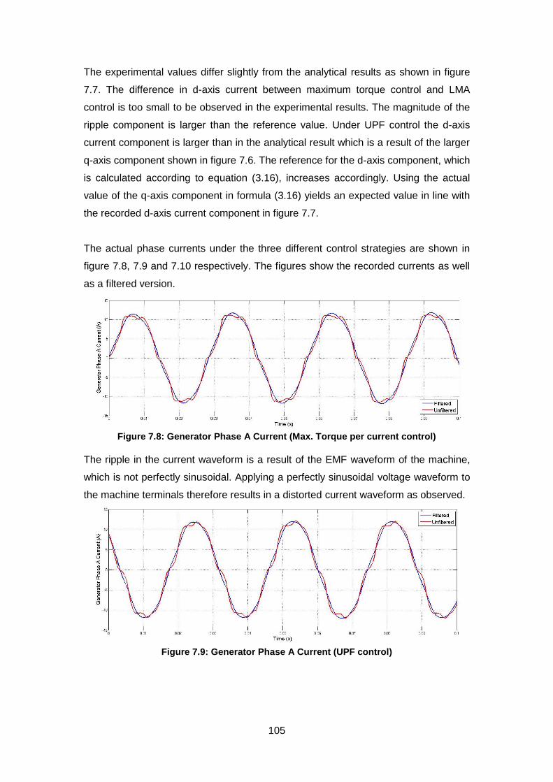
105

The experimental values differ slightly from the analytical results as shown in figure

7.7. The difference in d-axis current between maximum torque control and LMA

control is too small to be observed in the experimental results. The magnitude of the

ripple component is larger than the reference value. Under UPF control the d-axis

current component is larger than in the analytical result which is a result of the larger

q-axis component shown in figure 7.6. The reference for the d-axis component, which

is calculated according to equation (3.16), increases accordingly. Using the actual

value of the q-axis component in formula (3.16) yields an expected value in line with

the recorded d-axis current component in figure 7.7.

The actual phase currents under the three different control strategies are shown in

figure 7.8, 7.9 and 7.10 respectively. The figures show the recorded currents as well

as a filtered version.

Figure 7.8: Generator Phase A Current (Max. Torque per current control)

The ripple in the current waveform is a result of the EMF waveform of the machine,

which is not perfectly sinusoidal. Applying a perfectly sinusoidal voltage waveform to

the machine terminals therefore results in a distorted current waveform as observed.

Figure 7.9: Generator Phase A Current (UPF control)

106

Under UPF control a significant d-axis current is introduced, in accordance with

equation (3.16), which increases the total stator current. This can be observed in

figure 7.9.

Figure 7.10: Generator Phase A Current (LMA control)

The phase current under LMA control is shown in figure 7.10. No significant changes

are observed compared to the maximum torque control. This is expected from the

minimal change in d-axis current component.

7.4.1.2. Grid Side Performance

The DC-Link Reference Voltage was kept at 400V throughout all experimental tests.

A plot of the actual recorded DC-Link Voltage is shown in figure 7.11.


The DC-Voltage is maintained at its desired value under all three control strategies.

As discussed in section 3.4, this is achieved by modifying the d-axis current

component at the grid-side converter as required. The q-axis current component is

maintained at zero throughout, thus forcing the reactive power to 0. The

experimentally obtained d-axis current components are shown in figure 7.12. In

accordance with the analytical and simulated results all three control strategies result

107

in the same d-axis current component as the power produced by the generator is

essentially the same under all control strategies.

Figure 7.12: Grid-side d-axis current component under different control strategies

Part of the captured current waveform on the grid-side is shown in figure 7.13. This

waveform was obtained while operating the system under maximum torque per

current control. Waveforms under the other two control schemes have been omitted

as they do not differ. Figure 7.14 shows the same currents transformed to the dq-

reference frame.

Figure 7.13: Captured grid currents (Generator in Max. Torque Control)

The currents captured on the grid side, shown in figure 7.13, display a considerable

variation in magnitude over time which is reflected in the transformed d- and q-axis

currents in figure 7.14. During the experimental setup it was found that the 220V

provided by the transformer includes some voltage imbalance as well as harmonic

distortion. Furthermore the grid-filter components were found to be not completely

identical. The inductances in the three phases of the filter were found to vary up to

15%. These two factors contribute to the fluctuations in the grid-currents.

108

Figure 7.14: Captured grid currents in dq-frame (Generator in Max. Torque Control)

The stepped down grid phase voltages are captured and transformed to the dq-

reference frame as shown in figure 7.15 and 7.16 respectively.

Figure 7.15: Captured grid voltages

Figure 7.16: Captured grid voltages in the dq-reference frame

The transformed grid voltages, shown in figure 7.16. The imbalance in the grid

voltages are evident, which leads to a 3V peak-to-peak ripple in the transformed grid

voltages. The grid-side controller uses these voltages to control the grid-currents as

shown in figure 3.5. From the current waveforms it is evident that the ripple in the dq-

voltages is carried through to the currents as evident in figure 7.14.

109

7.4.2. Complete System Response to a Step in Wind Speed

The focus of the work carried out lies with implementation and operation of a WECS.

Focus is given to the steady-state performance of the system as a whole as well as

the individual components as presented earlier. In addition a step-response test was

carried out. The purpose of the step test is to verify the dynamic capabilities of the

system. It also proves that further work can be carried out on the developed setup,

including dynamic behaviour based around real wind data. The wind speed applied

was stepped from 3.5m/s to 4m/s as shown in figure 7.17.

Figure 7.17: Wind Speed Step

In order to track the MPP the generator needs to be accelerated. This is achieved by

reducing the quadrature current component to allow the machine to accelerate. The

recorded generator currents in the dq-frame are shown in figure 7.18.

Figure 7.18: Generator Current Response to a step in wind speed

The recorded currents compare favourably to the simulated results presented in

figure 5.25. The simulated currents are slightly larger than the experimental currents.

This can be attributed to the absence of friction in the simulated results, which

produces a large effective torque being applied to the generator. The transient period

observed in simulation is much shorter than in the experimental results, which can be

attributed to the omission of inertia in the simulation which allows for an almost

instantaneous change in machine speed. From the generator currents and voltages

the active and reactive power components can be computed according to equations

(2.15) and (2.16) as shown in figure 7.19 below.

110

Figure 7.19: Generator power components

Figure 7.20 shows the speed response obtained experimentally.

Figure 7.20: Generator speed response to a step in wind speed

Based on the applied wind speed and the measured generator speed the turbine

emulator calculated the turbine torque as shown in figure 7.21.

Figure 7.21: Turbine torque response to a step in wind speed

The aim of the MPPT algorithm is to maximise the power coefficient under any given

wind condition. Figure 7.22 shows the power coefficient and its behaviour during the

transient period.

Figure 7.22: Turbine power coefficient response to a step in wind speed

In figure 7.22 it can be observed how the power coefficient initially drops as the wind

speed is stepped up at t=3.5seconds. It climbs back up to its maximum values as the

turbine speed approaches the optimum speed before dropping again due to the

overshoot in turbine speed, evident from figure 7.20. As the turbine speed settles to

its optimum value, so does the power coefficient.

111

Figure 7.23: Developed turbine power response to a step in wind speed

The power extracted from the wind is shown in figure 7.23. It exhibits the same initial

dip as the wind speed is stepped up and overshoots thereafter before settling to its

steady-state value after t=4seconds.

The grid-side converter is expected to maintain the DC-voltage at 400V. The actual

DC-voltage measured is shown in figure 7.24.

Figure 7.24: DC-Link voltage

In order to maintain the desired DC-Link voltage the d-axis current component of the

grid currents is modified accordingly, whilst the q-axis current component remains

unchanged. This is shown in figure 7.25.

Figure 7.25: Grid currents

It can clearly be observed how the d-axis component of the grid current is increased

in response to the increase in DC-Link voltage. This counteracts the rise in DC-

voltage by increasing the transfer of real power to the grid, as shown in figure 7.26

112

Figure 7.26: Real and Reactive Power transferred to the grid

Based on the results presented in this section it can be concluded that the PM WECS

which was implemented provides a valid platform to perform static and dynamic

experimental tests on the performance of such a system. The MPPT tracks the MPP

accurately within less than 0.5 seconds when a step input is applied. As mentioned

previously, wind does not change instantaneously. However, the ability to deal with a

step change effectively is evidence that more realistic wind speed profiles can be

tracked accurately, within the applicable system limits.

7.4.3. Experimental Evaluation of different generator control strategies

and their impact on power production

In chapters 4 and 5, the use of a MPPT algorithm was discussed to obtain maximum

power from the incident wind. The control of the generator under three different

control strategies was also investigated, to minimise its losses. In the previous

section the experimental results for static and dynamic operation have been

presented and discussed, with attention given to the intermediate results, such as

currents, DC-voltage, etc.

This section presents and discusses the overall performance of the WECS, both at

the generator output and the grid side, and the impact that different control strategies

have on its performance.

7.4.3.1. Generator Side Performance

The real power output of the generator was measured under the three control

strategies. The output power as a function of wind speed is shown in figure 7.27

below.

113

Figure 7.27: Real generator power under the three control strategies investigated

There is no difference in the generator output power until approximately 6m/s. At

wind speeds above 6m/s, and therefore loading above 1.3kW, the UPF control

strategy produces less power than the maximum torque per current and LMA control.

This can be attributed to the increased copper losses, which is a result of the higher

stator current. Comparing the experimental results to the analytically calculated

generator power, shown in figure 4.10, validates these findings.

The generator efficiency was calculated as the ratio of real power output to the

mechanical shaft power applied by the turbine emulator according to:

𝜂𝐺𝑒𝑛 =𝑃𝐺𝑒𝑛

𝑃𝑠𝑕𝑎𝑓𝑡∙ 100% (7.1)

Figure 7.28 shows the obtained generator efficiency as a function of wind speed

under steady-state conditions.

114

Figure 7.28: Generator Efficiency under Steady-State Conditions vs. Wind Speeds

Comparing the experimental results to the analytical and simulated outcome shows

discrepancies between the absolute values obtained through simulations and

experimentally. However, the trends observed in the analytical and simulated results

are confirmed experimentally. The efficiency curves shown in figure 7.28 are a result

of the changing generator efficiency at different loading points. Lower wind speeds

translate into lower loading points. At higher wind speeds the PMSG is operated

closer to its rated values which results in higher efficiency, as evident in figure 7.28.

In the analytical as well as simulated results the Unity Power Factor control performs

worst, especially at higher wind speeds, with the two other control strategies showing

no difference in the wind speed range investigated. The experimental results

presented in figure 7.28 confirm this.

Several reasons contribute to the almost identical performance of the maximum

torque per current control and the LMA. These include the method of extracting

mechanical losses of the system as a function of speed, as described in chapter 6.1

and the assumptions made to obtain these values, which can lead to an error in the

model for the core losses. The LMA is based on the core loss model and will

therefore be affected. Furthermore the impact of temperature change has been

neglected in the experimental implementation as well as the analytical and simulated

results. However, temperature changes are present and do impact on the results in

an experimental environment, which are difficult to model in the analytical or

simulation environment.

115

7.4.3.2. Grid Side Performance

The real power transferred to the grid is shown in figure 7.29 at various wind speeds.

Figure 7.29: Real Grid Power under steady-state conditions vs. Wind speed

In figure 5.22 the simulated real power transferred to the grid is shown as a function

of wind speed. Both curves, simulated and experimentally obtained, exhibit the same

quadratic behaviour expected from the turbine characteristics. There is a difference

in absolute values between the two results. The same reasons as mentioned in the

discussion of the generator power and efficiency curves apply here. In addition

losses associated with the power converters, mainly switching losses, as well as the

grid filter impact on the experimental results. The inductors used in the laboratory

have a certain resistance which was not considered in the simulations. This will

cause additional losses. However, as previously mentioned these inaccuracies are

present under all three control strategies and do not impact on a comparison of

those.

To obtain the efficiency of the system as a whole, the real power transferred to the

grid was calculated as a percentage of turbine shaft power.

𝜂𝑆𝑦𝑠𝑡𝑒𝑚 =𝑃𝐺𝑟𝑖𝑑

𝑃𝑠𝑕𝑎𝑓𝑡∙ 100% (7.2)

Overall system efficiency at different wind speeds is shown in figure 7.30.

116

Figure 7.30: System Efficiency under Steady-State Conditions vs. Wind speed

The system efficiency curves are very close and differ less than one percent. As the

generator power measured shows the same behaviour, this is an expected outcome.

Losses associated with the power converters and grid filter do not differ as the grid

side converter control strategy is always the same.

7.5. Conclusions

The experimental results obtained in the laboratory have been presented and

discussed in this section. The individual system components were tested individually

to validate the correct operation of each part of the system. Subsequently, the WECS

was operated as a whole. A thorough analysis of the captured parameters under

steady-state conditions was presented and the outcome discussed. Furthermore, the

response of the system to a step change in wind change was shown and analysed.

Finally the impact of three different machine control strategies on the performance of

the WECS is presented.

117

Chapter 8

8. Conclusion and

Recommendations From the analytical, simulated and experimental results obtained throughout this

thesis certain conclusion can be drawn. These are discussed here. Based on these

conclusions, certain recommendations are given.

8.1. Conclusions In this thesis the analysis and implementation of a PM WECS is presented. Based on

the findings of the thesis, the following conclusions can be drawn:

8.1.1 The model of a wind turbine and its governing equations was formulated.

Based on the developed model, a wind turbine emulator was simulated and

implemented experimentally. The correct operation of the turbine emulator

was validated through simulation and a set of experimental tests. Based on

the experimental results obtained, it can be concluded that the turbine

emulator behaves as predicted in theory. The effect of furling, tower

shadowing and turbine inertia were omitted for simplicity. Due to the DC-

motor available the operating range was limited to 2.23kW, or a wind speed of

7m/s.

118

8.1.2 A detailed model of the PMSG has been developed. The control of the

machine has been discussed and investigated. This was done in theory,

simulation and finally experimentally. A series of tests were carried out to

validate the correct operation of the machine-side control, including current

and speed control as well as motor-mode and generator mode of operation.

These validated the correct operation of the controllers. Reference speeds

were applied to the controller and tracked correctly.

Due to the absence of a torque transducer the developed shaft torque was

estimated from loss models. In addition the impact of temperature changes

was neglected.

8.1.3 The options available to interface the WECS to the grid were investigated and

a grid-converter, together with a LCL-type grid filter was evaluated. Through

simulations the correct operation of the grid-tied inverter was validated. The

grid-current components were found to have some imbalance as well as a

considerable amount of current ripple. This can partly be attributed to the

mismatch between the components used as well as the use of non-ideal

components. This was necessitated by the available components.

Maintaining the DC-link voltage by transferring any energy to the grid is the

main objective of the grid-side converter. This was validated in simulation as

well as experimentally during the operation of the WECS as a whole. The DC-

link voltage was maintained as desired while the reactive power reference

was set to zero and tracked successfully.

8.1.4 The complete operation of the WECS was investigated. Combining the wind

turbine emulator, machine-side controller and the grid-tied inverter completes

the WECS. Steady-state operation is presented and discussed. Furthermore

the dynamic response to a step change is investigated in a simulated

environment as well as experimentally. The complete system was

implemented on two dSPACE kits, to control each converter through SVM.

Controlling the PMSG under the three proposed control strategies, while

observing overall system efficiency showed no considerable impact. The non-

salient machine design reduces the impact of the proposed LMA on the

machine efficiency.

119

8.2. Recommendations 8.2.1 The wind turbine emulator can be further improved by including the following

phenomena: turbine shadowing, furling as well as the impact of inertia and

friction on the turbine performance. Furthermore, the use of a large motor will

extend the operating range and match the PMSG’s full rating.

8.2.2 Using a torque transducer to accurately measure the developed shaft torque

should be investigated. This could lead to a more accurate loss model of the

machine, thereby increasing the accuracy of the predicted losses. The impact

of temperature on the PMSG’s performance should be investigated.

8.2.3 Using better matched and more ideal components to construct the grid-filter

should be considered. This could improve the performance of the grid-side

converter, whilst decreasing current ripple and imbalance.

Using more sophisticated design methods to obtain the filter components

should be investigated.

8.2.4 The operation of the whole system under a wider range of wind speeds

should be investigated to investigate the impact of loading on system

performance. Furthermore the system could be implemented using a different

PM machine, with saliency, to validate the LMA.

In addition, further investigation of the system’s performance under dynamic

wind conditions should be considered. This could be used to investigate

performance under real wind speed data.

120

References 1. D.C. Aliprantis, S.A. Papathanassiou, M.P. Papadopoulos, A.G. Kladas.

"Modeling and control of a variable-speed wind turbine equipped with permanent magnet synchronous generator", Proc. Of ICEM, 2000, Vol.3, pp.558-562.

2. Kenji Amei, Yukichi Takayasu, Takahisa Ohji, Masaaki Sakui, "A Maximum Power Control of Wmd Generator System Using a Permanent Magnet Synchronous Generator and a Boost Chopper Circuit", IEEE PCC, Osaka, 2002, pp. 1447-1452.

3. Christos Mademlis, Jannis Zypteras, Nikos Margaris, "Loss Minimization in

Surface Permanent-Magnet Synchronous Motor Drives", IEEE Transactions, Vol. 47, 2000

4. Antonio O. Di Tommaso, Rosario Miceli, Giuseppe Ricco Galluzzo, Marco Trapanese, "Efficiency Maximization of Permanent Magnet Synchronous Generators Coupled to Wind Turbines", Power Electronics Specialists Conference, 2007, PESC 2007

5. M. Chinchilla, S. Arnalte, J.C. Burgos, J.L. Rodriques, "Efficient Control of Permanent Magnet Synchronous Generators Applied to Variable Speed Wind Energy Systems", Renewable Energy Journal, Volume 31, Issue 9, July 2006, pp. 1455-1470

6. M. Chinchilla, Santiago Arnaltes, Juan Carlos Burgos, "Control of Permanent-Magnet Generators Applied to Variable-Speed Wind-Energy Systems Connected to the Grid", IEEE Transactions on Energy Conversion, Volume 21, Issue 1, 2006, pp. 130-135

7. Shigeo Morimoto, Yi Tong, Yoji Takeda, Takao Hirasa , "Loss Minimization Control of permanent Magnet Synchronous Motor Drives", IEEE Transactions on Industrial Electronics, Volume 41, Issue 5, 1994, pp 511-517

8. Shigeo Morimoto, Hajime Kato, Masayuki Sanada, Yoji Takeda, "Output Maximization Control for Wind Generation System with Interior Permanent Magnet Synchronous Generator", Conference Record of the 41st IEEE Industry Applications Conference, 2006, Volume 1, pp. 503-510

9. Shigeo Mrimoto, Hideaki Nakayama, Masayuki Sanada, Yoji Takeda, "Sensorless Output Maximization Control for Variable-Speed Wind Generation System Using IPMSG", Conference Record of the Industry Applications Conference, 2003, Volume 3, pp. 1464-1471

10. Bunlung Neammanee, Somporn Sirisumrannukul and Somchai Chatratana, "Development of a Wind Turbine Simulator for Wind Generator Testing", International Energy Journal, Volume 8, Issue 1, March 2007

11. M.B. Bana Sharifian, Y. Mohamadrezapour, M. Hosseinpour, S. Torabzade, "Maximum Power Control of Grid Connected Variable Speed Wind System

http://ieeexplore.ieee.org/xpl/mostRecentIssue.jsp?punumber=4341939


http://www.sciencedirect.com/science/journal/09601481

http://www.sciencedirect.com/science?_ob=PublicationURL&_tockey=%23TOC%235766%232006%23999689990%23616378%23FLA%23&_cdi=5766&_pubType=J&view=c&_auth=y&_acct=C000033878&_version=1&_urlVersion=0&_userid=635696&md5=e8feee0d3a0c449ae3701cbf7c134270





http://www.rericjournal.ait.ac.th/index.php/reric/issue/view/23

121

through Back to Back Converters", Journal of Applied Science, 2008, Volume 8, pp. 4416-4421

12. Harri Vihriala, "Control of Variable Speed Wind Turbines", PhD Thesis, October

2002, Tampere University of Technology

13. Seung-Ho Song, Shin-il Kang, Nyeon-Kun Hahm, "Implementation and Control of Grid Connected AC-DC-AC Power Converter for Variable Speed Wind Energy Conversion System", Eighteenth Annual IEEE Applied Power Electronics Conference and Exposition, 2003, Volume 1, pp. 154-158

14. Remus Teodorescu, Florin Iov and Frede Blaabjerg, "Flexible development and test system for llkW wind turbine", IEEE 34th Annual Power Electronics Specialist Conference, 2003, Volume 1, pp. 67-72

15. M. Chinchilla, S. Arnaltes, J.L. Rodriquiez-Amenedo, "Laboratory set-up for Wind Turbine Emulation", IEEE International Conference on Industrial Technology, 2004, Volume 1, pp. 553-557

16. P.E. Battaiotto, R.J. Mantz, P.F. Puleston, "A Wind Turbine Emulator based on a Dual DSP Processor System", Control Engineering Practice, Volume 4, Number 9, September 1996 , pp. 1261-1266

17. Bunlung Neammanee, Somporn Sirisumrannukul, Somchai Chatratana, "Development of a Wind Turbine Simulator for Wind Generator Testing", International Energy Journal, Volume 8, Issue 1, March 2007

18. Iulian Munteanu, Antoneta Iuliana Bratcu, Nicholas-Antonio Cutululis, Emil Caenga, "Optimal Control of Wind Energy Systems", 2008, Springer

19. Siegfried Heier, "Grid Integration of Wind Energy Conversion Systems", 2006, Wiley

20. Freede Blaabjerg, Remus Reodorescu, Zhe Chen, Marco Liserre, "Power Converters and Control of Renewable Energy Systems", Proceedings of the 6th International Conference on Power Electronics, 2004, Volume. 1, pp. 1–20

21. Kelvin Tan, Syed Islam, "Optimum Control Strategies in Energy Conversion of

PMSG Wind Turbine System Without Mechanical Sensors", IEEE Transactions on Energy Conversion, Vol. 19, No. 2, June 2004, pp. 392-400.

22. Mariusz Malinowski, Steffen Brenet, "Simple Control Scheme of Three-Level PWM Converter Connecting Wind Turbine with Grid", Chalmers University of Technology

23. Jianzhong Zhang, Ming Cheng, Zhe Chen, "Nonlinear Control for Variable-Speed Wind Turbines with Permanent Magnet Generators", International Conference on Electrical Machines and Systems, 2007, pp. 324-329

24. M. F. Moussa, A. helal, Y. Gaber H. A. Youssef, "Unity Power Factor Control of Permanent Magnet Motor Drive System", 12th International Power System Conference, 2008, pp.360-367






http://www.ingentaconnect.com/content/els/09670661;jsessionid=1p5vv8386739i.alice


122

25. Quincy Wang, Liuchen Chang, "PWM control strategies for wind turbine inverters", IEEE Canadian Conference on Electrical and Computer Engineering, 1998, Volume 1, pp. 309-312

26. Samuel Vasconcelos Araujo, Alfred Engler, Benjamin Sahan, Fernando Luiz Marcelo Antunes, "LCL Filter Design for grid-connected NPC inverters in offshore wind turbines", 7th International Conference on Power Electronics, 2007, pp.1133-1138

27. Mustapha Raou, Moulay Tahar Lamchich, "Average Current Moder Control of a Voltage SOurce Inverter connected to the Grid: Application to different filter cells ", Journal of Electrical Engineering, Volume 54, Number 3-4, 2004, pp.77-82

28. Pasi Peltoniemi, "Comparison of the Effect of Output Voltage Filters in the Total Harmonix Distortion of Line Current in Voltage Source Line Converters - Simulation Study", International Conference on Renewable Energies and Power Quality, 2006

29. Wei Sun, Zhe Chen and Xiaojie Wu, "Intelligent Optimize Design of LCL Filter for Three-Phase Voltage-Source PWM Rectifier", IEEE 6th International Power Electronics and Motion Control Conference, 2009, pp.970-974

30. M. Tavakoli Bina, E. Pashajavid, "An efficient procedure to design passive LCL-filters for active power filters", Electric Power Systems Research on Science Direct, Volume 79, 2008, pp. 606–614

31. M.A. Khan, "Contributions to Permanent Magnet Wind Generator Design Including the Application of Soft Magnetic Composites", PhD Thesis, 2006, University of Cape Town

32. P. Barendse, "Equivalent Circuit Parameters of the Permanent Magnet Machine", University of Cape Town







123

Appendix A: Analytical

Results


machine used in this project

Wind Speed (m/s)

Output Power Max. Torque

Output Power UPF

% Change compared to Max. Torque

Output Power LMA


4.00 379.21 379.18 -0.01 379.21 0.002

4.20 444.90 444.84 -0.01 444.91 0.002

4.40 517.13 517.03 -0.02 517.14 0.002

4.60 596.16 595.99 -0.03 596.17 0.002

4.80 682.25 681.98 -0.04 682.26 0.002

5.00 775.63 775.23 -0.05 775.64 0.002

5.20 876.56 875.97 -0.07 876.58 0.002

5.40 985.27 984.42 -0.09 985.29 0.002

5.60 1102.00 1100.79 -0.11 1102.02 0.002

5.80 1226.97 1225.30 -0.14 1226.99 0.002

6.00 1360.41 1358.13 -0.17 1360.44 0.002

6.20 1502.54 1499.46 -0.20 1502.57 0.002

6.40 1653.57 1649.48 -0.25 1653.60 0.002

6.60 1813.71 1808.33 -0.30 1813.74 0.002

6.80 1983.16 1976.16 -0.35 1983.20 0.002

7.00 2162.13 2153.11 -0.42 2162.18 0.002

7.20 2350.81 2339.27 -0.49 2350.86 0.002

7.40 2549.39 2534.76 -0.57 2549.44 0.002

7.60 2758.06 2739.65 -0.67 2758.11 0.002

7.80 2976.98 2953.98 -0.77 2977.04 0.002

8.00 3206.35 3177.79 -0.89 3206.41 0.002

8.20 3446.33 3411.09 -1.02 3446.39 0.002

8.40 3697.08 3653.85 -1.17 3697.15 0.002

8.60 3958.76 3906.03 -1.33 3958.84 0.002

8.80 4231.54 4167.53 -1.51 4231.62 0.002

9.00 4515.55 4438.24 -1.71 4515.64 0.002

124


modified machine

Wind Speed (m/s)

Output Power Max. Torque

Output Power UPF


Output Power LMA


4.00 63.38 63.43 0.07 63.83 0.71

4.20 81.44 81.51 0.08 81.95 0.63

4.40 101.67 101.77 0.10 102.26 0.58

4.60 124.18 124.32 0.11 124.86 0.54

4.80 149.08 149.27 0.13 149.84 0.51

5.00 176.46 176.70 0.14 177.31 0.48

5.20 206.42 206.74 0.16 207.38 0.46

5.40 239.07 239.48 0.17 240.15 0.45

5.60 274.51 275.03 0.19 275.71 0.44

5.80 312.84 313.48 0.20 314.17 0.42

6.00 354.16 354.94 0.22 355.63 0.41

6.20 398.58 399.52 0.24 400.19 0.41

6.40 446.18 447.30 0.25 447.96 0.40

6.60 497.07 498.40 0.27 499.02 0.39

6.80 551.35 552.92 0.28 553.49 0.39

7.00 609.12 610.94 0.30 611.46 0.38

7.20 670.48 672.58 0.31 673.03 0.38

7.40 735.53 737.92 0.33 738.30 0.38

7.60 804.36 807.07 0.34 807.36 0.37

7.80 877.07 880.11 0.35 880.33 0.37

8.00 953.76 957.15 0.35 957.28 0.37

8.20 1034.53 1038.26 0.36 1038.33 0.37

8.40 1119.47 1123.55 0.36 1123.57 0.37

8.60 1208.69 1213.10 0.36 1213.10 0.36

8.80 1302.27 1306.98 0.36 1307.00 0.36

9.00 1400.31 1405.29 0.36 1405.39 0.36

125

Appendix B: Tabulated

Simulation Results

Table B.1: Simulated Grid Power vs. Wind Speed

Wind Speed (m/s)

Shaft Power (W)

Grid Power (W) under Max. Torque Control

Grid Power (W) under UPF Control

Grid Power (W) und LMA Control

4 482.33 390.35 390.35 390.35

4.5 686.75 577.08 577.08 577.18

5 942.05 810.91 810.91 810.91

5.5 1253.9 1096.55 1095.65 1096.65

6 1627.8 1438.68 1436.78 1438.68

6.5 2069.7 1841.71 1838.21 1841.71

7 2585 2310.24 2304.04 2310.34

126

Appendix C: Tabulated

Experimental Results Table C.1: Real Generator power under Steady-State Conditions

Wind Speed [m/s] Tmax UPF

% Change compared to Max. Torque LMA


4 350.6 354.9 1.2 353.1 0.7

4.2 421.0 426.2 1.2 423.5 0.6

4.4 499.9 504.5 0.9 500.9 0.2

4.6 583.3 589.4 1.0 585.1 0.3

4.8 675.4 681.4 0.9 678.2 0.4

5 777.8 781.8 0.5 779.5 0.2

5.2 886.8 891.6 0.5 892.0 0.6

5.4 1007.3 1008.2 0.1 1008.3 0.1

5.6 1134.5 1134.6 0.0 1138.4 0.3

5.8 1272.1 1270.8 -0.1 1275.4 0.3

6 1418.4 1412.8 -0.4 1420.8 0.2

6.2 1585.1 1581.0 -0.3 1588.3 0.2

6.4 1747.6 1738.0 -0.5 1750.8 0.2

6.6 1929.0 1911.8 -0.9 1921.4 -0.4

6.8 2106.5 2069.5 -1.8 2100.9 -0.3

7 2278.1 2242.3 -1.6 2272.9 -0.2

127

Table C.2: Real Grid Power under Steady-State Conditions

Wind Speed [m/s] Tmax UPF

% Change compared to Max. Torque LMA


4 321.5 323.8 0.7 323.7 0.7

4.2 395.6 398.1 0.6 397.9 0.6

4.4 478.2 480.2 0.4 479.1 0.2

4.6 565.1 568.4 0.6 566.7 0.3

4.8 658.8 662.3 0.5 661.6 0.4

5 759.9 762.1 0.3 760.9 0.1

5.2 868.0 871.9 0.5 872.9 0.6

5.4 985.6 986.8 0.2 987.5 0.1

5.6 1109.6 1112.8 0.3 1113.4 0.3

5.8 1243.1 1246.6 0.3 1247.1 0.3

6 1384.2 1385.9 0.2 1387.0 0.1

6.2 1550.4 1553.1 0.4 1556.4 0.2

6.4 1709.6 1711.7 0.2 1713.5 0.1

6.6 1885.3 1874.4 0.1 1882.8 -0.4

6.8 2055.8 2044.1 -0.6 2050.9 -0.2

7 2217.4 2213.0 -0.2 2215.5 -0.2

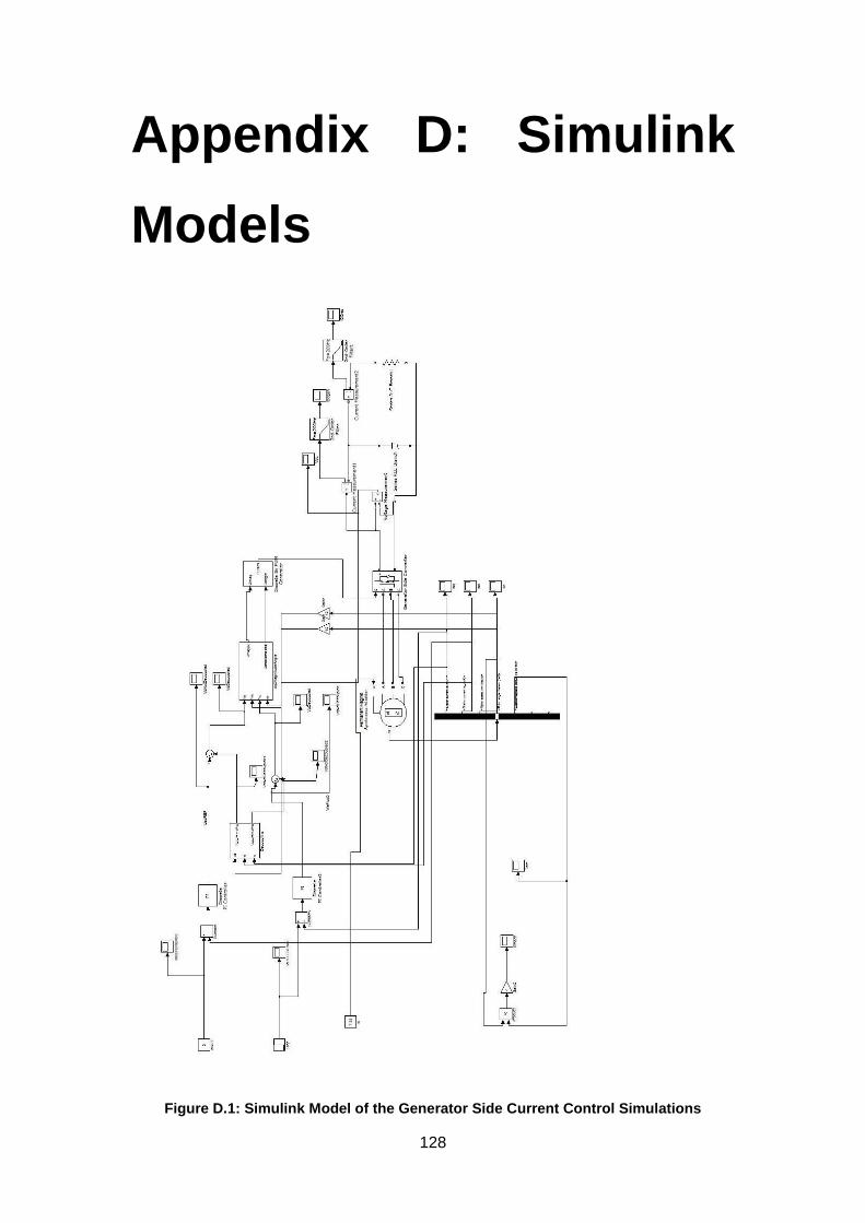
128

Appendix D: Simulink

Models

Figure D.1: Simulink Model of the Generator Side Current Control Simulations

129

Figure D.2: Simulink Model used in the complete system simulations

Chapter 3: Repair and rewind of induction motor

Documents

Transcript of Chapter 3: Repair and rewind of induction motor