Induction as a Search Procedure

Stasinos KonstantopoulosInstitute of Informatics & Telecommunications, NCSR ‘Demokritos’

P.O. BOX 60228, Ag. Paraskevi 15310, GreeceTel: +30 21 06503162, Fax: +30 21 06532175Email: konstant@iit.demokritos.gr

Rui CamachoFaculdade de Engenharia da Universidade do PortoR. Dr Roberto Frias, s/m, 4200-465 Porto, Portugal

Tel: +351 22 508 1849, Fax: +351 22 508 1443Email: rcamacho@fe.up.pt

andLaboratório de Inteligência Artificial e Ciências de Computadores,

Rua de Ceuta, 118, 6o, 4150-190 Porto, PortugalTel: +351 22 339 2090, Fax: +351 22 339 2099

Nuno A. FonsecaLaboratório de Inteligência Artificial e Ciências de Computadores,

University of PortoR. Campo Alegre 823, 4150 Porto, Portugal

Tel: +351 22 607 8830, Fax: +351 22 600 3654Email: nf@ncc.up.pt

Vítor Santos CostaCOPPE/Sistemas, Universidade Federal do Rio de Janeiro, Brasil

Centro de Tecnologia, Bloco H-319, Cx. Postal 68511, Rio de Janeiro, Brasil(CEP: 21945-970)

Tel: +55 21 2562 8648, Fax: +55 21 2562 8676Email: vitor@cos.ufrj.br

1

Induction as a Search Procedure

Abstract

This chapter introduces Inductive Logic Programming from the perspective of search al-gorithms in Computer Science. It first briefly considers the Version Spaces approach to induc-tion, and then focuses on Inductive Logic Programming: from its formal definition and maintechniques and strategies, to priors used to restrict the search space and optimized sequential,parallel, and stochastic algorithms. The authors hope that this presentation of the theory andapplications of Inductive Logic Programming will help the reader understand the theoreticalunderpinnings of inductive reasoning, and also provide a helpful overview of the State-of-the-Art in the domain.

1 INTRODUCTION

Induction is a very important operation in the process of scientific discovery, which has beenstudied from different perspectives in different disciplines. Induction, or inductive logic, is theprocess of forming conclusions that reach beyond the data (facts and rules), i.e., beyond the currentboundaries of knowledge. At the core of inductive thinking is the ‘inductive leap’, the stretch ofimagination that draws a reasonable inference from the available information. Therefore, inductiveconclusions are only probable, they may turn out to be false or improbable when given more data.

In this chapter we address the study of induction from an Artificial Intelligence (AI) perspec-tive and, more specifically, from a Machine Learning perspective, which aims at automating theinductive inference process. As is often the case in AI, this translates to mapping the ‘inductiveleap’ onto a search procedure. Search, therefore, becomes a central element of the automation ofthe inductive inference process.

We consider two different approaches to the problem of induction as a search procedure: Ver-sion Spaces is an informal approach, more in line with traditional Machine Learning approaches;and, by contrast, Inductive Logic Programming (ILP), relies on a formal definition of the searchspace. We compare the two approaches under several dimensions, namely, expressiveness of thehypothesis language underlying the space, completeness of the search, space traversal techniques,implemented systems and applications thereof.

2

Next, the chapter focuses on the issues related to a more principled approach to inductionas a search. Given a formal definition and characterization of the search space, we describe themain techniques employed for its traversal: strategies and heuristics, priors used to restrict its size,optimized sequential search algorithms, as well as stochastic and parallel ones.

The theoretical issues presented and exposed are complemented by descriptions of and refer-ences to implemented and applied systems, as well as real-world application domains where ILPsystems have been successful.

2 A PRAGMATIC APPROACH: VERSION SPACES

This section is structured into three parts. A first part presents a set of definitions and conceptsthat lay the foundations for the search procedure into which induction is mapped. In a second partwe mention briefly alternative approaches that have been taken to induction as a search procedureand finally in a third part we present the version spaces as a general methodology to implementinduction as a search procedure.

2.1 A Historical Road Map

Concept Leaning is a research area of Machine Learning that addresses the automation of the pro-cess of finding (inducing) a description of a concept (called the ‘target concept’ or hypothesis)given a set of instances of such concept. Concepts and instances have to be expressed in a con-cept description language or hypothesis language (L). Given a set of instances of some conceptit is usually a rather difficult problem to (automatically) induce the ‘target concept’. The majordifficulty is that there may be a lot, if not an infinite, number of plausible conjectures (hypotheses)that are ‘consistent’ with the given instances. Automating the induction process involves the gen-eration of the candidate concept descriptions (hypotheses), their evaluation, and the choice of ‘thebest one’ according to some criteria. The concept learning problem is often mapped into a searchproblem, that looks for a concept description that explains the given instances and lies within theconcept description language.

An important step towards the automation of the learning process is the definition of a (partial)order on L, thus ordering the search space. The existence of an ordered space makes it possibleto perform systematic searches, to justifiably discard some ‘uninteresting’ regions of candidatedescriptions, and to have a compact description of the search space. For that purpose it is usual todefine a ‘generalization’ order, that is, a partial order1 over the set of possible concept descriptionsthat allows us to compare pairs of such candidate concept descriptions. The suggestion that induc-tion may be automated by carrying a search through an order space was independently suggestedby Popplestone (1970) and Plotkin (1970).

3

The search space of the alternative concept descriptions may be traversed using any of the tra-ditional AI search strategies. In 1970 Winston (1970) describes a concept learning system usinga depth-first search. In Winston’s system one example at a time is analysed and a single conceptdescription is maintained as the current best hypothesis to describe the target concept. The cur-rent best hypothesis is tested against a new example and modified to become consistent with theexample while maintaining consistency with all previously seen examples. An alternative searchstrategy, breadth-first search, was used in concept learning by Plotkin (1970), Michalski (1973),Hayes-Roth (1974) and Vere (1975). These algorithms already take advantage of the order in thesearch space. Plotkin’s work is revisited in Section 3.4.2 below, as it forms the basis for severaldevelopments in Inductive Logic Programming.

2.2 Introducing Version Spaces

We now focus our attention on a general approach to concept learning, proposed by Mitchell(1978), called version spaces. A version space is the set of all hypotheses consistent with a set oftraining examples. In most applications the number of candidate hypotheses consistent with theexamples is very large or even infinite. It is therefore impractical—or even infeasible—to storean enumeration of such candidates. The version space uses a compact and elegant representationof the set of candidate hypotheses. The representation takes advantage of the order imposed oversuch hypotheses and stores only the most general and most specific set of descriptions that limitthe version space.

In order to make a more formal presentation of the version spaces approach to concept learninglet us introduce some useful definitions. Assume that the function tg(e) gives the ‘correct’ valueof the target concept for each instance e. A hypothesis h(e) is said to be consistent with a set ofinstances (examples) E iff it produces the same vale of tg(e) for each example e ∈ E. That is:

Consistent(h,E) ≡ ∀e∈E, h(e) = tg(e) (1)

Examples are of two kinds: positive and negative. Positive examples are instances of the targetconcept whereas negative examples are not.

The version space denoted by V SH,E with respect to the hypothesis space H2 and training setE, is the subset of hypotheses from H consistent with E.

V SH,E ≡ {h ∈ H|Consistent(h,E)} (2)

Since the set represented by the version space may be very large, a compact and efficient wayof describing such set is needed. To fully characterize the version space Mitchell proposes torepresent the most general and more specific elements, i.e., a version space is represented by theupper and lower boundaries of the ordered search space. Mitchell proposes also the CANDIDATE-ELIMINATION algorithm to efficiently traverse the hypothesis space.

4

In the CANDIDATE-ELIMINATION algorithm the boundaries of the version space are the onlyelements stored. The upper boundary is called G, the set of the most general elements of the space,and the lower boundary S, the set of the most specific hypotheses of the version space.

The upper (more general) general boundary G, with respect to hypothesis space H and exam-ples E, is the set of the maximally general members of H consistent with E.

G ≡ {g ∈ H|Consistent(g, E) ∧ ¬ (∃g′∈H)(g′ >g g) ∧ Consistent(g′, E)} (3)

where >g denotes the ‘more general than’ relation. The lower (more specific) boundary S, withrespect to hypothesis space H and training set E, is the set of maximally specific members of H

consistent with E.

S ≡ {s ∈ H|Consistent(s, E) ∧ ¬ (∃s′∈H)(s >g s′) ∧ Consistent(s′, E)} (4)

The CANDIDATE-ELIMINATION algorithm is outlined in Figure 1. The algorithm proceeds in-crementally, by analysing one example at a time. It starts with the most general set G containing allhypotheses from L consistent with the first example and with the most specific set S of hypothesesfrom L consistent with the first example (the set with the first example only). As each new exampleis presented, G gets specialized and S generalized, thus reducing the version space they represent.Positive examples lead to the generalization of S, whenever S is not consistent with a positiveexample. Negative examples prevent over-generalization by specializing G, whenever G is incon-sistent with the a negative example. When specializing elements of G, only specializations that aremaximally general and generalizations of some element of S are admitted. Symmetrically, whengeneralizing elements of S, only generalizations that are maximally specific and specializations ofsome element of G are admitted. When all examples are processed, the hypotheses consistent withthe presented data are the set of hypotheses from L within the G and S boundaries.

Some advantages of the version space approach with the CANDIDATE-ELIMINATION algo-rithm is that partial descriptions of the concepts may be used to classify new instances, and thateach example is examined only once and there is no need for backtracking. The algorithm iscomplete, i.e., if there is a hypothesis in L consistent with the data it will be found.

Version spaces and the CANDIDATE-ELIMINATION algorithm have been applied to severalproblems such as learning regularities in chemical mass spectroscopy (Mitchell, 1978) and controlrules for heuristic search (Mitchell et al., 1983). The algorithm was initially applied to inducerules for the DENDRAL knowledge-based system that suggested plausible chemical structure ofmolecules based on the analysis of information of the molecule chemical mass spectroscope data.Finally, Mitchell et al. (1983) uses the technique to acquire problem-solving heuristics for the LEX

system in the domain of symbolic integration.

5

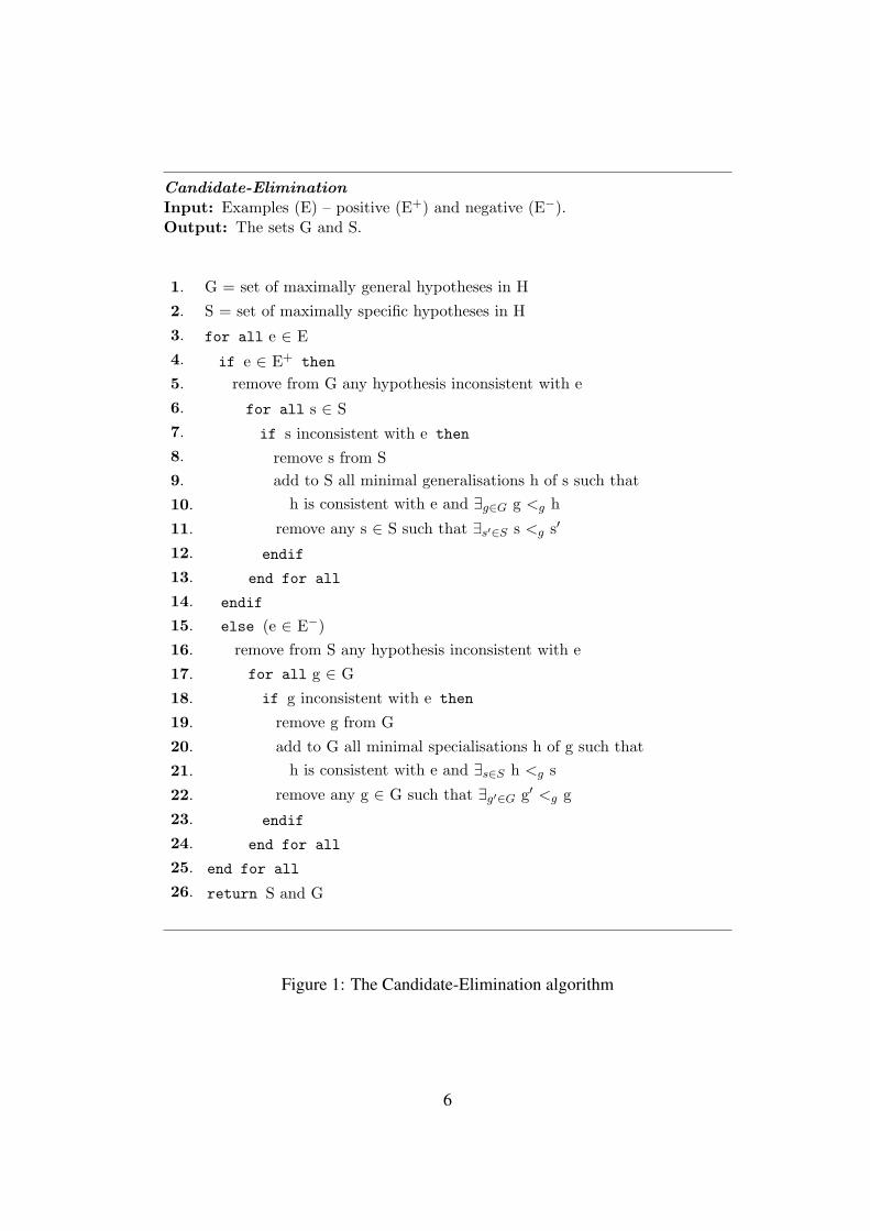
Candidate-EliminationInput: Examples (E) – positive (E+) and negative (E−).Output: The sets G and S.

1. G = set of maximally general hypotheses in H2. S = set of maximally specific hypotheses in H3. for all e ∈ E4. if e ∈ E+ then

5. remove from G any hypothesis inconsistent with e6. for all s ∈ S7. if s inconsistent with e then

8. remove s from S9. add to S all minimal generalisations h of s such that10. h is consistent with e and ∃g∈G g <g h

11. remove any s ∈ S such that ∃s′∈S s <g s′

12. endif

13. end for all

14. endif

15. else (e ∈ E−)16. remove from S any hypothesis inconsistent with e17. for all g ∈ G18. if g inconsistent with e then

19. remove g from G20. add to G all minimal specialisations h of g such that21. h is consistent with e and ∃s∈S h <g s

22. remove any g ∈ G such that ∃g′∈G g′ <g g

23. endif

24. end for all

25. end for all

26. return S and G

Figure 1: The Candidate-Elimination algorithm

6

2.3 A Simple Example

The technique of version spaces is independent of the hypothesis representation language. Ac-cording to the application, the hypothesis language used may be as simple as an attribute-valuelanguage or as powerful as First Order Logic. For illustrative purposes only (proof-of-concept) wepresent a very simple example using an attribute-value hypothesis language. We show an exam-ple of the CANDIDATE-ELIMINATION algorithm to induce a concept of a bird using five trainingexamples of animals.

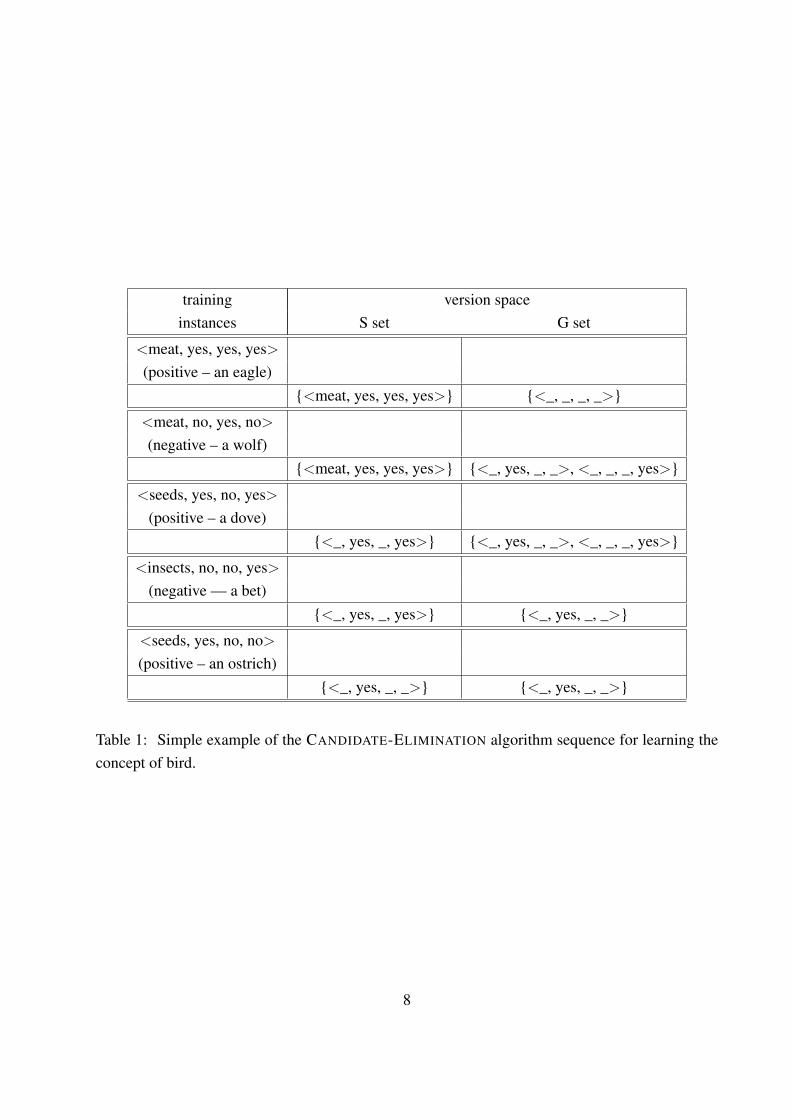
The hypothesis language will be the set of 4-tuples encoding the attributes eats, has feathers,has claws and flies. The domains of such attributes are: eats={meat, seeds, insects}, has feath-ers={yes, no}, has claws={yes, no} and flies={yes, no}. The representation of an animal that eatsmeat, has feathers, does not have claws and flies is the 4-tuple: <meat, yes, no, yes>. We use thesymbol _ (underscore) to indicate that any value is acceptable. We say that a hypothesis h1 matchesan example if every feature value of the example is either equal for the corresponding value in h1 orh1 has the symbol “_” for that feature (meaning “any value” is acceptable). Let us consider that ahypothesis h1 is more general than hypothesis h2 if h1 matches all the instances that h2 matches butthe reverse is not true. Figure 1 shows the sequence of values of the sets S and G after the analysisof five examples, one at a time. The first example is a positive example, an eagle (<meat, yes, yes,yes>), and is used to initialize the S set. The G set is initialized with the most general hypothesisof the language, the hypothesis that matches all the examples: <_, _, _, _>. The second example isnegative and is a description of a wolf (<meat, no, yes, no>). The second example is not matchedby the element of S and therefore S is unchanged. However the hypothesis in the G set covers thenegative example and has to be minimally specialized. Minimal specializations of <_, _, _, _>

that avoid covering the working example are: <seed, _, _, _>, <insects, _, _, _>, <_, yes, _, _>,<_, _, no, _>, <_, _, _, yes>. Among these five specializations only the third and the fifth areretained since they are the only ones that cover the element of S. Analysing the third example (adove – a positive example) leads the algorithm to minimally generalize the element of S since itdoes not cover that positive example. The minimal generalization of S’s hypothesis is <_, yes, _,yes> that covers all seen positive and is a specialization of at least one hypothesis in G. The forthexample is negative and is a description of a bet (<insects, no, no, yes>). This examples forces aspecialization of G. Finally the last example is a positive one (an ostrich – <seeds, yes, no, no>)that results in a minimal generalization of S. The final version space (delimited by the final S andG) defines bird as any animal that has a beak.

3 INDUCTIVE LOGIC PROGRAMMING THEORY

Inductive Logic Programming (ILP) is the machine learning discipline that deals with the inductionof First-Order Predicate Logic programs. Related research appears as early as the late 1960’s, but

7

training version spaceinstances S set G set

<meat, yes, yes, yes>(positive – an eagle)

{<meat, yes, yes, yes>} {<_, _, _, _>}

<meat, no, yes, no>

(negative – a wolf){<meat, yes, yes, yes>} {<_, yes, _, _>, <_, _, _, yes>}

<seeds, yes, no, yes>(positive – a dove)

{<_, yes, _, yes>} {<_, yes, _, _>, <_, _, _, yes>}

<insects, no, no, yes>(negative — a bet)

{<_, yes, _, yes>} {<_, yes, _, _>}

<seeds, yes, no, no>

(positive – an ostrich){<_, yes, _, _>} {<_, yes, _, _>}

Table 1: Simple example of the CANDIDATE-ELIMINATION algorithm sequence for learning theconcept of bird.

8

it is only in the early 1990’s that ILP research starts making rapid advances and the term itself wascoined.3

In this section we first present a formal setting for Inductive Logic Programming and highlightthe mapping of this theoretical setting into a search procedure. The formal definitions of theelements of the search and the inter-dependencies between these elements are explained, while atsame time the concrete systems that implement them are presented.

3.1 The Task of ILP

Inductive Logic Programming systems generalize from individual instances in the presence ofbackground knowledge, conjecturing patterns about yet unseen data. The patterns discovered byILP systems are usually expressed as logic programs, a subset of first-order (predicate) logic.

In general, an ILP system receives as input logic programs representing prior domain knowl-edge (usually called background knowledge in ILP literature) and a set of examples. The examplesare either positive or negative: positive examples represent true observations and negative exam-ples represent false ones.

An ILP system is then expected to induce a theory (a hypothesis) which covers the positiveobservations in the presence of the background knowledge without covering any of the negativeobservations, if such a theory is possible and necessary. This hypothesis must be formulated withina hypothesis or concept language, typically a subset of first-order logic such as Horn clauses. Thereare two ways in which this informal definition is underspecified: it neither defines the concept ofcoverage (often also called explanation or modelling), nor does it specify how in the presenceof the background knowledge should be interpreted. While coverage is formally defined by theexplanation semantics of a specific ILP setting, and will de dealt with later, we proceed with thetwo formal definitions of the ILP task appearing in the ILP literature, namely descriptive ILP (alsocalled non-monotonic) and predictive:

Definition 1 Given background knowledge B, positive training data E+, negative training dataE−, and hypothesis language L, and if the following prior conditions hold:

(Prior Satisfiability) B does not cover E−

(Prior Necessity) B does not cover E+

then a descriptive ILP algorithm constructs a hypothesis H ∈ L with the following properties:(Posterior Satisfiability) H does not cover B ∧ E−

(Posterior Sufficiency) H covers B ∧ E+

if such a hypothesis exists.

Definition 2 Given background knowledge B, positive training data E+, negative training dataE−, and hypothesis language L, and if the following prior conditions hold:

9

(Prior Satisfiability) B does not cover E−

(Prior Necessity) B does not cover E+

then a predictive ILP algorithm constructs a hypothesis H ∈ L with the following properties:(Posterior Satisfiability) B ∧H does not cover E−

(Posterior Sufficiency) B ∧H covers E+

if such a hypothesis exists.

Informally, these definitions state that first of all the negative data must be consistent with thebackground, since otherwise no consistent hypothesis can ever be constructed; and that a hypoth-esis must be necessary because the background is not a viable hypothesis on its own. Given that,descriptive ILP identifies a hypothesis that covers (describes) the situation arising when we com-bine existing knowledge with the observations we are trying to explain. Predictive ILP, on the otherhand, augments existing (background) knowledge with a hypothesis, so that the combined resultcovers (predicts) the data.

3.1.1 Explanation Semantics

At the core of the ILP task definition is the concept of explaining observations by hypothesis,or, in other words, of hypotheses being models or covering. There are two major explanationsemantics for ILP, which substantiate this concept in different ways: learning from interpretationsand learning from entailment.

Under learning from interpretations, a logic program covers a set of ground atoms which is aHerbrand interpretation of the program, if the set is a model of the program. That is, the interpre-tation is a valid grounding of the program’s variables. Under learning from entailment, a programcovers a set of ground atoms, if the program entails the ground atoms, that is, if the ground atomsare included in all models of the program. As De Raedt (1997) notes, learning from interpretationsreduces to learning from entailment. This means that learning from entailment is a stronger expla-nation model, and solutions found by learning from interpretations can also be found by learningfrom entailment, but not vice versa.

From a practical point of view, in learning from interpretations each example is a separateProlog program, consisting of multiple ground facts representing known properties of the example.A hypothesis covers the example when the latter is a model of the former, i.e., the example providesa valid grounding for the hypothesis. In learning from entailment, on the other hand, each exampleis a single fact. A hypothesis covers the example when the hypothesis entails the example.

Other explanation semantics have been proposed as well, like learning from satisfiability andlearning from proofs. When learning from satisfiability (De Raedt & Dehaspe, 1997), examplesand hypotheses are both logic programs, and a hypothesis covers an example if the conjunctionof the hypothesis and the example is satisfiable. Learning from satisfiability is stronger than bothlearning from entailment and learning from interpretations.

10

Under learning from proofs, the ‘examples’ are the proof trees of positive and negative deriva-tions, which are generalized (lifted) to the clauses that generate the positives without generatingthe negatives. Learning from proofs has been applied to the induction of Stochastic Logic Pro-grams (De Raedt et al., 2005; Passerini et al., 2006).

3.1.2 ILP Settings

A setting of ILP is a complete specification of the task and the explanation semantics, optionallycomplemented with further restrictions on the hypothesis language and the examples representa-tion.

Although in theory all combinations are possible, descriptive ILP is most suitable to learningfrom interpretations, since under this semantics, the data is organized in a way that is convenient fortackling the descriptive ILP task. Symmetrically, predictive ILP typically operates under learningfrom entailment semantics. In fact, this coupling is so strong, that almost all ILP systems operatein either the non-monotonic or the normal setting.4

In the non-monotonic setting (De Raedt, 1997), descriptive ILP operates under learning frominterpretations. The non-monotonic setting has been successfully applied to several problems,including learning first-order decision trees (Blockeel & De Raedt, 1998), learning associationrules (Dehaspe & Toironen, 2000), and performing first-order clustering (De Raedt & Blockeel,1997). Another area of application is subgroup discovery (Wrobel, 1997), where the notion ofexplanation is relaxed to admit hypotheses that satisfy ‘softer’ acceptance criteria like, for example,similarity or associativity.

In the normal setting (Muggleton, 1991), also called explanatory ILP or strong ILP, predictiveILP operates under learning from entailment semantics. Most ILP systems operate in this setting,or rather a specialization of the normal setting called the example setting of the definite seman-tics (Muggleton & De Raedt, 1994). This setting imposes the restrictions that the examples areground instances of the target and the background and hypothesis are formulated as definite clauseprograms. As noted by Muggleton & De Raedt (ibid., Section 3.1, pp. 635–6), the restriction todefinite semantics greatly simplifies the ILP task, since for every definite program T there is amodelM+(T ) (its minimal Herbrand model) in which all formulae are decidable and the ClosedWorld Assumption holds. In this setting, the task of ILP is defined follows:

Definition 3 Given background knowledge B, positive training data E+, and negative trainingdata E−, an ILP algorithm constructs a hypothesis H with the following properties:

(Prior Satisfiability) All e ∈ E− are false inM+(B)

(Prior Necessity) Some e ∈ E+ are false inM+(B)

(Posterior Satisfiability) All e ∈ E− are false inM+(B ∧H)

(Posterior Sufficiency) All e ∈ E+ are true inM+(B ∧H)

11

Sofia

Fernanda

Jose ArcadioRenataBabilonia

Mauricio

Aureliano

Babilonia

Jose Arcadio

Buendia

Remedios Aureliano II

Amaranta

Jose Arcadio II

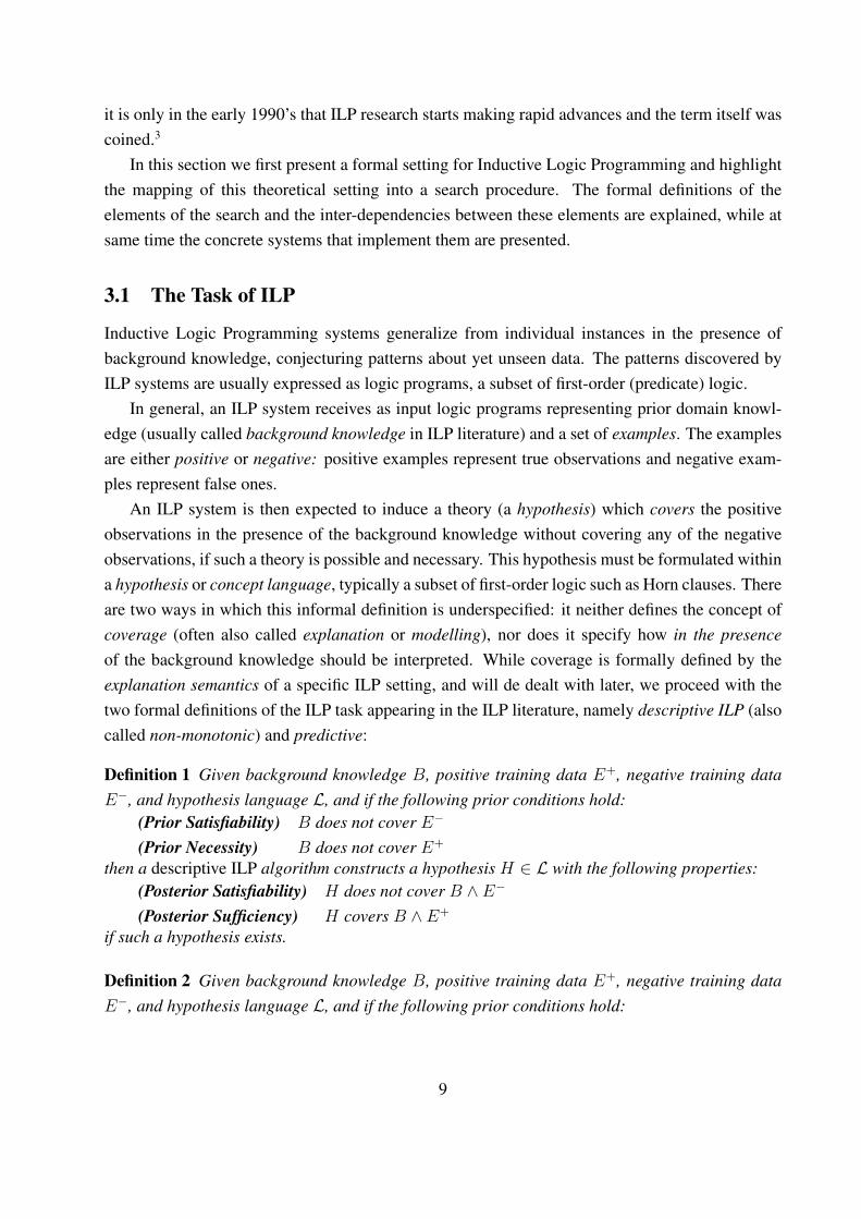
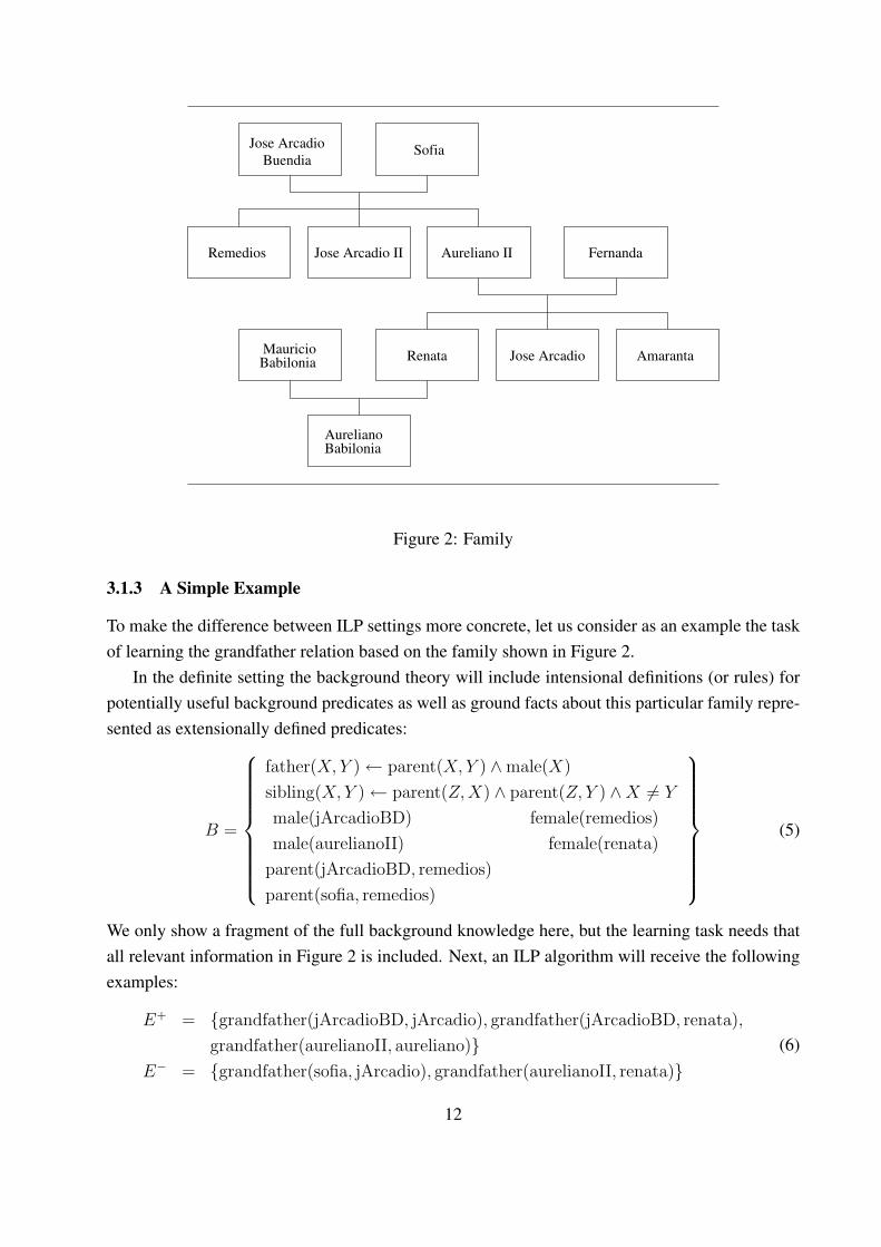
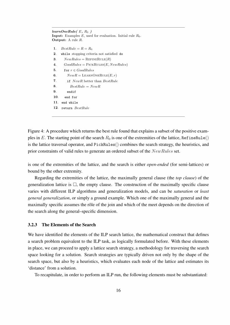
Figure 2: Family

3.1.3 A Simple Example

To make the difference between ILP settings more concrete, let us consider as an example the taskof learning the grandfather relation based on the family shown in Figure 2.

In the definite setting the background theory will include intensional definitions (or rules) forpotentially useful background predicates as well as ground facts about this particular family repre-sented as extensionally defined predicates:

B =

father(X, Y )← parent(X, Y ) ∧male(X)

sibling(X, Y )← parent(Z,X) ∧ parent(Z, Y ) ∧X 6= Y

male(jArcadioBD) female(remedios)

male(aurelianoII) female(renata)

parent(jArcadioBD, remedios)

parent(sofia, remedios)

(5)

We only show a fragment of the full background knowledge here, but the learning task needs thatall relevant information in Figure 2 is included. Next, an ILP algorithm will receive the followingexamples:

E+ = {grandfather(jArcadioBD, jArcadio), grandfather(jArcadioBD, renata),

grandfather(aurelianoII, aureliano)}E− = {grandfather(sofia, jArcadio), grandfather(aurelianoII, renata)}

(6)

12

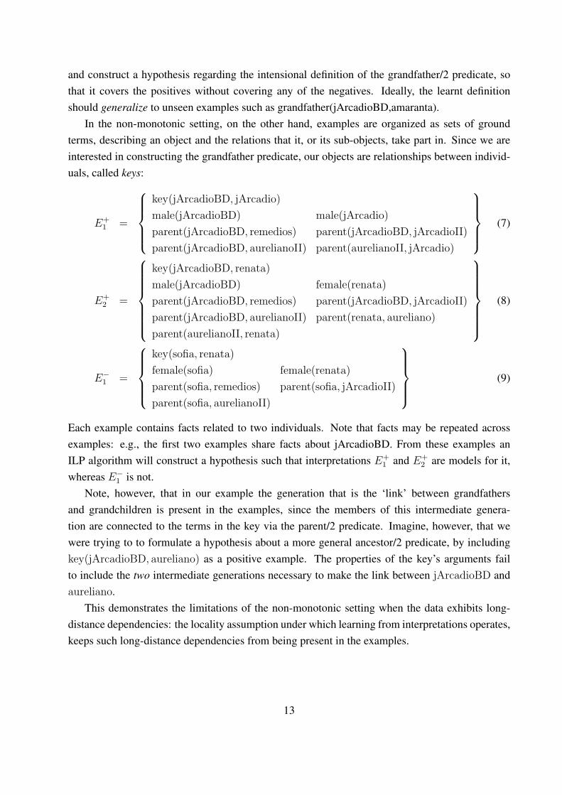
and construct a hypothesis regarding the intensional definition of the grandfather/2 predicate, sothat it covers the positives without covering any of the negatives. Ideally, the learnt definitionshould generalize to unseen examples such as grandfather(jArcadioBD,amaranta).

In the non-monotonic setting, on the other hand, examples are organized as sets of groundterms, describing an object and the relations that it, or its sub-objects, take part in. Since we areinterested in constructing the grandfather predicate, our objects are relationships between individ-uals, called keys:

E+1 =

key(jArcadioBD, jArcadio)

male(jArcadioBD) male(jArcadio)

parent(jArcadioBD, remedios) parent(jArcadioBD, jArcadioII)

parent(jArcadioBD, aurelianoII) parent(aurelianoII, jArcadio)

(7)

E+2 =

key(jArcadioBD, renata)

male(jArcadioBD) female(renata)

parent(jArcadioBD, remedios) parent(jArcadioBD, jArcadioII)

parent(jArcadioBD, aurelianoII) parent(renata, aureliano)

parent(aurelianoII, renata)

(8)

E−1 =

key(sofia, renata)

female(sofia) female(renata)

parent(sofia, remedios) parent(sofia, jArcadioII)

parent(sofia, aurelianoII)

(9)

Each example contains facts related to two individuals. Note that facts may be repeated acrossexamples: e.g., the first two examples share facts about jArcadioBD. From these examples anILP algorithm will construct a hypothesis such that interpretations E+

1 and E+2 are models for it,

whereas E−1 is not.

Note, however, that in our example the generation that is the ‘link’ between grandfathersand grandchildren is present in the examples, since the members of this intermediate genera-tion are connected to the terms in the key via the parent/2 predicate. Imagine, however, that wewere trying to to formulate a hypothesis about a more general ancestor/2 predicate, by includingkey(jArcadioBD, aureliano) as a positive example. The properties of the key’s arguments failto include the two intermediate generations necessary to make the link between jArcadioBD andaureliano.

This demonstrates the limitations of the non-monotonic setting when the data exhibits long-distance dependencies: the locality assumption under which learning from interpretations operates,keeps such long-distance dependencies from being present in the examples.

13

3.2 Setting up the Search

As mentioned earlier, the definition of the task of ILP is agnostic as to how to search for goodhypotheses and even as to how to verify entailment.5 Leaving aside the issue of mechanizing en-tailment for the moment, we discuss first how to choose candidate hypotheses among the membersof the hypothesis language.

The simplest, naïve way to traverse this space of possible hypotheses would be to use agenerate-and-test algorithm that first, lexicographically enumerates all possible hypotheses, andsecond, evaluates each hypothesis’ quality. This approach is impractical for any non-trivial prob-lem, due the large (possibly infinite) size of the hypothesis space. Instead, inductive machine learn-ing systems (both propositional rule learning systems as well as first-order ILP systems) structurethe search space in order to allow for the application of well-tested and established AI searchtechniques and optimizations. This structure must be such that, first, it accommodates a heuristics-driven search that reaches promising candidates as directly as possible; and, second, it allows foruninteresting sub-spaces to be efficiently pruned without having to wade through them.

3.2.1 Sequential Cover

Predictive ILP systems typically take advantage of the fact that the hypotheses are logic programsand therefore sets of clauses to use a strategy called sequential cover or cover removal, a greedyseparate-and-conquer strategy that breaks the problem of learning a set of clauses into iterations ofthe problem of learning a single clause.

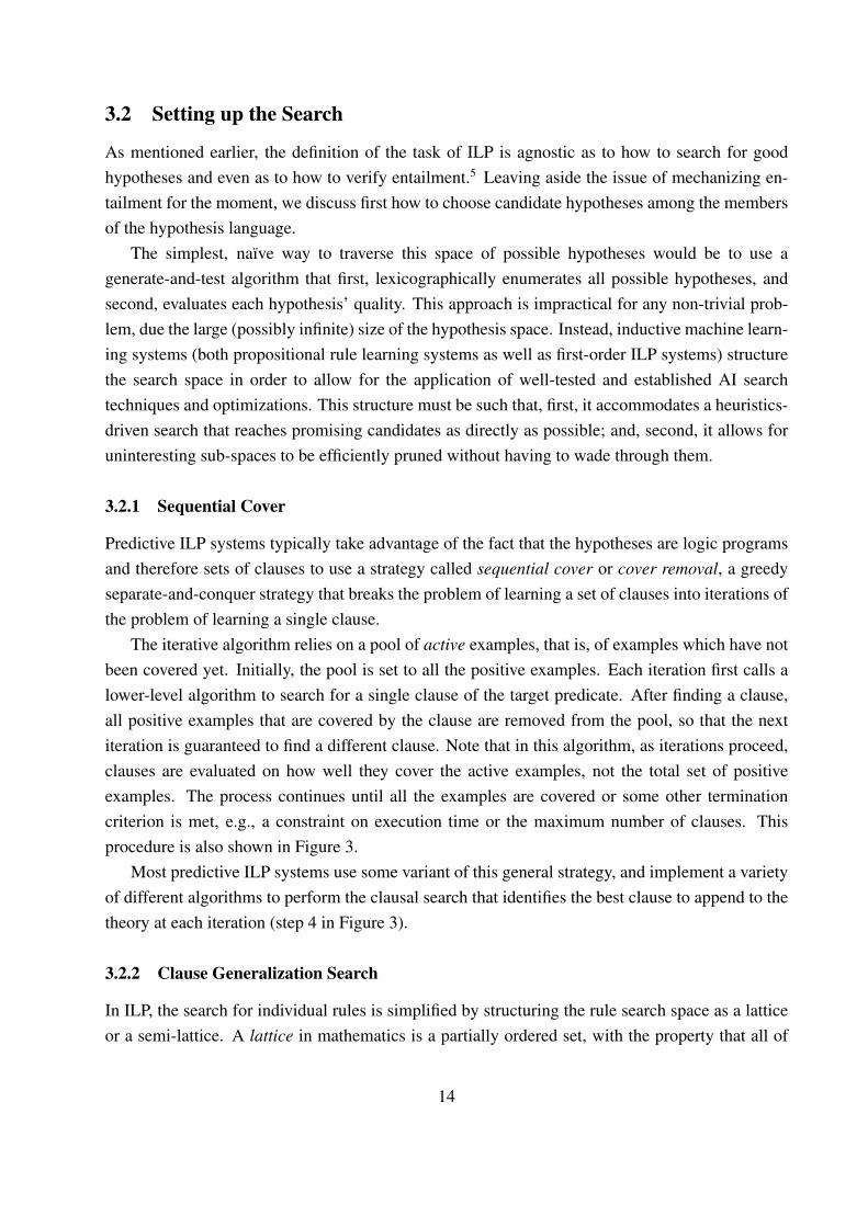
The iterative algorithm relies on a pool of active examples, that is, of examples which have notbeen covered yet. Initially, the pool is set to all the positive examples. Each iteration first calls alower-level algorithm to search for a single clause of the target predicate. After finding a clause,all positive examples that are covered by the clause are removed from the pool, so that the nextiteration is guaranteed to find a different clause. Note that in this algorithm, as iterations proceed,clauses are evaluated on how well they cover the active examples, not the total set of positiveexamples. The process continues until all the examples are covered or some other terminationcriterion is met, e.g., a constraint on execution time or the maximum number of clauses. Thisprocedure is also shown in Figure 3.

Most predictive ILP systems use some variant of this general strategy, and implement a varietyof different algorithms to perform the clausal search that identifies the best clause to append to thetheory at each iteration (step 4 in Figure 3).

3.2.2 Clause Generalization Search

In ILP, the search for individual rules is simplified by structuring the rule search space as a latticeor a semi-lattice. A lattice in mathematics is a partially ordered set, with the property that all of

14

covering(E)Input: Positive and negative examples E+, E−.Output: A set of consistent rules.

1. Rules Learned = ∅2. while E+ 6= ∅ do

3. R = LearnOneRule(E,START RULE)4. Rules Learned = Rules Learned ∪R

5. E+ = E+ \Coverage(R,E+)6. end while

7. return Rules Learned

Figure 3: The Sequential Cover strategy. The LearnOneRule() procedure returns the best rulefound that explains a subset of the positive examples E+. Coverage() returns the subset of E+

covered by R.

its non-empty finite subsets have both a supremum (called join) and an infimum (called meet). Asemi-lattice has either only a join or only a meet. The partial order is reflexive, anti-symmetric,and transitive binary relation.

This definition is carried over to ILP as follows:

Definition 4 A lattice is a partially ordered set in which every pair of elements a, b has a greatestlower bound (glb, a u b) and least upper bound (lub, a t b).

The partial ordering is based of the concept of generality, which places clauses along general–specific axes. Such a partial ordering is called a generalization ordering or a generalization model,and has the advantage of imposing a structure that is convenient for systematically searching forgeneral theories and for focusing on parts of the structure that are known to be interesting. Gener-ality is semantically defined using the concept of entailment:

Definition 5 Given two clauses C1 and C2, we shall call C1 more general (more specific) than C2,and write C1 >g C2 (C1 <g C2), if and only if C1 entails C2 (C2 entails C1).

Later in this chapter, we shall describe various generalization models, each based on different in-ference mechanisms for deducing entailment. Each of these defines a different refinement operatorwhich maps a clause into one or more general (or more specific, depending on the direction of thesearch) clauses.

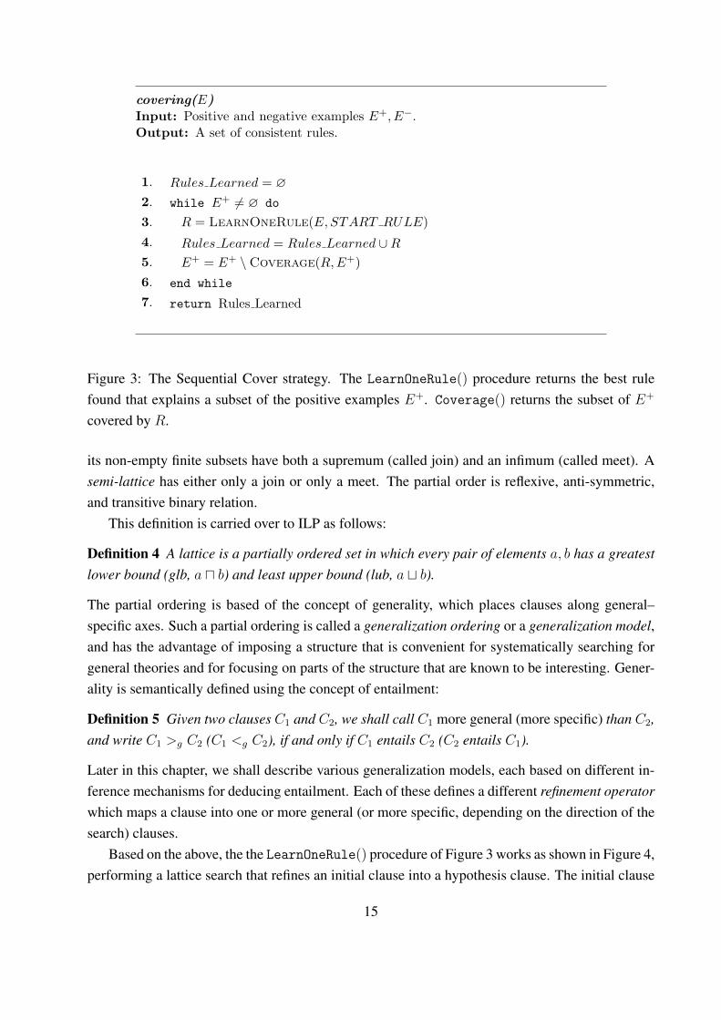
Based on the above, the the LearnOneRule() procedure of Figure 3 works as shown in Figure 4,performing a lattice search that refines an initial clause into a hypothesis clause. The initial clause

15

learnOneRule( E, R0 )Input: Examples E, used for evaluation. Initial rule R0.Output: A rule R.

1. BestRule = R = R0

2. while stopping criteria not satisfied do

3. NewRules = RefineRule(R)

4. GoodRules = PickRules(E, NewRules)

5. for r ∈ GoodRules

6. NewR = LearnOneRule(E, r)

7. if NewR better than BestRule

8. BestRule = NewR

9. endif

10. end for

11. end while

12. return BestRule

Figure 4: A procedure which returns the best rule found that explains a subset of the positive exam-ples in E. The starting point of the search R0 is one of the extremities of the lattice, RefineRule()is the lattice traversal operator, and PickRules() combines the search strategy, the heuristics, andprior constraints of valid rules to generate an ordered subset of the NewRules set.

is one of the extremities of the lattice, and the search is either open-ended (for semi-lattices) orbound by the other extremity.

Regarding the extremities of the lattice, the maximally general clause (the top clause) of thegeneralization lattice is �, the empty clause. The construction of the maximally specific clausevaries with different ILP algorithms and generalization models, and can be saturation or leastgeneral generalization, or simply a ground example. Which one of the maximally general and themaximally specific assumes the rôle of the join and which of the meet depends on the direction ofthe search along the general–specific dimension.

3.2.3 The Elements of the Search

We have identified the elements of the ILP search lattice, the mathematical construct that definesa search problem equivalent to the ILP task, as logically formulated before. With these elementsin place, we can proceed to apply a lattice search strategy, a methodology for traversing the searchspace looking for a solution. Search strategies are typically driven not only by the shape of thesearch space, but also by a heuristics, which evaluates each node of the lattice and estimates its‘distance’ from a solution.

To recapitulate, in order to perform an ILP run, the following elements must be substantiated:

16

• The hypothesis language, which is the set of eligible hypothesis clauses. The elements ofthis set are also the elements that form the lattice.

• A refinement operator that in-order visits the search space, following either the general-to-specific or the specific-to-general direction.

• the top and bottom clause, the extremities of the lattice. The top clause is the empty-bodiedclause that accepts all examples, and the bottom clause is a maximally specific clause thataccepts a single examples. The bottom clause is constructed by a process called saturation.

• The search strategy applied to the lattice defined by the three elements above.

• The heuristics that drive the search, an estimator of a node’s ‘distance’ from a solution. Dueto the monotonic nature of the definite programs, this distance can be reasonably estimatedby an evaluation function that assigns a value to each clause related to its ‘quality’ as asolution.

We now proceed to describe how various ILP algorithms and systems realize these five ele-ments, and show the impact of each design decision on the system’s performance. The focus willbe on the clause-level search performed by sequential-cover predictive ILP systems, but it shouldbe noted that the same general methodology is followed by theory-level predictive ILP and (to alesser extend) descriptive ILP algorithms as well.

3.3 Hypothesis Language

One of the strongest, and most widely advertised, points in favour of ILP is the usage of priorknowledge to specify the hypothesis language within which the search for a solution is to be con-tained. ILP systems offer a variety of tools for specifying the exact boundaries of the search space,which modify the space defined by the background theory, the clausal theory that represents theconcrete facts and the abstract, first-order generalizations that are known to hold in the domain ofapplication.

In more practical terms, the background predicates, the predicates defined in the backgroundtheory, are the building blocks from which hypothesis clauses are constructed. The backgroundpredicates should, therefore, represent all the relevant facts known about the domain of the conceptbeing learnt; the ILP algorithm’s task is to sort though them and identify the ones that, connectedin an appropriate manner, encode the target concept. Even ILP algorithms that go one step furtherand revise the background theory (cf. Section 3.8.2 below), rely on the original background to useas a starting point.

Prior knowledge in ILP is not, however, restricted to the set of predefined concepts availableto the ILP algorithm, but extends to include a set of syntactic and semantic restrictions imposed

17

on the set of admissible clauses, effectively restricting the search space. Such restrictions cannotbe encoded in the background theory program of Definitions 2 and 2, but ILP systems provideexternal mechanisms in order to enforce them.6 These mechanisms should be thought of as filtersthat reject or accept clauses—and, in some cases, whole areas of the search space—based onsyntactic or semantic pre-conditions.

3.3.1 Hypothesis Checking

As explained before, managing the ILP search space often depends on having filters that rejectuninteresting clauses. The simplest, but crudest approach, is to include or omit background predi-cates. By contract, some ILP systems, e.g., ALEPH (Srinivasan, 2004), allow users to build them-selves filters that verify whether the clause is eligible for consideration or whether it should beimmediately dropped. Such a hypothesis checking mechanism allows the finest level of controlover the hypothesis language, but is highly demanding on the user and should be complementedwith tools or mechanisms that facilitate the user’s task.

Hypothesis checking mechanisms can be seen as a way to bias the search language, andtherefore usually known as the bias language. One very powerful such example are declarativelanguages such as antecedent description grammars, definite-clause grammars that describe ac-ceptable clauses (Cohen, 1994; Jorge & Brazdil, 1995), or the DLAB language of clause tem-plates (Dehaspe & De Raedt, 1996) used in CLAUDIEN (De Raedt & Dehaspe, 1996), one of theearliest descriptive ILP systems. As Cohen notes, however, such grammars may become verylarge and cumbersome to formulate and maintain; newer implementations of the CLAUDIEN al-gorithm (CLASSICCL, Stolle et al. 2005) also abandon DLAB and replace it with type and modedeclarations (see below).

Finally, note that hypothesis checking mechanisms can verify a variety of parameters, bothsyntactic and semantic. As an example of semantic parameter, it is common for ILP systems todiscard clauses with very low coverage, as such clauses often do not generalize well.

3.3.2 Determinacy

A further means of controlling the hypothesis language is through the concept of determinacy,introduced in this context by Muggleton & Feng (1990). Determinacy is a property of the variablesof a clause and, in a way, specifies how ‘far’ they are from being bound to ground terms: a variablein a term is j-determinate if there are up to j variables in the same term. Furthermore, a variableis ij-determinate if it is j-determinate and its depth is up to i. A clause is ij-determinate is all thevariables appearing in the clause are ij-determinate.

The depth of a variable appearing in a clause is recursively defined as follows :

18

Definition 6 For clause C and variable v appearing in C, the depth of v, d(v), is

d(v) =

{0 if v is in the head of C

1 + minw∈var(C,v) d(w) otherwise

where var(C, v) are all the variables appearing in those atoms of the body of C where v alsoappears.

The intuition behind this definition is that depth increases by 1 each time a body literal is neededto ‘link’ two variables, so that a variable’s depth is the number of such links in the ‘chain’ ofbody literals that connects the variable with a variable of the head.7 Simply requiring that thehypothesis language only include determinate clause, i.e., clauses with arbitrarily large but finitedeterminacy parameters, has a dramatic effect in difficulty of the definite ILP task, as it rendersdefinite hypotheses PAC-learnable (De Raedt & Džeroski, 1994). Naturally, specifying smallervalues for the determinacy parameters tightens the boundaries of the search space. Consider, forexample, the following clause as a possible solution for our grandfather-learning example:

C = grandfather(X, Y )← father(X, U)∧ father(U, V )∧mother(W, V )∧mother(W, Y ) (10)

This clause perfectly classifies the instances of our example (Figure 2) and is 2, 2-determinate.8

Although this clause satisfies the posterior requirements for a hypothesis, a domain expert mighthave very good reasons to believe that the grandfather relation is a more direct one, and that solu-tions should be restricted to 1, 2-determinate clauses. Imposing this prior requirement would forcea learning algorithm to reject clause C (Eq. 10) as a hypothesis and formulate a more direct one,for example:

D = grandfather(X, Y )← father(X, U) ∧ parent(U, Y ) (11)

3.3.3 Type and Mode Declarations

Type and mode declarations are further bias mechanisms that provide ILP algorithms with priorinformation regarding the semantic properties of the background predicates as well as the targetconcept. Type and mode declarations were introduced in PROGOL (Muggleton, 1995) and havesince appeared in many modern ILP systems, most notably including the CLASSICCL (Stolle etal., 2005) re-implementation of CLAUDIEN, where they replace the declarative bias language usedin the original implementation.

Mode declarations state that some literal’s variables must be bound at call time (input, +) or not(output, −) and thus restrict the ways that literals can combine to form clauses. Mode declarationalso specify the places where constants may appear (constant, #). For example, with the followingmode declarations in the background:

B =

mode(grandfather(+,−))

mode(father(+, +))

mode(parent(+, +))

(12)

19

clause D (Eq. 11) can not be formulated, as variable Y cannot be bound in the parent/2 literal if itis unbound in the head. The desired ‘chain’ effect of input/output variables may be achieved withthe following background:

B =

mode(grandfather(+,−))

mode(father(+,−))

mode(parent(+,−))

(13)

achieves the desired ‘chain’ effect of input/output variables: X is bound in the head, so that father/2can be applied to bind the unbound variable U , which in its turn can serve as input to parent/2.Modes are usually combined with recall bounds that restrict the number of possible instantiationsof a literal’s variables for each mode of application:

B =

mode(1, grandfather(+, +)) ∨mode(2, grandfather(+,−))

mode(1, father(+, +)) ∨mode(3, father(+,−))

mode(1, parent(+, +)) ∨mode(3, parent(+,−))

mode(1, female(+)) ∨mode(5, female(−))

(14)

This background restricts the second mode of grandfather/2 to two possible instantiations, so thathypothesis D (Eq. 11) becomes unattainable and a different solution has to be identified. Consider,for example:

E = grandfather(X,Y )← father(X, U) ∧ parent(U, Y ) ∧ female(Y ) (15)

Clause E focuses on grandfathers of grand-daughters, and so satisfies the requirements of Eq. 14.Finally, mode declarations are extended with a rudimentary type system, such that different

modes apply to different instances. To demonstrate, the following background knowledge:

B =

mode(2, grandfather(+M,−M)) ∨mode(2, grandfather(+F,−F ))

mode(2, father(+M,−M)) ∨mode(2, father(+M,−F ))

mode(2, parent(+M,−M)) ∨mode(2, parent(+M,−F ))

∨mode(2, parent(+F,−M)) ∨mode(2, parent(+F,−F ))

mode(1, female(+F )) ∨mode(5, female(−F ))

mode(1, male(+M)) ∨mode(5, male(−M))

(16)

admits hypotheses like D (Eq. 11) which cover up to two grandchildren of each gender. Note,however, that types in ILP systems are most often flat tags; they do not support the supertype–subtype hierarchy that is so fundamental to modern type systems. As a result, it is not, for example,possible to express the fact that that although the parent/2 predicate can be instantiated for up to2 children of each gender, it can be instantiated for up to 3 children of either gender, as this wouldrequire the definition of a person supertype for the M and F types.

20

3.4 Refinement Operators

As already seen above, the elements of the hypothesis language are organized in a lattice by apartial-ordering operator. In theory, it would suffice to have an operator that simply evaluates therelation between two given clause as ‘more general than’, ‘less general than’, or neither. Thiswould, however, be impractical since it would require that the whole search space is generated andthe relationship between all pairs of search nodes is evaluated before the search starts.

Instead, ILP systems use generative operators which refine a single given clause into one ormore clauses that succeed the original clause according to the partial ordering. Using such arefinement operator only the fragment of the search space that is actually visited is generated asthe search proceeds. There are three main desiderata for the refinement operator:

• it should only generate clauses that are in the search space,

• it should generate all the clauses that are in the search space,

• it should be efficient and generate the most interesting candidate hypotheses first.

Satisfying these points does not only involve the refinement operator, but also its interaction withthe other elements of the search. Prior knowledge, in particular, defines the hypothesis languageand thus the elements of the search space and operates on the assumption of a monotonic entailmentstructure of the search space: whenever C <g D, it must be that C � D (Definition 5). This placesthe requirement that the refinement operator is a syntactic inference operator that mechanizes theprocess of validating semantic entailment. Deductive inference operators that deduce D from C

only when C � D are called sound and those that deduce D from C for all C, D where C � D arecalled complete.

A variety of sound first-order deductive inference operators have been proposed in the logicprogramming literature, each with their own advantages and limitations with respect to complete-ness and efficiency. ILP borrows the deductive operators from the logic programming commu-nity for searching in the general-to-specific direction and derives their inductive inversions for thespecific-to-general direction.

3.4.1 Subsumption

The earliest approaches to first-order induction were based on θ-subsumption (Plotkin, 1970), asound deductive operator which deduces clause B from clause A if the antecedents of A are asubset of the antecedents of B, up to variable substitution:

Definition 7 If there is a substitution θ such that Aθ ⊆ B, then A θ-subsumes B (A � B).

21

So, for example, given the clauses C and D:

C = mother(X, Y )← parent(X, Y ) ∧ female(X)

D = mother(sofia, Y )← parent(sofia, Y ) ∧ female(sofia) ∧ female(Y )(17)

it is the case that C � D, since Cθ ⊆ D for θ = {X/sofia}. And, indeed, it is also the case that C

entails D since the mothers of daughters are a subset of mothers of children of either gender.In practice, θ-subsumption is a purely syntactic operator: using θ-subsumption to make a clause

more specific amounts to either adding a literal or binding a variable in a literal to a term. Inversely,generalization is done by dropping literals, replacing ground terms with variables, or introducinga new variable in the place of an existing one that occurs more than once in the same literal. Whensearching in either direction (specific-to-general or general-to-specific) between a (typically veryspecific) clause {H,¬B1,¬B2, . . . ,¬Bn} and the most general clause {H} (where H contains noground terms and all variables are different), the search space is confined within the power-set of{¬Bi}

The FOIL algorithm (Quinlan, 1990) uses θ-subsumption to perform open-ended search. FOIL

is the natural extension of the propositional rule-learning system CN2 (Clark & Niblett, 1989) tofirst order: it employs the same open-ended search strategy starting with an empty-bodied topclause and specializing it by adding literals. FOIL searches using a best-first strategy, where eachstep consists of adding all possible literals to the current clause, evaluating their quality, and thenadvancing to the next ‘layer’ of literals once the best clause at the current clause length has beenidentified. The list of candidate-literals at each layer consists of all background predicates withall possible arguments according to the current language, that is, new variables, variables alreadyappearing in the body so far, and all constants and function symbols. FOIL allows some bias toconstraint the search space. First, each new literal must have have at least one variable that alreadyappears in the current clause. Second, FOIL supports a simple type system that restricts the numberof constants, functions and variables that can be placed as arguments.

3.4.2 Relative Least General Generalization

The direct approach of performing an open-ended θ-subsumption can generate search spaces witha very high branching factor. The problem is that whenever we expand a clause with a new literalwe need to consider every literal allowed by the language, that is, every literal in the language forwhich we have input variables bound. This is especially problematic if the new literal can haveconstants as arguments: in this case, we always need to consider every constant in the (typed)language when we expand a clause with a literal.

In order to achieve more informed search-coming, Muggleton & Feng (1990) introduced theconcept of the bottom clause, the minimal generalization of a set of clauses. The process of achiev-ing this idea is somewhat involved, but the original idea was based on Plotkin’s (1970) work on

22

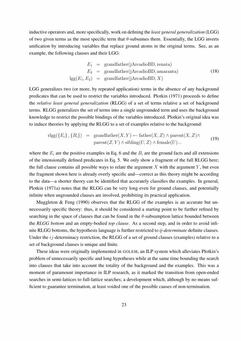
inductive operators and, more specifically, work on defining the least general generalization (LGG)of two given terms as the most specific term that θ-subsumes them. Essentially, the LGG invertsunification by introducing variables that replace ground atoms in the original terms. See, as anexample, the following clauses and their LGG:

E1 = grandfather(jArcadioBD, renata)

E2 = grandfather(jArcadioBD, amaranta)

lgg(E1, E2) = grandfather(jArcadioBD, X)

(18)

LGG generalizes two (or more, by repeated application) terms in the absence of any backgroundpredicates that can be used to restrict the variables introduced. Plotkin (1971) proceeds to definethe relative least general generalization (RLGG) of a set of terms relative a set of backgroundterms. RLGG generalizes the set of terms into a single ungrounded term and uses the backgroundknowledge to restrict the possible bindings of the variables introduced. Plotkin’s original idea wasto induce theories by applying the RLGG to a set of examples relative to the background:

rlgg({Ei} , {Bi}) = grandfather(X, Y )← father(X,Z) ∧ parent(X, Z)∧parent(Z, Y ) ∧ sibling(U,Z) ∧ female(U)...

(19)

where the Ei are the positive examples in Eq. 6 and the Bi are the ground facts and all extensionsof the intensionally defined predicates in Eq. 5. We only show a fragment of the full RLGG here;the full clause contains all possible ways to relate the argument X with the argument Y , but eventhe fragment shown here is already overly specific and—correct as this theory might be accordingto the data—a shorter theory can be identified that accurately classifies the examples. In general,Plotkin (1971a) notes that the RLGG can be very long even for ground clauses, and potentiallyinfinite when ungrounded clauses are involved, prohibiting its practical application.

Muggleton & Feng (1990) observes that the RLGG of the examples is an accurate but un-necessarily specific theory: thus, it should be considered a starting point to be further refined bysearching in the space of clauses that can be found in the θ-subsumption lattice bounded betweenthe RLGG bottom and an empty-bodied top clause. As a second step, and in order to avoid infi-nite RLGG bottoms, the hypothesis language is further restricted to ij-determinate definite clauses.Under the ij-determinacy restriction, the RLGG of a set of ground clauses (examples) relative to aset of background clauses is unique and finite.

These ideas were originally implemented in GOLEM, an ILP system which alleviates Plotkin’sproblem of unnecessarily specific and long hypotheses while at the same time bounding the searchinto clauses that take into account the totality of the background and the examples. This was amoment of paramount importance in ILP research, as it marked the transition from open-endedsearches in semi-lattices to full-lattice searches; a development which, although by no means suf-ficient to guarantee termination, at least voided one of the possible causes of non-termination.

23

3.4.3 Inverse Resolution

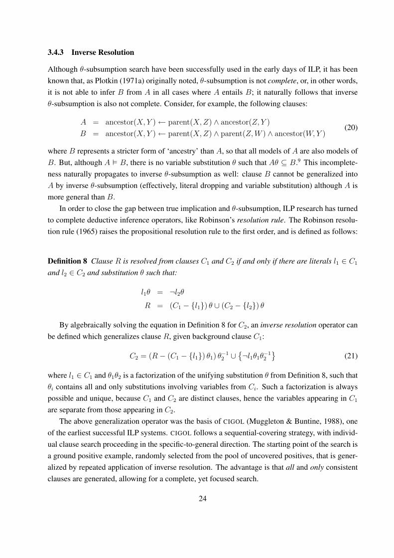
Although θ-subsumption search have been successfully used in the early days of ILP, it has beenknown that, as Plotkin (1971a) originally noted, θ-subsumption is not complete, or, in other words,it is not able to infer B from A in all cases where A entails B; it naturally follows that inverseθ-subsumption is also not complete. Consider, for example, the following clauses:

A = ancestor(X, Y )← parent(X, Z) ∧ ancestor(Z, Y )

B = ancestor(X, Y )← parent(X, Z) ∧ parent(Z,W ) ∧ ancestor(W, Y )(20)

where B represents a stricter form of ‘ancestry’ than A, so that all models of A are also models ofB. But, although A � B, there is no variable substitution θ such that Aθ ⊆ B.9 This incomplete-ness naturally propagates to inverse θ-subsumption as well: clause B cannot be generalized intoA by inverse θ-subsumption (effectively, literal dropping and variable substitution) although A ismore general than B.

In order to close the gap between true implication and θ-subsumption, ILP research has turnedto complete deductive inference operators, like Robinson’s resolution rule. The Robinson resolu-tion rule (1965) raises the propositional resolution rule to the first order, and is defined as follows:

Definition 8 Clause R is resolved from clauses C1 and C2 if and only if there are literals l1 ∈ C1

and l2 ∈ C2 and substitution θ such that:

l1θ = ¬l2θ

R = (C1 − {l1}) θ ∪ (C2 − {l2}) θ

By algebraically solving the equation in Definition 8 for C2, an inverse resolution operator canbe defined which generalizes clause R, given background clause C1:

C2 = (R− (C1 − {l1}) θ1) θ−12 ∪

{¬l1θ1θ

−12

}(21)

where l1 ∈ C1 and θ1θ2 is a factorization of the unifying substitution θ from Definition 8, such thatθi contains all and only substitutions involving variables from Ci. Such a factorization is alwayspossible and unique, because C1 and C2 are distinct clauses, hence the variables appearing in C1

are separate from those appearing in C2.The above generalization operator was the basis of CIGOL (Muggleton & Buntine, 1988), one

of the earliest successful ILP systems. CIGOL follows a sequential-covering strategy, with individ-ual clause search proceeding in the specific-to-general direction. The starting point of the search isa ground positive example, randomly selected from the pool of uncovered positives, that is gener-alized by repeated application of inverse resolution. The advantage is that all and only consistentclauses are generated, allowing for a complete, yet focused search.

24

3.4.4 Mode-Directed Inverse Entailment

While inverted resolution is complete, it disregards the background (modulo a single backgroundclause at each application), so it does not provide for a focused search. RLGG-based search, onthe other hand, does take into account the whole of the background theory, but it relies on invertingθ-subsumption, so it performs an incomplete search that can potentially miss good solutions.

In order to combine completeness with the informedness of the minimal-generalization bottom,Muggleton (1995) explores implication between clauses and ways of reducing inverse implicationto a θ-subsumption search without loss of completeness, and defines the inverse entailment opera-tor, based on the following proposition:

Lemma 1 Let C, D be definite, non-tautological clauses and S(D) be the sub-saturants of D.Then C � D if and only if there exists C ′ ∈ S(D) such that C � C ′.

where the sub-saturants of a clause D are, informally,10 all ungrounded clauses that can be con-structed from the symbols appearing in D and cannot prove the complement of D (i.e., do notresolve to any of the atoms in the Herbrand model of the complement of D).

Inverse entailment starts by saturating a ground positive example into a bottom clause, anungrounded clause which can prove only one ground positive example and no other. Because ofLemma 1, any clause which entails the original example will also θ-subsume the bottom clause; itis now sufficient to perform a θ-subsumption search in the full lattice between the empty-bodiedtop clause and the bottom clause without loss of completeness.

Mode-directed inverse entailment (MDIE) is a further refinement of inverse entailment wherethe semantics of the background predicates are taken into consideration during saturation (seebelow). The search in MDIE is organized in the general-to-specific direction in the original PRO-GOL system (Muggleton, 1995), as well as in most other successful MDIE ILP systems, like, e.g.,ALEPH (Srinivasan, 2004), INDLOG (Camacho, 2000), CILS (Anthony & Frisch, 1999), and APRIL

(Fonseca, 2006) although the alternative direction has been explored as well (Ong et al., 2005).

3.5 Saturation

Saturation is the process of constructing a bottom clause11 which constitutes the most-specificend of the search lattice in mode-directed inverse entailment. The most prominent characteristicof saturation is that it fills the ‘gap’ between θ-subsumption and entailment: the literals of thebottom clause are the sub-saturants of a clause C, hence identifying clauses that entail C amountsto identifying clauses that θ-subsume the bottom clause (Lemma 1).

Saturation is performed by repeated application of inverse resolution on a ground example,called the seed. This introduces variables in place of the ground terms in a ‘safe’ manner: thebottom clause is guaranteed to include all of and only the sub-saturants of the seed.

25

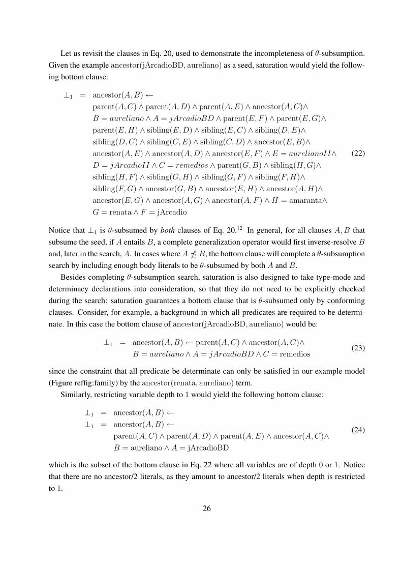
Let us revisit the clauses in Eq. 20, used to demonstrate the incompleteness of θ-subsumption.Given the example ancestor(jArcadioBD, aureliano) as a seed, saturation would yield the follow-ing bottom clause:

⊥1 = ancestor(A, B)←parent(A, C) ∧ parent(A, D) ∧ parent(A, E) ∧ ancestor(A, C)∧B = aureliano ∧ A = jArcadioBD ∧ parent(E, F ) ∧ parent(E, G)∧parent(E, H) ∧ sibling(E, D) ∧ sibling(E, C) ∧ sibling(D, E)∧sibling(D, C) ∧ sibling(C, E) ∧ sibling(C, D) ∧ ancestor(E, B)∧ancestor(A, E) ∧ ancestor(A, D) ∧ ancestor(E, F ) ∧ E = aurelianoII∧D = jArcadioII ∧ C = remedios ∧ parent(G, B) ∧ sibling(H, G)∧sibling(H, F ) ∧ sibling(G, H) ∧ sibling(G, F ) ∧ sibling(F, H)∧sibling(F, G) ∧ ancestor(G, B) ∧ ancestor(E, H) ∧ ancestor(A, H)∧ancestor(E, G) ∧ ancestor(A, G) ∧ ancestor(A, F ) ∧H = amaranta∧G = renata ∧ F = jArcadio

(22)

Notice that ⊥1 is θ-subsumed by both clauses of Eq. 20.12 In general, for all clauses A, B thatsubsume the seed, if A entails B, a complete generalization operator would first inverse-resolve B

and, later in the search, A. In cases where A � B, the bottom clause will complete a θ-subsumptionsearch by including enough body literals to be θ-subsumed by both A and B.

Besides completing θ-subsumption search, saturation is also designed to take type-mode anddeterminacy declarations into consideration, so that they do not need to be explicitly checkedduring the search: saturation guarantees a bottom clause that is θ-subsumed only by conformingclauses. Consider, for example, a background in which all predicates are required to be determi-nate. In this case the bottom clause of ancestor(jArcadioBD, aureliano) would be:

⊥1 = ancestor(A, B)← parent(A, C) ∧ ancestor(A, C)∧B = aureliano ∧ A = jArcadioBD ∧ C = remedios

(23)

since the constraint that all predicate be determinate can only be satisfied in our example model(Figure reffig:family) by the ancestor(renata, aureliano) term.

Similarly, restricting variable depth to 1 would yield the following bottom clause:

⊥1 = ancestor(A, B)←⊥1 = ancestor(A, B)←

parent(A, C) ∧ parent(A, D) ∧ parent(A, E) ∧ ancestor(A, C)∧B = aureliano ∧ A = jArcadioBD

(24)

which is the subset of the bottom clause in Eq. 22 where all variables are of depth 0 or 1. Noticethat there are no ancestor/2 literals, as they amount to ancestor/2 literals when depth is restrictedto 1.

26

3.6 Search Strategy

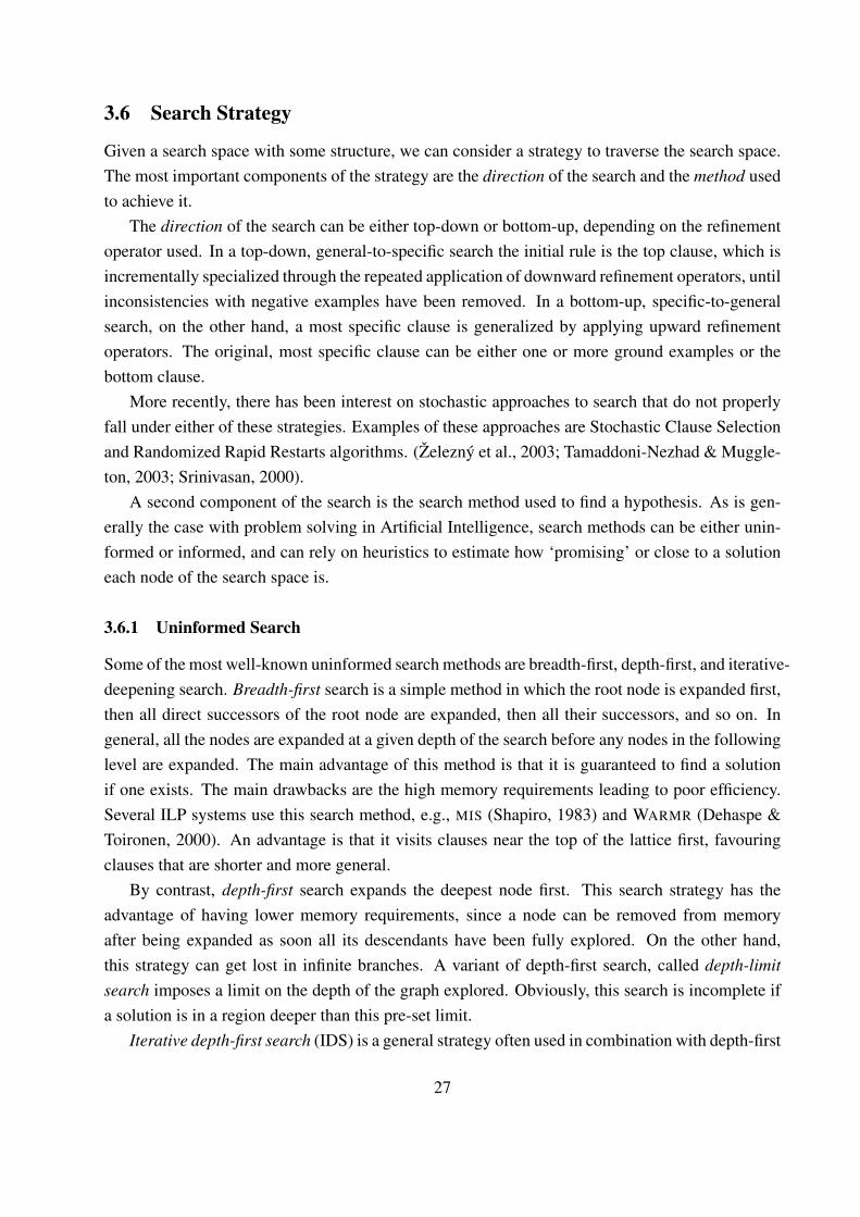
Given a search space with some structure, we can consider a strategy to traverse the search space.The most important components of the strategy are the direction of the search and the method usedto achieve it.

The direction of the search can be either top-down or bottom-up, depending on the refinementoperator used. In a top-down, general-to-specific search the initial rule is the top clause, which isincrementally specialized through the repeated application of downward refinement operators, untilinconsistencies with negative examples have been removed. In a bottom-up, specific-to-generalsearch, on the other hand, a most specific clause is generalized by applying upward refinementoperators. The original, most specific clause can be either one or more ground examples or thebottom clause.

More recently, there has been interest on stochastic approaches to search that do not properlyfall under either of these strategies. Examples of these approaches are Stochastic Clause Selectionand Randomized Rapid Restarts algorithms. (Železný et al., 2003; Tamaddoni-Nezhad & Muggle-ton, 2003; Srinivasan, 2000).

A second component of the search is the search method used to find a hypothesis. As is gen-erally the case with problem solving in Artificial Intelligence, search methods can be either unin-formed or informed, and can rely on heuristics to estimate how ‘promising’ or close to a solutioneach node of the search space is.

3.6.1 Uninformed Search

Some of the most well-known uninformed search methods are breadth-first, depth-first, and iterative-deepening search. Breadth-first search is a simple method in which the root node is expanded first,then all direct successors of the root node are expanded, then all their successors, and so on. Ingeneral, all the nodes are expanded at a given depth of the search before any nodes in the followinglevel are expanded. The main advantage of this method is that it is guaranteed to find a solutionif one exists. The main drawbacks are the high memory requirements leading to poor efficiency.Several ILP systems use this search method, e.g., MIS (Shapiro, 1983) and WARMR (Dehaspe &Toironen, 2000). An advantage is that it visits clauses near the top of the lattice first, favouringclauses that are shorter and more general.

By contrast, depth-first search expands the deepest node first. This search strategy has theadvantage of having lower memory requirements, since a node can be removed from memoryafter being expanded as soon all its descendants have been fully explored. On the other hand,this strategy can get lost in infinite branches. A variant of depth-first search, called depth-limitsearch imposes a limit on the depth of the graph explored. Obviously, this search is incomplete ifa solution is in a region deeper than this pre-set limit.

Iterative depth-first search (IDS) is a general strategy often used in combination with depth-first

27

search, that finds the best depth limit. It does this by gradually increasing the depth limit (first 0,then 1, then 2, and so on) until a solution is found. The drawback of IDS is the wasteful repetition ofthe same computations. Iterative deepening search is used in ILP systems like ALEPH (Srinivasan,2004) and INDLOG (Camacho, 2000).

3.6.2 Informed Search

Informed (heuristic) search methods can be used to find solutions more efficiently than uninformedbut can only be applied if there is a measure to evaluate and discriminate the nodes. Severalheuristics have been proposed for ILP.

A general approach to informed searching is best-first search. Best-first search is similar tobreadth-first but with the difference that the node selected for expansion is the one with the leastvalue of an evaluation function that estimates the ‘distance’ to the solution.

Note that the evaluation functions will return an estimate of the quality of a node. This estimateis given by a heuristics, a function that tries to predict the cost/distance to the solution from a givennode.

Best-first search is used in many ILP systems, like FOIL,CIGOL, INDLOG, and ALEPH. A formof best-first search is greedy best-first search as it expands only the node estimated to be closer tothe solution on the grounds that it would lead to a solution quickly. The most widely known formof best-first search is called A∗ search, which evaluates nodes by combining the cost to reach thenode and the distance/cost to the solution. This algorithm is used by the PROGOL ILP system.

The search algorithms mentioned so far explore the search space systematically. Alternatively,local search algorithms is a class of algorithms commonly used for solving computationally hardproblems involving very large candidate solution spaces. The basic principle underlying localsearch is to start from an initial candidate solution and then, iteratively, make moves from one can-didate solution to another candidate solution in its direct neighbourhood. The moves are based oninformation local to the node, and continue until a termination condition is met. Local search algo-rithms, although not systematic, have the advantage of using little memory and can find reasonablesolutions in large or infinite search spaces, where systematic algorithms are unsuitable.

Hill-climbing search Russell & Norvig (2003) is one example of a local search algorithm. Thealgorithm does not look ahead beyond the immediate successor nodes of the current node, and forthis reason it is sometimes called greedy local search. Although it has the advantage of reaching asolution more rapidly, it has some potential problems. For instance, it is possible to reach a foothill(local maxima or local minima), a state that is better than all its neighbours but it is not better thansome other states farther away. Foothills are potential traps for the algorithm. Hill-climbing isgood for a limited class of problems where we have an evaluation function that fairly accuratelypredicts the actual distance to a solution. ILP systems like FOIL and FORTE (Richards & Mooney,1995) use hill-climbing search algorithms.

28

3.7 Preference Bias and Search Heuristics

Prior knowledge representations described so far express strict constraints imposed on the hypoth-esized clauses, realized in the form of yes–no decisions on the acceptability of a clause. Theprevious section demonstrated the need for heuristics that identify the solution closest to the un-known target predicate, but, in the general case, there may be multiple solutions that satisfy therequirements of the problem; or we may have no solution but still want the best approximation.ILP algorithms therefore need to choose among partial solutions and provide justification for thischoice besides consistency with the background and the examples. Preference bias does just that:it assigns a ‘usefulness’ rating to clauses which typically says how close we are to the best solution.In practice, the is translated into an evaluation function that tries to estimate how well a clause willperform when applied to data unseen during training.

The user may provide general preferences, for instance towards shorter clauses, or towardsclauses that achieve wide coverage, or towards clauses with higher predictive accuracy on thetraining data, or any other problem-specific preference deemed useful. Preference bias also mustnavigate a balance between specificity and generality: a theory with low coverage may describethe data too tightly and may not generalize well (overfit). Indeed, at its extreme may it only acceptsthe positive examples it was constructed from and nothing else. On the other hand, a theory thatmakes unjustified generalizations can underfit, and at the extreme, accept everything as a positive.

3.7.1 Entropy and m-Probability

Evaluation functions will typically judge a clause semantically and so the most commonly usedevaluation functions refer to a clause’s coverage over positive and negative examples. Such func-tions include simple coverage, information gain (Clark & Niblett 1989, based on the concept ofentropy as defined by Shannon 1948), m-probability estimate (Cestnik, 1990), and the Laplaceexpected accuracy:

Coverage(P, N) = P −N (25)

InfGain(P, N) = −Prel · log2 Prel −Nrel · log2 Nrel (26)

MEstm,P0(P, N) = (P + m · P0) / (P + N + m) (27)

Laplace(P, N) = (P + 1) / (P + N + 2) (28)

where P , N is the positive and negative coverage, Prel = P/(P + N), Nrel = 1 − Prel therelative positive and negative coverage, P0 is the prior probability of positive examples (i.e., theprobability that a random example is positive) and m a parameter that weighs the prior probabilityagainst the observed accuracy. It should be noted that the Laplace function is a specialization ofthe m-probability estimate for uniform prior distribution of positives and negatives (P0 = 0.5) withthe m parameter set to a value of 2, a value that balances between prior and observation.

29

Inf. Gain Laplace Acc.C1 (980,20) 0.141 0.979

C2 (98,2) 0.141 0.971

C3 (1,0) 1.000 0.667

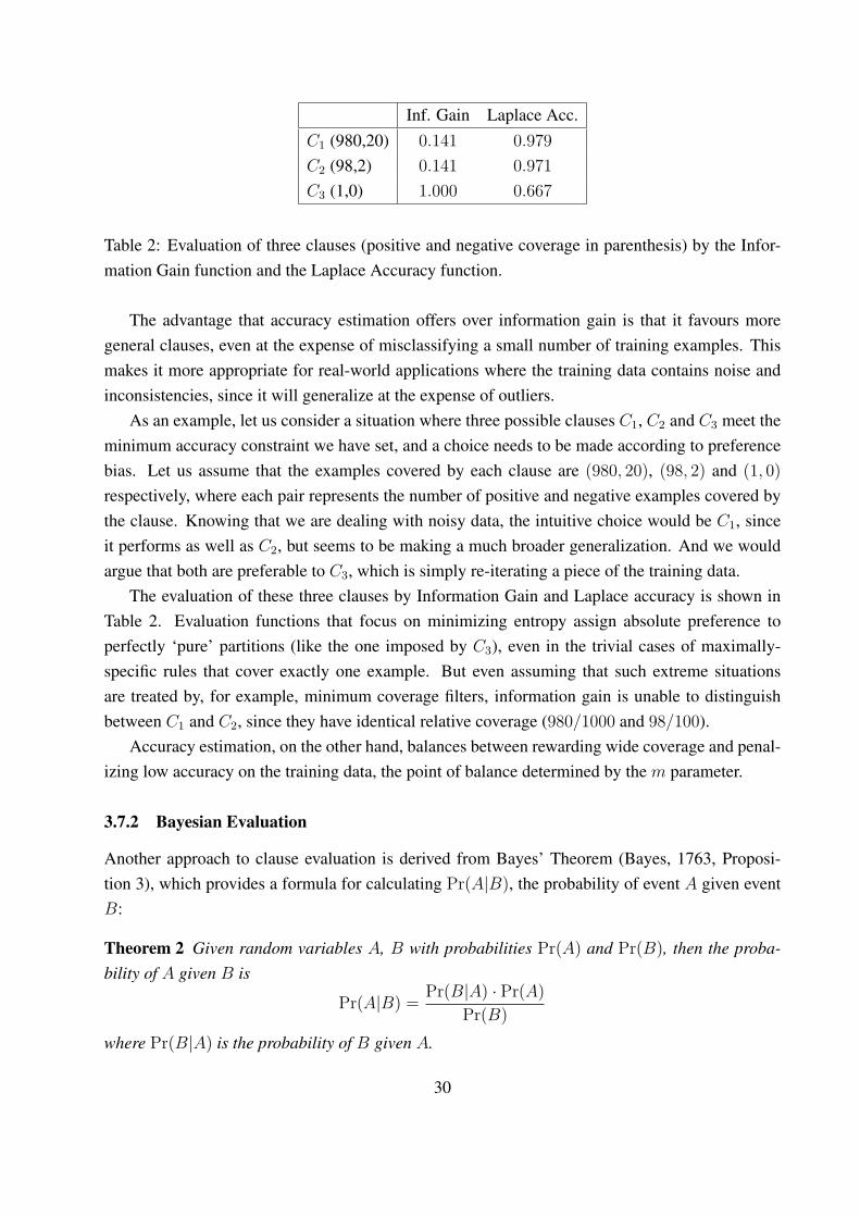
Table 2: Evaluation of three clauses (positive and negative coverage in parenthesis) by the Infor-mation Gain function and the Laplace Accuracy function.

The advantage that accuracy estimation offers over information gain is that it favours moregeneral clauses, even at the expense of misclassifying a small number of training examples. Thismakes it more appropriate for real-world applications where the training data contains noise andinconsistencies, since it will generalize at the expense of outliers.

As an example, let us consider a situation where three possible clauses C1, C2 and C3 meet theminimum accuracy constraint we have set, and a choice needs to be made according to preferencebias. Let us assume that the examples covered by each clause are (980, 20), (98, 2) and (1, 0)

respectively, where each pair represents the number of positive and negative examples covered bythe clause. Knowing that we are dealing with noisy data, the intuitive choice would be C1, sinceit performs as well as C2, but seems to be making a much broader generalization. And we wouldargue that both are preferable to C3, which is simply re-iterating a piece of the training data.

The evaluation of these three clauses by Information Gain and Laplace accuracy is shown inTable 2. Evaluation functions that focus on minimizing entropy assign absolute preference toperfectly ‘pure’ partitions (like the one imposed by C3), even in the trivial cases of maximally-specific rules that cover exactly one example. But even assuming that such extreme situationsare treated by, for example, minimum coverage filters, information gain is unable to distinguishbetween C1 and C2, since they have identical relative coverage (980/1000 and 98/100).

Accuracy estimation, on the other hand, balances between rewarding wide coverage and penal-izing low accuracy on the training data, the point of balance determined by the m parameter.

3.7.2 Bayesian Evaluation

Another approach to clause evaluation is derived from Bayes’ Theorem (Bayes, 1763, Proposi-tion 3), which provides a formula for calculating Pr(A|B), the probability of event A given eventB:

Theorem 2 Given random variables A, B with probabilities Pr(A) and Pr(B), then the proba-bility of A given B is

Pr(A|B) =Pr(B|A) · Pr(A)

Pr(B)

where Pr(B|A) is the probability of B given A.

30

Suppose we have a clause of the form A ← B, and Pr(A), Pr(B) are the probabilities that predi-cates A and B hold for some random example. We can now apply Bayes’ Theorem to calculate theprobability that, for some random example, if the clause’s antecedents hold, then the subsequentholds. In a semantics sense, this is the probability that the clause accurately classifies the exam-ple. Probability Pr(A|B) is called the posterior distribution of A, by contrast to prior distributionPr(A), the distribution of A before seeing the example.

Bayes (idem., Proposition 7) continues by using the empirical data to estimate an unknownprior distribution. This last result is transferred to ILP by Cussens (1993) as the pseudo-bayes13

evaluation function:Acc = P/(P + N)

K = Acc · (1− Acc) / (P0 − Acc)2

PBayes = (P + K · P0) / (P + N + K)

(29)

where P0 is the positive distribution observed in the data, and P and N are the positive and negativecoverage of the clause. A comparison of the pseudo-Bayes evaluation function with m-estimation(Eq. 27) shows that one way of looking at pseudo-Bayes evaluation is as an empirically justifiedway of calculating the critical m parameter of m-estimation.

3.7.3 Syntactic Considerations

Some evaluation functions will also refer to syntactic aspects of the hypothesized clause, imple-menting (for example) preference bias towards shorter or simpler clauses, in accordance with thegeneral principle of parsimony known as Ockham’s Razor. The simplest such function is

CoverShort(P, N, L) = P −N − L + 1 (30)

where P , N is the positive and negative coverage and L is the number of literals in the clause.More sophisticated approaches to quantifying ‘simplicity’ are based on Rissanen’s (1978) min-

imum description length (MDL) principle that the most probable hypothesis H given data D is theone that minimizes the complexity of H given D, defined as the logarithmic version of the BayesTheorem:

K(H|D) = K(H) + K(D|H)−K(D) + c (31)

where c is a constant and K(·) is the Kolmogorov complexity (1965) of a logic program.The MDL has given rise to various evaluation functions proposing different approximations

of the Kolmogorov complexity of a logic program. Tang & Mooney (2001), for example, do notsimply count the number of literals L in a clause to determine its size, but take into account theirstructural complexity as well:

size(T ) =

1 if T is a variable2 if T is a constant2 +

∑ni=1 size (argi (T )) if T is a term of arity n

(32)

31

This quantification of clause complexity was used in the MDL evaluation function of the COCK-TAIL ILP system (idem.).

On the other hand, Muggleton, Srinivasan, & Bain (1992) take a different approach and re-introduce a semantic element in the notion of logic program complexity: the proof complexity C ofa logic program given a dataset is the number of choice-points that SLDNF resolution goes thoughin order to derive the data from the program. The proof encoding length Lproof of the hypothesis foreach example can be approximated by combining the proof complexity with coverage results whichestimate the compression achieved by the hypothesis and with the total (positive and negative)coverage, which is taken as a measure of the generality of the clause (idem., Section 3):

Lproof = (P + N) ·(

Cav + log1

AccAcc · (1− Acc)1−Acc

)(33)

where Acc is the observed accuracy P/ (P + N) and Cav the average proof complexity of thehypothesis over all the examples. It is easy to see that the logarithmic term (which representsthe performance of the hypothesis) is dominated by the proof complexity term and the generalityfactor, so that it comes into consideration when comparing hypotheses with similar (semantic)generality and (syntactic) complexity characteristics.

3.7.4 Positive-Only Evaluation

One other category of evaluation functions that should be particularly noted is those that facilitatelearning in the absence of negative examples (positive examples only). Conventional semanticevaluation functions cannot be used because in this case, in the absence of negative examples, thetrivial clause that accepts all examples will always score best.

For this reason, positive-only evaluation functions balance positive coverage against a clause’sgenerality, to avoid favouring over-generalization. Generality can be estimated syntactically aswell as semantically, as in the posonly function (Muggleton, 1996):

PosOnlyC,Rall(P, R, L) = log P − C log

R + 1.0

Rall + 2.0− L

P(34)

where (R+1.0)/(Rall +2.0) is a Laplace-corrected estimation of the clause’s generality. The esti-mation is made by randomly generating Rall examples and measuring the clause’s coverage R overthem. The formula is balancing between rewarding coverage (the first term) and penalizing gener-ality (the second term), so as to avoid over-general clauses in the absence of negative data. The C

parameter implements prior preference towards more general or more specific clauses and the thirdterm implements syntactic bias towards shorter clauses, unless extended coverage compensates forthe length penalty.

32

3.8 Other Approaches to ILP

We have so far focused ILP systems that perform a clause-level search on a pre-defined, staticsearch space. Although these systems form the mainstream of ILP research, other options havebeen explored as well, namely searching at the theory level and searching in a dynamic space.

3.8.1 Theory-level Search

The sequential cover strategy has a profound impact on the size of the search space, as it restrictsthe search to the space of single clauses. It does so, however, at the risk of missing out on goodsolutions, since the the concatenation of good clauses is not necessarily a good theory: the bestclause, given a set of positives, might leave a positives pool that is not easily separable, whereas a(locally) worse clause might allow for a better overall theory.

This is especially true for systems that saturate examples to build the bottom clause, as the(random) choice of the seed is decisive for the search sub-space that will be explored. An unfortu-nate seed choice might ‘trap’ subsequent clausal searches with an unnecessarily difficult positivespool. In sequential-cover systems the problem can be somewhat alleviated by saturating multipleseeds; in the ALEPH system, to name one example, the user can specify the number of examplesthat must be saturated for each positives pool. After performing as many searches as there werebottom clauses constructed, the best clause is appended to the theory and the process re-iterates.

Such techniques can improve the quality of the constructed theories, but not completely solvethe problem, which can only be tackled by evaluating the theory as a whole at each step for thesearch. In theory-level searching the search space is the lattice formed by the set all admissibletheories (as opposed to clauses), structured into a lattice by a theory-level refinement operator.It is immediately obvious that not only does search space become dramatically larger, but therefinement operator also gains more degrees of indeterminism, making the search even harder: therefinement operator can (a) specify or generalize a clause, (b) delete a clause altogether, or (c) starta new (top or bottom) clause.

In order to handle the increase in the size and complexity of the search space ILP systems thatsupport theory-level search, like ALEPH, exploit randomized search methods to improve efficiency.Randomized search methods and other efficiency optimizations used in ILP systems are furtherdescribed below.

3.8.2 Dynamically Changing Search Spaces

We end the section with an overview of algorithms that tackle dynamically changing search spaces,due to bias shift and background theory revision (background predicate invention and refinement).

Descriptive ILP systems readily offer themselves to predicate invention, since they are orientedtowards discovering ‘property clusters’ in the data and multi-predicate learning. Systems like

33

CLAUDIEN (De Raedt & Dehaspe, 1996) propose predicates that separate such clusters, and alsore-use these predicates in the definitions of subsequently constructed predicate clauses.

Single-predicate learning, predictive ILP systems, on the other hand, typically assumed that thebackground predicates are both correct and sufficient to solve the problem, and no attempt is madeto revise or supplement them. Some systems, however, do attempt background theory revision.SPECTRE (Boström, 1996), for example, attempts background theory refinement by examining theSLD proof-trees generated during hypothesis matching. When pruning a background predicate’sproof-tree (effectively, specializing the predicate) eliminates negative coverage, the backgroundpredicate is amended accordingly.

The same idea was further explored in the MERLIN2.0 system (Boström, 1998), this time at-tempting predicate invention, which expands the background theory with new predicates deemeduseful for constructing a theory. MERLIN2.0 unfolds the SLD proof-trees of background predi-cates, and identifies new sub-predicates (in the semantic sense of predicates achieving a subset ofthe original predicate’s coverage) which improve accuracy when used to construct a theory.

Inverse resolution also offers an opportunity for predicate invention: Muggleton (1988) pro-poses a predicate invention algorithm which asserts a predicate when its presence allows an—otherwise unattainable—inverse resolution step to proceed, if the generalization performed by thisstep evaluates well on the data. This idea was implemented in CIGOL (Muggleton & Buntine,1988), an inverse-resolution ILP system, but was later abandoned as predictive ILP research movedtowards inverse entailment systems that use θ-subsumption as their refinement operator.

4 EFFICIENT INDUCTIVE LOGIC PROGRAMMING

A crucial point for the applicability of ILP is its efficiency in terms of computational resourcesneeded to construct a theory. As has been experimentally verified Železný et al. (2003), ILP sys-tems’ run-times exhibit considerable variability, depending on the heuristics, the problem instance,and the choice of seed examples.

The total execution time of an ILP system can be roughly divided into three major components:

• time spent generating clauses, which can be a major concern for large real-world problems,and particularly in novel application domains where prior domain knowledge is fragmentaryand the search space cannot be restricted without risking to exclude good solutions;

• time spent evaluating clauses, typically due to the size of the data, although Botta et al.(2003) have shown that there are circumstances under which evaluation can become ex-tremely hard, even if model-spaces and datasets are quite small; and

• time spent accessing the data, as some datasets can be extremely large, e.g., biologicaldatabases arising from sequencing animal and plant genomes. Constructing models of such

34

data requires an ILP system to be able to efficiently access millions of data items.

The relative weight of each component depends on the ILP system used, on the search algorithm,on the parameter settings, and on the data, but in most cases evaluating rule quality is responsiblefor most of the execution time.

In this section we describe methods for improving the efficiency of ILP systems directly relatedto the three concerns raised above (large search spaces, large datasets, evaluation). Some of thesemethods are improvements and optimizations of the sequential execution of ILP systems, whereassome are stochastic approaches to search or parallelisms of the search strategy.

Before proceeding, we provide a classification of the techniques regarding their correctness.In this context, a correct technique should be understood as yielding the same results as somereference algorithm that does not employ the technique. An approximately correct technique doesnot preserve correctness, but still gives results that are, with high probability, similar (in quality)to the results produced by the reference technique.

4.1 Reducing the Search Space

In the Hypothesis Language section above, we have discussed a variety of tools that ILP systemsoffer for controlling the search space. More specifically, we have discussed how the search spaceis initially defined by the vocabulary provided by the background theory and then further refinedby language bias such as hypothesis checking and pruning, determinacy constrains, and type-modedeclarations.

In the theoretic context of our previous discussion of these tools, they have been presented asa means of excluding potentially good solutions on grounds that the ILP algorithm cannot accessthrough example-driven evaluation, like non-conformance with a theoretical framework. We shallhere revisit the same tools in order to review them from a different perspective: instead of a meansof excluding empirically good solutions that should be avoided on theoretical grounds, they areviewed as an optimization that excludes bad solutions before having to evaluate them in order toreject them.

4.1.1 Hypothesis Checking and Pruning

We have seen how hypothesis checking can be used to impose syntactic as well as as semanticconstraints on the hypothesis language. In many situations it is possible to capitalize on the mono-tonicity of definite clause logic in order to direct the search away not from individual clauses, butfrom whole areas of the search space that are known to not contain any solutions.

Consider, for example, a clause containing in its body literals that are known to be inconsistentwith each other, say male(X) and female(X). Not only is such a clause bound to not cover anyexamples, but all its specializations can also safely ignored. In systems that support pruning, prior

35

knowledge can be provided which, once such a clause in encountered during the search, prunesaway the whole sub-space subsumed by the clause.

Another method that takes advantage of prior expert knowledge to reduce the hypothesis lan-guage is redundancy declarations. Fonseca et al. (2004) propose a classification of redundancy inthe hypothesis language and show how expert knowledge can be provided to an ILP system to inorder reduce it. The technique is correct (if complete search is performed) and yields good results.

Two things must be noted at this point: first that useful as they might be, semantic hypothe-sis checking and pruning are bound to make a smaller difference with respect to efficiency thattheir syntactic counterparts since they require the—potentially expensive—coverage computationsto be carried out whereas purely syntactic checking can discard a hypothesis beforehand. And,second, that the hypothesis checking, pruning, and redundancy declarations must be provided bythe domain expert. This task that can be tedious and error-prone and has not been successfullyautomated.

4.1.2 Determinacy and Type-mode Declarations

Determinacy and type-mode declarations can also be used to state not a theoretical restriction, butan actual fact about the background theory. When used in this manner they are not excluding em-pirically possible—but otherwise unacceptable—solutions, but they are rather steering the searchaway from areas of the search that are known to be infertile.

Consider, for example, the declarations in Eq. 16 above. While the type-mode declarations forthe grandfather/2 predicate are, as we have already discussed, enforcing a genuine restriction, therest are stating actual facts about the semantics of the background predicates. So, for instance, theparent/2 declaration is prohibiting the consideration of hypotheses like this one:

C = grandfather(X, U)← father(X, Y ) ∧ parent(Y, U) ∧male(U)∧parent(Y, V ) ∧male(V ) ∧ parent(Y,W ) ∧male(W )

(35)

which only admits grand-fatherhood in the presence of three or more grand-sons. This clauseis rejected because the background theory does not allow instantiations where three children aremale. The clause can only succeed by unifying two of U, V,W and can be safely ignored: no ILPalgorithm would have chosen this clause anyway, as the model of our example identical semanticscan be achieved by a simpler clause.

In general, providing the smallest determinacy values that will not leave any solutions out ofthe hypothesis space is a correct optimization of the ILP search. Similarly for type declarations,where assigning incompatible types can help avoid evaluating obviously inconsistent clauses like,for example:

D = grandfather(X, Y )← femaleX ∧ father(X, Z) ∧ parent(Z, Y ) (36)

36

Prior knowledge of small, but safe, determinacy and type-mode parameters can significantlytighten the search space around the solutions. These semantic characteristics of the backgroundtheory are typically expected as user input, but research on their automatically extraction from thebackground has also been pursued (McCreath & Sharma, 1995).

4.1.3 Incremental Search

Another approach is to not restrict the hypothesis language, but to incrementally consider largerand larger subsets thereof. The whole hypothesis language will only be considered if we cannotfind a model within one of these subsets. Srinivasan et al. (2003) propose a technique that exploreshuman expertise to provide a relevance ordering on the set of background predicates. The tech-nique follows a strategy of incrementally including sets of background knowledge predicates indecreasing order of relevance and has shown to yield good results.

Another technique that incrementally increases the hypothesis space is Incremental LanguageLevel Search (ILLS) (Camacho, 2002). It uses an iterative search strategy to, starting from one,progressively increase the upper-bound on the number of occurrences of a predicate symbol in thegenerated hypotheses. This technique is correct if a complete search is performed and Camachoreport substantial efficiency improvements on several ILP applications.

4.2 Efficient Evaluation

As described above, hypotheses are evaluated by metrics that make reference to their coverageover the training data. Coverage is calculated by matching (or testing) all examples against thehypothesis; this involves finding a substitution such that the body of one of the hypothesis’ clausesis true given the example and background knowledge.

An often used approach in ILP to match hypotheses is to use logical querying. The logicalquerying approach to clause matching involves the use of a Prolog engine to evaluate the clausewith the examples and background knowledge. The execution time to evaluate a query dependson the number of examples, number of resolution steps, and on the execution time of individualliterals. Thus, scalability problems may arise when dealing with a great number of examples or/andwhen the computational cost to evaluate a rule is high. Query execution using SLDNF resolutiongrows exponentially with the number of literals in the query (Struyf, 2004). Hence, evaluating asingle example can take a long time.

Several techniques have been proposed to improve the efficiency of hypotheses evaluation.Firstly, the evaluation of a hypothesis can be optimized by transforming the hypothesis into anequivalent one that can be more efficiently executed (Santos Costa et al., 2000; Santos Costa,Srinivasan, et al., 2003). An important characteristic of these techniques is that the transforma-tions between equivalent hypothesis are correct. The transformation can be done at the level of

37

individual hypotheses (Santos Costa et al., 2000; Struyf & Blockeel, 2003) or at the level of sets ofhypotheses (Tsur et al., 1998; Blockeel et al., 2002).

A different method to speedup evaluation explores the existing redundancy on the sets ofhypotheses evaluated: similar hypotheses are generated and evaluated in batches, called querypacks (Blockeel et al., 2002), thus avoiding the redundant repetition of the same proof steps indifferent, but similar, hypotheses.

Approximate evaluation is another well-studied way of reducing the execution time of hypoth-esis evaluation. Stochastic matching (Sebag & Rouveirol, 1997), or stochastic theorem proving,was tested with the PROGOL ILP system, and has yielded considerable efficiency improvements,without sacrificing predictive accuracy or comprehensibility. This approach was further pursuedby Giordana et al. (2000), making the benefits of replacing deterministic matching with stochasticmatching clearly visible. A variety of other approximate matching schemes (Srinivasan, 1999; Ki-jsirikul et al., 2001; DiMaio & Shavlik, 2004; Bockhorst & Ong, 2004) have also been successfullytried.

Another technique, called lazy evaluation,14 of examples (Camacho, 2003) aims at speedingup the evaluation of hypotheses by avoiding the unnecessary use of examples in the coveragecomputations, yielding considerable reduction of the execution time. The rationale underlying lazyevaluation is the following: a hypothesis is allowed to cover a small number of negative examples(the noise level) or none. If a clause covers more than the allowed number of negative examples itmust be specialized. Lazy evaluation of negatives can be used when we are interested in knowingif a hypothesis covers more than the allowed number of negative examples or not. Testing stops assoon as the number of negative examples covered exceeds the allowed noise level or when there areno more negative examples to be tested. Therefore, the number of negative examples effectivelytested may be very small, since the noise level is quite often very close to zero. If the evaluationfunction used does not involve negative coverage in its calculations, then this produces exactly thesame results (clauses and accuracy) as the non-lazy approach but with a reduction on the numberof negative examples tested.

One may also allow positive coverage to be computed lazily (lazy evaluation of positives). Aclause is either specialized (if it covers more positives than the best consistent clause found so far)or justifiably pruned away otherwise. When using lazy evaluation of positives it is only relevant todetermine if a hypothesis covers more positives than the current best consistent hypothesis or not.We might then just evaluate the positive examples until we exceed the best cover so far. If the bestcover is exceeded we retain the hypothesis (either accept it as final if it is consistent or refine itotherwise) or we may justifiably discard it. We need to evaluate its exact positive cover only whenaccepting a consistent hypothesis. In this latter case we don’t need to restart the positive coveragecomputation from scratch, we may simply continue the test from the point where we left it before.

Storing intermediate results during the evaluation for later use (i.e., by performing a kind of acache) can be a solution to reduce the time spent in hypothesis evaluation. The techniques that fol-

38

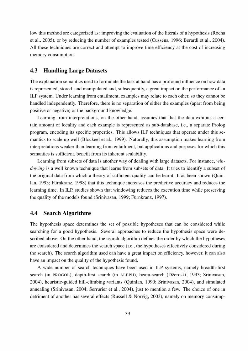
low this method are categorized as: improving the evaluation of the literals of a hypothesis (Rochaet al., 2005), or by reducing the number of examples tested (Cussens, 1996; Berardi et al., 2004).All these techniques are correct and attempt to improve time efficiency at the cost of increasingmemory consumption.

4.3 Handling Large Datasets

The explanation semantics used to formulate the task at hand has a profound influence on how datais represented, stored, and manipulated and, subsequently, a great impact on the performance of anILP system. Under learning from entailment, examples may relate to each other, so they cannot behandled independently. Therefore, there is no separation of either the examples (apart from beingpositive or negative) or the background knowledge.

Learning from interpretations, on the other hand, assumes that that the data exhibits a cer-tain amount of locality and each example is represented as sub-database, i.e., a separate Prologprogram, encoding its specific properties. This allows ILP techniques that operate under this se-mantics to scale up well (Blockeel et al., 1999). Naturally, this assumption makes learning frominterpretations weaker than learning from entailment, but applications and purposes for which thissemantics is sufficient, benefit from its inherent scalability.

Learning from subsets of data is another way of dealing with large datasets. For instance, win-dowing is a well known technique that learns from subsets of data. It tries to identify a subset ofthe original data from which a theory of sufficient quality can be learnt. It as been shown (Quin-lan, 1993; Fürnkranz, 1998) that this technique increases the predictive accuracy and reduces thelearning time. In ILP, studies shown that windowing reduces the execution time while preservingthe quality of the models found (Srinivasan, 1999; Fürnkranz, 1997).

4.4 Search Algorithms

The hypothesis space determines the set of possible hypotheses that can be considered whilesearching for a good hypothesis. Several approaches to reduce the hypothesis space were de-scribed above. On the other hand, the search algorithm defines the order by which the hypothesesare considered and determines the search space (i.e., the hypotheses effectively considered duringthe search). The search algorithm used can have a great impact on efficiency, however, it can alsohave an impact on the quality of the hypothesis found.

A wide number of search techniques have been used in ILP systems, namely breadth-firstsearch (in PROGOL), depth-first search (in ALEPH), beam-search (Džeroski, 1993; Srinivasan,2004), heuristic-guided hill-climbing variants (Quinlan, 1990; Srinivasan, 2004), and simulatedannealing (Srinivasan, 2004; Serrurier et al., 2004), just to mention a few. The choice of one indetriment of another has several effects (Russell & Norvig, 2003), namely on memory consump-

39

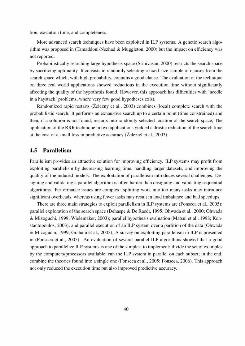
tion, execution time, and completeness.

More advanced search techniques have been exploited in ILP systems. A genetic search algo-rithm was proposed in (Tamaddoni-Nezhad & Muggleton, 2000) but the impact on efficiency wasnot reported.

Probabilistically searching large hypothesis space (Srinivasan, 2000) restricts the search spaceby sacrificing optimality. It consists in randomly selecting a fixed-size sample of clauses from thesearch space which, with high probability, contains a good clause. The evaluation of the techniqueon three real world applications showed reductions in the execution time without significantlyaffecting the quality of the hypothesis found. However, this approach has difficulties with ‘needlein a haystack’ problems, where very few good hypotheses exist.

Randomized rapid restarts (Železný et al., 2003) combines (local) complete search with theprobabilistic search. It performs an exhaustive search up to a certain point (time constrained) andthen, if a solution is not found, restarts into randomly selected location of the search space, Theapplication of the RRR technique in two applications yielded a drastic reduction of the search timeat the cost of a small loss in predictive accuracy (Železný et al., 2003).

4.5 Parallelism

Parallelism provides an attractive solution for improving efficiency. ILP systems may profit fromexploiting parallelism by decreasing learning time, handling larger datasets, and improving thequality of the induced models. The exploitation of parallelism introduces several challenges. De-signing and validating a parallel algorithm is often harder than designing and validating sequentialalgorithms. Performance issues are complex: splitting work into too many tasks may introducesignificant overheads, whereas using fewer tasks may result in load imbalance and bad speedups.

There are three main strategies to exploit parallelism in ILP systems are (Fonseca et al., 2005):parallel exploration of the search space (Dehaspe & De Raedt, 1995; Ohwada et al., 2000; Ohwada& Mizoguchi, 1999; Wielemaker, 2003); parallel hypothesis evaluation (Matsui et al., 1998; Kon-stantopoulos, 2003); and parallel execution of an ILP system over a partition of the data (Ohwada& Mizoguchi, 1999; Graham et al., 2003). A survey on exploiting parallelism in ILP is presentedin (Fonseca et al., 2005). An evaluation of several parallel ILP algorithms showed that a goodapproach to parallelize ILP systems is one of the simplest to implement: divide the set of examplesby the computers/processors available; run the ILP system in parallel on each subset; in the end,combine the theories found into a single one (Fonseca et al., 2005; Fonseca, 2006). This approachnot only reduced the execution time but also improved predictive accuracy.

40

5 APPLICATIONS

In this section we briefly outline and provide references to various real-world applications of ILP,from medicine and biology, to language technology where ILP systems have made significantcontributions to the discovery of new scientific knowledge.

Although we discuss in more detail applications in the three main areas of Life Sciences, Lan-guage Processing, and Engineering, ILP has been used in a variety of other domains. Examplesof important applications of ILP must, at the very least, include domains such as music (Pompeet al., 1996; Tobudic & Widmer, 2003), the environment (Džeroski et al., 1995; Blockeel et al.,2004), intelligence analysis (Davis, Dutra, et al., 2005), and mathematical discovery (Colton &Muggleton, 2003; Todorovski et al., 2004).

5.1 Life Sciences

Inductive Logic Programming has been applied in a wide variety of domains of the Life Sciences,ranging over domains as diverse as Medical Support Systems (Carrault et al., 2003) and Computa-tional Biochemistry (Srinivasan et al., 1994; Page & Craven, 2003).

Clinical data is one of the major sources of challenging datasets for ILP. To cite but a fewexample applications we will mention successful work on the characterization of cardiac arrhyth-mias (Quiniou et al., 2001), intensive care monitoring (Morik et al., 1999), diagnosis support sys-tems for rheumatic diseases (Zupan & Džeroski, 1998) or breast cancer (Davis, Burnside, et al.,2005).

One of the major applications of Inductive Logic Programming so far has been in the areaof Structure-Activity Relationships (SAR), the task of predicting the activity of drug moleculesbased on their structure. Early examples of this work include detecting mutagenic (Srinivasan etal., 1994) and carcinogenic (Srinivasan et al., 1997) properties in compounds. In the continuation,researchers have used ILP for 3D-SAR, where one uses a 3D description of the main elements inthe compound to find pharmacophores that explain drug activity Finn et al. (1998). Among thesuccessful examples of ILP applications one can mention pharmacophores for dopamine agonists,ACE inhibitors, Thermolysin inhibitors, and antibacterial peptides (Enot & King, 2003). A relatedapplication with a different approach is the work in Diterpene structure elucidation by Džeroski etal. (1996).

ILP has also made significant contributions to the expanding area of Bioinformatics and Com-putational Biology. One major interest in this area has been in explaining protein structure, in-cluding secondary structure (Muggleton, King, & Sternberg, 1992; Mozetic, 1998) and fold pre-diction (Turcotte et al., 2001). Another very exciting area of ILP research is helping understandcell machinery; the work of Bryant et al. (2001) should be mentioned as the seminal work onunderstanding metabolic pathways of yeast. Finally, in genetics, recent work has also achieved

41

promising results on using ILP to predict the functional class of genes (King, 2004) and to under-stand the combination of gene expression data with structure and/or function gene data (Struyf etal., 2005).

Recent studies on automating the scientific discovery process King et al. (2004) embed ILPsystems in the cycle of scientific experimentation. The cycle includes the automatic generationof hypotheses to explain observations, the devising of experiments to evaluate the hypotheses,physically run the experiments using a laboratory robot, interprets the results to falsify hypothesesinconsistent with the data and then repeats the cycle.

5.2 Language Technology

The ability to take advantage of explicit background knowledge and bias constitutes one of thestrongest points in favour of applying ILP to language technology tasks, as it provides a means ofdirectly exploiting a very long and rich tradition of theoretical linguistics research.

More specifically, syntactic bias allows for the restriction of the hypothesis space within thelimits of a meta-theory or theoretical framework. Except for the theoretical merit it carries onits own, this ability also offers the opportunity to capitalize on linguistic knowledge in order toreduce the computational cost of searching the hypothesis space, whereas many alternative learningschemes cannot make such explicit use of existing knowledge.

Language technology experimentation with ILP runs through the whole range of fields of thestudy of language, from phonology and morphology all the way to syntax, semantics and discourseanalysis: we will mention work on prediction of past tenses (Muggleton & Bain, 1999), nomi-nal paradigms (Džeroski & Erjavec, 1997), part-of-speech tagging (Dehaspe & De Raedt, 1997;Cussens, 1997), learning transfer rules (Boström, 2000), and focus on parsing and phonotactics(below).

Another exciting application of ILP is in the area of Information Extraction (IE). This includeswork on document analysis and understanding (Esposito et al., 1993) and work on web page char-acterization that has had a profound practical impact (Craven & Slattery, 2001). Interesting resultshave been achieved when using ILP for performing IE over scientific literature (Califf & Mooney,1999; Goadrich et al., 2004; Malerba et al., 2003).

5.2.1 Parser Construction

The syntax of an utterance is the way in which words combine to form grammatical phrases andsentences and the way in which the semantics of the individual words combine to give rise to thesemantics of phrases and sentences. It is, in other words, the structure hidden behind the (flat)utterance heard and seen on the surface.

Since the seminal work of Chomsky (1957), it is the fundamental assumption of linguisticsthat this structure has the form of a tree, where the terminal symbols are the actual word-forms and

42

the non-terminal symbols abstractions of words or multi-word phrases. It is the task of a compu-tational grammar to describe the mapping between syntactic trees structures and flat utterances.Computational grammars are typically Context-Free or Definite Clause Grammars,15 which de-scribe syntactic structures in terms of derivations. Such grammars are used to control a parser,the piece of computational machinery that builds the parse tree of the phrase from the derivationsnecessary to successfully recognise the phrase.

Definite Clause Grammars can be naturally represented as Definite Clause Programs and theirderivations map directly to Definite Logic Programming proofs. This does not, however, meanthat grammar construction can be trivially formulated as an ILP task for various reasons, but mostimportantly because ILP algorithms will typically perform single-predicate learning without at-tempting background knowledge revision.

Because of these difficulties, the alternative of refining an incomplete original grammar hasbeen explored. In this approach learning is broken down in an abductive example generation andan inductive example generalization step. In the first step, examples are generated from a linguisticcorpus as follows: the incomplete parser is applied to the corpus and, each time a parse fails, themost specific missing piece of the proof tree is identified. In other words, for all sentences that failto parse, a ground, phrase-specific rule is identified that—if incorporated in the grammar—wouldhave allowed that phrase’s parse to succeed.

For the inductive step the parsing mechanism and the original grammar are included in thebackground knowledge and an ILP algorithm generalizes the phrase-specific rule examples intogeneral rules that are appended to the original grammar to yield a complete grammar of the lan-guage of the corpus.

This abductive-inductive methodology has been successfully applied to Definite Clause gram-mars of English in two different parsing frameworks: (Cussens & Pulman, 2000) uses it to to extendthe coverage of a chart parser (Pereira & Warren, 1983) by learning chart-licensing rules and Zelle& Mooney (1996) to restrict the coverage of an overly general shift-reduce parser (Tomita, 1986)by learning control rules for the parser’s shift and reduce operators.

5.2.2 Phonotactic Modelling

The Phonotactics of a given language is the set of rules that identifies what sequences of phonemesconstitute a possible word in that language. The problem can be broken down to the syllable struc-ture (i.e. what sequences of phonemes constitute a possible syllable) and the processes that takeplace at the syllable boundaries (e.g. assimilation). Phonotactic models assist in many InformationExtraction tasks, like optical character recognition and speech recognition, as they can be appliedto catch recognition errors or limit the space of possibilities that the main recognition algorithmhas to consider.

Phonotactic modelling tasks have been tackled by various Machine Learning methodologies

43

and in various languages. Just to mention learning the syllable structure of the Dutch languagefrom the CELEX (Burnage, 1990) lexical corpus, we find symbolic methods, like abduction (TjongKim Sang & Nerbonne, 2000) and ILP (Nerbonne & Konstantopoulos, 2004), as well as stochasticand distributed models, like Hidden Markov Models (Tjong Kim Sang, 1998) and Simple Recur-rent Networks (Stoianov et al., 1998).

Nerbonne & Konstantopoulos (2004) compare the results of all these approaches, and identifythe relative advantages and disadvantages of ILP. In short, ILP and abduction achieve similar ac-curacy, but ILP constructs a first-order syllabic theory which is formulated in about one fifth of thenumber of rules used by abduction to formulate a propositional syllabic theory.

Furthermore, it should be noted that the background knowledge in these experiments is bothlanguage-neutral and unrelated to the problem at hand. In a second series of experiments, both ILPand abduction are fortified with a background theory that transfers results from phonology theory.ILP was given access to background encoding a hierarchical feature-class description of Dutchphonetic material (Booij, 1995), a theory which is language-specific but not related to the problemat hand. Abduction was biased toward a general theory of syllable structure (Cairns & Feinstein,1982), which is language-neutral but does constitute a step towards solving the problem at hand.In these second series of experiments, the first-order ILP solution is expressed in one tenth of theclauses of the propositional one.16 These results leave ample space for further experimentation,since the backgrounds provided to the two algorithms are not directly comparable, but do show avery clear tendency of ILP to take very good advantage of sophisticated background knowledgewhen such is provided.

5.3 Engineering

ILP has been applied to a wide variety of engineering applications. One classical application of ILPis in finite element mesh design for structure analysis (“Finite element mesh design: an engineeringdomain for ILP applications”, 1994; Dolšak et al., 1997). This is a difficult task that depends onbody geometry, type of edges, boundary conditions and loading.

Camacho (1998, 2000) have used ILP to automatically construct an autopilot for a flight simu-lator. The approach used was based on a reverse engineering technique called behavioural cloning.The basic idea is to have a human expert pilot flying the flight simulator and collect state and con-trol variables of the plane during the flight manoeuvres conducted by the human pilot. In a secondstep the collected traces of the flights are pre-processed and taken as examples for a MachineLearning (ILP in our case) algorithm. The learning algorithm produces a model of the human pilotfor each of the flight manoeuvres. These models are put together and an auto-pilot is assembled.

Further examples include traffic control (Džeroski et al., 1998), spatial data mining (Popelin-sky, 1998), and intrusion detection in computer networks (Gunetti & Ruffo, 1999; Ko, 2000)

44

6 CONCLUSIONS

In this chapter we have described Inductive Logic Programming and demonstrated how it buildsupon Artificial Intelligence strategies for searching in lattices. ILP relies on the vast body ofresearch on search strategies that has been developed within AI. On the other hand, ILP fortifieslattice searching with powerful tools for expressing prior knowledge to control the search space,which constitutes a significant theoretical and computational contribution. We argue, therefore,that ILP is of significant interest to AI’s research on search.

ILP systems are very versatile tools, that have been adapted to an extensive domain of appli-cations. As these applications expand to range over more sophisticated and complex domains,ILP has needed to tackle larger searcher spaces. Indeed, David & Srinivasan (2003) argue thatimprovements in search are one of the critical areas where ILP research should focus on. Thischapter shows a number of recent works on improving search in ILP, through techniques such asstochastic search and parallelism. We expect that this research will continue and we believe thatmajor contributions will be of interest to the whole AI community. In the end, ILP is not the silverbullet that will tackle all AI problems, but a sound understanding of its strengths and weaknessescan yield fruitful results in many domains.

6.1 The Limitations of ILP

ILP inherits from its logical foundations the difficulties of symbolic (as opposed to numerical)computation: it is computationally demanding and difficult to scale up, and does not handle nu-merical data well.

With respect to the computational demands of ILP, it should be noted that most often cost isdominated by hypothesis matching, which relies on performing unification and symbolic manipu-lation on a large scale. Although many important optimizations have been proposed, as discussedearlier, the elementary search step in ILP is very inefficient when compared to other machinelearning and pattern recognition methodologies. On a more optimistic note, the inefficiency of theelementary search step is counter-balanced by the fact that fewer such steps need to be taken toreach a solution, as ILP is particularly good at capitalizing on prior domain knowledge to restrictthe search space and perform a more focused search.

Scalability issues pertaining to the volume of the data that needs to be processed are alsodifficult to tackle, but considerable ground has been covered in that direction as well. First of all,learning from interpretations takes advantage of localities in the data and scales up well. But underthe stronger model of learning from entailment, where no such data locality assumptions are made,stochastic evaluation and parallelization techniques allow ILP systems to handle large volumes ofdata, as discussed.

A second limitation is that handling numerical data is difficult and cumbersome in ILP, as

45

is usually the case with symbolic manipulation systems. In fact, it is only very recently thathybrid modelling languages like Stochastic Logic Programming (Cussens, 2000) and BayesianLogic Programming (Kersting & Raedt, 2001) combine first-order inference with probability cal-culus. Searching in this combined hypothesis language is a very promising and exciting new sub-discipline of ILP (Muggleton, 2003; Kersting & Raedt, 2002; Santos Costa, Page, et al., 2003).

6.2 The Argument for Prior Knowledge

The explicit control over the exact boundaries of the hypothesis language that ILP systems offer,constitutes one of the strongest advantages of ILP. This is of relevance to theoretical as well ascomputational aspects of Artificial Intelligence.

From a theoretical point of view, it provides a means of restricting the search space withinthe limits of a meta-theory or theoretical framework. Such a framework might be justified bytheoretical grounds and not necessarily relate to (or be derivable from) the empirical evaluationof hypotheses, hence purely empirical machine learning algorithms will not necessarily proposeconforming hypotheses.

From a computational point of view, it is generally accepted in the Computer Science liter-ature and practice that one of the most important aspects of setting up a search task properly istightly delineating the search space so that it contains the solution, but as little more than that aspossible. Explicit control over the hypothesis language offers an opportunity to capitalize on priordomain knowledge in order to reduce the computational cost of searching the hypothesis space, byencoding known qualities that good hypotheses possess, so that the search for a solution focuseson clauses where these qualities are present.

This is, of course, not to argue that control over the feature set, constraint satisfaction andbias cannot be implemented in statistical or distributed-computation approaches to machine learn-ing. But the qualitative difference that ILP makes, is the ability to express those in Definite Hornclauses, an explicit and symbolic formalism that is considered—for reasons independent from itsbeing at the foundations of ILP—to be particularly suitable for knowledge representation.

6.3 The Versatility of ILP

We have seen how several different evaluation measures have been proposed that estimate thequality of a hypothesis, reviewed here and also by Lavrac et al. (1999) and Fürnkranz & Flach(2003). This diversity a consequence of the variety of learning tasks and applications that ILPhas been applied to, and different evaluation methods have been designed for different kinds ofproblems.

One point that should made here is the flexibility that this wide range of evaluation functionsgives to ILP. In particular the ability to take advantage of explicit negative examples should be

46

noted, by allowing the distinction between explicit negative examples (propositions that shouldnot be covered) and non-positives examples (propositions that are not in the set of proposition thatshould be covered, propositions that are not interesting.)

At the same time, the ability to exploit negatives does not imply a reliance on their existenceor their reliability. Restrictions on maximum negative coverage can be relaxed to accommodatenoisy domains and some evaluation functions, like the the m-probability estimate, also provideparameters for applying a preference bias towards stricter or more liberal clauses. Finally, inthe total absence of explicit negatives, positive-only evaluation is employed. This last approachmost closely resembles some regression-based machine learning disciplines in that they are bothtrying to guess a concept’s boundaries by interpolating between positive data-points, rather thanby looking for a separating line between the positive and the negative points.

6.4 Future Directions of ILP

As more and more data is stored in more powerful computers, ILP systems face a number ofchallenges. David & Srinivasan propose five areas as critical to the future of ILP: the ability toprocess and reason with uncertain information, leading to the use of probabilities; improvementsin search; the ability to take best advantages of progress in computing power, and namely of parallelcomputing; and, last not least, improvements in user interaction that will facilitate using ILP acrossa wider community. This is but a simplification. Current research shows a number of other excitingdirections such as progress in database interfacing, better usage of propositional learners, learningsecond order extensions such as aggregated functions, and even a recent revival of areas suchas predicate invention. Most important, ILP is now being applied on larger, and more complexdatasets than some would believe was possible a few years ago, with exciting results. Ultimately,we believe it is the fact that ILP is indeed useful for practical applications that will drive its growth,and that will guarantee its contribution to the wider Computer Science community.

APPENDIX A: Logic Programming

This chapter assumes that the reader is familiar with Logic Programming terminology. We providehere a very short and incomplete introduction to Logic Programming for ease of reference, but fora more complete treatment the reader is referred to Logic Programming textbooks like the one byLloyd (1997).

A term of arity N is a functor symbol followed by an N -tuple of terms. A variable is also aterm. Thus, f is a term of arity 0 and g(h(a, b, c), X) is a term of arity 2 with sub-terms g(a, b, c)

(arity 3) and variable X . An atom is a predicate symbol of arity N followed by a N -tuple of terms.If A is an atom, then A is a positive literal and ¬A is a negative literal.

47

A clause is a disjunction of literals. All the variables in a clause are implicitly universallyquantified. The empty clause and the logical constant false are represented by �. A Horn clauseis a disjunction of any number of negated literals and up to one non-negated literal, for example:

h ∨ ¬l1 ∨ ¬l2... ∨ ¬ln

¬l1 ∨ ¬l2... ∨ ¬ln

h

The positive literal is called the head of the clause and the negative literals (if any) are collectivelyknown as the body. Horn clauses can be equivalently represented as sets of literals that are meantto be logically or’ed together or as Prolog clauses:

{h,¬l1,¬l2, . . .¬ln} h← l1, l2, . . . ln.

{¬l1,¬l2, . . .¬ln} ⇐⇒ ⊥ ← l1, l2, . . . ln.

{h} h.

A definite Horn clause is a Horn clause with exactly one positive literal, for example:

h ∨ ¬l1 ∨ ¬l2... ∨ ¬ln

h

A substitution is a function that maps a set of variables to a set of terms or variables. We applya substitution to a term by replacing all variables in the term with the terms or variables indicatedby the mapping. We usually denote a substitution as a set of from/to pairs and we write Aθ todenote the result of applying substitution θ to term A. For example, if θ = {X/Z, Y/aureliano}and A = parent(X, Y ) then Aθ = parent(Z, aureliano).

Related to substitution is the concept of unification. Unification is the operation of makingtwo terms identical by substitution. Such substitutions are called unifiers of the terms. The mostgeneral unifier is the unifier which minimally instantiates the two terms.

A predicate is a disjunction of definite Horn clauses where (a) no pair of clauses shares acommon variable and (b) the heads of the clauses are the same up to substitution, i.e. they areterms with the same functor and arity. A program is a conjunction of predicates where no pairof predicates shares a common variable. The empty program and the logical constant true arerepresented by �.

The Herbrand base of a clause, predicate, or program is the set of all ground (variable-free)atoms composed from symbols found in the clause, predicate, or program. An interpretation is atotal function from ground atoms to {true, false}. A Herbrand interpretation for program P is aninterpretation for all the atomic symbols in the Herbrand base of P . The valuation of a non-atomicclauses, predicates, and programs can be derived from the definitions of the logical connectives(conjunction, disjunction, negation, implication, existential and universal quantification) used toconstruct them from atoms. The logical connectives are set-theoretically defined in the usual man-ner (intersection, union, complement, etc) which we shall not re-iterate here.

48

We shall use the term interpretation to mean Herbrand interpretation. An interpretation M forP is a model of P if and only if P is true under M . Every program P has a unique minimalHerbrand modelM+(P ) such that every atom a in P is true underM+(P ) if and only if a is trueunder all models of P .

Let P and Q be programs. We say that P entails Q P � Q if and only if every model of P isalso a model of Q. A clause, predicate, or program is satisfiable if and only if there exists a modelfor it. Equivalently, P is satisfiable if and only if P 2 � and unsatisfiable if and only if P � �.

A query is a conjunction of positive literals. Posing a query Q to a program P amounts toasking about the satisfiability of P � Q; if the program P 2 Q is satisfiable then the querygets an affirmative answer. Computational algorithms for answering first-order logical queriesrely on deductive methods which can infer semantic entailment by syntactic manipulation of theprograms involved. Deductive inference that deduces D from C only when C � D (according tothe set-theoretic, semantic definitions of the logical symbols and connectives) is called sound anddeductive inference that deduces D from C for all C, D where C � D is called complete. Tableauxmethods and resolution and sound and complete deductive methodologies.

Selection linear definite resolution (SLD resolution) is an algorithm for resolving define clauseprograms. SLD negation-as-failure resolution (SLDNF resolution) extends SLD resolution to nor-mal clause programs, which admit negative literals as premises, but only under the closed worldassumption (CWA). CWA is the assumption that statements that cannot be proved true, are nottrue. Prolog is a resolution engine that operates under the CWA to perform SLDNF resolution.Almost all ILP systems (and especially predictive ILP systems) rely on a Prolog implementationfor inferring entailment relationships.

Notes1A partial order on a set S is a binary relation on S that is reflexive anti-symmetric and transitive.2The set of all hypotheses that are part of L.3To the best of our knowledge, Muggleton was the first to use the term as the title of his invited talk at the first

conference on Algorithmic Learning Theory (Tokyo, 1990). It is noteworthy that Muggleton & Feng presented aresearch paper on the ILP system GOLEM at the same conference where the term does not appear at all. The term ILPwas formally introduced by Muggleton one year later at his landmark publication with the New Generation Computingjournal (Muggleton, 1991).

4To the best of our knowledge, TILDE (Blockeel & De Raedt, 1998) is the only ILP system that breaks this coupling,by tacking the predictive ILP task under learning from interpretations.

5Inferring entailment is necessary for validating a hypothesis under learning from entailment semantics. Similarly,learning under interpretations requires a procedure for inferring whether an example is a model of a hypothesis.

6Only a second-order background theory would be able to represent such restrictions, and handling such a back-ground theory would be far beyond the scope of current ILP. The external mechanisms currently used, effectivelyamount to ‘mildly’ second-order expressivity, that allows for certain kinds of restrictions to be represented and extra-logically tested. It might, in theory, be possible to identify a logic which captures only and all of these restrictions and

49

thus incorporate them into the background theory. Such a line of research has not, however, been pursued by the ILPcommunity which builds upon Logic Programming and first-order SLDNF resolution engines.

7Variable depth is defined as the shortest link path to a head variable in various of Muggleton’s publications,including the original definition (Muggleton & Feng, 1990, p. 8) and the Journal of Logic Programming article aboutthe theory of ILP (Muggleton & De Raedt, 1994, p. 657). There is one notable exception, however, as Muggleton(1995, p 11) defines depth to be the longest path to the variable in his PROGOL article. The authors tested current ILPimplementations, and found them conforming to the original definition.

8Variables X and Y have depth 0; variables U and W have depth 1; variable V has depth 2.9Z/W is forced in order to unify the ancestor/2 literals, but then parent(W,Y) cannot unify with either

parent(Z,Y) or parent(W,Z) unless we further substitute X/Z, which would render the heads ununifiable.10Muggleton (1995, Section 6) offers a formal and complete exposition of this reduction of implication to a θ-

subsumption search and its logical foundations.11Not to be confused with what is usually called bottom in logic programming, namely the empty predicate. There

is an analogy, however, in that in the sense used here, the bottom is also the ‘most specific’ clause.12For θ1 = {X/A, Y/B,Z/E,W/G} we get Aθ ⊆⊥1 and Bθ ⊆⊥1.13‘Pseudo’ in the sense that a true posterior probability can only be derived from a true prior probability, whereas

here we only have an empirical approximation of the true prior.14The term is used in the sense of making the minimal computation to obtain useful information.15Many grammatical formalisms of greater computational complexity, like Combinatory Categorial Grammar (CCG)

or Head Phrase-driven Structure Grammar (HPSG) have also been proposed in the literature and gained wide accep-tance. It is, however, the general consensus that grammatical formalisms beyond DCGs are justified on grounds oflinguistic-theoretical conformance and compression on the grammar and that definite-clause (or even context-free)grammars are powerful enough to capture the actual linguistic phenomena.

16The propositional theory describes syllable structure with 674 prevocalic and 456 postvocalic clauses. The first-order theory comprises 13 and 93 clauses, resp. When no language-specific prior phonological knowledge is used,the exact numbers are: for the propositional theory 577 clauses for the prevocalic and 577 clauses for the postvocalicmaterial, and for the first-order theory 145 and 36 clauses, resp.

References

Anthony, S., & Frisch, A. M. (1999, January). Cautious induction: An alternative to clause-at-a-time induction in inductive logic programming. New Generation Computing, 17(1), 25–52.

Bayes, T. (1763). An essay towards solving a problem in the doctrine of chances. PhilosophicalTransactions of the Royal Society of London, 53, 370–418.

Berardi, M., Varlaro, A., & Malerba, D. (2004). On the effect of caching in recursive theorylearning. In Proceedings of the 14th international conference on inductive logic programming(pp. 44–62). Berlin: Springer-Verlag.

Blockeel, H., Dehaspe, L., Demoen, B., Janssens, G., Ramon, J., & Vandecasteele, H. (2002). Im-proving the efficiency of Inductive Logic Programming through the use of query packs. Journalof Machine Learning Research, 16, 135–166.

50

Blockeel, H., & De Raedt, L. (1998). Top-down induction of first-order logical decision trees.Artificial Intelligence, 101(1–2), 285–297.

Blockeel, H., Džeroski, S., Kompare, B., Kramer, S., Pfahringer, B., & Laer, W. V. (2004). Exper-iments in predicting biodegradability. Applied Artificial Intelligence, 18(2), 157–181.

Blockeel, H., Raedt, L. D., Jacobs, N., & Demoen, B. (1999). Scaling up inductive logic program-ming by learning from interpretations. Data Mining and Knowledge Discovery, 3(1), 59–93.

Bockhorst, J., & Ong, I. M. (2004). FOIL-D: Efficiently scaling FOIL for multi-relational datamining of large datasets. In Proceedings of the 14th international conference on inductive logicprogramming (pp. 63–79).

Booij, G. (1995). The phonology of Dutch. Oxford: Clarendon Press.

Boström, H. (1996). Theory-guided induction of logic programs by inference of regular languages.In Proc. of the 13th international conference on machine learning (pp. 46–53). San Francisco:Morgan Kaufmann.

Boström, H. (1998). Predicate invention and learning from positive examples only. In Proceedingsof the tenth european conference on machine learning (pp. 226–237). Berlin: Springer Verlag.

Boström, H. (2000, June). Induction of recursive transfer rules. In J. Cussens & S. Džeroski(Eds.), Lecture notes in computer science: Vol. 1925. Learning Language in Logic (pp. 237–246). Berlin: Springer-Verlag.

Botta, M., Giordana, A., Saitta, L., & Sebag, M. (2003). Relational learning as search in a criticalregion. Journal of Machine Learning Research, 4, 431–463.

Bryant, C., Muggleton, S., Oliver, S., Kell, D., Reiser, P., & King, R. (2001). Combining InductiveLogic programming, Active Learning and robotics to discover the function of genes. ElectronicTransactions on Artificial Intelligence, 5(B1), 1–36.

Burnage, G. (1990). CELEX: A guide for users.

Cairns, C., & Feinstein, M. (1982). Markedness and the theory of syllable structure. LinguisticInquiry, 13.

Califf, M. E., & Mooney, R. J. (1999, July). Relational learning of pattern-match rules for in-formation extraction. In Proceedings of the 17th national conference on artificial intelligence.Orlando, FL.

51

Camacho, R. (1998). Inducing models of human control skills. In C. Nedellec & C. Rouveirol(Eds.), Lecture notes in computer science: Vol. 1398. ECML (pp. 107–118). Berlin: Springer-Verlag.

Camacho, R. (2000). Inducing models of human control skills using machine learning algorithms.Unpublished doctoral dissertation, Department of Electrical Engineering and Computation, Uni-versidade do Porto.

Camacho, R. (2002). Improving the efficiency of ILP systems using an incremental language levelsearch. In Annual machine learning conference of Belgium and the Netherlands.

Camacho, R. (2003). As lazy as it can be. In P. Doherty, B. Tassen, P. Ala-Siuru, & B. Mayoh(Eds.), The eighth Scandinavian conference on Artificial Intelligence (SCAI ’03), Bergen, Nor-way, November 2003 (pp. 47–58).

Carrault, G., Cordier, M., Quiniou, R., & Wang, F. (2003, July). Temporal abstraction and Induc-tive Logic Programming for arrhythmia recognition from electrocardiograms. Artificial Intelli-gence in Medicine, 28(3), 231–63.

Cestnik, B. (1990). Estimating probabilities: A crucial task in machine learning. In Europeanconference on artificial intelligence (pp. 147–149).

Chomsky, N. (1957). Syntactic structures. The Hague: Mouton. (first mention of trees and such)

Clark, P., & Niblett, T. (1989). The CN2 induction algorithm. Machine Learning, 3(4), 261–83.

Cohen, W. W. (1994). Grammatically biased learning: Learning logic programs using an explicitantecedent description language. Artificial Intelligence, 68, 303–366.

Colton, S., & Muggleton, S. (2003). ILP for mathematical discovery. In T. Horváth (Ed.), Lecturenotes in computer science: Vol. 2835. ILP (pp. 93–111). Berlin: Springer-Verlag.

Craven, M., & Slattery, S. (2001, April). Relational learning with statistical predicate invention:Better models for hypertext. Machine Learning, 43(1/2), 97–119.

Cussens, J. (1993). Bayes and pseudo-Bayes estimates of conditional probabilities and theirreliability. In Proceedings of the european conference on machine learning (ecml93) (pp. 136–152). Berlin: Springer Verlag.

Cussens, J. (1996). Part-of-speech disambiguation using ILP (Tech. Rep. No. PRG-TR-25-96).Oxford University Computing Laboratory.

52

Cussens, J. (1997). Part-of-speech tagging using progol. In S. Džeroski & N. Lavrac (Eds.),Lecture notes in artificial intelligence: Vol. 1297. Proceedings of the 7th International Workshopon Inductive Logic Programming (pp. 93–108). Berlin: Springer-Verlag.

Cussens, J. (2000). Stochastic logic programs: Sampling, inference and applications. InC. Boutilier & M. Goldszmidt (Eds.), Proceedings of the 16th annual conference on uncertaintyin artificial intelligence. Morgan Kaufmann.

Cussens, J., & Džeroski, S. (Eds.). (2000). Learning language in logic. Berlin: Springer-Verlag.

Cussens, J., & Pulman, S. (2000). Experiments in inductive chart parsing. In J. Cussens &S. Džeroski (Eds.), Lecture notes in artificial intelligence: Vol. 1925. Learning Language inLogic. Berlin: Springer-Verlag.

David, P. C., & Srinivasan, A. (2003, August). ILP: A short look back and a longer look forward.Journal of Machine Learning Research(4), 415–430.

Davis, J., Burnside, E. S., Dutra, I. d. C., David, P. C., & Santos Costa, V. (2005). Knowledge dis-covery from structured mammography reports using inductive logic programming. In Americanmedical informatics association 2005 annual symposium.

Davis, J., Dutra, I. d. C., Page, C. D., & Santos Costa, V. (2005). Establishing identity equivalencein multi-relational domains. In Proceedings of the 2005 International Conference on IntelligenceAnalysis.

Dehaspe, L., & De Raedt, L. (1995). Parallel inductive logic programming. In Proceedings ofthe MLnet familiarization workshop on statistics, machine learning and knowledge discovery indatabases.

Dehaspe, L., & De Raedt, L. (1996, July). DLAB: a declarative language bias for concept learningand knowledge discovery engines (Tech. Rep. No. CW 214). Leuven: Department of ComputingScience, K.U.Leuven.

Dehaspe, L., & De Raedt, L. (1997). Mining association rules in multiple relations. In S. Džeroski& N. Lavrac (Eds.), Lecture notes in artificial intelligence: Vol. 1297. Proceedings of the 7thInternational Workshop on Inductive Logic Programming (pp. 125–132). Berlin: Springer-Verlag.

Dehaspe, L., & Toironen, H. (2000). Relational data mining. In (pp. 189–208). Berlin: Springer-Verlag.

De Raedt, L. (1997). Logical settings for concept-learning. Artificial Intelligence, 95(1), 187–201.

53

De Raedt, L., & Blockeel, H. (1997). Using logical decision trees for clustering. In Proceedings ofthe 7th international workshop on inductive logic programming (pp. 133–140). Springer-Verlag.

De Raedt, L., & Dehaspe, L. (1996). Clausal discovery (Tech. Rep. No. CW 238). Leuven:Department of Computing Science, K.U.Leuven.

De Raedt, L., & Dehaspe, L. (1997). Learning from satisfiability. In Proceedings of the ninthdutch conference on artificial intelligence (NAIC’97) (pp. 303–312).

De Raedt, L., & Džeroski, S. (1994). First-order jk-clausal theories are pac-learnable. ArtificialIntelligence, 70(1-2), 375–392.

De Raedt, L., Kersting, K., & Torge, S. (2005). Towards learning stochastic logic programs fromproof-banks. In Proceedings of the 23th national conference on artificial intelligence, (AAAI2005) (pp. 752–757).

DiMaio, F., & Shavlik, J. W. (2004). Learning an approximation to inductive logic program-ming clause evaluation. In Proceedings of the 14th international conference on inductive logicprogramming (pp. 80–97).

Dolšak, B., Bratko, I., & Jezernik, A. (1997). Application of Machine Learning in finite elementcomputation. In R. Michalski, I. Bratko, & M. Kubat (Eds.), Machine learning, data mining andknowledge discovery: Methods and applications. John Wiley and Sons.

Džeroski, S. (1993). Handling imperfect data in inductive logic programming. In Proceedings ofthe 4th scandinavian conference on artificial intelligence (pp. 111–125). IOS Press.

Džeroski, S., Dehaspe, L., Ruck, B., & Walley, W. (1995). Classification of river water quality datausing machine learning. In Proceedings of the 5th international conference on the developmentand application of computer techniques to environmental studies.

Džeroski, S., & Erjavec, T. (1997). Induction of Slovene nominal paradigms. In N. Lavrac &S. Džeroski (Eds.), Lecture notes in computer science: Vol. 1297. ILP (pp. 141–148). Berlin:Springer-Verlag.

Džeroski, S., Jacobs, N., Molina, M., & Moure, C. (1998). ILP experiments in detecting trafficproblems. In C. Nedellec & C. Rouveirol (Eds.), Lecture notes in computer science: Vol. 1398.ECML (pp. 61–66). Berlin: Springer-Verlag.

Džeroski, S., Schulze-Kremer, S., Heidtke, K., Siems, K., & Wettschereck, D. (1996). ApplyingILP to diterpene structure elucidation from 13C NMR spectra. In Proceedings of the MLnetFamiliarization Workshop on Data Mining with Inductive Logic Programing (pp. 12–24).

54

Enot, D. P., & King, R. D. (2003). Application of inductive logic programming to structure-baseddrug design. In N. Lavrac, D. Gamberger, H. Blockeel, & L. Todorovski (Eds.), Lecture notesin computer science: Vol. 2838. Proceedings of the 7th European Conference on Principles ofData Mining and Knowledge Discovery (pp. 156–167). Berlin: Springer-Verlag.

Esposito, F., Malerba, D., & Semeraro, G. (1993). Automated acquisition of rules for documentunderstanding. In Proceedings of the 2nd international conference on document analysis andrecognition (pp. 650–654).

Finite element mesh design: an engineering domain for ILP applications. (1994). In Proc. ofthe 4th international workshop on inductive logic programming (ILP-94), Bad Honnef/Bonn,Germany, September 12–14.

Finn, P. W., Muggleton, S. H., Page, C. D., & Srinivasan, A. (1998). Pharmacophore discoveryusing the inductive logic programming system PROGOL. Machine Learning, 30(2-3), 241-270.

Fonseca, N. A. (2006). Parallelism in inductive logic programming systems. Unpublished doctoraldissertation, University of Porto.

Fonseca, N. A., Santos Costa, V., Camacho, R., & Silva, F. (2004). On avoiding redundancy inInductive Logic Programming. In R. Camacho, R. D. King, & A. Srinivasan (Eds.), Lecturenotes in artificial intelligence: Vol. 3194. Proceedings of the 14th International Conferenceon Inductive Logic Programming, Porto, Portugal, September 2004 (pp. 132–146). Berlin:Springer-Verlag.

Fonseca, N. A., Silva, F., Santos Costa, V., & Camacho, R. (2005). Strategies to paralilize ILPsystems. In Lecture notes in ai. 15th International Conference on Inductive Logic Programming(ILP 2005), Bonn, August 2005 (pp. 136–153). Berlin: Springer-Verlag. (Best paper ILP 2005)

Fürnkranz, J. (1997, August). Dimensionality reduction in ILP: a call to arms. In L. De Raedt &S. H. Muggleton (Eds.), Proceedings of the IJCAI-97 workshop on frontiers of inductive logicprogramming (pp. 81–86). Nagoya, Japan.

Fürnkranz, J. (1998). Integrative windowing. Journal of Machine Learning Research, 8, 129–164.

Fürnkranz, J., & Flach, P. (2003). An analysis of rule evaluation metrics. In Proceedings of the 20thinternational conference on machine learning (icml-03). San Francisco: Morgan Kaufmann.

Giordana, A., Saitta, L., Sebag, M., & Botta, M. (2000). Analyzing relational learning in the phasetransition framework. In Proceedings of the 17th international conference on machine learning(pp. 311–318). San Francisco: Morgan Kaufmann.

55

Goadrich, M., Oliphant, L., & Shavlik, J. W. (2004). Learning ensembles of first-order clausesfor recall-precision curves: A case study in biomedical information extraction. In R. Camacho,R. D. King, & A. Srinivasan (Eds.), Lecture notes in computer science: Vol. 3194. ILP (pp.98–115). Berlin: Springer-Verlag.

Graham, J., Page, C. D., & Kamal, A. (2003). Accelerating the drug design process throughparallel inductive logic programming data mining. In Proceeding of the computational systemsbioinformatics (csb’03). IEEE.

Gunetti, D., & Ruffo, G. (1999). Intrusion Detection through Behavioral Data. In S. Wrobel (Ed.),Lecture notes in computer science. Proc. of The Third Symposium on Intelligent Data Analysis.Berlin: Springer-Verlag.

Hayes-Roth, F. (1974). Schematic classification problems and their solution. Pattern Recognition,6(2), 105-113.

Horváth, T. (Ed.). (2003). Inductive logic programming: Proceeding of the 13th internationalconference, ILP 2003, Szeged, Hungary, September 29–October 1, 2003. Berlin: Springer-Verlag.

Jorge, A., & Brazdil, P. (1995). Architecture for iterative learning of recursive definitions. InL. De Raedt (Ed.), Proceedings of the 5th international workshop on inductive logic program-ming (pp. 95–108). Department of Computer Science, Katholieke Universiteit Leuven.

Kersting, K., & Raedt, L. D. (2001, November). Bayesian logic programs (Tech. Rep. No.151). Georges-Koehler-Allee, D-77110, Freiburg: Institute for Computer Science, University ofFreiburg.

Kersting, K., & Raedt, L. D. (2002). Basic principles of learning bayesian logic progras (Tech.Rep. No. 174). Georges-Koehler-Allee, D-77110, Freiburg: Institute for Computer Science,University of Freiburg.

Kijsirikul, B., Sinthupinyo, S., & Chongkasemwongse, K. (2001). Approximate match of rulesusing backpropagation neural networks. Machine Learning, 44(3), 273–299.

King, R. D. (2004). Applying inductive logic programming to predicting gene function. AIMagazine, 25(1), 57–68.

King, R. D., Whelan, K. E., Jones, F. M., Reiser, P. G., Bryant, C. H., Muggleton, S. H., et al.(2004, January). Functional genomic hypothesis generation and experimentation by a robotscientist. Nature, 427(6971), 247–252.

56

Ko, C. (2000). Logic induction of valid behavior specifications for intrusion detection. In SP2000: Proceedings of the 2000 IEEE symposium on security and privacy. Washington, DC,USA: IEEE Computer Society.

Kolmogorov, A. (1965). Three approaches to the quantitative definition of information. Problemsof Information Transmission, 1, 1–7.

Konstantopoulos, S. (2003, September). A data-parallel version of Aleph. In Proceedings ofthe workshop on parallel and distributed computing for Machine Learning, co-located withECML/PKDD’2003. Dubrovnik, Croatia.

Lavrac, N., & Džeroski, S. (Eds.). (1997). Proceedings of the 7th international workshop oninductive logic programming (ILP-97), Prague, Czech Republic, September 17-20, 1997. Berlin:Springer-Verlag.

Lavrac, N., Flach, P., & Zupan, B. (1999, June). Rule evaluation measures: A unifying view. InS. Džeroski & P. Flach (Eds.), Lecture notes in artificial intelligence: Vol. 1634. Proceedingsof the 9th International Workshop on Inductive Logic Programming (pp. 174–185). Berlin:Springer-Verlag.

Lloyd, J. W. (1997). Foundations of logic programming (2nd ed.). Berlin: Springer-Verlag.

Malerba, D., Esposito, F., Altamura, O., Ceci, M., & Berardi, M. (2003). Correcting the documentlayout: A machine learning approach. In Icdar (p. 97-). IEEE Computer Society.

Matsui, T., Inuzuka, N., Seki, H., & Itoh, H. (1998). Comparison of three parallel implementationsof an induction algorithm. In 8th int. parallel computing workshop (pp. 181–188). Singapore.

Matwin, S., & Sammut, C. (Eds.). (2003). Proceedings of the 12th international workshop oninductive logic programming (ilp 2002). Berlin: Springer Verlag.

McCreath, E., & Sharma, A. (1995, November). Extraction of meta-knowledge to restrict thehypothesis space for ILP systems. In X. Yao (Ed.), Proceedings of the eighth australian jointconference on artificial intelligence (pp. 75–82). World Scientific.

Michalski, R. S. (1973). Aqval/1-computer implementation of a variable-valued logic system vl1and examples of its application to pattern recognition. In Proceeding of the first internationaljoint conference on pattern recognition (p. 3-17).

Mitchell, T. M. (1978). Version spaces: An approach to concept learning. Unpublished doctoraldissertation, Stanford University.

57

Mitchell, T. M., Utgoff, P., & Banerji, R. (1983). Learning by experimentation: Acquiring and re-fining problem-solving heuristics. In R. Michalski, J. Carbonnel, & T. Mitchell (Eds.), Machinelearning: An artificial intelligence approach. Palo Alto, CA: Tioga.

Morik, K., Brockhausen, P., & Joachims, T. (1999). Combining statistical learning with aknowledge-based approach — a case study in intensive care monitoring. In I. Bratko &S. Džeroski (Eds.), Icml (pp. 268–277). San Francisco: Morgan Kaufmann.

Mozetic, I. (1998, December). Secondary structure prediction by inductive logic programming.In Third meeting on the critical assessment of techniques for protein structure prediction, casp3(pp. 38–38). Asilomar, CA: CASP3 organizers.

Muggleton, S. H. (1988). A strategy for constructing new predicates in first order logic. InD. Sleeman (Ed.), Proceedings of the 3rd european working session on learning (pp. 123–130).Pitman.

Muggleton, S. H. (1991). Inductive logic programming. New Generation Computing, 8(4), 295–317.

Muggleton, S. H. (1995). Inverse entailment and Progol. New Generation Computing, Specialissue on Inductive Logic Programming, 13(3–4), 245–286.

Muggleton, S. H. (1996). Learning from positive data. In Proceedings of the sixth internationalworkshop on inductive logic programming, lnai 1314 (pp. 358–376). Berlin: Springer-Verlag.

Muggleton, S. H. (2003). Learning structure and parameters of stochastic logic programs. InS. Matwin & C. Sammut (Eds.), Lecture notes in artificial intelligence: Vol. 2583. Proceedingsof the 12th International Workshop on Inductive Logic Programming (ILP 2002) (pp. 198–206).Berlin: Springer Verlag.

Muggleton, S. H., & Bain, M. (1999). Analogical prediction. In S. Džeroski & P. A. Flach (Eds.),Lecture notes in computer science: Vol. 1634. ILP (pp. 234–244). Berlin: Springer-Verlag.

Muggleton, S. H., & Buntine, W. (1988). Machine invention of first-order predicates by invertingresolution. In Proceedings of the 5th international conference on machine learning (pp. 339–352). Kaufmann.

Muggleton, S. H., & De Raedt, L. (1994). Inductive Logic Programming: Theory and methods.Journal of Logic Programming, 19(20), 629–679. (Updated version of technical report CW 178,May 1993, Department of Computing Science, K.U. Leuven)

Muggleton, S. H., & Feng, C. (1990). Efficient induction of logic programs. In Proceedings of the1st conference on algorithmic learning theory (pp. 368–381). Tokyo: Ohmsha.

58

Muggleton, S. H., King, R. D., & Sternberg, M. J. E. (1992). Protein secondary structure pre-diction using logic. In S. H. Muggleton (Ed.), Report ICOT TM-1182. Proceedings of the 2ndInternational Workshop on Inductive Logic Programming (pp. 228–259).

Muggleton, S. H., Srinivasan, A., & Bain, M. (1992). Compression, significance and accuracy.In D. Sleeman & P. Edwards (Eds.), Proceedings of the 9th international workshop on machinelearning (pp. 338–347). San Francisco: Morgan Kaufmann.

Nedellec, C., & Rouveirol, C. (Eds.). (1998). Proceedings of the 10th european conference onmachine learning (ECML 1998), Chemnitz, Germany, April 21-23. Berlin: Springer-Verlag.

Nerbonne, J., & Konstantopoulos, S. (2004, May). Phonotactics in Inductive Logic Programming.In M. Klopotek, S. Wierzchon, & K. Trojanowski (Eds.), Advances in soft computing. Intelli-gent Information Processing and Web Mining. Proceedings of the International IIS: IIPWM’04Conference, Zakopane, Poland, May 17–20, 2004 (pp. 493–502). Berlin: Springer-Verlag.

Ohwada, H., & Mizoguchi, F. (1999). Parallel execution for speeding up inductive logic program-ming systems. In Lecture notes in artificial intelligence. Proceedings of the 9th InternationalWorkshop on Inductive Logic Programming (pp. 277–286). Springer-Verlag.

Ohwada, H., Nishiyama, H., & Mizoguchi, F. (2000). Concurrent execution of optimal hypoth-esis search for inverse entailment. In J. Cussens & A. Frisch (Eds.), Lecture notes in artificialintelligence: Vol. 1866. Proceedings of the 10th International Conference on Inductive LogicProgramming (pp. 165–173). Berlin: Springer-Verlag.

Ong, I. M., Dutra, I. d. C., Page, C. D., & Santos Costa, V. (2005). Mode directed path finding. InLecture notes in computer science: Vol. 3720. Proceedings of the 16th European Conference onMachine Learning (pp. 673–681).

Page, C. D., & Craven, M. (2003). Biological applications of multi-relational data mining.SIGKDD Explor. Newsl., 5(1), 69–79.

Passerini, A., Frasconi, P., & De Raedt, L. (2006). Kernels on prolog proof trees: Statisticallearning in the ILP setting. In Probabilistic, logical and relational learning. Towards a synthesis.30 Jan - 4 Febr 2005 (pp. 307–342). Internationales Begegnungs- und Forschungszentrum fürInformatik (IBFI), Schloss Dagstuhl, Germany.

Pereira, F., & Warren, D. S. (1983). Parsing as deduction. In dunno (Ed.), Proceedings of the 21stconference of the acl (pp. 137–44).

Plotkin, G. D. (1970). A note on inductive generalization. In B. Meltzer & D. Michie (Eds.),Machine intelligence (Vol. 5, pp. 153–163). Edinburgh University Press.

59

Plotkin, G. D. (1971a). Automatic methods of inductive inferrence. Unpublished doctoral disser-tation, University of Edinburgh.

Plotkin, G. D. (1971b). A further note on inductive generalization. In D. Michie, N. L. Collins, &E. Dale (Eds.), Machine intelligence (Vol. 6, pp. 101–124). Edinburgh University Press.

Pompe, U., Kononenko, I., & Makše, T. (1996). An application of ILP in a musical database:Learning to compose the two-voice counterpoint. In Proceedings of the MLnet FamiliarizationWorkshop on Data Mining with Inductive Logic Programing (pp. 1–11).

Popelinsky, L. (1998, September). Knowledge discovery in spatial data by means of ILP. In J. M.Zytkow & M. Quafafou (Eds.), Lecture notes in computer science: Vol. 1510. Principles of DataMining and Knowledge Discovery. PKDD’98 Nantes France. (pp. 271–279). Berlin: SpringerVerlag.

Popplestone, R. J. (1970). An experiment in automatic induction. In Machine Intelligence (Vol. 5,p. 204-215). Edinburgh University Press.

Quiniou, R., Cordier, M.-O., Carrault, G., & Wang, F. (2001). Application of ILP to cardiac ar-rhythmia characterization for chronicle recognition. In C. Rouveirol & M. Sebag (Eds.), Lecturenotes in computer science: Vol. 2157. ILP (pp. 220–227). Berlin: Springer-Verlag.

Quinlan, J. R. (1990). Learning logical definitions from relations. Machine Learning, 5, 239–266.

Quinlan, J. R. (1993). C4.5: programs for machine learning. San Francisco: Morgan KaufmannPublishers Inc.

Richards, B. L., & Mooney, R. J. (1995). Automated refinement of first-order horn-clause domaintheories. Machine Learning, 19(2), 95–131.

Rissanen, J. (1978). Modeling by shortest data description. Automatica, 14, 465–471.

Robinson, J. A. (1965). A machine-oriented logic based on the resolution principle. Journal ofthe ACM, 12(1), 23–41.

Rocha, R., Fonseca, N. A., & Costa, V. S. (2005). On Applying Tabling to Inductive LogicProgramming. In Lecture notes in artificial intelligence: Vol. 3720. Proceedings of the 16thEuropean Conference on Machine Learning, ECML-05, Porto, Portugal, October 2005 (pp.707–714). Berlin: Springer-Verlag.

Russell, S., & Norvig, P. (2003). Artificial intelligence: A modern approach (2nd edition ed.).Prentice-Hall, Englewood Cliffs, NJ.

60

Santos Costa, V., Page, C. D., Qazi, M., & Cussens, J. (2003, August). CLP(BN ): ConstraintLogic Programming for Probabilistic Knowledge. In Proceedings of the 19th conference onuncertainty in artificial intelligence (UAI03), Acapulco, Mexico (pp. 517–524).

Santos Costa, V., Srinivasan, A., & Camacho, R. (2000). A note on two simple transformations forimproving the efficiency of an ILP system. In Proceedings of the 10th international conferenceon inductive logic programming (pp. 225–242).

Santos Costa, V., Srinivasan, A., Camacho, R., Blockeel, H., Demoen, B., Janssens, G., et al.(2003). Query transformations for improving the efficiency of ILP systems. Journal of MachineLearning Research, 4, 465–491.

Sebag, M., & Rouveirol, C. (1997). Tractable induction and classification in first order logicvia stochastic matching. In Proceedings of the 15th international joint conference on artificialintelligence (pp. 888–893). San Francisco: Morgan Kaufmann.

Serrurier, M., Prade, H., & Richard, G. (2004). A simulated annealing framework for ILP. InProceedings of the 14th international conference on inductive logic programming (pp. 288–304).

Shannon, C. E. (1948, July, October). The mathematical theory of communication. Bell SystemsTechnical Journal, 27, 379–423, 623–656.

Shapiro, E. (1983). Algorithmic program debugging. The MIT Press.

Srinivasan, A. (1999). A study of two sampling methods for analysing large datasets with ILP.Data Mining and Knowledge Discovery, 3(1), 95–123.

Srinivasan, A. (2000). A study of two probabilistic methods for searching large spaces with ILP(Tech. Rep. No. PRG-TR-16-00). Oxford University Computing Laboratory.

Srinivasan, A. (2004). The Aleph manual. (Available at http://www.comlab.ox.ac.uk/oucl/research/areas/machlearn/Aleph/)

Srinivasan, A., King, R. D., & Bain, M. E. (2003). An empirical study of the use of relevanceinformation in Inductive Logic Programming. Journal of Machine Learning Research.

Srinivasan, A., King, R. D., Muggleton, S., & Sternberg, M. J. E. (1997). Carcinogenesis pre-dictions using ILP. In N. Lavrac & S. Džeroski (Eds.), Lecture notes in computer science: Vol.1297. Inductive Logic Programming (pp. 273–287). Berlin: Springer-Verlag.

Srinivasan, A., Muggleton, S., King, R. D., & Sternberg, M. J. E. (1994). ILP experiments in anon-determinate biological domain. In S. Wrobel (Ed.), Gmd-studien. Proceedings of the Fourth

61

International ILP Workshop (pp. 217–232). Gesellschaft für Mathematik und DatenverarbeitungMBH.

Stoianov, I., Nerbonne, J., & Bouma, H. (1998). Modelling the phonotactic structure of naturallanguage words with Simple Recurrent Networks. In Proceedings of the 8th conference oncomputational linguistics in the netherlands (CLIN 98).

Stolle, C., Karwath, A., & De Raedt, L. (2005). CLASSIC’CL: an integrated ILP system. In Lec-ture notes in artificial intelligence: Vol. 3735. Proceedings of the 8th International Conferenceof Discovery Science, DS 2005 (pp. 354–362). Berlin: Springer-Verlag.

Struyf, J. (2004). Techniques for improving the efficiency of inductive logic programming inthe context of data mining. Unpublished doctoral dissertation, Katholieke Universiteit LeuvenDepartment of Computer Science.

Struyf, J., & Blockeel, H. (2003). Query optimization in inductive logic programming by reorder-ing literals. In Proceedings of the 13th international conference on inductive logic programming(pp. 329–346).

Struyf, J., Džeroski, S., Blockeel, H., & Clare, A. (2005). Hierarchical multi-classification withpredictive clustering trees in functional genomics. In C. Bento, A. Cardoso, & G. Dias (Eds.),Lecture notes in computer science: Vol. 3808. Progress in Artificial Intelligence, 12th Por-tuguese Conference on Artificial Intelligence, EPIA 2005, Covilhã, Portugal, December 5-8,2005, Proceedings (pp. 272–283). Berlin: Springer-Verlag.

Tamaddoni-Nezhad, A., & Muggleton, S. (2000). Searching the subsumption lattice by a geneticalgorithm. In J. Cussens & A. Frisch (Eds.), Lecture notes in artificial intelligence: Vol. 1866.Proceedings of the 10th International Conference on Inductive Logic Programming (pp. 243–252). Springer-Verlag.

Tamaddoni-Nezhad, A., & Muggleton, S. (2003). A genetic algorithm approach to ILP. InS. Matwin & C. Sammut (Eds.), Lecture notes in artificial intelligence: Vol. 2583. Proceedingsof the 12th International Conference on Inductive Logic Programming (pp. 285–300). Berlin:Springer-Verlag.

Tang, L. R., & Mooney, R. J. (2001). Using multiple clause constructors in inductive logic pro-gramming for semantic parsing. In Lecture notes in computer science: Vol. 2167. Proceedingsof the 12th European Conference on Machine Learning (ECML-2001). Berlin: Springer Verlag.

Tjong Kim Sang, E. F. (1998). Machine learning of phonotactics (Doctoral dissertation, Rijksuni-versiteit Groningen). Groningen Dissertations in Linguistics Series.

62

Tjong Kim Sang, E. F., & Nerbonne, J. (2000). Learning the logic of simple phonotactics. InJ. Cussens & S. Džeroski (Eds.), Lecture notes in artificial intelligence: Vol. 1925. LearningLanguage in Logic. Berlin: Springer-Verlag.

Tobudic, A., & Widmer, G. (2003). Relational ibl in music with a new structural similaritymeasure. In T. Horváth (Ed.), Lecture notes in computer science: Vol. 2835. ILP (pp. 365–382).Berlin: Springer-Verlag.

Todorovski, L., Ljubic, P., & Džeroski, S. (2004). Inducing polynomial equations for regression.In J.-F. Boulicaut, F. Esposito, F. Giannotti, & D. Pedreschi (Eds.), Lecture notes in computerscience: Vol. 3201. Proceedings of the 15th European Conference on Machine Learning (pp.441–452). Berlin: Springer-Verlag.

Tomita, M. (1986). Efficient parsing for natural language. Boston: Kluwer Academic Publishers.

Tsur, D., Ullman, J. D., Abiteboul, S., Clifton, C., Motwani, R., Nestorov, S., et al. (1998). Queryflocks: a generalization of association-rule mining. In SIGMOD ’98: Proceedings of the 1998ACM SIGMOD international conference on management of data (pp. 1–12). New York, NY,USA: ACM Press.

Turcotte, M., Muggleton, S. H., & Sternberg, M. J. E. (2001, April). The effect of relational back-ground knowledge on learning of protein three-dimensional fold signatures. Machine Learning,43(1/2), 81–95.

Vere, S. A. (1975). Induction of concepts in the predicate calculus. In Proceedings of the 4thinternational joint conference on artificial intelligence (p. 281-287).

Železný, F., Srinivasan, A., & Page, C. D. (2003). Lattice-search runtime distributions may beheavy-tailed. In S. Matwin & C. Sammut (Eds.), Lecture notes in artificial intelligence: Vol.2583. Proceedings of the 12th International Workshop on Inductive Logic Programming (ILP2002) (pp. 333–345). Berlin: Springer Verlag.

Wielemaker, J. (2003). Native preemptive threads in SWI-Prolog. In C. Palamidessi (Ed.), Lecturenotes in artificial intelligence: Vol. 2916. Proceedings of the 19th International Conference onLogic Programming (pp. 331–345). Springer-Verlag.

Winston, P. H. (1970). Learning structural descriptions from examples. Unpublished doctoraldissertation, MIT.

Wrobel, S. (1997). An algorithm for multi-relational discovery of subgroups. In Proceedings of thefirst european symposium on principles of data mining and knowledge discovery (pp. 78–87).Springer-Verlag.

63

Zelle, J. M., & Mooney, R. J. (1996). Learning to parse database queries using Inductive LogicProgramming. In dunno (Ed.), Proceedings of the 13th national conference on artificial intelli-gence, Portland, USA.

Zupan, B., & Džeroski, S. (1998). Acquiring background knowledge for machine learning usingfunction decomposition: a case study in rheumatology. Artificial Intelligence in Medicine, 14(1–2), 101-117.

64