Urban Ecosystems, 8: 107–124, 2005c© 2005 Springer Science + Business Media, Inc. Manufactured in The Netherlands.

Changes in chemical and physical propertiesof stream water across an urban-rural gradientin western Georgia

JON E. SCHOONOVER∗ schooje@auburn.eduB. GRAEME LOCKABY lockabg@auburn.eduSHUFEN PAN panshuf@auburn.eduAuburn University, School of Forestry and Wildlife Sciences, 108 M.W. Smith Hall, Auburn University, AL 36849

Abstract. The Middle Chattahoochee River Watershed in western Georgia is undergoing rapid urban develop-ment. Consequently, Georgia’s water quality is threatened by extensive development as well as other land usessuch as grazing. Maintenance of stream water quality, as land development occurs, is critical for the protectionof drinking water, biotic integrity, and stream morphology. A two-phase, watershed-scale study was establishedto develop relationships among land use and water quality within western Georgia. During phase 1 (year one),physio-chemical, biological and morphological measurements were taken within 16 sub-watersheds, ranging insize from 500–2500 ha. Nutrient and fecal coliform concentrations within watersheds with impervious surface >5% often exceeded those in other watersheds during both baseflow and storm flow. Also, fecal coliform bacteriain more urbanized areas often exceeded the US EPA’s standard for recreational waters. During the second phaseof the study, models will be tested and calibrated based on newly chosen watersheds.

Keywords: urbanization, fecal coliform, land use, stormflow, nutrients

Introduction

Urbanization is an invasive and rapidly expanding land use pattern in the United States. Thesoutheastern U.S. has been particularly vulnerable to land conversion, with Texas, Georgia,and Florida leading the US in land development between 1982 and 1997 (USDA-NRCS,2004). With population growth rates continuing to increase, as they have over the past 10years, the relationship between the growing human population and forest land loss throughconversion will likely continue. Consequently, population growth has increased the demandon an already diminishing natural resource.

In addition to land use conversion, urban sprawl will also continue to threaten waterresources. In 1998, the US EPA’s water quality report to Congress indicated that 291,000miles of rivers and streams do not meet water quality standards (US EPA, 2000). They alsoreported that 12% of the assessed (3,221 mi) ocean shorelines were considered polluted.The dominant pollutant sources were urban runoff, storm sewers, and land disposal ofwaste, which increased bacteria, turbidity, and nutrients along the ocean shorelines (USEPA, 2000).

∗Author to whom all correspondence should be addressed.

108 SCHOONOVER, LOCKABY AND PAN

A major impact of urbanization is the hydrological response to increased impervious areawithin a watershed (Dunne and Leopold, 1978; Imbe et al., 1997; Finkenbine et al., 2000;Lee and Bang, 2000; Bledsoe and Watson, 2001; Rose and Peters, 2001; Brezonik andStadelmann, 2002). Impervious areas decrease the amount of water that infiltrates into thesoil, therefore, increasing overland flow and causing quicker pulses in storm hydrographs(Hirsch et al., 1990). To support this increase in flow volume, a stream must undergogeomorphic change that, in turn, increases channel erosion (Arnold et al., 1982; Gregoryet al., 1992). In many regions of the country, as little as 10% increases in impervioussurface area can result in stream degradation (Schueler, 1995; Bledsoe and Watson, 2001),with degradation becoming increasingly more severe as impervious surface areas increase.Other potential problems associated with urban development include increased sedimentloads (Walling and Gregory, 1970; Waller and Hart, 1986; Wahl et al., 1997), heavy metals(Hunter et al., 1979; Norman, 1991; Callender and Rice, 2000), nutrients (Emmerth andBayne, 1996; Herlihy et al., 1998; Lee and Bang, 2000; Rose, 2002), and bacteria loadings(Gregory and Frick, 2000).

An example of an impacted area is the Piedmont physiographic region of the southeasternU.S., where water quality impairment due to urbanization and land conversion is common.River basins near Atlanta, Georgia, have been intensively monitored for fecal coliform (Gre-gory and Frick, 2000), major ions (Rose, 2002), and phosphorus and sediment (Emmerthand Bayne, 1996). Each of these studies reported significant impairments in water qualitythat could be related to long-term urbanization.

Also in the Piedmont, landscapes near Columbus, Georgia have also undergone extensiveurbanization and continue to rapidly develop, particularly in the last decade. Columbus ismuch less urbanized than major metro centers such as Atlanta, and consequently, offers anopportunity to examine water quality under more recent development conditions. Nutrientand bacteriological data are available for the Columbus area (Columbus Water Works, 2001),but were collected in much larger watersheds with a wide array of land uses. This researchconcentrates on relatively small watersheds (∼1500 ha) in which relationships betweenwater quality and land use are more easily recognized.

Increased inputs of any of the previously mentioned constituents may lead to degradedwater quality, poor biological habitat, low aesthetic quality, health hazards, or loss of recre-ational opportunity. To fully understand landscape level non-point source pollution, onemust understand how particular land uses influence water quality. Also, one must acknowl-edge the interactions between multiple land uses within a single watershed. A key questionto be answered involves the extent to which urbanization can affect physical, chemical,and biological aspects of stream health in the Piedmont physiographic province. This as-sessment will assist land use planners and environmental managers in estimating potentialnutrient- and sediment-related impacts of development within the Middle ChattahoocheeWatershed.

Study area

Watersheds selected for study are located in west-central Georgia in Muscogee, Harris,and Meriwether counties (figure 1), which represent a gradient in land use from urban to

CHANGES IN CHEMICAL AND PHYSICAL PROPERTIES OF STREAM WATER 109

Figure 1. Watershed locations within the study area.

rural. The 16 watersheds are tributaries within the Middle Chattahoochee River Water-shed, which drains into the Chattahoochee River. The Middle Chattahoochee Watershedis 7865 km2 and has 7,418 perennial river kilometers (US EPA, 2002). Each watershedunder study is located within the Piedmont physiographic province north of Columbus,GA.

The study watersheds encompass an array of land uses and population densities (Lock-aby et al. 2005). The expansiveness of the city of Columbus covers Muscogee County,the most highly urbanized county. Harris County reflects the transition from rural to ur-ban and is undergoing intense urban development, stemming from the city of Columbus.Meriwether County is classified as rural, where a mosaic of forest and pasture land usesdominate the landscape. No row crop agriculture has been documented within any of thewatersheds.

Study sites were selected using satellite imagery (Landsat-7 TM). First, a watershed sizecriterion was established. A size was selected where one land use category could dominatethe majority of the watershed’s land area (500–2500 ha). Watershed boundaries were thendelineated on the satellite image, and the study sites were selected based on the dominantland use within the watersheds (developing sites were confirmed by ground-truthing). Ap-proximately three watersheds from each of the five dominant land use categories (i.e., urban,developing, managed forest, pasture, and unmanaged forest) were chosen (Table 1). A de-tailed methodology for site selection and land use classification is reported by Lockaby et al.(2005).

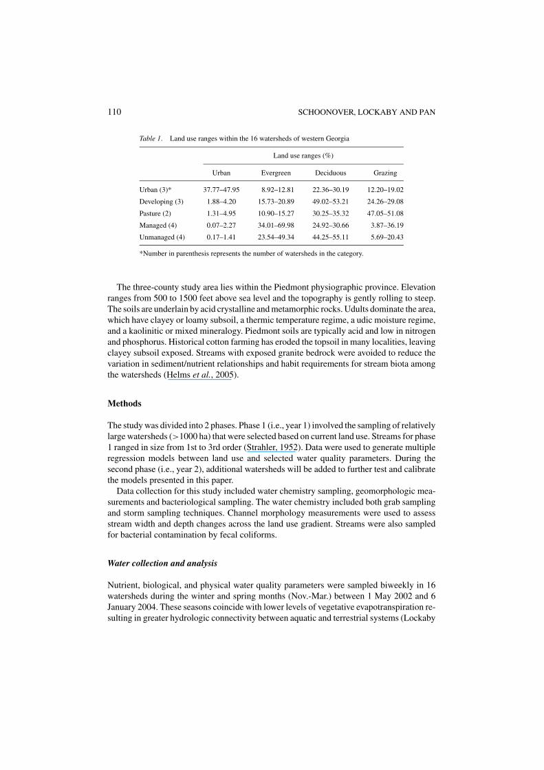
110 SCHOONOVER, LOCKABY AND PAN

Table 1. Land use ranges within the 16 watersheds of western Georgia

Land use ranges (%)

Urban Evergreen Deciduous Grazing

Urban (3)* 37.77–47.95 8.92–12.81 22.36–30.19 12.20–19.02

Developing (3) 1.88–4.20 15.73–20.89 49.02–53.21 24.26–29.08

Pasture (2) 1.31–4.95 10.90–15.27 30.25–35.32 47.05–51.08

Managed (4) 0.07–2.27 34.01–69.98 24.92–30.66 3.87–36.19

Unmanaged (4) 0.17–1.41 23.54–49.34 44.25–55.11 5.69–20.43

*Number in parenthesis represents the number of watersheds in the category.

The three-county study area lies within the Piedmont physiographic province. Elevationranges from 500 to 1500 feet above sea level and the topography is gently rolling to steep.The soils are underlain by acid crystalline and metamorphic rocks. Udults dominate the area,which have clayey or loamy subsoil, a thermic temperature regime, a udic moisture regime,and a kaolinitic or mixed mineralogy. Piedmont soils are typically acid and low in nitrogenand phosphorus. Historical cotton farming has eroded the topsoil in many localities, leavingclayey subsoil exposed. Streams with exposed granite bedrock were avoided to reduce thevariation in sediment/nutrient relationships and habit requirements for stream biota amongthe watersheds (Helms et al., 2005).

Methods

The study was divided into 2 phases. Phase 1 (i.e., year 1) involved the sampling of relativelylarge watersheds (>1000 ha) that were selected based on current land use. Streams for phase1 ranged in size from 1st to 3rd order (Strahler, 1952). Data were used to generate multipleregression models between land use and selected water quality parameters. During thesecond phase (i.e., year 2), additional watersheds will be added to further test and calibratethe models presented in this paper.

Data collection for this study included water chemistry sampling, geomorphologic mea-surements and bacteriological sampling. The water chemistry included both grab samplingand storm sampling techniques. Channel morphology measurements were used to assessstream width and depth changes across the land use gradient. Streams were also sampledfor bacterial contamination by fecal coliforms.

Water collection and analysis

Nutrient, biological, and physical water quality parameters were sampled biweekly in 16watersheds during the winter and spring months (Nov.-Mar.) between 1 May 2002 and 6January 2004. These seasons coincide with lower levels of vegetative evapotranspiration re-sulting in greater hydrologic connectivity between aquatic and terrestrial systems (Lockaby

CHANGES IN CHEMICAL AND PHYSICAL PROPERTIES OF STREAM WATER 111

et al., 1993). This sampling regime has been used with success in studying relationshipsbetween water quality and land cover/use (Basnyat et al., 2000). Monthly samples and stormsamples were collected throughout the remainder of the year.

Sampling locations were identified and permanently marked near the outlet of each wa-tershed. Polypropolene bottles that were rinsed with deionized water, and again with streamwater at the sites were used for sample collection. Also, pre-rinsed tissue culture flaskswere used to sample for all cations and anions to ensure that low-level concentrations weredetected. Grab samples were collected following guidelines from the USGS interagencyfield manual for the collection of water quality data, and the samples were collected beforeany other work was performed at the site to prevent the risk of stream disturbance (Lurry andKolbe, 2000). Samples were kept on ice and then refrigerated at 4◦C until analyzed. A reportfrom Coweeta Hyrologic Laboratory in Georgia showed that grab sample estimates werewithin 1 to 5% of the values from proportional sampling techniques (those that integratebaseflow and stormflow) (Swank and Crossley, 1988).

During each collection, stream discharge was recorded to allow for determination ofnutrient and sediment loads. Discharge was determined by measuring the velocity andcross-sectional areas of sub-sections across the stream channel. Generally, at least 20 sub-sections, at 0.1, 0.2, or 0.5 m intervals, were measured across the stream channel accordingto USGS stream gauging guidelines (Rantz, 1982). A Marsh-McBirney Flo-Mate 2000 wasused to measure the velocity within each subsection (Marsh-McBirney, 1990).

Discharge data were correlated with stage measurements to develop rating curves foreach watershed. To record the stream stage, InSitu pressure transducers (InSitu, Laramie,WY) were installed at each sampling location. Stage data also allowed examination of stormhydrographs in order to clarify changes in stream response times to rainfall events.

In addition to the grab samples, all of the watersheds were instrumented with stacked-polesamplers (depth integrated water samplers) (Van Lear, 1997). These samplers are composedof a vertical series of bottles that are designed to capture the rising limb of a storm event.One depth-integrated sampler was installed at the outlet of each watershed near the grabsampling sites, and data were collected following storm events that resulted in stream stageincreases greater than 30 cm. All water samples collected were immediately cooled andtransported to Auburn University (∼40 miles) for analysis. Grab samples were analyzed fornutrients, bacteria, and total suspended solids (TSS), while the depth-integrated samplerswere analyzed only for TSS due to the time of collection following storm events.

Grab samples were analyzed within two days of collection for both nutrients and sed-iment. Anions and cations (NO−

3 , Cl−, SO2−4 , Na+, NH+

4 , and K+) were analyzed usinga DX-120 Ion Chromatograph (Dionex, Sunnyvale, CA). Total phosphorus was measuredusing the molybdate-blue method (Murphy and Riley, 1962; Watanabe and Olsen, 1965).Conductivity was determined using a Fisher Accumet conductivity meter (Fisher Scien-tific, Pittsburgh, PA.). TSS was determined using gravimetric filtration methods outlinedby the USEPA (1999). Dissolved organic carbon (DOC) analysis was performed using aRosemont DC80 organic carbon analyzer. Fecal coliform (FC) colonies were isolated onsterile, nitrocellulose membrane filters (0.47 um pore size, 47 mm diameter, Millipore Cor-poration, Bedford, MA) following the procedure outlined by the standard methods for theexamination of water and wastewater (APHA, 1998).

112 SCHOONOVER, LOCKABY AND PAN

Channel morphology

Stream morphological changes were assessed in each of the sixteen watersheds to offerinsight for sediment origin analyses and to provide an assessment of channel stability acrossthe land use gradient. In each watershed, six permanent cross-sections were identified. Threeof the cross-sections were established near the watershed outlets, while the others wererandomly located in the headwater tributaries. All cross-sections were located in a straightreach to ensure that stable sections were sampled and to maintain consistent samplingamong watersheds. Width and depth measurements were taken quarterly at each samplingpoint. To aid in the measurement, the permanent sampling locations were identified byusing a 1 m section of rebar on each side of the stream. A string level was used to levelthe rebar endpoints on each side of the channel. During the measuring process a stringand measuring tape were stretched between the endpoints and measurements were takenat consistent intervals (1 m) across the stream so re-measurement of the exact point waspossible. These data will provide an assessment of annual channel aggradation and/ordegradation.

All watersheds were delineated using 30 m Digital Elevation Models in ArcGIS. Also,high resolution (1-meter) aerial photographs were taken in March (leaf-off) of 2003 and usedto delineate impervious surfaces. Detailed methods for land use classification are outlinedby Lockaby et al. (2005).

Statistical analysis

Five dominant land use categories were determined from satellite images; these include:unmanaged forests (dominated by mixed hardwood stands), managed forests (dominatedby pine plantations), pasture, developing, and urban. The developing land use was separatedfrom the other land uses by the evidence of subdivisions and construction areas. Althoughwe anticipated a continuum across the land uses, a gap was apparent between impervioussurface percentages of developing (∼3.5%) and urban (>30%) watersheds (reference as anexample figure 3). Nonparametric tests (Kruskal-Wallis tests) were used for data comparisonanalyses. This distribution-free analysis was used to compare urban (ie., >5% impervioussurfaces) and non-urban (ie., <5% impervious surfaces) land uses. MAXR regression andPearson correlations were used to examine relationships between land use variables andabiotic and bacteriological parameters. All dependent variables used in the regression andcorrelation analyses were log10-transformed to meet normality assumptions. The regressionmodels were created using the average annual concentrations (log10-transformed) vs. landuse and hydrological predictor variables.

MAXR selects the one-variable model with the highest r2, followed by the best two-variable model, etc, until the full model (i.e., all independent variables included) is estimated(Cody and Smith, 1997). MAXR results and Mallow’s Cp (the total square errors, whichindicates lack of fit) were assessed in the final outputs. A high r2 and a low Cp indicatethe best predictive models (Yu, 2000). Examination of the output allows for the selectionof the best predictive model based on the r2 and Cp changes between each step. Becausethe models are tested in steps, the models can range in the number of predictor variables

CHANGES IN CHEMICAL AND PHYSICAL PROPERTIES OF STREAM WATER 113

used in the final models. SAS Version 8 software was used for all statistical analyses (SASInstitute, 1999).

Results and discussion

Hydrology

The 30 yr average rainfall is 132 cm yr−1 and falls predominately in the form of rain (NCDC,2004). During 2002, annual precipitation was 15 cm below the 30 year average due to adeficit during the summer and fall. However, between January and July of 2003, monthlyaverages were exceeded by 25 cm (NCDC, 2004). This resulted in drought conditions duringthe first summer and fall, followed by unusually wet conditions during the subsequent springand summer.

Although watersheds varied in size, streamflow generation was similar on a per hectarebasis for each land use. Watersheds with greater than 33.5% pine cover have significantlylower (p = 0.001) stream discharges (63.0 L sec.−1) vs. all other land use categories (281 Lsec.−1). At the watershed scale, Bosch and Hewlett (1982) reported that a 10% reduction inconifer forests increased water yields by 40 mm, while a deciduous forest reduction of thesame size increased water yields by approximately 25 mm. Brooks et al. (1997) suggestedthat high evapotranspiration, due to longer growing seasons and dense foliage, in coniferforests likely contributed to the lower stream discharges.

On an annual basis, stream discharge was significantly higher in the urban (353 L s−1)streams than all other land uses combined (169 L s−1) (p = 0.0129). Urban streamsalso portrayed “flashy” characteristics such as high peak discharges and steep declines indischarge during the recession limbs of the storm hydrographs (Leopold, 1968; Hirsch et.al., 1990; Rose and Peters, 2001).

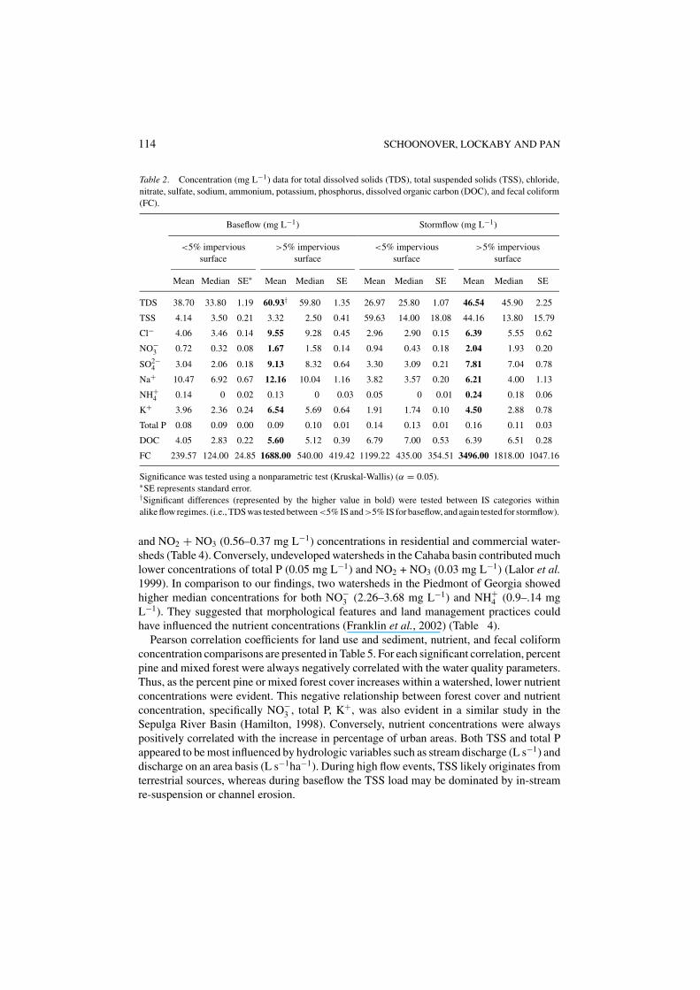
Nutrients

Mean concentration data for baseflow and stormflow are illustrated in Table 2 and loaddata are reported in Table 3. During both baseflow and stormflow TDS, Cl−, NO−

3 , SO2−4 ,

Na+, and K+ concentrations and loads were all significantly higher in watersheds withgreater than 5% impervious surfaces. NH+

4 concentrations and loads were only higherduring stormflow conditions, which likely results from leaky sewer and septic systems, orfertilizer runoff from lawns during storm events. Mean anion concentrations and total P inbaseflow and stormflow across all land uses ranked as follows: SO2−

4 > NO−3 > total P.

Similar nutrient relationships were reported by Arienzo et al. (2001).Baseflow concentrations for SO2−

4 and NO−3 were comparable to those of Rose (2002)

for both urban and non-urban streams near Atlanta. Potassium concentrations nearly dou-bled during both baseflow and stormflow compared to those reported by Rose (2002) inPeachtree Creek, an urbanized watershed near Atlanta, Ga. Similarly, Na+ exhibited a 2-fold increase only during baseflow conditions in both urban and non-urban watershedscompared to the two Piedmont streams near Atlanta (Rose, 2002). A study of the CahabaRiver Watershed near Birmingham, AL reported relatively high total P (0.32–0.37 mg L−1)

114 SCHOONOVER, LOCKABY AND PAN

Table 2. Concentration (mg L−1) data for total dissolved solids (TDS), total suspended solids (TSS), chloride,nitrate, sulfate, sodium, ammonium, potassium, phosphorus, dissolved organic carbon (DOC), and fecal coliform(FC).

Baseflow (mg L−1) Stormflow (mg L−1)

<5% impervious >5% impervious <5% impervious >5% impervioussurface surface surface surface

Mean Median SE∗ Mean Median SE Mean Median SE Mean Median SE

TDS 38.70 33.80 1.19 60.93† 59.80 1.35 26.97 25.80 1.07 46.54 45.90 2.25

TSS 4.14 3.50 0.21 3.32 2.50 0.41 59.63 14.00 18.08 44.16 13.80 15.79

Cl− 4.06 3.46 0.14 9.55 9.28 0.45 2.96 2.90 0.15 6.39 5.55 0.62

NO−3 0.72 0.32 0.08 1.67 1.58 0.14 0.94 0.43 0.18 2.04 1.93 0.20

SO2−4 3.04 2.06 0.18 9.13 8.32 0.64 3.30 3.09 0.21 7.81 7.04 0.78

Na+ 10.47 6.92 0.67 12.16 10.04 1.16 3.82 3.57 0.20 6.21 4.00 1.13

NH+4 0.14 0 0.02 0.13 0 0.03 0.05 0 0.01 0.24 0.18 0.06

K+ 3.96 2.36 0.24 6.54 5.69 0.64 1.91 1.74 0.10 4.50 2.88 0.78

Total P 0.08 0.09 0.00 0.09 0.10 0.01 0.14 0.13 0.01 0.16 0.11 0.03

DOC 4.05 2.83 0.22 5.60 5.12 0.39 6.79 7.00 0.53 6.39 6.51 0.28

FC 239.57 124.00 24.85 1688.00 540.00 419.42 1199.22 435.00 354.51 3496.00 1818.00 1047.16

Significance was tested using a nonparametric test (Kruskal-Wallis) (α = 0.05).∗SE represents standard error.†Significant differences (represented by the higher value in bold) were tested between IS categories withinalike flow regimes. (i.e., TDS was tested between<5% IS and>5% IS for baseflow, and again tested for stormflow).

and NO2 + NO3 (0.56–0.37 mg L−1) concentrations in residential and commercial water-sheds (Table 4). Conversely, undeveloped watersheds in the Cahaba basin contributed muchlower concentrations of total P (0.05 mg L−1) and NO2 + NO3 (0.03 mg L−1) (Lalor et al.1999). In comparison to our findings, two watersheds in the Piedmont of Georgia showedhigher median concentrations for both NO−

3 (2.26–3.68 mg L−1) and NH+4 (0.9–.14 mg

L−1). They suggested that morphological features and land management practices couldhave influenced the nutrient concentrations (Franklin et al., 2002) (Table 4).

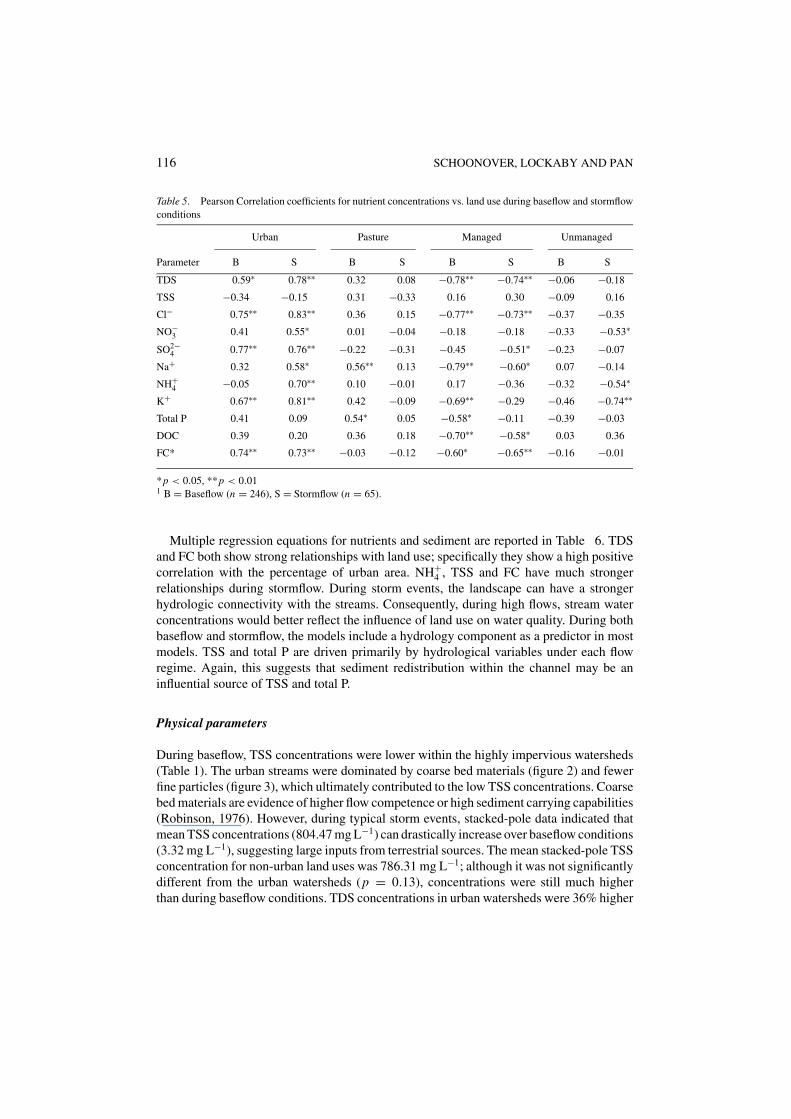
Pearson correlation coefficients for land use and sediment, nutrient, and fecal coliformconcentration comparisons are presented in Table 5. For each significant correlation, percentpine and mixed forest were always negatively correlated with the water quality parameters.Thus, as the percent pine or mixed forest cover increases within a watershed, lower nutrientconcentrations were evident. This negative relationship between forest cover and nutrientconcentration, specifically NO−

3 , total P, K+, was also evident in a similar study in theSepulga River Basin (Hamilton, 1998). Conversely, nutrient concentrations were alwayspositively correlated with the increase in percentage of urban areas. Both TSS and total Pappeared to be most influenced by hydrologic variables such as stream discharge (L s−1) anddischarge on an area basis (L s−1ha−1). During high flow events, TSS likely originates fromterrestrial sources, whereas during baseflow the TSS load may be dominated by in-streamre-suspension or channel erosion.

CHANGES IN CHEMICAL AND PHYSICAL PROPERTIES OF STREAM WATER 115

Table 3. Load (g d−1ha−1) data for total dissolved solids (TDS), total suspended solids (TSS), chloride, nitrate,sulfate, sodium, ammonium, potassium, phosphorus, and dissolved organic carbon (DOC)

Baseflow (g d−1 ha−1) Stormflow (g d−1 ha−1)

<5% impervious >5% impervious <5% impervious >5% impervioussurface surface surface surface

Mean Median SE∗ Mean Median SE Mean Median SE Mean Median SE

TDS 143.88 140.19 7.21 232.73† 201.54 23.26 944.43 709.41 100.05 1753.90 1779.13 205.35

TSS 21.21 13.36 1.95 12.21 6.63 2.36 1368.76 357.84 345.51 3026.37 472.99 1252.01

Cl− 14.92 13.67 0.79 35.50 30.48 3.26 96.53 79.32 8.77 221.43 211.97 27.80

NO−3 3.87 1.01 0.49 7.41 6.36 1.01 26.54 11.59 4.14 78.97 68.14 11.35

SO2−4 11.89 8.51 0.83 30.82 30.90 2.79 117.12 88.80 15.17 284.83 291.22 34.27

Na+ 28.13 24.37 1.50 35.23 31.76 2.96 125.37 101.27 13.31 199.87 178.08 35.13

NH+4 0.29 0 0.04 0.58 0 0.14 1.53 0 0.40 7.91 5.25 1.98

K+ 10.69 10.19 0.51 19.10 16.84 1.71 62.17 50.25 6.92 155.64 122.99 27.81

Total P 0.31 0.19 0.03 0.33 0.26 0.04 4.74 3.65 0.63 7.05 4.13 1.99

DOC 13.49 10.90 0.92 20.97 15.96 2.40 243.00 152.60 33.95 285.55 230.94 54.64

Significance was tested using nonparametric statistics(Kruskal-Wallis) (α = 0.05).∗SE represents standard error.†Significant differences (represented by the higher value in bold) were tested between IS categories within alikeflow regimes. (i.e., TDS was tested between <5% IS and >5% IS for baseflow, and again tested for stormflow).

Table 4. Combined baseflow and stormflow nutrient ranges for total P, NO3, and NH4 in southeastern watershedsfrom a variety of land uses

Total PLocation Land use (mg L−1) NO−

3 (mg L−1) NH+4 (mg L−1) Reference

Cahaba River, Residential and 0.32–0.37† . . Lalor et al. (1999)

Birmingham, AL Commercial 0.10–0.32††

Cahaba River, Undeveloped 0.05† . . Lalor et al. (1999)

Birmingham, AL 0.05††

Ecoregion IX Aggregate of level 0.022–0.1††† . . USEPA (2000)III streams

Greenbrier and Rose 27% Agriculture . 2.08–3.68†† 0.09-0.14†† Franklin et al. (2002)

Creeks, Oconee and 69% Forest

Greene Counties, GA 0.1% Residential

Peachtree Creek, 54.7% Urban . 2.4–2.8† . Rose (2002)

Atlanta, GA 54.7% Forest

†Mean††Median†††Based on the 25th percentile for all season data over a decade of record.

116 SCHOONOVER, LOCKABY AND PAN

Table 5. Pearson Correlation coefficients for nutrient concentrations vs. land use during baseflow and stormflowconditions

Urban Pasture Managed Unmanaged

Parameter B S B S B S B S

TDS 0.59∗ 0.78∗∗ 0.32 0.08 −0.78∗∗ −0.74∗∗ −0.06 −0.18

TSS −0.34 −0.15 0.31 −0.33 0.16 0.30 −0.09 0.16

Cl− 0.75∗∗ 0.83∗∗ 0.36 0.15 −0.77∗∗ −0.73∗∗ −0.37 −0.35

NO−3 0.41 0.55∗ 0.01 −0.04 −0.18 −0.18 −0.33 −0.53∗

SO2−4 0.77∗∗ 0.76∗∗ −0.22 −0.31 −0.45 −0.51∗ −0.23 −0.07

Na+ 0.32 0.58∗ 0.56∗∗ 0.13 −0.79∗∗ −0.60∗ 0.07 −0.14

NH+4 −0.05 0.70∗∗ 0.10 −0.01 0.17 −0.36 −0.32 −0.54∗

K+ 0.67∗∗ 0.81∗∗ 0.42 −0.09 −0.69∗∗ −0.29 −0.46 −0.74∗∗

Total P 0.41 0.09 0.54∗ 0.05 −0.58∗ −0.11 −0.39 −0.03

DOC 0.39 0.20 0.36 0.18 −0.70∗∗ −0.58∗ 0.03 0.36

FC* 0.74∗∗ 0.73∗∗ −0.03 −0.12 −0.60∗ −0.65∗∗ −0.16 −0.01

*p < 0.05, **p < 0.011 B = Baseflow (n = 246), S = Stormflow (n = 65).

Multiple regression equations for nutrients and sediment are reported in Table 6. TDSand FC both show strong relationships with land use; specifically they show a high positivecorrelation with the percentage of urban area. NH+

4 , TSS and FC have much strongerrelationships during stormflow. During storm events, the landscape can have a strongerhydrologic connectivity with the streams. Consequently, during high flows, stream waterconcentrations would better reflect the influence of land use on water quality. During bothbaseflow and stormflow, the models include a hydrology component as a predictor in mostmodels. TSS and total P are driven primarily by hydrological variables under each flowregime. Again, this suggests that sediment redistribution within the channel may be aninfluential source of TSS and total P.

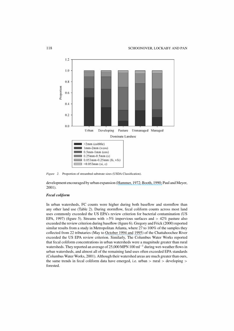
Physical parameters

During baseflow, TSS concentrations were lower within the highly impervious watersheds(Table 1). The urban streams were dominated by coarse bed materials (figure 2) and fewerfine particles (figure 3), which ultimately contributed to the low TSS concentrations. Coarsebed materials are evidence of higher flow competence or high sediment carrying capabilities(Robinson, 1976). However, during typical storm events, stacked-pole data indicated thatmean TSS concentrations (804.47 mg L−1) can drastically increase over baseflow conditions(3.32 mg L−1), suggesting large inputs from terrestrial sources. The mean stacked-pole TSSconcentration for non-urban land uses was 786.31 mg L−1; although it was not significantlydifferent from the urban watersheds (p = 0.13), concentrations were still much higherthan during baseflow conditions. TDS concentrations in urban watersheds were 36% higher

CHANGES IN CHEMICAL AND PHYSICAL PROPERTIES OF STREAM WATER 117

Table 6. Multiple regression models for baseflow and stormflow nutrient concentrations, dependentvariables were log transformed to meet normality assumptions

Parameter Prediction equation1 r2 p-value

BaseflowNO−

3 y = 0.02(U) + 1.41(QLS) − 6.01 0.58 0.0033

NH+4 y = 1.12(QWA) + 0.23 0.17 0.1133

Total P y = −0.01(M)–0.01(E) − 1.95 0.56 0.0051

TDS y = 0.01(U) − 0.01(E) − 0.16(QLS) − 0.36(QWA) + 3.23 0.90 <0.0001

TSS y = 1.19(QWA) + 0.04(P) + 3.58 0.45 0.0203

FC y = 0.04(U) + 0.02(M) + 0.56(QLS) − 0.59(QWA) + 0.14 0.76 0.0019

Stormflow

NO−3 y = 0.02(U) − 0.03(M) + 0.47 0.41 0.0457

NH+4 y = 0.05(U) − 0.97(QWA) − 4.84 0.56 0.0074

Total P y = −0.19(QLS) + 0.49(QWA) − 0.51 0.28 0.1351

TDS y = 0.01(U) − 0.01(E) + 3.45 0.78 0.0001

TSS y = 0.01(P) + 1.49(QWA) + 4.07 0.47 0.0231

FC y = 0.04(U) + 0.03(M) + 0.39(QLS) − 0.46(QWA) + 2.08 0.81 0.0013

1U = % UrbanD = % DevelopingE = % Evergreen ForestM = % Mixed ForestP = % PastureQLS = Discharge L s−1

QWA = Discharge/Watershed Area (L s−1 ha−1).

during baseflow and 42% higher during stormflow (Table 2). Rose (2002) reported a 30%increase in baseflow TDS concentrations in urban watersheds compared to lesser developedwatersheds. TDS is often much higher in streams influenced by anthropogenic factors(Knighton, 1984).

Cross-section data revealed that aggressive downcutting was evident in one of the urbanchannels. The watershed draining to the impaired channel has undergone recent urban de-velopment relative to the other urban watersheds. The two urban watersheds in southernColumbus are very wide with deep channels that have downcut to resistant substrates andare composed of relatively coarse sediments that have remained stable during the study.The recently developed urban watershed is located on the northern fringe of Columbusand still has a relatively small stream channel, but the channel is experiencing rapid ge-omorphic changes. Figures 4 and 5 compare the cross-section measurements between anurban stream and a stream in a primarily forested watershed; both channels are 1st or-der streams (Strahler, 1952). Currently, the urban channel is downcutting approximately20 cm every 6 months, while streams from other land uses are remaining stable or ap-pear to be redistributing sediments within their cross-sections. The urban channel’s rapidlychanging morphology suggests that the stream is experiencing an erosional phase of channel

118 SCHOONOVER, LOCKABY AND PAN

Figure 2. Proportion of streambed substrate sizes (USDA Classification).

development encouraged by urban expansion (Hammer, 1972; Booth, 1990; Paul and Meyer,2001).

Fecal coliform

In urban watersheds, FC counts were higher during both baseflow and stormflow thanany other land use (Table 2). During stormflow, fecal coliform counts across most landuses commonly exceeded the US EPA’s review criterion for bacterial contamination (USEPA, 1997) (figure 5). Streams with >5% impervious surfaces and > 42% pasture alsoexceeded the review criterion during baseflow (figure 6). Gregory and Frick (2000) reportedsimilar results from a study in Metropolitan Atlanta, where 27 to 100% of the samples theycollected from 22 tributaries (May to October 1994 and 1995) of the Chattahoochee Riverexceeded the US EPA review criterion. Similarly, The Columbus Water Works reportedthat fecal coliform concentrations in urban watersheds were a magnitude greater than ruralwatersheds. They reported an average of 25,000 MPN 100 ml−1 during wet-weather flows inurban watersheds, and almost all of the remaining land uses often exceeded EPA standards(Columbus Water Works, 2001). Although their watershed areas are much greater than ours,the same trends in fecal coliform data have emerged, i.e. urban > rural > developing >

forested.

CHANGES IN CHEMICAL AND PHYSICAL PROPERTIES OF STREAM WATER 119

Figure 3. Relationship between percent urban area and the proportion of very fine sand (0.053–.25 mm) (r2 =0.31, p =< 0.0001).

Figure 4. Cross-section of an urban channel in the erosional phase of development (dominant land use: 48%urban, 31% forested, and 19% pasture).

120 SCHOONOVER, LOCKABY AND PAN

Figure 5. Cross-section of stable channel in a watershed dominated by mixed forest (dominant land use: 94%forested, 6% pasture).

Figure 6. Fecal coliform across the dominant land use classes (bars represent ±1 standard error).

CHANGES IN CHEMICAL AND PHYSICAL PROPERTIES OF STREAM WATER 121

FC is often associated with pathogens such as Giardia, Shigella, Salmonella, and E. coli,which are found in cattle and/or humans. Ingestion of such fecal pathogens may result inintestinal illness or even death (Wang et al., 2002). Geldreich (1970) reported that when fecalcoliform counts were greater than 2000 colony forming units (cfu) per 100 ml, Salmonellaexisted with nearly 100% occurrence. Hsu et al. (2001) observed significant correlationsbetween fecal coliform and Giardia concentrations.

Conclusions

Stream water quality was tested along an urban-rural gradient in the Piedmont of westernGeorgia and results showed significantly higher nutrient contributions to urban streams.High resolution (1-meter) aerial photography and 30 m satellite imagery were used todetermine the percent impervious surfaces and the array of land use within 16 watersheds,respectively. Concentrations of TDS, Cl−, NO−

3 , Na+, SO2−4 , and K+ were consistently

higher during both base flow and stormflow in urban watersheds, while NH+4 concentration

and loads were only higher during stormflow conditions. TSS and total P appeared to beeither driven by hydrologic variables or were inputs from all land uses. FC counts weresignificantly higher in urban watersheds and exceeded the US EPA’s review criterion of 400MPN 100 ml−1.

A recently developed urban watershed appeared to be undergoing an erosional phase ofchannel development where active streambed downcutting was evident. Remaining water-sheds were experiencing little bed movement or undergoing redistribution of substrates.Streambeds in urban and developing watersheds were predominately composed of coarsematerials, whereas others had greater proportions of finer particle sizes.

Data from this study provide the basis for regression models that predict water qualitybased on land use. Additional data from newly chosen watersheds will be used to testand calibrate these models. Additionally, land use will be delineated using high resolution(1-meter) aerial photography to improve the land use classification.

Acknowledgments

Funding for this research was provided by the Center for Forest Sustainability through thePeaks of Excellence program at Auburn University. Additional funds were also providedby Auburn University’s Environmental Institute. The authors thank Robin Governo whoassisted with laboratory analysis and all of those who assisted in field sampling. We wouldalso like to acknowledge Philip Chaney and Rebecca Xu who helped with the land useclassification used for this project.

References

American Public Health Association, American Water Works Association, and Water Environment Federation(1998) Standard Methods for the Examination of Water and Wastewater. 20th edition. (Lenore S. Clesceri,Arnold E. Greenberg and Andrew D. Eaton, eds.), APHA, Washington, DC.

122 SCHOONOVER, LOCKABY AND PAN

Arienzo, M., Adamo, P., Bianco, M.R. and Violante, P. (2001) Impact of land use and urban runoff on thecontamination of the Sarno River basin in southwestern Italy. Water, Air, and Soil Pollution 131, 349–366.

Arnold, C., Boison, P. and Patton, P. (1982) Sawmill Brook: An example of rapid geomorphic change related tourbanization. Journal of Geology 90, 155–166.

Basnyat, P., Teeter, L., Lockaby, B.G. and Flynn, K.M. (2000) Land use characteristics and water quality: Amethodology for valuing forested buffers. Environmental Management 26, 153–161.

Bledsoe, B.P. and Watson, C.C. (2001) Effects of urbanization on channel instability. Journal of the AmericanWater Resources Association 37, 255–270.

Booth, D.B. (1990) Stream channel incision following drainage-basin urbanization. Water Resources Bulletin 26,407–417.

Bosch, J.M. and Hewlett, J.D. (1982) A review of catchment experiments to determine the effect of vegetationchanges on water yield and evapotranspiration. Journal of Hydrology 55, 3–23.

Brezonik, P.L. and Stadelmann, T.H. (2002) Analysis and predictive models of stormwater runoff volumes, loads,and pollutant concentrations from watersheds in the Twin Cities metropolitan area, Minnesota, USA. WaterResearch 36, 1743–1757.

Brooks, K.N., Ffolliott, P.F., Gregersen, H.M. and DeBano, L.F. (1997) Hydrology and the Management of Wa-tersheds, 2nd edition. Iowa State University Press. Ames, IA.

Callender, E. and Rice, K.C. (2000) The urban environmental gradient: anthropogenic influences on the spatialand temporal distributions of lead and zinc in sediments. Environmental Science and Technology 34, 232–238.

Cody, R.P. and Smith, J.K. (1997) Applied Statistics and the SAS Programming Language. 4th edition. PrenticeHall, Inc., New Jersey.

Columbus Water Works. (2001) Wet weather demonstration projects: CSO technology testing, source waterassessment and protection, watershed assessment and management. Draft Summary Report. WWETCO, LLC.

Dunne, T. and Leopold, L.B. (1978) Water in Environmental Planning. New York, Freeman. 818pp.Emmerth, P.P. and Bayne, D.R. (1996) Urban influence on phosphorus and sediment loading of West Point Lake,

Georgia. Water Resources Bulletin 32, 145–154.Finkenbine, J.K., Atwater, D.S. and Mavinic, D.S. (2000) Stream health after urbanization. Journal of the American

Water Resources Association 36, 1149– 1160.Franklin, D.H., Steiner, J.L., Cabrera, M.L. and Usery, E.L. (2002) Distribution of inorganic nitrogen and phos-

phorus concentrations in stream flow of two southern Piedmont watersheds. Journal of Environmental Quality31, 1910–1917.

Geldreich, E.E. (1970) Applying bacteriological parameters to recreational water quality. Journal of the AmericanWater Works Association 6, 113–120.

Gregory, K., Davis, R. and Downs, P. (1992) Identification of river channel change due to urbanization. AppliedGeography 12, 299–318.

Gregory, M.B. and Frick, E.A. (2000) Fecal-coliform bacteria concentrations in streams of the ChattahoocheeRiver National Recreation Area, metropolitan Atlanta, Georgia, May-October 1994 and 1995. U.S. GeologicalSurvey Water-Resources Investigations Report. 00–4139.

Hamilton, A.K. (1998) Relation of land uses to water quality in the Sepulga River Basin of Alabama. Thesis,Auburn University, Auburn, AL.

Hammer, T.R. (1972) Stream channel enlargement due to urbanization. Water Resources Research 8, 1530–1540.

Helms, B.S., Feminella, J.W. and Pan, S. (2005) Detection of biotic responses to urbanization using fish assemblagesfrom small streams of western Georgia, USA. Urban Ecosystems 8, 39–57.

Herlihy, A.T., Stoddard, J.L. and Johnson, C.B. (1998) The relationship between stream chemistry and watershedland cover data in the mid-Atlantic region, U.S. Water, Air, and Soil Pollution 105, 377–386.

Hirsch, R.M., Walker, J.F., Day, J.C. and Kallio, R. (1990) The influence of man on hydrologic systems. InSurface Water Hydrology (The Geology of America, vol. 0–1, M.G. Wolman and H.C. Riggs (eds.). Boulder,CO, Geological Society of America, pp. 329–359.

Hsu, B., Huang, C., Hsu, Y., Jiang, G. and Hsu, C.L. (2001) Evaluation of two concentration methods for detectinggiardia and cryptosporidium in water. Water Research 35, 419–424.

Hunter, J.V., Sabatino, T., Gomperts, R. and Mackenzie, M.J. (1979) Contribution of urban runoff to hydrocarbonpollution. Journal of. Water Pollution Control Federation, WEF 51, 2129–2138.

CHANGES IN CHEMICAL AND PHYSICAL PROPERTIES OF STREAM WATER 123

Imbe, M., Ohta, T. and Takano, N. (1997) Quantitative assessment of improvements in hydrological water cyclein urbanized river basin. Water Science and Technology 36, 219–222.

Knighton, D. (1984) Fluvial Forms and Processes. Edward Arnold (Publishers) Ltd., London.Lalor, M.M., Griffin, D.H., Clark, S., Crawford, S. and Beckom, N. (1999) Stormwater nutrient contributions in

urbanizing watersheds. Report to Alabama Department of Environmental Management.Lee, J.H. and Bang, K.W. (2000) Characterization of urban stormwater runoff. Water Research 34, 1773–

1780.Leopold, L.B. (1968) Hydrology for Urban Land Planning-A Guidebook on the Hydrologic Effects of Urban Land

Use. USGS Circular, 554.Lockaby, B.G., McNabb, K. and Hairston, J. (1993) Changes in groundwater nitrate levels along an agroforestry

drainage continuum. In Proceedings, Conference on Riparian Ecosystems in the Humid US: Functions, Valuesand Management. pp. 412–417, Atlanta, Georgia.

Lockaby, B.G., Zhang, D., McDaniel J., Tian, H. and Pan, S. (2005) Interdisciplinary research at the urban-ruralinterface: the west Georgia project. Urban Ecosystems 8, 7–21.

Lurry, D.L. and Kolbe, C.M. (2000) Interagency field manual for the collection of water-quality data. U.S. Geo-logical Survey. Open-File Report 00-213.

Marsh-McBirney, Inc. (1990) Model 2000 installation and operations manual. Marsh-McBirney, Inc. Fredrick,Maryland.

Murphy, J. and Riley, J.P. (1962) A modified single solution method for the determination of phosphate in naturalwaters. Analytical Chemistry 27, 31–36.

NCDC (National Climatic Data Center). (2004) Annual Climatological Summary, Georgia.http://cdo.ncdc.noaa.gov/ancsum/ACS?state=GA. Station ID #’s: 092166, 096148, 099291, 099506.

Norman, C.G. (1991) Urban runoff effects on Ohio River water quality. Water Environ. Technol 3, 44–46.

Paul, M.J. and Meyer, J.L. (2001) Streams in the urban landscape. Annual Review of Ecology and Systematics 32,333–365.

Rantz, S.E. (1982) Measurement of discharge by conventional current-meter-method. Ch 5. USGS Water SupplyPaper 2175.

Robinson, A.M. (1976) The effects of urbanization on stream channel morphology. In National Symposium onUrban Hydrology, Hydraulics, and Sediment Control. University of Kentucky, Lexington, Kentucky, pp. 115–127.

Rose, S. and Peters, N.E. (2001) Effects of urbanization on streamflow in the Atlanta area (Georgia, USA): Acomparative hydrological approach. Hydrological Processes 15, 1441–1457.

Rose, S. (2002) Comparative major ion geochemistry of Piedmont streams in the Atlanta, Georgia region: Possibleeffects of urbanization. Environmental Geology 42, 102–113.

SAS Institute (1999) SAS Version 8 for Window. Cary, North Carolina.Schueler, T. (1995) The importance of imperviousness. Watershed Protection Techniques 1, 100–111.Strahler, A.N. (1952) Dynamic basis of geomorphology. Geological Society of America Bulletin 63, 923–938.Swank, W.T. and Crossley, D.A. Jr. (1988) Ecological Studies, vol. 66: Forest Hydrology and Ecology at Coweeta.

Springer-Verlag, New York, Inc.USDA, NRCS. (2004) Natural Resources Data and Analysis. http//:www.nrcs.usda.gov/technical/nri data.html.

State of the Land.U.S. Environmental Protection Agency. (1997) EPA guidelines for preparation of the comprehensive state water-

quality assessments. Washington, D.C., U.S. Environmental Protection Agency, Office of Water, EPA-841-B-97-002a.

U.S. Environmental Protection Agency. (1999) Standard operating procedure for the analysis of residue, non-filterable (suspended solids) water. Method 160.2 NS.

US Environmental Protection Agency. (2000) The quality of our nation’s waters. EPA841-S-00-001.US Environmental Protection Agency. (2000) Ambient water quality criteria recommendations: Rivers and streams

in ecoregion IX. EPA 822-B-00-019.US Environmental Protection Agency. (2002) Surf your watershed. http://www.epa.gov/surf.Van Lear, D.A., Taylor, G.B. and Hansen, W.F. (1997) Sediment sources to the Chattooga river. Proceedings of

the Ninth Biennial Southern Silviculture Conference. Technical Paper 19. pp. 357–362.

124 SCHOONOVER, LOCKABY AND PAN

Wahl, M.H., McKellar, H.N., Williams, T.M. (1997) Patterns of nutrient loading in forested and urbanized coastalstreams. Journal of Experimental Marine Biology and Ecology 213, 11–131.

Waller, D. and Hart, W.C. (1986) Solids, nutrients and chlorides in urban runoff. In NATO ASI Series, vol. G10,(H.C. Torno, J. Marsalek and M. Desbordes, eds.). Urban Runoff Pollution. Springer-Verlag, Berlin, Heidelberg,pp. 59–85.

Walling, D.E. and Gregory, K.J. (1970) The measurement of the effects of building construction on drainage basindynamics. Journal of Hydrology 11, 129–144.

Wang, L., Mankin, K.R. and Marchin, G.L. (2002) Fecal bacteria survival in animal manure. ASAE AnnualInternational Meeting / CIGR XVth World Congress. Chicago, IL. Paper No. 024099.

Watanabe, F.S. and Olsen, S.R. (1965) Test of an ascorbic acid method for determining phosphorus in water andNaHCO3 extracts from soil. Soil Science Society of America Journal 29, 677–678.

Yu, C.H. (2000) An overview of remedial tools for collinearity in SAS. In Proceedings of 2000 Western Users ofSAS Software Conference, pp. 196–201.