ch03b: Descriptive Statistics II: Numerical Methods - Part B
34
1 © 2001 © 2001 South-Western /Thomson Learning South-Western /Thomson Learning Anderson Anderson Sweeney Sweeney Williams Williams Slides Prepared by JOHN LOUCKS Slides Prepared by JOHN LOUCKS CONTEMPORARY CONTEMPORARY BUSINESS BUSINESS STATISTICS STATISTICS WITH MICROSOFT WITH MICROSOFT EXCEL EXCEL
Transcript of ch03b: Descriptive Statistics II: Numerical Methods - Part B
1 Slide
© 2001 © 2001 South-Western /Thomson LearningSouth-Western /Thomson Learning
Anderson Anderson Sweeney Sweeney WilliamsWilliams
Slides Prepared by JOHN LOUCKS Slides Prepared by JOHN LOUCKS
CONTEMPORARYCONTEMPORARYBUSINESSBUSINESS
STATISTICSSTATISTICSWITH MICROSOFTWITH MICROSOFT EXCEL EXCEL

2 Slide
Chapter 3Chapter 3 Descriptive Statistics II: Descriptive Statistics II: Numerical Methods - Part BNumerical Methods - Part B
Measures of Relative Measures of Relative Location and Detecting Location and Detecting OutliersOutliers
Exploratory Data Exploratory Data AnalysisAnalysis
Measures of Association Measures of Association between Two Variablesbetween Two Variables
The Weighted Mean and The Weighted Mean and Working with Grouped Working with Grouped DataData

3 Slide
Measures of Relative LocationMeasures of Relative Locationand Detecting Outliersand Detecting Outliers
z-Scoresz-Scores Chebyshev’s TheoremChebyshev’s Theorem The Empirical RuleThe Empirical Rule Detecting OutliersDetecting Outliers
4 Slide
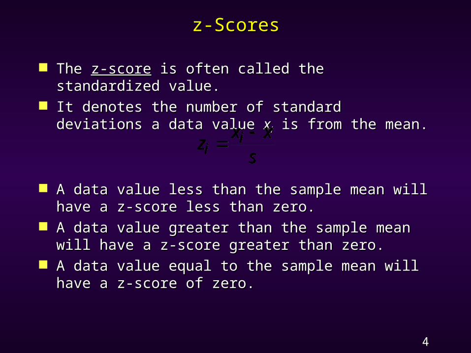
z-Scoresz-Scores
The The z-scorez-score is often called the is often called the standardized value.standardized value.
It denotes the number of standard It denotes the number of standard deviations a data value deviations a data value xxii is from the mean. is from the mean.
A data value less than the sample mean will A data value less than the sample mean will have a z-score less than zero.have a z-score less than zero.
A data value greater than the sample mean A data value greater than the sample mean will have a z-score greater than zero.will have a z-score greater than zero.
A data value equal to the sample mean will A data value equal to the sample mean will have a z-score of zero.have a z-score of zero.
z x xsi
i

5 Slide
z-Score of Smallest Value (425)z-Score of Smallest Value (425)
Standardized Values for Apartment RentsStandardized Values for Apartment Rents
z x xs
i
425 49080
5474 120.. .
-1.20 -1.11 -1.11 -1.02 -1.02 -1.02 -1.02 -1.02 -0.93 -0.93-0.93 -0.93 -0.93 -0.84 -0.84 -0.84 -0.84 -0.84 -0.75 -0.75-0.75 -0.75 -0.75 -0.75 -0.75 -0.56 -0.56 -0.56 -0.47 -0.47-0.47 -0.38 -0.38 -0.34 -0.29 -0.29 -0.29 -0.20 -0.20 -0.20-0.20 -0.11 -0.01 -0.01 -0.01 0.17 0.17 0.17 0.17 0.350.35 0.44 0.62 0.62 0.62 0.81 1.06 1.08 1.45 1.451.54 1.54 1.63 1.81 1.99 1.99 1.99 1.99 2.27 2.27
Example: Apartment RentsExample: Apartment Rents

6 Slide
Chebyshev’s TheoremChebyshev’s Theorem
At least (1 - 1/At least (1 - 1/kk22) of the items in any ) of the items in any data set will bedata set will be
within within kk standard deviations of the mean, standard deviations of the mean, where where k k isis
any value greater than 1.any value greater than 1.• At least 75% of the items must be within At least 75% of the items must be within k k = 2 standard deviations of the mean.= 2 standard deviations of the mean.
• At least 89% of the items must be within At least 89% of the items must be within kk = 3 standard deviations of the mean.= 3 standard deviations of the mean.
• At least 94% of the items must be within At least 94% of the items must be within kk = 4 standard deviations of the mean.= 4 standard deviations of the mean.

7 Slide
Example: Apartment RentsExample: Apartment Rents
Chebyshev’s TheoremChebyshev’s Theorem
Let Let kk = 1.5 with = 490.80 and = 1.5 with = 490.80 and ss = = 54.7454.74
At least (1 - 1/(1.5)At least (1 - 1/(1.5)22) = 1 - 0.44 = 0.56 or ) = 1 - 0.44 = 0.56 or 56% 56% of the rent values must be betweenof the rent values must be between - - kk((ss) = 490.80 - 1.5(54.74) = ) = 490.80 - 1.5(54.74) = 409409 andand + + kk((ss) = 490.80 + 1.5(54.74) = 573) = 490.80 + 1.5(54.74) = 573
x
x
x

8 Slide
Chebyshev’s Theorem (continued)Chebyshev’s Theorem (continued) Actually, 86% of the rent Actually, 86% of the rent
valuesvalues are between 409 and 573. are between 409 and 573. 425 430 430 435 435 435 435 435 440 440440 440 440 445 445 445 445 445 450 450450 450 450 450 450 460 460 460 465 465465 470 470 472 475 475 475 480 480 480480 485 490 490 490 500 500 500 500 510510 515 525 525 525 535 549 550 570 570575 575 580 590 600 600 600 600 615 615
Example: Apartment RentsExample: Apartment Rents

9 Slide
The Empirical RuleThe Empirical Rule
For data having a bell-shaped For data having a bell-shaped distribution:distribution:
• Approximately Approximately 68%68% of the data values will be of the data values will be within within oneone standard deviation of the mean. standard deviation of the mean.
• Approximately Approximately 95%95% of the data values will be of the data values will be within within twotwo standard deviations of the mean. standard deviations of the mean.
• Almost allAlmost all of the items (99.7%) will be of the items (99.7%) will be within within threethree standard deviations of standard deviations of the mean.the mean.

10 Slide
Example: Apartment RentsExample: Apartment Rents
The Empirical RuleThe Empirical Rule IntervalInterval % in % in
IntervalIntervalWithin +/- 1Within +/- 1ss 434366.06 to 545.54.06 to 545.5448/70 = 69%48/70 = 69%Within +/- 2Within +/- 2ss 381.32 to 600.28381.32 to 600.2868/70 = 97%68/70 = 97%Within +/- 3Within +/- 3ss 326.58 to 655.02326.58 to 655.0270/70 = 100%70/70 = 100%
425 430 430 435 435 435 435 435 440 440440 440 440 445 445 445 445 445 450 450450 450 450 450 450 460 460 460 465 465465 470 470 472 475 475 475 480 480 480480 485 490 490 490 500 500 500 500 510510 515 525 525 525 535 549 550 570 570575 575 580 590 600 600 600 600 615 615

11 Slide
Detecting OutliersDetecting Outliers
An An outlieroutlier is an unusually small or is an unusually small or unusually large value in a data set.unusually large value in a data set.
A data value with a z-score less than -A data value with a z-score less than -3 or greater than +3 might be 3 or greater than +3 might be considered an outlier. considered an outlier.
It might be an incorrectly recorded It might be an incorrectly recorded data value.data value.
It might be a data value that was It might be a data value that was incorrectly included in the data set.incorrectly included in the data set.
It might be a correctly recorded data It might be a correctly recorded data value that belongs in the data set !value that belongs in the data set !
12 Slide
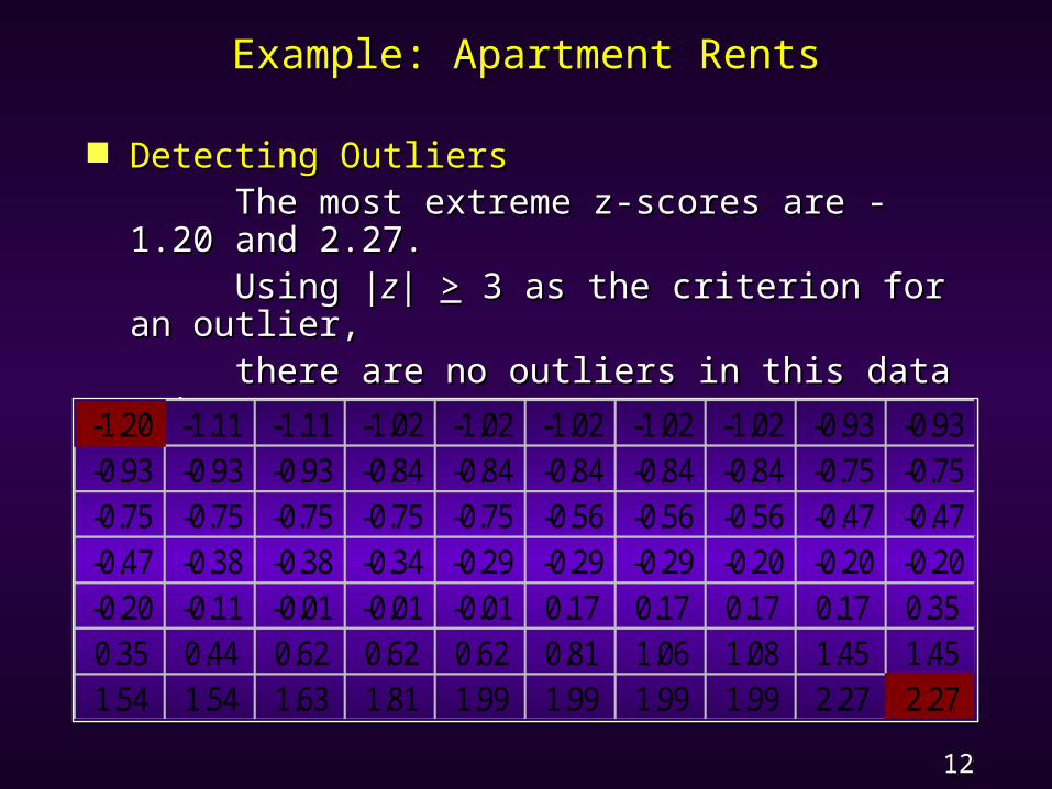
Example: Apartment RentsExample: Apartment Rents
Detecting OutliersDetecting OutliersThe most extreme z-scores are -The most extreme z-scores are -
1.20 and 2.27.1.20 and 2.27.Using |Using |zz| | >> 3 as the criterion for 3 as the criterion for
an outlier, an outlier, there are no outliers in this data there are no outliers in this data
set. set. Standardized Values for Apartment RentsStandardized Values for Apartment Rents
-1.20 -1.11 -1.11 -1.02 -1.02 -1.02 -1.02 -1.02 -0.93 -0.93-0.93 -0.93 -0.93 -0.84 -0.84 -0.84 -0.84 -0.84 -0.75 -0.75-0.75 -0.75 -0.75 -0.75 -0.75 -0.56 -0.56 -0.56 -0.47 -0.47-0.47 -0.38 -0.38 -0.34 -0.29 -0.29 -0.29 -0.20 -0.20 -0.20-0.20 -0.11 -0.01 -0.01 -0.01 0.17 0.17 0.17 0.17 0.350.35 0.44 0.62 0.62 0.62 0.81 1.06 1.08 1.45 1.451.54 1.54 1.63 1.81 1.99 1.99 1.99 1.99 2.27 2.27
13 Slide
Exploratory Data AnalysisExploratory Data Analysis
Five-Number SummaryFive-Number Summary Box PlotBox Plot
14 Slide
Five-Number SummaryFive-Number Summary
Smallest ValueSmallest Value First QuartileFirst Quartile MedianMedian Third QuartileThird Quartile Largest ValueLargest Value
15 Slide
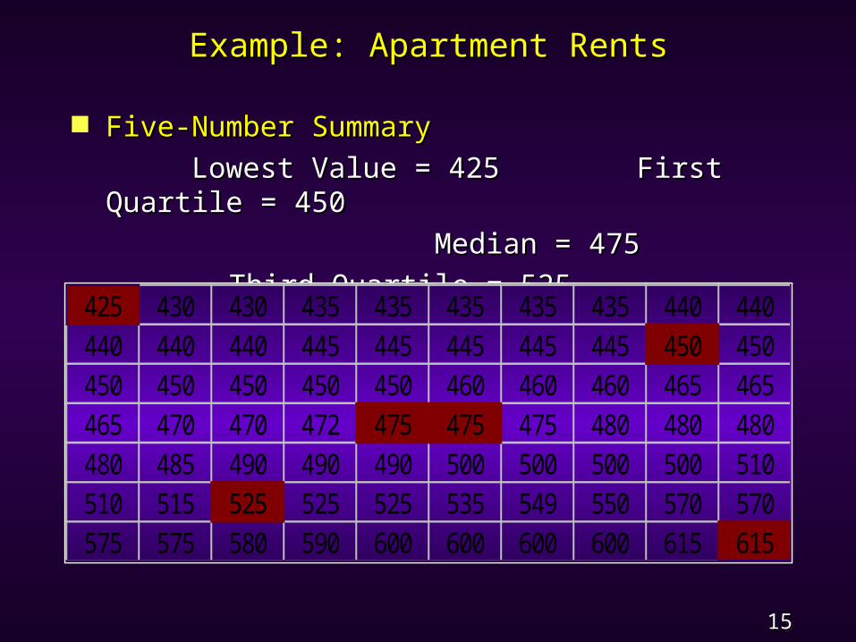
Example: Apartment RentsExample: Apartment Rents
Five-Number SummaryFive-Number SummaryLowest Value = 425Lowest Value = 425 First First
Quartile = 450Quartile = 450 Median = 475Median = 475
Third Quartile = 525 Third Quartile = 525 Largest Value = 615Largest Value = 615425 430 430 435 435 435 435 435 440 440
440 440 440 445 445 445 445 445 450 450450 450 450 450 450 460 460 460 465 465465 470 470 472 475 475 475 480 480 480480 485 490 490 490 500 500 500 500 510510 515 525 525 525 535 549 550 570 570575 575 580 590 600 600 600 600 615 615

16 Slide
Box PlotBox Plot
A box is drawn with its ends located at A box is drawn with its ends located at the first and third quartiles.the first and third quartiles.
A vertical line is drawn in the box at A vertical line is drawn in the box at the location of the median.the location of the median.
Fences are located (not drawn) using Fences are located (not drawn) using the interquartile range (IQR).the interquartile range (IQR).• The inner fences are located 1.5(IQR) The inner fences are located 1.5(IQR) below below QQ1 and 1.5(IQR) above 1 and 1.5(IQR) above QQ3.3.
• The outer fences are located 3(IQR) The outer fences are located 3(IQR) below below QQ1 and 3(IQR) above 1 and 3(IQR) above QQ3.3.
… … continuedcontinued

17 Slide
Box Plot (Continued)Box Plot (Continued)
Whiskers (dashed lines) are drawn from Whiskers (dashed lines) are drawn from the ends of the box to the smallest and the ends of the box to the smallest and largest data values inside the inner largest data values inside the inner fences.fences.
The locations of mild outliers are The locations of mild outliers are shown with the symbolshown with the symbol * * ..
The locations of extreme outliers are The locations of extreme outliers are shown with the symbol shown with the symbol oo . .

18 Slide
Example: Apartment RentsExample: Apartment Rents
Box PlotBox Plot Inner Fences: Q1 - 1.5(IQR) = 450 Inner Fences: Q1 - 1.5(IQR) = 450 - 1.5(75) = 337.5 - 1.5(75) = 337.5
Q3 + 1.5(IQR) = 525 + Q3 + 1.5(IQR) = 525 + 1.5(75) = 637.51.5(75) = 637.5
Outer Fences: Q1 - 3(IQR) = 450 - Outer Fences: Q1 - 3(IQR) = 450 - 3(75) = 225 3(75) = 225
Q3 + 3(IQR) = 525 + Q3 + 3(IQR) = 525 + 3(75) = 7503(75) = 750There are no mild or extreme outliers.There are no mild or extreme outliers.375
400
425
450
475
500
525
550 575 600 625

19 Slide
Measures of Association Measures of Association between Two Variablesbetween Two Variables
CovarianceCovariance Correlation CoefficientCorrelation Coefficient

20 Slide
CovarianceCovariance
The The covariancecovariance is a measure of the is a measure of the linear association between two linear association between two variables.variables.
Positive values indicate a positive Positive values indicate a positive relationship.relationship.
Negative values indicate a negative Negative values indicate a negative relationship.relationship.

21 Slide
CovarianceCovariance
If the data sets are samples, the If the data sets are samples, the covariance is denoted by covariance is denoted by ssxyxy..
If the data sets are populations, the If the data sets are populations, the covariance is denoted by .covariance is denoted by .
s x x y ynxy
i i
( )( )
1
xyi x i yx y
N
( )( )xy
22 Slide
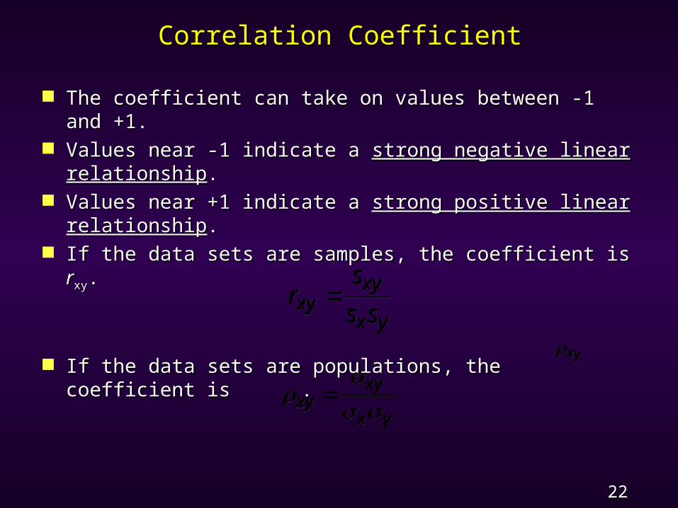
Correlation CoefficientCorrelation Coefficient
The coefficient can take on values between -1 The coefficient can take on values between -1 and +1.and +1.
Values near -1 indicate a Values near -1 indicate a strong negative linear strong negative linear relationshiprelationship..
Values near +1 indicate a Values near +1 indicate a strong positive linear strong positive linear relationshiprelationship..
If the data sets are samples, the coefficient is If the data sets are samples, the coefficient is rrxyxy..
If the data sets are populations, the If the data sets are populations, the coefficient is .coefficient is .
rss sxy
xy
x y
xyxy
x y
xy

23 Slide
Using Excel to Compute theUsing Excel to Compute theCovariance and Correlation Covariance and Correlation
CoefficientCoefficient Formula WorksheetFormula Worksheet
A B C D E
1Average Drive
18-Hole Score
2 277.6 69 Pop. Covariance =COVAR(A2:A7,B2:B7)3 259.5 71 Sam p. Correlation =CORREL(A2:A7,B2:B7)4 269.1 705 267.0 706 255.6 717 272.9 698
24 Slide
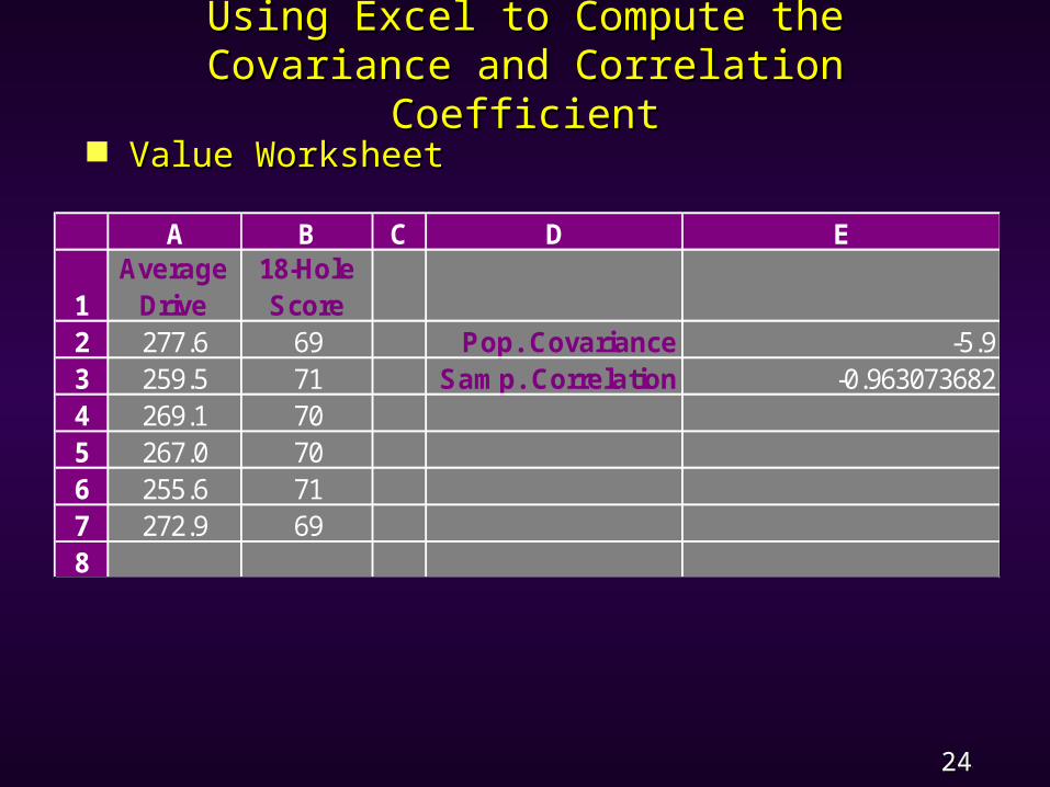
Using Excel to Compute theUsing Excel to Compute theCovariance and Correlation Covariance and Correlation
CoefficientCoefficient Value WorksheetValue Worksheet
A B C D E
1Average Drive
18-Hole Score
2 277.6 69 Pop. Covariance -5.93 259.5 71 Sam p. Correlation -0.9630736824 269.1 705 267.0 706 255.6 717 272.9 698

25 Slide
The Weighted Mean andThe Weighted Mean andWorking with Grouped DataWorking with Grouped Data
The Weighted MeanThe Weighted Mean Mean for Grouped DataMean for Grouped Data Variance for Grouped DataVariance for Grouped Data Standard Deviation for Grouped DataStandard Deviation for Grouped Data
26 Slide
The Weighted MeanThe Weighted Mean
When the mean is computed by giving each When the mean is computed by giving each data value a weight that reflects its data value a weight that reflects its importance, it is referred to as a importance, it is referred to as a weighted meanweighted mean..
In the computation of a grade point In the computation of a grade point average (GPA), the weights are the number average (GPA), the weights are the number of credit hours earned for each grade.of credit hours earned for each grade.
When data values vary in importance, the When data values vary in importance, the analyst must choose the weight that best analyst must choose the weight that best reflects the importance of each value.reflects the importance of each value.

27 Slide
The Weighted MeanThe Weighted Mean
xxwtwt = = wwi i xxii
wwii
where:where: xxii = value of observation = value of observation
ii wwi i = weight for = weight for
observation observation ii

28 Slide
Grouped DataGrouped Data
The weighted mean computation can be used The weighted mean computation can be used to obtain approximations of the mean, to obtain approximations of the mean, variance, and standard deviation for the variance, and standard deviation for the grouped data.grouped data.
To compute the weighted mean, we treat the To compute the weighted mean, we treat the midpoint of each classmidpoint of each class as though it were as though it were the mean of all items in the class.the mean of all items in the class.
We compute a weighted mean of the class We compute a weighted mean of the class midpoints using the midpoints using the class frequenciesclass frequencies as as weights.weights.
Similarly, in computing the variance and Similarly, in computing the variance and standard deviation, the class frequencies standard deviation, the class frequencies are used as weights.are used as weights.
29 Slide
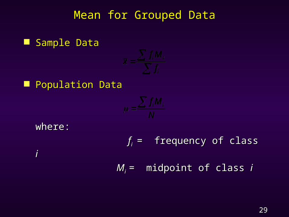
Mean for Grouped DataMean for Grouped Data
Sample DataSample Data
Population DataPopulation Data
where: where: ffi i = frequency of class = frequency of class
ii MMi i = midpoint of class = midpoint of class ii
i
ii
fMf
x
NMf ii

30 Slide
Example: Apartment RentsExample: Apartment Rents
Given below is the previous sample of Given below is the previous sample of monthly rentsmonthly rents
for one-bedroom apartments presented here for one-bedroom apartments presented here as groupedas grouped
data in the form of a frequency data in the form of a frequency distribution. distribution.
Rent ($) Frequency420-439 8440-459 17460-479 12480-499 8500-519 7520-539 4540-559 2560-579 4580-599 2600-619 6

31 Slide
Example: Apartment RentsExample: Apartment Rents
Mean for Grouped DataMean for Grouped Data
This This approximationapproximation differs by $2.41 fromdiffers by $2.41 from
the actual the actual samplesample mean of $490.80.mean of $490.80.
Rent ($) f i M i f iM i
420-439 8 429.5 3436.0440-459 17 449.5 7641.5460-479 12 469.5 5634.0480-499 8 489.5 3916.0500-519 7 509.5 3566.5520-539 4 529.5 2118.0540-559 2 549.5 1099.0560-579 4 569.5 2278.0580-599 2 589.5 1179.0600-619 6 609.5 3657.0Total 70 34525.0
x 3452570 49321, .
32 Slide
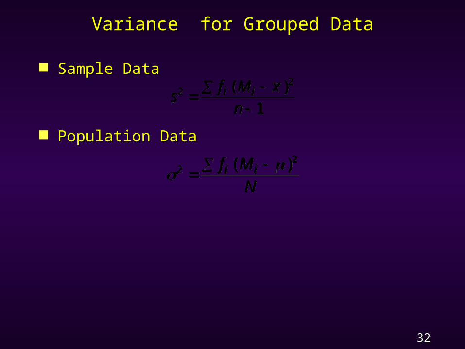
Variance for Grouped DataVariance for Grouped Data
Sample DataSample Data
Population DataPopulation Data
s f M xn
i i22
1
( )
22
f M
Ni i( )
33 Slide
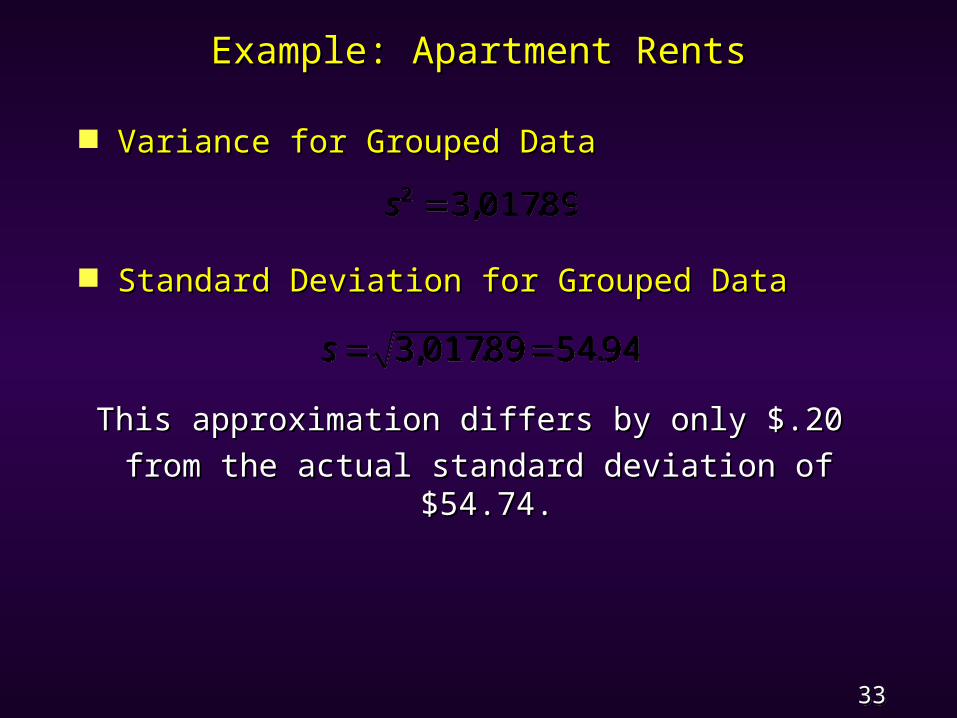
Example: Apartment RentsExample: Apartment Rents
Variance for Grouped DataVariance for Grouped Data
Standard Deviation for Grouped DataStandard Deviation for Grouped Data
This approximation differs by only $.20 This approximation differs by only $.20 from the actual standard deviation of from the actual standard deviation of
$54.74. $54.74.
s2 3 01789 , .
s 3 01789 5494, . .

34 Slide
End of Chapter 3, Part BEnd of Chapter 3, Part B