499 DESCRIPTIVE STATISTICS FOR NONPARAMETRIC ...

499J. Rojo (ed.), Selected Works of E. L. Lehmann, Selected Works in Probability and Statistics, DOI 10.1007/978-1-4614-1412-4_44, © Springer Science+Business Media, LLC 2012

The Annals of Statistics 1976, Vol. 4, No.6, 1139-1158

DESCRIPTIVE STATISTICS FOR NONPARAMETRIC MODELS. III. DISPERSION

BY P. J. BICKEL AND E. L. LEHMANN 1

University of California, Berkeley

Measures of dispersion are defined as functionals satisfying certain equivariance and order conditions. In the main part of the paper attention is restricted to symmetric distributions . Different measures are compared in terms of asymptotic relative efficiency, i.e., the inverse ratio of their standardized variances. The efficiency of a trimmed to the untrimmed standard deviation turns out not to have a positive lower bound even over the family ofTukey models. Positive lower bounds for the efficiency (over the family of all symmetric distributions for which the measures are defined) exist if the trimmed standard deviations are replaced by pth power deviations. However, these latter measures are no longer robust, although for p < 2 they are more robust than the standard deviation. The results of the paper suggest that a positive bound to the efficiency may be incompatible with robustness but that trimmed standard deviations and pth power deviations for p = 1 or 1.5 are quite satisfactory in practice.

1. Measures of dispersion. In analogy with the definition of a measure of location, we shall define a measure of dispersion to be a functional (defined over a sufficiently large family of distributions) which satisfies certain in variance conditions and which in addition has the property of assigning a larger value to G than to F if G is more dispersed than F. In the present paper we shall consider the problem for symmetric distributions (see BL IV for the asymmetric case) and assume that X is a random variable whose distribution F is symmetric about p .

It then seems natural to interpret dispersion in terms of the distance of X from p, that is , in terms of the magnitude of IX- f-11, and to consider Y as more dispersed about 1.1 than X about p if

( 1.1) I Y - vi is stochastically larger than IX - PI . (This is essentially the "peakedness"-ordering introduced by Z. W . Birnbaum (1948).)

Note that

(a) any symmetric random variable is more dispersed than a constant; (b) aX is more dispersed than X if a > 1.

If F and G are symmetric about 0 with densities f and g, a simple sufficient

Received February 1975; revised April 1976. 1 This paper was prepared with support of U.S. Office of Naval Research Contract No.

N00014-69-A-0200-!038/NR042-036 and National Science Foundation Grant No. GP-38485 . AMS 1970 subject classifications. 61G05, 62G20, 62G30, 62G35. Key words and phrases. Dispersion, estimation, standardized asymptotic variance, asymptotic

efficiency, Tukey model, standard deviation, trimmed standard deviation, pth power deviation. substitution of an estimate of location, scaling a positive distribution.

500

P. J. BICKEL AND E. L. LEHMANN

condition for ( 1.1) with f1 = l.i = 0 is

( 1.2) g(x)IJ(x) is increasing for x > 0 .

IfF and G are symmetric about zero, and G is more dispersed than F, and if

(1.3) H 0(x) = 8G(x) + ( 1 - 8)F(x) ,

then H 0 is more dispersed than F for any 0 < () < 1. As an illustration, note that a standard normal distribution contaminated with another normal distribution with zero mean and variance > 1 (Tukey model) is more dispersed than the uncontaminated standard normal distribution.

An important class of examples is provided by the following result, which is a generalization of a lemma of Birnbaum (1948).

THEOREM 1. Let Xi, Yi (i = 1, 2) be independent with distributions Fi, Gi (i = 1, 2) which are symmetric about zero, and suppose that

(i) Yi is more dispersed than X t for i = 1, 2 and (ii) F 1 and G2 have unimodal densities and possibly some probability mass at zero.

Then yl + y2 is more dispersed than XI + x2.

PROOF. Consider the probability

P(jX1 + X2j <c)= 2 ~ ;' [F1(x + c) - F1(x- c)] dF2(x).

The unimodality of F 1 implies that the integrand on the right-hand side is a decreasing function of x. From the fact that (F2 , G2) satisfies (1.1), it then follows that this last integral is decreased when F2 is replaced by G2• Thus,

P(jX1 + X2 j ~c) :2:2 ~ ;' [F1(x +c)- F 1(x- c)]dG2(x)

= 2 ~ ;' [G2(x + c) - G2(x - c)] dF1(x).

Repeating the argument (this time using the unimodality of G2), we arrive at the desired result. Birnbaum has shown that Theorem 1 no longer holds when assumption (ii) is dropped.

Consider now a functional r(F) [also denoted by r(X) when X is a random variable with distribution F] defined over a sufficiently large class of symmetric distributions which is closed under changes of location and scale. We shall require r to be nonnegative and to satisfy

(1.4)

and

( 1.5)

r(aX) = jajr(X)

r(X + b) = r(X)

for a> 0

for all b .

It follows from (1.5) and the symmetry ofF that

(1.6) r( -X)= r(X)

so that (1.4) holds for all a* 0.

501

NONPARAMETRIC MODELS

From (1.4) and (1.5) it is easily seen that

(1.7) <(c) = 0 for any constant c .

For by (1.4), we have <(0) = <(2 X 0) = 2r-(O) and hence <(0) = 0, and by (1.5), r-(c) = <(0). The converse, that <(X) = 0 requires X to be a constant with probability 1, will in general not hold. An example is provided by the trimmed standard deviation defined in Section 3 below.

A nonnegative functional r- satisfying (1.4) and (1.5) will be called a measure of dispersion if it satisfies in addition

(1.9) r-(F) ~<(G) whenever G is more dispersed than F.

Note that if r-(F) is a measure of dispersion, so is h(F) for any k > 0. A large and important class of dispersion measures is provided by the

functionals

( 1.1 0)

where F is assumed to be symmetric about p., F * denotes the distribution of IX - P.l, A is any probability distribution on (0, 1) and r any positive number.

That (1.10) satisfies (1.4) and (1.5) is easily checked; that it satisfies (1.9) follows from the fact that F * -1( t) ~ G * -1( t) for all t when G * is stochastically larger than F *.

A special case of ( 1.1 0) is the standard deviation (SD) of F defined as

(1.11) SD(F) = [~ (x- p.)2 dF(x)]!.

This is easily seen to be given by ( 1.1 0) with r = 2 and A the uniform distribution on (0, 1 ). The following three important classes of measures, all special cases of ( 1.1 0) provide the alternatives to the standard deviation with which we shall be concerned.

( i) A generalization r-(F; p) of the standard deviation is the pth power deviation obtained by replacing r by p in (1.10) and letting A be the uniform distribution on(0,1).

( ii) The doubly trimmed standard deviation r-( F; a, f3) is given by ( 1 .1 0) with r = 2 and A the uniform distribution on (a, 1 - f3). The most important example of this is the case a = 0.

(iii) The ath quantile is obtained from (1.10) by letting A assign probability 1 to the point a. The resulting measure is independent of r.

The standard deviation is of course a member of both (i) and (ii). The ath quantile is the limit of the doubly trimmed standard deviation as f3 ~a.

2. Estimation. A most important aspect in comparing two measures of scale r-i(F) and r-;(F) is the accuracy with which they can be estimated. Unfortunately, it is no longer possible to compare these accuracies directly in terms of the asymptotic variances of the estimators. This is clearly seen by considering the

502

P, J. BICKEL AND E. L. LEHMANN

case r 2 = cr 1 where c is any positive constant. If r 1 is a possible measure of scale and its estimator is o1 , one would be equally happy to use r 2 and estimate it by o2 = co1; of course the asymptotic variance does not remain the same but gets multiplied by c2 • For this reason, a natural measure of accuracy of an estimator of r(F) with asymptotic variance n-1v2(F) is not n-1v2(F) itself but the scale invariant standardized asymptotic variance (already proposed by Daniell ( 1920))

(2.1)

The asymptotic efficiency e2 , 1 of o2 (estimating r 2) to o1 (estimating r 1) will then be defined as

(2.2) e (F) = vl2(F)/v22(F) . 2,1 rt2(F) r22(F)

If (ni)~(o;- ri) is asymptotically normally distributed for i = 1, 2 as the number ni of observations tends to infinity, the usual argument shows that the asymptotic efficiency (2.2) is the limiting ratio of the numbers of observations required by the two estimators to achieve the same standardized variance.

That the above definitions are reasonable can be seen from another point of view. The logarithm of o is an estimator of the location parameter log r(F). Suppose that the distribution of n!(o - r) tends to the normal distribution with zero mean and variance v2 • Then the distribution of ni(log o - log r) tends to the normal distribution with mean zero and variance V2/r2(F); that is, v2fr 2(F) is the asymptotic variance of the location estimate logo.

When studying the estimators of functionals such as those defined in Section 1, it is convenient first to consider F restricted to distributions which are symmetric about a known point p. On the other hand, in order even to define the estimators of r we wish to study, it is necessary to extend r to asymmetric distributions. In all the examples to be considered here, there is a natural functional form of r which applies also to asymmetric distributions. Given this extension, we define as estimator of i(F) the functional r evaluated at the empirical distribution function ft of X 1 , ••• , X,.. In what follows, we shall assume without loss of generality that the known value p of the center of symmetry of F is p = 0.

The point of view in the present paper will be that the standard measure of scale is the standard deviation r(F; 0, 0) which (since p = 0) is estimated by

(2.3)

This estimator is well known to be very unsatisfactory because of its extreme sensitivity to outlying observations. We shall therefore look at the other functionals under consideration as competitors of r 1 and hence shall be interested principally in comparing their behavior with that of r 1• Unfortunately, we are only able to make these comparisons asymptotically. For L: XNn, it is of course obvious from the central limit theorem that n![L; X/fn - a2 ] is asymptotically normal

503


with zero mean and variance Var (X2) provided the later variance is finite. Here

a 2 = E(X2) denotes the variance of X.

It follows that ni( o1 - a) is asymptotically normal with mean zero and variance

Var (X2)/4a2• Thus the standardized variance is

(2.4) V12(F) = Var (X2) = _!__ [ E(X•) _ 1]. -r 12(F) 4a• 4 a•

In the next sections we shall obtain the corresponding expansion for the

estimators of some other functionals, and then study the efficiencies (2.2).

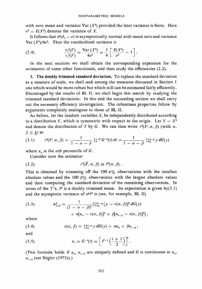
3. The doubly trimmed standard deviation. To replace the standard deviation

as a measure of scale, we shall seek among the measures discussed in Section 1

one which would be more robust but which still can be estimated fairly efficiently.

Encouraged by the results of BL II, we shall begin this search by studying the

trimmed standard deviations. In this and the succeeding section we shall carry

out the necessary efficiency investigation. The robustness properties follow by

arguments completely analogous to thos~ of BL II. As before, let the random variables X; be independently distributed according

to a distribution F, which is symmetric with respect to the origin. Let Y = X 2

and denote the distribution of Y by G. We can then write -r2(F; a, f') (with a,

f' ;£ !) as

(3.1) r 2(F; a, f') = l ~~-P G-1(t) dt = 1 ~:~-P y dG(y) 1-a-f' 1-a-f'

where ua is the ath percentile of G.

Consider now the estimator

(3.2)

This is obtained by trimming off the 100 a% observations with the smallest

absolute values and the 100 f'% observations with the largest absolute values

and then computing the standard deviation of the remaining observations. In

terms of the Y's, f 2 is a doubly trimmed mean. Its expectation is given by(3.1)

and the asymptotic variance of nif2 is (see, for example, BL II)

(3.3)

where

(3.4)

and

(3 .5)

w~ .• = 1 0:1-p [y - c(a, f')]2 dG(y) ~ ( l - a - /')2 a

+ a[ua - c(a, f')Y + f'[u 1_p - c(a, {')]2},

c(a, f') = ~:~-P y dG(y) + aua + f'u 1_p,

u, = G-l(t) = [ p-1 ( t ~ 1) J (This formula holds if ua, u1 _P are uniquely defined and G is continuous at ua,

u1_P (see Stigler (1973)).)

504

P. J. BICKEL AND E. L . LEHMANN

The standardized asymptotic variance off is thus w2(r4 where T 2 is given by (3 .1 ).

To get an idea of the behavior of such procedures with respect to the untrimmed standard deviation we consider some representative cases, namely the (singly) trimmed standard deviations with f3 = .1, .2, a = 0. The tables below computed by Winston Chow and W . Carmichael show the efficiencies (2.2) of these estimators with respect to the standard deviation for the following three classes of distributions .

(a) t-distributions with 5, 6, 7, 8, 9, 10, 25, 50 degrees of freedom. (b) Symmetric beta distributions with densities

(3.6)

for r = !, 2, 4, 6, 8, 10, 20, 30. (c) Tukey normal gross error distributions, i.e.,

(3 .7) F(x) = (1 - c)(x) + c<l> ( ~),

for c = .025, .075, .10, .20, .40, .50 and A = 2, 4, 6. These models were selected as representing a range of long and short tailed

distributions and for ease of computation. The figures suggest that, on the whole, for heavy-tailed distributions both

trimmed SD's are better than the untrimmed SD and that for the ranges considered f3 = .1 is preferable to f3 = .2. For light-tailed distributions such as the Beta-distribution, the untrimmed SD does best, f3 = .1 does better than f3 = .2, and f3 = .1 performs reasonably well.

A surprising feature of Table 3.3 are the extremely high efficiency values for small c > 0 and large A. These seem to arise in cases where there is enough trimming to insure with very high probability that only a small proportion of

TABLE 3.1

Asymptotic efficiency of {3-trimmed with respect to untrimmed SD: !-distribution with f degrees of freedom

f 5 6 7

f3 = .I 2.35 1.56 1.29 f3 = .2 2.11 1. 36 1. 11

8

1.16 .99

9

1.08 .92

TABLE 3.2

10

1.03 .87

25

.85

.69

50

.81

.66

Asymptotic efficiency of {3-trimmed with respect to untrimmed SD: Beta distribution with density (3.6)

00

.78

.63

r . 5 1.0 2 .0 4.0 6.0 8.0 10.0 0.0 30.0 00

/3= . 1 1.30 . 86 . 72 . 70 . 71 . 72 . 73 . 75 . 76 . 78 f3 = .2 . 83 .57 .52 .54 .55 .57 .57 .60 .61 .63

505


TABLE 3.3

Asymptotic efficiency of {'-trimmed with respect to untrimmed SD: Tukey model (3 .7)

.:1

fi =: .l fi== .2

2 4 6 2 4 6

0 .78 .78 .78 .63 .63 .63 .025 .98 3.97 10.04 .80 3.27 8.36 .075 1.19 4 .01 6.48 .99 3.57 6.03 . 10 1.23 3.48 4.79 1.03 3.27 4.93 .20 1.21 1.46 .76 1.05 2.04 2.26 .40 .96 .63 .50 .87 .68 .38 .50 .87 .63 .55 .79 .52 . 36

the gross errors is retained in the trimmed sample . The standardized variance of the untrimmed SD then rises very sharply with A while that of the trimmed SD is affected only little as A gets large. The curious "dip" which occurs in the neighborhood of e = f3 is predicted by the asymptotic theory of the next section.

4. Nonexistence of a lower bound. The numerical results of the preceding section are encouraging and raise the hope that, as in the case of the trimmed means as measures of location, the efficiencies of the trimmed to the untrimmed SD have a positive lower bou'nd. Unfortunately, this turns out not to be the case even if attention is restricted to unimodal distributions. In fact, even within the class of Tukey models (3.7), the efficiencies can take on arbitrarily small values .

THEOREM 2. Let e(f3; e, A) denote the asymptotic efficiency of the trimmed standard deviation f(O, /3) relative to the untrimmed standard deviation, in the Tukey model (3.7). Then

( 4.1) lim, ~ .. e(f3; f3, A) = 0 .

The proof of this result is based on the following two lemmas.

LEMMA 1. For the Tukey model (3.7), the standardized asymptotic variance of the SD

(4 .2) 1 [ E(X') _ 1] 4 £2(X2)

is bounded above uniformly in A for any fixed e.

PROOF . For the model (3. 7), the standardized variance (4.2) becomes

_!_ (3[(1- e)+ d'] _ t). 4 [(1 -e) + d 2] 2

Since this is continuous in A we need only consider its behavior as A ~ oo

when it is clearly bounded.

506


LEMMA 2. If~ = {3 in (3. 7) and if u1 _~ = ui~P is given by (3 .5), then as a function of A.,

as ). ----+ oo .

PROOF . Let

Then x(A.) satisfies

(4.3) (1 - {3)(x) + {3<1> ( ~) = 1 - ~ .

First note that as ). ----+ oo we must have

(4.4) x().) ----+ oo ,

and

(4.5)

For if ( 4.4) does not hold there exists a sequence A.,. such that

x( A.,.) ----+ c < oo . Then,

(1 - {3)(x('A.,.)) + {3<1> (x(A.,.))----+ (1 - {3)(c) + }!_ < 1 - p_, ~ 2 2

and this contradicts (4.3). Similarly if (4.4) holds but (4.5) is violated we could

find a sequence {A,.'} such that

lim,. ( 1 - {3)<1>( x( A.,.')) + {3<1> ( x~ ).;')) > 1 - {3 , .. and we would again have a contradiction.

Now, by (4.4) and (4.5),

(4.6) - [x(J.)) = SO~~i~)] [1 + o(1)],

and

(4.7) (x(J.)) _ __!_ = so(O)x(A)[l + v(l)]. X 2 A

Substituting (4.6) and (4.7) in (4.3), cancelling, and then taking logs we obtain

(4.8) x2(A) {3

- -logx(A) = logx(J.) -log).+ log + o(l). 2 1-{3

By (4.4) log x(A) = o(x2('A.)),

and we conclude that

(4.8a) xV)(1 + o(1)) = 2log).

which was to be proved. 0

507


PROOF OF THEOREM 2. In view of Lemma 1 we only need to show that

(4.9) w~.P ~ = while

( 4.10) r 2(F; 0, /3) = 0(1) as I.~=.

To show (4.10) we calculate,

( 1 - f3)r 2(F; 0, /3) = ( 1 - /3) ~ z_c;:,, x\o(x) dx + ~ ~ z_c;;,, x2cp ( ~ ) dx

~ (1 - /3) + 2/3?.2 ~o c ,,n icp(y) dy

~ ( 1 _ /3) + 2f3~(0) xy) , and the result follows. This argument and Lemma 2 show that

( 4.11) c(O, /3) = (1 - f3)r 2(F; 0, /3) + j3u1_p .- j3u1_p,

where c(a, /3) is given by (3.4). Finally, from (4.11)

(1 - f3)2w~.P > f3(u1_p- c(O, /3))2 .- /3(1 - f3)2uLP

which tends to =, and ( 4. 9) and the theorem follow. 0

REMARK 1. The same arguments show that the result of Theorem 2 continues to hold if r 2(F; 0, /3) is replaced by r 2(F; a, /3) for any a < 1 - f3, and if as before e = f3.

REMARK 2. In addition to predicting that the efficiency of the /3-trimmed SD to the SD tends to 0 as r ~ = for e = f3 the asymptotic theory also gives a positive limit for e * f3. Roughly speaking, for e > f3 the behavior is governed by the contaminant while for e < f3 it is governed by the main portion. Clearly Table 3.3 reflects this only very crudely. For the values of r we have given, the efficiency ate = f3 remains quite large. However, further numerical calculations for extremely large values of r (of the order of 50 and above) confirm the asymptotic theory although convergence is slow. It is seen from the tables that small efficiency values do appear for smaller values of rand e > f3. These presumably reflect small positive limits which are approached more rapidly than the asymptotic value for e = f3.

REMARK 3. An interesting limiting case of the doubly trimmed standard deviations arises as both a and f3 tend to ! · The limiting functional is naturally taken to be

(4.12)

the median of the distribution of IX- f11 which, since X is symmetric about p, coincides with

508


the interquartile range of F. The estimator -r(ft; ~.~)has asymptotic standardized variance

(4 .13) 1

where F(x + p) = i· Again for the Tukey model with s = .5 the asymptotic efficiency of this

estimator relative to the SD tends to zero as ,{ ~ oo. Numerical values of the efficiency similar to those shown in Table 3.3 are given in Table 4.1 computed by Winston Chow. They are clearly much less satisfactory than the corresponding values for (3 = .1 in Table 3. 3. In particular, the low values at the uncontaminated normal make this measure unsuitable .

TABLE 4.1

Asymptotic efficiency of r(F; !, t) with respect to the SD for

the Tukey model (3.7)

A.

2 4 6

0 .37 .37 .37 . I .62 2.05 3.16 .2 .65 1.43 1. 78 .3 .61 1.01 1.11 .4 .56 .73 .70 .5 .51 .52 .43

The result of Theorem 2 is rather disappointing, particularly since it is in such contrast to the general (asymmetric) location case. One may ask whether a positive lower bound can be obtained if the trimmed SD is replaced by a measure of the form (i .10) with r = 2 but some other A. An essentially negative answer (if attention is restricted to robust measures) is provided by the following generalization of Theorem 2.

THEOREM 3. Suppose that -r(F) is given by (1.10) where r = 2 and the weight function A has a density A' which vanishes outside [a, 1 - (3] with 0 < a < 1 -(3 < 1, is bounded, and is bounded away from 0 inside. Then the relative efficiency of -r(F) relative to the standard deviation tends to 0 as ,{ ~ oo in the Tukey model

(3 . 7) with s = (3 .

For the proof we require the following lemma.

LEMMA 3. If r- 12 and r-22 are two functionals of the form (1.10) with r = 2 and weight functions A~' A2 , and if the A; have densities A/ satisfying

(4.14) 0 ~ a~ A2'(t)/A/(t) ~ A < oo ,

then the efficiency of the estimator of r-2 to that of r- 1 satisfies

(4.15) e2 , 1(F)2a2/A2 •

509


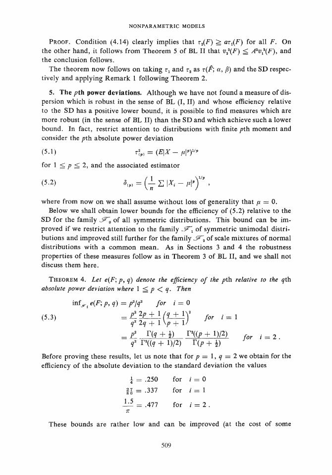
PROOF. Condition (4.14) clearly implies that r 2(F) ~ ar1(F) for all F. On the other hand, it follows from Theorem 5 of BL II that v22(F) s A2V12(F), and the conclusion follows.

The theorem now follows on taking r 1 and r 2 as r(F; a,~) and the SD respectively and applying Remark 1 following Theorem 2.

5. The pth power deviations. Although we have not found a measure of dispersion which is robust in the sense of BL (I, II) and whose efficiency relative to the SD has a positive lower bound, it is possible to find measures which are more robust (in the sense of BL II) than the SD and which achieve such a lower bound. In fact, restrict attention to distributions with finite pth moment and consider the pth absolute power deviation

( 5.1)

for 1 ~ p ~ 2, and the associated estimator

(5.2)

where from now on we shall assume without loss of generality that p. = 0. Below we shall obtain lower bounds for the efficiency of (5.2) relative to the

SD for the family ff0 of all symmetric distributions. This bound can be improved if we restrict attention to the family ~ of symmetric unimodal distributions and improved still further for the family~ of scale mixtures of normal distributions with a common mean. As in Sections 3 and 4 the robustness properties of these measures follow as in Theorem 3 of BL II, and we shall not discuss them here.

THEOREM 4. Let e(F; p, q) denote the efficiency of the pth relative to the qth absolute power deviation where 1 < p < q. Then

inf_,..-1 e(F; p, q) = p2fq2 for i = 0

(5.3) = p2 2p + 1 (q + 1)2 for i = 1 q2 2q + 1 p + 1

_ p2 r(q + !) P((p + 1)/2) - t P((q + 1)/2) f(p + ~)

for i = 2.

Before proving these results, let us note that for p = 1, q = 2 we obtain for the efficiency of the absolute deviation to the standard deviation the values

t = .250 for i = 0

H = .337 for i = 1

~ = .477 for i = 2. tr

These bounds are rather low and can be improved (at the cost of some

510


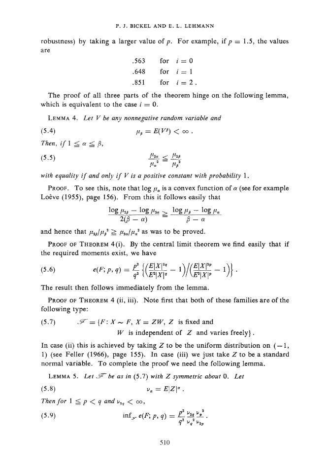
robustness) by taking a larger value of p. For example, if p = 1.5, the values are

.563 for i = 0

.648 for i = l

.851 for i=2.

The proof of all three parts of the theorem hinge on the following lemma, which is equivalent to the case i = 0.

LEMMA 4. Let V be any nonnegative random variable and

(5.4)

Then , if 1 ~ a < (3,

(5.5)

p.f! = E(Vf!) < oo .

f12a < f-12{!

P.a2 = f-1/ with equality if and only if V is a positive constant with probability 1.

PROOF. To see this , note that log P.a is a convex function of a (see for example Loeve (1955), page 156). From this it follows easily that

log p.2f! - log f1 2a > log f-lf! - log P.a

2((3 - a) = (3 - a

and hence that p.2f!/ p./ ;;:;;:; f12a/ P.a2 as was to be proved.

PROOF OF THEOREM 4(i). By the central limit theorem we find easily that if the required moments exist, we have

(5.6) . _ P2 {(EIXI2q )/(EIXI 2

" )} e(F, p, q) - Cf E'2!XIq - 1 PIX!~' - 1 .

The result then follows immediately from the lemma.

PROOF OF THEOREM 4 (ii , iii). Note first that both of these families are of the following type:

(5.7) ff = {F: X,.., F, X= ZW, Z is fixed and

W is independent of Z and varies freely} .

In case (ii) this is achieved by taking Z to be the uniform distribution on ( -1, 1) (see Feller (1966), page 155). In case (iii) we just take Z to be a standard normal variable . To complete the proof we need the following lemma.

LEMMA 5. Let ff be' as in (5 . 7) with Z symmetric about 0. Let

(5 .8)

Then for 1 ;£ p < q and l.J2 q < oo,

(5.9)

511


PROOF . Let

Then from (5.6) and (5.7)

(F. ) _ p2 (v2qfv/)wq- 1 _ p2 (v2qfvq2)p- (1/wP) e ' p' q - - - - -'-'=-...!....!-'------''-'---"-'-

q2 (v2P/v/)wP - 1 q 2 (v2P/v/) - (1/wP)

where p = w qfw P and where X = ZW has distribution F. Keeping w P fixed, this is minimized by taking for p its minimum value which is 1 by Lemma 4. Since by Lemma 4, v2qfv/ :2:: v2P/v/, we now obtain a lower bound for the efficiency by letting wP ~ oo. To show that this lower bound is sharp we need to exhibit a sequence of distributions for W such that p ~ 1 and w P ~ oo. Take

( 5.1 0) with probability 11:

= a with probability 1 - 11: •

Then,

w = 11: + (1 - tr)a2P

P (rr + (1 - rr)aP)2

As a~ oo, 1

w ~--p 1 - 11:

and p ~ 1.

Now letting 11: ~ 1 we can extract the requisite sequence of distributions. The lemma follows. 0

The theorem now follows from the standard formulas for the absolute moments of uniform and standard normal variables. 0

REMARK. Note that for case (iii) of formula (5.3) for the trimmed standard deviations, an extremal sequence is provided by an appropriate sequence of Tukey models. In fact, the distributions defined by (5.10) are of this type.

As we have noted, the lower bound to the efficiency of the mean deviation is rather low even for ff2• However, as we found for trimmed standard deviations, in reasonable situations the bound is very conservative. Here are some numerical results for the pth power deviation for p = 1, 1.5 and a selection of the distributions given in Tables 3.1-3.3.

Qualitatively the behavior of these measures closely parallels that of the corresponding Tables 3.1-3. 3. For reasonable distributions the mean deviation

TABLE 5.1

Asymptotic efficiency of pth power deviations with respect to standard deviation !-distribution with f degrees of freedom

f p = l p = 1.5

5

2.35 1.88

10

1.12 1.12

25

.94 1.01

50

.91

.99

00

. 88

.97

512


TABLE 5.2

Asymptotic efficiency of pth p~wer deviation with respect to SD: Beta distribution with density (3.6)

r .5 1.0 2.0 4 6 8 10 20 30 00

p = l .53 .60 .68 .75 .78 .80 .81 .84 .85 .88

p = 1.5 .76 .80 .85 .89 .92 .93 .94 .96 .97 .97

TABLE 5.3

Asymptotic efficiency of pth power deviation witn respect to standard deviation. Tukey model (3. 7)

,{

p = l p = 1.5

2 4 6 2 4 6

0 .88 .88 .88 .97 .97 .97 .025 1.06 3.08 5.18 1.10 1.99 2.33 .075 1.22 2.53 2.66 1.18 1.61 1.51 . 10 1.25 2.21 2.14 1.19 1.48 1.35 .20 1.24 1.50 1.31 1.17 1.20 1.09 .40 1.09 1.04 .92 1.08 1.02 .96 .50 1.03 .95 .85 1.05 .99 .94

particularly seems to do even better than the trimmed deviations. Of course,

for sufficiently heavy tailed distributions, for example t-distributions with suf

ficiently low degrees of freedom, it can break down badly.

6. Measuring the scale of positive random variables. The concepts and

results developed so far also apply to a somewhat different problem. Consider

a random variable X with distribution F, which is known to be positive. Then

one may be interested in scaling this distribution by defining a suitable measure

a of its distance from zero . Of such a measure we shall require (in analogy with

the earlier axioms for r)

(6 . 1) a( aX) = aa( X) for a> 0

and

(6.2) a(Y) ~ a(X) if Y is stochastically larger than X.

There is a simple correspondence between such measures and the earlier

measures r , defined by

(6.3) r(X) = a(IX- p[)

where p = PF as before denotes the center of symmetry of X. Given a measure

a defined over positive random variables and satisfying (6.1) and (6 .2), let X be

a symmetric variable whose center of symmetry is denoted by p . Then (6.3)

513


defines a measure satisfying (1.4), (1.5) and (1.9). Conversely, let r be a measure of dispersion defined over symmetric random variables, and let Z be any positive random variable . Extend Z to negative values so that it is symmetric about 0 and denote the resulting random variable by X. Then p. = 0 and IX - p.j = lXI = Z. The measure a(Z) defined through (6.3) satisfies (6.1) and (6 .2).

Examples of scale measures a are provided by the median of a positive random variable X, by the first moment E(X) , by the square root of the second moment (E(X2))', or by trimmed versions of these latter measures. Using (6.3), it is a trivial matter to adapt the results of Sections 3 and 4 to comparisons of the estimator of (E(X2W with its trimmed versions. This is, however, not quite appropriate since the scale measures of greatest interest for positive random variables are those corresponding to E(X) and its trimmed versions .

We believe that the results of numerical and theoretical comparisons of the sample mean and its trimmed competitors qualitatively will be quite similar to those obtained for the sample SD and its trimmed competitors, but we have not carried out this program. In addition to this, Theorem 4 of Section 5 reveals that the sample mean, which is the estimator of E(X), has for p > 1 efficiency bounded from below with respect to estimators of [E(XP)]l/p for the families

~ = {All distributions on the positive axis with finite second moment}

~ ={All members of ~ with monotone nonincreasing densities}

ffa = {All members of ffa which are scale mixtures of half normal

distributions} .

7. Unknown center of symmetry. In estimating dispersion we have so far restricted attention to symmetric distributions and have assumed the center of symmetry to be known. If the center p. of symmetry is unknown, it is tempting to estimate p. by a suitable estimate of location and to substitute this for p. in the estimator of r . The question naturally arises what effect this has on the asymptotic distribution and hence on the efficiency of the estimator. For the measures of dispersion considered in this paper it turns out that under suitable regularity conditions the asymptotic distribution is unchanged by this substitution. We have not investigated the small sample behavior of these procedures.

The theorem below gives a simple sufficient condition for substitution of an estimate of location to work in this sense. We subsequently check that this condition is satisfied by trimmed standard deviations and pth power deviations among others.

To formalize the process of substitution we appeal to the discussion of Section 6 in which we indicated that there is a 1-1 correspondence between measures of dispersion r for symmetric distributions and measures of scale a for positive random variables via (6 .3) . Let us start then with such a a defined for nonnegative variables. For reasons similar to those given at the beginning of Section 2, we need to consider extensions of a to larger families of distributions, namely to the family of all distributions F for which a(jXI) is defined. To avoid

514


proliferation of notation we also call the extension a and define it by

a(X) = a(JXJ) .

For example, if a2(X) = ~ 0 x2 dF for nonnegative variables, the extension of a2

is the second moment. If a( X) is the median of the distribution on (0, oo ), the extension is the median of the distribution of JXJ.

Let p.(F) be a measure of location satisfying (1.1) and (1.2) of BL II. Suppose also that X 1, ••• , X,. are independently distributed each with distribution F and let ft be the empirical cdf. Define

p = p.(F)

as the usual estimator of p.(F) and let

Fp(x) = F(x + p.)

denote the cdf of X- p.. Note that the empirical cdf of X1 - p, · ··,X,. - p is then Fr,.

If F is symmetric about p. the measure of dispersion corresponding to a by (6.3) is

r(F) = a(Fp) .

The estimator of r we have used for known p. is a(F"). Failing this knowledge we use f defined by

For example if f = a(P,) .

p.(F) = ~~"' x dF(x),

a 2(F) = ~ 0 x 2 dG(x) ,

where G is the cdf of JXJ, then

and f is the sample SD. If

~ 1 a2(F") = - L; (Xi - p.)2

n

p.(F) = p -1(!)'

a(F) = G- 1(!),

then f is the median of the absolute deviations from the median of the obser. vations.

THEOREM 5. Suppose that the underlying distribution F is symmetric about p. and suppose without loss of generality that p. = 0. Suppose further that:

(7 . 1) a(F") is differentiable in p. at p. = 0,

(7.2) limM_"' limsup,.P[n~JP. J 2: M] = 0,

(7.3) lim310 limsup,.P[sup{n~Ja(F")- a(F")- a(F)

+ a(F)J: Jp.J < o}?: e] = 0 for all e > 0.

515


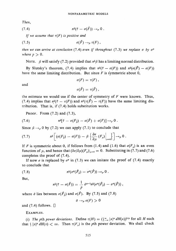
Then,

(7 .4)

If we assume that -r(F) is positive and

(7.5) a(F) -p -r(F),

then we can arrive at conclusion (7 .4) even if throughout (7 .3) we replace a by aP

where p > 0.

NoTE. p will satisfy (7 .2) provided that nt p has a limiting normal distribution.

By Slutsky's theorem, (7 .4) implies that nt(f - a( F)) and nt(a(F) - a(F)) have the same limiting distribution. But since F is symmetric about 0,

and a(F) = -r(F) ,

a(F) = -r(F) ,

the estimate we would use if the center of symmetry ofF were known. Thus, (7 .4) implies that ~t(f - -r(F)) and n~(-r(F) - -r(F)) have the same limiting distribution. That is, if (7 .4) holds substitution works.

PROOF. From (7.2) and (7.3),

(7.6)

Since p -P 0 by (7 .2) we can apply (7 .1) to conclude that

(7.7) nt [(a(F;,) - a( F)) - p {!!__ (F,) I }] -P 0. a p. p=O

IfF is symmetric about 0, if follows from (1.4) and (1.6) that a(F,) is an even function of p., and hence that(aa;ap.)(F,)I,=o = 0. Substituting in (7. 7) and (7 .6) completes the proof of (7.4).

If now a is replaced by aP in (7 .3) we can imitate the proof of (7 .4) exactly to conclude that

(7.8)

But, A 1 A A

nt(f- a(F)) =- a~>-1n;(a~'(F;,) - a~'(F)), p

where a lies between a(F;,) and a(F). By (7.5) and (7.8)

a -P a(F) > 0 and (7.4) follows. 0

EXAMPLES.

(i) The pth power deviations. Define -r(H) = O :"' lxiP dH(x))11~' for all H such that ~ lxiP dH(x) < oo. Then -r(F1..) is the pth power deviation. We shall check

516


that (7.3) holds for r 71 under the condition

(7.9) ~ lxl271 dF(x) < oo.

For fl.< 11, we find

E(n;(rP(F.) - rP(Fp) - rP(F.) + rP(Fp))) 2 = Var (IXl - lllp - IXl - fl-1 11).

If p > 1 this variance is bounded by

E(IX1 - 11IP - IX, - rlpY ~ p 2(11- f1.) 2 sup {EIX1 - -<l 2p-2 : .< E [fl., 11]}

~ C(11- rY if 111 1, lrl ~ M,

where C is a constant depending on M. If p = 1,

Var (IX1 - 111 - IX1 - rl) ~ E[(11- r)(21£x191 - 1) + 2(11- X1)/£p<xt<"Jr

~ C(11 - r)2 if 1111, lrl ~ M.

In any event

E(n;(rP(F.) - rP(F") - r 11(F.) + rP(F"))Y :S C(11- f1.) 2

and an argument using Theorem 12.3, page 95 in [3] completes the proof. Since

(7. 9) implies (7 .5) as well as the asymptotic normality of r(F) we see that any

measure p. satisfying (7 .2), for instance the mean, can be substituted without

affecting the asymptotic behavior of the estimators.

(ii) (L) estimators. Suppose r is given by

(7 .10)

where A is symmetric about !· IfF is symmetric about fl., and if we define A(t) = 2A((l + t)/2)- 1, then

r( F ") is the measure defined in ( 1.1 0).

Suppose that

(7 .11)

(7.12)

A places no mass outside an interval (aj2, 1 - aj2), 0 < a < ! F is differentiable with derivative f which is positive

and continuous.

We shall now show that (7.3) holds for r 7 under these assumptions, so that

we may safely substitute an estimate of location in the singly and doubly

trimmed standard deviations. Here is a sketch proof. Let

G(x, r) = P[IX1 - fl-1 1 ~ x] ,

and let G(x, fl.) be the empirical cdf of IXl- rl 7 , •• ·,IX,.- rlr. Define

G(x) = G(x, 0) , G(x) = G(x, 0) .

Finally let G-1(t, fl.), G-1(t, fl.) be the corresponding inverses (in x).

517


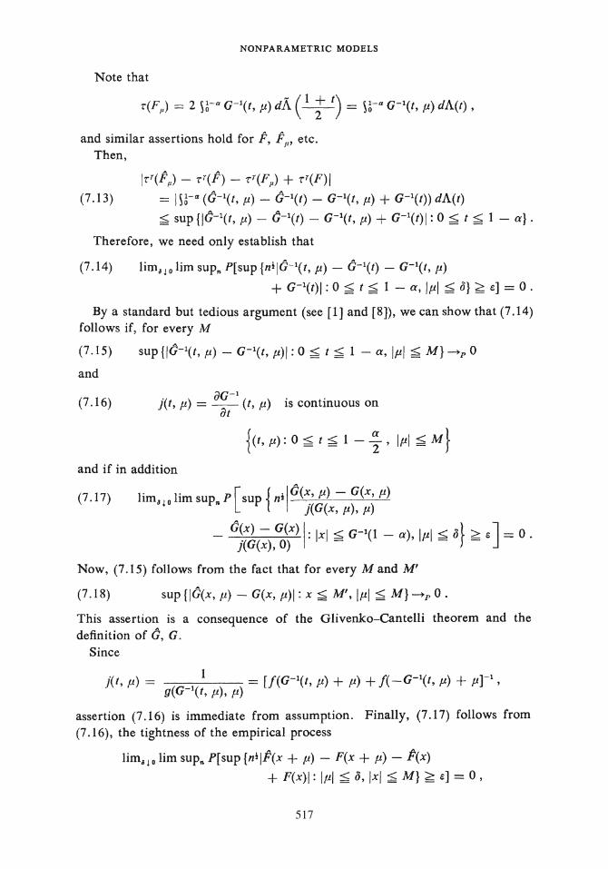
Note that

and similar assertions hold for F, FP, etc. Then,

lr'(F11) - r'(F) - r'(F11 ) + r 7(F)I

(7.13) = IS~-a(G- 1(t, fl.)- G-1(t)- G-1(t, fl.)+ G-1(t))dA(t)

~ sup {jG-1(t, fl.) - G-1(t) - G-1(t, fl.) + G-1(t)i: o ~ t ~ 1 - a}.

Therefore, we need only establish that

(7.14) limn 0 limsup,.P[sup{nijG-1(t, fl.)- G-1(t)- G-1(t, fl.)

+ G-1(t)i: 0 ~ t ~ 1 - a, ifll ~ o} ~ s] = 0.

By a standard but tedious argument (see [1] and [8]), we can show that (7.14) follows if, for every M

(7.15) sup{jG-1(t, fl.)- G-1(t, tJ.)I: 0 ~ t ~ 1- a, lfll ~ M}~P 0

and

(7 .16) .( ) aG-1 ( ) • . J t, f1. = -- t, fl. 1s contmuous on at

{ (t, fl.): 0 ~ t ~ 1 - ~ ' ltJ.I ~ M} and if in addition

(7 .17) limJ~o lim sup,. P [sup { niiG(~, fl.) - G(x, fl.) J(G(x, fl.), fl.)

- G(x)- G(x) I= lxl ~ G-1(1- a) '"' ~ o} 2 s] = 0. j(G(x), 0) - ' r - -

Now, (7.15) follows from the fact that for every M and M'

(7.18) sup {IG(x, fl.) - G(x, tJ.)I: x ~ M', lfll ~ M} ~P 0.

This assertion is a consequence of the Glivenko-Cantelli theorem and the

definition of G, G.

Since

j(t, fl.) = (G-1( 1 ) ) = [f(G-I(t, fl.)+ fl.) + /( -G-1(t, fl.) + f.l.]-1, g t, fl. 'fl.

assertion (7 .16) is immediate from assumption. Finally, (7 .17) follows from

(7.16), the tightness of the empirical process

limd~o lim sup,. P[sup {nijF(x +fl.)- F(x + p.)- F(x)

+ F(x)j: ltJ.I < o, lxl ~ M} ~ s] = 0,

518


and the boundedness (in probability) of sup,. n~!G(x)- G(x)j. Therefore, (7.13) holds for r defined by (7.10). As before (7.1) and (7.5) are usually obvious under our assumptions and we conclude that substitution of location estimates satisfying (7 .2) such as the median is legitimate.

REFERENCES

[1] BICKEL, P. J. (1973). On some analogues to linear combinations of order statistics in the linear model. Ann. Statist. 1 597- 616.

[2] BICKEL, P . J. and LEHMANN, E. L. (1975) . Descriptive statistics for nonparametric models. I. Introduction. Ann. Statist. 3 1038-1044; II. Location. Ann. Statist. 3 1045-1069; IV. Spread. To appear in Hajek volume. These papers are referred to as BL I, II, IV.

[3] BILLINGSLEY, P. (1968). Weak Convergence of Probability Measures. Wiley, New York. [4] BJRN·BAUM, Z. W. (1948). On random variables with comparable peakedness. Ann. Math.

Statist. 37 1593-160 I. (5] DANIELL, P. J. (1920). Observations weighted according to order. Amer. J. Math. 42 222-

236. [6] FELLER, WILLIAM (1966) . An Introduction to Probability Theory and Its Applications 2. Wiley,

New York. [7] LOEVE, MICHEL (1955) . Probability Theory. Van Nostrand, New York. (8] PYKE, R. and SHORACK, G. (1968). Weak convergence of a two-sample empirical process

and a new approach to Chernoff-Savage theorems. Ann. Math. Statist. 39 755-771. (9] STIGLER, STEPHEN M. (1973). The asymptotic distribution of the trimmed mean. Ann.

Statist. 1 474-477. DEPARTMENT OF STATISTICS UNIVERSITY OF CALIFORNIA BERKELEY, CALIFORNIA 94720

499 DESCRIPTIVE STATISTICS FOR NONPARAMETRIC ...

Documents

Transcript of 499 DESCRIPTIVE STATISTICS FOR NONPARAMETRIC ...