Ce document est le fruit d'un long travail approuvé par le
179
AVERTISSEMENT Ce document est le fruit d'un long travail approuvé par le jury de soutenance et mis à disposition de l'ensemble de la communauté universitaire élargie. Il est soumis à la propriété intellectuelle de l'auteur. Ceci implique une obligation de citation et de référencement lors de l’utilisation de ce document. D’autre part, toute contrefaçon, plagiat, reproduction illicite encourt une poursuite pénale. ➢ Contact SCD Nancy 1 : [email protected] LIENS Code de la Propriété Intellectuelle. articles L 122. 4 Code de la Propriété Intellectuelle. articles L 335.2- L 335.10 http://www.cfcopies.com/V2/leg/leg_droi.php http://www.culture.gouv.fr/culture/infos-pratiques/droits/protection.htm
-
Upload
khangminh22 -
Category
Documents
-
view
0 -
download
0
Transcript of Ce document est le fruit d'un long travail approuvé par le
AVERTISSEMENT
Ce document est le fruit d'un long travail approuvé par le jury de soutenance et mis à disposition de l'ensemble de la communauté universitaire élargie. Il est soumis à la propriété intellectuelle de l'auteur. Ceci implique une obligation de citation et de référencement lors de l’utilisation de ce document. D’autre part, toute contrefaçon, plagiat, reproduction illicite encourt une poursuite pénale. Contact SCD Nancy 1 : [email protected]
LIENS Code de la Propriété Intellectuelle. articles L 122. 4 Code de la Propriété Intellectuelle. articles L 335.2- L 335.10 http://www.cfcopies.com/V2/leg/leg_droi.php http://www.culture.gouv.fr/culture/infos-pratiques/droits/protection.htm
FACULTE DES SCIENCES ET TECHNOLOGIES
U.F.R. Sciences & Techniques Mathématiques, Informatique, Automatique
Ecole Doctorale I.A.E.M Lorraine
Département de Formation Doctorale ‘‘Electronique et Electrotechnique’’
THESE présentée pour l’obtention du titre de
Docteur de l’Université Henri Poincaré, Nancy I en Génie Electrique
par
Tingting DING Master en Génie Electrique de Shandong University - Chine
Etude et optimisation de machines à aimants permanents à
démarrage direct sur le réseau (Study and optimization of line-start Permanent Magnet Motors)
Soutenance publiquement le 8 avril 2011
Membres du jury :
Président : J.M. KAUFFMANN Professeur, Université de Franche-Comté, FC-Lab Rapporteurs : A TOUNZI Professeur, Université de Lille 1, L2EP
A. DJERDIR MCF-HDR, UTBM, Belfort, SeT
Examinateurs : A. REZZOUG Professeur, UHP, Nancy I, GREEN
Dir. de Thèse : F.M. SARGOS Professeur, INPL-Nancy, GREEN
Co-directeur : N. TAKORABET Professeur, INPL-Nancy, GREEN
Invités : F. MEIBODY-TABAR Professeur, INPL-Nancy, GREEN
X. H. WANG Professeur, Shandong University – China
Groupe de Recherche en Electrotechnique et Electronique de Nancy
Faculté des Sciences & Technologies, BP 239 54506 Vandoeuvre-lès-Nancy Cedex

REMERCIEMENTS
Les travaux de recherche exposés dans ce mémoire ont été menés au sein du Groupe de Recherche en Electrotechnique et en Electronique de Nancy (GREEN).
J’adresse mes respectueux remerciements à Monsieur A. REZZOUG, Professeur à l’Université Henry Poincaré de Nancy et ancien Directeur du GREEN qui a bien voulu m’accepter dans son laboratoire pour l’élaboration de cette thèse et de m’avoir fait l’honneur de faire partie de mon jury.
Je tiens à exprimer ma sincère gratitude à Monsieur F. M. SARGOS, Professeur Emérite à l’INPL de Nancy, pour avoir été mon Directeur de thèse. Ses connaissances et son expérience ont été une source constante de savoir.
Je tiens de remercier de tout cœur Monsieur N. TAKORABET, Professeur à l’INPL, pour avoir encadré ma thèse. Son engagement scientifique et ses précieux conseils m’ont aidé à me dépasser durant ces années.
Je suis particulièrement sensible à l’honneur que m’ont fait Monsieur J.M.KAUFFANN, Professeur Emérite à Université de Franche-Comté, en acceptant d’être Président du jury ainsi que Messieurs A.TOUNZI, Professeur a l’Université de Lille 1 et A.DJERDIR Maître de Conférences à l’Université de technologie BELFORT-MONTBELIARD, qui ont accepté d’être rapporteurs de ma thèse et pour leurs précieuses remarques.
Mes remerciements s’adresse aussi à Monsieur X.H.WANG, Professeur à l’Université de Shandong, pour l’intérêt qu’il porte à mon travail.
Je tiens de remercier Monsieur J.P CARON, les techniciens I. SCHWENKER et F.TESSON du laboratoire GREEN pour leurs conseils et leur aide pendant les manipulations.
J’ai sincèrement apprécie durant ces années la bonne et chaleureuse ambiance entretenue par les doctorants et les docteurs du laboratoire GREEN que je remercie vivement. Je tiens à saisir cette occasion pour remercier P.MAGNE, R.ANDREUX, S.ZAIM, M.ZANDI, B.HUANG, A.PAYMAN, D.LEBLANC, N. LEBOEUF, S.CHAITHONGSUK, R.GAVAGSAZ, O.BERRY, A.E.M.SHAHBAZI, N.VELLY. B.VASEGHI M.PHATTANASAK, W, KAEWMANEE, A.B.AWAN, et tout le corps de recherche du laboratoire du GREEN et leur souhaite du succès dans tout ce qu’ils entreprendront.
Je voudrais remercier mes copines X.Y.HE et X.Q.MAO pour leur sympathie et leurs conseils et leur aide.
Je souhaite aussi remercier toutes les personnes qui m’ont encouragé durant ma vie par leur savoir et leur gentillesse.
Je suis immensément reconnaissant à mes parents, mon oncle, ma tante qui m’a soutenu tout au long de ma vie.

Contents
RESUME DETAILLE EN FRANÇAIS 1
INTRODUCTION 13
I. WHY USE LINE START PM MOTORS IN THE CONTEXT OF ENERGY SAVING? 19
I.1. INTRODUCTION 19 I.2. A SHORT HISTORY OF ELECTRICAL MACHINES AND THEIR PROGRESS 19 I.2.1. ROLE OF MATERIALS IN ELECTRIC MACHINES 21 I.2.2. THE SUPPLY BY INVERTERS 24 I.3. ENERGETIC EFFICIENCY OF ELECTRIC DRIVES 24 I.3.1. ENERGETIC STANDARDS FOR ELECTRIC MOTORS 24 I.3.2. SHARE OF ELECTRIC MOTORS IN ENERGY CONSUMPTION 26 I.4. CHOICE OF ELECTRICAL MACHINES IN INDUSTRIAL APPLICATIONS 27 I.4.1. INDUCTION MOTORS 27 I.4.2. SYNCHRONOUS MOTORS 28 I.4.3. LINE-START PM SYNCHRONOUS MOTORS 28 I.4.4. LINE-START PMSM FOR OIL PUMP APPLICATION 31 I.4.5. REQUIREMENTS OF THE OIL PUMP APPLICATION 32 I.4.6. THE THREE ARCHITECTURES OF LINE-START PM MOTOR 33
II. STUDY OF THE SYNCHRONOUS OPERATION 37
II.1. INTRODUCTION 37 II.2. MODELLING OF THE PERMANENT MAGNET MACHINE 37 II.2.1. STATOR CONFIGURATIONS 37 II.2.2. ROTOR CONFIGURATIONS 41 II.3. NO-LOAD CHARACTERISTICS 42 II.3.1. CALCULATION OF THE BACK-EMF 42 II.3.2. SPECTRAL ANALYSIS OF BACK-EMF 50 II.3.3. ELECTROMAGNETIC TORQUE 56 II.4. COMPUTATION OF EXTERNAL PARAMETERS 66 II.4.1. INTRODUCTION 66 II.4.2. RESISTANCE 66 II.4.3. SELF AND MUTUAL INDUCTANCES 67 II.4.4. DIRECT AND QUADRATURE INDUCTANCES 70 II.5. COGGING TORQUE ANALYSIS 76 II.5.1. INTRODUCTION 76 II.5.2. PRINCIPLE OF COGGING TORQUE MODELLING 76 II.5.3. PRINCIPLES OF COGGING TORQUE REDUCTION 81 II.5.4. SURFACE-INSET PM MOTOR 82 II.5.5. SOLID-ROTOR IPM MOTOR 84 II.5.6. U-SHAPE IPM MOTOR 85 II.6. SYNTHESIS AND DISCUSSION 88 II.7. CONCLUSION 88
III. STUDY OF ASYNCHRONOUS OPERATION 93
III.1. INTRODUCTION 93 III.2. LINE-START CAPABILITY 93 III.3. MODELLING OF LSPM MOTOR AT ASYNCHRONOUS OPERATION 95 III.3.1. CIRCUIT MODEL 95 III.3.2. COUPLED FIELD-CIRCUIT MODEL 102 III.4. TRANSIENT CHARACTERISTICS –STARTING CURRENT AND TORQUE 107 III.4.1. SURFACE-INSET PM MOTOR 108 III.4.2. SOLID-ROTOR IPM MOTOR 113 III.4.3. U-SHAPE IPM MOTOR 115 III.5. STEADY STATE PERFORMANCES: POWER FACTOR AND EFFICIENCY 117 III.5.1. SURFACE-INSET PM MOTOR 117 III.5.2. SOLID-ROTOR IPM MOTOR 118 III.5.3. U-SHAPE IPM MOTOR 119 III.5.4. CONCLUSION 120 III.6. COMPUTATION OF THE THERMAL EFFECT DURING STARTING 121 III.6.1. SURFACE-INSET PM MOTOR 122 III.6.2. THE SOLID-ROTOR IPM MOTOR 123 III.6.3. U-SHAPE IPM MOTOR 124 III.7. CONCLUSION 125
IV. EXPERIMENTAL VALIDATION 129
IV.1. INTRODUCTION 129 IV.2. REQUIREMENTS OF THE EXPERIMENTAL STUDY 129 IV.2.1. STATOR GEOMETRY 129 IV.2.2. PRE-DESIGN OF THE ROTOR 130 IV.2.3. THEORETIC PREDICTION OF THE PROTOTYPE PERFORMANCES: 133 IV.2.4. PROTOTYPE MANUFACTURING AND TEST BENCH 135 IV.3. EXPERIMENTAL RESULTS 136 IV.3.1. THE NO-LOAD TEST 136 IV.3.2. STARTING OPERATION TESTS 140 IV.3.3. STEADY STATE LOAD TESTS 141 IV.4. CONCLUSIONS 142
CONCLUSION 145
BIBLIOGRAPHY 149
APPENDIX A.1 159
ANALYTICAL ANALYSIS OF COGGING TORQUE IN U-SHAPE IPM MOTORS 159

Résumé détaillé en Français


Résumé détaillé de la thèse
1
Résumé détaillé de la thèse :
Introduction
L’accroissement incessant du coût de l’énergie et la nouvelle législation européennes en termes de performances énergétiques pousse les constructeurs ainsi que les utilisateurs des systèmes énergétiques à favoriser les dispositifs les moins gourmands en énergie. Le domaine des entraînements électriques n’échappe pas à cette réalité contemporaine, et particulièrement dans le secteur industriel ; en effet, il s’avère que plus de la moitié de la consommation de l’énergie électrique en Europe, est due aux moteurs électriques, principalement les moteurs asynchrones utilisés dans les pompes, les ventilateurs ou les compresseurs. Ces moteurs sont caractérisés par des rendements et des facteurs de puissance relativement faibles comparés à ceux des moteurs à aimants permanents.
Il est possible d’améliorer les rendements des machines asynchrones de forte ou moyenne puissance avec un surcoût acceptable, mais pour les machines de faible puissance, les contraintes mécaniques sur les dimensions des entrefers restent un obstacle important pour obtenir de très bonnes performances.
Les machines à aimants permanents présentent de très bons rendements et facteurs de puissance même pour les faibles puissances. La baisse du coût des aimants observée durant ces deux dernières décennies les rend très compétitive sur le marché. Ces machines ont fait une véritable percée dans le domaine de l’entraînement électrique à vitesse variable grâce, aussi, aux développements des convertisseurs statiques et des méthodes de commande vectorielle. Néanmoins, pour les applications à vitesse constante, ces convertisseurs statiques représentent un surcoût inutile, si bien que les machines synchrones à aimants permanents ne leurs sont pas parfaitement adaptées.
Les machines à aimants permanents ayant la capacité de démarrage autonome lorsqu’elles sont connectées au réseau, présentent un intérêt certain pour remplacer les moteurs asynchrones dans les entraînements à vitesse constante. Elles ne nécessitent pas de convertisseurs statiques et présentent de très bons rendements et facteurs de puissance. La capacité de démarrage autonome est assurée par des parties conductrices au rotor sur le principe des machines synchrones à rotor bobiné démarrant en asynchrone. Cependant, ces machines ont des comportements particuliers qu’il convient d’étudier de près, tel que le courant de démarrage élevé qui risque de démagnétiser les aimants. De plus certaines structures présentent une saillance au rotor qui risque de remettre en cause l’accrochage au réseau.
Cette thèse traite de l’étude et l’optimisation de trois structures de rotor pour les machines à aimants à démarrage autonome sur le réseau pour une application industrielle de moyenne puissance. Le mémoire de thèse s’articule sur quatre chapitres que nous décrivons ci-dessous.
Chapitre 1 : Les machines électriques furent inventées pour la première fois au début du 19ème siècle ;
elles n’ont cessé de s’améliorer en termes de simplicité de fabrication, d’encombrement, de coût de fabrication ou alors de rendement et facteur de puissance. Plusieurs facteurs ont contribué à cette évolution spectaculaire en si peu de temps: l’inventivité des chercheurs qui
Résumé détaillé en français
2
n’ont cessé d’imaginer et de tester de nouvelles structures de machines de plus en plus innovantes, et les progrès considérables dans les principaux matériaux qui constituent une machine électrique à savoir :
Les conducteurs de courant électrique : Le cuivre et l’aluminium sont les principaux matériaux utilisés dans les machines électriques. Néanmoins, certains alliages permettent d’avoir de très bonnes conductivités tout en leur alliant des propriétés mécaniques ou thermiques indispensables dans certaines applications.
Les matériaux magnétiques doux : Pour canaliser le flux magnétique, la perméabilité magnétique est une propriété importante recherchée par les fabricants de moteurs mais les pertes spécifiques sont aussi un paramètre important permettant d’augmenter le rendement. Ces propriétés ont connu une évolution importante durant le siècle dernier.
Les aimants permanents : ces matériaux ont connu une réelle évolution durant les années 1960 où les aimants à base de terres rares furent développés. Leur coût de fabrication n’a cessé de baisser alors même que leurs performances n’ont cessé d’augmenter.
Des études statistiques ont montré que la consommation de l’énergie électrique en Europe est principalement due aux moteurs électriques dont les moteurs asynchrones, de faible rendement, utilisés dans les pompes, les ventilateurs ou les compresseurs, qui prennent la plus grande part. C’est beaucoup d’énergie qui est consommée sous forme de pertes ! Il est donc intéressant, voire urgent de remplacer ces machines asynchrones par des machines ayant un meilleur rendement. L’utilisation des machines à aimants permanents, ayant de meilleurs rendements et facteurs de puissance, est intéressante mais ces machines nécessitant l’usage de convertisseurs statiques. Les entraînements électriques à vitesse constante ne nécessitent pas de convertisseurs statiques, l’utilisation des machines à aimants permanents ayant le pouvoir de démarrage autonome sur le réseau est une solution très intéressante. Cependant, ces machines ont des comportements spéciaux car elles combinent deux modes de conversion différents et qui se contrarient pendant les phases de démarrage ; Il faut donc étudier ces machines de très près et tenter d’optimiser la structure du rotor pour concilier bon démarrage et bonnes performances en régime permanent. Les problèmes qu’il faut regarder de près sont :
Le courant et le couple lors du démarrage
Le rendement et le facteur de puissance en charge.
Pour une application de pompage utilisant déjà des moteurs asynchrones, nous allons étudier trois configurations de rotors sans modifier le stator afin de réduire les coûts de ce remplacement. Le stator est caractérisé par 54 encoches, 3 paires de pôles alimentés sous une tension de phase de 230V à la fréquence industrielle de 50 Hz. La puissance nominale de ce moteur est de 22 kW.
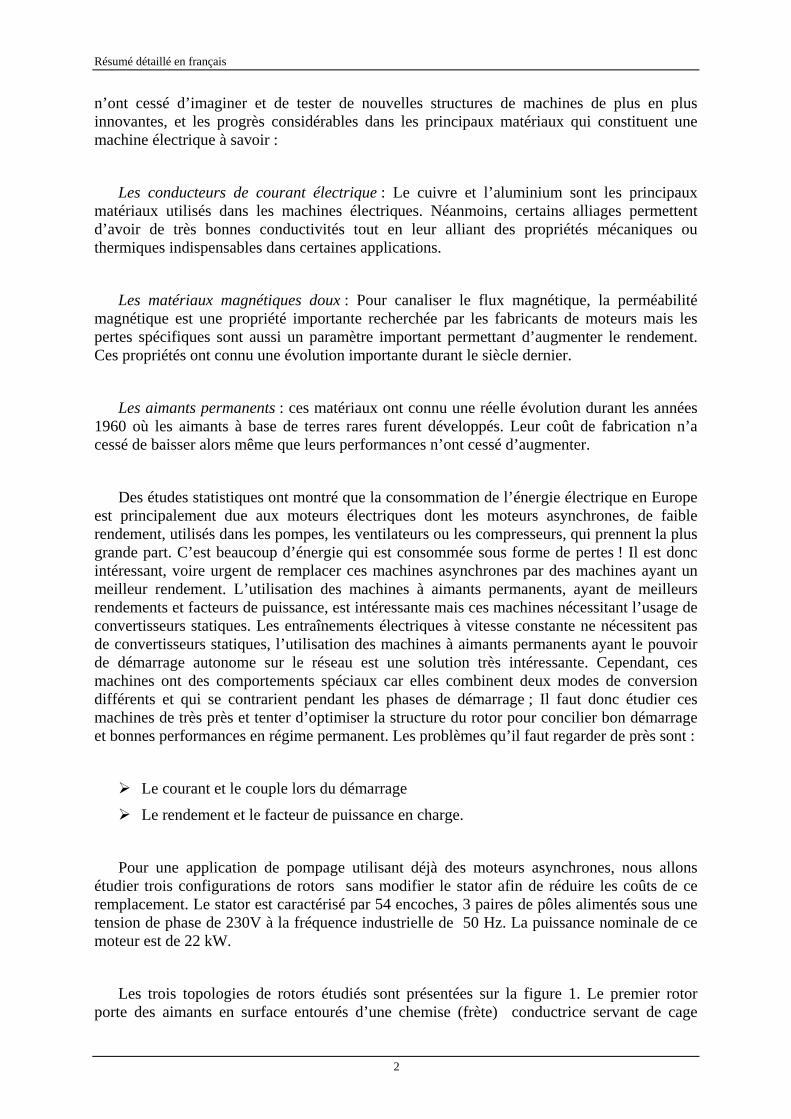
Les trois topologies de rotors étudiés sont présentées sur la figure 1. Le premier rotor porte des aimants en surface entourés d’une chemise (frète) conductrice servant de cage
Résumé détaillé en français
3
destinée au démarrage ; le second rotor utilise des aimants insérés dans un cylindre massif conducteur et massif servant de cage à 6 barres ; la troisième topologie utilise un rotor à cage classique dans lequel sont insérés des aimants en forme de U.
a) Surface inset b) Solid rotor c) U-shape
Figure 1 : Les trois architectures rotoriques étudiées
Chapitre 2 :
Dans un premier temps, nous étudions les trois machines comme s’il s’agissait de machines synchrones à aimants standards; nous allons dimensionner ces trois machines et étudier leurs performances en régime permanent en faisant abstraction des éléments conducteurs qui servent au démarrage.
Le premier objectif est d’obtenir les machines qui satisfont le cahier des charges avec le minimum d’ondulations de couple ; Pour ce faire, nous pouvons agir sur le mode de bobinage au stator ainsi que leur dimensions du rotor.
Le nombre d’encoches au stator et la polarité étant fixés, l’action sur le stator est restreinte à l’étude des coefficients de bobinage en fonction des différents raccourcissements envisageables. Le raccourcissement 8/9 semble être le mieux adapté car il présente le plus faible taux d’harmoniques. Une modélisation analytique permettant de déterminer l’induction dans l’entrefer en fonction des données géométriques pour les trois structures du rotor a été mise en œuvre. Elle sert au dimensionnement du rotor et à la prédiction du contenu harmonique de l’induction d’entrefer qui est en relation directe avec les harmoniques de la force électromotrice.
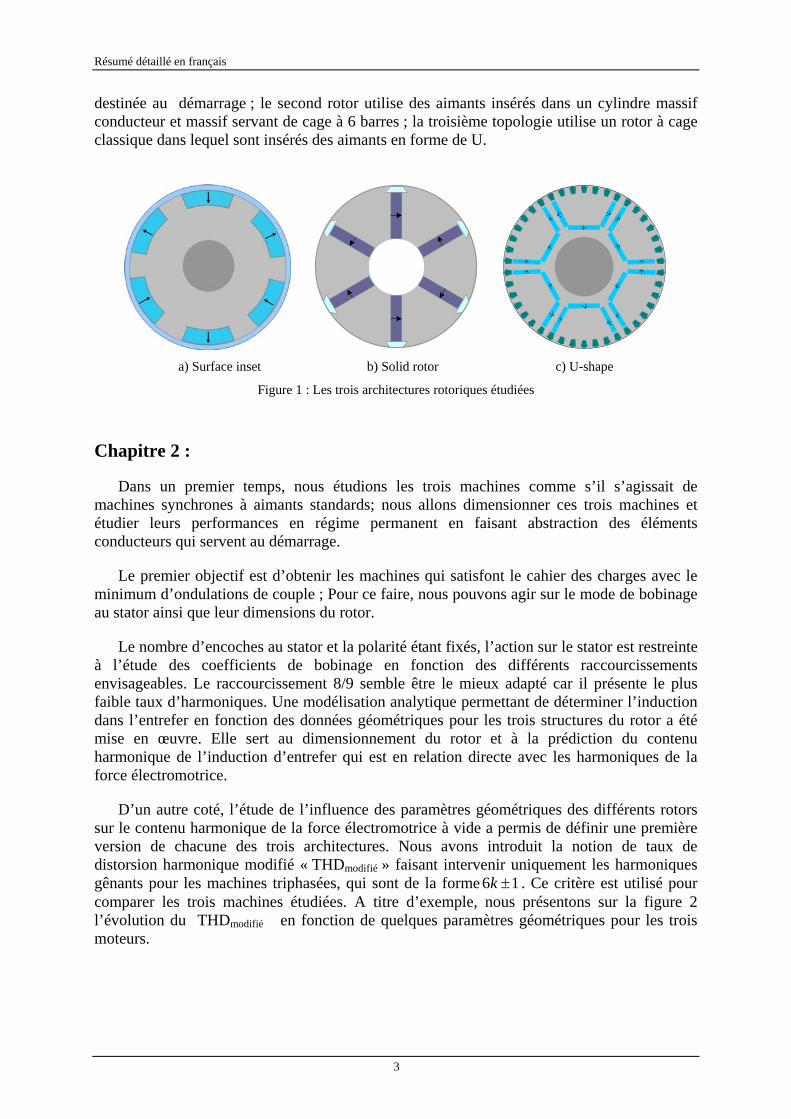
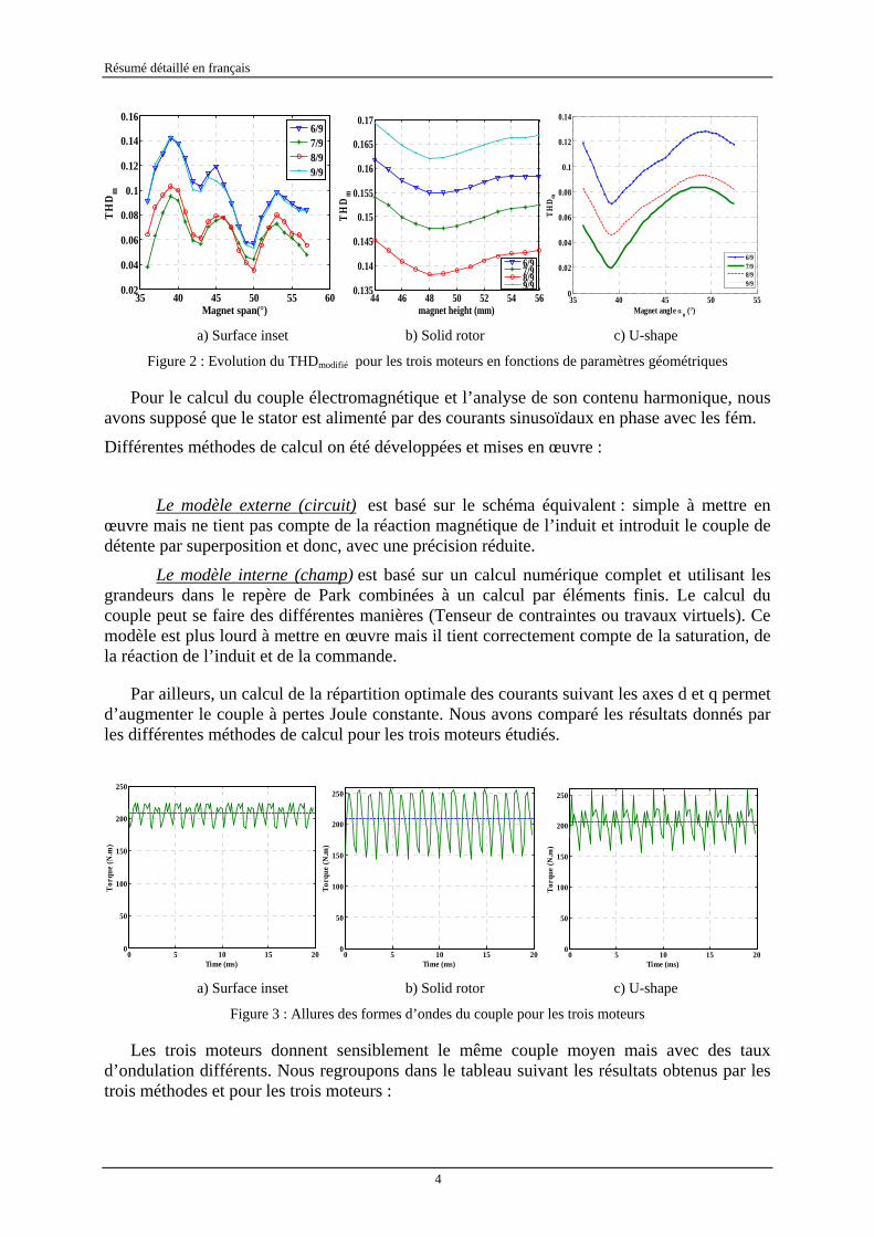
D’un autre coté, l’étude de l’influence des paramètres géométriques des différents rotors sur le contenu harmonique de la force électromotrice à vide a permis de définir une première version de chacune des trois architectures. Nous avons introduit la notion de taux de distorsion harmonique modifié « THDmodifié » faisant intervenir uniquement les harmoniques gênants pour les machines triphasées, qui sont de la forme 16 ±k . Ce critère est utilisé pour comparer les trois machines étudiées. A titre d’exemple, nous présentons sur la figure 2 l’évolution du THDmodifié en fonction de quelques paramètres géométriques pour les trois moteurs.
Résumé détaillé en français
4
35 40 45 50 55 600.02
0.04
0.06
0.08
0.1
0.12
0.14
0.16
Magnet span(°)
TH
Dm
6/97/98/99/9
44 46 48 50 52 54 560.135
0.14
0.145
0.15
0.155
0.16
0.165
0.17
magnet height (mm)
TH
Dm
6/97/98/99/9
35 40 45 50 550
0.02
0.04
0.06
0.08
0.1
0.12
0.14
Magnet angle α u (°)
THD m
6/97/98/99/9
a) Surface inset b) Solid rotor c) U-shape
Figure 2 : Evolution du THDmodifié pour les trois moteurs en fonctions de paramètres géométriques
Pour le calcul du couple électromagnétique et l’analyse de son contenu harmonique, nous avons supposé que le stator est alimenté par des courants sinusoïdaux en phase avec les fém.
Différentes méthodes de calcul on été développées et mises en œuvre :
Le modèle externe (circuit) est basé sur le schéma équivalent : simple à mettre en œuvre mais ne tient pas compte de la réaction magnétique de l’induit et introduit le couple de détente par superposition et donc, avec une précision réduite.
Le modèle interne (champ) est basé sur un calcul numérique complet et utilisant les grandeurs dans le repère de Park combinées à un calcul par éléments finis. Le calcul du couple peut se faire des différentes manières (Tenseur de contraintes ou travaux virtuels). Ce modèle est plus lourd à mettre en œuvre mais il tient correctement compte de la saturation, de la réaction de l’induit et de la commande.
Par ailleurs, un calcul de la répartition optimale des courants suivant les axes d et q permet d’augmenter le couple à pertes Joule constante. Nous avons comparé les résultats donnés par les différentes méthodes de calcul pour les trois moteurs étudiés.
0 5 10 15 200
50
100
150
200
250
Torq
ue (N
.m)
Time (ms)0 5 10 15 20
0
50
100
150
200
250
Torq
ue (N
.m)
Time (ms) 0 5 10 15 20
0
50
100
150
200
250
Torq
ue (N
.m)
Time (ms) a) Surface inset b) Solid rotor c) U-shape
Figure 3 : Allures des formes d’ondes du couple pour les trois moteurs
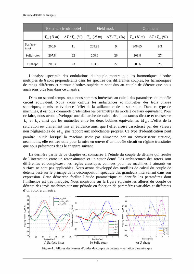
Les trois moteurs donnent sensiblement le même couple moyen mais avec des taux d’ondulation différents. Nous regroupons dans le tableau suivant les résultats obtenus par les trois méthodes et pour les trois moteurs :
Résumé détaillé en français
5
External circuit model Field model Optimum
).( mNTav (%)/ avTTΔ ).( mNTav (%)/ avTTΔ ).( mNTav (%)/ avTTΔ
Surface- inset 206.9 11 205.98 9 208.65 9.3
Solid-rotor 207.8 22 208.6 26 208.8 27
U-shape 206.3 23 193.3 27 206.6 25
L’analyse spectrale des ondulations du couple montre que les harmoniques d’ordre multiples de 6 sont prépondérants dans les spectres des différentes couples, les harmoniques de rangs différents et surtout d’ordres supérieurs sont dus au couple de détente que nous analysons plus loin dans ce chapitre.
Dans un second temps, nous nous sommes intéressés au calcul des paramètres du modèle circuit équivalent. Nous avons calculé les inductances et mutuelles des trois phases statoriques, et mis en évidence l’effet de la saillance et de la saturation. Dans ce type de machines, il est plus commode d’identifier les paramètres du modèle de Park équivalent. Pour ce faire, nous avons développé une démarche de calcul des inductances directe et transverse
dL et qL , ainsi que les mutuelles entre les deux bobines équivalentes dqM . L’effet de la saturation est clairement mis en évidence ainsi que l’effet croisé caractérisé par des valeurs non négligeables de dqM par rapport aux inductances propres. Ce type d’identification peut paraître inutile lorsque la machine n’est pas alimentée par un convertisseur statique, néanmoins, elle est très utile pour la mise en œuvre d’un modèle circuit en régime transitoire que nous présentons dans le chapitre suivant.
La dernière partie de ce chapitre est consacrée à l’étude du couple de détente qui résulte de l’interaction entre un rotor aimanté et un stator denté. Les architectures des rotors sont différentes et complexes ; les règles classiques connues pour les machines à aimants en surface ne sont pas applicables. Nous avons développé des modèles de calcul du couple de détente basé sur le principe de la décomposition spectrale des grandeurs intervenant dans son expression. Cette démarche facilite l’étude paramétrique et identifie les paramètres dont l’influence est très marquée. Nous montrons sur la figure suivante les allures du couple de détente des trois machines sur une période en fonction de paramètres variables et différents d’un rotor à un autre.
0 20 40 60 80 100 120-25
-20
-15
-10
-5
0
5
10
15
20
25
Position (°mec)
Cog
ging
torq
ue T
cog (
N.m
)
αp1=αp2=0.68
αp1=0.68 αp2=0.76
αp1=αp2=0.76
0 1 2 3 4 5 6 7-30
-20
-10
0
10
20
30
Position(°mec)
Cog
ging
torq
ue T
cog (
N.m
)
τc=10°
τc=13.5°
τc=13.8°
τc=14°
τc=14.6°
0 1 2 3 4 5 6 7-20
-15
-10
-5
0
5
10
15
20
Cog
ging
torq
ue T
cog (
N.m
)
Position(°mec)
Nr=36
Nr= 41
Nr= 42
Nr= 54
a) Surface inset b) Solid rotor c) U-shape
Figure 4 : Allures des formes d’ondes du couple de détente – variation paramétrique

Résumé détaillé en français
6
Dans ce chapitre, nous avons étudié et optimisé les trois topologies de rotor pour une même application et avec les mêmes contraintes. Il a été l’occasion de développer différents modèles et méthodes de calcul de différents phénomènes intervenant dans les machines synchrones à aimants permanents. Ces études font abstraction du phénomène d’induction dû à la présence de pièces conductrices dans le rotor et qui ne servent qu’au démarrage ; ce sera l’objet du chapitre suivant qui est spécialement dédié aux régimes dynamiques et en charge de ces moteurs.
Chapitre 3 :
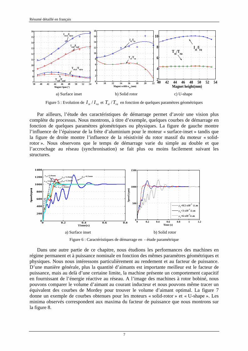
Dans le troisième chapitre, nous étudions la machine en régime dynamique ; nous nous intéressons particulièrement aux performances lors du démarrage. Nous commençons par mettre en œuvre un modèle circuit en régime dynamique qui permet de prédire le comportement de la machine en régime transitoire. Un modèle couplant le calcul interne par éléments finis et le comportement externe (circuit) est mis en œuvre à l’aide d’un logiciel commercial adapté (Flux2D). Nous nous intéressons à l’étude de l’influence des paramètres géométriques et les propriétés des matériaux sur le démarrage de la machine. Nous focalisons l’étude sur le couple de démarrage qui doit être suffisamment grand pour assurer le démarrage en charge et éviter le phénomène de rampage (Gorges) au voisinage de la moitié de la vitesse de synchronisme ; ce phénomène est bien connu dans les machines à fortes saillances démarrant en asynchrone. L’autre critère important auquel nous nous intéressons est le pic du courant de démarrage. Contrairement aux machines synchrones à rotor bobiné démarrant en asynchrone et pour lesquelles le courant de démarrage n’a de conséquence que sur le bobinage statorique, les machines à aimants sont très sensibles à ce courant à cause du risque de démagnétisation des aimants rotoriques. Nous définissons donc les rapports admissibles rast II / et rast TT / du courant de démarrage sur le courant nominal ainsi que du couple de démarrage sur le couple nominal que nous évaluons dans notre étude.
Pour chacune des trois structures, nous avons identifié les paramètres influents et effectué une étude paramétrique. La machine à aimants en surface munie d’une frète conductrice (surface inset), est naturellement sensible à l’épaisseur de la frète et au matériel qui la constitue. Plus la frète est épaisse, moins elle est résistive et a un meilleur pouvoir d’accrochage mais l’entrefer magnétique devient important affaiblissant ainsi le facteur de puissance en régime permanent. Par ailleurs, le pic du courant est plus grand lorsque la résistance rotorique équivalente est faible. Plusieurs solutions peuvent être envisagées ; mais la préférence est données à une frète en aluminium d’épaisseur 1 mm.
En ce qui concerne la structure ayant des aimants insérés dans un rotor massif (solid rotor), le matériau du rotor massif ainsi que les dimensions des aimants sont les principaux paramètres sur lesquels nous pouvons agir. Il est prévisible qu’une bonne conductivité du rotor permet de se rapprocher plus de la vitesse de synchronisme et par le fait facilite l’accrochage au réseau. Par ailleurs, moins le rotor est résistif, plus grands sont les courants de démarrage. La figure 5 montre une illustration de l’évolution des critères rast II / et rast TT / en fonction de quelques paramètres géométriques.
Résumé détaillé en français
7
38 40 42 44 46 48 50 52 547
8
9
10
11
12
13
14
15
16
Magnet Span (°)
Istcu/Iracu
Istal/Iraal
Tstcu/Tracu
Tstal/Traal8 10 12 14 16 18 20 22
0
2
4
6
8
10
12
14
16
18
Magnet width wm (mm)
Ist/Ira
Tst/Tra
40 42 44 46 48 50 52 542
4
6
8
10
Magnet height(mm)
Tst/Tra
Ist/Ira
a) Surface inset b) Solid rotor c) U-shape
Figure 5 : Evolution de rast II / et rast TT / en fonction de quelques paramètres géométriques
Par ailleurs, l’étude des caractéristiques de démarrage permet d’avoir une vision plus complète du processus. Nous montrons, à titre d’exemple, quelques courbes de démarrage en fonction de quelques paramètres géométriques ou physiques. La figure de gauche montre l’influence de l’épaisseur de la frète d’aluminium pour le moteur « surface-inset » tandis que la figure de droite montre l’influence de la résistivité du rotor massif du moteur « solid-rotor ». Nous observons que le temps de démarrage varie du simple au double et que l’accrochage au réseau (synchronisation) se fait plus ou moins facilement suivant les structures.
0 0.2 0.4 0.6 0.80
200
400
600
800
1000
1200
1400
Time(s)
Spee
d (r
pm)
α al=0.5mmα al=1.0mm
α al=1.5mm
α al=2.0mm
α al=3.0mm
α al=4.0mm
0 0.2 0.4 0.6 0.8 1 1.20
500
1000
1500
Time (s)
Spee
d (r
pm)
ρr=0.5 x10⁻⁷ Ω .m
ρr=3 x10⁻⁷ Ω .m
ρr=6 x10⁻⁷Ω .m
a) Surface inset b) Solid rotor
Figure 6 : Caractéristiques de démarrage en - étude paramétrique
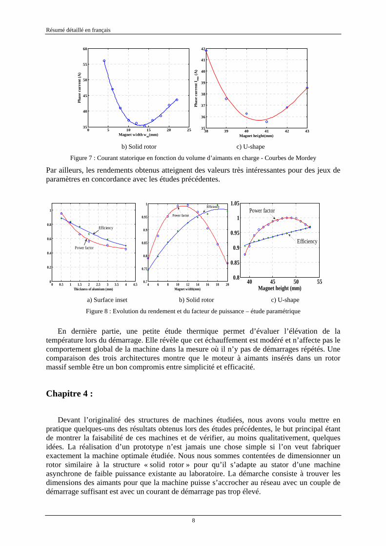
Dans une autre partie de ce chapitre, nous étudions les performances des machines en régime permanent et à puissance nominale en fonction des mêmes paramètres géométriques et physiques. Nous nous intéressons particulièrement au rendement et au facteur de puissance. D’une manière générale, plus la quantité d’aimants est importante meilleur est le facteur de puissance, mais au delà d’une certaine limite, la machine présente un comportement capacitif en fournissant de l’énergie réactive au réseau. A l’image des machines à rotor bobiné, nous pouvons comparer le volume d’aimant au courant inducteur et nous pouvons même tracer un équivalent des courbes de Mordey pour trouver le volume d’aimant optimal. La figure 7 donne un exemple de courbes obtenues pour les moteurs « solid-rotor » et « U-shape ». Les minima observés correspondent aux maxima du facteur de puissance que nous montrons sur la figure 8.
Résumé détaillé en français
8
0 5 10 15 20 2535
40
45
50
55
60
Magnet width wm(mm)
Phas
e cu
rren
t (A
)
38 39 40 41 42 4335
36
37
38
39
40
41
42
Phas
e cu
rren
t Irm
s (A)
Magnet height(mm) b) Solid rotor c) U-shape
Figure 7 : Courant statorique en fonction du volume d’aimants en charge - Courbes de Mordey
Par ailleurs, les rendements obtenus atteignent des valeurs très intéressantes pour des jeux de paramètres en concordance avec les études précédentes.
0 0.5 1 1.5 2 2.5 3 3.5 4 4.50
0.2
0.4
0.6
0.8
1
Thickness of alumium (mm)
Power factor
Efficiency
4 6 8 10 12 14 16 18 200.7
0.75
0.8
0.85
0.9
0.95
1
Magnet width(mm)
Efficiency
Power factor
40 45 50 550.8
0.85
0.9
0.95
1
1.05
Magnet height (mm)
Power factor
Efficiency
a) Surface inset b) Solid rotor c) U-shape
Figure 8 : Evolution du rendement et du facteur de puissance – étude paramétrique
En dernière partie, une petite étude thermique permet d’évaluer l’élévation de la température lors du démarrage. Elle révèle que cet échauffement est modéré et n’affecte pas le comportement global de la machine dans la mesure où il n’y pas de démarrages répétés. Une comparaison des trois architectures montre que le moteur à aimants insérés dans un rotor massif semble être un bon compromis entre simplicité et efficacité.
Chapitre 4 :
Devant l’originalité des structures de machines étudiées, nous avons voulu mettre en pratique quelques-uns des résultats obtenus lors des études précédentes, le but principal étant de montrer la faisabilité de ces machines et de vérifier, au moins qualitativement, quelques idées. La réalisation d’un prototype n’est jamais une chose simple si l’on veut fabriquer exactement la machine optimale étudiée. Nous nous sommes contentées de dimensionner un rotor similaire à la structure « solid rotor » pour qu’il s’adapte au stator d’une machine asynchrone de faible puissance existante au laboratoire. La démarche consiste à trouver les dimensions des aimants pour que la machine puisse s’accrocher au réseau avec un couple de démarrage suffisant est avec un courant de démarrage pas trop élevé.
Résumé détaillé en français
9
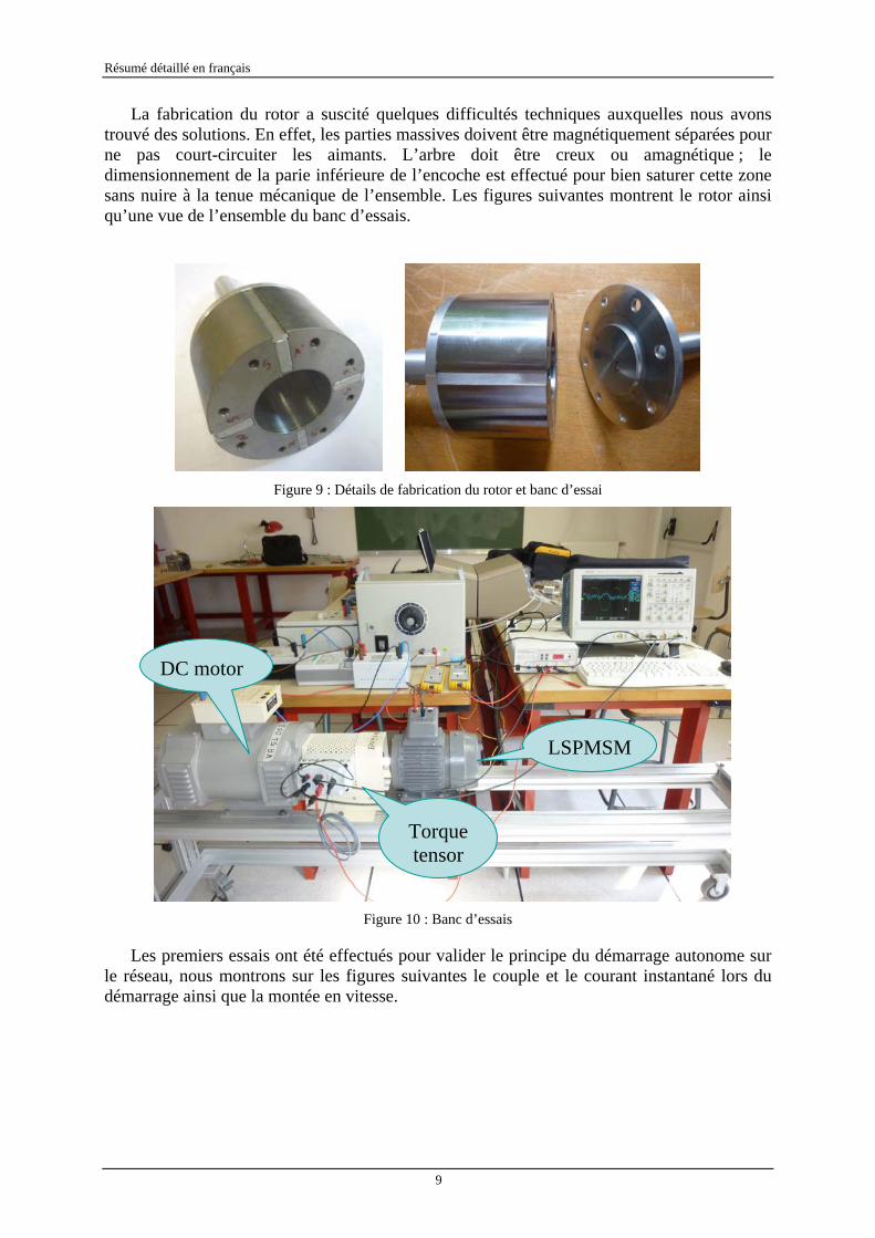
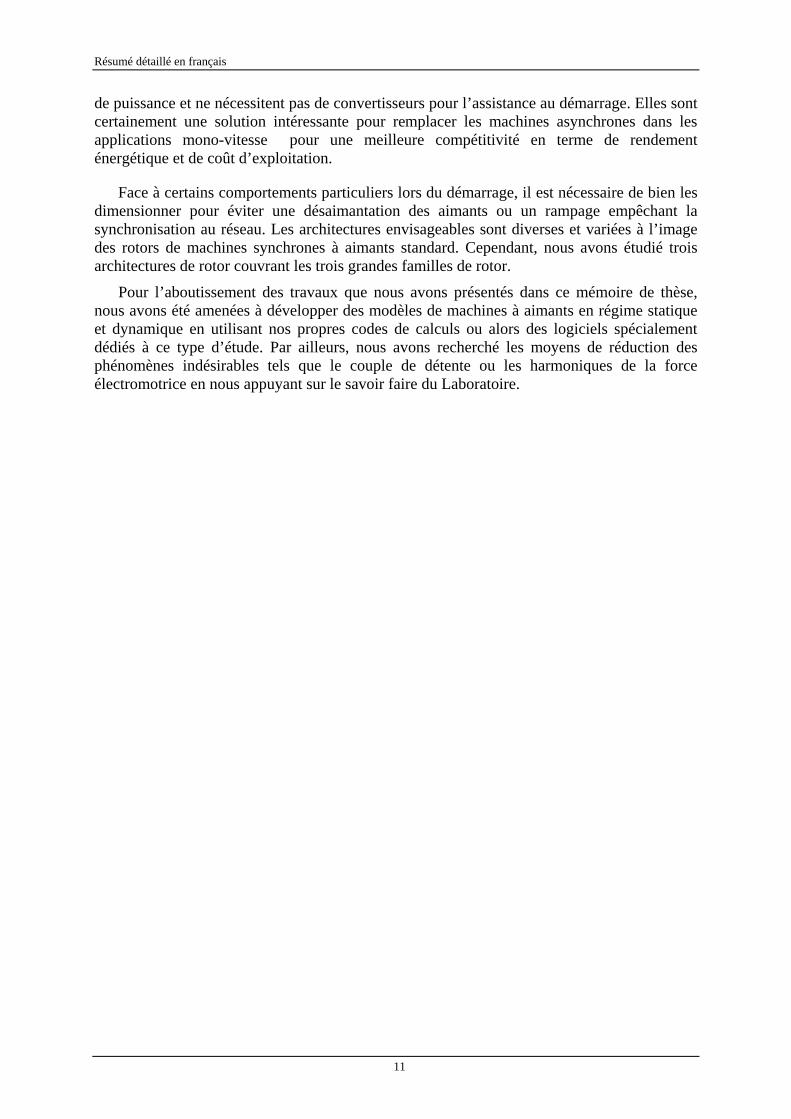
La fabrication du rotor a suscité quelques difficultés techniques auxquelles nous avons trouvé des solutions. En effet, les parties massives doivent être magnétiquement séparées pour ne pas court-circuiter les aimants. L’arbre doit être creux ou amagnétique ; le dimensionnement de la parie inférieure de l’encoche est effectué pour bien saturer cette zone sans nuire à la tenue mécanique de l’ensemble. Les figures suivantes montrent le rotor ainsi qu’une vue de l’ensemble du banc d’essais.
Figure 9 : Détails de fabrication du rotor et banc d’essai
Figure 10 : Banc d’essais
Les premiers essais ont été effectués pour valider le principe du démarrage autonome sur le réseau, nous montrons sur les figures suivantes le couple et le courant instantané lors du démarrage ainsi que la montée en vitesse.
DC motor
LSPMSM
Torque tensor

Résumé détaillé en français
10
0 0.1 0.2 0.3 0.4 0.5 0.6 0.7 0.8-15
-10
-5
0
5
10
15
20To
rque
(N.m
)
Time (s)0 0.1 0.2 0.3 0.4 0.5 0.6 0.7 0.8
0
500
1000
1500
2000
2500
Time (s)
Spee
d (r
pm)
0 0.1 0.2 0.3 0.4 0.5 0.6 0.7 0.8-15
-10
-5
0
5
10
15
Phas
e cu
rren
t (A
)
Time (s) Figure 11 : Couple, vitesse et courant lors du démarrage (Relevés expérimentaux)
Lors des essais, des courant trop élevés, dus à une erreur de manipulation a provoqué la démagnétisation des aimants. Ceci a pour effet d’affaiblir les performances du prototype par rapport au dimensionnement initial. Un essai en génératrice a permis de confirmer cet incident dans la mesure où l’on obtient des formes d’ondes des fém à vide identiques à celles prévues par le calcul mais à un coefficient près. L’analyse spectrale des fém confirme ce propos (Figure 12). A partir de ce constat, il était nécessaire d’identifier quels aimants ont été démagnétisés et à quel degré. Pour ce faire, il a fallu retirer le rotor, mesurer le champ à sa surface et comparer les résultats des mesures à ceux donnés par des calculs numériques effectués dans les mêmes conditions. Il s’est avéré qu’un aimant a été fortement démagnétisé, ce qui montre par ailleurs au fanage la rapidité du phénomène de démagnétisation.
0 5 10 15 20-200
-150
-100
-50
0
50
100
150
200
Time (ms)
Back
-EM
F (v
)
Pre-designed motorPrototype
0 5 10 15 20 25 30 350
50
100
150
200
Harmonic order
Back
-FEM
(v)
Pre-designed motorPrototype
Figure 12 : Affaiblissement de la Fém à vide (comparaison des mesures aux prévisions)
A travers cette erreur de manipulation, nous avons pu étudier un cas concret de démagnétisation du rotor qui nous souligne l’importance des études faites au troisième chapitre cherchant à limiter le courant de démarrage. Il n’empêche que cette étude expérimentale méritant d’être faite et donne une première expérience pour la fabrication et la manipulation des machines à aimants avec un démarrage autonome sur le réseau. Elle donne aussi l’occasion de faire des essais sur les machines présentant un défaut d’aimantation pour de futurs travaux.
Conclusion :
Cette thèse traite de l’étude et de l’optimisation de machines à aimants permanents avec un démarrage asynchrone sur le réseau. Ces machines ont de très bons rendements et facteurs
Résumé détaillé en français
11
de puissance et ne nécessitent pas de convertisseurs pour l’assistance au démarrage. Elles sont certainement une solution intéressante pour remplacer les machines asynchrones dans les applications mono-vitesse pour une meilleure compétitivité en terme de rendement énergétique et de coût d’exploitation.
Face à certains comportements particuliers lors du démarrage, il est nécessaire de bien les dimensionner pour éviter une désaimantation des aimants ou un rampage empêchant la synchronisation au réseau. Les architectures envisageables sont diverses et variées à l’image des rotors de machines synchrones à aimants standard. Cependant, nous avons étudié trois architectures de rotor couvrant les trois grandes familles de rotor.
Pour l’aboutissement des travaux que nous avons présentés dans ce mémoire de thèse, nous avons été amenées à développer des modèles de machines à aimants en régime statique et dynamique en utilisant nos propres codes de calculs ou alors des logiciels spécialement dédiés à ce type d’étude. Par ailleurs, nous avons recherché les moyens de réduction des phénomènes indésirables tels que le couple de détente ou les harmoniques de la force électromotrice en nous appuyant sur le savoir faire du Laboratoire.


Introduction


Introduction
15
The constantly increasing cost of energy and the new European legislation in terms of energy effectiveness incite manufacturers and users of energy systems to promote devices which consume less energy. The field of electric drives does not escape from this recent reality, especially in industrial applications. Indeed, it appears that more than half of the electric energy consumption in Europe is due to electric motors, mainly induction motors used in pumps, fans or compressors. These motors are characterized by relatively low efficiencies and power factors compared to permanent magnet motors. It is possible to improve the efficiency of high or medium power induction motors with an acceptable extra cost, but for low power machines, the mechanical dimensions of the gaps remain a major obstacle to obtain high performances.
Permanent magnet machines have very good efficiencies and power factors even for low powers. The decrease of magnet cost observed during the past two decades makes them very competitive, so that they have been widely used in electric variable speed drive as well, thanks to the development of static converters and control methods. However, for constant speed applications, these static converters represent an unnecessary expense so that the permanent magnet synchronous machines are not quite suitable for such applications.
Permanent magnet motors having the capacity of self-starting when connected to the grid (line), henceforth called “Line-Start PM motors”, are interesting to replace induction motors in constant speed drives. They do not require static converters and have very good efficiencies and power factors. The self-starting capability is ensured by conducting parts in the rotor following the principle of wound rotor synchronous machines with asynchronous starting. However, these machines have specific behaviours that should be closely studied, such as the high starting current that could demagnetize the rotor magnets. Also, some structures have a saliency in the rotor which can make the synchronization with the grid difficult.
This thesis deals with the study and the optimization of three structures of line-start permanent magnet motors for an industrial application of medium power. The thesis is structured in four chapters that we describe below.
The first chapter begins with a brief history of electrical machines by tracing their evolution from the early 19th century. The main parameters influencing the performance improvement are then presented with a specific attention to the role of materials. Then we emphasize the economic and energy issues as well as actual standards corresponding to electric motors used in industry. This section introduces and justifies the use of line start permanent magnet (LSPM) motors in many applications. We present at the end of chapter three rotor architectures that will be studied throughout this thesis.
The second chapter is devoted to the study and optimization of the three structures of LSPM motors as if they were conventional synchronous PM motors operating in steady state. As the stator lamination and the pole number are fixed, the improvement of the waveforms of electromotive forces in terms of harmonic content passes through a spectral study on the winding and the effect of the rotor component dimensions. We have developed our own computation models based on finite element method in order to have a greater flexibility in the parametric study. Furthermore, we study the performance in terms of average torque and torque ripple as well as the reduction of cogging torque by appropriate techniques. In a second part, we have developed a model parameter calculation in the two-coordinate frame of references (Park frame) to highlight the influence of the saturation and the stator teeth on the direct and transverse inductances as well as the mutual between the two equivalent coils which allows to take into account the cross coupling effect. This identification model is the basis for the dynamic model developed in Chapter III.
Introduction
16
In the third chapter, we study the machine dynamic behaviour and we are particularly interested in performance during starting operation. To do this, we have implemented a parametric study by varying the geometry and the type of materials to achieve the desired performances. The study is focused on the starting torque, which must be greater than three times the rated torque, and the starting current which must be less than ten times the rated current. Following the geometry optimizing the performance in starting operation, steady state performances are investigated and the effect of some geometrical parameters is highlighted. This study confirms the results obtained in chapter II and provides additional information that the static model does not take into account. A small thermal study is carried out to evaluate the temperature rise during starting operation. It shows that this increase of the temperature is weak and does not affect the overall behavior of the machine if there are no repeated starts. A comparison of the three architectures shows that the solid rotor LSPM motor with magnets inserted in a solid rotor seems to be a good compromise between simplicity and efficiency.
In the fourth chapter, an experimental study is carried out to validate the principle of self-starting and the synchronization to the network for one of three structures selected above. We describe the conditions of manufacture and design of a prototype of reduced power. The developed models are carried out to design the rotor so that it can be combined with the stator of an existing induction motor; this approach allows a gain in the duration and the cost of manufacturing. The prototype is tested in starting operation, steady state in both no-load and full load operations. The measurements concern mainly the current, the torque and speed curves versus time in starting operation while we focus the measurements on the efficiency and power factor in full load steady state operation. Unfortunately, a handling mistake has caused too strong currents to demagnetize some magnets. This has led to the weakening of the prototype performance compared to those initially predicted by the design. The research on the nature of the demagnetization has been the subject of several investigations, by comparing field measurements and finite element calculations.
For the achievement of the work that will be presented in this thesis, we have been led to develop models of permanent magnet machines in static and dynamic conditions, using our own calculation codes or specialized software such as Flux2D. In addition, we have investigated some techniques to reduce undesirable phenomena such as cogging torque or harmonics of electromotive force based on the expertise of the host laboratory.

Chapter I : Why use Line Start PM motors in the context
of energy saving ?

Chapter I : Why use Line Start PM motors in the context of energy saving?
19
I. Why use Line Start PM motors in the context of energy saving?
I.1. Introduction
Electric machines are now used everywhere in our daily life and industry; they have different shapes, sizes, functions and different powers. Most existing machines are motors. Generators are mainly located in power stations but also on cars, or are isolated or autonomous power systems using fossil fuels as a primary source. If try looking around, we realize that these electromechanical converters surround us in our daily lives even we do not pay attention to them. The motors are present in domestic appliances (refrigerator, dishwasher, blender ...), in computers (disk drives, fans ...) and in our cars (starters, window-lifts ...) etc. Their shapes are more complex but are all based on the same basic principles of electromechanical conversion.
This energy conversion cannot be done without loss, this revealing the concept of efficiency to which we are not careful when using a machine to drill a hole in the wall or when using our robot to prepare shredded carrots! However, the managers of large industrial parks involving many motors of medium or high power begin to think seriously about this issue, due to the constant growth of the energy cost. Indeed, the energy bill becomes heavier if the motors are of poor performance. Moreover, private individuals are also beginning to be aware of this problem by looking carefully at the energy label in major household appliances before to engaging in a new purchase.
The share of electromechanical conversion in the energy consumption is significant, so that increasing its performance becomes an interesting point. Improving the energy performance of a motor can be carried out either by keeping a basic structure and using more efficient materials or by a radical change of the conversion mode, replacing the initial motors by more appropriate and more efficient ones. This thesis lies in this last theme and this first chapter introduces the subject with emphasis on dealing with the improvement of efficiency of motors.
We begin this chapter with a brief history of electric machines since the invention of the first machine in 1821. We then describe the role of materials in terms of motor performances. In a third step, we present the share of electric motors in the energy consumption and energy standards applied to them. The last part of this chapter is devoted to the description of the main types of electric motors used and the justification for the use of line start permanent magnet motors in oil pumping applications. At last, we describe the three motor topologies we plan to study throughout this thesis.
I.2. A short history of electrical machines and their progress
In 1821, soon after the Danish physicist and chemist, Hans Christian Ørsted discovered the phenomenon of electromagnetism, Michael Faraday built two devices to produce what he called electromagnetic rotation, a continuous circular motion from the circular magnetic force around a wire and a wire extending into a pool of mercury with a magnet placed inside would rotate around the magnet if supplied with current from a chemical battery, Fig. I.1. The device is known as the first motor in the world.

Chapter I : Why use Line Start PM motors in the context of energy saving?
20
Fig.I. 1: The first electric motor (Michael Faraday 1821)
The first commutator-type direct current electric motor capable of turning machinery was invented by the British scientist William Sturgeon in 1832. Following Sturgeon's work, a commutator-type direct-current electric motor made for a commercial use was built by Americans Emily and Thomas Davenport and patented in 1837. Their motors ran at up to 600 rpm and powered machine tools and a printing press. Due to the high cost of the zinc electrodes required by primary battery power, the motors were commercially unsuccessful and the Davenports went bankrupt. Several inventors followed Sturgeon in the development of DC motors but all encountered the same cost issues with primary battery power.
Fig.I. 2: The first commutator type DC motor (William Strugeon 1832)
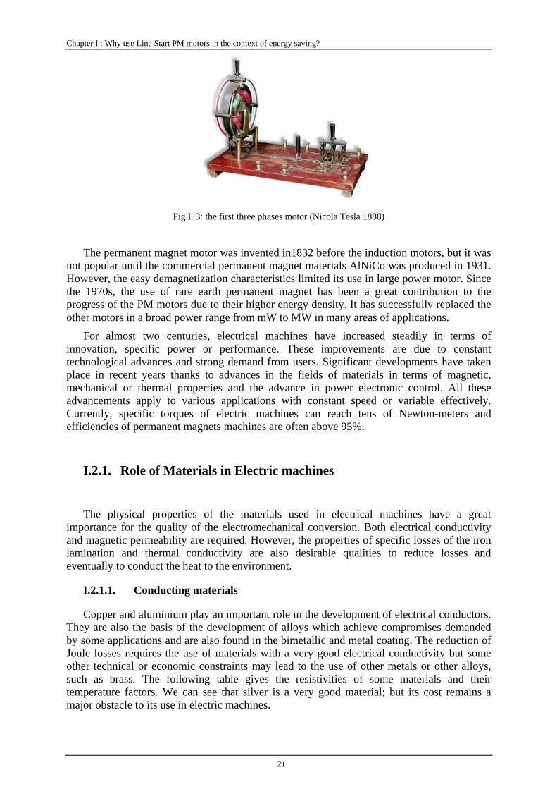
The induction motor (IM), invented by Nicola Tesla in 1888, has become the most common motor used in industry and public life applications for the last hundred years. Its good features include simple construction and low maintenance. Recent development of semiconductor switches and controllers for inverters has allowed induction motor to be used even when close control over speed and position is required. However, the IM has an inherently lower efficiency than the permanent magnet motor as its torque is produced by the interaction of the currents in the stator windings and the rotor windings.
Chapter I : Why use Line Start PM motors in the context of energy saving?
21
Fig.I. 3: the first three phases motor (Nicola Tesla 1888)
The permanent magnet motor was invented in1832 before the induction motors, but it was not popular until the commercial permanent magnet materials AlNiCo was produced in 1931. However, the easy demagnetization characteristics limited its use in large power motor. Since the 1970s, the use of rare earth permanent magnet has been a great contribution to the progress of the PM motors due to their higher energy density. It has successfully replaced the other motors in a broad power range from mW to MW in many areas of applications.
For almost two centuries, electrical machines have increased steadily in terms of innovation, specific power or performance. These improvements are due to constant technological advances and strong demand from users. Significant developments have taken place in recent years thanks to advances in the fields of materials in terms of magnetic, mechanical or thermal properties and the advance in power electronic control. All these advancements apply to various applications with constant speed or variable effectively. Currently, specific torques of electric machines can reach tens of Newton-meters and efficiencies of permanent magnets machines are often above 95%.
I.2.1. Role of Materials in Electric machines
The physical properties of the materials used in electrical machines have a great importance for the quality of the electromechanical conversion. Both electrical conductivity and magnetic permeability are required. However, the properties of specific losses of the iron lamination and thermal conductivity are also desirable qualities to reduce losses and eventually to conduct the heat to the environment.
I.2.1.1. Conducting materials
Copper and aluminium play an important role in the development of electrical conductors. They are also the basis of the development of alloys which achieve compromises demanded by some applications and are also found in the bimetallic and metal coating. The reduction of Joule losses requires the use of materials with a very good electrical conductivity but some other technical or economic constraints may lead to the use of other metals or other alloys, such as brass. The following table gives the resistivities of some materials and their temperature factors. We can see that silver is a very good material; but its cost remains a major obstacle to its use in electric machines.
Chapter I : Why use Line Start PM motors in the context of energy saving?
22
Currently, research is conducted on superconducting materials of which electrical resistance is theoretically zero. However, this technology leads to other problems such as cryogenics and mechanical stress. We will not discuss about these items since they are not the case of the subject of my thesis.
Table.I. 1 Electric conductivities of some metallic materials
Resistivity ρ and temperature coefficient α of the materials and conductive alloys
Materials or alloys 0ρ at 20°C( m10 8 ⋅Ω− ) α at 20°C( -18 k 10− )
Aluminium
Silver
Copper
Gold
Sodium
AGS alloy
2.8
1.6
1.72
2.4
4.6
3.25
4
3.8
3.9
3.4
4.8
3.6
AGS alloy is the alloy of magnesium, silicon and aluminium in which aluminum (Al) is the predominant metal
I.2.1.2. Soft magnetic materials
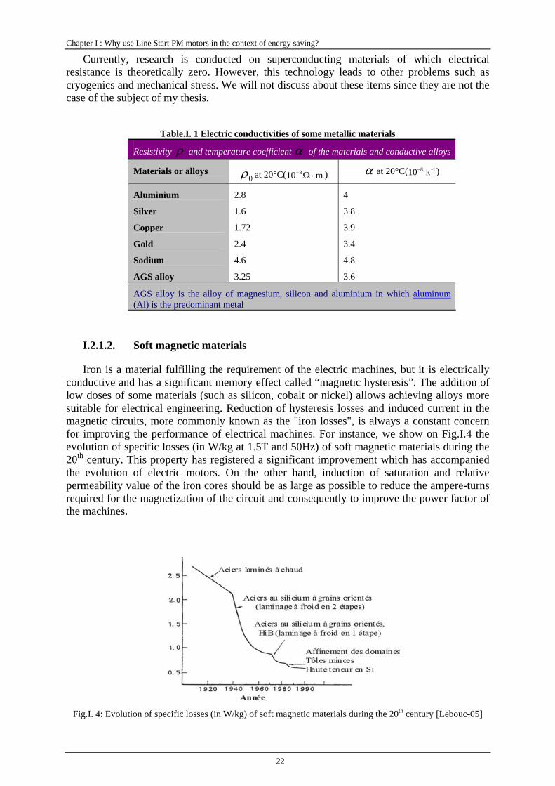
Iron is a material fulfilling the requirement of the electric machines, but it is electrically conductive and has a significant memory effect called “magnetic hysteresis”. The addition of low doses of some materials (such as silicon, cobalt or nickel) allows achieving alloys more suitable for electrical engineering. Reduction of hysteresis losses and induced current in the magnetic circuits, more commonly known as the "iron losses", is always a constant concern for improving the performance of electrical machines. For instance, we show on Fig.I.4 the evolution of specific losses (in W/kg at 1.5T and 50Hz) of soft magnetic materials during the 20th century. This property has registered a significant improvement which has accompanied the evolution of electric motors. On the other hand, induction of saturation and relative permeability value of the iron cores should be as large as possible to reduce the ampere-turns required for the magnetization of the circuit and consequently to improve the power factor of the machines.
Fig.I. 4: Evolution of specific losses (in W/kg) of soft magnetic materials during the 20th century [Lebouc-05]
Chapter I : Why use Line Start PM motors in the context of energy saving?
23
I.2.1.3. Hard magnetic materials
Hard magnetic materials commonly known as Permanent Magnet materials have been used since the earliest days of electrical engineering, but only quite recently the high performance rare-earth magnets became available, with a sufficient energy density to be used in demanding applications. Reduced magnet costs and advantages of size and efficiency make PM motors even more popular.
The permanent magnet materials are characterised by the following main parameters.
− Remanent flux density rB : the maximum magnetic flux density of the magnets without external field in a short-circuited magnetic circuit. Any reluctance in the circuit will of course reduce this flux density.
− Coercive force cH : the value of demagnetizing field intensity required to bring the magnetic flux density to zero. High coercive force means that it can withstand high demagnetisation field.
− Maximum magnetic energy density ( )maxBH : the maximum magnetic energy that can be produced by a permanent magnet in the external space.
− Curie temperature: the temperature at which the magnetisation ceases.
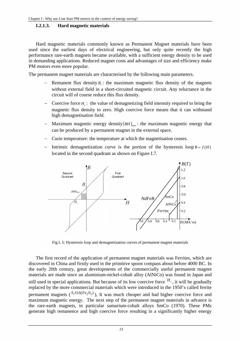
− Intrinsic demagnetization curve is the portion of the hysteresis loop )(HfB = located in the second quadrant as shown on Figure I.7.
)(TB
NdFeB SmCo
AlNiCo
Ferrite
)/( mMAH0.1 8.0 6.0 4.0 2.0
2.0
4.0
6.0
8.0
0.1
2.1
Fig.I. 5: Hysteresis loop and demagnetization curves of permanent magnet materials
The first record of the application of permanent magnet materials was Ferrites, which are discovered in China and firstly used in the primitive spoon compass about before 4000 BC. In the early 20th century, great developments of the commercially useful permanent magnet materials are made since an aluminium-nickel-cobalt alloy (AlNiCo) was found in Japan and still used in special applications. But because of its low coercive force cH , it will be gradually replaced by the more commercial materials which were introduced in the 1950’s called ferrite permanent magnets ( )0(6. 32FeOSr ), It was much cheaper and had higher coercive force and maximum magnetic energy. The next step of the permanent magnet materials in advance is the rare-earth magnets, in particular samarium-cobalt alloys SmCo (1970). These PMs generate high remanence and high coercive force resulting in a significantly higher energy
Chapter I : Why use Line Start PM motors in the context of energy saving?
24
product than ferrites can achieve. These properties and the large reversible demagnetization range (high intrinsic coercive force ciH ) made these magnets to be the superior choice for high performance machines. This research led to the nowadays well known neodymium-iron-boron NdFeB magnets, introduced in 1983. Although cheaper than SmCo and of even higher energy density, NdFeB is not always superior owing to its lower thermal stability, caused by the lower Curie temperature, and its reactivity which leads for instance to corrosion problems and subsequently loss of magnetic properties. Another rare earth material, Sa2Fe17N3 , magnet is still on going; it is a promising new candidate for permanent magnet applications for their high resistance to demagnetisation, high magnetisation and increased resistance to corrosion and temperature when compared with neodymium iron boron.
Today, high performance rare-earth magnets are widespread in small motors. The PM machines are gradually employed for their commercial applications in higher power machines. Permanent magnet motors have consequently been made more attractive in the last two decades by the availability of much improved PM materials. Although SmCo has the advantage of withstanding high temperatures, the lower price and necessary volume of NdFeB make it a likely choice for a commonplace motor.
I.2.2. The supply by inverters
In the last decade, inverter drives have become widely available. Fast switching of devices such as MOSFETs and IGBTs has allowed PWM synthesis of sinusoidal waveforms, with quite low harmonic content. The voltage magnitude and frequency can be varied according to programmed sequences, and motor speed or position may be fed back or estimated to allow induction motors or synchronous motors to be closely controlled. As well as soft-starting the motor, and good effects on motor life and the supply voltage, inverter drives allow efficient operation at variable speed. When a speed reduction can be used in place of throttling the fluid flow, very large energy savings can be obtained.
In spite of the improvements in inverter drives, a motor that operates efficiently and without any power electronics is likely to have the advantage for simple, single speed applications, as long as enough such motors are produced to keep the cost lower than a motor with its inverter.
I.3. Energetic efficiency of electric drives
As in all sectors, the energy saving was launched in the recent years and of course it concerns the field of electrical machines. Energy standards are in place to classify the electrical machines and the machine manufacturers are making considerable efforts to improve the energy performance of their motors to be competitive in the market of electromechanical conversion.
I.3.1. Energetic standards for electric motors
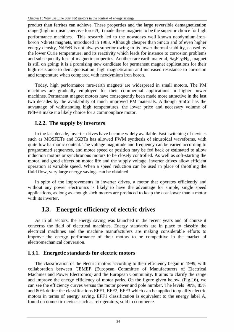
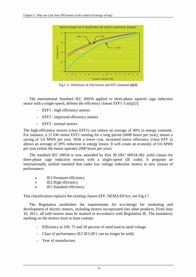
The classification of the electric motors according to their efficiency began in 1999, with collaboration between CEMEP (European Committee of Manufacturers of Electrical Machines and Power Electronics) and the European Community. It aims to clarify the range and improve the energy efficiency of motor parks. On the figure given below, (Fig.I.6), we can see the efficiency curves versus the motor power and pole number. The levels 90%, 85% and 80% define the classifications EFF1, EFF2, EFF3 which can be applied to qualify electric motors in terms of energy saving. EFF1 classification is equivalent to the energy label A, found on domestic devices such as refrigerators, sold in commerce.
Chapter I : Why use Line Start PM motors in the context of energy saving?
25
Fig.I. 6 : Definition of efficiencies and EFF standards [@1]
The international Standard IEC 60034 applied to three-phase squirrel cage induction motor with a single-speed, defines the efficiency classes EFF1-3 as[@2]:
− EFF1 : high efficiency motors
− EFF2 : improved efficiency motors
− EFF3 : normal motors
The high-efficiency motors (class EFF1) can reduce an average of 40% in energy consume. For instance, a 15 kW motor EFF1 running for a long period (6000 hours per year), means a saving of 3.6 MWh per year. With a lower cost, increased motor efficiency (class EFF 2) allows an average of 20% reduction in energy losses. It will create an economy of 0.6 MWh per year (when the motor operates 2000 hours per year).
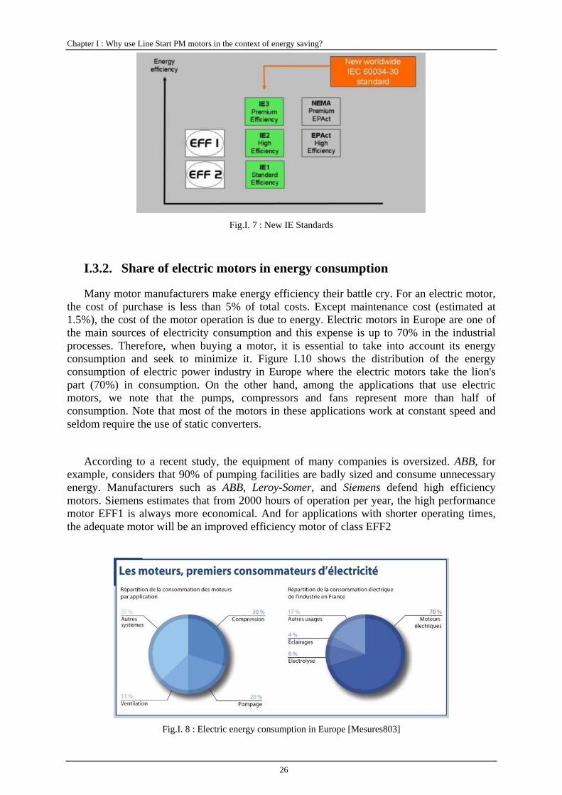
The standard IEC 60034 is now amended by Part 30 (IEC 60034-30): yield classes for three-phase cage induction motors with a single-speed (IE code). It proposes an internationally unified standard that ranks low voltage induction motors in new classes of performance:
• IE3 Premium efficiency • IE2 High efficiency • IE1 Standard efficiency
This classification replaces the existing classes EFF, NEMA/EPAct, see Fig.I.7.
The Regulation establishes the requirements for eco-design for marketing and development of electric motors, including motors incorporated into other products. From June 16, 2011, all sold motors must be marked in accordance with Regulation IE. The mandatory marking on the motors must at least contain:
− Efficiency at 100, 75 and 50 percent of rated load at rated voltage
− Class of performance IE2 IE3 (IE1 can no longer be sold)
− Year of manufacture.
Chapter I : Why use Line Start PM motors in the context of energy saving?
26
Fig.I. 7 : New IE Standards
I.3.2. Share of electric motors in energy consumption
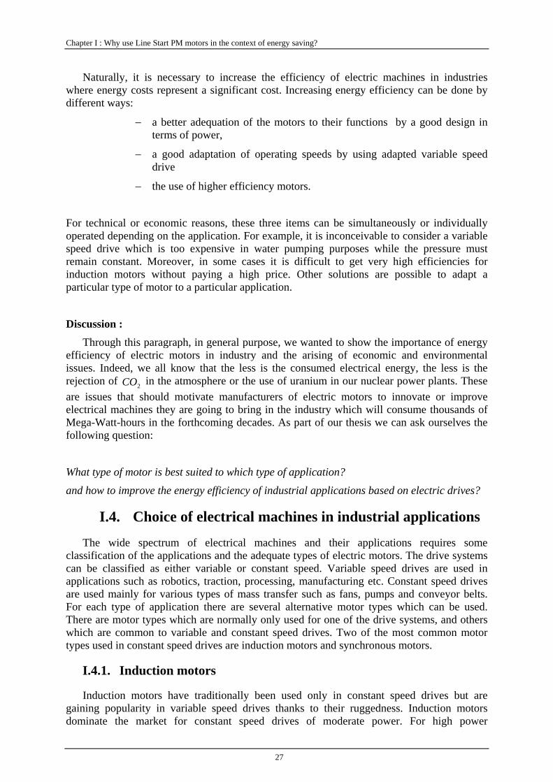
Many motor manufacturers make energy efficiency their battle cry. For an electric motor, the cost of purchase is less than 5% of total costs. Except maintenance cost (estimated at 1.5%), the cost of the motor operation is due to energy. Electric motors in Europe are one of the main sources of electricity consumption and this expense is up to 70% in the industrial processes. Therefore, when buying a motor, it is essential to take into account its energy consumption and seek to minimize it. Figure I.10 shows the distribution of the energy consumption of electric power industry in Europe where the electric motors take the lion's part (70%) in consumption. On the other hand, among the applications that use electric motors, we note that the pumps, compressors and fans represent more than half of consumption. Note that most of the motors in these applications work at constant speed and seldom require the use of static converters.
According to a recent study, the equipment of many companies is oversized. ABB, for example, considers that 90% of pumping facilities are badly sized and consume unnecessary energy. Manufacturers such as ABB, Leroy-Somer, and Siemens defend high efficiency motors. Siemens estimates that from 2000 hours of operation per year, the high performance motor EFF1 is always more economical. And for applications with shorter operating times, the adequate motor will be an improved efficiency motor of class EFF2
Fig.I. 8 : Electric energy consumption in Europe [Mesures803]
Chapter I : Why use Line Start PM motors in the context of energy saving?
27
Naturally, it is necessary to increase the efficiency of electric machines in industries where energy costs represent a significant cost. Increasing energy efficiency can be done by different ways:
− a better adequation of the motors to their functions by a good design in terms of power,
− a good adaptation of operating speeds by using adapted variable speed drive
− the use of higher efficiency motors.
For technical or economic reasons, these three items can be simultaneously or individually operated depending on the application. For example, it is inconceivable to consider a variable speed drive which is too expensive in water pumping purposes while the pressure must remain constant. Moreover, in some cases it is difficult to get very high efficiencies for induction motors without paying a high price. Other solutions are possible to adapt a particular type of motor to a particular application.
Discussion :
Through this paragraph, in general purpose, we wanted to show the importance of energy efficiency of electric motors in industry and the arising of economic and environmental issues. Indeed, we all know that the less is the consumed electrical energy, the less is the rejection of 2CO in the atmosphere or the use of uranium in our nuclear power plants. These are issues that should motivate manufacturers of electric motors to innovate or improve electrical machines they are going to bring in the industry which will consume thousands of Mega-Watt-hours in the forthcoming decades. As part of our thesis we can ask ourselves the following question:
What type of motor is best suited to which type of application?
and how to improve the energy efficiency of industrial applications based on electric drives?
I.4. Choice of electrical machines in industrial applications
The wide spectrum of electrical machines and their applications requires some classification of the applications and the adequate types of electric motors. The drive systems can be classified as either variable or constant speed. Variable speed drives are used in applications such as robotics, traction, processing, manufacturing etc. Constant speed drives are used mainly for various types of mass transfer such as fans, pumps and conveyor belts. For each type of application there are several alternative motor types which can be used. There are motor types which are normally only used for one of the drive systems, and others which are common to variable and constant speed drives. Two of the most common motor types used in constant speed drives are induction motors and synchronous motors.
I.4.1. Induction motors
Induction motors have traditionally been used only in constant speed drives but are gaining popularity in variable speed drives thanks to their ruggedness. Induction motors dominate the market for constant speed drives of moderate power. For high power
Chapter I : Why use Line Start PM motors in the context of energy saving?
28
installations, synchronous motors are more popular as they allow the reactive power to be controlled.
It is well known that induction motors have generally a lower efficiency than synchronous or permanent magnet motors. There are obstacles to introduce higher efficiency induction motors in some industrial applications because of the extra investment required by nature. The efficiency of small induction motors is low and it is costly to improve to a large degree, due to the fact that there is a limit on how small the air-gap can be allowed to be. The tolerances on the die stamping of the laminations is fairly low, so to improve matters the rotor is generally machined as a final step before assembly. For small induction motors the efficiency is thus limited and other motor types can provide superior performance.
I.4.2. Synchronous motors
Generally wound synchronous motors are avoided in many drive systems because of the drawbacks due to the ring-brushes system. Brushless motors are preferred in such situations. Permanent Magnet Synchronous Motors (PMSM) are good candidate to replace induction motors in many applications. Compared to the traditional induction motors, the permanent magnet synchronous motors operate under the similar principle as the electric excited synchronous motors. For induction motor, the stator current consists of two components: the magnetising current and the torque current. However, in a permanent magnet motor the magnets produce the flux in the air-gap instead of the excitation winding and the stator current can be entirely used as a torque current. There are no rotor currents and consequently no rotor losses, increasing the efficiency. It also has a relatively simple structure, no collecting ring and no brush, which improves the reliability of operation and also reduces the cost of maintenance. As permanent magnets are now produced at low prices, the use of PM motors has increased during the past decades.
For energy concerns, the permanent magnet motors become a good option for all kinds of applications. They are widely used in industry, agriculture, vessels, aeronautics and domestic life: servo drives, vehicle drives, automation process, traction motors, fans, pumps and the electrical equipments in our families. They can have larger air-gaps without affecting the efficiency to the same degree as in induction motors. With larger air-gaps the required amount of magnet material, and the associated cost, increases but for small motor sizes the magnet cost is not so troublesome. For small motor sizes the PMSM can provide a high efficiency at a competitive cost. The PMSM however requires a variable frequency drive (VFD), for the start sequence; this is generally considered as too expensive for constant speed applications and also reduces the overall efficiency.
I.4.3. Line-start PM synchronous motors
In the case of constant speed drives such as pumps or fans, the use of synchronous motors with a self starting ability should be interesting to take advantage of the high efficiency of synchronous motors. Wound synchronous motors with self starting ability have been used since many decades and the additional rotor cage is used as dampers to improve the stability of the machine in transient operation. A similar idea is envisaged for PM motors which are more efficient than wound synchronous motors thanks to the absence of rotor losses. The combination of the self start ability as an induction motor and the synchronisation with the grid as a synchronous motor is generally known as Line Start Permanent Magnet Motor, (LSPM) motor. It has the ability to start when connected directly to the line (mains).
Chapter I : Why use Line Start PM motors in the context of energy saving?
29
I.4.3.1. History and Principle
The history of line start permanent magnet motors can be traced back from at least 50 years. The idea of combining the high epfficiency of the PMSM with the starting ability of an induction motor drive dates back to the 1950’s [Modeer-07]. The LSPM motor has had a limited market penetration, probably due to many reasons such as the extra cost of magnet material compared to induction motors and the complex rotor construction. Another major reason is probably that the motor market is fairly conservative and that there has been little incentive to develop high efficiency motors. The cost of high performance magnets has decreased since the introduction of neodymium magnets in the 1980’s but it is not until the last decade that LSPMSMs have become available in a commercial setting.
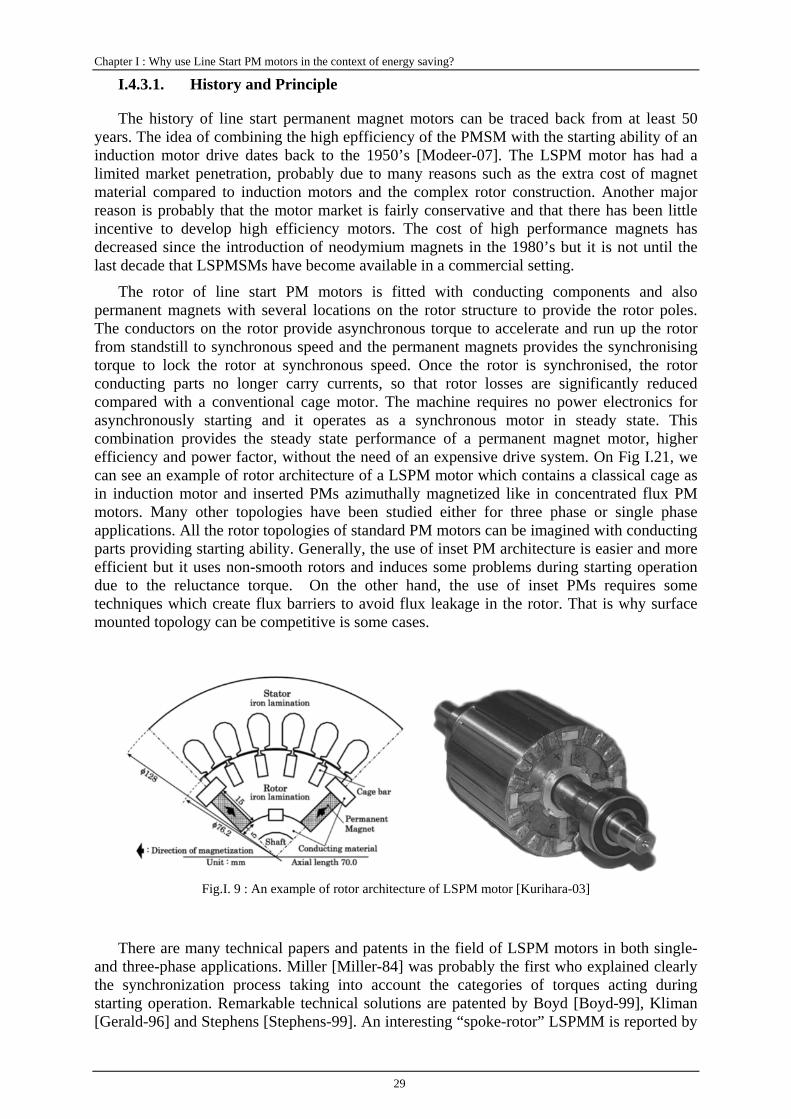
The rotor of line start PM motors is fitted with conducting components and also permanent magnets with several locations on the rotor structure to provide the rotor poles. The conductors on the rotor provide asynchronous torque to accelerate and run up the rotor from standstill to synchronous speed and the permanent magnets provides the synchronising torque to lock the rotor at synchronous speed. Once the rotor is synchronised, the rotor conducting parts no longer carry currents, so that rotor losses are significantly reduced compared with a conventional cage motor. The machine requires no power electronics for asynchronously starting and it operates as a synchronous motor in steady state. This combination provides the steady state performance of a permanent magnet motor, higher efficiency and power factor, without the need of an expensive drive system. On Fig I.21, we can see an example of rotor architecture of a LSPM motor which contains a classical cage as in induction motor and inserted PMs azimuthally magnetized like in concentrated flux PM motors. Many other topologies have been studied either for three phase or single phase applications. All the rotor topologies of standard PM motors can be imagined with conducting parts providing starting ability. Generally, the use of inset PM architecture is easier and more efficient but it uses non-smooth rotors and induces some problems during starting operation due to the reluctance torque. On the other hand, the use of inset PMs requires some techniques which create flux barriers to avoid flux leakage in the rotor. That is why surface mounted topology can be competitive is some cases.
Fig.I. 9 : An example of rotor architecture of LSPM motor [Kurihara-03]
There are many technical papers and patents in the field of LSPM motors in both single- and three-phase applications. Miller [Miller-84] was probably the first who explained clearly the synchronization process taking into account the categories of torques acting during starting operation. Remarkable technical solutions are patented by Boyd [Boyd-99], Kliman [Gerald-96] and Stephens [Stephens-99]. An interesting “spoke-rotor” LSPMM is reported by
Chapter I : Why use Line Start PM motors in the context of energy saving?
30
Kurihara and Rahman [Kurihara-03] with design and experimental results. A. Knight gave also a significant contribution to the study of single phase LSPM motors in terms of structure design [Knight-99], [Knight-00]. Chinese and Korean researchers have investigated LSPM motors in the recent years especially for domestic applications [Wang-10] [Jung-07] [Soo-whang-10] [Liang-09].
The transient operation of line start PM motors has been widely studied due to the inherent difficulties of synchronizing this motor. Indeed, during starting operation, the braking torque due to the magnets makes the starting process different from that of a classical induction motor and the saliency of the rotor makes this operation more complicated [Soulard-00] [Liang-09-2].
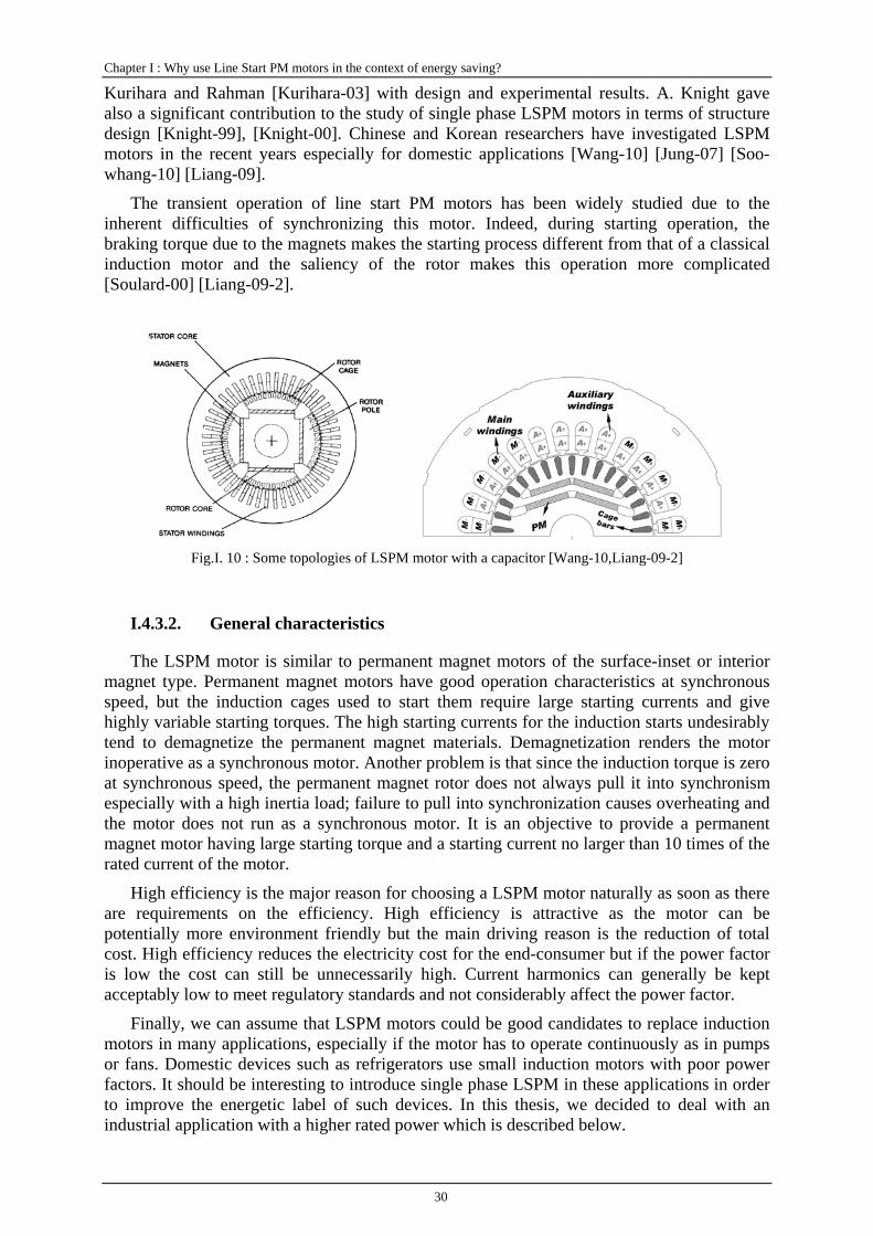
Fig.I. 10 : Some topologies of LSPM motor with a capacitor [Wang-10,Liang-09-2]
I.4.3.2. General characteristics
The LSPM motor is similar to permanent magnet motors of the surface-inset or interior magnet type. Permanent magnet motors have good operation characteristics at synchronous speed, but the induction cages used to start them require large starting currents and give highly variable starting torques. The high starting currents for the induction starts undesirably tend to demagnetize the permanent magnet materials. Demagnetization renders the motor inoperative as a synchronous motor. Another problem is that since the induction torque is zero at synchronous speed, the permanent magnet rotor does not always pull it into synchronism especially with a high inertia load; failure to pull into synchronization causes overheating and the motor does not run as a synchronous motor. It is an objective to provide a permanent magnet motor having large starting torque and a starting current no larger than 10 times of the rated current of the motor.
High efficiency is the major reason for choosing a LSPM motor naturally as soon as there are requirements on the efficiency. High efficiency is attractive as the motor can be potentially more environment friendly but the main driving reason is the reduction of total cost. High efficiency reduces the electricity cost for the end-consumer but if the power factor is low the cost can still be unnecessarily high. Current harmonics can generally be kept acceptably low to meet regulatory standards and not considerably affect the power factor.
Finally, we can assume that LSPM motors could be good candidates to replace induction motors in many applications, especially if the motor has to operate continuously as in pumps or fans. Domestic devices such as refrigerators use small induction motors with poor power factors. It should be interesting to introduce single phase LSPM in these applications in order to improve the energetic label of such devices. In this thesis, we decided to deal with an industrial application with a higher rated power which is described below.
Chapter I : Why use Line Start PM motors in the context of energy saving?
31
I.4.4. Line-start PMSM for oil pump application
In refineries, filling and emptying of tanks of oil and their derivatives as fuel and kerosene is a common operation that uses pumps powered with induction motors of medium power (several tens of kilowatts). These motors operate for long periods and consume a huge amount of energy that should be reduced in order to fulfil European standards for the energy saving and economic criteria, that we discussed earlier in this chapter.
Considering the energy saving, the line-start permanent magnet motor has features which make it attractive for this application. As noticed in the beginning of this chapter, it has been estimated that in Europe, induction machines consume around 50% of all electricity generated. It is also true in China, electricity consumptions occupies a large share of more than 60% of the total industrial electricity consumption. Cage induction motors have been widely used because of their low price, robustness and minimum maintenance. However, cage induction motors have a lower power factor and a lower efficiency(less than 0.9), the losses caused temperature rise resulting in the dramatic reduction of the use-life and high maintenance of motors, especially when working in a poor environment of oil fields.
In general, the line-start PM motors can be justified as an economical alternative because of the annual saving of the electric energy. This saving of energy is a function of the hours of operation per year and the energy consumed. For instance, we try here to evaluate the cost of operation in an application of oil pumping when using either an induction motor or a line start PM motor.
For example, we consider a 22kW, 1000 rpm oil-pump motor with an average annual operating time of 2000 hours and a cost of the electric power of 0.16 Euro/kWh. Below, we list the main data of the example:
− Standard induction motor efficiency =88% , price : 500 Euros
− Power input=22/0.88=25 kW
− LSPM motor efficiency=93% ; price 1500 Euros
− Power input=22/0.93=23.65kW
− Annual energy saving =(25-23.65)*2000=2700kWh
− Annual power cost saving=2700*0.16=432 euros
− Initial cost difference=1500-500=1000 Euros
− Time to recover initial cost=1000/432=2.3 years
For this application, this simple example indicates a very favourable cost/benefit ratio for this application when using a LSPM motor instead of an induction motor. We show on Fig.I.11 the total cost due to the use of both induction motor and LSPM motor versus the operating time in years. We can see that after the third year, the cost of induction motor becomes higher than that of LSPM motor. In addition, it must be noticed that the cost of the consumed energy per year is very high compared to the price of both motors as it was mentioned in the beginning of this chapter.

Chapter I : Why use Line Start PM motors in the context of energy saving?
32
-1 0 1 2 3 4 5 6 70
1
2
3
4
5x 10
4
Cos
t of o
pera
tion
(Eur
os)
Time (year)
Induction motorLine-start PM motor
Fig.I. 11 : The cost of operation versus time
Although the economics vary by application, a line-start PMSM motor under typical operation will often pay for reduced energy bills within three years despite its higher purchase price.
I.4.5. Requirements of the oil pump application
In this thesis, we will deal with an oil pomp application of 22kW using induction motor which should be replaced by line start PM motor. However, the study could be carried out on any other application using an induction motor during a long period.
A 22kW, 6 pole motor is required with specific starting and steady performances. The starting performances required are mainly a low starting current and a high starting torque in order to achieve the starting operation without risking any damage to the electrical equipment even at full load. The required specifications on the steady state operation performances concern the power factor and the efficiency for thermal and economic considerations. The designed motors are expected to achieve these specifications as a robust line start structure which has a power factor higher than 0.93 and a high efficiency. For starting operations, the starting torque is expected to be three times the rated torque at least, and maximum values of starting current less than ten times of the rated current. Some other important specifications are given in the following table.
Table.I. 2 : Required performances and specifications
Performance VALUE Output power kW 22
Speed rpm 1000
Torque N.m 210
Voltage V 380
frequency Hz 50
Starting/rated current 10
Starting/rated Torque 3
The IM cost is higher than the LSPM motor cost
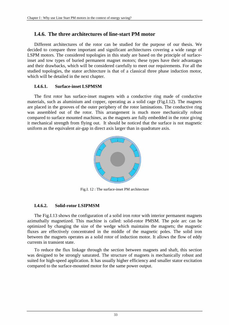
Chapter I : Why use Line Start PM motors in the context of energy saving?
33
I.4.6. The three architectures of line-start PM motor
Different architectures of the rotor can be studied for the purpose of our thesis. We decided to compare three important and significant architectures covering a wide range of LSPM motors. The considered topologies in this study are based on the principle of surface-inset and tow types of buried permanent magnet motors; these types have their advantages and their drawbacks, which will be considered carefully to meet our requirements. For all the studied topologies, the stator architecture is that of a classical three phase induction motor, which will be detailed in the next chapter.
I.4.6.1. Surface-inset LSPMSM
The first rotor has surface-inset magnets with a conductive ring made of conductive materials, such as aluminium and copper, operating as a solid cage (Fig.I.12). The magnets are placed in the grooves of the outer periphery of the rotor laminations. The conductive ring was assembled out of the rotor. This arrangement is much more mechanically robust compared to surface mounted machines, as the magnets are fully embedded in the rotor giving it mechanical strength from flying out. It should be noticed that the surface is not magnetic uniform as the equivalent air-gap in direct axis larger than in quadrature axis.
Fig.I. 12 : The surface-inset PM architecture
I.4.6.2. Solid-rotor LSIPMSM
The Fig.I.13 shows the configuration of a solid iron rotor with interior permanent magnets azimuthally magnetized. This machine is called: solid-rotor PMSM. The pole arc can be optimized by changing the size of the wedge which maintains the magnets; the magnetic fluxes are effectively concentrated in the middle of the magnetic poles. The solid iron between the magnets operates as a solid rotor of induction motor. It allows the flow of eddy currents in transient state.
To reduce the flux linkage through the section between magnets and shaft, this section was designed to be strongly saturated. The structure of magnets is mechanically robust and suited for high-speed application. It has usually higher efficiency and smaller stator excitation compared to the surface-mounted motor for the same power output.
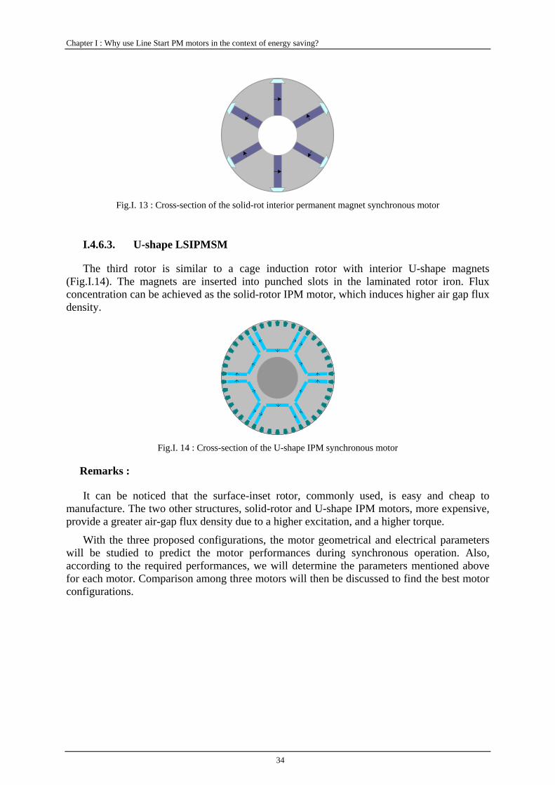
Chapter I : Why use Line Start PM motors in the context of energy saving?
34
Fig.I. 13 : Cross-section of the solid-rot interior permanent magnet synchronous motor
I.4.6.3. U-shape LSIPMSM
The third rotor is similar to a cage induction rotor with interior U-shape magnets (Fig.I.14). The magnets are inserted into punched slots in the laminated rotor iron. Flux concentration can be achieved as the solid-rotor IPM motor, which induces higher air gap flux density.
Fig.I. 14 : Cross-section of the U-shape IPM synchronous motor
Remarks :
It can be noticed that the surface-inset rotor, commonly used, is easy and cheap to manufacture. The two other structures, solid-rotor and U-shape IPM motors, more expensive, provide a greater air-gap flux density due to a higher excitation, and a higher torque.
With the three proposed configurations, the motor geometrical and electrical parameters will be studied to predict the motor performances during synchronous operation. Also, according to the required performances, we will determine the parameters mentioned above for each motor. Comparison among three motors will then be discussed to find the best motor configurations.

Chapter II :
Study of the synchronous operation

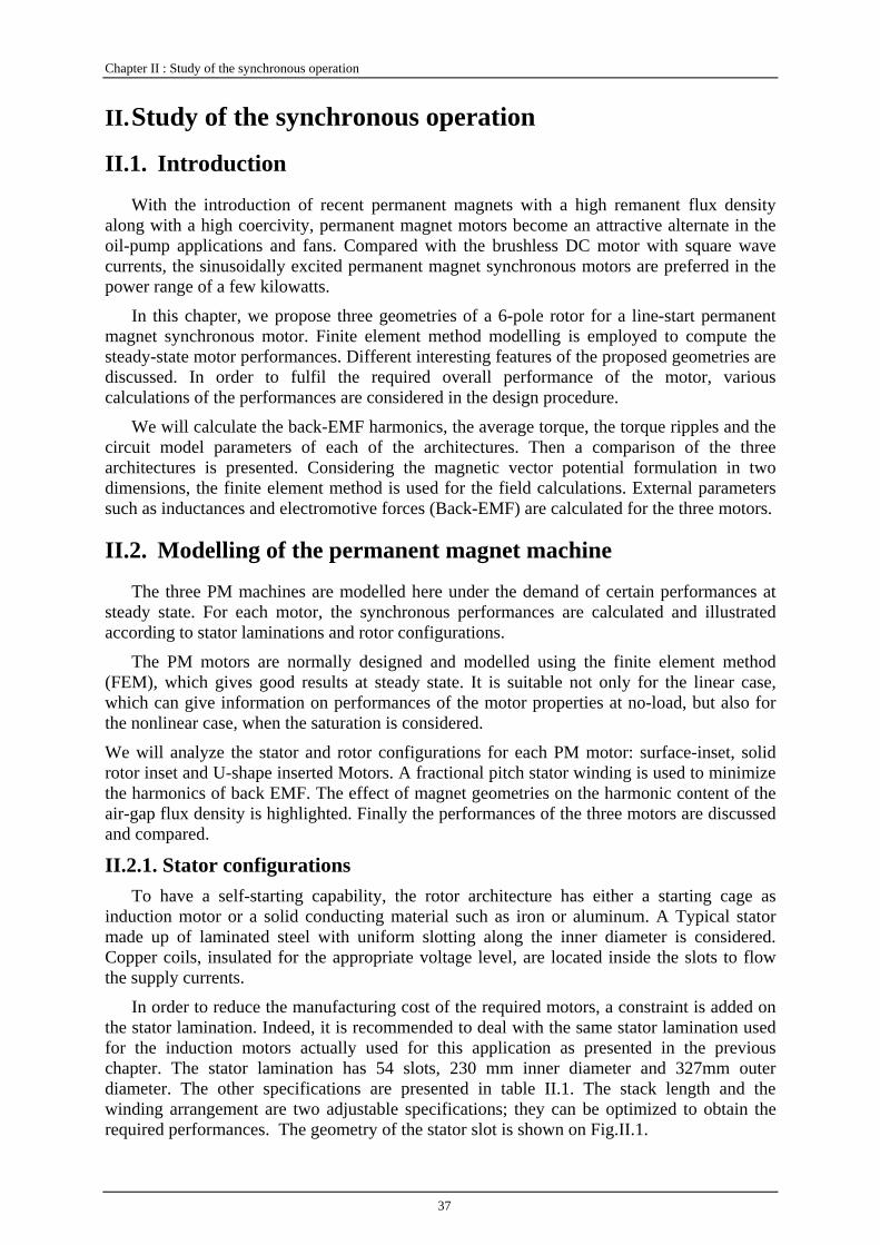
Chapter II : Study of the synchronous operation
37
II. Study of the synchronous operation
II.1. Introduction
With the introduction of recent permanent magnets with a high remanent flux density along with a high coercivity, permanent magnet motors become an attractive alternate in the oil-pump applications and fans. Compared with the brushless DC motor with square wave currents, the sinusoidally excited permanent magnet synchronous motors are preferred in the power range of a few kilowatts.
In this chapter, we propose three geometries of a 6-pole rotor for a line-start permanent magnet synchronous motor. Finite element method modelling is employed to compute the steady-state motor performances. Different interesting features of the proposed geometries are discussed. In order to fulfil the required overall performance of the motor, various calculations of the performances are considered in the design procedure.
We will calculate the back-EMF harmonics, the average torque, the torque ripples and the circuit model parameters of each of the architectures. Then a comparison of the three architectures is presented. Considering the magnetic vector potential formulation in two dimensions, the finite element method is used for the field calculations. External parameters such as inductances and electromotive forces (Back-EMF) are calculated for the three motors.
II.2. Modelling of the permanent magnet machine
The three PM machines are modelled here under the demand of certain performances at steady state. For each motor, the synchronous performances are calculated and illustrated according to stator laminations and rotor configurations.
The PM motors are normally designed and modelled using the finite element method (FEM), which gives good results at steady state. It is suitable not only for the linear case, which can give information on performances of the motor properties at no-load, but also for the nonlinear case, when the saturation is considered.
We will analyze the stator and rotor configurations for each PM motor: surface-inset, solid rotor inset and U-shape inserted Motors. A fractional pitch stator winding is used to minimize the harmonics of back EMF. The effect of magnet geometries on the harmonic content of the air-gap flux density is highlighted. Finally the performances of the three motors are discussed and compared.
II.2.1. Stator configurations To have a self-starting capability, the rotor architecture has either a starting cage as
induction motor or a solid conducting material such as iron or aluminum. A Typical stator made up of laminated steel with uniform slotting along the inner diameter is considered. Copper coils, insulated for the appropriate voltage level, are located inside the slots to flow the supply currents.
In order to reduce the manufacturing cost of the required motors, a constraint is added on the stator lamination. Indeed, it is recommended to deal with the same stator lamination used for the induction motors actually used for this application as presented in the previous chapter. The stator lamination has 54 slots, 230 mm inner diameter and 327mm outer diameter. The other specifications are presented in table II.1. The stack length and the winding arrangement are two adjustable specifications; they can be optimized to obtain the required performances. The geometry of the stator slot is shown on Fig.II.1.
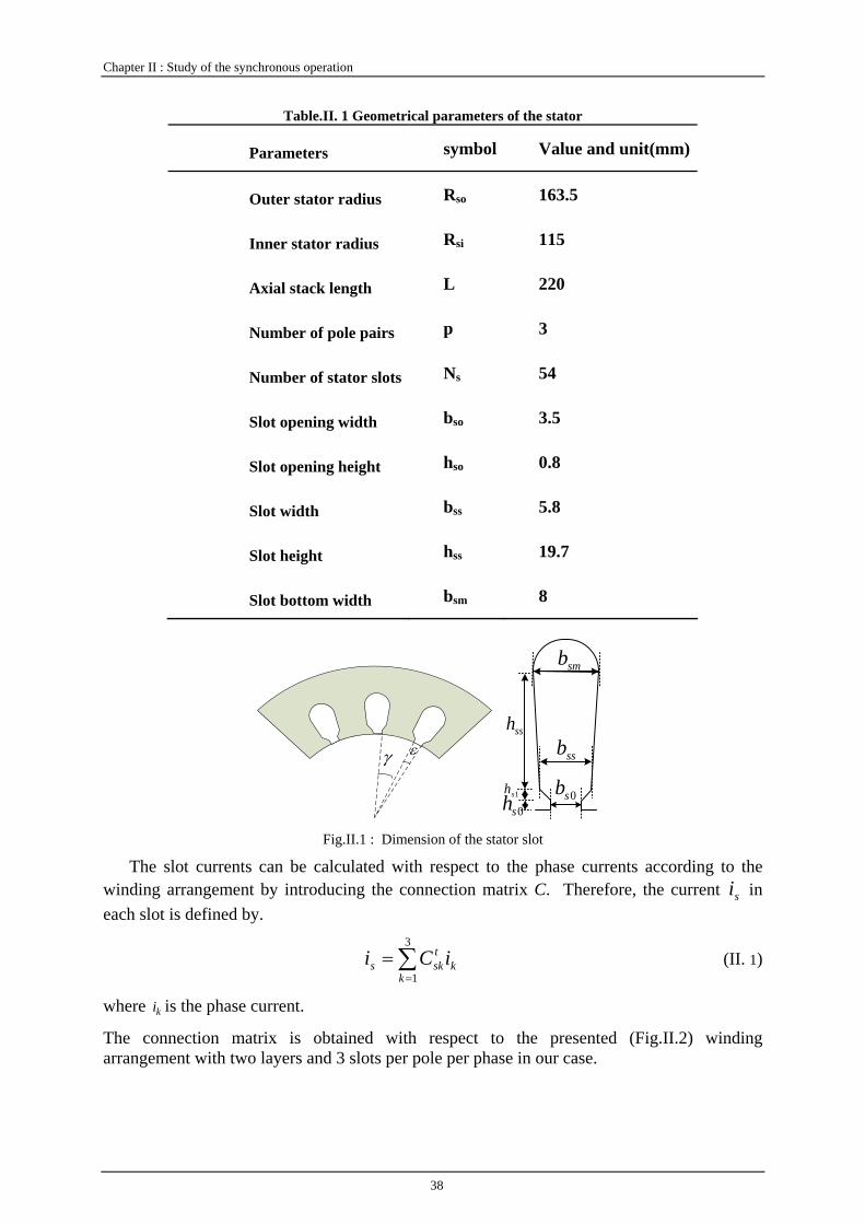
Chapter II : Study of the synchronous operation
38
Table.II. 1 Geometrical parameters of the stator
Parameters symbol Value and unit(mm)
Outer stator radius Rso 163.5
Inner stator radius Rsi 115
Axial stack length L 220
Number of pole pairs p 3
Number of stator slots Ns 54
Slot opening width bso 3.5
Slot opening height hso 0.8
Slot width bss 5.8
Slot height hss 19.7
Slot bottom width bsm 8
γ ε
0sb
ssb
smb
0sh 1sh
ssh
Fig.II.1 : Dimension of the stator slot
The slot currents can be calculated with respect to the phase currents according to the winding arrangement by introducing the connection matrix C. Therefore, the current si in each slot is defined by.
kk
tsks iCi ∑
==
3
1 (II. 1)
where ki is the phase current.
The connection matrix is obtained with respect to the presented (Fig.II.2) winding arrangement with two layers and 3 slots per pole per phase in our case.
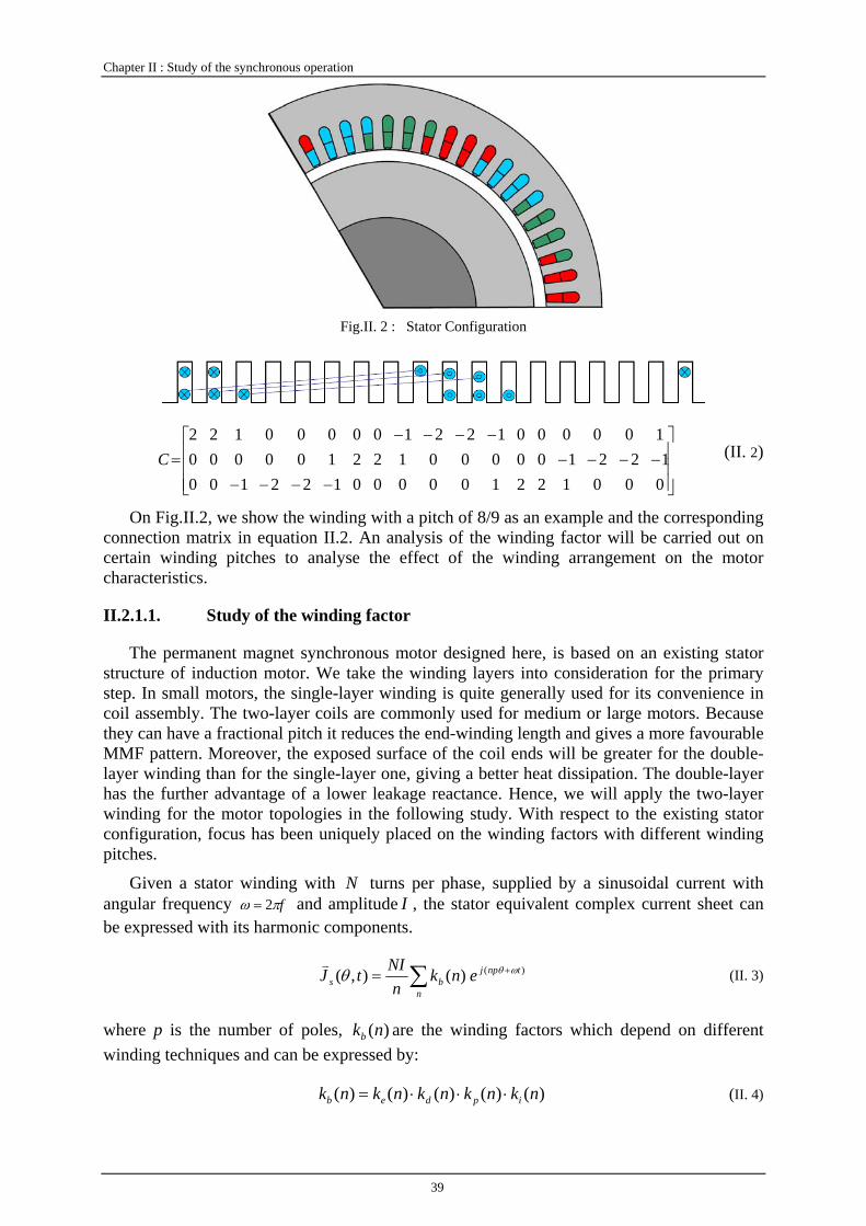
Chapter II : Study of the synchronous operation
39
Fig.II. 2 : Stator Configuration
⎥⎥⎥
⎦
⎤
⎢⎢⎢
⎣
⎡
−−−−−−−−
−−−−=
000122100000122100122100000122100000
100000122100000122C (II. 2)
On Fig.II.2, we show the winding with a pitch of 8/9 as an example and the corresponding connection matrix in equation II.2. An analysis of the winding factor will be carried out on certain winding pitches to analyse the effect of the winding arrangement on the motor characteristics.
II.2.1.1. Study of the winding factor
The permanent magnet synchronous motor designed here, is based on an existing stator structure of induction motor. We take the winding layers into consideration for the primary step. In small motors, the single-layer winding is quite generally used for its convenience in coil assembly. The two-layer coils are commonly used for medium or large motors. Because they can have a fractional pitch it reduces the end-winding length and gives a more favourable MMF pattern. Moreover, the exposed surface of the coil ends will be greater for the double-layer winding than for the single-layer one, giving a better heat dissipation. The double-layer has the further advantage of a lower leakage reactance. Hence, we will apply the two-layer winding for the motor topologies in the following study. With respect to the existing stator configuration, focus has been uniquely placed on the winding factors with different winding pitches.
Given a stator winding with N turns per phase, supplied by a sinusoidal current with angular frequency fπω 2= and amplitude I , the stator equivalent complex current sheet can be expressed with its harmonic components.
∑ +=n
tnpjbs enk
nNItJ )()(),( ωθθ
v (II. 3)
where p is the number of poles, )(nkb are the winding factors which depend on different winding techniques and can be expressed by:
)()()()()( nknknknknk ipdeb ⋅⋅⋅= (II. 4)

Chapter II : Study of the synchronous operation
40
where:
• )(nke is the slot opening factor,
2/)2/sin()(
εε
nnnke = (II. 5)
where ε is the slot opening in electrical radians
• )(nkd is the winding distribution factor
)2/sin()2/sin()(
γγ
nqnqnkd = (II. 6)
where γ is the tooth pitch in electrical radians and q is the number of slots per pole and per phase
• )(nk p is the winding pitch factor )2/sin()( βπnnk p = (II. 7)
where βπ is the coil pitch in electrical radians.
• )(nki is the skewing factor
qpnzqpnznki 2/
)2/sin()(ππ
= (II. 8)
where z is the skew in number of slots
As the stator lamination and the number of poles are fixed, the winding pitch factor is the unique parameter we can optimize. A star connection is chosen to eliminate the harmonic orders; which are multiple of three. The remaining harmonics will be reduced by an appropriate choice of different winding factors, rotor configurations and magnet dimensions.
It is well known that the skewing of winding can effectively eliminate some high order harmonics. However, the stator lamination is not skewed in this study for economic reasons. The slot opening and distribution factor are fixed due to the given geometry of the lamination. Therefore, the unique parameter that we can change is the pole pitch. Four winding pitches β are considered: 9/9, 8/9, 7/9, 6/9. The winding factors will be analyzed according to these four pitches.
0 5 10 15 20 25 300
0.2
0.4
0.6
0.8
1
Harmonics
k p
9/98/97/96/9
Fig.II. 3 : Winding distribution factor
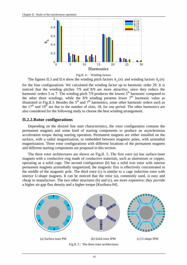
Chapter II : Study of the synchronous operation
41
0 5 10 15 20 25 300
0.2
0.4
0.6
0.8
1
Harmonics
k b
9/98/97/96/9
Fig.II. 4 : Winding factors
The figures II.3 and II.4 show the winding pitch factors )(nk p and winding factors )(nkb for the four configurations. We calculated the winding factor up to harmonic order 29. It is noticed that the winding pitches 7/9 and 8/9 are more attractive, since they reduce the harmonic orders 5 or 7. The winding pitch 7/9 produces the lowest 5th harmonic compared to the other three windings, while the 8/9 winding presents lower 7th harmonic value as illustrated in Fig.II.3. Besides the 5th and 7th harmonics, some other harmonic orders such as the 17th and 19th are due to the number of slots, 18, for one period. The other harmonics are also considered for the following study to choose the best winding arrangement.
II.2.2. Rotor configurations Depending on the desired line start characteristics, the rotor configuration contains the
permanent magnets and some kind of starting components to produce an asynchronous acceleration torque during starting operation. Permanent magnets are either installed on the surface, with a radial magnetization, or embedded between magnetic poles, with azimuthal magnetization. Three rotor configurations with different locations of the permanent magnets and different starting components are proposed in this section.
The three rotor architectures are shown on Fig.II. 5. The first rotor (a) has surface-inset magnets with a conductive ring made of conductive materials, such as aluminium or copper, operating as a solid cage. The second configuration (b) has a solid iron rotor with interior permanent magnets azimuthally magnetized; the magnetic flux is effectively concentrated in the middle of the magnetic pole. The third rotor (c) is similar to a cage induction rotor with interior U-shape magnets. It can be noticed that the rotor (a), commonly used, is easy and cheap to manufacture. The two other structures (b) and (c), are more expensive; they provide a higher air-gap flux density and a higher torque [Kurihara-04].
(a) Surface-inset PM (b) Solid-rotor IPM (c) U-shape IPM
Fig.II. 5 : The three rotor architectures

Chapter II : Study of the synchronous operation
42
With the proposed three configurations, the geometrical and electrical parameters will be studied to predict the motor performances during synchronous operation. According to the required performances, we will also determine these parameters mentioned above for each motor. A comparison of the three motors will then be discussed to find the best motor configurations.
II.3. No-load characteristics
jLω R
V E
I
Fig.II. 6 : Equivalent circuit of synchronous motor
Two-dimension field calculations are carried out with finite element method (FEM) to study the motor characteristics. The FEM uses the formulations in terms of the magnetic vector potential A
r. No-load back electromotive force (back-EMF) can be calculated from the
magnetic vector potential after successive magnetostatic field calculations. The parameters (resistance R , inductance L and back-EMF E ) of the equivalent circuit shown on Fig.II. 6 can be determined under any geometrical data.
II.3.1. Calculation of the Back-EMF
Bv nv
x
y
z
L
s
x
y
z
L
2zA1zA 1 2
1′ 2′
Fig.II. 7 : Computation of the magnetic flux
In two-dimensional field analysis, the surface integral is replaced by a line integral by using some mathematical theorems. For instance, the magnetic flux through a surface S characterized by the normal unity nv is defined as the surface integral of flux density B
r.
Applying Stokes theorem, it can be obtained by a line integral of the magnetic vector potential Ar
over a closed path )(SL bordering the surface S . Refer to Fig.II. 7, the magnet flux is equal to the difference of Az between the two points, multiplied the length zL in z-axis direction.
( )( ) zzzSL
SS
LAAdltA
dsnAdsnB
)2()1(
)(
rrr
rrrr
−=⋅=
⋅×∇=⋅=
∫∫∫∫∫ϕ
(II. 9)
Chapter II : Study of the synchronous operation
43
In the case of massive conductors, it is convenient to consider the average value of the magnetic vector potential zA on the surface cuS .Especially, in the case of electrical machines the coils are manufactured from a certain number of wires located in one slot, we consider the “average value” of the vector potential over the slot surface. Therefore, we can define the “slot flux” of the slot i as:
∫∫=iS z
i
ui dsA
SLϕ (II. 10)
where uL is the axial active length of the windings.
The connection matrix C has been previously introduced to define the current in the slots as a function of the phase currents. The connection matrix is also used to determine the phase fluxes from the slot fluxes. Thus, the flux linkage ( 3..1, =kkψ ) of the phase k is calculated.
i
N
ikistk
s
CN ϕψ ∑=
=1
/ (II. 11)
where )/(/ pqNN st = is the number of turns per slot.
The fluxes are computed for different values of the position θ of the rotor over one electrical period. The back-EMF can be obtained by the derivation of the flux according to:
Ω∂∂
=∂∂
= pt
E kkk θ
ψψ (II. 12)
where dtd
pθ1
=Ω is the mechanical speed.
The Fourier analysis is applied to analyze the harmonic components of the back-EMF based on the following formula:
∑=
=hN
n
jnnnk eEE
1, )( θθ (II. 13)
θθ θdeET
E jnT
kn−⋅= ∫0 )(1 (II. 14)
To evaluate the harmonic effects and thereby choose the optimal rotor configuration and the winding arrangement, a level of harmonic distortion is defined and called “modified total harmonic distortion” ( mTHD ). In this definition, we consider only the harmonics that we wish to minimize, such as 5, 7, 11, 13, 15, 17, 19, 23 and 25. Some harmonics, like the multiples of three, will be eliminated by applying star connection to the stator windings.
1
25231917131175
1
EEEEEEEEE
EE
THD mm
+++++++=
=∑ (II. 15)
The corresponding study will be shown in section II.3.2.1 and the evolution of the back-EMF and its harmonic contents according to different rotor geometries and winding pitches will be presented.
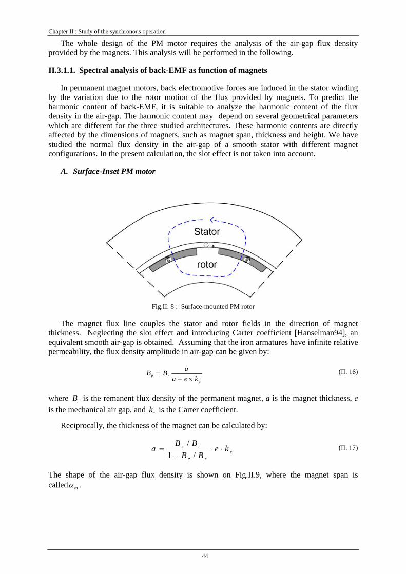
Chapter II : Study of the synchronous operation
44
The whole design of the PM motor requires the analysis of the air-gap flux density provided by the magnets. This analysis will be performed in the following.
II.3.1.1. Spectral analysis of back-EMF as function of magnets
In permanent magnet motors, back electromotive forces are induced in the stator winding by the variation due to the rotor motion of the flux provided by magnets. To predict the harmonic content of back-EMF, it is suitable to analyze the harmonic content of the flux density in the air-gap. The harmonic content may depend on several geometrical parameters which are different for the three studied architectures. These harmonic contents are directly affected by the dimensions of magnets, such as magnet span, thickness and height. We have studied the normal flux density in the air-gap of a smooth stator with different magnet configurations. In the present calculation, the slot effect is not taken into account.
A. Surface-Inset PM motor
Fig.II. 8 : Surface-mounted PM rotor
The magnet flux line couples the stator and rotor fields in the direction of magnet thickness. Neglecting the slot effect and introducing Carter coefficient [Hanselman94], an equivalent smooth air-gap is obtained. Assuming that the iron armatures have infinite relative permeability, the flux density amplitude in air-gap can be given by:
cre kea
aBB×+
= (II. 16)
where rB is the remanent flux density of the permanent magnet, a is the magnet thickness, e is the mechanical air gap, and ck is the Carter coefficient.
Reciprocally, the thickness of the magnet can be calculated by:
cre
re keBB
BBa ⋅⋅−
=/1
/ (II. 17)
The shape of the air-gap flux density is shown on Fig.II.9, where the magnet span is called mα .
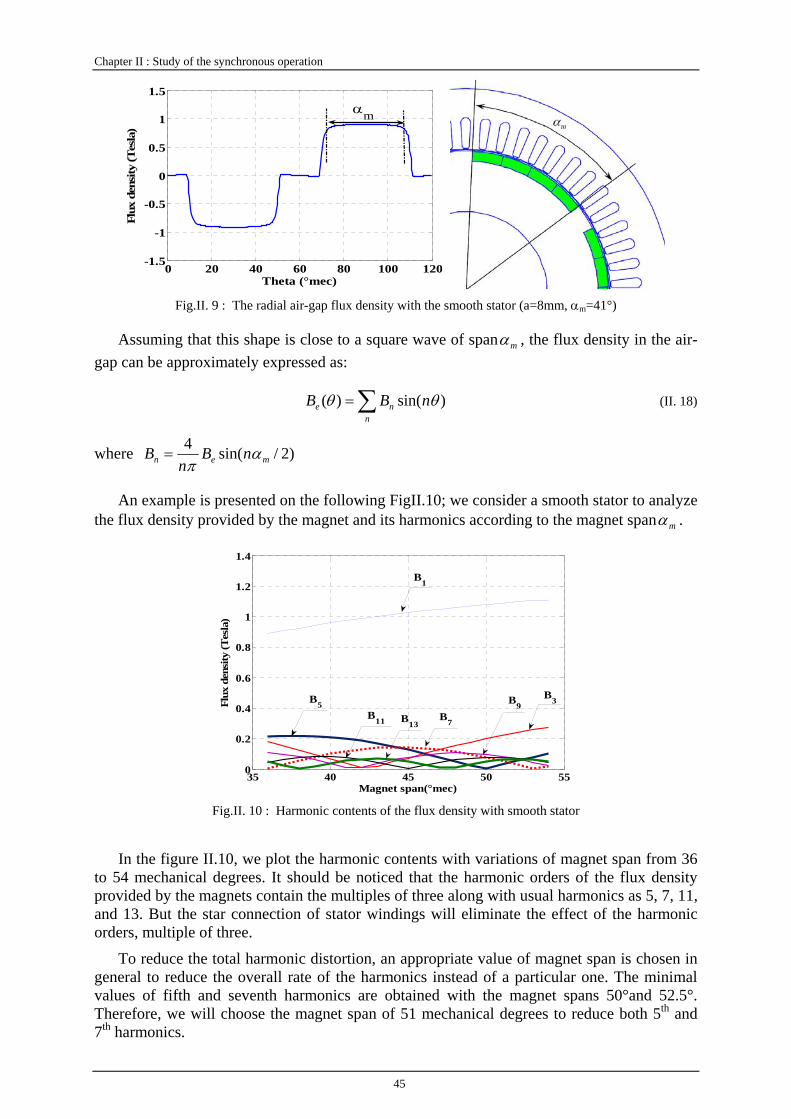
Chapter II : Study of the synchronous operation
45
0 20 40 60 80 100 120-1.5
-1
-0.5
0
0.5
1
1.5
Theta (°mec)
Flux
den
sity
(Tes
la)
αm
Fig.II. 9 : The radial air-gap flux density with the smooth stator (a=8mm, αm=41°)
Assuming that this shape is close to a square wave of span mα , the flux density in the air-gap can be approximately expressed as:
∑=n
ne nBB )sin()( θθ (II. 18)
where )2/sin(4men nB
nB α
π=
An example is presented on the following FigII.10; we consider a smooth stator to analyze the flux density provided by the magnet and its harmonics according to the magnet span mα .
35 40 45 50 550
0.2
0.4
0.6
0.8
1
1.2
1.4
Flux
den
sity
(Tes
la)
Magnet span(°mec)
B1
B3B5B7
B11 B13
B9
Fig.II. 10 : Harmonic contents of the flux density with smooth stator
In the figure II.10, we plot the harmonic contents with variations of magnet span from 36 to 54 mechanical degrees. It should be noticed that the harmonic orders of the flux density provided by the magnets contain the multiples of three along with usual harmonics as 5, 7, 11, and 13. But the star connection of stator windings will eliminate the effect of the harmonic orders, multiple of three.
To reduce the total harmonic distortion, an appropriate value of magnet span is chosen in general to reduce the overall rate of the harmonics instead of a particular one. The minimal values of fifth and seventh harmonics are obtained with the magnet spans 50°and 52.5°. Therefore, we will choose the magnet span of 51 mechanical degrees to reduce both 5th and 7th harmonics.

Chapter II : Study of the synchronous operation
46
0 10 20 30 400
0.2
0.4
0.6
0.8
1
1.2
1.4
Har
mon
ic m
agni
tude
(Tes
la)
Harmonic order Fig.II. 11 : Harmonic components in air-gap (magnet span 51°, a=8mm)
The amplitudes of harmonic contents for this magnet dimension are smaller than 0.1T (Fig.II. 11). Similar harmonic calculations and analysis will be processed for the two other motors, which will be compared with the surface-Inset PM motor.
B. Solid-rotor interior permanent magnet motor
Fig.II. 12 : Motor topology with smooth stator
The flux density in the air-gap depends on the magnet geometry, shown in Fig.II.12 with a smooth stator. Appling the above analysis, we can obtain the flux density as [Fordorean09]
m
ca
a
p
re
wke
ss
BB×
+=
22
μσ (II. 19)
σ is the coefficient of the flux leakage of the magnet .In general, it is neglected or set to1 to 1.15 according to finite element results. pS and aS are the section areas of the rotor pole and
of the magnet. aμ is the relative permeability of the magnets. mh is the magnet width.
mα
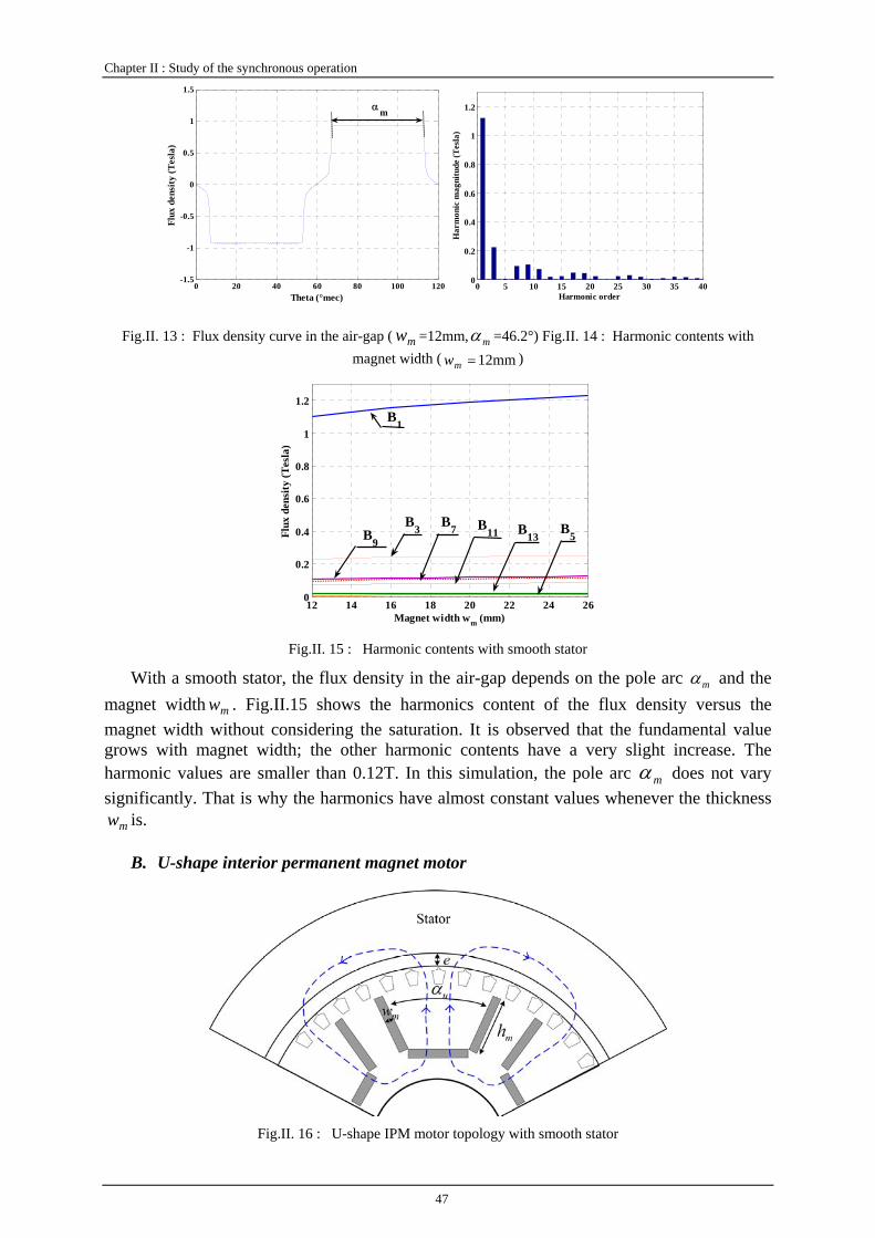
Chapter II : Study of the synchronous operation
47
0 20 40 60 80 100 120-1.5
-1
-0.5
0
0.5
1
1.5
Theta (°mec)
Flux
den
sity
(Tes
la)
αm
0 5 10 15 20 25 30 35 400
0.2
0.4
0.6
0.8
1
1.2
Har
mon
ic m
agni
tude
(Tes
la)
Harmonic order
Fig.II. 13 : Flux density curve in the air-gap ( mw =12mm, mα =46.2°) Fig.II. 14 : Harmonic contents with magnet width ( 12mm=mw )
12 14 16 18 20 22 24 260
0.2
0.4
0.6
0.8
1
1.2
Flux
den
sity
(Tes
la)
Magnet width wm (mm)
B1
B3B9B11 B13
B5B7
Fig.II. 15 : Harmonic contents with smooth stator
With a smooth stator, the flux density in the air-gap depends on the pole arc mα and the magnet width mw . Fig.II.15 shows the harmonics content of the flux density versus the magnet width without considering the saturation. It is observed that the fundamental value grows with magnet width; the other harmonic contents have a very slight increase. The harmonic values are smaller than 0.12T. In this simulation, the pole arc mα does not vary significantly. That is why the harmonics have almost constant values whenever the thickness
mw is.
B. U-shape interior permanent magnet motor
Fig.II. 16 : U-shape IPM motor topology with smooth stator
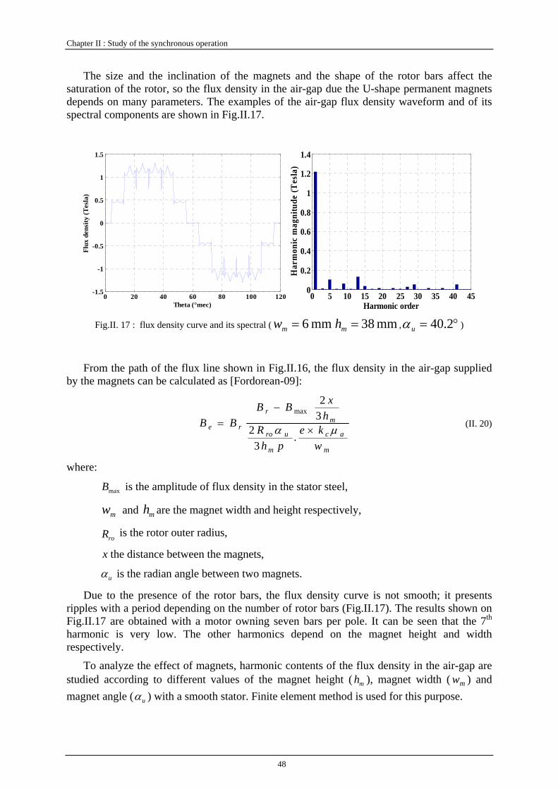
Chapter II : Study of the synchronous operation
48
The size and the inclination of the magnets and the shape of the rotor bars affect the saturation of the rotor, so the flux density in the air-gap due the U-shape permanent magnets depends on many parameters. The examples of the air-gap flux density waveform and of its spectral components are shown in Fig.II.17.
0 20 40 60 80 100 120-1.5
-1
-0.5
0
0.5
1
1.5
Theta (°mec)
Flux
den
sity
(Tes
la)
0 5 10 15 20 25 30 35 40 45
0
0.2
0.4
0.6
0.8
1
1.2
1.4
Har
mon
ic m
agni
tude
(Tes
la)
Harmonic order Fig.II. 17 : flux density curve and its spectral ( mm 6=mw mm 38=mh , °= 2.40uα )
From the path of the flux line shown in Fig.II.16, the flux density in the air-gap supplied by the magnets can be calculated as [Fordorean-09]:
m
ac
m
uro
mr
re
wke
phR
hxBB
BB μα ×
−=
.3
232
max
(II. 20)
where:
maxB is the amplitude of flux density in the stator steel,
mw and mh are the magnet width and height respectively,
roR is the rotor outer radius,
x the distance between the magnets,
uα is the radian angle between two magnets.
Due to the presence of the rotor bars, the flux density curve is not smooth; it presents ripples with a period depending on the number of rotor bars (Fig.II.17). The results shown on Fig.II.17 are obtained with a motor owning seven bars per pole. It can be seen that the 7th harmonic is very low. The other harmonics depend on the magnet height and width respectively.
To analyze the effect of magnets, harmonic contents of the flux density in the air-gap are studied according to different values of the magnet height ( mh ), magnet width ( mw ) and magnet angle ( uα ) with a smooth stator. Finite element method is used for this purpose.
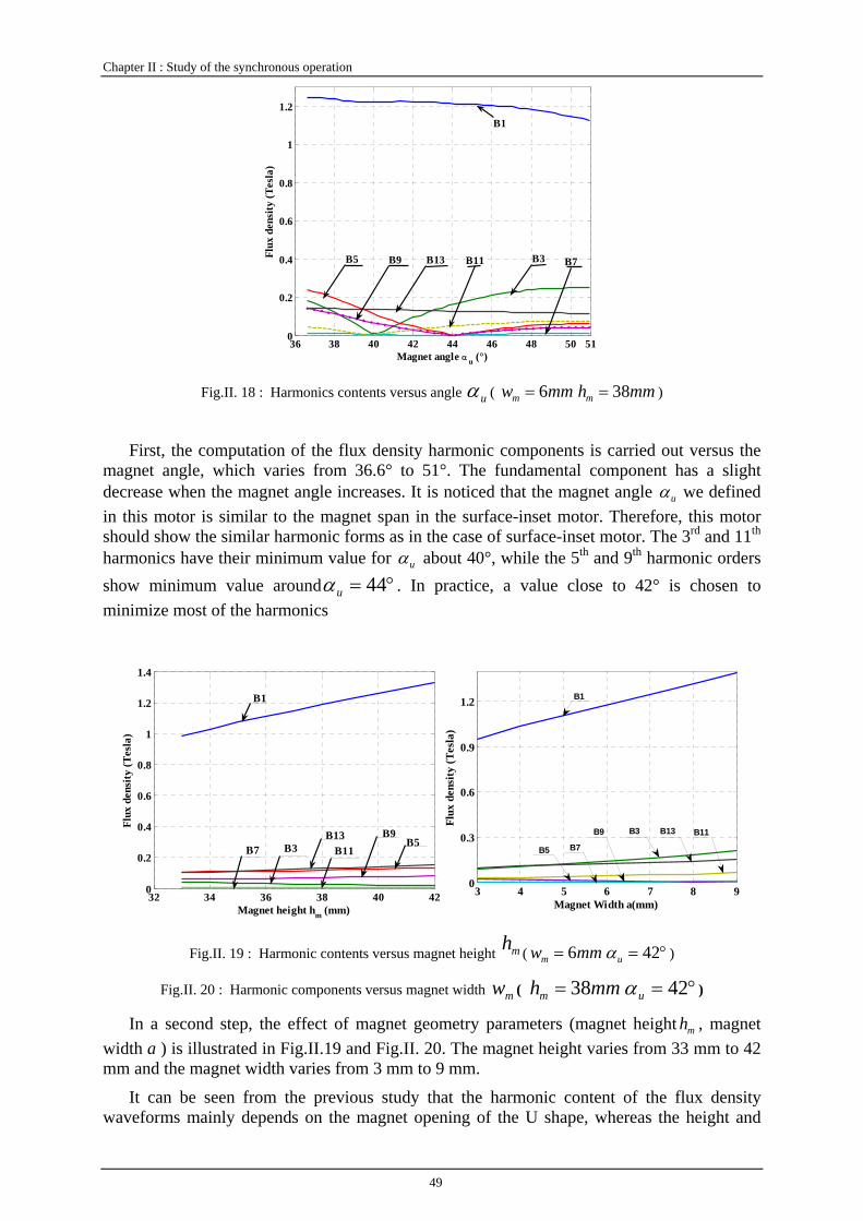
Chapter II : Study of the synchronous operation
49
36 38 40 42 44 46 48 50 510
0.2
0.4
0.6
0.8
1
1.2
Magnet angle α u (°)
Flux
den
sity
(Tes
la)
B1
B3B5 B13B9 B11 B7
Fig.II. 18 : Harmonics contents versus angle uα ( mmwm 6= mmhm 38= )
First, the computation of the flux density harmonic components is carried out versus the magnet angle, which varies from 36.6° to 51°. The fundamental component has a slight decrease when the magnet angle increases. It is noticed that the magnet angle uα we defined in this motor is similar to the magnet span in the surface-inset motor. Therefore, this motor should show the similar harmonic forms as in the case of surface-inset motor. The 3rd and 11th harmonics have their minimum value for uα about 40°, while the 5th and 9th harmonic orders show minimum value around °= 44uα . In practice, a value close to 42° is chosen to minimize most of the harmonics
32 34 36 38 40 420
0.2
0.4
0.6
0.8
1
1.2
1.4
Magnet height hm (mm)
Flux
den
sity
(Tes
la)
B1
B3 B5B7 B11
B9B13
3 4 5 6 7 8 90
0.3
0.6
0.9
1.2
Magnet Width a(mm)
Flux
den
sity
(Tes
la)
B1
B3 B13 B11
B5 B7
B9
Fig.II. 19 : Harmonic contents versus magnet height mh ( mmwm 6= °= 42uα )
Fig.II. 20 : Harmonic components versus magnet width mw ( mmhm 38= °= 42uα )
In a second step, the effect of magnet geometry parameters (magnet height mh , magnet width a ) is illustrated in Fig.II.19 and Fig.II. 20. The magnet height varies from 33 mm to 42 mm and the magnet width varies from 3 mm to 9 mm.
It can be seen from the previous study that the harmonic content of the flux density waveforms mainly depends on the magnet opening of the U shape, whereas the height and
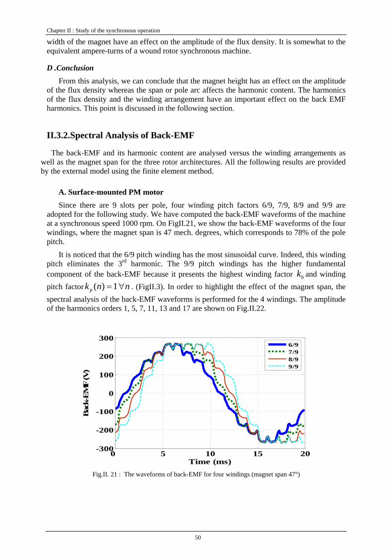
Chapter II : Study of the synchronous operation
50
width of the magnet have an effect on the amplitude of the flux density. It is somewhat to the equivalent ampere-turns of a wound rotor synchronous machine.
D .Conclusion From this analysis, we can conclude that the magnet height has an effect on the amplitude
of the flux density whereas the span or pole arc affects the harmonic content. The harmonics of the flux density and the winding arrangement have an important effect on the back EMF harmonics. This point is discussed in the following section.
II.3.2. Spectral Analysis of Back-EMF
The back-EMF and its harmonic content are analysed versus the winding arrangements as well as the magnet span for the three rotor architectures. All the following results are provided by the external model using the finite element method.
A. Surface-mounted PM motor Since there are 9 slots per pole, four winding pitch factors 6/9, 7/9, 8/9 and 9/9 are
adopted for the following study. We have computed the back-EMF waveforms of the machine at a synchronous speed 1000 rpm. On FigII.21, we show the back-EMF waveforms of the four windings, where the magnet span is 47 mech. degrees, which corresponds to 78% of the pole pitch.
It is noticed that the 6/9 pitch winding has the most sinusoidal curve. Indeed, this winding pitch eliminates the 3rd harmonic. The 9/9 pitch windings has the higher fundamental component of the back-EMF because it presents the highest winding factor bk and winding pitch factor nnkp ∀=1)( . (FigII.3). In order to highlight the effect of the magnet span, the spectral analysis of the back-EMF waveforms is performed for the 4 windings. The amplitude of the harmonics orders 1, 5, 7, 11, 13 and 17 are shown on Fig.II.22.
0 5 10 15 20-300
-200
-100
0
100
200
300
Time (ms)
Bac
k-E
MF
(V)
6/97/98/99/9
Fig.II. 21 : The waveforms of back-EMF for four windings (magnet span 47°)
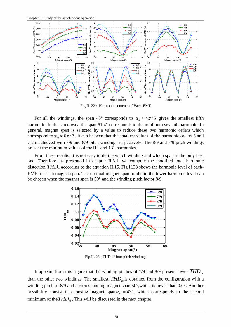
Chapter II : Study of the synchronous operation
51
35 40 45 50 55 60200
220
240
260
280
300
320
Magnet span (°)
The
1st
har
mon
ic o
f EM
F (V
)
6/97/98/99/9
35 40 45 50 55 600
2
4
6
8
10
12
14
Magnet span (°)
The
5th
har
mon
ic o
f EM
F (V
) 6/97/98/99/9
35 40 45 50 55 600
2
4
6
8
Magnet span (°)
The
7th
har
mon
ic o
f EM
F (V
) 6/97/98/99/9
35 40 45 50 55 600
1
2
3
4
5
Magnet span (°)
The
11th
har
mon
ic o
f EM
F (V
) 6/97/98/99/9
35 40 45 50 55 600
0.5
1
1.5
2
2.5
3
3.5
Magnet span (°)
The
13th
har
mon
ic o
f EM
F (V
) 6/97/98/99/9
35 40 45 50 55 600
2
4
6
8
10
Magnet span (°)
The
17th
har
mon
ic o
f EM
F (V
) 6/97/98/99/9
Fig.II. 22 : Harmonic contents of Back-EMF
For all the windings, the span 48° corresponds to 5/4πα ≈m gives the smallest fifth harmonic. In the same way, the span 51.4° corresponds to the minimum seventh harmonic. In general, magnet span is selected by a value to reduce these two harmonic orders which correspond to 7/6πα ≈m . It can be seen that the smallest values of the harmonic orders 5 and 7 are achieved with 7/9 and 8/9 pitch windings respectively. The 8/9 and 7/9 pitch windings present the minimum values of the11th and 13th harmonics.
From these results, it is not easy to define which winding and which span is the only best one. Therefore, as presented in chapter II.3.1, we compute the modified total harmonic distortion mTHD according to the equation II.15. Fig.II.23 shows the harmonic level of back-EMF for each magnet span. The optimal magnet span to obtain the lower harmonic level can be chosen when the magnet span is 50° and the winding pitch factor 8/9.
35 40 45 50 55 600.02
0.04
0.06
0.08
0.1
0.12
0.14
0.16
Magnet span(°)
TH
Dm
6/97/98/99/9
Fig.II. 23 : THD of four pitch windings
It appears from this figure that the winding pitches of 7/9 and 8/9 present lower mTHD than the other two windings. The smallest mTHD is obtained from the configuration with a winding pitch of 8/9 and a corresponding magnet span 50°,which is lower than 0.04. Another possibility consist in choosing magnet span o43=mα , which corresponds to the second minimum of the mTHD . This will be discussed in the next chapter.

Chapter II : Study of the synchronous operation
52
B. Solid-rotor IPM motor
For the solid-rotor interior permanent magnet motor, two geometric parameters are combined: the magnet height mh and the magnet width mw . The back-EMF and its harmonics are studied according to these two parameters for the four windings presented before.As for the first motor configuration, the back-EMF curves are plotted for the 4 windings (Fig.II.24). The same set of harmonics is also analyzed in the following.
0 5 10 15 20-300
-200
-100
0
100
200
300
Bac
k-EM
F (V
)
Time (ms)
6/97/98/99/9
Fig.II. 24 Back-EMF waveform of solid-rotor IPM motor
44 46 48 50 52 54 56240
260
280
300
320
340
Magnet height (mm)
The
1st
har
mon
ic o
f EM
F (V
) 6/97/98/99/9
44 46 48 50 52 54 560.4
0.6
0.8
1
1.2
1.4
1.6
1.8
Magnet height (mm)
The
5th
har
mon
ic o
f EM
F (V
)
6/97/98/99/9
44 46 48 50 52 54 561
2
3
4
5
6
Magnet height (mm)
The
7th
har
mon
ic o
f EM
F (V
)
6/97/98/99/9
44 46 48 50 52 54 560
0.5
1
1.5
2
2.5
3
3.5
Magnet height (mm)
The
11th
har
mon
ic o
f EM
F (V
)
6/97/98/99/9
44 46 48 50 52 54 560
0.5
1
1.5
2
Magnet height (mm)
The
13th
har
mon
ic o
f EM
F (V
) 6/97/98/99/9
44 46 48 50 52 54 5616
18
20
22
24
Magnet height (mm)
The
17th
har
mon
ic o
f EM
F (V
) 6/97/98/99/9
Fig.II. 25 : Harmonic contents of back-EMF versus magnet height mh ( mm12=mw )
44 46 48 50 52 54 560.135
0.14
0.145
0.15
0.155
0.16
0.165
0.17
magnet height (mm)
TH
Dm
6/97/98/99/9
Fig.II. 26 : mTHD with different magnet height mh ( mm 12=mw )
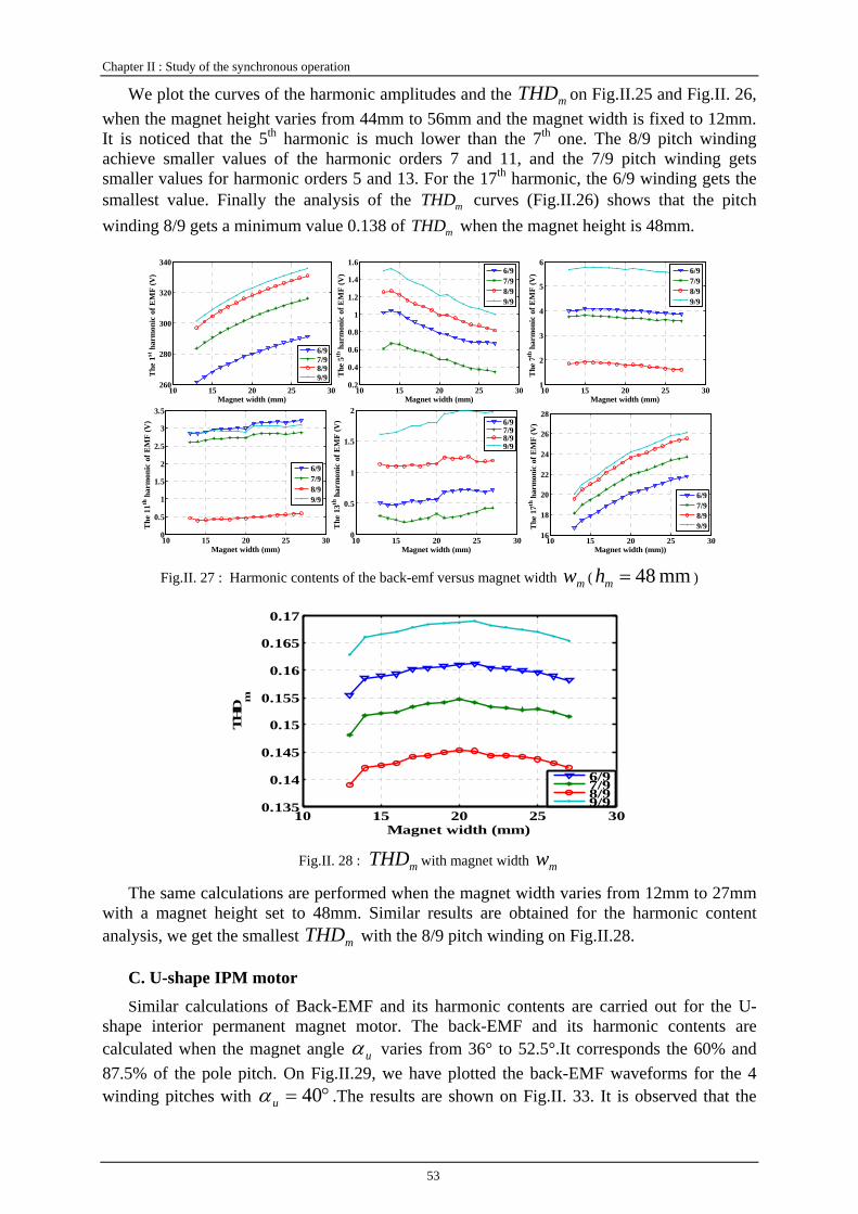
Chapter II : Study of the synchronous operation
53
We plot the curves of the harmonic amplitudes and the mTHD on Fig.II.25 and Fig.II. 26, when the magnet height varies from 44mm to 56mm and the magnet width is fixed to 12mm. It is noticed that the 5th harmonic is much lower than the 7th one. The 8/9 pitch winding achieve smaller values of the harmonic orders 7 and 11, and the 7/9 pitch winding gets smaller values for harmonic orders 5 and 13. For the 17th harmonic, the 6/9 winding gets the smallest value. Finally the analysis of the mTHD curves (Fig.II.26) shows that the pitch winding 8/9 gets a minimum value 0.138 of mTHD when the magnet height is 48mm.
10 15 20 25 30260
280
300
320
340
Magnet width (mm)
The
1st
har
mon
ic o
f EM
F (V
)
6/97/98/99/9
10 15 20 25 300.2
0.4
0.6
0.8
1
1.2
1.4
1.6
Magnet width (mm)
The
5th
har
mon
ic o
f EM
F (V
) 6/97/98/99/9
10 15 20 25 301
2
3
4
5
6
Magnet width (mm)
The
7th
har
mon
ic o
f EM
F (V
) 6/97/98/99/9
10 15 20 25 300
0.5
1
1.5
2
2.5
3
3.5
Magnet width (mm)
The
11th
har
mon
ic o
f EM
F (V
)
6/97/98/99/9
10 15 20 25 300
0.5
1
1.5
2
Magnet width (mm)
The
13th
har
mon
ic o
f EM
F (V
) 6/97/98/99/9
10 15 20 25 3016
18
20
22
24
26
28
Magnet width (mm))
The
17th
har
mon
ic o
f EM
F (V
)
6/97/98/99/9
Fig.II. 27 : Harmonic contents of the back-emf versus magnet width mw ( mm 48=mh )
10 15 20 25 300.135
0.14
0.145
0.15
0.155
0.16
0.165
0.17
Magnet width (mm)
TH
Dm
6/97/98/99/9
Fig.II. 28 : mTHD with magnet width mw
The same calculations are performed when the magnet width varies from 12mm to 27mm with a magnet height set to 48mm. Similar results are obtained for the harmonic content analysis, we get the smallest mTHD with the 8/9 pitch winding on Fig.II.28.
C. U-shape IPM motor Similar calculations of Back-EMF and its harmonic contents are carried out for the U-
shape interior permanent magnet motor. The back-EMF and its harmonic contents are calculated when the magnet angle uα varies from 36° to 52.5°.It corresponds the 60% and 87.5% of the pole pitch. On Fig.II.29, we have plotted the back-EMF waveforms for the 4 winding pitches with °= 40uα .The results are shown on Fig.II. 33. It is observed that the

Chapter II : Study of the synchronous operation
54
7/9 winding presents the lowest mTHD when the magnet angle uα is 39.2°, which will be chosen to reduce the harmonic contents of the back-EMF.
0 5 10 15 20-400
-300
-200
-100
0
100
200
300
400
Time (ms)
Back
-EM
F (V
)
6/97/98/99/9
Fig.II. 29 : Back-EMF waveform of the U-shape IPM motor
35 40 45 50 55240
250
260
270
280
290
300
310
Magnet angle α u (°)
The
Fund
amen
tal (
V)
6/97/98/99/9
35 40 45 50 550
2
4
6
8
10
12
14
Magnet angle α u (°)
The
5th h
arm
onic
(V)
6/97/98/99/9
35 40 45 50 550.2
0.4
0.6
0.8
1
1.2
1.4
1.6
Magnet angle α u (°)
The
7th h
arm
onic
(V)
6/97/98/99/9
35 40 45 50 550
1
2
3
4
5
6
Magnet angle α u (°)
The
11th
har
mon
ic (V
)
6/97/98/99/9
35 40 45 50 550
2
4
6
8
10
12
Magnet angle αu (°)
The
13th
har
mon
ic (V
)
6/97/98/99/9
35 40 45 50 550
1
2
3
4
5
6
7
8
Magnet angle α u (°)
The
17th
har
mon
ic (V
)
6/97/98/99/9
Fig.II. 30 : Harmonic contents of the back-emf versus magnet angle uα
35 40 45 50 550
0.02
0.04
0.06
0.08
0.1
0.12
0.14
Magnet angle α u (°)
THD m
6/97/98/99/9
Fig.II. 31 : Harmonic contents versus magnet angle uα
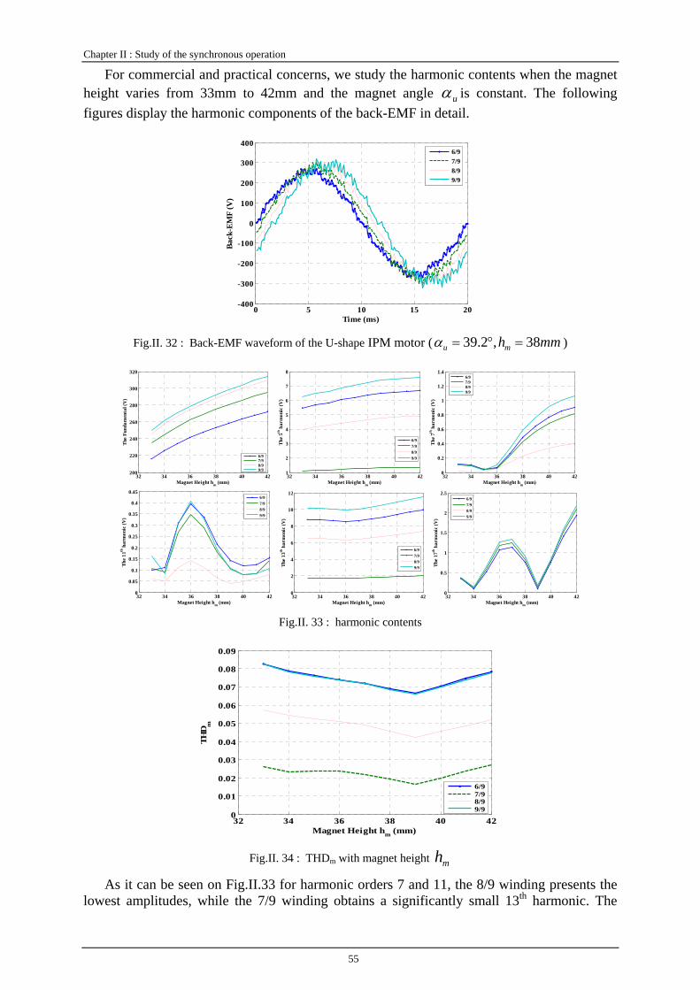
Chapter II : Study of the synchronous operation
55
For commercial and practical concerns, we study the harmonic contents when the magnet height varies from 33mm to 42mm and the magnet angle uα is constant. The following figures display the harmonic components of the back-EMF in detail.
0 5 10 15 20-400
-300
-200
-100
0
100
200
300
400
Time (ms)
Back
-EM
F (V
)
6/97/98/99/9
Fig.II. 32 : Back-EMF waveform of the U-shape IPM motor ( mmhmu 38,2.39 =°=α )
32 34 36 38 40 42200
220
240
260
280
300
320
Magnet Height hm (mm)
The
Fund
amen
tal (
V)
6/97/98/99/9
32 34 36 38 40 421
2
3
4
5
6
7
8
Magnet Height hm (mm)
The
5th h
arm
onic
(V)
6/97/98/99/9
32 34 36 38 40 420
0.2
0.4
0.6
0.8
1
1.2
1.4
Magnet Height hm (mm)
The
7th h
arm
onic
(V)
6/97/98/99/9
32 34 36 38 40 420
0.05
0.1
0.15
0.2
0.25
0.3
0.35
0.4
0.45
Magnet Height hm (mm)
The
11th
har
mon
ic (V
)
6/97/98/99/9
32 34 36 38 40 420
2
4
6
8
10
12
Magnet Height hm (mm)
The
13th
har
mon
ic (V
)
6/97/98/99/9
32 34 36 38 40 420
0.5
1
1.5
2
2.5
Magnet Height hm (mm)
The
17th
har
mon
ic (V
)
6/97/98/99/9
Fig.II. 33 : harmonic contents
32 34 36 38 40 420
0.01
0.02
0.03
0.04
0.05
0.06
0.07
0.08
0.09
Magnet Height hm (mm)
THD m
6/97/98/99/9
Fig.II. 34 : THDm with magnet height mh
As it can be seen on Fig.II.33 for harmonic orders 7 and 11, the 8/9 winding presents the lowest amplitudes, while the 7/9 winding obtains a significantly small 13th harmonic. The
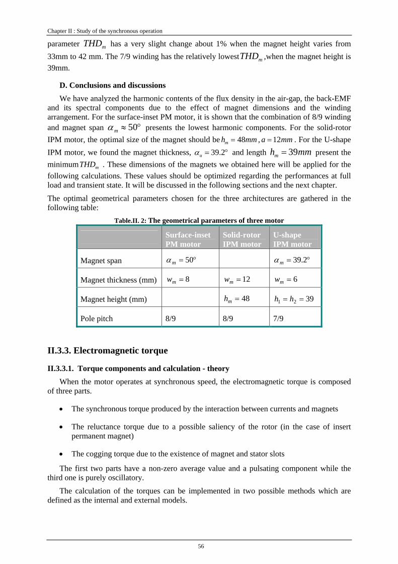
Chapter II : Study of the synchronous operation
56
parameter mTHD has a very slight change about 1% when the magnet height varies from 33mm to 42 mm. The 7/9 winding has the relatively lowest mTHD ,when the magnet height is 39mm.
D. Conclusions and discussions We have analyzed the harmonic contents of the flux density in the air-gap, the back-EMF
and its spectral components due to the effect of magnet dimensions and the winding arrangement. For the surface-inset PM motor, it is shown that the combination of 8/9 winding and magnet span °≈ 50mα presents the lowest harmonic components. For the solid-rotor IPM motor, the optimal size of the magnet should be mmhm 48= , mma 12= . For the U-shape IPM motor, we found the magnet thickness, °= 2.39uα and length mmhm 39= present the minimum mTHD . These dimensions of the magnets we obtained here will be applied for the following calculations. These values should be optimized regarding the performances at full load and transient state. It will be discussed in the following sections and the next chapter.
The optimal geometrical parameters chosen for the three architectures are gathered in the following table:
Table.II. 2: The geometrical parameters of three motor
Surface-inset PM motor
Solid-rotor IPM motor
U-shape IPM motor
Magnet span °= 50mα °= 2.39mα
Magnet thickness (mm) 8=mw 12=mw 6=mw
Magnet height (mm) 48=mh 3921 == hh
Pole pitch 8/9 8/9 7/9
II.3.3. Electromagnetic torque
II.3.3.1. Torque components and calculation - theory When the motor operates at synchronous speed, the electromagnetic torque is composed
of three parts.
• The synchronous torque produced by the interaction between currents and magnets
• The reluctance torque due to a possible saliency of the rotor (in the case of insert permanent magnet)
• The cogging torque due to the existence of magnet and stator slots
The first two parts have a non-zero average value and a pulsating component while the third one is purely oscillatory.
The calculation of the torques can be implemented in two possible methods which are defined as the internal and external models.
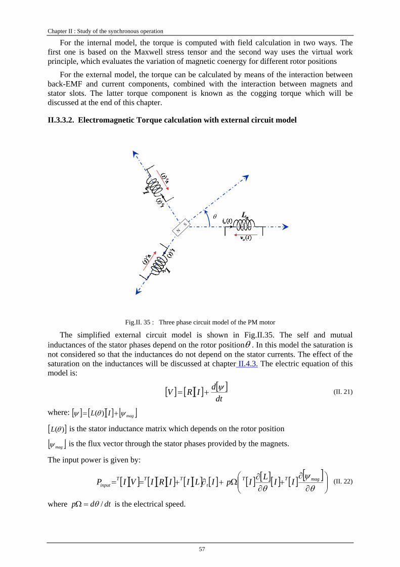
Chapter II : Study of the synchronous operation
57
For the internal model, the torque is computed with field calculation in two ways. The first one is based on the Maxwell stress tensor and the second way uses the virtual work principle, which evaluates the variation of magnetic coenergy for different rotor positions
For the external model, the torque can be calculated by means of the interaction between back-EMF and current components, combined with the interaction between magnets and stator slots. The latter torque component is known as the cogging torque which will be discussed at the end of this chapter.
II.3.3.2. Electromagnetic Torque calculation with external circuit model
Fig.II. 35 : Three phase circuit model of the PM motor
The simplified external circuit model is shown in Fig.II.35. The self and mutual inductances of the stator phases depend on the rotor positionθ . In this model the saturation is not considered so that the inductances do not depend on the stator currents. The effect of the saturation on the inductances will be discussed at chapter II.4.3. The electric equation of this model is:
[ ] [ ][ ] [ ]dt
dIRV ψ+= (II. 21)
where: [ ] [ ][ ] [ ]magIL ψθψ += )(
[ ])(θL is the stator inductance matrix which depends on the rotor position
[ ]magψ is the flux vector through the stator phases provided by the magnets.
The input power is given by:
[ ][ ] [ ][ ][ ] [ ][ ] [ ] [ ] [ ][ ] [ ] [ ]⎟⎟⎠
⎞⎜⎜⎝
⎛∂
∂+
∂∂
Ω+∂+==θ
ψθ
magTTt
TTTinput IILIpILIIRIVIP (II. 22)
where dtdp /θ=Ω is the electrical speed.
θ
N S
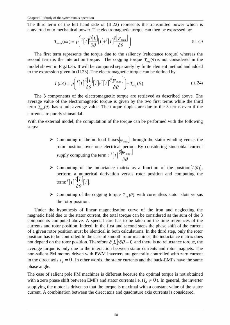
Chapter II : Study of the synchronous operation
58
The third term of the left hand side of (II.22) represents the transmitted power which is converted onto mechanical power. The electromagnetic torque can then be expressed by:
[ ] [ ][ ] [ ] [ ]⎟⎟⎠
⎞⎜⎜⎝
⎛∂
∂+
∂∂
=− θψ
θω magTT
me IILIptT )( (II. 23)
The first term represents the torque due to the saliency (reluctance torque) whereas the second term is the interaction torque. The cogging torque )(θcogT is not considered in the model shown in Fig.II.35. It will be computed separately by finite element method and added to the expression given in (II.23). The electromagnetic torque can be defined by
[ ] [ ][ ] [ ] [ ])()( θ
θψ
θω cog
magTT TIILIptT +⎟⎟⎠
⎞⎜⎜⎝
⎛∂
∂+
∂∂
= (II. 24)
The 3 components of the electromagnetic torque are retrieved as described above. The average value of the electromagnetic torque is given by the two first terms while the third term )(θcogT has a null average value. The torque ripples are due to the 3 terms even if the currents are purely sinusoidal.
With the external model, the computation of the torque can be performed with the following steps:
Computing of the no-load fluxes [ ]magψ through the stator winding versus the rotor position over one electrical period. By considering sinusoidal current
supply computing the term : [ ] [ ]θ
ψ∂
∂ magT I
Computing of the inductance matrix as a function of the position [ ])(θL , perform a numerical derivation versus rotor position and computing the
term: [ ] [ ][ ]ILIT
θ∂∂ .
Computing of the cogging torque )(θcogT with currentless stator slots versus the rotor position.
Under the hypothesis of linear magnetization curve of the iron and neglecting the magnetic field due to the stator current, the total torque can be considered as the sum of the 3 components computed above. A special care has to be taken on the time references of the currents and rotor position. Indeed, in the first and second steps the phase shift of the current of a given rotor position must be identical in both calculations. In the third step, only the rotor position has to be controlled.In the case of smooth rotor machines, the inductance matrix does not depend on the rotor position. Therefore [ ] 0=∂∂ θL and there is no reluctance torque, the average torque is only due to the interaction between stator currents and rotor magnets. The non-salient PM motors driven with PWM inverters are generally controlled with zero current in the direct axis 0=di . In other words, the stator currents and the back-EMFs have the same phase angle.
The case of salient pole PM machines is different because the optimal torque is not obtained with a zero phase shift between EMFs and stator currents i.e. ( 0≠di ). In general, the inverter supplying the motor is driven so that the torque is maximal with a constant value of the stator current. A combination between the direct axis and quadrature axis currents is considered.
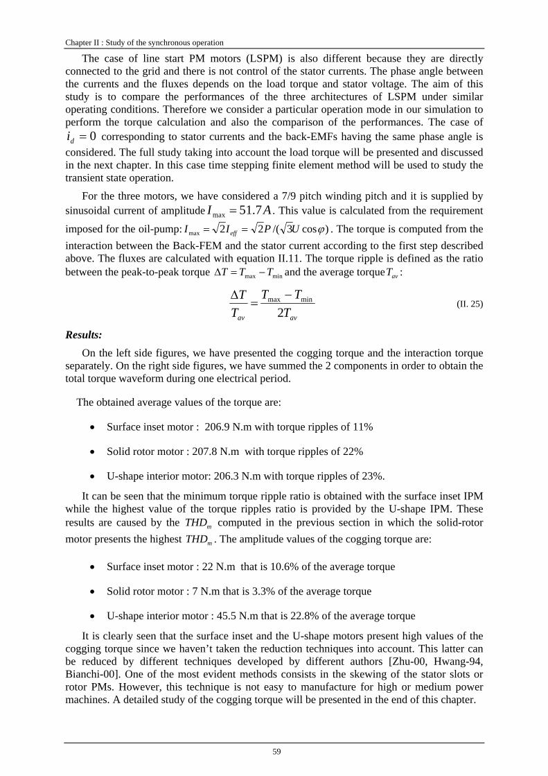
Chapter II : Study of the synchronous operation
59
The case of line start PM motors (LSPM) is also different because they are directly connected to the grid and there is not control of the stator currents. The phase angle between the currents and the fluxes depends on the load torque and stator voltage. The aim of this study is to compare the performances of the three architectures of LSPM under similar operating conditions. Therefore we consider a particular operation mode in our simulation to perform the torque calculation and also the comparison of the performances. The case of
0=di corresponding to stator currents and the back-EMFs having the same phase angle is considered. The full study taking into account the load torque will be presented and discussed in the next chapter. In this case time stepping finite element method will be used to study the transient state operation.
For the three motors, we have considered a 7/9 pitch winding pitch and it is supplied by sinusoidal current of amplitude AI 7.51max = . This value is calculated from the requirement
imposed for the oil-pump: )cos3/(22max ϕUPII eff == . The torque is computed from the interaction between the Back-FEM and the stator current according to the first step described above. The fluxes are calculated with equation II.11. The torque ripple is defined as the ratio between the peak-to-peak torque minmax TTT −=Δ and the average torque avT :
avav TTT
TT
2minmax −=
Δ (II. 25)
Results: On the left side figures, we have presented the cogging torque and the interaction torque
separately. On the right side figures, we have summed the 2 components in order to obtain the total torque waveform during one electrical period.
The obtained average values of the torque are:
• Surface inset motor : 206.9 N.m with torque ripples of 11%
• Solid rotor motor : 207.8 N.m with torque ripples of 22%
• U-shape interior motor: 206.3 N.m with torque ripples of 23%.
It can be seen that the minimum torque ripple ratio is obtained with the surface inset IPM while the highest value of the torque ripples ratio is provided by the U-shape IPM. These results are caused by the mTHD computed in the previous section in which the solid-rotor motor presents the highest mTHD . The amplitude values of the cogging torque are:
• Surface inset motor : 22 N.m that is 10.6% of the average torque
• Solid rotor motor : 7 N.m that is 3.3% of the average torque
• U-shape interior motor : 45.5 N.m that is 22.8% of the average torque
It is clearly seen that the surface inset and the U-shape motors present high values of the cogging torque since we haven’t taken the reduction techniques into account. This latter can be reduced by different techniques developed by different authors [Zhu-00, Hwang-94, Bianchi-00]. One of the most evident methods consists in the skewing of the stator slots or rotor PMs. However, this technique is not easy to manufacture for high or medium power machines. A detailed study of the cogging torque will be presented in the end of this chapter.

Chapter II : Study of the synchronous operation
60
0 5 10 15 20-50
0
50
100
150
200
250
Time (ms)
Torq
ue (N
.m)
EI/ΩCogging torque
0 5 10 15 200
50
100
150
200
250
Torq
ue (N
.m)
Time (ms)
Fig.II. 36 : Torque waveforms with circuit model for surface-mounted motor (magnet span 50°)
0 5 10 15 20-50
0
50
100
150
200
250
Time (ms)
Torq
ue (N
.m)
EI/ΩCogging torque
0 5 10 15 20
0
50
100
150
200
250
Torq
ue (N
.m)
Time (ms) Fig.II. 37 : Torque waveforms with circuit model for solid-rotor IPM motor ( mm12=a mm49=mh )
0 5 10 15 20-50
0
50
100
150
200
250
Time (ms)
Torq
ue (N
.m)
EI/ΩCogging torque
0 5 10 15 200
50
100
150
200
250
Torq
ue (N
.m)
Time (ms) Fig.II. 38 : Torque waveforms with circuit model for U-shape IPM motor ( mm3921 == hh )
II.3.3.3. Electromagnetic Torque calculation with internal field model
The circuit model presented above uses finite element method for the identification of [ ]magψ and [ ])(θL . The field created by the stator currents is not taken into account. It is based on the principle of superimposition and does not correctly consider the saturation. Indeed, the calculation of the fluxes is performed with nonlinear magnetostatic finite element code. This model has the advantage of being easy to implement and is not CPU time consuming in comparison with the other methods.
In order to take into account both saturation and stator currents effect, it is possible to perform finite element computation with supplied slots and the presence of the magnets. This is so called internal field model. It is based on the complete numerical calculation using the
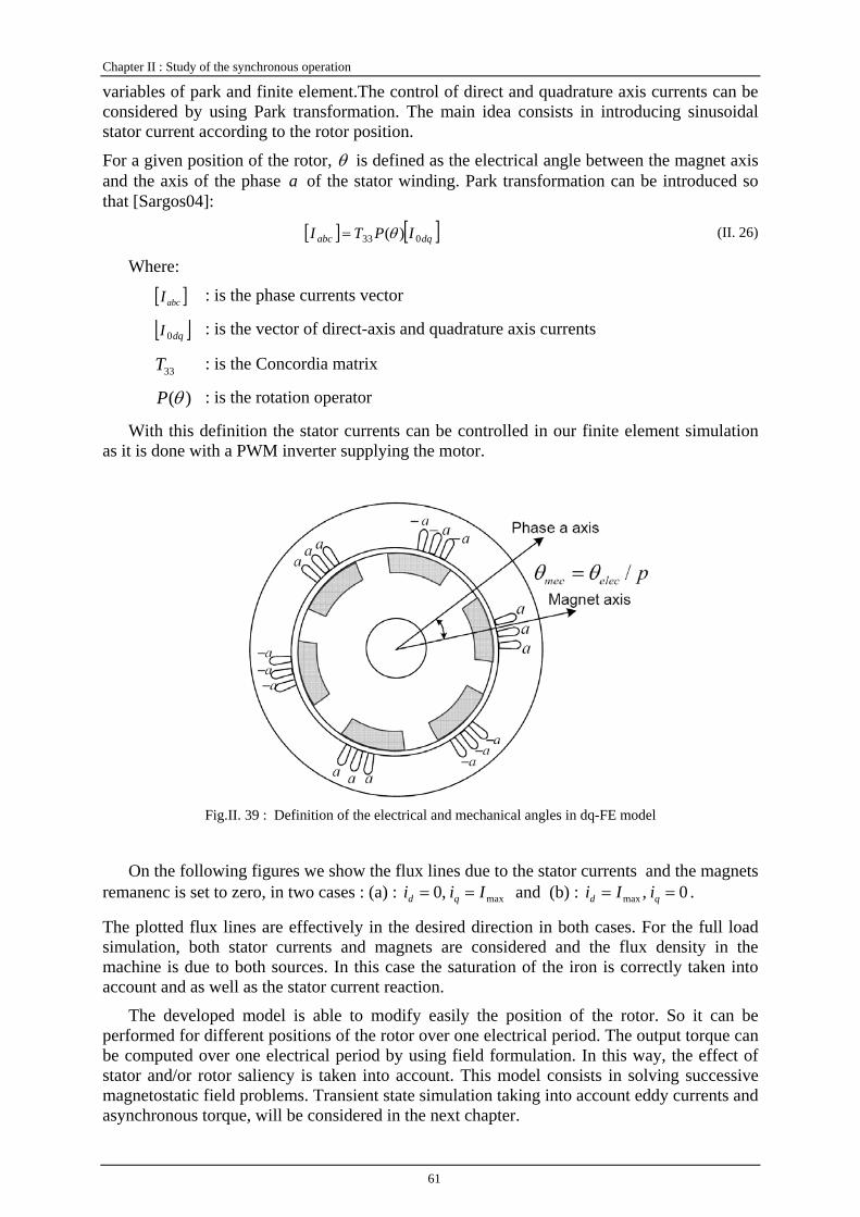
Chapter II : Study of the synchronous operation
61
variables of park and finite element.The control of direct and quadrature axis currents can be considered by using Park transformation. The main idea consists in introducing sinusoidal stator current according to the rotor position.
For a given position of the rotor, θ is defined as the electrical angle between the magnet axis and the axis of the phase a of the stator winding. Park transformation can be introduced so that [Sargos04]:
[ ] [ ]dqabc IPTI 033 )(θ= (II. 26)
Where:
[ ]abcI : is the phase currents vector
[ ]dqI 0 : is the vector of direct-axis and quadrature axis currents
33T : is the Concordia matrix
)(θP : is the rotation operator
With this definition the stator currents can be controlled in our finite element simulation as it is done with a PWM inverter supplying the motor.
Fig.II. 39 : Definition of the electrical and mechanical angles in dq-FE model
On the following figures we show the flux lines due to the stator currents and the magnets remanenc is set to zero, in two cases : (a) : max,0 Iii qd == and (b) : 0,max == qd iIi .
The plotted flux lines are effectively in the desired direction in both cases. For the full load simulation, both stator currents and magnets are considered and the flux density in the machine is due to both sources. In this case the saturation of the iron is correctly taken into account and as well as the stator current reaction.
The developed model is able to modify easily the position of the rotor. So it can be performed for different positions of the rotor over one electrical period. The output torque can be computed over one electrical period by using field formulation. In this way, the effect of stator and/or rotor saliency is taken into account. This model consists in solving successive magnetostatic field problems. Transient state simulation taking into account eddy currents and asynchronous torque, will be considered in the next chapter.
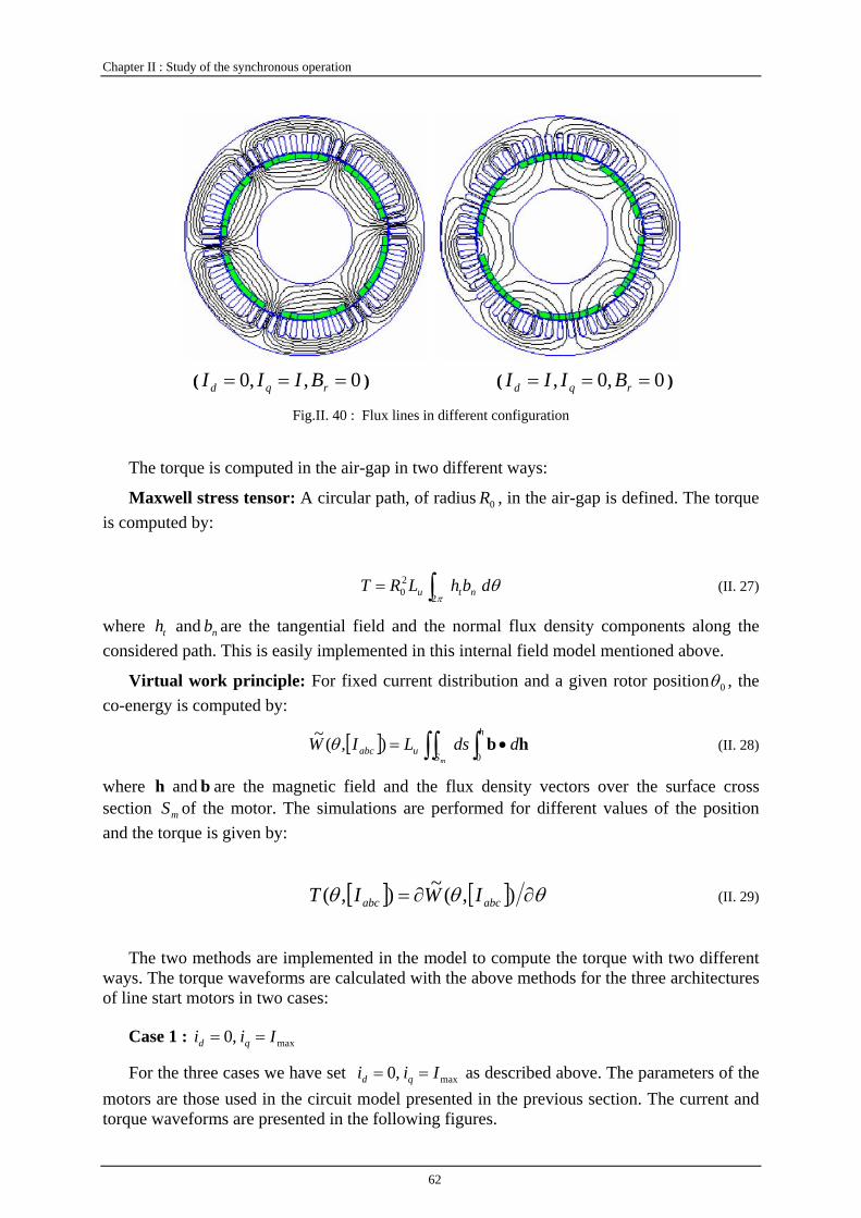
Chapter II : Study of the synchronous operation
62
( 0,,0 === rqd BIII ) ( 0,0, === rqd BIII )
Fig.II. 40 : Flux lines in different configuration
The torque is computed in the air-gap in two different ways:
Maxwell stress tensor: A circular path, of radius 0R , in the air-gap is defined. The torque is computed by:
∫=π
θ2
20 dbhLRT ntu (II. 27)
where nt bh and are the tangential field and the normal flux density components along the considered path. This is easily implemented in this internal field model mentioned above.
Virtual work principle: For fixed current distribution and a given rotor position 0θ , the co-energy is computed by:
[ ] ∫∫ ∫ •=mS
h
uabc ddsLIW hb0
),(~ θ (II. 28)
where bh and are the magnetic field and the flux density vectors over the surface cross section mS of the motor. The simulations are performed for different values of the position and the torque is given by:
[ ] [ ] θθθ ∂∂= ),(~),( abcabc IWIT (II. 29)
The two methods are implemented in the model to compute the torque with two different ways. The torque waveforms are calculated with the above methods for the three architectures of line start motors in two cases:
Case 1 : max,0 Iii qd ==
For the three cases we have set max,0 Iii qd == as described above. The parameters of the motors are those used in the circuit model presented in the previous section. The current and torque waveforms are presented in the following figures.
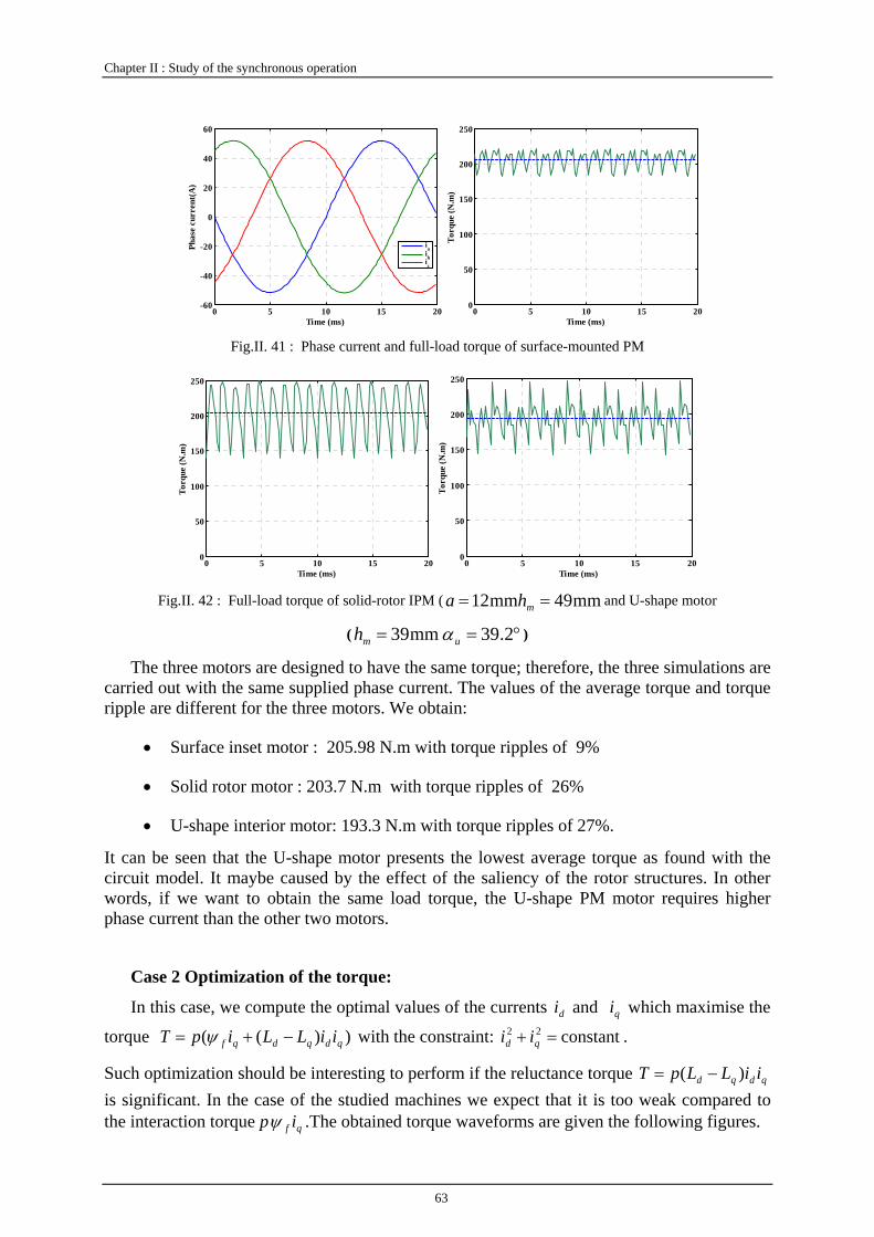
Chapter II : Study of the synchronous operation
63
0 5 10 15 20-60
-40
-20
0
20
40
60
Time (ms)
Phas
e cu
rren
t(A
)
iaibic
0 5 10 15 200
50
100
150
200
250
Torq
ue (N
.m)
Time (ms)
Fig.II. 41 : Phase current and full-load torque of surface-mounted PM
0 5 10 15 200
50
100
150
200
250
Time (ms)
Torq
ue (N
.m)
0 5 10 15 200
50
100
150
200
250
Torq
ue (N
.m)
Time (ms) Fig.II. 42 : Full-load torque of solid-rotor IPM ( mm49mm12 == mha and U-shape motor
( °== 2.39mm39 umh α )
The three motors are designed to have the same torque; therefore, the three simulations are carried out with the same supplied phase current. The values of the average torque and torque ripple are different for the three motors. We obtain:
• Surface inset motor : 205.98 N.m with torque ripples of 9%
• Solid rotor motor : 203.7 N.m with torque ripples of 26%
• U-shape interior motor: 193.3 N.m with torque ripples of 27%.
It can be seen that the U-shape motor presents the lowest average torque as found with the circuit model. It maybe caused by the effect of the saliency of the rotor structures. In other words, if we want to obtain the same load torque, the U-shape PM motor requires higher phase current than the other two motors.
Case 2 Optimization of the torque:
In this case, we compute the optimal values of the currents di and qi which maximise the
torque ))(( qdqdqf iiLLipT −+= ψ with the constraint: constant22 =+ qd ii .
Such optimization should be interesting to perform if the reluctance torque qdqd iiLLpT )( −= is significant. In the case of the studied machines we expect that it is too weak compared to the interaction torque qf ipψ .The obtained torque waveforms are given the following figures.
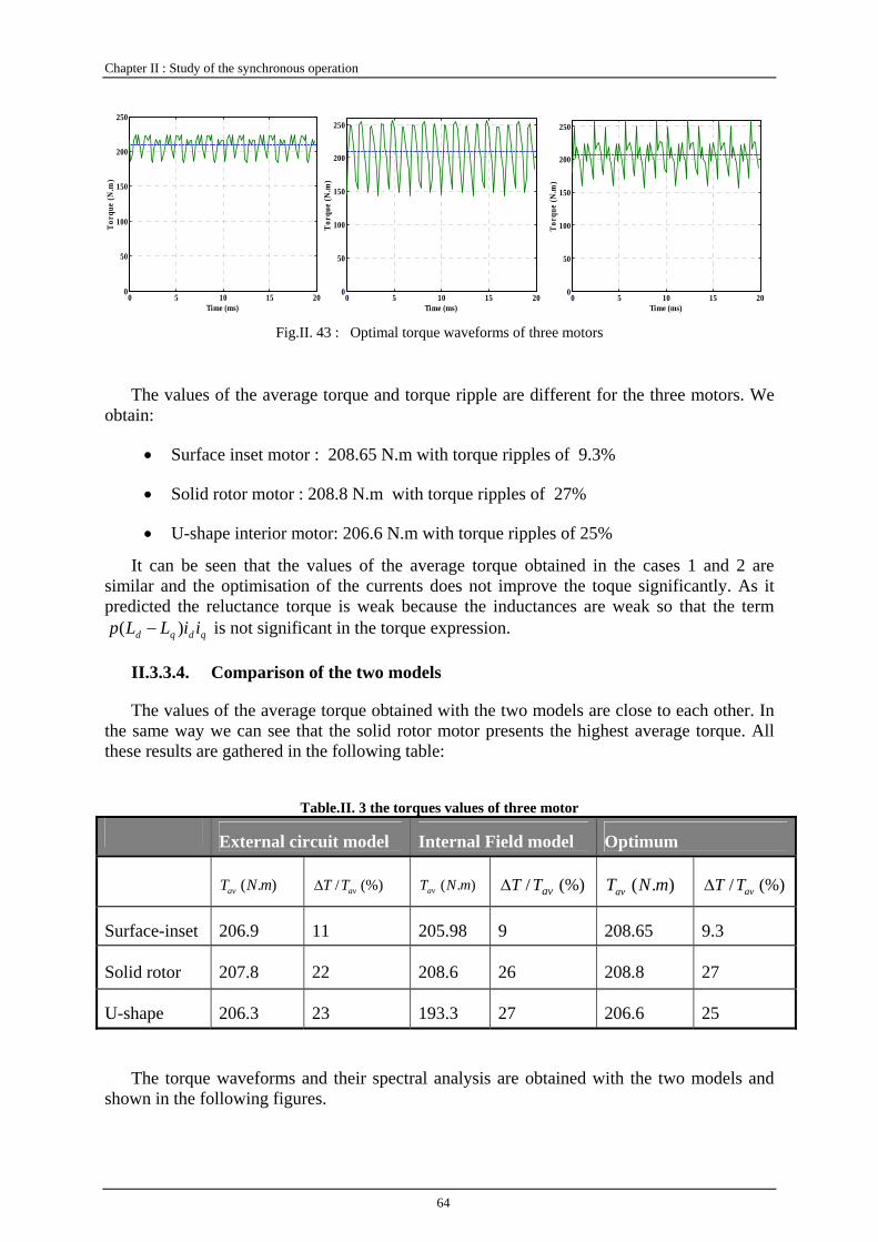
Chapter II : Study of the synchronous operation
64
0 5 10 15 200
50
100
150
200
250To
rque
(N.m
)
Time (ms)0 5 10 15 20
0
50
100
150
200
250
Torq
ue (N
.m)
Time (ms) 0 5 10 15 20
0
50
100
150
200
250
Torq
ue (N
.m)
Time (ms) Fig.II. 43 : Optimal torque waveforms of three motors
The values of the average torque and torque ripple are different for the three motors. We obtain:
• Surface inset motor : 208.65 N.m with torque ripples of 9.3%
• Solid rotor motor : 208.8 N.m with torque ripples of 27%
• U-shape interior motor: 206.6 N.m with torque ripples of 25%
It can be seen that the values of the average torque obtained in the cases 1 and 2 are similar and the optimisation of the currents does not improve the toque significantly. As it predicted the reluctance torque is weak because the inductances are weak so that the term
qdqd iiLLp )( − is not significant in the torque expression.
II.3.3.4. Comparison of the two models
The values of the average torque obtained with the two models are close to each other. In the same way we can see that the solid rotor motor presents the highest average torque. All these results are gathered in the following table:
Table.II. 3 the torques values of three motor
External circuit model Internal Field model Optimum
).( mNTav (%)/ avTTΔ ).( mNTav (%)/ avTTΔ ).( mNTav (%)/ avTTΔ
Surface-inset 206.9 11 205.98 9 208.65 9.3
Solid rotor 207.8 22 208.6 26 208.8 27
U-shape 206.3 23 193.3 27 206.6 25
The torque waveforms and their spectral analysis are obtained with the two models and shown in the following figures.
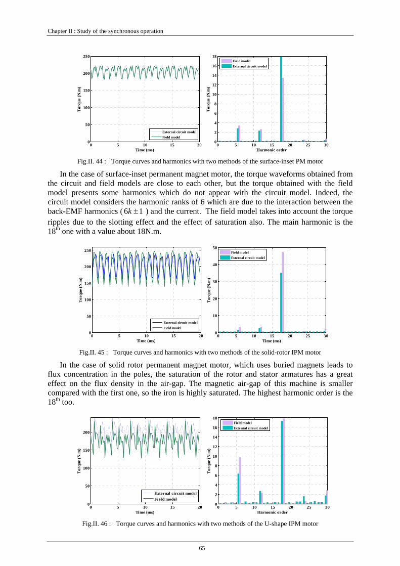
Chapter II : Study of the synchronous operation
65
0 5 10 15 200
50
100
150
200
250
Time (ms)
Torq
ue (N
.m)
External circuit modelField model
0 5 10 15 20 25 30
0
2
4
6
8
10
12
14
16
18
Harmonic order
Torq
ue (N
.m)
Field modelExternal circuit model
Fig.II. 44 : Torque curves and harmonics with two methods of the surface-inset PM motor
In the case of surface-inset permanent magnet motor, the torque waveforms obtained from the circuit and field models are close to each other, but the torque obtained with the field model presents some harmonics which do not appear with the circuit model. Indeed, the circuit model considers the harmonic ranks of 6 which are due to the interaction between the back-EMF harmonics ( 16 ±k ) and the current. The field model takes into account the torque ripples due to the slotting effect and the effect of saturation also. The main harmonic is the 18th one with a value about 18N.m.
0 5 10 15 200
50
100
150
200
250
Time (ms)
Torq
ue (N
.m)
External circuit modelField model
0 5 10 15 20 25 300
10
20
30
40
50
Time (ms)
Torq
ue (N
.m)
Field modelExternal circuit model
Fig.II. 45 : Torque curves and harmonics with two methods of the solid-rotor IPM motor
In the case of solid rotor permanent magnet motor, which uses buried magnets leads to flux concentration in the poles, the saturation of the rotor and stator armatures has a great effect on the flux density in the air-gap. The magnetic air-gap of this machine is smaller compared with the first one, so the iron is highly saturated. The highest harmonic order is the 18th too.
0 5 10 15 200
50
100
150
200
Time (ms)
Torq
ue (N
.m)
External circuit modelField model
0 5 10 15 20 25 30
0
2
4
6
8
10
12
14
16
18
Harmonic order
Torq
ue (N
.m)
Field modelExternal circuit model
Fig.II. 46 : Torque curves and harmonics with two methods of the U-shape IPM motor
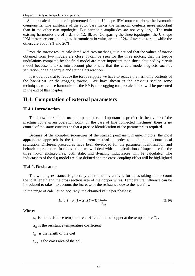
Chapter II : Study of the synchronous operation
66
Similar calculations are implemented for the U-shape IPM motor to show the harmonic components. The existence of the rotor bars makes the harmonic contents more important than in the other two topologies. But harmonic amplitudes are not very large. The main existing harmonics are of orders 6, 12, 18, 30. Comparing the three topologies, the U-shape IPM motor presents the highest harmonic ratio value, around 27% of average torque while the others are about 9% and 26%.
From the torque results calculated with two methods, it is noticed that the values of torque obtained from two models are close. It can be seen for the three motors, that the torque undulations computed by the field model are more important than those obtained by circuit model because it takes into account phenomena that the circuit model neglects such as saturation, cogging torque and stator slots reaction.
It is obvious that to reduce the torque ripples we have to reduce the harmonic contents of the back-EMF or the cogging torque. We have shown in the previous section some techniques to reduce harmonics of the EMF; the cogging torque calculation will be presented in the end of this chapter.
II.4. Computation of external parameters
II.4.1. Introduction
The knowledge of the machine parameters is important to predict the behaviour of the machine for a given operation point. In the case of line connected machines, there is no control of the stator currents so that a precise identification of the parameters is required.
Because of the complex geometries of the studied permanent magnet motors, the most appropriate approach is the finite element method in order to take into account local saturation. Different procedures have been developed for the parameter identification and behaviour prediction. In this section, we will deal with the calculation of impedance for the three motor architectures; both static and dynamic inductances will be calculated. The inductances of the d-q model are also defined and the cross coupling effect will be highlighted
II.4.2. Resistance
The winding resistance is generally determined by analytic formulas taking into account the total length and the cross section area of the copper wires. Temperature influence can be introduced to take into account the increase of the resistance due to the heat flow.
In the range of calculation accuracy, the obtained value per phase is:
( )coil
coilcus s
lTTTR )(1)( 00 −+= αρ (II. 30)
Where:
0ρ is the resistance temperature coefficient of the copper at the temperature 0T .
cuα is the resistance temperature coefficient
coill is the length of the coil
coils is the cross area of the coil

Chapter II : Study of the synchronous operation
67
II.4.3. Self and mutual Inductances
The calculation of inductance in permanent magnet motors can be performed in different ways that depend on the degree of assumption taken in the model. With respect to the linear materials, the presence of flux supplied by the magnets does not affect the values of the inductances. In practice, the motors are designed so that the iron operates at a given level of saturation, so that it is necessary to take into account the effect of the magnets. In addition, it is interesting to compute the inductances in the direct and quadrature axes which directly depend on the magnet flux. These two approaches will be discussed in the following.
II.4.3.1. Linear model
When the iron core is not saturated, the inductances do not depend on the flux provided by the magnets. In this case, the self- and mutual inductances can be calculated by computing the flux linkage when only one phase is supplied and when the permanent magnet remanence is set to zero. We call this situation “switched off magnets”. The flux through the phase a is defined by:
magcacbabaaaa IMIMIL ψψ +++= (II. 31)
where Laa is the self inductance of phase a, Mab is the mutual inductance between phase a and b, Mac is the mutual inductance between phases a and c. magψ is the flux of the phase a due to the magnets.
0,0 , ===
cbmaga
aaa iI
Lψ
ψ 0,0 , ==
=cbmaga
bab iI
Mψ
ψ0,0 , ==
=cbmaga
cac iI
Mψ
ψ (II. 32)
Due to the saliency of the three rotors the inductance calculation is performed for different values of the rotor position over one electrical period.
The figures II.47, II.48 and II.49 show the self and mutual inductances versus the rotor position for the three motors. In the case of the surface-inset motor, we observe that the maximum value of the self inductance is about 3 mH while the minimum value is 1.5mH. These two values correspond to the cases where the magnets and phase a axes are orthogonal and parallel respectively. Similar results are obtained for the solid rotor motor though the maximal value of the inductance is higher (about 6.5 mH); this is due to the fact that the magnetic air-gap of this motor is relatively smaller than that of the surface-inset motor. The effect of the saliency on the inductances of solid rotor motor is important. The U-shape IPM presents smaller variations of self and mutual inductances because the rotor is more magnetically homogeneous. These results give an idea about the values of the inductances. The calculation method does not take into account saturation so these values are not significant and cannot be used in the circuit model.
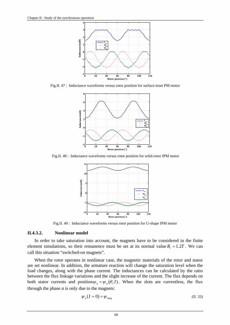
Chapter II : Study of the synchronous operation
68
0 20 40 60 80 100 120-3
-2
-1
0
1
2
3
4
Rotor position (°)In
duct
ance
(mH
)
LaaMabMac
Fig.II. 47 : Inductance waveforms versus rotor position for surface-inset PM motor
0 20 40 60 80 100 120-4
-2
0
2
4
6
8
Rotor position (°)
Indu
ctan
ce(m
H)
LaaMabMac
Fig.II. 48 : Inductance waveforms versus rotor position for solid-rotor IPM motor
0 20 40 60 80 100 120-10
-5
0
5
10
15
Rotor position (°)
Indu
ctan
ce(m
H)
Laa
Mab
Mac
Fig.II. 49 : Inductance waveforms versus rotor position for U-shape IPM motor
II.4.3.2. Nonlinear model In order to take saturation into account, the magnets have to be considered in the finite
element simulations, so their remanence must be set at its normal value TBr 2.1= . We can call this situation “switched-on magnets”.
When the rotor operates in nonlinear case, the magnetic materials of the rotor and stator are set nonlinear. In addition, the armature reaction will change the saturation level when the load changes, along with the phase current. The inductances can be calculated by the ratio between the flux linkage variations and the slight increase of the current. The flux depends on both stator currents and position ),( Iaa θψψ = . When the slots are currentless, the flux through the phase a is only due to the magnets:
maga I ψψ == )0( (II. 33)
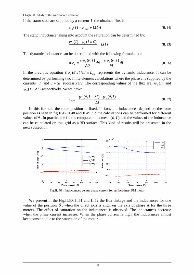
Chapter II : Study of the synchronous operation
69
If the stator slots are supplied by a current I the obtained flux is:
IILI maga )()( +=ψψ (II. 34)
The static inductance taking into account the saturation can be determined by:
)()0()( ILI
II aa ==−ψψ
(II. 35)
The dynamic inductance can be determined with the following formulation:
dII
IdId aaa ∂
∂+
∂∂
=),(),( θψθ
θθψψ (II. 36)
In the previous equation dyna LII ≡∂∂ /),(θψ represents the dynamic inductance. It can be determined by performing two finite element calculations where the phase a is supplied by the currents I and II Δ+ successively. The corresponding values of the flux are: )(Iaψ and
)( IIa Δ+ψ respectively. So we have:
IIIIL aa
dyn Δ−Δ+
=),(),( θψθψ
(II. 37)
In this formula the rotor position is fixed. In fact, the inductances depend on the rotor position as seen in fig II.47 II.48 and II.49. So the calculations can be performed for different values ofθ . In practice the flux is computed on a mesh ( I,θ ) and the values of the inductance can be calculated on this grid as a 3D surface. This kind of results will be presented in the next subsection.
0 20 40 60 80 100 120 140-1
-0.5
0
0.5
1
1.5
Phase current (A)
Flux
link
age
(Wb)
ψa(Wb)
ψb(Wb)
ψc(Wb)
-150 -100 -50 0 50 100 150-1
-0.5
0
0.5
1
1.5
2
2.5x 10
-3
Phase current (A)
Indu
ctan
ce(H
)
LaaMabMac
Fig.II. 50 : Inductances versus phase current for surface-inset PM motor
We present in the Fig.II.50, II.51 and II.52 the flux linkage and the inductances for one value of the position θ , when the direct axis is align on the axis of phase A for the three motors. The effect of saturation on the inductances is observed. The inductances decrease when the phase current increases. When the phase current is high, the inductances almost keep constant due to the saturation of the motor.
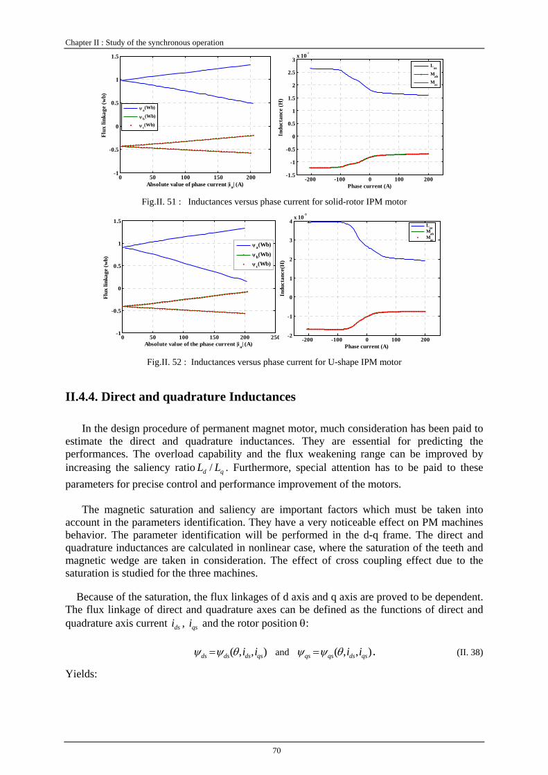
Chapter II : Study of the synchronous operation
70
0 50 100 150 200-1
-0.5
0
0.5
1
1.5
Absolute value of phase current |ia| (A)
Flux
link
age
(wb)
ψ a(Wb)
ψ b(Wb)
ψ c(Wb)
-200 -100 0 100 200-1.5
-1
-0.5
0
0.5
1
1.5
2
2.5
3x 10
-3
Phase current (A)
Indu
ctan
ce (H
)
Laa
Mab
Mac
Fig.II. 51 : Inductances versus phase current for solid-rotor IPM motor
0 50 100 150 200 250-1
-0.5
0
0.5
1
1.5
Absolute value of the phase current |ia| (A)
Flux
link
age
(wb)
ψa(Wb)
ψb(Wb)ψc(Wb)
-200 -100 0 100 200-2
-1
0
1
2
3
4x 10
-3
Phase current (A)
Indu
ctan
ce(H
)
LaaMabMac
Fig.II. 52 : Inductances versus phase current for U-shape IPM motor
II.4.4. Direct and quadrature Inductances In the design procedure of permanent magnet motor, much consideration has been paid to
estimate the direct and quadrature inductances. They are essential for predicting the performances. The overload capability and the flux weakening range can be improved by increasing the saliency ratio qd LL / . Furthermore, special attention has to be paid to these parameters for precise control and performance improvement of the motors.
The magnetic saturation and saliency are important factors which must be taken into
account in the parameters identification. They have a very noticeable effect on PM machines behavior. The parameter identification will be performed in the d-q frame. The direct and quadrature inductances are calculated in nonlinear case, where the saturation of the teeth and magnetic wedge are taken in consideration. The effect of cross coupling effect due to the saturation is studied for the three machines.
Because of the saturation, the flux linkages of d axis and q axis are proved to be dependent. The flux linkage of direct and quadrature axes can be defined as the functions of direct and quadrature axis current dsi , qsi and the rotor position θ:
),,( qsdsdsds iiθψψ = and ),,( qsdsqsqs iiθψψ = . (II. 38)
Yields:

Chapter II : Study of the synchronous operation
71
qsqs
qsdsdsds
ds
qsdsdsqsdsdsqsdsds di
iii
dii
iid
iiiid
∂
∂+
∂
∂+
∂
∂=
),,(),,(),,(),,(
θψθψθ
θθψ
θψ (II. 39)
qsqs
qsdsqsds
ds
qsdsqsqsdsqsqsdsqs di
iii
dii
iid
iiiid
∂
∂+
∂
∂+
∂
∂=
),,(),,(),,(),,(
θψθψθ
θθψ
θψ (II. 40)
The direct and quadrature fluxes are due to the excitation currents and to the permanent magnets. Their derivative versus current represents the dynamic inductances in direct and quadrature axis .The voltage equations of the PM motor in the d-q system are:
⎪⎪⎩
⎪⎪⎨
⎧
++=
−+=
dsqs
qssqs
qsds
dssds
dtd
iRV
dtd
iRV
ωψψ
ωψψ
(II. 41)
They can be rewritten as
dtd
ii
dtd
ii
ii
ii
RR
VV
dsqs
qsds
qs
ds
qs
qs
ds
qs
qs
ds
ds
ds
qs
ds
s
s
qs
ds θ
ψθ
ψ
ψθ
ψ
ψψ
ψψ
⎥⎥⎥⎥
⎦
⎤
⎢⎢⎢⎢
⎣
⎡
+∂
∂
−∂
∂
+⎥⎦
⎤⎢⎣
⎡
⎥⎥⎥⎥⎥
⎦
⎤
⎢⎢⎢⎢⎢
⎣
⎡
∂
∂
∂
∂
∂∂
∂∂
+⎥⎦
⎤⎢⎣
⎡⎥⎦
⎤⎢⎣
⎡=⎥
⎦
⎤⎢⎣
⎡0
0 (II. 42)
The direct and quadrature inductances are defined as the partial derivation of the flux linkages
cteiiiL
qsds
ds
ds
dsdd =Δ
Δ≈
∂∂
=ψψ
cteiiiM
qsds
qs
ds
qsqd =Δ
Δ≈
∂∂
=ψψ
cteiii
Ldsqs
qs
qs
qsqq =Δ
Δ≈
∂
∂=
ψψ
cteiiiM
dsqs
ds
qs
dsqd =Δ
Δ≈
∂∂
=ψψ
(II. 43)
The classical d-q model, uncoupled, linear and with constant parameters, applied to salient pole synchronous machines may be inadequate for an accurate modelling and characteristic prediction of our permanent magnet synchronous motors because of the phenomenon of cross coupling [Stumberger-03]. The cross-coupling is the magnetic interaction between the d and q axes, which is essentially due to the saturation. This phenomenon may be interpreted as follows: the magnetic flux produced by the direct current saturates some zones of the machine, distorting the flux linkage produced by the quadrature current, and vice versa. A special care is taken to the negative values of dsi , which represent a flux weakening operation mode. In this case, the iron is not saturated and the cross-coupling is too weak ( 0≈dqM ).But for small or positive values of direct current, the machine is highly saturated and the cross-coupling mutual inductance is high and depends on the position of the rotor.
II.4.4.1. Calculation results and discussion
To perform the whole calculation process, a suitable program package is developed using FEMM- and Matlab coupled softwares, and is applied to compute the d-q parameters of the three motors. Firstly, the automatic generation of the FE is performed. Secondly, the definition of the direct and quadrature currents is applied as presented in Eq. (II.26). Finally
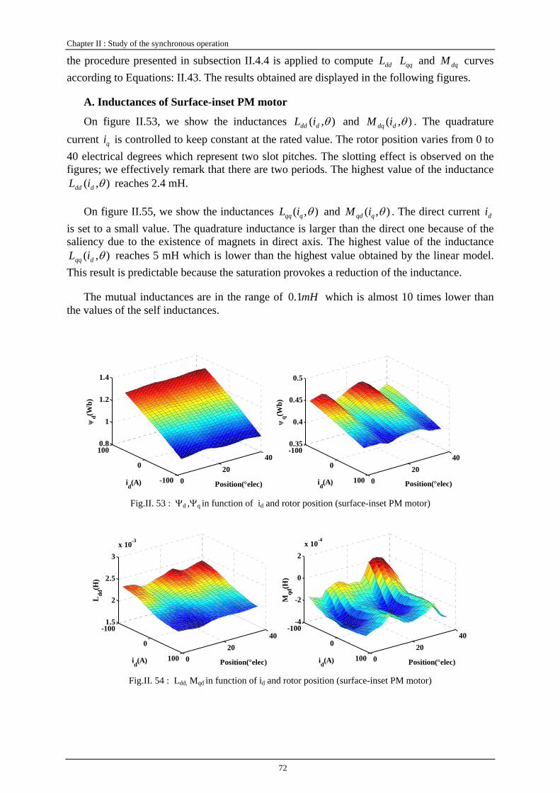
Chapter II : Study of the synchronous operation
72
the procedure presented in subsection II.4.4 is applied to compute ddL qqL and dqM curves according to Equations: II.43. The results obtained are displayed in the following figures.
A. Inductances of Surface-inset PM motor
On figure II.53, we show the inductances ),( θddd iL and ),( θddq iM . The quadrature current qi is controlled to keep constant at the rated value. The rotor position varies from 0 to 40 electrical degrees which represent two slot pitches. The slotting effect is observed on the figures; we effectively remark that there are two periods. The highest value of the inductance
),( θddd iL reaches 2.4 mH.
On figure II.55, we show the inductances ),( θqqq iL and ),( θqqd iM . The direct current di is set to a small value. The quadrature inductance is larger than the direct one because of the saliency due to the existence of magnets in direct axis. The highest value of the inductance
),( θdqq iL reaches 5 mH which is lower than the highest value obtained by the linear model. This result is predictable because the saturation provokes a reduction of the inductance.
The mutual inductances are in the range of mH1.0 which is almost 10 times lower than the values of the self inductances.
020
40
-100
0
1000.8
1
1.2
1.4
Position(°elec)id(A)
ψd(W
b)
020
40-100
0
100
0.35
0.4
0.45
0.5
Position(°elec)id(A)
ψq(W
b)
Fig.II. 53 : Ψd ,Ψq in function of id and rotor position (surface-inset PM motor)
020
40-100
0
100
1.5
2
2.5
3x 10⁻³
Position(°elec)id(A)
Ldd
(H)
020
40-100
0
100
-4
-2
0
2x 10⁻⁴
Position(°elec)id(A)
Mqd
(H)
Fig.II. 54 : Ldd, Mqd in function of id and rotor position (surface-inset PM motor)
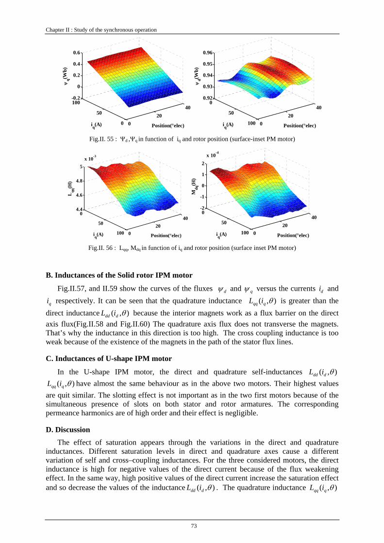
Chapter II : Study of the synchronous operation
73
020
40
0
50
100-0.2
0
0.2
0.4
0.6
Position(°elec)iq(A)
ψq(W
b)
020
400
50
100
0.92
0.93
0.94
0.95
0.96
Position(°elec)iq(A)
ψd(W
b)
Fig.II. 55 : Ψd ,Ψq in function of iq and rotor position (surface-inset PM motor)
020
400
50
100
4.4
4.6
4.8
5x 10⁻³
Position(°elec)iq(A)
Lqq
(H)
020
400
50
100
-2
-1
0
1
2x 10
-4
Position(°elec)iq(A)
Mdq
(H)
Fig.II. 56 : Lqq, Mdq in function of iq and rotor position (surface inset PM motor)
B. Inductances of the Solid rotor IPM motor
Fig.II.57, and II.59 show the curves of the fluxes dψ and qψ versus the currents di and
qi respectively. It can be seen that the quadrature inductance ),( θqqq iL is greater than the direct inductance ),( θddd iL because the interior magnets work as a flux barrier on the direct axis flux(Fig.II.58 and Fig.II.60) The quadrature axis flux does not transverse the magnets. That’s why the inductance in this direction is too high. The cross coupling inductance is too weak because of the existence of the magnets in the path of the stator flux lines.
C. Inductances of U-shape IPM motor
In the U-shape IPM motor, the direct and quadrature self-inductances ),( θddd iL ),( θqqq iL have almost the same behaviour as in the above two motors. Their highest values
are quit similar. The slotting effect is not important as in the two first motors because of the simultaneous presence of slots on both stator and rotor armatures. The corresponding permeance harmonics are of high order and their effect is negligible.
D. Discussion The effect of saturation appears through the variations in the direct and quadrature
inductances. Different saturation levels in direct and quadrature axes cause a different variation of self and cross–coupling inductances. For the three considered motors, the direct inductance is high for negative values of the direct current because of the flux weakening effect. In the same way, high positive values of the direct current increase the saturation effect and so decrease the values of the inductance ),( θddd iL . The quadrature inductance ),( θqqq iL

Chapter II : Study of the synchronous operation
74
is high at no load ( 0=qi ) in all cases, and decreases when the current qi increases. However the values of ),( θddd iL are different from one architecture to another because of the rotor topology.
Among these three motors, the U-shape IPM shows the largest cross-coupling inductance.It can reach even 40% of self-inductance in some cases. The solid-rotor IPM motor has the smallest cross-coupling inductance, less than 5% of the self-inductance. The effects of the slot opening upon the inductances are observed too. At the position when the rotor axis faces the slot opening, the minimum values are obtained by the method.
Generally, the identification of the parameters of electric machines in the d-q frame is very useful for the vector control which the motors are controlled by electronic equipments. The studied motors, designed to be connected to the grid without any power electronic devices, have to present a line start capability. However, the external modelling of salient pole machines is more suitable in d-q frame event if the machines are not supplied by inverters. The study of transient state operation is easier with such models. The identification of the d-q parameters according to the position and the values of di and qi to take into account both saturation and slotting effects is important to ensure the accuracy of the equivalent circuit model. The equivalent circuit model will be presented in the next chapter and we will focus the study on the starting operation which is an important point to such machines.
020
40
-100
0
100
0.2
0.25
0.3
0.35
Position(°elec)id(A)
ψd(W
b)
020
40-100
0
100
0.08
0.09
0.1
0.11
Position(°elec)id(A)
ψq(W
b)
Fig.II. 57 : Ψd ,Ψq in function of id and rotor position (solid rotor IPM motor)
020
40-100
0
100
4
6
8
10x 10-4
Position(°elec)id(A)
Ldd
(H)
020
40-100
0
100
-2
-1.5
-1
-0.5
0x 10
-4
Position(°elec)id(A)
Mqd
(H)
Fig.II. 58 : Ldd, Mqd in function of id and rotor position (solid rotor IPM motor)

Chapter II : Study of the synchronous operation
75
020
400
50
100
0.24
0.245
0.25
0.255
0.26
Position(°elec)iq(A)
ψd(W
b)
020
40
0
50
100-0.05
0
0.05
0.1
0.15
Position(°elec)iq(A)
ψq(W
b)
Fig.II. 59 : Ψd ,Ψq in function of iq and rotor position (solid rotor IPM motor)
020
400
50
100
1.2
1.4
1.6
1.8x 10
-3
Position(elec)iq(A)
Lqq
(H)
020
400
50
100
-2
-1
0
1x 10⁻⁴
Position(°elec)iq(A)
Mdq
(H)
Fig.II. 60 : Lqq , Mqd in function of id and rotor position (solid rotor IPM motor)
020
40
-100
0
1000.5
1
1.5
2
Position(°elec)id(A)
ψd(W
b)
020
40
-100
0
100-0.8
-0.6
-0.4
-0.2
0
Position(°elec)id(A)
ψq(W
b)
Fig.II. 61 : Ψd ,Ψq in function of id and rotor position (U-shape PM motor)
020
40-100
0
100
2
4
6
8
10x 10-3
Position(°elec)id(A)
Ldd
(H)
020
40-100
0
100
1
2
3
4x 10⁻³
Position(°elec)id(A)
Mqd
(H)
Fig.II. 62 : Ldd , Mqd in function of id and rotor position (U-shape PM motor)
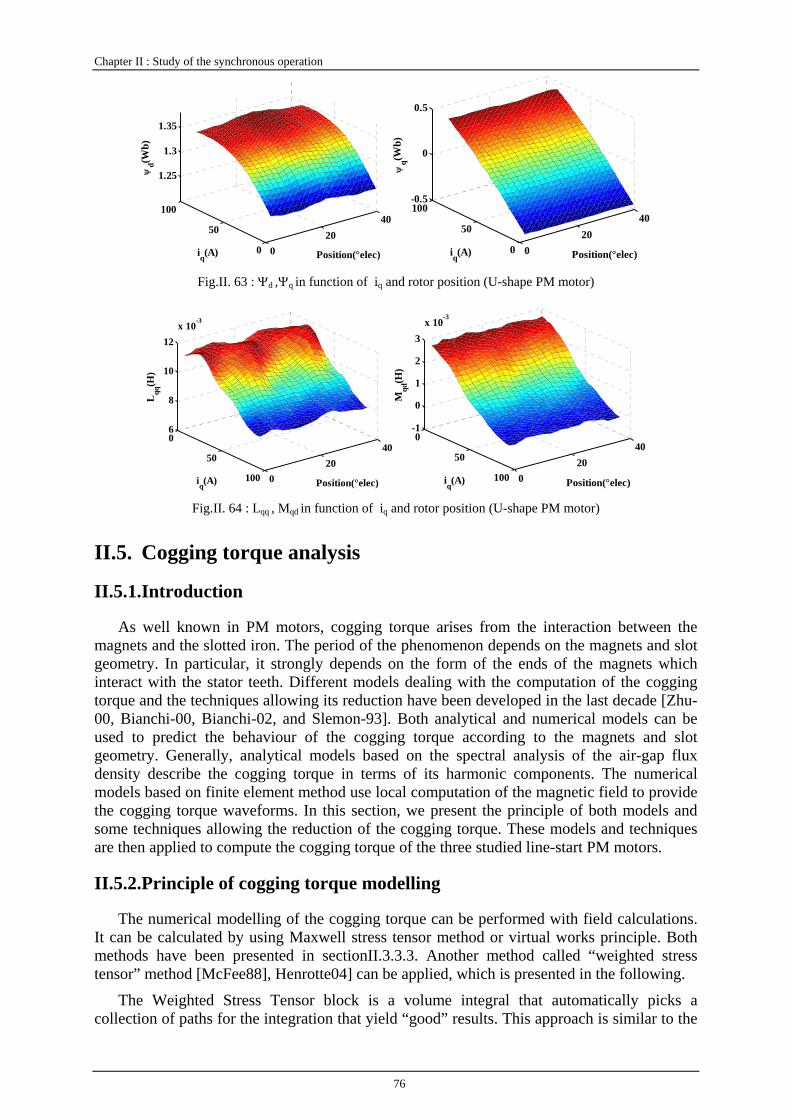
Chapter II : Study of the synchronous operation
76
020
40
0
50
100
1.25
1.3
1.35
Position(°elec)iq(A)
ψd(W
b)
020
40
0
50
100-0.5
0
0.5
Position(°elec)iq(A)
ψq(W
b)
Fig.II. 63 : Ψd ,Ψq in function of iq and rotor position (U-shape PM motor)
020
400
50
100
6
8
10
12x 10
-3
Position(°elec)iq(A)
Lqq
(H)
020
400
50
100
-1
0
1
2
3x 10⁻³
Position(°elec)iq(A)
Mqd
(H)
Fig.II. 64 : Lqq , Mqd in function of iq and rotor position (U-shape PM motor)
II.5. Cogging torque analysis
II.5.1. Introduction
As well known in PM motors, cogging torque arises from the interaction between the magnets and the slotted iron. The period of the phenomenon depends on the magnets and slot geometry. In particular, it strongly depends on the form of the ends of the magnets which interact with the stator teeth. Different models dealing with the computation of the cogging torque and the techniques allowing its reduction have been developed in the last decade [Zhu-00, Bianchi-00, Bianchi-02, and Slemon-93]. Both analytical and numerical models can be used to predict the behaviour of the cogging torque according to the magnets and slot geometry. Generally, analytical models based on the spectral analysis of the air-gap flux density describe the cogging torque in terms of its harmonic components. The numerical models based on finite element method use local computation of the magnetic field to provide the cogging torque waveforms. In this section, we present the principle of both models and some techniques allowing the reduction of the cogging torque. These models and techniques are then applied to compute the cogging torque of the three studied line-start PM motors.
II.5.2. Principle of cogging torque modelling
The numerical modelling of the cogging torque can be performed with field calculations. It can be calculated by using Maxwell stress tensor method or virtual works principle. Both methods have been presented in sectionII.3.3.3. Another method called “weighted stress tensor” method [McFee88], Henrotte04] can be applied, which is presented in the following.
The Weighted Stress Tensor block is a volume integral that automatically picks a collection of paths for the integration that yield “good” results. This approach is similar to the

Chapter II : Study of the synchronous operation
77
stress tensor approach. The Weighted Stress Tensor method consists in computing the “weighting function” by solving an additional Laplace equation over the air surrounding the blocks upon which the torque is to be computed. The stress tensor is then evaluated as volume integration, and the results are typically more accurate than the Maxwell Stress Tensor line integral, since all possible contours have been averaged to yield the Weighted Stress Tensor torque. This method is implemented in some Finite element software such as FEMM [Meeker-09]
The Maxwell stress tensor method uses a line integral which presents a higher level of the relative error when linear elements are considered. This is the case of FEMM software which uses the mesh generator TRIANGLE [Meeker-9]. Finally, the virtual works method uses a derivation of the coenergy versus the position. In this case any numerical error on the value of the coenergy may lead to a non negligible error on the torque. It is well known that the numerical derivation amplifies the numerical errors especially if it uses the first order definition.
II.5.2.1. Numerical models
The numerical models use the finite element method for the calculation of the field distribution in the motor. The computation of the cogging torque is based on the three methods described above by adopting the following steps:
1. Generate the geometry
2. Mesh and compute the field distribution
3. Compute the energy and the torque
4. Change the rotor position and go to step 2
The cogging torque waveforms obtained can then be analyzed in order to discuss their harmonic contents. Such methods have the advantage of taking into account the exact geometries of both stator teeth and magnets as well as the local saturation of the stator armature. However it is necessary to perform the finite element computations for many rotor positions and all the considered geometries. These simulations are generally consuming CPU time and space memory
In order to obtain valuable results, a special care has to be paid on the mesh size and the number of positions considered in the FE simulations. Indeed the air-gap regions have to be correctly meshed but there is a risk to increase the numerical errors due to the huge size of the stiffness matrix if the solver is not adapted.
Fig.II. 65 : Cogging torque with three methods
0 1 2 3 4 5 6 7-20
-15
-10
-5
0
5
10
15
20
Theta of one slot
Cog
ging
torq
ue (N
.m)
Maxwell stress tensorWeighted maxwell stress tensorVirtual work
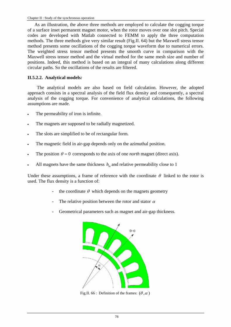
Chapter II : Study of the synchronous operation
78
As an illustration, the above three methods are employed to calculate the cogging torque of a surface inset permanent magnet motor, when the rotor moves over one slot pitch. Special codes are developed with Matlab connected to FEMM to apply the three computation methods. The three methods give very similar result (Fig.II. 64) but the Maxwell stress tensor method presents some oscillations of the cogging torque waveform due to numerical errors. The weighted stress tensor method presents the smooth curve in comparison with the Maxwell stress tensor method and the virtual method for the same mesh size and number of positions. Indeed, this method is based on an integral of many calculations along different circular paths. So the oscillations of the results are filtered.
II.5.2.2. Analytical models:
The analytical models are also based on field calculation. However, the adopted approach consists in a spectral analysis of the field flux density and consequently, a spectral analysis of the cogging torque. For convenience of analytical calculations, the following assumptions are made.
• The permeability of iron is infinite.
• The magnets are supposed to be radially magnetized.
• The slots are simplified to be of rectangular form.
• The magnetic field in air-gap depends only on the azimuthal position.
• The position 0=θ corresponds to the axis of one north magnet (direct axis).
• All magnets have the same thickness mh and relative permeability close to 1
Under these assumptions, a frame of reference with the coordinate θ linked to the rotor is used. The flux density is a function of:
- the coordinate θ which depends on the magnets geometry
- The relative position between the rotor and stator α
- Geometrical parameters such as magnet and air-gap thickness.
Fig.II. 66 : Definition of the frames: ),( αθ
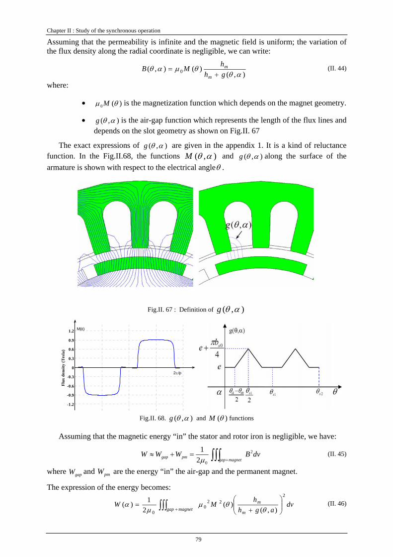
Chapter II : Study of the synchronous operation
79
Assuming that the permeability is infinite and the magnetic field is uniform; the variation of the flux density along the radial coordinate is negligible, we can write:
),()(),( 0 αθ
θμαθghhMB
m
m
+= (II. 44)
where:
• )(0 θμ M is the magnetization function which depends on the magnet geometry.
• ),( αθg is the air-gap function which represents the length of the flux lines and depends on the slot geometry as shown on Fig.II. 67
The exact expressions of ),( αθg are given in the appendix 1. It is a kind of reluctance function. In the Fig.II.68, the functions ),( αθM and ),( αθg along the surface of the armature is shown with respect to the electrical angleθ .
Fig.II. 67 : Definition of ),( αθg
-1.2
-0.9
-0.6
-0.3
0
0.3
0.6
0.9
1.2
Flux
den
sity
(Tes
la)
2π/p
M(θ)
Fig.II. 68. ),( αθg and )(θM functions
Assuming that the magnetic energy “in” the stator and rotor iron is negligible, we have:
∫∫∫ +=+≈
magnetgappmgap dvBWWW 2
021μ
(II. 45)
where gapW and pmW are the energy “in” the air-gap and the permanent magnet.
The expression of the energy becomes:
∫∫∫ + ⎟⎟⎠
⎞⎜⎜⎝
⎛+
=magnetgap
m
m dvagh
hMW
222
00 ),(
)(2
1)(θ
θμμ
α (II. 46)
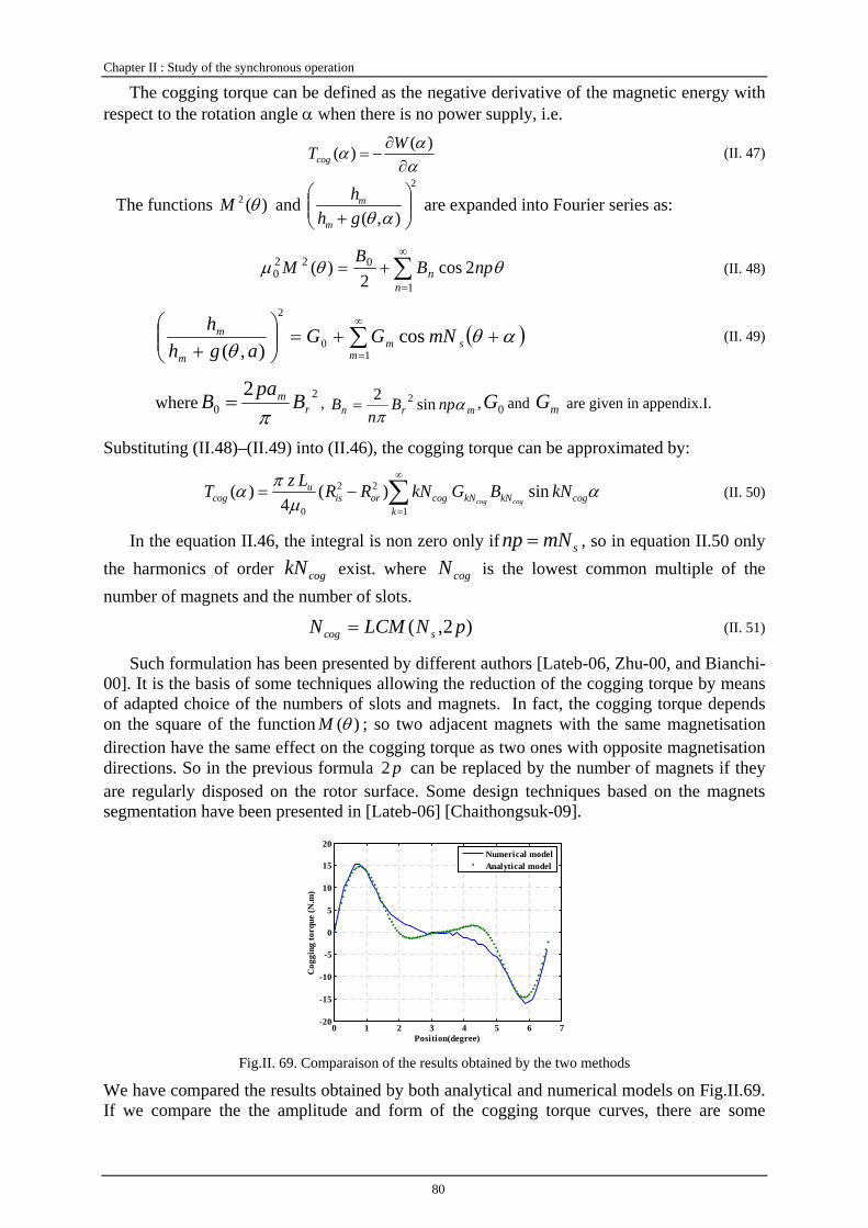
Chapter II : Study of the synchronous operation
80
The cogging torque can be defined as the negative derivative of the magnetic energy with respect to the rotation angle α when there is no power supply, i.e.
ααα
∂∂
−=)()( WTcog (II. 47)
The functions )(2 θM and 2
),( ⎟⎟⎠
⎞⎜⎜⎝
⎛+ αθgh
hm
m are expanded into Fourier series as:
∑∞
=
+=1
0220 2cos
2)(
nn npB
BM θθμ (II. 48)
( )∑∞
=++=⎟⎟
⎠
⎞⎜⎜⎝
⎛+ 1
0
2
cos),( m
smm
m mNGGagh
h αθθ
(II. 49)
where 20
2r
m BpaBπ
= , mrn npBn
B απ
sin2 2= , 0G and mG are given in appendix.I.
Substituting (II.48)–(II.49) into (II.46), the cogging torque can be approximated by:
∑∞
=
−=1
22
0
sin)(4
)(k
cogkNkNcogorisu
cog kNBGkNRRLzTcogcog
αμ
πα (II. 50)
In the equation II.46, the integral is non zero only if smNnp = , so in equation II.50 only the harmonics of order cogkN exist. where cogN is the lowest common multiple of the number of magnets and the number of slots.
)2,( pNLCMN scog = (II. 51)
Such formulation has been presented by different authors [Lateb-06, Zhu-00, and Bianchi-00]. It is the basis of some techniques allowing the reduction of the cogging torque by means of adapted choice of the numbers of slots and magnets. In fact, the cogging torque depends on the square of the function )(θM ; so two adjacent magnets with the same magnetisation direction have the same effect on the cogging torque as two ones with opposite magnetisation directions. So in the previous formula p2 can be replaced by the number of magnets if they are regularly disposed on the rotor surface. Some design techniques based on the magnets segmentation have been presented in [Lateb-06] [Chaithongsuk-09].
0 1 2 3 4 5 6 7-20
-15
-10
-5
0
5
10
15
20
Position(degree)
Cog
ging
torq
ue (N
.m)
Numerical modelAnalytical model
Fig.II. 69. Comparaison of the results obtained by the two methods
We have compared the results obtained by both analytical and numerical models on Fig.II.69. If we compare the the amplitude and form of the cogging torque curves, there are some
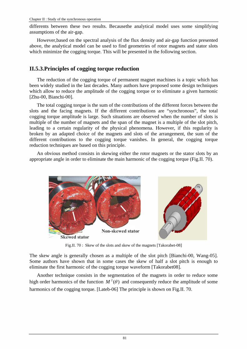
Chapter II : Study of the synchronous operation
81
differents between these two results. Becausethe analytical model uses some simplifying assumptions of the air-gap.
However,based on the spectral analysis of the flux density and air-gap function presented above, the analytical model can be used to find geometries of rotor magnets and stator slots which minimize the cogging torque. This will be presented in the following section.
II.5.3. Principles of cogging torque reduction
The reduction of the cogging torque of permanent magnet machines is a topic which has been widely studied in the last decades. Many authors have proposed some design techniques which allow to reduce the amplitude of the cogging torque or to eliminate a given harmonic [Zhu-00, Bianchi-00].
The total cogging torque is the sum of the contributions of the different forces between the slots and the facing magnets. If the different contributions are “synchronous”, the total cogging torque amplitude is large. Such situations are observed when the number of slots is multiple of the number of magnets and the span of the magnet is a multiple of the slot pitch, leading to a certain regularity of the physical phenomena. However, if this regularity is broken by an adapted choice of the magnets and slots of the arrangement, the sum of the different contributions to the cogging torque vanishes. In general, the cogging torque reduction techniques are based on this principle.
An obvious method consists in skewing either the rotor magnets or the stator slots by an appropriate angle in order to eliminate the main harmonic of the cogging torque (Fig.II. 70).
Fig.II. 70 : Skew of the slots and skew of the magnets [Takorabet-08]
The skew angle is generally chosen as a multiple of the slot pitch [Bianchi-00, Wang-05]. Some authors have shown that in some cases the skew of half a slot pitch is enough to eliminate the first harmonic of the cogging torque waveform [Takorabet08].
Another technique consists in the segmentation of the magnets in order to reduce some high order harmonics of the function )(2 θM and consequently reduce the amplitude of some harmonics of the cogging torque. [Lateb-06] The principle is shown on Fig.II. 70.
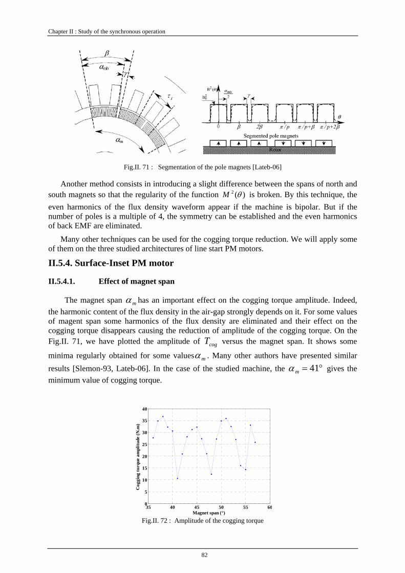
Chapter II : Study of the synchronous operation
82
Fig.II. 71 : Segmentation of the pole magnets [Lateb-06]
Another method consists in introducing a slight difference between the spans of north and south magnets so that the regularity of the function )(2 θM is broken. By this technique, the even harmonics of the flux density waveform appear if the machine is bipolar. But if the number of poles is a multiple of 4, the symmetry can be established and the even harmonics of back EMF are eliminated.
Many other techniques can be used for the cogging torque reduction. We will apply some of them on the three studied architectures of line start PM motors.
II.5.4. Surface-Inset PM motor
II.5.4.1. Effect of magnet span
The magnet span mα has an important effect on the cogging torque amplitude. Indeed, the harmonic content of the flux density in the air-gap strongly depends on it. For some values of magent span some harmonics of the flux density are eliminated and their effect on the cogging torque disappears causing the reduction of amplitude of the cogging torque. On the Fig.II. 71, we have plotted the amplitude of cogT versus the magnet span. It shows some
minima regularly obtained for some values mα . Many other authors have presented similar results [Slemon-93, Lateb-06]. In the case of the studied machine, the °= 41mα gives the minimum value of cogging torque.
35 40 45 50 55 600
5
10
15
20
25
30
35
40
Cog
ging
torq
ue a
mpl
itude
(N.m
)
Magnet span (°) Fig.II. 72 : Amplitude of the cogging torque

Chapter II : Study of the synchronous operation
83
II.5.4.2. Effect of combined pole arc coefficients
Fig.II. 73 : Two pole configures (a) conventional same pole arcs (b) Applied different pole arcs
One of the methods which minimize the cogging torque is to vary the magnet pole arcs as shown in FigII.72. The adjacent pole arcs are designed with two different pole arc coefficients
1pα and 2pα .
pmp ταα 11 = (II. 52)
pmp ταα 22 = (II. 53)
where mα and pτ are the magnet arc and rotor pole pitch respectively.
Fig.II. 74 : The distribution of )(2 θM
In this case, the flux density function )(2 θM in air-gap varies with the different pole arc coefficients, which can be illustrated as a function of rotor positionθ .
∑∞
=+=
1
02 cos2
)(n
n npBBM θθ (II. 54)
It is approximately estimated on FigII.73. The expression of the Fourier coefficients of the function )(2 θM are given by:
⎟⎟⎠
⎞⎜⎜⎝
⎛⎟⎟⎠
⎞⎜⎜⎝
⎛−+⎟⎟
⎠
⎞⎜⎜⎝
⎛= π
ααα
πα
πnn
nB
B p
p
pnpn 2
sin)1(2
sin 22
2
211
20 (II. 55)
For the 6-pole 54-slot motor, the slot number per pole is integer, and only thk18 Fourier coefficients have effects on the cogging torque. In order to minimize the cogging torque, the expression of the coefficients of the form kB18 that contains parameter 1pα and 2pα is set to be zero, which yields:
0182
sin182
sin18
22
2
211
20 =⎟
⎟⎠
⎞⎜⎜⎝
⎛⎟⎟⎠
⎞⎜⎜⎝
⎛+⎟⎟
⎠
⎞⎜⎜⎝
⎛π
ααα
πα
πkk
kB p
p
pp (II. 56)
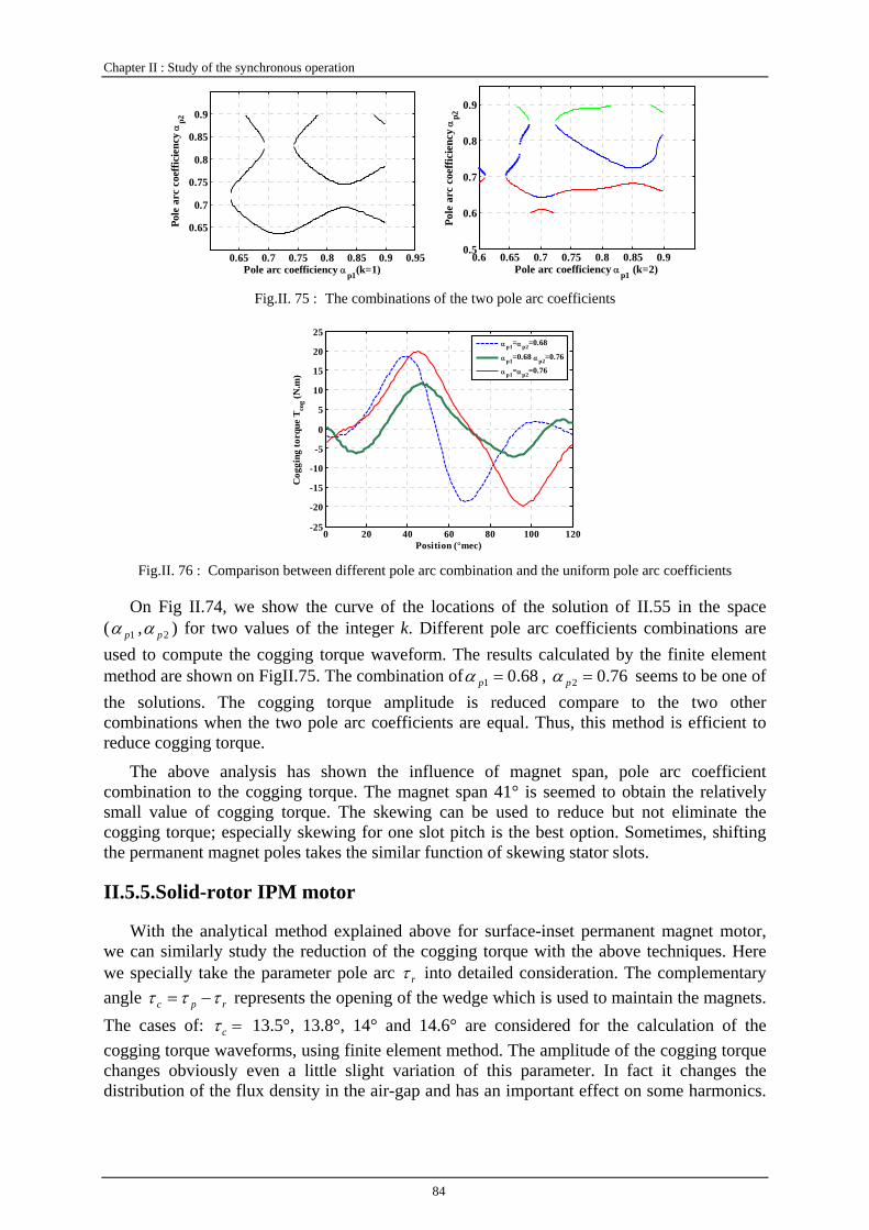
Chapter II : Study of the synchronous operation
84
0.65 0.7 0.75 0.8 0.85 0.9 0.95
0.65
0.7
0.75
0.8
0.85
0.9
Pole arc coefficiency αp1(k=1)
Pole
arc
coe
ffici
ency
αp2
0.6 0.65 0.7 0.75 0.8 0.85 0.9
0.5
0.6
0.7
0.8
0.9
Pole arc coefficiency αp1 (k=2)
Pole
arc
coe
ffici
ency
αp2
Fig.II. 75 : The combinations of the two pole arc coefficients
0 20 40 60 80 100 120-25
-20
-15
-10
-5
0
5
10
15
20
25
Position (°mec)
Cog
ging
torq
ue T
cog (N
.m)
αp1=αp2=0.68
αp1=0.68 αp2=0.76
αp1=αp2=0.76
Fig.II. 76 : Comparison between different pole arc combination and the uniform pole arc coefficients
On Fig II.74, we show the curve of the locations of the solution of II.55 in the space ( 1pα , 2pα ) for two values of the integer k. Different pole arc coefficients combinations are used to compute the cogging torque waveform. The results calculated by the finite element method are shown on FigII.75. The combination of 68.01 =pα , 76.02 =pα seems to be one of the solutions. The cogging torque amplitude is reduced compare to the two other combinations when the two pole arc coefficients are equal. Thus, this method is efficient to reduce cogging torque.
The above analysis has shown the influence of magnet span, pole arc coefficient combination to the cogging torque. The magnet span 41° is seemed to obtain the relatively small value of cogging torque. The skewing can be used to reduce but not eliminate the cogging torque; especially skewing for one slot pitch is the best option. Sometimes, shifting the permanent magnet poles takes the similar function of skewing stator slots.
II.5.5. Solid-rotor IPM motor
With the analytical method explained above for surface-inset permanent magnet motor, we can similarly study the reduction of the cogging torque with the above techniques. Here we specially take the parameter pole arc rτ into detailed consideration. The complementary angle rpc τττ −= represents the opening of the wedge which is used to maintain the magnets. The cases of: =cτ 13.5°, 13.8°, 14° and 14.6° are considered for the calculation of the cogging torque waveforms, using finite element method. The amplitude of the cogging torque changes obviously even a little slight variation of this parameter. In fact it changes the distribution of the flux density in the air-gap and has an important effect on some harmonics.
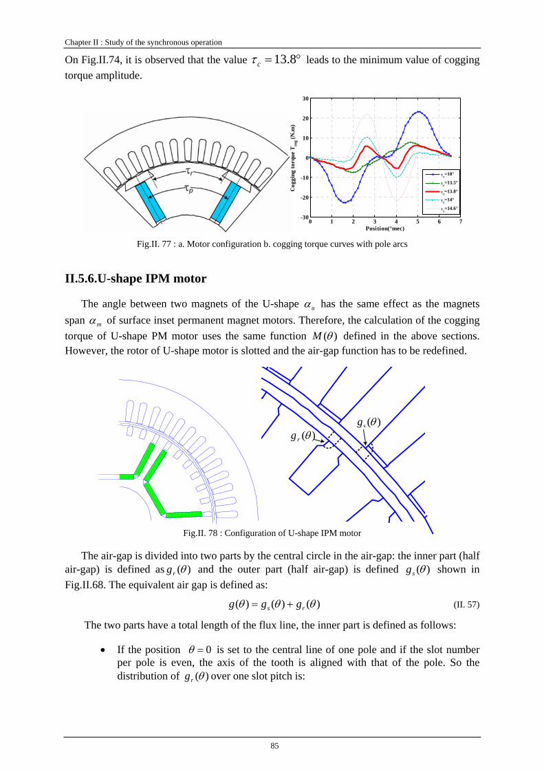
Chapter II : Study of the synchronous operation
85
On Fig.II.74, it is observed that the value °= 8.13cτ leads to the minimum value of cogging torque amplitude.
0 1 2 3 4 5 6 7-30
-20
-10
0
10
20
30
Position(°mec)
Cog
ging
torq
ue T
cog (N
.m)
τc=10°
τc=13.5°
τc=13.8°
τc=14°
τc=14.6°
Fig.II. 77 : a. Motor configuration b. cogging torque curves with pole arcs
II.5.6. U-shape IPM motor
The angle between two magnets of the U-shape uα has the same effect as the magnets span mα of surface inset permanent magnet motors. Therefore, the calculation of the cogging torque of U-shape PM motor uses the same function )(θM defined in the above sections. However, the rotor of U-shape motor is slotted and the air-gap function has to be redefined.
)(θsg)(θrg
Fig.II. 78 : Configuration of U-shape IPM motor
The air-gap is divided into two parts by the central circle in the air-gap: the inner part (half air-gap) is defined as )(θrg and the outer part (half air-gap) is defined )(θsg shown in Fig.II.68. The equivalent air gap is defined as:
)()()( θθθ rs ggg += (II. 57)
The two parts have a total length of the flux line, the inner part is defined as follows:
• If the position 0=θ is set to the central line of one pole and if the slot number per pole is even, the axis of the tooth is aligned with that of the pole. So the distribution of )(θrg over one slot pitch is:
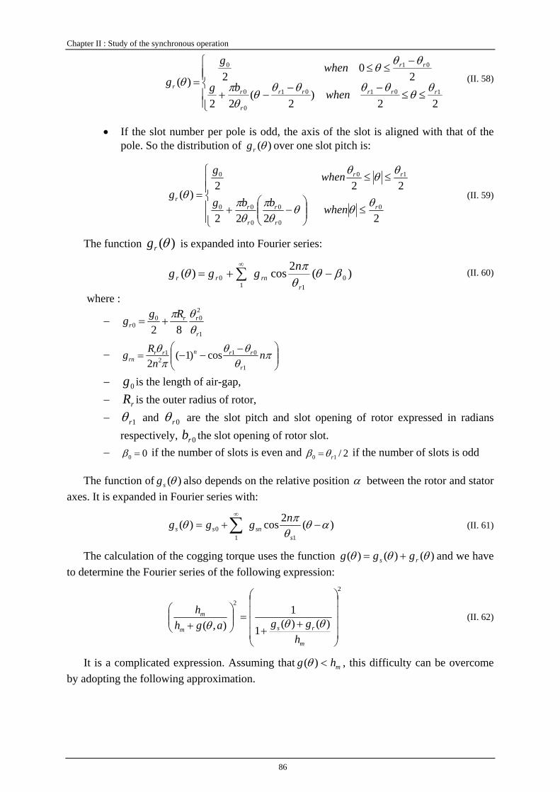
Chapter II : Study of the synchronous operation
86
⎪⎪⎩
⎪⎪⎨
⎧
≤≤−−
−+
−≤≤
=
22)
2(
22
20
2)(10101
0
0
010
rrrrr
r
r
rr
rwhenbg
wheng
g θθθθθθθθπ
θθθθ (II. 58)
• If the slot number per pole is odd, the axis of the slot is aligned with that of the pole. So the distribution of )(θrg over one slot pitch is:
⎪⎪⎩
⎪⎪⎨
⎧
≤⎟⎟⎠
⎞⎜⎜⎝
⎛−+
≤≤
=
2222
222)(
0
0
0
0
00
100
r
r
r
r
r
rr
r
whenbbg
wheng
gθθθ
θπ
θπ
θθθ
θ (II. 59)
The function )(θrg is expanded into Fourier series:
)(2cos)( 011
0 βθθπθ −+= ∑
∞
rrnrr
nggg (II. 60)
where :
− 1
200
0 82 r
rrr
Rggθθπ
+=
− ⎟⎟⎠
⎞⎜⎜⎝
⎛ −−−= π
θθθ
πθ n
nRg
r
rrnrrrn
1
012
1 cos)1(2
− 0g is the length of air-gap, − rR is the outer radius of rotor, − 1rθ and 0rθ are the slot pitch and slot opening of rotor expressed in radians
respectively, 0rb the slot opening of rotor slot. − 00 =β if the number of slots is even and 2/10 rθβ = if the number of slots is odd
The function of )(θsg also depends on the relative position α between the rotor and stator axes. It is expanded in Fourier series with:
)(2cos)(11
0 αθθπθ −+= ∑
∞
ssnss
nggg (II. 61)
The calculation of the cogging torque uses the function )()()( θθθ rs ggg += and we have to determine the Fourier series of the following expression:
2
2
)()(1
1),(
⎟⎟⎟⎟
⎠
⎞
⎜⎜⎜⎜
⎝
⎛
++
=⎟⎟⎠
⎞⎜⎜⎝
⎛+
m
rsm
m
hggagh
hθθθ
(II. 62)
It is a complicated expression. Assuming that mhg <)(θ , this difficulty can be overcome by adopting the following approximation.
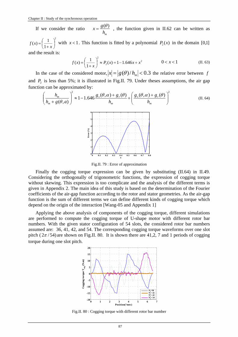
Chapter II : Study of the synchronous operation
87
If we consider the ratio mh
gx )(θ= , the function given in II.62 can be written as
2
11)( ⎟
⎠⎞
⎜⎝⎛+
=x
xf with 1<x . This function is fitted by a polynomial )(2 xP in the domain ]1,0[
and the result is: 2
2
2
646.11)(1
1)( xxxPx
xf +−=≈⎟⎠⎞
⎜⎝⎛+
= 10 << x (II. 63)
In the case of the considered motor, 0.3/)( <= mhgx θ the relative error between f and 2P is less than 5%; it is illustrated in Fig.II. 79. Under theses assumptions, the air gap function can be approximated by:
22)(),()(),(646.11
),( ⎟⎟⎠
⎞⎜⎜⎝
⎛ ++
+−≈⎟⎟
⎠
⎞⎜⎜⎝
⎛+ m
rs
m
rs
m
m
hgg
hgg
aghh θαθθαθθ
(II. 64)
0 0.1 0.2 0.3 0.4 0.5 0.6 0.7 0.80
1
2
3
4
5
6
x
Erro
r (%
)
Fig.II. 79 : Error of approximation
Finally the cogging torque expression can be given by substituting (II.64) in II.49. Considering the orthogonally of trigonometric functions, the expression of cogging torque without skewing. This expression is too complicate and the analysis of the different terms is given in Appendix 2. The main idea of this study is based on the determination of the Fourier coefficients of the air-gap function according to the rotor and stator geometries. As the air-gap function is the sum of different terms we can define different kinds of cogging torque which depend on the origin of the interaction [Wang-05 and Appendix 1]
Applying the above analysis of components of the cogging torque, different simulations are performed to compute the cogging torque of U-shape motor with different rotor bar numbers. With the given stator configuration of 54 slots, the considered rotor bar numbers assumed are: 36, 41, 42, and 54. The corresponding cogging torque waveforms over one slot pitch ( )54/2π are shown on Fig.II. 80. It is shown there are 41,2, 7 and 1 periods of cogging torque during one slot pitch.
0 1 2 3 4 5 6 7-20
-15
-10
-5
0
5
10
15
20
Cog
ging
torq
ue T
cog (N
.m)
Position(°mec)
Nr=36Nr= 41Nr= 42Nr= 54
Fig.II. 80 : Cogging torque with different rotor bar number
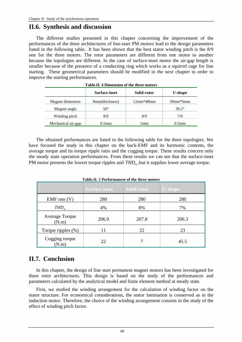
Chapter II : Study of the synchronous operation
88
II.6. Synthesis and discussion
The different studies presented in this chapter concerning the improvement of the performances of the three architectures of line-start PM motors lead to the design parameters listed in the following table.. It has been shown that the best stator winding pitch is the 8/9 one for the three motors. The rotor parameters are different from one motor to another because the topologies are different. In the case of surface-inset motor the air-gap length is smaller because of the presence of a conducting ring which works as a squirrel cage for line starting. These geometrical parameters should be modified in the next chapter in order to improve the starting performances.
Table.II. 4 Dimension of the three motors
Surface-inset Solid-rotor U-shape
Magnet dimension 8mm(thickness) 12mm*48mm 39mm*6mm
Magnet angle 50° 39.2°
Winding pitch 8/9 8/9 7/9
Mechanical air-gap 0.5mm 1mm 0.5mm
The obtained performances are listed in the following table for the three topologies. We have focused the study in this chapter on the back-EMF and its harmonic contents, the average torque and its torque ripple ratio and the cogging torque. These results concern only the steady state operation performances. From these results we can see that the surface-inset PM motor presents the lowest torque ripples and mTHD ,but it supplies lower average torque.
Table.II. 5 Performances of the three motors
Surface-inset Solid-rotor U-shape
EMF rms (V) 280 280 280
mTHD 4% 8% 7%
Average Torque (N.m) 206.9 207.8 206.3
Torque ripples (%) 11 22 23
Cogging torque (N.m) 22 7 45.5
II.7. Conclusion
In this chapter, the design of line start permanent magnet motors has been investigated for three rotor architectures. This design is based on the study of the performances and parameters calculated by the analytical model and finite element method at steady state.
First, we studied the winding arrangement for the calculation of winding factor on the stator structure. For economical considerations, the stator lamination is conserved as in the induction motor. Therefore, the choice of the winding arrangement consists in the study of the effect of winding pitch factor.
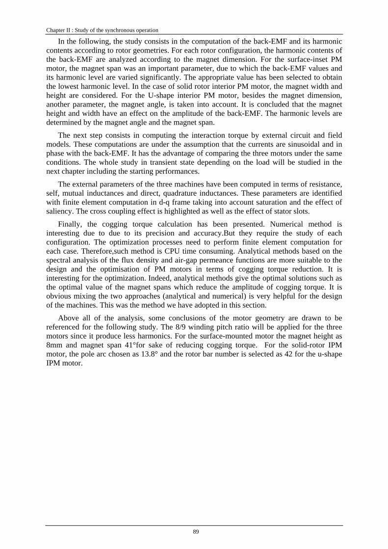
Chapter II : Study of the synchronous operation
89
In the following, the study consists in the computation of the back-EMF and its harmonic contents according to rotor geometries. For each rotor configuration, the harmonic contents of the back-EMF are analyzed according to the magnet dimension. For the surface-inset PM motor, the magnet span was an important parameter, due to which the back-EMF values and its harmonic level are varied significantly. The appropriate value has been selected to obtain the lowest harmonic level. In the case of solid rotor interior PM motor, the magnet width and height are considered. For the U-shape interior PM motor, besides the magnet dimension, another parameter, the magnet angle, is taken into account. It is concluded that the magnet height and width have an effect on the amplitude of the back-EMF. The harmonic levels are determined by the magnet angle and the magnet span.
The next step consists in computing the interaction torque by external circuit and field models. These computations are under the assumption that the currents are sinusoidal and in phase with the back-EMF. It has the advantage of comparing the three motors under the same conditions. The whole study in transient state depending on the load will be studied in the next chapter including the starting performances.
The external parameters of the three machines have been computed in terms of resistance, self, mutual inductances and direct, quadrature inductances. These parameters are identified with finite element computation in d-q frame taking into account saturation and the effect of saliency. The cross coupling effect is highlighted as well as the effect of stator slots.
Finally, the cogging torque calculation has been presented. Numerical method is interesting due to due to its precision and accuracy.But they require the study of each configuration. The optimization processes need to perform finite element computation for each case. Therefore,such method is CPU time consuming. Analytical methods based on the spectral analysis of the flux density and air-gap permeance functions are more suitable to the design and the optimisation of PM motors in terms of cogging torque reduction. It is interesting for the optimization. Indeed, analytical methods give the optimal solutions such as the optimal value of the magnet spans which reduce the amplitude of cogging torque. It is obvious mixing the two approaches (analytical and numerical) is very helpful for the design of the machines. This was the method we have adopted in this section.
Above all of the analysis, some conclusions of the motor geometry are drawn to be referenced for the following study. The 8/9 winding pitch ratio will be applied for the three motors since it produce less harmonics. For the surface-mounted motor the magnet height as 8mm and magnet span 41°for sake of reducing cogging torque. For the solid-rotor IPM motor, the pole arc chosen as 13.8° and the rotor bar number is selected as 42 for the u-shape IPM motor.

90

Chapter III :
Study of the Asynchronous
operation

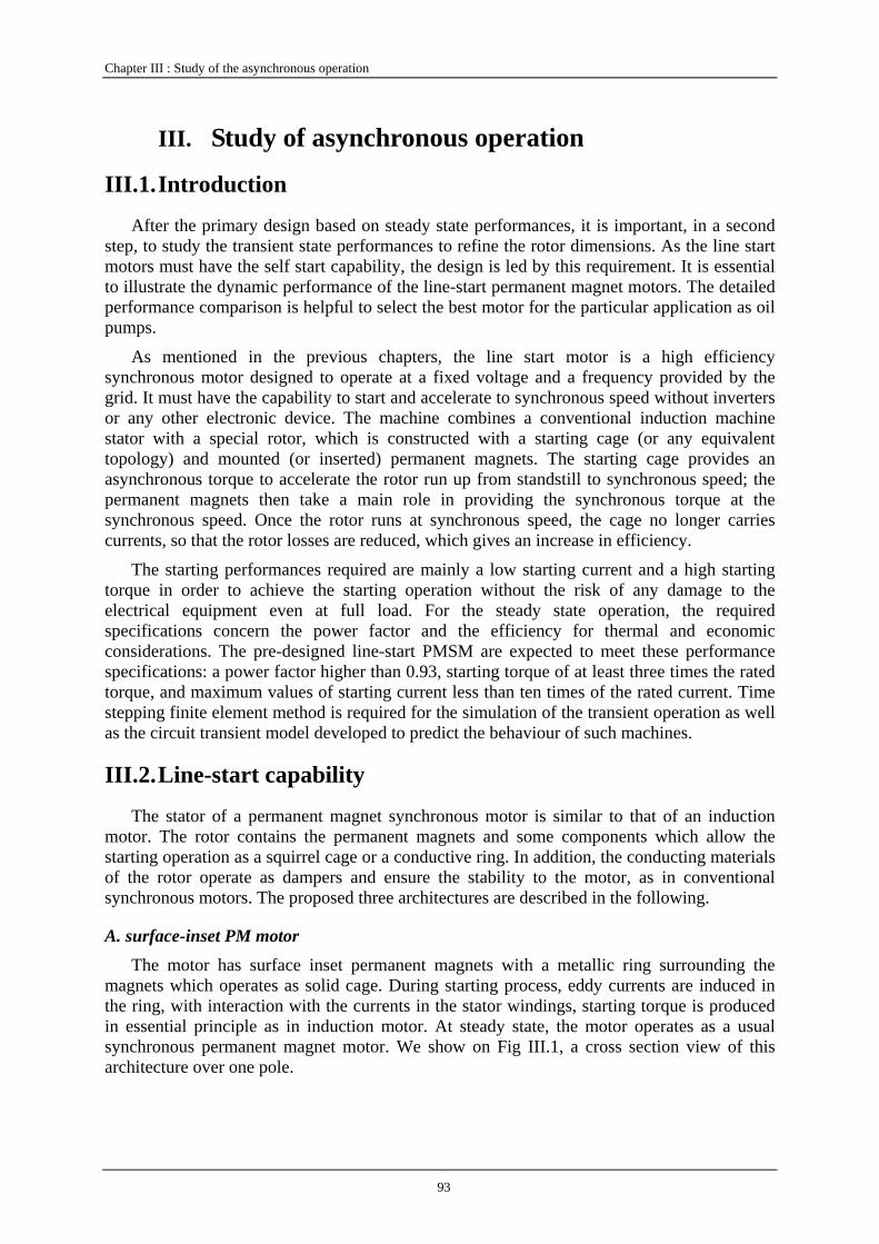
Chapter III : Study of the asynchronous operation
93
III. Study of asynchronous operation
III.1. Introduction
After the primary design based on steady state performances, it is important, in a second step, to study the transient state performances to refine the rotor dimensions. As the line start motors must have the self start capability, the design is led by this requirement. It is essential to illustrate the dynamic performance of the line-start permanent magnet motors. The detailed performance comparison is helpful to select the best motor for the particular application as oil pumps.
As mentioned in the previous chapters, the line start motor is a high efficiency synchronous motor designed to operate at a fixed voltage and a frequency provided by the grid. It must have the capability to start and accelerate to synchronous speed without inverters or any other electronic device. The machine combines a conventional induction machine stator with a special rotor, which is constructed with a starting cage (or any equivalent topology) and mounted (or inserted) permanent magnets. The starting cage provides an asynchronous torque to accelerate the rotor run up from standstill to synchronous speed; the permanent magnets then take a main role in providing the synchronous torque at the synchronous speed. Once the rotor runs at synchronous speed, the cage no longer carries currents, so that the rotor losses are reduced, which gives an increase in efficiency.
The starting performances required are mainly a low starting current and a high starting torque in order to achieve the starting operation without the risk of any damage to the electrical equipment even at full load. For the steady state operation, the required specifications concern the power factor and the efficiency for thermal and economic considerations. The pre-designed line-start PMSM are expected to meet these performance specifications: a power factor higher than 0.93, starting torque of at least three times the rated torque, and maximum values of starting current less than ten times of the rated current. Time stepping finite element method is required for the simulation of the transient operation as well as the circuit transient model developed to predict the behaviour of such machines.
III.2. Line-start capability
The stator of a permanent magnet synchronous motor is similar to that of an induction motor. The rotor contains the permanent magnets and some components which allow the starting operation as a squirrel cage or a conductive ring. In addition, the conducting materials of the rotor operate as dampers and ensure the stability to the motor, as in conventional synchronous motors. The proposed three architectures are described in the following.
A. surface-inset PM motor The motor has surface inset permanent magnets with a metallic ring surrounding the
magnets which operates as solid cage. During starting process, eddy currents are induced in the ring, with interaction with the currents in the stator windings, starting torque is produced in essential principle as in induction motor. At steady state, the motor operates as a usual synchronous permanent magnet motor. We show on Fig III.1, a cross section view of this architecture over one pole.
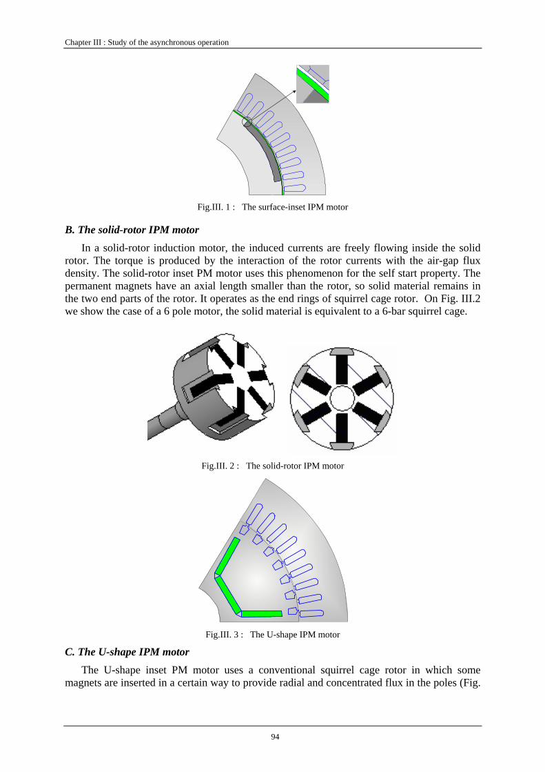
Chapter III : Study of the asynchronous operation
94
Fig.III. 1 : The surface-inset IPM motor
B. The solid-rotor IPM motor
In a solid-rotor induction motor, the induced currents are freely flowing inside the solid rotor. The torque is produced by the interaction of the rotor currents with the air-gap flux density. The solid-rotor inset PM motor uses this phenomenon for the self start property. The permanent magnets have an axial length smaller than the rotor, so solid material remains in the two end parts of the rotor. It operates as the end rings of squirrel cage rotor. On Fig. III.2 we show the case of a 6 pole motor, the solid material is equivalent to a 6-bar squirrel cage.
Fig.III. 2 : The solid-rotor IPM motor
Fig.III. 3 : The U-shape IPM motor
C. The U-shape IPM motor The U-shape inset PM motor uses a conventional squirrel cage rotor in which some
magnets are inserted in a certain way to provide radial and concentrated flux in the poles (Fig.
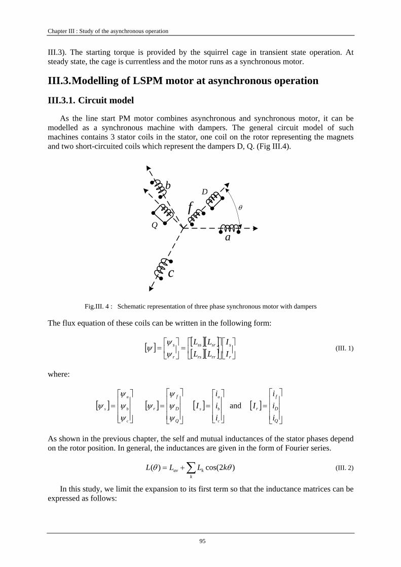
Chapter III : Study of the asynchronous operation
95
III.3). The starting torque is provided by the squirrel cage in transient state operation. At steady state, the cage is currentless and the motor runs as a synchronous motor.
III.3. Modelling of LSPM motor at asynchronous operation
III.3.1. Circuit model
As the line start PM motor combines asynchronous and synchronous motor, it can be modelled as a synchronous machine with dampers. The general circuit model of such machines contains 3 stator coils in the stator, one coil on the rotor representing the magnets and two short-circuited coils which represent the dampers D, Q. (Fig III.4).
a
b
c
D
Q
f θ
Fig.III. 4 : Schematic representation of three phase synchronous motor with dampers
The flux equation of these coils can be written in the following form:
[ ] [ ][ ]
[ ][ ] ⎥
⎦
⎤⎢⎣
⎡⎥⎦
⎤⎢⎣
⎡=⎥
⎦
⎤⎢⎣
⎡=
r
s
rr
sr
rs
ss
r
s
II
LL
LL
ψψ
ψ (III. 1)
where:
[ ]⎥⎥⎥
⎦
⎤
⎢⎢⎢
⎣
⎡=
c
b
a
s
ψψψ
ψ [ ]⎥⎥⎥
⎦
⎤
⎢⎢⎢
⎣
⎡
=
Q
D
f
r
ψψψ
ψ [ ]⎥⎥⎥
⎦
⎤
⎢⎢⎢
⎣
⎡=
c
b
a
s
iii
I and [ ]⎥⎥⎥
⎦
⎤
⎢⎢⎢
⎣
⎡
=
Q
D
f
r
iii
I
As shown in the previous chapter, the self and mutual inductances of the stator phases depend on the rotor position. In general, the inductances are given in the form of Fourier series.
)2cos()( θθ kLLLk
kav ∑+= (III. 2)
In this study, we limit the expansion to its first term so that the inductance matrices can be expressed as follows:
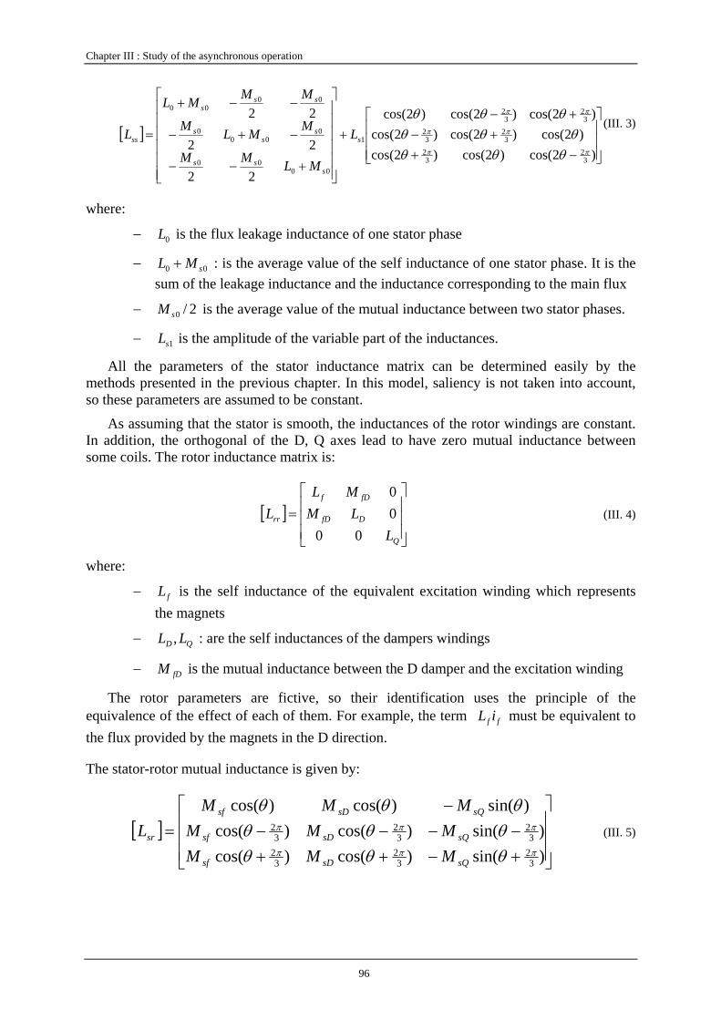
Chapter III : Study of the asynchronous operation
96
[ ]⎥⎥⎥
⎦
⎤
⎢⎢⎢
⎣
⎡
−++−
+−+
⎥⎥⎥⎥⎥⎥
⎦
⎤
⎢⎢⎢⎢⎢⎢
⎣
⎡
+−−
−+−
−−+
=)2cos()2cos()2cos(
)2cos()2cos()2cos()2cos()2cos()2cos(
22
22
22
32
32
32
32
32
32
1
0000
000
0
0000
ππ
ππ
ππ
θθθθθθ
θθθ
s
sss
ss
s
sss
ss L
MLMM
MMLM
MMML
L(III. 3)
where:
− 0L is the flux leakage inductance of one stator phase
− 00 sML + : is the average value of the self inductance of one stator phase. It is the sum of the leakage inductance and the inductance corresponding to the main flux
− 2/0sM is the average value of the mutual inductance between two stator phases.
− 1sL is the amplitude of the variable part of the inductances.
All the parameters of the stator inductance matrix can be determined easily by the methods presented in the previous chapter. In this model, saliency is not taken into account, so these parameters are assumed to be constant.
As assuming that the stator is smooth, the inductances of the rotor windings are constant. In addition, the orthogonal of the D, Q axes lead to have zero mutual inductance between some coils. The rotor inductance matrix is:
[ ]⎥⎥⎥
⎦
⎤
⎢⎢⎢
⎣
⎡
=
Q
DfD
fDf
rr
LLM
MLL
0000
(III. 4)
where:
− fL is the self inductance of the equivalent excitation winding which represents the magnets
− QD LL , : are the self inductances of the dampers windings
− fDM is the mutual inductance between the D damper and the excitation winding
The rotor parameters are fictive, so their identification uses the principle of the equivalence of the effect of each of them. For example, the term ff iL must be equivalent to the flux provided by the magnets in the D direction.
The stator-rotor mutual inductance is given by:
[ ]⎥⎥⎥
⎦
⎤
⎢⎢⎢
⎣
⎡
+−++−−−−
−=
)sin()cos()cos()sin()cos()cos(
)sin()cos()cos(
32
32
32
32
32
32
πππ
πππ
θθθθθθθθθ
sQsDsf
sQsDsf
sQsDsf
sr
MMMMMM
MMML (III. 5)
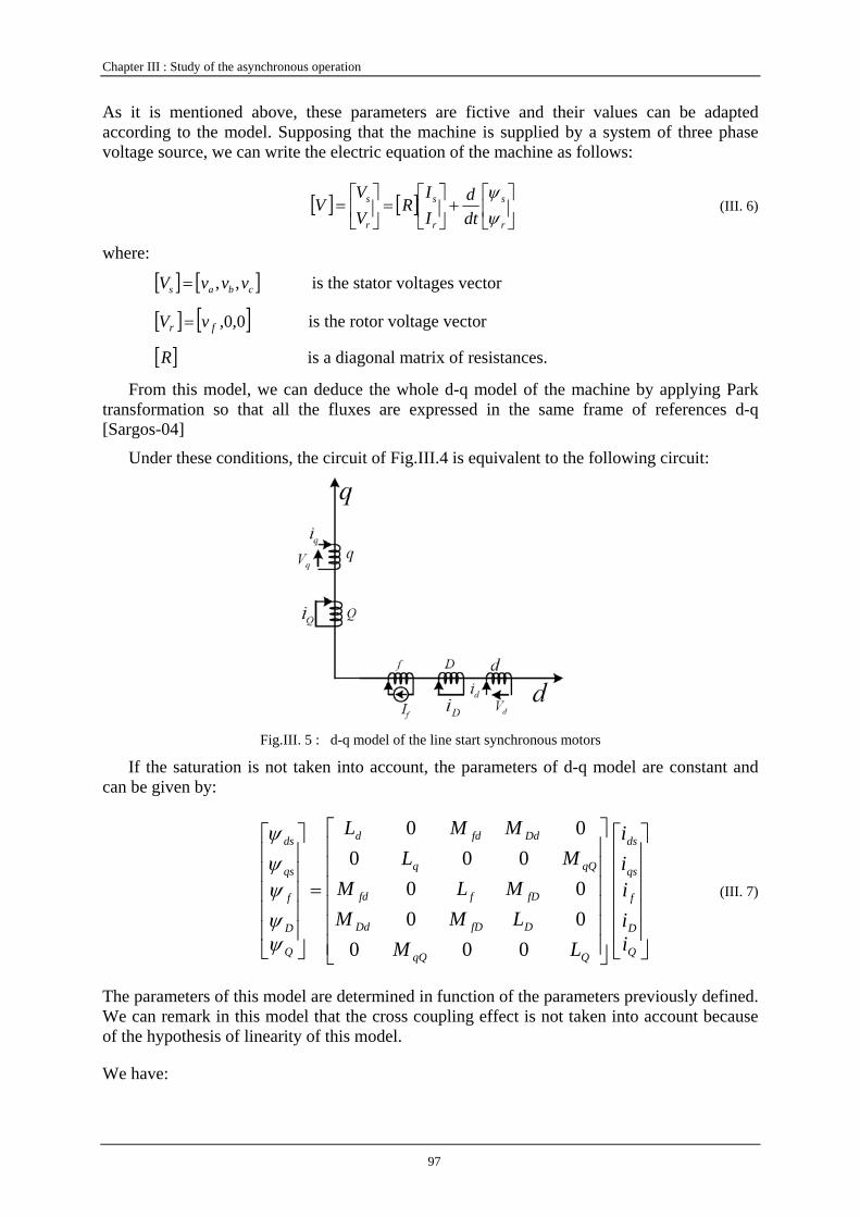
Chapter III : Study of the asynchronous operation
97
As it is mentioned above, these parameters are fictive and their values can be adapted according to the model. Supposing that the machine is supplied by a system of three phase voltage source, we can write the electric equation of the machine as follows:
[ ] [ ] ⎥⎦
⎤⎢⎣
⎡+⎥
⎦
⎤⎢⎣
⎡=⎥
⎦
⎤⎢⎣
⎡=
r
s
r
s
r
s
dtd
II
RVV
Vψψ
(III. 6)
where:
[ ] [ ]cbas vvvV ,,= is the stator voltages vector
[ ] [ ]0,0,fr vV = is the rotor voltage vector
[ ]R is a diagonal matrix of resistances.
From this model, we can deduce the whole d-q model of the machine by applying Park transformation so that all the fluxes are expressed in the same frame of references d-q [Sargos-04]
Under these conditions, the circuit of Fig.III.4 is equivalent to the following circuit:
Fig.III. 5 : d-q model of the line start synchronous motors
If the saturation is not taken into account, the parameters of d-q model are constant and can be given by:
⎥⎥⎥⎥⎥
⎦
⎤
⎢⎢⎢⎢⎢
⎣
⎡
⎥⎥⎥⎥⎥⎥
⎦
⎤
⎢⎢⎢⎢⎢⎢
⎣
⎡
=
⎥⎥⎥⎥⎥
⎦
⎤
⎢⎢⎢⎢⎢
⎣
⎡
Q
D
f
qs
ds
QqQ
DfDDd
fDffd
qQq
Ddfdd
Q
D
f
qs
ds
iiiii
LMLMM
MLMML
MML
0000000
00000
ψψψψψ
(III. 7)
The parameters of this model are determined in function of the parameters previously defined. We can remark in this model that the cross coupling effect is not taken into account because of the hypothesis of linearity of this model.
We have:
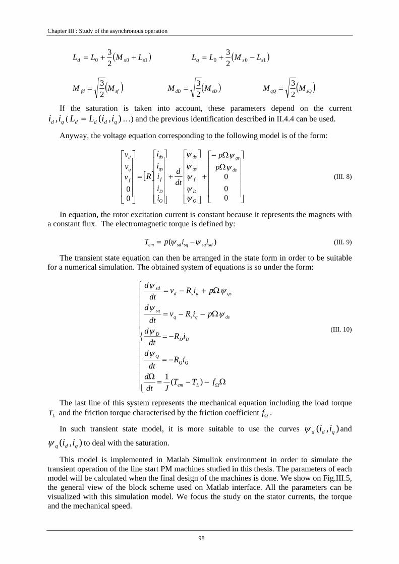
Chapter III : Study of the asynchronous operation
98
( )100 23
ssd LMLL ++= ( )100 23
ssq LMLL −+=
( )sffd MM23
= ( )sDdD MM23
= ( )sQqQ MM23
=
If the saturation is taken into account, these parameters depend on the current qd ii , ( ),( qddd iiLL = …) and the previous identification described in II.4.4 can be used.
Anyway, the voltage equation corresponding to the following model is of the form:
[ ]
⎥⎥⎥⎥⎥
⎦
⎤
⎢⎢⎢⎢⎢
⎣
⎡ΩΩ−
+
⎥⎥⎥⎥⎥⎥
⎦
⎤
⎢⎢⎢⎢⎢⎢
⎣
⎡
+
⎥⎥⎥⎥⎥⎥
⎦
⎤
⎢⎢⎢⎢⎢⎢
⎣
⎡
=
⎥⎥⎥⎥⎥
⎦
⎤
⎢⎢⎢⎢⎢
⎣
⎡
000
00
ds
qs
Q
D
f
qs
ds
Q
D
f
qs
ds
f
q
d
pp
dtd
iiiii
Rvvv
ψψ
ψψψψψ
(III. 8)
In equation, the rotor excitation current is constant because it represents the magnets with a constant flux. The electromagnetic torque is defined by:
)( sdsqsqsdem iipT ψψ −= (III. 9)
The transient state equation can then be arranged in the state form in order to be suitable for a numerical simulation. The obtained system of equations is so under the form:
⎪⎪⎪⎪⎪⎪
⎩
⎪⎪⎪⎪⎪⎪
⎨
⎧
Ω−−=Ω
−=
−=
Ω−−=
Ω+−=
ΩfTTJdt
d
iRdt
d
iRdt
d
piRvdt
d
piRvdt
d
Lem
QQQ
DDD
dsqsqsq
qsdsdsd
)(1
ψ
ψ
ψψ
ψψ
(III. 10)
The last line of this system represents the mechanical equation including the load torque LT and the friction torque characterised by the friction coefficient Ωf .
In such transient state model, it is more suitable to use the curves ),( qdd iiψ and
),( qdq iiψ to deal with the saturation.
This model is implemented in Matlab Simulink environment in order to simulate the transient operation of the line start PM machines studied in this thesis. The parameters of each model will be calculated when the final design of the machines is done. We show on Fig.III.5, the general view of the block scheme used on Matlab interface. All the parameters can be visualized with this simulation model. We focus the study on the stator currents, the torque and the mechanical speed.

Chapter III : Study of the asynchronous operation
99
Considering the starting performances, the initial conditions used in such a simulation are zero currents in all the windings except the fictive winding which represents the magnets. As an illustration, we show on Fig. III.7 and Fig.III.8 some results provided by this model for an approximate set of parameters of our machine. The evolution of the stator currents and the mechanical speed give us information about the starting performances. We remember that the required performances are mainly a high starting torque and low starting current. Therefore, we will study the starting performances according to these two parameters.
7wm2
6Tem
5wr
4i2d
3i2q
2iq
1id
Tem
Tlwm
w_m
psai_q
i2qiq
i_q
psai_d
i2did
i_d
Q_2q
iqi2q
i_2q
Q_2d
idi2d
i_2d
QdiqQq
id
Tem
Tem1
Speed
Uq
psai_d
wr
iq
psai_q
Q_q
Ud
psai_q
wr
id
psai_d
Q_d
i2q Q2q
Q_2q
i2d Q2d
Q_2d
Product
Np
Np3
T_L
2Uq
1Ud
Fig.III. 6 : Implemented model on Matlab Simulink environment
0 0.1 0.2 0.3 0.4 0.5 0.6-400
-300
-200
-100
0
100
200
300
400
Time (s)
Phas
e cu
rren
t (A
)
0 0.2 0.4 0.6 0.8-500
-400
-300
-200
-100
0
100
200
300
400
500
Time (s)
D,Q
axi
s cur
rent
(A)
iq
id
Phase currents cba iii ,, d-q currents qd ii ,
Fig.III. 7 : Simulation results at starting operation (stator currents)

Chapter III : Study of the asynchronous operation
100
0 0.2 0.4 0.6 0.8-400
-200
0
200
400
600
800
1000
Time (s)
Elec
trom
agne
tic to
rque
(N.m
)
0 0.2 0.4 0.6 0.8-200
0
200
400
600
800
1000
1200
Times (s)
Spee
d (t
r/m
)
Fig.III. 8 : Simulation results at starting operation (mechanical properties)
The transient state model presented above allows determining the behaviour of the line start motor during the starting process. However it is not suitable to determine the average torque provided by each part of the rotor. Indeed, during starting process, the total instantaneous torque contains cage torque, braking torque and oscillatory torque. The cage torque is produced by the interaction between winding currents and induced rotor cage current. The magnets which are permanently magnetized produce braking torque at all asynchronous speeds except standstill [Miller-84]. They work as a brake and slow down the increase of the speed as long as the synchronous speed isn’t reached. Under the hypothesis of linear materials, we can try to separate the two phenomena in order to highlight the effect of each of the two parts:
• Cage torque To calculate the cage torque, a traditional steady state induction motor equivalent circuit
can be used Fig.III.9. The torque produced by the cage is the power consumed in the
resistance '2
1 Rs
s− divided by the angular speed of the rotor. It can be calculated by the
following expression:
( )⎥⎥
⎦
⎤
⎢⎢
⎣
⎡++⎟
⎟⎠
⎞⎜⎜⎝
⎛+
=2'
21
2'2
'22
2
3
σσπ cXXs
RcRf
sR
pVT
s
cag (III. 11)
where V is the phase RMS voltage, p the number of poles, σσ 211 XXc ′+= , σ1X , '2σX are the
stator and rotor leakage reactances, mX is the magnetizing reactance.
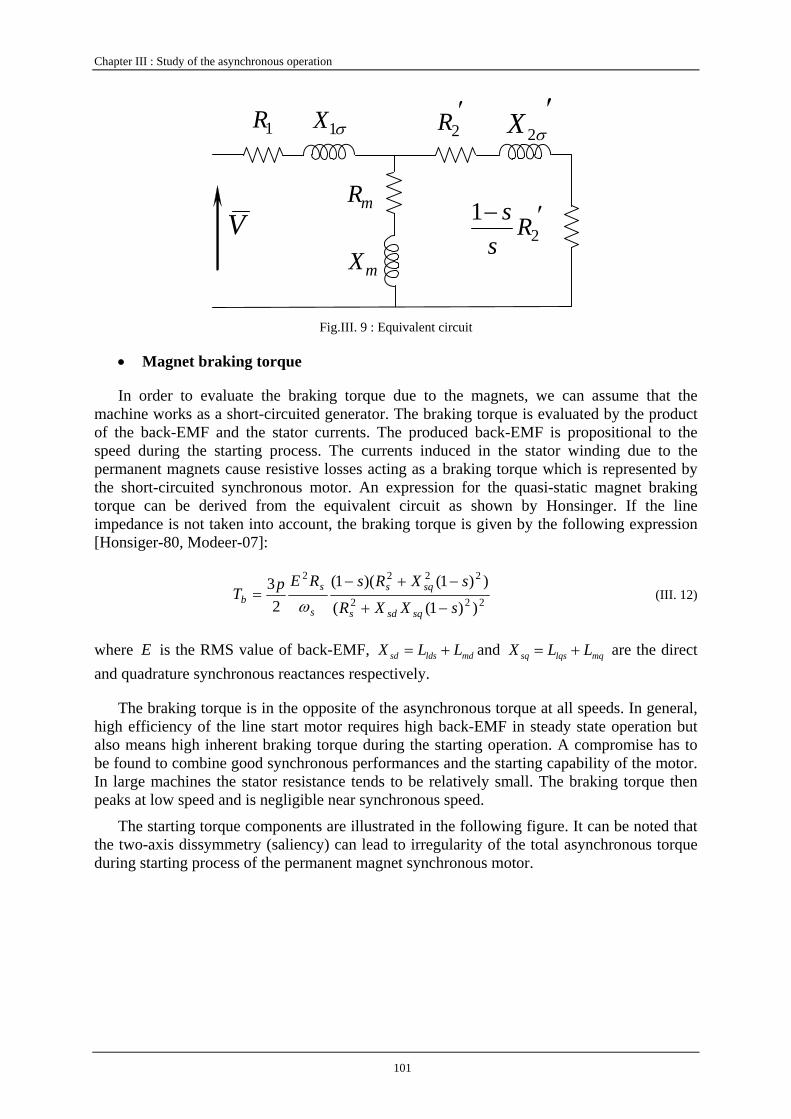
Chapter III : Study of the asynchronous operation
101
1R
V
′2R
′−2
1 Rs
smR
mX
σ1X ′σ2X
Fig.III. 9 : Equivalent circuit
• Magnet braking torque
In order to evaluate the braking torque due to the magnets, we can assume that the machine works as a short-circuited generator. The braking torque is evaluated by the product of the back-EMF and the stator currents. The produced back-EMF is propositional to the speed during the starting process. The currents induced in the stator winding due to the permanent magnets cause resistive losses acting as a braking torque which is represented by the short-circuited synchronous motor. An expression for the quasi-static magnet braking torque can be derived from the equivalent circuit as shown by Honsinger. If the line impedance is not taken into account, the braking torque is given by the following expression [Honsiger-80, Modeer-07]:
222
2222
))1((
))1()(1(2
3sXXR
sXRsREpTsqsds
sqs
s
sb
−+
−+−=
ω (III. 12)
where E is the RMS value of back-EMF, mdldssd LLX += and mqlqssq LLX += are the direct and quadrature synchronous reactances respectively.
The braking torque is in the opposite of the asynchronous torque at all speeds. In general, high efficiency of the line start motor requires high back-EMF in steady state operation but also means high inherent braking torque during the starting operation. A compromise has to be found to combine good synchronous performances and the starting capability of the motor. In large machines the stator resistance tends to be relatively small. The braking torque then peaks at low speed and is negligible near synchronous speed.
The starting torque components are illustrated in the following figure. It can be noted that the two-axis dissymmetry (saliency) can lead to irregularity of the total asynchronous torque during starting process of the permanent magnet synchronous motor.
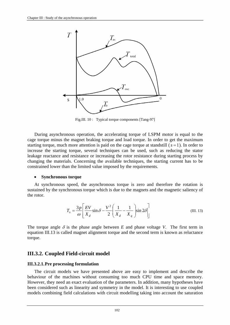
Chapter III : Study of the asynchronous operation
102
Fig.III. 10 : Typical torque components [Tang-97]
During asynchronous operation, the accelerating torque of LSPM motor is equal to the cage torque minus the magnet braking torque and load torque. In order to get the maximum starting torque, much more attention is paid on the cage torque at standstill ( 1=s ). In order to increase the starting torque, several techniques can be used, such as reducing the stator leakage reactance and resistance or increasing the rotor resistance during starting process by changing the materials. Concerning the available techniques, the starting current has to be constrained lower than the limited value imposed by the requirements.
• Synchronous torque At synchronous speed, the asynchronous torque is zero and therefore the rotation is
sustained by the synchronous torque which is due to the magnets and the magnetic saliency of the rotor.
⎥⎥⎦
⎤
⎢⎢⎣
⎡⎟⎟⎠
⎞⎜⎜⎝
⎛−−= δδ
ω2sin11
2sin3 2
qdds XX
VXEVpT (III. 13)
The torque angle δ is the phase angle between E and phase voltage V. The first term in equation III.13 is called magnet alignment torque and the second term is known as reluctance torque.
III.3.2. Coupled Field-circuit model
III.3.2.1. Pre processing formulation
The circuit models we have presented above are easy to implement and describe the behaviour of the machines without consuming too much CPU time and space memory. However, they need an exact evaluation of the parameters. In addition, many hypotheses have been considered such as linearity and symmetry in the model. It is interesting to use coupled models combining field calculations with circuit modelling taking into account the saturation
Chapter III : Study of the asynchronous operation
103
and exact geometry of the machine. In this case, there is no explicit need to determine the parameters of the model.
Many commercial softwares (Cedrat, Maxwell, Opera) have been developed for such a purpose. Some of them are specialized in electric machine simulation. We decided to use software Flux2D developed by CEDRAT because of its adequacy to the modelling of such problems.
The field-circuit calculation of electric machines is based on a time-stepping, finite-element analysis. In the case of two dimensional problems, the field is assumed as plane and the end effects are considered under assumption. The end effects in the motor are taken into account with in the circuit equations by adding resistances and inductances of the end-windings. Voltage is supplied in formulations through the circuit equation of the windings which are solved together with field equations.
We present in the following the principle of coupled field-circuit modelling of electric machines in two dimensions. The different softwares use this principle but the adaptation to the different types of machines can be different from one to another.
The electromagnetic problem description of a motor is based on the solution of a set of partial differential equations. Usually the problem is assumed to be quasi-static, thus the displacement current is neglected. In laminated stators, there are no eddy currents, so the problem is magnetostatic in the stator region sΩ and can be described by the following equation:
0=+⎟⎟⎠
⎞⎜⎜⎝
⎛∂∂
∂∂
+⎟⎠⎞
⎜⎝⎛
∂∂
∂∂
ss
ss
s Jya
yxa
x
vvνν (III. 14)
where:
sν is the stator reluctivity which depends on the flux density.
sJ is the stator current density in the slots, which depends on the stator currents and the winding arrangement.
In the rotor region rΩ , the field equation is written as follows:
0=⎟⎠⎞
⎜⎝⎛ −∂∂
−⎟⎟⎠
⎞⎜⎜⎝
⎛∂∂
∂∂
+⎟⎠⎞
⎜⎝⎛
∂∂
∂∂
lu
ta
ya
yxa
xbrr
rr
r
vvvσνν (III. 15)
where bu is the voltage of each bar of the rotor cage and σ is the electric conductivity.
These field equations are combined with the following circuit equation in the stator circuit:
⎪⎭
⎪⎬⎫
⎪⎩
⎪⎨⎧
∂∂
−∂∂
++= ∫∫∫∫−+
)(IlIRVss
dst
adst
as
nldtd sse
sssss
vv (III. 16)
where +s and
−s respectively represent the go and return cross section areas of the stator slots.
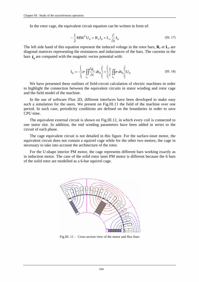
Chapter III : Study of the asynchronous operation
104
In the rotor cage, the equivalent circuit equation can be written in form of:
bebeb tILIRUMM
21 T
∂∂
+=− (III. 17)
The left side hand of this equation represent the induced voltage in the rotor bars, Re et Le are diagonal matrices representing the resistances and inductances of the bars. The currents in the bars bI are computed with the magnetic vector potential with:
bbs
bs
rb ds
lds
ta
bb
U1I⎪⎭
⎪⎬⎫
⎪⎩
⎪⎨⎧
+⎪⎭
⎪⎬⎫
⎪⎩
⎪⎨⎧
∂∂
−= ∫∫∫∫ σσv
(III. 18)
We have presented these outlines of field-circuit calculation of electric machines in order to highlight the connection between the equivalent circuits in stator winding and rotor cage and the field model of the machine.
In the use of software Flux 2D, different interfaces have been developed to make easy such a simulation for the users. We present on Fig.III.11 the field of the machine over one period. In such case, periodicity conditions are defined on the boundaries in order to save CPU time.
The equivalent external circuit is shown on Fig.III.12, in which every coil is connected to one stator slot. In addition, the end winding parameters have been added in series to the circuit of each phase.
The cage equivalent circuit is not detailed in this figure. For the surface-inset motor, the equivalent circuit does not contain a squirrel cage while for the other two motors, the cage in necessary to take into account the architecture of the rotor.
For the U-shape interior PM motor, the cage represents different bars working exactly as in induction motor. The case of the solid rotor inset PM motor is different because the 6 bars of the solid rotor are modelled as a 6-bar squirrel cage.
Fig.III. 11 : Cross section view of the motor and flux lines

Chapter III : Study of the asynchronous operation
105
Fig.III. 12 : Coupling of the filed and with circuit
III.3.2.2. Post processing treatment and formulation Some performances such as stator currents, torque, and output power are rederived from
the computation of the field-circuit equations. They can be visualized and dealt directly after each simulation.
We can show on Fig.III.13 an example of stator currents and electromagnetic torque from starting to synchronous speed.
0 0.1 0.2 0.3 0.4 0.5-1000
-500
0
500
1000
1500
2000
Ele
ctro
mag
netic
torq
ue (N
.m)
Time (s)0 0.1 0.2 0.3 0.4 0.5
-1000
-500
0
500
1000
Phas
e cu
rren
t (A
)
Time (s) Fig.III. 13 : Stator currents and torque during starting operation
Some other characteristics, such as power factor or efficiency are not directly accessible. We need to perform some post treatment for their evaluation. We present in the following the adopted methods for the calculation of the power factor and the efficiency in steady state operation.
• Computation of the efficiency
The efficiency of the motor at steady state can be computed with classical definition by analyzing the external characteristics over the last electrical periods of the simulation.
The input power is given by performing the product of voltage and currents on the three phases:
dttitvT
PT
kkk
in ∫∑=
=0
3
1)()(1 (III. 19)

Chapter III : Study of the asynchronous operation
106
The output power is calculated with the product of the load torque and the mechanical speed at each time step
dtttTT
PT
semout ∫ Ω=0
)()(1 (III. 20)
These two parameters are given by the software, and their ratio defines the efficiency of the motor at each operation point.
inout PP /=η (III. 21)
• Computation of the power factor
The calculation of the power factor is performed in sequence of the following steps.
- Perform the transient simulation until synchronous speed
-Verify if the curves of voltage (V) and current (I) are sinusoidal
- Compute the phase angle ϕ between the voltage and current at synchronous speed
In the case where both the current and voltage are sinusoidal with the same frequency as of voltage source, the time shift between the voltage and current corresponds with the electrical angle (Fig. III. 14). The power factor is calculated by:
)/2cos( TtPF Δ= π (III. 22)
0.3 0.32 0.34 0.36 0.38 0.4-500
-400
-300
-200
-100
0
100
200
300
400
500
Time (s)
Phase voltage (V)Phase current (A)Active power (Kw)
V(t)
i(t) P(t)
0.38 0.385 0.39 0.395 0.4 0.405-400
-300
-200
-100
0
100
200
300
400
Time (s)
Phase voltagePhase current
Δt =1.5ms
Fig.III. 14 : Last period of voltage, active power and current waveforms
In the general case, if the currents are not sinusoidal, we can use the following approach:
• Calculate the phase voltage rmsV and current rmsI for the time T
∫=T
kk dttvT
V 2)(1 ∫=
Tkk dtti
TI 2)(1
(III. 23)
• Compute the active power by the formula

Chapter III : Study of the asynchronous operation
107
dttitvT
PT kk
k∫∑
=
= )()(1 3
1 (III. 24)
• Compute the apparatus power by the formula
∑=
=3
1kkk IVS (III. 25)
• Calculate the Power factor by:
SPPF /= (III. 26)
Conclusion:
Two models have been presented in this subsection. The first one, based on circuit modelling (CM) is useful for transient state simulations but it needs an accurate identification of the parameters. The second model is a coupled field-circuit model performed with software Flux2D. It has been adapted in order to evaluate the external performances of the motors such as power factor, and efficiency.
The second model based on finite element calculation is more accurate than the CM because it does not need parameter identification and takes into account the exact geometry of the machine and the local saturation of the materials. It will be used for the study and the comparison of the performances of three motors. The circuit model will be used after the identification of the parameters of the final designed motors.
III.4. Transient characteristics –starting current and torque
The modelling calculation at steady state has given us a preliminary dimension of the motors. The study of the transient characteristics will be carried out with these dimensions of the three motors. The aim of this study is to illustrate the effect of the geometrical parameters and physical properties on the transient performances. We will compare the performances of the three motor to find the optimal design to achieve the required characteristics.
As mentioned before, we have two important required transient properties which are relative the starting torque and current:
− The starting torque must be at least 3 times higher than the rated torque
− The starting current must be less that 10 times the rated current
Therefore, the transient performances are analyzed in terms of the ratios between starting and rated currents ( rast II / ) and starting and rated torques ( rast TT / ) respectively, which will be studied entirely. The transient magnetic analyses are carried out to study the starting performance during asynchronous process.
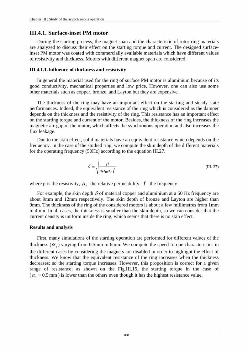
Chapter III : Study of the asynchronous operation
108
III.4.1. Surface-inset PM motor During the starting process, the magnet span and the characteristic of rotor ring materials
are analyzed to discuss their effect on the starting torque and current. The designed surface-inset PM motor was coated with commercially available materials which have different values of resistivity and thickness. Motors with different magnet span are considered.
III.4.1.1. Influence of thickness and resistivity
In general the material used for the ring of surface PM motor is aluminium because of its good conductivity, mechanical properties and low price. However, one can also use some other materials such as copper, bronze, and Layton but they are expensive.
The thickness of the ring may have an important effect on the starting and steady state performances. Indeed, the equivalent resistance of the ring which is considered as the damper depends on the thickness and the resistivity of the ring. This resistance has an important effect on the starting torque and current of the motor. Besides, the thickness of the ring increases the magnetic air-gap of the motor, which affects the synchronous operation and also increases the flux leakage.
Due to the skin effect, solid materials have an equivalent resistance which depends on the frequency. In the case of the studied ring, we compute the skin depth of the different materials for the operating frequency (50Hz) according to the equation III.27.
frμπμρδ
0= (III. 27)
where ρ is the resistivity, rμ the relative permeability, f the frequency
For example, the skin depth δ of material copper and aluminium at a 50 Hz frequency are about 9mm and 12mm respectively. The skin depth of bronze and Layton are higher than 9mm. The thickness of the ring of the considered motors is about a few millimetres from 1mm to 4mm. In all cases, the thickness is smaller than the skin depth, so we can consider that the current density is uniform inside the ring, which seems that there is no skin effect.
Results and analysis
First, many simulations of the starting operation are performed for different values of the thickness ( sα ) varying from 0.5mm to 6mm. We compute the speed-torque characteristics in the different cases by considering the magnets are disabled in order to highlight the effect of thickness. We know that the equivalent resistance of the ring increases when the thickness decreases; so the starting torque increases. However, this proposition is correct for a given range of resistance; as shown on the Fig.III.15, the starting torque in the case of ( mm 5.0=sα ) is lower than the others even though it has the highest resistance value.
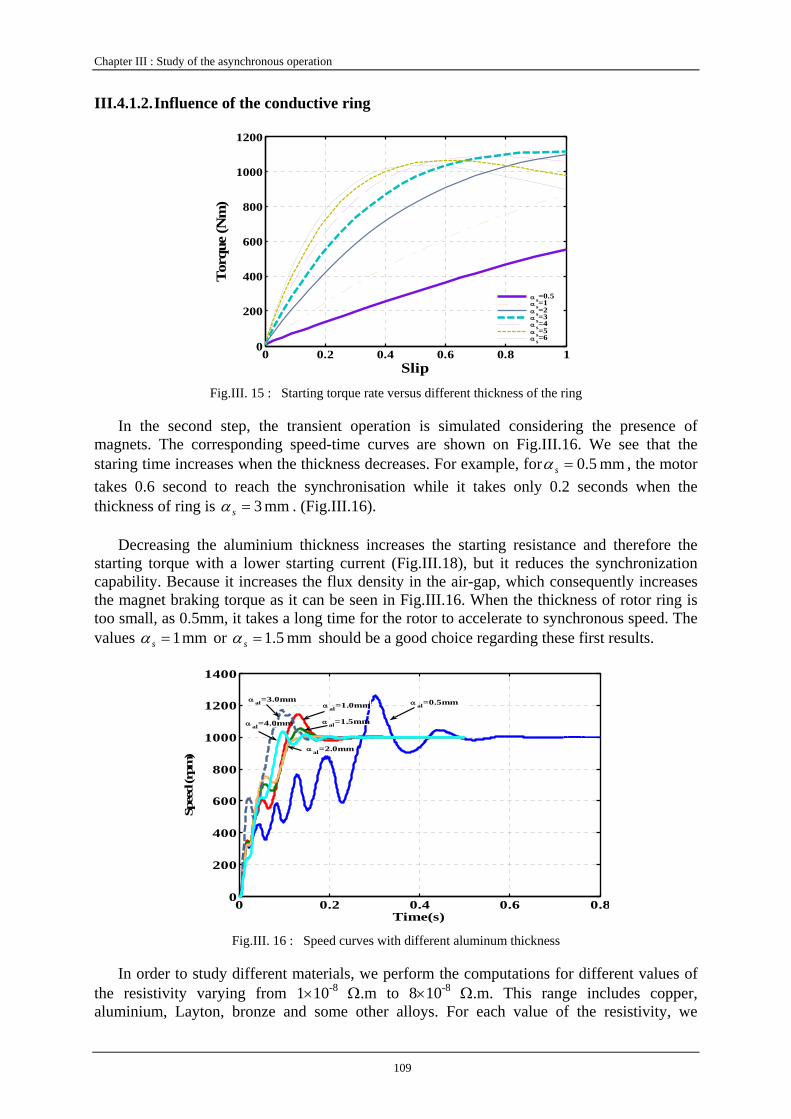
Chapter III : Study of the asynchronous operation
109
III.4.1.2. Influence of the conductive ring
0 0.2 0.4 0.6 0.8 10
200
400
600
800
1000
1200
Slip
Tor
que
(Nm
)
α s=0.5α s=1α s=2α s=3α s=4α s=5α s=6
Fig.III. 15 : Starting torque rate versus different thickness of the ring
In the second step, the transient operation is simulated considering the presence of magnets. The corresponding speed-time curves are shown on Fig.III.16. We see that the staring time increases when the thickness decreases. For example, for mm 5.0=sα , the motor takes 0.6 second to reach the synchronisation while it takes only 0.2 seconds when the thickness of ring is mm 3=sα . (Fig.III.16).
Decreasing the aluminium thickness increases the starting resistance and therefore the starting torque with a lower starting current (Fig.III.18), but it reduces the synchronization capability. Because it increases the flux density in the air-gap, which consequently increases the magnet braking torque as it can be seen in Fig.III.16. When the thickness of rotor ring is too small, as 0.5mm, it takes a long time for the rotor to accelerate to synchronous speed. The values mm 1=sα or mm 5.1=sα should be a good choice regarding these first results.
0 0.2 0.4 0.6 0.80
200
400
600
800
1000
1200
1400
Time(s)
Spee
d (r
pm)
α al=0.5mmα al=1.0mm
α al=1.5mm
α al=2.0mm
α al=3.0mm
α al=4.0mm
Fig.III. 16 : Speed curves with different aluminum thickness
In order to study different materials, we perform the computations for different values of the resistivity varying from 1×10⁻⁸ Ω.m to 8×10⁻⁸ Ω.m. This range includes copper, aluminium, Layton, bronze and some other alloys. For each value of the resistivity, we
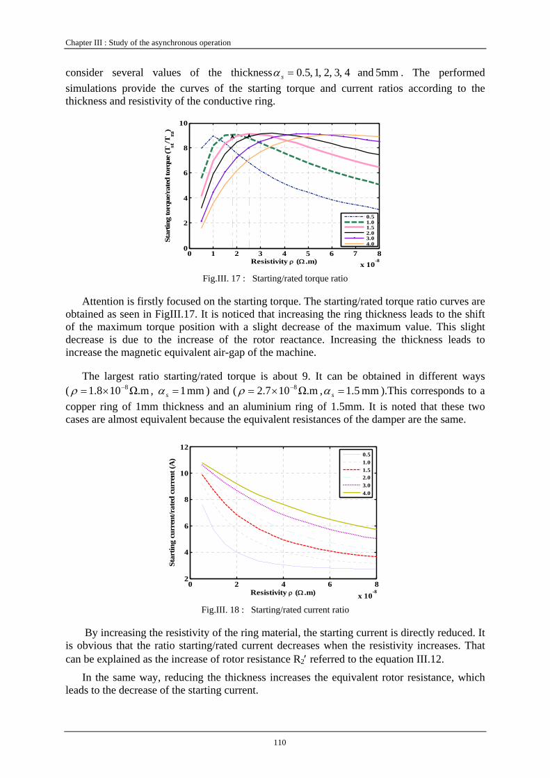
Chapter III : Study of the asynchronous operation
110
consider several values of the thickness mm5 and 4,3,2,1,5.0=sα . The performed simulations provide the curves of the starting torque and current ratios according to the thickness and resistivity of the conductive ring.
0 1 2 3 4 5 6 7 8x 10
-8
0
2
4
6
8
10
Resistivity ρ (Ω .m)
Star
ting
torq
ue/r
ated
torq
ue (T
st/T
ra)
0.51.01.52.03.04.0
Fig.III. 17 : Starting/rated torque ratio
Attention is firstly focused on the starting torque. The starting/rated torque ratio curves are obtained as seen in FigIII.17. It is noticed that increasing the ring thickness leads to the shift of the maximum torque position with a slight decrease of the maximum value. This slight decrease is due to the increase of the rotor reactance. Increasing the thickness leads to increase the magnetic equivalent air-gap of the machine.
The largest ratio starting/rated torque is about 9. It can be obtained in different ways ( Ω.m108.1 8−×=ρ , mm 1=sα ) and ( Ω.m107.2 8−×=ρ , mm 5.1=sα ).This corresponds to a copper ring of 1mm thickness and an aluminium ring of 1.5mm. It is noted that these two cases are almost equivalent because the equivalent resistances of the damper are the same.
0 2 4 6 8x 10
-8
2
4
6
8
10
12
Resistivity ρ (Ω .m)
Star
ting
curr
ent/r
ated
cur
rent
(A) 0.5
1.01.52.03.04.0
Fig.III. 18 : Starting/rated current ratio
By increasing the resistivity of the ring material, the starting current is directly reduced. It is obvious that the ratio starting/rated current decreases when the resistivity increases. That can be explained as the increase of rotor resistance R2′ referred to the equation III.12.
In the same way, reducing the thickness increases the equivalent rotor resistance, which leads to the decrease of the starting current.
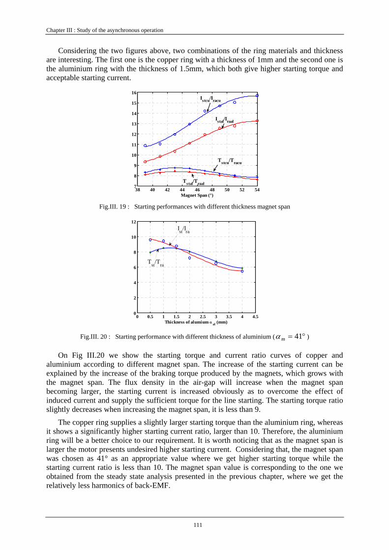
Chapter III : Study of the asynchronous operation
111
Considering the two figures above, two combinations of the ring materials and thickness are interesting. The first one is the copper ring with a thickness of 1mm and the second one is the aluminium ring with the thickness of 1.5mm, which both give higher starting torque and acceptable starting current.
38 40 42 44 46 48 50 52 547
8
9
10
11
12
13
14
15
16
Magnet Span (°)
Istcu/Iracu
Istal/Iraal
Tstcu/Tracu
Tstal/Traal
Fig.III. 19 : Starting performances with different thickness magnet span
0 0.5 1 1.5 2 2.5 3 3.5 4 4.50
2
4
6
8
10
12
Thickness of alumium α al (mm)
Tst/Tra
Ist/Ira
Fig.III. 20 : Starting performance with different thickness of aluminium ( °= 41mα )
On Fig III.20 we show the starting torque and current ratio curves of copper and aluminium according to different magnet span. The increase of the starting current can be explained by the increase of the braking torque produced by the magnets, which grows with the magnet span. The flux density in the air-gap will increase when the magnet span becoming larger, the starting current is increased obviously as to overcome the effect of induced current and supply the sufficient torque for the line starting. The starting torque ratio slightly decreases when increasing the magnet span, it is less than 9.
The copper ring supplies a slightly larger starting torque than the aluminium ring, whereas it shows a significantly higher starting current ratio, larger than 10. Therefore, the aluminium ring will be a better choice to our requirement. It is worth noticing that as the magnet span is larger the motor presents undesired higher starting current. Considering that, the magnet span was chosen as 41° as an appropriate value where we get higher starting torque while the starting current ratio is less than 10. The magnet span value is corresponding to the one we obtained from the steady state analysis presented in the previous chapter, where we get the relatively less harmonics of back-EMF.
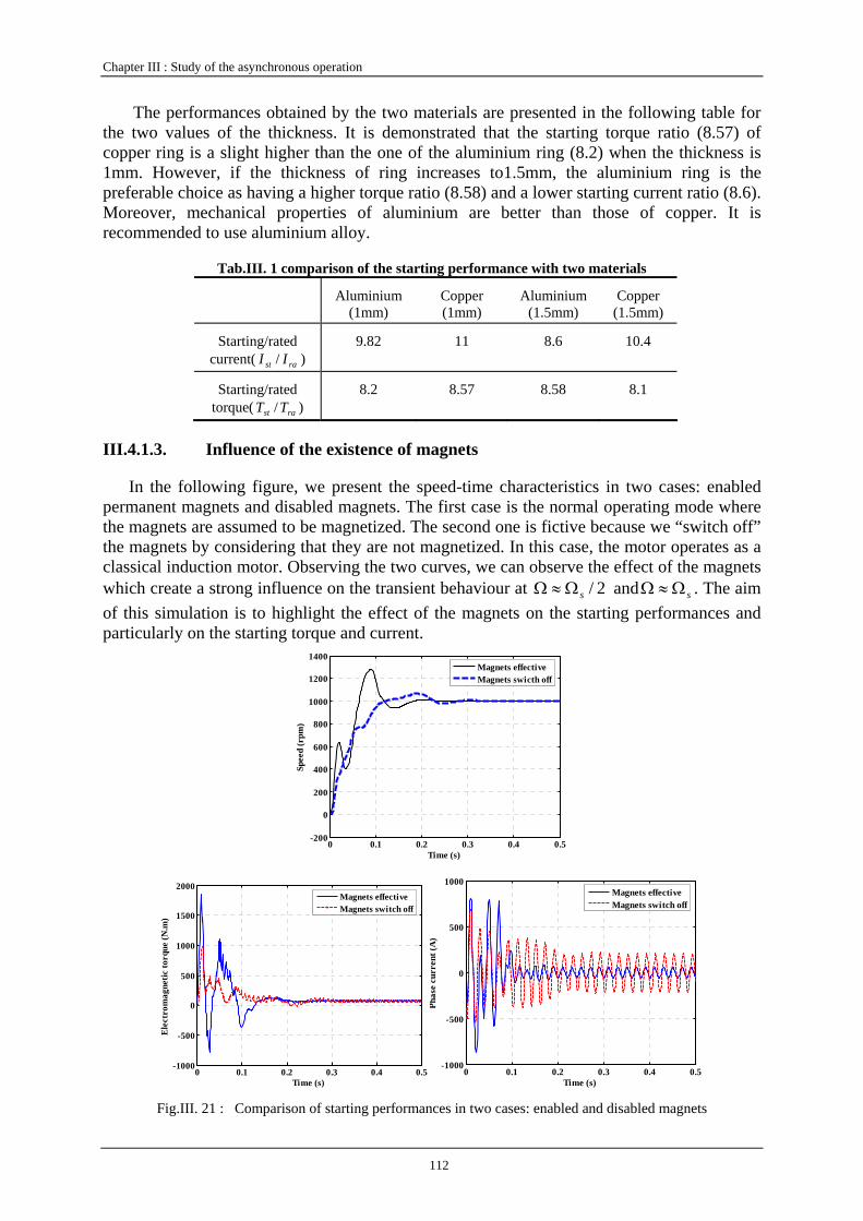
Chapter III : Study of the asynchronous operation
112
The performances obtained by the two materials are presented in the following table for the two values of the thickness. It is demonstrated that the starting torque ratio (8.57) of copper ring is a slight higher than the one of the aluminium ring (8.2) when the thickness is 1mm. However, if the thickness of ring increases to1.5mm, the aluminium ring is the preferable choice as having a higher torque ratio (8.58) and a lower starting current ratio (8.6). Moreover, mechanical properties of aluminium are better than those of copper. It is recommended to use aluminium alloy.
Tab.III. 1 comparison of the starting performance with two materials
Aluminium (1mm)
Copper (1mm)
Aluminium (1.5mm)
Copper (1.5mm)
Starting/rated current( rast II / )
9.82 11 8.6 10.4
Starting/rated torque( rast TT / )
8.2 8.57 8.58 8.1
III.4.1.3. Influence of the existence of magnets
In the following figure, we present the speed-time characteristics in two cases: enabled permanent magnets and disabled magnets. The first case is the normal operating mode where the magnets are assumed to be magnetized. The second one is fictive because we “switch off” the magnets by considering that they are not magnetized. In this case, the motor operates as a classical induction motor. Observing the two curves, we can observe the effect of the magnets which create a strong influence on the transient behaviour at 2/sΩ≈Ω and sΩ≈Ω . The aim of this simulation is to highlight the effect of the magnets on the starting performances and particularly on the starting torque and current.
0 0.1 0.2 0.3 0.4 0.5-200
0
200
400
600
800
1000
1200
1400
Spee
d (r
pm)
Time (s)
Magnets effectiveMagnets swicth off
0 0.1 0.2 0.3 0.4 0.5-1000
-500
0
500
1000
1500
2000
Elec
trom
agne
tic to
rque
(N.m
)
Time (s)
Magnets effectiveMagnets switch off
0 0.1 0.2 0.3 0.4 0.5-1000
-500
0
500
1000
Phas
e cu
rren
t (A
)
Time (s)
Magnets effectiveMagnets switch off
Fig.III. 21 : Comparison of starting performances in two cases: enabled and disabled magnets
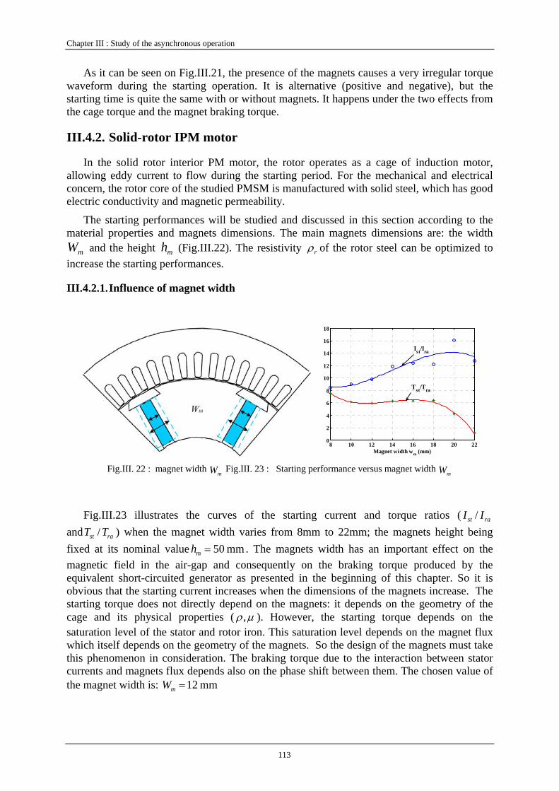
Chapter III : Study of the asynchronous operation
113
As it can be seen on Fig.III.21, the presence of the magnets causes a very irregular torque waveform during the starting operation. It is alternative (positive and negative), but the starting time is quite the same with or without magnets. It happens under the two effects from the cage torque and the magnet braking torque.
III.4.2. Solid-rotor IPM motor
In the solid rotor interior PM motor, the rotor operates as a cage of induction motor, allowing eddy current to flow during the starting period. For the mechanical and electrical concern, the rotor core of the studied PMSM is manufactured with solid steel, which has good electric conductivity and magnetic permeability.
The starting performances will be studied and discussed in this section according to the material properties and magnets dimensions. The main magnets dimensions are: the width
mW and the height mh (Fig.III.22). The resistivity rρ of the rotor steel can be optimized to increase the starting performances.
III.4.2.1. Influence of magnet width
8 10 12 14 16 18 20 220
2
4
6
8
10
12
14
16
18
Magnet width wm (mm)
Ist/Ira
Tst/Tra
Fig.III. 22 : magnet width
mW Fig.III. 23 : Starting performance versus magnet width mW
Fig.III.23 illustrates the curves of the starting current and torque ratios ( rast II / and rast TT / ) when the magnet width varies from 8mm to 22mm; the magnets height being fixed at its nominal value mm 50=mh . The magnets width has an important effect on the magnetic field in the air-gap and consequently on the braking torque produced by the equivalent short-circuited generator as presented in the beginning of this chapter. So it is obvious that the starting current increases when the dimensions of the magnets increase. The starting torque does not directly depend on the magnets: it depends on the geometry of the cage and its physical properties ( μρ , ). However, the starting torque depends on the saturation level of the stator and rotor iron. This saturation level depends on the magnet flux which itself depends on the geometry of the magnets. So the design of the magnets must take this phenomenon in consideration. The braking torque due to the interaction between stator currents and magnets flux depends also on the phase shift between them. The chosen value of the magnet width is: mm 12=mW
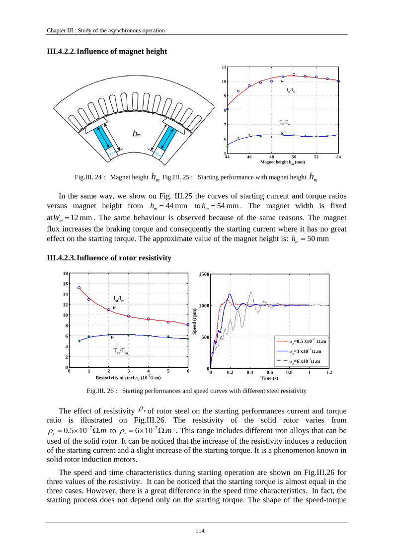
Chapter III : Study of the asynchronous operation
114
III.4.2.2. Influence of magnet height
44 46 48 50 52 545
6
7
8
9
10
11
Magnet height hm (mm)
Ist/Ira
Tst/Tra
Fig.III. 24 : Magnet height mh Fig.III. 25 : Starting performance with magnet height mh
In the same way, we show on Fig. III.25 the curves of starting current and torque ratios versus magnet height from mm 44=mh to mm 54=mh . The magnet width is fixed at mm 12=mW . The same behaviour is observed because of the same reasons. The magnet flux increases the braking torque and consequently the starting current where it has no great effect on the starting torque. The approximate value of the magnet height is: mm 50=mh
III.4.2.3. Influence of rotor resistivity
0 1 2 3 4 5 60
2
4
6
8
10
12
14
16
18
Resistivity of steel ρr (10-7Ω .m)
Ist/Ira
Tst/Tra
0 0.2 0.4 0.6 0.8 1 1.20
500
1000
1500
Time (s)
Spee
d (r
pm)
ρr=0.5 x10⁻⁷ Ω .m
ρr=3 x10⁻⁷ Ω .m
ρr=6 x10⁻⁷Ω .m
Fig.III. 26 : Starting performances and speed curves with different steel resistivity
The effect of resistivity rρ of rotor steel on the starting performances current and torque ratio is illustrated on Fig.III.26. The resistivity of the solid rotor varies from
mr .105.0 7Ω×= −ρ to mr .106 7Ω×= −ρ . This range includes different iron alloys that can be used of the solid rotor. It can be noticed that the increase of the resistivity induces a reduction of the starting current and a slight increase of the starting torque. It is a phenomenon known in solid rotor induction motors.
The speed and time characteristics during starting operation are shown on Fig.III.26 for three values of the resistivity. It can be noticed that the starting torque is almost equal in the three cases. However, there is a great difference in the speed time characteristics. In fact, the starting process does not depend only on the starting torque. The shape of the speed-torque
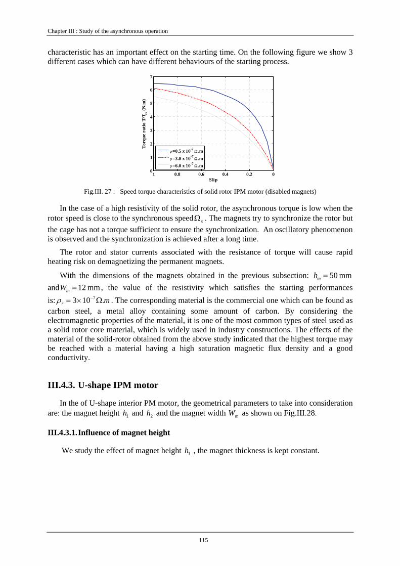
Chapter III : Study of the asynchronous operation
115
characteristic has an important effect on the starting time. On the following figure we show 3 different cases which can have different behaviours of the starting process.
00.20.40.60.810
1
2
3
4
5
6
7
Slip
Torq
ue r
atio
T/T
ra (N
.m)
ρ=0.5 x 10⁻⁷ Ω .mρ=3.0 x 10⁻⁷ Ω .mρ=6.0 x 10⁻⁷ Ω .m
Fig.III. 27 : Speed torque characteristics of solid rotor IPM motor (disabled magnets)
In the case of a high resistivity of the solid rotor, the asynchronous torque is low when the rotor speed is close to the synchronous speed sΩ . The magnets try to synchronize the rotor but the cage has not a torque sufficient to ensure the synchronization. An oscillatory phenomenon is observed and the synchronization is achieved after a long time.
The rotor and stator currents associated with the resistance of torque will cause rapid heating risk on demagnetizing the permanent magnets.
With the dimensions of the magnets obtained in the previous subsection: mm 50=mh and mm 12=mW , the value of the resistivity which satisfies the starting performances is: mr .103 7Ω×= −ρ . The corresponding material is the commercial one which can be found as carbon steel, a metal alloy containing some amount of carbon. By considering the electromagnetic properties of the material, it is one of the most common types of steel used as a solid rotor core material, which is widely used in industry constructions. The effects of the material of the solid-rotor obtained from the above study indicated that the highest torque may be reached with a material having a high saturation magnetic flux density and a good conductivity.
III.4.3. U-shape IPM motor
In the of U-shape interior PM motor, the geometrical parameters to take into consideration are: the magnet height 1h and 2h and the magnet width mW as shown on Fig.III.28.
III.4.3.1. Influence of magnet height
We study the effect of magnet height 1h , the magnet thickness is kept constant.
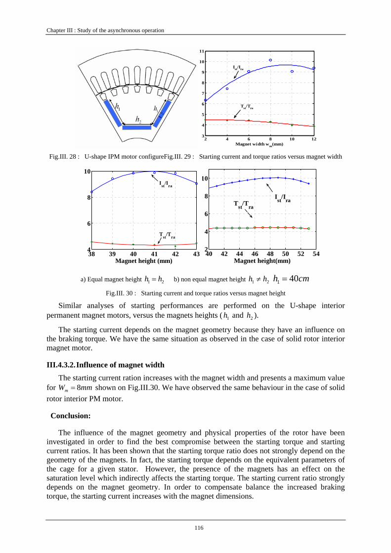
Chapter III : Study of the asynchronous operation
116
2 4 6 8 10 123
4
5
6
7
8
9
10
11
Magnet width wm(mm)
Ist/Ira
Tst/Tra
Fig.III. 28 : U-shape IPM motor configureFig.III. 29 : Starting current and torque ratios versus magnet width
38 39 40 41 42 434
6
8
10
Magnet height (mm)
Ist/Ira
Tst/Tra
40 42 44 46 48 50 52 542
4
6
8
10
Magnet height(mm)
Tst/Tra
Ist/Ira
a) Equal magnet height 21 hh = b) non equal magnet height 21 hh ≠ cmh 401 =
Fig.III. 30 : Starting current and torque ratios versus magnet height
Similar analyses of starting performances are performed on the U-shape interior permanent magnet motors, versus the magnets heights ( 1h and 2h ).
The starting current depends on the magnet geometry because they have an influence on the braking torque. We have the same situation as observed in the case of solid rotor interior magnet motor.
III.4.3.2. Influence of magnet width
The starting current ration increases with the magnet width and presents a maximum value for mmWm 8= shown on Fig.III.30. We have observed the same behaviour in the case of solid rotor interior PM motor.
Conclusion:
The influence of the magnet geometry and physical properties of the rotor have been investigated in order to find the best compromise between the starting torque and starting current ratios. It has been shown that the starting torque ratio does not strongly depend on the geometry of the magnets. In fact, the starting torque depends on the equivalent parameters of the cage for a given stator. However, the presence of the magnets has an effect on the saturation level which indirectly affects the starting torque. The starting current ratio strongly depends on the magnet geometry. In order to compensate balance the increased braking torque, the starting current increases with the magnet dimensions.

Chapter III : Study of the asynchronous operation
117
III.5. Steady state performances: power factor and efficiency
We have reviewed the starting performances of the three machines and some theoretic conclusions have been drawn. The motors operate most of time at steady state and therefore, their performances at steady state are of great importance. In the chapter 2, we have already studied the synchronous operation regardless of the self-starting techniques. In fact, when they operate at steady state, these techniques have no effect on the steady state performances.
In this part, we will analyse the parameters of steady-state operation of the motors with time-stepping finite element method. The study of performance consists in the analysis of the external variables (currents, voltage, power…) at the last periods of the electrical simulation as shown in section III.3.2.2. The study is focused on the influence of geometrical parameters on the power factor and efficiency at steady state.
III.5.1. Surface-inset PM motor
40 45 50 550.7
0.75
0.8
0.85
0.9
0.95
1
1.05
1.1
Magnet span (°)
Power factor
Efficiency
0 0.5 1 1.5 2 2.5 3 3.5 4 4.50
0.2
0.4
0.6
0.8
1
Thickness of alumium (mm)
Power factor
Efficiency
Fig.III. 31: Power factor and efficiency with magnet span Fig.III. 32 : Power factor and efficiency with
thickness of aluminum
In these simulations, the thickness of aluminium ring is 1mm. We show on Fig.III.31 that the efficiency and the power factor increase with the magnet span. This situation is predictable because the flux grows almost proportionally to the magnet size.
The thickness of the aluminium ring has an important effect on the steady state performances (power factor and efficiency). In fact, it increases the magnetic equivalent air-gap and induces a reduction of the air-gap flux density, which leads to poor power factor and efficiency (Fig. III.32). It is difficult to get good steady state performances without scarifying the synchronization capability. To balance the requirement of power factor and the starting process, the magnet span was selected as 41° and thickness of aluminium as 1mm. The magnet span 50° should have been chosen since the power factor is near to the unit with this value. But it arises the problem that the starting current ratio is larger than 10, which exceed the permitted value.

Chapter III : Study of the asynchronous operation
118
III.5.2. Solid-rotor IPM motor
44 46 48 50 52 540.7
0.75
0.8
0.85
0.9
0.95
1
1.05
1.1
Magnet height hm (mm)
Power factor
Efficiency
4 6 8 10 12 14 16 18 200.7
0.75
0.8
0.85
0.9
0.95
1
Magnet width wm (mm)
Power factor
Efficiency
Fig.III. 33 : Power factor and efficiency versus magnet width and height
44 46 48 50 52 5435
36
37
38
39
40
Phas
e cu
rren
t(A
)
Magnet height hm (mm)0 5 10 15 20 25
35
40
45
50
55
60
Magnet width wm(mm)
Phas
e cu
rren
t (A
)
Fig.III. 34 : Phase current versus magnet height
We have seen in the above sections that the minimisation of magnet braking torque can result from the minimization of magnet material. But the magnets are the source of the flux in steady state operation and they affect the steady state performances. In this section we compute the performances of the machine in terms of efficiency and power factor according to the two geometrical parameters of the inset PMs (Fig. III.33) On Fig.III.34, we show the curves of stator current versus magnets geometry. It can be seen that there is an optimal value of the magnet dimension as width mmWm 12= and height mmhm 50= which lead to the highest power factor and thus the lowest line current. This behaviour is similar to the self-reactive power operation well known in wound synchronous motor and illustrated by Mordey’s V-curves (Fig.III.34).
When the motor operates at synchronous speed, the resistivity of steel has almost no effect to the power factor as shown in FigIII.34, since there is almost no eddy current in the rotor. However, the presence of space harmonics of the stator equivalent current sheet leads to eddy currents on the surface of the solid rotor; they are mainly due to the 5th and 7th space harmonics which create eddy currents of pulsation ω6 in the rotor. Increasing the rotor resistivity reduces the eddy current losses in the rotor and consequently increases the efficiency of the motor.
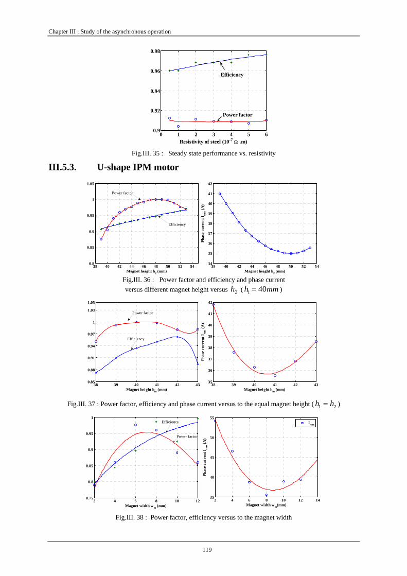
Chapter III : Study of the asynchronous operation
119
0 1 2 3 4 5 60.9
0.92
0.94
0.96
0.98
Resistivity of steel (10-7 Ω .m)
Efficiency
Power factor
Fig.III. 35 : Steady state performance vs. resistivity
III.5.3. U-shape IPM motor
38 40 42 44 46 48 50 52 540.8
0.85
0.9
0.95
1
1.05
Magnet height h2 (mm)
Power factor
Efficiency
38 40 42 44 46 48 50 52 5434
35
36
37
38
39
40
41
42
Phas
e cu
rren
t Irm
s (A)
Magnet height h2 (mm) Fig.III. 36 : Power factor and efficiency and phase current versus different magnet height versus 2h ( mmh 401 = )
38 39 40 41 42 430.85
0.88
0.91
0.94
0.97
1
1.03
1.05
Magnet height hm (mm)
Power factor
Efficiency
38 39 40 41 42 4335
36
37
38
39
40
41
42
Phas
e cu
rren
t Irm
s (A)
Magnet height hm (mm) Fig.III. 37 : Power factor, efficiency and phase current versus to the equal magnet height ( 21 hh = )
2 4 6 8 10 120.75
0.8
0.85
0.9
0.95
1
Magnet width wm (mm)
Power factor
Efficiency
2 4 6 8 10 12 1435
40
45
50
55
Magnet width wm(mm)
Phas
e cu
rren
t Irm
s (A)
Irms
Fig.III. 38 : Power factor, efficiency versus to the magnet width
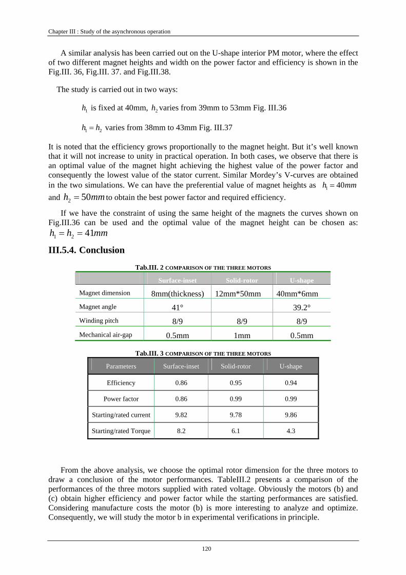
Chapter III : Study of the asynchronous operation
120
A similar analysis has been carried out on the U-shape interior PM motor, where the effect of two different magnet heights and width on the power factor and efficiency is shown in the Fig.III. 36, Fig.III. 37. and Fig.III.38.
The study is carried out in two ways:
1h is fixed at 40mm, 2h varies from 39mm to 53mm Fig. III.36
21 hh = varies from 38mm to 43mm Fig. III.37
It is noted that the efficiency grows proportionally to the magnet height. But it’s well known that it will not increase to unity in practical operation. In both cases, we observe that there is an optimal value of the magnet hight achieving the highest value of the power factor and consequently the lowest value of the stator current. Similar Mordey’s V-curves are obtained in the two simulations. We can have the preferential value of magnet heights as mmh 401 = and mmh 502 = to obtain the best power factor and required efficiency.
If we have the constraint of using the same height of the magnets the curves shown on Fig.III.36 can be used and the optimal value of the magnet height can be chosen as:
mmhh 4121 ==
III.5.4. Conclusion
Tab.III. 2 COMPARISON OF THE THREE MOTORS
Surface-inset Solid-rotor U-shape
Magnet dimension 8mm(thickness) 12mm*50mm 40mm*6mm Magnet angle 41° 39.2° Winding pitch 8/9 8/9 8/9 Mechanical air-gap 0.5mm 1mm 0.5mm
Tab.III. 3 COMPARISON OF THE THREE MOTORS
Parameters Surface-inset Solid-rotor U-shape
Efficiency 0.86 0.95 0.94
Power factor 0.86 0.99 0.99
Starting/rated current 9.82 9.78 9.86
Starting/rated Torque 8.2 6.1 4.3
From the above analysis, we choose the optimal rotor dimension for the three motors to draw a conclusion of the motor performances. TableIII.2 presents a comparison of the performances of the three motors supplied with rated voltage. Obviously the motors (b) and (c) obtain higher efficiency and power factor while the starting performances are satisfied. Considering manufacture costs the motor (b) is more interesting to analyze and optimize. Consequently, we will study the motor b in experimental verifications in principle.
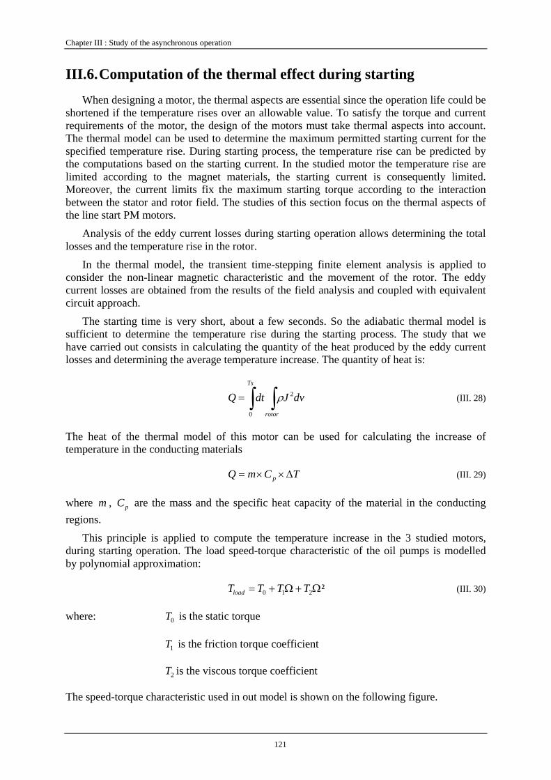
Chapter III : Study of the asynchronous operation
121
III.6. Computation of the thermal effect during starting
When designing a motor, the thermal aspects are essential since the operation life could be shortened if the temperature rises over an allowable value. To satisfy the torque and current requirements of the motor, the design of the motors must take thermal aspects into account. The thermal model can be used to determine the maximum permitted starting current for the specified temperature rise. During starting process, the temperature rise can be predicted by the computations based on the starting current. In the studied motor the temperature rise are limited according to the magnet materials, the starting current is consequently limited. Moreover, the current limits fix the maximum starting torque according to the interaction between the stator and rotor field. The studies of this section focus on the thermal aspects of the line start PM motors.
Analysis of the eddy current losses during starting operation allows determining the total losses and the temperature rise in the rotor.
In the thermal model, the transient time-stepping finite element analysis is applied to consider the non-linear magnetic characteristic and the movement of the rotor. The eddy current losses are obtained from the results of the field analysis and coupled with equivalent circuit approach.
The starting time is very short, about a few seconds. So the adiabatic thermal model is sufficient to determine the temperature rise during the starting process. The study that we have carried out consists in calculating the quantity of the heat produced by the eddy current losses and determining the average temperature increase. The quantity of heat is:
dvJdtQTs
rotor∫ ∫=0
2ρ (III. 28)
The heat of the thermal model of this motor can be used for calculating the increase of temperature in the conducting materials
TCmQ p Δ××= (III. 29)
where m , pC are the mass and the specific heat capacity of the material in the conducting regions.
This principle is applied to compute the temperature increase in the 3 studied motors, during starting operation. The load speed-torque characteristic of the oil pumps is modelled by polynomial approximation:
²210 Ω+Ω+= TTTTload (III. 30)
where: 0T is the static torque
1T is the friction torque coefficient
2T is the viscous torque coefficient
The speed-torque characteristic used in out model is shown on the following figure.
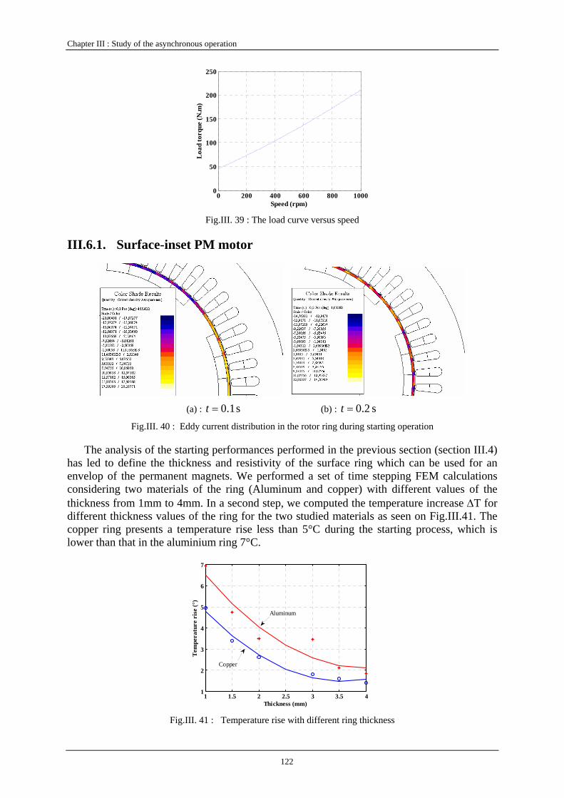
Chapter III : Study of the asynchronous operation
122
0 200 400 600 800 10000
50
100
150
200
250
Speed (rpm)Lo
ad to
rque
(N.m
)
Fig.III. 39 : The load curve versus speed
III.6.1. Surface-inset PM motor
(a) : s 1.0=t (b) : s 2.0=t
Fig.III. 40 : Eddy current distribution in the rotor ring during starting operation
The analysis of the starting performances performed in the previous section (section III.4) has led to define the thickness and resistivity of the surface ring which can be used for an envelop of the permanent magnets. We performed a set of time stepping FEM calculations considering two materials of the ring (Aluminum and copper) with different values of the thickness from 1mm to 4mm. In a second step, we computed the temperature increase ΔT for different thickness values of the ring for the two studied materials as seen on Fig.III.41. The copper ring presents a temperature rise less than 5°C during the starting process, which is lower than that in the aluminium ring 7°C.
1 1.5 2 2.5 3 3.5 41
2
3
4
5
6
7
Thickness (mm)
Tem
pera
ture
ris
e (°
)
Aluminum
Copper
Fig.III. 41 : Temperature rise with different ring thickness
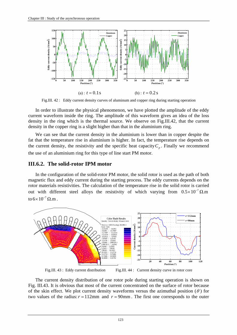
Chapter III : Study of the asynchronous operation
123
0 50 100 150 200 250 300 350-150
-100
-50
0
50
100
150
Position (°)
Eddy
cur
rent
den
sity
(A/m
m2 )
AluminumCopper
0 50 100 150 200 250 300 350-25
-20
-15
-10
-5
0
5
10
15
20
25
Position (°)
Eddy
cur
rent
den
sity
(A/m
m2 )
AluminumCopper
(a) : s 1.0=t (b) : s 2.0=t
Fig.III. 42 : Eddy current density curves of aluminum and copper ring during starting operation
In order to illustrate the physical phenomenon, we have plotted the amplitude of the eddy current waveform inside the ring. The amplitude of this waveform gives an idea of the loss density in the ring which is the thermal source. We observe on Fig.III.42, that the current density in the copper ring is a slight higher than that in the aluminium ring.
We can see that the current density in the aluminium is lower than in copper despite the fat that the temperature rise in aluminium is higher. In fact, the temperature rise depends on the current density, the resistivity and the specific heat capacity pC . Finally we recommend the use of an aluminium ring for this type of line start PM motor.
III.6.2. The solid-rotor IPM motor
In the configuration of the solid-rotor PM motor, the solid rotor is used as the path of both magnetic flux and eddy current during the starting process. The eddy currents depends on the rotor materials resistivities. The calculation of the temperature rise in the solid rotor is carried out with different steel alloys the resistivity of which varying from Ω.m105.0 7−× to Ω.m106 7−× .
Color Shade ResultsQuantity : Current density A/(square mm) Time (s.) : 0,005 Pos (deg): 205,98E-3Scale / Color-21,01293 / -18,3851-18,3851 / -15,75907-15,75907 / -13,13214-13,13214 / -10,50521-10,50521 / -7,87829-7,87829 / -5,25136-5,25136 / -2,62443-2,62443 / 2,49672E-32,49672E-3 / 2,629422,62942 / 5,256355,25635 / 7,883287,88328 / 10,5102110,51021 / 13,1371413,13714 / 15,7640615,76406 / 18,3909918,39099 / 21,01792
20 40 60 80 100 120-25
-20
-15
-10
-5
0
5
10
15
20
25
Position (°)
Cur
rent
den
sity
(A/m
m2 )
r=112mm
r=90mm
Fig.III. 43 : Eddy current distribution Fig.III. 44 : Current density curve in rotor core
The current density distribution of one rotor pole during starting operation is shown on Fig. III.43. It is obvious that most of the current concentrated on the surface of rotor because of the skin effect. We plot current density waveforms versus the azimuthal position (θ ) for two values of the radius: mm112=r and mm90=r . The first one corresponds to the outer
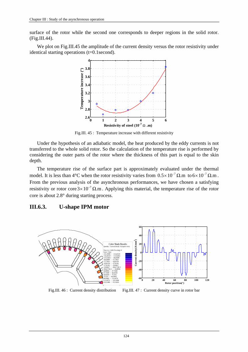
Chapter III : Study of the asynchronous operation
124
surface of the rotor while the second one corresponds to deeper regions in the solid rotor. (Fig.III.44).
We plot on Fig.III.45 the amplitude of the current density versus the rotor resistivity under identical starting operations (t=0.1second).
0 1 2 3 4 5 62.6
2.8
3
3.2
3.4
3.6
3.8
4
Tem
pera
ture
incr
ease
(°)
Resistivity of steel (10-7 Ω .m) Fig.III. 45 : Temperature increase with different resistivity
Under the hypothesis of an adiabatic model, the heat produced by the eddy currents is not transferred to the whole solid rotor. So the calculation of the temperature rise is performed by considering the outer parts of the rotor where the thickness of this part is equal to the skin depth.
The temperature rise of the surface part is approximately evaluated under the thermal model. It is less than 4°C when the rotor resistivity varies from Ω.m105.0 7−× to Ω.m106 7−× . From the previous analysis of the asynchronous performances, we have chosen a satisfying resistivity or rotor core Ω.m103 7−× . Applying this material, the temperature rise of the rotor core is about 2.8° during starting process.
III.6.3. U-shape IPM motor
Color Shade ResultsQuantity : Current density A/(square mm) Time (s.) : 0,001 Pos (deg): 0Scale / Color-151,35985 / -132,45219-132,45219 / -113,54454-113,54454 / -94,63689-94,63689 / -75,72923-75,72923 / -56,82158-56,82158 / -37,91393-37,91393 / -19,00627-19,00627 / -98,61755E-3-98,61755E-3 / 18,8090418,80904 / 37,7166937,71669 / 56,6243456,62434 / 75,531175,5311 / 94,4396594,43965 / 113,34731113,34731 / 132,25496132,25496 / 151,16263
0 20 40 60 80 100 120-60
-40
-20
0
20
40
60
Rotor position(°)
Cur
rent
den
sity
(A/m
m2 )
Fig.III. 46 : Current density distribution Fig.III. 47 : Current density curve in rotor bar
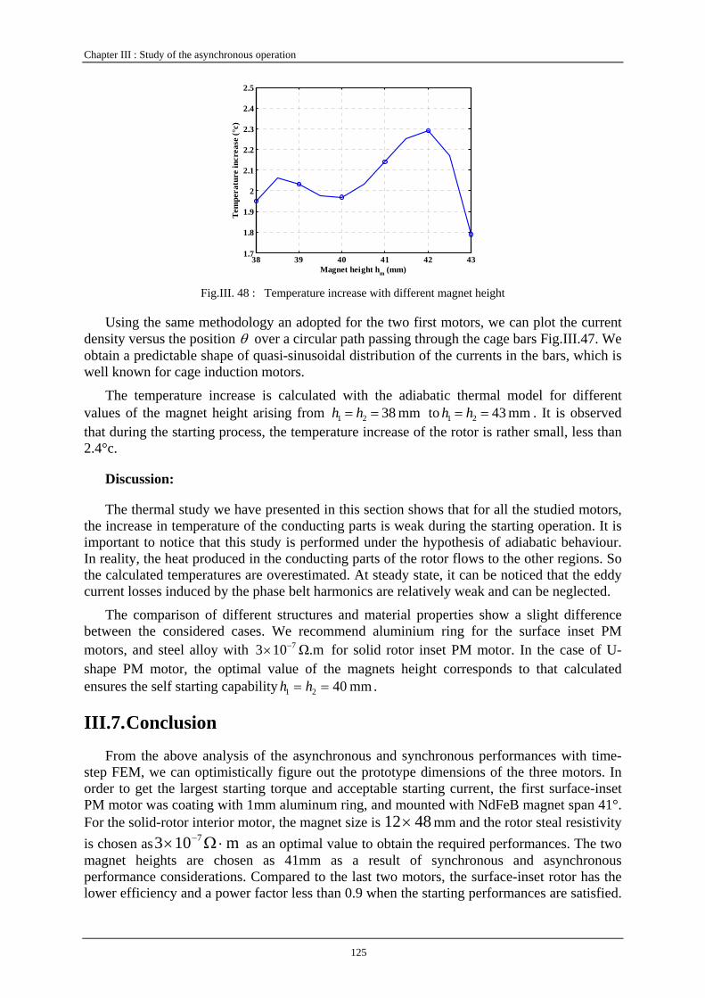
Chapter III : Study of the asynchronous operation
125
38 39 40 41 42 431.7
1.8
1.9
2
2.1
2.2
2.3
2.4
2.5
Tem
pera
ture
incr
ease
(°c)
Magnet height hm (mm) Fig.III. 48 : Temperature increase with different magnet height
Using the same methodology an adopted for the two first motors, we can plot the current density versus the position θ over a circular path passing through the cage bars Fig.III.47. We obtain a predictable shape of quasi-sinusoidal distribution of the currents in the bars, which is well known for cage induction motors.
The temperature increase is calculated with the adiabatic thermal model for different values of the magnet height arising from mm 3821 == hh to mm 4321 == hh . It is observed that during the starting process, the temperature increase of the rotor is rather small, less than 2.4°c.
Discussion:
The thermal study we have presented in this section shows that for all the studied motors, the increase in temperature of the conducting parts is weak during the starting operation. It is important to notice that this study is performed under the hypothesis of adiabatic behaviour. In reality, the heat produced in the conducting parts of the rotor flows to the other regions. So the calculated temperatures are overestimated. At steady state, it can be noticed that the eddy current losses induced by the phase belt harmonics are relatively weak and can be neglected.
The comparison of different structures and material properties show a slight difference between the considered cases. We recommend aluminium ring for the surface inset PM motors, and steel alloy with Ω.m103 7−× for solid rotor inset PM motor. In the case of U-shape PM motor, the optimal value of the magnets height corresponds to that calculated ensures the self starting capability mm 4021 == hh .
III.7. Conclusion
From the above analysis of the asynchronous and synchronous performances with time-step FEM, we can optimistically figure out the prototype dimensions of the three motors. In order to get the largest starting torque and acceptable starting current, the first surface-inset PM motor was coating with 1mm aluminum ring, and mounted with NdFeB magnet span 41°. For the solid-rotor interior motor, the magnet size is 4812× mm and the rotor steal resistivity is chosen as m103 7 ⋅Ω× − as an optimal value to obtain the required performances. The two magnet heights are chosen as 41mm as a result of synchronous and asynchronous performance considerations. Compared to the last two motors, the surface-inset rotor has the lower efficiency and a power factor less than 0.9 when the starting performances are satisfied.
Chapter III : Study of the asynchronous operation
126
The interior PM motors present a near unity power factor and efficiency more than 0.93. For commercial consideration, the interior motors are preferable, while the solid-rotor PM motor is easier to manufacture.
With respect to thermal effect, the temperature was calculated with traditional methods during the starting process. The calculated temperature rise of the surface-inset PM motor was less than 8°C, while the interior motors are less than 4°C. These temperature rises, however, are not very reliable because they show only local temperatures and we didn’t consider the cooling system. But they provide a heating reference which should be taken into account when designing the rotor main dimensions.

Chapter IV :
Experimental validation

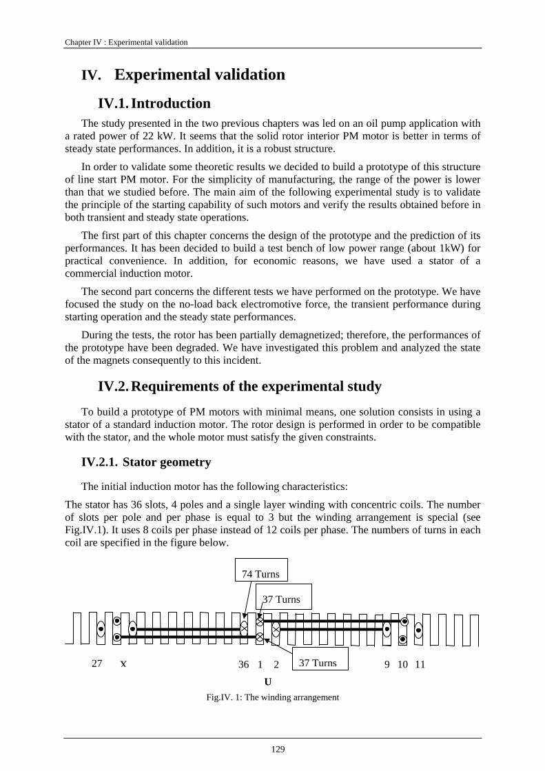
Chapter IV : Experimental validation
129
IV. Experimental validation
IV.1. Introduction The study presented in the two previous chapters was led on an oil pump application with
a rated power of 22 kW. It seems that the solid rotor interior PM motor is better in terms of steady state performances. In addition, it is a robust structure.
In order to validate some theoretic results we decided to build a prototype of this structure of line start PM motor. For the simplicity of manufacturing, the range of the power is lower than that we studied before. The main aim of the following experimental study is to validate the principle of the starting capability of such motors and verify the results obtained before in both transient and steady state operations.
The first part of this chapter concerns the design of the prototype and the prediction of its performances. It has been decided to build a test bench of low power range (about 1kW) for practical convenience. In addition, for economic reasons, we have used a stator of a commercial induction motor.
The second part concerns the different tests we have performed on the prototype. We have focused the study on the no-load back electromotive force, the transient performance during starting operation and the steady state performances.
During the tests, the rotor has been partially demagnetized; therefore, the performances of the prototype have been degraded. We have investigated this problem and analyzed the state of the magnets consequently to this incident.
IV.2. Requirements of the experimental study
To build a prototype of PM motors with minimal means, one solution consists in using a stator of a standard induction motor. The rotor design is performed in order to be compatible with the stator, and the whole motor must satisfy the given constraints.
IV.2.1. Stator geometry
The initial induction motor has the following characteristics:
The stator has 36 slots, 4 poles and a single layer winding with concentric coils. The number of slots per pole and per phase is equal to 3 but the winding arrangement is special (see Fig.IV.1). It uses 8 coils per phase instead of 12 coils per phase. The numbers of turns in each coil are specified in the figure below.
Fig.IV. 1: The winding arrangement
1 2 9 10 11 36
74 Turns
37 Turns
2928
U
27 X 37 Turns
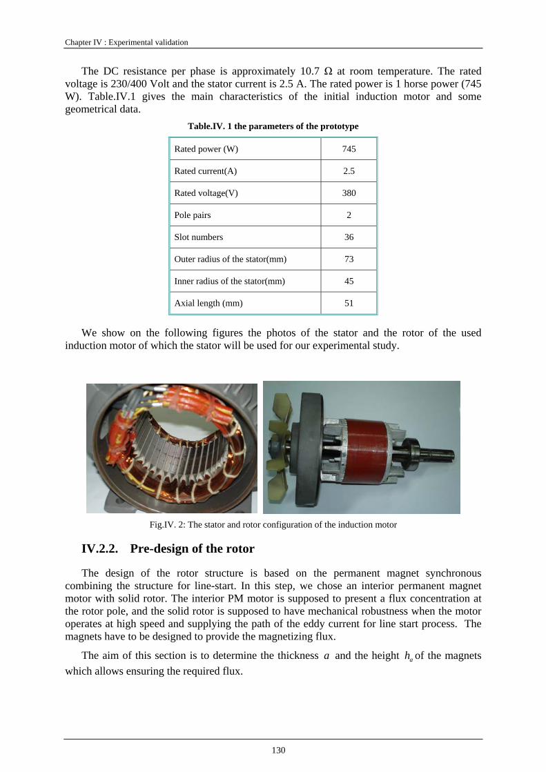
Chapter IV : Experimental validation
130
The DC resistance per phase is approximately 10.7 Ω at room temperature. The rated voltage is 230/400 Volt and the stator current is 2.5 A. The rated power is 1 horse power (745 W). Table.IV.1 gives the main characteristics of the initial induction motor and some geometrical data.
Table.IV. 1 the parameters of the prototype
Rated power (W) 745
Rated current(A) 2.5
Rated voltage(V) 380
Pole pairs 2
Slot numbers 36
Outer radius of the stator(mm) 73
Inner radius of the stator(mm) 45
Axial length (mm) 51
We show on the following figures the photos of the stator and the rotor of the used induction motor of which the stator will be used for our experimental study.
Fig.IV. 2: The stator and rotor configuration of the induction motor
IV.2.2. Pre-design of the rotor
The design of the rotor structure is based on the permanent magnet synchronous combining the structure for line-start. In this step, we chose an interior permanent magnet motor with solid rotor. The interior PM motor is supposed to present a flux concentration at the rotor pole, and the solid rotor is supposed to have mechanical robustness when the motor operates at high speed and supplying the path of the eddy current for line start process. The magnets have to be designed to provide the magnetizing flux.
The aim of this section is to determine the thickness a and the height ah of the magnets which allows ensuring the required flux.

Chapter IV : Experimental validation
131
aha
Fig.IV. 3: The pre-designed rotor configuration prototype
Air-gap: The air-gap determines the outer diameter of the rotor. It is an important parameter for both starting capabilities and performances at rated speed. Large air-gaps smooth the flux form and reduce the harmonic effects but also reduce the flux density in air-gap and hence influence the back-EMF. The assembling procedure is difficult if the air-gap is too small and also may raise the friction losses at rated operation. Bear in mind the above consideration, the air-gap was fixed to mme 5.0= .
Air-gap flux density:
We assume the following hypotheses:
• The iron has an infinite magnetic permeability
• The equivalent magnetic air-gap is : eke c ⋅=′ , where ck is the Carter coefficient
• All the flux of the magnets magψ passes through the air-gap (no leakage flux).
By using Ampere’s theorem and flux conservation principle, we can determine the air-gap flux density as a function of the geometrical parameters of the magnets by the following expression:
ae
ssBB
a
pre '2
2
1
+×= (IV. 1)
where ps and as are the pole and magnet surfaces respectively and rB is the remanence of the magnets.
If we consider that the magnets have a relative permeability 1≈aμ and if only special part of the magnetic flux ( ( ) magψσ−1 ) passes through the air-gap, the flux leakage is
then: magleakage σψψ = and equation IV.1 becomes:
ae
ssBB
aa
pre '2
2)1(
1
μσ
+−
×= (IV. 2)
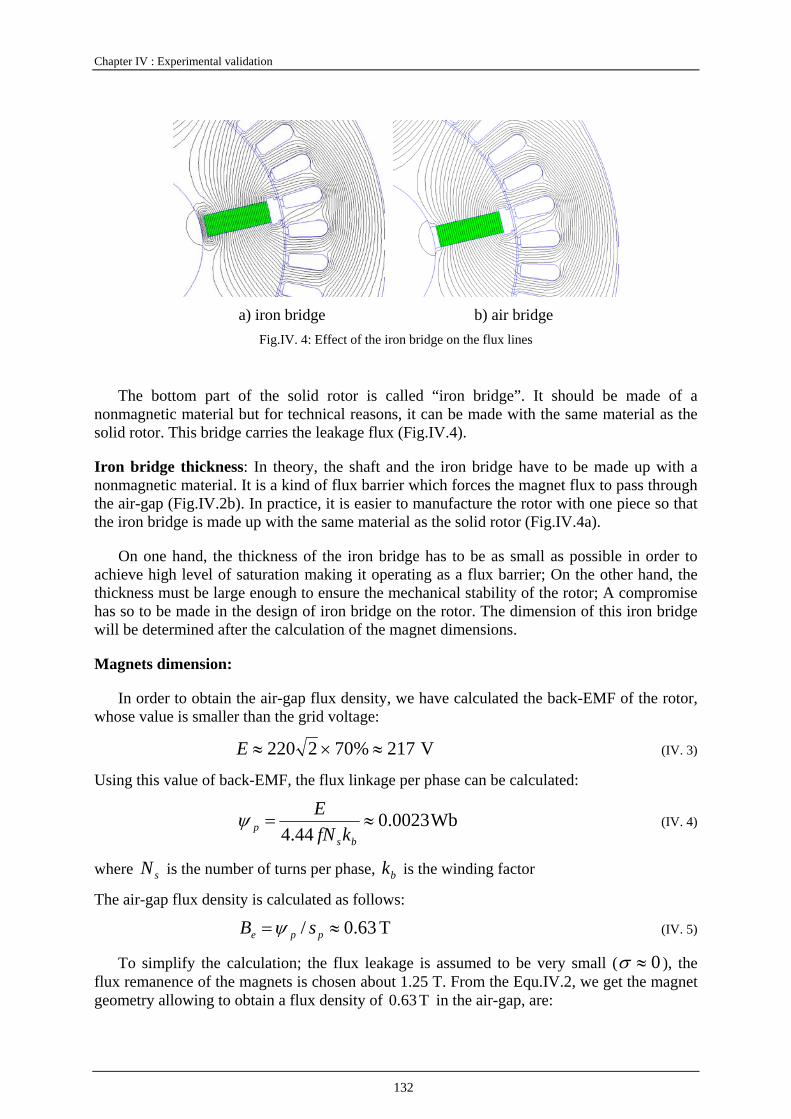
Chapter IV : Experimental validation
132
a) iron bridge b) air bridge
Fig.IV. 4: Effect of the iron bridge on the flux lines
The bottom part of the solid rotor is called “iron bridge”. It should be made of a nonmagnetic material but for technical reasons, it can be made with the same material as the solid rotor. This bridge carries the leakage flux (Fig.IV.4).
Iron bridge thickness: In theory, the shaft and the iron bridge have to be made up with a nonmagnetic material. It is a kind of flux barrier which forces the magnet flux to pass through the air-gap (Fig.IV.2b). In practice, it is easier to manufacture the rotor with one piece so that the iron bridge is made up with the same material as the solid rotor (Fig.IV.4a).
On one hand, the thickness of the iron bridge has to be as small as possible in order to achieve high level of saturation making it operating as a flux barrier; On the other hand, the thickness must be large enough to ensure the mechanical stability of the rotor; A compromise has so to be made in the design of iron bridge on the rotor. The dimension of this iron bridge will be determined after the calculation of the magnet dimensions.
Magnets dimension:
In order to obtain the air-gap flux density, we have calculated the back-EMF of the rotor, whose value is smaller than the grid voltage:
V217%702220 ≈×≈E (IV. 3)
Using this value of back-EMF, the flux linkage per phase can be calculated:
Wb0023.044.4
≈=bs
p kfNEψ (IV. 4)
where sN is the number of turns per phase, bk is the winding factor
The air-gap flux density is calculated as follows:
T 63.0/ ≈= ppe sB ψ (IV. 5)
To simplify the calculation; the flux leakage is assumed to be very small ( 0≈σ ), the flux remanence of the magnets is chosen about 1.25 T. From the Equ.IV.2, we get the magnet geometry allowing to obtain a flux density of T 63.0 in the air-gap, are:
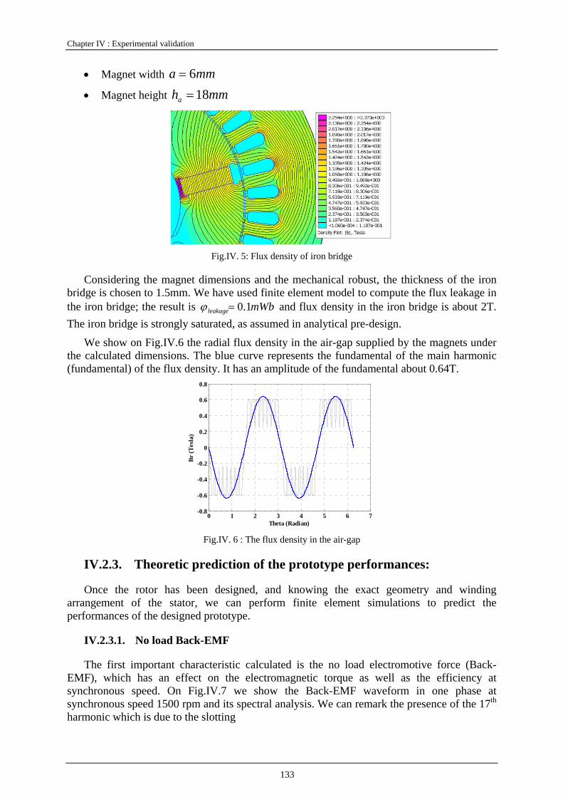
Chapter IV : Experimental validation
133
• Magnet width mma 6=
• Magnet height mmha 18=
Fig.IV. 5: Flux density of iron bridge
Considering the magnet dimensions and the mechanical robust, the thickness of the iron bridge is chosen to 1.5mm. We have used finite element model to compute the flux leakage in the iron bridge; the result is mWbleakage 1.0=ϕ and flux density in the iron bridge is about 2T. The iron bridge is strongly saturated, as assumed in analytical pre-design.
We show on Fig.IV.6 the radial flux density in the air-gap supplied by the magnets under the calculated dimensions. The blue curve represents the fundamental of the main harmonic (fundamental) of the flux density. It has an amplitude of the fundamental about 0.64T.
0 1 2 3 4 5 6 7-0.8
-0.6
-0.4
-0.2
0
0.2
0.4
0.6
0.8
Br (T
esla
)
Theta (Radian) Fig.IV. 6 : The flux density in the air-gap
IV.2.3. Theoretic prediction of the prototype performances:
Once the rotor has been designed, and knowing the exact geometry and winding arrangement of the stator, we can perform finite element simulations to predict the performances of the designed prototype.
IV.2.3.1. No load Back-EMF
The first important characteristic calculated is the no load electromotive force (Back-EMF), which has an effect on the electromagnetic torque as well as the efficiency at synchronous speed. On Fig.IV.7 we show the Back-EMF waveform in one phase at synchronous speed 1500 rpm and its spectral analysis. We can remark the presence of the 17th harmonic which is due to the slotting

Chapter IV : Experimental validation
134
. 0 5 10 15 20
-200
-150
-100
-50
0
50
100
150
200
Back
-EM
F(V
)
Time (ms)0 5 10 15 20 25 30
0
50
100
150
200
Back
-EM
F(V
)
Harmonic Fig.IV. 7: The back-EMF waveforms
IV.2.3.2. Starting performances
Transient operation of the line-start PM motor has been studied by time step finite element method coupled with circuit modelling, by using the software Flux2D. The starting characteristics are given in Fig.IV.8 to Fig.IV.10. We focus the study on the speed, the current and the torque during starting operation. On Fig.IV.11, we show the eddy currents distribution in the solid rotor at a given time during the starting operation ( st 2.0= )
With the chosen design, the motor should have the self-starting capability with a starting time of 0.2s and a starting current ratio close to 5.( 5/ ≈rast II ).
As shown in the previous chapter, the speed-time and torque-time characteristics present some oscillations during the acceleration period.
0 0.2 0.4 0.6 0.8 1 1.2 1.4-500
0
500
1000
1500
2000
Spee
d (r
pm)
Time (s) 0 0.2 0.4 0.6 0.8 1 1.2 1.4
-20
-15
-10
-5
0
5
10
15
20
Phas
e cu
rren
t (A
)
Time (s)
Fig.IV. 8: Speed during starting Fig.IV. 9: Phase current during starting
0 0.2 0.4 0.6 0.8 1 1.2 1.4-30
-20
-10
0
10
20
30
Elec
trom
agne
tic to
rque
(N.m
)
Time (s)
Color Shade ResultsQuantity : Current density A/(square mm) Time (s.) : 0.2 Pos (deg): 872.208Scale / Color-8.62527 / -7.5471-7.5471 / -6.46894-6.46894 / -5.39078-5.39078 / -4.31262-4.31262 / -3.23446-3.23446 / -2.1563-2.1563 / -1.07813-1.07813 / 27.65656E-627.65656E-6 / 1.078191.07819 / 2.156352.15635 / 3.234513.23451 / 4.312674.31267 / 5.390845.39084 / 6.46816.4681 / 7.547167.54716 / 8.62532
Fig.IV. 10: Magnetic torque during starting Fig.IV. 11: Eddy currents in the solid rotor
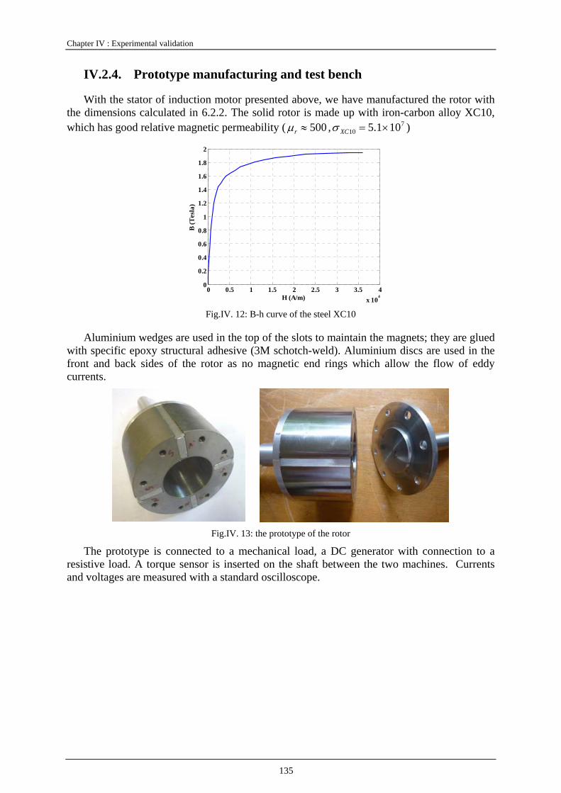
Chapter IV : Experimental validation
135
IV.2.4. Prototype manufacturing and test bench
With the stator of induction motor presented above, we have manufactured the rotor with the dimensions calculated in 6.2.2. The solid rotor is made up with iron-carbon alloy XC10, which has good relative magnetic permeability ( 500≈rμ , 7
10 101.5 ×=XCσ )
0 0.5 1 1.5 2 2.5 3 3.5 4x 10
4
0
0.2
0.4
0.6
0.8
1
1.2
1.4
1.6
1.8
2
B (T
esla
)
H (A/m) Fig.IV. 12: B-h curve of the steel XC10
Aluminium wedges are used in the top of the slots to maintain the magnets; they are glued with specific epoxy structural adhesive (3M schotch-weld). Aluminium discs are used in the front and back sides of the rotor as no magnetic end rings which allow the flow of eddy currents.
Fig.IV. 13: the prototype of the rotor
The prototype is connected to a mechanical load, a DC generator with connection to a resistive load. A torque sensor is inserted on the shaft between the two machines. Currents and voltages are measured with a standard oscilloscope.
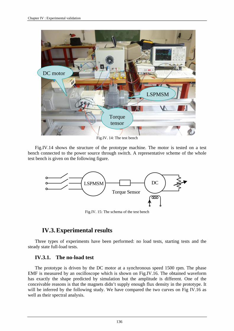
Chapter IV : Experimental validation
136
Fig.IV. 14: The test bench
Fig.IV.14 shows the structure of the prototype machine. The motor is tested on a test bench connected to the power source through switch. A representative scheme of the whole test bench is given on the following figure.
LSPMSM DC
Torque Sensor
Fig.IV. 15: The schema of the test bench
IV.3. Experimental results
Three types of experiments have been performed: no load tests, starting tests and the steady state full-load tests.
IV.3.1. The no-load test
The prototype is driven by the DC motor at a synchronous speed 1500 rpm. The phase EMF is measured by an oscilloscope which is shown on Fig.IV.16. The obtained waveform has exactly the shape predicted by simulation but the amplitude is different. One of the conceivable reasons is that the magnets didn’t supply enough flux density in the prototype. It will be inferred by the following study. We have compared the two curves on Fig IV.16 as well as their spectral analysis.
DC motor
LSPMSM
Torque tensor
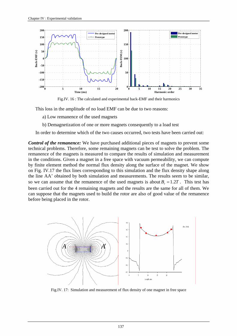
Chapter IV : Experimental validation
137
0 5 10 15 20-200
-150
-100
-50
0
50
100
150
200
Time (ms)
Back
-EM
F (v
)Pre-designed motorPrototype
0 5 10 15 20 25 30 350
50
100
150
200
Harmonic order
Back
-FEM
(v)
Pre-designed motorPrototype
Fig.IV. 16 : The calculated and experimental back-EMF and their harmonics
This loss in the amplitude of no load EMF can be due to two reasons:
a) Low remanence of the used magnets
b) Demagnetization of one or more magnets consequently to a load test
In order to determine which of the two causes occurred, two tests have been carried out:
Control of the remanence: We have purchased additional pieces of magnets to prevent some technical problems. Therefore, some remaining magnets can be test to solve the problem. The remanence of the magnets is measured to compare the results of simulation and measurement in the conditions. Given a magnet in a free space with vacuum permeability, we can compute by finite element method the normal flux density along the surface of the magnet. We show on Fig. IV.17 the flux lines corresponding to this simulation and the flux density shape along the line AA’ obtained by both simulation and measurements. The results seem to be similar, so we can assume that the remanence of the used magnets is about TBr 2.1= . This test has been carried out for the 4 remaining magnets and the results are the same for all of them. We can suppose that the magnets used to build the rotor are also of good value of the remanence before being placed in the rotor.
Fig.IV. 17: Simulation and measurement of flux density of one magnet in free space
A′A
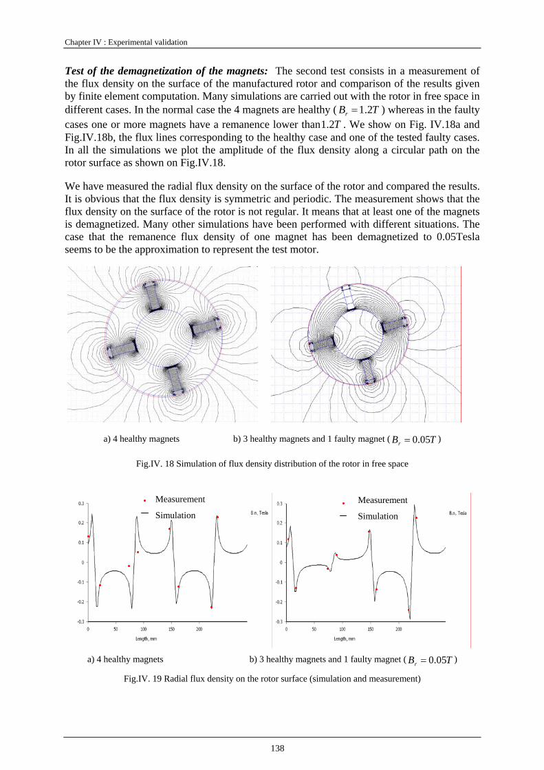
Chapter IV : Experimental validation
138
Test of the demagnetization of the magnets: The second test consists in a measurement of the flux density on the surface of the manufactured rotor and comparison of the results given by finite element computation. Many simulations are carried out with the rotor in free space in different cases. In the normal case the 4 magnets are healthy ( TBr 2.1= ) whereas in the faulty cases one or more magnets have a remanence lower than T2.1 . We show on Fig. IV.18a and Fig.IV.18b, the flux lines corresponding to the healthy case and one of the tested faulty cases. In all the simulations we plot the amplitude of the flux density along a circular path on the rotor surface as shown on Fig.IV.18.
We have measured the radial flux density on the surface of the rotor and compared the results. It is obvious that the flux density is symmetric and periodic. The measurement shows that the flux density on the surface of the rotor is not regular. It means that at least one of the magnets is demagnetized. Many other simulations have been performed with different situations. The case that the remanence flux density of one magnet has been demagnetized to 0.05Tesla seems to be the approximation to represent the test motor.
a) 4 healthy magnets b) 3 healthy magnets and 1 faulty magnet ( TBr 05.0= )
Fig.IV. 18 Simulation of flux density distribution of the rotor in free space
a) 4 healthy magnets b) 3 healthy magnets and 1 faulty magnet ( TBr 05.0= )
Fig.IV. 19 Radial flux density on the rotor surface (simulation and measurement)
Measurement
Simulation
Measurement
Simulation
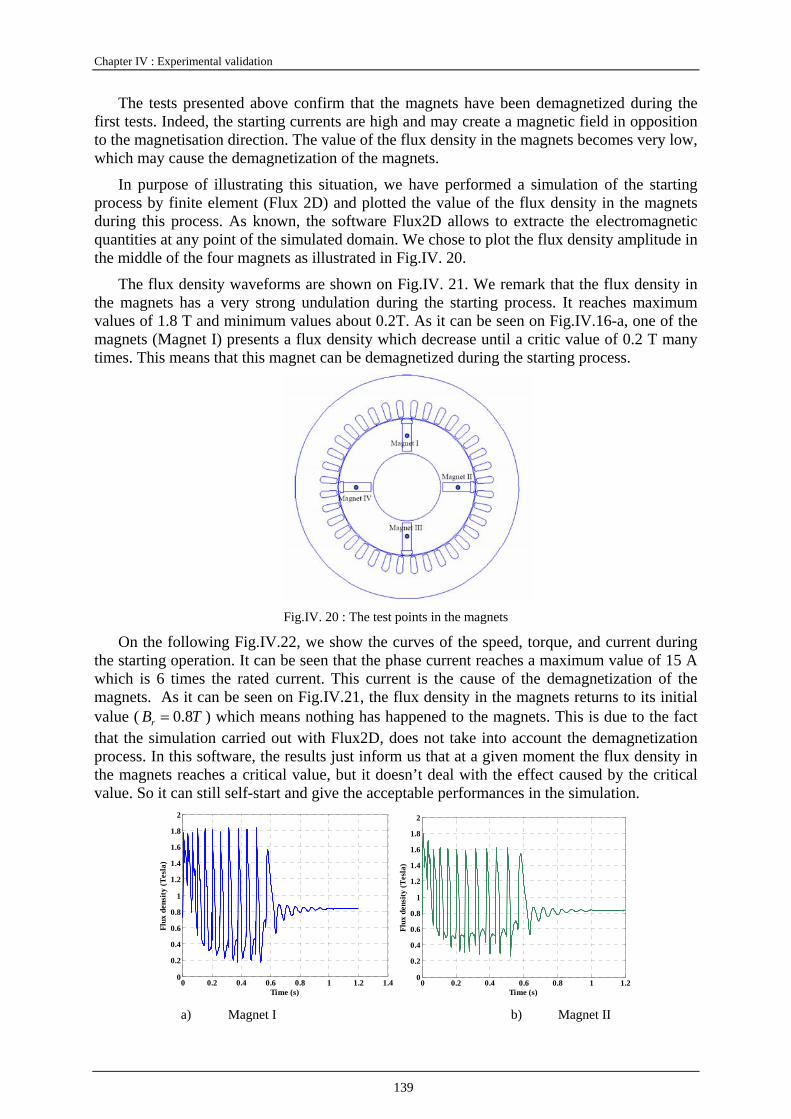
Chapter IV : Experimental validation
139
The tests presented above confirm that the magnets have been demagnetized during the first tests. Indeed, the starting currents are high and may create a magnetic field in opposition to the magnetisation direction. The value of the flux density in the magnets becomes very low, which may cause the demagnetization of the magnets.
In purpose of illustrating this situation, we have performed a simulation of the starting process by finite element (Flux 2D) and plotted the value of the flux density in the magnets during this process. As known, the software Flux2D allows to extracte the electromagnetic quantities at any point of the simulated domain. We chose to plot the flux density amplitude in the middle of the four magnets as illustrated in Fig.IV. 20.
The flux density waveforms are shown on Fig.IV. 21. We remark that the flux density in the magnets has a very strong undulation during the starting process. It reaches maximum values of 1.8 T and minimum values about 0.2T. As it can be seen on Fig.IV.16-a, one of the magnets (Magnet I) presents a flux density which decrease until a critic value of 0.2 T many times. This means that this magnet can be demagnetized during the starting process.
Fig.IV. 20 : The test points in the magnets
On the following Fig.IV.22, we show the curves of the speed, torque, and current during the starting operation. It can be seen that the phase current reaches a maximum value of 15 A which is 6 times the rated current. This current is the cause of the demagnetization of the magnets. As it can be seen on Fig.IV.21, the flux density in the magnets returns to its initial value ( TBr 8.0= ) which means nothing has happened to the magnets. This is due to the fact that the simulation carried out with Flux2D, does not take into account the demagnetization process. In this software, the results just inform us that at a given moment the flux density in the magnets reaches a critical value, but it doesn’t deal with the effect caused by the critical value. So it can still self-start and give the acceptable performances in the simulation.
0 0.2 0.4 0.6 0.8 1 1.2 1.40
0.2
0.4
0.6
0.8
1
1.2
1.4
1.6
1.8
2
Time (s)
Flux
den
sity
(Tes
la)
0 0.2 0.4 0.6 0.8 1 1.20
0.2
0.4
0.6
0.8
1
1.2
1.4
1.6
1.8
2
Time (s)
Flux
den
sity
(Tes
la)
a) Magnet I b) Magnet II

Chapter IV : Experimental validation
140
0 0.2 0.4 0.6 0.8 1 1.20
0.2
0.4
0.6
0.8
1
1.2
1.4
1.6
1.8
2
Time (s)
Flux
den
sity
(Tes
la)
0 0.2 0.4 0.6 0.8 1 1.20
0.2
0.4
0.6
0.8
1
1.2
1.4
1.6
1.8
2
Time (s)
Flux
den
sity
(Tes
la)
c) Magnet III d) Magnet IV
Fig.IV. 21 : Flux density in magnets during starting operation (simulation)
0 0.2 0.4 0.6 0.8 1 1.2 1.4-500
0
500
1000
1500
2000
Spee
d (r
pm)
Time (s) 0 0.2 0.4 0.6 0.8 1 1.2 1.4
-30
-20
-10
0
10
20
30
Elec
trom
agne
tic to
rque
(N.m
)
Time (s) 0 0.2 0.4 0.6 0.8 1 1.2 1.4
-20
-15
-10
-5
0
5
10
15
20
Phas
e cu
rren
t (A
)
Time (s) Fig.IV. 22 : Speed, torque and currents waveforms during starting operation (simulation)
IV.3.2. Starting operation tests
The first experimental test we have made in transient state consists in verify the starting capability of the prototype we have built. First, we have made the starting test at no-load with a voltage source of 230V per phase. The torque, speed and current waveforms measured during this test are shown on fig.17. It can be seen that the starting time is about 0.4 seconds and the peak value of the current reaches 12A which is 5 times greater than the rated current. The speed-time curve presents many undulations due to the braking torque of the magnets. The same behaviour is also obtained by simulation.
0 0.1 0.2 0.3 0.4 0.5 0.6 0.7 0.8-15
-10
-5
0
5
10
15
20
Torq
ue (N
.m)
Time (s)0 0.1 0.2 0.3 0.4 0.5 0.6 0.7 0.8
0
500
1000
1500
2000
2500
Time (s)
Spee
d (r
pm)
0 0.1 0.2 0.3 0.4 0.5 0.6 0.7 0.8-15
-10
-5
0
5
10
15
Phas
e cu
rren
t (A
)
Time (s) Fig.IV. 23 : Torque, speed and current waveforms at starting operation (measurement)
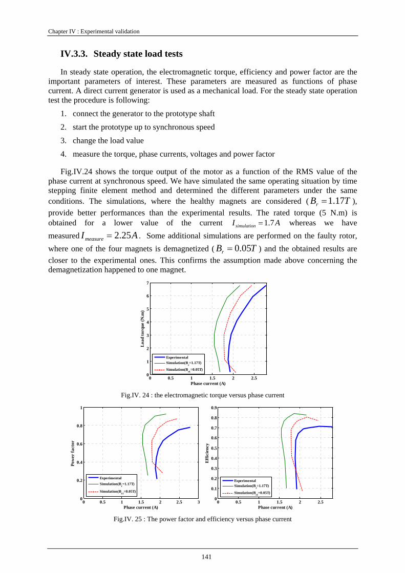
Chapter IV : Experimental validation
141
IV.3.3. Steady state load tests
In steady state operation, the electromagnetic torque, efficiency and power factor are the important parameters of interest. These parameters are measured as functions of phase current. A direct current generator is used as a mechanical load. For the steady state operation test the procedure is following:
1. connect the generator to the prototype shaft
2. start the prototype up to synchronous speed
3. change the load value
4. measure the torque, phase currents, voltages and power factor
Fig.IV.24 shows the torque output of the motor as a function of the RMS value of the phase current at synchronous speed. We have simulated the same operating situation by time stepping finite element method and determined the different parameters under the same conditions. The simulations, where the healthy magnets are considered ( TBr 17.1= ), provide better performances than the experimental results. The rated torque (5 N.m) is obtained for a lower value of the current AIsimulation 7.1= whereas we have measured AImeasure 25.2= . Some additional simulations are performed on the faulty rotor, where one of the four magnets is demagnetized ( TBr 05.0= ) and the obtained results are closer to the experimental ones. This confirms the assumption made above concerning the demagnetization happened to one magnet.
0 0.5 1 1.5 2 2.50
1
2
3
4
5
6
7
Phase current (A)
Load
torq
ue (N
.m)
ExperimentalSimulation(Br=1.17T)
Simulation(Br1=0.05T)
Fig.IV. 24 : the electromagnetic torque versus phase current
0 0.5 1 1.5 2 2.5 30
0.2
0.4
0.6
0.8
1
Phase current (A)
Pow
er fa
ctor
ExperimentalSimulation(Br=1.17T)
Simulation(Br1=0.05T)
0 0.5 1 1.5 2 2.50
0.1
0.2
0.3
0.4
0.5
0.6
0.7
0.8
0.9
Phase current (A)
Effic
ienc
y
ExperimentalSimulation(Br=1.17T)
Simulation(Br1=0.05T)
Fig.IV. 25 : The power factor and efficiency versus phase current

Chapter IV : Experimental validation
142
On Fig.IV.26 and Fig.IV.27, we show the evaluation of the torque, the phase current, the power factor and the efficiency versus the output power obtained form simulations and experiments. The simulations have been carried out with healthy magnets (green curves) and one demagnetized magnet (dashed red curves).
The general shape of theses curves is quite predictable:
a- The currents increase with the power, in fact only the active component of the current increases.
b- The measured currents are slightly higher than simulated ones because of the demagnetization problem. The same remarks can be made for the efficiency and power factor curves.
0 200 400 600 800 1000 12000
1
2
3
4
5
6
7
Output power (w)
Load
torq
ue (N
.m)
ExperimentalSimulation(Br=1.17T)
Simulation(Br1=0.05T)
0 200 400 600 800 1000 12000
0.5
1
1.5
2
2.5
3
Output power (w)
Phas
e cu
rren
t (A
)
ExperimentalSimulation(Br=1.17T)
Simulation(Br1=0.05T)
Fig.IV. 26 : Load torque, phase current versus output power
0 200 400 600 800 1000 12000
0.1
0.2
0.3
0.4
0.5
0.6
0.7
0.8
0.9
Output power (w)
Effic
ienc
y
ExperimentalSimulation(Br=1.17T)
Simulation(Br1=0.05T)
0 200 400 600 800 1000 12000
0.2
0.4
0.6
0.8
1
Output power (w)
Pow
er fa
ctor
ExperimentalSimulation(Br=1.17T)
Simulation(Br1=0.05T)
Fig.IV. 27 : The power factor and efficiency versus output power
IV.4. Conclusions
In this chapter, we have presented the experimental tests we have carried out on a prototype designed and manufactured in the laboratory. The main objective of this part of our thesis is to verify the principle of line start PM motors and validate the theoretic models developed all along our research work.
Chapter IV : Experimental validation
143
It is important to mention that the prototype power is small and the interest of such kind of motors is important for medium or high power motors in continuous operation such as oil pumps for compressors.
Only one architecture has been tested, which is the “solid rotor interior PM motor” because of the interesting performances and practical convenience to manufacture of such motor.
In starting operation, the line current is important and causes the demagnetization of the magnets. This important criterion has been studied in chapter 4, in order to avoid high transient currents absorbed form the grid and possible demagnetization of the magnets. Unfortunately, one of the magnets has been demagnetized during starting test with inappropriate load. This situation observed during the tests has been analyzed by measuring the flux density in the magnets. Different finite element simulations have been carried out in order to verify this purpose.


Conclusion

Conclusion
147
The problem of energy saving concerns all the sectors of life and particularly the industrial sector which consumes a large part of the energy provided by our power stations. Induction motor used in pumps, fans or compressors take an important part of this consumption but they have a relatively low efficiency. Their replacement by permanent magnet machines allows a considerable gain in competitiveness and operating cost. This thesis took place within this context and had as objective the study and the optimization of various structures of line start permanent magnet synchronous (LSPM) motors in order to replace induction motors in such applications.
We started this thesis by introducing and justifying the use of LSPM motors in some applications, despite their complexity and inherent difficulties during starting operation. Certainly, electrical machines have known an important development thanks to improvements made on materials, design and supply, but the mechanical or thermal stresses may impose limits to improve their performance. This is the case of induction machines whose efficiency depends on the size of the air-gap. LSPM motors are more efficient because of the use of high energy density PMs which can compensate the effect of large air-gaps. However, these machines have specified behaviors because they combine two different conversion modes and which interfere during the starting operation. These motors have to be studied very closely and rotor structures are optimized to achieve good performances in both starting and steady state operations. So we define the objectives of our study during this thesis:
Reduce the current and maximize the torque in starting operation Increase the efficiency and power factor at full load steady state operation
In the second chapter, we designed and studied three structures of LSPM at synchronous operation for the same specifications with the same constraints and optimize structures to reduce the torque ripples. Computational models of machines have been developed for this work as well as methods of reducing the cogging torque. The identification of machine parameters taking into account the saturation and the cross coupling effect has been implemented for an external circuit model, which is proved to be fairly accurate. A comparison of the three structures showed that the motor using magnets inserted into a solid rotor seems to be a good compromise between efficiency, simplicity and robustness.
In the third chapter, we have studied the machine dynamic behavior and were are particularly interested in performance during starting operation regarding the starting current and torque. We have implemented a parametric study by varying the geometry and the type of materials in order to obtain the performances. The geometry is consequently optimized to achieve the desired performance in starting operation, steady state performances were investigated and the effect of some geometrical parameters was highlighted. A small thermal study was carried out to evaluate the temperature rise during starting operation. It showed that the increase of the temperature is weak and does not affect the overall behavior of the machine provided there are no repeated starts. A comparison of the three architectures showed that the solid rotor LSPM motor with inserted magnets seems to be a good compromise between simplicity and efficiency.
In the fourth chapter, an experimental study was carried out to validate the principle of self-starting and the synchronization to the grid for one of three structures selected above. We

Conclusion
148
described the conditions of manufacture and design of a prototype of reduced power. The first tests were carried out and the synchronization was successful. The measurements of torque and current currents waveforms during startup were performed. A handling error has resulted too strong currents causing the demagnetization of the magnets. This has the effect of reducing the performance of the prototype compared to the initial design. An interesting identification work of the consequences of this incident led us to perform magnetic field measurements and calculations under particular conditions to characterize its effects. In any case, this experimental study has allowed us to have an experience in manufacturing special machines but also to reinforce our conviction that the good design of such motors against serious incidents is essential.
The research work we have begun during this thesis is a first step in the study of such special motors which have a promising future in the context of energy saving. These machines can be used in many applications even in domestic ones. In such cases, single phase capacitor line start PM motor could be closely studied. Concerning the full-load torque, high undulations exist in the solid-rotor and U-shape PM motors; we have given the analytical results of geometry influence on torque ripples. Some other techniques may be interesting to apply to the reduction of torque ripples. The starting behavior we observed can be improved by decreasing the starting current under the constraint of required starting torque to avoid demagnetizing of the magnets. Some further study on the circuit model which we haven’t exploited in this thesis will be carried out as well as the identification of the parameters for the simulation and experimentation.The optimization of the rotor structures can be developed in increasing the full-load efficiency without sacrificing the ability to start the motor from a fixed frequency supply.

Bibliography

Bibliography
151
[Boyd-99] Boyd, J.H.: “Line start permanent magnet motor”, U.S. Patent Nr. 5,952,757/1999.
[Bianchi-00] N. Bianchi and S. Bolognani, “Reducing torque ripple in PM synchronous motors, ”in Proc. Int. Conf. Electrical Machines, ICEM 2000, Helsinki, Finland, Aug. 28-30, pp. 1222-1226
[Bianchi-02] Nicola Bianchi and Silverio Bolognani, “ Design techiniques for reducing the cogging torque in surface-mounted PM motors”, IEEE Trans. Magn, vol. 38, pp. 1259-1265, 2002
[Breton-00] C. Breton, J. Bartolomé, J. A. Benito, G. Tassinario, I. Flotats, C. W. Lu, and B. J. Chalmers, “Influence of machine symmetry on reduction of cogging torque in permanent-magnet brushless motors,” IEEE Trans.Magn., vol. 36, no. 5, pp. 3819–3823, Sep. 2000.
[@1] “La classification pour le rendement des moteurs”, EUEODEEM, http://re.jrc.ec.europa.eu/energyefficiency/eurodeem/index.htm.
[@2] “New efficiency classes for low-voltage three-phase motors (IE-code)”, http://www.cemep.org/index.php?id=53.
[Chaithongsuk-09] Chaithongsuk, S. Takorabet, N. Meibody-Tabar, F. “On the Use of Pulse Width Modulation Method for the Elimination of Flux Density Harmonics in the Air-Gap of Surface PM Motors”, IEEE Trans. Magn, vol. 45 no.3, pp.1736-1739, March,2009.
[Chu-05] Chu, Ming-Tsung et al: “Rotor structure of line start permanent magnet synchronous motor”, U.S. Patent Nr. 6,844,652/2005.
[Fordorean-09]D. Fordorean, A. Miraoui, “Dimensionnement rapide des machines synchrones à aimants permanents (MSAP)”, Techniques de l’ingénieur,Nov 10, 2009.
[Gerald-96] Gerald B. Kliman: “Permanent magnet line start motor having magnets outside the starting cage”, U.S. Patent Nr. 5,548,172/1996.
[Hamdi-95] Hamdi E.S., Mubarak A.N.: “Design of line-start permanent magnet motors – a review”, ELECTROMOTION, No. 2, 1995, pp.53-61.
[Hanselman-97]D. C. Hanselman, “Effect of skew, pole count and slot count on brushless motor radial force, cogging torque and back EMF,” in Inst. Elect. Eng.Proc.—Electr. Power Appl., vol. 144, Sep. 1997, pp. 325–330.
[Han99] K. J Han, et al., “Optimal core shape design for cogging torque reduction of BLDC motor using algorithm ” Proc. Compumag’99, pp. 332-333, 1999
[Hanselman-94]D.C.Halseman, Brushless Permanennt-mangnet Motor Design,Maine, USA,1994.
Bibliography
152
[Henrotte-04] François Henrotte, Geoffrey Deliége, Kay Hameyer, “The eggshell approach for the computation of electromagnetic forces in 2D and 3D ” COMPEL: The International Journal for Computation and Mathematics in Electrical and Electronic Engineering, Vol. 23 Iss: 4, pp.996 - 1005,2004
[Honsinger-80]V.B.Honsinger,“Permanent magnet machines: asynchronous operation”, IEEE Trans. Power App.and Sys. Vol.PAS-99, no.4 July/Aug 1980
[Hwang-94] S. Hwang and D. K. Lieu, “Design techniques for reduction of reluctance torque in brushless permanent magnet motors,” IEEE Trans. Magn., vol.30, no. 6, pp. 4287–4289, Nov. 1994.
[Hwang-00] S.-M. Hwang, J.-B. Eom, W.-B. Jeong, and Y.-H. Jung, “Cogging torque and accoustic noise reduction in permanent magnet motors by teeth pairing,” IEEE Trans. Magn., vol. 36, no. 5, pp. 3144–3146, Sep.2000.
[Hwang-01] S.-M. Hwang, J.-B. Eom, Y.-H. Jung, D.-W. Lee, and B.-S. Kang, “Various design techniques to reduce cogging torque by controlling energy variation in permanent magnet motors,” IEEE Trans. Magn., vol. 37, no.4, pp. 2806–2809, Jul. 2001.
[Ishikawa-93] T. Ishikawa and G. R. Slemon, “A method of reducing ripple torque in permanent magnet motors without skewing,” IEEE Trans. Magn., vol.29, no. 2, pp. 2028–2031, Mar. 1993.
[Jahns-96] T. M. Jahns andW. L. Soong, “Pulsating torque minimization techniques for permanent magnet AC motors drives—A review,” IEEE Trans. Ind. Electron., vol. 43, no. 2, pp. 321–330, Apr. 1996.
[Jung-07] Dae-Sung Jung; Seung-Bin Lim; Jin-Hun Lee; Sang-Hoon Lee; Hyung-Bin Lim; Youn-Hyun Kim; Ju Lee; "A study on the design and the characteristics in single-phase line-start permanent magnet motor” Int. Conf. on Electrical Machines and Systems, ICEMS. Page(s): 878 – 881, 2007.
[Knight-99] Knight, A.M.; Williamson, S.: “Influence of magnet dimensions on the performance of a single-phase line-start permanent magnet motor”, Electric Machines and Drives, 1999. International Conference IEMD'99, pp. 770 -772.
[Knight-00] Knight, A.M., McClay, C.I.: “The design of high-efficiency line-start motors”, IEEE Transactions on Industry Applications, Volume: 36 Issue: 6, Nov.-Dec. 2000, pp. 1555 -1562.
[Kurihara-03] Kurihara K., Rahman, A.: “High efficiency line-start interior permanent magnet synchronous motor”, IAS Conference 2003.
[Kurihara-04] K. Kurihara and A. Rahman, “High-efficiency linestart interior permanent-magnet synchronous motors,” IEEE Trans. Ind. Appl., vol. 40, no. 3, pp.789–796.. May/Jun. 2004.
Bibliography
153
[Lateb-06] R. Lateb, N. Takorabet, F. Meibody-Tabar, “Effect of magnet segmentation on cogging torque in surface-mounted permanent magnet motors,” IEEE Trans Magn, vol42,no.3,pp442-445, Mar,2006
[Lebouc-05] Afef Leouc, ,“Electromagnétisme &matériaux magnétiques pour le genie electrique” cours 2ème NRJ-ENSIEG,2005/2006.
[Li-88] Touzhu Li, G.Slemonet., “Reduction of cogging torque in permanent magnet motors”, IEEE Trans. Magnetism, vol. 24, pp. 2901-2903, 1988
[Liang-09-1] Liang Fang; Lee, B.H.; Jung-Pyo Hong; Hyuk Nam; “Estimation of Magnet Reduction in Single-Phase Line-Start Permanent Magnet Synchronous Motor” IEEE Industry Applications Society Annual Meeting, 2009. IAS, 2009.
[Liang-09-2] Liang Fang; Lee, B.H.; Jung-Pyo Hong; Hyuk Nam;, "Rotor saliency improved structural design for cost reduction in single-phase line-start permanent magnet motor”, IEEE Energy Conversion Congress and Exposition, ECCE'09, pp. 139 – 146, 2009
[Lukaniszyn-04] M. Lukaniszyn, et al., “Optimization of permanent magnet shape for minimum cogging torque using a genetic algorithm, ” IEEE Trans. Magn., vol. 40, no. 2, 2004
[Meeker-07] D.Meeker, “Finite element method magnetics ”,user’s manual,version 4.2.
[Mesures803] “La rentalibilité énergétique les entrainements”,Mesures 803-Mars2008, www.mesures.com.
[McFee-88] S. McFee, J. P. Webb, and D. A. Lowther, “A tunable volume integration formulation for force calculation in finite-element based computational magnetostatics,” IEEE Trans. Magn., vol.24,no.1,pp.439-442, Jan. 1988.
[Miller-84] T.J.E.Miller,”Synchronization of line-start permanent –magnet AC motors”,IEEE Trans. Power App.Syst.,vol.PAS-103,no.7,July1984.
[Miller-03] Popescu, M., Miller, T.J.E.: “Line start PM motor: single phase starting performance analysis”, IEEE Trans., IA-39, No.4, 2003, pp.1021-1030.
[Modeer-07] Tomas Modeer,”Modeling and testing of line start permanent magnet motors”, Licentiate thesis,Royal Insitute of Technology of Stockholm, KTH,Sweden 2007.
[Sargos-04] F. Sargos, F. Meibody-Tabar, “Modèles dynamiques des machines synchrones » chapitre du livre « Modèles pour la commande des actionneurs électriques » sous la direction de J. P. Louis, 2dition Lavoisier, Paris, 2004.
[Selmon-93] Ishikawa,T. Slemon,G.R, “A method of reducing ripple torque in permanent magnet motors without skewing”, IEEE Trans. Magn., vol. 29, no.2, pp. 2028–2031, Mar,1993.
Bibliography
154
[Smith-07] E. Peralta-Sanchez and A.C. Smith, “Line-start permanent-magnet machines using a canned rotor,”Proc. IEMDC 2007, 3-5 May 2007, vol. 2, pp. 1084–1089.
[Soo-whang-10]Soo-whang Baek; Myung-hyun Choi; Byung-il Kwon; Byung-taek Kim, "Design methodology of a single-phase line start PM motor using conditions for magnetic balance and copper loss minimization” IEEE Conference on Electromagnetic Field Computation (CEFC), 2010
[Soulard-00] J. Soulard and H.P. Nee, “Study of the synchronization of line-start permanent magnet synchronous motors,” Proc. of 2000 IEEE Ind. Appl. Conf., Roma, 8-12 vol. 1, pp. 424–431. Oct. 2000.
[Stephens-98] Stephens, C.M.; Kliman, G.B.; Boyd, J.: “A line-start permanent magnet motor with gentle starting behavior”, Industry Applications Conference, 1998. Thirty-Third IAS Annual Meeting. The 1998 IEEE, Volume: 1, 1998, pp. 371 -379, vol.1.
[Stephens-99] Stephens, Ch. M. “Starting and synchronizing system for line-start permanent magnet motor”, U.S. Patent Nr. 5,859,513/1999.
[Stumberger-03]Stumberger,B, Stumberger.G. Dolinar. D. “Evaluation of saturation and cross-magnetization effects in interior permanent-magnet synchronous motor”, IEEE Trans. Ind. Appl., vol. 39, no.5, Sept/Oct, 2003
[Tang-97] Renyan Tang, “Modern permanent magnet machines-theory and design”, Beijing, 1997.
[Ding-09] Tingting Ding, N. Takorabet, F.M. Sargos, Xiuhe. Wang “Design and Analysis of different Line-Start PM Synchronous Motors for Oil-pump Applications”, IEEE transactions on magnetics, 45(3), March 2009
[Takorabet-08]N.Takorabet, J.P.Caron,B.Vaseghi,B.Nahid-mobarakeh and F.Meibody-Tabar, “ Study of different architectures of fault tolerant actuator using a double-star PM motor”, Industry Applications Society Annual Meeting (IAS’08), IEEE, Oct. 2008
[Wang-05] Xiuhe Wang,Tingting Ding, Yubo Yang, et al “Study of cogging torque in line-start permanent magnet synchronous motors” [J]. Proceedings of the CSEE, 2005, 25(18): 167-170.
[Wang-10] Baohua Wang; Huajie Yin, “A Single-Phase Line-Start PM Motor Design Method from Three-Phase to Single-Phase”, Electrical and Control Engineering (ICECE), 2010 International Conference on, Page(s): 4966 – 4969, 2010.
[Yun–08] Jong-Bo Yun, Seung-Joo Kim, Jae-Young Park, Jong-Bin Im and Ju Lee : “A Study on the Starting Characteristics in Single-phase Line-start Permanent Magnet Motor”, Int. Conf. on Electrical Machines and Systems ICEMS’08, pp. 3090-3093, 2008
Bibliography
155
[Zhu-00] Z. Q. Zhu and D. Howe, “Influence of design parameters on cogging torque in permanent magnet machines,” IEEE Trans. Energy Convers.,vol. 15, no. 4, pp. 407–412, Dec. 2000.
[Zhu-03] Z.Q.Zhu,S.Ruangsinchaiwanich,N.Schofield, and D.Howe, “Reduction of cogging torque in interior- magnet brushless machines”, IEEE trans Magn,vol 39,no 5, pp.3238-3240,Sep. 2003
[Zhu-06] Z. Q. Zhu, S. Ruangsinchaiwanich, and David Howe, “Synthesis of cogging-torque waveform from analysis of a single stator slot”, IEEE Trans. Ind. Appl., vol. 42, no.3, May/June, 2006


Appendix


Appendix A.1
159
Appendix A.1
Analytical Analysis of Cogging Torque in U-shape IPM Motors
A.1 : Analytical calculation of cogging torque
Assuming that the permeability is infinite and the magnetic field is uniform; the variation of the flux density along the radial coordinate is negligible, we can write:
),()(),( 0 αθ
θμαθghhMB
m
m
+= (A 1)
where:
• )(0 θμ M is the magnetization function which depends on the magnet geometry.
• α is the relative position between the stator and rotor in Fig.A.1.
• ),( αθg is the air-gap function which represents the length of the flux lines and
depends on the slot geometry
In the Fig.A.3, the functions ),( αθM is shown with respect to the electrical angleθ .
)(θsg)(θrg
Fig.A. 1 Configuration of U-shape IPM motor Fig.A. 2 : Definition of ),( αθg

Appendix A.1
160
-1.2
-0.9
-0.6
-0.3
0
0.3
0.6
0.9
1.2
Flux
den
sity
(Tes
la)
2π/p
M(θ)
Fig.A.3 : )(θM and )(θsg functions
Fig.A.4: The )(θrg function in two cases
Assuming that the magnetic energy “in” the stator and rotor iron is negligible, we have:
∫∫∫ +=+≈
magnetgappmgap dvBWWW 2
021μ
(A 2)
where gapW and pmW are the energy “in” the air-gap and the permanent magnet.
The expression of the energy becomes:
∫∫∫ + ⎟⎟⎠
⎞⎜⎜⎝
⎛+
=magnetgap
m
m dvagh
hMW2
20
0 ),()(
21)(
θθμ
μα (A 3)
The cogging torque can be defined as the negative derivative of the magnetic energy with respect to the rotation angle α when there is no power supply, i.e.
ααα
∂∂
−=)()( WTcog (A 4)
The functions )(2 θM and 2
),( ⎟⎟⎠
⎞⎜⎜⎝
⎛+ αθgh
hm
m are expanded into Fourier series as:
0
20g
20rθ− 1rθ θ
20rθ
201 rr θθ −
),( αθsg
20g
21sθ
201 ss θθ − 1sθ 2sθ θ0
),( αθrg
0
20g
21rθ
201 rr θθ − 1rθ
2rθ θ
),( αθrg

Appendix A.1
161
∑∞
=
+=1
02 cos2
)(n
n npBBM θθ (A 5)
where 20 r
ur BpaB
π= , urrn npB
nB α
πsin2 2=
The air-gap is divided into two parts by the central circle in the air-gap: the inner part (half air-
gap) is defined as )(θrg shown in Fig.A.3 and the outer part (half air-gap) is defined )(θsg the
equivalent air gap is defined as:
)()()( θθθ rs ggg += (A 6)
The outer part )(θsg can be defined as:
⎪⎪⎩
⎪⎪⎨
⎧
≤≤−−
−+
−≤≤
=
22)
2(
22
20
2)(10101
0
0
010
sssss
s
s
ss
swhenbg
wheng
g θθθθθθθθπ
θθθθ (A 7)
It is expanded in Fourier series with considering the relative positionα :
)(2cos)(11
0 αθθπθ −+= ∑
∞
ssnss
nggg (A 8)
where
− 1
200
0 82 s
sss
Rggθθπ
+=
− ⎟⎟⎠
⎞⎜⎜⎝
⎛ −−−= π
θθθ
πθ n
nRg
s
ssnsssn
1
012
1 cos)1(2
− 0g is the length of air-gap, − sR is the inner radius of rotor, − 1sθ and 0sθ are the slot pitch and slot opening of stator expressed in radians respectively,
0rb the slot opening of rotor slot.
The inner part )(θrg is defined in two cases
• If the position 0=θ is set to the central line of one pole and if the slot number per pole is even, the axis of the tooth is aligned with that of the pole. So the distribution of
)(θrg over one slot pitch is:
⎪⎪⎩
⎪⎪⎨
⎧
≤≤−−
−+
−≤≤
=
22)
2(
22
20
2)(10101
0
0
010
rrrrr
r
r
rr
rwhenbg
wheng
g θθθθθθθθπ
θθθθ (A 9)
Appendix A.1
162
• If the slot number per pole is odd, the axis of the slot is aligned with that of the pole. So the distribution of )(θrg over one slot pitch is:
⎪⎪⎩
⎪⎪⎨
⎧
≤⎟⎟⎠
⎞⎜⎜⎝
⎛−+
≤≤
=
2222
222)(
0
0
0
0
00
100
r
r
r
r
r
rr
r
whenbbg
wheng
gθθθ
θπ
θπ
θθθ
θ (A 10)
The function )(θrg is expanded into Fourier series:
)(2cos)( 011
0 βθθπθ −+= ∑
∞
rrnrr
nggg (A 11)
where :
− 1
200
0 82 r
rrr
Rggθθπ
+=
− ⎟⎟⎠
⎞⎜⎜⎝
⎛ −−−= π
θθθ
πθ n
nRg
r
rrnrrrn
1
012
1 cos)1(2
− rR is the outer radius of rotor, − 1rθ and 0rθ are the slot pitch and slot opening of rotor expressed in radians
respectively, 0rb the slot opening of rotor slot. − 00 =β if the number of slots is even and 2/10 rθβ = if the number of slots is odd
The calculation of the cogging torque uses the function )()()( θθθ rs ggg += and we have to
determine the Fourier series of the follows expression:
2
2
)()(1
1),(
⎟⎟⎟⎟
⎠
⎞
⎜⎜⎜⎜
⎝
⎛
++
=⎟⎟⎠
⎞⎜⎜⎝
⎛+
m
rsm
m
hggagh
hθθθ
(A 12)
It is a complicated expression. Assuming that mhg <)(θ , this difficulty can be overcome by adopting the following approximation.
If we consider the ratio mh
gx )(θ= , the function given in A.11 can be written as
2
11)( ⎟
⎠⎞
⎜⎝⎛+
=x
xf
with 1<x . This function is fitted by a polynomial )(2 xP in the domain ]1,0[ and the result is:
22
2
646.11)(1
1)( xxxPx
xf +−=≈⎟⎠⎞
⎜⎝⎛+
= 10 << x (A 13)

Appendix A.1
163
In the case of the considered motor, 0.3/)( <= mhgx θ the relative error between f and 2P
is less than 5%; it is illustrated in Fig.II. 76. Under theses assumptions, the air gap function can be approximated by:
22)(),()(),(646.11
),( ⎟⎟⎠
⎞⎜⎜⎝
⎛ ++
+−≈⎟⎟
⎠
⎞⎜⎜⎝
⎛+ m
rs
m
rs
m
m
hgg
hgg
aghh θαθθαθθ
(A 14)
0 0.1 0.2 0.3 0.4 0.5 0.6 0.7 0.80
1
2
3
4
5
6
x
Erro
r (%
)
Fig.A. 5 : Error of approximation
Substituting equation A.14, A5 into equation A.3, the expression of cogging torque without skewing is:
⎭⎬⎫
=+−=−+−+
=−−=++++
=±±+
−+
+
⎪⎩
⎪⎨⎧
⎟⎟⎠
⎞⎜⎜⎝
⎛−+
−=
∑∑∑
∑∑∑
∑∑∑
∑
∑
∑
∞
=
∞
=
∞
=
∞
=
∞
=
∞
=
∞
=
∞
=
∞
=
∞
=
∞
=
∞
=
)0202()sin(
)0202()sin(
)02(2sin2
)(sin2
2sin
sin646.1)(24
)()(
21211 1 1
02121
21211 1 1
02121
111 1 1
2
10112
0
11
212
11
21002
0
22
2
1
1
1
kznzmporkznzmpwhenkznzggnBhz
kznzmporkznzmpwhenkznzggnBhz
kznzmpwhenmpggmBhp
mzggmzhB
mzBgmzh
mzBgmzh
ggh
RRLT
m n krksmrm
m
m n krksmrm
m
m n ksksmrm
m
m zmz
rsm
m
r
m pmz
rsm
m
m pmz
rsm
mrs
m
rsFecog
βαπ
βαπ
απ
βαπ
απ
απμ
α
(A 15)
Where feL is the axial length of armature lamination, 1z 2z the slot number of stator and rotor.
When the laminated stator is skewed sk slot pitch, the expansion of )(θrg corresponding to axial
position L is
)(2cos)( 111
0 ssFes
snss kLLnggg θαθ
θπθ −−+= ∑
∞
(A 16)
So the expression of cogging torque with skewing is:

Appendix A.1
164
⎭⎬⎫
=+−=−+−++
=−−=+++++
=±±++
−++
++
⎪⎩
⎪⎨⎧
+⎟⎟⎠
⎞⎜⎜⎝
⎛−+
−=
∑∑∑
∑∑∑
∑∑∑
∑
∑
∑
∞
=
∞
=
∞
=
∞
=
∞
=
∞
=
∞
=
∞
=
∞
=
∞
=
∞
=
∞
=
0202()2
sin(sin2
)0202()2
sin(sin2
)02()2
(2sin2sin4
)2
(sinsin4
)2
(2sin2sin2
)2
(sinsin646.1)(228
)()(
21211 1 1
0211
12
21211 1 1
0211
12
111 1 1
1
12
10
112
0
1
112
1
11
2002
0
221
2
1
1
1
kznzmporkznzmpwhenkzknZnznkggBh
kznzmporkznzmpwhenkzknZnznkggBh
kznzmpwhenkmpZ
mpkggBh
kmzmkgghB
kmzmkBgh
kmzmkBgh
gghk
RRLZT
m n ksssrksmrm
m
m n ksssrksmrm
m
m n k
ssssksmrm
m
m
sss
zmz
rsm
m
r
m
sss
pmz
rsm
m
m
sss
pmz
rsm
mrs
ms
rsFecog
βθαπ
βθαπ
θαπ
βθ
απ
θαπ
θαπμ
α
(A 17)
A.2 : Discussion about cogging torque
Based on the above expression A.15, the effects of number of slots and poles, skewing will be discussed in the following. We divided the cogging torque into 4 terms, of which the features will be discussed with respect to the reduction techniques of cogging torque.
A.2.1 : Cogging torque of first kind The first component of cogging torque in Equ.A.15 is mainly caused by the interaction
between the magnets and stator slots. In the range of one slot pitch, the number of periods of this term is determined by the number of poles and the number of stator slot.The number of periods of
the cogging torque is the smallest m (integer) which enables pmz 2 be an integer. It is calculated
as
)2,(2
11 pZGCD
pm = (A 18)
where )2,( 1 pzGCD is the great common divisor between 1z and p2 . The poles, number of
slots, and number of periods corresponding to the four curves are shown in Tab.A.1. On FigA.6, it can be seen that the more periods, the lower the peak of cogging torque. The peak of cogging torque mainly depends on
pzm
rB
211 the more the periods, the bigger the 1m , thus the smaller the peak
of cogging torque.
Fig.A. 6 : Cogging torque waveforms with different combinations of poles and slots

Appendix A.1
165
Tab.A. 1: Combinations of poles and slots
Curves Poles Stator slots
Periods
B 6 36 1 C 6 39 2 D 6 38 3 E 6 37 6
A.2.2 : Cogging torque of second kind
This component is a function of stator slots, and rotor slots. The magnitude is in direct
proportion to 0rB In one slot pitch; the number of periods is determined by the combination of
number of stator slot and rotor slot It can be seen from equation (A.15) that the number of periods
2m is the smallest integer which enables 2
1
zmz be an integer, and can be expressed as follows.
),( 21
22 ZZGCD
zm = (A 19)
Fig..A.7 shows the wavefroms this component during rotation of one slot pitch for different combinations. The combinations of number of stator slots, number of rotor slots, and number of periods corresponding to the four curves are shown in Tab.A.2
Tab.A. 2: Combinations of slots Curves Stator Rotor Periods
B 36 36 1 C 54 36 2 D 48 36 3 E 42 36 6
Fig.A. 7 : Cogging torque waveforms with different stator and rotor slots Fig.A. 8: Cogging torque of the third kind
A.2.3 : Cogging torque of the third kind
This component is caused by the interaction between harmonics in )(2 θrB and stator slots. The
rotor slot has no effects on it, but the distribution is different from the first kind cogging torque in number of periods, which is determined by pole number and number of stator slots. Due to the
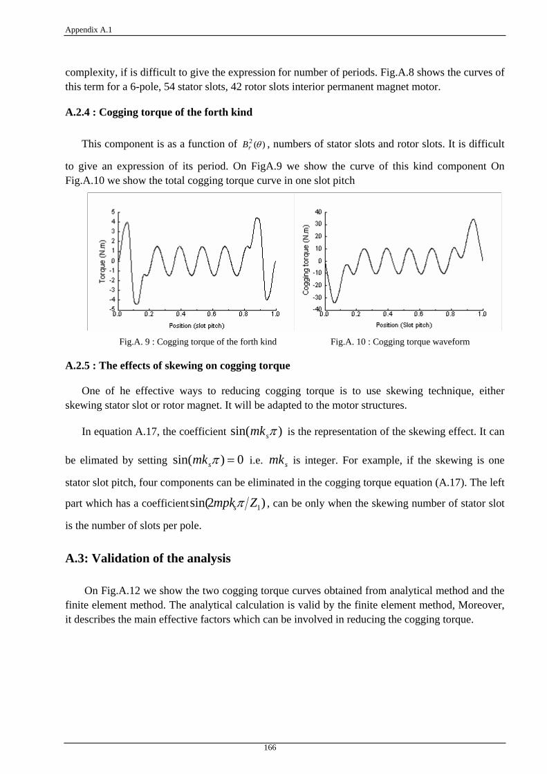
Appendix A.1
166
complexity, if is difficult to give the expression for number of periods. Fig.A.8 shows the curves of this term for a 6-pole, 54 stator slots, 42 rotor slots interior permanent magnet motor.
A.2.4 : Cogging torque of the forth kind
This component is as a function of )(2 θrB , numbers of stator slots and rotor slots. It is difficult
to give an expression of its period. On FigA.9 we show the curve of this kind component On Fig.A.10 we show the total cogging torque curve in one slot pitch
Fig.A. 9 : Cogging torque of the forth kind Fig.A. 10 : Cogging torque waveform
A.2.5 : The effects of skewing on cogging torque
One of he effective ways to reducing cogging torque is to use skewing technique, either skewing stator slot or rotor magnet. It will be adapted to the motor structures.
In equation A.17, the coefficient )sin( πsmk is the representation of the skewing effect. It can
be elimated by setting 0)sin( =πsmk i.e. smk is integer. For example, if the skewing is one
stator slot pitch, four components can be eliminated in the cogging torque equation (A.17). The left
part which has a coefficient )2sin( 1Zmpksπ , can be only when the skewing number of stator slot
is the number of slots per pole.
A.3: Validation of the analysis
On Fig.A.12 we show the two cogging torque curves obtained from analytical method and the finite element method. The analytical calculation is valid by the finite element method, Moreover, it describes the main effective factors which can be involved in reducing the cogging torque.

Appendix A.1
167
Fig.A. 11 : Magnetic field distributionFig.A. 12 : Comparison of FEM and analytical method

168

Na ney-Université ~ . Université
Henri Poincaré
Madame,
A NANCY, le 21 mars 2011
No étudiant : 26006nS
DING TINGTING
57 SHUNGENG ROAD WEIDONGXINDU 15-1-401
250002,JINAN,SHANDONG,P.R.CHINA 250002,JINAN CHINE
Par décision en date du 21 mars 2011, vous avez été autorisée à présenter en soutenance vos travaux en vue de l'obtention du diplOme :
DOCTORAT UHP GENIE ELECTRIQUE
La soutenance aura lieu le 08 avril 2011 à 14h00 à l'adresse suivante :
Faculté des Sciences & Technologies - Amphithéâtre n° 8 (bâtiment du second cycle) - Campus Victor Grignard 54500 Vandoeuvre-lès-Nancy
La soutenance sera publique,
Je vous prie d'agréer, Madame, l'expression de mes salutations distinguées.
Le Président de l'Université
1 2~ - JO l1J!' liOnooli 1 BP 60120 ~4001 NARrV rMPY , ~UNn