Capacity of Multi-Channel Wireless Networks:Impact of Number of Channels and Interfaces

Pradeep KyasanurDept. of Computer Science, andCoordinated Science Laboratory,

University of Illinois at Urbana-Champaign

kyasanur@uiuc.edu

Nitin H. VaidyaDept. of Electrical and Computer Eng., and

Coordinated Science Laboratory,University of Illinois at Urbana-Champaign

nhv@uiuc.edu

ABSTRACTThis paper studies how the capacity of a static multi-channelnetwork scales as the number of nodes, n, increases. Guptaand Kumar have determined the capacity of single-channelnetworks, and those bounds are applicable to multi-channelnetworks as well, provided each node in the network has adedicated interface per channel.In this work, we establish the capacity of general multi-

channel networks wherein the number of interfaces, m, maybe smaller than the number of channels, c. We show that thecapacity of multi-channel networks exhibits different boundsthat are dependent on the ratio between c and m. When thenumber of interfaces per node is smaller than the numberof channels, there is a degradation in the network capacityin many scenarios. However, one important exception is arandom network with up to O (log n) channels, wherein thenetwork capacity remains at the Gupta and Kumar bound

of ΘWq

nlog n

bits/sec, independent of the number of in-

terfaces available at each node. Since in many practicalnetworks, number of channels available is small (e.g., IEEE802.11 networks), this bound is of practical interest. Thisimplies that it may be possible to build capacity-optimalmulti-channel networks with as few as one interface pernode. We also extend our model to consider the impactof interface switching delay, and show that in a random net-work with up to O (log n) channels, switching delay may notaffect capacity if multiple interfaces are used.

Categories and Subject DescriptorsC.2.1 [Computer-Communication Networks]: NetworkArchitecture and Design—Wireless communication

General TermsTheory, Performance

Permission to make digital or hard copies of all or part of this work forpersonal or classroom use is granted without fee provided that copies arenot made or distributed for profit or commercial advantage and that copiesbear this notice and the full citation on the first page. To copy otherwise, torepublish, to post on servers or to redistribute to lists, requires prior specificpermission and/or a fee.MobiCom’05, August 28–September 2, 2005, Cologne, Germany.Copyright 2005 ACM 1-59593-020-5/05/0008 ...$5.00.

KeywordsCapacity, Multiple Channels, Multiple Interfaces, Ad hocnetworks, Mesh networks

1. INTRODUCTIONPrevious research (e.g., [9, 10]) has characterized the ca-

pacity of wireless networks. One approach for enhancing thenetwork capacity is to use multiple channels. Past researchon wireless network capacity has typically considered wire-less networks with a single channel, although the results areapplicable to a wireless network with multiple channels aswell, provided that at each node there is a dedicated inter-face per channel. With a dedicated interface per channel, anode can use all the available channels simultaneously. How-ever, the number of available channels in a wireless networkcan be fairly large (e.g., IEEE 802.11a [11] has provisionedfor up to 12 non-overlapping channels), and it may not befeasible to have a dedicated interface per channel at eachnode. When nodes are not equipped with a dedicated in-terface per channel, then capacity degradation may occur,compared to using a dedicated interface per channel. Inthis paper, we characterize the impact of number of chan-nels and interfaces per node on the network capacity, andshow that in a random network with up to O (log n) chan-nels, even with a single interface per node, there is no ca-pacity degradation. This implies that it may be possible tobuild capacity-optimal multi-channel networks with as fewas one interface per node.When a dedicated interface per channel is not available,

the available interfaces can potentially be switched amongdifferent channels to use any of the available channels. Suchan interface switching technique is often used to improvechannel utilization [15,22,23]. However, interface switchingincurs a delay, which may reduce the achievable networkcapacity. In this paper, we include a preliminary study ofthe impact of interface switching delay on network capacity.We show that in a random network with up to O (log n)channels, interface switching delay has no impact on networkcapacity, even when there are end-to-end delay constraints,provided that a few additional interfaces are provisioned forat each node.

1.1 Modeling multi-channel multi-interfacenetworks

We consider a static wireless network containing n nodes.We use the term “channel” to refer to a part of the fre-

43

quency spectrum with some specified bandwidth. There arec channels, and we assume that every node is equipped withm interfaces, 1 ≤ m ≤ c. We assume that an interface iscapable of transmitting or receiving data on any one channelat a given time. We use the notation (m, c)-network to referto a network with m interfaces per node, and c channels.We define two channel models to represent the data rate

supported by each channel:

Channel Model 1: In model 1, we assume that the totaldata rate possible by using all channels is W . The totaldata rate is divided equally among the channels, and there-fore the data rate supported by any one of the c channelsis W/c. This was the channel model used by Gupta andKumar [10], and we primarily use this model in our analy-sis. In this model, as the number of channels increases, eachchannel supports a smaller data rate. This model is appli-cable to the scenario where the total available bandwidth isfixed, and new channels are created by partitioning existingchannels.

Channel Model 2: In model 2, we assume that each chan-nel can support a fixed data rate of W , independent of thenumber of channels. Therefore, the aggregate data rate pos-sible by using all c channels is Wc. This model is applicableto the scenario where new channels are created by utilizingadditional frequency spectrum.

The results presented in this paper are derived assumingchannel model 1. However, all the derivations are applicablefor channel model 2 as well, and the results for model 2 canbe obtained by replacing W in the results of model 1 byWc [14]. In the rest of this paper, we will only present theresults for channel model 1, but discuss implications of theresults with channel model 2 where appropriate.

1.2 DefinitionsWe study the capacity of static multi-channel wireless net-

works under the two settings introduced by Gupta and Ku-mar [10].

Arbitrary Networks: In the arbitrary network setting, thelocation of nodes, and traffic patterns can be controlled.Since any suitable traffic pattern and node placement canbe used, the bounds for this scenario are applicable to anynetwork. Therefore, the arbitrary network bounds may beviewed as the best case bounds on network capacity, as thebounds are applicable to all networks. The network capacityis measured in terms of “bit-meters/sec” (originally intro-duced by Gupta and Kumar [10]). The network is said totransport one “bit-meter/sec” when one bit has been trans-ported across a distance of one meter in one second.

Random Networks: In the random network setting, nodelocations are randomly chosen, i.e. independently and uni-formly chosen, on the surface of an unit torus. Each nodesets up one flow to a randomly chosen destination. Thenetwork capacity is defined to be the aggregate throughputover all the flows in the network, and is measured in termsof bits/sec.

We use the following notation to represent asymptoticbounds:

1. f(n) = O(g(n)) implies there exists some constant dand integer N such that f(n) ≤ dg(n) for n > N .

2. f(n) = o(g(n)) implies that limn→∞f(n)g(n)

= 0.

3. f(n) = Ω(g(n)) implies g(n) = O(f(n)).

4. f(n) = ω(g(n)) implies g(n) = o(f(n)).

5. f(n) = Θ(g(n)) implies f(n) = O(g(n)) and g(n) =O(f(n)).

6. MINO (f(n), g(n)) is equal to f(n), if f(n) = O(g(n)),else, is equal to g(n).

The bounds for random networks hold with high probabil-ity (whp). In this paper, whp implies with “probability 1when n → ∞.”

1.3 Main ResultsGupta and Kumar [10] have shown that in an arbitrary

network, network capacity scales as Θ (W√n) bit-meters/sec,

and in a random network, the network capacity scales as

ΘWq

nlog n

bits/sec. Under the channel model 1, which

was the model used by Gupta and Kumar [10], the capacityof a network with a single channel and one interface per node(that is, a (1, 1)-network in our notation) is equal to the ca-pacity of a network with c channels and m = c interfacesper node (that is, a (c, c)-network). This equivalence arisesbecause the c interfaces can operate in parallel over channelsof data rate W

cto mimic the operation of one interface oper-

ating over a channel of data rate W (this is formally provedin Lemma 1). Furthermore, under both channel models, thecapacity of a (c, c)-network is at least as large as the capac-ity of a (m, c)-network, when m ≤ c (this is trivially true,by not using c− m interfaces in the (c, c)-network). In theresults presented in this paper, we capture the impact ofusing fewer than c interfaces per node by establishing theloss in capacity, if any, of a (m, c)-network in comparison toa (c, c)-network.

The goal of this work is to study the impact of the numberof channels c, and the number of interfaces per node m, onthe capacity of arbitrary and random networks. Our resultsshow that the capacity is dependent on the ratio c

m, and not

on the exact values of either c or m (as proven in Lemma2). We now state our main results under channel model 1.

1. Results for arbitrary network: The network capacityof a (m, c)-network has two regions (see Figure 1) as follows(from Theorem 1 and Theorem 2):

1. When cmis O(n), the network capacity is Θ

Wp

nmc

bit-meters/sec (segment A-B in Figure 1). Comparedto a (c, c)-network, there is a capacity loss by a factorof 1−p

mc.

2. When cm

is Ω(n), the network capacity is ΘW nm

c

bit-meters/sec (line B-C in Figure 1). In this case,there is a larger capacity degradation than case 1, asnmc

≤pnmc

when cm

≥ n.

Therefore, there is always a capacity loss in arbitrary net-works whenever the number of interfaces per node is fewerthan the number of channels.

44

1

B

A

C

Net

wor

k ca

paci

ty

W

Wn

n n2

W√

n

W√

nlog n

log n

Capacity loss

Ratio of channels to interfaces(

cm

)

Capacity when c = m

Figure 1: Impact of number of channels on capacityscaling in arbitrary networks (figure is not to scale).There is a degradation in capacity when the ratio ofchannels to interfaces is ω(1).

2. Results for random network: The network capacity ofa (m, c)-network has three regions (see Figure 2) as follows(from Theorem 3 and Theorem 4):

1. When cmis O(log n), network capacity is Θ

Wq

nlog n

bits/sec (segment D-E in Figure 2). In this case, thereis no loss compared to a (c, c)-network. Hence, inmany practical scenarios where c may be constant orsmall, a single interface per node suffices.

2. When cm

is Ω(log n) and also O

n

log log nlog n

2, the

network capacity is ΘWp

nmc

bits/sec (segment E-

F in Figure 2). In this case, there is some capacityloss. Furthermore, in this region, the capacity of a(m, c)-random network is the same as that of a (m, c)-arbitrary network (segment E-F in Figure 2 overlapspart of segment A-B in Figure 1), implying “random-ness” does not incur a capacity penalty.

3. When cmis Ω

n

log log nlog n

2, the network capacity is

Θ

Wnm log log nc log n

bits/sec (line F-G in Figure 2). In

this case, there is a larger capacity degradation thancase 2. Furthermore, in this region, the capacity of a(m, c)-random network is smaller than that of a (m, c)-arbitrary network, in contrast to case 2.

3. Other results: The results presented above are derivedunder the assumption that there is no delay in switching aninterface from one channel to another. However, we showthat in a random network with up to O (log n) channels,even if interface switching delay is considered, the networkcapacity is not reduced, provided a few additional interfacesare provisioned for at each node. This implies that it maybe possible to hide the interface switching delay by using ex-tra interfaces in conjunction with carefully designed routingand transmission scheduling protocols.

The rest of the paper is organized as follows. We presentrelated work in Section 2. In Section 3, we establish the

1

Net

wor

k ca

paci

ty D E

G

F

n2

W√

nlog n

log n

W log log nn log n

W log nlog log n

n(

log log nlog n

)2

Capacity when c = m

Ratio of channels to interfaces(

cm

)

Capacity loss

Figure 2: Impact of number of channels on capacityscaling in random networks (figure is not to scale).There is no degradation in capacity when the ratioof channels to interfaces is O (log n).

capacity of multi-channel networks under arbitrary networksetting. Section 4 establishes the capacity of multi-channelnetworks under random network setting. Section 5 char-acterizes the impact of interface switching delay. Section 6discusses the practical implications of the theoretical results.We conclude in Section 7.

2. RELATED WORKIn their seminal work, Gupta and Kumar [10] derived the

capacity of ad hoc wireless networks. The results are appli-cable to single channel wireless networks, or multi-channelwireless networks where every node has a dedicated interfaceper channel. We extend the results of Gupta and Kumar tothose multi-channel wireless networks where nodes may nothave a dedicated interface per channel, and also consider theimpact of interface switching delay on network capacity.Grossglauser and Tse [9] showed that mobility can im-

prove network capacity, though at the cost of increased end-to-end delay. Subsequently, other research [3, 20] has ana-lyzed the trade-off between delay and capacity in mobile net-works. Gamal et al. [7] characterize the optimal throughput-delay trade-off for both static and mobile networks. In thispaper, we adapt some of the proof techniques presented byGamal et al. [7] to the multi-channel capacity problem.Recent results have shown that the capacity of wireless

networks can be enhanced by introducing infrastructure sup-port [1,12,17]. Other approaches for improving network ca-pacity include the use of directional antennas [31], and theuse of unlimited bandwidth resources (UWB) albeit withpower constraints [19,32].Li et al. [16] have used simulations to evaluate the capacity

of multi-channel networks based on IEEE 802.11. Otherresearch on capacity is based on considerations of alternatecommunication models [8,26,27].Several researchers have proposed wireless protocols for

multi-channel networks (cf. [2, 6, 15, 18, 22, 23]). Some so-lutions are based on using a single interface at each node[2, 23–25], while other solutions require a dedicated inter-face for each channel [6, 18]. More recently, solutions havebeen proposed that require multiple interfaces, but fewer in-terfaces than the number of channels [13,15,22]. Although,there are several proposals for multi-channel networks, it is

45

not apparent in those proposals how many interfaces are ac-tually required to maximally utilize the available channels.

3. CAPACITY RESULTS FOR ARBITRARYNETWORKS

We model the impact of interference by using the protocolmodel proposed by Gupta and Kumar [10]. The transmis-sion from a node i to a node j on some channel x is success-ful, if for every other node k simultaneously transmitting onchannel x, the following condition holds

d(k, j) ≥ (1 + ∆)d(i, j), ∆ > 0

where d(i, j) is the distance between nodes i and j, and∆ is a “guard” parameter that ensures that concurrentlytransmitting nodes are sufficiently farther away from thereceiver to prevent excessive interference.It is shown in [10] that the protocol model is equivalent

to an alternate physical model that is based on receivedSignal-to-Interference-Noise Ratio (SINR) (when path lossexponent is greater than 2). Therefore, the results in thispaper are applicable under the physical model as well. Wedo not consider other physical layer characteristics such aschannel fading in our analysis.We derive the capacity results for arbitrary and random

networks under the assumption that there is no switching de-lay. We extend our model to consider the impact of switch-ing delay in Section 5.

In an arbitrary network, the location of nodes, and traf-fic patterns can be controlled. Recall that the network issaid to transport one “bit-meter/sec” when one bit has beentransported across a distance of one meter in a second. Thenetwork capacity of an arbitrary network is measured interms of bit-meters per second, instead of bits per second.The bit-meters/sec metric is a measure of the “work” thatis done by the network in transporting bits. In the case ofrandom networks, the average distance traveled by any bitis Θ(1), and therefore the “bit-meters/sec” and “bits/sec”capacity is of the same order.We assume that n nodes can be located anywhere on the

surface of a torus of unit area, as in [7]. The assumption ofa torus enables us to avoid technicalities arising out of edgeeffects, but the results are applicable for nodes located on anunit square as well. We first establish an upper bound on thenetwork capacity of arbitrary networks, and then constructa network to prove that the bound is tight.

3.1 Upper bound on capacityThe capacity of multi-channel arbitrary networks is lim-

ited by two constraints (described below), and each of themis used to obtain a bound on the network capacity. The min-imum of the two bounds (the bounds depend on ratio be-tween the number of channels c and the number of interfacesm) is an upper bound on the network capacity. While theremay be other constraints on capacity as well, the constraintswe consider are sufficient to provide a tight bound. Laterin this section, we will present a lower bound that matchesthe upper bound established by the two constraints, whichvalidates our claim that the constraints are tight. We derivethe bounds under channel model 1, although the derivationcan be applied to channel model 2 as well1.

1Recall that the results under channel model 2 can be ob-

Constraint 1 – Interference constraint: The capacity ofany wireless network is constrained by interference. Sincethe wireless channel is a shared medium, under the assumedprotocol model of interference, two nodes simultaneously re-ceiving a packet from two different transmitters must havea minimum separation between them, which depends on ∆.This implies that there is a bound on the maximum num-ber of simultaneous transmissions in the network. Basedon this observation, using the proof techniques presentedin [10] with some modifications to account for multiple in-terfaces and channels, one bound on the network capacityis O

Wp

nmc

bit-meters/sec. The detailed derivation is in

Appendix A.

Constraint 2 – Interface bottleneck constraint: The ca-pacity of a wireless network is also constrained by the max-imum number of bits that can be transmitted simultane-ously over all interfaces in the network. Since each nodehas m interfaces, there are a total of mn interfaces in the(m, c)-network. Each interface can transmit at a rate of W

cbits/sec. Also, the maximum distance a bit can travel in thenetwork is O(1) meters. Hence, the total network capacityis at most O

W nm

c

bit-meters/sec. This bound is tight

when cm

is Ω(n).

Combining the two constraints, the network capacity isOMINO

Wp

nmc,W nm

c

bit-meters/sec, under channel

model 1. Therefore, we have the following theorem on thenetwork capacity of arbitrary networks (Figure 1 has a pic-torial representation).

Theorem 1. The upper bound on the capacity of a (m, c)-arbitrary network under channel model 1 is as follows:

1. When cm

is O(n), network capacity is OWp

nmc

bit-

meters/sec.

2. When cm

is Ω(n), network capacity is OW nm

c

bit-

meters/sec.

The network capacity of a (c, c)-network is O (W√n) bit-

meters/sec under channel model 1, which was the result ob-tained by Gupta and Kumar [10]. When fewer interfaces areavailable, there is a capacity degradation by at least a factorof 1−p

mc. Intuitively, the capacity degradation arises be-

cause the total bits that can be simultaneously transmitteddecreases.

3.2 Constructive lower boundIn this section, we construct a network to establish a lower

bound on the network capacity. The lower bound matchesthe upper bound, implying that the bounds are tight. Wefirst establish two results that we use in the rest of the paper.The results are proved under channel model 1, but hold forchannel model 2 as well.

Lemma 1. Suppose m, c, c are positive integers such thatc = c

m. Then, a (m, c)-network can support at least the

capacity supported by a (1, c)-network.

tained by replacing W with Wc in the results derived underchannel model 1.

46

Individual Channels Channel groups

Mapping

Group c

Group 11m

c = cm

(c − 1)m + 1

Figure 3: Lemma 1 construction: Forming c chan-nel groups, with m channels per group, in a (m, c)-network.

Proof. Consider a (m, c)-network. We group the c chan-nels into c groups (numbered from 1 to c), with m chan-nels per group as shown in Figure 3. Specifically, chan-nel group i, 1 ≤ i ≤ c, contains all channels j such that(i− 1)m+ 1 ≤ j ≤ im.Assume that time on the channels is divided into slots of

duration τ . Consider any slot s. Suppose a node X in the(1, c)-network has its interface on some channel i, 1 ≤ i ≤ c,in slot s. We simulate this behavior in the (m, c)-network byassigning the m interfaces of X in the slot s to the m chan-nels in the channel group i. In this fashion, in any slot, them interfaces of any node in the (m, c)-network are mappedto a channel group. The aggregate data rate of each channelgroup is Wm/c = W/c (since c = mc). Therefore, a chan-nel group in the (m, c)-network can support the same datarate as a channel in the (1, c)-network. This mapping allowsthe (m, c)-network to mimic the behavior of (1, c)-network;the Wτ/c bits sent on some channel in any time slot s inthe (1, c)-network can be simulated by sending Wτ/c bits(in the same slot s) on each of the m channels in the cor-responding channel group of the (m, c)-network. Hence, a(m, c)-network can support the capacity of a (1, c) network,when c = mc.

Lemma 2. Suppose m and c are positive integers. Then,a (m, c)-network can support at least 1

2the capacity sup-

ported by a1,

cm

-network.

Proof. Suppose

cm

= c

m. Then the result directly fol-

lows from the previous lemma. Otherwise, m < c, and weuse c′ = m

cm

of the channels in the (m, c)-network, and

ignore the rest of the channels. This can be viewed as a(m, c′)-network, with a total data rate of W ′ = W m

c

cm

(as each channel supports W

cbits/sec). Using Lemma 1,

a (m, c′)-network with total data rate of W ′ can supportat least the capacity of a

1,

cm

-network with total data

rate of W ′. However, when W ′ < W , the (m, c′)-networkwith total data rate W ′ can achieve only a fraction W ′

Wof

the capacity of a1,

cm

-network with total data rate W

(instead of W ′). Now,

W ′

W=

m

c

j c

m

k

=

cm

cm

≥

cm

cm

+ 1

, sincec

m≤j c

m

k+ 1

≥ 1

2, since

j c

m

k≥ 1

S2S1

R3

R4

R2

S4

S3

R1

rr∆ r∆

l = 2(1 + 2∆)r

r(1 + ∆)

Figure 4: The placement of nodes within a cell.There are k nodes at each of the labeled positions.

Hence, a (m, c)-network can support at least 12the ca-

pacity supported by a1,

cm

network. This implies that

asymptotically, a (m, c)-network has the same order of ca-pacity as a

1,

cm

-network.

We now provide the following construction to establishthat a capacity of Ω

MINO

Wp

nmc,W nm

c

bit-meters/sec

is achievable in a (1, c)-network under the channel model 1.The result is then extended to a (m, c)-network by usingLemma 2.

Step 1: We consider a torus of unit area. Let k = minc, n

8

.

This implies that k ≤ c. Partition the square area into n8k

equal-sized square cells, and place 8k nodes in each cell.Since the total area is 1, each cell has an area of 8k

n, and

sides of length l =q

8kn.

Step 2: The 8k nodes within each cell are distributedby placing k nodes at each of the eight positions shown inFigure 4. Nodes placed at locations S1, S2, S3, S4 act assenders, and nodes placed at remaining locations act as re-ceivers. The sender locations S1 through S4 are at a dis-tance of r∆ from the center of the cell (recall that ∆ is the“guard” parameter from the protocol model of interference),

where r = l2(1+2∆)

= 1(1+2∆)

q2kn. The receiver locations R1

through R4 are at a distance of r(1 +∆) from the center ofthe cell. Therefore, the distance between S1-R1, S2-R2, S3-R3, and S4-R4 is equal to r. Each receiver location is at adistance of r∆ from nearest edge of the cell, and each senderlocation is at a distance of r(1 + ∆) from the nearest edgeof the cell.

Step 3: Label the k nodes in any location (S1 through S4,R1 through R4) as 1 through k. The jth node in each senderlocation, 1 ≤ j ≤ k, communicates with the jth node in thenearest receiver location (at a distance of r) on channel j.Consider any pair of communicating nodes A and B that arelocated at, say, S1 and R1 respectively. Then, the nearestsenders within the cell, other than A (located at S1), whichare sending on the same channel as A are located at one

47

of S2, S3, S4, and are at least a distance of r(1 + ∆) awayfrom B (located at R1). Similarly, in every cell, senders areat least r(1 + ∆) distance from the cell boundary. There-fore, senders in adjacent cells of B are at least a distance ofr(1 + ∆) away from B as well. Hence, under the protocolmodel of interference, the transmission between A and B isnot interfered with by any other transmission in the net-work, and this property holds for all communicating pairs.

From the above construction, there are n2pairs of nodes

in the (1, c)-network, each transmitting at a rate of Wcover

a distance r = 1(1+2∆)

q2kn. Hence, the total capacity of the

network (summing over all n nodes) is n2

Wcr = W

c1

(1+2∆)

qnk2

bit-meters/sec. Recall that k = minc, n

8

. Substituting for

k in the above derivation, we obtain the capacity of a (1, c)-network to be Ω

MINO

Wp

nc,W n

c

bit-meters/sec un-

der channel model 1, since ∆ is a constant.Using Lemma 2, the capacity of a (m, c)-network un-

der channel model 1 is Ω

MINO

Wq

n c

m ,W

n c

m

bit-

meters/sec. Since 1 c

m ≥ 1

cm, we have the capacity of

arbitrary networks to be ΩMINO

Wp

mnc,W mn

c

bit-

meters/sec, which leads to the following theorem:

Theorem 2. The achievable network capacity of a (m, c)-arbitrary network under channel model 1 is as follows:

1. When cm

is O(n), network capacity is ΩWp

nmc

bit-

meters/sec.

2. When cm

is Ω(n), network capacity is ΩW nm

c

bit-

meters/sec.

The upper bound (Theorem 1) and lower bound (Theorem2) on the order of the capacity of arbitrary networks match,indicating the bounds are tight.

3.3 ImplicationsA common scenario of operation is when the number of

channels is not too large ( cm= O(n)). Under this scenario,

the capacity of a (m, c)-network in the arbitrary settingscales as Θ

Wp

nmc

under channel model 1. Similarly, un-

der channel model 2, the capacity of the network scales asΘ (W

√nmc). Under either model, the capacity of a (m, c)-

network goes down by a factor of 1−pmc, when compared

with a (c, c)-network. Therefore, doubling the number ofinterfaces at each node (as long as number of interfaces issmaller than the number of channels) increases the channelcapacity by a factor of only

√2.

Furthermore, the ratio betweenm and c decides the capac-ity, rather than the individual values of m and c. Increasingthe number of interfaces may result in a linear increase inthe cost but only a sub-linear (proportional to square-rootof number of interfaces) increase in the capacity. There-fore, the optimal number of interfaces to use may be smallerthan the number of channels depending on the relationshipbetween cost of interfaces and utility obtained by higher ca-pacity.

Different network architectures have been proposed forutilizing multiple channels when the number of available in-terfaces is smaller than the number of available channels

[6, 15, 22]. The construction used in proving lower boundimplies that maximal capacity is achieved when all channelsare utilized. One architecture used in the past [6] is to useonly m channels when m interfaces are available, leadingto wastage of the remaining c − m channels. That archi-tecture results in a factor of 1 − m

closs in capacity which

can be significantly higher than the optimal 1 − pmcloss

(when cm

= O(n)). Hence, in general, higher capacity maybe achievable by architectures that use all channels, possiblyby dynamically switching channels.

4. CAPACITY RESULTS FOR RANDOMNETWORKS

We assume that n nodes are randomly located on the sur-face of a torus of unit area. Each node selects a destinationrandomly to which it sends λ(n) bits/sec. The highest valueof λ(n) which can be supported by every source-destinationpair with high probability is defined as the per-node through-put of the network. The traffic between a source-destinationpair is referred to as a “flow”. Since there are a total of nflows, the network capacity is defined to be nλ(n).Note that each node picks a destination node randomly,

and so a node may be the destination of multiple flows. LetD(n) be the maximum number of flows for which a node inthe network is a destination. We use the following result tobound D(n).

Lemma 3. The maximum number of flows for which a

node in the network is a destination, D(n), is Θ

log nlog log n

,

with high probability.

Proof. The process of nodes selecting a random desti-nation may be mapped to the well-known “Balls into Bins”problem [21]. Each source node may be viewed as a “ball”,and each destination node may be viewed as a “bin”. Theprocess of selecting a destination node may be viewed asrandomly dropping a “ball” into a “bin”. Based on thismapping, the proof of the lemma follows from well-knownresults (cf. [21], Section 4).

4.1 Upper boundThe capacity of multi-channel random networks is limited

by three constraints, and each of them is used to obtain abound on the network capacity. The minimum of the threebounds (the bounds depend on ratio between the numberof channels c and the number of interfaces m) is an upperbound on the network capacity. While there may be otherconstraints on capacity as well, the constraints we considerare sufficient to provide a tight bound. We derive the boundsunder channel model 1, but the results are applicable underchannel model 2 as well.

Constraint 1 – Connectivity constraint: The capacity ofrandom networks is constrained by the need to ensure thenetwork is connected, so that every source-destination paircan successfully communicate. Since node locations are ran-domly chosen, there is some minimum transmission rangeeach node should use to ensure the network is connected.Since all transmissions cover at least an area proportionalto the square of the minimum transmission range, there isa bound on the number of simultaneous transmissions thatcan occur in the network. Based on this observation, Guptaand Kumar [10] have presented one bound on the network

48

capacity to be OWq

nlog n

bits/sec. This bound is appli-

cable to multi-channel networks as well.

Constraint 2 – Interference constraint: A random net-work is a special case of an arbitrary network, and thereforethe arbitrary network constraints are applicable to randomnetworks as well. Therefore, the capacity of multi-channelrandom networks is also constrained by interference (thisis same as constraint 1 listed for arbitrary networks in Sec-tion 3.1). This constraint was already captured in the upperbound for arbitrary networks, and we had obtained a boundof O

Wp

nmc

bit-meters/sec. In a random network, each

of the n source-destination pairs are separated by an averagedistance of Θ(1) meter. Consequently, the network capacityof random networks is at most O

Wp

nmc

bits/sec. We do

not explicitly use the second arbitrary network constraint(“Interface bottleneck constraint” from Section 3.1) in therandom network proof as the bounds established by thatconstraint are not tight, and that bound is subsumed by thebound for “destination bottleneck constraint”.

Constraint 3 – Destination bottleneck constraint: The ca-pacity of a multi-channel network is constrained by the datathat can be received by a destination node. Consider a nodeX which is the destination of the maximum number (that is,D(n)) of flows. Recall that in a (m, c)-network, each channelsupports a data rate of W

cbits/sec. Therefore, the total data

rate at which X can receive data over m interfaces is Wmc

bits/sec. Since X has D(n) incoming flows, the data rate ofthe minimum rate flow is at most Wm

cD(n)bits/sec. Therefore,

by definition of λ(n), λ(n) ≤ WmcD(n)

, implying that network

capacity (which by definition is nλ(n)) is at most O

WmncD(n)

bits/sec. Substituting for D(n) from Lemma 3, the network

capacity is at most O

Wmn log log nc log n

bits/sec.

The bound obtained from constraint 3 is applicable to anynetwork, including mobile networks, as long as the destina-tion of every flow is randomly chosen among the nodes in thenetwork. Even whenm = c, this bound implies that the per-

flow throughput, λ(n), is at most O

W log log nlog n

bits/sec.

Previous results on capacity of mobile networks [4,7,9] havestated a per-flow throughput of O(W ) bits/sec is possible,as in their models, each node does not randomly select adestination node. In our work, we choose the destinationof a flow randomly from among n− 1 possible destinations,similar to Gupta and Kumar [10]. Considering our discus-sion above, the O(W ) bits/sec bound with mobility cannotapply when destination nodes are randomly chosen. Theprevious results for mobile networks hold under other mod-els of selecting destination nodes, wherein each node is thedestination of at most O(1) flows (for example, such a con-straint is satisfied when permutation routing is used).

Combining the three bounds, the network capacity is at

most OMINO

Wq

nlog n

,Wp

nmc, Wmn log log n

c log n

bits/sec

under channel model 1. From this, we have the followingtheorem on the upper bound on capacity of random net-works (Figure 2 has a pictorial representation).

Theorem 3. The upper bound on the capacity of a (m, c)-random network under channel model 1 is as follows:

1. When cm

is O(log n), network capacity is OWq

nlog n

bits/sec.

2. When cm

is Ω(log n) and also O

n

log log nlog n

2, net-

work capacity is OWp

nmc

bits/sec.

3. When cm

is Ω

n

log log nlog n

2, the network capacity is

O

Wmn log log nc log n

bits/sec.

An interesting observation from this theorem is that aslong as c

mis O(log n), the number of interfaces has no impact

on channel capacity. This implies that when the number ofchannels is O(log n) (which is the common case today), thereis no loss in network capacity even if each node has a singleinterface.

4.2 Lower boundThe lower bound is established by constructing a routing

scheme and a transmission schedule for any random network.The lower bound matches the upper bound implying thatthe bounds are tight. We will provide a construction fora (1, c)-network (a network wherein each node has a singleinterface) under channel model 1, and then invoke Lemma 2to extend the result to a (m, c)-network. The steps involvedin the construction are described next.

4.2.1 Cell constructionThe surface of the unit torus is divided using a square grid

into square cells (see Figure 5), each of area a(n), similar tothe approach used in [7]. The key difference in our work from[7] is that the size of the cell, a(n), varies with the numberof channels, and has to be carefully chosen to meet multipleconstraints (which are described later in the text). In par-

ticular, we set a(n) = min

max

100 log n

n, c

n

,

1D(n)

2,

where D(n) = Θ

log nlog log n

as described before. Intuitively,

the three values that influence a(n) are based on the threeconstraints that were described in the upper bound proof:cell size needed to ensure connectivity, cell size needed whencapacity is constrained by interference, and cell size neededwhen capacity is constrained by the maximum number offlows to any destination node, respectively.We need to bound the number of nodes that are present

in each cell. We state the bound here, and present a proofof the bound in Appendix B.

Lemma 4. If a(n) > 50 log nn

, then each cell has Θ(na(n))nodes per cell, with high probability.

Proof. See Appendix B.

By construction, we ensure that a(n) ≥ 100 log nn

for large

n (as max

100 log nn

, cn

is at least 100 log n

n, and

1

D(n)

2

is

asymptotically larger than 100 log nn

). Thus, with our choiceof a(n), Lemma 4 holds for suitably large n, and each cellhas Θ (na(n)) nodes per cell, whp.

The transmission range2 of each node, r(n), is set to bep8a(n). With this transmission range, a node in one cell

2Transmission range is defined to be the maximum distanceover which any node can communicate.

49

S

D

1/a(n) cells each of area a(n)

Figure 5: Routing through cells: Packets are routedthrough the cells intersected by the line joining thesource and the destination. Within each cell, a spe-cific node is chosen for forwarding all packets of aflow.

can communicate with any node in its eight neighboringcells. Note that when the cell size a(n) increases, largertransmission range is required, as r(n) is dependent on a(n).A transmission originating from a node S interferes with

another transmission from A to B, only if S is within a dis-tance of (1 + ∆)r(n) of receiver B (using the interferencedefinition of protocol model). Since the distance betweenA and B is at most r(n), the distance between the twotransmitters, S and A, must be less than (2 + ∆)r(n) ifthe transmissions were to interfere. Thus, any transmis-sion can possibly interfere with only those transmissionsfrom transmitters within a distance of (2 + ∆)r(n). There-fore, nodes in a cell can be interfered with by only nodes incells within a distance of (2 + ∆)r(n), and this interferingarea can be completely enclosed in a larger square of side3(2 + ∆)r(n) (this is a loose bound). Consequently, there

are at most (3(2+∆)r(n))2

a(n)= 72(2 + ∆)2 interfering cells (re-

call r(n) =p8a(n)). Hence, the number of interfering cells,

kinter ≤ 72(2 + ∆)2, is a constant that only depends on ∆(and is independent of a(n) and n).

4.2.2 Routing SchemePackets are routed through the cells that lie along the

straight line joining the source and the destination node. Anode in each cell through which the line passes is used torelay traffic along that flow (we will describe the choice ofthe node later). Figure 5 shows an example of the cells usedto route data for a flow between source S and destinationD.In previously proposed constructions for proving lower

bound on capacity [7,10], it was immaterial which node in achosen cell forwarded packets for some flow. However, suchan approach may “overload” certain nodes, leading to ca-pacity degradation, when the number of interfaces per node

is smaller than the number of channels. Consequently, itis important to ensure that the routing load is distributedamong the nodes in a cell. This is a key extension to therouting procedure used in earlier capacity results [10], andthe extension is described next.

For each flow passing through a cell, one node in the cellis “assigned” to the flow. The assigned node of a flow in acell is the only node in that cell which may receive/transmitdata along that flow. The assignment is done using a flowdistribution procedure as below:

Step 1 – Assign source and destination nodes: For anyflow that originates in a cell, the source node S is assignedto the flow (S is necessarily in the originating cell). Simi-larly, for any flow that terminates in a cell, the destinationnode D is assigned to the flow. Since a single node in eachcell is allowed to receive or transmit data for a flow, it isrequired that the source and destination nodes be assignedto flows originating or terminating from them.

Step 2 – Balance distribution of remaining flows: Afterstep 1 is complete, we are left with only those flows that passthrough a cell. Each such remaining flow passing througha cell is assigned to the node in the cell that has the leastnumber of flows assigned to it so far. This step balancesthe assignment of flows to ensure that all nodes are assigned(nearly) the same number of flows. The node assigned to aflow will receive packets from some node in the previous celland send the packet to a node in the next cell.

Each node is the originator of one flow. Each node isthe destination of at most D(n) flows, which by Lemma 3

is Θ

log nlog log n

. Therefore, step 1 of the flow distribution

procedure assigns to each node at most 1 +D(n) flows.We use the following result to bound the number of source-

destination lines that pass through any cell (and are assignedin step 2); we omit the proof as it has already been presentedearlier in [7].

Lemma 5. The maximum number of source-destinationlines that intersect any cell (including lines originating and

terminating in the cell) is Onp

a(n), with high probabil-

ity.

Step 2 of the flow distribution procedure carefully assignsthe remaining flows among the nodes in the cell to ensurethat all nodes end up with nearly same number of flows. ByLemma 4, each cell has Θ (na(n)) nodes, and by Lemma 5 at

most Onp

a(n)flows pass through a cell. Therefore, step

2 will assign to any node in the network at most O

1√a(n)

flows. Therefore the total flows assigned to any node is

at most O

1 +D(n) + 1√

a(n)

. When choosing the size

of a(n) earlier, the maximum value of a(n) was at most1

D(n)

2

, which implies 1√a(n)

is at least D(n). Hence, the

total flows assigned to any node is always asymptotically

dominated by 1√a(n)

, and is therefore equal to O

1√a(n)

flows.

50

4.2.3 Scheduling transmissionsThe transmission scheduling scheme is responsible for gen-

erating a transmission schedule for each node in the (1, c)-network that satisfies the following constraints:

Constraint 1: When a node X transmits a packet to anode Y over a channel j for some flow, X and Y shouldnot be scheduled to transmit/receive at the same time forany other flow (since each node is assumed to have a singleinterface in the construction).

Constraint 2: Any two simultaneous transmissions on anychannel should not interfere.

The multi-channel construction differs from the mecha-nisms used in earlier constructions [7,10] in two ways. First,the scheduling is on a per-node basis since flows are dis-tributed among nodes, whereas in the past work it was suf-ficient to schedule on a per-cell basis. Second, since there isa single interface, but c channels are available (recall thatwe are assuming a (1, c)-network for now), the schedulehas to additionally ensure that at most a single transmis-sion/reception is scheduled for a node at any time (con-straint 1 above).

We build a suitable schedule using a two-step process. Inthe first step, we satisfy constraint 1 by scheduling trans-missions in “edge-color” slots so that at every node duringany edge-color slot, at most one transmission or receptionis scheduled. In the second step, we satisfy constraint 2 bydividing each edge-color slot into “mini-slots”, and assign-ing mini-slots to channels such that any scheduled trans-mission is interference-free. By using the two-step process,each transmission in a mini-slot satisfies both constraint 1and constraint 2.

Step 1 – Build a routing graph: We build a graph, calledthe “routing graph”, whose vertices are the nodes in the net-work. One edge is inserted between all node pairs, say A andB, for every flow on which A and B are consecutive nodes(the routing scheme for selecting nodes along a flow was de-scribed earlier). Therefore, by this construction, every hop3

in the network along any flow is associated with one edge inthe routing graph. The resulting routing graph is a multi-

graph4 in which each node has at most O

1√a(n)

edges,

since each flow through a node can result in at most twoedges, one incoming and one outgoing, and we have already

shown that each node is assigned to at most O

1√a(n)

flows. It is a well-known result [30] that a multi-graph withat most e edges per vertex can be edge-colored5 with at most3e2colors. Therefore, the routing graph can be edge colored

with at most some f = O

1√a(n)

colors.

We use edge coloring to ensure that when a transmissionis scheduled along an edge, the interfaces on the nodes at ei-

3A hop is a pair of consecutive nodes on a flow.4A graph with possibly multiple edges between a pair ofnodes.5Edge-coloring requires any two edges incident on a commonvertex to use different colors.

ther end of the edge are free, thereby satisfying constraint 1.

We divide every 1 second period into f (O

1√a(n)

) “edge-

color” slots, each of length 1f(Ωp

a(n)) seconds. Each of

these edge-color slots is associated with an unique edge color.An edge is scheduled for transmission in the slot associatedwith its edge color. Since edge coloring ensures that at avertex, all edges connected to the vertex use different col-ors, each node will have at most one transmission/receptionscheduled in any edge-color slot. By construction, each edgecorresponds to a hop in the network. Therefore this schemeensures that during every 1 second interval, along any flowin the network, one transmission is scheduled on each hopof a flow.

Step 2 – Build an interference graph: In step 2, eachedge-color slot is further sub-divided into “mini-slots” as ex-plained below, and every node has an opportunity to trans-mit in some mini-slot. We develop a schedule for using mini-slots, which satisfies constraint 2. The schedule decides onwhich mini-slot within an edge-color slot and on what chan-nel a node may transmit, and the same schedule is used inevery edge-color slot.We build another graph, called the “interference graph”,

wherein, vertices are nodes in the network, and there is anedge between two nodes if they may interfere with eachother. Since every cell has at most some constant kinter

number of cells that may interfere with each other, andeach cell has Θ (na(n)) nodes, each node has at most g =O (na(n)) edges in the interference graph. It is well-knownthat a graph with maximum degree e can be vertex-colored6

with at most e + 1 colors [30]. Therefore, the graph canbe vertex-colored with some O (na(n)) colors, i.e., at mostk1na(n) colors for some constant k1. Transmissions of twonodes assigned the same vertex-color do not interfere witheach other. Hence, they can be scheduled to transmit on thesame channel at the same time. On the other hand, nodescolored with different colors may interfere with each other,and need to be scheduled either on different channels, or atdifferent time slots on the same channel.We divide each edge-color slot into

lk1na(n)

c

mmini-slots on

every channel, and number the slots on each channel from

1 tol

k1na(n)c

m. There is a total of c

lk1na(n)

c

mmini-slots

across the c channels. Channels are numbered from 1 to c.A node which is allocated a color p, 1 ≤ p ≤ k1na(n) is al-lowed to transmit in mini-slot

pc

on channel (p mod c)+1.

The node may actually transmit if the edge-coloring has al-located an outgoing edge from the node to the correspondingedge-color slot.

Figure 6 depicts a schedule of transmissions on the net-work developed after the two-step scheduling process. Thefirst step allocates one edge-color slot for each hop of everyflow. The second step decides within each edge-color slotwhen the transmitter node on a hop may actually transmita packet.

As seen in step 1, each edge-color slot is of length Ωp

a(n)

seconds. As seen in step 2, each edge-color slot is sub-

6Vertex-coloring requires any two vertices sharing a commonedge to use different colors.

51

Mini−slot

1

2

c

c−1

One Second

Edge−color slot

Figure 6: Transmission schedule: Every hop alongevery flow is assigned to exactly one edge-color slotin each one second interval. Within the edge-colorslot assigned to a hop, a specific mini-slot is chosenduring which the transmitter node on that hop maytransmit.

divided intol

k1na(n)c

mmini-slots. Therefore, each mini-slot

is of length Ω

√a(n)l

k1na(n)c

mseconds. Each channel can trans-

mit at the rate of Wc

bits/second. Hence, in each mini-

slot, λ(n) = Ω

W√

a(n)

cl

k1na(n)c

mbits can be transported. Since

lk1na(n)

c

m≤ k1na(n)

c+ 1, we have, λ(n) = Ω

W√

a(n)

k1na(n)+c

bits/sec. Depending on the asymptotic order of c, eitherna(n) or c will dominate the denominator of λ(n). Hence,

λ(n) = Ω

MINO

W

n√

a(n),

W√

a(n)

c

bits/sec. Since each

flow is scheduled to receive one mini-slot on each hop dur-ing every 1 second interval, every source-destination flow cansupport a per-node throughput of λ(n) bits/sec. Therefore,the total network capacity is equal to nλ(n) which is equal

to Ω

MINO

W√a(n)

,Wn

√a(n)

c

bits/sec.

Recall that a(n) is set to min

max

100 log n

n, c

n

,

1D(n)

2,

where D(n) = Θ

log nlog log n

. Substituting for the three val-

ues, and then applying Lemma 2 to extend the results to an(m, c)-network, we have the following theorem.

Theorem 4. The achievable capacity of a (m, c)-randomnetwork under channel model 1 is as follows:

1. When cm

is O(log n), a(n) = Θ

log nn

, and the net-

work capacity is ΩWq

nlog n

bits/sec.

2. When cm

is Ω(log n) and also O

n

log log nlog n

2, a(n) =

Θ

cmn

, and the network capacity is Ω

Wp

nmc

bits/sec.

3. When cm

is Ω

n

log log nlog n

2, a(n) = Θ

log log n

log n

2,

and the network capacity is Ω

Wmn log log nc log n

bits/sec.

The lower bound matches the upper bound (Theorem 3)implying that the bounds are tight. Recall that the trans-mission range r(n) has been set to

p8a(n). Hence, the

transmission range is larger in case 2 and case 3 of Theo-rem 4 as compared to case 1 (since a(n) increases). Thisimplies that in multi-channel networks with large number ofchannels, higher transmission power is necessary for meetingcapacity bounds than is required in a single channel network.

4.3 ImplicationsThe above result implies that the capacity of multi-channel

random networks with total channel data rate of W is thesame as that of a single channel network with data rateW aslong as the ratio c

mis O(log n). When the number of nodes

n in the network increases, we can also scale the numberof channels (for example, by using additional bandwidth, orby dividing available bandwidth into multiple sub-channels).Even then, as long as the channels are scaled at a rate notmore than log n, there is no loss in capacity even if a sin-gle interface is available at each node. In particular, if thenumber of channels c is a fixed constant, independent ofthe node density, then as the node density increases beyondsome threshold density (at which point c ≤ log n), there isno loss in capacity even if just a single interface is availableper node. Thus, this result may be used to roughly estimatethe number of interfaces each node has to be equipped withfor a given node density and a given number of channels.

In a single channel random network, i.e., a (1, 1)-network,the capacity bottleneck arises out of the channel becomingfully utilized, and not because interface at any node is fullyutilized. On an average, the interface of a node in a sin-gle channel network is busy only for 1

Xfraction of the time,

where X is the average number of nodes that interfere witha given node. In a (1, 1)-random network with n nodes, eachnode on an average has Θ(log n) neighbors to maintain con-nectivity [10]. This implies that in a single channel network,

each interface is busy for only Θ

1log n

time. Intuitively,

our construction above utilizes this slack time of interfacesto support up to O(log n) channels without loss in capac-ity. In general, there is no loss in capacity in a randomnetwork as long as the number of channels is smaller thanthe average number of nodes in any neighborhood7 of a node.

In earlier capacity results [7, 10], the transmission range,and therefore the neighborhood size, is a function of onlythe node density. However, for multi-channel networks, thetransmission range has to be chosen based on ratio of chan-nels to interfaces, in addition to the node density. For exam-ple, with a given node density, when the number of channelsto interfaces is large (specifically, ω(logn)), the number ofinterfaces in a neighborhood will be smaller than the totalnumber of channels. Therefore, even if all the interfaces arebeing used continuously, it is not possible to fully saturatethe available channels. This can result in significant capacitydegradation.The capacity degradation can be reduced by increasing

the size of a neighborhood, thereby ensuring the numberof interfaces in a neighborhood is equal to the number ofchannels. Therefore, the lower bound construction requiresthe cell size to be chosen such that the number of inter-faces (or nodes, when each node has a single interface) ineach neighborhood is greater than or equal to the number

7The neighborhood of a node consists of all other nodes thatmay interfere with it.

52

of channels. Thus, it turns out that the optimal strategyfor maximizing capacity when number of channels is largeis to sufficiently increase the cell size a(n), which implies alarger transmission range r(n) is needed to allow communi-cation with neighboring cells. However, there is still somecapacity loss because larger transmission range (than that isneeded for connectivity alone) lowers capacity by “consum-ing” more area. In summary, in a single channel random net-work, the transmission range is chosen to be large enough toensure connectivity. However, in the case of multi-channelnetworks, the transmission range has to be chosen such thatit is sufficiently large to ensure that all channels are utilized,in addition to guaranteeing connectivity.

4.4 Optimal routing and transmissionscheduling approaches

The construction used in demonstrating that the lowerbound is achievable can be used to develop optimal routingand transmission scheduling approaches. The lower boundconstruction suggests that load balancing (i.e., distributingflows) among nodes in a given neighborhood is essential forfull utilization of multiple channels. In a single channel net-work, load balancing is sometimes used to balance energyconsumption across nodes, or to improve resilience of thenetwork. However, load balancing in the same neighbor-hood is not always required in single channel networks formaximizing capacity.For example, consider a simple scenario with two flows

from A to B and C to D as shown in Figure 7. The flows passthrough a cell with two nodes E and F. Assume that node Eis being used to forward data for flow A-B. In a single chan-nel network with channel rate W , the per-flow throughputis the same whether node E or node F is chosen to forwarddata along flow C-D. In particular, the per-flow throughputis W

4as the channel rate is split between receiving and send-

ing data at the intermediate nodes. This is because E andF interfere with each other, and therefore cannot simulta-neously transmit. Now, consider the scenario wherein twochannels of data rate W

2are available, but each node has

a single interface. In this scenario, if node E is chosen toforward data along both flows A-B and C-D, the interfaceon node E can transmit/receive at most W

2bits/sec, leading

to a lower per-flow throughput of W8. Instead, if node F is

chosen to forward data along C-D, and links A-E and E-Buse one channel, while C-F and F-D use the other channel,a higher per-flow throughput of W

4can be achieved. This

example highlights the need for distributing flows (“load”).The routing protocol should therefore explicitly try to bal-ance load among nodes in every neighborhood, and selectroutes with lower load.

In the transmission scheduling scheme used for lower boundconstruction, it suffices for a node to always transmit on aspecific channel without requiring to switch channels for dif-ferent packets (recall that the same mini-slot on a specificchannel is used by a node in all “edge-color” slots). However,a node may have to switch channels for receiving data. Analternate construction is to use a scheduling scheme whichensures that a node receives all data on a specific channel,but may have to switch channels when sending data. Itcan be shown that the alternate construction is equivalentto the lower bound construction by modifying the mini-slotassignment to be done on a per-receiver basis instead of a

FA B

C

D

E

Figure 7: Need for balancing load among nodes in aneighborhood. If A is transmitting to B through E,it is better for C to transmit to D through F.

per-sender basis. This intuition can be used to develop apractical scheme that uses two interfaces per node. One in-terface can be used for receiving data and is always fixedto a single channel. The second interface can be used forsending data and is switched between channels, as neces-sary. Existing multi-channel protocols have often requiredtight synchronization among nodes. The use of two inter-faces, with a dedicated interface on a fixed channel obviatesthe need for tight synchronization as a node receives data ona well-known channel. Furthermore, using a fixed channelfor reception does not degrade capacity since it is based onthe (optimal) alternate construction.We have already used some of the insights gained from this

work to develop routing and channel assignment protocols[13,15] that are well-suited for multi-channel networks.

5. IMPACT OF SWITCHING DELAYThe previous discussion on multi-channel capacity has not

considered the impact of interface switching delay. Whenthe number of interfaces at each node is smaller than thenumber of channels, interfaces may have to be switched be-tween channels. Switching an interface from one channel toanother may incur a switching delay, say S. For example,existing IEEE 802.11-based wireless interfaces require [22]between few tens to hundreds of microseconds to switch fromone channel to another. Switching delay is, however, inde-pendent of the number of nodes in the network.

We will show that if there are no end-to-end delay con-straints, switching delay will not affect network capacity.For this, we will use the end-to-end delay constraint defini-tion from [7]. Each packet is assumed to have a size L, andL is scaled with respect to the throughput obtained for eachend-to-end flow. If each flow can transport λ bits/sec, theneach flow is assumed to send packets of size L = λ. In thelower bound construction provided before, if packet sizes areset to λ bits, each packet traverses at least one hop in onesecond. Therefore, the end-to-end delay of a flow will bebounded by the number of hops on the flow, when there is

53

no interface switching latency. Let us assume that the min-imum end-to-end delay in the absence of interface switchinglatency is Dopt. A reasonable delay constraint in the pres-ence of switching latency is to require that the end-to-enddelay is at most a small constant multiple of Dopt; other-wise applications may see a large increase in the end-to-enddelay. This requirement may be equivalently translated toallow a maximum packet size of L.

5.1 Capacity in the absence of end-to-enddelay constraints

In the case of arbitrary networks, capacity bounds are metwithout requiring interface switching at all (as was shownin the construction used for lower bound). Hence, switch-ing delay will not impact the capacity of arbitrary networks,even if there is an end-to-end delay constraint. In the ab-sence of any end-to-end delay constraints, we show next thatthe capacity of random networks is independent of switchingdelay (the construction is described next).In the construction we use to establish lower bound for

random networks, interfaces may have to be switched be-tween channels (when receiving data). In the worst case,an interface may have to be switched between channels forevery packet transmission. If there is no end-to-end delayconstraint, then we propose a simple “guard slot” approachwhich ensures that capacity loss can be made arbitrarilysmall even in the presence of switching delay.

The “guard slot” approach is as follows. Suppose thateach packet is L bits long. This implies that the length ofeach edge color slot is T = Lc

Wseconds (since each channel

supports a data rate of Wcbits/sec under channel model 1).

One simple way of hiding the interface switching delay S isto insert a “guard” slot of duration S between two “edge-color” slots during which all channels are idle, to ensurethere is sufficient time for interface switching. With this ap-proach, the network capacity will be only T

T+Sfraction of

the capacity when there is no switching delay. However, thecapacity reduction can be made arbitrarily small by send-ing extremely large packets (L λ) resulting in T S,leading to large end-to-end delay. Therefore, in the absenceof end-to-end delay constraints, by using large data packets,the capacity degradation in random networks can be madearbitrarily small.

5.2 Capacity in the presence of end-to-enddelay constraints

As we discussed above, even in the presence of delay con-straints, the capacity of arbitrary networks is not affectedby switching delay, since switching is not required to meetthe capacity bounds. In the case of random networks aswell, the upper bound proofs do not mandate interfaces tobe switched, and therefore, even with switching delay, theremay be no change in the capacity. However, it is still an openquestion if the capacity of random networks is independentof the switching delay when there are end-to-end delay con-straints.

In the presence of end-to-end delay constraints, switch-ing delay does reduce the achievable network capacity in thelower bound constructions proposed earlier. For example,considering the guard-slot approach described above, whenthere is a restriction on the maximum packet size, each edge-

color slot is bounded by some length T , and the networkcapacity will be only T

T+Sof the capacity without switching

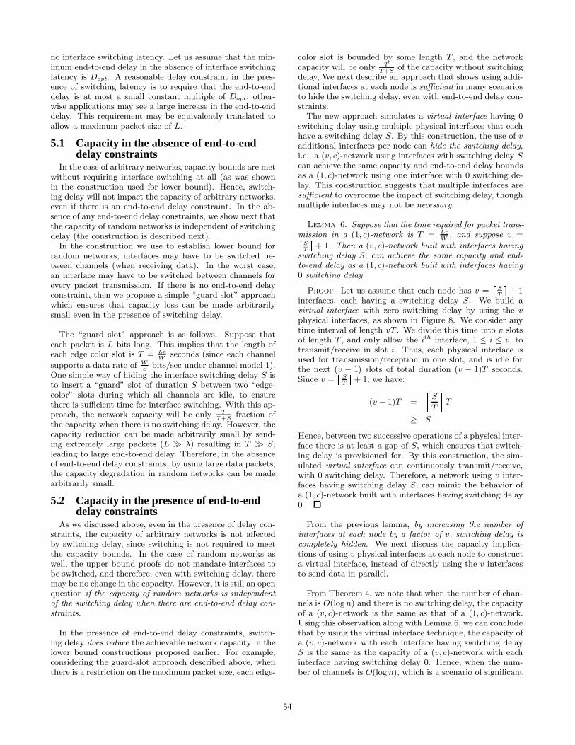
delay, We next describe an approach that shows using addi-tional interfaces at each node is sufficient in many scenariosto hide the switching delay, even with end-to-end delay con-straints.The new approach simulates a virtual interface having 0

switching delay using multiple physical interfaces that eachhave a switching delay S. By this construction, the use of vadditional interfaces per node can hide the switching delay,i.e., a (v, c)-network using interfaces with switching delay Scan achieve the same capacity and end-to-end delay boundsas a (1, c)-network using one interface with 0 switching de-lay. This construction suggests that multiple interfaces aresufficient to overcome the impact of switching delay, thoughmultiple interfaces may not be necessary.

Lemma 6. Suppose that the time required for packet trans-mission in a (1, c)-network is T = Lc

W, and suppose v =

ST

+ 1. Then a (v, c)-network built with interfaces having

switching delay S, can achieve the same capacity and end-to-end delay as a (1, c)-network built with interfaces having0 switching delay.

Proof. Let us assume that each node has v =

ST

+ 1

interfaces, each having a switching delay S. We build avirtual interface with zero switching delay by using the vphysical interfaces, as shown in Figure 8. We consider anytime interval of length vT . We divide this time into v slotsof length T , and only allow the ith interface, 1 ≤ i ≤ v, totransmit/receive in slot i. Thus, each physical interface isused for transmission/reception in one slot, and is idle forthe next (v − 1) slots of total duration (v − 1)T seconds.Since v =

ST

+ 1, we have:

(v − 1)T =

S

T

T

≥ S

Hence, between two successive operations of a physical inter-face there is at least a gap of S, which ensures that switch-ing delay is provisioned for. By this construction, the sim-ulated virtual interface can continuously transmit/receive,with 0 switching delay. Therefore, a network using v inter-faces having switching delay S, can mimic the behavior ofa (1, c)-network built with interfaces having switching delay0.

From the previous lemma, by increasing the number ofinterfaces at each node by a factor of v, switching delay iscompletely hidden. We next discuss the capacity implica-tions of using v physical interfaces at each node to constructa virtual interface, instead of directly using the v interfacesto send data in parallel.

From Theorem 4, we note that when the number of chan-nels is O(log n) and there is no switching delay, the capacityof a (v, c)-network is the same as that of a (1, c)-network.Using this observation along with Lemma 6, we can concludethat by using the virtual interface technique, the capacity ofa (v, c)-network with each interface having switching delayS is the same as the capacity of a (v, c)-network with eachinterface having switching delay 0. Hence, when the num-ber of channels is O(log n), which is a scenario of significant

54

T TS12

(v−1) slots

(v−1) slots

v slots

vv−1

Figure 8: Constructing one virtual interface withzero switching delay by using v physical interfaceswith switching delay S. Each packet transmissionrequires T seconds.

practical interest, there is no capacity loss even with switch-ing delay, provided multiple interfaces are used.

Again, from Theorem 4, we note that when the number ofchannels is larger (Ω(log n)) and there is no switching delay,the capacity of a (1, c)-network is the lower than that ofa (v, c)-network. Hence, using this observation along withLemma 6, we can conclude that using the virtual interfacetechnique when the number of channels is larger (Ω(log n)),a (v, c)-network with each interface having switching delayS will have lower capacity than a (v, c)-network with eachinterface having switching delay 0.Using Theorem 4, we can show that in this case, the

capacity will be lower by a factor of 1√v

≈q

TT+S

(since

v ≈ T+ST

) when number of channels is between Ω(log n)

and O

n

log log nlog n

2, and by a factor of 1

v≈ T

T+Swhen

number of channels is Ω

n

log log nlog n

2. In contrast, if the

guard slot approach is used, the capacity is lower by a fac-tor T

T+Sin all cases, independent of the number of channels.

Therefore, although there is a capacity loss with switchingdelay for certain scenarios using the virtual interface tech-nique, it is still significantly better than the guard slot ap-proach when the number of channels is small. It is partof our future work to study if alternate constructions arepossible that will not have any capacity loss at all.

6. PRACTICAL IMPLICATIONSThe theoretical analysis has studied the capacity of wire-

less networks with the number of channels varying acrossa wide range. The region where the number of channels isscaled as O(log n) seems to be of immediate practical inter-est, since the number of channels provisioned for in currentwireless technologies is not too large. However, there aremany recent efforts aimed at utilizing frequency spectrumin higher frequency bands, where significantly larger band-width is available for use. For example, there is around7 GHz of spectrum available for unlicensed use in the 60GHz band [5], whereas the total bandwidth used in cur-rent wireless technologies, such as IEEE 802.11, is less than500 MHz. The bandwidth that may become available inhigher frequency bands can be split up into a large number

of channels, and therefore the region with number of chan-nels greater than Ω(log n) may be of practical interest in thenear future.

The capacity analysis has shown that a single interfacemay suffice for random networks with up to O(log n) chan-nels. The capacity-optimal lower bound construction usedto support the above claim is based on certain assumptions,all of which may not be satisfied in practice. For example, weassume that interface switching delay is zero, transmissionrange of interfaces can be carefully controlled, and there isa centralized mechanism for co-ordinating route assignmentand scheduling. In addition, the theoretical analysis derivesasymptotic results, and capacity can be improved by con-stant factors in the lower bound constructions by using mul-tiple interfaces. From Section 5, we note that when interfaceswitching delay is not zero, having more than one interfacemay be beneficial. Furthermore, our research on protocoldesign [15] has identified many benefits of using at least twointerfaces at each node, such as allowing full-duplex transfer,and simplifying the development of distributed protocols forutilizing multiple channels.

Simulation and testbed experiments [13, 22] have shownthat having more than one interface may be beneficial inpractice. However, these experiments do not prove multipleinterfaces are necessary for obtaining all the observed per-formance improvement. In addition, some results also showthat [13] it is not necessary to have one interface per channelto utilize all the channels, and in fact even many (e.g., 12)channels can be fully utilized by using only two interfaces,which partly validates the theoretical claim.Furthermore, there are other proposals [2,25], which show

that a single interface solution can also effectively utilizemultiple channels, though at the cost of increased protocolcomplexity. Therefore, in practice, the theoretical claim thata single interface suffices with O(log n) channels is reason-ably accurate, with the caveat that additional interfaces maybe useful in simplifying protocol design and hiding switchingdelay.

7. CONCLUSIONSIn this paper, we have derived the lower and upper bounds

on the capacity of static multi-channel wireless networks.We have considered wireless networks having c channels,and m ≤ c interfaces per node. Each interface is capable ofselecting appropriate transmission power, and lower boundconstructions require global knowledge. Under this model,we have shown that in an arbitrary network, there is a lossin the network capacity when the number of interfaces pernode is smaller than the number of channels. However, wehave shown that surprisingly, in a random network, a singleinterface may suffice for utilizing multiple channels, as longas the number of channels is scaled as O(log n). We havethen considered the impact of non-zero interface switchingdelay on capacity, and shown that in a random networkwith up to O(log n) channels, interface switching delay hasno impact on capacity, provided each node is provisionedwith a few extra interfaces. As part of our future work, weintend to apply the insights gained from this work to buildpractical routing and MAC algorithms that approach thecapacity limit.

55

8. ACKNOWLEDGMENTSWe would like to thank the anonymous referees for their

valuable comments, and our shepherd Thyaga Nandagopalfor guiding us in improving the paper. This research wassupported in part by NSF grant ANI-0125859 and a Voda-fone Graduate Fellowship.

9. REFERENCES[1] A. Agarwal and P. R. Kumar. Capacity bounds for

ad-hoc and hybrid wireless networks. ACMSIGCOMM Computer Communication Review,34(3):71–81, July 2004.

[2] P. Bahl, R. Chandra, and J. Dunagan. SSCH: Slottedseeded channel hopping for capacity improvement inIEEE 802.11 ad-hoc wireless networks. In ACMMobicom, 2004.

[3] N. Bansal and Z. Liu. Capacity, delay and mobility inwireless ad-hoc networks. In Infocom, pages1553–1563, 2003.

[4] S. Diggavi, M. Grossglauser, and D. Tse. Evenone-dimensional mobility increases adhoc wirelesscapacity. Technical report, UC Berkeley, 2003.

[5] C. H. Doan, S. Emami, D. A. Sobel, A. M. Niknejad,and R. W. Brodersen. Design considerations for 60GHz CMOS radios. IEEE Communications Magazine,42(132-140), Dec 2004.

[6] R. Draves, J. Padhye, and B. Zill. Routing inmulti-radio, multi-hop wireless mesh networks. InACM Mobicom, 2004.

[7] A. E. Gamal, J. Mammen, B. Prabhakar, andD. Shah. Throughput-delay trade-off in wirelessnetworks. In Infocom, 2004.

[8] M. Gastpar and M. Vetterli. On the capacity ofwireless networks: The relay case. In Infocom, pages1577–1586, New York, USA, June 2002.

[9] M. Grossglauser and D. Tse. Mobility increases thecapacity of ad-hoc wireless networks. In Infocom, 2001.

[10] P. Gupta and P. R. Kumar. The capacity of wirelessnetworks. IEEE Transactions on Information Theory,46(2):388–404, March 2000.

[11] IEEE Standard for Wireless LAN-Medium AccessControl and Physical Layer Specification, P802.11,1999.

[12] U. C. Kozat and L. Tassiulas. Throughput capacity ofrandom ad hoc networks with infrastructure support.In Mobicom, 2003.

[13] P. Kyasanur and N. H. Vaidya. Routing inmulti-channel multi-interface ad hoc wirelessnetworks. Technical report, University of Illinois atUrbana-Champaign, December 2004.

[14] P. Kyasanur and N. H. Vaidya. Capacity ofmulti-channel wireless networks: Impact of number ofchannels and interfaces. Technical report, Universityof Illinois at Urbana-Champaign, March 2005.

[15] P. Kyasanur and N. H. Vaidya. Routing and interfaceassignment in multi-channel multi-interface wirelessnetworks. In WCNC, 2005.

[16] J. Li, Z. J. Haas, , and M. Sheng. Capacity evaluationof multi-channel multi-hop ad hoc networks. InInternational Conference on PersonalCommunications, 2002.

[17] B. Liu, Z. Liu, and D. Towsley. On the capacity ofhybrid wireless networks. In Infocom, 2003.

[18] A. Nasipuri, J. Zhuang, and S. Das. A multichannelCSMA MAC protocol for multihop wireless networks.In WCNC, September 1999.

[19] R. Negi and A. Rajeswaran. Capacity of powerconstrained ad-hoc networks. In Infocom, 2004.

[20] E. Perevalov and R. Blum. Delay limited capacity ofad hoc networks: Asymptotically optimal transmissionand relaying strategy. In Infocom, 2003.

[21] M. Raab and A. Steger. “Balls into Bins” - A simpleand tight analysis. In 2nd Workshop onRandomization and Approximation Techniques inComputer Science, 1998.

[22] A. Raniwala and T. Chiueh. Architecture andalgorithms for an IEEE 802.11-based multi-channelwireless mesh network. In Infocom, 2005.

[23] J. So and N. H. Vaidya. Multi-channel MAC for adhoc networks: Handling multi-channel hiddenterminals using a single transceiver. In Mobihoc, 2004.

[24] J. So and N. H. Vaidya. Routing and channelassignment in multi-channel multi-hop wirelessnetworks with single-nic devices. Technical report,University of Illinois at Urbana-Champaign, December2004.

[25] J. So and N. H. Vaidya. A routing protocol forutilizing multiple channels in multi-hop wirelessnetworks with a single transceiver. Technical report,University of Illinois at Urbana-Champaign, October2004.

[26] S. Toumpis. Capacity bounds for three classes ofwireless networks: Asymmetric, cluster, and hybrid. InMobihoc, 2004.

[27] S. Toumpis and A. J. Goldsmith. Large wirelessnetworks under fading, mobility, and delayconstraints. In Infocom, 2004.

[28] V. N. Vapnik. Estimation of Dependences based onEmpirical Data. Springer-Verlag, New York, 1982.

[29] V. N. Vapnik and A. Chervonenkis. On the uniformconvergence of relative frequencies of events to theirprobabilities. Theory of Probability and itsApplications, 16(2):264–280, 1971. 1971.

[30] D. B. West. Introduction to Graph Theory. PrenticeHall, 2 edition, 2001.

[31] S. Yi, Y. Pei, and S. Kalyanaraman. On the capacityimprovement of ad hoc wireless networks usingdirectional antennas. In Mobihoc, pages 108–116,USA, 2003.

[32] H. Zhang and J. C. Hou. Capacity of wireless ad-hocnetworks under ultra wide band with powerconstraint. In Infocom, 2005.

APPENDIX

A. UPPER BOUND IN ARBITRARYNETWORKS

Theorem 5. The arbitrary network capacity of a (m, c)-network is O

Wp

nmc

bit-meters/sec under channel model

1.

Proof. We prove the result under channel model 1. Theproof is based on a proof in [10]. We assume that nodes

56

are synchronized, and slotted transmissions of duration τare used. We assume that each source node originates λbits/sec. Let the average distance between source and des-tination pairs be L. Therefore, the capacity of the networkis λnL bit-meters/sec.We consider any time period of length one second. In this

time interval, consider a bit b, 1 ≤ b ≤ λn. We assume thatbit b traverses h(b) hops on the path from its source to itsdestination, where the h-th hop traverses a distance of rh

b .Since the distance traversed by a bit from its source to itsdestination is at least equal to the length of the line joiningthe source and the destination, by summing over all bits weobtain,

λnXb=1

h(b)Xh=1

rhb ≥ λnL (1)

Let us define H to be the total number of hops traversedby all bits in a second, i.e. H =

Pλnb=1 h(b). Therefore,

the number of bits transmitted by all nodes in a second(including bits relayed) is equal to H . Since each node hasm interfaces, and each interface transmits over a channelwith rate W/c (assuming channel model 1), the total bitsthat can be transmitted by all nodes over all interfaces is atmost Wmn

2c(Transporting a bit across one hop requires two

interfaces, one each at the transmitting and the receivingnodes). Hence, we have,

H ≤ Wmn

2c(2)

Under the protocol model, a transmission over a hop oflength r is successful only if there is no transmitter within adistance of (1 + ∆)r. Suppose node A is transmitting a bitto node B, while node C is simultaneously transmitting a bitto node D, and both the transmissions are over a commonchannel. Then, using the interference model, we have

d(C,B) ≥ (1 + ∆)d(A,B)

d(A,D) ≥ (1 + ∆)d(C,D)

Adding the above two expressions together, and applyingtriangle inequality, we obtain,

d(B,D) ≥ ∆

2(d(A,B) + d(C,D))

This implies that the receivers of two simultaneous trans-missions are separated by a distance proportional to thedistance from their senders. This may be viewed as eachhop consuming a disk of radius ∆

2times the length of the

hop around each receiver. Since the area “consumed” oneach channel is bounded above by the area of the domain(1 sq meter), summing over all channels (which can in totalpotentially transport W bits) we have the constraint,

λnXb=1

h(b)Xh=1

π∆2

4(rh

b )2 ≤ W (3)

which can be rewritten as,

λnXb=1

h(b)Xh=1

1

H(rh

b )2 ≤ 4W

π∆2H(4)

Since the expression on the left hand side is convex, wehave,

(λnXb=1

h(b)Xh=1

1

Hrh

b )2 ≤

λnXb=1

h(b)Xh=1

1

H(rh

b )2 (5)

Therefore, from (4) and (5),

λnXb=1

h(b)Xh=1

rhb ≤

r4WH

π∆2(6)

Substituting for H from (2), and using (1) we have,

λnL ≤ W

r2mn

π∆2c(7)

This proves that the network capacity of an arbitrary net-work is O

Wp

nmc

bit-meters/sec under channel model

1.

B. RESULTS FOR ESTABLISHING LOWERBOUND IN RANDOM NETWORKS

Lemma 4: If a(n) > 50 log nn

, then each cell has Θ(na(n))nodes per cell, with high probability.

Proof. A similar result was stated in [7] without proof.Here we provide a proof based on VC-theory (see [28] for de-tails on VC-theory), similar to the approach used by Guptaand Kumar [10]. The total number of square cells is 1

a(n).

Since nodes are randomly located on the torus, the proba-bility that any given node will lie in a specific cell is a(n).We want to derive bounds on number of nodes in every cellin the square grid, which requires a proof of uniform con-vergence. The set of axis-parallel squares C are known tohave VC-dimension 3. By applying the Vapnik-Chervonekistheorem [29], similar to the approach used in [10], we havethe following bound on the number of nodes NC in any cellC:

Prob

supC∈C

NC

n− a(n)

≤ 50 log n

n

> 1− 50 log n

n(8)

where the constants in the above expression have been care-fully chosen to satisfy the Vapnik-Chervonekis theorem. Theabove result implies that with high probability, we have

na(n)− 50 log n ≤ NC ≤ na(n) + 50 log n

provided a(n) > 50 log nn

.

Hence, we can conclude that the number of nodes in anycell is Θ(na(n)) with high probability, as long as a(n) >50 log n

n.

57