On the Capacity of MIMO Wireless Channels with Dynamic CSIT

IEEE JOURNAL ON SELECTED AREAS IN COMMUNICATIONS, VOL. 25, NO. 7, SEPTEMBER 2007 1269

On the Capacity of MIMO Wireless Channels withDynamic CSIT

Mai Vu, Member, IEEE, and Arogyaswami Paulraj, Fellow, IEEE

Abstract— Transmit channel side information (CSIT) can sig-nificantly increase MIMO wireless capacity. Due to delay inacquiring this information, however, the time-selective fadingwireless channel often induces incomplete, or partial, CSIT.In this paper, we first construct a dynamic CSIT model thattakes into account channel temporal variation. It does so byusing a potentially outdated channel measurement and thechannel statistics, including the mean, covariance, and temporalcorrelation. The dynamic CSIT model consists of an effectivechannel mean and an effective channel covariance, derived asa channel estimate and its error covariance. Both parametersare functions of the temporal correlation factor, which indicatesthe CSIT quality. Depending on this quality, the model coverssmoothly from perfect to statistical CSIT.

We then summarize and further analyze the capacity gains andthe optimal input with dynamic CSIT, asymptotically at low andhigh SNRs. At low SNRs, dynamic CSIT often multiplicativelyincreases the capacity for all multi-input systems. The optimalinput is typically simple single-mode beamforming. At highSNRs, for systems with equal or fewer transmit than receiveantennas, it is well-known that the capacity gain diminishes tozero because of equi-power optimal input. With more transmitthan receive antennas, however, the capacity gain is additive. Theoptimal input then is highly dependent on the CSIT. In contrastto equi-power, it can drop modes for channels with a strongmean or strongly correlated transmit antennas. For such mode-dropping at high SNRs in special cases, simple conditions on thechannel K factor or the transmit covariance condition numberare subsequently quantified.

Next, using a convex optimization program, we study theMIMO capacity with dynamic CSIT non-asymptotically. Particu-larly, we numerically analyze effects on the capacity of the CSITquality, the relative number of transmit and receive antennas,and the channel K factor. For example, the capacity gain basedon dynamic CSIT is more sensitive to the CSIT quality at higherqualities. The program also helps to evaluate a simple, analyticalcapacity lower-bound based on the Jensen optimal input. Thebound is tight at all SNRs for systems with equal or fewertransmit than receive antennas, and at low SNRs for others.

Index Terms— Capacity, MIMO wireless, partial CSIT, corre-lated Rician fading, temporal correlation.

Manuscript received June 1, 2006; revised Dec 28, 2006. Parts of thispaper were presented at the 37th and 39th Asilomar Conference on Signals,Systems, and Computers, Pacific Grove, Nov 2003 and 2005, and the 43rdAllerton Conference on Communication, Control, and Computing, Sept. 2005.This work was supported in part by the Rambus Stanford Graduate Fellowshipand the Intel Foundation PhD Fellowship. This work was also supported inpart by NSF Contract DMS-0354674-001 and ONR Contract N00014-02-0088.

Mai Vu is with the School of Engineering and Applied Sciences, HarvardUniversity, Cambridge, MA 02138 (e-mail: [email protected]).

Arogyaswami Paulraj is with the Information System Lab, Departmentof Electrical Engineering, Stanford University, Stanford, CA 94305 (e-mail:[email protected]).

Digital Object Identifier 10.1109/JSAC.2007.070902.

I. INTRODUCTION

W ITH PERFECT channel information at the receiver,channel side information at the transmitter (CSIT)

can significantly increase MIMO channel capacity. Assumingfrequency-flat fading, this benefit comes from the spatial chan-nel dimension. In contrast to temporal CSIT, which providesdiminishing capacity gain at medium-to-high SNR [1], spatialCSIT can enhance channel capacity in both low and high SNRregions, depending on the relative number of antennas. Forexample, in a 4-transmit 2-receive antenna system, perfectCSIT doubles the capacity at -5dB SNR and adds 2bps/Hzadditional capacity at 15dB SNR [2]. Perfect spatial CSIT hasbeen analyzed for fading channels in both ergodic and outagecapacities, showing significant capacity gains [3], [4]. Thesegains promise valuable increase in the transmission rate ofwireless systems.

The time-varying nature of the wireless channel, coupledwith the inherent delay in CSIT acquisition, however, ofteninduces partial CSIT. To account for the channel temporalvariation, we explicitly formulate a dynamic CSIT model, bycombining a potentially outdated channel measurement withthe channel statistics. The formulation allows evaluating theCSIT based on the channel temporal correlation factor ρ,which is a function of the delay and the channel Dopplerspread. When ρ = 1, the CSIT is perfect; when ρ → 0,the CSIT approaches the actual channel statistics. Specifically,dynamic CSIT consists of an estimate of the channel atthe transmit time and the associated error covariance, whichfunction effectively as the channel mean and the channelcovariance, respectively.

To establish the capacity with dynamic CSIT, it is necessaryto find the optimal input signal. For memoryless channelwith perfect channel information at the receiver, the optimalinput is Gaussian distributed with zero-mean [5]. Therefore,the objective remains to find its optimal covariance. Thiscovariance eigenvectors function as transmit beam directions,and the eigenvalues as the beam power allocation. For dynamicCSIT, involving a non-zero effective channel mean and a non-trivial effective channel covariance, the capacity optimizationproblem involves evaluating an expectation over the non-central Wishart distribution. Solutions exist partially only forspecial cases: covariance CSIT, when the channel covarianceis non-trivial but the mean is zero [6], [7], and mean CSIT,when the channel mean is non-zero but the covariance isthe identity matrix [8], [9]. In these cases, the optimal beamdirections are known analytically (as the eigenvectors of themean or covariance matrix), but not the power allocation. Thelatter usually requires numerical optimization, where efficient

0733-8716/07/$25.00 c© 2007 IEEE

1270 IEEE JOURNAL ON SELECTED AREAS IN COMMUNICATIONS, VOL. 25, NO. 7, SEPTEMBER 2007

iterative algorithms exist for covariance CSIT [10] and meanCSIT [11].

After formulating the capacity with dynamic CSIT, wefirst analyze the optimal input covariance and the capacitygain from the CSIT asymptotically at low and high SNRs.Asymptotic MIMO capacity have been studied by variousauthors. We summarize some of the existing results in thecontext of capacity gain and develop new results on optimalmode-dropping at high SNRs. Specifically, at low SNRs, theoptimal input typically becomes simple single-mode beam-forming, and the capacity gain is multiplicative [12]. At highSNRs, the optimal solution depends on the relative numbersof transmit and receive antennas. For systems with equal orfewer transmit than receive antennas, it is well-known thatthe optimal input approaches equi-power and the capacity gaindiminishes to zero. For others, however, both the optimal inputand the capacity gain depend heavily on the CSIT. In contrastto equi-power, the optimal input may drop modes at highSNRs in systems with more transmit than receive antennas.We establish conditions for mode dropping for representativechannels with a high K factor or strong transmit antennacorrelation. These conditions provide intuition to when it isoptimal to activate only a fraction of the available eigen-modesat all SNRs, given the CSIT. In such cases, CSIT provides anadditive capacity gain at high SNRs.

Fortunately, capacity optimization with dynamic CSIT isa convex problem, hence allowing efficient numerical imple-mentation [13]. Using the program in [14], we study thenon-asymptotic capacity impacts of the channel mean, thetransmit covariance, the CSIT quality, and the K factor. Theprogram also helps evaluate a sub-optimal input covariance,which maximizes Jensen’s bound on capacity, and establishconditions with which, using this covariance creates a tightlower-bound to the capacity, hence allowing a simple, analyt-ical capacity approximation.

The paper is organized as follows. Section II discussesthe wireless channel model. Section III then establishes thedynamic CSIT model. Section IV formulates the channelcapacity with dynamic CSIT. Asymptotic capacity results areanalyzed in the next two sections. Section V establishes thecapacity gains at low and high SNRs, and Section VI charac-terizes the optimal input. Numerical capacity results follow inSection VII. Section VIII then provides the conclusion.

Notation used in this paper is as follows. (.)∗ for conjugatetranspose, E[.] for expectation, tr(.) for trace, ||.||F for theFrobenius norm, λ(.) for eigenvalues, (.)+ for a positivevalue inside the parenthesis or zero, and � for the matrixpositive semi-definite relation. Matrices are denoted by bold-face capital letters, and their vectorized version is denotedby the corresponding lower-case letter in bold-face, with anysubscript carried through (for example, h0 = vec(H0)).

II. CHANNEL MODEL

Consider a frequency flat, quasi-static block fading channelwith N transmit and M receive antennas. The channel can bemodeled as a complex Gaussian process, represented by a ma-trix Hs of size M ×N , with s indicating the time. Assumingthat the channel is stationary, it can be specified by its time-invariant mean, covariance, and auto-covariance. Specifically,

omitting the time subscript for brevity, the channel H can bedecomposed as into fixed and variable parts as

H = Hm + H , (1)

where Hm is the complex channel mean, and H is a zero-mean complex Gaussian random matrix.

A. Channel covariance and antenna correlations

The channel covariance R0 captures the spatial correlationamong all the transmit and receive antennas. In other words,it defines the correlation among all MN channel elements asa MN × MN matrix

R0 = E[hh∗] , (2)

where h = vec(H), and (.)∗ denotes a conjugate transpose.R0 is a positive semi-definite Hermitian matrix. Its diagonalelements represent the power gain of the MN scalar channels,and the off-diagonal elements are the cross-coupling betweenthese scalar channels.

The covariance R0 sometimes assumes a simple Kroneckerstructure with separable transmit and receive antenna correla-tions [15]. The channel covariance can now be decomposedas

R0 = RTt ⊗ Rr , (3)

where ⊗ denotes the Kronecker product [16]. Both Rt and Rr

are complex Hermitian positive semi-definite. The channel (1)can then be written as

H = Hm + R1/2r HwR1/2

t , (4)

where Hw is a M × N matrix, whose entries have the realand imaginary parts independent and identically distributedas zero-mean Gaussian with unit-variance. Here R1/2

t is theunique square-root of Rt, such that R1/2

t R1/2t = Rt; similarly

for R1/2r .

The Kronecker correlation model has been experimentallyverified in indoor environments for up to 3 × 3 antennaconfigurations [17], [18], and in outdoor environments for upto 8 × 8 configurations [19]. Other more general covariancestructures have been proposed in the literature [20], [21],where the transmit covariances corresponding to differentreference receive antennas are assumed to have the sameeigenvectors, but not necessarily the same eigenvalues; simi-larly for the receive covariances.

B. Channel mean and the Rician K factor

The channel mean Hm (M ×N ) is the fixed component ofthe channel, usually corresponding to a line-of-sight propaga-tion path or a cluster of strong paths, obtained as

Hm = E[H] . (5)

The elements of the mean can have different amplitudes andarbitrary phase. The strength of a channel mean can be looselyquantified by the Rician K factor. It defines the ratio of thepower in the channel mean and the average power in thechannel variable component as

K =||Hm||2Ftr(R0)

, (6)

VU and PAULRAJ: ON THE CAPACITY OF MIMO WIRELESS CHANNELS WITH DYNAMIC CSIT 1271

where ||.||F is the matrix Frobenius norm, and tr(.) is thetrace of a matrix. The K factor can take any real valuebetween 0 and infinity. When K = 0, the channel has Rayleighdistribution, otherwise it is Rician fading. When K → ∞,the channel becomes deterministic. Measurements of fixedbroadband channels have shown that the K factor can havea wide range from 0 to up-to 30dB in practice, and it tendsto decrease with the distance between the transmitter and thereceiver [22].

C. Channel auto-covariance and the Doppler spread

The channel auto-covariance characterizes how rapidly thechannel decorrelates with time. Because of the stationarityassumption, the covariance between two channels samplesH0 and Hs depends only on the time difference but not theabsolute time

Rs = E[h0h∗

s

], (7)

where h denotes the vectorized version of the zero-mean partof the corresponding channel matrix. Note that when s = 0,this auto-covariance coincides with the channel covariance R0

(2); when s becomes large, it eventually decays to zero.For a MIMO channel, the covariance R0 captures the spatial

correlation between all the transmit and receive antennas,while the auto-covariance at a non-zero delay Rs capturesboth channel spatial and temporal correlations. Based on thepremise that the channel temporal statistics can be the samefor all antenna pairs, it may be assumed that the temporalcorrelation is homogeneous and identical for any channelelement. Then, the two correlation effects are separable, andthe channel auto-covariance becomes their product as

Rs = ρsR0 , (8)

where ρs is the temporal correlation of a scalar channel. Inother words, all the MN scalar channels between the Mtransmit and N receive antennas have the same temporalcorrelation function. This correlation is a function of the timedifference s and the channel Doppler spread. For example, inClark’s model, ρs = J0(2πfds), where J0 is the zeroth orderBessel function of the first kind, and fd is the Doppler spread[23]. Similar assumptions for MIMO temporal correlationhave also been used in constructing channel models andverifying measurement data in [18], [21].

The channel statistics, Hm, R0 and Rs, can be obtainedby averaging instantaneous channel measurements over tensof channel coherence times; they remain valid for a period oftens to hundreds coherence time, during which, the channelcan be considered as stationary.

III. DYNAMIC CSIT

A. CSIT acquisition

While a receiver can directly estimate the channel fromthe received signal, the transmitter must obtain channel infor-mation indirectly by using the reverse-channel information,relying on the reciprocity principle, or by feedback fromthe receiver. Reciprocity applies to the “over-the-air” channelbetween the transmit and receive antennas and requires theforward and reverse links to occur at the same time, frequency,

and space instance. In practice, it requires careful hardwarecalibration to make the transmit and receive RF chains iden-tical and is usually applicable only in time-division-duplex(TDD) systems with small turn-around time between thereverse and forward transmissions [24]. Feedback can beused in both time and frequency division-duplex systems,provided that the feedback lag is relatively small compared tochannel dynamics. In either case, there exists a delay betweenmeasuring the channel information at a receiver and usingthis information at the transmitter. This delay may affect thereliability of the obtained channel information, depending onthe type of information.

Consider the channel statistics and instantaneous channelmeasurements. In practice, the channel statistics often remainunchanged for a relatively long time compared to the trans-mission intervals. Assuming stationarity, these statistics are notaffected by the delay in channel acquisition, and hence becomereliable CSIT. Channel statistics, however, are only partialinformation and therefore provide partial capacity gains. Incontrast, instantaneous channel information provides the high-est capacity gain, but is sensitive to the CSIT acquisitiondelay due to channel temporal variation. This delay leadsto a potential mismatch between the instantaneous channelmeasurement and the current channel. For the purpose ofthis paper, the initial channel measurement is assumed to beaccurate. The only cause of the mismatch then is channelvarying over the delay period.

More reliable and complete CSIT provides more capacitygain. This principle suggests combining both the channelstatistics and instantaneous measurements to create a CSITmodel robust to channel variation, while optimally capturingthe potential gain.

B. CSIT modeling

Consider CSIT at the transmit time s in the form of achannel estimate Hs and its error covariance Re,s, which canbe expressed as

Hs = Hs + Es ,Re,s = E

[ese∗s

] (9)

where Es is the zero-mean estimation error and es =vec (Es). Assuming unbiased estimates, Es can be modeledas a stationary Gaussian random process. The error covarianceRe,s is then dependent on s and the Doppler spread.

Now assume that the transmitter has an initial channelmeasurement H0 at time 0, together with the channel statisticsHm, R0, and Rs. Furthermore, the channel matrix coefficientsare jointly Gaussian. Based on MMSE estimation theory [25],an optimal estimate of the channel at time s and the estimationerror covariance can be established as

hs = E[hs|h0

]= hm + R∗

sR−10

[h0 − hm

]Re,s = cov

[hs|h0

]= R0 − R∗

sR−10 Rs ,

(10)

where hs = vec(Hs

)(again the lower-case letters h denote

the vectorized version of the corresponding upper-case matri-ces H). A similar model was proposed in [26] for estimatinga scalar time-varying channel from a vector of out-datedestimates. CSIT formulations conditioned on noisy channelestimates were also studied in [27], [28].


The two quantities {Hs,Re,s} constitute the CSIT. Theyeffectively function as a new channel mean and covariance.Thus Hs and Re,s are also referred to as the effective meanand effective covariance, respectively, and the pair forms aneffective statistics.

We next apply the simplified temporal correlation model(8). This model helps to isolate the effect of temporal channelvariation on the CSIT; it has also been used to fit data in somechannel measurements [18], [21]. The channel estimate and itserror covariance then become

Hs = ρsH0 + (1 − ρs)Hm ,Re,s =

(1 − ρ2

s

)R0 .

(11)

The CSIT can now be simply characterized as a function ofρs, the initial channel measurement H0, and the channel meanHm and covariance R0. The channel estimate becomes alinear combination between the initial measurement and thechannel mean. The error covariance is a linear function of thechannel covariance alone. With Kronecker antenna correlation(3), the transmit and receive covariances are separable. Forthe estimated channel, the effective antenna correlations canbe decomposed as

Rt,s =√

1 − ρ2s Rt ,

Rr,s =√

1 − ρ2s Rr ,

(12)

which again follow a Kronecker structure. Since the scalingfactors ultimately affect the received power, this decomposi-tion is for convenience from the analysis and signal processingperspectives. When the antennas at the receiver are uncorre-lated, Rr = I, then the effective channel is also assumedto have no receive correlation (Rr,s = I), and the effectivetransmit correlation becomes

Rt,s =(1 − ρ2

s

)Rt . (13)

In the constructed CSIT models (11), (12) and (13), ρs

acts as a channel estimate quality dependent on the timedelay s. For a zero or short delay, ρs is close to one; theestimate depends heavily on the initial channel measurement,and the error covariance is small. As the delay increases,ρs decreases in magnitude to zero, reducing the impact ofthe initial measurement. The estimate then moves toward thechannel mean Hm, and the error covariance grows toward thechannel covariance R0. Therefore, the estimate and its errorcovariance (11) constitute a form of CSIT, ranging betweenperfect channel knowledge (when ρ = 1) and the channelstatistics (when ρ = 0). By taking into account channeltime variation, this framework optimally captures the availablechannel information and creates a dynamic CSIT model.

C. Special CSIT cases

Here we define the terminology for several special cases ofdynamic CSIT. When ρ = 1, it is perfect CSIT. When 0 ≤|ρ| < 1, it is partial CSIT, consisting of an effective channelmean and an effective covariance. For ρ = 0, the CSIT isreferred to as statistical CSIT. If either the mean or covarianceis trivial, then the CSIT collapses to a special case. Whenthe covariance is arbitrary but the mean is zero (Hm = 0),we have covariance CSIT. More specifically, transmit antenna

correlation alone (without receive correlation) gives transmitcovariance CSIT. When the mean Hm is arbitrary but thecovariance is an identity matrix (R0 = I), we have meanCSIT. Finally, when ρ = 0, Hm = 0, and R0 = I, we haveno CSIT, equivalent to an i.i.d Rayleigh fading channel withno channel information at the transmitter.

IV. CHANNEL ERGODIC CAPACITY WITH DYNAMIC CSIT

Consider the ergodic capacity of a MIMO channel witha constant sum power across all transmit antennas at everytime instance. Assume perfect channel state information atthe receiver (CSIR) and dynamic CSIT (11) with a givenestimate quality ρ. With perfect CSIR, the capacity is achievedby a zero-mean complex Gaussian input [5] with covariancedependent on the CSIT. With dynamic CSIT, this optimal inputcovariance and the ergodic capacity are obtained by two-stageaveraging.

In the first stage, each initial channel measurement H0

with estimate quality ρ produces CSIT value {H,Re} (11).The channel seen from the transmitter thus effectively hasmean H and covariance Re. Assuming that this effectivestatistics is valid for a reasonable duration, and using a zero-mean Gaussian input with covariance Q, we can then cal-culate the average mutual information given H0 as I(H0) =EH [logdet(I + γHQH∗)]. The signal covariance Q that max-imizes I(H0) is the optimizer of the problem

Io(H0) = maxQ EH

[logdet(I + γHQH∗)

]subject to

tr(Q) = 1Q � 0 ,

(14)

where γ is the SNR. The equality constraint results fromthe constant sum transmit power, and the inequality from thepositive semi-definite property of a covariance matrix. Notethat the expectation is evaluated over the effective channelstatistics with mean H and covariance Re.

In the second stage, based on ergodicity, we can averageIo(H0) over the distribution of H0 to obtain the channelergodic capacity. For a given CSIT quality ρ, therefore, thecapacity is

C = EH0 [Io(H0)] , (15)

where H0 has the actual channel statistics, Gaussian dis-tributed with mean Hm and covariance R0.

Establishing the capacity with dynamic CSIT thus essen-tially requires solving (14). This problem is to find the optimalinput covariance and capacity for a channel with statisticalCSIT, involving arbitrary channel mean and covariance. Notethat the input covariance can be decomposed into its eigen-values and eigenvectors as

Q = UQΛQUQ . (16)

The columns of UQ function as orthogonal eigen-beam di-rections (patterns), and ΛQ represents the power allocationon these beams. The problem has analytical solution for theeigenvectors UQ in special cases of mean CSIT and covari-ance CSIT. For mean CSIT, UQ is given by the right singular-vectors of the mean matrix [8], [9]. For covariance CSIT, itis by the eigenvector of the transmit antenna correlation [6],[7]. For a non-Kronecker covariance, however, analytical result


for UQ is so far scarce. A general condition on the channelstructure for isotropic input to achieve the capacity is given in[10]. In all cases of partial CSIT, the eigenvalue ΛQ has noclosed-form solution and usually requires numerical solution.Fortunately, the optimization problem is convex, allowingefficient numerical solutions for all CSIT cases [10], [11], [14].

A. The Jensen-optimal input covariance

Here we discuss a lower-bound on the capacity by usinga sub-optimal input covariance. Consider QJ that maximizesJensen’s bound on the mutual information. The Jensen boundon the average mutual information is

E [log det(I + HQH∗)] ≤ log det (I + E[H∗H]Q) .

Given CSIT, the transmitter can establish G = E[H∗H]. Thecovariance QJ is then obtained by standard water-filling [5]on G. Using the Jensen covariance QJ as the input covarianceresults in a Jensen mutual information value

IJ = I(QJ ) , (17)

satisfying IJ ≤ Io in (14). For statistical CSIT, IJ can be usedto lower-bound the capacity. For dynamic CSIT, averaging IJ

over the initial channel measurement distribution (15), a lowerbound to the channel ergodic capacity is obtained as

CJ = EH0 [IJ ] . (18)

The tightness of this capacity lower bound will be numericallyevaluated in Section VII.

V. ASYMPTOTIC-SNR CAPACITY GAINS

This section summarizes the analytical results on the asymp-totic capacity gains from dynamic CSIT at low and high SNRs.Most of these results are simple and have been derived inone form or another by various authors. Here we cast themin a common context of asymptotic capacity gains, therebyconnecting these results and identifying the open problems,which we will provide a partial solution to in the next section.

In particular, the asymptotic capacity gain at low SNRsis multiplicative and is achieved typically by single-modebeamforming. The gain at high SNRs is additive and requiresmulti-mode transmission. These gains also depend on theCSIT.

A. Low-SNR optimal beamforming and capacity gain

1) Low-SNR optimal beamforming: The optimal signal atlow SNRs is typically single-mode beamforming with thedirection given by the CSIT.

Theorem 1: (Verdu [12]) As the SNRs γ → 0, the optimalinput covariance of problem (14) converges to a rank-one ma-trix with a unit eigenvalue and the corresponding eigenvectorgiven by the dominant eigenvector of

G = E[H∗H] ,

provided the dominant eigenvalue is unique. In other words,the optimal input becomes a single-mode beamforming signalalong the dominant eigenvector of G. If there are multiple

dominant eigenvalues of G, the transmit power must splitequally among their eigenvector directions.

Note that for the channel model (3) without receive antennacorrelation, G = E[H∗H] = H∗H + MRt,s. With dynamicCSIT, the optimal beam direction changes with each update ofH0 and ρ. This theorem can be proved by a simple applicationof the Taylor expansion to I(H0) in (14).

When G has multiple dominant eigenvalues, consideringwideband transmission, equally distributing power amongthem minimizes the wideband slope (the derivative of thecapacity at the minimum bit energy point), hence minimizingthe required bandwidth [12]. In the i.i.d. case when G is ascaled-identity matrix, distributing power equally is in factcapacity optimal for all SNRs [29], [30].

2) Low-SNR capacity ratio gain with statistical CSIT: Withthe optimal input at low SNRs, the capacity gain with statis-tical CSIT is multiplicative and can be quantified precisely.

Theorem 2: As the SNR γ → 0, the ratio between theoptimal mutual information in (14) and the value obtainedby equi-power isotropic input approaches

r =Nλmax(G)

tr(G). (19)

This ratio scales linearly with the number of transmit antennasand is related to the condition of the channel correlationmatrix G = E[H∗H].

The derivation of this result is quite straightforward [12](see Eqs. 52-53). The result implies that, at low SNRs, thetransmitter has little power, and the CSIT allows it to focusall this power on the strongest known direction in the channel,rather than spreading it equally everywhere. More transmitantennas will increase the focusing and hence the capacitygain at low SNRs in (19). As an extreme example, when Gis rank-one, the ratio equals the number of transmit antennasN .

For dynamic CSIT with a given quality ρ, each initial chan-nel measurement H0 provides an effective channel correlationG. The capacity gain is then obtained by averaging the ratio(19) over the distribution of H0.

3) Low-SNR capacity ratio gain with perfect CSIT: PerfectCSIT also multiplicatively increases the capacity at low SNRs.Moreover, the asymptotic gain can be quantified in the limitof a large number of antennas.

Theorem 3: As the SNR γ → 0, the ratio of the ergodiccapacity with perfect CSIT to that without CSIT equals

r =E[λmax(H∗H)]1N E[tr(H∗H)]

, (20)

where the expectations are performed over the actual channeldistribution.

For an i.i.d channel, if the number of antennas increases toinfinity, provided the transmit to receive antenna ratio N/Mstays constant, this ratio approaches a fixed value as

rN→∞−→

(1 +

√N

M

)2

. (21)

This limit is always greater than 1.


Fig. 1. Ratio of the capacity of i.i.d channels with perfect CSIT to thatwithout CSIT. The legend denotes the numbers of transmit and receiveantennas. The asymptotic capacity ratio, in the limit of large number ofantennas, while keeping the number of transmit antennas twice the receive,is 5.83.

Expression (20) is straightforward from Theorem 1 and[29]. Expression (21) is implicitly derived in [12] (Eqs. 204-205) and requires a simple application of the largest eigenvalueresult of large-dimension random matrices [31], [32].

Figure 1 shows examples of the capacity ratio for 4 channelswith twice the number of transmit as receive antennas. Theratio increases as the SNRs decreases and as the number ofantenna increases. Keeping the antenna proportion the same,as the number of antennas increases to infinity, this ratiowill approach 5.83. CSIT at low SNRs thus can increase thecapacity significantly.

B. High-SNR capacity gain

At high SNRs, the optimal input and the capacity gaindepend on the channel rank and the relative antenna configura-tion. For full-rank channels, dynamic CSIT does not increasethe capacity at high SNRs for systems with equal or fewertransmit than receive antennas (N ≤ M ), but does for systemswith more transmit antennas (N > M ). For rank-deficientchannels with a non-full-rank Rt, transmit covariance CSITalways helps increase the capacity. Each case is considerednext.

1) Full-rank channels with equal or fewer transmit thanreceive antennas: When N ≤ M , asymptotically at highSNRs, it is well-known that isotropic input is optimal for(14), independent of the CSIT (for example, the case N = Mis analyzed in [33]). For full-rank channel H, the conditionN ≤ M makes H∗H full-rank, hence I(H0) at high SNRscan be decomposed as

I γ→∞≈ EH[log det(γH∗HQ)] (22)

= EH [log det(H∗H)] + log det(γQ) .

Maximizing this expression, subject to tr(Q) = 1, leads toQ = I/N . For these systems, the capacity gain from CSITdiminishes to 0 at high SNRs.

Fig. 2. Incremental capacity gain from perfect CSIT for i.i.d. channels. Thelegend denotes the numbers of transmit and receive antennas.

2) Full-rank channels with more transmit than receiveantennas: On the contrary, when N > M , dynamic CSIT canprovide capacity gain at high SNRs. The gain here is additive.Since H∗H is rank-deficient in this case, the decomposition(22) does not apply. The optimal input covariance of (14)at high SNRs depends on the channel statistics, or the CSIT{H,Re}. An analytical optimal covariance for arbitrary H andRe is still an open problem. In the next section, we providethe solutions for some simplified cases.

The capacity gain in this case is maximum with perfectCSIT (ρ = 1, H = H0, and R = 0), with which this gaincan be accurately quantified.

Theorem 4: For N > M , at high SNRs, the incrementalcapacity gain from perfect CSIT (ρ = 1), over the mutualinformation obtained by equi-power isotropic input, equals

∆C = M log(

N

M

). (23)

This gain scales linearly with the number of receive antennasand depends on the ratio of the number of transmit to receiveantennas.

Intuitively, with N > M , the channel seen from the trans-mitter has a null-space. By knowing the channel, the trans-mitter can avoid sending any power into this null-space andtherefore achieve a capacity gain. For example, for systemswith twice the number of transmit as receive antennas, thecapacity incremental gain approaches the number of receiveantennas in bps/Hz and can be achieved at an SNR as low as20dB, as shown in Figure 2.

The derivation of this result is straightforward. Althoughthe ingredients used in proving the result have been used bydifferent authors in different contexts (e.g. see [34] for largeantenna analysis, and [35] for power offset analysis), we arenot aware of a proof prior to [36] and hence provide one herefor completeness.

Proof. With perfect CSIT, the solution for (14) isstandard water-filling on H∗

0H0 [5]. Let σ2i be the

eigenvalues of H∗0H0, then the optimal eigenvalues of

Q are λi =(µ − 1

γσ2i

)+

, where µ is chosen to satisfy


∑i λi = 1. The ergodic capacity (15) then becomes C =∑Mi=1 Eσi

[log

(µγσ2

i

)], where σ2

i has the distribution ofthe underlying Wishart matrix eigenvalues. For full-rankH0, as γ → ∞, µ → 1

M , and the capacity approaches

C γ→∞≈ M log(

1M

)+ M log(γ) +

M∑i=1

E[log

(σ2

i

)].

(24)Without CSIT, on the other hand, using an equi-power isotropic input with covariance Q = I/N ,the ergodic mutual information is given by C0 =∑M

i=1 Eσi

[log

(1 + 1

N γσ2i

)]. At high SNRs, this expres-

sion approaches

C0

γ→∞≈ M log(

1N

)+ M log(γ) +

M∑i=1

E[log

(σ2

i

)].

(25)Subtracting (24) and (25) side-by-side yields the capacitygain in (23). �

3) Rank-deficient channels with a non-full-rank Rt: Wenow consider channels with rank-deficient Rt, zero mean anduncorrelated receive antennas. In this case, transmit covarianceCSIT helps increase the capacity additively at high SNRs,regardless of the number of receive antennas. Let Kt be therank of Rt (Kt < N ), this capacity gain can be quantified inthe case Kt ≤ M as

∆C = Kt log(

N

Kt

). (26)

The derivation of this result is as follows. For transmitcovariance CSIT, the optimal input beam directions are givenby Rt eigenvectors. The mutual information can then bewritten as

I = log det (IM + γHwΛtΛQH∗w)

= log det (IN + γH∗wHwΛtΛQ) ,

where Λt is the eigenvalue matrix of Rt. With Kt ≤ M ,the matrix H∗

wHwΛt has rank Kt, hence at high SNRs,the optimal ΛQ approaches equi-power on the Kt non-zeroeigenmodes of Λt. (Note that this equi-power input is notalways optimal at high SNRs if Kt > M , but a capacity gainstill exists.) Without the CSIT, however, the optimal input hasequi-power on all N eigenmodes of Rt. The difference in thecorresponding mutual information then gives (26), similar tothe proof of Theorem 4.

Figure 3 provides an example of the capacity with andwithout transmit covariance CSIT for rank-one correlatedchannels with various antenna configurations at 10dB SNR.The capacity without CSIT plus the gain (26) is also included.Note that for rank-one correlation, having more transmit an-tennas helps to increase the capacity with transmit covarianceCSIT, but does not without the CSIT.

VI. OPTIMAL INPUT CHARACTERIZATIONS

The capacity-optimal input signal with dynamic CSIT canbe analytically established in certain cases. At low SNRs, asspecified in Theorem 1, it is single-mode beamforming withdirection as a function of CSIT, implying mode-dropping.

Fig. 3. Capacity of channels with a rank-one transmit correlation at SNR =10dB, without and with transmit covariance CSIT.

At high SNRs, the optimal input depends not only on theCSIT, but also on the antenna configurations. For systemswith equal or fewer transmit than receive antennas, the optimalinput approaches isotropic equi-power. For systems with moretransmit than receive antennas, however, it may not approachequi-power at high SNRs, depending on the CSIT. Specifically,for statistical CSIT with a high-K mean or highly-conditionedtransmit covariance, signifying a strong antenna correlation,mode-dropping may also occur at high SNRs. The intuitioncan be obtained by considering a 4× 2 channel with differentCSIT scenarios. With perfect CSIT, the optimal input has only2 eigen-modes at high SNRs. Without CSIT, however, theoptimal input is i.i.d isotropic, which has 4 modes. Thereforethere exists partial CSIT, with which the optimal input has 3modes at high SNRs, implying mode-dropping.

In this section, we consider impacts of antenna configura-tions and the CSIT on the optimal input covariance. We firstbriefly discuss the optimal input for systems with N ≤ M . Wethen provide simplified analysis on the conditions for mode-dropping at high SNRs in systems with N > M . Two effectsare considered: of the K factor and of the transmit antennacorrelation. To isolate each effect, a simplified channel modelis used in each case.

A. Systems with equal or fewer transmit than receive antennas

For N ≤ M systems with dynamic CSIT, the optimal inputsignal is known asymptotically at both low and high SNRs. Atlow SNRs, it is single-mode beamforming, and at high SNRs,it approaches equi-power. Interestingly, it turns out that theoptimal input covariance here can be closely approximated bythe closed-form Jensen input covariance discussed in SectionIV-A (see Section VII for numerical verification). This Jensencovariance becomes optimal at both low and high SNRs.At other SNRs, it produces a mutual information that is atight lower-bound to the capacity. For the two special cases,transmit covariance CSIT and mean CSIT, the Jensen beamdirections are optimal at all SNRs; only the power allocationis then approximated.


B. Systems with more transmit than receive antennas

For N > M systems with dynamic CSIT, the capacity-optimal input, especially its power allocation, depends heavilyon the channel effective mean and covariance matrices. If thechannel is uncorrelated with zero mean, as with i.i.d Rayleighfading, then the optimal input covariance is the identity matrixat all SNRs [29], implying equi-power allocation. However,if the mean is strong, characterized by a high K factor, orthe transmit antennas are highly correlated, characterized bya large condition number of Rt, the optimal input may dropmodes even at high SNRs. A closed-form solution for theoptimal input covariance, as a function of the channel meanand covariance, is still unknown. Furthermore, the Jensencovariance, which approaches equi-power at high SNRs, isno longer a good approximation.

This section provides some simple characterizations oneffects of the K factor and the transmit antenna correlationon the optimal input. The analysis focuses on two simplechannel models, belonging to the special mean CSIT andcovariance CSIT cases. Of these, the optimal beam directionsare known [6]-[9], thus only the power allocation needs tobe specified. Each considered model results in the optimalallocation with only two distinct power levels. Conditions thatlead to dropping the lower power level at high SNRs areanalyzed.

1) Effects of the K factor: In an uncorrelated channelwith N > M , given statistical CSIT, as K increases from0 to infinity, the optimal number of input modes at highSNRs reduces from N to M . Thus, a sufficiently high Kwill result in less than N optimal modes. The mode-droppingeffect, however, depends more broadly on the channel meaneigenvalues, of which K is a function. To isolate the impactof K alone, consider an uncorrelated channel, in which thechannel mean has equal eigenvalues and hence is unitary. Inpractice, such a mean may be found in an isotropic channel asthe measured channel mean, which changes slowly over time,or as a channel estimate. With this channel mean structure, thepower allocation depends solely on K , but not the entire Hm.The threshold for K , above which mode dropping occurs athigh SNRs, can be obtained as follows.

Theorem 5: Consider a channel with N > M , uncorrelatedantennas, and unitary channel mean. Specifically, the meanand transmit covariance are given as

HmH∗m =

K

K + 1IM , Rt =

1K + 1

IN (27)

and the receive covariance is Rr = I.With statistical CSIT, the condition on K , with which the

optimal input activates only M out of the maximum N modesat all SNRs, is given as

tr

⎛⎜⎝E

⎡⎢⎣⎛⎝ M∑

j=1

(√Kej + hw,j

)(√Kej + h∗

w,j

)⎞⎠−1

⎤⎥⎦⎞⎟⎠ ≤ 1,

(28)where ei is the M -vector with the ith element equal to 1 and

the rest zero, and hw,j ∼ N (0, IM ) are i.i.d.The matrix expression under expectation in (28) has the

inverted non-central complex Wishart distribution. This expec-

tation has no closed-form solution so far, but can be evaluatednumerically.

Proof: Given mean and transmit covariance (27), letβ =

√K/(K + 1), and perform the SVD of the mean

asHm = βUmV∗

m , (29)

then the optimal beam directions are given by Vm. Theoptimal power allocation can be completely character-ized by the K factor, or β, and the SNRs. Becauseof symmetry, this optimal solution contains only twodifferent power levels: λ1 for the first M eigen-modes,corresponding to the non-zero eigen-modes of H∗

mHm,and λ2 for the rest N −M modes, where λ1 ≥ λ2 [37].Thus the optimal solution Q for problem (14) has theform

Q = VmΛQV∗m , (30)

where ΛQ is a diagonal matrix with M diagonal entriesas λ1 and N − M as λ2. Let H be the zero-meanpart of U∗

mHVm, then its N columns are i.i.d. withthe distribution hj ∼ N (

0, (1 − β2)IM

). The first M

columns of U∗mHVm can then be expressed as gi =

βei + hi, 1 ≤ i ≤ M . Problem (14) can now be writtenas (31). Of interested is the condition on K (or β) thatresults in the optimal λ�

1 = 1/M and λ�2 = 0, implying

mode-dropping. Based on the convexity of this problem,the sufficient and necessary condition for this optimalityis

tr

⎛⎜⎝Ehj

⎡⎢⎣⎛⎝I +

γ

M

M∑j=1

(βej + hj)(βej + hj)∗

⎞⎠

−1⎤⎥⎦⎞⎟⎠

≤ M

1 + γ (1 − β2), (32)

where hj ∼ N (0, (1 − β2)IM

). The derivation is given

in Appendix A. This condition depends on M , β and γand can be evaluated numerically. The condition, how-ever, is independent of the number of transmit antennasN . From this condition, a threshold for K , above whichmode-dropping occurs, can be established. As γ → ∞,it becomes (28), which signifies mode-dropping at allSNRs. �

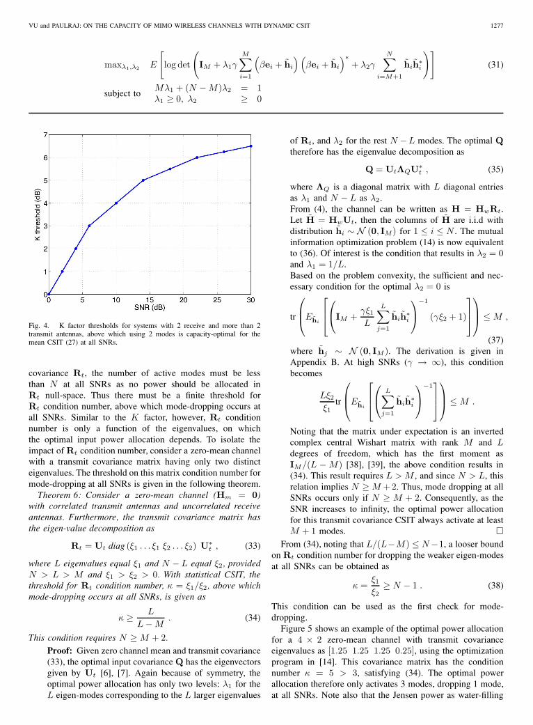
The threshold (32) is independent of the number of transmitantennas N . Thus if the channel mean is strong enough, therank of this mean will dictate the number of active modes,regardless of the larger number of antennas. Figure 4 providesexamples of this K factor threshold versus the SNR, derivedfrom (32), for systems with 2 receive- and more than 2transmit-antennas. When K is above this threshold, signifyinga strong channel mean or a good channel estimate, the optimalpower allocation activates only two modes and drops the restat all SNRs.

2) Effects of the transmit antenna correlation: In a zero-mean channel, the condition number of the transmit covariancematrix Rt can influence the number of optimal input modes.When the condition number is 1, corresponding to an identitycovariance matrix, all N transmit modes are active. Whenthe condition number is infinite, implying a rank-deficient


maxλ1,λ2 E

[log det

(IM + λ1γ

M∑i=1

(βei + hi

)(βei + hi

)∗+ λ2γ

N∑i=M+1

hih∗i

)](31)

subject toMλ1 + (N − M)λ2 = 1λ1 ≥ 0, λ2 ≥ 0

Fig. 4. K factor thresholds for systems with 2 receive and more than 2transmit antennas, above which using 2 modes is capacity-optimal for themean CSIT (27) at all SNRs.

covariance Rt, the number of active modes must be lessthan N at all SNRs as no power should be allocated inRt null-space. Thus there must be a finite threshold forRt condition number, above which mode-dropping occurs atall SNRs. Similar to the K factor, however, Rt conditionnumber is only a function of the eigenvalues, on whichthe optimal input power allocation depends. To isolate theimpact of Rt condition number, consider a zero-mean channelwith a transmit covariance matrix having only two distincteigenvalues. The threshold on this matrix condition number formode-dropping at all SNRs is given in the following theorem.

Theorem 6: Consider a zero-mean channel (Hm = 0)with correlated transmit antennas and uncorrelated receiveantennas. Furthermore, the transmit covariance matrix hasthe eigen-value decomposition as

Rt = Ut diag (ξ1 . . . ξ1 ξ2 . . . ξ2) U∗t , (33)

where L eigenvalues equal ξ1 and N − L equal ξ2, providedN > L > M and ξ1 > ξ2 > 0. With statistical CSIT, thethreshold for Rt condition number, κ = ξ1/ξ2, above whichmode-dropping occurs at all SNRs, is given as

κ ≥ L

L − M. (34)

This condition requires N ≥ M + 2.

Proof: Given zero channel mean and transmit covariance(33), the optimal input covariance Q has the eigenvectorsgiven by Ut [6], [7]. Again because of symmetry, theoptimal power allocation has only two levels: λ1 for theL eigen-modes corresponding to the L larger eigenvalues

of Rt, and λ2 for the rest N −L modes. The optimal Qtherefore has the eigenvalue decomposition as

Q = UtΛQU∗t , (35)

where ΛQ is a diagonal matrix with L diagonal entriesas λ1 and N − L as λ2.From (4), the channel can be written as H = HwRt.Let H = HwUt, then the columns of H are i.i.d withdistribution hi ∼ N (0, IM ) for 1 ≤ i ≤ N . The mutualinformation optimization problem (14) is now equivalentto (36). Of interest is the condition that results in λ2 = 0and λ1 = 1/L.Based on the problem convexity, the sufficient and nec-essary condition for the optimal λ2 = 0 is

tr

⎛⎜⎝Ehi

⎡⎢⎣⎛⎝IM +

γξ1

L

L∑j=1

hih∗i

⎞⎠

−1

(γξ2 + 1)

⎤⎥⎦⎞⎟⎠ ≤ M ,

(37)where hj ∼ N (0, IM ). The derivation is given inAppendix B. At high SNRs (γ → ∞), this conditionbecomes

Lξ2

ξ1tr

⎛⎜⎝Ehi

⎡⎢⎣⎛⎝ L∑

j=1

hih∗i

⎞⎠

−1⎤⎥⎦⎞⎟⎠ ≤ M .

Noting that the matrix under expectation is an invertedcomplex central Wishart matrix with rank M and Ldegrees of freedom, which has the first moment asIM/(L − M) [38], [39], the above condition results in(34). This result requires L > M , and since N > L, thisrelation implies N ≥ M +2. Thus, mode dropping at allSNRs occurs only if N ≥ M + 2. Consequently, as theSNR increases to infinity, the optimal power allocationfor this transmit covariance CSIT always activate at leastM + 1 modes. �

From (34), noting that L/(L−M) ≤ N −1, a looser boundon Rt condition number for dropping the weaker eigen-modesat all SNRs can be obtained as

κ =ξ1

ξ2≥ N − 1 . (38)

This condition can be used as the first check for mode-dropping.

Figure 5 shows an example of the optimal power allocationfor a 4 × 2 zero-mean channel with transmit covarianceeigenvalues as [1.25 1.25 1.25 0.25], using the optimizationprogram in [14]. This covariance matrix has the conditionnumber κ = 5 > 3, satisfying (34). The optimal powerallocation therefore only activates 3 modes, dropping 1 mode,at all SNRs. Note also that the Jensen power as water-filling


maxλ1,λ2 E

⎡⎣log det

⎛⎝IM + γλ1ξ1

L∑j=1

hih∗i + γλ2ξ2

N∑j=L+1

hih∗i

⎞⎠⎤⎦ (36)

subject toLλ1 + (N − L)λ2 = 1λ1 ≥ 0 , λ2 ≥ 0 .

Fig. 5. Input power allocations for a 4×2 zero-mean channel with transmitcovariance eigenvalues [1.25 1.25 1.25 0.25]. Each allocation schemecontains 4 power levels, corresponding to the 4 eigen-modes of the transmitcovariance. The optimal allocation has 3 equal modes, as does the Jensenpower at low SNRs. The fourth mode of the optimal scheme always has zeropower.

on E[H∗H] starts deviating from optimal at an SNR as lowas 8dB.

3) Remarks: The two conditions (28) and (34), althoughspecific to each respective channel and CSIT model, provideintuition on effects of the channel mean and the transmitantenna correlation on the optimal input power allocation.They can provide an initial check for mode-dropping withany CSIT by, for example, approximating the K factor usingthe minimum nonzero eigenvalue of the channel mean, orapproximating Rt condition number by the ratio of its firstand second largest eigenvalues. Furthermore, the condition forchannels with both a non-zero mean and a transmit antennacorrelation are likely to be more relaxed, such that modedropping occurs at all SNRs for even a lower K factor anda lower transmit covariance condition number. Subsequently,channels with high K or strong transmit antenna correlationtends to result in mode dropping with statistical CSIT at allSNRs.

VII. NUMERICAL CAPACITY ANALYSIS

Establishing the capacity with dynamic CSIT for non-asymptotic SNRs usually requires numerical computation. Forthe special CSIT cases (mean CSIT or covariance CSIT), theoptimal beam directions are known analytically, and transmitpower optimization can be efficiently performed using aniterative algorithm involving the MMSE of the data streamstransmitted on separate eigen-beams [10], [9]. For generaldynamic CSIT, however, the optimal beam directions are still

Fig. 6. Capacity and mutual information of a 4 × 4 system (above) andthe corresponding power allocations (below). The channel mean and transmitcovariance parameters are specified in Appendix C.

unknown, requiring an optimization for the whole covariancematrix Q [14].

In this section, we use the program developed in [14] tostudy the non-asymptotic MIMO capacity. We numericallyevaluate the Jensen input-covariance and the tightness ofthe capacity lower bound (18). Then using this bound andthe optimization program, MIMO capacity is analyzed interms of various parameters: relative transmit-receive antennaconfiguration, CSIT quality ρ, and the channel K factor.

A. Tightness of the capacity lower bound based on the Jenseninput covariance

This section discusses the tightness of the Jensen mutualinformation (17) compared to the capacity, using statistical


Fig. 7. Capacity and mutual information of a 4 × 2 system (above) andthe corresponding power allocations (below). The channel mean and transmitcovariance parameters are specified in Appendix C.

CSIT as a representative. Based on simulating a wide range ofchannel parameters (number of antennas, mean and covariancematrices), we observed that this tightness depends on therelative transmit-receive antenna configuration and the SNR.For systems with equal or fewer transmit than receive antennas(N ≤ M ), simulation results show that the Jensen mutualinformation is a tight lower-bound to the channel capacity atall SNRs. Any minor difference between IJ and the capacityoccurs only at mid-range SNRs, due to small difference inpower allocation. Otherwise, the Jensen covariance approachesoptimal at low and high SNRs. A similar observation isreported for channels with rank-one transmit covariance anduncorrelated receive antennas on both ergodic and outage ca-pacities in [40]. Figure 6 shows a typical example with a 4×4channel with the mean and transmit antenna correlation givenin Appendix C. The plot includes the channel capacity andthe Jensen mutual information (above), and the eigenvaluesof Q� and QJ (below). The mutual information with equalpower allocation is also included for comparison.

For systems with more transmit than receive antenna (N >M ), the Jensen mutual information is a tight lower-bound tothe channel capacity at low SNRs. At high SNRs, however,

Fig. 8. Ergodic capacity versus the CSIT quality ρ at SNR = 4dB for 4× 4channels (above) and 4 × 2 channels (below).

it exhibits a gap to the capacity. This gap depends on thechannel mean and the transmit antenna correlation. A higherK or more correlated channel (measured by, for example, ahigher condition number of the correlation matrix) results ina bigger gap. The main reason for the gap at high SNRs isthe difference in the power allocation. In contrast to the equi-power of the Jensen covariance, the capacity-optimal inputcan converge to non-equi-power at high SNRs. The optimalconvergence values are still unknown analytically ( Theorems5 and 6 provide some partial results). Figure 7 provides anexample of the mutual information and input power allocationsfor a 4 × 2 channel with the mean and correlation matricesgiven in Appendix C.

These comparisons also reveal that the value of CSITdepends on the antenna configuration and the SNRs. ForN ≤ M , CSIT helps increase the capacity only at low SNRs.For N > M , however, CSIT helps increase the capacity at allSNRs.

B. Capacity versus dynamic CSIT quality

Since the capacity lower bound IJ is tight at low SNRs,it is used to plot the capacity versus CSIT quality ρ inFigure 8. The capacity increases with higher ρ. The increment,


Fig. 9. Ergodic capacity and mutual information versus the K factor withSNR = -2dB (above) and SNR = 12dB (below).

however, is sensitive to ρ only when ρ is larger than about0.6, corresponding to a relatively good channel estimate. Thisobservation implies that in dynamic CSIT, the initial channelmeasurement adds value only when its correlation with thecurrent channel is relatively strong; otherwise statistical CSITprovides most information.

Figure 8 examines two antenna configurations: 4×4 (above)and 4 × 2 (below). In each configuration, an i.i.d channeland a Rician correlated channel (with mean and covariancematrices given in Appendix C) are studied. Results show thatthe range of capacity gain for i.i.d channels is larger thanfor the correlated ones. Note that as the SNR increases, thecapacity gain for the 4×4 channels decreases to 0, but for the4 × 2 channels, it increases to up to 2 bps/Hz. For reference,the capacity of the non i.i.d channel without any CSIT is alsoincluded. In non i.i.d channels, knowing the channel statisticsalone (ρ = 0) can enhance the capacity. Furthermore, at lowSNRs, non i.i.d channels can have higher capacity than i.i.dones, as seen in the second sub-figure.

C. Effects of the K factor

The channel Rician K factor affects the ergodic capacitydifferently depending on the SNR. Figure 9 shows the ca-

Fig. 10. K factor threshold for 4 × 2 channels for tight lower-bound tothe ergodic capacity using the Jensen mutual information (difference < 0.03bps/Hz).

pacity versus K at two different SNRs for the 4 × 2 Riciancorrelation channels. Notice that at a low SNR (-2dB), thecapacity is a non-monotonous function of the K factor, anda minimum exists. This minimum is partly caused by thetransmit antenna correlation impact: at low K , the correlationeffect becomes more dominant, and because of the low SNR,stronger correlation helps increase the capacity. At a higherSNR (12 dB), the correlation impact diminishes for full-rankcorrelation. Provided that the channel mean is also full-rank,the capacity then monotonically increases with the K factor.The increment, however, diminishes with higher K .

For systems with more transmit than receive antennas, ahigher K factor also causes the SNR point, at which theJensen mutual information starts diverging from the channelcapacity, to increase. This effect implies that with higher Kfactor, the bound is tight for larger range of SNRs. Figure10 presents this K factor threshold versus the SNR for the4×2 channels (keeping the same transmit antenna correlationbut only varying its power with K). When K is above thisthreshold, the Jensen mutual information is a tight lower boundto the capacity. The difference then is less than 0.03 bps/Hz,which is within the numerical precision for optimizing thecapacity.

VIII. CONCLUSION

In this paper, we propose a dynamic CSIT model andstudy the corresponding channel capacity. Dynamic CSIT isa model for transmit channel side information that takes intoaccount the channel temporal variation. The model consists ofa channel estimate and its error covariance, built on an initial,accurate channel measurement and the channel mean, covari-ance, and temporal correlation factor ρ. This factor functionsas the CSIT quality, with 1 corresponding to perfect, and 0 tostatistical information. Parameterized by ρ, the CSIT providesan effective channel mean and an effective covariance. Thismodel can be applied to a general Rician correlated fadingMIMO channel.

Asymptotic capacity analyses show that, at low SNRs,dynamic CSIT helps increase the capacity multiplicatively


maxλ1

g(λ1) = Ehj

⎡⎣log det

⎛⎝IM + λ1γ

M∑j=1

gjg∗j +

1 − Mλ1

N − Mγ

N∑j=M+1

hjh∗j

⎞⎠⎤⎦ (39)

subject to1N

≤ λ1 ≤ 1M

,

0 ≤ Ehj

⎡⎢⎣tr

⎡⎢⎣⎛⎝IM +

γ

M

M∑j=1

gjg∗i

⎞⎠

−1 ⎛⎝γ

M∑j=1

gjg∗i − γM

N − M

N∑j=M+1

hjh∗j

⎞⎠⎤⎥⎦⎤⎥⎦

(a)= M2 − MEhj

⎡⎢⎣tr

⎡⎢⎣⎛⎝IM +

γ

M

M∑j=1

gjg∗i

⎞⎠

−1 ⎛⎝IM +

γ

N − M

N∑j=M+1

hjh∗j

⎞⎠⎤⎥⎦⎤⎥⎦ , (40)

for all MIMO systems, and the optimal input is typicallysimple single-mode beamforming. At high SNRs, the capacitygain depends on the relative number of antennas. For systemswith equal or fewer transmit than receive antennas, the gaindiminishes to zero, since the optimal input approaches equi-power with increasing SNRs. For systems with more transmitthan receive antennas, however, we show that the gain dependson the CSIT. Specifically, systems with strong transmit antennacorrelation or strong mean can lead to an optimal input withmode-dropping at high SNRs, producing an additive capacitygain with the CSIT. For systems with rank-deficient transmitcorrelation, knowing this correlation at the transmitter can alsoadditively increase the capacity at high SNRs.

A convex optimization program is then used to study thecapacity non-asymptotically. We compare the capacity to alower-bound based on the Jensen-optimal input. This simplelower-bound is often tight at all SNRs for systems with equalor fewer transmit than receive antennas. For systems with moretransmit than receive antennas, however, the bound is tightat low SNRs but diverges at high SNRs. The divergence athigh SNRs is caused by the difference in power allocationand depends on CSIT parameters – the channel mean and thetransmit antenna correlation. A stronger mean or correlationcauses a larger divergence. Furthermore, a higher channel Kfactor results in a higher SNR, at which the divergence begins.

Applied to dynamic CSIT, optimization results illustrateincreasing capacity with better CSIT quality ρ. However, thecapacity gain is sensitive to ρ for large ρ only, at roughly ρ ≥0.6. Otherwise, the gain equals that with ρ = 0, correspondingto statistical CSIT. This observation suggests that, in dynamicCSIT, the initial channel measurement is useful only when itscorrelation with the current channel is relatively strong (ρ ≥0.6); otherwise, using the channel statistics alone achievesmost of the gain. Furthermore, the capacity gain depends notonly on ρ but also on the channel statistics. Compared toa correlated Rician channel, the gain is higher for an i.i.dchannel at high ρ, but becomes lower as ρ decreases.Thusevaluating the capacity gain requires knowing both the CSITquality factor and the channel statistical parameters, the meanand covariance.

APPENDIX

A. K-factor threshold for mode-dropping at all SNRs

This section provides the derivation for (32). In problem(31), replacing λ2 as a function of λ1, noting that the optimalλ1 ≥ λ2, the problem becomes equivalent to (39), where gj =(βej + hj

). Since problem (31) is convex, this problem is

convex. Thus, to have the optimal λ�1 = 1/M , it is sufficient

and necessary that dg(λ1)dλ1

∣∣∣λ1=1/M

≥ 0, which translates to

(40), where (a) follows from adding and subtracting MIM inthe second parenthetic factor inside the trace expression, andhj and gj are independent. Due to this independence, andnoting that hj ∼ N (

0, (1 − β2)IM

), the above inequality

leads to (41). This expression results in (32).

B. Rt condition number threshold for mode-dropping at allSNRs

This section provides the derivation for (37). In problem(36), replacing λ1 as a function of λ2 and noting thatλ1 ≥ λ2, the problem becomes equivalent to (42), wherehi ∼ N (0, IM ). The condition for the optimal λ2 = 0 is∂f∂λ2

∣∣∣λ2=0

≤ 0, which translates to (43), where (a) follows

from mutually exclusive, independent sums and that

E

⎡⎣ N∑

j=L+1

hjh∗j

⎤⎦ = (N − L)IM .

Inequality (43) then leads to (37).

C. Parameters for capacity optimization

This section lists the CSIT parameters for capacity opti-mization in Sections VII. All simulated channels have 4 trans-mit and either 2 or 4 receive antennas. The normalized transmitcovariance matrix (such at tr(Rt) = MN ) is given in (44).This matrix has the eigenvalues [2.717 , 0.997 , 0.237 , 0.049]and a condition number of 55.5, representing strong antennacorrelation. The normalized mean (such at tr(HmH∗

m) =NM ) for the 4 × 2 channel is given in (45). The normalizedmean for the 4×4 channel is given in (46). These parametersare then scaled according to the channel K factor in the


M ≥ tr

⎛⎜⎝Ehj

⎡⎢⎣⎛⎝IM +

γ

M

M∑j=1

gjg∗i

⎞⎠

−1⎤⎥⎦Ehj

⎡⎣IM +

γ

N − M

N∑j=M+1

hjh∗j

⎤⎦⎞⎟⎠

= tr

⎛⎜⎝Ehj

⎡⎢⎣⎛⎝IM +

γ

M

M∑j=1

gjg∗i

⎞⎠

−1⎤⎥⎦ [

1 + γ(1 − β2

)]⎞⎟⎠ . (41)

maxλ2

f(λ2) = Ehi

⎡⎣log det

⎛⎝IM + γ

1 − (N − L)λ2

Lξ1

L∑i=1

hih∗i + γλ2ξ2

N∑j=L+1

hjh∗j

⎞⎠⎤⎦ (42)

subject to 0 ≤ λ2 ≤ 1N

,

0 ≥ Ehi

⎡⎢⎣tr

⎡⎢⎣⎛⎝IM +

γξ1

L

L∑j=1

hih∗i

⎞⎠

−1 ⎛⎝γξ2

N∑j=L+1

hjh∗j − γξ1

N − L

L

L∑i=1

hih∗i

⎞⎠⎤⎥⎦⎤⎥⎦

(a)= tr

⎛⎜⎝Ehi

⎡⎢⎣⎛⎝IM +

γξ1

L

L∑j=1

hih∗i

⎞⎠

−1 ⎛⎝γξ2IM − γξ1

L

L∑j=1

hih∗i

⎞⎠ (N − L)

⎤⎥⎦⎞⎟⎠

= tr

⎛⎜⎝Ehi

⎡⎢⎣⎛⎝IM +

γξ1

L

L∑j=1

hih∗i

⎞⎠

−1 ⎡⎣(γξ2 + 1)IM −

⎛⎝IM +

γξ1

L

L∑j=1

hih∗i

⎞⎠⎤⎦⎤⎥⎦⎞⎟⎠ (N − L)

=

⎡⎢⎣tr

⎛⎜⎝Ehi

⎡⎢⎣⎛⎝IM +

γξ1

L

L∑j=1

hih∗i

⎞⎠

−1

(γξ2 + 1)

⎤⎥⎦⎞⎟⎠− M

⎤⎥⎦ (N − L) , (43)

Rt =

⎡⎢⎢⎣

0.8758 −0.0993− 0.0877i −0.6648− 0.0087i 0.5256− 0.4355i−0.0993 + 0.0877i 0.9318 0.0926 + 0.3776i −0.5061− 0.3478i−0.6648 + 0.0087i 0.0926− 0.3776i 1.0544 −0.6219 + 0.5966i

0.5256 + 0.4355i −0.5061 + 0.3478i −0.6219− 0.5966i 1.1379

⎤⎥⎥⎦ . (44)

simulations. The simulated channels have K = 0.1, exceptfor the studies of the capacity versus the K factor.

REFERENCES

[1] A. Goldsmith and P. Varaiya, “Capacity of fading channels with channelside information,” IEEE Trans. Inform. Theory, vol. 43, no. 6, pp. 1986–1992, Nov. 1997.

[2] M. Vu and A. Paulraj, “MIMO wireless linear precoding,” accepted toIEEE Signal Processing Mag..

[3] G. Raleigh and J. Cioffi, “Spatio-temporal coding for wireless commu-nication,” IEEE Trans. Commun., vol. 46, pp. 357–366, Mar 1998.

[4] A. Grant, “Rayleigh fading multi-antenna channels,” EURASIP Journalon Applied Signal Processing, pp. 316–329, Mar 2002.

[5] T. Cover and J. Thomas, Elements of Information Theory. John Wiley& Sons, Inc., 1991.

[6] E. Visotsky and U. Madhow, “Space-time transmit precoding withimperfect feedback,” IEEE Trans. Inform. Theory, vol. 47, no. 6, pp.2632–2639, Sep. 2001.

[7] S. Jafar and A. Goldsmith, “Transmitter optimization and optimalityof beamforming for multiple antenna systems,” IEEE Trans. WirelessCommun., vol. 3, no. 4, pp. 1165–1175, July 2004.

[8] S. Venkatesan, S. Simon, and R. Valenzuela, “Capacity of a GaussianMIMO channel with nonzero mean,” Proc. IEEE Vehicular Tech. Conf.,vol. 3, pp. 1767–1771, Oct. 2003.

[9] D. Hosli and A. Lapidoth, “The capacity of a MIMO Ricean channelis monotonic in the singular values of the mean,” Proc. 5th Int’l ITGConf. on Source and Channel Coding, Jan. 2004.

[10] A. Tulino, A. Lozano, and S. Verdu, “Capacity-achieving input co-variance for single-user multi-antenna channels,” IEEE Trans. WirelessCommun., vol. 5, no. 3, pp. 662–671, Mar. 2006.

[11] D. Hosli and A. Lapidoth, “How good is an isotropic gaussian inputon a MIMO Ricean channel?” Proc. Int’l Symp. on Info. Theory (ISIT),July 2004.

[12] S. Verdu, “Spectral efficiency in the wideband regime,” IEEE Trans.Inform. Theory, vol. 48, no. 6, pp. 1319–1343, June 2002.

[13] S. Boyd and L. Vandenberghe, Convex Optimization. Cambridge,UK: Cambridge University Press, 2003. [Online]. Available:http://www.stanford.edu/∼boyd/cvxbook.html

[14] M. Vu and A. Paulraj, “Capacity optimization for Rician correlatedMIMO wireless channels,” Proc. 39th Asilomar Conf. Sig., Sys. andComp., pp. 133–138, Nov. 2005.

[15] D. Shiu, G. Foschini, M. Gans, and J. Kahn, “Fading correlation and itseffect on the capacity of multielement antenna systems,” IEEE Trans.Commun., vol. 48, no. 3, pp. 502–513, Mar. 2000.

[16] A. Graham, Kronecker Products and Matrix Calculus with Application.Ellis Horwood Ltd., 1981.


Hm =√

10[

0.0749− 0.1438i 0.0208 + 0.3040i −0.3356 + 0.0489i 0.2573− 0.0792i0.0173− 0.2796i −0.2336− 0.2586i 0.3157 + 0.4079i 0.1183 + 0.1158i

]. (45)

Hm =√

10

⎡⎢⎢⎣

0.2976 + 0.1177i 0.1423 + 0.4518i −0.0190 + 0.1650i −0.0029 + 0.0634i−0.1688− 0.0012i −0.0609− 0.1267i 0.2156− 0.5733i 0.2214 + 0.2942i

0.0018− 0.0670i 0.1164 + 0.0251i 0.5599 + 0.2400i 0.0136− 0.0666i−0.1898 + 0.3095i 0.1620 − 0.1958i 0.1272 + 0.0531i −0.2684− 0.0323i

⎤⎥⎥⎦ . (46)

[17] K. Yu, M. Bengtsson, B. Ottersten, D. McNamara, P. Karlsson, andM. Beach, “Second order statistics of NLOS indoor MIMO channelsbased on 5.2 GHz measurements,” Proc. IEEE Global Telecomm. Conf.,vol. 1, pp. 25–29, Nov. 2001.

[18] J. Kermoal, L. Schumacher, K. Pedersen, P. Mogensen, and F. Fred-eriksen, “A stochastic MIMO radio channel model with experimentalvalidation,” IEEE J. Select. Areas Commun., vol. 20, no. 6, pp. 1211–1226, Aug. 2002.

[19] D. Bliss, A. Chan, and N. Chang, “MIMO wireless communicationchannel phenomenology,” IEEE Trans. Antennas Propagat., vol. 52,no. 8, pp. 2073–2082, Aug. 2004.

[20] A. Sayeed, “Deconstructing multiantenna fading channels,” IEEE Trans.Signal Processing, vol. 50, no. 10, pp. 2563–2579, Oct. 2002.

[21] W. Weichselberger, M. Herdin, H. Ozcelik, and E. Bonek, “A stochasticMIMO channel model with joint correlation of both link ends,” IEEETrans. Wireless Commun., vol. 5, no. 1, pp. 90–100, Jan. 2006.

[22] D. Baum, D. Gore, R. Nabar, S. Panchanathan, K. Hari, V. Erceg, andA. Paulraj, “Measurement and characterization of broadband MIMOfixed wireless channels at 2.5ghz,” Proc. Int’l Conf. Per. Wireless Comm.,pp. 203–206, Dec. 2000.

[23] W. Jakes, Microwave Mobile Communications. IEEE Press, 1994.[24] A. Paulraj and C. Papadias, “Space-time processing for wireless com-

munications,” IEEE Signal Processing Mag., vol. 14, no. 6, pp. 49–83,Nov. 1997.

[25] T. Kailath, A. Sayed, and B. Hassibi, Linear Estimation. Prentice Hall,2000.

[26] D. Goeckel, “Adaptive coding for time-varying channels using outdatedfading estimates,” IEEE Trans. Commun., vol. 47, no. 6, pp. 844–855,June 1999.

[27] A. Narula, M. Lopez, M. Trott, and G. Wornell, “Efficient use of sideinformation in multiple-antenna data transmission over fading channels,”IEEE J. Select. Areas Commun., vol. 16, no. 8, pp. 1423–1436, Oct.1998.

[28] G. Jongren, M. Skoglund, and B. Ottersten, “Combining beamformingand orthogonal space-time block coding,” IEEE Trans. on Info. Theory,vol. 48, no. 3, pp. 611–627, Mar. 2002.

[29] I. Telatar, “Capacity of multi-antenna Gaussian channels,” Bell Labora-tories Technical Memorandum, http://mars.bell-labs.com/papers/proof/,Oct. 1995. [Online]. Available: http://mars.bell-labs.com/papers/proof/

[30] A. Lozano, A. Tulino, and S. Verdu, From Array Processing to MIMOCommunications. Cambridge University Press, 2006, ch. Multiantennacapacity: Myths and Realities.

[31] J. Silverstein, “The smallest eigenvalue of a large dimensional Wishartmatrix,” Annals of Probability, vol. 13, no. 4, pp. 1364–1368, Nov. 1985.

[32] S. Geman, “A limit theorem for the norm of random matrices,” Annalsof Probability, vol. 8, no. 2, pp. 252–261, Apr. 1980.

[33] C.-N. Chuah, D. Tse, J. Kahn, and R. Valenzuela, “Capacity scaling inMIMO wireless systems under correlated fading,” IEEE Trans. Inform.Theory, vol. 48, no. 3, pp. 637–650, Mar 2002.

[34] A. Tulino, A. Lozano, and S. Verdu, “MIMO capacity with channelstate information at the transmitter,” Proc. IEEE Int’l Symp. on SpreadSpectrum Tech. & Apps., pp. 22–26, Sept 2004.

[35] A. Lozano, A. Tulino, and S. Verdu, “High-SNR power offset inmultiantenna communication,” IEEE Trans. Inform. Theory, vol. 51,no. 12, pp. 4134–4151, Dec 2005.

[36] M. Vu and A. Paulraj, “Some asymptotic capacity results for MIMOwireless with and without channel knowledge at the transmitter,” Proc.

37th Asilomar Conf. Sig., Sys. and Comp., vol. 1, pp. 258–262, Nov.2003.

[37] D. Hosli, Y.-H. Kim, and A. Lapidoth, “Monotonicity results forcoherent MIMO Rician channels,” IEEE Trans. Inform. Theory, vol. 51,no. 12, pp. 4334–4339, Dec. 2005.

[38] D. Maiwald and D. Kraus, “Calculation of moments of complex Wishartand complex inverse Wishart distributed matrices,” IEE ProceedingsRadar, Sonar and Navigation, no. 4, pp. 162–168, Aug. 2000.

[39] P. Graczyk, G. Letac, and H. Massam, “The complex Wishart distribu-tion and the symmetric group,” The Annals of Statistics, vol. 31, no. 1,pp. 287–309, Feb. 2003.

[40] M. Ivrlac, W. Utschick, and J. Nossek, “Fading correlations in wirelessMIMO communication systems,” IEEE J. Select. Areas Commun.,vol. 21, no. 5, pp. 819–828, June 2003.

Mai Vu was born in Vietnam. She received aBE degree in Computer Systems Engineering fromRMIT, Australia in 1997, an MSE degree in Electri-cal Engineering from the University of Melbourne,Australia in 1999, an MS and a PhD degrees both inElectrical Engineering from Stanford University, CAin 2006. She is currently a Lecturer in EngineeringSciences at the School of Engineering and AppliedSciences, Harvard University, Cambridge, MA.

Her research interests span the areas of signalprocessing for communications, wireless networks,

information theory, and convex optimization. Her PhD focus has been onthe impact of and techniques to exploit partial channel knowledge at thetransmitter in multiple-input multiple-output (MIMO) wireless systems.

Ms. Vu has been a recipient of several awards including the AustralianInstitute of Engineers Award at RMIT, the Rambus Corporation StanfordGraduate Fellowship and the Intel Foundation PhD Fellowship at StanfordUniversity.

Arogyaswami Paulraj received the Ph.D. degreefrom the Indian Institute of Technology, New Delhiin 1973. He is currently a professor with the De-partment of Electrical Engineering, Stanford Uni-versity, where he supervises the Smart AntennasResearch Group, working on applications of space-time techniques for wireless communications. Hisnon-academic positions have included Head, SonarDivision, Naval Oceanographic Laboratory, Cochin,India; Director, Center for Artificial Intelligence andRobotics, India; Director, Center for Development

of Advanced Computing, India; Chief Scientist, Bharat Electronics,India;CTO and Founder, Iospan Wireless Inc., Co-Founder and CTO of BeceemCommunications Inc.. His research has spanned several disciplines, empha-sizing estimation theory, sensor signal processing, parallel computer architec-tures/algorithms, and space-time wireless communications. His engineeringexperience has included development of sonar systems, massively parallelcomputers, and broadband wireless systems. Dr. Paulraj has won severalawards for his research and engineering contributions, including the IEEESignal Processing Society’s Technical Achievement Award. He is the authorof over 300 research papers and holds twenty patents. He is a Member ofboth the National Academy of Engineering (NAE) and the Indian NationalAcademy of Engineering and a Fellow of the IEEE.

On the Capacity of MIMO Wireless Channels with Dynamic CSIT

Documents

Transcript of On the Capacity of MIMO Wireless Channels with Dynamic CSIT