
The Capacity of Finite-State Markov Channels With Feedback
19
780 IEEE TRANSACTIONS ON INFORMATION THEORY, VOL. 51, NO. 3, MARCH 2005 The Capacity of Finite-State Markov Channels With Feedback Jun Chen, Student Member, IEEE, and Toby Berger, Fellow, IEEE Abstract—We consider a class of finite-state Markov channels with feedback. We first introduce a simplified equivalent channel model, and then construct the optimal stationary and nonsta- tionary input processes that maximize the long-term directed mutual information. Furthermore, we give a sufficient condition under which the channel’s Shannon capacity can be achieved by a stationary input process. The corresponding converse coding theorem and direct coding theorem are proved. Index Terms—Channel capacity, feedback, Markov channel, typicality. I. INTRODUCTION W E study the capacity of a feedback channel whose state process can be affected by its input and whose state in- formation is available at both the transmitter and the receiver. Our channel model is illustrated in Fig. 1. Were it not for the feedback, our channel would belong to the family of finite- state channels (FSC). The FSC literature is vast; see, for ex- ample, [1]–[3]. In [4], Verdú and Han gave a general capacity formula for channels without feedback. If in our model, the state process were not affected by the input, i.e., , then our model would reduce to a special case in the general framework of [5] and [6]. The feedback channel coding problem goes back to early work by Shannon [7], Dobrushin [8], and Wolfowitz [9]. Tatikonda [10] introduced a model of feedback channels which can be viewed as a generalization of the formulation in [4], derived a general formula for the capacity of channels in this class, and used dynamic programming to compute the optimal input distribution. We show that channels described by our model, which are called Markov channels in [10], possess under certain conditions a relatively simple capacity formula and that the corresponding optimal input distribution can be computed with markedly less complexity than in the general case. It is easy to see that if we let and then Fig. 1 can be simplified to the model shown in Fig. 2. Therefore, we henceforth consider only this simplified channel model. The model in Fig. 2 was perhaps first introduced in [11], Manuscript received October 2, 2003; revised September 8, 2004. This work was supported in part by the National Science Foundation under Grant CCR- 9980616, by ARO P-40116-PH-MUR, DAAD 19-99-1-0215, and a grant from the National Academies Keck Futures Initiative (NAKFI). The authors are with the School of Electrical and Computer Engineering, Cornell University, Ithaca, NY 14853 USA (e-mail: [email protected]; [email protected]). Communicated by R. W. Yeung, Associate Editor for Shannon Theory. Digital Object Identifier 10.1109/TIT.2004.842697 [12]. Ying and Berger [13] analyzed the capacity of this channel model when the output is binary. In this paper, we will give a more general treatment. The rest of this paper is divided into eight sections. In Sec- tion II, we introduce several basic notations and definitions. In Section III, we prove the converse channel coding theorem for our model, which provides an upper bound on the achiev- able rate of information transmission through the channel. Then we give a recursive formula to calculate the maximal directed mutual information in Section IV. In Section V, we analyze the optimum stationary input distribution that maximizes the long-term directed mutual information. We generalize in Sec- tion VI to analyze the optimum not-necessarily-stationary input. A sufficient condition under which the optimum stationary input is actually optimum among all the input distributions is given in Section VII. We prove the direct channel coding theorem and suggest a coding scheme in Section VIII. Finally, several direc- tions to extend our results are discussed in Section IX which serves as a conclusion. II. PRELIMINARIES A. Notation We assume throughout the paper that the channel input and output alphabets both are finite. Without loss of generality, we let and . B. Code Description An feedback code for our channel consists of the following. 1) An encoding function that maps the set of messages to channel input words of block length through a sequence of functions that depend only on the message and the channel outputs up to time , i.e., (1) Although it may seem to be more general to let this actually is equivalent to (1), as shown by the following argument: 0018-9448/$20.00 © 2005 IEEE
-
Upload
khangminh22 -
Category
Documents
-
view
2 -
download
0
Transcript of The Capacity of Finite-State Markov Channels With Feedback

780 IEEE TRANSACTIONS ON INFORMATION THEORY, VOL. 51, NO. 3, MARCH 2005
The Capacity of Finite-State Markov ChannelsWith Feedback
Jun Chen, Student Member, IEEE, and Toby Berger, Fellow, IEEE
Abstract—We consider a class of finite-state Markov channelswith feedback. We first introduce a simplified equivalent channelmodel, and then construct the optimal stationary and nonsta-tionary input processes that maximize the long-term directedmutual information. Furthermore, we give a sufficient conditionunder which the channel’s Shannon capacity can be achieved bya stationary input process. The corresponding converse codingtheorem and direct coding theorem are proved.
Index Terms—Channel capacity, feedback, Markov channel,typicality.
I. INTRODUCTION
WE study the capacity of a feedback channel whose stateprocess can be affected by its input and whose state in-
formation is available at both the transmitter and the receiver.Our channel model is illustrated in Fig. 1. Were it not for thefeedback, our channel would belong to the family of finite-state channels (FSC). The FSC literature is vast; see, for ex-ample, [1]–[3]. In [4], Verdú and Han gave a general capacityformula for channels without feedback. If in our model, the stateprocess were not affected by the input, i.e.,
, then our model would reduce to a special case inthe general framework of [5] and [6].
The feedback channel coding problem goes back to earlywork by Shannon [7], Dobrushin [8], and Wolfowitz [9].Tatikonda [10] introduced a model of feedback channels whichcan be viewed as a generalization of the formulation in [4],derived a general formula for the capacity of channels in thisclass, and used dynamic programming to compute the optimalinput distribution. We show that channels described by ourmodel, which are called Markov channels in [10], possess undercertain conditions a relatively simple capacity formula and thatthe corresponding optimal input distribution can be computedwith markedly less complexity than in the general case.
It is easy to see that if we let and
then Fig. 1 can be simplified to the model shown in Fig. 2.Therefore, we henceforth consider only this simplified channelmodel. The model in Fig. 2 was perhaps first introduced in [11],
Manuscript received October 2, 2003; revised September 8, 2004. This workwas supported in part by the National Science Foundation under Grant CCR-9980616, by ARO P-40116-PH-MUR, DAAD 19-99-1-0215, and a grant fromthe National Academies Keck Futures Initiative (NAKFI).
The authors are with the School of Electrical and Computer Engineering,Cornell University, Ithaca, NY 14853 USA (e-mail: [email protected];[email protected]).
Communicated by R. W. Yeung, Associate Editor for Shannon Theory.Digital Object Identifier 10.1109/TIT.2004.842697
[12]. Ying and Berger [13] analyzed the capacity of this channelmodel when the output is binary. In this paper, we will give amore general treatment.
The rest of this paper is divided into eight sections. In Sec-tion II, we introduce several basic notations and definitions.In Section III, we prove the converse channel coding theoremfor our model, which provides an upper bound on the achiev-able rate of information transmission through the channel. Thenwe give a recursive formula to calculate the maximal directedmutual information in Section IV. In Section V, we analyzethe optimum stationary input distribution that maximizes thelong-term directed mutual information. We generalize in Sec-tion VI to analyze the optimum not-necessarily-stationary input.A sufficient condition under which the optimum stationary inputis actually optimum among all the input distributions is given inSection VII. We prove the direct channel coding theorem andsuggest a coding scheme in Section VIII. Finally, several direc-tions to extend our results are discussed in Section IX whichserves as a conclusion.
II. PRELIMINARIES
A. Notation
We assume throughout the paper that the channel input andoutput alphabets both are finite. Without loss of generality, welet and .
B. Code Description
An feedback code for our channel consists ofthe following.
1) An encoding function that maps the set of messagesto channel input words of block length
through a sequence of functions that dependonly on the message and the channel outputs up to time
, i.e.,
(1)
Although it may seem to be more general to let
this actually is equivalent to (1), as shown by the followingargument:
0018-9448/$20.00 © 2005 IEEE

CHEN AND BERGER: THE CAPACITY OF FINITE-STATE MARKOV CHANNELS WITH FEEDBACK 781
Fig. 1. Our model.
Fig. 2. An equivalent model.
It follows easily by induction that
so (1) is of full generality.2) A decoding function that maps a received sequence of
channel outputs to the message set suchthat the average probability of decoding error satisfies
where
(2)
Note: The encoding function and decoding functionboth depend on the initial channel state .
Definition 1: is an -achievable rate given the initialstate if for every there exists, for all sufficiently large
, an code such that . isachievable if it is -achievable for all . The supremum ofall achievable rates is defined as the feedback capacitygiven the initial state .
III. CONVERSE CHANNEL CODING THEOREM
This section is devoted to the proof of the converse channelcoding theorem.
Theorem 1 (Converse Channel Coding Theorem): Given theinitial state , information transmission with an arbitrary smallexpected frequency of errors is not possible if
Here
and is the set of input distributions on which con-sists of all the probability mass functions that satisfy
Proof: In the proof we implicitly assume thatand thus use instead of .
Let be the message random variable. For anycode, by Fano’s inequality
(3)
Since
we have
which we rewrite as
(4)
As , . Hence, the channel capacity
(5)

782 IEEE TRANSACTIONS ON INFORMATION THEORY, VOL. 51, NO. 3, MARCH 2005
Fig. 3. Example 1.
We have
(6)
where holds because, when conditioned on the input andthe previous output (i.e., the current channel state), thechannel output becomes independent of both the message
and the earlier outputs .We call the directed mutual informa-
tion. The concept of directed mutual information was introducedby Massey [14] who attributes it to Marko [15]. See [10] for adetailed discussion of this concept. It has been shown in [13]that the maximum directed mutual information for our channelmodel is attained inside ; i.e., no loss of generality re-sults from restricting to when maximizing thedirected information.
So we have
We remark that the upper bound on theachievable rate is not always tight. Consider, for example, Fig. 3in which the transition probability associated with every arrowin the middle figure is . The following is apparent.
1) If , we can transmit no information through thischannel.
2) If or , we can transmit 1 bit of information perchannel use.
3) If , then with probability , whereuponfor all . Then half of the time , in which
case for all . The other half time , in whichcase we can transmit 1 bit of information per channel useafter that.
According to Definition 1, the capacity of the channel of Fig. 3is if the initial channel state . However, one readily cancompute that , an equal mixture of thechannel capacity for and that for .
IV. RECURSIVE FORMULA FOR THE MAXIMUM DIRECTED
MUTUAL INFORMATION
We mentioned in Section III that the maximum directedmutual information of our channel model is attained inside
. This not only greatly simplifies the structure of theinput distribution that maximizes the directed mutual informa-tion but also makes the joint (input, output) process possess aMarkov structure, as described by the following lemma.
Lemma 1 [11], [13]: If we restrict the distribution of inputto , then we have
1) is a first-order Markov chain;2) also is a first-order Markov
chain.
Lemma 1 evidences how the underlying Markov structure inour channel model allows us to bring to bear on the problemat hand powerful techniques from Markov theory and dynamicprogramming. This is partially reflected in the following the-orem.
Theorem 2:
for any (7)
where
1) is the distribution of the first input when is the initialstate (The inclusion of in the subscript is intended tostress that this distribution generally depends on ; weemphasize that is not the input distribution at time
.);2)
3) is the channel transition probability matrix for state ,i.e.,
4)
where is the th component of the probabilityvector ;
5) for .
CHEN AND BERGER: THE CAPACITY OF FINITE-STATE MARKOV CHANNELS WITH FEEDBACK 783
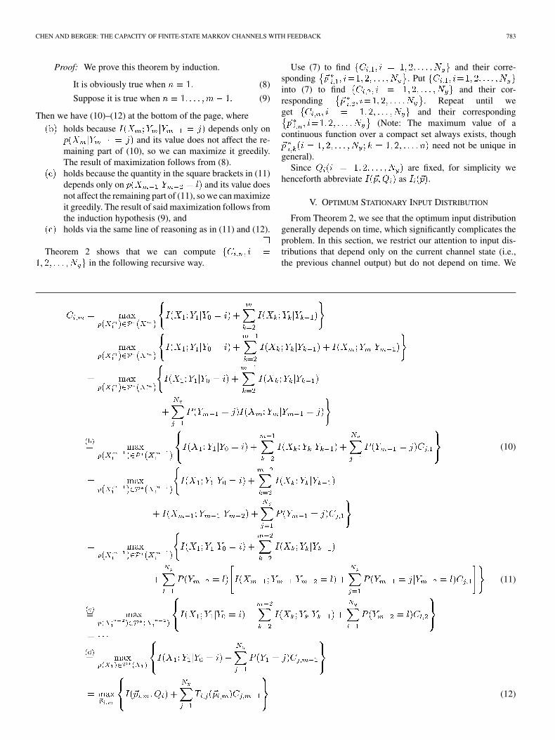
Proof: We prove this theorem by induction.
It is obviously true when (8)
Suppose it is true when (9)
Then we have (10)–(12) at the bottom of the page, where
holds because depends only onand its value does not affect the re-
maining part of (10), so we can maximize it greedily.The result of maximization follows from (8).holds because the quantity in the square brackets in (11)depends only on and its value doesnot affect the remaining part of (11), so we can maximizeit greedily. The result of said maximization follows fromthe induction hypothesis (9), andholds via the same line of reasoning as in (11) and (12).
Theorem 2 shows that we can computein the following recursive way.
Use (7) to find and their corre-sponding . Putinto (7) to find and their cor-responding . Repeat until weget and their corresponding
(Note: The maximum value of acontinuous function over a compact set always exists, though
need not be unique ingeneral).
Since are fixed, for simplicity wehenceforth abbreviate as .
V. OPTIMUM STATIONARY INPUT DISTRIBUTION
From Theorem 2, we see that the optimum input distributiongenerally depends on time, which significantly complicates theproblem. In this section, we restrict our attention to input dis-tributions that depend only on the current channel state (i.e.,the previous channel output) but do not depend on time. We
(10)
(11)
(12)

784 IEEE TRANSACTIONS ON INFORMATION THEORY, VOL. 51, NO. 3, MARCH 2005
call these the stationary1 input distributions, and we let de-note the set of such distributions. Correspondingly, definedin Section III is the set of nonstationary input distributions. Let
denote the input distribution when the channel state is . Thenno loss in generality results from writing an element of as
. It is clear that, if we restrict the input dis-tribution into , then is a homogeneousMarkov chain.
When the input distribution is stationary, we can easily findthe following recursive formula:
(13)
where
1) ;
2) with.
It follows from (13) that
(14)
Using matrix representation, we can write (14) as
......
(15)
where
......
. . ....
is a transition matrix for the homogeneous Markov chain. It follows easily from (15) that
......
(16)
1Here, the term “stationary” does not have its usual connotation in the theoryof random processes. Specifically, since we do not rule out initial conditionsthat cause the state process’s marginals to undergo a transient, similar transientbehavior may well be exhibited by the marginals of the input process. Whatmotivates our use of the term “stationary” is that, if the channel satisfies certainconditions (which will be made clear in Section VI) and the input distribution is“stationary” under our definition, then the joint input and output process (i.e., thejoint input and state process) forms an irreducible and aperiodic homogeneousMarkov chain and thus is asymptotically mean stationary in the sense of [16],[17].
Since is a homogenous Markov chain, wecan divide its states into two categories: the transient states andthe recurrent states. Recurrent states can be decomposed intodisjoint irreducible closed sets. Furthermore, there are two kindsof irreducible closed sets: aperiodic and periodic. Now we dis-cuss them separately.
a) Aperiodic irreducible closed set (suppose it containsstates ).
Now consider the principal submatrix of with respectto the th th th columns and rows, which wedenote by . Clearly, we can derive from (16) that
......
(17)
where
......
. . ....
By the Markov convergence theorem for an aperiodic ir-reducible closed set (see, e.g., [18]), we have
......
. . ....
as (18)
where is the unique stationary (or equilib-rium) distribution for the aperiodic irreducible closed set
. So by (17) and (18)
......
.... . .
......
as . Thus, we have
(19)
which is independent of ; that is,starting from any state in a given aperiodic irreducibleclosed set, the limiting average directed mutual informa-tion is identical.
b) Periodic irreducible closed set (suppose it containsstates and suppose the period is . Let
be the cyclic decomposition of the statespace).

CHEN AND BERGER: THE CAPACITY OF FINITE-STATE MARKOV CHANNELS WITH FEEDBACK 785
Now consider the principal submatrix of with respectto the th th th columns and rows, henceforthdenoted by . Clearly, we can derive from (16) that
......
(20)
where
......
. . ....
By the Markov convergence theorem for a periodic irre-ducible closed set (see, e.g., [18]), we have
where is the component on the th row and thcolumn of matrix
is the unique stationary (or equilib-rium) distribution for the aperiodic irreducible closed set
. More specifically, if and(actually we just need the subscript of the cyclic statespace that they belong to differ by ),then we have
(21)
(22)
It follows by (20), (21), and (22) that
(23)
which is independent of ; that is,starting from any state in a given periodic irreducibleclosed set, the limiting average directed mutual informa-tion is identical.
Since the limiting average directed mutual information is seento have the same expression for an aperiodic irreducible closedset as for a periodic irreducible closed set, in order to find the
stationary input that maximizes the average directed mutual in-formation given the initial state , we can proceed as fol-lows, where without loss of generality we suppose .
i) Let be the space containing all the probabilityvectors. Now consider the product space
where for all . Decomposeinto disjoint subsets such that
and the have the property that for any, the indices of the positions that are
in the binary expansion of correspond to the statesthat form an irreducible closed set with state .For example, let and ; then, the binaryexpansion of is . For any
states , , form an irreducible closed set. For any
state is either a transient state or an irreducibleclosed set formed by itself.
ii) The maximum average directed mutual information fora stationary input distribution can be obtained by
(24)if the above maximization operation is feasible. Here,is the set containing the indices of the positions that are
in the binary expansion of . For the previousexample, if , then .
iii) In ii), we did not consider in the maximization.Clearly, under some stationary input distribution
, if state forms an irreducible closedset by itself, then
if state is transient, then we have
where is the probability that the Markov chain willend in the irreducible closed set and is the limitingaverage directed mutual information for this irreducibleclosed set as was discussed in a) and b). The examplediscussed in Section III is a special case of iii).
When the initial state is transient under any input distribution,it may seem to be a good choice to maximize the probability thatthe Markov chain will be absorbed in the irreducible closed set

786 IEEE TRANSACTIONS ON INFORMATION THEORY, VOL. 51, NO. 3, MARCH 2005
Fig. 4. Example 2.
that has the largest limiting average directed mutual informa-tion. To see that the problem actually is much more complicated,consider the example shown in Fig. 4. If , then we canlet or (other inputs will drive the Markov chain intostate which is a dead end). But if we choose , thenwith probability , the Markov chain will be driven to stateand stuck there forever; also, with probability , the Markovchain will be driven to state and we can transmit 1 bit of in-formation per channel use after that. If we choose , thenthe Markov chain will be driven to state and we can transmit
bits of information per channel use after that. Clearly,for this channel model, if we want to drive the Markov chain intoan irreducible closed set with highest limiting average directedmutual information—namely, —then we need to take therisk that we may actually end in the bad irreducible closed set
. The feedback channel capacity introduced in Definition 1can be roughly interpreted as the maximal reliable communica-tion rate in the worst case scenario. So for this channel model,it is easy to check that . By Example 1 and 2,we can see that if there does not exist a input distribution underwhich all the channel states form a single irreducible set, thefeedback channel capacity given in Definition 1 may not revealthe intrinsic structure of the channel. Outage capacity seems tobe a more proper concept in this context.
VI. OPTIMAL NONSTATIONARY INPUT DISTRIBUTION
Next, we study the nonstationary input distribution that max-imizes the limiting average directed mutual information. Here,“nonstationary” means the input depends both on the currentchannel state (i.e., the previous channel output) and on time,whereas “stationary” (as was discussed in Section V) meansthe input depends only on current channel state. As we sawin Section V, the transition matrix of the Markov process
depends on the input distribution. If the input isstationary, then is a homogeneous Markovchain and we have a simple way to determine the unique de-composition of the state space into disjoint irreducible closedsets and transient state sets. But when the input distribution isnot stationary, then becomes an inhomoge-neous Markov chain and there is no simple method to determinewhether a state is transient or recurrent. Roughly speaking, if weview a Markov chain as a random walk on a directed graph, thenthe connectivity of this graph (which is determined by the tran-sition matrix) is fixed for a homogeneous Markov chain, while it
changes with time for an inhomogeneous Markov chain. In ourcase, the connectivity of the graph is determined by the inputdistribution, so it will change with time if the input is nonsta-tionary. In order to make the analysis tractable, we need to im-pose some restrictions on our model.
First we introduce two concepts: strong irreducibility andstrong aperiodicity. Here, we imitate the definitions of irre-ducibility and aperiodicity in the classic Markov theory.
Definition 2 (Strong Irreducibility): Let
We say there exists a directed edge from state to state if. We say a Markov chain is
strongly irreducible if for any two states and ( can be equalto ), there exists a directed path from to . For simplicity,we just say , the matrix whose is , isstrongly irreducible, since contains all the information thatdetermines whether the Markov chain isstrongly irreducible or not.
Definition 3: Where the “length” of a path is the number ofedges comprising the path, let be the set of lengths of all thepossible closed paths from state to state . Let be the greatestcommon divisor of . is called the period of state .
The following result says that period is a class property.
Lemma 2: If the Markov chain is stronglyirreducible, then for any and .
Proof: Let and be the integers such that there exist adirected path of length from state to state and a directedpath of length from state to state . So there exists a directedpath of length from state to state . Hence, .
Let ; by Definition 3, there exists a directed path oflength from state to state . So ,and hence . Since is arbitrary, .
Interchanging the roles of and gives , and hence,.
So for a strongly irreducible Markov chain, all the states have the same period, which we shall
denote by .
Definition 4 (Strong Aperiodicity): We say a strongly irre-ducible Markov chain is strongly aperiodicif .
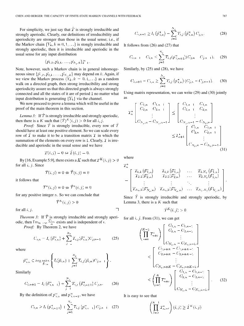
CHEN AND BERGER: THE CAPACITY OF FINITE-STATE MARKOV CHANNELS WITH FEEDBACK 787
For simplicity, we just say that is strongly irreducible andstrongly aperiodic. Clearly, our definitions of irreducibility andaperiodicity are stronger than those in the usual sense; i.e., ifthe Markov chain is stongly irreducible andstrongly aperiodic, then it is irreducible and aperiodic in theusual sense for any input distribution
Note, however, such a Markov chain is in general inhomoge-neous since may depend on . Again, ifwe view the Markov process as a randomwalk on a directed graph, then strong irreducibility and strongaperiodicity assure us that this directed graph is always stronglyconnected and all the states of it are of period no matter whatinput distribution is generating via the channel.
We now proceed to prove a lemma which will be useful in theproof of the main theorem in this section.
Lemma 3: If is strongly irreducible and strongly aperiodic,then there is a such that for all .
Proof: Since is strongly irreducible, every row ofshould have at least one positive element. So we can scale everyrow of to make it to be a transition matrix in which thesummation of the elements on every row is . Clearly, is irre-ducible and aperiodic in the usual sense and we have
By [16, Example 5.9], there exists a such thatfor all , . Since
it follows that
for any positive integer . So we can conclude that
for all .
Theorem 3: If is strongly irreducible and strongly aperi-odic, then exists and is independent of .
Proof: By Theorem 2, we have
(25)
where
Similarly
(26)
By the definition of and , we have
(27)
(28)
It follows from (26) and (27) that
(29)
Similarly, by (25) and (28), we have
(30)
Using matrix representation, we can write (29) and (30) jointlyas
......
...
(31)
where
......
. . ....
Since is strongly irreducible and strongly aperiodic, byLemma 3, there is a such that
for all , . From (31), we can get
...
...
...(32)
It is easy to see that

788 IEEE TRANSACTIONS ON INFORMATION THEORY, VOL. 51, NO. 3, MARCH 2005
for all positive integers , , . Let
Clearly, we have . Let
By (32), we can get
and thus we have
It follows by recursion that
(33)
and thus,
By (31), it is easy to show that is monotonically decreasing,is monotonically increasing, and both of them are bounded,
so their limits exist. Hence,
implies
That is, exists and is independent of .So we can conclude that
exists and is independent of .
Now we begin to analyze the convergence rate of
which is useful for Section VII.By (33), we have, for any and
(34)
where
and
Note: .
VII. CONVERGENCE OF NONSTATIONARY INPUT TO
STATIONARY INPUT
We now show that under certain conditions, the limitingmaximum average directed mutual information actually can beachieved by a stationary input. Before proving the main the-orem in this section, we need to introduce several definitions.
Definition 4 (The Vector -Norms): For
Specifically, for , we have
Definition 5 (the Matrix -Norms): For
Specifically, for , we have
is the square root of the
largest eigenvalue of
For the detailed discussion of the properties of the vector-norms and matrix -norms, see [19].
Definition 6: Let denote the set of all probabilityvectors. We say an channel transition probability ma-trix if there exists a subset such that thefollowing three conditions are satisfied.
i) .ii) For any
iii) There exists a positive constant such that
for any nonidentical and with the directionfrom to .
is called the -subset.See Appendix I for the detailed discussion of Definition 6.

CHEN AND BERGER: THE CAPACITY OF FINITE-STATE MARKOV CHANNELS WITH FEEDBACK 789
We also need the following lemma concerning the backwardproduct of matrices.
Lemma 4 [13]: If , then for any, there exists a positive number such that, for all
where , are stochastic matrices.
Now we are ready to prove the main theorem in this section.
Theorem 4: If is strongly irreducible and strongly aperi-odic and , then
where is the equilibrium distribution of thechannel output process induced by the stationary input distribu-tion .
Proof: Let be the -subset. Since
where , Definition 6 and thediscussion in the Appendix assure us that
is attained inside and there exists a unique suchthat
First, we derive a bound on the convergence rate of . Let
We have
and thus,
(35)
where the direction of is from to (We temporarilysuppose that ). Since is the max-imum value of and the direction of is from to
, it follows that
(36)
Since is linear with respect to, it follows that
Then, by Definition 6, we have
(37)
Since is the maximum value of and the direc-tion of is from to , it follows that
(38)
Putting (38) into (37), we get
(39)
By (35), (36), and (39), we have
or equivalently
(40)
It follows from (34) that
and it is easy to check that
So for any we have
(41)

790 IEEE TRANSACTIONS ON INFORMATION THEORY, VOL. 51, NO. 3, MARCH 2005
It is obvious that (41) also holds when . Thus,
(42)
for any as . Hence, is a Cauchy sequence.Since is complete, there exists such that .Clearly, this result holds for all .
Let , where and are defined in theequations at the bottom of the page. By Holder’s inequalityand (42)
Clearly, we have
where . Hence,
Applying Lemma 4, we deduce that for any , there existsa positive number such that, for all
(43)
Since for every , it follows that for any , thereexists a positive number such that, for all
... (44)
Let . In the remaining part of this proof,we implicitly assume . Now we have
...
...
...
where , the he input distributions of are
respectively.Similarly, we have
...
......
. . ....
and
......
. . ....

CHEN AND BERGER: THE CAPACITY OF FINITE-STATE MARKOV CHANNELS WITH FEEDBACK 791
...
...
All the input distributions of are
. So we have
(45)
where are given in equations at the bottom ofthe page. Now we evaluate , and , respectively, in(46)–(48) at the bottom of the following page.
Clearly, we have
(49)
(50)
... (51)
By (43)
(52)
since if .By (44)
... (53)
since if .Putting (49)–(53) into (48) yields
(54)
Now put (46), (47), and (54) back into (45), obtaining
Since here is arbitrary, it follows that
(55)
The strong irreducibility of guarantees that the outputprocess induced by any stationary inputdistribution form an irreducible Markov chain on the state space
. So from the analysis in Section V, we have
where is the equilibrium distribution of thechannel output process induced by the stationary input distribu-tion . Hence,
(56)
......
...
...
...
...

792 IEEE TRANSACTIONS ON INFORMATION THEORY, VOL. 51, NO. 3, MARCH 2005
It is obvious that the limiting average directed mutual informa-tion induced by the optimal input distribution is always greaterthan or equal to the limiting average directed mutual informa-tion induced by any stationary input distribution, so we have
(57)
Combining (56) and (57) and noticing the arbitrariness of ,we can conclude that
(58)for all .
i) ...
... (46)
ii) ...
... (47)
iii) ...
...
...
...
...
...
...
... (48)

CHEN AND BERGER: THE CAPACITY OF FINITE-STATE MARKOV CHANNELS WITH FEEDBACK 793
Remark: The condition isintroduced for purely technical reasons. It enables us to provethat converges to exponentially fast by exploiting thestrict concavity property of mutual information function. The-orem 4 still holds when this condition is removed. However, theproof will be less direct compared with the current one.
VIII. DIRECT CHANNEL CODING THEOREM
In this section, we prove the direct channel coding theoremand suggest a coding scheme for our channel model.
Theorem 5 (Direct Channel Coding Theorem): If isstrongly irreducible and strongly aperiodic, then all rates lessthan
are achievable, where is the equilibrium dis-tribution of the channel output process induced by the stationaryinput distribution .
Proof: We shall implicitly assume that .It has been shown in [10] that the general formula for the
capacity of feedback channels is
where
1)
is the set of all channel input distributions;2)
3) the in probability of a sequence of random vari-ables , denoted by , isdefined as the largest extended real number such that
, .Let
Let
for ; ; . Sinceis strongly irreducible and strongly aperiodic, we can check thatthe joint process induced by the stationaryinput distribution constitutes an irreducible
Markov chain with convergingto , where is the equilibriumdistribution of the channel output process induced by the sta-tionary input distribution . Note:
1) The recurrent state space of this Markov chain maybesmaller than
The strong irreducibility and strong aperiodicity of onlyguarantees that induced by the sta-tionary input distribution form an ir-reducible and aperiodic Markov chain on the state space
.2) We assume the strong irreducibility and strong aperiod-
icity of only for simplicity. More generally, we wouldneed to decompose the state space into disjoint irreducibleclosed sets, whereupon the proof would proceed along thesame lines.
Now we have
Since
is a function of , and is an er-godic process, it follows that
is also an ergodic process. So we have
in probability

794 IEEE TRANSACTIONS ON INFORMATION THEORY, VOL. 51, NO. 3, MARCH 2005
Fig. 5. FSC with state information available at transmitter and receiver.
which implies that
Now the proof is complete since
Theorem 6: If is strongly irreducible and strongly aperi-odic and , then
and is independent of the initial state .Proof: By Theorem 1
If is strongly irreducible and strongly aperiodic,, by Theorem 4
Theorem 5 shows the tightness of this upper bound and com-pletes the proof.
In the remainder of this section, we suggest a coding schemefor our channel model, which also makes the meaning of thecapacity formula transparent.
We first consider the channel model shown in Fig. 5, in whichthe state information is simultaneously available to both thetransmitter T and the receiver R. If the state process is stationaryand ergodic, then it is well known [9], [20], [21] that the channelcapacity is
where is the number of channel states and is the stationarydistribution of the ergodic state process . The followingis the outline of the coding scheme for this channel [21].
Let
Fix the block length . Let be the number of times duringthe symbols for which the channel state is , i.e.,
Let . Since the state process is stationary and er-godic, we have and
in probability.An code for this channel is constructed
by multiplexing codes
, where code correspondsto the channel state . By doing this, weactually decompose the channel into memoryless channelsand the existence of these codes follows immediately from thedirect coding theorem for memoryless channels. Since isnot necessarily equivalent to , the codes are truncated if
and zero filled if . Represent each messageas a -dimensional vector with
and map the th index (i.e., ) into a codeword form the thcode (i.e., the code with parameters ),for . If , then the transmitter sends asthe th symbol the next unsent symbol of the codeword cor-responding to the th index of the message from the th code
.Since the receiver knows exactly the state information that
was used at the transmitter, it can demultiplex the receivedstream into separate codewords and decode them. Since thestate process is stationary and ergodic, as , the rate
is achievable.It is easy to see that the capacity formula of this channel
model closely resembles ours in that both of them can be repre-sented as the average of mutual information over the stationary

CHEN AND BERGER: THE CAPACITY OF FINITE-STATE MARKOV CHANNELS WITH FEEDBACK 795
distribution of the channel state process. This suggests that themultiplexing coding scheme may work in our channel model aswell. But we should note that in our model, the current channelstate is the previous channel output, so it will be affected by thechannel input. Although we have shown that if the input processis stationary, the output process (i.e., channel state process) isan irreducible homogeneous Markov chain and thus is ergodic,it does not imply that the output process induced by a spe-cific codeword is still ergodic (or close to ergodic). The randomcoding argument based on strong typicality tells us that for a dis-crete memoryless channel with finite input and output alphabets,the statistics of the output process induced by a good codewordare close to those of the output process induced by the optimalinput distribution that achieves the channel capacity. But strongtypicality only guarantees that the statistics of a whole code-word are close to the optimal input distribution, while a trun-cated version may not have this property. In the multiplexingscheme, the output process is generated by several multiplexedcodewords, each of which is designed for its corresponding de-composed memoryless channel. And the length of a multiplexedcodeword is proportional to the stationary probability measureassigned on its corresponding state. We want the statistics ofthe output process induced by the multiplexed codewords to beclose to the equilibrium distribution induced by the optimal sta-tionary input. Clearly, this depends highly on the cooperationof the multiplexed codewords. Even a small fluctuation of thestatistics in a portion of a multiplexed codeword may have adomino effect on the transmission of the other multiplexed code-words and finally make the output process deviate from the de-sired distribution. The result of the large deviation in the outputprocess is that the symbols in some multiplexed codewords aretotally sent while many symbols in some others of the multi-plexed codewords are still unsent. So, in order to guarantee thestability of the multiplexing scheme, we need the multiplexedcodewords to behave better than those codewords in the sensethat their empirical distributions well-approximate the input dis-tribution to which they correspond. Theorem 7 below shows thatfor a discrete memoryless channel with finite input and outputalphabets, the empirical statistics of each of the words of a goodcode can be made to closely approximate the optimum input dis-tribution even despite their being subjected to truncation.
Before proving Theorem 7, we need to give a definition.We consider an information source , where
are independent and identically distributed (i.i.d.) with distribu-tion . Let denote the cardinality of the set of valuesmay assume. Here we suppose and for all
.
Definition 7: The super-typical set with respect tois the set of sequences such
that
for all and all , where isthe number of occurrences of in the sequence , and is anarbitrarily small positive real number. The members ofare called super-typical sequences.
It’s clear that the super-typical set is a subset of thestrongly typical set . But the following lemma says that asand go to infinity, these two sets have no essential difference.
Lemma 5: For any , , there exists a positiveinteger such that when , we have
Proof: See Appendix II.
This lemma implies that no loss of generality results fromrestricting attention to the super-typical set. It is obvious thatthe random coding argument based on strong typicality canbe translated to an argument based on super typicality withoutany change. So for any discrete memoryless channel with finiteinput and output alphabets, there exists a good codebook, all thecodewords of which are super-typical. This is summarized inTheorem 7.
Theorem 7: Let be any discrete memoryless channelwith finite input and output alphabets. For any input distribution
that is consistent with , for any ,there exists such that for all , there exists a
code with average probability of error less thanand . Furthermore, each of thesecodewords is super-typical with respect to .
Proof: The proof is omitted since it is almost the sameas the standard proof of direct coding theorem for memorylesschannel based on weak typicalicy or strong typicality, see [22].The only difference is that we require that the randomly gener-ated codewords satisfy super typicality. And Lemma 5 assuresus that there is no essential difference between strong typicalityand super typicality when the alphabets are finite.
We want to point out another difference between the multi-plexing coding scheme for our feedback channel and that forthe channel model shown in Fig. 5. Zero filling is not a goodchoice for our channel when , since this will makethe statistics of the codeword deviate from the correspondinginput distribution and thus induce a big deviation at the output.Instead, we will fill in the letters so as to ensure that the length-ened codewords still satisfy super typicality and/or we willtry to drive the channel into those states that still have unsentsymbols.
IX. CONCLUSION
We derived a simple formula for the capacity of finite-stateMarkov channels with feedback when the channel transitionprobability satisfies certain conditions. Actually, the same ca-pacity formula holds under much weaker conditions. It will beshown elsewhere [23], [24] that based on the classification ofMarkov decision processes [25], the capacity of Markov chan-nels with feedback can be studied in full generality.
Finally, we mention the relationship between the channelwhose state process cannot be affected by the input and theone whose state process can be affected. We assume in bothcases the realization of the state process is available both attransmitter and receiver. For the channel whose state processcannot be affected by the input, the conventional multiplexing

796 IEEE TRANSACTIONS ON INFORMATION THEORY, VOL. 51, NO. 3, MARCH 2005
coding scheme [20], [21] can be viewed as a greedy algorithmwhich tries to maximize the immediate mutual information.For the channel whose state process can be affected by theinput, this greedy algorithm is not optimal since we not onlywant to maximize the immediate mutual information but alsowant to visit the preferable states as often as possible. So theoptimal coding scheme is a tradeoff between these two goals.From this perspective, it seems appropriate to call this type ofcode an error-correction and state-control code in contrast witha conventional error-correction code. Since the optimal codingscheme needs to exploit the ergodicity of the state process,however, it usually causes a long delay in decoding, especiallywhen the state space is big and/or the probability measuresassigned to some states are close to zero. Therefore, in somedelay-limited applications, certain kinds of greedy schemes aremore attractive. In this sense, a channel whose state processcan be affected by the input is considerably more flexible thanone whose state process cannot be affected, since we can use“idle” periods to drive the channel into preferable states andthereby increase the efficiency when we really need to usethe channel for information transmission. In a quite generalmanner of speaking, such a channel can be “matched” to aninformation source in the spirit of [11]. Perhaps this is one ofthe reasons why many real neural networks possess structurethat subscribes to the channel models treated in this paper.
APPENDIX IDISCUSSION OF DEFINITION 6
Lemma 6: For any channel transition probabilitymatrix , if , then .
Proof: Let be an arbitrary -dimensional vector withthe constraint . Let . We have
If , then is invertible, whereupon it followsthat
So
which implies that
(59)
We have
(60)
where
Combining (59) and (60), we have
(61)
Since
and
is linear with respect to , it follows that
(62)
Now let . It is easy to verify that Conditions i) andii) in Definition 6 are trivially satisfied. Furthermore, for anynonidentical and with the direction from to ,by (62), we have
where . So Condition iii) in Definition 6 is also satis-fied.
Now we begin to discuss the implications of three conditionsin Definition 6, which immediately suggests a way to construct
in the general case.Consider the following equivalence relation:
if and only if is in the null space of
Let be a partition of generated by the above equivalencerelation such that for any , if and only if .

CHEN AND BERGER: THE CAPACITY OF FINITE-STATE MARKOV CHANNELS WITH FEEDBACK 797
Condition i) implies that for any . Conditioniii) implies that for each , contains at most one elementsince if there exist two nonidentical , then
where the last equality follows from the fact that is in the nullspace of . Hence, contains exactly one element.
Let with
Condition ii) implies that
where the last equality is because is a constant for.
Now we are ready to present the procedure of constructing .
1) Let . By singular value decompo-sition, there exist orthogonal matrices and
such that
where
with .2) Let . Then we have
Let . Parti-tion as and let . Then
(63)
where is a solution to the fol-lowing constrained optimization problem:
(64)
subject to .3)
where .
It is easy to check that the resulting satisfies Conditions i)and ii) in Definition 6 and we have
for any nonidentical . We are unable to prove that
is uniformly bounded away from as required in Definition 6.However, we believe it is true under fairly general conditions.
Now consider the following maximization problem:
(65)
where is an arbitrary real vector. Suppose the max-imum is attained inside for some . Let be that uniqueelement of . Now we have
where follows from the fact that is a constantfor . So the maximum is attained inside . Furthermore,there exists a unique that achieves this maximal value.Since if there are nonidentical such that
by taking derivative with direction from to , we have
i.e.,
which is contradictory to Condition iii) in Definition 6.
APPENDIX IIPROOF OF LEMMA 5
We write
where . Then , , are i.i.d.random variables with and
. Note that
Let . Clearly

798 IEEE TRANSACTIONS ON INFORMATION THEORY, VOL. 51, NO. 3, MARCH 2005
and
Let . Now
Terms in the sum of the form
and
are (if , , , are distinct) since the expectation of the productis the product of the expectations, and in each case one of theterms has expectation . The only terms that do not vanish arethose of form and . There are and
of these terms, respectively. The last observation im-plies
Chebyshev’s inequality gives us
Hence,
Note: An alternative approach is to use Chernoff bound, whichyields a tighter upper bound on for largeand .
Since
there exists a positive integer , when , we have
Hence,
when .
ACKNOWLEDGMENT
The authors wish to thank two anonymous referees for theirvaluable comments and suggestions.
REFERENCES
[1] D. Blackwell, L. Breiman, and A. J. Thomansian, “Proof of Shannon’stransmission theorem for finite-state indecomposable channels,” Ann.Math. Statist., vol. 29, pp. 1209–1220, 1958.
[2] R. G. Gallager, Information Theory and Reliable Communica-tion. New York: Wiley, 1968.
[3] R. M. Gray, M. O. Dunham, and R. L. Gobbi, “Ergodicity of Markovchannels,” IEEE Tran. Inf. Theory, vol. IT-33, no. 5, pp. 656–664, Sep.1987.
[4] S. Verdú and T. S. Han, “A general formula for channel capacity,” IEEETran. Inf. Theory, vol. 40, no. 4, pp. 1147–1157, Jul. 1994.
[5] G. Caire and S. Shamai (Shitz), “On the capacity of some channels withchannel state information,” IEEE Tran. Inf. Theory, vol. 45, no. 6, pp.2007–2019, Sep. 1999.
[6] C. E. Shannon, “Channels with side information at the transmitter,” IBMJ. Res. Develop., vol. 2, pp. 289–293, Oct. 1958.
[7] , “The zero error capacity of a noisy channel,” IRE Trans. Inf.Theory, vol. IT-2, no. 3, pp. S8–S19, Sep. 1956.
[8] R. L. Dobrushin, “Information transmission in a channel with feedback,”Theory Probab. Appl., pp. 395–412, Dec. 1958.
[9] J. Wolfowitz, Coding Theorems of Information Theory. EnglewoodCliffs, NJ: Prentice-Hall, 1961.
[10] S. C. Tatikonda, “Control under communication constraints,” Ph.D. dis-sertation, MIT, Cambridge, MA, 2000.
[11] T. Berger, “Living information theory (Shannon Lecture),” presentedat the IEEE Int. Symp. Information Theory, Lausanne, Switzerland,Jun./Jul. 2002.
[12] T. Berger and Y. Ying, “Characterizing optimum (input,output) pro-cesses for finite-state channels with feedback,” in Proc. IEEE Int. Symp.Information Theory , Yokohama, Japan, Jun./Jul. 2003, p. 117.
[13] Y. Ying and T. Berger, “Capacity of binary feedback channels with unitmemory at the output,” IEEE Trans. Inf. Theory, submitted for publica-tion.
[14] J. Massey, “Causality, feedback, and directed information,” in Proc.1990 Int. Symp. Information Theory and its Applications, Hawaii, Nov.27–30, 1990, pp. 303–305.
[15] H. Marko, “The bidirectional communication theory—A generalizationof information theory,” IEEE Tran. Commun., vol. COM-21, no. 12, pp.1345–1351, Dec. 1973.
[16] R. M. Gray and J. C. Kieffer, “Asymptotically mean stationary mea-sures,” Ann. Probab., vol. 8, pp. 962–973, 1980.
[17] R. M. Gray, Entropy and Information Theory. New York: Springer-Verlag, 1991.
[18] R. Durret, Probability: Theory and Examples, 2nd ed. Belmont, CA:Duxbury, 1995.
[19] G. H. Gloum and C. F. Van Loan, Matrix Computations, 3rd ed. Bal-timore, MD: The Johns Hopkins Univ. Press, 1996.
[20] A. J. Goldsmith and P. P. Varaiya, “Capacity of fading channels withchannel side information,” IEEE Trans. Inf.. Theory, vol. 43, no. 6, pp.1986–1992, Nov. 1997.
[21] H. Viswanathan, “Capacity of Markov channels with receiver CSI anddelayed feedback,” IEEE Trans. Inf. Theory, vol. 45, no. 2, pp. 761–771,Mar. 1999.
[22] T. Cover and J. A. Thomas, Elements of Information Theory. NewYork: Wiley, 1991.
[23] J. Chen, P. Suksompong, and T. Berger, “Communication through a fi-nite-state machine with markov property,” in Proc. Conf. InformationSciences and Systems, 2004.
[24] , “Interactive Markov game and TDMA communication,” in prepa-ration.
[25] M. L. Puterman, Markov Decision Processes. New York: Wiley Inter-science, 1994.