Calculo I LIMITES
49
Transcript of Calculo I LIMITES

IMEF - FURG - IMEF - FURG - IMEF - FURG - IMEF - FURG - IMEF - FURG - IMEF - FURG - IMEF - FURG - IMEF - FURG - IMEF - FURG - IMEF - FURG - IMEF - FURG - IMEF - FURG - IMEF - FURG - IMEF - FURG - IMEF - FURG - IMEF - FURG - IMEF - FURG - IMEF - FURG -
IMEF - FURG - IMEF - FURG - IMEF - FURG - IMEF - FURG - IMEF - FURG - IMEF - FURG - IMEF - FURG - IMEF - FURG - IMEF - FURG - IMEF - FURG - IMEF - FURG - IMEF - FURG - IMEF - FURG - IMEF - FURG - IMEF - FURG - IMEF - FURG - IMEF - FURG - IMEF - FURG -
NotasdeAuladeCál ulo
Limites
BárbaraRodriguez
CinthyaMeneghetti
CristianaPo�al
11demaiode2013

IMEF - FURG - IMEF - FURG - IMEF - FURG - IMEF - FURG - IMEF - FURG - IMEF - FURG - IMEF - FURG - IMEF - FURG - IMEF - FURG - IMEF - FURG - IMEF - FURG - IMEF - FURG - IMEF - FURG - IMEF - FURG - IMEF - FURG - IMEF - FURG - IMEF - FURG - IMEF - FURG -
IMEF - FURG - IMEF - FURG - IMEF - FURG - IMEF - FURG - IMEF - FURG - IMEF - FURG - IMEF - FURG - IMEF - FURG - IMEF - FURG - IMEF - FURG - IMEF - FURG - IMEF - FURG - IMEF - FURG - IMEF - FURG - IMEF - FURG - IMEF - FURG - IMEF - FURG - IMEF - FURG -
UniversidadeFederaldoRioGrande-FURG
NOTASDEAULADECÁLCULO
InstitutodeMatemáti a,Estatísti aeFísi a-IMEF
Materialelaborado omoresultadodoprojetoREUNI-PROPESPN
o
:033128/2012
- oordenadopelasprofessorasBárbaraRodriguez,CinthyaMeneghettieCristiana
Po�al om
parti ipaçãodabolsistaREUNI:ElizangelaPereira.
1NotasdeauladeCál ulo-FURG

I
M
E
F
-
F
U
R
G
-
I
M
E
F
-
F
U
R
G
-
I
M
E
F
-
F
U
R
G
-
I
M
E
F
-
F
U
R
G
-
I
M
E
F
-
F
U
R
G
-
I
M
E
F
-
F
U
R
G
-
I
M
E
F
-
F
U
R
G
-
I
M
E
F
-
F
U
R
G
-
I
M
E
F
-
F
U
R
G
-
I
M
E
F
-
F
U
R
G
-
I
M
E
F
-
F
U
R
G
-
I
M
E
F
-
F
U
R
G
-
I
M
E
F
-
F
U
R
G
-
I
M
E
F
-
F
U
R
G
-
I
M
E
F
-
F
U
R
G
-
I
M
E
F
-
F
U
R
G
-
I
M
E
F
-
F
U
R
G
-
I
M
E
F
-
F
U
R
G
-
I
M
E
F
-
F
U
R
G
-
I
M
E
F
-
F
U
R
G
-
I
M
E
F
-
F
U
R
G
-
I
M
E
F
-
F
U
R
G
-
I
M
E
F
-
F
U
R
G
-
I
M
E
F
-
F
U
R
G
-
I
M
E
F
-
F
U
R
G
-
I
M
E
F
-
F
U
R
G
-
I
M
E
F
-
F
U
R
G
-
I
M
E
F
-
F
U
R
G
-
I
M
E
F
-
F
U
R
G
-
I
M
E
F
-
F
U
R
G
-
I
M
E
F
-
F
U
R
G
-
I
M
E
F
-
F
U
R
G
-
I
M
E
F
-
F
U
R
G
-
I
M
E
F
-
F
U
R
G
-
I
M
E
F
-
F
U
R
G
-
I
M
E
F
-
F
U
R
G
-
Sumário
1 Limites de funções reais de uma variável 4
1.1 De�nições importantes . . . . . . . . . . . . . . . . . . . . . . . . . . 5
1.2 Motivação para a de�nição de limite . . . . . . . . . . . . . . . . . . 6
1.3 De�nição formal de limite �nito . . . . . . . . . . . . . . . . . . . . . 10
1.4 Construção geométri a que ilustra a noção de limite . . . . . . . . . . 12
1.5 Limites Laterais . . . . . . . . . . . . . . . . . . . . . . . . . . . . . . 14
1.5.1 De�nição de limite à direita . . . . . . . . . . . . . . . . . . . 14
1.5.2 De�nição de limite à esquerda . . . . . . . . . . . . . . . . . . 14
1.6 Propriedades usadas no ál ulo de limites . . . . . . . . . . . . . . . . 20
1.6.1 Limite de uma onstante . . . . . . . . . . . . . . . . . . . . . 20
1.6.2 Limite da função identidade . . . . . . . . . . . . . . . . . . . 20
1.6.3 Limite da soma . . . . . . . . . . . . . . . . . . . . . . . . . . 20
1.6.4 Limite da diferença . . . . . . . . . . . . . . . . . . . . . . . . 21
1.6.5 Limite do produto . . . . . . . . . . . . . . . . . . . . . . . . 21
1.6.6 Limite do quo iente . . . . . . . . . . . . . . . . . . . . . . . . 23
1.6.7 Limite da multipli ação por uma onstante . . . . . . . . . . . 23
1.6.8 Limite da poten iação . . . . . . . . . . . . . . . . . . . . . . 23
1.6.9 Limite da radi iação . . . . . . . . . . . . . . . . . . . . . . . 24
1.6.10 Limite de uma função polinomial . . . . . . . . . . . . . . . . 24
1.6.11 Limite de uma função ra ional . . . . . . . . . . . . . . . . . . 24
1.6.12 Limite do logaritmo natural de uma função . . . . . . . . . . . 25
1.7 Limites in�nitos . . . . . . . . . . . . . . . . . . . . . . . . . . . . . . 30
1.8 Limites no in�nito . . . . . . . . . . . . . . . . . . . . . . . . . . . . 32
1.8.1 Limites no in�nito de xn. . . . . . . . . . . . . . . . . . . . . 34
1.9 Limites espe iais . . . . . . . . . . . . . . . . . . . . . . . . . . . . . 35
2

I
M
E
F
-
F
U
R
G
-
I
M
E
F
-
F
U
R
G
-
I
M
E
F
-
F
U
R
G
-
I
M
E
F
-
F
U
R
G
-
I
M
E
F
-
F
U
R
G
-
I
M
E
F
-
F
U
R
G
-
I
M
E
F
-
F
U
R
G
-
I
M
E
F
-
F
U
R
G
-
I
M
E
F
-
F
U
R
G
-
I
M
E
F
-
F
U
R
G
-
I
M
E
F
-
F
U
R
G
-
I
M
E
F
-
F
U
R
G
-
I
M
E
F
-
F
U
R
G
-
I
M
E
F
-
F
U
R
G
-
I
M
E
F
-
F
U
R
G
-
I
M
E
F
-
F
U
R
G
-
I
M
E
F
-
F
U
R
G
-
I
M
E
F
-
F
U
R
G
-
I
M
E
F
-
F
U
R
G
-
I
M
E
F
-
F
U
R
G
-
I
M
E
F
-
F
U
R
G
-
I
M
E
F
-
F
U
R
G
-
I
M
E
F
-
F
U
R
G
-
I
M
E
F
-
F
U
R
G
-
I
M
E
F
-
F
U
R
G
-
I
M
E
F
-
F
U
R
G
-
I
M
E
F
-
F
U
R
G
-
I
M
E
F
-
F
U
R
G
-
I
M
E
F
-
F
U
R
G
-
I
M
E
F
-
F
U
R
G
-
I
M
E
F
-
F
U
R
G
-
I
M
E
F
-
F
U
R
G
-
I
M
E
F
-
F
U
R
G
-
I
M
E
F
-
F
U
R
G
-
I
M
E
F
-
F
U
R
G
-
I
M
E
F
-
F
U
R
G
-
SUMÁRIO
1.9.1 Indeterminação do tipo
00. . . . . . . . . . . . . . . . . . . . . 36
1.9.2 Indeterminação do tipo
∞∞ . . . . . . . . . . . . . . . . . . . . 38
1.9.3 Indeterminação do tipo ∞−∞ . . . . . . . . . . . . . . . . . 38
1.9.4 Indeterminação tipo 0 · ∞ . . . . . . . . . . . . . . . . . . . . 38
1.10 Teorema do onfronto . . . . . . . . . . . . . . . . . . . . . . . . . . . 39
1.11 Limites fundamentais . . . . . . . . . . . . . . . . . . . . . . . . . . . 40
1.11.1 Limite fundamental trigonométri o . . . . . . . . . . . . . . . 40
1.11.2 Limite fundamental exponen ial I . . . . . . . . . . . . . . . . 42
1.11.3 Limite fundamental exponen ial II . . . . . . . . . . . . . . . 43
1.12 Lista de Exer í ios . . . . . . . . . . . . . . . . . . . . . . . . . . . . 45
3 Notas de aula de Cál ulo - FURG

I
M
E
F
-
F
U
R
G
-
I
M
E
F
-
F
U
R
G
-
I
M
E
F
-
F
U
R
G
-
I
M
E
F
-
F
U
R
G
-
I
M
E
F
-
F
U
R
G
-
I
M
E
F
-
F
U
R
G
-
I
M
E
F
-
F
U
R
G
-
I
M
E
F
-
F
U
R
G
-
I
M
E
F
-
F
U
R
G
-
I
M
E
F
-
F
U
R
G
-
I
M
E
F
-
F
U
R
G
-
I
M
E
F
-
F
U
R
G
-
I
M
E
F
-
F
U
R
G
-
I
M
E
F
-
F
U
R
G
-
I
M
E
F
-
F
U
R
G
-
I
M
E
F
-
F
U
R
G
-
I
M
E
F
-
F
U
R
G
-
I
M
E
F
-
F
U
R
G
-
I
M
E
F
-
F
U
R
G
-
I
M
E
F
-
F
U
R
G
-
I
M
E
F
-
F
U
R
G
-
I
M
E
F
-
F
U
R
G
-
I
M
E
F
-
F
U
R
G
-
I
M
E
F
-
F
U
R
G
-
I
M
E
F
-
F
U
R
G
-
I
M
E
F
-
F
U
R
G
-
I
M
E
F
-
F
U
R
G
-
I
M
E
F
-
F
U
R
G
-
I
M
E
F
-
F
U
R
G
-
I
M
E
F
-
F
U
R
G
-
I
M
E
F
-
F
U
R
G
-
I
M
E
F
-
F
U
R
G
-
I
M
E
F
-
F
U
R
G
-
I
M
E
F
-
F
U
R
G
-
I
M
E
F
-
F
U
R
G
-
I
M
E
F
-
F
U
R
G
-
Capítulo 1
Limites de funções reais de uma
variável
Apresentação
O ál ulo é fundamentalmente diferente da matemáti a estudada durante
o ensino médio. Ele trata de variação e de movimento, bem omo de quantidades
que tendem a outras quantidades. Ele teve sua origem em quatro problemas nos
quais os matemáti os europeus estavam trabalhando durante o sé ulo XVII. São
eles:
• O problema da reta tangente;
• O problema da velo idade e da a eleração;
• O problema de máximos e mínimos;
• O problema da área.
Cada um destes problemas envolve o on eito de limite e é possível in-
troduzir o ál ulo diferen ial e integral a partir de qualquer um deles.
Neste apítulo serão apresentados os on eitos de limites que permitem
estudar o omportamento de uma função nas proximidades de um determinado
ponto.
4
I
M
E
F
-
F
U
R
G
-
I
M
E
F
-
F
U
R
G
-
I
M
E
F
-
F
U
R
G
-
I
M
E
F
-
F
U
R
G
-
I
M
E
F
-
F
U
R
G
-
I
M
E
F
-
F
U
R
G
-
I
M
E
F
-
F
U
R
G
-
I
M
E
F
-
F
U
R
G
-
I
M
E
F
-
F
U
R
G
-
I
M
E
F
-
F
U
R
G
-
I
M
E
F
-
F
U
R
G
-
I
M
E
F
-
F
U
R
G
-
I
M
E
F
-
F
U
R
G
-
I
M
E
F
-
F
U
R
G
-
I
M
E
F
-
F
U
R
G
-
I
M
E
F
-
F
U
R
G
-
I
M
E
F
-
F
U
R
G
-
I
M
E
F
-
F
U
R
G
-
I
M
E
F
-
F
U
R
G
-
I
M
E
F
-
F
U
R
G
-
I
M
E
F
-
F
U
R
G
-
I
M
E
F
-
F
U
R
G
-
I
M
E
F
-
F
U
R
G
-
I
M
E
F
-
F
U
R
G
-
I
M
E
F
-
F
U
R
G
-
I
M
E
F
-
F
U
R
G
-
I
M
E
F
-
F
U
R
G
-
I
M
E
F
-
F
U
R
G
-
I
M
E
F
-
F
U
R
G
-
I
M
E
F
-
F
U
R
G
-
I
M
E
F
-
F
U
R
G
-
I
M
E
F
-
F
U
R
G
-
I
M
E
F
-
F
U
R
G
-
I
M
E
F
-
F
U
R
G
-
I
M
E
F
-
F
U
R
G
-
I
M
E
F
-
F
U
R
G
-
1.1. DEFINIÇÕES IMPORTANTES
1.1 De�nições importantes
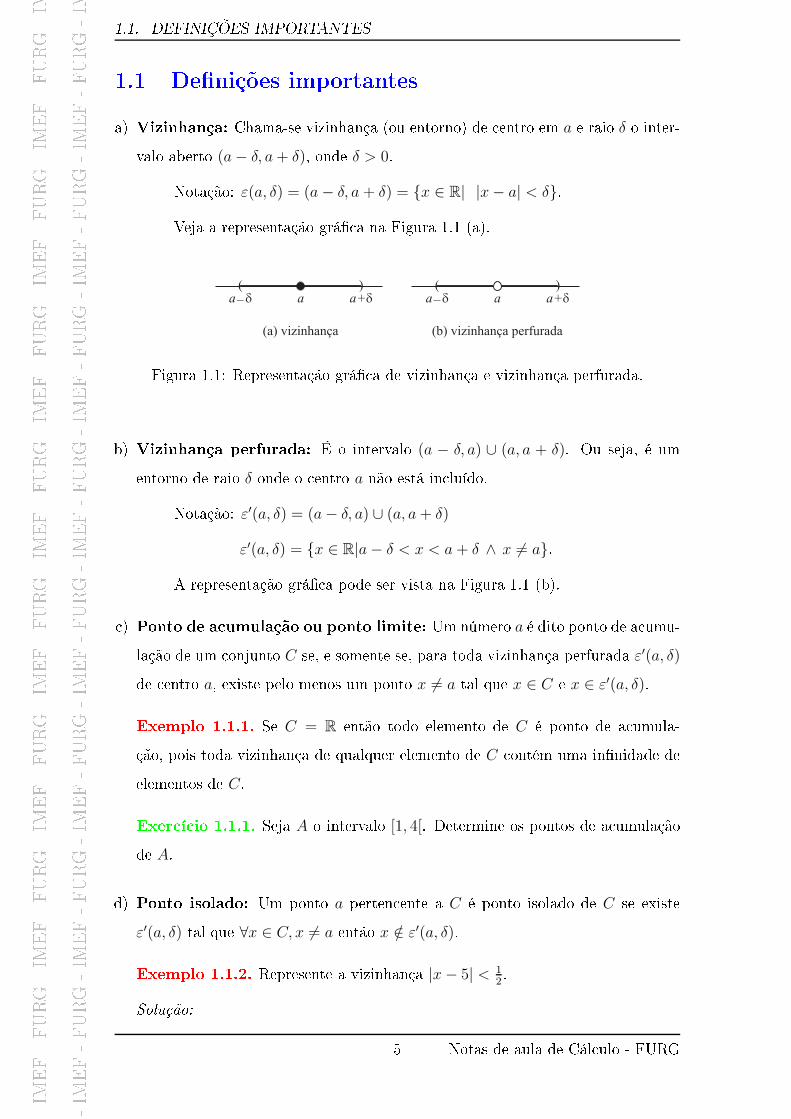
a) Vizinhança: Chama-se vizinhança (ou entorno) de entro em a e raio δ o inter-
valo aberto (a− δ, a+ δ), onde δ > 0.
Notação: ε(a, δ) = (a− δ, a + δ) = {x ∈ R| |x− a| < δ}.
Veja a representação grá� a na Figura 1.1 (a).
( )a d_ a a d+
( )a d_ a a d+
(a) vizinhança (b) vizinhança perfurada
Figura 1.1: Representação grá� a de vizinhança e vizinhança perfurada.
b) Vizinhança perfurada: É o intervalo (a − δ, a) ∪ (a, a + δ). Ou seja, é um
entorno de raio δ onde o entro a não está in luído.
Notação: ε′(a, δ) = (a− δ, a) ∪ (a, a+ δ)
ε′(a, δ) = {x ∈ R|a− δ < x < a + δ ∧ x 6= a}.
A representação grá� a pode ser vista na Figura 1.1 (b).
) Ponto de a umulação ou ponto limite: Um número a é dito ponto de a umu-
lação de um onjunto C se, e somente se, para toda vizinhança perfurada ε′(a, δ)
de entro a, existe pelo menos um ponto x 6= a tal que x ∈ C e x ∈ ε′(a, δ).
Exemplo 1.1.1. Se C = R então todo elemento de C é ponto de a umula-
ção, pois toda vizinhança de qualquer elemento de C ontém uma in�nidade de
elementos de C.
Exer í io 1.1.1. Seja A o intervalo [1, 4[. Determine os pontos de a umulação
de A.
d) Ponto isolado: Um ponto a perten ente a C é ponto isolado de C se existe
ε′(a, δ) tal que ∀x ∈ C, x 6= a então x /∈ ε′(a, δ).
Exemplo 1.1.2. Represente a vizinhança |x− 5| < 12.
Solução:
5 Notas de aula de Cál ulo - FURG

I
M
E
F
-
F
U
R
G
-
I
M
E
F
-
F
U
R
G
-
I
M
E
F
-
F
U
R
G
-
I
M
E
F
-
F
U
R
G
-
I
M
E
F
-
F
U
R
G
-
I
M
E
F
-
F
U
R
G
-
I
M
E
F
-
F
U
R
G
-
I
M
E
F
-
F
U
R
G
-
I
M
E
F
-
F
U
R
G
-
I
M
E
F
-
F
U
R
G
-
I
M
E
F
-
F
U
R
G
-
I
M
E
F
-
F
U
R
G
-
I
M
E
F
-
F
U
R
G
-
I
M
E
F
-
F
U
R
G
-
I
M
E
F
-
F
U
R
G
-
I
M
E
F
-
F
U
R
G
-
I
M
E
F
-
F
U
R
G
-
I
M
E
F
-
F
U
R
G
-
I
M
E
F
-
F
U
R
G
-
I
M
E
F
-
F
U
R
G
-
I
M
E
F
-
F
U
R
G
-
I
M
E
F
-
F
U
R
G
-
I
M
E
F
-
F
U
R
G
-
I
M
E
F
-
F
U
R
G
-
I
M
E
F
-
F
U
R
G
-
I
M
E
F
-
F
U
R
G
-
I
M
E
F
-
F
U
R
G
-
I
M
E
F
-
F
U
R
G
-
I
M
E
F
-
F
U
R
G
-
I
M
E
F
-
F
U
R
G
-
I
M
E
F
-
F
U
R
G
-
I
M
E
F
-
F
U
R
G
-
I
M
E
F
-
F
U
R
G
-
I
M
E
F
-
F
U
R
G
-
I
M
E
F
-
F
U
R
G
-
I
M
E
F
-
F
U
R
G
-
1.2. MOTIVA�O PARA A DEFINI�O DE LIMITE
Comparando om a de�nição de vizinhança, tem-se que o entro é
a = 5 e o raio é δ = 12. Para omprovar, utiliza-se a de�nição de módulo para
en ontrar o intervalo que representa a vizinhança:
|x− 5| < 1
2⇔ −1
2< x− 5 <
1
2.
Assim, tem-se:
−12
< x− 5 < 12
−12+ 5 < x− 5 + 5 < 1
2+ 5
92
< x < 112.
Portanto, a vizinhança é representada por ε(
5, 12
)
=(
92, 11
2
)
. A repre-
sentação grá� a pode ser vista na Figura 1.2.
( )5 0,5
_5 5 0,5+
Figura 1.2: Representação da vizinhança ε(
5, 12
)
.
1.2 Motivação para a de�nição de limite
A idéia de limite apare e intuitivamente em muitas situações. Na Físi a,
por exemplo, para de�nir a velo idade instantânea de um móvel utiliza-se o ál ulo
da velo idade média para o aso onde o intervalo de tempo seja muito próximo de
zero. A velo idade média vm é al ulada omo vm =s1 − s0t1 − t0
=△s
△t, onde s é a
posição e t é o tempo (veja na Figura 1.3). Então, a velo idade instantânea vi é
de�nida omo:
vi = lim△t→0
△s
△t.
Em outras palavras, a velo idade instantânea é o limite da velo idade
média quando △t tende a zero.
6 Notas de aula de Cál ulo - FURG

I
M
E
F
-
F
U
R
G
-
I
M
E
F
-
F
U
R
G
-
I
M
E
F
-
F
U
R
G
-
I
M
E
F
-
F
U
R
G
-
I
M
E
F
-
F
U
R
G
-
I
M
E
F
-
F
U
R
G
-
I
M
E
F
-
F
U
R
G
-
I
M
E
F
-
F
U
R
G
-
I
M
E
F
-
F
U
R
G
-
I
M
E
F
-
F
U
R
G
-
I
M
E
F
-
F
U
R
G
-
I
M
E
F
-
F
U
R
G
-
I
M
E
F
-
F
U
R
G
-
I
M
E
F
-
F
U
R
G
-
I
M
E
F
-
F
U
R
G
-
I
M
E
F
-
F
U
R
G
-
I
M
E
F
-
F
U
R
G
-
I
M
E
F
-
F
U
R
G
-
I
M
E
F
-
F
U
R
G
-
I
M
E
F
-
F
U
R
G
-
I
M
E
F
-
F
U
R
G
-
I
M
E
F
-
F
U
R
G
-
I
M
E
F
-
F
U
R
G
-
I
M
E
F
-
F
U
R
G
-
I
M
E
F
-
F
U
R
G
-
I
M
E
F
-
F
U
R
G
-
I
M
E
F
-
F
U
R
G
-
I
M
E
F
-
F
U
R
G
-
I
M
E
F
-
F
U
R
G
-
I
M
E
F
-
F
U
R
G
-
I
M
E
F
-
F
U
R
G
-
I
M
E
F
-
F
U
R
G
-
I
M
E
F
-
F
U
R
G
-
I
M
E
F
-
F
U
R
G
-
I
M
E
F
-
F
U
R
G
-
I
M
E
F
-
F
U
R
G
-
1.2. MOTIVA�O PARA A DEFINI�O DE LIMITE
s0
s1
t1t0
t
s
D
D
t
s
Figura 1.3: Grá� o da posição de um móvel ao longo do tempo.
O ál ulo de limites serve para des rever omo uma função se omporta
quando a variável independente tende a um dado valor.
Notação: limx→a
f(x) = L.
Lê-se: �L é o limite de f(x) quando x se aproxima de a�.
O matemáti o fran ês Augustin-Louis Cau hy (1789-1857) foi a primeira
pessoa a atribuir um signi� ado matemati amente rigoroso às frases �f(x) se apro-
xima arbitrariamente de L� e �x se aproxima de a�.
Observação 1.2.1. A expressão limx→a
f(x) = L des reve o omportamento de f(x)
quando x está muito próximo de a, e não quando x = a.
Exemplo 1.2.1. Como será o omportamento da função f(x) = x2− x+1 quando
x se aproximar ada vez mais de 2?
Solução:
A determinação do omportamento de f(x) para valores próximos de 2
pode ser analisada de várias formas. Ini ialmente, atribuem-se valores que se aproxi-
mam de 2 para x e, al ulando f(x) para ada um desses valores, pode-se onstruir
a seguinte tabela:
Tabela 1: Valores da função f(x) para valores próximos de 2.
x 1 1,5 1,9 1,99 1,999 2 2,001 2,01 2,1 2,5 3
f(x) 1 1,75 2,71 2,9701 2,997001 - 3,003001 3,0301 3,31 4,75 7
aproximação à esquerda → ← aproximação à direita
Primeiramente, observe que não foi olo ado na tabela o valor de f(x)
7 Notas de aula de Cál ulo - FURG

I
M
E
F
-
F
U
R
G
-
I
M
E
F
-
F
U
R
G
-
I
M
E
F
-
F
U
R
G
-
I
M
E
F
-
F
U
R
G
-
I
M
E
F
-
F
U
R
G
-
I
M
E
F
-
F
U
R
G
-
I
M
E
F
-
F
U
R
G
-
I
M
E
F
-
F
U
R
G
-
I
M
E
F
-
F
U
R
G
-
I
M
E
F
-
F
U
R
G
-
I
M
E
F
-
F
U
R
G
-
I
M
E
F
-
F
U
R
G
-
I
M
E
F
-
F
U
R
G
-
I
M
E
F
-
F
U
R
G
-
I
M
E
F
-
F
U
R
G
-
I
M
E
F
-
F
U
R
G
-
I
M
E
F
-
F
U
R
G
-
I
M
E
F
-
F
U
R
G
-
I
M
E
F
-
F
U
R
G
-
I
M
E
F
-
F
U
R
G
-
I
M
E
F
-
F
U
R
G
-
I
M
E
F
-
F
U
R
G
-
I
M
E
F
-
F
U
R
G
-
I
M
E
F
-
F
U
R
G
-
I
M
E
F
-
F
U
R
G
-
I
M
E
F
-
F
U
R
G
-
I
M
E
F
-
F
U
R
G
-
I
M
E
F
-
F
U
R
G
-
I
M
E
F
-
F
U
R
G
-
I
M
E
F
-
F
U
R
G
-
I
M
E
F
-
F
U
R
G
-
I
M
E
F
-
F
U
R
G
-
I
M
E
F
-
F
U
R
G
-
I
M
E
F
-
F
U
R
G
-
I
M
E
F
-
F
U
R
G
-
I
M
E
F
-
F
U
R
G
-
1.2. MOTIVA�O PARA A DEFINI�O DE LIMITE
quando x = 2. Esse valor foi omitido, pois se deseja estudar apenas os valores de
f(x) quando x está próximo de 2, e não o valor da função quando x = 2.
Per ebe-se que quando x se aproxima de 2 (em qualquer sentido) f(x) se
aproxima de 3. Logo, pode-se dizer que limx→2
f(x) = 3.
Observe a Figura 1.4. Comprova-se que o grá� o da função se aproxima
para o mesmo valor quando x está se aproximando de 2, tanto para valores maiores
quanto para valores menores do que 2.
−3 −2 −1 1 2 3
−1
1
2
3
4
5
x
y
Figura 1.4: Grá� o de f(x).
Nesse aso, o valor do limite oin idiu om o valor da função quando
x = 2, pois f(2) = 3. Mas nem sempre esse omportamento vai se veri� ar, omo
pode ser visto no próximo exemplo.
Exemplo 1.2.2. Como será o omportamento da função f(x) =
2x− 1, se x 6= 3
3, se x = 3
quando x está ada vez mais próximo de 3?
Solução:
Assim omo no exemplo anterior, primeiramente atribuem-se valores para
x e, en ontrando os valores de f(x) orrespondentes, pode-se onstruir a seguinte
tabela:
Tabela 2: Valores da função f(x) para valores próximos de 3.
x 2 2,5 2,9 2,99 2,999 3 3,001 3,01 3,1 3,5 4
f(x) 3 4 4,8 4,98 4,998 - 5,002 5,02 5,2 6 7
aproximação à esquerda → ← aproximação à direita
8 Notas de aula de Cál ulo - FURG
I
M
E
F
-
F
U
R
G
-
I
M
E
F
-
F
U
R
G
-
I
M
E
F
-
F
U
R
G
-
I
M
E
F
-
F
U
R
G
-
I
M
E
F
-
F
U
R
G
-
I
M
E
F
-
F
U
R
G
-
I
M
E
F
-
F
U
R
G
-
I
M
E
F
-
F
U
R
G
-
I
M
E
F
-
F
U
R
G
-
I
M
E
F
-
F
U
R
G
-
I
M
E
F
-
F
U
R
G
-
I
M
E
F
-
F
U
R
G
-
I
M
E
F
-
F
U
R
G
-
I
M
E
F
-
F
U
R
G
-
I
M
E
F
-
F
U
R
G
-
I
M
E
F
-
F
U
R
G
-
I
M
E
F
-
F
U
R
G
-
I
M
E
F
-
F
U
R
G
-
I
M
E
F
-
F
U
R
G
-
I
M
E
F
-
F
U
R
G
-
I
M
E
F
-
F
U
R
G
-
I
M
E
F
-
F
U
R
G
-
I
M
E
F
-
F
U
R
G
-
I
M
E
F
-
F
U
R
G
-
I
M
E
F
-
F
U
R
G
-
I
M
E
F
-
F
U
R
G
-
I
M
E
F
-
F
U
R
G
-
I
M
E
F
-
F
U
R
G
-
I
M
E
F
-
F
U
R
G
-
I
M
E
F
-
F
U
R
G
-
I
M
E
F
-
F
U
R
G
-
I
M
E
F
-
F
U
R
G
-
I
M
E
F
-
F
U
R
G
-
I
M
E
F
-
F
U
R
G
-
I
M
E
F
-
F
U
R
G
-
I
M
E
F
-
F
U
R
G
-
1.2. MOTIVA�O PARA A DEFINI�O DE LIMITE
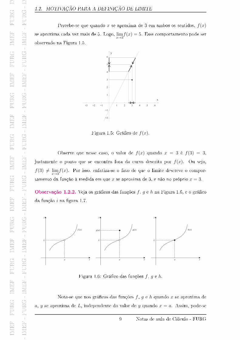
Per ebe-se que quando x se aproxima de 3 em ambos os sentidos, f(x)
se aproxima ada vez mais de 5. Logo, limx→3
f(x) = 5. Esse omportamento pode ser
observado na Figura 1.5.
−3 −2 −1 1 2 3 4 5 6
−2
−1
1
2
3
4
5
6
x
y
Figura 1.5: Grá� o de f(x).
Observe que nesse aso, o valor de f(x) quando x = 3 é f(3) = 3,
justamente o ponto que se en ontra fora da urva des rita por f(x). Ou seja,
f(3) 6= limx→3
f(x). Por isso, enfatiza-se o fato de que o limite des reve o ompor-
tamento da função à medida em que x se aproxima de 3, e não no próprio x = 3.
Observação 1.2.2. Veja os grá� os das funções f , g e h na Figura 1.6, e o grá� o
da função i na �gura 1.7.
x
y
a
L
f x( )
x
y
a
L
g x( )g a( )
x
y
a
L
h x( )
Figura 1.6: Grá� o das funções f , g e h.
Nota-se que nos grá� os das funções f , g e h quando x se aproxima de
a, y se aproxima de L, independente do valor de y quando x = a. Assim, pode-se
9 Notas de aula de Cál ulo - FURG

I
M
E
F
-
F
U
R
G
-
I
M
E
F
-
F
U
R
G
-
I
M
E
F
-
F
U
R
G
-
I
M
E
F
-
F
U
R
G
-
I
M
E
F
-
F
U
R
G
-
I
M
E
F
-
F
U
R
G
-
I
M
E
F
-
F
U
R
G
-
I
M
E
F
-
F
U
R
G
-
I
M
E
F
-
F
U
R
G
-
I
M
E
F
-
F
U
R
G
-
I
M
E
F
-
F
U
R
G
-
I
M
E
F
-
F
U
R
G
-
I
M
E
F
-
F
U
R
G
-
I
M
E
F
-
F
U
R
G
-
I
M
E
F
-
F
U
R
G
-
I
M
E
F
-
F
U
R
G
-
I
M
E
F
-
F
U
R
G
-
I
M
E
F
-
F
U
R
G
-
I
M
E
F
-
F
U
R
G
-
I
M
E
F
-
F
U
R
G
-
I
M
E
F
-
F
U
R
G
-
I
M
E
F
-
F
U
R
G
-
I
M
E
F
-
F
U
R
G
-
I
M
E
F
-
F
U
R
G
-
I
M
E
F
-
F
U
R
G
-
I
M
E
F
-
F
U
R
G
-
I
M
E
F
-
F
U
R
G
-
I
M
E
F
-
F
U
R
G
-
I
M
E
F
-
F
U
R
G
-
I
M
E
F
-
F
U
R
G
-
I
M
E
F
-
F
U
R
G
-
I
M
E
F
-
F
U
R
G
-
I
M
E
F
-
F
U
R
G
-
I
M
E
F
-
F
U
R
G
-
I
M
E
F
-
F
U
R
G
-
I
M
E
F
-
F
U
R
G
-
1.3. DEFINI�O FORMAL DE LIMITE FINITO
dizer que o limite da função f quando x tende a a é L (es reve-se limx→a
f(x) = L) e o
mesmo pode ser dito sobre as funções g e h.
x
y
a
L
i x( )
i a( )
Figura 1.7: Grá� o da função i.
Já para a função i, quando x se aproxima de a para valores maiores que
a, i se aproxima de i(a), e quando x se aproxima de a por valores menores que a,
i(x) tende a L. Ou seja, não há um valor úni o ao qual i(x) se aproxima quando x
tende a a. Assim, não existe o limite da função i para x tendendo a a.
1.3 De�nição formal de limite �nito
A linguagem utilizada até aqui não é uma linguagem matemáti a, pois ao
dizer, por exemplo, �x su� ientemente próximo de a�, não se sabe quanti� ar o quão
próximo x está de a. Então omo exprimir em linguagem matemáti a a de�nição
de limx→a
f(x) = L?
(a) f(x) deve ser arbitrariamente próximo de L para todo x su� i-
entemente próximo de a (e diferente de a).
É ne essário de�nir o on eito de proximidade arbitrária. Para tal,
utilizam-se pequenos valores representados geralmente pelas letras ǫ (epsilon) e δ
(delta), que servem de parâmetro de omparação para determinar se um valor está
ou não próximo de outro.
Considere um ǫ > 0, arbitrário. Os valores de f(x) são tais que
L− ǫ < f(x) < L+ ǫ,
isto é, sua distân ia a L é menor do que de ǫ, ou seja, |f(x) − L| < ǫ. Portanto,
10 Notas de aula de Cál ulo - FURG

I
M
E
F
-
F
U
R
G
-
I
M
E
F
-
F
U
R
G
-
I
M
E
F
-
F
U
R
G
-
I
M
E
F
-
F
U
R
G
-
I
M
E
F
-
F
U
R
G
-
I
M
E
F
-
F
U
R
G
-
I
M
E
F
-
F
U
R
G
-
I
M
E
F
-
F
U
R
G
-
I
M
E
F
-
F
U
R
G
-
I
M
E
F
-
F
U
R
G
-
I
M
E
F
-
F
U
R
G
-
I
M
E
F
-
F
U
R
G
-
I
M
E
F
-
F
U
R
G
-
I
M
E
F
-
F
U
R
G
-
I
M
E
F
-
F
U
R
G
-
I
M
E
F
-
F
U
R
G
-
I
M
E
F
-
F
U
R
G
-
I
M
E
F
-
F
U
R
G
-
I
M
E
F
-
F
U
R
G
-
I
M
E
F
-
F
U
R
G
-
I
M
E
F
-
F
U
R
G
-
I
M
E
F
-
F
U
R
G
-
I
M
E
F
-
F
U
R
G
-
I
M
E
F
-
F
U
R
G
-
I
M
E
F
-
F
U
R
G
-
I
M
E
F
-
F
U
R
G
-
I
M
E
F
-
F
U
R
G
-
I
M
E
F
-
F
U
R
G
-
I
M
E
F
-
F
U
R
G
-
I
M
E
F
-
F
U
R
G
-
I
M
E
F
-
F
U
R
G
-
I
M
E
F
-
F
U
R
G
-
I
M
E
F
-
F
U
R
G
-
I
M
E
F
-
F
U
R
G
-
I
M
E
F
-
F
U
R
G
-
I
M
E
F
-
F
U
R
G
-
1.3. DEFINI�O FORMAL DE LIMITE FINITO
dizer que f(x) é arbitrariamente próximo de L é o mesmo que dizer: dado um ǫ > 0,
tem-se |f(x)− L| < ǫ.
Assim, (a) pode ser rees rito omo:
(b) Dado ǫ > 0, deve-se ter |f(x) − L| < ǫ para todo x su� ientemente
próximo de a (e diferente de a).
Dizer que x é su� ientemente próximo de a para |f(x)− L| < ǫ signi� a
dizer que a sua distân ia a a é su� ientemente pequena para que isto o orra, ou
seja, existe δ > 0 tal que, se |x− a| < δ e x 6= a, então |f(x)− L| < ǫ.
Em suma, dando um ǫ > 0 qualquer, �xa-se a proximidade de f(x) a L.
Então se limx→a
f(x) = L, deve ser possível en ontrar um δ > 0 em orrespondên ia a
ǫ > 0 , tal que para todo x 6= a uja a distân ia até a seja menor que δ , tem-se a
distân ia de f(x) a L menor que ǫ. A partir de (a) e (b), pode-se agora formular a
de�nição formal de limite �nito:
De�nição 1.3.1. Dada uma função f om domínio D(f), seja �a� um ponto de
a umulação de D(f), e L um número, diz-se que o número L é o limite de f(x) om
x tendendo a �a� se, dado qualquer ǫ > 0, existe δ > 0 tal que se ∀x ∈ D(f) e
0 < |x− a| < δ então |f(x)− L| < ǫ.
Para indi ar essa de�nição, es reve-se limx→a
f(x) = L.
Observação 1.3.1. Na de�nição formal de limites, emprega-se o on eito de mó-
dulo. A ideia bási a no on eito de módulo de um número real é medir a distân ia
desse número até a origem.
Teorema 1.3.1. (Uni idade do limite) Se limx→a
f(x) = L1 e limx→a
f(x) = L2, então
L1 = L2.
Demonstração:
Supondo-se que L1 6= L2. Sem perda de generalidade, pode-se es rever
que L > M . Tomando-se ǫ =L−M
2> 0.
Se limx→a
f(x) = L1, então existe δ1 > 0, tal que se 0 < |x− a| < δ1 ⇒
|f(x)−M | < L−M
2, então
f(x) <L+M
2. (1.3.1)
11 Notas de aula de Cál ulo - FURG

I
M
E
F
-
F
U
R
G
-
I
M
E
F
-
F
U
R
G
-
I
M
E
F
-
F
U
R
G
-
I
M
E
F
-
F
U
R
G
-
I
M
E
F
-
F
U
R
G
-
I
M
E
F
-
F
U
R
G
-
I
M
E
F
-
F
U
R
G
-
I
M
E
F
-
F
U
R
G
-
I
M
E
F
-
F
U
R
G
-
I
M
E
F
-
F
U
R
G
-
I
M
E
F
-
F
U
R
G
-
I
M
E
F
-
F
U
R
G
-
I
M
E
F
-
F
U
R
G
-
I
M
E
F
-
F
U
R
G
-
I
M
E
F
-
F
U
R
G
-
I
M
E
F
-
F
U
R
G
-
I
M
E
F
-
F
U
R
G
-
I
M
E
F
-
F
U
R
G
-
I
M
E
F
-
F
U
R
G
-
I
M
E
F
-
F
U
R
G
-
I
M
E
F
-
F
U
R
G
-
I
M
E
F
-
F
U
R
G
-
I
M
E
F
-
F
U
R
G
-
I
M
E
F
-
F
U
R
G
-
I
M
E
F
-
F
U
R
G
-
I
M
E
F
-
F
U
R
G
-
I
M
E
F
-
F
U
R
G
-
I
M
E
F
-
F
U
R
G
-
I
M
E
F
-
F
U
R
G
-
I
M
E
F
-
F
U
R
G
-
I
M
E
F
-
F
U
R
G
-
I
M
E
F
-
F
U
R
G
-
I
M
E
F
-
F
U
R
G
-
I
M
E
F
-
F
U
R
G
-
I
M
E
F
-
F
U
R
G
-
I
M
E
F
-
F
U
R
G
-
1.4. CONSTRUÇ�O GEOMÉTRICA QUE ILUSTRA A NOÇ�O DE LIMITE
Se limx→a
f(x) = L2, então existe δ2 > 0, tal que se 0 < |x− a| < δ2 ⇒
|f(x)− L| < L−M
2, então
L+M
2< f(x). (1.3.2)
De (1.3.1) e (1.3.2), tem-se que para δ = min{δ1, δ2}, 0 < |x− a| < δ
que impli a que f(x) < f(x), o que é um absurdo. Logo a suposição ini ial é falsa
e L = M .
1.4 Construção geométri a que ilustra a noção de
limite
Sendo onhe idos f , a, L e ǫ, sabendo que limx→a
f(x) = L, ne essita-se
a har δ que satisfaça a de�nição de limite. Observe a Figura 1.8. Mar am-se L+ ǫ e
L−ǫ no eixo y e por esses pontos traçam-se retas paralelas ao eixo x , que en ontram
o grá� o de f nos pontos A e B. Traçando retas paralelas ao eixo dos y por esses
pontos, obtêm-se os pontos C e D, interse ções dessas retas om o eixo x. Basta
tomar δ > 0 tal que a−δ e a+δ sejam pontos do segmento CD. Observe que δ não é
úni o e equivale à distân ia de a ao extremo mais próximo do intervalo representado
pelo segmento CD.
x
y
a
L
f x( )
x
y
a
L
f x( )
L + e
L _ eA
B
C D
a _d a d+
d d
Figura 1.8: Representação geométri a de limite.
Exemplo 1.4.1. Prove formalmente que limx→3
(2x− 4) = 2.
12 Notas de aula de Cál ulo - FURG

I
M
E
F
-
F
U
R
G
-
I
M
E
F
-
F
U
R
G
-
I
M
E
F
-
F
U
R
G
-
I
M
E
F
-
F
U
R
G
-
I
M
E
F
-
F
U
R
G
-
I
M
E
F
-
F
U
R
G
-
I
M
E
F
-
F
U
R
G
-
I
M
E
F
-
F
U
R
G
-
I
M
E
F
-
F
U
R
G
-
I
M
E
F
-
F
U
R
G
-
I
M
E
F
-
F
U
R
G
-
I
M
E
F
-
F
U
R
G
-
I
M
E
F
-
F
U
R
G
-
I
M
E
F
-
F
U
R
G
-
I
M
E
F
-
F
U
R
G
-
I
M
E
F
-
F
U
R
G
-
I
M
E
F
-
F
U
R
G
-
I
M
E
F
-
F
U
R
G
-
I
M
E
F
-
F
U
R
G
-
I
M
E
F
-
F
U
R
G
-
I
M
E
F
-
F
U
R
G
-
I
M
E
F
-
F
U
R
G
-
I
M
E
F
-
F
U
R
G
-
I
M
E
F
-
F
U
R
G
-
I
M
E
F
-
F
U
R
G
-
I
M
E
F
-
F
U
R
G
-
I
M
E
F
-
F
U
R
G
-
I
M
E
F
-
F
U
R
G
-
I
M
E
F
-
F
U
R
G
-
I
M
E
F
-
F
U
R
G
-
I
M
E
F
-
F
U
R
G
-
I
M
E
F
-
F
U
R
G
-
I
M
E
F
-
F
U
R
G
-
I
M
E
F
-
F
U
R
G
-
I
M
E
F
-
F
U
R
G
-
I
M
E
F
-
F
U
R
G
-
1.4. CONSTRUÇ�O GEOMÉTRICA QUE ILUSTRA A NOÇ�O DE LIMITE
Solução:
Comparando ao limite geral limx→a
f(x) = L, tem-se nesse aso que a = 3,
f(x) = 2x− 4 e L = 2. Assim, deve-se provar que dado qualquer ǫ > 0, existe δ > 0
tal que se x ∈ D(f) e 0 < |x− 3| < δ então |(2x− 4)− 2| < ǫ. Cal ulando:
|(2x− 4)− 2| = |2x− 6||(2x− 4)− 2| = 2 · |x− 3|.
Mas omo 0 < |x− 3| < δ, então 2 · |x− 3| < 2 · δ. Es olhendo δ =ǫ
2:
|(2x− 4)− 2| = 2 · |x− 3| < 2 · δ = 2 · ǫ2= ǫ. Portanto, |(2x− 4)− 2| < ǫ.
Logo, dado qualquer ǫ > 0, existe δ =ǫ
2tal que se x ∈ D(f) e
0 < |x− 3| < δ então |(2x− 4)− 2| < ǫ, que é justamente a de�nição de limite.
Assim, limx→3
(2x− 4) = 2.
Exemplo 1.4.2. Prove formalmente que limx→2
x2 = 4.
Solução:
Comparando om o limite geral limx→a
f(x) = L, tem-se que a = 2,
f(x) = x2e L = 4. Assim, deve-se provar que dado um ǫ > 0, existe δ > 0 tal que se
x ∈ D(f) e 0 < |x−2| < δ então |(x2)−4| < ǫ. Fatorando: |x2−4| = |x−2| · |x+2|.É pre iso en ontrar uma desigualdade envolvendo |x+2| e um valor ons-
tante. Como |x− 2| < δ , então supondo δ = 1 tem-se que |x− 2| < 1. Portanto:
−1 < x− 2 < 1
1 < x < 3
3 < x+ 2 < 5.
Como |x − 2| < δ e |x + 2| < 5, então |x − 2| · |x + 2| < 5 · δ. Assim,
es olhendo δ = min{
1,ǫ
5
}
, ou seja, o menor entre os valores 1 e
ǫ
5, tem-se:
|x− 2| · |x+ 2| < 5 · δ|x2 − 4| < 5 · ǫ
5
|x2 − 4| < ǫ.
Logo, dado qualquer ǫ > 0, existe δ = min{
1,ǫ
5
}
tal que se x ∈ D(f) e
0 < |x− 2| < δ então |x2 − 4| < ǫ.
13 Notas de aula de Cál ulo - FURG

I
M
E
F
-
F
U
R
G
-
I
M
E
F
-
F
U
R
G
-
I
M
E
F
-
F
U
R
G
-
I
M
E
F
-
F
U
R
G
-
I
M
E
F
-
F
U
R
G
-
I
M
E
F
-
F
U
R
G
-
I
M
E
F
-
F
U
R
G
-
I
M
E
F
-
F
U
R
G
-
I
M
E
F
-
F
U
R
G
-
I
M
E
F
-
F
U
R
G
-
I
M
E
F
-
F
U
R
G
-
I
M
E
F
-
F
U
R
G
-
I
M
E
F
-
F
U
R
G
-
I
M
E
F
-
F
U
R
G
-
I
M
E
F
-
F
U
R
G
-
I
M
E
F
-
F
U
R
G
-
I
M
E
F
-
F
U
R
G
-
I
M
E
F
-
F
U
R
G
-
I
M
E
F
-
F
U
R
G
-
I
M
E
F
-
F
U
R
G
-
I
M
E
F
-
F
U
R
G
-
I
M
E
F
-
F
U
R
G
-
I
M
E
F
-
F
U
R
G
-
I
M
E
F
-
F
U
R
G
-
I
M
E
F
-
F
U
R
G
-
I
M
E
F
-
F
U
R
G
-
I
M
E
F
-
F
U
R
G
-
I
M
E
F
-
F
U
R
G
-
I
M
E
F
-
F
U
R
G
-
I
M
E
F
-
F
U
R
G
-
I
M
E
F
-
F
U
R
G
-
I
M
E
F
-
F
U
R
G
-
I
M
E
F
-
F
U
R
G
-
I
M
E
F
-
F
U
R
G
-
I
M
E
F
-
F
U
R
G
-
I
M
E
F
-
F
U
R
G
-
1.5. LIMITES LATERAIS
Portanto, limx→2
x2 = 4.
Exemplo 1.4.3. Considere que limx→2
x2 = 4. Dado ǫ = 0, 05, determine δ > 0 tal
que |x− 2| < δ sempre que |(x2)− 4| < ǫ.
Solução:
Do exemplo anterior, foi visto que es olhendo δ = min{
1,ǫ
5
}
se obtém
a de�nição do limite para esse aso. Como ǫ = 0, 05, então:
δ = min{
1, 0,055
}
= min
{
1,1
100
}
=1
100
δ = 0, 01.
Assim, |x− 2| < 0, 01 sempre que |(x2)− 4| < 0, 05.
Exer í io 1.4.1. Mostre que limx→−2
(3x+ 7) = 1. Em seguida, dado ǫ = 0, 03,
determine δ > 0 tal que |(3x+ 7)− 1| < ǫ sempre que |x+ 2| < δ.
Exer í io 1.4.2. Prove que o limite de f(x) =
1, se x ≤ 0
2, se x > 0quando x tende a
zero não existe.
1.5 Limites Laterais
1.5.1 De�nição de limite à direita
Seja uma função f de�nida pelo menos em um intervalo (a, b), diz-se que
o número L é o limite de f(x) om x tendendo a a pela direita se, dado qualquer
ǫ > 0 , existe δ > 0 tal que se 0 < x− a < δ então |f(x)− L| < ǫ .
Para indi ar essa expressão, es reve-se limx→a+
f(x) = L.
1.5.2 De�nição de limite à esquerda
Seja uma função f de�nida pelo menos em um intervalo (c, a) , diz-se que
o número L é o limite de f(x) om x tendendo a a pela esquerda se, dado qualquer
ǫ > 0 , existe δ > 0 tal que se −δ < x− a < 0 então |f(x)− L| < ǫ .
14 Notas de aula de Cál ulo - FURG

I
M
E
F
-
F
U
R
G
-
I
M
E
F
-
F
U
R
G
-
I
M
E
F
-
F
U
R
G
-
I
M
E
F
-
F
U
R
G
-
I
M
E
F
-
F
U
R
G
-
I
M
E
F
-
F
U
R
G
-
I
M
E
F
-
F
U
R
G
-
I
M
E
F
-
F
U
R
G
-
I
M
E
F
-
F
U
R
G
-
I
M
E
F
-
F
U
R
G
-
I
M
E
F
-
F
U
R
G
-
I
M
E
F
-
F
U
R
G
-
I
M
E
F
-
F
U
R
G
-
I
M
E
F
-
F
U
R
G
-
I
M
E
F
-
F
U
R
G
-
I
M
E
F
-
F
U
R
G
-
I
M
E
F
-
F
U
R
G
-
I
M
E
F
-
F
U
R
G
-
I
M
E
F
-
F
U
R
G
-
I
M
E
F
-
F
U
R
G
-
I
M
E
F
-
F
U
R
G
-
I
M
E
F
-
F
U
R
G
-
I
M
E
F
-
F
U
R
G
-
I
M
E
F
-
F
U
R
G
-
I
M
E
F
-
F
U
R
G
-
I
M
E
F
-
F
U
R
G
-
I
M
E
F
-
F
U
R
G
-
I
M
E
F
-
F
U
R
G
-
I
M
E
F
-
F
U
R
G
-
I
M
E
F
-
F
U
R
G
-
I
M
E
F
-
F
U
R
G
-
I
M
E
F
-
F
U
R
G
-
I
M
E
F
-
F
U
R
G
-
I
M
E
F
-
F
U
R
G
-
I
M
E
F
-
F
U
R
G
-
I
M
E
F
-
F
U
R
G
-
1.5. LIMITES LATERAIS
Para indi ar essa expressão, es reve-se limx→a−
f(x) = L.
Teorema 1.5.1. (Existên ia do limite �nito) O limite limx→a
f(x) = L existe e é
igual a L se, e somente se, os limites laterais limx→a+
f(x) e limx→a−
f(x) existirem e ambos
forem iguais a L.
Demonstração:
Tem-se que limx→a
f(x) = L. Portanto, pela de�nição de limite, ∀ ǫ > 0 ∃ δ > 0 tal
que se 0 < |x− a| < δ então |f(x)− L| < ǫ.
Note que
0 < |x− a| < δ se e somente se − δ < |x− a| < 0 ou 0 < x− a < δ.
Pode-se a�rmar que ∀ ǫ > 0 ∃ δ > 0 tal que
se − δ < x− a < 0 então |f(x)− L| < ǫ
e
se 0 < x− a < δ então |f(x)− L| < ǫ.
Finalmente, limx→a−
f(x) = L e limx→a+
f(x) = L.
Exemplo 1.5.1. Considere as funções f(x) =|x|x
e g(x) = |x|. Cal ule, se houver:
a) limx→0+
f(x)
b) limx→0−
f(x)
) limx→0
f(x)
d) limx→0+
g(x)
e) limx→0−
g(x)
f) limx→0
g(x).
Solução:
Antes de determinar os limites soli itados será onstruído o grá� o da
função f(x).
Considere um número real a > 0. Cal ulando o valor de f(x) para x = a:
f(a) =|a|a
=a
a
f(a) = 1.
15 Notas de aula de Cál ulo - FURG

I
M
E
F
-
F
U
R
G
-
I
M
E
F
-
F
U
R
G
-
I
M
E
F
-
F
U
R
G
-
I
M
E
F
-
F
U
R
G
-
I
M
E
F
-
F
U
R
G
-
I
M
E
F
-
F
U
R
G
-
I
M
E
F
-
F
U
R
G
-
I
M
E
F
-
F
U
R
G
-
I
M
E
F
-
F
U
R
G
-
I
M
E
F
-
F
U
R
G
-
I
M
E
F
-
F
U
R
G
-
I
M
E
F
-
F
U
R
G
-
I
M
E
F
-
F
U
R
G
-
I
M
E
F
-
F
U
R
G
-
I
M
E
F
-
F
U
R
G
-
I
M
E
F
-
F
U
R
G
-
I
M
E
F
-
F
U
R
G
-
I
M
E
F
-
F
U
R
G
-
I
M
E
F
-
F
U
R
G
-
I
M
E
F
-
F
U
R
G
-
I
M
E
F
-
F
U
R
G
-
I
M
E
F
-
F
U
R
G
-
I
M
E
F
-
F
U
R
G
-
I
M
E
F
-
F
U
R
G
-
I
M
E
F
-
F
U
R
G
-
I
M
E
F
-
F
U
R
G
-
I
M
E
F
-
F
U
R
G
-
I
M
E
F
-
F
U
R
G
-
I
M
E
F
-
F
U
R
G
-
I
M
E
F
-
F
U
R
G
-
I
M
E
F
-
F
U
R
G
-
I
M
E
F
-
F
U
R
G
-
I
M
E
F
-
F
U
R
G
-
I
M
E
F
-
F
U
R
G
-
I
M
E
F
-
F
U
R
G
-
I
M
E
F
-
F
U
R
G
-
1.5. LIMITES LATERAIS
Agora, al ulando f(x) quando x = −a:
f(−a) =| − a|−a
=a
−a
f(−a) = −1.
Como o denominador de f(x) não pode ser nulo, então essa função não
está de�nida para x = 0. Assim, a função f(x) pode ser rees rita da seguinte forma:
f(x) =
−1, se x < 0
1, se x > 0e seu grá� o pode ser visto na Figura 1.9, junto om o
grá� o de g(x).
−3 −2 −1 1 2 3
−3
−2
−1
1
2
3
x
y
−3 −2 −1 1 2 3
−2
−1
1
2
3
x
y
f ( )x =| |xx g x x( ) = | |a) b)
Figura 1.9: Grá� os de f(x) e g(x).
a) limx→0+
f(x) orresponde ao limite lateral para x tendendo a 0 pela direita. Na
Figura 1.10, pode-se ver que quando x se aproxima de 0 pela direita, o valor de
y se mantém igual a 1.
Assim, limx→0+
f(x) = 1.
b) limx→0−
f(x) orresponde ao limite lateral para x tendendo a 0 pela esquerda. Observa-
se na Figura 1.11 que à medida que x se aproxima de 0 pela esquerda, y se mantém
om valor igual a −1.
Ou seja, limx→0−
f(x) = −1.
16 Notas de aula de Cál ulo - FURG

I
M
E
F
-
F
U
R
G
-
I
M
E
F
-
F
U
R
G
-
I
M
E
F
-
F
U
R
G
-
I
M
E
F
-
F
U
R
G
-
I
M
E
F
-
F
U
R
G
-
I
M
E
F
-
F
U
R
G
-
I
M
E
F
-
F
U
R
G
-
I
M
E
F
-
F
U
R
G
-
I
M
E
F
-
F
U
R
G
-
I
M
E
F
-
F
U
R
G
-
I
M
E
F
-
F
U
R
G
-
I
M
E
F
-
F
U
R
G
-
I
M
E
F
-
F
U
R
G
-
I
M
E
F
-
F
U
R
G
-
I
M
E
F
-
F
U
R
G
-
I
M
E
F
-
F
U
R
G
-
I
M
E
F
-
F
U
R
G
-
I
M
E
F
-
F
U
R
G
-
I
M
E
F
-
F
U
R
G
-
I
M
E
F
-
F
U
R
G
-
I
M
E
F
-
F
U
R
G
-
I
M
E
F
-
F
U
R
G
-
I
M
E
F
-
F
U
R
G
-
I
M
E
F
-
F
U
R
G
-
I
M
E
F
-
F
U
R
G
-
I
M
E
F
-
F
U
R
G
-
I
M
E
F
-
F
U
R
G
-
I
M
E
F
-
F
U
R
G
-
I
M
E
F
-
F
U
R
G
-
I
M
E
F
-
F
U
R
G
-
I
M
E
F
-
F
U
R
G
-
I
M
E
F
-
F
U
R
G
-
I
M
E
F
-
F
U
R
G
-
I
M
E
F
-
F
U
R
G
-
I
M
E
F
-
F
U
R
G
-
I
M
E
F
-
F
U
R
G
-
1.5. LIMITES LATERAIS
−3 −2 −1 1 2 3
−3
−2
−1
1
2
3
x
y
Figura 1.10: Representação do limite lateral à direita em f(x).
−3 −2 −1 1 2 3
−3
−2
−1
1
2
3
x
y
Figura 1.11: Representação do limite lateral à esquerda em f(x).
) Para limx→0
f(x) existir, os limites laterais para x tendendo a 0 pela direita e pela
esquerda devem existir e serem iguais. Como foi visto nos itens anteriores, esses
limites existem, mas são diferentes. Logo, limx→0
f(x) não existe. Observe na Figura
1.12 omo os valores da função não onvergem para um mesmo ponto para valores
x próximos de 0.
d) Para en ontrar limx→0+
g(x), analisam-se os valores de y quando x se aproxima de
0 pela direita. Observando o grá� o de g(x) na Figura 1.13, per ebe-se que y
também � a ada vez mais próximo de 0 nesse sentido, ou seja, limx→0+
g(x) = 0.
e) limx→0−
g(x) é en ontrado observando o omportamento de y quando x se aproxima
de 0 pela esquerda. Pode ser veri� ado na Figura 1.14 que y se aproxima de 0
quando x tende a 0 pela esquerda, então limx→0−
g(x) = 0.
17 Notas de aula de Cál ulo - FURG

I
M
E
F
-
F
U
R
G
-
I
M
E
F
-
F
U
R
G
-
I
M
E
F
-
F
U
R
G
-
I
M
E
F
-
F
U
R
G
-
I
M
E
F
-
F
U
R
G
-
I
M
E
F
-
F
U
R
G
-
I
M
E
F
-
F
U
R
G
-
I
M
E
F
-
F
U
R
G
-
I
M
E
F
-
F
U
R
G
-
I
M
E
F
-
F
U
R
G
-
I
M
E
F
-
F
U
R
G
-
I
M
E
F
-
F
U
R
G
-
I
M
E
F
-
F
U
R
G
-
I
M
E
F
-
F
U
R
G
-
I
M
E
F
-
F
U
R
G
-
I
M
E
F
-
F
U
R
G
-
I
M
E
F
-
F
U
R
G
-
I
M
E
F
-
F
U
R
G
-
I
M
E
F
-
F
U
R
G
-
I
M
E
F
-
F
U
R
G
-
I
M
E
F
-
F
U
R
G
-
I
M
E
F
-
F
U
R
G
-
I
M
E
F
-
F
U
R
G
-
I
M
E
F
-
F
U
R
G
-
I
M
E
F
-
F
U
R
G
-
I
M
E
F
-
F
U
R
G
-
I
M
E
F
-
F
U
R
G
-
I
M
E
F
-
F
U
R
G
-
I
M
E
F
-
F
U
R
G
-
I
M
E
F
-
F
U
R
G
-
I
M
E
F
-
F
U
R
G
-
I
M
E
F
-
F
U
R
G
-
I
M
E
F
-
F
U
R
G
-
I
M
E
F
-
F
U
R
G
-
I
M
E
F
-
F
U
R
G
-
I
M
E
F
-
F
U
R
G
-
1.5. LIMITES LATERAIS
−3 −2 −1 1 2 3
−3
−2
−1
1
2
3
x
y
Figura 1.12: Grá� o de f(x).
−3 −2 −1 1 2 3
−2
−1
1
2
3
x
y
Figura 1.13: Representação do limite lateral à direita em g(x).
−3 −2 −1 1 2 3
−2
−1
1
2
3
x
y
Figura 1.14: Representação do limite lateral à esquerda em g(x).
f) Para limx→0
g(x) existir, os limites laterais para x tendendo a 0 pela direita e pela
esquerda devem existir e serem iguais. Foi visto nos itens anteriores que eles
18 Notas de aula de Cál ulo - FURG
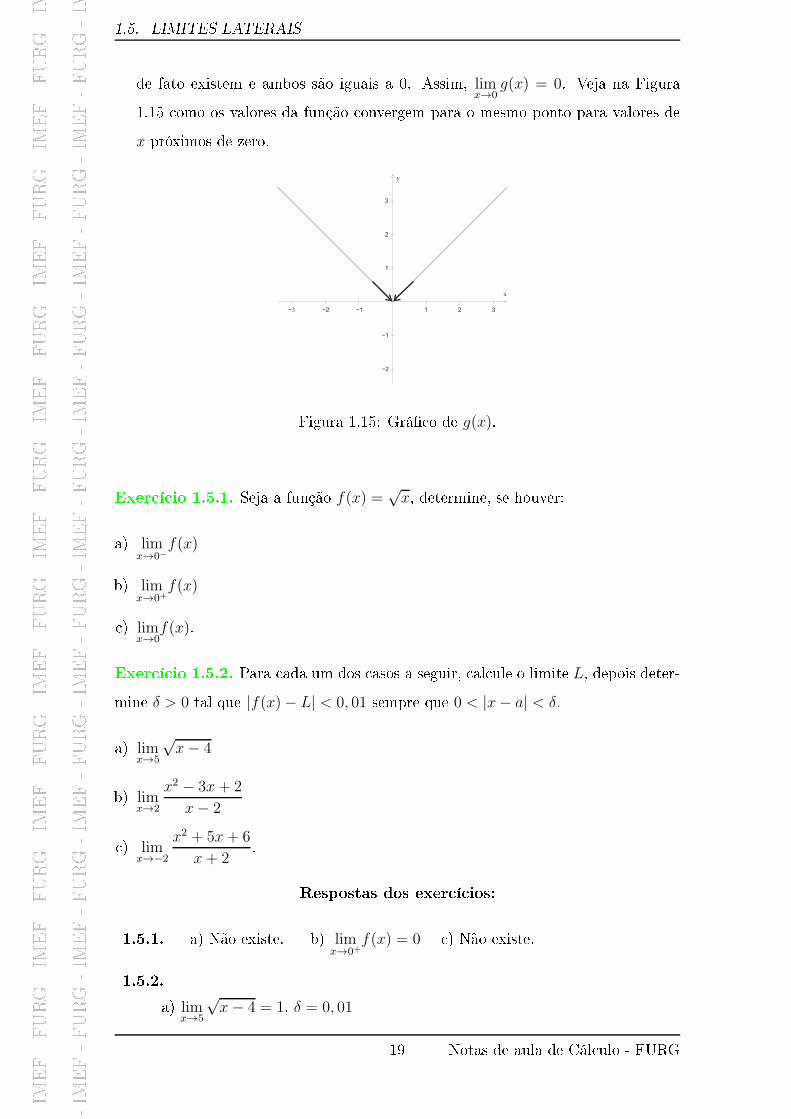
I
M
E
F
-
F
U
R
G
-
I
M
E
F
-
F
U
R
G
-
I
M
E
F
-
F
U
R
G
-
I
M
E
F
-
F
U
R
G
-
I
M
E
F
-
F
U
R
G
-
I
M
E
F
-
F
U
R
G
-
I
M
E
F
-
F
U
R
G
-
I
M
E
F
-
F
U
R
G
-
I
M
E
F
-
F
U
R
G
-
I
M
E
F
-
F
U
R
G
-
I
M
E
F
-
F
U
R
G
-
I
M
E
F
-
F
U
R
G
-
I
M
E
F
-
F
U
R
G
-
I
M
E
F
-
F
U
R
G
-
I
M
E
F
-
F
U
R
G
-
I
M
E
F
-
F
U
R
G
-
I
M
E
F
-
F
U
R
G
-
I
M
E
F
-
F
U
R
G
-
I
M
E
F
-
F
U
R
G
-
I
M
E
F
-
F
U
R
G
-
I
M
E
F
-
F
U
R
G
-
I
M
E
F
-
F
U
R
G
-
I
M
E
F
-
F
U
R
G
-
I
M
E
F
-
F
U
R
G
-
I
M
E
F
-
F
U
R
G
-
I
M
E
F
-
F
U
R
G
-
I
M
E
F
-
F
U
R
G
-
I
M
E
F
-
F
U
R
G
-
I
M
E
F
-
F
U
R
G
-
I
M
E
F
-
F
U
R
G
-
I
M
E
F
-
F
U
R
G
-
I
M
E
F
-
F
U
R
G
-
I
M
E
F
-
F
U
R
G
-
I
M
E
F
-
F
U
R
G
-
I
M
E
F
-
F
U
R
G
-
I
M
E
F
-
F
U
R
G
-
1.5. LIMITES LATERAIS
de fato existem e ambos são iguais a 0. Assim, limx→0
g(x) = 0. Veja na Figura
1.15 omo os valores da função onvergem para o mesmo ponto para valores de
x próximos de zero.
−3 −2 −1 1 2 3
−2
−1
1
2
3
x
y
Figura 1.15: Grá� o de g(x).
Exer í io 1.5.1. Seja a função f(x) =√x, determine, se houver:
a) limx→0−
f(x)
b) limx→0+
f(x)
) limx→0
f(x).
Exer í io 1.5.2. Para ada um dos asos a seguir, al ule o limite L, depois deter-
mine δ > 0 tal que |f(x)− L| < 0, 01 sempre que 0 < |x− a| < δ.
a) limx→5
√x− 4
b) limx→2
x2 − 3x+ 2
x− 2
) limx→−2
x2 + 5x+ 6
x+ 2.
Respostas dos exer í ios:
1.5.1. a) Não existe. b) limx→0+
f(x) = 0 ) Não existe.
1.5.2.
a) limx→5
√x− 4 = 1, δ = 0, 01
19 Notas de aula de Cál ulo - FURG

I
M
E
F
-
F
U
R
G
-
I
M
E
F
-
F
U
R
G
-
I
M
E
F
-
F
U
R
G
-
I
M
E
F
-
F
U
R
G
-
I
M
E
F
-
F
U
R
G
-
I
M
E
F
-
F
U
R
G
-
I
M
E
F
-
F
U
R
G
-
I
M
E
F
-
F
U
R
G
-
I
M
E
F
-
F
U
R
G
-
I
M
E
F
-
F
U
R
G
-
I
M
E
F
-
F
U
R
G
-
I
M
E
F
-
F
U
R
G
-
I
M
E
F
-
F
U
R
G
-
I
M
E
F
-
F
U
R
G
-
I
M
E
F
-
F
U
R
G
-
I
M
E
F
-
F
U
R
G
-
I
M
E
F
-
F
U
R
G
-
I
M
E
F
-
F
U
R
G
-
I
M
E
F
-
F
U
R
G
-
I
M
E
F
-
F
U
R
G
-
I
M
E
F
-
F
U
R
G
-
I
M
E
F
-
F
U
R
G
-
I
M
E
F
-
F
U
R
G
-
I
M
E
F
-
F
U
R
G
-
I
M
E
F
-
F
U
R
G
-
I
M
E
F
-
F
U
R
G
-
I
M
E
F
-
F
U
R
G
-
I
M
E
F
-
F
U
R
G
-
I
M
E
F
-
F
U
R
G
-
I
M
E
F
-
F
U
R
G
-
I
M
E
F
-
F
U
R
G
-
I
M
E
F
-
F
U
R
G
-
I
M
E
F
-
F
U
R
G
-
I
M
E
F
-
F
U
R
G
-
I
M
E
F
-
F
U
R
G
-
I
M
E
F
-
F
U
R
G
-
1.6. PROPRIEDADES USADAS NO CÁLCULO DE LIMITES
b) limx→2
x2 − 3x+ 2
x− 2= 1, δ = 0, 01
) limx→−2
x2 + 5x+ 6
x+ 2= 1, δ = 0, 01.
1.6 Propriedades usadas no ál ulo de limites
Sejam L, M , a e k números reais e limx→a
f(x) = L e limx→a
g(x) = M . Então,
as seguintes propriedades são válidas:
1.6.1 Limite de uma onstante
O limite de uma onstante é a própria onstante:
limx→a
k = k.
Demonstração:
Seja ǫ > 0, deve-se mostrar que existe δ > 0 tal que se 0 < |x − a| < δ
então |k − k| < ǫ.
Mas omo |k − k| = 0, pode-se atribuir qualquer número positivo para δ
tal que se 0 < |x− a| < δ então |k − k| < ǫ.
Logo limx→a
k = k.
1.6.2 Limite da função identidade
O limite da função identidade f(x) = x é o valor de a:
limx→a
x = a.
Exer í io 1.6.1. Utilizando a de�nição formal de limite, mostre que limx→a
x = a.
1.6.3 Limite da soma
O limite da soma de duas funções é a soma de seus limites:
limx→a{f(x) + g(x)} = L+M .
20 Notas de aula de Cál ulo - FURG

I
M
E
F
-
F
U
R
G
-
I
M
E
F
-
F
U
R
G
-
I
M
E
F
-
F
U
R
G
-
I
M
E
F
-
F
U
R
G
-
I
M
E
F
-
F
U
R
G
-
I
M
E
F
-
F
U
R
G
-
I
M
E
F
-
F
U
R
G
-
I
M
E
F
-
F
U
R
G
-
I
M
E
F
-
F
U
R
G
-
I
M
E
F
-
F
U
R
G
-
I
M
E
F
-
F
U
R
G
-
I
M
E
F
-
F
U
R
G
-
I
M
E
F
-
F
U
R
G
-
I
M
E
F
-
F
U
R
G
-
I
M
E
F
-
F
U
R
G
-
I
M
E
F
-
F
U
R
G
-
I
M
E
F
-
F
U
R
G
-
I
M
E
F
-
F
U
R
G
-
I
M
E
F
-
F
U
R
G
-
I
M
E
F
-
F
U
R
G
-
I
M
E
F
-
F
U
R
G
-
I
M
E
F
-
F
U
R
G
-
I
M
E
F
-
F
U
R
G
-
I
M
E
F
-
F
U
R
G
-
I
M
E
F
-
F
U
R
G
-
I
M
E
F
-
F
U
R
G
-
I
M
E
F
-
F
U
R
G
-
I
M
E
F
-
F
U
R
G
-
I
M
E
F
-
F
U
R
G
-
I
M
E
F
-
F
U
R
G
-
I
M
E
F
-
F
U
R
G
-
I
M
E
F
-
F
U
R
G
-
I
M
E
F
-
F
U
R
G
-
I
M
E
F
-
F
U
R
G
-
I
M
E
F
-
F
U
R
G
-
I
M
E
F
-
F
U
R
G
-
1.6. PROPRIEDADES USADAS NO CÁLCULO DE LIMITES
Demonstração:
Seja ǫ > 0, onsidera-se ǫ2para ser utilizado na de�nição de limite. Assim:
Existe δ1 > 0 tal que se 0 < |x− a| < δ1 então |f(x)− L| < ǫ
2. (1.6.1)
Existe δ2 > 0 tal que se 0 < |x− a| < δ2 então |f(x)−M | < ǫ
2. (1.6.2)
Deve-se es olher δ > 0 tal que (1.6.1) e (1.6.2) sejam verdadeiras, o que
a onte e para δ = min{δ1, δ2}. De fato:
Se 0 < |x−a| < δ então |f(x)+g(x)−(L+M)| ≤ |f(x)−L|+|g(x)−M | < ǫ2+ ǫ
2= ǫ.
Portanto, limx→a{f(x) + g(x)} = L+M .
1.6.4 Limite da diferença
O limite da diferença de duas funções é a diferença de seus limites:
limx→a{f(x)− g(x)} = L−M .
Exer í io 1.6.2. Apli ando a de�nição formal de limite, mostre que:
limx→a{f(x)− g(x)} = L−M.
1.6.5 Limite do produto
O limite do produto de duas funções é o produto de seus limites:
limx→a{f(x) · g(x)} = L ·M .
Demonstração:
Deseja-se provar que limx→a{f(x) · g(x)} = L ·M . Para tal, primeiro irá
se demonstrar um aso parti ular onde o produto dos limites de duas funções re-
sulta em zero, através da de�nição de limite, para que posteriormente, através das
propriedades apresentadas nessa seção, se obtenha a expressão pro urada.
Considerando o aso parti ular onde h é uma função tal que limx→a
h(x) = 0,
logo deseja-se provar que limx→a
h(x) · f(x) = 0.
Como por hipótese limx→a
f(x) = L e sendo ǫ > 0, onsidera-se ǫ = 1 para
ser utilizado na de�nição de limite. Assim:
Existe δ1 > 0 tal que se 0 < |x− a| < δ1 então |f(x)− L| < 1. (1.6.3)
21 Notas de aula de Cál ulo - FURG

I
M
E
F
-
F
U
R
G
-
I
M
E
F
-
F
U
R
G
-
I
M
E
F
-
F
U
R
G
-
I
M
E
F
-
F
U
R
G
-
I
M
E
F
-
F
U
R
G
-
I
M
E
F
-
F
U
R
G
-
I
M
E
F
-
F
U
R
G
-
I
M
E
F
-
F
U
R
G
-
I
M
E
F
-
F
U
R
G
-
I
M
E
F
-
F
U
R
G
-
I
M
E
F
-
F
U
R
G
-
I
M
E
F
-
F
U
R
G
-
I
M
E
F
-
F
U
R
G
-
I
M
E
F
-
F
U
R
G
-
I
M
E
F
-
F
U
R
G
-
I
M
E
F
-
F
U
R
G
-
I
M
E
F
-
F
U
R
G
-
I
M
E
F
-
F
U
R
G
-
I
M
E
F
-
F
U
R
G
-
I
M
E
F
-
F
U
R
G
-
I
M
E
F
-
F
U
R
G
-
I
M
E
F
-
F
U
R
G
-
I
M
E
F
-
F
U
R
G
-
I
M
E
F
-
F
U
R
G
-
I
M
E
F
-
F
U
R
G
-
I
M
E
F
-
F
U
R
G
-
I
M
E
F
-
F
U
R
G
-
I
M
E
F
-
F
U
R
G
-
I
M
E
F
-
F
U
R
G
-
I
M
E
F
-
F
U
R
G
-
I
M
E
F
-
F
U
R
G
-
I
M
E
F
-
F
U
R
G
-
I
M
E
F
-
F
U
R
G
-
I
M
E
F
-
F
U
R
G
-
I
M
E
F
-
F
U
R
G
-
I
M
E
F
-
F
U
R
G
-
1.6. PROPRIEDADES USADAS NO CÁLCULO DE LIMITES
Mas então |f(x)| = |f(x)−L+L| < |f(x)−L|+ |L| < 1+L, e portanto:
Existe δ1 > 0 tal que se 0 < |x− a| < δ1 então |h(x)| · |f(x)| < |h(x)| · (1 + |L|).(1.6.4)
Assim omo, sendo ǫ > 0, onsidera-se ǫ1+|L| para ser utilizado na de�ni-
ção de limite da função h tendendo a a da seguinte forma:
Existe δ2 > 0 tal que se 0 < |x− a| < δ2 então |h(x)− 0| = |h(x)| < ǫ
1 + |L| .(1.6.5)
Para que (1.6.4) e (1.6.5) se veri�quem, toma-se δ = min{δ1, δ2}, logo:
Existe δ > 0 tal que se 0 < |x−a| < δ então |h(x)·f(x)−0| < (1+|L|)· ǫ
1 + |L| = ǫ.
(1.6.6)
Portanto, limx→a
h(x) · f(x) = 0.
Agora, lembrando que limx→a
f(x) = L e limx→a
g(x) = M , observa-se que:
f(x)·g(x)−L·M = f(x)·g(x)−f(x)·M+f(x)·M−L·M = f(x)·[g(x)−M ]+M ·[f(x)−L].(1.6.7)
Ou ainda, através da propriedade do limite da soma (1.6.3):
limx→a
[f(x) · g(x)− L ·M ] = limx→a{f(x) · [g(x)−M ] + lim
x→a{M · [f(x)− L]}. (1.6.8)
Como limx→a
f(x) = L e limx→a
g(x) = M , então limx→a
f(x)− L = 0 e
limx→a
g(x)−M = 0, e portanto, através da propriedade demonstrada no aso parti-
ular, tem-se que:
limx→a
f(x) · [g(x)−M ] = 0 e limx→a
g(x) · [f(x)− L] = 0. (1.6.9)
De (1.6.8) e (1.6.9), e utilizando as propriedades do limite da diferença
(1.6.4) e do limite de uma onstante (1.6.1) on lui-se que:
limx→a
[f(x) · g(x)− L ·M ] = 0 + 0
limx→a
[f(x) · g(x)]− limx→a
[L ·M ] = 0
limx→a
[f(x) · g(x)] = limx→a
[L ·M ]
limx→a
[f(x) · g(x)] = L ·M.
Logo, limx→a
[f(x) · g(x)] = L ·M .
22 Notas de aula de Cál ulo - FURG

I
M
E
F
-
F
U
R
G
-
I
M
E
F
-
F
U
R
G
-
I
M
E
F
-
F
U
R
G
-
I
M
E
F
-
F
U
R
G
-
I
M
E
F
-
F
U
R
G
-
I
M
E
F
-
F
U
R
G
-
I
M
E
F
-
F
U
R
G
-
I
M
E
F
-
F
U
R
G
-
I
M
E
F
-
F
U
R
G
-
I
M
E
F
-
F
U
R
G
-
I
M
E
F
-
F
U
R
G
-
I
M
E
F
-
F
U
R
G
-
I
M
E
F
-
F
U
R
G
-
I
M
E
F
-
F
U
R
G
-
I
M
E
F
-
F
U
R
G
-
I
M
E
F
-
F
U
R
G
-
I
M
E
F
-
F
U
R
G
-
I
M
E
F
-
F
U
R
G
-
I
M
E
F
-
F
U
R
G
-
I
M
E
F
-
F
U
R
G
-
I
M
E
F
-
F
U
R
G
-
I
M
E
F
-
F
U
R
G
-
I
M
E
F
-
F
U
R
G
-
I
M
E
F
-
F
U
R
G
-
I
M
E
F
-
F
U
R
G
-
I
M
E
F
-
F
U
R
G
-
I
M
E
F
-
F
U
R
G
-
I
M
E
F
-
F
U
R
G
-
I
M
E
F
-
F
U
R
G
-
I
M
E
F
-
F
U
R
G
-
I
M
E
F
-
F
U
R
G
-
I
M
E
F
-
F
U
R
G
-
I
M
E
F
-
F
U
R
G
-
I
M
E
F
-
F
U
R
G
-
I
M
E
F
-
F
U
R
G
-
I
M
E
F
-
F
U
R
G
-
1.6. PROPRIEDADES USADAS NO CÁLCULO DE LIMITES
1.6.6 Limite do quo iente
O limite do quo iente de duas funções é o quo iente de seus limites, desde
que o limite do denominador não seja zero:
limx→a
{
f(x)
g(x)
}
=L
M, M 6= 0.
Exer í io 1.6.3. Utilizando a de�nição formal de limite, mostre que limx→a
{
f(x)
g(x)
}
=
L
M, M 6= 0.
1.6.7 Limite da multipli ação por uma onstante
O limite de uma onstante multipli ada por uma função é a onstante
multipli ada pelo limite da função:
limx→a{k · f(x)} = k · L.
Exer í io 1.6.4. Através da de�nição formal de limite, mostre que limx→a{k · f(x)} =
k · L.
1.6.8 Limite da poten iação
O limite da n-ésima potên ia de uma função é igual à n-ésima potên ia
do limite da função:
limx→a
[f(x)]n =[
limx→a
f(x)]n
= Ln.
Ou ainda:
limx→a
[f(x)]g(x) =[
limx→a
f(x)] limx→a
g(x)
= LM.
Demonstração:
Rees reve-se a potên ia omo uma multipli ação de n fatores:
limx→a
[f(x)]n = limx→a
[f(x) · f(x) · f(x) · ... · f(x)].
Da propriedade do limite do produto (1.6.5):
limx→a
[f(x)]n = limx→a
f(x) · limx→a
f(x) · limx→a
f(x) · ... · limx→a
f(x).
Mas omo são n fatores, então:
limx→a
[f(x)]n =[
limx→a
f(x)]n
.
Logo, limx→a
[f(x)]n =[
limx→a
f(x)]n
= Ln.
23 Notas de aula de Cál ulo - FURG

I
M
E
F
-
F
U
R
G
-
I
M
E
F
-
F
U
R
G
-
I
M
E
F
-
F
U
R
G
-
I
M
E
F
-
F
U
R
G
-
I
M
E
F
-
F
U
R
G
-
I
M
E
F
-
F
U
R
G
-
I
M
E
F
-
F
U
R
G
-
I
M
E
F
-
F
U
R
G
-
I
M
E
F
-
F
U
R
G
-
I
M
E
F
-
F
U
R
G
-
I
M
E
F
-
F
U
R
G
-
I
M
E
F
-
F
U
R
G
-
I
M
E
F
-
F
U
R
G
-
I
M
E
F
-
F
U
R
G
-
I
M
E
F
-
F
U
R
G
-
I
M
E
F
-
F
U
R
G
-
I
M
E
F
-
F
U
R
G
-
I
M
E
F
-
F
U
R
G
-
I
M
E
F
-
F
U
R
G
-
I
M
E
F
-
F
U
R
G
-
I
M
E
F
-
F
U
R
G
-
I
M
E
F
-
F
U
R
G
-
I
M
E
F
-
F
U
R
G
-
I
M
E
F
-
F
U
R
G
-
I
M
E
F
-
F
U
R
G
-
I
M
E
F
-
F
U
R
G
-
I
M
E
F
-
F
U
R
G
-
I
M
E
F
-
F
U
R
G
-
I
M
E
F
-
F
U
R
G
-
I
M
E
F
-
F
U
R
G
-
I
M
E
F
-
F
U
R
G
-
I
M
E
F
-
F
U
R
G
-
I
M
E
F
-
F
U
R
G
-
I
M
E
F
-
F
U
R
G
-
I
M
E
F
-
F
U
R
G
-
I
M
E
F
-
F
U
R
G
-
1.6. PROPRIEDADES USADAS NO CÁLCULO DE LIMITES
Exer í io 1.6.5. Mostre que limx→a
[f(x)]g(x) =[
limx→a
f(x)] limx→a
g(x)
= LM.
1.6.9 Limite da radi iação
O limite da raiz n-ésima de uma função é igual à raiz n-ésima do limite
da função:
limx→a
n
√
f(x) = n
√
limx→a
f(x) = n√L,
se L > 0 e n é um inteiro positivo ou se L ≤ 0 e n é um inteiro positivo ímpar.
1.6.10 Limite de uma função polinomial
Para qualquer polin�mio, p(x) = c0 + c1x + c2x2 + ... + cnx
ne qualquer
número real a, então:
limx→a
p(x) = p(a).
Demonstração:
Essa propriedade é onsequên ia direta das propriedades do limite da
soma (1.6.3) e do limite da multipli ação por uma onstante (1.6.7):
limx→a
p(x) = limx→a
[c0 + c1x+ c2x2 + ...+ cnx
n]
= limx→a
c0 + limx→a
c1x+ limx→a
c2x2 + ... + lim
x→acnx
n
= c0 + c1 · limx→a
x+ c2 · limx→a
x2 + ...+ cn · limx→a
xn
limx→a
p(x) = c0 + c1a + c2a2 + ...+ cna
n.
Logo limx→a
p(x) = p(a).
1.6.11 Limite de uma função ra ional
Seja a função ra ional f(x) =P (x)
Q(x), então seu limite é dado por:
limx→a
f(x) = limx→a
P (x)
Q(x)=
P (a)
Q(a), desde que Q(a) 6= 0.
Exer í io 1.6.6. Mostre que limx→a
f(x) = limx→a
P (x)
Q(x)=
P (a)
Q(a), desde que Q(a) 6= 0.
24 Notas de aula de Cál ulo - FURG

I
M
E
F
-
F
U
R
G
-
I
M
E
F
-
F
U
R
G
-
I
M
E
F
-
F
U
R
G
-
I
M
E
F
-
F
U
R
G
-
I
M
E
F
-
F
U
R
G
-
I
M
E
F
-
F
U
R
G
-
I
M
E
F
-
F
U
R
G
-
I
M
E
F
-
F
U
R
G
-
I
M
E
F
-
F
U
R
G
-
I
M
E
F
-
F
U
R
G
-
I
M
E
F
-
F
U
R
G
-
I
M
E
F
-
F
U
R
G
-
I
M
E
F
-
F
U
R
G
-
I
M
E
F
-
F
U
R
G
-
I
M
E
F
-
F
U
R
G
-
I
M
E
F
-
F
U
R
G
-
I
M
E
F
-
F
U
R
G
-
I
M
E
F
-
F
U
R
G
-
I
M
E
F
-
F
U
R
G
-
I
M
E
F
-
F
U
R
G
-
I
M
E
F
-
F
U
R
G
-
I
M
E
F
-
F
U
R
G
-
I
M
E
F
-
F
U
R
G
-
I
M
E
F
-
F
U
R
G
-
I
M
E
F
-
F
U
R
G
-
I
M
E
F
-
F
U
R
G
-
I
M
E
F
-
F
U
R
G
-
I
M
E
F
-
F
U
R
G
-
I
M
E
F
-
F
U
R
G
-
I
M
E
F
-
F
U
R
G
-
I
M
E
F
-
F
U
R
G
-
I
M
E
F
-
F
U
R
G
-
I
M
E
F
-
F
U
R
G
-
I
M
E
F
-
F
U
R
G
-
I
M
E
F
-
F
U
R
G
-
I
M
E
F
-
F
U
R
G
-
1.6. PROPRIEDADES USADAS NO CÁLCULO DE LIMITES
1.6.12 Limite do logaritmo natural de uma função
O limite do logaritmo natural de uma função é igual ao logaritmo natural
do limite da função:
limx→a{ln[f(x)]} = ln
[
limx→a
f(x)]
= ln(L), L > 0.
Exer í io 1.6.7. Mostre que limx→a{ln[f(x)]} = ln
[
limx→a
f(x)]
= ln(L).
Observação 1.6.1. A Propriedade 1.6.12 pode ser utilizada para logaritmos de
qualquer base.
Exemplo 1.6.1. Cal ule os limites:
a) limx→5
(x2 + 3x)
b) limx→3
x2 − 1
x+ 5
) limx→2+
(2x+ 5)
d) limx→3−
(x+ 4)5
e) limx→1+
√x− 1
f) limx→3−
√9− x2
g) limx→1+
[ln(x2 + 1)]
h) limx→3
[ln(x2 − 4x+ 4)]
Solução:
a) Como limx→5
(x2 + 3x) representa o limite de uma função polinomial, então basta
al ular o valor da função para x = 5 (para onde x está tendendo) utilizando a
propriedade do limite de um polin�mio (1.6.10). Assim:
limx→5
(x2 + 3x) = (5)2 + 3(5) = 40.
Portanto, limx→5
(x2 + 3x) = 40.
b) Pelo fato de limx→3
x2 − 1
x+ 5representar o limite de uma função ra ional, utilizando a
propriedade do limite de um quo iente (1.6.6) basta al ular o valor dessa função
para x = 3, desde que o denominador não seja nulo. Então:
limx→3
x2 − 1
x+ 5=
limx→3
(x2 − 1)
limx→3
(x+ 5)=
(3)2 − 1
(3) + 5= 1.
Logo, limx→3
x2 − 1
x+ 5= 1.
25 Notas de aula de Cál ulo - FURG

I
M
E
F
-
F
U
R
G
-
I
M
E
F
-
F
U
R
G
-
I
M
E
F
-
F
U
R
G
-
I
M
E
F
-
F
U
R
G
-
I
M
E
F
-
F
U
R
G
-
I
M
E
F
-
F
U
R
G
-
I
M
E
F
-
F
U
R
G
-
I
M
E
F
-
F
U
R
G
-
I
M
E
F
-
F
U
R
G
-
I
M
E
F
-
F
U
R
G
-
I
M
E
F
-
F
U
R
G
-
I
M
E
F
-
F
U
R
G
-
I
M
E
F
-
F
U
R
G
-
I
M
E
F
-
F
U
R
G
-
I
M
E
F
-
F
U
R
G
-
I
M
E
F
-
F
U
R
G
-
I
M
E
F
-
F
U
R
G
-
I
M
E
F
-
F
U
R
G
-
I
M
E
F
-
F
U
R
G
-
I
M
E
F
-
F
U
R
G
-
I
M
E
F
-
F
U
R
G
-
I
M
E
F
-
F
U
R
G
-
I
M
E
F
-
F
U
R
G
-
I
M
E
F
-
F
U
R
G
-
I
M
E
F
-
F
U
R
G
-
I
M
E
F
-
F
U
R
G
-
I
M
E
F
-
F
U
R
G
-
I
M
E
F
-
F
U
R
G
-
I
M
E
F
-
F
U
R
G
-
I
M
E
F
-
F
U
R
G
-
I
M
E
F
-
F
U
R
G
-
I
M
E
F
-
F
U
R
G
-
I
M
E
F
-
F
U
R
G
-
I
M
E
F
-
F
U
R
G
-
I
M
E
F
-
F
U
R
G
-
I
M
E
F
-
F
U
R
G
-
1.6. PROPRIEDADES USADAS NO CÁLCULO DE LIMITES
) Sendo limx→2+
(2x+ 5) um limite lateral om x tendendo a 2 pela direita, pode-se
fazer uma mudança de variável para se obter uma expressão que resulte no mesmo
limite soli itado. Note que se x tende a 2 por valores um pou o maiores do que
2, pode-se dizer que x = 2 + h, onde h é um número positivo muito próximo de
zero, e assim, obtém-se o seguinte limite:
limh→0
[2(2 + h) + 5].
Observe que h é a distân ia de x até o ponto para o qual x está tendendo,
assim, quando h se aproxima muito de 0, (2 + h) se aproxima muito de 2 pela
direita, por isso as duas expressões são equivalentes. Como o lado direito da
igualdade representa o limite �nito de uma função polinomial, basta al ular o
valor dessa função para h = 0. Assim:
limh→0
2(2 + h) + 5 = 2(2 + 0) + 5 = 9.
Portanto, limx→2+
(2x+ 5) = 9.
d) Assim omo no item anterior, pode-se obter um limite que produza o mesmo
resultado de limx→3−
(x+ 4)5. Como x se aproxima de 3 por valores um pou o
menores do que 3, substitui-se x por (3− h), onde h é positivo e muito próximo
de zero, e obtém-se:
limh→0
[(3− h) + 4]5.
O valor de h segue representando a distân ia de x até o ponto para onde
x está tendendo, nesse aso a distân ia até 3, e por isso se utiliza a expressão
3−h para representar valores à esquerda (menores) do que 3. E quando h tende
a 0 a função se aproxima do mesmo ponto de quando x se aproxima de 3 pela
esquerda. Cal ulando:
limh→0
[(3− h) + 4]5 = [(3− 0) + 4]5 = 16, 807.
Logo, limx→3−
(x+ 4) = 16, 807.
e) Sendo h a distân ia de x até o ponto para onde x está tendendo, substitui-se x
por (1 + h) e obtém-se o seguinte limite:
limh→0
√
(1 + h)− 1.
26 Notas de aula de Cál ulo - FURG

I
M
E
F
-
F
U
R
G
-
I
M
E
F
-
F
U
R
G
-
I
M
E
F
-
F
U
R
G
-
I
M
E
F
-
F
U
R
G
-
I
M
E
F
-
F
U
R
G
-
I
M
E
F
-
F
U
R
G
-
I
M
E
F
-
F
U
R
G
-
I
M
E
F
-
F
U
R
G
-
I
M
E
F
-
F
U
R
G
-
I
M
E
F
-
F
U
R
G
-
I
M
E
F
-
F
U
R
G
-
I
M
E
F
-
F
U
R
G
-
I
M
E
F
-
F
U
R
G
-
I
M
E
F
-
F
U
R
G
-
I
M
E
F
-
F
U
R
G
-
I
M
E
F
-
F
U
R
G
-
I
M
E
F
-
F
U
R
G
-
I
M
E
F
-
F
U
R
G
-
I
M
E
F
-
F
U
R
G
-
I
M
E
F
-
F
U
R
G
-
I
M
E
F
-
F
U
R
G
-
I
M
E
F
-
F
U
R
G
-
I
M
E
F
-
F
U
R
G
-
I
M
E
F
-
F
U
R
G
-
I
M
E
F
-
F
U
R
G
-
I
M
E
F
-
F
U
R
G
-
I
M
E
F
-
F
U
R
G
-
I
M
E
F
-
F
U
R
G
-
I
M
E
F
-
F
U
R
G
-
I
M
E
F
-
F
U
R
G
-
I
M
E
F
-
F
U
R
G
-
I
M
E
F
-
F
U
R
G
-
I
M
E
F
-
F
U
R
G
-
I
M
E
F
-
F
U
R
G
-
I
M
E
F
-
F
U
R
G
-
I
M
E
F
-
F
U
R
G
-
1.6. PROPRIEDADES USADAS NO CÁLCULO DE LIMITES
A propriedade do limite de uma radi iação (1.6.9) permite que se obtenha
a seguinte igualdade: limh→0
√
(1 + h)− 1 =√
limh→0
(1 + h)− 1. Como o índi e
da raiz é par, o limite limh→0
(1 + h)− 1 deve ser maior ou igual a zero para que
limh→0
√
(1 + h)− 1 exista. E omo (1 + h)− 1 representa uma função polinomial,
pode-se en ontrar o limite dessa função quando h tende a zero al ulando o valor
dessa função para h = 0, logo:
limh→0
√
(1 + h)− 1 =√
limh→0
(1 + h)− 1
=√
(1 + 0)− 1
limh→0
√
(1 + h)− 1 = 0.
Portanto, limx→1+
√x− 1 = 0.
f) Pelo fato de h representar a distân ia de x até o ponto para onde x está tendendo,
substituindo x por (3− h) tem-se que:
limh→0
√
9− (3− h)2.
Utilizando as propriedades do limite da radi iação (1.6.9) e do limite de um
polin�mio (1.6.10), al ula-se:
limh→0
√
9− (3− h)2 =√
limh→0
9− (3− h)2
=√
9− (3− 0)2
=√9− 9
limh→0
√
9− (3− h)2 = 0.
Portanto, limx→3−
√9− x2 = 0.
g) Sendo h a distân ia de x até o ponto para onde x está tendendo, substitui-se x
por (1 + h) e se obtém o seguinte limite:
limh→0
ln[(1 + h)2 + 1].
Utilizando as propriedades do limite de um logaritmo natural (1.6.12)
e do limite de um polin�mio (1.6.10), al ula-se:
27 Notas de aula de Cál ulo - FURG

I
M
E
F
-
F
U
R
G
-
I
M
E
F
-
F
U
R
G
-
I
M
E
F
-
F
U
R
G
-
I
M
E
F
-
F
U
R
G
-
I
M
E
F
-
F
U
R
G
-
I
M
E
F
-
F
U
R
G
-
I
M
E
F
-
F
U
R
G
-
I
M
E
F
-
F
U
R
G
-
I
M
E
F
-
F
U
R
G
-
I
M
E
F
-
F
U
R
G
-
I
M
E
F
-
F
U
R
G
-
I
M
E
F
-
F
U
R
G
-
I
M
E
F
-
F
U
R
G
-
I
M
E
F
-
F
U
R
G
-
I
M
E
F
-
F
U
R
G
-
I
M
E
F
-
F
U
R
G
-
I
M
E
F
-
F
U
R
G
-
I
M
E
F
-
F
U
R
G
-
I
M
E
F
-
F
U
R
G
-
I
M
E
F
-
F
U
R
G
-
I
M
E
F
-
F
U
R
G
-
I
M
E
F
-
F
U
R
G
-
I
M
E
F
-
F
U
R
G
-
I
M
E
F
-
F
U
R
G
-
I
M
E
F
-
F
U
R
G
-
I
M
E
F
-
F
U
R
G
-
I
M
E
F
-
F
U
R
G
-
I
M
E
F
-
F
U
R
G
-
I
M
E
F
-
F
U
R
G
-
I
M
E
F
-
F
U
R
G
-
I
M
E
F
-
F
U
R
G
-
I
M
E
F
-
F
U
R
G
-
I
M
E
F
-
F
U
R
G
-
I
M
E
F
-
F
U
R
G
-
I
M
E
F
-
F
U
R
G
-
I
M
E
F
-
F
U
R
G
-
1.6. PROPRIEDADES USADAS NO CÁLCULO DE LIMITES
limh→0
ln[(1 + h)2 + 1] = ln[
limh→0
(1 + h)2 + 1]
= ln[(1 + 0)2 + 1]
limh→0
ln[(1 + h)2 + 1] = ln(2).
Portanto, limx→1+
[ln(x2 + 1)] = ln(2).
h) Utilizando a propriedade do limite de um logaritmo natural (1.6.12) e do limite
de um polin�mio (1.6.10), al ula-se:
limx→3
[ln(x2 − 4x+ 4)] = ln[
limx→3
(x2 − 4x+ 4)]
= ln [(3)2 − 4(3) + 4]
= ln(1)
limx→3
[ln(x2 − 4x+ 4)] = 0.
Logo, limx→3
[ln(x2 − 4x+ 4)] = 0.
Exemplo 1.6.2. Considere a função f(x) =
x+ 1, se x < 1
x2 − 1, se x ≥ 1. Cal ule, se
houver:
a) limx→1+
f(x)
b) limx→1−
f(x)
) limx→1
f(x).
Solução:
a) Cal ular o limite de f(x) quando x tende a 1 pela direita signi� a determinar o
omportamento de f(x) quando x assume valores muito próximos de 1, mas
maiores que 1. Assim, para x ≥ 1, f(x) = x2 − 1. Para al ular o limite
lateral à direita, substitui-se x por (1 + h), e obtém-se o seguinte limite om
h tendendo a zero:
limh→0
(1 + h)2 − 1.
Utilizando a propriedade do limite de um polin�mio (1.6.10), al ula-se:
limh→0
(1 + h)2 − 1 = (1 + 0)2 − 1 = 0.
Logo, limx→1+
f(x) = 0.
28 Notas de aula de Cál ulo - FURG

I
M
E
F
-
F
U
R
G
-
I
M
E
F
-
F
U
R
G
-
I
M
E
F
-
F
U
R
G
-
I
M
E
F
-
F
U
R
G
-
I
M
E
F
-
F
U
R
G
-
I
M
E
F
-
F
U
R
G
-
I
M
E
F
-
F
U
R
G
-
I
M
E
F
-
F
U
R
G
-
I
M
E
F
-
F
U
R
G
-
I
M
E
F
-
F
U
R
G
-
I
M
E
F
-
F
U
R
G
-
I
M
E
F
-
F
U
R
G
-
I
M
E
F
-
F
U
R
G
-
I
M
E
F
-
F
U
R
G
-
I
M
E
F
-
F
U
R
G
-
I
M
E
F
-
F
U
R
G
-
I
M
E
F
-
F
U
R
G
-
I
M
E
F
-
F
U
R
G
-
I
M
E
F
-
F
U
R
G
-
I
M
E
F
-
F
U
R
G
-
I
M
E
F
-
F
U
R
G
-
I
M
E
F
-
F
U
R
G
-
I
M
E
F
-
F
U
R
G
-
I
M
E
F
-
F
U
R
G
-
I
M
E
F
-
F
U
R
G
-
I
M
E
F
-
F
U
R
G
-
I
M
E
F
-
F
U
R
G
-
I
M
E
F
-
F
U
R
G
-
I
M
E
F
-
F
U
R
G
-
I
M
E
F
-
F
U
R
G
-
I
M
E
F
-
F
U
R
G
-
I
M
E
F
-
F
U
R
G
-
I
M
E
F
-
F
U
R
G
-
I
M
E
F
-
F
U
R
G
-
I
M
E
F
-
F
U
R
G
-
I
M
E
F
-
F
U
R
G
-
1.6. PROPRIEDADES USADAS NO CÁLCULO DE LIMITES
b) Da mesma forma, quando x tende a 1 pela esquerda, signi� a que x está assu-
mindo valores menores que 1. Como para x < 1, f(x) = x+ 1, então o limite
lateral pode ser al ulado substituindo x por (1 − h), e obtendo o seguinte
limite om h tendendo a zero:
limh→0
(1− h) + 1.
Utilizando a propriedade do limite de um polin�mio (1.6.10), al ula-se:
limh→0
(1− h) + 1 = (1− 0) + 1 = 2.
Portanto, limx→1−
f(x) = 2.
) Segundo o teorema da existên ia do limite �nito, para um limite existir em um
determinado ponto, os limites laterais à direita e à esquerda devem existir e
serem iguais. Como limx→1+
f(x) 6= limx→1−
f(x), então não existe limite de f(x)
para x tendendo a 1.
Exemplo 1.6.3. A derivada de uma função f(x) representa a in linação da reta
tangente à urva em um ponto e é de�nida omo f ′(x) = limh→0
f(x+ h)− f(x)
h.
Determine a derivada da função f(x) = x2.
Solução:
Apli ando a fórmula de f ′(x) para o aso onde f(x) = x2, al ula-se:
f ′(x) = limh→0
(x+ h)2 − x2
h
= limh→0
x2 + 2xh+ h2 − x2
h
= limh→0
h(2x+ h)
h
f ′(x) = limh→0
(2x+ h).
Utilizando a propriedade do limite de um polin�mio (1.6.10):
limh→0
(2x+ h) = 2x+ (0) = 2x.
Portanto, f ′(x) = 2x.
29 Notas de aula de Cál ulo - FURG

I
M
E
F
-
F
U
R
G
-
I
M
E
F
-
F
U
R
G
-
I
M
E
F
-
F
U
R
G
-
I
M
E
F
-
F
U
R
G
-
I
M
E
F
-
F
U
R
G
-
I
M
E
F
-
F
U
R
G
-
I
M
E
F
-
F
U
R
G
-
I
M
E
F
-
F
U
R
G
-
I
M
E
F
-
F
U
R
G
-
I
M
E
F
-
F
U
R
G
-
I
M
E
F
-
F
U
R
G
-
I
M
E
F
-
F
U
R
G
-
I
M
E
F
-
F
U
R
G
-
I
M
E
F
-
F
U
R
G
-
I
M
E
F
-
F
U
R
G
-
I
M
E
F
-
F
U
R
G
-
I
M
E
F
-
F
U
R
G
-
I
M
E
F
-
F
U
R
G
-
I
M
E
F
-
F
U
R
G
-
I
M
E
F
-
F
U
R
G
-
I
M
E
F
-
F
U
R
G
-
I
M
E
F
-
F
U
R
G
-
I
M
E
F
-
F
U
R
G
-
I
M
E
F
-
F
U
R
G
-
I
M
E
F
-
F
U
R
G
-
I
M
E
F
-
F
U
R
G
-
I
M
E
F
-
F
U
R
G
-
I
M
E
F
-
F
U
R
G
-
I
M
E
F
-
F
U
R
G
-
I
M
E
F
-
F
U
R
G
-
I
M
E
F
-
F
U
R
G
-
I
M
E
F
-
F
U
R
G
-
I
M
E
F
-
F
U
R
G
-
I
M
E
F
-
F
U
R
G
-
I
M
E
F
-
F
U
R
G
-
I
M
E
F
-
F
U
R
G
-
1.7. LIMITES INFINITOS
Exer í io 1.6.8. Considere a função f(x) =
x2 − 1, se − 1 ≤ x < 0
2x, se 0 < x < 1
1, se x = 1
−2x+ 4, se 1 < x < 2
0, se 2 < x < 3
, res-
ponda:
a) Existe f(−1)? Em aso a�rmativo, al ule seu valor.
b) Existe limx→−1+
f(x)? Em aso a�rmativo, al ule seu valor.
) O valor de limx→−1+
f(x) é igual a f(−1)?
d) Existe f(1)? Em aso a�rmativo, al ule seu valor.
e) Existe limx→1
f(x)? Justi�que sua resposta.
f) Os valores de limx→1
f(x) e f(1) são iguais?
Resposta do exer í io:
1.6.8.
a) Sim, f(−1) = 0. b) Sim, limx→−1+
f(x) = 0. ) Sim.
d) Sim, f(1) = 1. e) Sim, limx→1
f(x) = 2. f) Não.
1.7 Limites in�nitos
Se os valores de f(x) res em inde�nidamente quando x tende a a,
es reve-se limx→a
f(x) = +∞. Isso signi� a que para ada M > 0, existe δ > 0 tal
que f(x) > M sempre que 0 < |x− a| < δ. Veja a representação grá� a na Figura
1.16.
Da mesma forma, se f(x) de res e inde�nidamente quando x tende a a,
es reve-se limx→a
f(x) = −∞. Formalmente, diz-se que para ada N < 0, existe δ > 0
tal que f(x) < N sempre que 0 < |x− a| < δ, omo pode ser visto na Figura 1.17.
De�nição 1.7.1. A reta verti al x = a é hamada assíntota verti al ao grá� o de
f(x) se pelo menos uma das seguintes ondições for verdadeira:
30 Notas de aula de Cál ulo - FURG

I
M
E
F
-
F
U
R
G
-
I
M
E
F
-
F
U
R
G
-
I
M
E
F
-
F
U
R
G
-
I
M
E
F
-
F
U
R
G
-
I
M
E
F
-
F
U
R
G
-
I
M
E
F
-
F
U
R
G
-
I
M
E
F
-
F
U
R
G
-
I
M
E
F
-
F
U
R
G
-
I
M
E
F
-
F
U
R
G
-
I
M
E
F
-
F
U
R
G
-
I
M
E
F
-
F
U
R
G
-
I
M
E
F
-
F
U
R
G
-
I
M
E
F
-
F
U
R
G
-
I
M
E
F
-
F
U
R
G
-
I
M
E
F
-
F
U
R
G
-
I
M
E
F
-
F
U
R
G
-
I
M
E
F
-
F
U
R
G
-
I
M
E
F
-
F
U
R
G
-
I
M
E
F
-
F
U
R
G
-
I
M
E
F
-
F
U
R
G
-
I
M
E
F
-
F
U
R
G
-
I
M
E
F
-
F
U
R
G
-
I
M
E
F
-
F
U
R
G
-
I
M
E
F
-
F
U
R
G
-
I
M
E
F
-
F
U
R
G
-
I
M
E
F
-
F
U
R
G
-
I
M
E
F
-
F
U
R
G
-
I
M
E
F
-
F
U
R
G
-
I
M
E
F
-
F
U
R
G
-
I
M
E
F
-
F
U
R
G
-
I
M
E
F
-
F
U
R
G
-
I
M
E
F
-
F
U
R
G
-
I
M
E
F
-
F
U
R
G
-
I
M
E
F
-
F
U
R
G
-
I
M
E
F
-
F
U
R
G
-
I
M
E
F
-
F
U
R
G
-
1.7. LIMITES INFINITOS
x
y
M
f x( )
f x M( ) >
a( )
a - d a + dx
Figura 1.16: Grá� o de f(x).
f x( )
N
f x N( ) <
Figura 1.17: Grá� o de f(x).
limx→a+
f(x) = +∞ limx→a+
f(x) = −∞
limx→a−
f(x) = +∞ limx→a−
f(x) = −∞.
Observação 1.7.1. Basta que um dos quatro limites da De�nição 2 se veri�que
para que a ondição de se ter uma assíntota verti al seja satisfeita.
Observação 1.7.2. Uma maneira de se determinar as assíntotas verti ais em um
grá� o é investigar pontos onde a função não está de�nida, pois aso a assíntota seja
a reta x = a, então obrigatoriamente a /∈ D(f).
Exemplo 1.7.1. Mostre que limx→0
1
x2= +∞.
31 Notas de aula de Cál ulo - FURG

I
M
E
F
-
F
U
R
G
-
I
M
E
F
-
F
U
R
G
-
I
M
E
F
-
F
U
R
G
-
I
M
E
F
-
F
U
R
G
-
I
M
E
F
-
F
U
R
G
-
I
M
E
F
-
F
U
R
G
-
I
M
E
F
-
F
U
R
G
-
I
M
E
F
-
F
U
R
G
-
I
M
E
F
-
F
U
R
G
-
I
M
E
F
-
F
U
R
G
-
I
M
E
F
-
F
U
R
G
-
I
M
E
F
-
F
U
R
G
-
I
M
E
F
-
F
U
R
G
-
I
M
E
F
-
F
U
R
G
-
I
M
E
F
-
F
U
R
G
-
I
M
E
F
-
F
U
R
G
-
I
M
E
F
-
F
U
R
G
-
I
M
E
F
-
F
U
R
G
-
I
M
E
F
-
F
U
R
G
-
I
M
E
F
-
F
U
R
G
-
I
M
E
F
-
F
U
R
G
-
I
M
E
F
-
F
U
R
G
-
I
M
E
F
-
F
U
R
G
-
I
M
E
F
-
F
U
R
G
-
I
M
E
F
-
F
U
R
G
-
I
M
E
F
-
F
U
R
G
-
I
M
E
F
-
F
U
R
G
-
I
M
E
F
-
F
U
R
G
-
I
M
E
F
-
F
U
R
G
-
I
M
E
F
-
F
U
R
G
-
I
M
E
F
-
F
U
R
G
-
I
M
E
F
-
F
U
R
G
-
I
M
E
F
-
F
U
R
G
-
I
M
E
F
-
F
U
R
G
-
I
M
E
F
-
F
U
R
G
-
I
M
E
F
-
F
U
R
G
-
1.8. LIMITES NO INFINITO
Exemplo 1.7.2. Cal ule os limites:
a) limx→4
x
x− 4d) lim
x→0
√3 + x2
x
b) limx→3
1
(x− 3)2e) lim
x→2
1
|x− 2|
) limx→3
ln(x− 3) f) limx→π
2
tg(π − x)
Exemplo 1.7.3. Considere a função f(x) =
1
x− 2, se x > 2
1
2− x, se x < 2
, al ule limx→2
f(x).
1.8 Limites no in�nito
Seja uma função f de�nida em todo x que perten e a um intervalo aberto
in�nito, o qual se estende na direção positiva do eixo x, es reve-se limx→+∞
f(x) = L
se dado qualquer ǫ > 0, há um número orrespondente M > 0 tal que |f(x)−L| < ǫ
se x > M , omo pode ser visto na Figura 1.18.
x
y
L
L - e
)
)
L + e
f x( )
M x
x M>
Figura 1.18: Grá� o de f(x).
Da mesma forma, seja f uma função de�nida para todo x que perten e a
um intervalo aberto in�nito, o qual se estende na direção negativa do eixo x, es reve-
se limx→−∞
f(x) = L se dado qualquer ǫ > 0, há um número orrespondente N < 0 tal
que |f(x)− L| < ǫ se x < N . Veja a representação grá� a na Figura 1.19.
32 Notas de aula de Cál ulo - FURG

I
M
E
F
-
F
U
R
G
-
I
M
E
F
-
F
U
R
G
-
I
M
E
F
-
F
U
R
G
-
I
M
E
F
-
F
U
R
G
-
I
M
E
F
-
F
U
R
G
-
I
M
E
F
-
F
U
R
G
-
I
M
E
F
-
F
U
R
G
-
I
M
E
F
-
F
U
R
G
-
I
M
E
F
-
F
U
R
G
-
I
M
E
F
-
F
U
R
G
-
I
M
E
F
-
F
U
R
G
-
I
M
E
F
-
F
U
R
G
-
I
M
E
F
-
F
U
R
G
-
I
M
E
F
-
F
U
R
G
-
I
M
E
F
-
F
U
R
G
-
I
M
E
F
-
F
U
R
G
-
I
M
E
F
-
F
U
R
G
-
I
M
E
F
-
F
U
R
G
-
I
M
E
F
-
F
U
R
G
-
I
M
E
F
-
F
U
R
G
-
I
M
E
F
-
F
U
R
G
-
I
M
E
F
-
F
U
R
G
-
I
M
E
F
-
F
U
R
G
-
I
M
E
F
-
F
U
R
G
-
I
M
E
F
-
F
U
R
G
-
I
M
E
F
-
F
U
R
G
-
I
M
E
F
-
F
U
R
G
-
I
M
E
F
-
F
U
R
G
-
I
M
E
F
-
F
U
R
G
-
I
M
E
F
-
F
U
R
G
-
I
M
E
F
-
F
U
R
G
-
I
M
E
F
-
F
U
R
G
-
I
M
E
F
-
F
U
R
G
-
I
M
E
F
-
F
U
R
G
-
I
M
E
F
-
F
U
R
G
-
I
M
E
F
-
F
U
R
G
-
1.8. LIMITES NO INFINITO
x
y
L
L - e
))
L + e
f x( )
x N
x N<
Figura 1.19: Grá� o de f(x).
De�nição 1.8.1. A reta horizontal y = L é hamada de assíntota horizontal ao
grá� o de f(x) se
limx→+∞
f(x) = L limx→−∞
f(x) = L.
Observação 1.8.1. Basta que apenas um dos limites da De�nição 1.8.1 se veri�que
para que se tenha uma assíntota horizontal.
Observação 1.8.2. O grá� o de uma função f(x) pode ter até duas assíntotas
horizontais limx→−∞
f(x) = L1 e limx→+∞
f(x) = L2. Veja na Figura 1.20.
x
y
L2
L1
Figura 1.20: Grá� o om duas assíntotas.
Exemplo 1.8.1. Considerando a função f(x) =1
x:
a) Cal ule limx→+∞
f(x) e limx→−∞
f(x);
33 Notas de aula de Cál ulo - FURG

I
M
E
F
-
F
U
R
G
-
I
M
E
F
-
F
U
R
G
-
I
M
E
F
-
F
U
R
G
-
I
M
E
F
-
F
U
R
G
-
I
M
E
F
-
F
U
R
G
-
I
M
E
F
-
F
U
R
G
-
I
M
E
F
-
F
U
R
G
-
I
M
E
F
-
F
U
R
G
-
I
M
E
F
-
F
U
R
G
-
I
M
E
F
-
F
U
R
G
-
I
M
E
F
-
F
U
R
G
-
I
M
E
F
-
F
U
R
G
-
I
M
E
F
-
F
U
R
G
-
I
M
E
F
-
F
U
R
G
-
I
M
E
F
-
F
U
R
G
-
I
M
E
F
-
F
U
R
G
-
I
M
E
F
-
F
U
R
G
-
I
M
E
F
-
F
U
R
G
-
I
M
E
F
-
F
U
R
G
-
I
M
E
F
-
F
U
R
G
-
I
M
E
F
-
F
U
R
G
-
I
M
E
F
-
F
U
R
G
-
I
M
E
F
-
F
U
R
G
-
I
M
E
F
-
F
U
R
G
-
I
M
E
F
-
F
U
R
G
-
I
M
E
F
-
F
U
R
G
-
I
M
E
F
-
F
U
R
G
-
I
M
E
F
-
F
U
R
G
-
I
M
E
F
-
F
U
R
G
-
I
M
E
F
-
F
U
R
G
-
I
M
E
F
-
F
U
R
G
-
I
M
E
F
-
F
U
R
G
-
I
M
E
F
-
F
U
R
G
-
I
M
E
F
-
F
U
R
G
-
I
M
E
F
-
F
U
R
G
-
I
M
E
F
-
F
U
R
G
-
1.8. LIMITES NO INFINITO
b) Cal ule limx→0+
f(x) e limx→0−
f(x);
) Determine a(s) assíntota(s) verti al(is), se houver;
d) Determine a(s) assíntotas(s) horizontal(is), se houver.
Exemplo 1.8.2. Cal ule os limites:
a) limx→+∞
1
x+ 1
b) limx→+∞
1√x+ 2
) limx→−∞
1√x− 2
.
Exemplo 1.8.3. O preço de um erto aparelho eletr�ni o sofre uma desvalorização
ao longo do tempo t de a ordo om a função p(t) = 40 +40
2 + t. O que a onte erá
om o preço desse aparelho quando o tempo res er inde�nidamente?
1.8.1 Limites no in�nito de xn
A função f(x) = xntem os seguintes limites no in�nito:
a) limx→+∞
xn = +∞, para qualquer n > 0.
b) limx→−∞
xn =
+∞, se n ∈ {2, 4, 6, 8, ...}−∞, se n ∈ {1, 3, 5, 7, ...}
.
Observação 1.8.3. Um polin�mio se omporta omo o seu termo de maior grau
quando x→ +∞ ou x→ −∞.
Exemplo 1.8.4. Cal ule:
a) limx→+∞
(8x2 + 3x)
b) limx→−∞
(7x5 − 6x4).
Exer í io 1.8.1. Dada a função f(x) = 4xx−2
, determine:
a) Uma assíntota verti al do grá� o de f(x);
b) Uma assíntota horizontal do grá� o de f(x).
34 Notas de aula de Cál ulo - FURG

I
M
E
F
-
F
U
R
G
-
I
M
E
F
-
F
U
R
G
-
I
M
E
F
-
F
U
R
G
-
I
M
E
F
-
F
U
R
G
-
I
M
E
F
-
F
U
R
G
-
I
M
E
F
-
F
U
R
G
-
I
M
E
F
-
F
U
R
G
-
I
M
E
F
-
F
U
R
G
-
I
M
E
F
-
F
U
R
G
-
I
M
E
F
-
F
U
R
G
-
I
M
E
F
-
F
U
R
G
-
I
M
E
F
-
F
U
R
G
-
I
M
E
F
-
F
U
R
G
-
I
M
E
F
-
F
U
R
G
-
I
M
E
F
-
F
U
R
G
-
I
M
E
F
-
F
U
R
G
-
I
M
E
F
-
F
U
R
G
-
I
M
E
F
-
F
U
R
G
-
I
M
E
F
-
F
U
R
G
-
I
M
E
F
-
F
U
R
G
-
I
M
E
F
-
F
U
R
G
-
I
M
E
F
-
F
U
R
G
-
I
M
E
F
-
F
U
R
G
-
I
M
E
F
-
F
U
R
G
-
I
M
E
F
-
F
U
R
G
-
I
M
E
F
-
F
U
R
G
-
I
M
E
F
-
F
U
R
G
-
I
M
E
F
-
F
U
R
G
-
I
M
E
F
-
F
U
R
G
-
I
M
E
F
-
F
U
R
G
-
I
M
E
F
-
F
U
R
G
-
I
M
E
F
-
F
U
R
G
-
I
M
E
F
-
F
U
R
G
-
I
M
E
F
-
F
U
R
G
-
I
M
E
F
-
F
U
R
G
-
I
M
E
F
-
F
U
R
G
-
1.9. LIMITES ESPECIAIS
Exer í io 1.8.2. Cal ule os limites:
a) limx→3
5x− 2 g) limx→3
[
x2 − 2x
x+ 1+ cos
(
7π
2− xπ
)]
b) limx→0
[
5
x− 1+ senh(x)
]
h) limx→2
x
x2 − 4
) limx→2
3x
2x− 4i) lim
x→−1
x2 − 6x+ 7
x2 − 3x+ 2
d) limx→3
x2 + 3x
x2 − x+ 3j) lim
x→5
x
x− 5
e) limx→−3
(
4x
x+ 3+
12
x+ 3
)
k) limx→2
(x− 1)(x− 2)
x+ 2
f) limx→2
x4 + x2 − 2
x2 + 2l) lim
x→2
e
3x− 4.
Resposta dos exer í ios:
1.8.1. a) x = 2 b) y = 4
1.8.2.
a) 13 b) −5 ) Não existe. d) 2
e) 4 f) 3 g)
34
h) Não existe.
i)
73
j) Não existe. k) 0 l)
e
2
1.9 Limites espe iais
Cal ula-se o limite para o qual tende erta função de variável real, apli ando-
se as propriedades para o ál ulo de limites. Em ertos asos, nos deparamos om
expressões que não terão um signi� ado onhe ido.
Exemplo 1.9.1. Observe os limites abaixo:
a) limx→0
x
2x=
1
2
b) limx→0
x2
4x= 0
) limx→0
(
e1/x)x
= e
d) limx→+∞
(2x)2/x = 4
e) limx→+∞
x
x= 1
35 Notas de aula de Cál ulo - FURG

I
M
E
F
-
F
U
R
G
-
I
M
E
F
-
F
U
R
G
-
I
M
E
F
-
F
U
R
G
-
I
M
E
F
-
F
U
R
G
-
I
M
E
F
-
F
U
R
G
-
I
M
E
F
-
F
U
R
G
-
I
M
E
F
-
F
U
R
G
-
I
M
E
F
-
F
U
R
G
-
I
M
E
F
-
F
U
R
G
-
I
M
E
F
-
F
U
R
G
-
I
M
E
F
-
F
U
R
G
-
I
M
E
F
-
F
U
R
G
-
I
M
E
F
-
F
U
R
G
-
I
M
E
F
-
F
U
R
G
-
I
M
E
F
-
F
U
R
G
-
I
M
E
F
-
F
U
R
G
-
I
M
E
F
-
F
U
R
G
-
I
M
E
F
-
F
U
R
G
-
I
M
E
F
-
F
U
R
G
-
I
M
E
F
-
F
U
R
G
-
I
M
E
F
-
F
U
R
G
-
I
M
E
F
-
F
U
R
G
-
I
M
E
F
-
F
U
R
G
-
I
M
E
F
-
F
U
R
G
-
I
M
E
F
-
F
U
R
G
-
I
M
E
F
-
F
U
R
G
-
I
M
E
F
-
F
U
R
G
-
I
M
E
F
-
F
U
R
G
-
I
M
E
F
-
F
U
R
G
-
I
M
E
F
-
F
U
R
G
-
I
M
E
F
-
F
U
R
G
-
I
M
E
F
-
F
U
R
G
-
I
M
E
F
-
F
U
R
G
-
I
M
E
F
-
F
U
R
G
-
I
M
E
F
-
F
U
R
G
-
I
M
E
F
-
F
U
R
G
-
1.9. LIMITES ESPECIAIS
f) limx→−∞
2x
x= 2
g) limx→+∞
(x− x) = 0
h) limx→+∞
[x− (x+ 1)] = 2.
Os exemplos a ima ilustram situações onde não é possível atribuir de
imediato o valor do limite, aso ele exista. Nos itens a) - d), pode-se observar uma
forma que rela iona uma quantidade variável que tende a zero om outra quantidade
variável que também tende a zero, hamada in�nitésimo.
Nos itens de e) à h) está representada outra relação: in�nitamente gran-
des om quantidades in�nitamente grandes (representadas por ∞).
Tais expressões re ebem o nome de indeterminações e neste aso, diz-
se que deve-se pro eder de modo a levantar estas indeterminações. Este pro esso
onsiste, basi amente, em rede�nir o próprio limite om o objetivo de eliminar pelo
menos um in�nitésimo ou um in�nitamente grande.
São indeterminações as substituições obtidas no ál ulo de limites que
resultam em
00,
∞∞ , ∞−∞ ou nas potên ias 1∞, 00, ∞0
.
1.9.1 Indeterminação do tipo
0
0
Função ra ional
Em um limite de uma função ra ional do tipo limx→a
P (x)
Q(x), quando o de-
nominador e o numerador forem ambos nulos em x = a, fatoram-se o numerador e
o denominador, an elando seus fatores omuns. Assim, pode-se reduzir a fração à
outra, onde o numerador e o denominador não sejam mais nulos em x = a. Se isso
a onte er, obtém-se o limite por substituição na fração simpli� ada.
Exemplo 1.9.2. Como é o omportamento da função f(x) =x2 − 6x+ 9
x− 3quando
x se aproxima de 3?
Exemplo 1.9.3. Cal ule os limites:
a) limx→6
x2 − 36
x− 6
b) limx→3
x2 − 3x
x2 − 2x− 3
36 Notas de aula de Cál ulo - FURG

I
M
E
F
-
F
U
R
G
-
I
M
E
F
-
F
U
R
G
-
I
M
E
F
-
F
U
R
G
-
I
M
E
F
-
F
U
R
G
-
I
M
E
F
-
F
U
R
G
-
I
M
E
F
-
F
U
R
G
-
I
M
E
F
-
F
U
R
G
-
I
M
E
F
-
F
U
R
G
-
I
M
E
F
-
F
U
R
G
-
I
M
E
F
-
F
U
R
G
-
I
M
E
F
-
F
U
R
G
-
I
M
E
F
-
F
U
R
G
-
I
M
E
F
-
F
U
R
G
-
I
M
E
F
-
F
U
R
G
-
I
M
E
F
-
F
U
R
G
-
I
M
E
F
-
F
U
R
G
-
I
M
E
F
-
F
U
R
G
-
I
M
E
F
-
F
U
R
G
-
I
M
E
F
-
F
U
R
G
-
I
M
E
F
-
F
U
R
G
-
I
M
E
F
-
F
U
R
G
-
I
M
E
F
-
F
U
R
G
-
I
M
E
F
-
F
U
R
G
-
I
M
E
F
-
F
U
R
G
-
I
M
E
F
-
F
U
R
G
-
I
M
E
F
-
F
U
R
G
-
I
M
E
F
-
F
U
R
G
-
I
M
E
F
-
F
U
R
G
-
I
M
E
F
-
F
U
R
G
-
I
M
E
F
-
F
U
R
G
-
I
M
E
F
-
F
U
R
G
-
I
M
E
F
-
F
U
R
G
-
I
M
E
F
-
F
U
R
G
-
I
M
E
F
-
F
U
R
G
-
I
M
E
F
-
F
U
R
G
-
I
M
E
F
-
F
U
R
G
-
1.9. LIMITES ESPECIAIS
) limx→1
x3 − x2 − 9x+ 9
x− 1
Função irra ional
Em uma função algébri a irra ional, uma maneira de en ontrar o limite
de uma função para qual a substituição direta leva a uma forma
0
0é usar a té ni a
de ra ionalização. Essa té ni a pode ser usada para ra ionalizar o denominador ou
o numerador.
Exemplo 1.9.4. Cal ule os limites:
a) limx→0
x√x+ 1− 1
b) limx→1
4√x− 1√x− 1
.
Exemplo 1.9.5. Seja f(x) =
x2 + x− 6
x− 2, se x < 2
2x3 − 3x2 − 8x+ 12
x2 − 4, se x > 2
, al ule limx→2
f(x).
Exer í io 1.9.1. Cal ule:
a) limx→0
x2 − x
x3 − xe) lim
x→7
2−√x− 3
x2 − 49
b) limx→1
√x− 1
3√x− 1
f) limx→0
√x+ 1−
√1− x
x
) limx→8
x− 83√x− 2
g) limx→4
3−√5 + x
1−√5− x
d) limx→a
x2 − a2√x−√a, a 6= 0 h) lim
x→−1
x2 + 6x+ 5
x2 − 3x− 4.
Resposta do exer í io:
1.9.1.
a) 1 b)
32
) 12 d) 4a√a
e) − 156
f) 1 g) −13
h) −45.
37 Notas de aula de Cál ulo - FURG

I
M
E
F
-
F
U
R
G
-
I
M
E
F
-
F
U
R
G
-
I
M
E
F
-
F
U
R
G
-
I
M
E
F
-
F
U
R
G
-
I
M
E
F
-
F
U
R
G
-
I
M
E
F
-
F
U
R
G
-
I
M
E
F
-
F
U
R
G
-
I
M
E
F
-
F
U
R
G
-
I
M
E
F
-
F
U
R
G
-
I
M
E
F
-
F
U
R
G
-
I
M
E
F
-
F
U
R
G
-
I
M
E
F
-
F
U
R
G
-
I
M
E
F
-
F
U
R
G
-
I
M
E
F
-
F
U
R
G
-
I
M
E
F
-
F
U
R
G
-
I
M
E
F
-
F
U
R
G
-
I
M
E
F
-
F
U
R
G
-
I
M
E
F
-
F
U
R
G
-
I
M
E
F
-
F
U
R
G
-
I
M
E
F
-
F
U
R
G
-
I
M
E
F
-
F
U
R
G
-
I
M
E
F
-
F
U
R
G
-
I
M
E
F
-
F
U
R
G
-
I
M
E
F
-
F
U
R
G
-
I
M
E
F
-
F
U
R
G
-
I
M
E
F
-
F
U
R
G
-
I
M
E
F
-
F
U
R
G
-
I
M
E
F
-
F
U
R
G
-
I
M
E
F
-
F
U
R
G
-
I
M
E
F
-
F
U
R
G
-
I
M
E
F
-
F
U
R
G
-
I
M
E
F
-
F
U
R
G
-
I
M
E
F
-
F
U
R
G
-
I
M
E
F
-
F
U
R
G
-
I
M
E
F
-
F
U
R
G
-
I
M
E
F
-
F
U
R
G
-
1.9. LIMITES ESPECIAIS
1.9.2 Indeterminação do tipo
∞∞
Se limx→+∞
f(x)
g(x)=∞∞ , divide-se o numerador e o denominador pela maior
potên ia de x que apare e no denominador.
Exemplo 1.9.6. Determine o valor dos seguintes limites:
a) limx→+∞
x
x− 3
b) limx→+∞
3x6 − 5x2 + 9
2x4 + 1
) limx→+∞
3x+ 5
6x3 − 7
d) limx→+∞
3x+√x2 + 9
2x+√4x2 + 9
.
1.9.3 Indeterminação do tipo ∞−∞
Para resolver limites do tipo limx→a
[f(x)− g(x)] = ∞ − ∞, utilizam-se
artifí ios algébri os para se obter indeterminações do tipo
0
0ou
∞∞ .
Exemplo 1.9.7. Resolva os limites:
a) limx→+1
(
1
x− 1− 3
1− x3
)
b) limx→0{cosec(x) − cotg(x)}
) limx→∞
[x(√x2 + 1− x)]
d) limx→∞
(√3x2 + x− 2x)
1.9.4 Indeterminação tipo 0 · ∞
Se limx→a
[f(x) · g(x)] = 0 · ∞, transforma-se o limite para que resulte em
outro tipo de indeterminação, através de artifí ios algébri os.
Exemplo 1.9.8. Cal ule limx→0{sen(x) · cosec(x)}.
Exer í io 1.9.2. Cal ule os limites:
38 Notas de aula de Cál ulo - FURG

I
M
E
F
-
F
U
R
G
-
I
M
E
F
-
F
U
R
G
-
I
M
E
F
-
F
U
R
G
-
I
M
E
F
-
F
U
R
G
-
I
M
E
F
-
F
U
R
G
-
I
M
E
F
-
F
U
R
G
-
I
M
E
F
-
F
U
R
G
-
I
M
E
F
-
F
U
R
G
-
I
M
E
F
-
F
U
R
G
-
I
M
E
F
-
F
U
R
G
-
I
M
E
F
-
F
U
R
G
-
I
M
E
F
-
F
U
R
G
-
I
M
E
F
-
F
U
R
G
-
I
M
E
F
-
F
U
R
G
-
I
M
E
F
-
F
U
R
G
-
I
M
E
F
-
F
U
R
G
-
I
M
E
F
-
F
U
R
G
-
I
M
E
F
-
F
U
R
G
-
I
M
E
F
-
F
U
R
G
-
I
M
E
F
-
F
U
R
G
-
I
M
E
F
-
F
U
R
G
-
I
M
E
F
-
F
U
R
G
-
I
M
E
F
-
F
U
R
G
-
I
M
E
F
-
F
U
R
G
-
I
M
E
F
-
F
U
R
G
-
I
M
E
F
-
F
U
R
G
-
I
M
E
F
-
F
U
R
G
-
I
M
E
F
-
F
U
R
G
-
I
M
E
F
-
F
U
R
G
-
I
M
E
F
-
F
U
R
G
-
I
M
E
F
-
F
U
R
G
-
I
M
E
F
-
F
U
R
G
-
I
M
E
F
-
F
U
R
G
-
I
M
E
F
-
F
U
R
G
-
I
M
E
F
-
F
U
R
G
-
I
M
E
F
-
F
U
R
G
-
1.10. TEOREMA DO CONFRONTO
a) limx→+∞
5x+ 1
2x− 5h) lim
x→+∞
5
x2o) lim
x→+∞
2x3 − x2 + 7x− 3
2− x+ 5x2 − 4x3
b) limx→+∞
3
x+ 4i) lim
x→+∞
(
2 +100
x
)
p) limx→+∞
x2 − 4x
x− 5
) limx→+∞
5x2 + 7
3x2j) lim
x→+∞
2x3 + 3x
x2 + 5q) lim
x→+∞x(√x2 − 1− x)
d) limx→−∞
√3x4 + x
x2 − 8k) lim
x→+∞
7x− 8√x2 + 1
r) limx→+∞
(√x2 + 3−
√x2 − 5
)
e) limx→−∞
(x2 − 10x+ 1) l) limx→+∞
x√x+ 1
s) limx→+∞
(√3x3 + 2x+ 1−
√2x)
f) limx→+∞
5x3 − x2 + x− 1
x4 + x3 − x+ 1m) lim
x→+∞
(√x+ 3−√x
)
t) limx→0
(
1
x− 1
x√1 + x
)
g) limx→−∞
ex2 − 2x+ 3
2x2 + 5x− 3n) lim
x→+∞
√x+ 5√16x+ 3
u) limx→π
2
[sec(x)− tg(x)].
Resposta do exer í io:
1.9.2.
a)
5
2b) 0 )
5
3d)
√3
e) +∞ f) 0 g)
e
2h) 0
i) 2 j) +∞ k) 7 l) +∞
m) 0 n)
1
4o) −1
2p) +∞
q) −12
r) 0 s) +∞ t)
1
2
u) 0.
1.10 Teorema do onfronto
Suponha que h(x) ≤ f(x) ≤ g(x) para qualquer x em um dado intervalo
aberto ontendo a, ex eto possivelmente quando x = a. Suponha também que
limx→a
g(x) = limx→a
h(x) = L, então limx→a
f(x) = L.
Veja os grá� os de f(x), g(x) e h(x) na Figura 1.21.
Demonstração:
Para ǫ > 0, existem δ1 > 0 e δ2 > 0 tais que |h(x) − L| < ǫ sempre que
0 < |x− a| < δ1 e |g(x)− L| < ǫ sempre que 0 < |x− a| < δ2.
39 Notas de aula de Cál ulo - FURG

I
M
E
F
-
F
U
R
G
-
I
M
E
F
-
F
U
R
G
-
I
M
E
F
-
F
U
R
G
-
I
M
E
F
-
F
U
R
G
-
I
M
E
F
-
F
U
R
G
-
I
M
E
F
-
F
U
R
G
-
I
M
E
F
-
F
U
R
G
-
I
M
E
F
-
F
U
R
G
-
I
M
E
F
-
F
U
R
G
-
I
M
E
F
-
F
U
R
G
-
I
M
E
F
-
F
U
R
G
-
I
M
E
F
-
F
U
R
G
-
I
M
E
F
-
F
U
R
G
-
I
M
E
F
-
F
U
R
G
-
I
M
E
F
-
F
U
R
G
-
I
M
E
F
-
F
U
R
G
-
I
M
E
F
-
F
U
R
G
-
I
M
E
F
-
F
U
R
G
-
I
M
E
F
-
F
U
R
G
-
I
M
E
F
-
F
U
R
G
-
I
M
E
F
-
F
U
R
G
-
I
M
E
F
-
F
U
R
G
-
I
M
E
F
-
F
U
R
G
-
I
M
E
F
-
F
U
R
G
-
I
M
E
F
-
F
U
R
G
-
I
M
E
F
-
F
U
R
G
-
I
M
E
F
-
F
U
R
G
-
I
M
E
F
-
F
U
R
G
-
I
M
E
F
-
F
U
R
G
-
I
M
E
F
-
F
U
R
G
-
I
M
E
F
-
F
U
R
G
-
I
M
E
F
-
F
U
R
G
-
I
M
E
F
-
F
U
R
G
-
I
M
E
F
-
F
U
R
G
-
I
M
E
F
-
F
U
R
G
-
I
M
E
F
-
F
U
R
G
-
1.11. LIMITES FUNDAMENTAIS
−3 −2 −1 1 2 3
−3
−2
−1
1
2
3
x
y
g x( )
f x( )
h x( )
Figura 1.21: Grá� os de f(x), g(x) e h(x).
Seja δ = min{δ1, δ2}, então se 0 < |x− a| < δ, tem-se que |h(x)−L| < ǫ
e |g(x) − L| < ǫ o que impli a que −ǫ < h(x) − L < ǫ e L − ǫ < h(x), e ainda
−ǫ < g(x)− L < ǫ e g(x) < L+ ǫ.
Por outro lado, omo h(x) < f(x) < g(x), tem-se L− ǫ < f(x) < L+ ǫ,
isto é, |f(x)− L| < ǫ.
Portanto, limx→a
f(x) = L.
Exemplo 1.10.1. Utilize o Teorema do Confronto para determinar limx→0
f(x), sa-
bendo que 4− x2 ≤ f(x) ≤ 4 + x2.
Exer í io 1.10.1. Mostre que limx→+∞
sen(x)x
= 0, utilizando o Teorema do Confronto.
1.11 Limites fundamentais
1.11.1 Limite fundamental trigonométri o
limx→0
sen(x)
x= 1.
Dedução:
Observe na Figura 1.22 que a área do triângulo △OAP é menor que
a área do setor OAP , que por sua vez é menor que a área do triângulo △OAT .
Pode-se expressar essas áreas em termos de θ da seguinte forma:
40 Notas de aula de Cál ulo - FURG

I
M
E
F
-
F
U
R
G
-
I
M
E
F
-
F
U
R
G
-
I
M
E
F
-
F
U
R
G
-
I
M
E
F
-
F
U
R
G
-
I
M
E
F
-
F
U
R
G
-
I
M
E
F
-
F
U
R
G
-
I
M
E
F
-
F
U
R
G
-
I
M
E
F
-
F
U
R
G
-
I
M
E
F
-
F
U
R
G
-
I
M
E
F
-
F
U
R
G
-
I
M
E
F
-
F
U
R
G
-
I
M
E
F
-
F
U
R
G
-
I
M
E
F
-
F
U
R
G
-
I
M
E
F
-
F
U
R
G
-
I
M
E
F
-
F
U
R
G
-
I
M
E
F
-
F
U
R
G
-
I
M
E
F
-
F
U
R
G
-
I
M
E
F
-
F
U
R
G
-
I
M
E
F
-
F
U
R
G
-
I
M
E
F
-
F
U
R
G
-
I
M
E
F
-
F
U
R
G
-
I
M
E
F
-
F
U
R
G
-
I
M
E
F
-
F
U
R
G
-
I
M
E
F
-
F
U
R
G
-
I
M
E
F
-
F
U
R
G
-
I
M
E
F
-
F
U
R
G
-
I
M
E
F
-
F
U
R
G
-
I
M
E
F
-
F
U
R
G
-
I
M
E
F
-
F
U
R
G
-
I
M
E
F
-
F
U
R
G
-
I
M
E
F
-
F
U
R
G
-
I
M
E
F
-
F
U
R
G
-
I
M
E
F
-
F
U
R
G
-
I
M
E
F
-
F
U
R
G
-
I
M
E
F
-
F
U
R
G
-
I
M
E
F
-
F
U
R
G
-
1.11. LIMITES FUNDAMENTAIS
Figura 1.22: Grá� o de g(x).
Área do triângulo △OAP =1
2· 1 · sen(θ) = sen(θ)
2;
Área do setor OAP =1
2· (1)2 · θ =
θ
2;
Área do triângulo △OAT =1
2· 1 · tg(θ) = tg(θ)
2.
Logo,
sen(θ)
2<
θ
2<
tg(θ)
2. A desigualdade não se altera ao se dividir
os três termos por
sen(θ)
2, que é positivo para 0 < θ <
π
2. Assim, tem-se que
1 <θ
sen(θ)<
1
cos(θ).
Tomando os re ípro os, a desigualdade é invertida: 1 >sen(θ)
θ> cos θ.
Como limθ→0+
cos(θ) = 1, pode-se utilizar o Teorema do Confronto para se
obter a expressão limθ→0+
sen(θ)
θ= 1.
Uma vez que sen(θ) e θ são funções ímpares, então f(θ) =sen(θ)
θé uma
função par, om grá� o simétri o em relação ao eixo y. Essa simetria impli a que o
limite à esquerda é igual ao limite à direita, logo, limx→0−
sen(x)
x= lim
x→0+
sen(x)
x= 1.
Portanto limx→0
sen(x)
x= 1.
Exemplo 1.11.1. Utilizando limx→0
sen(x)
x= 1, al ule os limites:
a) limx→0
cos(x)− 1
x
b) limx→0
sen(2x)
5x
41 Notas de aula de Cál ulo - FURG

I
M
E
F
-
F
U
R
G
-
I
M
E
F
-
F
U
R
G
-
I
M
E
F
-
F
U
R
G
-
I
M
E
F
-
F
U
R
G
-
I
M
E
F
-
F
U
R
G
-
I
M
E
F
-
F
U
R
G
-
I
M
E
F
-
F
U
R
G
-
I
M
E
F
-
F
U
R
G
-
I
M
E
F
-
F
U
R
G
-
I
M
E
F
-
F
U
R
G
-
I
M
E
F
-
F
U
R
G
-
I
M
E
F
-
F
U
R
G
-
I
M
E
F
-
F
U
R
G
-
I
M
E
F
-
F
U
R
G
-
I
M
E
F
-
F
U
R
G
-
I
M
E
F
-
F
U
R
G
-
I
M
E
F
-
F
U
R
G
-
I
M
E
F
-
F
U
R
G
-
I
M
E
F
-
F
U
R
G
-
I
M
E
F
-
F
U
R
G
-
I
M
E
F
-
F
U
R
G
-
I
M
E
F
-
F
U
R
G
-
I
M
E
F
-
F
U
R
G
-
I
M
E
F
-
F
U
R
G
-
I
M
E
F
-
F
U
R
G
-
I
M
E
F
-
F
U
R
G
-
I
M
E
F
-
F
U
R
G
-
I
M
E
F
-
F
U
R
G
-
I
M
E
F
-
F
U
R
G
-
I
M
E
F
-
F
U
R
G
-
I
M
E
F
-
F
U
R
G
-
I
M
E
F
-
F
U
R
G
-
I
M
E
F
-
F
U
R
G
-
I
M
E
F
-
F
U
R
G
-
I
M
E
F
-
F
U
R
G
-
I
M
E
F
-
F
U
R
G
-
1.11. LIMITES FUNDAMENTAIS
) limx→+∞
sen(1/x)
1/x
Exemplo 1.11.2. Cal ule limx→π
[(x− π) · cotg(x)].
1.11.2 Limite fundamental exponen ial I
limx→0
(1 + x)1x = e.
Teorema 1.11.1. Seja a função f(x) = (1 + x)1/x de�nida em x ∈ R tal que −1 < x
e x 6= 0 então limx→0
(1 + x)1/x = e.
Do teorema 1.11.1 de orrem os orolários:
Corolário 1.11.1. Seja a função f(x) =
(
1 +1
x
)x
de�nida em x ∈ R tal que
x < −1 ou x > 0 então limx→+∞
(
1 +1
x
)x
= e.
Corolário 1.11.2. Seja a função f(x) =
(
1 +1
x
)x
de�nida em x ∈ R tal que
x < −1 ou x > 0 então limx→−∞
(
1 +1
x
)x
= e.
Observação 1.11.1. Formas gerais do limite fundamental limx→0
(1 + x)1x = e:
a) limx→0
(1 + kx)1x = ek
b) limx→+∞
(
1 +k
x
)x
= ek
) limx→−∞
(
1 +k
x
)x
= ek.
Exemplo 1.11.3. Cal ule os limites:
a) limx→0
(1 + 3x)1x
e) limx→0
[1 + sen(x)]1
sen(x)
b) limx→0
(1− 5x)1x
f) limx→+∞
(
1 +2
x
)2x
) limx→0
(1− x2)1x
g) limx→+∞
(
1 +1
x
)2x
d) limx→0
ln(1 + 10x)
xh) lim
x→+∞
(
x− 1
x+ 3
)x+2
.
42 Notas de aula de Cál ulo - FURG

I
M
E
F
-
F
U
R
G
-
I
M
E
F
-
F
U
R
G
-
I
M
E
F
-
F
U
R
G
-
I
M
E
F
-
F
U
R
G
-
I
M
E
F
-
F
U
R
G
-
I
M
E
F
-
F
U
R
G
-
I
M
E
F
-
F
U
R
G
-
I
M
E
F
-
F
U
R
G
-
I
M
E
F
-
F
U
R
G
-
I
M
E
F
-
F
U
R
G
-
I
M
E
F
-
F
U
R
G
-
I
M
E
F
-
F
U
R
G
-
I
M
E
F
-
F
U
R
G
-
I
M
E
F
-
F
U
R
G
-
I
M
E
F
-
F
U
R
G
-
I
M
E
F
-
F
U
R
G
-
I
M
E
F
-
F
U
R
G
-
I
M
E
F
-
F
U
R
G
-
I
M
E
F
-
F
U
R
G
-
I
M
E
F
-
F
U
R
G
-
I
M
E
F
-
F
U
R
G
-
I
M
E
F
-
F
U
R
G
-
I
M
E
F
-
F
U
R
G
-
I
M
E
F
-
F
U
R
G
-
I
M
E
F
-
F
U
R
G
-
I
M
E
F
-
F
U
R
G
-
I
M
E
F
-
F
U
R
G
-
I
M
E
F
-
F
U
R
G
-
I
M
E
F
-
F
U
R
G
-
I
M
E
F
-
F
U
R
G
-
I
M
E
F
-
F
U
R
G
-
I
M
E
F
-
F
U
R
G
-
I
M
E
F
-
F
U
R
G
-
I
M
E
F
-
F
U
R
G
-
I
M
E
F
-
F
U
R
G
-
I
M
E
F
-
F
U
R
G
-
1.11. LIMITES FUNDAMENTAIS
Observação 1.11.2. O número e:
O número e é hamado de base exponen ial natural, número de Ne-
per ou número de Euler. É um número irra ional e tem valor aproximado de
2,7182818284..., obtido através da função f(n) =
(
1 +1
n
)n
quando os valores atri-
buídos a n res em inde�nidamente. Observe o omportamento da função na tabela
a seguir:
Tabela 3: Quadro de valores para a função f(n) =(
1 + 1n
)n.
n(
1 + 1n
)n
1 2
10 2,59374246. . .
100 2,70481383. . .
1.000 2,71692393. . .
10.000 2,71814593. . .
100.000 2,71826824. . .
1.000.000 2,71828047. . .
Per ebe-se que ao atribuir valores maiores para n a expressão resulta em
um valor ada vez mais próximo do número e. Diz-se então que:
limn→+∞
(
1 +1
n
)n
= e.
Modelam-se vários fen�menos de res imento om funções que envolvem
a base exponen ial natural. Seu surgimento o orreu no sé ulo XVII om o estudo
dos logaritmos feitos por John Napier, e por isso essa onstante � ou onhe ida omo
número de Neper. O símbolo e foi riado por Leonhard Euler, a quem é reditada a
fórmula eiπ + 1 = 0, onsiderada por muitos omo a mais bela fórmula da história
da matemáti a.
1.11.3 Limite fundamental exponen ial II
limx→0
akx − 1
kx= ln(a), a > 0, a 6= 1.
Dedução:
43 Notas de aula de Cál ulo - FURG

I
M
E
F
-
F
U
R
G
-
I
M
E
F
-
F
U
R
G
-
I
M
E
F
-
F
U
R
G
-
I
M
E
F
-
F
U
R
G
-
I
M
E
F
-
F
U
R
G
-
I
M
E
F
-
F
U
R
G
-
I
M
E
F
-
F
U
R
G
-
I
M
E
F
-
F
U
R
G
-
I
M
E
F
-
F
U
R
G
-
I
M
E
F
-
F
U
R
G
-
I
M
E
F
-
F
U
R
G
-
I
M
E
F
-
F
U
R
G
-
I
M
E
F
-
F
U
R
G
-
I
M
E
F
-
F
U
R
G
-
I
M
E
F
-
F
U
R
G
-
I
M
E
F
-
F
U
R
G
-
I
M
E
F
-
F
U
R
G
-
I
M
E
F
-
F
U
R
G
-
I
M
E
F
-
F
U
R
G
-
I
M
E
F
-
F
U
R
G
-
I
M
E
F
-
F
U
R
G
-
I
M
E
F
-
F
U
R
G
-
I
M
E
F
-
F
U
R
G
-
I
M
E
F
-
F
U
R
G
-
I
M
E
F
-
F
U
R
G
-
I
M
E
F
-
F
U
R
G
-
I
M
E
F
-
F
U
R
G
-
I
M
E
F
-
F
U
R
G
-
I
M
E
F
-
F
U
R
G
-
I
M
E
F
-
F
U
R
G
-
I
M
E
F
-
F
U
R
G
-
I
M
E
F
-
F
U
R
G
-
I
M
E
F
-
F
U
R
G
-
I
M
E
F
-
F
U
R
G
-
I
M
E
F
-
F
U
R
G
-
I
M
E
F
-
F
U
R
G
-
1.11. LIMITES FUNDAMENTAIS
Fazendo t = akx − 1, tem-se que akx = t + 1. Apli ando os logaritmos
neperianos nos dois lados da igualdade:
ln(akx) = ln(t+ 1)
kx · ln(a) = ln(t+ 1)
x = ln(t+1)k·ln(a) .
Quando x → 0, tem-se que t → 0, o que permite que se faça a seguinte
substituição de variável:
limx→0
akx−1kx
= limt→0
[
t
k· ln(t+1)k·ln(a)
]
= ln(a) · limt→0
1ln(t+1)
t
= ln(a) ·limt→0
1
limt→0
ln(t+1)t
limx→0
akx−1kx
= ln(a) · 1
limt→0
ln(t+1)1t
.
Utilizando a propriedade do limite de um logaritmo natural (1.6.12) e o
limite fundamental exponen ial I (1.11.2):
ln(a) · 1
limt→0
ln(t+1)1t
= ln(a) · 1
ln
[
limt→0
(t+1)1t
] = ln(a) · 1ln(e)
= ln(a) · 11
= ln(a).
Logo limx→0
akx−1kx
= ln(a).
Exemplo 1.11.4. Cal ule os limites:
a) limx→0
23x − 1
3x ) lim
x→0
3(2−a)x − 1
3x
b) limx→0
32x − 1
2xd) lim
x→0
eax − ebx
x.
Exer í io 1.11.1. Cal ule os limites:
44 Notas de aula de Cál ulo - FURG

I
M
E
F
-
F
U
R
G
-
I
M
E
F
-
F
U
R
G
-
I
M
E
F
-
F
U
R
G
-
I
M
E
F
-
F
U
R
G
-
I
M
E
F
-
F
U
R
G
-
I
M
E
F
-
F
U
R
G
-
I
M
E
F
-
F
U
R
G
-
I
M
E
F
-
F
U
R
G
-
I
M
E
F
-
F
U
R
G
-
I
M
E
F
-
F
U
R
G
-
I
M
E
F
-
F
U
R
G
-
I
M
E
F
-
F
U
R
G
-
I
M
E
F
-
F
U
R
G
-
I
M
E
F
-
F
U
R
G
-
I
M
E
F
-
F
U
R
G
-
I
M
E
F
-
F
U
R
G
-
I
M
E
F
-
F
U
R
G
-
I
M
E
F
-
F
U
R
G
-
I
M
E
F
-
F
U
R
G
-
I
M
E
F
-
F
U
R
G
-
I
M
E
F
-
F
U
R
G
-
I
M
E
F
-
F
U
R
G
-
I
M
E
F
-
F
U
R
G
-
I
M
E
F
-
F
U
R
G
-
I
M
E
F
-
F
U
R
G
-
I
M
E
F
-
F
U
R
G
-
I
M
E
F
-
F
U
R
G
-
I
M
E
F
-
F
U
R
G
-
I
M
E
F
-
F
U
R
G
-
I
M
E
F
-
F
U
R
G
-
I
M
E
F
-
F
U
R
G
-
I
M
E
F
-
F
U
R
G
-
I
M
E
F
-
F
U
R
G
-
I
M
E
F
-
F
U
R
G
-
I
M
E
F
-
F
U
R
G
-
I
M
E
F
-
F
U
R
G
-
1.12. LISTA DE EXERCÍCIOS
a) limx→−2
sen(x+ 2)
x2 − 4f) lim
x→+∞x2 ln
[
x2 + 4
x2 + 1
]
k) limx→0
1− 2tg(x)
tg(x)
b) limx→0
cos(5x)− 1
cotg(5x) · sen(5x) g) limx→a
tg(x)− tg(a)
x− a, a 6= 0 l) lim
x→0
1
xln
(
√
1 + x
1− x
)
) limx→0
x x√x+ 1
sen(2x)h) lim
h→0
sen(x+ h)− sen(x)
hm) lim
x→π
2
ecos(x) − 1
cos(x)
d) limx→2
3x2−4 − 1
x− 2i) lim
x→0
2x
sen(3x)n) lim
x→2
3√x − 3
√2
x− 2
e) limx→0
√
1 + sen(x)−√
1− sen(x)
23x − 1j) lim
x→0
1− cos2(x)
x2o) lim
x→+∞
(
x− 4
x+ 5
)x+2
.
Resposta do exer í io:
1.11.1.
a) −14
b) 0 )
e
2d) 4 ln(3)
e)
1
3 ln(2)f) 3 g)
1
cos2(a)h) cos(x)
i)
2
3j) 1 k) − ln(2) l) 1
m) 1 n)
√2 · 3
√2
4· ln(3) o)
1
e9
1.12 Lista de Exer í ios
1. Para ada a�rmação, assinale V, se for verdadeira, ou F, se for falsa.
a) ( ) A expressão limx→a
f(x) des reve o omportamento da função f quando x = a.
b) ( ) A expressão limx→a
f(x) = L signi� a que, dado um ǫ > 0, existe δ > 0 tal que
se 0 < |x− a| < δ então |f(x)− L| < ǫ.
) ( ) limx→a
f(x) só existe se a função estiver de�nida em x = a.
d) ( ) Para uma função f(x), se os limites laterais à direita e à esquerda de um
ponto a forem iguais, então existe limite de f(x) om x tendendo a a.
2. Considere o grá� o de f(x) na Figura 1.23. Para ada a�rmação, assinale V, se
for verdadeira, ou F, se for falsa. Justi�que suas respostas.
45 Notas de aula de Cál ulo - FURG

I
M
E
F
-
F
U
R
G
-
I
M
E
F
-
F
U
R
G
-
I
M
E
F
-
F
U
R
G
-
I
M
E
F
-
F
U
R
G
-
I
M
E
F
-
F
U
R
G
-
I
M
E
F
-
F
U
R
G
-
I
M
E
F
-
F
U
R
G
-
I
M
E
F
-
F
U
R
G
-
I
M
E
F
-
F
U
R
G
-
I
M
E
F
-
F
U
R
G
-
I
M
E
F
-
F
U
R
G
-
I
M
E
F
-
F
U
R
G
-
I
M
E
F
-
F
U
R
G
-
I
M
E
F
-
F
U
R
G
-
I
M
E
F
-
F
U
R
G
-
I
M
E
F
-
F
U
R
G
-
I
M
E
F
-
F
U
R
G
-
I
M
E
F
-
F
U
R
G
-
I
M
E
F
-
F
U
R
G
-
I
M
E
F
-
F
U
R
G
-
I
M
E
F
-
F
U
R
G
-
I
M
E
F
-
F
U
R
G
-
I
M
E
F
-
F
U
R
G
-
I
M
E
F
-
F
U
R
G
-
I
M
E
F
-
F
U
R
G
-
I
M
E
F
-
F
U
R
G
-
I
M
E
F
-
F
U
R
G
-
I
M
E
F
-
F
U
R
G
-
I
M
E
F
-
F
U
R
G
-
I
M
E
F
-
F
U
R
G
-
I
M
E
F
-
F
U
R
G
-
I
M
E
F
-
F
U
R
G
-
I
M
E
F
-
F
U
R
G
-
I
M
E
F
-
F
U
R
G
-
I
M
E
F
-
F
U
R
G
-
I
M
E
F
-
F
U
R
G
-
1.12. LISTA DE EXERCÍCIOS
y
3
2
0 a
x
Figura 1.23: Grá� o de f(x).
a) ( ) limx→a
f(x) não existe.
b) ( ) limx→a
f(x) = 2.
) ( ) limx→0
f(x) = 3.
3. Cal ule os limites:
a) limy→−5
y2
5− yf) lim
x→+∞
(√x+ 3−
√x+ 2
)
k) limv→−∞
√9v2 + v + 1√3v2 + 4
b) limz→0
(2z − 8)13
g) limm→0
sen(m) · cosec(m) l) limv→0+
[ln(v)− ln(sen(v))]
) limv→2
v3 − 8
v4 − 16h) lim
x→0
(
2
x2 − 1− 1
x− 1
)
m) limx→0+
cotg(x)
cosec(x)
d) limz→4
4z − z2
2−√z i) limy→−∞
5y3 − 12y + 7
8y2 − 1n) lim
x→0+
√x
√
sen(x)
e) limx→0
(
1
x− 1
x2
)
j) limy→+∞
2y3 − 4
5y + 3o) lim
x→−∞
ex − e−x
ex + e−x.
4. Cal ule os limites:
a) limx→0
5x − 5−x
5x2cotg(x)
b) limx→2
sen(x− 2) + x2 − 4x+ 4
x3 − 8.
5. Para ada limite da oluna 1, asso ie om seu resultado na oluna 2. Apresente
todo o desenvolvimento. (Para ada limite, há apenas um valor a ser assinalado).
46 Notas de aula de Cál ulo - FURG

I
M
E
F
-
F
U
R
G
-
I
M
E
F
-
F
U
R
G
-
I
M
E
F
-
F
U
R
G
-
I
M
E
F
-
F
U
R
G
-
I
M
E
F
-
F
U
R
G
-
I
M
E
F
-
F
U
R
G
-
I
M
E
F
-
F
U
R
G
-
I
M
E
F
-
F
U
R
G
-
I
M
E
F
-
F
U
R
G
-
I
M
E
F
-
F
U
R
G
-
I
M
E
F
-
F
U
R
G
-
I
M
E
F
-
F
U
R
G
-
I
M
E
F
-
F
U
R
G
-
I
M
E
F
-
F
U
R
G
-
I
M
E
F
-
F
U
R
G
-
I
M
E
F
-
F
U
R
G
-
I
M
E
F
-
F
U
R
G
-
I
M
E
F
-
F
U
R
G
-
I
M
E
F
-
F
U
R
G
-
I
M
E
F
-
F
U
R
G
-
I
M
E
F
-
F
U
R
G
-
I
M
E
F
-
F
U
R
G
-
I
M
E
F
-
F
U
R
G
-
I
M
E
F
-
F
U
R
G
-
I
M
E
F
-
F
U
R
G
-
I
M
E
F
-
F
U
R
G
-
I
M
E
F
-
F
U
R
G
-
I
M
E
F
-
F
U
R
G
-
I
M
E
F
-
F
U
R
G
-
I
M
E
F
-
F
U
R
G
-
I
M
E
F
-
F
U
R
G
-
I
M
E
F
-
F
U
R
G
-
I
M
E
F
-
F
U
R
G
-
I
M
E
F
-
F
U
R
G
-
I
M
E
F
-
F
U
R
G
-
I
M
E
F
-
F
U
R
G
-
1.12. LISTA DE EXERCÍCIOS
Coluna 1 Coluna 2
(a) limx→−1
3− 2x− x2
x2 − 1( ) 6
(b) limx→1
x2 − 25
x2 − 5x( )
1
2
( ) limx→3
12− 4x
3−√x+ 6
( ) ∄
(d) limx→−∞
4x2 − 12x5 + 12x4 − 3
3x− 2x4 + 3x5 + 6( ) 2
(e) limx→0
1− cos(x)
x2( ) 5
(f) limx→+∞
(
x+ 1
x− 1
)x
( ) e2
(g) limx→0
e2x − 1
x( ) −4
(h) limx→0
ln(1 + 5x)
x( ) 24
6. Sejam limx→0
f(x) = 1 e limx→0
g(x) = 5, al ule o valor de L = limx→0
2f(x)− g(x)
[f(x) + 7]23
.
7. Se limx→2
f(x)− 5
x− 2= 1, determine lim
x→2f(x).
8. Determine as assíntotas dos grá� os das seguintes funções:
a) f(x) =x+ 3
x+ 2
b) f(x) =−8
x2 − 4
) f(x) =x
x+ 8
d) f(x) =x+ 1
x
9. A derivada de uma função f(x) é de�nida omo f ′(x) = limh→0
f(x+ h)− f(x)
h.
Cal ule a derivada das seguintes funções:
a) f(x) = ex
b) f(x) = cos(x).
47 Notas de aula de Cál ulo - FURG
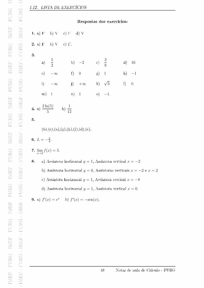
I
M
E
F
-
F
U
R
G
-
I
M
E
F
-
F
U
R
G
-
I
M
E
F
-
F
U
R
G
-
I
M
E
F
-
F
U
R
G
-
I
M
E
F
-
F
U
R
G
-
I
M
E
F
-
F
U
R
G
-
I
M
E
F
-
F
U
R
G
-
I
M
E
F
-
F
U
R
G
-
I
M
E
F
-
F
U
R
G
-
I
M
E
F
-
F
U
R
G
-
I
M
E
F
-
F
U
R
G
-
I
M
E
F
-
F
U
R
G
-
I
M
E
F
-
F
U
R
G
-
I
M
E
F
-
F
U
R
G
-
I
M
E
F
-
F
U
R
G
-
I
M
E
F
-
F
U
R
G
-
I
M
E
F
-
F
U
R
G
-
I
M
E
F
-
F
U
R
G
-
I
M
E
F
-
F
U
R
G
-
I
M
E
F
-
F
U
R
G
-
I
M
E
F
-
F
U
R
G
-
I
M
E
F
-
F
U
R
G
-
I
M
E
F
-
F
U
R
G
-
I
M
E
F
-
F
U
R
G
-
I
M
E
F
-
F
U
R
G
-
I
M
E
F
-
F
U
R
G
-
I
M
E
F
-
F
U
R
G
-
I
M
E
F
-
F
U
R
G
-
I
M
E
F
-
F
U
R
G
-
I
M
E
F
-
F
U
R
G
-
I
M
E
F
-
F
U
R
G
-
I
M
E
F
-
F
U
R
G
-
I
M
E
F
-
F
U
R
G
-
I
M
E
F
-
F
U
R
G
-
I
M
E
F
-
F
U
R
G
-
I
M
E
F
-
F
U
R
G
-
1.12. LISTA DE EXERCÍCIOS
Respostas dos exer í ios:
1. a) F b) V ) F d) V
2. a) F b) V ) F.
3.
a)
5
2b) −2 )
3
8d) 16
e) −∞ f) 0 g) 1 h) −1
i) −∞ j) +∞ k)
√3 l) 0
m) 1 n) 1 o) −1.
4. a)
2 ln(5)
5b)
1
12
5.
(b),(e),(a),(g),(h),(f),(d),( ).
6. L = −34.
7. limx→2
f(x) = 5.
8.
a) Assíntota horizontal y = 1, Assíntota verti al x = −2
b) Assíntota horizontal y = 0, Assíntotas verti ais x = −2 e x = 2
) Assíntota horizontal y = 1, Assíntota verti al x = −8
d) Assíntota horizontal y = 1, Assíntota verti al x = 0.
9. a) f ′(x) = ex b) f ′(x) = −sen(x).
48 Notas de aula de Cál ulo - FURG