by Juan Diego Soler A thesis submitted in conformity ... - TSpace
172
I N S EARCH OF AN I MPRINT OF MAGNETIZATION IN THE BALLOON- BORNE OBSERVATIONS OF THE POLARIZED DUST EMISSION FROM MOLECULAR CLOUDS by Juan Diego Soler A thesis submitted in conformity with the requirements for the degree of Doctor of Philosophy Graduate Department of Astronomy and Astrophysics University of Toronto c ⃝ Copyright by Juan Diego Soler 2013
-
Upload
khangminh22 -
Category
Documents
-
view
0 -
download
0
Transcript of by Juan Diego Soler A thesis submitted in conformity ... - TSpace

IN SEARCH OF AN IMPRINT OF MAGNETIZATION IN THE BALLOON-BORNEOBSERVATIONS OF THE POLARIZED DUST EMISSION FROM MOLECULAR CLOUDS
by
Juan Diego Soler
A thesis submitted in conformity with the requirementsfor the degree of Doctor of Philosophy
Graduate Department of Astronomy and AstrophysicsUniversity of Toronto
c⃝ Copyright by Juan Diego Soler 2013

Abstract
In Search of an Imprint of Magnetization in the Balloon-borne Observations of the Polarized
Dust Emission from Molecular Clouds
Juan Diego Soler
Doctor of Philosophy
Graduate Department of Astronomy and Astrophysics
University of Toronto
2013
The observation of the polarization of thermal emission from dust grains is a key method
in the study of the role of the magnetic fields in the star formation process. This dissertation
introduces BLASTPol, a submillimeter telescope for polarization designed for mapping dust
polarization in scales ranging from pre-stellar cores to sections of molecular clouds and the
Histogram of Relative Orientations (HRO), a new statistical tool for the analysis of the polar-
ization maps.
The observations of BLASTPol were possible thanks to a novel light-weight carbon fibre
sunshield structure and the detailed thermal modeling of the balloon-borne platform. The car-
bon fibre structure is based on the construction technique developed for the Spider gondola
which integrates detailed Finite Element Analysis with the use of composite materials and ad-
hesive joints. The thermal model uses 3D Computer Assisted Design allowing unprecedented
control of the sun avoidance limits and detailed modeling of the gondola components.
BLASTPol made observations of the Lupus I and Vela C molecular clouds, the Carina Neb-
ula, and the Puppis Cloud Complex in two balloon-borne flights over Antarctica in 2010 and
2012. The construction of polarization maps from the BLASTPol10 observations was affected
by multiple pathologies in the data. However, the preliminary maps indicate the need of
a statistical tool which allows relating these observations to magnetohydrodynamics (MHD)
simulations motivating the development of HRO. Most of the problems in the BLASTPol10
data were successfully addressed in BLASTPol12 and the construction of polarization maps of
the observed regions is currently in progress.
The HRO is a statistical tool which assesses the relative orientation between the magnetic
ii

field and the density structures. This tool was characterized by using simulated molecular
clouds with different magnetization indicating that: 1. There is an imprint of the magnetiza-
tion level in the relative orientation of the projected magnetic field with respect to the column
density structure. 2. This imprint of magnetization can be used to complement the current
estimates of magnetic field strength provided by the Chandrasekhar-Fermi method. HRO es-
tablishes a direct link with MHD simulations providing a common tool for the analysis of
polarization maps from BLASTPol.
iii

A Martha Sofia y Jairo por su amor y apoyo incondicional
iv

Acknowledgements
Thanks go to my PhD advisor Barth Netterfield for challenging and inspiring my research. I
thank him for his enthusiasm, his amazing scientific intuition, and for granting me his sup-
port to develop my own ideas. Thanks to Peter Martin for his wise observations, for his pa-
tience deciphering paisley diagrams, and for always teaching me something new. Thanks to
Marc-Antoine Miville-Deschenes and Patrick Hennebelle for believing in the use of a medical
physics method in the study of astrophysical problems. Thanks to the people at CITA for keep-
ing their doors open. Thanks to Dae-Sik Moon and Chris Matzner. Thanks to Martin Houde
for his insightful comments on this thesis.
Thanks to the entire BLASTPol collaboration. BLAST is the product of many years of hard
work and I’m indebted to all the people that put their best effort to make it possible. Thanks to
Mark Devlin for his example of dedication and diligence. Thanks to Giles Novak and Tristan
Matthews. Grazie to Elio Angile, Enzo Pascale, and Lorenzo Moncelsi for making McMurdo
feel very close to home. Thanks to Matt Truch and Tony Mroczkowski.
Thanks to the entire Spider collaboration. In this instant everyone is working extremely
hard to make this experiment awesome. Thanks to Bill Jones and John Ruhl. Thanks to Sasha
Rahlin, Jon Gudmundsson, Sean Bryan, and all the members of the field team. Special thanks
go to my officemates Laura Fissel, Natalie Gandilo, Steve Benton, and Jamil Shariff for sharing
with me all these years of adventures. Thanks to Taylor Martin. Thanks to Ivan Padilla and
Steven Li for learning so fast. Thanks to Gurmit Besla and all the people at the UofT Physics
machine shop. Thanks to everybody at CSBF for making our experiments possible.
This thesis would not have been possible without the support of the friends that bright-
ened my years in Canada. Thanks to Stephanie Benke for her patience, her love, and for
making me feel like the luckiest man on earth every time she looks at me. Thanks to Nicolas
Sanchez, Santiago Gonzalez, and Marco Viero. I am indebted to Fernando Flores-Mangas for
the conversation that disentangled it all. Thanks to Monica, Sebastian, Fermin, and Ana Paula.
Thanks to Tomek Religa for his wise words. Thanks to Renbin Yan and his family. Thanks to
my friends in Colombia who always made it feel like home. Thanks to Cuxo Quijano, Ashley
Barron, Inigo Ahedo, Roger Rodrıguez, Angelica Ramos, Hanna Kent, and all the artists that
inspired me with the devotion to their work and awakened my creativity with their ideas.
Thanks to Luis Martin Pulido, my grandfather, who more than anybody would have liked
to be here. Thanks to Lev Kaufmann and Andrew Lange for crossing through my life. May
peace be with them. I am incredibly lucky for being able to do what I love and share my time
with inspiring and admirable people. In a time of uncertainty when people around the world
still have to fight for their freedom and their basic needs I have been allowed to dream of the
Universe. I thank whatever gods may be for this opportunity.
v
Contents
1 Introduction 1
2 BLASTPol 4
2.1 BLASTPol in context . . . . . . . . . . . . . . . . . . . . . . . . . . . . . . . . . . 5
2.2 Optics and Detectors . . . . . . . . . . . . . . . . . . . . . . . . . . . . . . . . . . 5
2.2.1 Telescope . . . . . . . . . . . . . . . . . . . . . . . . . . . . . . . . . . . . 6
2.2.2 Re-imaging Optics . . . . . . . . . . . . . . . . . . . . . . . . . . . . . . . 7
2.2.3 Receiver . . . . . . . . . . . . . . . . . . . . . . . . . . . . . . . . . . . . . 8
Polarimetry . . . . . . . . . . . . . . . . . . . . . . . . . . . . . . . . . . . 8
Half-Wave Plate . . . . . . . . . . . . . . . . . . . . . . . . . . . . . . . . . 9
2.2.4 Cryogenics . . . . . . . . . . . . . . . . . . . . . . . . . . . . . . . . . . . . 10
2.2.5 Read-Out . . . . . . . . . . . . . . . . . . . . . . . . . . . . . . . . . . . . 12
2.3 Gondola . . . . . . . . . . . . . . . . . . . . . . . . . . . . . . . . . . . . . . . . . 12
2.3.1 Structural Elements . . . . . . . . . . . . . . . . . . . . . . . . . . . . . . . 13
Inner Frame . . . . . . . . . . . . . . . . . . . . . . . . . . . . . . . . . . . 13
Outer Frame . . . . . . . . . . . . . . . . . . . . . . . . . . . . . . . . . . . 14
Sunshields . . . . . . . . . . . . . . . . . . . . . . . . . . . . . . . . . . . . 15
2.3.2 Motion Systems . . . . . . . . . . . . . . . . . . . . . . . . . . . . . . . . . 15
2.3.3 Command and Control . . . . . . . . . . . . . . . . . . . . . . . . . . . . 16
2.3.4 Pointing . . . . . . . . . . . . . . . . . . . . . . . . . . . . . . . . . . . . . 17
Star Cameras . . . . . . . . . . . . . . . . . . . . . . . . . . . . . . . . . . 17
Gyroscopes . . . . . . . . . . . . . . . . . . . . . . . . . . . . . . . . . . . 18
GPS . . . . . . . . . . . . . . . . . . . . . . . . . . . . . . . . . . . . . . . . 18
Sun Sensor . . . . . . . . . . . . . . . . . . . . . . . . . . . . . . . . . . . . 18
Magnetometer . . . . . . . . . . . . . . . . . . . . . . . . . . . . . . . . . . 19
Clinometer . . . . . . . . . . . . . . . . . . . . . . . . . . . . . . . . . . . . 19
2.3.5 Power System . . . . . . . . . . . . . . . . . . . . . . . . . . . . . . . . . . 19
vi

3 Spider 21
3.1 Science Objectives . . . . . . . . . . . . . . . . . . . . . . . . . . . . . . . . . . . . 21
3.2 Optics and Detectors . . . . . . . . . . . . . . . . . . . . . . . . . . . . . . . . . . 22
3.2.1 Telescope . . . . . . . . . . . . . . . . . . . . . . . . . . . . . . . . . . . . 22
Polarimetry . . . . . . . . . . . . . . . . . . . . . . . . . . . . . . . . . . . 24
3.2.2 Receiver . . . . . . . . . . . . . . . . . . . . . . . . . . . . . . . . . . . . . 24
Bolometric Arrays . . . . . . . . . . . . . . . . . . . . . . . . . . . . . . . 24
3.2.3 Read-Out . . . . . . . . . . . . . . . . . . . . . . . . . . . . . . . . . . . . 26
3.2.4 Cryogenics . . . . . . . . . . . . . . . . . . . . . . . . . . . . . . . . . . . . 26
Structural Support and Thermal Coupling to the Vacuum Vessel . . . . . 28
3.3 Gondola . . . . . . . . . . . . . . . . . . . . . . . . . . . . . . . . . . . . . . . . . 28
3.3.1 Structural Elements . . . . . . . . . . . . . . . . . . . . . . . . . . . . . . . 28
Inner Frame . . . . . . . . . . . . . . . . . . . . . . . . . . . . . . . . . . . 30
Outer Frame . . . . . . . . . . . . . . . . . . . . . . . . . . . . . . . . . . . 30
Sunshields . . . . . . . . . . . . . . . . . . . . . . . . . . . . . . . . . . . . 30
3.3.2 Motion Systems . . . . . . . . . . . . . . . . . . . . . . . . . . . . . . . . . 30
3.3.3 Command and Control . . . . . . . . . . . . . . . . . . . . . . . . . . . . 31
3.3.4 Pointing . . . . . . . . . . . . . . . . . . . . . . . . . . . . . . . . . . . . . 31
Star Cameras . . . . . . . . . . . . . . . . . . . . . . . . . . . . . . . . . . 32
3.3.5 Power System . . . . . . . . . . . . . . . . . . . . . . . . . . . . . . . . . . 32
4 Thermal Design of the Balloon-borne Platform 33
4.1 The Balloon-borne Flight Thermal Environment . . . . . . . . . . . . . . . . . . 35
4.1.1 Ascent . . . . . . . . . . . . . . . . . . . . . . . . . . . . . . . . . . . . . . 35
4.1.2 Thermal Environment at Float . . . . . . . . . . . . . . . . . . . . . . . . 37
Solar Radiation . . . . . . . . . . . . . . . . . . . . . . . . . . . . . . . . . 38
Albedo . . . . . . . . . . . . . . . . . . . . . . . . . . . . . . . . . . . . . . 38
Planetary Radiation . . . . . . . . . . . . . . . . . . . . . . . . . . . . . . 39
4.2 Thermal Solutions . . . . . . . . . . . . . . . . . . . . . . . . . . . . . . . . . . . . 40
4.2.1 Shielding . . . . . . . . . . . . . . . . . . . . . . . . . . . . . . . . . . . . . 40
4.2.2 Conductive Coupling . . . . . . . . . . . . . . . . . . . . . . . . . . . . . 41
4.2.3 Surface Coatings . . . . . . . . . . . . . . . . . . . . . . . . . . . . . . . . 42
4.3 Computer Assisted Thermal Modeling . . . . . . . . . . . . . . . . . . . . . . . . 43
4.4 The BLASTPol Thermal Model . . . . . . . . . . . . . . . . . . . . . . . . . . . . 45
4.4.1 Sunshields . . . . . . . . . . . . . . . . . . . . . . . . . . . . . . . . . . . . 45
4.4.2 Telescope Elements . . . . . . . . . . . . . . . . . . . . . . . . . . . . . . . 48
vii

4.4.3 Inner Frame Electronics . . . . . . . . . . . . . . . . . . . . . . . . . . . . 49
4.4.4 Outer Frame Electronics . . . . . . . . . . . . . . . . . . . . . . . . . . . . 51
4.4.5 Motion Systems . . . . . . . . . . . . . . . . . . . . . . . . . . . . . . . . . 55
4.4.6 Passive Elements . . . . . . . . . . . . . . . . . . . . . . . . . . . . . . . . 56
Solar Array . . . . . . . . . . . . . . . . . . . . . . . . . . . . . . . . . . . 56
4.5 The Spider Thermal Model . . . . . . . . . . . . . . . . . . . . . . . . . . . . . . . 59
4.5.1 Sunshields . . . . . . . . . . . . . . . . . . . . . . . . . . . . . . . . . . . . 60
4.5.2 Inner Frame Electronics . . . . . . . . . . . . . . . . . . . . . . . . . . . . 60
4.5.3 Outer Frame Electronics . . . . . . . . . . . . . . . . . . . . . . . . . . . . 63
4.5.4 Motion Systems . . . . . . . . . . . . . . . . . . . . . . . . . . . . . . . . . 63
4.5.5 Preflight Model Calibration . . . . . . . . . . . . . . . . . . . . . . . . . . 64
5 Lightweight Platform for Balloon-borne Telescopes 65
5.1 Design Benchmarks . . . . . . . . . . . . . . . . . . . . . . . . . . . . . . . . . . . 66
5.1.1 The Spider Gondola . . . . . . . . . . . . . . . . . . . . . . . . . . . . . . 68
5.1.2 Critical Design Scenarios . . . . . . . . . . . . . . . . . . . . . . . . . . . 70
Chute Shock . . . . . . . . . . . . . . . . . . . . . . . . . . . . . . . . . . . 71
Pin release (Uneven loading) . . . . . . . . . . . . . . . . . . . . . . . . . 71
Landing: Resting on the base at 5g . . . . . . . . . . . . . . . . . . . . . . 72
Lateral acceleration of 5g . . . . . . . . . . . . . . . . . . . . . . . . . . . 73
On cart at 1g . . . . . . . . . . . . . . . . . . . . . . . . . . . . . . . . . . . 73
Frequency Analysis . . . . . . . . . . . . . . . . . . . . . . . . . . . . . . . 73
5.2 Suspension elements . . . . . . . . . . . . . . . . . . . . . . . . . . . . . . . . . . 73
5.2.1 Universal Joint . . . . . . . . . . . . . . . . . . . . . . . . . . . . . . . . . 74
5.2.2 Suspension Cables . . . . . . . . . . . . . . . . . . . . . . . . . . . . . . . 75
5.2.3 Spreader Bar . . . . . . . . . . . . . . . . . . . . . . . . . . . . . . . . . . . 76
5.3 Outer Frame . . . . . . . . . . . . . . . . . . . . . . . . . . . . . . . . . . . . . . . 77
5.3.1 Material selection and construction technique . . . . . . . . . . . . . . . 78
CFRP tubing . . . . . . . . . . . . . . . . . . . . . . . . . . . . . . . . . . . 78
Adhesive Joint . . . . . . . . . . . . . . . . . . . . . . . . . . . . . . . . . 79
5.3.2 Inserts . . . . . . . . . . . . . . . . . . . . . . . . . . . . . . . . . . . . . . 81
5.3.3 Joints . . . . . . . . . . . . . . . . . . . . . . . . . . . . . . . . . . . . . . . 81
5.3.4 Floor . . . . . . . . . . . . . . . . . . . . . . . . . . . . . . . . . . . . . . . 82
5.4 Motion Systems . . . . . . . . . . . . . . . . . . . . . . . . . . . . . . . . . . . . . 82
5.4.1 Elevation Drive . . . . . . . . . . . . . . . . . . . . . . . . . . . . . . . . . 83
Locking . . . . . . . . . . . . . . . . . . . . . . . . . . . . . . . . . . . . . 85
viii

Rocking . . . . . . . . . . . . . . . . . . . . . . . . . . . . . . . . . . . . . 85
5.4.2 Reaction wheel . . . . . . . . . . . . . . . . . . . . . . . . . . . . . . . . . 86
5.4.3 Pivot . . . . . . . . . . . . . . . . . . . . . . . . . . . . . . . . . . . . . . . 87
5.5 Sunshields . . . . . . . . . . . . . . . . . . . . . . . . . . . . . . . . . . . . . . . . 88
5.5.1 BLASTpol Baffle . . . . . . . . . . . . . . . . . . . . . . . . . . . . . . . . 88
5.5.2 Spider Sunshield . . . . . . . . . . . . . . . . . . . . . . . . . . . . . . . . 90
6 BLASTPol Observations 92
6.1 Data Reduction . . . . . . . . . . . . . . . . . . . . . . . . . . . . . . . . . . . . . 96
6.1.1 Bolometer Noise Characterization . . . . . . . . . . . . . . . . . . . . . . 96
6.2 The BLASTPol12 data . . . . . . . . . . . . . . . . . . . . . . . . . . . . . . . . . . 97
7 The Histogram of Relative Orientations (HRO) 101
7.1 The Histogram of Relative Orientations Method . . . . . . . . . . . . . . . . . . 103
7.1.1 Calculation of the Gradient . . . . . . . . . . . . . . . . . . . . . . . . . . 104
Gaussian Derivatives . . . . . . . . . . . . . . . . . . . . . . . . . . . . . . 105
7.1.2 Calculation of the Angle . . . . . . . . . . . . . . . . . . . . . . . . . . . . 106
7.1.3 Segmentation . . . . . . . . . . . . . . . . . . . . . . . . . . . . . . . . . . 107
7.2 Model Parameters . . . . . . . . . . . . . . . . . . . . . . . . . . . . . . . . . . . . 108
7.3 HRO Applied to Simulation Cubes . . . . . . . . . . . . . . . . . . . . . . . . . . 112
7.4 HRO Applied to Observations of the Simulation Cubes . . . . . . . . . . . . . . 115
7.5 Summary and Discussion . . . . . . . . . . . . . . . . . . . . . . . . . . . . . . . 123
7.5.1 HROs in 3D . . . . . . . . . . . . . . . . . . . . . . . . . . . . . . . . . . . 123
7.5.2 HROs in 2D . . . . . . . . . . . . . . . . . . . . . . . . . . . . . . . . . . . 129
7.5.3 Relation to Existing Studies . . . . . . . . . . . . . . . . . . . . . . . . . . 130
7.5.4 HROs in Observations . . . . . . . . . . . . . . . . . . . . . . . . . . . . . 131
7.5.5 Future Work . . . . . . . . . . . . . . . . . . . . . . . . . . . . . . . . . . . 131
8 Conclusions 134
Bibliography 136
ix

List of Tables
4.1 List of Optical Properties . . . . . . . . . . . . . . . . . . . . . . . . . . . . . . . . 41
4.2 List of Thermo-Physical Properties . . . . . . . . . . . . . . . . . . . . . . . . . . 42
4.3 BLASTPol Telescope Elements Heat Loads and Temperature Ratings . . . . . . 49
4.4 BLASTPol Inner Frame Electronics Heat Loads and Temperature Ratings . . . . 51
4.5 BLASTPol Outer Frame Electronics Heat Loads and Temperature Ratings . . . 53
4.6 BLASTPol Motors Heat Loads and Temperature Ratings . . . . . . . . . . . . . 56
4.7 BLASTPol Motors Heat Loads and Temperature Ratings . . . . . . . . . . . . . 59
4.8 Spider Inner Frame Electronics Heat Loads and Temperature Ratings . . . . . . 62
4.9 Spider Outer Frame Electronics Heat Loads and Temperature Ratings . . . . . . 63
4.10 Spider Motors Heat Loads and Temperature Ratings . . . . . . . . . . . . . . . . 64
5.1 Universal Joint Components . . . . . . . . . . . . . . . . . . . . . . . . . . . . . . 75
5.2 Minimum safety factors on the Spider gondola suspension cables . . . . . . . . 76
5.3 Spreader Bar Components . . . . . . . . . . . . . . . . . . . . . . . . . . . . . . . 76
5.4 Properties of the Spider Outer Frame Inserts . . . . . . . . . . . . . . . . . . . . 81
7.1 Model Parameters and Snapshots Times . . . . . . . . . . . . . . . . . . . . . . . 111
x

List of Figures
2.1 BLASTPol Telescope . . . . . . . . . . . . . . . . . . . . . . . . . . . . . . . . . . 6
2.2 BLASTPol Optical Layout . . . . . . . . . . . . . . . . . . . . . . . . . . . . . . . 7
2.3 BLASTPol Bolometers . . . . . . . . . . . . . . . . . . . . . . . . . . . . . . . . . 8
2.4 BLASTPol Polarizing Grid . . . . . . . . . . . . . . . . . . . . . . . . . . . . . . . 9
2.5 BLASTPol Halfwave Plate . . . . . . . . . . . . . . . . . . . . . . . . . . . . . . . 10
2.6 BLASTPol Cryostat . . . . . . . . . . . . . . . . . . . . . . . . . . . . . . . . . . . 11
2.7 BLASTPol Gondola . . . . . . . . . . . . . . . . . . . . . . . . . . . . . . . . . . . 13
2.8 BLASTpol Inner Frame . . . . . . . . . . . . . . . . . . . . . . . . . . . . . . . . . 14
2.9 BLASTpol Outer Frame . . . . . . . . . . . . . . . . . . . . . . . . . . . . . . . . 15
2.10 BLASTpol Sunshields . . . . . . . . . . . . . . . . . . . . . . . . . . . . . . . . . . 16
2.11 BLASTpol Sunshields and Solar Array . . . . . . . . . . . . . . . . . . . . . . . . 19
3.1 Spider Gondola . . . . . . . . . . . . . . . . . . . . . . . . . . . . . . . . . . . . . 23
3.2 Spider Telescope Insert . . . . . . . . . . . . . . . . . . . . . . . . . . . . . . . . . 23
3.3 Spider Detector Array . . . . . . . . . . . . . . . . . . . . . . . . . . . . . . . . . 25
3.4 Spider Detectors . . . . . . . . . . . . . . . . . . . . . . . . . . . . . . . . . . . . . 26
3.5 Spider Cryostat . . . . . . . . . . . . . . . . . . . . . . . . . . . . . . . . . . . . . 27
3.6 Spider Gondola . . . . . . . . . . . . . . . . . . . . . . . . . . . . . . . . . . . . . 29
4.1 Temperatures of BLASTPol Gondola Elements During Ascent . . . . . . . . . . 36
4.2 BLASTPol Flight Altitude . . . . . . . . . . . . . . . . . . . . . . . . . . . . . . . 37
4.3 Model of the Antarctic Flight Trajectory . . . . . . . . . . . . . . . . . . . . . . . 39
4.4 BLASTPol Flight Trajectories . . . . . . . . . . . . . . . . . . . . . . . . . . . . . 40
4.5 Renders of the BLASTPol Thermal Model . . . . . . . . . . . . . . . . . . . . . . 46
4.6 BLASTPol Gondola Sunlight Illumination . . . . . . . . . . . . . . . . . . . . . . 47
4.7 BLASTPol Sky Visibility . . . . . . . . . . . . . . . . . . . . . . . . . . . . . . . . 47
4.8 BLASTPol Outer Frame Electronics Heat Loads and Temperature Ratings . . . 50
4.9 Flight Temperatures of the BLASTPol Inner Frame Electronics . . . . . . . . . . 52
4.10 Flight Temperatures of the BLASTPol Outer Frame Electronics . . . . . . . . . . 54
xi

4.11 Flight Temperatures of the BLASTPol Motion Systems . . . . . . . . . . . . . . . 57
4.12 Flight Temperatures of the BLASTPol Ambient Thermometers . . . . . . . . . . 58
4.13 Renders of the Spider Thermal Model . . . . . . . . . . . . . . . . . . . . . . . . 61
4.14 Spider Gondola Sunlight Illumination . . . . . . . . . . . . . . . . . . . . . . . . 61
4.15 Spider Sky Visibility . . . . . . . . . . . . . . . . . . . . . . . . . . . . . . . . . . 62
5.1 Spider LDB Cryostat . . . . . . . . . . . . . . . . . . . . . . . . . . . . . . . . . . 66
5.2 Geometric Limits for Gondola Design . . . . . . . . . . . . . . . . . . . . . . . . 67
5.3 Structural Flexures of the Spider Cryostat . . . . . . . . . . . . . . . . . . . . . . 68
5.4 Conceptual Design of the Spider Gondola . . . . . . . . . . . . . . . . . . . . . . 68
5.5 Spider Gondola in Laboratory Configuration . . . . . . . . . . . . . . . . . . . . 69
5.6 Spider Suspension Cables . . . . . . . . . . . . . . . . . . . . . . . . . . . . . . . 69
5.7 Spider Outer Frame Resonant Modes . . . . . . . . . . . . . . . . . . . . . . . . . 74
5.8 Universal Joint . . . . . . . . . . . . . . . . . . . . . . . . . . . . . . . . . . . . . . 75
5.9 Spreader Bar . . . . . . . . . . . . . . . . . . . . . . . . . . . . . . . . . . . . . . . 77
5.10 Spider Outer Frame . . . . . . . . . . . . . . . . . . . . . . . . . . . . . . . . . . . 78
5.11 Spider Outer Frame Insert . . . . . . . . . . . . . . . . . . . . . . . . . . . . . . . 81
5.12 Spider Floor . . . . . . . . . . . . . . . . . . . . . . . . . . . . . . . . . . . . . . . 83
5.13 Spider Elevation Drive . . . . . . . . . . . . . . . . . . . . . . . . . . . . . . . . . 84
5.14 Detail of the Spider Elevation Drive: Trunnion Coupling . . . . . . . . . . . . . 84
5.15 Detail of the Spider Elevation Drive: Lock Pin . . . . . . . . . . . . . . . . . . . 85
5.16 Detail of the Spider Elevation Drive: Actuators . . . . . . . . . . . . . . . . . . . 86
5.17 Spider Reaction Wheel . . . . . . . . . . . . . . . . . . . . . . . . . . . . . . . . . 87
5.18 Spider Pivot . . . . . . . . . . . . . . . . . . . . . . . . . . . . . . . . . . . . . . . 88
5.19 BLASTPol Baffle . . . . . . . . . . . . . . . . . . . . . . . . . . . . . . . . . . . . . 89
5.20 Spider Sunshield . . . . . . . . . . . . . . . . . . . . . . . . . . . . . . . . . . . . 90
6.1 BLASTPol10 Window Filter . . . . . . . . . . . . . . . . . . . . . . . . . . . . . . 93
6.2 BLASTPol10 Beam Map Mosaic . . . . . . . . . . . . . . . . . . . . . . . . . . . . 93
6.3 BLASTPol10 Time Stream Comparison . . . . . . . . . . . . . . . . . . . . . . . . 94
6.4 Lupus I Polarization from BLASTPol10 . . . . . . . . . . . . . . . . . . . . . . . 95
6.5 Amplitude Spectrum of BLASTPol10 Detectors . . . . . . . . . . . . . . . . . . . 98
6.6 Preliminary Carina Nebula Polarization from BLASTPol12 . . . . . . . . . . . . 100
7.1 Map Characterization Using Gradients . . . . . . . . . . . . . . . . . . . . . . . . 107
7.2 HRO with Multiple Derivative Kernels . . . . . . . . . . . . . . . . . . . . . . . . 108
7.3 Segmentation of Column Density Map . . . . . . . . . . . . . . . . . . . . . . . . 109
xii

7.4 Comparison of HROs of Simulations Cubes with Different Magnetization . . . 113
7.5 HROs of Simulation Cubes . . . . . . . . . . . . . . . . . . . . . . . . . . . . . . . 114
7.6 HRO Shape Parameter as a Function of Density . . . . . . . . . . . . . . . . . . . 116
7.7 HRO of Projected Maps . . . . . . . . . . . . . . . . . . . . . . . . . . . . . . . . 119
7.8 Projected Magnetic Field and Column Density Maps (X-LOS) . . . . . . . . . . 120
7.9 Projected Magnetic Field and Column Density Maps (Y-LOS) . . . . . . . . . . . 121
7.10 Projected Magnetic Field and Column Density Maps (Z-LOS) . . . . . . . . . . 122
7.11 HROs of the Projected Simulations (X-LOS) . . . . . . . . . . . . . . . . . . . . . 124
7.12 HROs of the Projected Simulations (Y-LOS) . . . . . . . . . . . . . . . . . . . . . 125
7.13 HROs of the Projected Simulations (Z-LOS) . . . . . . . . . . . . . . . . . . . . . 126
7.14 HRO Shape Parameter as a Function of Column Density . . . . . . . . . . . . . 127
7.15 Polarization Percentage in Projected Simulations . . . . . . . . . . . . . . . . . . 132
xiii

Acronyms
BLAST03 BLAST test flight from Fort Sumner, NM in 2003. 50, 73
BLAST05 BLAST LDB flight from Kiruna, Sweden in 2005. 4, 17, 71
BLAST06 BLAST LDB flight from Antarctica in December 2006. 4, 17, 71, 73
BLASTPol10 BLASTPol LDB flight from Antarctica in December 2010. 4, 6, 17, 18, 35, 37, 40,
41, 48, 52–54, 58, 64, 73, 87, 91–93, 95, 96, 131
BLASTPol12 BLASTPol LDB flight from Antarctica in December 2012. 4, 6, 17, 18, 35, 37, 40,
41, 48, 52, 54, 58, 64, 73, 87, 93, 94, 96, 131, 132
AC Alternating Current. 29
ACS Attitude Control System. 16, 18, 31, 32, 48, 50, 52, 54, 61, 62, 66, 81
ADC Analogue-to-Digital Converter. 12, 16, 18, 31
ALMA Atacama Large Millimeter Array. 5, 128
BICEP Background Imaging of Cosmic Extragalactic Polarization. 22
BICEP-2 Background Imaging of Cosmic Extragalactic Polarization-2. 24, 25
BLAST Balloon-borne Large Aperture Submillimeter Telescope. 4, 13, 45, 82
BLASTPol Balloon-borne Large Aperture Submillimeter Telescope for Polarimetry. 4, 5, 16–
19, 40, 42, 45, 51, 59, 62, 86–89, 132
BOOMERanG Balloon Observations Of Millimetric Extragalactic Radiation and Geophysics.
58, 82
CAD Computer-Assisted Design. 34, 65
CARMA Combined Array for Research in Millimeter-Wave Astronomy. 128
xiv

CCD Charge-Coupled Device. 17, 18, 31, 32
CF Chandrasekhar-Fermi method. 2, 5, 100, 127
CFRP Carbon Fiber Reinforced Polymer. 24, 30, 48, 67–70, 72, 75–81, 84, 87–89
CMB Cosmic Microwave Background. 21, 22, 65
CMBR Cosmic Microwave Background Radiation. 21, 58
CNC Computer Numerical Control. 81
COM Center of Mass. 13
CSBF Columbia Scientific Balloon Facility. 2, 17, 19, 33, 36, 45, 50, 51, 54, 55, 58, 62, 66, 67,
70–72, 74
DAC Digital-to-analog Converter. 29
DAS Data Acquisition System. 12, 13, 16, 31, 48, 51
EBEX The E and B Experiment. 71
ESA European Space Agency. 100
FEA Finite Element Analysis. 64, 78, 81, 86
FOS Factor of Safety. 70–75, 79, 80, 84–86, 89
FOV Field of View. 5, 6, 8, 17, 18, 32
FPU Focal Plane Unit. 24, 28
FWHM Full Width Half Maximum. 5, 21, 22, 25
GMCs Giant Molecular Clouds. 5
GPS Global Positioning System. 17, 18, 31
HDD Hard Disk Drive. 93
HOG Histogram of Oriented Gradients. 101
HRO Histogram of Relative Orientations. ii, iii, 2, 94, 98, 101, 103, 105–107, 110–116, 120–128,
130–132
xv

HWP Half-Wave Plate. 9, 22, 24, 27, 29, 31, 61
ID Inner Diameter. 78, 84, 87, 89
IR Infrared. 42, 61, 91
IRAS Infrared Astronomical Satellite. 91
ISM Interstellar Medium. 4, 127, 132
ISO International Organization for Standardization. 66
JFET Junction-gate Field-Effect Transistor. 12
LDB Long Duration Balloons. 21, 27, 33, 35, 73
LHe Liquid 4He. 10, 11
LN Liquid Nitrogen. 11
LOS Line of Sight. 1, 17, 20
MCC MCE computer. 26, 61
MCE Multi-channel Electronics. 26, 29, 61
MCP Master Control Program. 16, 17, 20
MHD Magnetohydrodynamics. iii, 100, 106, 120, 127, 129, 130, 132
MLI Multi-Layer Insulation. 28, 47
MRR Mission Readiness Review. 62, 63
NASA National Aeronautics and Space Administration. 2, 33
NIST National Institute of Standards and Technology. 26
NOAA National Oceanic and Atmospheric Administration. 19
NTD Neutron Transmutation Doped. 8, 24
OD Outer Diameter. 85
PCM Program Control Master. 31
xvi

PET Polyethylene Terephthalate. 40
PILOT Polarized Instrument for Long wavelength Observation of the Tenuous insterstellar
medium. 128
PSD Power Spectral Density. 95
PSF Point Spread Function. 91
REC Receiver Electronics Crate. 12, 13, 48, 50, 51
RF Radio Frequency. 91, 96
RMS Root Mean-Square. 53, 54, 62
SCC Star Camera Computer. 18
SCUBA-2 Submillimeter Common-User Bolometer Array-2. 26
SIP Support Instrumentation Package. 14, 17, 45, 66, 68, 71, 72, 76, 77, 81
SMA Submillimeter Array. 128
SPARO Submillimeter Polarimeter for Antarctic Remote Observation. 9
SPIRE Spectral and Photometric Imaging Receiver. 4
SPT South-Pole Telescope. 22
SQUID Superconducting Quantum Interference Device. 24, 26
SSD Solid-State Disk. 32, 52, 93, 96
TDRSS Tracking and Data Relay Satellite System. 96
TES Transition-Edge Sensor. 25, 26
UHMW Ultra-High-Molecular-Weight Polyethylene. 24
UV Ultraviolet. 41, 74
VCS Vapor-Cooled Shield. 10–12
VDA Vapor-Deposited Aluminum. 40
xvii

Chapter 1
Introduction
Understanding how stars form is central to much of contemporary astrophysics [1, 2, 3, 4].
However, many of the details of the process that transforms gas into stars are still uncertain.
For example, we still do not know the distribution of physical conditions within star-forming
regions or why star formation occurs only in a small fraction of the available gas. These and
other questions have motivated both theoretical and observational research efforts which so
far point at large-scale, supersonic turbulence and the magnetic fields as the key elements
governing star formation.
Theories and models have been developed in which magnetism plays a crucial role in star
formation [5, 6]. These are confronted by theories and models in which the role of magnetic
fields is relatively minor [7, 8]. In recent years, both theory and simulations consider important
roles for both turbulent flow and magnetic field [9, 10, 11]. It seems the only possible way to
resolve the controversy about the process that drives star formation is to directly or indirectly
measure the magnetic field and compare these observations with the theoretical predictions
[12].
The magnetic fields in star forming clouds can be measured using multiple observational
methods. The component of the magnetic field parallel to the Line of Sight (LOS), BLOS , can
be estimated measuring the splitting of a spectral line into several components produced by
the local magnetic field, or Zeeman effect [13, 14]. Detections of the Zeeman effect in molecular
cloud are difficult because the frequency of the splitting is small when the field is weak. Fur-
thermore, it is impractical to study the large-scale magnetic field using the Zeeman effect given
the large number of measurements required to obtain statistically significant results [15]. In
diffuse regions, large scale BLOS can be estimated from the rotation of the polarization angle
of a background source propagating through a magnetized medium [100, 16, 101, 17].
The component of the magnetic field projected in the plane-of-the-sky, BPOS , can be esti-
mated in large scales from the total intensity or polarized intensity of synchrotron emission
1

CHAPTER 1. INTRODUCTION 2
[102, 103, 18]. BPOS can be estimated in small scales by measuring the linear polarization of
certain molecular emission lines caused by the magnetic field, or Goldreich-Kylafis (GK) ef-
fect [19]. The morphology of BPOS in scales ranging from pre-stellar cores to large molecular
clouds can be reconstructed by measuring the emission and extinction of light by aspherical
interstellar dust grains aligned with the local magnetic field [12, 20, 21].
The estimation of the field strength from polarization maps is possible with the use of
the Chandrasekhar-Fermi method (CF) and other statistical tools [22, 23, 24, 25]. Polarimetry
of dust emission toward molecular clouds is a standard observational tool, and increasingly
sensitive and extensive maps of magnetic field morphologies in the plane of the sky are being
produced [26, 27, 28, 29, 30]. Ground-based submillimeter polarimetric observations provide
insight into the general characteristics of molecular cloud magnetic fields. However, with only
a few exceptions (e.g., [31]), these maps have been restricted to dense cloud cores.
This dissertation discusses BLASTPol, a balloon-borne submillimeter telescope for po-
larimetry designed to map the large-scale magnetic fields in molecular clouds and introduces
the Histogram of Relative Orientations (HRO), a new statistical technique initially developed
for the analysis of the BLASTPol polarization observations. The overarching goal of this work
is the study of the role of magnetic fields in the star formation process. However, it extends
from the details of the thermal and mechanical design of the instrument to the analysis of the
correlations between the column density structure and the polarization observed with BLAST-
Pol, including details about the data reduction process and the bolometer noise characteriza-
tion.
This document is organized as follows: Chapter 2 describes the BLASTPol instrument.
Chapter 3 presents a description of Spider, a balloon-borne polarimeter where most of the in-
strumentation methods included in this dissertation were implemented. Chapter 4 describes
the modeling of the thermal environment and thermal control strategies that allow balloon-
borne observations. Chapter 5 introduces the design of light-weight structures and motion
systems for balloon-borne telescopes. Chapter 6 presents the results of the observations made
with BLASTPol and describes the characterization of the detector noise. Chapter 7 introduces
and describes HRO, a novel statistical tool to study the magnetization imprint and correlations
between magnetic field and density structure in polarized thermal dust emission observations.
Finally, Chapter 8 provides an overview and conclusions of the main results of this disserta-
tion.
The sections of Chapter 4 regarding BLASTPol were submitted and reviewed by the National Aero-
nautics and Space Administration (NASA) and the Columbia Scientific Balloon Facility (CSBF) as
part of the pre-flight requirements for BLASTPol. Chapter 5 was submitted and reviewed by NASA
and CSBF as part of the pre-flight requirements for Spider. The BLASTPol polarization maps presented

CHAPTER 1. INTRODUCTION 3
in Chapter 6 are preliminary and unpublished. They are shown for reference with the permission of the
BLASTPol collaboration. The contents of Chapter 7 have been submitted to the Astrophysical Journal
in March, 2013 and was accepted for publication in July, 2013.

Chapter 2
BLASTPol
The Balloon-borne Large Aperture Submillimeter Telescope for Polarimetry (BLASTPol) is
a balloon-borne observatory designed to map linearly polarized submillimeter emission. It
makes simultaneous measurements in three 30% wide bands centered at 250 µm, 350 µm, and
500 µm. These wavelengths are very difficult to observe from the ground but are accessible
at stratospheric altitudes. BLASTPol’s diffraction-limited optics were designed to provide a
resolution of 30′′, 42′′, and 60′′at the respective wavebands. The detectors and cold optics
are adapted from those used by Spectral and Photometric Imaging Receiver (SPIRE) in Her-
schel [32].
The Balloon-borne Large Aperture Submillimeter Telescope (BLAST) program has five
Long Duration Balloon (LDB) flights. The BLAST LDB flight from Kiruna, Sweden in 2005
(BLAST05) was the first large payload to be launched from Kiruna, Sweden. The instrument
was then refurbished with a new telescope and flew again in the BLAST LDB flight from
Antarctica in December 2006 (BLAST06). These first two flights produced several high-profile
results including a measurement of the FIR background at 250, 350, and 500µm [33, 34, 35],
and a map of the Vela Molecular Cloud [36] showing that pre-stellar cores require a support
mechanism to explain the observed long life-times. Magnetic support is one of the possible
mechanisms which can provide such phenomenon. Its study is one of the main science drivers
of BLASTPol.
This chapter introduces the main instrumentation aspects of BLASTPol and is organized
as follows: Section 2.1 describes the role of BLASTPol in the study of the magnetic fields in the
Interstellar Medium (ISM). Section 2.2 describes the BLASTPol telescope, receiver, and polar-
ization measurement features. Section 2.3 describes the balloon-borne pointed platform used
for the BLASTPol observations. The data analysis procedures and the observations following
the BLASTPol LDB flight from Antarctica in December 2010 (BLASTPol10) and the BLASTPol
LDB flight from Antarctica in December 2012 (BLASTPol12) are described in Chapter 6.
4

CHAPTER 2. BLASTPOL 5
2.1 BLASTPol in context
BLASTPol is designed for mapping the linearly polarized thermal emission from aspherical
dust grains in molecular clouds. The linearly polarized emission is the result of the alignment
of aspherical dust grains with respect to the local magnetic field [21]. The BLASTPol observa-
tions attempt to trace the field orientation projected on the sky. The magnetic field strength can
be estimated by measuring the dispersion of the polarization orientation angle CF [22, 37], or
studying the relative orientation between the projected magnetic field and the column density
structures as will be described in Chapter 7.
BLASTPol is the first submillimeter polarimeter with sufficient mapping speed to trace
magnetic fields across entire clouds and sub-arcminute spatial resolution to resolve this fields
in the scale of dense cores [38]. BLASTPol provides a critical link between the Planck all-sky
polarization maps, made with 5′ resolution and the planned Atacama Large Millimeter Array
(ALMA) polarization measurements at the scales of small individual cores in a ∼20′′ Field of
View (FOV).
BLASTPol observation targets comprise filamentary dark clouds as well as massive Gi-
ant Molecular Clouds (GMCs). The BLASTPol observations in the submillimeter permit the
polarization mapping of dense regions (visual extinction AV ≥ 4) with enough angular res-
olution to complement the magnetic field morphologies inferred from starlight polarization
measurements.
2.2 Optics and Detectors
The BLASTPol optical system, shown integrated to the gondola in Figure 2.2, consists of a
Cassegrain telescope, cryogenic re-imaging optics, and bolometric arrays. The objective of
this system is to deliver a diffraction-limited image of the sky at the detector focal plane with
a Gaussian point spread function with Full Width Half Maximum (FWHM) equal to 30′′, 42′′,
and 60′′at 250 µm, 350 µm, and 500 µm, respectively.
The 1.8 m, F/5 Cassegrain telescope, composed by a primary concave mirror (M1) and a
secondary convex mirror (M2), focuses the incoming radiation 0.2 m behind the surface of M1
as shown on the left hand side of Figure 2.2. The light passes to a re-imaging optical system,
composed by mirrors M3, M4, and M5, and kept inside a cryostat at a temperature ∼1.5 K. The
re-imaging optics direct the light to a flat focal plane as shown on the right hand side of Figure
2.2. A Lyot stop (M4) controls the level of side lobes, the illumination of the primary, and rejects
stray radiation that would otherwise illuminate the bolometer arrays. At the focal plane, the
bolometric detectors are fed through smooth-walled conical feed-horns. The frequency bands

CHAPTER 2. BLASTPOL 6
Figure 2.1: Render of the BLASTpol telescope elements mounted on the gondola. The primarymirror, the struts and the secondary mirror are highlighted in red. The cryostat, where there-imaging optics and the bolometer arrays are located, is shown in blue behind the primarymirror.
are selected with the feed-horn wave-guides and high-pass filters.
2.2.1 Telescope
The Cassegrain telescope design provides high telescope speed (low F/#, larger FOV) in a
relatively compact volume. During BLASTPol10 and BLASTPol12 the primary mirror was a
1.8 m paraboloid. This mirror was fabricated from a single piece of aluminum by Bosma
Machine and Tool Corporation, as well as the 0.4 m aluminum secondary mirror. Both mirrors
were machined by Lawrence Livermore National Laboratory to a surface roughness of 4 µm.
The support structure connecting the two mirrors consists of four carbon fibre struts fabri-
cated to have a zero linear coefficient of thermal expansion along the length of the strut. This
design aims to mitigate the effect of temperature fluctuations on the focus of the telescope.
The alignment between the two mirrors is achieved with a refocussing system: the secondary
mirror is held by three motorized actuators that allow axial displacement of M2 relative to M1
with an accuracy of ∼ 1 µm.

CHAPTER 2. BLASTPOL 7
Figure 2.2: Schematic of the optical layout of the BLAST telescope and receiver. BLASTPol isa Cassegrain telescope with a primary concave mirror (M1) and a secondary convex mirror(M2). The cold optics, located behind M1 and shown in an expanded view on the right, arekept at 1.5 K within the cryostat. The image of the sky formed at the Cassegrain focus is re-imaged onto the bolometer detector array at the focal plane using mirrors M3, M4, and M5.The mirror M4 serves as a Lyot stop, which defines the illumination of the primary mirrorfor each element of the bolometer detector array. The sapphire half-wave plate is mountedbetween the telescope focus and the re-imaging mirrors. The three wavelength bands areseparated by a pair of dichroic beam splitters (not shown) between M5 and the focal plane.
2.2.2 Re-imaging Optics
The re-imaging optics, along with the detectors, are contained inside an emissive and light-
tight box located inside the long-duration cryostat described in Section 2.2.4, with only one
aperture located at the Cassegrainian focus. Beyond the Cassegrainian focus, the incoming
light is split and focussed on three flat focal planes using two off-axis mirrors (M3 and M5)
which also correct aberrations of the main telescope. A third mirror (M4) placed between M3
and M5 is used as a Lyot stop. A hole in the center of M4 is coincident with the hole in the
center of M1. Located in this hole is a calibrator source which is flashed periodically during the
flight, producing a recognizable signal in the bolometers. This signal is used to characterize
the bolometer responsivity variations over the course of the flight.
After M5, two metal-mesh dichroic filters are used to split incident radiation into the three
BLASTPol bands. The first filter reflects wavelengths shorter than 300 µm and transmits longer
wavelengths. The second filter reflects wavelengths shorter than 400 µm and transmits longer
wavelengths. At each of the three focal planes the light is coupled to the detectors by a set
of smooth-walled conical horns. For all bands, the long wavelength cutoff is defined by the
2λ-long waveguide at the end of the bolometer feed horns. The short wavelength cutoff of the
three bands is defined by filters placed directly on top of the feed-horn blocks.

CHAPTER 2. BLASTPOL 8
Figure 2.3: Left: BLASTPol bolometers array. Right: Close-up to a BLASTPol spiderwebbolometer [42].
2.2.3 Receiver
The three BLASTPol arrays are composed of 149, 88 and 43 micro-mesh (spider-web) bolome-
ters at 250 µm, 350 µm, and 500 µm respectively. Each bolometer, shown in Figure 2.3, con-
sists of a silicon nitride (Si3N4) mesh absorber, which has good absorption efficiency over
a wide frequency range, and low heat capacity, while having a relatively small cosmic ray
cross-section, an important feature at balloon-borne flight altitude. A Neutron Transmutation
Doped (NTD) germanium thermistor is glued to the absorber and measures the temperature
of the mesh. This temperature gives a direct measurement of the power deposited on the ab-
sorber. The arrays are cooled to a temperature of 270 mK. Each array element is coupled to
the front optics by a set of smooth-walled conical feed-horns [39]. The array FOV is 14′×7′. A
detailed description of the operation of this bolometers can be found in [40, 41].
Polarimetry
A photo-lithographed polarizing grid is mounted in front of the feed-horn couplings of each
bolometer array as shown in Figure 2.4. The grid is patterned to alternate the polarization an-
gle sampled by 90◦ from horn-to-horn and thus bolometer-to-bolometer along the scan direc-
tion. This arrangement has proved effective in rejecting 1/f noise correlated among detectors
in the array (common mode).
BLASTPol scans a source on the sky along a row of detectors. The time required to measure
one of the Stokes parameters [43, 44], eitherQ or U , is equal to the separation between bolome-
ters divided by the scan speed. For example, in the 250 µm detector array the bolometers are
separated by 45′′; assuming a typical scan speed ∼0.05◦ s−1, the time between measurements
is 0.25 s. This timescale is short compared to the characteristic low frequency (1/f) noise knee

CHAPTER 2. BLASTPOL 9
Figure 2.4: Schematic of the BLASTpol polarizing grid (left) and photography of the grid in-stalled in front of the feed-horn couplings (right).
for the detectors at 0.035 mHz as described in Section 6.1.1.
Each grid cell is illuminated by the almost-Gaussian field produced by each feed-horn.
This way, the illumination is tapered at the edge of each grid such that cross-polar response
which could arise from partially illuminating the adjacent grid is negligible. The minimum
efficiency of the grid is 97%, while the cross polarization is estimated to be less than 0.07%.
Half-Wave Plate
The modulation of the Stokes parameters is made using a stepped achromatic Half-Wave Plate
(HWP), such that each detector measures I , Q, and U multiple times in each scan direction.
The HWP is rotated to 0◦, 22.5◦, 45◦, and 67.5◦at the end of the raster-scan on a given target.
The stepping of the HWP mitigates the effect of unbalanced gains between adjacent detectors
which would result in a large bias on the estimated Q and U if only detector differences are
used to estimate the Stokes parameter.
The BLASTPol HWP, shown in the left hand side panel of Figure 2.5, is 0.10 m in diameter.
It is constructed from five plates of sapphire, each 500 µm thick [45, 46]. Each plate is cut
aligning the extraordinary axis of the crystal parallel to the surface of the plates. The plates are
glued together with a 6 µm layer of polyethylene following a modified Pancharatnam design
optimized for achromaticity and efficiency across the three BLASTPol bands [47]. An anti-
reflective coating, made using metal mesh filter technology, is glued to each surface of the
HWP.
The HWP is operated in a stepped mode, rather than continuously rotating [48]. The rota-
tor system is based on the design implemented in the Submillimeter Polarimeter for Antarctic
Remote Observation (SPARO) [49]: it uses a pair of thin-section steel ball bearing housed in a
stainless structure as shown in the right hand side panel of Figure 2.5. The rotator is driven
through a gear train and a G10 fiberglass shaft leading to a stepper motor outside the cryo-

CHAPTER 2. BLASTPOL 10
Figure 2.5: Left: Rendered exploded view of the BLASTPol HWP. The labels α, β, and γ cor-respond to the sapphire plates, while 1 and 2 correspond by the 2-layer anti-reflective coating[45]. Right: Photograph of the HWP rotator assembly [46].
stat. A ferrofluidic vacuum seal is used to drive the shaft. The angle sensing at Liquid 4He
(LHe) temperatures is accomplished by a potentiometer in contact with phosphor bronze leaf
springs.
2.2.4 Cryogenics
The cryostat, shown in Figure 2.6, houses most of the receiver system and re-imaging op-
tics. Fabricated by Precision Cryogenics, it is constructed with aluminum and woven G10
fiberglass reinforced with resin epoxy. The cryostat is maintained at vacuum to prevent con-
vection. Each thermal stage fully encloses the next colder stage to reduce radiative thermal
loading, except for the optical path, which is thermally protected with infrared blocking fil-
ters. Super-insulation, consisting of twenty layers of aluminized mylar, is used to further
reduce the emissivity of the aluminum and the G10.
Liquid baths of nitrogen and helium maintain the temperatures of the 77 K and 4.2 K stages.
In flight, an absolute regulator is used to maintain 1.01325 bar (1 atm) of pressure on each
bath. A Vapor-Cooled Shield (VCS) is located between the nitrogen and helium stages. Boil-
off gas from the helium bath passes through a heat exchanger in thermal contact with the VCS
before venting out of the cryostat. The VCS reduces the thermal loading on the helium stage,
increasing the hold-time. Radiative and conductive loading is 7.2 W on the nitrogen tank and
71 mW on the helium tank. An additional effective load of 9 mW and 7 mW on the helium
tank is due to the liquid drawn into the pumped pot by the capillary, and heating required to
cycle the 3He refrigerator. The cryostat holds 43 L of nitrogen and 32 L of helium and has a

CHAPTER 2. BLASTPOL 11
Figure 2.6: Render of a cross-section of the BLASTPol cryostat model. The cryostat is dividedinto two parts by the cold plate. The LHe and LN tanks and the JFET cavity fill the top halfof the cryostat. The optics box fills the bottom half of the cryostat. The VCS separates the LNand LHe stages, reducing the load on the helium. Light from the Cassegrain telescope entersthe optics box through the window in the left. The 3He fridge which hangs from the cold platebehind the optics box is not shown [42].
hold time of more than 11 days.
A LHe pumped-pot maintains the optics box at 1.5 K. A long and thin capillary connects
the LHe bath to the pumped-pot. A pump line between the pot and the exterior of the cryostat
keeps the pot at near vacuum. The pressure difference between the helium bath and the pot
forces helium into the pot. The length and diameter of the capillary are tuned to provide the
minimum amount of helium to keep the pot cold. At ground-level, a vacuum pump is used
to lower the pressure. At float altitude, the pump line is open to the atmosphere which is at a
pressure ∼ 5 mbar (0.005 atm).
The bolometers and feed horns are maintained at < 300 mK by a closed-cycle 3He refrig-
erator. The 3He is condensed by the 1.5 K pumped-pot and collected in the 3He cold stage.
Once all the 3He has condensed, a charcoal sorption pump lowers the pressure above the 3He

CHAPTER 2. BLASTPOL 12
bringing the temperature below 300 mK. When the liquid 3He is exhausted, the charcoal is
heated to > 20 K, and the 3He is released to be condensed by the pumped-pot and the cycle
repeats. During a cycle, the added heat load on the helium tank increases the boil-off and
therefore further cools the VCS. The 3He refrigerator is able to extract 5 J of energy and needs
to be cycled very 48-60 hours. Each cycle takes less than 2.5 hours.
2.2.5 Read-Out
Each bolometer signal is amplified by a differential Junction-gate Field-Effect Transistor (JFET)
follower with noise 5-7 nV Hz1/2. The JFETs are located in the JFET cavity inside the cryostat
(Figure 2.6) to place them as close as possible to the bolometers, in order to dissociate the trans-
mission lines from the bolometer signal in the earliest possible stage. The JFETs are operated
at a temperature of ∼145 K. A set of cables route the signals out of the cryostat from the JFETs
to the Receiver Electronics Crate (REC). There, the signals are further amplified using a set of
Analog Devices 625 amplifiers and are filtered with a 100-Hz-wide bandpass centered around
208 Hz. After the REC, the signals are sent to the custom-built, multipurpose Analogue-to-
Digital Converter (ADC) cards composing the Data Acquisition System (DAS) for digitization,
lock-in and filtering.
The BLASTPol DAS is composed of fourteen of these multipurpose ADC read-out cards.
One additional card in the DAS rack provides capabilities for cryostat and bias generator card
logic, and general housekeeping. The ADC cards communicate with the flight computers over
a custom RS-485 synchronous serial bus known as the BLASTbus [50]. The data stream is
broken-up on the flight computers into frames. These frames have a fixed rate of 100.16 Hz.
Each signal retreived by BLASTPol is sampled at most once per frame. The bolometers, the
gyros, and other high-precision data are sampled once per frame. Data which are not needed
to such high precision, or are slowly varying, are sampled only once every 20 frames, resulting
in a 5 Hz sample rate.
2.3 Gondola
The gondola is the automated platform which supports the telescope. It consists of three main
components: the outer frame suspended from the balloon flight train by a motorized swivel
(pivot) and steel suspension cables, the inner frame which houses the telescope elements, and
a set of sunshields attached to the outer frame.

CHAPTER 2. BLASTPOL 13
Figure 2.7: Front and right views of the BLASTpol gondola and a 1 m penguin for scale.
2.3.1 Structural Elements
The BLASTPol gondola structure was designed and built by Empire Dynamic Structures Ltd,
based on initial designs from members of the BLAST collaboration. Schematics of the gondola
are shown in Figure 2.7.
Inner Frame
The inner frame of BLASTPol is shown in Figure 2.8. The frame is a monolithic structure
made of welded Al box-beams which form and connect two hexagons. The hexagons are
oriented such that two of the opposing vertexes are located along a horizontal axis. The beams
connecting these vertexes are reinforced to make the mounting points and rotation axis of the
inner frame. The top side of the hexagons supports two pedestals where star cameras are
mounted. The front hexagon inscribes a secondary welded Al structure where the primary
mirror is mounted. Balance of the inner frame is maintained by pumping liquid from one end
of the frame to the other to compensate for the change in the Center of Mass (COM) of the
cryostat due to cryogen blow-off.
The struts of the telescope are connected to the rim of the primary mirror on one side and
to the secondary mirror push plate on the other. The telescope baffle attaches directly to Al
flanges welded to the front hexagon. The space between the two hexagons houses the flight
cryostat. The REC and DAS are mounted inside the back hexagon. The gyrobox is mounted
to one of the beams connecting the two hexagons.

CHAPTER 2. BLASTPOL 14
Figure 2.8: Render of the BLASTpol Inner Frame.
Outer Frame
The outer frame of BLASTPol is shown in Figure 2.9. It is composed of a rectangular frame
of welded Al I-beams with three reinforcement I-beams. One of these reinforcement beams
is located directly in the middle of the rectangle and provides the housing for the flywheel
motor. A pair of welded Al pyramids are bolted to each side of the rectangular frame. On top
of each pyramid is a platform where a set of bearings (starboard pyramid) and the elevation
drive motor (port pyramid) are mounted. These two components are attached to the inner
frame allowing it to rotate in elevation. A Hexcel R⃝ Al honeycomb deck is mounted to the
main rectangular frame in the space beneath each pyramids. The flight computer, the ACS,
the serial hub, the batteries, and other outer frame electronics are mounted on these decks.
The flywheel is located directly over the inner frame. It is covered by another Hexcel R⃝ Al
honeycomb deck mounted on top of a four Al I-beams which partially surround the perimeter
of the wheel.
The main rectangular frame is suspended from the pivot by four steel ropes attached to
each corner. Below the main rectangular frame is a bolted Al tubing structure where the Sup-
port Instrumentation Package (SIP) is mounted. In each corner of the rectangular frame is a set
of legs which permits the gondola to stand freely in the lab over a set of casters. In the flight
configuration of the gondola, the legs provide the attachment points for the SIP solar arrays
and provide shock absorbtion and stability on landing.

CHAPTER 2. BLASTPOL 15
Figure 2.9: Render highlighting the BLASTpol outer frame.
Sunshields
BLASTPol is protected from the sun by a set of aluminized Mylar R⃝ sheets as shown in Figure
2.10 and described in detail in Chapter 4. The sheets are mounted to a tubular aluminum
skeleton formed by five welded frames attached to the main rectangle of the outer frame.
Additional shielding from the ground is provided by a frame mounted forward of the outer
frame (the chin). The sunshields define the regions the telescope can observe while avoiding
exposition to direct sunlight as will be explained in Section 4.4.1. At the top of the sunshields,
a Hexcel R⃝ Al honeycomb shelf provides a place to set the pivot down while it is not hanging.
This is important for transferring the gondola from and to the launch vehicle. The shelf also
traps the pivot, preventing it from striking the telescope after the termination of the balloon.
2.3.2 Motion Systems
The motion of the BLASTPol gondola is controlled in azimuth by the rotation of the flywheel
and the pivot. In elevation, the inner frame motion is controlled by an in-axis elevation drive.
The motors are controlled based on the input from the pointing sensors as described in [50, 51].
The flywheel is a 0.76 m radius and 76.2 mm thick Hexcel R⃝ Al honeycomb disk with 48
0.9 kg brass weights distributed in a circle at 0.70 m from the center of the disk. The total mass
of this assembly is ∼100 kg and its moment of inertia is 27.0 kg m2. The flywheel is mounted
on top of a Kollmorgen D063M-22-1320 direct drive brushless DC motor which sits on the

CHAPTER 2. BLASTPOL 16
Figure 2.10: BLASTpol gondola with aluminized mylar covered sunshields (photographies byMatthew Truch).
central beam of the outer frame. As a consequence of conservation of angular momentum,
the motion of the suspended gondola is controlled by the rotation of the flywheel. The pivot
regulates the speed of the flywheel on long time scales by dumping angular momentum to the
flight train.
The BLASTPol pivot is a custom made motorized swivel based on a Parker BaySide K178200-
6Y1 frameless DC motor. The fixed length of the suspension cables maintains the axis of rota-
tion of the pivot collinear with the rotation axis of the flywheel. BLASTPol scans in azimuth
and is stepped in elevation using an in-axis Kollmorgen C053A-13-3305 direct drive brushless
DC motor.
2.3.3 Command and Control
BLASTPol is designed to operate autonomously without the need of ground commanding.
Telescope control is provided by a pair of redundant flight computers with Intel R⃝ Celeron R⃝
processors at 366 and 850 MHz. The flight computers run a single, monolithic program, the
Master Control Program (MCP), written in C, which performs primary control of all aspects
of the telescope, including in-flight pointing solution, motion, commanding, telemetry, data
archiving, and thermal control.
The BLASTPol Attitude Control System (ACS) is built around four ADC cards. The ACS
provides analogue and digital sampling and control for systems which are neither handled
by the DAS nor connected to the flight computers via serial or Ethernet. It controls the mo-
tion systems, the power systems, the auxiliary motors, the star camera trigger and readout of
various housekeeping sensors.

CHAPTER 2. BLASTPOL 17
The communication link between the telescope and the ground is provided by CSBF through
a number of line-of-sight (LOS) transmitters and satellite links. The LOS data-link is available
while the payload is in line-of-sight of a receiving station, usually during the first part of the
flight. Satellite link is available for the whole duration of the flight. On board, the interface
between the flight computer and telemetry is provided by the SIP. The ground station com-
puters interface with CSBF’s ground station equipment to send commands to the payload and
display down-linked data.
The pointing strategy is driven by three requirements: (i) in-flight pointing accuracy; (ii)
in-flight positioning speed; and (iii) post-flight pointing reconstruction. Thanks to careful de-
sign, redundant attitude sensors, and smart and flexible software, we surpassed our point-
ing requirements for the Antarctic flight: the absolute pointing reconstruction of BLASTPol is
∼5′′at 1σ [42].
2.3.4 Pointing
Each target is observed in a slow raster-scan. Slow scanning is preferable to a mechanical
chopper for mapping large regions of the sky: when operated as a photometer, the stability
of the bolometers and the small atmospheric contribution at float eliminate the need for fast
chopping [52]. The telescope scans in azimuth at constant velocity ∼0.05◦ s−1. At the end of
each azimuthal scan, the elevation is stepped by 1/3 of the height of the array’s FOV (2.33′).
The in-flight attitude determination is made using a pair of bore-sight Charge-Coupled
Device (CCD) based star cameras which provide absolute pointing and fiber-optic rate gyros
that register velocity information which is integrated to obtain interpolation of the gondola at-
titude between star camera solutions. Coarse attitude determination is provided by a encoder
on the elevation axis, a tilt sensor on the inner frame, a sun sensor, a Global Positioning Sys-
tem (GPS) unit, and a magnetometer. MCP determines the quality of the data from each sensor
and automatically shifts to the next available sensor if there is a problem. This system provides
in-flight pointing reconstruction to less than 1 ′ and post-flight pointing reconstruction to less
than 5 ′′.
Star Cameras
Primary pointing is provided by a pair of redundant bore-sight star cameras, commonly re-
ferred to as the ISC and the OSC. The main purpose of these cameras is tracking stars during
the daytime while the gondola is moving, therefore providing absolute pointing information.
The ISC and the OSC were flown in the BLAST05, the BLAST06, BLASTPol10, and BLASTPol12.
Both cameras have a FOV of 2.5◦ ×2.0◦ and a plate scale of 7′′ px−1. The only substantive dif-

CHAPTER 2. BLASTPOL 18
ference between them is their CCD. Each camera is housed in a pressure vessel which also
contains a Star Camera Computer (SCC) built from a PC/104 stack. The details of the BLAST-
Pol star camera construction are given in [41].
The BLASTPol star cameras communicate with the flight computers via Ethernet. The
software running on the SCC retrieves images from the camera, detects blobs in the images,
and computes the position of the image on the celestial sphere. The position is transmitted to
the flight computer for input into the in-flight pointing solution and data archival. The details
of the BLASTPol star camera operation are given in [50].
Gyroscopes
BLASTPol has two sets of 1000 Hz digital fibre-optic gyroscopes. Each set contains three fibre-
optic gyroscopes, each measuring the rotation rate of the platform around one orthogonal
axis. These gyroscopes detect rotation by measuring the path length difference between light
traveling through a fibre-optic coil in the direction of the rotation and counter to the rotation
direction. The angular random walk noise of the gyroscopes used in BLASTPol10 and BLAST-
Pol12 is 4′ s−1/2. The gyroscopes provide a single output which is read in by an ADC card in
the ACS. Further details on the gyroscope operation are given in [50].
GPS
Information about position (latitude, longitude, and altitude), attitude (pitch, and roll), speed,
and time (used to synchronize clocks) is provided at 10 Hz by a PolaRx4 Pro R⃝ Septentrio GPS
unit. The three antennae of the unit were installed in an Al boom above the sunshields to
minimize multi-path reflections from the gondola.
Sun Sensor
BLASTPol can also obtain attitude information from a set of pin-hole sun sensors. These are
formed by a 2D Hamamatsu position sensitive detectors located behind a plate with a pin-
hole. These detectors use photodiode surface resistance and it provides continuous position
data in the X and Y coordinates of the light spot produced by the sunlight crossing the pin-
hole aperture. Each sensor has a FOV of 40◦, thus BLASTPol uses a couple of these sensors
to cover all the azimuth scan range. The position of the light spot combined with the sun
position information from the GPS unit allows reconstruction of the gondola attitude to ∼0.1◦
resolution.

CHAPTER 2. BLASTPOL 19
Figure 2.11: Render highlighting the BLASTpol sunshields and solar array.
Magnetometer
Another coarse azimuth sensor is a three-axis, flux-gale Honeywell magnetometer. This sensor
is used to determine the gondola’s attitude relative to the Earth’s magnetic field using the Na-
tional Oceanic and Atmospheric Administration (NOAA)’s World Magnetic Model, updated
every 5 yrs and only accounts for the Earth’s interior field. Although this system is less effec-
tive near the magnetic South Pole, the magnetometer-based pointing solution is good between
∼0.5◦ and 10.0◦.
Clinometer
Coarse attitude of the inner and the outer frame is also measured to ∼0.1◦ resolution using
a pair of biaxial Applied Geomechanics Clinometer Paks. The clinometers sensing element
is a liquid-filled electrolytic transducer. The transducer is read by low-noise electronics and
provides analog voltage signals of X tilt, Y tilt, and temperature. The clinometers are only
secondary attitude sensors since they are not sensitive to pendulations and are easily affected
by temperature variations.
2.3.5 Power System
BLASTPol is powered by an array of 15 Sunpower A-300 mono-crystalline Si cell solar panels.
They are mounted at the back of the telescope on the support structure of the sunshields as
show in Figure 2.11. This is the same kind of solar panels used to power the CSBF electronics.
The panels face the sunlight only on one side and radiatively cool on the other side. During

CHAPTER 2. BLASTPOL 20
normal operation, BLASTPol requires 500 W, divided between two independent systems: the
receiver and the rest of the gondola. During LOS operations, an additional 150 W are required
to power the transmitters.
The power provided by the solar array is stored in 4 Odyssey PC1200 lead-acid batter-
ies. The batteries are essentially only used during launch and ascent. At float, the solar array
provides full power to the experiment up to a sunlight incidence angle greater than 60◦. The
charging of the batteries is controlled by a TriStar MPPT-60 solar battery charger from Morn-
ingstar Corporation. The charge controller limits the current supplied to the batteries to a
maximum of 60 A. It reads out data using serial commands and it is fully integrated to MCP.

Chapter 3
Spider
Spider is an observatory designed to observe the sky at microwave frequencies around the
peak of the Cosmic Microwave Background Radiation (CMBR) [53, 54, 55]. It makes simulta-
neous measurements in three broad bands centered at 96 GHz, 150 GHz, and 280 GHz with a
Gaussian point spread function with FWHM equal to 58′, 40′, and 21′respectively.
Spider is designed to measure the imprint of gravitational waves from inflation in the
polarization of the Cosmic Microwave Background (CMB) with unprecedented sensitivity and
control of systematics. Spider is scheduled to fly from Antarctica in an Long Duration Balloons
(LDB) flight starting in early December 2013 observing the southern sky for about 20 days.
This chapter introduces the main instrumentation aspects of Spider. It is organized as
follows: Section 3.1 describes the science goals of Spider. Section 3.2 describes the Spider
telescope, receiver, and polarization measurement features. Finally, Section 2.3 describes the
balloon-borne pointed platform used for the Spider observations.
3.1 Science Objectives
The leading theoretical paradigm for the initial moment of the Big Bang is inflation, a period
of rapid exponential expansion of the early universe [56, 57]. Inflation does not only explain
the flatness and the homogeneity of the Universe, it also provides a natural mechanism to
generate the primordial Gaussian density fluctuations, the seeds that grow into galaxies, clus-
ters of galaxies and the temperature anisotropies in the CMB [58]. However, there is no direct
evidence in favor of this paradigm over its viable alternatives.
The predictions of alternative models and of inflation differ in one major way: inflation
predicts the existence of gravity waves in the early universe, which would result in an ob-
servable divergence-free polarization pattern in the CMB (B-modes) [59, 60, 61]. Alternative
models exclude the production of such perturbations at a detectable level. Therefore, B-modes
21
CHAPTER 3. SPIDER 22
are an unambiguous signature of inflation. Spider is designed to probe the polarization of the
microwave sky with unprecedented sensitivity and fidelity in search of the B-modes.
The energy scale of inflation sets the amplitude of the gravity wave (tensor) perturbations
relative to that of the density (scalar) perturbations in the form of the tensor-to-scalar ratio r.
Since no direct detection of the B-modes has yet been achieved, the state-of-the-art measure-
ments are in the form of higher limits for the values of r. The strongest constraint from B-mode
non-detection to date comes from Background Imaging of Cosmic Extragalactic Polarization
(BICEP): r < 0.72 [62]. Using a combination of measurements which include CMB observa-
tions from the South-Pole Telescope (SPT) and the latest constraints on the Hubble constant,
recent studies have found an upper limit of r < 0.17 [63]. Spider is expected to produce high
signal-to-noise /glsCMB polarization maps of 10% of the sky with the goal of detecting and
characterizing the B-mode for values of r down to 0.03 [55].
3.2 Optics and Detectors
Schematic of the Spider instrument are shown in Figure 3.1. The Spider optical system is
installed inside of the cryostat composing the inner frame of the gondola. It consists of six
monochromatic refracting telescopes in three frequency bands centered at 90, 150 and 280 GHz.
The design of Spider is extensively optimized to take full advantage of the low millimeter-
wave background from a stratospheric altitude, as well as to minimize the polarized system-
atics to the level need to characterize B-mode polarization.
3.2.1 Telescope
The design of the Spider telescope inserts is based on the successful Robinson/BICEP telescope
[64, 65]. Each telescope, shown in Figure 3.2, is a monochromatic, telecentric refractor contain-
ing anti-reflection-coated polyethylene lenses. The beam of each pixel subtends 35′ FWHM
on the sky. Both sides of the two lenses are simple conics and are separated by 550 mm with
an effective focal length of 583.5 mm. The optically active diameter of each lens is 289.5 mm
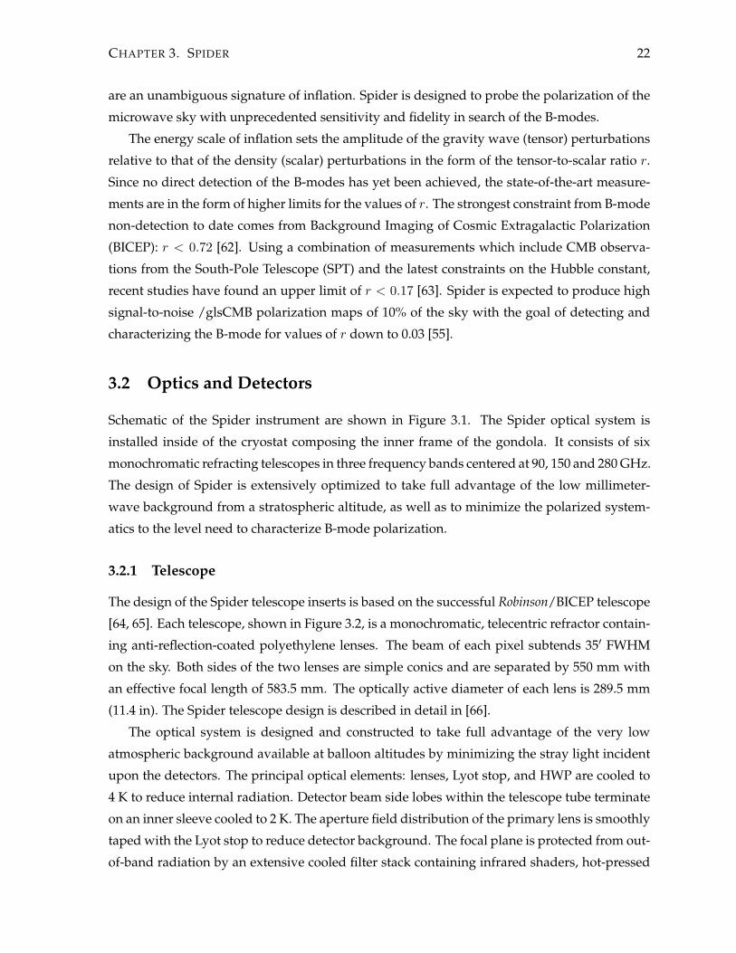
(11.4 in). The Spider telescope design is described in detail in [66].
The optical system is designed and constructed to take full advantage of the very low
atmospheric background available at balloon altitudes by minimizing the stray light incident
upon the detectors. The principal optical elements: lenses, Lyot stop, and HWP are cooled to
4 K to reduce internal radiation. Detector beam side lobes within the telescope tube terminate
on an inner sleeve cooled to 2 K. The aperture field distribution of the primary lens is smoothly
taped with the Lyot stop to reduce detector background. The focal plane is protected from out-
of-band radiation by an extensive cooled filter stack containing infrared shaders, hot-pressed

CHAPTER 3. SPIDER 23
Figure 3.1: Rendered front and side views of the Spider gondola and a 1 m penguin for scale.For clarity, the sunshields, the cart, and the solar array are hidden in the side view.
Figure 3.2: Left: Cross-section of the Spider telescope insert model with key components la-beled. Right: Photo of the Spider instrument insert without the outermost copper-clad G10wrap. Visible in the photo are the carbon fiber trusses, the high-µ magnetic shield called thespittoon, the cooled optics sleeve between the lenses, thermal straps, cables, and the cold plate.

CHAPTER 3. SPIDER 24
mesh filters, and nylon filters. The telescope aperture will be covered by a 0.125 in thick Ultra-
High-Molecular-Weight Polyethylene (UHMW) window with low emissivity.
A 1/2 in thick 1100-H14 gold-plated aluminum plate forms the base of each Spider insert.
The 3He sorption fridge is mounted on top of this plate giving it the denomination of cold plate.
The cold plate is the base for the Carbon Fiber Reinforced Polymer (CFRP) truss structure that
supports the optics and the focal plane. It is also the interface through which the telescope
inserts mount to the cryostat.
Polarimetry
A HWP is mounted in the aperture of each telescope and cooled to 4 K. The HWP assem-
bly consists of a single birefringent sapphire plate coated with a single layer of fused quartz
on each side. The HWP is rotated in steps around the optical axis using a worm-gear drive
train. The HWP shifts the polarization direction of the incident light while leaving the beams
unchanged. The use of the HWP allows a full measurement of the sky polarization using
each individual detector, eliminating or reducing many potential systematic effects. The use
of monochromatic telescopes results in a simplified design compared to the BLASTPol achro-
matic HWP. The details of the design and optical performance of the Spider HWP assembly
are described in [67].
3.2.2 Receiver
The focal plane architecture of the Spider telescopes is derived from the Background Imaging
of Cosmic Extragalactic Polarization-2 (BICEP-2) instrument, with extensive modifications to
improve magnetic shielding [66]. The left panel of Figure 3.3 shows a partially-assembled
Spider Focal Plane Unit (FPU). Four Si bolometer arrays constitute the microwave-sensitive
elements of each focal plane. These arrays are supported at a distance of 1/4-wavelength
above a superconducting Nb backshort plate, which defines an integrating cavity and provides
magnetic shielding. Flexible superconduction circuits connect the array to their associated
Superconducting Quantum Interference Device (SQUID) amplifiers. These are housed within
a magnetically-shielded box behind the focal plane as shown in the right panel of Figure 3.3.
The assembly is cooled to ∼300 mK by the 3He refrigerator. The temperature of each tile and
of the copper support plate are read out using NTD Ge thermistors.
Bolometric Arrays
The microwave sensitive elements of the focal plane are four large-format arrays of antenna-
coupled bolometers [68] shown in Figure 3.4. These arrays integrate beam and band-defining

CHAPTER 3. SPIDER 25
Figure 3.3: Left: Image of the Spider RevX focal plane. Right: Image is the focal plane assemblywithout the outer A4K high-µ shield. Visible in the photo are the diagonal 316 stainless passivethermal filters, the niobium box shield, the carbon fiber trusses, and copper thermal straps forthe high-µ shield.
elements with polarization-sensitive detectors into a single monolithic package, without the
need for external feed horns. Each array is a Si tile photolithographically patterned with an
8×8 (in 150 GHz) or 6×6 (in 90 GHz) array of spatial pixels.
A spatial pixel consists of two interleaved arrays of slot antennae, one for each of the two
perpendicular polarization components of incident light as shown on the left panel of Fig-
ure 3.3. A summing tree of microstrip transmission lines links each array of slots to form a
single antenna as show in the right panel of Figure 3.3. The slots are summed in-phase with
one another, producing a diffraction-limited beam that couples to the optics with single-mode
throughput. This arrangement gives each pixel a ∼13◦ FWHM beam, a ∼25% bandwidth set
by the slot dimensions, and a first side lobe at -15 dB.
The output of each summing tree passes through an on-chip band-defining filter and ter-
minates on a superconducting Transition-Edge Sensor (TES) bolometer [69]. Systematic differ-
ences between the two polarization channels in each spatial pixel are limited by their shared
optical path, the physical proximity of their bolometers, and the shared readout electronics
chain.
The Spider bolometers are similar to those used in BICEP-2, but are optimized for the lower
optical background available at a suborbital platform. The TES is a thin film of Ti on a silicon
nitride membrane, thermally isolated from the tile substrate by narrow legs of silicon nitride.
Power received by the antenna is dissipated in a gold termination resistor, which is maintained
at the TES critical temperature by electrothermal feedback [54].

CHAPTER 3. SPIDER 26
Figure 3.4: Right: Close-up image of one of the Spider TESs islands at 400X zoom (photo credit:A. Turner and J. Brevik). The meandered legs allow for the requisite low thermal conductivitybolometers to fit in a smaller island cut out. On the right hand side of the island is the goldresistive meander where the antenna summing tree is terminated. On the left part of the islandare the Ti and Al TESs in series with readout leads leaving the island to the left.
3.2.3 Read-Out
The TESs are read out using a time-domain SQUID multiplexer system developed by the Na-
tional Institute of Standards and Technology (NIST) [70]. The changing current through each
TES is detected by a corresponding first-stage SQUID. These SQUIDs are switched on one at
a time in rapid succession, so that each group of 33 SQUID channels (32 connected to bolome-
ters plus one dark channel to monitor amplifier drifts) may be read out through a single set
of wires at room temperature. The output of each first-stage SQUID group is amplified by a
second-stage SQUID and a series SQUID array [71] before reaching an ambient-temperature
amplifier. This configuration reduces the number of wires necessary to connect large-scale
focal planes.
The TESs and SQUID multiplexer systems are controlled and read out using the Multi-
channel Electronics (MCE) [72], an ambient-temperature electronics crate initially designed for
the Submillimeter Common-User Bolometer Array-2 (SCUBA-2) instrument. One MCE crate
maintains each focal plane, providing the necessary current and flux biases and linearizing the
response of each SQUID channel using a digital feedback loop. Each MCE crate is connected
to a MCE computer (MCC) through optical fiber.
3.2.4 Cryogenics
The Spider telescopes are kept at sub-Kelvin temperatures inside of a cylindrical LDB cryostat
shown in Figure 3.5. The cryogenic systems are described in detail in [73]. Starting from

CHAPTER 3. SPIDER 27
Figure 3.5: Schematic cross section of the Spider LDB cryostat.
the outermost layer, the LDB cryostat composed of a 2.43 m long and 2.05 m in diameter
cylindrical welded aluminum vacuum vessel, two vapor cooled shields (VCS1 and VCS2), a
1284 L liquid helium tank (MT) and a 16 L superfluid helium tank (SFT). The MT is shaped
like a 6-shot revolver cylinder with six bays around the outside which house the six telescope
inserts and a central cavity used to pass wiring to the HWPs and thermometry in front of the
inserts. The hold time of the MT is more than 25 days.
The six telescope insert cold plates described in Section 3.2.1 bolt to the MT via gold-plate
aluminum interface plates. The SFT is fed via a capillary tube from the MT and it is pumped
to 1.6 K. On the ground, this pumping is achieved with a vacuum pump. At float, the reduced
atmospheric pressure provides the pumping. The reduced pressure in the SFT makes the
liquid superfluid and it provides an intermediate temperature stage between the main liquid
helium bath and the sub-Kelvin stage.
The FPU is supported on eight 316 stainless steel blocks. These “heat capacity blocks”
connect the four sides of the FPU to a copper ring via copper supports. This structure is

CHAPTER 3. SPIDER 28
cooled to 300 mK by a 3He adsorption refrigerator and it is referred to as the sub-Kelvin stage.
It is supported by carbon fiber rods from another copper ring cooled to 1.6 K by the SFT. This
auxiliary copper ring is itself supported by an aluminum ring with carbon fiber rods.
Structural Support and Thermal Coupling to the Vacuum Vessel
The main tank is supported by the vacuum vessel through six G10/Al flexures symmetri-
cally placed on the cylinder sides as shown in Figure 3.5. The G10 is a lightweight and high
tensile strength fiberglass with extremely poor thermal conductivity commonly used in cryo-
genic applications [74]. The G10 flexures minimize heat conduction between the main tank
and the vacuum vessel providing structural support for the cryostat assembly. Heat flow
from the vacuum vessel to the main tank is dampen by heat sinking the flexures to VCS1 and
VCS2 using copper straps. Additional structural support is provided by more than a dozen
kevlar-tensioned snubber blocks. These snubber blocks make a suspension system designed
to minimize translation of the main tank with respect to the vacuum vessel.
The outer sides of the VC1 and VCS2 are covered with Multi-Layer Insulation (MLI): 16
layers outside of VCS1 and 52 layers outside of VCS2. Each layer of MLI is a 6.4 µm film of
Mylar R⃝ with a 35 nm thick aluminum layer on both sides with a packaging density of 14 lay-
ers cm−1. The MLI is designed to provide radiation damping and maintain large temperature
gradients between stages. Each layer of Mylar is separated by a 0.1 mm thick, spun-bound
polyester that reduces thermal conduction and prevents contact between the layers.
3.3 Gondola
The gondola is the automated platform which supports the telescope. It consists of three main
components: the outer frame, suspended from the balloon flight train by suspension cables
and a motorized swivel (pivot); an inner frame which houses the telescope and the cryostat;
and finally, a set of sun shields attached to the outer frame.
3.3.1 Structural Elements
The Spider cryostat was designed and built by Redstone Aerospace based on initial designs
from members of the Spider collaboration. The outer frame and the sunshields were custom
designed and built at University of Toronto. The design and assembly of those structures
constitute Chapter 5 of this thesis. A render and a photograph of the gondola are shown in
Figure 3.6.

CHAPTER 3. SPIDER 29
Figure 3.6: Render (left) and photograph (right) of the Spider gondola. On the render: theinner frame is highlighted in blue and the sunshields are made transparent. The photographyof the gondola shows the inner frame integrated to the outer frame sitting on the cart.

CHAPTER 3. SPIDER 30
Inner Frame
Additionally from housing the optic systems and the detectors, the Spider cryostat is effec-
tively the inner frame of the gondola. Six MCE crates, three MCE power supplies, the BLAST-
bus and pre-amplifier housekeeping crates, the Digital-to-analog Converter (DAC) box used
for the Alternating Current (AC) bias, and the HWP motor controller box are installed in the
lower part of the cryostat. A bore-sight star camera and a set of batteries are mounted on the
top of the cryostat.
The Spider cryostat is trunnion-mounted on a pair of SKF FSYE-3-NH pillow-box bearings
supported by the outer frame. The trunnions bolt-fastened to the blocks welded to the rein-
forced band around the cryostat. For installation purposes, the cryostat has 360◦of rotation
freedom around the pillow-box bearings. However, its elevation range is fixed to 20◦ to 45◦
when the elevation drive is installed.
Outer Frame
The CFRP tubing and aluminum structure that composes the Spider outer frame is in charge
of supporting the Spider cryostat, connecting it with the flight train, allowing the pointing
in azimuth and elevation, and housing control and readout electronics. The outer frame of
Spider is described in detail in Chapter 5.
Sunshields
Spider is protected from the sun by a set of aluminized Mylar R⃝ sheets as described in Chapter
4. The sheets are mounted to a tubular CFRP tubing and aluminum skeleton attached to the
main rectangle of the outer frame. The sunshields define the regions which the telescope can
observe while avoiding exposition to direct sunlight as will be explained in Section 4.5.1. At
the top of the sunshields, a Hexcel R⃝ Al honeycomb shelf provides a place to set the pivot down
while it is not hanging. This is important for transferring the gondola from and to the launch
vehicle. The shelf also traps the pivot and prevents it from striking the telescope after the
termination of the balloon. Details on the construction technique used to build this structure
are given in Section 5.5.
3.3.2 Motion Systems
The motion of the Spider gondola is controlled in azimuth by the rotation of the flywheel and
the pivot. The motion of the inner frame in elevation is controlled by an off-axis elevation
drive. The motors are controlled based on the input from the pointing sensors.
CHAPTER 3. SPIDER 31
Spider is stepped in elevation using an off-axis elevation drive based on a pair of linear
actuator on each side of the gondola. The inner frame trunnions are coupled to an aluminum
arm. The back side of each arm is attached to a VectacTM
VT209-12 linear actuator trunnion
mounted in the back joints of the gondola. The linear displacement of the actuator corresponds
to elevation motions of the inner frame.
The front of the arm has a clearance for a lock pin which engages at 1 m from the rotation
point of the arm. This distance provides enough mechanical advantage to guarantee the struc-
tural integrity of the gondola, the inner frame, and the elevation drive during pin release at
launch.
The Spider pivot is a twin of the BLASTPol pivot introduced in Section 2.3.2. The only
difference between the two assemblies is the steel casing with the tabs for the suspension
cables. There are only three tabs in the Spider pivot, corresponding to the back and front
suspension cables, but they are thicker and wider than the BLASTPol pivot tabs.
The Spider reaction wheel is composed of an aluminum hub with six 1.0 m long aluminum
arms with 6.69 kg (14.75 lb) brass bricks attached at their ends. The total mass of this assembly
is 50.34 kg and its moment of inertia is 44.77 kg m2. The wheel is mounted on the rotor of the
assembly of a Parker Bayside K178200-6Y1 brushless DC motor.
3.3.3 Command and Control
Spider is designed to operate autonomously, without the need of ground commanding. Tele-
scope control is provided by a pair of redundant flight computers with Intel R⃝ Celeron R⃝ pro-
cessors at 366 and 850 MHz. The flight computers run a single, monolithic program, the Pro-
gram Control Master (PCM), written in C, which performs primary control of all aspects of the
telescope, including in-flight pointing solution, motion, commanding, telemetry, data archiv-
ing, and thermal control.
The Spider ACS is built around four of the ADC cards described in Section 2.2.5. The ACS
provides analogue and digital sampling and control for systems which are neither handled
by the DAS nor connected to the flight computers via serial or Ethernet. It controls the mo-
tion systems, the power systems, the auxiliary motors, the star camera trigger and readout of
various housekeeping sensors.
3.3.4 Pointing
Spider’s observation strategy is designed to maximize sky coverage and crosslinking over a
region of the southern sky relatively free of Galactic foregrounds. Spider will scan in 110◦ peak
to peak azimuth scans at constant velocity ∼6.0◦ s−1 and punctuated by 0.1◦ elevation steps

CHAPTER 3. SPIDER 32
and HWP rotations [55]. Synching the elevation steps with sidereal time ensures maximum
sky coverage in declination.
The in-flight attitude determination system of Spider uses a pair of CCD based star cameras
which provide absolute pointing and fiber-optic rate gyros that provide velocity information
which is integrated to obtain interpolation of the gondola attitude between star camera solu-
tions. Coarse attitude determination is provided by a couple of encoders on the elevation axis,
a tilt sensor on the inner frame, a sun sensor, a GPS unit, and a magnetometer. PCM is capable
of determining the quality of the data from each sensor and automatically shifts to the next
available sensor in case of a problem. This system provides in-flight pointing reconstruction
to less than 1 ′ and post-flight pointing reconstruction to less than < 5 ′′.
Star Cameras
Spider’s attitude will be determined to 6′′ primarily by a pair of star cameras. These are a
pair of SBIG ST-1603ME cameras, each with a KAF-0402ME CCD. Pixels of 9.3′′ and a 2.43
square degree FOV are obtained using 200 mm f/2.8 lenses. These cameras are mounted on
an Aerotech ADRT 150-135 rotating platform and are oriented at 45◦ and 30◦ in elevation and
separated by 45◦ in azimuth. The platform rotates in azimuth opposite to the rotation of the
gondola holding the camera fixed relative to the sky, allowing deep integrations despite the
rapid motion rate of the gondola. The relative orientation of the platform with respect to the
telescope bore-sight is determined by optical encodes built into the rotary platform and which
are accurate to 5′′.
Each camera has a PC/104+ single-board computer, and a Solid-State Disk (SSD) to store
images. The software running on the star camera computers communicates with the star cam-
era and lens, detects blobs in the images, matches blob coordinates to stars in a catalogue
to produce a pointing solution, sends data packets and interprets commands from ACS and
flight computers. The position of the gondola between star camera pointing solutions will be
integrated using the same fibre optic rate gyroscopes used in BLASTPol.
3.3.5 Power System
The solar array, the charge controller and the flight batteries on board of Spider are the same
use in BLASTPol and described in Section 2.3.5.

Chapter 4
Thermal Design of the Balloon-borne
Platform
Balloons have been used for decades to conduct scientific studies above the bulk of the Earth’s
atmosphere. During 1911 and 1912, Victor Hess obtained the measurements which led to the
discovery of the cosmic rays, while flying on a balloon at altitudes up to 5.3 km. This work
won him the Nobel Prize in Physics in 1936 [75]. Lots of things have changed since that flight
and currently scientific balloons can be launched from locations worldwide and provide a
stable platform with typical flight durations around 20 days and altitude around 42 km above
the sea level.
The balloons and the facilities necessary to fly BLASTPol and Spider are provided by CSBF,
a division of the NASA dedicated to balloon flights. In over 25 years of operation, CSBF
has launched more than 1700 balloons for 35 universities, 23 other research agencies, and 33
foreign groups. Today, payloads weighing up to 2250 kg (5000 pounds) are quite common and
balloons of around 1 million cubic meters (∼30 million cubic feet) are flown routinely.
These balloons are constructed with polyethylene film, the same type material used for
plastic bags. This material is only 0.02 mm (8 × 10⁻⁴ inch) thick, about the same as an ordi-
nary sandwich wrap. The film is cut into banana-peel shaped sections called gores and heat
sealed together to form the balloon. Up to 180 gores are used to make NASA’s largest bal-
loons. These standard, zero-pressure, balloons are open to the atmosphere at the bottom to
equalize the internal pressure with the surroundings. The balloon system includes the bal-
loon, the parachute and a payload that holds instruments to conduct scientific measurements.
The balloon is launched being partially filled with helium and the payload is suspended be-
neath it. Once released, the balloon rises and the helium progressively expands as a result of
the atmospheric pressure decrease with increasing altitude.
The long duration balloons (LDBs) can carry a payload weighing as much as 2250 kg
33

CHAPTER 4. THERMAL DESIGN OF THE BALLOON-BORNE PLATFORM 34
(∼5000 lb), about the weight of three small cars. They can fly up to 42 km (26 miles) above
the sea level. After the science measurements are complete, flight controllers send a radio
command that separates the payload from the balloon. The payload floats back to the ground
on a parachute where it can be retrieved and flown again. Payload separation creates a large
tear in the balloon material, which releases any remaining helium. The balloon also falls to
the ground, where it is sometimes retrieved and discarded. The balloon and the payload land
approximately 45 minutes after separation.
One of the main challenges of the balloon-borne experiments is the effect of a changing
thermal environment. The payload is exposed to air temperatures ranging from less than -40◦C
in the tropopause to over 40◦C at ground level. At float altitude, the atmospheric pressure is
around ∼ 5 mbar (0.005 atm), making convective coupling to the air practically negligible, thus
the instrument has to rely on radiation as the main mechanism for cooling. The temperature
control of the balloon-borne platform is made by controlling the surface area, radiative envi-
ronment, and surface coating. For example, directly exposed to the sunlight and only cooling
radiatively at float, a 1 m2, bare aluminum plate would reach a maximum temperature close to
200◦C ; if the same plate is painted white, the maximum temperature is approximately 14◦C;
if the plate is painted white and has a thermal load of 10 W, the maximum temperature is
15◦C; if the bare aluminum plate is enclosed in an aluminized mylar shield open in the anti-
sun direction, the maximum temperature is approximately 90◦C; if the plate inside the shield
is painted white, the maximum temperature is close to -15◦C; if the plate inside the shield is
painted white and has a thermal load of 10 W, the maximum temperature is approximately
-10◦C.
The thermal models for the BLASTPol and Spider gondolas are both composed of over
100 conductively coupled elements. There are over 30 different heat loads produced by the
power consumption of the electronic components. The level of complexity of this thermal sys-
tem requires a Computer-Assisted Design (CAD) model of the gondola which accounts for
the ray tracing of the solar and thermal radiation between elements of the gondola, something
which has been done in the past using view factor coefficients specific to particular geometries.
Finding the solutions of the system of linear equations resulting from the thermal equilibrium
is a computationally challenging problem which has to be tackled using iterative methods.
This problem is addressed in the thermal modeling of BLASTPol and Spider by using Ther-
mal Desktop R⃝, a computational tool which integrates finite difference methods and CAD for
modeling thermal problems.
This chapter describes the thermal models of both BLASTPol and Spider and it is organized
as follows: Section 4.1 introduces the thermal environment during the balloon flight. Section
4.2 describes the methods used to solve thermal problems in the components of the balloon-

CHAPTER 4. THERMAL DESIGN OF THE BALLOON-BORNE PLATFORM 35
borne payload. Section 4.3 describes the implementation of the thermal model in Thermal
Desktop R⃝. Section 4.4 describes the BLASTPol thermal model and compares its predictions
with the results of BLASTPol10 and BLASTPol12. Finally, Section 4.5 introduces the Spider
thermal model.
4.1 The Balloon-borne Flight Thermal Environment
The LDB thermal environment in Antarctica is characterized by continuous but variable solar
illumination combined with small conductive coupling to the atmosphere. Changes in ra-
diative environment at the maximum altitude reached by the balloon (float) is dominated by
the diurnal changes in the position of the sun. Additionally, elements of the experiments are
heated when electric current flows through the electronic devices.
The thermal design of the experiment is required to maintaining the elements at tempera-
tures below their maximum temperature ratings in the absence of air convection. Additionally,
all the elements have to be kept at temperatures over their minimum temperature ratings when
the air couples them to cold layers of the atmosphere. This establishes two clear scenarios to
be considered in the thermal modeling: the ascent and float.
4.1.1 Ascent
Heat transfer by conduction is described by Fourier’s Law of Thermal Conduction [76]:
q = −k∇T[W/m2
](4.1)
where q is the heat transfer rate per unit of time and unit of area, k is the thermal conductivity,
and ∇T is the temperature gradient. In the 1-dimensional case, this can be approximated by
q = −kAdTdx
[W] (4.2)
whereA is the cross sectional area perpendicular to the temperature gradient. k is a property of
the materials and in the case of gases and liquids it depends on the pressure and temperature,
although it is not expected to decrease with lower air density [77]. At sealevel, at 1 atm and
0◦C, the thermal conductivity of the air is 0.0237 W m−1 K−1, a very small to be dominant over
radiation or conduction.
On the surface of the Earth, the temperature of the experiment is dominated by convective
air cooling. The heat transfer by convection is described by [76]:
q = h∆T [W] (4.3)

CHAPTER 4. THERMAL DESIGN OF THE BALLOON-BORNE PLATFORM 36
Figure 4.1: Temperatures of selected passive (left) and active elements (right) of the gondoladuring the ascent of BLASTPol10 (solid lines) and BLASTPol12 (segmented lines).
where h is the convective heat transfer coefficient. The calculation of h is non-trivial since it
depends on the flow properties and the shape of the object. Air at high altitude is less dense
than air at sea level, reducing its convective capability and overall heat capacity. The heat
transfer coefficient in naturally cooled systems can be expressed as a function of the Grashoff
and Prandtl numbers. In this case, the temperature and density dependence of the Grashoff
number dictates that the components convective coupling to the air decreases with altitude
[78].
The temperatures of passive elements at ∼ 15 km altitude, shown in Figure 4.1, are ev-
idence that the coupling between the air and the gondola components is important at the
lower layers of the atmosphere. This is particularly important since these layers include the
tropopause, the transitional layer between the troposphere and the stratosphere from approx-
imately 8 km at the poles to approximately 18 km at the equator. In the tropopause, the rate at
which the temperature changes with altitude (lapse rate) drops and the temperature remains
as cold as -57◦C (-70◦F) [79]. It is in this layer of the atmosphere where most elements of the
gondola may freeze.
Figure 4.1 shows the temperature of active (with heat load from electric power consump-
tion) and passive (without heat load) elements of the experiment during the ascent. While
transiting through the tropopause, the primary mirror cools down to ∼-15◦C, the pivot (turned
off) goes down to ∼-20◦C, and the the ambient thermometer on the tip of the front sunshields
reaches ∼-35◦C. Active elements in the inner frame such as the star cameras and the breakout
box reach ∼-5◦C, while electronics on the outer frame cool down to ∼-15◦C.
Thermal modeling of the convective heat transfer in the tropopause is very complex given
its dependence on the geometry and flow properties. Therefore, to guarantee the survival
and recovery of the active elements after its transit through the tropopause, all electronics and

CHAPTER 4. THERMAL DESIGN OF THE BALLOON-BORNE PLATFORM 37
Figure 4.2: Altitude during ascent (left) and at float (right) during BLASTPol10 (solid lines)and BLASTPol12 (segmented lines).
motors have been cold air tested at CSBF in Palestine, TX. The readout and motion systems
where operated in a sealed chamber filled with Nitrogen gas at -40◦C. All of the electronics
and motors operated normally after reaching temperatures around -30◦C. Air condensation
and low temperature in the tropopause are prevented by covering the electronic boxes with
transparent polyethylene bags and enclosing them in 1 inch thick StyrofoamTM
(blue foam)
boxes.
Figure 4.2 shows the altitude of BLASTPol10 and BLASTPol12 as a function of time. The
payload reaches floating altitude after ∼4 hours, spending a little more than 1 hour in the
tropopause. Once at float, the altitude of the payload changes diurnally between 40 and 37 km.
This change in altitude is caused by the expansion and contraction of the helium in the balloon
with different sun illuminations product of the diurnal cycles.
4.1.2 Thermal Environment at Float
The right panel of Figure 4.2 shows the float altitude and its change with the diurnal cycles in
BLASTPol10 and BLASTPol12. At a mean float altitude higher than ∼ 38 km, the telescope is
above 99% of the atmosphere, which is 98% transparent across the BLASTPol bands [50]. At
this altitude, the atmospheric pressure is ∼5 mbar (0.005 atm) and the air density is less than
7.3×10⁻⁴ kg m−3. In this near to vacuum environment, little or no thermal convection should
take place, except for surface boundary layers. The main heat transfer process is radiation.
The power transfer by radiation is described by the Stefan-Boltzmann law [76]:
P (rad) = ϵAσT 4 [W] (4.4)
where σ = 5.67× 10⁻⁸ W m−2 K−4 is the Stefan-Boltzmann constant. A and T are the effective

CHAPTER 4. THERMAL DESIGN OF THE BALLOON-BORNE PLATFORM 38
surface area and temperature of the object in consideration. The emissivity ϵ is the fraction of
the thermal radiation that is emitted.
The thermal equilibrium for a particular element of the gondola is described by
P +∑
αiAiIi = ϵAσT 4 (4.5)
P is the heat load resulting from the electrical power consumed by the element. Ii is the in-
tensity of each external radiation source illuminating the element, integrated over the relevant
wavelength band. Ai is the effective surface area as seen from each radiation source. αi is the
percentage of the incoming radiation that is absorbed by the element.
The emissivity ϵ is wavelength dependent, but for equilibrium temperatures around 300 K
the dominant thermal emission is produced around 10 µm. The effective surface area Ai de-
pends on the geometry of the gondola and the relative orientation of the elements on it, this is
usually not trivial to calculate by hand and it is estimated using CAD thermal modeling and
ray tracing algorithms. The absorptivity α is also wavelength dependent. However, the dom-
inant absorptivity considered in the study of the gondola is that around 500 nm, the central
frequency of sunlight since most of the illumination comes from direct or reflected sun light.
External illumination of the payload comes from 3 main sources: solar radiation, reflected
sunlight from the surface of the Earth (albedo), and the thermal emission from the surface of
the Earth (planetshine). The contribution of each one of these sources depends on the tra-
jectory of the flight and the time of the year. The model of the thermal environment at float
considers the Earth as a sphere with a 6356.8 km radius, axial tilt of 23◦26′24′′.41, and located
149.60×10⁶ km from the Sun. The payload is simulated in a circumpolar orbit at fixed latitude
78◦South at 38 km from the sea-level, starting on December 22 as shown in Figure 4.3.
Solar Radiation
The spectrum of the solar radiation is close to that of a black body with a temperature of about
5800 K. The sunlight flux density measured by satellites at the top of Earth’s atmosphere is
1366 W m−2. It is composed, dividing by total energy, of about 50% infrared light (λ > 0.7 µm),
40% visible light (0.7 µm < λ < 0.4 µm), and 10% ultraviolet light (λ < 0.4 µm) [80].
Albedo
In the context of the thermal model, the albedo is defined as the ratio of reflected radiation from
the surface of the Earth to incident radiation upon it. Being a dimensionless fraction, it may
also be expressed as a percentage, and is measured on a scale from zero for no reflecting power
of a perfectly black surface, to 1 for perfect reflection of a white surface. In detailed thermal

CHAPTER 4. THERMAL DESIGN OF THE BALLOON-BORNE PLATFORM 39
Figure 4.3: Render of the orbit defined for the BLASTPol thermal analysis. This is a circumpo-lar orbit at latitude 78◦S. The cylinder corresponds to the projected shadow of the Earth withthe Sun as a backlight source.
modeling, a bidirectional reflectance distribution function may be required to characterize the
scattering properties of a surface accurately, although for the purpose of the thermal modeling
of the payload, the albedo is a sufficient first approximation.
The average overall albedo of Earth (planetary albedo) is 30 to 35% because of the cover-
ing by clouds, but varies widely locally across the surface, depending on the geological and
environmental features. In Antarctica, the surface of the continent is covered by snow which
can be as much 95% reflective, while the surface of the Antarctic sea reflects only 10 to 15% of
the incoming sunlight. The historical record of Antarctic flight indicates that drift to latitudes
outside of the continent is unlikely, therefore an albedo of 95% is considered on the thermal
model of BLASTPol. This turned out to be an accurate estimation of the flight conditions as
shown in Figure 4.4.
Planetary Radiation
The planetary radiation, also called planetshine, is the thermal emission by the surface of the
Earth. The temperature of surface of the Earth is ∼270◦K, therefore the planetshine can be mod-
eled as a blackbody peaking at 10.73 µm. The radiance integrated between 8 µm and 15 µm is
38.01 W m−2 sr−1, which at 38 km from sea level corresponds to a flux density 237.18 W m−2.
In that frequency range, the emissivity of the ground is close to 0.99 [81]. The flux density from
planetshine reaching the balloon-borne platform is around ∼17% of the solar flux density.
An additional source of illumination is the diffuse sky radiation, which is solar radiation
scattered in elastic processes such as Rayleigh or Mie scattering by molecules in the atmo-

CHAPTER 4. THERMAL DESIGN OF THE BALLOON-BORNE PLATFORM 40
Figure 4.4: BLASTPol2010 (right) and BLASTPol2012 (left) circumpolar flight trajectories. Theimage on the left hand side shows the ground optical properties relevant in the estimation ofthe albedo: snow (green), ice shelf (dark blue), and sea water (blue).
sphere, and deviated from its path without being absorbed and with no change in wavelength.
Diffuse sky radiation can also be infrared when the scattering processes are inelastic and the
light is re-emitted with a longer wavelength. Although diffuse sky radiation can be relevant
in the optical performance of balloon-borne telescope, it does not significatively contribute to
the thermal performance of the payload and therefore is not considered on the thermal model.
4.2 Thermal Solutions
Given the thermal conditions of the balloon-borne flight described in 4.1 the strategies for the
control of the thermal performance of the experiment can be either: shielding of the elements
from direct exposure to sunlight, selection of surface coatings to enhance radiative cooling,
and finally, conductive coupling to radiators.
4.2.1 Shielding
Both Spider and BLASTPol fly during the Antarctic summer which means that the payloads
are continuously exposed to sunlight during the whole flight. Extensive shielding is needed to
regulate the temperature of the instrument. The sunshields define the azimuth ranges relative
to the sun where direct sunlight and albedo are blocked from the optics and all electronics,
except for the pivot and the sun sensor. The azimuth range defines the portions of the sky
which can be observed by the telescope, the sunshield geometry determines the targets and
sky coverage of the experiment as will be discussed in Sections 4.4.1 and 4.5.1.
BLASTPol and Spider are surrounded by shields comprised of DuralarTM
0.002 inch thick

CHAPTER 4. THERMAL DESIGN OF THE BALLOON-BORNE PLATFORM 41
Material Solar Infrared α/ϵAbsorptivity (α) Emissivity (ϵ)
Aluminium (machined, non-polished) 0.080 0.020 4.000Stainless Steel (machined, non-polished) 0.390 0.110 3.545Duralar Al Mylar R⃝ (2.0 mil, VDA) 0.170 0.760 0.223Lamart Al Mylar R⃝ (3.0 mil, bonded) 0.230 0.720 0.319Lamart Al Mylar R⃝ (5.0 mil, bonded) 0.190 0.770 0.246Polyethylene, LDB Balloon Film 0.016 0.050 0.320Polyimid, PCB 0.600 0.800 0.750Teflon Silver Tape, (5.0 mil) 0.080 0.810 0.098SunCat G10/FR4 0.123 0.940 0.130SunCat Laminate Back 0.630 0.950 0.663SunCat Solar Cell 0.895 0.940 0.952Black Paint 0.970 0.950 1.021White Paint 0.230 0.800 0.287Zinc Oxide White Paint 0.160 0.930 0.172
Table 4.1: Optical properties of selected surface coatings [82].
Mylar R⃝ or Polyethylene Terephthalate (PET) film with a 2×10⁻³ inch layer of Vapor-Deposited
Aluminum (VDA) and A-25-NPS Lamart 3×10⁻³ inch Mylar R⃝ film bonded to 3.5×10⁻⁴ inch
aluminum foil. During BLASTPol10 and BLASTPol12, the vapor deposited film was mounted
in the outer face of the shields while the bonded film is mounted in the inner face, with the
non-conducting (mylar) faces facing out on all surfaces that may be exposed to the Sun. As
shown in Table 4.1, the vapor deposited film has a greater emissivity which optimizes radiative
cooling to the outside of the gondola. The bonded film shows low in-band transmission such
that no StyrofoamTM
layer is needed. This configuration showed no considerable Ultraviolet
(UV) degradation during BLASTPol10 and BLASTPol12. Both mylar layers are taped directly
to the sunshield frames.
4.2.2 Conductive Coupling
The thermal control of the active elements of the gondola can be achieved by improving their
conductive coupling to large elements which act as heat sinks or large surface area elements
which serve as radiators. The heat transfer by conduction is described by Equation 4.2, which
can be rewritten as
q = −k(A
∆x
)∆T [W] (4.6)
assuming that the temperature gradient in the perpendicular plane to the direction of the heat
conduction is negligible. This assumption is in principle a good approximation to the heat
transfer between elements of the gondola and allows to characterize the geometric conductive

CHAPTER 4. THERMAL DESIGN OF THE BALLOON-BORNE PLATFORM 42
Material Density Heat capacity Thermal conductivity(kg m3) (kJ kg−1 K−1) (W m−1 K−1)
Air (sea-level, 0◦C) 1.29 1.005 0.0243Aluminium 6061-T6 2700 0.91 250.0Carbon Fiber 1550 0.71 24.0Copper 8790 0.39 401.0Mylar R⃝ 1380 1.00 0.24Styrofoam
TM30.0 1.30 0.03
Polyethylene 910.0 0.20 0.51Steel Carbon 1020 7820 0.49 54.0
Table 4.2: Thermo-physical properties of selected materials [83].
coupling by (A/x), the ratio of the cross-sectional area to the distance between isothermal
nodes. Throughout this document, the conductive couplings are expressed in terms of (A/x).
The materials whose thermal conductivities are included in Table 4.2.
The thermal model calculates the temperature of the electronic boxes assuming that the
electronic components and the box shell are in thermal equilibrium. The conductive couplings
are considered close to ideal by reducing the gaps between interfaces using DOW Corning R⃝
silicone grease TC-5026 or Stockwell conductive silicone sponge R-10400. In some particular
cases detailed modeling of internal components is necessary. For example, the model of the
BLASTPol and Spider computer boxes includes the individual chips and couplings to the faces
of the box.
4.2.3 Surface Coatings
The temperatures of the gondola elements at float can be regulated by changing the optical
properties of their surfaces. This can be achieved by applying surface coatings. Surface coat-
ings are characterized by the ratio between the absorbed solar radiation to emitted Infrared
(IR) radiation or solar absorptivity to IR emissivity α/ϵ. Surface coatings with α/ϵ greater than
1.0, such as bare aluminum and steel, absorb more radiation than they emit and this results in
heating of the gondola elements. Surface coatings with α/ϵ less than 1.0, such as white paint
and mylar, emit more radiation than they absorb and in consequence results in cooling of the
gondola elements. The properties of the most common surface coatings used on the BLASTPol
gondola are summarized in Table 4.1.
The absorption and emission also depends or the effective surface area of the gondola
elements. Small elements such as electronic boxes are particularly critical since their surface
area can be greatly affected by low quality painting. Additionally, the presence of multiple
connectors makes it easy to underestimate the effective surface area over which the box can
emit thermal radiation. Rust-Oleum R⃝ white specialty appliance epoxy (refrigerator paint) was

CHAPTER 4. THERMAL DESIGN OF THE BALLOON-BORNE PLATFORM 43
proved to be an effective solution in BLASTPol10 and BLASTPol12. More critical cases such as
the pivot controller box required more effective reflective and emissive coating such as silver
teflon tape.
The thermal model allows the definition of optically inactive regions in which the radiative
heat transfer is negligible. Surfaces such as the inside of the sunshield frame, the inside of the
inner frame and the inside of some boxes are defined as optically inactive to improve the speed
of the simulation.
4.3 Computer Assisted Thermal Modeling
The thermal modeling of both BLASTPol and Spider was made using the thermal network
analyzer SINDA/FLUINT R⃝ [84] and the CAD based thermal analysis and design software
Thermal Desktop R⃝ [85].
Thermal Desktop R⃝ is a program which receives as input a 3D AutoCAD R⃝ model of the
experiment. Each of the elements in the model is represented by a series of surfaces isother-
mal nodes. An isothermal node is the minimum element of the thermal model. Each surface
can contain one or more isothermal nodes which define the points where the temperature is
registered at the end of the calculation. Thermal Desktop R⃝ creates a thermal network with
the conductive couplings and the geometry of the gondola. The thermal network is the input
for RadCAD R⃝ a module which calculates radiation exchange factors and orbital heating rates
defined by the coordinates of the flight trajectory and the illumination sources described in
Section 4.1. RadCad R⃝ solves the heat transfer case generated as a result of the equilibrium
state and transient temperatures of the nodes defined in the model. The output of Thermal
Desktop R⃝ and RadCAD R⃝ is combined to create inputs for SINDA/FLUINT, a thermal/fluid
analyzer which iteratively solves the heat transfer equation system and generates transient or
equilibrium temperatures for each node in the model.
Figures 4.5 and 4.13 show the 3D AutoCAD R⃝ models of the BLASTPol and Spider gon-
dolas. Each of the surfaces is modeled by multiple surfaces elements and the heat transfer on
them is solved by finite differences methods. Each surface can contain one or more isothermal
nodes on which the output temperatures are calculated. Sensitive surfaces such as the BLAST-
Pol primary mirror are segmented in multiple nodes, while less sensitive components such as
the electronic boxes are modeled with multiple surface but only one isothermal node. Initial
temperatures are assigned to each node initially using an ansatz and then using final tempera-
tures from a previous run, and the thermo-physical and optical properties are assigned to each
surface. The thermal models of BLASTPol and Spider have over 600 surfaces and around 1000
isothermal nodes.

CHAPTER 4. THERMAL DESIGN OF THE BALLOON-BORNE PLATFORM 44
The objective of the calculations performed using SINDA/FLUINT R⃝ and Thermal Desktop R⃝
is to establish the temperature ranges of the elements of the experiment at float to evaluate so-
lutions which allow their normal operation during the flight. Each model is developed using
the following steps:
1. Sun-shield Design: An initial 3D model of the experiment is created and depending on
the science targets of each experiment, the sun avoidance angles are defined and the
geometry of the sunshields is decided.
2. Definition of Thermal Ranges: A list of the thermal operational ranges of all the elements
of the gondola is made. Additional validation and redefinition of the temperature ranges
are made by vacuum and cold operation testing.
3. Initial Calibration: The model is run using an initial guess of the optical properties and
conductive couplings, and including the heat loads defined by the electrical power con-
sumed by each element. The results of this ansatz model are calibrated with the temper-
atures registered in comparable elements on board of previous experiments, in this case
BLAST05, BLAST06 and Boomerang. The main objective of this step is to identify critical
elements which are expected to reach temperatures outside of their operational ranges.
To facilitate the calculations the evaluation of maximum and minimum temperatures can
be made identifying a cold case and a hot case instead of comparing transients. The hot
case corresponds to maximum power dissipation and maximum sun illumination, the
cold case corresponds to no power dissipation and minimum sun illumination.
4. Thermal Solutions are implement where needed. The thermal control strategies are de-
scribed in Section 4.2. Elements which overheat can be coupled to elements with an
emissive larger surface area that serve as radiators. Elements which run too cold can be
decoupled from heat sinks or their surface can be covered with less emissive coatings.
Boxes can overheat if they the are surrounded by elements which obstruct radiation, so
changing their location can also help.
5. Reevaluation of the model: Once the thermal solutions are implemented the model is
run again to check the effectiveness of the thermal control strategy.
6. Evaluation of Transient Solutions: Once the hot case and cold case are evaluated, transient
solutions are generated. These cover at least couple of days during the flight and allow
to see the long term behavior of the elements in the experiment. The effect of latitude
drifts during the flight are considered since they result in changes on the maximum sun
elevation during the day and different illumination of the gondola.

CHAPTER 4. THERMAL DESIGN OF THE BALLOON-BORNE PLATFORM 45
7. Keep Model Updated: The thermal model is only useful if it includes the updated infor-
mation of the experiment. The heat loads are updated by keeping track of the operation
currents on the different elements. Any changes in the geometry or the location of the
elements in the gondola are tracked.
The following sections describe the particularities of the BLASTPol and Spider thermal
models.
4.4 The BLASTPol Thermal Model
The BLASTPol thermal model includes all the optical systems outside of the cryostat, the inner
frame, outer frame, electronic boxes, reaction wheel, aluminum honeycomb decks, sunshield
panels and frames, solar array, CSBF solar array, SIP, suspension cables, pivot, ballast hopper,
and the balloon.
The thermal design of BLASTPol was driven by the telescope observation ranges and the
thermal performance of the electronics which evolved from the BLAST campaigns.
4.4.1 Sunshields
The main science goal of BLASTPol is the measurement of polarized dust emission in molec-
ular clouds. The main targets observed from Antarctica during the Austral summer are the
Vela Molecular Ridge and the Lupus Molecular Cloud. At this time of the year, Vela is located
at 140◦ left of the Sun in azimuth and between 30◦ and 50◦ in elevation. Sun-shielding for
this almost anti-sun observation is straight-forward, involving mainly covering the back of
the gondola. Less straight forward is the observation of Lupus, which is located at ∼40◦ left
of the Sun in azimuth and between 25◦ and 50◦ in elevation. The observation of this target
required unprecedented sunshielding which allows proximity to the direct illumination from
the Sun while maintaining the thermal stability of the experiment.
The solution for the azimuth sun-avoidance required by BLASTPol is illustrated in figure
4.5. The outer frame of the sunshields maintains the original design described in [42] although
only the starboard side of the gondola is covered to avoid reflection of the sunlight on the inner
face of the shields. The electronic boxes are kept in the port side where they are covered from
the direct sunlight. There, they have a large uncovered portion of the sky to radiate their heat.
The primary and the secondary mirrors are covered by a cylindrical baffle open in the port
side and extending 6 m from the surface of the primary. The design of this baffle required the
construction of a stiff, light-weight carbon-fiber and aluminum structure which is described in
Chapter 5. This solution introduces a small elevation dependence on the azimuth scan ranges,

CHAPTER 4. THERMAL DESIGN OF THE BALLOON-BORNE PLATFORM 46
Figure 4.5: Front and left views of the BLASTPol Thermal Model. The red surfaces correspondto the inner face of the sunshields. Purple corresponds to the outer face of the sunshields. Thesolar arrays are shown in grey.
but ultimately allows the sun avoidance during the observation of the sky between 40◦ and
140◦ in azimuth as illustrated in Figure 4.6.
Figure 4.7 shows the observational ranges allowed by the BLASTPol sunshields projected
in the sky. On the left of the observable region shown by the purple contours are the Lupus
I and Lupus IV regions. The thermal model makes possible the assessment of direct sunlight
illumination of the primary and secondary mirrors. Additionally it allows the evaluation of
the temperature changes which may result from pointing so close to the sun and which can
greatly damage the optical system of the telescope.
In the thermal model the sunshields as are simulated by two parallel layers of mylar sep-
arated by a distance equal to the diameter of the tubes in the sunshield frame. Each covered
triangle in the sunshield frame is represented by two independent mylar sheets. In the thermal
model the sheets are not conductively coupled each other or to the sunshield frame. Facing
outward, the outer layer has the optical properties of Duralar Al Mylar R⃝ (2.0 mil, VDA) and
facing the inside of the gondola, the inner layer has the optical properties of Lamart Al Mylar R⃝
(3.0 mil, bonded) as described in Table 4.1. The faces of the sunshield which are facing each
other are optically active and are simulated as bare aluminum.
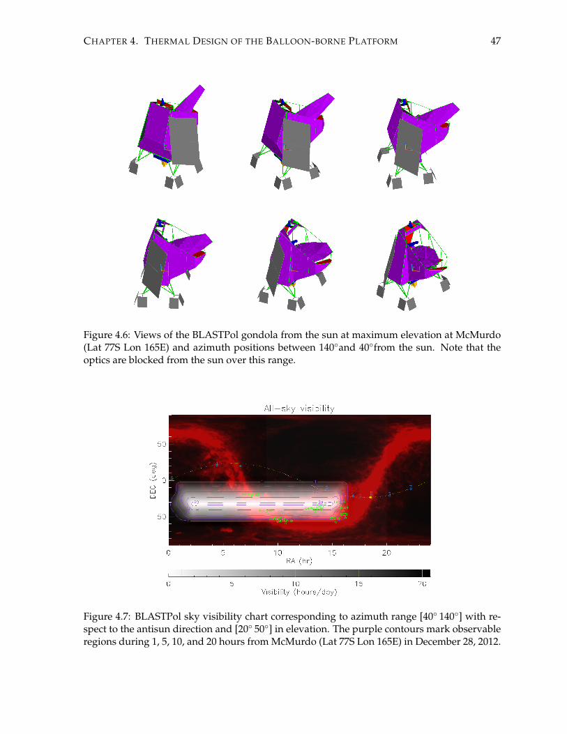
CHAPTER 4. THERMAL DESIGN OF THE BALLOON-BORNE PLATFORM 47
Figure 4.6: Views of the BLASTPol gondola from the sun at maximum elevation at McMurdo(Lat 77S Lon 165E) and azimuth positions between 140◦and 40◦from the sun. Note that theoptics are blocked from the sun over this range.
Figure 4.7: BLASTPol sky visibility chart corresponding to azimuth range [40◦ 140◦] with re-spect to the antisun direction and [20◦ 50◦] in elevation. The purple contours mark observableregions during 1, 5, 10, and 20 hours from McMurdo (Lat 77S Lon 165E) in December 28, 2012.

CHAPTER 4. THERMAL DESIGN OF THE BALLOON-BORNE PLATFORM 48
4.4.2 Telescope Elements
The BLASTPol telescope elements included in the thermal model are: the primary mirror,
the telescope struts, the secondary mirror and the secondary mirror push plate. The primary
mirror is simulated by a 1.8 m diameter concave shell, 1.0 inch thick and coupled to the inner
frame by three Al conductors with (A/x) = 5.0 inch, and optically active only on the side
facing the sky. This coupling simulates the thermal insulation from the frame by G10 spacers
while the inactive back face corresponds to the 12 layer MLI added in the gap between the
mirror and the frame. The inner frame is simulated by a set of box aluminum beams with
one isothermal node each. The nodes are coupled conductively by aluminum and (A/x) value
depending on the length of each segment. Mounted to the inner frame are the gyro box, the
star cameras, the REC and the DAS crate.
The primary mirror is also thermally coupled to the four CFRP struts covered with thin Al
fairings. A (A/x) = 1.0 inch aluminum coupling between the edge of the primary mirror and
the boxes that represent the struts simulates the aluminum inserts coupling both pieces. The
struts are conductively coupled to the push plate by an Al conductor with (A/x) = 1.0 inch.
The push plate has a thermal load of 10.5 W which corresponds to the linear actuators of the
automatic focusing system. The push plate is coupled to the secondary mirror by (A/x) =
1.0 inch aluminum conductor, a weak thermal coupling which represents the leaf-spring con-
nection between both pieces.
The modeling of the thermal behavior of large passive elements such as the primary mir-
ror and the struts is complicated for two reasons: (i) air coupling, which is not very well
determined, is relevant for passive elements in contrast to elements with thermal loads. (ii) A
passive element is considered large when its size is comparable to the size of the convective
cells at float, which is ∼1m2. The modeling convection in BLASTPol is very complicated given
the multiple surfaces and multiplicity of geometries. However, the scope of the thermal model
in the case of the optical elements is just to determine the presence of temperature gradients
or direct sunlight illumination. These two factors are more determinant in the performance
of the optical system than the equilibrium temperatures at float. Since the telescope elements
are not rated thermally and it is sufficient to let them passively cool down as long as they are
thermally stable.
Figure 4.8 shows the in-flight temperatures of the BLASTPol12 and BLASTPol10 telescope
elements compared to the thermal model predictions. The extreme values are summarized in
Table 4.3. The minimum temperatures on the telescope elements are not registered in the tran-
sit throughout the tropopause but during the lowest sun elevation periods at float. At float,
the diurnal temperature changes are ∼10◦ C for the primary mirror, ∼15◦ C for the secondary

CHAPTER 4. THERMAL DESIGN OF THE BALLOON-BORNE PLATFORM 49
Component Heat load Temperature range(◦ C)(W) Rating Model Flight
Min Max Min Max Min MaxPrimary mirror 0 — — -29.8 4.8 -25.2 1.4Secondary mirror 0 — — -47.3 -3.6 -34.1 -9.0Push plate X — — -47.2 -3.5 -33.9 1.9Strut bottom 0 — — -47.8 -3.0 -46.6 -5.0Strut side 0 — — -47.8 -3.1 -46.7 -10.0
Table 4.3: Heat loads and temperature ratings of BLASTpol outer frame elements. The maxi-mum and minimum temperatures of operation were determined during vacuum and cold airtest made at CSBF in the summer of 2010.
and ∼20◦ C for the struts.
The model is successful in determining the temperature of the primary and the secondary
within ∼10◦ C. However, the amplitude of the diurnal cycles is larger in the thermal model.
This behavior is consistent with convection or some other thermal coupling modulating the
temperature of the optical elements.
4.4.3 Inner Frame Electronics
The heat load and temperature ratings of the inner frame electronics are summarized in Table
4.4. The REC and the ACS crates are mounted to the back beams of the inner frame. Each box
is modeled as a 0.125 inch wall aluminum box reproducing the dimensions of the crates they
represent. Both sides of the box are optically active, with the inside surface as bare aluminum
and the outer face painted white. The heat load on the REC is 65.0 W, while the heat load on
the ACS is 27.0 W. Each box sits on an inner frame beam and is fastened by aluminum angles
making the conductive coupling approximately (A/x) = 1.0 inch Al.
The gyroscopes box (gyrobox) is mounted to one of the beams connecting the front and
the back of the inner frame. It is a 0.25 inch wall aluminum box with a heat load of 18.36 W.
It is directly fastened to the beam and this coupling is represented by a (A/x) = 10.5 inch
aluminum connection. The gyrobox has an internal heating resistor which is activated when
the box temperature is below 0◦C. This heater is not part of the model, where only the worse
case scenario is considered. The star cameras are mounted in aluminum pedestals on the
top front beam of the inner frame. During the BLAST test flight from Fort Sumner, NM in
2003 (BLAST03) flight, the star cameras froze at float and since then the outer surface of the
cylindrical enclosure has been kept as bare aluminum. The coupling between the star camera
enclosures and the inner frame is estimated to be (A/x) = 6.0 inch aluminum and the heat
load on each camera is 28.0 W.
The temperatures of the inner frame electronics during the BLASTPol12 and BLASTPol10

CHAPTER 4. THERMAL DESIGN OF THE BALLOON-BORNE PLATFORM 50
Figure 4.8: Flight Temperatures of the BLASTPol telescope elements and predictions of thethermal model.

CHAPTER 4. THERMAL DESIGN OF THE BALLOON-BORNE PLATFORM 51
Component Heat load Temperature range(◦ C)(W) Rating Model Flight
Min Max Min Max Min MaxDAS 35 -20 40 -15.8 15.9 -9.5 12.5REC 65 -20 40 -9.1 22.2 -2.9 11.7Gyrobox 18.36 -20 40 -16.8 17.9 -12.1 26.8ISC 28 -27 40 -11.4 23.1 -2.1 24.5OSC 28 -27 40 -11.4 23.1 -2.0 24.9
Table 4.4: Heat loads and temperature ratings of BLASTPol inner frame electronics. The maxi-mum and minimum temperatures of operation were determined during vacuum and cold airtest made at CSBF in the summer of 2010.
are shown in Figure 4.9 and summarized in Table 4.4. All of the electronics boxes operated
within the adequate temperature ranges and the temperatures predicted by the thermal model
are within ±10◦C of the temperatures at float. There is clearly a more pronounced diurnal
temperature change in the simulated temperatures which is related to the coupling between
the electronic boxes and the beams composing the inner frame. However, since the electronics
operated far from the temperature limits with the current thermal model configuration, no
further correction was considered necessary.
4.4.4 Outer Frame Electronics
The heat load and temperature rating of the outer frame electronics are summarized in Table
4.5. The ACS, the flight computer box, and the serial hub are mounted to a 0.5 inch thick
aluminum honeycomb platform which is mounted on the port side of the outer frame.
The thermal modeling of the aluminum honeycomb is challenging since the coupling be-
tween both planes is hard to model and depends on the adhesive used to fasten the thin alu-
minum sheets in the honeycomb with the 0.0625 inch aluminum slabs and honeycomb pattern
itself. The approach followed in the thermal modeling of BLASTPol and Spider is simulat-
ing the honeycomb composite as two separate layers of aluminum coupled radiatively by the
inner layers which have bare aluminum surfaces. Additionally, the conductive coupling is
simulated by thermal contact between both surfaces with a material with 1% the thermal con-
ductivity of aluminum. This model of Hexcel R⃝ Al honeycomb corresponds to a 1% surface
contact between the plates and the honeycomb, and without the explicit dependence on the
area of the plates it makes the thermal modeling more simple.
The ACS is modeled as a 0.125 inch wall aluminum box and the thermal load on it is
27.0 W. During BLASTPol10, both the inner and outer faces of the ACS were emissive and the
temperature at float was ∼10◦C lower than predicted by the model. For BLASTPol12 the one of
the outer faces of the ACS was partially covered with aluminum tape to reduce its emissivity.

CHAPTER 4. THERMAL DESIGN OF THE BALLOON-BORNE PLATFORM 52
Figure 4.9: Flight temperatures of the BLASTPol inner frame electronics.

CHAPTER 4. THERMAL DESIGN OF THE BALLOON-BORNE PLATFORM 53
Component Heat load Temperature range(◦ C)(W) Rating Model Flight
Min Max Min Max Min MaxACS 27 -33 55 -9.2 14.3 -16.7 6.9Battery (4) 50 -40 40 -18.3 13.6 -9.7 12.2Flight computers box 20 -31 54 -16.8 17.9 -12.1 26.8CPU(2) 15 2 70 18.7 43.5 12.7 33.7Serial hub 5 -31 54 -5.0 17.8 -17.1 10.8
Table 4.5: Heat loads and temperature ratings of BLASTPol outer frame electronics. The maxi-mum and minimum temperatures of operation where determined were tested during vacuumand cold air test made at CSBF in the summer of 2010.
The BLASTPol computer box is the descendant of the vacuum enclosure flown in BLAST03,
BLAST05, and BLAST06. The advent of SSD permits the use of non-pressurized enclosures
and the BLASTPol computer box is a compact solution to store the SSD and the two Moth-
erboards. However, this compact model does not have enough surface area to dissipate the
heat generated by the chips in the motherboard and for this reason, two cooper braid straps
are mounted directly to the aluminum heat sinks on top of the Motherboards. The other end
of the straps is connected to one of the aluminum legs of the port pyramid. The heat load
on the chips is estimated to be 15 W and the thermal coupling provided by the heat straps is
(A/x) = 6 inch of copper running between the chip and the pyramid leg. The serial hub is
modeled as a 0.125 inch aluminum box and a heat load of 5 W. It is mounted to the Hexcel R⃝
desk by aluminum angle beams and this coupling is simulated by a (A/x) = 5 inch aluminum
connection.
The temperatures of the outer frame electronics during the BLASTPol12 and BLASTPol10
are shown in Figure 4.10 and summarized in Table 4.5. All of the electronics boxes operated
within the adequate temperature ranges and the temperatures predicted by the thermal model
are within ±10◦C of the temperatures at float. The diurnal temperature change is larger in the
simulated data as discussed in the case of outer frame electronics. The ACS crate and the serial
reached minimum temperatures 10◦C lower than predicted by the model, although these are
15◦C over the minimum temperature of operation. The source of this discrepancy is possibly
the inner surface of both boxes is emissive and these were non-active in the model. In BLAST-
Pol12 an attempt to reduce the emissivity of the ACS was made by partially covering one of
its external faces with aluminium tape, but this proved to have no effect on the temperatures
at float as shown in Figure 4.10.

CHAPTER 4. THERMAL DESIGN OF THE BALLOON-BORNE PLATFORM 54
Figure 4.10: Flight temperatures of the BLASTPol outer frame electronics.

CHAPTER 4. THERMAL DESIGN OF THE BALLOON-BORNE PLATFORM 55
4.4.5 Motion Systems
The pivot, the elevation drive, and the reaction wheel motors are the elements of the BLAST-
Pol gondola with higher power consumption, therefore their thermal performance is critical
for the operation of the experiment. The estimated heat loads and thermal rating on these
elements are summarized in Table 4.6.
The elevation drive is simulated as a steel cube with a heat load of 6.725 W corresponding
to the Root Mean-Square (RMS) current measured during gondola pointing tests in the labo-
ratory. The comparison between the model expectations and the temperatures during flight,
shown in Figure 4.11, indicate that the coupling between the motor and the base was under-
estimated but the predicted temperature limits were adequate. The lower temperature of the
motor, ∼30◦C was correctly estimated, while the higher temperature limit was correct for the
azimuth position at 140◦from the sun.
The reaction wheel motor is simulated as a steel cylinder with a heat load of 42 W corre-
sponding to the RMS current during gondola pointing tests in the laboratory. During BLAST-
Pol10, the reaction wheel suffered damage and after the second day of flight it was unusable.
The temperatures registered during this flight, shown in Figure 4.11, indicate that the dam-
age was not caused by thermal malfunction. During BLASTPol12, the reaction wheel operated
normally, and the RMS current corresponds to a heat load of 46.1 W.
The pivot is the element of the gondola which presents more complications in the thermal
modeling as shown also in Figure 4.11. Located on top of the sunshields, the pivot is directly
exposed to the sunlight. It is simulated as a steel cylinder with a heat load of 10.4 W corre-
sponding to the 80% of RMS corresponding current measured during gondola pointing tests
in the laboratory. Beneath the pivot is the controller box, which is modeled as a 1/8 inch thick
Al box covered with silver teflon tape. The heat load on this box is 2.6 W, resulting from the
20% of the RMS corresponding current.
During BLASTPol10 the pivot temperature peaked at 34.5◦C, approximately 10◦C hotter
than predicted by model. This discrepancy can have three main sources: 1. Increased power
consumption due to its use as main pointing mechanism after the failure of the reaction wheel.
2. Kept in the sun and with a small surface area, the model of the pivot could underestimate
its effective radiative surface area. 3. The coupling to the suspension cables and the universal
joint could increase the temperature of the pivot because these elements have a high α/ϵ and
can get warm when directly exposed to the sunlight.
The similar temperatures registered during BLASTPol10 and BLASTPol12 evidence that the
power consumption is not determining the peak temperature of the pivot. This information is
important for Spider, since its pivot, a twin of the BLASTPol pivot, is going to be running at

CHAPTER 4. THERMAL DESIGN OF THE BALLOON-BORNE PLATFORM 56
Component Heat load Temperature range(◦ C)(W) Rating Model Flight
Min Max Min Max Min MaxElevation Drive 5.6 -3.0 29.0 -29.5 1.8 -28.4 -4.3Reaction Wheel 14.24 -4.0 32.0 -1.3 21.5 -16.7 38.7Pivot 10.4 -33.0 48.0 7.4 25.0 -21.6 34.5Pivot Motor Controller 2.6 -22.0 44.0 7.4 24.9 -24.4 35.1Lock Motor -27.0 51.0 -18.9 18.3 -24.1 31.9
Table 4.6: Heat loads and temperature ratings of the BLASTpol motors and motor controllers.The maximum and minimum temperatures of operation where determined were tested duringvacuum and cold air test made at CSBF in the summer of 2010.
least four times as much current. The suspension cables and universal joint were included on
the thermal model and their coupling to the pivot does not account for the 10◦C discrepancy.
Lastly, the change of the emissivity and absorptivity of the pivot by ∼20% accounts for changes
in the calculated temperature: the emission by relatively small elements in the model can
be easily overestimated since connector docks and detailed features can account for a large
portion of the emissive surface area.
4.4.6 Passive Elements
A series of thermometers were placed in passive elements of the gondola in order to calibrate
the thermal model and evaluate the role of convection in the thermal performance of the ex-
periment. This calibration is complicated but proved successful in elements such as the chin,
the port pyramid, and the outer frame as shown in Figure 4.12 and summarized in Table 4.7.
More difficult was the estimation of temperature in elements such as the rear sunshields and
the solar array, also in Figure 4.12, which are boundary layers exposed to convection and are
very extended, making its detailed treatment in the model unnecessarily complex and compu-
tationally slow.
Solar Array
The solar array is one of the critical elements in the thermal model. Its location is normal to the
middle of the azimuth range of the telescope, at 30◦from bore-sight. The solar array is exposed
to direct illumination from the sun on its active face and reflection from the sunshields on the
other face. The thermal model in this configurations predicts temperatures of up to 100◦C for
the surface of the array, in the absence of conduction or convection.
The solar array is simulated by two 0.07 inch thick G10 fiberglass plates at 1 inch from
each other and connected by 1% 6061 Al simulating the aluminum honeycomb structure of

CHAPTER 4. THERMAL DESIGN OF THE BALLOON-BORNE PLATFORM 57
Figure 4.11: Flight temperatures of the BLASTPol motion systems.

CHAPTER 4. THERMAL DESIGN OF THE BALLOON-BORNE PLATFORM 58
Figure 4.12: Flight temperatures of selected passive elements of BLASTPol.

CHAPTER 4. THERMAL DESIGN OF THE BALLOON-BORNE PLATFORM 59
Component Heat load Temperature range(◦ C)(W) Rating Model Flight
Min Max Min Max Min MaxChin - - - -46.5 27.7 -48.1 10.4Gondola frame port back - - - -5.4 13.7 -25.3 29.1Gondola frame starboard front - - - -0.1 24.5 -21.9 28.0Port pyramid leg - - - -26.7 2.7 -28.2 0.5Hexcel deck top - - - -2.7 20.4 -16.9 12.9Hexcel deck bottom - - - -2.6 20.5 -21.7 17.8Solar Array - - 100 39.8 107.6 -24.7 87.1Rear sunshield - - - -21.2 5.3 -32.4 47.7
Table 4.7: Heat loads and temperature ratings of the BLASTpol passive elements. The maxi-mum and minimum temperatures of operation where determined were tested during vacuumand cold air test made at CSBF in the summer of 2010.
the panel. The surface of the front of the panel is SunCat Solar Cell in the outside and SunCat
Laminate Black in the inside. The surface of the back of the panel is SunCat G10/FR4 on both
sides. This is the same configuration used by CSBF for the thermal modeling of their solar
array.
The SunCat solar panels are rated to 100◦C and this was estimated to be adequate for flight
considering that their surface is a boundary layer which can be cooled by convection. This
assumption was valid as shown in Figure 4.12, where the temperatures peaked at 80◦C. After
BLASTPol10, the back of the upper most panels of the solar array presented minor scorch-
ing most likely cause by the reflection of the sunlight on the sunshield and into the back of the
array. The temperatures of the solar array during BLASTPol10 and BLASTPol12 are not compa-
rable since the array configuration changed from 18 panels to 15 panels and the thermometers
were placed in different locations.
4.5 The Spider Thermal Model
The Spider thermal model is built on the legacy of the BLASTPol10 and BLASTPol12. In its
original flight trajectory, Spider was going to fly around Alice Springs, Australia in a trajec-
tory which include day and night cycles. In that flight’s conditions, the main objective of the
thermal model was to minimize the impact of the temperature gradients on the cryostat. This
required the detailed model of the cryostat surface and the couplings between the inner frame
electronic boxes and the walls of the vacuum vessel. The plans of a diurnal flight from Alice
Springs were abandoned and an Antarctic flight was chosen instead.
Spider is scheduled to fly from Antarctica in December of 2013. In the Antarctic flight,
the thermal design cornerstone is maximizing the area of the sky which can be observed by

CHAPTER 4. THERMAL DESIGN OF THE BALLOON-BORNE PLATFORM 60
increasing the sun avoidance range of the sunshields.
4.5.1 Sunshields
The main science goal of Spider is the measurement of the polarization in the CMBR in a
region of the sky relatively free of Galactic foregrounds. This region is a small patch of sky off
the Galactic plane previously observed with Balloon Observations Of Millimetric Extragalactic
Radiation and Geophysics (BOOMERanG) [86]. During the Austral summer in Antarctica this
region located between -70◦ and 90◦ from the sun position in azimuth and between 20◦ and
50◦ elevation. This mean that in a similar way the BLASTPol, the Spider observation targets
require an asymmetrical sunshield.
The Spider sunshielding strategy is illustrated in Figure 4.13. The main frame is an open
semi-cylindrical structure open in the telescope bore-sight direction and covering the interior
of the gondola all the way to the pivot. A wing is mounted on the port side of the main frame
extending at 70◦ from bore-sight to allow the observations at 70◦ from the sun. The scanning
range on the starboard direction is limited to 90◦ to avoid illumination of the inner face of
the sunshields as illustrated in Figure 4.6. The design of the Spider sunshield frame follows
the same construction method developed for the BLASTPol baffle which is described in 5.
This sunshielding solution limits the bore-sight observation range in elevation to 10◦ to 45◦ as
result of the payload height requirement for launch. However, the Spider sunshields allow the
observation of an extended region of sky as show in Figure 4.15.
In the Spider thermal model the sunshields are simulated in the same way as in the BLAST-
Pol thermal model.
4.5.2 Inner Frame Electronics
The inner frame of Spider is composed of the cryostat and the electronic boxes attached to
it. The internal components of the cryostat are decoupled from the outer shell as described
in Section 3.2.4 and they are not considered in the thermal modeling of the payload. The
components and heat loads on the inner frame of Spider are summarized in Table 4.8. The
thermal modeling of the Spider cryostat is described in [73].
The cryostat is considered as a cylindrical shell, 0.25 inch thick, and closed in the bottom
by an ellipsoidal shell and in the front by a disk with the apertures of the telescope bays, all
conductively coupled. In each telescope bay there is a short cylinder representing the flight
window docks, a truncated cone representing the baffles and a disk closing the aperture repre-
senting the flight window. With the exception of the baffles, the only optically active surfaces
are the ones facing outwards. The exterior of the cryostat is painted white.

CHAPTER 4. THERMAL DESIGN OF THE BALLOON-BORNE PLATFORM 61
Figure 4.13: Front and left views of the Spider Thermal Model. The yellow surfaces correspondto the inner face of the sunshields. Red corresponds to the outer face of the sunshields. Thesolar arrays are shown in orange.
Figure 4.14: Views of the Spider gondola from the sun at maximum elevation at McMurdo (Lat77S Lon 165E) and azimuth positions between -90◦and 70◦from the sun.

CHAPTER 4. THERMAL DESIGN OF THE BALLOON-BORNE PLATFORM 62
Figure 4.15: Spider sky visibility chart corresponding to azimuth range [-70◦ 90◦] with respectto the antisun direction and [10◦ 45◦] in elevation. The purple contours mark observable re-gions during 1, 5, 10, and 20 hours per day from McMurdo (latitude 77S and longitude 165E)in December 20, 2013.
Component Heat load Temperature(W) Rating (◦ C)
Min MaxMCE (6) 50 -20 40MCE power supply 35 -20 40Housekeeping BLASTbus 25 -33 55Housekeeping Preamp 25 -33 55HWP motor controller 10 -20 40
Table 4.8: Heat loads and temperature ratings of Spider inner frame elements.
The majority of the electronics dissipate their heat radiatively. A high IR emissivity is
achieved by painting electronics enclosures with white paint. Painting the interiors of boxes
white aids in radiative transfer between the electronics and the box. This is effective for all
boxes, except for the detector readout electronics boxes, each of which dissipates about 50 W.
To cool these boxes, emissive vertical plates were installed between each card to couple heat
from the electronics to the top and bottom walls of the boxes. A heat pipe is used to distribute
the heat to the walls of the box and the coupling flange.

CHAPTER 4. THERMAL DESIGN OF THE BALLOON-BORNE PLATFORM 63
Component Heat load Temperature(W) Rating (◦ C)
Min MaxACS 27 -33 55Battery (4) 50 -40 40Flight computers box 20 -31 54CPU(2) 15 2 70Charge Controller (2) 20 -30 50Elevation drive power (2) 50 TBD TBDGyrobox 18.36 -20 40MCC (6) 35 -20 40MCC power breakout 20 -20 40Pressure vessel (2) 20 -20 40Serial hub 5 -31 54Star camera 17 -20 40Synch box 6.75 TBD TBD
Table 4.9: Heat loads and temperature ratings of Spider outer frame elements.
4.5.3 Outer Frame Electronics
The outer frame electronics of Spider include the ACS, a flight computer box, a serial hub, two
charge controllers, a set flight batteries, six MCC, a gyrobox, two pressure vessels containing
the hard drives which store the flight data, the reaction wheel motor controller, the elevation
drive power breakout box, the star camera rotary table, and other secondary boxes. The tem-
perature ratings and heat loads on these elements are summarized in Table 4.9. All the boxes
are mounted on two hexcel decks held over the carbon fiber tubes by Al spacers.
The main challenge of the thermal design of the outer frame electronics is locating the boxes
such that most of the heat dissipation can be made by radiation. This means that the boxes
have to be distributed in the limited space of the deck without staking them and maximizing
the surface area free to radiate.
4.5.4 Motion Systems
The pivot and the reaction wheel motors are the elements of the Spider gondola with higher
power consumption. Their thermal performance is critical for the operation of the experiment.
The estimated heat loads and thermal rating on these elements are summarized in Table 4.10.
The reaction wheel motor is simulated as a cylinder with a heat load of 14.24 W corre-
sponding to the RMS during pointing tests in the highbay. The motor controller is located
on the ground side of the aluminum honeycomb floor, close to the port back corner of the
gondola. The Spider pivot is simulated in the same way as the BLASTPol pivot described
in Section 4.5.4. The linear actuators of the elevation drive and their respective motors are

CHAPTER 4. THERMAL DESIGN OF THE BALLOON-BORNE PLATFORM 64
Component Heat load Temperature(W) Rating (◦ C)
Min MaxElevation Drive (2) 5.6 -20 40Elevation Drive Motor Controller 27 -20 40Reaction Wheel 14.24 -33 48Reaction Wheel Motor Controller 2.6 -22 44Pivot 10.4 -33 48Pivot Motor Controller 2.6 -22 44Lock Motor (2) 10 -20 40Lock Motor Controller (2) -20 40
Table 4.10: Heat loads and temperature ratings of the Spider motors and motor controllers.
simulated by solid aluminum elements with the corresponding heat loads.
4.5.5 Preflight Model Calibration
At the time of completion of this dissertation the integration of Spider for the Mission Readi-
ness Review (MRR) is ongoing at the CSBF facilities in Palestine, Texas. The characterization
of the temperature ratings of the gondola elements through vacuum and cold tests is still in
progress and the final positioning of elements in the gondola is to be defined. Both of these
considerations are critical for the conclusion of the thermal model. Final estimates of tempera-
ture limits and transients will be ready after the MRR and previous to the Antarctic campaign
in December 2013.

Chapter 5
Lightweight Platform for
Balloon-borne Telescopes
Balloon-borne experiments are limited in mass by the buoyancy of the helium balloons used
to lift them. The mass of scientific equipment on board of the payload depends on the mass
of the structural elements that guarantee the integrity of the experiment during the balloon-
borne flight. Therefore, the structure of an ideal payload must combine durability and high
resistance per unit of mass. The optimization of strength and low mass is possible using com-
posite materials and aggressive light-weighting techniques derived from the results of detailed
Finite Element Analysis (FEA).
This chapter introduces the design of the Spider gondola: a pointed platform which com-
bines composite materials with light-weighted aluminum elements to provide support for the
Spider instrument. The design of the Spider gondola was motivated by the large and heavy
scientific equipment necessary to achieve the goals of the experiment. The structure was cus-
tom made to accommodate the cryostat which houses a set of six telescope. This cryostat is
unprecedentedly large and heavy compared to other balloon-borne experiments. The Spider
gondola also allows the motion of the cryostat in azimuth and elevation and protects its struc-
tural integrity during flight and after termination. Some of the products of the Spider design
such as the carbon fibre and aluminum sunshields as well as the pivot have successfully flown
in BLASTPol10 and BLASTPol12.
The technique used for the design of the Spider gondola is modular and can be extend to
future balloon-borne experiments. Some of the parts, such as the outer frame multi-tube joints,
are custom made but can be easily adapted to other payload geometries. Some others, such as
the sunshield hubs and inserts, can be used to produce structures with multiple geometries.
The motor assemblies and elevation drive sets can be scaled to accommodate the necessities of
other balloon-borne instruments. The specific requirements of the gondola change from exper-
65

CHAPTER 5. LIGHTWEIGHT PLATFORM FOR BALLOON-BORNE TELESCOPES 66
Figure 5.1: Spider LDB cryostat
iment to experiment and even from campaign to campaign. However, the general strategies
used on the Spider gondola implement the state-of-the-art CAD tools and novel composite
materials which can be useful for the design of any other experiment.
This chapter is organized as follows: Section 5.1 describes the structural requirements for
the balloon-borne platform and presents the critical scenarios considered for its design. Section
5.2 introduces the suspension elements which link the payload to the flight train. Section 5.3
describes the design and construction of the carbon fibre and aluminum structure composing
the Spider outer frame. Section 5.4 describes the motorized systems that allow the motion
of the telescope set in elevation and azimuth. Finally, Section 5.5 presents the design and
construction techniques used for the sunshield frames.
5.1 Design Benchmarks
The size of the Spider gondola is directly related to the science goals of the experiment. The
size of the Spider refracting telescopes is determined by the angular resolution adequate for
the observation of B-modes in the CMB polarization. The size of the cryostat is determined
by the diameter and length of the telescope inserts plus the volume necessary to hold enough
cryogens to achieve the necessary integration times. Finally, the size of the gondola is defined
by the dimensions of the cryostat, illustrated in Figure 5.1.
In practice, the geometrical limits are set by the space in the high-bay where the gondola
is assembled in Antarctica and the limits of the deployment vehicle. The launch procedure re-
quires that no part of the gondola intersects a plane 20◦from the vertical axis passing through
the attachment point between the launch vehicle and the gondola as shown in Figure 5.2. Ad-
ditionally, in order to transport the gondola to the integration and launch location, the separate

CHAPTER 5. LIGHTWEIGHT PLATFORM FOR BALLOON-BORNE TELESCOPES 67
Figure 5.2: Geometrical limits for the gondola design set by the CSBF deployment vehicle inAntarctica [87].
components of the gondola must fit in standard shipping containers which interior dimensions
are 2.38 m in height by 2.34 m in width, and can be 5.71 m or 12.03 m deep according to the
International Organization for Standardization (ISO) standard 6346.
The maximum mass of the scientific payload is ∼2268 kg (5000 lb), which corresponds
to the maximum gross lift of the balloon (8000 lb) minus the mass of the balloon itself, the
flight train, the SIP, the CSBF solar array, the ballast hooper and enough ballast to maintain
the altitude during the duration of the flight. The dry mass of the Spider cryostat is roughly
850 kg (1873.9 lb) and ∼1600 kg (3500 lb) when fully integrated and loaded with cryogens.
The remaining 668 kg (1500 lb) are distributed between the motorized systems which allow
pointing in azimuth and elevation, the ACS, the flight computers, the serial hub, batteries, the
solar array, pointing sensors, sunshields, miscellaneous electronic boxes, and the frame which
supports the whole assembly.
The structural support of the interior components of the inner frame relies on G10/aluminum
flexures symmetrically placed on the cylinder sides, as shown in Figure 5.3. The description
of the internal structure is described in Section 3.2.4. The design of the cryostat made by Red-
Stone Aerospace is made according to the CSBF requirements for balloon gondolas, thus the
analysis of the structural integrity of the inner frame is not included in this document.

CHAPTER 5. LIGHTWEIGHT PLATFORM FOR BALLOON-BORNE TELESCOPES 68
Figure 5.3: Rendered image of the structural flexures that support the main tank of the Spidercryostat.
Figure 5.4: Conceptual Design of the Spider Gondola
5.1.1 The Spider Gondola
The Spider gondola is composed by three main parts: 1. The outer frame, made out of alu-
minum and CFRP tubes, 2. The cryostat, which is effectively an inner frame trunnion mounted
onto the outer frame at two points along a horizontal axis as shown in Figure 5.4, and 3. A set
of sunshields which attaches to the outer frame.
The gondola is designed to work in two configurations. In the laboratory configuration, the
pivot rests on an aluminum honeycomb platform suspended from the top of the sunshields
and the gondola sits on top of a customized aluminum cart with pneumatic tires which allow
displacing the gondola without the need of a hoist as illustrated in Figure 5.5. In the flight
configuration, the pivot hangs from a hoist and the gondola is suspended from the cables. The
blocks attaching the inner frame to the cart are removed and the ballast hooper and the CSBF

CHAPTER 5. LIGHTWEIGHT PLATFORM FOR BALLOON-BORNE TELESCOPES 69
Figure 5.5: Spider cart and Spider gondola in the laboratory configuration.
Figure 5.6: Position of suspension cables and hanging angles of the Spider gondola
solar arrays are attached to the square frame beneath the SIP.
The outer frame is a customized truss structure composed by CFRP tubes with aluminum
inserts which are fastened together by multi-tube aluminum joints. It is suspended from the
pivot by three cables as illustrated in Figure 5.6. All the beams in the structure are distributed
in triangles in order to maintain axial forces and minimize moment on the truss elements. All
angles and distances have been chosen in order to locate the payload elements and optimize
the force distribution. The technique used to construct the outer frame is described in Section
5.3.
The outer frame geometry allows 360◦ rotation of the cryostat around the trunnions. This
feature facilitates the integration of the gondola and the installation of the telescope inserts in

CHAPTER 5. LIGHTWEIGHT PLATFORM FOR BALLOON-BORNE TELESCOPES 70
the cryostat. During the flight, the elevation limits are set by the elevation drive. The telescope
can point to a minimum of 10◦ and a maximum of 45◦ in elevation. The minimum elevation
corresponds to the orientation where the telescope observes the ground. The maximum ele-
vation is the orientation where the telescopes sees the balloon. Both values are obtained by
modeling the Spider beams as a set of truncated cones with a 10◦ aperture and coincident with
the telescope apertures.
The entire gondola can rotate to any azimuthal angle. The center-of-mass of the system
is on the rotational axis so that translation of the gondola does not generate torques that re-
orient the telescope. The limits of observation in azimuth are constrained by the exposure of
the telescope to direct sunlight. Therefore, the geometry of the sunshields defines the area of
the sky which can be observed as described in Section 4.5.1.
The Spider sunshield is also a truss structure composed by CFRP tubes with aluminum
inserts which are fastened together by multi-tube aluminum joints. The sunshields have less
demanding structural requirements than the outer frame, thus the technique used for its con-
struction is modular and less restrictive as discussed in Section 5.5.
5.1.2 Critical Design Scenarios
The geometry of the outer frame was defined through a series of beam mesh simulation made
with the SolidWorksTM
Simulation package. In this simulations, the frame is modeled by a
series of truss elements which have particular cross sections and material properties. The
trusses are connected with ideal nodes which constrain rotation or translation depending on
the design scenario. Gravity and accelerations can be defined in the model and loads can be
applied to the nodes and trusses. The result of the beam mesh simulation is a load table which
presents the axial forces, bending forces, and stresses on multiple segments of each truss.
The beam mesh model is run and tested in a set of critical design scenarios defined by large
accelerations and shocks suffered by the structure during the balloon-borne flight. The beam
mesh synthetic model is used in the first instance for optimizing the distribution of the truss
elements. Subsequently, the load tables are used to test and select the materials of the frame.
The selection of the CFRP tubes used in the Spider outer frame was made with series of beam
mesh simulations with tubes of different diameters and wall thicknesses. Once the tubes are
selected, the load tables from each study are used as an input for the simulation of individual
joints and inserts.
The following are the critical scenarios considered in the design of Spider.

CHAPTER 5. LIGHTWEIGHT PLATFORM FOR BALLOON-BORNE TELESCOPES 71
Chute Shock
All structural components of the gondola must survive a vertical acceleration of 97.8 m s−2
(10 g). Such acceleration results from the parachute opening and breaking the free-fall of the
gondola after balloon termination. The pull produced by the parachute is commonly denom-
inated as chute-shock and it is described as “a load 10 times the weight of the payload applied verti-
cally at the suspension point” according to the CSBF structural requirements for balloon gondolas
[87]. This is the dominant scenario in the design considerations of the Spider gondola as it is
the one which translates into largest forces on the structural elements.
The simulation of this scenario was made using two redundant models. The first one
was made by applying the forces corresponding to the tension on the suspension cables to
the corresponding nodes and constraining the nodes and trusses where the main loads are
located. The second one was made by assigning the mass of the different components to the
corresponding trusses and nodes and then applying a vertical acceleration of 97.8 m s−2. Both
methods overestimate the stresses on the frame but their results are adequate for validating
the design. The results of the first simulation produce slightly large values of stress in the truss
elements and those are the values used for validating the model.
The results of the simulation give a minimum Factor of Safety (FOS) of 4.14 when com-
paring the maximum stress with the tensile strength of the CFRP tubes (1896.05 MPa). This
value corresponds to the tensile stress on the member directly receiving the load from the
parachute. Comparison of the resulting tensile force with the results of the mechanical stress
test performed on prototypes of the Spider gondola tubes give a minimum FOS of 1.72 at room
temperature and 1.37 when pulled at lower temperature as will be explained in Section 5.3.1.
The effect of the chute shock on the inner frame was included in the design specifications
used by RedStone Aerospace for the design of the Spider cryostat. Additionally, in this sce-
nario each trunnion mount has a FOS of 1.24. The minimum FOS in the suspension cables and
the spreader bar is 2.85 and 3.79 respectively.
Pin release (Uneven loading)
At launch, the gondola will be suspended from a pin located on the extreme of the arm of
the deployment vehicle. The vehicle moves in order to maintain the balloon and the payload
aligned on a vertical axis before releasing. However, the wind can displace the balloon to form
an angle of a few degrees with the vertical axis. In a gondola suspended by cables, such as
Spider, the misalignment results in the momentary concentration of the load in one or one pair
of the suspension cables and subsequently an abrupt pull produced by the flight train catching
the payload after its is released for the pin. The result of this violent motion is a large angular

CHAPTER 5. LIGHTWEIGHT PLATFORM FOR BALLOON-BORNE TELESCOPES 72
acceleration of the inner frame. This angular acceleration has been estimated to be around
600◦ s−2 in the launch of BLAST06. This sudden rotation damaged the lock pin in BLAST05,
and destroyed the elevation drive in the 2009 flight of the The E and B Experiment (EBEX).
The prescription given by CSBF for treating this scenario is: “a load five times the weight of the
payload applied at the suspension point and 45◦ to the vertical ... if flexible cable suspension systems are
used, they must be able to withstand uneven loading caused by cable buckling.”. The worst scenario
in case of cable buckling would be having the whole payload hanging momentarily from a
single cable, a situation on which the minimum FOS is 1.10 for the Spider suspension cables.
For the Spider gondola, the effect of a 600◦ s−2 angular acceleration is mainly received
by three elements: the inner frame assembly, the elevation drive which locks the inner frame
in a fix elevation position, and the outer frame, which ultimately receives the impact of the
accelerating inner frame. The inner frame assembly is supported by G10 flexures designed
to support the cryostat during the chute shock. The flexures located in the extremes of the
cylinder are located at ∼1 m from the rotational axis and have enough mechanical advantage
to support the internal components.
The locking pin of Spider is located at 1 m of the rotation axis of the inner frame. This
distance was chosen to increase the mechanical advantage of the pin and minimize the effect
of the shock on the gondola. This locking strategy produces minimum FOS of 5.14, 2.16, and
1.48 for the inner frame, the trunnion and the locking arm respectively as described in Section
5.4.1.
The effect of the pin release on the outer frame is modeled by applying the force on the
lock pin the corresponding node. This force is calculated using the torque resulting from the
inner frame moment of inertia and the angular acceleration. The simulation of this load on the
outer frame gives a minimum safety factor of 2.45 on the truss elements.
Landing: Resting on the base at 5g
The BLAST gondola has feet designed to allow an upright landing. However, surface winds
and horizontal velocity on landing make an upright landing very unlikely, even with these
feet. Consequently, to save weight, no attempt has been made in the design of the spider gon-
dola to prevent the payload from rolling over onto one of its sides after landing. Mechanically,
the most demanding instant during such landing is the first contact with the ground. In this
stage the most exposed elements of the gondola are the lower frame and the supporting el-
ements of the SIP. In order to simulate this landing conditions, the gondola was required to
withstand a load equivalent to its mass at 5g while resting on its lower plane. The results of
the simulation give a FOS of 3.77 on the truss elements.

CHAPTER 5. LIGHTWEIGHT PLATFORM FOR BALLOON-BORNE TELESCOPES 73
Lateral acceleration of 5g
This scenario addresses a CSBF structural integrity requirement, for which all components of
the gondola must resist “a side acceleration of 5 g applied to all components and equipment attached
to and/or onboard the gondola structure or any portion of the flight system below the balloon.”. The
model of the outer frame of the Spider gondola has a minimum safety factor of 4.1 for the
truss elements in this case. The FOS considerations on the inner frame are redundant with the
results of the 10g analysis.
On cart at 1g
During integration, the outer frame is fastened to the cart on the nodes in the corners of the
upper square frame. The loads produced by the inner frame, the boxes and the SIP have been
tested at 10g on the outer frame in the parachute shock scenario. Given that the support points
are different, a new simulation was made to guarantee the structural integrity of the payload
during integration. This case is not as critical as the chute shock but it is very important
given that scientists and non-flight equipment are going to be around the structure during
the integration. With an additional load of 200 kg (441 lb) on the deck, the FOS of the truss
elements is larger to 10.
Frequency Analysis
As a consequence of the pointing requirements, the feedback rate of the control system is
10 Hz. To accommodate this, the outer frame is designed to be rigid with resonant frequencies
over that value. The minimum resonant frequency of the outer frame is located at 29.45 Hz
and the next harmonic is at 81.50 Hz. These resonant modes are show in Figure 5.7 and they
are calculated from a model of vibration response made with a static beam mesh model in
SolidWorksTM
.
The Spider outer frame profits from the excellent vibration damping provided by the fiber
winding in the CFRP. Similar to the behavior of handle structural tubes in mountain and road
bikes, the Spider tube mesh absorbs the vibrations of the structure. Nevertheless, particular at-
tention has been devoted to maintaining all mechanical tolerances to minimize backlash from
motors and service the bearing units with low-temperature grease to avoid further vibrations.
5.2 Suspension elements
The Spider gondola is attached to the flight train using a customized universal joint. The
universal joint is attached in one end the a steel wire ladder coming from the balloon and to

CHAPTER 5. LIGHTWEIGHT PLATFORM FOR BALLOON-BORNE TELESCOPES 74
Figure 5.7: Displacement diagram corresponding to the first two resonance modes of the Spi-der outer frame at 29.45 (left) and 81.50 Hz (right). The color red correspond to displacementsfrom equilibrium of around 100 mm, cyan corresponds to displacements around 10 mm, anddark blue corresponds to segments with negligible displacements.
the pivot shaft on the end. The shaft rotates inside a steel casing supported by a truss bearing.
Each of the three suspension cables is attached to a steel tabs welded to the aluminum casing.
The suspension cables end in thimbles which are fastened to the tabs by round pin anchor
shackles. The two front cables are attached to a carbon fiber and aluminum spreader bar that
avoids the effect of lateral forces on the outer frame. A single cable directly attaches the pivot
to the back of the gondola as illustrated in Figure 5.6.
5.2.1 Universal Joint
The universal joint used on Spider, shown in Figure 5.8, is a reproduction of the design suc-
cessfully flown in BLAST03, BLAST06, BLASTPol10 and BLASTPol12 and based on the original
design by AMEC Dynamic Structures. It is composed of a monolithic steel core with four
cylindrical shafts where four bored aluminum yokes are free to rotate. A steel snap ring at the
end of each shaft retains the Al yoke. Two of the Al yokes connect to the the flight train while
the other two connect to the pivot shaft. The two-rotation-axis design of the universal joint al-
lows free rotation up to 135 degrees in each direction. The larger thermal expansion coefficient
aluminum compared to steel guarantees that the side elements are free to rotate even when
exposed to the temperature changes experienced during the LDB flight. The Spider universal
joint includes oil-lubricated phosphor bronze flanged sleeve bearings which reduce the fric-
tion between the steel shaft and the aluminum bore. The properties and FOS of the universal
joint components are summarized in Table 5.1.

CHAPTER 5. LIGHTWEIGHT PLATFORM FOR BALLOON-BORNE TELESCOPES 75
Figure 5.8: Exploded view of the Spider Universal Joint. Part of the pivot steel casing arevisible in the bottom. The upper segment of the universal joint is fastened to a coupling blockprovide by CSBF.
Component Qty Material Mass Design Manufacture FOS(gr) at 10g
Core 1 4340 Steel 3288.10 AMEC UofT 7.48Yoke 4 7075-T6 926.66 AMEC UofT 3.22
Table 5.1: Properties of the universal joint components.
5.2.2 Suspension Cables
The Spider gondola is suspended by cables made with braided Technora R⃝, a high modulus
polyamide know for its high strength, heat resistance, low stretch, and better resistance to
flex-fatigue than other high modulus aramid fibers [88]. The Technora R⃝ cables are consid-
erable lighter than steel ropes of equivalent strength and make integration operations more
manageable. The degradation of the synthetic fibers by exposure to UV light is prevented us-
ing an aluminized mylar sleeve. This sleeve also prevents overheating which would produce
thermal degradation of the fibers.
The Spider suspension ropes are custom made by Helinets, a supplier of helicopter cargo
lines. Spider uses five 5/8 in diameter segments for the back and front suspension cables.
Each rope is hand braided and pre-stretched. This process results in length tolerance of around
0.30 m (1 ft). For this reason, the synthetic cables have to be combined with turnbuckles that
allow to fix the pin to pin distances required by the gondola design.
The 5/8 in and 3/4 in ropes are rated for maximum axial loads of 38700 lbf and 58500 lbf.
The minimum FOS of the suspension ropes is determined by CSBF: “Each cable, cable termi-
nation and cable attachment must have an ultimate strength greater than five times the weight of the
payload divided by the sine of the angle that the cable makes with horizontal, which should be larger

CHAPTER 5. LIGHTWEIGHT PLATFORM FOR BALLOON-BORNE TELESCOPES 76
Rope Pin to pin Load FOSlength (m) at 5g
Back 3.997 26416 1.47Front top 1.810 31063 1.25
Front bottom 2.094 25511 1.50
Table 5.2: Minimum safety factors on the Spider gondola suspension cables. The pin to pindistance refers to the nominal distance between the coupling points and thus it corresponds tothe length of the rope plus the turnbuckle plus the shackle.
Component Qty Material Mass Design Manufacture FOS(gr) at 10g
Insert Joint 2 Al 7075-T6 2301.93 JDS Quickparts 1.28Beam 1 CFRP 2268.29 AA70430A CST composites 3.79Shoulder bolts 4 Steel 735.44 91259A313 MacMasterCarr
Table 5.3: Properties of the components of the Spider spreader bar.
than 30◦, in a normal flight configuration.”. The FOS and nominal length of each cable are sum-
marized in Table 5.2.
5.2.3 Spreader Bar
A spreader bar cancels the horizontal components of the tension on the suspension cables
to minimize the lateral forces acting on the outer frame structure. The Spider spreader bar
consists of a CFRP tube and two aluminum inserts that attach to the closed spelter socket end
of the suspension cables as shown in figure 5.9.
The CFRP tubing was the straight forward solution for the spreader bar given the analysis
made for the design of the outer frame, which will be described in section 5.3. Given the role
of the spreader bar, the design goal of the inserts was maintaining the force produced by the
suspension cables acting on the axis of the tube, and this was achieved by constructing the part
around the node where the axis of the cables and the axis of the tube intersect. The minimum
safety factor obtained from simulations of the inserts is 1.28.
Because the design of the inserts guarantees on-axis force, the main failure mode for the
CFRP tube is Euler buckling. The Euler buckling, also known as elastic instability is charac-
terized by failure of a structural member subjected to high compressive stress. The criterium
derived by Euler for determining the critical force in columns with no consideration for lateral
forces is given by equation 5.1. In the case of the CFRP tube the flexural rigidity ((EI) factor
which is a product of the moment of inertia of the cross sectional area and the modulus of
elasticity) is particularly difficult to calculate due to the multiple orientation of the fibers on
the tube and the characteristics of the epoxy and is just given and guaranteed by the manu-

CHAPTER 5. LIGHTWEIGHT PLATFORM FOR BALLOON-BORNE TELESCOPES 77
Figure 5.9: Spreader Bar
facturer 1. The flexural rigidity for this product is 43.61 kN m2. Considering the worst case
scenario which is the beam being fixed at both ends κ =0.50, the critical force for this beam is
325.454 kN (73162 lbf) which corresponds to a safety factor of 3.79.
F =π2(EI)
(κL)2(5.1)
5.3 Outer Frame
The Spider outer frame, shown in Figure 5.10, is made up of two kinds of components: CFRP
tubes with aluminum joints on their extremes and multitube aluminum joints. The fastening
of the inserts and the CFRP tube is made with an epoxy adhesive. The inserts are bolted into
the faces of the aluminum joints that constrain the orientation angle of each tube. The final
mass of the Spider outer frame is 193.76 kg (427.17 lbs), accounting for only 5.9% of the total
mass of the experiment and 9.4% of the mass of the science mass.
The conceptual design of the Spider outer frame is inspired by truss structures made with
composite materials and it is largely influenced by the design of carbon fiber bicycles. The
original evaluation of the CFRP tubing design, made by Taylor G. Martin2 [89], pointed out the
difficulty of fastening multiple composite tubes and included several structures constructed
with aluminum beams, such as the SIP cage and the reaction wheel support. The final ver-
1CST composites2University of Toronto - Balloon Astrophysics Group Engineer from 2008 to 2009

CHAPTER 5. LIGHTWEIGHT PLATFORM FOR BALLOON-BORNE TELESCOPES 78
Figure 5.10: The Spider outer frame.
sion of the Spider outer frame is entirely made of CFRP tubes held together with monolithic,
custom-made multitube aluminum joints and a common aluminum insert glued to each end
of the CFRP tubes.
The geometry of the outer frame is set by the science requirements of the experiment. The
outer frame encloses the lower portion of the cryostat allowing its rotation. It also provide
two square frames: one for mounting the deck with the attitude control electronics and one
for supporting the SIP.
5.3.1 Material selection and construction technique
CFRP tubing
Carbon-fiber-reinforced polymer CFRP is a very strong and light-weight material. Although it
can be relatively expensive compared to aluminum and glass fiber, its high strength-to-weight
ratio and good rigidity make it the perfect candidate for a light-weight structure such as the
Spider outer frame.
CFRP tubes are constructed by pultrusion, a continuous process for manufacture of com-
posite materials with constant cross-section. The reinforced fibers are pulled through a resin,
followed by a separate preforming system, and then into a heated die where the resin under-
goes polymerization. The resin used for the Spider outer frame tubes is epoxy. CFRP tubes are
not weldable and drilling causes damage to the winding of the fibers, therefore they require
metallic inserts to join them [90].
The CFRP tubes of the Spider frame are provided by CST Composites, an Australian com-
pany with experience and support on high quality filament wound tubing for industrial and
marine applications. The selected product, usually used to construct masts on racing boats,

CHAPTER 5. LIGHTWEIGHT PLATFORM FOR BALLOON-BORNE TELESCOPES 79
is the carbon/epoxy tubing AA70430A with 70.4 mm Inner Diameter (ID) and a 3 mm wall
thickness. The linear density of this product is 1.056 kg m−1. It has a flexural rigidity (IE) of
43.61 kN m2 and maximum tensile strength of over 1896.05 MPa (275000 psi).
The selection of this product was made using a parametric static beam mesh study in SolidworksTM
.
The parachute shock and landing scenarios (5.1.2) were iteratively run on the model while
changing the diameter and wall thickness of the tube until an optimal compromise between
strength and estimated mass was achieved. According to the the FEA analysis, the largest ax-
ial load on the final design of the Spider outer frame is a 117211 N (26350 lbf), resulting from
the vertical pull of the front suspension cables at chute shock.
Adhesive Joint
Adhesives are commonly used to join unlike materials such as CFRP and aluminum [90]. The
adhesive fastener selected for the Spider outer frame is the 3MTM
Scotch-WeldTM
Epoxy Adhe-
sive 2216 B/A Gray. This is a flexible, two-part, room-temperature-curing epoxy with high
peel and shear strength. This product is recommended for bonding metals and plastics with
good retention of strength after environmental aging and resistance to extreme shock, vibra-
tion and flexing. The Scotch-WeldTM
2216 is widely used in aircraft and aerospace applications
and it meets the DOD-A-82720 Military Specification for adhesive, modified-epoxies, flexible, and
two-parts.
The main difficulty in the construction of bonded joints is the assembly process. One of
the main concerns in the case of the Spider CFRP tube was the galvanic corrosion. This can
occur between aluminum and CFRP due to their large contact potential [90]. This effect can
be minimized by selecting materials with lower contact potentials like titanium and CFRP.
However, the higher specific strength and corrosion preventing features of titanium do not
justify the greater cost, which is 5 to 10 times than aluminum [91]. Instead the Spider assembly
avoids galvanic corrosion by ensuring electrical insulation between the two materials. This can
be achieved by ensuring that the adhesive layer completely covers each overlapping surface
thus allowing the use of aluminum for the inserts. The use of fishing lines as spacers was
tested and dismissed because of the additional complexity in the assembly process and poor
results in the pull tests.
The final prescription for the surface preparation of the adhesive joint between the CFRP
tubes and the aluminum joints is:
1. Hand-sand the bonding surfaces of the aluminum insert to remove the corrosion layer
in the metal and impurities on the surface.

CHAPTER 5. LIGHTWEIGHT PLATFORM FOR BALLOON-BORNE TELESCOPES 80
2. Hand-sand the inside of the CFRP tube without breaking the outer layer of epoxy which
keeps the carbon fibers together.
3. Cover the edge of the outer face of the CFRP tube with masking tape to facilitate the
cleaning of the tube.
4. Clean both surface using acetone.
5. Activate the glue by combining the two elements of the formula. 18 gr glue are enough
for one outer frame insert. 3 gr of glue are enough for one sunshield insert.
6. Remove the bubbles trapped in the glue by putting the mix in a vacuum desiccator for a
couple of minutes.
7. Cover both surface distributing the glue in uniform thin layers.
8. Bring together both pieces slightly rotating the insert.
9. Install the tube in the clocking jig in the case of the outer frame tubes or in the assembly
in the case of the sunshield tubes.
The working time of the Scotch-WeldTM
2216 is 90 minutes. However, the glue thickens after
60 minutes of activation and it becomes harder to work with it. It is recommended to work
in small batches to facilitate the gluing process. The curing of the outer frame tubes is made
keeping the tube on a vertical position to avoid contact between the aluminum and the CFRP
before the glue solidifies. The excess of glue can be removed from the tube and the insert
using a rag with acetone. The glue cures after 8 to 12 hours depending on the temperature
conditions.
The difficulty in validating the strength of adhesive joints using finite element techniques
and control the adhesive joint in a relatively uncontrolled environment is addressed by evalu-
ating the maximum axial load that can be applied to each control tube in a pull test. Quality
assessment of each batch of glue is made by preparing a test assembly in which the Spider in-
serts are replaced by test inserts of the similar characteristics but designed for mechanical pull
tests. The pull test of the first batch of tubes was performed at Sling-Choker MFG Ltd. were
the adhesive joint was pulled to destruction when the load reached 201059.62 N (45200 lbf)
at room temperature and 161159.07N (36230lb) when the tube was immersed in dry ice. This
corresponds to a minimum FOS of 1.37 when compared to the largest axial load on the Spider
outer frame. The gluing of all the Spider outer frame tubes was made between September and
October, 2009. Pull test of the control tubes is scheduled at different times before the deploy-
ment of Spider to assess the adhesive joint after aging, stress on shipping, and exposure to
sunlight.

CHAPTER 5. LIGHTWEIGHT PLATFORM FOR BALLOON-BORNE TELESCOPES 81
Figure 5.11: Spider outer frame insert
Component Qty Material Mass Design Manufacture FOS(gr) at 10g
Insert 46 Al 7075-T6 570.59 JDS UofT/UBC 1.37Insert 26 Al 6061-T6 570.59 JDS UofT 1.43
Table 5.4: Properties of the Spider outer frame aluminum inserts.
5.3.2 Inserts
The inserts, shown in Figure 5.11, are monolithic pieces of aluminum. Depending on their
location on the outer frame, the inserts are made with either 6061-T6 or 7075-T6. Aluminum
6061-T6 is a tempered and precipitation hardened aluminium alloy. It is one of the most com-
mon used alloys of aluminium and it is often found as in bicycle frames and components
[92]. Aluminium 7075-T6 is also tempered and precipitation hardened aluminium alloy. Its
strength comparable to many steels, and has good fatigue strength. However it is more dif-
ficult to machine and considerable more expensive than 6061-T6. Each type of aluminum is
used to provide a minimum FOS of 2.0 in every joint.
The inserts have two main sections: an adhesive joint section and a bolt fastening section.
The adhesive joint is made between the cylindrical section of the insert and the CFRP tube. The
cylindrical section is reinforced by a fillet inside of the cavity. The neck of the piece is machined
to permit the location of the mounting bolts. All the inserts have a 3.175 mm diameter canal
that connects the interior of the cylindrical section with the mounting face and allows the air
to circulate from the inside of the glued tube into the exterior. The flange of the insert has
been pull tested to destruction at 183400.18 N (41230 lbf). The properties of the inserts which
compose the Spider outer frame are summarized in Table 5.4.
5.3.3 Joints
The geometry of the multi-tube joint of the Spider outer frame is determined by the orientation
of the CFRP tubes set during the frame design. The joints are polyhedrons with faces perpen-
dicular to the axis of the tubes. Each face fits the base of the insert and the eight bolt pattern,

CHAPTER 5. LIGHTWEIGHT PLATFORM FOR BALLOON-BORNE TELESCOPES 82
thus the dimensions of the insert flange ultimately determines the overall size of the joint.
The diversity of angles in the outer frame required customized design for at least half of
the tube connecting joints. In total 13 different joints were designed for the outer frame, some
of them with a mirrored version located on the other side of the gondola. The locations and
names of the joints are shown in Figure 5.10. There are three joints connected to the suspension
cables (A and D), two joints supporting the block bearings where the inner frame sits (C), four
joints supporting the flywheel (Z), two joints support the elevation drive (B), four joints form
the frame for the deck and provide attachment points for the cart and the sunshields (F and
G), and four joints form the frame where the SIP sits.
All the joints include light-weighting features defined by multiple FEA studies. Each fea-
tures reduce stress concentration in the joint minimizing its mass. The final geometry of each
joint aims to simplify the machining process. However, some of the joint geometries are largely
determined by the tubes they connect and their machining required a six-axis Computer Nu-
merical Control (CNC) mill.
5.3.4 Floor
The floor of the Spider gondola is the deck which supports the ACS, the flight computers, the
star camera, the batteries and others electronics. The floor is made with two Teklam Corp.
A510C 48 in×96 in and 1.0 in thick aluminum/aluminum honeycomb panels. These pan-
els are manufactured with Teklam process specification TPS-A-A-500 which guarantees their
“use for primary and secondary aerospace applications”. The density of the honeycomb panel is
4.54 kg m−2 (0.93 lb ft−2), which corresponds to a total mass of approximately 13.5 kg (29.7 lb)
per section.
The panels are mounted to the gondola using lightweight aluminum supports which are
fastened by two 3/8-16 bolts screwed to T-nuts on the upper face of deck. Each panel rests
on eight aluminum supports. The lower end of the aluminum supports fits around the CFRP
tubes and it is secured using a complementary bracket as shown in Figure 5.12. The bottom
bracket has a hole pattern to accommodate the line of sight transmitters.
5.4 Motion Systems
The Spider telescope is designed to smoothly scan in azimuth while at fixed elevation [54,
93]. The azimuth pointing of the telescope is controlled by two torque motors; the first spins
a large flywheel; the other torques against the flight train of the balloon. The two motors
provide enough torque to move the gondola in azimuth and to correct for random rotation of
the balloon. The elevation is controlled by tipping the inner frame with two linear actuators
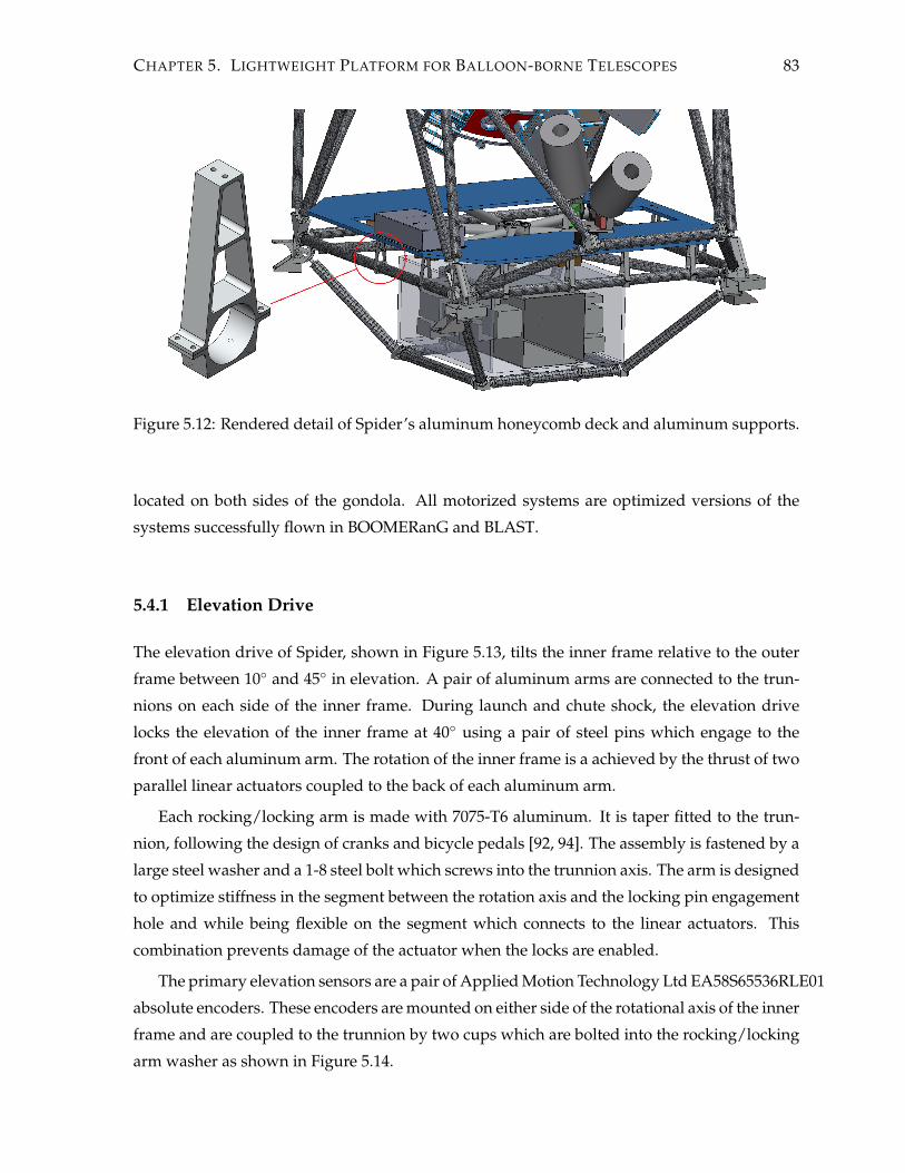
CHAPTER 5. LIGHTWEIGHT PLATFORM FOR BALLOON-BORNE TELESCOPES 83
Figure 5.12: Rendered detail of Spider’s aluminum honeycomb deck and aluminum supports.
located on both sides of the gondola. All motorized systems are optimized versions of the
systems successfully flown in BOOMERanG and BLAST.
5.4.1 Elevation Drive
The elevation drive of Spider, shown in Figure 5.13, tilts the inner frame relative to the outer
frame between 10◦ and 45◦ in elevation. A pair of aluminum arms are connected to the trun-
nions on each side of the inner frame. During launch and chute shock, the elevation drive
locks the elevation of the inner frame at 40◦ using a pair of steel pins which engage to the
front of each aluminum arm. The rotation of the inner frame is a achieved by the thrust of two
parallel linear actuators coupled to the back of each aluminum arm.
Each rocking/locking arm is made with 7075-T6 aluminum. It is taper fitted to the trun-
nion, following the design of cranks and bicycle pedals [92, 94]. The assembly is fastened by a
large steel washer and a 1-8 steel bolt which screws into the trunnion axis. The arm is designed
to optimize stiffness in the segment between the rotation axis and the locking pin engagement
hole and while being flexible on the segment which connects to the linear actuators. This
combination prevents damage of the actuator when the locks are enabled.
The primary elevation sensors are a pair of Applied Motion Technology Ltd EA58S65536RLE01
absolute encoders. These encoders are mounted on either side of the rotational axis of the inner
frame and are coupled to the trunnion by two cups which are bolted into the rocking/locking
arm washer as shown in Figure 5.14.

CHAPTER 5. LIGHTWEIGHT PLATFORM FOR BALLOON-BORNE TELESCOPES 84
Figure 5.13: Spider elevation drive. Highlighted in blue are the rocking/locking arm and thelinear actuator.
Figure 5.14: Location of the trunnion coupling (left) and exploded view of the elevation drivecoupling with the inner frame (right). The absolute encoder is shown in green. The pillow boxbearing is shown in blue.

CHAPTER 5. LIGHTWEIGHT PLATFORM FOR BALLOON-BORNE TELESCOPES 85
Figure 5.15: Location of the lock pin system (left) and detail of the lock pin assembly (right).
Locking
Locking of the inner frame is necessary to protect the linear actuators and the inner frame from
the effect of large angular accelerations resulting from the pin release as described in Section
5.1. In the case of Spider, a pair of steel pins lock the inner frame elevation on both sides at 1 m
from its rotational axis. Locking far from the axis increases the mechanical advantage of the
system and reduces the stress on the pin. Locking in both sides avoids torsion on the cryostat
and the gondola.
One of the locking assemblies is shown on the left panel of Figure 5.15. This assembly is
mounted on one of the faces of the multi-tube joint at Node D. The pin is moved in and out
from a hole aluminum arm using a MecVel ALI1F linear actuator powered by a brushed DC
motor. The pin moves inside a steel housing which also supports the linear actuator. The
housing and the aluminum arm have rulon-J bushings which facilitate the travel of the pin
by avoiding contact between metal surfaces. The inner frame is locked at 40◦ when the pin
is inserted. The impact resulting from the motion of the inner frame is absorbed by the steel
housing without compromising the actuator. The minimum FOS calculated for one of the lock
systems receiving the effect of the release angular acceleration is 1.2.
Rocking
A pair of VT-209-12 Vectac linear actuators are used in parallel to change the elevation of
the inner frame when the locks are not enabled. The arms of the linear actuator are screwed
into an aluminum insert glued to a 430 mm long, 40.2 mm ID, and 2.6 mm wall thickness
CFRP tube which serves as a extender. The other end of the composite tube is attached to the
rocking/locking aluminum arm using a steel pin and forming a hinge.

CHAPTER 5. LIGHTWEIGHT PLATFORM FOR BALLOON-BORNE TELESCOPES 86
Figure 5.16: Location of the linear actuators (left) and exploded view of the motor, gearboxand linear actuator assembly (right).
Each actuator is rated to a maximum thrust of 4003 N (900 lbf) and has 12 in of travel. The
linear actuator is trunnion mounted to the top of Node B as shown in Figure 5.16. Each linear
actuator is operated using a CM1 C23S30 CoolMuscle stepper motor in series with a Stober
ServoFit R⃝ P211 planetary gearbox (gear ratio 1:7) and a Nexen EclipseTM
Servo Motor Brake.
The brakes are enabled when the motors are not powered providing a secondary locking sys-
tem.
5.4.2 Reaction wheel
The reaction wheel allows the gondola to scan in azimuth by conservation of angular momen-
tum. The Spider reaction wheel is composed of an aluminum hub with six 1 m long, 4 in Outer
Diameter (OD), and 0.125 in wall cylindric aluminum arms ending on ∼7 kg brass bricks at
as shown in the left hand side of Figure 5.17. The bricks are fastened using 3/8-16 threaded
steel rods, which provide a FOS of 2.1 when the wheel is spinning at 145 rpm. The geometry
and mass of the flywheel are set by the azimuthal scan speed and the moment of inertia of the
whole gondola. The objective of this design is maximizing the moment of inertia needed for a
6◦ s−1 peak to peak azimuth scan while minimizing the total mass of the wheel.
The wheel mounts axially aligned to the rotor of a brushless DC motor. The motor is
custom designed and assembled around a frameless Bayside K178 motor kit. The assembly is
shown in the right hand side of Figure 5.17. It is supported by a SKF 61826 deep groove ball
bearing located close to the top of the motor and aligned by a SKF NK 90/25 roller bearing
in the bottom of the assembly. Location is read out from a 21PRCX Harowe encoder coupled
with the rotor and the stator mounting of the motor.
The flywheel is mounted on the Node Z in the middle of the outer frame where four joints

CHAPTER 5. LIGHTWEIGHT PLATFORM FOR BALLOON-BORNE TELESCOPES 87
Figure 5.17: Reaction wheel assembly (left) and section view of the reaction wheel motor(right).
are fastened around the mounting flange located on top of the motor case. The rotational axis
of the flywheel is designed to be collinear with the rotational axis of the pivot and intercept
the rotational axis of the inner frame. This configuration minimizes pendulations and other
dynamical effects which affect the gondola pointing.
5.4.3 Pivot
The pivot is the connection point between the cables supporting the outer frame and the flight
train. The pivot allows the gondola to rotate relative to the balloon acting as a motorized
swivel. The Spider and the BLASTPol pivots are custom designed and assembled around a
frameless Bayside K178200 brushless DC motor kit. The assembly is shown in Figure 5.18.
The design of the pivot is based on a SKF 51218 thrust ball bearing which supports all the
weight of the payload and SFK NK 90/25 and SFK NK 90/25 needle roller bearings which
center the shaft over and beneath the primary bearing. The thrust bearing is located between
a steel casing with tabs where the suspension cables are fastened and a steel rotor which con-
nects to the flight train through the universal joint. The bottom of the steel shaft is bolted to an
6061-aluminum cylinder which supports the rotor of the motor while the stator of the stator is
fastened to the motor case. Both components of the motor are glued using the adhesives pre-
scribed by the provider. Location is read out from a 21PRCX Harowe encoder coupled with
the rotor and the stator mounting of the motor.
The structurally critical parts of the pivot are the steel casing, the shaft, and the bearing, all
of which have been tested in the BLASTPol pivot. The FEA studies provide minimum FOS of
1.51, 2.79, and 1.46 respectively.

CHAPTER 5. LIGHTWEIGHT PLATFORM FOR BALLOON-BORNE TELESCOPES 88
Figure 5.18: Render (left) and section view (right) of the Spider pivot.
5.5 Sunshields
The Spider sunshields frame is mounted to the base of the outer frame using four aluminum
supports. The frame is covered with two layers of aluminized mylar as described in Section
4.4.1. The sunshields are built using a combination of CFRP tubing and aluminum joints in a
simplified version of the design used for the outer frame. This construction technique is based
on the design successfully tested in BLASTPol10 and BLASTPol12.
5.5.1 BLASTpol Baffle
The visibility of the BLASTPol science targets requires shielding the gondola from direct sun-
light at 40◦ from the sun position in azimuth. Successful observations were possible thanks
to the shielding provided by a baffle located around the primary mirror and extending 7 m in
the bore-sight direction. The baffle frame is a truncated cylindrical structure with a hexagonal
base made of CFRP tubes with aluminum inserts connected with aluminum hubs as shown in
Figure 5.19.
The CFRP tubes selected for this application are the CST composites AA20020A: a 20.0 mm
ID and 2.0 mm wall thickness CFRP tube. The selection of this product was made following a
series of mesh beam simulations as described in Section 5.3. Although the design constrains
and loads are not as demanding as in the case of the outer frame, the location of the baffle
structure directly around the observation field of the telescope demanded especial attention
to the rigidity and structural integrity after launch. The structure required aggressive light-
weighting to avoid increasing the moment of inertia of the inner frame over the capacity of

CHAPTER 5. LIGHTWEIGHT PLATFORM FOR BALLOON-BORNE TELESCOPES 89
Figure 5.19: BLASTPol baffle assembly. The detail shows the multi-tube coupling in the alu-minum hub.
the elevation drive. Additionally, the resonant frequencies of the structure had to be kept over
15 Hz to avoid resonance with the natural frequencies of the experiment.
The structure of the BLASTPol baffle starts with a hexagonal ring which dimensions are
determined by the clearance space around the primary mirror. Three more hexagonal rings
are set at equal distances between the first ring and the minimum distance necessary to keep
the sunlight off the primary and secondary mirrors at 40◦ in azimuth from the position of
the sun. Each hexagonal ring is offset by 30◦ from the orientation of the previous ring to
produce a triangular truss structure between each ring. The full cylindrical structure is not
needed to shield the primary or the secondary mirror so the port side of the structure is open
leaving only four sides of the hexagon on the third ring and only one in the fourth ring. The
asymmetry avoids reflection of sunlight on the inner part of the baffle without compromising
the structural integrity of the structure.
The joints connecting the tubes are aluminum octahedrons with two parallel faces (top and
bottom) and six faces perpendicular to the base forming a hexagon. They are centered on the
node where the axis of the tubes converge, making the faces of the hexagon perpendicular to
the tube axis. The inserts are made with aluminum plates which mount to the hexagonal faces
of the hub with two 1/4-20 bolts. The plates are welded to an aluminum cylinder oriented
in the direction of the axis of the tube. This cylinder serves as the coupling surface for the
adhesive joint with the CFRP tube as shown on the zoomed-in detail of Figure 5.19.
The large area covered by the mylar makes the wind force an important aspect in the design

CHAPTER 5. LIGHTWEIGHT PLATFORM FOR BALLOON-BORNE TELESCOPES 90
Figure 5.20: Spider sunshield assembly. The detail shows the multi-tube coupling at the alu-minum hub.
of the sunshield frame. The magnitude of the wind force can be calculated from:
Fair =1
2ρACv2 (5.2)
where A is the effective area facing the wind, v is the velocity of the wind, and C is a correc-
tion factor which depends on the geometry of the shields. In order to validate the model, a
worst-case scenario was considered where A corresponds to the largest effective area of the
shields and C = 1 corresponding to a flat surface perpendicular to the air flow. The BLASTPol
structure has a FOS superior to 2.0 under the load of 20 knot (10.3 m s−1) winds.
5.5.2 Spider Sunshield
The Spider sunshields follow the same construction technique and design concept described
in Section 5.5.1: the structure is a cylinder with a hexagonal base composed of CFRP tubes
fastened by aluminum inserts and joints. The main modification with respect to the design of
the BLASTPol baffle is the diameter of the CFRP tubing which has been increased according
to the larger loads on the structure. The chosen product is the CST Composites AA32018: a
32.0 mm ID and 1.8 mm wall thickness CFRP tube.
The Spider sunshields implement a new feature in the construction technique: the combi-
nation of custom-angle fixed aluminum inserts with universal-joint-type insert which can be

CHAPTER 5. LIGHTWEIGHT PLATFORM FOR BALLOON-BORNE TELESCOPES 91
oriented in two different angles as shown in Figure 5.20. A universal-joint-type insert follows
the tube incidence angle in two directions: one is defined by the hinge formed by the tube in-
sert and the yoke block. The other is defined by the rotation of the yoke over the plate fastened
to the aluminum. This versatile type of inserts constitutes a general solution for the assembly
of structures with moderated loads such as baffles and sunshields.
The gluing of this structure is made in place after dry assembling the structure. The dis-
tance between the joints is constrained by cutting the tubes to length with ±1 mm tolerance.
The assembly temporarily held together using ropes around the tubes. In the absence of an
extended flat surface to use as a reference for the assembly, the ropes constrain rotation of the
hubs and ensure that the elements are held in the right configuration. The gluing is made
triangle by triangle on several stages.
As well as in the BLASTPol baffle, one of the main considerations in the design of the
Spider sunshields is the lateral and vertical wind force. The Spider sunshields are designed
to hold the pivot during parachute shock and maintain structural integrity when covered and
exposed to 20 knot (10.3 m s−1) winds. Additionally, its lowest resonance frequency is over
15 Hz guaranteing that the vibrational modes will not affect the pointing of the gondola.

Chapter 6
BLASTPol Observations
The observations of BLASTPol10 began on December 27th, 2010 and continued during a 9.5
days flight around Antarctica. Nearly 200 hours of scan mode observations were made of
the Lupus I molecular cloud, the Vela C molecular cloud, the Carina Nebula, and the Puppis
Cloud Complex. Unfortunately, during ascent to observing altitude, the outermost IR blocking
filter melted introducing significant degradation of the submillimeter beam shape. The melted
filter, shown in Figure 6.1, produced an increased beam with non-Gaussian structure. The in-
flight submillimeter beams obtained from observations of the Infrared Astronomical Satellite
(IRAS) 08470-4243 ultracompact HII region (Mickey) are illustrated in Figure 6.2.
Additional to the non-Gaussian beam, an unexpected noise signal was found in the de-
tector time streams. The noise component, illustrated in Figure 6.3 and denominated popcorn
noise, was present in around 40% of the observations and is distributed over the entire flight.
In principle, the popcorn noise is present in the form of spikes on the time streams and it is
consistent with a Radio Frequency (RF) signal heating the detectors. The popcorn noise can be
identified using a passband filter but its statistical properties make it very hard to remove from
the contaminated sections of the bolometer time streams. Those segments are unsuitable for
the construction polarization maps.
After the launch, the motor of the reaction wheel presented high power consumption
which is consistent with mechanical stiction. Finally after a few hours the reaction wheel mo-
tor stopped responding and the azimuth pointing had to be made using only the pivot with
minimum consequences for the flight performance. The causes of the reaction wheel malfunc-
tion are still undetermined. It is possible that some oxidation of the bearing unit caused by air
condensation during ground testing combined with a large angular acceleration during pin
release could have cause the damage.
Eight days after the launch, the port side star camera (ISC) stopped responding and boot-
ing. The source of this malfunction is related to the Hard Disk Drive (HDD) of the star camera
92

CHAPTER 6. BLASTPOL OBSERVATIONS 93
Figure 6.1: BLASTPol10 window filter melted before flight [95].
Figure 6.2: Mosaic of BLASTPol10 beam maps corresponding to in-flight observations of theIRAS 08470-4243 ultracompact HII region with the 500 µm array. Courtesy of David Nutterand the BLASTPol collaboration.

CHAPTER 6. BLASTPOL OBSERVATIONS 94
Figure 6.3: BLASTPol10 flight data streams of a dark bolometer (B5D1) shown in top panelsand a regular bolometer (B5D03V) shown in the bottom panels. The left hand side panel showsgood data, the right hand side panel shows data with popcorn noise.
computer. This problem was addressed in BLASTPol12 by replacing the HDD with SSD.
The outcome of BLASTPol10 was a set of maps of the Lupus I, Vela C, and the Carina Neb-
ula smoothed to 22.5′in all three wavelengths to mitigate the non-Gaussianity of the beam. The
instrumental polarization was characterized using the technique of sky rotation as described
in [31]. Observations are broken into two bins based on the parallactic angle of the source.
The polarization is estimated using a method analogous to aperture photometry comparing
bright regions of the intensity map with low flux regions as described in [96]. The results are
assessed through a series of jack-knife tests which compare the results in different segments
of the flight, different target elevations, and different sky rotations. An example of a resulting
polarization map is shown in Figure 6.4.
From the thermal and mechanical point of view, BLASTPol10 was a successful campaign.
The telescope adequately pointed and made observations at 40◦ from the azimuth position of
the Sun, an unprecedented sun avoidance position. BLASTPol10 was also the first flight of the
carbon fiber and aluminum structure. The performance and survival of this structure after
landing were both excellent. The thermal behavior of the gondola components was adequate
and the predictions of the thermal model were within ±10◦C of the in-flight temperatures.
The BLASTPol10 polarization maps constitute a state-of-the-art measurement of the mag-
netic field morphology in the observed regions. However, the multiple pathologies in the data
set make it unsuitable for detailed statistical analysis. This was the main motivation for the
new flight plans that led to BLASTPol12, and ultimately the main reason for the development

CHAPTER 6. BLASTPOL OBSERVATIONS 95
Figure 6.4: Polarization map of the Lupus I region observed in BLASTPol10 [97]. Thered and green pseudovectors correspond to polarization observations at 500 µmand350 µmsuperimposed on a AV map of Lupus I (grayscale). The blue arc represents an esti-mate of the filament orientation.

CHAPTER 6. BLASTPOL OBSERVATIONS 96
of the HRO.
This chapter briefly describes the process of data reduction, emphasizing on the bolometer
noise characterization. Additionally it introduces the BLASTPol12 observations as a promising
data set to be studied using the HRO.
6.1 Data Reduction
The data reduction is the process of generating high-quality submillimeter intensity and po-
larization maps from the raw bolometer time streams. This process consists of ten main steps,
many of which are run in parallel [50]:
1. Initial data preparation
2. Detector cleaning
3. Pointing solution generation
4. Detector response profiling
5. Preliminary map making
6. Noise estimation
7. Flat fielding and absolute calibration
8. Detector alignment
9. Field alignment
10. Final map making
The initial data preparation, detector cleaning, and detector response profiling are de-
scribed in [98]. The preliminary map making made using NaivePol is described in [46]. The
flat fielding, calibration, pointing solution generation, and detector alignment are described in
[38, 96].
6.1.1 Bolometer Noise Characterization
There are two main types of noise in the bolometers: white noise and flicker noise. The white
noise is by definition a random signal with a flat (constant) power spectral density. The flicker
noise has a 1/f -noise spectrum. Both types of noise can be identified by calculating the Power
Spectral Density (PSD) of the in-flight bolometer time streams taken when the telescope is

CHAPTER 6. BLASTPOL OBSERVATIONS 97
pointing to a relatively low-signal-to-noise region in the sky. The white noise is characterized
by the value of the PSD at the plateau frequencies while the flicker noise is characterized by
the frequency where the 1/f -dependence of the PSD begins (1/f knee).
During BLASTPol10 the detector noise was characterized using a 15 minutes segment of
the time streams obtained while the telescope was pointing to ν Centauri. This region is rela-
tively homogenous in submillimetric wavelengths and was scheduled initially for star camera
calibrations. The PSD was obtained dividing the observation in 1 minute segments, calculating
the PSD of each segment and finally averaging the PSDs.
The bolometers PSD can be approximated by
PSD = w ·
√(fkneef
)2
+ 1 (6.1)
where w is the white noise level and fknee is the frequency which characterizes the 1/f depen-
dence of the noise PSD. These parameters can be obtained by fitting a line to the scatter plot of
(PSD)2 and 1/f2. The intercept is w2 and the slope is w2f2knee.
Figure 6.5 shows the PSD of selected bolometers at 250, 350 and 500 µm. The segmented
line in the figure corresponds to the best fit of (PSD)2 as a function of 1/f2. The white noise
level is on average 4.93, 4.13, and 3.84 ×10⁻⁶ V Hz−1/2 in the 250, 350 and 500 µm bolometers.
The 1/f knee was estimated to be at 0.11, 0.31, and 0.22 Hz respectively.
The 350 and 500 µm bolometers are more sensitive to the peak at 0.05 Hz which corre-
sponds to the pendulation frequency of the gondola. This feature tends to larger estimates of
the 1/f knee. This is not problematic in the case of BLASTPol10 since the naive maps can be
made enforcing a common high-pass filter over 0.5 Hz [38]. Nevertheless, optimal mapmaking
requires a more detailed characterization of the 1/f noise.
6.2 The BLASTPol12 data
The observations of BLASTPol12 began on December 27th, 2010 and continued during a twelve
days flight around Antarctica. Nearly 200 hours of scan mode observations were made of the
Lupus I molecular cloud, the Vela C molecular cloud, the Carina Nebula, and the Puppis
Cloud Complex. The melted filter which affected BLASTPol10 was replaced and the aperture
was protected by an aluminium shutter.
The popcorn noise was addressed by separating the charge control system of the receiver
from the rest of the gondola. During compatibility tests outside of the highbay it was observed
that the time streams were contaminated by RF of the neighboring Pegasus Air Field and the
pattern on the time streams was similar to the popcorn noise registered in BLASTPol10. During

CHAPTER 6. BLASTPOL OBSERVATIONS 98
Figure 6.5: Time streams (left) and amplitude spectra (right) of typical BLASTPol10 bolometersat 250 µm (top), 350 µm (middle), and 500 µm (bottom). The segmented lines correspond tothe results of the (PSD)2 versus 1/f2 fit.

CHAPTER 6. BLASTPOL OBSERVATIONS 99
flight, close inspection of the time streams revealed the presence of popcorn noise correlated
with the operation of the Tracking and Data Relay Satellite System (TDRSS) network high gain
antenna. The popcorn noise was largely mitigated by turning off the corresponding antenna
during most of the flight.
A few hours after reaching float altitude, the starboard star camera (OSC) stopped respond-
ing and booting. Nine days later, the port star camera (ISC) stopped responding or booting
ending the regular operation of the pointing system of BLASTPol. This malfunction is simi-
lar to problems in the SSD registered by the Super-TIGER Cosmic Ray Experiment [99] which
was flying over Antarctica at the same time as BLASTPol. Pointing reconstruction with one
star camera is possible and currently significant efforts are being made to generate pointing
solutions using the sun sensor and the Spider star camera flown on board of BLASTPol.
In sum, despite the star camera failure, the BLASTPol12 data is superior to the BLASTPol10
data. The presence of the popcorn noise was mitigated during most of the flight. The star cam-
era failure is being addressed by reconstruction of the pointing from the secondary pointing
detectors. The reaction wheel operated normally throughout most of the flight. The mapmak-
ing process is optimized by a new scanning strategy which includes reference regions around
the science targets. Polarization maps of the Lupus I molecular cloud, the Vela C molecular
cloud, the Carina Nebula, and the Puppis Cloud Complex are expected to be the outcome of
this flight.
At the moment when this document is concluded, significant work is being made in pro-
ducing an optimal mapmaker design for polarization maps. Additionally, detailed studies of
the beam shape and the polarization signal reconstruction [38, 96] are in progress. Prelimi-
nary polarization maps, such as the map of the Carina Nebula shown in Figure 6.6, present a
promising data set for the study of the polarization and the magnetic field using new statis-
tical tools which establish a bridge between observations and simulations of the star forming
clouds. The HRO, introduced in Chapter 7, is one of these tools.

CHAPTER 6. BLASTPOL OBSERVATIONS 100
Figure 6.6: Preliminary polarization map of the Carina Nebula observed in BLASTPol12. Pre-liminary result courtesy of Tristan Matthews and the BLASTPol collaboration.

Chapter 7
The Histogram of Relative Orientations
(HRO)
The study of the magnetic field in molecular clouds is crucial to understand the physical pro-
cesses relevant in molecular cloud evolution and star formation [1, 3, 12]. Although some the-
oretical models point out to supersonic turbulence as an important possibly dominant mecha-
nism in the formation of structure in molecular clouds [7, 8], recent studies indicate the mag-
netic field is also very important in particular regimes and scales [9, 10, 11]. The formulation
of a complete model of the process that transforms gas into stars requires the comparison
between the observations of the magnetic field and predictions from simulations.
The intensity of the magnetic field along the line of sight can be estimated using the Zee-
man effect [13, 14], the Faraday rotation of linearly polarized radiation from radio sources
[100, 101], and the synchrotron unpolarized emission [102, 103, 18]. The morphology of the
magnetic field projected onto the plate of the sky is observable by measuring polarized radia-
tion [15, 12].
A longstanding technique used to infer the morphology of the magnetic field projected on
the plane of the sky is the measurement of polarization of visible and near-infrared light back-
ground stars [20, 104, 105]. This technique assumes that aspherical dust grains are aligned
with respect to the interstellar magnetic field and the observed position angle of linear po-
larization is parallel to the plane-of-the-sky-projection of the field [104, 106]. A more recent
complementary technique is the measurement of the thermal polarized emission of dust in
the submillimeter wavelengths [26, 107, 108]. Measurable degrees of polarization on the order
of a few percent are typical for interstellar clouds in the submillimeter and the far-infrared
[109, 110]. The mechanism which produces the alignment of the grains is still the subject of
active research [111, 112, 113, 21, 114]. However, there is evidence indicating that it results
from radiative torques produced by anisotropic radiation flux with respect to the magnetic
101

CHAPTER 7. THE HISTOGRAM OF RELATIVE ORIENTATIONS (HRO) 102
field [115]. Theoretical understanding of the grain alignment indicates that even in relatively
dense clouds (visual extinction AV ∼ 10), dust polarization traces the underlying magnetic
field [116].
The strength of the magnetic field has been estimated from observations of the projected
component on the plane of the sky using the Chandrasekhar-Fermi method (CF) [22, 117, 25,
31]. This method is based on the dispersion of the orientation angles of the polarization pseu-
dovectors. Theoretical modeling of CF shows that the magnetic field strength estimates are
improved by separating the turbulent and uniform components of the magnetic field [23, 24].
Maps of local magnetic field strength around pre-stellar cores have been obtained by compar-
ing the polarization orientation angles and the intensity gradient, assuming ideal Magnetohy-
drodynamics (MHD) equations and spherical symmetry for the dust distribution in the core
[118].
Significant studies have been made to relate the magnetic field morphology inferred from
polarization to the density structure in both observed [10, 30] and simulated clouds [119, 120].
In the case of pre-stellar cores, a number of observations reveal an hourglass morphology in
the magnetic field [121, 122]. In the case of larger structures, the morphological analysis relies
on visual inspection and statistics of the orientation angles [123]. The results of observations
are inconclusive in establishing a global trend of relative orientation between the magnetic
field and the structure [124]. Theory and simulations try to identify extreme cases which il-
lustrate the scenarios where the formation of the structure in the cloud is dominated by ei-
ther the magnetic field or the turbulence. Some of the predictions of the models are helical
fields around filaments [125, 120], elongated structures along the magnetic field lines when
the medium is strongly compressed supersonically [119, 126, 23], and linear correlation of the
magnetic field strength with column density for supersonic turbulence [127].
Recent observations by the European Space Agency (ESA) Herschel Mission reveal ubiq-
uitous filamentary structures in molecular clouds [128, 129, 130]. These observations together
with starlight polarization measurements have been used to investigate the physical condi-
tions of gravitational collapse and star formation within the filaments. Seminal examples in
which the inferred magnetic field direction in adjacent lower density material is perpendicu-
lar to the densest filaments are in Taurus [30, 131], Serpens [132], the Musca Dark Cloud [133],
and the Pipe Nebula [134]. These studies provide insight into the physical processes involved
in the formation of filamentary structure but they do not probe the complex relationship of
column density and magnetic field morphologies in the dense regions of molecular clouds,
where stars predominantly form and which are fundamental to establishing a global picture
of molecular cloud formation [135].
The advent of new instruments for measuring the thermal dust polarized emission such
CHAPTER 7. THE HISTOGRAM OF RELATIVE ORIENTATIONS (HRO) 103
as ALMA [136], BLASTPol [137] and Planck [138] will produce an unprecedented volume
of polarization maps in scales ranging from pre-stellar cores to entire molecular cloud com-
plexes, including regions too extincted for starlight polarization observations. This large data
set motivates a common scheme for the morphological analysis of polarization maps. It is in
this context that we introduce the Histogram of Relative Orientations (HRO), a novel statis-
tical tool for characterizing column density morphologies on multiple scales. This technique,
developed for pattern recognition in machine vision, uses the gradient to characterize the di-
rectionality of the density structure in a 2D map and here in a 3D simulated cube. It provides
a robust characterization of the density field that can be used with polarization observations
to investigate the relative orientation of density structure with respect to the magnetic field.
This chapter is organized as follows: Section 7.1 introduces the Histogram of Relative Ori-
entations. Section 7.2 introduces the simulations of molecular clouds used to characterize our
statistical tool. Section 7.3 presents the HRO analysis of 3D simulated clouds and Section 7.4
shows how the proposed diagnostic obtained in 3D can also be found in the projected 2D
maps. Finally Section 7.5 summarizes the results and discusses the application of HROs to
observations of real molecular clouds.
7.1 The Histogram of Relative Orientations Method
The Histogram of Relative Orientations (HRO) is inspired by a family of detection algorithms
usually called Histogram of Oriented Gradients (HOG)s [139]. HOGs are used in pattern
recognition and are developed in the context of machine vision. These algorithms use the
gradient to describe the orientation of the edges in an image. The gradient is based on the
difference between pixels in a neighborhood and quantifies the edges: the magnitude carries
the information on the difference (edge strength) and the orientation defines the direction per-
pendicular to a contour line (edge direction). A histogram of the orientation angles of the
gradient rotated by 90◦ therefore summarizes statistically the orientation of the features in an
image. Further refinement of this method includes weighting the contribution of each pixel
(or voxel in 3D) to the histogram by the magnitude of the gradient at each point, allowing the
characterization of the image using only the stronger edges.
In the HRO, the gradient of the density (column density) characterizes the directionality
of the structures in a vector field which is directly compared to the magnetic field on each
voxel (pixel) using the scalar product of vectors. The result of this operation is a relative
orientation angle between both vectors in each pixel which is characterized by a histogram. In
3D, the HRO is the histogram of relative orientation angles between the magnetic field vector
B and the density gradient ∇n. In 2D, the HRO is the histogram of relative orientation angles

CHAPTER 7. THE HISTOGRAM OF RELATIVE ORIENTATIONS (HRO) 104
between the projected magnetic field pseudovector B and the column density gradient ∇Σ.
The calculation of the gradient and the estimation of the angle between vectors are described
in the following subsections.
7.1.1 Calculation of the Gradient
The orientation of the isodensity contours is characterized by the gradient of density:
∇n =
(∂n
∂x
)(l)
x+
(∂n
∂y
)(l)
y +
(∂n
∂z
)(l)
z. (7.1)
The subindex l is related to the size of the area on which the gradient is calculated or as sub-
sequently shown, the size of the Gaussian derivative kernel. To zeroth order, the components
of the gradient can be calculated using forward differences of adjacent pixels:
∂n
∂x∼ n(x+ 1, y, z)− n(x, y, z). (7.2)
Derivatives are linear and shift-invariant, and so the gradient calculation can be done by
convolving the image with a particular kernel. The result of the convolution of a slice of the
simulation cube n(x, y) = n(x, y, z = z0) with a l × l derivative kernel K(∂/∂x) is:
(∂n
∂x
)(l)
= n(x, y) ⋆ K(∂/∂x),(∂n
∂x
)(l)
ij
=
l−1∑t,u
ni+t−l/2,j+u−l/2K(∂/∂x)t,u . (7.3)
Forward differences can be calculated using the 2 × 2 Roberts kernels, but such a small
kernel is too sensitive to noise. The calculation of the gradient can be improved by using the
central differences:
∂n
∂x=
n(x+ 1, y)− n(x− 1, y)
2,
∂n
∂y=
n(x, y + 1)− n(x, y − 1)
2. (7.4)
Applying this operation to all the pixels in an image is equivalent to convolving the image
with 3× 3 Prewitt kernels:
K(∂/∂x) =1
6
−1 0 1
−1 0 1
−1 0 1
, K(∂/∂y) =1
6
−1 −1 −1
0 0 0
1 1 1
. (7.5)

CHAPTER 7. THE HISTOGRAM OF RELATIVE ORIENTATIONS (HRO) 105
Noise reduction is achieved by averaging over the vicinity of each pixel. This is imple-
mented to first order using the 3×3 Sobel kernels. Convolving with these kernels is equivalent
to smoothing the image over a 3 × 3 region and then calculating first derivatives, which is a
particular case of the Gaussian Derivatives method:
K(∂/∂x) =
−1 0 1
−2 0 2
−1 0 1
, K(∂/∂y) =
−1 −2 −1
0 0 0
1 2 1
. (7.6)
Gaussian Derivatives
In HROs, the computation of the gradient is performed using Gaussian derivative kernels.
The size of the Gaussian determines the area of the vicinity over which the gradient will be
calculated. Varying the size of the Gaussian kernel enables the sampling of different scales
and reduces the effect of noise in the pixels.
Convolution and differentiation are commutative and associative; therefore the smoothing
and derivative operators can be written as:
∂
∂x(I ⋆ G) = I ⋆
∂
∂xG (7.7)
G is the 2D-Gaussian kernel and I is a 2D image. This equation implies that filtering an image
and subsequently calculating the gradient is equivalent to the convolution of the image with
a kernel that is the first derivative of a gaussian kernel. This operation is called a Gaussian
derivative [140].
For the present study, we use the Gaussian derivatives method and following Equation 7.7
we obtained each component of the gradient by convolving slices of the density cube n(x, y) =
n(x, y, z = z0) and n(y, z) = n(x = x0, y, z) with a kernel formed by the derivative of a l × l
map of a two-dimensional Gaussian G(l):
(∂n(x, y, z = z0)
∂x
)(l)
= n(x, y) ⋆∂
∂xG(l)(x, y),(
∂n(x, y, z = z0)
∂y
)(l)
= n(x, y) ⋆∂
∂yG(l)(x, y), (7.8)(
∂n(x = x0, y, z)
∂z
)(l)
= n(y, z) ⋆∂
∂zG(l)(y, z).

CHAPTER 7. THE HISTOGRAM OF RELATIVE ORIENTATIONS (HRO) 106
In the 2D projected maps
(∂Σ
∂x
)(l)
= Σ ⋆∂
∂xG(l) (7.9)(
∂Σ
∂y
)(l)
= Σ ⋆∂
∂yG(l).
The orientation angle of the iso-Σ contours in the 2D project maps is:
ψ ≡ arctan
(∂Σ/∂x
∂Σ/∂y
), (7.10)
which according to the convention for position angles of polarization is measured counter-
clockwise from the top of the map.
Figure 7.1 illustrates the characterization of a simulated image using the gradient of the
column density ∇Σ. The vectors plotted over the image show the direction of the gradient
obtained using Gaussian kernels of different sizes. The histogram shows the orientation angles
of the structures in the image, measured counterclockwise with respect to the y-axis of the
image (convention for polarization position angles). Each peak in the histogram corresponds
to a dominant orientation of the features in the image. A histogram of a completely random
map would be flat. The histogram of a straight rod would be a delta function centered on its
orientation angle. The histogram of a blob would have a peak corresponding to the orientation
of its semi-major axis.
The HROs use the gradient of the density in 3D simulated cubes to generate a vector field
which characterizes isodensity contours and can be directly compared to the magnetic field
vectors. In 2D, the gradient of the column density (∇Σ) is compared to the orientation of the
linear polarization field, which is a pseudovector since it is invariant to a ±180◦ rotation.
7.1.2 Calculation of the Angle
The angle ϕ between the gradient and the magnetic field at each voxel is calculated using a
combination of the scalar and vector product of vectors:
ϕ = arctan
(|B×∇n|B · ∇n
)(7.11)
The result of this calculation is a cube (a map in 2D) with values of ϕ at each voxel (pixel
in 2D). As explained in Section 7.3, in the study of the alignment in 3D it is more natural to
construct the HROs as a function of cosϕ and not directly ϕ. The angle between the isodensity
contours and the magnetic field is ϕ±90◦. The histogram of values of cosϕ (ϕ in 2D) weighted

CHAPTER 7. THE HISTOGRAM OF RELATIVE ORIENTATIONS (HRO) 107
Figure 7.1: Left: Filamentary structure in the simulated column density. Overlaid are thegradient vectors obtained with derivative kernels with 9×9 (yellow), 25×25 (red), and 49×49(green) pixels. The squares on the upper right corner of the image show the sizes of thesekernels. Right: Histogram of orientation angles of the iso-Σ contours (ψ) calculated with eachderivative kernel. The histograms show that the structure is predominantly oriented at ψ from135◦ to 150◦ but also shows a secondary structure at 45◦.
by the magnitude of the gradient at each voxel (pixel) is what we call Histogram of Relative
Orientations.
Figure 7.2 shows a histogram of cosϕ calculated on a simulated cube and ϕ calculated on
a projection of the cube using three derivative kernels. Using these three kernels we observe
the same preferential relative orientation between B and ∇n in the cube and BPOS and ∇Σ in
the projection.
7.1.3 Segmentation
Individual regions of a cube (map) are studied by dividing it into bins of the parameters that
define it and subsequently masking each bin. This process is known in computer science as
image segmentation. Segmentation is a subject of active research in computer science and its
implementation in 3D (2D) HROs is limited to dividing the cube (image) in density (column
density) bins with the same number of voxels (pixels).
The objective of the segmentation is the study and comparison of the relative orientation
in density regimes where the dominant physical processes and the dust alignment efficiency ϵ
are different. The segmentation by column density of the maps resulting from the projection of
the simulated cubes is illustrated in the left-hand side of Figure 7.3. Using the column density

CHAPTER 7. THE HISTOGRAM OF RELATIVE ORIENTATIONS (HRO) 108
Figure 7.2: HROs obtained by applying three different derivative kernels to a simulation cube(left) and to a projected map obtained by integrating the cube along the z-axis (right). Thesimilarity of the curves within each plot shows that the predominant relative orientation ispresent in regions with scales ranging from 3 pixels to 49 voxels (pixels).
distribution, which is close to log-normal, we produce density bins with the same number of
pixels. An equal number of gradient vectors in each bin guarantees comparable statistics for
each density bin.
The segmentation by density or column density is motivated by the change of physical
conditions in the densest regions with respect to less dense regions. In the densest regions
self-gravity becomes relevant and the kinetic energy density is lower than the magnetic en-
ergy density, in contrast with the less dense regions where the balance between magnetic and
turbulent energy is different. The segmentation of maps by polarization percentage, line of
sight velocity or polarization angle dispersion is a potentially useful way to study physical
processes in observations of molecular clouds and will be addressed in future works.
7.2 Model Parameters
The cloud models used to characterize HRO are created by integrating the compressible ideal
MHD equations using the RAMSES-MHD code [141, 142]. RAMSES-MHD is a N-body and
MHD code with 3D Adaptive Mesh Refinement (AMR). The refinement criteria are based on
density as described in Dib et al. [143]. RAMSES-MHD uses constrained transport to guarantee
that ∇ ·B = 0 to machine accuracy at all time and uses the MUSCL-Hancock scheme, a finite
volume method that combines good accuracy with fast execution. The solutions are obtained
in a cubic box of side L with grids of 5123 zones, integrated from the AMR cubes with effective
resolution 20483.
The energy equation used in this simulation set is the barotropic equation of state: these
clouds are isothermal with T = 11.44 K (sound speed cs = 0.2 km s−1) for regions with density

CHAPTER 7. THE HISTOGRAM OF RELATIVE ORIENTATIONS (HRO) 109
Figure 7.3: Example of the map segmentation technique used in the HRO analysis. Left: Col-umn density distribution in projections of three simulations. Overlaid colors correspond todensity bins with equal number of pixels in regions with Σ > Σ. Gray regions correspondsto pixels with Σ < Σ. Right: Column density maps of the projections of three simulations.Overlaid colors correspond to regions with column densities shown in the histograms.

CHAPTER 7. THE HISTOGRAM OF RELATIVE ORIENTATIONS (HRO) 110
less than 104 times the initial density n0 and adiabatic for larger densities. In the absence of
fully time-dependent radiative transfer this represents a reasonable first approximation for the
gas at volume densities higher than the mean (comprising most of the matter) for conditions
appropriate to molecular clouds [144]. The solutions are obtained in a cubic box of side L
with initial uniform density n0 = nH2 = 536.41 cm−3, which is comparable to the density in
the Taurus-Auriga Dark Cloud Complex [145]. We apply periodic boundary conditions in all
models, simulating a portion of the interior of a molecular cloud.
The gravitational potential is computed from the density using standard Fourier methods.
The periodic boundary conditions exclude the k = 0 component of the density. Therefore, the
gravitational potential ϕG obeys the modified Poisson equation ∇2ϕG = 4πG(ρ − ρ), where
ρ =M/L3 is the mean density (mass divided by the volume of the box).
The relative importance of gravity and thermal pressure forces is related to L and n0. For
this analysis we have chosen L = 4 pc; the Jeans length LJ ≡ cs(π/Gρ0)1/2 is 0.88 pc for
ρ0 = µn0 and µ = 2.4mp, where mp is the proton mass (1.67262178× 10⁻²⁴ gr). The total mass
in the simulated cubes is 2.04 × 10³M⊙ and with L = 4 pc, it is comparable to small regions
within Dark Cloud Complexes such as Lupus I [146].
Turbulence in the simulation is introduced as an initial isotropic random velocity field δv
with a Kolmogorov energy spectrum E(k) ∝ k−5/3. δv is a Gaussian random perturbation
field with a power spectrum |δvk|2 ∝ k−11/3. The Kolmogorov energy spectrum is comparable
to the spectrum inferred for large-scale cold interstellar clouds [147] and the spectrum that
naturally follows from the evolution of incompressible turbulence. An identical realization of
the initial velocity field is used for all of the models, so that the initial states of the simulations
differ only in the strength of the mean magnetic field. The velocity field is a mixture of com-
pressible and solenoidal modes. In the current study we focus on the characterization models
with different magnetization. To keep this comparison simple, the turbulence decays during
the cloud evolution (it is not driven), avoiding the complexity introduced by modeling the
energy injection rate and the spectrum of driven turbulence. All simulations are initiated with
kinetic energy EK = 100ρL3c2s corresponding to an initial Mach number M ≡ σv/cs =10 and
include gravity.
Three different initial magnetization cases are considered and parameterized by the ratio of
the isothermal sound speed to the initial Alfven speed or equivalently, the ratio of the plasma
pressure to the initial magnetic pressure: β ≡ c2s/v2A,0 = ρc2s/(B
20/4π). We consider a “quasi-
hydrodynamical” model with β = 100.0, an “intermediate magnetization” model with β =
1.0, and a “high magnetization” model with β = 0.1. The physical value of the magnetic field

CHAPTER 7. THE HISTOGRAM OF RELATIVE ORIENTATIONS (HRO) 111
β < B0 > Snapshot Age(µG) (Myr) (tg) (tf )
100.0 0.35 0.48 0.11 0.25100.0 0.35 1.16 0.27 0.601.0 3.47 0.69 0.16 0.361.0 3.47 1.32 0.31 0.680.1 10.97 0.61 0.14 0.320.1 10.97 1.15 0.27 0.59
Table 7.1: Model parameters and times of snapshots. The snapshots are described in termsof the characteristic gravitational time scale tg = 4.27 Myr and the flow crossing time scaletf = 1.95 Myr.
is given by:
B0 = β−1/2
(T
10 K
)1/2 ( nH2
100 cm−3
)1/2µG. (7.12)
For the chosen initial density and temperature, the corresponding uniform magnetic field
strengths are 0.35, 3.47, and 10.97 µG. The evolved fields are spatially nonuniform and can
differ greatly from the initial values although the volume-averaged magnetic field is a con-
stant B0x in time. The value of β is proportional to the mass-to-magnetic flux ratio in the
simulation and cannot change with time.
The initial Alfven Mach number MA ≡⟨v2/v2A
⟩1/2= Mβ1/2 is 100, 10, and 3.16 for β =
100.0, 1.0, and 0.1 respectively, and therefore all models considered have initially supersonic
and super-Alfvenic flow. In this work, “high magnetization” is relative to thermal and mag-
netic pressures only, given that the turbulence is the dominant energy density in all considered
models. The initially uniform clouds are unstable to compressions transverse to the mean mag-
netic field (“magneto-Jeans unstable”) when the magneto-sonic wave crossing time exceeds
the characteristic gravitational contraction time, tg [22]. All models would be unstable by the
magneto-Jeans criterion (L/LJ = 4.56 < β−1/2). The three simulations are initially supercriti-
cal, with the mass M to magnetic flux Φ ratio over the critical value (M/Φ)crit = 1/(2πG1/2),
and (M/Φ)/(M/Φ)crit ≈ (tgvA/(πL))−1 is equal to 142.9, 14.3, and 4.52 respectively.
In Table 7.1, we describe the simulation snapshots under consideration in terms of the
sound crossing time tv ≡ L/cs = 19.5 Myr, which is fixed owing to the isothermal equation
of state, the flow crossing time tf ≡ L/σv = 1.95 Myr, where we use the Mach number
associated with the initial turbulent velocity and the characteristic gravitational time scale,
tg ≡ (π/Gρ)1/2 = 4.27 Myr. Two snapshots in this study are taken: one at t1 ∼ 0.03 tv and an-
other at t2 ∼ 0.06 tv. As in preceding studies [119, 126], this paper concentrates on structures
that form as a consequence of turbulence, and subsequently collapse gravitationally. The snap-
shots are taken when the gas has started to collapse and form dense structures at few places. At

CHAPTER 7. THE HISTOGRAM OF RELATIVE ORIENTATIONS (HRO) 112
t1, shock fronts moving through the gas initiate the formation of filaments and knots. At t2 the
collapse into very dense structures has taken place in certain regions producing over-densities
with n ∼ 103n.
7.3 HRO Applied to Simulation Cubes
The simulated cube contains the density, velocity, and magnetic field values for every voxel.
The HROs are used to summarize the relative orientation of the magnetic field vector B with
respect to the gradient of the density ∇n in each one of these voxels following the procedure
described in Section 7.1. The histogram of the angle ϕ between two sets of random vectors
in 3D is not uniform, i.e., in 3D, two random vectors are more likely to be perpendicular
than parallel. In 3D the uniformly distributed quantity is cosϕ and therefore we choose that
quantity for the histogram.
Figure 7.4 shows the HRO corresponding to all of the voxels in each of the three simulations
for a snapshot at t2 ∼ 0.3 tg. The peak at cosϕ = 0 shows that ∇n is predominantly oriented
perpendicular to B in the three simulations. This corresponds to B being mostly parallel to
the isodensity contours in the simulated volume.
The two snapshots considered here correspond to t < tg and t < tv. At these time scales,
the dynamics of the gas are dominated by shocks and the over-densities are not formed by
self-gravitation. The relative orientation revealed by the HRO is the result of the magnetic
field becoming strongly bent and stretched. The imprint of the initial magnetization was found
by studying and comparing the relative orientation in the highest densities regions. In these
regions, the relative orientation is the consequence of the locally strong self-gravity and the
interaction of the gas and the magnetic field.
The colored curves in Figure 7.5 correspond to the HRO of regions in a particular density
bin. The red and magenta curves correspond to regions with the highest densities, the gray
and blue curves to regions with densities close to the mean density of the cube (log n = 2.73)
and all others to intermediate densities. The segmentation of the cube in these density bins is
described in Section 7.1.3.
Figure 7.5 illustrates the difference in the relative orientation of ∇n and B in low and high
density regions in simulations with low and high magnetization. In the low and intermediate
magnetization cases (β = 100 and β = 1 ), ∇n and B are preferentially perpendicular to each
other, which corresponds to B being parallel to the isodensity contours. In the case of greater
magnetization (β = 0.1), ∇n is mostly perpendicular to B at densities close to the mean but
the relative orientation progressively changes when considering regions with greater densities
until ∇n and B are predominantly parallel to each other.

CHAPTER 7. THE HISTOGRAM OF RELATIVE ORIENTATIONS (HRO) 113
Figure 7.4: Histogram of Relative Orientation showing the cosine of the angle between themagnetic field vector B and the gradient of the density ∇n for the low, intermediate, and high-magnetization simulation cubes (β = 100, 1.0, and 0.1) in a snapshot taken at t ∼ 0.06 tv. Thehistogram is normalized such that a random distribution of B and ∇n would equal unity ineach bin (black dotted line). The histograms calculated from the simulated cubes show a peakat cosϕ ∼ 0 which corresponds to the magnetic fields predominantly tracing the isodensitycontours.

CHAPTER 7. THE HISTOGRAM OF RELATIVE ORIENTATIONS (HRO) 114
Figure 7.5: HROs corresponding to simulated cubes with β=100.0 (top), 1.0 (middle), and 0.1(bottom) in snapshots taken at t ∼ 0.03 tv (left) and t ∼ 0.06 tv (right). The colored curveswithin each plot correspond to voxels in the density ranges indicated in the figure. The his-tograms in the low magnetization case (top) peak at cosϕ ∼ 0 in regions with densities n ≥ nwhich corresponds to the magnetic field (B) predominantly tracing the isodensity contourseven at the greatest densities. The histograms from the intermediate (middle) and high mag-netization (bottom) cases also peak at cosϕ ∼ 0 in regions with densities n ∼ n. However, thehistograms flatten in higher density regions. At the highest densities the histograms peak atcosϕ ∼ ±1. This corresponds to B tracing the isodensity contours in regions with n ∼ n, thenshowing no particular relative orientation in intermediate density regions, and being orientedperpendicular to the isodensity contours in the highest density regions.

CHAPTER 7. THE HISTOGRAM OF RELATIVE ORIENTATIONS (HRO) 115
With this progressive change in relative orientation, the HRO curve changes from convex
to concave. To quantify this behavior we define the histogram shape parameter:
ζ ≡ Ac −Ae. (7.13)
Ac is the area under the central region of the HRO curve (−0.25 < cosϕ < 0.25) and Ae is the
area in the extremes of the HRO curve (−1.00 < cosϕ < −0.75 and 0.75 < cosϕ < 1.00). This
parameter characterizes a curve peaking at cosϕ ∼ 0.0 (convex) as ζ > 0.0 whereas a curve
peaking at cosϕ ∼ ±1.0 (concave) corresponds to ζ < 0.0 and a flat distribution corresponds
to ζ ∼ 0. The uncertainty in the determination of ζ is related to the standard deviation around
the calculated area in each region, i.e.,
σζ ≡√σ2Ac
+ σ2Ae. (7.14)
With these definitions, a noisy HRO will either produce ζ ∼ 0 which is consistent with a
random relative orientation or will increase σζ to a level in which it describes no preferential
orientation.
Figure 7.6 shows the value of ζ for the different column density segments in all six simu-
lations. The red curve illustrates the progressive change of the relative orientation of ∇n and
B with density in the simulations with the greatest magnetization: it changes from B prefer-
entially parallel to the isodensity contours (ζ > 0) for densities close to the mean (log n [cm−3]
∼ 2.7) to B perpendicular to the isodensity contours (ζ < 0) in the regions with densities
higher than about 50n. The curves corresponding to low and intermediate magnetization also
show a similar change in the relative orientation of ∇n and B with density although it is less
pronounced. Thus we find that the slope of ζ as a function of the mean density in the density
bin is a parameter which characterizes the initial magnetization state of the simulated cloud.
Additionally, we find that ζ becomes negative (B is preferentially perpendicular to the
isodensity contours) at the highest densities in the highest magnetization case. The value
of the threshold density, nT , above which ∇n and B are predominantly parallel (ζ becomes
negative) is also a parameter which characterizes the magnetization state of the simulated
cloud: higher magnetization corresponds to lower values of nT .
7.4 HRO Applied to Observations of the Simulation Cubes
The HRO analysis is applied to the maps of the column density Σ and polarization obtained
by integrating the six simulated data cubes along three different lines of sight (x, y, or z-axis).
The projection of the Stokes parameters into the plane of the sky incorporates a simple grain

CHAPTER 7. THE HISTOGRAM OF RELATIVE ORIENTATIONS (HRO) 116
Figure 7.6: HRO shape parameter ζ which parameterizes the relative orientation of the mag-netic field (B) and the gradient of the density ∇n. ζ > 0.0 corresponds to a HRO showingB predominantly perpendicular to ∇n (B parallel to the isodensity contours). ζ ∼ 0.0 corre-sponds to a flat HRO showing no predominant relative orientation between B and ∇n. ζ < 0.0corresponds to a HRO showing B predominantly parallel to ∇n (B perpendicular to the iso-density contours). The HROs of the low magnetization case show B predominantly parallel tothe isodensity contours with ζ > 0.0 even in the higher density regions. In contrast, the HROsof the high magnetization cases show B parallel to the isodensity contours with ζ > 0.0 in thelow density regions, changing to B perpendicular to the isodensity contours, with ζ < 0.0 inthe highest density regions. The shape parameter ζ as a function of density decreases faster inhigher magnetization simulations.

CHAPTER 7. THE HISTOGRAM OF RELATIVE ORIENTATIONS (HRO) 117
alignment efficiency model. This model uses the density in each voxel as a proxy for what
might actually be a column density dependence in grain alignment mechanism and intends to
illustrate the results of HROs in projections obtained with different dust grain alignment effi-
ciencies ϵ. A detailed treatment of grain alignment by anisotropic radiation flux with respect
to the magnetic field, such as in the radiative torques (RATs) mechanism [115], requires ray
tracing studies which are beyond the scope of this work.
The observed intensity of the polarized dust emission results from the combined effect of
ϵ and integration along the line of sight. The maps of the Stokes parameters I , Q, and U are
produced by integrating the density n and the magnetic field B in the cube along the x, y, or
z-direction. In the case of integration along the z-direction:
Iij ∝ Σij =∑k
nijk
Qij ∝∑k
ϵijknijk(B(x)ijkB
(x)ijk − B
(y)ijkB
(y)ijk) (7.15)
Uij ∝∑k
2ϵijknijkB(y)ijkB
(y)ijk ,
where
B(ξ)ijk =
B(ξ)ijk√
B(x)ijk ∗B(x)
ijk +B(y)ijk ∗B
(y)ijk +B
(z)ijk ∗B
(z)ijk
. (7.16)
ξ represents either the x or y-components of the field. This calculation can be extended to
integration along the x or y-direction with the appropriate permutation of components and
indexes.
This model of integration is based on the calculation of the Stokes parameters used in
previous studies [148, 149]. The projected magnetic field signal BPOS is calculated from the
projected Stokes parameters using:
|BPOS | ∝√Q2 + U2, (7.17)
ψB =
(1
2
)arctan(U/Q). (7.18)
For each cell of the simulated data cube we evaluate:
ϵijk =
{(nijk)
p if nijk ≥ n0
1.0 if nijk < n0(7.19)
In this toy-model we have chosen n0 = 500 cm−3, corresponding to a relatively diffuse region

CHAPTER 7. THE HISTOGRAM OF RELATIVE ORIENTATIONS (HRO) 118
within a molecular cloud. The case with p = 0 is used to test the line of sight integration inde-
pendently of the environment dependence of ϵ. The case with p < 0 simulates depolarization
effects in high column density regions [150, 151]. It also accounts to zeroth-order for the more
efficient grain alignment in regions of relatively low extinction as suggested by RATs. Similar
models assuming polarizability in each volume element proportional to the local density have
been previously studied [119, 152].
We compare results for uniform alignment efficiency (ϵ = 1) with the results of a model
with ϵ = 1 at n < n0 but decreasing ϵ with increasing n in regions with n > n0. This intends to
contrast the results of line of sight integration with a particular environmental dependence of
the alignment mechanism. The study of the projection effects produced by a particular align-
ment mechanism require detailed analysis of the radiative environment which are beyond the
scope of this work.
The result of the integration of the data cubes is a map of column density Σ and a weighted
projection of the magnetic field, a pseudovector that we call BPOS . The HROs of the simu-
lated maps are calculated using a process analogous to that used in the 3D data cubes. The
histogram of the angle ϕ between two sets of random vectors in 2D is uniform, and therefore
we choose ϕ as the variable.
Figure 7.7 shows the HROs corresponding to the angle ϕ between the projected magnetic
field pseudovector BPOS and the gradient of the column density ∇Σ in the projected maps.
The peak at 90◦ reveals that the relative orientation between ∇n and B observed in the 3D
(Figure 7.4) is also present in the polarization and column density maps and BPOS predom-
inantly follows the iso-Σ contours. This result can be confirmed by visual inspection of the
BPOS and Σ maps as shown in Figure 7.10.
Figures 7.8, 7.9, and 7.10 show maps of the logarithm of the column density (log Σ) and
overlaid magnetic field pseudovectors. The orientation of the pseudovectors shows that the
magnetic field is less affected by turbulence in the high magnetization case where the direction
projected field is more coherent than in the quasi-hydrodynamic case. The amplitude of the
projected pseudovectors is also more homogeneous in the high magnetization case: in the
quasi-hydrodynamic model the field is weak and prone to bends and changes of direction. The
projected map is the result of the integration of multiple orientations perpendicular to the line
of sight which cancel each other resulting in shorter pseudovectors. In the high magnetization
model, the magnetic field is stronger and therefore more coherent, resulting in the integration
of pseudovectors more homogeneously oriented than in the quasi-hydrodynamic case.
As in Section 7.3, we divided the maps in column density bins to check how the relative
orientation changes in the highest density regions. Figures 7.11, 7.12, and 7.13 show the HRO
curves corresponding to different column density regimes. The behavior of the HROs in 2D

CHAPTER 7. THE HISTOGRAM OF RELATIVE ORIENTATIONS (HRO) 119
Figure 7.7: HROs showing the angle between the projected magnetic field pseudovector BPOS
and the gradient of the column density ∇Σ in projections of the low, intermediate, and high-magnetization simulation cubes (β = 100, 1.0, and 0.1) in a snapshot taken at t ∼ 0.06 tv andusing grain alignment efficiency from Equation 7.19 with p = (top) and p = −1 (bottom). Theprojections are obtained following Equation 7.15. The histogram is normalized such that arandom distribution of BPOS and ∇Σ would equal unity in each bin (black dotted line). Thehistograms calculated from the simulated cubes show a peak at ϕ ∼ 90◦ which corresponds tothe magnetic fields predominantly tracing iso-Σ contours.

CHAPTER 7. THE HISTOGRAM OF RELATIVE ORIENTATIONS (HRO) 120
Figure 7.8: Maps of the logarithm of the column density (log Σ) and overlaid magnetic fieldpseudovectors as determined by Equations 7.15 and 7.19 with p = −1 and n0 = 500 cm−3.These maps correspond to projections along the X-axis of simulations with β = 100 (top), 1.0(middle), and 0.1 (bottom) in snapshots taken at t ∼ 0.03 tv (left) and t ∼ 0.06 tv (right).

CHAPTER 7. THE HISTOGRAM OF RELATIVE ORIENTATIONS (HRO) 121
Figure 7.9: Maps of the logarithm of the column density (log Σ) and overlaid magnetic fieldpseudovectors as determined by Equations 7.15 and 7.19 with p = −1 and n0 = 500 cm−3.These maps correspond to projections along the Y-axis of simulations with β = 100 (top), 1.0(middle), and 0.1 (bottom) in snapshots taken at t ∼ 0.03 tv (left) and t ∼ 0.06 tv (right).

CHAPTER 7. THE HISTOGRAM OF RELATIVE ORIENTATIONS (HRO) 122
Figure 7.10: Maps of the logarithm of the column density (log Σ) and overlaid magnetic fieldpseudovectors as determined by Equations 7.15 and 7.19 with p = −1 and n0 = 500 cm−3.These maps correspond to projections along the Z-axis of simulations with β = 100 (top), 1.0(middle), and 0.1 (bottom) in snapshots taken at t ∼ 0.03 tv (left) and t ∼ 0.06 tv (right).

CHAPTER 7. THE HISTOGRAM OF RELATIVE ORIENTATIONS (HRO) 123
is very similar to that observed in the 3D analysis: BPOS and ∇Σ are mainly perpendicular
in all the Σ bins of the low-magnetization map. The HROs of the intermediate and high-
magnetization cases show BPOS and ∇Σ predominantly perpendicular in regions of the map
with Σ ∼ Σ and parallel in the regions of the map with the greatest Σ.
In the same way as in the 3D analysis, the change in the HRO curves is parameterized by
the histogram shape parameter ζ defined in Equation 7.3. In this case Ac is the area under the
central region of the HRO curve (67.5◦ < ϕ < 112.5◦) and Ae is the area in the extremes of the
HRO curve (0◦ < ϕ < 22.5◦ and 157.5◦ < ϕ < 180◦). Both in 3D and 2D, the central region and
the extremes are defined based on the range of the HRO curve. The width of the central region
is one quarter and the extremes are the first and last eighths of the range. For this reason, the
cuts in ϕ in 2D are different than in the 3D HRO analysis.
Figure 7.14 shows the value of ζ as a function of the central column density of each bin.
The HROs of the low magnetization case show BPOS predominantly parallel to the isodensity
contours with ζ > 0.0 even in the highest Σ regions. In contrast, the HROs of the intermediate
and high magnetization cases show BPOS parallel to the isodensity contours with ζ > 0.0 but
changing into BPOS perpendicular to the isodensity contours with ζ < 0.0 predominately in
the highest Σ regions.
7.5 Summary and Discussion
We have introduced the Histogram of Relative Orientations (HRO), a tool to study the relative
orientation of the magnetic field and the density structure in MHD simulations and polariza-
tion observations. Using HROs on a set of simulated molecular clouds with decaying super-
sonic turbulence and with low, intermediate, and high initial magnetization (β = 100.0, 1.0,
and 0.1) we found a significant imprint of the magnetization in the relative orientation of the
magnetic field and the density structures.
7.5.1 HROs in 3D
In 3D, we found that B is oriented predominantly parallel to the isodensity contours in the
three simulations. When dividing the the simulated regions into density bins with equal num-
ber of voxels we found a change in the relative orientation of B with respect to the isodensity
contours in the highest density regions and this behavior is different for different initial mag-
netization as illustrated in Figure 7.5. In the high-magnetization case we found that B changes
from parallel to perpendicular to the isodensity contours in regions with density n > 50n. In
the intermediate magnetization case we found that B changes from parallel to no preferred

CHAPTER 7. THE HISTOGRAM OF RELATIVE ORIENTATIONS (HRO) 124
Figure 7.11: HROs corresponding to simulated cubes with β=100.0 (top), 1.0 (middle), and0.1 (bottom) in snapshots taken at t ∼ 0.03 tv (left) and t ∼ 0.06 tv (right) projected alongthe X-axis. The colored curves within each plot correspond to pixels in the column densityranges indicated in the figure. The HROs from the low magnetization simulation (top) peak atϕ ∼ 90 in regions with column densities Σ ≥ Σ which corresponds to the projected magneticfield (BPOS) predominantly tracing the iso-Σ contours even at the greatest column densities.The histograms from the intermediate (middle) and high magnetization (bottom) cases alsopeak at ϕ ∼ 90 in regions with column densities Σ ∼ Σ. However, the histograms flattenwhen considering higher Σ regions and in the highest densities they peak at ϕ ∼ 0◦ or 180◦.This corresponds to BPOS tracing the iso-Σ contours in regions with Σ ∼ Σ, then showingno particular relative orientation in intermediate Σ regions, and predominately orienting per-pendicular to the iso-Σ contours at the highest column density regions. As in the 3D analysis,the change of the relative orientation inferred from the histogram in different column densityregimes is parameterized by ζ as defined in Equation 7.3.

CHAPTER 7. THE HISTOGRAM OF RELATIVE ORIENTATIONS (HRO) 125
Figure 7.12: HROs corresponding to simulated cubes with β=100.0 (top), 1.0 (middle), and0.1 (bottom) in snapshots taken at t ∼ 0.03 tv (left) and t ∼ 0.06 tv (right) projected alongthe Y-axis. The colored curves within each plot correspond to pixels in the column densityranges indicated in the figure. The HROs from the low magnetization simulation (top) peak atϕ ∼ 90 in regions with column densities Σ ≥ Σ which corresponds to the projected magneticfield (BPOS) predominantly tracing the iso-Σ contours even at the greatest column densities.The histograms from the intermediate (middle) and high magnetization (bottom) cases alsopeak at ϕ ∼ 90 in regions with column densities Σ ∼ Σ. However, the histograms flattenwhen considering higher Σ regions and in the highest densities they peak at ϕ ∼ 0◦ or 180◦.This corresponds to BPOS tracing the iso-Σ contours in regions with Σ ∼ Σ, then showingno particular relative orientation in intermediate Σ regions, and predominately orienting per-pendicular to the iso-Σ contours at the highest column density regions. As in the 3D analysis,the change of the relative orientation inferred from the histogram in different column densityregimes is parameterized by ζ as defined in Equation 7.3.

CHAPTER 7. THE HISTOGRAM OF RELATIVE ORIENTATIONS (HRO) 126
Figure 7.13: HROs corresponding to simulated cubes with β=100.0 (top), 1.0 (middle), and0.1 (bottom) in snapshots taken at t ∼ 0.03 tv (left) and t ∼ 0.06 tv (right) projected alongthe Z-axis. The colored curves within each plot correspond to pixels in the column densityranges indicated in the figure. The HROs from the low magnetization simulation (top) peak atϕ ∼ 90 in regions with column densities Σ ≥ Σ which corresponds to the projected magneticfield (BPOS) predominantly tracing the iso-Σ contours even at the greatest column densities.The histograms from the intermediate (middle) and high magnetization (bottom) cases alsopeak at ϕ ∼ 90 in regions with column densities Σ ∼ Σ. However, the histograms flattenwhen considering higher Σ regions and in the highest densities they peak at ϕ ∼ 0◦ or 180◦.This corresponds to BPOS tracing the iso-Σ contours in regions with Σ ∼ Σ, then showingno particular relative orientation in intermediate Σ regions, and predominately orienting per-pendicular to the iso-Σ contours at the highest column density regions. As in the 3D analysis,the change of the relative orientation inferred from the histogram in different column densityregimes is parameterized by ζ as defined in Equation 7.3.

CHAPTER 7. THE HISTOGRAM OF RELATIVE ORIENTATIONS (HRO) 127
Figure 7.14: HRO shape parameter ζ which parameterizes the relative orientation of the pro-jected magnetic field (BPOS) and the gradient of the column density ∇Σ. ζ > 0.0 correspondsto a HRO showing BPOS predominantly perpendicular to ∇Σ (BPOS parallel to the iso-Σcontours). ζ ∼ 0.0 corresponds to a flat HRO showing no predominant relative orientationbetween BPOS and ∇Σ. ζ < 0.0 corresponds to a HRO showing BPOS predominantly parallelto ∇Σ (BPOS perpendicular to the iso-Σ contours). As in the 3D case, the HROs of the lowmagnetization case show BPOS predominantly parallel to the isodensity contours with ζ > 0.0even in the higher density regions. In contrast, the HROs of the intermediate and high mag-netization cases show BPOS parallel to the isodensity contours with ζ > 0.0 at low densitiesand changing into BPOS perpendicular to the isodensity contours, with ζ < 0.0 in the highestdensity regions. The shape parameter ζ as a function of density decreases faster for the highermagnetization simulations.

CHAPTER 7. THE HISTOGRAM OF RELATIVE ORIENTATIONS (HRO) 128
relative orientation in regions with n > 500n. In the low magnetization case B is parallel to
the isodensity contour in all density bins.
We found two features of the relative orientation between ∇n and B which depend on
the initial magnetization: 1. The rate of change from perpendicular ∇n and B to parallel in
regions with increasing mean bin density. 2. The value of the density nT over which ∇n and
B are parallel. We observe that the rate of change of the relative orientation parameter ζ is
greater and that nT is lower with higher magnetization as illustrated in Figure 7.6.
Both of the observed effects are related to the balance between the magnetic forces, the
turbulence, and the gravitational forces in each simulation. The three simulations are ini-
tially supercritical and superalfvenic, which means that turbulence and gravitational forces
are dominant over the magnetic field. Supercritical clouds can collapse gravitationally both
parallel and perpendicular to the field with unlimited asymptotic density, thus gravitational
collapse alone produces no preferred orientation between ∇n and B. Superalfvenic turbu-
lence means that in scales where the kinetic energy is larger than the magnetic energy the field
is dragged along with the matter resulting in density structures stretched the direction of the
field, thus favoring ∇n perpendicular to B.
The supersonic perturbations resulting from the initial turbulence are amplified or sup-
pressed depending on the strength of the initial magnetic field [153]. At the time of the snap-
shots in this analysis, the kinetic energy has cascaded into smaller scales and the equilibrium
between turbulence and magnetic field occurs at different scales for different values of the
initial magnetization. In the low and intermediate magnetization cases, the kinetic energy is
comparable to the magnetic field energy in scales smaller or close to the grid resolution, thus
the turbulence dominates on the scales resolved by the simulation which is coincident with
our observation of ∇n perpendicular to B. In the high-magnetization simulation the equilib-
rium between turbulence and magnetic field occurs at a scale corresponding to one-tenth of
the box size. In smaller scales the magnetic field is stronger than the turbulence and the field
lines are ordered in a range of scales that is well resolved by the simulation as illustrated in
Figure 7.10.
The turnover in the relative orientation of ∇n and B could be related to the ordered mag-
netic field routing the flow and producing collapse along the field but not perpendicular to
it. Flattening of the HRO in the densest regions is consisted with isotropic gravitational col-
lapse breaking the preferential relative orientation in the densest regions. Alternatively, the
relative orientation between supersonic shock fronts and the magnetic field could produce
over-densities with a particular orientation with respect to B. Alignment between B and the
gas velocity field has been reported in previous works [119, 154, 155, 11] but the exact pro-
cess which causes this relative orientation is not well understood yet. The relative orientation

CHAPTER 7. THE HISTOGRAM OF RELATIVE ORIENTATIONS (HRO) 129
of B perpendicular to the over-densities is close to the scenario described by Mouschovias
[156]. However, the interaction between supersonic turbulence and magnetic field which pro-
duces the final configuration of B and density structures is still the subject of active research
[157, 158, 159].
7.5.2 HROs in 2D
There are two main effects to be considered in the recovery of the imprint of magnetization on
the relative orientation in the projected maps. First is the effect of the integration along the line
of sight. The second is the effect of the alignment efficiency in weighting the reconstruction of
the projected magnetic field.
Figure 7.14 shows that the relative orientation in the projected map is analogous to the one
measured in 3D: BPOS and ∇Σ are preferentially aligned perpendicular to each other. In 3D
the highest density regions where we observed B perpendicular to the isodensity contours are
surrounded by lower density shells where B is parallel to the isodensity. In 2D we observed
BPOS parallel to ∇Σ in the highest density regions of the map showing that the relative ori-
entation in the lower density shell does not dominate in the projected map. More detailed
modeling of the integration along the line of sight and its effect on the HROs and ζ will be the
subject of future studies.
An interesting issue for the line of sight integration is the relative orientation of the mean
magnetic field with respect to the line of sight. All of the results presented here correspond
to lines of sight perpendicular to the plane of the initial magnetic field (Y or Z for initial B
along the X axis). Small variations about this orientation of the mean magnetic field with
respect to the line of sight do not affect the conclusions of the HRO study. However, the HROs
corresponding to projections along the X-axis (line of sight parallel to the initial magnetic field
direction) are not distinctively different for different initial magnetizations as show in Figure
7.14. Thus, further studies are required to draw conclusions from observations of clouds where
the mean magnetic field is oriented very close to the line of sight.
The effect of the alignment efficiency is illustrated in the two plots in Figure 7.14. The
slopes of the ζ − Σ curves corresponding to different initial magnetization are clearly distin-
guishable in the case of uniform ϵ = 1. However, when considering a decreasing alignment
efficiency, ϵ ∝ n−1, the curves corresponding to the low and intermediate magnetization are
degenerate and only the curve corresponding to the highest magnetization is distinctive. The
source of this effect is the weighting of the signal coming from different regions of the cube:
although the geometry of the field does not change with the alignment efficiency, the projected
magnetic field is dominated by the orientation of the field in the region with better alignment
efficiency.
CHAPTER 7. THE HISTOGRAM OF RELATIVE ORIENTATIONS (HRO) 130
The weighting effect is strongly dependent on the grain alignment mechanism which is yet
to be understood, thus the slope of the ζ − Σ curve requires further characterization before it
is used as a diagnostic of the magnetic field strength. In spite of that, ζ < 0 still corresponds to
magnetic field dominance in the projected maps, therefore the column density ΣT at which the
relative orientation changes can be used potentially as a comparative diagnostic of the BPOS
strength.
7.5.3 Relation to Existing Studies
In the current study we focus on the characterization of the HRO using models with differ-
ent magnetization. For the sake of simplicity, we choose decaying turbulence, avoiding the
complexity introduced by modeling the energy injection rate and the spectrum of driven tur-
bulence. The main purpose of turbulence driving is to maintain the energy which would
continuously decay otherwise. The behavior of turbulence in the ISM is still subject of study
[160, 158, 159] and the continuous energy input is an approximation used to add up multi-
ple snapshots and improve statistics in the study of the power spectrum or structure function
[161, 162]. This study focuses in the comparison of observation for which, by definition, we
get a single snapshot. Nevertheless, we expect no significant difference in the results of de-
caying and driven turbulence [154], although the multiplicity of forcing mechanisms requires
a detailed study beyond the scope of this paper [163].
Previous studies of projected maps from MHD simulations have assumed polarizability
proportional to the local density [119, 152]. The toy-model of polarization efficiency used in
this study constitutes just a zeroth-order model to take into account the grain alignment mech-
anism when integrating the Stokes parameters along the LOS. Further understanding of the
projected magnetic field morphology requires the detailed study of the dust grain alignment
mechanism and the environmental dependence of the dust chemistry.
The HRO is introduced as a statistical tool to complement the results of the CF. HRO
works with polarization data only in contrast to CF which requires velocity information from
spectral-line data. Given the pixel-by-pixel nature of the HRO studies, it can be used in polar-
ization maps where the number or distribution of polarization pseudovectors is not suitable
for the dispersion analysis required by CF. Although the HRO does not provide an estimate
for the magnetic field magnitude yet, it can be used to quantify and extend the relative orien-
tation studies which until now have relied on visual inspection of the maps [124, 164, 132, 131].
So far, [118] reported a correlation between the iso-Σ contours and the inferred magnetic field
direction which is used to estimate the magnetic field strength in scales close to the size of pre-
stellar cores. The HRO constitutes a tool to study similar correlations in scales which extend
to entire cloud complexes.

CHAPTER 7. THE HISTOGRAM OF RELATIVE ORIENTATIONS (HRO) 131
7.5.4 HROs in Observations
The HROs of the simulations discussed in this paper evaluate the relative orientation in scales
ranging from 2.34 × 10⁻² pc to 3.83 × 10⁻¹ pc (kernels of 3 × 3 to 49 × 49 pixels), which
correspond to angular scales of ∼30′′ to ∼10′ for a nearby cloud located at a distance of 150 pc,
e.g. Lupus [165], or ∼10′′ to ∼2′ for a nearby cloud located at a distance of 700 pc, e.g. Vela C
[36].
State-of-the-art instruments which observe the dust polarized thermal emission on large,
intermediate and small scales such as Planck [138], ALMA [136], and BLASTPol [137] have an-
gular resolutions which resolve the scales relevant for the HROs in this study: 5′ (at 857 GHz),
42′′ (at 857 GHz), and 0.1′′ (84 to 720 GHz) respectively. However, only instruments such as
Planck, PILOT [166], and BLASTPol are designed to produce extended polarization maps re-
solving scales between pre-stellar cores and cloud segments which are comparable to the pro-
jected maps analyzed in this study. High angular resolution observations such as those made
with Combined Array for Research in Millimeter-Wave Astronomy (CARMA) [167], Submil-
limeter Array (SMA) [168] and ALMA provide a lever arm for HROs in the high density and
small scales regime. However, the change in the relative orientation described in this study
requires measurements in multiple and larger scales.
The instrumental parameters necessary to make the polarization maps to apply HROs vary
from experiment to experiment and are subject to the particular control of the systematic ef-
fects present in polarization measurements. A minimum requirement for a polarization ex-
periment is the measurement of polarization levels of a few percent which are expected in
molecular clouds and obtained in the projected maps of the three simulations as shown in Fig-
ure 7.15. Estimations made using nominal values of the sensitivity of BLASTPol [34] in a 50
hours observation of a 1 square degree region indicate that polarization errors of 0.5% or less
can be achieved in regions which densities ∼ 2.38× 10²² NH cm−2, where the HRO show the
change of the relative orientation in the high-magnetization case.
The HROs can be used to characterize observations of starlight polarization, particularly
those with multiple polarization pseudovectors around filamentary structures and provide
enough data points to construct the histogram. However, it is important to consider that
starlight polarization is limited to low density regions and the change in relative orientation
described in this study is expected in regions with visual extinction AV > 4.
7.5.5 Future Work
The results of the HRO analysis show that the imprint of magnetization in simulated molecular
clouds is present in at least two diagnostics of the relative orientation of the magnetic field:

CHAPTER 7. THE HISTOGRAM OF RELATIVE ORIENTATIONS (HRO) 132
0.0 128.0 256.0 0.0 128.0 256.0
0.0 128.0 256.0 0.0 128.0 256.0
0.0 128.0 256.0 0.0 128.0 256.0
Figure 7.15: Polarization percentage P in units of maximum polarization percentage Pmax asa function of column density obtained from the projections of the three simulations with uni-form polarization efficiency ϵ = 1.0. The color scale corresponds to the density of points.Pmax ∼ 20% is determined empirically from submillimeter diffuse Galactic dust emission[109]. These different distributions and the systematic behavior, especially on the right, of-fer diagnostics relating parameters in MHD simulations to observations.

CHAPTER 7. THE HISTOGRAM OF RELATIVE ORIENTATIONS (HRO) 133
1. The change in the relative orientation of the projected magnetic field BPOS and the col-
umn density structures as a function of column density.
2. The value of the column density ΣT at which BPOS shifts from parallel to perpendicular
to the iso-Σ contours.
These two parameters allow the systematic comparison of simulations and observations; fur-
ther characterization of the magnetization conditions required detailed modeling of the grain
alignment mechanism.
This study focuses on the case of an isothermal molecular cloud with a particular behavior
of turbulence and magnetization with the purpose of introducing and characterizing the HRO
method. Nevertheless, the HRO analysis can be extended to simulations including more com-
plex realizations of molecular clouds [120, 169]. The study of multiple ages, environments and
dominant physics in simulations is one of the primary challenges facing the construction of
a complete and coherent picture of the star formation process. Characterization using HROs
is one of the multiple statistical techniques that will allow the study of multiple polarization
observations and its comparison with the great diversity of relevant physical conditions which
can be modeled using MHD simulations.

Chapter 8
Conclusions
The study of the magnetic field morphology is extremely challenging from the observational
and theoretical point of view. The measurement of the polarization of the thermal dust emis-
sion is a promising method which requires overcoming instrumental challenges and the de-
velopment of new statistical tools.
The BLASTPol observations constitute a state-of-the-art submillimeter polarization data
set covering the scales between pre-stellar cores and complete molecular clouds. These crit-
ical scales can be used to assess the role of the magnetic field and turbulence by means of a
statistical tool such as the HRO.
Chapters 4 and 5 introduced some of the challenges in the construction of a suborbital in-
strument to produce polarization maps. Both the thermal and mechanical design of BLASTPol
had two major goals. The first and most important goal was to guarantee the structural and
thermal performance of the experiment during the balloon-borne flight. The second was to
develop a design and construction technique useful for future balloon-borne telescopes. The
BLASTPol design was successful on both counts.
The thermal model of BLASTPol, described in Chapter 4, condenses the legacy of previous
balloon-borne experiments and illustrates a structured method of thermal analysis that can be
applied to future experiments.
The carbon fiber and aluminum structures developed for BLASTPol allowed the polar-
ization observations of the Lupus I cloud and constitute a landmark for the future design of
sunshielding structures for balloon-borne instruments as described in Chapter 5. This design
and construction techniques have already been implemented in the Spider gondola and con-
stitute a reference point for the construction of future balloon-borne payloads. The lessons
from BLASTPol10 and BLASTPol12 are already in practice in the design of SuperBLASTPol,
the next generation of this family of balloon-borne submillimeter polarimeters.
Chapter 6 described the obstacles that were found in the BLASTPol10 observations and
134

CHAPTER 8. CONCLUSIONS 135
how they were addressed in BLASTPol12. While the polarization maps are not yet at the level
required for a detailed statistical study, they allow an estimate of the challenges that will ap-
pear in the analysis of this kind of observation. How can we estimate the role of magnetization
beyond the Chandrasekhar-Fermi method? What kind of information can we get from the pro-
jected magnetic field morphology? How can we systematically compare these observations to
the results of MHD simulations? How can we evaluate the role of the dust alignment method
in our inference of the magnetic field morphology? Some of these questions are addressed
by the development of HRO, a novel technique introduced in Chapter 7 and developed to
quantify the relative orientation between the projected magnetic field and the column density
structure.
The HRO characterization using simulated clouds indicates that: 1. There is an imprint of
the magnetization level in the relative orientation of the projected magnetic field with respect
to the column density structure. 2. This imprint of magnetization can be used to comple-
ment the current estimates of magnetic field strength provided by the Chandrasekhar-Fermi
method. HRO establishes a direct link with MHD simulations that will provide context to the
analysis of polarization maps from BLASTPol, and potentially from Planck, ALMA, and other
experiments.
In conclusion, the controversy in the role of the magnetic field in star formation is still open.
To this date, the complexity of the problem indicates that there is no conclusive observation
or simulation that summarizes all the aspects of the problem. However, the identification
of archetypical cases both in observations and in simulations is the only way to assemble a
complete and robust scenario for the formation of structure in the ISM. Multiple observations
like those performed by BLASTPol and its systematic analysis with statistical tools such as the
HRO will provide deeper understanding of the process which turns gas into stars.

Bibliography
[1] F. H. Shu, F. C. Adams, and S. Lizano. Star formation in molecular clouds - Observation
and theory. araa, 25:23–81, 1987. doi: 10.1146/annurev.aa.25.090187.000323.
[2] R. B. Larson. The physics of star formation. Reports on Progress in Physics, 66:1651–1697,
October 2003. doi: 10.1088/0034-4885/66/10/R03.
[3] C. F. McKee and E. C. Ostriker. Theory of Star Formation. ARA&A, 45:565–687, Septem-
ber 2007. doi: 10.1146/annurev.astro.45.051806.110602.
[4] M.-M. Mac Low. From Gas to Stars over Cosmic Time. In IAU Symposium, volume 292
of IAU Symposium, pages 3–15, March 2013. doi: 10.1017/S1743921313000161.
[5] T. C. Mouschovias. Magnetic braking, ambipolar diffusion, cloud cores, and star forma-
tion - Natural length scales and protostellar masses. ApJ, 373:169–186, May 1991. doi:
10.1086/170035.
[6] T. C. Mouschovias and G. E. Ciolek. Magnetic Fields and Star Formation: A Theory
Reaching Adulthood. In C. J. Lada and N. D. Kylafis, editors, NATO ASIC Proc. 540: The
Origin of Stars and Planetary Systems, page 305, 1999.
[7] P. Padoan and A. Nordlund. A Super-Alfvenic Model of Dark Clouds. ApJ, 526:279–294,
November 1999. doi: 10.1086/307956.
[8] M.-M. Mac Low and R. S. Klessen. Control of star formation by supersonic turbulence.
Reviews of Modern Physics, 76:125–194, January 2004. doi: 10.1103/RevModPhys.76.125.
[9] T. Kudoh and S. Basu. Three-dimensional Simulation of Magnetized Cloud Fragmen-
tation Induced by Nonlinear Flows and Ambipolar Diffusion. ApJ, 679:L97–L100, June
2008. doi: 10.1086/589618.
[10] H.-b. Li, C. D. Dowell, A. Goodman, R. Hildebrand, and G. Novak. Anchoring Magnetic
Field in Turbulent Molecular Clouds. ApJ, 704:891–897, October 2009. doi: 10.1088/
0004-637X/704/2/891.
136

BIBLIOGRAPHY 137
[11] E. Vazquez-Semadeni, R. Banerjee, G. C. Gomez, P. Hennebelle, D. Duffin, and R. S.
Klessen. Molecular cloud evolution - IV. Magnetic fields, ambipolar diffusion and the
star formation efficiency. MNRAS, 414:2511–2527, July 2011. doi: 10.1111/j.1365-2966.
2011.18569.x.
[12] R. M. Crutcher. Magnetic Fields in Molecular Clouds. ARA&A, 50:29–63, September
2012. doi: 10.1146/annurev-astro-081811-125514.
[13] R. M. Crutcher and I. Kazes. The magnetic field of the NGC 2024 molecular cloud -
Detection of OH line Zeeman splitting. A&A, 125:L23–L26, September 1983.
[14] R. M. Crutcher, T. H. Troland, B. Lazareff, G. Paubert, and I. Kazes. Detection of the
CN Zeeman Effect in Molecular Clouds. ApJ, 514:L121–L124, April 1999. doi: 10.1086/
311952.
[15] C. Heiles, A. A. Goodman, C. F. McKee, and E. G. Zweibel. Magnetic fields in star-
forming regions - Observations. In E. H. Levy and J. I. Lunine, editors, Protostars and
Planets III, pages 279–326, 1993.
[16] M. Wolleben and W. Reich. Faraday screens associated with local molecular clouds.
A&A, 427:537–548, November 2004. doi: 10.1051/0004-6361:20040561.
[17] R. M. Crutcher and T. H. Troland. Testing Faraday Rotation Estimates of Magnetic Field
Strengths toward Dark Clouds. ApJ, 685:281–284, September 2008. doi: 10.1086/590404.
[18] T. R. Jaffe, J. P. Leahy, A. J. Banday, S. M. Leach, S. R. Lowe, and A. Wilkinson. Modelling
the Galactic magnetic field on the plane in two dimensions. MNRAS, 401:1013–1028,
January 2010. doi: 10.1111/j.1365-2966.2009.15745.x.
[19] P. Goldreich and N. D. Kylafis. On mapping the magnetic field direction in molecular
clouds by polarization measurements. ApJ, 243:L75–L78, January 1981. doi: 10.1086/
183446.
[20] W. A. Hiltner. Polarization of Light from Distant Stars by Interstellar Medium. Science,
109:165, February 1949. doi: 10.1126/science.109.2825.165.
[21] A. Lazarian and T. Hoang. Radiative torques: analytical model and basic properties.
MNRAS, 378:910–946, July 2007. doi: 10.1111/j.1365-2966.2007.11817.x.
[22] S. Chandrasekhar and E. Fermi. Magnetic Fields in Spiral Arms. ApJ, 118:113, July 1953.
doi: 10.1086/145731.

BIBLIOGRAPHY 138
[23] D. Falceta-Goncalves, A. Lazarian, and G. Kowal. Studies of Regular and Random Mag-
netic Fields in the ISM: Statistics of Polarization Vectors and the Chandrasekhar-Fermi
Technique. ApJ, 679:537–551, May 2008. doi: 10.1086/587479.
[24] R. H. Hildebrand, L. Kirby, J. L. Dotson, M. Houde, and J. E. Vaillancourt. Dispersion
of Magnetic Fields in Molecular Clouds. I. ApJ, 696:567–573, May 2009. doi: 10.1088/
0004-637X/696/1/567.
[25] M. Houde, J. E. Vaillancourt, R. H. Hildebrand, S. Chitsazzadeh, and L. Kirby. Disper-
sion of Magnetic Fields in Molecular Clouds. II. ApJ, 706:1504–1516, December 2009.
doi: 10.1088/0004-637X/706/2/1504.
[26] R. H. Hildebrand, M. Dragovan, and G. Novak. Detection of submillimeter polarization
in the Orion nebula. ApJ, 284:L51–L54, September 1984. doi: 10.1086/184351.
[27] R. L. Curran and A. Chrysostomou. Magnetic fields in massive star-forming regions.
MNRAS, 382:699–716, December 2007. doi: 10.1111/j.1365-2966.2007.12399.x.
[28] B. C. Matthews, C. A. McPhee, L. M. Fissel, and R. L. Curran. The Legacy of SCUPOL:
850 µm Imaging Polarimetry from 1997 to 2005. ApJS, 182:143–204, May 2009. doi:
10.1088/0067-0049/182/1/143.
[29] J. L. Dotson, J. E. Vaillancourt, L. Kirby, C. D. Dowell, R. H. Hildebrand, and J. A. David-
son. 350 µm Polarimetry from the Caltech Submillimeter Observatory. ApJS, 186:406–
426, February 2010. doi: 10.1088/0067-0049/186/2/406.
[30] N. L. Chapman, P. F. Goldsmith, J. L. Pineda, D. P. Clemens, D. Li, and M. Krco. The
Magnetic Field in Taurus Probed by Infrared Polarization. ApJ, 741:21, November 2011.
doi: 10.1088/0004-637X/741/1/21.
[31] G. Novak, J. L. Dotson, and H. Li. Dispersion of Observed Position Angles of Sub-
millimeter Polarization in Molecular Clouds. ApJ, 695:1362–1369, April 2009. doi:
10.1088/0004-637X/695/2/1362.
[32] M. J. Griffin, B. M. Swinyard, and L. G. Vigroux. SPIRE - Herschel’s Submillimetre
Camera and Spectrometer. In J. C. Mather, editor, Society of Photo-Optical Instrumentation
Engineers (SPIE) Conference Series, volume 4850 of Society of Photo-Optical Instrumentation
Engineers (SPIE) Conference Series, pages 686–697, March 2003.
[33] M. J. Devlin, P. A. R. Ade, I. Aretxaga, J. J. Bock, E. L. Chapin, M. Griffin, J. O. Gun-
dersen, M. Halpern, P. C. Hargrave, D. H. Hughes, J. Klein, G. Marsden, P. G. Martin,

BIBLIOGRAPHY 139
P. Mauskopf, L. Moncelsi, C. B. Netterfield, H. Ngo, L. Olmi, E. Pascale, G. Patanchon,
M. Rex, D. Scott, C. Semisch, N. Thomas, M. D. P. Truch, C. Tucker, G. S. Tucker, M. P.
Viero, and D. V. Wiebe. Over half of the far-infrared background light comes from galax-
ies at z greater than 1.2. Nature, 458:737–739, April 2009. doi: 10.1038/nature07918.
[34] G. Marsden, P. A. R. Ade, J. J. Bock, E. L. Chapin, M. J. Devlin, S. R. Dicker, M. Grif-
fin, J. O. Gundersen, M. Halpern, P. C. Hargrave, D. H. Hughes, J. Klein, P. Mauskopf,
B. Magnelli, L. Moncelsi, C. B. Netterfield, H. Ngo, L. Olmi, E. Pascale, G. Patanchon,
M. Rex, D. Scott, C. Semisch, N. Thomas, M. D. P. Truch, C. Tucker, G. S. Tucker, M. P.
Viero, and D. V. Wiebe. BLAST: Resolving the Cosmic Submillimeter Background. ApJ,
707:1729–1739, December 2009. doi: 10.1088/0004-637X/707/2/1729.
[35] M. P. Viero, P. A. R. Ade, J. J. Bock, E. L. Chapin, M. J. Devlin, M. Griffin, J. O. Gundersen,
M. Halpern, P. C. Hargrave, D. H. Hughes, J. Klein, C. J. MacTavish, G. Marsden, P. G.
Martin, P. Mauskopf, L. Moncelsi, M. Negrello, C. B. Netterfield, L. Olmi, E. Pascale,
G. Patanchon, M. Rex, D. Scott, C. Semisch, N. Thomas, M. D. P. Truch, C. Tucker, G. S.
Tucker, and D. V. Wiebe. BLAST: Correlations in the Cosmic Far-Infrared Background
at 250, 350, and 500 µm Reveal Clustering of Star-forming Galaxies. ApJ, 707:1766–1778,
December 2009. doi: 10.1088/0004-637X/707/2/1766.
[36] C. B. Netterfield, P. A. R. Ade, J. J. Bock, E. L. Chapin, M. J. Devlin, M. Griffin, J. O. Gun-
dersen, M. Halpern, P. C. Hargrave, D. H. Hughes, J. Klein, G. Marsden, P. G. Martin,
P. Mauskopf, L. Olmi, E. Pascale, G. Patanchon, M. Rex, A. Roy, D. Scott, C. Semisch,
N. Thomas, M. D. P. Truch, C. Tucker, G. S. Tucker, M. P. Viero, and D. V. Wiebe. BLAST:
The Mass Function, Lifetimes, and Properties of Intermediate Mass Cores from a 50
deg2 Submillimeter Galactic Survey in Vela C. ApJ, 707:1824–1835, December 2009. doi:
10.1088/0004-637X/707/2/1824.
[37] M. Houde, R. Rao, J. E. Vaillancourt, and R. H. Hildebrand. Dispersion of Magnetic
Fields in Molecular Clouds. III. ApJ, 733:109, June 2011. doi: 10.1088/0004-637X/733/
2/109.
[38] L. A. Fissel. Probing the Role of Magnetic Field in Star Formation with BLASTPol. PhD thesis,
University of Toronto, 2013.
[39] G. Chattopadhyay, J. Glenn, J. J. Bock, B. K. Rownd, M. Caldwell, and M. J. Griffin. Feed
horn coupled bolometer arrays for spire-design, simulations, and measurements. IEEE
Transactions on Microwave Theory Techniques, 51:2139–2146, October 2003. doi: 10.1109/
TMTT.2003.817428.

BIBLIOGRAPHY 140
[40] G. A. Marsden. Observing the Galactic Plane with the Balloon-borne Large-Aperture Submil-
limeter Telescope. PhD thesis, University of British Colombia, 2007.
[41] M. Rex. The balloon-borne large aperture submillimeter telescope (BLAST). PhD thesis, Uni-
versity of Pennsylvania, 2007.
[42] E. Pascale, P. A. R. Ade, J. J. Bock, E. L. Chapin, J. Chung, M. J. Devlin, S. Dicker, M. Grif-
fin, J. O. Gundersen, M. Halpern, P. C. Hargrave, D. H. Hughes, J. Klein, C. J. MacTavish,
G. Marsden, P. G. Martin, T. G. Martin, P. Mauskopf, C. B. Netterfield, L. Olmi, G. Patan-
chon, M. Rex, D. Scott, C. Semisch, N. Thomas, M. D. P. Truch, C. Tucker, G. S. Tucker,
M. P. Viero, and D. V. Wiebe. The Balloon-borne Large Aperture Submillimeter Tele-
scope: BLAST. ApJ, 681:400–414, July 2008. doi: 10.1086/588541.
[43] G. G. Stokes. On the composition and resolution of streams of polarized light from
different sources. Transactions of the Cambridge Philosophical Society, 9:399–416, 1852.
[44] E. Collett. Field Guide To Polarization. Field Guide Series. SPIE–the Inter-
national Society for Optical Engineering, 2005. ISBN 9780819458681. URL
http://books.google.ca/books?id=5lJwcCsLbLsC.
[45] L. Moncelsi, P. Ade, F. Elio Angile, S. Benton, M. Devlin, L. Fissel, N. Gandilo, J. Gun-
dersen, T. Matthews, C. Barth Netterfield, G. Novak, D. Nutter, E. Pascale, F. Poidevin,
G. Savini, D. Scott, J. Soler, L. Spencer, M. Truch, G. Tucker, and J. Zhang. Empirical
modelling of the BLASTPol achromatic half-wave plate for precision submillimetre po-
larimetry. ArXiv e-prints, August 2012.
[46] L. Moncelsi. BLAST: studying cosmic and Galactic star formation from a stratospheric balloon.
PhD thesis, University of Cardiff, 2012.
[47] S. Pancharatnam. Achromatic Combinations of Birefringent Plates. Part II: An Achro-
matic Quarter-Wave Plate. In Indian Academy of Sciences, editor, Proceedings of the In-
dian Academy of Sciences, volume 71 of Memoirs of the Raman Research Institute Bangalore,
pages 137–144, 1955.
[48] C. J. MacTavish, P. A. R. Ade, E. S. Battistelli, S. Benton, R. Bihary, J. J. Bock, J. R.
Bond, J. Brevik, S. Bryan, C. R. Contaldi, B. P. Crill, O. Dore, L. Fissel, S. R. Golwala,
M. Halpern, G. Hilton, W. Holmes, V. V. Hristov, K. Irwin, W. C. Jones, C. L. Kuo, A. E.
Lange, C. Lawrie, T. G. Martin, P. Mason, T. E. Montroy, C. B. Netterfield, D. Riley, J. E.
Ruhl, M. Runyan, A. Trangsrud, C. Tucker, A. Turner, M. Viero, and D. Wiebe. Spider
Optimization: Probing the Systematics of a Large-Scale B-Mode Experiment. ApJ, 689:
655–665, December 2008. doi: 10.1086/592732.
BIBLIOGRAPHY 141
[49] T. Renbarger, D. T. Chuss, J. L. Dotson, G. S. Griffin, J. L. Hanna, R. F. Loewenstein,
P. S. Malhotra, J. L. Marshall, G. Novak, and R. J. Pernic. Early Results from SPARO:
Instrument Characterization and Polarimetry of NGC 6334. PASP, 116:415–424, May
2004. doi: 10.1086/383623.
[50] D. V. Wiebe. BLAST: A Balloon-borne, Large Aperture, Submillimeter Telescope. PhD thesis,
University of Toronto, 2008.
[51] E. Pascale. The Balloon-borne Large Aperture Submillimeter Telescope: BLAST. PhD thesis,
University of Toronto, 2007.
[52] R. H. Hildebrand, J. A. Davidson, J. L. Dotson, C. D. Dowell, G. Novak, and J. E. Vail-
lancourt. A Primer on Far-Infrared Polarimetry. PASP, 112:1215–1235, September 2000.
doi: 10.1086/316613.
[53] J. Ruhl, P. A. R. Ade, J. E. Carlstrom, H.-M. Cho, T. Crawford, M. Dobbs, C. H. Greer,
N. w. Halverson, W. L. Holzapfel, T. M. Lanting, A. T. Lee, E. M. Leitch, J. Leong, W. Lu,
M. Lueker, J. Mehl, S. S. Meyer, J. J. Mohr, S. Padin, T. Plagge, C. Pryke, M. C. Run-
yan, D. Schwan, M. K. Sharp, H. Spieler, Z. Staniszewski, and A. A. Stark. The South
Pole Telescope. In C. M. Bradford, P. A. R. Ade, J. E. Aguirre, J. J. Bock, M. Dragovan,
L. Duband, L. Earle, J. Glenn, H. Matsuhara, B. J. Naylor, H. T. Nguyen, M. Yun, &
J. Zmuidzinas, editor, Society of Photo-Optical Instrumentation Engineers (SPIE) Conference
Series, volume 5498 of Society of Photo-Optical Instrumentation Engineers (SPIE) Conference
Series, pages 11–29, October 2004. doi: 10.1117/12.552473.
[54] J. P. Filippini, P. A. R. Ade, M. Amiri, S. J. Benton, R. Bihary, J. J. Bock, J. R. Bond,
J. A. Bonetti, S. A. Bryan, B. Burger, H. C. Chiang, C. R. Contaldi, B. P. Crill, O. Dore,
M. Farhang, L. M. Fissel, N. N. Gandilo, S. R. Golwala, J. E. Gudmundsson, M. Halpern,
M. Hasselfield, G. Hilton, W. Holmes, V. V. Hristov, K. D. Irwin, W. C. Jones, C. L. Kuo,
C. J. MacTavish, P. V. Mason, T. E. Montroy, T. A. Morford, C. B. Netterfield, D. T. O’Dea,
A. S. Rahlin, C. D. Reintsema, J. E. Ruhl, M. C. Runyan, M. A. Schenker, J. A. Shariff, J. D.
Soler, A. Trangsrud, C. Tucker, R. S. Tucker, and A. D. Turner. SPIDER: a balloon-borne
CMB polarimeter for large angular scales. In Society of Photo-Optical Instrumentation En-
gineers (SPIE) Conference Series, volume 7741 of Presented at the Society of Photo-Optical
Instrumentation Engineers (SPIE) Conference, July 2010. doi: 10.1117/12.857720.
[55] A. A. Fraisse, P. A. R. Ade, M. Amiri, S. J. Benton, J. J. Bock, J. R. Bond, J. A. Bonetti,
S. Bryan, B. Burger, H. C. Chiang, C. N. Clark, C. R. Contaldi, B. P. Crill, G. Davis,
O. Dore, M. Farhang, J. P. Filippini, L. M. Fissel, N. N. Gandilo, S. Golwala, J. E. Gud-
mundsson, M. Hasselfield, G. Hilton, W. Holmes, V. V. Hristov, K. Irwin, W. C. Jones,

BIBLIOGRAPHY 142
C. L. Kuo, C. J. MacTavish, P. V. Mason, T. E. Montroy, T. A. Morford, C. B. Netterfield,
D. T. O’Dea, A. S. Rahlin, C. Reintsema, J. E. Ruhl, M. C. Runyan, M. A. Schenker, J. A.
Shariff, J. D. Soler, A. Trangsrud, C. Tucker, R. S. Tucker, A. D. Turner, and D. Wiebe.
SPIDER: Probing the Early Universe with a Suborbital Polarimeter. ArXiv e-prints, June
2011.
[56] A. H. Guth. Inflationary universe: A possible solution to the horizon and flatness prob-
lems. Phys. Rev. D, 23:347–356, January 1981. doi: 10.1103/PhysRevD.23.347.
[57] D. Baumann, M. G. Jackson, P. Adshead, A. Amblard, A. Ashoorioon, N. Bartolo,
R. Bean, M. Beltran, F. de Bernardis, S. Bird, X. Chen, D. J. H. Chung, L. Colombo,
A. Cooray, P. Creminelli, S. Dodelson, J. Dunkley, C. Dvorkin, R. Easther, F. Finelli,
R. Flauger, M. P. Hertzberg, K. Jones-Smith, S. Kachru, K. Kadota, J. Khoury, W. H. Kin-
ney, E. Komatsu, L. M. Krauss, J. Lesgourgues, A. Liddle, M. Liguori, E. Lim, A. Linde,
S. Matarrese, H. Mathur, L. McAllister, A. Melchiorri, A. Nicolis, L. Pagano, H. V. Peiris,
M. Peloso, L. Pogosian, E. Pierpaoli, A. Riotto, U. Seljak, L. Senatore, S. Shandera,
E. Silverstein, T. Smith, P. Vaudrevange, L. Verde, B. Wandelt, D. Wands, S. Watson,
M. Wyman, A. Yadav, W. Valkenburg, and M. Zaldarriaga. Probing Inflation with CMB
Polarization. In S. Dodelson, D. Baumann, A. Cooray, J. Dunkley, A. Fraisse, M. G. Jack-
son, A. Kogut, L. Krauss, M. Zaldarriaga, and K. Smith, editors, American Institute of
Physics Conference Series, volume 1141 of American Institute of Physics Conference Series,
pages 10–120, June 2009. doi: 10.1063/1.3160885.
[58] V. F. Mukhanov and G. V. Chibisov. Quantum fluctuations and a nonsingular universe.
Soviet Journal of Experimental and Theoretical Physics Letters, 33:532, May 1981.
[59] A. G. Polnarev. Polarization and Anisotropy Induced in the Microwave Background by
Cosmological Gravitational Waves. Soviet Ast., 29:607, December 1985.
[60] R. Crittenden, J. R. Bond, R. L. Davis, G. Efstathiou, and P. J. Steinhardt. Imprint of
gravitational waves on the cosmic microwave background. Physical Review Letters, 71:
324–327, July 1993. doi: 10.1103/PhysRevLett.71.324.
[61] M. Kamionkowski, A. Kosowsky, and A. Stebbins. A Probe of Primordial Gravity
Waves and Vorticity. Physical Review Letters, 78:2058–2061, March 1997. doi: 10.1103/
PhysRevLett.78.2058.
[62] H. C. Chiang, P. A. R. Ade, D. Barkats, J. O. Battle, E. M. Bierman, J. J. Bock, C. D.
Dowell, L. Duband, E. F. Hivon, W. L. Holzapfel, V. V. Hristov, W. C. Jones, B. G. Keating,
J. M. Kovac, C. L. Kuo, A. E. Lange, E. M. Leitch, P. V. Mason, T. Matsumura, H. T.

BIBLIOGRAPHY 143
Nguyen, N. Ponthieu, C. Pryke, S. Richter, G. Rocha, C. Sheehy, Y. D. Takahashi, J. E.
Tolan, and K. W. Yoon. Measurement of Cosmic Microwave Background Polarization
Power Spectra from Two Years of BICEP Data. ApJ, 711:1123–1140, March 2010. doi:
10.1088/0004-637X/711/2/1123.
[63] R. Keisler, C. L. Reichardt, K. A. Aird, B. A. Benson, L. E. Bleem, J. E. Carlstrom, C. L.
Chang, H. M. Cho, T. M. Crawford, A. T. Crites, T. de Haan, M. A. Dobbs, J. Dudley, E. M.
George, N. W. Halverson, G. P. Holder, W. L. Holzapfel, S. Hoover, Z. Hou, J. D. Hrubes,
M. Joy, L. Knox, A. T. Lee, E. M. Leitch, M. Lueker, D. Luong-Van, J. J. McMahon,
J. Mehl, S. S. Meyer, M. Millea, J. J. Mohr, T. E. Montroy, T. Natoli, S. Padin, T. Plagge,
C. Pryke, J. E. Ruhl, K. K. Schaffer, L. Shaw, E. Shirokoff, H. G. Spieler, Z. Staniszewski,
A. A. Stark, K. Story, A. van Engelen, K. Vanderlinde, J. D. Vieira, R. Williamson, and
O. Zahn. A Measurement of the Damping Tail of the Cosmic Microwave Background
Power Spectrum with the South Pole Telescope. ApJ, 743:28, December 2011. doi:
10.1088/0004-637X/743/1/28.
[64] R. W. Aikin, P. A. Ade, S. Benton, J. J. Bock, J. A. Bonetti, J. A. Brevik, C. D. Dowell,
L. Duband, J. P. Filippini, S. R. Golwala, M. Halpern, V. V. Hristov, K. Irwin, J. P. Kauf-
man, B. G. Keating, J. M. Kovac, C. L. Kuo, A. E. Lange, C. B. Netterfield, H. T. Nguyen,
R. W. Ogburn, IV, A. Orlando, C. Pryke, S. Richter, J. E. Ruhl, M. C. Runyan, C. Sheehy,
S. A. Stokes, R. Sudiwala, G. P. Teply, J. E. Tolan, A. D. Turner, P. Wilson, and C. L. Wong.
Optical performance of the BICEP2 Telescope at the South Pole. In Society of Photo-Optical
Instrumentation Engineers (SPIE) Conference Series, volume 7741 of Society of Photo-Optical
Instrumentation Engineers (SPIE) Conference Series, July 2010. doi: 10.1117/12.857868.
[65] Y. D. Takahashi, P. A. R. Ade, D. Barkats, J. O. Battle, E. M. Bierman, J. J. Bock, H. C.
Chiang, C. D. Dowell, L. Duband, E. F. Hivon, W. L. Holzapfel, V. V. Hristov, W. C.
Jones, B. G. Keating, J. M. Kovac, C. L. Kuo, A. E. Lange, E. M. Leitch, P. V. Mason,
T. Matsumura, H. T. Nguyen, N. Ponthieu, C. Pryke, S. Richter, G. Rocha, and K. W.
Yoon. Characterization of the BICEP Telescope for High-precision Cosmic Microwave
Background Polarimetry. ApJ, 711:1141–1156, March 2010. doi: 10.1088/0004-637X/
711/2/1141.
[66] M. C. Runyan, P. A. R. Ade, M. Amiri, S. Benton, R. Bihary, J. J. Bock, J. R. Bond,
J. A. Bonetti, S. A. Bryan, H. C. Chiang, C. R. Contaldi, B. P. Crill, O. Dore, D. O’Dea,
M. Farhang, J. P. Filippini, L. Fissel, N. Gandilo, S. R. Golwala, J. E. Gudmundsson,
M. Hasselfield, M. Halpern, G. Hilton, W. Holmes, V. V. Hristov, K. D. Irwin, W. C.
Jones, C. L. Kuo, C. J. MacTavish, P. V. Mason, T. A. Morford, T. E. Montroy, C. B. Net-

BIBLIOGRAPHY 144
terfield, A. S. Rahlin, C. D. Reintsema, J. E. Ruhl, M. A. Schenker, J. Shariff, J. D. Soler,
A. Trangsrud, R. S. Tucker, C. E. Tucker, and A. Turner. Design and performance of the
SPIDER instrument. In Society of Photo-Optical Instrumentation Engineers (SPIE) Confer-
ence Series, volume 7741 of Presented at the Society of Photo-Optical Instrumentation Engi-
neers (SPIE) Conference, July 2010. doi: 10.1117/12.857715.
[67] S. A. Bryan, P. A. R. Ade, M. Amiri, S. Benton, R. Bihary, J. J. Bock, J. R. Bond, J. A. Bonetti,
H. C. Chiang, C. R. Contaldi, B. P. Crill, D. O’Dea, O. Dore, M. Farhang, J. P. Filippini,
L. Fissel, N. Gandilo, S. Golwala, J. E. Gudmundsson, M. Hasselfield, M. Halpern, K. R.
Helson, G. Hilton, W. Holmes, V. V. Hristov, K. D. Irwin, W. C. Jones, C. L. Kuo, C. J.
MacTavish, P. Mason, T. Morford, T. E. Montroy, C. B. Netterfield, A. S. Rahlin, C. D.
Reintsema, D. Riley, J. E. Ruhl, M. C. Runyan, M. A. Schenker, J. Shariff, J. D. Soler,
A. Transrud, R. Tucker, C. Tucker, and A. Turner. Modeling and characterization of
the SPIDER half-wave plate. In Society of Photo-Optical Instrumentation Engineers (SPIE)
Conference Series, volume 7741 of Presented at the Society of Photo-Optical Instrumentation
Engineers (SPIE) Conference, July 2010. doi: 10.1117/12.857837.
[68] C. L. Kuo, J. J. Bock, J. A. Bonetti, J. Brevik, G. Chattopadhyay, P. K. Day, S. Golwala,
M. Kenyon, A. E. Lange, H. G. LeDuc, H. Nguyen, R. W. Ogburn, A. Orlando, A. Trans-
grud, A. Turner, G. Wang, and J. Zmuidzinas. Antenna-coupled TES bolometer arrays
for CMB polarimetry. In Society of Photo-Optical Instrumentation Engineers (SPIE) Confer-
ence Series, volume 7020 of Society of Photo-Optical Instrumentation Engineers (SPIE) Con-
ference Series, August 2008. doi: 10.1117/12.788588.
[69] K. D. Irwin and G. C. Hilton. Transition-edge sensors. In Christian Enss, editor, Cryo-
genic Particle Detection, volume 99 of Topics in Applied Physics, pages 63–150. Springer
Berlin Heidelberg, 2005. ISBN 978-3-540-20113-7. doi: 10.1007/10933596 3. URL
http://dx.doi.org/10.1007/10933596_3.
[70] P. A. J. de Korte, J. Beyer, S. Deiker, G. C. Hilton, K. D. Irwin, M. MacIntosh, S. W.
Nam, L. R. Reintsema, C. D.and Vale, and M. E. Huber. Time-division superconducting
quantum interference device multiplexer for transition-edge sensors. Review of Scientific
Instruments, 74(8):3807–3815, 2003. doi: 10.1063/1.1593809.
[71] M. E. Huber, P. A. Neil, R. G. Benson, D. A. Burns, A. F. Corey, C. S. Flynn, Y. Kitay-
gorodskaya, O. Massihzadeh, J. M. Martinis, and G. C. Hilton. Dc squid series array
amplifiers with 120 mhz bandwidth. Applied Superconductivity, IEEE Transactions on, 11
(1):1251–1256, 2001. ISSN 1051-8223. doi: 10.1109/77.919577.

BIBLIOGRAPHY 145
[72] W. Holland, M. MacIntosh, A. Fairley, D. Kelly, D. Montgomery, D. Gostick, E. Atad-
Ettedgui, M. Ellis, I. Robson, M. Hollister, A. Woodcraft, P. Ade, I. Walker, K. Irwin,
G. Hilton, W. Duncan, C. Reintsema, A. Walton, W. Parkes, C. Dunare, M. Fich, J. Ky-
cia, M. Halpern, D. Scott, A. Gibb, J. Molnar, E. Chapin, D. Bintley, S. Craig, T. Chylek,
T. Jenness, F. Economou, and G. Davis. SCUBA-2: a 10,000-pixel submillimeter camera
for the James Clerk Maxwell Telescope. In Society of Photo-Optical Instrumentation En-
gineers (SPIE) Conference Series, volume 6275 of Society of Photo-Optical Instrumentation
Engineers (SPIE) Conference Series, July 2006. doi: 10.1117/12.671186.
[73] J. E. Gudmundsson, P. A. R. Ade, M. Amiri, S. J. Benton, R. Bihary, J. J. Bock, J. R. Bond,
J. A. Bonetti, S. A. Bryan, B. Burger, H. C. Chiang, C. R. Contaldi, B. P. Crill, O. Dore,
M. Farhang, J. Filippini, L. M. Fissel, N. N. Gandilo, S. R. Golwala, M. Halpern, M. Has-
selfield, G. Hilton, W. Holmes, V. V. Hristov, K. D. Irwin, W. C. Jones, C. L. Kuo, C. J.
MacTavish, P. V. Mason, T. E. Montroy, T. A. Morford, C. B. Netterfield, D. T. O’Dea,
A. S. Rahlin, C. D. Reintsema, J. E. Ruhl, M. C. Runyan, M. A. Schenker, J. A. Shariff,
J. D. Soler, A. Trangsrud, C. Tucker, R. S. Tucker, and A. D. Turner. Thermal architecture
for the SPIDER flight cryostat. In Society of Photo-Optical Instrumentation Engineers (SPIE)
Conference Series, volume 7741 of Presented at the Society of Photo-Optical Instrumentation
Engineers (SPIE) Conference, July 2010. doi: 10.1117/12.857925.
[74] M. C. Runyan and W. C. Jones. Thermal conductivity of thermally-isolating polymeric
and composite structural support materials between 0.3 and 4 K. Cryogenics, 48:448–454,
September 2008.
[75] Nobel Foundation and Nobelstiftelsen. Les Prix Nobel. Almquist & Wiksell, 1979. ISBN
9789197007283. URL http://books.google.ca/books?id=_8UeAQAAIAAJ.
[76] F. P. Incropera. Fundamentals of heat and mass transfer. Number v. 1 in Fundamentals of
Heat and Mass Transfer. John Wiley, 2007. ISBN 9780471457282.
[77] C. J. M. Lasance. The thermal conductivity of air at re-
duced pressures and length scales. electronics cooling magazine.
http://www.electronics-cooling.com/2002/11/the-thermal-conductivity-of-air-at-reduced-pressures-and-length-scales/,
Accessed: 2013-05-30.
[78] J. Rhee. Adjusting temperatures for high altitude. electronics cooling magazine.
http://www.electronics-cooling.com/1999/09/adjusting-temperatures-for-high-altitude/,
Accessed: 2013-05-15.
[79] Kshudiram Saha. The Earth’s Atmosphere: Its Physics and Dynamics. Springer Verlag, 2008.

BIBLIOGRAPHY 146
[80] J.R. Holton, J.A. Curry, and J.A. Pyle. Encyclopedia of atmospheric sciences. Elsevier Science,
2003. ISBN 9780122270901.
[81] Institute for Computational Earth System Science UCSB. Modis ucsb emissivity library.
http://www.icess.ucsb.edu/modis/EMIS/html/em.html, Accessed: 2010-09-
30.
[82] L. Kauder. Spacecraft thermal control coating references. Technical report, National
Aeronautics and Space Administration, 2005.
[83] Robert H. Perry and D.W. Green. Perry’s Chemical Engineers’ Handbook. McGraw Hill
professional. McGraw-Hill, 2007. ISBN 9780071593137.
[84] B. A. Cullimore, S. G. Ring, and D. A. Johnson. SINDA/FLUINT General Purpose Ther-
mal/Fluid Network Analyzer. User’s Manual., 5.5 edition, aug 2012.
[85] T. D. Panczak, S.G. Ring, D. Welch, M. J. Johnson, B. A. Cullimore, and D. P. Bell. Thermal
Desktop CAD Based Thermal Analysis and Design. User’s Manual., 5.5 edition, feb 2012.
[86] B. P. Crill, P. A. R. Ade, D. R. Artusa, R. S. Bhatia, J. J. Bock, A. Boscaleri, P. Cardoni, S. E.
Church, K. Coble, P. de Bernardis, G. de Troia, P. Farese, K. M. Ganga, M. Giacometti,
C. V. Haynes, E. Hivon, V. V. Hristov, A. Iacoangeli, W. C. Jones, A. E. Lange, L. Marti-
nis, S. Masi, P. V. Mason, P. D. Mauskopf, L. Miglio, T. Montroy, C. B. Netterfield, C. G.
Paine, E. Pascale, F. Piacentini, G. Polenta, F. Pongetti, G. Romeo, J. E. Ruhl, F. Scara-
muzzi, D. Sforna, and A. D. Turner. BOOMERANG: A Balloon-borne Millimeter-Wave
Telescope and Total Power Receiver for Mapping Anisotropy in the Cosmic Microwave
Background. apjs, 148:527–541, October 2003. doi: 10.1086/376894.
[87] CSBF. Structural requirements for balloon gondolas. Technical report, Columbia Scien-
tific Balloon Facility, 2011.
[88] Barry Cordage Ltd. Technical properties of synthetic fibers.
http://www.barry.ca/publication/rt-technical-properties-of-synthetic-fibres-oct-08.pdf,
Accessed: 2013-05-30.
[89] T. G. Martin. Mechanical design of spider, a balloon-borne precision cosmology experi-
ment. Master’s thesis, University of Toronto, 2008.
[90] R. D. Adams, J. Comyn, and W. C. Wake. Structural Adhesive
Joints in Engineering. Springer, 1997. ISBN 0412709201. URL
http://www.worldcat.org/isbn/0412709201.

BIBLIOGRAPHY 147
[91] W. D. Callister. Fundamentals of Material Science: An Integrated Approach. John Wiley and
Sons, October 2005.
[92] E. Oberg, F. D. Jones, H. L. Horton, and H. H Ryffel. Machinery’s Handbook. Industrial
Press Inc., October 2004.
[93] B. P. Crill, P. A. R. Ade, E. S. Battistelli, S. Benton, R. Bihary, J. J. Bock, J. R. Bond, J. Bre-
vik, S. Bryan, C. R. Contaldi, O. Dore, M. Farhang, L. Fissel, S. R. Golwala, M. Halpern,
G. Hilton, W. Holmes, V. V. Hristov, K. Irwin, W. C. Jones, C. L. Kuo, A. E. Lange,
C. Lawrie, C. J. MacTavish, T. G. Martin, P. Mason, T. E. Montroy, C. B. Netterfield,
E. Pascale, D. Riley, J. E. Ruhl, M. C. Runyan, A. Trangsrud, C. Tucker, A. Turner,
M. Viero, and D. Wiebe. SPIDER: a balloon-borne large-scale CMB polarimeter. In So-
ciety of Photo-Optical Instrumentation Engineers (SPIE) Conference Series, volume 7010 of
Society of Photo-Optical Instrumentation Engineers (SPIE) Conference Series, August 2008.
doi: 10.1117/12.787446.
[94] R. Norton. Machine Design, An Integrated Approach. Pearson, 1996.
[95] F. E. Angile, P. A. R. Ade, S. J. Benton, M. J. Devlin, B. Dober, L. M. Fissel, Y. Fukui,
N. N. Gandilo, J. O. Gundersen, P. C. Hargrave, J. Klein, A. L. Korotkov, T. G. Matthews,
L. Moncelsi, T. K. Mroczkowski, C. B. Netterfield, G. Novak, D. Nutter, L. Olmi, E. Pas-
cale, F. Poidevin, G. Savini, D. Scott, J. A. Shariff, J. D. Soler, N. E. Thomas, M. D. P. Truch,
C. E. Tucker, G. S. Tucker, and D. Ward-Thompson. The Balloon-borne Large Aperture
Submillimeter Telescope for Polarimetry (BLAST-Pol). To be submitted to ApJ, May
2013.
[96] T. Matthews. Probing the Role of Magnetic Field in Star Formation with BLASTPol. PhD
thesis, Northwestern University, 2013.
[97] T. G. Matthews, P. A. R. Ade, F. E. Angile, S. J. Benton, M. J. Devlin, B. Dober, L. M.
Fissel, Y. Fukui, N. N. Gandilo, J. O. Gundersen, P. C. Hargrave, J. Klein, A. L. Korotkov,
L. Moncelsi, T. K. Mroczkowski, C. B. Netterfield, G. Novak, D. Nutter, L. Olmi, E. Pas-
cale, F. Poidevin, G. Savini, D. Scott, J. A. Shariff, J. D. Soler, N. E. Thomas, M. D. P.
Truch, C. E. Tucker, G. S. Tucker, and D. Ward-Thompson. Balloon-borne Observations
of The Magnetic Field of the Filamentary Galactic Cloud Lupus I. To be submitted to
ApJ, May 2013.
[98] F. E. Angile. The Balloon-borne Large Aperture Submillimeter Telescope for Polarimetry
(BLASTPol). PhD thesis, University of Pennsylvania, 2013.

BIBLIOGRAPHY 148
[99] E. S. Seo. Direct measurements of cosmic rays using balloon borne experiments. As-
troparticle Physics, 39:76–87, December 2012. doi: 10.1016/j.astropartphys.2012.04.002.
[100] M. Simard-Normandin and P. P. Kronberg. Rotation measures and the galactic magnetic
field. ApJ, 242:74–94, November 1980. doi: 10.1086/158445.
[101] J. L. Han, R. N. Manchester, A. G. Lyne, G. J. Qiao, and W. van Straten. Pulsar Rotation
Measures and the Large-Scale Structure of the Galactic Magnetic Field. ApJ, 642:868–881,
May 2006. doi: 10.1086/501444.
[102] K. Beuermann, G. Kanbach, and E. M. Berkhuijsen. Radio structure of the Galaxy - Thick
disk and thin disk at 408 MHz. A&A, 153:17–34, December 1985.
[103] M.-A. Miville-Deschenes, N. Ysard, A. Lavabre, N. Ponthieu, J. F. Macıas-Perez, J. Au-
mont, and J. P. Bernard. Separation of anomalous and synchrotron emissions us-
ing WMAP polarization data. A&A, 490:1093–1102, November 2008. doi: 10.1051/
0004-6361:200809484.
[104] L. Davis, Jr. and J. L. Greenstein. The Polarization of Starlight by Aligned Dust Grains.
ApJ, 114:206, September 1951. doi: 10.1086/145464.
[105] C. Heiles and M. Haverkorn. Magnetic Fields in the Multiphase Interstellar Medium.
Space Sci. Rev., 166:293–305, May 2012. doi: 10.1007/s11214-012-9866-4.
[106] A. Z. Dolginov and I. G. Mitrofanov. Orientation of cosmic dust grains. Ap&SS, 43:
291–317, September 1976. doi: 10.1007/BF00640010.
[107] G. Novak, J. L. Dotson, C. D. Dowell, P. F. Goldsmith, R. H. Hildebrand, S. R. Platt, and
D. A. Schleuning. Polarized Far-Infrared Emission from the Core and Envelope of the
Sagittarius B2 Molecular Cloud. ApJ, 487:320, September 1997. doi: 10.1086/304576.
[108] J. E. Vaillancourt. Polarized Emission from Interstellar Dust. In M.-A. Miville-Deschenes
and F. Boulanger, editors, EAS Publications Series, volume 23 of EAS Publications Series,
pages 147–164, 2007. doi: 10.1051/eas:2007010.
[109] A. Benoıt, P. Ade, A. Amblard, R. Ansari, E. Aubourg, S. Bargot, J. G. Bartlett, J.-P.
Bernard, R. S. Bhatia, A. Blanchard, J. J. Bock, A. Boscaleri, F. R. Bouchet, A. Bourrachot,
P. Camus, F. Couchot, P. de Bernardis, J. Delabrouille, F.-X. Desert, O. Dore, M. Douspis,
L. Dumoulin, X. Dupac, P. Filliatre, P. Fosalba, K. Ganga, F. Gannaway, B. Gautier, M. Gi-
ard, Y. Giraud-Heraud, R. Gispert, L. Guglielmi, J.-C. Hamilton, S. Hanany, S. Henrot-
Versille, J. Kaplan, G. Lagache, J.-M. Lamarre, A. E. Lange, J. F. Macıas-Perez, K. Madet,

BIBLIOGRAPHY 149
B. Maffei, C. Magneville, D. P. Marrone, S. Masi, F. Mayet, A. Murphy, F. Naraghi,
F. Nati, G. Patanchon, G. Perrin, M. Piat, N. Ponthieu, S. Prunet, J.-L. Puget, C. Renault,
C. Rosset, D. Santos, A. Starobinsky, I. Strukov, R. V. Sudiwala, R. Teyssier, M. Tristram,
C. Tucker, J.-C. Vanel, D. Vibert, E. Wakui, and D. Yvon. First detection of polarization
of the submillimetre diffuse galactic dust emission by Archeops. A&A, 424:571–582,
September 2004. doi: 10.1051/0004-6361:20040042.
[110] J. E. Vaillancourt. Observations of Polarized Dust Emission at Far-infrared through Mil-
limeter Wavelengths. In P. Bastien, N. Manset, D. P. Clemens, and N. St-Louis, editors,
Astronomical Society of the Pacific Conference Series, volume 449 of Astronomical Society of
the Pacific Conference Series, page 169, November 2011.
[111] B. T. Draine and J. C. Weingartner. Radiative Torques on Interstellar Grains. I. Superther-
mal Spin-up. ApJ, 470:551, October 1996. doi: 10.1086/177887.
[112] B. T. Draine and J. C. Weingartner. Radiative Torques on Interstellar Grains. II. Grain
Alignment. ApJ, 480:633, May 1997. doi: 10.1086/304008.
[113] J. C. Weingartner and B. T. Draine. Radiative Torques on Interstellar Grains. III. Dynam-
ics with Thermal Relaxation. ApJ, 589:289–318, May 2003. doi: 10.1086/374597.
[114] T. Hoang and A. Lazarian. Grain Alignment Induced by Radiative Torques: Effects of
Internal Relaxation of Energy and Complex Radiation Field. ApJ, 697:1316–1333, June
2009. doi: 10.1088/0004-637X/697/2/1316.
[115] T. Hoang and A. Lazarian. Radiative torque alignment: essential physical processes.
MNRAS, 388:117–143, July 2008. doi: 10.1111/j.1365-2966.2008.13249.x.
[116] T. J. Bethell, A. Chepurnov, A. Lazarian, and J. Kim. Polarization of Dust Emission in
Clumpy Molecular Clouds and Cores. ApJ, 663:1055–1068, July 2007. doi: 10.1086/
516622.
[117] A. Pereyra and A. M. Magalhaes. Polarimetry toward the IRAS Vela Shell. II. Extinction
and Magnetic Fields. ApJ, 662:1014–1023, June 2007. doi: 10.1086/517906.
[118] P. M. Koch, Y.-W. Tang, and P. T. P. Ho. Magnetic Field Strength Maps for Molecular
Clouds: A New Method Based on a Polarization-Intensity Gradient Relation. ApJ, 747:
79, March 2012. doi: 10.1088/0004-637X/747/1/79.
[119] E. C. Ostriker, J. M. Stone, and C. F. Gammie. Density, Velocity, and Magnetic Field
Structure in Turbulent Molecular Cloud Models. ApJ, 546:980–1005, January 2001. doi:
10.1086/318290.

BIBLIOGRAPHY 150
[120] F. Nakamura and Z.-Y. Li. Magnetically Regulated Star Formation in Three Dimensions:
The Case of the Taurus Molecular Cloud Complex. ApJ, 687:354–375, November 2008.
doi: 10.1086/591641.
[121] J. M. Girart, R. Rao, and D. P. Marrone. Magnetic Fields in the Formation of Sun-Like
Stars. Science, 313:812–814, August 2006. doi: 10.1126/science.1129093.
[122] M. Attard, M. Houde, G. Novak, H.-b. Li, J. E. Vaillancourt, C. D. Dowell, J. Davidson,
and H. Shinnaga. Magnetic Fields and Infall Motions in NGC 1333 IRAS 4. ApJ, 702:
1584–1592, September 2009. doi: 10.1088/0004-637X/702/2/1584.
[123] P. F. Goldsmith, M. Heyer, G. Narayanan, R. Snell, D. Li, and C. Brunt. Large-Scale Struc-
ture of the Molecular Gas in Taurus Revealed by High Linear Dynamic Range Spectral
Line Mapping. ApJ, 680:428–445, June 2008. doi: 10.1086/587166.
[124] A. A. Goodman, P. Bastien, F. Menard, and P. C. Myers. Optical polarization maps of
star-forming regions in Perseus, Taurus, and Ophiuchus. ApJ, 359:363–377, August 1990.
doi: 10.1086/169070.
[125] J. D. Fiege and R. E. Pudritz. Polarized Submillimeter Emission from Filamentary Molec-
ular Clouds. ApJ, 544:830–837, December 2000. doi: 10.1086/317228.
[126] F. Heitsch, E. G. Zweibel, M.-M. Mac Low, P. Li, and M. L. Norman. Magnetic Field Di-
agnostics Based on Far-Infrared Polarimetry: Tests Using Numerical Simulations. ApJ,
561:800–814, November 2001. doi: 10.1086/323489.
[127] B. Burkhart, D. Falceta-Goncalves, G. Kowal, and A. Lazarian. Density Studies of MHD
Interstellar Turbulence: Statistical Moments, Correlations and Bispectrum. ApJ, 693:
250–266, March 2009. doi: 10.1088/0004-637X/693/1/250.
[128] N. Peretto, P. Andre, V. Konyves, N. Schneider, D. Arzoumanian, P. Palmeirim, P. Dide-
lon, M. Attard, J. P. Bernard, J. Di Francesco, D. Elia, M. Hennemann, T. Hill, J. Kirk,
A. Men’shchikov, F. Motte, Q. Nguyen Luong, H. Roussel, T. Sousbie, L. Testi, D. Ward-
Thompson, G. J. White, and A. Zavagno. The Pipe Nebula as seen with Herschel: for-
mation of filamentary structures by large-scale compression? A&A, 541:A63, May 2012.
doi: 10.1051/0004-6361/201118663.
[129] P. Andre, A. Men’shchikov, S. Bontemps, V. Konyves, F. Motte, N. Schneider, P. Dide-
lon, V. Minier, P. Saraceno, D. Ward-Thompson, J. di Francesco, G. White, S. Molinari,
L. Testi, A. Abergel, M. Griffin, T. Henning, P. Royer, B. Merın, R. Vavrek, M. Attard,
D. Arzoumanian, C. D. Wilson, P. Ade, H. Aussel, J.-P. Baluteau, M. Benedettini, J.-P.

BIBLIOGRAPHY 151
Bernard, J. A. D. L. Blommaert, L. Cambresy, P. Cox, A. di Giorgio, P. Hargrave, M. Hen-
nemann, M. Huang, J. Kirk, O. Krause, R. Launhardt, S. Leeks, J. Le Pennec, J. Z. Li, P. G.
Martin, A. Maury, G. Olofsson, A. Omont, N. Peretto, S. Pezzuto, T. Prusti, H. Rous-
sel, D. Russeil, M. Sauvage, B. Sibthorpe, A. Sicilia-Aguilar, L. Spinoglio, C. Waelkens,
A. Woodcraft, and A. Zavagno. From filamentary clouds to prestellar cores to the stellar
IMF: Initial highlights from the Herschel Gould Belt Survey. A&A, 518:L102, July 2010.
doi: 10.1051/0004-6361/201014666.
[130] S. Molinari, B. Swinyard, J. Bally, M. Barlow, J.-P. Bernard, P. Martin, T. Moore,
A. Noriega-Crespo, R. Plume, L. Testi, A. Zavagno, A. Abergel, B. Ali, L. Anderson,
P. Andre, J.-P. Baluteau, C. Battersby, M. T. Beltran, M. Benedettini, N. Billot, J. Blom-
maert, S. Bontemps, F. Boulanger, J. Brand, C. Brunt, M. Burton, L. Calzoletti, S. Carey,
P. Caselli, R. Cesaroni, J. Cernicharo, S. Chakrabarti, A. Chrysostomou, M. Cohen,
M. Compiegne, P. de Bernardis, G. de Gasperis, A. M. di Giorgio, D. Elia, F. Faustini,
N. Flagey, Y. Fukui, G. A. Fuller, K. Ganga, P. Garcia-Lario, J. Glenn, P. F. Goldsmith,
M. Griffin, M. Hoare, M. Huang, D. Ikhenaode, C. Joblin, G. Joncas, M. Juvela, J. M.
Kirk, G. Lagache, J. Z. Li, T. L. Lim, S. D. Lord, M. Marengo, D. J. Marshall, S. Masi,
F. Massi, M. Matsuura, V. Minier, M.-A. Miville-Deschenes, L. A. Montier, L. Morgan,
F. Motte, J. C. Mottram, T. G. Muller, P. Natoli, J. Neves, L. Olmi, R. Paladini, D. Paradis,
H. Parsons, N. Peretto, M. Pestalozzi, S. Pezzuto, F. Piacentini, L. Piazzo, D. Polychroni,
M. Pomares, C. C. Popescu, W. T. Reach, I. Ristorcelli, J.-F. Robitaille, T. Robitaille, J. A.
Rodon, A. Roy, P. Royer, D. Russeil, P. Saraceno, M. Sauvage, P. Schilke, E. Schisano,
N. Schneider, F. Schuller, B. Schulz, B. Sibthorpe, H. A. Smith, M. D. Smith, L. Spinoglio,
D. Stamatellos, F. Strafella, G. S. Stringfellow, E. Sturm, R. Taylor, M. A. Thompson,
A. Traficante, R. J. Tuffs, G. Umana, L. Valenziano, R. Vavrek, M. Veneziani, S. Viti,
C. Waelkens, D. Ward-Thompson, G. White, L. A. Wilcock, F. Wyrowski, H. W. Yorke,
and Q. Zhang. Clouds, filaments, and protostars: The Herschel Hi-GAL Milky Way.
A&A, 518:L100, July 2010. doi: 10.1051/0004-6361/201014659.
[131] P. Palmeirim, P. Andre, J. Kirk, D. Ward-Thompson, D. Arzoumanian, V. Konyves,
P. Didelon, N. Schneider, M. Benedettini, S. Bontemps, J. Di Francesco, D. Elia, M. Griffin,
M. Hennemann, T. Hill, P. G. Martin, A. Men’shchikov, S. Molinari, F. Motte, Q. Nguyen
Luong, D. Nutter, N. Peretto, S. Pezzuto, A. Roy, K. L. J. Rygl, L. Spinoglio, and G. L.
White. Herschel view of the Taurus B211/3 filament and striations: evidence of filamen-
tary growth? A&A, 550:A38, February 2013. doi: 10.1051/0004-6361/201220500.
[132] K. Sugitani, F. Nakamura, M. Watanabe, M. Tamura, S. Nishiyama, T. Nagayama,
R. Kandori, T. Nagata, S. Sato, R. A. Gutermuth, G. W. Wilson, and R. Kawabe. Near-

BIBLIOGRAPHY 152
infrared-imaging Polarimetry Toward Serpens South: Revealing the Importance of the
Magnetic Field. ApJ, 734:63, June 2011. doi: 10.1088/0004-637X/734/1/63.
[133] A. Pereyra and A. M. Magalhaes. Polarimetry toward the Musca Dark Cloud. I. The
Catalog. ApJ, 603:584–594, March 2004. doi: 10.1086/381702.
[134] J. Alves, M. Lombardi, and C. J. Lada. The Pipe Nebula: A Young Molecular Cloud Complex,
page 415. December 2008.
[135] C. J. Lada, M. Lombardi, and J. F. Alves. On the Star Formation Rates in Molecular
Clouds. ApJ, 724:687–693, November 2010. doi: 10.1088/0004-637X/724/1/687.
[136] A. B. Peck and A. J. Beasley. High resolution sub-millimeter imaging with ALMA. Jour-
nal of Physics Conference Series, 131(1):012049, October 2008. doi: 10.1088/1742-6596/
131/1/012049.
[137] E. Pascale, P. A. R. Ade, F. E. Angile, S. J. Benton, M. J. Devlin, B. Dober, L. M. Fis-
sel, Y. Fukui, N. N. Gandilo, J. O. Gundersen, P. C. Hargrave, J. Klein, A. L. Korotkov,
T. G. Matthews, L. Moncelsi, T. K. Mroczkowski, C. B. Netterfield, G. Novak, D. Nutter,
L. Olmi, F. Poidevin, G. Savini, D. Scott, J. A. Shariff, J. D. Soler, N. E. Thomas, M. D. P.
Truch, C. E. Tucker, G. S. Tucker, and D. Ward-Thompson. The balloon-borne large-
aperture submillimeter telescope for polarimetry-BLASTPol: performance and results
from the 2010 Antarctic flight. In Society of Photo-Optical Instrumentation Engineers (SPIE)
Conference Series, volume 8444 of Society of Photo-Optical Instrumentation Engineers (SPIE)
Conference Series, September 2012. doi: 10.1117/12.927211.
[138] Planck Collaboration, P. A. R. Ade, N. Aghanim, M. Arnaud, M. Ashdown, J. Aumont,
C. Baccigalupi, M. Baker, A. Balbi, A. J. Banday, and et al. Planck early results. I. The
Planck mission. A&A, 536:A1, December 2011. doi: 10.1051/0004-6361/201116464.
[139] Ales Leonardis, Horst Bischof, and Axel Pinz, editors. Histograms of Oriented Gradients
for Human Detection, volume 3951 of Lecture Notes in Computer Science, 2006. Springer.
ISBN 3-540-33832-2.
[140] R. A. Young. Simulation of Human Retinal Function with the Gaussian Derivative Model.
General Motors Corporation Research Laboratories. Computer Science Dept. 1986. URL
http://books.google.ca/books?id=SdyqHwAACAAJ.
[141] R. Teyssier. Cosmological hydrodynamics with adaptive mesh refinement. A new high
resolution code called RAMSES. A&A, 385:337–364, April 2002. doi: 10.1051/0004-6361:
20011817.

BIBLIOGRAPHY 153
[142] S. Fromang, P. Hennebelle, and R. Teyssier. A high order Godunov scheme with con-
strained transport and adaptive mesh refinement for astrophysical magnetohydrody-
namics. A&A, 457:371–384, October 2006. doi: 10.1051/0004-6361:20065371.
[143] S. Dib, P. Hennebelle, J. E. Pineda, T. Csengeri, S. Bontemps, E. Audit, and A. A.
Goodman. The Angular Momentum of Magnetized Molecular Cloud Cores: A Two-
dimensional-Three-dimensional Comparison. ApJ, 723:425–439, November 2010. doi:
10.1088/0004-637X/723/1/425.
[144] J. Scalo, E. Vazquez-Semadeni, D. Chappell, and T. Passot. On the Probability Density
Function of Galactic Gas. I. Numerical Simulations and the Significance of the Polytropic
Index. ApJ, 504:835, September 1998. doi: 10.1086/306099.
[145] S. W. Stahler and F. Palla. The Formation of Stars. 2005.
[146] L. Cambresy. Mapping of the extinction in giant molecular clouds using optical star
counts. A&A, 345:965–976, May 1999.
[147] R. B. Larson. Turbulence and star formation in molecular clouds. MNRAS, 194:809–826,
March 1981.
[148] P. G. Martin. Interstellar polarization from a medium with changing grain alignment.
ApJ, 187:461–472, February 1974. doi: 10.1086/152655.
[149] H. M. Lee and B. T. Draine. Infrared extinction and polarization due to partially aligned
spheroidal grains - Models for the dust toward the BN object. ApJ, 290:211–228, March
1985. doi: 10.1086/162974.
[150] B. C. Matthews, C. D. Wilson, and J. D. Fiege. Magnetic Fields in Star-forming Molecular
Clouds. II. The Depolarization Effect in the OMC-3 Filament of Orion A. ApJ, 562:400–
423, November 2001. doi: 10.1086/323375.
[151] M. Houde, P. Bastien, J. L. Dotson, C. D. Dowell, R. H. Hildebrand, R. Peng, T. G. Phillips,
J. E. Vaillancourt, and H. Yoshida. On the Measurement of the Magnitude and Orien-
tation of the Magnetic Field in Molecular Clouds. ApJ, 569:803–814, April 2002. doi:
10.1086/339356.
[152] P. Padoan, A. Goodman, B. T. Draine, M. Juvela, A. Nordlund, and O. E. Rognvaldsson.
Theoretical Models of Polarized Dust Emission from Protostellar Cores. ApJ, 559:1005–
1018, October 2001. doi: 10.1086/322504.

BIBLIOGRAPHY 154
[153] B. T. Draine and C. F. McKee. Theory of interstellar shocks. araa, 31:373–432, 1993. doi:
10.1146/annurev.aa.31.090193.002105.
[154] V. Ossenkopf and M.-M. Mac Low. Turbulent velocity structure in molecular clouds.
A&A, 390:307–326, July 2002. doi: 10.1051/0004-6361:20020629.
[155] R. Banerjee, E. Vazquez-Semadeni, P. Hennebelle, and R. S. Klessen. Clump morphology
and evolution in MHD simulations of molecular cloud formation. MNRAS, 398:1082–
1092, September 2009. doi: 10.1111/j.1365-2966.2009.15115.x.
[156] T. C. Mouschovias. Nonhomologous contraction and equilibria of self-gravitating, mag-
netic interstellar clouds embedded in an intercloud medium: Star formation. I For-
mulation of the problem and method of solution. ApJ, 206:753–767, June 1976. doi:
10.1086/154436.
[157] R. S. Klessen. Star Formation in Molecular Clouds. In C. Charbonnel and T. Mont-
merle, editors, EAS Publications Series, volume 51 of EAS Publications Series, pages 133–
167, November 2011. doi: 10.1051/eas/1151009.
[158] N. Schneider, S. Bontemps, R. Simon, V. Ossenkopf, C. Federrath, R. S. Klessen, F. Motte,
P. Andre, J. Stutzki, and C. Brunt. The link between molecular cloud structure and
turbulence. A&A, 529:A1, May 2011. doi: 10.1051/0004-6361/200913884.
[159] P. Hennebelle and E. Falgarone. Turbulent molecular clouds. A&A Rev., 20:55, Novem-
ber 2012. doi: 10.1007/s00159-012-0055-y.
[160] R. S. Klessen and P. Hennebelle. Accretion-driven turbulence as universal process:
galaxies, molecular clouds, and protostellar disks. A&A, 520:A17, September 2010. doi:
10.1051/0004-6361/200913780.
[161] P. Padoan, S. Boldyrev, W. Langer, and A. Nordlund. Structure Function Scaling in the
Taurus and Perseus Molecular Cloud Complexes. ApJ, 583:308–313, January 2003. doi:
10.1086/345351.
[162] P. Padoan, M. Juvela, A. Kritsuk, and M. L. Norman. The Power Spectrum of Supersonic
Turbulence in Perseus. ApJ, 653:L125–L128, December 2006. doi: 10.1086/510620.
[163] C. Federrath, J. Roman-Duval, R. S. Klessen, W. Schmidt, and M.-M. Mac Low. Compar-
ing the statistics of interstellar turbulence in simulations and observations. Solenoidal
versus compressive turbulence forcing. A&A, 512:A81, March 2010. doi: 10.1051/
0004-6361/200912437.

BIBLIOGRAPHY 155
[164] K. Tassis, C. D. Dowell, R. H. Hildebrand, L. Kirby, and J. E. Vaillancourt. Statistical
Assessment of Shapes and Magnetic Field Orientations in Molecular Clouds through
Polarization Observations. MNRAS, 399:1681–1693, November 2009. doi: 10.1111/j.
1365-2966.2009.15420.x.
[165] F. Comeron. The Lupus Clouds, page 295. December 2008.
[166] J.-P. Bernard, P. Ade, Y. Andre, P. Debernardis, O. Boulade, M. Bouzit, N. Brais, A. Cail-
lat, T. Camus, R. Daddato, J. P. Dubois, F. Douchin, E. Doumayrou, C. Engel, J. Evrard,
A. Gomes, P. Hargrave, R. Laureijs, Y. Lepennec, B. Leriche, Y. Longval, S. Maestre,
J. Martignac, C. Marty, W. Marty, S. Masi, F. Mirc, J. Narbonne, G. Otrio, F. Pajot, J. Pi-
mentao, N. Ponthieu, D. Rambaud, I. Ristorcelli, L. Rodriguez, G. Roudil, M. Salatino,
G. Savini, J. Tauber, J. P. Torre, C. Tucker, G. Versepuech, and G. Willman. PILOT: mea-
suring the FIR astrophysical dust emission. In 38th COSPAR Scientific Assembly, vol-
ume 38 of COSPAR Meeting, page 4075, 2010.
[167] C. L. H. Hull, R. L. Plambeck, A. D. Bolatto, G. C. Bower, J. M. Carpenter, R. M. Crutcher,
J. D. Fiege, E. Franzmann, N. S. Hakobian, C. Heiles, M. Houde, A. M. Hughes, K. Jame-
son, W. Kwon, J. W. Lamb, L. W. Looney, B. C. Matthews, L. Mundy, T. Pillai, M. W.
Pound, I. W. Stephens, J. J. Tobin, J. E. Vaillancourt, N. H. Volgenau, and M. C. H. Wright.
Misalignment of Magnetic Fields and Outflows in Protostellar Cores. ApJ, 768:159, May
2013. doi: 10.1088/0004-637X/768/2/159.
[168] Y.-W. Tang, P. T. P. Ho, P. M. Koch, S. Guilloteau, and A. Dutrey. Dust Continuum and
Polarization from Envelope to Cores in Star Formation: A Case Study in the W51 North
Region. ApJ, 763:135, February 2013. doi: 10.1088/0004-637X/763/2/135.
[169] P. Hennebelle, R. Banerjee, E. Vazquez-Semadeni, R. S. Klessen, and E. Audit. From
the warm magnetized atomic medium to molecular clouds. A&A, 486:L43–L46, August
2008. doi: 10.1051/0004-6361:200810165.