AGS MSc Thesis V4 - TSpace

i

Characterization of the Ultra-Short Echo Time Magnetic Resonance (UTE MR) Collagen Signal Associated With

Myocardial Fibrosis

by

Adrienne Grace Siu

A thesis submitted in conformity with the requirements for the degree of Master of Science

Graduate Department of Medical Biophysics University of Toronto

© Copyright by Adrienne Grace Siu 2014

ii

Characterization of the Ultra-Short Echo Time Magnetic

Resonance (UTE MR) Collagen Signal Associated With Myocardial

Fibrosis

Adrienne Grace Siu

Master of Science

Graduate Department of Medical Biophysics University of Toronto

2014

Abstract

Although late-stage heart failure is often identified in the clinic, prevention of the disease before

its full onset would be beneficial for improving patient outcomes. Specifically, the imaging of

diffuse myocardial fibrosis, a precursor of heart failure, would enable more efficient

identification of patients susceptible to this disease. Herein, I address the clinical problem by

using an ultra-short echo time (UTE) technique to characterize the magnetic resonance (MR)

signal properties of collagen associated with myocardial fibrosis. Via a model of bi-exponential

T2* with oscillation, the UTE MR signal of protons in the collagen molecule is measured,

described by a temporal frequency of ~ 1.1 kHz and a T2* of ~ 0.8 ms. These signal properties

are assessed in collagen solutions, and subsequently verified in ex vivo myocardial tissue. Direct

characterization of the collagen proton signal would potentially aid in the diagnosis of diffuse

myocardial fibrosis and evaluation of disease extent.

iii

Acknowledgments

I am indebted to my research supervisor, Dr. Graham Wright, for his guidance and

encouragement; to members of my supervisory committee, Drs. Charles Cunningham and Alex

Vitkin, for their interest in the project and advice; to Dr. Paul Dorian and his group, Drs.

Andrew Ramadeen and Xudong Hu, and Dr. Kim Connelly, for their collaboration and

generosity; to all members of the Wright Lab, including Dr. Garry Liu, Li Zhang, Dr. Mihaela

Pop, Dr. Nilesh Ghugre, Dr. Venkat Ramanan, and Robert Xu, for their advice and camaraderie;

to Dr. Lily Morikawa, Justin Lau, Rafal Janik, and Dr. Johann Le Floc’h for their assistance.

Last but not least, I would like to thank my parents for their encouragement and understanding.

iv

Table of Contents

Abstract ii

Acknowledgements iii

Contents iv

List of Tables vii

List of Figures viii

Chapter 1: Background 1

1.1 Motivation 1

1.2 Diffuse myocardial fibrosis 2

1.2.1 Cardiovascular MR techniques for the detection of diffuse

myocardial fibrosis 3

1.2.2 Collagen and myocardial fibrosis 4

1.3 Collagen MR signal properties 7

1.3.1 Chemical shift 8

1.3.2 T2 and T2* relaxation 10

1.4 UTE and its application in myocardial fibrosis 15

1.4.1 UTE 15

1.4.2 Myocardial fibrosis signal characterization using UTE 18

1.5 Thesis statement 23

v

Chapter 2: Characterization of the UTE MR Collagen Signal Associated with Myocardial

Fibrosis 24

2.1 Introduction 24

2.2 Experimental methods 25

2.2.1 Myocardial fibrosis model: Bi-exponential T2* with oscillation 25

2.2.2 Collagen solution preparation 27

2.2.3 Heart tissue preparation 28

2.2.4 MR measurements 29

2.2.5 Analysis of collagen solutions 31

2.2.6 Analysis of heart tissue 34

2.3 Results 35

2.3.1 Collagen solutions 35

2.3.2 Heart tissue 42

2.4 Discussion 46

2.5 Conclusion 55

Chapter 3: Future Directions 56

3.1 Introduction 56

3.2 TE sampling scheme for clinical application 56

3.2.1 Theory 57

3.2.2 Results 57

vi

3.2.3 Discussion 64

3.3 Comparison of the UTE MR collagen signal properties for formalin-fixed

and unfixed tissue 66

3.3.1 Theory and experimental methods 66

3.3.2 Results and discussion 67

3.4 Further investigations 69

3.4.1 Models of diffuse myocardial fibrosis 69

3.4.2 UTE MR collagen signal properties at clinical magnetic field

strengths 71

3.4.3 Future techniques 72

3.5 Concluding remarks 73

References 75

vii

List of Tables

Table 1-1. Collagen properties in the normal and diffusely fibrosed heart. 6

Table 1-2. Comparison of model parameter values for control and diseased hearts. 21

Table 2-1. Initial values of the fit parameters in Eq. 2.1. 33

Table 2-2. Collagen solution fit parameters. 40

Table 2-3. Fit parameters for the 2.5 % collagen solution under both loosely restricted

and restricted fitting schemes. 53

Table 2-4. Fit parameters for the 5 % collagen solution under both loosely restricted

and restricted fitting schemes. 53

Table 3-1. Undersampled collagen solution fits. 58

Table 3-2. Undersampled collagen solution fits with T2*collagen restricted. 59

Table 3-3. Undersampled collagen solution fits with fcollagen restricted. 60

Table 3-4. Undersampled collagen solution fits with both T2*collagen and fcollagen restricted. 61

Table 3-5. Parameter constraints for the undersampled collagen solution fits, with both

T2*collagen and fcollagen restricted. 61

viii

List of Figures

Figure 1-1. Comparison of focal and diffuse fibroses. 3

Figure 1-2. Cellular components of normal myocardial tissue. 5

Figure 1-3. Collagen: most abundant amino acids. 7

Figure 1-4. Proton MR spectrum of type I collagen powder, generated under magic-angle

spinning at 40 kHz. 9

Figure 1-5. Schematic of T2 and T2* relaxation. 14

Figure 1-6. 3D UTE sequence from Bruker BioSpin. 16

Figure 1-7. Radial sampling trajectory used in UTE (2D view). 17

Figure 1-8. Image subtraction using UTE: principle and comparison with histology. 19

Figure 1-9. Graph of T2* decays in control and diseased hearts, modelled according to

Eq. 1.9. 21

Figure 2-1. Analysis of the 50% collagen solution. 36

Figure 2-2. Collagen solution calibration plot. 39

Figure 2-3. Collagen MR spectra. 41

Figure 2-4. Workflow of histological analysis. 43

Figure 2-5. Canine heart sample analysis. 44

Figure 2-6. Analysis of the 2.5% collagen solution. 50

Figure 3-1. Canine heart tissue used for analysis. 62

Figure 3-2. Histological analysis pipeline. 63

ix

Figure 3-3. T2* decay of the fixed tissue sampled at the Nyquist frequency. 64

Figure 3-4. T2* decay of the fresh tissue. 68

Figure 3-5. T2* decay of the fixed tissue, sampled analogously to the fresh tissue. 69

1

Chapter 1 Background

1

1.1 Motivation

Heart failure is predicted to affect 500,000 Canadians, with 50,000 new diagnoses each year [1].

The average mortality rate for congestive heart failure is 10 % per annum, with a five-year

survival rate of 50 % [1]. A known contributor to heart failure is diffuse myocardial fibrosis.

This condition is characterized by an accumulation of collagen spread uniformly throughout the

heart. Although this process occurs naturally as one ages, diffuse myocardial fibrosis is

accelerated in diseases, including aortic stenosis, cardiomyopathy, and hypertension [2]. The

consequence is greater stiffness of the heart, resulting in diminished pump capacity and eventual

heart failure [3]. Currently, the gold standard for the detection of diffuse myocardial fibrosis is

endomyocardial biopsy; this procedure allows for estimation of the collagen volume fraction, a

useful predictor of patient outcome and appropriateness of treatment. An example is in aortic

stenosis, where endomyocardial biopsy is used to determine suitable patients for aortic valve

replacement; patients with a lower collagen volume fraction are prioritized, as they are less

symptomatic before surgery and have a better long-term clinical outcome [4]. Endomyocardial

biopsy, however, is invasive and prone to sampling error [5]. A noninvasive and more accurate

diagnostic method is, therefore, desired for assessment of the collagen volume fraction and

better patient care.

1

2

My long-term objective is to quantitatively detect diffuse myocardial fibrosis using

endogenous, collagen-specific magnetic resonance (MR) contrast. In support of this objective, I

consider the utility of an ultra-short echo time (UTE) pulse sequence to assess the MR

characteristics of collagen, both in solution and in ex vivo heart tissue. The powdered collagen

solutions enable me to quantitatively model the MR signal decay behaviour of collagen in a

hydrated environment mimicking cardiac muscle; subsequently, I demonstrate that this model

reflects the signal behaviour in ex vivo heart samples with diffuse myocardial fibrosis,

suggesting that such a method could enable the detection of collagen in this disease.

1.2 Diffuse myocardial fibrosis

Diffuse myocardial fibrosis is defined by an increase in collagen interspersed throughout the

myocardium; this diffuse distribution is contrasted with the focal distribution in myocardial

infarcts (Figure 1-1). The increase in collagen content is due to an imbalance of collagen

synthesis relative to collagen degradation, as regulated by fibroblasts and myofibroblasts [6].

This can occur in the absence of cardiomyocyte necrosis, for instance, in aging, hypertension,

diabetes, cardiomyopathy, and aortic stenosis [7]. Alternatively, diffuse myocardial fibrosis can

be associated with an inflammatory response, whereby collagen acts as scar tissue replacing

necrosed cardiomyocytes. Implicated diseases include toxic cardiomyopathies and chronic renal

insufficiency [7]. For both causes of diffuse myocardial fibrosis, the collagen accumulation

increases myocardial stiffness, causing decreased left ventricle distensibility and blood filling.

The resulting systolic and/or diastolic dysfunction leads to heart failure [3]. Current

pharmacologic therapies include beta-blockers and collagenase for preventing the development

of fibrosis [6]. Otherwise, one may consider disease-specific surgeries, such as aortic-valve

3

replacement in the case of aortic stenosis, as well as heart transplantation in advanced stages of

heart failure. My ultimate research objective is to improve the diagnosis of diffuse myocardial

fibrosis, in order for patients at risk of heart failure to receive proper treatment and care. In this

section, I will outline current knowledge of diffuse myocardial fibrosis, including methods for

its detection and its biological properties.

Figure 1-1. Comparison of focal and diffuse fibroses. Heart sections are stained with Picrosirius

Red: collagen is depicted in red, and cardiomyocytes are shown in yellow. Scale bars are 1 mm.

Adapted from [8].

1.2.1 Cardiovascular MR techniques for the detection of diffuse

myocardial fibrosis

Current cardiovascular MR methods for the detection of myocardial fibrosis employ

gadolinium-based contrast agents, and include late gadolinium enhancement (LGE) and T1

mapping. These techniques lack specificity in fibrosis detection, as fibrosis content is indirectly

4

quantified via correlation with the extracellular volume fraction. It is noted that extracellular

volume fraction increases may be due to causes other than fibrosis, including amyloid

deposition and edema [9]. Moreover, the kinetics of gadolinium diffusion between blood and

myocardium are affected by multiple factors, including patient cardiac output, amount of

contrast agent injected, and time from injection to imaging. This renders the comparison of

extracellular volume fraction between studies difficult, even when the experimental procedures

are standardized [7].

LGE is the imaging gold standard for the assessment of myocardial fibrosis; however, it

is unsuitable for the quantification of diffuse fibrosis [5]. In the diffuse case, there is no clear

signal intensity difference between healthy and fibrotic tissue, as each voxel is a mixture of both

tissue types [9]. By contrast, T1 mapping with a gadolinium-based contrast agent offers the

potential for the quantitative assessment of diffuse myocardial fibrosis. T1 is the relaxation time

constant characterizing the recovery of the longitudinal magnetization of 1H (hydrogen-1) nuclei

towards thermal equilibrium [10]. In this method, a map of the T1 of each voxel is generated;

this allows for a more accurate depiction of the tissue types, as the myocardial signal is

quantified on a standardized scale [7]. Nevertheless, as T1 mapping is governed by gadolinium

kinetics, it would be beneficial to find a more collagen-specific technique for the detection of

diffuse myocardial fibrosis.

1.2.2 Collagen and myocardial fibrosis

In order to directly characterize diffuse fibrosis by detecting the MR collagen signal, it is first

important to understand how collagen content and composition change with disease. Figure 1-2

is a schematic of the constituents of myocardial tissue. Collagen is found in the interstitium that

5

surrounds cardiomyocytes. Table 1-1 summarizes the key changes that occur as the heart

develops diffuse myocardial fibrosis.

monly affect diastole first andsubsequently involve systolicperformance (5).Subtypes of myocardial fibrosis.Different types of myocardial fi-brosis have been reported ac-cording to the cardiomyopathicprocess (Fig. 1).

REACTIVE INTERSTITIAL FIBROSIS.The first type of fibrosis is inter-

stitial reactive fibrosis with a diffuse distribution within theinterstitium, but it can also be more specifically perivascular

(23). This type of fibrosis has a progressive onset andfollows the increase in collagen synthesis by myofibroblastsunder the influence of different stimuli. It has mostly beendescribed in hypertension and diabetes mellitus, where theactivation of the renin-angiotensin aldosterone system,beta-adrenergic system, the excess of reactive oxygen spe-cies, and metabolic disturbances induced by hyperglycemiaare major contributors (23–28) (Fig. 2). But this type offibrosis is also present in the aging heart, in idiopathicdilated cardiomyopathy (2,21), and in left ventricular (LV)pressure-overload and volume-overload states induced bychronic aortic valve regurgitation and stenosis (29,30). It has

Abbreviationsand Acronyms

CMR ! cardiovascularmagnetic resonance

LGE ! late gadoliniumenhancement

LV ! left ventricle

MOLLI ! Modified Look-Locker Inversion Recovery

Figure 1 Etiophysiopathology of Myocardial Fibrosis

Myocardial fibrosis is a complex process that involves each cellular component of the myocardial tissue. The myocardial fibroblast has a central position in this processby increasing the production of collagen and other extracellular matrix components under the influence of various factors (renin-angiotensin system, myocyte apoptosis,pro-inflammatory cytokines, reactive oxygen species).

892 Mewton et al. JACC Vol. 57, No. 8, 2011Cardiovascular Magnetic Resonance and Fibrosis February 22, 2011:891–903

!!!! !!

!!!!

!!!!!!

Figure 1-2. Cellular components of normal myocardial tissue. The cardiac interstitium, which

forms 25 % of the myocardial volume, houses collagen. Cardiomyocytes are the cells that form

the muscle fibres of the heart. Adapted from [7].

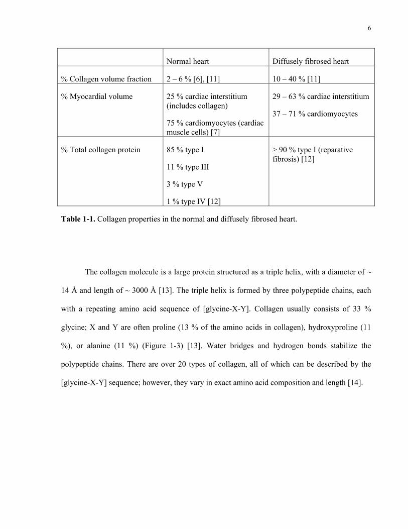
6

Normal heart Diffusely fibrosed heart

% Collagen volume fraction 2 – 6 % [6], [11] 10 – 40 % [11]

% Myocardial volume 25 % cardiac interstitium (includes collagen)

75 % cardiomyocytes (cardiac muscle cells) [7]

29 – 63 % cardiac interstitium

37 – 71 % cardiomyocytes

% Total collagen protein 85 % type I

11 % type III

3 % type V

1 % type IV [12]

> 90 % type I (reparative fibrosis) [12]

Table 1-1. Collagen properties in the normal and diffusely fibrosed heart.

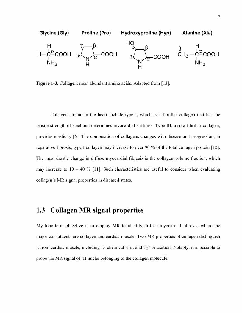
The collagen molecule is a large protein structured as a triple helix, with a diameter of ~

14 Å and length of ~ 3000 Å [13]. The triple helix is formed by three polypeptide chains, each

with a repeating amino acid sequence of [glycine-X-Y]. Collagen usually consists of 33 %

glycine; X and Y are often proline (13 % of the amino acids in collagen), hydroxyproline (11

%), or alanine (11 %) (Figure 1-3) [13]. Water bridges and hydrogen bonds stabilize the

polypeptide chains. There are over 20 types of collagen, all of which can be described by the

[glycine-X-Y] sequence; however, they vary in exact amino acid composition and length [14].

7

MAGNETIC RESONANCE IN CHEMISTRYMagn. Reson. Chem. 2004; 42: 276–284Published online in Wiley InterScience (www.interscience.wiley.com). DOI: 10.1002/mrc.1334

A solid-state NMR study of the fast and slow dynamicsof collagen fibrils at varying hydration levels

Detlef Reichert,1 Ovidiu Pascui,1 Eduardo R. deAzevedo,2 Tito J. Bonagamba,2

Klaus Arnold3 and Daniel Huster3,4!

1 Fachbereich Physik, Martin-Luther-Universitat Halle-Wittenberg, D-06108 Halle, Germany2 Instituto de Fısica de Sao Carlos, Universidade Sao Paulo, Caixa Postal 369, CEP 13560-970, Sao Carlos, SP, Brazil3 Institute of Medical Physics and Biophysics, University of Leipzig, Liebigstrasse 27, D-04103 Leipzig, Germany4 Junior Research Group ‘Solid-state NMR Studies of the Structure of Membrane-associated Proteins’, Biotechnological–Biomedical Centerof the University of Leipzig, Liebigstrasse 27, D-04103 Leipzig, Germany

Received 24 April 2003; Revised 2 July 2003; Accepted 2 July 2003

We report solid-state NMR investigations of the effect of temperature and hydration on the molecularmobility of collagen isolated from bovine achilles tendon. 13C cross-polarization magic angle spinning(MAS) experiments were performed on samples at natural abundance, using NMR methods that detectmotionally averaged dipolar interactions and chemical shift anisotropies and also slow reorientationalprocesses. Fast motions with correlation times much shorter than 40 µs scale dipolar couplings and chemicalshift anisotropies of the carbon sites in collagen. These motionally averaged anisotropic interactionsprovide a measure of the amplitudes of the segmental motions expressed by a molecular order parameter.The data reveal that increasing hydration has a much stronger effect on the amplitude of the molecularprocesses than increasing temperature. In particular, the Cg carbons of the hydroxyproline residues exhibita strong dependence of the amplitude of motion on the hydration level. This could be correlated withthe effect of hydration on the hydrogen bonding structure in collagen, for which this residue is knownto play a crucial role. The applicability of 1D MAS exchange experiments to investigate motions on themillisecond time-scale is discussed and first results are presented. Slow motions with correlation times ofthe order of milliseconds have also been detected for hydrated collagen. Copyright ! 2004 John Wiley &Sons, Ltd.

KEYWORDS: NMR; 13C NMR; DIPSHIFT; CODEX; order parameter; slow dynamics; fast dynamics

INTRODUCTION

Collagen is the most abundant protein on Earth and oneof the major constituents of higher animals. It is foundin bones, tendons, skin, ligaments, blood vessels, cartilageand other tissues.1 Collagen plays a crucial role in thestability and function of these biological tissues. For instance,collagen molecules form a rigid network in cartilage, whichprovides the scaffold for the mechanical stability of thetissue and restricts the swelling.2,3 Degeneration of thecollagen moiety of cartilage in the course of rheumaticdiseases limits the shock-absorbing capacity of the tissueand leads to pathological thinning of the cartilage layer ofthe bones. The result of that process is painful arthritis thataffects the majority of the citizens in industrialized countries.4

Understanding the relation between the biological function,the molecular structure and the dynamics of the components

!Correspondence to: Daniel Huster, Institute of Medical Physicsand Biophysics, University of Leipzig, Liebigstrasse 27, D-04103Leipzig, Germany. E-mail: [email protected]/grant sponsor: Bundesministerium fur Bildung undForschung !BMB C F".Contract/grant sponsor: Interdisciplinary Center for ClinicalResearch (IZKF); Contract/grant number: 01KS9504/1, Project A17.

of cartilage, in particular of the collagen, is thus a prerequisitefor the development of treatment strategies. One approachthat requires input from molecular research is tissueengineering of artificial cartilage for replacement surgerymethods.5

Collagen is a very large protein that occurs as fibers,which are formed by triple helices that are about 14 A indiameter and about 3000 A in length (see Fig. 1).1 Eachtriple helix consists of three individual polypeptide chainsthat themselves are organized as extended left-handedhelices with an average rise of 2.9 A per residue. To form

H C

H

NH2

COOH!

C

H

NH2

COOHCH3!"

HN

HO

COOH!

"#$N

COOH

H!

"#

$

Glycine Proline Hydroxyproline Alanine

Figure 1. Sketch of a collagen triple helix molecule and thestructure of the most abundant amino acids in collagen(glycine, Gly; alanine, Ala; proline, Pro; hydroxyproline, Hyp).

Copyright ! 2004 John Wiley & Sons, Ltd.

Glycine((Gly)((((((((((Proline((Pro)((((((((Hydroxyproline((Hyp)(((((((((Alanine((Ala)(

Figure 1-3. Collagen: most abundant amino acids. Adapted from [13].

Collagens found in the heart include type I, which is a fibrillar collagen that has the

tensile strength of steel and determines myocardial stiffness. Type III, also a fibrillar collagen,

provides elasticity [6]. The composition of collagens changes with disease and progression; in

reparative fibrosis, type I collagen may increase to over 90 % of the total collagen protein [12].

The most drastic change in diffuse myocardial fibrosis is the collagen volume fraction, which

may increase to 10 – 40 % [11]. Such characteristics are useful to consider when evaluating

collagen’s MR signal properties in diseased states.

1.3 Collagen MR signal properties

My long-term objective is to employ MR to identify diffuse myocardial fibrosis, where the

major constituents are collagen and cardiac muscle. Two MR properties of collagen distinguish

it from cardiac muscle, including its chemical shift and T2* relaxation. Notably, it is possible to

probe the MR signal of 1H nuclei belonging to the collagen molecule.

8

1.3.1 Chemical shift

In proton MR, the signal of 1H nuclei (protons) is measured. The protons precess about the

external magnetic field (B0) induced by the MR magnet, at the Larmor frequency (f0):

f0 =γ2π

B0 (Eq. 1.1)

where γ/2π is the gyromagnetic ratio for 1H, valued at 42.577 MHz/T. However, the actual

resonance frequency of each proton varies according to its chemical environment. Namely, the

orbital motion of neighbouring electrons induces a local magnetic field around the nucleus, as a

consequence of the external magnetic field generated by the magnet [10]. In this case,

feff = f0 (1−σ ) (Eq. 1.2)

where σ is a shielding constant determined by the electronic environment.

The change in resonance frequency of a proton (fp) relative to a chemical reference (fr) is called

the chemical shift (δ):

δ =( fp − fr )×10

6

fs (Eq. 1.3)

δ is measured in parts per million (ppm), and is independent of magnetic field strength. fs is the

frequency of the MR spectrometer. A typical chemical reference is tetramethylsilane (TMS),

which is assigned a chemical shift of 0 ppm.

9

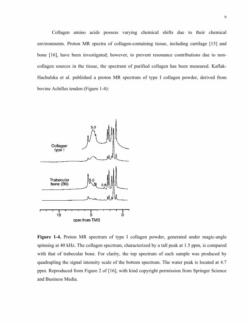
Collagen amino acids possess varying chemical shifts due to their chemical

environments. Proton MR spectra of collagen-containing tissue, including cartilage [15] and

bone [16], have been investigated; however, to prevent resonance contributions due to non-

collagen sources in the tissue, the spectrum of purified collagen has been measured. Kaflak-

Hachulska et al. published a proton MR spectrum of type I collagen powder, derived from

bovine Achilles tendon (Figure 1-4):

1) is typical of the P-OH groups on the crystal surface[60].

Assignment of the peaks at ca. 1 ppm (Fig. 1) is nottrivial. We have measured T1q

H for these peaks andfound that their relaxation characteristics are similar tothat of the 0 ppm peak, but completely di!erent fromthe relaxation of water resonating at 5 ppm (to bepublished). We infer that the peaks at ca. 1 ppm mightcome from structural hydroxyl groups, possibly disor-dered by the presence of structural water in hydroxylsites and thereby involved in some hydrogen bonding.Consider that discrete proton peaks in this spectral re-gion were detected for fluorohydroxyapatite [15]. It wasexplained that fluoride ions caused perturbations ofstructural hydroxyl groups, displacing them within theirchains and engaging into hydrogen bonding.

The monoclinic lattice of brushite contains 3 types ofequally populated hydroxyl groups [61]. There are 2crystallographically inequivalent water molecules, andthe HPO4

2) ions. The hydroxyl groups of the 3 speciesare involved in hydrogen bonds, which for the P-OHgroups of HPO4

2) are the strongest. The two crystallo-graphically inequivalent water molecules resonate at 4.1and 6.4 ppm, as indicated by the similar shapes andintensities of the peaks, and their location near andaround the peak position of the apatite water. Considerthat strong hydrogen bonding substantially increases theproton chemical shift, so the peak at 10.4 ppm is as-signed to the HPO4

2) ions.

The spectrum of human trabecular bone is verysimilar to that of collagen type I (Fig. 2), except that awater peak at 5.0 ppm is smaller and an extra tiny peakshows up at 2.8 ppm.

The 31P spectrum of human bone, recorded underMAS at 3 kHz, contains a single featureless peak at 3.1ppm (Fig. 3). The BD peak is from all the 31P nuclei inthe sample, while the CP peak is from the the 31P nucleilocated close to protons. The latter peak is broader.

Fig. 1. 1H NMR spectra of mineral standards recorded underMAS at 40 kHz.

Fig. 2. 1H NMR spectra of collagen type I and human tra-becular bone (B0), recorded under MAS at 40 kHz. For theupper spectra of both samples, the intensity scale was increased4 times.

Fig. 3. 31P CP and BD NMR spectra of human trabecularbone (B0), recorded under MAS at 3 kHz. The spectra arepresented with the same maximum intensities. Under the ab-solute scaling, theCP peak for the 1 ms contact time is 5 timeslower than the BD peak.

A. Kaflak-Hachulska et al.: NMR Study of Human Bone Mineral 479

Figure 1-4. Proton MR spectrum of type I collagen powder, generated under magic-angle

spinning at 40 kHz. The collagen spectrum, characterized by a tall peak at 1.5 ppm, is compared

with that of trabecular bone. For clarity, the top spectrum of each sample was produced by

quadrupling the signal intensity scale of the bottom spectrum. The water peak is located at 4.7

ppm. Reproduced from Figure 2 of [16], with kind copyright permission from Springer Science

and Business Media.

10

This was produced under magic-angle spinning at 40 kHz, allowing for narrow and well-

resolved spectral linewidths. Water is represented by the broad peak at 4.7 ppm. The remainder

of the peaks in the collagen spectrum are due to functional groups on its amino acid residues.

The tallest peak at 1.5 ppm is the most pertinent signature of collagen. Relative to water, this

peak is shifted 1.5 – 4.7 = -3.2 ppm, which corresponds to a frequency shift of ~ 1 kHz in a 7-T

external magnetic field. The chemical shift of collagen would be a valuable property in

distinguishing the collagen MR signal from that of water in myocardial tissue.

1.3.2 T2 and T2* relaxation

This work focuses on MR methods for characterizing T2, which is of interest because a defining

feature of collagen is that it has a short T2, relative to healthy myocardium [17]. In proton MR,

the protons or “spins” possess an initial bulk magnetization (M0) in the presence of an external

magnetic field (B0). M0 is oriented along the magnet bore, denoted the z-axis. With the

application of a radiofrequency pulse, M0 is tipped onto the transverse (xy-) plane.

T2 is the relaxation time constant describing the transverse magnetization (Mxy) decay of

spins; this is due to the irreversible loss of phase coherence, i.e. dephasing, of spins as they

interact with one another. The phenomenon is described by the following:

Mxy (t) =M0e−t/T2

(Eq. 1.4)

In a T2-weighted MR pulse sequence, the time t is the echo time (TE) parameter, defined as the

time from the application of the radiofrequency pulse to the start of data acquisition.

11

Tissues, including collagen and muscle, often possess multiple T2 components, derived

from various signal sources. In the collagen model of relaxation, three T2 components are

thought to exist, listed here from the shortest to the longest T2 component: the protons in

collagen strands (T2 ~ 0.02 ms), the protons in water surrounding collagen, known as the

“hydration layer water protons” (T2 ~ 4 ms), and the protons in free water (T2 ~ 20 ms). The T2

estimates refer to values obtained for articular cartilage, which consists mainly of type II

collagen [18]. Muscle also possesses several T2 components, including a 20 – 50 ms component

due to muscle-associated water, and a longer component > 80 ms due to free water [19]. For

simplicity, muscle T2 has been modelled as a single component; in the heart, a T2 of ~ 35 ms has

been found [20]. In addition to the “pure” T2 components attributed to specific tissue or water

“pools”, intermediate T2 components may arise from exchange between pools.

Mechanisms responsible for exchange include hydrodynamic effects, cross-relaxation,

and chemical exchange. Hydrodynamic effects are long-range interactions governing particles

undergoing Brownian motion in a continuum fluid [21], [22]. The local magnetic field

experienced by a proton changes as the molecule rotates, or as it moves past protons on other

molecules [23]. As a result, intramolecular dipole-dipole interactions (between protons on the

same molecule), as well as intermolecular dipole interactions (between protons on different

molecules) arise and are independent of external magnetic field strength [22]. Cross-relaxation

constitutes the magnetization transfer between two proton environments due to coupled

relaxation. The process occurs mainly between protons within the hydration water layer and

those from proteins [24]. Cross-relaxation increases with the concentration of protein in aqueous

solutions, and decreases as the magnetic field strength increases [22]. Chemical exchange

involves the chemical dissociation of protons, e.g. the formation and breakage of hydrogen

bonds, as molecules move between environments and exchange protons [23]. This may occur

12

between the hydration layer water protons and the bulk water protons, as well as between the

hydration layer water protons and protein protons [24]. Chemical exchange is most apparent

when there is a frequency difference between the two exchanging environments, due to

chemical shift. With increasing magnetic field strength, the frequency difference increases,

resulting in a shortening of T2. At high field, the effect of chemical exchange dominates over

that of cross-relaxation [24]. Hence, it is hypothesized that the most likely T2 exchange

mechanism to be observed at high field is chemical exchange.

Given the various T2 origins and exchange mechanisms in tissue, the modelling of T2

can be a complex task. However, simplifications can be made, according to the clinical

objective. A two-pool system for myocardial fibrosis is proposed, which includes two distinct

pools of collagen and cardiac muscle:

Mxy (t) = Pcollagene−t/T2,collagen +Pmusclee

−t/T2,muscle (Eq. 1.5)

“Collagen” represents protons from collagen and collagen-associated water, and “muscle”

represents protons from muscle and muscle-associated water. Pi denotes the observed population

fraction, and T2i the observed T2 relaxation time. In this case, each tissue constituent is modelled

as a mono-exponential T2 term, for simplicity. Rather than determination of the “true” multi-

component T2s, the objective is to characterize signal from each of the two pools, in order to

detect collagen; differentiation between the pools of collagen and muscle is possible due to their

difference in T2. Under the assumption that exchange is slow relative to the T2s of collagen and

collagen-associated water, intermediate T2 components due to exchange, including

hydrodynamic effects, chemical exchange, and cross-relaxation, are not modelled. Thus far,

collagen protons have been difficult to detect due to their short T2 relaxation.

13

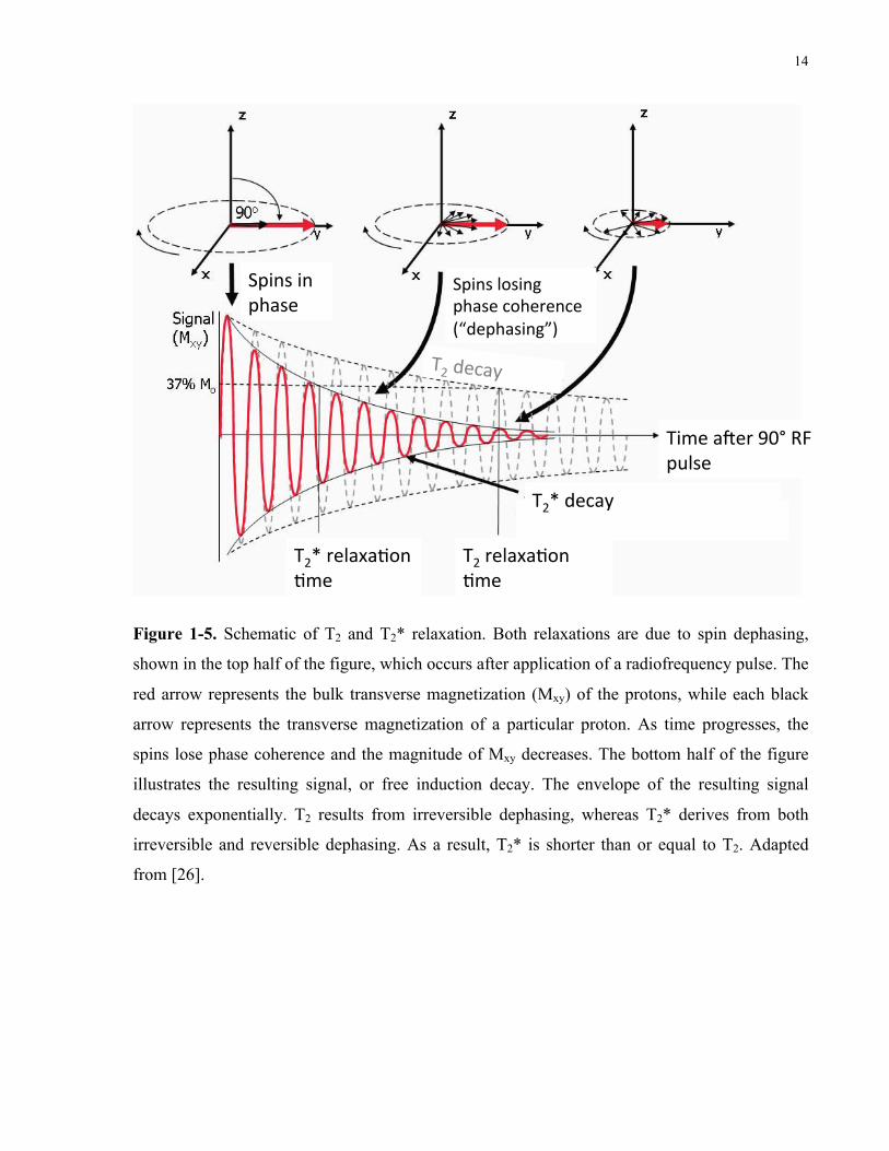
For investigating short T2 species such as collagen, a parameter of interest is the T2*

relaxation. T2* accounts for both irreversible dephasing effects from T2 relaxation, as well as

reversible dephasing effects, including local magnetic field inhomogeneities, differences in

magnetic susceptibilities between materials, and chemical shift [25] (Figure 1-5). In this case,

T2* is smaller than or equal to T2. Although T2 is an inherent property of a material, T2* is not

an intrinsic characteristic due to these experiment dependent dephasing effects. With a 180°

radiofrequency pulse, reversible dephasing may be removed, with only the irreversible

dephasing effects of T2 relaxation and diffusion remaining. When measuring T2, the addition of

a 180° radiofrequency pulse lengthens the minimum echo time, which is not desirable for

probing short T2 species, such as collagen. Instead, it is more suitable to probe for the T2*

relaxation, where short echo times can be achieved. In this case, the bi-exponential two-pool

model in terms of TE and T2* becomes:

S(TE) = S0,collagene−TE /T2*collagen + S0,musclee

−TE /T2*muscle (Eq. 1.6)

where the magnetization terms have been replaced by the signal intensities S. This equation may

be used for determining T2*collagen for collagen and T2*muscle for cardiac muscle. As T2*collagen is

expected to be much smaller than T2*muscle, the T2* decays of the tissue components should be

differentiable.

14

slowed down towards the Larmor frequency shorteningthe T1 value. Water- based tissues with a high macro-molecular content (e.g. muscle) therefore tend to haveshorter T1 values. Conversely, when the water contentis increased, for example by an inflammatory process,the T1 value also increases.

Significance of the T2 valueT2 relaxation is related to the amount of spin-spininteraction that takes place. Free water contains smallmolecules that are relatively far apart and movingrapidly and therefore spin-spin interactions are less fre-quent and T2 relaxation is slow (leading to long T2

relaxation times). Water molecules bound to large mole-cules are slowed down and more likely in interact, lead-ing to faster T2 relaxation and shorter T2 relaxationtimes. Water- based tissues with a high macromolecularcontent (e.g. muscle) tend to have shorter T2 values.Conversely, when the water content is increased, forexample by an inflammatory process, the T2 value alsoincreases. Lipid molecules are of an intermediate sizeand there are interactions between the hydrogen nucleion the long carbon chains (an effect known asJ-coupling) that cause a reduction of the T2 relaxationtime constant to an intermediate value. Rapidly repeatedrf pulses, such as those used in turbo or fast spin echo

Figure 4 Transverse (T2 and T2*) relaxation processes. A diagram showing the process of transverse relaxation after a 90° rf pulse is appliedat equilibrium. Initially the transverse magnetisation (red arrow) has a maximum amplitude as the population of proton magnetic moments(spins) rotate in phase. The amplitude of the net transverse magnetisation (and therefore the detected signal) decays as the proton magneticmoments move out of phase with one another (shown by the small black arrows). The resultant decaying signal is known as the Free InductionDecay (FID). The overall term for the observed loss of phase coherence (de-phasing) is T2* relaxation, which combines the effect of T2 relaxationand additional de-phasing caused by local variations (inhomogeneities) in the applied magnetic field. T2 relaxation is the result of spin-spininteractions and due to the random nature of molecular motion, this process is irreversible. T2* relaxation accounts for the more rapid decay ofthe FID signal, however the additional decay caused by field inhomogeneities can be reversed by the application of a 180° refocusing pulse.Both T2 and T2* are exponential processes with times constants T2 and T2* respectively. This is the time at which the magnetization hasdecayed to 37% of its initial value immediately after the 90° rf pulse.

Ridgway Journal of Cardiovascular Magnetic Resonance 2010, 12:71http://www.jcmr-online.com/content/12/1/71

Page 6 of 28

Spins$in$phase$

Spins$losing$phase$coherence$(“dephasing”)$

T2*$relaxa=on$=me$

T2$relaxa=on$=me$

T2*$decay$

Time$a@er$90°$RF$pulse$

T2$decay$

Figure 1-5. Schematic of T2 and T2* relaxation. Both relaxations are due to spin dephasing,

shown in the top half of the figure, which occurs after application of a radiofrequency pulse. The

red arrow represents the bulk transverse magnetization (Mxy) of the protons, while each black

arrow represents the transverse magnetization of a particular proton. As time progresses, the

spins lose phase coherence and the magnitude of Mxy decreases. The bottom half of the figure

illustrates the resulting signal, or free induction decay. The envelope of the resulting signal

decays exponentially. T2 results from irreversible dephasing, whereas T2* derives from both

irreversible and reversible dephasing. As a result, T2* is shorter than or equal to T2. Adapted

from [26].

15

1.4 UTE MR and its application in myocardial fibrosis

Ultra-short echo time (UTE) is a valuable technique for the measurement of the short collagen

T2* signal, achieving minimum TEs of ~ 0.008 ms [27]. While MR spectroscopy can yield

information about chemical shift, it cannot traditionally achieve short TEs for probing short T2*

species, such as collagen. It would be advantageous to measure the short T2* (~ 1 ms) of

collagen, as it would be differentiable from the long T2* (~ 35 ms) of muscle, and hence would

be highly specific to collagen. Recent literature has demonstrated the feasibility of UTE for

identification of focal and diffuse myocardial fibroses. It is my aim to expand on the findings in

published literature and develop a clinically relevant T2* model that accurately reflects diffuse

myocardial fibrosis.

1.4.1 UTE

UTE MR is a technique that enables the detection of short T2* species. If used for imaging

diffuse myocardial fibrosis, the contrast obtained would be specific to collagen. “Ultra-short”

denotes TEs from 0.008 to 0.50 ms; this is by comparison to “short”, which describes TEs from

0.5 to 5 – 10 ms [27]. A 3D UTE pulse sequence is shown in Figure 1-6.

16

Delay Acquisition time RSD

A-6-234

Measurement Methods

UTE3D (Ultrashort TE) 6.33

Principles 6.33.1The 3D implementation of the UTE technique (UTE3D) allows shorter echotimes than the 2D implementation (UTE) because of the use of a non-selectiveRF excitation. The minimum TE is limited only by the duration of the RF pulseand the time needed to switch between the RF excitation and the data acquisi-tion. Sampling is performed already on the rising gradient ramp and thereforestarts always from the k-space center and continues to the surface of a sphere.The number of scans and directions of the readout gradient for each scan arecalculated to achieve an even distribution of the "end points" at the spherewith a density that is required by the field of view. For the reconstruction of non-cartesian sampling patterns such as the radialone, the conventional Fourier transformation can not directly be applied. First, adensity compensation and data interpolation onto a cartesian grid (gridding)must be performed.The sensitivity of UTE to signals of very short T2 makes the method prone to

Figure 6.111: The UTE3D sequence. A hard pulse excitation is followed by a radial readout. Theachievable TE is limited only by the duration of the RF pulse and a short delayneeded to switch between excitation and data acquisition.

TE

TAQ

Gx

Gy

Gz

ReadSpoiler

Duration

RF

delay

A-6-234

Measurement Methods




TE

TAQ

Gx

Gy

Gz

ReadSpoiler

Duration

RF

delay

A-6-234

Measurement Methods




TE

TAQ

Gx

Gy

Gz

ReadSpoiler

Duration

RF

delay

A-6-234

Measurement Methods




TE

TAQ

Gx

Gy

Gz

ReadSpoiler

Duration

RF

delay

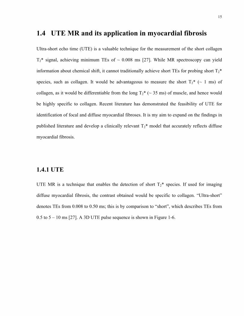
Figure 1-6. 3D UTE sequence from Bruker BioSpin. The sequence consists of a rectangular

radiofrequency pulse excitation and a 3D radial acquisition. The TE is defined as the time from

the middle of the pulse to the beginning of the gradient (G) ramp-up. Different combinations of

gradient amplitudes in Gx, Gy, and Gz are executed to sample k-space adequately (refer to Figure

1-7). The hardware delay is the time needed to shift from excitation to data acquisition. The

acquisition time is ~ 1.6 ms. RSD is the duration of the read spoiler (~ 1 ms), which destroys

remaining Mxy before the next repetition of the sequence. Adapted from [28].

Minimal TEs are achieved via a rectangular radiofrequency pulse of short duration (~ 0.02 ms)

and a small delay (~ 0.008 ms) required to switch between the radiofrequency excitation and

data acquisition [28]. At the beginning of data acquisition, linear gradients in each spatial

dimension (Gx, Gy, Gz) are turned on to allow for spatial localization of the imaged sample. The

precession frequency of a proton (in rad/s) is, hence, a function of its location:

17

ω(i) = γBtotal = γ (B0 +Gii) =ω0 +γGii for dimensions i = x, y, z

(Eq. 1.7)

Data is acquired in spatial frequency space, or k-space. The sampling trajectory in k-space is

radial from the centre of k-space, forming a 3D “koosh ball”. Figure 1-7 illustrates the trajectory

in 2D for clarity.

Consequently, the end-point of the rf excitation hasbecome a popular reference point from which TE ismeasured, although this approach can result in spuriouslyshort values for TE.

The UTE pulse sequence is not a spin echo or gradientrecalled echo (since reversed gradients are not used toform an echo). The FID is directly detected. There is noecho since the signal is not refocused and each half-

Figure 5. k-Space trajectories for the above imaging sequence. Each ‘spoke’represents the k-space trajectory due to the readout gradients. The dots representthe central points which are sampled on the gradient ramps, and the stars theperipheral points which are sampled on the gradient plateau. Practical acquisitionstypically include 128–512 spokes and 256–512 points on each spoke. The datapoints are regridded onto a Cartesian grid prior to 2D Fourier transformation

Figure 4. Pulse sequence diagram for a basic UTE sequence. The half rf pulses areapplied with the slice selection gradient Gz negative in the first half and with thisgradient positive in the second half. The rf pulse is truncated and followed rapidly bythe acquisition during which Gx2 and Gy2 are applied to give the radial gradient.These gradients ramp up to a plateau during data acquisition

Copyright # 2006 John Wiley & Sons, Ltd. NMR Biomed. 2006; 19: 765–780DOI: 10.1002/nbm

CLINICAL UTE IMAGING OF BONE AND OTHER CONNECTIVE TISSUES 771

kx

ky

Radial k-space sampling trajectory

Figure 1-7. Radial sampling trajectory used in UTE (2D view). Each spoke begins at the centre

of k-space, and characterizes a k-space trajectory, formed by a combination of gradient

waveform amplitudes. For instance, spokes in the upper right quadrant (with positive kx and ky)

represent cases when both Gx and Gy are positive. On each spoke, the dots near the centre of k-

space characterize the points that are sampled on the gradient ramp, whereas the stars represent

the points that are sampled on the gradient plateau (refer to Figure 1-6 for the gradient

waveforms). Adapted from [27].

18

The coordinates kx, ky, and kz are proportional to the areas under the gradient waveforms Gx, Gy,

and Gz:

k i (t) =γ

2πGi (τ )dτ for dimensions i = x, y, z

0

t

∫ (Eq. 1.8)

Each spoke in the trajectory is achieved by varying the amplitudes of the gradient waveforms,

allowing for sampling of all quadrants of k-space. For image reconstruction, the sampled points

are regridded in Cartesian coordinates, before an inverse Fourier transform is applied. For each

TE, the UTE pulse sequence would be repeated with the same imaging parameters, with the

exception of the TE. For instance, for detecting the T2* of protons in collagen, which are

expected to be below 1 ms, the TE range of 0.008 ms to 1 ms would be suitable. By sampling

the MR signal over a range of TEs, the T2* of the imaged sample may be characterized.

However, if the T2* of the sample is less than the acquisition time of ~ 1.6 ms, then there will be

significant T2* decay during the readout. As a result, the signal at high spatial frequencies will

be attenuated, causing a loss of spatial resolution. It is for this reason that MR images of short

T2* species are blurred, indicating the usefulness of T2* signal analysis over assessment of

image contrast from short T2* species.

1.4.2 Myocardial fibrosis signal characterization using UTE

Recent literature has suggested the plausibility of using UTE for detecting myocardial fibrosis.

Such research motivated my exploration of collagen T2* relaxation, in the context of diffuse

myocardial fibrosis. De Jong et al. showed that collagen from myocardial infarcts, i.e. focal

myocardial fibrosis, may be qualitatively visualized using UTE on a 7-T MR imaging scanner

19

[17]. The study employed five rats with six-week myocardial infarcts, scanned with an isotropic

resolution of 360 µm. For each heart, they acquired two UTE images: one at a short TE of 0.15

ms, and another at a long TE of 6 ms. By subtracting the image at TE = 6 ms from that at TE =

0.15 ms, the collagen signal was enhanced (Figure 1-8). This was owing to the fact that most of

the collagen signal had decayed by 6 ms, whereas the muscle signal remained relatively

constant.

fast decay (short T2 and T2*) compared to the signal of water mole-cules in soft tissues (Fig. 1), which leads to signal voids in collagen-rich areas. It has been demonstrated that sequences with echo times(TE) one or two orders of magnitude shorter than used for soft tissuecontrast in MRI can detect more “solid” tissue components, character-ized by the short T2* relaxation times [9]. This ultra short echo time(UTE) MRI technique has been used to image menisci, cartilage, liga-ments, tendons, cortical and trabecular bone, periosteum [10], andmyelin water in white matter [11].

This study is the first demonstration that UTE MRI can be used forthe direct detection of cardiac collagen as well. In this proof of princi-ple studywe focused on the detection of compact fibrosis. To ascertainexcessive fibrosis deposition of a compact type in the myocardium,a rat model of MI has been used. The MR images have been cross-referenced with histological sections to confirm the capability of col-lagen detection.

2. Methods

2.1. Animal preparation

Male Lewis rats (Charles River, Maastricht, the Netherlands)weighing between 300 and 350 g were housed in groups with foodand water given ad libitum. Animal experiments were approved bythe local Ethical Animal Experimental Committee and were in accor-dance with the institutional guidelines of the Utrecht UniversityCommon Animal Facility and with the Directive 2010/63/EU of theEuropean Parliament.

The MI was created by ligating the left anterior descending coro-nary artery (n=5) as described elsewhere [12], with small adapta-tions. Briefly, rats were anesthetized with 2.5% isoflurane in 40%oxygen and ventilated (Bear Medical Systems, Riverside, CA, USA) ata frequency of 75/min with a peak pressure of 12 cm H2O and PEEPof 4 cm H2O. The thoracic cavity was approached by blunt dissectionof the fifth intercostal space. The left anterior descending arterywas ligated just proximal of this first bifurcation with a suture. Tenminutes before ligation 10 μg/g lidocaine was injected intraperitone-ally to protect against ventricular arrhythmias [13]. After ligation, thethoracic cavity was closed and the superficial muscles were reposi-tioned after applying lidocaine locally. Sham-operated animals (n=2)

underwent the same surgery, except ligation of the coronary artery.To prevent (post-) operative stress, Carprofen (5 μg/g; Pfizer Inc,Capelle a/d IJssel, the Netherlands) was injected subcutaneously30 min prior to surgery, and at 12, 24, 36, and 48 h after surgery.

After six weeks, replacement of the infarcted area by fibrosis hasreached steady state [14]. Therefore, six weeks after surgery, animalswere anesthetized with 2.5% isoflurane in 40% oxygen and injectedwith heparin and Carprofen. Subsequently, the heart was excorpo-rated and cannulated to superfuse the coronary arteries with phos-phate buffered saline, followed by superfusion with fomblin (SolvaySolexis, Bollate, Italy). Hearts were placed in a custom-made plasticsetup and submerged in fomblin, which provides magnetic suscepti-bility matching, thereby avoiding artifacts from air-tissue boundaries[15].

2.2. MR imaging

Imaging was performed on a 7 T human MRI scanner (PhilipsHealthcare, Cleveland, OH, USA), using a home-built transmit/receivesurface coil. Care was taken to locate the heart in the isocenter of themagnet, to minimize artifacts in the UTE acquisition from gradientimperfections. Two sequences were acquired: 1) balanced steadystate free precession (bSSFP) for anatomical imaging; 2) 3D gradientecho with radial sampling, once with an ultra short TE of 0.15 msand once with a TE of 6.0 ms. Details of the scan parameters are pre-sented in Table 1.

The single echo 3D gradient echo images with TE=6.0 ms weresubtracted from the corresponding UTE images with TE=0.15 ms,to suppress signals from tissues with long T2* (T2*≫1 ms) andkeep only signal with a short T2*. Hereafter, signal in the subtractedimages is called short living signal (SLS). Before subtraction, all im-ages acquired at TE=6.0 ms were scaled with a scaling factor 1.3 tocompensate for signal loss due to T2* decay in tissue with long T2*.The scaling was such that no signal was left for normal myocardiumin the subtracted images.

2.3. Histology

AfterMRImeasurements, heartswere fixed in formalin. Hearts werecut transversally in four pieces and embedded in paraffin. For collagendetection, tissue sections of 4 μm were stained with Picrosirius Red asdescribed previously [16]. Briefly, slices were incubated in xylol for30 min, and dehydrated in an ethanol series. Subsequently, sliceswere stained with 0.1% Sirius Red (Polysciences Inc., Warrington,PA, USA) in picric acid (Sigma-Aldrich Chemie GmbH, Steinheim,Germany), for one hour. For examination, the stained sections weredigitalized with a film-scanner (CanoScan 4400F; Canon Nederland

Fig. 1. Simplified principle of using ultra short echo time (UTE)MRI to estimate collagencontent in cardiac tissue. T2* signal decay of collagen is much faster than the T2* signaldecay of cardiac muscle. Images acquired at TE=0.15 ms will therefore show signalsfrom both muscular and collagen structures, while images acquired at TE=6 ms willonly show signals from the muscular structures. If images acquired at TE=6 ms aresubtracted from images acquired at TE=0.15 ms, the subtracted image will showonly short living signal, in this case signal of collagen. AU = arbitrary units, TE =echo time.

Table 1Imaging parameters.

bSSFP 3D radialgradient echo(UTE)

3D radialgradient echo(long TE)

Field of view (mm3) 30!30!30 30!30!30 30!30!30Matrix (anterior–posterior!right–left! feet–head)

84!86!86 84!84!84 84!84!84

Resolution (μm3) 360!360!360 360!360!360 360!360!360Flip angle 20° 20° 20°Repetition time/echo time (ms) 8.3/4.2 14/0.15 14/6Bandwith (Hz/pixel) 203 502 502Number of averages 5 2a 2a

Scan time (min:s) 5:09 6:31 6:31

bSSFP = balanced steady state free precession.a Implemented as 200% oversampling of radial trajectories.

975S. de Jong et al. / Journal of Molecular and Cellular Cardiology 51 (2011) 974–979

Echo time, TE (ms)

Sig

nal i

nten

sity

(AU

)

be applied in a clinical setting. Firstly, the subtraction of the two UTEimages (image acquired at 0.15 ms minus the image acquired at6.0 ms) seems promising for the direct reflection of compact collagendeposition in scar tissue. However, as of yet, the method is not able toquantify the amount of fibrosis. Quantification of the local amount offibrosis requires further characterization of the multi-component T2*decay of collagen containing tissue. Quantification based on charac-terizing the MRI signal is challenging due to water exchange betweenthe hydration layer of collagen and the surrounding tissue [8,18].

Secondly, in this study only compact fibrosis in the infarctedarea is detected by UTE MRI. Next to the reparative fibrosis resultingfrom the MI, remodeling of the left ventricle will occur and fibroticstrands intermingle with viable myocardium. This reactive fibrosisis observed in the border zone of the infarction, but also in non-ischemic cardiac diseases such as hypertrophic cardiomyopathy.This type of fibrosis impairs conduction of the electrical impulseand plays a major role in the arrhythmogenic substrate (for reviewsee [19]). In addition, reactive fibrosis affects both the diastolic andsystolic cardiac function. Once quantification of the local collagenamount is possible, it is likely that also reactive fibrosis can bedetected as small quantities of collagen in otherwise normal tissue.This will be of great value in the clinical situation, since there is nonon-invasive technique available yet to detect reactive fibrosis. Inthe future, besides its use for compact and diffuse fibrosis detectionthis technique might also be used for the measurement of collagenformation in other processes such as in tissue repair, in atheroscle-rosis, in regenerative medicine, or monitoring physiological changesafter organ transplants.

Thirdly, in the current study, the selection of viable tissue that isneeded to determine the threshold for SLS is guided by histologicalimages. Guidance by histology was performed to ascertain reliableSLS detection in this proof of principle study. When applying theUTE MRI technique into the clinics, guidance by histology for thresh-old determination cannot be performed. This is a general limitationof non-invasive imaging in patients. Additional validation studies inanimals may help solving this issue, by validating a method to deter-mine signal of interest in imaging techniques. This might lead tostandardized threshold determination in non-invasive techniquessuch as MRI.

4.3. Study limitations

The locations of the SLS in the subtracted images correspondedwith the collagen-rich areas observed in histological sections, as thenormalized SLS area correlated well with the collagen-rich area ob-served in histological analysis (r=0.7). This confirms the hypothesisthat UTE MRI is capable of direct fibrosis detection. Nonetheless,the correlation between histology and MRI could have been expectedto be higher in a study with ex vivo hearts at high field MRI. In addi-tion, one anomalous case showed that the collagen deposition couldnot be detected with UTE MRI (Fig. 4). Two factors are thought toexplain this. First, imperfect matching between histology and MRI,due to the differences in tissue shape, angulation, and resolution.For optimal correspondence between the histological sections andthe MRI images, the longitudinal height of all histological sectionswas carefully tracked. However, shape differences between MRI and

Fig. 2. Corresponding histological and MR images. Upper row: Picrosirius Red staining of a section showing transmural infarction (left) and a section from a sham-operated heart(right). Yellow = myocardium, red = fibrosis. Middle row: Subtracted images corresponding to the histological sections. The short living signal is outlined in yellow. Lower row:Anatomical MR images corresponding to the histological sections. The bright signal in the right anatomical image originates from fluid captured between the heart and the plasticcover (arrowhead). Accumulation of this fluid between the heart and the plastic cover is due to the extreme hydrophobic characteristics of fomblin. SLS = short living signal.

977S. de Jong et al. / Journal of Molecular and Cellular Cardiology 51 (2011) 974–979

Subtracted UTE MR image

AnatomicalMR image

Histology (Picrosirius Red)

Collagen (short T2*)

Cardiac muscle (long T2*)

Figure 1-8. Image subtraction using UTE: principle and comparison with histology. The graph

on the left illustrates the theoretical T2* decays of collagen and cardiac muscle. Images at TE =

6 ms were subtracted from those at TE = 0.15 ms to enhance collagen signal (time points

indicated by the vertical lines). By TE = 6 ms, most of the collagen signal had decayed, with

muscle signal remaining. The schematic on the right demonstrates analogous histological and

MR images. The subtracted UTE image was produced by the method described previously. The

region of collagen is delineated in yellow, and aligns with the infarct (in red) shown from

histology. An anatomical MR image is displayed for reference. Adapted from [17].

20

The collagen area fraction from the MR image was correlated with the collagen area

fraction from the histological image, stained with Picrosirius Red. The analysis was conducted

on four infarcted hearts and two sham hearts, for three slices per heart. The partial correlation

coefficient was r = 0.7 (P = 0.002), which was significant, although lower than expected.

Reasons for discrepancies included non-ideal correspondence between histological and MR

images, resulting from differences in tissue shape and resolution. Moreover, the determination

of an objective threshold for collagen signal in the MR images was affected by noise, which

increased as a result of image subtraction. Although the authors did not attempt to characterize

the T2* decay of collagen, they hypothesized that the collagen signal originated from protons in

the hydration layer surrounding collagen. Theirs was the first demonstration that myocardial

fibrosis can be detected using UTE.

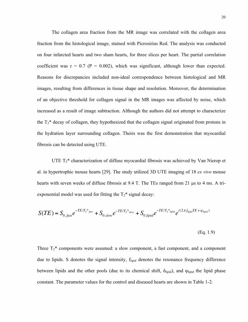
UTE T2* characterization of diffuse myocardial fibrosis was achieved by Van Nierop et

al. in hypertrophic mouse hearts [29]. The study utilized 3D UTE imaging of 18 ex vivo mouse

hearts with seven weeks of diffuse fibrosis at 9.4 T. The TEs ranged from 21 µs to 4 ms. A tri-

exponential model was used for fitting the T2* signal decay:

S(TE) = S0, faste−TE /T2* fast + S0,slowe

−TE /T2*slow + S0,lipide−TE /T2*lipid ei(2π flipidTE +ϕlipid )

(Eq. 1.9)

Three T2* components were assumed: a slow component, a fast component, and a component

due to lipids. S denotes the signal intensity, flipid denotes the resonance frequency difference

between lipids and the other pools (due to its chemical shift, δlipid), and φlipid the lipid phase

constant. The parameter values for the control and diseased hearts are shown in Table 1-2.

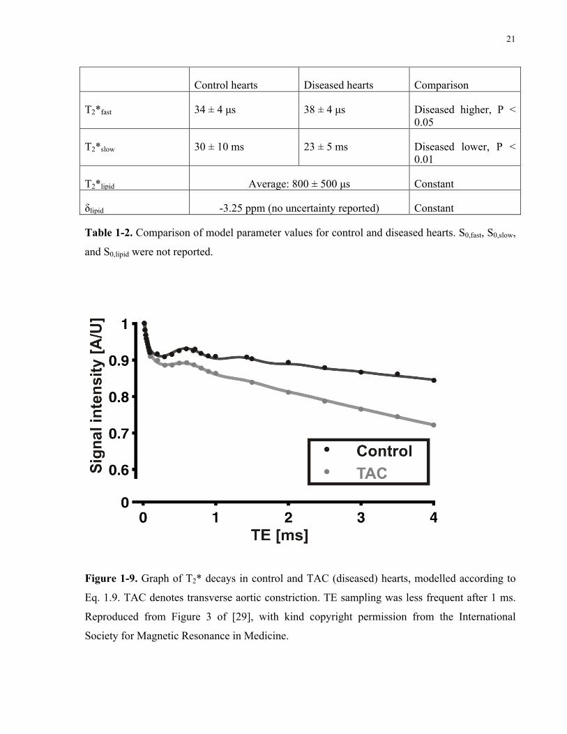
21

Control hearts Diseased hearts Comparison

T2*fast 34 ± 4 µs 38 ± 4 µs Diseased higher, P < 0.05

T2*slow 30 ± 10 ms 23 ± 5 ms Diseased lower, P < 0.01

T2*lipid Average: 800 ± 500 µs Constant

δlipid -3.25 ppm (no uncertainty reported) Constant

Table 1-2. Comparison of model parameter values for control and diseased hearts. S0,fast, S0,slow,

and S0,lipid were not reported.

In vivo ultra short TE (UTE) MRI detects diffuse fibrosis in hypertrophic mouse hearts Bastiaan J van Nierop

1, Jules L Nelissen

1, Noortje AM Bax

2, Abdallah G Motaal

1, Larry de Graaf

1, Klaas Nicolay

1, and Gustav J Strijkers

1 1Biomedical NMR, Department of Biomedical Engineering, Eindhoven University of Technology, Eindhoven, Noord Brabant, Netherlands, 2Soft Tissue Biomechanics

and Engineering, Department of Biomedical Engineering, Eindhoven University of Technology, Eindhoven, Noord Brabant, Netherlands

Target audience (Pre)clinical scientists interested in novel contrast mechanisms to improve diagnosis and risk stratification of heart failure patients.

Purpose Diffuse myocardial fibrosis is an important hallmark of various cardiac pathologies. The excessive

accumulation of extracellular matrix (ECM) proteins, particularly collagen, plays a pivotal role in the transition

towards heart failure (HF)1. Late gadolinium enhancement MRI can be used to detect diffuse myocardial

fibrosis, however this technique is highly depended on the Gd-chelate accumulation kinetics and timing of the

MRI examination. Ultra short TE (UTE) MRI can detect protons with very high transverse relaxation rates (low

T2 relaxation time) directly, including those associated with fibrotic tissue and especially collagen. Previously,

ex vivo UTE MRI was used to visualize replacement fibrosis in rat myocardial infarcts2. In vivo imaging of

diffuse fibrosis by UTE cardiovascular MRI has not been demonstrated thus far.

Methods Mouse model: Pressure overload hypertrophy was induced by a severe transverse aortic constriction in

C56BL/6 mice (ƃ, age 11 weeks, n = 18). MRI measurements were performed 11 weeks after surgery. Healthy

littermates were used as control (n = 10).

In vivo MRI: MRI was performed at 9.4T with a 3D UTE sequence, consisting of a non slice-selective RF

block-pulse followed by a radial readout, as previously described3. Sequence parameters were: TR=8.4 ms,

NSA=1, FOV=3x3x3 cm3, matrix size=128x128x128, minimum TE = 21 µs. Other TEs were 100, 300, 714 µs

and 1.429 ms. Mice were anesthetized with isoflurane. In vivo UTE measurements were ECG triggered and

respiratory gated to prevent motion artifacts. A blood-saturation slice in a short-axis orientation positioned

above the left ventricle (LV) base provided improved contrast between blood and myocardium. To limit the

acquisition time to about 14-16 min (depending on the mouse heart rate), 3 k-lines were measured after every

R-wave and the acquisition matrix was undersampled by a factor 2.

Histology: Immediately after MRI, mice were euthanized and their hearts were excised for ex vivo UTE

measurements. TE was varied between 21 µs and 4 ms. Finally, TAC (n=6) and control hearts (n=1) were

embedded in paraffin, cut in 5-µm-thick sections and collagen was stained with Picrosirius Red. The collagen

fractional area was determined from histology as a measure of the amount of diffuse fibrosis.

Data analysis: In vivo !UTE images were obtained by subtracting long-TE (1.429 ms) from short-TE (21 µs)

images and the average !UTE signal change was quantified using a region-of-interest based approach. The ex vivo MR signal behavior as a function of TE was fitted to a 3-component model using a Levenberg-Marquardt

least-squares algorithm4. All data analysis was done using Matlab (The Mathworks, Inc).

Results and Discussion Fig. 1 shows representative examples of short-axis midventricular UTE images of control and TAC hearts with

a short-TE, long-TE and the corresponding !UTE images. Due to time restrictions, only a limited number of

TE values could be measured in vivo. (Fig. 2). Alternatively, the !UTE signal decrease from TE=21 µs to

TE=1.429 ms was quantified. !UTE was larger for TAC hearts (0.21±0.07) as compared to control hearts

(0.13±0.04) (P < 0.001), which we attribute to the presence of diffuse fibrosis in the TAC hearts. To prove this

hypothesis, the ex vivo UTE signal behavior as a function of TE was studied in detail and related to the

fractional collagen area from histology.

Three signal components were revealed, i.e. a fast and slow exponential decaying pool, and an oscillating pool,

which likely resulted from the chemical shift resonance frequency difference of the lipid pool (Fig. 3). No

change in T2*lipid (average: T2* = 820 ± 470 µs) was detected. T2*fast was slightly increased in TAC hearts (38

± 3.9, P < 0.05) as compared to control hearts (34 ± 3.9) and T2*slow showed a moderate decrease in TAC (23 ±

4.7 ms) as compared to control hearts (30 ± 11 ms) (P = 0.09). Surprisingly, the relative contributions of the

different pools to the total signal remained essentially constant. Importantly, the amount of diffuse fibrosis

linearly correlated with T2* slow (r = 0.82, P = 0.01) (Fig. 4).

Conclusion

The in vivo !UTE signal change in TAC heart was larger as compared to control hearts. Ex vivo measurements

revealed that this can be attributed to changes in T2* as a consequence of the presence of diffuse fibrosis. Thus,

UTE cardiovascular MRI provides an unique opportunity for the noninvasive assessment of diffuse myocardial

fibrosis, without the use of contrast agents. Clinical translation of this method could ultimately improve risk

stratification of heart failure patients.

Acknowledgement This research was supported by the Center for Translational Molecular Medicine and the Dutch Heart

Foundation.

References 1) Creemers et al. Cardiovasc Res, 2011 (98), p265. 2) de Jong et al. J Moll Cell Cardiol, 2011(51), p974. 3) van Nierop et al. ISMRM 2012, 390. 4) O’Regan et al. Eur Radiol, 2008(18), p800.

Fig. 4. Picrosirius Red stained slices of a TAC heart with a small (A) and large amount of fibrosis (B). Relation between T2*slow and the collagen fractional area (C).The gray line is a linear fitting.

Fig. 1. Short-axis UTE images of a control heart and a TAC heart with a short-TE (21µs), long-TE (1.429 ms) and the corresponding !UTE image, in which no regional hyperenhancement was observed visually.

Fig 2. In vivo UTE signal behavior in a control and

TAC heart.

Fig. 3 Ex vivo UTE signal as a function of TE in a

control and TAC heart.

1360.Proc. Intl. Soc. Mag. Reson. Med. 21 (2013)

Figure 1-9. Graph of T2* decays in control and TAC (diseased) hearts, modelled according to

Eq. 1.9. TAC denotes transverse aortic constriction. TE sampling was less frequent after 1 ms.

Reproduced from Figure 3 of [29], with kind copyright permission from the International

Society for Magnetic Resonance in Medicine.

22

The lipid component accounted for the oscillations in signal intensity due to the

chemical shift between fat and water. At 9.4 T, fat and water are in phase every 0.73 ms, and out

of phase at 0.37 ms and every subsequent multiple of 0.73 ms [30]. The T2* of fat at this field

strength is approximately 50 ms, corresponding to its methylene (CH2) group that is shifted by

3.4 ppm from water [31]. As the oscillations in fat signal intensity are modulated by a long T2*,

it is expected that the oscillations would decay relatively little over a TE range of 0 to 4 ms.

However, the authors found a lipid T2* of 800 µs, and the oscillations appeared to decay within

2 ms. Due to the short T2*, it is debatable whether this component should be attributed to lipids.

I speculate that both the fast and slow components are mixtures of collagen and muscle.

As collagen has a much shorter T2* than muscle, one would expect T2*fast to be dominated by

collagen T2* relaxation, and T2*slow by muscle T2* relaxation. The relative fractions of the fast

(S0,fast) and slow (S0,slow) components were not reported; however, the authors noted that they

remained essentially constant between the control and diseased groups. As one would expect

S0,fast to increase in diseased hearts due to the higher collagen content, it is presumed that there

was little change in collagen content as a result of diffuse fibrosis. The average collagen

fractional area as estimated by Picrosirius Red histological staining was 0.2 % in one control

heart and 4 % in six diseased hearts. Despite the slight elevation in collagen content, the T2*fast

of the diseased hearts was found to be higher (P < 0.05) than that of control hearts. T2*slow was,

as expected, lower (P < 0.01) in diseased hearts when compared to control hearts. Nevertheless,

the T2* values of control hearts were within the uncertainties of those of diseased hearts. Due to

the very short nature of T2*fast, it is argued that T2*fast is highly reflective of a short collagen T2*

component. Directions that one may pursue from these findings include verifying the T2*fast of

approximately 35 µs in collagen, most likely attributable to the protons of the protein, as well as

correlating the relative signal fraction of S0,fast with the collagen area fraction.

23

1.5 Thesis statement

The objective of this thesis is to understand the origin of the UTE MR signal associated with

myocardial fibrosis and to demonstrate evidence of these signal properties in heart tissue. This

technique would be especially beneficial for the diagnosis of diffuse myocardial fibrosis, as

current MR methods yield contrast that is unspecific to collagen. I hypothesize that one can

directly isolate and characterize the signal from the protons in the collagen molecule. Based on a

bi-exponential T2* model that accounts for the chemical shift of collagen, I validate my

hypothesis: (1) in solutions of powdered collagen, and (2) in a heart tissue sample afflicted with

diffuse myocardial fibrosis. The experimental results are described in Chapter 2. Chapter 3

outlines future research directions for clinical application, based on the UTE MR signal

properties of collagen gleaned from Chapter 2; this includes TE undersampling, comparisons

between fixed and unfixed tissue, and future techniques. It is hoped that the characterization of a

collagen-specific UTE MR signal will aid in the clinical prediction of the severity of myocardial

fibrosis.

24

Chapter 2 Characterization of the UTE MR Collagen Signal

Associated with Myocardial Fibrosis

2

2.1 Introduction

Myocardial fibrosis is defined by increased collagen synthesis in the heart by fibroblasts and

myofibroblasts [7]. The collagen volume fraction of a normal heart is 2 – 6 % [6], [11];

however, fractions of 10 – 40 % may result from myocardial fibrosis [11]. The disease is

associated with impaired ventricular systolic function and stiffness, ultimately leading to heart

failure [7]. In order to prevent late-stage heart failure, it is important to detect and diagnose

myocardial fibrosis clinically.

As described in Chapter 1, current cardiovascular magnetic resonance techniques for

characterization of myocardial fibrosis include late gadolinium enhancement and T1 mapping,

which are influenced by gadolinium kinetics and are not specific to collagen [5], [7]. Recent

literature by De Jong et al. and Van Nierop et al. has demonstrated the feasibility of detection of

myocardial fibrosis using UTE MR imaging (MRI) [17], [29]. UTE is an intrinsic MR contrast

technique that can detect the short T2* decay, believed to be associated with collagen, via its

minimal echo times. Although Van Nierop et al. did not predict the source of the collagen short

T2* component, De Jong et al. hypothesized that it originated from the hydration layer water

surrounding collagen [17]. However, the T2* components in fibrosis have several potential

origins including: (1) the protons in the collagen molecule, (2) the protons belonging to the

24

25

hydration water layer attached to the collagen strands, and (3) the protons from the free water

surrounding collagen [18].

My objective is to isolate and characterize signal from collagen via UTE MRI, in order

to diagnose myocardial fibrosis clinically. Rather than the accurate modelling of all T2*

exchange mechanisms that occur between collagen and cardiac muscle, my approach is to

develop and evaluate a simplified bi-exponential T2* model that is sufficient for the clinical

detection of collagen within myocardial fibrosis. I hypothesize that the short T2* component

previously measured in myocardial fibrosis [17], [29] originates from the protons belonging to

the collagen molecule. These protons have a unique chemical shift relative to surrounding water

hydration layers. I propose a bi-exponential T2* model of myocardial fibrosis, which accounts

for the chemical shift of collagen protons. The model is first validated in collagen solutions,

where the chemical shift and T2* of collagen are evaluated, and the collagen signal fractions

determined by UTE MRI are correlated with the known concentrations. Subsequently, the model

is applied to a sample of ex vivo canine heart tissue, where the chemical shift and T2* properties

observed in the collagen solutions are verified.

2.2 Experimental methods

2.2.1 Myocardial fibrosis model: Bi-exponential T2* with oscillation

Kaflak-Hachulska et al. showed that the 1H MR spectrum of type I collagen powder from bovine

Achilles tendon is characterized by a predominant peak at -3.2 ppm relative to water, analogous

to a frequency of ~ 1 kHz at a magnetic field strength of 7 T [16]. As this chemical shift pertains

to the protons in collagen, rather than bound water, one may use this property to model the MR

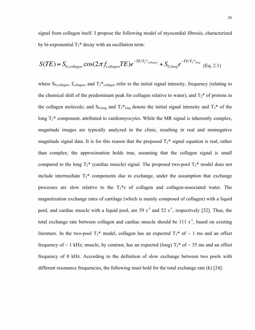
26

signal from collagen itself. I propose the following model of myocardial fibrosis, characterized

by bi-exponential T2* decay with an oscillation term:

S(TE) = S0,collagen cos(2π fcollagenTE)e−TE /T2*collagen + S0,longe

−TE /T2*long (Eq. 2.1)

where S0,collagen, fcollagen, and T2*collagen refer to the initial signal intensity, frequency (relating to

the chemical shift of the predominant peak for collagen relative to water), and T2* of protons in

the collagen molecule; and S0,long and T2*long denote the initial signal intensity and T2* of the

long T2* component, attributed to cardiomyocytes. While the MR signal is inherently complex,

magnitude images are typically analyzed in the clinic, resulting in real and nonnegative

magnitude signal data. It is for this reason that the proposed T2* signal equation is real, rather

than complex; the approximation holds true, assuming that the collagen signal is small

compared to the long T2* (cardiac muscle) signal. The proposed two-pool T2* model does not

include intermediate T2* components due to exchange, under the assumption that exchange

processes are slow relative to the T2*s of collagen and collagen-associated water. The

magnetization exchange rates of cartilage (which is mainly composed of collagen) with a liquid

pool, and cardiac muscle with a liquid pool, are 59 s-1 and 52 s-1, respectively [32]. Thus, the

total exchange rate between collagen and cardiac muscle should be 111 s-1, based on existing

literature. In the two-pool T2* model, collagen has an expected T2* of ~ 1 ms and an offset

frequency of ~ 1 kHz; muscle, by contrast, has an expected (long) T2* of ~ 35 ms and an offset

frequency of 0 kHz. According to the definition of slow exchange between two pools with

different resonance frequencies, the following must hold for the total exchange rate (k) [24]:

27

k << 1T2 *collagen

−1

T2 *long≈ 971 s−1 (Eq. 2.2)

k << fcollagen − flong ≈1000 s−1 (Hz) (Eq. 2.3)

where the expressions have been evaluated, based on the expected values for the the T2*s and

frequencies of the two pools. In this case, the exchange rate of 111 s-1 based on existing

literature satisfies both Eq. 2.2 and Eq. 2.3. Hence, it is hypothesized that the proposed two-pool

T2* model in the absence of exchange is a reasonable initial model. Given the frequency shift

and short T2* of protons in collagen, it is believed that the collagen T2* component will be

distinctive from the long T2* component. With the proposed simplified model involving

relatively few parameters, it is my hope that the collagen signal can be characterized practically

with limited data. This would aid in the identification of myocardial fibrosis and the

determination of severity.

2.2.2 Collagen solution preparation

In order to validate Eq. 2.1 in a controlled environment, collagen solutions of varying

concentrations were prepared and analyzed with UTE MRI. The collagen content was known

within the solutions, which possessed MR characteristics of muscle tissue water. The collagen

solutions were prepared by dissolving hydrolyzed type I and III collagen powder (NeoCell

Super Collagen Type I and III Powder, NeoCell, Irvine, CA, USA) in 0.125 mM manganese

chloride (MnCl2) solvent. Types I and III were appropriate, as they are the most abundant

collagen types in the heart [12]. Pharmaceutical food grade bovine hide collagen was the source

28

of the powder. The manganese chloride solution was prepared by dissolving the appropriate

amount of manganese(II) chloride tetrahydrate (MnCl2•4H2O) (ReagentPlus grade, Sigma-

Aldrich, Oakville, Ontario, Canada) in Milli-Q water (EMD Millipore, Billerica, MA, USA).

This MnCl2 solution approximated the long T2* of cardiac muscle, valued at ~ 35 ms [20]. To

dissolve the collagen, the solution was heated over a hot plate at < 100 °C and mixed. Collagen

powder residues on apparatuses were rinsed with Milli-Q water and poured into the solution,

ensuring that all of the powder was transferred. Concentrations, expressed as % mass/volume

(% m/v), were as follows: 0 %, 2.5 %, 5 %, 10 %, 20 %, 30 %, 40 %, 50 %. At 50 % m/v

concentration, i.e. with 50 g of collagen dissolved in a solution with total volume of 100 mL, the

solution approached the saturation point for collagen solubility; hence, higher concentrations

were not prepared. For scanning, the solutions were placed in 5-mL glass tubes.

2.2.3 Heart tissue preparation

For confirmation of the proposed myocardial fibrosis T2* model in the heart, ex vivo canine

heart tissue afflicted with diffuse myocardial fibrosis was employed. Animal procedures were

approved by the Animal Care Committee of St. Michael’s Hospital (Toronto, ON, Canada).

Detailed methods are provided in previously published work [33]. One mongrel dog aged 1 – 2

years, weighing 20 – 30 kg was used for the study. Pacemaker implantation was performed with

the dog anesthetized with 1 – 2 % isoflurane, and at a temperature of 37 °C sustained by a

heating blanket. The dog’s breathing was regulated with a mechanical ventilator (Harvard

Apparatus, Inc., Holliston, MA, USA) at 16 – 18 breaths/min and 12-14 mL/kg tidal volume.

Fluoroscopy was used to monitor pacemaker implantation. Via the left external jugular vein,

two bipolar IS-1 pacing leads (Pacesetter Tendril SDX, St. Jude Medical Minneapolis, MN,

29

USA) were attached to the right ventricular apex and right atrial appendage. The two pacing

leads were attached to a bipolar IS-1 pacemaker (Model 5156 Verity ADx XL SR, St. Jude

Medical Minneapolis, MN, USA). After a one-week recovery period, simultaneous

atrioventricular pacing at 220 bpm was induced by adjusting the pacemaker to VVI mode at 220

bpm, with a pulse width of 1 ms and a pulse amplitude of 5.0 V.

The same procedure for maintenance of animal anesthesia, temperature, and ventilation

was used at the end study. While the canine was heavily anesthetized, the heart was rapidly

removed. Ex vivo left atrial appendage heart tissue was fixed in 10 % neutral buffered formalin

for one day at 4 °C. Prior to scanning, the tissue was brought to room temperature. The sample

was cut to approximately 5 mm x 5 mm x 5 mm in size and wedged in a 5-mm diameter, 1-mL

glass tube, which was wrapped in Teflon tape to prevent motion. Magnetic susceptibility

artifacts at the air-tissue interface were minimized by filling the tube with Fluorinert (3M, Saint

Paul, MN, USA). For scanning, the tube was placed inside a 1.3 cm-diameter, 5-mL glass tube

and inserted into a cylindrical Teflon holder of slightly larger diameter; the holder contained a

locally made radiofrequency surface coil.

2.2.4 MR measurements

Experiments were performed on a 7-T horizontal-bore Bruker BioSpec 70/30 scanner (Bruker

BioSpin, Ettlingen, Germany), using ParaVision 5.1 software. The system had a gradient

amplitude of 200 mT/m and a maximum slew rate of 640 T/m/s [34]. A 4.8 cm x 1.5 cm locally

built surface radiofrequency coil was utilized for transmitting and receiving signal.

30

For UTE measurements of the collagen solutions and heart tissue, a 3D UTE Bruker

stock pulse sequence was employed, characterized by radial sampling and a non-selective

rectangular radiofrequency pulse of length 0.02 ms. A delay of 0.004 ms was required to switch

from radiofrequency excitation to data acquisition. To begin at the centre of k-space, sampling

was executed on the gradient ramp. The acquisition time was 1.6 ms; this was followed by a

spoiler in the readout direction for 1 ms, to remove spurious signals before the next repetition

time. Imaging parameters were as follows: repetition time = 30 ms, flip angle = 15°, number of

averages = 1, number of projections = 12,753, and polar undersampling factor = 1. Images were

reconstructed on the Bruker workstation, involving regridding of raw data to Cartesian

coordinates followed by an inverse Fourier transformation. Scans were conducted at a

temperature of 21 ± 2 °C. For the collagen solutions, the decay curve was sampled at high

density, particularly within the initial 5 ms to facilitate proper identification of important

chemical shift and T2* decay components. The following TEs were collected in sequential

fashion: 0.02, 0.06, 0.1, 0.14, 0.18, 0.22, 0.25, 0.3, 0.35, 0.4, …, 4.85, 4.9, 4.95, 5, 10, 15, 20,

25 ms, where the TEs from 0.25 ms to 5 ms were separated by intervals of 0.05 ms. The

duration of each scan was ~ 6.5 min, totalling to ~ 11.5 h for completion of all 106 TEs. The

field-of-view was 50 mm x 50 mm x 50 mm and the matrix size was 64 x 64 x 64, resulting in a

spatial resolution of 0.781 mm/pixel isotropic. The following TEs were collected consecutively

for the heart tissue: 0.02, 0.025, 0.030, 0.035, …, 1.985, 1.99, 1.995, 2, 3, 5, 10, 15, 20, and 25

ms; the TEs ranging from 0.02 ms to 2 ms were separated by intervals of 0.005 ms. Each scan

was ~ 6.5 min in length, which summed to ~ 43.7 h upon conclusion of all 403 TEs. A high

spatial resolution of 0.156 mm/pixel isotropic was achieved via a field-of-view of 10 mm x 10

mm x 10 mm and a matrix size of 64 x 64 x 64.

31

A non-localized spectroscopy (NSPECT) stock pulse sequence from Bruker was

executed for obtaining an MR spectrum of the 50 % collagen solution. This was acquired for

comparison with the collagen spectrum of Kaflak-Hachulska et al. [16]. A 90°-rectangular pulse

lasting 0.007 ms, followed by an acquisition delay of 0.05 ms, and a free induction decay

acquisition of 262.14 ms characterized the NSPECT sequence. 32,768 points were obtained,

each separated by a dwell time of 0.008 ms, and achieving a spectral resolution of 3.8147

Hz/point. 125 000 Hz was the spectral width. The repetition time was 1000 ms, the number of

averages was 10, and the number of repetitions was 1, amounting to a total scan time of 10 s.

2.2.5 Analysis of collagen solutions

UTE magnitude images reconstructed from the Bruker workstation were used for analysis, in

order to minimize phase artifacts; as my eventual objective is clinical implementation, I chose to

use the same type of images as those used in the clinic. Region-of-interest (ROI) selection and

data fitting were performed in MATLAB R2012a (The MathWorks, Natick, MA, USA). For

each collagen solution, a 10- x 8-pixel ROI was selected over an axial slice at the tube’s centre;

this was done to minimize the contributions of artifacts due to magnetic susceptibility, phase

differences, and Gibbs’ ringing. Pixels in the ROI were averaged to obtain the mean signal

intensity as a function of TE. T2* fitting of Eq. 2.1 over the ROI was conducted via a trust-

region-reflective nonlinear least-squares algorithm in MATLAB. This amounted to a five-

parameter fit, with the loose constraints specified in Table 2-1. Note that the full TE range was

fitted in a single step. Different methods of fitting exist, including strategies when the short and

long TEs are fitted in separate steps; however, I decided to minimize the assumptions in the

fitting procedure and employed a simple fitting procedure for validation of the proposed T2*

32

model. Uncertainties in the fit parameters of Eq. 2.1 were calculated as standard errors (standard

deviations), determined from the accuracy of the fit. Consider a nonlinear least-squares fit,

yielding residual ri for the ith data point and fit parameter βj for the jth parameter. The Jacobian

matrix J has entries Jij,, defined as follows:

Jij =∂ri∂β j

(Eq. 2.4)

The mean squared error (MSE) can be calculated from the sum of the squared 2-norms of the

residuals and the degrees of freedom ν:

MSE =ri

2

i∑ν

(Eq. 2.5)

Assuming that J is non-singular (invertible), one can determine the covariance matrix (COV),

based on J and MSE:

COV = (JT J )−1 ⋅MSE (Eq. 2.6)

The standard errors are the standard deviations of the fit parameters, i.e. the square roots of the

diagonal entries of the covariance matrix.

The collagen signal fraction determined from UTE was compared to its known concentration in

a calibration plot and regression analysis, performed in Excel for Mac 2011 (Microsoft,

Redmond, WA, USA). Below is the equation for the collagen signal fraction:

Collagen signal fraction =S0,collagen

S0,collagen + S0,long×100% (Eq. 2.7)

33

Parameter Initial estimate

Lower bound Upper bound

S0,long 40000 AU 0 1000000 AU

T2*long 20 ms 0 50 ms

S0,collagen 40000 AU 0 1000000 AU

T2*collagen 1 ms 0 4 ms

fcollagen 1 kHz 0 10 kHz

Table 2-1. Initial values of the fit parameters in Eq. 2.1 for the collagen solutions.

Table 2-1. Initial values of the fit parameters in Eq. 2.1.

Analysis of the NSPECT spectrum of the 50 % collagen solution was performed in

MestReNova 9.0.1 (Mestrelab Research, Santiago de Compostela, Spain). Using the software,

manual corrections for zero- and first-order phase and the baseline were achieved on the real

spectrum. To compare the NSPECT and UTE analyses, a frequency spectrum was generated

using the complex form of Eq. 2.1:

S(TE) = S0,collagene−i2π fcollagenTEe−TE /T2*collagen + S0,longe

−TE /T2*long (Eq. 2.8)

where the parameter values acquired from fitting Eq. 2.1 were substituted (refer to Table 2-2 for

the exact values for the 50 % solution). The Fourier transformation of the above equation was

taken, and its real part was produced as a spectrum. Eq. 2.8 was used to generate the real

spectrum; by contrast, the original Eq. 2.1 was fit with magnitude data, which would give rise to

a symmetric spectrum upon Fourier transformation.

34

2.2.6 Analysis of heart tissue

Histological processing and analysis were performed to compare histological and UTE MR

images. The 5 mm x 5 mm x 5 mm formalin-fixed heart sample was embedded in paraffin. A 4

µm-section was taken from the middle of the sample. The section was removed of paraffin,

hydrated, and stained with Hematoxylin (for nuclei), followed by Picrosirius Red (for collagen).

Following washes in acidified water, the section was dehydrated in ethanol and xylene, before

being mounted on a microscope slide [35]. The slide was processed with a Leica SCN400 F

brightfield scanner (Leica Biosystems, Vista, CA, USA) at a magnification of 20x. The

histological image was analyzed using Aperio ImageScope 11.2 (Leica Biosystems, Vista, CA,

USA). A 781.2 µm x 781.2 µm (5- x 5-pixel) ROI was extracted, avoiding sample edges and

voids due to tissue processing. Using code written in MATLAB, dark nuclei were selected from

the red channel of the ROI using a pixel threshold. These nuclei were removed from all colour

channels of the image via conversion to white pixels. Large areas with particle contamination

were subsequently removed from the image by manual segmentation in ImageJ 1.46r (National

Institutes of Health, Bethesda, MD, USA). A pixel threshold algorithm from ImageJ was used to

select for the red (i.e. collagen) pixels. The collagen area fraction was quantified as the

percentage of red pixels out of all pixels in the image. To determine the uncertainty in the

collagen area fraction, two pixel thresholds were chosen by visual inspection: (1) a low

threshold denoting a 2 % collagen area fraction, the lower limit for inclusion of collagen pixels,

and (2) a high threshold denoting a 6 % collagen area fraction, the upper limit at which non-

collagen pixels were included in the estimate. The collagen area fraction was evaluated to be 4 ±

2 %, referring to a middle pixel threshold with the uncertainty specifying the range of collagen

area fractions achieved from the low to high thresholds.

35

By visual inspection, I chose the UTE MRI slice that best aligned with the histological

image, when the sample edges were compared. Both histological and MR images were cropped

along their edges and resized to square matrices in MATLAB. With both images aligned side-

by-side on gridded coordinates, the ROI from histology was reproduced on the MR image. It is

noted that a large ROI lessened potential error contributions due to image artifacts, alignment

discrepancies, and changes in tissue shape. To obtain accurate values of the Eq. 2.1 fit

parameters, MR ROI analysis in the heart tissue was conducted as a two-step process, in lieu of

the one-step procedure used when analyzing the collagen solutions: (1) first by fitting the mean

signal intensities at finely sampled TEs ranging from 0.02 ms to 2 ms; then (2) by fitting the full

range of TEs from 0.02 ms to 25 ms, with the upper limit of T2*collagen fixed according to the

T2*collagen from (1). Emphasizing the short TE range via the separated fitting method ensured

that the short TEs were fitted, as the nonlinear least-squares algorithm was not compensating for

the sparsely sampled long component at the expense of the finely sampled short component; this

was an improvement over fitting the full range of TEs without fixing parameters. All unfixed

parameters were given the loose constraints outlined in Table 2-1.

2.3 Results

2.3.1 Collagen solutions

The T2* decays of the collagen solutions were analyzed, and the resulting collagen signal

fractions were compared with their concentrations. Figure 2-1 (a) demonstrates an axial UTE

image of a 50 % collagen solution at the shortest TE of 0.02 ms. The rectangle outlines the 10- x

8-pixel ROI over which the pixel signal intensities were averaged. Figure 2-1 (b) illustrates the

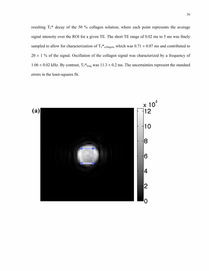
36

resulting T2* decay of the 50 % collagen solution, where each point represents the average

signal intensity over the ROI for a given TE. The short TE range of 0.02 ms to 5 ms was finely

sampled to allow for characterization of T2*collagen, which was 0.71 ± 0.07 ms and contributed to

20 ± 1 % of the signal. Oscillation of the collagen signal was characterized by a frequency of

1.06 ± 0.02 kHz. By contrast, T2*long was 11.3 ± 0.2 ms. The uncertainties represent the standard

errors in the least-squares fit.

Figure 2-1 (a). Axial UTE image of 50 % collagen solution at TE = 0.02 ms. The 10 x 8-pixel ROI is the outlined rectangle.

(a)

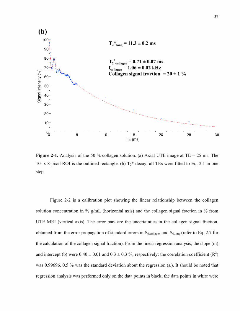
37

T2*long = 11.3 ± 0.2 ms T2

*collagen = 0.71 ± 0.07 ms

fcollagen = 1.06 ± 0.02 kHz Collagen signal fraction = 20 ± 1 %

Figure 2-1 (b). T2* decay of the 50 % collagen solution.

(b)

Figure 2-1. Analysis of the 50 % collagen solution. (a) Axial UTE image at TE = 25 ms. The

10- x 8-pixel ROI is the outlined rectangle. (b) T2* decay; all TEs were fitted to Eq. 2.1 in one

step.

Figure 2-2 is a calibration plot showing the linear relationship between the collagen

solution concentration in % g/mL (horizontal axis) and the collagen signal fraction in % from

UTE MRI (vertical axis). The error bars are the uncertainties in the collagen signal fraction,

obtained from the error propagation of standard errors in S0,collagen and S0,long (refer to Eq. 2.7 for

the calculation of the collagen signal fraction). From the linear regression analysis, the slope (m)

and intercept (b) were 0.40 ± 0.01 and 0.3 ± 0.3 %, respectively; the correlation coefficient (R2)

was 0.99696. 0.5 % was the standard deviation about the regression (sr). It should be noted that

regression analysis was performed only on the data points in black; the data points in white were

38

excluded due to large or undetermined uncertainties in the T2* fitting parameters, leading to

underestimation of the collagen signal contribution (vide infra).

The values of the fit parameters and their standard errors for each collagen solution are

displayed in Table 2-2. Values followed by an asterisk (*) could not be determined accurately,

due to a Jacobian matrix of residuals that was either singular or close to singular, and resulting

in an ill-defined covariance matrix (refer to Eq. 2.6). The main reason for a singular Jacobian

matrix was instability in the fit, apparent at collagen concentrations of 0 % and 2.5 %, due to a

low collagen signal that was difficult to characterize. Consequently, the solutions to the least-

squares fit were non-unique (linearly dependent), and could not be known exactly. Note that the

full bi-exponential T2* with oscillation equation was used for fitting the 0 % solution (i.e. the

0.125 mM MnCl2 solution); as expected, the collagen signal contribution (1 x 10-7 %) and

frequency (4 x 10-12 kHz) were negligible. Due to the reduced collagen signal, the estimation of

T2*collagen was not ideal for the 2.5 % and 5 % solutions, with values of 5 x 10-3 ms and 3 ± 2 ms,

respectively. As a result, the collagen signal contributions for these solutions were lower than

expected (0.1 % and 0.6 ± 0.3 %, respectively). It is apparent that the T2* and frequency of

collagen remained relatively constant for concentrations ranging from 10 % to 50 %, with

means of 0.75 ± 0.05 ms and 1.061 ± 0.004 kHz respectively. T2*long ranged from 11.3 ms to

38.2 ms, and decreased with increasing collagen concentration.

39

m = 0.40 ± 0.01 b = 0.3 ± 0.3 % R2 = 0.99696 sr = 0.5 %

Figure 2-2. Collagen solution calibration plot. The black points were included in the linear regression; the white points were excluded due to underestimation of the collagen signal fraction.

Figure 2-2. Collagen solution calibration plot. The error bars for the collagen signal fractions

were derived from the propagation of standard errors in S0,collagen and S0,long. The black points

were included in the linear regression; the white points were excluded due to large or

undetermined standard errors in S0,collagen and S0,long, resulting in underestimation of the collagen

signal fraction. Values of the slope (m), y-intercept (b), correlation coefficient (R2), and

standard deviation about the regression (sr) are given.

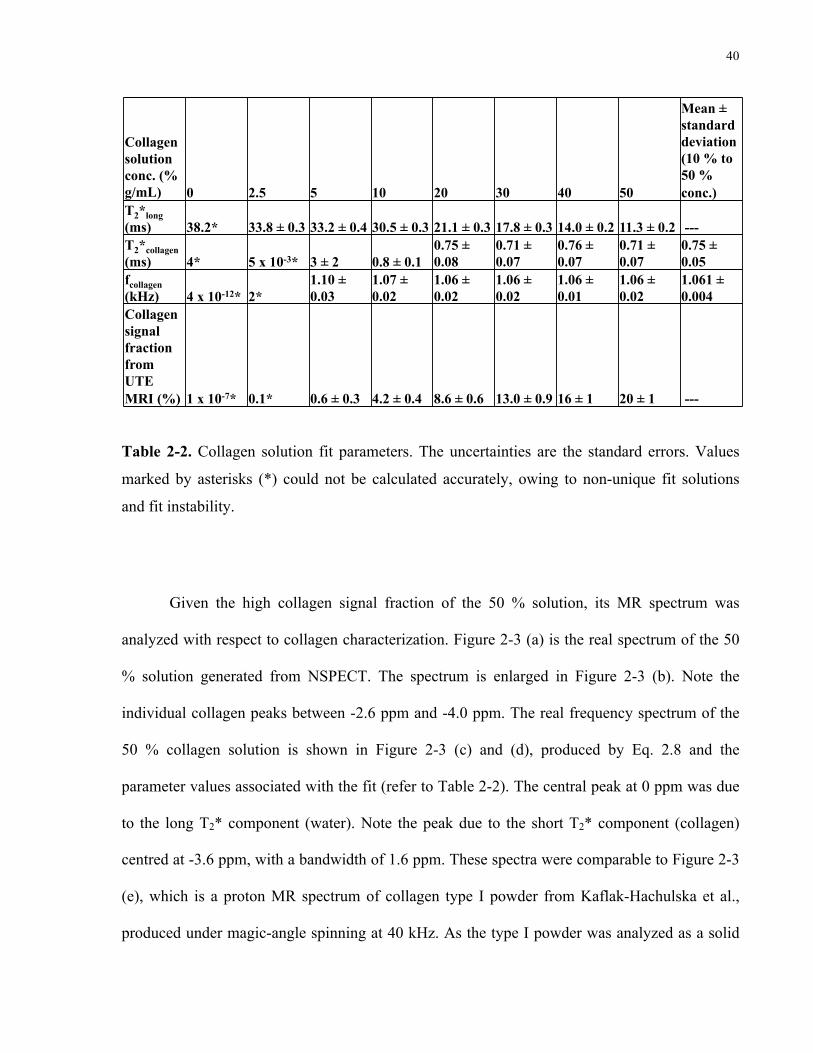
40

Collagen solution conc. (% g/mL) 0 2.5 5 10 20 30 40 50

Mean ± standard deviation (10 % to 50 % conc.)

T2*long (ms) 38.2* 33.8 ± 0.3 33.2 ± 0.4 30.5 ± 0.3 21.1 ± 0.3 17.8 ± 0.3 14.0 ± 0.2 11.3 ± 0.2 --- T2*collagen (ms) 4* 5 x 10-3* 3 ± 2 0.8 ± 0.1

0.75 ± 0.08

0.71 ± 0.07

0.76 ± 0.07

0.71 ± 0.07

0.75 ± 0.05

fcollagen (kHz) 4 x 10-12* 2*

1.10 ± 0.03

1.07 ± 0.02

1.06 ± 0.02

1.06 ± 0.02

1.06 ± 0.01

1.06 ± 0.02

1.061 ± 0.004

Collagen signal fraction from UTE MRI (%) 1 x 10-7* 0.1* 0.6 ± 0.3 4.2 ± 0.4 8.6 ± 0.6 13.0 ± 0.9 16 ± 1 20 ± 1 ---

Table 2-2. Collagen solution fit parameters. The uncertainties are standard errors. NaN = not a number; Inf = infinity.

Table 2-2. Collagen solution fit parameters. The uncertainties are the standard errors. Values

marked by asterisks (*) could not be calculated accurately, owing to non-unique fit solutions

and fit instability.

Given the high collagen signal fraction of the 50 % solution, its MR spectrum was

analyzed with respect to collagen characterization. Figure 2-3 (a) is the real spectrum of the 50

% solution generated from NSPECT. The spectrum is enlarged in Figure 2-3 (b). Note the

individual collagen peaks between -2.6 ppm and -4.0 ppm. The real frequency spectrum of the

50 % collagen solution is shown in Figure 2-3 (c) and (d), produced by Eq. 2.8 and the

parameter values associated with the fit (refer to Table 2-2). The central peak at 0 ppm was due

to the long T2* component (water). Note the peak due to the short T2* component (collagen)

centred at -3.6 ppm, with a bandwidth of 1.6 ppm. These spectra were comparable to Figure 2-3

(e), which is a proton MR spectrum of collagen type I powder from Kaflak-Hachulska et al.,

produced under magic-angle spinning at 40 kHz. As the type I powder was analyzed as a solid

41

in that paper, the water peak must have originated from bound water, rather than free water. The

collagen peaks were between 2.2 ppm and 1 ppm relative to TMS, corresponding to a range of

-2.5 ppm to -3.7 ppm relative to water (where water is chemically shifted 4.7 ppm from TMS).

(b)

(a) (c)

(d)

42

1) is typical of the P-OH groups on the crystal surface[60].

Assignment of the peaks at ca. 1 ppm (Fig. 1) is nottrivial. We have measured T1q

H for these peaks andfound that their relaxation characteristics are similar tothat of the 0 ppm peak, but completely di!erent fromthe relaxation of water resonating at 5 ppm (to bepublished). We infer that the peaks at ca. 1 ppm mightcome from structural hydroxyl groups, possibly disor-dered by the presence of structural water in hydroxylsites and thereby involved in some hydrogen bonding.Consider that discrete proton peaks in this spectral re-gion were detected for fluorohydroxyapatite [15]. It wasexplained that fluoride ions caused perturbations ofstructural hydroxyl groups, displacing them within theirchains and engaging into hydrogen bonding.

The monoclinic lattice of brushite contains 3 types ofequally populated hydroxyl groups [61]. There are 2crystallographically inequivalent water molecules, andthe HPO4

2) ions. The hydroxyl groups of the 3 speciesare involved in hydrogen bonds, which for the P-OHgroups of HPO4

2) are the strongest. The two crystallo-graphically inequivalent water molecules resonate at 4.1and 6.4 ppm, as indicated by the similar shapes andintensities of the peaks, and their location near andaround the peak position of the apatite water. Considerthat strong hydrogen bonding substantially increases theproton chemical shift, so the peak at 10.4 ppm is as-signed to the HPO4

2) ions.

The spectrum of human trabecular bone is verysimilar to that of collagen type I (Fig. 2), except that awater peak at 5.0 ppm is smaller and an extra tiny peakshows up at 2.8 ppm.

The 31P spectrum of human bone, recorded underMAS at 3 kHz, contains a single featureless peak at 3.1ppm (Fig. 3). The BD peak is from all the 31P nuclei inthe sample, while the CP peak is from the the 31P nucleilocated close to protons. The latter peak is broader.

Fig. 1. 1H NMR spectra of mineral standards recorded underMAS at 40 kHz.

Fig. 2. 1H NMR spectra of collagen type I and human tra-becular bone (B0), recorded under MAS at 40 kHz. For theupper spectra of both samples, the intensity scale was increased4 times.

Fig. 3. 31P CP and BD NMR spectra of human trabecularbone (B0), recorded under MAS at 3 kHz. The spectra arepresented with the same maximum intensities. Under the ab-solute scaling, theCP peak for the 1 ms contact time is 5 timeslower than the BD peak.

A. Kaflak-Hachulska et al.: NMR Study of Human Bone Mineral 479

(e)

Figure 2-3. Collagen MR spectra. (a) Real NSPECT spectrum of the 50 % collagen solution. (b)

Spectrum from (a), magnified 10 times. (c) Real spectrum of the 50 % collagen solution,

reconstructed from the fit parameters. (d) Spectrum from (c), magnified 10 times. (e) Type I

collagen and trabecular bone spectra, reproduced from Figure 2 of [16], with kind copyright

permission from Springer Science and Business Media. The upper spectrum of each sample is

magnified four times relative to its lower spectrum. The bound water and tallest collagen peaks

are located at 4.7 ppm and 1.5 ppm, respectively.

2.3.2 Heart tissue

Both histological and UTE MR T2* analyses were performed on the canine heart tissue, in order

to determine the collagen content. The histological image pertaining to the diffusely fibrosed

heart sample is illustrated in Figure 2-4 (a). Figure 2-4 (b) is an enlarged view of the ROI, used

for collagen area quantification. Nuclei and particle contamination were removed from the ROI

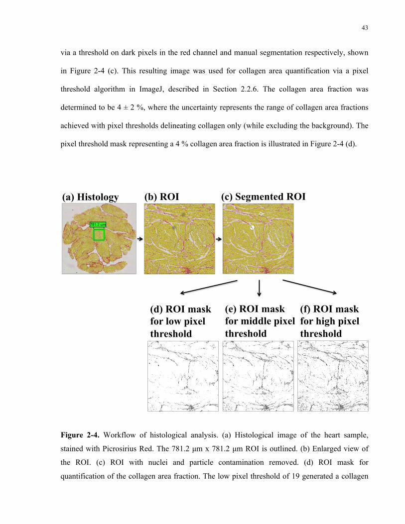
43

via a threshold on dark pixels in the red channel and manual segmentation respectively, shown

in Figure 2-4 (c). This resulting image was used for collagen area quantification via a pixel

threshold algorithm in ImageJ, described in Section 2.2.6. The collagen area fraction was

determined to be 4 ± 2 %, where the uncertainty represents the range of collagen area fractions

achieved with pixel thresholds delineating collagen only (while excluding the background). The

pixel threshold mask representing a 4 % collagen area fraction is illustrated in Figure 2-4 (d).

(a) Histology (b) ROI (c) Segmented ROI

(d) ROI mask for low pixel threshold

(e) ROI mask for middle pixel threshold

(f) ROI mask for high pixel threshold

Figure 2-4. Workflow of histological analysis. (a) Histological image of the heart sample,

stained with Picrosirius Red. The 781.2 µm x 781.2 µm ROI is outlined. (b) Enlarged view of

the ROI. (c) ROI with nuclei and particle contamination removed. (d) ROI mask for

quantification of the collagen area fraction. The low pixel threshold of 19 generated a collagen

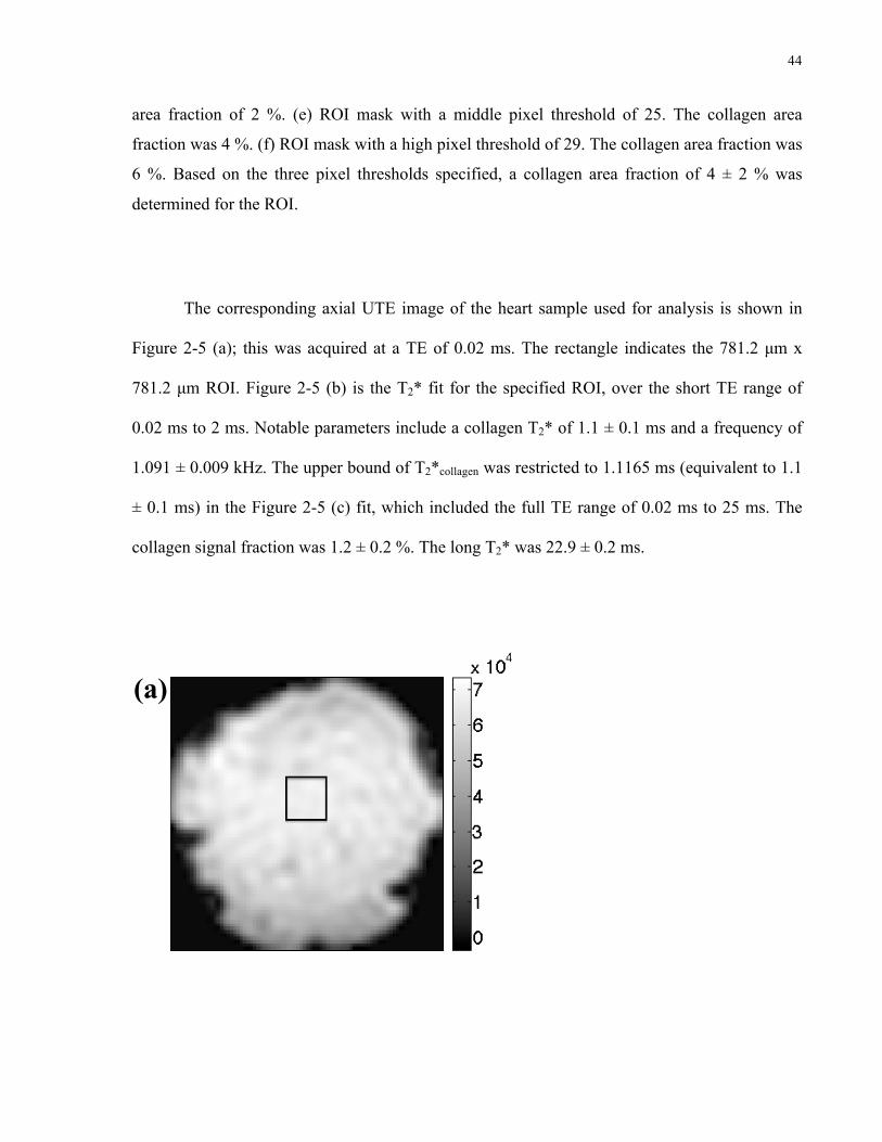
44

area fraction of 2 %. (e) ROI mask with a middle pixel threshold of 25. The collagen area

fraction was 4 %. (f) ROI mask with a high pixel threshold of 29. The collagen area fraction was

6 %. Based on the three pixel thresholds specified, a collagen area fraction of 4 ± 2 % was

determined for the ROI.

The corresponding axial UTE image of the heart sample used for analysis is shown in

Figure 2-5 (a); this was acquired at a TE of 0.02 ms. The rectangle indicates the 781.2 µm x

781.2 µm ROI. Figure 2-5 (b) is the T2* fit for the specified ROI, over the short TE range of

0.02 ms to 2 ms. Notable parameters include a collagen T2* of 1.1 ± 0.1 ms and a frequency of

1.091 ± 0.009 kHz. The upper bound of T2*collagen was restricted to 1.1165 ms (equivalent to 1.1

± 0.1 ms) in the Figure 2-5 (c) fit, which included the full TE range of 0.02 ms to 25 ms. The

collagen signal fraction was 1.2 ± 0.2 %. The long T2* was 22.9 ± 0.2 ms.

Figure 2-5 (a). Axial UTE image of the heart sample at TE = 0.02 ms. The rectangle outlines the 781.2 µm x 781.2 µm (5 x 5-pixel) ROI.

(a)

45

Figure 2-5 (b). T2* decay of the heart sample for TEs 0.02 ms to 2 ms. Note the smaller range of the y-axis.

T2*long = 28.4 ± 0.3 ms T2

*collagen = 1.1 ± 0.1 ms

fcollagen = 1.091 ± 0.009 kHz Collagen signal fraction = 1.16 ± 0.07 %

(b)

Figure 2-5 (c). T2* decay of the heart sample for TEs 0.02 ms to 25 ms. In the fit, the upper bound of T2*collagen was restricted to 1.1165 ms.

T2*long = 22.9 ± 0.2 ms T2



(c)

Figure 2-5. Canine heart sample analysis. (a) Axial UTE image at TE = 0.02 ms. The rectangle

outlines the 781.2 µm x 781.2 µm (5- x 5-pixel) ROI. (b) T2* decay for TEs 0.02 ms to 2 ms.

46

Note the smaller range of the y-axis. (c) T2* decay for TEs 0.02 ms to 25 ms. In the fit, the

upper bound of T2*collagen was restricted to 1.1165 ms.

2.4 Discussion

I have shown evidence that protons in the collagen molecule can be identified via UTE MRI;

signal from these protons appears to be associated with the short T2* signal observed in

myocardial fibrosis. As the frequency of the collagen signal is based on the -3.2 ppm chemical

shift of collagen relative to water [16], the short T2* component can be attributed to collagen

directly, rather than a bound water fraction. Using the model of bi-exponential T2* with

oscillation described in Eq. 2.1, I demonstrated: (1) the linear relationship between the collagen

signal fraction and concentration; (2) a short T2* component with a frequency shift relative to

water of ~ 1.1 kHz that is specific to collagen; (3) the T2* of protons on collagen at this

frequency of ~ 0.8 ms that is relatively constant with varying collagen concentrations; and (4)

preliminary validation of the proposed T2* model in ex vivo heart tissue. The specificity of the

collagen signal would be beneficial for its detection in the fibrosed heart.

The collagen solution calibration plot established a linear relationship between the

collagen signal fraction from UTE MRI and the known collagen concentration. A high

regression value of 0.99696 was reported, with a low standard deviation about the regression of

0.5 %. Hence, the utility of the proposed T2* model for estimating collagen was demonstrated.

The slope was 0.40 ± 0.01; for instance, a 10 % m/v collagen solution would produce a 4 %

collagen signal. It is reasonable that the slope is not equal to 1 because the collagen solution

concentration is expressed as % m/v, rather than % hydrogen nuclei in collagen/total hydrogen

nuclei. In this case, the mass of collagen powder and the final volume of the solution are known,

47

while the relative number of protons per unit mass associated with the fitted frequency is not. As

expected, the 0 % m/v collagen solution, which was fitted with the full model of bi-exponential

T2* with oscillation, revealed an insignificant collagen signal fraction of 1 x 10-7 %.

The proposed bi-exponential T2* model performed well for collagen solution

concentrations ≥ 10 % m/v, equivalent to ≥ 4 % collagen signal fractions. Assuming that a

collagen concentration of 10 % is equivalent to a collagen area fraction of 10 % in the heart, this

reflects the range where myocardial fibrosis is considered abnormal; hence, accurate

characterization for collagen concentrations below 10 % may not be important for disease

diagnosis. For the 10 % to 50 % concentrations, the mean T2*collagen and fcollagen were 0.75 ± 0.05

ms and 1.061 ± 0.004 kHz, respectively. As evident from the low standard deviations, these

values were relatively constant. The mean fcollagen corresponded to a chemical shift of -3.56 ±

0.01 ppm, which was close to the -3.2 ppm chemical shift of type I collagen found by Kaflak-

Hachulska et al. From the NSPECT spectrum, five collagen peaks were observed between -2.6

ppm and -4.0 ppm; these corresponded well with the five peaks between -2.3 ppm and -3.7 ppm

in Kaflak-Hachulska et al.’s spectrum (Figure 2-3 (e)). It is noted that my solutions were

composed of type I and III collagen from bovine hide, whereas Kaflak-Hachulska et al. used

type I collagen from bovine Achilles tendon. Differences in chemical shift could be attributed to

variations in amino acid composition between the collagen types, sample purity, and origin.

Moreover, the type I collagen spectrum was generated under magic-angle spinning at 40 kHz,

achieving narrower linewidths than those without spinning. The frequency spectrum generated

from parameters of Eq. 2.1 aligned with the NSPECT spectrum for the 50 % solution (Figure 2-

3). By fitting a broad frequency fcollagen in the T2* model, I treated the cluster of collagen peaks

between -2.6 and -4 ppm as one wide peak centred at -3.6 ppm, with a bandwidth of 1.6 ppm.

Although there were other collagen peaks near -1 ppm and +3.6 ppm in the NSPECT spectrum,

48

my objective was not necessarily to characterize all of the peaks; rather, I sought to find a

hallmark of collagen for its detection in the heart. In this case, a chemical shift of -3.6 ppm was

an adequate marker of collagen.

The mean T2*collagen of 0.75 ± 0.05 ms was attributed to the protons in collagen, due to

the association of T2*collagen with fcollagen. As T2*collagen was consistent over changing collagen

concentrations, the value appears independent of exchange effects. However, the uncertainty in

T2*collagen (~ 0.07 ms) did not change with increasing collagen concentration, indicating that

there was a systematic error affecting the precision of T2*collagen. One would normally expect the

uncertainty to decrease, as the random error (due to noise) would decrease with increasing

collagen signal. In this case, the systematic error was greater than the random error, and was

most likely due to the unmodelled signal in the T2* decay. From Figure 2-1 (b), it is observed

that Eq. 2.1 fitted the T2* decay, up to a TE of 3 ms. However, for TE > 3 ms, there was an

additional oscillatory component that was not accounted for in the model, probably attributed to

protons in collagen-associated water, and/or chemical exchange and cross-relaxation between

the collagen and long T2* components. Notably, both chemical exchange and cross-relaxation

may occur: (1) between the hydration layer water protons and bulk water protons, and (2)

between the hydration layer water protons and protein protons [24]. In my model, all of these

contributions would be aggregated into the long T2* component. Evidence for exchange was

demonstrated by comparing T2* decays at varying concentrations of collagen solution: as the

collagen concentration increased, the additional short oscillatory T2* component was more

apparent and the aggregate T2*long decreased from 38.2 ms to 11.3 ms. In an ideal bi-exponential

T2* model, one would expect T2*long to remain constant; its large range may indicate that the

term was accounting for collagen-associated water or exchange that was not modelled. My aim

was to simplify the T2* model for use in clinical diagnosis; the “pure” collagen short T2*

49

component in this model appears sufficient to characterize collagen content, at least for

concentrations ≥ 10 % m/v, supporting the use of this simplified model with a single frequency

offset term and no consideration of collagen-associated water nor exchange.

At lower concentrations, the collagen signal fractions tended to be underestimated.

Figure 2-6 (a) and (b) illustrate the T2* fit for the 2.5 % collagen solution. As the collagen T2*

component was very small, the amplitude of the signal oscillation became comparable to that of

noise. The frequency was found to be 2 kHz, with an undetermined uncertainty owing to

instability in the fit. Furthermore, the inherently short T2* of collagen rendered the component

difficult to detect by the fitting algorithm. This was indicated by a very small T2*collagen, valued

at 5 x 10-3 ms. As T2*collagen and fcollagen remained relatively constant for concentrations ≥ 10 %

m/v, I would be justified in assuming that these values would be constant for the low

concentrations as well. However, fixing parameters T2*collagen and/or fcollagen to their mean values

did not significantly improve the estimates of collagen signal fraction for the 2.5 % and 5 %

collagen solutions. Due to fit instability at these concentrations, many non-unique solutions to

the fit existed, and hence, the collagen signal fraction was not necessarily indicative of the

collagen content. The largest improvement was observed in the 2.5 % collagen solution fit

(Figure 2-6 (c) and (d)), when the upper bound of T2*collagen was restricted to 0.77 ms. Tables 2-

3 and 2-4 compare the unrestricted and restricted fits for the 2.5 % and 5 % solutions. For the

2.5 % solution, the collagen signal fraction was 0.6 ± 0.3 %, which was still low, compared to

its original value (0.1 %). The collagen frequency was 1.1 ± 0.1 kHz, which was close to the

mean fcollagen of 1.061 ± 0.004 kHz. Restriction of T2*collagen produced similar collagen signal

fractions compared to when both T2*collagen and fcollagen were restricted near their mean values. As

T2*collagen controlled the attenuation of the signal oscillation, its value affected the determination

of fcollagen, which explained the importance of fixing T2*collagen over fcollagen. By contrast, a 0.1 %

50

improvement in collagen signal fraction was witnessed in the 5 % solution, after restriction of

both T2*collagen and fcollagen. Due to the meager improvement in collagen signal fraction after

parameter fixing for both solutions, it is concluded that underestimation of the collagen signal

fraction at low collagen concentrations is an inherent limitation in the model of bi-exponential

T2* with oscillation, apparent for collagen concentrations < 10 %. Assuming that a collagen

concentration of 10 % can accurately represent a 10 % collagen area fraction in the heart, one

may conclude that UTE T2* modelling accuracy at the low collagen concentrations is not crucial

for the clinical diagnosis of myocardial fibrosis in its diseased state. This is owing to the fact

that a 10 % collagen area fraction corresponds to the minimum threshold used for the detection

of significant fibrosis [6], [11].

Figure 2-6 (a). T2* decay of the 2.5 % collagen solution.

T2*long = 33.8 ± 0.3 ms T2

*collagen = 5 x 10-3* ms

fcollagen = 2* kHz Collagen signal fraction = 0.1* %

(a)

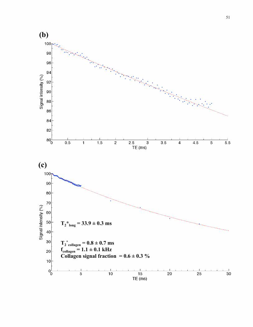
51

Figure 2-6 (b). T2* decay of the 2.5 % collagen solution, with an enlarged view of TEs 0.02 to 5.5 ms . Note the reduced range of the y-axis.

(b)

Figure 2-6 (c). T2* decay of the 2.5 % collagen solution. The fit was performed with the upper bound of T2*collagen restricted to 0.77 ms.

T2*long = 33.9 ± 0.3 ms T2



(c)

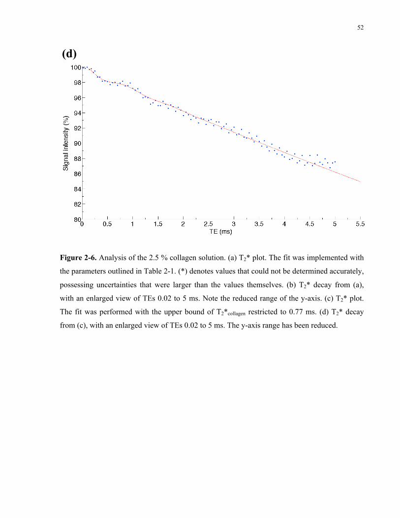
52

Figure 2-6 (d). T2* decay of the 2.5 % collagen solution, with an enlarged view of TEs 0.02 to 5.5 ms. The fit was performed with the upper bound of T2*collagen restricted to 0.77 ms. The y-axis range has been reduced.

(d)

Figure 2-6. Analysis of the 2.5 % collagen solution. (a) T2* plot. The fit was implemented with

the parameters outlined in Table 2-1. (*) denotes values that could not be determined accurately,

possessing uncertainties that were larger than the values themselves. (b) T2* decay from (a),

with an enlarged view of TEs 0.02 to 5 ms. Note the reduced range of the y-axis. (c) T2* plot.

The fit was performed with the upper bound of T2*collagen restricted to 0.77 ms. (d) T2* decay

from (c), with an enlarged view of TEs 0.02 to 5 ms. The y-axis range has been reduced.

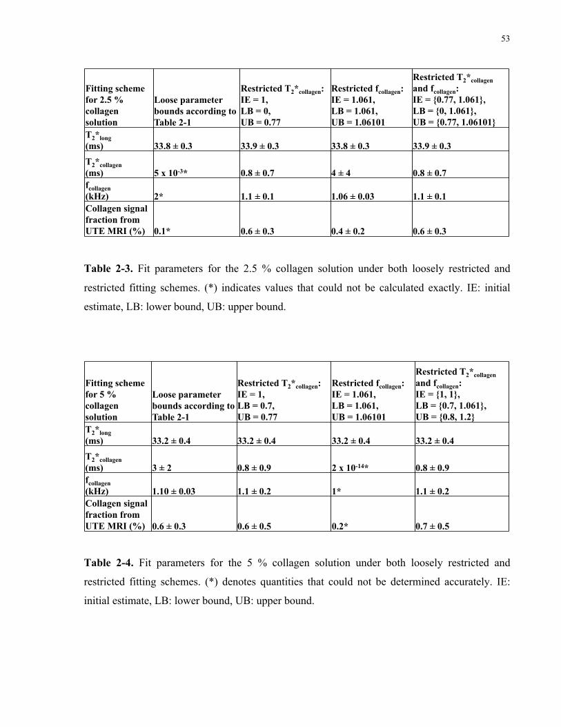
53

Fitting scheme for 2.5 % collagen solution

Loose parameter bounds according to Table 2-1

Restricted T2*collagen: IE = 1, LB = 0, UB = 0.77

Restricted fcollagen: IE = 1.061, LB = 1.061, UB = 1.06101

Restricted T2*collagen and fcollagen: IE = {0.77, 1.061}, LB = {0, 1.061}, UB = {0.77, 1.06101}

T2*long (ms) 33.8 ± 0.3 33.9 ± 0.3 33.8 ± 0.3 33.9 ± 0.3

T2*collagen (ms) 5 x 10-3* 0.8 ± 0.7 4 ± 4 0.8 ± 0.7 fcollagen (kHz) 2* 1.1 ± 0.1 1.06 ± 0.03 1.1 ± 0.1 Collagen signal fraction from UTE MRI (%)

0.1* 0.6 ± 0.3 0.4 ± 0.2 0.6 ± 0.3

Table 2-3. Fit parameters for the 2.5 % collagen solution under both loosely restricted and restricted fitting schemes. IE: initial estimate, LB: lower bound, UB: upper bound.

Table 2-3. Fit parameters for the 2.5 % collagen solution under both loosely restricted and

restricted fitting schemes. (*) indicates values that could not be calculated exactly. IE: initial

estimate, LB: lower bound, UB: upper bound.

Fitting scheme for 5 % collagen solution

Loose parameter bounds according to Table 2-1

Restricted T2*collagen: IE = 1, LB = 0.7, UB = 0.77

Restricted fcollagen: IE = 1.061, LB = 1.061, UB = 1.06101

Restricted T2*collagen and fcollagen: IE = {1, 1}, LB = {0.7, 1.061}, UB = {0.8, 1.2}

T2*long (ms) 33.2 ± 0.4 33.2 ± 0.4 33.2 ± 0.4 33.2 ± 0.4

T2*collagen (ms) 3 ± 2 0.8 ± 0.9 2 x 10-14* 0.8 ± 0.9 fcollagen (kHz) 1.10 ± 0.03 1.1 ± 0.2 1* 1.1 ± 0.2 Collagen signal fraction from UTE MRI (%) 0.6 ± 0.3 0.6 ± 0.5 0.2* 0.7 ± 0.5

Table 2-4. Fit parameters for the 5 % collagen solution under both loosely restricted and restricted fitting schemes. IE: initial estimate, LB: lower bound, UB: upper bound.

Table 2-4. Fit parameters for the 5 % collagen solution under both loosely restricted and

restricted fitting schemes. (*) denotes quantities that could not be determined accurately. IE:

initial estimate, LB: lower bound, UB: upper bound.

54

The collagen fractions assessed by MRI and histology were compared, in order to estimate the

collagen content. From histological analysis, the heart tissue had a collagen area fraction of 4 ±

2 %, which would be deemed healthy. The collagen signal fraction derived from UTE was 1.2 ±

0.2 %. Assuming the calibration curve for collagen solutions holds for tissue, this would

correspond to a collagen concentration of 2.3 ± 0.9 %. While the mass/volume collagen

concentration and the collagen area fraction may not be directly comparable, these two values

were of the same order of magnitude; hence, UTE analysis yielded a reasonable estimate of

collagen content. The low collagen signal fraction obtained in the heart tissue was expected,

given the limitation of the bi-exponential T2* with oscillation model for signal fractions < 4 %.

As T2*collagen was determined accurately in the finely sampled short TE range, it seemed

reasonable to restrict its value for the full TE range. When fitting the full TE range, T2*collagen

was limited to an upper bound of 1.1165 ms (determined from the short TE range fit), as it

affected the determination of S0,collagen. With unrestricted T2*collagen, its value was relatively high

and uncertain (5 ± 4 ms), amounting to a low collagen signal fraction of 0.8 ± 0.1 %. T2*collagen

and fcollagen were 1.1 ± 0.3 ms and 1.11 ± 0.02 kHz respectively, comparable to the mean values

of 0.75 ± 0.05 ms and 1.1061 ± 0.004 kHz in the collagen solutions. T2*collagen in the tissue

sample was slightly higher, although within the uncertainty of the T2* value in the solutions. As

observed in Figure 2-5 (c), T2*long was 22.9 ± 0.2 ms; however, this did not perfectly model the

T2* decay of the long component, which appeared bi-exponential. It is noted that the T2* decay

of muscle is multi-exponential in nature, due to intracellular compartments of muscle-associated

water [36]. As muscle-associated-water signal fractions should not contribute to the collagen

signal fraction, I deemed it reasonable to simplify the T2* behaviour of cardiac muscle to a

mono-exponential term. Interestingly, my results for T2*long, T2*collagen, and fcollagen were

comparable to the findings of Van Nierop et al. in a rat model of diffuse myocardial fibrosis at

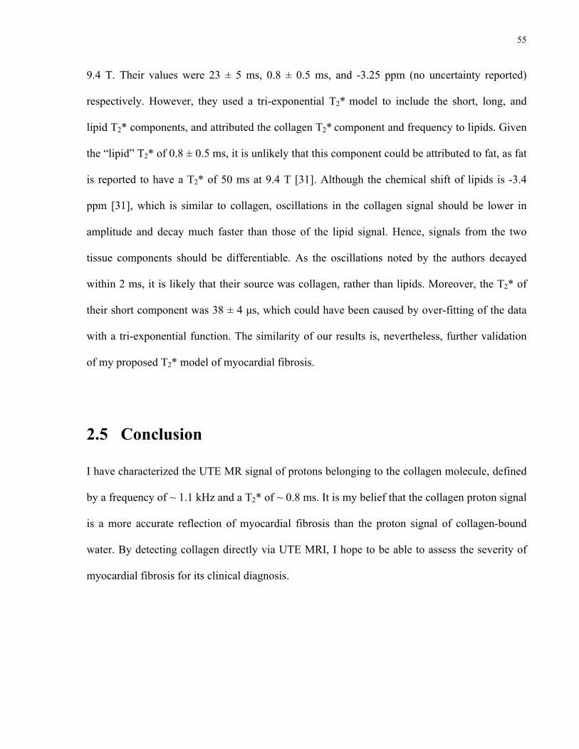
55

9.4 T. Their values were 23 ± 5 ms, 0.8 ± 0.5 ms, and -3.25 ppm (no uncertainty reported)

respectively. However, they used a tri-exponential T2* model to include the short, long, and

lipid T2* components, and attributed the collagen T2* component and frequency to lipids. Given

the “lipid” T2* of 0.8 ± 0.5 ms, it is unlikely that this component could be attributed to fat, as fat

is reported to have a T2* of 50 ms at 9.4 T [31]. Although the chemical shift of lipids is -3.4

ppm [31], which is similar to collagen, oscillations in the collagen signal should be lower in

amplitude and decay much faster than those of the lipid signal. Hence, signals from the two

tissue components should be differentiable. As the oscillations noted by the authors decayed

within 2 ms, it is likely that their source was collagen, rather than lipids. Moreover, the T2* of

their short component was 38 ± 4 µs, which could have been caused by over-fitting of the data

with a tri-exponential function. The similarity of our results is, nevertheless, further validation

of my proposed T2* model of myocardial fibrosis.

2.5 Conclusion

I have characterized the UTE MR signal of protons belonging to the collagen molecule, defined

by a frequency of ~ 1.1 kHz and a T2* of ~ 0.8 ms. It is my belief that the collagen proton signal

is a more accurate reflection of myocardial fibrosis than the proton signal of collagen-bound

water. By detecting collagen directly via UTE MRI, I hope to be able to assess the severity of

myocardial fibrosis for its clinical diagnosis.

56

Chapter 3 Future Directions

3

3.1 Introduction

The objective of this thesis research is to describe the UTE MR signal associated with

myocardial fibrosis, namely that of protons in the collagen molecule, in order to clinically assess

the extent of the disease. In the previous chapter, I characterized the frequency (~ 1.1 kHz) and

T2* of collagen protons (~ 0.8 ms) in a detailed manner that would not be feasible in a clinical

setting. Application of UTE MRI in the clinic would involve sampling with fewer TEs and MR

signal characterization of fresh, unfixed tissue containing elevated quantities of collagen. The

following chapter will consider the practicality of performing myocardial fibrosis UTE MR

measurements in the clinic.

3.2 TE sampling scheme for clinical application

The following section presents preliminary results to demonstrate the plausibility of using an

undersampled TE strategy for analysis of the UTE MR signal. The efficacy of restricting fit

parameters, namely T2*collagen and fcollagen, is also considered in this context.

56

57

3.2.1 Theory

Characterization of the collagen UTE MR signal in Chapter 2 was performed at high sampling

density, in order to accurately determine the chemical shift and signal decay properties. Notably,

sampling intervals of 0.005 ms to 0.05 ms were employed to delineate the short TE range. High

sampling densities (i.e. low sampling intervals), however, are not practical in the clinic, as they

prolong patient examination times. The optimal sampling scheme would involve sampling the

fewest number of points without sacrificing crucial signal information, particularly the

oscillation frequency. According to the Nyquist sampling theorem, the sampling frequency

should be at least twice the highest frequency observed in the signal. In this case, if I would like

to characterize a 1 kHz oscillation, the lowest sampling frequency required would be 2 kHz,

equivalent to a sampling interval of 0.5 ms. One can utilize the Nyquist sampling theorem to

develop an appropriate UTE MRI sampling scheme for the clinical diagnosis of myocardial

fibrosis, namely with TEs 0.02 (the minimum TE), 0.5, 1, 1.5, 2, 2.5, 3, 5, 10, 15, and 25 ms. I

tested this strategy by resampling the previously acquired data in collagen solutions at the above

TEs, and observing how the fit parameters were affected. Subsequently, I applied the sampling

scheme to a heart tissue sample.

3.2.2 Results

Table 3-1 illustrates the T2* fit results for the collagen solutions, where TEs 0.02, 0.5, 1, 1.5, 2,

2.5, 3, 5, 10, 15, and 25 ms were collected only. The loosely constrained fit parameters are given

in Table 2-1. In comparison with the fully sampled data set (Table 2-2), the collagen signal

fractions were similar; however, they were defined by large uncertainties, due to undersampling

and a lack of parameter constraints. Results for the undersampled fits with restrictions on

58

T2*collagen only, fcollagen only, and both T2*collagen and fcollagen, are found in Tables 3-2, 3-3, and 3-4,

respectively. For the fits where both T2*collagen and fcollagen were restricted, the constraints on the

fit parameters were adjusted accordingly to achieve T2*collagen and fcollagen values of

approximately 0.75 ms and 1.061 kHz, respectively (refer to Table 3-5). These quantities were

obtained from the mean values previously delineated in Table 2-2. Manual tuning of the

parameter constraints was necessary, as small deviations in values resulted in the inability of the

least-squares algorithm to find a set of solutions, and hence the data points were not fitted.

Overall, the three restriction strategies appeared to produce similar collagen signal fractions.

However, the collagen signal fractions were more accurate than those produced by the loosely

constrained fits, as the uncertainties were reduced.



T2*long (ms) 38 ± 1 34 ± 5 33 ± 1 29.4 ± 0.6 21.6 ± 0.6 19.0 ± 0.9 15.3 ± 0.7 12.5 ± 0.7 --- T2*collagen (ms) 2 x 10-2* 4* 2* 2 ± 1 0.6 ± 0.5 0.4 ± 0.2 0.6 ± 0.5 1 ± 1 0.8 ± 0.5 fcollagen (kHz) 1 x 10-3* 0.02* 10*

1.12 ± 0.03 1* 3* 1* 1* 1.4 ± 0.9

Collagen signal fraction from UTE MRI (%) 8 x 10-11* 0.4* 1* 3.7 ± 0.9 10 ± 3 18 ± 4 20 ± 10 20* ---

Table 3-1. Undersampled collagen solution fits. The fit parameters were loosely restricted, with the constraints specified in Table 2-1. The uncertainties are standard errors.

Table 3-1. Undersampled collagen solution fits. The fit parameters were loosely restricted, with

the constraints specified in Table 2-1. The uncertainties are standard errors. (*) indicates

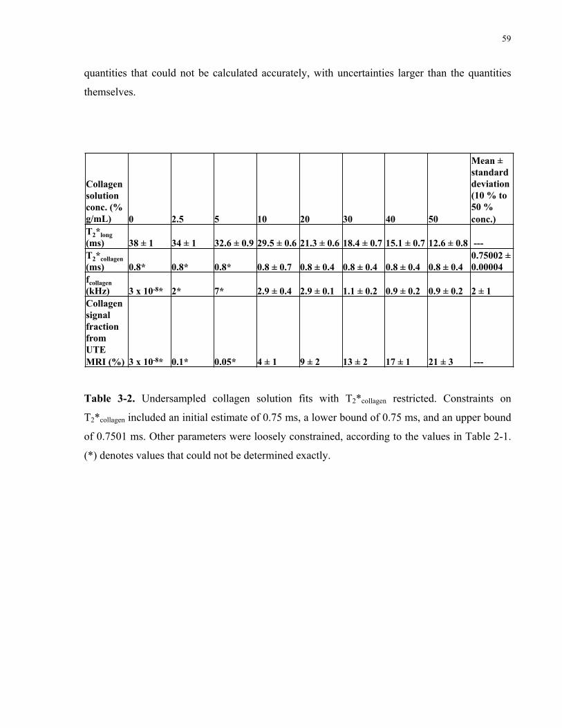
59

quantities that could not be calculated accurately, with uncertainties larger than the quantities

themselves.



T2*long (ms) 38 ± 1 34 ± 1 32.6 ± 0.9 29.5 ± 0.6 21.3 ± 0.6 18.4 ± 0.7 15.1 ± 0.7 12.6 ± 0.8 --- T2*collagen (ms) 0.8* 0.8* 0.8* 0.8 ± 0.7 0.8 ± 0.4 0.8 ± 0.4 0.8 ± 0.4 0.8 ± 0.4

0.75002 ± 0.00004

fcollagen (kHz) 3 x 10-8* 2* 7* 2.9 ± 0.4 2.9 ± 0.1 1.1 ± 0.2 0.9 ± 0.2 0.9 ± 0.2 2 ± 1 Collagen signal fraction from UTE MRI (%) 3 x 10-8* 0.1* 0.05* 4 ± 1 9 ± 2 13 ± 2 17 ± 1 21 ± 3 ---

Table 3-2. Undersampled collagen solution fits with T2*collagen restricted. Constraints on T2*collagen included an initial estimate of 0.75 ms, a lower bound of 0.75 ms, and an upper bound of 0.7501 ms. Other parameters were loosely constrained, according to the values in Table 2-1.

Rounding&is&to&the&digit&of&the&uncertainty.&If&this&produces&a&zero,&then&the&first&nonzero&digit&is&rounded.&

Table 3-2. Undersampled collagen solution fits with T2*collagen restricted. Constraints on

T2*collagen included an initial estimate of 0.75 ms, a lower bound of 0.75 ms, and an upper bound

of 0.7501 ms. Other parameters were loosely constrained, according to the values in Table 2-1.

(*) denotes values that could not be determined exactly.

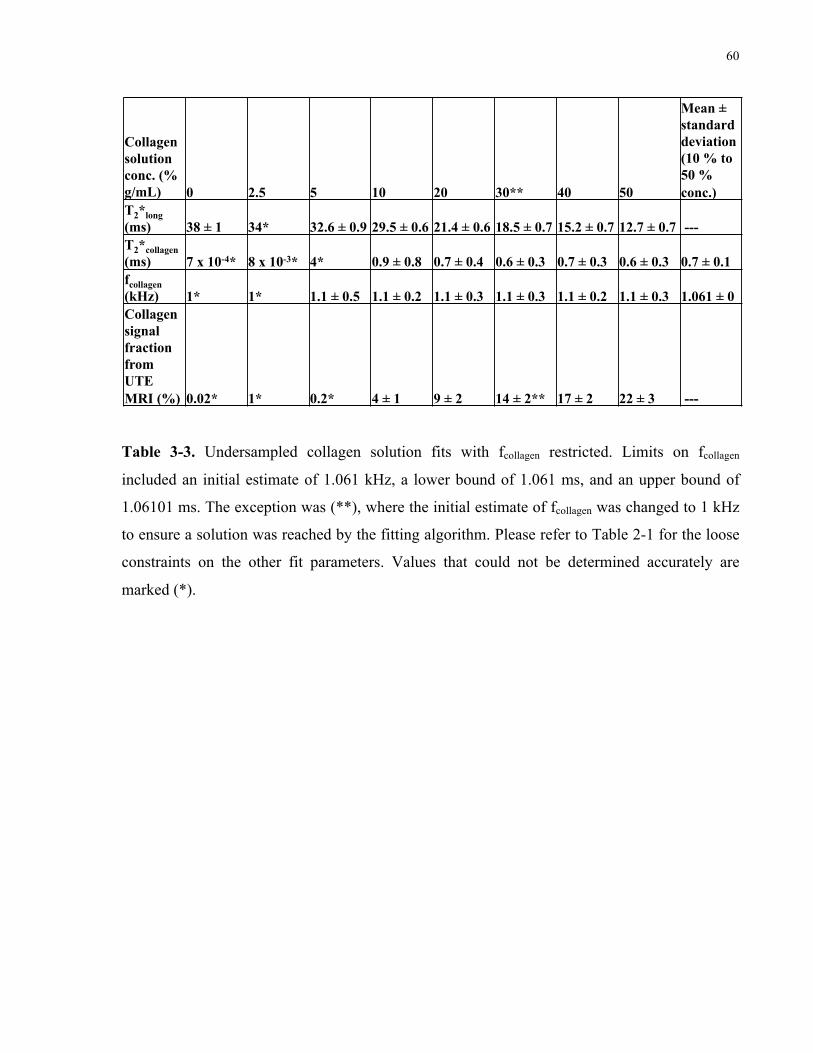
60

Collagen solution conc. (% g/mL) 0 2.5 5 10 20 30** 40 50


T2*long (ms) 38 ± 1 34* 32.6 ± 0.9 29.5 ± 0.6 21.4 ± 0.6 18.5 ± 0.7 15.2 ± 0.7 12.7 ± 0.7 --- T2*collagen (ms) 7 x 10-4* 8 x 10-3* 4* 0.9 ± 0.8 0.7 ± 0.4 0.6 ± 0.3 0.7 ± 0.3 0.6 ± 0.3 0.7 ± 0.1 fcollagen (kHz) 1* 1* 1.1 ± 0.5 1.1 ± 0.2 1.1 ± 0.3 1.1 ± 0.3 1.1 ± 0.2 1.1 ± 0.3 1.061 ± 0 Collagen signal fraction from UTE MRI (%) 0.02* 1* 0.2* 4 ± 1 9 ± 2 14 ± 2** 17 ± 2 22 ± 3 ---

Table 3-3. Undersampled collagen solution fits with fcollagen restricted. Limits on fcollagen included an initial estimate of 1.061 kHz, a lower bound of 1.061 ms, and an upper bound of 1.06101 ms. The exception was (**), where the initial estimate of fcollagen was changed to 1 kHz to ensure a solution was reached by the fitting algorithm. Please refer to Table 2-1 for the loose constraints on the other fit parameters.


Table 3-3. Undersampled collagen solution fits with fcollagen restricted. Limits on fcollagen

included an initial estimate of 1.061 kHz, a lower bound of 1.061 ms, and an upper bound of

1.06101 ms. The exception was (**), where the initial estimate of fcollagen was changed to 1 kHz

to ensure a solution was reached by the fitting algorithm. Please refer to Table 2-1 for the loose

constraints on the other fit parameters. Values that could not be determined accurately are

marked (*).

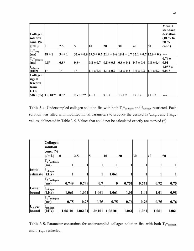
61



T2*long (ms) 38 ± 1 34 ± 1 32.6 ± 0.9 29.5 ± 0.7 21.4 ± 0.6 18.4 ± 0.7 15.1 ± 0.7 12.6 ± 0.8 --- T2*collagen (ms) 0.8* 0.8* 0.8* 0.8 ± 0.7 0.8 ± 0.5 0.8 ± 0.4 0.7 ± 0.4 0.8 ± 0.4

0.74 ± 0.01

fcollagen (kHz) 1* 1* 1* 1.1 ± 0.4 1.1 ± 0.2 1.1 ± 0.2 1.0 ± 0.3 1.1 ± 0.2

1.057 ± 0.007

Collagen signal fraction from UTE MRI (%) 4 x 10-9* 0.3* 2 x 10-8* 4 ± 1 9 ± 2 13 ± 2 17 ± 2 21 ± 3 ---

Table 3-4. Undersampled collagen solution fits with both T2*collagen and fcollagen restricted. Each solution was fitted with modified initial parameters to produce the desired T2*collagen and fcollagen values, delineated in Table 3-5.


Table 3-4. Undersampled collagen solution fits with both T2*collagen and fcollagen restricted. Each

solution was fitted with modified initial parameters to produce the desired T2*collagen and fcollagen

values, delineated in Table 3-5. Values that could not be calculated exactly are marked (*).


Initial estimate

T2*collagen (ms) 1 1 1 1 1 1 1 1 fcollagen (kHz) 1 1 1 1.061 1 1 1 1

Lower bound

T2*collagen (ms) 0.749 0.749 0.7 0 0.751 0.751 0.72 0.75 fcollagen (kHz) 1.061 1.061 1.061 1.061 1.01 1.01 1.01 0.98

Upper bound

T2*collagen (ms) 0.75 0.75 0.75 0.75 0.76 0.76 0.75 0.76 fcollagen (kHz) 1.06101 1.06101 1.06101 1.06101 1.061 1.061 1.061 1.061

Table 3-5. Parameter constraints for undersampled collagen solution fits, with both T2*collagen and fcollagen restricted.

Table 3-5. Parameter constraints for undersampled collagen solution fits, with both T2*collagen

and fcollagen restricted.

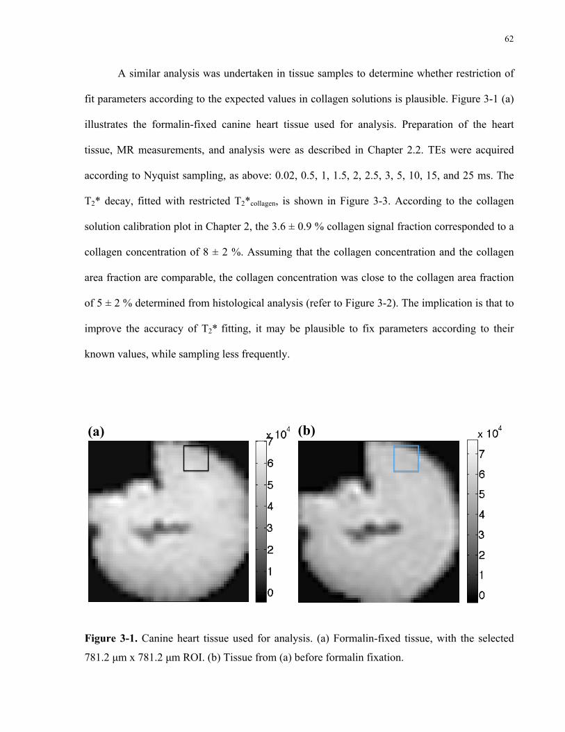
62

A similar analysis was undertaken in tissue samples to determine whether restriction of

fit parameters according to the expected values in collagen solutions is plausible. Figure 3-1 (a)

illustrates the formalin-fixed canine heart tissue used for analysis. Preparation of the heart

tissue, MR measurements, and analysis were as described in Chapter 2.2. TEs were acquired

according to Nyquist sampling, as above: 0.02, 0.5, 1, 1.5, 2, 2.5, 3, 5, 10, 15, and 25 ms. The

T2* decay, fitted with restricted T2*collagen, is shown in Figure 3-3. According to the collagen

solution calibration plot in Chapter 2, the 3.6 ± 0.9 % collagen signal fraction corresponded to a

collagen concentration of 8 ± 2 %. Assuming that the collagen concentration and the collagen

area fraction are comparable, the collagen concentration was close to the collagen area fraction

of 5 ± 2 % determined from histological analysis (refer to Figure 3-2). The implication is that to

improve the accuracy of T2* fitting, it may be plausible to fix parameters according to their

known values, while sampling less frequently.

(a) (b)

Figure 3-1. Canine heart tissue used for analysis. (a) Formalin-fixed tissue, with the selected

781.2 µm x 781.2 µm ROI. (b) Tissue from (a) before formalin fixation.

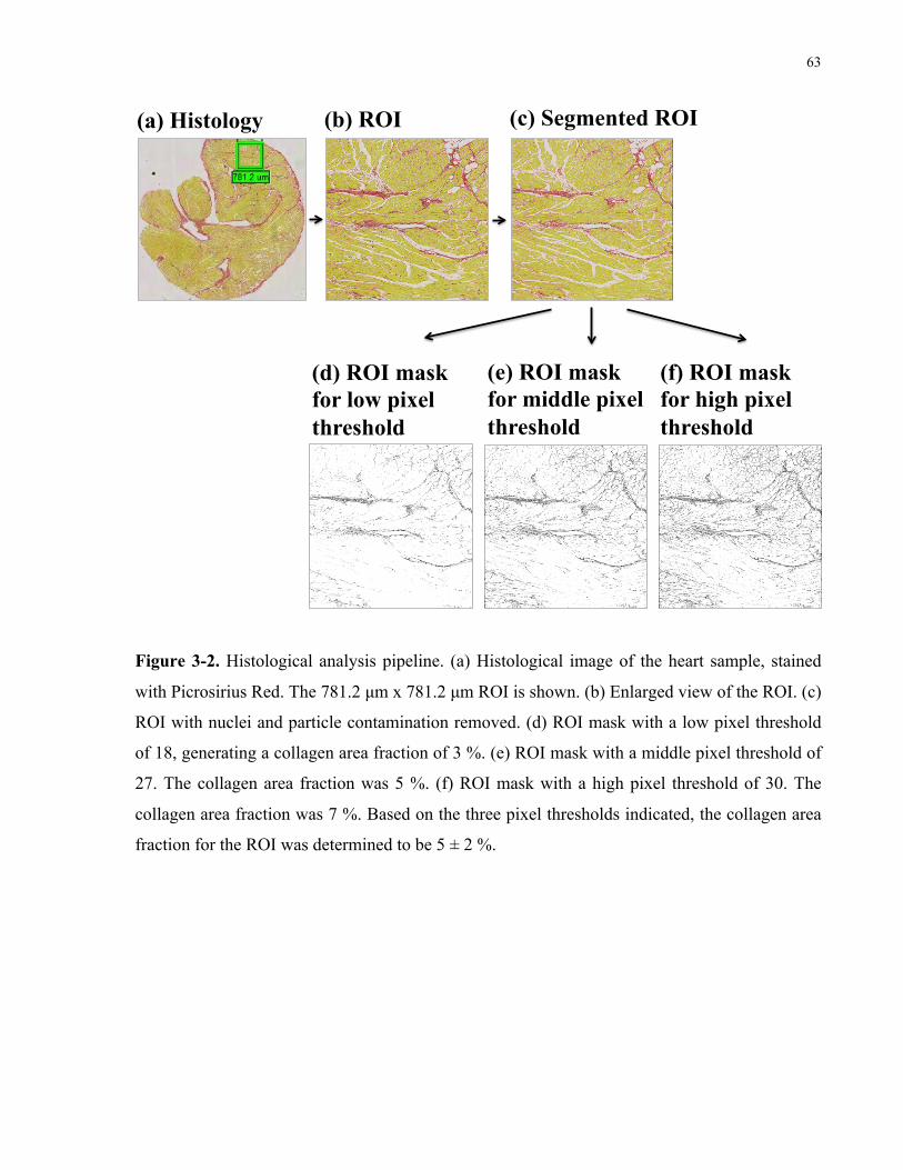
63

(a) Histology (b) ROI (c) Segmented ROI

(d) ROI mask for low pixel threshold

(e) ROI mask for middle pixel threshold

(f) ROI mask for high pixel threshold

Figure 3-2. Histological analysis pipeline. (a) Histological image of the heart sample, stained

with Picrosirius Red. The 781.2 µm x 781.2 µm ROI is shown. (b) Enlarged view of the ROI. (c)

ROI with nuclei and particle contamination removed. (d) ROI mask with a low pixel threshold

of 18, generating a collagen area fraction of 3 %. (e) ROI mask with a middle pixel threshold of

27. The collagen area fraction was 5 %. (f) ROI mask with a high pixel threshold of 30. The

collagen area fraction was 7 %. Based on the three pixel thresholds indicated, the collagen area

fraction for the ROI was determined to be 5 ± 2 %.

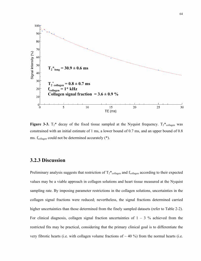
64

Figure 3-2. T2* decay of the fixed tissue sampled at the Nyquist frequency. T2*collagen was constrained with an initial estimate of 1 ms, a lower bound of 0.7 ms, and an upper bound of 0.8 ms.

T2*long = 30.9 ± 0.6 ms T2


fcollagen = 1* kHz Collagen signal fraction = 3.6 ± 0.9 %

Figure 3-3. T2* decay of the fixed tissue sampled at the Nyquist frequency. T2*collagen was

constrained with an initial estimate of 1 ms, a lower bound of 0.7 ms, and an upper bound of 0.8

ms. fcollagen could not be determined accurately (*).

3.2.3 Discussion

Preliminary analysis suggests that restriction of T2*collagen and fcollagen according to their expected

values may be a viable approach in collagen solutions and heart tissue measured at the Nyquist

sampling rate. By imposing parameter restrictions in the collagen solutions, uncertainties in the

collagen signal fractions were reduced; nevertheless, the signal fractions determined carried

higher uncertainties than those determined from the finely sampled datasets (refer to Table 2-2).

For clinical diagnosis, collagen signal fraction uncertainties of 1 – 3 % achieved from the

restricted fits may be practical, considering that the primary clinical goal is to differentiate the

very fibrotic hearts (i.e. with collagen volume fractions of ~ 40 %) from the normal hearts (i.e.

65

with collagen volume fractions of ~ 4 %). The differences in collagen signal fractions between

the three restriction strategies were minimal, suggesting that a restriction strategy can be chosen

according to the fit and the performance of the fitting algorithm.

From Table 3-5, it is evident that the fit parameter constraints needed to be modified

manually to ensure a set of solutions was reached by the fitting algorithm. As fewer points were

sampled, the number of possible solutions to the fit increased, resulting in the sensitivity of the

algorithm to constraints. This suggests that a globally applicable method of parameter

restriction, including the specification of exact constraint values, may not be possible. Arguably,

the values of the constraints are not important, as long as the expected T2*collagen and/or fcollagen

are resolved. For the tissue sample, T2*collagen was restricted. With this constraint, the signal

intensity contributions to the long and collagen T2* components were more certain than

T2*collagen (0.8 ± 0.7 ms) and fcollagen (1 kHz), resulting in a more accurate collagen signal fraction

of 3.6 ± 0.9 %. Based on the collagen solution calibration in Chapter 2, this corresponded to a

collagen concentration of 8 ± 2 %. This value was of the same order of magnitude as the 5 ± 2

% collagen area fraction obtained from histology, assuming correspondence between the

collagen concentration and the collagen area fraction. Hence, the preliminary conclusion is that

fit parameter restriction may be realistic in the clinic, as this will not compromise the

determination of the collagen signal fraction.

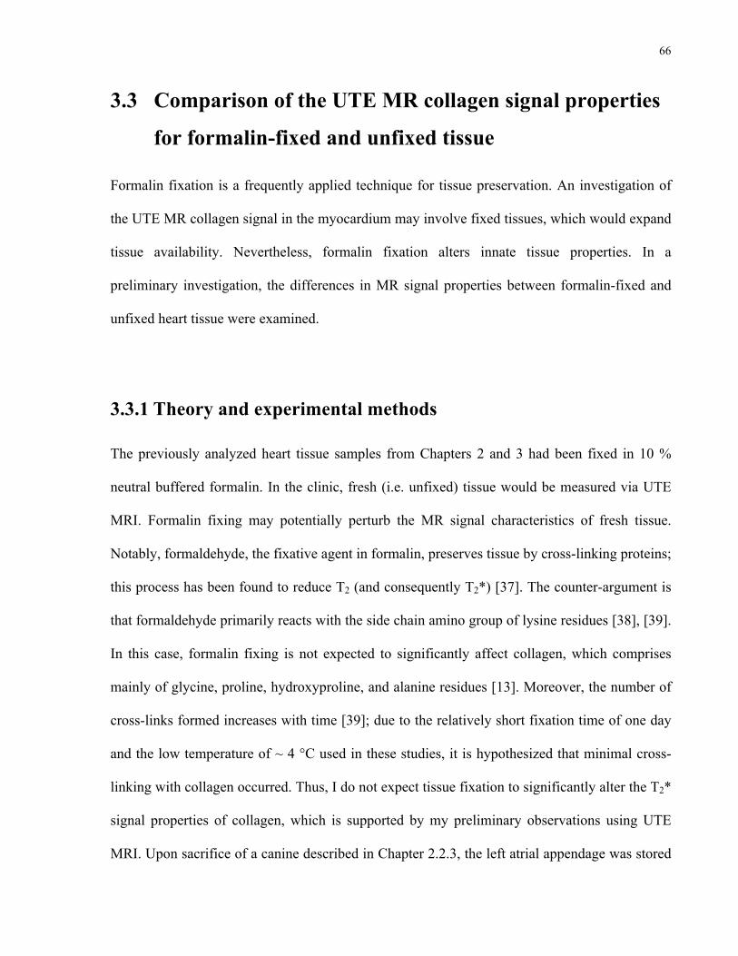
66

3.3 Comparison of the UTE MR collagen signal properties

for formalin-fixed and unfixed tissue

Formalin fixation is a frequently applied technique for tissue preservation. An investigation of

the UTE MR collagen signal in the myocardium may involve fixed tissues, which would expand

tissue availability. Nevertheless, formalin fixation alters innate tissue properties. In a

preliminary investigation, the differences in MR signal properties between formalin-fixed and

unfixed heart tissue were examined.

3.3.1 Theory and experimental methods

The previously analyzed heart tissue samples from Chapters 2 and 3 had been fixed in 10 %

neutral buffered formalin. In the clinic, fresh (i.e. unfixed) tissue would be measured via UTE

MRI. Formalin fixing may potentially perturb the MR signal characteristics of fresh tissue.

Notably, formaldehyde, the fixative agent in formalin, preserves tissue by cross-linking proteins;

this process has been found to reduce T2 (and consequently T2*) [37]. The counter-argument is

that formaldehyde primarily reacts with the side chain amino group of lysine residues [38], [39].

In this case, formalin fixing is not expected to significantly affect collagen, which comprises

mainly of glycine, proline, hydroxyproline, and alanine residues [13]. Moreover, the number of

cross-links formed increases with time [39]; due to the relatively short fixation time of one day

and the low temperature of ~ 4 °C used in these studies, it is hypothesized that minimal cross-

linking with collagen occurred. Thus, I do not expect tissue fixation to significantly alter the T2*

signal properties of collagen, which is supported by my preliminary observations using UTE

MRI. Upon sacrifice of a canine described in Chapter 2.2.3, the left atrial appendage was stored

67

at ~ 4 °C in phosphate-buffered saline. Before scanning, the tissue was brought to room

temperature and prepared as previously described (refer to Chapter 2.2.3). The UTE MRI scans

were acquired within ~ 5.5 h of sacrifice. Subsequently, the tissue was fixed in 10 % neutral

buffered formalin for one day at ~ 4 °C and rescanned for comparison.

3.3.2 Results and discussion

Images of the tissue sample before and after fixation are shown in Figure 3-1. The fixed tissue

had previously been analyzed in Chapter 3.2; however, the TEs were resampled according to

those acquired in the fresh tissue scans: 0.02, 0.06, 0.1, 0.14, 0.25, 0.5, 1, 1.5, 10, 15, and 25 ms.

Analogous MRI slices were chosen for the fixed (Figure 3-1 (a)) and fresh (Figure 3-1 (b))

tissue scans; the 781.2 µm x 781.2 µm ROI mask previously drawn on the fixed tissue image

was multiplied onto the cropped and resized fresh tissue image. The T2* decays of the fresh and

fixed tissues are shown in Figures 3-4 and 3-5, respectively. As the objective was to determine

whether there were changes in the collagen signal fraction, T2*collagen and fcollagen, due to fixation,

restrictive fit constraints were not imposed. The T2*collagens (~ 1 ms) and fcollagens (~ 1 kHz) for

the fresh and fixed tissue were within the uncertainty of one another, suggesting that the MR

signal decay properties may not significantly change as a result of fixation. The collagen signal

fractions of 6 ± 2 % and 3.5 ± 0.5 % corresponded to collagen concentrations of 14 ± 5 % and 8

± 1 % in fresh and fixed tissue, respectively. Histological analysis determined the collagen area

fraction to be 5 ± 2 % (refer to Figure 3-2). Studies on additional tissue samples are needed to

assess the significance in the collagen signal fraction change between fresh and fixed tissue.

Notably, if tissue samples with higher collagen content were analyzed, one could evaluate

whether the change in collagen signal fraction of ~ 2 % is absolute or relative to the collagen

68

content. Comparisons of fresh and fixed tissue would be beneficial for considering changes in

T2* analyses in a clinical setting.

Figure 3-3. T2* decay of the fresh tissue. Loose constraints on the fit parameters were imposed.

T2*long = 28 ± 1 ms T2

*collagen = 1* ms

fcollagen = 1.2 ± 0.1 kHz Collagen signal fraction = 6 ± 2 %

Figure 3-4. T2* decay of the fresh tissue. Loose constraints on the fit parameters were imposed.

T2*collagen could not be determined accurately (*).

69

Figure 3-4. T2* decay of the fixed tissue, sampled analogously to the fresh tissue.

T2*long = 31.0 ± 0.4 ms T2

*collagen = 1 ± 1 ms


Figure 3-5. T2* decay of the fixed tissue, sampled analogously to the fresh tissue.

3.4 Further investigations

The proceeding sections discuss potential areas of improvement and considerations for clinical

application, including models of diffuse myocardial fibrosis, UTE MR signal characteristics at

low magnetic field strengths, and spectroscopic imaging techniques utilizing short TEs.

3.4.1 Models of diffuse myocardial fibrosis

As previously suggested, the collagen content of the canine heart tissue analyzed was not

sufficiently high for modelling diffuse myocardial fibrosis in its diseased state. The collagen

area fractions of the samples analyzed thus far ranged from 2 – 7 %, short of the 10 – 40 %

70

fractions observed as a result of diffuse myocardial fibrosis [11]. In the animal model, fibrosis

was induced by rapid simultaneous atrioventricular pacing for two weeks. As the duration of

pacing was not very long, it is hypothesized that large-scale necrosis of cardiomyocytes had not

taken place, and thus, extensive collagen remodelling did not occur. Literature on a canine

model of rapid ventricular pacing shows that a maximum collagen volume fraction of ~ 20 % is

attained in the left atrial appendage after three months [40]. Hence, an option for obtaining

higher collagen content is to pace the heart for a longer duration.

Alternative sources of diffusely fibrosed heart tissue include small animal models of

diffuse myocardial fibrosis, namely in mice, and patients. However, animal models may not

produce very extensive interstitial fibrosis, unless the insult is induced for a long period of time.

Van Nierop et al. produced the disease in mice via transverse aortic constriction for seven

weeks, resulting in low collagen volume fractions of < 10 % [29]. By contrast, very extensive

states of diffuse myocardial fibrosis are present in deceased patients with late-stage heart failure

and hypertrophy. The 10 – 40 % collagen volume fractions reported were in failing human

hearts at varying stages of hypertrophy and systemic hypertension [11]. Development of fibrosis

was substantial, due to the replacement of necrosed cardiomyocytes with collagen [11]. The

challenges with studies of ex vivo human heart tissue are sample acquisition, due to scarcity and

autopsy regulations, and requirements for formalin fixation, resulting from infection control

protocols. Although large-scale studies and comparisons between fresh and fixed tissue may not

be feasible, human tissue may be valuable for rapid validation of the UTE MRI methodology in

fixed hearts with high collagen content.

For large studies of diseased states of diffuse myocardial fibrosis, a practical option is to

consider the border zone of myocardial infarcts, i.e. the boundary between the fibrotic core and

71

healthy myocardial tissue, containing viable and non-viable cardiomyocytes [41]. Our

laboratory has utilized a porcine model of chronic infarction, via a 90-min occlusion of the left

anterior descending artery using a percutaneous balloon dilation catheter [20], [42]. Four to six

weeks after the occlusion, extensive infarction was noted, with a border zone characterized by a

moderate fibrosis grade of 20 – 70 %, and dense scar with a severe fibrosis grade of ≥ 70 %

[42]. Hence, the border zone of myocardial infarcts may be a viable model for producing high

collagen content, if failing human hearts are not a viable option.

3.4.2 UTE MR collagen signal properties at clinical magnetic field

strengths

The experiments described thus far have been conducted on a pre-clinical small-animal MR

scanner at a magnetic field strength of 7 T. Notably, clinical scanners are often at lower field

strengths of 1.5 T and 3 T, potentially inciting different UTE MR collagen signal properties.

Specifically, a collagen frequency of 1 kHz at 7 T, corresponding to a chemical shift of -3.36

ppm, is equivalent to frequencies of 429 Hz at 3 T, and 214 Hz at 1.5 T. That is to say, as the

magnetic field strength decreases, the frequency decreases, and the period of signal oscillation

increases. At 3 T, this would cause the collagen T2* signal to be in phase every 2.3 ms, and out

of phase starting at 1.2 ms and in intervals of 2.3 ms. Similarly, at 1.5 T, the signal would be in

phase every 4.7 ms, and out of phase starting at 2.3 ms and in intervals of 4.7 ms. Recall that

T2* is dependent on T2, as well as local magnetic field variations: T2 is an inherent property of

matter due to spin-spin interactions and is independent of field strength. However, with

decreasing field strength, the local magnetic field variations decrease, resulting in a longer T2*.

Hence, both the period of oscillation and T2* are increased at clinical field strengths, which

72

would affect the collagen signal characterization. Accurate measurement of the T2* and

frequency of collagen would be dependent on judicious sampling of TEs, preferably spaced

further apart for the short TEs. Assuming that fewer TEs are sampled for clinical diagnosis,

collagen signal characterization may be challenging. Nevertheless, information on fcollagen and

T2*collagen acquired at 7 T would be beneficial for the determination of these signal

characteristics at clinical strengths of 1.5 T and 3 T.

3.4.3 Future techniques

The results of this thesis suggest that, in order to measure the UTE MR signal properties of

collagen in myocardial fibrosis clinically, the following are desired: short TEs, chemical shift

information, and high-density sampling (if possible). An MR technique that traditionally

possesses these traits, with the exception of short TEs, is MR spectroscopy. Localized MR

spectroscopy techniques include stimulated echo acquisition mode (STEAM) and point resolved

spectroscopy (PRESS), where MR spectra are acquired over a single voxel of interest [43]. The

challenge with these techniques is in the minimization of the TE: as the radiofrequency

excitation consists of trains of three pulses, this naturally lengthens the TE, which is defined as

the time from the excitation until the beginning of k-space sampling. Furthermore, imaging of a

small voxel of interest is not ideal for clinical diagnosis, where imaging of the entire heart is

desired. To address these challenges, MR spectroscopic imaging (SI) would be beneficial,

providing spectral information over multiple volumes, while modified to deliver short TEs. Two

such developments are noteworthy: UTE-CSI (chemical shift imaging) and UTESI.

CSI is commonly employed to specify the MR spectra, and hence the chemical shifts, on

a voxel-wise basis over an entire sample [44]. Upon application of phase encoding gradients for

73

spatial localization, a free induction decay is acquired and the Fourier transform is taken to yield

the MR spectra [45]. Recently, Robson et al. developed a 3D UTE-CSI technique that shortened

the minimum TE to 170 µs on a clinical 1.5-T system [46]. This was achieved by reducing the

delay before collection of each k-space point. Validation of the technique was performed via

23Na imaging in the healthy heart, achieving a 5 mm isotropic resolution and acquiring 128 data

points in the free induction decay. Alternatively, a 2D UTESI method was developed by Du et

al. [45], which consisted of a UTE acquisition at gradually increasing TEs; clinically acceptable

scan times were maintained via high angular undersampling in the image reconstruction. The

pulse sequence was implemented on a 3-T scanner, achieving a minimum TE of 8 µs for a total

scan time of 5 min. This was confirmed in cortical bone, imaged with a resolution of 0.78 mm;

as a T2* of 379 µs was resolved, this indicates that a collagen T2* of ~ 0.8 ms would be

detectable as well. Given their ability to effectively sample short T2* decays, spectroscopic

imaging techniques, when modified with short TEs, may be feasible for the characterization of

collagen associated with myocardial fibrosis.

3.5 Concluding remarks

The clinical diagnosis and quantification of diffuse myocardial fibrosis are important for

prevention of heart failure. However, the imaging of diffuse myocardial fibrosis remains a

challenge, due to the lack of collagen-specific contrast in current techniques. To overcome this,

the collagen T2* signal can be analyzed via UTE MRI. Proposing a simplified model of bi-

exponential T2* with oscillation, I characterized the short T2* component of collagen, described

by a collagen proton frequency of ~ 1.1 kHz and a short T2* of ~ 0.8 ms. Previously, the short

T2* component was thought to originate from the protons of collagen-bound water; by contrast,

74

I determined that the short T2* component originates from the protons in the collagen molecule,

as the frequency was derived from the chemical shift of collagen relative to water, a

characteristic that is not found in collagen-bound water. The detection of myocardial collagen

may be feasible in the clinic, with the judicious undersampling of TEs to reduce scan times, and

restriction of the collagen T2* and frequency in the T2* fit. As the ultimate objective is to image

patients with advanced stages of heart failure, further UTE MR collagen signal characterization

is needed in heart tissues with high collagen content. Potentially, short TE spectroscopic

imaging techniques may be considered for the delineation of collagen MR signal in the clinic. It

is hoped that improvement of patient outcomes can be achieved by developing MR techniques

for the diagnosis of diffuse myocardial fibrosis.

75

References

[1] Heart and Stroke Foundation, “Statistics on Heart Disease and Stroke in Canada,” 2013. [2] A. S. Flett, M. P. Hayward, M. T. Ashworth, M. S. Hansen, A. M. Taylor, P. M. Elliott,

C. McGregor, and J. C. Moon, “Equilibrium Contrast Cardiovascular Magnetic Resonance for the Measurement of Diffuse Myocardial Fibrosis: Preliminary Validation in Humans,” Circulation, vol. 122, no. 2, pp. 138–144, Jul. 2010.

[3] J. Díez, B. López, A. González, and R. Querejeta, “Clinical aspects of hypertensive myocardial fibrosis,” Curr Opin Cardiol, vol. 16, no. 6, pp. 328–335, Nov. 2001.

[4] F. Weidemann, S. Herrmann, S. Störk, M. Niemann, S. Frantz, V. Lange, M. Beer, S. Gattenlöhner, W. Voelker, G. Ertl, and J. M. Strotmann, “Impact of Myocardial Fibrosis in Patients With Symptomatic Severe Aortic Stenosis,” Circulation, vol. 120, pp. 577–584, Aug. 2009.

[5] D. M. Sado, A. S. Flett, and J. C. Moon, “Novel imaging techniques for diffuse myocardial fibrosis,” Future Cardiol, vol. 7, no. 5, pp. 643–650, Sep. 2011.

[6] A. M. Segura, O. H. Frazier, and L. M. Buja, “Fibrosis and heart failure,” Heart Fail Rev, Nov. 2012.

[7] N. Mewton, C. Y. Liu, P. Croisille, D. Bluemke, and J. A. C. Lima, “Assessment of Myocardial Fibrosis With Cardiovascular Magnetic Resonance,” J Am Coll Cardiol, Elsevier, vol. 57, no. 8, pp. 891–903, Feb. 2011.

[8] S. de Jong, T. A. B. van Veen, H. V. M. van Rijen, and J. M. T. de Bakker, “Fibrosis and Cardiac Arrhythmias,” J Cardiovasc Pharmacol, Lippincott Williams & Wilkins, vol. 57, no. 6, pp. 630–638, Jun. 2011.

[9] T. D. Karamitsos and S. Neubauer, “Detecting diffuse myocardial fibrosis with CMR: the future has only just begun,” J Am Coll Cardiol, vol. 6, no. 6, pp. 684–686, Jun. 2013.

[10] D. G. Nishimura, Principles of magnetic resonance imaging. 2001. [11] M. A. Rossi, “Connective tissue skeleton in the normal left ventricle and in

hypertensive left ventricular hypertrophy and chronic chagasic myocarditis,” Med Sci Monit, vol. 7, no. 4, p. 820, 2001.

[12] K. T. Weber, J. E. Jalil, J. S. Janicki, and R. Pick, “Myocardial collagen remodeling in pressure overload hypertrophy: A case for interstitial heart disease,” Am J Hypertens, vol. 2, no. 12, pp. 931–940, 1989.

[13] D. Reichert, O. Pascui, E. R. deAzevedo, T. J. Bonagamba, K. Arnold, and D. Huster, “A solid-state NMR study of the fast and slow dynamics of collagen fibrils at varying hydration levels,” Magn Reson Chem, Wiley, vol. 42, no. 2, pp. 276–284, Jan. 2004.

[14] J. Myllyharju and K. I. Kivirikko, “Collagens and collagen-related diseases,” Ann Med, vol. 33, no. 1, pp. 7–21, 2001.

[15] J. Schiller, D. Huster, B. Fuchs, L. Naji, J. Kaufmann, and K. Arnold, “Evaluation of Cartilage Composition and Degradation by High-Resolution Magic-Angle Spinning Nuclear Magnetic Resonance,” in Cartilage and Osteoarthritis, vol. 101, New Jersey: Humana Press, 2004, pp. 267–286.

[16] A. Kaflak-Hachulska, A. Samoson, and W. Kolodziejski, “1H MAS and 1H → 31P CP/MAS NMR Study of Human Bone Mineral,” Calcif Tissue Int, Springer, vol. 73, no. 5, pp. 476–486, Oct. 2003.

75

76

[17] S. de Jong, J. J. Zwanenburg, F. Visser, R. V. der Nagel, H. V. van Rijen, M. A. Vos, J. M. de Bakker, and P. R. Luijten, “Direct detection of myocardial fibrosis by MRI,” J Mol Cell Cardiol, Elsevier, vol. 51, no. 6, pp. 974–979, Dec. 2011.

[18] Y. Qian, A. A. Williams, C. R. Chu, and F. E. Boada, “Multicomponent T2* mapping of knee cartilage: technical feasibility ex vivo,” Magn Reson Med, vol. 64, no. 5, pp. 1426–1431, Nov. 2010.

[19] W. C. Cole, A. D. LeBlanc, and S. G. Jhingran, “The origin of biexponential T2 relaxation in muscle water,” Magn Reson Med, vol. 29, no. 1, pp. 19–24, Jan. 1993.

[20] N. R. Ghugre, M. Pop, J. Barry, K. A. Connelly, and G. A. Wright, “Quantitative magnetic resonance imaging can distinguish remodeling mechanisms after acute myocardial infarction based on the severity of ischemic insult,” Magn Reson Med, Nov. 2012.

[21] K. Hallenga and S. H. Koenig, “Protein rotational relaxation as studied by solvent proton and deuteron magnetic relaxation,” Biochem, vol. 15, no. 19, pp. 4255–4264, 1976.

[22] J. Zhong, J. C. Gore, and I. M. Armitage, “Quantitative studies of hydrodynamic effects and cross-relaxation in protein solutions and tissues with proton and deuteron longitudinal relaxation times,” Magn Reson Med, vol. 13, no. 2, pp. 192–203, Feb. 1990.

[23] J. C. Gore and R. P. Kennan, “Physical and physiological basis of magnetic relaxation,” Magn Reson Imaging, vol. 1, pp. 33–42, 1999.

[24] J. Zhong, J. C. Gore, and I. M. Armitage, “Relative contributions of chemical exchange and other relaxation mechanisms in protein solutions and tissues,” Magn Reson Med, vol. 11, no. 3, pp. 295–308, Sep. 1989.

[25] G. B. Chavhan, P. S. Babyn, B. Thomas, M. M. Shroff, and E. M. Haacke, “Principles, Techniques, and Applications of T2*-based MR Imaging and Its Special Applications,” Radiographics, vol. 29, no. 5, pp. 1433–1449, Sep. 2009.

[26] J. P. Ridgway, “Cardiovascular magnetic resonance physics for clinicians: part I,” J Cardiovasc Magn Reson, BioMed Central, vol. 12, no. 1, p. 71, Nov. 2010.

[27] M. D. Robson and G. M. Bydder, “Clinical ultrashort echo time imaging of bone and other connective tissues,” NMR Biomed, Wiley, vol. 19, no. 7, pp. 765–780, 2006.

[28] Bruker BioSpin MRI GmbH, “Paravision 5.1 Application Manual,” Jun. 2010. [29] B. J. van Nierop, J. L. Nelissen, N. A. Bax, A. G. Motaal, L. de Graaf, K. Nicolay, and

G. J. Strijkers, “In vivo ultra short TE (UTE) MRI detects diffuse fibrosis in hypertrophic mouse hearts,” Proc Int Soc Magn Reson Med, Abstract #1360. Apr. 2013.

[30] S. B. Reeder, I. Cruite, G. Hamilton, and C. B. Sirlin, “Quantitative assessment of liver fat with magnetic resonance imaging and spectroscopy,” J Magn Reson Imaging, vol. 34, no. 4, Sep. 2011.

[31] M. Gajdošík, M. Chmelík, I. Just-Kukurová, W. Bogner, L. Valkovic, S. Trattnig, and M. Krššák, “In vivo relaxation behavior of liver compounds at 7 tesla, measured by single-voxel proton MR spectroscopy,” J Magn Reson Imaging, Nov. 2013.

[32] G. J. Stanisz, E. E. Odrobina, J. Pun, M. Escaravage, S. J. Graham, M. J. Bronskill, and R. M. Henkelman, “T1, T2 relaxation and magnetization transfer in tissue at 3T,” Magn Reson Med, vol. 54, no. 3, pp. 507–512, 2005.

[33] A. Ramadeen, G. Laurent, C. C. dos Santos, X. Hu, K. A. Connelly, B. J. Holub, I. Mangat, and P. Dorian, “n-3 Polyunsaturated fatty acids alter expression of fibrotic and hypertrophic genes in a dog model of atrial cardiomyopathy,” Heart Rhythm, vol. 7, no. 4, pp. 520–528, Apr. 2010.

77

[34] “Technical Details BioSpec MRI - Multi Purpose High Field MRI/MRS Research Systems,” bruker.com. [Online]. Available: http://www.bruker.com/products/mr/preclinical-mri/biospec/technical-details.html. [Accessed: 27-Jul-2014].

[35] “Polysciences, Inc. - FAQ: Picrosirius Red Stain Kit. Technical Data Sheet 837,” polysciences.com. [Online]. Available: http://www.polysciences.com/SiteData/docs/837/013378013a29f7e25f8b87d15979dc58/837.pdf. [Accessed: 27-Jul-2014].

[36] W. C. Cole, A. D. LeBlanc, and S. G. Jhingran, “The origin of biexponential T2 relaxation in muscle water,” Magn Reson Med, vol. 29, no. 1, pp. 19–24, Jan. 1993.

[37] R. J. Dawe, D. A. Bennett, and J. A. Schneider, “Postmortem MRI of human brain hemispheres: T2 relaxation times during formaldehyde fixation,” Magn Reson Med, 2009.

[38] J. A. Gerrard, P. K. Brown, and S. E. Fayle, “Maillard crosslinking of food proteins I: the reaction of glutaraldehyde, formaldehyde and glyceraldehyde with ribonuclease,” Food Chem, 2002.

[39] R. Thavarajah, V. K. Mudimbaimannar, J. Elizabeth, U. K. Rao, and K. Ranganathan, “Chemical and physical basics of routine formaldehyde fixation,” J Oral Maxillofac Pathol, vol. 16, no. 3, p. 400, 2012.

[40] B. Avitall, J. Bi, A. Mykytsey, and A. Chicos, “Atrial and ventricular fibrosis induced by atrial fibrillation: Evidence to support early rhythm control,” Heart Rhythm, vol. 5, no. 6, pp. 839–845, Jun. 2008.

[41] P. C. Ursell, P. I. Gardner, A. Albala, J. J. Fenoglio, and A. L. Wit, “Structural and electrophysiological changes in the epicardial border zone of canine myocardial infarcts during infarct healing,” Circulation, 1985.

[42] M. Pop, N. R. Ghugre, V. Ramanan, L. Morikawa, G. Stanisz, A. J. Dick, and G. A. Wright, “Quantification of fibrosis in infarcted swine hearts by ex vivolate gadolinium-enhancement and diffusion-weighted MRI methods,” Phys Med Biol, vol. 58, no. 15, pp. 5009–5028, Jul. 2013.

[43] G. Hamilton, M. S. Middleton, and M. Bydder, “Effect of PRESS and STEAM sequences on magnetic resonance spectroscopic liver fat quantification,” J Magn Reson Imaging, 2009.

[44] T. R. Brown, B. M. Kincaid, and K. Ugurbil, “NMR chemical shift imaging in three dimensions,” Proc Nat Acad Sci, vol. 79, no. 11, pp. 3523–3526, Jun. 1982.

[45] J. Du, G. Hamilton, A. Takahashi, M. Bydder, and C. B. Chung, “Ultrashort echo time spectroscopic imaging (UTESI) of cortical bone,” Magn Reson Med, vol. 58, no. 5, pp. 1001–1009, Nov. 2007.

[46] M. D. Robson, D. J. Tyler, and S. Neubauer, “Ultrashort TE chemical shift imaging (UTE-CSI),” Magn Reson Med, vol. 53, no. 2, pp. 267–274, Feb. 2005.

AGS MSc Thesis V4 - TSpace

Documents

Transcript of AGS MSc Thesis V4 - TSpace