INSTITUTO POLITECNICO NACIONALCENTRO INTERDISCIPLINARIO DE CIENCIAS MARINAS

FEEDING ECOLOGY AND SEASONAL MOVEMENT PATTERNS OF THE BLUE WHALE

IN THE EASTERN PACIFIC OCEAN

TESIS

QUE PARA OBTENER EL GRADO DE DOCTORADO EN CIENCIAS MARINAS

PRESENTA

GERALDINE ROSALIE BUSQUETS VASS

LA PAZ, B.C.S., JULIO DE 2017

I

INDEX INDEX ........................................................................................................................ I

DEDICATION ............................................................................................................ IV

ACKNOWLEDGEMENTS .......................................................................................... V

THESIS ACHIEVEMENTS ...................................................................................... VIII

LIST OF FIGURES ...................................................................................................... X

LIST OF TABLES ................................................................................................... XIV

GLOSSARY .......................................................................................................... XVII

ABSTRACT ............................................................................................................ XXI

RESUMEN ........................................................................................................... XXIII

1. INTRODUCTION .................................................................................................... 1

2. BACKGROUND ................................................................................................... 10

3. JUSTIFICATION .................................................................................................. 21

4. HYPOTHESIS ...................................................................................................... 22

5. OBJECTIVES ........................................................................................................ 22

5.1. Specific objectives ........................................................................................... 22

6. MATERIALS AND METHODS .............................................................................. 23

6.1. Study area ...................................................................................................... 23

6.1.1. Northeast Pacific Ocean (NEP) ............................................................... 26

6.1.2. Southeast Pacific Ocean (SEP) ............................................................... 31

6.2. Sample collection and selection ..................................................................... 32

6.3. Skin biopsy separation into skin strata ........................................................... 35

6.4. Standardizing blue whale skin sample preparation ........................................ 37

6.5. Stable isotope analysis ................................................................................... 38

II

6.6. Statistical analysis .......................................................................................... 39

6.6.1. Assessing the effect of different processing methods in the isotope values

of blue whale skin samples ................................................................................ 39

6.6.2. Comparing the variability of blue whale skin isotope values by strata ..... 39

6.6.3. Estimating blue whale skin strata isotopic incorporation rate ................... 40

6.6.4. Determining the isotopic niche width and trophic overlap of blue whales in

the eastern Pacific, by region (SEP and NEP) and sex (females and males) .... 42

6.6.5. Quantifying the relative contribution of different foraging zones to the blue

whale diet in the NEP ........................................................................................ 44

6.6.6. Estimating blue whale baleen growth rates and isotopic niche width to infer

the movement patterns of individual blue whales in the NEP ............................ 45

7. RESULTS .............................................................................................................. 46

7.1. Assessing the effect of different processing methods in the isotope values of

blue whale skin samples ....................................................................................... 46

7.2. Comparing the variability of blue whale skin isotope values by strata ............ 46

7.3. Estimating blue whale skin strata isotopic incorporation rate ......................... 49

7.4. Isotopic niche width and trophic overlap of blue whales in the eastern Pacific

Ocean by region and sex ...................................................................................... 56

7.4.1. Blue whales in the NEP and SEP ............................................................ 56

7.4.2. Female and male blue whales in the eastern Pacific Ocean .................... 59

7.5. Quantifying the relative contribution of different foraging zones to the blue

whale diet in the NEP ............................................................................................ 61

7.6. Estimating blue whale baleen growth rates and isotopic niche width to infer the

seasonal movement patterns of individual blue whales in the NEP ....................... 63

7.7. δ13C values of skin and baleen plates ............................................................ 69

8. DISCUSSION ....................................................................................................... 73

III

8.1. Influence of lipid-extraction and DMSO preservation on skin δ13C and δ15N

values .................................................................................................................... 73

8.2. Skin δ15N isotopic incorporation rates ............................................................ 73

8.3. Isotopic niche width and overlap of blue whales in the SEP and NEP ............ 75

8.4. Relative contribution of different foraging zones to the blue whale diet in the

NEP ........................................................................................................................ 77

8.5. Blue whale baleen growth rates and isotopic niche width to infer seasonal

movement patterns of individual blue whales ........................................................ 78

8.6. δ15N trophic discrimination factors .................................................................. 81

8.7. Temporal consistency of baseline δ15N values among foraging zones ........... 81

8.8. δ13C values in blue whale skin and baleen plates .......................................... 83

8.9. δ13C and δ15N values along the baleen plate of a blue whale calf ................... 83

8.10. Summary ...................................................................................................... 85

9. CONCLUSIONS ................................................................................................... 86

10. RECOMENDATIONS ......................................................................................... 87

11. REFERENCES .................................................................................................... 88

12. APPENDIX ....................................................................................................... 120

IV

DEDICATION

I would like to dedicate this work to my amazing and passionate family: Salvador Busquets, alias piap: Dad, you gave me the tools in life to become a stronger person in every sense by giving me all your love, patience, guidance and support. Today I feel more confident than ever in my own skin because of your teachings. Chally Soto, alias miam: Mom, you have taught me how to always stand for my ideals, but also to be a critic of them. Thanks to you, I am ready to fight ever day to achieve my biggest dreams, I have become a dreamer with a purpose. Valerie Busquets (valpal), my sister: My best friend in life, whom has shown me to have passion for my work. We have shared so many adventures together, you are my other half. I adore you! Dante Busquets (hermaniosos), and his son Bruno: My big brother, I admire you deeply. I carry in my heart all those amazing moments we have shared. Mario A. Pardo, my husband! The owner of my most extreme emotions. The love of my life, my friend, my professor, my colleague, my everything. I have grown into the person I am today because of our free love, that has bonded us forever. I admire you and love you deeply. You are one of my favorite persons in life and I could have never imagined finding someone like YOU. YOU ARE EMBEDED IN MY SOUL. I LOVE YOU MARIO. My grandmother: We never know how fragile we are until we lose those we love. I carry within all the love and unforgettable moments that we shared in life, love you for the eternity. My friends and family. My furry creatures (Tika and Kaia; Rest in Peace: Orca, Tsunami, Benito): My little treasures (dead and live) and family. Because there is nothing more rewarding and heart comforting than cuddling with my critters. To the blue whale: One of biggest creations of evolution and the muse of all my projects. There is nothing more life-fulfilling for me than scanning the sea surface in search for cetaceans.

Big things have small beginnings....

This project started as a simple proposal while volunteering in a blue whale ship survey off Santa Barbara, California in 2012. Ever since, it evolved slowly through a series of incredible events that truly convinced me that we are the owners of our destiny while we are alive. Small steps and perseverance can take you anywhere you want, as long are you are ready to push yourself. Get out of you comfort zone and the magic will happen. Today I know that in the end time is ticking, we must live every day with passion even when we are tired and sad, even when things are not as we expected. Sooner or later we will all become dust....be true to yourself and others every single day, work hard, dream big and above all enjoy yourself.

V

ACKNOWLEDGEMENTS

This PhD thesis is the result of the collaboration of several institutions, colleagues and professors. I am deeply beholden of the intensive support that I have received during the development of this project. I would like to acknowledge the Centro Interdisciplinario de Ciencias marinas – Instituto Politécnico Nacional (CICIMAR-IPN) that allowed me to participate in the PhD program, and all the institutions that funded this project: the CONACYT (Consejo Nacional de Ciencia y Tecnología), BEIFI (Beca de Estímulo Institucional de Formación de Investigadores), Beca mixta CONACYT, COFA (Comisión de Operación y Fomento de Actividades Académicas del Instituto Politécnico Nacional), SAI-CICIMAR (Subdirección Académica y de Investigación del CICIMAR-IPN), Center for Stable Isotopes (CSI) at the University of New Mexico, Cascadia Research Collective (CRC), American Cetacean Society-Monterey Bay Chapter and Cetacean Society International. First, I would like to thank my thesis director, Dr. Diane Gendron, whom I thank for introducing me to the world of cetaceans, being my unconditional mentor and my inspiration to work harder every day. All the opportunities that she has given me, working in diverse projects and guiding bachelor students, have contributed to my development as researcher. I feel privileged to have been her student since the Master Degree, and cannot wait to develop more projects with her counseling. Dr. Seth D. Newsome gave me an opportunity without even knowing me. He opened the doors of his house and of his laboratory to me without restriction. After that I have never stopped learning from him. I thank him for all his patience, dedication, edits, guiding, and support. The energy that he transmits in every meeting is contagious, and he was the wings of this project, he gave me wings to pursue the first publication. There are no words to express how grateful I am to Seth Newsome and also his amazing family (Anne, Tessa & Mizou!). My thesis committee guided me constantly throughout 4 years of my life to finish this project, and I would like to thank each one of them. Dr. Sergio Aguíñiga-García, since the very beginning he strongly supported and trusted my ideas, even when the goals seemed far away. I thank him for always trusting my judgment and for helping me achieve my goals. Dr. Jaime Gómez-Gutiérrez, one of my role model scientist, he was very critical of my work, pushing me to go further, to question everything. I truly admire him and his work. It has been an incredible journey learning about the biology of krill with Dr. Gómez-Gutiérrez, and also working with him during cetacean surveys (and krill surveys!). I also want to thank him for thoroughly reviewing my thesis, his comments helped greatly improve this work. Dr. Hector Villalobos, my R mentor and Guru! I thank him for all the time and patience invested in this project, he has been incredibly supportive, and was always available to help me, especially during the last steps of the publication. I feel extremely privileged to have a had such an incredible and professional thesis committee.

VI

My co-author Jeff K. Jacobsen, has been a key element in the development of this project. His advice, help and guidance were constant. I would like to thank him for all his support and contributions. He also gave me a space in his house and allowed me to make an unconventional laboratory in one of the rooms, thanks JEFF! John Calambokidis gave me an amazing opportunity to work with one of the largest blue whale skin tissue bank in the world and I really appreciate that he trusted me to develop this project. I thank his constant critic, key observations and support. To my colleagues Gabriela Serra-Valente and Kelly Robertson, from the National Oceanic and Atmospheric Administration-Southwest Fisheries Science Center (NOAA-SWFSC), both invested so much time helping me, I think I will be forever in debt. Their constant support via e-mail was a trigger to the logistics of this project. Their kindness and friendship during this process was very motivating for me. Angel H. Ruvalcaba Díaz, from the stable isotope laboratory at CICIMAR-IPN, helped me intensively during the processing of samples, and really appreciate him sharing with me his knowledge on stable isotope analysis. It took a great amount of effort getting all the paperwork needed to start and end each of the eight semesters of this PhD project. This work would have never been possible without the support of Lic. Humberto Heleodoro Ceseña Amador (Thank you Dr. for all you support, patience and help!), Cesar Servando Casas Nuñez (Thank you for letting me invade the office and bombard you with questions), Lic. Maria Magdalena Mendoza Talpa (For all the patience and support during my grant applications), Lic. Jesús Adriana Toledo Acosta, Lic. Luz De La Paz Pinales Soria, M.A. Alondra Virginia Fernández, Lic. Jasmin Noyola Mendoza, Alma Sulema Arista Castro, Deyanira Rangel Meza, Lic. Ma de Jesús Aguilar Luna and Filiberto. I would also like to thank the support and friendship of Margarita Vargas Velázquez, Isadora Josefina Retes Arrambidez, Ma. De Lourdes Pineda Álvarez, Juan García Rangel, Martina Verdugo Ojeda, and Doña Martha Palma. Also I want to thank all the personal at CICIMAR-IPN, NOAA-SWFSC and the University of New Mexico that helped me during the process of developing this project. Mario A. Pardo-Rueda, my Bayesian professor. He has helped me throughout the process of learning the proper statistical methods, and has taught me to be extremely critical of my own work. He also encouraged me to trust myself, be pro-active in science, and to never let my background stop me from achieving my goals. I want to thank him for the time he has invested in helping me learn how to write code in R. It has changed the way I think and I am eager to learn to loop everything! I LOVE you, Dr. Pardous.....!! I don’t know what would I have done without all my amazing friends and lab mates in Mexico, La Paz, in La Jolla, in Arcata, and in New Mexico. I want to thank Milena Mercuri, Christian Salvadeo, Louisa Renero, Yadira Trejo, Fabiola Guerrero de la Rosa, Jenny Noble, Max Noble, Cath Arnold, Azucena Ugalde de la Cruz,

VII

Susana Cárdenas, Roberto Aguilera Angulo, Emily Evans, Marion Cruz, Gabriela Garcia, Hiram Rosales Nanduca, Anidia Blanco Jarvio, Tim Means, Carlos Means, Mark Lowry and Marylin Lowry for their friendship, all our adventures and endless discussions about life. This part of my life is really important to keep me going. I would also like to thank my friends at the lab in La Paz and from CSI, Leticia Carrillo, Ana Sofia Merina, Carlos Dominguez, Cristina Casillas, Vianney Jimenez, Aurora Paniagua, Emma Elliot-Smith, Sara Foster, Viorel Atudorei, Laura Burkemper, Laura Pages and Dave Vanhorn, Allyson Richins, Mauriel Rodriguez Curras, Mirsha (Ricardo) Mata, John Whiteman, Debora Boro and all the amazing people that I have met during the road of this PhD life. I would never change the course that I took and you all where there for me, thank you for sharing a part of your life with me. I would also like to acknowledge the institutions that facilitated the use of tissues samples and issued the permits to collect and process these samples: NOAA-SWFSC, CRC, CICIMAR-IPN, Humboldt State University-Vertebrate Museum, Museo de la Ballena y Ciencias del Mar (La Paz, BCS), the California Department of Parks and Recreation-Prairie Creek Redwoods State Park, NOAA/NMFS and SEMARNAT. I am also very grateful to all the personnel from the former institutions, the Stranding Network of California, and the CSI of the University of New Mexico who participated in the collection and processing of the tissue samples. I would also like to thank the John H. Prescott Marine Mammal Rescue Assistance Grant Program that has provided grants to the stranding networks. Jim Rice, Jerry Loomis, Thorvald Holmes, and Francisco J. Gómez-Díaz collaborated during the process of locating potential baleen plates for this study and I am very beholden for their support. We would also like to give special recognition to Kelly Robertson who helped with the logistics of sample selection and the sex identification of an important baleen sample at the genetics lab in SWFSC. All whale tissues used in this study were collected and processed under special permits issued by the Secretaría de Medio Ambiente y Recursos Naturales (SEMARNAT) in México (codes: 180796-213-03, 071197- 213-03, DOO 750-00444/99, DOO.0-0095, DOO 02.-8318, SGPA/DGVS-7000, 00624, 01641, 00560, 12057, 08021, 00506, 08796, 09760, 10646, 00251, 00807, 05036, 01110, 00987; CITES export permit: MX 71395), and the National Oceanic and Atmospheric Administration–National Marine Fisheries Service (NOAA/NMFS) (NMFS MMPA/Research permits codes: NMFS-873; 1026; 774-1427; 774-1714; 14097; 16111; CITES import permit: 14US774223/9) in the United States of America.

VIII

THESIS ACHIEVEMENTS PEER-REVIEWED PUBLICATION: Busquets-Vass G., S. D. Newsome, J. Calambokidis, G. Serra-Valente, J. K. Jacobsen, S. Aguíñiga-García & D. Gendron. 2017. Estimating blue whale skin isotopic incorporation rates and baleen growth rates: Implications for assessing diet and movement patterns in mysticetes. PLoS ONE 12(5): e0177880. https://doi.org/10.1371/journal.pone.0177880 MANUSCRIPT IN PREPARATION: Busquets-Vass G., S. D. Newsome, J. Calambokidis, G. Serra-Valente, J. K. Jacobsen, S. Aguíñiga-García & D. Gendron. 2017. Isotopic niche width of the blue whale in the eastern Pacific Ocean. Busquets-Vass G., S. D. Newsome, J. Calambokidis, G. Serra-Valente, J. K. Jacobsen, S. Aguíñiga-García & D. Gendron. 2017. Feeding ecology of the blue whale in the northeast Pacific Ocean inferred by stable isotopes of nitrogen. PRESENTATIONS: Busquets-Vass, G. R., S. D. Newsome, J. Calambokidis, S. Aguiñiga-García, G. Serra-Valente, J. K. Jacobsen & D. Gendron. 2016. Trophic overlap between blue whale foraging zones in the eastern Pacific Ocean. XXXV Reunión Internacional para el estudio de los mamíferos marinos. La Paz, Baja California Sur, Mexico, May 1-5, 2016. Oral presentation. Busquets-Vass, G. R., S. D. Newsome, J. Calambokidis, S. Aguiñiga-García, G. Serra-Valente, J. K. Jacobsen & D. Gendron. 2015. Foraging ecology and movement patterns of blue whales in the eastern Pacific Ocean inferred by stable isotopes. Abstract (Proceedings) 21st Biennial Conference on the Biology of Marine Mammals, San Francisco, California, December 14-18, 2015. Poster presentation. Busquets-Vass, G. R., S. D. Newsome, J. Calambokidis, S. Aguiñiga-García, G. Serra-Valente, J. K. Jacobsen & D. Gendron. Feeding ecology of the blue whale in the northeast Pacific. TV Interview: Tiempo de Ciencia, CONACYT-CIB. Available online: https://www.youtube.com/watch?v=sfoAGn7Wa54

IX

SUBVENTIONS: American cetacean society - Monterey Bay chapter request for grant proposals. May 2014. This subvention was used especifically for stable isotope analysis of blue whale skin samples. $1500 U.S. dollars. Cetacean Society International. September 2014. This subvention was used especifically for stable isotope analysis of blue whale baleen plates. $1000 U.S. dollars. AWARDS: 2015-2016- Outstanding Academic Achievement of the year 2015-2016. Award granted for having the highest GPA (10/10). 2016- Best PhD oral presentation: Busquets-Vass, G. R., S. D. Newsome, J. Calambokidis, S. Aguiñiga-García, G. Serra-Valente, J. K. Jacobsen & D. Gendron. 2016. Trophic overlap between blue whale foraging regions in the eastern Pacific Ocean. XXXV Reunion Internacional para el estudio de los mamíferos marinos. La Paz, Baja California Sur, Mexico. May 1-5, 2016.

(SEE APPENDIX X)

X

LIST OF FIGURES Figure 1. Blue whale. The mottled bluish-grey skin color pattern is unique to each

individual whale. A. Blue whale photographed in 1996. B. The same blue whale

photographed in 2005. Red circles show a section of the mottled pattern to

demonstrate that it does not change over time..............……..................................…..1

Figure 2. Distribution of blue whale song (or call type) worldwide, classified into nine regional types (1 to 9). (Image modified and reprinted from McDonald et al.,

2006)...........................................................................................…………………...…..2

Figure 3. Eastern Pacific Ocean. A) Eastern Pacific Ocean limits (image modified

and reprinted from OET & NOAA-OER workshop). B) Eastern Pacific Ocean major

surface currents (image modified and reprinted from Tomczak & Godfrey, 2003).....25

Figure 4. Eastern Pacific Ocean sampling zones. Dots represent blue whale skin

samples collected in the California Current System (CCS), Gulf of California (GC),

Costa Rica Dome (CRD), and Galapagos/Peru (GALPE). Dots with a cross represent

blue whale baleen plates collected from six dead stranded whales (stranding data for

one whale was not available)......................................................…………………...…33

Figure 5. Krill and lanternfish samples collected in the Gulf of California and Galapagos. Dots represent krill (red) and lanternfish (black) samples collected in: A)

Gulf of California (GC) and B) Galapagos (GAL)..........................………………….…34

XI

Figure 6. Methods for blue whale skin and baleen plate preparation. (A) Skin

biopsy separation into strata: Stratum Basale (SB), Stratum Spinosum (SS) Stratum

Externum (SE). The dermal papillae (DP) can be observed embedded in the skin.

Dashed lines show were the cuts were made to separate the skin into stratums. (B)

Blue whale baleen plate sampling: baleen powder was sub-sampled in 1 cm intervals

along the outer edge of the plate starting from the proximal section of the plate

nearest the gum...............................................................................................………36

Figure 7. GLM analysis relating skin δ15N values to time (Julian Date, presented in years). Points represent the actual δ15N values of blue whale skin collected in

different zones of the northeast Pacific. Lines represent the fit of the GLM model and

the fringe around the lines show the 95% confidence intervals. The gray shaded area

represents the meand ± SD of the trophic-corrected blue whale skin values for each

foraging zone; Gulf of California (GC), California Current System (CCS), and Costa

Rica Dome (CRD).……………….........................................................................……53 Figure 8. GAM analysis of the seasonal trend of skin strata δ15N values in two foraging zones. The points represent the actual δ15N values of skin collected from

whales within the Gulf of California (open circles) and the California Current System

(open triangles). The colored lines represent the GAM model fit (predictions) and the

fringe around the lines show the 95% confidence intervals. The gray shaded area

represents the mean ± SD of the trophic-corrected blue whale skin values for each

foraging zone: Gulf of California (GC), the California Current System (CCS) and the

Costa Rica Dome (CRS).……………................................................………………….54

Figure 9. Isotopic niche width (SEAC) of the blue whale in the eastern Pacific Ocean. The ellipses represent the isotopic niche width area of the Gulf of California

(blue), California Current System (green), Costa Rica Dome (red) and

Galapagos/Peru (orange)............................................................................................58

XII

Figure 10. Isotopic niche width (SEAC) of female and male blue whales in the eastern Pacific Ocean. The ellipses represent the isotopic niche width area of the

females (red) and males (black) in the: A. NEP (northeast Pacific) and B. SEP

(southeast Pacific).......................................................................................................60 Figure 11. Bayesian dietary isotopic mixing model results: Scaled posterior densities of the probability of the proportional contributions of different sources (zones) to consumer’s diet (blue whale). A. Bayesian Mixing Model using

a Δ15N:1.6±0.5‰; B. Bayesian Mixing Model using a Δ15N:1.9±0.3‰. CCS, California

Current System; CRD, Costa Rica Dome; GC, Gulf of California...............................62 Figure 12. δ15N values along the baleen plates from six whales, identified as A–F. Points represent actual values. The continuous line (blue: males; red: females)

represents the GAM model fit and the narrow fringe around the lines represent the

95% confidence intervals. The gray shaded area represents the mean ± SD of the

trophic-corrected blue whale skin values for each foraging zone: Gulf of California

(GC), the California Current System (CCS) and the Costa Rica Dome (CRS)...........66

Figure 13. δ15N and δ13C values along the baleen plates from the female calf, baleen code G. Points represent actual values. The continuous line represents the

GAM model fit and the narrow fringe around the lines represent the 95% confidence

intervals. The gray shaded area represents the mean ± SD of the δ15N trophic-

corrected blue whale skin values for each foraging zone: Gulf of California (GC), the

California Current System (CCS) and the Costa Rica Dome (CRS)...........................67

Figure 14. Isotopic niche width (SEAC) of the seven blue whale baleen plates (A to G). The ellipses represent the isotopic niche width area of the baleen plate of each

whale...........................................................................................................................68

XIII

Figure 15. GAM analysis relating skin δ13C values to Julian day (presented in months). The points represent the actual δ13C values of skin collected from whales

within the Gulf of California (open circles) and the California Current System (open

triangles). Lines represent the fit (projections) of the GAM model and the fringe

around the lines show the 95% confidence intervals..................................................71

Figure 16. δ13C values along the baleen plates from six whales, identified as A-F. Points represent actual values, the continuous line (blue: males; red: females)

represents the GAM model fit and the fringe around the lines show the narrow 95%

confidence intervals....................................................................................................72

XIV

LIST OF TABLES

Table 1. Skin samples (Skin biopsies and sloughed skin) collected in the eastern Pacific Ocean, selected from three tissue banks (NOAA-SWFSC, CRC, and CICIMAR-IPN). CCS, California Current System; GC, Gulf of California; CRD,

Costa Rica Dome; GALPE, Galapagos/Peru..............................................................32

Table 2. Max-t test results comparing the effect of different treatments on skin δ15N, δ13C and weight percent C/N ratios. LE, lipid-extracted skin; Diff, estimated

differences between group means; CI, confidence intervals; SE, Standard error; t, test

value; P, adjusted p values reported, values in bold were considered statistically

significant (<0.05)............................................................................................…….…47

Table 3. Max-t test results for the comparison of δ13C and δ15N values among different skin strata in the Gulf of California (GC) and California Current System (CCS). δ, isotope; Diff, estimated differences between group means; CI, confidence

intervals; SE, Standard error; t, test value; P, adjusted p values reported, values in

bold were considered statistically significant (<0.05)..................................................48 Table 4. GLM results relating blue whale skin δ15N values to time (Julian date) in the Gulf of California (GC), California Current System (CCS) and Costa Rica Dome (CRD). α, intercept parameter; β, slope parameter; SME, standard error of the

mean; CL, confident intervals of the mean; t, test values; P, p values reported, values

in bold were considered statistically significant (<0.05); a time, in the model represents

number of days...........................................................................................................51 Table 5. Trophic-corrected blue whale skin δ15N values for each foraging zone. Values were estimated by using the prey zone mean ± SD (Table 6) and assuming

Δ15N of 1.6‰........................................................……………………………………….51

XV

Table 6. Mean (±SD) δ13C, δ15N, and weight percent C/N ratios of potential blue whale prey in the eastern Pacific Ocean. N.s, Nyctiphanes simplex; Lf, Lanterfish;

T.s., Thysanoesa spinifera; E.p., Euphausia pacifica...............……………………..…52

Table 7. GAM results for the seasonal trends of δ15N and δ13C values in different skin strata sampled in the Gulf of California (GC) and California Current System (CCS). E.df., Estimated degrees of freedom; F, test of whether the

smoothed function significantly reduces model deviance; P, p-values in bold were

considered statistically significant (<0.05)................................……………………..…55

Table 8. δ15N isotopic incorporation rates of blue whale skin strata in the Gulf of California and California Current System. The number of days were estimated by

extrapolating from the GAM predictions (model fit and the upper and lower 95%

confidence limits) for skin δ15N values to change by 1.6‰ to isotopically equilibrate

with local prey in each zone......................................................……………………..…56

Table 9. δ15N and δ13C (Mean ± SD) in the eastern Pacific Ocean. NEP, Northeastern

Pacific; SEP, Southeastern Pacific; GC, Gulf of California; CCS, California Current

System; CRD, Costa Rica Dome; GALPE, Galapagos/Peru..........…………….....…..57

Table 10. Isotopic niche width (SEAB and SEAC) of blue whale skin in the eastern Pacific Ocean. NEP, Northeastern Pacific; SEP, Southeastern Pacific; GC,

Gulf of California; CCS, California Current System; CRD, Costa Rica Dome; GALPE,

Galapagos/Peru; CI, credibility intervals...................................……………………..…57

Table 11. Trophic overlap between different zones in the eastern Pacific Ocean. GC, Gulf of California; CCS, California Current System; CRD, Costa Rica Dome;

GALPE, Galapagos/Peru.........................................................................................…58

XVI

Table 12. Isotopic niche width (SEAB and SEAC) of female and male blue whales skin in the eastern Pacific Ocean. NEP, Northeastern Pacific; SEP, Southeastern

Pacific; CI, credibility intervals.....................................................................................59

Table 13. Trophic overlap between female and male blue whales in the eastern Pacific Ocean. NEP, northeast Pacific; SEP, southeast Pacific................................59 Table 14. Probability of the proportional contributions (%) of different sources (zones) to consumer’s diet (blue whales in the NEP). GC, Gulf of California; CCS,

California Current System; CRD, Costa Rica Dome; CI, credibility intervals..............61

Table 15. Information of baleen plates collected from seven blue whales (A‒G). ND, no data...................................................................................................................64

Table 16. GAM results to assess the fluctuations of δ15N and δ13C in baleen plates. E.df., Estimated degrees of freedom; F, test of whether the smoothed function

significantly reduces model deviance; P, p-values in bold were considered statistically

significant (<0.05)........................................................................................................65

Table 17. Blue whale baleen growth rate: estimated by using the distance between sequential δ15N minimums along the baleen plates from whales A to C..................................................................................................................................65

Table 18. Mean (±SD) δ13C, δ15N and weight percent C/N ratios of blue whale baleen plates collected from stranded whales.......................................................67 Table 19. Isotopic niche width (SEAB and SEAC) of blue whale skin in the eastern Pacific Ocean. CI, credibility intervals.............................................................68

Table 20. Trophic overlap between different baleen of blue whales identified as A to G.........................................................................................................................69

XVII

GLOSSARY Anabolism: Metabolic pathways that require inputs of energy. It includes all the

reactions that require energy ‒such as the synthesis of glucose, fats, or DNA‒ they

are called anabolic reactions or anabolism (constructive metabolism). The useful

forms of energy that are produced in catabolism are employed in anabolism to

generate complex structures from simple ones, or energy-rich states from energy-

poor ones (Berg et al., 2002).

Baleen growth rate: Rate of deposition and formation of the transverse ridges of

keratin that constitute the baleen plates from mysticetes. Baleen grow from the gums

down, but also abrade at the terminal end, therefore the tissue has a growth rate and

a wear rate. Ridges in rorqual baleen are believed to form annually (Lockyer, 1981;

Schell et al., 1989b).

Baleen plates: Baleen consists of transversely oriented keratin plates (inert tissue)

that are attached to the lateral parts of the upper jaw of mysticetes, leaving open a

portion off the palate along its midline. Thus, baleen forms two masses hanging from

the upper jaw in the form of a comb, one on each side of the oral cavity. Typically,

mysticetes can have approximately 300 plates in each side of the upper jaw (Perrin et

al., 2002; Berta et al., 2006). Baleen plates are largest in the middle part of the jaw

and decrease in size towards both the anterior and posterior part of the mouth.

Baleen are enclosed by a grey-white substance, known as Bartenzwischensubstanz,

and it also fills the space between the base of each neighboring plate (Fudge et al.,

2009).

Catabolism: Metabolic pathways that convert energy into biologically useful forms. It

includes the reactions that transform fuels into cellular energy, or catabolic reactions,

more generally called catabolism (destructive metabolism). During these reactions,

complex molecules are broken into smaller parts, and therefore are oxidized to

XVIII

release energy, or allocate it to other metabolic processes (i.e. anabolism) (Berg et

al., 2002).

Delta (δ): Stable isotope ratios (e.g. 13C/12C; 15N/14N) are usually expressed as delta

(δ) values, the normalized ratio of an unknown sample to an internationally accepted

standard (Newsome et al., 2010). It is calculated from the ratio-of-ratios: δ13C or δ15N

= 1000 [(Rsample / Rstandard) - 1], where R = 13C/12C or 15N/14N ratio of sample and

standard. Values are in units of parts per thousand or per mil (‰) and the

internationally accepted standards are atmospheric N2 for δ15N and Vienna-Pee Dee

Belemnite limestone (V-PDB) for δ13C (Fry, 2006).

Metabolic energy: Energy is generally defined in terms of potential capacity to

perform work, is an abstraction that can be measured only in its transformation from

one form to another (Kleiber, 1975). To perform work, cells require a constant supply

of metabolic energy. The energy-rich molecule adenosin triphospate (ATP) usually

provides this energy. All cells can generate ATP by breaking down organic nutrients

(carbohydrates, lipids, and proteins) (Nelson & Michael, 2005; Miller & Harley, 2009).

Feeding ecology: The processes that determine the general diet of organisms.

These processes include physiological, morphological, behavioral and environmental

factors that influence diet selection (Carss, 1995).

Isotope: Atoms of the same element that have the same number of protons (z) and

electrons (e-), but have a different atomic mass (A), or number of neutrons (N). In

nature, there are heavy and light isotopes. Heavy isotopes are atoms that have more

neutrons (N) compared to the light isotopes, and are less abundant than light

isotopes. The difference in mass between the heavy and the light isotopes of the

same element confers them different fractionation properties, and thus its distribution

in the ecosystems and biological systems is distinct (Unkovich et al., 2001; Fry,

2006).

XIX

Isotopic incorporation rate: The rate of elemental incorporation into animal tissues.

Tissue assimilate dietary nutrients at different temporal scales. The isotopic

incorporation rate, is the time that takes for a tissue to incorporate the specific stable

isotope ratios of any food source (Newsome et al., 2010). This rate is approximately

proportional to body mass (mb) to the ¾ power (Martínez del Río & Wolf, 2005;

Martínez Del Rio et al., 2009).

Isotopic niche: Isotopic niche is an area (in δ-space) with isotopic values (δ-values)

as coordinates. The isotopic niche of organisms can be estimated by using Standard

Isotopic Bayesian Ellipses Areas, measured in ‰2 units (Jackson et al., 2011). A

common tool to estimate these ellipses is the package SIBER in R language (Stable

Isotope Bayesian Ellipses in R). The areas of the ellipses represent the isotopic niche

width (or isotopic niche space), and are produced by estimating the co-variance

matrix of δ13C and δ15N, which is the equivalent to the standard deviation for

univariate data (Jackson et al., 2011). Radioactive isotope: Unstable isotopes that decompose by emission of nuclear

electrons or helium nucleus and radiation, thus becoming a stable nuclear

composition. During decay alpha particles, beta particles, and gamma particles may

be emitted (Poulsen, 2010). Skin: The integument of an animal. This tissue is the external limiting layer that

protects the body of animals from the environment. It if formed by the dermis and

epidermis. The dermis provides structural support to the epidermis. The epidermis

serves as the physical and chemical barrier between the interior body and the

external environment, the epidermis is constituted by different layers of cells or

stratums (basale, spinosum and externum). The outermost layers of skin (stratum

externum) is continuously sloughed to environment as sloughed skin (Geraci et al.,

1986; Brodell & Rosenthal, 2008).

XX

Stable isotope: Isotopes that are relatively stable and do not decompose or decay

through time (Fry, 2006; Poulsen, 2010).

Stable isotope mixing models: Models that are designed to estimate the relative

contribution of a set of isotopically distinct dietary resources to a consumer’s diet,

based on their respective isotope values. There are several statistical packages that

can be used to apply these models. MixSIAR GUI is a graphical user interface in R

that allows to develop and run Bayesian stable isotope mixing models (Semmens et

al., 2009; Parnell et al., 2010). This package incorporates several years of advances

in Bayesian mixing models. The Bayesian framework improve upon simple linear

models by taking into account the uncertainty in source values and prior information

Semmens et al., 2009; Parnell et al., 2010).

Trophic discrimination: In trophic studies, trophic discrimination denotes the

difference between the isotopic composition of a consumer and its diet. These

differences are product of metabolic fractionation of the heavy and the light isotopes.

Trophic discrimination is estimate by using the formula: Δ hXA-B = δ hXA - δ hXB, where

A is the consumer’s tissue, B is the diet and hX is the isotope system of interest

(Martínez Del Rio et al., 2009; Newsome et al., 2010).

Trophic level: A trophic level refers to a level or a position in a food web. Each level

is occupied by organisms that have similar dietary requirements. The relative trophic

position of an organism is determined by the distance between the organism and the

direct use of solar energy. Trophic level 1 in any given food web is occupied by

primary producers (Odum & Barrett, 2004).

Vagrant: (zoology) a migratory animal that is off course (Collins English Dictionary,

2014).

Zone: An area characterized by a particular set of organisms whose presence is

determined by environmental conditions (Collins English Dictionary, 2014).

XXI

ABSTRACT

Blue whales in the eastern Pacific Ocean migrate between ecosystems that exhibit

contrasting baseline nitrogen (δ15N) and carbon (δ13C) isotope values and these

differences are reflected in their prey. I hypothesized that blue whale tissues also

record these isotopic differences, and thus provide insights into the feeding ecology

and seasonal movement patterns of this species. To test this, I analyzed the δ15N and

δ13C values of blue whale skin (n = 444) and baleen plates (n = 7) collected in the

northeast Pacific (California Current System, Gulf of California and Costa Rica

Dome), and skin (n = 25) collected in the southeast Pacific (Galapagos/Peru), from

1996 to 2015. Skin δ15N exhibited regional gradients: Gulf of California (14.8 ± 0.9‰),

California Current System (13.3 ± 0.9‰), Costa Rica Dome (12.1 ± 1‰) and

Galapagos-Peru (7.4 ± 0.9‰). These gradients were in accordance with those of their

potential prey within each foraging zone, demonstrating that blue whale skin δ15N

values can be used to make inferences of this species’ diet. Isotopic niche metrics

(Standard Bayesian Ellipse Areas-‰2) showed a trophic overlap (0.1-0.2%) among

the first three zones (Gulf of California, California Current System, and Costa Rica

Dome). This trophic overlap could be attributed to the isotopic turnover of the skin

(163 ± 91 days), which I indirectly estimated by using a generalized additive model of

the seasonal trends in δ15N skin strata (stratum basale, externum and sloughed skin)

collected in the Gulf of California and California Current System. δ15N range (5-9‰)

and isotopic niche width of whale skin in Galapagos/Peru did not overlap (0%) with

the other zones, indicating that these whales generally did not feed further north. In

the northeast Pacific, two Bayesian dietary mixing models (MixSIAR) revealed that

the relative contribution of the California Current System and Gulf of California to the

blue whale’s diet was 30‒35 % and 47‒54 %, respectively, suggesting that blue

whales forage intensively in both zones. The contribution from the Costa Rica Dome

(16‒18 %) was lower, indicating that feeding is less intense in this zone. A mean

(±SD) baleen growth rate of 15.5 ± 2.2 cm y-1 was estimated by using seasonal

oscillations in δ15N values along baleen from three whales (two females and one

male). These oscillations also showed some individual whales have a high fidelity to

XXII

specific foraging zones in the northeast Pacific across years. The absence of

oscillations in δ15N values along the baleen from three male whales suggests these

individuals remained within a specific zone for several years prior to death. δ13C

values of both whale tissues (skin and baleen) and prey were not distinct among

foraging zones. An exception to the latter patterns were the δ13C values of the baleen

plate from a calf, that were ~2‰ lower than adult whales. This pattern is probably

driven by the nutrient transfer during lactation, given that maternal milk has a high

lipid content, and lipids have lower δ13C values. This pattern has also been described

in different marine mammal tissues (e.g. bone collagen and teeth). The δ15N

oscillation in the baleen of this calf could be reflecting the weaning period, when the

calf switches diet, from milk to zooplankton. The results of this study provide new

insights into the feeding ecology in terms of the use of different feeding zones,

individual seasonal movement strategies that are potentially sex-specific, and tissue

physiology (isotopic incorporation rate of skin, baleen growth rate, and mother-to-

offspring transfer of nutrients during lactation) of blue whales in the eastern Pacific

Ocean.

XXIII

RESUMEN

Las ballenas azules en el Océano Pacífico oriental migran entre ecosistemas que

exhiben valores isotópicos de nitrógeno (δ15N) y carbono (δ13C) contrastantes a nivel

de la base de la red trófica y estas diferencias se reflejan en sus presas. Se

hipotetizó que los tejidos de ballena azul registran estas diferencias isotópicas y por

lo tanto proporcionar información de la ecología alimentaria y los patrones de

movimiento estacionales de esta especie. Para probar esta hipótesis, se analizaron

los valores de δ15N y δ13C en piel de ballena azul (n = 444) y barbas (n = 7)

colectadas en el Pacífico nororiental (Sistema de la Corriente de California, Golfo de

California y Domo de Costa Rica), y piel (n = 25) colectada en el Pacífico suroriental

(Galápagos/Perú) de 1996 a 2015. El δ15N en piel exhibió gradientes regionales:

Golfo de California (14.8 ± 0.9‰), Sistema de la Corriente de California

(13.3 ± 0.9‰), Domo de Costa Rica (12.1 ± 1‰) y Galápagos-Perú (7.4 ± 0.9‰).

Estos gradientes fueron consistentes con los de sus presas potenciales en cada zona

de alimentación, demostrando que los valores de δ15N en piel de ballena azul son

útiles para realizar inferencias sobre la dieta de esta especie. Las medidas de nicho

isotópico (Áreas Estándar de Elipses Bayesianas-‰2) mostraron una superposición

trófica (0.1-0.2%) entre las tres primeras regiones (Golfo de California, Sistema de la

Corriente de California y Domo de Costa Rica). Esta superposición trófica se asoció a

la tasa de incorporación isotópica de la piel (163 ± 91 días), que se estimó utilizando

un modelo aditivo generalizado de las tendencias estacionales en el δ15N de las

capas de la piel (capa basal, externa y piel descamada) colectada en el Golfo de

California y el Sistema de la Corriente de California. El rango de δ15N (5-9‰) y la

amplitud del nicho isotópico de la piel de ballena en Galápagos/Perú no se solaparon

(0%) con las otras regiones, indicando que estas ballenas azules generalmente no se

alimentan en zonas norteñas. En el Pacífico nororiental, dos modelos de dieta

Bayesianos (MixSIAR) mostraron que la contribución relativa del Sistema Corriente

de California y del Golfo de California a la dieta de la ballena azul fue de 30‒35 % y

47‒54 %, respectivamente, lo que sugiere que estas ballenas se alimentan

intensamente en ambas zonas. La contribución relativa del Domo de Costa Rica

XXIV

(16‒18 %) fue menor, lo que indica que las ballenas se alimentan en menor

intensidad en esta zona. La tasa de crecimiento de las barbas de ballena azul fue

15.5 ± 2.2 cm año-1. Esta tasa de crecimiento se estimó mediante el uso de las

oscilaciones estacionales de δ15N a lo largo de las barbas de tres ballenas (dos

hembras y un macho). Estas oscilaciones indican que algunos individuos de ballena

azul tienen una alta fidelidad a zonas específicas en el Pacífico nororiental a través

de los años. La ausencia de oscilaciones en δ15N a lo largo de las barbas de tres

machos sugiere que estos individuos permanecieron dentro de una zona específica

durante varios años antes de su muerte. El δ13C en tejidos de las ballenas (piel y

barbas) y presas no fueron contrastantes entre las diferentes zonas de alimentación.

Una excepción a este patrón fueron los valores de δ13C de la barba de una cría, que

fueron ~2‰ menores que en los adultos. Este patrón probablemente está asociado a

la transferencia de nutrientes durante la lactancia, dado que la leche tiene un alto

contenido de lípidos y estos lípidos tienen valores bajos de δ13C. Este mismo patrón

se ha descrito en otros tejidos (e.g. colágeno de huesos y dientes) de mamíferos

marinos. La oscilación del δ15N de la barba de la cría podría estar reflejando el

periodo de destete, durante el cual la cría cambia de dieta, de leche a zooplancton.

Los resultados de este estudio proporcionan nuevas perspectivas sobre la ecología

alimentaria en términos de uso de diferentes zonas de alimentación, las estrategias

de movimiento estacional individuales que potencialmente son sexo-específicas y la

fisiología de los tejidos (tasa de incorporación isotópica de la piel, tasa de crecimiento

de las barbas y transferencia de nutrientes durante la lactancia) de las ballenas

azules en el Océano Pacífico oriental.

1

1. INTRODUCTION

The blue whale (Balaenoptera musculus) is an endangered migratory marine

mammal (Reilly et al., 2008a) that is classified in the Infraorder Cetacea, Parvorder

Mysticeti (Baleen whales), Family Balaenopteridae (Rorquals) (Berta & Sumich,

2006). This species can measure up to 30 meters in total length (Berta & Sumich,

2006) and weigh ~57 tons (Barlow et al., 2008), hence is also referred to as the

largest mammal on Earth (Berta & Sumich, 2006). One of the main characteristics of

the species is its mottled bluish-grey skin color, which is unique to each whale,

allowing to identify them individually by using photographic-identification (Fig. 1)

(Sears, 1987). Blue whales are distributed worldwide. McDonald et al. (2006)

suggested that blue whale song, or call types, can be used to identify populations,

and described nine call types worldwide (Fig. 2).

Figure 1. Blue whale. The mottled bluish-grey skin color pattern is unique to each

individual whale. A. Blue whale photographed in 1996. B. The same blue whale

photographed in 2005. Red circles show a section of the mottled pattern to

demonstrate that it does not change over time.

2

Figure 2. Distribution of blue whale song (or call type) worldwide, classified into nine regional types (1 to 9). (Image modified and reprinted from McDonald et al.,

2006).

In the eastern Pacific Ocean, there are still many gaps in our understanding of

the feeding ecology and seasonal movement patterns of the blue whale. In the

northeast Pacific (NEP) the sampling effort (i.e. cetacean surveys, tagging individual

whales, and tissue collection) has been greater compared to the southeast Pacific

(SEP). Acoustic recordings on call type (Stafford et al., 2001), photographic-

identification (Calambokidis et al., 2009a), and satellite track (Bailey et al., 2009) data

suggest that the blue whales observed within the NEP are a separated population

from the blue whales in the northwest Pacific. Thus, they can be divided into the

putative northeast (i.e. California feeding population) and northwest populations.

In the NEP, during summer and fall, blue whales are distributed as far north as

the Gulf of Alaska (Rice, 1974; Calambokidis et al., 2009a; Bailey et al., 2009), but

the highest aggregations have been observed off southern California (Calambokidis &

Barlow, 2004). By mid-fall (~October), blue whales usually migrate south to the west

coast of the Baja California Peninsula (Reilly & Thayer, 1990; Mate et al., 1999;

Calambokidis & Barlow, 2004; Etnoyer et al., 2004, 2006; Bailey et al., 2009) and

then continue migrating to one of two regions that are recognized as overwintering

3

zones: a calving ground in the Gulf of California (Tershy et al., 1990; Gendron, 2002;

Sears et al., 2013; Pardo et al., 2013), or the Costa Rica Dome, in the eastern tropical

Pacific (Reilly & Thayer, 1990; Mate et al., 1999; Bailey et al., 2009). Blue whales are

present year round in the Costa Rica Dome (Reilly & Thayer, 1990), and calves have

been occasionally observed, but little is known about the population dynamics in this

zone (Hoyt, 2009). The general migratory patterns of blue whales in the NEP were

initially described by Rice (1974) and subsequently complemented with satellite

tracks from individual blue whales (Mate et al., 1999; Etnoyer et al., 2004, 2006;

Bailey et al., 2009; Hazen et al., 2016), cetacean surveys, and photographic-

identifications (Reilly & Thayer, 1990; Carretta et al., 2000; Gendron, 2002;

Calambokidis, 2009; Calambokidis et al., 2009a; Ugalde de la Cruz, 2015). However,

there are still many gaps in our understanding of individual movement patterns across

multi-year timescales.

Blue whales in the NEP forage throughout their annual migratory cycle mainly

on aggregations of krill (Order: Euphausiacea) (Nemoto & Kawamura, 1977;

Gendron, 1990, 2002; Schoenherr, 1991; Del Angel-Rodríguez, 1997; Fiedler et al.,

1998; Croll et al., 2005; Matteson, 2009; Jiménez-Pinedo, 2010) and occasionally on

other crustaceans (i.e. copepods, Calanus spp.; pelagic red crab Pleurocondes

planipes) (Nemoto & Kawamura, 1977; Calambokidis & Steiger, 1997) or small fish

(i.e. lanternfish: Family Myctophidae) (Jiménez-Pinedo, 2010). The observation that

blue whales forage year-round suggests that this species has high energetic

demands relative to other migratory mysticetes like the humpback whale (Megaptera

novaeangliae) (Baraff et al., 1991) and the gray whale (Eschrichtius robustus) (Oliver

et al., 1983), that typically fast for months during their breeding season in low

latitudes. Even though there is evidence that blue whales forage year-round in the

NEP, the relative contribution of different foraging zones to the species diet has never

been estimated.

In the southeast Pacific Ocean (SEP) there are potentially two breeding

population units or subspecies, the Antarctic and the Chilean populations

4

(Torres‐Florez et al., 2014). The presence of Antarctic blue whales in SEP and in the

eastern tropical Pacific have only been described by acoustic records (Stafford et al.,

2004; Torres‐Florez et al., 2014), therefore it has been suggested that the whales that

produce these vocalizations are vagrants or admixed individuals (Torres‐Florez et al.,

2014). In the case of the Chilean population, the evidence obtained via blue whale

surveys (aerial and boat-based), genetic analysis, photo-identification techniques,

and satellite-tracking suggests that these whales visit Chilean waters to feed and

nurse their calves during the austral summer-fall months (December to May) and then

migrate to the eastern tropical Pacific to feed (and possibly also reproduce) in the

austral winter-spring months (June to November), particularly to the zones near Peru

and Galapagos (Hucke-Gaete et al., 2004; Torres‐Florez et al., 2014, 2015).

Recently, photo-identification techniques revealed that one blue whale photographed

and identified in Galapagos migrated to the Costa Rica Dome (Douglas et al., 2015).

However, it’s still unclear if a large proportion of Chilean whales from the SEP migrate

as far as the Costa Rica Dome to feed. If the former assumption was true, these blue

whales would exhibit a trophic overlap with the blue whales that visit the Costa Rica

Dome. However, whether there is a trophic overlap or the magnitude of this overlap is

not known.

Understanding the feeding ecology and seasonal movement patterns of the

blue whale can provide insights into the predator-prey interactions, energy transfer in

marine food webs, resource partitioning, habitat selection, and population dynamics

and structure. This information is critical for the management and conservation of this

species. However, obtaining information on these ecological aspects is a challenging

task because of the complexity of the life history of the blue whale. Some of the

limiting factors are: 1). its wide-range distribution, which difficult the location of the

individuals; 2). its migratory patterns, that involve the movement between diverse

ecosystems; and 3). its diving behavior, whales spend 75 to 95 % of the time

submerged and therefore most of their activities occur underwater (Lagerquist et al.,

2000). To overcome some of these limiting factors and obtain information to assess

the feeding ecology and seasonal movement patterns of migratory mysticetes at

5

different spatial and temporal scales, a useful approach has been the use of

endogenous markers like stable isotope ratios in mysticetes tissues (Schell et al.,

1989a, 1989b; Caraveo-Patiño & Soto, 2005; Caraveo-Patiño et al., 2007; Lysiak,

2009; Newsome et al., 2010; Witteveen et al., 2011, 2012).

Stable isotope ratios (e.g. 15N/14N, 13C/12C, S34/S32, H2/H1, O18/O16), hereafter

referred as isotope values, within animal tissues are intrinsic biogeochemical tracers

that can provide information of the diet, relative trophic position, isotopic niche width,

trophic overlap, movement patterns, animal physiology, and from the different

ecosystems that organisms use (DeNiro & Epstein, 1978, 1981; Gannes et al., 1998;

Kelly, 2000; Newsome et al., 2010; Jackson et al., 2011). The isotopic values of the

abiotic and biotic components of ecosystems are products of different physical,

chemical and metabolic fractionations of the heavy and light isotopes (DeNiro &

Epstein, 1978, 1981; Unkovich et al., 2001; Michener & Lajtha, 2007). Primary

producers incorporate the baseline isotope values into the food webs of ecosystems

(Rau & Anderson, 1981; Rau et al., 1982, 1983; Kline, 1999; Perry et al., 1999;

Graham et al., 2010). Physiological processes produce predictable offsets in isotope

values between consumers and their diet, which is often called trophic discrimination.

In general, consumer tissues have carbon (δ13C) and nitrogen (δ15N) isotope values

that are 0.5–3.0‰ and 2–5‰ higher than that of their prey respectively, depending on

the species, diet quality, and type of tissue analyzed (Schoeller, 1999; Martínez Del

Río et al., 2009; Newsome et al., 2010).

Tissues assimilate dietary inputs at different temporal scales. Most

metabolically active tissues (e.g. blood cells, liver, skin, muscle) reflect recent dietary

inputs, consumed within days to months (DeNiro & Epstein, 1978, 1981; Rau et al.,

1983; Schoeller, 1999; Vander Zanden & Rasmussen, 2001), depending on their

isotopic incorporation rates that typically scale with body mass such that larger

animals have slower incorporation rates (Thomas & Crowther, 2015). In contrast,

metabolically inert tissues (e.g. whiskers, nails, baleen) deposit at distinct intervals,

and each deposition of tissue retains the isotopic composition of dietary sources

6

incorporated when anabolized, thus reflecting dietary input over several years

depending on tissue growth rate (Martínez Del Río et al., 2009; Newsome et al.,

2010). Consequently, to make accurate inferences on ecological aspects (e.g.

feeding ecology and movement patterns) of free ranging animals by using SIA it is

essential to have information on the isotopic incorporation rate of metabolically active

tissues and the growth rates of metabolically inert tissues; otherwise, the

interpretation of the data can be highly misleading.

Skin samples collected via dart biopsy sampling from free-ranging whales

(Barrett-Lennard et al., 1996), and baleen plates from stranded mysticetes are

typically the type of tissues that can be obtained for stable isotope analysis, and these

tissues have been useful to infer diet and seasonal movements of this difficult to

study group of cetaceans (Schell et al., 1989a, 1989b; Rowntree et al., 2008;

Witteveen et al., 2011, 2012; Matthews & Ferguson, 2013, 2015).

Cetacean skin is divided in a dermis and epidermis. The dermis consists a

series of dermal papillae or dermal ridges that are embedder in the epidermis. Dermal

ridges are evenly-spaced and aligned parallel, obliquely to the long axis of the body

and fins (Harrison & Thurley, 1974). The epidermis is a metabolically active tissue,

located above the dermis, and is subdivided into cellular strata: the stratum basale,

the stratum spinosum, and the stratum externum (Harrison & Thurley, 1974; Geraci et

al., 1986). Skin growth begins in the stratum basale a single row of cells that

continuously divide via mitotic divisions. Newly formed cells constantly displace the

older cells upward, first to the stratum spinosum, and subsequently to the stratum

externum, the outermost layer of skin. Finally, the stratum externum is shed off to the

environment, and this skin stratum is called sloughed skin (Harrison & Thurley, 1974;

Geraci et al., 1986; Gendron & Mesnick, 2001). The variation in the isotopic

composition among these strata has never been described for any cetacean species.

The isotopic incorporation rates of cetacean skin have only been measured in

controlled “diet switch” feeding experiments on captive odontocetes (Browning et al.,

2014; Giménez et al., 2016). These studies used exponential fit models because

7

theoretically, after diet switch, changes in the isotopic composition of tissues will

follow an exponential curve over time (Tieszen et al., 1983; Voigt, 2003; Evans-

Ogden et al., 2004; Podlesak et al., 2005). Estimates of the isotopic incorporation for

carbon (δ13C) and nitrogen (δ15N) in odontocete skin slightly differ; incorporation for

δ13C is 2 to 3 months, while that for δ15N is longer and more variable at 2 to 6 months

(Browning et al., 2014; Giménez et al., 2016). The increasing use of stable isotope

analysis in mysticetes tissues to characterize diet and movement patterns requires

the development of a method to estimate skin isotopic incorporation rates for free-

ranging populations.

The integration of different isotopic metrics has allowed to use the isotope

values in cetacean skin to model their diet, characterize isotopic niche width and

estimate trophic overlap between different groups or species (Semmens et al., 2009;

Parnell et al., 2010; Jackson et al., 2011; Witteveen et al., 2012; Foote et al., 2013).

Dietary isotopic mixing models currently can be analyzed in a Bayesian framework

(e.g. using the packages “SIAR” and “MixSIAR” in R) (Semmens et al., 2009; Parnell

et al., 2010). These models use the isotopic data from consumers (cetacean) and

their potential dietary sources (prey) to estimate the probability of the contribution of

each source to the consumers’ diet (Semmens et al., 2009; Parnell et al., 2010). The

isotopic niche of organisms (including cetacean) can be estimated by using Standard

Isotopic Bayesian Ellipses Areas (e.g. using the package “SIBER” in R), measured in

‰2 units (Jackson et al., 2011). The areas of the ellipses represent the isotopic niche

width (or isotopic niche space) of organisms, and are produced by estimating the co-

variance matrix of δ13C and δ15N, which is the equivalent to the standard deviation for

univariate data (Jackson et al., 2011). The trophic overlap between groups or species

can then be calculated by estimating the area of the isotopic niche space that

intersects between different groups or species (Jackson et al., 2011). Quantifying the

isotopic niche of organisms provides information on resource use, geographic

diversity and the degree of trophic overlap among other groups or communities

(Newsome et al., 2007). So far, these models have never been used to make

inferences on the feeding ecology of blue whales.

8

Baleen consists of a series of keratin plates inserted in the upper gum of

mysticetes that functions as a filter-feeding apparatus (Berta et al., 2006). In contrast

to skin, baleen is a metabolically inert tissue that grows continuously from the gums

and abrades at the terminal end (Fudge et al., 2009). The oscillations in isotope

values along the length of baleen plates can be used to estimate growth rates and

generate multi-year records of individual movement strategies, habitat use, and diet

(Schell et al., 1989a, 1989b; Best & Schell, 1996; Lee et al., 2005; Mitani et al., 2006;

Bentaleb et al., 2011; Matthews & Ferguson, 2015). Baleen growth rates have been

estimated in several species of mysticetes (Schell et al., 1989a, 1989b; Best & Schell,

1996; Mitani et al., 2006; Bentaleb et al., 2011; Aguilar et al., 2014), but currently

there are no published estimates for blue whale baleen.

Potential prey of blue whales in the NEP (California Current System: west

coast of U.S. and Baja California peninsula, Gulf of California, and Costa Rica Dome)

and SEP (Galapagos/Peru) have contrasting isotope values (Sydeman et al., 1997;

Miller, 2006; Becker et al., 2007; Aurioles-Gamboa et al., 2009, 2013; Hipfner et al.,

2010; Williams, 2013; Carle, 2014; Busquets-Vass et al., 2017) due to differences in

oceanographic and biogeochemical processes that influence baseline isotope values

in these zones (Popp et al., 2007; Aurioles-Gamboa et al., 2009, 2013; Williams,

2013; Williams et al., 2014). Specifically, δ15N values of prey (e.g. krill) are higher in

the Gulf of California, intermediate in the California Current System, lower in the

Costa Rica Dome, and lowest in Galapagos/Peru (Sydeman et al., 1997; Miller, 2006;

Becker et al., 2007; Hipfner et al., 2010; Aurioles-Gamboa et al., 2013; Williams,

2013; Carle, 2014). In the present research, I hypothesized that blue whale skin strata

(stratum basale, stratum externum, and sloughed skin) and baleen plates record

these isotopic differences, and by using the seasonal patterns in isotope values of

these tissues I indirectly estimated the isotopic incorporation rate of blue whale skin

and baleen growth rates. Then, I characterized the feeding ecology and movement

patterns of the eastern Pacific Ocean blue whales at different levels: 1). I determined

the isotopic niche width and trophic overlap among blue whales in the NEP and SEP;

9

2). Estimated the relative contribution of different foraging zones to the blue whale’s

diet in the NEP; 3). Inferred the movement patterns of blue whales in the NEP by

using the oscillations along baleen plates; and 4). I also assessed if carbon isotopes

(δ13C) were useful for examining blue whale diet and movement patterns in the

eastern Pacific Ocean, however, I expected little variation in δ13C values of prey

among foraging zones based on previous studies of zooplankton in these zones

(Sydeman et al., 1997; Miller, 2006; Becker et al., 2007; Aurioles-Gamboa et al.,

2009, 2013; Hipfner et al., 2010; Williams, 2013; Carle, 2014). Overall, the results of

this study provide new insights into the tissue physiology, feeding ecology, and

individual foraging strategies of the blue whales in the eastern Pacific Ocean.

10

2. BACKGROUND

The blue whale is classified as “endangered” in the red list of the International

Union for Conservation of Nature (IUCN) (Reilly et al., 2008af). To dimension the

importance of the remaining blue whale populations today, it is important to mention

the past interactions of humans with this species during the whaling era. This species,

like many other cetacean species, was almost hunted to extinction during the whaling

era because of the great value of whale oil. In the second half of the nineteen century

and throughout the first half of the twentieth century, the development of modern

whaling techniques made it possible to hunt the large whales or “Great Whales”, and

eventually the blue whale became one of the main targets because it yielded a much

larger amount of whale oil, meat, and baleen. Blue whale populations were protected

at different years, but by the 1966 blue whale hunting was banned worldwide by the

International Whaling Commission (IWC), although illegal whaling continued until the

1970s (Calambokidis et al., 2009b; Mikhalev, 1997; Reilly et al., 2008a).

Approximately 370,000 blue whales were killed worldwide. A rough estimate of the

present blue whale global abundance worldwide is 10,000 to 25,000 individuals

(Reilly et al., 2008a).

After 50 years of protected status the recovery of the blue whale populations

has been slow in comparison to other mysticete species (e.g. humpback whale)

(Reilly et al., 2008b). Interspecific competition and changes in prey abundance, which

in turn would result in nutritional stress and low reproductive rates, are a possible

explanation for the slow recovery. Hence, studies that assess the feeding ecology

and movement patterns of blue whales are essential to obtain information about

potential trophic overlap (between different groups of blue whales and/or other

mysticetes species), their energetic requirements, vulnerability to changes in prey

abundance, and population dynamics.

The NEP blue whale population, generally referred to as the California feeding

population, is considered one of the healthiest worldwide (Calambokidis et al., 2009a;

11

Torres‐Florez et al., 2014). Numerous studies have focused on describing the

acoustic behavior (Stafford et al., 2001; Oleson et al., 2007a, 2007b, 2007c;

Paniagua-Mendoza et al., 2017), abundance (Carretta et al., 2000; Calambokidis &

Barlow, 2004; Barlow & Forney, 2007; Ugalde de la Cruz, 2008; Barlow, 2010; Becker

et al., 2012), distribution (Calambokidis et al., 1990; Gendron, 2002; Reilly & Thayer,

1990; Mate et al., 1999; Carretta et al., 2000; Etnoyer et al., 2004, 2006; Croll et al.,

2005; Calambokidis et al., 2009a; Bailey et al., 2009; Pardo et al., 2013, 2015;

Ugalde de la Cruz, 2015), genetic aspects (Costa-Urrutia et al., 2013; Moreno-

Santillán et al., 2016; Leduc et al., 2017), health (Acevedo-Whitehouse et al., 2010;

Flores-Cascante, 2012), reproduction (Gendron, 2002; Sears et al., 2013), physiology

(Acevedo-Gutierrez et al., 2002; Flores-Lozano, 2006; Rueda-Flores, 2007; Espino-

Pérez, 2009; Martinez-Levasseur et al., 2013; Morales-Guerrero et al., 2016;

Busquets-Vass et al., 2017) and diet (Schoenherr, 1991; Del Angel-Rodríguez, 1997;

Fiedler et al., 1998; Croll et al., 2005; Matteson, 2009) of this population. However,

there are still gaps in our understanding about their feeding ecology and individual

movement strategies across years.

The results of satellite telemetry tags deployed on NEP whales (Acevedo-

Gutierrez et al., 2002; Croll et al., 2005; Bailey et al., 2009), and in situ feeding

observations (Gendron, 1990, 2002; Schoenherr, 1991; Fiedler et al., 1998; Acevedo-

Gutierrez et al., 2002; Croll et al., 2005; Bailey et al., 2009) indicate that blue whales

mainly feed in localized zones where the high primary production and topographic

characteristics of the bottom enhance the formation of dense aggregations of krill,

thus it has been hypothesized that the species movement patterns are closely linked

to the oscillations in prey abundance in different ecosystems. These studies also

proposed that blue whales are highly vulnerable to changes in prey abundance given

that their feeding strategy, commonly known as lunge-feeding, has an elevated

energetic cost, and thus limits the diving time of individual whales (Acevedo-Gutierrez

et al., 2002; Goldbogen et al., 2011, 2013; Potvin et al., 2012).

12

Blue whales are classified as a stenophagous-planktivore species, foraging

almost exclusively on krill aggregations (Nemoto, 1959; Nemoto & Kawamura, 1977;

Gendron, 1990; Schoenherr, 1991; Del Angel-Rodríguez, 1997; Fiedler et al., 1998;

Croll et al., 2005; Matteson, 2009; Jiménez-Pinedo, 2010). Off California blue whales

feed on dense aggregations of the krill species Thysanoesa spinifera and Euphausia

pacifica (Schoenherr, 1991; Fiedler et al., 1998; Croll et al., 2005). Nevertheless, blue

whales have also been observed feeding on pelagic red crab (Pleuroncodes planipes)

off the Baja California peninsula (Calambokidis & Steiger, 1997), though these events

are considered opportunistic. Furthermore, in the Gulf of California, although blue

whales prey extensively on dense aggregations of mainly the krill species

Nyctiphanes simplex (Gendron, 1990; Del Angel-Rodríguez, 1997), molecular

scatology revealed that lanternfish from the family Myctophidae was also present in

98 % of the fecal samples (Jiménez-Pinedo, 2010). In the Costa Rica Dome, blue

whales have been observed feeding mainly on krill aggregations (Matteson, 2009).

The former information suggests that blue whales are mainly stenophagous on krill,

however their lunge feeding strategy facilitates the opportunistic consumption of other

prey resources in different ecosystems. Currently, although there is evidence that

feeding occurs along in the summer-fall zones (California Current System) and the

winter-spring zones (Gulf of California and Costa Rica Dome), the relative

contribution of these feeding zones to the blue whales’ diet has never been

estimated; and the information on individual movement strategies across several

years is still uncommon, since satellite telemetry tags (at best) collect a single year of

movement information from each whale.

In the SEP, the information on the feeding ecology, seasonal movement

patters and population structure of this species is scarce. The feeding ecology of the

Chilean population has been briefly described. In the austral summer months

(Dec‒May) blue whales have been observed feeding intensively off Chile. It has been

proposed that these blue whales feed on krill in this zone, however this information

has not been confirmed by fecal sample analysis. Photo-identification and satellite

tracking (Torres‐Florez et al., 2014) confirmed that these whales migrate to lower

13

latitudes (eastern tropical Pacific) in the austral winter months (Jun‒Nov), including

Galapagos and zones near Peru. In Galapagos blue whales have been observed

foraging on large aggregations of krill (Palacios, 1999). Interestingly, the former

information suggests that like the NEP blue whales, SEP whales forage year-round

throughout their annual migratory cycle, thus exhibit similar energetic requirements.

Recently, the results from genetic analysis (microsatellite and mtDNA sequence

analyses) indicated that the eastern tropical Pacific is differentially used by blue

whales from the SEP and NEP. These results also revealed that the whales from the

SEP showed a stronger affinity to the zones of Peru and Ecuador, whereas the

whales from the NEP where more inclined to use Costa Rica Dome (Leduc et al.,

2017). However, one blue whale migrated from the zone of Galapagos to the Costa

Rica Dome, indicating that some of the SEP whales can also use the Costa Rica

Dome. If blue whales from the Chilean population visit the Costa Rica Dome, these

individuals would be using the same food resources than the blue whales in the NEP,

and a trophic overlap in would be expected between blue whales in the SEP and

NEP.

Several methods have been used to study the feeding ecology of migratory

marine mammals. These methods include: 1). Direct observations of feeding behavior

(Würsig & Clark, 1993), 2). Stomach content analysis (Nemoto & Kawamura, 1977),

3). Feces analysis, via visual identification of prey structures (Del Angel-Rodríguez,

1997; Fiedler et al., 1998) or molecular scatology (Deagle et al., 2005), 4). energy

reserve estimations inferred by blubber thickness (Víkingsson, 1990) or body

condition (using aerial photographs) (Christiansen et al., 2014), 5). Fatty acids profiles

of blubber (Walton et al., 2008), and 6). Stable isotope ratios analysis of tissues

(Newsome et al., 2010). The first three methods can only be used to obtain

information of feeding strategies and of the recently consumed prey at a given

location. Energy reserve estimation and measurements of body condition are useful

to infer seasonal feeding and energetic requirements, but yield little information on the

amount of feeding. Fatty acid analysis of marine mammal blubber has been used to

study stock structure, dietary changes over time, and dietary differences between sex

14

and age classes (reviewed in Walton et al., 2008). Nevertheless, to make accurate

interpretation of fatty acid profiles it is preferable to have access to samples of the

whole blubber layer from the species of interest, which can only be obtained from

species that can be captured, like pinnipeds (e.g. seals, sea lions, fur seals,

walruses), or whale species that are legally hunted. The analysis of stable isotope

ratios in animal tissues is a method that has been increasingly used over the last two

decades because it can provide quantitative information to infer diet, nutrient transfer,

trophic relationships, habitat use, movement patterns, population connectivity, and

tissue physiology of animals (Post, 2002: Newsome et al., 2007; Graham et al., 2010;

Newsome et al., 2010).

To use stable isotope analysis as a tool to study ecological aspects and the

physiology of animals it is necessary to understand some fundamentals of the

method. Isotopes are atoms from the same element that have the same number of

protons and electrons but different number of neutrons (Unkovich et al., 2001). The

number of protons in an atom is called atomic number, and the number of nucleons

(both number of protons and neutrons) determines the mass number. Therefore,

heavy isotopes are atoms that have more neutrons in their nucleus compared to the

lighter isotopes. Stable isotopes are atoms that are relatively stable over time, and do

not undergo radioactive decay. Most compounds on Earth are composed of an

overwhelmingly abundant lighter isotope and one or two heavy isotopes of relatively

minor abundance (Unkovich et al., 2001). For example, in terrestrial environments the

percent abundance of the lighter isotope of carbon (12C) is 98.98 %, whereas the

heavy isotope (13C) is 1.11 % (Unkovich et al., 2001; Fry, 2006). These fundamental

isotope abundances on Earth were determined at the start of the universe, during the

Big Bang, in interstellar space and in stars where new atoms are produced during

nuclear reactions of fission and fusion (Penzias, 1979; reviewed in Fry, 2006). Stable

isotope ratios, of the heavy-to-light isotopes (e.g. 13C/12C), are generally expressed as

delta (δ) values, or the normalized ratio of an unknown sample to an arbitrary (but

internationally accepted) standard. These relative values of deviation from an

internationally accepted standard are expressed in per mil (‰) units (or part per

15

thousand) (Unkovich et al., 2001; Fry, 2006) (see Materials and Methods, section 6.5

for details on δ calculation).

The mass differences between the isotopic forms of an element cause

isotopes to react differently in physical processes and chemical reactions. Molecules

with heavier isotopes have chemical bonds that are more stable, and so take more

energy to break. During isotopic exchange reactions (also known as equilibrium

reactions or thermodynamic fractionation), which are dependent on isotopic bond

strength differences, the heavier isotope usually accumulates in the compound or

phase which is the densest (and/or with the highest oxidation state), or where bonds

are strongest. Thus, the dense compound becomes enriched in the heavier isotopes,

whereas the less dense compound becomes depleted on the heavier isotopes, but

enriched on the lighter isotopes (Gannes et al., 1998; Unkovich et al., 2001; Fry,

2006). In contrast, lighter isotopes tend to form weaker bonds and react faster to form

products, compared to the heavier isotopes. In kinetic reactions, which are

determined by reaction rates of molecules, light isotopes usually react faster. As a

consequence of this physicochemical differences between isotopes of different mass,

the abundance of stable isotopes of an element will vary between chemical species.

The change in the abundance of isotopes, due to physical or chemical processes is

termed fractionation. In enzyme-mediated reactions, the enzyme can “discriminate”

against one isotopic species over another, which then results in isotope fractionation

or a differential distribution of the heavy and the light isotopes (Gannes et al., 1998;

Unkovich et al., 2001; Fry, 2006).

In ecological studies, the principle of stable isotope analysis is that the isotopic

composition (i.e. the stable isotope ratios of the heavy-to-light isotope) of animal

tissues generally resemble its diet (DeNiro & Epstein, 1978, 1981; Gannes et al.,

1998; Vander Zanden et al., 2001, 2015). However, the isotopic composition of

consumers’ tissues is not identical to its diet, because there are fractionation

processes during metabolism which selectively result in the excretion of the lighter

isotopes (DeNiro & Epstein, 1978, 1981; Gannes et al., 1998; Newsome et al., 2010;

16

Vander Zanden et al., 2015). Therefore, usually consumers tissues are enriched on

the heavy isotopes and have higher isotope values, compared to those of their diet.

Another factor that determines the isotopic composition of animal tissues is the

isotopic composition at the base of the food webs, or baseline isotope values (Rau &

Anderson, 1981; Rau, 1982; Rau et al., 1983; Kline, 1999; Perry et al., 1999), which

are the primary sources of inorganic N or C (or other elements) that are used by

primary producers from the environment and then incorporated to the food web. A

primary source can be either natural (e.g. upwelled new nitrate: 3NO− , and

ammonium: 4NH+ ; bicarbonate: 3HCO− ; disolved carbon dioxide 2( )CO aq ), recycled

inorganic N or C (from animal activity, ammonification, etc.), or of anthropogenic

origin (e.g 4NH+ or 3NO− pollutants from river runoff or seawage) (Unkovich et al.,

2001). Thus, isotope values not only provide information of the food sources

consumed, but also of the ecosystems where these sources have been consumed

(Hobson, 1999; Hobson et al., 1996). However, an important factor that has to be

considered when using stable isotopes in animal tissues to make inferences on

different ecological aspects is that tissues are anabolized at different rates, depending

on their biochemical composition, thus reflect information on the food sources

consumed at different temporal scales (from days to several years), depending on

their specific isotopic incorporation rates in metabolically active tissue or growth rates

for metabolically inert tissue (DeNiro & Epstein, 1978, 1981; Tieszen et al., 1983;

Schoeller, 1999; Vander Zanden & Rasmussen, 2001; Post, 2002).

Nitrogen (δ15N: 15N/14N) and carbon (δ13C: 13C/12C) isotope values are the most

common isotope systems used to assess ecological aspects of marine organism

because both systems are mainly determined by the food that has been assimilated

(McConnaughey & McRoy, 1979; Martínez Del Río et al., 2009; Hobson et al., 2010;

Newsome et al., 2010). Nitrogen in animal tissues is mainly sourced from the proteins

of animal’s diet, (Gannes et al., 1998; Newsome et al., 2010). Consumer’s tissues

have δ15N values that are +2‰ to +5‰ higher than their diet. This difference, appears

17

to be related with trophic discrimination (or fractionation) during deamination and

transamination. Deamination enzymes preferably remove 14N, thus excreted nitrogen

(i.e. ammonia, uric acid, or urea) is 14N-enriched. Transamination favors 14N-

containing amine groups, as a result, the nitrogen of glutamate, which is usually

source for transamination to other amino acids and deamination in the urea cycle, is

15N-enriched compared to nitrogen in dietary glutamate and other amino acids

(reviewed in Gannes et al., 1998). In any given ecosystem, δ15N values of consumers

will increase (typically +2‰ to +5‰ with each trophic level) in a stepwise manner in

relation to its baseline isotope values, therefore the relative trophic position of

consumers within a food web can also be estimated via stable isotope analysis of

animal tissues (DeNiro & Epstein, 1978, 1981; Martínez Del Río et al., 2009;

Newsome et al., 2010). Animals that feed on primary producers will have lower

isotope values and trophic level compared to those that feed on secondary or tertiary

consumers, which will exhibit higher isotope values (and trophic level). In general,

δ15N values in marine organisms have been used to make inferences on diet, tissue

physiology, trophic level, and movement between ecosystems that exhibit contrasting

baseline isotope values (DeNiro & Epstein, 1978, 1981; Rau et al., 1983; Newsome et

al., 2010; McMahon et al., 2013, 2015).

Carbon in animal tissues is sourced from dietary proteins, lipids and

carbohydrates, which may have different isotope composition (see Materials and

Methods, section 6.4) (Nelson & Michael, 2005; Newsome et al., 2010). In marine

ecosystems, generally consumer’s tissues have δ13C values that are +0.5‰ to 3‰

higher compared to those of their diet. δ13C values have been used in the same

manner as δ15N values to study marine organisms, however, this isotope system also

provides information of the movement of animals between coastal/oceanic and

benthic/pelagic ecosystems (Rau & Anderson, 1981; Kline, 1999; Perry et al., 1999;

Martínez Del Río et al., 2009; Newsome et al., 2010; Carle, 2014). In general, in

coastal or nearshore ecosystems nutrient inputs via upwelling events result in higher

phytoplankton growth rates. During photosynthesis, primary producers preferentially

uptake 12C, thus in coastal zones the δ13C values of aqueous CO2 increase by a few

18

per mil (‰) (Goericke & Fry, 1994; Popp, 1998). When nutrients are depleted, the low

concentrations of CO2 lead to lower isotopic fractionation and thus the δ13C values of

phytoplankton remains higher in the coastal (Goericke & Fry, 1994; Popp, 1998;

Newsome et al., 2010). In contrast, in oceanic or offshore ecosystems, low nutrient

inputs lead to low growth rates, resulting in lower δ13C compared to coastal

ecosystems (Goericke & Fry, 1994; Popp, 1998). Phytoplankton size and taxa-

specific isotopic fractionation are two factors that can also affect the δ13C gradient

between coast and oceanic ecosystems (Pancost et al., 1997; Rau et al., 2001). In

the case of benthic and pelagic ecosystems, the former generally has higher δ13C

values than the latter (Hobson & Ambrose, 1995).

Only three studies that have used stable isotope analysis in blue whale tissues

(feces, muscle and skin). Rau (1982) reported the isotope values (δ15N and δ13C) for

blue whale muscle collected from a whale that was struck and killed by a ship in the

waters off San Diego, California, USA. The isotopic data of this whale and other

marine organisms was used to describe the relationship between trophic level and

stable isotopes values. Subsequently, Gendron et al. (2001) compared the isotope

values of the tissues (feces and skin) of three rorqual species (blue whale; fin whale,

Balaenoptera physalus; and Bryde’s whale, Balaenoptera edeni), and those of their

potential prey (krill and sardines) sampled within the Gulf of California. The results of

this study showed that tissue δ15N values were higher in Bryde’s whales

(skin:15.8 ± 0.6‰), lower in fin whales (skin: 15.4 ± 1.1‰; feces: 11.1 ± 1.0‰), and

lowest in blue whale tissues (skin: 12.9 ± 0.3‰; feces: 8.6‰). The isotopic gradient

among species was associated to the stenophagous feeding habits of blue whales

(mainly feeding on krill), the generalist feeding habits of fin whales (feeding on both

krill and fish), and the ictyophagous feeding habits of Bryde’s whale (usually feeding

on fish and rarely on krill). Therefore, the Bryde’s whale had the highest trophic level,

the fin whale intermediate trophic level, and the blue whale had the lowest trophic

level. The relationship between trophic level and δ13C values in skin of the three

rorquals was not clear, because the blue whales (-18.2 ± 0.6‰) and the Bryde’s

whales (-18.1 ± 1.5‰) exhibited similar values, whereas the fin whale (-16.0 ± 0.6‰)

19

had higher values. A possible explanation to this is that δ13C values were reflecting

the movement between coastal ecosystems with higher values (fin whales), and

oceanic ecosystems with lower values (blue whale and Bryde’s whale). The limitation

of the former studies was sample size, given that some of their conclusions were

drawn from n<5.

Busquets-Vass (2008), analyzed the isotope values variability in blue whale

tissues collected within the Gulf of California by using a larger database (feces,

n = 11; skin, n = 104), and included prey samples (Krill species Nyctiphanes simplex,

n = 16). This study was the first to briefly describe the isotopic variability among blue

whale skin strata (stratum basale, externum and sloughed skin) in the Gulf of

California. The range of blue whale skin δ15N (11 to 17‰) and δ13C (-18 to 15‰)

values was much broader than the previously described by Rau (1982) and Gendron

et al. (2001). Blue whale skin δ15N values showed a marked seasonal increase

(January-April), which was associated to the seasonal diet switch of this species, from

prey in the California Current System with lower values to the prey of the Gulf of

California with higher values. Thus, it was concluded that blue whale skin isotopic

incorporation rate was approximately 3 months. Blue whale skin δ13C did not exhibit

any seasonal trends, and this result was linked to the movement of blue whales

between coastal and oceanic ecosystems, which would result in intermediate δ13C

values between both ecosystems. In this study trophic discrimination factors (Δ15N

and Δ13C), or the per mil difference between blue whale skin and prey, were

estimated to be between 1.4‰ to 1.6‰ for δ15N and 1.2‰ for δ13C. One of the

confines of this study was the lack biological samples such as blue whale skin and

prey samples collected in different feeding zone, which would provide conclusive

results on whether the seasonal variability observed in blue whale skin isotope values

was effectively reflecting diet switch. In addition, the estimation of skin isotopic

incorporation rate was made for the overall skin, integrating all skin strata, instead of

separating each skin strata.

20

A study that combines the use of niche metrics (Dietary isotopic mixing models

and stable isotope Bayesian ellipses) with a large dataset of isotope values in blue

whale tissues (e.g. skin and baleen) and potential prey tissues obtained in different

regions of the eastern Pacific Ocean would provide a wider scope of the feeding

ecology and seasonal movement patterns of this species. This information cannot be

obtained otherwise, given that observational data (marine mammal surveys) and

tagging techniques have logistic and economical limitations. From a conservation

perspective, this information is essential to understand how this species uses different

ecosystems, and could eventually help define critical habitats.

21

3. JUSTIFICATION

Numerous studies have asserted that the high energetic demands of the blue

whales in conjunction with the elevated cost of their feeding strategy (lunge-feeding)

make this species particularly vulnerable to changes in prey abundance (Acevedo-

Gutierrez et al., 2002; Croll et al., 2005). This assertion is further supported by the

fact that after 50 years of protection from commercial whaling, the recuperation of this

species has been slow in comparison to other mysticetes (Reilly et al., 2008a;

Calambokidis et al., 2009b). A crucial factor in determining the reproductive success

and survival of individuals is the ecosystems they occupy (Gunnarson et al., 2005).

Blue whales migrate between different ecosystems in search of potential prey

sources. Studies that address the feeding ecology and movement patterns of blue

whales can contribute to understand the importance of different ecosystems to the

species life cycle. A limitation is that blue whales have a wide geographic distribution,

thus feeding observations are limited to boat-based surveys in specific regions.

Currently, although the general migratory patterns and feeding ecology of this species

has been described in the eastern Pacific Ocean, specific information on their diet,

trophic width and individual movement patterns is still lacking in both the NEP and

SEP.

Stable isotope analysis of blue whale tissues (skin and baleen) and potential

prey can provide information on their feeding ecology and seasonal movement

patterns among different ecosystems. In this context, the present study would be the

first to characterize the isotopic niche width of the blue whales in the eastern Pacific

Ocean, quantify the relative contribution of the different foraging zones of the NEP to

the blue whale’s diet, and describe individual seasonal movement patterns across

several years. The blue whale skin database used for this research potentially

represents the largest worldwide, and offered a unique opportunity to study this

species. Furthermore, these types of collaborative studies enhance the proper design

of management plans to assure the protection of this species throughout its migratory

cycle.

22

4. HYPOTHESIS

Blue whale tissues (skin and baleen plates) record biogeochemical changes, at an

isotopic level, which occur at the base of different food webs in the eastern Pacific

Ocean. Hence, stable isotope analysis of blue whale tissues would provide

information of the feeding ecology and seasonal movement patterns of this species.

5. OBJECTIVE Characterize some aspects of the feeding ecology and seasonal movement patterns

of blue whales in the eastern Pacific Ocean by using stable isotopes of nitrogen and

carbon in different tissues (skin and baleen) of this species.

5.1. Specific objectives

a) Assess the effect of different processing methods in the isotope values of blue

whale skin samples

b) Compare the variability of blue whale skin isotope values by strata

c) Estimate blue whale skin strata isotopic incorporation rate

d) Determine the isotopic niche width and trophic overlap of blue whales in the

eastern Pacific, by region (SEP and NEP) and sex (females and males)

e) Quantify the relative contribution of different foraging zones to the blue whale

diet in the NEP

f) Estimate blue whale baleen growth rates and isotopic niche width to infer the

movement patterns of individual blue whales in the NEP

23

6. MATERIALS AND METHODS 6.1. Study area

The present research focused its sampling effort on the eastern Pacific Ocean

(Fig. 3). There is no strict consensus on how to divide the eastern Pacific from the

western Pacific, but the Ocean Exploration Trust (OET) and the National Oceanic and

Atmospheric Administration Office of Ocean Exploration and Research (NOAA-OER)

held a workshop on 2014 and suggested the limits shown in Figure 3A. Given the

geographic extension, there are numerous processes that influence the dynamics of

this region at different levels. In general, the prevailing winds (the northern

hemisphere westerlies, the northern trade winds, the southeast trade winds and the

“roaring forties” or southern hemisphere westerlies) sweep across the ocean surface

and drive the ocean surface circulation (Tomczak & Godfrey, 2003). The major ocean

surface currents, which are product of the patterns of the prevailing winds, are shown

in Figure 3B. The surface currents in the Pacific Ocean link up to form gyres, which

are large areas that are defined by the currents flowing in a circular pattern (Fig. 3B)

(Tomczak & Godfrey, 2003). Due to the geographic extension of the eastern Pacific, I

will limit this section to describe some of the general biogeochemical and

oceanographic processes that affect the distribution of stable isotopes of nitrogen and

carbon in the ocean; specifically, the processes that can alter the baseline isotope

values of food webs.

As mentioned in the Background section (2. Background, 14‒17 p.), the

“primary sources” of inorganic N or C, are directly used by primary producers from the

surroundings. This process incorporates the baseline stable isotope rations into the

food webs or the trophic structure (Unkovich et al., 2001). In marine ecosystems,

dissolved inorganic forms of nitrogen (nitrate 3NO− , ammonium 4NH+ , and dissolved

gaseous nitrogen 2N ) represent the most important form of primary sources that

sustains planktonic and benthic primary production (Dugdale, 1967). The 15N

abundance of dissolved inorganic N can vary spatially and temporally due to

24

physicochemical processes and this influences the baseline isotope values of food

webs. Additionally, 2N fixation and assimilation (Hoering & Ford, 1960; Macko et al.,

1982), and biological oxidation-reduction processes (nitrification and denitrification)

(Cline & Kaplan, 1975) have shown to modify the isotope ratios of primary N sources;

and catabolic biochemical processes (excretion of organic or inorganic N sources,

decomposition and remineralization) can also result in production of regenerated N

pools with δ15N values distinctly different from those of primary sources (Miyake &

Wada, 1971). Thus, baseline nitrogen isotope values in marine ecosystems are

mainly influenced by variations in the natural abundance of 15N of dissolved inorganic

nitrogen, and the metabolism of primary producers.

Dissolved inorganic C is the largest pool of carbon in marine ecosystems. This

C pool is product of the equilibrium exchange reactions of the atmospheric carbon

dioxide (CO2) with the ocean carbonate system. Bicarbonate ( 3HCO− ) is the most

abundant pool of dissolved inorganic carbon and comprises virtually all (~99 %) of the

total pool (Benson & Krause, 1984). The second abundant pool of dissolved inorganic

carbon is CO2. Variations in the stoichiometry of carbonate-CO2 can significantly alter

the δ13C signatures of source dissolved inorganic carbon used by primary producers.

Other factors that influence the 13C natural abundance, and thus the baseline carbon

isotope values, are localized patterns of photosynthesis, respiration and

decomposition, upwelling of deep-ocean water (which due to decomposition of

isotopically light material, contain 13C-depleted inorganic C) (Anderson & Arthur,

1983), species composition of phytoplankton communities (Pancost et al., 1997),

photon flux density, temperature, latitude and nutrient availability (Goericke & Fry,

1994; Uncovich et al., 2001). It is important to note that carbon is initially fractionated

during photosynthesis by primary producers. In general, carbon fractionation is mainly

due to enzymatic reactions which catalyze initial carboxylation. Carboxylation is

regulated by the enzyme ribulose-1,5-biphospate carboxylase (RUBISCO) for C3

plants and phytoplankton (although there is evidence that some diatoms also use a

form of the C4 pathway) (Fontugne & Dupplesy, 1981; Roberts et al., 2007).

RUBISCO has a higher affinity for 12CO2 than 13CO2, thus discriminates against 13C.

25

Figure 3. Eastern Pacific Ocean. A) Eastern Pacific Ocean limits (image modified

and reprinted from OET & NOAA-OER workshop). B) Eastern Pacific Ocean major

surface currents (image modified and reprinted from Tomczak & Godfrey, 2003).

26

The range of carbon fractionation between tissues of marine phytoplankton

and CO2 or 3HCO− dissolved in seawater can be between 27‰ to over 30‰ (Sackett

et al., 1965).

In the present study, the sampling effort comprehends several zones from the

NEP (California Current System, Gulf of California and the Costa Rica Dome) and the

SEP (Galapagos and Peru) in the eastern Pacific Ocean. These zones have

contrasting baseline isotope values of nitrogen, whereas carbon isotope values are

less variable between zones. In the following subsections, I will mention briefly some

of the main oceanographic characteristics of these zones and the potential processes

that influence the baseline isotope values:

6.1.1. Northeast Pacific Ocean (NEP)

The California Current System, is formed by the California Current, which is the

eastern limb of the north Pacific gyre. The California Current flows in direction to the

equator (equatorward) throughout the year, along the west coast of U.S. and the Baja

California Peninsula, to the North Equatorial current (Fig. 3B). Except near the coast,

the California Current is a surface current (0‒300 m). Off Central California the

California Current subarctic subsurface waters (0‒500 m). Near the coast (within 150

Km) the California Current there is a seasonal (during fall and winter) change in

direction of the surface flow. The flow is often poleward, flows along Southern

California and Baja California, and it is referred to as the Inshore Countercurrent (or

Davidson Current). In addition to the seasonal Inshore Countercurrent, the California

Undercurrent, which is considered to originate in the eastern equatorial Pacific, also

flows poleward along the North America Coast. This current is characterized low

temperature, low salinity and high dissolved oxygen, except on its western side (850

to 900 km off the California Coast), in the California frontal zone, where

physicochemical characteristics change abruptly (Lynn & Simpson, 1987; Collins et

al., 2003).

27

The California Current is a highly productive zone and represents a key

ecosystem for numerous species of marine megafauna including cetaceans (Barlow

et al., 2008; Pardo et al., 2015). Enhanced productivity in the California Current

System is the result of seasonal upwelling, which is caused mainly by seasonal

northwesterly winds and the coastal topography. Although the California Current is an

open ocean system, the effect of upwelling and its biological response confers

complex physicochemical characteristics to this zone with time/scales of variability

smaller compared to the open ocean. This zone also exhibits dissolved nitrate with

relatively high δ15N values, compared to the central and western Pacific, which exhibit

δ15N values similar to the deep ocean. It has been suggested that the unusual δ15N

values of the California Current System are product of the entrance of waters from the

eastern tropical Pacific via the California Undercurrent. The eastern tropical Pacific

has a marked oxygen minimum zone (Liu & Kaplan, 1989). Oxygen minimum zones,

or shadow zones, are regions of the ocean where dissolved oxygen in the water

column is reduced or absent (Below 2 mg/l), due to poor ventilation, low water

circulation, and a high demand of microbial aerobic respiration (Ulloa et al., 2013).

These regions are considered “hotspots” for oxygen-sensitive nitrogen

transformations, where nitrate is the main terminal electron acceptor for the oxidation

of organic matter. Thus, denitrification and anaerobic ammonium oxidation

(anammox) contribute to the removal of fixed nitrogen as N2 (reviewed in Ulloa et al.,

2013). Denitrification preferentially consumes 143NO− which results in an increase in

nitrate δ15N values in oceanic zones that have marked oxygen minimum zones (Liu &

Kaplan, 1989; Voss et al., 2001; Popp et al., 2007; Aurioles-Gamboa et al., 2013). As

described in the Background section (2. Background, 14‒17 p.), δ13C also tend to be

higher in coastal ecosystems vs. offshore ecosystems in this zone; although sporadic

inputs of nutrients via upwelling events can also influence baseline δ13C. The

difference in coastal (nearshore) vs. oceanic (offshore ecosystems) δ13C in the

norther part of the California Current have been used to infer the longitudinal

movements of pinnipeds (reviewed in Newsome et al., 2010).

28

El Niño – La Niña, Southern Oscillations (ENSO), are inter-annual variation in

the wind intensity and surface temperatures, which affect the eastern tropical Pacific.

El Niño, is a warm phase oscillation, and La Niña is a cold phase. These oscillations

change the intensity of the major currents, and affect the mean depth of the

thermocline (Durazo et al., 2005), which in turn could modify the baseline isotope

values of δ13C and δ15N of the California Current System. Altabet et al. (1999) studied

the nitrogen isotope biogeochemistry of the sinking particles, and linked the reduction

of 3NO− concentrations and particle flux to an El Niño phase. The modifications in

baseline isotope values would be mainly attributed to the reduction or suppression of

upwelling during El Niño phase. Although the effects of ENSO in the baseline isotope

values can be measured, it is difficult to determine if these variations extend to the

complete trophic food web in the California Current System, as well as in the eastern

tropical Pacific.

The Gulf of California is in the northwestern portion of Mexico (Fig. 4). This

zone is highly productive; thus, it is one of the most important fishing region of

Mexico, and refuge to a wide variety of marine organisms (Lluch-Cota et al., 2007). It

is 1130 km long and 80‒209 km wide. This inland sea separates the semiarid Baja

California Peninsula from arid States of Sonora, Sinaloa and Nayarit. The southern

part of the Gulf of California is in direct contact with the Pacific. The mountain range

(1‒3 km of elevation) of the Baja California Peninsula reduces the effect of the Pacific

in the Gulf of California’s climate, which results in higher evaporation rates and a wide

range of annual temperatures in the atmosphere and the surface seawater. In the

northern region of the Gulf of California the mean depth is 200 m. The Gulf increases

in depth towards the entrance (or mouth), with depth basins reaching over 3000 km

(Álvarez-Borrego & Lara-Lara, 1991; Lluch-Cota et al., 2007). Atmospheric forcing is

a strongly seasonal; weak southeasterly winds blow through the summer and

stronger northwesterly during winter (Marinone et al., 2004). In winter mean sea

surface temperatures are between 15°C and 17°C, and in summertime 30°C and

32°C (Thunell, 1998).

29

The circulation of the Gulf of California is influenced by semiannual seasonal

changes and the diurnal, semidiurnal and fortnightly tidal cycles. Tides co-oscillate

with those of the Pacific Ocean and the semidiurnal component, with amplitudes at

the north four times greater than those in the mouth. It has been proposed that the

Pacific Ocean forces the Gulf of California through an internal baroclinic Kelvin wave

of annual period, which enters on the eastern coast of the Gulf and traverses

cyclonically around the entire coastline (Ripa, 1997). This hypothesis would explain

the seasonal circulation and the balances of temperature and salinity. Other important

features of the Gulf of California circulation are the large-scale gyres in the northern

Gulf and meso-scale seasonal gyres along the center of the Gulf (Lavín et al., 1997).

In the Gulf of California there are several water masses. Above 200 m, there

are three water masses: the California Current water mass, of low temperature

(12 < TºC < 18) and low salinity (S‰ < 34.5); the Eastern Tropical Pacific superficial

water mass with intermediate temperature (T > 18ºC) y and salinity (S‰ < 35), and

the Gulf of California water mass which has higher temperature (12 > TºC < 22) and

salinity (S‰ > 35), thus is located above the other two water masses (Torrez-Orozco,

1993). There also three water masses at depth: Sub-superficial Subtropical water

mass (34.5 < S‰ < 35; 9 < TºC < 18), Pacific Intermediate water mass

(34.5 < S‰ < 34.8; 4 < TºC < 9), and Deep water from the Pacific (S‰ < 34.5;

T < 4ºC; Torres-Orozco, 1993).

Nutrient input in the Gulf of California is mostly attributed to year-round, strong

tidal mixing around the islands, and the wind-driven coastal upwelling during winter

along the eastern coast. Lower sea surface temperature on the west coast of the

Gulf, during summer, has been interpreted as coastal upwelling, but several lines of

evidence indicate that this pattern is related to the differences in temperature between

the mainland side of the Gulf and the peninsular side (Mitchell et al., 2002).

The Gulf of California has unusually high δ15N at the base of the food wed, and

by extension all marine organisms within this zone tend to exhibit relatively higher

30

δ15N values compared to those of other zones in the NEP (Altabet et al., 1999;

Aurioles-Gamboa et al., 2013), including the California Current System. This pattern

is possible attributed to a combination of factors: the 3NO− concentrations in the Gulf

of California, the presence of the oxygen minimum zone, the year-round tidal mixing

around the islands, and coastal upwelling. In summer, 3NO− concentrations can reach

25 µM at depth; hence, tidal mixing and upwelling enhances the injection of nutrients

including 3NO− that are at depth. In addition to the presence of 3NO− at depth, the Gulf

has a strong oxygen minimum zone between 300 and 900 m, and largely

corresponds to the intrusion of Pacific Intermediate Water into the Gulf from the

eastern tropical north Pacific. As mentioned earlier, in the absence of O2 bacteria turn

to nitrate to respire organic matter via denitrification, which preferentially removes 14N-enriched nitrate and leaves the residual nitrate strongly 15N-enriched (Altabe et

al., 1999; Voss et al., 2001; Popp et al., 2007; Newsome et al., 2010; Aurioles-

Gamboa et al., 2013). This combination would potentially explain the high δ15N in the

Gulf of California food webs. As described earlier, δ13C also tend to be higher in

coastal ecosystems vs. offshore ecosystems in this zone, and this difference has

been useful to differentiate offshore and nearshore bottlenose dolphin ecotypes

(Díaz-Gamboa, 2003).

The Costa Rica Dome (Fig. 4) is an open-ocean upwelling zone with great

biological importance. This dome is localized near 9°N, 90°W. It is caused by a

seasonally changing combination of interconnected features (Fiedler & Lavin, 2006).

It is similar to other tropical thermocline domes because it is part of an east-west

thermocline ridge associated with equatorial circulation, surface currents flow

cyclonically around it, and its seasonal cycle is affected by large-scale wind patterns

(Fiedler & Lavin, 2006). Primary and secondary production are relatively high at the

Dome, and it is common to observe cetacean aggregations in this zone (Reilly &

Thayer, 1990; Pardo et al., 2015). Relatively low δ15N values in particulate organic

matter (POM) have been described in this zone, particularly in the upper 50 m. A

possible explanation to this observation is that there is incomplete nitrate utilization,

attributed to the preferential selection of 143NO− (14N-enriched nitrate) by

31

phytoplankton (Newsome et al., 2010; Williams et al., 2014). Zooplankton δ13C values

tend to be lower compared to other zones (López-Ibarra, 2008), however, changes in

nutrient availability potentially affect phytoplankton growth rates, thus it exhibits a high

variability.

6.1.2. Southeast Pacific Ocean (SEP)

The SEP comprehends a wide variety of ecosystems, however the samples

used for this study comprehend mainly the zones from Galapagos and Peru (GALPE;

Fig. 4). Galapagos is an offshore archipelago that is near extremely productive

eastern boundary current systems, which include the Panama and Humboldt (also

known as Peru current) Currents (Sachs & Ladd, 2010). The zone off Peru is

considered one of the most important upwelling zone in the eastern tropical Pacific

(Lavín et al., 2006). This zone supports one of the largest fishery in the world,

although it has an extremely high inter-annual variability (Lavín et al., 2006). Blue

whales have been frequently observed feeding in this zone (Donovan, 1984). δ15N

values of sea lion pup hair (Aurioles-Gamboa et al., 2009) in these zones were

unusually lower than those described for the Gulf of California (Aurioles-Gamboa, et

al., 2009). This pattern could be related to the fact that the oxygen minimum zone is

generally thinner in Galapagos and Peru, hence, denitrification would not affect the

upper layers of the water. In this scenario, baseline δ15N values in Galapagos and

Peru would resemble those of open ocean and deep ocean food webs (Farrell et al.,

1995; Aurioles-Gamboa et al., 2009). This hypothesis would be in accordance with

the results of bottom sediments δ15N (5.5‰) from samples collected near Galapagos,

which exhibited isotope values 5.3‰ lower than those of bottom sediments in the Gulf

of California (10.8‰) (Farrell et al., 1995; Aurioles-Gamboa et al., 2009). In the case

of δ13C, a regional variability could also reflect differences between coastal vs

oceanic ecosystems in Galapagos and Peru. However, the δ13C values of sea lion

pups was not contrasting between pups sampled in Galapagos (Galapagos sea lion,

Zalophus wollebaeki) vs Gulf of California (California sea lion, Z. californianus),

32

indicating that baseline δ13C values in both hemispheres are mostly uniform

(Goericke & Fry, 1994; Aurioles-Gamboa et al. 2009).

6.2. Sample collection and selection

Blue whale skin biopsies and sloughed skin (Table 1) were selected from

tissue banks at NOAA Southwest Fisheries Science Center (NOAA-SWFSC),

Cascadia Research Collective (CRC), and Centro Interdisciplinario de Ciencias

Marinas-Instituto Politecnico Nacional (CICIMAR-IPN). These samples were collected

from 1996–2015 in the NEP (Gulf of California-GC, California Current System-CCS

and Costa Rica Dome-CRD; Table 1, Fig. 4) and SEP (Galapagos/Peru-GALPE; Table 1, Fig. 4). Skin samples were collected during marine mammal surveys

conducted by NOAA-SWFSC, CRC, and CICIMAR-IPN. Skin biopsies were collected

via dart sampling methods (Barrett-Lennard et al., 1996), and sloughed skin was

directly collected from the water with a net (Gendron & Mesnick, 2001) or from

suction cups of satellite-tagged whales.

Table 1. Skin samples (Skin biopsies and sloughed skin) collected in the eastern Pacific Ocean, selected from three tissue banks (NOAA-SWFSC, CRC, and CICIMAR-IPN). CCS, California Current System; GC, Gulf of California; CRD,

Costa Rica Dome; GALPE, Galapagos/Peru. Eastern Pacific Ocean Zone Skin

biopsy (n) Sloughed skin (n)

Months

Northeastern Pacific (NEP) CCS 129 93 June‒DecemberGC 115 81 January‒AprilCRD 26 0 June‒December

Southeastern Pacific (SEP) GALPE 25 0 June‒December

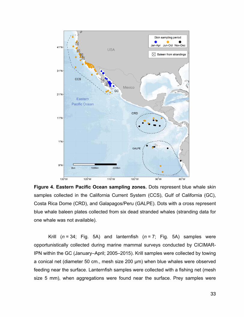
33

Figure 4. Eastern Pacific Ocean sampling zones. Dots represent blue whale skin

samples collected in the California Current System (CCS), Gulf of California (GC),

Costa Rica Dome (CRD), and Galapagos/Peru (GALPE). Dots with a cross represent

blue whale baleen plates collected from six dead stranded whales (stranding data for

one whale was not available).

Krill (n = 34; Fig. 5A) and lanternfish (n = 7; Fig. 5A) samples were

opportunistically collected during marine mammal surveys conducted by CICIMAR-

IPN within the GC (January‒April; 2005‒2015). Krill samples were collected by towing

a conical net (diameter 50 cm., mesh size 200 µm) when blue whales were observed

feeding near the surface. Lanternfish samples were collected with a fishing net (mesh

size 5 mm), when aggregations were found near the surface. Prey samples were

34

preserved frozen in liquid nitrogen (-195°C). The assignment of lanternfish to the

Family Myctophidae (Wisner, 1974) and classification of krill species (Brinton et al.,

2000) was made using identification guides; Nyctiphanes simplex was the only krill

species present in all samples. Additionally, the tissue bank at CICIMAR-IPN had

samples (n = 3) from the krill collected in Galapagos (Fig. 5B), which were donated by

an external researcher (PhD. Daniel Palacios), and we included these samples in our

analysis.

Figure 5. Krill and lanternfish samples collected in the Gulf of California and Galapagos. Dots represent krill (red) and lanternfish (black) samples collected in: A)

Gulf of California (GC) and B) Galapagos (GAL).

35

Baleen plates collected from seven dead stranded blue whales were obtained

from Humboldt State University Vertebrate Museum (HSU-VM), CICIMAR-IPN, the

California Department of Parks and Recreation-Prairie Creek Redwoods State Park

(CDPR-PCRSP), and the Oregon Marine Mammal Stranding Network (OMMSN).

Stranding reports including sex identification were available for all but one individual.

The sex of this whale was determined at NOAA-SWFSC using genetic methods

(Morin et al., 2005, 2006).

6.3. Skin biopsy separation into strata

To assess the isotope variability between blue whale skin strata it was

necessary to identify tissue structure. Histological preparations of five skin biopsies

were stained with hematoxylin & eosin following the protocol of Sheehan and

Hrapchak (1980). Based on these preparations the skin biopsy was divided into two

strata: (1) stratum basale, closest to the blubber, and (2) stratum externum, the

outermost layer that easily separated from the stratum spinosum (Fig. 6A). We did not

include stratum spinosum in our analysis because we assumed it would exhibit

intermediate isotope values between the stratum basale and the stratum externum.

Some skin biopsy samples were incomplete as they had been used for previous

studies, and only one of the two strata were available. Sloughed skin samples were

also included in the analysis, but were only available for some years.

36

Figure 6. Methods for blue whale skin and baleen plate preparation. (A) Skin

biopsy separation into strata: Stratum Basale (SB), Stratum Spinosum (SS) Stratum

Externum (SE). The dermal papillae (DP) can be observed embedded in the skin.

Dashed lines show were the cuts were made to separate the skin into stratums. (B)

Blue whale baleen plate sampling: baleen powder was sub-sampled in 1 cm intervals

along the outer edge of the plate starting from the proximal section of the plate

nearest the gum.

37

6.4. Standardizing blue whale skin sample preparation

Numerous studies show that two factors that are unrelated to ecology can alter

isotope values of metabolically active tissues. The first factor is tissue lipid content.

Lipids have lower δ13C values than associated carbohydrates and proteins (DeNiro &

Epstein, 1977; McConnaughey & McRoy, 1979; Newsome et al., 2010). Thus, the

potential influence of lipid content on bulk tissue δ13C values must be considered

when using stable isotope analysis of animal tissues to make ecological inferences

(Newsome et al., 2010; Lesage et al., 2010; Ryan et al., 2012). Chemical lipid-

extraction removes the influence of lipids on bulk tissues, but a side effect of this

procedure is that it may affect δ15N values of tissues (Lesage et al., 2010; Ryan et al.,

2012). To evaluate the effect of lipid-extraction on the isotope values of blue whale

skin, five skin samples were divided into two subsamples, one subsample was lipid-

extracted with three ~24 hour soaks in a 2:1 chloroform:methanol solvent solution,

rinsed with ionized water and lyophilized. The second subsample was simply

lyophilized, and analyzed as bulk tissue.

The second factor that can alter tissue isotopic composition is how samples

are preserved prior to isotopic analysis. Ideally, all tissues would be stored frozen

since freezing does not alter isotope values (Kaehler & Pakhomov, 2001; Sarakinos

et al., 2002; Barrow et al., 2008; Newsome et al., 2010). Most of the skin samples

selected for this study were stored frozen prior to isotope analysis, but some

(n = 100) were stored in a 20% salt saturated solution of dimethyl sulfoxide (DMSO).

Previous studies have shown that the effect of DMSO on the isotope values of tissues

can be removed via lipid-extraction (Todd et al., 1997; Lesage et al., 2010; Burrows et

al., 2014). To determine if this strategy would work for blue whale skin samples

preserved in DMSO, we selected 25 sloughed skin samples from the GC (2005–

2007). During field collection, each of these skin samples were divided into two

sections and preserved one of two ways for one year before they were prepared for

isotope analysis: the first set was preserved in DMSO and the second (control) set

was frozen in liquid nitrogen (-195°C).

38

6.5. Stable isotope analysis

All skin and prey samples were lipid-extracted, lyophilized, and homogenized

by grinding them into a fine powder; as noted above the small set of subsamples that

were analyzed to test the effects of lipid-extraction were not lipid-extracted (bulk

tissue). Baleen plates were cleaned with a solution of 2:1 chloroform:methanol to

remove surface contaminants. Sub-samples of keratin powder were collected with a

Dremel rotatory drill fitted to a flexible engraving shaft at 1 cm intervals along the

outer edge of each baleen, starting at the proximal section inserted in the gum (which

represents the newest tissue) (Fig. 6B). Baleen grows uniformly on the transverse

perspective at a constant (but unknown) rate; thus our sampling strategy would yield

equal time intervals between adjacent sub-samples (Schell et al., 1989a, 1989b; Best

& Schell, 1996; Caraveo-Patiño & Soto, 2005; Mitani et al., 2006; Bentaleb et al.,

2011; Aguilar et al., 2014). Previous studies have confirmed the consistency of

isotope values along the length of two adjacent baleen plates of a gray whale

(Eschrichtius robustus) (Caraveo-Patiño & Soto, 2005) and two plates from opposing

sides of the mouth of a bowhead whale (Balaena mysticetus) (Schell et al., 1989b).

Consequently, we assumed that each baleen provides a consistent record of the past

foraging history for each blue whale. Lastly, we compiled δ13C and δ15N data from the

literature of potential blue whale prey zones in the eastern Pacific Ocean (see

Results, section 7.3.).

Approximately 0.5-0.6 mg of each tissue sample (dried skin, baleen, and prey)

was weighed into a tin capsule. Carbon (δ13C) and nitrogen (δ15N) isotope values

were measured with a Costech 4010 elemental analyzer coupled to Thermo Scientific

Delta V isotope ratio mass spectrometer at the Center for Stable Isotopes at the

University of New Mexico (Albuquerque, NM). Isotope data are reported as delta δ

values, δ13C or δ15N = 1000 [(Rsample / Rstandard) - 1], where R = 13C/12C or 15N/14N

ratio of sample and standard (Fry, 2006). Values are in units of parts per thousand or

per mil (‰) and the internationally accepted standards are atmospheric N2 for δ15N

and Vienna-Pee Dee Belemnite limestone (V-PDB) for δ13C (Fry, 2006). Within-run

39

analytical precision was estimated via analysis of two proteinaceous internal

reference materials, which was ±0.2‰ for both δ13C and δ15N values. We also

measured the weight percent carbon and nitrogen concentration of each sample and

used the C/N ratio as a proxy of lipid content (Logan et al., 2008).

6.6. Statistical analysis

6.6.1. Assessing the effect of different processing methods in the isotope values of

blue whale skin samples

All statistical analyses were performed using R language (R Development

Core, 2017). The effects of preservation (DMSO-lipid extracted vs frozen-lipid

extracted) and the different treatments (lipid removal vs bulk tissue) on skin δ13C,

δ15N and C/N ratios were evaluated with a max-t test for multiple comparisons of

means. This procedure was chosen because it is designed to work in scenarios of

unbalanced group sizes, non-normality and heteroscedasticity (Herberich et al.,

2010).

6.6.2. Comparing the variability of blue whale skin isotope values by strata

The isotope values variability between skin strata (basale, externum, sloughed

skin) was also evaluated by using the max-t test, which has a higher power to detect

differences between group means compared to other methods (Herberich et al.,

2010). These analyses were performed separately for each zone (GC and CCS) and

isotope (δ13C or δ15N). The CRD and GALPER skin isotope values were excluded

from these analysis as sloughed skin samples were not available for these zones.

40

6.6.3. Estimating blue whale skin strata isotopic incorporation rate

The prey data were used to establish the reference mean (±SD) baseline

isotope values within each zone, hereafter called the prey zone mean, which was

estimated by pooling the means and variances of all the data. The pooled prey zone

mean for the GC included lanternfish and the krill species Nyctiphanes simplex,

because molecular analysis of fecal samples has shown that blue whales forage only

on combined aggregations of both taxonomic groups in this zone (Del Angel-

Rodríguez, 1997; Jiménez-Pinedo, 2010). Lanternfish was the only teleost fish

present in blue whale fecal samples (Jiménez-Pinedo, 2010). In the CCS, we

included isotope values of its main prey, the krill species Thysanoessa spinifera and

Euphausia pacifica (Fiedler et al., 1998; Croll et al., 2005). In the CRD, diving

behavior and the presence of whale fecal samples confirmed that blue whales forage

on patches of krill (Matteson, 2009), however, the species of krill was not identified,

so we used previously reported data for krill in this zone (Williams, 2013).

Our approach to estimate the blue whale skin isotopic incorporation rate was to

mimic a diet switch in controlled feeding experiments, but at population level

(sampling the same individual whale across its annual migratory cycle is logistically

impossible). Blue whales in the northeast Pacific are ideal for this approach because

they feed year-round and seasonally migrate between zones that have distinct

baseline isotope values (Altabet et al., 1999; Miller, 2006; Miller et al., 2008; Williams,

2013; Aurioles-Gamboa et al., 2013; Williams et al., 2014). To achieve this, first we

evaluated if blue whale skin δ13C and δ15N values exhibited seasonal trends in the

GC (Jan-Apr) and the CCS (Jun-Dec). Sampling effort within each zone was not

homogenous for all years, thus blue whale skin samples collected in different years

were integrated into a single analysis. We assessed the seasonal trend by fitting a

generalized additive model (GAM) of the skin δ15N and δ13C values as functions of

time (Julian day, which ranges from 1 to 365). This was done separately for each skin

stratum (basale, externum, and sloughed skin) in both foraging zones (GC and CCS).

We used GAMs because they are especially useful when the functional form of the

41

relationship between the response (e.g. δ15N and δ13C values) and explanatory

variables (e.g. time) is unknown (Yee & Mitchell, 1991). GAMs were fitted using the

“mgcv” package in R (Wood, 2006; R Development Core, 2017). To model the main

trend of the data, the smoothing parameters (degrees of freedom) were set to three.

This conservative approach can be applied when sample size is low (Xiang, 2001).

Blue whale skin strata δ13C did not show seasonal trends (see Results, section 7.7.),

therefore, the isotopic incorporation rate was only estimated for skin δ15N.

To compare the δ15N values of the three skin strata to potential prey, we

assumed a trophic discrimination factor (Δ15N) of 1.6‰, based on controlled feeding

experiments on captive bottlenose dolphins (Tursiops truncatus) (Browning et al.,

2014; Giménez et al., 2016), and calculated the trophic-corrected mean blue whale

skin values for each zone by adding this trophic discrimination factor to the prey zone

mean values. These trophic-corrected skin values would represent the expected

mean δ15N values if blue whale skin had fully equilibrated with that of local prey (or

reached steady-state isotopic equilibrium), and we assumed that this method would

allow us to assign any given blue whale skin isotope value to a specific foraging zone.

Based on the gradient in the prey mean isotope values for each foraging zone

(GC > CCS > CRD; see Results), and the trophic-corrected blue whale skin values

(see Results), our hypothesis was that blue whales would arrive to the GC with lower

skin δ15N values due to consumption of prey in the CCS and CRD. Skin isotope

values would then increase throughout the winter season as they equilibrate with

local prey (see Results). In contrast, most whales would arrive in the CCS with higher

skin isotope values, except for individuals that migrated from the CRD. Thus, we

predicted that skin isotope values would decrease throughout the summer season as

skin isotopically equilibrated with the local prey in the CCS. Therefore, we used the

GAMs seasonal predictions to estimate the isotopic incorporation rate for each skin

stratum, as the days that it would take for the skin δ15N to increase (GC) or decrease

(CCS) by the assumed trophic discrimination factor (Δ15N= 1.6‰) to reach isotopic

equilibrium with the local diet. This period was derived by extrapolating from the

42

distance between the predicted extremes in δ15N for each stratum, from the lowest to

the highest in the GC and vice versa for the CCS (see Results, Appendix I and II). In

this case, we assumed that the equivalent to the diet switch stage would be the

lowest initial δ15N value within the GC and the highest initial δ15N value in the CCS

(see Results, Appendix I and II). We used the same method with the 95% upper and

lower confidence intervals to assess uncertainty. Unfortunately, the uncertainty

associated to individual variability in isotopic incorporation rates given the potential

variation in individual arrival and departure times to/from the GC and CCS, could not

be considered in the model.

Due to sample size limitations, we had to integrate all the skin data collected in

different years into a single seasonal model to estimate blue whale δ15N isotopic

incorporation rate. This assumes that the relative difference in prey δ15N values

between foraging zones is consistent across years, which has been suggested in

previous studies (Aurioles-Gamboa et al., 2013; Fleming et al., 2016). We evaluated

this assumption by fitting a generalized linear model (GLM) of skin δ15N values as a

function of time (Julian Date, or date of sample collection). Julian Dates are a

continuous count of days based on a standard starting point, which we chose as

January 1, 1970 (Universal Time, Coordinated). This analysis was made separately

for each foraging zone (GC, CCS and CRD) by using all skin strata, which allowed us

to evaluate the trends in skin δ15N across years in each zone. The GLMs were fitted

by using the “glm” function in R (reviewed in Mangiafico, 2016).

6.6.4. Determining the isotopic niche width and trophic overlap of blue whales in the

eastern Pacific, by region (SEP and NEP) and sex (females and males)

Isotopic niche width was estimated by using stable isotope Bayesian ellipses

(SEAB), implemented with the R package “SIBER 2.1.0” (Jackson et al.., 2011). The

shape and size of the ellipses is defined by the co-variance matrix of δ13C and δ15N,

while its position is specified by the means of both variables. Isotopic niche

parameters are estimated in a Bayesian framework, which has the advantage of

43

using explicit probabilistic inference. To estimate parameters, this method uses vague

normal priors for the means describing the likely range of δ13C and δ15N, and a vague

Inverse-Wishart prior for the covariance matrix (Jackson et al., 2011; McCarthy 2007).

Marcov Chain Montercalo Simulations are used to construct the posterior estimates of

the parameters. Parameters were finally constructed by using the priors and the

likelihoods. This approach allows to incorporate uncertainties associated to parameter

construction and small sample size into niche metrics. The isotopic niche width is

expressed as the Bayesian standard ellipse area (SEAB) in ‰2. SEAB contains

approximately 95 % of the data. To graphically represent the isotopic niche width of

all groups we used the standard ellipse areas corrected for small sample size (SEAC),

which has the same properties than SEAB, but is unbiased to sample size. The

overlap between isotopic niches was estimated as a proportion of the non-

overlapping area between two ellipses. This proportion ranged from 0 when the

ellipses were distinct, to 1 when there was a total overlap in niche space. Isotopic

niche width was estimated separately for each foraging zone in the NEP (CCS, GC

and CRD), and SEP (GALPE). With the aim of increasing sample size and obtaining

additional isotopic information, the skin biopsies of GALPE (n=25) were also divided

into strata (stratum basale and externum).

A proportion of the blue whale skin samples selected from the different tissue

banks (NOAA-SWFSC, CRC, and CICIMAR-IPN) were sexed by using genetic

methods (Morin et al., 2005, 2006). To further explore if blue whale females and

males exhibited differences in their isotopic niche we compared these groups

separately for the NEP and SEP, by using SEAB and posteriorly calculating the

degree of overlap between isotopic niches spaces, which as mentioned earlier it is

expressed as the proportion of the non-overlapping area between to ellipses, and its

scaled from 0 to 1.

44

6.6.5. Quantifying the relative contribution of different foraging zones to the blue

whale diet in the NEP

The relative contribution of different foraging zones to the isotopic composition

of the blue whale skin collected in the NEP was estimated by using a Bayesian

dietary isotopic mixing model. The model was developed with the package “MixSIAR

3.1” for R (Stock and Semmens, 2016). These models are used to calculate the likely

proportional contribution of different prey to a consumer’s diet based on their

respective isotope values and the trophic discrimination factor (Acevedo-Gutierrez et

al., 2002; Semmens et al., 2009; Parnell et al., 2010). Analyzing these models in a

Bayesian framework allows to consider the uncertainty associated to the final

estimations of the relative contribution of different prey sources to the consumer’s

diet. I used vague priors for the Bayesian model, because of the lack of information

on the proportional contribution of different prey to the diet of blue whales in the NEP.

The variables introduced to the model were the nitrogen isotope values (δ15N)

of the consumers (blue whales), potential prey (see 7. Results, section 7.3., 49 p.)

and I used the trophic discrimination factor derived from the longest controlled feeding

experiment with captive bottlenose dolphins (Δ15N: 1.6 ± 0.5‰) (Giménez et al..,

2016), which is similar to the trophic discrimination factor estimated for the blue whale

(Δ15N: 1.4‒1.6‰) in the GC (Busquets, 2008). I only used one biotracer, δ15N values,

because δ13C values did not show seasonal trends in blue whale skin which could

indicate that this biotracer is not effectively reflecting diet (see Results, section 7.7.). I

only used one biotracer, δ15N values, because δ13C values did not show seasonal

trends in blue whale skin which could indicate that this biotracer is not effectively

reflecting diet (see Results, section 7.7.).

Given that these models are highly sensitive to the trophic discrimination

factor, I additionally ran a Bayesian dietary isotopic mixing model using a trophic

discrimination factor of Δ15N: 1.9 ± 0.5‰, which was estimated in this study by using

45

isotopic data of blue whale baleen plates and prey (see 8. Discussion, section 8.6.

δ15N trophic discrimination factors, 82 p).

6.6.6. Estimating blue whale baleen growth rates and isotopic niche width to infer the

movement patterns of individual blue whales in the NEP

Oscillations in δ13C and δ15N values of baleen plates were also evaluated with

a GAM model and smoothing parameters were selected by standard data-driven

methods for time series using Akaike Information Criteria (Peng et al., 2006; Chuang

et al., 2011). Similar to skin, baleen δ13C values were not distinct among foraging

zones (see Results, section 7.7.), consequently growth rates were estimated using

δ15N values. Blue whale baleen growth rate was determined by assuming that the

oscillation in δ15N values along the total length of the outer edge of the baleen plates

represent the annual movement between winter/spring and summer/fall foraging

grounds. Thus, the distance between two sequential δ15N minimums represents the

growth of the baleen plate during a single year (Schell et al., 1989a, 1989b; Best &

Schell, 1996; Bentaleb et al., 2011; Aguilar et al., 2014). To characterize the

movement of whales among isotopically distinct foraging zones, we compared baleen

δ15N values with the trophic-corrected δ15N values for each foraging zone based on

the same Δ15N used in the skin analysis (Browning et al., 2014; Giménez et al.,

2016). Additionally, I calculated the isotopic niche width and overlap of the seven blue

whale baleen plates by using SEAB (see Materials and Methods, section 6.6.4).

46

7. RESULTS

7.1. Assessing the effect of different processing methods in the isotope values of blue

whale skin samples

The max-t test results comparing the effect of different treatments (bulk tissue

vs lipid-extracted; frozen vs DMSO) on skin δ15N, δ13C and C/N ratios are presented

in Table 2 (Appendix III and IV). Lipid-extracted skin (-16.5 ± 0.1) had mean δ13C

values that were significantly higher (1.9‰) than the bulk skin samples (-18.4 ± 0.4;

t = -10.4, p = <0.001), and the weight percent C/N ratios of bulk skin were significantly

higher (4.2 ± 0.1) than lipid extracted samples (3.2 ± 0.0; t= 12.9, p = <0.001). In

contrast, skin δ15N values did not differ significantly between lipid-extracted

(14.6 ± 0.3) and bulk skin (14.5 ± 0.3; t = -0.4, p = 0.7). Lastly, δ15N, δ13C, and C/N

ratios of skin samples stored in DMSO (δ15N: 13.9 ± 0.9; δ13C: -16.9 ± 0.5; C/N:

3.0 ± 0.2) did no differ significantly from skin samples stored frozen (δ15N: 14.0 ± 0.9;

δ13C: -16.9 ± 0.6; C/N: 3.0 ± 0.2); δ15N: t = 0.2, p = 0.8; δ13C: t = 0.2, p = 0.8; and

C/N: t = -0.4, p = 0.7.

7.2. Comparing the variability of blue whale skin isotope values by strata

The max-t test results comparing the δ15N and δ13C values among skin strata

(basale, externum and sloughed skin) in each zone (GC and CCS) are shown in

Table 3 (Appendix V). Skin δ15N and δ13C did not differ significantly between different

skin strata within the GC (Table 3). In the CCS, mean δ15N values of sloughed skin

(13.6 ± 0.7‰) and stratum externum (13.4 ± 1.1‰) did not differ significantly (t= -0.4,

p = 0.7), and both of these strata had slightly but significantly higher δ15N (stratum

externum: t=2.6, p = <0.001; sloughed skin: t= -4.9, p = <0.001) than the stratum

basale (13.0 ± 0.8‰). δ13C values did not differ significantly among strata in the CCS

(Table 3).

47

Table 2. Max-t test results comparing the effect of different treatments on skin δ15N, δ13C and weight percent C/N ratios. LE, lipid-extracted skin; Diff, estimated differences between group means; CI, confidence intervals; SE, Standard

error; t, test value; P, adjusted p values reported, values in bold were considered statistically significant (<0.05).

A. Comparison between bulk skin vs lipid-extracted skin

Mean ± SD (n)

Variable Bulk skin Lipid extracted Treatment comparison Diff CI: 95% SE t Pδ15N 14.5 ± 0.3 (5) 14.6 ± 0.3 (5) Bulk skin - Lipid extracted -0.1 -0.6 ‒ 0.4 0.2 -0.4 0.7 δ13C -18.4 ± 0.3 (5) -16.5 ± 0.1 (5) Bulk skin - Lipid extracted -1.9 -2.3 ‒ -1.5 0.2 -10.4 <0.001C/N ratio 4.2 ± 0.1 (5) 3.2 ± 0.0 (5) Bulk skin - Lipid extracted 1.0 0.8 ‒ 1.2 0.1 12.9 <0.001

B. Comparison between skin preserved in DMSO vs preserved Frozen

Mean ± SD (n)

Frozen/LE DMSO/LE Treatment comparison Diff CI: 95% SE t Pδ15N 14.0 ± 0.9 (25) 13.9 ± 0.9 (25) Frozen/LE - DMSO/LE 0.1 -0.5 ‒ 0.6 0.2 0.2 0.8 δ13C -16.9 ± 0.6 (25) -16.9 ± 0.5 (25) Frozen/LE - DMSO/LE 0.0 -0.3 ‒ 0.4 0.2 0.2 0.8 C/N ratio 3.0 ± 0.2 (25) 3.1 ± 0.2 (25) Frozen/LE - DMSO/LE -0.0 -0.1 ‒ 0.1 0.1 -0.4 0.7

48

Table 3. Max-t test results for the comparison of δ13C and δ15N values among different skin strata in the Gulf of California (GC) and California Current System (CCS). δ, isotope; Diff, estimated differences between group means; CI,

confidence intervals; SE, Standard error; t, test value; P, adjusted p values reported, values in bold were considered

statistically significant (<0.05).

Zone δ Mean ± SD (n)

Strata comparison Diff CI: 95% SE t P Stratum Basale Stratum Externum Sloughed Skin

GC

δ15N 14.9 ± 0.7 (101) 14.9 ± 0.8 (85) 14.7 ± 1.0 (81) Basale - Sloughed 0.2 -0.2‒0.5 0.1 1.1 0.5Externum - Sloughed 0.2 -0.2‒0.5 0.2 1.1 0.5Externum - Basale 0.0 -0.2‒0.3 0.1 0.1 1

δ13C -16.7 ± 0.7 (101) -16.7 ± 0.5 (85) -16.7 ± 0.6 (81) Basale - Sloughed 0.0 -0.2‒0.3 0.1 0.4 0.9Externum - Sloughed 0.1 -0.2‒0.3 0.1 0.5 0.9Externum - Basale 0.0 -0.2‒0.2 0.1 0.1 1

CCS

δ15N 13 ± 0.8 (120) 13.4 ± 1.1 (63) 13.6 ± 0.7 (93) Basale - Sloughed -0.5 -0.8 ‒ -0.3 0.1 -4.9 <0.001Externum - Sloughed -0.1 -0.5‒0.2 0.2 -0.7 0.7Externum - Basale 0.4 0.0‒0.8 0.2 2.6 <0.001

δ13C -16.8 ± 0.7 (120) -16.9 ± 0.7 (63) -17 ± 0.9 (93) Basale - Sloughed 0.2 -0.1‒0.4 1.4 1.4 0.3Externum - Sloughed 0.0 -0.2‒0.4 0.5 0.5 0.9Externum - Basale -0.1 -0.3‒0.1 -0.9 -0.9 0.6

49

7.3. Estimating blue whale skin strata isotopic incorporation rate

The GLM model of blue whale skin δ15N values as a function of time (Julian

Date) was not significant (t = -1.4; p = 0.3) in the CRD (1999–2003; Table 4, Fig. 7).

Conversely, the relationship between these variables was significant and positive in

the GC (t = 3.1; p < 0.001) and the CCS (t = 7.3; p < 0.001) (Table 4, Fig. 7). The

GLM model predicts an overall increase of 1.2‰ over 15 years (1996–2011) in the

CCS, and an increase of 0.8‰ over 13 years (2002–2015) in the GC (Table 4, Fig. 7);

overall, these shifts results in a 0.1‰ increase per year in each zone. Thus, skin δ15N

values showed a slight and consistent trend in both zones, therefore the gradient in

δ15N values between zones would also remain constant. This result would validate

the integration of blue whale skin δ15N values in a single seasonal GAM model to

infer skin δ15N isotopic incorporation rate for each zone.

Prey from the three zones had distinct δ15N values (Tables 5 and 6), with

values decreasing from the GC to the CCS and CRD. The trophic-corrected blue

whale skin δ15N values for each foraging zone are presented in Table 5. The

magnitude of differences in prey between these zones ranged from 1.9‰ to 6.1‰

(Table 6), which allowed us to assign the origin of measured δ15N values of the

different blue whale skin strata, independently of the zone where whales were

sampled (Table 5, Fig. 8).

The GAM results of the relationship between blue whale skin δ15N values and

time (seasonal trend) are shown in Table 7. The GAM that used δ15N values in blue

whale skin stratum basale and externum in relation to time indicated a weak, but

slightly significant positive relationship in the GC, and a weak, but slightly significant

negative relationship for the CCS (Table 7, Fig. 8). These relationships were

anticipated based on the observed pattern in prey δ15N values among zones and the

trophic-corrected blue whale skin values for each foraging zone (Tables 6 and 7). For

samples collected in the GC, δ15N values increased to ~17‰ by April (Fig. 8), which

likely reflected isotopic equilibration with the δ15N of local prey (Table 5). The

50

opposite pattern was observed in the CCS, were the δ15N values decreased with time

to a low of ~13‰ by December (Fig. 8), which also suggests gradual equilibration of

the tissue to the local prey. In contrast, the relation between sloughed skin δ15N

values and time was not significant in the GC or CCS (Table 7). The GAM model for

sloughed skin showed a parabolic relationship with time, with a slight tendency of the

δ15N values to increase and subsequently decrease with time in both zones (Fig. 8).

Therefore, we used the same method than that for the stratum basale and externum

within each zone to estimate the isotopic incorporation rate of sloughed skin

(Appendix I).

The CRD skin δ15N values were used as a reference to determine if the

isotopic signal of this foraging zone was present in the skin sampled in the GC and

the CCS. Some of the observed δ15N values in the stratum basale and stratum

externum from skin sampled in the CCS could represent transitional values between

the CRD isotopic signal and the CCS signal. One of the values observed in the

stratum externum sampled in August was assigned to the CRD (Fig. 5).

The deviance explained in the relationship between skin δ15N values and time

for all six GAM models was low (6.7 to 21.1%; Table 7) due to the high degree of

dispersion observed in skin data. This degree of variation was expected since the

duration of time individual whales had spent in the zone where skin was collected was

unknown at the time of sampling. As such, this variation is likely driven by a

combination of recently arrived whales that had isotope values reflective of other

foraging zones, individuals in the equilibration period with intermediate isotope values

that represent a mixture of prey consumed in two foraging zones, or individuals that

had reached skin steady-state isotopic equilibrium with the isotopic composition of

local prey (Fig. 8).

51

Table 4. GLM results relating blue whale skin δ15N values to time (Julian date) in the Gulf of California (GC), California Current System (CCS) and Costa Rica Dome (CRD). α, intercept parameter; β, slope parameter; SME,

standard error of the mean; CL, confident intervals of the mean; t, test values; P, p values reported, values in bold were

considered statistically significant (<0.05); a time, in the model represents number of days.

Zone n Model Coefficient ± SME CI (95%) t Residual deviance df AIC P

GC 267 δ15Nskin =12.4 + 1.8e-4·timea α = 12.4 ± 0.6 β = 1.8e-4 ± 4.7e-5

11.2 – 13.7 8.5e-5 – 3.0e-4 3.8 190.6 265 673.8 < 0.001

CCS 276 δ15Nskin =10.5 + 2.2e-4·timea α = 10.5 ± 0.4 β = 2.2e-4 ± 3.0e-5

9.7 – 11.2 2.0e-4 – 2.8e-4 7.3 184.9 274 678.7 < 0.001

CRD 16 δ15Nskin =17 – 4.5e-4·timea α = 17 ± 4.7 β = 4.5e-4 ± 4.2e-4

7.9 – 26.2 -1.3e-3 – 3.8e-4 -1.4 38.2 36 114.08 0.3

Table 5. Trophic-corrected blue whale skin δ15N values for each foraging zone. Values were estimated by using the

prey zone mean ± SD (Table 6) and assuming Δ15N of 1.6‰.

Zone Prey zone mean (±SD) δ15N Δ15N Trophic-corrected blue whale skin δ15N

Gulf of California 14.6 ± 1.0 1.6 16.2 ± 1.0 California Current System 10.4 ± 0.3 1.6 12.0 ± 0.3 Costa Rica Dome 8.5 ± 1.1 1.6 10.1 ± 1.1

52

Table 6. Mean (±SD) δ13C, δ15N, and weight percent C/N ratios of potential blue whale prey in the eastern Pacific Ocean. N.s, Nyctiphanes simplex; Lf, Lanterfish;

T.s., Thysanoesa spinifera; E.p., Euphausia pacifica.

Zones Years Prey n Mean ± SD Source δ13C δ15N C/N

Gulf of California

2000-2001 N.s. 5 -17.7 ± 0.1 12.6 ± 0.1 - (Jaume-Schinkel, 2004) 2004 N.s. 1 -17.8 15.0 2.9 This study2005 N.s. 7 -17.9 ± 0.5 14.6 ± 0.6 3.2 ± 0.1 This study2006 N.s. 7 -17.8 ± 1.4 13.5 ± 1.6 3.0 ± 0.0 This study

2006-2007 N.s. 8 -18.1 ± 0.5 14.7 ± 0.8 - (Sampson et al., 2010) 2013 N.s. 3 -18.2 ± 1.8 13.8 ± 1.2 3.4 ± 0.0 This study 2014 N.s. 5 -18.1 ± 0.2 15.4 ± 1.5 3.3 ± 0.2 This study 2015 N.s. 11 -18.3 ± 0.9 14.1 ± 0.8 3.3 ± 0.1 This study 2013 Lf 3 -17 ± 0.3 18.1 ± 0.5 3.2 ± 0.1 This study 2014 Lf 1 -16.7 18.1 3.3 This study 2015 Lf 3 -17.7 ± 0.6 16.7 ± 1.5 3.2 ± 0.1 This study

Mean ± SDa -17.9 ± 0.9 14.6 ± 1

California Current System

1994 T.s./E.p. 5 -20.2 ± 0.3 11.2 ± 0.5 - (Sydeman et al., 1997)

2000 E.p. 24 -20.0 ± 0.1 9.7 ± 0.2 - (Miller, 2006) 2000 T.s. 58 -18.6 ± 0.1 11.2 ± 0.1 - (Miller, 2006) 2002 E.p. 11 -17.9 ± 0.3 9.1 ± 0.2 - (Miller, 2006) 2002 T.s. 21 -16.9 ± 0.3 10.1 ± 0.1 - (Miller, 2006)

2001-2002 E.p. 10 -19.7 ± 0.8 9.9 ± 0.4 - (Becker et al., 2007) 2002 T.s. 5 -18.6 ± 2 11.1 ± 0.8 - (Hipfner et al., 2010) 2013 T.s. 10 -17.3 ± 0.4 9.6 ± 0.6 - (Carle, 2014)

Mean ± SDa -18.6 ± 0.4 10.4 ± 0.3

Costa Rica Dome 2007-2008 Krill 14-15 -20.8 ± 2b 8.5 ± 1.1 5.8 ± 0.2 (Williams, 2013)

Mean ± SD

-20.8 ± 2b 8.5 ± 1.1

Galapagos Krill 3 -21.7 ± 0.1 4.5 ± 0.1 3.4 ± 0.1 This study

Mean ± SD -21.7 ± 0.1 4.5 ± 0.1

a The mean ± SD isotope values of the prey from these zones were estimated by pooling the means and variances of the data from this study and from the literature. b Krill samples used in that study were not lipid-extracted. Williams et al. (2013) provided a mean weight percent C/N ratio of 5.8 for bulk krill samples. If krill δ13C data from the Costa Rica Dome is lipid-normalized using this C/N ratio and equations in McConnaughey and McRoy (1979), the mean δ13C value would be -19.4‰ and there would be greater overlap in δ13C values among prey of different zones (Costa Rica Dome, California Current System and Gulf of California).

53

Figure 7. GLM analysis relating skin δ15N values to time (Julian Date, presented in years). Points represent the actual δ15N values of blue whale skin collected in

different zones of the northeast Pacific. Lines represent the fit of the GLM model and

the fringe around the lines show the 95% confidence intervals. The gray shaded area

represents the meand±SD of the trophic-corrected blue whale skin values for each

foraging zone; Gulf of California (GC), California Current System (CCS), and Costa

Rica Dome (CRD).

54

Figure 8. GAM analysis of the seasonal trend of skin strata δ15N values in two foraging zones. The points represent the actual δ15N values of skin collected from

whales within the Gulf of California (open circles) and the California Current System

(open triangles). The colored lines represent the GAM model fit (predictions) and the

fringe around the lines show the 95% confidence intervals. The gray shaded area

represents the mean ± SD of the trophic-corrected blue whale skin values for each

foraging zone: Gulf of California (GC), the California Current System (CCS) and the

Costa Rica Dome (CRS).

55

Table 7. GAM results for the seasonal trends of δ15N and δ13C values in different skin strata sampled in the Gulf of California (GC) and California Current System (CCS). E.df., Estimated degrees of freedom; F, test of whether the

smoothed function significantly reduces model deviance; P, p-values in bold were

considered statistically significant (<0.05).

Isotope Skin stratum Zone n E.df. F Adjusted R2 P Deviance explained (%)

δ15N

Basale GC 101 1.9 13.4 0.2 < 0.001 21.1Basale CCS 120 1.0 8.4 0.6 < 0.01 6.7Externum GC 85 1.9 7.4 0.1 < 0.01 14.7Externum CCS 63 1.0 5.5 0.1 < 0.05 8.3Sloughed skin GC 81 1.8 3.3 0.1 0.7 7.7Sloughed skin CCS 93 1.8 2.6 0.0 0.7 6.7

δ13C

Basale GC 101 1.0 0.2 -0.0 0.7 0.2Basale CCS 120 1.9 3.6 0.1 < 0.05 6.2Externum GC 85 1.5 1.3 0.1 0.4 2.8Externum CCS 63 1.5 0.6 0.0 0.6 2.8Sloughed skin GC 81 1.0 1.3 0.0 0.3 1.6Sloughed skin CCS 93 1.0 0.1 -0.0 0.8 0.1

Estimates of δ15N isotopic incorporation rate of blue whale skin strata in each

foraging zone are shown in Table 8 and Appendix II. In the GC, the stratum basale

(81 d), stratum externum (81 d), and sloughed skin (90 d) had similar incorporation

rates (Table 8). In the CCS, the stratum basale had longer incorporation rates (262 d)

than the stratum externum (192 d). Sloughed skin (272 d) had the lowest isotopic

incorporation rate in CCS, although the later estimate had a high degree of

uncertainty (Table 8). The average skin strata isotopic incorporation rate in the CCS

(242 d) was 158 days lower than the GC (84 d) (Table 8). The overall mean of the

δ15N isotopic incorporation rate of blue whale skin was estimated, integrating all strata

in both zones (163 d, Table 8).

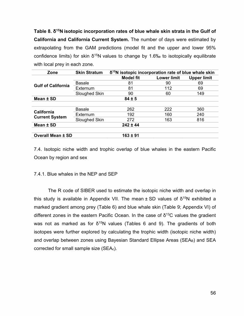
56

Table 8. δ15N isotopic incorporation rates of blue whale skin strata in the Gulf of California and California Current System. The number of days were estimated by

extrapolating from the GAM predictions (model fit and the upper and lower 95%

confidence limits) for skin δ15N values to change by 1.6‰ to isotopically equilibrate

with local prey in each zone. Zone Skin Stratum δ15N isotopic incorporation rate of blue whale skin

Gulf of California

Model fit Lower limit Upper limit Basale 81 90 69Externum 81 112 69Sloughed Skin 90 60 149

Mean ± SD 84 ± 5

California Current System

Basale 262 222 360 Externum 192 160 240 Sloughed Skin 272 163 816

Mean ± SD 242 ± 44

Overall Mean ± SD 163 ± 91

7.4. Isotopic niche width and trophic overlap of blue whales in the eastern Pacific

Ocean by region and sex

7.4.1. Blue whales in the NEP and SEP

The R code of SIBER used to estimate the isotopic niche width and overlap in

this study is available in Appendix VII. The mean ± SD values of δ15N exhibited a

marked gradient among prey (Table 6) and blue whale skin (Table 9; Appendix VI) of

different zones in the eastern Pacific Ocean. In the case of δ13C values the gradient

was not as marked as for δ15N values (Tables 6 and 9). The gradients of both

isotopes were further explored by calculating the trophic width (isotopic niche width)

and overlap between zones using Bayesian Standard Ellipse Areas (SEAB) and SEA

corrected for small sample size (SEAc).

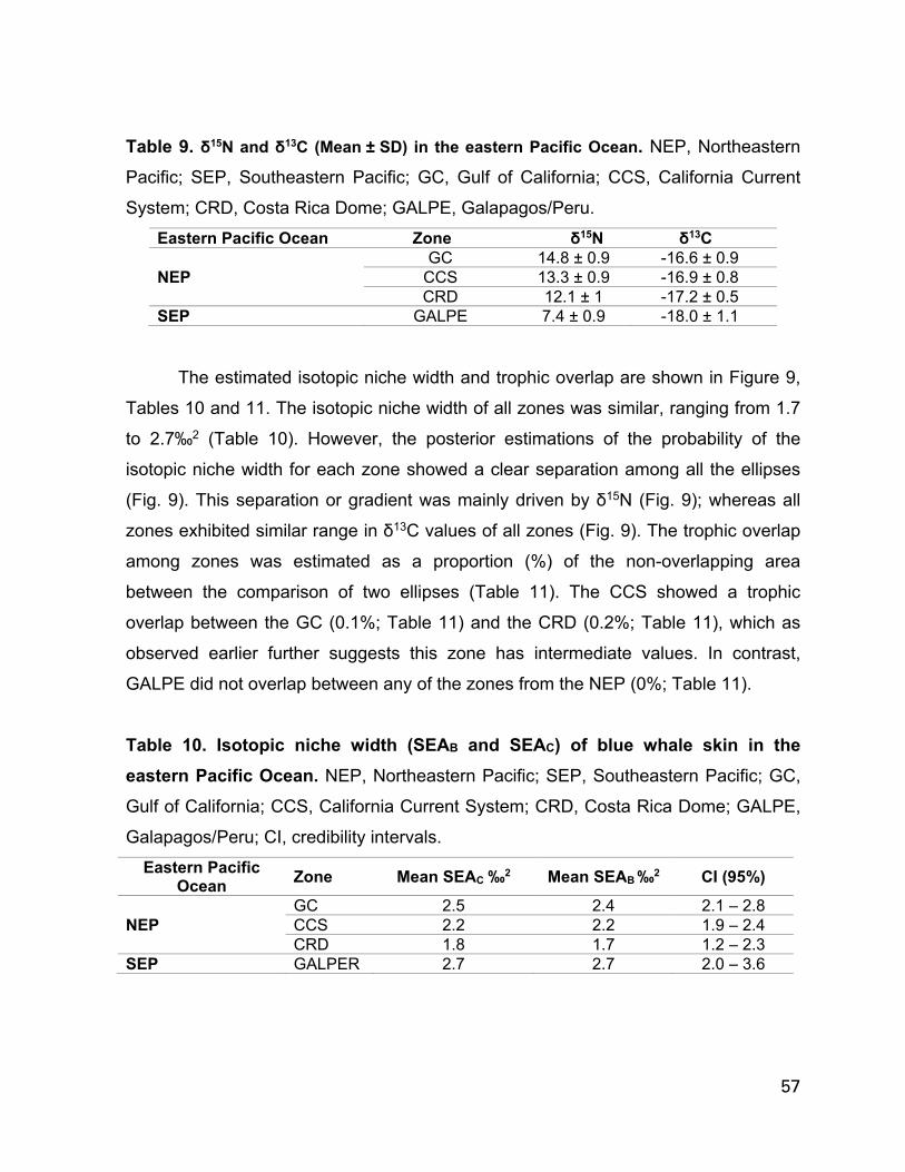
57

Table 9. δ15N and δ13C (Mean ± SD) in the eastern Pacific Ocean. NEP, Northeastern

Pacific; SEP, Southeastern Pacific; GC, Gulf of California; CCS, California Current

System; CRD, Costa Rica Dome; GALPE, Galapagos/Peru. Eastern Pacific Ocean Zone δ15N δ13C

NEP GC 14.8 ± 0.9 -16.6 ± 0.9

CCS 13.3 ± 0.9 -16.9 ± 0.8CRD 12.1 ± 1 -17.2 ± 0.5

SEP GALPE 7.4 ± 0.9 -18.0 ± 1.1 The estimated isotopic niche width and trophic overlap are shown in Figure 9,

Tables 10 and 11. The isotopic niche width of all zones was similar, ranging from 1.7

to 2.7‰2 (Table 10). However, the posterior estimations of the probability of the

isotopic niche width for each zone showed a clear separation among all the ellipses

(Fig. 9). This separation or gradient was mainly driven by δ15N (Fig. 9); whereas all

zones exhibited similar range in δ13C values of all zones (Fig. 9). The trophic overlap

among zones was estimated as a proportion (%) of the non-overlapping area

between the comparison of two ellipses (Table 11). The CCS showed a trophic

overlap between the GC (0.1%; Table 11) and the CRD (0.2%; Table 11), which as

observed earlier further suggests this zone has intermediate values. In contrast,

GALPE did not overlap between any of the zones from the NEP (0%; Table 11).

Table 10. Isotopic niche width (SEAB and SEAC) of blue whale skin in the eastern Pacific Ocean. NEP, Northeastern Pacific; SEP, Southeastern Pacific; GC,

Gulf of California; CCS, California Current System; CRD, Costa Rica Dome; GALPE,

Galapagos/Peru; CI, credibility intervals. Eastern Pacific

Ocean Zone Mean SEAC ‰2 Mean SEAB ‰2 CI (95%)

NEP GC 2.5 2.4 2.1 ‒ 2.8CCS 2.2 2.2 1.9 ‒ 2.4CRD 1.8 1.7 1.2 ‒ 2.3

SEP GALPER 2.7 2.7 2.0 ‒ 3.6

58

Table 11. Trophic overlap between different zones in the eastern Pacific Ocean. GC, Gulf of California; CCS, California Current System; CRD, Costa Rica Dome;

GALPE, Galapagos/Peru.

Zone comparison Proportion (%) of the non-overlapping area of the two ellipses

GC ‒ CCS 0.1GC ‒ CRD 0GC ‒ GALPE 0CCS ‒ CRD 0.2CCS ‒ GALPE 0CRD ‒ GALPE 0

Figure 9. Isotopic niche width (SEAC) of the blue whale in the eastern Pacific Ocean. The ellipses represent the isotopic niche width area of the Gulf of California

(GC), California Current System (CCS), Costa Rica Dome (CRD) and

Galapagos/Peru (GALPE).

59

7.4.2. Female and male blue whales in the eastern Pacific Ocean

The results of the SEAB, in Table 13 and Figure 10, showed that blue whale

skin strata of females in the NEP (δ15N: 14.0 ± 1.2, δ13C: -16.9 ± 0.8, n = 214) and

SEP (δ15N: 7.4 ± 0.9, δ13C: -18.0 ± 1.2, n = 18) had a slightly wider isotopic niche

than males (NEP, δ15N: 14.0 ± 1.2, δ13C: -16.6 ± 0.6, n = 134; and SEP,

δ15N: 7.5 ± 1.0, δ13C: -17.7 ± 0.8, n = 7). The probability that blue whale females have

a wider isotopic niche than males is 100% in the NEP, and 60% in the SEP. The

trophic overlap (Table 13) between females and males was high in both the NEP

(0.5%) and SEP (0.6%).

Table 12. Isotopic niche width (SEAB and SEAC) of female and male blue whales skin in the eastern Pacific Ocean. NEP, Northeastern Pacific; SEP, Southeastern

Pacific; CI, credibility intervals. Eastern Pacific

Ocean Sex Mean SEAC ‰2 Mean SEAB ‰2 CI (95%)

NEP Female 3.0 3.0 2.6 ‒ 3.3

Male 2.2 2.1 1.8 ‒ 2.3

SEP Female 2.8 2.9 1.9 ‒ 4.0 Male 2.1 2.4 1.1 ‒ 4.1

Table 13. Trophic overlap between female and male blue whales in the eastern Pacific Ocean. NEP, northeast Pacific; SEP, southeast Pacific.

Eastern Pacific Ocean Sex comparison

Proportion (%) of the non-overlapping area of

the two ellipses NEP Females ‒ Males 0.5

SEP Females ‒ Males 0.6

60

Figure 10. Isotopic niche width (SEAC) of female and male blue whales in the eastern Pacific Ocean. The ellipses represent the isotopic niche width area of the

females (red) and males (black) in the: A. NEP (northeast Pacific) and B. SEP

(southeast Pacific).

61

7.5. Quantifying the relative contribution of different foraging zones to the blue whale

diet in the NEP

The results from the Bayesian dietary mixing model using a trophic

discrimination factor of Δ15N:1.6 ± 0.5‰ show that the mean ± SD posterior

probability contribution of the CCS (0.30 ± 15 %) and the GC (0.54 ± 05 %) to the

blue whale’s diet in the NEP was high (Table 14, Fig. 11A). Although the estimated

probability for GC was ~24 % higher than the CCS. In contrast, the estimation for the

CRD was lower at 0.16 ± 10 %. The code of the Bayesian dietary mixing model,

deviance information criteria, summary statistics, and model diagnosis of this model

are available in Appendix VIII.

In the case of the Bayesian dietary mixing model using a trophic discrimination

factor of Δ15N: 1.9 ± 0.5‰, the mean ± SD posterior probability contribution of all

zones were similar to the model using Δ15N: 1.6 ± 0.5‰ (Table 14, Fig. 11B).

Deviance information criteria, summary statistics, and model diagnosis of this model

are available in Appendix IX.

Table 14. Probability of the proportional contributions (%) of different sources (zones) to consumer’s diet (blue whales in the NEP). GC, Gulf of California; CCS,

California Current System; CRD, Costa Rica Dome; CI, credibility intervals.

A. Bayesian Mixing Model using a Δ15N:1.6±0.5‰ Probability of proportion (CI)

Zone Mean ± SD (%) 25% 50% 75% 95% GC 0.54 ± 05 0.54 0.53 0.57 0.62

CCS 0.30 ± 15 0.18 0.31 0.43 0.51CRD 0.16 ± 10 0.07 0.15 0.24 0.34

B. Bayesian Mixing Model using a Δ15N:1.9±0.5‰ Probability of proportion (CI)

Zone Mean ± SD (%) 25% 50% 75% 95% GC 0.47 ± 06 0.42 0.47 0.51 0.57

CCS 0.35 ± 17 0.20 0.36 0.50 0.60CRD 0.18 ± 12 0.08 0.17 0.28 0.39

62

Figure 11. Bayesian dietary isotopic mixing model results: Scaled posterior densities of the probability of the proportional contributions of different sources (zones) to consumer’s diet (blue whale). A. Bayesian Mixing Model using

a Δ15N: 1.6 ± 0.5‰; B. Bayesian Mixing Model using a Δ15N: 1.9 ± 0.3‰. CCS,

California Current System; CRD, Costa Rica Dome; GC, Gulf of California.

63

7.6. Estimating blue whale baleen growth rates and isotopic niche width to infer the

seasonal movement patterns of individual blue whales in the NEP

Stranding information of baleen plates collected from seven blue whales (A to

F), is presented in Table 15 and Figure 4. The cause of dead of whales A, B, C, E

and F was ship strike. Whale G, a calf, potentially died due to malnutrition. In the case

of whale D, the cause of dead is unknown since the stranding information for this

whale was not available.

The results of the GAM models to assess the fluctuations in δ15N values along

baleen plates, and of baleen growth rates estimations are shown in Tables 16 and 17,

respectively. The GAM fit showed that the amplitude of the oscillations differed

among individuals (Tables 16 and 17, Figs. 12 and 13). Three baleen plates (A–C,

one male and two females; Tables 15 and 17) exhibited the expected fluctuations in

δ15N ranging from 10.6‰ to 14.9‰ (Fig. 12A–12C), and the length of baleen between

these fluctuations ranged between 13 and 19 cm (Table 17). The other three baleen

plates (D–F, all males; Tables 15 and 17) maintained relatively constant δ15N values,

ranging between 11.7‰ and 13.1‰ along the plate (Fig. 12D–12F).

By using the trophic-corrected skin δ15N values based on that of prey (Table

5), it was possible to associate these oscillations with the potential foraging zone that

each individual whale visited. From these data, it could be inferred that whale B

moved between all three zones, showing relatively regular cycles (Fig. 12B), whereas

whale C did not enter the GC, but moved constantly between the CCS and the CRD,

in less regular cycles (Fig. 12C). Whale A remained mainly within the CCS, potentially

only migrating twice to the CRD (Fig. 12A). In the case of whales D, E and F, the data

suggests that these individuals remained within the CCS, throughout several years

(Fig. 12D–12F). Only whales A, B, and C were used to estimate the baleen growth

rates (Fig. 12A–12C). The mean (±SD) growth per year of baleen plates was

estimated for each whale (A=13.5 ± 2.2; B=14.8 ± 1.7; C=17.5 ± 1.5 cm y-1; Table

17), and also integrated in an overall mean (±SD) (15.5 ± 2.2 cm y-1; Table 17). The

64

mean(±SD) of δ15N values are presented in Table 18, and the GAM fit for the blue

whale calf (Sample code G) is presented in Figure 13. This whale exhibited a single

wide oscillation in δ15N along the baleen plate (Fig. 13).

Table 15. Information of baleen plates collected from seven blue whales (A‒G). ND, no data.

Sample Code

Whale Length (m) Sex Age

Category Stranding Date Latitude Longitude

A 21.3 M Adult 01/11/2015 42.5 -124.4B 25.9 F Adult 28/03/2007 25.3 -112.1C 22.3 F Adult 19/10/2009 39.4 -123.8D* ND M* ND ND ND NDE 26.5 M Adult 03/09/1988 37.7 -122.5F 20.7 M Adult 23/06/1986 36.3 -121.9G 16.0 F Calf 04/04/2013 26.7 -113.6

*The stranding data for this baleen plate was unavailable, the sex identity was determined at NOAA-SWFSC by using the genetic methods in Morin et al. (2005; 2006)

The results of the isotopic niche width and trophic overlap among the seven

blue whale baleen plates are shown in Figure 14, Tables 19 and 20. Baleen plates of

adult female blue whales (B and C; Table 19) exhibited a wider isotopic niche than

males (Table 19, Fig. 14). The blue whale female calf has the narrowest isotopic

niche (G; Table 19). All baleen from adult whales overlapped (Table 20, Fig. 14).

Conversely, the female calf, code G, did not exhibit a trophic overlap with the rest of

the baleen. The separation of the ellipse (or the isotopic niche space) of the calf, from

the rest of the whales, was driven by the carbon isotopes, δ13C (Fig. 14).

65

Table 16. GAM results to assess the fluctuations of δ15N and δ13C in baleen plates. E.df., Estimated degrees of freedom; F, test of whether the smoothed function

significantly reduces model deviance; P, p-values in bold were considered statistically

significant (<0.05). Isotope Baleen

code n E.df. F Adjusted R2 P Deviance

explained (%)

δ15N

A 41 23.8 61.4 1 < 0.001 99.0B 68 27.2 108.0 1 < 0.001 98.7C 67 27.3 95.9 1 < 0.001 98.6D 55 23.3 25.2 0.9 < 0.001 95.7E 71 26.5 27.2 0.9 < 0.001 94.8F 58 23.8 31.3 0.9 < 0.001 96.3G 49 20.9 244.4 0.9 < 0.001 99.6

δ13C

A 41 21.9 55.8 1 < 0.001 98.8B 68 20.3 15.6 0.9 < 0.001 89.3C 67 27.7 64.9 1 < 0.001 98.0D 55 24.9 68.4 1 < 0.001 98.5E 71 27.5 65.1 1 < 0.001 97.8F 58 25.0 25.1 0.9 < 0.001 95.7G 49 19.7 21.3 0.9 < 0.001 94.9

Table 17. Blue whale baleen growth rate: estimated by using the distance between sequential δ15N minimums along the baleen plates from whales A to C.

Baleen code Sex Intervals between δ15N minimums (cm) Growth rate (cm y-1)

A Male 10-24 14.0 24-37 13.0

Mean ± SD 13.5 ± 0.7

B Female

4-17 13.0 17-31 14.0 31-48 17.0 48-63 15.0

Mean ± SD 14.8 ± 1.7

C Female

9-27 18.0

27-46 19.0 46-62 16.0

Mean ± SD 17.5 ± 1.5 Overall Mean ± SD 15.5 ± 2.2

66

Figure 12. δ15N values along the baleen plates from six whales, identified as A–F. Points represent actual values. The continuous line (blue: males; red: females)

represents the GAM model fit and the narrow fringe around the lines represent the

95% confidence intervals. The gray shaded area represents the mean ± SD of the

trophic-corrected blue whale skin values for each foraging zone: Gulf of California

(GC), the California Current System (CCS) and the Costa Rica Dome (CRS).

67

Table 18. Mean (±SD) δ13C, δ15N and weight percent C/N ratios of blue whale baleen plates collected from stranded whales.

Baleen code Sex n Mean ± SD δ13C δ15N C/N

A M 40 -16.8 ± 0.4 12.2 ± 0.4 3.4 ± 0.1 B F 67 -17.0 ± 0.5 13.3 ± 1.1 3.6 ± 0.1 C F 66 -17.3 ± 0.3 12.1 ± 0.7 3.5 ± 0.0 D M 54 -17.4 ± 0.3 12.2 ± 0.3 3.5 ± 0.1 E M 70 -17.2 ± 0.4 12.4 ± 0.3 3.5 ± 0.0 F M 57 -17.4 ± 0.4 12.3 ± 0.4 3.5 ± 0.1 G F 49 -19.3 ± 0.1 12.0 ± 0.5 3.5 ± 0.0

Figure 13. δ15N and δ13C values along the baleen plates from the female calf, baleen code G. Points represent actual values. The continuous line represents the

GAM model fit and the narrow fringe around the lines represent the 95% confidence

intervals. The gray shaded area represents the mean ± SD of the δ15N trophic-

corrected blue whale skin values for each foraging zone: Gulf of California (GC), the

California Current System (CCS) and the Costa Rica Dome (CRS).

68

Figure 14. Isotopic niche width (SEAC) of the seven blue whale baleen plates (A to G). The ellipses represent the isotopic niche width area of the baleen plate of each

whale.

Table 19. Isotopic niche width (SEAB and SEAC) of blue whale skin in the eastern Pacific Ocean. CI, credibility intervals.

Baleen code Mean SEAC ‰2 Mean SEAB ‰2 CI (95%) A 0.5 0.5 0.4 ‒ 0.7 B 1.3 1.3 1.0 ‒ 1.6 C 0.6 0.5 0.5 ‒ 0.8 D 0.4 0.4 0.3 ‒ 0.5 E 0.3 0.4 0.3 ‒ 0.4 F 0.3 0.3 0.3 ‒ 0.4 G 0.2 0.2 0.1 ‒ 0.3

69

Table 20. Trophic overlap between different baleen of blue whales identified as A to G.

Baleen comparison Proportion (%) of the non-overlapping area of the two ellipses

A ‒ B 0.1A ‒ C 0.1A ‒ D 0.1A ‒ E 0.2A ‒ F 0.1A ‒ G 0B ‒ C 0.1B ‒ D 0.1B ‒ E 0.1B ‒ F 0.1B ‒ G 0C ‒ D 0.3C ‒ E 0.3C ‒ F 0.3C ‒ G 0D ‒ E 0.4D ‒ F 0.8D ‒ G 0E ‒ F 0.3E ‒ G 0F ‒ G 0

7.7. δ13C values of skin and baleen plates

The mean δ13C value of the prey in the GC was 0.7‰, 2.9‰ and 3.8‰ higher

than the other zones (CCS, CRD and GALPE; Table 6). However, the standard

deviation of the CRD overlapped with all the zones and it was not possible to

accurately assign the origin of measured δ13C from skin nor baleen plates. As

mentioned in earlier, the isotopic niche width results also showed that the range of

δ13C were similar for all zones (see Results, section 7.4).

The GAM model revealed a very weak though significant positive relationship

between the δ13C and time for the stratum basale sampled within the CCS (Table 7,

Fig. 15). The GAMs applied to the other skin strata, from the other two foraging

70

zones, did not show any relationship between the δ13C values and time (Table 7, Fig.

15), and thus the isotopic incorporation rate of δ13C in blue whale skin could not be

estimated.

Mean (±SD) δ13C values of the seven baleen plates (A–G) are presented in

Table 18. The GAM fits (Table 16, Fig. 16) showed that all individuals presented small

oscillations in the δ13C values along the baleen that ranged between -18.3 to -16.1.

These oscillations could not be linked to the foraging zones because of the overlap in

prey δ13C among zones (Table 6). Therefore, baleen growth rates were inferred only

using baleen δ15N values. The only exception to this pattern were the δ13C values

along the baleen plate of the calf whale G (Fig. 13), which exhibited ~2‰ lower

values than the adult blue whales (Table 13, Fig. 13), and this was also observed via

the estimation of isotopic niche width and trophic overlap of baleen plates (Tables 19

and 20, Fig. 13).

71

Figure 15. GAM analysis relating skin δ13C values to Julian day (presented in months). The points represent the actual δ13C values of skin collected from whales

within the Gulf of California (open circles) and the California Current System (open

triangles). Lines represent the fit (projections) of the GAM model and the fringe

around the lines show the 95% confidence intervals.

72

Figure 16. δ13C values along the baleen plates from six whales, identified as A-F. Points represent actual values, the continuous line (blue: males; red: females)

represents the GAM model fit and the fringe around the lines show the narrow 95%

confidence intervals.

73

8. Discussion 8.1. Influence of lipid-extraction and DMSO preservation on skin δ13C and δ15N

values

Our results suggest that lipid-extraction is necessary to remove biases in skin

δ13C values associated with lipid content (Table 2), which agrees with previous

studies on mysticetes (Lesage et al., 2010; Ryan et al., 2012). In regard to the effects

of lipid-extraction on δ15N values of cetacean skin, some authors (Lesage et al., 2010;

Ryan et al., 2012; Giménez et al., 2016) recommend analyzing bulk tissues because

lipid-extraction can influence δ15N values, although this effect varied between species

(Lesage et al., 2010; Ryan et al., 2012) and tissues (Ryan et al., 2012). In our study,

we only compared the δ15N of five biopsy samples from which we analyzed paired

bulk and lipid-extracted subsamples; however, δ15N values between these treatments

did not differ significantly, which would be in accordance with the results reported for

other marine organisms (Ingram et al., 2007). With regard to preservation in DMSO

(Table 2), after lipid-extraction, blue whale skin δ13C, δ15N and C/N ratios of samples

preserved in DMSO were similar to those of samples preserved frozen. Our results

concur with previous studies that show lipid-extraction via a 2:1 chloroform:methanol

solvent solution was a sound method for removing the combined effect that DMSO

and tissue lipid content have on skin δ13C values (Lesage et al., 2010; Burrows et al.,

2014).

8.2. Skin δ15N isotopic incorporation rates

Only two studies have estimated isotopic incorporation rates of cetacean skin,

and both utilized controlled feeding experiments on captive bottlenose dolphins

(Browning et al., 2014; Giménez et al., 2016). Our approach was to use gradients in

baseline δ15N values between the GC and CCS as a natural diet switch experiment

(Fig. 8, Appendix I and II). Our mean estimate of δ15N isotopic incorporation rates

(163±91 d; Table 8) for blue whale skin is similar to that observed in the longest

74

experiment on captive bottlenose dolphins (180±71 d) (Giménez et al., 2016). The

similarity in incorporation rate estimates for these two distantly related cetacean

species that differ in weight by over two orders of magnitude is striking, but suggests

that these estimates can be applied to other odontocetes and mysticetes.

We found that isotopic incorporation rates varied among skin strata and

foraging zones (Table 8); however, all of these estimates fell within the range of those

observed for bottlenose dolphins in previous studies (106-275 d and ~60-90

d)(Browning et al., 2014; Giménez et al., 2016). It is possible that the observed

variation in skin incorporation rates among zones could be influenced by water

temperature (Schneider et al., 2005; Chelton et al., 2007; Lluch-Cota et al., 2007;

McClatchie et al., 2009; Escalante et al., 2013; Pardo et al., 2013), with higher rates

in the warmer waters of GC in comparison to the CCS (Table 8). In cold waters,

marine mammals reduce peripheral blood flow to maintain a constant internal body

temperature, which results in a decrease of epidermal metabolism (Irving & Hart,

1957; Boily, 1995; Silva, 2004). In contrast, incursion into warmer waters accelerates

the turnover of superficial skin cells and increase the proliferation rate of cells by

intensifying blood flow to the skin stratum basale (St Aubin et al., 1990). Observations

suggest that odontocetes, such as belugas (Delphinapterus leucas) (St Aubin et al.,

1990) and killer whales (Orcinus orca) (Durban & Pitman, 2012), move from colder to

warmer waters to molt or promote skin regeneration. A study on blue whales in the

GC and CCS found that at sites with lower water temperatures, sloughed skin was

observed less often in comparison to warmer sites (Gendron & Mesnick, 2001).

A novel aproach in this study was to analyze different skin strata: basale,

externum, and sloughed skin (Figs. 5A and 5; Appendix IV). We hypothesised that the

different skin strata could provide information about temporal shifts in diet. The

stratum basale, where cells are constantly produced, would most likely reflect the

most recent dietary information, while the isotopic composition of stratum externum

and sloughed skin would record information of the diet consumed in the past, perhaps

when individuals were in a different foraging zone than the one where skin samples

75

were collected. The isotopic comparison of strata in the CCS supports this hypothesis

since the stratum basale had significantly lower δ15N values than the stratum

externum and sloughed skin (Table 3), suggesting that the stratum basale was

equilibrating with local prey, characterized by lower δ15N values than those which

occur in the GC (Tables 5 and 6). In the GC, skin strata did not have significantly

different δ15N values; however, some sloughed skin samples collected in February

and March had δ15N values that were similar to those expected if the skin was grown

in the CCS (Table 5, Fig. 8), suggesting that sloughed skin samples have a higher

probability of providing information about past diets. Thus, skin samples collected

from migratory mysticetes can reflect information about past diets independent of

where sampling occurs, demonstrating that skin is a valuable tissue to estimate

relative contributions of food consumed in different foraging zones utilized during the

annual life cycle. Since collecting skin from free ranging cetaceans is cost- and time-

intensive, we recommend dividing skin biopsies into strata and collecting sloughed

skin when available to increase the amount of information that can be gleaned from

isotope analysis of this tissue.

8.3. Isotopic niche width and overlap of blue whales in the SEP and NEP

The isotopic niche width (or trophic width) of the blue whales in the NEP and

SEP where similar in area ‰2 (Table 10), indicating that in all zones the species has

a similar isotopic niche. This analysis showed the marked gradient among zones in

the NEP (Tables 9 to 11, Fig. 9), and between hemispheres (NEP vs SEP). The main

separation of the ellipses was driven by δ15N values, whereas δ13C values had a

similar range in all four zones (Fig. 9). The gradients in δ15N values were in

accordance with the gradients of their main prey in each foraging zone (Table 6),

indicating that blue whale skin is recording the biogeochemical changes at the base

of the food webs. Hence, blue whale skin is a useful tissue to make inferences of the

feeding ecology of this species in the eastern Pacific Ocean. As mentioned in the

Materials and Methods section (see 6. Materials and Methods, 6.1. Study area; 23‒31

p.), the baseline gradients between these zones are mainly driven by the presence of

76

an oxygen minimum zone in the eastern tropical Pacific, which influences both the

CCS and the GC, via superficial and sub-superficial currents. The unusually high δ15N

values of the GC could also be attributed to high 3NO− concentrations (25 µM) at

depth, which are incorporated to the upper layers during upwelling events. In the CRD

incomplete nitrate utilization could be an explanation to its lower baseline δ15N

values, however, there could be other processes that are not well understood

(Williams et al., 2014). The factors that determines the unusually low δ15N values in

GALPE are still not well understood. It is possible that this system is less influenced

by the presence of the oxygen minimum zone, given that this layer is not as thick (in

vertical extension) as in the upper eastern tropical Pacific. Hence, this zone would

exhibit baseline δ15N values that are similar to open-ocean systems.

In the NEP, the CCS was the only zone that overlapped with the other two

zones (GC and CRD), confirming that this zone exhibits intermediate values (Table

11, Fig. 9). The dispersion of the skin data was high among the different zones in the

NEP (Fig. 9), this can be attributed to the skin isotopic incorporation rate (~163 days),

given that skin samples have a high probability of reflecting feeding events that

occurred in the past, independently of the zone where the individual whale was

sampled.

The zone of the SEP (GALPE) exhibited mean ± SD that were 4.7 to 7.4‰

lower than the NEP (Table 9), and the trophic overlap analysis showed that the blue

whale skin nitrogen isotope values from this zone did not overlap with the zones in

the NEP (Table 11, Fig. 9). This was also consistent when comparing the isotope

values of prey from the GALPE to those of the other zones (Table 6). Remarkably,

the difference observed between the mean blue whale skin δ15N values of the GC

and Galapagos (7.4‰) fall within the same range (7.9‰) observed in a previous

study that compared the δ15N values in hair of sea lion pups sampled in the GC and

Galapagos (Aurioles-Gamboa et al., 2009); a species that has a higher trophic level

than the blue whale.

77

Blue whale skin δ15N data, obtained in this study, is supporting the hypothesis

that blue whales from zones of GALPE usually do not migrate and feed further north,

in the CRD. Interestingly, this result is in accordance with those found by using

genetic analysis, which indicated that the blue whales in the SEP showed a higher

affinity to the waters of Peru and Ecuador, whereas the blue whales in the NEP

favored the CRD (Leduc et al., 2017). Even though one blue whale was reported to

migrate from Galapagos to the CRD (Douglas et al., 2015), the former evidence

suggests that these events are uncommon.

The similar range in δ13C values in all four zones (Fig. 9) is also in accordance

with the range observed in prey within each zone (Table 6). This result indicates that

the baseline δ13C values in both hemispheres are mostly uniform, which has been

proposed in other studies (Aurioles-Gamboa et al. 2009). However, within each

specific zone the local variability in δ13C values in different ecosystems

(coast/oceanic or benthic/pelagic), could be useful to study resident marine

mammals.

8.4. Relative contribution of different foraging zones to the blue whale diet in the NEP

This study represents the first effort to estimate the relative contribution of

different feeding zones to the blue whale’s diet. Typically, it had been suggested that

all mysticetes species go through fasting periods in their overwintering grounds, to

invest energy only in reproduction (i.e. courtship, mating) and nursing their calves.

The blue whale is a notable exception to this long-believed assumption. The predicted

contribution from the CCS and GC was of 30‒35 % and 47‒54 % (Table 14 and Fig.

11), respectively, indicating that whales forage on both zones. The estimation for the

GC is a novel result, since it would be the first for the GC and would support the

assertion that this zone is an important feeding zone for this species. Previous studies

have suggested that the CCS is an important blue whale feeding ground (Barlow et.

al., 2004), however it has never been estimated the global proportion of the

contribution of this zone to the blue whale’s diet. The two models estimated a

78

contribution of 30‒35 % to the diet of this species. A physiological factor that could

affect this estimation would be the specific δ15N isotopic incorporation rate of skin in

this zone (~242 days), which is lower than the GC (~84 days). If skin has a lower

isotopic incorporation rate the isotopic signal of the GC would remain within the tissue

for a longer period, even when the whales are feeding in CCS. Thus, the GC relative

contribution would be overestimated, and the CCS underestimated.

The prediction of the relative contribution from the CRD to the blue whale’s diet

was 16‒18 %. This result could reflect that blue whale sampled in the CCS and GC,

generally don’t migrate to the CRD or do not feed intensively, given that skin is not

frequently reflecting the isotopic signal of this zone. This assumption would also be

supported by the fact the photo-recaptures between the CRD and the two other

zones, GC and CCS, are relatively low (Ugalde de la Cruz, 2015). In this photo-

identification study, the author compared 101 photos of blue whales photographed in

the CRD to the blue whale photographic catalog from the GC. In the GC catalog,

there are ~800 different blue whales. Only seven blue whales photo-identified in the

Gulf were photo-recaptured in the CRD.

The results of the Bayesian dietary isotopic mixing model would support that

blue whale have higher energetic requirements compared to other mysticetes, and

the species is highly vulnerable to changes in the abundance of their prey. This would

also support the hypothesis that blue whale distribution is strongly linked to that of

their prey, as it has been previously proposed (Acevedo-Gutierrez et al., 2002;

Gendron, 2002; Croll et al., 2005).

8.5. Blue whale baleen growth rates and isotopic niche width to infer seasonal

movement patterns of individual blue whales

The estimate of baleen growth rates for blue whales (~15.5 ± 2.2 cm y-1; Table

17), from this study, are consistent with previous estimates for other balaenopterids,

such as the fin whale (20 ± 2.6 cm y-1) (Bentaleb et al., 2011; Aguilar et al., 2014),

79

and minke whale (Balenoptera acutorostrata, 12.9 cm y-1) (Mitani et al., 2006), as well

as for other mysticetes such as bowhead whales (16–25 cm y-1 in adults) (Schell et

al., 1989a, 1989b). In contrast, baleen growth rate estimates were lower than those

for southern right whales (Eubalaena australis, ~27 cm y-1) (Best & Schell, 1996).

Variation in baleen growth rates among blue whales sampled in this study (Table 17)

could be influenced by differences in individual movement strategies (Fig. 12A–12C),

a hypothesis proposed in previous studies of other mysticete species (Schell et al.,

1989b; Bentaleb et al., 2011; Aguilar et al., 2014; Matthews & Ferguson, 2015). For

example, variation in the period of time spent within a specific foraging zone or in

migration between zones would produce wider or narrower oscillations in baleen

δ15N, which would influence growth rate estimates (Table 19, Fig. 12).

Three of the six baleen plates we analyzed did not show marked oscilations in

the δ15N values (Fig. 12D–12F). These individuals were males: two adults, and one of

unknown age class (Tables 15 and 17). A potential explanation for a lack of inter-

annual variation in δ15N is that these whales remained close or within the CCS

foraging zone for several years prior to their death. By applying the mean annual

growth rate of ~15.5 cm y-1 to the baleen records of these three males, they remained

within the CCS ecosystems for ~3.5 (Fig. 12D), ~4.5 (Fig. 12E) and ~3.7 (Fig. 12F)

years. In contrast, the other three baleen plates, collected from one male and two

females, exhibited oscillations in the δ15N values along their outer edge that indicate

cyclical migrations between foraging zones during ~2.5 (Fig. 12A), ~4.3 (Fig. 12B)

and ~4.2 (Fig. 12C) years.

The observed differences in movement strategies of blue whale individuals

may be influenced by a combination of the following factors. One general explanation

is related to changes in the availability of prey in different foraging zones because it is

known that blue whale distribution is influenced by variations in the abundance of

their primary prey (Bailey et al., 2009; Calambokidis et al., 2009a). A more specific

explanation is that females are more likely to migrate to warmer waters in

winter/spring to nurse their calves, a hypothesis that has been proposed for other

80

mysticetes, although other mysticetes generally do not feed while on their

winter/spring breeding grounds (Corkeron & Connor, 1999). Moreover, the patterns in

the baleen of whale C and B (Fig. 12C–12B) suggest a high fidelity of females to

returning to specific winter/spring foraging grounds year after year. This result is

supported by photo-identification and genetic analysis (Gendron, 2002; Sears et al.,

2013; Costa-Urrutia et al., 2013) of females that winter in the GC. Moreover, the

results of the skin isotopic niche width analysis between whales of different sex (see

Results, sections 7.4.2) indicated that in both regions (NEP and SEP) females had a

slightly wider niche (Table 12, Fig. 9), which would also suggest that generally

females move more frequently between zones, compared to male (Fig. 9).

In the case of males, our data indicate that only one male, out of four, migrated

twice to the CRD (Fig. 12A). The female:male sex ratio (1.4:1) in the GC is biased

towards females (Gendron, 2002; Costa-Urrutia et al., 2013), suggesting that only a

portion of the males in the NEP are using this zone in winter/spring. Photo-

identification data has also shown that some males have a high site fidelity to the GC

(Gendron, 2002). Baleen isotope data from male A in our study also indicates that it

had a high fidelity to the CRD, since it migrated only to this zone (Fig. 12A).

Conversely, baleen data from the other three males D, E, F (Fig. 12D–12F) indicated

that these whales remained within the CCS several years before their death. Blue

whales are not frequently sighted in the CCS during winter and spring (Forney &

Barlow, 1998; Carretta et al., 2000), although this could be attributed to low search

effort during this season. However, vocalizations specific to male blue whales have

been recorded year-round in the CCS (Stafford et al., 2001; Oleson et al., 2007a,

2007b, 2007c). Therefore, we hypothesize that there are two migratory strategies for

blue whale males in the NEP. Some individuals migrate to winter/breeding grounds in

the GC or CRD, while others remain within the CCS. How these two migratory

strategies influence mating success for males is not known.

81

8.6. δ15N trophic discrimination factors

δ15N trophic discrimination factors have not been estimated for blue whale

tissues, therefore our approach was to assume a 1.6‰ (Table 5) discrimination factor

between whales and their prey based on the controlled feeding experiments on

bottlenose dolphins (Browning et al., 2014; Giménez et al., 2016). Borrell et al..

(Borrell et al., 2012) suggested using a trophic discrimination factor of 2.8‰ for

balaenopterid skin and baleen plates. However, the mean (±SD) baleen δ15N value of

the three male blue whales (D: 12.2 ± 0.3; E: 12.4 ± 0.3; F: 12.3 ± 0.4; Table 18, Fig.

12D–12F) that presumably remained within the CCS for ~2–3 years prior to death,

and by extension were isotopically equilibrated with local food sources, were enriched

by only 1.7–1.9‰ relative to local prey sources (10.5 ± 0.2; Table 6). This is similar to

both: the estimates for skin of captive bottlenose dolphins (Δ15N: 1.6±0.5‰)

(Browning et al., 2014; Giménez et al., 2016), and to the estimates of the trophic

discrimination factor for blue whales in the GC inferred by comparing the isotope

values of blue whale prey, skin and blue whale fecal samples (Δ15N: 1.4 to 1.6‰)

(Busquets-Vass, 2008).

8.7. Temporal consistency of baseline δ15N values among foraging zones

The observed seasonal trend in skin δ15N values within each zone and the

oscillations along baleen plates support our hypothesis that these tissues record

baseline shifts in nitrogen isotope values across the NEP. Our approach assumes

that such baseline gradients are temporarily consistent at a decadal scale. To test this

assumption, it would be ideal to have prey δ15N data from each foraging zone for

each year blue whales were sampled; however, such sampling resolution is

logistically impossible. Our approach was to use a GLM to evaluate inter-annual

trends in skin δ15N values, which showed that they slightly increased in the GC and

CCS (see Results); no evident trend was observed in the CRD (Table 4, Fig. 7).

82

Published datasets show that isotope values of blue whale prey and

zooplankton collected from the CCS were consistent over decadal timescales (1994,

2000-2001, 2013) and between sites (Monterey Bay and British Columbia) (Sydeman

et al., 1997; Rau et al., 2003; Miller, 2006; Hipfner et al., 2010; Carle, 2014).

Moreover, the δ15N values in blue whale baleen plates that were assigned to the CCS

show a remarkably consistent pattern regardless of when the baleen was collected

(1980s vs. 2000s; Table 15, Fig. 12). These patterns suggest that a relatively stable

δ15N baseline existed in the CCS for nearly three decades. Furthermore, these data

suggest that the slight inter-annual increase in skin δ15N values of blue whales in the

CCS is likely the result of uneven seasonal sampling rather than a shift in the

baseline.

δ15N values of the dominant krill species (Nyctiphanes simplex) in the GC are

variable, likely due to their omnivorous feeding behavior (Mauchline, 1980), but are

consistently higher than krill in the CCS and the CRD (Table 6) (Jaume-Schinkel,

2004; Miller, 2006; Becker et al., 2007; Hipfner et al., 2010; Sampson et al., 2010;

Williams, 2013; Aurioles-Gamboa et al., 2013; Carle, 2014). Isotope data for potential

blue whale prey from the CRD were only available from one study (Table 6) (Williams,

2013), but zooplankton data also suggest that this zone has lower δ15N values in

comparison to the CCS and GC (Popp et al., 2007). Additionally, baleen δ15N

patterns from whales that likely visited the CRD (Fig. 12A–12C) indicate that baseline

δ15N values may be consistently lower than those of the other zones. Another factor

that may contribute to the observed differences in δ15N values among foraging zones

is that blue whales in the GC forage on combined aggregations of krill and higher

trophic level lanternfish (Jiménez-Pinedo, 2010). Thus, blue whale tissues synthetized

in the GC will have higher δ15N values that result from a combination of baseline and

diet factors relative to tissues grown in other foraging zones in the NEP (Table 5,

Appendix II, Figs. 7 and 11).

In the case of the SEP, the low sampling effort limits our inferences on whether

there is a consistency in the baseline values in this region across years. However,

83

other studies using zooplankton and marine mammals, may indicate that there is a

relatively stable baseline in this zones, given that the values reported are consistently

lower than other zones (Aurioles-Gamboa et al., 2009; Páez-Rosas et al., 2012;

Drago et al., 2016), and in similar magnitude than the observed in the present study

(Aurioles-Gamboa et al., 2009).

8.8. δ13C values in blue whale skin and baleen plates

δ13C incorporation rates for skin could not be estimated because of the

similarity in δ13C values among prey from different foraging zones (Table VI), and by

extension δ13C values were not useful to estimate baleen growth rates. The lack of

marked gradients in δ13C values also extended to the zones of GALPE. Another

variable that could contribute to the lack of spatial signal in δ13C is movement of blue

whales between coastal 13C-enriched and 13C-depleted oceanic ecosystems

(Newsome et al., 2010) within a specific foraging zone (Bailey et al., 2009). Thus, any

latitudinal variation in blue whale skin and baleen δ13C values between the CCS, GC,

and CRD may be obscured by longitudinal movement between coastal and offshore

areas within foraging zones.

8.9. δ13C and δ15N values along the baleen plate of a blue whale calf

The δ13C and δ15N values of the blue whale calf were distinct (Figs. 13 and

14). Baleen δ15N only exhibited one marked oscillation (Fig. 13). Similar δ15N patterns

have been observed in juvenile right whales (Lysiak, 2009), and have been

associated to the weaning period. The decrease in δ15N may be reflecting the diet

switch from a higher trophic level diet of milk to a lower trophic level diet of

zooplankton. Lactating females catabolize their own tissues to produce milk, therefore

milk generally has similar δ15N values to maternal tissues. In fin whale, milk proteins

exhibited similar δ15N values (9.8±0.4‰) compared to those of skin (10±0.3‰) and

muscle (9.9±0.6‰) from adult fin whales (Borrell et al., 2012, 2015). Therefore,

nursing calves should have a relatively higher trophic level than their mothers,

84

because they are literally feeding on the mother’s tissues. However, the mother-to-

offspring trophic discrimination varies between marine mammal species. Generally, in

species that feed on protein rich diets (e.g. fish), like pinniped (e.g. fur seal,

Callorhinus ursinus, and California sea lion), the nursing offspring is one trophic level

higher (~3‰) than their mothers (Newsome et al., 2010); these results were obtained

by analyzing bone collagen, and tooth annuli in sea lions. However, in some species

of marine mammals, milk is isotopically lighter than other maternal tissues, and the

mother-to-offspring trophic discrimination is much lower (Δ15N = 0.5‰) (Jenkins et al.,

2001). Busquets-Vass (2008) determined that the mother-to-offspring trophic

discrimination between skin of blue whale nursing females and skin of their calves

was Δ15N = 1‰.

The former information can be used to make inferences on the δ15N oscillation

and patterns in the blue whale calf baleen (Fig. 13). A possible scenario is that this

blue whale calf was potentially born in the CRD, were the mother would have lower

δ15N (~11‰), but the calf would exhibit δ15N values that resemble those of the CCS

(~12‰), due to the trophic discrimination during milk consumption. In Figure 13, this

period would be the interval between the 49 to 43 cm of the baleen (the oldest section

of the baleen). The period of diet switch, from milk to zooplankton, would be the flat

long phase when the δ15N values drop between the 42 to 20 cm of the baleen. The

posterior increase in δ15N values would reflect another diet switch, but this time from

krill with lower δ15N values in the CRD to krill with higher values in the CCS. This calf

finally stranded on the west coast of the Baja California Peninsula (Table 15, Fig. 4).

The possible cause of death was malnutrition, due to its poor body condition.

Malnutrition could be related with the weaning period, when calves have to start

searching for food to feeding on their own (when they are 7 to 8 months old), and

sometimes are not successful.

δ13C values were relatively constant and ~2‰ lower than those observed in

adults (Table 18, Figs. 13‒14, and 16), thus the isotopic niche of the calf did not

overlap with the adults exhibiting a marked separation driven by δ13C values (Table

85

20, Fig. 14). δ13C transfer from mother-to-offspring during nursing is variable between

different species of marine mammals. Generally, δ13C are lower in the offspring

tissues compared to the mothers; although in some cases they are higher or equal to

the mother tissues (Newsome et al., 2006; Cherel et al., 2015). One of the main

factors that affects δ13C transfer from mother-to-offspring is the lipid content of milk.

Lipids are 13C-depleted, thus have lower δ13C values than associated carbohydrates

and protein (see Material and Methods, section 6.4) (DeNiro & Epstein, 1977;

McConnaughey & McRoy, 1979). Animals with lipid-rich milk nurse their young with a

diet that has lower δ13C. Bulk milk samples from mammary glands of hunted fin

whales, in western Spain, had δ13C values that were ~6‰ lower compared to lipid-

free milk (Borrell et al., 2016). Given that blue whale milk also has a high

concentration of fat (35 to 50 %), the low δ13C in the baleen of the calf would be

expected, due to nutrient transfer. Therefore, the lower δ13C values along the baleen

plate of the calf (Fig. 13) potentially indicate that although this calf had gone through

the weaning period, his lipid reserves were still reflecting the nutrient transfer during

the lactation period. Interestingly, this information would allow to categorize stranded

blue whales as calves, if the information on length is unavailable.

8.10. Summary

Overall the results of the present study show that blue whale tissues (skin and

baleen) are effectively recording baseline differences of the ecosystems different

where whales feed. Therefore, this technique is extremely useful to make inferences

on tissue physiology, feeding ecology and movement patterns of this species in the

eastern Pacific Ocean. Specifically, the results support the hypothesis that blue whale

feed year-round, which would also indicate that this species has high energetic

demands, and are highly vulnerable to changes in the abundance of prey. In a

conservation perspective, this information is essential to develop adequate

management plans for the species.

86

9. CONCLUSIONS

• Blue whale tissues are effectively recording baseline isotopic gradients among

the ecosystems where they migrate and feed.

• Skin δ15N exhibited marked gradients in the eastern Pacific Ocean, which

decrease from GC, CCS, CRD to GALPE. These gradients were consistent

with those of prey within each zone, demonstrating that blue whale skin can be

used to make inferences of the feeding ecology of this species.

• Blue whale skin isotopic incorporation rate, is similar to odontocetes, and skin

strata (basale, externum, sloughed skin) can record different feeding periods.

Baleen growth rate for blue whales is similar to other mysticetes.

• Blue whales from SEP, generally do not migrate to feed to the CRD. Whereas,

in the NEP, blue whales feed in similar intensity in the CCS and GC, and in

lesser intensity in the CRD.

• Individual blue whales exhibited distinct movement patterns that may be sex-

specific strategies. Females generally tend to migrate seasonally among the

different feeding zones, whereas males can either migrate or restrict their

movements and remain within specific zones for several years.

• δ13C values of both whale tissues (skin and baleen) and prey were not distinct

among foraging zones. Thus, were not useful to infer about the physiology, diet

or movement patterns of adult blue whales.

• δ13C and δ15N along baleen of a blue whale calf reflected nutrient transfer

during lactation and the weaning period.

87

10. RECOMENDATIONS

We recommend collecting skin samples (biopsies and sloughed skin)

throughout the seasonal residency of migratory mysticetes within specific foraging

zones, and dividing skin biopsies into strata. This approach allows to make accurate

interpretations of skin isotopic data by increasing the probability of obtaining

information about diet at the place of collection in addition to data about past diet from

other foraging zones. Moreover, analyzing both skin and baleen can provide

information on the inter-annual variability of baseline isotope values within and among

isotopically distinct feeding zones, as well as provide information about the migratory

strategies of individual whales over several years of life. Information about individual

migratory strategies over several years cannot currently be obtained from satellite-

tagging technologies, which at best can collect a single year of movement information

(Bailey et al., 2009).

This study used some of the skin samples available from the SEP, and the

results contributed with important information on the feeding ecology of the species in

this zone. However, we recommend collecting baleen plates and increasing the skin

sample tissue banks for this zone. The combination of both tissues would provide

additional information that would expand our understanding on the individual

movement strategies of this population.

88

11. REFERENCES Acevedo-Gutierrez, A., D. A. Croll & B. R. Tershy. 2002. High feeding costs limit dive

time in the largest whales. J. Exp. Biol., 205: 1747–1753.

Acevedo-Whitehouse, K., A. Rocha-Gosselin & D. Gendron. 2010. A novel non-

invasive tool for disease surveillance of free-ranging whales and its relevance

to conservation programs. Anim. Conserv., 13: 217–225.

Aguilar, A., J. Giménez, E. Gómez-Campos, L. Cardona & A. Borrell. 2014. δ15N

value does not reflect fasting in mysticetes. PLoS One, 9: e92288.

Altabet, M. A., C. Pilskaln, R. Thunell, C. Pride, D. Sigman, F. Chavez & R. Francois.

1999. The nitrogen isotope biogeochemistry of sinking particles from the

margin of the Eastern North Pacific. Deep Sea Res. Part I Oceanogr. Res.

Pap., 46: 655–679.

Álvarez-Borrego, S. & J. L. Lara-Lara. 1991. The physical environment and primary

productivity of the Gulf of California. 555-567, In: B. R. T. & J. P. Dauphin

(eds). The Gulf and peninsular province of the Californias. American

Association of Petroleum Geologists. Memoirs No. 47. Oklahoma.

Anderson, T. F. & M. A. Arthur. 1983. Stable isotopes of oxygen and carbon and their

application to sedimentologic and paloenvironmental problems. 1.1‒1.151, In:

M. A. Arthur, T. F. Anderson, J. Veizer & L. S. Land. Society of Economic

Paleontologists and Mineralogists, Tulsa, Oklahoma.

Aurioles-Gamboa, D., S. D. Newsome, S. Salazar-Pico & P. L. Koch. 2009. Stable

isotope differences between sea lions (Zalophus) from the Gulf of California

and Galapagos Islands. J. Mammal., 90: 1410–1420.

89

Aurioles-Gamboa, D., M. Rodríguez-Pérez, L. Sánchez-Velasco & M. Lavín. 2013.

Habitat, trophic level, and residence of marine mammals in the Gulf of

California assessed by stable isotope analysis. Mar. Ecol. Prog. Ser., 488:

275–290.

Bailey, H., B. R. Mate, D. M. Palacios, L. Irvine, S. J. Bograd & D. P. Costa. 2009.

Behavioural estimation of blue whale movements in the northeast Pacific from

state-space model analysis of satellite tracks. Endanger Species Res., 10: 93–

106.

Baraff, L. S., P. J. Clapham & D. K. Mattila. 1991. Feeding behavior of a humpback

whale in low-latitude waters. Mar. Mammal Sci., 7: 197–202.

Barlow, J. 2010. Cetacean abundance in the California Current estimated from a

2008 ship-based line-transect survey. U.S. Department of Commerce, NOAA

Technical Memorandum, NMFS-SWFSC-456. 19 p.

Barlow, J. & K. A. Forney. 2007. Abundance and population density of cetaceans in

the California Current ecosystem. Fish Bull., 105: 509–526.

Barlow, J., M. Kahru & B. J. Mitchell. Cetacean biomass, prey consumption, and

primary production requirements in the California Current Ecosystem. Mar.

Ecol. Prog. Ser., 371: 509–526.

Barrett-Lennard, L. G., T. G. Smith & G. M. Ellis. 1996. A cetacean biopsy system

using lightweight pneumatic darts, and its effect on the behavior of killer

whales. Mar. Mammal Sci., 12: 14–27.

Barrow, L. M., K. A. Bjorndal & K. J. Reich. 2008. Effects of preservation method on

stable carbon and nitrogen isotope values. Physiol. Biochem. Zool., 81: 688–

693.

90

Becker, E. A., K. A. Forney, M. C. Ferguson & J. Barlow. 2012. Predictive modeling of

cetacean densities in the California Current ecosystem based on summer/fall

ship surveys in 1991- 2008. NOAA Technical Memorandum NMFS-SWFSC-

499, U.S. Department of Commerce, National Marine Fisheries Service,

Southwest Fisheries Science Center, La Jolla, CA. 45 p.

Becker, B. H., M. Z. Peery & S. R. Beissinger. 2007. Ocean climate and prey

availability affect the trophic Level and reproductive success of the marbled

murrelet, an endangered seabird. Mar. Ecol. Prog. Ser., 329: 267–279.

Benson, B. B. & D. Jr. Krause. 1984. The concentrations and isotopic fractionation of

oxygen dissolved in freshwater and seawater in equilibrium with the

atmosphere. Limnol. Ocenogr., 29: 620–632.

Bentaleb, I., C. Martin, M. Vrac, B. Mate, P. Mayzaud, D. Siret, R. de Stephanis & C.

Guinet. 2011. Foraging ecology of mediterranean fin whales in a changing

environment elucidated by satellite-tracking and baleen plate stable isotopes.

Mar. Ecol. Prog. Ser., 438: 285–302.

Berg, J., J. Tymoczko & L. Stryer. 2002. Biochemistry. W.H. Freeman, Ed. Nueva

York, 1515 p.

Berta, A., J. Sumich & K. Kovacs. 2006. Marine mammals: Evolutionary biology. Third

edit. Academic Press, Ed. San Diego, CA. 547 p.

Best, P. B. & D. M. Schell. 1996. Stable isotopes in southern right whale (Eubalaena

australis) baleen as indicators of seasonal movements, feeding and growth.

Mar. Biol., 124: 483–494.

91

Boily, P. 1995. Theoretical heat flux in water and habitat selection of phocid seals and

beluga whales during the annual molt. J. Theor. Biol., 172: 235–244.

Borrell, A., J. Giménez & A. Aguilar. 2012. Discrimination of stable isotopes in fin

whale tissues and application to diet assessment in cetaceans. Rapid

Commun. Mass Spectrom., 26: 1596–1602.

Borrell, A., E. Gómez-Campos & A. Aguilar. 2016. Influence of reproduction on

stable-isotope ratios: nitrogen and carbon isotope discrimination between

mothers, fetuses, and milk in the fin whale, a capital breeder. Physiol.

Biochem. Zool., 89: 41–50.

Brinton, E., M. D. Ohman, A. W. Townsend, M. D. Knight & A. L. Bridgeman. 2000.

Euphausiids of the World Ocean (cd-room Expert System). Springer-Verlag,

Heildeberg.

Browning, N. E., C. Dold, J. I-Fan & G. A. J. Worthy. 2014. Isotope turnover rates and

diet-tissue discrimination in skin of ex situ bottlenose dolphins (Tursiops

truncatus). Clin. Cancer Res., 217: 214–221.

Burrows, D. G, W. L Reichert & M. B. Hanson. 2014. Effects of decomposition and

storage conditions on the δ13C and δ15N isotope values of killer whale (Orcinus

orca) skin and blubber tissues. Mar. Mammal Sci., 30: 747–762.

Busquets-Vass, G. 2008. Variabilidad de isotopos estables nitrógeno y carbono en

piel de ballena azul (Balaenoptera musculus). M.Sc. Thesis, Centro

Interdisciplinario de Ciencias Marinas-Instituto Politécnico Nacional. 84 p.

Busquets-Vass G., S. D. Newsome, J. Calambokidis, G. Serra-Valente, J. K.

Jacobsen, S. Aguíñiga-García & D. Gendron. 2017. Estimating blue whale skin

92

isotopic incorporation rates and baleen growth rates: Implications for assessing

diet and movement patterns in mysticetes. PLoS ONE, 12(5): e0177880.

Calambokidis, J. 2009. Abundance estimates of humpback and blue whales off the

US West Coast based on mark-recapture of photo-identified individuals

through 2008. Report # PSRG-2009-07 to Pacific Scientific Review Group, San

Diego, CA 3-5 November 2009.

Calambokidis, J. & J. Barlow. 2004. Abundance of blue and humpback whales in the

eastern North Pacific estimated by capture-recapture and line-transect

methods. Mar. Mammal Sci., 20: 63–85.

Calambokidis, J., J. Barlow, J. K. B. Ford, T. E Chandler & A. B. Douglas. 2009a.

Insights into the population structure of blue whales in the eastern North Pacific

from recent sightings and photographic identification. Mar. Mammal Sci., 25:

816–832.

Calambokidis, J., G. S. Schorr, G. H. Steiger, J. Francis, M. Bakhtiari, G. Marshall, E.

M. Oleson, D. Gendron & K. Robertson. 2009b. Insights into the underwater

diving, feeding, and calling behavior of blue whales from a suction-cup-

attached video-imaging Tag (CRITTERCAM). Mar. Technol. Soc. J., 41: 19–

29.

Calambokidis, J. & G. Steiger. 1997. Blue whales. Worldlife. Stillwater, MN. 72 p.

Calambokidis, J., G. H. Steiger, J. C. Cubbage, K. C. Balcomb, C. Ewald, S. Kruse,

R. Wells & R. Sears. 1990. Sightings and movements of blue whales off central

California 1986-88 from photo-identification of individuals. Rep. to Int. Whal.

Com., 343–348.

93

Caraveo-Patiño, J., K. A. Hobson & L. A. Soto. 2007. Feeding ecology of gray whales

inferred from stable-carbon and nitrogen isotopic analysis of baleen plates.

Hydrobiologia, 586: 17–25.

Caraveo-Patiño, J. & L. A. Soto. 2005. Stable carbon isotope ratios for the gray whale

(Eschrichtius robustus) in the breeding grounds of Baja California Sur, Mexico.

Hydrobiologia, 539: 99–107.

Carle, R. 2014. Seasonal and sex-specific diet in rhinoceros auklets. M.Sc. Thesis,

The Faculty of Moss Landing Marine Laboratories. 50 p.

Carretta, J., M. Lowry, C. E. Stinchcomb, M. S. Lynn & R. E. Cosgrove. 2000.

Distribution and abundance of marine mammals at San Clemente Island and

surrounding offshore waters: results from aerial and ground surveys in 1998

and 1999. Administrative Report LJ-00-02, available from Southwest Fisheries

Science Center, P.O. Box 271, La Jolla, CA USA 92038. 44 p.

Carss, D. N.1995. Foraging behaviour and feeding ecology of the otter Lutra lutra: a

selective review. Hystrix, 7: 179–194.

Chelton, D. B., M. G. Schlax & R. M. Samelson. 2007. Summertime coupling between

sea surface temperature and wind stress in the California Current System. J.

Phys. Oceanogr., 37: 495–517.

Cherel, Y., K. A. Hobson & C. Guinet. 2015. Milk isotopic values demonstrate that

nursing fur seal pups are a full trophic level higher than their mothers. Rapid

Commun. Mass Spectrom., 29: 1485–1490.

Christiansen, F., G. A. Víkingsson, M. H. Rasmussen & D. Lusseau. 2014. Female

body condition affects foetal growth in a capital breeding mysticete. Funct.

Ecol., 28: 579–588.

94

Chuang, Y., S. Mazumdar, T. Park, G. Tang, V. C. Arena & M. J. Nicolich. 2011.

Generalized linear mixed models in time series studies of air pollution. Atmos.

Pollut. Res., 3: 148.

Cline, J. D. & I. R. Kaplan. 1975. Isotopic fractionation of dissolved nitrate during

denitrification in the eastern tropical North Pacific Ocean. Mar. Chem. 3: 271–

299.

Collins, C. A., J. T. Pennington, C. G. Castro, T. A. Rago & F. P. Chavez. 2003. The

California Current system off Monterey, California: physical and biological

coupling. Deep-Sea Res. Pt. II, 50: 2389‒2404.

Collins English Dictionary – Complete and Unabridged, 12th Edition 2014. (1991,

1994, 1998, 2000, 2003, 2006, 2007, 2009, 2011, 2014). Retrieved June 14

2017 from http://www.thefreedictionary.com/zones+out

Corkeron, J. & C. Connor. 1999. Why do baleen whales migrate? Mar. Mammal Sci.,

15: 1228–1245.

Costa-Urrutia, P., S. Sanvito, N. Victoria-Cota, L. Enríquez-Paredes & D. Gendron.

2013. Fine-scale population structure of blue whale wintering aggregations in

the Gulf of California. PLoS One, 8: e58315.

Croll, D., B. Marinovic, S. Benson, F. P. Chavez, N. Black, R. Ternullo & B. R. Tershy.

2005. From wind to whales: trophic links in a coastal upwelling system. Mar.

Ecol. Prog. Ser., 289: 117–130.

Deagle, B. E., D. J. Tollit, S. N. Jarman, M. A. Hindell, A. W. Trites & N. J. Gales.

2005. Molecular scatology as a tool to study diet: analysis of prey DNA in scats

from captive Steller sea lions. Mol. Ecol., 14(6): 1831–1842.

95

Del Angel-Rodríguez, J. A. 1997. Hábitos alimentarios y distribución espacio-

temporal de los rorcuales común (Balaenoptera physalus) y azul

(Balaenoptera musculus) en la Bahía de La Paz, B.C.S., México. M.Sc. Thesis,

Centro Interdisciplinario de Ciencias Marinas-Instituto Politécnico Nacional. 68

p.

DeNiro, M. J. & S. Epstein. 1977. Mechanism of carbon isotope fractionation

associated with lipid synthesis. Science, 197(4300): 261–263.

DeNiro, M. J. & S. Epstein. 1978. Influence of diet on the distribution of carbon

isotopes in animals. Geochim. Cosmochim. Acta, 42: 495–506.

DeNiro, M.J. & S. Epstein. 1981. Influence of diet on the distribution of nitrogen

isotopes in animals. Geochim. Cosmochim. Acta, 45: 341–351.

Díaz-Gamboa, R. E. 2003. Diferenciación entre Tursiones Tursiops truncatus

costeros y oceánicos en el Golfo de California por medio de isótopos estables

de carbono y nitrógeno. M.Sc. Thesis, Centro Interdisciplinario de Ciencias

Marinas-Instituto Politécnico Nacional. 62 p.

Donovan, G.P. 1984. Blue whales off Peru, December 1982, with special reference to

pygmy blue whales. Rep. to Int. Whal. Com., 34: 473–476.

Douglas, A., R. Sears, J. Denkinger, E. Dobson, P. Olson, T. Gerrodette & J.

Calambokidis. 2015. Movement of a blue whale (Balaenoptera musculus)

between the Costa Rica Dome and the Galapagos: Management implications

of the first documented cross-equatorial movement. In: December 13-18, ed.

21st Biennial Conference of the Society for Marine Mammalogy. San

Francisco, California, USA.

96

Drago, M., V. Franco-Trecu, L. Cardona, P. Inchausti, W. Tapia & D. Páez-Rosas.

2016. Stable isotopes reveal long-term fidelity to foraging grounds in the

Galapagos sea lion (Zalophus wollebaeki). PLoS One, 11: 1–16.

Dugdale, 1967. Nutrient limitation in the sea: dynamics, identification and

significance. Limnol. Oceanogr., 12: 685–689.

Durazo, R., G. Gaxiola-Castro, B. Lavaniegos, R. Castro-Valdez, J. Gómez-Valdés &

A. D. S. Mascarenhas Jr. 2005. Oceanographic conditions west of the Baja

California coast, 2002–2003: A weak El Niño and subarctic water

enhancement. Cienc. Mar., 31(3):537-552.

Durban, J. W. & R. L. Pitman. 2012. Antarctic killer whales make rapid, round-trip

movements to subtropical waters: evidence for physiological maintenance

migrations? Biol. Lett., 8: 274–7.

Escalante, F., J. E. Valdez-Holguín, S. Álvarez-Borrego & J. R. Lara-Lara. 2013.

Temporal and spatial variation of sea surface temperature, chlorophyll a, and

primary productivity in the Gulf of California. Cienc. Mar., 39: 203–215.

Espino-Pérez, N.M. 2009. Variación temporal en los perfiles de ácidos grasos de

ballenas azules Balaenoptera musculus que visitan el Golfo de California.

M.Sc. Thesis, Centro Interdisciplinario de Ciencias Marinas-Instituto

Politécnico Nacional. 51 pp.

Etnoyer, P., D. Canny, B. R, Mate & L. Morgan. 2004. Persistent pelagic habitats in

the Baja California to Bering Sea (B2B) ecoregion. Oceanography,17: 90–101.

Etnoyer, P., D. Canny, B. R. Mate, L. E. Morgan, J. G. Ortega-Ortiz & W. J. Nichols.

2006. Sea-surface temperature gradients across blue whale and sea turtle

97

foraging trajectories off the Baja California Peninsula, Mexico. Deep Sea Res.

Part II Top Stud. Oceanogr., 53: 340–358.

Evans-Ogden, L. J., K. A. Hobson & D. B. Lank. 2004. Blood isotopic (δ13C and δ15N)

turnover and diet-tissue fractionation factors in captive dunlin (Calidris alpina

pacifica). Auk, 121: 170–177.

Farrell, J., T. Pederson, S. Calvert & B. Nielsen. 1995. Glacial-interglacial changes in

nutrient utilization in the equatorial Pacific Ocean. Nature, 377: 514–517.

Fiedler, P. C. & M. F. Lavin. 2006. Introduction: A review of eastern tropical Pacific

oceanography. Prog. Oceanogr., 69: 94–100.

Fiedler, P. C., S. B. Reilly, R. P. Hewitt, D. Demer, V. A. Philbrick, S. Smith, W.

Armstrong, D. A. Croll, B. R. Tershy & B. R. Mate. 1998. Blue whale habitat

and prey in the California Channel Islands. Deep Sea Res. Part II Top Stud.

Oceanogr., 45: 1781–1801.

Fleming, A. H., C. T. Clark, J. Calambokidis & J. Barlow. 2016. Humpback whale

diets respond to variance in ocean climate and ecosystem conditions in the

California Current. Glob. Chang. Biol., 22: 1214–1224.

Flores-Cascante, L. & D. Gendron. 2012. Application of McMaster’ s technique in live

blue whales. Vet. Rec., 179: 220–0.

Flores-Lozano, N. 2006. Plaguicidas organoclorados y bifenil policlorados como

indicadores de la estructura poblacional de la ballena azul (Balaenoptera

musculus) del Golfo de California. M.Sc. Thesis, Centro Interdisciplinario de

Ciencias Marinas-Instituto Politécnico Nacional. 80 p.

98

Fontugne, M. R. & J. C. Dupplesy. 1981. Organic carbon isotopic fractionation by

marine plankton in the temperature range -1 to 31°C. 4(1): 85–90.

Foote, A. D., J. Newton, M. C. Ávila-Arcos, M. L. Kampmann, J. A. Samaniego, K.

Post, A. Rosing-Asvid, M. H. S. Sinding & T. P. Gilbert. 2013. Tracking niche

variation over millennial timescales in sympatric killer whale lineages. Proc. R.

Soc. B., 280: 20131481.

Forney, K. A. & J. Barlow. 1998. Seasonal patterns in the abundance and distribution

of California cetaceans, 1991-1992. Mar. Mammal Sci., 14: 460–489.

Fry, B. 2006. Stable Isotope Ecology. Springer New York, Ed. New York, 308 p.

Fudge, D. S., L. J. Szewciw & A. N. Schwalb. 2009. Morphology and development of

blue whale baleen: An annotated translation of Tycho Tullberg’s classic 1883

paper. Aquat. Mamm., 35: 226–252.

Gannes, L. Z., C. Martínez del Río & P. Koch. 1998. Natural abundance variations in

stable isotopes and their use in animal physiological ecology. Comp. Biochem.

Physiol., 119: 725–737.

Gendron, D .1990. Relación entre la abundancia de eufaúsidos y de ballenas azules

(Balaenoptera musculus) en el Golfo de California. M.Sc. Thesis, Centro

Interdisciplinario de Ciencias Marinas-Instituto Politécnico Nacional. 64 p.

Gendron, D. 2002. Ecología poblacional de la ballena azul, Balaenoptera musculus,

de la Península de Baja California. Ph.D. Thesis, Centro de Investigación

Científica y de Educación Superior de Ensenada. 112 pp.

99

Gendron, D., S. Aguíñiga & J. D. Carriquiry. 2001. δ15N and δ13C in skin biopsy

samples: a note on their applicability for examining the relative trophic level in

three rorqual species. J. Cetacean Res. Manag., 3: 41–44.

Gendron, D. & S. L. Mesnick. 2001. Sloughed skin: A method for the systematic

collection of tissue samples from Baja California blue whales. J. Cetacean Res.

Manag., 3(1)77-79.

Geraci, J. R., D. J. St. Aubin & B. D. Hicks. 1986. The epidermis of odontocetes: a

view from within. 3-21, In: Bryden, M. M. & R. Harrison (eds). Research on

Dolphins, Part I. Oxford: Clarendon Press.

Giménez, J., F. Ramírez, J. Almunia, M. G. Forero & R. de Stephanis. 2016. From the

pool to the sea: Applicable isotope turnover rates and diet to skin

discrimination factors for bottlenose dolphins (Tursiops truncatus). J. Exp. Mar.

Bio. Ecol., 475: 54–61.

Goericke, R. & B. Fry. 1994. Variations of marine plankton δ13C with latitude,

temperature, and dissolved CO2 in the world ocean. Global Biogeochem.

Cycles, 8: 85–90.

Goldbogen, J. A., J. Calambokidis, A. S. Friedlaender, J. Francis, S. L. DeRuiter, A.

K. Stimpert, E. Falcone & B. L. Southall. 2013. Underwater acrobatics by the

world’s largest predator: 360° rolling manoeuvres by lunge-feeding blue

whales. Biol. Lett., 9(1): 1–4.

Goldbogen, J. A., J. Calambokidis, E. Oleson, J. Potvin, N. D. Pyenson & R. E.

Shadwick. 2011. Mechanics, hydrodynamics and energetics of blue whale

lunge feeding: efficiency dependence on krill density. J. Exp. Biol., 214: 131–

46.

100

Graham, B. S., P. L. Koch, S. D. Newsome, K. W. McMahon & D. Aurioles-Gamboa.

2010. Using isoscapes to trace the movements and foraging behavior of top

predators in oceanic ecosystems. 299–318, In: J. B. West, G. J. Bowen, T. E.

Dawson & K. P. Tu (eds). Isoscapes: Understanding movement, pattern, and

process on Earth through isotope mapping. Springer Netherlands: Dordrecht.

Gunnarson, T. G., J. A. Gill, J. Newton, P. M. Potts & J. Sutherland. 2005. Seasonal

matching of habitat quality and fitness in a migratory bird. Proc. R. Soc. B.,

271: 2319–2323.

Harrison, R. & K. W. Thurley. 1974. Structure of the epidermis in Tursiops, Delphinus,

Orcinus and Phocoena. 45–71, In: R. J. Harrison (eds). Functional Anatomy of

Marine Mammals, Vol. 2. London: Academic Press.

Hazen, E. L., D. M. Palacios, K. A. Forney, E. A. Howell, E. Becker, A. L. Hoover, L.

Irvine, M. DeAngelis, S. J. Bograd, B. R. Mate & H. Bailey. 2016. WhaleWatch:

a dynamic management tool for predicting blue whale density in the California

Current. J. Appl. Ecol.

Herberich, E., J. Sikorski & T. Hothorn. 2010. A robust procedure for comparing

multiple means under heteroscedasticity in unbalanced designs. PLoS One, 5:

1–8.

Hipfner, J. M., J. Dale & K. J. McGraw. 2010. Yolk carotenoids and stable isotopes

reveal links among environment, foraging behavior and seabird breeding

success. Oecologia, 163: 351–360.

Hobson, K.A. 1999. Tracing origins and migration of wildlife using stable isotopes: a

review. Oecologia, 120: 314–326.

101

Hobson, K. A. & W. G. Ambrose. 1995. Sources of primary production, benthic-

pelagic coupling, and trophic relationships within the Northeast Water Polynya:

insights from δ13C and δ15N analysis. Mar. Ecol. Prog. Ser., 128: 1–10.

Hobson, K. A., R. Barnett-Johnson & T. Cerling. 2010. Using isoscapes to track

animal migration. 273–298, In: J. B. West, G. J. Bowen, T. E. Dawson & K. P.

Tu (eds). Isoscapes: understanding movement, pattern, and process on Earth

through isotope mapping. Springer Netherlands: Dordrecht.

Hobson, K. A., D. M. Schell, D. Renouf & E. Noseworthy. 1996. Stable carbon and

nitrogen isotopic fractionation between diet and tissues of captive seals:

implications for dietary reconstructions involving marine mammals. Can J Fish

Aquat. Sci., 53: 528–533.

Hoering, T. C. & H. T. Ford. 1960. Isotopic effect in the fixation of nitrogen by

Azotobacter. J. Am. Chem. Soc. 53: 528–533.

Hoyt, E. 2009. The Blue Whale, Balaenoptera Musculus: An Endangered Species

Thriving on the Costa Rica Dome. 2009. Rep. WDC., 1–11. Available:

www.cbd.int/cms/ui/forums/attachment.aspx?id=73

Hucke-Gaete, R., L. P. Osman, C. A. Moreno, K. P. Findlay & D. K. Ljungblad. 2004.

Discovery of a blue whale feeding and nursing ground in southern Chile. Proc.

R. Soc. B. Biol Sci., 271: S170–S173.

Ingram, T., B. Matthews & C. Harrod. 2007. Lipid extraction has little effect on the

δ15N of aquatic consumers. Limnol. Oceanogr. Methods., 5: 338–342.

Irving, L. & J. S. Hart. 1957. The metabolism and insulation of seals as bare-skinned

mammals in cold water. Can. J. Zool., 35: 497–511.

102

Jackson, A. L., R. Inger, A. C. Parnell & S. Bearhop. 2011. Comparing isotopic niche

widths among and within communities: SIBER - Stable Isotope Bayesian

Ellipses in R. J. Anim. Ecol., 80: 595–602.

Jaume-Schinkel, S. M. 2004. Hábitos alimentarios del rorcual común Balaenoptera

physalus en el Golfo de California mediante el uso de isótopos estables de

nitrógeno y carbono. M.Sc. Thesis, Centro Interdisciplinario de Ciencias

Marinas-Instituto Politécnico Nacional. 64 p.

Jenkins, S. G., S. T. Partridge, T. R. Stephenson, S. D. Farley & C. T. Robbins. 2001.

Nitrogen and carbon isotope fractionation between mothers, neonates, and

nursing offspring. Oecologia, 129: 336-341.

Jiménez-Pinedo, N. C. 2010. Hábitos alimentarios y relación interespecífica entre la

ballena azul (Balaenoptera musculus) y la ballena de aleta (B. physalus) en el

suroeste del Golfo de California. M.Sc. Thesis, Centro Interdisciplinario de

Ciencias Marinas-Instituto Politécnico Nacional. 78 p.

Kaehler, S. & E. A. Pakhomov. 2001. Effects of storage and preservation on the δ13C

and δ15N signatures of selected marine organisms. Mar. Ecol. Prog. Ser., 219:

299–304.

Kelly, J. F. 2000. Stable isotopes of carbon and nitrogen in the study of avian and

mammalian trophic ecology. Can. J. Zool., 78: 1–27.

Kleiber, M. 1975. The Fire of Life: an introduction to animal energetics. 2nd Edition.

Robert E. Krieger: New York. 454 p.

Kline, T. C. 1999. Temporal and spatial variability of 13C/12C and 15N/14N in pelagic

biota of Prince William Sound, Alaska. Can. J. Fish Aquat. Sci., 56: 94–117.

103

Lagerquist, B. A., K. M. Stafford & B. R. Mate. 2000. Satellite-Monitored Blue Whales

(Balaenoptera Musculus) Off the Central California Coast. Mar. Mammal Sci.,

16: 375–391.

Lavín, M. F., P. C. Fiedler, J. A. Amador, L. T. Ballance, J. Färber-Lorda & A. M.

Mestas-Nuñez. 2006. A review of eastern tropical Pacific oceanography:

Summary. Prog. Oceanogr., 69: 391–398.

Lavín, M. F., R. Durazo, E. Palacios, M. L. Argote & L. Carrillo. 1997. Lagrangian

observations of the circulation in the northern Gulf of California. J. Phys.

Oceanogr., 27: 2298–2305.

Leduc, R. G., F. I. Archer, A. R. Lang, K. K. Martien, B. Hancock-Hanser, J. P.

Torres-Florez, R. Huecke-Gaete, H.C. Rosenbaum, K. Van Waerebeek, Jr. R.

L. Brownell & B. L. Taylor. 2017. Genetic variation in blue whales in the

eastern pacific: implication for taxonomy and use of common wintering

grounds. Mol. Ecol., 26: 740–751.

Lee, S., D. Schell, T. McDonald & W. Richardson. 2005. Regional and seasonal

feeding by bowhead whales Balaena mysticetus as indicated by stable isotope

ratios. Mar. Ecol. Prog. Ser., 285: 271–287.

Lesage, V., Y. Morin, È. Rioux, C. Pomerleau, S. Ferguson & É Pelletier. 2010.

Stable isotopes and trace elements as indicators of diet and habitat use in

cetaceans: predicting errors related to preservation, lipid extraction, and lipid

normalization. Mar. Ecol. Prog. Ser., 419: 249–265.

Liu, K.-K. & I. R. Kaplan. 1989. The eastern Pacific as a source of 15N-enriched

nitrate in seawater off southern California. Limnol. Oceanogr. 34(5): 820–830.

104

Lluch-Cota, S. E., E. A. Aragón-Noriega, F. Arreguín-Sánchez, D. Aurioles-Gamboa,

J. J. Bautista-Romero, R. C. Brusca, R. Cervantes-Duarte, R. Cortés-

Altamirano, P. Del-Monte-Luna, A. Esquivel- Herrera, G. Fernández, M. E.

Hendrickx, S. Hernández-Vázquez, D. B. Lluch-Cota, J. López-Martínez, S. G.

Marinone, M. O. Nevárez-Martínez, S. Ortega-García, M. Ramírez-Rodríguez,

C. A. Salinas-Zavala, R. A. Schwartzlose & A. P. Sierra-Beltrán. 2007. The

Gulf of California: Review of ecosystem status and sustainability challenges.

Prog. Oceanogr., 73: 1–26.

Logan, J. M., T. D. Jardine, T. J. Miller, S. E. Bunn, R. A. Cunjak & M. E. Lutcavage.

2008. Lipid corrections in carbon and nitrogen stable isotope analyses:

comparison of chemical extraction and modelling methods. J. Anim. Ecol., 77:

838–46.

López-Ibarra, G. A. 2008. Estructura trófica de los copépodos pelágicos en el océano

Pacífico oriental tropical. Ph.D. Thesis, Centro Interdisciplinario de Ciencias

Marinas-Instituto Politécnico Nacional. 92 p.

Lynn, R. J. & J. J. Simpson. 1987. The California Current System: The seasonal

variability of its physical characteristics. J. Geophys. Res., 92(C12): 12947–

12966.

Lysiak, N. S. 2009. Investigations into the migration and foraging ecology of North

Atlantic right whales with stable isotope geochemistry of baleen and

zooplankton. Ph.D. Thesis, Boston University Graduate School of Arts and

Sciences. 202 p.

Macko, S. A., W. Y. Lee & P. L. Parker. 1982. Nitrogen and carbon isotope

fractionation by two species of marine amphipods: laboratory and field studies.

J. Exp. Mar. Biol. Ecol., 63: 145–149.

105

Mangiafico, S. S. 2016. Summary and analysis of extension education program

evaluation in R. Rutgers Cooperative Extension, New Brunswick, NJ.

Marinone, S. G., A. Parés-Sierra, R. Castro & A. Mascarenhas. 2004. Correction to

Temporal and Spatial variation of the surface winds in the Gulf of California.

Geophys. Res. Let., 31: L10305.

Martinez-Levasseur, L. M., M. A. Birch-Machin, A. Bowman, D. Gendron, E.

Weatherhead, R. J. Knell & K. Acevedo-Whitehouse. 2013. Whales use distinct

strategies to counteract solar ultraviolet radiation. Sci, Rep., 3: 2386.

Martínez Del Río, C., B. Wolf, S. A. Carleton & L. Z. Gannes. 2009. Isotopic ecology

ten years after a call for more laboratory experiments. Biol. Rev., 84: 91–111.

Mate, B. R., B. A. Lagerquist & J. Calambokidis.1999. Movements of North Pacific

blue whales during the feeding season off southern California and their

southern fall migration. Mar. Mammal Sci., 15: 1246–1257.

Matteson, R. S. 2009. The Costa Rica Dome: A study of physics, zooplankton and

blue whales. M.Sc. Thesis, Oregon State University. 36 p.

Matthews, C.J D. & S. H. Ferguson. 2013. Spatial segregation and similar trophic-

level diet among eastern Canadian Arctic/north-west Atlantic killer whales

inferred from bulk and compound specific isotopic analysis. J. Mar. Biol. Assoc.

U. K., 94: 1343–1355.

Matthews, C. J. D. & S. H. Ferguson. 2015. Seasonal foraging behaviour of eastern

Canada-West Greenland bowhead whales: An assessment of isotopic cycles

along baleen. Mar. Ecol. Prog. Ser., 522: 269–286.

106

Mauchline, J. 1980. The biology of mysids and euphausiids. Advances in marine

biology. Academic Press: London and New York. 681 p.

McClatchie, S, R. Goericke, F. B. Schwing, S. J. Bograd, W. T. Peterson, R. T.

Emmett, R. Charter, W. Watson, N. LO, K. Hill, C. Collins, M. Kahru, B. G.

Mitchell, J. Gomez-Valdes, B. E. Lavaniegos, G. Gaxiola-Castro, J.

Gottschalck, M. L’Heureux, Y. Xue, M. Manzano-Sarabia, E. Bjorkstedt, S.

Ralston, J. Field, L. Rogers-Bennet, L. Munger, G. Campbell, K. Merkens, D.

Camacho, A. Havron, A. Douglas & J. Hildebrand. 2009. The state of the

California Current, spring 2008-2009: Cold conditions drive regional differences

in coastal production. Calif. Coop. Ocean. Fish Investig. Reports., 50: 43–68.

McConnaughey, T. & C. P. McRoy. 1979. Food-Web structure and the fractionation of

carbon isotopes in the Bering sea. Mar. Biol., 53: 257–262.

McDonald, M. A., S. L. Mesnick & J. A. Hildebrand. 2006. Biogeographic

characterization of blue whale song worldwide: using song to identify

populations. J. Cetacean Res. Manage., 8(1): 55–65.

McMahon, K. W., L. L. Hamady & S. R. Thorrold. 2013. A review of ecogeochemistry

approaches to estimating movements of marine animals. Limnol. Oceanogr.,

58: 697–714.

McMahon, K. W, S. R. Thorrold, T. S. Elsdon & M. D. Mccarthy. 2015. Trophic

discrimination of nitrogen stable isotopes in amino acids varies with diet quality

in a marine fish. Limnol. Oceanogr., 60: 1076–1087.

Michener, R. H. & K. Lajtha. 2007. Stable isotopes in ecology and environmental

science. Second Edition (Michener, Robert and K Lajtha, eds.). Blackwell

publishing, Ed. Malden, MA. 566 p.

107

Mikhalev, Y. A. 1997. Additional information about the catches of Soviet whaling fleet

Sovetskaya Ukraina. Rep. to Int. Whal. Com., 47: 147–150.

Miller, T. W. 2006. Trophic Dynamics of Marine Nekton and Zooplankton in the

Northern California Current Pelagic Ecosystem. Ph.D. Thesis, Oregon State

University. 196 p.

Miller, T. W., R. D. Brodeur & G. H. Rau. 2008. Carbon stable isotopes reveal

relative contribution of shelf-slope production to the Northern California Current

pelagic community. Limnol. Oceanogr., 53: 1493–1503.

Miller, S. A & J. P. Harley. 2009. Zoology. 5th Edition. McGraw Hill, Ed. Boston, MA,

608 p.

Mitani, Y., T. Bando, N. Takai & W. Sakamoto. 2006. Patterns of stable carbon and

nitrogen isotopes in the baleen of common minke whale Balaenoptera

acutorostrata from the western North Pacific. Fish Sci., 72: 69–76.

Mitchell, D. L., D. Ivanova, R. Rabin, T. J. Brown & K. Redmond. 2002. Gulf of

California sea surface temperatures and the North American monsoon:

Mechanistic implications from observations. J. Climate, 15: 2261–2281.

Miyake, Y. & E. Wada. 1971. The abundance ratio of 15N/14N in marine environments.

Rec. Oceanographic Works, Jap., 7: 37–57.

Morales-Guerrero, B., C. Barragán-Vargas, G. R. Silva-Rosales, C. D. Ortega-Ortiz,

D. Gendron & L. M. Martínez-Levasseur .2016. Melanin granules

melanophages and a fully-melanized epidermis are common traits of

odontocete and mysticete cetaceans. Vet. Dermatol., 28(2): 213-e50.

108

Moreno-Santillán, D. D., E. A. Lacey, D. Gendron & J. Ortega. 2016. Genetic variation

at exon 2 of the MHC class II DQB locus in blue whale (Balaenoptera

musculus) from the Gulf of California. PLoS One, 11: 1–15.

Morin, P. A., R. G. LeDuc, K. M. Robertson, N. M. Hedrick, W. F. Perrin, M. Etnier, P.

Wade & B. L. Taylor. 2006. Genetic analysis of killer whale (Orcinus orca)

historical bone and tooth samples to identify western U.S. ecotypes. Mar.

Mammal Sci., 22: 897–909.

Morin, P. A., A. Nestler, N. T. Rubio-Cisneros, K. M. Robertson & S. L. Mesnick.

2005. Interfamilial characterization of a region of the ZFX and ZFY genes

facilitates sex determination in cetaceans and other mammals. Mol. Ecol., 14:

3275–3286.

Nelson, D. L. & C. M. Michael .2005. Lehninger principles of biochemistry. 6th Edition.

W H Freeman & Co (Sd), Ed. New York, 1340 p.

Nemoto, T. 1959. Food of baleen whales with references to whale movements. Sci.

Reports Whales. Res. Inst., 14: 149–290.

Nemoto, T. & A. Kawamura.1977. Characteristics of food habits and distribution of

baleen whales with special reference to the abundance of North Pacific sei and

Bryde’s whales. Rep. Int. Whal. Com. Spec. Issue., 80–87.

Newsome, S. D., M. T. Clementz & P. L. Koch. 2010. Using stable isotope

biogeochemistry to study marine mammal ecology. Mar. Mammal Sci., 26:

509–572.

Newsome, S. D., P. L. Koch, M. A. Etnier & D. Aurioles-Gamboa. 2006. Using carbon

and nitrogen isotope values to investigate maternal strategies in northeast

pacific otariids. Mar. Mammal Sci., 22: 556–572.

109

Newsome, S. D., C. Martínez del Río, S. Bearhop & D. L. Phillips. 2007. A niche for

isotopic ecology. Front. Ecol. Environ., 5: 429–436.

Ocean Exploration Trust & National Oceanic and Atmospheric Administration Office

of Ocean Exploration and Research. 2014. Workshop: Telepresence-enabled

exploration of the eastern Pacific Ocean. December 11‒13. Exploratorium, San

Francisco. Website: http://www.oceanexplorationtrust.org/2014pacificworkshop

Odum, E. P. & G. W. Barrett. 2004. Fundamentals of Ecology. 5th Edition. Thomson

Brooks/Cole: Belmont, CA. 624 p.

Oleson, E. M., J. Calambokidis, J. Barlow & J. A. Hildebrand. 2007a. Blue whale

visual and acoustic encounter rates in the southern California bight. Mar.

Mammal Sci., 23: 574–597.

Oleson, E. M., J. Calambokidis, W. C. Burgess, M. A. McDonald, C. A. LeDuc & J. A.

Hildebrand. 2007b. Behavioral context of call production by eastern North

Pacific blue whales. Mar. Ecol. Prog. Ser., 330: 269–284.

Oleson, E. M., S. M. Wiggins & J. A. Hildebrand. 2007c. Temporal separation of blue

whale call types on a southern California feeding ground. Anim. Behav., 74:

881–894.

Oliver, J. S., P. N. Slattery, M. A. Silberstein & E. F. O’Connor. 1983. A comparison of

gray whale, Eschrichtius robustus, feeding in the Bering Sea and Baja

California. Fish. Bull., 81: 513–522.

Páez-Rosas, D., D. Aurioles-Gamboa, J. J. Alava & D. M. Palacios. 2012. Stable

isotopes indicate differing foraging strategies in two sympatric otariids of the

Galapagos Islands. J. Exp. Mar. Bio. Ecol., 424–425: 44–52.

110

Palacios, D. M. 1999. Blue whale (Balaenoptera musculus) occurrence off the

Galapagos Islands, 1978-1995. J. Cetacean Res. Manag., 1: 41–51.

Pancost, R. D., K. H. Freeman, S. G. Wakeham, C. Y. Robertson. 1997. Controls on

carbon isotope fractionation by diatoms in the Peru upwelling region. Geochim

Cosmochim Acta, 61: 4983–4991.

Paniagua-Mendoza, A., D. Gendron, E. Romero-Vivas & J. A. Hildebrand. 2017.

Seasonal acoustic behavior of blue whales (Balaenoptera musculus) in the

Gulf of California, Mexico. Mar. Mammal. Sci., 33: 206–218.

Pardo, M. A., T. Gerrodette, E. Beier, D. Gendron, K. A. Forney, S. J. Chivers, J.

Barlow & D. M. Palacios. 2015. Inferring cetacean population densities from

the absolute dynamic topography of the ocean in a hierarchical bayesian

framework. PLoS One, 10: 1–23.

Pardo, M. A., N. Silverberg, D. Gendron, E. Beier & D. M. Palacios. 2013. Role of

environmental seasonality in the turnover of a cetacean community in the

southwestern Gulf of California. Mar. Ecol. Prog. Ser., 487: 245–260.

Parnell, A. C., R. Inger, S. Bearhop & A. L. Jackson. 2010. Source partitioning using

stable isotopes: coping with too much variation. PLoS One, 5: e9672.

Peng, R. D., F. Dominici & T. A. Louis. 2006. Model choice in time series studies of

air pollution and mortality. J. R. Stat. Soc. Ser. A., 169: 179–203.

Penzias, A. A. 1979.The origin of the elements. Science, 205:549–554.

Perrin, W. F., B. Würsig & J. G. M. Thewissen. 2002. Encyclopedia of marine

mammals. Academic Press: San Diego, CA. 1414 p.

111

Perry, R. I., P. A. Thompson, D. L. Mackas, P. J. Harrison & D. R. Yelland. 1999.

Stable carbon isotopes as pelagic food web tracers in adjacent shelf and slope

regions off British Columbia, Canada. Can. J. Fish. Aquat. Sci., 56:

2477‒2486.

Podlesak, D. W., S. R. McWilliams & K. A. Hatch. 2005. Stable isotopes in breath,

blood, feces and feathers can indicate intra-individual changes in the diet of

migratory songbirds. Oecologia, 142: 501–510.

Popp, B., E. A. Laws, R. R. Bidigare, J. E. Dore, K. L. Hanson & S. G. Wakeham.

1998. Effect of phytoplankton cell geometry on carbon isotopic fractionation.

Geochim. Cosmochim. Acta, 62: 69–77.

Popp, B. N., B. S. Graham, R. J. Olson, C. C. S. Hannides, M. J. Lott, G. A. López-

Ibarra, F. Galván-Magaña & B. Fry. 2007. Insight into the trophic ecology of

yellowfin tuna, Thunnus albacares, from compound-specific nitrogen isotope

analysis of protenaceous amino acids. Isot as Indic Ecol Chang., 1:173–190.

Post, D. M. 2002. Using stable isotopes to estimate trophic position: models,

methods, and assumptions. Ecology, 83: 703–718.

Potvin, J., J. A. Goldbogen & R. E. Shadwick. 2012. Metabolic expenditures of lunge

feeding rorquals across scale: implications for the evolution of filter feeding and

the limits to maximum body size. PLoS One, 7: e44854.

Poulsen, T. 2010. Introduction to Chemistry. CK-112 Foundations, Ed. U.S.A., 250 p.

R Development Core T. 2017. R: A language and environment for statistical

computing. R Foundation for Statistical Computing: Vienna, Austria.

112

Rau, G. 1982. The relationship between trophic level and stable isotopes of carbon

and nitrogen. 143–148, In: W. Bascom (ed). Coastal water research project

biennal report for the years 1981-1982. Southern California coastal water

research project annual report. Ed. W. Bascom. California, Long Beach.

Rau, G. H. & N. H. Anderson. 1981. Use of 13C/12C to trace dissolved and particulate

organic matter utilization by populations of an aquatic invertebrate. Oecologia,

48: 19–21.

Rau, G. H., F. P. Chavez & G. E. Friederich. 2001. Plankton 13C/12C variations in

Monterey Bay, California: Evidence of non-diffusive inorganic carbon uptake by

phytoplankton in an upwelling environment. Deep Res. Part I Oceanogr. Res.

Pap., 48: 79–94.

Rau, G. H., A. J. Mearns, D. R. Young, R. J. Olson, H. A. Schafer & I. R. Kaplan.

1983. Animal 13C/12C correlates with trophic level in pelagic food webs.

Ecology, 64: 1314–1318.

Rau, G. H., M. D. Ohman & A. Pierrot-Bults. 2003. Linking nitrogen dynamics to

climate variability off central California: a 51year record based on 15N/14N in

CalCOFI zooplankton. Deep Sea Res. Part II Top Stud. Oceanogr., 50: 2431–

2447.

Rau, G. H., R. E. Sweeney & I. R. Kaplan. 1982. Plankton 13C:12C ratio changes with

latitude: differences between northern and southern oceans. Deep Sea Res.

Part A, Oceanogr. Res. Pap., 29: 1035–1039.

Reilly, S. B., J. L. Bannister, P. B. Best, M. Brown, Jr. R. L. Brownell, D. S.

Butterworth, P. J. Clapham, J. Cooke, G. P. Donovan, J. Urbán & A. N. Zerbini.

2008a. Balaenoptera musculus. IUCN Red List Threat Species,

e.T2477A9447146.

113

Reilly, S. B., J. L. Bannister, P. B. Best, M. Brown, Jr. R. L. Brownell, D. S.

Butterworth, P. J. Clapham, J. Cooke, G. P. Donovan, J. Urbán & A. N. Zerbini.

2008b. Megaptera novaeangliae. IUCN Red List Threat Species,

e.T13006A3405371.

Reilly, S. B. & V. G. Thayer .1990. Blue whale (Balaenoptera musculus) distribution in

the eastern tropical Pacific. Mar. Mammal Sci., 6: 265–277.

Rice, D. W. 1974. Whales and whale research in the eastern North Pacific. 170–195,

In: W. E. Schevill (ed.). The whale problem: a status report. Harvard University

Press: Cambridge, MA.

Ripa, P. 1997. Towards a physical explanation of the seasonal dynamics and

thermodynamics of the Gulf of California. J. Phys. Oceanogr., 27: 597–614.

Roberts, K., E. Granum, R. C. Leegood & J. A. Raven. 2007. C3 and C4 pathways of

photosynthetic carbon assimilation in marine diatoms are under genetic, not

environmental, control. Plant Physiol., 145: 230‒235.

Rowntree, V. J., L. O. Valenzuela, P. F. Fraguas & J. Seger. 2008. Foraging

behaviour of southern right whales (Eubalaena australis) inferred from variation

of carbon stable isotope ratios in their baleen. Rep. to Int. Whal. Com., 19:

256–263.

Rueda-Flores, M. 2007. Variabilidad de perfiles de ácidos grasos de ballena azul,

Balaenoptera musculus, en el Golfo de California. M.Sc. Thesis, Centro

Interdisciplinario de Ciencias Marinas-Instituto Politécnico Nacional. 67 p.

Ryan, C., B. McHugh, C. N. Trueman, C. Harrod, S. D. Berro & I. O’Connor. 2012.

Accounting for the effects of lipids in stable isotope (δ13C and δ15N values)

114

analysis of skin and blubber of balaenopterid whales. Rapid Commun. Mass

Spectrom., 26: 2745–2754.

Sachs, J. P. & S. N. Ladd. 2010. Climate and oceanography of the Galapagos in the

21st century: expected changes and research needs. Galapagos Res., 67: 50–

54.

Sackett, W. M., W. R. Eckelmann, M. L. Bender & A. W. H. Be. 1965. Temperature

dependence of carbon isotopic composition in marine plankton and sediments.

Science, 148: 235‒237.

Sampson, L., F. Galván–Magaña, R. De Silva-Dávila, S. Aguiniga-Garcia & J. B.

O’Sullivan. 2010. Diet and trophic position of the devil rays Mobula thurstoni

and Mobula japanica as inferred from stable isotope analysis. Mar. Biol. Assoc.

United Kingdom., 90: 969–976.

Sarakinos, H. C. H., M. L. Johnson & M. Vander Zanden. 2002. A synthesis of tissue-

preservation effects on carbon and nitrogen stable isotope signatures. Can. J.

Zool., 80: 381–387.

Schell, D. M., S. M. Saupe & N. Haubenstock. 1989a. Natural isotope abundances in

bowhead whale (Balaena mysticetus) baleen: markers of aging and habitat

usage. 260–269, In: P. W. Rundel, J. R. Ehleringer & K. A. Nagy (eds.). Stable

isotopes in ecological research. Springer-Verlag, New York.

Schell, D. M., S. M. Saupe & N. Haubenstock. 1989b. Bowhead whale (Balaena

mysticetus) growth and feeding as estimated by δ13C techniques. Mar. Biol.,

103: 433–443.

Schneider, N., E. Di Lorenzo & P. P. Niiler. 2005. Salinity Variations in the Southern

California Current. J. Phys. Oceanogr., 35: 1421–1436.

115

Schoeller, D. A. 1999. Isotope fractionation: Why aren’t we what we eat? J. Archaeol.

Sci., 26: 667–673.

Schoenherr, J. R. 1991. Blue whales feeding on high concentrations of euphausiids

around Monterey Submarine Canyon. Can. J. Zool., 69: 583–594.

Sears, R. 1987. The photographic identification of individual blue whales

(Balaenoptera musculus) in the Sea of Cortez. Cetus. 7:14-17.

Sears, R., C. Ramp, A. B. Douglas & J. Calambodikis. 2013. Reproductive

parameters of eastern North Pacific blue whales Balaenoptera musculus.

Endanger. Species Res., 22: 23–31.

Semmens, B. X., E. J. Ward, J. W. Moore & C. T. Darimont. 2009. Quantifying inter-

and intra-population niche variability using hierarchical bayesian stable isotope

mixing models. PLoS One, 4: e6187.

Sheehan, D. & B. B. Hrapchak. 1980. Theory and practice of histotechnology. 2nd

Edition. St. Louis, MO: C.V, Ed. Mosby Co. 481p.

Silva, R. G. 2004. Assessment of body surface temperature in cetaceans: an iterative

approach. Braz. J. Biol., 64: 719–24.

St Aubin, D. J., T. G. Smith & J. R. Geraci. 1990. Seasonal epidermal molt in beluga

whales, Delphinapterus leucas. Can. J. Zool., 68: 359–364.

Stafford, K. M., D. R. Bohnenstiehl, M. Tolstoy, E. Chapp, D. K. Mellinger & S. E.

Moore. 2004. Antarctic-type blue whale calls recorded at low latitudes in the

Indian and eastern Pacific Oceans. Deep Sea Res. Part I Oceanogr. Res.

Pap., 51: 1337–1346.

116

Stafford, K. M., S. L. Nieukirk & C. G. Fox. 2001. Geographic and seasonal variation

of blue whale calls in the North Pacific. J. Cetacean Res. Manag., 3: 65–76.

Stock, B. & B. X. Semmens. 2016. MixSIAR GUI User Manual. Version 3.1.

Sydeman, W. J., K. A. Hobson, P. Pyle & E. B. McLaren. 1997. Trophic relationships

among seabirds in central California: Combined stable isotope and

conventional dietary approach. Condor, 99: 327–336.

Tershy, B. R., D. Breese & C. S. Strong. 1990. Abundance, seasonal distribution and

population composition of balenopterid whales in the Canal de Ballenas, Gulf

of California, Mexico. Reports Int. Whal. Comm., 369–375.

Thomas, S. M. & T. W. Crowther. 2015. Predicting rates of isotopic turnover across

the animal kingdom: A synthesis of existing data. J. Anim. Ecol., 84: 861–870.

Thunell, R. C. 1998. Seasonal and annual variability in particle fluxes in the Gulf of

California. Deep Sea Res. Part I Oceanogr. Res. Pap., 45(12): 2059‒2083.

Tieszen, L. L., T. W. Boutton, K. G. Tesdahl & N. A. Slade. 1983. Fractionation and

turnover of stable carbon isotopes in animal tissues: Implications for δ13C

analysis of diet. Oecologia, 57: 32–37.

Todd, S., P. Ostrom, J. Lien & J. Abrajano. 1997. Use of biopsy samples of

humpback whale (Megaptera novaeangliae) skin for stable isotope (δ13C)

determination. J. Northw. Atl. Fish. Sci., 22: 71–76.

Tomczak., M. & J. S. Godfrey. 2003. Regional oceanography: An introduction. 2nd

ed. Daya Publishing House, Ed. Delhi. 390 p.

117

Torres-Florez, J. P., P. A. Olson, L. Bedriñana-Romano, H. C. Rosenbaum, J. Ruiz,

R. LeDuc & R. Hucke-Gaete. 2015. First documented migratory destination for

eastern South Pacific blue whales. Mar. Mammal Sci., 31: 1580–1586.

Torres‐Florez, J., R. Hucke‐Gaete, R. LeDuc, A. Lang, B. Taylor, L. E. Pimper, L.

Bedriñana-Romano & H. C. Rosenbaum & C. C. Figueroa. 2014. Blue whale

population structure along the eastern South Pacific Ocean: evidence of more

than one population. Mol. Ecol., 23: 5998–6010.

Torres-Orozco, E. 1993. Análisis volumétrico de las masas de agua del Golfo de

California. M.Sc. Thesis, CICESE. Ensenada, B.C., México. 79 p.

Ugalde de la Cruz, A. 2008. Abundancia y tasas de supervivencia de ballenas azules

en el Golfo de California. M.Sc. Thesis, Centro Interdisciplinario de Ciencias

Marinas-Instituto Politécnico Nacional. 54 p.

Ugalde de la Cruz, A. 2015. Movimientos migratorios, estructura poblacional y tasa

de supervivencia de las ballenas azules del Pacífico noroeste con base en

datos de foto-identificación. Ph.D. Thesis, Centro Interdisciplinario de Ciencias

Marinas-Instituto Politécnico Nacional. 75 p.

Ulloa, O., J. J. Wright, L. Belmar & S. J. Hallam. 2013. 7.- Pelagic oxygen minimum

zone microbial communities. 113–122, In: E. F. Rosenberg, S. Lory E.

Stackebrandt & F. Thompson (eds). The prokaryotes: Prokaryotic communities

and ecophysiology. Springer-Verlag, Ed. Berlin, Heidelberg.

Unkovich, M., J. Pate, A. McNeill & D. J. Gibbs. 2001. Stable isotope techniques in

the study of biological processes and functioning of ecosystems. Springer

Netherlands, Ed. Dordrecht, 289 p.

118

Víkingsson, G. A. 1990. Energetic studies on fin and sei whales caught off Iceland.

Rep. Int. Whal. Comm. 40:365–373.

Voigt, C. C. 2003. Low turnover rates of carbon isotopes in tissues of two nectar-

feeding bat species. J. Exp. Biol., 206: 1419–1427.

Voss, M., J. W. Dippner & J. P. Montoya. 2001. Nitrogen isotope patterns in the

oxygen-deficient waters of the Eastern Tropical North Pacific Ocean. Deep Sea

Res. Part I Oceanogr. Res. Pap., 48: 1905–1921.

Walton, M. J., M. A. Silva, S. M. Magalhães, R. Prieto & R. S. Santos. 2008. Fatty

acid characterization of lipid fractions from blubber biopsies of sperm whales

Physeter macrocephalus located around the Azores. J. Mar. Biol. Assoc. U.K.,

88(6): 1109–1115.

Williams, R. 2013. Trophic ecology of oxygen minimum zone zooplankton revealed by

Carbon and Nitrogen Stable Isotopes. Ph.D. Thesis, University of Rhode

Island. 150 p.

Williams, R. L., S. Wakeham, R. McKinney & K. F. Wishner. 2014. Trophic ecology

and vertical patterns of carbon and nitrogen stable isotopes in zooplankton

from oxygen minimum zone regions. Deep Res. Part I Oceanogr. Res. Pap.,

90: 36–47.

Wisner, R. L. 1974. The taxonomy and distribution of lanternfishes (family

Myctophidae) of the eastern Pacific Ocean. Navy Ocean Research and

Development Activity; Bay St. Louis, Miss.

Witteveen, B. H., J. M. Straley, E. Chenoweth, C. S. Baker, J. Barlow, C. Matkin, C.

M. Gabriele, J. Neilson, D. Steel, O. v. Ziegesar, A. G. Andrews & A. Hirons.

2011. Using movements, genetics and trophic ecology to differentiate inshore

119

from offshore aggregations of humpback whales in the Gulf of Alaska.

Endanger Species Res., 14: 217–225.

Witteveen, B. H., G. A. J. Worthy, R. J. Foy & K. M. Wynne. 2012. Modeling the diet

of humpback whales: An approach using stable carbon and nitrogen isotopes

in a Bayesian mixing model. Mar. Mammal Sci., 28: 1–18.

Wood, S.N. 2006. Generalized additive models: an introduction with R. 384 p.

Würsig, B. & C. Clark. 1993. Behavior. 157–199, In: J. J. Burns, J. J. Montague & C.

J. Cowles (eds). The bowhead whale. Alien Press, Lawrence, K.S.

Xiang, D. 2001. Fitting generalized additive models with the GAM procedure. SAS

Institute, Cary, NC., Paper 256-26 p.

Yee, T. W. & N. D. Mitchell. 1991. Generalized additive models in plant ecology (DW

Pond, Ed.). J. Veg. Sci., 2: 587–602.

Vander Zanden, M. J., M. K. Clayton, E. K. Moody, C. T. Solomon & B. C. Weidel.

2015. Stable isotope turnover and half-life in animal tissues: A literature

synthesis. PLoS One, 10: 1–16.

Vander Zanden, M. J. & J. B. Rasmussen. 2001. Variation in δ15N and δ13C trophic

fractionation: Implications for aquatic food web studies. Limnol. Oceanogr., 46:

2061–2066.

120

12. APPENDIX APPENDIX I. Sections used from the GAM model predictions to infer δ15N isotopic incorporation rates of blue whale skin strata in each foraging zone. The lines represent the GAM model fit (predictions) in the Gulf of California (green) and the California Current System (blue). The fringe around the lines show the 95% confidence intervals. The black dot represents the initial point (i.e. diet switch) and the red dot the final point of the sections from the predictions that were used from the fit and the lower and upper confidence intervals. Per mil (‰) differences and days passed between points were estimated and then used to extrapolated to a 1.6‰ increase in the Gulf of California, or decrease in California Current System, for skin to reach steady-state isotopic equilibrium with the local prey isotopic signal.

121

APPENDIX II. Results from the GAM model sections used to infer δ15N isotopic incorporation rates of blue whale skin strata in Gulf of California (GC) and California Current System (CCS). CI, confidence interval limit.

Zone Strata Model section Initial δ15N (diet switch) Final δ15N Per mil

differences (‰) Days passed between initial and final δ15N

Extrapolate to a 1.6‰ change

GC

Basale Fit 14.6 15.7 1.1 56 81Basale Upper 95% CI 14.8 16.1 1.3 56 69Basale Lower 95% CI 14.4 15.4 1.0 56 90Externum Fit 14.6 15.7 1.1 56 81Externum Upper 95% CI 14.9 16.2 1.3 56 69Externum Lower 95% CI 14.4 15.2 0.8 56 112Sloughed skin Fit 13.9 14.9 1.0 56 90Sloughed skin Upper 95% CI 14.6 15.2 0.6 56 149Sloughed skin Lower 95% CI 13.2 14.7 1.5 56 60

CCS

Basale Fit 13.4 12.3 -1.1 180 262Basale Upper 95% CI 13.6 12.8 -0.8 180 360Basale Lower 95% CI 13.1 11.8 -1.3 180 222Externum Fit 14.0 12.5 -1.5 180 192Externum Upper 95% CI 14.5 13.3 -1.2 180 240Externum Lower 95% CI 13.4 11.6 -1.8 180 160Sloughed skin Fit 13.7 13.4 -0.3 51 272Sloughed skin Upper 95% CI 13.9 13.8 -0.1 51 816Sloughed skin Lower 95% CI 13.5 13.0 -0.5 51 163

122

APPENDIX III. δ15N and δ13C in blue whale skin processed using different processing methods. Graphs show all the blue whale skin isotopic data (blue dots), and the mean ± SD (black dot and whiskers) for each treatment. A) Treatment: Lipid-extracted vs bulk skin

B) Preservation method: Skin preserved frozen (control) vs DMSO

123

APPENDIX IV. Weight percent C/N ratios in blue whale skin processed using different treatments. Graphs show all the blue whale C/N ratios (blue dots), and the mean ± SD (black dot and whiskers) for each treatment. A) Treatment: Lipid-extracted vs bulk skin

B) Preservation method: Skin preserved frozen (control) vs DMSO skin

124

APPENDIX V. δ15N and δ13C in blue whale skin strata. Graphs show all the blue whale skin isotopic data (blue dots), and the mean ± SD (black dot and whiskers) of each skin strata. A) Gulf of California

B) California Current System

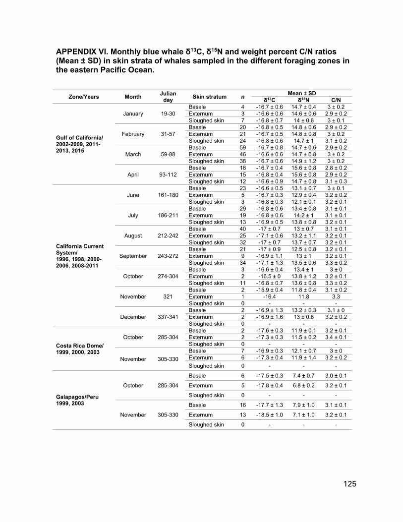
125

APPENDIX VI. Monthly blue whale δ13C, δ15N and weight percent C/N ratios (Mean ± SD) in skin strata of whales sampled in the different foraging zones in the eastern Pacific Ocean.

Zone/Years Month Julian day Skin stratum n Mean ± SD

δ13C δ15N C/N

Gulf of California/ 2002-2009, 2011-2013, 2015

January 19-30 Basale 4 -16.7 ± 0.6 14.7 ± 0.4 3 ± 0.2Externum 3 -16.6 ± 0.6 14.6 ± 0.6 2.9 ± 0.2Sloughed skin 7 -16.8 ± 0.7 14 ± 0.6 3 ± 0.1

February 31-57 Basale 20 -16.8 ± 0.5 14.8 ± 0.6 2.9 ± 0.2Externum 21 -16.7 ± 0.5 14.8 ± 0.8 3 ± 0.2Sloughed skin 24 -16.8 ± 0.6 14.7 ± 1 3.1 ± 0.2

March 59-88 Basale 59 -16.7 ± 0.8 14.7 ± 0.6 2.9 ± 0.2Externum 46 -16.6 ± 0.6 14.7 ± 0.8 3 ± 0.2Sloughed skin 38 -16.7 ± 0.6 14.9 ± 1.2 3 ± 0.2

April 93-112 Basale 18 -16.7 ± 0.4 15.6 ± 0.8 2.8 ± 0.2Externum 15 -16.8 ± 0.4 15.6 ± 0.8 2.9 ± 0.2Sloughed skin 12 -16.6 ± 0.9 14.7 ± 0.8 3.1 ± 0.3

California Current System/ 1996, 1998, 2000-2006, 2008-2011

June 161-180 Basale 23 -16.6 ± 0.5 13.1 ± 0.7 3 ± 0.1Externum 5 -16.7 ± 0.3 12.9 ± 0.4 3.2 ± 0.2Sloughed skin 3 -16.8 ± 0.3 12.1 ± 0.1 3.2 ± 0.1

July 186-211 Basale 29 -16.8 ± 0.6 13.4 ± 0.8 3.1 ± 0.1Externum 19 -16.8 ± 0.6 14.2 ± 1 3.1 ± 0.1Sloughed skin 13 -16.9 ± 0.5 13.8 ± 0.8 3.2 ± 0.1

August 212-242 Basale 40 -17 ± 0.7 13 ± 0.7 3.1 ± 0.1Externum 25 -17.1 ± 0.6 13.2 ± 1.1 3.2 ± 0.1Sloughed skin 32 -17 ± 0.7 13.7 ± 0.7 3.2 ± 0.1

September 243-272 Basale 21 -17 ± 0.9 12.5 ± 0.8 3.2 ± 0.1Externum 9 -16.9 ± 1.1 13 ± 1 3.2 ± 0.1Sloughed skin 34 -17.1 ± 1.3 13.5 ± 0.6 3.3 ± 0.2

October 274-304 Basale 3 -16.6 ± 0.4 13.4 ± 1 3 ± 0Externum 2 -16.5 ± 0 13.8 ± 1.2 3.2 ± 0.1Sloughed skin 11 -16.8 ± 0.7 13.6 ± 0.8 3.3 ± 0.2

November 321 Basale 2 -15.9 ± 0.4 11.8 ± 0.4 3.1 ± 0.2Externum 1 -16.4 11.8 3.3Sloughed skin 0 - - -

December 337-341 Basale 2 -16.9 ± 1.3 13.2 ± 0.3 3.1 ± 0Externum 2 -16.9 ± 1.6 13 ± 0.8 3.2 ± 0.2Sloughed skin 0 - - -

Costa Rica Dome/ 1999, 2000, 2003

October 285-304 Basale 2 -17.6 ± 0.3 11.9 ± 0.1 3.2 ± 0.1Externum 2 -17.3 ± 0.3 11.5 ± 0.2 3.4 ± 0.1Sloughed skin 0 - - -

November 305-330 Basale 7 -16.9 ± 0.3 12.1 ± 0.7 3 ± 0Externum 6 -17.3 ± 0.4 11.9 ± 1.4 3.2 ± 0.2Sloughed skin 0 - - -

Galapagos/Peru 1999, 2003

October 285-304

Basale 6 -17.5 ± 0.3 7.4 ± 0.7 3.0 ± 0.1

Externum 5 -17.8 ± 0.4 6.8 ± 0.2 3.2 ± 0.1

Sloughed skin 0 - - -

November 305-330

Basale 16 -17.7 ± 1.3 7.9 ± 1.0 3.1 ± 0.1

Externum 13 -18.5 ± 1.0 7.1 ± 1.0 3.2 ± 0.1

Sloughed skin 0 - - -

126

APPENDIX VII. SIBER code to estimate SEAB, SEAC, and the overlap between ellipses. Code obtained from: https://github.com/AndrewLJackson/SIBER ############################################################################## ######### SIBER introduction and guide: Estimating SEAB and SEAC ###################### ############################################################################## knitr::opts_chunk$set(collapse = TRUE, comment = "#>", fig.width = 6, fig.height = 5) # Load the viridis package and create a new palette with 3 colours, one for # each of the 3 groups we have in this dataset. library(viridis) palette(viridis(4)) # This user manual introduces the basic functionality of this standalone version # of SIBER, which was previously part of the siar package. SIBER contains two # types of analysis, although both are founded on the same principle of fitting # ellipses to groups of data. The questions are very different though and it is # important that you satisfy yourself with which one you want for the questions # you have of your own data. There are additional learning resources available at # SIAR-examples-and-queries. N.B. these examples currently still use the SIBER # functions embedded within the SIAR package, which I will update shortly, but # the concepts are exactly the same. # Setting up our R session for this demonstration # In this example, we are going to work with a bundled example dataset that # I created previously using the function generateSiberData(). This dataset # is loaded using data("demo.siber.data") but it is also provided as a raw *.csv # file which is more usually the format you would work with when organising # your own dataset for analysis using SIBER. We then use createSiberObject() # to convert this raw data form into an object that contains information summary # statistics that are useful for plotting, and a z-score transformed version of # the data which is used in the model fitting process before being back-transformed # using the summary statistic information. # remove previously loaded items from the current environment and remove previous # graphics. rm(list=ls()) graphics.off()

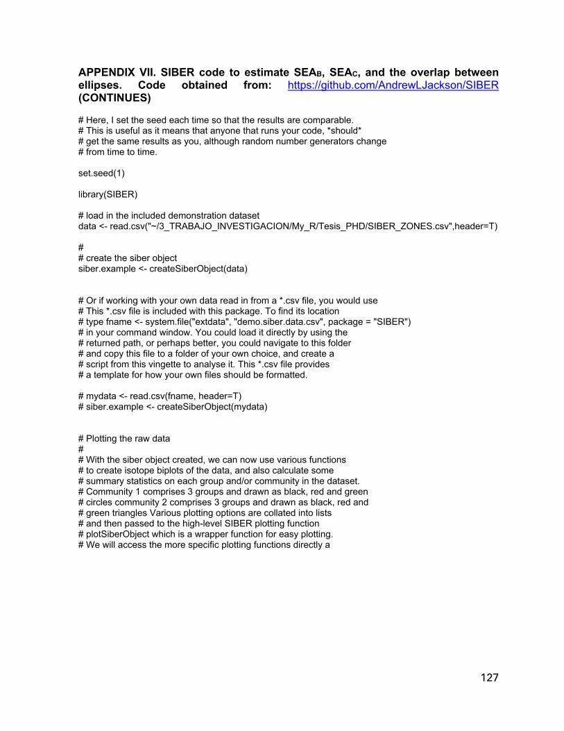
127

APPENDIX VII. SIBER code to estimate SEAB, SEAC, and the overlap between ellipses. Code obtained from: https://github.com/AndrewLJackson/SIBER (CONTINUES) # Here, I set the seed each time so that the results are comparable. # This is useful as it means that anyone that runs your code, *should* # get the same results as you, although random number generators change # from time to time. set.seed(1) library(SIBER) # load in the included demonstration dataset data <- read.csv("~/3_TRABAJO_INVESTIGACION/My_R/Tesis_PHD/SIBER_ZONES.csv",header=T) # # create the siber object siber.example <- createSiberObject(data) # Or if working with your own data read in from a *.csv file, you would use # This *.csv file is included with this package. To find its location # type fname <- system.file("extdata", "demo.siber.data.csv", package = "SIBER") # in your command window. You could load it directly by using the # returned path, or perhaps better, you could navigate to this folder # and copy this file to a folder of your own choice, and create a # script from this vingette to analyse it. This *.csv file provides # a template for how your own files should be formatted. # mydata <- read.csv(fname, header=T) # siber.example <- createSiberObject(mydata) # Plotting the raw data # # With the siber object created, we can now use various functions # to create isotope biplots of the data, and also calculate some # summary statistics on each group and/or community in the dataset. # Community 1 comprises 3 groups and drawn as black, red and green # circles community 2 comprises 3 groups and drawn as black, red and # green triangles Various plotting options are collated into lists # and then passed to the high-level SIBER plotting function # plotSiberObject which is a wrapper function for easy plotting. # We will access the more specific plotting functions directly a

128

APPENDIX VII. SIBER code to estimate SEAB, SEAC, and the overlap between ellipses. Code obtained from: https://github.com/AndrewLJackson/SIBER (CONTINUES) # little later on to create more customised graphics. # ax.pad determines the padding applied around the extremes of # the data. # iso.order is a vector of length 2 specifying which isotope # should be plotted on the x and y axes.N.B. there is currently a # problem with the addition of the group ellipses using if you # deviate from the default of iso.order = c(1,2). This argument # will be deprecated in a future release, and plotting order will # be acheived at point of data-entry. I recommond you set up your # original data with the chemical element you want plotted on the # x-axis being the first column, and the y-axis in the second. # Convex hulls are drawn between the centres of each group within a # community with hulls = T. # Ellipses are drawn for each group independently with ellipses = T. # These ellipses can be made to be maximum likelihood standard # ellipses by setting p = NULL, or can be made to be predicition # ellipses that contain approximately p proportion of data. # For example, p = 0.95 will draw an ellipse that encompasses # approximately 95% of the data. The parameter n determines how # many points are used to make each ellipse and hence how smooth the # curves are. Convex hulls are draw around each group # independently with group.hulls = T. Create lists of plotting # arguments to be passed onwards to each of the three plotting functions. community.hulls.args <- list(col = 1, lty = 1, lwd = 1) group.ellipses.args <- list(n = 100, p.interval = 0.40, lty = 1, lwd = 2) group.hull.args <- list(lty = 2, col = "grey20") par(mfrow=c(1,1)) plotSiberObject(siber.example, ax.pad = 2, hulls = F, community.hulls.args, ellipses = T, group.ellipses.args, group.hulls = T, group.hull.args, bty = "L", iso.order = c(1,2), xlab = expression({delta}^13*C~'\u2030'), ylab = expression({delta}^15*N~'\u2030') )

129

APPENDIX VII. SIBER code to estimate SEAB, SEAC, and the overlap between ellipses. Code obtained from: https://github.com/AndrewLJackson/SIBER (CONTINUES) # Summary statistics and custom graphic additions # Although the intention of SIBER is to use Bayesian methods to allow # us to make statistical comparisons of what are otherwise typically # point estimates of dispersion within and among communities and # groups, the basic summary statistics are informative and useful # for checking that our Bayesian analysis is working as intended.One # feature of the Standard Ellipse is that it contains approximately # 40% of the data. SIBER now includes code to scale this ellipse so # that it contains approximately any % of the data you wish. # Additionally, the ellipse can be scaled so that it represents # a % confidence ellipse of the bivariate means # (rather than of the data). We create the bi-plot again here # and this time add the additional ellipses overlayed on the basic # plot that this time omits group hulls and group standard ellipses. community.hulls.args <- list(col = 1, lty = 1, lwd = 1) group.ellipses.args <- list(n = 100, p.interval = 0.95, lty = 1, lwd = 2) group.hull.args <- list(lty = 2, col = "grey20") # this time we will make the points a bit smaller by # cex = 0.5 par(mfrow=c(1,1)) plotSiberObject(siber.example, ax.pad = 2, hulls = F, community.hulls.args, ellipses = F, group.ellipses.args, group.hulls = F, group.hull.args, bty = "L", iso.order = c(1,2), xlab=expression({delta}^13*C~'\u2030'), ylab=expression({delta}^15*N~'\u2030'), cex = 0.5 )

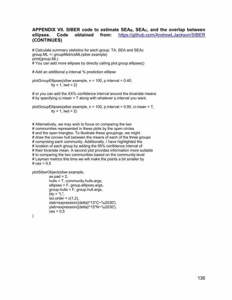
130

APPENDIX VII. SIBER code to estimate SEAB, SEAC, and the overlap between ellipses. Code obtained from: https://github.com/AndrewLJackson/SIBER (CONTINUES) # Calculate summary statistics for each group: TA, SEA and SEAc group.ML <- groupMetricsML(siber.example) print(group.ML) # You can add more ellipses by directly calling plot.group.ellipses() # Add an additional p.interval % prediction ellilpse plotGroupEllipses(siber.example, n = 100, p.interval = 0.40, lty = 1, lwd = 2) # or you can add the XX% confidence interval around the bivariate means # by specifying ci.mean = T along with whatever p.interval you want. plotGroupEllipses(siber.example, n = 100, p.interval = 0.95, ci.mean = T, lty = 1, lwd = 2) # Alternatively, we may wish to focus on comparing the two # communities represented in these plots by the open circles # and the open triangles. To illustrate these groupings, we might # draw the convex hull between the means of each of the three groups # comprising each community. Additionally, I have highlighted the # location of each group by adding the 95% confidence interval of # their bivariate mean. A second plot provides information more suitable # to comparing the two communities based on the community-level # Layman metrics this time we will make the points a bit smaller by # cex = 0.5 plotSiberObject(siber.example, ax.pad = 2, hulls = T, community.hulls.args, ellipses = F, group.ellipses.args, group.hulls = F, group.hull.args, bty = "L", iso.order = c(1,2), xlab=expression({delta}^13*C~'\u2030'), ylab=expression({delta}^15*N~'\u2030'), cex = 0.5 )

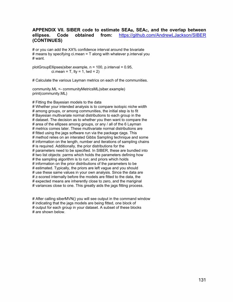
131

APPENDIX VII. SIBER code to estimate SEAB, SEAC, and the overlap between ellipses. Code obtained from: https://github.com/AndrewLJackson/SIBER (CONTINUES) # or you can add the XX% confidence interval around the bivariate # means by specifying ci.mean = T along with whatever p.interval you # want. plotGroupEllipses(siber.example, n = 100, p.interval = 0.95, ci.mean = T, lty = 1, lwd = 2) # Calculate the various Layman metrics on each of the communities. community.ML <- communityMetricsML(siber.example) print(community.ML) # Fitting the Bayesian models to the data # Whether your intended analysis is to compare isotopic niche width # among groups, or among communities, the initial step is to fit # Bayesian multivariate normal distributions to each group in the # dataset. The decision as to whether you then want to compare the # area of the ellipses among groups, or any / all of the 6 Layman # metrics comes later. These multivariate normal distributions are # fitted using the jags software run via the package rjags. This # method relies on an interated Gibbs Sampling technique and some # information on the length, number and iterations of sampling chains # is required. Additionally, the prior distributions for the # parameters need to be specified. In SIBER, these are bundled into # two list objects: parms which holds the parameters defining how # the sampling algorithm is to run; and priors which holds # information on the prior distributions of the parameters to be # estimated. Typically, the priors are left vague and you should # use these same values in your own analysis. Since the data are # z-scored internally before the models are fitted to the data, the # expected means are inherently close to zero, and the mariginal # variances close to one. This greatly aids the jags fitting process. # After calling siberMVN() you will see output in the command window # indicating that the jags models are being fitted, one block of # output for each group in your dataset. A subset of these blocks # are shown below.

132

APPENDIX VII. SIBER code to estimate SEAB, SEAC, and the overlap between ellipses. Code obtained from: https://github.com/AndrewLJackson/SIBER (CONTINUES) # options for running jags parms <- list() parms$n.iter <- 2 * 10^4 # number of iterations to run the model for parms$n.burnin <- 1 * 10^3 # discard the first set of values parms$n.thin <- 10 # thin the posterior by this many parms$n.chains <- 2 # run this many chains # define the priors priors <- list() priors$R <- 1 * diag(2) priors$k <- 2 priors$tau.mu <- 1.0E-3 # fit the ellipses which uses an Inverse Wishart prior # on the covariance matrix Sigma, and a vague normal prior on the # means. Fitting is via the JAGS method. ellipses.posterior <- siberMVN(siber.example, parms, priors) # Comparing among groups using the Standard Ellipse Area # When comparing individual groups with each other, be it within a # single community, or groups among communities, the Standard # Ellipse Area (SEA) is the recommended method. Since the # multivariate normal distributions have already been fitted to # each group, it only remains to calculate the SEA on the posterior # distribution of covariance matrice for each group, thereby # yielding the Bayesian SEA or SEA-B. We can also use the summary # statistics we calcluated earlier to add the maximum likelihood # estimates of SEA-c to the Bayesian esimates. # Plotting is via the function siberDensityPlot() which is # essentially the same as siardensityplot() from the older # version of SIAR. Credible intervals can be extracted by calling # the function hdr from the hdrcde package.

133

APPENDIX VII. SIBER code to estimate SEAB, SEAC, and the overlap between ellipses. Code obtained from: https://github.com/AndrewLJackson/SIBER (CONTINUES) # The posterior estimates of the ellipses for each group can be used # to calculate the SEA.B for each group. SEA.B <- siberEllipses(ellipses.posterior) siberDensityPlot(SEA.B, xticklabels = colnames(group.ML), xlab = c("Community | Group"), ylab = expression("Standard Ellipse Area " ('\u2030' ^2) ), bty = "L", las = 1, main = "SIBER ellipses on each group" ) OUT <- data.frame(SEA.B) write.csv(OUT, file = "SEAB.csv") # Add red x's for the ML estimated SEA-c points(1:ncol(SEA.B), group.ML[3,], col="red", pch = "x", lwd = 2) APPENDIX VIII. MixSIAR model in R, deviance information criteria, summary statistics and model diagnosis. ################################################################################## SIBER introduction and guide: Overlap ##################### #################################################################### # Fix spatstat bug

# # install.packages("devtools") # install if necessary

# devtools::install_github("andrewljackson/SIBER",

# build_vingettes = TRUE)

library(SIBER)

## ---- echo = FALSE-------------------------------------------------------

knitr::opts_chunk$set(collapse = TRUE, comment = "#>",

fig.width = 6, fig.height = 5)

134

APPENDIX VII. SIBER code to estimate SEAB, SEAC, and the overlap between ellipses. Code obtained from: https://github.com/AndrewLJackson/SIBER (CONTINUES)

## ------------------------------------------------------------------------

# remove previously loaded items from the current environment and remove previous graphics.

rm(list=ls())

graphics.off()

# Here, I set the seed each time so that the results are comparable.

# This is useful as it means that anyone that runs your code, *should*

# get the same results as you, although random number generators change

# from time to time.

set.seed(1)

# load SIBER

library(SIBER)

library(viridis)

# set a new three-colour palette from the viridis package

palette(viridis::viridis(4))

# load in the included demonstration dataset

data <-

read.csv("~/3_TRABAJO_INVESTIGACION/My_R/Tesis_PHD/SIBER_Thesis/ZONES/SIBER_ZONES

.csv",header=T)

#

# create the siber object

siber.example <- createSiberObject(data)

# Or if working with your own data read in from a *.csv file, you would use

# This *.csv file is included with this package. To find its location

# type

# fname <- system.file("extdata", "demo.siber.data.csv", package = "SIBER")

135

APPENDIX VII. SIBER code to estimate SEAB, SEAC, and the overlap between ellipses. Code obtained from: https://github.com/AndrewLJackson/SIBER (CONTINUES)

# in your command window. You could load it directly by using the

# returned path, or perhaps better, you could navigate to this folder

# and copy this file to a folder of your own choice, and create a

# script from this vingette to analyse it. This *.csv file provides

# a template for how your own files should be formatted.

# mydata <- read.csv(fname, header=T)

# siber.example <- createSiberObject(mydata)

# Create lists of plotting arguments to be passed onwards to the

# plotting functions. With p.interval = NULL, these are SEA. NB not SEAc though

# which is what we will base our overlap calculations on. This implementation

# needs to be added in a future update. For now, the best way to plot SEAc is to

# add the ellipses manually following the vignette on this topic.

group.ellipses.args <- list(n = 100, p.interval = 0.40, lty = 1, lwd = 2)

par(mfrow=c(1,1))

plotSiberObject(siber.example,

ax.pad = 2,

hulls = F, community.hulls.args,

ellipses = T, group.ellipses.args,

group.hulls = F, group.hull.args,

bty = "L",

iso.order = c(1,2),

xlab = expression({delta}^13*C~'\u2030'),

ylab = expression({delta}^15*N~'\u2030')

)

136

APPENDIX VII. SIBER code to estimate SEAB, SEAC, and the overlap between ellipses. Code obtained from: https://github.com/AndrewLJackson/SIBER (CONTINUES)

## ---- MLoverlap----------------------------------------------------------

# In this example, I will calculate the overlap between ellipses for groups 2

# and 3 in community 1 (i.e. the green and yellow open circles of data).

# The first ellipse is referenced using a character string representation where

# in "x.y", "x" is the community, and "y" is the group within that community.

# So in this example: community 1, group 2

ellipse1 <- "1.1"

# Ellipse two is similarly defined: community 1, group3

ellipse2 <- "1.2"

# The overlap of the maximum likelihood fitted standard ellipses are

# estimated using

sea.overlap <- maxLikOverlap(ellipse1, ellipse2, siber.example,

p.interval = 0.40, n = 1000)

# the overlap betweeen the corresponding 95% prediction ellipses is given by:

ellipse95.overlap <- maxLikOverlap(ellipse1, ellipse2, siber.example,

p.interval = 0.40, n = 1000)

# so in this case, the overlap as a proportion of the non-overlapping area of

# the two ellipses, would be

prop.95.over <- ellipse95.overlap[3] / (ellipse95.overlap[2] +

ellipse95.overlap[1] -

ellipse95.overlap[3])

137

APPENDIX VII. SIBER code to estimate SEAB, SEAC, and the overlap between ellipses. Code obtained from: https://github.com/AndrewLJackson/SIBER (CONTINUES)

## ---- bayesOverlap-------------------------------------------------------

# options for running jags

parms <- list()

parms$n.iter <- 2 * 10^4 # number of iterations to run the model for

parms$n.burnin <- 1 * 10^3 # discard the first set of values

parms$n.thin <- 10 # thin the posterior by this many

parms$n.chains <- 2 # run this many chains

# define the priors

priors <- list()

priors$R <- 1 * diag(2)

priors$k <- 2

priors$tau.mu <- 1.0E-3

# fit the ellipses which uses an Inverse Wishart prior

# on the covariance matrix Sigma, and a vague normal prior on the

# means. Fitting is via the JAGS method.

ellipses.posterior <- siberMVN(siber.example, parms, priors)

# and teh corresponding Bayesian estimates for the overlap between the

# 95% ellipses is given by:

bayes95.overlap <- bayesianOverlap(ellipse1, ellipse2, ellipses.posterior,

draws = 500, p.interval = 0.40, n = 500)

OUT <- data.frame(bayes95.overlap)

write.csv(OUT, file = "ZONES_95.csv")

138

APPENDIX VII. SIBER code to estimate SEAB, SEAC, and the overlap between ellipses. Code obtained from: https://github.com/AndrewLJackson/SIBER (CONTINUES)

# a histogram of the overlap

hist(bayes95.overlap[,3], 10)

# and as above, you can express this a proportion of the non-overlapping area of

# the two ellipses, would be

bayes.prop.95.over <- (bayes95.overlap[,3] / (bayes95.overlap[,2] +

bayes95.overlap[,1] -

bayes95.overlap[,3])

)

hist(bayes.prop.95.over, 10)

OUT <- data.frame(bayes.prop.95.over)

write.csv(OUT, file = "ZONES_95.csv")

139

APPENDIX VIII. MixSIAR model in R, deviance information criteria, summary statistics and model diagnosis. A) Model in R # source$data_type: means

# source$by_factor: NA

# random effects: 0

# fixed effects: 0

# nested factors:

# factors:

# continuous effects: 0

# error structure: Residual * Process

# source$conc_dep: FALSE

model{

for(src in 1:n.sources){

for(iso in 1:n.iso){

src_mu[src,iso] ~ dnorm(MU_array[src,iso], n_array[src]/SIG2_array[src,iso]); # Eqn 3.8 but with

precision instead of variance

tmp.X[src,iso] ~ dchisqr(n_array[src]);

src_tau[src,iso] <- tmp.X[src,iso]/(SIG2_array[src,iso]*(n_array[src] - 1)); # Eqn 3.9, following the

simulation on p.580

}

}

# Draw p.global (global proportion means) from an uninformative Dirichlet,

# Then ilr.global is the ILR-transform of p.global

p.global[1:n.sources] ~ ddirch(alpha[1:n.sources]);

for(src in 1:(n.sources-1)){

gmean[src] <- prod(p.global[1:src])^(1/src);

ilr.global[src] <- sqrt(src/(src+1))*log(gmean[src]/p.global[src+1]); # page 296, Egozcue 2003

}

140

APPENDIX VIII. MixSIAR model in R, deviance information criteria, summary statistics and model diagnosis. (CONTINUES)

# DON'T generate individual deviates from the global/region/pack mean (but keep same model

structure)

for(i in 1:N) {

for(src in 1:(n.sources-1)) {

ilr.ind[i,src] <- 0;

ilr.tot[i,src] <- ilr.global[src] + ilr.ind[i,src]; # add all effects together for each individual (in ilr-

space)

}

}

# Inverse ILR math (equation 24, page 294, Egozcue 2003)

for(i in 1:N){

for(j in 1:(n.sources-1)){

cross[i,,j] <- (e[,j]^ilr.tot[i,j])/sum(e[,j]^ilr.tot[i,j]);

}

for(src in 1:n.sources){

tmp.p[i,src] <- prod(cross[i,src,]);

}

for(src in 1:n.sources){

p.ind[i,src] <- tmp.p[i,src]/sum(tmp.p[i,]);

}

}

for(src in 1:n.sources) {

for(i in 1:N){

# these are weights for variances

p2[i,src] <- p.ind[i,src]*p.ind[i,src];

}

}

141

APPENDIX VIII. MixSIAR model in R, deviance information criteria, summary statistics and model diagnosis. (CONTINUES)

# For each isotope and population, calculate the predicted mixtures

for(iso in 1:n.iso) {

for(i in 1:N) {

mix.mu[iso,i] <- inprod(src_mu[,iso],p.ind[i,]) + inprod(frac_mu[,iso],p.ind[i,]);

}

}

# Multiplicative residual error

for(iso in 1:n.iso){

resid.prop[iso] ~ dunif(0,20);

}

# Calculate process variance for each isotope and population

for(iso in 1:n.iso) {

for(i in 1:N) {

process.var[iso,i] <- inprod(1/src_tau[,iso],p2[i,]) + inprod(frac_sig2[,iso],p2[i,]);

}

}

# Construct Sigma, the mixture precision matrix

for(ind in 1:N){

for(i in 1:n.iso){

for(j in 1:n.iso){

Sigma.ind[ind,i,j] <- equals(i,j)/(process.var[i,ind]*resid.prop[i]);

}

}

}

# Likelihood

for(i in 1:N) {

X_iso[i,] ~ dmnorm(mix.mu[,i], Sigma.ind[i,,]);

}

} # end model

142

APPENDIX VIII. MixSIAR model in R, deviance information criteria, summary statistics and model diagnosis. (CONTINUES) b) Deviance information criteria (DIC) and summary statistics #################################################################

# Summary Statistics

#################################################################

Deviance Information Criteria = 1925.242

Mean SD 2.5% 5% 25% 50% 75% 95% 97.5%

p.global.CCS 0.300 0.152 0.018 0.037 0.180 0.317 0.430 0.517 0.529

p.global.CRD 0.165 0.105 0.008 0.016 0.075 0.153 0.246 0.348 0.364

p.global.GC 0.535 0.051 0.451 0.459 0.494 0.530 0.574 0.623 0.633

c) Model diagnosis ################################################################################

# Gelman-Rubin Diagnostic

################################################################################

Generally, the Gelman diagnostic should be < 1.05

Out of 5 variables: 0 > 1.01

0 > 1.05

0 > 1.1

The worst variables are:

Point est. Upper C.I.

p.global[2] 1.0009415 1.0046040

p.global[1] 1.0008949 1.0044371

p.global[3] 1.0007618 1.0036784

resid.prop 1.0003020 1.0022550

deviance 0.9996427 0.9997924

143

APPENDIX VIII. MixSIAR model in R, deviance information criteria, summary statistics and model diagnosis. (CONTINUES)

And here are the Gelman diagnostics for all variables:

Point est. Upper C.I.

deviance 0.9996427 0.9997924

p.global[1] 1.0008949 1.0044371

p.global[2] 1.0009415 1.0046040

p.global[3] 1.0007618 1.0036784

resid.prop 1.0003020 1.0022550

################################################################################

# Geweke Diagnostic

################################################################################

The Geweke diagnostic is a standard z-score, so we'd expect 5% to be outside +/-1.96

Number of variables outside +/-1.96 in each chain (out of 5):

Chain 1 Chain 2 Chain 3

Geweke 4 4 1

And here are the Geweke diagnostics for all variables:

chain1 chain2 chain3

deviance -0.251 0.992 0.362

p.global[1] -3.539 2.078 1.116

p.global[2] 3.586 -1.987 -1.214

p.global[3] 3.311 -2.260 -0.916

resid.prop -2.481 2.426 2.007

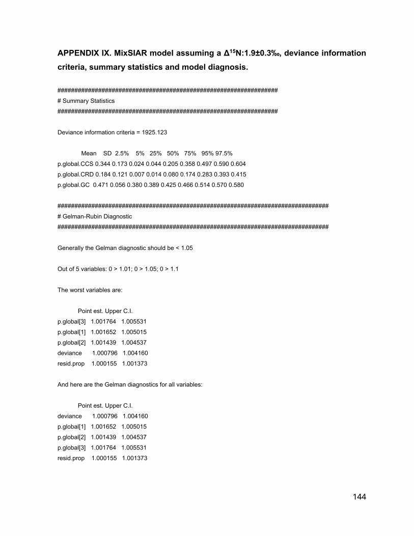
144

APPENDIX IX. MixSIAR model assuming a Δ15N:1.9±0.3‰, deviance information criteria, summary statistics and model diagnosis.

#################################################################

# Summary Statistics

#################################################################

Deviance information criteria = 1925.123

Mean SD 2.5% 5% 25% 50% 75% 95% 97.5%

p.global.CCS 0.344 0.173 0.024 0.044 0.205 0.358 0.497 0.590 0.604

p.global.CRD 0.184 0.121 0.007 0.014 0.080 0.174 0.283 0.393 0.415

p.global.GC 0.471 0.056 0.380 0.389 0.425 0.466 0.514 0.570 0.580

################################################################################

# Gelman-Rubin Diagnostic

################################################################################

Generally the Gelman diagnostic should be < 1.05

Out of 5 variables: 0 > 1.01; 0 > 1.05; 0 > 1.1

The worst variables are:

Point est. Upper C.I.

p.global[3] 1.001764 1.005531

p.global[1] 1.001652 1.005015

p.global[2] 1.001439 1.004537

deviance 1.000796 1.004160

resid.prop 1.000155 1.001373

And here are the Gelman diagnostics for all variables:

Point est. Upper C.I.

deviance 1.000796 1.004160

p.global[1] 1.001652 1.005015

p.global[2] 1.001439 1.004537

p.global[3] 1.001764 1.005531

resid.prop 1.000155 1.001373

145

################################################################################

# Geweke Diagnostic

################################################################################

The Geweke diagnostic is a standard z-score, so we'd expect 5% to be outside +/-1.96

Number of variables outside +/-1.96 in each chain (out of 5):

Chain 1 Chain 2 Chain 3

Geweke 0 0 0

And here are the Geweke diagnostics for all variables:

chain1 chain2 chain3

deviance 0.820 0.587 -0.610

p.global[1] 0.637 -0.542 1.632

p.global[2] -0.649 0.586 -1.557

p.global[3] -0.628 0.471 -1.789

resid.prop 0.918 -0.070 1.853

146

APPENDIX X. Thesis achievements:

RESEARCH ARTICLE

Estimating blue whale skin isotopic

incorporation rates and baleen growth rates:

Implications for assessing diet and movement

patterns in mysticetes

Geraldine Busquets-Vass1, Seth D. Newsome2, John Calambokidis3, Gabriela Serra-

Valente4, Jeff K. Jacobsen5, Sergio Aguıñiga-Garcıa1, Diane Gendron1*

1 Instituto Politecnico Nacional, Centro Interdisciplinario de Ciencias Marinas, La Paz, Baja California Sur,

Mexico, 2 Biology Department, University of New Mexico, Albuquerque, New Mexico, United States of

America, 3 Cascadia Research Collective, Olympia, Washington, United States of America, 4 Marine

Mammal and Turtle Division, Southwest Fisheries Science Center, National Marine Fisheries Service,

National Oceanic and Atmospheric Administration, La Jolla, California, United States of America,

5 Vertebrate Museum, Department of Biological Sciences, Humboldt State University, Arcata, California,

United States of America

* dianegendroncicimar@gmail.com

Abstract

Stable isotope analysis in mysticete skin and baleen plates has been repeatedly used to

assess diet and movement patterns. Accurate interpretation of isotope data depends on

understanding isotopic incorporation rates for metabolically active tissues and growth rates

for metabolically inert tissues. The aim of this research was to estimate isotopic incorpo-

ration rates in blue whale skin and baleen growth rates by using natural gradients in baseline

isotope values between oceanic regions. Nitrogen (δ15N) and carbon (δ13C) isotope values

of blue whale skin and potential prey were analyzed from three foraging zones (Gulf of Cali-

fornia, California Current System, and Costa Rica Dome) in the northeast Pacific from

1996–2015. We also measured δ15N and δ13C values along the lengths of baleen plates col-

lected from six blue whales stranded in the 1980s and 2000s. Skin was separated into three

strata: basale, externum, and sloughed skin. A mean (±SD) skin isotopic incorporation rate

of 163±91 days was estimated by fitting a generalized additive model of the seasonal trend

in δ15N values of skin strata collected in the Gulf of California and the California Current Sys-

tem. A mean (±SD) baleen growth rate of 15.5±2.2 cm y-1 was estimated by using seasonal

oscillations in δ15N values from three whales. These oscillations also showed that individual

whales have a high fidelity to distinct foraging zones in the northeast Pacific across years.

The absence of oscillations in δ15N values of baleen sub-samples from three male whales

suggests these individuals remained within a specific zone for several years prior to death.

δ13C values of both whale tissues (skin and baleen) and potential prey were not distinct

among foraging zones. Our results highlight the importance of considering tissue isotopic

incorporation and growth rates when studying migratory mysticetes and provide new

insights into the individual movement strategies of blue whales.

PLOS ONE | https://doi.org/10.1371/journal.pone.0177880 May 31, 2017 1 / 25

a1111111111

a1111111111

a1111111111

a1111111111

a1111111111

OPENACCESS

Citation: Busquets-Vass G, Newsome SD,

Calambokidis J, Serra-Valente G, Jacobsen JK,

Aguıñiga-Garcıa S, et al. (2017) Estimating blue

whale skin isotopic incorporation rates and baleen

growth rates: Implications for assessing diet and

movement patterns in mysticetes. PLoS ONE 12

(5): e0177880. https://doi.org/10.1371/journal.

pone.0177880

Editor: Mark S. Boyce, University of Alberta,

CANADA

Received: January 16, 2017

Accepted: May 4, 2017

Published: May 31, 2017

Copyright: This is an open access article, free of all

copyright, and may be freely reproduced,

distributed, transmitted, modified, built upon, or

otherwise used by anyone for any lawful purpose.

The work is made available under the Creative

Commons CC0 public domain dedication.

Data Availability Statement: All relevant data are

within the paper and its Supporting Information

files.

Funding: The authors received financial support

from Instituto Politecnico Nacional:SIP: 20130223;

20140495; 20150115; 20160496 (http://www.ipn.

mx/Paginas/inicio.aspx) and the University of New

Mexico Center for Stable Isotopes (Albuquerque,

NM; http://csi.unm.edu/). GBV received a PhD

Introduction

The blue whale (Balenoptera musculus) in the northeast Pacific is an endangered migratory

mysticete [1]. In summer and fall, blue whales are distributed as far north as the Gulf of Alaska

[2,3], but the highest aggregations have been observed off southern California [4]. By mid-fall

(~October), they usually migrate south to the west coast of the Baja California Peninsula [2,4–

8] and then continue migrating to one of two regions that are recognized as overwintering

zones: a calving ground in the Gulf of California [2,9–12], or the Costa Rica Dome in the east-

ern tropical Pacific [2,7,8]. Calves have also been observed in the Costa Rica Dome, but little is

known about the population dynamics in this zone [13].

Blue whales forage throughout their annual migratory cycle mainly on aggregations of krill

(Order: Euphausiacea) [14–18] and occasionally on other crustaceans (i.e. copepods, Calanusspp.) [16,19] or small fish (i.e. lanternfish: Family Myctophidae) [20]. The observation that

blue whales forage year-round suggests this species has high energetic demands relative to

other migratory mysticetes like the humpback whale (Megaptera novaeangliae) and the gray

whale (Eschrichtius robustus), that typically fast for months during their breeding season in

low latitudes [21,22]. The general migratory patterns of blue whales in the northeast Pacific

have been described [2,3,5,7,10,11,23], specifically for the California feeding population [3];

however, there are still many gaps in our understanding of their feeding ecology and plasticity

in individual movement patterns across multi-year timescales.

Stable isotope analysis (SIA) is a proven tool for studying the diet and movement patterns

of marine mammals [24]. The isotopic composition of animal tissues are influenced by diet

[25–27] and the isotopic composition of the base of the food web, which can vary in time and

space within and among oceanic ecosystems [24,28–31]. Physiological processes produce pre-

dictable offsets in isotope values between consumers and their diet, which is often called tro-

phic discrimination [24,32]. In general, consumer tissues have carbon (δ13C) and nitrogen

(δ15N) isotope values that are 0.5–3.0‰ and 2–5‰ higher than that of their prey respectively,

depending on the species, diet quality, and type of tissue analyzed [24–26,33,34].

Tissues assimilate dietary inputs at different temporal scales. Most metabolically active

tissues reflect recent dietary inputs, consumed within days to months (e.g. plasma, muscle),

depending on their isotopic incorporation rates that typically scale with body mass such that

larger animals have slower incorporation rates [35]. In contrast, metabolically inert tissues

(e.g. whiskers, nails) deposit at distinct intervals, and each deposition of tissue retains the isoto-

pic composition of dietary sources incorporated when anabolized, thus reflecting dietary input

over several years depending on tissue growth rate [24,36]. Consequently, to make accurate

inferences on ecological aspects of free ranging animals by using SIA it is essential to have infor-

mation on the isotopic incorporation rate of metabolically active tissues and the growth rates of

metabolically inert tissues; otherwise, the interpretation of the data can be highly misleading.

SIA of mysticete skin and baleen plates has frequently been used to infer diet and seasonal

movements of this difficult to study group of cetaceans [37–44]. Cetacean skin (epidermis) is a

metabolically active tissue, subdivided into cellular strata: the stratum basale, the stratum spi-

nosum, and the stratum externum [45,46]. Skin growth begins in the stratum basale a single

row of cells that replicate actively. Newly formed cells constantly displace the older cells up-

ward, first to the stratum spinosum, and subsequently to the stratum externum, the outermost

layer of skin. Finally, the stratum externum is sloughed off to the environment as sloughed

skin [45]. Variation in the isotopic composition among these strata has never been described

for any cetacean species. The isotopic incorporation rates of cetacean skin have only been mea-

sured in controlled “diet switch” feeding experiments on captive odontocetes [47,48]. These

studies used exponential fit models because theoretically, after diet switch, changes in the

Blue whale skin isotopic incorporation rates and baleen growth rates

PLOS ONE | https://doi.org/10.1371/journal.pone.0177880 May 31, 2017 2 / 25

grant from the Consejo Nacional de Ciencia y

Tecnologıa (CONACyT; http://www.conacyt.mx/), a

research grant from Cetacean Society International

(http://www.csiwhalesalive.org/index.php)

specifically for processing the baleen plates, and a

grant from American Cetacean Society - Monterey

Bay (http://acsonline.org/) to process skin

samples. The funders had no role in study design,

data collection and analysis, decision to publish, or

preparation of the manuscript.

Competing interests: The authors have declared

that no competing interests exist.

isotopic composition of tissues will follow an exponential curve over time [49–52]. Estimates

of the isotopic incorporation for carbon (δ13C) and nitrogen (δ15N) in odontocete skin slightly

differ; incorporation for δ13C is 2 to 3 months, while that for δ15N is longer and more variable

at 2 to 6 months [47,48]. The increasing use of SIA in mysticetes to characterize diet and move-

ment patterns requires the development of a method to estimate skin isotopic incorporation

rates for free-ranging populations.

Baleen consists of a series of keratin plates inserted in the upper gum of mysticetes that

functions as a filter-feeding apparatus [53]. In contrast to skin, baleen is a metabolically inert

tissue that grows continuously from the gums and abrades at the terminal end [54]. The oscil-

lations in isotope values along the length of baleen plates can be used to estimate growth rates

and generate multi-year records of individual movement strategies, habitat use, and diet

[38,42–44,55–57]. Baleen growth rates have been estimated in several species of mysticetes

[37,42–44,55,57], but currently there are no published estimates for blue whale baleen.

Potential prey of blue whales in their distinct summer–fall (California Current System: west

coast of U.S. and Baja California Peninsula; Fig 1) and winter–spring (Gulf of California and

Costa Rica Dome; Fig 1) foraging zones have contrasting isotope values [58–64] due to differ-

ences in oceanographic and biogeochemical processes that influence baseline isotope values in

these zones [31,58,62,65]. Specifically, δ15N values of prey (e.g. krill) are higher in the Gulf of

California, intermediate in the California Current System, and lowest in the Costa Rica Dome

[58–64]. We assumed that blue whale skin strata (stratum basale, stratum externum, and

sloughed skin) and baleen plates record these isotopic differences. Then, we evaluated if the

seasonal patterns of tissue isotope values could be used to estimate the isotopic incorporation

rates and baleen growth rates of blue whale skin and baleen, respectively. We also assessed if

carbon isotopes were useful for examining blue whale diet and movement patterns in the

northeast Pacific, however, we expected little variation in δ13C values of prey among foraging

zones based on previous studies [58–64]. Overall, our results highlight the importance of care-

fully considering the temporal window represented by metabolically active and inert tissues

when studying migratory mysticetes.

Materials and methods

Ethic statement

All whale tissues used in this study were collected and processed under special permits issued

by the Secretarıa de Medio Ambiente y Recursos Naturales (SEMARNAT) in Mexico (codes:

180796-213-03, 071197–213–03, DOO 750-00444/99, DOO.0-0095, DOO 02.-8318, SGPA/

DGVS-7000, 00624, 01641, 00560, 12057, 08021, 00506, 08796, 09760, 10646, 00251, 00807,

05036, 01110; 00987; CITES export permit: MX 71395), and the National Oceanic and Atmo-

spheric Administration–National Marine Fisheries Service (NOAA/NMFS) (NMFS MMPA/

Research permits codes: NMFS-873; 1026; 774–1427; 774–1714; 14097; 16111; CITES import

permit: 14US774223/9) in the United States of America. All tissues were collected using non-

lethal sampling techniques.

Sample collection

Blue whale skin biopsies (n = 255) and sloughed skin (n = 174) were selected from tissue banks

at NOAA Southwest Fisheries Science Center (NOAA-SWFSC), Cascadia Research Collective

(CRC), and Centro Interdisciplinario de Ciencias Marinas-Instituto Politecnico Nacional

(CICIMAR-IPN). These samples were collected from 1996–2015 in the Gulf of California

(GC) (Jan–Apr; n = 115 biopsies, n = 81 sloughed skin; Fig 1), California Current System

(CCS) (Jun–Dec; n = 129 biopsies, n = 93 sloughed skin; Fig 1) and the Costa Rica Dome

Blue whale skin isotopic incorporation rates and baleen growth rates

PLOS ONE | https://doi.org/10.1371/journal.pone.0177880 May 31, 2017 3 / 25

(CRD) (Oct–Nov; n = 11 biopsies; Fig 1). Skin samples were collected during marine mammal

surveys conducted by NOAA-SWFSC, CRC, and CICIMAR-IPN. Skin biopsies were collected

via dart sampling methods [66], and sloughed skin was directly collected from the water with a

net [67] or from suction cups of satellite-tagged whales.

Krill (n = 34) and lanternfish (n = 7) samples were opportunistically collected during

marine mammal surveys conducted by CICIMAR-IPN within the GC (2005–2015). Krill sam-

ples were collected by towing a conical net (diameter 50 cm., mesh size 200 μm) when blue

Fig 1. Northeast Pacific sampling zones. Dots represent blue whale skin samples collected in the California Current System (CCS), Gulf of California

(GC) and Costa Rica Dome (CRD). Dots with a cross represent blue whale baleen plates collected from dead stranded whales.

https://doi.org/10.1371/journal.pone.0177880.g001

Blue whale skin isotopic incorporation rates and baleen growth rates

PLOS ONE | https://doi.org/10.1371/journal.pone.0177880 May 31, 2017 4 / 25

whales were observed feeding near the surface. Lanternfish samples were collected with a fish-

ing net (mesh size 5 mm), when aggregations were found near the surface. Prey samples were

preserved frozen in liquid nitrogen (-195˚C). The assignment of lanternfish to the Family

Myctophidae and classification of krill species was made using identification guides [68,69];

Nyctiphanes simplex was the only krill species present in all samples.

To assess the isotope variability between blue whale skin strata it was necessary to identify

tissue structure. Histological preparations of five skin biopsies were stained with hematoxylin

& eosin following the protocol of Sheehan and Hrapchak [70]. Based on these preparations the

skin biopsy was divided into two strata: (1) stratum basale, closest to the blubber, and (2) stra-

tum externum, the outermost layer that easily separated from the stratum spinosum (Fig 2A).

We did not include stratum spinosum in our analysis because we assumed it would exhibit

intermediate isotope values between the stratum basale and the stratum externum. Some skin

biopsy samples were incomplete as they had been used for previous studies, and only one of

the two strata were available. Sloughed skin samples were also included in the analysis, but

were only available for some years (S1 Dataset).

Baleen plates collected from six dead stranded blue whales were obtained from Humboldt

State University Vertebrate Museum (HSU-VM), CICIMAR-IPN, the California Department

of Parks and Recreation-Prairie Creek Redwoods State Park (CDPR-PCRSP), and the Oregon

Marine Mammal Stranding Network (OMMSN) (S1 Table). Stranding reports including sex

identification were available for all but one individual, which was determined at NOAA-

SWFSC using genetic methods [71,72].

Standardizing blue whale skin sample preparation

Numerous studies show that two factors that are unrelated to ecology can alter isotope values

of metabolically active tissues. The first factor is tissue lipid content. Lipids have lower δ13C

values than associated carbohydrates and proteins [24,73,74]. Thus, the potential influence of

lipid content on bulk tissue δ13C values must be considered when using SIA to make ecological

inferences [24,75,76]. Chemical lipid-extraction removes the influence of lipids on bulk tissues,

but a side effect of this procedure is that it may affect δ15N values of tissues [75,76]. To evaluate

the effect of lipid-extraction on the isotope values of blue whale skin, five skin samples were

divided into two subsamples, one subsample was lipid-extracted with three ~24 hour soaks in

a 2:1 chloroform:methanol solvent solution, rinsed with ionized water and lyophilized. The

second subsample was simply lyophilized, and analyzed as bulk tissue.

The second factor that can alter tissue isotopic composition is how samples are preserved

prior to isotopic analysis. Ideally, all tissues would be stored frozen since freezing does not

alter isotope values [24,77–79]. Most of the skin samples selected for this study were stored fro-

zen prior to isotope analysis, but some (n = 100) were stored in a 20% salt saturated solution of

dimethyl sulfoxide (DMSO). Previous studies have shown that the effect of DMSO on the iso-

tope values of tissues can be removed via lipid-extraction [76,80,81]. To determine if this strat-

egy would work for blue whale skin samples preserved in DMSO, we selected 25 sloughed skin

samples from the GC (2005–2007). During field collection, each of these skin samples were

divided into two sections and preserved one of two ways for one year before they were pre-

pared for isotope analysis: the first set was preserved in DMSO and the second (control) set

was frozen in liquid nitrogen (-195˚C).

Stable isotope analysis

All skin and prey samples were lipid-extracted, lyophilized, and homogenized by grinding

them into a fine powder; as noted above the small set of subsamples that were analyzed to test

Blue whale skin isotopic incorporation rates and baleen growth rates

PLOS ONE | https://doi.org/10.1371/journal.pone.0177880 May 31, 2017 5 / 25

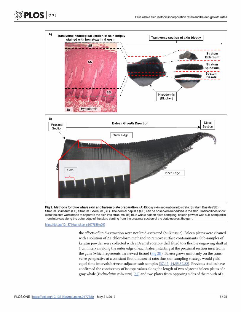
the effects of lipid-extraction were not lipid-extracted (bulk tissue). Baleen plates were cleaned

with a solution of 2:1 chloroform:methanol to remove surface contaminants. Sub-samples of

keratin powder were collected with a Dremel rotatory drill fitted to a flexible engraving shaft at

1 cm intervals along the outer edge of each baleen, starting at the proximal section inserted in

the gum (which represents the newest tissue) (Fig 2B). Baleen grows uniformly on the trans-

verse perspective at a constant (but unknown) rate; thus our sampling strategy would yield

equal time intervals between adjacent sub-samples [37,42–44,55,57,82]. Previous studies have

confirmed the consistency of isotope values along the length of two adjacent baleen plates of a

gray whale (Eschrichtius robusutu) [82] and two plates from opposing sides of the mouth of a

Fig 2. Methods for blue whale skin and baleen plate preparation. (A) Biopsy skin separation into strata: Stratum Basale (SB),

Stratum Spinosum (SS) Stratum Externum (SE). The dermal papillae (DP) can be observed embedded in the skin. Dashed lines show

were the cuts were made to separate the skin into stratums. (B) Blue whale baleen plate sampling: baleen powder was sub-sampled in

1 cm intervals along the outer edge of the plate starting from the proximal section of the plate nearest the gum.

https://doi.org/10.1371/journal.pone.0177880.g002

Blue whale skin isotopic incorporation rates and baleen growth rates

PLOS ONE | https://doi.org/10.1371/journal.pone.0177880 May 31, 2017 6 / 25

bowhead whale (Balaena mysticetus) [43]. Consequently, we assumed that each baleen pro-

vides a consistent record of the past foraging history for each blue whale. Lastly, we compiled

δ13C and δ15N data from the literature of blue whale prey from foraging zones in the northeast

Pacific (S2 Table).

Approximately 0.5–0.6 mg of each tissue sample (dried skin, baleen, and prey) was weighed

into a tin capsule. Carbon (δ13C) and nitrogen (δ15N) isotope values were measured with a Cost-

ech 4010 elemental analyzer coupled to Thermo Scientific Delta V isotope ratio mass spectrom-

eter at the Center for Stable Isotopes at the University of New Mexico (Albuquerque, NM).

Isotope data are reported as delta δ values, δ13C or δ15N = 1000 [(Rsample / Rstandard)—1],

where R = 13C/12C or 15N/14N ratio of sample and standard [83]. Values are in units of parts per

thousand or per mil (‰) and the internationally accepted standards are atmospheric N2 for

δ15N and Vienna-Pee Dee Belemnite limestone (V-PDB) for δ13C [83]. Within-run analytical

precision was estimated via analysis of two proteinaceous internal reference materials, which

was ±0.2‰ for both δ13C and δ15N values. We also measured the weight percent carbon and

nitrogen concentration of each sample and used the C/N ratio as a proxy of lipid content [84].

Statistical analysis

All statistical analyses were performed using R [85]. The effects of preservation (DMSO-lipid

extracted vs frozen-lipid extracted) and the different treatments (lipid-removal vs bulk tissue)

on skin δ13C, δ15N and C/N ratios were evaluated with a max-t test for multiple comparisons

of means. This procedure was chosen because it is designed to work in scenarios of unbalanced

group sizes, non-normality and heteroscedasticity [86]. The isotopic variability between skin

strata (basale, externum, sloughed skin) was also evaluated by using the max-t test, which has a

higher power to detect differences between group means compared to other methods [86].

These analyses were performed separately for each zone (GC and CCS) and isotope (δ13C or

δ15N). The CRD skin isotope values were excluded from this analysis as sloughed skin samples

were not available for this zone.

The prey data were used to establish the reference mean (±SD) baseline isotope values

within each zone, hereafter called the prey zone mean, which was estimated by pooling the

means and variances of all the data. The pooled prey zone mean for the GC included lantern-

fish and the krill species Nyctiphanes simplex, because molecular analysis of fecal samples has

shown that blue whales forage only on combined aggregations of both taxonomic groups in

this zone [14,20]. Lanternfish was the only teleost fish present in blue whale fecal samples [20].

In the CCS, we included isotope values of its main prey, the krill species Thysanoessa spiniferaand Euphausia pacifica [15,18]. In the CRD, diving behavior and the presence of whale fecal

samples confirmed that blue whales forage on patches of krill [17], however, the species of krill

was not identified, so we used previously reported data for krill in this zone [62].

Our approach to estimate the blue whale skin isotopic incorporation rate was to mimic a

diet switch in controlled feeding experiments, but at population level (sampling the same indi-

vidual whale across its annual migratory cycle is logistically impossible). Blue whales in the

northeast Pacific are ideal for this approach because they feed year-round and seasonally

migrate between zones that have distinct baseline isotope values [28,31,58,62,64,87]. To

achieve this, first we evaluated if blue whale skin δ13C and δ15N values exhibited seasonal

trends in the GC (Jan-Apr) and the CCS (Jun-Dec). Sampling effort within each zone was not

homogeneous for all years, thus blue whale skin samples collected in different years were inte-

grated into a single analysis. We assessed the seasonal trend by fitting a generalized additive

model (GAM) of the skin δ15N and δ13C values as functions of time (Julian day, which ranges

from 1 to 365). This was done separately for each skin stratum (basale, externum, and sloughed

Blue whale skin isotopic incorporation rates and baleen growth rates

PLOS ONE | https://doi.org/10.1371/journal.pone.0177880 May 31, 2017 7 / 25

skin) in both foraging zones (GC and CCS). We used GAMs because they are especially useful

when the functional form of the relationship between the response (e.g. δ15N and δ13C values)

and explanatory variables (e.g. time) is unknown [88]. GAMs were fitted using the “mgcv”

package in R [85,89]. To model the main trend of the data, the smoothing parameters (degrees

of freedom) were set to three. This conservative approach can be applied when sample size is

low [90]. Blue whale skin strata δ13C did not show seasonal trends (see Results and S1 Fig),

therefore, the isotopic incorporation rate was only estimated for skin δ15N.

To compare the δ15N values of the three skin strata to potential prey, we assumed a trophic

discrimination factor (Δ15N) of 1.6‰, based on controlled feeding experiments on captive bot-

tlenose dolphins (Tursiops truncatus) [47,48], and calculated the trophic-corrected mean blue

whale skin values for each zone by adding this trophic discrimination factor to the prey zone

mean values. These trophic-corrected skin values would represent the expected mean δ15N val-

ues if blue whale skin had fully equilibrated with that of local prey (or reached steady-state iso-

topic equilibrium), and we assumed that this method would allow us to assign any given blue

whale skin isotope value to a specific foraging zone.

Based on the gradient in the prey mean isotope values for each foraging zone (GC>CCS>

CRD; S2 Table), and the trophic-corrected blue whale skin values (see Results), our hypothesis

was that blue whales would arrive to the GC with lower skin δ15N values due to consumption

of prey in the CCS and CRD. Skin isotope values would then increase throughout the winter

season as they equilibrate with local prey (see Results). In contrast, most whales would arrive

in the CCS with higher skin isotope values, except for individuals that migrated from the CRD.

Thus, we predicted that skin isotope values would decrease throughout the summer season as

skin isotopically equilibrated with the local prey in the CCS. Therefore, we used the GAMs sea-

sonal predictions to estimate the isotopic incorporation rate for each skin stratum, as the days

that it would take for the skin δ15N to increase (GC) or decrease (CCS) by the assumed trophic

discrimination factor (Δ15N = 1.6‰) to reach isotopic equilibrium with the local diet. This

period was derived by extrapolating from the distance between the predicted extremes in δ15N

for each stratum, from the lowest to the highest in the GC and vice versa for the CCS (S3

Table, S2 Fig). In this case, we assumed that the equivalent to the diet switch stage would be

the lowest initial δ15N value within the GC and the highest initial δ15N value in the CCS (S2

Fig). We used the same method with the 95% upper and lower confidence intervals to assess

uncertainty (S3 Table, S2 Fig). Unfortunately, the uncertainty associated to individual variabil-

ity in isotopic incorporation rates given the potential variation in individual arrival and depar-

ture times to/from the GC and CCS, could not be considered in the model.

Due to sample size limitations, we had to integrate all the skin data collected in different

years into a single seasonal model to estimate blue whale δ15N isotopic incorporation rate.

This assumes that the relative difference in prey δ15N values between foraging zones is consis-

tent across years, which has been suggested in previous studies [58,91]. We evaluated this

assumption by fitting a generalized linear model (GLM) of skin δ15N values as a function of

time (Julian Date, or date of sample collection). Julian Dates are a continuous count of days

based on a standard starting point, which we chose as January 1, 1970 (Universal Time, Coor-

dinated). This analysis was made separately for each foraging zone (GC, CCS and CRD) by

using all skin strata, which allowed us to evaluate the trends in skin δ15N across years in each

zone. The GLMs were fitted by using the “glm” function in R [92].

Oscillations in δ13C and δ15N values of baleen plates were also evaluated with a GAM

model and smoothing parameters were selected by standard data-driven methods for time

series using Akaike Information Criteria [93,94]. Similar to skin, baleen δ13C values were not

distinct among foraging zones (see Results and S3 Fig), consequently growth rates were esti-

mated using δ15N values. Blue whale baleen growth rate was determined by assuming that the

Blue whale skin isotopic incorporation rates and baleen growth rates

PLOS ONE | https://doi.org/10.1371/journal.pone.0177880 May 31, 2017 8 / 25

oscillation in δ15N values along the total length of the outer edge of the baleen plates represent

the annual movement between winter/spring and summer/fall foraging grounds. Thus, the

distance between two sequential δ15N minimums represents the growth of the baleen plate

during a single year [37,42–44,55]. Additionally, to characterize the movement of whales

among isotopically distinct foraging zones, we compared baleen δ15N values with the trophic-

corrected δ15N values for each foraging zone based on the same Δ15N used in the skin analysis

[47,48].

Results

Blue whale skin isotope values are available in S1 Dataset. The max-t test results comparing the

effect of different treatments (bulk tissue vs lipid-extracted; frozen vs DMSO) on skin δ15N,

δ13C and C/N ratios are presented in S4 Table. Lipid-extracted skin (-16.5±0.1) had mean δ13C

values that were significantly higher (1.9‰) than bulk skin samples (-18.4±0.4; t = -10.4, p =<

0.001), and the weight percent C/N ratios of bulk skin were significantly higher (4.2±0.1)

than lipid extracted samples (3.2±0.0; t = 12.9, p =<0.001). In contrast, skin δ15N values did

not differ significantly between lipid-extracted (14.6±0.3) and bulk skin (14.5±0.3; t = -0.4,

p = 0.7). Lastly, δ15N, δ13C, and C/N ratios of skin samples stored in DMSO (δ15N: 13.9±0.9;

δ13C: -16.9±0.5; C/N: 3.0±0.2) did no differ significantly from skin stored frozen (δ15N: 14.0±0.9; δ13C: -16.9±0.6; C/N: 3.0±0.2); δ15N: t = 0.2, p = 0.8; δ13C: t = 0.2, p = 0.8; C/N: t = -0.4,

p = 0.7.

The max-t test results comparing the δ15N and δ13C values among skin strata (basale, exter-

num and sloughed skin) in each zone (GC and CCS) are shown in S5 Table. Skin δ15N and

δ13C did not differ significantly between different skin strata within the GC (S5 Table). In the

CCS, mean δ15N values of sloughed skin (13.6±0.7‰) and stratum externum (13.4±1.1‰) did

not differ significantly (t = -0.4, p = 0.7), and both of these strata had slightly but significantly

higher δ15N (stratum externum: t = 2.6, p =<0.001; sloughed skin: t = -4.9, p =<0.001) than

the stratum basale (13.0±0.8‰). δ13C values did not differ significantly among strata in the

CCS (S5 Table).

The GLM model of blue whale skin δ15N values as a function of time (Julian Date) was not

significant in the CRD (1999–2003; S6 Table, S4 Fig). Conversely, the relationship between

these variables was significant and positive in the GC and the CCS (S6 Table, S4 Fig). The

GLM model predicts an overall increase of 1.2‰ over 15 years (1996–2011) in the CCS, and

an increase of 0.8‰ over 13 years (2002–2015) in the GC (S6 Table, S4 Fig); overall, these shifts

results in a 0.1‰ increase per year in each zone. Thus, skin δ15N values showed a slight and

consistent trend in both zones, therefore the gradient in δ15N values between zones would also

remain constant. This result would validate the integration of blue whale skin δ15N values in a

single seasonal GAM model to infer skin δ15N isotopic incorporation rate for each zone.

Skin isotopic incorporation and baleen growth rates

Prey from the three zones had distinct δ15N values (S2 Table), with values decreasing from the

GC to the CCS and CRD. The trophic-corrected blue whale skin δ15N values for each foraging

zone are presented in Table 1. The magnitude of differences in prey between these zones ran-

ged from 1.9‰ to 6.1‰ (S2 Table), which allowed us to assign the origin of measured δ15N

values of the different blue whale skin strata, independently of the zone where whales were

sampled (Table 1, Fig 3).

The GAM results of the relationship between blue whale skin δ15N values and time (sea-

sonal trend) are shown in Table 2. The GAM that used δ15N values in blue whale skin stratum

basale and externum in relation to time indicated a weak, but slightly significant positive

Blue whale skin isotopic incorporation rates and baleen growth rates

PLOS ONE | https://doi.org/10.1371/journal.pone.0177880 May 31, 2017 9 / 25

relationship in the GC, and a weak, but slightly significant negative relationship for the CCS

(Table 2, Fig 3). These relationships were anticipated based on the observed pattern in prey

δ15N values among zones and the trophic-corrected blue whale skin values for each foraging

zone (Table 1, S2 Table). For samples collected in the GC, δ15N values increased to ~17‰ by

April (Fig 3), which likely reflected isotopic equilibration with the δ15N of local prey (Table 1).

The opposite pattern was observed in the CCS, were the δ15N values decreased with time to a

low of ~13‰ by December (Fig 3), which also suggests gradual equilibration of the tissue to

the local prey. In contrast, the relation between sloughed skin δ15N values and time was not

significant in the GC or CCS (Table 2). The GAM model for sloughed skin showed a parabolic

relationship with time, with a slight tendency of the δ15N values to increase and subsequently

decrease with time in both zones (Fig 3). Therefore, we used the same method than that for the

stratum basale and externum within each zone to estimate the isotopic incorporation rate of

sloughed skin (S2 Fig).

The CRD skin δ15N values were used as a reference to determine if the isotopic signal of

this foraging zone was present in the skin sampled in the GC and the CCS. Some of the

observed δ15N values in the stratum basale and stratum externum from skin sampled in the

CCS could represent transitional values between the CRD isotopic signal and the CCS signal.

One of the values observed in the stratum externum sampled in August was assigned to the

CRD (Fig 3).

The deviance explained in the relationship between skin δ15N values and time for all six

GAM models was low (6.7 to 21.1%; Table 2) due to the high degree of dispersion observed in

skin data. This degree of variation was expected since the duration of time individual whales

had spent in the zone where skin was collected was unknown at the time of sampling. As such,

this variation is likely driven by a combination of recently arrived whales that had isotope val-

ues reflective of other foraging zones, individuals in the equilibration period with intermediate

isotope values that represent a mixture of prey consumed in two foraging zones, or individuals

that had reached skin steady-state isotopic equilibrium with the isotopic composition of local

prey (Fig 3).

Estimates of δ15N isotopic incorporation rate of blue whale skin strata in each foraging

zone are shown in Table 3 and S3 Table. In the GC, the stratum basale (81 d), stratum exter-

num (81 d), and sloughed skin (90 d) had similar incorporation rates (Table 3). In the CCS,

the stratum basale had longer incorporation rates (262 d) than the stratum externum (192 d).

Sloughed skin (272 d) had the lowest isotopic incorporation rate in CCS, although the later

estimate had a high degree of uncertainty (Table 3). The average skin strata isotopic incorpo-

ration rate in the CCS (242 d) was 158 days lower than the GC (84 d) (Table 3). The overall

mean of the δ15N isotopic incorporation rate of blue whale skin was estimated, integrating all

strata in both zones (163 d, Table 3).

Blue whale baleen isotope values are available in S1 Dataset and S7 Table. Stranding infor-

mation of baleen plates collected from six blue whales (A to F), is presented in S1 Table and

Table 1. Trophic-corrected blue whale skin δ15N values for each foraging zone.

Zone Prey zone mean (±SD) δ15N Δ15N Trophic-corrected blue whale skin δ15N

Gulf of California 14.6±1.0 1.6 16.2±1.0

California Current

System

10.4±0.3 1.6 12.0±0.3

Costa Rica Dome 8.5±1.1 1.6 10.1±1.1

Values were estimated by using the prey zone mean±SD (S2 Table) and assuming Δ15N of 1.6‰.

https://doi.org/10.1371/journal.pone.0177880.t001

Blue whale skin isotopic incorporation rates and baleen growth rates

PLOS ONE | https://doi.org/10.1371/journal.pone.0177880 May 31, 2017 10 / 25

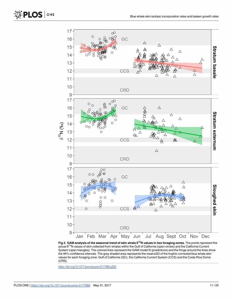
Fig 3. GAM analysis of the seasonal trend of skin strata δ15N values in two foraging zones. The points represent the

actual δ15N values of skin collected from whales within the Gulf of California (open circles) and the California Current

System (open triangles). The colored lines represent the GAM model fit (predictions) and the fringe around the lines show

the 95% confidence intervals. The gray shaded area represents the mean±SD of the trophic-corrected blue whale skin

values for each foraging zone: Gulf of California (GC), the California Current System (CCS) and the Costa Rica Dome

(CRS).

https://doi.org/10.1371/journal.pone.0177880.g003

Blue whale skin isotopic incorporation rates and baleen growth rates

PLOS ONE | https://doi.org/10.1371/journal.pone.0177880 May 31, 2017 11 / 25

Fig 1. The results of the GAM models to assess the fluctuations in δ15N values along baleen

plates, and of baleen growth rates estimations are shown in Tables 4 and 5, respectively. The

GAM fit showed that the amplitude of the oscillations differed among individuals (Tables 4

and 5, Fig 4). Three baleen plates (A–C, one male and two females; S1 Table) exhibited the

expected fluctuations in δ15N ranging from 10.6‰ to 14.9‰ (Fig 4A–4C), and the length of

baleen between these fluctuations ranged between 13 and 19 cm (Table 5). The other three

baleen plates (D–F, all males; S1 Table) maintained relatively constant δ15N values, ranging

between 11.7‰ and 13.1‰ along the plate (Fig 4D–4F). Inter-individual differences in the

amplitude of the oscillations are likely related to the individual migratory strategies and resi-

dency time within each foraging zone [37,38,43,55]. By using the trophic-corrected skin δ15N

values based on that of prey (Table 1), it was possible to associate these oscillations with the

potential foraging zone that each individual whale visited. From these data, it could be inferred

that whale B moved between all three zones, showing relatively regular cycles (Fig 4B), whereas

whale C did not enter the GC, but moved constantly between the CCS and the CRD, in less

Table 2. GAM results for the seasonal trends of δ15N and δ13C values in different skin strata sampled in the Gulf of California (GC) and California

Current System CCS).

Isotope Skin stratum Zone n E.df. F Adjusted R2 P Deviance explained (%)

δ15N Basale GC 101 1.9 13.4 0.2 < 0.001 21.1

Basale CCS 120 1.0 8.4 0.6 < 0.01 6.7

Externum GC 85 1.9 7.4 0.1 < 0.01 14.7

Externum CCS 63 1.0 5.5 0.1 < 0.1 8.3

Sloughed skin GC 81 1.8 3.3 0.1 0.7 7.7

Sloughed skin CCS 93 1.8 2.6 0.0 0.7 6.7

δ13C Basale GC 101 1.0 0.2 -0.0 0.7 0.2

Basale CCS 120 1.9 3.6 0.1 < 0.1 6.2

Externum GC 85 1.5 1.3 0.1 0.4 2.8

Externum CCS 63 1.5 0.6 0.0 0.6 2.8

Sloughed skin GC 81 1.0 1.3 0.0 0.3 1.6

Sloughed skin CCS 93 1.0 0.1 -0.0 0.8 0.1

E.df., Estimated degrees of freedom; F, test of whether the smoothed function significantly reduces model deviance; P, p-values in bold were considered

statistically significant (<0.05).

https://doi.org/10.1371/journal.pone.0177880.t002

Table 3. δ15N isotopic incorporation rates of blue whale skin strata in the Gulf of California and California Current System. The number of days

were estimated by extrapolating from the GAM predictions (model fit and the upper and lower 95% confidence limits) for skin δ15N values to change by 1.6‰

to isotopically equilibrate with local prey in each zone.

Zone Skin Stratum δ15N isotopic incorporation rate of blue whale skin

Model fit Lower limit Upper limit

Gulf of California Basale 81 90 69

Externum 81 112 69

Sloughed Skin 90 60 149

Mean±SD 84±5

California Current System Basale 262 222 360

Externum 192 160 240

Sloughed Skin 272 163 816

Mean±SD 242±44

Overall Mean±SD 163±91

https://doi.org/10.1371/journal.pone.0177880.t003

Blue whale skin isotopic incorporation rates and baleen growth rates

PLOS ONE | https://doi.org/10.1371/journal.pone.0177880 May 31, 2017 12 / 25

regular cycles (Fig 4C). Whale A remained mainly within the CCS, potentially only migrating

twice to the CRD (Fig 4A). In the case of whales D, E and F, the data suggests that these indi-

viduals remained within the CCS, throughout several years (Fig 4D–4F). Only whales A, B,

and C were used to estimate the baleen growth rates (Fig 4A–4C). The mean (±SD) growth per

year of baleen plates was estimated for each whale (A = 13.5±2.2; B = 14.8±1.7; C = 17.5±1.5

cm y-1; Table 5), and also integrated in an overall mean (±SD) (15.5±2.2 cm y-1; Table 5).

δ13C values of skin and baleen plates

The mean δ13C value of the prey in the GC was 0.7‰ and 2.9‰ higher than the CCS and the

CRD, respectively (S2 Table). However, the standard deviation of the CRD overlapped with all

the zones and it was not possible to accurately assign the origin of measured δ13C from skin

nor baleen plates.

Table 4. GAM results to assess the fluctuations of δ15N and δ13C in baleen plates.

Isotope Baleen code n E.df. F Adjusted R2 P Deviance explained (%)

δ15N A 41 23.8 61.4 1 < 0.001 99.0

B 68 27.2 108.0 1 < 0.001 98.7

C 67 27.3 95.9 1 < 0.001 98.6

D 55 23.3 25.2 0.9 < 0.001 95.7

E 71 26.5 27.2 0.9 < 0.001 94.8

F 58 23.8 31.3 0.9 < 0.001 96.3

δ13C A 41 21.9 55.8 1 < 0.001 98.8

B 68 20.3 15.6 0.9 < 0.001 89.3

C 67 27.7 64.9 1 < 0.001 98.0

D 55 24.9 68.4 1 < 0.001 98.5

E 71 27.5 65.1 1 < 0.001 97.8

F 58 25.0 25.1 0.9 < 0.001 95.7

E.df., Estimated degrees of freedom; F, test of whether the smoothed function significantly reduces model deviance; P, p-values in bold were considered

statistically significant (<0.05).

https://doi.org/10.1371/journal.pone.0177880.t004

Table 5. Blue whale baleen growth rate: Estimated by using the distance between sequential δ15N

minimums along the baleen plates from whales A to C.

Baleen code Sex Intervals between δ15N minimums (cm) Growth rate (cm y-1)

A Male 10–24 14.0

24–37 13.0

Mean±SD 13.5±0.7

B Female 4–17 13.0

17–31 14.0

31–48 17.0

48–63 15.0

Mean±SD 14.8±1.7

C Female 9–27 18.0

27–46 19.0

46–62 16.0

Mean±SD 17.5±1.5

Overall Mean±SD 15.5±2.2

https://doi.org/10.1371/journal.pone.0177880.t005

Blue whale skin isotopic incorporation rates and baleen growth rates

PLOS ONE | https://doi.org/10.1371/journal.pone.0177880 May 31, 2017 13 / 25

The GAM model revealed a very weak though significant positive relationship between the

δ13C and time for the stratum basale sampled within the CCS. The GAMs applied to the other

skin strata, from the other two foraging zones, did not show any relationship between the δ13C

values and time (Table 2, S1 Fig), and thus the isotopic incorporation rate of δ13C in blue

whale skin could not be estimated.

Fig 4. δ15N values along the baleen plates from six whales, identified as A–F. Points represent actual values. The continuous line (blue: males; red:

females) represents the GAM model fit and the narrow fringe around the lines represent the 95% confidence intervals. The gray shaded area represents

the mean±SD of the trophic-corrected blue whale skin values for each foraging zone: Gulf of California (GC), the California Current System (CCS) and the

Costa Rica Dome (CRS).

https://doi.org/10.1371/journal.pone.0177880.g004

Blue whale skin isotopic incorporation rates and baleen growth rates

PLOS ONE | https://doi.org/10.1371/journal.pone.0177880 May 31, 2017 14 / 25

Mean (±SD) δ13C values of six baleen plates (A–F) are presented in S7 Table. The GAM fits

(Table 4, S3 Fig) showed that all individuals presented small oscillations in the δ13C values

along the baleen that ranged between -18.3 to -16.1. These oscillations could not be linked to

the foraging zones because of the overlap in prey δ13C among zones (S2 Table). Therefore,

baleen growth rates were inferred only using baleen δ15N values.

Discussion

Influence of lipid-extraction and DMSO preservation on skin δ13C and

δ15N values

Our results suggest that lipid-extraction is necessary to remove biases in skin δ13C values asso-

ciated with lipid content (S4 Table), which agrees with previous studies on mysticetes [75,76].

In regard to the effects of lipid-extraction on δ15N values of cetacean skin, some authors

[48,75,76] recommend analyzing bulk tissues because lipid-extraction can influence δ15N val-

ues, although this effect varied between species [75,76] and tissues [75]. In our study, we only

compared the δ15N of five biopsy samples from which we analyzed paired bulk and lipid-

extracted subsamples; however, δ15N values between these treatments did not differ signifi-

cantly, which would be in accordance with the results reported for other marine organisms

[95]. With regard to preservation in DMSO (S4 Table), after lipid-extraction, blue whale skin

δ13C, δ15N and C/N ratios of samples preserved in DMSO were similar to those of samples pre-

served frozen. Our results concur with previous studies that show lipid-extraction via a 2:1

chloroform:methanol solvent solution was a sound method for removing the combined effect

that DMSO and tissue lipid content have on skin δ13C values [76,81].

Skin δ15N isotopic incorporation rates

Only two studies have estimated isotopic incorporation rates of cetacean skin, and both uti-

lized controlled feeding experiments on captive bottlenose dolphins [47,48]. Our approach

was to use gradients in baseline δ15N values between the GC and CCS as a natural diet switch

experiment (Fig 3). Our mean estimate of δ15N isotopic incorporation rates (163±91 d;

Table 3) for blue whale skin is similar to that observed in the longest experiment on captive

bottlenose dolphins (180±71 d) [48]. The similarity in incorporation rate estimates for these

two distantly related cetacean species that differ in weight by over two orders of magnitude is

striking, but suggests that these estimates can be applied to other odontocetes and mysticetes.

We found that isotopic incorporation rates varied among skin strata and foraging zones

(Table 3); however, all of these estimates fell within the range of those observed for bottlenose

dolphins in previous studies (106–275 d and ~60–90 d)[47,48]. It is possible that the observed

variation in skin incorporation rates among zones could be influenced by water temperature

[10,96–100], with higher rates in the warmer waters of GC in comparison to the CCS (Table 3).

In cold waters, marine mammals reduce peripheral blood flow to maintain a constant internal

body temperature, which results in a decrease of epidermal metabolism [101–103]. In contrast,

incursion into warmer waters accelerates the turnover of superficial skin cells and increase the

proliferation rate of cells by intensifying blood flow to the skin stratum basale [104]. Observa-

tions suggest that odontocetes, such as belugas (Delphinapterus leucas) [104] and killer whales

(Orcinus orca) [105], move from colder to warmer waters to molt or promote skin regeneration.

A study on blue whales in the GC and CCS found that at sites with lower water temperatures,

sloughed skin was observed less often in comparison to warmer sites [67].

A novel aproach in this study was to analyze different skin strata: basale, externum, and

sloughed skin (Figs 2A and 3). We hypothesised that the different skin strata could provide

Blue whale skin isotopic incorporation rates and baleen growth rates

PLOS ONE | https://doi.org/10.1371/journal.pone.0177880 May 31, 2017 15 / 25

information about temporal shifts in diet. The stratum basale, where cells are constantly

produced, would most likely reflect the most recent dietary information, while the isotopic

composition of stratum externum and sloughed skin would record information of the diet

consumed in the past, perhaps when individuals were in a different foraging zone than the one

where skin samples were collected. The isotopic comparison of strata in the CCS supports this

hypothesis since the stratum basale had significantly lower δ15N values than the stratum exter-

num and sloughed skin (S5 Table), suggesting that the stratum basale was equilibrating with

local prey, characterized by lower δ15N values than those which occur in the GC (Table 1,

S2 Table). In the GC, skin strata did not have significantly different δ15N values; however,

sloughed skin had δ15N values that were similar to those expected if the skin was grown in the

CCS (Table 1, Fig 3), suggesting that sloughed skin samples have a higher probability of pro-

viding information about past diets. Thus, skin samples collected from migratory mysticetes

can reflect information about past diets independent of where sampling occurs, demonstrating

that skin is a valuable tissue to estimate relative contributions of food consumed in different

foraging zones utilized during the annual life cycle. Since collecting skin from free ranging

cetaceans is cost- and time-intensive, we recommend dividing skin biopsies into strata and col-

lecting sloughed skin when available to increase the amount of information that can be gleaned

from isotope analysis of this tissue.

Baleen growth rates

Our estimate of baleen growth rates for blue whales (~15.5±2.2 cm y-1; Table 5) are consistent

with previous estimates for other balaenopterids, such as the fin whale (Balaenoptera physalus,20±2.6 cm y-1) [37,55], and minke whale (Balenoptera acutorostrata, 12.9 cm y-1) [57], as well

as for other mysticetes such as bowhead whales (16–25 cm y-1 in adults) [42,43]. In contrast,

baleen growth rate estimates were lower than those for southern right whales (Eubalaena aus-tralis, ~27 cm y-1) [44]. Variation in baleen growth rates among blue whales sampled in this

study (Table 4) could be influenced by differences in individual movement strategies (Fig 4A–

4C), a hypothesis proposed in previous studies of other mysticete species [37,38,43,55]. For

example, variation in the period of time spent within a specific foraging zone or in migration

between zones would produce wider or narrower oscillations in baleen δ15N, which would

influence growth rate estimates (Table 5, Fig 4).

Three of the six baleen plates we analyzed did not show marked oscilations in the δ15N val-

ues (Fig 4D–4F). These individuals were males: two adults, and one of unknown age class (S1

Table). A potential explanation for a lack of inter-annual variation in δ15N is that these whales

remained close or within the CCS foraging zone for several years prior to their death. By apply-

ing the mean annual growth rate of ~15.5 cm y-1 to the baleen records of these three males,

they remained within the CCS ecosystems for ~3.5 (Fig 4D), ~4.5 (Fig 4E) and ~3.7 (Fig 4F)

years. In contrast, the other three baleen plates, collected from one male and two females,

exhibited oscillations in the δ15N values along their outer edge that indicate cyclical migrations

between foraging zones during ~2.5 (Fig 4A), ~4.3 (Fig 4B) and ~4.2 (Fig 4C) years.

The observed differences in movement strategies of blue whale individuals may be influ-

enced by a combination of the following factors. One general explanation is related to changes

in the availability of prey in different foraging zones because it is known that blue whale distri-

bution is influenced by variations in the abundance of their primary prey [2,3]. A more specific

explanation is that females are more likely to migrate to warmer waters in winter/spring to

nurse their calves, a hypothesis that has been proposed for other mysticetes, although other

mysticetes generally do not feed while on their winter/spring breeding grounds [106]. More-

over, the patterns in the baleen of whale C (Fig 4C) suggest a high fidelity of females to

Blue whale skin isotopic incorporation rates and baleen growth rates

PLOS ONE | https://doi.org/10.1371/journal.pone.0177880 May 31, 2017 16 / 25

returning to specific winter/spring foraging grounds year after year. This would be in accor-

dance with the high site fidelity observed in GC of some well-identified females obtained via

photo-identification and genetic analysis [9,11,107]. In the case of males, our data indicate

three males remained in the CCS and one migrated twice to the CRD (Fig 4). The female:male

sex ratio (1.4:1) in the GC is biased towards females [9,107], suggesting that only a portion of

the males in the northeast Pacific are using this zone in winter/spring. Photo-identification

data has also shown that some males have a high site fidelity to the GC [9] or possibly other

winter/spring foraging grounds. Baleen isotope data from one male in our study also indicates

that it had a high fidelity to the CRD, since it migrated only to this zone (Fig 4A). Blue whales

are not frequently sighted in the CCS during winter and spring [108,109], although this could

be attributed to low search effort during this season. However, vocalizations specific to male

blue whales have been recorded year round in the CCS [110–113]. The baleen data of males D,

E, F (Fig 4D–4F) is in agreement with this observation. Therefore, we hypothesize that there

are two migratory strategies for blue whale males in the northeast Pacific. Some individuals

migrate to winter/breeding grounds in the GC or CRD, while others remain within the CCS.

How these two migratory strategies influence mating success for males is not known.

δ15N trophic discrimination factors

δ15N trophic discrimination factors have not been estimated for blue whale tissues, therefore

our approach was to assume a 1.6‰ (Table 1) discrimination factor between whales and their

prey based on the controlled feeding experiments on bottlenose dolphins [47,48]. Borrell et al.[114] suggested using a trophic discrimination factor of 2.8‰ for balaenopterid skin and

baleen plates. However, the mean (±SD) baleen δ15N value of the three male blue whales (D:

12.2±0.3; E: 12.4±0.3; F: 12.3±0.4; S7 Table, Fig 4D–4F) that presumably remained within the

CCS for ~2–3 years prior to death, and by extension were isotopically equilibrated with local

food sources, were enriched by only 1.7–1.9‰ relative to local prey sources (10.5±0.2; S2

Table), and is similar to estimates for skin of captive bottlenose dolphins (1.6±0.5‰) [47,48].

Temporal consistency of baseline δ15N values among foraging zones

The observed seasonal trend in skin δ15N values within each zone and the oscillations along

baleen plates support our hypothesis that these tissues record baseline shifts in nitrogen iso-

tope values across the northeast Pacific. Our approach assumes that such baseline gradients

are temporarily consistent at a decadal scale. To test this assumption, it would be ideal to have

prey δ15N data from each foraging zone for each year blue whales were sampled; however,

such sampling resolution is logistically impossible. Our approach was to use a GLM to evaluate

inter-annual trends in skin δ15N values, which showed that they slightly increased in the GC

and CCS (see Results); no evident trend was observed in the CRD (S6 Table, S4 Fig).

Published datasets show that isotope values of blue whale prey and zooplankton collected

from the CCS were consistent over decadal timescales (1994, 2000–2001, 2013) and between

sites (Monterey Bay and British Columbia) [60,61,63,64,115]. Moreover, the δ15N values in

blue whale baleen plates that were assigned to the CCS show a remarkably consistent pattern

regardless of when the baleen was collected (1980s vs. 2000s; S1 Table, Fig 4). These patterns

suggest that a relatively stable δ15N baseline existed in the CCS for nearly three decades. Fur-

thermore, these data suggest that the slight inter-annual increase in skin δ15N values of blue

whales in the CCS is likely the result of uneven seasonal sampling rather than a shift in the

baseline.

δ15N values of the dominant krill species (Nyctiphanes simplex) in the GC are variable, likely

due to their omnivorous feeding behavior [116], but are consistently higher than krill in the

Blue whale skin isotopic incorporation rates and baleen growth rates

PLOS ONE | https://doi.org/10.1371/journal.pone.0177880 May 31, 2017 17 / 25

CCS and the CRD (S2 Table) [58–62,64,117,118]. Isotope data for potential blue whale prey

from the CRD were only available from one study (S2 Table) [62], but zooplankton data also

suggest that this zone has lower δ15N values in comparison to the CCS and GC [65]. Addition-

ally, baleen δ15N patterns from whales that likely visited the CRD (Fig 4A–4C) indicate that

baseline δ15N values may be consistently lower than those of the other zones. Another factor

that may contribute to the observed differences in δ15N values among foraging zones is that

blue whales in the GC forage on combined aggregations of krill and higher trophic level lan-

ternfish [20]. Thus, blue whale tissues synthetized in the GC will have higher δ15N values that

result from a combination of baseline and diet factors relative to tissues grown in other forag-

ing zones in the northeast Pacific (Table 1, S3 Table, Figs 3 and 4).

δ13C values in blue whale skin and baleen plates

δ13C incorporation rates for skin could not be estimated because of the similarity in δ13C val-

ues among prey from different foraging zones (S2 Table), and by extension δ13C values were

not useful to estimate baleen growth rates. Another variable that could contribute to the lack

of spatial signal in δ13C is movement of blue whales between coastal 13C-enriched and 13C-

depleted oceanic ecosystems [24] within a specific foraging zone [2]. Thus, any latitudinal

variation in blue whale skin and baleen δ13C values between the CCS, GC, and CRD may be

obscured by longitudinal movement between coastal and offshore areas within foraging zones.

Conclusions

Blue whale skin isotopic incorporation rates and baleen growth rates are similar to other odonto-

cetes and mysticetes, respectively. We recommend collecting skin samples throughout the sea-

sonal residency of migratory mysticetes within specific foraging zones, and dividing skin biopsies

into strata. This approach allows for an assessment of seasonal variation in isotope values that

could provide insights into movement and/or shifts in seasonal foraging strategies. Furthermore,

analyzing both skin and baleen can provide information on the inter-annual variation in prey iso-

tope values within and among foraging zones, as well as provide information about the migratory

strategies of individual whales over several years of life, that currently cannot be obtained from

satellite telemetry tags that (at best) collect a single year of movement information [2].

Supporting information

S1 Fig. GAM analysis relating skin δ13C values to Julian day (presented in months). The points

represent the actual δ13C values of skin collected from whales within the Gulf of California (open

circles) and the California Current System (open triangles). Lines represent the fit (projections) of

the GAM model and the fringe around the lines show the 95% confidence intervals.

(TIF)

S2 Fig. Sections used from the GAM model predictions to infer δ15N isotopic incorpo-

ration rates of blue whale skin strata in each foraging zone. The lines represent the GAM

model fit (predictions) in the Gulf of California (green) and the California Current System

(blue). The fringe around the lines show the 95% confidence intervals. The black dot repre-

sents the initial point (i.e. diet switch) and the red dot the final point of the sections from the

predictions that were used from the fit and the lower and upper confidence intervals. Per mil

(‰) differences and days passed between points were estimated and then used to extrapolated

to a 1.6‰ increase in the Gulf of California, or decrease in California Current System, for skin

to reach steady-state isotopic equilibrium with the local prey isotopic signal.

(TIF)

Blue whale skin isotopic incorporation rates and baleen growth rates

PLOS ONE | https://doi.org/10.1371/journal.pone.0177880 May 31, 2017 18 / 25

S3 Fig. δ13C values along the baleen plates from six whales, identified as A-F. Points repre-

sent actual values, the continuous line (blue: males; red: females) represents the GAM model

fit and the fringe around the lines show the narrow 95% confidence intervals.

(TIF)

S4 Fig. GLM analysis relating skin δ15N values to time (Julian date, presented in years).

Points represent the actual δ15N values of blue whale skin collected in different zones of the

northeast Pacific. Lines represent the fit of the GLM model and the fringe around the lines

show the 95% confidence intervals. The gray shaded area represents the meand±SD of the tro-

phic-corrected blue whale skin values for each foraging zone; Gulf of California (GC), Califor-

nia Current System (CCS), and Costa Rica Dome (CRD).

(TIF)

S1 Table. Information of baleen plates collected from six blue whales.

(DOCX)

S2 Table. Mean (±SD) δ13C, δ15N, and weight percent C/N ratios of potential blue whale

prey from each of the three foraging zones in the northeast Pacific.

(DOCX)

S3 Table. Results from the GAM model sections used to infer δ15N isotopic incorporation

rates of blue whale skin strata in Gulf of California (GC) and California Current System

(CCS).

(DOCX)

S4 Table. Max-t test results comparing the effect of different treatments on skin δ15N, δ13C

and weight percent C/N ratios.

(DOCX)

S5 Table. Max-t test results for the comparison of δ13C and δ15N values among different

skin strata in the Gulf of California (GC) and California Current System (CCS).

(DOCX)

S6 Table. GLM results relating blue whale skin δ15N values to time (Julian date) in the Gulf

of California (GC), California Current System (CCS) and Costa Rica Dome (CRD).

(DOCX)

S7 Table. Mean (±SD) δ13C, δ15N and weight percent C/N ratios of blue whale baleen plates

collected from stranded whales.

(DOCX)

S1 Dataset. δ13C, δ15N and weight percent C/N ratios of blue whale skin and baleen plates

used in this study.

(XLSX)

Acknowledgments

We would like to thank the institutions that facilitated the use of tissues samples and issued the

permits to collect and process these samples: NOAA-SWFSC, CRC, CICIMAR-IPN, HSU-

Vertebrate Museum, Museo de la Ballena y Ciencias del Mar (La Paz, BCS), the California

Department of Parks and Recreation-Prairie Creek Redwoods State Park, NOAA/NMFS and

SEMARNAT. We are also very grateful to all the personnel from the former institutions, the

Stranding Network of California, and the Center for Stable Isotopes of the University of New

Mexico who participated in the collection and processing of the tissue samples. We would also

Blue whale skin isotopic incorporation rates and baleen growth rates

PLOS ONE | https://doi.org/10.1371/journal.pone.0177880 May 31, 2017 19 / 25

like to thank the John H. Prescott Marine Mammal Rescue Assistance Grant Program that has

provided grants to the stranding networks. J. Rice, J. Loomis, T. Holmes, and F.J. Gomez-Dıaz

collaborated during the process of locating potential baleen plates for this study and we are

very beholden for their support. We would also like to give special recognition to K. Robertson

who helped with the logistics of sample selection and the sex identification of an important

baleen sample at the genetics lab in SWFSC. M.A. Pardo, H. Villalobos-Ortiz, C. Arnold, and

two anonymous reviewers made some valuable comments to improve the manuscript.

Author Contributions

Conceptualization: GBV SDN DG.

Formal analysis: GBV.

Funding acquisition: GBV SDN DG SAG.

Investigation: GBV SDN GSV JKJ.

Methodology: GBV DG.

Project administration: GBV.

Resources: GBV SDN JC GSV JKJ SAG DG.

Visualization: GBV SDN.

Writing – original draft: GBV SDN DG.

Writing – review & editing: GBV SDN JC GSV JKJ SAG DG.

References1. Reilly SB, Bannister JL, Best PB, Brown M, Brownell RL Jr., Butterworth DS, et al. Balaenoptera mus-

culus. IUCN Red List Threat Species. 2008; e.T2477A9447146.

2. Bailey H, Mate BR, Palacios DM, Irvine L, Bograd SJ, Costa DP. Behavioural estimation of blue whale

movements in the Northeast Pacific from state-space model analysis of satellite tracks. Endanger

Species Res. 2009; 10: 93–106.

3. Calambokidis J, Barlow J, Ford JKB, Chandler TE, Douglas AB. Insights into the population structure

of blue whales in the Eastern North Pacific from recent sightings and photographic identification. Mar

Mammal Sci. 2009; 25: 816–832.

4. Calambokidis J, Barlow J. Abundance of blue and humpback whales in the eastern North Pacific esti-

mated by capture-recapture and line-transect methods. Mar Mammal Sci. 2004; 20: 63–85.

5. Etnoyer P, Canny D, Mate BR, Morgan LE, Ortega-Ortiz JG, Nichols WJ. Sea-surface temperature

gradients across blue whale and sea turtle foraging trajectories off the Baja California Peninsula,

Mexico. Deep Sea Res Part II Top Stud Oceanogr. 2006; 53: 340–358.

6. Etnoyer P, Canny D, Mate BR, Morgan L. Persistent pelagic habitats in the Baja California to Bering

Sea (B2B) Ecoregion. Oceanography. 2004; 17: 90–101.

7. Mate BR, Lagerquist BA, Calambokidis J. Movements of North Pacific blue whales during the feeding

season off southern California and their southern fall migration. Mar Mammal Sci. 1999; 15: 1246–

1257.

8. Reilly SB, Thayer VG. Blue whale (Balaenoptera musculus) distribution in the eastern tropical Pacific.

Mar Mammal Sci. 1990; 6: 265–277.

9. Gendron D. Ecologıa poblacional de la ballena azul, Balaenoptera musculus, de la Peninsula de Baja

California. Ph.D. Thesis, Centro de Investigacion Cientıfica y de Educacion Superior de Ensenada.

2002.

10. Pardo MA, Silverberg N, Gendron D, Beier E, Palacios DM. Role of environmental seasonality in the

turnover of a cetacean community in the southwestern Gulf of California. Mar Ecol Prog Ser. 2013;

487: 245–260.

Blue whale skin isotopic incorporation rates and baleen growth rates

PLOS ONE | https://doi.org/10.1371/journal.pone.0177880 May 31, 2017 20 / 25

11. Sears R, Ramp C, Douglas AB, Calambodikis J. Reproductive parameters of eastern North Pacific

blue whales Balaenoptera musculus. Endanger Species Res. 2013; 22: 23–31.

12. Tershy BR, Breese D, Strong CS. Abundace, seasonal distribution and popultion composition of bale-

nopterid whales in the Canal de Ballenas, Gulf of California, Mexico. Reports Int Whal Comm. 1990;

369–375.

13. Hoyt E. The blue whale, Balaenoptera Musculus: An endangered species thriving on the Costa Rica

Dome. Rep WDC. 2009; 1–11. Available: www.cbd.int/cms/ui/forums/attachment.aspx?id=73

14. Del Angel-Rodrıguez JA. Habitos alimentarios y distribucion espacio-temporal de los rorcuales comun

(Balaenoptera physalus) y azul (Balaenoptera musculus) en la Bahıa de La Paz, B.C.S., Mexico. M.

Sc. Thesis, Centro Interdisciplinario de Ciencias Marinas-Instituto Politecnico Nacional. 1997. Avail-

able: http://tesis.ipn.mx/handle/123456789/3026

15. Croll DA, Marinovic B, Benson S, Chavez FP, Black N, Ternullo R, et al. From wind to whales: trophic

links in a coastal upwelling system. Mar Ecol Prog Ser. 2005; 289: 117–130.

16. Nemoto T, Kawamura A. Characteristics of food habits and distribution of baleen whales with special

reference to the abundance of North Pacific sei and bryde’s whales. Rep Int Whal Com Spec Issue.

1977; 80–87.

17. Matteson RS. The Costa Rica Dome: A study of physics, zooplankton and blue whales. M.Sc. Thesis,

Oregon State University. 2009. Available: http://scholar.google.com/scholar?hl=en&btnG=Search&q=

intitle:No+Title#0

18. Fiedler PC, Reilly SB, Hewitt RP, Demer D, Philbrick VA, Smith S, et al. Blue whale habitat and prey in

the California Channel Islands. Deep Sea Res Part II Top Stud Oceanogr. 1998; 45: 1781–1801.

19. Calambokidis J, Steiger G. Blue whales. Stillwater, Minnesota: Worldlife Series Library, Voyager

Press; 1997.

20. Jimenez-Pinedo NC. Habitos alimentarios y relacion interespecıfica entre la ballena azul (Balaenop-

tera musculus) y la ballena de aleta (B. physalus) en el suroeste del Golfo de California. M.Sc. Thesis,

Centro Interdisciplinario de Ciencias Marinas-Instituto Politecnico Nacional. 2010. Available: http://

www.repositoriodigital.ipn.mx/bitstream/handle/123456789/13508/jimenezp1.pdf?sequence=1

21. Oliver JS, Slattery PN, Silberstein MA, O’Connor EF. A comparison of gray whale, Eschrichtius robus-

tus, feeding in the Bering Sea and Baja California. Fish Bull. 1983; 81: 513–522.

22. Baraff LS, Clapham PJ, Mattila DK. Feeding behavior of a humpback whale in low-latitude waters. Mar

Mammal Sci. 1991; 7: 197–202.

23. Hazen EL, Palacios DM, Forney KA, Howell EA, Becker E, Hoover AL, et al. WhaleWatch: a dynamic

management tool for predicting blue whale density in the California Current. J Appl Ecol. 2016;

24. Newsome SD, Clementz MT, Koch PL. Using stable isotope biogeochemistry to study marine mammal

ecology. Mar Mammal Sci. 2010; 26: 509–572.

25. DeNiro MJ, Epstein S. Influence of diet on the distribution of nitrogen isotopes in animals. Geochim

Cosmochim Acta. 1981; 45: 341–351.

26. DeNiro MJ, Epstein S. Influence of diet on the distribution of carbon isotopes in animals. Geochim Cos-

mochim Acta. 1978; 42: 495–506.

27. Gannes LZ, Martınez del Rio C, Koch P. Natural abundance variations in stable isotopes and their use

in animal physiological ecology. Comp Biochem Physiol. 1998; 119: 725–737.

28. Altabet MA., Pilskaln C, Thunell R, Pride C, Sigman D, Chavez F, et al. The nitrogen isotope biogeo-

chemistry of sinking particles from the margin of the Eastern North Pacific. Deep Sea Res Part I Ocea-

nogr Res Pap. 1999; 46: 655–679.

29. Graham BS, Koch PL, Newsome SD, Mcmahon KW, Aurioles D. Using isoscapes to trace the move-

ments and foraging behavior of top predators in oceanic ecosystems. 2010; 299–318.

30. McMahon KW, Hamady LL, Thorrold SR. A review of ecogeochemistry approaches to estimating

movements of marine animals. Limnol Oceanogr. 2013; 58: 697–714.

31. Williams RL, Wakeham S, McKinney R, Wishner KF. Trophic ecology and vertical patterns of carbon

and nitrogen stable isotopes in zooplankton from oxygen minimum zone regions. Deep Res Part I

Oceanogr Res Pap. Elsevier; 2014; 90: 36–47.

32. Mcmahon KW, Thorrold SR, Elsdon TS, Mccarthy MD. Trophic discrimination of nitrogen stable iso-

topes in amino acids varies with diet quality in a marine fish. Limnol Oceanogr. 2015; 60: 1076–1087.

33. Vander Zanden MJ, Rasmussen JB. Variation in δ15N and δ13C trophic fractionation: Implications for

aquatic food web studies. Limnol Oceanogr. 2001; 46: 2061–2066.

34. McCutchan JH, Lewis WM, Kendall C, McGrath CC. Variation in trophic shift for stable isotope ratios

of carbon, nitrogen, and sulfur. Oikos. 2003; 102: 378–390.

Blue whale skin isotopic incorporation rates and baleen growth rates

PLOS ONE | https://doi.org/10.1371/journal.pone.0177880 May 31, 2017 21 / 25

35. Thomas SM, Crowther TW. Predicting rates of isotopic turnover across the animal kingdom: A synthe-

sis of existing data. J Anim Ecol. 2015; 84: 861–870. https://doi.org/10.1111/1365-2656.12326 PMID:

25482029

36. Martınez Del Rio C, Wolf N, Carleton SA, Gannes LZ. Isotopic ecology ten years after a call for more

laboratory experiments. Biological Reviews. 2009. pp. 91–111. https://doi.org/10.1111/j.1469-185X.

2008.00064.x PMID: 19046398

37. Aguilar A, Gimenez J, Gomez-Campos E, Cardona L, Borrell A. δ15N value does not reflect fasting in

mysticetes. PLoS One. 2014; 9: e92288. https://doi.org/10.1371/journal.pone.0092288 PMID:

24651388

38. Matthews CJD, Ferguson SH. Seasonal foraging behaviour of eastern Canada-West Greenland bow-

head whales: An assessment of isotopic cycles along baleen. Mar Ecol Prog Ser. 2015; 522: 269–286.

39. Matthews CJD, Ferguson SH. Spatial segregation and similar trophic-level diet among eastern Cana-

dian Arctic/north-west Atlantic killer whales inferred from bulk and compound specific isotopic analysis.

J Mar Biol Assoc United Kingdom. 2013; 94: 1343–1355.

40. Gendron D, Aguıñiga S, Carriquiry JD. δ15N and δ13C in skin biopsy samples: a note on their applica-

bility for examining the relative trophic level in three rorqual species. J Cetacean Res Manag. 2001; 3:

41–44.

41. Witteveen BH, Worthy GAJ, Foy RJ, Wynne KM. Modeling the diet of humpback whales: An approach

using stable carbon and nitrogen isotopes in a Bayesian mixing model. Mar Mammal Sci. 2012; 28: 1–18.

42. Schell DM, Saupe SM, Haubenstock N. Natural isotope abundances in bowhead whale (Balaena mys-

ticetus) baleen: markers of aging and habitat usage. In: Rundel PW, Ehleringer JR, Nagy KA, editors.

Stable isotopes in ecological research. Springer-Verlag, New York; 1989. pp. 260–269.

43. Schell DM, Saupe SM, Haubenstock N. Bowhead whale (Balaena mysticetus) growth and feeding as

estimated by δ13C techniques. Mar Biol. 1989; 103: 433–443.

44. Best PB, Schell DM. Stable isotopes in southern right whale (Eubalaena australis) baleen as indicators

of seasonal movements, feeding and growth. Mar Biol. 1996; 124: 483–494.

45. Geraci J, St. Aubin DJ, Hicks B. The epidermis of odontocetes: a view from within. In: Bryden MM, Har-

rison R, editors. Research on Dolphins, Part I. Oxford: Clarendon Press; 1986. pp. 3–21.

46. Harrison R, Thurley KW. Structure of the epidermis in Tursiops, Delphinus, Orcinus and Phocoena. In:

Harrison RJ, editor. Functional Anatomy of Marine Mammals, Vol. 2. London: Academic Press;

1974. pp. 45–71.

47. Browning NE, Dold C, I-Fan J, Worthy GAJ. Isotope turnover rates and diet-tissue discrimination in

skin of ex situ bottlenose dolphins (Tursiops truncatus). Clin Cancer Res. 2014; 217: 214–221.

48. Gimenez J, Ramırez F, Almunia J, Forero MG, de Stephanis R. From the pool to the sea: Applicable

isotope turnover rates and diet to skin discrimination factors for bottlenose dolphins (Tursiops trunca-

tus). J Exp Mar Bio Ecol. 2016; 475: 54–61.

49. Podlesak DW, McWilliams SR, Hatch KA. Stable isotopes in breath, blood, feces and feathers can

indicate intra-individual changes in the diet of migratory songbirds. Oecologia. 2005; 142: 501–510.

https://doi.org/10.1007/s00442-004-1737-6 PMID: 15586297

50. Tieszen LL, Boutton TW, Tesdahl KG, Slade NA. Fractionation and turnover of stable carbon isotopes

in animal tissues: Implications for δ13C analysis of diet. Oecologia. 1983; 57: 32–37. https://doi.org/10.

1007/BF00379558 PMID: 28310153

51. Evans Ogden LJ, Hobson KA, Lank DB. Blood isotopic (δ13C and δ15N) turnover and diet-tissue frac-

tionation factors in captive dunlin (Calidris alpina pacifica). Auk. 2004; 121: 170–177.

52. Voigt CC. Low turnover rates of carbon isotopes in tissues of two nectar-feeding bat species. J Exp

Biol. 2003; 206: 1419–1427. PMID: 12624176

53. Berta A, Sumich J, Kovacs K. Marine mammals: Evolutionary biology. 2nd ed. San Diego, California:

Academic Press; 2006.

54. Fudge DS, Szewciw LJ, Schwalb AN. Morphology and development of blue whale baleen: An anno-

tated translation of Tycho Tullberg’s classic 1883 paper. Aquat Mamm. 2009; 35: 226–252.

55. Bentaleb I, Martin C, Vrac M, Mate B, Mayzaud P, Siret D, et al. Foraging ecology of mediterranean fin

whales in a changing environment elucidated by satellitetracking and baleen plate stable isotopes.

Mar Ecol Prog Ser. 2011; 438: 285–302.

56. Lee SH, Schell DM, McDonald TL, Richardson WJ. Regional and seasonal feeding by bowhead

whales Balaena mysticetus as indicated by stable isotope ratios. Mar Ecol Prog Ser. 2005; 285: 271–

287.

Blue whale skin isotopic incorporation rates and baleen growth rates

PLOS ONE | https://doi.org/10.1371/journal.pone.0177880 May 31, 2017 22 / 25

57. Mitani Y, Bando T, Takai N, Sakamoto W. Patterns of stable carbon and nitrogen isotopes in the

baleen of common minke whale Balaenoptera acutorostrata from the western North Pacific. Fish Sci.

2006; 72: 69–76.

58. Aurioles-Gamboa D, Rodrıguez-Perez M, Sanchez-Velasco L, Lavın M. Habitat, trophic level, and res-

idence of marine mammals in the Gulf of California assessed by stable isotope analysis. Mar Ecol

Prog Ser. 2013; 488: 275–290.

59. Becker BH, Peery MZ, Beissinger SR. Ocean climate and prey availability the trophic level and repro-

ductive success of the marbled murrelet, an endangered seabird. Mar Ecol Prog Ser. 2007; 329: 267–

279.

60. Hipfner JM, Dale J, McGraw KJ. Yolk carotenoids and stable isotopes reveal links among environ-

ment, foraging behavior and seabird breeding success. Oecologia. 2010; 163: 351–360. https://doi.

org/10.1007/s00442-010-1618-0 PMID: 20397031

61. Carle RD. Seasonal and sex-specific diet in rhinoceros auklets. M.Sc. Thesis, The Faculty of Moss

Landing Marine Laboratories. 2014. Available: http://scholarworks.sjsu.edu/etd_theses/4454/

62. Williams R. Trophic ecology of Oxygen Minimum Zone zooplankton revealed by carbon and nitrogen

stable isotopes. Ph.D. Thesis, University of Rhode Island. 2013. Available: http://digitalcommons.uri.

edu/cgi/viewcontent.cgi?article=1148&context=oa_diss

63. Sydeman WJ, Hobson KA, Pyle P, McLaren EB. Trophic relationships among seabirds in central Cali-

fornia: Combined stable isotope and conventional dietary approach. Condor. 1997; 99: 327–336.

64. Miller TW. Trophic dynamics of marine nekton and zooplankton in the northern California Current

pelagic ecosystem. Ph.D. Thesis, Oregon State University. 2006. Available: http://ir.library.

oregonstate.edu/xmlui/bitstream/handle/1957/2589/TMiller_Dissertation_FINAL.pdf?sequence=1

65. Popp BN, Graham BS, Olson RJ, Hannides CCS, Lott MJ, Lopez-Ibarra G a, et al. Insight into the tro-

phic ecology of yellowfin tuna, Thunnus albacares, from compound-specific nitrogen isotope analysis

of protenaceous amino acids. In: Dawson T, Siegwolf R, editors. Stable isotopes as indicators of eco-

logical changes. Amsterdam, Netherlands: Elsevier Academic Press; 2007; pp 173–190.

66. Barrett-Lennard LG, Smith TG, Ellis GM. A cetacean biopsy system using lightweight pneumatic

darts, and its effect on the behavior of killer whales. Mar Mammal Sci. 1996; 12: 14–27.

67. Gendron D, Mesnick SL. Sloughed skin: A method for the systematic collection of tissue samples from

Baja California blue whales. J Cetacean Res Manag. 2001; 3: 77–79.

68. Brinton E, Ohman MD, Townsend AW, Knight MD, Bridgeman AL. Euphausiids of the World Ocean

(cd-room Expert System). Springer-Verlag, Heildeberg; 2000.

69. Wisner RL. The taxonomy and distribution of lanternfishes (family Myctophidae) of the eastern Pacific

Ocean. Bay St. Louis, Miss.: Navy Ocean Research and Development Activity; 1974.

70. Sheehan D, Hrapchak BB. Theory and Practice of Histotechnology. 2nd Edition. St. Louis, MO: C.V.

Mosby Co.; 1980.

71. Morin PA, LeDuc RG, Robertson KM, Hedrick NM, Perrin WF, Etnier M, et al. Genetic analysis of killer

whale (Orcinus orca) historical bone and tooth samples to identify western U.S. ecotypes. Mar Mam-

mal Sci. 2006; 22: 897–909.

72. Morin PA, Nestler A, Rubio-Cisneros NT, Robertson KM, Mesnick SL. Interfamilial characterization of

a region of the ZFX and ZFY genes facilitates sex determination in cetaceans and other mammals.

Mol Ecol. 2005; 14: 3275–3286. https://doi.org/10.1111/j.1365-294X.2005.02651.x PMID: 16101791

73. DeNiro M, Epstein S. Mechanism of carbon isotope fractionation associated with lipid synthesis. Sci-

ence. 1977; 197: 261–263. PMID: 327543

74. McConnaughey T, McRoy CP. Food-web structure and the fractionation of carbon isotopes in the

Bering sea. Mar Biol. 1979; 53: 257–262.

75. Ryan C, McHugh B, Trueman CN, Harrod C, Berrow SD, O’Connor I. Accounting for the effects of lip-

ids in stable isotope (δ13C and δ15N values) analysis of skin and blubber of balaenopterid whales.

Rapid Commun Mass Spectrom. 2012; 26: 2745–2754. https://doi.org/10.1002/rcm.6394 PMID:

23124665

76. Lesage V, Morin Y, Rioux E, Pomerleau C, Ferguson S, Pelletier E. Stable isotopes and trace ele-

ments as indicators of diet and habitat use in cetaceans: predicting errors related to preservation, lipid

extraction, and lipid normalization. Mar Ecol Prog Ser. 2010; 419: 249–265.

77. Kaehler S, Pakhomov EA. Effects of storage and preservation on the δ13C and δ15N signatures of

selected marine organisms. Mar Ecol Prog Ser. 2001; 219: 299–304.

78. Sarakinos HCH, Johnson ML, Vander Zanden M. A synthesis of tissue-preservation effects on carbon

and nitrogen stable isotope signatures. Can J Zool. 2002; 80: 381–387.

Blue whale skin isotopic incorporation rates and baleen growth rates

PLOS ONE | https://doi.org/10.1371/journal.pone.0177880 May 31, 2017 23 / 25

79. Barrow LM, Bjorndal KA, Reich KJ. Effects of preservation method on stable carbon and nitrogen iso-

tope values. Physiol Biochem Zool. 2008; 81: 688–693. https://doi.org/10.1086/588172 PMID:

18752417

80. Todd S, Ostrom P, Lien J, Abrajano J. Use of biopsy samples of humpback whale (Megaptera

novaeangliae) skin for stable isotope (δ13C) determination. J Northwest Atl Fish Sci. 1997; 22: 71–76.

81. Burrows DG, Reichert WL, Bradley Hanson M. Effects of decomposition and storage conditions on the

δ13C and δ15N isotope values of killer whale (Orcinus orca) skin and blubber tissues. Mar Mammal

Sci. 2014; 30: 747–762.

82. Caraveo-Patiño J, Soto LA. Stable carbon isotope ratios for the gray whale (Eschrichtius robustus) in

the breeding grounds of Baja California Sur, Mexico. Hydrobiologia. 2005; 539: 99–107.

83. Fry B. Stable Isotope Ecology. New York, NY: Springer New York; 2006.

84. Logan JM, Jardine TD, Miller TJ, Bunn SE, Cunjak RA, Lutcavage ME. Lipid corrections in carbon and

nitrogen stable isotope analyses: comparison of chemical extraction and modelling methods. J Anim

Ecol. 2008; 77: 838–46. https://doi.org/10.1111/j.1365-2656.2008.01394.x PMID: 18489570

85. R Development Core T. R: A language and environment for statistical computing. Vienna, Austria: R

Foundation for Statistical Computing; 2011. Available: http://www.r?project.org/

86. Herberich E, Sikorski J, Hothorn T. A robust procedure for comparing multiple means under heterosce-

dasticity in unbalanced designs. PLoS One. 2010; 5: 1–8.

87. Miller TW, Brodeur RD, Rau GH. Carbon stable isotopes reveal relative contribution of shelf-slope pro-

duction to the Northern California Current pelagic community. Limnol Oceanogr. 2008; 53: 1493–

1503.

88. Yee TW, Mitchell ND. Generalized additive models in plant ecology. Pond DW, editor. J Veg Sci.

1991; 2: 587–602.

89. Wood SN. Generalized additive models: an introduction with R. Wiley Interdisciplinary Reviews. 2006.

90. Xiang D. Fitting generalized additive models with the GAM procedure. SAS Institute, Cary, NC. 2001;

256–26. Available: http://www2.sas.com/proceedings/sugi26/p256-26.pdf

91. Fleming AH, Clark CT, Calambokidis J, Barlow J. Humpback whale diets respond to variance in ocean

climate and ecosystem conditions in the California Current. Glob Chang Biol. 2016; 22: 1214–1224.

https://doi.org/10.1111/gcb.13171 PMID: 26599719

92. Mangiafico SS. Summary and analysis of extension education program evaluation in R. Rutgers

Cooperative Extension, New Brunswick, NJ; 2016. Available: http://rcompanion.org/documents/

RHandbookProgramEvaluation.pdf

93. Peng RD, Dominici F, Louis TA. Model choice in time series studies of air pollution and mortality. J R

Stat Soc Ser A. 2006; 169: 179–203.

94. Chuang Y, Mazumdar S, Park T, Tang G, Arena VC, Nicolich MJ. Generalized linear mixed models in

time series studies of air pollution. Atmos Pollut Res. Elsevier; 2011; 3: 148.

95. Ingram T, Matthews B, Harrod C, Stephens T, Grey J, Markel R, et al. Lipid extraction has little effect

on the δ15N of aquatic consumers. Limnol Oceanogr Methods. 2007; 5: 338–342.

96. Chelton DB, Schlax MG, Samelson RM. Summertime coupling between sea surface temperature and

wind stress in the California Current System. J Phys Oceanogr. 2007; 37: 495–517.

97. Escalante F, Valdez-Holguın JE, Alvarez-Borrego S, Lara-Lara JR. Temporal and spatial variation of

sea surface temperature, chlorophyll a, and primary productivity in the Gulf of California. Cienc Mar.

2013; 39: 203–215.

98. Lluch-Cota SE, Aragon-Noriega EA, Arreguın-Sanchez F, Aurioles-Gamboa D, Jesus Bautista-

Romero J, Brusca RC, et al. The Gulf of California: Review of ecosystem status and sustainability chal-

lenges. Prog Oceanogr. 2007; 73: 1–26.

99. McClatchie S, Goericke R, Schwing FB, Bograd SJ, Peterson WT, Emmett R, et al. The state of the

California Current, spring 2008–2009: Cold conditions drive regional differences in coastal production.

Calif Coop Ocean Fish Investig Reports. 2009; 50: 43–68.

100. Schneider N, Di Lorenzo E, Niiler PP. Salinity variations in the Southern California Current. J Phys

Oceanogr. 2005; 35: 1421–1436.

101. Irving L, Hart JS. The metabolism and insulation of seals as bare-skinned mammals in cold water. Can

J Zool. 1957; 35: 497–511.

102. Silva RG. Assessment of body surface temperature in cetaceans: an iterative approach. Braz J Biol.

2004; 64: 719–24. Available: http://www.ncbi.nlm.nih.gov/pubmed/15620012 PMID: 15620012

103. Boily P. Theoretical heat flux in water and habitat selection of phocid seals and beluga whales during

the annual molt. J Theor Biol. 1995; 172: 235–244.

Blue whale skin isotopic incorporation rates and baleen growth rates

PLOS ONE | https://doi.org/10.1371/journal.pone.0177880 May 31, 2017 24 / 25

104. St Aubin DJ, Smith TG, Geraci JR. Seasonal epidermal molt in beluga whales, Delphinapterus leucas.

Can J Zool. 1990; 68: 359–364.

105. Durban JW, Pitman RL. Antarctic killer whales make rapid, round-trip movements to subtropical

waters: evidence for physiological maintenance migrations? Biol Lett. 2012; 8: 274–7. https://doi.org/

10.1098/rsbl.2011.0875 PMID: 22031725

106. Corkeron J, Connor C. Why do baleen whales migrate? Mar Mammal Sci. 1999; 15: 1228–1245.

107. Costa-Urrutia P, Sanvito S, Victoria-Cota N, Enrıquez-Paredes L, Gendron D. Fine-scale population

structure of blue whale wintering aggregations in the Gulf of California. PLoS One. 2013; 8: e58315.

https://doi.org/10.1371/journal.pone.0058315 PMID: 23505485

108. Forney KA, Barlow J. Seasonal patterns in the abundance and distribution of California cetaceans,

1991–1992. Mar Mammal Sci. 1998; 14: 460–489.

109. Carretta JV, Lowry MS, Stinchcomb CE, Lynn MS, Cosgrove RE. Distribution and abundance of

marine mammals at San Clemente Island and surrounding offshore waters: results from aerial and

ground surveys in 1998 and 1999. La Jolla, California: Southwest Fisheries Science Center Report.

2000.

110. Oleson EM, Wiggins SM, Hildebrand JA. Temporal separation of blue whale call types on a southern

California feeding ground. Anim Behav. 2007; 74: 881–894.

111. Oleson EM, Calambokidis J, Burgess WC, McDonald MA, LeDuc CA, Hildebrand JA. Behavioral con-

text of call production by eastern North Pacific blue whales. Mar Ecol Prog Ser. 2007; 330: 269–284.

112. Oleson EM, Calambokidis J, Barlow J, Hildebrand JA. Blue whale visual and acoustic encounter rates

in the southern California bight. Mar Mammal Sci. 2007; 23: 574–597.

113. Stafford KM, Nieukirk SL, Fox CG. Geographic and seasonal variation of blue whale calls in the North

Pacific. J Cetacean Res Manag. 2001; 3: 65–76.

114. Borrell A, Gimenez J, Aguilar A. Discrimination of stable isotopes in fin whale tissues and application

to diet assessment in cetaceans. 2012; 1596–1602. https://doi.org/10.1002/rcm.6267 PMID:

22693115

115. Rau GH, Ohman MD, Pierrot-Bults A. Linking nitrogen dynamics to climate variability off central Cali-

fornia: a 51 year record based on 15N/14N in CalCOFI zooplankton. 2003; 50: 2431–2447.

116. Mauchline J. The biology of mysids and euphausiids. Advances in marine biology. London and New

York: Academic Press; 1980.

117. Jaume-Schinkel SM. Habitos alimentarios del rorcual comun Balaenoptera physalus en el Golfo de

California mediante el uso de isotopos estables de nitrogeno y carbono. M.Sc. Thesis, Centro Interdis-

ciplinario de Ciencias Marinas-Instituto Politecnico Nacional. 2004. Available: http://www.

repositoriodigital.ipn.mx/bitstream/handle/123456789/14439/jaume1.pdf?sequence=1

118. Sampson L, Galvan-Magaña F, De Silva-Davila R, Aguiniga-Garcia S, O’Sullivan JB. Diet and trophic

position of the devil rays Mobula thurstoni and Mobula japanica as inferred from stable isotope analy-

sis. Mar Biol Assoc United Kingdom. 2010; 90: 969–976.

Blue whale skin isotopic incorporation rates and baleen growth rates

PLOS ONE | https://doi.org/10.1371/journal.pone.0177880 May 31, 2017 25 / 25

Obtuvo el PRIMER LUGAR en la modalidad

presentación oral: nivel Doctorado

De que el trabajo

TRASLAPE TRÓFICO ENTRE REGIONES DE ALIMENTACIÓN DE LA BALLENA

AZUL EN EL PACÍFICO ORIENTAL.

Busquets-Vass G, Newsome S, Calambokidis J, Aguíñiga-García S, Serra-

Valente G, Jacobsen J, Gendron D

Geraldine Rosalie Busquets Vass

CICIMAR-IPN

AMERICAN CETACEAN SOCIETY MONTEREY BAY P.O. Box HE

Pacific Grove, CA 93950 May 9, 2014

Geraldine R. Busquets Vass, MC Estudiante del Doctorado en Ciencias Marinas Centro Interdisciplinario de Ciencias Marinas – Instituto Politecnico Nacional Departamento de Pesquerias y Biologia Marina Laboratorio de Ecologia de Cetaceos y Quelonios La Paz, Baja California Sur, Mexico http://www.cicimar.ipn.mx Dear Geraldine R. Busquets Vass, Congratulations! We are pleased to inform you that our Board has approved an award of $1,500.00 (US) to support your research: Foraging Ecology of the Blue Whale in the Northeast Pacific Inferred by Stable Isotopes of Nitrogen and Carbon We wish you success in your work and ask that the American Cetacean Society/Monterey Bay be acknowledged in any publications which may result from this research. Sincerely, Chair, Grant Awards Committee

CETACEAN SOCIETY INTERNACIONAL -CSI

September 04, 2014

Dear Geraldine, Thank you for your very clear answers. Your US$1000 CSI grant was sent to you, "Geraldine Rosalie Busquets Vass". It is very important that you tell both of us immediately when you receive the money, or if there are problems. We wish you great success, Executive Director, Advocacy, Science & Grants Cetacean Society International 65 Redding Road-0953 Georgetown, CT 06829-0953 USA t/c: 203.770.8615 www.csiwhalesalive.org