
104 - Repositorio Digital CEPAL
213
-
Upload
khangminh22 -
Category
Documents
-
view
1 -
download
0
Transcript of 104 - Repositorio Digital CEPAL


Rev
iew
economic commission foR
Latin ameRicaand the caRibbean


Rev
iew
economic commission foR
Latin ameRicaand the caRibbean
Osvaldo SunkelChairman of the Editorial Board
André HofmanDirector
Miguel TorresTechnical Editor
issn 0251-2920
104NO
AUGUST • 2011
Alicia BárcenaExecutive Secretary
Antonio PradoDeputy Executive Secretary

The cepal Review was founded in 1976, along with the corresponding Spanish version, Revista de la cepal, and is published three times a year by the United Nations Economic Commission for Latin America and the Caribbean, which has its headquarters in Santiago, Chile. The Review, however, has full editorial independence and follows the usual academic procedures and criteria, including the review of articles by independent external referees. The purpose of the Review is to contribute to the discussion of socio-economic development issues in the region by offering analytical and policy approaches and articles by economists and other social scientists working both within and outside the United Nations. The Review is distributed to universities, research institutes and other international organizations, as well as to individual subscribers.
The opinions expressed in the signed articles are those of the authors and do not necessarily reflect the views of the organization. The designations employed and the way in which data are presented do not imply the expression of any opinion whatsoever on the part of the secretariat concerning the legal status of any country, territory, city or area or its authorities, or concerning the delimitation of its frontiers or boundaries.
A subscription to the cepal Review in Spanish costs US$ 30 for one year (three issues) and US$ 50 for two years. A subscription to the English version costs US$ 35 or US$ 60, respectively. The price of a single issue in either Spanish or English is US$ 15, including postage and handling.
The complete text of the Review can also be downloaded free of charge from the eclac web site (www.cepal.org).
United Nations publicationISSN 0251-2920ISBN 978-92-1-021079-9e-ISBN 978-92-1-055008-6LC/G.2498-PCopyright © United Nations, August 2011. All rights reserved.Printed in Santiago, Chile
Requests for authorization to reproduce this work in whole or in part should be sent to the Secretary of the Publications Board. Member States and their governmental institutions may reproduce this work without prior authorization, but are requested to mention the source and to inform the United Nations of such reproduction. In all cases, the United Nations remains the owner of the copyright and should be identified as such in reproductions with the expression “© United Nations 2008” (or other year as appropriate).
This publication, entitled the cepal Review, is covered in the Social Sciences Citation Index (ssci), published by Thomson
Reuters, and in the Journal of Economic Literature (jel), published by the American Economic Association
To subscribe, please apply to eclac Publications, Casilla 179-D,Santiago, Chile, by fax to (562) 210-2069 or by e-mail to [email protected]. The subscription form may be requested by mail or e-mail or can be downloaded from the Review’s Web page:http://www.cepal.org/revista/noticias/paginas/5/20365/suscripcion.pdf.

C E P A L r E v i E w 1 0 4
A U G U S T 2 0 1 1
A r t i c l e s
Macroeconomy for development: countercyclical policies and production sector transformation 7José Antonio Ocampo
Latin America: school bullying and academic achievement 37Marcela Román and F. Javier Murillo
Tourism competitiveness in the Caribbean 55Bineswaree Bolaky
Argentina: householdsand labour market changes (2004-2009) 77Fernando Groisman
Argentine industry in the early twenty-first century (2003-2008) 99Germán Herrera and Andrés Tavosnanska
Productivity differencesin Brazilian manufacturing firms, by industrial sector 119Ronivaldo Steingraber and Flávio Gonçalves
innovation, r&d investment and productivity in Chile 135Roberto Álvarez, Claudio Bravo-Ortega and Lucas Navarro
The quality gap in Chile’s education system 161José Luis Drago and Ricardo D. Paredes
Colombia: public capitaland manufacturing productivity 175Sergio Jiménez R. and Jaime Sanaú V.
Maquila, currency misalignment and export-led growth in Mexico 191Carlos A. Ibarra
Guidelines for contributors to cepal Review 207

Explanatory notesThe following symbols are used in tables in the Review:… Three dots indicate that data are not available or are not separately reported.(–) A dash indicates that the amount is nil or negligible. A blank space in a table means that the item in question is not applicable.(-) A minus sign indicates a deficit or decrease, unless otherwise specified.(.) A point is used to indicate decimals.(/) A slash indicates a crop year or fiscal year; e.g., 2006/2007.(-) Use of a hyphen between years (e.g., 2006-2007) indicates reference to the complete period considered, including the beginning
and end years.The word “tons” means metric tons and the word “dollars” means United States dollars, unless otherwise stated. References to annual rates of growth or variation signify compound annual rates. Individual figures and percentages in tables do not necessarily add up to the corresponding totals because of rounding.
C E P A L R E V I E W 1 0 4 • A U G U S T 2 0 1 1
7
This article is based on a keynote lecture delivered at the Economic Commission for Latin America and the Caribbean (eclac) in Santiago, Chile, on 12 April 2011 on the occasion of the tenth lecture in the Raúl Prebisch Memorial Lecture Series.
Macroeconomy for development: countercyclicalpolicies and production sector
transformation
José Antonio Ocampo
The argument that I will be making here is that the key to a well-designed
macroeconomic policy for development is a mix of sound countercyclical
policies and a proactive strategy for diversifying production structures.
These two concepts are deeply rooted in eclac thinking. Countercyclical
policies must withstand the challenges posed by abrupt external financing
cycles and sharp fluctuations in commodity prices. Fiscal policy is of pivotal
importance, but it must be coupled with equally countercyclical monetary and
exchange-rate policies. In the light of the experience over the past decade,
this policy mix seems to be achievable if intermediate exchange regimes
are introduced alongside macroprudential policies, including regulation of
capital flows. At the same time, the strategy used to spur the development
of the production sector should foster innovative economic activities that
generate domestic production linkages. The concept of innovation must be
understood in a broad sense, but the critical test is its contribution to the
accumulation of technological capabilities.
KEYWORDS
Macroeconomics
Economic development
ECLAC
Economic analysis
Economic policy
Monetary policy
Fiscal policy
Balance of payments
Exchange rates
Diversification of production
Innovations
Development strategies
Latin America
José Antonio Ocampo
Professor and member of the
Committee on Global Thought
at Columbia University and
former Executive Secretary of the
Economic Commission for Latin
America and the Caribbean (eclac)
8
MACRoEConoMy foR dEVELoPMEnT: CoUnTERCyCLICAL PoLICIES And PRodUCTIon SECToR TRAnSfoRMATIon • JoSé AnTonIo oCAMPo
C E P A L R E V I E W 1 0 4 • A U G U S T 2 0 1 1
The ideas explored in this article have been developed in the course of discussions with many different colleagues, to whom I am immensely grateful. In addition, the literature on these issues is voluminous, and, in all likelihood, I fail to do it full justice here. In attempting to synthesize a number of my writings, I have drawn heavily upon them here.
The recent international financial crisis has been a trial by fire for macroeconomic analysis, just as the Great Depression of the 1930s was. The orthodox economic ideas about self-regulating markets that had prevailed in the years leading up to each of these crises did not emerge from them unscathed. The Great Depression also spawned what we now call macroeconomic analysis, which came to the fore under the intellectual leadership of John Maynard Keynes. Unfortunately, macroeconomic thought has not always remained loyal to his legacy. Concern about the possible inflationary effects of Kenyesian monetary and fiscal activism was at the root of the new orthodoxies that arose in the form of monetarism in the 1950s and 1960s. The recent crisis has led to a revival of Keynesian thought, particularly with respect to his ideas about the inherent instability of financial systems and the predominant role played by aggregate demand in determining the levels of economic activity and employment.
For the developing world, in general, and for Latin America, in particular, crises have also spurred the development of new economic ideas and practices. The Great Depression of the 1930s planted the seed for the school of economic thought that was later to be developed at the Economic Commission for Latin America and the Caribbean (eclac) under the intellectual leadership of Raúl Prebisch and that would eventually come to be known as Latin American structuralism. More recently, the implications of the sharp international financial cycles experienced by the developing countries since the 1970s, together with those of the financial and balance-of-payments crises that have accompanied them, have inspired new macroeconomic ideas. The developing world’s relative success in coping with the worldwide economic disturbances of the last few years would seem to be a sign that we have finally learned how to deal with these situations. And that is why it is
crucial for use to correctly interpret the significance of the factors that have helped us to do so.
Macroeconomic analysis arose out of the need to understand short-run macroeconomic dynamics, but later on it came to encompass the analysis of economic growth. The core ideas in this respect emerged in the 1940s and 1950s and were elaborated upon in the following decades. The idea that took centre-stage had to do with the role of technological change as an engine of growth, although it was also closely tied to the concept of physical and human capital formation. For the developing countries, this analysis was, from the very start, associated with three other concepts: (i) the role of surplus labour and the dualism in labour markets to which it gives rise (which ties in very closely with the work of the Caribbean economist W. Arthur Lewis); (ii) the idea that balance-of-payments constraints play a critical role in the short-term and long-term macroeconomic dynamics of developing countries; and (iii) the crucial role of industrialization as a mechanism for the transmission of technological progress. This last mechanism operates, in part, via investment in machinery and equipment, but one of its more interesting aspects is the dynamic economies of scale that generate the learning processes associated with industrialization.
eclac and structuralist economic thought have been, in the past, as now, at the centre of this debate. Raúl Prebisch, in whose honour this lecture series is named, was obviously the one who pioneered these ideas. Section II therefore provides an overview of some of the main contributions made by Prebisch and eclac to macroeconomic analysis. This discussion is followed up in section III with a look at the major determinant of business cycles in the world in recent decades –international financial cycles– and what this implies for a proper countercyclical management of macroeconomic policy. The relationship between economic growth and the production structure, and between the macroeconomy and production-sector development, are the focus of section IV, which also looks at the crucial role played by the exchange rate. These last two sections also include a discussion of Latin America’s recent experiences and what they can tell us about how closely the region has followed the policies suggested by these lines of thinking. The conclusions of the analysis are presented in section V.
Iintroduction

9
MACRoEConoMy foR dEVELoPMEnT: CoUnTERCyCLICAL PoLICIES And PRodUCTIon SECToR TRAnSfoRMATIon • JoSé AnTonIo oCAMPo
C E P A L R E V I E W 1 0 4 • A U G U S T 2 0 1 1
1. Classic writings
At the risk of erring on the side of oversimplification, the major eclac contributions to macroeconomic thought can be said to revolve around two concepts. The first has to do with the crucial role of the balance of payments in shaping the business cycle in developing countries and, hence, its further role as the focus of countercyclical policy. The second is the importance of changing these countries’ production structures in ways that will underpin long-term growth, with industrialization being the most prominent manifestation of those changes. Both of these ideas have implications for State intervention. They are also both linked to a conceptualization of the international economic order as a system, composed of a centre and a periphery, in which business cycles and technical progress originate in the centre and are then propagated to the periphery. At least two more ideas could be added in: the need to improve financing mechanisms; and what has come to be known as the structuralist theory of inflation. For the sake of brevity, however, these latter two concepts will be dealt with only tangentially in this analysis.
The first of these ideas emerged during the Great Depression of the 1930s. The link between external shocks and business cycles was already quite well-understood in the region, and this was reflected in the fact that, in many countries, economic policymakers had tended to take the currency off the gold or silver standard for fairly long periods of time, although their intention had always been to return to it later on and follow the associated “rules of the game”. The Great Depression of the 1930s changed all this, because it destroyed the mainstays of this orthodox view by triggering the complete collapse of the gold standard at the centre of the economic order itself. Economic theory and practice changed radically: the pivotal idea, which was expressed in Keynesian thought, is that the basic task of macroeconomic policymakers is to use proactive monetary and fiscal policies to smooth out business cycles.
Countercyclical macroeconomic policies were also introduced in Latin America as a result of the Great Depression, but the ways in which they were used to influence the market were different, since the determinants of the business cycle in the centre and the periphery of the world economy also differed. Whereas the focal point
of Keynesian thought was the stabilization of aggregate demand through the use of proactive fiscal and monetary policies, the prevalence of external commodity-price and capital-account shocks in Latin America steered the attention of the countries of the region towards the balance of payments.
Traditional macroeconomic analysis has developed the concept of “fiscal dominance” (which might be more aptly referred to as “fiscal predominance”) in reference to situations in which monetary policy is determined by public finances. The concept developed by eclac might, by analogy, be referred to as “balance-of-payments predominance” in short-run macroeconomic dynamics. This implies that the basic macroeconomic task of economic policymakers is to devise ways of moderating external aggregate supply shocks rather than managing aggregate demand. The performance of this latter task is therefore contingent upon the scope of action that economic policymakers can create through skilful management of external supply shocks. What is more, the crucial problem with respect to the behaviour of aggregate demand is that external cycles tend to produce what are essentially procyclical effects via exporters’ earnings, the supply and cost of external finance, and the impact that this has on domestic interest rates; the effects on the exchange rate are less straightforward . These questions will be discussed later on.
Action designed to influence the balance of payments thus became the focus of macroeconomic policy in the Latin America countries as decision-makers strove to deal with both negative and positive external shocks. The types of measures used for this purpose became more and more varied and came to include, with some differences from country to country, foreign exchange and capital controls; import duties and quantitative restrictions on imports; taxes on traditional exports combined with incentives for non-traditional ones; multiple exchange rates; and, from the mid-1960s on, gradual managed devaluations (crawling exchangerate pegs). Starting in the 1970s, many of these types of measures began to be restructured and/or dismantled under the countries’ economic liberalization programmes, leaving a single tool —the exchange rate— for the management of the balance of payments. The effects that this has had on economic activity in the short run are, as we will see, ambiguous.
IIeclac and macroeconomic analysis

10
MACRoEConoMy foR dEVELoPMEnT: CoUnTERCyCLICAL PoLICIES And PRodUCTIon SECToR TRAnSfoRMATIon • JoSé AnTonIo oCAMPo
C E P A L R E V I E W 1 0 4 • A U G U S T 2 0 1 1
As can be seen from the types of measures used, they were closely linked to the second component of macroeconomic policy, for which the focus was long-term growth: the industrialization strategy. The basic idea underlying this policy is that growth is a process of structural change in which primary sectors give way to modern industries and services and in which industrial activity is the main channel for the transmission of technical progress from the centre to the periphery —a process that Prebisch found to be “slow and irregular”.
There has always been an essential paradox in this process because of the complexities involved in managing economies whose static comparative advantages clearly lie in the production of primary commodities. In the classic eclac approach to the subject, industrialization strategies were also tied in with the assumption that there is a secular downward trend in commodity prices but, at least in the way it was framed at the time, this postulate has not been borne out by actual events.1 A much more solid line of reasoning is based on the fact that different sectors of the economy have very different capacities for transmitting technical progress and for generating new knowledge. This means that the classical justification for industrialization did not rely on the existence of a downward trend in commodity prices. Moreover, in the 1930s or immediately after the Second World War, there was little need to champion industrialization, since, in the wake of the collapse of the world economy, the only opportunities available were, by and large, those offered by domestic markets.
According to this approach, which was best expressed in the “Latin American manifest”, as Albert Hirschman dubbed the report issued by the Economic Commission in 1949 (Prebisch, 1973), the solution was not to isolate the region’s economies from the international economy, but rather to redefine the international division of labour so that Latin American countries could also reap the benefits of technological change, which they rightly saw as being closely associated with industrialization. In other words, this industrialization strategy sought to create new comparative advantages. Industrialization policies were modified as time passed in order to correct their own excesses and to take advantage of the new export opportunities that began to open up in the world economy in the 1960s. From that point on, eclac thinking
1 The empirical evidence shows that, while there was a downturn in the twentieth century (but not in the nineteenth), it was not a steady trend but rather the result of two sharp declines during the crises of the 1920s and of the 1980s (Ocampo and Parra, 2010).
began to evolve from an import-substitution strategy (with the institution becoming critical of the excesses associated with it) to a “mixed” model that combined import substitution with export diversification and regional integration.2 This eventually led to the region’s widespread adoption of export promotion policies, a partial reorganization of the complex system of tariffs and quantitative import restrictions,, the streamlining or elimination of multiple exchange-rate systems, and the introduction of crawling pegs in economies with a long history of inflation.3
An inherent problem in dealing with the intersection between factors influencing the business cycle and the long-term economic strategy is that the changes in relative prices precipitated by external cycles make it difficult to hold to that strategy. Commodity price booms tend to generate incentives for a return to a heavier reliance on primary production, both via international price levels themselves and via the effects that those booms have on exchange rates. Both of these factors tend to exert downward pressure on the relative prices of manufactured exports and of industrial goods destined for the domestic market. Capital-account booms often coincide with sharp upswings in commodity prices and have similar effects on the exchange rate. In the past, the policy tools devised to manage commodity price booms included taxes on commodity exports, multiple exchange-rate regimes that discriminated against those exports, and incentives for non-traditional exports, while capital controls were designed to deal with shifts in financing cycles. The disappearance of many of these policy instruments gave rise, later on, to new challenges, and, too often, governments succumbed to the temptation to fall into step with external cycles and, in many instances, heightened their impacts, rather than mitigating them.
The industrialization strategy entailed a range of other elements, including the need to raise the rate of investment in industry and physical infrastructure. This gave rise to a demand for multilateral external financing and to the development of domestic mechanisms such as development banking and direct investment by the State in infrastructure and some industrial activities, although the level of investment varied sharply across the region. For the sake of brevity, however, these topics will not be explored here.
2 For histories of the development of eclac thought, see Bielschowsky, 1998; Rodríguez, 2006; and Rosenthal, 2004. For a review of the first half-century of the Economic Survey of Latin America and the Caribbean, see eclac, 1998c.3 See Ffrench-Davis, Muñoz and Palma (1998); Ocampo (2004); and Bértola and Ocampo (2010).

11
MACRoEConoMy foR dEVELoPMEnT: CoUnTERCyCLICAL PoLICIES And PRodUCTIon SECToR TRAnSfoRMATIon • JoSé AnTonIo oCAMPo
C E P A L R E V I E W 1 0 4 • A U G U S T 2 0 1 1
Nor will this article delve into the work done during those years on the dynamics of inflation. In the structuralist view, which was pioneered by Noyola (1956) and Sunkel (1958),4 a distinction is drawn between inflationary shocks as such and inflation propagation mechanisms. In later work on inertial inflation theories, inflationary shocks were seen as primarily taking the form of disturbances in the exchange rate and in food prices, while mechanisms for the propagation of inflation were primarily associated with the indexation of prices, especially of wages, the exchange rate (in gradual devaluation schemes) and finance costs. As part of this dynamic, commodity price or exchange rate shocks drive up inflation, which is then perpetuated by indexation. These shocks can therefore give rise to a sustained increase in inflation, whose level may change later on with the advent of additional shocks; consequently, inflation, at whatever rate, is always at an unstable equilibrium. Therefore, the only way to lower inflation is, ultimately, to stabilize basic macroeconomic prices and do away with indexation mechanisms, as the heterodox experiments in the stabilization of inflation of the 1980s indicated. The success or failure of those experiments was determined by the aggregate demand effects associated with those inflationary processes. In effect, this type of inflationary dynamic has a recessionary impact because of its impact on aggregate demand, whereas the measures used to curb inflation are expansionary. Accordingly, attempts to stabilize inflation will be successful only if they are combined with measures that will counteract those expansionary pressures (Taylor, 1991, chap. 4).5
These ideas were formulated long before similar Keynesian theories that focused on the stickiness of inflation expectations. The policy implications of these later theories were quite different, since the focus shifted to the credibility of anti-inflation policies. The two schools of thought agree on some points, especially with regard to situations in which reductions in inflation must be supported by the elimination of indexation mechanisms (a concession on the part of orthodox theorists to the structuralists) and those in which it becomes necessary to adopt policies to curb demand in order to allow heterodox policies for the stabilization of inflation to succeed (a concession on the part of these theorists to the orthodox school of thought).
4 See also the contribution made somewhat later on by Olivera (1964).5 As shown by Taylor (1991) and other authors, aggregate demand effects operate primarily through the differing propensities to consume (or, more generally, to spend) of the various economic agents. Thus, rising inflation works to the benefit of the recipients of capital rents, while its stabilization benefits those who are receiving labour income.
2. Contributions in the last two decades
The ground-breaking study entitled Changing Production Patterns with Social Equity. The Prime Task of Latin American and Caribbean Development in the 1990s (eclac, 1990) marked the beginning of a complete reworking of eclac thinking which, with some alterations, has exhibited a remarkable degree of continuity over the past two decades. One of the crucial elements has been the continuing commitment to the promotion of equity and, going even further, equality, especially with regard to citizens’ rights. This commitment also underpins the Commission’s most recent contribution, Time for Equality: Closing Gaps, Opening Trails (eclac, 2010a), as well as its turn-of-the-century Equity, Development and Citizenship (eclac, 2000). Here again, the allotted space is too limited to do justice to the major effort that was undertaken to draw clear connections between economic policy and its social outcomes, so the discussion presented here will have to be confined to those contributions that are most closely related to countercyclical policy management and structural change.
In developing its approach to countercyclical policy as part of a broader policy package designed to give shape to a new fiscal covenant, eclac (1998b) demonstrated the need to move away from the procyclical orientation that, for the most part, public finances continued to demonstrate in Latin America in the 1990s. The key element in the Commission’s proposal was the idea of isolating the cyclical components of public finances from its structural components in terms of both expenditure and revenues and to set fiscal targets in line with structural rules. This proposal, which has recently been embraced in international forums, represents a departure from the fiscal responsibility laws that were in vogue at the time. Those types of laws, which established targets for the current fiscal deficit or set public debt ceilings and which were advocated at the time by international financial institutions and taken up by the European Union in the Treaty of Maastricht, are intrinsically procyclical.
eclac also proposed that the proceeds from short-lived upswings in fiscal revenues occasioned by high prices for given natural resources or by cyclical increases in tax revenues in general should be used to set up stabilization funds, rather than being spent during economic booms, so that they could be used to finance public spending during crises. It also pointed out the need to find ways of keeping accurate accounts on the quasi-fiscal expenditures involved in extending loan guarantees to the financial system and hedging private infrastructure investment risk. Both of these types

12
MACRoEConoMy foR dEVELoPMEnT: CoUnTERCyCLICAL PoLICIES And PRodUCTIon SECToR TRAnSfoRMATIon • JoSé AnTonIo oCAMPo
C E P A L R E V I E W 1 0 4 • A U G U S T 2 0 1 1
of guarantees are inherently procyclical, since these contingent expenditures are incurred during booms but are actually disbursed during busts, when they often displace other types of expenditure as well.
Another short-run issue that was addressed by various authors, particularly eclac (1998a and 2000), revolved around the management of external financing cycles, whose ravages had already been felt in the region. The main policy recommendation offered in this respect was to take precautions to ensure that the real exchange rate did not become overvalued during booms. Whereas the prevailing line of thinking at the time was that exchange-rate regimes should be at one or the other extreme of the continuum of possible systems (either completely flexible or absolutely fixed, such as dollarization or the convertibility system adopted at the time by Argentina), eclac advocated intermediate systems, such as managed floats. It also proposed that steps should be taken to smooth out external financing cycles by reducing capital inflows during periods of financial-market euphoria through the use of measures such as the reserve requirements on capital inflows that were being used at that time by Chile and Colombia.
eclac (2000, vol. III, chap. 1) then went even further, suggesting that domestic financial regulations could be used as countercyclical tools. This implied that prudential regulation should take into account not only microeconomic risks but also the macroeconomic risks incurred during periods of rapid credit growth. In order to do so, eclac suggested that capital and liquidity requirements for financial institutions should be raised during credit booms, that the asset-liability currency mismatches that tended to proliferate when external financing was in ample supply should be corrected, and that caps should be placed on the value of assets that could be used as collateral during periods of asset price inflation. To use the terminology proposed soon thereafter by the Bank of International Settlements, which came into general use during the recent crisis, eclac was nearly a decade ahead of its peers in proposing the use of “macroprudential” regulations to manage capital inflows and domestic credit.
In line with the proposals concerning economic growth that it put forward in its seminal 1990 study, eclac (1998a, 2000, 2007 and 2008a) went on to offer up an agenda for the development of the production sector in open economies. The point of departure for this agenda, as well as for the Commission’s more classic theories,
was the idea that development is a process of structural change in which progress hinges on the economy’s ability to develop more technologically advanced production sectors. Accordingly, together with the promotion of more competitive production structures and “horizontal” policies to correct factor-market failures,6 eclac proposed a series of policies for developing more dynamic production structures by fostering innovative activities with greater technological content (national innovation systems) and promoting exports (diversification of export products, domestic export linkages and the conquest of new markets). It also suggested ways of developing inter-sectoral synergies and complementarities in order to achieve “systemic competitiveness”, which was the seminal concept put forward in Changing Production Patterns with Social Equity.
One of the situations that this type of policy ran up against (and, for the most part, continues to do so) is the institutional void that was created with the elimination of the mechanisms for supporting production sectors that had been created in the region during the period of State-led industrialization. eclac advocated the idea of forming public-private partnerships (which each country should establish in line with its own characteristics and development history) to rebuild these institutional frameworks. The destruction of earlier institutions and the failure to build others to replace them were seen as the root causes of the fragility of the region’s production structures. This strategy was also tied in with short-term macroeconomic policy because of policymakers’ obsession with maintaining competitive exchange rates, which were viewed as an essential ingredient of proactive policies for fostering the diversification of the production sector.
The recent turns taken by economic debates appear to have validated the approach taken by eclac to short-run macroeconomic policy. The widespread acceptance in the past few years of innovation strategies also reaffirms the validity of the approach which eclac advocated during Latin America’s industrialization stage and which it has continued to endorse and to adapt to changing circumstances in the region that affect its development process.
6 These policies focused on providing small and medium-sized enterprises (smes) with access to long-term capital and, more generally, to credit, as well as to technology, skilled human resources and land.
13
MACRoEConoMy foR dEVELoPMEnT: CoUnTERCyCLICAL PoLICIES And PRodUCTIon SECToR TRAnSfoRMATIon • JoSé AnTonIo oCAMPo
C E P A L R E V I E W 1 0 4 • A U G U S T 2 0 1 1
1. Contemporary forms of “balance-of-payment predominance”
International trade continues to have a powerful impact on the balance of payments in developing countries, in general, and in Latin American countries, in particular. This is especially true in the case of the terms of trade for commodity producers. The recent crisis has demonstrated that the quantum of exports of manufactures and services (especially in the tourism industry, which is the region’s largest service export sector) is also procyclical. The issues relating to commodity prices, which continue to have a strong influence on the Latin American countries, will be explored in a later section.
The importance of these trade variables notwithstanding, since the 1970s the capital account has played a central role in the economic fluctuations experienced by developing countries, particularly the growing number of them that have access to international private capital markets. Moreover, although a considerable part of the instability generated by external financing cycles is transmitted through public-sector accounts (as was particularly the case in Latin America in the 1970s and 1980s), the predominant factor in recent decades has been the steep fluctuations in private expenditure and balance sheets associated with these cycles. One outcome of all this has been the proliferation, since the 1970s, of “twin crises” (i.e., combined external and domestic financial crises). The crises that broke out in the early 1980s in the Southern Cone were some of the first of this type.
This is, of course, just one manifestation of a more general problem: the tendency of financial sectors to experience boom-bust cycles. This was a central concern in the Keynesian revolution and was analysed with remarkable insight by Minsky (1982). The existence of this pattern has been corroborated, at an empirical level, by the classic writings of Kindleberger (see Kindleberger and Aliber, 2005), the more recent work of Reinhart and Rogoff (2009) and, in relation to emerging economies and those of Latin America in particular, the studies of Agosin and Huaita (2009) and Ffrench-Davis and Griffith-Jones (2011), among others. The emblematic aspects of this pattern are volatility and contagion. As the cycle unfolds, financial agents alternate between “appetite for risk” (or, perhaps more accurately, an
underestimation of risk) and “flight to quality” (risk aversion); these perceptions and expectations feed into one another, generating, first, a contagion of optimism, followed by a contagion of pessimism. The information asymmetries that characterize financial markets, as well as the use of risk-assessment models and certain market practices (“competitive benchmarking”, for example), tend to accentuate these trends.
The effects of these cycles are particularly harsh in the case of agents that are considered by the market as high risks. These agents have ample access to financing during booms but find themselves cut off from financing during downturns in the business cycle. At the country level, these agents are smes and low-income households, while, at the international level, they are emerging and developing economies.7 This situation can be interpreted as one in which the financial integration of the developing world is segmented; in other words, market integration is segmented into different risk levels and developing countries are placed in high-risk categories and are therefore subject to particularly strong cyclical shocks (Frenkel, 2008).
As a result, countries experience boom-bust cycles that are somewhat removed from their economies’ macroeconomic fundamentals (Calvo, Leiderman and Reinhart, 1993; and Calvo and Talvi, 2008). The countries considered to be “successful” are particularly liable to experience such booms, which tend to give rise to large private-sector deficits that can ultimately leave them in vulnerable positions (Ffrench-Davis, 2005; and Marfán, 2005). As a consequence of this dynamic, economies that are at one point regarded as success stories may end up being pariahs in the international financial community.
Volatility is reflected in risk premiums as well as in the supply and maturity profile of financing, which are all procyclical. Risk levels also tend to be higher in developing countries owing to shortcomings in the development of their financial sectors, which show up in the form of currency and maturity mismatches on firms’ balance sheets. Although all forms of financing tend to
7 The term “emerging economies” has no clear definition, so the broader term of “developing countries” will be used to refer to the countries in this category here.
IIICountercyclical policies

14
MACRoEConoMy foR dEVELoPMEnT: CoUnTERCyCLICAL PoLICIES And PRodUCTIon SECToR TRAnSfoRMATIon • JoSé AnTonIo oCAMPo
C E P A L R E V I E W 1 0 4 • A U G U S T 2 0 1 1
be procyclical, this pattern is more marked in short-term finance, which therefore carries a higher level of risk (Rodrik and Velasco, 2000). Foreign direct investment, by contrast, tends to be somewhat more stable.
Although strong short-term shocks —such as the Russian moratorium of August 1998 or the collapse of Lehman Brothers in September 2008— are especially traumatic, medium-term fluctuations generate even more serious problems. Since the mid-1970s, we have witnessed three cycles of this type and we may be in the midst of a fourth one. The boom of the second half of the 1970s was followed by the crisis of the 1980s; the boom of 1990-1997 (with the brief interruption of the Mexican crisis in December 1994) gave way to the crisis in Asia and other emerging economies that broke out in 1997; the boom seen between 2003 and mid-2008 was followed by the sharp contraction triggered by the collapse of Lehman Brothers; and the boom that started in mid-2009.
Figure 1 traces the changes seen in risk premiums since 1997 and illustrates the fact that the intensity and duration of the shock generated by the Russian moratorium of August 1998 were far greater than those seen during the most recent crisis. One reason for this is that the duration of any given crisis is directly correlated with the scale of the measures taken by industrialized countries to contain it. This is why the Mexican crisis of December 1994 did not have a major impact on the developing world, and the same is true of the most recent international financial crisis. Another reason is that the improvement in macroeconomic policies has succeeded in reducing emerging economies’ external vulnerability. This was one of the factors in the steep reduction in
risk premiums for emerging economies experienced in 2004-2007, which bottomed out shortly before the subprime mortgage crisis erupted in the United States in August 2007, as well as, in particular, the lessened impact of the crisis triggered by the bankruptcy of Lehman Brothers. In that sense, the events that have occurred in international financial markets since the mid-2000s can be interpreted as signalling a reduction in the market segmentation of preceding decades thanks to better-designed macroeconomic policies (Frenkel, 2010).
The problems posed by these medium-term cycles have to do not only with the procyclical behaviour of private expenditure, but also with the pressure exerted on decision-makers to adopt procyclical macroeconomic policies and the declining effectiveness of countercyclical policies. As we will see, this problem is particularly evident in the case of monetary policy. In fact, precisely because of the limited effectiveness of the different policies and the constraints involved, it is important to have a wide range of policy tools to choose from. This is especially the case because macroeconomic stability —the core objective of countercyclical policies— it not simply a matter of price levels (as it is portrayed as being in many studies), but also of stability in financial activity, economic activity and employment (real economic stability).
In fact, while a great deal of progress has been made in curbing inflation and, during the recent upheaval, in averting national financial crises, the intensity of the business cycle has not abated so far. In fact, the 2009 recession was quite deep in the region, with gross domestic product (gdp) falling more sharply than at any other time since 1983, and this is true regardless of whether
FIGURE 1
Latin America: sovereign bond spreads and yields, 1997-2010
Source: J.P. Morgan.
21.0
16.0
11.0
6.0
1.0
Spreads Yields
Mar
-199
7
Oct
-199
7
May
-199
8
Dec
-199
8
Jul-
1999
Feb-
2000
Feb-
2007
Sep-
2000
Sep-
2007
Apr
-200
1
Nov
-200
1
Apr
-200
8
Nov
-200
8
Jun-
2002
Jan-
2003
Aug
-200
3
Aug
-201
0
Mar
-200
4
Oct
-200
4
May
-200
5
Dec
-200
5
Jul-
2006
Jun-
2009
Jan-
2010

15
MACRoEConoMy foR dEVELoPMEnT: CoUnTERCyCLICAL PoLICIES And PRodUCTIon SECToR TRAnSfoRMATIon • JoSé AnTonIo oCAMPo
C E P A L R E V I E W 1 0 4 • A U G U S T 2 0 1 1
the drop is measured in terms of weighted growth rates or a simple average for the various Latin American economies, which indicates that it occurred across the board (see figure 2). The region’s performance was also worse than any other world region except Central and Eastern Europe (Ocampo and others, 2010), although it rebounded vigorously, especially in the case of the South American economies. Hence the importance of continuing to refine the design of countercyclical policies.
The following discussion will focus on how effective three different types of policies —fiscal, monetary and exchange-rate policies— are in smoothing out the business cycle. Because these policies are so closely interrelated, they will be approached as a single unit. We will also look at what Epstein, Grabel and Jomo (2003) termed “capital management techniques” (Ocampo, 2008), although here I will refer to them as macroprudential policies, in line with the most recent terminology being used.
2. Countercyclical fiscal policies
In open economies, it is very difficult to use monetary policy as a countercyclical tool, especially when the capital account has been opened. This is why fiscal policy is clearly a better instrument for the job. In countries where commodity price fluctuations are one of the
primary sources of cyclical swings, one alternative is to set up stabilization funds. The most instructive example of this approach in recent years is provided by Chile; going back a few years further, another is Colombia’s National Coffee Fund. Based on these experiences and in line with recommendations made by eclac (1998b), consideration should be given to setting up stabilization funds for public revenues on a larger scale in order to absorb the transitory components of government revenues.
More generally, as also proposed by eclac andas Chile has been doing, it would be a good idea to establish structural rules for the management of public finances in order to isolate the cyclical components of both public revenues and expenditures. This is no easy task, of course, because, among other things, the trend of gdp may not be independent from the business cycle in economies that are hit by strong cyclical swings (Heymann, 2000) and because commodity price shocks often generate changes that ultimately become permanent (i.e., they reverse a pre-existing trend).
Be that as it may, the implication is that structural rules should guide public expenditure on the basis of its long-term trend. Strictly speaking, this is a neutral (or acyclical) rule in terms of the business cycle and should therefore be coupled with strictly countercyclical
FIGURE 2
Latin America: gdp growth, 1975-2011(Percentages)
Source: Original estimates based on information drawn from the database maintained by the Economic Commission for Latin America and the Caribbean (eclac).
gdp: gross domestic product.
7
5
3
1
–1
1975
1977
1979
1981
1983
1985
1987
1989
1991
1993
1995
1997
1999
2001
2003
2005
2007
2009
2011
–3
Weighted average Simple average

16
MACRoEConoMy foR dEVELoPMEnT: CoUnTERCyCLICAL PoLICIES And PRodUCTIon SECToR TRAnSfoRMATIon • JoSé AnTonIo oCAMPo
C E P A L R E V I E W 1 0 4 • A U G U S T 2 0 1 1
expenditures.8 However, in order to avoid lags in the fiscal policy response, it is better to have some components of expenditure that respond automatically to variations in the business cycle.
Industrialized countries’ experiences suggest that it is best to have automatic stabilizers linked to social protection mechanisms. Although unemployment insurance fulfils this role in those countries, it is not necessarily the best mechanism to use in developing economies, where the informal sector accounts for a large part of job creation. It may therefore be wise to use additional instruments, such as emergency employment schemes that kick in automatically when a crisis hits. Conditional cash transfers were used for this purpose in a number of Latin American countries during the recent crisis, but it is highly unlikely that they can be cut back during economic booms, as a good countercyclical policy measure should be.
In addition to policies on expenditure, tax measures can also be designed to serve countercyclical purposes. The best tool is a progressive income tax, which acts as an automatic stabilizer. Other tax measures can also be designed to act as stabilizers (e.g., taxes that will directly absorb a portion of commodity producers’ windfall profits, with the tax receipts going to the corresponding stabilization fund). A similar argument can be made for taxing capital inflows during credit booms. It should be noted that this argument is based on fiscal considerations, in addition to the monetary and exchange-rate factors (which will be discussed later on) that make this type of tax advisable. Using the same approach, a value-added tax (vat) could be designed whose rates varied in step with the business cycle. Temporary tax cuts to spur demand are another option that was used in some countries of the region during the recent crisis.
There are, of course, economic and political constraints on the implementation of countercyclical fiscal policies. The most serious economic problems in this respect are the lack of access to financing during recessions and the pressure exerted by the market (and, possibly, the International Monetary Fund (imf), although its stance in this respect has changed in recent years) for the adoption of fiscal austerity policies to generate credibility —i.e., to give signs that there is no default risk. If the authorities are obliged to adopt austerity policies, they will have a difficult time, politically, in justifying the continuation of those policies once economic conditions have improved. This sets up a vicious circle
8 See, for example, the analysis of Chilean fiscal mechanisms in Ffrench-Davis (2010).
in which austerity measures during a crisis are followed by increases in spending during the recovery, thus giving shape to a procyclical pattern in public finances.
Nor is it an easy task to justify austerity measures during economic booms as a means of counterbalancing the exuberance of private spending and, in particular, of upswings in expenditure in high-income groups (Marfán, 2005). This is especially the case if cuts are made in items of expenditure that have a progressive social impact, since countercyclical fiscal policies will then be seen as having a regressive effect. What is more, policymakers may also face classic time inconsistencies associated with political decision-making. In particular, the practice of setting funds aside during booms may spark pressure to spend them (as occurred in Chile during the boom that preceded the recent global crisis) or even to squander them in the form of unsustainable and unwise tax cuts (as was done in the United States after the Clinton Administration built up a budget surplus).
The countercyclical management of public expenditure can also generate inefficiencies (e.g., interruptions of public works during booms that ultimately increase their cost) or long-term rigidities (increases in social spending or tax cuts during crises that then become permanent). In addition, for strictly political reasons, it may be difficult to design countercyclical tax measures, as demonstrated by the opposition to tax increases for commodity exporters during boom periods.
For all of these reasons, countercyclical fiscal policies have been the exception rather than the rule in the developing world. In their study of cyclical patterns in public expenditure in over 100 countries in 1960-2003, Kaminsky, Reinhart and Végh (2004) found that —unlike what had occurred in industrialized countries— fiscal policies had indeed tended to be procyclical in developing countries, especially in Africa and Latin America. Working on the basis of these estimates, Ocampo and Vos (2008, chap. IV) have shown that this procyclical pattern is associated with lower long-term growth. In the case of Latin America, Martner and Tromben (2003) concluded that procyclical episodes outnumbered the periods in which neutral or countercyclical policies were in place during the years from 1990 to 2001. This finding has also been corroborated by Bello and Jiménez (2008) for the period 1990-2006. Procyclical patterns in social expenditure have also been a recurring theme in the analyses presented in the annual studies published by eclac in the Social Panorama of Latin America series (see, for example, eclac, 2010b).
There is no clear indication that anything approaching steady progress has been made in this area in recent years.

17
MACRoEConoMy foR dEVELoPMEnT: CoUnTERCyCLICAL PoLICIES And PRodUCTIon SECToR TRAnSfoRMATIon • JoSé AnTonIo oCAMPo
C E P A L R E V I E W 1 0 4 • A U G U S T 2 0 1 1
Some countries have tended to adopt countercyclical policies, but procyclical patterns continue to predominate.9 Figure 3 illustrates the characteristic pattern for the region as a whole over the last two decades: with moderate deficits (which indicates that this is not a recent achievement but rather the product of adjustments made during the “lost decade”), primary expenditure exhibits a procyclical pattern with a one- or two-year lag. This pattern can be outlined as follows: during booms, the upturn in revenues precedes the recovery of primary expenditure, but the latter speeds up towards the end of the boom (2006-2008, in the latest one); spending continues to rise during the initial phase of the crisis (2009, as well as in 1999), but then slows as policymakers strive to reduce fiscal imbalances. These lags make it seem as though a countercyclical policy is being followed during the initial phases of booms and busts, but the underlying pattern is actually procyclical. An analysis of the most recent cycle at the country level clearly shows that countries in which primary expenditure has been countercyclical are the exception rather than the rule. Table 1 shows the different categories of countries, with the vast majority exhibiting a procyclical pattern. It also includes a third
9 See, inter alia, idb (2008), eclac (2008b, chap. IV) and Ocampo (2007) for a discussion of the boom that preceded the most recent crisis and imf (2010, chap. 4) for an analysis of the most recent business cycle as a whole.
category corresponding to countries that have tended to increase expenditure levels during both phases of the cycle.
Notwithstanding the headway made in terms of fiscal discipline —which, as noted earlier, dates quite far back at this point— and the reductions seen in almost all of the countries’ public debt levels, much remains to be done in designing appropriate countercyclical fiscal policies and in building the necessary institutions to back them up.
3. Monetary and exchange-rate autonomy in economies characterized by “balance-of-payments predominance”
An examination of the crises experienced by the developing world in recent decades demonstrates the accuracy of the Economic Commission’s characterization of the developing countries as being subject to “balance-of-payments predominance” and, especially in the past few decades, to capital-account cycles. It also provides categorical evidence that one of the main problems is that these cycles put pressure on decision-makers to employ procyclical monetary and exchange-rate policies. This is particularly true in the case of monetary policy, since economies that have opened up their capital accounts come under pressure to lower interest rates during booms and raise them during crises. When the
FIGURE 3
Latin America: public-sector revenues and primary expenditure, 1990-2010(Percentages of gdp)
Source: Original estimates based on information drawn from the database maintained by the Economic Commission for Latin America and the Caribbean (eclac).
gdp: gross domestic product.
18
16
20
22
Perc
enta
ge
14
12
1990
1992
1994
1996
1998
2000
2002
2004
2006
2008
2010
Revenues Primary expenditure

18
MACRoEConoMy foR dEVELoPMEnT: CoUnTERCyCLICAL PoLICIES And PRodUCTIon SECToR TRAnSfoRMATIon • JoSé AnTonIo oCAMPo
C E P A L R E V I E W 1 0 4 • A U G U S T 2 0 1 1
TABLE 1
Latin America: features of public expenditure
Real increase in primary spen-ding (percentages)
Increase in spending, 2004-2008, vs. gdp growth in:
2004-2008 2009 2010 2004-2008 1990-2010
Countercyclical Chile 5.5 15.3 4.4 1.15 1.10 El Salvador 1.6 10.8 5.1 0.49 0.47 Paraguay 2.0 28.0 11.4 0.42 0.73 Peru 7.3 12.7 12.6 0.96 1.66
Acyclical (moderate increase) Guatemala 2.3 4.6 3.3 0.52 0.62
Acyclical (steady increase) Argentina 12.3 19.7 14.5 1.46 3.03 Colombia 7.7 10.9 –4.2 1.41 2.21 Costa Rica 7.6 10.6 3.3 1.29 1.61 Uruguay 7.0 7.4 10.7 0.84 2.02
ProcyclicalBolivia (Plurinational State of) 10.2 0.2 10.2 2.12 2.67
Brazil 7.9 2.2 10.6 1.67 2.91 Dominican Republic 11.7 –12.1 0.7 1.67 2.26 Ecuador 19.7 6.0 7.4 3.66 6.34 Honduras 8.1 3.5 –3.8 1.38 2.29 Mexico 5.7 3.4 –3.6 1.71 2.05 Nicaragua 6.9 5.1 3.0 1.73 2.33 Panama 12.8 –0.3 6.3 1.46 2.26 Venezuela (Bolivarian Republic of) 12.6 –1.4 –12.5 1.22 4.28 Average 8.3 7.0 4.4 1.40 2.27
Source: Original estimates based on information drawn from the database maintained by the Economic Commission for Latin America and the Caribbean (eclac).
authorities do not allow themselves to be swayed by this pressure and opt for a countercyclical policy, they simply shift the pressure onto the exchange rate, which results in a stronger currency during booms and a weaker one during busts. This indicates that the authorities in charge of monetary and exchange-rate policies are not actually autonomous and that all they can do is to choose between the two types of procyclical effects.10 Although this may be more or less the case in different countries, it nonetheless speaks to a highly conspicuous facet of monetary and exchange-rate dynamics in economies with open capital accounts.
The exchange-rate fluctuations generated by capital movements have ambiguous effects in the short run and counterproductive ones in the long run. Their main
10 This is something akin to what Robert Mundell famously said when he noted that, in the presence of a fixed exchange rate, the authorities cannot control the money supply, but can only influence the mix of domestic and external assets on the central bank’s balance sheets.
countercyclical effect is reflected in the current account of the balance of payments, which tends to deteriorate during booms and to improve during crises. Beyond a certain level, however, this pattern is counterproductive. In fact, revaluation and the resulting deterioration in the current account during booms have been the root cause of crises in the past, since, although they help to “absorb” excess credit during booms, they then become the main source of economic vulnerability when capital movements change direction. In view of this fact and the ambiguous effects that exchange-rate volatility has on specialization and growth patterns (a topic that we will return to later), the structuralist literature has come down firmly on the side of those who are not in favour of using this type of adjustment mechanism, at least beyond a certain level.11
11 See, for example, Ffrench-Davis (2005); Frenkel (2007 and 2010); Ocampo (2003 and 2008); Ocampo, Rada and Taylor (2009); and Stiglitz and others (2006).

19
MACRoEConoMy foR dEVELoPMEnT: CoUnTERCyCLICAL PoLICIES And PRodUCTIon SECToR TRAnSfoRMATIon • JoSé AnTonIo oCAMPo
C E P A L R E V I E W 1 0 4 • A U G U S T 2 0 1 1
This effect of exchange-rate fluctuations has often proved to be weaker than the procyclical effects of two other factors that have a great deal to do with the ambiguity of the exchange rate’s effects on aggregate demand and thus on its usefulness as a countercyclical instrument. The first and perhaps most important of these two factors is the impact that the exchange rate has on private-sector balance sheets in economies in which this sector is a net debtor to the rest of the world, as has tended to be the case in Latin America.12 In these cases, a revaluation brought about by an abundance of capital during booms generates capital gains that boost aggregate demand; by the same token, devaluations during crises trigger capital losses that have recessionary effects. These impacts are compounded by the distributional effects that have been discussed in the traditional literature on the recessionary impacts of devaluations (Díaz-Alejandro, 1988, chap. 1; and Krugman and Taylor, 1978). The simplest way of visualizing this is to look at real wages: a revaluation tends to cause them to rise, which will have an expansionary effect if there is a high propensity to spend labour income, while a devaluation during a crisis will depress real wages, which will further reduce aggregate demand.
The traditional macroeconomic literature has characterized the constraints that economic authorities face as a “trilemma” in open economies. The most important implication here is that, in economies with open capital accounts, the authorities can control the exchange rate or the interest rate, but not both. In the years leading up to the crisis, this prompted advocates of this view to proclaim that the only sustainable (or “credible”) exchange-rate regimes were those that were completely flexible (those in which the authorities choose to maintain their monetary autonomy but entirely give up their autonomy in handling the exchange rate) or those with fixed or managed exchange rates (in which the authorities opt for autonomy in dealing with the exchange rate but relinquish the ability to manage monetary policy). Moreover, since fixed but readjustable exchange rates are prone to destabilizing speculative movements, the best approach in such cases —in this view— is to opt for a rigid regime based on currency boards or dollarization, in which the authorities give up their autonomy in respect of both monetary and exchange-rate policy.
The line of reasoning being followed in this analysis indicates that the problem with the second of
12 This also applies to public-sector balance sheets, but this effect has already been analysed in the preceding subsection.
these options is that it is clearly procyclical and, more importantly, when it is adopted in an extreme form that lacks credibility, its collapse can be chaotic, as was seen in Argentina at the start of the twenty-first century and in many countries when the gold standard was abandoned in the 1930s.
The option of having flexible exchange rates and an inflation-targeting monetary policy does, on the other hand, have some countercyclical virtues, provided that (and, therefore, to the extent that) aggregate domestic demand is the main determinant of inflation.13 Nonetheless, the exchange-rate variations that this system allows to take place tend to have procyclical effects on aggregate demand, however, for the reasons already mentioned. Moreover, given the interrelationship between the exchange rate and inflation, it can have procyclical effects under a pure inflation targeting system: since a revaluation will tend to push prices down during a boom, interest rates do not climb enough to contain the surge in demand; on the other hand, the inflationary effect of a devaluation prompts decision-makers to adopt a tight monetary policy during crises. Thus, as noted by theorists who look at inflation targeting systems, a strict regime of this type tends to heighten the volatility of economic activity (Svensson, 2000).
Clearly, with a “flexible” system of inflation targeting –in which the level of economic activity is also taken into account– these problems are at last partially corrected, but the effects that the exchange rate has on price levels also need to be corrected. What is more, if external shocks and indexation are the fundamental determinants of inflation, rather than fluctuations in aggregate demand (as posited in structuralist theory), then the foundations for using inflation targeting as a rule for monetary policy management crumble.14 It therefore makes much more sense to say, as is implicitly assumed in flexible inflation targeting regimes, that, within the constraints that they face in trying to reconcile their various goals, central banks of developing countries should focus on at least three different types of objectives: inflation, economic
13 Under these conditions, what macroeconomic theorists have called the “divine coincidence” comes into play. This coincidence is one in which the achievement of inflation targets will ensure success in stabilizing economic activity at full employment. Needless to say, this outcome has yet to be seen even in industrialized countries.14 This analytical framework also assumes that demand is sensitive to interest rates and that the interest rates set by the central bank have a significant influence on the rates that affect consumption and investment decisions. Both of these assumptions may not hold in developing countries, and this is certainly the case in economies with underdeveloped financial systems.
20
MACRoEConoMy foR dEVELoPMEnT: CoUnTERCyCLICAL PoLICIES And PRodUCTIon SECToR TRAnSfoRMATIon • JoSé AnTonIo oCAMPo
C E P A L R E V I E W 1 0 4 • A U G U S T 2 0 1 1
activity and the exchange rate.15 In addition, financial stability objectives should be added, as stability in financial markets is closely tied to macroeconomic stability. This does not mean, of course, that inflation should be a secondary or contingent goal. Quite to the contrary, in economies with a tradition of inflation such as those of Latin America, it must obviously be one of the primary objectives.
An alternative reading of this “trilemma” is that freedom of capital movements is what should be relinquished. The need to set multiple targets, as noted above, also means that the authorities need to have a wider array of policy tools for meeting those targets, and this is all the more so when the effectiveness of individual tools is limited.16 This situation points up one of the underlying problems in the macroeconomic management of open economies: the cost of doing without given policy instruments is high in economies subject to balance-of-payments predominance. In the past, Latin American economies had countless policy instruments at their disposal for mitigating external shocks, including trade policy tools and capital and exchange-rate regulations. When they gave up these tools, the full burden of managing external shocks was shifted onto the exchange rate, which is not necessarily the most appropriate countercyclical policy tool, as discussed above. If the instruments used in the past are now not sufficient for dealing with the challengesnow being faced by Latin American economies, then the authorities must devise new ones.
In the face of these dilemmas, economic authorities in the developing world have arrived at the pragmatic conclusion that, not only are extreme regimes counterproductive, but also that other tools need to be used in order to regain monetary and exchange-rate policy autonomy. The two most popular types of policies have been the active management of foreign exchange reserves and a return to the regulation of capital flows. Both of these instruments are being used with clearly countercyclical objectives in mind and show that exchange-rate management in the developing world is moving in the direction of “intermediate” exchange-rate regimes based on a form of “administered” (and, in many cases,
15 The Federal Reserve Act of the United States establishes a number of objectives. There is no mention of the exchange rate, but one of the goals set forth in the Act is the promotion of moderate long-term interest rates. The stated objective for economic activity is defined as “maximum employment,” which is listed before the objective of stable prices.16 This is the underlying message in one of the most well-known writings of Stiglitz (1998).
such as those seen in East Asian nations and Peru, heavily administered) flexible exchange-rate regimes. One way of thinking about this is to say that these countries are taking up positions inside the triangle formed by the “trilemma”. They have also been adding another policy tool —countercyclical prudential regulations— into the mix. These regulations, in conjunction with regulations on capital flows, have been included in policymakers’ macroprudential toolkits, which also sometimes include traditional monetary instruments, such as the active management of bank reserve requirements. This latter policy tool was reintroduced by various Latin American countries during the 2003-2008 boom and was used for opposite purposes, as an expansionary instrument, during the crisis.17
The chief advantage of a policy stance whereby the authorities actively manage foreign exchange reserves is that they can then control both the exchange rate and interest rates, even in the presence of capital mobility —within, of course, certain limits. This point has also been made by Frenkel (2007). During boom times, this obviously calls for the sterilized accumulation of foreign exchange reserves. As demonstrated by the developing world’s experience during the most recent global financial crisis, the availability of reserves provides more manoeuvring room for the adoption of expansionary monetary policy measures during crises in order to counter contractions in aggregate demand. Proactive management of these reserves makes it possible to cushion the impact of capital flows on the exchange rate during booms, while at the same time helping to stave off future crises. Maintaining reserves at high levels therefore helps to ensure the stability of intermediate exchange-rate regimes. This policy is not cost-free, however, especially since building up sterilized reserves is expensive. At the national level, the yield on reserve assets is lower than the yield of capital inflows during booms, and from the standpoint of the central bank, the cost of sterilization instruments is generally higher than the yield of reserves (although, over time, the capital gains generated by the management of such reserves may offset that cost).
The existence of these costs is precisely what justifies the reintroduction of a second instrument, although on a smaller scale: the regulation of capital flows in order to curb volatile capital inflows during booms. The term “capital account regulation” is preferable to the term “capital controls”, since, in practice, it operates much
17 This was also done, for example, by imf (2010, chap. 3), but it is best to draw a clear distinction between the two.

21
MACRoEConoMy foR dEVELoPMEnT: CoUnTERCyCLICAL PoLICIES And PRodUCTIon SECToR TRAnSfoRMATIon • JoSé AnTonIo oCAMPo
C E P A L R E V I E W 1 0 4 • A U G U S T 2 0 1 1
like other forms of financial regulation. Since these types of regulations avert volatile capital inflows, they have prudential effects and can therefore rightly be called “prudential capital account regulations”. They have two types of effects: they make the structure of external liabilities less volatile, and they provide more scope for the adoption of countercyclical macroeconomic policies. Consequently, like the proactive management of foreign exchange reserves, they increase governments’ monetary and exchange-rate autonomy. These effects tend to be limited and temporary in nature, but this does not mean that these tools should not be used: it simply means that they should be employed to the extent that they can be effective and should be fine-tuned to compensate for financial markets’ tendency to evade them; these mechanisms do, in any event, entails costs which contribute to the effectiveness of these regulations.18 One promising approach for heightening their effects and blending them with other regulatory instruments is to convert the traditional bank reserve requirements for capital inflows, such as those used in the past by Chile and Colombia, into reserve requirements for foreign-currency liabilities of the financial sector and of non-financial agents. This would be in line with other monetary and financial regulatory instruments that target stocks rather than flows.
In addition to these instruments, domestic financial regulations can also be used as countercyclical tools. This option, which Spain pioneered in the year 2000, is precisely what the Bank of International Settlements and eclac have been recommending for more than a decade now.19 The current crisis has steered the debate towards an active use of these types of instruments. The approach adopted by the Basel Committee on Banking Supervision in 2010 tends to favour the use of capital requirements as a countercyclical tool. This tool could be supplemented, however, with the countercyclical use of loan-loss provisions (the Spanish system) or liquidity requirements, along with the broader range of policy measures discussed earlier, and especially those designed to cope with the procyclical effects of asset prices. An important point here is the need to avoid currency mismatches in countries’ balance sheets, since they generate high levels of risk for developing countries and are one of the main sources of the procyclical effects of exchange-rate fluctuations.
18 For a review of the literature on this question, see Ocampo (2008) and Ostry and others (2010).19 For a review of the background and debate on this issue, see Griffith-Jones and Ocampo (2010); for a review of Spain’s experience, see Saurina (2009).
In addition to these two types of countercyclical regulations for managing capital account or domestic financial cycles, there are a number of others. One that was in great favour during the 2003-2008 boom focuses on the improvement of the structure of public-sector liabilities. Tax measures are one type of instrument that has not yet been used for this purpose, however. One possibility would be to introduce tax provisions that discourage the use of external credit by lowering the allowable tax deduction for the financial costs associated with such liabilities, as suggested by Stiglitz and Bhattacharya (2000) more than a decade ago.
The recent empirical literature on the subject is overwhelmingly in favour of this approach. It shows, in particular, that the developing economies’ lower level of external vulnerability was a decisive factor in their relatively strong performance during the recent global financial crisis. Different studies have linked this lower level of external vulnerability with different combinations of five interrelated factors: (i) smaller current account deficits; (ii) competitive exchange rates; (iii) ample foreign exchange reserves; (iv) low levels of short-term external liabilities; and (v) the regulation of capital flows.20 This emphasis on external vulnerability validates the idea that the macroeconomic predominance of the balance of payments is the crucial factor that must be addressed in developing economies.
This is the underlying source of the solid macroeconomic position of developing countries over the past decade, rather than sound fiscal positions (with some notable exceptions, such as India) or the expansion of independent central banks that adopt inflation targeting and flexible exchange rates as their policy framework. A flexible system of administered exchange rates has come into general practice, along with, implicitly, approaches to monetary and exchange-rate management that combine inflation targeting with targets for the level of economic activity and the exchange rate. This administered flexibility and its combination with varying mixes of proactive and macroprudential measures for managing foreign exchange reserves, including the regulation of capital flows, have succeeded in reducing the countries’ external exposure and increasing their monetary and exchange-rate autonomy.
Latin America’s main achievement during the 2003-2008 boom was the reduction of its external debt and, in particular, the improvement of its net foreign exchange reserves position, as shown in figure 4, thanks
20 See, among many others, Frankel and Saravelos (2010); Frenkel (2010); Llaudes, Salman and Chivakul (2010); Ostry and others (2010).

22
MACRoEConoMy foR dEVELoPMEnT: CoUnTERCyCLICAL PoLICIES And PRodUCTIon SECToR TRAnSfoRMATIon • JoSé AnTonIo oCAMPo
C E P A L R E V I E W 1 0 4 • A U G U S T 2 0 1 1
both to debt reduction and to the build-up of reserves. The development of a domestic government bond market was an important step in this process because it helped to reduce the public sector’s long-standing dependence on external financing. The factors underlying this improvement were not the reduction in the region’s fiscal disequilibria as such, which has actually been in place for the past two decades (see figure 3), nor the increasing propensity to use countercyclical fiscal policies, which, as we have seen, continue to be the exception rather than the rule. Nor was it a slowdown in the growth rate of aggregate demand, which, in fact, was climbing steeply. These observations are corroborated by figure 5, which shows
that there was, on average, an improvement in the current account, although this was due more to the upswing in the terms of trade than to austerity measures. In fact, when adjusted for the terms of trade, the figures point to a sharp deterioration in the current account. This indicates that Latin America, on average, spent the proceeds from the boom in commodity prices. This has actually been the rule, with the exception of only a handful of countries (Ocampo, 2009). Be this at it may, what were, overall, fairly well-balanced current account results, helped along by booming commodity prices, contributed to an improvement in external balance sheets which, in turn, gave macroeconomic policymakers greater autonomy.
FIGURE 4
Latin America: external debt as a percentage of gdp, 1998-2010(Dollars at 2000 prices)
Source: Original estimates based on information drawn from the database maintained by the Economic Commission for Latin America and the Caribbean (eclac).
gdp: gross domestic product.
20
10
15
25
30
35
40
Perc
enta
ge
5
0
1998
1999
2000
2001
2002
2003
2004
2005
2006
2007
2008
2009
2010
External debt Debt net of international reserves

23
MACRoEConoMy foR dEVELoPMEnT: CoUnTERCyCLICAL PoLICIES And PRodUCTIon SECToR TRAnSfoRMATIon • JoSé AnTonIo oCAMPo
C E P A L R E V I E W 1 0 4 • A U G U S T 2 0 1 1
1. Patterns of specialization and economic growth
Economic growth is invariably accompanied by changes in production structures, including changes in the composition of gdp and employment and in international specialization patterns. In addition, in developing countries, sharp gains in productivity are invariably linked to shifts in labour from low- to high-productivity sectors, as noted in classic development theory and discussed more recently by Ros (2000). Most traditional studies ignore this link between economic growth and the production structure, however, portraying this structure as simply a by-product of growth. The essence of the structuralist views, including those that eclac has espoused over the years, is that these changes are neither mere by-products nor neutral in terms of their effects; quite to the contrary, they are the actual engine of economic growth. Seen
from this perspective, development can be understood as an economy’s capacity to generate new dynamic production activities (Ocampo, 2005). By the same token, an absence of growth is linked to an interruption of the process of structural change.
In industrialized countries, this process is driven by technological change. Since technology generation is highly concentrated at the world level, it creates a centre-periphery pattern, as explained by Prebisch. In developing countries, growth is driven by the capacity to absorb, with a certain lag, these technological changes and economic activities as they become technologically mature and are gradually transferred to the periphery, or by the capacity to respond to the demand for commodities generated by economic expansion at the centre. The transfer of technology and production activities is not a passive process: it entails an active effort to attract given industries and production activities that shift from the
FIGURE 5
Latin America: Current account balance adjusted by the terms of trade, 1997-2010(Percentages)
Source: Original estimates based on information drawn from the database maintained by the Economic Commission for Latin America and the Caribbean (eclac).
–3.0
–2.0
–1.0
0.0
1.0
2.0
–4.0
–5.0
1997
1998
1999
2000
2001
2002
2003
2004
2005
2006
2007
2008
2009
2010
Current account balance Balance adjusted by the terms of trade
IVEconomic growth and structural change

24
MACRoEConoMy foR dEVELoPMEnT: CoUnTERCyCLICAL PoLICIES And PRodUCTIon SECToR TRAnSfoRMATIon • JoSé AnTonIo oCAMPo
C E P A L R E V I E W 1 0 4 • A U G U S T 2 0 1 1
centre to the periphery as value chains disintegrate. These industries and activities are nonetheless new arrivals for the periphery and therefore still demand an active technological learning process that can also generate secondary innovations (Katz, 1987). If efforts to narrow the technological gap succeed, then these lags will be reduced and developing countries may even become secondary sources of technology.
This emphasis on changing production structures is not at odds with the need to achieve higher rates of investment. Rapidly growing economies also have high investment rates, but this link is much less systematic than the one that exists between economic growth and structural change (Ocampo, Rada and Taylor, 2009, chap. 3). This is because high investment rates are actually more of an effect than a cause of dynamic structural change. This is why more attention will be devoted here to structural change than to investment. This does not mean, however, that there may not be other determinants of capital formation, such as, in particular, factors related to financing mechanisms, although they will not be discussed here.
There are a number of reasons why economic growth and changes in production structures are interrelated. The first explanation, which has the longest history in development thought, is that different branches of production create very different opportunities for generating and transmitting technical progress and, hence, for boosting the economy’s productivity. The classic defence of industrialization made the argument that industrial activities were the best channel for transferring technology and spurring other innovations. Some primary-sector activities, such as agriculture and mining, may also experience steep increases in productivity, but they have been less effective in transmitting those increases to other sectors of production.
This leads us to the second explanation, which has to do with different sectors’ production linkages. The more traditional sorts of linkages, which are the type focused on by Hirschman (1958), are created by the demand that a new activity generates for others (backward linkages) and the opportunities that it offers for the development of other activities (forward linkages). The key feature to notice in this connection, as well as in the case of the transmission of technical progress, is that, in order to generate growth dynamics in a given nation, these effects must take place within a given territory and must not radiate out to the rest of the world, although this is exactly what tends to occur in an increasingly integrated world economy.
A more recently identified type of linkage has to do with what Hidalgo and others (2007) call the “product
space”. In these authors’ view, the factors and inputs used in a given branch of production are invariably specific in nature: particular kinds of production plants or facilities, workers with certain types of skills, specific intermediate inputs, etc. Consequently, they cannot be directly shifted over to other economic activities except at the cost of lower levels of productivity. They can, however, be used or adapted for use in activities that are near to the “product space”. In this view, a production activity’s capacity to innovate and diversify will depend on what activities are “nearby”. Thus, depending on the “density” of nearby production activities (the authors use the simile of a forest which is more dense in some areas and sparser in others), they will generate very different opportunities for the diversification of production.
These two phenomena, which, in a broad sense, can be referred to as “innovation” and “complementarities”, are the essential components of any production-sector development policy. The interrelationship between the two is the source of most externalities and, hence of market failures: coordination problems and the leaks and diffusion of information (including technological information). In the first case, the key problem lies in the interrelationship among the investment decisions of different economic agents, since, in the absence of coordination among those agents (which the market does not guarantee), investments may not be made or may be made at suboptimal levels. In the second case, the “new information” may be costly for the agent that needs to generate or acquire it, while the benefits may largely be reaped by other agents. As a result, the investment made in acquiring that information may also be suboptimal.
There is plentiful evidence of a link between specialization patterns and growth rates. In the recent literature, Hausmann, Hwang and Rodrik (2007) have made what is perhaps the most ambitious effort to demonstrate that the technological content or “quality” of countries’ exports is a fundamental determinant of their growth. These authors estimate that content as the “income level” embodied in a country’s exports (the value of exports, weighted by the income level of the countries that typically export those same products).
Ocampo, Rada and Taylor (2009, chap. 4) engage in a simpler exercise in which they estimate the relationship between economic growth and the dominant technological contents of a country’s exports, using the technological categories proposed by Sanjaya Lall. This exercise indicates that countries specializing in high-technology exports tend to grow the fastest, followed by those that mainly export intermediate- and low-technology

25
MACRoEConoMy foR dEVELoPMEnT: CoUnTERCyCLICAL PoLICIES And PRodUCTIon SECToR TRAnSfoRMATIon • JoSé AnTonIo oCAMPo
C E P A L R E V I E W 1 0 4 • A U G U S T 2 0 1 1
exports, while countries whose export structures are based on natural resources tend to grow more slowly. This tendency is not as obvious during periods when commodity prices are high, which indicates that one of the reasons why, over the long term, growth based on high- and even low-technology industries is preferable is that it relies less on price spikes or windfall profits and thus engenders a more stable development process. Interestingly enough, mid-level technology exports (which are largely composed of standardized iron and steel products and chemicals, i.e., industrial commodities) do not afford the same advantage.
When value chains disintegrate, the link between the technological content of export products and production activities may be broken, especially in the case of maquila. In these cases, and in export industries that use large volumes of imported inputs, the complementarities may also be very limited. Many export manufacturing activities may therefore lack the virtues that they are portrayed as having in the economic literature.
Various disadvantages that are associated with a specialization in natural resources have been explored in the course of the controversy about the “natural-resource curse”.21 Two main problems with this type of specialization have been identified by Agosin (2007): the structural effects of this pattern of specialization as such (i.e., production/technological effects) and macroeconomic vulnerability (“portfolio effects” in his terminology). To use the terms employed by Hidalgo and others (2007), the first problem may be understood as the fact that countries with abundant endowments of natural resources (including oil) are situated in sparsely populated areas of the product space, which limits their opportunities for diversifying their production activities. The second is that countries that specialize in natural resources are more prone to crises emanating from the export sector owing to their less diversified export structures and their vulnerability to sharp fluctuations in the terms of trade. One of the consequences of this is a strong propensity to use procyclical policies and vulnerability to crises that they generate.22 “Dutch disease” links the two problems: in this case, the crucial problem is that commodity price booms can spark exchange rate appreciations that can
21 The paper of Sachs and Warner (1995) is the most well-known attempt to devise an econometrictest of the adverse growth effects of natural-resource-based specialization patterns. Lederman and Maloney (2007) offer a different interpretation according to which, above and beyond the economic issues addressed in the paper, they posit that this “curse” can also be linked to political economy factors, and particularly the associated rent-seeking behaviour to which it gives rise. 22 See also Manzano and Rigobón (2007).
have lasting effects on production structures —effects that can turn out to be very costly when the terms of trade subside.23 The issues involved in exchange-rate management will be discussed in a later section.
There is also, however, an opposing body of literature that postulates that the forward and backward linkages of primary production activities can be used to leverage the diversification of production. Sweden and Finland boast two of the best success stories of this type of production-sector diversification (Blomström and Kokko, 2007), along with Australia and New Zealand (eclac, 2006, chap. V). There are also certain technologically demanding niches for commodities in terms of quality, processing, storage or transport, some of which also afford access to dynamic markets (Akyüz, 2003, chap. 1; eclac, 2008a, chaps. III and V).
In view of this situation, and looking beyond the specific issues involved in natural-resource specialization, the critical issue for Latin America is the low technological content of its production activities and its scant levels of research and development, not only in comparison to the more successful East Asian economies, but also to developed countries whose exports are natural-resource intensive. The data shown in table 2, which have been drawn from Cimoli and Porcile (2011) and from a broader eclac study (2007), corroborate these findings.
Numerous studies have shown that one of the major differences between the success stories of East Asia and the experiences of Latin America has been that East Asian economies have made the transition to knowledge generation, whereas Latin America is still lagging behind in this respect (eclac, 2008a, chap. III; Cimoli and Porcile, 2011; and Palma, 2009 and 2011). Hausmann (2011) has demonstrated that the region’s slower long-term growth rate is correlated with a poorer-quality export basket and with the fact that it is, in general, located in less dense portions of the product space. In contrast, industrialized countries are, for the most part, situated in high-density portions of that space, and the rapidly growing economies of East Asia have been moving in that direction.
The main lesson to be drawn is that, above and beyond the fact that different branches of production have differing capacities for promoting productivity gains, the key to robust growth is the synchronization of export development, production linkages and technological capacity-building.
23 There are many analyses of this problem; for one of the most insightful, see Krugman (1987).

26
MACRoEConoMy foR dEVELoPMEnT: CoUnTERCyCLICAL PoLICIES And PRodUCTIon SECToR TRAnSfoRMATIon • JoSé AnTonIo oCAMPo
C E P A L R E V I E W 1 0 4 • A U G U S T 2 0 1 1
TABLE 2
Specialization, the production structure and growth
PR1 PR2 KI AI Percentage NR r&d PatentsPer capita
gdp
Latin America 0.30 0.23 0.78 0.44 70 0.40 0.5 1.6Natural-resource-based developed economies 0.70 0.72 0.33 1.32 59 1.89 65.4 2.3Emerging Asian economies 0.80 0.99 0.39 2.33 30 1.21 30.5 4.8Mature economies 0.88 0.97 0.16 1.80 24 2.43 132.6 2.0
Source: Mario Cimoli and Gabriel Porcile, “Learning, technological capabilities and structural dynamics”, in The Oxford Handbook of Latin American Economics, José Antonio Ocampo and Jaime Ros (eds.), New York, Oxford University Press, 2011.Note:Mature economies: France, Italy, United Kingdom, United States, Japan and Sweden.Developed countries based on natural resources (NR): with 40% or more of the exports based on those resources.PR1: Share of industrial value added accounted for by engineering industries (coefficient relative to the United States, 1982-2002).PR2: Share of industrial value added accounted for by engineering industries (coefficient relative to the United States, 2002-2007).Patents: Total number of patents per 1 million persons (1996-2007).gdp pc: gdp growth per capita (1970-2008).AI: Adaptability Index (1985-2000).KI: Krugman Index (vs. United States)R&D: Investment in research and development as a percentage of gdp (1996-2007).
2. Production-sector development policies in open economies
The relationship between production structures and economic growth has major economic policy implications. Inasmuch as development is closely linked with changes in production structures, an essential task of economic policy is ensuring that the economy has the capacity to bring about dynamic changes in its production patterns by putting into place proactive production-sector development policies. This concept is preferable to that of industrial policies because it does not necessarily assume, as used to be the case, that these measures are specific to manufacturing industries but instead recognizes that they can be implemented in natural-resource or service-intensive sectors as well. One of the virtues of this approach is that it opens up development opportunities for many countries of the region that do not have the capacity to export high-technology products.
In open economies such as those of Latin America today, progress in this area is closely intertwined with the capacity to develop increasingly high-technology export structures. The domestic market should not be overlooked, however, because it plays a critical role in economic growth. For most of the countries in the region, regional integration should serve the same purpose as a larger domestic market would, but, in order for this to be possible, the many economic (strong susceptibility to the business cycle) and political obstacles that are hindering the implementation of such integration initiatives will have to be overcome. Particular attention also needs to be devoted to export activities’ production
linkages, which represent what might be thought of as the “domestic market” generated by an export activity. These linkages are some of the complementarities created by this type of activity. It can also be argued that the competitiveness of a given export sector, which makes it less prone to relocation, lies precisely in the complementary production activities that supply it with inputs or services at the local level, especially in the case of non-tradable (or imperfectly tradable) goods and services. These complementarities are, to use the term employed by eclac (1990), sources of system-wide competitiveness.
The debate surrounding types of production-sector development policies has raised a number of questions that will be looked at only very briefly here. The first question is what the focus of such policies should be. The literature tends to advocate placing emphasis on innovative activities that generate externalities in a given economic area (see Ocampo, 2005; Rodrik, 2007a, chap. 4; and Cimoli, Dosi and Stiglitz, 2009). This approach underscores a factor that is of key importance, as we have seen, in a world where value chains are breaking down. In turn, the term “innovation” should not be understood as being restricted to technological innovation, but should instead be interpreted in a broader sense as referring to new types of activity. It thus includes not only technology (new production processes and new products), but also marketing and markets (for example, new ways of marketing products and the conquest of new markets), new ways of structuring a company or an industry, and the development of new sources of raw materials. This is an approach that I have advocated in an earlier paper

27
MACRoEConoMy foR dEVELoPMEnT: CoUnTERCyCLICAL PoLICIES And PRodUCTIon SECToR TRAnSfoRMATIon • JoSé AnTonIo oCAMPo
C E P A L R E V I E W 1 0 4 • A U G U S T 2 0 1 1
(Ocampo, 2005), but it is also the one used by Australia and New Zealand in their innovation policies (eclac, 2006, chap. V). The generation of externalities (which may be technological, commercial or both) is crucial, since their presence implies that the benefits of innovation will not be appropriated exclusively by the innovating firm but can instead be replicated.24
In the long run, the chief objective of any production-sector development policy is, in any event, to build technological capabilities. This raises a second series of questions. Some of them refer to the coexistence of high- and low-productivity sectors and ways of promoting the diffusion of technology. Others have to do with the relationship between building production capacities and the accumulation of technological capabilities. Acquiring new production capacities inevitably involves learning how to use a given technology, but the acquisition of technological capabilities is a more active process encompassing everything from adapting technologies, introducing small innovations or modifying a product design to developing the capacity to generate new technologies and new products.
In the early stages of development and, in some industries, even today, technological learning is a by-product of the development of new production sectors. In this case, technology plays an important, but passive, role. Accordingly, the policy focus should be on promoting the sector, rather than on explicit technological strategies. This was, to some extent, done during the stage of State-led industrialization. During that stage, technological development was a by-product, rather than the objective, of technological policy as such, which was absent from Latin America, apart from a few notable exceptions (including agriculture). The substitution of that strategy by trade liberalization certainly created incentives for the adoption of the best available technology so that producers could compete and obliged them to streamline their production processes. This strategy placed more emphasis on importing technology than on adapting and developing it, however. In some cases, this even led to the dismantlement of technological centres and institutions that had been developed in the past. Thus, in terms of their effectiveness in inducing economic growth, these processes proved to be less satisfactory in Latin America than the preceding strategy.
It is therefore of crucial importance to determine when or in what sectors the focus should be production
24 When a country or region comes to be recognized as a reliable supplier of a given product, this generates marketing channels that benefit other producers.
activities as such or the development of an innovation system. There is no single “right” answer to this question. In some cases, local technological innovation is essential for competitiveness. This occurs in high-technology sectors in the region (Brazil’s aeronautics industry, for example), but it may also be the case in natural-resource-intensive sectors (e.g., the role of national research institutes in the development of agroindustrial complexes of Argentina and Brazil). In any event, the adaptation and creation of knowledge are always “infant industries” and should therefore be given preferential treatment in any production-sector development policy.
When production-sector development policies are being actively implemented, it may not be clear which “innovative activity” should be promoted, and the idea of fostering innovation may, as a result, be identified with the promotion of a given sector’s development. In this type of situation, saying that all selective strategies are misguided because they entail “picking winners” is to ignore the intrinsic characteristics of production-sector development policies. The first point that is being overlooked is that a learning process is involved in determining what should be promoted and, even more importantly, how to go about doing so. Many things have to be learned along the way, and mistakes will be made. Seen from this angle, the types of choices to be made are not very different from those that any private firm makes when it decides to expand into new product lines and has to make a strategic gamble based on the capacities that the firm has built up over time. Firms in this position are liable to make mistakes, too. The second point is that policies of this type are designed to create conditions that will lead to the initiative’s success, so that rather than “picking winners”, they are actually aimed at “creating winners”. Yet another consideration is the fact that, in line with one of the basic conclusions of modern international trade theory, when scale economies (including learning processes) are present, comparative advantages are, in large measure, created.
Regardless of whether a technological or sectoral approach is being taken, incentives may be either horizontal or selective. There are some crucial horizontal components that should be a part of any production-sector development policy, such as measures for fostering innovation and the diffusion of technology, improving long-term financing mechanisms, and supporting micro-, small and medium-sized enterprises. Compelling arguments can be made, however, for selective strategies, since opportunities for innovation do not arise across the entire range of the production structure. What is more, advocates of the general preference for horizontal schemes overlook
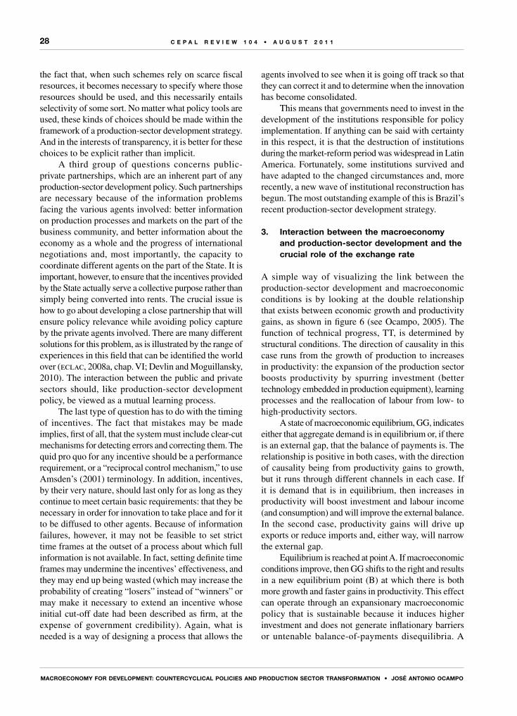
28
MACRoEConoMy foR dEVELoPMEnT: CoUnTERCyCLICAL PoLICIES And PRodUCTIon SECToR TRAnSfoRMATIon • JoSé AnTonIo oCAMPo
C E P A L R E V I E W 1 0 4 • A U G U S T 2 0 1 1
the fact that, when such schemes rely on scarce fiscal resources, it becomes necessary to specify where those resources should be used, and this necessarily entails selectivity of some sort. No matter what policy tools are used, these kinds of choices should be made within the framework of a production-sector development strategy. And in the interests of transparency, it is better for these choices to be explicit rather than implicit.
A third group of questions concerns public-private partnerships, which are an inherent part of any production-sector development policy. Such partnerships are necessary because of the information problems facing the various agents involved: better information on production processes and markets on the part of the business community, and better information about the economy as a whole and the progress of international negotiations and, most importantly, the capacity to coordinate different agents on the part of the State. It is important, however, to ensure that the incentives provided by the State actually serve a collective purpose rather than simply being converted into rents. The crucial issue is how to go about developing a close partnership that will ensure policy relevance while avoiding policy capture by the private agents involved. There are many different solutions for this problem, as is illustrated by the range of experiences in this field that can be identified the world over (eclac, 2008a, chap. VI; Devlin and Moguillansky, 2010). The interaction between the public and private sectors should, like production-sector development policy, be viewed as a mutual learning process.
The last type of question has to do with the timing of incentives. The fact that mistakes may be made implies, first of all, that the system must include clear-cut mechanisms for detecting errors and correcting them. The quid pro quo for any incentive should be a performance requirement, or a “reciprocal control mechanism,” to use Amsden’s (2001) terminology. In addition, incentives, by their very nature, should last only for as long as they continue to meet certain basic requirements: that they be necessary in order for innovation to take place and for it to be diffused to other agents. Because of information failures, however, it may not be feasible to set strict time frames at the outset of a process about which full information is not available. In fact, setting definite time frames may undermine the incentives’ effectiveness, and they may end up being wasted (which may increase the probability of creating “losers” instead of “winners” or may make it necessary to extend an incentive whose initial cut-off date had been described as firm, at the expense of government credibility). Again, what is needed is a way of designing a process that allows the
agents involved to see when it is going off track so that they can correct it and to determine when the innovation has become consolidated.
This means that governments need to invest in the development of the institutions responsible for policy implementation. If anything can be said with certainty in this respect, it is that the destruction of institutions during the market-reform period was widespread in Latin America. Fortunately, some institutions survived and have adapted to the changed circumstances and, more recently, a new wave of institutional reconstruction has begun. The most outstanding example of this is Brazil’s recent production-sector development strategy.
3. interaction between the macroeconomy and production-sector development and the crucial role of the exchange rate
A simple way of visualizing the link between the production-sector development and macroeconomic conditions is by looking at the double relationship that exists between economic growth and productivity gains, as shown in figure 6 (see Ocampo, 2005). The function of technical progress, TT, is determined by structural conditions. The direction of causality in this case runs from the growth of production to increases in productivity: the expansion of the production sector boosts productivity by spurring investment (better technology embedded in production equipment), learning processes and the reallocation of labour from low- to high-productivity sectors.
A state of macroeconomic equilibrium, GG, indicates either that aggregate demand is in equilibrium or, if there is an external gap, that the balance of payments is. The relationship is positive in both cases, with the direction of causality being from productivity gains to growth, but it runs through different channels in each case. If it is demand that is in equilibrium, then increases in productivity will boost investment and labour income (and consumption) and will improve the external balance. In the second case, productivity gains will drive up exports or reduce imports and, either way, will narrow the external gap.
Equilibrium is reached at point A. If macroeconomic conditions improve, then GG shifts to the right and results in a new equilibrium point (B) at which there is both more growth and faster gains in productivity. This effect can operate through an expansionary macroeconomic policy that is sustainable because it induces higher investment and does not generate inflationary barriers or untenable balance-of-payments disequilibria. A

29
MACRoEConoMy foR dEVELoPMEnT: CoUnTERCyCLICAL PoLICIES And PRodUCTIon SECToR TRAnSfoRMATIon • JoSé AnTonIo oCAMPo
C E P A L R E V I E W 1 0 4 • A U G U S T 2 0 1 1
successful production-sector development policy will shift the TT function upward, as it leads both to more economic growth and higher productivity (point C in figure 6).
As pointed out by Ocampo (2005) and Ocampo, Rada and Taylor (2009), this implies that the relationship between increases in productivity and in growth runs in two directions, rather than, as in the traditional view, it simply being one in which productivity is the cause and economic growth is the effect.25 More specifically, a poor growth performance tends to undercut the rate of productivity growth. There can be various reasons for this, including a balance-of-payments crisis or a destructive restructuring process in the production sector. Declines in productivity will operate through the pathways mentioned earlier: lower investment, less learning and a perverse reallocation of labour to informal sectors. A strong macroeconomic performance will have the opposite effect.
Although this conceptual scheme can be used to analyse many different types of problems, here we will focus on the real exchange rate, which is perhaps the most critical macroeconomic variable in open economies. It also establishes a fundamental connection between the
25 The fundamental problem has to do with the assumption of full employment of resources used in traditional growth models, in which the direction of causality runs only from productivity to growth.
analysis of growth and the analysis of countercyclical policies presented earlier.
The exchange rate has a number of complex features. One is that, because it is a macroeconomic variable, it cannot generate the selective incentives that a trade regime can, and it can therefore serve only as a partial, but not complete, substitute for a production-sector development policy. Another is that it is, at one and the same time, both the price of a set of financial assets and one of the determinants of the relative price of internationally traded goods and services.
This latter feature gives rise to a number of well-known complex effects. For example, one of the main ideas underlying the concept of an “anti-export bias” was that protection led to an overvaluation of the exchange rate, which undermined the incentive to export. In orthodox theory, the expectation was therefore that any reduction in protection would trigger a real devaluation that would spur the development of the export sector. However, the experiences of the countries of the Southern Cone in the 1970s have shown us that, if the move to open up the current account is coupled with an expansion of capital inflows because the capital account has been opened up at the same time, not only does the expected real devaluation not occur, but it may have the exact opposite effect: a real appreciation. This blocks the pathway through which liberalization would correct the “anti-export bias” and can even give rise to
FIGURE 6
relationship between gdp and productivity growth
Source: The author.
gdp: gross domestic product.
growth
Prod
uctiv
ity g
row
th
G’G
G’
G
T
T’
T
T’C
BA

30
MACRoEConoMy foR dEVELoPMEnT: CoUnTERCyCLICAL PoLICIES And PRodUCTIon SECToR TRAnSfoRMATIon • JoSé AnTonIo oCAMPo
C E P A L R E V I E W 1 0 4 • A U G U S T 2 0 1 1
a paradoxical situation in which economic growth is driven by domestic demand rather than by exports. This has often occurred in Latin America (see, among many others, Vos and others, 2006, chap. 3).
The empirical evidence shows that the real exchange rate is one of the determinants of economic growth. According to Rodrik’s estimates (2007b) for developing countries in the period from 1950 to 2004, a 10% undervaluation of the exchange rate was associated with 0.27% in additional growth per year. One of the explanations that he offers has to do with the externalities generated by producers of tradables and indicates that an undervaluation of the exchange rate functions as a partial substitute for a production-sector development policy. Hausmann, Pritchet and Rodrik (2005) show that one of the factors behind an acceleration in growth rates in developing countries is a competitive exchange rate. This evidence is also in line with the findings of Prasad, Rajan and Subramanian (2008) and the results of Frenkel’s and Rapetti’s review of the literature (2010), which indicate that higher growth rates are associated with improved current account balances.
Frenkel and Taylor (2007) call this effect of the real exchange rate on growth the “development effect” and draw a distinction between this and other effects of this variable, such as its short-run macroeconomic effect, which, as we have seen, is ambiguous, and its impact on employment. The development effect is linked, first of all, with the externalities generated by the dynamic development of tradables, which include the repercussions that this has on the diversification of the export structure. Second, it is associated with the fact that economies with a robust current account are less sensitive to sharp turnarounds in the capital account, which, as we have seen, has been one of the most important lessons learned from recent crises. One way of understanding these effects is to see that a stable, competitive exchange rate shifts TT upward (see figure 6) (i.e., serves as a partial substitute for a production-sector development policy) and shifts GG to the right (i.e., moves the macroeconomy towards a balanced position).
Apart from these development effects, the exchange rate has, as noted by Frenkel and Taylor (2007), additional
implications for employment that have to do with its effect on labour-output elasticity. A real revaluation tends to reduce this elasticity in two different ways: first, it lowers the price of production equipment in economies that import a large share of their machinery and equipment, which leads to a substitution of capital for labour; second, it tends to bias the selection of inputs in production processes towards imported inputs, which weakens domestic production linkages.
Instability in the real exchange rate also heightens risk and thereby depresses investment in the production of tradable goods and services that can be exported or used as import substitutes. This problem is compounded by the greater vulnerability to international price shocks displayed by countries that are dependent on commodity exports. And, in point of fact, the greater volatility of the real exchange rate in the countries of South America, as illustrated in figure 7, is associated with this subregion’s greater reliance on such products.
This underscores the fact that the macroeconomic challenges are especially formidable in economies where a considerable portion of the export base is composed of natural-resource-based goods. In order to deal with this situation, mechanisms need to be developed that can soften the macroeconomic impacts of fluctuations in the prices of these types of goods. This brings us back to the importance of the role of stabilization funds in these economies.
It should be remembered, however, that even in economies in which natural-resource-based products make up a large share of exports, the real exchange rate is not determined solely by export prices. Figure 7 shows, for example, that Peru has been much more successful in avoiding exchange-rate volatility than other South American countries, thanks to its central bank’s active intervention in foreign-exchange markets. The other side of the coin is that the introduction of more flexible exchange rates heightens the volatility of the real exchange rate, especially in economies dependent upon natural-resource-based exports. This points in the direction of the use of managed flexible exchange rates as part of the broader countercyclical policies that have been examined in earlier sections of this lecture.
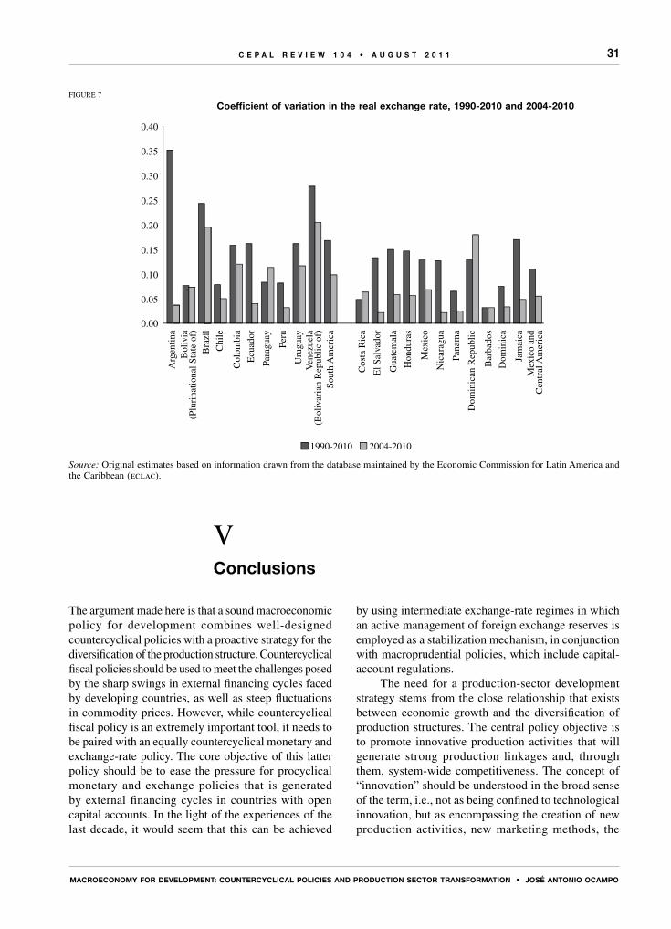
31
MACRoEConoMy foR dEVELoPMEnT: CoUnTERCyCLICAL PoLICIES And PRodUCTIon SECToR TRAnSfoRMATIon • JoSé AnTonIo oCAMPo
C E P A L R E V I E W 1 0 4 • A U G U S T 2 0 1 1
The argument made here is that a sound macroeconomic policy for development combines well-designed countercyclical policies with a proactive strategy for the diversification of the production structure. Countercyclical fiscal policies should be used to meet the challenges posed by the sharp swings in external financing cycles faced by developing countries, as well as steep fluctuations in commodity prices. However, while countercyclical fiscal policy is an extremely important tool, it needs to be paired with an equally countercyclical monetary and exchange-rate policy. The core objective of this latter policy should be to ease the pressure for procyclical monetary and exchange policies that is generated by external financing cycles in countries with open capital accounts. In the light of the experiences of the last decade, it would seem that this can be achieved
by using intermediate exchange-rate regimes in which an active management of foreign exchange reserves is employed as a stabilization mechanism, in conjunction with macroprudential policies, which include capital-account regulations.
The need for a production-sector development strategy stems from the close relationship that exists between economic growth and the diversification of production structures. The central policy objective is to promote innovative production activities that will generate strong production linkages and, through them, system-wide competitiveness. The concept of “innovation” should be understood in the broad sense of the term, i.e., not as being confined to technological innovation, but as encompassing the creation of new production activities, new marketing methods, the
FIGURE 7
Coefficient of variation in the real exchange rate, 1990-2010 and 2004-2010
Source: Original estimates based on information drawn from the database maintained by the Economic Commission for Latin America and the Caribbean (eclac).
0.40
0.35
0.30
0.25
0.20
0.15
0.10
0.05
0.00
1990-2010 2004-2010
Arg
entin
aB
oliv
ia(P
luri
natio
nal S
tate
of)
Bra
zil
Chi
le
Col
ombi
a
Ecu
ador
Para
guay
Uru
guay
Ven
ezue
la(B
oliv
aria
n R
epub
lic o
f)
Peru
Sout
h A
mer
ica
Cos
ta R
ica
Mex
ico
and
Cen
tral
Am
eric
a
Gua
tem
ala
El S
alva
dor
Hon
dura
s
Mex
ico
Nic
arag
ua
Pana
ma
Dom
inic
an R
epub
lic
Bar
bado
s
Dom
inic
a
Jam
aica
VConclusions
32
MACRoEConoMy foR dEVELoPMEnT: CoUnTERCyCLICAL PoLICIES And PRodUCTIon SECToR TRAnSfoRMATIon • JoSé AnTonIo oCAMPo
C E P A L R E V I E W 1 0 4 • A U G U S T 2 0 1 1
conquest of new markets and new ways of organizing a company or an industry. The critical test, however, is the extent to which it helps an economy build up technological capabilities. The challenge is particularly formidable in economies that, like most of those of Latin America, have static, natural-resource-based comparative advantages. The exploitation of those advantages should not, however, be a barrier to the diversification of the production structure, and steps should be taken to ensure that increasingly sophisticated technologies are incorporated into the countries’ natural-resource-based production activities. Wise management of the exchange rate throughout the business cycle is essential if this is to be accomplished.
Countercyclical policy and the diversification of production are crucial elements in the contributions to economic thought made by eclac and, in particular, Raúl Prebisch, in whose honour this lecture series was created. And they, in turn, are based on two other fundamental concepts: the key importance of managing the external vulnerabilities of economies whose macroeconomic dynamics are subject to “balance-of-payments predominance”, and the close relationship that exists between economic growth and changing production patterns. These two pivotal ideas are as valid today as they were in the past and demonstrate the cogency of the concepts that eclac has espoused throughout its history.
Bibliography
Agosin, Manuel (2007), “Trade and growth: why Asia grows faster than Latin America”, Economic Growth with Equity: Challenges for Latin America, Ricardo Ffrench-Davis and José Luis Machinea (eds.), Houndmills, Palgrave/eclac.
Agosin, Manuel and Franklin Huaita (2009), “Overreaction in capital flows to emerging markets: booms and sudden stops”, Working Paper, No. 295, Santiago, Chile, Department of Economics, University of Chile.
Akyüz, Yilmaz (ed.) (2003), Developing Countries and World Trade: Performance and Prospects, Geneva, United Nations Conference on Trade and Development (unctad).
Amsden, Alice (2001), The Rise of “The Rest”: Challenges to the West from Late-Industrializing Economies, New York, Oxford University Press, September.
Bello, Omar and Juan Pablo Jiménez (2008), “Política fiscal y ciclo económico en América Latina”, Santiago, Chile, Economic Commission for Latin America and the Caribbean (eclac).
Bértola, Luis and José Antonio Ocampo (2010), Desarrollo, vaivenes y desigualdad: una historia económica de América Latina desde la independencia, Madrid, Ibero-American Secretariat.
Bielschowsky, Ricardo (1998), “Cincuenta años de pensamiento de la cepal”, Cincuenta años de pensamiento de la cepal, Santiago, Chile, Fondo de Cultura Económica/eclac.
Blomström, Magnus and Ari Kokko (2007), “From natural resources to high-tech production: the evolution of industrial competitiveness in Sweden and Finland”, Natural Resources: Neither Curse nor Destiny, Daniel Lederman and William F. Maloney (eds.), Washington, D.C., World Bank.
Calvo, Guillermo, Leonardo Leiderman and Carmen Reinhart (1993), “Capital inflows and real exchange rate appreciation in Latin America: the role of external factors”, imf Staff Papers, No. 40, Washington, D.C., International Monetary Fund, March.
Calvo, Guillermo and Ernesto Talvi (2008), “Sudden stop, financial factors and economic collapse: a view from the Latin American frontlines”, The Washington Consensus Reconsidered: Towards a New Global Governance, Narcis Serra and Joseph E. Stiglitz (eds.), New York, Oxford University Press.
Cimoli, Mario and Gabriel Porcile (2011), “Learning, technological capabilities and structural dynamics”, The Oxford Handbook of Latin American Economics, José Antonio Ocampo and Jaime Ros (eds.), New York, Oxford University Press.
Cimoli, Mario, Giovanni Dosi and Joseph E. Stiglitz (2009), “The future of industrial policies in the new millennium: toward a knowledge-centered development agenda”, The Political Economy of Capabilities Accumulation: the Past and Future of Policies for Industrial Development, Mario Cimoli, Giovanni Dosi and Joseph E. Stiglitz (eds.), New York, Oxford University Press.
Devlin, Robert and Graciela Moguillansky (2010), Alianzas público-privadas para una nueva visión estratégica del desarrollo, Libros de la cepal series, No. 108 (LC/G.2426-P), Santiago, Chile, Economic Commission for Latin America and the Caribbean (eclac)/Ibero-American Secretariat.
Díaz-Alejandro, Carlos F. (1988), Trade, Development and the World Economy: Selected Essays, Andrés Velasco (ed.), Oxford, Basil Blackwell.
eclac (Economic Commission for Latin America and the Caribbean) (2010a), Time for Equality: Closing Gaps, Opening Trails (LC/G.2432(SES.33/3)), Santiago, Chile.
(2010b), Social Panorama of Latin America, Santiago, Chile. (2008a), Structural Change and Productivity Growth,
20 Years Later. Old Problems, New Opportunities (LC/G.2367(SES.32/3)), Santiago, Chile.
(2008b), Economic Survey of Latin America and the Caribbean 2007-2008 (LC/G.2386-P), Santiago, Chile. United Nations publication, Sales No. E.08.II.G.2.
(2007), Progreso técnico y cambio estructural en América Latina (LC/W.136), Santiago, Chile, eclac/International Development Research Centre (idrc).
(2006), Latin America and the Caribbean in the World Economy, 2005-2006 (LC/G.2313-P), Santiago, Chile. United Nations publication, Sales No. E.06.II.G.67.
(2000), Equity, Development and Citizenship (LC/G.2071(SES.28/3)), Santiago, Chile.

33
MACRoEConoMy foR dEVELoPMEnT: CoUnTERCyCLICAL PoLICIES And PRodUCTIon SECToR TRAnSfoRMATIon • JoSé AnTonIo oCAMPo
C E P A L R E V I E W 1 0 4 • A U G U S T 2 0 1 1
(1998a), Latin America and the Caribbean: Policies to Improve Linkages with the Global Economy (LC/G.1800/Rev.1-P), Santiago, Chile.
(1998b), The Fiscal Covenant: Strengths, Weaknesses, Challenges (LC/G.1997/Rev.1-P), Santiago, Chile. United Nations publication, Sales No. E.98.II.G.5.
(1998c), Economic Survey of Latin America and the Caribbean, 1997-1998 (LC/G.2032-P), Santiago, Chile. United Nations publication, Sales No. E.98.II.G.2.
(1990), Changing Production Patterns with Social Equity: The Prime Task of Latin American and Caribbean Development in the 1990s (LC/G.1601-P), Santiago, Chile. United Nations publication, Sales No. E.90.II.G.6.
Epstein, Gerald, Ilene Grabel and K.S. Jomo (2003), “Capital management techniques in developing countries”, Challenges to the World Bank and the imf: Developing Country Perspectives, Ariel Buira (ed.), London, Anthem Press.
Ffrench-Davis, Ricardo (2010), “Latin America: the structural fiscal balance policy in Chile: a move toward counter-cyclical macroeconomics”, Journal of Globalization and Development, vol. 1, No. 1, Berkeley Electronic Press.
(2005), Reformas para América Latina: después del fundamentalismo neoliberal, Buenos Aires, Siglo XXI Editores Argentina.
(2001), Financial Crises in ‘Successful’ Emerging Economies, Washington, D.C., Brookings Institution Press.
Ffrench-Davis, Ricardo and Stephany Griffith-Jones (2011), “Taming capital account shocks: managing booms and busts”, The Oxford Handbook of Latin American Economics, José Antonio Ocampo and Jaime Ros (eds.), New York, Oxford University Press.
Ffrench-Davis, Ricardo, Oscar Muñoz and Gabriel Palma (1998), “The Latin American economies, 1959-1990”, Latin America: Economy and Society Since 1930, Leslie Bethell (ed.), Cambridge, Cambridge University Press.
Frankel, Jeffrey and George Saravelos (2010), “Are leading indicators of financial crises useful for assessing country vulnerability? Evidence from the 2008-2009 global crisis”, nber Working Paper, No. 16047, Cambridge, Massachusetts, National Bureau of Economic Research, June.
Frenkel, Roberto (2010), “Lecciones de la política macroeconómica para el desarrollo a la luz de la experiencia de la última década”, document presented at the XV Reunión de investigadores de los bancos centrales del continente americano, organized by the Centre for Latin American Monetary Studies (cemla) and the Central Bank of Bolivia (3 - 5 November).
(2008), “From the boom in capital inflows to financial traps”, Capital Market Liberalization and Development, José Antonio Ocampo and Joseph E. Stiglitz (eds.), New York, Oxford University Press.
(2007), “The sustainability of monetary sterilization policies”, cepal Review, No. 93 (LC/G.2347-P), Santiago, Chile, Economic Commission for Latin America and the Caribbean (eclac), December.
Frenkel, Robert and Lance Taylor (2007), “Real exchange rate, monetary policies and employment”, Policy Matters: Economic and Social Policies to Sustain Equitable Development, José
Antonio Ocampo, Jomo K.S. and Sarbuland Khan (eds.), Hyderabad, Orient Longman.
Frenkel, Robert and Martin Rapetti (2010) “Economic development and the international financial system”, Time for a Visible Hand: Lessons from the 2009 World Financial Crisis, Stephany Griffith-Jones, José Antonio Ocampo and Joseph E. Stiglitz (eds.), New York, Oxford University Press.
Griffith-Jones, Stephany and José Antonio Ocampo (2010), “Building on the Counter-Cyclical Consensus: A Policy Agenda” [online] http://www.g24.org/research.htm
Hausmann, Ricardo (2011), “Structural transformation and economic growth in Latin America”, The Oxford Handbook of Latin American Economics, José Antonio Ocampo and Jaime Ros (eds.), New York, Oxford University Press.
Hausmann, Ricardo, Jason Hwang and Dani Rodrik (2007), “What you export matters”, Journal of Economic Growth, vol. 12, No. 1, Berlin, Springer.
Hausmann, Ricardo, Lant Pritchet and Dani Rodrik (2005), “Growth accelerations”, Journal of Economic Growth, vol. 10, No. 4, Berlin, Springer.
Heymann, Daniel (2000), “Major macroeconomic disturbances, expectations and policy responses”, cepal Review, No. 70 (LC/G.2095-P), Santiago, Chile, Economic Commission for Latin America and the Caribbean (eclac), April.
Hidalgo, C.A. and others (2007), “The product space conditions the development of nations”, Science, vol. 317, No. 5837, Washington, D.C., American Association for the Advancement of Science, July.
Hirschman, Albert O. (1958), The Strategy of Economic Development, New Haven, Yale University Press.
idb (Inter-American Development Bank) (2008), All That Glitters May Not Be Gold: Assessing Latin America’s Recent Macroeconomic Performance, Washington, D.C., April.
imf (International Monetary Fund) (2010), Regional Economic Outlook, Western Hemisphere: Heating up in the South, Cooler in the North. Washington, D.C., October.
Kaminsky, Graciela L., Carmen M. Reinhart and Carlos A. Végh (2004), “When it rains, it tours: pro-cyclical capital flows and macroeconomic policies”, nber Working Paper, No. 10780, Cambridge, Massachusetts, National Bureau of Economic Research.
Katz, Jorge (2001), Structural Reforms, Productivity and Technological Change in Latin America, Santiago, Chile, eclac/Fondo de Cultura Económica.
(1987), “Domestic technology generation in LDCs: a review of research findings”, Technology Generation in Latin American Manufacturing Industries, Jorge Katz (ed.), London, Macmillan.
Kindleberger, Charles P. and Robert Aliber (2005), Manias, Panics, and Crashes: A History of Financial Crises, New York, John Wiley and Sons.
Krugman, Paul (1987), “The narrow moving band, the Dutch disease and the competitive consequences of Mrs. Thatcher: notes on trade in the presence of scale dynamic economies”, Journal of Development Economics, vol. 27, No. 1-2, Amsterdam, Elsevier.
Krugman, Paul and Lance Taylor (1978), “Contractionary effects of devaluations”, Journal of International Economics, vol. 8, No. 3, Amsterdam, Elsevier.

34
MACRoEConoMy foR dEVELoPMEnT: CoUnTERCyCLICAL PoLICIES And PRodUCTIon SECToR TRAnSfoRMATIon • JoSé AnTonIo oCAMPo
C E P A L R E V I E W 1 0 4 • A U G U S T 2 0 1 1
Lederman, Daniel and William F. Maloney (2007), “Trade structure and growth”, Natural Resources: Neither Curse nor Destiny, Daniel Lederman and William F. Maloney (eds.), Washington, D.C., World Bank.
Llaudes, Ricardo, Ferhan Salman and Mali Chivakul (2010), “The impact of the great recession on emerging markets”, imf Working Paper, No. 10/237, Washington, D.C., International Monetary Fund, October.
Manzano, Ozmel and Roberto Rigobón (2007), “Resource curse or debt overhang?”, Natural Resources: Neither Curse nor Destiny, Daniel Lederman and William F. Maloney (eds.), Washington, D.C., World Bank.
Marfán, Manuel (2005), “La eficacia de la política fiscal y los déficit privados: un enfoque macroeconómico”, Más allá de las reformas: dinámica estructural y vulnerabilidad macroeconómica, José Antonio Ocampo (ed.), Bogota, Alfaomega.
Martner, Ricardo and Varinia Tromben (2003), “Tax reforms and fiscal stabilization in Latin America”, Tax Policy, Rome, Bank of Italy.
Minsky, Hyman P. (1982), Can “it” Happen Again?: Essays on Instability and Finance, Armonk, New York, M.E. Sharpe.
Noyola, Juan (1956), “El desarrollo económico y la inflación en México y otros países latinoamericanos”, Investigación económica, vol. 16, No. 4, Mexico City, National Autonomous University of Mexico.
Ocampo, José Antonio (2009), “Latin America and the global financial crisis”, Cambridge Journal of Economics, vol. 33, No. 4, Oxford University Press, July.
(2008), “A broad view of macroeconomic stability”, The Washington Consensus Reconsidered, Narcis Serra and Joseph E. Stiglitz (eds.), New York, Oxford University Press.
(2007), “The macroeconomics of the Latin American economic boom”, cepal Review, No. 93 (LC/G.2347-P), Santiago, Chile, Economic Commission for Latin America and the Caribbean (eclac), December.
(2005), “La búsqueda de la eficiencia dinámica: dinámica estructural y crecimiento económico en los países en desarrollo”, Más allá de las reformas: dinámica estructural y vulnerabilidad macroeconómica, José Antonio Ocampo (ed.), Bogota, Alfaomega.
(2004), “La América Latina y la economía mundial en el largo siglo XX”, El trimestre económico, vol. 71(4), No. 284, Mexico City, Fondo de Cultura Económica, October-December.
(2003), “Capital account and counter-cyclical prudential regulations in developing countries”, From Capital Surges to Drought: Seeking Stability for Emerging Markets, Ricardo Ffrench-Davis and Stephany Griffith-Jones (eds.), Basingstoke, Palgrave.
Ocampo, José Antonio and Robert Vos (2008), Uneven Economic Development, Himayatnagar, Orient Longman.
Ocampo, José Antonio, Codrina Rada and Lance Taylor (2009), Growth and Policy in Developing Countries: A Structuralist Approach, New York, Columbia University Press.
Ocampo, José Antonio and Mariángela Parra (2010), “The terms of trade for commodities since the mid-nineteenth century”, Journal of Iberian and Latin American Economic History/
Revista de historia económica, vol. 28, No. 1, Cambridge University Press, March.
Ocampo, José Antonio and others (2010), “The Great Recession and the Developing World”, document prepared for the Spanish Presidency of the European Union, June.
Olivera, J.H.G. (1964), “On structural inflation and Latin American structuralism”, Oxford Economic Papers, vol. 16, No. 3, Oxford, Oxford University Press, November.
Ostry, Jonathan D. and others (2010), “Capital inflows: the role of controls”, Staff Position Note, No. 2010/04, February [online] www.imf.org
Palma, José Gabriel (2011), “Why has productivity growth stagnated in most Latin American countries since the neo-liberal reforms?”, The Oxford Handbook of Latin American Economics, José Antonio Ocampo and Jaime Ros (eds.), New York, Oxford University Press.
(2009), “Flying geese and waddling ducks: the different capabilities of East Asia and Latin America to ‘demand-adapt’ and ‘supply-upgrade’ their export productive capacity”, The Political Economy of Capabilities Accumulation: the Past and Future of Policies for Industrial Development, Mario Cimoli, Giovanni Dosi and Joseph E. Stiglitz (eds.), New York, Oxford University Press.
Prasad, Eswar S., Raghuram R. Rajan and Arvind Subramanian (2008), “Foreign capital and economic development”, Brookings Papers on Economic Activity, No. 1, Washington, D.C., The Brookings Institution.
Prebisch, Raúl (1973), Interpretación del proceso de desarrollo latinoamericano en 1949, Serie conmemorativa del XXV aniversario de la cepal, Santiago, Chile, Economic Commission for Latin America and the Caribbean (eclac).
Reinhart, Carmen and Kenneth Rogoff (2009), This Time is Different: Eight Centuries of Financial Folly, Princeton, Princeton University Press.
Rodríguez, Octavio (2006), El estructuralismo latinoamericano, Mexico City, Siglo XXI Editores/eclac.
Rodrik, Dani (2007a), One Economics, Many Recipes: Globalization, Institutions and Economic Growth, Princeton, Princeton University Press.
(2007b), The Exchange Rate and Economic Growth: Theory and Evidence, Cambridge, Harvard University, John F. Kennedy School of Government, July.
Rodrik, Dani and Andrés Velasco (2000), “Short-term capital flows”, Proceedings of the Annual World Bank Conference on Development Economics 1999, Washington, D.C., World Bank.
Ros, Jaime (2000), Development Theory and the Economics of Growth, Ann Arbor, University of Michigan Press.
Rosenthal, Gert (2004), “eclac: a commitment to a Latin American way towards development”, Unity and Diversity in Development Ideas: Perspectives from the un Regional Commissions, Yves Berthelot (ed.), Bloomington, Indiana University Press.
Sachs, Jeffrey and Andrew Warner (1995), “Economic reform and the process of global integration”, Brookings Papers on Economic Activity, vol. 26, No. 1, Washington, D.C., The Brookings Institution.
Saurina, Jesús (2009), “Dynamic provisioning, the experience of Spain”, Policy for the Private Sector, Note, No. 7, Washington, D.C., World Bank, July.
35
MACRoEConoMy foR dEVELoPMEnT: CoUnTERCyCLICAL PoLICIES And PRodUCTIon SECToR TRAnSfoRMATIon • JoSé AnTonIo oCAMPo
C E P A L R E V I E W 1 0 4 • A U G U S T 2 0 1 1
Stiglitz, Joseph E. (1998), “More Instruments and Broader Goals: Moving toward the Post-Washington Consensus” [online] http://www.wider.unu.edu/events/annual-lecture/Past-annual-lectures/en_GB/1998/
Stiglitz, Joseph E. and Amar Bhattacharya (2000), “The underpinnings of a stable and equitable global financial system: from old debates to a new paradigm”, Proceedings of the Annual World Bank Conference on Development Economics 1999, Washington, D.C., World Bank.
Stiglitz, Joseph E. and others (2006), Stability with Growth: Macroeconomics, Liberalization, and Development, New York, Oxford University Press.
Sunkel, Osvaldo (1958), “La inflación chilena: un enfoque heterodoxo”, El trimestre económico, vol. 25, No. 4, Mexico City, Fondo de Cultura Económica, October-December.
Svensson, Lars E.O. (2000), “Open-economy inflation targeting”, Journal of International Economics, vol. 50, No. 1, Amsterdam, Elsevier.
Taylor, Lance (1991), Income Distribution, Inflation and Growth, Cambridge, Massachusetts, The mit Press.
Vos, Robert and others (2006), Who Gains from Free Trade? Export-led Growth, Inequality and Poverty in Latin America, London, Routledge.


C E P A L R E V I E W 1 0 4 • A U G U S T 2 0 1 1
37
Latin America: school bullyingand academic achievement
Marcela Román and F. Javier Murillo
The work done here involved estimating the extent of bullying in
Latin American schools and its impact on the academic achievement of
primary school students. Pupils’ socio-demographic characteristics were
analysed and linked with bullying. Three- and four-multilevel models were
applied to data from the Second Regional Comparative and Explanatory
Study (serce) conducted by the United Nations Educational, Scientific
and Cultural Organization (unesco), analysing 2,969 schools, 3,903
classrooms and 91,223 sixth-grade students in 16 Latin American
countries (not including Mexico for the association between school bullying
and academic performance). The study found that bullying is a serious
problem throughout the region; students who suffer peer aggression yield
a significantly lower performance in reading and math than those who do
not; and those in classrooms with more episodes of physical or verbal
violence perform worse than those in less violent classroom settings.
KEYWORDS
Students
Bullying
Schools
Academic achievement
Primary education
Statistical data
Latin America
Marcela Román
Senior Researcher, Centre
for Educational Research and
Development (cide)
Alberto Hurtado University, Chile
F. Javier Murillo
Senior Professor, Autonomous
University of Madrid, Spain

38
LATIn AMERICA: SChooL bULLyInG And ACAdEMIC AChIEVEMEnT • MARCELA RoMán And f. JAVIER MURILLo
C E P A L R E V I E W 1 0 4 • A U G U S T 2 0 1 1
Aggressive and violent behaviour among school pupils has become a research and public policy priority, owing to its consequences for children’s and young people’s development and academic performance and outcomes. This type of conduct, which is becoming a daily occurrence in schools and is known and to some extent sanctioned by adults and the students themselves, flies in the face of what is expected from school: a place where young citizens receive ethical, moral, emotional and cognitive education. It also seriously jeopardizes the school’s possibility of acting as a forum for the exchange of knowledge in a healthy and socially democratic and fair environment. Students must be able to learn without fear in a secure and reliable environment in order to build skills of all types and absorb the learning they need to develop comprehensively and participate fully in society.
Bullying impinges upon many dimensions; this article examines and discusses its impact on students’
learning and outcomes in the areas of reading and math, using data from the Second Regional Comparative and Explanatory Study (serce) (llece, 2008). This research compiles data on incidents of theft and physical and verbal violence that directly or indirectly involve sixth-grade students in 16 Latin American countries. The impact of those situations on student performance was analysed for 15 of those 16 countries. Mexico was not included in the analysis because the questionnaire on family-related factors was not administered there.
The second section of the article offers a conceptual framework on the basis of a review of the literature on school bullying and its link with academic learning and outcomes at the regional and international levels. The third section presents the objectives and methodology which structure and underpin the study, while the fourth and fifth sections set forth and discuss the main findings. Lastly, the main conclusions of the work are shared.
Iintroduction
IITheoretical basis
Authors who have studied school bullying in order to understand or try to prevent it, or both, agree that Olweus was the first researcher to develop a framework and a set of criteria for describing violent behaviour among peers in the school setting. In the 1970s, Olweus (1978) raised the alert by denouncing aggression and abuse as a common and systemic practice among pupils in Norwegian schools. Today this phenomenon is known universally as “bullying”, which refers to different types of repeatedly occurring intimidation, harassment, abuse, mistreatment and victimization (Rigby, 1996; García, 2010).
Bullying refers to repeated and ongoing situations of injustice and abuse of power (psychological or physical) and it has different, though all equally worrying, consequences for the students involved (Olweus, 1989, 1993, 1998; Smith and Sharpe, 1994; oecd, 2004; Cerezo, 2006; Skrzypiec, 2008). The available evidence distinguishes at least three actors in peer situations: (i) the student or students who do the harassing or bullying; (ii) the student or students who are harassed or bullied;
and (iii) the students who see or are otherwise aware of the bullying (Schäfer and others, 2005). As many as six roles may be identified if we include those who assist the perpetrator, reinforcers of bullying and defenders of victims (Rigby, 2003; Andreou and Metallidou, 2004; Rey and Ortega, 2007; Slee and Mohyla, 2007).
At the root of these behaviours lie cultural patterns of domination and submission among peers living closely together on a daily basis in institutionalized environments. The literature identifies four main forms of bullying: physical, verbal, psychological and social (Rivers and Smith, 1994; Espelage and Swearer, 2003; Smith, 2003; Avilés, 2005; Cerezo, 2006).
1. Climate, school culture and bullying
Researching the form or magnitude of violence among students within schools means exploring more deeply one of the dimensions of the school climate. School bullying is a complex phenomenon arising in the

39
LATIn AMERICA: SChooL bULLyInG And ACAdEMIC AChIEVEMEnT • MARCELA RoMán And f. JAVIER MURILLo
C E P A L R E V I E W 1 0 4 • A U G U S T 2 0 1 1
context of daily life in the school and therefore within the framework of the rules, routines, processes, systems of interaction and exchange, subjectivities and cultural patterns of each institution. Underlying violent conduct are the behaviours, beliefs and attitudes of all the actors involved, be they affection, regard, satisfaction, friendship, collaboration or tolerance, as well as dislike, prejudice, discrimination, exclusion and intolerance (Ortega, 2000; Kuperminc, Leadbeater and Blatt, 2001; Loukas and Robinson, 2004; Blaya and others, 2006; Gazelle, 2006).So bullying and its various forms are an integral part of the school and classroom life and climate which pupils live and breathe. They affect and impinge not only upon the well-being of every member of the educational community, but also upon their practices and performance. The universal presence and magnitude of school bullying and, above all, its consequences for the socio-affective and cognitive development of students, make it a priority in the analysis of school climate and coexistence, which are key to students’ learning and development (Ortega, 2005; Orpinas and Horne, 2006).
2. Bullying and school achievement: the international evidence
Bullying as a phenomenon has been extensively researched and analysed over the past two decades, mainly from the standpoint of psychology and educational sociology. From a psychological perspective, attention has centred on practices and behaviours which are associated with and involved in peer harassment, especially aggressive and violent conduct and the problems of different types of victimization and their psychological and social consequences for victims (Hawker and Boulton, 2000; Espelage, Holt and Henkel, 2003; Rigby, 2003; Perren and Alsaker, 2006). From the sociological perspective, efforts have been made to identify the social factors associated with bullying (poverty, social exclusion, youth delinquency, drug and alcohol consumption, youth culture), aiming to recognize and prevent bullying and reduce high-risk behaviour (Martínez-Otero, 2005; Blaya and others, 2006; Barker and others, 2008).
We know that peer violence and bullying is not a new or isolated phenomenon and it is not confined to certain schools or countries (Abramovay and Rua, 2005; Berger, Rodkin and Karimpour, 2008; Plan International, 2008). Bullying is a common and cross-cutting phenomenon that affects a large percentage of students as victims (the majority), perpetrators or observers or spectators and it has been documented in many works of research in different countries and world regions (Olweus, 1978,
1993; Schäfer and others, 2005; Ortega, 2005; Blaya and others, 2006; Smith, Kanetsuna and Koo, 2007).
The most common and frequent forms of bullying found in the evidence are insults, name-calling and nicknames; hitting, direct aggression and theft; and threats, rumour-spreading and social exclusion or isolation (Whitney and Smith, 1993; Owens, Daly and Slee, 2005). Lately there has been an upsurge in cyber bullying, whereby pupils are bullied and denigrated in different ways using mobile phones, websites, blogs, social networks such as Facebook, Hi5 and Twitter, YouTube and other media that are used and shared by school communities on the Internet (Skrzypiec, 2008).
Sex and age are factors in the magnitude and type of bullying. Male students are more likely to be involved in physical bullying (hitting), while female students are more likely to engage in social or psychological bullying (Skrzypiec, 2008). Bullying decreases for both sexes at higher levels of schooling (Pellegrini and Long, 2002; Dake, Price and Telljohann, 2003; Smith, 2003).
The first works of research on the magnitude of bullying in Europe include Whitney and Smith (1993), which found a victimization rate of 10% for the United Kingdom, with 6% admitting to being aggressors. Ten years later, Dake, Price and Telljohann (2003) found bullying rates in European primary schools varying from 11% in Finland to 49% in Ireland, while in the United States the rate was nearly 20%. In Spain, one in four pupils experiences school bullying, with a rate seven times higher in primary school than in secondary school and the main type of violence being psychological (Voors, 2005).
In Australia, 17.4% of pupils aged 7 to 9 reported serious bullying, and 31% reported having suffered mild bullying (Skrzypiec, 2008). Recent figures released by the Organization for Economic Cooperation and Development (oecd, 2009) on its member countries show that an average of 26% suffer bullying in primary school, 20% in lower secondary and 10% in upper secondary.
Studies conducted in Latin America also show differences between countries and levels of schooling. For example, 11% of students in Mexican primary schools have stolen something from or threatened a classmate, and just over 7% have done so in secondary school (Aguilera, Muñoz and Orozco, 2007). In Brazil, the percentage of primary pupils who report being repeatedly threatened in both public and private schools ranges from 21% to 40%, depending on the state (Abramovay and Rua, 2005).
For Peru, the data indicate a bullying rate of 47% (Oliveros and others, 2008), while in Chile 11% of

40
LATIn AMERICA: SChooL bULLyInG And ACAdEMIC AChIEVEMEnT • MARCELA RoMán And f. JAVIER MURILLo
C E P A L R E V I E W 1 0 4 • A U G U S T 2 0 1 1
students report having suffered bullying in the form of continual threats, discrimination or both (National School Violence Survey, 2007). The main forms of aggression reported are psychological (22.2%), physical (17.7%), discrimination or rejection (13.5%), continual threats or harassment (11.1%), attacks on personal property (9.6%), assault with a weapon (4.3%) and sexual violence (3%).
In Argentina, almost a third of secondary students report having school supplies or other objects they have taken to school broken (32%). Between 12% and 14%, depending on the grade, have experienced verbal bullying (shouting, mocking and insults); 10% say they have been threatened by a peer and 8% have experienced social bullying (exclusion). Lastly, just over 7% say they have been struck by a classmate and 4.5% say they have been robbed with intimidation or by force (García, 2010).
3. Effects of bullying on learning and school achievement
This brief review concludes by sharing the main findings of research on bullying and its implications for students’ learning and achievement.
On the basis of data for 2001 and 2002, a group of researchers analysed the relationship between bullying, school attendance, academic achievement, self-perception, and sense of belonging and security among primary pupils in urban public schools in the United States (Glew and others, 2005). The results show 22% of students involved in bullying in some capacity (victim, bully or both). The victims showed a greater likelihood of low achievement and lesser sense of belonging and security than those who did not report being bullied. More recently, a study by Holt, Finkelhor and Kantor (2007) found an association between victimization, psychological distress and academic difficulties in fifth-grade urban primary students in the north-east of the United States.
Research carried out with Greek primary students (Andreou and Matallidou, 2004) looked at the relationship between cognitive outcomes and the role played by students in bullying situations (bully, victim, assistant, reinforcer, defender and outsider). The results suggested associations between cognitions and the roles played by children in bullying.
Luciano and Savage (2007) explored bullying risk in Canadian fifth-grade students with and without learning difficulties, and its associations in terms of cognition and self-perception in inclusive school settings. The findings showed that students with learning difficulties, boys and girls alike, experience more bullying than children
without learning difficulties. This study also found that peer rejection and victimization may reflect the social impact of language difficulties in bullied students.
Research by Skrzypiec (2008) involving almost 1,400 seventh-, eighth- and ninth-graders in Australian primary schools examined the effects of bullying on students’ learning and their social and emotional well-being and mental health status. The analysis found that a third of students who had been seriously bullied also reported having serious difficulties in concentrating and paying attention in class because of bullying and the fear associated with it.
In 2007, Plan International, a non-governmental organization, conducted a study on school violence in 49 developing and 17 developed countries. The study identified three main types of violence experienced by children at school: corporal punishment, sexual violence and bullying. The report finds that bullying is common in schools throughout the world and that bullied students often develop concentration problems and learning difficulties (Plan International, 2008).
In Latin America, analyses conducted by unesco (llece, 2001) in the framework of the first international regional comparative study found better performance in students who reported few violent situations (fights and so on) in school and in those who reported that they had friendships at school.
More recently, the results of a study on school violence conducted in 2002 in 13 state capitals in Brazil (Abramovay and Rua, 2005) showed that 45% of primary and secondary pupils reported that violent incidents prevented them from concentrating on their work. A third said they felt nervous and tired, and another third (between 27% and 34%, depending on the state) acknowledged that bullying affected their motivation to go to school.
Lastly, a recently published study by Konishi and others (2010) examines the links between school bullying and student-teacher relationships and academic achievement in Canadian schools. The study worked with data for almost 28,000 15-year-old students participating in the Programme for International Student Assessment (pisa) conducted by oecd in 2006. Results of multilevel analyses showed that math and reading achievement was negatively related to school bullying and positively related to student-teacher connectedness. In other words, students who reported being bullied or suffering some other form of peer mistreatment showed lower math and reading achievements than their non-bullied peers. Students who reported a better rapport with their teachers also showed higher math and reading achievements.

41
LATIn AMERICA: SChooL bULLyInG And ACAdEMIC AChIEVEMEnT • MARCELA RoMán And f. JAVIER MURILLo
C E P A L R E V I E W 1 0 4 • A U G U S T 2 0 1 1
The main purpose of this research is to determine the associations between school bullying and academic achievement in primary-school students in Latin America. It also estimates and analyses the magnitude of peer violence in schools in 16 countries of the region, identifying the socio-demographic factors that appear to be linked to bullying.
The data for the work are obtained from the Second Regional Comparative and Explanatory Study (serce) conducted by unesco between 2005 and 2009 (llece, 2008), whose main purpose was to gain insights into the learning acquired by Latin American third- and sixth-grade primary students in math and reading. The unesco study applied standardized achievement tests to a sample of third- and sixth-graders in 16 countries, along with context questionnaires for the students, their families, teachers and management of the school establishments involved. School bullying was included only for the sixth-graders; consequently, this part of the study does not work with data for third-graders.
The present work uses multilevel analysis at four levels (student, classroom, school and country) for data for the entire region; and at three levels (student, classroom and school) for the analysis at the country level. Since family data were not collected for objective 3 (Determine the relationship between school bullying and academic achievement) in Mexico, data from that country are not used.
1. variables
The variables used may be classified in three groups: bullying variables, socio-demographic variables and achievement variables.
There were six variables on bullying, grouped in two major blocks. The first consisted of variables relating to direct experiences of bullying in the past month at school: having been robbed, insulted or threatened, or physically struck or mistreated. The second consisted of variables relating to knowledge of bullying of classmates in the past month, with the same elements as the first: having been robbed, insulted or threatened, or physically struck or mistreated. Another two variables were created to examine the impact of bullying on achievement: “victim of bullying”, a dichotomous variable indicating
whether or not the student reports having suffered some type of aggression; and “classroom violence” prepared on the basis of typified average values for the “victim of bullying” variable for all the children in the class.
Seven socio-demographic variables were used: socioeconomic status of the student’s family, a typified variable based on the parents’ professions and the household possessions; the cultural level of the student’s family, obtained by averaging and typifying the highest qualification obtained by both parents; a dichotomous variable for sex; a dichotomous variable for mother tongue(i.e. whether or not the student’s mother tongue was Spanish); years of preschooling (i.e. the number of years the student attended an educational establishment before compulsory education); socioeconomic level of the school, a typified variable based on the opinion of the principal; and the human development index of the country, based on official data from unesco for 2006.
Student achievement variables were performance in math and reading. Both were estimated using item response theory and set to a scale with a mean of 500 and a standard deviation of 50.
2. The sample
Four units of analysis were used for the multilevel study model: country, school, classroom and student. Data were obtained for 16 countries, 2,969 schools, 3,903 classrooms and 91,223 sixth-grade primary students (see table 1). Since the family questionnaires were not administered in Mexico, this country was not included in the study on the impact of bullying on academic achievement; hence for this objective the study related to 2,809 schools, 3,683 classrooms and 86,372 students in 15 countries. The sample was selected in each country using stratified random sampling of conglomerates. The stratification criteria were type of management and geographical area (urban public, urban private and rural); school size (small: school with one section in the grade; medium: with two or three sections in the grade, and large: with four or more sections in the grade), and the ratio between sixth grade enrolment and third grade enrolment (E6/E3 ≥ 0.8; 0<E6/E3<0.8; E6/E3= 0; and3rd grade enrolment = 0). The conglomerates were the schools in the universe. A sample of schools was selected in each stratum, in a
IIIObjectives and methodology

42
LATIn AMERICA: SChooL bULLyInG And ACAdEMIC AChIEVEMEnT • MARCELA RoMán And f. JAVIER MURILLo
C E P A L R E V I E W 1 0 4 • A U G U S T 2 0 1 1
single stage with all the schools in the stratum having equal probabilities of selection. The sample of pupils in each stratum consisted of all the pupils in the schools selected in each stratum.
TABLE 1
Latin America (16 countries): number of schools, classrooms and students examined in each country
Country Schools Classrooms Students
Argentina 167 353 6 696Brazil 157 245 5 456Colombia 203 207 6 035Costa Rica 171 150 4 766Cuba 206 383 5 910Chile 165 263 7 025Ecuador 192 215 5 427El Salvador 182 235 6 346Guatemala 231 267 5 560Mexico 160 220 4 861Nicaragua 205 250 6 789Panama 155 247 5 655Paraguay 209 208 4 839Peru 165 243 4 701Dominican Republic 183 114 4 646Uruguay 218 303 6 511
Total 2 969 3 903 91 223
Source: prepared by the authors.
3. instruments
The variables described were compiled by means of four types of test:
Information on bullying was obtained from a questionnaire administered to the sixth-grade students in the sample.
The output variables (math and reading achievement) were compiled using standardized tests which were validated for all the countries. The tests used matrix sampling, and were divided into different booklets, testing two dimensions: first, curricular elements known to be common to the region and, second, a life-skills approach. The items in the test were designed to assess comprehensive use of the various codes and rules that form the conceptual fields in each discipline evaluated, with an emphasis on the ability to infer meaning and problem-solving in students’ day-to-day lives.
Information on the socio-demographic adjustment variables was obtained from questionnaires administered to the students (gender and mother tongue), their families
(cultural level and socioeconomic status of family and student’s years of preschooling) and school address (socio-educational level of the school).
The family questionnaire was not administered in Mexico, so no data were obtained on students’ cultural level and socio-demographic status. Accordingly, this country had to be excluded from the analysis of relations between bullying and school achievement.
4. Data analysis
The analysis strategy varied depending on the objective. Accordingly, incidence of bullying in Latin American schools was analysed by performing a simple description for each country. The situation for the region overall was estimated by weighting the results for the individual countries. In order to identify the socio-demographic factors associated with school bullying, a contingency coefficient was estimated for the dichotomous variables and a Student t statistic for the scale variables.
The statistics used to determine links between school bullying and academic performance were rather more complex, since here multilevel models were used. First, multilevel models with four levels of analysis were applied. The procedure for each of the output variables was: (i) estimate the null model; (ii) calculate the model with the adjustment variables, and (iii) include the bullying variables (two, in this case: one was a construct for victims of bullying and the other referred to classroom violence) in the adjusted model and estimate the contribution of each.
Thus two multilevel models were estimated (one for each output variable) analogous to:
y NSE NCultijkl jkl jkl ijkl jkl ijkl jkl= + + +β β β β0 1 2 3
Pr eeesc Mujer Otra LM
N
ijkl jkl ijkl jkl ijkl
l
+ + +
+
β β
β4 5
6
_
SSE esc IDH paiskl l ijkl_ _+ +β ε7
β β ϕ υ µ0 0 0 0 0jkl l kl jkl= + + +
β β ϕ υ µ
β β ϕ υ µ1 1 1 1 1
5 5 5 5 5
jkl l kl jkl
jkl l kl j
= + + + …
= + + +
.
kkl
β β ϕ6 6 6l l= +

43
LATIn AMERICA: SChooL bULLyInG And ACAdEMIC AChIEVEMEnT • MARCELA RoMán And f. JAVIER MURILLo
C E P A L R E V I E W 1 0 4 • A U G U S T 2 0 1 1
with:
ε σ
µ
ε ε ε
µ
02
0
0
0
0ijkl
jkl
N
N
=
~
~
( , ) :
( , )
Ω Ω
Ω ::
( , ) :
Ω
Ω Ω
µ µ
υ υ υ
σ
υ σ
ϕ
=
=
0
0
2
02
0
0kl
l
N~
=
~N( , ) :0
0
2Ω Ωϕ ϕ ϕσ
where:yijk are the different measures of student
achievementNSEijkl, is the socioeconomic status of the student’s
family;N_Cultijkl, is the cultural level of the student’s
family;
Preescolijkl, is the student’s years of preschooling;Mujerijkl, if the student is female;Otra_LMijkl, if the student’s mother tongue is not
Spanish;NSE_escjkl, is the socioeconomic level of the school;
andIDH_paisk, is the country’s human development index
ranking.
The two bullying variables were then added to these to calculate the contribution made by each factor. Four four-level multilevel models were thus estimated.
On the basis of this data, the contribution of each variable was calculated for each country. Accordingly, 30 three-level multilevel models were calculated for each of the explanatory variables (15 countries x 2 output variables).
IVFindings
Consistently with the aims of the study, the findings were organized in three main categories: an estimate of the extent of bullying in Latin America, a study of the socio-demographic characteristics associated with bullying and an analysis of its impact on school achievement.
1. Extent of bullying
According to the analyses, just over half (51.1%) of sixth-grade primary students had been robbed, insulted or struck by peers at school during the month prior to the data collection. The most frequent sort of aggression was theft (39.4%), followed by verbal violence (26.6%) and, lastly, physical violence (16.5%). This order is the same in all the countries, but the specific figures vary a great deal (see table 2).
Whereas in Colombia over half of sixth-graders report having suffered some sort of theft in the preceding month, the figure for Cuba is only 1 in 10. In the other countries the figure for this category is at least one in three, showing how serious and widespread theft is. The problem is even worse, however, in Colombia, Ecuador, Nicaragua, Costa Rica, the Dominican Republic and Peru (over 45% in all cases).
The pattern is similar in the case of insults or threats, although here Argentina exhibits the highest
figures, followed by Peru, Costa Rica and Uruguay, in all of which over 30% of students report having suffered verbal abuse from another student during the month before data were collected.
Lastly, five countries should a particularly high rate of physical violence among students: Argentina (23.5%), Ecuador (21.9%), Dominican Republic (21.8%), Costa Rica (21.2%) and Nicaragua (21.2%). At the other extreme, Cuba again figures as the country with the lowest percentage of children reporting having been struck recently (only 4.4%).
Different figures are obtained when students are asked if they know anyone in their class who has been robbed, insulted or struck at school in the past month. 62.4% say they know of or have witnessed a bullying incident, of whatever type, at school involving one of their classmates. Specifically, 46.7% stated that one of their classmates had been robbed, 35.7% reported knowing someone in their class who had been insulted or threatened, while 38.9% reported knowing of a classmate who had been struck or hurt in the period (see table 3). Thus theft and then physical aggression were the most reported acts of violence.
There were large differences between countries in all cases. In four (Colombia, Panama, Argentina and Costa Rica), over 70% of students reported knowing

44
LATIn AMERICA: SChooL bULLyInG And ACAdEMIC AChIEVEMEnT • MARCELA RoMán And f. JAVIER MURILLo
C E P A L R E V I E W 1 0 4 • A U G U S T 2 0 1 1
TABLE 2
Latin America (16 countries): percentage of six-grade primary students who report having been robbed, insulted or struck in the past month, by country
Country Robbed Insulted or threatened Physically bullied Any bullying incidenta
Argentina 42.09 37.18 23.45 58.62Brazil 35.00 25.48 12.94 47.62Colombia 54.94 24.13 19.11 63.18Chile 32.54 22.43 11.55 43.08Cuba 10.55 6.86 4.38 13.23Costa Rica 47.25 33.16 21.23 60.22Ecuador 47.60 28.84 21.91 56.27El Salvador 33.42 18.63 15.86 42.55Guatemala 35.56 20.88 15.06 39.34Mexico 40.24 25.35 16.72 44.47Nicaragua 47.56 29.01 21.16 50.70Panama 36.99 23.66 15.91 57.32Paraguay 32.23 24.11 16.93 46.34Peru 45.37 34.39 19.08 44.52Dominican Republic 45.79 28.90 21.83 59.93Uruguay 32.42 31.07 10.10 50.13
Total for Latin America b 39.39 26.63 16.48 51.12
Average 38.72 25.88 17.20 48.67
Source: prepared by the authors.
a Percentage of students reporting having suffered some type of bullying (of whatever type) at school during the past month.b Results for Latin America as a total calculated by weighting the results for each country.
TABLE 3
Latin America (16 countries): percentage of six-grade primary students who report knowing a classmate who has been robbed, insulted, threatened or struck in the past month, by country
Country Robbed Insulted or threatened Physically bullied Any bullying incidenta
Argentina 53.60 49.61 50.23 74.67Brazil 45.89 36.89 42.27 67.04Colombia 58.60 33.21 38.29 72.83Chile 42.04 29.69 25.13 57.36Cuba 12.07 7.38 7.42 16.25Costa Rica 63.34 47.67 48.25 78.56Ecuador 53.25 33.67 38.95 65.99El Salvador 41.92 24.29 31.52 55.21Guatemala 43.21 24.93 31.58 57.66Mexico 47.19 32.88 33.98 56.88Nicaragua 60.55 39.95 47.08 63.87Panama 47.64 36.88 38.57 73.99Paraguay 38.43 29.37 31.73 63.41Peru 49.40 42.68 42.16 56.00Dominican Republic 46.55 35.41 38.79 69.98Uruguay 45.56 45.49 42.98 60.08
Total for Latin America b 46.72 35.74 38.91 62.42
Average 46.82 34.37 36.80 62.24
Source: prepared by the authors.
a Percentage of students reporting having suffered some type of bullying (of whatever type) at school during the past month.b Results for Latin America as a total calculated by weighting the results for each country.

45
LATIn AMERICA: SChooL bULLyInG And ACAdEMIC AChIEVEMEnT • MARCELA RoMán And f. JAVIER MURILLo
C E P A L R E V I E W 1 0 4 • A U G U S T 2 0 1 1
someone in their class who had been bullied, in whatever way. Cuba alone stood at the other extreme (16%). The rest ranged from 55% (El Salvador) to 70% (Dominican Republic.)
In Costa Rica and Nicaragua, 63.3% and 60.1% of six-graders, respectively, reported that someone in their class had had something stolen recently. The figure was over 50% in another three countries —Colombia, Argentina and Ecuador— and below 40% in only two: Paraguay (38.4%) and Cuba (12.1%).
More than 40% of children in Argentina, Costa Rica, Uruguay and Peru say they know someone in their class who has been insulted or threatened. Over 40% of children reported having experienced physical violence in Argentina, Costa Rica, Nicaragua, Uruguay, Brazil and Peru. Cuba and Chile report the lowest figures in relation to physical violence (7.4% and 25.1%, respectively).
2. Socio-demographic characterization of bullying
The second objective of this study was to identify student socio-demographic variables keyed to bullying. The variables analysed were: gender, family socioeconomic status and cultural level and area of residence (rural or urban).
The data indicate the existence of a statistically significant relationship between gender and having been robbed, insulted, threatened or physically bullied. The chi-squared test clearly shows that the three dependent variables examined (having been robbed, verbally bullied or physically bullied) are statistically related to gender. Boys suffer more thefts, insults, threats, and physical aggression than girls.
These findings were valid for all the countries, but varied from one to another. As shown in table 4, the results of the chi-squared tests performed show an association between bullying and gender in almost all the countries. The exceptions are Cuba, where both genders experience bullying equally across the three dependent variables, and Colombia, Costa Rica, Ecuador, Guatemala, Nicaragua, Panama and Peru, where there are no differences in the number of boys and girls reporting having been robbed in the past month.
The results are clear, too, with respect to area of residence: students in rural areas experience less theft and aggression and fewer insults than those in urban areas. Yet the data show that these differences are the tonic in most countries, but not all (see table 4). In Brazil, Guatemala, Peru and Uruguay no differences were observed at all between rural and urban students for any of the types of bullying.
TABLE 4
Latin America (16 countries): association between bullying and gender and area of residence (rural or urban) by country. results of contingency coefficientestimation: level of significance
CountryGender Area of residence
Robbed Insulted or threatened
Struck Robbed Insulted or threatened
Struck
Argentina 0.000 0.000 0.000 0.001 0.006 0.260Brazil 0.001 0.000 0.007 0.083 0.010 0.738Colombia 0.117 0.000 0.000 0.000 0.000 0.000Chile 0.000 0.026 0.000 0.058 0.006 0.417Cuba 0.179 0.268 0.839 0.000 0.000 0.019Costa Rica 0.219 0.000 0.000 0.000 0.004 0.222Ecuador 0.066 0.000 0.000 0.849 0.000 0.000El Salvador 0.005 0.000 0.000 0.000 0.000 0.003Guatemala 0.863 0.000 0.000 0.787 0.637 0.601Mexico 0.000 0.000 0.000 0.001 0.000 0.169Nicaragua 0.155 0.000 0.010 0.000 0.004 0.007Panama 0.060 0.001 0.067 0.508 0.002 0.080Paraguay 0.918 0.000 0.002 0.000 0.000 0.000Peru 0.513 0.000 0.000 0.665 0.488 0.757Dominican Republic 0.034 0.007 0.000 0.000 0.020 0.033Uruguay 0.037 0.000 0.006 0.152 0.054 0.728
Region (16 countries) 0.000 0.000 0.000 0.000 0.000 0.000
Source: prepared by the authors.

46
LATIn AMERICA: SChooL bULLyInG And ACAdEMIC AChIEVEMEnT • MARCELA RoMán And f. JAVIER MURILLo
C E P A L R E V I E W 1 0 4 • A U G U S T 2 0 1 1
The last two analyses sought to determine whether there was any relation between bullying and the cultural and socioeconomic levels of students’ families. The findings of the Student t statistic for all the students of the region are curious to say the least. These show that: — There is a relation between having been robbed
and the parents’ cultural level, but not the family’s socioeconomic status.
— There is a relation between having been insulted or threatened and the family’s socioeconomic status, but not the parents’ cultural level.
— There is a relation between having been struck and the parents’ cultural level, but not the family’s socioeconomic status.A detailed review of these relations in each of the
countries reveals a rather complex picture (see table 5). Accordingly, family socioeconomic status or cultural level cannot be stated to be linked in any general way with the incidence of bullying, of any type.
3. impact on academic achievement
As noted earlier, to determine the impact of school bullying on student achievement, first multilevel models were used with four levels to form an overall picture,
then with three levels for the analysis at the individual country level. The first step was to prepare the initial or adjustment models, which include the variables whose effect has to be “discounted” to ascertain the real impact of bullying on academic achievement. Table 6 shows the results of the two initial models. It shows that the seven adjustment variables are linked to student achievement in both disciplines. Reference is also made to both the five student variables (socioeconomic status and family’s cultural level, years of preschooling, gender and mother tongue), and the socioeconomic status of the school or human development index of the country.
The two target variables —victim of bullying (student variable, dichotomous) and violence in the classroom (classroom variable, typified)— were then included in each of the two adjusted models. Table 7 shows the contribution of the estimated coefficient in each model, first with each variable separately and then with the two together. Two ideas emerge from the analysis: first, the fact that all the coefficients are statistically significant confirms the relation between bullying and student achievement in reading and math. It may also be observed that the coefficients are practically the same when they are estimated independently and together, which implies that their contribution is additive.
TABLE 5
Latin America (15 countries): relation between bullying and families’cultural level and socioeconomic status by country. results of student t statistic: level of bilateral significance
Country
Family’s cultural level Family’s socioeconomic status
Robbed Insulted or threatened
Struck Robbed Insulted or threatened
Struck
Argentina 0.000 0.228 0.006 0.000 0.244 0.095Brazil 0.360 0.797 0.874 0.500 0.189 0.348Colombia 0.584 0.252 0.345 0.046 0.028 0.926Chile 0.207 0.377 0.063 0.111 0.076 0.306Cuba 0.510 0.456 0.020 0.009 0.094 0.207Costa Rica 0.000 0.012 0.090 0.000 0.020 0.118Ecuador 0.546 0.135 0.961 0.515 0.916 0.214El Salvador 0.892 0.981 0.570 0.000 0.002 0.823Guatemala 0.514 0.438 0.113 0.814 0.463 0.001Nicaragua 0.002 0.109 0.171 0.000 0.007 0.277Panama 0.050 0.144 0.951 0.440 0.000 0.218Paraguay 0.099 0.004 0.016 0.600 0.022 0.007Peru 0.000 0.038 0.000 0.000 0.021 0.000Dominican Republic 0.092 0.069 0.954 0.181 0.774 0.214Uruguay 0.000 0.064 0.757 0.000 0.000 0.007
Region (15 countries) 0.000 0.124 0.000 0.088 0.000 0.167
Source: prepared by the authors.Note: Mexico is not included, because the family questionnaire was not administered in that country.

47
LATIn AMERICA: SChooL bULLyInG And ACAdEMIC AChIEVEMEnT • MARCELA RoMán And f. JAVIER MURILLo
C E P A L R E V I E W 1 0 4 • A U G U S T 2 0 1 1
Two conclusions may be drawn from this:— A primary student in Latin America who reports
having been robbed or physically or verbally bullied has a significantly lower level of reading and math achievement than students who have not.
— Students in classroom settings with a higher incidence of theft or physical or verbal bullying also score worse in reading and math than those in classrooms with a lower level of violence. The procedure for analysing the impact of bullying
on student achievement in each of the 15 Latin American countries examined is the same as that used for the countries as a group, except that three-level models are used for the data.
The findings of the study on the effect of being a victim of bullying on student achievement in each country (see table 8) clearly indicate that the impact exists to a greater or lesser extent throughout the region. The data show that the contribution of this variable is significant for reading but not for math in Chile, Ecuador and the Dominican Republic, and significant for math but not for reading in Colombia and Cuba.
It is also readily observed that the countries with a higher level of bullying also show a lower impact of bullying on achievement. It may be supposed that where bullying is widespread it makes less difference to performance inasmuch as it affects all students equally.
TABLE 6
results of four-level adjusted multilevel models for math and reading achievement
Math achievement Reading achievement
Coefficient (s.e.) Coefficient (s.e.)
Constant Intercept 502.53 (9.25) 495.78 (6.93) Family’s socioeconomic status 2.53 (0.51) 3.27 (0.47) Family’s cultural level 9.20 (0.49) 10.65 (0.45) Preschooling 1.89 (0.277) 1.96 (0.26) Gender (male or female) -7.58 (0.77) 6.31 (0.72) Mother tongue (Spanish or other) -14.01 (2.04) -20.74 (1.80) School’s socioeconomic status 16.67 (1.51) 21.58 (1.26) Country’s human development index 30.66 (9.52) 26.37 (7.11)
Random Between countries 1 332.08 (482.25) 741.00 (269.47) Between schools 2 071.47 (108.92) 1 400.70 (73.03) Between classrooms 681.89 (53.98) 417.05 (32.17) Between students 6 459.38 (42.74) 6 185.30 (39.14)
Source: prepared by the authors.Note: all coefficients are significant at α=0.05.s.e.: standard error.
TABLE 7
Coefficients and standard error of bullying variables based on multilevel models for each of the variables examined, estimated independently and together
Independent estimation Combined estimation
Math achievement
Reading achievement
Math achievement
Reading achievement
Coefficient (s.e.) Coefficient (s.e.) Coefficient (s.e.) Coefficient (s.e.)
Victim of bullying (level 1) -9.55 (0.81) -9.68 (0.75) -9.40 (0.81) -9.53 (0.75)
Violence in the classroom (level 2) -7.32 (1.05) -5.92 (0.83) -6.88 (1.05) -5.60 (0.84)
Source: prepared by the authors.Note: all coefficients are significant at α=0.05.s.e.: standard error.

48
LATIn AMERICA: SChooL bULLyInG And ACAdEMIC AChIEVEMEnT • MARCELA RoMán And f. JAVIER MURILLo
C E P A L R E V I E W 1 0 4 • A U G U S T 2 0 1 1
The impact of the variable “classroom violence” on student achievement in each country was also examined (see table 9). The results place the countries in three groups: (i) those in which reading and math achievement are clearly influenced by violence in the classroom setting (Brazil, Chile, Cuba, Ecuador, Nicaragua, Paraguay and Uruguay); (ii) those in which classroom violence shows no impact on either measure
of achievement (El Salvador, Guatemala, Panama and Peru), and (iii) those in which the impact is seen in either reading (Argentina and Colombia) or math (Dominican Republic).
The study therefore produced clear empirical evidence on the relation between bullying and school achievement for the Latin American countries as a group and for each of the 15 countries individually.
TABLE 9
Latin America (15 countries): coefficients of the variable “violence in the classroom” on the basis of three-level multilevel models, by country
CountryAchievement
in math in reading
Argentina -11.46* -6.31Brazil -11.17* -11.49*Chile -18.48* -9.40*Colombia -6.47* -1.61Costa Rica -6.62 -12.49*Cuba -13.45* -5.33*Ecuador -12.54* -7.89*El Salvador -3.31 -3.00Guatemala 1.27 -0.57Nicaragua -6.20* -5.87*Panama -4.06 -6.41Paraguay -7.82* -8.24*Peru -1.14 -1.34Dominican Republic -3.55 -8.48*Uruguay -8.04* -5.18*
Total Latin America -7.32 -5.92
Source: prepared by the authors.Note: bold type denotes coefficients significant at α=0.05.Data for Mexico are not included because the family questionnaire was not administered in that country.* Indicates that the variable is significant at α=0.05.
TABLE 8
Latin America (15 countries): coefficients of the variable “victim of bullying” based on three-level multilevel models, by country
CountryAchievement
in math in reading
Argentina -7.84* -13.19*Brazil -12.21* -9.85*Chile -9.57 -8.07*Colombia -6.68* -2.44Costa Rica -17.61* 15.97*Cuba -16.32* -7.88Ecuador 0.19 -8.99*El Salvador -7.61* -9.95*Guatemala -9.52* -11.37*Nicaragua -6.93* -7.65*Panama -8.90* -12.78*Paraguay -13.82* -13.78*Peru -6.74* -10.03*Dominican Republic 0.64 -7.17*Uruguay -10.32* -9.80*
Total for Latin America -9.55 -9.68
Source: prepared by the authors.Note: bold type denotes coefficients significant at α=0.05.Data for Mexico are not included because the family questionnaire was not administered in that country.* Indicates that the variable is significant at α=0.05.

49
LATIn AMERICA: SChooL bULLyInG And ACAdEMIC AChIEVEMEnT • MARCELA RoMán And f. JAVIER MURILLo
C E P A L R E V I E W 1 0 4 • A U G U S T 2 0 1 1
The outcomes of this research are consistent with the findings of regional and international studies and reviews on the problem of bullying, its magnitude and its impact on learning and academic achievement. As well as backing up earlier findings, however, it also contributes a specific perspective for Latin American students and a comparison between the countries of the region.
1. Scope or magnitude of bullying
This study reports on and analyses the phenomenon of bullying from two different perspectives: being a victim of bullying, and knowing of or having witnessed a classmate being bullied. The figures show that just over half of sixth-graders in Latin American primary schools had directly suffered some sort of violence at the hands of their peers in the month before the data collection, and almost 62% had witnessed such an incident. It is therefore possible that more students are victims than the study outcomes suggest, since children often do not like to acknowledge that they have been bullied, even in an anonymous questionnaire.
These results coincide with the findings of previous research inasmuch as they show that bullying in all its forms is present and widespread in schools throughout the world (Abramovay and Rua, 2005; Ortega, 2005; Blaya and others, 2006; Smith, Kanetsuna and Koo, 2007; Berger, Rodkin and Karimpour, 2008). They differ, however, with respect to the magnitude of the phenomenon in other regions. For example, the study by Dake, Price and Telljohann (2003) for Europe found bullying rates ranging from 11% among primary students in Finland to 49% in Ireland. Skrzypiec (2008) looked at different degrees of bullying and found that it affected 48% of primary students in Australia, who reported being seriously or mildly bullied. For the group of oecd countries, the percentage of students reporting primary school bullying is 26% (oecd, 2009). In the case of the United States, the figures show that around 20% of students have been bullied (Glew and others, 2005; Dake, Price and Telljohann, 2003).
This comparison suggests that school bullying in Latin America is of a greater magnitude than in other regions, and is especially serious and complex in some of the region’s countries. Whereas 63% of primary students
report having suffered bullying in Colombia, the figure is only 13% in Cuba. This broad spectrum may be divided into three groups of countries. In the first, over half of students report having experienced some type of bullying (Colombia, Costa Rica, Argentina, Ecuador, Panama and the Dominican Republic); in the second, bullying victims represent between 40% (Uruguay, Paraguay, Nicaragua) and 50% (Brazil, Peru, Mexico, Guatemala, El Salvador and Chile) of the total, and third is Cuba on its own, with only 13%. Accordingly, preventive action and measures to reduce bullying need to be different from one country to another.
With regard to Latin America, there are still few studies examining the magnitude of school bullying at the national level and none at the regional level, which makes the research conducted here all the more important.
2. Type of bullying
The study identifies and researches three main types of bullying: robbery, insults or threats and physical aggression. The analysis found that the acts of bullying most reported were robbery, followed by insults and threats. After that came physical aggression in any of its forms. The results are also consistent with those on the main forms of school bullying reported in the international literature. The evidence available shows that among the most significant forms are insults (verbal aggression), name-calling and nicknames, physical aggression, blows, robbery, threats, rumour-spreading and social exclusion or isolation (Whitney and Smith, 1993; Owens, Daly and Slee, 2005, García, 2010).
3. variables associated with bullying
Based on the analyses of student socio-demographic variables and their relation with physical or verbal aggression, it may be concluded that more boys than girls suffer all forms of bullying (physical, psychological and verbal) in Latin American schools and it is more widespread in urban than in rural areas. These findings again reaffirm those reported in the international research, which report that both gender and age affect the magnitude of bullying and the form it takes. Male students are found to be involved mostly in physical
VDiscussion

50
LATIn AMERICA: SChooL bULLyInG And ACAdEMIC AChIEVEMEnT • MARCELA RoMán And f. JAVIER MURILLo
C E P A L R E V I E W 1 0 4 • A U G U S T 2 0 1 1
aggression, and female students mostly in social or psychological forms of bullying (Pellegrini and Long, 2002, Skrzypiec, 2008). This difference does not emerge in the present study, in which it can be affirmed only that in Latin America primary schools boys experience more robbery, insults, threats and physical aggression than girls. It was also found that robbery, insults, threats and physical aggression are less frequent among pupils of rural schools than those attending urban schools.
4. impact of bullying on achievement
The study supports the conclusion that primary students who have been bullied at school show significantly poorer math and reading achievement than those who have not. Students in classes in which physical or verbal aggression is more common also show lower achievement levels than students in less violent classroom settings. Consequently, it may be argued that both being bullied and witnessing the bullying of a classmate have a negative impact on achievement levels among Latin American primary students.
These important findings bear out the contributions of international literature and research in which it is found that bullying has a deleterious effect on student achievement, regardless of the role played by individual students in the aggression. First, they ratify the findings of the first regional comparative and explanatory study in Latin America and the Caribbean (llece, 2001), which
showed better school performance among students who reported little bullying at school.
Similar conclusions were reached by Glew and others (2005), whose study found a greater probability of low achievement among primary students who had been bullied in the United States. Lastly, our findings coincide fully with the recently published study by Konishi and others (2010) on the links between bullying and school achievement in Canadian students. By means of a multilevel analysis, the present study concludes that those students reporting being bullied achieved lower scores in math and reading than peers who did not report being bullied.
Lastly, the data support the statement that countries with a higher rate of school bullying are also those in which students’ achievement is the least affected by bullying. It appears that the effect of bullying on achievement is cancelled out where bullying is generalized or, put in another way, in contexts of widespread bullying the effect on school achievement is smaller and in some cases disappears altogether.
Unfortunately, no information is available from other studies with which to compare the findings of this research. Further research is therefore needed, not only because of the importance of the issue in relation to students’ cognitive performance, but also because of its implications for school settings in which bullying is part of the ways of relating and coexistence of the student body overall, i.e. the school culture.
VIConclusions
This section offers a number of conclusions that, far from closing the discussion, point up the importance of taking bullying seriously at both the global and local levels, and generating relevant alternatives to help prevent and reduce it.
1. School bullying: a new challenge for schools and teachers in Latin America
One of the basic conditions that must be fulfilled in order for students to develop fully, learn and acquire knowledge is the ability to attend school without fear, in a safe and motivating environment. Promoting and strengthening positive and non-violent peer relations
is therefore essential for students to co-exist happily at school and learn. Children who are bullied are significantly affected not only emotionally and behaviourally, but also in terms of their ability to learn and achieve in disciplines that are essential for their education and development.
Yet episodes of violence and acts of bullying are most often invisible to teaching staff, which makes it more difficult to respond and intervene to prevent or eradicate them. It is not easy, nor can it be, for teachers to recognize the codes, languages, signs and practices through which students bully or harass each other. Nevertheless, bullying must be eradicated as a matter of urgency in the interest of achieving quality education.

51
LATIn AMERICA: SChooL bULLyInG And ACAdEMIC AChIEVEMEnT • MARCELA RoMán And f. JAVIER MURILLo
C E P A L R E V I E W 1 0 4 • A U G U S T 2 0 1 1
2. School systems and their responsibility in the forms and magnitude of bullying
The significant differences observed in bullying from one country to another invite us to reflect upon the factors within schools and education systems that could influence this serious and complex phenomenon. We must at least ask which elements or dynamics in school systems could be generating or encouraging violent or aggressive forms of relating: perhaps, for example, more competitive or success- or achievement-oriented national systems or practices of exclusion. In other words, the education system and schools must not only take responsibility in preventing and reducing bullying, but also hold themselves accountable for its origin and forms of expression.
3. relevant and differentiated strategies for preventing and reducing bullying
In the past few years many programmes and policies have been put in place with the aim of improving the day-to-day relations within schools. Most of these, however, focus on the institution and seek to regulate —through teaching staff— acceptable and desirable student behaviour. It is quite clear that these strategies will not work unless they are designed and built in way that is student-centred, based on the dynamics and subjectivities of students and their interests, motivations, strengths and weaknesses.
School bullying also needs to be approached differently depending on the level of schooling, the school
setting and the gender of the students. The outcomes of this research confirm international findings on the alarming figures relating to bullying in primary schools, and the differences in the type of violence between boys and girls and between rural and urban schools.
4. The risk of treating bullying as a normal type of peer relations
The small effect of victimization on student achievement in countries with high rates of bullying raises at least two questions. First, the seriousness of treating bullying and aggressive forms of relating with peers as normal and habitual and, consequently, failing to take action to denounce, reduce or prevent it. Usually the existence or gravity of a problem is brought to light through its impacts or consequences. Accordingly, it is much more difficult to prevent or reduce violent behaviour when it appears to have no effect on school achievement.
Second, it is important to understand and turn a spotlight on the consequences for students’ personal and social development. Growing and learning in a hostile setting is a far cry from doing so in a positive and non-violent environment, however true it is that “most of my classmates are in the same situation”. Schools in which violence and bullying has become the norm are in no position to build the tolerance, cooperation, solidarity and other principles and values which are essential pillars for fairer, more democratic and inclusive societies.
(Original: Spanish)
Bibliography
Abramovay, M. (2005), “Violencia en las escuelas: un gran desafío”, Revista iberoamericana de educación, No. 38, Madrid, Organization of Ibero-American States for Education, Science and Culture.
Abramovay, M. and M. Rua (2005), Violences in Schools. Concise Version, Brasilia, United Nations Educational, Scientific and Cultural Organization (unesco).
Aguilera, M., G. Muñoz and A. Orozco (2007), Disciplina, violencia y consumo de sustancias nocivas a la salud en escuelas primarias y secundarias de México, Mexico City, National Institute for Educational Assessment and Evaluation.
Andreou, E. and P. Metallidou (2004), “The relationship of academic and social cognition to behaviour in bullying situations among Greek primary school children”, Educational Psychology, vol. 24, No. 1, Philadelphia, Taylor & Francis.
Avilés, J.M. (2005), Bullying: Intimidación y maltrato entre el alumnado, Bilbao, Sindicato de Trabajadores de la Enseñanza
de Euskadi-Euzkadiko Irakaskuntzako Lagileen Sindikatua (stee-eilas).
Barker, E.D. and others (2008), “Joint development of bullying and victimization in adolescence: relations to delinquency and self-harm”, Journal of the American Academy of Child and Adolescent Psychiatry, vol. 47, No. 9, Amsterdam, Elsevier.
Berger, C., P.C. Rodkin and R. Karimpour (2008), “Bullies and victims at school: perspectives and strategies for primary prevention”, School Violence and Primary Prevention, T. Miller (comp.), New York, Springer-Verlag.
Blaya, C. and others (2006), “Clima y violencia escolar. Un estudio comparativo entre España y Francia”, Revista de educación, No. 339, Madrid, Ministry of Education.
Cerezo, F. (2006), “Violencia y victimización entre escolares. El bullying: Estrategias de identificación y elementos para la intervención a través del test Bull-s”, Revista electrónica de investigación psicoeducativa, vol. 4, No. 9, Madrid, Editorial eos.
52
LATIn AMERICA: SChooL bULLyInG And ACAdEMIC AChIEVEMEnT • MARCELA RoMán And f. JAVIER MURILLo
C E P A L R E V I E W 1 0 4 • A U G U S T 2 0 1 1
Dake, J., J. Price and S. Telljohann (2003), “The nature and extent of bullying at school”, Journal of School Health, vol. 73, No. 5, Hoboken, Wiley.
Espelage, D. and S. Swearer (2003), “Research on school bullying and victimization: What have we learned and where do we go from here?”, School Psychology Review, vol. 32, No. 3, Bethesda, National Association of School Psychologists.
Espelage, D., M. Holt and R. Henkel (2003), “Examination of peer-group contextual effects on aggression during early adolescence”, Child Development, vol. 74, No. 1, Wiley.
García, M. (coord.) (2010), Violencia en las escuelas. Un relevamiento desde la mirada de los alumnos, Buenos Aires, Ministry of Education.
Gazelle, H. (2006), “Class climate moderates peer relations and emotional adjustment in children with an early history of anxious solitude: a child x environment model”, Developmental Psychology, vol. 42, No. 6, Washington, D.C., American Psychological Association.
Glew, G. and others (2005), “Bullying, psychosocial adjustment, and academic performance in elementary school”, Archives of Pediatrics & Adolescent Medicine, vol. 159, No. 11, Chicago, American Medical Association.
Hawker, D.S. and M.J. Boulton (2000), “Twenty years’ research on peer victimization and psychosocial maladjustment: a meta-analytic review of cross-sectional studies”, Journal of Child Psychology and Psychiatry, vol. 41, No. 4, Oxford, Blackwell Publishers.
Holt, M.K., D. Finkelhor and G.K. Kantor (2007), “Multiple victimization experiences of urban elementary school students: Associations with psychosocial functioning and academic performance”, Child Abuse and Neglect, vol. 31, No. 5, Orlando, Elsevier.
Konishi, C. and others (2010), “Do school bullying and student-teacher relationships matter for academic achievement? A multilevel analysis”, Canadian Journal of School Psychology, vol. 25, No. 1, Thousand Oaks, sage Publications.
Kuperminc, G., B. Leadbeater and S. Blatt (2001), “School social climate and individual differences in vulnerability to psychopathology among middle school students”, Journal of School Psychology, vol. 39, No. 2, Amsterdam, Elsevier.
llece (Latin American Laboratory for Assessment of the Quality of Education) (2008), Los aprendizajes de los estudiantes de América Latina y el Caribe. Primer reporte de los resultados del Segundo Estudio Regional Comparativo y Explicativo, Santiago, Chile, unesco Regional Office for Education in Latin America and the Caribbean.
(2001), Primer estudio internacional comparativo sobre lenguaje, matemáticas y factores asociados, para alumnos del tercer y cuarto grado de la educación básica. Informe técnico, Santiago, Chile, unesco Regional Office for Education in Latin America and the Caribbean.
Loukas, A. and S. Robinson (2004), “Examining the moderating role of perceived school climate in early adolescent adjustment”, Journal of Research on Adolescence, vol. 14, No. 2, Malden, Blackwell Publishers.
Luciano, S. and R. Savage (2007), “Bullying risk in children with learning difficulties in inclusive educational settings”, Canadian Journal of School Psychology, vol. 22, No. 1, Thousand Oaks, sage Publications.
Madriaza, P. (2009), “Violencia en las escuelas”, Seguridad y prevención: la situación en Argentina, Chile y Uruguay durante 2007, C. Guajardo (comp.), Santiago, Chile, International Centre for the Prevention of Crime/Alberto Hurtado University.
Martínez-Otero, V. (2005), “Conflictividad escolar y fomento de la convivencia”, Revista iberoamericana de educación, No. 38, Madrid, Organization of Ibero-American States for Education, Science and Culture.
Ministry of Education/Ministry of the Interior (2008), Encuesta nacional de violencia escolar 2007, Santiago, Chile, Ministry of Education/adimark.
oecd (Organisation for Economic Co-operation and Development) (2009), Take the Test: Sample Questions from oecd’s pisa Assessments, Paris.
__________ (2004), Taking Fear Out of Schools: A Report of an International Policy and Research Conference on School Bullying and Violence, Paris.
Oliveros, M. and others (2008), “Violencia escolar (bullying) en colegios estatales de primaria en el Perú”, Revista peruana de pediatría, vol. 61, No. 4, Lima, Sociedad Peruana de Pediatría.
Olweus, D. (1998), Conductas de acoso y amenazas entre escolares, Madrid, Ediciones Morata.
(1993), Bullying at School. What We Know and What We Can Do, Oxford, United Kingdom, Blackwell.
(1989), “Bully/victim problems among school children: basic facts and effects of a school based intervention programmed”, The Development and Treatment of Childhood Aggression, D.J. Pepler and K.H. Rubin (comps.), Hillsdale, N.J., Lawrence Erlbaum.
(1978), Aggression in the Schools. Bullies and Whipping Boys, Washington, D.C., Hemisphere Press.
Orpinas, P. and A. Horne (2006), Bullying Prevention: Creating a Positive School Climate and Developing Social Competence, Washington, D.C., American Psychological Association.
Ortega, R. (2005), La convivencia escolar: qué es y cómo abordarla, Sevilla, Consejería de Educación y Ciencia.
(comp.) (2000), Educar la convivencia para prevenir la violencia, Madrid, Editorial Antonio Machado Libros.
Owens, L., A. Daly and P.T. Slee (2005), “Sex and age differences in victimization and conflict resolution among adolescents in a South Australian school”, Aggressive Behavior, vol. 31, No. 1, Wiley.
Pellegrini, A.D. and J.D. Long (2002), “A longitudinal study of bullying, dominance, and victimization during the transition from primary school to secondary school”, British Journal of Developmental Psychology, vol. 20, No. 2, Leicester, British Psychological Society.
Perren, S. and F. Alsaker (2006), “Social behavior and peer relationships of victims, bully-victims, and bullies in kindergarten”, Journal of Child Psychology and Psychiatry, vol. 47, No. 1, Oxford, Blackwell Publishers.
Plan International (2008), Aprender sin miedo: la campaña mundial para terminar con la violencia en las escuelas [online] http://plan-international.org/learnwithoutfear/files-es/learn-without-fear-global-campaign-report-spanish
Rey, R. and R. Ortega (2007), “Violencia escolar: claves para comprenderla y afrontarla”, Revista escuela abierta, No. 10, Sevilla, Fundación San Pablo Andalucía.

53
LATIn AMERICA: SChooL bULLyInG And ACAdEMIC AChIEVEMEnT • MARCELA RoMán And f. JAVIER MURILLo
C E P A L R E V I E W 1 0 4 • A U G U S T 2 0 1 1
Rigby, K. (2003), “Consequences of bullying in school”, Canadian Journal of Psychiatry, vol. 48, Ottawa, Canadian Psychiatric Association.
(1996), Bullying in School. And What to Do About It, London, Jessica Kingsley.
Rivers, I. and P. Smith (1994), “Types of bullying behavior and their correlates”, Aggressive Behavior, vol. 20, No. 5, Wiley.
Schäfer, M. and others (2005), “Bullying roles in changing contexts: the stability of victim and bully roles from primary to secondary school”, International Journal of Behavioral Development, vol. 29, No. 4, sage Publications.
Skrzypiec, G. (2008), Living and Learning at School, document presented at the Annual Conference of the Australian Association for Research in Education [online] www.aare.edu.au/08pap/skr081125.pdf
Slee, P.T. and J. Mohyla (2007), “The peace pack: an evaluation of interventions to reduce bullying in four Australian primary
schools”, Educational Research, vol. 49, No. 2, Philadelphia, Taylor & Francis.
Smith, P.K. (coord.) (2003), Violence in Schools: The Response in Europe, London, Routledge.
Smith, P.K. and S. Sharpe (1994), School Bullying. Insights and Perspectives, London, Routledge.
Smith, P.K., T. Kanetsuna and H. Koo (2007), “Cross-national comparison of ‘bullying’ and related terms: Western and Eastern perspectives. Contemporary research on aggression: school violence”, Proceedings of the XVI World Meeting of the International Society for Research on Aggression, Santorini, Greece.
Voors, W. (2005), Bullying. El acoso escolar, Madrid, Oniro.Whitney, I. and P. Smith (1993), “A survey of the nature and extend of
bullying in Juner/middle and secondary schools”, Educational Research, vol. 35, London, Routledge.


C E P A L R E V I E W 1 0 4 • A U G U S T 2 0 1 1
55
Tourism competitivenessin the Caribbean
Bineswaree Bolaky
This article analyses the main determinants of competitiveness in
the Caribbean tourism stay-over industry using panel data for the period
1995-2006, based on an augmented version of an empirical model by
Craigwell (2007). The ex post measure of competitiveness used is the
share of world outbound tourists from Canada, the United Kingdom of
Great Britain and Northern Ireland and the United States of America arriving
in a Caribbean destination. The study finds evidence that Caribbean
tourism competitiveness can be enhanced through policy measures that
favour, among others, increases in investment, private sector development,
better infrastructure, lower government consumption, a more flexible
labour market, reduced vulnerability to natural disasters, higher human
development and slow rises in oil prices. This article is an attempt to fill
the gap on econometric research relating to tourism competitiveness for
the Caribbean region.
KEYWORDS
Tourism
Tourism infrastructure
Competitiveness
Measurement
Economic research
Econometric models
Tourism policy
Caribbean region
Bineswaree Bolaky
Economic Affairs Officer
Division for Africa, Least Developed
Countries and Special Programmes;
United Nations Conference on
Trade and Development (unctad)

56
ToURISM CoMPETITIVEnESS In ThE CARIbbEAn • bInESWAREE boLAky
C E P A L R E V I E W 1 0 4 • A U G U S T 2 0 1 1
Tourism is the dominant economic activity in the Caribbean,1 which is in fact the most tourism-penetrated region in the world. The establishment of tourism as a major economic activity was initially driven by a post-independence economic restructuring throughout the region away from traditional agriculture and towards services and manufacturing. This restructuring was deemed necessary in the face of declining competitiveness in traditional sectors (namely agriculture) and a need to build competitiveness in non-traditional areas.
According to the latest comprehensive report for the Caribbean published by the World Travel and Tourism Council (wttc, 2004), travel and tourism demand in the region amounted to US$ 40.3 billion in 2004 (out of US$ 5.5 trillion worldwide, or 0.7% of the total), and is expected to rise to US$81.9 billion by 2014. By this indicator, the largest travel and tourism economies in the Caribbean are Puerto Rico (22.4% of total regional demand), the Dominican Republic (12.9%), Cuba (12.0%), the Bahamas (9.0%) and Jamaica (8.2%). These five destinations account for almost two thirds of the total market demand. The smallest travel and tourism economies are Anguilla, Dominica, Grenada, Saint Kitts and Nevis and Saint Vincent and the Grenadines, accounting for 1.7% of the total demand. In terms of output generation, three small island groups (Anguilla, Antigua and Barbuda and the British Virgin Islands) have more than 70% of their gross domestic product (gdp) originating in the travel and tourism industry. For Aruba, the Bahamas and Barbados, the contribution of this sector to gdp lies in the range of 50%-70%. In terms of job creation, travel and tourism activities account for more than two thirds of employment in Anguilla, Aruba, the Bahamas, Antigua and Barbuda and the British Virgin Islands, the figures being 95% for the latter two. For another seven Caribbean countries (Barbados, Cayman Islands, Jamaica, Saint Kitts and Nevis, Saint Lucia, Saint Vincent and the Grenadines and the United States Virgin Islands), employment dependency ranges between 30% and 60%; and for a further five countries (Bermuda, Dominica,
The views expressed in this article are those of the author and do not necessarily reflect the views of the Organization.1 Defined as the 32 member countries and territories of the Caribbean Tourism Organization excluding Mexican destinations (Cancún and Cozumel).
Dominican Republic, Grenada and Guadeloupe), the range is between 15% and 30%.2
In a regional report, wttc estimated that the travel and tourism economy contributed about 14.5% to the region’s gdp in 2009, the highest level in the world (wttc, 2009). The sector also generated some 2,052,000 jobs, or 11.9% of total employment. However, the report also ranked the Caribbean as the region with the second-weakest expected annual real gdp growth rate from tourism for the next 10 years. These figures seem to point to one major conclusion: the Caribbean is the most tourism-dependent region in the world and yet its prospects for future growth are not as bright as in other regions, such as Asia. The high dependency of most Caribbean States on tourism makes it imperative for the region as a whole to understand and analyse the major determinants of its tourism competitiveness. Such analysis can contribute to informing policymakers on the choice of public policies and strategies that the tourism sector needs in order to enhance its competitiveness.
From the outset, there is a need to recognize, however, that competitiveness in Caribbean tourism is a long-standing issue. In 2005, for instance, the World Bank published a report on the state of competitiveness in the Caribbean highlighting that the Caribbean Community (caricom) tourism sector’s performance had, in recent years, not lived up to expectations and that tourism growth in the Caribbean tended to lag world growth (World Bank, 2005). The report recommended that the region should put in place strategies to increase competitiveness.
This study estimates an empirical model of competitiveness in the tourism sector using panel data for 32 Caribbean countries over the period 1995-2006. Such an exercise is necessary in order to define viable competitiveness strategies for the region based on empirical analysis. The second section defines the concept of tourism competitiveness and discusses its major determinants and measures. In the third section, the model to be estimated is introduced, while the fourth section presents some econometric results on the main drivers of tourism competitiveness in the Caribbean. The fifth section presents the author’s conclusions.
2 All figures in this paragraph refer to 2004 unless otherwise indicated, as reported by the wttc 2004 report.
Iintroduction

57
ToURISM CoMPETITIVEnESS In ThE CARIbbEAn • bInESWAREE boLAky
C E P A L R E V I E W 1 0 4 • A U G U S T 2 0 1 1
Tourism competitiveness is influenced by a wide set of factors or determinants. The literature on tourism recognizes tourism competitiveness as a relative, multidimensional, complex concept determined by a range of economic, political, ecological and cultural variables (Craigwell, 2007).
An ex ante measure of tourism competitiveness that has been commonly used is the wttc Tourism Competitiveness Index, which is built around eight dimensions: (i) price competitiveness; (ii) infrastructure development; (iii) environmental quality; (iv) technology advancement; (v) degree of openness; (vi) human resources; (vii) social development; and (viii) human tourism indicators. This index focuses on the macroeconomic
determinants of competitiveness and sheds light on the competitive strengths and weaknesses of tourist destinations. Table 1 summarizes and describes the different components of the index.
The World Economic Forum has taken over the wttc Tourism Competitiveness Index and since 2007 has produced the Travel and Tourism Competitiveness Index for 124 countries, rating them on three dimensions: travel and tourism regulatory framework; business environment and infrastructure; and human, cultural and natural resources. Table 2 summarizes and describes the different components of this index. Both price and non-price determinants of competitiveness are factored in.
IIMeasures and Determinants of
Tourism Competitiveness
TABLE 1
world Travel and Tourism Council Tourism Competitiveness index: main sub-indexes and components
Main sub-indexes Components
Price competitiveness Hotel prices, indirect taxes, purchasing power paritiesHuman tourism Volume and value of inbound and outbound tourismInfrastructure Roads, railways, water, sanitationEnvironment Population density, carbon emissions, ratification of international treaties on the environmentTechnology Internet access, telephones, mobile telephones, high-tech exportsHuman resources Life expectancy, literacy, school enrolment rates, employment in travel and tourism, unemployment,
population, gender indicators Openness Visa requirements, trade openness, taxes on trade, tourism opennessSocial development Human Development Index, personal computers, televisions, newspapers, crime rates
Source: World Travel and Tourism Council, Tourism Satellite Accounting, London, 2006.
TABLE 2
world Economic Forum Travel and Tourism Competitiveness index: main sub-indexes and components
Main sub-indexes Components
Regulatory framework Policy rules and regulations, environmental regulation, safety and security, health and hygiene, and prioritization of travel and tourism strategies
Business environment and infrastructure Air transport infrastructure, ground transport infrastructure, tourism infrastructure, information and communications technology infrastructure, and price competitiveness
Human, cultural and natural resources Education and training, availability of qualified labour, workforce wellness, national tourism perception, and natural and cultural resources
Source: World Economic Forum, The Travel & Tourism Competitiveness Report 2007: Furthering the Process of Economic Development, Geneva, 2007.

58
ToURISM CoMPETITIVEnESS In ThE CARIbbEAn • bInESWAREE boLAky
C E P A L R E V I E W 1 0 4 • A U G U S T 2 0 1 1
Craigwell (2007) assumes that a country’s international stay-over tourist arrivals (V) depend on three key factors: technological advantage (A); industrial organizational advantage (O) and price advantage (P). The author also postulates that a change in a country’s tourist arrivals from period T-1 to T will be driven by deviations in the competitiveness conditions of that country’s tourism sector relative to those prevailing in its competitors. In the present study, the framework used by Craigwell is refined and augmented by borrowing both from the model of destination competitiveness of Dwyer and Kim (2003) and the wttc Tourism Competitiveness Index outlined above to postulate that:
V = Φ(P, I, E, A, O, S, EX) (1)
whereP = Price competitiveness advantages;I = Infrastructure advantages;E = Environmental advantages; A = Technological advantages; O = Industrial organizational advantages reflecting
the market-based conditions that can influence the competitive environment faced by firms and industries, such as the degree of openness, government intervention, access to human resources, access to finance and regulatory environment;
S = Social advantages, including quality of the human environment, such as health and sanitation;
EX = Exogenous advantages determined by history, culture and geography.
The estimated panel regression equation is of the following form:
S
V
VP I
O
ijtijt
itijt jt jt jt
jt
= = + + + + +
+
α β β β β
β β
1 2
5 66 7S EXjt j jt+ +β ε
E A3 4 (2)
whereSijt = Tourism performance indicator reflecting ex post
competitiveness of Caribbean destination j from source market i in year t;
Vijt = Total stay-over tourist arrivals at Caribbean destination j from source market i in year t,
where i = Canada, the United Kingdom and the United States (the three main source markets in the Caribbean);
Vit = Total world outbound tourists from Canada, the United Kingdom and the United States in year t;
Pijt = Measures of price competitiveness advantages for Caribbean destination j vis-à-vis source market i in year t;
Ijt = Measures of infrastructure advantages for Caribbean destination j in year t;
Ejt = Measures of environmental advantages for Caribbean destination j in year t;
Ajt = Measures of technological advantages for Caribbean destination j in year t;
Ojt = Measures of industrial organizational advantages for Caribbean destination j in year t;
Sjt = Measures of social advantages for Caribbean destination j in year t;
EXj = Measures of exogenous advantages for Caribbean destination j (fixed factors);
εjt = Disturbance term for Caribbean destination j in year t, which can be decomposed into εjt = ηj + vjt , where ηj is a country-specific random error term with mean zero and constant variance and vjt is a random disturbance term that has mean zero and constant variance for each country j and varies across j.
Assumptions: E(εjt) = 0, that is, εjt has mean zero; Var(εit) = σj , that is, εjt has constant variance within each country j but varies across j; Cov (εjt, Xjt) = Cov (ηj, Xjt) = Cov (νjt, Xjt) = 0, that is, the error terms and their components are uncorrelated with the explanatory variables Xjt; E(εjt, εjt+1) = 0, that is, there is no serial autocorrelation in error term within a country j; and E(εst, εjt+1) = 0, that is, there is no contemporaneous correlation in the error terms across any countries j and s.
These assumptions imply that the panel regression equation will be estimated under the assumption of cross-sectional heteroskedasticity. The model is estimated using three alternative methods: ordinary least squares (ols) (pooled regressions), generalized least squares (gls) and random effects (re). The latter is preferred over fixed effects according to standard Hausman tests.
IIIEmpirical Modelling

59
ToURISM CoMPETITIVEnESS In ThE CARIbbEAn • bInESWAREE boLAky
C E P A L R E V I E W 1 0 4 • A U G U S T 2 0 1 1
1. variables and data description
The starting point is a sample that consists of the 32 member countries and territories of the Caribbean Tourism Organization (excluding the Mexican destinations indicated in footnote 1) for the period 1995-2006, resulting in a potential maximum sample of 384 annual observations.
Dwyer, Forsyth and Rao (2000) distinguish between two components of tourism price competitiveness (P) for a destination: a component that reflects the cost of ground content at the destination (accommodation, tour services, food and beverage, entertainment etc.) and a component that reflects the cost of transport services to and from the destination and the source market. Based on this, in a first instance two measures of price competitiveness are included in the regression equation, namely (i) the bilateral real exchange rate calculated as the ratio of the price level in the source market to the price level at the destination denominated in the latter’s national currency; and (ii) the growth rate of international oil prices. The latter is used as a proxy for airfares between the destination and the source market and as a proxy for the costs of ground transport at the destination.
In a second instance, three measures of transport costs are also included, one per source market. Following Craigwell (2007), these are constructed as the product of the growth rate in oil prices and the geographical travelling distance from the source market to the Caribbean destination relative to the distance from the source market to the destination’s major non-Caribbean competitor. The growth rate in prices is taken instead of the price level itself because of the non-stationary behaviour of the latter. This implies that tourism competitiveness is more sensitive to the pace of growth in oil prices rather than to the growth in oil prices alone. Faster and larger increases in oil prices hurt tourism competitiveness much more than slow, moderate increases, as the former are likely to pass through faster to transport costs.3 For
3 An increase in oil prices by, say, 1% may cause transport companies not to increase their prices in order not to lose customers. However, a high increase in oil prices by, say, 10% may incite transport companies to immediately adjust their prices, passing that increase through as higher transport costs in order to prevent large losses in profits. In addition, there are costs to transport companies for adjusting their
the British source market, the major non-Caribbean competitor is taken to be Spain; for the United States, it is taken to be Mexico; and for Canada, it is taken to be the United States and is proxied to be Florida.4 It is expected that the share of American, British and Canadian tourists to each Caribbean destination will increase with a real depreciation of the local currency relative to the source market’s currency, with slower rate of growth in oil prices and with lower transport costs.
As a measure of infrastructural competitive advantage (I), the share of real gross fixed capital formation in gdp is used as a proxy for infrastructure and capital upgrading.5 This measure should capture investment efforts in expanding and improving general infrastructure at the destination. It is expected that tourism competitiveness increases with higher levels of infrastructure investment.
Population density and an index of environmental vulnerability are used to capture environmental advantages (E). The former is expected to reduce tourism competitiveness to the extent that it is associated with factors such as overcrowding, pollution or environmental degradation that may reduce the attractiveness of the destination to certain types of tourists, especially ecotourists. However, population density can also be associated with a higher prevalence of urban, leisure and cultural facilities, such as shopping, entertainment and sports, which may increase the attractiveness of the destination to other types of tourists in certain niche markets (shopping, sports, gambling and the like). The effect of population density on tourism competitiveness is therefore ambiguous.
Higher environmental vulnerability however —for instance, exposure to natural disasters such as hurricanes, environmental degradation and marine pollution— is
prices in relation to fuel costs; these adjustment costs fall with faster and larger increases in fuel costs.4 In 2006, according to statistics of the World Tourism Organization (unwto), Spain was the top tourist destination for British tourists, Mexico was the top tourist destination for Americans and the United States was the top tourist destination for Canadians.5 This measure includes government expenditure on investment but excludes government expenditure on consumption of goods and services. Although, ideally, investment in the tourism sector alone should have been used, such sector-specific gdp data are unfortunately not available.
IVEconometric results

60
ToURISM CoMPETITIVEnESS In ThE CARIbbEAn • bInESWAREE boLAky
C E P A L R E V I E W 1 0 4 • A U G U S T 2 0 1 1
expected to reduce tourism competitiveness. In the Caribbean context, exposure to natural disasters, such as hurricanes, can have a strong impact on tourism performance. This particular determinant is entered as a fixed factor in the regression using data from the United Nations Environment Programme and the South Pacific Applied Geoscience Commission’s environmental vulnerability index, which is available for a single year only. The expectation is that greater exposure to natural disasters reduces the attractiveness of a destination as a safe haven and impacts negatively on its competitiveness.
Technological competitiveness advantage (A) is captured in the regression equation by the inclusion of an indicator on telephone mainlines in use, with the expectation that such an indicator is likely to be positively correlated with other sources of technological advantages reflected in the wttc Tourism Competitiveness Index, such as Internet access or mobile telephone use. Access to good technology not only raises tourism competitiveness by increasing the attractiveness of a destination as a comfortable destination for tourists, it also raises the destination’s attractiveness as an investment location for tourism investors whose capital finances the expansion of supply in the tourism sector. Due to limited data availability, telephone mainlines are used as the sole indicator of technological advantage; and the initial values at the start of the sample alone are used to minimize gaps in the time series data.
Industrial organizational advantages (O) are taken to reflect factors that will affect the competitiveness of the business environment faced by firms in the tourism industry. Four main factors are identified that can affect the cost competitiveness of the destination tourism industry: local private sector development, degree of trade openness, labour market competitiveness and government intervention in the economy.
The tourism sector is input-intensive; in destinations where the local private sector is undeveloped, this translates into high import-intensiveness as most inputs need to be imported rather than sourced locally at cheaper prices. Import leakage rates in the Caribbean tourism sector are recognized to be very high (eclac 2003 and 2008a). Support for development of the local private sector at tourism destinations can raise tourism price competitiveness by making cheaper local inputs available. It can also raise the attractiveness of the destination by making a range of privately supplied facilities available to tourists, thereby expanding the domestic tourism value chain. Accordingly, domestic credit to the private sector as a share of gdp is included
in the regression equation to capture this dimension. In addition, open trade policies that stifle domestic private sector development and increase import dependency may harm tourism competitiveness. However, openness to trade can also facilitate the use of cheaper and higher-quality imported inputs over dearer and lesser-quality local inputs for the tourism sector, thereby augmenting competitiveness. Overall, trade openness can either benefit or harm tourism competitiveness and this remains to be settled empirically. A measure of trade openness (namely, exports plus imports as a share of gdp) is entered in the regression equation to control for this factor.
Tourism is also a labour-intensive industry (Jayawardena, 2002). Tourism competitiveness therefore will directly depend on labour market conditions in the destination country. Factors such as real wage levels, ease of hiring and firing workers, labour regulations and quality of human resources will affect the destination’s cost competitiveness. In Caribbean countries with fixed exchange rate regimes, wage competitiveness and rising labour productivity become especially relevant as drivers of cost competitiveness. Competitiveness of the labour market is accounted for by entering an employment index measuring rigidity in the labour market6 in the regression equation. The data are taken from the World Bank’s Doing Business database. Data for the Caribbean are available from the year 2006 onwards. Under the assumption that labour market reforms are slow to occur and that institutional quality takes time to improve, the earliest observation available for each destination is used to enter the index as a time-invariant factor in the equation.
Tourism is, moreover, essentially a private sector activity, though it needs an appropriate physical, regulatory, fiscal and social framework to grow in a sustainable fashion that can only be provided by governments or public sector authorities (unwto, 2000). In accordance with current literature, this article recognizes the early role played by government incentives in stimulating development of the tourism industry in the Caribbean. Such tourism-targeted public incentives have included in the past preferential tax treatment, tax exemptions, guarantees such as profit repatriation for foreign investors, streamlining of procedures and provision of tourism-related services. However, the effectiveness of these incentives in maintaining the Caribbean as a competitive
6 The rigidity of employment index is an average of three indices that measure how difficult it is to hire new workers, how rigid the regulations on working hours are and how difficult it is to dismiss a redundant worker.

61
ToURISM CoMPETITIVEnESS In ThE CARIbbEAn • bInESWAREE boLAky
C E P A L R E V I E W 1 0 4 • A U G U S T 2 0 1 1
destination has been questioned.7 In addition, such types of incentive have been emulated in other regions, thereby blunting their effectiveness as a driver of competitiveness for the Caribbean relative to other regions. In the absence of data on real government expenditure by sector, the share of real government final consumption expenditure in gdp is added as a proxy to reflect targeted public spending on tourism. However, the share of real government final consumption expenditure in gdp can also capture distortion-inducing government activity in the economy that can harm tourism competitiveness. For instance, high government consumption financed by higher taxes on the private sector (including the private tourism sector) will harm tourism competitiveness.
To reflect social advantages (S), such as level of human development, as a determinant of a destination’s tourism competitiveness, two health-related variables are included in the equation, namely start-of-sample values for the tuberculosis death rate per 100,000 inhabitants and the number of new hiv/aids cases reported.8 The quality of the health environment, and environmental safety in general, have been recognized as important factors affecting tourism arrivals in the Caribbean (Caribbean Epidemiology Center (carec)/Pan American Health Organization (paho)).9 It is expected that improvements in health and human development indicators will raise the attractiveness of a country as a safe and comfortable destination. Owing to the limited availability of data on crime and murder rates, this variable is left out.
Lastly, a set of exogenously given determinants of destination competitiveness (EX) is included in the regression equation. These determinants can be fixed factors intended to account for size, historical and cultural advantages that a particular destination may possess. A dummy variable for former British and Spanish colonies is included to reflect any advantages a destination may
7 According to the World Bank (2005), Caribbean governments have long relied on the use of incentives to attract foreign investment in the tourism industry, sometimes granting preferential treatment to larger international investors. However, the same report notes that most countries in fact now offer similar types of incentive, thereby levelling the playing field in terms of competitive advantages. In addition, the report questions the effectiveness of some of these incentives; for instance, tax incentives can be discretionary and introduce elements of uncertainty for foreign and domestic investors alike (page 108). While a detailed discussion of such incentives lies outside the scope of this article, the interested reader can refer to Duval (2005) for further discussion.8 Initial values alone are used to minimize significant gaps in time series.9 The reader can refer to http://www.carec.org/projects/hotels/qtc_project.htm for an overview of the carec/paho Quality Tourism for the Caribbean initiative, which is aimed at promoting competitiveness in tourism by promoting health and environmental safety and standards.
have for a given source market on account of historical or colonial background, language ties or cultural heritage. It is expected that the coefficient of the Spanish dummy variable will be large and significant given the dominance of the three Spanish-speaking countries in Caribbean tourism, in terms of both level and growth of stay-over arrivals (Cuba, the Dominican Republic and Puerto Rico account for 45%-50% of the total stay-over market in the Caribbean). However, it is also expected that English-speaking countries have a relative advantage for American, British and Canadian source markets.
Exogenously given determinants that relate to domestic conditions in the source markets or world business conditions are also controlled for. Real income growth in the source markets as an exogenous determinant of tourism competitiveness is included, with the expectation that faster real income growth in source markets raises Caribbean tourism competitiveness relative to other regions closer to these source markets, as the purchasing power of the visitors increases and makes long-distance travel more affordable. A weighted average index of real income growth across the three source markets is constructed with the weights given by the initial share of these source markets in total stay-over arrivals in the given destination. Lastly, time dummy variables for the period 1995-2005 are included to control for changes in the given external world environment. Table 3 provides a summary description of the variables and the sources used.
The final sample consists of only 80 observations out of a potential 384 due to limited data availability for most Caribbean States and territories. Nine countries are covered; they are Belize, the Dominican Republic, Grenada, Jamaica, Saint Kitts and Nevis, Saint Lucia, Saint Vincent and the Grenadines, Suriname and Trinidad and Tobago. Panel unit root tests (Levin-Lin-Chu tests) were carried out to ensure that all explanatory variables are stationary. Simple correlation coefficients between the dependent variable Sij and each explanatory variable were also calculated.10
10 At a 10% level of significance, we find that the significant positive correlates with the tourism competitiveness indicator in the sample are: the former Spanish colony dummy variable, the number of new cases of hiv/aids reported and the tuberculosis prevalence rate. The significant negative correlates include: a weighted index of real exchange rate appreciation between the currency of the destination relative to the currencies of the three source markets (both when aggregated across all three source markets and when disaggregated by source market), real government final consumption expenditure in gdp, trade openness, domestic credit to the private sector as a percentage of gdp, the former British colony dummy variable and the number of telephone mainlines in use per 100 inhabitants. The unit root test and correlation coefficients are available upon request from the author.

62
ToURISM CoMPETITIVEnESS In ThE CARIbbEAn • bInESWAREE boLAky
C E P A L R E V I E W 1 0 4 • A U G U S T 2 0 1 1
TABLE 3
Summary description of variables
Variable Description Sources
Sij Share of American, British and Canadian stay-over arrivals (aggregated) to destination j in total world outbound American, British and Canadian tourist arrivalsi = Source markets (Canada, United Kingdom and United States)j = Caribbean destinationSij = (TUKj + TUSj + TCANj) / (WUK +WUS + WCAN)where Tij = Total stay-over arrivals to destination j from source i; and Wi = total world outbound stay-over tourists from country i.
World Tourism Organization
Yj Weighted average of gdp growth in Canada, the United Kingdom and the United States; weights are shares of each of those three countries in the total stay-over market of Caribbean destination j as at 1995. These shares are adjusted so that the weights sum to 1.
World Bank (World Development Indicators); Caribbean Tourism Organization
YUSYw
gdp growth rate of the United States and gdp growth rate of the world, respectively
World Bank (World Development Indicators)
GPOIL Annual growth rate in world crude oil prices (United States dollars per barrel)
Energy Information Administration
TCUK, jTCUS, jTCCAN, j
Transport costs from Canada/United Kingdom/United States to destination j calculated as the product of growth rate in oil prices and DISTUK, j, or DISTUS, j, or DISTCAN,j, respectively where:DISTUK, j = Distance from the United Kingdom international airport (London Heathrow) to the main international airport of Caribbean destination j relative to the distance from the United Kingdom international airport (London Heathrow) to the Spain international airport (Madrid)DISTUS, j = Distance from the United States international airport (New York John F. Kennedy) to the main international airport of Caribbean destination j relative to the distance from the United States international airport (New York John F. Kennedy) to the Mexico international airport (Mexico City)DISTCAN, j = Distance from the Canada international airport (Toronto Pearson) to the main international airport of Caribbean destination j relative to the distance from the Canada international airport (Toronto Pearson) to the United States international airport (Miami, using Florida as a proxy)
Energy Information Administration www.webflyer.com
RERj
RERUK, jRERUS, jRERCAN, j
Weighted average of real exchange rate of Canada, the United Kingdom and the United States; weights are share of each of those three countries in the total stay-over market of Caribbean destination j as at 1995. These shares are adjusted so that the weights sum to 1.Real exchange rate of source country i relative to Caribbean destination j is calculated as follows:RERi, j = (Pi / Pj)* EE = Nominal exchange rate of local currency per United States dollar divided by nominal exchange rate of source market i per dollar = Nominal exchange rate of source market i currency per local currencyP = gdp deflators (base 1990, national currency) as proxies for price levels
United Nations Common Database
INVj Share of gross fixed capital formation in gdp (at constant prices, national currency)
United Nations Common Database
GCONSj Share of government final consumption expenditure in gdp (at constant prices, national currency)
United Nations Common Database
TRADEOPENj Ratio of the sum of exports and imports of goods and services to gdp (at constant prices, national currency)
United Nations Common Database
POPDENSj Population density calculated as total population divided by total land area in hectares
United Nations Common Database
CREDITPSj Domestic credit to private sector (percentage of gdp) World Bank (World Development Indicators)

63
ToURISM CoMPETITIVEnESS In ThE CARIbbEAn • bInESWAREE boLAky
C E P A L R E V I E W 1 0 4 • A U G U S T 2 0 1 1
(concluded)
Variable Description Sources
Fixed factors/ Time-invariant variables:
EMPLINDEXj Rigidity of employment index (values as at 2006 or 2007, whichever is available)
World Bank (Doing Business database)
COLSPAINj Dummy variable for a country that was a colony of Spain prior to its independence
Government of the United States of America (Central Intelligence Agency, The World Factbook)
COLUKj Dummy variable for a country that was colony of the United Kingdom prior to its independence
cia
EVIj
EVIDj
EVI = Environmental vulnerability index. The index is computed from an aggregate of 50 indicators with values ranging from years 1993 to 2004. EVID refers to the indicator on exposure to natural disasters.
United Nations Environment Programme and South Pacific Applied Geoscience Commission
Time-invariant variables where initial values (1995) are taken:
AIDSj New reported cases of hiv/aids (1995 values) United Nations Common Database
TUBERj Tuberculosis death rate per 100,000 (1995 values) United Nations Common Database
TELj Telephone mainlines in use per 100 inhabitants (1995 values or previous earliest value available)
United Nations Common Database
Source: Prepared by the author.
2. regression results
Table 4 shows two sets of regression estimation results for two different equation specifications (A and B), using pooled ordinary least squares (ols), pooled generalized least squares (gls) and random effects (re) model estimations, all allowing for cross-sectional heteroskedasticity. To verify the appropriateness of the latter method as opposed to the fixed effects (fe) model estimation, Hausman tests were performed to check for the non-correlation of the country-specific random term (ηj) in the error term with the explanatory variables under both specifications A and B. In both cases, the null hypothesis that the random effects model produces efficient estimators could not be rejected at the 1% level of significance. It is worth noting the high goodness of fit of all regressions, as revealed by an R-squared value of 98% in the ols and re estimations, coupled with Wald chi-squared statistics that are statistically different from zero in all regressions regardless of the estimation method used. These results imply a rejection of the null hypothesis that all explanatory variables taken together are statistically insignificant in affecting the behaviour of tourism competitiveness.
In model specification A, the real income growth variable is included as a weighted average of the gdp growth rate in each source country (Yj) as defined in table 3. The same is true in the case of the real exchange rate
variable (rerj). Likewise, the rate of growth of oil prices (gpoil) is included as a single proxy variable for transport costs. The econometric results provide evidence at the 1% level of significance that tourism competitiveness in the Caribbean is negatively affected by real appreciation of the local currency relative to the currencies of the source markets, trade openness (tradeopen), rigidity in employment conditions (empindex), exposure to natural disasters (evid) and the prevalence rate of hiv/aids. These results hold independently of the estimation method used (ols, gls or re).
In addition, higher rates of growth in oil prices are found to depress tourism competitiveness using either the ols or the gls method, although only at the 10% level of significance. Former British colonies are found to be at a competitive disadvantage relative to other former colonies, despite their language advantage, as revealed by the negative estimated parameter associated with coluk. This result may be driven by the presence of the Dominican Republic in the sample, which is one of the three dominant Spanish-speaking markets in Caribbean tourism (together with Cuba and Puerto Rico). The other side of the coin is confirmed as well, i.e. that former Spanish colonies have a large competitive edge in the region relative to other former colonies, as evidenced by the relative high positive values exhibited by the estimated parameters linked to colspain, which are statistically different from zero at the 1% level of

64
ToURISM CoMPETITIVEnESS In ThE CARIbbEAn • bInESWAREE boLAky
C E P A L R E V I E W 1 0 4 • A U G U S T 2 0 1 1
TABLE 4
regression resultsa
(Dependent variable Sij b; sample 1995-2006; annual frequency)
Model specification A Model specification B
OLSc GLSd Random Effects OLSc GLSd Random Effects
yj -0.0004(0.510)
-0.0001(0.808)
-0.0004(0.604)
.. .. ..
yus .. .. .. 0.3371*(0.094)
0.3238*(0.088)
0.3371(0.191)
yw .. .. .. 1.4045*(0.061)
1.2898*(0.068)
1.4045(0.143)
gpoilj -0.0031*(0.055)
-0.0027*(0.078)
-0.0031(0.120)
.. .. ..
tcuk, j .. .. .. -0.0071**(0.049)
-0.0063*(0.067)
-0.0071(0.119)
tcus, j .. .. .. 0.0870*(0.061)
0.0721(0.107)
0.0870(0.119)
tccan, j .. .. .. -0.0482*(0.057)
-0.0410*(0.096)
-0.0482(0.117)
rerj 0.0005***(0.000)
0.0004***(0.001)
0.0005***(0.000)
.. .. ..
rerUk, j .. .. .. -0.0457(0.140)
-0.0502*(0.090)
-0.0457(0.183)
rerus, j .. .. .. -0.1000(0.111)
-0.0734(0.214)
-0.1000(0.138)
rercan, j .. .. .. 0.2745***(0.000)
0.2558***(0.000)
0.2745***(0.000)
invj -0.0012(0.306)
-0.0001(0.957)
-0.0012(0.395)
-0.0003(0.757)
0.0008(0.367)
-0.0003(0.817)
gconsj -0.0067*(0.067)
-0.0064*(0.058)
-0.0068*(0.093)
-0.0090**(0.020)
-0.0075**(0.033)
-0.0090**(0.032)
tradeopenj -0.0014***(0.000)
-0.0014***(0.000)
-0.0014***(0.000)
-0.0013***(0.000)
-0.0012***(0.000)
-0.0013***(0.000)
popdensj 1.7766***(0.000)
1.1103***(0.000)
1.7766***(0.000)
1.7239***(0.000)
1.1838***(0.000)
1.7239***(0.000)
creditpsj 0.0027**(0.034)
0.0030***(0.007)
0.0027*(0.085)
0.0037***(0.004)
0.0030***(0.006)
0.0037**(0.023)
emplindexj -0.6496***(0.000)
-0.4081***(0.000)
-0.6496***(0.000)
-0.6216***(0.000)
-0.4323***(0.000)
-0.6216***(0.000)
colspainj 13.0408***(0.000)
.. 13.0408***(0.000)
12.377***(0.000)
19.1195***(0.001)
12.3768***(0.000)
colukj -5.3441***(0.000)
-11.3570***(0.000)
-5.3441***(0.000)
-5.1121***(0.000)
6.9959*(0.053)
-5.1120***(0.000)
evidj -4.7653***(0.000)
-2.9667***(0.000)
-4.7653***(0.000)
-4.5567***(0.000)
-3.1437***(0.000)
-4.5567***(0.000)
aidsj -0.0131***(0.000)
-0.0076***(0.001)
-0.0131***(0.000)
-0.0121***(0.000)
-0.0080***(0.000)
-0.0121***(0.000)
tuberj -0.0004(0.755)
0.0003(0.760)
-0.0004(0.801)
0.0003(0.797)
0.00004(0.970)
0.0003(0.840)
telj 0.1576***(0.000)
0.0984***(0.000)
0.1575***(0.000)
0.1507***(0.000)
0.1030***(0.000)
0.1507***(0.000)
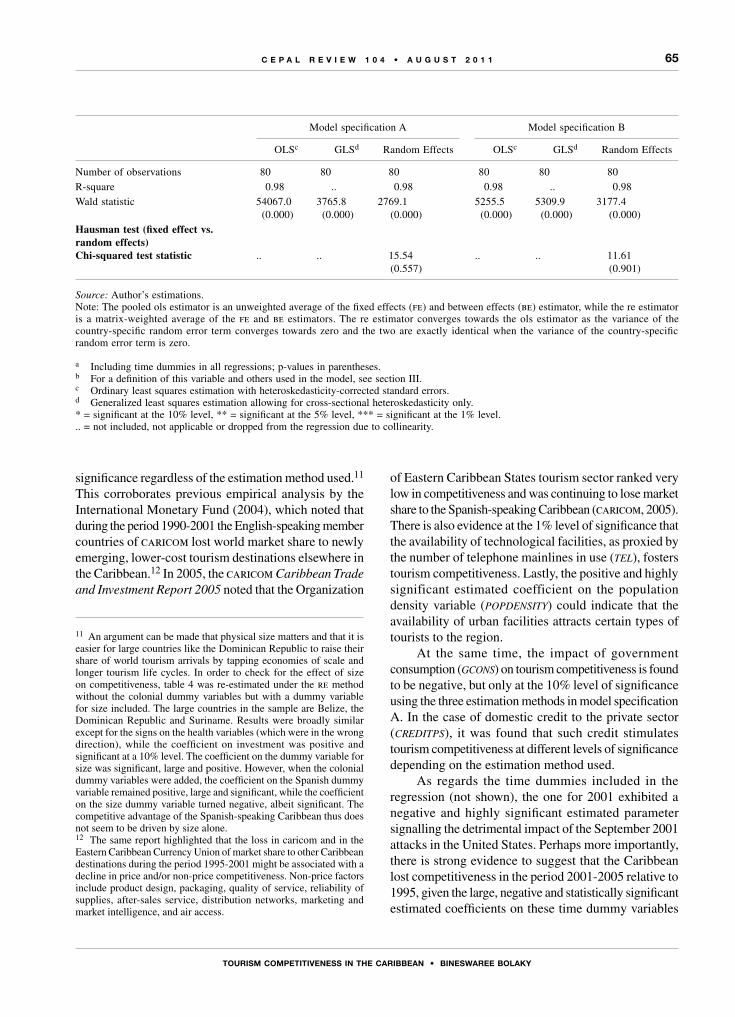
65
ToURISM CoMPETITIVEnESS In ThE CARIbbEAn • bInESWAREE boLAky
C E P A L R E V I E W 1 0 4 • A U G U S T 2 0 1 1
significance regardless of the estimation method used.11 This corroborates previous empirical analysis by the International Monetary Fund (2004), which noted that during the period 1990-2001 the English-speaking member countries of caricom lost world market share to newly emerging, lower-cost tourism destinations elsewhere in the Caribbean.12 In 2005, the caricom Caribbean Trade and Investment Report 2005 noted that the Organization
11 An argument can be made that physical size matters and that it is easier for large countries like the Dominican Republic to raise their share of world tourism arrivals by tapping economies of scale and longer tourism life cycles. In order to check for the effect of size on competitiveness, table 4 was re-estimated under the re method without the colonial dummy variables but with a dummy variable for size included. The large countries in the sample are Belize, the Dominican Republic and Suriname. Results were broadly similar except for the signs on the health variables (which were in the wrong direction), while the coefficient on investment was positive and significant at a 10% level. The coefficient on the dummy variable for size was significant, large and positive. However, when the colonial dummy variables were added, the coefficient on the Spanish dummy variable remained positive, large and significant, while the coefficient on the size dummy variable turned negative, albeit significant. The competitive advantage of the Spanish-speaking Caribbean thus does not seem to be driven by size alone. 12 The same report highlighted that the loss in caricom and in the Eastern Caribbean Currency Union of market share to other Caribbean destinations during the period 1995-2001 might be associated with a decline in price and/or non-price competitiveness. Non-price factors include product design, packaging, quality of service, reliability of supplies, after-sales service, distribution networks, marketing and market intelligence, and air access.
of Eastern Caribbean States tourism sector ranked very low in competitiveness and was continuing to lose market share to the Spanish-speaking Caribbean (caricom, 2005). There is also evidence at the 1% level of significance that the availability of technological facilities, as proxied by the number of telephone mainlines in use (tel), fosters tourism competitiveness. Lastly, the positive and highly significant estimated coefficient on the population density variable (popdensity) could indicate that the availability of urban facilities attracts certain types of tourists to the region.
At the same time, the impact of government consumption (gcons) on tourism competitiveness is found to be negative, but only at the 10% level of significance using the three estimation methods in model specification A. In the case of domestic credit to the private sector (creditps), it was found that such credit stimulates tourism competitiveness at different levels of significance depending on the estimation method used.
As regards the time dummies included in the regression (not shown), the one for 2001 exhibited a negative and highly significant estimated parameter signalling the detrimental impact of the September 2001 attacks in the United States. Perhaps more importantly, there is strong evidence to suggest that the Caribbean lost competitiveness in the period 2001-2005 relative to 1995, given the large, negative and statistically significant estimated coefficients on these time dummy variables
Model specification A Model specification B
OLSc GLSd Random Effects OLSc GLSd Random Effects
Number of observations 80 80 80 80 80 80R-square 0.98 .. 0.98 0.98 .. 0.98Wald statistic 54067.0
(0.000)3765.8
(0.000)2769.1
(0.000)5255.5
(0.000)5309.9
(0.000)3177.4
(0.000)Hausman test (fixed effect vs. random effects)Chi-squared test statistic .. .. 15.54
(0.557).. .. 11.61
(0.901)
Source: Author’s estimations. Note: The pooled ols estimator is an unweighted average of the fixed effects (fe) and between effects (be) estimator, while the re estimator is a matrix-weighted average of the fe and be estimators. The re estimator converges towards the ols estimator as the variance of the country-specific random error term converges towards zero and the two are exactly identical when the variance of the country-specific random error term is zero.
a Including time dummies in all regressions; p-values in parentheses. b For a definition of this variable and others used in the model, see section III.c Ordinary least squares estimation with heteroskedasticity-corrected standard errors. d Generalized least squares estimation allowing for cross-sectional heteroskedasticity only. * = significant at the 10% level, ** = significant at the 5% level, *** = significant at the 1% level... = not included, not applicable or dropped from the regression due to collinearity.

66
ToURISM CoMPETITIVEnESS In ThE CARIbbEAn • bInESWAREE boLAky
C E P A L R E V I E W 1 0 4 • A U G U S T 2 0 1 1
(significant at the 1% level using either the ols or the gls estimation method). This is a worrying outcome.
All in all, two surprising results stand out. First, there is no evidence that higher levels of investment (inv) in the Caribbean will benefit the tourism sector in terms of competitiveness. Second, real income growth in the source markets (y) is not statistically significant in affecting tourism competitiveness in the region. Thus, real income growth in the source markets on average does not seem to impact on tourism competitiveness at all. It is possible, however, that the inclusion of the time dummy variables is capturing the impact of world business economic cycles, which are strongly correlated with real income growth in countries such as Canada, the United Kingdom and the United States, and that such inclusion is rendering the income variables insignificant due to collinearity.
To address this latter issue, another regression specification (b) was estimated disaggregating both the income growth variable (y) and the real exchange rate variable (rer) used in specification A into their individual source market components. Accordingly, variable Y was disaggregated into real income growth in Canada (ycan), the United Kingdom (yuk) and the United States (yus). However, since the series on real income growth in the first two countries failed to pass the Levin-Lin-Chu test for stationarity, only real income growth in the United States was included, along with real income growth in the world (yw), as the two series showed stationary behaviour. The latter variable was used as a proxy variable for real income growth in Canada and the United Kingdom. The simple correlation coefficient between yw and ycan and between yw and yuk is 0.54 in both cases, and it is statistically significant at the 5% level. By the same token, the real exchange rate index (rer) was disaggregated into the three bilateral real exchange rates between the local currency and the currency of each source market (rercan, reruk, rerus), which were included in the regression specification. In addition, three transport cost variables were included —one for each source market (tccan , tcuk , tcus)— combining oil price trends and the distance between the source and destination markets (see table 3 for details), in place of the single proxy variable gpoil used in specification A. The results are shown in table 4.
As can be seen, there is strong evidence13 that tourism competitiveness in the Caribbean is significantly (at the 1% level) positively correlated with population density
13 The coefficients are significant across all three estimation methods at levels of significance of 10% or less.
(popdens) and technological facilities (tel) and negatively correlated with openness to trade (tradeopen), rigidities in the labour market (empindex), vulnerability to natural disasters (evid) and hiv/aids prevalence (aids). All these results are consistent with the previous findings from the estimation of specification A using the ols, gls or re methods. The high positive and statistically significant impact of the former Spanish colony dummy variable (colspain) is also confirmed. However, the negative impact found in specification A for the former British colonies (coluk) is corroborated only using the ols and re model estimations, but not when applying the gls method (actually, the sign of the estimated coefficient is positive and significant at the 10% level). In addition, government consumption (gcons) is found to negatively affect tourism competitiveness at the 5% level of significance (at the 10% level in specification A), whereas the surprising result found in the estimation of specification A about the insignificant effect of investment (inv) on tourism competitiveness is confirmed. Notwithstanding, under specification B most of the time dummy variables are no longer significant except for the time dummy for year 2004 (results not shown in table 4), which showed a negative estimated coefficient. This may be related to the impacts of hurricanes Jeanne, Ivan, Frances and Charley in that year. The year 2004 was marked by an unusually active hurricane season with all four hurricanes striking within a two-month period.14
Perhaps more interesting are the results that differ from the previous estimation, i.e. specification A. There is partial evidence from the ols and gls estimations that both real income growth in the United States and in the world —a rough proxy for income growth rates in Canada and the United Kingdom, which exhibited non-stationary behaviour— raise tourism competitiveness in the Caribbean, though just at the 10% level of significance. In addition, there is evidence to suggest that British and Canadian tourists are more sensitive to increases in transport costs induced by higher oil prices than are their American counterparts. This is revealed by the negative coefficients associated with tccan and tcuk in both the ols and the gls estimations, which are statistically different from zero at the 10% level of significance (at the 5% level of significance in the case of tcuk using the ols method). The latter result does
14 The Economic Commission for Latin America and the Caribbean (eclac) estimated losses to have been more than US$ 2.2 billion in 2004 from the hurricanes, which struck four countries (Bahamas, Dominican Republic, Grenada and Jamaica), three of which are included in our sample.

67
ToURISM CoMPETITIVEnESS In ThE CARIbbEAn • bInESWAREE boLAky
C E P A L R E V I E W 1 0 4 • A U G U S T 2 0 1 1
not hold, however, using the re estimation method. Thus, increases in transport costs would deter British and Canadian tourists from travelling to the Caribbean and induce them to shift to relatively less-distant non-Caribbean destinations (such as Spain or the United States) with lower airfares.
By the same token, there is some indication that higher transport costs resulting from higher oil prices may actually induce American tourists to switch to nearer, Caribbean destinations relative to more-distant, non-Caribbean countries, as revealed by the positive estimated coefficients associated with tcus (though this coefficient is significant only at the 10% level in the ols estimation method). Canadian tourists seem to be the most price-sensitive as compared with their American and British counterparts. Indeed, it is found that a real appreciation of the local currency relative to the Canadian currency has a large and significant (at the 1% level) negative impact on tourism competitiveness under all three estimation methods.
In contrast, British and, especially, American tourists seem to be price-insensitive.15 This could reflect differences in the income segments of tourists targeted by the destination across its source markets. Canadian travellers to the Caribbean tend to be low-budget travellers who target the low-cost end of the tourism market and concentrate mostly on the Spanish-speaking Caribbean with its range of low-to-medium-budget accommodation. In fact, some 60% of Canadians travelling to the Caribbean end up in either Cuba or the Dominican Republic, according to the Caribbean Tourism Organization. Dependency on the Canadian source market is generally low in the non-Spanish-speaking Caribbean (it is less than 10% for most countries, save Guyana, Haiti and the Turks and Caicos) (eclac, 2008b). Conversely, British tourists to the Caribbean are more likely to be upper-income travellers targeting the high end of the market, with Barbados as their destination of choice. Of course, low-budget travellers are expected to be far more price-sensitive than travellers from the upper end of the market.
3. robustness checks
Two robustness checks are now performed on the results. The first is to control for potential endogeneity between some explanatory variables and the error disturbance term. Under the standard assumptions of the classical
15 Although the negative estimated coefficient associated with tcuk is significant at the 10% level in the gls estimation method.
linear regression model, estimation by ordinary least squares yields unbiased and efficient estimators for the parameters on the explanatory variables as long as there is no contemporaneous correlation between the explanatory variables and the error disturbance term and such explanatory variables are determined exogenously to the estimation model. However, such an assumption is usually violated if there are omitted variables from the model that turn out to be contemporaneously correlated with the explanatory variables included in the model and/or if the dependent variable is thought to contemporaneously influence the explanatory variables. To address such sources of potential endogeneity, models A and B again are estimated using one-period-lagged values for the explanatory variables that are time-variant within a given panel and that can potentially be influenced contemporaneously by the dependent variable. Such explanatory variables are: the bilateral real exchange rates, trade openness, domestic credit to the private sector, the share of gross fixed capital formation in gdp and the share of government final consumption expenditure in gdp. The remaining time-variant variables within the panels, namely the transport costs (which vary with growth in oil prices only), the growth in real income in the source markets and population density are taken to satisfy the condition of exogeneity. It is reasonable to argue that growth in oil prices and income growth rates in the source markets are unlikely to be correlated with the determinants of competitiveness specific to each Caribbean tourism destination. Oil prices are set by world demand and world supply forces that Caribbean destinations take as exogenous, while income growth in Canada, the United Kingdom and the United States is unlikely to be influenced or correlated with Caribbean-specific competitiveness conditions. Population density for a given destination is likely to change slowly over a 10-year period (as land size is fixed), while changes in population are slow and determined exogenously to tourism competitiveness conditions.
Table 5 reports the results when the potentially endogenous explanatory variables are lagged by one year.
Comparing table 4 with table 5, it can be seen from model A that the results remain broadly robust. The main differences are that, under model B, the evidence that appreciation of the local currency relative to the Canadian currency significantly undermines tourism competitiveness of the local destination vanishes and, for the first time, it is found that increases in gross fixed capital formation in gdp could significantly raise tourism competitiveness (using the gls method).

68
ToURISM CoMPETITIVEnESS In ThE CARIbbEAn • bInESWAREE boLAky
C E P A L R E V I E W 1 0 4 • A U G U S T 2 0 1 1
TABLE 5
regression resultsa
(Dependent variable Sij b; sample 1996-2006; annual frequency)
Model specification A Model specification B
OLSc GLSd Random Effects OLSc GLSd Random Effects
yj -0.0007(0.234)
0.0001(0.795)
-0.0007(0.335)
.. .. ..
yus .. .. .. 0.2569(0.109)
0.2347(0.130)
0.2569(0.259)
yw .. .. .. 1.1187*(0.067)
0.9221(0.119)
1.1187(0.196)
gpoilj -0.0014***(0.000)
-0.0011***(0.000)
-0.0014***(0.001)
.. .. ..
tcuk,j .. .. .. -0.0054*(0.067)
-0.0042(0.143)
-0.0054(0.182)
tcus,j .. .. .. 0.0662*(0.078)
0.0496(0.168)
0.0662(0.184)
tccan,j .. .. .. -0.0387*(0.057)
-0.0300(0.125)
-0.0387(0.160)
Lagged rerj 0.0005***(0.000)
0.0003*(0.014)
0.0004***(0.000)
.. .. ..
Lagged reruk,j .. .. .. 0.0041(0.894)
-0.0294(0.275)
0.0041(0.902)
Lagged rerus,j .. .. .. -0.0118(0.861)
0.0206(0.716)
-0.0118(0.861)
Lagged rercan,j .. .. .. 0.0539(0.521)
0.0783(0.263)
0.0539(0.513)
Lagged invj 0.0011(0.384)
0.0023(0.957)
0.0011(0.499)
0.0015(0.184)
0.0028***(0.002)
0.0015(0.343)
Lagged gconsj -0.0088***(0.009)
-0.0079**(0.013)
-0.0088**(0.027)
-0.0110***(0.000)
-0.0077***(0.002)
-0.0110***(0.003)
Lagged tradeopenj -0.0011***(0.000)
-0.0011***(0.000)
-0.0011***(0.000)
-0.0010***(0.000)
-0.0010***(0.000)
-0.0010***(0.000)
popdensj 1.5940***(0.000)
1.2653***(0.000)
1.5940***(0.000)
1.6839***(0.000)
0.9991***(0.000)
1.6839***(0.000)
Lagged creditpsj 0.0029**(0.019)
0.0026**(0.020)
0.0029**(0.044)
0.0031**(0.005)
0.0029***(0.002)
0.0031**(0.028)
emplindexj -0.5875***(0.000)
-0.4681***(0.000)
-0.5875***(0.000)
-0.6140***(0.000)
-0.3689***(0.000)
-0.6140***(0.000)
colspainj 16.6041***(0.000)
.. 16.6041***(0.000)
12.437***(0.000)
.. 12.4368***(0.000)
colukj .. -13.2328***(0.000)
.. -4.9507***(0.000)
-10.3839***(0.000)
-4.9507***(0.000)
evidj -4.2998***(0.000)
-3.4032***(0.000)
-4.2998***(0.000)
-4.4926***(0.000)
-2.6660***(0.000)
-4.4926***(0.000)
aidsj -0.0117***(0.000)
-0.0089***(0.000)
-0.0117***(0.000)
-0.0122***(0.000)
-0.0067***(0.000)
-0.0122***(0.000)
tuberj -0.0004(0.703)
-0.0005(0.611)
-0.0004(0.756)
-0.0007(0.519)
-0.0005(0.575)
-0.0007(0.616)
telj 0.1410***(0.000)
0.1101***(0.000)
0.1410***(0.000)
0.1464***(0.000)
0.0852***(0.000)
0.1464***(0.000)
Number of observations 72 72 72 80 80 80R-square 0.98 .. 0.98 0.98 .. 0.98Wald statistic 4294.2
(0.000)4266.5
(0.000)2938.0
(0.000)6176.0
(0.000)4368.2
(0.000)3512.8
(0.000)
Source: Author’s estimations. Note: The Hausman tests failed and thus are not reported.
a Including time dummies in all regressions. The estimated coefficients of the dummies on years 2004 and 2005 were negative and significant at a 10% level in all three cases in model A. The estimated coefficient on year 2004 was negative and significant at a 10% level in two cases in model B. P-values in parentheses.
b For a definition of this variable and others used in the model, see section III.c Ordinary least squares estimation with heteroskedasticity-corrected standard errors. d Generalized least squares estimation allowing for cross-sectional heteroskedasticity only. * = significant at the 10% level, ** = significant at the 5% level, *** = significant at the 1% level... = not included, not applicable or dropped from the regression due to collinearity.

69
ToURISM CoMPETITIVEnESS In ThE CARIbbEAn • bInESWAREE boLAky
C E P A L R E V I E W 1 0 4 • A U G U S T 2 0 1 1
A second robustness check consists of testing for the sensitivity of the results to the potential presence of influential observations in the data. The figure below
plots leverage points against the normalized standard residuals when estimating models A and B by the ols method.
FIGURE1
Leverage versus normalized standard residuals plots
Model A
Model B
Source: Prepared by the author.Note: These are obtained by estimating models A and B as described in table 4 using the ols method only
Normalized residual squared
.050
1
.8
Lev
erag
e
.6
.4
.2
.1 .15 .2
1
.8
Lev
erag
e
.6
.4
.2
Normalized residual squared
.02 .040 .06 .08 .1

70
ToURISM CoMPETITIVEnESS In ThE CARIbbEAn • bInESWAREE boLAky
C E P A L R E V I E W 1 0 4 • A U G U S T 2 0 1 1
Points in the upper left-hand corner signal the presence of leverage points,16 while points in the lower right corner signal unusually high normalized standard residuals. From these plots, visually there are several observations that can potentially be influential (high leverage and/or high standardized residuals). To control for influential observations, the estimations are carried out as in table 4, this time omitting variables with a Cook’s statistic that exceeds the cut-off value of 4/n, where n is the sample size (in this case 80), as is standard procedure.17 The results are reported in table 6.
Comparing table 6 with table 4, it can be seen that the results are fairly robust using both models. Results from model specification B show some slight differences as compared with table 4, though. After controlling for influential observations, there is partial evidence that increases in gross fixed capital formation in gdp can benefit tourism competitiveness (using the gls method). In addition, there is evidence that growth in incomes in the United States and worldwide results in a greater share of tourists landing in the Caribbean. Both income growth variables are significant at either the 10% or the 5% level.
In table 7, both endogeneity and influential observations are controlled for as compared with table 4. Doing so yields a set of robust results. There is firm evidence that tourism competitiveness in the Caribbean is significantly hampered by growth in oil prices, increases in government final consumption expenditure in gdp, trade openness, rigidity in employment and labour market conditions, exposure to natural disasters and health concerns (such as hiv/aids) in the destination country. At the same time, competitiveness benefits from increases in gross fixed capital formation in gdp, credit support to the private sector, population density and better infrastructure as mirrored by increases in the number of telephone mainlines in the destination country. There is also firm evidence that Spanish-speaking countries have
16 According to Kennedy (2007), there are two kinds of outliers that may have a strong influence on estimates produced by the ols method. The first type of outlier consists of observations with unusually large errors, and the second type consists of leverage points, that is, observations with unusual values on an explanatory variable. What should be controlled for are not outliers per se but rather influential observations, i.e. outliers that have a strong influence on ols estimates. Such influential observations are data points whose removal from the estimation would dramatically alter the coefficients obtained from the regression model.17 The ols method is used to estimate models A and B in table 4 and to calculate the Cook’s statistic for these two models respectively. Then, table 4 is estimated again by omitting variables with a Cook’s statistic exceeding 0.05 (4/80). For a definition and explanation of the Cook’s statistic, see Cook (1977).
a comparative advantage relative to the English-speaking countries in the Caribbean. There is partial evidence that British tourists may be price-insensitive in the sense that a real appreciation of the destination currency relative to the pound sterling does not deter them from spending their holidays in the Caribbean. In addition, there is partial evidence to suggest that Canadian tourists are more price-sensitive relative to American and British tourists and that a real appreciation of the local destination currency relative to the Canadian dollar induces them to substitute with non-Caribbean destinations. However, there is no evidence from model B that income growth in source markets matters or that geographical distance by source market matters as opposed to growth in oil prices alone. No evidence is found from model A that the weighted average of bilateral real exchange rates exerts a significant impact on tourism competitiveness. These three findings are inconsistent with some of the previous findings shown in tables 4 - 6.
Summing up the results from tables 5 and 7, the robustness checks actually enhance the significance of most of the explanatory variables used and with signs in the expected direction. However, in the case of the income growth variables, real exchange rates and transport costs by source market, the evidence obtained is mixed.
Based on the re estimation under model A in table 7,18 in terms of the impacts that are significant at least at a 1% level, we find that:(i) An increase in the rate of growth of oil prices leads
to a fall in the share of world outbound American, British and Canadian tourists travelling to the Caribbean. This is in line with the notion that price and cost competitiveness are important elements of competitiveness (Craigwell, 2007). Faster oil price increases impact on the costs of air travel and can result in airlines reducing the frequency of flights to the Caribbean, thereby reducing the attractiveness of the region as a destination (Odle, 2008). Research by Browne, Edwards and Moore (2009) and by Mitchell (2010) reported evidence that unexpected shocks such as oil price shocks can have transitory effects on tourism in a few Caribbean destinations. A report by the World Tourism Organization in 2006 noted, for instance, that one of the short-term risks created with the increase in oil prices is that the frequency of tourist
18 Among all sets of results, greater weight is given to those estimated from the equation that controls for endogeneity and influential observations and that allows for country-specific effects (i.e. results from table 7 under the re method).

71
ToURISM CoMPETITIVEnESS In ThE CARIbbEAn • bInESWAREE boLAky
C E P A L R E V I E W 1 0 4 • A U G U S T 2 0 1 1
TABLE 6
regression resultsa
(Dependent variable Sij b; sample 1995-2006; annual frequency)
Model specification A Model specification B
OLSc GLSd Random Effects OLSc GLSd Random Effects
yj -0.0006(0.121)
-0.0003(0.399)
-0.0006(0.226)
.. .. ..
yus .. .. .. 0.3984**(0. 029)
0.3030*(0.067)
0.3984*(0.090)
yw .. .. .. 1.5944**(0.020)
1.1521*(0.065)
1.5944*(0.070)
gpoilj -0.0016(0.168)
-0.0018*(0.088)
-0.0016(0.267)
.. .. ..
tcuk,j .. .. .. -0.0077**(0.021)
-0.0053*(0.079)
-0.0077*(0.064)
tcus,j .. .. .. 0.109**(0.015)
0.0430*(0.051)
0.1095*(0.055)
tccan,j .. .. .. -0.0606**(0.013)
-0.0430*(0.051)
-0.0606*(0.053)
rerj 0.0004***(0.000)
0.0003***(0.000)
0.0004***(0.000)
.. .. ..
reruk,j .. .. .. -0.0478*(0.094)
-0.0601**(0.022)
-0.0478*(0.100)
rerus,j .. .. .. -0.0388(0.565)
0.0483(0.413)
-0.0388(0.563)
rercan,j .. .. .. 0.2241***(0.005)
0.1573**(0.021)
0.2241***(0.008)
invj -0.0001(0.934)
-0.0004(0.683)
-0.0001(0.948)
0.0010(0.283)
0.0021**(0.012)
0.0010(0.440)
gconsj -0.0082***(0.003)
-0.0093***(0.000)
-0.0082***(0.005)
-0.0098***(0.002)
-0.0063**(0.023)
-0.0098**(0.013)
tradeopenj -0.0014***(0.000)
-0.0013***(0.000)
-0.0014***(0.000)
-0.0011***(0.000)
-0.0011***(0.000)
-0.0011***(0.000)
popdensj 1.0279***(0.000)
0.8007***(0.000)
1.0279***(0.000)
1.6368***(0.000)
1.0816***(0.000)
1.6368***(0.000)
creditpsj 0.0040***(0.000)
0.0033***(0.000)
0.0040***(0.000)
0.0019*(0.079)
0.0012(0.215)
0.0019(0.154)
emplindexj -0.3748***(0.000)
-0.2922***(0.000)
-0.3748***(0.000)
-0.5992***(0.000)
-0.4076***(0.000)
-0.5992***(0.000)
colspainj 10.2161***(0.000)
7.8508***(0.000)
20.0426***(0.000)
17.0588***(0.000)
11.7165***(0.000)
..
colukj .. .. 9.8265***(0.000)
.. .. -17.0588***(0.000)
evidj -2.7267***(0.000)
-2.1065***(0.000)
-2.7267***(0.000)
-4.3757***(0.000)
-2.9453***(0.000)
-4.3757***(0.000)
aidsj -0.0067***(0.000)
-0.0049***(0.003)
-0.0067***(0.001)
-0.0121***(0.000)
-0.0081***(0.000)
-0.0121***(0.000)
tuberj 0.0011(0.217)
0.0011(0.200)
0.0011(0.339)
-0.0012(0.278)
-0.0020**(0.044)
-0.0012(0.376)
telj 0.0917***(0.000)
0.0712***(0.000)
0.0917***(0.000)
0.1427***(0.000)
0.0936***(0.000)
0.1427***(0.000)
Number of observations 73 73 73 68 68 68R-square 0.99 .. 0.99 0.99 .. 0.99Wald statistic 8011.5
(0.000)8004.1
(0.000)8574.1
(0.000)4592.2
(0.000)4554.1
(0.000)4663.3
(0.000)
Source: Author’s estimations. Note: The Hausman tests failed and thus are not reported.
a Including time dummies in all regressions. The dummies on years 2001-2005 were negative and significant at a 1% level in all three cases in model A. The dummy on year 2004 was negative and significant at a 5% level in two cases in model B. P-values in parentheses.
b For a definition of this variable and others used in the model, see section III.c Ordinary least squares estimation with heteroskedasticity-corrected standard errors. d Generalized least squares estimation allowing for cross-sectional heteroskedasticity only. * = significant at the 10% level, ** = significant at the 5% level, *** = significant at the 1% level... = not included, not applicable or dropped from the regression due to collinearity.

72
ToURISM CoMPETITIVEnESS In ThE CARIbbEAn • bInESWAREE boLAky
C E P A L R E V I E W 1 0 4 • A U G U S T 2 0 1 1
TABLE 7
regression resultsa
(Dependent variable Sij b; sample 1996-2006; annual frequency)
Model specification A Model specification B
olsc glsd Random Effects olsc glsd Random Effects
yj -0.0004(0.449)
0.0004(0.272)
-0.0004(0.558)
.. .. ..
yus .. .. .. 0.2021(0. 212)
0.2122(0.168)
0.2021(0.355)
yw .. .. .. 0.8413(0.177)
0.8093(0.171)
0.8413(0.322)
gpoilj -0.0013***(0.000)
-0.0008***(0.088)
-0.0013***(0.000)
.. .. ..
tcuk,j .. .. .. -0.0040(0.179)
-0.0036(0.201)
-0.0040(0.312)
tcus,j .. .. .. 0.0602(0.134)
0.0508(0.163)
0.0602(0.258)
tccan,j .. .. .. -0.0350(0.109)
-0.0302(0.129)
-0.0350(0.232)
Lagged rerj -0.0000(0.879)
-0.0001(0.286)
-0.0000(0.928)
.. .. ..
Lagged reruk,j .. .. .. -0.0198(0.537)
-0.0487*(0.090)
-0.0198*(0.539)
Lagged rerus,j .. .. .. -0.0408(0.589)
0.0551(0.360)
-0.0408(0.570)
Lagged rercan,j .. .. .. 0.1378*(0.098)
0.0804(0.250)
0.1378*(0.097)
Lagged invj 0.0039***(0.000)
0.0041***(0.000)
0.0039***(0.012)
0.0031***(0.001)
0.0031***(0.000)
0.0031**(0.034)
Lagged gconsj -0.0110***(0.002)
-0.0070**(0.019)
-0.0082***(0.005)
-0.0104***(0.000)
-0.0066***(0.007)
-0.0104***(0.004)
Lagged tradeopenj -0.0008***(0.000)
-0.0010***(0.000)
-0.0110**(0.011)
-0.0010***(0.000)
-0.0011***(0.000)
-0.0010***(0.000)
popdensj 1.3620***(0.000)
0.9654***(0.000)
1.3620***(0.000)
1.5435***(0.000)
0.9343***(0.000)
1.5435***(0.000)
Lagged creditpsj 0.0041***(0.000)
0.0025***(0.004)
0.0041***(0.003)
0.0027**(0.014)
0.0025***(0.007)
0.0027*(0.067)
emplindexj -0.4975***(0.000)
-0.3565***(0.000)
-0.4975***(0.000)
-0.5644***(0.000)
-0.3476***(0.000)
-0.5644***(0.000)
colspainj 13.8995***(0.000)
10.0422***(0.000)
13.8995***(0.000)
16.0136***(0.000)
9.8202***(0.000)
28.0555***(0.000)
colukj .. .. .. .. .. -17.0588***(0.000)
evidj -3.6248***(0.000)
-2.5662***(0.000)
-3.6248***(0.000)
-4.1155***(0.000)
-2.5058***(0.000)
-4.1155***(0.000)
aidsj -0.0092***(0.000)
-0.0062***(0.001)
-0.0092***(0.001)
-0.0111***(0.000)
-0.0063***(0.001)
-0.0111***(0.000)
tuberj 0.0001(0.894)
-0.0006(0.474)
0.0001(0.921)
-0.0010(0.309)
-0.0009(0.263)
-0.0010(0.442)
telj 0.1173***(0.000)
0.0810***(0.000)
0.1173***(0.000)
0.1330***(0.000)
0.0793***(0.000)
0.1330***(0.000)
Number of observations 66 66 66 68 68 68R-square 0.99 .. 0.99 0.99 .. 0.99Wald statistic 11671.7
(0.000)11838.1
(0.000)3140.4
(0.000)4869.7
(0.000)4832.1
(0.000)6540.0
(0.000)
Source: Author’s estimations.Note: The Hausman tests failed and thus are not reported.
a Including time dummies in all regressions. The estimated coefficient for 2004 was negative and significant at the 10% level using either the ols or the gls estimation method in model A. The coefficient for 2005 was similarly negative and significant at a 10% level for the ols and gls estimations. In model B, the estimated coefficients for 2004 and 2005 were both negative and significant at the 10% level only using the ols method. P-values in parentheses.
b For a definition of this variable and others used in the model, see section III.c Ordinary least squares estimation with heteroskedasticity-corrected standard errors. d Generalized least squares estimation allowing for cross-sectional heteroskedasticity only. * = significant at the 10% level, ** = significant at the 5% level, *** = significant at the 1% level... = not included, not applicable or dropped from the regression due to collinearity.

73
ToURISM CoMPETITIVEnESS In ThE CARIbbEAn • bInESWAREE boLAky
C E P A L R E V I E W 1 0 4 • A U G U S T 2 0 1 1
visits to some of the developing countries would decline as prices increased, making their tourism products less competitive with other destinations geographically closer to the major generating markets (unwto, 2006).
(ii) An increase in the share of gross fixed capital formation in gdp causes the share of world outbound American, British and Canadian tourists travelling to the Caribbean to increase in the following year, while a fall in the share of government final consumption expenditure in gdp increases the Caribbean’s share of world outbound American, British and Canadian tourist arrivals in the following year. This evidence corroborates the policy recommendation made by the World Bank in its 2005 report on Caribbean competitiveness that policy regimes need to focus on public goods (such as infrastructure) rather than on incentives (World Bank, 2005). Investments that lead to improvements in the general infrastructure of a destination raise returns for the whole tourism sector as opposed to targeted public incentives, which raise returns for single private operators only. Focusing on general infrastructure rather than incentives provides a more holistic approach to raising destination competitiveness. Khadaroo and Seetanah (2008) found evidence as well that various forms of infrastructure, including transport infrastructure, are significant determinants of tourism demand for a given destination. However, a word of caution is in order here. This result is not taken to imply that governments do not have an important role in further stimulating competitiveness in the Caribbean, but rather it sheds light on the form that such government support should take. As noted in the World Bank report, the role played by governments in deepening the tourism benefits from emerging market niches is likely to become more complex. Governments have a key role to play in terms of setting the long-term strategic vision for the sector, stimulating linkages between tourism and the rest of the economy and building public-private partnerships in the sector.
(iii) A fall in the ratio of exports and imports to gdp causes the world share of outbound American, British and Canadian tourists travelling to the Caribbean to increase in the following year. The result is interpreted to imply that greater trade openness can harm tourism competitiveness.19 The
19 Greater trade openness can undermine local private sector development and the use of local products by foreign investors and
high import leakage rates in Caribbean tourism (Meyer, 2006) signal an overuse of imported inputs to the detriment of locally sourced ones in the sector. In order to build competitiveness, the Caribbean needs to go beyond the traditional fare of mass tourism based on “sand, sun and sea” driven by foreign direct investment and heavy use of imported inputs and instead develop other stay-over segments, such as “culture and heritage tourism” and “community tourism”, based on small, local enterprise development and the use of local goods and services.20
(iv) Increased domestic credit to the private sector and higher population density favour increases in the share of world outbound American, British and Canadian tourists travelling to the Caribbean. This supports the argument that development of the local private sector enhances the attractiveness of a given destination. Tourism competitiveness upgrading strategies based on selling the “local authenticity” of the destination to tourists seeking a cultural experience, for instance, rely on the supply of a whole range of locally produced goods and services. The supply of cheaper local products by the domestic private sector can also lower the costs of doing business in a given destination by allowing tourism investors to substitute away from the use of more-expensive imported inputs facilitated by open trade policies. The World Tourism Organization has been promoting the use of public-private partnerships as a way to enhance tourism competitiveness (wto, 2000). A vibrant domestic private sector can be engaged to supply the finance and expertise needed to deepen the domestic tourism value chain. At the same time, higher population density —to the extent that it is associated with the supply of amenities and attractions— increases the attractiveness of a destination.
(v) An increase in the index of exposure to natural disasters, in reported new cases of hiv/aids and in labour market rigidities can cause, respectively, the share of world outbound British, American and Canadian tourists to fall. The negative impact of tropical storms and hurricanes on tourism arrivals in the Caribbean is obvious and has been well
can inhibit the development of the domestic tourism value chain, meaning the forging of linkages between the tourism sector and the rest of the local economy 20 See policy recommendation in World Bank (2005) and Bolaky (2008).

74
ToURISM CoMPETITIVEnESS In ThE CARIbbEAn • bInESWAREE boLAky
C E P A L R E V I E W 1 0 4 • A U G U S T 2 0 1 1
documented. Granvorka and Strobl (2010) found econometric evidence of a significant negative impact of hurricanes on tourism arrivals. The relevance of a competitive and flexible labour market (leading to competitive wage levels) for Caribbean tourism was highlighted earlier by Randall and Wendel (2003). Their paper noted in reference to the Eastern Caribbean Currency Union countries that, given the prevailing fixed exchange rate regimes, the Union should seek to enhance wage competitiveness.
(vi) An increase in the number of telephone mainlines in use can increase tourism competitiveness. This result captures the relevance of technology in enhancing the attractiveness of a destination
through, among others, its impact on utility costs. The International Monetary Fund (imf, 2004) noted a sensitivity of tourism demand in the Caribbean to telecommunications costs. The report stated that, in caricom, there was a statistically significant negative relationship between hotel accommodation and both electricity and non-residential telephone subscription costs, indicating a negative association between operating costs and tourist arrivals.
(vii) The competitive advantage of the Spanish-speaking Caribbean relative to the English-speaking Caribbean is confirmed. This advantage persists even when differences in physical scale are controlled for.
VConclusions: Main Drivers of Tourism
Competitiveness in the Caribbean and Policy
recommendations
This article has focused on only one ex post competitiveness indicator (namely, share in world arrivals), whereas it will be important to assess as well the factors that affect other measures of competitiveness, such as the share of tourism expenditure in gdp. Given the significance of the tourism sector in the Caribbean, there is an urgent need to undertake detailed country case studies in order to carefully analyse the determinants of tourism competitiveness by source market in most Caribbean countries.
Based on the above econometric results, the main findings are:(i) A real exchange rate depreciation could increase
tourism competitiveness, but only in relation to stay-over arrivals of Canadian tourists. In contrast, British tourists tend to be price-insensitive with regard to exchange rate fluctuations;
(ii) When increases in transport costs are linked to hikes in oil prices, there is a drop in stay-over arrivals, especially from Canada and the United Kingdom. It may be the case that this fosters tourism from the United States, as the Caribbean is a closer destination, with presumably lower air fares;
(iii) Former Spanish colonies seem to have an advantage in terms of tourism competitiveness over former British colonies;
(iv) Other factors that negatively and robustly affect tourism competitiveness in the Caribbean include government consumption, trade openness, rigidities in the labour market and non-price factors such as environmental safety (measured by exposure to natural disasters and by the hiv/aids prevalence rate);
(v) Other factors that positively and robustly affect tourism competitiveness in the Caribbean include population density, domestic credit to the private sector, gross fixed capital formation in gdp and number of telephone mainlines in use;
(vi) There is no strong evidence that real income growth in source markets (i.e. Canada, the United Kingdom and the United States) plays a major role in tourism competitiveness behaviour in the Caribbean.There is evidence that Caribbean competitiveness
in stay-over tourism is slowing down; and this has been confirmed in previous studies by the International Monetary Fund, the World Bank and caricom. The region as a whole has not made any significant gains in the total world market share of stay-over arrivals for almost four decades. Thus, the Caribbean countries will need to find new ways to stimulate tourism competitiveness for greater economic gains. To maintain or enhance their tourism competitiveness, Caribbean destinations will need to become more cost- and price-competitive at

75
ToURISM CoMPETITIVEnESS In ThE CARIbbEAn • bInESWAREE boLAky
C E P A L R E V I E W 1 0 4 • A U G U S T 2 0 1 1
home. This may involve supporting local private sector development in order to reduce import leakage and build linkages between the tourism sector and the rest of the economy, reducing government consumption to maintain competitive tax rates, reducing vulnerability to natural disasters, reforming labour markets and business regulations in general, maintaining a healthy and safe environment, investing in human development and technology and developing a transport/aviation policy that will result in lower transport costs to and from the region and greater air access.
The Caribbean will also need to reduce its vulnerability to external factors that are not within its control, such as income shocks from abroad and oil price shocks. Small, English-speaking Caribbean countries are
particularly vulnerable, even more so in the context of the dominance of the larger, Spanish-speaking countries in the tourism sector, despite the embargo on Cuba. In the medium term, reducing vulnerability to external forces that can have a serious impact on tourism competitiveness will require further market diversification within the tourism sector as well as continually attracting price- and income-insensitive tourists from the upper end of the tourism markets. To this end, the creation and worldwide promotion of the “Caribbean brand” as a tourist destination would be very helpful and would also foster regional integration, a goal that has been pursued by Caribbean countries for decades.
(Original: English)
Bibliography
Archibald, Xiomara, Jason Lacorbinière and Winston Moore (2008), Analysis of Tourism Competitiveness in the Caribbean: A Gravity Model Approach, Bridgetown, Central Bank of Barbados/University of West Indies Cavehill Campus.
Bolaky, Bineswaree (2008), “Tourism life cycle, tourism competitiveness and upgrading strategies in the Caribbean” (LC/CAR/L.166), Port of Spain, eclac subregional headquarters for the Caribbean, December.
(2007), “Tourism in the Caribbean: competitiveness, upgrading, linkages and the role of public-private partnerships and public policy” (LC/CAR/L.151), Port of Spain, eclac subregional headquarters for the Caribbean, December.
Browne, Rudolph, Laisha Edwards and Winston Moore (2009), Tourism and Unexpected Shocks, Bridgetown, Department of Economics, University of the West Indies Cavehill Campus.
caricom (Caribbean Community) (2005), “The competitiveness of Caribbean countries”, Caribbean Trade and Investment Report 2005: Corporate Integration and Cross-Border Development, Georgetown.
Cervino, Julio and José María Cubillo (2005), “Hotel and tourism development in Cuba: opportunities, management challenges and future trends”, Cornell Hotel and Restaurant Administration Quarterly, vol. 46, No. 2, Michigan Gale Group, May.
Cook, R. Dennis (1977), “Detection of influential observations in linear regression”, Technometrics, vol. 19, No. 1, Alexandria, American Statistical Association.
Craigwell, Roland (2007), “Tourism competitiveness in small island developing states”, unu-wider Research Paper, No. 2007/19, Helsinki, United Nations University (unu)- World Institute for Development Economics Research (wider), April.
Craigwell, Roland and Delisle Worrell (2008), “The competitiveness of selected Caribbean tourism markets”, Social and Economic Studies, vol. 57, No. 1, Kingston, Sir Arthur Lewis Institute of Social and Economic Studies (salises).
De Albuquerque, Klaus and Jerome McElroy (1992), “Caribbean small-island tourism styles and sustainable strategies”, Environmental Management, vol. 16, No. 5, New York, Springer.
Duval, David Timothy (2005), Tourism in the Caribbean: Trends, Development, Prospects, London, Routledge.
Dwyer, Larry and Chulwon Kim (2003), “Destination competitiveness: determinants and indicators”, Current Issues in Tourism, vol. 6, No. 5, London, Routledge.
Dwyer, Larry, Peter Forsyth and Prasada Rao (2000), “The price competitiveness of travel and tourism destinations: a comparison of 19 destinations”, Tourism Management, vol. 21, No. 1, Amsterdam, Elsevier.
eclac (Economic Commission for Latin America and the Caribbean) (2008a), Structural Change and Productivity Growth, 20 Years Later: Old Problems, New Opportunities (LC/G.2367(SES.32/3)), Santiago, Chile.
(2008b), “Tourism life cycle, tourism competitiveness and upgrading strategies in the Caribbean” (LC/CAR.L.166), chapter 2, Port of Spain, eclac subregional headquarters for the Caribbean.
(2003), “Caribbean tourism, trends, policies and impact” (LC/CAR/G.765), Port of Spain, eclac subregional headquarters for the Caribbean, December.
Gooroochurn, Nishaal and Guntur Sugiyarto (2005), “Competitiveness indicators in the travel and tourism industry”, Tourism Economics, vol. 5, No. 11, London, IP Publishing Ltd.
(2004), “Measuring competitiveness in the travel and tourism industry”, Discussion Papers, No. 2004/7, Nottingham, Nottingham University Business School.
Granvorka, Charley and Eric Strobl (2010), The Impact of Hurricanes Strikes on the Tourism in the Caribbean, St. Augustine, Sir Arthur Lewis Institute of Social and Economic Studies (salises), March.
Griffith, Jennifer (2000), “The impact of vat on tourism in Barbados”, Central Bank of Barbados Working Papers, Barbados, Central Bank of Barbados.
imf (International Monetary Fund) (2004), “Eastern Caribbean currency union: selected issues”, imf Country Report, No. 04/335, Washington, D.C., April.

76
ToURISM CoMPETITIVEnESS In ThE CARIbbEAn • bInESWAREE boLAky
C E P A L R E V I E W 1 0 4 • A U G U S T 2 0 1 1
Jayawardena, Chandana (2002), “Mastering Caribbean tourism”, International Journal of Contemporary Hospitality Management, vol. 4, No. 2, Brighton, Emerald Publishing.
Kennedy, Peter (2007), A Guide to Econometrics, Oxford, Wiley-Blackwell Publishing.
Khadaroo, Jameel and Boopen Seetanah (2008), “The role of transport infrastructure in international tourism development: a gravity model approach”, Tourism Management, vol. 29, No. 5, Amsterdam, Elsevier, October.
Mangion, Marie-Louise, Ramesh Durbarry and M. Thea Sinclair (2004), “Tourism competitiveness: price and quality”, Discussion Papers, No. 2004/12, Nottingham, Nottingham University Business School.
McBain, Helen (2007), “Caribbean tourism and agriculture, linking to enhance development and competitiveness” (LC/CAR/L.076), Studies and Perspectives, No. 1, Port of Spain, eclac subregional headquarters for the Caribbean, March.
Meyer, Dorothea (2006), Caribbean Tourism, Local Sourcing and Enterprise Development: Review of the Literature, Sheffield, Centre for Tourism and Cultural Change, Sheffield Hallam University.
Mitchell, Travis (2010), “The resilience of Caribbean tourism to external shocks”, St. Augustine, Sir Arthur Lewis Institute of Social and Economic Studies (salises), March.
Odle, Maurice (2008), From Sub-prime to Sublime Disaster, Implications for the Caribbean Region of the Current Financial Crisis in the usa, Georgetown, Caribbean Community (caricom).
Randall, Ruby and Samuel Wendel (2003), “Tourism in the Eastern Caribbean: meeting the competitive threat”, Eastern
Caribbean Currency Union: Selected Issues, imf Country Report, No. 03/88, Washington, D.C., International Monetary Fund, March.
Romeu, Rafael (2008), “Vacation over: implications for the Caribbean of opening U.S.-Cuba Tourism”, imf Working Papers, WP/08/162, Washington, D.C., International Monetary Fund, July.
Rosensweig, Jeffrey (1988), “Elasticities of substitution in Caribbean tourism”, Journal of Development Economics, vol. 29, No. 1, Amsterdam, Elsevier, July.
Wilkinson, Paul F. (1997), Tourism Policy and Planning: Case Studies from the Commonwealth Caribbean, New York, Cognizant Communication Corporation.
World Bank (2005), A Time to Choose: Caribbean Development in the 21st Century”, Washington, D.C., April.
World Economic Forum (2007), The Travel & Tourism Competitiveness Report 2007: Furthering the Process of Economic Development, Geneva.
World Travel and Tourism Council (2009), Travel and Tourism Economic Impact Caribbean 2009, London.
(2006), Tourism Satellite Accounting, London. (2004), The Impact of Travel and Tourism on Jobs and the
Economy, London.wto (World Tourism Organization) (2006), The Impact of Rising
Oil Prices on International Tourism. Special Report number 26, Madrid.
(2000), Public-Private Sector Cooperation: Enhancing Tourism Competitiveness, Madrid.

C E P A L R E V I E W 1 0 4 • A U G U S T 2 0 1 1
77
Argentina: households and labour marketchanges (2004-2009)
Fernando Groisman
T his article outlines the changes that occurred in employment
between 2004 and 2009 and reviews the links that households established
with the labour market. An increase in the number of jobs registered with
the social security system was one of the key features of the period.
Moreover, half of the rise in the observed employment rate represented
jobs obtained by household members other than heads of household. The
increase in protected employment also benefited social sectors that have
traditionally been neglected, although there are factors that restrict the
access of certain population groups to such jobs. Another research finding
is that if the head of the household has a protected job, other household
members have better chances of gaining a similar job themselves.
KEYWORDS
Employment
Labour market
Employment creation
Households
Family
Family income
Social conditions
Employment statistics
Econometric models
Argentina
Fernando Groisman
National Council of Scientific and
Technical Research (conicet) and
University of Buenos Aires (uba)

78
ARGEnTInA: hoUSEhoLdS And LAboUR MARkET ChAnGES (2004-2009) • fERnAndo GRoISMAn
C E P A L R E V I E W 1 0 4 • A U G U S T 2 0 1 1
Any review of the social changes that have occurred in Argentina over the last few years must inevitably focus on the labour market, given the sustained recovery in the level of employment and progressive rebuilding of labour incomes that have taken place. A direct way to do this is by examining the trend of employment indicators that summarize the functioning of this market.1 The research is also enhanced when households are used as the unit of analysis, since it then becomes possible to study people’s patterns of participation in economic activity, in relation to the positions they occupy in the family structure or their contribution to the household’s monetary income, or both, among other potential dimensions of analysis. This article used this relatively less common approach,2 which provided new information on the type of linkages households established with the labour market during the economic upswing phase.
The characteristics of the economic recovery process following the 2001 crisis also make the proposed analysis timely. In addition to increases in the volume of the employment and higher wages, as mentioned above, another characteristic is the sharp rise in the number of jobs registered with the social security system. Such jobs represent higher quality employment, because, having been declared by employers, they enjoy the protection provided by labour laws; and persons working in those jobs also receive higher wages than their counterparts in precarious jobs. In the five-year period 2004-2009, the number of registered workers increased by 44.1%, whereas the number of workers in unregistered jobs grew by 6.8% (see table 1). The rate of growth of protected employment distinguishes this stage from previous episodes of recomposition of the level of economic activity, which have succeeded one another since the mid-1970s at least, when new employment mainly represented precarious jobs. Between 1970 and 2001, the
The author is grateful to an anonymous referee for comments made on a previous version of this article. Any remaining error or omission is the author’s exclusive responsibility.1 There is a direct link between the labour market and the social situation, which has been frequently discussed in the literature. Different approaches to this can be found in the work of Stallings and Weller (2001); Tokman (2006); Márquez and others (2007), among others.2 Although they had different emphases than those developed in this article, progress from this perspective can also be consulted in Arriagada (2007) and ilo/undp (2009).
share of unregistered jobs in the employment structure increased by 10 percentage points.3
The new labour-market scenario clearly reflects a trend change in the registration of employment relations compared to that prevailing in recent decades. Nonetheless, factors seem to persist in Argentine society that restrict or obstruct access to protected jobs by certain population groups. Although in 2009 the number of registered jobs matched the number of households that mainly depended on the labour income of their members (the ratio had been 0.7 in 2004),4 this increase was not generalized throughout the population as a whole.
Investigating why the creation of lower-quality jobs tended to be concentrated among a certain type of household should make it possible to recommend policies aimed at ensuring that economic growth generates higher levels of integration and social cohesion. This is the purpose of the rest of this article.
The information used in this article comes from the Permanent Household Survey (eph) conducted by the National Institute of Statistics and Censuses (indec). The eph is conducted in Argentina’s main cities, and encompasses about 70% of the total urban population. Since 2003, the survey has collected information continuously, producing quarterly estimates for certain variables and half-yearly estimates for others. This article used the micro-databases corresponding to the first quarters of 2004, 2005, 2006, 2007, 2008 and 2009. The period 2002-2003 was excluded from the analysis, because it corresponded to a period of rebound from the trough of the 2001 crisis in Argentina.5 This makes it possible to focus on the changes that occurred in Argentine society once a certain growth threshold had been achieved. The article thus provides an overview of the social situation and the changes that occurred in it in the period 2004-2009.
3 Data for the Greater Buenos Aires conurbation —the only information available for the period considered (Permanent Household Survey (eph) of the National Institute of Statistics and Censuses (indec)).4 Calculated as the quotient between registered wage-earning workers and households whose heads were employed or unemployed.5 In the first quarter of 2004, gross domestic product (gdp) was slightly below its level in early 2001, before the subsequent abrupt slump. For an analysis of the macroeconomic characteristics of the period, see Cetrángolo, Heymann and Ramos (2007).
Iintroduction
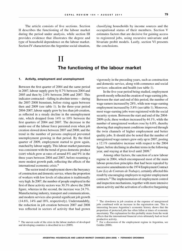
79
ARGEnTInA: hoUSEhoLdS And LAboUR MARkET ChAnGES (2004-2009) • fERnAndo GRoISMAn
C E P A L R E V I E W 1 0 4 • A U G U S T 2 0 1 1
The article consists of five sections. Section II describes the functioning of the labour market during the period under analysis, while section III provides evidence that illustrates the degree and type of household dependence on the labour market. Section IV characterizes the Argentine social situation,
classifying households by income sources and the occupational status of their members. Section V estimates factors that are decisive for gaining access to registered jobs, using recursive univariate and bivariate probit models. Lastly, section VI presents the conclusions.
IIThe functioning of the labour market
1. Activity, employment and unemployment
Between the first quarter of 2004 and the same period in 2007, labour supply grew by 0.7% between 2004 and 2005 and then by 2.8% between 2006 and 2007. This indicator contracted—falling in absolute terms— during the 2007-2008 biennium, before rising again between then and 2009 (see table 1). In the three-year period 2004-2007, labour supply grew by less than job creation, as reflected in a steady decline in the unemployment rate, which dropped from 14% to 10% between the first quarters of 2004 and 2007. The decrease in the under-use of the labour force persisted even when job creation slowed down between 2007 and 2008; and the trend in the number of persons employed prevented unemployment growing in that period. By the third quarter of 2009, employment started to grow again, matched by labour supply. This labour-market panorama was consistent with the trend of gross domestic product (gdp) which grew at rates of around 8% and 9% in the three years between 2004 and 2007, before resuming a more modest growth path, reflecting the effects of the international economic crisis.6
The sector trend of employment shows the buoyancy of construction and domestic service, where the proportion of workers with low levels of education is traditionally very high. In 2007, the number of people employed in the first of these activity sectors was 30.3% above the 2004 figure, whereas in the second, the increase was 24.7%. Manufacturing industry, transport and communications, and modern services also posted significant job growth (14.6%, 14% and 18%, respectively). Understandably, the reduction in job creation between 2007 and 2008 was reflected in sectors of activity that had grown
6 The uneven scale of the crisis in the labour markets of developed and developing countries is described in ilo (2009).
vigorously in the preceding years, such as construction and domestic service, along with commerce and social services: education and health (see table 1).
In the five-year period being studied, employment growth mostly reflected the creation of wage-earning jobs. Between the start and end of this period, the number of wage earners increased by 28%, while non-wage-earning employment increased by 5.8% (see table 1). Moreover, most wage-earning jobs were registered with the social security system. Between the start and end of the 2004-2009 cycle, these workers increased by 44.1%, while the number of unregistered workers rose by 6.8%, thereby showing that employment conditions improved through the twin channels of higher employment and better quality jobs. It should also be noted that the number of unregistered wage earners grew only up to 2007, posting a 12.1% cumulative increase with respect to the 2004 figure, before declining in absolute terms in the following year, and staying at that level until 2009.7
Among other factors, the sanction of a new labour regime in 2004, which encompassed most of the main labour-protection principles that had been repealed by successive amendments to the 1974 Employment Contract Law (Ley de Contrato de Trabajo), certainly affected this result by encouraging employers to register employment contracts.8 The implementation of employment control and inspection mechanisms, together with more intensive union activity and the activation of collective bargaining
7 The slowdown in job creation at the expense of unregistered jobs combined with an increase in the registration rate. This is interesting because Argentina’s economic history shows that the proportion of protected jobs has often fallen at times of economic uncertainty. The explanation for this probably stems from the weak effects that the international financial crisis ultimately had on local productive activity. 8 For a discussion of the employment regime in Argentina, see Goldín (2008).

80
ARGEnTInA: hoUSEhoLdS And LAboUR MARkET ChAnGES (2004-2009) • fERnAndo GRoISMAn
C E P A L R E V I E W 1 0 4 • A U G U S T 2 0 1 1
TABLE 1
Selected labour market indicators, 2004-2009(Total urban agglomerates)
Q1 2004 Q1 2005 Q1 2006 Q1 2007 Q1 2008 Q1 2009
Total economically active 100 100.7 102.6 105.5 104.8 107.5Total economically active (1) 100 102.2 105.2 109.7 109.9 113.0Total employed 100 102.3 106.2 111.1 112.1 114.9Total employed (1) 100 104.2 109.4 116.5 118.6 121.9Total wage earners (1) 100 105.8 112.8 120.9 125.3 128.0Registered wage earners 100 105.0 116.5 127.7 139.3 144.1Unregistered wage earners (1) 100 106.8 107.9 112.1 106.7 106.8Non wage earners 100 99.9 100.5 104.6 101.1 105.8Employment plans 100 74.1 57.9 32.0 14.7 10.2 Employed
Industry 100 111.6 111.4 114.6 117.7 119.6Construction 100 99.9 113.3 130.3 125.1 133.3Domestic service 100 111.3 119.0 124.7 124.9 126.5Commerce 100 99.7 102.0 109.5 109.3 110.5Transport 100 107.2 108.5 114.0 116.6 121.8Social services 100 102.5 105.4 106.0 106.0 106.9Public sector 100 94.2 101.4 98.2 101.3 107.1Modern services 100 106.3 108.5 118.0 117.1 125.5
Employed (1)
Low education level 100 103.3 103.8 109.9 107.5 110.1High education level 100 104.9 114.5 122.4 128.6 132.6
Non-wage earners
Low education level 100 95.9 97.1 97.8 93.5 97.1High education level 100 104.2 104.2 112.1 109.4 115.4
Wage earners (1)
Low education level 100 106.5 106.8 115.1 113.6 115.7High education level 100 105.2 117.9 125.8 135.0 138.3
Registered wage earners
Low education level 100 104.5 111.3 122.3 129.5 130.3High education level 100 105.3 119.1 130.3 144.2 151.0
Unregistered wage earners (1)
Low education level 100 108.0 103.6 110.1 102.6 105.5High education level 100 105.0 114.9 115.4 113.6 108.9
Position in the household
Head 100 106.5 109.3 116.2 117.6 120.0Spouse 100 105.5 113.6 121.2 130.9 134.6Other members 100 104.8 118.0 128.4 133.9 136.7
Source: Prepared on the basis of eph-indec data.
(1) Excludes employment plans.
instruments during these years, probably also have had an influence in the same direction.
Another feature of the functioning of the labour market during the period was a steady reduction in the number of workers covered by employment plans.9 Only
9 In 2002, a conditional income-transfer programme was implemented to mitigate the effects of unemployment, known as the Unemployed Heads of Household Plan (Plan Jefas y Jefes de Hogar Desocupados), which eventually accounted for about 7% of total employment.
10.2% of beneficiaries in the first quarter of 2004 were still beneficiaries in the first quarter of 2009.
Consideration of the position occupied by persons in the household —heads of household, their spouses, and other members (mostly children)—, reveals a variety of paths. Between the beginning and end of the period, the categories showing the largest increases in wage-earning employment were spouses (34.6%) and other family members (36.7%), while household heads displayed an increase of 20% between the start

81
ARGEnTInA: hoUSEhoLdS And LAboUR MARkET ChAnGES (2004-2009) • fERnAndo GRoISMAn
C E P A L R E V I E W 1 0 4 • A U G U S T 2 0 1 1
and end of the five-year period (see table 1). As would be expected, a similar trend applies to registered jobs. This behaviour justifies evaluating the distribution of protected jobs among households; in other words, evaluating the determinants of access to these jobs by household members who are not heads of family. That issue is considered in section V.
2. The educational level of the labour force
Workers with a higher education level (secondary education complete) benefited most from the greater job opportunities. The number of wage earners that had completed this education level increased by 38.3% between 2004 and 2009, whereas those with low education (who did not complete the middle education level) grew by 15.7% in that period, having already achieved 15.1% growth by 2007 (see table 1). Access to jobs registered with social security grew by a similar percentage. The number of wage earners of higher educational levels in such jobs increased by 51% between the start and end of the period, while those with low education levels in similar jobs increased by 30.3%. The few job opportunities available to individuals with low education levels is also reflected in the economic participation of this group. The activity rate among those with low education levels barely exceeded 40%: the precise figure was 42.3%, or
41.9% if employment plan beneficiaries are excluded from the calculation, whereas the equivalent figures for more educated individuals were 71.9% and 71.7% (with and without employment plans, respectively) (see table 2). This disparity in economic participation by the two population groups can be viewed partly as an expression of discouragement among those who fail to obtain a job. This point will be discussed further below, although it should be noted that the trend of the activity rate is also compatible with this interpretation. Precisely between 2004 and 2009, the economic participation of individuals with low levels of education declined, but this did not happen with individuals of higher education levels.
The uneven trend of access to employment according to a person’s education level seems to have reflected both demand and supply-side factors. The availability of surplus labour in the Argentine economy in the first few years of this decade would have enabled firms to raise the education threshold needed for the new jobs created. Given the persistence of a wide gap in registration rates according to wage earners’ education levels, this would probably have occurred more frequently for better quality jobs, although the growth of such jobs affected all sectors of activity (see table 3). It should be noted that this would have happened even though jobseekers had educational credentials in excess of those specified
TABLE 2
Activity and unemployment rate (total and by education level), 2004-2009(Total urban agglomerates) (Percentages)
Q1 2004 Q1 2005 Q1 2006 Q1 2007 Q1 2008 Q1 2009
Activity rate Total 55.2 55.0 55.3 55.5 54.4 55.2Low education level 44.8 44.9 43.7 43.5 41.7 42.3High education level 71.4 70.6 72.2 72.2 71.2 71.9
Unemployment rate
Total 14.3 12.9 11.3 9.7 8.3 8.4Low education level 14.4 13.9 12.8 10.5 9.0 9.1High education level 14.2 12.0 10.0 9.0 7.8 7.8
With employment plan beneficiaries considered as inactive
Activity rate Total 52.2 52.9 53.6 54.6 54.0 54.9Low education level 40.9 41.8 41.5 42.3 41.2 41.9High education level 70.0 69.7 71.4 71.7 71.0 71.7
Unemployment rate
Total 15.1 13.5 11.7 9.9 8.4 8.4Low education level 15.7 14.9 13.5 10.8 9.1 9.2High education level 14.5 12.1 10.1 9.0 7.8 7.8
Source: Prepared on the basis of eph-indec data.

82
ARGEnTInA: hoUSEhoLdS And LAboUR MARkET ChAnGES (2004-2009) • fERnAndo GRoISMAn
C E P A L R E V I E W 1 0 4 • A U G U S T 2 0 1 1
as requirements for the post in question. Given the sector pattern of employment growth, based on labour-intensive import-substituting industries, construction and, to a lesser extent, services, the hypothesized prevalence of a genuine demand for skills as a dominant feature, seems to be less well founded. Moreover, the employment chances for lower-education workers also could have been the result of other factors, including the adverse effects of socioeconomic residential segregation: stigmatization based on place of residence, public transport deficits, the circulation of information on job vacancies, among others.10
The trend of employment by education level, position in the household and occupational category (registered or unregistered wage earner) is partly influenced by differential labour-market participation rates by activity sector. About 40% of heads of household with low education levels were employed in construction, domestic service (basically women heads of household in this case) and commerce. The equivalent figure was less than 20% in the case of heads of household with higher education levels (see table 4).
10 On this point, see Kaztman (2007); Groisman (2008 and 2010) and Sabatini and Brian (2008).
3. The increase in the registered employment rate
The factors driving the increase in protected employment can be estimated using the evidence presented in subsections 1 and 2. The change in the rate of registration of employment between 2004 and 2009 can be explained by two factors: firstly, changes in the composition of wage earners in terms of their education level and position in the household (structure effect); and secondly, variations in the specific rates for each group (rate or propensity effect). The exercise simulated the rate of registered employment in 2009 if the structure of wage earners had not varied by education level or household position, on the one hand, or on the rates of registration in each of the groups considered, on the other. The differences between the new rates thus obtained and the rate observed in 2009 confirms the effects described above.
The calculation performed showed that of the 7.2 percentage points (p.p.) by which the registration rate increased, the structure effect had a marginal incidence of 0.6 p.p. Consequently, the overall variation was mostly explained by the change in registration rates (see table 5).
In particular, of the remaining 6.4 p.p. (after deducting the structural and residual effects) 4.2 percentage points reflect the increase in the rates of
TABLE 3
rates of wage earning registered in employment by education level and sector of activity, 2004-2009(Total urban agglomerates) (Percentages)
Q1 2004 Q1 2005 Q1 2006 Q1 2007 Q1 2008 Q1 2009
Position in the household and education level Head of household with low education level 54.3 51.9 55.0 54.9 57.0 57.9Head of household with high education level 76.3 76.2 78.0 77.7 79.8 81.3Spouse with low education level 26.4 28.3 31.0 35.8 41.0 37.4Spouse with high education level 78.1 77.1 75.4 79.0 78.6 82.0Other members with low education level 25.5 25.1 27.7 28.7 34.0 33.4Other members with higher education level 55.6 57.1 58.5 61.8 65.8 66.2
Sector of activity Industry 66.6 64.5 65.7 67.7 71.1 72.0Construction 23.8 21.1 25.4 32.1 35.8 40.5Domestic service 6.4 4.9 6.6 9.5 12.6 12.7Commerce 48.2 49.0 51.7 53.5 55.2 54.6Transport 50.0 51.6 56.4 60.9 62.5 60.4Social services 67.1 66.4 69.1 67.8 71.6 74.0Public sector 90.0 91.4 90.5 91.6 92.9 92.7Modern services 64.0 65.3 70.9 70.1 73.5 73.7
Source: Prepared on the basis of eph-indec data.
Excludes employment plan beneficiaries.

83
ARGEnTInA: hoUSEhoLdS And LAboUR MARkET ChAnGES (2004-2009) • fERnAndo GRoISMAn
C E P A L R E V I E W 1 0 4 • A U G U S T 2 0 1 1
TABLE 4
Sector distribution of employment of heads of household by education level, 2004-2009 (Total urban agglomerates) (Percentages)
Q1 2004 Q1 2005 Q1 2006 Q1 2007 Q1 2008 Q1 2009
Head of household with low education level Industry 21.4 20.9 20.3 20.4 20.3 18.7Construction 10.2 11.2 13.1 14.5 12.2 12.5Domestic service 12.3 12.6 14.0 13.3 14.0 13.9Commerce 18.5 17.3 16.1 16.6 16.9 18.2Transport 11.3 12.6 10.9 12.0 11.8 12.4Social services 9.1 8.5 8.8 8.5 8.6 8.4Public sector 11.5 10.2 10.8 9.1 10.6 11.1Modern services 5.8 6.8 6.0 5.6 5.5 4.9Total 100.0 100.0 100.0 100.0 100.0 100.0
Head of household with high education level Industry 17.8 16.6 16.3 14.5 15.9 16.5Construction 2.9 2.2 1.8 3.4 3.3 4.4Domestic service 2.5 3.2 3.8 3.1 3.2 2.7Commerce 15.4 15.6 16.0 15.3 16.6 15.2Transport 7.9 8.1 7.5 8.1 7.2 6.9Social services 12.7 12.9 14.0 12.9 13.7 13.8Public sector 27.5 27.8 29.2 29.1 27.9 27.8Modern services 13.3 13.7 11.5 13.6 12.2 12.8Total 100.0 100.0 100.0 100.0 100.0 100.0
Source: Prepared on the basis of eph-indec data.
TABLE 5
Breakdown of the variation in the rate of registered employment, 2004-2009(Percentages)
Q1 2004 Q1 2005 Q1 2006 Q1 2007 Q1 2008 Q1 2009
Rate of registered employment (excluding employment plan beneficiaries)
56.8 56.4 58.7 60.0 63.2 64.0
Annual difference (p.p.) -0.4 2.3 1.3 3.2 0.8Difference between extremes 7.2 Education structure in effect and position in the household
0.6
Effects of specific rates by groups
Head of household with low education level 0.9Head of household with high education level 1.2Spouse with low education level 0.9Spouse with high education level 0.5Other members with low education level 1.0Other members of higher education level 1.9Total effects of specific rates by groups 6.4
Residual 0.15
Source: Prepared on the basis of eph-indec data.

84
ARGEnTInA: hoUSEhoLdS And LAboUR MARkET ChAnGES (2004-2009) • fERnAndo GRoISMAn
C E P A L R E V I E W 1 0 4 • A U G U S T 2 0 1 1
registration among household members other than heads. The contribution by spouses was 1.4 p.p. —0.9 p.p. for those of low education levels and 0.5 p.p. for those with higher education levels. Among other household members (mostly children) 1.9 percentage points were contributed by an increased registration of those with higher education, while one percentage point corresponded to those of low education. The increase
in the rate of registration of heads of household (2.1 p.p.) was due to a 0.9 p.p. increase among those with high education levels and 1.2 p.p. among those with a low level of education.
The results of this exercise highlight the leading role played by workers who are not heads of their households in the overall improvement of employment quality indicators.
IIIDependency on the labour market:
an analysis at the household level
Before characterizing the effect of changes in labour market on Argentina’s social structure, the degree to which households depend on the labour incomes of their members needs to be measured.
Table 6 shows that about eight out of every 10 households obtained monetary income as a result of an employment activity undertaken by their members. The proportion of households that depended exclusively on the labour market was 58.6% in 2004, dropping to 52.6% in 2009; while the proportion of households that received non-labour incomes only (mainly pensions of various kinds) remained stable. Both behaviour patterns reflect an expansion of pension-system coverage during this five-year period.
The classification of households according to the education level attained by their heads (Low: up to secondary education incomplete; Medium: Up to higher education incomplete; and High: Higher education complete) also shows that the overall change basically reflected what had happened among lower-income households.
Although the number of households that received both labour and non-labour incomes increased, the composition of monetary income (between labour and non-labour sources) remained stable overall, with labour income continuing to account for about 80% of household budgets. This figure is what best reflects the central role played by the labour market in the well-being to which Argentine households can aspire. It should also be noted that the proportion of income obtained from labour sources rises with the level of education of the head of household, which means that households headed by individuals of low education level rely more heavily on income from pensions.
Table 7 shows that two thirds of non-labour income came from pensions, broadly unchanged in the five-year period under analysis; while income obtained from second jobs accounts for a small proportion.
Heads of households are the main household income-earners. Income obtained from the head of household’s main occupation accounts for a majority of household income, outweighing all contributions made by other household members together (see table 8). Nonetheless, and in keeping with the employment trend noted in section II, its share declined by 5.6 p.p., from 63.7% to 57.9%, at the expense of a relative increase in contributions made by the other household members, particularly non-spouses. Although the relative reduction in the income share contributed by heads of household was generalized across all household strata, an analysis by the education level of the head of household reveals a number of differences.
In households headed by persons with low levels of education, the proportion of income contributed by them fluctuated around 50%, whereas in households with more educated heads, the equivalent figure was around 60%. The second characteristic worth stressing is the smaller contribution made by spouses in households with low-education heads —about 15% of the household’s total labour income, compared to 20% in the case of households with headed by persons with higher levels of education.
Considering the type of occupational activity (see table 8), the main source of labour income for households in general was registered wage-earning employment: 56.6% of total household income in 2004, rising to 61.7% in 2009. This trend is consistent with the higher registration rate noted earlier. This relative increase
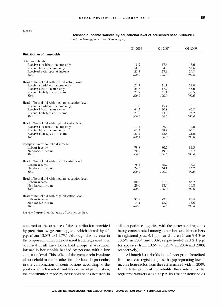
85
ARGEnTInA: hoUSEhoLdS And LAboUR MARkET ChAnGES (2004-2009) • fERnAndo GRoISMAn
C E P A L R E V I E W 1 0 4 • A U G U S T 2 0 1 1
occurred at the expense of the contribution provided by precarious wage-earning jobs, which shrank by 4.1 p.p. (from 18.8% to 14.7%). Although this increase in the proportion of income obtained from registered jobs occurred in all three household groups, it was more intense in households headed by persons with a low education level. This reflected the greater relative share of household members other than the head. In particular, in the combination of contributions according to the position of the household and labour-market participation, the contribution made by household heads declined in
all occupation categories, with the corresponding gains being concentrated among other household members in registered jobs: 4.1 p.p. for children (from 9.4% to 13.5% in 2004 and 2009, respectively) and 2.1 p.p. for spouses (from 10.6% to 12.7% in 2004 and 2009, respectively).
Although households in the lower group benefited from access to registered jobs, the gap separating lower-income households from the rest remained wide in 2009. In the latter group of households, the contribution by registered workers was nine p.p. less than in households
TABLE 6
Household income sources by educational level of household head, 2004-2009(Total urban agglomerates) (Percentages)
Q1 2004 Q1 2007 Q1 2009
Distribution of households
Total households Receive non-labour income only 18.9 17.6 17.6 Receive labour income only 58.6 54.8 52.6 Received both types of income 22.5 27.6 29.8 Total 100.0 100.0 100.0
Head of household with low education level Receive non-labour income only 21.7 21.1 21.0 Receive labour income only 55.6 47.9 43.6 Receive both types of income 22.7 31.1 35.5 Total 100.0 100.0 100.0
Head of household with medium education level Receive non-labour income only 17.0 15.4 16.1 Receive labour income only 61.2 60.8 60.8 Receive both types of income 21.8 23.8 23.2 Total 100.0 99.9 100.0
Head of household with high education level Receive non-labour income only 11.7 9.4 10.0 Receive labour income only 65.2 68.4 66.1 Receive both types of income 23.2 22.3 24.0 Total 100.1 100.0 100.0
Composition of household income Labour income 79.8 80.7 81.3 Non-labour income 20.2 19.3 18.7 Total 100.0 100.0 100.0
Head of household with low education level Labour income 75.4 75.9 76.3 Non-labour income 24.6 24.1 23.7 Total 100.0 100.0 100.0
Head of household with medium education level Labour income 80.0 81.6 83.2 Non-labour income 20.0 18.4 16.8 Total 100.0 100.0 100.0
Head of household with high education level Labour income 85.9 87.0 86.4 Non-labour income 14.1 13.0 13.6 Total 100.0 100.0 100.0
Source: Prepared on the basis of eph-indec data.

86
ARGEnTInA: hoUSEhoLdS And LAboUR MARkET ChAnGES (2004-2009) • fERnAndo GRoISMAn
C E P A L R E V I E W 1 0 4 • A U G U S T 2 0 1 1
TABLE 7
Breakdown of labour and non-labour income of households by education level of head, 2004-2009(Total urban agglomerates) (Percentages)
Q1 2004 Q1 2007 Q1 2009
Total households Income from main jobs 93.9 93.2 93.8 Labour income from second jobs 6.1 6.8 6.2 Total labour income 100.0 100.0 100.0 Income from pensions 65.3 62.6 65.8 Other non-labour income 34.7 37.4 34.2 Total non-labour income 100.0 100.0 100.0
Head of household with low education level Income from main jobs 94.5 94.9 95.3 Labour income from second jobs 5.5 5.1 4.7 Total labour income 100.0 100.0 100.0 Income from pensions 72.8 69.2 71.7 Other non-labour income 27.2 30.8 28.3 Total non-labour income 100.0 100.0 100.0
Head of household with medium education level Income from main jobs 95.8 94.6 94.9 Labour income from second jobs 4.2 5.4 5.1 Total labour income 100.0 100.0 100.0 Income from pensions 53.4 56.3 56.7 Other non-labour income 46.6 43.7 43.3 Total non-labour income 100.0 100.0 100.0
Head of household with high education level Income from main jobs 91.2 89.5 90.7 Labour income from second jobs 8.8 10.5 9.3 Total labour income 100.0 100.0 100.0 Income from pensions 64.1 54.4 63.9 Other non-labour income 35.9 45.6 36.1 Total non-labour income 100.0 100.0 100.0
Source: Prepared By the authors on the basis of eph-indec data.
headed by persons with high and medium education levels (56.1% compared to 65.1% and 65.2%, respectively), and the contribution from unregistered jobs (22.7%) was double the proportion in households headed by persons of medium education level (11.1%) and nearly three times the level of households in the higher category (8%) (see table 8).
This analysis can be enhanced by identifying the income sources on which households depend, and hence the degree to which households can draw on different sources of income. Table 9 shows that between 75.3% (in 2004) and 73% (2009) of households obtained their income from a single source (in registered jobs, unregistered jobs, self-employment, or else as employers). This reveals the limited scope available to households to develop strategies enabling them to arrange the type of job to which their members can gain access. The situation in 2009 shows that 41.3% of households received income exclusively from registered jobs; 16.2% from unregistered jobs only; 12.3% from self-employment; and 3.2% as bosses or
employers. There was a sharp reduction (8.2 percentage points) in the number of households that depended only on income from unregistered jobs between 2004 and 2009 (see table 9). In the same period, families depending exclusively on income obtained from self-employment activities decreased by about two p.p. (from 14.1% to 12.3%), whereas the proportion of families obtaining income from jobs registered with social security increased by seven p.p. (from 34.3% to 41.3%). There were no significant changes in the distribution of households by combination of sources. Although the proportion of households depending exclusively on income obtained from registered jobs increased in all three household groups, the increase was greater in those headed by persons with low levels of education. Nonetheless, one third of those households (31.9%) were still in that situation in 2009, compared to 49% of households headed by a person with a medium level of education, and 53.8% in households headed by a person with a high level of education.

87
ARGEnTInA: hoUSEhoLdS And LAboUR MARkET ChAnGES (2004-2009) • fERnAndo GRoISMAn
C E P A L R E V I E W 1 0 4 • A U G U S T 2 0 1 1
TABLE 8
income from main jobs by education level of household head, 2004-2009(Total urban agglomerates) (Percentages)
Q1 2004 Q1 2007 Q1 2009
Total households Labour income of unregistered heads 9.3 8.4 6.7 Labour income of registered heads 36.7 35.0 35.4 Labour income of self-employed heads 11.0 9.8 9.4 Labour income of employer heads 6.7 7.7 6.4 Labour income of unregistered spouses 3.7 2.5 2.5 Labour income of registered spouses 10.6 11.3 12.7 Labour income of self-employed spouses 2.9 2.8 2.9 Labour income of employer spouses 1.4 1.5 1.7 Labour income of other unregistered members 5.8 5.8 5.6 Labour income of other registered members 9.4 12.2 13.5 Labour income of other self-employed members 2.2 2.1 2.3 Labour income of other employer members 0.3 0.9 0.7 Total 100.0 100.0 100.0
Head with low education level Labour income of unregistered heads 13.3 11.5 8.7 Labour income of registered heads 26.6 27.5 26.9 Labour income of self-employed heads 12.8 10.5 9.9 Labour income of employer heads 3.8 4.5 3.7 Labour income of unregistered spouses 5.0 3.4 3.8 Labour income of registered spouses 6.4 7.4 8.9 Labour income of self-employed spouses 2.9 2.4 2.6 Labour income of employer spouses 0.5 0.8 1.0 Labour income of other unregistered members 10.5 9.8 10.3 Labour income of other registered members 14.8 17.7 20.2 Labour income of other self-employed members 3.1 3.5 3.2 Labour income of other employer members 0.3 1.2 0.7 Labour income from main jobs 100.0 100.0 100.0
Head with medium education level Labour income of unregistered heads 7.8 6.9 6.0 Labour income of registered heads 39.1 37.0 39.8 Labour income of self-employed heads 11.0 9.3 8.4 Labour income of employer heads 8.2 9.4 7.8 Labour income of unregistered spouses 3.5 2.1 2.0 Labour income of registered spouses 12.7 13.4 14.9 Labour income of self-employed spouses 2.8 2.9 3.1 Labour income of employer spouses 1.6 1.4 1.7 Labour income of other unregistered members 3.9 4.2 3.1 Labour income of other registered members 7.1 11.6 10.4 Labour income of other self-employed members 2.0 1.4 1.5 Labour income of other employer members 0.3 0.7 1.0 Labour income from main jobs 100.0 100.0 100.0
Head with high education level Labour income of unregistered heads 5.5 6.0 4.6 Labour income of registered heads 47.6 42.9 41.9 Labour income of self-employed heads 8.8 9.6 9.7 Labour income of employer heads 9.2 10.4 8.4 Labour income of unregistered spouses 1.9 1.9 1.4 Labour income of registered spouses 14.0 14.2 15.3 Labour income of self-employed spouses 2.9 3.4 3.1 Labour income of employer spouses 2.6 2.5 2.9 Labour income of other unregistered members 1.6 2.1 2.0 Labour income of other registered members 4.5 5.2 7.9 Labour income of other self-employed members 1.2 1.1 2.2 Labour income of other employer members 0.3 0.7 0.4 Labour income from main jobs 100.0 100.0 100.0
Source: prepared by the authors on the basis of eph-indec data.

88
ARGEnTInA: hoUSEhoLdS And LAboUR MARkET ChAnGES (2004-2009) • fERnAndo GRoISMAn
C E P A L R E V I E W 1 0 4 • A U G U S T 2 0 1 1
TABLE 9
Distribution of households by employment activity of their members, 2004, 2007 and 2009 (Total urban agglomerates) (Percentages)
Q1 2004 Q1 2007 Q1 2009
Unregistered only 24.4 19.5 16.2Self-employed only 14.1 12.7 12.3Employers only 2.5 2.8 3.3Registered only 34.3 37.4 41.3
Total single source 75.3 72.3 73.0 With unregistered and self-employed 6.0 4.9 4.2 With unregistered and registered 9.1 11.3 10.8 With unregistered and employers 1.0 1.3 0.9 With registered and employers 1.0 1.4 1.5 With a registered and self-employed 5.4 6.5 6.7 With employers and self-employed 0.6 0.4 0.4
Total two different sources 23.1 25.9 24.5 With employers, self-employed and registered 0.0 0.1 0.1 With employers, self-employed and unregistered 0.1 0.2 0.2 With registered, self-employed and unregistered 1.2 1.2 1.6 With registered, employers and unregistered 0.2 0.3 0.2
Total three different sources 1.5 1.8 2.1 With registered, employers, unregistered and self-employed 0.0 0.0 0.0 Total 100 100 100
Source: Prepared on the basis of eph-indec data.
IVAn approach to the change in the social
situation of Argentina
Based on the results discussed above, the population was classified in different groups according to three dimensions summarizing the degree of dependency of households with respect to the labour market: (i) The share of labour income in the household’s total
monetary income; (ii) The head of household’s employment category;
and (iii) The presence of other household members employed
in registered jobs.The trends outlined in the foregoing sections justify
the criteria used for this classification. In particular, it will be remembered that labour income was the main component of households’ monetary income, and that the head of household made the largest contribution. It was also shown that job registration was more intensive among non-head household members. Combining these criteria made it possible to define a typology of households
that provides a succinct panorama of the social situation and how it has changed in the period 2004-2009.
Nine groups were formed which, while not representing a linear ranking, reflect different degrees of social inclusion/exclusion (see table 10). The first four groups encompass households showing a high level of social vulnerability or greater exposure to social risk. The first two groups include families in which low-quality employment was either the only income source (group 1), or the majority source —over 50% of total household income (group 2). In fact in both groups the head of household was neither employed in a registered job nor an employer; and the households in question did not have other members in protected wage-earning jobs. While the two groups accounted for 36% of the population in 2004 their share had dropped to 26.1% in 2009. This significant reduction was entirely due to what happened in the first of the groups (those with labour

89
ARGEnTInA: hoUSEhoLdS And LAboUR MARkET ChAnGES (2004-2009) • fERnAndo GRoISMAn
C E P A L R E V I E W 1 0 4 • A U G U S T 2 0 1 1
incomes only), which saw their relative weight reduced by around 12 p.p. (from 26.8% to 14.7% between 2004 and 2009, respectively). In the same period, group 2 increased its relative weight by 2.2 p.p. (from 9.2% to 11.4%) which is consistent with the higher rates of retirement among lower-income sectors.
Groups 3 and 4 encompass individuals living in households for which the prevailing monetary incomes came from non-labour sources — essentially pensions of various kinds, as noted above. The joint share of the two groups remained virtually unchanged around 16%. Group 5 consists of members of households whose head was the only person with a protected job. This group of households accounted for just over 20% of the total population, and grew by about one percentage point between the start and end of the period. Group 6, unlike the previous one, included households that have other members in registered jobs, but subject to the condition that the head of household was either unemployed or working in a precarious job. The relative share of this segment grew by 4.2 p.p., from 8.3% in 2004 to 12.5% in
2009, reflecting the pronounced effect of the registration of jobs held by non-head household members. Group 7 was defined similarly to the previous group, except that the head of household was self-employed. In this case, the increase was less than one p.p. between the start and end of the five-year period. Group 8 included all households whose head was in a registered job and which also had another family member working in a registered job. This segment, which accounted for 9.4% of the population in 2004, had grown to 14% by the end of the period. Lastly, group 9 comprises households headed by a person working as a boss or employer, which accounted for between 3.9% and 4.6%.
One way to approach a validation of the proposed classification is by comparing it with a series of socio-demographic characteristics linked to situations of social vulnerability (see table 11).
The table reveals a clear correspondence between the ranking of the social groups constructed and per capita family income. Groups 1 and 2 have a value below average income (67% and 68%, respectively). Groups
TABLE 10
Distribution of the population by household typology, 2004-2009(Total urban agglomerates) (Percentages)
Groups Definition Q1 2004 Q1 2005 Q1 2006 Q1 2007 Q1 2008 Q1 2009
1 Depends exclusively on the labour market, head of household is not employer or registered wage earner, and there are no registered members in the household 26.8 25.2 21.4 17.4 15.5 14.7
2 Does not depend exclusively on the labour market, head of household is not employer or registered wager on and there are no registered members in the household 9.2 9.7 11.7 11.6 11.4 11.4
3 No employed household members 10.8 10.2 10.2 9.8 9.7 9.9
4 Depends on the labour market on a secondary basis 6.3 7.1 6.0 6.8 6.3 6.0
5 Head of household is a registered wage earner and there are no other household members with this status 21.3 21.7 21.7 22.4 22.9 22.2
6 Head of household is an unregistered wage earner or not employed, and there are other registered wage earners in the household 8.3 8.9 9.4 11.0 11.8 12.5
7 Head of household is self-employed and there are other registered wage earners in the household 3.9 3.5 4.0 4.3 4.3 4.8
8 Head of household is a registered wage earner and there are other registered wage earners in the household 9.4 9.8 11.5 12.0 13.3 14.0
9 Head of household is an employer 3.9 3.9 4.1 4.7 4.9 4.6
Total 100 100 100 100 100 100
Source: Prepared on the basis of eph-indec data.

90
ARGEnTInA: hoUSEhoLdS And LAboUR MARkET ChAnGES (2004-2009) • fERnAndo GRoISMAn
C E P A L R E V I E W 1 0 4 • A U G U S T 2 0 1 1
3 and 4 were also below average, although the distance from the average was less. Groups 5, 6 and 7 were around the average level, while groups 8 and 9 clearly displayed characteristics that easily exceeded the average value. This evidence corroborates the timely creation, since late 2009, of a non-contributory subsystem known as the Universal Child Allowance for Social Protection (Asignación Universal por Hijo para Protección Social). This program consists of an income transfer for children and adolescents that do not have any other family subsidy provided for by law, and belong to family groups that are unemployed or working in the informal economy and receiving low levels of income.11
The household typology also shows a close relation to the education level of the head of household: groups 1 and 2 (59.4% and 73.3%, respectively) included households headed by persons who had not completed the medium education level; whereas at the other extreme, groups 8
11 On the relation between informality and poverty, see Devicienti, Groisman and Poggi (2010).
and 9, the equivalent proportions were 31% and 33.2%, respectively. In addition, women heads of household were more common in the lower groups, particularly in group 2 (40.7%) whereas in groups 8 and 9 the proportion of households headed by women was 16.9% and 13.6%, respectively. It is also not surprising that this indicator is high in groups 3 and 4, since these households consist of retired people or pensioners where women’s longer life expectancy is consistent with the prevalence of female-headed households (these households are relatively smaller). Employment rates in households in groups 1 and 2 are below those of the higher groups, which jointly reflects the fewer job opportunities available to this group and unequal exposure to the constraints faced by their members in becoming part of labour supply. The presence of children under 10 years of age is also more frequent in group 1 and 2 households. Lastly, in terms of the sector participation achieved by members of these households, there is significant gravitation towards the construction and domestic service sectors, in general, for households in groups 1 and 2 (around 30%), compared to rates of around 6% and 11% for group 8 and 9 households, respectively.
TABLE 11
Selected characteristics of the constructed household groups (Q1 2009)(Total urban agglomerates)
Groups
Per capita income gap
in relation to the average
Household size
Number of pensioners
Percentages of
households headed by
women
Percentages of
households with low income heads
Employment rate
Children under three
years of age
Percentages employment in industry
Percentages employment
in construction
Percentages employment in domestic
service
Percentages employment in commerce
1 0.67 3.3 0.0 28.5 59.4 56.5 0.62 12.2 15.5 13.5 29.92 0.68 4.1 0.2 40.7 73.3 48.0 0.78 10.0 18.0 13.9 32.93 0.84 1.8 0.8 54.1 62.9 … 0.12 … … … …4 0.95 3.1 0.4 50.8 63.1 41.9 0.38 12.2 8.5 17.6 24.85 1.15 3.3 0.0 25.8 39.8 52.4 0.66 18.7 6.0 6.6 18.76 0.93 4.1 0.4 47.5 65.3 53.3 0.50 16.2 7.0 7.4 21.87 1.08 4.1 0.0 14.2 50.4 71.8 0.51 13.5 10.8 5.1 24.78 1.42 3.8 0.0 16.9 31.0 70.9 0.55 14.9 4.1 1.8 15.99 1.65 3.4 0.0 13.6 33.2 66.7 0.47 18.9 8.8 2.1 32.0
Source: Prepared on the basis of eph-indec data.

91
ARGEnTInA: hoUSEhoLdS And LAboUR MARkET ChAnGES (2004-2009) • fERnAndo GRoISMAn
C E P A L R E V I E W 1 0 4 • A U G U S T 2 0 1 1
This section summarizes the foregoing discussion. The clear and sustained increase in jobs registered with the social security system is one of the outstanding features of the Argentine labour market during the period under analysis. As shown in the previous sections, the expansion of protected jobs reached previously neglected social sectors and significantly improved their social situation, unlike what happened in previous economic recovery periods. The vigorous expansion of protected employment in the five-year period 2004-2009 was not generalized, however, so a large proportion of households did not have members working in social-security-registered jobs. This scenario makes it worth investigating whether there are factors in the Argentine labour market that condition or restrict access to these jobs by certain population groups. One way to do this is to model the probability of obtaining a registered job, which entails focusing on the higher tendency among non-head household members to occupy protected jobs. As analysed in section II, 70% of the increase in the rate of registration of wage-earning employment reflected what happened to these members.
A two-stage methodological strategy was developed. Firstly, the probabilities of gaining precarious jobs were estimated for the population as a whole; and then the chances of spouses and other members of the household other than the head gaining registered jobs were evaluated.
1. views of access to registered jobs
As noted above, unregistered or precarious jobs are those that do not fulfil employment regulations. Two alternative interpretations can be put forward to explain their existence. The first is that, owing to various circumstances (inability to bear the costs involved in labour regulations or simple evasion), firms decide to hire certain workers without fulfilling the legal obligations. A second explanation focuses on a shift in workers’ preferences for these jobs. In this case, it has been argued that flexibility of working hours, the possibility of obtaining higher wages or both, encourage young people and women (groups in which unregistered employment is highest) to choose these occupations.12 Nonetheless, it
12 There is a lot of evidence on this (see Perry and others, 2007).
should be noted that the available evidence for Argentina supports the hypothesis that unregistered employment is involuntary (see Beccaria and Groisman, 2008).
When the position of persons within households is included in the analysis, it can be argued that the economic activities of household members are related. In particular, some interpretations have claimed that the decision by spouses and children to take a registered or unregistered job is influenced (or conditioned) by the occupational status of the household head, who, as will be recalled, is the main income-earner.13 The fact that the head of household has a protected job may provide an incentive for the other household members, if they enter economic activity, to take jobs that are not registered in social security. This would reflect the fact that the household detects that a significant part of the benefits of registration become redundant if more than one member of the family nucleus has a protected job; for example, access by the family group to the benefits of the health or some system of social benefit requires just one of the spouses to contribute to it. Another factor justifying such behaviour is the presumed weak relation between the contribution to social security during the person’s active life and the level of pension benefits eventually paid. Similarly, it is also pointed out that unregistered workers are in a better position to negotiate a higher in-pocket wage, in exchange for non-registration by employers. The two latter arguments are also applicable to heads of households.
Nonetheless, from a different perspective than that outlined above, it is also possible to argue for an inverse relation, namely that the probabilities of access to protected jobs by spouses and other family members are greater when heads of household occupy jobs registered with social security. Firms tend to start their search for candidates to fill vacancies through consultation procedures within the productive unit, which, in many cases, reduces search costs and guarantees a closer match between the characteristics demanded and those offered. In this sense, workers who form part of stable payrolls in firms (registered jobs) have privileged access
13 In a related line of research, albeit different than what is being developed here, the specialized literature has also tested the existence of the additional-worker phenomenon (for the case of Argentina, see Paz, 2009).
VAccess to better quality jobs

92
ARGEnTInA: hoUSEhoLdS And LAboUR MARkET ChAnGES (2004-2009) • fERnAndo GRoISMAn
C E P A L R E V I E W 1 0 4 • A U G U S T 2 0 1 1
to this information, which they then transmit within their household. Moreover, many firms prefer to hire family members of existing workers for various reasons, for example as a way of encouraging commitment to the task, thereby obtaining beneficial effects on competitiveness. Similarly, workers who are unionized (only applicable to those in registered jobs) also tend to have greater access to preferential information on vacancies arising in the economic activity in which they participate. Other arguments can also be made to sustain such a relation. In societies with high levels of social exclusion, the spatial distribution of families is tending to change, causing or intensifying residential socioeconomic segregation. In this case, through a neighbourhood or social-capital effect, or both, the chances of accessing registered jobs would be greater for household members living in urban environments that are better integrated into the productive sector.
Whatever the argument used, it is reasonable to postulate that the occupation of the spouse of the head of household and other family members is an endogenous variable, for which reason the model used should take this constraint into account.
2. The models used
The chances of accessing a precarious job need to be estimated using models with a limited or binary dependent variable, with two possible categories: employment in a job that is registered with social security, or employment in a job that is not registered. Unlike linear probability estimations, equivalent standard deviation (probit) models satisfy this condition (see Wooldridge, 2002).
Formally, the model is based on the following equation:
P y X G X( | )= =1 β) ( (1)
Such that G(.) takes values in the interval (0.1), in other words, 0 < G(z) < 1.
The model assumes a normal distribution function and is estimated through the maximum-likelihood method.
G z v dvz
( ) ( )=−∞∫ ϕ (2)
Interpretation of the coefficients requires estimating the marginal effects:
∂∂
= ≡p x
xg x g z
dG
dzz
jj
( )( ) ( ) ( )β β where (3)
In the analysis of the probabilities of non-head household members gaining access to a registered job, potential endogeneity problems need to be considered, so a bivariate and recursive probit model is specified.14 Unlike the classical bivariate probit simultaneous equations model, this specification makes it possible to consider the employment of the head of household and other household members as the outcomes of related decisions. The high incidence of unregistered employment among non-head household members, mostly women and young people, suggests that certain aspects of family dynamics have an influence on their greater propensity for precarious employment.
Formally,
y1 1 1 1= +β χ ε (4)
y y z2 2 2 2 1 1 2 2 2= + = + +β χ ε δ δ ε (5)
where χ1 represents the observable exogenous determinants of the head of household’s decision to take a registered job, and z2 represents the observable exogenous determinants of the probability that non-head members of the household gain a registered job.
The error terms of equations [4] and [5] are assumed independent and identically distributed as bivariate normal, with zero mean and unit variance, such that ρ = corr (ɛ1, ɛ2). The exogeneity condition can be established in terms of ρ, which can be interpreted as the correlation of the unobservable and/or omitted explanatory variables of the two equations. The coefficients of the model as presented can be efficiently estimated using the maximum-likelihood method. From the econometric standpoint, the endogenous nature of y1 in the second equation of the model does not alter the likelihood function of a standard bivariate probit; so, unlike what happens in a linear simultaneous equation model, if the two dependent variables are determined jointly, one of them is merely included as the regressor in the other equation (see Greene, 2003).
3. variables used and results obtained
(a) Probit modelThe dependent variable was defined dichotomously,
being equal to 1 when the individual worked as a wage
14 An example of the application of this methodology to a similar topic can be found in Galiani and Weinschelbaum (2007).
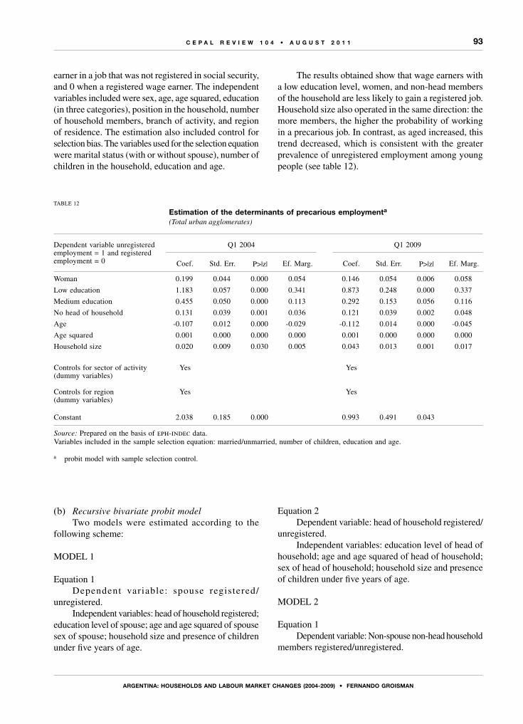
93
ARGEnTInA: hoUSEhoLdS And LAboUR MARkET ChAnGES (2004-2009) • fERnAndo GRoISMAn
C E P A L R E V I E W 1 0 4 • A U G U S T 2 0 1 1
earner in a job that was not registered in social security, and 0 when a registered wage earner. The independent variables included were sex, age, age squared, education (in three categories), position in the household, number of household members, branch of activity, and region of residence. The estimation also included control for selection bias. The variables used for the selection equation were marital status (with or without spouse), number of children in the household, education and age.
The results obtained show that wage earners with a low education level, women, and non-head members of the household are less likely to gain a registered job. Household size also operated in the same direction: the more members, the higher the probability of working in a precarious job. In contrast, as aged increased, this trend decreased, which is consistent with the greater prevalence of unregistered employment among young people (see table 12).
TABLE 12
Estimation of the determinants of precarious employmenta
(Total urban agglomerates)
Dependent variable unregistered employment = 1 and registered employment = 0
Q1 2004 Q1 2009
Coef. Std. Err. P>|z| Ef. Marg. Coef. Std. Err. P>|z| Ef. Marg.
Woman 0.199 0.044 0.000 0.054 0.146 0.054 0.006 0.058
Low education 1.183 0.057 0.000 0.341 0.873 0.248 0.000 0.337
Medium education 0.455 0.050 0.000 0.113 0.292 0.153 0.056 0.116
No head of household 0.131 0.039 0.001 0.036 0.121 0.039 0.002 0.048
Age -0.107 0.012 0.000 -0.029 -0.112 0.014 0.000 -0.045
Age squared 0.001 0.000 0.000 0.000 0.001 0.000 0.000 0.000
Household size 0.020 0.009 0.030 0.005 0.043 0.013 0.001 0.017
Controls for sector of activity (dummy variables)
Yes Yes
Controls for region (dummy variables)
Yes Yes
Constant 2.038 0.185 0.000 0.993 0.491 0.043
Source: Prepared on the basis of eph-indec data.Variables included in the sample selection equation: married/unmarried, number of children, education and age.
a probit model with sample selection control.
(b) Recursive bivariate probit model Two models were estimated according to the
following scheme:
MODEL 1
Equation 1Dependent variable: spouse registered/
unregistered.Independent variables: head of household registered;
education level of spouse; age and age squared of spouse sex of spouse; household size and presence of children under five years of age.
Equation 2Dependent variable: head of household registered/
unregistered.Independent variables: education level of head of
household; age and age squared of head of household; sex of head of household; household size and presence of children under five years of age.
MODEL 2
Equation 1 Dependent variable: Non-spouse non-head household
members registered/unregistered.

94
ARGEnTInA: hoUSEhoLdS And LAboUR MARkET ChAnGES (2004-2009) • fERnAndo GRoISMAn
C E P A L R E V I E W 1 0 4 • A U G U S T 2 0 1 1
Independent variables: head of household registered; education level of spouse; age and age squared of spouse; sex of spouse; household size and presence of children up to five years of age.
Equation 2Dependent variable: head of household registered/
and registeredIndependent variables: education level of head of
household; age and age squared of head of household; sex of head of household; household size and presence of children under five years of age.
Both cases involved probability equations estimated through the recursive bivariate probit model, for heads of household and spouses in model 1 and for other household members in model 2. The universe of analysis includes all households composed by both spouses, who are also employed in wage-earning jobs for model 1. Model 2 included households composed by a head and at least one other (non-spouse) member who were also wage earners. The recursive characteristic of the model stems from the fact that the variable defining the registered/unregistered wage-earning status of household heads has been included as an independent variable for estimating the same probability for spouses and other household members in each model.
(c) ResultsTable 13 reports the coefficients of the estimated
models and the marginal effects of interest for the beginning and end of the period being analysed. The parameters estimated for the independent variables had the expected signs: access to a registered job was greater for individuals with a high education level, males, and as age increased, although the increases were not linear. Moreover, household size and the presence of children under five were variables that reduced the chances of gaining a job with these characteristics.
The most interesting result is that when the household head was employed in a registered wage earning job, the spouse was more likely also to be working in a job of that type. In absolute terms, this was shown by the fact that spouses in households whose heads had a registered job had probabilities between 34.8% and 41% higher, for 2004 and 2009, respectively, than those of wage-earning spouses in households whose heads were wage earners in unregistered jobs. The results of the second model confirmed a similar finding for non-spouse household members in 2009, although they were not significant in 2004. In 2009, the likelihood that these household members, basically children, had a protected job was 20% higher than for those living in households whose heads were wage earners in precarious jobs.

95
ARGEnTInA: hoUSEhoLdS And LAboUR MARkET ChAnGES (2004-2009) • fERnAndo GRoISMAn
C E P A L R E V I E W 1 0 4 • A U G U S T 2 0 1 1
TABLE 13
Estimation of the determinants of registered employment,a 2004-2009(Total urban agglomerates)
Q1 2004 Q1 2009
Coef. Std. Err. P>|z| Elast. Coef. Std. Err. P>|z| Elast.
Model 1Dependent variable: Spouse registered = 1 and unregistered =0
Head registered 0.901 0.390 0.021 0.348 1.095 0.253 0.000 0.410Medium education level 0.906 0.144 0.000 0.298 0.775 0.123 0.000 0.210High education level 1.602 0.182 0.000 0.469 1.164 0.145 0.000 0.307Age 0.107 0.044 0.015 0.039 0.061 0.030 0.039 0.019Age squared -0.001 0.001 0.044 0.000 -0.001 0.000 0.098 0.000Male -0.064 0.198 0.748 -0.023 0.188 0.136 0.166 0.055Household size -0.081 0.038 0.033 -0.029 -0.062 0.034 0.067 -0.019Children under 5 years of age -0.022 0.122 0.855 -0.008 -0.047 0.100 0.641 -0.014Constant -3.424 0.830 0.000 -2.252 0.553 0.000
Dependent variable: Head registered =1 and unregistered = 0
Medium education level 0.480 0.112 0.000 0.638 0.099 0.000 High education level 0.931 0.145 0.000 0.772 0.122 0.000 Age 0.159 0.041 0.000 0.092 0.034 0.007 Age squared -0.002 0.000 0.000 -0.001 0.000 0.007 Male 0.302 0.193 0.118 0.533 0.128 0.000 Household size -0.044 0.035 0.210 -0.034 0.033 0.309 Children under 5 years of age 0.065 0.118 0.582 0.063 0.106 0.555 Constant -3.357 0.835 0.000 -2.028 0.691 0.003 Rho -0.223 0.250 -0.493 0.151
Model 2Dependent variable: Spouse registered = 1 and unregistered 0
Head registered 0.554 0.359 0.123 0.182 0.523 0.259 0.044 0.200Medium education level 0.485 0.104 0.000 0.181 0.607 0.089 0.000 0.239High education level 1.200 0.173 0.000 0.446 1.077 0.155 0.000 0.376Age 0.013 0.005 0.009 0.005 0.009 0.004 0.030 0.004Age squared 0.000 0.000 0.058 0.000 0.000 0.000 0.457 0.000Male 0.266 0.094 0.005 0.099 0.173 0.079 0.030 0.069Household size -0.234 0.067 0.001 -0.088 -0.213 0.049 0.000 -0.085Children under 5 years of age 0.242 0.167 0.148 0.093 0.257 0.112 0.022 0.102Constant -0.921 0.216 0.000 -0.571 0.197 0.004
Dependent variable: Head registered =1 and unregistered = 0
Medium education level 0.499 0.109 0.000 0.539 0.094 0.000 High education level 0.688 0.188 0.000 1.190 0.148 0.000 Age 0.153 0.027 0.000 0.134 0.023 0.000 Age squared -0.002 0.000 0.000 -0.001 0.000 0.000 Male 0.619 0.096 0.000 0.693 0.081 0.000 Household size 0.019 0.024 0.430 -0.057 0.020 0.005 Children under 5 years of age -0.448 0.113 0.000 -0.028 0.100 0.778 Constant -3.784 0.602 0.000 -3.236 0.544 0.000 Rho -0.082 0.240 -0.118 0.167
Source: Prepared on the basis of eph-indec data.
a recursive bivariate probit models.

96
ARGEnTInA: hoUSEhoLdS And LAboUR MARkET ChAnGES (2004-2009) • fERnAndo GRoISMAn
C E P A L R E V I E W 1 0 4 • A U G U S T 2 0 1 1
The characteristics of Argentina’s economic recovery provide a favourable scenario for exploring the relation between the functioning of the labour market and changes in households’ social situation. Following the 2002-2003 biennium, when the level of production prevailing in early 2001 had almost been regained, the economy continued to grow vigorously. Job creation and wage increases were two of the pillars on which this expansionary phase was based. In addition, as a distinctive feature in the economic history of the last three decades, there was an intensive increase in jobs registered with social security. In the five years between 2004 and 2009, those high-quality jobs grew faster than unregistered jobs, which resulted in a significant reduction in the rate of precarious employment. Accordingly, the social outlook improved in line with the labour market trend.
A classification of households based on the type of labour-market participation by their members provides an approach to this phenomenon. Using this procedure, it was estimated that the population living in households that basically rely on the employment of their members and do not have wage earners registered in social security decreased from 36% to 26.1%. Although the improvement was considerable, it is hard deny that quality-employment remained elusive for a large group of people.
Part of the explanation from the persistence of households whose members did not gain protected jobs is to be found in the type of employment activity they undertake. It should be remembered that indices of unregistered employment —despite improvements in the registration of employment relations observed during the five-year period— are generally very high in certain sectors of activity —such as domestic service, construction and commerce— where workers from lower-income households are more heavily concentrated.
The segmentation prevailing in the distribution of job opportunities would also have operated in the same direction. In fact, most households obtain their monetary income from a single employment source, in other words from just one category of labour-market participation: as non-wage earners, registered wage earners or unregistered wage earners. This is compatible with the effect that labour-market participation by the main income earner would have on the job opportunities of other household members. In particular, a new finding in this study is that the increase in registration was very intense among
non-head household members —spouses and children basically. The change in the registration rate between 2004 and 2009 reflected this to a significant degree. It was also found that the chances of these household members obtaining a registered job was affected by the employment status of the head of household: members of households whose heads were in a job registered with social security were more likely to gain a higher-quality job themselves.
The results obtained are compatible with the persistence of a social structure that is segmented on the basis of the type of labour-market participation achieved by individuals —basically whether or not they gain access to registered wage-earning jobs. That diagnostic reduces the validity of the assumption that the mere passage of time, given certain macroeconomic fundamentals, will gradually correct these inequities. This opinion is based on the magnitude of the quality employment deficit still observable in Argentine society. It should be noted that 45% of the urban employed consists of unregistered wage earners and nonprofessional self-employed workers (Permanent Household Survey (eph) of the National Institute of Statistics and Censuses (indec), 2010). In fact, it can be speculated that although the economic conditions for an expansion of registered employment may be maintained in the short and medium terms (competitive exchange rate, high international prices for commodity exports, stimulus to domestic consumption, among others), specific policies will be needed to facilitate access to these jobs by individuals that have failed to avoid precarious employment.
Key measures among these policies aim to reduce indices of unregistered employment in the economic sectors that employ the lowest-income workers, namely domestic service, construction and the retail trade. Moreover, the intensification of procedures for regularizing employment in larger firms could help reduce precariousness in these economic units. The low activity rate in the poorest households also suggests the need for policies that help adult household members to fully engage with the labour market, by discouraging the acceptance of precarious jobs. In this regard, upgrading job skills among lower skilled workers, providing quality childcare centres, and improving communication channels and access to and from the neighbourhoods in which low-income households live have been shown to
VIFinal comments
97
ARGEnTInA: hoUSEhoLdS And LAboUR MARkET ChAnGES (2004-2009) • fERnAndo GRoISMAn
C E P A L R E V I E W 1 0 4 • A U G U S T 2 0 1 1
have positive effects. Of course, these initiatives need to be supported by policies to stimulate labour demand, for which incentives for productive units to locate in those spatially segregated zones would be highly recommendable. Lastly, it should be noted that in moving
towards a fairer society in terms of job opportunities, income-transfer policies have proven suitable mechanisms for sustaining welfare levels among households that are unable to obtain quality jobs.
(Original: Spanish)
Bibliography
Arriagada, I. (comp.) (2007), “Familias y políticas públicas en América Latina: una historia de desencuentros”, Libros de la cepal series, No. 96 (LC/G.2345-P), Santiago, Chile, Economic Commission for Latin America and the Caribbean (eclac). United Nations publication, Sales No. S.07.II.G.97.
Beccaria, L. and F. Groisman (2008), “Informalidad y pobreza en Argentina”, Investigación económica, vol. 67, No. 266, Mexico City, National Autonomous University of Mexico.
Cetrángolo, O., D. Heymann and A. Ramos (2007), “Macroeconomía en recuperación: la Argentina post-crisis”, Crisis, recuperación y nuevos dilemas. La economía argentina 2002-2007 (LC/W.165), B. Kosacoff (comp.), Buenos Aires, eclac office in Buenos Aires.
Devicienti, F., F. Groisman and A. Poggi (2010), “Are informality and poverty dynamically interrelated? Evidence from Argentina”, Research on Economic Inequality, vol. 18, Bingley, Emerald.
Galiani, S. and F. Weinschelbaum (2007), “Modeling informality formally: households and firms”, Working Paper, No. 47, La Plata, Center for Distributive, Labor and Social Studies (cedlas).
Goldín, A. (2008), “Normas laborales y mercados de trabajo argentino: seguridad y flexibilidad”, Macroeconomía del desarrollo series, No. 74 (LC/L.2985-P), Santiago, Chile, Economic Commission for Latin America and the Caribbean (eclac). United Nations publication, Sales No. S.08.II.G.91.
Greene, W.H. (2003), Econometric Analysis, New Jersey, Prentice Hall.
Groisman, F. (2010), “La persistencia de la segregación residencial socioeconómica en Argentina”, Estudios demográficos y urbanos, vol. 25, No. 2, Mexico City, El Colegio de México.
(2008), “Distributive effects during the expansionary phase in Argentina (2002-2007)”, cepal Review, No. 96 (LC/G.2396-P), Santiago, Chile.
ilo (International Labour Organization) (2009), World of Work Report 2009. The Global Jobs Crisis and Beyond, Geneva.
ilo/undp (International Labour Organization/United Nations Development Programme) (2009), Trabajo y familia: hacia nuevas formas de conciliación con corresponsabilidad social, Santiago, Chile.
Kaztman, R. (2007), “La calidad de las relaciones sociales en las grandes ciudades de América Latina: viejos y nuevos determinantes, Revista pensamiento iberoamericano, Madrid.
Márquez and others (comps.) (2007), ¿Los de afuera? Patrones cambiantes de exclusión en América Latina y el Caribe, Washington, D.C., Inter-American Development Bank.
Paz, J. (2009), “El efecto del trabajador adicional. Evidencia para Argentina (2003-2007)”, Cuadernos de economía, vol. 46, Santiago, Chile, Catholic University of Chile.
Perry, G. and others (2007), Informality: Exit and Exclusion, Washington, D.C., World Bank.
Sabatini, F. and I. Brian (2008), “La segregación, los guetos y la integración social urbana: mitos y claves”, Eure, vol. 34, No. 103, Santiago, Chile, Catholic University of Chile.
Stallings, B. and J. Weller (2001), “Employment in Latin America: cornerstone of social policy”, cepal Review, No. 75 (LC/G.2150-P), Santiago, Chile.
Tokman, V. (2006), “Inserción laboral, mercados de trabajo y protección social”, Financiamiento del desarrollo series, No. 170 (LC/L.2507-P), Santiago, Chile. United Nations publication, Sales No. S.06.II.G.39.
Wooldridge, J.M. (2002), “Discrete response models”, Econometric Analysis of Cross-section and Panel Data, Cambridge, Massachusetts, The mit Press.


C E P A L R E V I E W 1 0 4 • A U G U S T 2 0 1 1
99
Argentine industry in theearly twenty-first century
(2003-2008)
Germán Herrera and Andrés Tavosnanska
This article studies the exceptional industrial growth that occurred
in Argentina between 2003 and 2008. In addition to reviewing aggregate
indicators of this growth, the article discusses evidence of changes in
sector shares during these years along with a number of specific features
in the trend of manufacturing employment. It also analyses the main
patterns of Argentine industry’s external trade in that period. These contain
positive features such as greater relative participation by local production
in external markets, and the emergence of a new group of domestic
firms with rapidly growing manufacturing exports. Alongside this, and as
a residual structural characteristic, imports are supplying an increasing
share of the domestic demand for manufactured goods.
KEYWORDS
Industry
Industrial development
Industrial production
Manufacturing enterprises
Manufactures
Exports
Imports
Employment
Wages
Industrial statistics
Argentina
Germán Herrera
Professor at the National University
of Quilmes and Chief Economist
at the Production Research Centre
(cep), Argentina.
Andrés Tavosnanska
Member of the Steering Committee
of the Economic Association for
Argentine Development (aeda)
and economist at the Production
Research Centre (cep), Argentina.

100
ARGEnTInE IndUSTRy In ThE EARLy TWEnTy-fIRST CEnTURy (2003-2008) • GERMán hERRERA And AndRéS TAVoSnAnSkA
C E P A L R E V I E W 1 0 4 • A U G U S T 2 0 1 1
The collapse of the currency-board regime —the so called Convertibility Plan— opened the door to a new macroeconomic framework that attempted to lift economy out of its crisis situation and sustain rapid economic growth without having to resort to external financing. The new framework was based on a high real exchange rate, rising levels of retention applied to the main commodities (soybeans, oil, meat, wheat, and others), low or negative real interest rates, subsidized public-utility charges, and a tax and income policy that encouraged expansion in the domestic market.1
Boosted by this new macroeconomic regime, manufacturing industry is growing on a sustained basis and at very high rates, thus bringing to an end a long process of de-industrialization in the domestic economy. Moreover, having shed workers continuously for 25 years, manufacturing industry has started to create jobs once more. In addition, industrial exports performed very vigorously, growing at 19% per year between 2003 in 2007, to represent 26% of industrial output in
Earlier versions of this paper were presented at the Annual Congress of the Economic Association for Argentine Development (aeda) in September 2009, and at an event honouring Jorge Schvarzer held at the Faculty of Economic Sciences of the University of Buenos Aires in November 2009. We are grateful for the generous contributions made by Fernando Porta, Bernardo Kosacoff, Paula Español, and by various economists at the Production Research Centre (cep) and the Centre for the Study of State and Society (cedes), and for valuable comments made by an anonymous referee on previous versions of this article. Any remaining omissions or shortcomings are the exclusive responsibility of its authors.1 Detailed descriptions of the functioning of the new macroeconomic model can be found in Goldstein, Peirano and Tavosnanska (2009), Kiper (2009) and Kulfas (2009).
the latter year —a much higher level than recorded in the previous decade.
A number of research papers have recently been published in response to this auspicious framework of recovery, highlighting different but complementary aspects and aiming to describe the scope and depth of the change that has occurred in the domestic productive framework (Arceo, Monsalvo and Wainer, 2007; Briner, Sacroisky and Bustos Zavala, 2007; Anlló, Lugones and Peirano, 2008; Fernández Bugna and Porta, 2008; Lugones and Suárez, 2006, among others). With varying explicit emphases, these analyses seek to throw light on the following question: to what extent have the changes in the macroeconomic scenario since the collapse of the currency-board regime had repercussions on the morphology of the Argentine productive structure? The studies thus aim to reconstruct in greater detail the dynamics of the sectoral and microeconomic changes that took place in the productive framework during these growth years.
This article forms part of this line of research, exploring certain aspects that seem to have changed along with others that underlie the aggregate indicators of the recent manufacturing growth.
The article is structured in five sections including this introduction. The following section provides a brief general description of the trend of manufacturing activity over the last few years, before making a comparison of the inter-sectoral dynamic of Argentine industry during the expansionary phase of the past decade and the recent growth period. The third section analyses some of the main trends in industrial employment. The fourth section discusses the trend of industry’s external trade in the last five years; and the last section provides a number of final thoughts.
Iintroduction

101
ARGEnTInE IndUSTRy In ThE EARLy TWEnTy-fIRST CEnTURy (2003-2008) • GERMán hERRERA And AndRéS TAVoSnAnSkA
C E P A L R E V I E W 1 0 4 • A U G U S T 2 0 1 1
1. industrial growth in 2003- 2008 and investment strategies
Since 2003, Argentina has returned to a high-growth path, posting an average annual expansion of 8%. The largest contributions to this expansion were made by consumption and then investment, which achieved its highest share of gross domestic product (gdp) (23%) since the mid-1970s. Exports were also unusually buoyant, growing by a cumulative 134% in the period 2003-2008, or even more (174%) if manufactures of industrial origin (mio) are included.
Against this backdrop, and following nearly five years of agony in which manufacturing activity shrank by about 35%, Argentine industry started to expand, posting average annual growth of 10% over a six-year period. Figure 1 reveals the exceptional duration and intensity of this industrial growth period: never before, since the end of the 1964-1974 boom, had there been 24
consecutive quarters of manufacturing growth (lasting from the third quarter of 2002 until the second quarter of 2008, inclusive).
The expansionary period that began after the 2002 devaluation can be divided into two phases. The first phase was one of recovery, with exceptionally high growth rates. In 2003 and 2004 manufacturing activity grew by nearly 16% per year. This was followed by a second phase lasting from 2005 to 2008, in which growth stabilized an average rate of 8.9%.
The distinction largely coincides with the different characteristics of the investment process. During the first two years of recovery, the upturn in the domestic market provided firms with buoyant demand that they could supply by putting their plants back to work and exploiting their huge idle capacity. But as this began to be used up in the various sectors, new investments became necessary. Since 2005, therefore, most production has been based on the creation of new productive capacity: in 2005 and
IIPost-currency-board industrial recovery:
growth, investment and changes in the
sectoral structure
FIGURE 1
industrial production: physical volume index (pvi) year-on-year percentage variation, 1970-2008
Source: Prepared by the authors on the basis of the Monthly Industrial Survey conducted by the National Institute of Statistics and Censuses (indec) of Argentina.
The 1970s: end of the
1964-74 growth cycle
The 1990s: 17 consecutive growth quarters
The recent period: 24 consecutive growth quarters
1971
Q1
1972
Q1
1973
Q1
1974
Q1
1975
Q1
1976
Q1
1977
Q1
1978
Q1
1979
Q1
1980
Q1
1981
Q1
1982
Q1
1983
Q1
1984
Q1
1985
Q1
1986
Q1
1987
Q1
1988
Q1
1989
Q1
1990
Q1
1991
Q1
1992
Q1
1993
Q1
1994
Q1
1995
Q1
1996
Q1
1997
Q1
1998
Q1
1999
Q1
2000
Q1
2001
Q1
2002
Q1
2003
Q1
2004
Q1
2005
Q1
2006
Q1
2007
Q1
2008
Q1
25
Perc
enta
ge
20
15
10
5
0
–5
–10
–15
–20
–25

102
ARGEnTInE IndUSTRy In ThE EARLy TWEnTy-fIRST CEnTURy (2003-2008) • GERMán hERRERA And AndRéS TAVoSnAnSkA
C E P A L R E V I E W 1 0 4 • A U G U S T 2 0 1 1
2006, three quarters of the expansion of production was the result of capacity expansion, whereas in 2007 this was true of nearly all output growth (see table 1).
TABLE 1
Expansion of industrial production and installed capacity, 2003-2008(Percentages)
2003 2004 2005 2006 2007 2008 (Q3)
Capacity expansion 0.6 2.6 5.9 6.2 7.2 4.4
emi 16.2 10.7 8.0 8.4 7.5 6.1
Source: Prepared by the authors on the basis of Jorge Schvarzer and others, “La actividad productiva en 2007. Un crecimiento que se consolida en distintos ámbitos”, Notas de coyuntura, No. 24, Buenos Aires, Faculty of Economics Sciences, University of Buenos Aires, 2008.
emi: Monthly industrial estimator.
This second stage involved firms with considerable liquidity obtained from the high profit margins earned in the initial phase, which made it possible to finance investments. In the first instance, these were small and incremental; productive expansion needs were covered by lengthening shifts, purchasing machinery to alleviate specific bottlenecks, or expanding plants by purchasing neighbouring land plots. By 2007, however the limits of this productive expansion strategy were becoming evident; and growth itself forced firms to take investment decisions of increasing scope, involving a higher level of complexity and financial commitment.
Many firms implemented major investment projects to set up new factories, thereby giving an additional boost to the competitiveness of certain sectors. Others, however, adopted a different strategy: either as a result of their reluctance to invest, owing to the complexity of setting up a new plant, or because of an inability to respond to demand that was growing too fast, many firms started to import increasing volumes of goods to supplement their own output.
2. Changes in the productive structure
During the twentieth century, Argentina went through a process of industrialization that certainly had its share of difficulties and contradictions. Despite this, the country had made headway in gradually developing a relatively integrated and diversified industry; and it had managed to enter a number of activities of highly technological complexity.
Nonetheless, the mid-1970s represented a turning point, inaugurating a long process aimed at dismantling the import-substitution-industrialization model (Bisang and others, 1996). This not only entailed a reduction in industry’s share of gdp (which certainly occurred and was very pronounced) but also a clear sectoral disarticulation to the detriment of activities producing consumer durables and capital goods (categories that are relatively intensive in domestic value-added and in the use of engineering services) and in favour of the production of certain basic industrial products that make intensive use of domestic natural resources (Katz, 1993, p. 386).
The growing process of trade liberalization and currency appreciation that occurred in the 1990s aggravated the regressive restructuring and sectoral concentration, causing a partial return to specialization in food products and other natural-resource-intensive goods. At the same time, concentration within sectors increased; whereas the bulk of the industrial framework faced a highly adverse scenario and developed defensive strategies to survive (Kosacoff, 1996), a few small firms, largely of foreign origin, substantially increased their relative share of global industrial output (Kulfas and Schorr, 2000; Schorr, 2001).
The final stage of this industrial “primarization” process can be seen in table 2. From 1993 to 2002, the fastest-growing sectors were food and beverages (sectors that make intensive use of natural resources), along with the chemical and basic metal industries. In 1993 these sectors jointly contributed over half of industrial value-added (52%), but by 2002 their share had grown to two-thirds (66.4%). Over the same period, engineering- and labour-intensive sectors saw their share of industrial structure shrink by 30%.
The change in macroeconomic regime marks a break in the economy’s return to producing natural-resource-intensive-commodities. The recent phase of manufacturing growth has not been confined to certain “traditional” branches of the local industrial structure (food and beverages, motor vehicles, non-metallic minerals, basic metal industries); the most dynamic sectors also include several metal- machinery or engineering-intensive activities, such as the manufacture of machinery and equipment, medical instruments and metal products —segments that were particularly hard hit during the 1990s.2
2 Along the same lines, in a study of new firms showing rapid employment growth in the post-currency- board period, Attoresi and others (2007, p.20) argued that “[…] activities associated with the production of food and beverages have lost share, whereas engineering and labour intensive branches have expanded in relative terms”.

103
ARGEnTInE IndUSTRy In ThE EARLy TWEnTy-fIRST CEnTURy (2003-2008) • GERMán hERRERA And AndRéS TAVoSnAnSkA
C E P A L R E V I E W 1 0 4 • A U G U S T 2 0 1 1
Table 2 shows that engineering-intensive sectors (excluding the automotive sector), which in 2002 accounted for just 10% of industrial value added, in 2007 had grown their share to 15%, while the share of value-added produced by labour-intensive sectors grew from a 19% in 2002 to 21.5% in 2007. Meanwhile, the food and other natural-resource-intensive sectors retreated during the period, with their joint share shrinking from 47.8% to 40.2%. This trend is not confined to the initial years of the industrial recovery, but was sustained in the following years, although the installed capacity of several of these sectors had become exhausted and growth came to depend on new investments.
Table 3 shows the contribution made by different sectors to total manufacturing growth, comparing the recent expansion with the zenith of the currency-board regime. The two most significant changes are, firstly, the greater contribution made by engineering- and labour-intensive sectors; and, as a counterpart, the sharp fall in the share of food and other natural-resource-intensive products. The first two groups mentioned explained just 20% of growth in industrial value-added between 1993 and 1998 (note the near zero contribution of the metal-machinery sector at a time of pronounced activity expansion); nonetheless, from 2002 to 2007, these sectors accounted for 46% of total industrial value-added.
The opposite occurs with food and other natural-resource-intensive products, which contributed almost half of additional value-added between 1993 and 1998, but explain just 30% of the expansion in 2002-2007.
Similarly, the automotive, basic metals and chemical industries —sometimes hailed as the only sectors responsible for post-currency-board industrial growth— in those years contributed the same or less than in the upswing phase of the past decade, and significantly less than the engineering- and labour-intensive sectors.
TABLE 3
Contribution to the growth of industry value-added, 1993-1998 and 2002-2007(Percentages based on figures expressed in pesos at constant 1993 prices)
Sectors 1993-1998 2002-2007
Food and beverages and tobacco 31.6 19.0Automotive 9.7 9.9Engineering-intensive 0.5 21.4Natural-resource-intensive 17.6 10.7Labour-intensive 19.4 24.8Basic metals and chemicals 21.2 14.2
Source: Prepared by the authors on the basis of the national accounts.
Apart from the smaller contribution to growth made by the food sector, as noted above, oil refining, chemicals, rubber, plastics and furniture all saw their shares fall sharply. In contrast, strongly performing sectors included textiles and clothing, construction materials and metallic products, along with various capital goods (machinery and equipment, electrical appliances, medical instruments, among others).
TABLE 2
Contribution to industrial value added, 1993-2007(Percentages based on figures in pesos at constant 1993 prices)
SectorFood and beverages
and tobacco Automotive Engineering-intensive
Natural- resource-intensive Labour-intensive Basic metals and
chemicalsYear
1993 22.7 6.5 16.3 15.4 25.1 13.91998 24.0 7.0 14.0 15.7 24.3 15.01999 26.8 5.3 12.4 16.2 23.7 15.62000 26.6 5.7 12.3 15.8 23.2 16.42001 28.0 4.5 11.6 16.5 21.8 17.62002 30.5 4.7 9.9 17.3 19.1 18.62003 28.0 4.3 11.5 16.9 21.2 18.02004 26.4 5.0 13.0 16.9 21.4 17.42005 26.4 5.6 13.6 15.9 21.6 16.92006 25.9 6.3 14.2 15.2 21.0 17.42007 25.7 6.8 14.7 14.5 21.5 16.8
Source: Prepared by the authors on the basis of the national accounts.Note: The sector blocks were based on the classification used by Katz and Stumpo (2001), adapted to the Argentine industrial framework. They include the following groupings from the International Standard Industrial Classification of all Economic Activities (isic): Food and beverages and tobacco; Motor vehicles. Engineering intensive: Metal products, machinery and equipment, electrical appliances; Radio, television and communications equipment; Medical and precision instruments; Transport equipment. Natural resource intensive: Wood and products of wood; Paper; Oil refining; Rubber; Non-metallic minerals. Labour-intensive: Textile products; Wearing apparel, Tanning of leather and footwear manufacture; Publishing and printing; Plastic products; Basic metals and Chemicals.

104
ARGEnTInE IndUSTRy In ThE EARLy TWEnTy-fIRST CEnTURy (2003-2008) • GERMán hERRERA And AndRéS TAVoSnAnSkA
C E P A L R E V I E W 1 0 4 • A U G U S T 2 0 1 1
This change in the engines of industrial growth also afforded a more leading role to relatively less concentrated activities, with a preponderance of small and medium-sized enterprises (smes) —unlike what happened during the currency-board period when the fastest-growing sectors were producers of basic industrial products (metal sheets, fuels, oils and others) which tend to be capital intensive and highly concentrated.
Clearly, and although it is premature to claim the existence of substantive changes in the sectoral structure of industry, there has been a turnaround in the pattern of growth towards metal-machinery or engineering-intensive sectors, in contrast to the concentration and “primarization” process through which the Argentine economy passed during the currency-board period.
IIITrend of industrial employment
1. The halt to the shedding of employment and trend of wages
This section investigates one of the greatest novelties of the recent cycle: the pronounced trend of job creation shown by manufacturing industry from 2003 to 2008, which interrupted a period of industrial worker lay off that had lasted for about 25 years.
As noted above, there is a degree of consensus that the second half of the 1970s was a decisive turning point for industry. In terms of employment, the trend is clear. After following a substantial expansionary path until 1976 (albeit with intervals of stagnation), industrial employment then entered a sustained path of contraction that lasted until the collapse of the currency-board system (see table 4).
During that period, industry shed jobs continuously, with an initial sharp adjustment (at an annual rate of about 7% against a backdrop of recession under the military government) and with dramatic accelerations at the
epicentres of the crises (the hyperinflationary episodes of 1989-1990 and the collapse of 2002). Nonetheless, employment also declined in periods when manufacturing activity was expanding at positive, albeit moderate, rates. This pattern of growth with shrinking employment was particularly visible during the boom of the 1990s.
As shown in table 4, manufacturing employment recovered at an annual average rate of 5.8% in 2003-2008, during which two phases can be distinguished: firstly, after falling by 9% in 2002, employment bounced back at rates between 6% and 10% from 2003 to 2005. Once this initial rebound had been accomplished, job creation continued at rates of around 5% year-on-year until the first half of 2008. As a result, 1,200,141 formal workers were employed in industry in the first quarter of 2008 —55% more than at the bottom of the cycle in the first quarter of 2002.3
3 Ministry of Labour, Employment and Social Security.
TABLE 4
Trend of employment and industrial production, 1975-2008
Historical reference YearsAnnual average rate of
employment growth (Percentages)
Average annual rate of output growth
(Percentages)
“Rodrigazo” and military government 1975-1982 -6.8 -2.1“Alfonsinismo” 1983-1988 -0.9 1.2Hyperinflationary episodes 1989-1990 -12.9 -9.6Currency board 1991-2001 -4.2 0.9Collapse of the currency board 2002 -9.1 -9.7Post-currency board 2003-2008 5.8 11.2
Source: Prepared by the authors on the basis of data from the Annual Industrial Survey conducted by the National Institute of Statistics and Censuses (indec) of Argentina.

105
ARGEnTInE IndUSTRy In ThE EARLy TWEnTy-fIRST CEnTURy (2003-2008) • GERMán hERRERA And AndRéS TAVoSnAnSkA
C E P A L R E V I E W 1 0 4 • A U G U S T 2 0 1 1
In this context, industrial workers were able to obtain substantial pay rises. From 2003 and until the first half of 2008, the nominal wage grew at an average annual rate of 24%, while the economy as a whole grew at 16.8%.4 Thus, the sharp fall in the real industrial wage seen in 2002, following the devaluation and the surge in inflation in that year, was not validated in terms of a new “equilibrium” level, but represented a point in a path of growth from its previous levels. This expansion contrasts sharply with what happened in other historical sequences of sharp falling real wages, as shown in figure 2.
As noted above, the industrial nominal wage grew at a rate of 24% between 2003 in 2008, which raised the real wage 32% above pre-crisis levels by 2006. Given the scale of this increase, it is interesting to consider its potential effect on competitiveness (in other words, a measure of the wage in terms of production costs). Although there is no single scenario applicable to the different sectors, table 5 provides a synthesis of trends in industry generally.
As shown in the table, the recovery of wages was compatible with a reduction in wage costs in relation
4 National Institute of Statistics and Censuses (indec): Wage index per worker and index of the general wage level
to those prevailing during the currency-board period. This was partly due to productivity growth (which in 2007 exceeded the 2001 levels by 22%) and, also, to adjustments in the prices of industrial goods. The two factors combined to push average industry wage costs in 20% below their pre-devaluation level in 2007.
2. Beyond the general trend: significant cross-sections
As noted above, the recent industrial expansion phase has been distinguished by a trend of job creation, largely reflecting the sector composition of the recent manufacturing growth, which was biased towards labour- and engineering-intensive sectors.
Table 6 summarizes the sector trend of industrial employment during the latest phase of manufacturing growth.5 From 2002 to 2007 industry created over 410,000 new jobs, representing a 55% increase since
5 Registered employment data are used here because this makes it possible to work with the absolute number of jobs in each sector. The figures are available as from 1996, so the share in job creation from 2002 to 2007 is compared with the average employment structure during the period 1996-2001.
FIGURE 2
Trend of the real industrial wage in three historical crises(Indices initial period t0=100)
Source: Prepared by the authors on the basis of data from the National Institute of Statistics and Censuses (indec) of Argentina (Annual Industrial Survey).
160
140
120
100
80
60
40t0
t1
t2
t3
t4
t5
Collapse of currency board (t0 = 2001)
Hyperination 1989 (t0 = 1988)Wage freeze 1976 (t
0 = 1975)

106
ARGEnTInE IndUSTRy In ThE EARLy TWEnTy-fIRST CEnTURy (2003-2008) • GERMán hERRERA And AndRéS TAVoSnAnSkA
C E P A L R E V I E W 1 0 4 • A U G U S T 2 0 1 1
TABLE 5
Trend of wage costs in industry and its components, 1998-2007(Indices 1997 = 100)
Year ivfa ihtb Productivity (ivf/iht)
Hourly wage index (ish)
Producer price index (ipp)
ish/ippProductivity-adjusted
wage costc
1998 99.6 95.3 104.5 102.0 99.1 103.0 98.42001 77.7 70.9 109.6 106.1 95.6 111.0 101.22002 70.2 62.9 111.7 109.1 145.5 80.4 71.92005 102.6 84.1 121.9 186.8 222.7 83.7 68.62006 112.1 87.5 128.0 237.8 240.9 98.6 77.02007 122.5 91.3 134.1 291.7 269.4 108.2 80.7
Percentage variation 2007/2001 57.6 28.8 22.4 175.0 181.9 -2.5 -20.3
Source: Prepared by the authors on the basis of data from the National Institute of Statistics and Censuses (indec) of Argentina.
a Physical volume index. b Index of hours worked. c (ish*iht)/(ivf*ipp): Formula used to calculate the “productivity-adjusted wage cost.”
TABLE 6
registered industrial employment, 2002-2007: sector trend and share in job creation
isic - description of activity
Percentage change with respect to the previous year
Variation in 2007 with respect to 2002 Contribution to
job creation2007 with respect to
2002
Share of the employment
structure, 1996-20012003 2004 2005 2006 2007
Number of persons employed
Percentage
General level 7.1 12.5 9.7 7.9 6.2 411 848 54.2 100.0 100.0
15 Food and beverages 6.5 8.7 3.8 4.2 4.2 73 996 30.5 18.2 29.716 Tobacco 11.3 12.8 1.3 4.3 -7.2 1 091 23.2 0.4 0.517 Textile products 19.9 12.5 8.8 7.5 3.3 26 345 62.9 6.8 5.818 Wearing apparel 25.4 18.2 13.1 12.5 5.8 25 782 99.7 6.3 3.919 Leather and footwear 18.4 -0.1 9.5 4.0 3.2 11 574 39.1 3.0 3.920 Wood and wood products 22.1 15.3 8.2 7.9 2.6 13 697 68.7 3.6 2.621 Paper and paper products 7.0 11.4 6.7 5.7 3.0 9 230 38.5 2.4 2.922 Publishing and printing 4.1 8.7 9.0 4.4 3.9 12 589 33.8 2.6 4.623 Oil refining 1.9 1.0 7.4 2.9 1.6 1 472 15.6 0.4 0.924 Chemical products 8.5 8.4 8.1 5.4 5.1 28 144 40.9 6.7 8.325 Rubber and plastic 16.6 12.8 9.5 6.8 5.8 24 030 62.7 5.9 4.826 Non-metallic minerals 15.4 12.2 13.2 9.3 8.4 17 675 73.8 4.2 3.627 Basic metals 11.2 11.1 8.1 7.0 3.9 13 400 48.4 3.3 3.728 Metallic products 20.8 19.7 15.1 9.7 9.5 45 030 100.2 11.0 6.429 Machinery and equipment 22.5 18.3 11.1 7.0 7.6 30 177 85.2 7.6 4.930 Office machines 37.1 28.6 17.5 16.5 24.5 1 644 200.5 0.4 0.131 Electrical machinery 16.5 17.1 13.0 7.3 11.9 9 375 85.0 2.1 1.732 TV and communications equipment 4.3 25.4 17.5 10.0 14.6 4 059 93.8 0.7 0.933 Medical and precision instruments 12.3 14.0 12.3 6.1 5.3 2 922 60.5 0.7 0.634 Motor vehicles 8.9 19.5 16.3 13.5 14.0 36 977 95.7 8.2 6.135 Transport equipment 13.4 19.5 16.5 16.9 8.9 5 325 100.9 1.3 0.836 Furniture and n.e.s. 16.0 17.6 13.4 9.7 8.5 17 314 84.3 3.9 3.3
Source: Prepared by the authors on the basis of data from the Observatory of Employment and Business Dynamics (Ministry of Labour, Employment and Social Security). The variations and shares were calculated from information relating to the fourth quarter of each year.
isic: International Standard Industrial Classification of all Economic Activities.n.e.s.: Sectors not elsewhere specified.

107
ARGEnTInE IndUSTRy In ThE EARLy TWEnTy-fIRST CEnTURy (2003-2008) • GERMán hERRERA And AndRéS TAVoSnAnSkA
C E P A L R E V I E W 1 0 4 • A U G U S T 2 0 1 1
the start of the period. Employment growth was widespread; all sectors recorded significant increases in a range varying from 15% to 200%. Nonetheless, a number of sectoral trends are worth highlighting.
The right-hand section of table 6 shows the sector share in manufacturing job creation in the period 2002-2007, compared to the previous structure. Predictably, the food-producing sector, up by 18%, accounts for the majority of new jobs created. Nonetheless, this increase is significantly less than the sector’s previous share in the structure of industrial employment (it accounted for nearly 30% of total manufacturing employment in 1996-2001). Employment in this activity sector grew by less than the industry average every year since the collapse of the currency board, yielding leadership to sectors that are much smaller but particularly dynamic in terms of labour demand.
Ten sectors of activity display highly dynamic and sustained trends in terms of job creation, growing above the general level in at least four of the five years reviewed. These sectors will be divided into three groups for analysis.
The first group contains textile garments and furniture manufacture, two highly labour-intensive sectors that operate basically in the domestic market
and benefited from the import-substitution process launched immediately after the devaluation. The garment sector doubled its workforce in 2002 and 2007, while employment in the furniture sector grew by 84%. The two sectors jointly account for 10% of total industrial employment generated during the period.
The second group includes the manufacture of non-metallic minerals, a sector directly related to the vigorous expansion of construction in recent years. Sector employment grew by almost 74%, and explains just over 4% of aggregate industrial job creation.
Lastly, there is a group of engineering-intensive activities with rates of employment growth between 85% and 200% that are way above the industrial average. The jobs created by these sectors represented slightly over 31% of total industrial employment generated —particularly noteworthy considering that these sectors accounted for just 21% of industrial employment on average between 1996 and 2001.
The sector trends identified in the previous section are thus tending to repeat themselves. A group of activities that suffered badly in the 1990s (labour-intensive sectors, such as the textile complex and engineering-intensive sectors such as metal and machinery) are now growing particularly fast.
IVSelected trends in industrial foreign trade
Having analysed a number of aspects of the changing pattern of manufacturing development since the abandonment of the currency board, this section will discuss the trend of external trade display in industrial products.
1. Trend of industrial exports
From 2003 onwards, industrial exports grew very rapidly, accumulating a 130% increase in just five years and thus breaking out of the stagnation that had prevailed since 1998 (see figure 3). The expansion of industrial exports in 2003-2007 was slightly greater than in 1993-1997 (19% per year compared to 18%). It should also be noted that in both periods the country enjoyed a substantial
improvement in its terms of trade, mainly driven by rising prices among agricultural products.6
The exponential growth of exports increased their share of industry sales. During the currency-board period, the ratio between exports and gross production value (gpv) rose sharply, from 8% in 1993 to 15% in 2001. Nonetheless, this increase was concentrated in the years 1995 and 2000-2001, two periods of sharply falling activity, thus underscoring the fundamental importance of the contraction in the domestic market for the outcome observed. Following the devaluation, the export ratio rose
6 For further details on the trend of prices and export volumes, see Schvarzer and others, 2008.

108
ARGEnTInE IndUSTRy In ThE EARLy TWEnTy-fIRST CEnTURy (2003-2008) • GERMán hERRERA And AndRéS TAVoSnAnSkA
C E P A L R E V I E W 1 0 4 • A U G U S T 2 0 1 1
in two phases. In the first, in 2002, it reached a peak of 28%, combining a pronounced change in relative prices caused by the devaluation, with the collapse of domestic sales. This quickly eased, however, reversing by 24% in 2003, when the economic recovery began and relative prices returned to a degree of normality. That gave rise to a second stage (2003-2007) in which the ratio slowly recovered to reach 26% in 2007, against a backdrop of intensive expansion in the domestic market. Exports grew vigorously without responding to a forced need to sell surplus production as a result of a contraction in domestic activity.
The export ratio displays major differences between sectors (see table 7). As would be expected, the highest levels are seen in sectors related to natural resources (food, leather and oil refinery), in which between 25% and 40% of sales went to foreign markets. In addition to the traditional export sectors, the export ratio has grown in chemicals and basic metals, with levels exceeding 20% in 2007; and also in other sectors, which, starting from low values, such as textiles, paper, rubber and plastic, machinery and equipment, and electrical
apparatus, surpassed 10%.7 In nearly all sectors, by 2007 the coefficient had easily surpassed the levels recorded in 1998, although in many cases it was below the 2003 level because the domestic market was still very depressed in that year. The automotive industry displays specific features owing to the managed trade regime in the Southern Common Market (mercosur), which results in intra-industry trade with high import and export coefficients. The counterpart of the increase in the export ratio from 29% to 43% is the rise in the import ratio from 40% to 50%.
A greater export orientation has a number of positive effects on the industrial structure: it enables firms to gain access to new sources of information on markets, technologies and products; increase the scale of their production and thus spread the burden of overheads; and
7 The figure for “Other transport equipment” was influenced by the external purchase and hire (or return abroad) of aircraft, by airlines, which are often recorded as imports (exports) when they pass through customs. Nonetheless, there has been a genuine increase in exports in this sector, particularly ships.
FIGURE 3
industrial exports and the export ratio as a proportion of gross production value, 1993-2007(Millions of dollars at current prices)
Source: Prepared by the authors on the basis of data from the National Institute of Statistics and Censuses (indec) of Argentina.
Exports/Gross production value (left-hand axis)
Exports (right-hand axis)
Gross production value
30
25
Perc
enta
ge
20
15
10
5
50 000
45 000
40 000
35 000
30 000
25 000
20 000
15 000
10 000
5 000
1993
1994
1995
1996
1997
1998
1999
2000
2001
2002
2003
2004
2005
2006
2007

109
ARGEnTInE IndUSTRy In ThE EARLy TWEnTy-fIRST CEnTURy (2003-2008) • GERMán hERRERA And AndRéS TAVoSnAnSkA
C E P A L R E V I E W 1 0 4 • A U G U S T 2 0 1 1
diversify the risks of market shrinking. In this regard the change of regime shows one of its most successful facets —industrial growth driven by combined, and relatively balanced expansion of production both for the domestic market and for export. It is therefore difficult to speak of growth based exclusively on the domestic market, since exports have been the most dynamic component (growing at a rate of 19% per year, while production for the domestic market has grown at 16%); or of export-driven growth, because even today, two thirds of production continues to be sold on the local market.8
Changes in the sector composition of foreign sales between 2003 and 2007 show falls in the share of food products, leather and footwear, oil refining, and chemicals, matched by increases in automotive and, to
8 Nonetheless, in some sectors, particularly those related to certain foods and fuels, there are tensions owing to the increase in international prices and external demand, which are driving domestic prices upwards. The paradigm case was bovine meat, in which exports were prohibited to reduce repercussions on domestic prices.
a lesser extent, machinery and equipment exports (see table 7). Nonetheless, an analysis of the last 10 years reveals a different picture: only oil derivatives and basic metal industries grew their export share. In contrast, the weight of automotive and leather and footwear exports decreased, as to a lesser extent did that of textiles, food products and publishing and printing. Accordingly, while the share of exports recovered in some sectors between 2003 and 2007, the composition of foreign sales has changed little since 1998. Moreover, among the few changes that have actually taken place over the last 10 years, the most significant were increases in exports of basic industrial products (oil refining and basic metals).9
9 This is heavily influenced by price increases in certain sectors (particularly soybean derivatives, meat, and dairy products, oil, steel and aluminium) which significantly increase their share of total exports, overshadowing the export performance of other sectors that did not have the same luck, but which still increased their export volumes.
TABLE 7
Export coefficient as a percentage of gpv and composition of exports,by sector of manufacturing industry, 1998-2007
SectorExports/gpv Composition of exports
1998 2003 2007 1998 2003 2007
Food and beverages 19.7 33.0 37.8 43.9 45.4 43.4Tobacco products 0.9 0.8 0.8 0.1 0.1 0.0Textile products 4.6 11.4 10.0 1.3 1.2 0.9Garments and leather clothing 3.3 8.5 7.6 0.6 0.4 0.3Tanning and leather manufactures 25.7 34.8 30.1 4.7 3.8 2.7Wood, cork and fibre materials 2.7 11.4 8.0 0.4 0.9 0.7Paper products 7.3 12.3 12.4 1.5 1.7 1.3Publishing and printing 2.5 3.1 2.0 0.8 0.3 0.2Oil refining 6.2 23.1 27.6 3.9 11.2 10.2Chemical substances and products 11.2 19.8 22.4 9.9 11.4 10.1Rubber and plastic 4.7 8.3 11.4 1.7 1.5 1.8Non-metallic minerals 3.8 7.7 5.6 0.7 0.6 0.5Basic metals 18.3 28.2 25.2 5.9 7.4 7.4Products made from metal 3.6 6.2 7.3 0.9 0.6 0.8Machinery and equipment 10.0 15.4 15.0 3.1 2.4 2.9Office machinery 30.6 36.5 46.1 0.2 0.1 0.1Electrical machinery and appliances 9.7 21.9 17.1 1.1 0.7 0.8Radio, TV and communications equipment 4.0 28.5 25.1 0.3 0.2 0.3Medical, optical and precision instruments 14.8 37.7 40.7 0.4 0.4 0.5Automobiles 29.5 37.6 43.2 17.4 7.7 13.6Other transport equipment 9.8 83.0 74.1 0.5 1.0 1.0Furniture and other manufacturing industries 3.1 22.5 7.3 0.7 1.1 0.3
Manufacturing industry 13.0 24.0 26.1 100.0 100.0 100.0
Source: Prepared by the authors on the basis of National Institute of Statistics and Censuses (indec) of Argentina.
gpv: Gross production value.

110
ARGEnTInE IndUSTRy In ThE EARLy TWEnTy-fIRST CEnTURy (2003-2008) • GERMán hERRERA And AndRéS TAVoSnAnSkA
C E P A L R E V I E W 1 0 4 • A U G U S T 2 0 1 1
The following paragraphs analyse exports of manufactures of industrial origin (mio) by size and origin of capital. For this purpose, the 500 largest exporters of mios were divided into groups according to their position in the export ranking and origin of capital in 2007. The results make it possible to highlight a number of stylized facts regarding the recent boom in industrial exports.
The most salient feature is the preponderant role of transnational corporations (tnc) in manufacturing exports. Over 40% of the 500 leading industrial exporters are majority foreign-owned and jointly account for about two thirds of the exports of these 500 firms (see table 8). Transnationals are pre-eminent among the 100 leading exporters, with a ratio of two tncs to every one domestically owned firm. This asymmetric relation is reversed further down the ranking: in the next
100, practically half are national enterprises and half foreign, whereas in the lower groups, the ratio rises to 59%, 66% and 72%, respectively, in favour of national firms. Although these results are surprising, they are merely one manifestation of the high level of foreign involvement in the Argentine economy (Kulfas and Schorr, 2000; Schorr, 2001).
Secondly, even within a general context of export growth, there are differences according to the origin of capital and the size of the firms in question. Here again, there is a turnaround in the behaviour of the main tnc: in 1998, the 36 largest firms exported over US$ 3.3 billion; but this amount declined significantly in subsequent years, and was only surpassed in 2004. Since then, the exports of the main tnc have started to grow at a rate of 30% per year. Thus, the US$ 2.5 billion exported in 2003
TABLE 8
The 500 largest mio export enterprises by origin of capital, 1998-2008(Millions of dollars at current prices)
Ranking Origin Number of firms 1998 2003 2008 Growth 2003-2008
(Percentages)
01-50 tnc 36 3 373 2 536 9 292 29.7ne 14 964 1 490 3 665 19.7
Total 0-50 50 4 337 4 026 12 958 26.3
51-100 tnc 29 302 301 870 23.7ne 21 232 216 586 22.1
Total 51-100 50 535 517 1 456 23.0
101-200 tnc 49 197 300 736 19.7ne 51 121 180 731 32.3
Total 101-200 100 318 480 1 467 25.0
201-300 tnc 41 154 214 364 11.2ne 59 119 169 495 23.9
Total 201-300 100 273 383 859 17.5
301-400 tnc 34 72 100 205 15.5ne 66 85 112 382 27.7
Total 301-400 100 157 212 587 22.6
401-500 tnc 28 39 46 120 21.3ne 72 83 75 296 31.7
Total 401-500 100 122 121 416 28.1
General total 500 5 742 5 738 17 743 25.3
National subtotal 51-500 640 753 2 490 27.0
Source: Prepared by the authors on the basis of data from the National Institute of Statistics and Censuses (indec) of Argentina.
mio: Manufactures of industrial origintnc: Transnational corporationsne: National enterprises

111
ARGEnTInE IndUSTRy In ThE EARLy TWEnTy-fIRST CEnTURy (2003-2008) • GERMán hERRERA And AndRéS TAVoSnAnSkA
C E P A L R E V I E W 1 0 4 • A U G U S T 2 0 1 1
became nearly US$ 9.3 billion in 2080, which means that these 36 firms alone explain just over half of the total growth of the country’s exports of manufactures of industrial origin.
The 14 national firms among the top-ranked 50 have increased their exports at an average rate of 20%, rising from US$ 1.5 billion in 2003 to US$ 3.6 billion in 2008. Their exports grew at a slower rate than the average of the 500 firms analysed (25%) between 2003 and 2008, although in this case they did not start from a situation of stagnation, as occurred with the tnc. This group of 14 firms explains 18% of the increase in mio exports considered in the period 2003-2008.
The third stylized fact is that the buoyancy of the largest tnc —the 36 firms mentioned above— is not repeated among the smaller transnationals. In particular, the tnc ranked in positions 101 to 400 have growth rates which, in all groups, are below 20%, and lower than those of national enterprises, thus reversing the pattern described among the 50 largest export enterprises.
Lastly, there is a core of medium-sized national firms displaying considerable growth, particularly those corresponding to the second hundred leading exporters, whose foreign sales grew at 32% per year, making these 51 firms the most dynamic export group of the 500 enterprises analysed. To gain a deeper understanding of the dynamic of national mio exporters, a study was made of those which, without being among the 50 largest, display a minimum growth floor (10% per year) and in
2008 exported more than the maximum achieved between 1998 and 2001. This produced a group of 224 national firms which in 2008 exported between US$ 3.5 million and US$ 40 million. These enterprises in 2003 exported an average of slightly less than US$ 2 million each, but in the five subsequent years grew at an average annual rate of 36%, so by 2008 were exporting more than US$ 9 million on average per year.
Table 9 classifies these firms by activity sector. Note the heavy presence of producers of capital goods and other metal-machinery products, which, even excluding vehicle-part manufacturers (classified in another group), comprise a total of 91 firms that jointly exported over US$ 800 million in 2008. These sectors posted the highest growth rates in the last five years, outpacing the already high average level of the group (36%). The exports of these firms thus help to explain the change in the productive structure described in section II, which reveals a greater bias towards the metal-machinery sectors.
But this phenomenon is not confined to the metal-machinery complex. The group also contains 48 chemical firms, 17 plastics manufacturers, 14 manufacturers of vehicle parts, and 11 iron and steel makers, among others. Even in the textile and clothing sector (the latter included among “Others”), there are a number of rapidly growing national exporters.
Table 10 compares part of this dynamic exporter group (67 firms) with other industrial enterprises, an shows that these tend to be more “innovative” and
TABLE 9
Fast-growing domestic mio exporting firms, 1998-2008(Millions of dollars at current prices)
Sectors 1998 2003 2008 Number of firms
Growth in2003-2008
(Percentages)
Machinery and equipment 69.6 98.9 505.3 56 38.6Chemical substances and products 110.0 141.4 506.8 48 29.1Rubber and plastic 11.6 25.6 136.0 17 39.7Electrical machinery and appliances 12.8 17.1 105.8 15 44.0Automobiles 19.6 32.0 144.6 14 35.2Products made from metal 20.6 22.7 147.8 14 45.4Basic metals 5.7 14.9 84.0 11 41.3Non-metallic minerals 14.5 13.3 53.9 9 32.4Paper products 18.7 25.5 66.2 7 21.0Publishing and printing 2.5 7.8 34.2 6 34.3Medical, optical and precision instruments 11.9 11.8 73.2 6 44.2Textile products 4.9 6.3 55.1 5 54.4Other 15.7 19.7 143.0 16 48.6
Total 318.1 436.9 2 056.0 224 36.3
Source: Prepared by the authors on the basis of data from the National Institute of Statistics and Censuses (indec) of Argentina.
mio: Manufactures of industrial origin.

112
ARGEnTInE IndUSTRy In ThE EARLy TWEnTy-fIRST CEnTURy (2003-2008) • GERMán hERRERA And AndRéS TAVoSnAnSkA
C E P A L R E V I E W 1 0 4 • A U G U S T 2 0 1 1
US$ 8 billion floor to which industrial imports had fallen in 2002, thus multiplied to reach the previous high in 2006; and, by 2007, industrial imports were standing at US$ 41 billion, 40% above the maximum achieved during the currency-board period. Thus, imports continued to penetrate the local market, until they accounted for over one quarter of all industrial products consumed (see figure 4).
The penetration of industrial imports was widespread. In a total of 22 sectors, the imports/ apparent consumption ratio was lower in 2007 than in 1998 in just five cases: food and beverages, wood, paper, publishing and printing and metallic products. In addition, a number of sectors have seen the ratio rise, albeit by a small amount: tobacco, non-metallic minerals, basic metals and machinery and equipment. In the other sectors, in contrast, the share of imports in the respective markets has grown considerably, particularly in the cases of textiles; wearing apparel; oil refining; chemical products; radio, TV and communications equipment; and furniture manufacture (see table 11).
The evidence shows that, although in 2002 and 2003 the share of industrial imports in total consumption was less than in the late 1990s, it subsequently recovered rapidly and surpassed those levels. Thus, contrary to part of the discourse on the recent trend of the Argentine economy, the rise in the real exchange rate seems not to have caused a stable and significant import-substitution process. Although within sectors there are probably certain products for which local production has replaced imports, such cases seem to have been offset by others in which the imported products gained ground. Thus, not only is it impossible to discern a pattern of import substitution at the sector level, but, in several cases, local sector production has retreated substantially.10
The data shown in table 11 make it possible to analyse changes in the sector composition of imports. Between 2003 and 2007, the largest increases occurred in imports of consumer durable goods, which were badly hit during the crisis: motor vehicles, television sets, cellphones, air-conditioning equipment, and other items; and a number of basic inputs (steel, aluminium
10 In a review of the industrial development process between 1880 and 1993, Schvarzer (1998, p.9) highlights the analysis made by Dorfman, who suggested that the process was insignificant and insufficient in relation to the trend and possibilities of the local economy; and, to demonstrate his conclusions, he compares it with other variables. One of these is the growth of imports, whose value multiplied fivefold over the same period; hence [Dorfman] deduces that “the domestic market has grown faster than domestic manufacturing industry, which was overwhelmed by foreign competition.”
TABLE 10
innovation by fast-growing firms compared to other industrial enterprises, 2002-2004(Percentages)
Fast growing
Rest of industry
“Innovative” 91 60Innovating 84 49tpp innovators 82 45r&d/sales 2002-2004 0.64 0.20Innovation/sales 2002-2004 1.88 1.19Human resources in r&d 5.40 1.80Human resources in innovation 9.10 2.90Professional human resources 24 14
Source: Prepared by the authors on the basis of data from the National Institute of Statistics and Censuses (indec) of Argentina.Note: “Innovative” firms are those with expenditure on innovation activities; Innovating firms are those that have obtained positive results from such activities; tpp innovators are those that have achieved product or process innovations (in other words, not organizational or marketing innovations).
r&d: Research and developmentrrhh: Human resourcesr&d/sales: r&d expenditure/total salesInnovation/sales: Innovation expenditure/total salesHuman resources in r&d: Proportion of human resources working in r&d activitiesHuman resources in innovation: Proportion of human resources working on innovation activitiesProfessional human resources: Professional staff
innovating than the average, while they devote more human resources and a larger proportion of their sales to innovation and research and development (r&d) activities. Moreover, of the 224 firms in the group, 60 had undertaken “innovative” projects, with financing from the Argentine Technological Fund (fontar).
In short, one of the most interesting changes caused by the high exchange rate was the boost given to a core of dynamic nationally owned export enterprises that show promising growth prospects.
2. The trend of imports and the balance of industrial trade
In the 1990s, tariff reduction and an over-appreciated exchange rate had generated a massive inflow of imports, leading to a widening trade deficit. Industrial imports, which in 1993 amounted to US$ 16 billion, grew over a five-year period to US$ 30 billion in 1998. Imported products satisfied 13% of apparent consumption in 1993, and 19% in 1998. This process was temporarily halted in 1998, with the onset of the recession that resulted in the collapse of the currency board, but it regained strength on the back of recovering activity levels. The

113
ARGEnTInE IndUSTRy In ThE EARLy TWEnTy-fIRST CEnTURy (2003-2008) • GERMán hERRERA And AndRéS TAVoSnAnSkA
C E P A L R E V I E W 1 0 4 • A U G U S T 2 0 1 1
FIGURE 4
industrial imports and the share of imports in the apparent consumption of manufacturing industry, 1993-2007(Millions of dollars at current prices)
Imports/Apparent consumption (left-hand axis)
Imports (right-hand axis)
28
24
Perc
enta
ge 16
12
8
4
0
45 000
40 000
35 000
30 000
25 000
25 000
20 000
15 000
10 000
5 000
1993
1994
1995
1996
1997
1998
1999
2000
2001
2002
2003
2004
2005
2006
2007
20
TABLE 11
Share of imports in apparent consumption and composition of imports by industry sector, 1998-2007(Percentages)
SectorImport/apparent consumption Composition of imports
1998 2003 2007 1998 2003 2007
Food products and beverages 3.1 2.0 2.4 3.6 2.9 1.8Tobacco products 0.2 1.0 1.1 0.0 0.1 0.1Textile products 13.5 17.2 21.1 2.6 3.0 2.1Leather clothing and garments 6.5 5.7 11.6 0.8 0.4 0.5Leather tanning and manufacture 10.0 8.4 14.0 0.9 1.0 1.0Wood, cork, and fibre materials 6.8 5.1 5.6 0.7 0.6 0.4Paper products 22.1 15.3 19.1 3.4 3.4 2.2Publishing and printing 5.2 2.9 3.3 1.0 0.5 0.3Oil refining 3.0 2.3 14.4 1.1 1.4 4.4Chemical substances and products 25.6 29.3 36.9 16.8 30.4 20.1Rubber and plastic 14.1 14.9 20.0 3.6 4.7 3.5Non-metallic minerals 11.2 10.1 12.1 1.3 1.3 1.1Base metals 19.8 13.3 20.4 4.1 4.6 5.5Products made from metal 19.3 14.4 19.2 3.4 2.5 2.5Machinery and equipment 45.8 38.8 46.8 14.9 13.6 13.9Office machinery 93.8 92.9 97.4 4.2 3.9 3.3Electrical machinery and appliances 49.5 48.5 54.6 6.2 4.0 4.8Radio, TV and communications equipment 58.3 80.2 90.3 6.8 3.8 7.8Medical, optical and precision instruments 64.8 71.8 77.6 2.6 2.7 2.4Motor vehicles 40.7 38.2 49.8 17.8 12.5 17.4Other transport equipment 46.0 81.0 90.3 2.3 1.4 3.3Furniture and other manufacturing industries 11.6 18.9 26.4 1.9 1.4 1.6
Manufacturing industry 19.3 16.5 26.4 100.0 100.0 100.0
Source: Prepared by the authors on the basis of data from the National Institute of Statistics and Censuses (indec) of Argentina.
Source: Prepared by the authors on the basis of data from the National Institute of Statistics and Censuses (indec) of Argentina.

114
ARGEnTInE IndUSTRy In ThE EARLy TWEnTy-fIRST CEnTURy (2003-2008) • GERMán hERRERA And AndRéS TAVoSnAnSkA
C E P A L R E V I E W 1 0 4 • A U G U S T 2 0 1 1
and petroleum products). In contrast, imports of chemical products, food and beverages, textiles, wood and paper products, rubber and plastic have all seen their shares decline. Comparing this with the situation in 1998 makes it possible to analyse changes in the sector composition of imports, isolated from the effects of the currency-board crisis. Increases basically occurred in imports of industrial and agricultural inputs, whereas imports of various metal-machinery and natural-resource-intensive products have declined.
As noted above, there was a substantial increase in industrial exports in 2003-2008. Both exports of agribusiness manufactures (mao) and those of industrial origin (mio) grew strongly at average rates of 19% and 23% respectively. Nonetheless, the industry trade balance deteriorated steadily during the recent period. Although the mao trade balance tripled between 2002 and 2008, basically driven by exports of soya flour and soybean oil, this has been more than offset by a decline
in the balance of mios. From 2003 to 2008, mio imports quadrupled from US$ 12 billion to US$ 48 billion. Consequently, the mio trade balance in 2008 reached a level of US$ 26 million, thus outweighing the mao surplus and accentuating the deficit of manufacturing industry as a whole (see table 12).
The deficit is widespread: nine out of every 10 mio subsectors, classified according to the International Standard Industry Classification of all Economic Activities (isic) at the four-digit level, posted negative trade balances in 2008. Nonetheless, most of the deficit is explained by a few sectors (see table 13).
Significantly, in 2008, more than a quarter of the mio deficit is explained by trade in machinery and equipment and electric materials. The dismantling of the machinery and equipment producing sector —a direct legacy of neoliberal policies— resulted in forced growth of capital goods imports, as a result of the rising rates of investment experienced by the economy over the
TABLE 12
mao and mio trade balance (Millions of dollars at current prices)
1993 1998 2002 2003 2004 2005 2006 2007 2008
mao exports 4 930 8 761 8 138 9 938 11 926 13 141 15 244 19 187 23 803mao imports 840 1 389 395 539 648 715 812 1 065 1 296mao trade balance 4 089 7 372 7 743 9 399 11 279 12 426 14 432 18 122 22 507mio exports 3 678 8 624 7 601 7 675 9 616 11 985 14 826 17 321 21 970mio imports 15 024 28 240 7 683 12 103 19 979 25 392 30 395 38 990 48 654mio trade balance -11 346 -19 616 -82 -4 429 -10 363 -13 407 -15 569 -21 669 -26 684
Source: Prepared by the authors on the basis of data from the National Institute of Statistics and Censuses (indec) of Argentina.
mio: Manufactures of industrial origin.mao Manufacturers of agribusiness origin.
TABLE 13
industrial trade balance, 1993-2008(Millions of dollars at current prices)
Year Electrical machinery
and materials
Electronic and
household appliances
ChemicalsMotor
vehiclesOther metal-machinery
Textiles, clothing and
footwearOil refining
Food and beverages
Rest
1993 -2 627 -2 357 -1 676 -1 506 -1 218 -503 475 3 827 -8081998 -5 171 -3 520 -3 175 -2 067 -2 171 -786 398 7 091 -1 8212003 -1 482 -1 023 -1 574 -41 -427 -196 2 101 8 859 1 3522004 -2 740 -2 499 -2 051 -989 -1 247 -343 2 624 10 455 8202005 -3 536 -3 524 -2 314 -1 317 -1 558 -503 2 708 11 559 6592006 -4 337 -4 166 -2 667 -1 367 -1 718 -636 2 932 13 800 7502007 -5 872 -4 901 -4 246 -1 701 -2 444 -864 2 349 17 107 -1462008 -7 092 -5 200 -4 820 -2 939 -3 075 -1 181 1 479 21 620 -951
Source: Prepared by the authors on the basis of data from the National Institute of Statistics and Censuses (indec) of Argentina.

115
ARGEnTInE IndUSTRy In ThE EARLy TWEnTy-fIRST CEnTURy (2003-2008) • GERMán hERRERA And AndRéS TAVoSnAnSkA
C E P A L R E V I E W 1 0 4 • A U G U S T 2 0 1 1
last few years. Currently, 60% of investment in durable equipment corresponds to imported goods.11
In second place are electronic and household appliances, which respond directly to the growth of the consumption of durable products. Here also, imports are significant, in the form of cellular phones, computers, air-conditioning units and other similar goods not produced in the country, or which are only an assembled locally from imported components. In 2008, the trade deficit in these products amounted to US$ 5.2 billion, 50% above the maximum level of the 1990s. The third group is chemical products, with a value that reached US$ 4.8 billion in 2008. This group in turn consists of basic chemicals, agro-chemicals and pharmaceutical products. Another US$ 3 billion of the deficit is accounted for by the automotive sector. Although trade is managed in this sector, it is in deficit because automobile production continues largely to depend on imported parts and spares (of which about 45% came from Brazil in 2008).
In 2008, the four groups jointly accounted for a trade gap of US$ 20 billion, which explains the bulk of the mio deficit.
As discussed in the literature, the regressive restructuring that occurred in the 1990s forced firms to adopt defensive practices, which included, among other things, increasingly obtaining supply and production from abroad (Porta, 1996; Bisang and others, 1996). The incorporation of imported inputs, and even finished goods to supplement local supply, was a widespread response by local business to pressure from trade liberalization and
11 This is a historically high value, comparable only to levels recorded by Argentina in the early twentieth century. Until the mid-1970s, and even for the most of the 1980s, only 10% of equipment was imported. The proportion grew to one quarter while the Martínez de Hoz tablita exchange-rate policy was in force, and exceeded 50% in the 1990s.
currency revaluation.12 Thus, and in line with the data discussed above, it can be stated that despite the various changes caused by the abandonment of the currency-board system, the openness of the supply and production function does not seem to have changed greatly.
The industrial trade gap —and particularly the mio deficit— is therefore due to the entry of a large number of final products for which there is little or no local production (such as cellphones, computers, and a large number of capital goods), intermediate inputs in activity sectors that were vertically broken up in the previous liberalization process (vehicle parts and spares, pharmochemicals, for example), and final consumption goods that supplement local supply (typically textiles and certain metal-machinery products). In other words, most of the trade deficit reflects the existence of “empty cells” in the productive structure inherited from the structural adjustment period.
It is significant that, in the period analysed, and unlike so many other experiences in the past, the industrial trade deficit has not resulted in a “traditional” balance of payments crisis. Nonetheless, this outcome seems to have been significantly affected by the unusual improvement in the terms of trade, which enabled the country to run a large overall trade surplus, sufficient even to meet external debt payments. In other words, the widely discussed failings of Argentina’s industrial structure, although clearly inherited from the past, remained concealed —and their effects probably postponed— by the external boom; and no decisive attempt was made to solve them in the recent period.
12 This feature was exacerbated in the case of tnc, which normally show a higher propensity to import (Chudnovsky and López, 2001), replacing local suppliers by global agents as a result of choices made by their parent companies.

116
ARGEnTInE IndUSTRy In ThE EARLy TWEnTy-fIRST CEnTURy (2003-2008) • GERMán hERRERA And AndRéS TAVoSnAnSkA
C E P A L R E V I E W 1 0 4 • A U G U S T 2 0 1 1
Between mid-2002 and late 2008, Argentine industry enjoyed an exceptional growth period. Although the start of this process was influenced by the deep recession from which it started, the recovery quickly turned into a sustained growth process that lasted until the international crisis made itself felt. As noted above, the various phases of this process represented both breaks and continuities compared to the patterns seen in recent decades, particularly the 1990s.
In the first place, the growth in these years displayed a new bias in terms of the sectors leading the upswing. Unlike what had happened in the last quarter of the twentieth century, this time the protagonists were not sectors linked to natural resources, particularly food and beverages, and capital-intensive sectors. The industrial “primarization” process seems to have been halted, at least temporarily, in 2002; after which more engineering- and labour-intensive sectors gained momentum. In other words, the contribution made to industrial growth by sectors such as iron and steel, petrochemicals, or oil, although very important, as a whole was less in those years than that of engineering- and labour-intensive activities, such as the production of agricultural machinery, medical instruments, electrical materials, equipment for compressed natural gas (cng), textiles, plastics and clothing, among others.
Secondly, this turning point in the pattern of industrial growth had a direct correlation in employment. For the first time in 30 years, industry created jobs again, making a substantial contribution to reducing the unemployment that prevailed in the period. This break was closely related to the change in the sector bias of industrial expansion. In addition, real wages trended steadily upwards, rapidly surpassing their pre-crisis levels and breaking with the traditional wage freeze and establishment of a new floor that had been a feature of real-wage reduction episodes in the past.
Thirdly, the expansion of industry in these years was based on balanced growth of the domestic market
and exports, with the latter’s greater dynamism making it possible to continue increasing the industrial export coefficient. Despite the emergence of a new group of medium-sized national firms exporting more complex products, it proved impossible to alter the country’s profile of international participation, which is overly reliant on sales of agricultural and industrial commodities.
Fourthly, the new macroeconomic framework (often referred to as a competitive exchange rate) does not seem to have been effective in preventing a massive inflow of industrial imports, which steadily increased their share of the domestic market in nearly all sectors. Accordingly, the period analysed does not seem to have experienced a deep and sustained import-substitution process. On the contrary, the rapid increase of industrial imports generated a growing mio trade deficit, particularly concentrated in capital goods, consumer durables (mainly electronic products) and intermediate inputs. Although this trade gap reached levels that even exceeded the previous highs of the post currency-board period, it did not cause balance of payments difficulties because it could be financed by the growing trade surplus achieved by agricultural manufactures.
In short, the new regime promoted rapid growth of production and industrial employment, and a recovery in the productive framework and expansion of industry into external markets; but it proved inadequate in terms of restoring linkages and recovering lost production lines —starting a gradual process of import substitution— and moving the country’s international participation towards higher-value-added products.
The recent experience of Argentine industry should help to explain the benefits and limitations of the new macroeconomic framework, highlighting the need for the change in macroeconomic policy to be supported by a far-reaching reconsideration of the industrial policy framework. This is essential if the aim is to make progress on the key problems that hamper industrial development in Argentina.
V Conclusions and final comments
117
ARGEnTInE IndUSTRy In ThE EARLy TWEnTy-fIRST CEnTURy (2003-2008) • GERMán hERRERA And AndRéS TAVoSnAnSkA
C E P A L R E V I E W 1 0 4 • A U G U S T 2 0 1 1
Anlló, Guillermo, Gustavo Lugones and Fernando Peirano (2008), “La innovación en la Argentina post-devaluación, antecedentes previos y tendencias a futuro”, Crisis, recuperación y nuevos dilemas. La economía argentina 2002-2007 (LC/W.165), B. Kosacoff (comp.), Buenos Aires, eclac office in Buenos Aires.
Arceo, Nicolás, Ana Paula Monsalvo and Andrés Wainer (2007), “Patrón de crecimiento y mercado de trabajo: La Argentina de la posconvertibilidad”, Realidad económica, No. 226, Buenos Aires, Instituto Argentino para el Desarrollo Económico (iade).
Attorresi, Paula and others (2007), “Las nuevas empresas con alto crecimiento del empleo en Argentina. Evidencias de su importancia y principales características en las post-convertibilidad”, Trabajo, ocupación y empleo series, No. 8, Buenos Aires, Ministry of Work, Employment and Social Security.
Bisang, Roberto and others (1996), “La transformación industrial en los noventa. Un proceso con final abierto”, Desarrollo económico, vol. 36, Buenos Aires, Institute of Economic and Social Development.
Briner, María Agustina, Ariana Sacroisky and Magdalena Bustos Zavala (2007), “Desafíos de la reconfiguración productiva en Argentina”, Documento de trabajo, No. 16, Buenos Aires, Centro de Economía y finanzas para el desarrollo de la Argentina (cefid-ar).
Chudnovsky, Daniel and Andrés López (2001), La transnacionalización de la economía argentina, Buenos Aires, Eudeba.
Fernández Bugna, Cecilia and Fernando Porta (2008), “El crecimiento reciente de la industria argentina. Nuevo régimen sin cambio estructural”, Crisis, recuperación y nuevos dilemas. La economía argentina 2002-2007, B. Kosacoff (comp.), Buenos Aires, eclac office in Buenos Aires.
Goldstein, Evelin, Fernando Peirano and Andrés Tavosnanska (2009), “El crecimiento de Argentina entre 2003 y 2008: virtudes, tensiones y aspectos pendientes”, document prepared for the Seminar-workshop “Las políticas económicas de los gobiernos del Cono Sur: elementos comunes, diferencias y aprendizajes”, organized by the Friedrich Ebert Foundation (Buenos Aires, 6 - 7 August).
Katz, Jorge (2006), “Structural change and domestic technological capabilities”, cepal Review, No. 89 (LC/G.2312-P), Santiago, Chile, August.
(1993), “Organización industrial, competitividad internacional y política pública”, El desafío de la competitividad. La industria argentina en transformación, B. Kosacoff (comp.), Buenos Aires, Editorial Alianza.
Katz, Jorge and Giovanni Stumpo (2001), “Regímenes competitivos sectoriales, productividad y competitividad internacional”, Desarrollo productivo series, No. 103 (LC/L.1578-P), Santiago,
Chile, Economic Commission for Latin America and the Caribbbean (eclac). United Nations publication, Sales No. S.01.II.G.120.
Kiper, Esteban (2009), “El crecimiento económico. La industria. La inflación”, Historia de la economía argentina en el siglo XX, fascicle No. 59, Buenos Aires, Página/12.
Kosacoff, Bernardo (1996), “Estrategias empresariales en la transformación industrial argentina”, Working Paper, No. 67 (LC/BUE/L.150), Buenos Aires, eclac office in Buenos Aires.
Kosacoff, Bernardo and Adrián Ramos (2005), “Comportamientos microeconómicos en entornos de alta incertidumbre: la industria argentina”, Boletín informativo Techint, No. 318, Buenos Aires, Argentina.
Kulfas, Matías (2009), “Cambio de régimen y dilemas del largo plazo. La economía argentina entre 2003 y 2007”, aeda Annual Congress (Buenos Aires, 24 - 25 August).
Kulfas, Matías and Martín Schorr (2000), Concentración en la industria manufacturera argentina durante los años noventa, Buenos Aires, Latin American Faculty of Social Sciences (flacso).
Lugones, Gustavo and Diana Suárez (2006), “Los magros resultados de las políticas para el cambio estructural en América Latina: ¿problema instrumental o confusión de objetivos?”, Documento de trabajo, No. 27, Buenos Aires, redes.
Novick, Marta, Ximena Mazorra and Diego Schleser (2008), “Un nuevo esquema de políticas públicas para la reducción de la informalidad laboral”, Aportes a una nueva visión de la informalidad laboral en la Argentina, Buenos Aires, Ministry of Work, Employment and Social Security/World Bank.
Porta, Fernando (1996), “Los desequilibrios de la apertura”, Los límites de la apertura. Liberalización, reestructuración industrial y medio ambiente, D. Chudnovsky and others (comps.), Buenos Aires, Alianza Editorial.
Schorr, Martín (2001), Mitos y realidades del pensamiento neoliberal: la evolución de la industria manufacturera argentina durante la década de los noventa, Buenos Aires, Latin American Faculty of Social Sciences (flacso).
Schvarzer, Jorge (1998), “Nuevas perspectivas sobre el origen del desarrollo industrial argentino (1880-1930)”, Anuario del iehs, No. 13, Tandil, Argentina, Universidad Nacional del Centro.
Schvarzer, Jorge and Maximiliano D’Onghia (2008), “Las exportaciones industriales hacia la América Latina. Dinamismo fabril y constitución de un mercado”, Documento de trabajo, No. 16, Buenos Aires, Centro de Estudios de la Situación y Perspectivas de la Argentina.
Schvarzer, Jorge and others (2008), “La actividad productiva en 2007. Un crecimiento que se consolida en distintos ámbitos”, Notas de coyuntura, No. 24, Buenos Aires, Faculty of Economic Sciences, University of Buenos Aires.
Bibliography


C E P A L R E V I E W 1 0 4 • A U G U S T 2 0 1 1
119
Productivity differences in Brazilian manufacturingfirms, by industrial sector
Ronivaldo Steingraber and Flávio Gonçalves
T his article attempts to explain how the innovation process
is determined by factors external to the firm, whose productivity is
calculated and analysed in terms of systemic innovation factors. To
that end, it describes the internal innovation capabilities of firms, which
explain variations in their productivity across sectors. The productivity
of manufacturing firms is constructed using the Abramovitz residual
method (social accounting), referred to as total factor productivity (tfp),
or the Solow residual. Nonetheless, a number of theoretical problems are
avoided, such as the effect of scale, aggregation and the heterogeneity of
the factors considered in the model. The tfp of Brazilian manufacturing
firms is explained by their internal capabilities and by product innovation
in the sector to which they belong, which shows that innovation depends
on institutions located within the industry.
KEYWORDS
Industrial enterprises
Innovations
Productivity
Industrial sector
Measurement
Mathematical models
Brazil
Ronivaldo Steingraber
PhD in Development Economics
Federal University of
Santa Catarina
Flávio Gonçalves
Professor, Postgraduate Course
in Development Economics
Federal University of Paraná

120
PrODUCTiviTy DiFFErEnCES in BrAziLiAn MAnUFACTUrinG FirMS, By inDUSTriAL SECTOr • RonIVALdo STEInGRAbER And fLáVIo GonçALVES
C E P A L R E V I E W 1 0 4 • A U G U S T 2 0 1 1
Economic growth has broad synergy with productivity growth in firms and the innovation process. Productivity and innovation are closely related, with two-way causality: a productivity increase leads to innovations being introduced in firms, and the innovation process leads to productivity growth.
This study attempts to explain how the innovation process is affected by factors external to the firm. Enterprise productivity is calculated and analysed in terms of systemic innovation factors, for which the firms’ internal capabilities for innovation are identified. These capabilities cause differences in enterprise productivity across sectors. Separating the analysis into different sectors reflects the notion that firms have varying productivity levels —partly stemming from sectoral differences in institutions and the formation of social capital, but also from the structure of the industry itself. Product innovation by sector was adopted as a systemic factor of innovation (broadly defined) in the empirical model. This type of process depends on interaction between the firm and external agents or institutions —typically the government and universities, among others— and interaction with other firms (competitors, suppliers, distributors, or specialized service providers, consulting firms, and so forth). This interaction is referred to as social capital and is an important step towards promoting the innovation process in the economy.
The productivity of manufacturing firms is constructed using the Abramovitz residual method (social accounting). This is referred to as total factor productivity (tfp), or the Solow residual; but the analysis is conducted in a way that avoids several theoretical problems raised by the critique made by the Schumpeterian literature, such the effect of scale, aggregation and the heterogeneity of the factors considered in the tfp calculation.
A multilevel regression model is used to explain tfp in terms of the internal capabilities of firms in relation to the innovation process, the sectoral characteristics of Brazilian industry, and the presence of product innovation in industrial sectors. This approach makes it possible to analyse intra-group effects in the observations studied, which represent sector productivity differences and the repercussions of product innovation by industrial sectors on productivity at the firm level.
Product innovation was chosen because of the need to identify the effect of institutional variables on the
process of innovation and productivity growth among firms in Brazilian industry. The analysis was based on data from the Survey of Technological Innovation (pintec)1 for 2005. Innovation can be viewed in three categories: products, processes or organization.2
This article is organized in six sections apart from this introduction. Section II analyses the internal capabilities of the innovation and productivity-growth process in firms. Using the Hall and Mairesse (2006) model, innovation and productivity gains are found to be the initial sources of the systemic innovation process. The analysis of productivity is more wide ranging, since not all Brazilian manufacturing firms were innovators in 2005, according to pintec data. Using productivity makes it possible to compare firms included in the database of the Brazilian Geographical and Statistical Institute. With a more general model, the role of capabilities, institutions and the sector in enterprise productivity can be identified more easily.
Section III reviews the debate over the existence of productivity differences between firms even within the same industrial sector. Institutional and sectoral differences are highlighted in keeping with the Schumpeterian systemic innovation literature.3 The sectoral approach of the analysis is justified by the research done in recent years, which has had an exclusively micro - or macroeconomic focus. This exercise aims to make a sectoral (meso-economic) contribution to analyse the innovation process in Brazilian industry, based on microeconomic capabilities for innovation, as a function of the institutions involved in product innovation in the macroeconomic environment of Brazilian manufacturing industry.
Section IV identifies total factor productivity, which, as noted above, is calculated through the Abramovitz residual. Critiques of the use of tfp in the heterodox literature are also commented on in this section.
1 Research on Technological Innovation of the ibge. Total factor productivity is calculated using data from the Annual Industrial Survey (pia); enterprise capabilities are identified through various variables obtained from the ibge database.2 The empirical research was done through a research project undertaken with the ipea, for the use of ibge micro data. The work was restricted to the available resources. In the future, other research projects could analyse the subject in greater depth, considering other forms of innovation or interaction with the environment.3 Innovation systems are as follows: the National Innovation System (sni), the Sectoral Innovation System (ssi), the Regional Innovation System (sri) and the Technological System (st).
Iintroduction

121
PrODUCTiviTy DiFFErEnCES in BrAziLiAn MAnUFACTUrinG FirMS, By inDUSTriAL SECTOr • RonIVALdo STEInGRAbER And fLáVIo GonçALVES
C E P A L R E V I E W 1 0 4 • A U G U S T 2 0 1 1
Section V analyses the multilevel model on two levels, capturing the differences between sectors in enterprise tfp. Total factor productivity is also analysed at the first level as a deviation from the sector average resulting from the firm’s innovation capabilities. At the second level, tfp is analysed as a sector average based on the deviation from the general average of Brazilian industry and the impact of institutions, captured by the average of product innovation.
Section VI describes and discusses the results obtained. These confirm the hypothesis that the innovation
process is systemic, since meso-economic factors (from industry) as well as institutional ones and social capital, influence tfp through the innovation capabilities possessed by the Brazilian manufacturing firms analysed. Section VII, setting out the conclusions, identifies the Brazilian industrial sectors that are most sensitive to the systemic innovation process through sector control and product innovation in the sector. Nearly one third of Brazilian industrial sectors display productivity differences above and below the industry average related to the product-innovation process.
IIEnterprise innovation capacity
The study by Solow (1956) helped to establish the crucial role of technical progress in the economic growth process. This seminal contribution, based on a macroeconomic approach using a Cobb-Douglas-type production function, opened up a vast field of theoretical and empirical research in neoclassical economics. This line of research has no microfoundations, however, and it assumes exogenous technology and the introduction of innovations based on the calculation of tfp. Nonetheless, following the pioneering work of Nelson and Winter (1982), the study of economic growth driven by technological progress has made progress in incorporating microfoundations.
In Nelson and Winter (1982) the firm allocates time and resources for the purpose of learning new modes of production, incorporating technical knowledge into its operational routines (production, planning, marketing, among others). These authors analyse the routine of the firms, which they define as the way skills are processed, and the behaviour and organizational structure of the firm, which are strongly path dependent in relation to accumulated resources. The firm’s learning is linked to its routine and accumulated capabilities, which will determine its innovation capacity in the future.
In the Schumpeterian literature, the microeconomic emphasis in the innovation process can be seen in the firm’s set of skills and capabilities devoted to the generation, absorption and the use of technical know-how, which allow innovations to take place.4
4 The concept of “capability” is defined in the seminal article by Teece, Pisano and Shuen (1997), which analyses the formation and importance of capabilities in firms.
According to Vakratsas and Ma (2009) a firm’s innovation capabilities are multifaceted, because they possess several components that can be divided into three groups: capabilities for innovation, capabilities for absorption and capabilities for adaptation. In general, capabilities for innovation focus on the creation of new technological knowledge, and their economic application in the form of new products or services. Absorption capabilities concern interaction with elements outside the firm, which incorporate the new forms of knowledge presented in society; absorption in this sense is nothing more than what is learnt by the firm in terms of knowledge that is new (for the firm or for the market). Lastly, adaptation capabilities show that the firm’s organizational structure needs to be adapted in response to new knowledge developed or absorbed by the firm.
The approach adopted by Vakratsas and Ma (2009) envisages technological knowledge that can be transformed into innovations. The author justifies focusing on knowledge, rather than just innovation, owing to the development of specific capabilities in the firm that fulfil different functions, often preceding the innovation process, or occurring afterwards.
Thus, the review of microeconomic factors, such as capital (through investment) or human capital, do not make it possible to define the knowledge profile adopted by the firm, or how innovation is developed and contacts and networks established with institutions for the development, absorption and use of knowledge. More information is needed to identify the strategic focus adopted by the firm and its organizational routines. Mulder and others (2001) also consider

122
PrODUCTiviTy DiFFErEnCES in BrAziLiAn MAnUFACTUrinG FirMS, By inDUSTriAL SECTOr • RonIVALdo STEInGRAbER And fLáVIo GonçALVES
C E P A L R E V I E W 1 0 4 • A U G U S T 2 0 1 1
decision-making rules in addition to enterprise routine and the organization of capabilities in relation to the innovation process, which means that firms with similar capabilities could have a different innovation strategies and outcomes, based on their different internal strategy and organizational rules.
According to the dynamic of the innovating firm presented by Hall and Mairesse (2006), the firm has various capabilities for innovating and generating productivity gains; these capabilities precede innovation itself, are factors of knowledge accumulation and are present in the marketing stages of the innovative product.
In general, the analysis of innovation based on enterprise capabilities only shows the microeconomic side of the process, while ignoring the firm’s relationship with the institutional environment and the sector constraints imposed on the firms.
Another important point is the influence of the industry on the innovation dynamic. The industry has its own concentration which determines firm size. The size of the firm determines its capacity for investment in research and development, and the exploitation of economic opportunities for innovation (such as investments in the marketing of new products). In general, larger firms can distribute the fixed costs more effectively and deal better with innovation risk compared to smaller firms.
According to Dosi (1982) and Antonelli (1999), the industry also follows a specific technological path. The central idea is that the technological path (the generation, application and use of scientific knowledge) is concentrated at the industry level. This knowledge can spill over into other industrial sectors to generate new opportunities, as noted by Mowery and Rosenberg (2005); but the initial focus of the new technology and its development are present in the industry.
The firm’s knowledge and how innovations are incorporated cannot be identified merely by analysing the innovative product or patents generated. For Hall and Mairesse (2006) this knowledge comes from investments in innovation and expenditure on research
and development (r&d). Nonetheless, these investments can be absorbed from other enterprises and industries, forming a spillover effect. Other institutional actors that generate technological knowledge and innovations, such as universities and research centres, are equally important in the innovation process but not counted in the firm’s r&d expenditure.
Antonelli (1999) shows that the institutional environment is oriented towards the development of innovations through the formation of a structure for supplying innovation services. These services are absorbed by the firms through channels and networks of relations with other actors, whether economic (such as other firms) or social (such as universities).
Analysis of the innovation process should take account of its systemic elements, such as the institutional environment for innovation, which includes the formation of social capital (social relations) between the firm and institutional actors and with other firms, the economic structure of the industry, and geographic limits involving other economic and institutional actors. On the geographical impact of innovation, Dosi, Llerena and Labini (2006) show that the technological knowledge incorporated in organizations and individuals is geographically concentrated. This limits the absorption of knowledge and the development of innovations, because greater distance means less knowledge absorption by more individuals and firms.
To capture the internal and external capabilities of the innovating firm, a multilevel regression model was used, which will be presented in section IV. Next, the theoretical reasons why firms have productivity differences are discussed. This fundamental hypothesis is premised on the notion of heterogeneity among the economic and social actors involved in the innovation process; otherwise, technological convergence would ensure equal micro- and meso-economic performance for all firms and industries, thereby obviating the need to analyse the systemic characteristics of innovation which would tend towards an average value in the economy.

123
PrODUCTiviTy DiFFErEnCES in BrAziLiAn MAnUFACTUrinG FirMS, By inDUSTriAL SECTOr • RonIVALdo STEInGRAbER And fLáVIo GonçALVES
C E P A L R E V I E W 1 0 4 • A U G U S T 2 0 1 1
The analysis of firms’ innovation capabilities shows how these depend on interaction with the external environment, forming a systemic innovation process that involves institutions and social capital, in addition to the meso-economic conditions of the industry itself, such as the technological path. There is also an interdependent relationship between innovation and productivity, as identified by the Hall and Mairesse (2006) model. Innovation capabilities show the importance of innovation in the firm and its productivity, and depend on external factors, as Kelley and Helper (1999) and Encaoua and others (2000) who highlight in their studies.
Thus, the identification of innovation or the productivity of the firm must be related to the institutional development, social capital, and structural characteristics of the industry. This requires more in-depth analysis of productivity models;5 and their critiques and applicability should be extended to the concept of systemic innovation.
Traditionally, productivity is analysed using a Cobb-Douglas- type production function to explain economic growth, following the Solow model.6 That model has two limiting factors in its definition of productivity based on technical progress. The first is aggregation, because the model was designed to explain macroeconomic growth (of countries rather than firms), so it lacks a microeconomic foundation. In the Schumpeterian literature, the microeconomic foundations are different from neoclassical assumptions. The aggregate production function thus has to incorporate the different sector (industry) and enterprise production functions. This breakdown cannot assume the same conditions as the macroeconomic model, because the firm in the Schumpeterian literature has its own capabilities for innovation, apart from depending on institutions and the formation of social capital.
5 The choice of productivity as the analytical variable to be explained is justified for two reasons. The first is historical; the economic literature has traditionally focused more on the study of productivity. Secondly, information on innovation is generally in the form of dummy variables, of the type “innovated” or “did not innovate”. It was decided to analyse productivity (of all firms) and to explain this in terms of systemic capabilities for innovation and other characteristics of the firm, sector and institutional environment. Clearly, the inverse relation is also valid: innovation can also be explained by productivity.6 See Romer (2001) for an analysis of the different growth models in the economics literature.
The second limiting factor in Solow’s aggregate model is the assumption of constant returns to scale. While this can be assumed in relation to the macroeconomic study, in a study of the impact of technological change and innovations on the productivity of the industry and firms, constant returns to scale contradicts one of the main characteristics of innovation namely increasing returns to the application of knowledge in the innovation process. Increasing returns to scale in the application of knowledge generates productivity differences between firms. In the Schumpeterian literature these differences form the principle of heterogeneity among economic agents, both between firms and between industries. Heterogeneity can also be explained by institutional differences and the formation of social capital; in other words, not only may institutions differ between economic sectors, but —within the same sector— the same institution forms different arrangements and connections with firms, which thus produce different results and impacts in terms of productivity and firms’ capacity to innovate.
Antonelli (1999) argues that the heterogeneity present in the innovation process is a function of the organization of knowledge, which can be embodied in four different organizational-structural processes, defined as: (i) entrepreneurship; (ii) institutional variety; (iii) vertical integration; and (iv) technological cooperation.
The way knowledge occurs, according to the four classifications of Antonelli (1999), shows interdependence in the construction of a “social contract” between firms and institutions, which is the definition of social capital.7
Bottazzi and others (2001) analyse the evolution of technology and innovations in the pharmaceutical industry, concluding that heterogeneity tends to persist because firms differ in their propensities to innovate, since new markets are created through innovations. Logically, the capacity for new markets to open in response to the innovation process differs from industry to industry.
Dosi (2006) shows that the differences between industries are explained by more than merely the trend
7 See Putnam (2001), Coleman (1988) and Knack and Keefer (1997) for the definition of social capital, and Nelson and Sampat (2001) for the importance of social capital in the process of innovation in the economy.
IIIwhy do firms have different productivity levels?
124
PrODUCTiviTy DiFFErEnCES in BrAziLiAn MAnUFACTUrinG FirMS, By inDUSTriAL SECTOr • RonIVALdo STEInGRAbER And fLáVIo GonçALVES
C E P A L R E V I E W 1 0 4 • A U G U S T 2 0 1 1
of demand.8 For this author, heterogeneity among firms and industries is explained by different perceptions and capacity to exploit economic opportunities relating to innovation. These opportunities, in the first analysis, depend on the characteristics of the firm; the firm accumulates knowledge, but depends on its own characteristics and on the economic and social environments that permeate the generation, dissemination and use of technology.
The modernization of the firm’s technology depends on the evolution of its path within the technological paradigms to which it belongs. Dosi (1982 and 2006) show that the technology path can be analysed in an industry on the basis of the specific characteristics of the structure and institutions present in the industry, which determine the evolution of technology. The interaction between the characteristics of the industry and institutions forms social capital, which depends on geographic factors related to industrial concentration and defines the pace of evolution of the technological paths.
In relation to the role of geographic concentration in the innovation process in the industry, Audretsch and Dohse (2007) envisage the problem of the search for innovation in the firm as depending on the characteristics of the industry and its location. The presence of institutions and the formation of social capital become territorially specific, depending on the industries present and the level of agglomeration of the firms in question. The authors suggest that the combination of these factors favours the development of additional knowledge that will culminate in more innovations.
Knowledge becomes a social function, and the firm, given its geographic and economic limits, has to interact with actors that are involved in the development and dissemination of knowledge. Although the absorption of this knowledge depends on the characteristics of the firm, the role of the actors involved in the process is also important. Audretsch, Lehmann and Warning (2005) show how the relation between the economic and social environment models the innovation process in defining the concept of technological entrepreneurship. For these authors, technological entrepreneurship depends on the construction of a knowledge network focused on the promotion of new businesses based on knowledge application, supported by the university and mainly involving small firms. This entrepreneurial spirit
8 Demand plays a role in the definition of innovations, but it is not the only explanation. The consumer is an information source in the innovation process, but other sources, such as distributors, suppliers and institutions are also important. See Dosi (2006) for a critique of the evolutionary model of demand-pull innovations.
depends on the knowledge cycle in the industry. Mature industries, dominated by large firms, do not form social capital promoting entrepreneurship. New technologies open up economic opportunities for technological innovation; but the exploitation of these opportunities depends on the network established between university and the small firms.
Sector differences in the innovation process are explored in the study by Klevorick and others (1995), who analyse the differences in r&d between industries, and define three explanatory factors. The first stems from market structure and firm size, which is considered a weak and easily refutable argument. The second factor is market size and the growth of demand. The third factor is the extent to which scientific knowledge can be appropriated, which depends on: (i) the progress of scientific knowledge; (ii) progress arising from outside of the industry; and (iii) feedback of the technology.
The factors highlighted by Klevorick and others (1995) depend directly on the organizational structure of the firm in the innovation process, because the way the firm relates with the environment is what determines its learning capacity for innovation. Lam (2004) highlights the role of organizational innovation in the firm’s innovation process and views organizational innovation as a pre-requisite for technological innovation related to endogenous factors in the firm, such as values, learning capacity, interests and the power of change for technological adaptations. Nonetheless, the mere presence of organizational innovations does not ensure that the firm can develop innovative products or processes; but it is a necessary but insufficient condition for innovation in the firm. Organizational innovation shows that the firm needs a format for communicating with institutions and forming the social capital needed to absorb technological knowledge and the development of innovations.
Lastly, Martin and Scott (2000) discuss the role of public support for innovation. The government encourages the formation of relevant research in universities through its public policies; it promotes information exchange between industry and academia; it supports marketing and commercialization processes; it links professionals in the technology domain, and it promotes technological dissemination.9 Nelson (2006) presents the firm as an organization that needs to develop capabilities to establish communication channels and knowledge capture with institutions. The observed outcome reflects differences in access to technology between the firms.
9 The government’s role in innovation processes can be analysed in the studies by Kim (2005).

125
PrODUCTiviTy DiFFErEnCES in BrAziLiAn MAnUFACTUrinG FirMS, By inDUSTriAL SECTOr • RonIVALdo STEInGRAbER And fLáVIo GonçALVES
C E P A L R E V I E W 1 0 4 • A U G U S T 2 0 1 1
Nelson (2006) insists that the firm’s productivity does not depend solely on the volume of factors used, but also on its internal capabilities and the institutional environment in which it operates, which varies between industrial sectors.
In other words, firms are seen as organizations with their own characteristics that generate tools for interacting with the environment to absorb knowledge and develop innovations in their organizational routines. The change caused by the introduction of an innovation depends on organizational changes (innovations). The heterogeneity of firms stems from their own decisions on the innovation strategy. In this way, the analysis of the firm’s characteristics is complex, because consideration needs to be given to how social capital is formed (scope and durability of co-operation partnerships) with institutions and other important actors in the innovation process.
Systemic innovation is investigated on two levels here. The first level is the firm, seen as an organization that communicates with the external environment, with the aim of absorbing technological knowledge to innovate.10 The second level involves the industry, viewed as a system combining various actors involved in evolution of the technology used, and the availability of the structure (location, concentration, among other factors), institutions and social capital present in each type of industry.
An economic model for empirical analysis of the innovation process will be presented in the next section.
10 This point also shows that microeconomic research into the innovation process in Schumpeterian theory is broad and complex. Analysis merely of the factors of production used ignores the internal effort needed for a firm to succeed in innovating, which involves its relation with the external environment.
IVModelling inter-sector productivity differences
Although tfp is traditionally calculated as the Solow residual, this does not explain the presence of internal factors (capabilities) and external ones (institutions and industry characteristics), which the Schumpeterian literature considers decisive for innovations and productivity gains. According to Nelson (2006), while these effects can be considered exogenous, they are known to be important and form part of the structure of the innovation process, directly and systematically affecting enterprise productivity. Thus, external elements relating to sector characteristics (of the industry), the location of the firm and its relation with institutions, need to be included in the analysis of the firm’s productivity.
Calculating tfp as a way to analyse the technological progress of the economy is also criticized in non-orthodox theories. Felipe and McCombie (2007) argue that the tfp calculation is tautological and does not explain the existence of growth differences (in this case between countries).
The critique of the use of tfp as a determinant of aggregate technological progress is mitigated by using sector data. The study by the Organization for Economic Cooperation and Development (oecd, 2001) moves
in this direction and shows the sector contribution of productivity rather than calculating aggregate tfp for the economy as a whole.
In that regard, the more disaggregated the tfp calculation is, the more consistent is the result, since the factors measured are more homogeneous and allow for more precise comparisons. The sector analysis avoids the mistake of measuring an average economy-wide productivity that does not reflect the microeconomic heterogeneity of the factors used in economic activity.
The use of microdata in econometric models allows for even greater progress. Total factor productivity can be calculated by firm, aggregated by sector (or subsectors) of the economy, according to the level of homogeneity desired in the study.
The major problem in using tfp, as shown in the critique by Felipe and McCombie (2007), is the tautology present in the (neoclassical) model. The calculation of tfp does not explain its origin, which stems from efficiency gains in economic activity or from increased factor use. Hulten (2000) discusses the importance and shortcomings of analysing productivity through the Solow residual, and concludes that merely calculating tfp is not sufficient, since it needs to be explained

126
PrODUCTiviTy DiFFErEnCES in BrAziLiAn MAnUFACTUrinG FirMS, By inDUSTriAL SECTOr • RonIVALdo STEInGRAbER And fLáVIo GonçALVES
C E P A L R E V I E W 1 0 4 • A U G U S T 2 0 1 1
in terms of the characteristics that determine the firm’s productivity.
Although productivity differences between firms need to be identified and explained by their capabilities, they also reflect differences between industries.
The relation between the firm’s productivity and its external characteristics is captured by the multilevel regression model, in which grouping factors explain its independent variables. The grouping used is specifically the economic sector or industry, according to the National Classification of Economic Activities (cnae 1.0).11
Before estimating the model itself, the nonexistence of the productivity variable (including tfp) in the database used was verified. Thus, the first step in the empirical model presented here is to develop a productivity estimate. The tfp estimation has various empirical alternatives in the economic literature, but the Abramovitz residual (1956)12 was chosen in this case, as suggested by Antonelli (2003).
The Abramovitz residual can be determined as follows:
11 National Classification Economic Activities maintained by the ibge.12 Despite similarity with the Solow model, Abramovitz (1956) uses social accounting to define the portion of output that is not explained by factors of production. He does not discuss the form of the production function or its type of returns. The tfp estimate developed in this paper introduces the scale variable (contracts) to specify a production function with increasing returns to scale.
TFP dYdy
dkdK
dy
dldL= −
−
(1)
where dY is the variation in output. The derivatives
dy
dk
dy
dl
and represent elasticities of output with
respect to capital and labour, respectively; and dK and dL are the variation in capital (investment) and labour in relation to output.
The advantage of using the tfp estimate in (1) consists of the relation between investment as a factor explaining the variation of capital with respect to output, since the industrial production statistic contained in the Annual Industrial Survey (pia) does not give a specific value for capital. Another advantage is the fact that the elasticities of factors with respect to output do not measure their marginal contribution but their relative share.
As the productivity calculated in (1) is a differential, it reflects the variation of the factors used from one year to another. This characteristic makes it possible to determine the origin of productivity through variables specific to the firm, along with the sector and institutional variables present in the initial year. As the variables related to explaining innovation and the institutions needed for technical progress are included in the pintec study, with three data series (2000, 2003 and 2005), tfp can be calculated in these years as a function of its respective previous years. The year 2005 was chosen as the focus of this study since it is the last year available. Future research could extend the analysis to other years.
VEstimating tfp using the multilevel
regression model
According to Hsiao (2003), the multilevel regression model can deal with the problems of cross-section estimates that make the parameters indeterminate, when analysing individual or inter-temporal differences. According to this author, another solution would be to introduce dummy variables to capture these differences. Nonetheless, the use of dummy variables does not deal with the problem in estimating the model if there are differences between the population groupings studied, and it does not explain differences between groups in terms of individual behaviour.
These are the specific advantages of using the multilevel model: to determine the differences between groups and the sensitivity of these differences in the behaviour of the individuals in the different groupings. In other words, if the elasticities between the groups are different, the multilevel model can provide good estimates of these differences and their inter-relationships in the population studied.
Raudenbush and Bryk (2002) describe the two-level multilevel model used in this article, while Hsiao (2003) presents a three-level multilevel model. The

127
PrODUCTiviTy DiFFErEnCES in BrAziLiAn MAnUFACTUrinG FirMS, By inDUSTriAL SECTOr • RonIVALdo STEInGRAbER And fLáVIo GonçALVES
C E P A L R E V I E W 1 0 4 • A U G U S T 2 0 1 1
levels explain deviations of productivity from the average of the sector and Brazilian industry, respectively.
Equations (2) and (3) show that using ordinary least squares (ols) is inefficient owing to the unequal distribution of observations between the groups. Nonetheless, apart from generalized least squares, the model can be estimated using the maximum-likelihood method.
The variables chosen to estimate the model at the first level are:
TFPijt ijt ijt ijt
ijt ijt
= + + + +
+
β β β β
β β1 2 3 4
5 6
L I PeD
E CE ++ ξijt
(4)
where TFPijt is the centred total factor productivity of firm i in sector j. L is a vector containing the firm’s human capital characteristics, I is a vector of the firm’s physical capital investment, PeD is a vector of research and development variables, E is a vector containing scale variables,13 and CE is a vector representing the firm’s external trade. Equation (4) also contains a linear coefficient (α1) that captures the effect of sector and macroeconomic variables on the firm’s productivity, and the random error ξ ijt.
The variables used are defined in Annex A, and the results are presented in the next section. The complete model and discussion of the methodology are discussed in Steingraber (2009).
13 The scale variables introduced into the model aim to alleviate the theoretical problem of assuming constant returns to scale in the tfp estimation.
difference is in the capacity of the third level to capture the evolution of the groups through time. Use of the three-level model is compromised by the fact that data are only available for three years, which does not form a consistent time series.
The two-level multilevel model starts by determining the fixed effects at the first level. The statistically significant parameters in the first level are then explained in the second level.
The first level consists of the dependent variable, total factor productivity (TFPij), where i represents firm (i = 1, 2, 3 … nj) and j the industry sector to which the firm i belongs ( j = 1, 2, 3 … J ). The dependent variable can be explained as a function of a fixed effect (β 0 j) and a random effect (rij), defined as:
TFP rij j ij= +β0 (2)
The fixed effect (β0 j) captures the average of sector j to which firm i belongs. The random effect (rij) captures the effects outside the control sector j, in other words, the general average of all industry sectors analysed (J), which corresponds to the average of Brazilian industry and is defined as:
β α α τ0 01
j si
S
sj jZ= + +=∑ (3)
where αsi
S
sjZ=∑
1
is the set of s external variables,
belonging to the grouping (industry), which explains the average tfp of the industry in (2).
The variables are used are centred on the mean, which shows that the variables of the first and second
VIresults
The results obtained in the estimation of (4) are shown in table 1 below.
The independent term, which is significant and positive, is the sector average tfp, which means that the sectors have a positive impact on the productivity of the firms (as an animal spirit effect).14 The non-significant
14 A concept used by Keynes to describe the emotions or feelings that influence human behaviour, which can be measured in terms of consumer confidence.
results are interpreted as not differing from the sector average; the significant results represent the deviations in the tfp of firms in their sector, and can be either positive (the tfp of the firms considered is above the average tfp of the industry) or negative (the tfp of the firms considered is below the industry average tfp).

128
PrODUCTiviTy DiFFErEnCES in BrAziLiAn MAnUFACTUrinG FirMS, By inDUSTriAL SECTOr • RonIVALdo STEInGRAbER And fLáVIo GonçALVES
C E P A L R E V I E W 1 0 4 • A U G U S T 2 0 1 1
The values calculated show that value exported15 and capital turnover are not significant. In other words, these variables affect the tfp of firms (negatively and positively, respectively) in a similar way to the sector average, so they do not explain differences in firms’ tfp above or below the average tfp of the sector.
The variables reporting a negative sign were: the percentage of the labour force with tertiary education, average income, and the average time for which the worker has been employed in the firm, the firm’s market share,16 and the percentage of imported inputs. These variables help explain the tfp of firms in each sector of Brazilian industry, but their contribution is below the average of sector j to which firm i belongs (measured in the independent term).
The negative result in the tfp impact of these variables can be explained by differences between and within sectors. The inter-sectoral difference stems from the smaller impact of these variables on the industry-average
15 In relation to the non-significant result for value exported, the negative sign shows that the impact on productivity is below the sector average for Brazilian manufacturing firms. Araújo (2006) shows that industrial enterprises display ex ante productivity gains (related to innovation) and then increase exports. The economics literature (see Greenaway and Kneller (2007)) refers to this effect as “learning by exporting” and confirms the hypothesis that productivity gains fade as exports grow through time.16 In this article, as indicated in table 1, the firm’s market share is calculated through two variables: (1) the share of total employment in the sector and (2) total sector income. For a more detailed definition of the variables used in the estimatd models in this article see annex.
tfp, taking account of the impact of the other variables of the model. The intra-sector difference stems from the smaller impact of these variables on sector tfp compared to the impact of other variables on the average tfp of the sector in question. While the difference between sectors points to the impact of macroeconomic variables that are not yet explicit in the model, the intra-sector difference reflects productivity differences between firms in the same sector based on meso-economic characteristics. The origin of productivity differences between firms in relation to innovation capabilities are thus explained by factors external to the firm, and pertain to the meso-economic and institutional environment relevant for the innovation process and productivity gains.
The significant variables that have a positive impact on the tfp of firms by sector are: schooling, work experience (in the sector), the presence of innovative labour, patents, firm size and imports. This group of variables had an influence on the formation of above- sector-average productivity gains at the firm level.
The mere search for human capital does not increase firms’ tfp or introduce human capital for innovation. The search for innovative labour —rather than just more labour with higher education, higher income and more experience in the firm— is what has the greatest impact on the firm’s productivity. Firms that import more (in total value terms) obtain productivity gains over and above what is explained by the additional imported inputs per se. This means that the imports also embody technological factors because inputs will be purchased where they cost least.
TABLE 1
results of the estimation of first-level fixed effects
Variable Estimation Standard deviation t-statistic Probability ρ
Intercept 4 374 488 845 294 5.18 <.0001Percentage of the labour force with tertiary education -63 163 11 488 -5.50 <.0001Average income -4 199.43 1 333.66 -3.15 0.0016Average time of employment -83 276 36 689 -2.27 0.0232Average schooling 1 517 495 720 916 2.10 0.0353Average experience 576 563 273 520 2.11 0.0351Innovating labour force 1 104 337 35 880 30.78 <.0001Number of patent applications 1 221 765 81 187 15.05 <.0001Share of employmenta -1.09*1011 57 253 332 -1.90 0.0575Share of incomeb -7.18*1011 45 752 467 -15.70 <.0001Contracts 9 112.79 1 528.66 5.96 <.0001Value exported -0.00395 0.01850 -0.21 0.8309Value imported 13 797 0.03175 43.45 <.0001Percentage of international inputs -336 793 52 556 -6.41 <.0001Capital turnover 20 881 186 859 0.11 0.9110
Source: Prepared by the authors on the basis of data from the Brazilian Geographical and Statistical Institute (ibge).
a Firms’s share in total sector employment.b Firms’s share in total sector capital income.
129
PrODUCTiviTy DiFFErEnCES in BrAziLiAn MAnUFACTUrinG FirMS, By inDUSTriAL SECTOr • RonIVALdo STEInGRAbER And fLáVIo GonçALVES
C E P A L R E V I E W 1 0 4 • A U G U S T 2 0 1 1
The weak influence that human capital has on enterprise productivity is consistent with the results obtained by Landesmann and Stehrer (2007). These authors show that in Latin America, the distribution of workers’ pay following the introduction of innovations is not convergent between high- and low-technology sectors, according to results obtained in developed and East Asian countries. Thus, the negative relation found between productivity and human capital formation (generation of employment in the firm, more workers with higher education, higher income) shows that, on average, many firms obtain low returns from the introduction of innovations and human capital improvements. In other words, there are microeconomic differences between firms in their capabilities for innovation, apart from productivity gains.
In relation to experience, time employed in the firm generates less productivity gains than time employed in the sector (in other firms). This result shows that firms tend to seek skilled labour in the market rather than invest in training for their workers. This reflects a lack of institutions to protect firms from opportunistic appropriation of their human capital investments.
The second-level equation (3) considered in the estimation explores how external productivity gains (in the sector) reflect product innovation in the sector. This in turn depends on the presence of institutions, such as the government, universities, in addition to interaction between the innovative firm and other firms, suppliers, distributors, etc. The equation to be estimated at the second level is:
β β β.j jIno prod e= + +0 1 (5)
where β0ij is the linear coefficient estimated in (2), and Ino prod is product innovation. Substituting equation (5) in (2) gives the two-level multilevel regression in a single equation, expressed as:
TFPijt
TFP of the firm Average TFP of the sector= β0 ++
+
β
β
0
1
Xsijt
sjtIno prod
Fixed effect of the firm
++ ++
β2Ino prod esjt sijt jtX X
Fixed effect of the sectorssijt jr
Random effects Total error+ .
(6)
In general, equation (6) can be divided into three components: a fixed effect of the firm (first level), a fixed effect of the firm based on the sector-control variable (second level), and a random sector-control effect in relation to the fixed variables of the firm by sector. The results are shown in table 2.
The results presented in table 2 show that enterprise tfp can be explained by the sector influence (product innovation) on the firm’s individual capabilities.
In relation to the behaviour of the variables, capital turnover was not significant for the firm. Thus, greater investment in capital goods by the firm does not influence its productivity in the same year, possibly reflecting the longer rather than the short-term impact of investments on productivity gains in the firm.
The worker’s experience in the sector, in addition to market share (via the total volume of employment in the sector) and firm size (measured by the number of jobs), were not significant for the firm’s productivity, or for product innovation in the sector. Nonetheless, these variables were significant in explaining tfp at the firm level in the first estimation. Firm size and experience in the sector are important explanations of productivity change; but inter-sectoral differences do not explain productivity gains or losses in Brazilian manufacturing firms in 2005 in relation to these capabilities.
Thus, the firm size that influences productivity is proportional to the sector. An increase in firm size does not explain additional productivity gains beyond the gains obtained in other sectors, which undermines the notion that sector concentration leads to greater innovation and productivity growth. This is restricted, however, to the structure and capacity of innovation capacity of the sector, as shown in the trend of technology paths.
Export and import values display symmetrically inverse signs in the estimates. In the individual sphere of the firm in relation to the sector, imports produce additional productivity gains, while exports produce tfp gains below the sector average. In terms of product innovation in the sector, this relation remained unchanged. In relation to the sector’s influence on the firm’s capabilities, the impact of exports produced additional productivity gains for sectors in relation to the industry, while imports produced gains below the industry average. This shows that imports have a greater impact on productivity at the firm level. Exports generate productivity gains above the average gain of the industry, but they do not represent a generalized capability for tfp gains for all firms, since the gains are limited to certain sectors.
The share of international inputs in the productivity of Brazilian manufacturing enterprises behaves identically to the value exported, with the same significant signs. It is therefore concluded that the share of international inputs in the productivity of industrial firms depends on the sector in question.
The number of patent applications is associated with above-average productivity gains for the firm in relation

130
PrODUCTiviTy DiFFErEnCES in BrAziLiAn MAnUFACTUrinG FirMS, By inDUSTriAL SECTOr • RonIVALdo STEInGRAbER And fLáVIo GonçALVES
C E P A L R E V I E W 1 0 4 • A U G U S T 2 0 1 1
to the sector, and for sectors in relation to the industry.17 Product innovation in the sectors produces tfp gains above the industry average. A larger number of patents is not associated with the above-average productivity gains in firms, which are explained by sector variables rather than by product innovation.
In relation to the labour force working on innovation, tfp gains are both internal to the firm and reflect product innovation by the sectors. The sector influence on enterprise productivity gains related to innovating labour was below the sector average.
17 This result shows that some sectors generate more patents than others and obtain productivity gains above the industry average.
TABLE 2
results of the regression of total factor productivity of Brazilian manufacturing firms on two levels
Variable Estimation t ρ
Percentage of workers with tertiary education -96 685 -4.76 <.0001Average worker income 31 102 12.69 <.0001Average time for which worker has been employed -180 851 -2.78 0.0055Average worker schooling -3 565 841 -2.87 0.0041Worker experience -479 255 -1.01 0.3131Innovating labour -934 803 -12.45 <.0001Number of patent applications 1 090 004 6.62 <.0001Share of employmenta 99 001 114 1.42 0.1563Share of incomeb 683 539 815 10.78 <.0001Contracts – No. of employees 471 315.191 1.39 0.1651Value of exports 0.70348 21.51 <.0001Value of imports -209.545 -23.73 <.0001Percentage of international inputs 187 772 1.98 0.0479Turnover -87 257 -0.20 0.8415
Product innovation 5 033 511 1.57 0.1170Percentage of labour force with tertiary education*innovation -217 299 -3.26 0.0011Average income*innovation -102 467 -14.24 <.0001Average time employed *innovation 671 894 2.76 0.0059Average schooling*innovation 17 152 108 3.35 0.0008Experience*innovation 1 299 569 0.66 0.5089Innovating labour force*innovation 6 096 515 33.04 <.0001Number of patent applications*innovation -1 780 638 -3.26 0.0011Employment share*innovation 195 471 311 0.87 0.3845Income share*innovation -2 421 054 910 -12.32 <.0001Contracts*innovation 23 283 1.57 0.1156Value exported*innovation -148 718 -12.71 <.0001Value imported*innovation 540 728 30.57 <.0001Percentage international inputs*innovation -483 132 -1.68 0.0927Capital turnover*innovation 382 039 0.24 0.8080
R2 0.8326Adjusted R2 0.8329Number of observations 25 677Number of observations used 15 144Observations lost 10 533Fisher test 2 597.65 <.0001
Source: Prepared by the authors on the basis of data from the Brazilian Geographical and Statistical Institute (ibge).* indicates a multiplication (first level by second level)
a Share of firm in total sector employment.b Share of firm in total sector earnings.
Human capital displays different results among the variables analysed. In general, the variables showed below-average productivity gains. Only time of employment in the firm and schooling produced additional productivity gains related to the presence of product innovation in the sector, which shows that learning, whether codified (present in longer schooling) or tacit (present in longer experience in the firm), is an important form of productivity gain in manufacturing firms related to the introduction of product innovations. Schooling was also associated with additional tfp gains in the firms; and income reported tfp gains related to the sector; thus, workers’ pay increases productivity in certain sectors only.

131
PrODUCTiviTy DiFFErEnCES in BrAziLiAn MAnUFACTUrinG FirMS, By inDUSTriAL SECTOr • RonIVALdo STEInGRAbER And fLáVIo GonçALVES
C E P A L R E V I E W 1 0 4 • A U G U S T 2 0 1 1
The firm’s share in sector income moved in line with sector income, exports and the share of international inputs in the production of Brazilian manufacturing firms in 2005.
The sector differences in product innovation explain the microeconomic differences in the impact of innovation capabilities in the tfp gains achieved by Brazilian manufacturing firms in 2005. This confirms
the hypothesis that innovation is systemic and explained by sector characteristics.
The sector impact on the tfp of firms and the impact of product innovation on that productivity is clear. The question that now arises is: which sectors display the most tfp gains above and below the industry average, as identified in the third part of the multilevel regression. The results are shown in table 3.
TABLE 3
Sectors impacting on tfp
Sector Product innovation
Iron ore extraction (+)***Slaughtering and dressing of meat and fish products (+)**Production of vegetable and animal oils and fats (-)***Dairy products (+)**Milling, manufacture of cereal products and balanced animal feed (-)*Manufacture of refined sugar (+)*Manufacture of beverages (+)**Manufacture of tobacco products (+)***Manufacture of cellulose and other pastes for paper manufacture (+)***Manufacture of various paper, cardboard and card products (+)**Publishing and printing (+)**Production of recorded materials (+)**Manufacture of inorganic chemical products (-)***Manufacture of pharmaceutical products (+)**Manufacture of defensive agricultural products (-)***Manufacture of cement (-)**Production of pig iron and iron alloys (+)**Iron and steel (+)**Manufacture of piping (+)**Metallurgy of non-ferrous metals (-)**Manufacture of tractors and machinery and equipment for agriculture, poultry breeding, and the obtaining of animal products
(-)**
Manufacture of machine tools (+)**Manufacture of weapons, ammunition and military equipment (-)**Manufacture of machinery and equipment for electronic data-processing systems (-)**Manufacture of equipment for the distribution and control of electrical energy (-)**Manufacture of wires, cables and insulated electric conductors (+)**Manufacture of basic electronics material (-)*Manufacture of telephony and radio telephony equipment and television and radio transmitters (-)**Manufacture of machinery, equipment for electronic systems used in industrial automation and the control of productive processes
(-)**
Manufacture of clocks and watches (+)*Manufacture of automobiles, vans, and utility vehicles (+)***Manufacture of trucks and buses (-)**Construction, assembly and repair of railway rolling stock (+)**Construction, assembly and repair of aircraft (-)***
Significant sectors 34Positive 19Negative 15
Source: Prepared by the authors on the basis of data from the Brazilian Geographical and Statistical Institute (ibge).
*** ρ<0.001; ** 0.001<ρ<0.05; * 0.05<ρ<0.1tfp: Total factor productivity.

132
PrODUCTiviTy DiFFErEnCES in BrAziLiAn MAnUFACTUrinG FirMS, By inDUSTriAL SECTOr • RonIVALdo STEInGRAbER And fLáVIo GonçALVES
C E P A L R E V I E W 1 0 4 • A U G U S T 2 0 1 1
VIIConclusions
The main conclusion of this study is that total factor productivity can be explained by the firm’s capabilities, many of which target innovation. These capabilities are differentiated by sector and the presence of product innovation in the sector.
Some capabilities, such as exports, worker income, the number of patent applications, the firm’s market share, and the share of international inputs in the firm’s production, depended on the sector to have an above-industry-average impact on productivity at the enterprise level.
Other variables, such as the presence of innovating labour and the accumulation of knowledge, whether tacit (in the worker’s experience in the firm) or codified (in the worker’s years of schooling), and the value of imports, are influenced by the presence of product innovation in the sector, in generating additional productivity gains in the firms.
On the other hand, many variables explain tfp at the firm level, so the three levels are important for explaining how the firm’ productivity is composed. If only productivity were calculated as a residual, the explanation would be that this arises from the application of technological progress in the firm’s production. Nonetheless, as Hulten (2000) points out, many factors can be held responsible for the unexplained part of the firm’s production function.
The multilevel model constructed in this article shows that innovation (and its interdependent relationship with productivity) is systemic, and can be explained by the capabilities of the firm, sector characteristics, and the institutions and formation of social capital, identified through product innovation in the sector.
The multilevel regression model was used in response to the Schumpeterian problem of systemic innovation. The impact of product innovation in the sectors was verified through the explanation of tfp at the firm level. Sector differences are also important in explaining productivity differences, product innovation and the role of institutions and social capital in the firms.
This article contributes to the discussion of sectoral innovation systems and the formulation of public policies on innovation. The role of the industrial sector, institutions and social capital should be taken into account, since they affect the firm’s capabilities and its productivity. Sectors displaying below-industry-average productivity gains warrant in-depth analysis of their characteristics and the facts that explain the smaller impact of the sector on the firms. Moreover, sectors with additional tfp gains based on sector characteristics are more productive and competitive; and industrial policy could provide economic incentives for greater international engagement by Brazilian industry.
The data contained in table 3 show that 19 sectors reported additional productivity improvements associated with product innovation in the sector. Another 15 sectors recorded below-industry-average productivity improvements relating to the presence
of product innovation in the sector. In total, 34 sectors displayed productivity differences linked to product innovation, which represents 31.19% of the Brazilian industrial sectors studied in this research (109 sectors).

133
PrODUCTiviTy DiFFErEnCES in BrAziLiAn MAnUFACTUrinG FirMS, By inDUSTriAL SECTOr • RonIVALdo STEInGRAbER And fLáVIo GonçALVES
C E P A L R E V I E W 1 0 4 • A U G U S T 2 0 1 1
The variable “Percentage of workers with tertiary education” is calculated as the percentage of persons employed that have completed a higher education course compared to the total number of workers in the firm. “Average worker income” is the average income in reais (R$) of all workers in the firm, with “Average worker schooling” being similarly defined. “Time for which worker has been employed” is the worker’s number of years in the firm, his or her experience and total number of years working. “Innovating labour” is measured as the percentage of jobs involved in rdi activities, such as engineers and professionals involved in r&d (as r&d analysts and technicians), constructed by the statistics team at the Institute for Applied Economic research (ipea) through the occupational definition. The number of workers in the firm is presented as the number of contracts, and the firm’s share is calculated as its share of total employment in the sector and in total sector income. All of these variables are contained in the 2005Annual Social Information Report (rais).18 As each firm defines the skill levels of its workers recorded in the rais,
18 The model also estimated the average time of employment and average experience (time for which the worker has been in the firm) from the rais database, but these variables were not significant in the estimation.
the number of workers engaged in research and development and innovation activities could be underestimated.
The variable “Number of patent applications” is measured by the number of patent applications filed with the National Industrial Property Institute (inpi) in 2005 and the two previous years (2003 and 2004) by firm i from sector j.
The export and import values are obtained from the secex database expressed as the dollar value in 2005.
The pia database provided definitions for three variables. The share of international inputs used by the firm was calculated as the value of the firm’s imports (converted at the average exchange rate in 2005)19 divided by the firm’s average income (in reais). The “Turnover” variable was calculated as the firm’s stock of capital in the form of machinery and equipment in 2005 as a proportion of the total capital stock. The stock of capital in the pia is calculated as the sum of assets (machinery and equipment, installations, other assets and loss of value through depreciation).
19 The average exchange rate used was R$ 2.41, according to ipeadata figures, which has been used in other estimates by the ipea itself.
(Original: Portuguese)
Abramovitz, M. (1956), Resource and Output Trends in the United State Since 1870, Cambridge, Massachusetts, National Bureau of Economic Research (nber).
Antonelli, C. (2003), The Economics of Innovation, New Technologies and Structural Change, London, Routledge.
(1999), “The evolution of the industrial organization of the production of knowledge”, Cambridge Journal of Economics¸ vol. 23, No. 2, Oxford, Oxford University Press.
Araújo, B.C.P.O. de (2006), Análise empírica dos efeitos ex-post das exportações sobre a produtividade, emprego e renda das empresas brasileiras, XXIV National Encounter of Economics, Salvador, National Association of Centers for Post-graduation in Economics (anpec).
Audretsch, D.B. and D. Dohse (2007), “Location: a neglected determinant of firm growth”, Review of World Economics, vol. 143, No. 1, Springer.
Audretsch, D.B., E.E. Lehmann and S. Warning (2005), “University spillovers and new firm location”, Research Policy, vol. 34, No. 7, Amsterdam, Elsevier.
Bottazzi, G. and others (2001), “Innovation and corporate growth in the evolution of the drug industry”, International Journal of Industrial Organization, vol. 19, No. 7, Amsterdam, Elsevier.
Coleman, J.S. (1988), “Social capital in the creation of human capital”, The American Journal of Sociology, vol. 94 Supplement S95-S120, Chicago, The University of Chicago.
Cooley, T.F. and V. Quadrini (2001), “Financial markets and firm dynamics”, American Economic Review, vol. 91, No. 5, Nashville, Tennessee, American Economic Association.
Dosi, G. (2006), Mudança técnica e transformação industrial: a teoria e uma aplicação à indústria dos semicondutores, Campinas, State University at Campinas (unicamp).
(1982), “Technological paradigms and technological trajectories: a suggested interpretation of the determinants and directions technical change”, Research Policy, vol. 11, No. 3, Amsterdam, Elsevier.
Dosi, G., P. Llerena and M.S. Labini (2006), “The relationships between science, technologies and their industrial exploitation: an illustration through the myths and realities of the so-called ‘European Paradox’”, Research Policy, vol. 35, No. 10, Amsterdam, Elsevier.
Encaoua, D. and others (2000), “The economics and econometrics of innovation: overview”, The Economics and Econometrics of Innovation, D. Encaoua and others, Berlin, Springer.
Felipe, J. and J.S.L. McCombie (2007), “Is a theory of total factor productivity really needed?”, Metroeconomica, vol. 58, No. 1, Blackwell Publishing.
ANNEX
Definition of the variables
Bibliography

134
PrODUCTiviTy DiFFErEnCES in BrAziLiAn MAnUFACTUrinG FirMS, By inDUSTriAL SECTOr • RonIVALdo STEInGRAbER And fLáVIo GonçALVES
C E P A L R E V I E W 1 0 4 • A U G U S T 2 0 1 1
Greenaway, D. and R. Kneller (2007), “Industry differences in the effect of export market entry: learning by exporting?”, Review of World Economics, vol. 143, No. 3, Springer.
Hall, B. and J. Mairesse (2006), “Empirical studies of innovation in the knowledge-driven economy”, Economics of Innovation and New Technology¸ vol. 15, No. 4-5, Taylor and Francis.
Hsiao, C. (2003), Analysis of Panel Data, Cambridge, Cambridge University.
Hulten, C.R. (2000), “Total factor productivity: a short biography”, nber Working Paper, No. 7471, Cambridge, Massachusetts, National Bureau of Economic Research.
Kelley, M. and S. Helper (1999), “Firm size and capabilities, regional agglomeration, and the adoption of new technology”, Economics of Innovation and New Technology, vol. 8, No. 1, Routledge.
Kim, L. (2005), “Da imitação à inovação: a dinâmica do aprendizado tecnológico da Coréia”, Revista de economia política, vol. 26, No. 4, Campinas, State University at Campinas (unicamp).
Klevorick, A.K. and others (1995), “On the sources and significance of interindustry differences in technological opportunities”, Research Policy, vol. 24, No. 2, Amsterdam, Elsevier.
Knack, S. and P. Keefer (1997), “Does social capital have an economic payoff? A cross-country investigation”, Quarterly Journal of Economics, vol. 112, No. 4, Cambridge, Massachusetts, mit Press.
Lam, A. (2004), “Organizational innovation”, The Oxford Handbook of Innovation, J. Fagerberg, D. Mowery and R.R. Nelson, Oxford, Oxford University.
Landesmann, M.A. and R. Stehrer (2007), “Income distribution, technical change and the dynamics of international economic integration”, Metroeconomica, vol. 58, No. 1, Blackwell Publishing.
Malerba, F. (2006), “Innovation and the evolution of industries”, Journal of Evolutionary Economics, vol. 16, No. 1, Springer.
(2002), “Sectoral systems of innovation and production”, Research Policy, vol. 31, No. 2, Amsterdam, Elsevier.
Martin. S. and J.T. Scott (2000), “The nature of innovation failure and the design of public support for private innovation”, Research Policy, vol. 29, No. 4-5, Amsterdam, Elsevier.
Mowery, D.C. and N. Rosenberg (2005), Trajetórias da inovação: a mudança tecnológica nos Estados Unidos da América no século XX, Campinas, State University at Campinas (unicamp).
Mulder, P., H.L.F. de Groot and M.W. Hofkes (2001), “Economic growth and technological change: a comparison of insights from a neo-classical and an evolutionary perspective”, Technological Forecasting and Social Changes, vol. 68, No. 2, Amsterdam, Elsevier.
Nelson, R.R. (2006), As fontes do crescimento econômico, Campinas, State University at Campinas (unicamp).
Nelson, R.R. and S.G. Winter (2002), “Evolutionary theorizing in economics”, Journal of Economics Perspectives, vol. 16, No. 2, Nashville, Tennessee, American Economic Association.
(1982), An Evolutionary Theory of Economic Change, Harvard, Harvard University Press.
Nelson, R.R. and B.N. Sampat (2001), “Making sense of institutions as a factor shaping economic performance”, Journal of Economic Behavior & Organization, vol. 44, No. 1, Amsterdam, Elsevier.
oecd (Organisation for Economic Co-operation and Development) (2001), oecd Manual - Measuring Productivity: Measurement of Aggregate and Industry-level Productivity Growth, Paris.
Putnam, R. (2001), Social Capital: Measurement and Consequences, Paris, Organisation for Economic Co-operation and Development (oecd).
Raudenbush, S.W. and A.S. Bryk (2002), Hierarchical Linear Models: Application and Data Analysis Methods, London, Sage.
Romer, D. (2001), Advanced Macroeconomics, New York, McGraw Hill.
Solow, R.M. (1956), “A contribution to the theory of economic growth”, The Quarterly Journal of Economics, vol. 70, No. 1, Oxford, Oxford University Press.
Steingraber, R. (2009), “Inovação e produtividade: o papel dos sistemas de inovação para a indústria brasileira”, Ph.D. thesis, Curitiba, Federal University of Parana.
Teece, D.J., G. Pisano and A. Shuen (1997), “Dynamic capabilities and strategic management”, Strategic Management Journal, vol. 18, No. 7, John Wiley & Sons.
Vakratsas, D. and Z. Ma (2009), “Firm adaptiveness and performance heterogeneity: the case of sales-advertising dynamics in an involving product market”, Journal of Evolutionary Economics, vol. 19, No. 1, Berlin, Springer.

C E P A L R E V I E W 1 0 4 • A U G U S T 2 0 1 1
135
Innovation, r&d investmentand productivity in Chile
Roberto Álvarez, Claudio Bravo-Ortega and Lucas Navarro
This paper studies the relationships between investment in research
and development (r&d), innovation and productivity in the Chilean
manufacturing industry using data from four waves of the national
Technological Innovation Survey during the past decade. The analysis
is based on a multi-equation model that takes into account the whole
process of innovation, considering the determinants of firms’ decisions
to engage in innovation activities, the results of those efforts in terms of
innovation and their impact on productivity. It is found that: (a) larger plants
are more likely to invest in r&d, (b) r&d intensity increases the probability
of process innovation, (c) r&d intensity does not affect the probability
of product innovation, (d) low appropriability reduces the probability of
process innovation, (e) larger firms are more likely to introduce product
innovation, and (f) process innovation increases productivity.
KEYWORDS
Investments
Research and development
Productivity
Industry
Manufactures
Technological innovations
Data analysis
Econometric models
Chile
Roberto Álvarez
Associate Professor, Economics
Department University of Chile
Claudio Bravo-Ortega
Assistant Professor, Economics
Department University of Chile
Lucas Navarro
Assistant Professor,
ilades-Alberto Hurtado University

136
InnoVATIon, R&d InVESTMEnT And PRodUCTIVITy In ChILE • RobERTo áLVAREz, CLAUdIo bRAVo-oRTEGA And LUCAS nAVARRo
C E P A L R E V I E W 1 0 4 • A U G U S T 2 0 1 1
The relationship between productivity and research and development (r&d) has been a topic of inquiry since the early work of Schultz (1953) and Griliches (1958). Since then, this area of research has produced a significant amount of empirical and subsequent theoretical work. Several recent theoretical models have attributed a substantial role to r&d in driving productivity and hence economic growth (Romer, 1990; Grossman and Helpman, 1991; Rivera-Batiz and Romer, 1991; Aghion and Howitt, 1992). From an empirical perspective, the literature has found that close to half of the income per capita and growth rate differentials across countries can be explained by differences in total factor productivity (tfp) (Hall and Jones, 1999), but most importantly it has also found that r&d activities could explain up to 75% of tfp growth rates, once externalities are considered (Griliches, 1995).
The rapid economic growth of East Asian economies has drawn attention to the role that r&d activities might play in charting the course of development. The Republic of Korea, for example, had an r&d-to-gdp ratio of close to 0.35% in the 1960s. During the four subsequent decades this figure increased almost constantly, to reach 2.4% in recent years. This increment has been credited as one of the causes of the significant growth in tfp and per capita gdp in the Republic of Korea since the
1960s. While yearly tfp growth averaged 1.11% for the period 1960-2000, per capita income expanded by over 6% each year during the same period.1
In contrast, Latin American and Caribbean countries showed a very modest rate of economic growth during the past decade, despite unusually favourable economic conditions. Unfortunately, this poor performance is not new in the region. Indeed, during the last four decades of the twentieth century the per capita income of the region grew 1.44% per year, while its tfp rose by a modest 0.29%.
Light may be shed on the poor economic performance of Latin America by comparing its r&d effort with that of other regions (see table 1). This indicator shows that the decade average for the Organization for Economic Cooperation and Development (oecd) during the period 1960-2000 fluctuated between 1.87% and 2.25%. The r&d effort of the Scandinavian countries increased from 1.12% in the 1960s to 2.71% in the 1990s. In contrast, r&d expenditure in Latin America fluctuated between
The authors are grateful to the Inter-American Development Bank for financial support and to Gustavo Crespi for his useful comments and suggestions. They also thank Waldo Riveras for his able research assistance.1 See Bravo-Ortega and García (2007).
Iintroduction
TABLE 1
real expenditure on r&d as a percentage of gdp by country grouping (purchasing power parity), 1960-1999(Percentages)
1960-1969 1970-1979 1980-1989 1990-1999
Sub-Saharan Africa 0.21 0.32 0.53 0.56Scandinavia 1.12 1.32 1.92 2.71East Asia and Pacific 0.35 0.30 0.67 0.91Europe and Central Asia (non-oecd) – – 0.64 0.90Middle East and North Africaa 0.03 1.67 0.28 1.46oecd 2.04 1.87 2.25 2.23South Asia 0.23 0.39 0.74 0.64Latin America and the Caribbean 0.44 0.48 0.36 0.52
Source: Prepared by the authors on the basis of A. Heston, R. Summers and B. Aten, Penn World Table Version 6.1, Center for International Comparisons of Production, Income and Prices, Philadelphia, University of Pennsylvania, 2002; D. Lederman and L. Saenz, “Innovation and development around the world, 1960-2000”, Policy Research Working Paper Series, No. 3774, Washington, D.C., World Bank, 2005; and United Nations Educational, Scientific and Cultural Organization (unesco), Institute for Statistics, “r&d Expenditure Table”, 2005 [online] http://stats.uis.unesco.org/unesco/TableViewer/document.aspx?ReportID=136&IF_Language=eng&BR_Topic=0
a Excludes Israel.

137
InnoVATIon, R&d InVESTMEnT And PRodUCTIVITy In ChILE • RobERTo áLVAREz, CLAUdIo bRAVo-oRTEGA And LUCAS nAVARRo
C E P A L R E V I E W 1 0 4 • A U G U S T 2 0 1 1
0.36% and 0.52% of gdp during that period. Thus, an interesting question is: why is the r&d effort in Latin America —and in Chile particularly— so low?
The vast literature on the relationship between innovative activities and productivity has focused on developed countries (Hall and Rosenberg, 2010). Until recently, few innovation surveys had been conducted in developing countries. In addition, as pointed out by Figueiredo (2006), the existing studies for developing countries show an overwhelming majority of qualitative studies. In the recently published Handbook of the Economics of Innovation, Fagerberg, Srholec and Verspagen (2010) report only eight developing country studies that are similar in methodology to the analysis presented here. Most importantly, no clear statistical patterns can be inferred from those studies. This makes it extremely important, for the case of developing countries, to have as many country-specific studies available as possible.
Thus, the present study adds the case of Chile to the scarce quantitative evidence on the relationship between innovation and productivity in developing countries. To chart this evidence, use is made of a novel data set that merges several years of Technological Innovation Survey results with those of the Annual National Manufacturing Survey.
This paper aims to contribute to an understanding of the relationship between r&d and productivity in Latin America by focusing on the Chilean experience. The Chilean case is interesting for several reasons. First, Chile ranks relatively low in terms of innovation efforts. In fact, it spends only about 0.7% of its gdp on r&d, less than one third of the oecd average (oecd, 2007). Second, this level of r&d investment is lower than would be expected in relation to Chile’s per capita income. Several works have shown that Chile suffers from an innovation shortfall (Kharas et al., 2008; Maloney and Rodríguez-Clare, 2007). Third, in the wake of the Asian financial crisis, the Chilean economy has been unable to recover the high productivity growth rates experienced during the preceding decades. This slowdown in productivity has occurred despite several public programmes to increase private r&d investment.
The study uses an estimation methodology developed by Crépon, Duguet and Mairesse (1998) for analysing the empirical relationship among r&d investment, innovation outcomes and productivity in
Chilean manufacturing plants. This approach is based on a multi-equation model that takes into account the whole process of innovation. It considers the determinants of firms’ decisions to engage in innovation activities, the results of those efforts in terms of innovation and their impact on productivity. Data are drawn from four waves of the national Technological Innovation Survey —for the years 1995, 1998, 2001 and 2004— and from the Annual National Manufacturing Survey for several years. The fact that the two surveys use the same plant identification numbers made it possible to merge the two sources of information at the plant level. This, in turn, enabled analysis of the impact of innovation not only on current productivity but also on future productivity.
A number of empirical analyses have examined the determinants of innovation using different versions of the innovation surveys carried out in Chile. Crespi and Katz (1999) and Crespi (1999) analysed how industry and plant characteristics might explain differences in innovation using the first version of the survey. Benavente (2005) extended that analysis using three versions of the surveys. Álvarez (2001) and Álvarez and Robertson (2004) focused on trade-related variables as main drivers of innovation activity. There is, however, little evidence of the effects of innovation on productivity in the case of Chile.2
This study’s robust results across different specifications are as follows: (a) larger plants are more likely to invest in r&d, (b) r&d intensity increases the probability of process innovation, (c) r&d intensity does not affect the probability of product innovation, (d) low appropriability reduces the probability of process innovation, (e) larger firms are more likely to introduce product innovation, and (f) process innovation increases productivity.
The paper has the following structure: section 2 contains a description of the data; section 3 presents the methodology; section 4 shows the econometric results; and section 5 summarizes the findings.
2 One exception is Benavente (2006), which shows —using results from the 1998 wave of the Technological Innovation Survey— that research and innovation activities are positively affected by firm size and market power, but a firm’s productivity is not affected by innovative results or by research expenditure. For evidence for Argentina, see Chudnovsky, López and Pupato (2006).

138
InnoVATIon, R&d InVESTMEnT And PRodUCTIVITy In ChILE • RobERTo áLVAREz, CLAUdIo bRAVo-oRTEGA And LUCAS nAVARRo
C E P A L R E V I E W 1 0 4 • A U G U S T 2 0 1 1
The main source of data on innovation activities in Chile is the national Technological Innovation Survey carried out by the National Institute of Statistics. The survey has been conducted every three years since 1995, with the exception of the last available survey (carried out in 2005). The questionnaire follows the guidelines of the Frascati Manual developed by oecd. Although there are some variations over time in the number and types of questions, the main structure of the survey is similar across the different versions. The questions are structured into the following main sections: (a) types of innovation implemented by the firm in the past three years, (b) goals of those innovations, (c) sources of the innovation ideas, (d) purchases of equipment, (e) obstacles to innovation, (f) links with science and technology institutions, (g) importance of innovation in the firm’s business, (h) cost and financing of innovation, (i) expenditure on r&d, and (j) outlook for future innovations.
The present study drew upon information about innovation activities from four waves of the Technological Innovation Survey (1995, 1998, 2001 and 2004) complemented by firm characteristics from the Annual National Manufacturing Survey. These two sources of information were merged at the plant level using a plant identification number employed in both data sets. This matching between the two sources of information offers the advantage of using data to analyse not only the impact
of innovation on current productivity, but also whether there are lagged effects. In fact, for the greater part of the four waves, it is possible to estimate the effect of innovation on forward values for productivity levels.
Inasmuch as the Annual National Manufacturing Survey covers only manufacturing industries, the study of the relationship between innovation and productivity is thus confined to that sector. The Technological Innovation Survey is intended to be representative at the 2-digit level of industry classification. The figure 1 shows the distribution of firms across the nine sectors for each wave of the survey. Although the distribution in general varies across the various waves of the survey, two sectors represent a large proportion of the firms surveyed: food and machinery, with shares close to 30% and 20%, respectively.3
Table 2 summarizes the descriptive statistics for each wave of the survey, including the number of available observations and the mean values for the dependent and explanatory variables used in the estimations. All variables are computed using expansion factors. It should be noted that descriptive statistics for several variables changed significantly from one survey wave to the next.
3 The appendix presents a brief description of the Chilean manufacturing industry in the period 1995-2005.
IIData description
FIGURE 1
Distribution of firms by sector and year(Percentages)
Source: Prepared by the authors on the basis of the national Technological Innovation Survey.
40
35
30
25
20
15
10
5
0Food
Perc
enta
ge
Textiles Wood Pulp andPaper
Chemicals Non-metallic Metallic Machinery Othermanufactures
1995 1996 2001 2005

139
InnoVATIon, R&d InVESTMEnT And PRodUCTIVITy In ChILE • RobERTo áLVAREz, CLAUdIo bRAVo-oRTEGA And LUCAS nAVARRo
C E P A L R E V I E W 1 0 4 • A U G U S T 2 0 1 1
TABLE 2
Data description: national Technological innovation SurveyMeans of variables across survey waves, 1995-2004
1995 1998 2001 2004
Innovation variables r&d intensitya 57.34 31.41 37.66 1113.7 Investment in r&d 0.270 0.121 0.175 0.842 Process innovation 0.491 0.094 0.310 0.348 Product innovation 0.293 0.140 0.358 0.231
Firm characteristics Labour productivitya 19 568 30 553 21 521 54 272 Capital per workera 2 488 3 008 9 880 2 963 Competition 0.040 0.145 0.061 0.104 Employmentb 87.52 74.81 81.50 81.9 Public support 0.040 0.012 0.092 0.189 Appropriability 0.102 0.043 0.088 0.068 Cooperation 0.149 0.062 0.122 0.016 Market share 0.007 0.005 0.008 0.009 Investment intensitya 556.8 884.2 965.6 1781.1 Distance to frontier 1.999 2.418 2.191 2.196
Demand pull Quality: high 0.295 0.248 0.332 0.333 Quality: low 0.272 0.202 0.165 0.133 Environment: high 0.429 0.435 0.424 0.287 Environment: low 0.298 0.261 0.247 0.152
Source of innovation Internal firm 0.099 0.014 0.083 0.225 Government 0.001 0.002 0.001 0.041 Internal group 0.001 0.003 0.001 0.205 Universities 0.029 0.007 0.007 0.010 Suppliers and customers 0.058 0.035 0.035 0.028 Competitors 0.027 0.006 0.015 0.013
Observations 525 390 410 823
Source: Prepared by the authors on the basis of the national Technological Innovation Survey. Note: Nominal variables were deflated using industry-specific deflators.Unless otherwise indicated, the unit of measurement is the percentage, with the exception of distance to frontier, which represents the logarithmical difference with respect to the top 10% of the most productive firms in each industry.
a In thousands of pesos per workerb Workers
This is explained partly by changes in the firm sample, as not all firms were interviewed in successive waves of the innovation survey. In addition, the possibility of significant measurement errors in these variables cannot be ruled out. This problem has been partly remedied by excluding outliers at the top and bottom 1% of the distribution for productivity and the top 1% for r&d expenditure. Since the majority of the significant changes occurred in the most recent survey wave, all
the regressions in the present study were run excluding the year 2004. The results of this exercise, which are provided in the appendix, are similar to those presented in the following sections.4
4 These results show changes in the statistical significance, but not the sign, of the coefficients for some variables.

140
InnoVATIon, R&d InVESTMEnT And PRodUCTIVITy In ChILE • RobERTo áLVAREz, CLAUdIo bRAVo-oRTEGA And LUCAS nAVARRo
C E P A L R E V I E W 1 0 4 • A U G U S T 2 0 1 1
This section follows the empirical research line initiated by the influential work of Crépon, Duguet and Mairesse (1998), known as the cdm model after its authors, and looks at the empirical relationship between r&d, innovation and firm productivity. The approach here is based on a multi-equation model that takes into account the whole process of innovation, considering the decisions of firms to engage in r&d activities, the results of those efforts and the subsequent impact on productivity.
The model is inspired by previous empirical and theoretical findings. Using firm-level data for the United States of America, Pakes and Griliches (1980) originally observed a positive correlation between firms’ r&d expenditure and patent applications, which gave rise to the idea of a knowledge production function. As noted in the introduction, several theoretical models attribute a substantial role to r&d as an engine of productivity and economic growth (Romer, 1990; Grossman and Helpman, 1991; Rivera-Batiz and Romer, 1991; Aghion and Howitt, 1992). Aghion and Howitt (2005) presented a model of endogenous growth with innovation that incorporates effects of market structure and institutional factors that are consistent with several aspects of the cdm model.
Using microdata, Blundell, Griffith and Van Reenen (1999) analysed the impact of market structure on innovation. Competition was measured using market share, concentration and import penetration. As pointed out by Aghion and Griffith (2005), there are two main interpretations of Schumpeter’s work. Under one interpretation, firms may need to rely on internal funds to finance innovation in the presence of market imperfections. Thus, larger firms have easier access to funds and therefore innovate more. Under the other interpretation, monopolists tend to innovate more than entrants because of the reduction in industry profits resulting from the entrance of new firms (the pre-emption effect). Conversely, some researchers have argued that monopolists innovate less because innovation reduces their rents, but it does not have this effect on entrants. However, Blundell, Griffith and Van Reenen (1999) found that industries with higher concentration and lower import penetration displayed less aggregate innovation and that firms with a larger market share innovated more. Their findings, then, favour the pre-emption effect of the
innovation hypothesis discussed above. On a theoretical level, Aghion and Howitt (1992) argued that monopoly power is a central feature of the innovation process. This notwithstanding, in their model firms innovate in order to secure monopoly power, but once they are incumbent they do not. These Shumpeterian creative destruction models were successfully adapted by Howitt and Mayer-Foulkes (2005) in order to explain income convergence patterns across groups of countries, which in turn depend on patterns of r&d, implementation of new technologies and absorptive capacity.
The baseline model consists of four equations: (a) the firm’s decision to invest in r&d, (b) the intensity of r&d, (c) the knowledge production function linking r&d intensity and innovation outcomes, and (d) the output production function, in which firm productivity is a function of innovation outcome.
The present analysis follows closely the estimation approach of Griffith et al. (2006). First, we perform a generalized Tobit model estimation that considers the decision to invest and the amount invested in r&d. Second, the predicted value of r&d intensity is taken as an explanatory variable in the knowledge production function, where the innovation outcome is measured by two categorical variables that account for product and process innovation. Finally, we use the predicted values of innovation outcomes as explanatory variables in the output production function.5 Given that Chilean surveys differ from those applied in Europe, the sources of these differences are discussed when defining the dependent and explanatory variables.
1. investment in r&d
A generalized Tobit framework is used to model the decision to invest and the amount invested in research activities. Hence, there are two linked equations: (a) the decision to invest in r&d, and (b) the amount of resources involved, measured as r&d expenditure per employee (in
5 This model may be estimated using alternative econometric techniques such as asymptotic least squares. In fact, the original paper by Crépon, Duguet and Mairesse (1998) used this methodology. However, recent works on this issue have tended to prefer the less computationally intensive technique of estimating the three components of the model separately using instrumental variables (Griffith et al., 2006; Hall, Lotti and Mairesse, 2008).
IIIinnovation, r&d and productivity: the cdm model

141
InnoVATIon, R&d InVESTMEnT And PRodUCTIVITy In ChILE • RobERTo áLVAREz, CLAUdIo bRAVo-oRTEGA And LUCAS nAVARRo
C E P A L R E V I E W 1 0 4 • A U G U S T 2 0 1 1
logarithms). More precisely, it is assumed that a latent dependent variable Ri
* exists for the firm i given by the following equation:
R Xi i i* '
1 β ε= + (1)
where X i'1 is a vector of explanatory variables, β is a vector
of parameters and ε is an error term. The econometrician will observe that resources are invested in r&d activities if Ri
* is positive or greater than a given threshold.The following selection equation is assumed,
describing whether or not a firm is investing in r&d:
RD if RD W e c and 0 otherwisei i i i= = + >1 * ' ,α (2)
where RDi is an observed binary variable equal to 0 for firms not investing in r&d and equal to 1 for those investing in r&d, RDi
* is the corresponding latent variable such that a firm decides to invest in r&d if it is above a certain threshold denoted by c, and W is a vector of explanatory variables.
Conditional on investing in r&d, the observed r&d investment (Ri) is given by:
RR Z if RD
if RDi
i i i i
i
== + =
=
* 'β ε 1
0 0 (3)
The system of equations (2) and (3) is estimated as a generalized Tobit model by maximum likelihood.
The vectors of explanatory variables W and Z follow closely those used by Griffith et al. (2006) and are based on the original theoretical model proposed by Pakes and Griliches (1980) and subsequently studied by others.6 Based on this, Crépon, Duguet and Mairesse (1998) suggested that a firm’s probability of engaging in r&d increases with firm size, market share and with demand pull and technology push indicators. They also expected r&d intensity to increase with all the same variables except size (as research capital might be expected to be strictly proportional to size). Therefore, the firm’s decision on whether to invest in r&d is modelled here considering the following explanatory variables:— International competition: defined as the exports-to-
sales ratio. This variable is used to capture exposure to international competition, and differs from that
6 See, for example, Cohen and Levin (1989); Arvanitis and Hollenstein (1994) and Klepper (1996).
used by Griffith et al. (2006). In that work, a dummy variable identified whether the international market was the firm’s most important market.7
— Appropriability conditions: defined as a dummy variable that takes the value 1 if the firm declares that ease of imitation is a major obstacle to innovation. This variable is intended to capture the effect of legal and formal protection of intellectual property in the country. In contrast to Griffith et al. (2006), Chilean surveys lack information on formal and strategic protection.
— Firm size: a set of four dummy variables is included for firms of 50-99 workers (size 1), 100-249 workers (size 2), 250-999 workers (size 3) and over 1,000 workers (size 4). The base category is small firms with fewer than 50 workers. There are other alternatives for defining firm size, such as total employment, sales or value added. This paper follows previous literature by using dummy variables, which offers the advantage of making its results comparable with other similar studies in this area.
— Technological opportunities and other invariant industry characteristics are controlled for by using a dummy variable for each 2-digit industry. The set of explanatory variables for r&d intensity
includes all the variables defined above except size (as suggested by Crépon, Duguet and Mairesse, 1998) and, in addition, the following ones:— Cooperation: captured by a dummy variable that
takes the value 1 if the firm has some cooperative arrangement on innovation activities. In the Chilean case, this variable measures specifically the existence of formal contracts with universities or technological institutes.
— Public resources: defined as a dummy variable that indicates whether the firm uses public resources for funding r&d investments. In contrast to Griffith et al. (2006), Chilean surveys do not distinguish between regional and national sources of funding.8
— Demand conditions: four variables are considered, related to the importance of quality standards and environmental considerations for engaging in innovation. All these variables are defined as
7 It is acknowledged that this is not the only source of international competition faced by domestic firms. For a small open economy such as Chile, import competition may also generate significant competitive pressures in domestic markets. However, differences in import competition across manufacturing industries are captured in part by industry-fixed effects. 8 For European countries, surveys distinguish between public financing from local and national governments and resources from the European Union.

142
InnoVATIon, R&d InVESTMEnT And PRodUCTIVITy In ChILE • RobERTo áLVAREz, CLAUdIo bRAVo-oRTEGA And LUCAS nAVARRo
C E P A L R E V I E W 1 0 4 • A U G U S T 2 0 1 1
industry-level shares. The first variable is the share of firms for which improvement of quality through the implementation of standards (iso 9000 and others) was of high/medium importance. The second variable is the share of firms for which quality improvement was of low importance for innovation. The other two variables are defined in terms of the importance of reducing environmental damage through innovation. Thus, the third variable is the share of firms for which environmental concerns were of high/medium importance for innovation. And, finally, the fourth variable is the share of firms for which the environment was of low importance for innovation. The reference group in both cases is the share of firms for which quality and the environment, respectively, were qualified as not important.9
— Sources of information: six possible sources are considered, giving a set of six dummy variables that take the value of 1 when the firm considers the source as being of high importance for innovation. The six different sources are: (a) internal sources within the firm, (b) internal sources within the group to which the firm belongs, (c) universities, (d) public institutes, (e) suppliers and customers, and (f) competitors. There are two differences vis-à-vis the variable used by Griffith et al. (2006). First, that study had data on the importance of the government as a source of information. In the present analysis, that variable is replaced with information coming from activities carried out by public institutes. Second, it is not possible in this study to distinguish between suppliers and customers since, unfortunately, the surveys in Chile enquire into both in the same question.Apart from their utility for the present study’s
identification strategy, some of the variables included in the r&d intensity equation might be perfect predictors of positive spending on r&d as suggested by Benavente (2006). This could be the case of the variables related to public funds, cooperation and sources of information. As an example, firms could decide to spend on r&d simply because public funds are available.
Several papers have included as an explanatory variable a proxy for market competition (Crépon, Duguet
9 The majority of the questions in the Chilean surveys use scales based on five possible values, ranging from 0 (no importance) to 4 (highest importance). In this case, medium/high importance is defined for responses with values of 3 and 4 and low importance for values of 1 and 2.
and Mairesse, 1998; Benavente, 2006). Traditionally, this effect is captured by the market share of the firm. Therefore, in its robustness check, the present analysis considers the firm’s market share (in logarithms) as an explanatory variable in r&d decisions.10
Finally, the authors acknowledge ignoring the effect of human capital on r&d decisions and intensity. The main reason for this is that the data on human resources allocated to innovation are available only for the last wave of the innovation survey. In addition, the Annual National Manufacturing Survey data only allow distinguishing between blue- and white-collar workers. Therefore, based on the data available, it is not possible to produce acceptable measures of human capital affecting r&d. Despite this problem, the fact that some variables included in the set of controls (such as firm size and sector) are correlated with human capital means that the latter’s effect is indirectly captured in the study specification.
2. knowledge production function
In general, innovation output is assumed to be related to improvements in a firm’s productivity. From an empirical standpoint, there are several ways to proxy innovation output. The most common proxies are number of patents and share of innovative sales. Following Griffith et al. (2006), two indicators of innovation output are used here. The first indicator relates to process innovation, and is defined as a dummy variable that takes the value 1 when the firm has introduced significant improvements in technological processes during the previous three years. The four available waves of the Chilean survey, however, differ in their questions regarding process innovation. In the last three waves, firms were asked whether they had introduced new technological processes for the market.11 The second indicator relates to product innovation and is defined as a dummy variable that takes the value 1 for firms having introduced new products on the market during the previous three years.
10 Data from the Annual National Manufacturing Survey are used to compute the market share for each firm as its participation in total sales at 3-digit industries.11 Actually, the survey included three questions for product and process innovation. In the case of product innovation, firms were also asked about technological improvements to products and introduction of a product that was new for the firm but not new for the market. For process innovation, the approach was similar. Firms were asked about partial but important improvements and about technological processes that were new for the firm but not new on the market. The choice used here is based on the idea of innovations that were new to the firm and the market.

143
InnoVATIon, R&d InVESTMEnT And PRodUCTIVITy In ChILE • RobERTo áLVAREz, CLAUdIo bRAVo-oRTEGA And LUCAS nAVARRo
C E P A L R E V I E W 1 0 4 • A U G U S T 2 0 1 1
Two separate probit models are estimated for product and process innovation. These in turn can be modelled as follows:
I R Yi i i i= + +δ γ µ* ' (4)
where Ii is equal to 1 when the firm has introduced an innovation; Ri
* is the predicted value of the firm’s innovative effort (logarithm of r&d per worker) from the estimated generalized Tobit equations described above; and Yi
' is a vector of explanatory variables. This instrumental variable estimation, including the predicted value of Ri
*, takes into account the potential endogeneity of r&d investment.
The set of explanatory variables, following Griffith et al. (2006), considers:— The predicted values of r&d intensity obtained
from the Tobit model;— Investment in machinery per employee.12 It is
assumed that this variable affects only process and not product innovation. The idea is that new machinery may challenge firms to change their technological processes but not necessarily the type of product they produce (at least not in a significant way);
— The same set of variables capturing demand conditions as used in the equation of determinants of r&d intensity;
— The four dummy variables for firm size; — Dummy variables for each 2-digit industry.
The last three sets of variables tend to capture the idea that factors related to market structure and demand conditions —but not to research efforts— can affect incentives and flexibility to innovate. For example, product innovations can be used as a means for reducing competitive pressure in industries with highly standardized products. The basic identifying assumption in this methodology is that there are some variables affecting the r&d intensity decision that do not affect the innovation outcome. There are several variables —included in r&d decisions but not innovation outcomes— for which this assumption is likely to hold. Consider, for example, sources of information. It is difficult to argue that sources of information may directly increase the probability of introducing new products or new technological processes. By the same token, variables likely to affect the resources invested in
12 For the 2001 and 2005 survey waves, it was necessary to use total investment, as information disaggregated by type of investment was not available.
r&d but not necessarily the innovation outcomes include cooperation and international competition.13
3. Output production function
Assuming a Cobb-Douglas production function, the effect of innovation on productivity can be estimated with the following specification:
y k Ii i i i= + +α α υ1 1 (5)
where y is labour productivity (logarithm of sales per worker), k is the logarithm of capital per worker14 and I is the knowledge input proxied by product and process innovation.
As will be discussed below, the importance of product innovations in sales and exports is used as a measure of innovation outcomes. One way to deal with the endogeneity of this variable is to introduce in equation (5) the predicted values of the innovation variables from equation (4). As in the previous equation, the identification assumption is that some variables included in the knowledge production function —specifically, lower appropriability and interaction with suppliers and customers— affect the probability of introducing innovations but do not directly affect the productivity of the firms. As additional covariates for explaining productivity, the full set of size and industry dummy variables is included.
Estimations are presented for pooling the four different waves of the survey. Survey year-specific effects are included to control for time-varying shocks that may affect all plants. One better alternative would have been to exploit the panel dimension of the data. This would make it possible to control for firm-specific heterogeneity and to analyse dynamic issues more properly. However, the number of common firms covered in the different waves of the survey is too small to give meaningful results.15
13 The national Technological Innovation Survey also provides information on the importance of innovated products relative to sales and exports. The first variable (the ratio of innovated products to sales) was used in previous work (Benavente, 2006; Crépon, Duguet and Mairesse, 1998). That information is used here as well, in an estimation of a linear model using innovative exports and sales as a dependent variable. The results, in general, do not show any impact of the innovation outcomes thus defined on productivity. 14 Given that information on capital per worker is available for almost the entire period, this variable is preferred to gross investment per worker, as used in previous studies (Griffith et al., 2006).15 An earlier version of this paper contained four cross-section estimations for each wave of the survey. However, as the parameters tend to change in magnitude and significance across survey waves, the analysis became very confusing.

144
InnoVATIon, R&d InVESTMEnT And PRodUCTIVITy In ChILE • RobERTo áLVAREz, CLAUdIo bRAVo-oRTEGA And LUCAS nAVARRo
C E P A L R E V I E W 1 0 4 • A U G U S T 2 0 1 1
Table 3 presents the results of the generalized Tobit model for both equations regarding r&d decisions.16 As can be seen, no significant relationship is found between international competition and the decision to invest in r&d or the intensity of r&d. This is unexpected, especially in a very open economy such as Chile. It seems that exports do not contribute to increasing r&d efforts in Chile. A number of hypotheses may explain this result and they deserve further attention in future research. For instance, developing countries may be specialized in sectors where innovation is not especially important for international competition. In that case, export markets are not necessarily an incentive for investing more in r&d. There is evidence in the Chilean case that, in most export-oriented sectors, expanding the technological frontier is not a typical feature in successful Chilean industries. Case studies of firms in the wine sector and agro-industry have shown evidence in this regard (Moguillanski, Salas and Cares, 2006).
The effect of low appropriability of innovation is not statistically significant for either of the dependent variables, suggesting that imitation may not be an important issue in the Chilean context. In addition, use of public resources does not affect r&d intensity. This is an interesting result considering that, during the last decade, Chile developed several public instruments and programmes for increasing innovation. The present findings cast some doubts on the effectiveness of public resources in augmenting the r&d investment of private firms.
The demand pull variables are generally associated with higher intensity of r&d. Regarding the different sources of information for innovation activities, the results are generally not significant, with the exception of universities, whose presence as a source of information has a negative effect on r&d intensity by firms. Finally, in the case of r&d intensity, the analysis reveals a positive and significant effect of cooperation through formal contracts between firms and universities and/or technological institutes. In terms of plant size, the results
16 All regressions exclude potential outliers. The top and bottom 1% of firms have been excluded in the distribution of productivity and the top 1% in the distribution of r&d intensity. The bottom 1% was not excluded because the tail of the distribution contained many firms reporting no expenditure on r&d.
suggest that larger firms —especially those with more than 100 workers— are more likely to invest in r&d.
In addition, important differences are found across manufacturing industries with regard to the probability of investing and investment in r&d. Recalling that the food industry was excluded from the computation of industry dummy variables, the parameters for the other industries represent the differences with respect to this one. The results in table 6 show that, controlling for all other variables, most of the industries have a lower probability of investing in r&d. However, for most of these industries r&d intensity is found to be greater than in the food industry.17 In general, there is no clear association between natural-resources intensity and investment in r&d. The wood and pulp and paper industries, which may be qualified as resource-intensive industries, are less likely to invest in r&d than is the food industry, which is also a resource-intensive sector.18
Table 4 shows the results for the estimation of the knowledge production function using process and product innovation as indicators of innovation performance. In general, the predicted value of r&d intensity is positively associated with both indicators, although its statistical significance is lower for product innovation. Two further results are interesting to note. First, lower appropriability reduces process innovation, but it does not affect product innovation. Second, the relationship between size and innovation does not present a clear pattern. It is for the most part not significant for process innovation, but it is positive for product innovation.
These results notwithstanding, the main objective of this analysis is to investigate the effect of innovation on productivity. Table 5 shows the estimates for the output production function. The first column contains the results for contemporaneous productivity. They show that process innovation is associated positively with productivity, but there are no effects on product innovation. However, it can be argued that innovation takes some time to affect a firm’s productivity. Taking
17 This last result, as shown in the robustness check presented in table 9, is only valid for the chemicals industry.18 One interesting extension of this work could be a deeper analysis of these differences across industries, including how and why innovation may be carried out in manufactures or in the sector that exploits the resource directly. With the current information, this is not possible and lies beyond the scope of this paper.
IVEconometric results

145
InnoVATIon, R&d InVESTMEnT And PRodUCTIVITy In ChILE • RobERTo áLVAREz, CLAUdIo bRAVo-oRTEGA And LUCAS nAVARRo
C E P A L R E V I E W 1 0 4 • A U G U S T 2 0 1 1
TABLE 3
r&d decisions(Parameters)
Investment in r&d r&d intensity
Competition 0.133 0.175(0.95) (0.75)
Cooperation -- 0.346-- (2.35)*
Appropriability 0.030 0.247(0.25) (1.06)
Public resources -- -0.112-- (0.66)
Demand pull Quality: high -- 0.577-- (0.35)
Quality: low -- 1.465-- (0.91)
Environment: low -- 3.571-- (3.10)**
Environment: high -- 3.989-- (3.55)**
Sources of information Internal firm -- 0.251-- (1.80)
Government -- 0.288-- (1.25)
Internal group -- 0.214-- (1.48)
Universities -- -0.860-- (2.20)*
Suppliers and customers -- -0.261-- (1.18)
Competitors -- 0.090
-- (0.21)
Size Size 1: 50-99 0.140 --(1.49) --
Size 2: 100-249 0.477 --(6.03)** --
Size 3: 250-999 0.599 --(7.46)** --
Size 4: >1 000 0.916 --(4.55)** --
Sector dummies Textiles -0.438 0.172(3.94)** (0.76)
Wood -0.460 0.780(3.66)** (2.74)**
Pulp and paper -0.302 0.508(2.59)** (2.26)*
Chemicals -0.160 0.670(1.72) (3.58)**
Non-metallic 0.100 1.103(0.67) (2.31)*
Metallic -0.187 0.316(1.14) (0.90)
Machinery -0.279 0.692(3.10)** (3.33)**
Other manufactures -0.284 1.276(1.29) (3.56)**
Observations 1 731 1 731Wald test (rho=0): p value 0.000 --
Source: Prepared by the authors on the basis of the national Technological Innovation Survey.Note: Survey-year dummy variables were included in the estimation. Robust z statistics in parentheses.
* Significant at 5%; ** significant at 1%.

146
InnoVATIon, R&d InVESTMEnT And PRodUCTIVITy In ChILE • RobERTo áLVAREz, CLAUdIo bRAVo-oRTEGA And LUCAS nAVARRo
C E P A L R E V I E W 1 0 4 • A U G U S T 2 0 1 1
this into consideration, the model is estimated using labour productivity up to two periods after innovation as a dependent variable. For the surveys conducted in year t, the effect of innovation outcomes on productivity is estimated one and two years later (t+1 and t+2). The results are shown in the second and third columns. Both cases fail to show any strong positive relationship between product innovation and productivity, but the positive impact of process innovation holds for future values of productivity.
1. robustness analysis
A number of exercises were conducted to check the robustness of the results. First, and considering the significant change in the descriptive statistics of some of the variables in 2004 as reported in table 2, estimates were made using a restricted sample that excluded 2004 (see tables 3-5). The results are qualitatively identical to the ones for the whole sample and are reported in tables A1, A2 and A3 in the appendix.
Second, the Tobit model was estimated considering the total expenditure in innovation reported by firms, i.e. not just the investment in r&d. The results for the three equations are shown in tables 6-8. For r&d decisions, most of variables are not statistically significant, with the exception of size dummies in the decision of investing in r&d. For innovation and productivity the main results are, in general, unchanged. The positive effect of r&d intensity on the probability of introducing process innovations and the positive effect of this last variable on productivity are robust to the change in the innovation investment variable.
The last set of robustness results corresponds to the inclusion of two additional variables in the first and second equations. First, the r&d regressions were run including a proxy variable for market structure. It is usually argued that innovation may be affected by the market share of a firm. As in Crépon, Duguet and Mairesse (1998) and Benavente (2006), this variable (in logarithms) was included in the selection and outcome equation of the generalized Tobit model. Second, in the spirit of Acemoglu, Aghion and Zilibotti (2006), a variable was included regarding the firm’s distance to the technological frontier. This distance is defined as labour productivity relative to the average of the top 10% of the most productive firms in each 3-digit industry. This variable (measured in logarithms) is included in the innovation outcome equations.
The results for r&d decisions and the knowledge production function are shown in tables 9 and 10,
TABLE 4
knowledge production function(Parameters)
Process innovation
Product innovation
r&d intensity 0.334 0.067(5.26)** (1.10)
Investment intensity 0.000(0.39)
Appropriability -0.200 -0.021(3.75)** (0.44)
Quality: high 0.003 0.520(0.01) (1.89)
Quality: low 0.088 -0.643(0.27) (1.97)*
Environment: high -0.321 0.468(1.08) (1.54)
Environment: low -0.705 0.740(2.12)* (2.22)*
Size 1: 50-99 0.095 0.088(2.39)* (2.08)*
Size 2: 100-249 0.008 0.148(0.14) (2.85)**
Size 3: 250-999 0.038 0.202(0.63) (3.35)**
Size 4: >1 000 0.039 0.275(0.40) (3.14)**
Textiles 0.079 0.129(1.16) (1.93)
Wood 0.024 0.021(0.33) (0.30)
Pulp and paper -0.002 -0.008(0.04) (0.16)
Chemicals -0.082 0.074(1.84) (1.75)
Non-metallic -0.357 0.185(3.26)** (1.89)
Metallic -0.137 -0.336(1.81) (4.48)**
Machinery -0.043 0.066(0.80) (1.28)
Other manufactures -0.089 0.079(0.66) (0.73)
Observations 1 689 1 728
Source: Prepared by the authors on the basis of the national Technological Innovation Survey.Note: Survey-year dummy variables were included in the estimation. Robust z statistics in parentheses.
* Significant at 5%; ** significant at 1%.

147
InnoVATIon, R&d InVESTMEnT And PRodUCTIVITy In ChILE • RobERTo áLVAREz, CLAUdIo bRAVo-oRTEGA And LUCAS nAVARRo
C E P A L R E V I E W 1 0 4 • A U G U S T 2 0 1 1
TABLE 5
Output production function(Parameters)
Productivity (t) Productivity (t+1) Productivity (t+2)
Capital per worker 0.356 0.431 0.424(19.12)** (17.08)** (14.70)**
Process innovation 1.104 0.981 1.586(3.36)** (2.40)* (3.18)**
Product innovation -0.055 -0.108 -0.161(0.16) (0.27) (0.34)
Size 1: 50-99 -0.015 -0.121 -0.125(0.17) (1.09) (0.84)
Size 2: 100-249 0.007 -0.081 -0.089(0.07) (0.66) (0.57)
Size 3: 250-999 -0.163 -0.263 -0.279(1.36) (1.73) (1.49)
Size 4: >1 000 -0.434 -0.462 -0.451(2.57)* (1.94) (1.58)
Textiles -0.366 -0.464 -0.462(4.92)** (4.99)** (3.65)**
Wood -0.190 -0.160 -0.189(1.97)* (1.28) (1.40)
Pulp and paper -0.105 -0.080 0.030(1.17) (0.74) (0.24)
Chemicals 0.067 -0.020 0.062(0.98) (0.27) (0.65)
Non-metallic -0.082 -0.104 0.088(0.74) (0.79) (0.55)
Metallic 0.529 0.104 0.263(2.93)** (0.49) (1.16)
Machinery -0.250 -0.257 -0.244(3.45)** (2.86)** (1.89)
Other manufactures -0.305 0.064 0.102(2.26)* (0.25) (0.36)
Constant 7.096 6.800 6.467(30.69)** (25.54)** (18.25)**
Observations 1 520 1 090 730R-squared 0.44 0.49 0.50
Source: Prepared by the authors on the basis of the national Technological Innovation Survey.Note: Survey-year dummy variables were included in the estimation. Robust t statistics in parentheses.
* Significant at 5%; ** significant at 1%.

148
InnoVATIon, R&d InVESTMEnT And PRodUCTIVITy In ChILE • RobERTo áLVAREz, CLAUdIo bRAVo-oRTEGA And LUCAS nAVARRo
C E P A L R E V I E W 1 0 4 • A U G U S T 2 0 1 1
TABLE 6
r&d decisions: Total investment in innovation(Parameters)
Investment in r&d r&d intensity
Competition 0.115 0.223(0.83) (1.04)
Cooperation 0.210(1.45)
Appropriability 0.040 0.108(0.33) (0.47)
Public resources -0.193(1.13)
Demand pull Quality: high -1.285(0.77)
Quality: low -0.411(0.26)
Environment: high 0.094(0.08)
Environment: low 0.464(0.39)
Sources of information Internal firm 0.137(0.99)
Government 0.335(1.41)
Internal group 0.163(1.12)
Universities -0.825(1.91)
Suppliers and customers -0.058(0.24)
Competitors -0.040(0.09)
Size Size 1: 50-99 0.154(1.64)
Size 2: 100-249 0.499(6.22)**
Size 3: 250-999 0.604(7.38)**
Size 4: >1 000 0.869(4.54)**
Sector dummies Textiles -0.436 -0.288(3.91)** (1.24)
Wood -0.460 -0.108(3.66)** (0.37)
Pulp and paper -0.303 0.147(2.60)** (0.63)
Chemicals -0.150 0.578(1.61) (3.23)**
Non-metallic 0.088 0.385(0.59) (0.79)
Metallic -0.170 0.467(1.04) (1.43)
Machinery -0.277 0.071(3.09)** (0.35)
Other manufactures -0.262 0.224(1.15) (0.64)
Observations 1 730 1 730
Wald test: rho / p value 0.44 / 0.000 --
Source: Prepared by the authors on the basis of the national Technological Innovation Survey.Note: Survey-year dummy variables were included in the estimation. Robust z statistics in parentheses.
* Significant at 5%; ** significant at 1%.

149
InnoVATIon, R&d InVESTMEnT And PRodUCTIVITy In ChILE • RobERTo áLVAREz, CLAUdIo bRAVo-oRTEGA And LUCAS nAVARRo
C E P A L R E V I E W 1 0 4 • A U G U S T 2 0 1 1
TABLE 7
knowledge production function(Parameters)
Process innovation Product innovation
r&d intensity 0.329 0.052(3.49)** (0.57)
Investment intensity 0.000(0.32)
Appropriability -0.154 -0.012(3.07)** (0.26)
Quality: high 0.120 0.544(0.41) (1.96)*
Quality: low 0.272 -0.604(0.84) (1.85)
Environment: high 0.458 0.631(1.76) (2.36)*
Environment: low 0.075 0.906(0.26) (3.12)**
Size 1: 50-99 0.143 0.099(3.82)** (2.41)*
Size 2: 100-249 0.202 0.188(6.07)** (5.37)**
Size 3: 250-999 0.279 0.252(8.30)** (7.20)**
Size 4: >1 000 0.294 0.325(5.10)** (5.21)**
Textiles -0.030 0.109(0.42) (1.71)
Wood -0.037 0.012(0.49) (0.17)
Pulp and paper -0.083 -0.021(1.49) (0.40)
Chemicals -0.130 0.071(2.46)* (1.42)
Non-metallic -0.246 0.209(2.23)* (2.24)*
Metallic -0.256 -0.348(3.06)** (4.33)**
Machinery -0.069 0.064(1.24) (1.23)
Other manufactures -0.027 0.098(0.21) (0.92)
Observations 1 689 1 728
Source: Prepared by the authors on the basis of the national Technological Innovation Survey.Note: Survey-year dummy variables were included in the estimation. Robust z statistics in parentheses.
* Significant at 5%; ** significant at 1%.

150
InnoVATIon, R&d InVESTMEnT And PRodUCTIVITy In ChILE • RobERTo áLVAREz, CLAUdIo bRAVo-oRTEGA And LUCAS nAVARRo
C E P A L R E V I E W 1 0 4 • A U G U S T 2 0 1 1
TABLE 8
Output production function(Parameters)
Productivity (t) Productivity (t+1) Productivity (t+2)
Capital per worker 0.353 0.428 0.426(18.93)** (17.07)** (14.65)**
Process innovation 1.695 1.619 1.705(4.24)** (3.46)** (2.80)**
Product innovation -0.183 -0.321 -0.268(0.53) (0.80) (0.57)
Size 1: 50-99 -0.087 -0.201 -0.131(0.93) (1.72) (0.84)
Size 2: 100-249 -0.086 -0.173 -0.099(0.81) (1.35) (0.57)
Size 3: 250-999 -0.295 -0.395 -0.298(2.23)* (2.48)* (1.37)
Size 4: >1 000 -0.581 -0.605 -0.440(3.18)** (2.55)* (1.46)
Textiles -0.303 -0.403 -0.440(3.89)** (4.25)** (3.23)**
Wood -0.150 -0.133 -0.209(1.55) (1.08) (1.55)
Pulp and paper -0.087 -0.085 0.008(0.97) (0.82) (0.06)
Chemicals 0.086 -0.003 0.054(1.26) (0.04) (0.58)
Non-metallic 0.013 0.012 0.131(0.11) (0.09) (0.76)
Metallic 0.525 0.062 0.200(2.91)** (0.30) (0.89)
Machinery -0.203 -0.219 -0.247(2.74)** (2.47)* (1.87)
Other manufactures -0.254 0.083 0.021(1.89) (0.34) (0.08)
Constant 6.804 6.515 6.428(26.53)** (22.94)** (16.55)**
Observations 1 520 1 090 730
R-squared 0.45 0.49 0.50
Source: Prepared by the authors on the basis of the national Technological Innovation Survey.Note: Survey-year dummy variables were included in the estimation. Robust t statistics in parentheses.
* Significant at 5%; ** significant at 1%.

151
InnoVATIon, R&d InVESTMEnT And PRodUCTIVITy In ChILE • RobERTo áLVAREz, CLAUdIo bRAVo-oRTEGA And LUCAS nAVARRo
C E P A L R E V I E W 1 0 4 • A U G U S T 2 0 1 1
TABLE 9
r&d decisions including market share(Parameters)
Investment in r&d r&d intensity
Competition 0.246 0.229(1.72) (0.99)
Cooperation 0.347(2.35)*
Appropriability 0.092 0.264(0.77) (1.14)
Public resources -0.122(0.72)
Demand pull Quality: high 0.401(0.24)
Quality: low 1.427(0.88)
Environment: high 3.632(3.15)**
Environment: low 3.957(3.51)**
Sources of information Internal firm 0.253(1.82)
Government 0.294(1.28)
Internal group 0.214(1.46)
Universities -0.861(2.21)*
Suppliers and customers -0.262(1.18)
Competitors 0.092(0.22)
Market share 0.080 0.017
(6.23)** (0.44)
Size Size 1: 50-99 0.290(2.96)**
Size 2: 100-249 0.596(7.34)**
Size 3: 250-999 0.674(8.24)**
Size 4: >1 000 0.918(4.52)**
Sector dummies Textiles -0.295 0.243(2.55)* (1.07)
Wood -0.321 0.852(2.48)* (2.99)**
Pulp and paper -0.151 0.596(1.24) (2.67)**
Chemicals -0.019 0.754(0.19) (4.06)**
Non-metallic 0.260 1.147(1.64) (2.41)*
Metallic -0.047 0.376(0.28) (1.08)
Machinery -0.103 0.782(1.07) (3.78)**
Other manufactures -0.129 1.332(0.56) (3.71)**
Wald test: rho / p value 0.48/0.00Observations 1 731 1 731
Source: Prepared by the authors on the basis of the national Technological Innovation Survey. Note: Survey-year dummy variables were included in the estimation. Robust z statistics in parentheses.
* Significant at 5%; ** significant at 1%.

152
InnoVATIon, R&d InVESTMEnT And PRodUCTIVITy In ChILE • RobERTo áLVAREz, CLAUdIo bRAVo-oRTEGA And LUCAS nAVARRo
C E P A L R E V I E W 1 0 4 • A U G U S T 2 0 1 1
TABLE 10
knowledge production function(Parameters)
Process innovation Product innovation
r&d intensity 0.258 0.054(4.82)** (1.04)
Investment intensity 0.000(0.29)
Appropriability -0.206 -0.020(3.83)** (0.42)
Quality: high 0.163 0.588(0.58) (2.13)*
Quality: low 0.151 -0.643(0.47) (1.97)*
Environment: high -0.248 0.432(0.86) (1.46)
Environment: low -0.580 0.734(1.79) (2.27)*
Distance to frontier -0.020 -0.030(1.30) (1.96)*
Size 1: 50-99 0.018 0.065(0.38) (1.34)
Size 2: 100-249 -0.056 0.124(0.86) (1.99)*
Size 3: 250-999 -0.020 0.180(0.26) (2.49)*
Size 4: >1 000 -0.004 0.263(0.04) (2.69)**
Textiles -0.035 0.090(0.50) (1.38)
Wood -0.067 -0.003(0.89) (0.04)
Pulp and paper -0.107 -0.040(1.89) (0.76)
Chemicals -0.166 0.049(3.26)** (1.01)
Non-metallic -0.370 0.174(3.34)** (1.73)
Metallic -0.200 -0.328(2.41)* (4.13)**
Machinery -0.150 0.035(2.59)** (0.64)
Other manufactures -0.132 0.064(0.98) (0.58)
Observations 1 689 1 728
Source: Prepared by the authors on the basis of the national Technological Innovation Survey.Note: Survey-year dummy variables were included in the estimation. Robust z statistics in parentheses.
* Significant at 5%; ** significant at 1%.

153
InnoVATIon, R&d InVESTMEnT And PRodUCTIVITy In ChILE • RobERTo áLVAREz, CLAUdIo bRAVo-oRTEGA And LUCAS nAVARRo
C E P A L R E V I E W 1 0 4 • A U G U S T 2 0 1 1
respectively. An increase in market share seems to be positive and significantly associated with an increase in the probability of investing in r&d. Regarding r&d intensity, the effect of market share is positive, but not significant. The results for the knowledge production function suggest that distance to the frontier has a negative effect on the probability of introducing product and process innovations, but the effect is only significant for product innovation. This is consistent with Acemoglu, Aghion and Zilibotti (2006), meaning that less-efficient firms are less likely to innovate.
The results for productivity in t, t+1 and t+2 are shown in table 11. Including these two additional variables generates an important change vis-à-vis previous results for productivity. As can be seen, the positive effect of
process innovation on productivity remains unchanged, but now product innovation also affects productivity positively. In addition, the lagged effects of process innovation still hold and now product innovation also has lagged effects on productivity.
Table 12 summarizes the main and most interesting results across different specifications to show which results are more robust than others. In general, the robust results tend to be that: (a) larger plants are more likely to invest in r&d, (b) r&d intensity increases the probability of process innovation, (c) r&d intensity does not affect the probability of product innovation, (d) low appropriability reduces the probability of process innovation, (e) larger firms are more likely to introduce product innovation, and (f) process innovation increases productivity.

154
InnoVATIon, R&d InVESTMEnT And PRodUCTIVITy In ChILE • RobERTo áLVAREz, CLAUdIo bRAVo-oRTEGA And LUCAS nAVARRo
C E P A L R E V I E W 1 0 4 • A U G U S T 2 0 1 1
TABLE 11
Output production function(Parameters)
Productivity (t) Productivity (t+1) Productivity (t+2)
Capital per worker 0.299 0.347 0.344(16.62)** (14.04)** (12.21)**
Process innovation 2.988 3.498 4.322(9.77)** (9.13)** (9.06)**
Product innovation 1.429 1.262 0.925(4.34)** (3.32)** (2.18)*
Size 1: 50-99 -0.407 -0.615 -0.628(5.05)** (6.36)** (4.68)**
Size 2: 100-249 -0.601 -0.831 -0.866(6.92)** (7.88)** (6.49)**
Size 3: 250-999 -1.013 -1.321 -1.352(9.63)** (10.16)** (8.58)**
Size 4: >1 000 -1.519 -1.930 -1.907(9.59)** (9.14)** (7.69)**
Textiles -0.110 -0.034 -0.026(1.71) (0.42) (0.23)
Wood 0.213 0.290 0.166(2.41)* (2.59)** (1.38)
Pulp and paper 0.118 0.274 0.375(1.42) (2.81)** (3.31)**
Chemicals 0.044 0.075 0.127(0.69) (1.07) (1.43)
Non-metallic 0.098 0.204 0.484(0.84) (1.41) (2.98)**
Metallic 1.307 0.989 0.942(7.68)** (4.98)** (4.55)**
Machinery 0.028 0.136 0.144(0.43) (1.75) (1.27)
Other manufactures -0.108 0.449 0.347(0.84) (1.98)* (1.41)
Constant 5.882 5.450 5.087(32.72)** (27.58)** (17.70)**
Observations 1 520 1 090 730R-squared 0.51 0.56 0.58
Source: Prepared by the authors on the basis of the national Technological Innovation Survey.
* Significant at 5%; ** significant at 1%.

155
InnoVATIon, R&d InVESTMEnT And PRodUCTIVITy In ChILE • RobERTo áLVAREz, CLAUdIo bRAVo-oRTEGA And LUCAS nAVARRo
C E P A L R E V I E W 1 0 4 • A U G U S T 2 0 1 1
TABLE 12
Summary of results and robustness(Parameters)
Basic modelTotal investment in
innovationr&d investment + market share
and distance to frontier
r&d decisions Cooperation increases r&d intensity No Yes Larger plants are more likely to invest in r&d Yes Yes
Knowledge production function r&d intensity increases the probability of process innovation Yes Yes r&d intensity does not affect the probability of product innovation Yes Yes Low appropriability reduces the probability of process innovation Yes Yes Larger firms are more likely to introduce product innovation Yes Yes
Output production function Process innovation increases productivity Yes Yes Product innovation increases productivity Yes Yes
Source: Prepared by the authors on the basis of the national Technological Innovation Survey.
156
InnoVATIon, R&d InVESTMEnT And PRodUCTIVITy In ChILE • RobERTo áLVAREz, CLAUdIo bRAVo-oRTEGA And LUCAS nAVARRo
C E P A L R E V I E W 1 0 4 • A U G U S T 2 0 1 1
The vast body of literature on the relationship between innovative activities and productivity has focused on finding evidence for developed countries (Hall and Rosenberg, 2010). The present analysis adds the Chilean case to the scarce and inconclusive quantitative evidence on the relationship between innovation and productivity in developing countries.
This paper presented a quantitative analysis of the effect of innovation activities on productivity in Chilean manufacturing plants. The analysis was conducted using technological innovation surveys matched with plant-level data taken from official surveys for four years (1995, 1998, 2001 and 2004) and following the approach of Crépon, Duguet and Mairesse (1998) and Griffith et al. (2006).
Faced with the technical impossibility of using panel data, the analysis focused on pooled regressions whose results can be interpreted as the average across different surveys. The robustness of the results was checked against different specifications. In general, the results were found to be robust, supporting the assertions that: (a) larger plants are more likely to invest in r&d, (b) r&d intensity increases the probability of process innovation, (c) r&d intensity does not affect the probability of product innovation, (d) low appropriability reduces the probability of process innovation, (e) larger firms are more likely to introduce product innovation, and (f) process innovation increases productivity.
In particular, robust evidence was found of a contemporaneous effect of process innovation on productivity, together with less-robust evidence that product innovation affects productivity contemporaneously. This
VConclusions
less-robust effect of product innovation contrasts with evidence from studies of other countries. The study results show as well the presence of lagged effects of process innovation on productivity, and again less-robust evidence of such a lagged effect for product innovation.
The presence of lagged effects of process and product innovation on productivity might be consistent with a very slow process of learning by doing in the mastering of new production processes by Chilean firms. These slow and, most of the time uncertain, gains in productivity could help to explain the low levels of investment in r&d activities by Chilean firms.
The analysis yields some important findings for policy discussion. First, it was found that public financing is not positively associated with innovation investment. This casts doubts on whether or not the increase in public funds channelled to innovation in recent years has been an effective tool for increasing innovation and productivity in the Chilean economy. More research is needed to investigate where these public resources are going and why they are not generating an increase in private investment in innovation. Second, the study also found significant differences across manufacturing industries with regard to the probability of investing and investment in r&d. At least for the industries considered in the study, there is no apparent relationship between innovation investment and natural-resources intensity. Further work needs to be done to identify the causes of these differences and whether or not public policy should consider specific policies for lagged industries in innovation activities.
(Original: English)

157
InnoVATIon, R&d InVESTMEnT And PRodUCTIVITy In ChILE • RobERTo áLVAREz, CLAUdIo bRAVo-oRTEGA And LUCAS nAVARRo
C E P A L R E V I E W 1 0 4 • A U G U S T 2 0 1 1
APPENDIX
TABLE A1
r&d decisions: Sample 1995-2001(Parameters)
Investment in r&d r&d intensity
Competition 0.198 0.264(1.33) (0.85)
Cooperation 0.256(1.69)
Appropriability 0.010 0.210(0.07) (0.65)
Public resources 0.058(0.26)
Quality: high 1.151(0.47)
Quality: low 1.672(0.88)
Environment: high 3.241(2.13)*
Environment: low 3.443(2.30)*
Internal firm 0.075(0.38)
Government 0.938(2.83)**
Internal group 0.457(2.13)*
Universities -1.009(2.12)*
Suppliers and customers -0.463(1.69)
Competitors -0.697(1.22)
Size 1: 50-99 0.127(1.22)
Size 2: 100-249 0.431(5.06)**
Size 3: 250-999 0.553(6.56)**
Size 4: >1 000 0.924(4.42)**
Textiles -0.539 -0.161(4.28)** (0.48)
Wood -0.549 0.718(3.93)** (1.84)
Pulp and paper -0.325 0.480(2.50)* (1.43)
Chemicals -0.124 0.948(1.26) (4.28)**
Non-metallic 0.157 1.439(1.02) (2.01)*
Metallic -0.118 0.677(0.67) (1.60)
Machinery -0.331 0.848(3.37)** (3.34)**
Other manufactures -0.515 2.180(1.35) (2.54)*
Observations 1 321 1 321
Source: Prepared by the authors on the basis of the national Technological Innovation Survey.Note: Survey-year dummy variables were included in the estimation. Robust z statistics in parentheses.
* Significant at 5%; ** significant at 1%.
TABLE A2
knowledge production function: Sample 1995-2001(Parameters)
Process innovation
Product innovation
r&d intensity 0.118 -0.047(1.63) (0.65)
Investment intensity 0.000(0.13)
Appropriability -0.154 -0.029(2.60)** (0.54)
Quality: high 0.337 0.370(0.84) (0.97)
Quality: low 0.452 -0.659(1.20) (1.81)
Environment: high 0.050 0.673(0.14) (1.89)
Environment: low -0.337 1.050(0.87) (2.72)**
Size 1: 50-99 0.177 0.194(3.60)** (3.74)**
Size 2: 100-249 0.202 0.285(3.38)** (4.60)**
Size 3: 250-999 0.289 0.351(4.25)** (4.88)**
Size 4: >1000 0.295 0.405(2.75)** (3.83)**
Textiles 0.051 -0.009(0.43) (0.08)
Wood 0.061 -0.026(0.61) (0.27)
Pulp and paper -0.020 -0.051(0.26) (0.72)
Chemicals -0.043 0.125(0.82) (2.48)*
Non-metallic -0.096 0.274(0.64) (2.09)*
Metallic -0.161 -0.287(1.89) (3.43)**
Machinery -0.004 0.025(0.06) (0.36)
Other manufactures 0.276 0.004(1.44) (0.02)
Observations 1 297 1 321
Source: Prepared by the authors on the basis of the national Technological Innovation Survey.Note: Survey-year dummy variables were included in the estimation. Robust z statistics in parentheses. * Significant at 5%; ** significant at 1%.
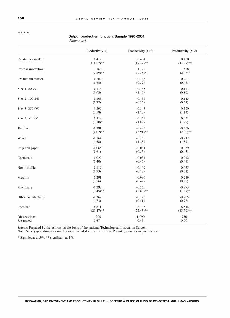
158
InnoVATIon, R&d InVESTMEnT And PRodUCTIVITy In ChILE • RobERTo áLVAREz, CLAUdIo bRAVo-oRTEGA And LUCAS nAVARRo
C E P A L R E V I E W 1 0 4 • A U G U S T 2 0 1 1
TABLE A3
Output production function: Sample 1995-2001(Parameters)
Productivity (t) Productivity (t+1) Productivity (t+2)
Capital per worker 0.412 0.434 0.430(18.07)** (17.47)** (14.97)**
Process innovation 1.168 1.122 1.538(2.59)** (2.35)* (2.35)*
Product innovation -0.262 -0.133 -0.207(0.68) (0.32) (0.43)
Size 1: 50-99 -0.116 -0.163 -0.147(0.92) (1.19) (0.80)
Size 2: 100-249 -0.103 -0.135 -0.113(0.72) (0.85) (0.51)
Size 3: 250-999 -0.290 -0.345 -0.320(1.58) (1.70) (1.14)
Size 4: >1 000 -0.519 -0.529 -0.451(2.10)* (1.89) (1.22)
Textiles -0.391 -0.423 -0.436(4.02)** (3.91)** (2.90)**
Wood -0.164 -0.156 -0.217(1.58) (1.25) (1.57)
Pulp and paper -0.065 -0.061 0.059(0.61) (0.55) (0.43)
Chemicals 0.029 -0.034 0.042(0.40) (0.45) (0.43)
Non-metallic -0.119 -0.109 0.055(0.93) (0.78) (0.31)
Metallic 0.291 0.096 0.219(1.56) (0.47) (0.99)
Machinery -0.298 -0.265 -0.273(3.45)** (2.89)** (1.97)*
Other manufactures -0.367 -0.125 -0.205(1.73) (0.51) (0.78)
Constant 6.811 6.735 6.514(23.47)** (22.43)** (15.59)**
Observations 1 206 1 090 730R-squared 0.47 0.49 0.50
Source: Prepared by the authors on the basis of the national Technological Innovation Survey.Note: Survey-year dummy variables were included in the estimation. Robust z statistics in parentheses.
* Significant at 5%; ** significant at 1%.

159
InnoVATIon, R&d InVESTMEnT And PRodUCTIVITy In ChILE • RobERTo áLVAREz, CLAUdIo bRAVo-oRTEGA And LUCAS nAVARRo
C E P A L R E V I E W 1 0 4 • A U G U S T 2 0 1 1
Acemoglu, D., P. Aghion and F. Zilibotti (2006), “Distance to frontier, selection, and economic growth”, Journal of the European Economic Association, vol. 4, No. 1, Cambridge, Massachusetts, The mit Press.
Aghion, P. and R. Griffth (2005), Competition and Growth. Reconciling Theory and Evidence, Cambridge, Massachusetts, The mit Press.
Aghion, P. and P. Howitt (2005), “Growth with quality-improving innovations: an integrated framework”, Handbook of Economic Growth, vol. 1, Part 1, Amsterdam, Elsevier.
(1992), “A model of growth through creative destruction”, Econometrica, vol. 60, No. 2, New York, Econometric Society.
Álvarez, R. (2001), “External sources of technological innovation in Chilean manufacturing industry”, Estudios de economía, vol. 28, No. 1, Santiago, Chile, University of Chile.
Álvarez, R. and R. Robertson (2004), “Exposure to foreign markets and firm-level innovation: evidence from Chile and Mexico”, Journal of International Trade and Economic Development, vol. 13, No. 1, Taylor and Francis.
Arvanitis, S. and H. Hollenstein (1994), “Demand and supply factors in explaining the innovative activity of Swiss manufacturing firms”, Economics of Innovation and New Technology, vol. 3, No. 1, Routledge.
Benavente, J.M. (2006), “The role of research and innovation in promoting productivity in Chile”, Economics of Innovation and New Technology, vol. 15, No. 4-5, Routledge.
__________ (2005), “Investigación y desarrollo, innovación y productividad: un análisis econométrico a nivel de la firma”, Estudios de economía, vol. 32, No. 1, Santiago, Chile, University of Chile.
Blundell, R., R. Griffith and J. Van Reenen (1999), “Market share, market value and innovation in a panel of British manufacturing firms”, Review of Economic Studies, vol. 66, No. 3, Oxford, Blackwell Publishing.
Bravo-Ortega, C. and A. García (2007), “Cerrando la brecha innovativa latinoamericana: ¿qué podemos aprender de Corea, Israel y Finlandia?”, Estudios socio/económicos, No. 35, Santiago, Chile, Economic Research Corporation for Latin America (cieplan).
Chudnovsky, D., A. López and G. Pupato (2006), “Innovation and productivity in developing countries: a study of Argentine manufacturing firms’ behavior: 1992–2001”, Research Policy, vol. 35, No. 2, Amsterdam, Elsevier.
Cohen, W. and R. Levin (1989), “Empirical studies of r&d and market structure”, Handbook of Industrial Organization, R. Schmalensee and R. Willig (comps.), Amsterdam, North Holland.
Crépon, B., E. Duguet and J. Mairesse (1998), “Research and development, innovation and productivity: an econometric analysis at the firm level”, Economics of Innovation and New Technology, vol. 7, No. 2, Routledge.
Crespi, G. (1999), “Determinantes de la innovación tecnológica en la industria manufacturera chilena”, Estadística y economía, No. 17, Santiago, Chile, National Institute of Statistics.
Crespi, G. and J. Katz (1999), “r&d expenditure, market structure and technological regimes in Chilean manufacturing industry”,
Estudios de economia, vol. 26, No. 2, Santiago, Chile, University of Chile.
Fagerberg, J., M. Srholec and B. Verspagen (2010), “Innovation and economic development”, Handbook of the Economics of Innovation, B. Hall and N. Rosenberg (comps.), Amsterdam, Elsevier.
Figueiredo, P. (2006), “Introduction”, International Journal of Technology Management, vol. 36, No. 1-2-3, Inderscience Publishers.
Griffith, R. and others (2006), “Innovation and productivity across four European countries”, Oxford Review of Economic Policy, vol. 22, No. 4, Oxford, Oxford University Press.
Griliches, Z. (1995), “r&d and productivity: econometric results and measurement issues”, Handbook of the Economics of Innovation and Technological Change, P. Stoneman (comp.), Oxford, Basil Blackwell.
(1958), “Research costs and social returns: hybrid corn and related innovations”, Journal of Political Economy, vol. 66, No. 5, Chicago, University of Chicago Press.
Grossman, G.M. and E. Helpman (1991), Innovation and Growth in the Global Economy, Cambridge, Massachusetts, The mit Press.
Hall, B. and N. Rosenberg (2010), Handbook of the Economics in Innovation, Amsterdam, Elsevier.
Hall, B., F. Lotti and J. Mairesse (2008), “Innovation and productivity in smes: empirical evidence for Italy”, nber Working Paper, No. 14594, Cambridge, Massachusetts, National Bureau of Economic Research.
Hall, B., J. Mairesse and P. Mohnen (2010), “Measuring the returns to r&d”, Handbook of the Economics of Innovation, B. Hall and N. Rosenberg (comps.), Amsterdam, North Holland.
Hall, R. and C. Jones (1999), “Why do some countries produce so much more output per worker than others?”, Quarterly Journal of Economics, vol. 114, No. 1, Cambridge, Massachusetts, The mit Press.
Heston, A., R. Summers and B. Aten (2002), Penn World Table Version 6.1, Philadelphia, Center for International Comparisons of Production, Income and Prices, University of Pennsylvania, October.
Howitt, P. and D. Mayer-Foulkes (2005), “r&d, implementation, and stagnation: a Schumpeterian theory of convergence clubs”, Journal of Money, Credit and Banking, vol. 37, No. 1, Oxford, Blackwell Publishing, February.
Kharas, H. and others (2008), Chilean Growth through East Asian Eyes, Washington, D.C., World Bank.
Klenow, P. and A. Rodríguez-Claire (2005), “Externalities and growth”, Handbook of Economic Growth, P. Aghion and S. Durlaf (comps.), Amsterdam, Elsevier.
Klepper, S. (1996), “Entry, exit, and innovation over the product lifecycle”, American Economic Review, vol. 86, No. 3, Nashville, Tennessee, American Economic Association.
Lederman, D. and L. Saenz (2005), “Innovation and development around the world, 1960-2000”, Policy Research Working Paper Series, No. 3774, Washington, D.C., World Bank.
Maloney, W. and A. Rodríguez-Clare (2007), “Innovation shortfalls”, Review of Development Economics, vol. 11, No. 4, Oxford, Blackwell Publishing.
Bibliography

160
InnoVATIon, R&d InVESTMEnT And PRodUCTIVITy In ChILE • RobERTo áLVAREz, CLAUdIo bRAVo-oRTEGA And LUCAS nAVARRo
C E P A L R E V I E W 1 0 4 • A U G U S T 2 0 1 1
Moguillansky, G., J.C. Salas and G. Cares (2006), “Capacidad de innovación en industrias exportadoras de Chile: la industria del vino y la agroindustria hortofrutícola”, Comercio internacional series, No. 79 (LC/L.2619-P), Santiago, Chile, Economic Commission for Latin America and the Caribbean (eclac). United Nations publication, Sales No. S.06.II.G.143.
oecd (Organisation for Economic Co-operation and Development) (2007), Reviews of Innovation Policy: Chile, Paris.
Pakes, A. and Z. Griliches (1980), “Patents and r&d at the firm level: a first report”, Economics Letters, vol. 5, No. 4, Amsterdam, Elsevier.
Rivera-Batiz, L.A. and P. Romer (1991), “International trade with endogenous technological change”, European Economic Review, vol. 35, No. 4, Amsterdam, Elsevier.
Romer, P. (1990), “Endogenous technological change”, Journal of Political Economy, vol. 98, No. 5, Chicago, University of Chicago Press.
Schultz, T. (1953), The Economic Organization of Agriculture, New York, McGraw Hill.
unesco Institute for Statistics (2005), “r&d Expenditure Table” [online] http://stats.uis.unesco.org/unesco/TableViewer/document.aspx?ReportID=136&IF_Language=eng&BR_Topic=0

C E P A L R E V I E W 1 0 4 • A U G U S T 2 0 1 1
161
The quality gap in Chile’seducation system
José Luis Drago and Ricardo D. Paredes
T he quality gap in education between Chilean schools with
different administrative structures (especially in the case of municipal
schools and private subsidized schools) has long been a subject of
analysis and discussion within the wider debate surrounding the relative
efficiency and role of public education. Unconditioned differences in
the results of standardized tests that point to higher levels of quality in
private schools diminish when sociodemographic factors are controlled
for, but the question as to what control variables should be used and
which methodology is the most appropriate, as well as the extent of the
reduction, all continue to be a subject of debate. Here we undertake
a meta-analysis of 17 of the main studies that have been done on the
subject. The analysis shows how sensitive the results are to the controls
and estimation methods that are used. In the aggregate, private subsidized
schools score approximately four points higher than municipal schools do.
This is a statistically significant and educationally relevant differential.
KEYWORDS
Education
Educational policy
Educational reform
Educational quality
Public schools
Private schools
Measurement
Statistical methodology
Chile
José Luis Drago
School of Engineering, Catholic
University of Chile
Ricardo D. Paredes
Professor, School of Engineering,
Catholic University of Chile, and
Centre for the Study of Educational
Policy and Practice (ceppe)

162
ThE qUALITy GAP In ChILE’S EdUCATIon SySTEM • JoSé LUIS dRAGo And RICARdo d. PAREdES
C E P A L R E V I E W 1 0 4 • A U G U S T 2 0 1 1
We would like to thank the Ministry of Education for having provided us with access to the System for Measuring the Quality of Education (simce) database and to Rómulo Chumacero, Alejandro Carrasco, Cristián Cox, Alejandra Mizala, Paulo Volante and, in particular, a cepal Review referee for their comments and suggestions. We are also grateful for the funding supplied by the National Fund for Scientific and Technological Development (fondecyt) under Project No. 1095176 and by the Centre for the Study of Educational Policy and Practice (ceppe) under the cie01 project of the National Commission for Scientific and Technological Research (conicyt). Any errors or omissions in this article are the sole responsibility of the authors.
Chile’s reform of its education system in the 1980s and, in particular, its introduction of a large-scale voucher scheme were designed to decentralize the system and to promote competition among publicly funded schools as a means of improving the quality of instruction (Aedo and Sapelli, 2001; Mizala, Romaguera and Ostoic, 2004). The government did provide funding for some private schools before the 1980s, but the reform expanded this arrangement so much that it reached a point where there was no significant difference between the level of government funding provided to private and public schools. Later on, however, institutionally based differences in working conditions for teachers did arise, as did differences in the schools’ organizational structures and, ultimately, their funding. The resulting difficulty of drawing direct comparisons between the performance levels of students in the different types of schools has sparked a heated debate about school administration and its effect on scholastic achievement.
One of the central hypotheses put forward in the vast body of literature that has grown up around this issue is that the private schools are better-run. This proposition is primarily based on the sharp differences between the unconditioned scores on standardized tests of students in the different types of schools. The ensuing public debate has focused on the sustainability of public education, especially in view of the fact that, as a percentage of the total, the 80% public school enrolment rate registered in 1980 had dropped to less than 45% by 2010 and that this steep reduction could be the result, at least in part, of the declining quality of the education being provided by the country’s municipalities, where inter-school segmentation, admissions screening and
inequities are raising some doubts about the success of the earlier reforms.1
The fact that sharp unconditioned differences are systematically found between the scores on standardized tests of students in one type of school or the other is not a sufficient basis for concluding that the quality of instruction provided by these schools differs, however. The view in some quarters is that the reform has led to a sharper stratification of the education system, with the most vulnerable students being left in the public schools, and that this accounts, at least in part, for the gap (Hsieh and Urquiola, 2006). As discussed in a number of studies, this view has fuelled the controversy surrounding the quantification of these differences in terms of production functions of education. The findings have varied, with some authors arriving at conclusions that are diametrically opposed to those of others: some have determined that subsidized private schools are turning in better performances; others have found no statistically relevant differential; and still others (after isolating a number of factors) have argued that public schools are the best performers. An additional factor to be taken into account is that there are also sharp differentials between one public school and the next (Paredes and Paredes, 2009).
The public policy implications of each of these different findings are, naturally, quite different. Gallego (2002), for example, contends that, despite the lack of any clear-cut difference between the scholastic achievement of pupils in municipal schools and those in subsidized private schools, the system in general has benefited from the increased competition and has consequently improved. Hsieh and Urquiola (2006) argue that the better results exhibited by subsidized private schools are primarily attributable to selection effects rather than to better administration. These differing positions are reflections of discussions that are taking place at differing levels, however. While the former position is taking an equilibrium analysis approach, the latter is not necessarily tackling the question from the same vantage point. Thus, even if private education were to prove to
1 For a discussion of these issue, see Hsieh and Urquiola, 2003; Paredes and Pinto, 2009; Chumacero and Paredes, 2009; and Marcel and Raczinsky, 2010.
Iintroduction

163
ThE qUALITy GAP In ChILE’S EdUCATIon SySTEM • JoSé LUIS dRAGo And RICARdo d. PAREdES
C E P A L R E V I E W 1 0 4 • A U G U S T 2 0 1 1
be “more efficient” than public education, this could be due to a student selection effect, and the underlying overall effects therefore cannot be identified unless a comprehensive study is conducted. The debate in Chile is thus centred on the point of departure, since the main point at issue at this juncture is whether or not such a gap actually exists at all.2
The purpose of this study is to delimit the discussion concerning empirical results by means of a meta-analysis. Meta-analyses are a tool that is widely used in the social sciences to distil and differentiate among the hypotheses put forward by many different studies when they fail to arrive at an agreed conclusion. It is only recently being applied in the field of education, however (e.g., Adesope
2 The authors wish to thank the referee of the cepal Review for raising this point.
and others, 2010; Credé, Roch and Kieszczynka, 2010; and Bowman, 2010). Based on a very strict adherence to the eligibility standards put forward by Raudenbush and Bryk (2002), 17 studies on the efficiency differences between private and municipal schools in Chile were selected. A robust statistical model was then used to check whether the results of the meta-analysis fit in with a general, robust specification and estimation method.
Four sections follow this introduction. Section II provides a description of the Chilean education system. Section III outlines the methodology that was used and describes the studies that were selected for the meta-analysis. Section IV presents the results. The conclusions are set forth in section V.
IIThe Chilean education system
1. Background
Until the early 1980s, nearly 80% of the country’s schools were run by the State. The Ministry of Education was in charge of funding and running Chile’s schools, supervising and developing curricula, and investing in and building public school infrastructure. The system had high dropout and repeater rates, however, and was viewed as delivering a poor-quality education owing to its excessively bureaucratic nature, insufficient coverage and failure to provide schools with proper incentives.3 This gave rise to a far-ranging reform of the education system based on the work done by Friedman (1955). Chile was one of the first countries in the world to introduce a reform of this type, or at least a reform of this scale and nature. State-run schools were handed over to the country’s municipalities and were financed with subsidies that did not differentiate between pupils attending municipal schools and those attending non-fee private voucher schools (Mizala and Romaguera
3 Hanushek (1998) indicates, for example, that, in 1970, the test scores for Chile’s students were 50% lower than the those of students in France and the United States and 20% lower than those of students in Japan and were only 10% higher than students in India and the Islamic Republic of Iran. Barro (1999) reported that Chile’s scores were 50% lower than what they would be expected to be given its level of development. For a detailed analysis, see Paredes and Hayl (2010).
1998). The reform gave rise to three types of schools: (i) municipal, State-funded schools (with funding provided by per-student subsidies); ii) privately run, State-funded subsidized schools (with funding provided by per-student subsidies); and (iii) privately run schools funded by tuition payments.
In order to make the education system better and more equitable so as to benefit the more vulnerable sectors of the population, in the early 1990s a number of programmes were put in place to supplement the school subsidy scheme, including special support programmes for schools serving underprivileged children (e.g., the “900 Schools” programme for poor sectors of the population, the Education Improvement Project and the Quality and Equity in Education Programme).4 In 1991 the Teachers Statute, which re-established teacher benefits that had been withdrawn in the 1980s, was passed. Among other things, it re-introduced collective negotiations on wages and on job security for the faculty of municipal schools. Apart from the advantages of this agreement, however, the Teachers Statute has heightened the differences between one education system and another by making the administrative arrangements for municipal schools more rigid. In 1996 an incentive system —the National Performance Evaluation System
4 The reasons why the effort to achieve greater equity takes the form of programme implementation rather than modifications of the subsidy are explained in Weinstein and Muñoz (2009). See also Weinstein, Fuenzalida and Muñoz (2010).

164
ThE qUALITy GAP In ChILE’S EdUCATIon SySTEM • JoSé LUIS dRAGo And RICARdo d. PAREdES
C E P A L R E V I E W 1 0 4 • A U G U S T 2 0 1 1
(sned)— was put in place in order to recognize and enhance teachers’ best practices.
In 1993 a new provision was introduced to supplement State funding. Under this statute, some of the subsidized schools were allowed to charge parents for a portion of the tuition, and subsidized private schools and some public schools were authorized to receive donations or grants, which would be deducted from the State subsidy.5 This led to a steep rise in private school enrolment that has cast some doubt over the sustainability of the municipal school system (Paredes and Pinto, 2009).
These policies succeeded in bringing about a steep reduction in dropout rates and a steady increase in enrolment rates. The scores on the System for Measuring the Quality of Education (simce) tests, however, indicate that the quality of education remains quite limited and that striking differences between the performance of students in different socio-economic sectors continue to pose a major challenge.6 Hsieh and Urquiola (2003) argue that the reform spurred an exodus of middle-class students from municipal schools to private subsidized ones, which left the municipal schools with a much greater proportion of students from vulnerable sectors and therefore drove down their average scores. Along these same lines, Mizala, Romaguera and Ostoic (2004) point out that municipal schools, unlike their private counterparts, have to accept all applicants (as long as they have room) and that it is quite difficult from them to expel students.
The consensus view is that these three types of schools are serving sharply stratified socio-economic groups. As shown in table 1, the majority of students in
5 Secondary municipal schools can opt for the co-financing system if authorized to do so by a majority of parents and guardians.6 Chilean students scored substantially higher on the 2006 Programme for International Student Assessment (pisa) test, especially in the humanities (oecd, 2008). The reason for this improvement would be a highly interesting research topic.
municipal schools are from the lower-income quintiles (70%), and this has been the situation for a number of years now. In contrast, subsidized private schools receive a larger percentage of middle-income students and even a considerable number of students from high-income sectors.
The overall results are not good either. The principal performance indicator for education in Chile is the standardized simce test, and the scores on that test are much higher in fee-paying private schools than they are in the other two types of educational establishments.7
2. Context and results
Once the reform had been carried out, questions began to arise as to its repercussions and implications for the quality of education. One way of approaching this issue, which, although not a study of the reform’s overall effects, could shed some light on one of its direct repercussions, is to analyse the performance differentials between municipal and subsidized private schools. There have been a plethora of studies on the subject in recent years, but they have arrived at very different conclusions, and this has added fuel to the debate over the years in ways that have often steered it into the realm of differing ideologies.
The conceptual and empirical foundations underlying this discussion clearly extend beyond the specific case of Chile. Hanushek (2003) suggests that, in recent years, the cost of public education has risen sharply without attaining the expected results. Chubb (2001) contends that, if education were privatized, schools would have powerful incentives for cutting costs and that this would push them to innovate and become more efficient. Others argue that this type of system would prompt private schools to cut costs in ways (e.g., recruiting less qualified teachers at lower salaries) that would lower the quality of the education that they provide. In addition, this system could lead to discriminatory practices whereby schools would give preference to students that would be less costly for them (Levin, 2002). In Hoxby’s view (2001), this kind of situation arises because, in a flat-rate subsidization system, subsidized private schools have no incentive to take on students who are in more vulnerable situations, since they will require a larger investment in order to achieve better scores.
Chile’s case is alluded to indirectly by Gallego (2002), who has developed a model for determining the effect of competition between municipal and subsidized
7 For further information on the scores, see www.simce.cl
TABLE 1
Enrolment, by type of school(Percentages)
Income quintile
Type of school I II III IV V
Municipal 42.39 27.60 16.06 10.66 4.24
Private (subsidized) 22.34 22.63 21.26 20.59 13.37
Private (fee-paying) 4.64 4.64 4.49 12.37 75.26
Source: Prepared by the authors on the basis of the 2006 National Characterization Socio-economic Survey (casen) database.

165
ThE qUALITy GAP In ChILE’S EdUCATIon SySTEM • JoSé LUIS dRAGo And RICARdo d. PAREdES
C E P A L R E V I E W 1 0 4 • A U G U S T 2 0 1 1
private schools. Gallego finds a positive correlation between competition and performance, particularly in subsidized private schools, and interprets this as being a consequence of the existence of stronger incentives for a rapid response to potential competition. This would also, however, have a positive impact on municipal schools. Sapelli (2003), while working to draw general lessons from these experiences, talks about a form of market duality, inasmuch as Chile’s public schools and subsidized private schools are not subject to the same external rules. Municipal schools, unlike their subsidized private counterparts, are subject to “soft” budgetary constraints in the sense that they often receive additional funding from the municipality, which is a disincentive for more efficient operations. On the other side, subsidized private schools have the option of obtaining more funding from the students’ parents. Carnoy (1997) questions the idea that competition will have a positive effect and instead argues that such a system will only benefit higher-income students because, if schools are in competition with one another, they will try to select for the top students.
Valenzuela, Bellei and de los Ríos (2008) find that the crucial issue in Chile’s education system is the striking differentials between the scores of students in the different types of schools, which are closely correlated with household income. Tokman (2002) finds that, following the reform, the municipal system lost its best students, who transferred to subsidized private schools, which lowered public schools’ scores. By the same token, Hsieh and Urquiola (2006) state that, after the reform, the private subsidized schools’ better showing was primarily due to the fact that they had selected out the best students.
Fontaine (2003) maintains that the use being made of the co-financing arrangement attests to the fact that
many parents are willing to cover part of their children’s educational costs if this will provide them with a higher-quality education and more individual attention. In addition, subsidized private schools are required to use 10% of their tuition proceeds to provide scholarships for poor students, which clearly is of great benefit for poorer sectors of the population. Given the highly stratified nature of the education system, Tokman (2002), Carnoy (1997) and, in particular, McEwan (2003) all contend that the poorer performance of students in municipal schools is attributable to a peer effect (i.e., when less gifted students are grouped together, they are less likely to do well scholastically). This last proposition is open to discussion, since it has not been definitively resolved. There are, for example, schools of thought according to which this factor is irrelevant, and the segregation of students by abilities allows educators to use specific techniques that are geared towards overcoming their limitations.
The above discussion highlights the fact that a comparison of the performance of students in fee-paying private, subsidized private and municipal schools is a complex proposition. A series of studies have been conducted in an effort to assess relative performance levels using econometric models that are designed to take all the various factors affecting student performance into consideration. The choices made when selecting the operational approach, the variables to be taken into account and the estimation methods to be used are also, however, part of the discussion. As noted by Bellei (2005), the findings of studies designed to answer the question as to whether subsidized private education is better are determined, to a great extent, by the research methodology that they use, since quite small changes can have a strong impact on their ultimate results.

166
ThE qUALITy GAP In ChILE’S EdUCATIon SySTEM • JoSé LUIS dRAGo And RICARdo d. PAREdES
C E P A L R E V I E W 1 0 4 • A U G U S T 2 0 1 1
1. Meta-analysis
Meta-analysis is a technique for reviewing and aggregating the findings of different studies in an attempt to answer a given scientific question (Letón and Pedromingo, 2001). It began to come into use in the social sciences and agriculture in the 1930s. The term “meta-analysis” was coined by Glass (1976) and, since the 1980s, its use has become widespread, especially in the field of medicine and the social sciences. The greatest advantage that it offers is that it provides a way of determining how a number of different studies tie in with one another (Lipsey and Wilson, 2001), which, in turn, makes it possible to arrive at an overarching conclusion concerning any given hypothesis by first determining what the strengths and weaknesses of each study are and why their findings differ.
More recently, meta-analysis has come into use in the field of education. Adesope and others (2010) have used it to estimate the effect of bilingualism on cognitive outcomes. Credé, Roch and Kieszczynka (2010) have used it to determine the correlations between students’ grades and class attendance. Bowman (2010) has employed the methodology to try to establish a relationship between a school’s racial diversity and its students’ cognitive development.
A meta-analysis has two stages: (i) compiling relevant studies, and (ii) relating the selected studies to one another. In the compilation stage, a formal set of selection criteria has to be established in order to minimize the bias generated by the choice of studies. In the case at hand, the selection criteria are: (i) that the studies refer either directly or indirectly to differences in academic performance between public and private schools in Chile; (ii) that they were published after 1997 (so as to limit the range of studies to the more recent ones); (iii) that they have had a fairly notable impact in the field, as measured by the stature of the publisher or the number of times that they have been cited in other research papers; (iv) that their estimates have been arrived at through the use of econometric models; and (v) that they have used representative datasets.
The techniques used in the second stage of a meta-analysis are classical statistical methods. Meta-analyses are used for statistical inference, measurement of the
overall effect size, variance estimation, confidence intervals, and statistical contrast and its significance.
The methodology for relating a set of studies to one another is based on the model proposed by Raudenbush and Bryk (2002), who used hierarchical linear modelling (hlm) to obtain the mean and overall variance of the parameter to be estimated. It makes sense to use hlm because of the nested structure of the variables in question. The model has two levels. The first is related to each study’s results and their variance, while the second refers to the overall parameter to be estimated (the parameter being sought) and the variance among the studies being analysed. The first step is to obtain the standardized mean of the effect to be analysed for each study included in the meta-analysis, which is represented by dj. For study j, this is obtained by (1). Thus, for the j-nth study, dj is expressed by the following equation:
dY Y
SjEj cj
j
=−
(1)
where YEj is the mean for the experimental group; Ycj is the mean for the control group; and Sj is the standard deviation of the difference between the two. Equation (1) yields a standardized value for the standard deviation for each study, thereby assigning a greater weighting to studies with less variability.
At the first level, the model is:
d e e N Vj j j j j= +δ , ~ ( , )0 (2)
For each study j, ej is the error associated with the variable dj. The statistical distribution of ej is a normal one with a mean of 0 and a variance of Vj, while δj corresponds to the real value of the variable in study j. In this case, the relevant variable (linked to the parameter “subsidized private school”) obtained from each study is dj, and its corresponding variance is Vj (both known values). At the second level, a similar model is used:
δ γ u= +0j j (3)
IIIMethodology and data

167
ThE qUALITy GAP In ChILE’S EdUCATIon SySTEM • JoSé LUIS dRAGo And RICARdo d. PAREdES
C E P A L R E V I E W 1 0 4 • A U G U S T 2 0 1 1
where:γ0 is the overall mean, anduj is the error at the second level, which distributes
uj ∼N(0, τ).Thus, by introducing equation (3) into (2), for each
study we obtain the final model:
d u ej j j= + +γ 0 (4)
Therefore, dj distributes normally dj ~ N(γ0 ⋅ τ0 + Vj). This yields the overall parameter (γ10) and the overall standard deviation (τ0). It is possible to estimate whether τ0 is actually statistically different from 0 so that we can then determine if a relevant difference exists among the selected studies. To do so, we use a hypothesis test where H0:τ0 = 0, with the statistic:
Q Vj j−∑ 1 2( .)= −d d (5)
where dV d
Vj j
j
. = ∑∑
−
−∗1
1 . This statist ic has a
distribution of χ2 with j-1 degrees of freedom, while
Q is the term discussed by Hedges (1982). To estimate δj (Bayes estimator), the steps involved are as follows: on the one hand, .j is an unbiased estimator of δj with a variance of Vj, but, on the other, γ0 can be regarded as a common estimator for each δj. The optimum estimator for each study can be calculated using the optimum Bayes estimator (δ j
∗ ) (Lindley and Smith, 1972), since it combines the two parameters discussed above in an optimum manner:
δ λj j j jY*.
ˆ= + −1 0( )λ γ (6)
where λj is equal to the reliability of .j as an estimator of δj.
λδ τ
τjj
j j
Var
Var Y V= =
+
( )
( ) ( ).
0
0
(7)
From (7) it can be inferred that, when the sample is highly reliable, there will tend to be a marked preponderance of .j in the value of δ j
∗ , given its proximity. This means that λj will have a value close to 1. If, on the other hand, the sample is not reliable, Y0 will tend to have a greater weight in the value of δ j
∗, while λj will tend towards a value close to 0.
2. Selected studies and data
A total of 17 studies were selected. These studies use a nationwide sample of simce test scores to estimate the effect by means of multiple regressions using ordinary least squares (ols), the Heckman correction (hc), propensity score matching (psm) or hierarchical linear modelling (hlm). The most complete model in which the estimates and conclusions were the most coherent was used for each study. Of course, given the differences in the models, bases, levels of aggregation, specifications and estimation techniques used in the various studies, their results are not the same. And this is precisely what the meta-analysis is intended to address. Table 2 shows that the biggest differences are in the year, grades and subjects used for the sample. The models’ levels of aggregation also differ, since some studies worked at the school level and others at that of individual students. The study samples vary as well, while screening differences and a lack of data in some cases could account for part of the differences in their results. Imputation methodologies can, of course, also explain inter-study differences.
The methodologies used also differed. In the first generation of studies —Mizala and Romaguera (1998); Bravo, Contreras and Sanhueza (1999); McEwan and Carnoy (2000); Gallego (2002); Tokman (2002); and Sapelli (2003)— the results were analysed while controlling for individual, family and geographic factors at the school level. ols were used to estimate an educational output function; no consensus was reached, although subsidized private schools did tend to yield somewhat more favourable results. These studies suffer from a number of limitations, however, with the main one being that their data were compiled at the school level, which did not allow them to look at within-school variations.
The second-generation studies were conducted at the level of individual students using ols and hc models: McEwan, 2001; González, Mizala and Romaguera, 2002; Sapelli and Vial, 2002; Bellei, 2005; Contreras, Bustos and Sepúlveda (2007); and García and Paredes, 2010. McEwan (2001), Contreras, Bustos and Sepúlveda (2007) and García and Paredes (2010) took the endogeneity of school choice into consideration to some degree and Heckman-corrected their ols models. Mizala and Romaguera (2003), Manzi and others (2008) and Mizala, Romaguera and Ostoic (2004) based their estimates on two-level hlm models so as to address the heterogeneity of students attending different schools.
Each study controls for different variables, although they almost all share a certain number of them. The

168
ThE qUALITy GAP In ChILE’S EdUCATIon SySTEM • JoSé LUIS dRAGo And RICARdo d. PAREdES
C E P A L R E V I E W 1 0 4 • A U G U S T 2 0 1 1
third column of table 3 shows the variables included in each model. All the studies control for socio-economic characteristics, although the specific variable changes from one to the next (for example: vulnerability index, linear income, quadratic income). Socio-economic status is systematically approximated by the parents’ level of education, either at the average level per school or for individual students, depending on the nature of each model. Table 3 shows the results for each of the 17 studies. Ten of the studies suggest that subsidized private schools provide a better education; five find no statistically significance difference, and two indicate that municipal schools offer a better-quality education.
The variation in these results is quite striking, with conditioned differences ranging from -6.948 to 18.107, with a mean standard deviation of 6.338. Both
the mean (4.358) and the median (3.431) are positive, which suggests that most of the studies point to a better performance on the part of subsidized private schools than municipal schools.
In summary, there are some variables that have been used in almost all of the studies, while there are others that have been used in only one or a few (e.g., sex of the student, presence of indigenous students) (for a detailed description, see Drago, 2010). No clear relationship between the types of control variables and differences in performance outcomes for municipal and subsidized private schools emerges, however. Nonetheless, there does appear to be a difference in terms of the number of controls, especially in the case of fixed effects identified by hlm, in which case the difference, in either direction, declines.
TABLE 2
Datasets for each study
Study Year/grade/subjecta Level Model Sampleb
Mizala and Romaguera (1998) 1996/4thE/M and L School ols 5 133 (63.3%)Bravo, Contreras and Sanhueza (1999) 1996/4thE/M School ols 5 110 (63.0%)McEwan and Carnoy (2000) 1996/4thE/M School ols 5 490 (67.7%)McEwan (2001) 1997/4thE/M Student hc 158 872 (67.4%)Gallego (2002) 1996/4thE/M and L School ols 4 904 (62.9%)González, Mizala and Romaguera (2002) 1999/4thE/M Student ols 202 754 (88.8%)Sapelli and Vial (2002) 1998/2ndS/L Student hc 46 223 (25.2%)Tokman (2002) 1996/4thE/M School ols 2 789 (37.2%)Sapelli (2003) 1999/4thE/M School ols 4 784 (61.5%)Mizala and Romaguera (2003) 1998/2ndS/M Student hlm 69 402 (30.9%)Mizala, Romaguera and Ostoic (2004) 1999/4thE/M Student hlm 226 860 (83.5%)Bellei (2005) 2002/4thE/M Student ols 199 112 (83.3%)Contreras, Bustos and Sepúlveda (2007) 2005/4thE/M Student hc 161 619 (61.1%)Manzi and others (2008) 2005/4thE/M Student hlm 233 338 (88.2%)Mizala, Anand and Repetto (2009) 2002/4thE/L Student psm 77 921 (32.6%)García and Paredes (2010) 2005/4thE/M Student hc 225 206 (85.1%)Mizala, Repetto and Lara (2009) 2006/2ndS/M Student psm 20 000 aprox.c
Source: Prepared by the authors.
a Year, grade (E: elementary, S: secondary) and subject (L: language, M: mathematics) are characteristics of the datasets of simce scores used to develop the models.
b For the studies conducted at the school level, the size of the sample corresponds to the number of schools that were surveyed. For the studies conducted at the student level, the sample size corresponds to the number of individual students in that sample, but it will differ enormously depending on data imputations or the criteria used to eliminate observations in which data were missing.
c In this case, samples from different years were used.ols: ordinary least squares. hc: Heckman correction. hlm: hierarchical linear modelling. psm: propensity score matching.

169
ThE qUALITy GAP In ChILE’S EdUCATIon SySTEM • JoSé LUIS dRAGo And RICARdo d. PAREdES
C E P A L R E V I E W 1 0 4 • A U G U S T 2 0 1 1
TABLE 3
Characteristics of the selected studies
Study Control variables Result (standard deviation)a
Effect on scoresb
Mizala and Romaguera (1998)
Socio-economic level/fee-paying private, subsidized private or municipal school/ mixed school/preschool education/ teachers’ experience/student-teacher ratio/number of teachers/ geographic index
1.981 (1.042) +
Bravo, Contreras and Sanhueza (1999)
Socio-economic level/ fee-paying private, subsidized private or municipal school, mixed school/ preschool education/ aid programmes/acceptance of schoolwork/ student-teacher ratio/ number of teachers/ geographic index/ rural
-0.484 (0.494) =
McEwan and Carnoy (2000)
Socio-economic level/parents’ average level of education/ completion of elementary school by parents /fee-paying private, subsidized private or municipal school/number of students in school/series of teacher characteristics/geographic index/ rural
13.073 (2.478) +
McEwan (2001) Household income and average household income for the grade /parents’ average level of education /indigenous mother/ sex of student /number of books in home /fee-paying private, subsidized private or municipal school/percentage of indigenous mothers / rural
-6.948 (3.940) -
Gallego (2002) Socio-economic level/ fee-paying private, subsidized private or municipal school/competence
1.774 (1.258) +
González, Mizala and Romaguera (2002)
Household income and household income2 /income deviation per school/parents’ average level of education /fee-paying private, subsidized private or municipal school /full-length school day/number of students enrolled and number of students enrolled2 /Payment per student / teachers’ experience/ student-teacher ratio
11.794 (0.293) +
Sapelli and Vial (2002)
Household income/parents’ level of education/indigenous family/subsidized private or municipal school
6.900 (1.50) +
Tokman (2002) Logarithm of income/vulnerability index and poverty line index / parents’ level of education /number of persons in household/subsidized private or municipal school/ teachers’ experience/percentage of teachers with university degrees, men/number of teachers /hours worked/ rural
5.827 (49.057) =
Sapelli (2003) Logarithm of mothers’ level of education and standard deviation of mother’s level of education /subsidized private or municipal school / rural
0.790 (3.740) =
Mizala and Romaguera (2003)
Socio-economic level of school/household income and household income2 / fee-paying private, subsidized private or municipal school/ mixed school/school with science and humanities curricula or schools with science, humanities and vocational curricula / logarithm of the number of students enrolled/ teachers’ experience/ student-teacher ratio
18.107 (6.924) +
Mizala, Romaguera and Ostoic (2004)
Socio-economic level of school and student /length of school day in hours /students who repeat a grade / preschool education/ fee-paying private, subsidized private or municipal school/ mixed school/ full-length school day/ logarithm of the number of students enrolled / teachers’ experience/ student-teacher ratio/ rural
3.431 (0.751) +
Bellei (2005) Logarithm of household income and socio-economic level of the school/ parents’ level of education / parents’ expectations/ sex of student/students who repeat a grade/ number of books in the home/ fee-paying private, subsidized private or municipal school/ percentages of students regularly attending the school and repeating a grade /school expels students if they have to repeat a grade /average number of years that students have been in school
-0.310 (0.620) =
Contreras, Bustos and Sepúlveda (2007)
Household income, household income2 /parents’ level of education /sex of student / municipal or subsidized private school / rural/ number of students/ teachers’ experience/ selection
0.470 (0.340) =
Manzi and others (2008)
Socio-economic level of school and of individual students/ number of books in the home/number of persons per household/ municipal or subsidized private school/number of students/selection/ parent participation and use of information/ rural/ northern, central or metropolitan areas
-3.261 (0.674) -
Mizala, Anand and Repetto (2009)
Socio-economic level of school and of individual students / parents’ level of education/ parents’ participation and expectations/ preschool education/ municipal or subsidized private school / selection
10.072 (2.195) +
García and Paredes (2010)
Household income. household income2/ parents’ level of education / parents’ participation/ fee-paying private, subsidized private or municipal school/ payment per student/ team management/teachers’ qualifications/teacher evaluations/ monitoring of teachers/ rural
7.260 (0.346) +
Mizala. Repetto and Lara (2009)
Socio-economic level of school and of individual students / parents’ level of education / parents’ participation and expectations/students who have to repeat a grade/number of books in the home/ preschool education/ municipal or subsidized private school / selection
3.613 (1.892) +
Source: Prepared by the authors.
a Differences (in points) in simce scores calculated in each study; positive values indicate a better outcome for subsidized private schools while negative values indicate a better outcome for municipal schools.
b +: positive effect for subsidized private education; =: no statistically significant difference; -: negative effect for subsidized private education (90% significance).

170
ThE qUALITy GAP In ChILE’S EdUCATIon SySTEM • JoSé LUIS dRAGo And RICARdo d. PAREdES
C E P A L R E V I E W 1 0 4 • A U G U S T 2 0 1 1
1. Meta-analysis
The results of the meta-analysis are presented in table 4. The figures show that subsidized private schools out-perform municipal schools by 3.9 points, with a confidence interval of 95%. The same table also shows that the standard deviation between studies is 5.9, which indicates how sensitive the selected models are to the datasets used and their specification. Once again, a homogeneity test of this parameter rules out the homogeneity hypothesis (p < 0.01).
Figure 1 provides a clearer picture of the results of the meta-analysis and of the different studies. For each study, a numerical value is given on the horizontal axis for each coefficient of the dummy variable for a subsidized private school (relative to a municipal school) and the respective confidence interval. Each
IVresults
study is represented by a square whose size corresponds to its weighting in the meta-analysis, which bears a direct relationship to the precision of each estimator, and by a horizontal line that shows the confidence interval of the estimator (the greater the quotient of the estimator and its variance, the greater that study’s weighting). The rhombus at the bottom represents the estimated value yielded by the meta-analysis of all the studies (3.923), while the distance between the horizontal sides represents the standard deviation of that estimate. The dotted vertical line rising from the rhombus provides a point of reference for gauging how the estimate for each study compares to the overall estimate.
The optimum Bayes estimators, i.e., the estimator for each study corrected by the overall estimated effect, can also be obtained (see table 5).
TABLE 4
results of the meta-analysis for all of the selected studies
Overall parameter Minimum value Maximum value Standard deviation Q (homogeneity test) Value p
3.923 0.851 6.996 5.900 942.200 0.000
Source: Prepared by the authors.
FIGURE 1
Graphic representation of the meta-analysis results
Source: Prepared by the authors.
–100 –50 0 50 100Result
Mizala and Romaguera (1998)Bravo, Contreras and Sanhueza (1999)
McEwan and Carnoy (2000)McEwan (2001)Gallego (2002)
González, Mizala and Romaguera (2002)Sapelli and Vial (2002)
Tokman (2002)Sapelli (2003)
Mizala and Romaguera (2003)Mizala, Romaguera and Ostoic (2004)
Bellei (2005)Contreras, Bustos and Sepúlveda (2007)
Manzi and others (2008)García and Paredes (2010)
Combined

171
ThE qUALITy GAP In ChILE’S EdUCATIon SySTEM • JoSé LUIS dRAGo And RICARdo d. PAREdES
C E P A L R E V I E W 1 0 4 • A U G U S T 2 0 1 1
2. A more robust specification
In order to determine how much the results of the meta-analysis may have been influenced by the rigidity of the specifications, a model can be estimated using the most robust possible structure. At the same time, we can use both ols and hlm estimates in order to check whether or not the results are sensitive to the method chosen. In other words, if the results obtained after estimating a model using two different methods —ols and hlm— with a highly robust specification (without any bias due to the omission of variables) differ by something on the order of 4 points, then the controversy could be attributable to a specification problem, rather than to the grade chosen or the screening of the sample. If, however, they differ by an amount that is substantially different from the results of the meta-analysis, then the controversy about the reasons for this difference continues, although the nature of the point at issue can be defined somewhat more precisely. The scores on the simce math test for students in the fourth grade in 2008 will be used for this purpose.
One particularly interesting aspect in this case is that the robust specification takes selection variables into account, since selection is presumably more of a factor in subsidized private schools than in municipal ones. And, in fact, 67% of the subsidized private schools report that they do practise some sort of admissions screening, whereas, for municipal schools, the figure is 37%. We therefore include a set of interactive terms that also make the estimate more robust.
In sum, the specification for the two-level hlm model is as follows. At the student level:
Y Ln g EdPad EdMad
Ed
ij j j ij j ij j ij
j
= + + + +β β β β
β0 1
5
( )
PrresCol Gen MadInd
N Hab Es
ij j ij j ij
j ij j
+ + +
+
β β
β β6 7
80
9 ppPad rij ij
3 4
(8)
where Yij is the score on the simce mathematics test of student i, who attends school j. rij is the level-1 error term, which is distributed r Nij ∼ ( , )0 2σ , where σ 2 represents the level-1 variance.
The model at the school level (level 2) is as follows:
β γ γ γ γ
γ γ0 00 01 02 03
04 05
j PS PP Ln SchSes
Urbano
= + + + +
+ TTamClas TamClas
Ln Ex of Selección
+ ++
γγ γ
062
07 08( )Pr ++ µ j0
( )
(9)
where γ00, γ01, …, γ08 are the level-2 coefficients. µj0 is the level-2 error term, which is distributed µj0~N(0, τ00) and covariance τ00.
Four models are estimated using ols and hlm; this permits different controls to be used (see table 6).
The results given in table 6 show that the fewer controls there are (model A), the greater the differential in favour of subsidized schools. These results, particularly in the case of the hlm model with more controls, are consistent with the results of the meta-analysis in that they show that subsidized private schools out-perform municipal schools. The differential yielded by this model is substantially greater than the differential suggested by the meta-analysis, however. This could be attributable –apart from possible factors such as aggregation– to the grade and year chosen.
TABLE 5
Estimators and confidence intervals of Bayes optimums
Study Result Corrected result Minimum Maximum
Mizala and Romaguera (1998) 1.981 2.030 0.340 3.720Bravo, Contreras and Sanhueza (1999) -0.494 -0.430 -1.270 0.350McEwan and Carnoy (2000) 13.073 11.580 7.820 15.350McEwan (2001) -6.948 -3.630 -9.050 1.790Gallego (2002) 1.774 1.850 -0.170 3.880González, Mizala and Romaguera (2002) 11.800 11.770 11.270 12.250Sapelli and Vial (2002) 6.900 6.680 4.290 9.080Tokman (2002) 5.827 3.510 -6.290 13.300Sapelli (2003) 0.790 1.580 -3.640 6.810Mizala and Romaguera (2003) 18.107 9.470 2.010 16.930Mizala, Romaguera and Ostoic (2004) 3.431 3.430 2.210 4.660Bellei (2005) -0.310 -0.270 -1.280 0.750Contreras, Bustos and Sepúlveda (2007) 0.470 0.48 -0.080 1.04Manzi and others (2008) -3.261 -3.170 -4.270 -2.070García and Paredes (2010) 7.260 7.250 6.680 7.810
Source: Prepared by the authors.
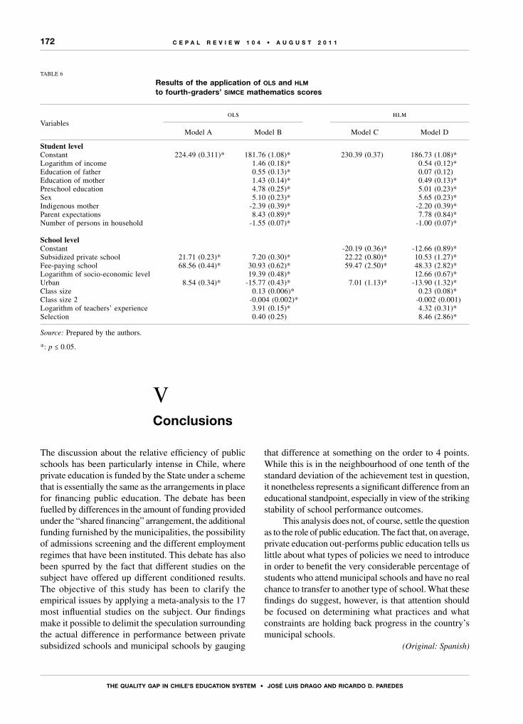
172
ThE qUALITy GAP In ChILE’S EdUCATIon SySTEM • JoSé LUIS dRAGo And RICARdo d. PAREdES
C E P A L R E V I E W 1 0 4 • A U G U S T 2 0 1 1
The discussion about the relative efficiency of public schools has been particularly intense in Chile, where private education is funded by the State under a scheme that is essentially the same as the arrangements in place for financing public education. The debate has been fuelled by differences in the amount of funding provided under the “shared financing” arrangement, the additional funding furnished by the municipalities, the possibility of admissions screening and the different employment regimes that have been instituted. This debate has also been spurred by the fact that different studies on the subject have offered up different conditioned results. The objective of this study has been to clarify the empirical issues by applying a meta-analysis to the 17 most influential studies on the subject. Our findings make it possible to delimit the speculation surrounding the actual difference in performance between private subsidized schools and municipal schools by gauging
that difference at something on the order to 4 points. While this is in the neighbourhood of one tenth of the standard deviation of the achievement test in question, it nonetheless represents a significant difference from an educational standpoint, especially in view of the striking stability of school performance outcomes.
This analysis does not, of course, settle the question as to the role of public education. The fact that, on average, private education out-performs public education tells us little about what types of policies we need to introduce in order to benefit the very considerable percentage of students who attend municipal schools and have no real chance to transfer to another type of school. What these findings do suggest, however, is that attention should be focused on determining what practices and what constraints are holding back progress in the country’s municipal schools.
(Original: Spanish)
TABLE 6
results of the application of ols and hlm
to fourth-graders’ simce mathematics scores
Variablesols hlm
Model A Model B Model C Model D
Student levelConstant 224.49 (0.311)* 181.76 (1.08)* 230.39 (0.37) 186.73 (1.08)*Logarithm of income 1.46 (0.18)* 0.54 (0.12)*Education of father 0.55 (0.13)* 0.07 (0.12)Education of mother 1.43 (0.14)* 0.49 (0.13)*Preschool education 4.78 (0.25)* 5.01 (0.23)*Sex 5.10 (0.23)* 5.65 (0.23)*Indigenous mother -2.39 (0.39)* -2.20 (0.39)*Parent expectations 8.43 (0.89)* 7.78 (0.84)*Number of persons in household -1.55 (0.07)* -1.00 (0.07)*
School levelConstant -20.19 (0.36)* -12.66 (0.89)*Subsidized private school 21.71 (0.23)* 7.20 (0.30)* 22.22 (0.80)* 10.53 (1.27)*Fee-paying school 68.56 (0.44)* 30.93 (0.62)* 59.47 (2.50)* 48.33 (2.82)*Logarithm of socio-economic level 19.39 (0.48)* 12.66 (0.67)*Urban 8.54 (0.34)* -15.77 (0.43)* 7.01 (1.13)* -13.90 (1.32)*Class size 0.13 (0.006)* 0.23 (0.08)*Class size 2 -0.004 (0.002)* -0.002 (0.001)Logarithm of teachers’ experience 3.91 (0.15)* 4.32 (0.31)*Selection 0.40 (0.25) 8.46 (2.86)*
Source: Prepared by the authors.
*: p ≤ 0.05.
VConclusions

173
ThE qUALITy GAP In ChILE’S EdUCATIon SySTEM • JoSé LUIS dRAGo And RICARdo d. PAREdES
C E P A L R E V I E W 1 0 4 • A U G U S T 2 0 1 1
Adesope, O. and others (2010), “A systematic review and meta-analysis of the cognitive correlates of bilingualism”, Review of Educational Research, vol. 80, No. 2, Washington, D.C., American Educational Research Association.
Aedo, C. and C. Sapelli (2001), “El sistema de vouchers en la educación: una revisión de la teoría y la evidencia empírica para Chile”, Working Paper, No. 307, Santiago, Chile, Centro de Estudios Públicos.
Barro, R. (1999), “Determinants of economic growth: implications of the global evidence for Chile”, Cuadernos de economía, vol. 36, No. 107, Santiago, Chile, Catholic University of Chile.
Bellei, C. (2005), The Private-Public School Controversy: the Case of Chile, Cambridge, Massachusetts, John F. Kennedy School of Government, Harvard University.
Bowman, N. (2010), “College diversity experiences and cognitive development: a meta-analysis”, Review of Educational Research, vol. 180, No. 1, Washington, D.C., American Educational Research Association.
Bravo, D., D. Contreras and C. Sanhueza (1999), “Rendimiento educacional, desigualdad y brecha de desempeño público/privado: Chile 1982-1997”, Working Paper, No. 163, Santiago, Chile, University of Chile.
Brunner, J. and others (2005), Educación preescolar: estrategias Bicentenario, Santiago, Chile, Ministry of Education.
Carnoy, M. (1997), “Is privatization through education vouchers really the answer? A comment on West”, World Bank Research Observer, vol. 12, No. 1, Oxford, Oxford University Press.
Chubb, J. (2001), “The profit motive”, Education Matters, vol. 1, Cambridge, Massachusetts, Education Matters.
Chumacero, R. and R. Paredes (2009), “Should for-profit schools be banned?”, mpra Paper, No. 15099, Munich, University Library of Munich.
Contreras, D., S. Bustos and P. Sepúlveda (2007), “Cuando los colegios son los que eligen: el efecto de la selección en Chile”, Working Paper, Santiago, Chile, University of Chile.
Credé, M., S. Roch and U. Kieszczynka (2010), “Class attendance in college: a meta-analytic review of the relationship of class attendance with grades and student characteristics”, Review of Educational Research, vol. 180, No. 2, Washington, D.C., American Educational Research Association.
Drago, J. (2010), “La educación en Chile: una revisión y meta-análisis de resultados”, thesis, Santiago, Chile, Catholic University of Chile.
eclac (Economic Commission for Latin America and the Caribbean) (2001), Latin American and Caribbean Regional Plan of Action on Human Settlements (LC/G.2143), Santiago, Chile.
Fontaine, A. (2003), “Cuotas obligatorias de alumnos vulnerables en la educación subvencionada: antecedentes para la discusión”, Puntos de referencia, No. 267, Santiago, Chile, Centro de Estudios Públicos.
Friedman, M. (1955), “The role of government in education”, Economics and the Public Interest, R. Solo (comp.), New Brusnwick, Rutgers University Press.
Gallego, F. (2002), “Competencia y resultados educativos: teoría y evidencia para Chile”, Cuadernos de economía, vol. 39, No. 118, Santiago, Chile, Catholic University of Chile.
García, C. and R. Paredes (2010), “Reducing the educational gap: good results in vulnerable groups”, Journal of Developments Studies, vol. 46, No. 3, Taylor and Francis.
Glass, G. (1976), “Primary, secondary, and meta-analysis of research”, Educational Researcher, No. 5, Washington, D.C., American Educational Research Association.
González, P., A. Mizala and P. Romaguera (2002), “Recursos diferenciados a la educación en Chile”, Economía series, No. 150, Santiago, Chile, Centre for Applied Economics, University of Chile.
Hanushek, E. (2003), “The failure of input-based schooling policies”, The Economic Journal, vol. 113, No. 485, Wiley.
(1998), “Conclusion and controversies about the effectiveness of school resources”, Economic Policy Review, New York, Federal Reserve Bank of New York, March.
Heckman, J. (1978), “Sample selection bias as a specification error”, Econometrica, vol. 47, No. 1, New York, Econometric Society.
Hedges, L. (1982), “Fitting continuous models to effect size data”, Journal of Educational and Behavioral Statistics, vol. 7, No. 4, Washington, D.C., American Educational Research Association.
Hoxby, C. (2001), School Choice and School Productivity. Could School Choice be a Tide that Lifts All Boats?, Cambridge, Massachusetts, National Bureau of Economics Research, February.
Hsieh, C. and M. Urquiola (2006), “The effects of generalized school choice on achievement and stratification: evidence from Chile’s voucher program”, Journal of Public Economics, vol. 90, No. 8-9, Amsterdam, Elsevier.
(2003), “When schools compete, how do they compete? An assessment of Chile’s nationwide school voucher program”, nber Working Papers, No. 10008, Cambridge, Massachusetts, National Bureau of Economics Research.
Letón, E. and A. Pedromingo (2001), Introducción al análisis de datos en meta-análisis, Madrid, Diaz de Santos Editores.
Levin, H. (2002), “Potential of for-profit schools for educational reform”, Occasional Paper Series, No. 47, Columbia, Center for the Study of Privatization in Education, Teachers College.
Lindley, D. and V. Smith (1972), “Bayes estimates for the linear model”, Journal of the Royal Statistical Society, Series B, vol. 34, No. 1, London, Royal Statistical Society.
Lipsey, M. and D. Wilson (2001), Practical Meta-Analysis, Thousand Oaks, Sage.
Manzi, J. and others (2008), Quality of Education in Chile, Santiago, Chile, Centro Medición mide uc.
Marcel, M. and D. Raczynski (2010), La asignatura pendiente, Santiago, Chile, Uqbar Editores.
McEwan, P. (2003), “Peer effect on student achievement: evidence from Chile”, Economics of Education Review, vol. 22, No. 2, Amsterdam, Elsevier.
(2001), “The effectiveness of public, catholic, and non-religious private schools in Chile’s voucher system”, Education Economics, vol. 9, No. 2, Taylor and Francis.
McEwan, P. and M. Carnoy (2000), “The effectiveness of public, catholic, and non-religious private schools in Chile’s voucher system”, Educational Evaluation and Policy Analysis, vol. 22,
Bibliography
174
ThE qUALITy GAP In ChILE’S EdUCATIon SySTEM • JoSé LUIS dRAGo And RICARdo d. PAREdES
C E P A L R E V I E W 1 0 4 • A U G U S T 2 0 1 1
No. 3, Washington, D.C., American Educational Research Association.
mineduc (Ministry of Education) (2008), pisa 2006: rendimientos de estudiantes de 15 años en ciencias, lectura y matemática, Santiago, Chile.
Mizala, A. and P. Romaguera (2003), “Equity and educational performance”, Working Paper, No. 136, Santiago, Chile, Centre for Applied Economics, University of Chile.
(1998), “Desempeño escolar y elección de escuelas: la experiencia chilena”, Working Paper, No. 36, Santiago, Chile, Centre for Applied Economics, University of Chile.
Mizala, A., P. Anand and A. Repetto (2009), “Using school scholarships to estimate the effect of private education on the academic achievement of low-income students in Chile”, Economics of Education Review, vol. 28, No. 3, Amsterdam, Elsevier.
Mizala, A., A. Repetto and B. Lara (2009), “The effectiveness of private voucher education: evidence from structural school switches”, Working Paper, No. 263, Santiago, Chile, Centre for Applied Economics, University of Chile.
Mizala, A., P. Romaguera and C. Ostoic (2004), “Equity and achievement in the Chilean school choice system”, Working Paper, No. 185, Santiago, Chile, Centre for Applied Economics, University of Chile.
oecd (Organisation for Economic Co-operation and Development) (2008), pisa 2006. Science Competencies for Tomorrow’s World, Paris.
Paredes, R. and M. Hayl (2010), “Un diagnóstico sobre la calidad de la educación en Chile”, Working Paper, Santiago, Chile, Catholic University of Chile.
Paredes, R. and V. Paredes (2009), “Chile: academic performance and educational management under a rigid employment regime”, cepal Review, No. 99 (LC/G.2418-P), Santiago, Chile, December.
Paredes, R. and J. Pinto (2009), “¿El fin de la educación pública en Chile?”, Estudios de economía, vol. 36, No. 1, Santiago, Chile, University of Chile, June.
Raudenbush, S. and A. Bryk (2002), Hierarchical Linear Models: Applications and Data Analysis Methods, Thousand Oaks, Sage Publications.
Sapelli, C. (2003), “The Chilean voucher system: some new results and research challenges”, Cuadernos de economía, vol. 40, No. 121, Santiago, Chile, Catholic University of Chile.
Sapelli, C. and B. Vial (2002), “The performance of private and public schools in the Chilean voucher system”, Cuadernos de economía, vol. 39, No. 118, Santiago, Chile, Catholic University of Chile.
Tokman, A. (2002), “Is private education better? Evidence from Chile”, Working Paper, No. 147, Santiago, Chile, Central Bank of Chile
Valenzuela, J., C. Bellei and D. de los Ríos (2008), Evolución de la segregación socioeconómica de los estudiantes chilenos y su relación con el financiamiento compartido, Santiago, Chile, Ministry of Education.
Weinstein, J. and G. Muñoz (2009), “Calidad para todos. La reforma educacional en el punto de quiebre”, Más acá de los sueños, más allá de lo posible: la Concertación en Chile, Bascuñan and others (comps.), vol. II, Santiago, Chile, lom.
Weinstein, J., A. Fuenzalida and G. Muñoz (2010), “La subvención preferencial: desde una difícil instalación hacia su institucionalización”, in press.
C E P A L R E V I E W 1 0 4 • A U G U S T 2 0 1 1
175
Colombia: public capital and manufacturingproductivity
Sergio Jiménez R. and Jaime Sanaú V.
T he work described in this article takes an approach based
on duality theory to examine the impact of public infrastructures on
manufacturing productivity in Colombia between 1990 and 2005. The
effect on the manufacturing cost structure of public capital investment
is analysed by means of the substitution or complementarity among the
various factors of private production and public capital.
KEYWORDS
Public investment
Physical infrastructure
Industry
Manufactures
Productivity
Costs
Econometric models
Colombia
Sergio Jiménez R.
Assistant Professor,
Department of Economics
University of Pamplona, Colombia
Jaime Sanaú V.
Professor of Applied Economics
Department of Economic History
and Applied Economics
University of Zaragoza, Spain

176
CoLoMbIA: PUbLIC CAPITAL And MAnUfACTURInG PRodUCTIVITy • SERGIo JIMénEz R. And JAIME SAnAú V.
C E P A L R E V I E W 1 0 4 • A U G U S T 2 0 1 1
The authors wish to thank anonymous assessors for their suggestions and the editors of the cepal Review whose work undoubtedly added value to the article. The research was carried out by the Explanatory Factors in Economic Growth in Developed Countries (fecepad) group at the University of Zaragoza and funded by the Government of Aragon, the University of Zaragoza and the European Social Fund.
Economies need good quality transport, energy and hydraulic infrastructure in order to expand their domestic markets and compete on the international front. Economists first broached the idea that public investment in infrastructure (or public capital) helps to increase productivity several decades ago and a number of authors were writing on the subject as early as the 1950s.
During the final decades of the twentieth century, politicians and economists became increasingly anxious to establish why productivity growth had slowed in the United States in the 1970s after rising rapidly in the 1960s. This led to renewed research interest in the factors that drive productivity and economic growth and gave rise to a number of ground-breaking papers, including Aschauer (1989). In his work published in 1989, referring to the United States economy, Aschauer reported findings to the effect that public capital was an “important factor” in production, with an output elasticity of 0.39. A large body of literature followed this seminal work and produced extremely varied findings.
Many of the more recent studies based on Aschauer’s results have found a perhaps more plausible output elasticity for public capital. Others have adopted different methodologies with as much (or even more) scientific endorsement, but have cast doubt on the hypothesis that public capital is such a strong driver of productivity gains as had been suggested by Aschauer’s pioneering work—although they do not deny its importance.
Further research into the relationship between public infrastructure and manufacturing productivity is motivated by the fact that rather different results are obtained when two different methodologies —the production function and the dual cost function— are used.
Intuitively, it seems logical that roads, highways, ports, airports, water transport systems, sewerage systems and so forth provide a propitious setting for private production. This premise has been common currency in various branches of economic literature for decades,
but came into its own as a research topic in the late 1980s when Aschauer published his study contributing empirical evidence to the idea.
Aschauer was followed by other authors who conducted similar research for a number of industrialized countries, both nationwide and by regions or sectors of production, and from a variety of perspectives. Munnell (1990) and Sanaú (1998), among others, looked at the links between public capital and productivity using the production function and other authors adopted the dual cost function approach.
Most studies of this sort have focused on countries of the Organization for Economic Cooperation and Development (oecd), particularly Spain and the United States. Calderón and Servén (2010a and 2010b) examined the link between infrastructure endowment and growth and economic development processes in low- and middle-income countries, but little empirical evidence exists for these countries and still less for Colombia. Yet economic analysts in Latin America often agree that that the failings of public infrastructure in the region’s countries constitute one of its greatest handicaps in terms of consolidating development and one of the main drags on its export competitiveness. This work seeks to contribute empirical evidence from a middle-income country on the link between public capital, productivity and economic growth more broadly.
Major institutional changes over the years in Colombia have ostensibly brought about greater macroeconomic stability and more robust aggregate production, as well as a considerable improvement in living standards. During the period covered in this study (not including the recession of 1998-1999), gross domestic product (gdp) expanded at an average annual rate of 3.7% in real terms and manufacturing exports rose by 14% per year on average. The share of manufacturing in total exports rose from 25% in 1990 to 35% in 2005.
Infrastructure investment in Colombia received a boost in the 1990s from a substantial legislative change adopted in 1991 allowing private sector investment in infrastructure projects. Hitherto, infrastructure investment had been a monopoly of the State and therefore depended largely on the balance of the public accounts, whose frequently negative position placed constraints on such investment.
Iintroduction

177
CoLoMbIA: PUbLIC CAPITAL And MAnUfACTURInG PRodUCTIVITy • SERGIo JIMénEz R. And JAIME SAnAú V.
C E P A L R E V I E W 1 0 4 • A U G U S T 2 0 1 1
Advances were made in infrastructure in Colombia after the 1991 legislative change, as rising participation by private enterprise more than offset a slight fall in public investment levels. The private sector began to account for a significant proportion of total investment in infrastructure in the years immediately following the new legislation, with an average of 28% between 1991 and 1994. Its share continued to increase thereafter, however, and reached 48% in 1995-2004.
Generally speaking, between 1989 and 2004, total investment in infrastructure (whether publicly or privately financed) rose by an average of 9.2% per year, in theory providing conditions for the different sectors of the economy to increase productivity and growth.
This work is structured as follows. Section II introduces the theoretical model based on the duality theory; from this we derive expressions for the marginal contributions of public and private capital to the reduction of variable costs (i.e. shadow costs) and for output and cost elasticities with respect to both types of capital. We then describe the variables and data, as well as the process for estimating the public and private capital stock series and the econometric model used for empirical testing. The findings of this exercise are also compared with those of some of the major research works in the field. Lastly, we offer the main conclusions arising from the findings.
IITheoretical model, data and estimates
1. Theoretical model
Duality theory, which employs a cost function to represent the returns on investment in infrastructure, offers a slightly different approach to the production function structure used in numerous other works. Morrison and Schwartz (1996) note that a useful characteristic of the cost function approach is its representation of behavioural response and technological linkages assuming that cost minimization is reasonable supposition.
Another asset of the cost function structure is that it produces demand factor equations with endogenous dependent variables, unlike estimation equations derived using the production function approach (very often the production function itself), in which the levels of the inputs are the arguments of the function.
The point of departure, following Boscá, Escribá and Dabán (1999) and Moreno, López-Bazo and Artís (2002), is a production function in which Y represents output and Xi (i = 1,…, s) is the i-th factor:
Y F X Xs= ( )1 … , , (1)
It is supposed that firms must accept a price vector of the factors of production, P1,…, Ps, such that optimization lies in choosing the quantity of factors that minimize the cost of producing a given output level, Y. A set of demand functions for private factors may be obtained such that:
X X Yi i s= ( )1, , ,…P P (2)
where Xi is the optimum quantity of the i-th factor. In this case, the optimum level of costs (C) produces a cost function which is dual to the production function, since it depends on price factors and on output:
C C P P Ys= ( )1, , ,… (3)
It is assumed, then, that all the factors of production may be adjusted over a period of time, such that the firm can instantly determine long-term demand factors.
There are grounds for supposing that certain factors do not adjust instantly to their long-term equilibrium values, however, including investment costs, disinvestment and institutional constraints that lie outside the control of an individual firm in the short term. Accordingly, a distinction is drawn between production factors that are in equilibrium —variable inputs— and non-variable or fixed inputs. This set-up is known as “partial static equilibrium”. In the structure adopted here, variable factors are distinguished from fixed factors. Businesses aim to minimize the cost of variable factors conditioned by a given stock of fixed factors.
Since one of the purposes of the empirical work is to obtain elasticities of public capital, the approach

178
CoLoMbIA: PUbLIC CAPITAL And MAnUfACTURInG PRodUCTIVITy • SERGIo JIMénEz R. And JAIME SAnAú V.
C E P A L R E V I E W 1 0 4 • A U G U S T 2 0 1 1
starts with an extended production function with public capital as an unpaid factor, and this must be taken into account in calculating the corresponding cost function. Accordingly, the variable cost function used treats public capital as an external fixed factor:
CV CV P P Y K KL M P G= ( ), , , , (4)
Equation (4) contains two variable private inputs: labour (L) and intermediate materials (M), which appear in the cost function represented by their prices, PL and PM, respectively; a fixed factor: private capital, KP; and Y as production and KG as public capital, which acts as an external factor. Consequently, public infrastructure is treated as an unpaid fixed factor in the production process and one over which firms have almost no control.
The function of total short-term costs is the sum of the variable costs and the cost of existing private capital:
C CV P KKP P= ⋅( ) + ⋅ (5)
where PKP is the cost of private capital.The (short-term) effect of infrastructure investment
on production occurs through firms’ adjustment of their decisions with respect to the quantities of the different private variable inputs used in the production process. These decisions, in turn, depend on the degree to which these inputs are complemented or substituted by infrastructure following upgrading, given the existing quantity of fixed factors such as private capital.
Differentiating the variable cost function, CV(.), from KP, gives the shadow price, ZKP, associated with private capital, which is defined as:
ZCV
KKPP
≡ −∂ ⋅( )
∂ (6a)
The same procedure may be applied for public capital, KG, to define its shadow price, ZKG, as:
ZCV
KKGG
≡ −∂ ⋅( )
∂ (6b)
Shadow prices reveal the marginal utility for firms associated with an increase in the public and private capital stock. They offer a measure of businesses’
implicit short-term willingness to pay for private or public capital. Specifically, they are defined as the reduction in variable costs arising from a marginal increase in the stock of public or private capital. As long as a shadow price remains in positive territory, firms benefit from the additional infrastructure inasmuch as it allows them to achieve savings in their variable costs.1
Supposing that the prices of variable factors are exogenous to producers, Shephard’s lemma may be applied to derive the vector of the cost-minimizing variable factors, i.e. cost-minimizing demands:2
X X P P Y K KCV
Pi L Mi i L M P G
i
= ( ) = ∂∂
=, , , , , (7)
The cost-minimizing conditional factor demand functions may take the following specific form:
L P P Y K K
CV
P
M P P Y K KCV
L M P GL
L M P G
, , , ,
, , , ,
( ) =∂ ⋅( )
∂
( ) =∂ ⋅(( )
∂PM
(8)
Based on the conditional factor demand functions, we may rewrite the variable cost function as:
CV P P Y K K P L P ML M P G L M, , , ,( ) = ⋅( ) + ⋅( ) (9)
Equation (9) is useful for determining the degree of complementarity or substitution between each fixed factor included in the calculation and each of the variable factors. From (6a) and (6b) it follows that the shadow prices of KP and KG are given by:
1 In this case the only requirement is a positive shadow price, since the structure proposed here assumes that firms do not pay for public capital, which is treated as an exogenous factor. However, although firms do not directly perceive the costs of public capital accumulation, they pay for infrastructure indirectly through taxation. Nevertheless, since taxes are not directly related to the costs incurred by the government in augmenting the capital stock, the price may be considered nil for the firm. This is the approach usually taken in preceding work and has therefore been adopted for this calculation too.2 Shephard’s lemma is used to generate cost-minimizing demand functions. Accordingly, it may be used to generate as many equations additional to the cost function as productive factors are involved in the production process. Estimating the system of cost function and of derived factor demand leads to more efficient parameter coefficients than could be obtained from a calculation based solely on cost function.

179
CoLoMbIA: PUbLIC CAPITAL And MAnUfACTURInG PRodUCTIVITy • SERGIo JIMénEz R. And JAIME SAnAú V.
C E P A L R E V I E W 1 0 4 • A U G U S T 2 0 1 1
Z
CV
KP
L
KP
M
K
Z
KPP
LP
MP
KP KP
KG
≡ − ∂∂
= −∂ ⋅( )
−∂ ⋅( )∂
= +
≡ − ∂∂
= −∂ ⋅( )∂
−∂ ⋅( )∂
= +CV
KP
L
KP
M
KL M
GL
GM
GKG KG
L M
(10)
The shadow prices are broken down into the effect on costs of an increase in KP and KG, and the adjustment effects on labour and on intermediate expenditure. If LKP (MKP) is less than 0, labour (intermediate expenditure(s)) is (are) complementary to private capital. If LKP (MKP) is greater than 0, then intermediate expenditure(s)) on labour substitute for private capital. These same conclusions are valid, as well, for public capital.
We may also define each share of the factor (Si), i.e. the percentage of the presumed cost by the i-th factor:
SP X
CV
CV
P
CV
P
P
CVi L Mi
i i
i i
i=⋅
= ∂∂
= ∂∂
=ln
ln, (11)
The set of equations (4) and (11) constitute the solution to what may be defined as the short-term equilibrium relating to the variable factors. Demand functions may also be used, in which case the set of equations would be (4) and (8).
Next, we define a number of total cost elasticities in relation to the variable factors. First, elasticity is calculated with respect to private capital. Since firms pay for private capital, cost elasticity includes the price effect, such that:
εCKP
K KP
P
C
KP Z
K
C= ∂
∂= −( )ln
lnP P (12)
When Kp = Kp*, it is because PKp = ZKp, so εCKp = 0. However, outside stationary equilibrium, i.e. where firms cannot adjust Kp instantly, ε CKp ≠ 0.
Second, since the purpose here is to assess the change in total short-term costs associated with a marginal rise in the infrastructure stock, short-term cost elasticity must be calculated with respect to public capital:
εCKG G
G
G
G
G
C
K
C
K
K
C
CV
K
K
C= ∂
∂= ∂
∂= ∂
∂ln
ln (13)
The elasticity of variable costs with respect to public capital may be obtained from (13) and (6a, 6b):
ZCV
K
CV
KKG
CVKG
≡ − ∂∂
= −
ε
G G (14)
from which we derive that:3
εCVKG G
G
G
CV
K
CV
K
K
CV= ∂
∂= ∂
∂ln
ln (15)
Since firms do not pay directly for infrastructure, we
may affirm that εCK KG
G GZ
K
C= −
, such that the
sole condition that must be satisfied for the investment in public capital to generate a positive effect on production is that ZKG
> 0. If ZKG> 0, then εCKG < 0. This will
occur to the extent that public capital acts as a substitute for variable factors, i.e. as long as public infrastructures increase efficiency by reducing the usage of variable inputs and, thus, variable costs.
We may affirm that businesses will adjust their production decisions with respect to their own variable factors depending on the way these factors relate to public capital. This effect may be calculated as the (short-term) elasticity of conditional variable factor demand with respect to infrastructure:
εX Ki
G
i
G
G
ii G
X
K
X
K
K
Xi L M=
∂∂
=∂∂
=ln
ln, (16)
Some of the variables defined on the basis of cost function are found to be closely related to the usual measures of production function elasticities. Using the expressions derived above, output elasticities with respect to capital stock may be related to the shadow shares of those factors in total cost. Output elasticities with respect to fixed factors may be obtained from (6) and (11):
3 In formulating the model it is assumed that public infrastructures affect efficiency through changes in the use of variable inputs (quantity effect). Price effects, which are not considered in this article, also arise, however, inasmuch as broader or upgraded transport infrastructure may lower the cost of firms’ intermediate inputs. Nevertheless, this effect may also cheapen and facilitate imports, limiting the market power of local manufacturers and eroding their products’ sale prices.

180
CoLoMbIA: PUbLIC CAPITAL And MAnUfACTURInG PRodUCTIVITy • SERGIo JIMénEz R. And JAIME SAnAú V.
C E P A L R E V I E W 1 0 4 • A U G U S T 2 0 1 1
εY KPP P
P
P
PY
K
Y
K
K
Y
Y
C
C
K
K
Y
CMa
,
ln
ln≡ ∂
∂= ∂
∂⋅ = ∂
∂⋅ ∂∂
⋅ =
= 1 ⋅⋅ ⋅ ≡ZK
Y
SKP
P KP
C Y
*
,ε
(17)
εY KGG G
G
G
GY
K
Y
K
K
Y
Y
C
C
K
K
Y
CMa
,
ln
ln≡ ∂
∂= ∂
∂⋅ = =∂
∂⋅ ∂∂
⋅
= ⋅1ZZ
K
Y
SKG
G KG
C Y
⋅ ≡*
,ε
(18)
where
εC Y
C
Y
C
Y
Y
C
CMa
C Y,
ln
ln≡ ∂
∂= ∂
∂⋅ = (19)
showing that the ratio between marginal cost and average cost determines cost elasticity in relation to short-term output, εC,Y, which is related in turn to the elasticity of variable costs with respect to output, εCV,Y.
2. Data
Much of the statistical information used for the variables of the model is compiled and published by the National Administrative Department of Statistics (dane), the government body responsible for statistics in Colombia. However, we will also describe the process used for estimating two of the basic components for this study: private capital stock and public capital stock. These variables are not calculated by dane and had not previously been estimated for Colombia for the study period covered here.
For empirical testing we used annual data on prices and quantities of factors and production for the different sectors of Colombia’s manufacturing industry for 1990-2005, which were compiled from several sources. This is the only period for which full information is available on all the necessary variables. Accordingly, the empirical analysis could not be conducted for more recent years, since although statistical information on the variables relating to manufacturing activity levels is updated to 2007, data on infrastructure investment, which is essential for the analysis, are available only up to 2005.
Data on production, consumption of intermediate inputs, number of workers and wages in the manufacturing sectors were obtained from the Annual Manufacturing Survey, which is produced and published by dane.
Data on gross fixed capital formation (gfcf) come from Colombia’s national accounts (dane) and data on investment in infrastructure used to build the private capital stock and the public capital stock were taken from the Infrastructure and Sustainable Energy Division of the National Planning Department. All the data in monetary quantities are expressed in Colombian pesos at constant 1994 prices.
With respect to the period 1990-2000, the data originally disaggregated for 29 manufacturing subsectors, then revised as of 2001 in line with the International Standard Industrial Classification of All Economic Activities (isic Rev. 3) for 67 industrial classifications, were finally grouped in 12 major sectors, following Nadiri and Mamuneas (1994). Annex I shows the sectoral classification employed, which must naturally be borne in mind when interpreting the results.4
Several authors, including Nadiri and Mamuneas (1994), Boscá, Escribá and Dabán (1999), and Moreno, López-Bazo and Artís (2002), measure each sector’s output by the value of gross manufacturing production at constant prices. The value of gross production is defined as the sum of gross value added (gva) and expenditures on intermediate inputs. Intermediate inputs are quantified, in turn, as the value of firms’ intermediate consumption (materials, energy and services purchased). The labour factor is measured as the number of employees (workers and administrative staff) in each sector. No alternative measures for labour, such as hours worked, or data on human capital were available.
The price index for intermediate inputs was obtained for all the years covered by the implicit price index of total supply and demand from the national accounts published by dane. The price of labour is wage per worker, taken from the Annual Manufacturing Survey conducted by dane. Wages per worker are calculated as the ratio between gross wages and the number of workers, divided by the gdp implicit price deflator. The price of private capital, or the rental rate of capital, is calculated —following Moreno, López-Bazo and Artís (2002)— as PKP = q(r + d), where q is the implicit price index of gfcf taken from the national accounts published by dane, r is the bank lending rate taken from the historical
4 In 2005, for example, the sectors “Food products, beverages and tobacco”, “Chemicals and chemical products”, “Refined petroleum, fuels and petroleum derivatives” (which tripled its invoicing between 1990 and 2005) and “Common metals and basic metallic products” represented almost two thirds of manufacturing production. Conversely, “Machinery and electrical, electronic and scientific equipment”, “General-purpose machinery” and “Wood and products of wood and cork” represented less than 2% each.

181
CoLoMbIA: PUbLIC CAPITAL And MAnUfACTURInG PRodUCTIVITy • SERGIo JIMénEz R. And JAIME SAnAú V.
C E P A L R E V I E W 1 0 4 • A U G U S T 2 0 1 1
statistics of the National Planning Department and d is the rate of private capital depreciation taken from Mas, Pérez and Uriel (2005).5
Both public and private capital were measured as total net stock at year-end and, since no valuations exist for those stocks in Colombia, both were estimated. More recent literature has tended to estimate and use capital services, however, rather than net capital stock, as in oecd (2001), Mas, Pérez and Uriel (2005), and Schreyer and Dupont (2006), for example.
Schreyer and Dupont (2006) argue that two dimensions must be distinguished in the measurement of capital. Net capital stocks and changes therein are useful for measuring capital as a store of wealth, whereas productive stock and its rate of variation, i.e. the flow of capital services, is more suitable for measuring capital as a factor of production. According to these authors, the quantity of capital services —not net capital stock— is conceptually the correct measurement for analysing productivity and production. However, it was not possible to use capital services flow figures, because the statistical data needed to construct and estimate those series for Colombia far exceed the amount of reliable statistical information available.
Accordingly, given these information constraints, the most viable option was to estimate the net capital stock and work with those series. Net endowments of public and private capital were estimated using a function which accumulates gfcf in the first case and investment in infrastructure in the second, discounting part of investments made in the past for depreciation. The system used was the permanent inventory method, which starts with an initial stock, adds annual spending on gross investment and deducts imputed depreciation. This method was employed recently in the eu klems Project carried out to examine technology stocks.6
Private capital was estimated on the basis of the series which disaggregate gfcf by fixed assets invested for each of the 12 branches of manufacturing examined (data obtained from the dane annual survey). The permanent inventory method was applied to these series expressed in Colombian pesos at constant 1994 prices, to obtain the private capital stock for each of the 12
5 An alternative source in this case would be to use data on the cost of private capital utilization. Data on the cost of capital usage index employed in Botero, Hassan and Palacio (2007) for Colombia were also tried here, but this produced no major differences in the findings compared to those obtained using the rental rate of private capital.6 See O’Mahony and others (2008) for a description of sources and methods used for estimating technology stocks, published in: www.euklems.net.
branches of manufacturing, using a procedure similar to that employed for infrastructure endowments, as described below.
Public capital stock was estimated using annual data on public and private investment in infrastructure issued by the National Planning Department.7 In keeping with the empirical literature on the subject, public capital stock enters the model with a year’s lag, on the basis that the infrastructure completed in any given year begins to have a consistent impact on manufacturing activity the following year.
The formula applied is based on the proposal by Soete and Patel (1985), that KGt = θ INV∑ ⋅ −1 ,i t where KGt is the capital stock in the period t; θi refers to the lag with which public or private investment in capital augments the stock and also captures the rate of depreciation of physical capital; and INVt-1 is gfcf (or investment in infrastructure) in the period prior to t. The rates of depreciation employed to estimate the two types of stocks correspond to the annual rate of fixed capital consumption used by Mas, Pérez and Uriel (2005) to calculate public and private capital stocks in Spain.8
Thus, following the permanent inventory method, the initial capital stock KG was calculated as:
KG IN G
KG g KG
i t i i t
i t i i
, , ,
,
+ + −
+
= + −( )= +( ) ⋅
1
1
1
1
θ δ
,,
,
t
i t i t
i i t i
IN G
g KG INV
+ −( ) =
+( ) ⋅ ⇒+ −1 1
1
θ δ
,,
,
t
tG
+ − =
+ − −( )
1
1 1
θ
δ
t iV K
, ,V K
i ig K
(20)
from which we obtain KGINV
gi ti t
i,
,=+
+ −1 θ
δ, where t is
the initial period KGi,t; is the initial capital stock; θ is the lag structure (the average lag between the materialization of the investment and the derivation of its effects), which reduces possible simultaneity biases; gi is the cumulative average annual rate of growth of gfcf of sector i during a particular period; and δ is the rate of depreciation of the previous year’s capital stock. Here, the formula for calculating the initial stock for sector i, i.e. for 1990, would be as follows:
7 Investment in public infrastructure spans four categories: telecommunications, transport, energy and hydraulics.8 The outcomes were found to vary very little using higher or slightly lower depreciation rates than those used by Mas, Pérez and Uriel (2005).

182
CoLoMbIA: PUbLIC CAPITAL And MAnUfACTURInG PRodUCTIVITy • SERGIo JIMénEz R. And JAIME SAnAú V.
C E P A L R E V I E W 1 0 4 • A U G U S T 2 0 1 1
KG
INV
g
INV
gii t
i
i
i,90
1 2 89=+
=+
+ −, ,
δ δ (21)
3. Estimating the cost function
Since the main objective is to test the impact of public capital endowments on the costs of Colombian manufacturing firms, the empirical work performed here was based on a Leontief generalized cost function, in the form shown in equation (20), which takes into account the theoretical propositions discussed in subsection 1.
In this case we use a time trend t to capture technological change, which has also been employed, for example, by Morrison and Schwartz (1996).9 This functional form makes it possible to consider a large number of possibilities for substitution between factors, as well as the existence of fixed short-term factors, and it may be adapted for any production technology without the need to impose restrictions a priori on returns to scale.
Bearing in mind the variable inputs, labour (L) and intermediate consumption (M), the Leontief generalized cost function, composed basically of three equations, may take the following form:— Variable cost function:
CV Y P s
P s
ij i j im i mmiji
i mn
+∑∑∑∑
γ
1 2 1 2 1 2/ / /
mm nnmi
ik i k ii
mk m
s
Y P x P s
1 2 1 2
1 2 1 2 1 2
/ /
/ / /
∑∑∑
∑
+
+ xx
P x x
kkmki
ii
kkg k kgkgk
1 2
1 2 1 2
/
/ /
∑∑∑∑
∑ ∑∑
+
γ
α δP P= +
δ γ
(22)
where Pi and Pj are the prices of the variable factors; Xi; xk y xkg are the fixed factors; and sm and sn are the rest of the arguments (for example, production Y, and time t).
9 There are no series on research and development (r&d) or for technological capital stock in the Colombian economy for the period studied.
— Variable demand factor equations (one for each factor):
X
Y
CV
P YP Pi
iij
ij i
im mm
mn m
= ∂∂
= ( ) +
+
∑
∑
1 1 2
1 2 1 2
α
δ γ
/
ss
Y x s x
nnm
ik k mk m kkmk
1 2
1 2 1 2 1 2 1 2
/
/ / / /
+
+
∑∑
∑∑∑−
+
− ∑∑Y x xkkg k kgkgk
1 1 2 1 2γ / /
/ /s s
δ γ (23)
The two variable input demand equations are obtained by applying Shephard’s lemma to the variable cost function, and are expressed as input-output equations so as to correct for heteroskedasticity problems upon empirical testing of the model.
To complete the system formed by the three equations, Morrison and Schwartz (1996) and Boscá, Escribá and Dabán (1999) add another expression to represent short-term utility-maximizing behaviour. This equation represents the equalizing condition between output price (P) and short-term marginal cost (CMa). This condition is not imposed and is estimated simply as another equation in the system.— Price and marginal cost equalization equation:
P CMaCV
YP P
Ps P
ij i jji
im i mmi
i
= = ∂∂
+
∑∑
∑∑
α
δ
1 2 1 2
1 2
/ /
/ γγ mn m nnmi
ik i k ii
mk
s s
Y P x P s
1 2 1 2
1 2 1 21 2
/ /
/ /
+
+
∑∑∑
∑−mm k
kmki
iY ii
ii
x
Y P Y P
1 2 1 2
1 2 1 21 2
/ /
/ /
∑∑∑∑
∑ ∑
+
+δ γγ
γ
mY mm
ii
Yk kk
s
P x
1 2
1 21 2
/
/
∑
∑ ∑
+
= +
δ γ (24)
We may thus proceed to estimate this four-equation system in order to obtain the relevant cost function parameters. These are then used to calculate the shadow prices and elasticities which will provide a basis on which to analyse the impacts of infrastructure and private capital on the productivity of the different branches of manufacturing, as set forth below.
4. Findings
Since the results derived from the separate regression exercises are not statistically equivalent to those obtained

183
CoLoMbIA: PUbLIC CAPITAL And MAnUfACTURInG PRodUCTIVITy • SERGIo JIMénEz R. And JAIME SAnAú V.
C E P A L R E V I E W 1 0 4 • A U G U S T 2 0 1 1
when the estimates are performed using a system of equations, the regression method employed was the system of seemingly unrelated regression equations (sure), which confers structure and robustness and makes the estimators more efficient (higher t-statistics). This method allows us to impose equality restrictions between parameters by means of equations to adjust them to the theoretical models.10
Equations (22), (23) and (24) were estimated using the sure method, employing the stata econometric software. The cost equation estimated in the specification finally chosen was average variable costs (CV/Y), however, since this corrects possible heteroskedasticity problems in the model which can arise when, as occurs in this work,
10 An ambitious public investment programme exerts short-term demand effects which may be quantified using various methodologies, including the Leontief generalized cost function within the input-output framework. These are not the effects examined in this work, however, which estimates the supply-side effects generated once the infrastructure is operational. Before performing these estimates a Granger causality test was run to allow rejection, on the one hand, of the nil hypothesis that infrastructure has no causal relationship with either output or the variable costs of the 12 major groups in Colombian manufacturing. On the other hand, the test did not rule out the possibility that output or variable costs in those sectors cause infrastructure, in the sense of Granger causality. It was concluded that the direction of causality was that determined by the model.
we consider together individual firms whose explanatory variables can vary considerably in value.
Table 1 shows the results of the estimation, giving the values obtained for each of the parameters and t-statistics. Owing to the complexity of the Leontief generalized cost function, we cannot interpret the sign and magnitude of the coefficients directly. It may be observed, however, that most of the parameters are statistically significant at the usual levels. Also, the four equations estimated generally show a good level of adjustment. In interpreting the results, it must be recalled that firms are grouped in one of the 12 major sectors of activity examined according to the criteria employed by dane, and that these are very different in nature and account for very different shares in Colombia’s overall manufacturing production.
Tables 2 and 3 summarize some of the most important effects of investment in private capital and infrastructure. Specifically, those relating to the shadow values of the two types of capital and substitution or complementarity (or both) existing between each type of capital and each of the variable inputs (see table 2). Table 3 shows the effects on the elasticities of output and of total short-term costs with respect to public and private capital. All these effects were calculated for each of the 12 manufacturing groups, as average values for
TABLE 1
Estimated coefficients. Leontief generalized cost function
Parameter Coefficient t-statistic Parameter Coefficient t-statistic
αPLPL -0.149134000 -5.05 δPMKG -0.024718500 -2.20αPMPM 0.254143300 2.89 γPLYKP -0.000022600 -1.61αPLPM 0.077230900 10.07 γPLYKG -0.000001100 -0.22δPLY 0.000054300 2.82 γPLTKP 0.004589800 0.88δPMY -0.000100500 -2.29 γPLTKG -0.002259400 -2.11δPLT -0.003830200 -0.43 γPMYKP 0.000064200 2.17δPMT 0.078250300 3.00 γPMYKG -0.000048000 -3.89γPLYY -0.000000007 -1.83 γPMTKP 0.029168300 2.39γPLYT 0.000000691 0.36 γPMTKG 0.002838700 1.06γPLTT -0.003612300 -1.83 γPLKPKG -0.003545400 -2.19γPMYY 0.000000011 1.47 γPLKPKP -0.011634600 -1.94γPMYT -0.000001340 -0.35 γPLKGKG -0.000110400 -0.32γPMTT -0.003969500 -1.00 γPMKPKG 0.013560900 3.83δPLKP 0.084150700 3.28 γPMKPKP -0.030954500 -2.27δPLKG 0.021917900 4.39 γPMKGKG -0.001359800 -1.90δPMKP -0.303561200 -4.82
Average variable cost function: R2 = 0.3537Labour demand function: R2 = 0.8688Intermediate consumption demand function: R2 = 0.3478Price and marginal cost equalizing equation: R2 = 0.9979
Source: prepared by the authors.Note: sample period 1990-2005. Twelve sectors of manufacturing. Number of observations: 192.

184
CoLoMbIA: PUbLIC CAPITAL And MAnUfACTURInG PRodUCTIVITy • SERGIo JIMénEz R. And JAIME SAnAú V.
C E P A L R E V I E W 1 0 4 • A U G U S T 2 0 1 1
TABLE 2
Shadow prices and substitution or complementarity.Sector averages
ZKG ZKP LKG MKG LKP MKP
Food products, beverages and tobacco 0.0594 0.0364 -0.0058 0.0651 0.0087 0.0276Textiles, textile products, leather and footwear 0.0162 0.0546 -0.0018 0.0179 -0.0053 0.0599Wood and products of wood and cork 0.0027 -0.0068 -0.0006 0.0033 0.0112 -0.0179Pulp, paper, paper products, printing and publishing 0.0109 0.0484 -0.0024 0.0133 -0.0135 0.0619Coke, refined petroleum products and nuclear fuel 0.0104 0.0260 -0.0047 0.0151 -0.0323 0.0583Chemicals and chemical products 0.0215 0.0356 -0.0059 0.0274 -0.0240 0.0596Rubber and plastic products 0.0070 0.0450 -0.0018 0.0088 -0.0113 0.0563Other non-metallic mineral products 0.0070 0.0580 -0.0007 0.0077 0.0010 0.0570Basic metals and fabricated metal products 0.0112 0.0522 -0.0017 0.0130 -0.0077 0.0599Machinery and equipment, n.e.c. 0.0036 -0.0055 -0.0014 0.0050 -0.0096 0.0041Electrical and optical equipment 0.0033 0.0267 -0.0014 0.0047 -0.0014 0.0281Transport equipment 0.0072 -0.0005 -0.0036 0.0108 -0.0474 0.0469
Overall average 0.0134 0.0309 -0.0026 0.0160 -0.0110 0.0418
Source: prepared by the authors.Note: ZKG is the shadow price of public capital; ZKP is the shadow price of private capital; LKG is the direct effect of public capital on employment; MKG is the direct effect of public capital on intermediate inputs; LKP is the direct effect of private capital on employment, and MKP is the direct effect of private capital on intermediate inputs.
TABLE 3
Output and cost elasticity with respect to public and private capital.Sector averages
εY,KG εY,KP εC,KG εC,KP
Food products, beverages and tobacco 0.0576 0.0175 -0.1792 0.3737Textiles, textile products, leather and footwear 0.0902 0.0787 -0.1276 0.4869Wood and products of wood and cork 0.3092 0.1013 -0.2035 0.5194Pulp, paper, paper products, printing and publishing 0.0824 0.0709 -0.1213 0.4709Coke, refined petroleum products and nuclear fuel -0.0349 0.0376 -0.1371 0.4551Chemicals and chemical products 0.0646 0.0223 -0.1607 0.4240Rubber and plastic products 0.0947 0.0835 -0.1200 0.4592Other non-metallic mineral products 0.0870 0.1913 -0.0813 0.6151Basic metals and fabricated metal products 0.0908 0.0955 -0.1189 0.4917Machinery and equipment, n.e.c. 0.2104 0.0184 -0.2200 0.4029Electrical and optical equipment 0.1386 0.0925 -0.1193 0.5231Transport equipment 0.1105 0.0065 -0.1935 0.2976
Overall average 0.1084 0.0680 -0.1486 0.4600
Source: prepared by the authors.Note: εY,KG is output elasticity with respect to public capital; εY,KP is output elasticity with respect to private capital εC,KG is cost elasticity with respect to public capital; and εC,KP is cost elasticity with respect to private capital.

185
CoLoMbIA: PUbLIC CAPITAL And MAnUfACTURInG PRodUCTIVITy • SERGIo JIMénEz R. And JAIME SAnAú V.
C E P A L R E V I E W 1 0 4 • A U G U S T 2 0 1 1
the period 1990-2005 weighted by the magnitude of each sector.11
It will be recalled that the duality approach was adopted to overcome one of the main limitations occurring in analysis of the impacts of public capital on economic development by using production functions (mainly of the Cobb-Douglas type), i.e. by imposing strict “substitutability” among the factors of production and treating all the factors as variable. Once this obstacle is overcome, it is valid to discuss relations between the shadow prices of fixed factors and their utilization cost, as will be done later.
The first two columns of table 2 show those shadow prices with average values for the 16 years of the sample for each of the 12 manufacturing sectors. The shadow price of public capital, ZKG, is positive in all the manufacturing sectors examined and for every year of the sample, with an average value of 0.0134, albeit with notable differences: from 0.0027 for “Wood and products of wood and cork” to 0.0594 for “Food products, beverages and tobacco”.12
The fact that the shadow price of public capital stock is positive for all sectors and years reflects the marginal utility experienced by the manufacturing industry from public capital investments. It also shows the marginal contribution to the reduction in variable costs in Colombia’s manufacturing sector, inasmuch as the magnitude of the shadow price represents the willingness of private industry to pay for additional units of public capital.
This implicit willingness of private industry to pay for infrastructure in the short term across all sectors implies a relation of net substitution between public capital stock and the variable production factors considered in the model (labour and intermediate consumption) during the period examined. The positive value of the shadow price may also be interpreted as showing that firms save
approximately 1.34 cents in variable costs for every
11 We also calculated these outcomes for each of the 16 years of the period studied and the average values for the set of 12 manufacturing sectors. The resulting coefficients showed that the shadow price of public capital tended to grow in magnitude over the 16 years, which may indicate that the mismatch between infrastructure and manufacturing activity increased in this period. The tables of results are available from the authors upon request.12 Wide variance in the shadow price of public capital between sample individuals is documented in other works too. Boscá, Escribá and Dabán (1999), for example, obtained very uneven results, with shadow prices varying from –0.077 in Extremadura (the Spanish region with the lower per capita gdp) to 0.229 in the Basque Region (the region with the highest per capita gdp).
additional Colombian peso (the country’s monetary unit) invested in infrastructure.
As may be expected (and hence the interest in analysing the manufacturing sector at a disaggregated level), shadow prices behaved fairly unevenly, although always positively, across different sectors of manufacturing, indicating that some sectors enjoy greater marginal impacts from public capital investment.
The greatest impact was registered in the sector “Food products, beverages and tobacco”, followed at a considerable distance by “Chemicals and chemical products”, “Textiles, textile products, leather and footwear” and “Basic metals and fabricated metal products”. These findings are even more significant in view of the fact that in recent years these four sectors have been the largest in Colombian manufacturing, in terms of contribution to gdp and workers employed. The outcomes for the shadow price of public capital have economic policy implications for improving the performance of the Colombian economy and boosting growth in manufacturing gdp.
The links between investment in public capital and employment will be seen more clearly later, in the discussion on elasticity of substitution (or complementarity) between public capital and the two variable factors included in the model (labour and intermediate consumption).
The manufacturing groupings whose variable costs were reduced least by investment in physical capital were “Wood and products of wood and cork”, “Machinery and equipment, n.e.c.” and “Electrical and optical equipment”. The considerable variation in the value of shadow prices highlights the importance of disaggregated analysis of manufacturing, since not all sectors obtain the same benefits from investment in infrastructure.
In turn, the shadow prices of private capital, ZKP, show an uneven pattern between sectors and over the years, unlike public capital shadow prices. Overall average values differ considerably too, and the shadow price of private capital is more than double that of public capital (see table 2).
Interestingly, private capital shadow prices follow a pattern similar to that of interest rates in Colombia. Throughout the 1990s, Colombian businesses had to contend with the highest interest rates in the country’s recent history: over 40% per annum between 1994 and 1998, in which year they peaked. This situation pushed up the cost of capital utilization enormously, making investment in fixed capital very burdensome and unbalancing firms’ cost structures.
In the sectoral analysis of ZKP, the largest positive

186
CoLoMbIA: PUbLIC CAPITAL And MAnUfACTURInG PRodUCTIVITy • SERGIo JIMénEz R. And JAIME SAnAú V.
C E P A L R E V I E W 1 0 4 • A U G U S T 2 0 1 1
impacts were registered in “Textiles, textile products, leather and footwear”, “Other non-metallic mineral products“ and “Basic metals and fabricated metal products”. Conversely, “Wood and products of wood and cork”, “Machinery and equipment, n.e.c.” and “Transport equipment” recorded, on average, the smallest marginal contributions to variable cost reduction as a result of investment in physical capital.
Table 2 shows another important perspective on the findings: a breakdown of the shadow price, ZKG, into the direct impact of public capital on employment-related costs, LKG, and the costs associated with intermediate inputs, MKG, i.e. the possible saving or additional utilization of each of the two variable factors. As shown in the two middle columns in table 2, public capital complemented labour and substituted intermediate consumption in the 12 sectors during the 16 years examined here, with average values of –0.003 and 0.016, respectively.13
In other words, an increase in the public capital stock gave rise to higher labour costs but reduced costs associated with use of intermediate materials. More detailed examination of the two figures above shows that the variable cost reduction in the form of saving in intermediate consumption exerted a much larger influence (six times greater) than the variable cost increase produced by greater utilization of labour. The overall result of this is that the direction —and hence the predominant relationship between public capital and variable production factors— is one of substitution, i.e. the same result obtained in the analysis of shadow price, except that here we know the origin of the effect.
In the analysis by sector of production, “Food products, beverages and tobacco”, “Coke, refined petroleum products and nuclear fuel” and “Chemicals and chemical products” showed the greatest complementarity effect between public capital stock and labour: above the average for manufacturing overall.
Sector analysis for the other variable factor, intermediate consumption, shows an uneven degree of substitution among the 12 manufacturing groupings. “Food products, beverages and tobacco”, “Textiles, textile products, leather and footwear” and “Coke, refined petroleum products and nuclear fuel” achieved the largest savings in cost variables through lower consumption of intermediate inputs. This is all the more significant
13 Infrastructures that were financed mainly by private enterprise during the period under study showed complementarity to labour and substitution for intermediate consumption, as occurred with private capital. This will be discussed later. Boscá, Escribá and Dabán (1999) obtained similar results.
given that these three sectors alone account for almost half of the gross value added generated by Colombian manufacturing, making productivity gains in these segments of manufacturing fairly powerful.
In the breakdown of private capital shadow price into the effect of decreasing (or increasing) labour costs, LKP, and the effect of decreasing (or increasing) intermediate consumption costs, MKP (see the last two columns of table 2), generally speaking, private capital is complementary to labour (with the notable exceptions of “Food products, beverages and tobacco”, “Wood and products of wood and cork” and “Other non-metallic mineral products”) and substitutes for intermediate inputs (except in the cases of “Wood and products of wood and cork”).
On the basis of the figures shown in table 2, we may conclude that the saving induced by private capital through lower consumption of intermediate materials far outweighed the increase in costs associated with additional utilization of labour. This combined effect is reflected in the magnitude and positive sign of the private capital shadow price shown in the second column of table 2.
In short, as occurred with the magnitudes of shadow prices, the figures for the direct effects of private capital on costs associated with the two variable factors were considerably stronger than those for the direct effects of public capital. This pattern is commonly observed in the literature relating to other countries’ economies.
Another interesting way to look at the effects of public capital investment and private investment in physical capital on the production of the various manufacturing sectors is to convert shadow prices into cost elasticities in relation to the two types of capital considered here, (εC,KG and εC,KP), or into output elasticities in relation to the two types of capital stock, (εY,KG and εY,KP). Table 3 shows measurements of these two elasticities which complement the analysis of shadow prices.
In the first column of table 3 the public capital elasticity of output, εY,KG, is 0.108, which indicates that a 1% rise in the public capital stock would increase production in Colombian manufacturing by approximately 0.11%. This estimated value for εY,KG is within the range of values found in other studies conducted using the Cobb-Douglas function structure, for example, for the United States, Germany, Sweden and Spain. This particular finding leads us to question whether, as some authors have suggested, output elasticity with respect to public capital is much greater in developing than in developed countries.
Output elasticity with respect to public capital does

187
CoLoMbIA: PUbLIC CAPITAL And MAnUfACTURInG PRodUCTIVITy • SERGIo JIMénEz R. And JAIME SAnAú V.
C E P A L R E V I E W 1 0 4 • A U G U S T 2 0 1 1
vary considerably between sectors of manufacturing, however. “Wood and products of wood and cork”, “Machinery and equipment, n.e.c.” and “Electrical and optical equipment” showed the greatest impacts from public capital investment. Although the types of infrastructure studied here —telecommunications, transport, energy and hydraulics— also satisfy the needs of individuals (through communications, transport, energy, access to drinking water and so forth) and are used by firms across the rest of the production sector, the results suggest that the long-maturing investments made were not the most suited to stimulating manufacturing production: these activities did increase their share in Colombia’s manufacturing output between 1990 and 2005, but still represented less than 6% at the end of the period. Conversely, “Food products, beverages and tobacco”, “Chemicals and chemical products” and “Textiles, textile products, leather and footwear”, which accounted for over half of manufacturing output in that period, lost share of that output and registered below-average output elasticities with respect to public capital.14
Output elasticity in relation to private capital (second column of table 3, 0.068) was smaller than for public capital (0.1084), indicating that private capital had a lesser effect on productivity. εY,KP also varied considerably between industries.
Another interesting perspective for analysis is cost elasticity with respect to public and private capital.15 The last two columns of table 3 show the values obtained for these elasticities. The first point to mention is that the cost elasticity in relation to private capital, εC,KP (where the influence is through the cost of capital utilization) is positive, i.e. production costs are higher where private capital is used more intensively in manufacturing. This elasticity is expected to be negative, not positive as here.
This occurs because the decline in variable costs attributable to private capital investment (reflected in the positive value of the shadow price) is offset by the higher costs reflected in the payments businesses must make for additional units of private fixed capital. This pattern may be attributed to the very high cost of private capital utilization throughout the period under study and
14 It should be recalled that the study period consists of two stages. In the first, the decade of the 1990s, the value of production of Colombian manufacturing overall hardly grew at all. By contrast, in the second stage there were two growth spurts in 2000 and 2003, each followed by bienniums of more moderate growth.15 As well as yielding shadow prices, the other great advantage of using duality theory is that it enables derivation of cost elasticities with respect to public and private capital.
especially from 1994 onwards, which far exceeded the shadow price in the 12 manufacturing groupings for all the years, and even more so in the last 10 years of the sample. Underlying the high cost of private capital utilization was undoubtedly the interest rate, one of the variables that most influences the cost of using private capital. From 1990 to 1999 the average annual borrowing rate was 29.24% and the average annual lending rate, 39.72%.16
A simple simulation exercise using an interest rate similar to that observed in developed countries in those years yields results more consistent with expected values and the shadow prices of private capital in that case were higher than the cost of capital utilization and, of course, cost elasticity with respect to private capital, εC,KP, was negative as would be expected.17
According to Botero, Hassan and Palacio (2007), the real interest rate exerts the most important effect in explaining the decline in the cost of private capital utilization in Colombia between 2001 and 2005: in fact it explains that decline almost entirely. From this work we may also conclude that falling interest rates are the main determinant of rising investment in fixed assets in Colombia in the latter years of the period under study, given the strong negative correlation between the cost of capital utilization and private capital investment.
The pattern of cost elasticity with respect to public capital was more in keeping with expectations and was negative across all sectors, especially in “Food products, beverages and tobacco”; “Wood and products of wood and cork”; “Chemicals and chemical products”; and “Machinery and equipment, n.e.c.”. On average, Colombian manufacturing showed an εC,KG of (–0.1486), indicating that a 1% increase in public
16 Works by Moreno, López-Bazo and Artís (2002), among others, use the discount rate on government bonds of more than two years maturity as a reference interest rate for constructing the series of private capital utilization cost (or the price of capital). Reliable data could not be found to complete the 1990-2005 period for the case of Colombia, however, since the official statistics published by the Central Bank of Colombia include this variable only from 1999 onwards.17 The simulation exercise performed with interest rates for European countries showed that in Colombia greater macroeconomic stability, as reflected in lower interest rates than those recorded between 1990 and 2005, would have enabled, ceteris paribus, lower private capital utilization costs and, therefore, shadow prices for private capital higher than its usage cost, as well as negative cost elasticity with respect to private capital as would be expected. This suggests that sustained growth in manufacturing production and in Colombia’s gdp more broadly, requires not only adequate endowments of human, technological, private and public capital, but also other conditions, such as economic institutions favourable to enterprise and macroeconomic stability to underpin relatively moderate rates of inflation and interest to avoid jeopardizing decisions to invest in those stocks.

188
CoLoMbIA: PUbLIC CAPITAL And MAnUfACTURInG PRodUCTIVITy • SERGIo JIMénEz R. And JAIME SAnAú V.
C E P A L R E V I E W 1 0 4 • A U G U S T 2 0 1 1
capital stock reduces manufacturing companies’ total costs by approximately 0.15%. This may be interpreted to mean that Colombia’s public capital stock is below its optimum level and that it would be socially efficient to build it up.18
In sum, the model proposed and estimated here attributes greater productivity effects (εY,KG) and cost saving effects (εC,KG) to public capital investment than to private capital investment, although the shadow prices (positive in both cases) are lower for public than for private capital. In addition, generally speaking, private and public capital behave similarly in the cost structure of Colombian manufacturing, i.e. they show complementarity to labour and substitute intermediate inputs.19
As seen earlier, in the case of variable cost savings (represented by the shadow price), the sectors benefiting most from public capital investments were “Food products, beverages and tobacco”, “Textiles, textile products, leather and footwear”, and “Chemicals and chemical products”, whereas private capital investment afforded greatest benefits to “Textiles, textile products, leather and footwear”, “Pulp, paper, paper products, printing and publishing” and “Rubber and plastic products”.
Comparison of the results obtained here with some earlier findings, such as those of Boscá, Escribá and Dabán (1999) for Spanish manufacturing in 1980-1993, which also estimated a Leontief generalized cost function very similar to that employed in this subsection, reveals the same relations of substitution and complementarity between fixed and variable factors, i.e. both types of capital substitute intermediate consumption and both complement employment. The shadow prices of public and private capital, though smaller than those found by Boscá, Escribá and Dabán, show the same pattern, i.e. higher in the case of private capital than public.
The findings obtained here may also be compared
18 This is especially true in regions where there is a concentration of businesses in the sectors of “Food products, beverages and tobacco”; “Wood and products of wood and cork”; “Chemicals and chemical products”; and “General-purpose machinery”.19 Nevertheless, all these measurements show considerable variation between industries. The greatest savings effects from public capital investment were seen in “Foods, beverages and tobacco”, “Wood and products of wood and cork”, “Chemicals and chemical products” and “General-purpose machinery”. The greatest savings effects from private capital investment were achieved in “Food products, beverages and tobacco”, “Chemicals and chemical products”, General-purpose machinery” and “Transport equipment”.
with those of Calderón and Servén (2010a), although not so exactly, since that work concerned groups of countries rather than individual economies. It also used a different methodology to the duality theory approach and measured variables by synthetic indexes, rather than by the monetary values represented by public capital stock of infrastructure, such as those used here.20 Nevertheless, that methodology serves to contextualize the discussion on the role played by infrastructure in growth in Latin America.
These authors analyse main components to build synthetic indexes that capture data on the quantity and quality of three sectors of infrastructure: roads, telecommunications and electrical power. By regressing an augmented growth equation with the synthetic indexes of infrastructure development for a sample of 97 countries (including Latin America’s largest economies) and taking as a reference period 1960-2005, the authors find that the indexes of both quantity and quality for infrastructure yield a significant positive coefficient, meaning that infrastructure contributes to economic growth. The estimates suggest that the same effects apply to Latin American countries when they are analysed separately.
On the basis of this study, Calderón and Servén (2010a) conclude that growth in Latin America could be increased by almost 2% per year on average mainly (1.5%) by increasing the quantity of infrastructure, whereas in the Andean countries (to which group Colombia belongs) growth would benefit (by almost 3.1% per year) owing mainly (2.4%) to a better quality of infrastructure.21
These results confirm the findings of the work described here: an increase in investment in infrastructure in Colombia (in terms of both quantity and quality) translates into a higher gdp growth rate, through more rapid growth of its manufacturing industry.
20 The dependent variable used by these authors is per capita gdp, not manufacturing production as in this work.21 In order to arrive at these outcomes, Calderón and Servén (2010a) supposed that the level of infrastructure in each Latin American country would increase to the average level observed in the middle-income countries (not including Latin America), such as those shown, for example, by Turkey and Bulgaria in terms of quantity, and Saudi Arabia and Tunisia in terms of quality.

189
CoLoMbIA: PUbLIC CAPITAL And MAnUfACTURInG PRodUCTIVITy • SERGIo JIMénEz R. And JAIME SAnAú V.
C E P A L R E V I E W 1 0 4 • A U G U S T 2 0 1 1
Most of the existing empirical literature on the relationship between public infrastructure and productivity gains in the manufacturing industry has taken two methodological approaches: production functions and dual cost functions. The greatest disadvantages found in the use of production functions lie in the use of very limited suppositions, either imposed by technology (usually the Cobb-Douglas function) or by the failure to consider the prices of private inputs, which can affect the intensity of their use. Other disadvantages include the imposition of constant returns and instantaneous adjustment and, therefore, failure to distinguish between the long and short terms.
By contrast, the dual approach based on cost function offers a more comprehensive estimate of the determinants of the optimizing firm’s behaviour. This methodology also enables us to examine complementarity or substitution between public and private factors, as well as the marginal effects of public capital on businesses’ cost structure.
This work used a model calculated under the structure of a Leontief generalized cost function (dual approach) and, generally speaking, found public capital investment to have greater productivity effects (εY,KG) and cost saving effects (εC,KG) than private capital investment. Shadow prices, which were positive for both types of capital, were found to be larger for private capital, however. Private capital and public capital both were complementary to labour in Colombian manufacturing, but substituted for intermediate inputs.
All these measurements show considerable variation between industries. In the case of marginal contribution to variable cost reduction (shadow prices), the greatest positive impacts of public capital investment were seen in “Food products, beverages and tobacco”, “Textiles, textile products, leather and footwear”, “Chemicals and chemical products” and “Basic metals and fabricated
metal products”, which together account for just over half of Colombian manufacturing. The sectors befitting the most from private capital investment were “Textiles, textile products, leather and footwear”, “Pulp, paper, paper products, printing and publishing”, “Rubber and plastic products” and “Other non-metallic mineral products”.
We may deduce that the findings on shadow prices and on the different elasticities are plausible and reflect the reality in Colombia, as well as being consistent with the results of works carried out for other economies on the magnitudes and signs of these effects.
However, the empirical evidence produced in this work leads us to question whether output elasticity with respect to public capital is considerably higher in middle- or low-income economies than in the developed countries. The shadow price of public capital allows us to infer that the major effort made since the 1990s in Colombia to expand and upgrade telecommunications, transport, energy and hydraulic infrastructures may not have been as well directed as it might have been to augment manufacturing production or did not have the desired effect during much of the period studied. This is not to disregard the fact that infrastructure also helps to meet the needs of individuals and is used by firms in other branches of economic activity not examined in this study.
It may be concluded, then, that infrastructure boosted Colombian manufacturing production, especially after 2000, but its impacts were not as great as might have been expected. This may reflect not only a lack of macroeconomic and institutional stability, but also a policy of public capital provision not entirely aligned with the reality in the country. These are issues which will certainly need to be addressed in the future although with methodologies different from those used in this article.
IIIConclusions

190
CoLoMbIA: PUbLIC CAPITAL And MAnUfACTURInG PRodUCTIVITy • SERGIo JIMénEz R. And JAIME SAnAú V.
C E P A L R E V I E W 1 0 4 • A U G U S T 2 0 1 1
ANNEX
TABLE A-1
Colombia: 12 sectors of manufacturing
Sector 1 Food products, beverages and tobaccoSector 2 Textiles, textile products, leather and footwearSector 3 Wood and products of wood and corkSector 4 Pulp, paper, paper products, printing and publishingSector 5 Coke, refined petroleum products and nuclear fuelSector 6 Chemicals and chemical productsSector 7 Rubber and plastic productsSector 8 Other non-metallic mineral productsSector 9 Basic metals and fabricated metal productsSector 10 Machinery and equipment, n.e.c.Sector 11 Electrical and optical equipmentSector 12 Transport equipment
Source: prepared by the authors.
(Original: Spanish)
Bibliography
Aschauer, D.A. (1989), “Is public expenditure productive?”, Journal of Monetary Economics, vol. 23, No. 2, Amsterdam, Elsevier.
Boscá, J.E., J. Escribá and T. Dabán (1999), “Capital privado e infraestructuras en la producción industrial regional”, Revista de economía aplicada, vol. 7, No. 21, Zaragoza, University of Zaragoza.
Botero, J.A., A. Hassan and J.F. Palacio (2007), “El costo de uso del capital y la inversión en Colombia 1990-2007”, Working Papers, No. 1, Medellín, eafit University.
Calderón, C. and L. Servén (2010a), “Infrastructure in Latin America”, World Bank Policy Research Working Paper, No. 5317, Washington, D.C., World Bank, May.
(2010b), “Infrastructure and economic development in Sub-Saharan Africa”, Journal of African Economies, vol. 19 (suppl. 1), Oxford, Oxford University Press.
dane (National Administrative Department of Statistics) (various years), “Encuesta Anual Manufacturera”, Carrera 59, No. 26-70 Interior 1 – can, Bogota.
(various years), “Cuentas nacionales anuales”, Carrera 59, No. 26-70 Interior 1 – can, Bogota.
dnp (National Planning Department), “Estadísticas de inversión en infraestructuras”, Infrastructure and Sustainable Energy Division [online] www.dnp.gov.co.
Mas, M., F. Pérez and E. Uriel (2005), El stock y los servicios del capital en España, (1964-2002). Nueva metodología, Bilbao, Fundación bbva.
Moreno, R., E. López-Bazo and M. Artís (2002), “Public infrastructure and the performance of manufacturing industries: short- and long-run effects”, Regional Science and Urban Economics, vol. 32, No. 1, Amsterdam, Elsevier.
Morrison, C.J. and A.E. Schwartz (1996), “State infrastructure and productive performance”, The American Economic Review,
vol. 86, No. 5, Nashville, Tennessee, American Economic Association.
Munnell, A.H. (1990), “Why has productivity growth declined? Productivity and public investment”, New England Economic Review, Boston, Federal Reserve Bank of Boston, January-February.
Nadiri, I. and T. Mamuneas (1994), “The effects of public infrastructure and r&d capital on the cost structure and performance of US manufacturing industries”, The Review of Economics and Statistics, vol. 76, No. 1, Cambridge, Massachusetts, The mit Press.
oecd (Organization for Economic Cooperation and Development) (2001), Measuring Capital - oecd Manual: Measurement of Capital Stocks, Consumption of Fixed Capital and Capital Services, Paris.
O’Mahony, M. and others (2008), “euklems – Linked Data: Sources and Methods”, Birmingham, University of Birmingham, unpublished.
Sanaú, J. (1998), “Telecommunications infrastructure and economic growth: an analysis of Spanish manufacturing industry”, Telecommunications and Socio-Economic Development, S. Macdonald and G. Madden (comps.), Amsterdam, North Holland.
Schreyer, P. and J. Dupont (2006), “oecd capital services estimates: methodology and a first set of results”, Growth, Capital and New Technologies, M. Mas and P. Schreyer (comps.), Bilbao, Fundación bbva.
Soete, L. and P. Patel (1985), “Recherche-développement, importations de technologie et croissance économique: une tentative de comparaison internationales”, Revue économique, vol. 36, No. 5, Programme National Persée.

C E P A L R E V I E W 1 0 4 • A U G U S T 2 0 1 1
191
Maquila, currency misalignment and export-ledgrowth in Mexico
Carlos A. Ibarra
The paper argues that the weak effect of exports on gdp growth
in Mexico is partly explained by two features of the Mexican economy
that arose subsequent to trade liberalization: the peso’s continued real
appreciation and the large and rising share of the maquila sector in
manufacturing exports. The argument is developed through an analytical
example for a stationary economy with no investment. As motivation for
the example’s main assumptions, the paper presents empirical evidence
gathered from the country’s Annual Industrial Survey and the estimation
of cointegration equations for maquila and non-maquila intermediate
imports. The empirical evidence shows that (a) exports are highly
dependent on imports and thus benefit from trade liberalization, and
(b) while real exchange rate changes can induce substitution between
local and imported intermediate goods generally, this is not the case in
the maquila sector.
KEYWORDS
Trade liberalization
Economic growth
Gross domestic product
Maquila industry
Exports
Imports
Manufactures
Economic indicators
Mexico
Carlos A. Ibarra
Professor, Department of Economics
Universidad de las Américas Puebla

192
MAqUILA, CURREnCy MISALIGnMEnT And ExPoRT-LEd GRoWTh In MExICo • CARLoS A. IbARRA
C E P A L R E V I E W 1 0 4 • A U G U S T 2 0 1 1
As part of the debate on the causes underlying the slow growth of the Mexican economy, several analysts have focused on the effects of trade liberalization in that country. While some have expressed their concern about the increased import-intensity of economic activity and the possible tightening of the external constraint on the country’s economic growth, others — including in international economic organizations and the Mexican government— argue that trade liberalization should be pursued further.1 The premise is that, by improving access to imported intermediate goods, further liberalization would make local firms more competitive and thus accelerate export and gdp growth. The ratios of foreign trade to gdp, in this view, are still too low in Mexico.
The present paper argues that focusing on the level of foreign trade ratios in Mexico can be misleading. The country’s experience shows that the export ratio can increase sharply —as happened during the two episodes of gdp growth acceleration recorded after the enactment in 1994 of the North American Free Trade Agreement (nafta)— and yet have a relatively weak effect on average gdp growth. Rather than looking at export and import ratio levels, which may be too high or too low depending on the analyst, the paper argues that the weakness of export-led growth in Mexico is partly explained by two features of the economy subsequent to trade liberalization: the continued real appreciation of the peso (see Galindo and Ros, 2008; and Ibarra, 2008a
1 For the first view, see Moreno-Brid (1999); López and Cruz (2000); Ocegueda (2000); Guerrero de Lizardi (2003); Cardero and Galindo (2005); Pacheco-López (2005); Moreno-Brid, Santamaría and Rivas (2005); and Pacheco-López and Thirlwall (2007). For the second view, see oecd (2005); Moissinac (2006); Haugh, Jamin and Rocha (2008); and wto (2008a and 2008b). While it is generally acknowledged that Mexico has a very open trade regime, in supporting their case for further trade liberalization Haugh, Jamin and Rocha (2008) stress (a) the presence of relatively high most favoured nation tariff barriers, (b) the complexity of trade policy settings arising from the combination of multiple regional trade agreements and (c) relatively high non-tariff barriers.
and 2010b) and the large and rising share of maquila goods (an extreme example of vertical specialization of production) in the country’s export basket. The two features imply that, while trade flows can respond positively to trade liberalization and increase as a share of gdp, their effect on gdp growth will be weak.
The negative impact on profit margins and investment in the tradables sector has been a core factor whereby the peso’s appreciation has held back Mexico’s economic growth, as studied elsewhere (see Ibarra, 2008b and 2010a). Investment, however, is not central to the argument of the present paper, which is thus developed through an analytical example for an economy with no investment and constant potential output. The analysis focuses on how trade liberalization and the subsequent rise in the export and import ratios can have different effects on output, depending on the level of the real exchange rate and the share of the maquila sector in exports.
The argument relies on three assumptions: first, that exports use intermediate imports intensively, and thus benefit from trade liberalization; second, that despite the tight link between exports and intermediate imports, the real exchange rate can induce substitution between local and imported intermediate goods; and third, that the maquila sector is qualitatively different, because of the absence of substitution.
The initial sections of the paper provide empirical support for those assumptions. Section II calculates the use of intermediate imports by the top non-maquila exporting classes within Mexico’s manufactures, according to data from the country’s Annual Industrial Survey. Section III presents separate cointegration equations that measure the response of maquila and non-maquila intermediate imports to variations in exports and the real exchange rate. Section IV develops the paper’s main argument, while section V summarizes the results. Two appendices contain details about the calculation of the import share in the Annual Industrial Survey and the sources and definitions of the data used in section III.
Iintroduction

193
MAqUILA, CURREnCy MISALIGnMEnT And ExPoRT-LEd GRoWTh In MExICo • CARLoS A. IbARRA
C E P A L R E V I E W 1 0 4 • A U G U S T 2 0 1 1
Following the enactment of nafta in 1994, there were two episodes of growth acceleration in Mexico, in the periods 1996-2000 and 2004-2007. The average annual gdp growth rate increased from less than 1% in the preceding three years to 5.5% during the first episode and to 3.8% during the second one. Both episodes were characterized by an initial depreciation of the currency (particularly sharp in the first case) and the expansion of manufactured exports.
Reflecting the leading role of exports in Mexico’s growth, the ratio of manufacturing exports to gdp increased from 10.6% in 1993 to 29.9% in 2000 (at the end of the first episode) and to 37.1% in 2007 (at the end of the second one). The ratio of imports to gdp followed a similar trend, increasing from 16.3% before the enactment of nafta to 34.8% in 2000 and to 43.6% in 2007. Intermediate goods were the largest component, accounting for at least three quarters of goods imports (see table 1).
The simultaneous increase in export and intermediate import ratios suggests that exports are more intensive in the use of imports than is the rest of production: given the difference in import intensity, the intermediate import ratio would rise as the composition of industrial production shifts towards exports. This section and the next present empirical evidence of import use in export production, beginning here with a set of indicators taken from Mexico’s Annual Industrial Survey.
The Survey presents annual data, from 1994 to 2003, for 205 manufacturing classes that comprise about 65% of non-maquila manufacturing employment and 85% of gross production. Among other variables, the Survey contains series for the nominal value of domestic and external sales and of local and imported intermediate goods. The data can be used to calculate the share of imports in the intermediate basket of each manufacturing class as an indicator of the import intensity of production.2 Ideally, the import share should be calculated separately for domestic-market and export production, but the Survey data do not allow that separation. Instead, the analysis will proceed by identifying the top exporting classes within the Survey in order to contrast their import intensity with that of the rest of the classes.
By types of good, manufacturing exports in Mexico are very concentrated (see Chiquiar, Fragoso and Ramos-Francia, 2007; and Gallagher, Moreno-Brid and Porzecanski, 2008). In 1994, 50.5% of Survey exports came from only three classes: auto and truck production and assembly (33.3%); auto parts and engines (11.2%); and computer production, assembly and repair (6%). By 2003, the percentage was even higher. Comparatively, the share of the top 25 classes in total exports was 79%
2 The intermediate basket consists of parts, components and raw materials.
IIExports and intermediate imports in
manufactures
TABLE 1
Mexico: foreign trade, selected ratios and years
1993 1996-2000 2001-2003 2004-2007 2006
Average gdp growth ratea 1.9 5.5 0.7 3.8 4.8Goods imports/gdp 0.1626 0.2120-0.3477 0.3423-0.3424 0.3678-0.4357 0.4159Intermediate imports/gdp 0.1196 0.1744-0.2767 0.2679-0.2700 0.2903-0.3271 0.3168Non-maquila intermediate imports/gdp 0.0787 0.0927-0.1323 0.1311-0.1277 0.1315, n.a. 0.1251Maquila intermediate imports/gdp 0.0409 0.0818-0.1444 0.1368-0.1423 0.1588, n.a. 0.1917Maquila imports/maquila exports 0.7539 0.7965-0.8317 0.8317-0.8428 0.8566, n.a. 0.8763Maquila exports/manufactured exports 0.5105 0.4859-0.5799 0.5666-0.5689 0.5781, n.a. 0.6056Manufactured exports/gdp 0.1063 0.2113-0.2993 0.2902-0.2968 0.3208-0.3712 0.3611
Source: Author’s calculations with national accounts data in real 1993 pesos from the National Institute of Statistics and Geography (inegi) of Mexico.Note: All ratios are expressed in proportional terms.n.a.= not available.
a The gdp growth rate is the average of the period delimited by the initial and final year in the first row.

194
MAqUILA, CURREnCy MISALIGnMEnT And ExPoRT-LEd GRoWTh In MExICo • CARLoS A. IbARRA
C E P A L R E V I E W 1 0 4 • A U G U S T 2 0 1 1
in 1994. The high contribution of the top exporting classes stems not only from their size (larger than the average) but also from the high share of exports in their sales (see table 2).3
The Survey data confirm that the top exporting classes use imports intensively, well above the average for manufactures. In 1994, the aggregate share of imports in the intermediate basket, excluding the top 25 exporting classes, was 26.8%; the import share for the top 25 classes, in contrast, was 47.7%. A more detailed look reveals that it was the top three classes that made the difference, with an import share of 66.2%.
It can be expected that the import intensity of export production, already high when nafta came into effect, increased over time, as part of the worldwide trend towards the vertical specialization of industrial production (see Feenstra, 1998; and Hummels, Ishii and Yi, 2001). To explore this possibility, the import shares for 2003 were plotted against those for 1994 (see figure 1).4 As can be
3 While the ranking of the top three exporting classes remained constant between 1994 and 2003, there were some shifts within the list of the top 25 classes. For example, in 2003 there were six new classes in the top 25 (ranked 26, 27, 42, 44, 56 and 58 in 1994), which increased their share in total exports from 3.5% in 1994 to 4.7% in 2003. At the same time, the six classes leaving the list (ranked 12, 14, 18, 20, 21 and 24 in 1994) declined from 6.1% to 2.3% of total exports.4 The intermediate basket of each class consists of both local and imported goods, whose relative prices (the “intermediate” real
seen, in the export boom that followed the enactment of nafta most of the top exporting classes intensified their use of intermediate imports; notably, import intensification took place despite a sharp depreciation of the peso in 1995.
Figure 1 also shows, however, that the top two exporting classes moved in the opposite direction. As a result, while the average import share for the top exporting classes —not including the top two— increased from 26.2% in 1994 to 37.5% in 2003, the share for the top two fell 10 points, to 56.3%. The net result is that the average import share for the top 25 classes remained at a high but unchanged level of just under 50% (see table 2).
The above-mentioned indicators suggest that, compared with production for the domestic market, export production is particularly dependent on imports. Trade liberalization, by improving the access of local firms to intermediate imports, may boost exports, regardless of the behaviour of other determinants, such as the real exchange rate.
exchange rate) may change over time. The change in relative prices affects the estimated value of the import share, even if no change in real quantities has taken place. For instance, a rise in the relative price of imported goods would spuriously increase the value of the import share. To avoid this measurement error, the import share for the top 25 manufacturing export classes was calculated at purchasing power parity (see the explanation in appendix A).
TABLE 2
Mexico: Annual industrial Survey, selected indicators and years
Share in Survey sales Share in Survey exports Share of exports in sales(weighted average)
Share of imports in intermediate basketa(weighted average)
1994 1996 2003 1994 1996 2003 1994 1996 2003 1994 1996 2003
Auto and truck production and assembly 0.1202 0.1429 0.1517 0.3327 0.4034 0.4182 0.4465 0.8276 0.7605 0.6402 0.6792 0.4887Auto parts and engines 0.0313 0.0349 0.0275 0.1119 0.0752 0.0600 0.5757 0.6317 0.6013 0.6234 0.5671 0.4865Computer production, assembly and repair 0.0121 0.0263 0.0257 0.0599 0.0803 0.0888 0.7952 0.8949 0.9541 0.9361 0.9486 0.9891
Top 3 0.1636 0.2041 0.2048 0.5045 0.5589 0.5670 0.4971 0.8028 0.7634 0.6622 0.7008 0.5631Top 25 0.4010 0.4280 0.4039 0.7895 0.7907 0.7859 0.3552 0.5418 0.5366 0.4772 0.4920 0.4827Top 25 excluding the top 3 0.2373 0.2238 0.1991 0.2851 0.2318 0.2189 0.2360 0.3037 0.3032 0.2623 0.2705 0.3745Survey excluding the top 25 0.5990 0.5720 0.5961 0.2105 0.2093 0.2141 0.0529 0.1073 0.0991 0.2683 n.a. n.a.
Source: Author’s calculations using data from the Annual Industrial Survey of the National Institute of Statistics and Geography (inegi) of Mexico.
a See appendix A for the calculation of the share of imports in intermediate goods.

195
MAqUILA, CURREnCy MISALIGnMEnT And ExPoRT-LEd GRoWTh In MExICo • CARLoS A. IbARRA
C E P A L R E V I E W 1 0 4 • A U G U S T 2 0 1 1
To further investigate the link between exports and imports, this section presents several cointegration equations for the determination of intermediate imports in Mexico. The equations include both exports and the industrial production index as regressors. A positive export coefficient implies that a shift in the composition of production towards exports, leaving the production level constant, raises intermediate imports—in other words, that export production is more intensive in imports than is the rest of industrial production. The equations, therefore, complement the evidence gathered from the Annual Industrial Survey.
Exports may affect imports indirectly, by inducing changes in the real exchange rate. An exogenous rise in exports, for example, may appreciate the currency and encourage a heavier use of imports. To control for the latter effect, the equations include the real exchange rate as a regressor. The specification in addition allows for testing whether intermediate imports respond to changes
in the real exchange rate, a key element of the analysis to be carried out in the next section. Also in preparation for that analysis, separate estimation results are presented here for maquila and non-maquila imports.
The presumed cointegration equation takes the form:
MINT NEXP IPI REERLR = + + +δ δ δ δ0 1 2 3 (1)
where mint is total imports of intermediate goods, excluding the maquila sector, and nexp is total exports of goods, excluding oil and the maquila sector. Originally expressed in United States dollars, both variables were deflated with the United States producer price index and transformed to natural logs. ipi is the natural log of Mexico’s industrial production index, while reer is the natural log of the Bank of Mexico’s real effective exchange rate index, a weighted ratio of foreign to Mexican
FIGURE 1
Mexico: top 25 exporting classesintermediate import share, 1994 and 2003
IIICointegration equations for
intermediate imports
Source: Author’s calculations using data from the Annual Industrial Survey of the National Institute of Statistics and Geography (inegi) of Mexico.
1.0
0.9
1.0
0.9
0.8
0.8
0.7
0.7
0.6
0.6
Third
SecondFirst
0.5
0.5
1994
0.4
0.4
0.3
0.3
0.2
0.2
0.1
0.10.0
0.0
2003

196
MAqUILA, CURREnCy MISALIGnMEnT And ExPoRT-LEd GRoWTh In MExICo • CARLoS A. IbARRA
C E P A L R E V I E W 1 0 4 • A U G U S T 2 0 1 1
consumer prices (see appendix B for data sources and definitions). To capture the “long-run” effects, all the variables are measured in levels.
Following the bounds testing approach of Pesaran, Shin and Smith (2001), equation (1) can be implicitly estimated by an autoregressive distributed lag (ardl) model in error-correction form:
∆ ∆
∆
MINT MINT
b Z MINT
t j t jj
n
i j i t j tj
n
= +
+
−=
− −=
∑ a
σ
1
10
, ,∑∑ −i
ii
i td Z d1
3
1
3
1 0,= =∑ ∑+ +
(2)
where ∆ indicates the first difference of the variable and Zi stands for the import determinants.
Equation (2) has two segments. The first two terms on the right side, with the variables measured in first difference, capture the short-run, transitory effects on imports. The remaining terms, consisting of a constant plus the lagged levels of the dependent variable and its determinants, represent the long-run segment of the model. More specifically, once the existence of cointegration has been statistically established, the long-run coefficients can be retrieved as δi = -di/σ.
An attractive feature of ardl models in general is that they yield unbiased estimates of the long-run coefficients, even if some of the regressors are endogenous (see Pesaran and Shin, 1998). In addition, estimation following the bounds testing approach can combine in the same equation variables that are integrated of order zero I(0) or one I(1), in contrast to other popular approaches, such as Johansen’s vector-error correction model, which require the same order of integration. Finally, the error-correction form of the ardl model estimates in a single stage both the short- and long-run coefficients, including the speed of adjustment coefficient (σ), which in a standard error-correction model would correspond to the coefficient on the (lagged) long-run error, mint-mintLR.
The estimation proceeds in two steps. In the first step, the statistical adequacy of the model must be tested. This requires determining the optimal number of lags for the variables in first difference —resorting, for example, to Akaike’s information criterion— and confirming that the model passes the standard diagnostics tests. Once the statistical adequacy of the model has been tested, the second step explores the existence of cointegration.
There are two cointegration tests. First, the speed of adjustment coefficient σ must be negative, indicating that the dependent variable moves over time towards its
long-run equilibrium level. Pesaran, Shin and Smith (2001) provide critical values for the corresponding t-test, with lower and upper bounds depending on whether the variables in the equation are purely integrated of order one (upper bound) or zero (lower bound). Cointegration is unambiguously accepted when the absolute value of the statistic lies above the upper bound. The second is an F-test for the significance of the level coefficients, under the null that σ and the d’s in equation (2) are jointly equal to zero. Again, Pesaran, Shin and Smith (2001) provide lower and upper critical values, with cointegration being accepted when the F-statistic lies above the upper bound.
Equation (2) was estimated using monthly series from January 1988 (after completion of the first stage of trade liberalization in Mexico (see unctad, 2007; and Moreno-Brid, Santamaría and Rivas, 2005) to December 2006 (the latest available official statistics for the non-maquila manufacturing sector), for a total of 228 observations. Table 3 shows that the variables used are integrated of order zero or one but not higher, thus validating the use of the bounds testing approach.
Table 4 presents the estimation results. While significance tests cannot properly be performed on the individual coefficients because of the presence of unit roots, table 4 still reports the coefficients’ p-values as a quick indication of statistical significance. The number of lags, detailed in the table, was determined by Akaike and the results of diagnostics tests. The equation in column 1 of table 4 is:
MINT NEXP IPI REERtLR
t t t= + + −4 53 0 40 1 18 0 28. . . . (3)
which the two bounds tests amply accept as a cointegration equation.
The estimation results show that exports have a significant effect on intermediate imports. Since the analysis controls for industrial production, the results confirm that export production is more intensive in imports than is the rest of industrial production. The estimation also yields a negative real exchange rate coefficient, indicating that, despite the tight link between exports and intermediate imports, the real exchange rate can induce substitution between local and imported intermediate goods.5
5 Ibarra (2010c) estimates cointegration equations for intermediate imports in Mexico using Johansen’s vector error-correction model. The estimated elasticities —0.42 for exports, 1.08 for industrial production and -0.20 for the real exchange rate— are very similar to those presented in equation (3).

197
MAqUILA, CURREnCy MISALIGnMEnT And ExPoRT-LEd GRoWTh In MExICo • CARLoS A. IbARRA
C E P A L R E V I E W 1 0 4 • A U G U S T 2 0 1 1
TABLE 3
Mexico: unit root tests(Estimation period: January 1988 to December 2006, 228 observations)
Augmented Dickey-Fuller testa Phillips-Perron testb
Level Level with trend First difference Level Level with trend First difference
imaq -2.7663 * -0.8910 -4.1442 *** -1.9884 -4.8803 *** 34.1115 ***ipi -1.0422 -2.0306 -9.5999 *** -1.0545 -2.2630 -17.4655 ***maq -2.7754 * -0.9390 -3.8992 *** -1.9007 -4.8266 *** 33.0994 ***mint -2.4646 -3.3888 * -16.3921 *** -2.2449 -4.8167 *** -28.4717 ***nexp -1.2307 -0.8688 -4.7172 *** -1.0564 -3.7786 ** 31.2868 ***reer -2.8356 * -2.9708 -11.7618 *** -2.5983 * -2.6175 -11.6694 ***
Source: Author’s calculations. Note: See appendix B for definitions and sources.***, **, *: Unit root hypothesis is rejected at 1%, 5%, 10%.
a Augmented Dickey-Fuller test with intercept and lag length determined by the Schwarz information criterion, with maximum lag set at 12; the test uses MacKinnon one-sided p-values.
b Phillips-Perron test with intercept, Bartlett kernel and Newey-West bandwidth; the test uses MacKinnon one-sided p-values.
TABLE 4
Mexico: intermediate-import equations, long-run coefficients from error-correction ardl models(Estimation period: January 1988 to December 2006, 228 observations)
Non-maquila trade flows Maquila trade flows
(Jan. 1988 to Dec. 2006, 132 observations)
(1) (2) (3) (4)
Speed of adjustment -0.235 -0.284 -0.425 -0.378Constant 4.527 (0.001) -1.007 (0.005) -0.879 (0.002) -0.820 (0.007)Exports (nexp or maq) 0.401 (0.000) 1.185 (0.000) 1.061 (0.000) 1.001 (0.000)Real exchange rate, reer -0.278 (0.056) 0.131 (0.001) 0.113 (0.002) 0.128 (0.001)Industrial production index, ipi 1.185 (0.011) -0.541 (0.000) -0.165 (0.134)
Adjusted R-sq 0.668 0.984 0.997 0.997Jarque-Bera 0.579 [0.749] 3.356 [0.187] 3.395 [0.183] 1.301 [0.522]Breusch-Godfrey (1) 1.046 [0.308] 0.326 [0.569] 0.000 [0.999] 0.339 [0.561]Breusch-Godfrey (3) 0.348 [0.791] 1.638 [0.182] 1.131 [0.340] 0.809 [0.492]Breusch-Godfrey (6) 0.413 [0.870] 1.003 [0.425] 2.841 [0.014] 2.840 [0.013]arch 1.773 [0.184] 0.779 [0.378] 0.017 [0.897] 0.119 [0.731]reset 0.137 [0.712] 0.050 [0.824] 0.334 [0.564] 0.034 [0.853]
Bounds t-stat -5.01 *** -5.20 *** -4.64 *** -4.72 ***Bounds F-stat 5.44 ** 7.78 *** 5.90 *** 9.49 ***
Source: Author’s estimations.Notes:(a) For illustrative purposes, p-values for the di coefficients from equation (2) (see main text) are shown in brackets.(b) Diagnostics: The null hypotheses are that residuals are normally distributed (Jarque-Bera) and that there is no serial correlation of up to
nth order (Breusch-Godfrey), no autoregressive conditional heteroskedasticity (arch) and no misspecification error (the Ramsey regression equation specification error test (Reset)). F-statistics (χ2 for Jarque-Bera) are presented with p-values in brackets.
(c) In column 2, trade data were seasonally adjusted with the X12 procedure, using the multiplicative method, and default seasonal and trend filters.
(d) The number of lags in first-differenced variables is two in column 1, five in column 2 and six in columns 3 and 4.(e) Column 2 includes separate 0-1 dummies for the months of January from 1990 to 1996, December from 1990 to 1994, plus March 1990,
June 1994 and April 1997 and 1998.(f) Bounds testing: *** (**) Test statistic lies above the upper bound at the 1% (5%) significance level. The 1% upper critical value is -4.37
for the t-test and 5.61 for the F-test. The 5% upper critical value is 4.35 for the F-test [from Pesaran, Shin and Smith (2001), table CI(iii), case III, k=3 regressors].

198
MAqUILA, CURREnCy MISALIGnMEnT And ExPoRT-LEd GRoWTh In MExICo • CARLoS A. IbARRA
C E P A L R E V I E W 1 0 4 • A U G U S T 2 0 1 1
Although excluded from the previous estimations, the maquila sector plays a large and increasing role in Mexico’s trade. The country’s ratio of imports to gdp rose from 16.3% in 1993 to 41.6% in 2006, that is, 25.3 points of gdp. Intermediate imports accounted for 19.7 of those 25.3 points, the greatest part of which —15.1 points— were destined for the maquila sector. In other words, the maquila sector accounted for 76.6% of the increase in intermediate imports and 60% of the increase in the import ratio from 1993 to 2006 (see table 1).
The high impact of the maquila sector on the evolution of the import ratio has two sources. First, the use of intermediate imports intensified: although by definition the maquila sector is characterized by a high ratio of imports to gross production (see Buitelaar and Padilla, 2000; and unctad, 2002), the import intensity increased over time, with a rise in the import-export ratio from 0.754 in 1993 to 0.876 in 2006.
And second, manufacturing export growth was biased towards the maquila sector: while the ratio of manufactured exports to gdp increased from 0.106 in 1993 to 0.361 in 2006, the share of the sector in manufactured exports rose from 0.511 to 0.606; as a result, maquila exports increased from 5.4% to 21.9% of gdp. The bias towards the maquila sector originated in the sluggishness of non-maquila manufactured exports, which recorded an average annual growth rate of only 6.2% from 1997 to 2006 (after growing at 29.7% during the period 1994-1996).6
The series for maquila exports and imports show very strong —but transitory— seasonal patterns in the early 1990s, making it difficult to obtain a statistically acceptable model. To deal with this problem, the original data were seasonally adjusted and the estimation of cointegration equations included separate 0–1 dummies mainly for the months of January and December in the first half of the 1990s (see notes at table 4). The dependent variable in the equations is maquila imports (imaq), while the right side variables consist of maquila exports (maq) —both variables in real dollar terms and expressed as natural logs— and the industrial production and real exchange rate indices.
6 Likely factors retarding the growth of non-maquila exports are the currency appreciation and low dynamism of investment that have characterized the economy in the past decades. Indeed, recent studies conclude that episodes of growth acceleration typically feature a competitive real exchange rate level and a simultaneous boom in export and investment (see Rodrik, 2005; Hausmann, Pritchett and Rodrik, 2005; Freund and Pierola, 2008; and Ros, 2009).
The estimated equation (see column 2 in table 4) is:
IMAQ MAQ IP EERLRt t1 1 1 19 5 3= − . . – . .0 0 0+ +I R4 1 (4)
which, again, is amply accepted as a cointegration equation by the bounds tests.
The equation shows a positive real exchange rate coefficient, indicating that a real currency depreciation raises the real dollar value of maquila imports. The result indicates that, once maquila exports are controlled for, changes in the real exchange rate have no negative effect on import volumes. To the contrary, a depreciation may create expectations of further export expansion, leading firms to demand intermediate imports beyond the requirements of current production (see Cerra and Dayal-Gulati (1999) for a similar finding in the Chinese case).
The erratic behaviour of the maquila series in the early 1990s forced the introduction of a large number of dummies in the import equation, as otherwise diagnostic tests failed. To check for the robustness of results, the import equation was re-estimated, but without dummies, for a shorter sample beginning in January 1996 (see column 4 in table 4). The estimated equation is:
IMAQ MAQ REERtLR
t t= − + +0 82 1 0 0 13. . . (5)
There are two results. First, the equation for the original sample showed a negative effect of industrial production on maquila imports —which was unexpected and hard to explain. In the reduced sample, in contrast, dropping the industrial production index from the import equation improves the results of the cointegration tests (compare the F-test in columns 3 and 4 of table 4). Dropping industrial production is intuitive: since the equation controls for the level of maquila exports, an increase in industrial production specifically means an increase in non-maquila production —which by definition should have no effect on imports in the maquila sector, since the maquila and non-maquila industrial sectors are delinked. Second, and more importantly for our present purposes, estimation with the reduced sample yields again a positive coefficient on the real exchange rate, confirming that real currency depreciation fails to reduce the use of intermediate imports in the maquila sector.

199
MAqUILA, CURREnCy MISALIGnMEnT And ExPoRT-LEd GRoWTh In MExICo • CARLoS A. IbARRA
C E P A L R E V I E W 1 0 4 • A U G U S T 2 0 1 1
As part of the debate on the causes underlying the slow growth of the Mexican economy, several analysts have argued that trade liberalization in Mexico has not gone far enough: further liberalization would improve the access of local firms to imported intermediate goods, and thus accelerate export and gdp growth. In this view, the ratios of foreign trade to gdp are still too low in Mexico (see references in the introduction).
But focusing on the level of foreign trade ratios in Mexico may mislead. The country’s experience, particularly after the enactment of nafta in 1994, shows that the export ratio can increase sharply and yet have a weak effect on gdp growth. In the present section, it is argued that the weak response of gdp is related to two features of the Mexican economy subsequent to trade liberalization: the continued real appreciation of the peso and the high and rising share of the maquila sector in manufacturing exports.
The negative impact of the peso’s appreciation on profit margins and investment in the tradables sector is arguably a core factor in explaining the slow growth of the Mexican economy (see Ibarra, 2008b and 2010a). Investment, however, is not central to the argument presented here, which thus is developed through an analytical example for an economy with no investment and constant potential output.
The analysis relies on three assumptions motivated by the empirical results of the preceding sections: first, since exports are intensive in the use of imports, they are expected to respond positively to trade liberalization —which improves the access by local firms to a wider variety of foreign-produced goods and thus makes their exports more competitive (see Goldberg and others, 2009); second, despite the tight link between exports and intermediate imports, variations in the real exchange rate can induce substitution between local and imported intermediate goods; and third, not only does maquila production display a particularly tight link between imports and exports, but that link does not respond to variations in the real exchange rate.
Consider, then, an economy with three sectors: a manufacturing export sector that uses both local and imported intermediate goods; an intermediate
sector that sells its production to the export sector; and a consumption sector that produces non-tradable services without intermediate goods. The export sector demands a <1 units of intermediate goods per unit of gross production X, with an import share σ. The demand for local intermediate goods, equal to the intermediate sector’s gross production, is therefore a(1-σ)X. The intermediate sector demands m <1 imports per unit of gross production. Finally, consumption demand consists of an exogenous component Co of non-tradable services and a component c1Y, c1<1, which depends on income. A fraction f <1 of the latter is imported.
Total output can be calculated either as value added across the three sectors or as consumption demand plus net exports. Thus, with imports a σ σ+ −( ) +m X C fY1 1 , total output is:
YC m
C fGG =
+ − + −( ) − −
0
1
1 1
1 1( )
a σm X (6)
Exports are assumed to depend positively on the real exchange rate q (the ratio of foreign to local prices) and the import ratio σ, where, as mentioned, the intuition for the latter effect is that greater access to foreign goods makes local producers more competitive in the export market. On the other hand, the import ratios m and σ are assumed to depend negatively on both q and the level of trade barriers. An implication is that trade liberalization, by reducing those barriers, will increase exports for a given level of the real exchange rate.
In the setting of a stationary economy, external equilibrium requires net exports to be equal to zero. By equating imports to exports and solving for Y, the output level satisfying that condition is found to be:
Ym m X
C fEE =
− + −( ) 1 1
1
a σ (7)
The goods market and external equilibrium conditions expressed above in equations (6) and (7)
IVMaquila, currency misalignment
and trade liberalization
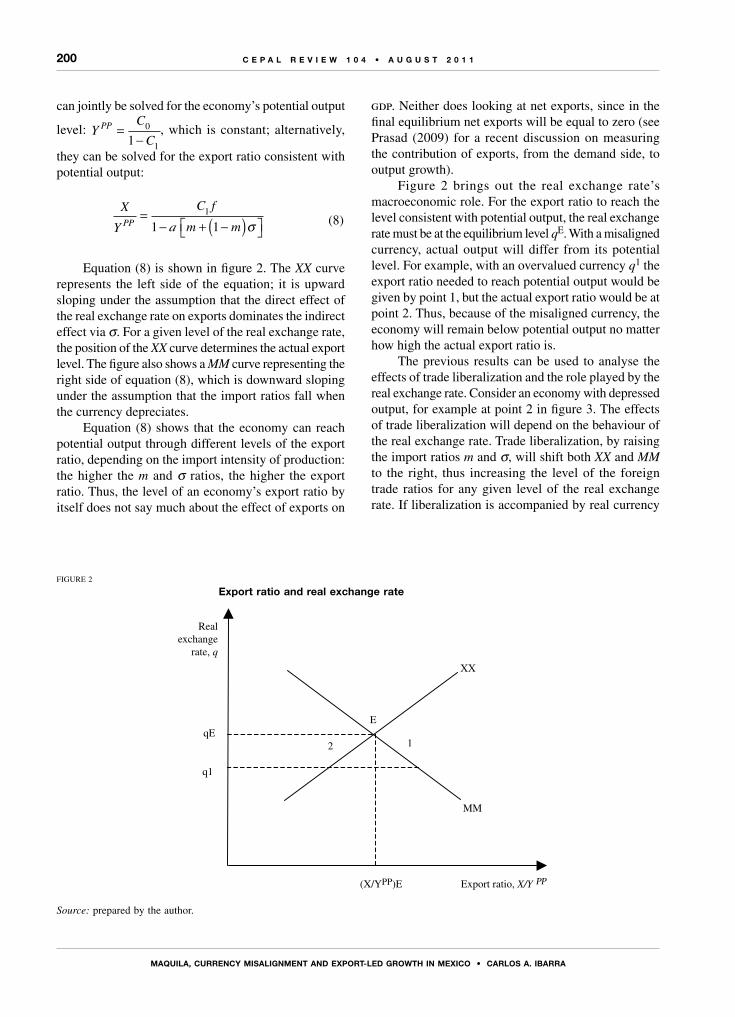
200
MAqUILA, CURREnCy MISALIGnMEnT And ExPoRT-LEd GRoWTh In MExICo • CARLoS A. IbARRA
C E P A L R E V I E W 1 0 4 • A U G U S T 2 0 1 1
can jointly be solved for the economy’s potential output
level: YC
CPP =
−0
11, which is constant; alternatively,
they can be solved for the export ratio consistent with potential output:
X
Y
C fPP
=− + −( )
1
a σ1 1m m (8)
Equation (8) is shown in figure 2. The XX curve represents the left side of the equation; it is upward sloping under the assumption that the direct effect of the real exchange rate on exports dominates the indirect effect via σ. For a given level of the real exchange rate, the position of the XX curve determines the actual export level. The figure also shows a MM curve representing the right side of equation (8), which is downward sloping under the assumption that the import ratios fall when the currency depreciates.
Equation (8) shows that the economy can reach potential output through different levels of the export ratio, depending on the import intensity of production: the higher the m and σ ratios, the higher the export ratio. Thus, the level of an economy’s export ratio by itself does not say much about the effect of exports on
gdp. Neither does looking at net exports, since in the final equilibrium net exports will be equal to zero (see Prasad (2009) for a recent discussion on measuring the contribution of exports, from the demand side, to output growth).
Figure 2 brings out the real exchange rate’s macroeconomic role. For the export ratio to reach the level consistent with potential output, the real exchange rate must be at the equilibrium level qE. With a misaligned currency, actual output will differ from its potential level. For example, with an overvalued currency q1 the export ratio needed to reach potential output would be given by point 1, but the actual export ratio would be at point 2. Thus, because of the misaligned currency, the economy will remain below potential output no matter how high the actual export ratio is.
The previous results can be used to analyse the effects of trade liberalization and the role played by the real exchange rate. Consider an economy with depressed output, for example at point 2 in figure 3. The effects of trade liberalization will depend on the behaviour of the real exchange rate. Trade liberalization, by raising the import ratios m and σ, will shift both XX and MM to the right, thus increasing the level of the foreign trade ratios for any given level of the real exchange rate. If liberalization is accompanied by real currency
FIGURE 2
Export ratio and real exchange rate
Source: prepared by the author.
(X/YPP)E
MM
XX
12
E
Real exchange
rate, q
qE
q1
Export ratio, X/Y PP

201
MAqUILA, CURREnCy MISALIGnMEnT And ExPoRT-LEd GRoWTh In MExICo • CARLoS A. IbARRA
C E P A L R E V I E W 1 0 4 • A U G U S T 2 0 1 1
depreciation, the economy will move to point E', reaching potential output with a higher export ratio.7
With a misaligned (overvalued) currency, in contrast, the transmission of a higher export ratio to output may fail, as shown by the move from point 2 to point 3 in figure 3. The export ratio at points 2 and 3, from the goods market equilibrium condition expressed in equation (6) and the definition of potential output, is:
X
Y
C f CY
Y
m m
PP
=
− −( ) −
− + −( )
1 1
1 1
1 1
a σ (9)
which simplifies to equation (8) when output is at its potential level. Equation (9) shows that a deepening of trade liberalization (leading to further increments in the import ratios) will keep pushing the actual export ratio up, and yet there may be no effect on the gap between potential and actual output. The reason is not that the
7 Figure 3 shows a case in which the equilibrium real exchange rate remains practically unchanged after trade liberalization, which is not necessarily so in practice. See Li (2003) for a theoretical survey and panel econometric evidence regarding the effects of trade liberalization on the real exchange rate.
export ratio is too low, or that the import ratio is too high, but that the currency is misaligned.
Consider now the influence of the other key stylized fact of the Mexican economy, the high and rising share of the maquila sector in manufacturing exports. To assess the effect of the increasing role of the maquila sector, recall equation (8), which shows the export ratio needed to reach potential output. Maquila production is defined by very high values of the a and σ coefficients, which combined imply a high ratio of intermediate imports to gross production—0.876 in 2006 (see table 1). As equation (8) shows, with those parameter values the export ratio that is necessary to reach potential output may be extremely high; in fact, the necessary export ratio tends to infinity as a and σ tend to one. In terms of figure 2, there would be no intersection between the XX and MM curves.
To the extent that export growth is biased towards maquila goods, the growth of exports will keep pushing the export ratio up, with little effect on gdp. While non-maquila exports also may be intensive in imports, a key difference is that non-maquila intermediate imports appear to respond significantly to variations in the real exchange rate, while maquila imports do not. Thus, the shortcomings of maquila exports as an engine of gdp growth cannot be removed by adjustments in the real exchange rate.
FIGURE 3
Effects of trade liberalization
Source: prepared by the author.
(X/YPP)2 (X/YPP)3
MM
XX
XX’
MM’
2
3
E’
Realexchange
rate, q
q1
Export ratio, X/YPP

202
MAqUILA, CURREnCy MISALIGnMEnT And ExPoRT-LEd GRoWTh In MExICo • CARLoS A. IbARRA
C E P A L R E V I E W 1 0 4 • A U G U S T 2 0 1 1
Mexico presents the puzzling picture of an economy that liberalized its trade regime and sharply raised its ratio of manufacturing exports to gdp, and yet failed to sustain fast rates of gdp growth. While some analysts argue that the puzzle is explained by the simultaneous rise of the import ratio, others claim that trade liberalization has not gone far enough: further liberalization would improve the access of local firms to foreign goods, increasing their competitiveness and therefore the growth rates of exports and gdp. In this view, Mexico’s foreign trade ratios are still too low.
The paper argued that focusing on import and export ratio levels can be misleading, and that Mexico’s puzzle is better explained by two of the economy’s stylized facts subsequent to trade liberalization: the tendency of the peso to appreciate in real terms and the large and increasing share of the maquila sector in the country’s export basket. The argument, which was developed through the simple example of an economy with no investment and constant potential output, was motivated by two pieces of empirical evidence.
First, export production uses imports intensively. According to data from Mexico’s Annual Industrial Survey, which covers the non-maquila manufacturing sector, the share of imports in the intermediate basket is particularly high among the top exporting classes, and in some cases tended to further increase after the enactment of nafta. The high import-intensity of exports was confirmed by the estimation of several cointegration equations for the determination of intermediate imports. The equations showed that a rise in exports increases imports for given levels of industrial production and the real exchange rate. The implication is that exports are more intensive in imports than is the rest of industrial production.
A second piece of evidence from the cointegration equations underscores a critical difference between maquila and non-maquila production. In the latter case, there can be substitution between local and imported intermediate goods, with a real currency depreciation reducing intermediate imports for given levels of exports and industrial production. In contrast, there is
no substitution in maquila production. The contrast is important because of the maquila sector’s large share in Mexico’s trade, accounting for 60% of manufacturing exports and total intermediate imports in 2006.
Since exports are intensive in imports, trade liberalization —by improving the access of local firms to imports— tends to increase the export ratio irrespective of the real exchange rate situation. Further trade liberalization, as recommended by different analysts, may indeed keep pushing the export ratio up, but with an uncertain effect on output. It was shown in particular that with a misaligned (overvalued) currency, the rise in the export ratio will necessarily have a weak effect on output, which in the analytical example appears as a failure to reach the economy’s potential output level.
A similar result obtains under a pattern of export growth biased towards the maquila sector. The maquila sector features a particularly high ratio of imports to gross production —a shortcoming that cannot be removed by an adjustment in the real exchange rate. The high import ratio implies a weak (direct and indirect) effect on gdp, irrespective of how high the export ratio may be. The bias of manufacturing exports towards the maquila sector is thus a second factor in the puzzling mix of sharply rising export ratios and slow gdp growth in Mexico.
Finally, regarding policy implications, the paper points to the importance of trying to keep a competitive level for the real exchange rate. A competitive rate not only stimulates faster growth of non-maquila manufactured exports, but also amplifies the positive effect of exports on gdp.
The real exchange rate may be affected by different variables. In the specific case of Mexico during the period under analysis, there is already evidence that the real exchange rate can be significantly influenced by sustained changes in the stance of monetary policy. In particular, a reduction in the difference between peso and dollar short-term interest rates tends to depreciate the peso (see Ibarra, 2010b). This implies that adjustments in the monetary policy stance may affect the rate of economic growth through the real exchange rate channel.
VConclusions

203
MAqUILA, CURREnCy MISALIGnMEnT And ExPoRT-LEd GRoWTh In MExICo • CARLoS A. IbARRA
C E P A L R E V I E W 1 0 4 • A U G U S T 2 0 1 1
The data in Mexico’s Annual Industrial Survey are reported in nominal terms. Since the intermediate basket consists of both local and imported goods, tracking over time the share of imports requires controlling for possible changes in the “intermediate” real exchange rate of each class. Each manufacturing class i uses both local and imported intermediate goods, identified by the sub-indices j and j*, respectively. By definition, the nominal value of the intermediate imports must be Qi, j
*n = SPi, j*Qi, j
*, where Qi, j
* is the real amount of intermediate imports, Pi, j*
the corresponding price index (in dollars, the foreign currency) and S the nominal exchange rate (in pesos per dollar). The nominal value of the local intermediate goods must be Qi, j
n = Pi, jQi, j. Using the Survey data, the import share that can be readily calculated for each year is:
sharei
Qi jn
Qi jn Qi j
n=+
=,*
,*
,
SPi jQi j
SPi jQi j Pi jQi j
,*
,*
,*
,*
, ,+=
11
1+Qi j
qiQi j
,*
,
(A.1)
where qi = SPi, j*/Pi, j is the “intermediate” real exchange
rate based on the prices of the intermediate goods used by class i.
Equation (A.1) shows that the import share calculated directly from the Survey can be spuriously affected by variations in each class’s intermediate real exchange rate. To avoid that effect, the following adjustment was made. First, for each year and class, an “intermediate” purchasing-power-parity (ppp) nominal exchange rate (Si
p) was calculated. Setting arbitrarily the initial value of qi equal to one, the ppp rate is Si
p =Pi, j / Pi, j*.
Second, for each year and class the ppp rate was used to obtain a “misalignment” ratio µ= Si
p/S, also equal to one in
1994. Finally, using the value of µi for each year and class, an adjusted import share was calculated that reflects only changes in volumes (because each class’s intermediate real exchange rate is kept constant):
shareia Qi j
n
Qi jn Qi j
n Qi j
Qi
=+
=
+
µ
µ
,*
,* *
1
1,, j
, , (A.2)
Note: The superscript a is used to indicate the calculation of the “adjusted” share, to differentiate it from the non-adjusted share as calculated in equation (A.1).
Since series for each sector’s specific price index of intermediate imports Pi, j
* are not available, the calculation of qi had to rely on one of two aggregate indices: the Bank of Mexico’s dollar index of import prices (a valid proxy since most of Mexico’s imports consist of intermediate goods) or the United States producer price index for intermediate goods (valid because most of Mexico’s imports originate in the United States). While some exploration showed that the two indices behave in a similar way, the results reported in the present paper are based on the Bank of Mexico’s index of import prices.
The prices of the local intermediate goods Pi, j were obtained from a series of producer price indices calculated by the Bank of Mexico and based on the basket of intermediates consumed by different sectors of activity. However, while the Survey identifies 205 manufacturing classes, the Bank of Mexico’s price index is calculated at the more aggregate level of 49 manufacturing subsectors. Thus, each of the top 25 exporting classes from the Survey was assigned to one of the 49 manufacturing sectors identified by the Bank of Mexico, matching as closely as possible the definition of the production activity presented by each source.
APPENDIX A
The import share in the Annual Industrial Survey

204
MAqUILA, CURREnCy MISALIGnMEnT And ExPoRT-LEd GRoWTh In MExICo • CARLoS A. IbARRA
C E P A L R E V I E W 1 0 4 • A U G U S T 2 0 1 1
imaq: Natural logarithm of maquila imports.Source: Bank of Mexico.
ipi: Natural logarithm of the industrial production index, seasonally adjusted.Source: National Institute of Statistics and Geography (inegi) of Mexico.
maq: Natural logarithm of maquila exports.Source: Bank of Mexico.
8 The original balance-of-payments data, in dollars, were deflated using the United States producer price index.
mint: Natural logarithm of imports of intermediate goods, excluding the maquila sector.Source: Bank of Mexico.
nexp: Natural logarithm of exports of goods, excluding oil and the maquila sector.Source: Bank of Mexico.
reer: Natural logarithm of the consumer price index-based, real effective exchange rate index calculated by the Bank of Mexico. A higher index indicates a peso depreciation.Source: Bank of Mexico.
(Original: English)
APPENDIX B
Data sources and definitions for section III8
Bibliography
Buitelaar, R.M. and R. Padilla (2000), “Maquila, economic reform and corporate strategies”, World Development, vol. 28, No. 9, Amsterdam, Elsevier.
Cardero, M.A. and L.M. Galindo (2005), “From the import substitution model to the import-export model: reassessing Mexico’s trade liberalization process during the last two decades”, Journal of Economic Asymmetries, vol. 2, No. 2, Chicago, Athenian Policy Forum, December.
Cerra, V. and A. Dayal-Gulati (1999), “China’s trade flows: changing price sensitivities and the reform process”, imf Working Paper, No. 99/1, Washington, D.C., International Monetary Fund, January.
Chiquiar, D., E. Fragoso and M. Ramos-Francia (2007), “Comparative advantage and the performance of Mexican manufacturing exports during 1996-2005”, Working Papers, No. 2007-12, Mexico City, Banco de México.
Feenstra, R.C. (1998), “Integration of trade and disintegration of production in the global economy”, Journal of Economic Perspectives, vol. 12, No. 4, Nashville, Tennessee, American Economic Association.
Freund, C. and M.D. Pierola (2008), “Export surges: the power of a competitive currency”, Policy Research Working Paper, No. 4750, Washington, D.C., World Bank, October.
Galindo, L.M. and J. Ros (2008), “Alternatives to inflation targeting in Mexico”, International Review of Applied Economics, vol. 22, No. 2, London, Taylor and Francis.
Gallagher, K.P., J.C. Moreno-Brid and R. Porzecanski (2008), “The dynamism of Mexican exports: lost in (Chinese) translation?”, World Development, vol. 36, No. 8, Amsterdam, Elsevier.
Goldberg, P. and others (2009), “Trade liberalization and new imported inputs”, American Economic Review, vol. 99, No. 2, May, Nashville, Tennessee, American Economic Association.
Guerrero de Lizardi, C. (2003), “Modelo de crecimiento restringido por la balanza de pagos. Evidencia para México 1940 - 2000”, El Trimestre Económico, vol. 70, No. 2, Mexico City, Fondo de Cultura Económica.
Haugh, D., R. Jamin and B. Rocha (2008), “Maximising Mexico’s gains from integration in the world economy”, Working Paper, No. 657, Paris, Organisation for Economic Co-operation and Development (oecd), December.
Hausmann, R., L. Pritchett and D. Rodrik (2005), “Growth accelerations”, Journal of Economic Growth, vol. 10, No. 4, Springer.Hummels, D., J. Ishii and K-M Yi (2001), “The nature and growth of
vertical specialization in world trade”, Journal of International Economics, vol. 54, No. 1, Amsterdam, Elsevier.
Ibarra, C.A. (2010a), “Exporting without growing: investment, real currency appreciation, and export-led growth in Mexico”, Journal of International Trade and Economic Development, vol. 19, No. 3, Taylor and Francis.
(2010b), “Monetary policy and real currency appreciation: a beer model for the Mexican peso”, International Economic Journal, March, forthcoming.
(2010c), “Import elasticities and the external constraint in Mexico”, Economic Systems, September, forthcoming.
(2008a), “Disinflation and real currency appreciation in Chile and Mexico: the role of monetary policy”, Investigación económica, vol. 67, No. 266, Mexico City, National Autonomous University of Mexico.
(2008b), “Mexico’s slow-growth paradox”, cepal Review, No. 95 (LC/G.2382-P), Santiago, Chile.
Li, X. (2003), “Trade liberalization and real exchange rate movement”, imf Working Paper, No. 03/124, Washington, D.C., International Monetary Fund, June.
López, J. and A. Cruz (2000), “Thirlwall’s law and beyond: the Latin American experience”, Journal of Post Keynesian Economics, vol. 22, No. 3, Armonk, M.E. Sharpe, Inc.
Moissinac, V. (2006), “A survey of conditions for growth in Mexico, in international perspective”, Mexico: Selected Issues, Washington, D.C., International Monetary Fund.
Moreno-Brid, J.C. (1999), “Mexico’s economic growth and the balance of payments constraint: a cointegration analysis”, International Review of Applied Economics, vol. 13, No. 2, London, Taylor and Francis.

205
MAqUILA, CURREnCy MISALIGnMEnT And ExPoRT-LEd GRoWTh In MExICo • CARLoS A. IbARRA
C E P A L R E V I E W 1 0 4 • A U G U S T 2 0 1 1
Moreno-Brid, J.C., J. Santamaría and J.C. Rivas (2005), “Industrialization and economic growth in Mexico after nafta: the road travelled”, Development and Change, vol. 36, No. 6, Blackwell Publishing.
Ocegueda, J. (2000), “La hipótesis del crecimiento restringido por la balanza de pagos. Una evaluación de la economía mexicana 1960-1997”, Investigación económica, vol. 60, No. 232, Mexico City, National Autonomous University of Mexico.
oecd (Organization for Economic Cooperation and Development) (2005), “The benefits of liberalizing product markets and reducing barriers to international trade and investment in the oecd”, oecd Working Paper, No. 463, Paris, December.
Pacheco-López, P. (2005), “The impact of trade liberalization on exports, imports, the balance of payments and growth: the case of Mexico”, Journal of Post Keynesian Economics, vol. 27, No. 4, Armonk, M.E. Sharpe, Inc.
Pacheco-López, P. and A.P. Thirlwall (2007), “Trade liberalization and the trade-off between growth and the balance of payments in Latin America”, International Review of Applied Economics, vol. 21, No. 4, London, Taylor and Francis.
Pesaran, M.H. and Y. Shin (1998), “An autoregressive distributed-lag approach to cointegration analysis”, Econometrics and Economic Theory in the 20th Century. The Ragnar Frisch Centennial Symposium, S. Strom (comp.), Cambridge, Cambridge University Press.
Pesaran, M.H., Y. Shin and R.J. Smith (2001), “Bounds testing approaches to the analysis of level relationships”, Journal of Applied Econometrics, vol. 16, No. 3, John Wiley & Sons.
Prasad, E.S. (2009), “Rebalancing growth in Asia”, nber Working Paper, No. 15169, Cambridge, Massachusetts, National Bureau of Economic Research, July.
Rodrik, D. (2005), “Growth strategies”, Handbook of Economic Growth, vol. 1A, P. Aghion and S.N. Durlauf (comps.), Amsterdam, Elsevier.
Ros, J. (2009), “Política fiscal, tipo de cambio y crecimiento en regímenes de alta y baja inflación: la experiencia de México”, Working Paper, Notre Dame, University of Notre Dame, January.
unctad (United Nations Conference on Trade and Development) (2007), Trade and Development Report 2007 (unctad/tdr/2007), New York, United Nations. United Nations publication, Sales No. E.07.II.D.11.
(2002), Trade and Development Report 2002 (unctad/tdr/2002), New York, United Nations. United Nations publication, Sales No. E.02.II.D.10.
wto (World Trade Organization) (2008a), “Trade Policy Review” (wt/tpr/g/195), Geneva, Trade Policy Review Body, January.
(2008b), “Trade Policy Review. Report by the wto Secretariat”, (wt/tpr/s/195), Geneva, Trade Policy Review Body, January.


C E P A L r E v i E w 1 0 4
A U G U S T 2 0 1 1
207
Guidelinesfor contributorsto cepal Review
In order to facilitate the submission, consideration and publication of articles, the editorial board of the cepal Review has prepared the following information and suggestions to serve as a guide for future contributors.
The submission of an article implies an undertaking by the author not to submit it simultaneously to other publications. The copyright to all articles published in the Review shall be owned by the United Nations.
All articles will be submitted to external referees.
Papers should be submitted in the original language (English, French, Portuguese or Spanish). They will be translated into the appropriate language by the relevant eclac services.
Each article must be accompanied by a summary, no more than 150 words in length, giving a brief description of its subject matter and main conclusions.
Papers should be no longer than 10,000 words, including the summary, notes and bibliography. Shorter papers will also be considered.
Articles should be sent either by e-mail (to [email protected]) or by regular mail, on cd or diskette, to: cepal Review, Casilla 179-D, Santiago, Chile. They should not be submitted in pdf format.
Style guide:
Titles should not be excessively long.
Footnotes
– It is recommended that footnotes be kept to a minimum.
– It is recommended that footnotes not be used to cite bibliographical references; such references should preferably be incorporated into the text.
– Footnotes should be numbered consecutively using superscript Arabic numerals.
Tables and figures
– It is recommended that tables and figures be kept to a minimum, avoiding any redundancy with the text.
– Tables, figures and other elements should be inserted at the end of the text in the format in which they were designed; they should not be inserted as “pictures”. Figures in Excel should include the corresponding worksheets.
– The location of tables and figures in the body of the article should be indicated in the appropriate place as follows:
Insert figure 1Insert table 1
– Tables and figures should include an explicit and complete reference to their sources.
– Tables should indicate the period covered at the end of the title, and should indicate the units in which the data are expressed in a subtitle (in italics and between brackets).
– The symbols referred to in the “Explanatory notes” which appear on the page preceding the table of contents should be taken into account in the preparation of tables and figures.
– Footnotes to tables and figures should be ordered consecutively using superscript lower-case letters.
– Figures should be prepared bearing in mind that they will be printed in black and white.
Acronyms and abbreviations
– Acronyms and abbreviations should not be used unless absolutely necessary, in which case the full name should be written out the first time it occurs in the article.
Bibliography
– Bibliographical references should be directly related to the content of the article and should not be excessively long.
– At the end of the article, under the title “Bibliography”, all the necessary information should be included accurately and in alphabetical order by author: name of author(s), year of publication, full name of article (if any) and publication (including any subtitle), city of publication, publisher and, in the case of a periodical, month of publication.
The editorial board of the Review reserves the right to make any necessary editorial changes in the articles, including their titles.
Authors will receive a one-year courtesy subscription to the Review, plus 30 offprints of their article in Spanish and 30 in English, at the time of publication in each language.

Publicaciones de la CEPAL / ECLAC publications Comisión Económica para América Latina y el Caribe / Economic Commission for Latin America and the Caribbean
Casilla 179-D, Santiago de Chile. E-mail: [email protected] Véalas en: www.cepal.org/publicaciones
Publications may be accessed at: www.eclac.org
Revista CEPAL / CEPAL Review La Revista se inició en 1976 como parte del Programa de Publicaciones de la Comisión Económica para América Latina y el Caribe, con el propósito de contribuir al examen de los problemas del desarrollo socioeconómico de la región. Las opiniones expresadas en los artículos firmados, incluidas las colaboraciones de los funcionarios de la Secretaría, son las de los autores y, por lo tanto, no reflejan necesariamente los puntos de vista de la Organización.
La Revista CEPAL se publica en español e inglés tres veces por año. Los precios de suscripción anual vigentes para 2011 son de US$ 30 para ambas versiones. El precio por ejemplar suelto es de US$ 15 para
ambas versiones. Los precios de suscripción por dos años son de US$ 50 para ambas versiones. CEPAL Review first appeared in 1976 as part of the Publications Programme of the Economic Commission for Latin America and the Caribbean, its aim being to make a contribution to the study of the economic and social development problems of the region. The views expressed in signed articles, including those by Secretariat staff members, are those of the authors and therefore do not necessarily reflect the point of view of the Organization.
CEPAL Review is published in Spanish and English versions three times a year. Annual subscription costs for 2011 are US$ 30 for both versions. The price of single issues is US$ 15 in both cases. The cost of a two-year
subscription is US$ 50 for both versions.
Informes periódicos institucionales / Annual reports Todos disponibles para años anteriores / Issues for previous years also available • Balance preliminar de las economías de América Latina y el Caribe, 2009, 176 p. Preliminary Overview of the Economies of Latin America and the Caribbean, 2009, 160 p. • Estudio económico de América Latina y el Caribe 2009-2010, 136 p. Economic Survey of Latin America and the Caribbean 2009-2010, 128 p. • Panorama de la inserción internacional de América Latina y el Caribe, 2009-2010, 178 p. Latin America and the Caribbean in the World Economy, 2009-2010, 168 p. • Panorama social de América Latina, 2010, 266 p. Social Panorama of Latin America, 2010, 256 p. • La inversión extranjera directa en América Latina y el Caribe, 2010, 220 p. Foreign Direct Investment of Latin America and the Caribbean, 20010, 216 p. • Anuario estadístico de América Latina y el Caribe / Statistical Yearbook for Latin America and the Caribbean (bilingüe/bilingual),
2010, 310 p.
Libros de la CEPAL 111 Protección social inclusiva en América Latina. Una mirada integral, un enfoque de derechos, Simone Cecchini y Rodrigo Martínez,
284 p. 110 Envejecimiento en América Latina. Sistema de pensiones y protección social integral, Antonio Prado y Ana Sojo (eds.), 304 p. 109 Modeling Public Policies in Latin America and the Caribbean, Carlos de Miguel, José Durán Lima, Paolo Giordiano, Julio
Guzmán, Andrés Schuschny and Masazaku Watanuki (eds.), 322 p. 108 Alianzas público-privadas. Para una nueva visión estratégica del desarrollo, Robert Devlin y Graciela Moguillansky, 2010, 196 p.

107 Políticas de apoyo a las pymes en América Latina. Entre avances innovadores y desafíos institucionales, Carlos Ferraro y Giovanni Stumpo, 392 p.
106 Temas controversiales en negociaciones comerciales Norte-Sur, Osvaldo Rosales V. y Sebastián Sáez C. (compiladores), 322 p. 105 Regulation, Worker Protection and Active Labour-Market Policies in Latin America, Jürgen Weller (ed.), 2009, 236 p. 104 La República Dominicana en 2030: hacia una sociedad cohesionada, Víctor Godínez y Jorge Máttar (coords.), 2009, 582 p. 103 L’Amérique latine et les Caraïbes au seuil du troisième millénaire, 2009, 138 p. 102 Migración interna y desarrollo en América Latina entre 1980 y 2005, Jorge Rodríguez y Gustavo Busso, 2009, 272 p. 101 Claves de la innovación social en América Latina y el Caribe, Adolfo Rodríguez Herrera y Hernán Alvarado Ugarte, 2009, 236 p. 100 Envejecimiento, derechos humanos y políticas públicas, Sandra Huenchuan (ed.), 2009, 232 p. 99 Economía y territorio en América Latina y el Caribe. Desigualdades y políticas, 2009, 212 p. 98 La sociedad de la información en América Latina y el Caribe: desarrollo de las tecnologías y tecnologías para el desarrollo, Wilson Peres
y Martin Hilbert (eds.), 2009, 388 p. 97 América Latina y el Caribe: migración internacional, derechos humanos y desarrollo, Jorge Martínez Pizarro (ed.), 2008, 375 p. 96 Familias y políticas públicas en América Latina: una historia de desencuentros, Irma Arriagada (coord.), 2007, 424 p. 95 Centroamérica y México: políticas de competencia a principios del siglo XXI, Eugenio Rivera y Claudia Schatan (coords.), 2008, 304 p. 94 América Latina y el Caribe: La propiedad intelectual después de los tratados de libre comercio, Álvaro Díaz, 2008, 248 p.
Copublicaciones recientes / Recent co-publications Las clases medias en América Latina. Retrospectiva y nuevas tendencias, Rolando Franco, Martín Hopenhayn y Arturo León (eds.),
CEPAL/Siglo XXI, México, 2010. Innovation and Economic Development. The Impact of Information and Communication Technologies in Latin America, Mario Cimoli,
André Hofman and Nanno Mulder, ECLAC/Edward Elgar Publishing, United Kingdom, 2010. Sesenta años de la CEPAL. Textos seleccionados del decenio 1998-2008, Ricardo Bielschowsky (comp.), CEPAL/Siglo Veintiuno, Argentina, 2010. El nuevo escenario laboral latinoamericano. Regulación, protección y políticas activas en los mercados de trabajo, Jürgen Weller (ed.),
CEPAL/Siglo Veintiuno, Argentina, 2010. Internacionalización y expansión de las empresas eléctricas españolas en América Latina, Patricio Rozas, CEPAL/Lom, Chile, 2009. Gobernanza corporativa y desarrollo de mercados de capitales en América Latina, Georgina Núñez, Andrés Oneto y Germano M. de Paula
(coords.), CEPAL/Mayol, Colombia, 2009. EnREDos. Regulación y estrategias corporativas frente a la convergencia tecnológica, Marcio Wohlers y Martha García-Murillo (eds.),
CEPAL/Mayol, Colombia, 2009. Desafíos y oportunidades de la industria del software en América Latina, Paulo Tigre y Felipe Silveira Marques (eds.), CEPAL/Mayol,
Colombia, 2009. ¿Quo vadis, tecnología de la información y de las comunicaciones?, Martin Hilbert y Osvaldo Cairó (eds.), CEPAL/Mayol, Colombia, 2009. O Estruturalismo latino-americano, Octavio Rodríguez, CEPAL/Civilização Brasileira, 2009. L’avenir de la protection sociale en Amérique latine. Accessibilité, financement et solidarité, CEPALC/Eska, France, 2009. Fortalecer los sistemas de pensiones latinoamericanos. Cuentas individuales por reparto, Robert Holzmann, Edward Palmer y Andras Uthoff (eds.), CEPAL/Mayol, Colombia, 2008. Competition Policies in Emerging Economies. Lessons and Challenges from Central America and Mexico, Claudia Schatan and
Eugenio Rivera Urrutia (eds.), ECLAC/Springer, USA, 2008.
Coediciones recientes / Recent co-editions Perspectivas de la agricultura y del desarrollo rural en las Américas: una mirada hacia América Latina y el Caribe,
CEPAL/FAO/IICA, 2011. The Oulook for Agriculture and Rural Development in the Americas: A Perspective on Latin America and the Caribbean,
ECLAC/FAO/IICA, 2011. Pobreza infantil en América Latina y el Caribe, CEPAL/UNICEF, Chile, 2010. Espacios iberoamericanos: vínculos entre universidades y empresas para el desarrollo tecnológico, CEPAL/SEGIB, 2010 Espaços ibero-Americanos: vínculos entre universidades e empresas para o desenvolvimento tecnológico, CEPAL/SEGIB, 2010 Clases medias y desarrollo en América Latina, Alicia Bárcena y Narcís Serra (eds.), CEPAL/SEGIB/CIDOB, Chile, 2010. Innovar para crecer. Desafíos y oportunidades para el desarrollo sostenible e inclusivo en Iberoamérica, CEPAL/SEGIB, Chile, 2010. Espacios iberoamericanos. Iberoamérica frente a la crisis, CEPAL/SEGIB, Chile, 2009. Espaços Ibero-Americanos. A Ibero-América em face da crise, CEPAL/SEGIB, Chile, 2009. The United Nations Regional Commissions and the Climate Change Challenges, ECLAC/ECA/ECE/ESCAP/ESCWA, 2009. Hacia un desarrollo inclusivo. El caso de Chile, Osvaldo Sunkel y Ricardo Infante (eds.), CEPAL/OIT/Fundación Chile 21, Chile, 2008. Reformas para la cohesión social en América Latina. Panorama antes de la crisis, Alicia Bárcena y Narcís Serra (eds.),
CEPAL/SEGIB/CIDOB, Chile, 2008. El envejecimiento y las personas de edad. Indicadores sociodemográficos para América Latina y el Caribe, CEPAL/UNFPA, 2009.

Espacios iberoamericanos: la economía del conocimiento, CEPAL/SEGIB, Chile, 2008. Hacia la revisión de los paradigmas del desarrollo en América Latina, Oscar Altimir, Enrique V. Iglesias, José Luis Machinea (eds.),
CEPAL/SEGIB, Chile, 2008. Por uma revis o dos paradigmas do desenvolvimento na América Latina, Oscar Altimir, Enrique V. Iglesias, José Luis Machinea (eds.),
CEPAL/SEGIB, Chile, 2008. Hacia un nuevo pacto social. Políticas económicas para un desarrollo integral en América Latina, José Luis Machinea y Narcís Serra (eds.)
CEPAL/CIDOB, España, 2008.
Cuadernos de la CEPAL 94 El cuidado en acción. Entre el derecho y el trabajo, Sonia Montaño Virreira y Coral Calderón Magaña (coords.), 2010, 236 p. 93 Privilegiadas y discriminadas. Las trabajadoras del sector financiero, Flavia Marco Navarro y María Nieves Rico Ibáñez (eds.), 2009, 300 p. 92 Estadísticas para la equidad de género: magnitudes y tendencias en América Latina, Vivian Milosavljevic, 2007, 186 pp.
Cuadernos estadísticos de la CEPAL 39 América Latina y el Caribe: indicadores macroeconómicos del turismo. Solo disponible en CD, 2010. 38 Indicadores ambientales de América Latina y el Caribe, 2009. Solo disponible en CD, 2010. 37 América Latina y el Caribe: Series históricas de estadísticas económicas 1950-2008. Solo disponible en CD, 2009. 36 Clasificaciones estadísticas internacionales incorporadas en el Banco de Datos de Comercio Exterior de América Latina y el Caribe de la
CEPAL (Revisión 3). Solo disponible en CD, 2008. 35 Resultados del Programa de Comparación Internacional para América del Sur. Solo disponible en CD, 2007.
Observatorio demográfico ex Boletín demográfico / Demographic Observatory formerly Demographic Bulletin (bilingüe/bilingual) Edición bilingüe (español e inglés) que proporciona información estadística actualizada, referente a estimaciones y proyecciones de población de los países de América Latina y el Caribe. Incluye también indicadores demográficos de interés, tales como tasas de natalidad, mortalidad, esperanza de vida al nacer, distribución de la población, etc.
El Observatorio aparece dos veces al año, en los meses de enero y julio. Suscripción anual: US$ 20.00. Valor por cada ejemplar: US$ 15.00. Bilingual publication (Spanish and English) proving up-to-date estimates and projections of the populations of the Latin American and Caribbean countries. Also includes various demographic indicators of interest such as fertility and mortality rates, life expectancy, measures of population distribution, etc.
The Observatory appears twice a year in January and July. Annual subscription: US$ 20.00. Per issue: US$ 15.00.
Notas de población Revista especializada que publica artículos e informes acerca de las investigaciones más recientes sobre la dinámica demográfica en la región, en español, con resúmenes en español e inglés. También incluye información sobre actividades científicas y profesionales en el campo de población.
La revista se publica desde 1973 y aparece dos veces al año, en junio y diciembre. Suscripción anual: US$ 20.00. Valor por cada ejemplar: US$ 12.00.
Specialized journal which publishes articles and reports on recent studies of demographic dynamics in the region, in Spanish with abstracts in Spanish and English. Also includes information on scientific and professional activities in the field of population.
Published since 1973, the journal appears twice a year in June and December. Annual subscription: US$ 20.00. Per issue: US$ 12.00.
Series de la CEPAL Comercio internacional / Desarrollo productivo / Desarrollo territorial / Estudios estadísticos y prospectivos / Estudios y perspectivas (Bogotá, Brasilia, Buenos Aires, México, Montevideo) / Studies and Perspectives (The Caribbean, Washington) / Financiamiento del desarrollo / Gestión pública / Informes y estudios especiales / Macroeconomía del desarrollo / Manuales / Medio ambiente y desarrollo / Mujer y desarrollo / Población y desarrollo / Políticas sociales / Recursos naturales e infraestructura / Seminarios y conferencias. Véase el listado completo en: www.cepal.org/publicaciones / A complete listing is available at: www.cepal.org/publicaciones

Las publicaciones de la Comisión Económica para América Latina y el Caribe (CEPAL) y las del Instituto Latinoamericano y del Caribe de Planificación Económica y Social (ILPES) se pueden adquirir a los distribuidores locales o directamente a través de:
Publicaciones de las Naciones Unidas Publicaciones de las Naciones Unidas 2 United Nations Plaza, Room DC2-853 Sección de Ventas Nueva York, NY, 10017 Palais des Nations Estados Unidos 1211 Ginebra 10 Tel. (1 800)253-9646 Fax (1 212)963-3489 Suiza E-mail: [email protected] Tel. (41 22)917-2613 Fax (41 22)917-0027 Unidad de Distribución Comisión Económica para América Latina y el Caribe (CEPAL) Av. Dag Hammarskjöld 3477, Vitacura 7630412 Santiago Chile Tel. (56 2)210-2056 Fax (56 2)210-2069 E-mail: [email protected]
Publications of the Economic Commission for Latin America and the Caribbean (ECLAC) and those of the Latin American and the Caribbean Institute for Economic and Social Planning (ILPES) can be ordered from your local distributor or directly through:
United Nations Publications United Nations Publications 2 United Nations Plaza, Room DC2-853 Sales Sections New York, NY, 10017 Palais des Nations USA 1211 Geneva 10 Tel. (1 800)253-9646 Fax (1 212)963-3489 Switzerland E-mail: [email protected] Tel. (41 22)917-2613 Fax (41 22)917-0027 Distribution Unit Economic Commission for Latin America and the Caribbean (ECLAC) Av. Dag Hammarskjöld 3477, Vitacura 7630412 Santiago Chile Tel. (56 2)210-2056 Fax (56 2)210-2069 E-mail: [email protected]