Buckling curves of hot rolled H steel sections submitted to fire

S C I E N C E RESEARCH D E V E L O P M E N T

E U R O P E A N

COMMISSION

technical steel research

Properties and in-service performance

Buckling curves of hot rolled H steel sections submitted to fire

h Report

W EUR 18380 EN STEEL RESEARCH

EUROPEAN COMMISSION

Edith CRESSON, Member of the Commission responsible for research, innovation, education, training and youth

DG XII/C.2 — RTD actions: Industrial and materials technologies — Materials and steel

Contact: Mr H. J.-L. Martin Address: European Commission, rue de la Loi 200 (MO 75 1/10), B-1049 Brussels — Tel. (32-2) 29-53453; fax (32-2) 29-65987

European Commission

technical steel research Properties and in-service performance

Buckling curves of hot rolled H steel sections submitted to fire

J.B. Schleich, L-G. Cajot ProfilARBED-Recherches

66, rue de Luxembourg L-4002 Esch/Alzette

J. Kruppa, D. Talamona CTICM

Domaine de St. Paul BP1

F-78470 St.-Rémy-les-Chevreuse

W. Azpiazu, J. Unanue LABEIN

Cuesta de Olabeaga 16 E-48013 Bilbao

L. Twilt, J. Fellinger, R-J. Van Foeken TNO

PO Box 49 2600 AA Delft

The Netherlands

J-M. Franssen Université de Liège

Quai Banning 6 B-4000 Liège

Contract No 7210-SA/316/515/618/931 1 July 1992 to 30 June 1995

Final report

Directorate-General Science, Research and Development

1998 EUR 18380 EN

LEGAL NOTICE

Neither the European Commission nor any person acting on behalf of the Commission is responsible for the use which might be made of the following information.

A great deal of additional information on the European Union is available on the Internet. It can be accessed through the Europa server (http://europa.eu.int).

Cataloguing data can be found at the end of this publication.

Luxembourg: Office for Official Publications of the European Communities, 1998

ISBN 92-828-4603-2

© European Communities, 1998

Reproduction is authorised provided the source is acknowledged.

Printed in Luxembourg

PRINTED ON WHITE CHLORINE-FREE PAPER

BUCKLING CURVES OF HOT ROLLED H STEEL SECTIONS SUBMITTED TO FIRE

C.KC. Agreement N° 7210-SA/316/515/618/931

DRAFT FINAL REPORT (01.07.1992 to 30.06.1995)

SUMMARY

The research has lead to new formulae for the design of steel columns in case of fire: - a new N/M interaction formula - new buckling curves instead of the buckling curve c divided by 1,2 proposed in the present

version of Eurocode 3 Part 1.2. These formulae are presented in Design tables useful for the practical engineer. These formulae were deduced and calibrated from a very large amount of numerical simulations (more than 300 000) and from a database comprising 141 test results including the 29 tests made in the frame of the research.

For the study of the axially loaded columns, 21 tests have been performed in the Laboratory of LABEIN in Bilbao and 8 tests have been made in the CTICM laboratory in Maizières-les-Metz to analyse columns subjected to a normal force and a constant bending moment distribution.

The numerical simulations were made by using the five programs available in the different organizations: CEFICOSS and SAFIR (ProfilARBED Recherches and University of Liège), DIANA (TNO), LENAS and SISMEF (CTICM).

R E S U M E

La recherche a permis de définir de nouvelles formules pour le calcul des colonnes en acier

soumises au feu:

une nouvelle formule d'interaction N/M

de nouvelles courbes de flambement à la place de la courbe c divisée par 1,2 de la version

actuelle de l'Eurocode 3 Part 1.2.

Ces formules sont présentées sous forme d'abaques facilement utilisables par les ingénieurs de

bureaux d'études. Ces formules ont été déduites et calibrées suite à un grand nombre de

simulations numériques (plus de 300 000) et à partir d'une base de données comprenant les

résultats de 141 tests incluant 29 tests réalisés dans le cadre de cette recherche.

Pour l'étude des colonnes chargées axiallement 21 tests ont été réalisés au laboratoire de

LABEIN à Bilbao tandis que 8 tests ont eu lieu au laboratoire du CTICM à MaizièreslesMetz

pour analyser les colonnes soumises à une force normale et à un moment fléchissant constant.

Les simulations ont été faites en utilisant 5 logiciels disponibles auprès des différents

partenaires: CEFICOSS et SAFIR (ProfilARBED Recherches et Université de Liège), DIANA

(TNO), LENAS et SISMEF (CTICM).

Ζ U S A M M Ε Ν. F A S S U Ν G

Das vorliegende Projekt hat zu neuen Formeln zur Bemessung von Stahlstützen im Brandfall

geführt:

eine neue Formel zur N/M Interaktion

neue Knickkurven, anstatt der empfohlene Kurve c geteilt durch 1,2 der jetzigen Fassung

von EC 3 Teil 1.2.

Diese Formeln werden den Anwendern in praktische Bemessungstafeln vorgestellt. Diese

Formeln wurden abgeleitet und kalibriert durch eine hohe Anzahl von numerischen

Simulationen (über 300 000) und aus einer Datenbank mit den Resultaten von 141 Versuchen

einschließlich der 29 Versuche im Rahmen dieses Projektes.

Für die Untersuchung der axial belasteten Stützen wurden 21 Versuche bei LABEIN in Bilbao

sowie für die Untersuchung der axial belasteten Stützen mit konstantem Biegemoment wurden

8 Versuche bei CTICM in MaizièreslesMetz durchgeführt.

Die numerischen Simulationen wurden durchgeführt unter Zuhilfenahme von 5 den

verschiedenen Partnern zur Verfügung stehenden Programmen: CEFICOSS und SAFIR

(ProfilARBED Forschung und Universität Lüttich), DIANA (TNO), LENAS und SISMEF

(CTICM).

TABLE OF CONTENTS

1. INTRODUCTION 7 2. EXPERIMENTAL WORK: FIRE TESTS ON STEEL COLUMNS 11 2.1 INTRODUCnON 11 2.2 GENERAL DESCRIPHON AND MAIN RESULTS 11 2.3 LABEIN TESTS 13 2.3.1 Data 13 2.3.2 Measurements done before testing 14 2.3.3 Measurements done during testing 14 2.3.4 Heating procedure 15 2.3.5 Summary of results 15 2.3.6 Southwell plot method applied to LABEIN tests 21 2.4 CnCMTESTS 24 2.4.1 Data 24 2.4.2 Measurements done before testing 25 , 2.4.3 Measurements done during testing 25 2.5 DA TABASE OF TESTS 26 2.5.1 Field Names 26 2.5.2 Explanations of the database field names 2 7 3. CALCULATION MODELS 37 3.1 COMPARISON BETWEEN NUMERICAL PROGRAMS (SAFIR, CEFICOSS, LENAS, SISMEF, DIANA) 37 3.1.1 INTRODUCTION 3 7 3.1.2 Example Definition 3 7 3.1.3 Simulation Results 40 3.2 NUMERICAL SIMULA TIONS OF THE LABEIN TESTS 41 3.3 NUMERICAL SIMULA BONS OF THE CTICM TESTS. 42 4. NUMERICAL SIMULA TIONS 46 4.1 CALCULA ΉΟΝ OF AXIALLY LOADED MEMBERS: A PROPOSAL FOR AN ANALYnCAL PROPOSAL 46 4.1.1 INTRODUCTION 46 4.1.2 THE GENERAL MODEL 46 4.1.3 THE NUMERICAL SIMULA TIONS IN CASE OF UNIFORM TEMPERA TURE 49 4.1.4 A new proposal based on numerical results 55 4.1.5 Unprotected sections submitted to ISO heating 5 7 4.2 CALCULA ΉΟΝ OF COLUMNS IN COMPRESSION AND BENDING: A FORMULA FORM-NINTERACnON 59 4.2.1 Sensitiveness analysis of the results in relation to the column discretization 60 4.2.2 Numerical Analysis 64 4.2.3 Determination of a formula for M-N interaction 72 5. CALIBRATION OF THE FORMULAE BY COMPARISON WITH EXPERIMENTAL

RESULTS 83 5.1 INTRODUCTION 83 5.2 RESULTS OF THE EXPERIMENTAL TESTS 84 5.2.1 Testfrom Borehamwood. 84 5.2.2 Tests from Gent. 85 5.2.3 Tests from Germany. 86

5.2.4 Test from Rennes. 8 7

5.2.5 Test from Bilbao. 88

5.2.6 Summary of the available tests. 89

5.3 CALIBRATION: DETERMINATION OF THE SEVERITY FACTOR 89

5.4 INFLUENCE OF THE YIELD STRENGTH 93

5.5 VERIFICATION OF THE PROPOSED FORMULAE IN CASE OF ECCENTRICALLY

LOADED COLUMNS 94

6. DESIGN RULES 97

6.1 ANALYTICAL FORMULA 97

6.1.1 Centrally loaded column 9 7

6.1.2 Eccentrically loaded column 95

6.2 DESIGN TABLES WO

6.2.1 Design tables (S235, S355, S460) ι oo

6.3 DESIGN EXAMPLES j 03

6.4 NOMOGRAM ¡07

7. CONCLUSIONS W9

8. NOTATIONS m

9. REFERENCES ]]5

ANNEX 1 U9

ANNEX 2 139

ANNEX 3 155

ANNEX 4 159

ANNEX 5 189

ANNEX 6 203

ANNEX 7 207

ANNEX 8 215

ANNEX 9 247

ANNEX 10 251

ANNEX 11 259

ANNEX 12 279

ANNEX 13 283

ANNEX 14 291

ANNEX 15 HI

ANNEX 16 317

ANNEX 17 325

1. INTRODUCTION The following financially independent partners have participated in the research:

- ProfilARBED Recherches, Luxembourg and University of Liège (Belgium) as subcontractor

- CTICM, France - TNO, The Netherlands - LABEIN and ENSIDESA (SPAIN)

The technical coordination has been handled by ProfilARBED Department "Recherches et Promotion Techniques Structure (RPS)".

It was decided that only one final ECSC report will be written by the leader ProfilARBED-Recherches. This final report includes the contributions of

- Mr. J.-M Franssen for University of Liège, - Mr. Azpiazu and Mr. Unanue for LABEIN, - Mr. Talamona and Mr. Kruppa for CTICM, - Mr Twilt, Mr Fellinger and Mr. van Foeken for TNO.

This research was composed of an experimental part and a theoretical part divided into three main subjects • calculation models • numerical simulations • design rules

In all the items, the two following loadings were considered: • axially loaded columns • members subjected to a normal force and a bending moment distribution

In the experimental part, 21 tests on axially loaded columns have been performed in the LABEIN laboratory in Bilbao and 8 tests on eccentrically loaded columns in the CTICM laboratory of Maizières-les-Metz. Moreover 112 test results were obtained from different laboratories (Braunschweig, Berlin, Gent, Borehamwood, Rennes ...) and were stored in a database. This database includes 141 test results which have been used to calibrate the design formulae later.

As different software was available to the different partners (CEFICOSS, DIANA, LENAS, SAFIR and SISMEF), they were compared by using a set of calibration examples dealing with axial and eccentric loads. They were also used to simulate the 21 LABEIN tests and the 8 CTICM tests. Both exercises (calibration examples and comparison with test results) pointed out a good correspondence between the different numerical results and the measurements.

The software SAFIR was used to simulate the centrally loaded columns and the following cases were calculated. • Two nominal yield strength, fy = 235 MPa and fy = 355 MPa, have been considered, • H sections were given their nominal dimensions, according to the catalogue of the ARBED

(1994) company, comprising European, American and British series,

• as the beam finite element does not allow local buckling to be taken into account, the sections which are classified under class 4 in pure compression according to EC3 1992 have not been considered. The fire resistance of class 4 profiles should therefore be assessed by means of experimental tests or by means of numerical simulations taking into account local buckling, which was beyond the scope of this project. Finally 339 sections of H steel profiles were considered for steel S235 and 258 sections for steel S355,

• for each section and each yield strength, buckling around the major axis, as well as around the minor axis, have been taken into account separately,

• for each section, yield strength and buckling axis, 10 different lengths have been considered, with the slenderness at ambient temperature λ equal to 20, 40, 60, ..., 200 where λ = H/i slenderness of the column, with i radius of gyration of the section.

• for each length, an average of 15 different load cases where applied, leading each time to a different value of the ultimate critical temperature.

The total number of single simulations is estimated to ( 339 + 258 ) χ 2 χ 10 χ 15 « 180,000 cases for centrally loaded columns at uniform temperature. In order to sort those results and derive some conclusions, it was necessary to establish an interpolation procedure which allows us to determine the ultimate load Nu as a function of the temperature θ and of the length H, once the cross section, the buckling plane and the yield strength have been chosen. The interpolation procedure is based on sinusoidal functions in the direction of H, owing to the fact that the buckling curves at each temperature have a very continuous and regular pattern. In the direction of θ on the other hand, the curves are made of multi linear segments, due to the fact that the material characteristics are linearly interpolated between values given every 100°C. In this direction the utilization of linear B-splines - and least square method in order to cope with redundant points - allowed us to calculate the ultimate loads leading to ultimate temperatures θ of 400, 500, ... 900°C.

For eccentrically loaded columns, the software LENAS was mainly used. Some checks were done by using DIANA. Owing to the fact that the study on centrally loaded columns already showed a low dependency of the section type on the results when this work on eccentrically loaded columns started, and also because the number of parameters is here increased by 2 - the eccentricity of the load at each end of the column - , it was decided that not all the possible section types would be analysed. 28 steel sections were selected, covering the whole range from IPE 80 to HEM 1000. • Three types of bending moment distribution (uniform, triangular and bi-triangular) over the

length of the column have been analysed. • 7 different eccentricities of the load were studied to find out the shape of the M-N

interaction curve: δ = 0.00 , 0.05 , 0.10 , 0.50 , 1.00 , 3.00 , and 5.00 χ i, with i the radius of gyration of the section.

• Because residual stresses have an influence only on centrally loaded columns, the effect of the yield strength on the shape of the M-N interaction curves was supposed to be negligible and only steel S235 has been considered.

• As for the axially loaded columns, an interpolation procedure was used to deduce the results for 400°C, 500°C, 600°C, 700°C, 800°C and 900°C.

In case of eccentrically loaded members, the effect of a thermal gradient on the N-M interaction curve was analysed by using DIANA.

The numerical simulations have allowed the proposal of an analytical formula for the buckling coefficient in case of central loading and an analytical expression for the interaction N-M curve in case of eccentrical loading. The expression for the buckling coefficient contains one scalar parameter, the severity factor β, which has been calibrated as to ensure the appropriate safety level. The interaction formula has also been validated against a large set of experimental results. Those calibration and verifications were made by using the tests database. Finally the comparison with the database has lead to Design formulae and Design tables useful for the practical engineer.

2. EXPERIMENTAL WORK: FIRE TESTS ON STEEL COLUMNS

2.1 INTRODUCTION

Of course some experimental test results are available in the literature and will be considered in the research. However, in order to avoid possible bias in the conclusions, it is desirable to obtain an experimental base as wide as possible, as well concerning the total number of tests as concerning the number of different independent sources, i.e. different laboratories. As it was not possible to find all the necessary experimental situations, it was decided to perform two new series of experimental tests; • One series on columns with small eccentricity of the load. The same cross section was used

for all the tests and the length of the column was changed in order to analyze the effect of this buckling length. In most of the available test results, the length of the column is fixed by the dimensions of the furnace, and the slenderness is changed by means of changes of the end supports and/or of the section type.

• One series on columns with very large eccentricities of the load. This situation has been seldom analyzed experimentally in the past.

2.2 GENERAL DESCRIPTION AND MAIN RESULTS

21 fire tests were performed in Spain in the LABEIN laboratory and 8 others at the Fire Station of CTICM (France).

The specimens were electrically heated by means of ceramic mat elements at a rate of; • 5 K/min for the tests made by LABEIN, • 10 K/min up to 400°C and 5 K/min beyond 400°C for the tests made by CTICM. Automatic control of separate heating elements was present in order to ensure a uniform temperature distribution along the length of the elements. The temperature field has been measured with thermocouples welded on the specimens. The number of measurement points on each column varied from 17 to 35 depending on the length of the column. In the case that somewhat lower temperatures were recorded near the supports, the failure temperature of the element was estimated as the mean temperature of the thermocouples located in the central part of the column. The load as well as the axial expansion and horizontal displacements at mid level were monitored during the test. TABLE 2.2.1 is a summary of the tests made in LABEIN - first part of the table -and CTICM. In this table; • N° is the number of the test in the test report, • Bue. axis defines the buckling axis as S for major and W for minor axis. • i2 is the imperfection at L/4, i3 the imperfection at 2L/4, and ¡4 the imperfection at 3L/4,

n

TABLE 2.2.1 Results of the experimental tests made by LABEIN and CTICM.

N*

ALI BLI CLI DLI AL3 BL3 CL3 DL3 SL40 SL41 SL42 SL43 SL44 AL5 BL5 CL5 DL5 AL6 BL6 CL6 DL6 PI P2 P3 P4 P5 P6 P7 P8

H mm 513 513 513 513 1270 1272 1271 1269 2020 2026 2020 2021 2023 2770 2772 2771 2772 3510 3510 3510 3510 4000 4000 2000 2000 2000 5000 2000 5000

Θ. °c 20 532 694 863 20 390 474 749 525 509 485 20 495 457 587 587 .886 20 446 493 727 664 575 599 537 753 572 539 507

Bue axis W W W W w w w w w w w w w w w w w w w w w w w s w s s s s

e mm 5 5 5 5 5 5 5 5 5 5 5 5 5 5 5 5 5 5 5 5 5 100 300 650 300 250 500 100 100

N kN 537 362 110 40 490 292 251 24 170 174 171 366 173 127 73 34 7.7 176 105 90 11.5 100 100 100 150 100 100 160 100

fy. MPa 300 300 316 309 300 300 316 309 286 286 286 286 286 300 300 316 309 300 300 316 309 314 314 314 314 344 344 304 304

fy. MPa 280 286.5 292.5 282.5 280 286.5 292.5 282.5 280 280 280 280 280 280 286.5 292.5 282.5 280 286.5 292.5 282.5 275 275 275 275 271 271 260 260

b mm

101.90 101.85 101.78 102.28 101.95 101.93 101.90 102.15

101.84 101.82 101.84 101.68 101.94 101.76 102.03 102.15 101.99 101.88 102.05 101.68 200.2 200.3 200.3 200.3 163.4 163.5 141.5 139.8

H mm 99.20 98.85 99.07 99.12 99.08 98.90 99.25 99.15

98.97 99.04 98.89 99.17 99.06 98.95 99.25 99.16 99.08 98.93 99.12 99.17 201.4 201.4 201.3 201.4 180.2 180.4 137.5 133.8

tw mm 6.10 5.92 6.43 6.13 5.97 5.97 6.13 6.02

5.73 5.76 5.80 5.73 5.78 5.76 5.98 5.96 5.79 5.93 5.94 5.73 9.04 9.04 9.04 9.04 14 14 5.61 5.61

ta mm 7.80 7.61 7.80 7.68 7.67 7.64 7.82 7.73

7.58 7.61 7.57 7.60 7.68 7.62 7.76 7.72 7.66 7.63 7.71 7.60 15.04 15

14.96 15

22.68 22.62 8.96 8.28

12 mm

0.60 0.90 -0.40 0.50 -0.07 0.30 0.70 0.80 -0.70 0.80 0.70 0.80 -0.5 -1 -0.5 1.5 0.5 2 0 1

13 mm 0.00 0.00 0.00 0.00 0.00 0.20 0.40 0.30

0.70 1.70 0.00 1.10 -0.04 1.00 0.80 1.60 -0.40 1.00 0.80 1.60 -0.5 -3 -0.5 0.5 0 3 0 0.5

M mm

0.70 0.90 0.00 0.60 0.60 0.80 0.80 0.80 0.60 0.30 0.80 0.80 -0.5 -3 -0.5 0.5 0 1.5 -0.5 0.5

Note; • The values given for the ultimate temperature, the yield strengths and the dimensions of the

section result from the average between several measured values. • The elements were placed vertically. They were turned in such a way that the effect of the

imperfection was added to the effect of the load eccentricity if the value of i2, i3 or i4 has a positive sign in TABLE 2.2.1.

• The measured residual stresses were in the order of magnitude of 0.10 χ 235 MPa.

The sections were HEA100 profiles for the LABEIN tests and HEA140, HEM160 and HEB200 for the CTICM tests. Geometrical dimensions of the section and geometrical imperfections - i.e. out of straightness - of the column and were measured for each tested element. Residual stresses and yield strengths were measured from coupons belonging to the same production as the tested elements. The load was applied before the test and kept constant during the heating. It was applied with a well defined eccentricity through a very sharp knife support (or rollers at CTICM). The end rotation around this axis was free, and the rotation around the other axis was supposed to be restrained by the action of the knife (see FIGURE 2.2.1). Different buckling lengths from 510 to 5000 mm were considered, with different load levels.

12

FIGURE 2.2.1 Experimental test rig. Due to the fact that tests ALI, AL3, SL43 and AL6 were performed at ambient temperature, that test SL40 was a preliminary test performed to verify the heating equipment on an element which had not been precisely measured, and that some technical difficulties lead to uncertainties in tests DL3 and CL5, 14 tests from those performed at elevated temperature with a small eccentricity remain for consideration in the data base. 2.3 LABEIN TESTS

2.3.1 Data Twenty-one HE 100A specimens, with five different slenderness ratios, have been extracted from five primary profiles A, B, C, D and S and tested according to the following procedure.

FAILURE TEMPERATUR

EXPECTED

(°C)

ROOM

400 500

600 700 850

LENGTH (mm) Ll=510

ALI

BLI

CLI DLI

L3=1270 AL3

BL3 CL3

DL3

L4=2020

SL4.3

SL4.0/4.1/4.2/4.4

L5=2770

AL5

BL5 CL5 DL5

L6=3510 AL6

BL6 CL6

DL6

Applied LOAD

0->· FAILURE

LOAD Esumateti b Numerical Simulations

13

The notations of the tests are xLy.z where χ is A B, C, D or S corresponding to the primary

profile from which the specimens were obtained, where y is 1, 3, 4, 5 or 6 to identify the

specimen length and where ζ is the number of the test in case of same length and same primary

profile.

Four tests have been performed to determine the failure load at room temperature. For the

other 17 tests, the procedure is represented in FIGURE 2.3.1:

• The load has been applied before heating. These loads have been provided for each

specimen by the University of Liège so that the failure happens at the expected temperature.

• The load has been applied with an eccentricity of 5 mm.

• The buckling was along the weak axis.

• After loading the temperature has been increased by a ratio of 5°C/min until failure.

• A knife support has been used in top and bottom ends (FIGURE 2.3.2).

2.3.2 Measurements done before testing

2.3.2.1 Dimensional Measurements (See Annex 1)

2.3.2.2 Residual Stresses (See Annex 2)

2.3.2.3 Mechanical properties ofsteel

Six tensile tests (three for the web and three for the flange) have been done by Ensidesa in each

primary profile (A B, C, D and S) from which the specimens were obtained. All the tensile test

results are given in Annex 3. The measured yield stress fy is between 280 and 316 MPa.

2.3.3 Measurements done during testing

The temperature field has been measured with thermocouples welded on the specimens. The

number of measurement points has been from 17 for 510 mm length specimens up to 23 for the

length of 3500 mm. (See FIGURE 2.3.3 for test SL 4.2)

Load applied. (See FIGURE 2.3.4 for test SL 4.2)

Vertical displacement. (See FIGURE 2.3.4 for test SL 4.2)

The horizontal deflection in the middle cross section has been measured with two transducers

attached to the flanges. (See FIGURE 2.3.4 for test SL 4.2)

The instrumentation used allows measuring to the 1 % uncertainty level. All the figures for the

other tests are given in Annex 4.

14

2.3.4 Heating procedure

Ceramic mat heating elements (resistors) have been fixed on the web and on the flanges of the profiles and covered with an insulating fabric.

The resistors have been controlled by means of the thermocouples welded on the specimens in order to obtain a temperature field as uniform as possible.

2.3.5 Summary of results

Specimen type LI, 510 mm length

ALI

BLI

CLI

DLI

Test

Cold

Hot

Hot

Hot

Failure load

(kw

536.55

361.51

109.95

40.07

Vertical disp.

(mm)

4.37

6.23

5.82

1L55

Horizontal

disp 1 (mm)

2,90

14.14

20.22

32.25

Horizontal

disp 2 (mm)

2.65

13.93

21.34

30.43

Av. temperature

( ° 0

ROOM

532

664

863

tcmpcr.iiiiri (°C;

ROOM

500

700

850

Specimen type L3, 1270 mm length

AL3

BL3

CL3

DL3

Test

Cold

Hot

Hot

Hot

Failure load

ikN)

489.74

292.47

250.97

24.05

Vertical disp.

(mm)

4.39

1.33

2.22

0.10

:■::. Horizontal *.

dtsp i tmni)

6.99

14.65

18.24

40.62

Horizontal

d.sp. ^imm)

7.02

12.33

17.75

40.68

Av temperature

(°C)

ROOM

372

474

749

Expected

te «perai reí C)

ROOM

400

500

850

Specimen type SL4, 2020 mm length

** SIA

SL4.

SIA

SIA

SL4.

Test

Hot

Hot

Hot

Cold

Hot

Failure load (kN)

170.00

174.17

170.76

365.97

172.87

Vertical disp. · (mm)

9.74

8.59

4.22

8.25

Πυπ/onta)

disp. 1 (ran ■

18.22

22.38

24.08

11.03

26.22

Horizontal

disp. 2 (mm)

17.91

22.41

25.59

9.83

22.62

Av temperature

525

509

485

ROOM

495

Expected

»emperaMirciTi

500

500

500

ROOM

500


AL5

BL5

CL5

DL5

Test

Hot

Hot

Hot

Hot

Failure load

(kN)

127.12

72.72

34.49

6.59

Vertical disp.

(mm)

12.58

16.74

16.16

14.17

Horizontal

disp 1 (mm)

34.99

33.54

38.78

76.18

Horizontal

disp. 2 (mm)

36.70

39.74

Av. temperature C O ■■■

457

587

587

858

Expected

tei · ! 'ι re Γ

500

600

700

850


15

AL6

BL6

CL6

DL6

Test ι ι' ¡'ν load (kN)

Cold

Hot

Hot

Hot

175.91

105.28

90.43

11.50

Vertical disp '■ (mmi :

3.23

13.48

13.62

Horizontal

disp. 1 (mm)

30.59

32.49

45.70

94.69

i lori/onta!

disp. 2 (mm)

Av. temperato»

ROOM

446

493

727

temperature C O

ROOM

400

500

850

* This specimen has a sinusoidal imperfection of 7 mm in the middle cross section.

** This test was made in order to adjust the test equipment.

*** The buckling sections were 360 mm approx. from the ends, due to the temperature in the regions of thermocouples 19 and 20 being higher than the rest.

16

o

N»

o O fï οα

η

σο

Ε/5

T(°C)Á

Failure temperature

ROOM

P(kN)

Ρ Applied load

t (min)

Ρ: Applied load, corresponding to the expected failure temperature, provided by the University of Liege thanks to SAFIR simulations.

FIGURE 2.3.2 End conditions

M12

*k i ^ - 0 8

l i l I I I I II 11 π ι I Ι Μ Ι Ι II ι

111111111111 ιι> I I I I Ι Ι Ι Ι Ι I I 111

Ι Ι Ι Ι Ι Ι I I Ι Ι Ι Ι Ι ■< VI I I I I I I I

ι ι ι ι ι ι 11 11 ι ι ι ι Η Μ ι 111 I I I 11 I I I I I I

ie

o o OJ

•200-

18

FIGURE 2.3.3 Thermocouple and resistor distribution for 2020 mm length specimens

(R5)

R5

(R6)

R4

(R7)

R3

L/2

1/4

100

(R8)

R2

(R1)

R1

R10 S5

S4

R9 S3

S2

Τ 1

R10 ▲

S1

<- 5 mm DV +

718

O 117

-Θ

()720

115

0-

-Θ 116

714

-Θ

-θ 1U

79 78 77

O Q O ►"" Q712

O O O ► «1 710 711 76

75

-Θ

-Γ^+

73

Θ-72

-Θ ()719

71

19

FIGURE 2.3.4 SPECIMEN SL4.2

TEMPERATURE CURVES

600

40 60 80

Time (minutes)

Thermocouple

120

LOAD AND DISPLACEMENT CURVES

CO O

600

500 -

400

300

200

100

100 200 300 400 Average Temperature (°C)

500

100

90

80

^70

60

50

40

30

teo 10

0

-10

Ξ E. c ω E α> o ϋ? o . <Λ

•20 600

Load Vertical Disp. Horizontal Disp.

20

2.3.6 Southwell plot method applied to LABEIN tests

2.3.6.1 Theory of the Southwell plot for buckling tests (at 20°Q

During a column test we can draw f/P as a function of the horizontal displacement f (see

FIGURE 2.3.6).

Τ

FIGURE 2.3.5

max

FIGURE 2.3.6

JCX 7CX

if e¡(x) = e„ + i sin — and ea(x) = f sin — then βχ(χ) = e¡ + ed Li Lt

if — = M ô ' e .

ΕΙ δχ2

Ρ , , . . πχ _ . π χ . „π . π χ (e0 +1 sin — + f s in—) = f —r sin —

EI L L L2 L

• In the point χ = L/2

with:

e 0+i + f = f/P πΈΙ

e0 + i + f = PE · f/P

ed(x) the horizontal displacement of the column ei(x) the initial imperfection of the column eo the eccentricity of the load βχ(χ) the level arm of the load f the horizontal displacement at mid-height

21

1

L PE

the initial imperfection at mid-height the buckling length of the column the Euler load

• In case of a column test at room temperature, the FIGURE 2.3.6 becomes the FIGURE

2.3.7 where the curve is in fact a straight line with the equation: Y = —ÍX+(e0 +i)i

f/P i

(e+i) FIGURE 2.3.7

The slope of the line is the inverse of the Euler load and its intersection with the horizontal axis gives the effective eccentricity (eo + i).

These two values enable us to check the buckling length and the real eccentricity. • In case of pure bending, the eccentricity eo is infinite and the FIGURE 2.3.7 becomes the

FIGURE 2.3.8 The Southwell theory is not more valid because the deformed shape is in fact an arc of a circle instead of a sinusoid.

22

kvp

-χ—χ—χ—χ—χ—χ χ χ-

FIGURE 2.3.8

2.3.6.2 Southwell Plot for fire tests

Ρ = Constant

FIGURE 2.3.9

During a fire test, the load is kept constant during the heating phase. This implies that the Southwell plot becomes a straight line passing by the zero point and with a slope equal to the inverse of the applied load.

23

2.3.6.3 Southwell method applied to the measurements of the LABEIN tests It was foreseen to apply the Southwell method to the LABEIN tests in order to check some tests for which the agreement between the simulation and the test results was not as good as the other tests. Unfortunately the measurements before heating of both tests are not precise enough to use the Southwell method. Moreover the Southwell method is only valid for rather small eccentricities as proved by the following table showing the application ofthat method to numerical results. In case of a buckling length of 3,5 m, an eccentricity of 3,5 mm appears to be the maximum value allowed to apply the Southwell method.

Length

3.50 m 3.50 m 3.50 m 3.50 m 3.50 m 3.50 m

End conditions

hinged-hinged hinged-hinged hinged-hinged hinged-hinged hinged-hinged

fixed-fixed

Eccentricity eo

0.0 mm 1.0 mm 3.0 mm 5.0 mm 10.0 mm 0.0 mm

Imperfection e¡

3.5 mm 3.5 mm 3.5 mm 3.5 mm 3.5 mm 3.5 mm

Eccentricity right Southwell

3.5 mm 4.5 mm 6.5 mm 8.5 mm 13.5 mm 3.5 mm

3.5 mm 4.7 mm 7.3 mm 9.7 mm 16.0 mm 3.0 mm

Buckling length right Southwell

3.50 m 3.50 m 3.50 m 3.50 m 3.50 m 1.75 m

3.45 m 3.45 m 3.46 m 3.50 m 3.52 m 1.74 m

In conclusion, tests on axially loaded columns could be made with a very small eccentricity of which the precise value would be determined afterwards by the Southwell method. However this procedure needs to measure precisely the displacements during the loading before testing.

2.4 CTICM TESTS

2.4.1 Data

During May 1994, eight column tests subjected to fire were performed at the Fire Station of C.T.I.C.M. at Maizières-Lès-Metz. The columns were heated with electric flexiheaters and the temperatures were measured with thermocouples fixed on the columns. The heating procedure was similar to the one used by LABEIN. For more information about the implantation of the thermocouples, the heating programs and the tests arrangement refer to the reports [13 to 20] of the Fire Station of C.T.I.C.M or to Annex 5.

The columns were tested vertically. The tests are described in TABLE 2.4.1 The flexiheaters were fixed on one side of each flange and on one side of the web of the H profiles protected with Rockwool insulation. The heating rate was 10°C per minute up to 400°C and beyond 400°C only 5°C per minute, except for P2 the first column tested, which has a constant heating rate of 10°C per minute. For PI an electrical breakdown of 4 minutes occurred after 86 minutes. For this reason the heating and all the measurements stopped. The transducers of displacement were reset when the electricity came back.

24

Name Profile Testn° Length (m) λ NfcNl Ecc. (m) Steel Buck. axis.

PI HE200B 94-S-190

4 78.9 100 0.1

S 235 Weak

P2 HE200B 94-S-186

4 78.9 100 0.3

S 235 Weak

P3 HE200B 94-S-200

2 23.42 100 0.65

S 235 Strong

P4 HE200B 94-S-199

2 39.5 150 0.3

S 235 Weak

P5 HE160M 94-S-201

2 27.59 100 0.25

S 235 Strong

P6 HE160M 94-S-197

5 70.63 100 0.5

S 235 Strong

P7 HE140A 94-S-202

2 34.9 160 0.1

S 235 Strong

P8 HE140A 94-S-194

5 87.26 100 0.1

S 235 Strong

TABLE 2.4.1 Dimensions of the columns tested and load applied.

2.4.2 Measurements done before testing

2.4.2.1 Dimensional Measurements (see Annex 5)

2.4.2.2 Mechanical Properties (see Annex 5)

2.4.3 Measurements done during testing

The ultimate temperature and the load applied are given in table TABLE 2.2.1. Annex 5 explains in details how these ultimate temperatures were deduced from the measurements. The displacement of the mid-height of the column as a function of time is given in Annex 6.

25

2.5 DATABASE OF TESTS

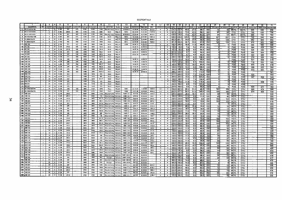
This Database has been called SCOFIDAT for Steel Column in Fire/Database of Tests.

It is available on an EXCEL file and it contains 141 tests. The database field names and the whole database are given hereafter.

SCOFIDAT Version 1.0 Date: 14.07.95

141 test results belong to the Database.

2.5.1 Field Names

1) Profile Name 2) Insulating Material Description 3) Number of the test 4) Buckling Axis 5) Steelgrade: S 235, 355, 460 6) Measured yield point 7) Measured tensile strength 8) Length of the column 9) Buckling length 10) Applied load 11) Name of the Laboratory ( City) 12) Name of the Country 13) Reference of the Laboratory report 14) Date of the test 15) Date of the report 16) Ultimate Load at room temperature (calculated according to EC3 part 1.1) 17) Imperfection of the column 18) Residual Stresses 19) Measured height of the steel section 20) Measured width of the steel section 21) Measured thickness of flange of the steel section 22) Measured thickness of web of the steel section 23) Time of fire resistance 24) Type of fire curve 25) Eccentricity of the load at the top of the column 26) Eccentricity of the load at the bottom of the column 27) Type of top end condition for the column 28) Type of bottom end condition for the column 29) Maximum of temperature in the column at the failure time 30) Minimum of temperature in the column at the failure time 31) Mean of temperature in the column at the failure time

26

2.5.2 Explanations of the database field names

1. NAMEPROFIL

Designation of the steel section according to the catalogue : ARBED , Sales propramme, Structural Shapes.

Ex: HD 210X210X198

Type = character WIDTH: 18

2. PROTECTION

Two possibilities are used: "n" or "y".


3. NUMTEST

NUMTEST is the numérotation of this DATABASE FILE in DBASE4 ( or EXCEL ).

Type = numeric WIDTH. 4 Dec: 0

4. AXIS

Two possibilities are used: "W" or "S".

The letter "W" means that the buckling resistance with respect to the WEAK AXIS was tested. The letter "S" means that the buckling resistance with respect to the STRONG AXIS was tested.


5. STEELGRADE

The structural steel grades must be according to EN 10027

Ex: S 355 ( S 235, S 275, S 355, S 420, S 460 )


6. M YIELDSTR

Corresponds to the measured yield strength of the steel ( in N/mnv).

Ex: 364

Type = numeric WIDTH: 3 Dec: 0

27

7. M TENSISTR

Corresponds to the measured tensile strength of the steel ( in N/mm*).

Ex: 523


8. COLULENGTH

Corresponds to the total length ( in mm ) of the column.

Ex: 5700


9. BUCKLENGTH Corresponds to the buckling length ( in mm ) of the column.


10. LOAD

Corresponds to the applied load during the test, expressed in kN.

Ex: 1100.0


11. LABORATORY

Enter the name of the city where the test was performed.

Ex: BRAUNSCHWEIG


12. COUNTRY

Country of the Laboratory.

Ex: Germany


28

13. NUMREPORT

Reference of the Laboratory report.

Ex: 1618/8510


14. TESTDATE

Date of the test written as follow: day / month / year

Ex: 02 / 09 / 88

Type = date WIDTH: 8

15. REPORTDATE

Date of the report written as follow: day / month / year

Ex 14 /12 /88

Type = date WIDTH: 8

16. NULT

Nu j t is the ultimate load expressed in kN in cold condition ( γΜο =1,1 and γΜι =1,1 ) according to EC3 Part 1.1 (April. 92) with the theoretical section sizes and the actual yield strength

Type - numeric WIDTH: 7 Dec: 1

17. IMPERFECTI

Note the imperfection ( in mm ) at the mid-height of the column in the buckling plane. (See FIGURE 2.5.1).

29

¡s AXIAL

IMPERFECTION

(>OTOLEFTT

FIGURE 2.5.1

Type = numeric

18. RESIDSTRES

WIDTH: 5 Dec: 1

Two possibilities are used: "N" or " Y " if the residual stresses have been measured.


19 SIZES H

Measured height of the steel section expressed in millimetres.

Ex: 270.3 (HD 210x210x198 )


20 SIZES Β

Measured width of flange of the steel section expressed in millimetres.

Ex: 222.4 ( HD 210x210x198 )


21 SIZES TF

Measured thickness of flange of the steel section expressed in millimetres.

Ex: 44.6 (HD 210x210x198 )


22 SIZES TW

Measured thickness of web of the steel section expressed in millimetres.

30

Ex: 44.6 (HD 210x210x198 )


23 FIRERESIST

Time of fire resistance expressed in minutes.

Ex: 38 (HD 210x210x198)


24 FIRECURVE

Two possibilities are used: " ISO " or "."

Ex. ISO


25 TOPECCENTR

Eccentricity of the load expressed in millimetres at the top of the column. ( > 0 TO THE RIGHT see FIGURE 2.5.2, a positive excentricity and a positive imperfection see § 17 - act in the same way )

Ex. 10

Type = numeric WIDTH: 4

26 BOTECCENTR

Eccentricity of the load expressed in millimetres at the bottom of the column. ( > 0 TO THE RIGHT see FIGURE 2.5.2, a positive excentricity and a positive imperfection · see § 17 - act in the same way )

Ex. 10


31

Top eccentricity

-Jr,

Χ Bottom eccentrìcit

FIGURE 2.5.2

27 TOPSUPPORT

Type of top end condition for the column.

Ex: mcyl ( See figure 3/II.2 )

Write " knif" or " cyli " or" mcyl" or " fixe "


knife

FIGURE 2.5.3

28 BOTSUPPORT

cylinder mid cylinder

\ \ \ \ \ \ \ \ \ \ \ \ \ \ \ \ \ \ \ N

fixed

Type of bottom end condition for the column

Ex: mcyl ( See FIGURE 2.5.3)

Write "knif" or " cyli " or" mcyl" or " fixe"


32

29 MAXCOLTEMP

Maximum of temperature in ° Celsius measured in the column at the failure time

Ex: 800


30 MTNCOLTEMP

Minimum of temperature in ° Celsius measured in the column at the failure time

Ex: 600

Type - numeric WIDTH: 4

31 MEANCOLTEMP

Mean of temperature in ° Celsius measured in the column at the failure time

Ex: 700


33

SCOFIDAT.XLS

ï l

2

3

4

b

6

7:

:β:

s 10

η

13

14

1 *

1« 17

18

W

ae Î 1

22

;:»: 24 2b

2b"

2 /

28

29

30

31

;.« 33

34

38

36

37 38

sa 40

41

42

43

44

45

46

4 /

48

49

bO

b1

b2

b3

54

55

56

57

58

59

60:

1

HO 210x210x1SB

HD 3101310x500

HO 310x310x500

HD 400x400x100·

W 310x410x314

W 350x410x314

HEB 300

■pe leo

IPE 160

■PE 200

IPE 3O0

HEB 130

HEB 120

HEB ÍBO

ΚΕΑ 200

HEA 300

HEA 220

HEB 200

HEB 140

HEB 140

IPE 220

IPE 230

HD 400.400x744

HD 400x400x744

HEM 220

HEB 120

HEB 220

HEB 220

HEB 120

HEM 220

HEB 220

HEA 220

HEM 220

HEB 120

HEB 330

HEB 220

HEB 220

HEB 220

HEB 120

HEB 130

HEB 120

HEB 120

HEB 130

HEB 120

HEM 220

HEM 110

HEM 110

HEA 140

HEA 140

HEB 1*0

HEB ITC

HEB ÍBO

HEB 180

HEB 220

HEB 220

HEB 220

HEB 220

HEB 150

2

PRT.

" » " " " " Y

> 1

ï

y

» Y

y

y

V

f

y

ν

y

y

y

n y

n

" n

n

» n

" n

" ■

y

ï

Y

y

y

y

y

y

y

y

y

y

y

< * y

* y

y

y

y

f

y

y

3

FVJMTEST

1

2

3

4

6

B

7

8

9

10

11

13

14

16

17

IB

19

IO

21

22

23

34

36

26

27

28

29

30

31

32

33

34

36

36

37

38

39

40

41

42

43

44

46

46

47

46

49

CO

El

62

E3

64

66

66

67

6Θ

69

60

« AXIS

w

s

W

W

W

W

W

w

w

w

w

w

w

w

w

w

w

w

w

w

w

w

w

w

s

s

5

s

5

S

S

s

s

s

Ξ

S

s

s

8 s

s

s

s

s

s

s

s

ε

s

s

s

s

s

s

s

s

s

s

6

Sieda1»«

S 366

S 366

S 366

8 366

S 366

S 460

S 236

S 236

S 236

S 236

S 236

S 236

S 236

S 236

S 236

S 336

S 236

S 336

S 336

S 236

S 236

& 236

S 336

S 336

S 236

S 236

S 236

8 236

S 236

8 236

S 236

S 236

S 236

S 336

8 236

8 236

8 236

8 236

S 236

8 236

8 236

S 236

S 236

S 236

S 236

8 236

S 336

8 336

8 236

& 236

S 236

8 236

S 236

S 236

6 336

8 236

8 336

8 336

6

M YtLOST*

384

396.6

297

390

401

498

371

270.6

270.6

277

277

260

260

37E

379

269

362

218

247

247

273

273

338

341

368.6

368.4

243.9

343.3

267

289

201

309

269

267

239.9

229.6

236.1

347.1

276.9

246.6

287.6

276.9

266.2

244.4

270.3

238.2

237.3

269.2

263.3

246.6

269

267

249

269

249.6

263.3

272

261.8

" ' V M TESSISI*.

623

490

490

674

636

67Θ

421

406

406

430

430

430

430

420

433

442

430

430

8

Cslirtrvjn

670O

4140

6700

4140

4140

4140

4380

4380

4380

4380

4380

4380

4380

4380

4380

4380

4380

4380

4380

4380

4380

4380

3960

3960

6800

6900

3800

3800

3800

3800

3800

3800

4800

4800

3800

3800

3800

3800

6800

680Q

6800

6B0O

6 eoo

6800

6800

6800

6800

6900

6800

3880

3860

3860

3860

3700

3700

3700

3700

4700

g

BUCKLENOIM

670O

4140

6700

4140

4140

4140

1890

1890

1890

1890

1890

1890

1690

ISSO

1890

1890

1916

1916

1916

1916

1916

191E

4140

4140

6900

6800

3800

3800

3800

30 00

3800

3800

4800

4800

3800

3800

3800

3800

6800

6800

6800

6800

6800

6800

6800

6800

6900

6800

6800

3860

3880

3860

3860

3700

3700

3700

3700

4700

10

LOAD

1100

2000

I860

4000

1800

1800

20O0

106.2

164.3

203.2

266.9

362.9

267

602.7

676.8

1607.3

972

08t

641.7

372

319

410

3400

3400

1118

103

661.6

386.4

317.8

1267.6

767.1

783.8

696

106

661.6

386.4

661.6

713.1

138.3

138.3

97.1

164

290

226

781.1

696.6

466

172.3

138.9

663

664

B91

876

1469

162B

1)36

1030

766

11

LASCRMOHY

Braunichweig

Geni

B r . u n . c h w . i g

G i r j

Gand

G i r J

Gand

Gand

G ì r i

Gand

Oend

Gand

G i r l

Gand

G t n d

G a r d

G a r d

G a r *

Gand

O a r d

Gand

G a r d

Gai J

Gand

Braunachwe ig

Brau nach wei g

Braun« c h w e i g

Brau n i c n w sig

ftaun.chw.ig

ftWMCnw..g

Braunachwe ig

Braunachwe ig

Braunachwe ig

» a u n . c h w e . g

& e u n a c h w „ g

B r a u n a c h w e i g

Braunachwe ig

B . a y n . c h w . , 3

B r e u n a c h w . i g

Braunachwe ig

B r e u n . c h w e i g

B r i u n a c n w e i g

Br.un.eh*. ,g

B.un.chw.ig

Braunachweig

»aun.cl.wtig

Brau nach w.ig

Braunachweig

Brau nach weig

Btuttgari

Braunacnweig

Slungan

Briun.chw.ig

Braunachweig

Braunachweig

Brau nach w.ig

Braun.chw.ig

, 2

Country

Germany

Brig um

Germany

Balg um

Belg um

Beigum

Be'gum

Beigum

Belgium

Belg u m

B e i g u m

Belgium

Belgium

Belgium

Belgium

Belgium

Belgium

Belgium

Belgium

Belgium

Be'31 u m

Belgium

Belgium

Belgium

G e r m a n /

C a r m a n /

G e r m a n /

Germany

Germany

Germany

G e r m a n /

Germany

G e r m a n y

G e r m a n /

G e r m a n /

German/

Germany

Germany

German/

Germany

Germany

Germany

Germany

German/

German/

German/

German/

Germany

Germany

Germany

Germany

German/

Germany

Germany

Germany

Germany

German/

13

Nurt í tp í r t

1 6 1 B / 8 6 1 0

6 B 7 3

1 6 1 8 / 8 6 1 0

6 8 7 4

6 8 7 2

6 8 7 1

2 7 0 4

6 0 9 1

6 0 9 2

1 4 B 0 1 1/1

1 4 8 D 1 2/1

1 4 8 0 1 1/11

1 4 8 0 1 4/11

1 4 8 0 1 3

1 4 8 0 1 4

1 4 8 0 1 6

1 4 8 0 1 6

1 4 B 0 1 7

1 4 8 0 1 β

1 4 8 0 1 2/11

1 4 B 0 1 3/11

1 4 8 0 1 6/11

1 4 8 0 1 I / I I I

1 4 0 O 1 11/11

1 4 Θ 0 1 14/11

1 4 B 0 1 16/11

1 4 8 0 1 18/111

1 4 B 0 1 1 / r v

1 4 B 0 1 2 / r v

1 4 B 0 1 3/111

1 4 8 0 1 4/111

1 4 8 0 1 E/Ni

1 4 8 D 1 ϋ ' I I I

1 4 8 0 1 7/111

1 4 B 0 1 KT. IHR

1 4 8 0 1 S I I 2 S

1 4 8 0 1 B S I I 2 S

1 4 8 0 1 fill 1 ïi

H O O I V 1

1 4 8 0 1 V 2

1 4 8 0 1 V 3

1 4 8 0 1 V 4

1 4 B D 1 V I 1

14

TES1DAIE

02.09.B8

06.10.88

07.09.B8

13.10.88

29.09.88

22.09.88

29.06.79

06.06.79

18.06.79

26.03.79

07.03.79

16.06.79

11.06.79

19.04.79

07.06.79

02.06.79

02.10.84

14.01.BE

197BBO

197B BO

197B80

197880

197677

197677

197677

1976 77

197677

197677

197860

197880

1978 80

197880

197880

197B80

197680

197B80

197B 00

197B80

197880

197BBO

1978 BO

1Θ78ΒΟ

197880

198183

198183

198183

198183

190103

198183

1981B3

198183

198163

15

Reportaste

04.12.88

24.04. B9

04.13.86

34.04.89

24.04.89

20.04.89

09.08.79

09.06.79

09.08.79

13.08.79

13.08.70

14.08.79

14.08.79

14.Off" 71»

14.08.79

20.08.79

17.00.86

22.06.86

02.06.06

02.06.06

02.06.06

02.06.06

30.06.06

30.06.06

30.06.06

30.06.06

30.06.06

30.06.06

02.06.06

02.06.06

02.06.06

03.06.06

02.06.06

02.00.06

03 06.06

02.06.06

03.06.06

02.06.06

02.06.06

02.06.06

02.06,06

02.06.06

02.06.06

06.06.06

06.06.06

06.06.06

06.06.06

06.00.06

06,06.06

06.06.06

06.06.06

06.06.06

16

NIAT

3213.0

11716.0

9644.0

13824.0

6086.0

7326.0

7966.0

8364.0

1914.4

240.7

849.9

847.4

610.6

2131,0

1261.3

1613.7

1168.6

188.7

8 3 0 . fi

603.3

827.0

1123.0

243.9

217.8

263.6

286.2

272.B

216.3

1366.1

902.4

686.3

296.6

233.1

2603.4

2638.7

1889.4

1761.0

1236.4

17

iweRFEcTi

0

0

0

0

1

•4

0

0

0

0

0

0

0

0

0

0

0

0

■4.1

4.1

0

0

0

0

0

0

0

0

0

0

0

0

0

0

0

0

0

0

0

0

0

0

0

0

0

0

0

0

0

υ

0

0

0

0

18

KeadUM

Ν

Ν

Ν

Ν

Ν

Ν

Η

Ν

Ν

Ν

Ν

Ν

Ν

Ν

Ν

Ν

Ν

Ν

Ν

Ν

Ν

Ν

Ν

Ν

Ν

Η

Ν

Ν

Ν

Ν

Ν

Ν

Η

Ν

Ν

Ν

Ν

Η

Ν

Ν

Ν

Ν

Ν

Ν

Ν

Ν

Ν

Ν

Ν

Ν

Η

Ν

Η

Ν

Ν

Ν

Ν

Ν

19

SIZES Η

270.3

4 2 7 0

428.0

568.0

4 0 2 8

401 0

306.0

162.0

163.0

201 0

201.0

124.0

124.5

180.0

193.3

296.3

213 3

200.0

140.0

140.0

220.0

220.0

500.0

500.0

240.0

120.0

220.0

2200

1200

240.0

220.0

210.0

240 0

120.0

220.0

220.0

220.0

220.0

120.0

120.0

120.0

1200

120.0

120.0

240.0

180.0

180.0

133.0

1330

180 0

1800

180.0

180.0

220.0

220.0

220.0

220.0

160.0

20

SIZES Β

222.4

335 0

335.0

446.0

401.7

400.0

298.0

83.0

82.0

101.0

101.0

120.0

120.0

180.0

198.0

2990

220.0

200.0

140.0

140.0

108.0

108.0

427.0

427.0

226.0

120.0

220.0

220.0

120 0

226.0

220.0

220.0

226.0

120.0

220.0

220.0

220.0

220.0

120.0

120.0

120.0

1200

120.0

120.0

226.0

166.0

166.0

140.0

140.0

180 0

180.0

180.0

180.0

2 2 0 0

220.0

220.0

220.0

160.0

21

SUES IF

44.6

7 3 0

73.6

1250

39.0

38.7

18.4

7.4

8.0

8.7

8.7

10.5

10.5

13.2

9.4

13.4

10.0

15.0

11.9

11.9

9.8

9.6

88.0

88.5

26.0

11.0

16.0

16.0

11.0

26.0

16.0

11.0

2 6 0

11.0

16.0

16.0

16.0

16.0

11.0

11.0

11.0

11.0

11.0

11.0

2 6 0

23.0

23.0

8.5

8.5

14.0

14.0

14.0

14.0

16.0

16.0

16.0

16.0

130

22

SIZES TW

27.5

4 2 0

42.0

71.0

20.8

23.0

11.0

5.0

4.0

4.8

4.8

6.7

8 3

10.0

4.7

7.7

7.2

9.2

7.3

7.4

7.0

7.0

51.0

51.0

15.5

6.5

9.5

9.5

6.5

15.5

9.5

7.0

15.5

6.5

9.5

9.5

9.5

9.5

6.5

6.5

6.5

6.5

6.5

6.5

15.5

14.0

14.0

5.5

5.5

8.5

8.5

8.5

8.5

9.5

9.5

9.5

9.5

8.0

S T

FRERESiSl

38.0

68.0

60.0

68.0

34.6

37.5

68.0

37.0

64.0

92.0

45.0

55.0

130.0

90.0

85.0

110.0

116.0

231.0

124.0

115.0

101.0

82.0

45.0

145.0

23.0

11.0

9.0

12.0

12.0

18.0

14.5

11.6

20.0

16.0

73.0

97.0

93.0

94.0

49.0

43.5

66.5

63.0

30.0

25.5

132.0

97.0

99.0

64.0

50.0

68.0

57.5

69.0

67.0

56.0

40.0

80.0

63.0

35.0

24

Fxfeuxvt

ISO

ISO

ISO

ISO

ISO

ISO

ISO

ISO

ISO

ISO

ISO

ISO

ISO

ISO

ISO

ISO

ISO

ISO

ISO

ISO

ISO

ISO

ISO

ISO

ISO

ISO

ISO

ISO

ISO

ISO

ISO

ISO

ISO

ISO

ISO

ISO

ISO

ISO

ISO

ISO

ISO

ISO

ISO

ISO

ISO

ISO

ISO

ISO

ISO

ISO

ISO

ISO

ISO

ISO

ISO

ISO

ISO

ISO

25

10PECCENTR

10

85

34

227

120

120

0

0

0

0

0

0

0

0

0

0

0

0

0

0

0

180

180

49

45

102

102

0

12

12

12

14

12

102

102

102

55

55

55

55

30

27

55

120

45

90

33

66

30

30

0

0

12

12

12

55

12

26

B01ECCENIR

10

85

34

227

120

120

0

0

0

0

0

0

0

0

0

0

0

0

0

0

0

180

180

49

45

102

102

0

12

12

12

14

12

102

102

102

55

55

55

55

30

27

55

120

45

90

33

66

30

30

0

0

12

12

12

55

12

27

TOPSJPPORt

MCYL

CYLI

MCYL

CYLI

CYLI

CYLI

FIXE

FIXE

FIXE

FIXE

FIXE

FIXE

FIXE

FIXE

FIXE

FIXE

FIXE

FIXE

FIXE

FIXE

FIXE

FIXE

CYLI

CYLI

MCYL

MCYL

MCYL

MCYL

MCYL

MCYL

MCYL

MCYL

MCYL

MCYL

MCYL

MCYL

MCYL

MCYL

MCYL

MCYL

MCYL

MCYL

MCYL

MCYL

MCYL

MCYL

MCYL

MCYL

MCYL

MCYL

MCYL

MCYL

MCYL

MCYL

MCYL

MCYL

MCYL

MCYL

28

BOISJPPOAT

MCYL

CYLI

MCYL

CYLI

CYLI

CYLI

FIXE

FIXE

FIXE

FIXE

FIXE

FIXE

FIXE

FIXE

FIXE

FIXE

FIXE

FIXE

FIXE

FIXE

FIXE

FIXE

CYLI

CYLI

CYLI

CYLI

CYLI

CYLI

CYLI

CYLI

CYLI

CYLI

CYLI

CYLI

CYLI

CYLI

CYLI

CYLI

CYLI

CYLI

CYLI

CYLI

CYLI

CYLI

CYLI

CYLI

CYLI

CYLI

CYLI

CYLI

CYLI

CYLI

CYLI

CYLI

CYLI

CYLI

CYLI

CYLI

29

MAXCOLTEMP

695

795

885

740

862

870

666

584

525

599

404

531

710

675

573

525

567

525

666

674

30

MP.CO.TEMP

635

630

755

545

501

563

566

529

440

504

389

506

533

578

551

529

508

231

474

428

31

MtxnCCLIEMP

656

700

784

644

652

680

588

564

475

559

394

519

585

616

556

561

502

549

516

576

522

360

566

608

530

555

550

610

560

600

590

560

650

685

430

550

500

545

350

325

520

498

210

160

562

500

490

473

458

418

417

475

446

335

230

478

378

232

SCOFIDAT.XLS

N A M F. PROF K. lABORATCfY

M:

62

63

64

65

66

67

68

69

70

71

72

73

74

75

76

77

78

79

8¿

81

:β2:

83

84

85

Β6

87 ï

88

89

30

91 '

92

93

54

96

9«

97

9Β

100 >

101 i 102 i

103'

104 ;

105 ;

106 ;

ίο* ; 108 » 109 ; no; m ; 112. 113 ► 114 ; ne ; 116 ï 117 ; vie ; 119. 12S Ρ

Garmxny

19B1S3

UBI IK)

14B01 VIII E

14801 VIII IO

14801 VIII 1

ttxunich

EPpunfchwtig

□ ermjiiy

Qeimxny

1S30

1930

Borotixmhood

S 236

S 23E

15 Îïp5taetT

05.08.OS

06.Oe.OS

06.06.06

06.06.06

06.08.06

06.08.06

06.06.06

05.00.06

06.08.06

06.08.06

06.08.06

2800

171.0

120.0

120.0 120.0

180.0

180.0 120.0

20 SI2ES Β

220.0

166.0

150.0

180.0

140.0

101.8

13.0

23.0

12.0

10.7

140

14.0

14.0

11.0

12.5

6.0

6.0

5.9

Î T

54.5

81.0

47.0

36.0

64.6

110.0

47.0

68.6

70.0 88.0

85.0

77.0

31.0

62.0 52.0

73.0

60.0

180.0

24 Fxfñxvt

ISO

ISO

ISO

ISO

ISO

ISO

ISO

ISO ISO

ISO

ISO

ISO

ISO

3Γ

25

35

70

ΤΓ

140

140

57

105

ΤΓ 2ÍT MAXCOLTEMP

MCYL

MCYL

MCYL

MCYL CYLI

MCYL

CYLI

CYLI

MCYL

CYLI

MCYL

MCYL

MCYL

MCYL CYLI

FIXED

MCYL

MCYL

CYLI

MCYL CYLI

FIXED

FIXED

FIXED FIXED

CYLI

MCYL

MCYL

MCYL

MCYL

MCYL

MCYL

MCYL

MCYL

MCYL MCYL

MCYL

MCYL

KNIF

KNIF

MCYL

MCYL

FIXED

SCOFIDAT.XLS

121

122

123

124

125

126

127

128

129

130

131

132

133

134

135

136

137

138

139

140

141

1

NAMEPROFH.

HEA 100

HEA 100

HEA 100

HEA 100

HEA 100

HEA 100

HEA 100

HEA 100

HEA 100

HEA 100

HEA 100

HEA 100

HEB 200

HEB 200

HEB 200

HEB 200

HEM ISO

HEM 110

HEA 140

HEA 140

2

PRI.

" " " n n

n n

" n n n

n

" n n n n

n n

" n

3

NUMTÍ3T

121

122

123

124

126

12S

127

128

129

130

131

132

133

134

136

138

137

138

139

140

141

4

AXlS

w

w

w

w

w

w

w

w

w

w

w

w

w

w

w

s

w

s

5

s

s

5

S 236

8 236

8 236

8 236

S 236

S 236

8 236

S 236

8 236

S 236

S 236

S 236

S 236

S 236

S 236

S 236

S 236

6 236

S 236

3 236

S 236

6

289.8

298.2

288.9

281.4

2B1.4

281.4

28472

289.7

298.2

288.8

289.8

298.1

288.7

276

276

276

276

271

271

200

260

Γ"

44B.9

460.ï

444.6

444.6

444.6

444.E

441.8

440.9

460.2

444.6

446.9

460.2

444.6

468

468

46B

468

483

463

410

410

8

40O0

4000

2000

2000

2000

6000

2000

60O0

9

1272

1271

12S9

2020

2020

2023

2770

2772

2771

2772

3610

3610

3610

4000

40O0

2000

2000

2000

6000

2000

6000

-Ίο-

292

261

24

174

171

173

127

73

34

8.42

106

ao

11.6

100

loo 100

160

100

100

ιβο

100

11

Labern

Labein

labe.»

La bem

L.bein

Ubein

labern

Libem

le bei η

Laotin

labern

Latem

CTICM

CTICM

CTICM

CTICM

CTICM

CTICM

CTICM

CTICM

12

Spam

Spam

Spam

Spam

Spam

Spam

Spam

Spam

Spam

Spam

Spam

Spam

Spam

France

Franc.

France

France

Franc.

France

France

France

13

94-8

94-S

94-8

94-S

94-S

94-S

94-S

94-S

190

186

200

199

201

197

202

194

14

06.06.94

06.04.94

17.U6.94

16.06.94

18.06 94

19.06.94

19.06.94

09.06.94

15

00.10.1994

00.10.1994

Ü0.10.1994

00.10.1994

00.10.1994

00.10.1994

00.10.1994

00.10.1994

16 17

0.2

0.4

0.3

0.7

1.7

1.1

■0.4

1

0.8

1.8

1.6

1.8

1.1

1.E

2

1

1

3.6

1

1

1

18

Y

Y

Y

Y

Y

Y

Y

Y

Y

Y

Y

Y

Y

N

N

N

N

N

N

N

N

19

98.9

99.3

99.2

99.0

99.0

9 9 2

99.1

99.0

99.3

99.2

98.9

99.1

99.2

201.4

201.4

2 0 1 3

201.4

1802

180.4

137.5

133.8

20

101.9

101.9

102 2

101.8

101.8

1017

101.9

101.8

1020

102.2

101.9

102.1

101.7

200.2

200.3

200.3

200.3

163.4

1635

141.5

139.8

21

7.6

7.8

7.7

7.6

7.6

7.6

7.7

7.6

7.8

7.7

7.6

7.7

7.6

15.0

15.0

15.0

15.0

22.7

22.7

9.0

8.3

22

6.0

6.1

6.0

5.7

5.8

5.7

5.8

5.8

6.0

6.0

5.9

5.9

5.7

9.0

9.0

9.0

9.0

14.0

14.0

5.6

5.6

23

87.0

92.0

166.0

83.0

97.0

92.0

89.0

110.0

122.0

173.0

E5.0

94.0

150.0

96.0

68.0

81.0

70.0

1220

76.0

67.0

66.0

24 25

5

5

5

5

5

5

5

5

5

5

5

5

5

100

300

650

300

250

500

100

100

26

5

5

5

5

5

5

5

5

5

5

5

5

5

100

300

650

300

250

500

100

100

,...,,.

KNIF

KNIF

KNIF

KNIF

KNIF

KNIF

KNIF

KNIF

KNIF

KNIF

KNIF

KNIF

KNIF

MCYL

MCYL

MCYL

MCYL

MCYL

MCYL

MCYL

MCYL

28

KNIF

KNIF

KNIF

KNIF

KNIF

KNIF

KNIF

KNIF

KNIF

KNIF

KNIF

KNIF

KNIF

MCYL

MCYL

MCYL

MCYL

MCYL

MCYL

MCYL

MCYL

29

600

634

574

777

599

577

560

ECSC Research 7210SA 515 " Buckling Curves in Case of Fire "

Partners : ProfilARBED Research (Luxembourg) as leader of this Research

Université de Liège (Belgium)

TNO (The Netherlands)

CTICM (France)

LABEIN (Spain)

For information, please contact: ProfilARBED Research

Service RPS

66, rue de Luxembourg

L4221 Esch/Alzette

Telefax:35253132199

Phone: 352 53132183

30

540

544

467

732

484

512

443

31

390

474

749

509

485

495

457

587

587

858

446

493

727

664

575

599

537

753

572

539

507

3. CALCULATION MODELS

3.1 COMPARISON BETWEEN LENAS, SISMEF, DIANA)

NUMERICAL PROGRAMS (SAFIR, CEFICOSS,

3.1.1 INTRODUCTION

As different programs are used in this research, a set of calibration examples has been established at the University of Liège and these examples have been calculated with the five programs available in the different organizations: CEFICOSS and SAFIR (ProfilARBED Recherches and University of Liège), DIANA (TNO), LENAS and SISMEF (CTICM).

3.1.2 Example Definition

Three types of structure (A B, C) have been defined. For each type different kinds of heating have been analysed. The first structure A is a theoretical example called "Lee's Frame"; the other ones are a steel column with different load eccentricities. All the parameters needed for the simulations (material law and characteristics, loads, cross section, end conditions, heating conditions ...) are given hereafter:

STRUCTURE A: LEE'S FRAME

. 24 . 96

120

O

Ό Section : rectangular : b = 3

h = 2 => A = 6

1 = 2 Units have to be consistent.

Test A. 1. ambient temperature.

The material is elastic. E = 720. Apply a vertical downward load on the horizontal beam, at a distance of 24 from the beam column connection.

37

Produce one EXCEL file showing the evolution of the vertical and the horizontal displacement under the load for every load step of 0.1 up to 1.7. for every converged point beyond 1.7. Test A.2. uniform temperature.

The material is EC3 steel. E = 720, fy = 3. Temperature is uniform in the section. A vertical load of 0.2 is applied. The temperature in the profile gradually increases. Calculate the ultimate temperature ( precision 0.5 °C). Produce one EXCEL file showing the evolution of the vertical and the horizontal displacement under the load for every step of 32°C (20,52,84,.. ) up to 596°C, for every converged point beyond 596°C.

STRUCTURE B; ECCENTRICALLY LOADED COLUMN

Profile Buckling End conditions

Dead weight Total length Imperfection Loading

Residual stresses Material and thermal laws

Test B.l. ambient temperatui

HE200B. weak axis. pined at both ends. 235 MPa. neglected ( simulate one half of the column). 4 m. 4 mm, sinusoidal. axial load N + bending moment M = Ν χ 0.10 m. The bending moment has the same effect on transverse displacements as the imperfection. bitriangular, max. value = 117.5 MPa. EC3, part 10 ε = 0.5 and h = 25 when needed. no shadow effect.

'e

Calculate the ultimate axial load ( precision 0.5 kN ). Produce one EXCEL file with;

- the shortening of one half of the column, - the transversal displacement ( both in mm)

for every step of 64 kN up to 320 kN, for every converged point beyond 320 kN.

Test Β.2. uniform temperature

Temperature is uniform in the section. An axial load of 250 kN is applied (+ M = 25 kN m ). The temperature in the profile gradually increases. Calculate the ultimate temperature ( precision 0.5 °C). Produce one EXCEL file with;

- the elongation of one half of the column ( negative at 20°C), - the transversal displacement ( both in mm),

38

for every step of 32 °C ( 20, 52, 84,..) up to 404°C, for every converged point beyond 404°C.

TestB.3. ISO curve

The profile is submitted to the ISO curve. Apply a load of 250 kN ( + M = 25 kN m ). Calculate the fire resistance of the column ( criteria = buckling ) with a precision of 1 sec. Produce one EXCEL file with;

- the elongation of one half of the column ( negative at 20°c), - the transversal displacement ( both in mm),

for every step of 64" up to 576", for every converged point beyond 576",

STRUCTURE C; CENTRICALLY LOADED COLUMN.

Profile

Buckling

End conditions

Dead weight

Total length

Imperfection

Loading

Residual stresses

Material and thermal laws

Test C. 1. ambient temperature

■ HE200B.

weak axis.

pined at both ends.

235 MPa

neglected ( simulate one half of the column)

4m

4 mm, sinusoidal.

axial load.

bitriangular, max. value = 117.5 MPa

EC3, part 10

ε = 0.5 and h = 25 when needed.

no shadow effect

Calculate the ultimate load ( precision 0.5 kN ) Produce one EXCEL file with;

- the shortening of one half of the column, - the transversal displacement ( both in mm)

for every step of 64 kN up to 1024 kN, for every converged point beyond 1088 kN,

Test C.2. uniform temperature

Temperature is uniform in the section. A load of 500 kN is applied. The temperature in the profile gradually increases Calculate the ultimate temperature ( precision 0.5 °C ) Produce one EXCEL file with;

- the elongation of one half of the column ( negative at 20°C), - the transversal displacement ( both in mm),

for every step of 32 °C ( 20, 52, 84,..) up to 500°C,

39

for every converged point beyond 500 °C,

Test C.3. ISO curve

The profile is submitted to the ISO curve. Calculate the temperature distribution. Show the obtained field of temperature after 960 sec by your own graphic tools. Produce one EXCEL file showing the average temperature for every step of 320 sec. up to 1920 sec. Apply a load of 500 kN. Calculate the fire resistance of the column ( criteria = buckling ) with a precision of 1 sec. Produce one EXCEL file with;

- the elongation of one half of the column (negative at 20°C), - the transversal displacement ( both in mm),

for every step of 64" up to 640", for every converged point beyond 640",

3.1.3 Simulation Results

The following summary points out quite a good agreement between numerical models. All the results are described in the paper "A comparison between five structural Fire Codes applied to Steel Elements" [1] and given in Annex 7.

SUMMARY

SAFIR

CEFICOSS

DIANA

LENAS

SISMEF

A - l

LOAD

1,85

1,86

1,855

1,84

1,84

A - 2

Temp.

626°C

625°C

628°C

621°C

625°C

B - l

LOAD

417 kN

416kN

437kN

414kN

414kN

B - 2

Temp.

432°C

433°C

450°C

428°C

427°C

B - 3

Time

604 sec

606 sec

608 sec

589 sec

589 sec

C - l

LOAD

1144kN

1154kN

1113 kN

1166kN

1117kN

C - 2

Temp.

524°C

524°C

515°C

518°C

519°C

C - 3

Time

745 sec

745 sec

717 sec

730 sec

722 sec

40

Experimental LABEIN tests versus SAFIR curves

for different column length

u u u ■

500 -

400 -

•a α - 300 -Ό

Q. Q. <

200 -

100-

0 -

•

□

♦

χ

χ«. \

■X. > v

" 4 ? \

^ \ ■ · " · * ~ " b ^ \

* — ' · \ \

""öAI I I I , U I J 111111

• TESTS, 513 mm

SAFIR, 1270 mm

α TESTS, 1270 mm

SAFIR, 2020 mm

♦ TESTS, 2020 mm

SAFIR, 2770 mm

Δ TESTS, 2770 mm

SAFIR, 3510 mm

χ TESTS, 3510 mm

w ^ . *· V Ne»

1 1 1 1 1 1 |__ί 'JUL A " 100 200 300 400 500

Critical temperature [°C] 600 700 800 900

2 rt δ1

d sr

3

¡

a J w ero

•o th o <. απ» ocr ν

m

cg

•Ό O ÏÏ Vi

O C

cr rt

CTO O O CX

O o a o o

cr rt

rt

S

ë 3 α» 3 . o

on

.1

1

¡ Co

1 Co

a

3.3 NUMERICAL SIMULATIONS OF THE CTICM TESTS. Annex 6 presents the comparison between the horizontal displacements measured during the tests and the displacements calculated with LENAS. There were two transducers of displacement at mid height of the column (FIGURE 3.3.1a if the buckling is around the major axis and FIGURE 3.3.1b if the buckling is around the minor axis) to check that there was no rotation of the section of the column or lateral buckling.

Π "Π 0

D'

o

D'

a) buckling around the major axis

FIGURE 3.3.1

b) buckling around the minor axis

The following comments have to be made to have a good understanding of this Annex 6.

For the column PI the electric power broke down after 86 minutes and came back 4 minutes later. That's why there is no increasing of displacement between 86 and 90 minutes. This black out does not appear in LENAS simulation because the step of calculation was too large and because a linear interpolation is made between two points of the curve. As the transducers were reset, the curve after 90 minutes was "pasted", at the end of the first recording, with an offset equal to the oldest value recorded.

For the column P2 the computer did not record any displacement before 22 minutes and when it starts recording, the initial value was zero (the transducer was reset). There was only the relative displacement from the time t = 22 minutes. An additional displacement equal to the value calculated with LENAS (at t = 22) was added to the data recorded. From zero to 22 minutes the displacement kept constant and equal to the value calculated with LENAS at ambient temperature. For this reason, there is a small step after 22 minutes.

It is strange that for column P4 the initial displacement calculated with LENAS is the half of the displacement measured on the column. This difference seems to stay constant with the increasing of the temperature. It can come from incorrect initialisation of the transducers of displacement, or of local initial imperfection (material properties or geometry) that has not been measured.

For all the other tests there is a good agreement between simulation and experimentation.

42

The critical temperatures obtained with LENAS are on the safe side compared to the measured temperatures (TABLE 3.3.1 and FIGURE 3.3.1) except for column P6 where LENAS gives a temperature higher of 20°C than the one measured during this test.

COLUMN PI P2 P3 P4 P5 P6 P7 P8

TLENAS SIMU - Ttest (°C) -9 -25 -3 -18 -36 +20 -8 0

TLENAS SIMU (°C) 655 540 605 510 726 591 535 520

Ttest (°C) 664 575 608 528 762 571 543 520

TABLE 3.3.1 comparison LENAS (SLMU) and test

Ttest(°C)

100 200 300 400 500 600 700 800 Τ LENAS (°C)

FIGURE 3.3.2 comparison of the critical temperatures (tests - LENAS)

Six calculations were made for each column. The results of these calculations are given in TABLE 3.3.2 and TABLE 3.3.3. TABLE 3.3.2 presents the time (in minutes) when the failure occurred and TABLE 3.3.3 presents the equivalent uniform temperature (at the time from TABLE 3.3.2). The six calculations were made with the following hypothesis:

43

SLMU : The calculation is as close as possible to the real column tested. For this, the temperatures, the yield stress and the geometry measured were used in the calculation. The dead weight is neglected. (These results were plotted in FIGURE 3.3.2).

TEMP. : It is the same as SLMU (see column in TABLE 3.3.2 and TABLE 3.3.3) except that the temperature is uniform in the cross section and along the column.

GEO.

-SIG

-SIGI

SIG2

: It is also the same as SIMU (see column in TABLE 3.3.2 and TABLE 3.3.3) but this time the geometry of the cross section is taken form ARBED's catalogue and the initial imperfection is equal to L/1000.

: It is the same as SIMU but ay = 235 MPa as given theoretically for a S235 steel profile.

: It is the same as SIG but Oyw of the whole section is taken equal to the σ# measured for the flanges.

o ^ S f + a S : It is the same as SIG but σ„ = -^— y*_^»_

sf+sv

The last column of TABLE 3.3.2 and TABLE 3.3.3 called ESSAI gives the time of failure (TABLE 3.3.2) of the column during the test performance and in TABLE 3.3.3 the equivalent critical temperature.


GEO 94.75 54.62

82 66.88 115.9 80.75 60.88 64.25

SIG 91.12 51.62

74 55.62 109.6 75.12 59.88 60.25

SIGI 95.0 55.0 80

67.12 114.3 79.65 64.25 65.25

SIG2 95.75 55.5 81

68.5 116.5 81.5

65.62 66.88

TEMP 94.62 54.62

80 68.25 115.3 79.88 65.75 64.88

SIMU 95

55.0 80

67.12 115.3 80.25 65.12 66.12

ESSAI 96.75 58.5

80.56 70.58 122.4 76.25 66.7 66.1

TABLE 3.3.2 Time of collapse of the columns (min)


GEO 654 535 615 509 729 594 514 511

SIG 636 505 545 543 698 565 509 491

SIGI 655 540 605 510 721 588 531 516

SIG2 659 545 610 517 732 597 358 524

TEMP 653 536 605 516 726 589 539 514

SIMU 655 540 605 510 726 591 535 520

ESSAI 664 575 608 528 762 571 543 520

TABLE 3.3.3 Equivalent temperature of collapse of the columns (°C)

44

From these calculations it can be concluded that it is not a bad approximation to take : The theoretical geometry. A uniform temperature in the column. A Cy uniform in the cross section as defined for SIGI or SIG2. Note that the fact of using es y equal to the theoretical value of 235 MPa is too safe.

45

4. NUMERICAL SIMULATIONS

4.1 CALCULATION OF AXIALLY LOADED MEMBERS: A PROPOSAL FOR AN ANALYTICAL PROPOSAL

4.1.1 INTRODUCTION In Eurocode 3 - part 10 [2] two different calculation methods are presented to determine the fire resistance of axially loaded members; - the general calculation model based on acknowledged principles and assumptions of the

theory of structural mechanics, takes into account the effect of temperature. The application of this method requires the use of non linear computer programs,

- the simple calculation model, based on an analytical formula which can be applied with the use of tabulated data and/or a pocket calculator. This analytical formula has been recently amended in Eurocode 3 - Part 1.2. [3].

It is considered that, as stated in [2], " the general calculation models lead to a more realistic analysis of structures exposed to fire. Compared with simple calculation models, they give an improved approximation of the actual structural behaviour under fire conditions ". Simplified methods should therefore be allowed only if they prove to be safer than the more general methods.

One aim of the research is to verify the validity of the simplified method of [2] and [3] and to make an alternative proposal if necessary. The methodology consisted of the application of the general model to a very large number of examples and to compare the results with the results provided by the analytical proposals and by real tests.

4.1.2 THE GENERAL MODEL

4.1.2.1 The numerical code

The general model has been applied by using of the computer code S AFLR, a non linear finite element program dedicated to the step by step simulation of the behaviour of structures submitted to fire. The 2D beam finite element that has been used in this study is based on the following formulations and hypotheses:

- Displacement type element. - Prismatic element. - The displacement of the node line is described by the displacements of 3 nodes:

2 nodes at the ends of the element, supporting 2 translations and one rotation, 1 node at mid length supporting the non linear part of the longitudinal displacement.

- The longitudinal displacement of the node line is a 2n<* order power function of the longitudinal co-ordinate.

- The transversal displacement of the node line is a 3fd order power function of the longitudinal co-ordinate.

- The plane sections remain plane and perpendicular to the node line. i.e. the shear energy is not considered ( Bernoulli hypothesis ).

46

. *+ j_f r*yÄ (2) ox 2L_[\óx)

The strains are small ( Von Karman hypothesis ), i.e.

Ι * « ι (i) 2<5x

The non linear part of the strain is averaged on the length of the element to avoid locking,

i.e.

■LA

The formulation is according to the total corrotational description.

The angles between the deformed node line and the undeformed but translated node line are

small, i.e.

sin φ Ξ φ

(3) cos ç? Ξ 1

The longitudinal integration is numerically calculated by the method of Gauss.

The cross section is discretized by means of triangular or quadrilateral fibres. At every

longitudinal point of integration, all variables such as temperature, strain, stress, ... are

uniform in each fibre.

The tangent stiffness matrix is evaluated at each iteration of the convergence process

(Newton Raphson method).

Residual stresses are considered by means of initial residual strains [4].

4.1.2.2 Hypotheses of the numerical simulations

End conditions : simply supported, i.e. rotation not restrained.

Load eccentricity : no eccentricity, i.e. axial load.

Column imperfection : sinusoidal, maximum value = H/1000.

Dead weight : neglected, i.e. only one half of the length is simulated, by means of

5 beam elements.

Longitudinal integration : 2 points of Gauss

Cross section : only one half is simulated. The dimensions are according to

FIGURE 4.1.1, where only 1/4 of the section is represented.

47

FIGURE 4.1.1 Cross-section.

a/2 d d

I I I I ns layers

ncou layers

na layers

B/20 B/40

-f—H

/ I-

In FIGURE 4.1.1 dimension of the triangle having the same surface as the root fillet.

4 (d2/2) (4)

ns

(2/f - nr2

d = 0.655 r ncou : number of layers on the thickness of the flange,

dimension = tf/ncou where tf = flange thickness : number of layers on the length of one flange, dimension = ( 17 Β / 40 - a/2 - 2d )/ns where Β = width of the section,

a = web thickness. : number of layers on one half of the web. dimension = ( H/2 - tf - d )/na where Η = Height of the section.

The values for ncou, ns and na in the simulations have been set according to TABLE 4.1.1

na

TABLE 4.1.1 Parameters of the discretization.

Buckling around ncou na ns

major axis 3 5 5

minor axis 1 4 10

- residual stresses: -constant across the thickness of the web and of the flanges, -triangular distribution,

48

-maximum value = 0.30 or 0.50 χ 235 MPa depending on the value of H/B, -no residual stress in the triangle accounting for the root fillet.

4.1.3 THE NUMERICAL SIMULA TIONS IN CASE OF UNIFORM TEMPERA TURE The situation of uniform temperature has been considered as the limit case of insulated sections. With very important thermal insulation, the heating rate is so limited that the high thermal diftusivity of steel has time to homogenise the field of temperature in the section. The other limit case leading to the most severe thermal gradient in the sections is when unprotected profiles are submitted to the ISO heating. It will be considered in another section.

4.1.3.1 S235 The nominal yield strength of 235 MPa has first been considered. The nominal value has been adapted depending on the thickness of the flange according to EN. 10025 [4], i.e.

fy = 235MPa fy = 225 MPa fy = 215MPa fy=195MPa

if if if if

tf < 16 < tf < 40 < tf < 100 < tf

16 mm 40 mm 100 mm

4.1.3.2 Strategy The sections which are classified under class 4 according to EC3 part 1 [6] have not been considered because the beam element does not allow us to take local buckling into account whereas it is clearly stated in [1] that " If there are failure modes, not covered by the general calculation model, they shall be excluded by appropriate detailing. " The fire resistance of class 4 profiles should therefore be assessed by means of tests or by means of numerical simulations taking local buckling into account, which is beyond the scope of this project.

The Η sections from the catalogue [7] of the Arbed company have been considered. In this catalogue, some sections have different names but same geometrical characteristics. In that case, one of the two twin profiles has been eliminated, which left 400 different Η sections. For grade S235, 61 sections are classified as class 4 under axial loading according to [6]. 339 sections had thus to be considered;

34 128

6 28 41 28 32 42

HD HE HL HP IPE UB UC W

sections sections sections sections sections sections sections sections

For each section, buckling around the major axis as well as around the minor axis has been taken into account separately.

49

For each section and buckling axis, 10 different lengths have been considered, with the relative

slenderness at ambient temperature λ equal to 0.20, 0.40, 0.60 2.00

For each length, an average of 12 different loads have been successively applied and the

ultimate temperature corresponding to the loss of stability has been recorded.

When the applied load level is progressively decreased by very short time steps, the curve

describing the decrease of the ultimate load as a function of temperature can be drawn. It

appears that when the temperature is uniform in the section, this curve is made of linear

segments of 100°C steps. Due to this fact, linear Bspline functions could be applied in order

to determinate the loads which would lead to the ultimate temperatures of 400, 500, 600, 700,

800 and 900°C

Example:

For

ΕΡΕΑ 80 section,

buckling around the major axis,

H = 1.272 m,

fy = 235MPa,

TABLE 4.1.2 gives the ultimate temperatures found for the 16 different loads that have been

applied.

TABLE 4.1.2 Original points : ultimate temperatures.

Load[N]

84696

81167

77638

70580

63522

49406

39525

25409

I 18351

15528

12704

9881

9175

7764

7058

5646

Ult. temp. [°C]

409.84

431.14

451.75

492.84

519.45

567.12

601.25

668.89

704.37

736.86

767.50

798.56

815.03

852.48

871.75

920.66

TABLE 4.1.3 gives the loads corresponding to the ultimate temperatures of 400, 500 ...

900°C. Those loads have been found by application of linear ßspline functions and least

square method in order to cope with redundant points.

50

TABLE 4.1.3 Computed points : ultimate load

Temp. [°C]

400

500

600

700

800

900

Ult. load [N]

86476

69288

39794

18822

9747

5988

FIGURE 4.1.2 Validation of the method of linear ßspline functions shows how well the original results from TABLE 4.1.2 and the computed results from TABLE 4.1.3 compare when plotted on the same graph.

FIGURE 4.1.2 Validation of the method of linear ßspline functions.

90000

80000

70000

60000

=* 50000 α

§ 40000

"* 30000 +

20000

400.00 500.00 600.00 700.00

TEMPERATURE [°C]

800.00 900.00

Note : In order to obtain sufficient precision on the computed values for N(400°C) and N(900°C), at least one original point must exist for a temperature between 400 and 430°C, and one point between 870 and 900°C. For each section, each buckling axis and each nominal yield strength, a matrix was built such as the one found in TABLE 4.1.4.

TABLE 4.1.4 Computed matrix. Uitin

Temp_.

j 20

400

500

600

1 700

800

900

0

149.93

149.93

116.95

70.47

34.48

16.49

9.00

0.636

146.64

120.20

93.83

56.31

27.74

13.25

7.23

1.272

141.16

86.47

69.29

39.79

18.82

9.75

5.99

1.908

131.61

71.60

58.81

32.14

14.66

8.24

5.53

iate loads in kN for ΕΡΕΑ 80, major axis

Il Length Tml

2.544

116.45

62.15

51.86

27.53

12.17

7.30

5.08

3.180

95.23

53.30

44.83

23.51

10.20

6.36

4.49

3.816

74.41

44.29

37.41

19.52

8.38

5.37

3.84

4.452

57.97

36.00

30.54

15.88

6.77

4.44

3.21

5.088

45.86

29.25

24.88

12.90

5.48

3.64

2.65

, S235.

5.724

36.98

24.00

20.45

10.58

4.49

3.00

2.21

6.360

30.38

19.95

17.02

8.80

3.72

2.51

1.85 ||

51

Each horizontal line of TABLE 4.1.4 is the buckling curve for the corresponding temperature.

Those curves have a very regular and continuous shape. Therefore a sinusoidal expression is

used when the ultimate load has to be found for a temperature belonging to the matrix ( Τ =

600°C for example ), but for intermediate length ( Η = 2 m for example ) ;

N(T,H) = A,(T) + MT)-f- + ±B,(T)J^) (5) "max ¿=1 V " m « J

where N(T,H) axial load corresponding to temperature Τ ( belonging to the matrix )

and height H,

H m a x maximum height ( corresponding to λ = 2.00 ) for which calculations

have been made ( H m a x = 6.360 m in TABLE 4.1.4),

Ax (Τ), A2 (Τ), Bi (Τ) coefficients to be calculated from the 11 computed points at

temperature Τ

note : it comes immediately that A¡(T) = N(T,0)

A2(T) = N(T,Hmax)N(T,0)

When the ultimate load has to be found for a temperature and a length that do not belong to

the matrix ( t = 660°C and Η = 3 m for example), eq. 5 is applied twice for the temperatures of

the matrix immediately superior and inferior to the target temperature ( 600 and 700°C in this

case ) and a linear interpolation is made on the temperature between the two results.

4.1.3.3 Results for steel S235

In order to allow comparisons with the formula of [3], the results have first been presented in

the form of buckling coefficient as a function of the relative slenderness evaluated at 20°C. The

buckling coefficient is defined as ;

_^_ = ^ ^ = ^ L _ ._ x/ (6) NAT) MT)n KJyfi>a /K

where Npj(T) plastic load at temperature T,

fy(T) yield strength at temperature T,

fy yield strength at ambient temperature,

Ω cross sectional area

Kfy fy(T)/fy according to [ 1 ].

χ buckling coefficient calculated from the cstut curve [1],

κ correction factor, equal to 1.20 in [1].

Ten different values of λ , from 0.20 to 2.00, have been considered. For each relative

slenderness, the buckling coefficient has been evaluated for the 339 sections, for 2 buckling

axes, and for 5 ultimate temperatures ( 400, 500,..800°C).

Note : The temperature of 900°C has not been considered because it leads to higher buckling

coefficients than the other temperatures and gives the false impression of a high scatter

between the numerical results when presented in FIGURE 4.1.3. This temperature of 900°C

corresponds in fact to very low load levels and is not very commonly reached in practical

situations. As the results that are not considered give higher buckling coefficients than those

that are used in the comparisons, the approximation is on the safe side anyway. 3390 buckling

coefficients have thus been calculated for each relative slenderness.

52

In FIGURE 4.1.3, SAFIR max is the curve linking the maximum values that have been calculated by the general model, SAFER min links the minimum values and SAFER 50% means that 50% of the numerical results are below this curve. The analytical proposal made by the project team of EC3 - Part 10 in [1] is also drawn on FIGURE 4.1.3 ( it corresponds in fact to the curve c of EC3 part 1 [6] divided by the correction factor of 1.20 ). It can be observed that the analytical curve is too conservative for short columns ( λ < 0.20 ) whereas for intermediate length columns ( 0.30 < λ < 1.20 ) the simplified model systematically provides results that are less safe than the general model. Also for very high columns ( 1.20 < λ ) the result provided by the simple model is unsafe when compared with the general model for more than 50 % of the cases. The shape of the numerical buckling strand ( i.e. the area between SAFER min and SAFER max ) is too different from the shape of the analytical curve to let any hope that a modification of the correction factor that appears in the simple model could lead to a better correlation.

FIGURE 4.1.3. S235, uniform temperature, 339 sections, 2 axes, 5 ultimate temperatures.

0.2 0.4 0.6 0.8 1 1.2 1.4 RELATIVE SLENDERNESS AT 20*C.

1.6 1.8

In order to allow comparisons with the analytical formula of [2], the results have then been presented in the form of buckling coefficient as a function of the relative slenderness evaluated at the ultimate temperature. FIGURE 4.1.4 presents the curves SAFER max, SAFER min and SAFER 50% as well as the analytical proposal of EC3 - Part 1.2. [3] ( it corresponds also to the curve c of EC3 part 1 [6] divided by the correction factor of 1.20 , but the variable on the horizontal axis of the diagram is evaluated at the ultimate temperature).

53


0.9

I

0.8

1

Z 0.7 UJ

w· '

5 E 0.6 ι u. UJ

8 05 O 2 0.4 I SC g 0.3 m

0.2

0.1

0

C

k

"N

T^V.N.

:..TVV»·· .V.

I ^ s ¿ > . ^

^^• i fc . * *"*

i [

^ ^ n · ^ L ^**»»^ —» I

^ ^ ^ ^ ^ ^ . ^ * ^ " * ^,* w

ι i

SAFIR max

SAFIR 50%

SAFIR min

■ EC3 Part 1.2.

New proposal

· .__

^í^^â

¡ i i

I i ! ;

) 0.2 0.4 0.6 0.8 1 1.2 1.4 1.6 1.8 2

RELATIVE SLENDERNESS AT FAILURE TEMPERATURE

The analytical curve is also conservative for short columns ( λ < 0.20 ) whereas it

systematically provides results that are less safe than the general model for 0.40 < λ < 1.00.

For very high columns the result provided by the simple model tends to become safer when

compared with the general model.

The buckling strand is thinner in FIGURE 4.1.4 than it was in FIGURE 4.1.3. This means that

there is a better possibility to represent the results of the general model without excessive

safety by an analytical expression in which the relative slenderness is evaluated at elevated

temperature.

4.1.3.4 Results for steel S3 55

The nominal yield strength of 355 MPa has also been considered.

The nominal value has been adapted depending on the thickness of the flange according to

EN 10025 [4], i.e.

fy = 355MPa if

fy = 345 MPa if

fy = 335MPa if

fy = 325 MPa if

fy = 315MPa if

fy = 295 MPa if

16 <

40 <

63 <

80 <

100 <

tf < 16 mm

tf < 40 mm

tf < 63 mm

tf < 80 mm

tf < 100 mm

tf

The sections which are classified under class 4 according to EC3 part 1 [6] have not been

considered, which leaves 258 sections from the catalogue [6] to be considered.

34

106

4

23

25

6

32

28

HD sections

HE sections

HL sections

HP sections

D?E sections

UB sections

UC sections

W sections

54

FIGURE 4.1.5 presents the results when the relative slenderness is evaluated at the ultimate

temperature. As 2 buckling axes and 5 ultimate temperatures are considered, 2580 buckling

coefficients have been evaluated at each relative slenderness.


— SAFIR max

· SAFIR50%

SAFIR min

EC3 Part 1.2

New proposal

0.2 0.4 0.6 0.8 1 1.2 1.4 1.6

RELATIVE SLENDERNESS AT FAILURE TEMPERATURE

1.8

The numerical strand is higher on the vertical axis for S3 5 5 than it was for S235. This is due to

the fact that the residual stresses do not depend on the yield strength. Their relative influence is

therefore smaller when the yield strength is increased. This phenomena is not accounted for in

the simplified model of [3], where the buckling coefficient does not vary with the yield

strength.

4.1.4 A new proposal based on numerical results

The simplified models proposed in [2] or in [3] lead to safety levels that can be significantly

lower than the general method. It appears that the safety level of the simple models is different

at different slenderness. Therefore, a simple modification of the proposed method, such as a

new value for the correction factor, would oblige to take a high value to ensure safety of

intermediate length columns (see FIGURE 4.1.4) and would lead to an excessively

uneconomical situation for short and long columns..

A new proposal has been made. The equation is;

N = χΝρ1{Τ) = xKfyfyO. (7)

The buckling coefficient χ is given by

X = rJ=t=r (8) <p + φ2-λ2

where <p= -il + aÅ + Å2) (9)

with α : imperfection factor

= β ε, β = 1,2 in this chapter: the value of the severity factor β will be

fixed by comparing with the database oftest ( see chapter 5 )

55

-Fff. fy ( fyinMPa)

λ : relative slenderness evaluated at temperature Τ

with KE=E(T¡/E according to [1]

The buckling curve calculated according to Eq. 8 has been drawn in FIGURE 4.1.4 and

FIGURE 4.1.5. This curve varies with the yield strength due to the parameter ε that appears in

the imperfection factor. Eq. 8 is exactly the same as the one defined at ambient temperature in

[6], except that the threshold limit of 0.20 for λ does not appear in Eq. 9. This makes the new

curve start at χ = 1.00 for λ =0.00 but makes it decrease even for very low slenderness

instead of having an horizontal plateau up to λ =0.20.

For the situations where the temperature is known, Eq. 9, 8 and 7 allow to the direct

calculation of the ultimate load. If the ultimate temperature is the unknown, an iterative

process has to be applied owing to the fact that the relative slenderness is evaluated at the

ultimate temperature. This process is no problem for pocket calculators or for computers. It

converges very quickly (one iteration necessary) , especially if the initial value of the

slenderness is chosen according to;

I = 1.20xI(20°C).

The determination of the ultimate load is even faster with the help of tabulated data. Eq. 7 can

indeed be rewritten in the form;

Ν = x K f y f y n = f · Ω (10)

where Ω is the area of the cross section ι

f — is the critical compression stress for a given temperature and a given γ,θ,λ

t

slenderness, f = χ KA, fv

y,O,λ J J

It is possible to draw directly tables providing the critical stress as a function of the relative

slenderness evaluated at 20°C. The effect of the reduction of the material properties as well

as the effect of buckling are simultaneously incorporated. Such tables are given in chapter 6.

56

Notes. 1. Low temperatures: The formula should probably be adapted in the temperature range from 20 to 400°C. From 20 to 100°C for example, the stress - strain relationship of steel is not modified (Kfy = Kfp = KE = 1.00) and there is no reason why the failure load should decrease. From 100 to 400°C, a linear interpolation could be proposed between the load calculated at 100°C ( = to the load at 20°C, calculated according to [6] ) and the load calculated at 400°C by the simple model for elevated temperature. This is true whatever the analytical proposal at elevated temperature. 2. Linear interpolations: Strictly speaking, the interpolation on the temperature in the tables of chapter 6 for the calculation of f - should not be linear because of the temperature dependency of the

γ,θ,λ relative slenderness. In fact, the influence of Kfy is overwhelming in the determination of the overall buckling coefficient, and a linear interpolation is amply sufficient.

3. Different buckling curves: A more detailed analysis of the numerical results shows that the classification established at ambient temperature between different buckling curves a, b, c and d tends to vanish at elevated temperature. The fact of using a different severity factor, and therefore a different buckling curve, according to the same classification as at 20°C would therefore not reduce the significant safety level that is achieved in some cases. Two other options have been considered without better success : either considering a different buckling curve for each ultimate temperature or differentiating between both buckling axes. 4.1.5 Unprotected sections submitted to ISO heating The case of unprotected profiles submitted to ISO heating leads to the most severe thermal gradients in the steel section, except if a more severe heating curve is applied ( hydrocarbon curve for example). All the other cases of thermally protected profiles should have results between those calculated previously in chapter 4.1 for uniform temperature (totally protected) and those that could be calculated for unprotected profiles. The general model has been used to calculate the temperature distribution in the steel sections heated by the ISO curve The boundary conditions have been taken according to Eurocode Actions, Chapter 20 [54] and the thermal properties of steel according to Eurocode 3 Part 1.2 [27]. For S235 steel, for all the sections, for both buckling axes and for 10 different column lengths, 8 different loads have been applied and the fire resistance noted. The average temperature of the non uniform distribution at the moment of failure, Tmean , has also been noted. For the 50.000 odd non uniform results calculated by the general model, the load leading to the same ultimate temperature in the uniform situation has been calculated, as well as the ratio between both values Niso(Tmean,H) and ^"^""(Τπ,^η,Η). Values higher than 1.00 indicate that the ISO heating is not as severe as the uniform heating, whereas values lower than 1.00 indicate that the ISO heating leads to a lower ultimate temperature. FIGURE 4.1.6 representing the distribution of the N' /N1111'*0"11 ratio shows that the difference between ISO and uniform temperature seldom exceeds 1,15.

FIGURE 4.1.7 representing the cumulative distribution shows that in 95% of cases, the ISO load is equal to at least 90% of the UNIFORM load. In fact, the question is whether the new analytical proposal made in chapter 4.1.4 for totally protected sections (uniform temperatures) can be safely applied to unprotected profiles submitted to the ISO fire, and hence to normally protected profiles as well. Thus, the

57

meaningful ratio is between Niso(Tmean,H) calculated by the general model and Nanalyt.(xmeanH) calculated by the new proposal (eqn. 7). FIGURE 4.1.8 representing the distribution of the Νίδ0/Ν3η3ΐ.ν*· ratio shows that the ISO buckling load is generally higher than that calculated by eqn. 7. FIGURE 4.1.8 representing the cumulative distribution shows us that in 95% of the cases, the ISO load is higher than the load calculated according to eqn. 7. That means that the new proposal can be safely used for unprotected steel profiles, although it has been established from results based on the uniform temperature distribution.

'S 0.14 * 0.12 | 0.1 ~ - 0.08 £ o 0.06 1 0.04 ! 0.02 o o. 0 i

u c

S235

t ι ; f t i ï

t \ i \ ;· i !

Î tD_ Is"; 00 0> τ τ ; Ν « * K)

N(iso)/N(uniform)

FIGURE 4.1.6 Distribution of the ISO/UNIFORM ratio. N(iso) and N(uniform) calculated by the general model.

1 .

cu

mu

late

d p

op

ula

tio

n

pp

oo

oo

oo

o

0

S 2 3 5

1 J_

___)

— _, τ ·

1 ' "Γ " . J .

1 L

I I

___|

ι J_

— I

— I —

— ι — 1 Γ 1 1 1_ 1

1_

— {

1

1

1

< ΓΙ 1 l _ 1

|_ 1

_ l 1

1

1 —

—i

t

1 1

' U »

_ L 1

_l

—^ — — γ —

τ I

1 / 1 /

Λ1 ¡y

*^4 —

1 y.

JA

■/—i

/ ι 1 τ I

Τ " . _L .

ι . L J

ι

— + —

ι

— λ—

— Η

r ΤΙ

Τ

J_ ι ι

— ! ~

ι

1

1

Γ Γ

Ι ΓΙ ι ι

1

__| 1

1

_ Ι Ι

1

ι ι

ι ι ι

1

5 0.6 0.7 0.8 0.9 1 1.1 1.2 1.3 1.4 1

N(iso)/N(uniform)

5

FIGURE 4.1.7 Cumulative distribution of the ISO/UNIFORM ratio. N(iso) and N(uniform) calculated by the general model.

58

"S 0.04

■5 0.035

I 0.03

1 0.025

i Ρ 0.02 Q . »

c 0.015

1 0.01

1, 0.005

£ n CL U 4

c

S235

J } ]

e q o i T T c N i e o ^ i q c o h " ;

N(iso)/N(new proposal)

FIGURE 4.1.8 Distribution of the ISO/New proposal ratio

1

c 0 . 9

.2 0.8 | 0.7

§0.6 £θ .5 H0.4" | 0.3 I 0.2 °0.1

n . υ ■·

0.

S235

1

1 Ι

. L Ι Ι

τ ι

1

Ι

L Ι Ι

ι τ

ι 1

1

1 ι

. _1_ ι ι

' τ ι

1

JI

J Ι

ι τ

1

Η —

1ι

J _ ι ι

τ ι

Η — _

_L Ι

J . . Ι

ι τι

t_3>»

h —

μ ι

_L Ι Ι

Τ

ι

L (.

ι /

- -\/--\

/ τ ' y ι Γ f.

h —

( . — I

_ L _ I 1

~r ι y

•y^+—

1

. _i 1 1

ι 1 i . —

y—

μ

ι

L /

/ Π I

y

I

. _l 1 1

τ I

1·

J^xj.

_1 1 I

~r I

\ —

, _i 1

_1 1 I

~T I

\

^ \ 1

_1 1 1

~I 1

\ _l

1

_1 1 I

~I 1

— t —

( 1 1

_l 1 1

~I 1

_ | _ J

1

_1 1 1

~I 1

— ι —

1

1 —

1 1

_l 1 1

π 1

1

_4 1

_l 1 1

~I 1

1

7 0.8 0.9 1 1.1 1.2 1.3 1.4 1.5 1.6 1.

N(iso)/N(new proposal)

7

FIGURE 4.1.9 Cumulative distribution of the ISO/new proposal ratio

4.2 CALCULATION OF COLUMNS IN FORMULA FOR M-N INTERACTION

COMPRESSION AND BENDING: A

After the validation of the LENAS software used for this research (see chapter 3), it is possible to check the MN interaction formula of Eurocode 3 Part 1.2 in order to find out if the simple transposition to hot conditions of the formulae developed with columns in ambient temperature is correct.

However, since the results from finite element calculations depend on the way a structure is discretized, the determination of an optimum mesh necessary for the calculations was carried out.

59

4.2.1 Sensitiveness analysis of the results in relation to the column discretization

The sensitiveness analysis of the failure temperature in relation to the fineness of the discretization of the column (over its length and in section) was carried out with 8 different mesh types (4 about the minor axis and 4 about the major axis) submitted to 4 different loads (2 generating a buckling of the column about its minor axis and 2 about its major axis).

These load cases consisted of an axial compressive force combined with a uniform or bi-triangular moment distribution over the column height.

The dimensions of the analysed column were as follows:

- steel section HE 200 Β

- steel S235

- length 4 m

- initial deformation e0 = l/1000 (sinusoidal deformation)

- residual stress bi-triangular distribution in the web and flanges

(maximum value 0.5 χ 235 MPa)

The load types under analysis were as follows :

- As concerns buckling about the major axis : - an axial compressive force N=100 kN combined with a uniform moment distribution M=10

kN.m

- an axial compressive force N=100kN combined with a bi-triangular moment distribution M=10kN.m

- As concerns buckling about the minor axis:

- an axial compressive force N=10 kN combined with a uniform moment distribution M=40 kN.m

- an axial compressive force N=50kN combined with a bitriangular moment distribution M=50kN.m

The discretization into a number of beam elements and of section divisions (fibers) is defined in TABLE 4.2.1 as concerns buckling about the minor axis, and in TABLE 4.2.2 as concerns buckling about the minor axis.

60

reference of discretization number of elements over the length number of fibers in section

discretization in section

Tl

20

80

|

T2

20

60

T3

10

60

ρ _ t _ _m_

T4

6

60

TABLE 4.2.1 Discretization for the analysis of buckling about the minor axis

reference of discretization

T5 T6 T7 T8

number of elements over the length

20 20 10

number of fibers in section

146 60 60 60

discretization in section

TABLE 4.2.2 Discretization for buckling about the major axis

61

FIGURE 4.2.1 to FIGURE 4.2.4 show the results of the numerical simulations for these 8 cases of discretization of the column.

Déplacement Horizontal (mm)

300

250

200

150

100.

50

0

TI

T2

T3

T4

— i ¡ ¡ i i i i ¡ i i 50 100 150 200 250 300 350 400 450 500

Température (*C)

FIGURE 4.2.1 Influence of the mesh buckling about the minor axis and uniform moment distribution


1.6

1.4

1.2

1

0.8

0.6

0.4

0.2

! : ! I I j l

T1

T2

T3

• · T4

i

! I I l ; l

! ! i ; I

J_ f

1 i

■■■■■:Jr''.:'.'...

i

, . '

j ; j

Í ï 100 200 300 400 500 600

Température (*C)

FIGURE 4.2.2 Influence of the mesh buckling about the minor axis and bitriangular moment distribution

62


250

200 -

150 -

100 -

sn

o-

T5

T6

Τ7

Τ8

i i ί i i ί i ! ¡ 50 100 150 200 250 300 350 400 450

Température (°C)

FIGURE 4.2.3 Influence of the mesh buckling about the major axis and uniform moment distribution


1.8

1 6

1 4

1 2

1

0 8

06

0 4

η?

0

! ! ! Ι ! j

T5

Τ6

Τ7

Τ8

! · Ι

t :

Ι i l i l

ι | ι

: ¿τ

ί i i ί _ - ^ · = τ ~ - ;

i 1 100 200 300 400 500 600

Température (°C)

FIGURE 4.2.4 Influence of the mesh - buckling about the major axis and bi-triangular moment distribution

On FIGURE 4.2.2 and FIGURE 4.2.4, it can be seen that the meshes with only 6 elements over the length of the column give calculation results quite different from those carried out with 10 and 20 elements. The difference in failure temperature between these meshes is

63

however only 1%, but the difference in displacement is very large, especially for a bi-triangular moment distribution about the minor axis. Meshes with 10 and 20 elements give very similar results.

As concerns the discretization in section, neither the increase of the number of fibers over the web depth (case Tl for buckling about the minor axis), nor the increase of the number of fibers over the flange width (case T5 for buckling about the major axis), generated a change in the results.

Consequently, a mesh into 10 elements over the column height with a section division Type T3 (TABLE 4.2.1) for buckling about the minor axis, and T7 (TABLE 4.2.2) for buckling about the major axis, shall be used.

Since the columns subject to a uniform moment over their height are perfectly symmetrical, they may be simulated by taking only half a length. Since the columns subject to a triangular or bi-triangular moment do not have any symmetry (because of the load), it shall be necessary to discretize the whole column.

4.2.2 Numerical A nalysis

Taking into account some gaps in the formulae of Part 1.2 of Eurocode 3 as concerns the fire resistance of steel columns in compression and bending, a numerical analysis must be carried out on a sufficiently representative set of specimens.

However, this analysis will be restricted to the columns subject to temperatures ranging from 400 to 900°C, since below 400°C steel does not lose much of its strength (the yield point remains unchanged and the modulus of elasticity decreases by 30%). In addition, in Eurocode 3 Part 1.2, a conventional temperature of 350°C is recommended for Class 4 steel sections. Besides, beyond 900°C, the interest of calculations is much limited since such a critical temperature means that the column is practically not loaded (less than 10% in relation to its failure load at ambient temperature).

The survey of the laws of variation of the mechanical properties of steel according to Eurocode 3 Part 1.2 shows that these properties vary linearly by steps of 100°C.

Calculations carried out on an HEB 200 (FIGURE 4.2.5) show that the failure temperature also varies linearly by steps of 100°C. It is therefore possible, from two numerical results within a range of 100°C (e.g. the 600-700°C range) to extrapolate the failure load to both ends of this range. Thus, with a reduced number of calculations between 400°C and 900°C, it is possible to determine the failure loads for temperatures of 400, 500, 600, 700, 800 and 900°C. This method was retained for the following part of this survey.

64

N (daN)

120000-,-

100000--

80000

60000--

40000

20000

400 500 600 700 800 900

Température (°C)

FIGURE 4.2.5 Example of linear interpolation between the results obtained with LENAS

4.2.2.1 Calculation assumptions

The calculations were carried out on the following steel sections :

- HE AA 100, 200, 400, 600 and 1000

- HE A 100, 200, 400, 600 and 1000

- HE Β 100, 200, 400, 600 and 1000

- HE M 100, 200, 400, 600 and 1000

- IPE 80, 200, 400, 600, IPE 750x137, IPE 750x147, IPE 750x173, and IPE 750x193

Though some of the selected steel sections are Class 3 (e.g. HE 400 AA) or 4 (HE 1000 Β is

Class 4 in pure compression and Class 1 in pure bending), this cannot lead to errors in the

results since the numerical model used (on the basis of "beam" finished elements) does not take

the risk of local instability into account. These steel sections were not selected for their Class,

but in order to cover a complete range of steel section dimensions.

The calculation assumptions are as follows :

- buckling lengths equivalent to reduced slenderness ratios of λ = 0.2 to 2.0 with a 0.2 step.

- sinusoidal initial deformation with a maximum deformation e0 = 1 /1000

65

- residual stresses with a bi-triangular distribution in the flanges and in the web, with a maximum value of 0.5 χ 235 MPa or 0.3 χ 235 MPa depending on the section dimensions of the steel section (as recommended in Eurocode 3 Part 1.1 of 1984)

- column pinned at both ends

- eccentricity of the load of : δ = 0, 0.05 χ r, 0.1 χ r, 0.5 χ r, 1 χ r, 3 χ r, 5 χ r, 20 χ r and 50 χ r (r is the radius of gyration of the column).

- dead weight of the column disregarded.

- radii in section disregarded.

- the yield point of the steel varies depending on the thickness of the flanges tf (in conformity with standard EN 10025 [5]), i.e.:

-fy = 235MPa

- fy = 225 MPa

-fy = 215MPa

-fy=195MPa

if

if

if

if

tf

16

40

100

<

<

<

<

16

tf

tf

tf

mm

<

<

40 mm

100 mm

Three types of moment distribution over the height of the column are analysed :

- uniform.

- triangular.

- bi-triangular.

FIGURE 4.2.6 shows an example of results of these calculations (see also Annex 8). The value of the plastic moment Mpj was calculated for each steel section by using the proper yield point (defined above) and disregarding the radii (since they are disregarded in the calculations carried out with LENAS).

66

N/Nu

1 H

09

OR

0 7

0 6

ns

04

m

n?

01

0

3· γ

KO

fco j

«"tjjjT |

! «k. 1 i i v

^

i i i—■■ i

\

%

i i i & I

1 Φ 0.1 0.2 0.3 0.4 0.5 0.6 0.7 0.8 0.9 1

M/Mpl

FIGURE 4.2.6 Example of results of interaction between normal force and bending moment buckling about the minor axis, uniform moment distribution, λ20 = 0.6 and temperature of 400°C

4.2.2.2 Interpretation of the results

The analysis of the numerical results allows us to distinguish three main ranges:

A) The variation of the MN interaction curve depending on the failure temperature.

B) The evolution of the MN interaction curve depending on the slenderness ratio of the column.

C) The dispersion of the results depending on the section of the column.

A) Influence of the failure temperature

FIGURE 4.2.7, FIGURE 4.2.8 and FIGURE 4.2.9 show the MN interaction curves from 400°C to 900°C, for an HE 200 Β steel section with a reduced slenderness ratio of 1.4 (at ambient temperature), in which buckling occurs about the minor axis. Each figure shows a moment distribution type (uniform moment distribution on FIGURE 4.2.7, triangular on FIGURE 4.2.8 and bitriangular on FIGURE 4.2.9).

67

N/Nu

FIGURE 4.2.7 Evolution of the M-N interaction curve for an HE 200 Β (buckling about minor axis, λ2ο — 1.4 and uniform moment) depending on the failure temperature

N/Nu

FIGURE 4.2.8 Evolution of the M-N interaction curve for an HE 200 Β (buckling about minor axis, λ2ο = 1.4 and triangular moment) depending on the failure temperature

68

N/Nu

1 ,

0 9 -

OR

0 7 -

OR

0 5 -

0 4 -

0 3 -

0?

m

0 - i i

■ Ί00°Ο '

— D — 5 0 0 ° C I

o 700°C '

ι 800°C :

—Δ—900"C j

ί — : ¡ 1 1 ί j i 1 0.1 0.2 0.3 0.4 0.5 0.6 0.7 0.8 0.9 1

M/Mpl

FIGURE 4.2.9 Evolution of the M-N interaction curve for an HE 200 Β (buckling about minor axis, λ2ο =1.4 and bi-triangular moment) depending on the failure temperature It can be noted that : - The dispersion of the results is not very large depending on the temperature, except for the

curve obtained at a failure temperature of 900°C which always give a greater strength.

- The relative position of the curves changes depending on the ratio I—— . That is to say,

the greater this ratio, the more concave the M-N interaction curve will be. In fact, for a

fixed ratio N/Nu, the greater the ratio vy,e

χΕ,θ , the lower the value M/Mpl will be. If N/Nu

is taken as 0.3, for instance, for a failure temperature of 700°C, the result will be vy.e

Έ,Θ

1.33 and M/Mpi = 0.32, while at 900°C, vy.e _

Ε,Θ 0.94 and M/Mpl = 0.455.

Because of the relatively low dispersion of the results, it seems possible to limit the analysis to one only interaction curve. Hence, the average curve, obtained for a failure temperature of 400°C, was retained. In fact, if the results obtained for a failure temperature of 900°C are

disregarded, the ratio | -^- varies from 1.33 (at 700°C) to 1.1 (at 800°C) at the most, and it Ε.Θ

is equal to 1.19 for a failure temperature of 400°C, which corresponds approximately to the average of both extreme values.

B) Influence of the slenderness ratio

69

FIGURE 4.2.10, FIGURE 4.2.11 and FIGURE 4.2.12 show the evolution of the M-N interaction curves, for a failure temperature of 400°C and the buckling about the minor axis of an HE 200 Β steel section depending on the slenderness ratio.

N/Nu

»* 0.9 1

M/Mpl FIGURE 4.2.10 Evolution of the M-N interaction curve for an HE 200 Β (buckling about minor axis, a temperature of 400°C and uniform moment) depending on λ

N/Nu

FIGURE 4.2.11 Evolution of the M-N interaction curve for an HE 200 Β (buckling about minor axis, a temperature of 400°C and triangular moment) depending on λ

70

N/Nu

M/Mpl

FIGURE 4.2.12 Evolution of the M-N interaction curve for an HE 200 Β (buckling about minor axis, a temperature of 400°C and bi-triangular moment) depending on λ Generally, the more the slenderness ratio increases, the more the curves takes on a concave shape. It can also be noted that for a small increase in the slenderness ratio for values of λ ranging from 0.2 to 0.6, the variation of the curve is large. On the other hand, a variation of the slenderness ratio, when λ is high (1.2 to 2), does not alter the M-N interaction curve much.

71

C) Influence of the shape of the section

09

| u

03

0.2

lUZTJJfZ

I k i

I

ι ι j Ι ι ι \ ι ι ! *α·

: :

: : α :

i i i i ¡ Ï — ¿

..Otfti»^..

L.Ü5..

n" 0 01 02 0 3 04 05 08 0 7 OS 09 1 0 01 02 0 3 04 0.5 06 0 7 0B 09 1

a uniform moment, major axis

, . : Agte ■

0 01 02 03 04 05 06 07 0β 0 « 1

b uniform moment, minor axis

· * ί α -

i~-.«a..

0 01 0 1 03 04 OS 00 07 0 1 00

c - triangular moment, major axis

0 0 1 03 03 04 D i 06 07 00 OJ ι

e - bi-triangular moment, major axis

d - triangular moment, minor axis

09 ■ 08 ■

•-OfWJ>r^f-~o—

0 01 02 03 04 05 06 07 08 08 1

f - bi-triangular moment, minor axis

FIGURE 4.2.13 Results for all the sections = 0.4, Temperature of 400°C

It can be seen that the dispersion of the results for buckling about the major axis is relatively

low. In the case of buckling about the minor axis, this dispersion is somewhat higher. In

addition, for both buckling axes, the dispersion increases from the uniform moment distribution

to the bi-triangular moment distribution. However, in all cases, it seems possible to define only

one interaction law for all the steel sections.

4.2.3 Determination of a formula for M-N interaction

From the results obtained through numerical simulations for about 150 000 different cases, an

analytical expression was worked out to allow the determination of the fire resistance of steel

columns subject to the combined effects of an axial force and of a bending moment.

For the first stage, an alteration of the formula of Eurocode 3 - Part 1.2 will be proposed. And,

for the second stage, a new formulation, on the basis of a different approach, will be given.

For each of these formulae, a preliminary sensitivity analysis in relation to the various

parameters used in these formulae will be carried out in order to obtain adjusted factors.

72

X(0)y A fy,e butky< 1.5

but μγ < 0.9

4.2.3.1 Analysis of the parameters of Eurocode 3 Part 1.2

The formulation for Class 1 and 2 steel sections is :

_ * * ! + k J4*L_<i (H) Ä m

A f y . e yWpl,yfy,e

with :

ky = 1 -¿¿—rr- butkv<1.5 (12)

(13)

In a first step, we shall study the influence of some parameters such as ky, μ-y, or the influence of the ratio of the modulus of plastic bending divided by the modulus of elastic bending. A) Influence of the ratio modulus of plastic bending Modulus of elastic bending

WBl ~

Wel

As a rule, the ratio — generates but a very small variation of μγ since it must be added "el

to Xy (2β 4). This ratio varies between 0.08 and 0.22 if we consider buckling about the major axis, and between 0.51 and 0.59 for buckling about the minor axis. It seems simpler to take this ratio as equal to a constant C.

For instance, C = 0.15 (major axis), and C = 0.55 (minor axis).

B) Influence of μ,,

Py mainly depends on the bending moment distribution and on the slenderness ratio (but also on the modulus of elastic and plastic bending, which is practically equal to a constant). For the values of ßM,y between 1.1 and 2, the value of py is negative, and if ßM,y is between 2 and 2.5, then py is positive (if ßM,y = 2, then py = 0).

We try to determine the maximum and minimum values of μγ . These values are obtained for the maximum value of the slenderness ratio.

/k" Now, in our analysis, the fixed limit is λ = 2. In addition, λ is a function of the ratio I— ,

VkE

which gives a maximum λ of 2.66 at 700°C. Thus we can find the values of μΥ)πιίηϊ = -4.8 a Hy,maxi= 2.66.

But, since μγ is limited to 0.9 (equation 13), the value of 2.66 is never reached. This limitation generates a maximum interaction curve which can never be exceeded in any case.

73

It can be noted on FIGURE 4.2.14 that the deviation is smaller between the curves obtained

with μγ equal to 2 and 4 than for those obtained with μγ equal to 0.8 and 0.9. This type of

curve is very sensitive to a small variation of μγ when this value is near 0.9, whereas if μγ is

negative, a small variation of μγ generates but a small alteration of the curve.

N/Nu

1 .

0.9

0 8

0 7

0.6

0.5

0.4

0.3

0.2

0.1

0

\ Λ *."■■·... ■" "r* — ~~ i 1 I I

\ \ I "*"■.J """"■■■■!.. "~"~"""l^ ^ ^ ^ ^ L I \ Η

v'~. I ''"·[.. T ^^ ^ ^ \ I

\ \ \ ■. ï··... V j

\ !

■■

ι \ \ r·. i ι \ \ ι ·.. !

! V N . V I I x

¡V h·.

1 \ \ . ! • \ Tv.

" " ! ! '""■■·. i x \

' " :'"'■■".' ! "'·'.' i i \ T\ I : ~. >.. \ ; \ ·

' v . | j '··.. j \ j \ j

v"f·.. ! Ι '""J f'. h \ !

I ; " v f \ "".J Γ'". ''·.. \ \ μ = 0.9 μ = 2

μ = 0 1 1 1 = i i ί ί i :^i==ss*¿3

0.1 0.2 0.3 0.4 0.5 0.6 0.7 0.8 0.9 1

M/Mpl

FIGURE 4.2.14 Sensitiveness of the formula to py

C) Influence of ky

In the formulation of Eurocode 3 Part 1.2, the value of ky must be less than or equal to 1.5.

This limitation creates a linear part on the MN interaction curve, as soon as the value

calculated from equation 5.2 is greater than 1.5 (FIGURE 4.2.15).

The equation of this linear part is :

N t_ M . = 1.5 + 1

Ν.. M„, (14)

74

N/Nu 1

0 9 -

0.8 -

0 7 -

06 -

05 -

0 4 -

0 3 -

0.2-

01

0 - i- ¡ ί — ■ ■ ί

: Ν. :

i i

I l i μ -1 μ = - 2

μ = - 4 μ = - 5

i

f } ]

Y 'JJ^r$Ê^ãs>» 0 0.1 0.2 0.3 0.4 0.5 0.6

FIGURE 4.2.15 Linear part created by the limitation of ky

0.7 0.8 0.9 1

M/Mpl

The value of ky = 1.5 is reached when the loading of the column tends towards a uniform moment distribution (since μy is negative). The greater the slenderness ratio of the column, the more preponderant this phenomenon becomes.

4.2.3.2 Evolution of the formula of Eurocode 3 Part 1.2

In order to work out an evolution of the formula of Eurocode 3 Part 1.2, the maximum value that ky can reach must be found during the first stage. Then, a formula is developed (depending on the slenderness ratio of the column) for each load case and about both buckling axes. Eventually, a global MN interaction formula is developed.

75

A) Determination of the maximum value of ky

A first analysis of the MN interaction curves (FIGURE 4.2.16) shows that when a column is

subject to a uniform moment distribution and when its slenderness ratio is large enough, the

limitation of factor ky to 1.5 leads to an overestimation of the strength of the column as

compared to its actual strength. Indeed, for this type of column, it shows a linear part when M

stays relatively low, but ky should be limited to 3 (FIGURE 4.2.16).

N/Nu

FIGURE 4.2.16 Maximum value of ky (buckling about minor axis uniform moment

distribution λ20 = 2 400 °C)

B) Equation for each load case

From all the available results on the one hand, and the general formulation of the interaction

curve (equation 15) on the other hand, it is possible to determine the value of μy (formula 16).

Ν Sd

mmm A f

: Υ.Θ

ι μ ν

Ν Sd

Χ(θ)ν A f3

M y .Sd

yfij W f v v

pl ,y 1

y ,9

<1 (15)

hence:

N Sd M

Ä , A f, +

y.sd

y.e W f VYpi,y

iy , e

*(Q)y A fy,e Wpl>y f3 y.e

N Sd M (16)

y,Sd

76

For the results obtained the dispersion of the points is acceptable if we disregard the points found out for the very large load eccentricities (20 χ r and 50 χ r) which lead to eccentricities of up to 20 metres (FIGURE 4.2.17).

0 . 5 - -

o --

-0.5

-1

-1.5

-2 0.5 1.5 2.5

FIGURE 4.2.17 Evolution of ρ according to the slenderness ratio (buckling about minor axis -triangular moment) (see also Annex 10).

The calculations carried out for large load eccentricities do not reach the failure load of the column, but underestimate it, due to the fact that it is numerically extremely difficult to simulate failure through pure bending : the failure of the structure generally occurs through the considerable deformations generated by bending, and not through the creation of a plastic hinge due to the total plasticization of a section. This phenomenon is particularly distinct for a load with a uniform or triangular moment distribution.

In order to estimate the evolution of factor μy as a function of λ, the average of all μy is calculated for each slenderness ratio (disregarding both maximum eccentricities of each column) and for each load type (FIGURE 4.2.18 and FIGURE 4.2.19)

77

FIGURE 4.2.18 Average of py according to the slenderness ratio and selected approximations for buckling about the minor axis

1.5

1

0.5

0

-0.5

-1

-1.5

-2

-2.5

— ■ — Uniforme

— □ — Triangulaire

— · — Bi-triangulaire

Equation_4

Equation_5

Equation_6

FIGURE 4.2.19 Average of py according to the slenderness ratio and selected approximations for buckling about the major axis

78

From the points calculated through an average of factors μy , the following interpolation functions can be determined:

About the minor axis:

Uniform moment:

Equation_l ρ = 1.68 λθ + 0.5 (17)

Triangular moment:

Equation_2 ρ = 0.84 λθ +1 (18)

Bitriangular moment:

Equation_3 ρ = 0.8 (19)

About the major axis:

Uniform moment:

Equation_4 p = 2.8 λθ +0.78 butX2o<l.l (20)

Triangular moment:

Equation_5 μ = 1.4 λβ + 1.09 but λ2ο < 1.1 (21)

Bitriangular moment:

Equation_6 μ = 0.8 (22)

Equations (17) to (22) define the starting point which is indispensable for developing a global formula.

C) Final equation

The final formula must be a function of the load type, i.e. it must include factor ßM,y. For this purpose, we shall keep the principle of the formula of Eurocode 3 Part 1.2, that is to say that we shall carry out, for the calculation of py, a linear interpolation between ßM,y =1.1 and 1.8 which is extended for values greater than 1.8, py being limited to a maximum value.

The formulation of μy is determined about the minor axis by solving two systems of two equations with two unknown values:

79

1.1 A + B = 1.68

1.8 A + B = 0.84

1.1C + D = 1

1.8C + D = 0.5

Thus, we find out : A = 1.2, Β = 3, C = 0.71 and D = 0.29

The formulation of μy is then as follows :

μγ = (l.2 ßM y 3) λβ + 0.71 ß^y 0.29 with μγ < 0.8

Similarly, we can obtain the formulation of μγ about the major axis, i.e. :

μ, = (2 ßM.y 5) λβ + 0.44 ßH y + 0.29 with μγ < 0.8

and λ2ο < 1.1

(23)

(24)

(25)

From the equations above and the definition of β (β = 1,80,7ψ and ψ = M,

M,

(26)

with

Ι Μι I ^ IM21, Mj and M2 being the end bending moments), we can obtain the following

equation system:

N. Sd

%(*L· A f, + k

M y,sd

y.e

y W f v v

pl ,y 1

y,6

<1 (27)

ly

1 ,S d

with:

μ, Ν

k y " ! ~ X(ö)y A fy,e

If buckling occurs about the minor axis:

μ , = 0 ,84λ Θ (ψ + ΐ)-0,5ψ + 1,00

If buckling occurs about the major axis:

μγ =-1,40 λθ(ψ +1)-0,31ψ +1,09

but ky < 3

with μγ < 0.8

but μγ < 0.8

and λ2ο < 1.1

(28)

(29)

(30)

80

D) Formula - Numerical results comparison

These formulae developed for a failure temperature of 400°C have the advantage of showing the same type of curve evolution (from convex to concave) depending on the temperature.

A comparison is carried out between the failure temperature obtained numerically, and that obtained analytically with the formulation above (for temperatures from 400 to 900°C). This comparison is carried out through an adimensional standard (FIGURE 4.2.20) defined by:

numeric«!

analytical

! + M;

» + M : Ρ ρ

(31)

(32)

These graphs (FIGURE 4.2.21) show on the x-axis the value of standard Dnumerical ' n

relation to the numerical results, and on the y-axis the value of standard Danalytical obtained with the formula defined above. The 45° straight line represents a perfect equality between these two values. While the straight line which is slightly above represents an error of+10%"of the analytical value as compared to the numerical value (therefore unconservative), the straight line which is slightly below the bisectrix represents, on the other hand, an error of-10% of the analytical value as compared to the numerical value (conservative).

Mb Ms «j M/Mpl

FIGURE 4.2.20 OB = numerical result; OA = analytical result

81

Proposit¡on_1

1.2 τ

0.8

0.6

0.4

0.2

0.2 0.4 0.6 0.8 1.2

LENAS

FIGURE 4.2.21 Analytical formula numerical results comparison at 400°C for buckling

about minor axis and triangular moment distribution (See also Annex 11)

In this annex, it can be noted that, as a rule, most points can be found in between those two

straight lines, except in the case of buckling about the minor axis where some points are

slightly above the permissible maximum. Actually, these points correspond to the values of

both largest eccentricities.

For a bitriangular moment distribution, it can be noted that the clouds of points form a

straight line. This is due to the fact that the analytical formula gives a curve with the shape of

an arc of a circle for a value of μγ of 0.8. The calculated value Danalytical is therefore

constant.

E) Other formulation

f Another approach based on the equation

Ν Y Sd

Af,

M y .Sd

W f pi.y y.β

< 1 has been analysed VXmin Λ íyfiJ

(see Annex 12). However the formulation defined in C (see (27) to (30)) has been kept in the

following because it is easier to extend it for 3D behaviour.

82

5. CALIBRATION OF THE FORMULAE BY COMPARISON WITH EXPERIMENTAL RESULTS

5.1 INTRODUCTION In the previous chapter numerical models have been applied on virtually all the combinations of yield strength, buckling axis, buckling length, ultimate temperature and cross section for the basic case of simply supported steel columns. The effects of initial deflections, residual stresses and large displacements have been considered and the non linear stress-strain relationships were taken from EC3 Part 1.2.

This work has allowed the proposal of an analytical formula for the buckling coefficient in case of central loading and an analytical expression for the interaction N-M curve in case of eccentrical loading. The expression for the buckling coefficient contains one scalar parameter, the severity factor β, which has to be calibrated as to ensure the appropriate safety level. It is also desirable that the interaction formula is validated against a large set of experimental results before any real confidence can be placed in the proposed method. Those calibration and verifications are really necessary for various reasons; • any analytical, numerical or theoretical model is much more likely to be accepted by

authorities if it is backed and supported by a set of good old real life tests - although it can be questioned that a furnace test is closer to real life than a numerical test -,

• the numerical tests have been made with characteristic values for the initial out of straightness and for the residual stresses, which are likely to produce excessively severe results,

• the parameters of the material taken from Eurocode 1995 are linearly interpolated between values given every 100°C. It would be amazing if mother nature had provided us with such a strange material. The only thing we can take for granted about this material model is that it can surely not correspond to reality. It is hoped, and the model has been formulated in a manner that, the model is a reasonable approximation of reality.

Therefore the proposed formulae were compared with available experimental tests results from literature (see chapter 3). This has allowed us to determine the severity factor to be used in order to obtain the desired safety level. Only tests when the actual yield strength had been measured were considered. When not measured, the nominal values have been used for the geometrical dimensions of the cross section. A recent sensitive analysis by Talamona [32] has shown that the yield strength is largely predominant before other characteristics such as geometrical imperfections, cross sectional area, residual stresses,... As only a limited number of tests have been made on simply supported axially loaded columns, the results of the tests made with other end conditions were supposed to represent a test made on an equivalent simply supported column with its length equal to the buckling length of the actual element. The analyses that will be detailled in this chapter have been repeated with the results sorted in three groups according to the support conditions , pinned - pinned, pinned -fixed , and fixed - fixed , and no significant difference emerged between the three groups, which seems as an indication that it was valid to consider the tests that are not simply supported.

One scalar parameter is present in the proposed formula to calibrate the model: the severity factor β which has an influence on the buckling coefficient χ , i.e. on the ultimate load under

83

central compression. Strictly speaking, the severity factor should be experimentally evaluated only from tests made on centrally loaded columns.

Tests when the load has been applied with a defined eccentricity have been considered provided that this eccentricity is sufficiently small. This was judged by the fact that, when the column is calculated by an interaction formula such as the one from Eurocode 3 [25], the stress produced by the axial load is at least equal to 75% of the total stress. Tests where the stress produced by the bending moment is larger than 25% of the total stress were considered to be too sensitive to the interaction and were dismissed. It has also been verified at the end of this project that the 33 tests with a small eccentricity lead to the same conclusion as the 40 tests made on axially loaded column.

Only füll scale tests were considered. As the majority of available furnaces have a height in the range 3 to 4 meters, a large number of different cross section types have been tested, but very often with the same length of the column. In order to circumvent that fact, it was decided to perform an original set of experimental tests made on the same cross section, but for different length and different load factors as already mentioned in chapter 2.

5.2 RESULTS OF THE EXPERIMENTAL TESTS

5.2.1 Test from Borehamwood

One test result was found in the Compendium [35] published by BSC and BRE in the United Kingdom. Columns with blockedin web which are also reported were not considered here because of the high thermal gradient existing in the section. The test which could be used is labelled as 41 in ref [35]. It is labelled as 117 in the database given in chapter 2.5. The actual dimensions of the section have been measured, as well as the yield strength in the flange. The ends of the column were encased in concrete caps and, as the element was restrained in rotation by the loading system, end fixity was assumed and an effective length of λΑ of the exposed length has been adopted in this paper in order to be consistent with the interpretation of the tests made in Gent, although 0.70 of the exposed length was chosen in the interpretation of ref [35].

1 9

1.0

effic

ien

o

bo

8 0.6

c

| 0.4 CD

0.2

π η

0.0

D

D D

^ *S >

'>

» ^ ^

D D

■ D

ό τ 0 * ^ -

■ Borehamwood π Others

Analyt, 349 MPa

] D

igû D ^ ^ D ^ D D

0.5

°~β"°ο— α —τΡ

Relative slenderness at Tu

1.0 1.5 2.0

FIGURE 5.2.1 Test of Borehamwood

84

FIGURE 5.2.1 shows the experimental buckling coefficients plotted versus the relative slenderness at the ultimate temperature. 2 tests results are not visible on the figure because the relative slenderness was higher than 2. The result of Borehamwood is highlighted on this figure and it appears that it is one of the more favourable results. Had the test been interpreted as having a buckling length of 0.70 L as in ref [35] , this point would have been shifted to the right and would have appeared as even more favourable. The analytical curve has been drawn with the yield strength of the Borehamwood test and with the severity factor ensuring that the ratio between the analytical results and the experimental results has an mean value of 1.00, see the following paragraph 5.2.4 «Determination of the severity factor». The general trend of all the experimental tests is practically the same as the analytical curve.

5.2.2 Tests from Gent 16 test results from Gent are considered. The results have been taken from the original test reports from the laboratory of Professor Minne at the University of Gent and some values may differ slightly from what has been reported elsewhere. The test labelled as N° 2.4 in ref [36] has not been considered here because of the uncertainty mentioned in the original test report on the position of the load resulting from problems in the welding of the end plates on the specimen. The test labelled as N° 2.18 in ref [36] has not been considered because of the very severe longitudinal gradients existing in the temperature distribution. A difference of almost 300°C is found in the test report between two different cross sections. The geometrical dimensions have been measured in each element and the yield strength was measured for each section type. In the evaluation of each fire test, the mean value of the available tension test results was used. The columns were clamped in special end fixtures intended to provide a perfect rotational restraint at both ends. This hypothesis of rotational fixity was experimentally verified by 4 tests made at room temperature, see ref [31], and was also confirmed by the shape of the elements observed after the fire tests. The tests were therefore interpreted as tests made on simply supported elements with a length equal to 0.50 the exposed length of the actual elements, and buckling around the minor axis.

FIGURE 5.2.2 shows the buckling coefficients derived from the tests of Gent in function of the relative slenderness at the ultimate temperature

85

1.2

1.0 Έ § 0.8 != 8 0.6 σ> c ? 0.4 3 m

0.2 0.0

0.0

α

α

-·

--

□ ■

t" ■

© ° o

1

D

■ α j

1 —

■

α

ha a

D

Gent

Others

Analyt., 263 MPa

D

G


1

0.5 1.0 1.5 2.0

FIGURE 5.2.2 Tests of Gent

5.2.3 Tests from Germany.

25 test results from the Technische Universität Braunschweig and 3 test results from Stuttgart

were obtained. The results of those tests have been collected and transmitted to the authors by

Dora [39], with the exception oftest N° 1, see the database given in chapter 2.5, taken from

ref [41]. Most of the results from Braunschweig have been published in the reports [42] of

Sonderforschungsbereich 148.

FIGURE 5.2.3 shows how the tests made in Braunschweig are located on the graph whereas

FIGURE 5.2.4 refers to the tests made in Stuttgart.

Λ η

Buck

ling c

oeffic

ient

p

o

O

»·

*»

CO

C

O

Ö

Κ

0.2

η η υ.υ

0.0

G

α π

G

■

α G

O i G

0.5

■ Braunschweig

α Others

Analyt., 276 MPa

■

■

□ —tf Relative slenderness at Tu

1.0 1.5 2.0

FIGURE 5.2.3 Tests of Braunschweig

86

1.0-

0.9-

0.8 ■

g 0.7 -

ε 0.6-Φ

8 0.5

| 0.4-

| 0.3

0.2

0.1 -

0.0 -

α

—α-

α

m Dl

α

α α

*ϊ

1—

D

D

D

D D

°-P ° rfl r, D J3»^

DQ^J

■ Stuttgart

D others

Analyt, 257 MPa

D

3 α D t f l ^ ^ ^ D

□ " CP


1 1

0.0 0.5 1.0 1.5 2.0

FIGURE 5.2.4 Tests of Stuttgart

5.2.4 Test from Rennes.

14 axially loaded simply supported columns were tested at the INS A in Rennes and reported by Aribert and Randriantsara [37]. All the tests were made on HE A100 sections, half of them under increasing temperature and constant load, half of them at constant temperature and increasing load. The length of all the elements was 1.994 m, which gives for one slenderness the influence of the load level on the ultimate temperature. One measured value is reported for the yield strength as well as the second moment of area and the sectional area. The fact that all the tests have been made on the same cross section type and for one buckling length is clearly reflected on FIGURE 5.2.5. The points are not exactly at the same horizontal distance because the relative slenderness is evaluated at the ultimate temperature and this one was not the same in the different tests. The fact that the higher values from Rennes are shifted to the left and the lower values to the right when the slenderness is evaluated at the ultimate temperature indeed reduce the scattering from the analytical curve.

1.2

1.0

■♦*

.1 0.8 υ ε Φ

8 0.6 O)

_c

"I 0.4 ω

0.2

0.0

0.

D

s a a

D D

0

D D

Ό,α

f&a ι

0.5

■ Rennes D Others

Analyt, 300 MPa

D

α

D T L P


1.0 1.5 2.0

FIGURE 5.2.5 Tests of Rennes

87

5.2.5 Test from Bilbao. These tests have already been described in chapter 3. Only the main items are given here. • The values given for the ultimate temperature, the yield strengths and the dimensions of the

section result from the average between several measures on the specimen. • The elements were placed vertically. They were turned in such a way that the effect of the

imperfection was added to the effect of the load eccentricity. • The measured residual stresses were in the order of magnitude of 0.10 χ 235 Mpa.

Tests N° ALI, AL3, SL43 and AL6 were performed at ambient temperature and will not be considered in the evaluation of the analytical formula for buckling at elevated temperatures. They were conducted to verify the loading equipment and to provide reference points at 20°C. Test N° SL40 was a preliminary test performed to verify the heating equipment. It was performed on an element which had not been precisely measured. The specimen N° DL3 was accidentally heated when the elongation was restrained in the loading system. This was recognised early and the temperature was decreased before the test was restarted with free axial displacement. Due to this preheating history, the specimen had an initial sinusoidal imperfection of 7 mm before the actual test. If an imperfection of H/1000 = 2 mm could be regarded as a usual structural imperfection, it can be considered that the load had been applied with a first order eccentricity of5 + ( 7 - 2 ) = 1 0 mm. The test can therefore be used for the validation of computer programs or for M-N interaction formula but in this case, it leads to a bending stress that is too important before the axial stress and this test can no longer be regarded as representative of axial buckling, see § 5.1 Introduction. In test N° CL5, the temperature was significantly higher in the regions near the supports than in the middle of the column. This was confirmed by the fact that the buckling sections were 360 mm approximately from the ends. Because of the uncertainty on the real buckling length, this test will not be used in the comparison with the simple model. Due to this severe examination of the 17 hot tests, 14 tests performed at elevated temperature remain for consideration in the data base. They are plotted on FIGURE 5.2.6.

1 9 -

1.0 -»-» .£ 0.8 ε 8 0.6-CO

Ί 0.4-00

0.2

η η -

0.0

■ ■ D

^ ^ \D

D D

D

o. a s S D

l j O ° l

0.5

■ Labein D Others

Analyt., 289 MPa

, D

d k \ a ^ Í ^ U O ^ D

■ ' Φ


1.0 1.5 2.0

FIGURE 5.2.6 Tests of Bilbao

88

5.2.6 Summary of the available tests.

The 73 experimental test results that have been considered for the evaluation of the analytical formula and the determination of the severity factor have been noted in bold in the chapter 2.5.

5.3 CALIBRATION: DETERMINATION OF THE SEVERITY FACTOR

If a value of the severity factor is chosen, say βι , it is possible to calculate for each test the ratio between the value of the ultimate load calculated with the use of the analytical formula (see Eq. 7 to 10 of chapter 4.1) and the experimental load. The analytical load is of course evaluated at the ultimate temperature of the test. This ratio is also the ratio between the analytical and the experimental buckling coefficient.

Nm ana lyt

* l =

■ " I I I

li analyt

XÍ exp.

/ = !,. ...,73 (33)

The analytical proposal is safe if it leads to values of x, lower than 1, and unsafe for values

higher than 1. For each chosen severity factor, the average value and the standard deviation of

the 73 x, are calculated.

Mx =

dx =

73

Σ*. — i=i

73 (34)

FIGURE 5.3.1 shows how the mean value Mx varies depending on the choice that has been made for the severity factor β. This figure confirms what has already been mentioned, that the value of 1.20 is very safe because it leads to an analytical load that is equal, on average, to 82.5% of the experimental load. In order to calibrate the analytical proposal to obtain, on average, the same ultimate loads as in experimental tests, β has to be given the value of 0.65

0.0 0.2 0.4 0.6 0.8 1.0 1.2 1.4 1.6 1.8 2.0

FIGURE 5.3.1 Evolution of the mean value with β.

89

FIGURE 5.3.2 Percentage of safe results

On the base of the mean value and the standard deviation, and assuming a normal distribution, it is possible to calculate the proportion of tests which are safely calculated by the analytical formula, FIGURE 5.3.2 shows the evolution of this percentage with the severity factor. It comes immediately from FIGURE 5.3.1 that a severity factor of 0.65 leads to 50% of safe results. It can be noticed that the value of 1.20, which ensures that the formula is safe with respect to the numerical simulations performed with characteristic imperfections, also leads to a safe result with respect to the tests in 88% of the cases. In order to reach a safety level of 95%, β has to be given the value of 1.46, which leads to the very conservative value of 0.77 for the average result It is the opinion of the authors that for practical applications a value of 0.65 should be chosen, in order to represent the tests results as close as possible and that no additional safety margin should be added when the fire resistance of an element is assessed by means of an analytical formula. The first reason for choosing the mean value when establishing the analytical formula is that the same objective is in fact used when the assessment of the fire resistance is made by experimental testing. When a new structural system or a separating element has to be tested against fire, it is seldom the case that a statistically significant series of tests is performed and the element is required to succeed in 95% of the tests. Usually, one single positive result is enough for the authorities. The other reason is that the formula has been calibrated using the actual yield strength as measured on the tested specimens. In a real life use of the formula, the nominal yield strength of the material would be used, which for commonly delivered elements introduces an additional safety margin. Recognising that a discrepancy existed when the fire resistance of a steel column was determined on one hand by a standard fire resistance test and on the other hand by the E.C.C.S. analytical approach [45] based on characteristic values, Petterson and Witteveen [46] had already developed a correction procedure in order to obtain improved consistency between analytically and experimentally determined fire resistance values. Moreover axially loaded columns without any eccentricity are very seldom met in practice. In real situations, bending moments are practically always present. In the case of eccentrically loaded columns, the safety is still increased as explained in chapter 5.5.

90

Q. Χ Φ

1.75

1.50

1.25

75 1.00

0.75

0.50

o EC3Part10[2]

Linear regresion

o ° t ¿> o o °oo*

o *^o> l o o o

«5 O

O

o <>p<i

o o ? o

S .A

O

* ._

O Q o "

o o

Slenderness at 20°C

1 1 1

0.0 0.5 1.0 1.5 2.0

FIGURE 5.3.3 EC3 proposal

When the analytical loads was calculated according to EC3 part 1.2 as proposed in ref. [2], i.e. with the buckling curve c divided by 1.20, then the average value of the ratio between the analytical and the experimental load was equal to 1.06. FIGURE 5.3.3 illustrates that this proposal tended to be unsafe and that the safety level was not uniform with the slenderness, decreasing with higher buckling lengths ( one test, not seen on FIGURE 5.3.3, has a ratio of 2.1 for a slenderness of 1.7).

α χ Φ

1.75

1.50

1.25

f 1.00 c π

Z 0.75

0.50

_ o EC3Part1.2[3]

^ ^ Linear regresion

o

o

o o go

^ 0 _ < y e i *><Jf ~»—Λ — Λ · 0 —Æ a

f? »h * *t $ *t X.o o.... o . A B A ■

o 1 1

o o _....©

° Slenderness at 20°C o

1

0.0 0.5 1.0 1.5 2.0

FIGURE 5.3.4 Dublin proposal

When the relative slenderness is evaluated at the ultimate temperature [3], then the average value of the ratio between the analytical and the experimental load is equal to 0.93. FIGURE 5.3.4 illustrates that this proposal tends to be eccessively safe. Due to the fact that the relative slenderness is evaluated at the ultimate temperature, the safety level is more uniform, slightly increasing for increasing slenderness. The values 1.06 and 0.93 indicate that those analytical methods had also been calibrated in such a way that the calculated loads are, more or less, equal to the experimental loads. The value of b = 0.65 has been used to draw the analytical line on FIGURE 5.2.1 to FIGURE 5.2.6. It has to be mentioned that the analytical curve depends on the yield strength of steel,

91

see Eq. 9. In each of those figures, a choice had to be made and the mean value of the yield strength for the tests highlighted on the figure was considered. FIGURE 5.3.5 summarises all the test results as well as the analytical proposal, drawn with the characteristic value of the severity factor, β = 1.20, as well as with the value for practical applications, β = 0.65. The curves have been drawn with a yield strength of 281 Mpa, average value of all the experimental tests. It must be mentioned that FIGURE 5.3.5 gives an excessive impression of variation around the mean value because the analytical curve could be drawn for one single value of the yield strength. In fact, when calculating the ratio of analytical and experimental test, the actual value of the yield strength is considered for each test, which tends to reduce the scatter. This can unfortunately not be put on a single graph.

o Tests

beta = 0.65

• beta = 1.20

0.5 1.5

FIGURE 5.3.5 All the test results

It comes as no surprise on FIGURE 5.3.6 that the average value of the ratio between the analytical and the experimental load is equal to 1.00 when the analytical load is calculated according to the present proposal and with β = 0.65. More significant is the fact that the analytical expression deduced from the extensive numerical simulations leads to a safety level that is totally independent of the slenderness.

Q. X Φ

1.75

1.50

1.25

f 1.00 c ra

Z 0.75

0.50

o Present

—— Linear regresion

o o « S>«o 0> ** o

° o o t _ o $ ·

o 1 1

u—

o,

o~.

O

O

ô

o o

Slenderness at 20°C

1

0.0 0.5 1.0 1.5 2.0

FIGURE 5.3.6 The present proposal

92

FIGURE 5.3.7 shows the experimental results when the discrimination has been made on the fact that the nominal eccentricity of the load was 0 or that there was a small but acceptable eccentricity. It can be noticed that the general trend is the same, which is an a posteriori justification to the fact that tests with small eccentricities were taken into account in the calibration of the formula established for centrally loaded columns.

0.0

l .xt -

■g 1.0 -φ 'δ

Bu

cklin

g c

oeff

i

ρ ρ

o

o

c

b

k>

A

σ>

α

ι

ι ι

ι ι

D

□ ■

* S η "

D

1 :

1

■ eccentricity = 0

D eccentricity > 0

D

α

'" .-,■ Π D

D D

1

cP

0.5 1.0 1.5

Relative slenderness at the ultimate temperature

2.0

FIGURE 5.3.7 Influence of a small eccentricity

The fact that a value of 0,65 has to be chosen to be in line with the test database while the numerical simulations lead to a higher value of β (see chapter 4) confirm that assumptions considered in the numerical simulations, especially the structural imperfection and the residual stresses, are too severe and don't correspond to the values generally met during the tests. In fact the assumptions corresponded to the characteristic values while the average values have to be used to better represent the experimental results. That's why it is advised to consider an initial imperfection of 0,25 . Η/1000 (H being the length column) and residual stresses equal to 0,25 . 235 N/mm2 when using the advanced calculation method to determine the behaviour of a column in case of fire.

5.4 INFLUENCE OF THE YIELD STRENGTH

The proposed formula for the buckling coefficient (see chapter 4) is dependant upon the yield strength (see factor ε in formula (9) in chapter 4.1) The formula has been deduced by numerical simulations on steel S235 and S355 (see chapter 4). Simulations with CEFICOSS for steel S460 have confirmed the beneficial effect of high yield strength on the buckling coefficient and have proved that the formula can be also used for S460. FIGURE 5.4.1 is an experimental validation of the fact that the buckling coefficient is favorably influenced by increasing nominal yield strength. On this figure, tests are only plotted if the yield strength at ambient temperature differs by more than 10% from the average value of the complete tests series. It can be noticed that the 4 tests with a high yield strength have higher buckling coefficients than the 12 tests with a low yield strength.

93

1.2

c 10 Φ

g 0.8 Φ

o » 0.6 οι c

S 0.4 3

m 0.2

0.0

I

I I

I

αqbí

ft1

ί — I I I

I

I I 1 1 1 1 1

r -

■ a

e-a-

D D

. —! _

1

- 4 1

I

1

1

—1

■ fy >

afy <

ι

309 MPa

253 MPa ι

ι

1

! ° '

- ί 0.0 0.5 1.0 1.5

Relative slenderness at the ultimate temperature 2.0

FIGURE 5.4.1 Influence of the yield strength

5.5 VERIFICATION OF THE PROPOSED FORMULAE IN CASE OF ECCENTRICALLY LOADED COLUMNS

The calibration has been made on the central load only. The global formula, including the bending term, has to be compared with experimental evidence. When all admissible results are considered, no matter the eccentricity of the load, the data base comprises 141 results of full scale experimental tests. For each test the ultimate temperature corresponding to the applied load has been estimated by the new analytical proposal. Each test is represented by one point on FIGURE 5.5.1. Most of the evaluated ultimate temperatures are within 10% of the experimental temperature ( when expressed in °C ).

900

01 E « IS E je 3

H JS 3 O ra Ü

600

300

UNSAFE +10%

/HvtT* ^ ^ 1 0 %

^^ΥΥ^ψ " »

t ^ ^

■ " ■ "

1 1

SAFE |

300 600

Measured ultimate temperature

900

FIGURE 5.5.1 Comparison for all the available tests

FIGURE 5.5.2 is another presentation of the comparison. The histogram shows that most of

the points are on the safe side and very few of them overestimate the ultimate temperature by

10%. This is another reason why the value of 0.65 could be accepted for the severity factor.

When bending moments are introduced, as is practically always the case in real situations, a

94

new safety margin appears compared to the cases of centrally loaded columns. The average of all the temperature ratio, including the 71 centrally loaded test results, is now less than 95%. When only eccentrically loaded columns are considered, the average value of the temperature ratio becomes 87%.

Analytical/experimental temperature ratio

FIGURE 5.5.2 Histogram for all the available tests

95

6. DESIGN RULES

6.1 ANALYTICAL FORMULA

6.1.1 Centrally loaded column In fire

Nb,fi = XOAkmax,efy · ) with, for θ > 400 °C

1 but χ < 1

Φ(θ) + [φ(θ)2-λβ|

where Φ(θ)=0,5|1+αλθ+λθ]

α = 0,65 ε is an imperfection factor

with λ is the slenderness for the relevant buckling mode at 20°C

^λ,θ

ε =

:Ε,Θ

(35)

(36)

(37)

(38)

(39)

235 fy in MPa is the nominal yield (40)

strength, i.e. not reduced according to EN 10025[34] depending on the flange thickness.

•)for9<100°C, χ is calculated according to Eurocode 3 Part l.l.[25],asfor0 = 2O°C

• ) for 100°C < θ < 400°C, χ is linearly interpolated between the values calculated for 100 and 400°C

Simplification for λ < 0,8 λθ can be considered constant and equal to 1,2 λ if λ is smaller than 0,8 (see Annex 14)

At room temperature ENV 1993-1-1 [6]

N b ) Rd=xAf y /y M 1

with

X = } Z7r5X b u t X < l Φ+ Φ 2 - λ θ

where Φ=0,5[ ΐ+α(λ-0 ,2) + λ Ί

α is an imperfection factor λ = [Αίχ/Ν„]°·5=λ/λ, λ is the slenderness for the relevant buckling mode

λ 1 =π[Ε/ ί γ ]° ' 5 =93,9ε

ε=[23 5/fy f* (fy in N/mm2) and Nc r is the elastic critical force for the relevant buckling mode.

97

6.1.2 Eccentrically loaded column

6.1.2.1 Bending moment and buckling around the strong axis

In fire

N Π. Ed

+k„ M y.fi,Ed

<1 Xy,6

A ^max.e f y "pl.y ^max.e * j

where

, t Hy Nfi)Ed ky = 1 :

Xy,e A kmaX)e fy

p y = ( 2 ß M > y 5 ) X e + 0 , 4 4 ß M y + 0 , 2 9

but py < 0,8 and λ < 1,1

but ky < 3

At room temperature

ENV 199311 [61

Ν Sd +k. M y3d

XyA fy/YMl Wpl,yfy/YM1

where

MvNsd k v = l y M but k v < l , 5

y XyAfy y

Wp l , y

We l . y

<1

μ ϊ=(2βΜ ,γ-4)λ W el.y

but py < 0,9

with ßM,y > the equivalent uniform moment factor for flexural buckling. In case of end

moments, ß M v = 1,80,7ψ

Note: 1) The formula has been deduced from numerical simulations on column subjected to

axial compression combined with uniform, triangular and bitriangular bending

moment distributions. Moreover, thanks to the ßM,y> t n e formulae could be

extended to other type of bending moment distributions as though it is at room

temperature.

2) For cross sections in class 3, Wpi γ has to be replaced by We j y as though it is at

room temperature.

6.1.2.2 Bending moment and buckling around the weak axis

In fire

Ν fi,Ed +k, M z,fi,Ed

Χζ,θ A kmax.e f y ™pU ^max.Ø fy <1

where

k z = l μ ζ N f i ) E d

but k7 < 3 Χζ,θ A kmax,ø fy

p z = ( l ,2ß M z 3 ) λ θ +0 ,71β Μ ζ 0 ,29

but p z < 0,8

At room temperature

ENV 199311 [61

Ν Sd +k„

M z,Sd

Xz Afy/γ MI W p U f y / y <1

Ml

where

kz = l_.bÄL bu t k z < l , 5 X z A f y

μ ζ = ( 2 β Μ . ζ 4 ) λ ζ + w p U w e U

w d,z

but p z < 0,9

with ßjyf z , the equivalent uniform moment factor for flexural buckling. In case of end

moments, ßjyj z = 1,80,7ψ

98

Note: 1) The formula has been deduced from numerical simulations on column subjected to

axial compression combined with uniform, triangular and bitriangular bending

moment distributions. Moreover, thanks to the ßMz » t n e formulae could be

extended to other type of bending moment distributions as though it is at room

temperature.

2) For cross sections in class 3, Wpi z has to be replaced by Wej)Z as though it is at

room temperature.

6.1.2.3 Bending moments and axial compression

In fire

N fi.Ed

Xmin.e ■"•^πΐίχ,θ *y

+ ky M y A M

f. yw„, k pl.y πωχ,θ y

M z,fi,Ed z W k f

<1

in which

k y = l - "y Nfi^d but ky < 3 Xy,0 A ^max,0 fy

ρν=(2βΜ>ν-5)λβ+0,44 ßMy+0,29

but py < 0,8 and λ < 1,1

μζΝβ,Βα kz = l but k, < 3

Χζ,θ A krøax Θ fy

μζ = ( 1 , 2 ^ 3 ) ^ + 0 , 7 1 ^ 0,29

but ρ ζ < 0,8

Xmin is the lesser of %yQ and X^Q

At room temperature

ENV 1993-1-1Γ6Ί

Ν Sd

Xmin Aíy/YMl

M.

•+k. M y,Sd

pi.y y /Y MI

'z,Sd

w p u f y / r <1

Ml

in which

k v = l - y bd but k v < l , 5 XvAfv

μ Υ =(2β Μ ^-4)λ ϊ + " p l . y " e l . y

w el,y

but p z < 0,9

k _i_üzNsd_ b t k < 1 5

v Af

μ ζ=(2βΜ . ζ 4)λζ+ wp l ,2w e U

w el.z

but p z < 0,9

Xmin is the lesser of xy and χ ζ

and ßM,y and ßM,z a r e equivalent uniform moment factors for flexural buckling.

Note: 1) The formulae has been deduced from numerical simulations on columns subjected to

axial compression with bending moment in the buckling plane (Mz and buckling

about weak axis or My and buckling about strong axis). The formulae has been

extended here to bending moments about both axes as though it was at room

temperature.

2) For cross sections in class 3, Wpi γ and Wpi z have to be replaced respectively by

Weiy and Wei>z.

99

6.2 DESIGN TABLES

6.2.1 Design tables (S235, S355, S460)

As already explained in chapter 4 (see equation 10), the analytical formula can be rewritten in

the following way:

Nb.fi = ΧΘ A kjmKß fy = fyQ^ A (41)

where A is the area of the cross section

and f θ χ = Xe kmax Q fy is the critical compression stress for a given temperature θ and a

given slenderness ratio λ.

Table 6.2.1. gives the critical compression stress for S235 steel, Table 6.2.2. can be used for

S355 steel and Table 6.2.3. for 460. It should be added that the yield stress fy has to be

reduced according to EN 10025[34] for large flange thickness; in that case, this reduction

factor stress had to multiply the critical compression stress given in the tables.

ι

TABLE 6.2.1 Critical compression stress f Q^ for S235 steel

λ (20°C)

0.0

0.1

0.2

0.3

0.4

0.5

0.6

0.7

0.8

0.9

1.0

1.1

1.2

1.3

1.4

1.5

1.6

1.7

1.8

1.9

2.0

Temperature θ

400°C 500°C 600°C 700°C 800°C 900°C

{yftX rN/mm2]

235

218

202

187

171

156

140

126

112

99

88

78

70

62

56

50

45

41

37

34

31

183

171

159

147

136

124

113

102

91

81

73

65

58

52

47

42

38

35

31

29

26

110

102

94

87

80

72

65

58

51

45

40

35

31

28

25

22

20

18

17

15

14

54

50

46

42

38

34

30

26

23

20

18

16

14

12

11

10

9

8

7

7

6

26

24

22

21

19

18

16

15

13

12

11

9

8

8

7

6

6

5

5

4

4

14

13

13

12

11

10

10

9

8

7

7

6

6

5

5

4

4

4

3

3

3

100

TABLE 6.2.2 Critical compression stress f e¿ for S355 steel

λ (20°C)

0.0

0.1

0.2

0.3

0.4

0.5

0.6

0.7

0.8

0.9

1.0

1.1

1.2

1.3

1.4

1.5

1.6

1.7

1.8

1.9

2.0

Temperature θ

400 °C 500 °C 600 °C 700 °C 800 °C 900 °C

W [N/mm2

] 355

334

313

293

272

250

227

204

182

161

143

126

112

100

89

80

72

65

59

54

49

277

261

246

231

215

199

182

165

148

132

118

105

93

83

75

67

61

55

50

46

42

167

157

147

137

126

116

105

94

83

73

65

57

51

45

40

36

32

29

26

24

22

82

76

71

66

60

54

49

43

38

33

29

25

22

19

17

15

14

13

11

10

9

39

37

35

33

31

28

26

24

21

19

17

15

14

12

11

10

9

8

7

7

6

21

20

19

18

17

16

15

14

13

12

11

10

9

8

8

7

6

6

5

5

4

101

TABLE 6.2.3 Critical compression stress f Q χ for S460 steel

λ (20°C)

0.0

0.1

0.2

0.3

0.4

0.5

0.6

0.7

0.8

0.9

1.0

1.1

1.2

1.3

1.4

1.5

1.6

1.7

1.8

1.9

2.0

Temperature θ

400 °C 500 °C 600 °C 700 °C 800 °C 900 °C

fyQX [N/mm2]

460

435

412

388

362

335

305

276

246

218

193

170

151

134

119

107

96

87

79

72

66

359

341

323

305

286

266

245

222

200

179

159

142

126

112

100

90

81

73

67

61

56

216

204

193

181

169

155

141

127

112

99

87

77

68

60

54

48

43

39

35

32

29

106

100

93

87

80

73

66

58

51

44

39

34

30

26

23

21

18

17

15

14

12

51

48

46

43

41

38

35

32

29

26

23

21

19

17

15

13

12

11

10

9

8

28

26

25

24

23

22

21

19

18

16

15

14

12

11

10

9

8

8

7

6

6

TABLE 6.2.4 Parameters of the stress strain relationship of steel [3]

Temperature (°C)

20

1 100 200

; 300

| 400

500

600

700

800

900

kmax.fi 1.00

1.00

1.00

1.00

1.00

0.78

0.47

0.23

0.11

0.06

kpñ

1.00

1.00

0.90

0.80

0.70

0.60

0.31

0.13

0.09

0.0675

k*.G 1.00

1.00

1.05

1.12

1.20

1.14

1.23 |

1.33

1.11

0.94

102

6.3 DESIGN EXAMPLES

The proposed examples apply to the following element;

• Section HE 220 A

• radius of gyration iz = 5.51cm

• sectional area Ω = 64.34 cm2

• Buckling axis minor

• Length L = 3.30m

• Yield strength fy = 355 Mpa

Preliminary calculations are;

ε = I— = 0.814 seeEq. (40)

V Jy

2 L/ 3300/ X(20°C) = , . = -^— = ¿55JL = 0.784

v ' ÅE(20PC) 93.91 f 93.91x0.814

EXAMPLE 1.

Nd = 150 kN, determine the ultimate temperature.

Method 1 : critical compression stress (TABLE 6.2.2).

Nona 150000 Λ„ „ „T.

W = -ψ-

= "o^iT

= 23'3 N/mm See

<41

>

The ultimate temperature has to be found by interpolations in table 4

At 700°C; for λ = 0.70, f' a r = 43

for λ =0.80, f ' A r = 3 8

=> for λ = 0.784, f' j « 38,3

At 800°C; for λ = 0.70, f' fl = = 24

for λ =0.80, fy,0,x:=21

=> for λ = 0.784, fy Q % =21,7

=> for λ = 0.784 and f' Q^ = 23,3 θ = 790 °C

Method 2 : analytical expression.

Nb.fi = Χθ A kmax,9 fy see Eq. (35)

is rewritten in the form

103

Nb,fi k,nax-e ν A f ( · 4 2 ^

First calculation with the initial assumption; JQ = 1,201 = 1,20 χ 0,784 = 0,941 The calculation is then made as shown hereafter.

φ(β) = - il + α λβ + λΐ) see Eq. (37)

φφ) = - ( l + 0,65 χ 0,814 χ 0,941 + 0,9412) = 1,191

χ(θ) / see Eq. (36) φ[θ) + ^φ2(θ)-λθ

χ(θ) = * = 0,520 1,191+ 7l,1912-0,9412

Nbfl k

m«,«=—tr . see Eci· ( 4 2 ) Χ θ A f y

150000 Λ1Λ<(Γ km«fl = = 0,126 ^ 0,520 χ 6434 χ 355

From the values of TABLE 6.2.4, k ^ θ = 0.126 gives θ = 786°C For this temperature, TABLE 6.2.4 yields kg Q = 0.095 The relative slenderness at 786°C is then calculated, according to Eq. (39), as;

1(786° C) = p l 2 ^ 0.784 = 0.902 v ' V 0.095 It can be noticed that a direct interpolation on k^ø in TABLE 6.2.4 gives a very good

approximation.

As the first calculation has been made with the assumption of λ ø = 0,941, an iteration will be

made.

Iteration 1.

φ{θ) = (1+ 0.65x0.814 χ 0.902+ 0.9022) = 1.145

χ(θ) = = = 0.540 1.145+ ^/l.l4520.9022

150000 Λ 1 „ „ kmaxfl = = 0122

maxö 0.540x6434x355

From the values of TABLE 6.2.4, kmax θ = 0.122 gives θ = 790°C

For this temperature, TABLE 6.2.4, yields kE ø = 0.094

104

The relative slenderness at 790°C is then calculated, according to Eq. (39), as;

1(790° C) = [ P i 2 2 0.784 = 0.892 v ' V 0.094

Iteration 2.

φ(θ) = (1 +0.65 χ 0.814 χ 0.892+ 0.8922) = 1.134

χ(θ) = . l = 0.545 v ' 1.134 + Λ/Π3420.8922

150000 Λ , „ Λ

= 0.120 ' m " · * 0.545 χ 6434 χ 355

From the values of TABLE 6.2.4, k , ^ θ = 0.120 gives θ = 791°C

For this temperature, TABLE 6.2.4, yields kE ø = 0.093

The relative slenderness at 791°C is then calculated, according to Eq. (39), as;

1(791° C) = p ! 2 ^ 0.784 = 0.890 v ' V 0.093

This value of 791°C is the converged solution of the analytical equations. The utilisation of the

critical compression stress as well as the analitycal calculation limited to one iteration provide

answers with a precision of 1°C.

EXAMPLE 2.

Determine the ultimate load knowing that the ultimate temperature is equal to 653°C.

N.B : this temperature exists in the unprotected HE 220 A section after an exposure of 15

minutes to the ISO fire.

Method 1 : critical compression stress (TABLE 6.2.2).

The ultimate temperature has to be found by interpolations in TABLE 6.2.2

At 600°C; for λ = 0.70, f ' = 94 yfl¿

for λ =0.80, f' = 8 3 Ί,θλ

=> for λ = 0.784, f ' - = 84,8 y,6¿

105

At 700°C; for λ = 0.70, f n = 43 γ,θ,λ

f o r i =0.80, f' = 3 8 γ,θ,λ

=> for λ =0.784, f' = 3 8 , 8 Υ,θ,λ

=> for λ = 0.784 and θ = 653°C, f ' = 60,3 yßA

Nb,fi = A f ' β j = 6434 χ 60,3 = 387970 Newtons see Eq. (41)

Method 2 : analytical expression.

From the values of TABLE 6.2.4, θ = 653°C gives kmax^e = 0.343 and kE θ = 0.215

A(653°C) = /==£¿(20° C) seeEq. (39) ν kE,0

= p 3 4 3 0,784 = 1,264 χ 0,784 = 0,991 V 0,215

φ[θ) = -Ιί + αλβ+Τθ) seeEq. (37)

φ(θ) = - (1 + 0.65x0.814 χ 0.991 + 0.9912) = 1.253

Χ(θ) = / see Eq. (36) φ{θ) + ^φ2{θ)-λβ

χ(θ) = . 1 = 0.495 1.253+ 7l.2532-0.9912

Nb,fí = Χθ Α kmax,e fy see Eq. (35)

Nb,fi (653°C) = 0,495 χ 6434 χ 0,343 χ 355 = 387736 Newtons

No iteration is required in this case where the ultimate temperature belongs to the data. The

utilisation of the tables with the compression stress gives virtually the same ultimate load as the

use of the analytical formula.

106

6.4 NOMOGRAM

The ECCS (European Convention for Constructional Steelwork) has published the ECCS Technical Note No 89 which describes how to calculate unprotected and protected internal Steelwork by using a Nomogram based on the European Prestandard ENV 199312 [3]. This Technical Note No 89 is given in Annex 16. The result of this research can be very easily included in the nomogram if the following changes are made.

Technical Note No 89 Improvement based on the ESC S research 7210 SA 316/515/618/931

2.3 Temperature Distribution

An adaptation factor κ is introduced to take account of a non

uniform temperature distribution over the height and alongside the

steel section. The value of the adaptation factor κ should be taken as

follows:

beams:

■ exposed on all four sides:

■ exposed on three sides, with a composite

or concrete slab on side four:

statically indeterminate beams at support:

■ exposed on all four sides:

■ exposed on three sides, with a composite


stability problems:

κ=1,0

κ = 0,7

κ = 0,85

κ = 0,6

κ =1,2

3. Calculation procedure

Rfj J is calculated using Λ ^ « „ , ^ as given above, the yield

strength fv at room temperature and buckling curve c

2.3 Temperature Distribution

An adaptation factor κ is introduced to take account of a non

uniform temperature distribution over the height and alongside the

steel section. The value of the adaptation factor κ should be taken as

follows:

beams:

exposed on all four sides: exposed on three sides, with a composite



exposed on all four sides:

exposed on three sides, with a composite


lateral torsional buckling

column:

κ =1,0

κ = 0,7

κ = 0,85

κ = 0,6

κ =1,2

κ =1,0

3. Calculation procedure

R j d 0 is calculated using Λ f¡ g m a x as given above, the yield

strength f at room temperature and the buckling curve established in

the scope of the ECSC research 7210 SA 316/515/618/931 (see

chapter 6.1.1).

The table lb and lc has to be adapted and become

Tab. lb Critical steel temperature of internal columns for £CT g 0 = 0,5 L

μ0,ο

0,30

0,35

0,40

0,45

0,50

0,55

0,60

^o,c

0,20

670

647

627

609

592

577

563

0,40

678

655

635

617

601

586

572

0,60

688

665

645

628

612

598

584

0,80

699

677

657

640

625

611

598

1,00

714

689

670

653

638

625

612

1,20

729

701

682

666

651

637

625

1,40

744

715

692

676

661

648

636

1,60

758

727

700

684

670

657

645

1,80

771

738

709

690

676

663

652

2,00

781

747

717

695

681

668

657

107

Tab. le Critical steel temperature of top storey columns for £CT f¡ 0 = 0,7 L

μ0,ο

0,30

0,35

0,40

0,45

0,50

0,55

0,60

0,20

636

612

591

572

554

537

520

0,40

640

617

596

578

561

544

528

0,60

643

621

601

583

566

550

535

0,80

648

626

606

589

573

558

544

λ

1,00

652

631

613

596

581

566

553

o,c

1,20

656

635

617

601

587

573

560

1,40

659

638

621

605

591

577

565

1,60

660

640

623

607

593

580

568

1,80

661

641

624

609

595

582

570

2.00

662

642

625

610

596

584

572

p 0 c = design load in fire / design buckling resistance for θ = 20°C, tçx = 1,0 L, buckling curve

ECSC 7210 SA 316/515/618/931, y M f i = 1,0

o,c non dimensional slenderness of column for £Q = 1,0 L.

In the nomogram, the curve corresponding to the columns is thanks to this ECSC research, the

curve noted κ = 1,0 instead of the curve noted κ = 1,2 which is required by the present

Technical Note No 89.

108

7. CONCLUSIONS The behavior of centrally and eccentrically loaded steel column at elevated temperatures has been investigated by a very wide series of numerical tests. The buckling of steel columns at elevated temperatures has been the subject of quite a lot of investigations and publications in the last decades. The most distinctive aspects of the work that has been reported here are:

• the numerical study has considered virtually every possible combination of all the parameters such as the profile section, the yield strength, the buckling axis, the thermal distribution, the slenderness and the load level.

• the numerical study was based on non linear stress - strain relationships, whereas most of the previous works on the subject sticked to bilinear behaviour. The influence of the residual stresses has been considered on the basis of principles of structural mechanics, see ref [49].

For centrally loaded columns, • the shape of the buckling curve is different from the shape observed at ambient temperature, • the results are more consistently presented when the relative slenderness is evaluated at the

ultimate temperature. In this case, the buckling curve does not depend significantly on the temperature,

• the buckling coefficient increases with increasing nominal yield strength, • the scatter between different section or different buckling planes is not significant.

For eccentrically loaded columns, the following additional observations could be made; • in case of uniform bending moment distribution, the unsymetrical character of the

interaction curve in the M-N plane is more pronounced than at ambient temperature, • the slenderness and the shape of the bending moment diagram have a very great importance,

as is the case at 20°C, • the shape of the interaction curve is different in each buckling plane.

An analytical proposal has been made for the design in case of fire of centrally and eccentrically loaded columns. The research has lead to a new formula for the buckling coefficient which depends upon the yield strength and to a new formula for the N-M interaction. These analytical formulae have been made, similar in its form, to what exists for room temperature in ENV 1993-l-2[3].

This proposal, based on the extensive numerical study of the problem, has been calibrated on the basis of 73 experimental tests made on centrally loaded columns in order to obtain, on average, the same result with the formula than those observed in the tests. When test results from eccentrically loaded columns are also considered, an additional safety margin appears to be provided by the analytical proposal. The safety level does not depend on the slenderness ratio. The parameters which were identified as significant by the numerical study have seen their role confirmed by the comparison with experimental tests. It should be noted the calibration of the proposed analytical solution was founded on a significant number of carefully scrutinized experimental results from 6 different laboratories. 80% of those tests come from sources that are independent from the partners of the research.

109

In addition to the new analytical formula which can be easily used by hand (as illustrated by the design examples) or programmed in a computer, design tables have been provided for the practical designers which enable them to calculate very quickly a column in case of fire. The benefit of this research is illustrated by the two following figures which compares the ESCS 7210 SA/ 316/515/618/931 proposal to the ENV 199312 proposal [3].

χ

0.8

0.6

0.4

0.2

0 0

V i l l i X&fc ....r>

_35s ^sV*..

^ s ^ ,

ECSC proposai

235 355 460

ENV 199312

Curve c (Aø)/1.2

N^,V

::i:i::::::: f H^Säs^

^ ^ ^ i m M . ^

0.5 1.5 _ 2

λθ

2.5

FIGURE 7.1 ECSC 7210 SA 316,515,931,618 proposal for Buckling Curves in Case of Fire

110

■kjECSC Rj ENV 199312 1 N

b.fi ~Ly

b£

»j ENV 199312 1 N

b,fi

20%

10%

0

|

1 lf

β » " " " "

i*"

.,<*'.... ^ > ^ ^ ν

/ ^ >

, _ <

235 355 460

0 0.5 1.5 _ 2

λθ

2.5

FIGURE 7.2

Moreover this research has provided design formulae and tables which have been checked with a database of 141 tests, which enables us to avoid any suspicious comments because formulae and tables have been deduced from both numerical simulations (made by five different software) and experimental tests.

in

8. NOTATIONS

Latin case letters

A Area of the cross section

Dnumerici failure temperature obtained numerically

Duuiyticai failure temperature obtained analytically

e eccentricity of the load [ mm ]

e0 sinusoïdal initial imperfection

ed(x) horizontal displacement of the column

βί(χ) initial imperfection of the column er(x ) level arm of the load f horizontal displacement at mid-height of the column fy yield strength at room temperature [ MPa ] f ' - critical compression stress for a given temperature θ and a given slenderness

ratio λ fy(T) yield strength at temperature [ Τ ] kE reduction factor of the Young's Modulus with the temperature knux reduction factor of the yield stress with the temperature ky factor multiplying the bending moment M in the N/M interaction formula k ~χ reduction factor of A with the temperature H Length of the columnf m ] Hm« maximum height [ m ] i radius of gyration of the section i2 imperfection at L/4 i3 imperfection at 2.L/4 i4 imperfection at 3.L/4 L buckling length of the column Msd design applied bending moment Ncr elastic critical force for the relevant buckling curve N(T,H) axial load at temperature Τ and for a column length Η Npi(T) plastic load at temperature Τ Nsd design applied normal force Nu ultimate load PE Euler load r radius of gyration of the column t time [ min ] T temperature [ °C] Wpi modulus of plastic bending We modulus of elastic bending

Greek lower case letters

α imperfection factor β severity factor

113

JM equivalent uniform moment for flexural buckling in case non uniform bending distribution

235 ε - / — (fy in MPa)

Py factor multiplying Nsa in the ky formula δ eccentricity of the load κ correction factor λ relative slenderness ratio at room temperature (20°C) χ buckling coefficient θ temperature [°C]

Greek upper case letters

Ω cross sectional area

Indices

Latin case letters

b cr d el E fi,Ed fi min max pi Rd u y ζ

buckling critical design elastic relative to the Young's Modulus design action in case of fire in case of fire minimum maximum plastic design resistance ultimate relative to strong axis yy relative to weak axis zz

Greek case letters

λ θ

relative slenderness temperature [°C]

114

9. REFERENCES

[I] Franssen J.M., Schleich J.B., Cajot L.G., Talamona D., Zhao B., Twilt L., Both K. "A Comparison between five Structural Fire Codes applied to Steel Elements". Fire Safety ScienceProceeding of the fourth international symposium, pp 11251136.

[2] Knippa J., Law M. and Twilt L., Eurocode No. 3 Design of Steel Structures. Part 10: Structural Fire Design, Commission of the European Communities, Draft April 1990.

[3] prENV 199312. Eurocode 3. Design of steel structures. Draft part 1.2. Structural fire design, July 1993 version, CEN, 1993.

[4] Franssen J.M., "Modélisation et influence des contraintes résiduelles dans les profils métalliques soumis à l'incendie" Construction Métallique: 3, 3542, 1989.

[5] EN 10025, Hot rolled products of nonalloy structural steels: Technical delivery conditions, CEN, Brussels, 1990.

[6] ENV 199311. Eurocode 3: Design of steel structures. Part 1.1: General rules and rules for buildings. CEN, April 1992.

[7] ARBED. Sale programme. Structural shapes, ARBED, Luxembourg, January 1993. [8] Talamona D., CTICM. SA 316 Interaction MN, Comparison between LENAS and the

EC3 formulas, October 1993. [9] Cajot L.G., Chantrain Ph., Mathieu J,. Schleich J.B.; REF AO ΙΠ. Practical Design Tools

for Unprotected Steel Columns Submitted to ISOFire. / C.E.C Research 7210SA/505; Final Report. Eur 14348 EN, Luxembourg 1992, RPS Report n° 11/91.

[10] Schlussbericht Teilprojekt Dl. Sicherheitstheoretische Untersuchungen zur Versagenswahrscheinlichkeit von brandbeanspruchten Bauteilen bzw. Bauwerkabschnitten. Karl Kordina, Volker Henke, Braunschweig. April 1987.

[II] Dorn T., Institut fur Baustoffe, Massivbau und Brandschutz, Braunschweig; data discs 3,5", file: Datenb2.xls, Dezember 1993.

[12] Minne R, Laboratorium voor Aanwending der Brandstoffen en Warmteoverdracht; University of Gent; Reports: 5091 to 5099, 5871 to 5874, 5925 to 5927.

[13] Station d'Essais du C.T.I.C.M., Rapport d'essai n° 94S186, France, 1994. [14] Station d'Essais du C.T.I.C.M., Rapport d'essai n° 94S190, France, 1994. [15] Station d'Essais du C.T.I.C.M., Rapport d'essai n° 94S194, France, 1994. [16] Station d'Essais du C.T.I.C.M., Rapport d'essai n° 94S197, France, 1994. [17] Station d'Essais du C.T.I.C.M., Rapport d'essai n° 94S199, France, 1994. [18] Station d'Essais du C.T.I.C.M., Rapport d'essai n° 94S200, France, 1994. [19] Station d'Essais du C.T.I.C.M., Rapport d'essai n° 94S201, France, 1994. [20] Station d'Essais du C.T.I.C.M., Rapport d'essai n° 94S202, France, 1994. [21] Ossenbruggen, P., J., Aggarwal, V. and Culver, C, G, "Steel Column Failure Under

Thermal Gradients.", ASCE, J. struct, division, Vol. 99, No. ST4, pp. 727739, 1973. [22] Aribert, J.M. and Abdel Aziz, M. "Simulation du comportement à l'incendie de poteaux

comprimés et fléchis en présence de gradients quelconques de température.", CTICM, Construction Métallique, N°2, 1987.

[23] Culver, C, Aggarwal, V, and Ossenbruggen, Ρ, "Buckling of Steel Columns at Elevated Temperatures.", ASCE, J. Str. Division,, Vol. 99, No. ST4, pp. 715726, 1973.

[24] ECCSTechnical Committee 3 Fire Safety of Steel Structures, "European Recommendations for the Fire Safety of Steel Structures.", Elsevier, 1983.

[25] ENV 199311. Eurocode 3 : Design of Steel structures. Part 1.1 : General rules and rules for buildings. CEN, April 1992.

115

[26] Knippa, J., Law, M. and Twilt, L., Eurocode No. 3 Design of Steel Structures. Part 10:

Structural Fire Design, Commission of the European Communities, Draft April 1990.

[27]prENV 199312. Eurocode 3. Design of steel structures. Draft part 1.2. Structural fire

design, July 1993 version, CEN, 1993.

[28] C.E.C. Agreement 7210SA / 316 / 515 / 618 / 931, Buckling Curves of Hot Rolled H

Steel Sections Submitted to Fire, semestrial report n° 3.

[29] Rubert, A. and Schaumann, P., "Temperaturabhängige Werkstoffeigenshaften von

Baustahl bei Brandbeanspruchung.", Stahlbau 54, Heft 3, S.8186, 1985.

[30] Olesen, F., B., "Fire tests on steel columns.", Inst, of Building Techn. and Struct. Eng.,

Aalborg, Denmark; 1980.

[31] Vandamme, M., Janss, J., "Buckling of Axially Loaded Steel Columns in Fire

Conditions.", IABSE Periodica, 3/1981.

[32] Talamona, D.,"SA 316. Interaction MN. Comparison between LENAS and

tests.",CTICM report INC 94/246 DT, 1994.

[33] Burgess, I., W., Olawale, A, O. and Plank, R, J., "Failure of Steel Columns in Fire.", Fire

Safety Journal, 1991.

[34] EN 10025, Hot rolled products of nonalloy structural steels : Technical delivery

conditions, CEN, Brussels, 1990.

[35] Compendium of UK Standard Fire Test Data. Unprotected Structural Steel 1, BSC

S winden Laboratories, Rotherham, 1988

[36] Janss, J. and Minne, R. "Buckling of Steel Columns in Fire Conditions.", Fire Safety

Journal, Vol. 4, 1982.

[37] Aribert, J.M., and Randriantsara , C , "Etude du flambement à des températures

d'incendie. Action du fluage.", CTICM, Construction Métallique, N°4, 1980.

[38] Azpiazu, W., and Unanue, J., Α., "Buckling curves of hot rolled Η steel sections

submitted to fire.", LABEIN, Report n° 97.7982ME/V, 1993.

[39] Dorn, T., IBMB, Braunschweig, letter Dn/Dn 9341, private communication, 1993.

[40] Olawale, Α., O, and Plank, R, J., "The collapse analysis of steel columns in fire using a

finite strip method.", Int. j . num. meth. in eng., Vol. 26, 27552764, 1988.

[41]Cajot, L.G, Chantrain, Ph., Mathieu, J. and Schleich, J.Β., "REFAOΠΙ, Practical

Design Tools for Unprotected Steel Columns Submitted to ISOFire.", Research 7210

SA/505, Final Report Eur 14348 EN, C.E.C., Luxembourg, 1992

[42] Sonderforschungsbereich 148. Brandverhalten von Bauteilen. TUBraunschweig, from

1977.

[43] Evaluation du risque d'incendie. Méthode de calcul., Société suisse des ingénieurs et des

architectes, document SIA 81.

[44] Knippa, J., "Calcul des températures critiques des structures en acier.", Construction

Métallique, CTICM, Sept. 1976.

[45] European Recommendations for Steel Constructions. E.C.C.S., 1978.

[46] Petterson, O., and Witteveen, J., "On the fire resistance of structural steel elements

derived from standard fire tests or by calculation.", Fire Safety Journal, 7387, Vol. 2,

1980.

[47] Setti, P., "Buckling of axially loaded steel columns with imperfections at elevated

temperature.", Third Int. Colloquium on Stability of metal structures, Paris, CTICM,

preliminary report, 167174,1983.

[48] Burgess, I., W. and Najjar, S., R., "A Simple Approach to the Behaviour of Steel

Columns in Fire.", J. Construct. Steel Research, 31, 115134, 1994.

[49] Franssen, J.M., "Modélisation et influence des contraintes résiduelles dans les profils

métalliques soumis à l'incendie.", Construction Métallique, 3, 3542, 1989.

116

[50] Aasen, Β., "An Experimental Study on Steel Columns Behaviour at Elevated Temperatures.". The Norwegian Inst, of Technology, Trondheim, 1985.

[51] Margaret Law & Turlogh O'Brien Fire Safety of Bare External Structural Steel Constructional Steel Research and Development Organisation Constrado May 1981

[52] Joris Fellinger & Kees Both Modellering van Straling en Convective in Holle Ruimten in Potentiaalstroomberekeningen volgens de Eindige Elementen Methode TNO Bouw report 95-CVB-R0392 April 1995

[53] DIANA User's Manual Volume 7: Potential Flow Analysis TNO: Release 5.1; Revision A, Delft April 1993

[54] Eurocode 1 Basis of Design and Actions on Structures, Part 2.2: Actions on Structures Exposed to Fire ENV 1991-2-2 April 1993

[55] ECCS Technical Note No 89, Fire Resistance of Steel Structures, Brussels 1996

117

ANNEX 1: 1. LABEIN TESTS - DIMENSIONAL MEASUREMENTS

1.1 MEASUREMENTS MADE ON THE SPECIMENS

Twenty HE 100 A specimens to be tested, with five different slenderness ratio, have been measured in order to determine the variation in cross-sectional area and shape and the initial curvature of the web.

The specimens with buckling lengths of 510 and 1,270 mm have been measured in three cross sections, the two end sections and the mean section (see FIGURE 1.1). The rest of the specimens have been measured in five cross sections according FIGURE 1.2. The dimensions taken in each cross sections appears in FIGURE 1.3.

1.2 PROCEDURE

The measurements have been taken according to ECCS report n° 36 "TESTING PROCEDURES" part 3.4.

All cross section measurements have been taken with a digital calibre TESA DIGIT CAL n/s 2, certificate 01.02.93 Departamento de Metrologia. Dossier 52/01/93.

The initial curvature of the web (imperfection) has been measured with a theodolite ZEISS Ni 1 s/n 160103 stationed in line with the column and near one of the ends.

1.3 RESULTS

In TABLE 1.1 to TABLE 1.20 appear the results of the readings. All dimensions are in millimeters.

The location on the measurements are shown on FIGURE 1.1 to FIGURE 1.3.

119

CROSS SECTIONS Si IN SPECIMENS A_DL1 AND AJDL3

FIGURE 1.1

120

CROSS SECTIONS Si IN SPECIMENS A_DL5,SL41_4 AND A_DL6

FIGURE 1.2

121

-θ-

l i ι .

o CN

O CN

B1

Γ -

ΟΟ

ΓΟ

Cf CN

Cbr

A/S C f r

^

CM X

5' 35

<±

B|2

5;

: i

CROSS SECTION MEASUREMENTS

FIGURE 1.3

122

¿ SPECIMEN

'}\- BUÇKUNG I IENGHT

EXCENTRICITY

AL1

513.0

5.0


CROSS

SECTION

S1

S2

S3

B1

101.6

101.6

101.6

B2

102.3

102.3

102.1

H1

98.8

99.1

99.3

H2

99.6

99.3

99.1

W1

6.1

5.7

5.9

W2

6.6

6.0

6.2

. T 1

7.2

7.2

7.3

■ US

7.9

8.1

8.4

73

8.2

7.9

8.1

T4

7.5

7.5

7.5

Tf

7.7

7.5

7.6

f2'

8.6

8.2

8:2

;Τ3·':.

8.1

8.2

8.1

líltfS

7.7

7.7

7.7

Cbl

47.7

47.9

47.8

Cbr

47.8

48.0

47.9

GfJ

49.0

48.9

48.7

'.Qfr*

46.7

47.4

47.2

I

0.0

0.0

0.0

TABLE 1.1

SPECIMEN

BUCKLING LENGHT

EXCENTRICITY

BL1

513.0

5.0


CROSS

SECTION

S1

S2

S3

B1:

101.9

102.0

101.9

B2

101.8

101.8

101.7

Hi

98.8

98.8

98.9

H2

98.9

98.7

99.0

W1

6.0

5.8

6.0

W2

6.0

5.9

5.8

T1

7.4

7.4

7.4

T2

8.0

8.1

8.2

T3

8.1

8.0

8.0

T4

7.4

7.4

7.5

Tf

7.1

7.1

7.1

:'···Τ2' '

7.9

7.7

7.8

T3'

7.8

7.7

7.8

T4'

7.2

7.3

7.3

Cbl

48.4

48.8

48.8

Cbr

47.5

47.4

47.1

Cfl

48.0

48.1

48.2

Cfr

47.8

47.8

47.7

:';i'.;

0.0

0.0

0.0

TABLE 1.2

SPECIMEN

BUCKLING LENGHT

EXCENTRICITY

CL1

513.0

5.0

CROSS SECTION

S1

S2

S3

B1

101.6

101.6

101.5

62

101.9

102.1

102.0

H1

98.9

99.1

98.1

H2

99.6

99.4

99.3


W1

6.6

5.9

6.2

W2

7.2

6.3

6.4

T1

7.4

7.3

7.4

T2

8.1

8.1

8.2

T3

7.8

7.8

7.8

¡T4

7.5

7.4

7.4

T f

7.6

7.6

7.6

T2'

8.5

8.6

8.3

T3*

8.1

8.1

8.2

T4'

7.5

7.5

7.5

Cbl

46.0

45.8

45.4

Cbr

49.0

49.9

49.9

Cfl

46.0

46.8

46.4

Cfr

48.7

49.0

49.2

TABLE 1.3

0.0

0.0

0.0

SPECIMEN

BUCKLING LENGHT

EXCENTRICITY

CROSS SECTION

S1

S2

S3

B1

102.0

102.0

101.8

B2

102.7

102.7

102.5

Hi

98.8

98.9

99.2

H2

99.4

99.3

99.1

DL1

513.0

5.0

W1

5.8

6.0

5.9


W2

6.4

6.3

6.4

T1

7.3

7.2

7.1

T2

7.9

7.8

7.7

T3

7.8

7.8

7.8

T4

7.3

7.4

7.3

T f

7.5

7.5

7.6

f 2'

8.1

8.1

8.2

T3'

8.0

8.1

8.1

T 4 '

7.5

7.5

7.6

Cbl

48.0

48.0

47.9

Cbr

48.2

48.0

48.0

Cfl

49.0

48.9

48.9

Cfr

47.3

47.5

47.2

1

0.0

0.0

0.0

TABLE 1.4

I O

SPECIMEN

BUCKLING LENGHT

EXCENTRICITY

AL3

1,270.0

5.0


CROSS SECTION

S1

S2

S3

B1

101.5

101.7

101.7

B2

102.2

102.4

102.2

Hi

99.8

99.6

99.3

H2

98.5

98.7

98.6

W1

5.7

5.9

6.0

W2

6.1

6.1

6.0

TI

7.4

7.3

7.2

T2

7.9

7.7

8.1

T3

7.9

7.9

8.0

T4

7.2

7.1

7.2

T f

7.6

7.5

7.4

T2'

8.0

8.0

.8.0

T3*

8.2

8.1

8.2

T4',..

7.4

7.5

7.3

Cbl

47.8

47.8

48.0

Cbr

48.0

48.0

47.7

<3fl:

47.0

47.1

47.3

Cfr

49.1

49.2

48.9

1

0.0

0.0

0.0

TABLE 1.5

SPECIMEN

BUCKLING LENGHT

EXCENTRICITY

BL3

1,272.0

5.0

GROSS SECTION MEASUREMENTS

CROSS SECTION

S1

S2

S3

B1

102.0

102.1

102.0

B2

101.7

101.9

101.9

Ή1

98.4

98.3

98.4

H2

99.5

99.6

99.2

W1

6.1

5.7

6.0

W2

6.1

5.8

6.1

•TT

7.4

7.3

7.3

T2

8.4

8.0

8.0

T3

8.1

8.0

8.4

T4;

7.4

7.4

7.4

T f

7.1

7.0

7.1

T2'

8.0

7.9

7.9

Ì3':;:::

8.1

7.6

7.9

T4'

7.3

7.2

7.1

\Cbi ;

48.9

49.1

48.7

Cbr

47.0

47.3

47.3

Cfl

48.2

48.3

47.7

cfr

47.4

47.8

48.1

1

0.0

0.2

0.0

TABLE 1.6

SPECIMEN

BUCKUNG LENGHT

EXCENTRICITY

CL3

1,271.0

5.0


CROSS SECTION

S1

S2

S3

B1

101.4

101.7

102.0

B2

101.8

102.2

102.3

H1

99.5

99.6

99.8

H2

99.0

99.0

98.6

WT

6.1

6.0

6.1

W2

6.0

6.3

6.3

Y;Jt'

7.4

7.4

7.2

T2

8.1

7.9

7.7

T3

8.2

8.0

8.0

T4

7.3

7.2

7.2

Tf

7.7

7.7

7.6

T2'

8.3

8.3

8.4

T3'

8.4

8.4

8.4

: T4'

7.5

7.7

7.6

Cbl

49.0

49.1

49.1

Cbr

46.3

46.6

46.8

Cfl

48.4

48.2

47.7

Cfr

47.4

47.7

48.3

I

0.0

0.4

0.0

TABLE 1.7

SPECIMEN

BUCKLING LENGHT

EXCENTRICITY

DL3

1,269.0

5.0


CROSS SECTION

S1

S2

S3

B1

102.7

102.5

102.4

B2

101.9

101.7

101.7

H1

99.8

99.7

99.5

H2

98.5

98.8

98.6

W1

6.2

6.2

6.0

W2

5.7

6.0

6.0

TT

7.6

7.5

7.5

T2

8.2

8.1

8.2

T3

8.2

8.1

8.2

T4

7.5

7.6

7.4

T f

7.5

7.4

7.4

T2'

7.9

7.8

7.9

T3'

8.0

8.0

7.9

T4'

7.2

7.2

7.2

Cbl

47.3

47.3

47.3

Cbr

49.2

49.0

49.1

Cfl

48.0

47.9

48.0

Cfr

48.2

47.8

47.7

Wi

0.0

0.3

0.0

TABLE 1.8

î

to ■^1

SPECIMEN

BÜCKLING LENGHT

EXCENTRICITY

SL41

2,026.0

5.0

X


GROSS

SECTION

S1

S2

S3

S4

S5

BT

101.8

102.0

102.0

101.9

101.8

B2

101.7

101.9

102.0

101.8

101.5

H1

98.5

98.4

98.3

98.5

98.5

H2

99.4

99.4

99.7

99.6

99.4

W1

5.5

5.9

5.7

5.8

5.9

W2

5.8

5.5

5.7

5.9

5.6

TT

7.1

7.0

7.1

7.1

7.1

T2

7.8

7.9

7.8

7.8

7.9

T 3

7.8

7.7

7.7

7.7

7.8

T4

7.2

7.2

7.2

7.3

7.2

.TÍ', '"

7.4

7.2

7.3

7.4

7.4

T2'

8.0

8.0

7.9

8.0

8.0

T3' ;

8.0

8.0

8.0

8.2

8.0

T4'

7.5

7.4

7.3

7.4

7.4

■ Gij)

48.0

48.0

48.0

47.6

47.6

Cbr

48.3

48.1

48.3

48.5

48.3

Cfl

48.7

49.0

48.9

48.6

48.5

'•Cfr;';,.

47.2

47.4

47.4

47.3

47.4

. I

0.0

0.6

0.7

0.7

0.0

î

ro oc

SPECIMEN

BÜCKLING LENGHT

EXCENTRICITY

SL42

2,020.0

5.0


CROSS

SECTION

S1

S2

S3

S4

S5

Bl

101.8

101.9

101.7

101.9

102.0

B2

101.7

101.7

101.8

101.9

101.8

HT

98.4

98.5

98.6

98.3

98.5

H2

99.5

99.7

99.6

99.6

99.7

W1

6.2

5.7

5.4

5.6

6.1

W2

5.6

5.7

5.7

5.8

5.8

TT

7.4

7.4

7.4

7.5

7.3

T2

8.4

8.0

8.0

8.1

8.1

T3

8.1

8.1

8.1

8.0

8.0

T4

7.4

7.5

7.5

7.5

7.3

T f

7.0

7.1

7.1

7.0

7.0

T2'

7.7

7.9

7.9

7.8

7.8

T3'

7.7

7.8

7.8

7.6

7.8

T4'

7.2

7.2

7.3

7.2

7.4

Cbl

48.5

48.7

48.6

48.8

48.5

Cbr

47.1

47.5

47.7

47.5

47.4

Cfl

48.1

48.0

47.9

47.8

47.8

Cfr

48.0

48.0

48.2

48.3

48.2

I

0.0

0.9

1.7

0.9

0.0

lO

VO

. SPECIMEN

BUCKLING LENGHT

• : ·' EXCENTRICITY

SL43

2,021.0

5.0


;ORO|S|

SECTION

S1

S2

S3

S4

S5

gjïV;

102.2

102.0

102.1

101.8

101.7

B2

101.7

101.9

101.8

101.7

101.5

H1S

98.6

98.8

99.1

99.2

99.8

tø

99.2

98.6

98.7

98.8

98.1

"wiV

5.9

5.8

6.1

6.1

5.7

W2

5.5

5.6

5.9

5.7

5.7

T1

7.2

7.2

7.2

7.2

7.3

V'T2\

7.7

7.7

7.6

7.7

7.7

T3 *

7.8

7.8

7.7

7.8

7.8

T4

7.1

7.0

7.0

7.1

7.0

Tf

7.3

7.4

7.4

7.4

7.4

T2'

8.0

8.0

8.0

8.0

8.3

: | l i | | | |

uni ï

8.0

7.9

8.0

8.1

8.0

Ç',?£V:Ï5ÎÎ5ÎÎ.

■,:::,':s :■:■::':,':

T4'

7.4

7.3

7.3

7.4

7.4

S.Í:Í.SSS;SÍ

mumm

48.2

48.1

48.2

48.2

48.3

Cbr ■ .

48.1

48.1

47.8

47.5

47.7

ii··:·:;-ί«:«;* Cfl

xwAiSvvV..:.·

47.8

47.8

47.5

47.4

47.2

mmmmmm , ν ν-- , ,ν . , ί · ' ; , ' , : ' , " : ; ; . . · , ' , '■' .■-- .

48.4

48.5

48.4

48.6

48.6

lili

0.0

-0.4

0.0

0.0

0.0

ε K)

'_xJ

SPECIMEN

BUCKLING LENGHT

EXCENTRICITY

SL44

2,023.0

5.0


CROSS

SECTION

S1

S2

S3

S4

S5

B1

101.7

101.7

101.7

101.6

101.6

B2

101.7

101.7

101.8

101.7

101.6

H1

99.4

99.0

99.4

99.0

98.6

H2

99.4

99.3

98.6

99.6

99.4

W1

5.7

5.7

5.8

5.7

5.7

W2

6.0

5.4

5.6

5.8

5.9

T1

7.0

7.0

7.0

7.2

7.1

T2

7.7

7.8

7.8

7.9

7.8

T3

7.7

7.6

7.7

7.7

8.1

T4

7.2

7.2

7.2

7.2

7.3

Tf

7.3

7.4

7.4

7.4

7.4

T2'

8.0

8.0

8.1

8.3

8.2

T3'

8.0

8.0

8.0

8.0

8.2

T4'

7.4

7.3

7.4

7.4

7.5

Cbl

47.6

47.8

47.8

47.6

47.6

Cbr

48.4

48.2

48.1

48.3

48.3

Cfl

48.2

48.7

48.8

48.5

48.3

Cfr:

47.5

47.6

47.4

47.4

47.4

1

0.0

0.5

1.1

0.6

0.0

5 W

5

u

SPECIMEN

BUCKLING LENGHT

EXCENTRICITY

AL5

2,770.0

5.0

•


CROSS

SECTION

S1

S2

S3

S4

S5

B1

102.3

102.2

102.4

102.4

102.1

B2

101.6

101.7

101.7

101.5

101.5

lift

99.5

99.3

99.8

99.8

99.5

. H2

98.6

98.7

98.4

98.5

98.5

: W1

6.1

5.6

5.9

6.0

5.9

W2

5.6

5.6

5.7

5.7

5.7

TT

7.4

7.4

7.4

7.5

7.5

T2

8.0

8.0

8.1

8.1

8.1

¡liai

8.2

8.1

8.3

8.3

8.1

T4

7.3

7.5

7.4

7.5

7.4

T f

7.3

7.3

7.4

7.3

7.4

T2'.

7.8

7.9

8.3

7.9

7.8

Ta'.V

7.8

8.0

7.9

8.0

7.9

•·:Τ4' :.

7.1

7.2

7.1

7.1

7.2

Çbl

47.0

47.4

47.2

47.2

47.2

Cbr

49.2

49.2

49.3

49.2

49.0

..Çfl..

47.9

47.9

47.8

47.7

47.9

Cfr

48.1

48.2

48.2

48.1

47.9

Γ

0.0

0.7

0.4

0.6

0.0

ro

SPECIMEN

BUCKLING LENGHT

EXCENTRICITY

BL5

2,772.0

5.0


CROSS

SECTION

S1

S2

S3

S4

S5

B1

101.7

101.8

102.0

102.1

101.8

B2

101.5

101.5

101.8

101.8

101.6

HT

99.6

99.6

99.4

99.5

99.5

H2

98.2

98.5

98.4

98.3

98.5

W f

6.0

5.6

5.8

5.7

5.8

W2

6.0

5.7

5.7

5.5

5.8

TI

7.5

7.3

7.4

7.4

7.4

T2

8.0

8.3

8.1

8.1

8.0

fiai

8.3

8.1

8.2

8.0

8.2

T4

7.5

7.4

7.4

7.3

7.4

T f

7.3

7.2

7.3

7.2

7.2

T2'

7.7

7.8

7.9

7.6

7.6

T3'

8.0

7.9

7.7

7.8

7.8

T4'

7.2

7.1

7.0

7.0

7.0

Cbl

47.0

47.4

47.5

47.3

47.3

Cbr

48.7

48.8

48.7

49.1

48.7

Cfl

47.7

47.8

48.2

48.0

47.8

"at?;

47.8

48.0

47.9

48.3

48.0

I

0.0

0.8

1.0

0.3

0.0

g ε . I—·

U)

SP

BUCKLING LENGHT

EXCENTRICITY

CL5

2,771.0

5.0

•


CROSS

SECTION

S1

S2

S3

S4

S5

B1

102.0

102.2

102.3

102.1

102.2

B2

101.8

102.0

102.0

101.8

101.9

W

99.2

98.9

98.8

99.0

98.8

H2

99.4

99.5

99.6

99.6

99.7

W1

6.2

6.3

6.0

5.9

6.2

W2

5.8

5.8

5.7

5.9

6.0

SKI 7.7

7.5

7.6

7.7

7.7

β!

8.4

8.3

8.3

8.4

8.4

T3

8.4

8.3

8.2

8.3

8.5

T4

7.7

7.6

7.6

7.6

7.7

T f

7.1

7.1

7.1

7.0

7.0

T2'

7.9

7.8

7.9

7.8

7.8

T3'

7.9

7.9

7.7

7.8

7.9

T4'

7.3

7.3

7.2

7.3

7.5

Cbl

48.1

48.5

48.9

48.8

48.9

Cor;

47.7

47.4

47.4

47.4

47.1

Cfl

47.3

47.9

47.9

47.8

47.9

cti.

48.7

48.3

48.4

48.1

48.0

1

0.0

0.7

0.8

0.8

0.0

î

SPECIMEN

BUCKLING LENGHT

EXCENTRICITY

DL5

2,772.0

5.0


CROSS

SECTION

S1

S2

S3

S4

S5

B1

102.4

102.4

102.3

102.4

102.6

B2

101.9

102.0

101.9

101.6

102.0

HT

99.6

99.8

99.6

99.8

99.5

H2

98.6

98.5

98.6

98.7

98.9

W1

5.9

5.8

5.8

5.9

6.1

W2

5.9

5.8

5.8

5.7

6.9

TT

7.5

7.5

7.5

7.5

7.5

T2

8.1

8.1

8.1

8.2

8.2

T3

8.3

8.3

8.5

8.3

8.3

T4

7.4

7.5

7.5

7.5

7.5

T f .

7.3

7.3

7.4

7.4

7.4

T2'

7.9

7.8

7.8

7.9

7.8

T3'

8.0

8.0

7.9

8.0

8.0

T4'

7.1

7.0

7.1

7.1

7.1

Cbl;;

47.3

47.4

47.1

47.1

47.2

Cbr

49.2

49.2

49.4

49.4

49.3

Cfl

47.9

48.1

47.8

47.8

48.0

cfr

48.1

48.1

48.3

48.1

47.1

1

0.0

0.8

1.6

0.8

0.0

s r

SPECIE

BUCKLING LENGHT

EXCENTRICITY

AL6

3,510.0

5.0

•


CROSS

SECTION

S1

S2

S3

S4

S5

B1

102.4

102.2

102.1

102.4

102.5

B2

101.8

101.7

101.4

101.6

101.8

HI

98.7

98.8

98.7

98.7

99.1

H2

99.5

99.4

99.6

99.5

98.8

W1

5.7

5.9

5.9

5.9

6.0

; W2

5.9

5.7

5.5

5.6

5.8

TT

7.5

7.4

7.4

7.5

7.5

β!

8.2

8.3

8.2

8.2

8.2

T3

8.1

8.0

8.1

8.1

8.0

T4

7.5

7.5

7.4

7.4

7.5

Tf

7.1

7.1

7.1

7.0

7.1

'TZ'"'

7.9

7.9

7.8

7.8

7.8

T3'

7.8

7.9

7.8

7.8

7.8

! T4'

7.3

7.3

7.4

7.3

7.3

Cbl

49.6

49.3

49.1

49.1

48.9

Cbr

47.1

47.0

47.1

47.4

47.6

pfl·

48.1

48.1

48.0

48.2

48.4

Cfr

47.8

47.9

47.9

47.8

47.6

I

0.0

1.3

1.0

0.2

0.0

w f

oe

SPECIMEN

BUCKUNG LENGHT

EXCENTRICITY

BL6

3,510.0

5.0


CROSS

SECTION

S1

S2

S3

S4

S5

BT

101.8

101.9

101.7

101.6

101.9

B2

102.0

102.1

101.9

101.8

102.1

H1

99.0

98.4

98.6

98.5

98.5

H2

98.8

99.3

99.3

99.7

99.2

W1

5.9

5.8

5.6

5.8

5.9

W2

6.0

5.9

5.8

6.8

5.8

TT

7.1

7.0

7.0

7.0

7.0

'.;T2':;;

8.0

7.8

7.9

7.9

7.8

T3

7.8

7.7

7.9

7.8

7.7

T4

7.3

7.2

7.3

7.2

7.2

T f

7.4

7.3

7.4

7.5

7.3

T2'

8.2

8.2

8.1

8.2

8.2

T3'

8.0

8.1

8.1

8.2

8.1

T4', ':

7.5

7.4

7.4

7.5

7.4

Cbl :

47.9

47.9

47.9

47.8

48.0

Çbr

48.0

48.2

48.2

48.0

48.0

Cfl

48.5

48.7

48.7

47.7

48.8

Cfr

47.5

47.5

47.4

47.3

47.5

I

0.0

1.4

1.5

0.5

0.0

ï 5

U)

SPECIMEN

BUCKLING LENGHT

EXCENTRICITY

CL6

3,510.0

5.0

-


CROSS

SECTION

S1

S2

S3

S4

S5

• B1 '

101.8

101.9

101.7

101.7

101.8

B2

102.3

102.5

102.3

102.2

102.3

HT

99.2

98.6

98.9

99.0

98.7

: H2

98.6

99.6

99.7

99.4

99.5

W1

6.1

5.8

5.9

5.7

5.7

W2

6.2

6.1

6.1

6.0

5.8

TT

7.2

7.0

7.1

7.1

7.1

T2

8.0

7.9

8.0

7.9

7.9

T?

8.0

7.8

7.9

7.8

8.0

T4

7.3

7.3

7.4

7.3

7.3

T f

7.5

7.5

7.5

7.5

7.4

T2'

8.2

8.2

8.3

8.1

8.1

T3*

8.2

8.2

8.2

8.2

8.2

' T4',.:

7.4

7.5

7.6

7.6

7.5

Cbl

48.1

48.3

48.1

48.3

48.1

Cbr

47.6

47.8

47.7

47.7

48.0

Cfl

48.6

49.1

49.2

49.2

49.2

Cfr

47.5

47.3

47.0

47.0

47.3

I

0.0

0.8

1.8

1.6

0.0

g h-

oc

SPECIMEN

BUCKLING LENGHT

EXCENTRICITY

DL6

3,510.0

5.0

: CROSS SECTION MEASUREMENTS

CROSS

SECTION

S1

S2

S3

S4

S5

BT

101.7

101.7

101.7

101.6

101.6

B2

101.7

101.7

101.8

101.7

101.6

HT

99.4

99.0

99.4

99.0

98.6

H?

99.4

99.3

98.6

99.6

99.4

WT

5.7

5.7

5.8

5.7

5.7

W2

6.0

5.4

5.6

5.8

5.9

TT

7.0

7.0

7.0

7.2

7.1

T2

7.7

7.8

7.8

7.9

7.8

T3

7.7

7.6

7.7

7.7

8.1

T4

7.2

7.2

7.2

7.2

7.3

Tf

7.3

7.4

7.4

7.4

7.4

T2'

8.0

8.0

8.1

8.3

8.2

T3'

8.0

8.0

8.0

8.0

8.2

T4'

7.4

7.3

7.4

7.4

7.5

Cbl

47.6

47.8

47.8

47.6

47.6

Cbr

48.4

48.2

48.1

48.3

48.3

Cfl

48.2

48.7

48.8

48.5

48.3

Cfr

47.5

47.6

47.4

47.4

47.4

I

0.0

0.5

1.1

0.6

0.0

ANNEX 2: 2. LABEIN TESTS-RESIDUAL STRESSES MEASUREMENTS ON HOT ROLLED HE 100 A PROFILES

2.1 SPECIMENS Residual stresses have been measured on five one meter length specimens marked as A, B, C, D and S. Each one of them were obtained from the same primary profile from which the specimens to be tested later were obtained.

On 29.03.93 the test specimens were received from ENSIDESA cutted from five primary rolling lengths according to TABLE 2.1 below.

I MAIN ! PROFILE

A Β C D S

TEST SPECIMENS RECEIVED

FOR TESTING

510 mm 1 1 1 1

1270 1 1 1 1

2020

5

2770 1 1 1 1

3520 1 1 1 1

FORR.S. MEASUREMENT

1000 mm

TABLE 2.1

2.2 MEASUREMENT PROCEDURE The slicing method has been chosen. Electrical strain gages have been used as measurement devices. These were set at the cross sections of each one meter length specimens (see FIGURE 2.1, FIGURE 2.2 and FIGURE 2.3).

The first step was to measure the resistance of the strain gages with a high accuracy digital Wheatstone bridge. The second step was to cut the one meter specimens to obtain 120 mm samples, which were later sliced to obtain thirteen "Unstrained" coupons (see FIGURE 2.1 FIGURE 2.2 and FIGURE 2.3).

The resistance of the gages was then remeasured in the third step to obtain the residual stresses as reported in the following pages.

The differences in resistance between first and second records give the residual stresses values reported.

In order to avoid interferences by temperature and other effects during measuring a precision resistance was used to calibrate the Wheatstone bridge and an identical strain gage was set on a strip with the same dimensions and material properties than the strips used for measurements. This permitted to correct temperature effects.

139

On specimen marked as A, strain gages were fastened in pairs on both sides of flanges and web. For the rests of the specimens strain gages were only set on one side (see FIGURE 2.2 and FIGURE 2.3)

For each strain gage four measurement were made in each step in order to obtain statistical data to calculate measurement uncertainty.

2.3 EQUIPMENT AND MEASURING CONDITIONS STRAIN GAGES

MICRO-MEASUREMENTS DIVISION

RESISTANCE AT 24°C

GAGE FACTOR AT 24°C

Kt

ADHESIVE

COAT

CEA-06-250 UW-350

350.0±0.3% Ω

2.085±0.5%

+0.4±0.2%

M-BOND 200

M-COAT D

MEASUREMENT INSTRUMENT

HBM DMP39 precision Wheatstone bridge

CALIBRATION ERROR

RESOLUTION FOR 350 Ω RANGE

UNCERTAINTY

CERTIFICATE

n/s 23905

< ±5. IO"6

10-4 Ω

< 10"4 of measured value

LNE Dossier n° 2050058 DMI/16 27.05.92

RESISTANCE STANDARD

TETTEX 3276/KT

RESISTANCE AT 24°C

UNCERTAINTY

CERTIFICATE

ENVIRONMENTAL CONDITIONS

TEMPERATURE

HUMIDITY

CONDITIONING TIME

n/s 132412

99.9999 Ω

8.4 ppm

Laboratorio Central Oficial de Electrotecnia. Dossier SCI 01975, 06.03.92

20±0.5°C

57±2%

24 hours prior to making measurements.

140

2.4 CALCULATION PROCEDURE

AR. λ ε-Λ= -ßU- -jr Κ = gage factor

σα = £j]E E = 205800 N/mm2

i = Al to A24, Bl to B13, Cl to C13, Dl to D13 and SI to S13.

4

y

imean ~ 5 σ. Ä

Uncertainty:

The uncertainty of the standard was evaluated at 104 of the measured value for the complete measurement chain (including wheatstone bridge and standard resistor).

Uncertainty e 95 % confidence interval = U

^ = ^ L d a r d+ 4

^ > 1 ·σ

4 )

Usundard 2.85 Χ 1(H % or ± 0.30 N/mm2

S„.i = Standard Deviation of measured values.

141

2.5 RESULTS

STRAIN GAGE

A1

A2

A3

A4

A5

A6

A7

A8

A9

A10

A11

A12

A13

A14

A15

A16

A17

A18

A19

A20

A21

A22

A23

A24

RESIDUAL STRESSES (N/mm*)

o-/

-30.80

-7.35

69.97

-36.38

-8.93

-10.22

-29.94

-4.33

-33.17

30.14

-10.09

24.95

9.94

-8.21

-3.74

-10.07

13.54

-0.43

7.63

-31.66

-20.85

23.61

17.57

-15.97

i:%2 g l

-30.80

-7.20

69.82

-36.52

-8.93

-10.22

-29.80

-4.18

-33.31

29.99

-10.09

24.95

10.23

-8.21

-3.89

-10.22

13.68

-0.43

7.77

-31.52

-20.85

23.61

17.43

-15.97

σ 3 .

-29.79

-7.20

69.97

-36.52

-8.93

-9.79

-29.80

-4.62

-33.17

29.56

-10.09

24.95

10.23

-8.21

-3.60

-10.07

13.82

-0.43

7.77

-31.66

-20.85

23.61

17.72

-15.82

tf4

-30.08

-6.91

69.97

-36.52

-8.79

-9.79

-29.80

-4.18

-33.17

29.70

-10.09

25.09

9.94

-8.06

-3.60

-10.36

13.54

-0.29

7.77

-31.66

-20.99

23.75

17.72

-15.82

ornean

-30.37

-7.17

69.93

-36.49

-8.90

-10.00

-29.83

-4.33

-33.21

29.85

-10.09

24.99

10.09

-8.17

-3.71

-10.18

13.64

-0.40

7.74

-31.63

-20.88

23.64

17.61

-15.90

U (N/mm2)

1.06

0.47

0.33

0.33

0.33

0.58

0.33

0.51

0.33

0.60

0.30

0.33

0.45 J

0.33

0.41

0.41

0.41

0.33

0.33

0.33

0.33

0.33

0.41

0.34 Specimen A

142

75

60

45

30

15

0

15

30

45

60

75

F 3-

1 TSDT

EXTERIOR S

INTERIOR □

30,37

15,9

7,17

17,61

69,93 36,49

29,63

•8,9

10

og ε m m o

M BE

24 23 m o u i o ü x o w ö u t ö w

ί» . *

SS

^

s

22

21

20

I I

8

9

10

18 19 11 12

17 16 15 14 13

EXTERIOR □

INTERIOR Q

13,64

-0,4

-10,18

7,74

-3,71 -8,17

-10,09

10,09

24,99

143

STRAIN

GAGE

B1

B2

B3

B4

B5

B6

B7

B8

B9

B10

B11

B12

B13

RESIDUAL STRESSES (N/mm2)

. σ

ι

8.20

8.93

21.73

4.75

14.39

44.87

13.10

25.90

6.62

29.23

49.22

1.01

7.63

■;;σ

2: v ;

8.49

8.93

21.73

4.75

14.68

44.87

13.10

25.90

6.48

29.08

49.22

1.15

7.20

Υ °"3

8.35

8.93

21.73

4.46

14.54

44.87

13.10

25.75

6.48

29.08

49.22

1.01

6.91

·*«

8.64

8.93

21.73

4.75

14.54

44.73

12.81

25.75

6.48

29.23

49.22

1.15

7.05

ornean

8.42

8.93

21.73

4.68

14.54

44.84

13.03

25.82

6.51

29.15

49.22

1.08

7.20

u

(N/mm2)

0.48

0.30

0.30

0.42

0.38

0.33

0.42

0.34

0.33

0.34

0.30

0.34

0.69

Specimen Β

144

75

60

45

30

15

0

15

30

45

60

75

"E] ^ " 1

150J S.

N/mmA2l3 8,42 8,93 21,73 4,68 14,54

□ w o g õ 5 o S o m o

^

i

75

60

45

30

15

0

15

30

45

60

75

7

8

13 12 11 10 9

I l'\M

1 TS^T

N/mm/v

2Kl 7,2 1,08 49,22 29,15 6,51

145

STRAIN

GAGE

C1

C2

C3

C4

C5

C6

C7

C8

C9

C10

C11

C12

C13

RESIDUAL STRESSES (N/mm2)

σι

10.94

0.72

4.03

4.32

16.86

64.21

20.44

5.04

27.63

3.17

74.13

26.62

0.58

■ΧΜ

10.94

0.86

3.89

4.32

16.86

64.35

20.44

5.04

27.78

3.31

74.13

26.76

0.58

σ*

10.79

0.72

3.74

4.32

16.86

63.78

20Æ8

5.18

27.63

3.17

74.13

26.76

0.58

o A

10.79

0.72

3.74

4.32

16.86

63.63

20.30

8.20

27.63

3.17

74.13

26.76

0.29

v^mean

10.86

0.76

3.85

4.32

16.86

63.99

20.44

5.87

27.67

3.21

74.13

26.73

0.50

U

(N/mm2)

0.34

0.33

0.41

0.30

0.30

0.75

0.38

3.12

0.33

0.33

0.30

0.33

0.42

Specimen C

146

iN/mm^BI 10,86 0,76 3,85 -4,32 16,86

1

f > ga g à ë ΰ> c

tm h

1

¿ft ι

ΰ ο υ* fi 3

13

8

12 11 10 75

60

45

30

15

0

-15

-30

-45

-60

-75

I l \ M I N/mm" 2 0 -0,5 -26,73 74,13 -3,21 -27,67

147

STRAIN

GAGE

D1

D2

D3

D4

D5

D6

D7

D8

D9

D10

D11

D12

D13

RESIDUAL STRESSES (N/mm2 )

αΛ

-8.94

-41.22

69.92

-1.58

-23.92

3.03

-18.17

-38.20

9.07

1.01

-3.46

-4.32

24.47

All! -9.37

-41.51

69.92

-1.73

-23.92

3.03

-18.17

-38.20

9.36

1.15

-3.46

-4.61

24.18

σ3

-9.37

-41.51

69.92

-1.58

-23.63

3.03

-18.32

-38.20

9.50

1.01

-3.60

-4.46 "

24.18

σ«

-9.37

-41.22

69.78

-1.73

-23.78

3.17

-18.32

-38.48

9.36

1.15

-3.46

-4.89

24.18

mean

-9.26

-41.37

69.88

-1.66

-23.81

3.06

-18.24

-38.27

9.32

1.08

-3.49

-4.57

24.25

U

(N/mm2)

0.52

0.45

0.33

0.34

0.41

0.33

0.34

0.42

0.47

0.34

0.33

0.57

0.41

Specimen D

148

75

60

45

30

15

0

-15

-30

-45

-60

-75

r 3 i i

1

Ν/ηΐΓηΛ2Ν -9,26 -41,37 69,88 -1,66 -23,81

□ ά Α ώ - - y Λ a -j Ο m O U O U O U O U

s 8

13 12 11 10 an^rn

N/mnA2Ñ 24,25 -4,57 -3,49 1,08 9,32

149

STRAIN

GAGE

S1

S2

S3

S4

S5

S6

S7

S8

S9

S10

S11

S12

S13

RESIDUAL STRESSES (N/mm2 )

||#|ϊ|ί -13.25

-10.94

33.85

-11.09

-8.20

32.40

-31.54

-23.91

-25.08

6.19

19.03

-30.68

34.69

■ σ 2 ·.

-13.39

-10.94

33.71

-10.80

-8.34

32.11

-31.68

-23.91

-25.08

6.05

19.03

-30.54

34.69

σ3

-13.25

-10.94

33.85

-10.94

-8.49

31.96

-31.25

-23.91

-25.08

6.19

18.88

-30.54

34.83

■■■ σ 4

-12.96

-10.65

33.85

-10.80

-8.49

31.96

-31.54

-23.63

-25.08

5.90

19.03

-30.68

35.12

: τ mean

-13.21

-10.87

33.82

-10.91

-8.38

32.11

-31.50

-23.84

-25.08

6.08

18.99

-30.61

34.83

■ U

(N/mm2)

0.47

0.41

0.33

0.41

0.41

0.50

0.47

0.42

0.30

0.41

0.33

0.34

0.50

Specimen S

150

75

60

45

30

15

0

15

30

•45

60

75

tü Ξ i

"S—SST

N/mmÄ

2Q| 13,21 10,87 33,82 10,91 Ι -βϋβ

33 W O W i- ¿> ω * σ> J

o w o w o w S w

75

60

45

30

15

0

15

30

45

60

75

13 12

8

11 10 9

1 1

N/mm/ s

2Q 34,83 30,61 18,99 6,08 25,08

151

Il II

τ—ί

ο o o | U ¡U

η ι 1

Li

o CN

Ρ ι III 1

lii!

Il II II II II

FIGURE 2.1

II

152

100

STRAIN GAGES IN SPECIMEN A

FIGURE 2.2

153

100

STRAIN GAGES IN SPECIMENS B, C, D AND S

FIGURE 2.3

154

ANNEX3:

3. LABEIN TESTS MECHANICAL PROPERTIES OF STEEL

AVILES INSPECCIÓN BE PROBÜCTOS/E.MECÁNICOS

Muestras de PERFIL Para PROYECTO"CURVAS DE PANDEO DE

VIGAS SOMETIDAS AL FUEGO" Enviadas por D. BENJAMIN FERNANDEZ

4s

MUESTRA

COLADA

CALIDAD

PROBETA

DENOMINACIÓN

ORIENTACIÓN

ESPESOR (mm)

ANCHO (mm)

LONGITUD (mm)

LONGITUD FINAL(mm)

LIMITE ELASTICO

0,2%

CARGA DE

ROTURA

Kg.

MPa

Kg

MPa

ALARGAMIENTO %

ESPESOR FINAL (mm)

ANCHO FINAL (mm)

Σ %

PERFIL HEA 100

223892

A-42b

200x25

AMI

ALMA

6.0

25.0

200.0

256.0

4.656

304.5

6.900

451.3

28.0

3.4

17.7

59.9

200x25

AM2

ALMA

6.0

25.0

200.0

252.0

4.560

298.2

6.780

443.4

26.0

3.6

18.0

56.8

200x25

AM3

ALMA

6.0

25.0

200.0

252.0

4.560

298.2

6. 760

442.1

26.0

3.2

18.0

57.6

200x25

ALI

ALA

7.0

25.0

200.0

252.0

5.040

282.5

7.840

439.5

26.0

4.1

17.0

60.2

200x25

AL2

ALA

7.1

25.0

200.0

253.0

5.088

281.2

8.020

443.2

26.5

4.5

17.0

56.9

200x25

AL3

ALA

7.0

25.0

200.0

255.0

4.920

275.8

7.820

438.4

27.5

4.3

17.0

58.2 1

VQBQ Observad ones :

MAIN PROFILE A fl

xk

155

1 JENSSJTJDHE&A

AVILES

INSPECCIÓN BE PROBÌICWS/E.MECÁNICOS

Muestras de PERFIL Para PROYECTO "CURVAS DE PANDEO DE

VIGAS SOMETIDAS AL FUEGO" Enviadas vor D. BENJAMIN FERNANDEZ

V/5 n

■1 fu 1\ i

ñ h

MUESTRA

COLADA

CALIDAD

PROBETA

1 DENOMINACIÓN

¡ ORIENTACIÓN

ESPESOR (mm)

ANCHO (mm)

LONGITUD (mm)

LONGITUD FINAL(mm)

LIMITE ELASTICO

0,2%

CARGA

DE ROTURA

Kg.

MPa

Kg

MPa

ALARGAMIENTO %

| ESPESOR FINAL (mm)

ANCHO FINAL (mm)

I Σ %

PERFIL HEA 100 )

223892 1 A-42b

200x25

BM1

ALMA

5.9

25.0

200.0

248.0

4.464

296.9

6. 760

449.6

24.0

3.3

18.0

59. 7

200x25

BM2

ALMA

5.9

25.0

200.0

255.0

4.560

303.3

6.840

454.9

27.5

3.3

17.5

60.8

200x25

BM3

ALMA

5.9

25.0

200.0

257.0

4.512

300.1

6.840

454.9

28.5

3.5

17.5

58.4

200x25

BL1

ALA

7.1

25.0

200.0

258.0

5.256

290.5

8.020

443.2

29.0

4.4

17.0

57.8

200x25

BL2

ALA

7.1

25.0

200.0

255.0

5.136

283.8

8.040

444.3

27.5

4.3

17.0

58.2

200x25

BL3

ALA

7.0

25.0

200.0

256.0

5.088

285.2

7.980

447.3

28.0

4.2

17.5

58.0

VQBQ Observaciones :

MAIN PROFILE Β

1

J/r j£^

156

AVILES INSPECCIÓN BE PROBVCWS/E,MECÁNICOS

Muestras de PERFIL Para PROYECTO "CURVAS DE PANDEO DE

VIGAS SOMETIDAS AL FUEGO" Enviadas por D. BENJAMIN FERNANDEZ

MUESTRA

COLADA

CALIDAD

PROBETA

DENOMINACIÓN

ORIENTACIÓN

ESPESOR (mm)

ANCHO (mm)

LONGITUD (mm)

LONGITUD FINAL(mm)

LIMITE ELASTICO

0,2%

CARGA DE

ROTURA

Kg.

MPa

Kg

MPa

ALARGAMIENTO %

ESPESOR FINAL (mm)

ANCHO FINAL (mm)

Σ %

PERFIL HEA 100

223892

A-42b

200x25

CM1

ALMA

6.2

25.0

200.0

253.0

5.328

337.2

7.240

458.2

26.5

3.7

17.5

58.2

200x25

CM2

ALMA

6.1

25.0

200.0

252.0

4. 752

305. 7

6.960

447.7

26.0

3. 7

17.5

57.5

200x25

CM3

ALMA

6.1

25.0

200.0

254.0

4. 752

305.7

6.960

447.4

27.0

4.0

17.2

54.9

200x25

CL1

ALA

7.1

25.0

200.0

252.0

5.376

297.1

8.100

447.7

26.0

4. 7

17.0

55.0

200x25

CL2

ALA

7.0

25.0

200.0

257.0

5.376

301.4

8.120

455.2

28.5

4.8

17.2

52.8

200x25

CL3

ALA

7.5

25.0

200.0

.250.0

5.328

278.8

8.540

446.8

25.0

4.8

17.0

56.5

VQBQ Observad ones :

MAIN PROFILE C

157

OC

AVILES

INSPECCIÓN E PROBVCWS/EÆCANICOS

Muestras de PERFIL . Para PROYECTO"'CURVAS DE PANDEO DE

VTGAS SQMETinAS AL FUEGO"

Enviadas por "- BENJAMIN FERNANDEZ

MUESTRA

COLADA

CALIDAD

PROBETA

DENOMINACIÓN

ORIENTACIÓN

ESPESOR (mm)

ANCHO (mm)

LONGITUD (mm)

LONGITUD FINAL(mm)

LIMITE ELASTICO

0.2X

CARGA DE

ROTURA

Kg.

MPa

Kg

MPa

ALARGAMIENTO X

ESPESOR FINAL (mm)

ANCHO FINAL (mm)

Σ Χ

PERFIL HEA 100

223892

A-42b

200x25

DM1

ALMA

6.1

25.0

200.0

252.0

4.800

308.8

6.920

445.1

26.0

4.2

17.6

51.5

200x25

DM2

ALMA

6.1

25.0

200.0

253.0

4.752

305.7

6.820

438.7

26.5

3.9

17.5

55.2

200x25

DM3

ALMA

6.1

25.0

200.0

255.0

4.848

311.9

6.840

440.0

27.5

4.0

17.4

54.4

200x25

DL1

ALA

7.1

25 io

200.0

252.0

5.112

282.5

7.980

441.0

26.0

4.5

17.0

56.9

200x25

DL2

ALA

7.1

25.0

200.0

255.0

5.088

281.2

8.080

446.6

27.5

4.6

17.2

55.4

200x25

DL3

ALA

7.1

25.0

200.0

254.0

5.136

283.8

.8.120

448.8

27.0

4.8

17.0

54.0

JSNSXJDIS&A

AVILES

INSPECCIÓN DE PROWCTOS/E .MECÁNICOS

« i i » c t r « ! de PERFIL P r / i PROYECTO"CURVAS DE PANDEO DE

VTGAS SOMETIDAS AL FUEGO"

Enviadas por D. BENJAMIN FERNANDEZ

s/s

I k MUESTRA

COLADA

CALIDAD

PROBETA

DENOMINACIÓN

ORIENTACIÓN

ESPESOR (mm)

ANCHO (mm)

LONGITUD (mm)

LONGITUD FINAL(mm)

LIMITE ELASTICO

0,2%

CARGA DE

ROTURA

Kg.

MPa

Kg

MPa

ALARGAMIENTO X

ESPESOR FINAL (mm)

ANCHO FINAL (mm)

Σ Χ

PERFIL HEA 100

tf

i r^»

223892

A-42b

200x25

SM1

ALMA

6.0

25.0

200.0

254.0

4.320

282.5

6.760

442.4

27.0

4.2

17.9

49.8

200x25

SM1

ALMA

6.0

25.0

200.0

261.0

4.440

290.4

6.740

440.5

30.5

4.1

17.0

53.5

200x25

SL1

ALA

7.1

25.0

200.0

254.0

5.040

278.5

8.040

444.4

27.0

4.4

17.0

57.8

200x25

SL2

ALA

7.1

25.0

200.0

252.0

5.088

281.2

8.080

446.4

26.0

4.2

16.5

60.9

VBBB Observaciones :

HAIN PROFILE 0

vees Observaciones :

HAIN PROFILE S

2 o

t T(°C)Á "O I O O n o. c ι O

3> "1 σο

en

Failure temperature

Ui VO

ROOM

P(kN)

ti

t (min)

NN

P Applied load

Ρ: Applied load, corresponding to the expected failure temperature, provided by the University of Liege thanks to SAFIR simulations.

FIGURE 4.2 End conditions

■V

100

'Tri ■ > !

Λ\ Á

"i

rrv f=r¡ I I *

· I

O CSI

Τ in to

M12

4¡V; ï v

— Ø B I l I M I I I I I I M l | l t i l l i I M t I I I I I t i

I I I I I I I Ι Ι Ι Ι Ι ||>

ι I I 1 1 n i l I I I I

^ΓΠΤΠΤΠΤΤΤΤΤ

VI Μ ι ι ι ι ι ι ι t ι ι t

11111111111111.» ι π 11111111111111

je

ο ο

J 3EL·

•200

160

FIGURE 4.3 Thermocouples and resistors distribution for S10 mm length specimens

R3

L/2

100

R2

£J τ ! τ_ι

S3

S2

S1 u R4

5 mm DV +

Θ-

711

-Θ ()113

112

16 15 14

ο φ o ►W1

O O Q ►■>* 17 18 19

11

-θ ( )13

Θ-

Ί-

161

FIGURE 4.4 SPECIMEN ALI (cold test)


600

500

400

iz ¿¿

•α 300 co o

—1

200

100

0

(

L 3

/\

! / I ■ j

i :

I ■ i : !

. . . , ί . . . . i . . . . I 2 3 4 5 (

Time (minutes)

Load Vertical Disp. —

¡

536.55

; . i : i

\

y

;

i

'■i

:

/ \

=J^r " i ¡

3 7 8

— Horizontal Disp.

I

100

90

80

70

60

50

40

30

20

10

0

10

on

Ì

F

ε, »—« c ω

E (D ϋ ro o . Q

162

FIGURE 4.5 SPECIMEN BLI

TEMPERATURE CURVES 600

40 60 80 Time (minutes)

100

Thermocouple

120


100 200 300 400 Average Temperature (°C)

500 600


163

FIGURE 4.6 SPECIMEN CLI TEMPERATURE CURVES

o o ω S φ Q. E ω

800

700

600

500

400

300

200

100

:

!

ί j A

• i i

I ]

I XX ,

•^^ i V* I

I

i

' " ■ -

■ · A

i )

r | i

ί :

i i

1 |

¡ !

! j I ,1 .1 1 1. .1, j 1 1 ,1 i 1 j ,1 I I , 1 1

. 1 . 1. ! t _ l

20 40 60 80 100 120

Time (minutes)

140 160

Thermocouple

180 200


T3 ro o

600

500

400

300

100

200 :

100

100 200 300 400 500 600

Average Temperature (°C)

700 800

E E,

c ω E <ΰ Ü ro o . en


164

FIGURE 4.7 SPECIMEN DLI

TEMPERATURE CURVES

o o Π) ι— 3 tn l_ ω α. E ω 1-

1000

900 800 700 600

500 400 300 200

100 · I l i i l

20 40 60 80 100 120 Time (minutes)

140 160 180

Thermocouple


300 400 500 600 700 Average Temperature (°C)

900 1000

E E.

-χ—* d ω E ω o ro Q.


165

FIGURE 4.8 Thermocouples and resistors distribution for 1270 mm length specimens

R5

R4

R3

L/2 R2 L/4

100 R 1 I

1

R6

<- 5 mm

S5

S4

S3

S2

S1

DV +

117

116

-Θ

113

-Θ Ql15

Θ-114

18 17 16

Q Q O ► m

()112

Ο Ό O ► on; 19 I t ) 111

13 -Θ

-: ' +

G-14

O"

Θ-

11

-θ

12

166

FIGURE 4.9 SPECIMEN AL3 (cold test)


■α ro o

600 r

500

400

300

200 r

100 —

E E,

c ω E ω o ro o .

2 3 4

Time (minutes)

Load Vertical Disp. — Horizontal Disp.

167

FIGURE 4.10 SPECIMEN BL3 TEMPERATURE CURVES

500

40 60 Time (minutes)

80

Thermocouple

100

LOAD AND DISPLACEMENT CURVES 600

E E c ω ε 03 Ο 03 Ο ΙΟ

b

200 300 Average Temperature (°C)

400


168

FIGURE 4.11 SPECIMEN CL3 TEMPERATURE CURVES

600

500

O o 0) ι— 3 m ι— ω CL E ω ι—

400

300

200

100

i

20 40 60 Time (minutes)

80 100

Thermocouple


ro o

600

500 -

400

300

200

100

E E « 4 — * c ω E Q) ϋ _ro o. (Λ

200 300 400 Average Temperature (°C)


169

FIGURE 4.12 SPECIMEN DL3

TEMPERATURE CURVES

»uu

800

700

5" 600 o

§ 500

ro ω 400 o. E β 300

200

100

η

l i l i l í I • ι ! I ;

I ! i i

ί

I

:

^ ^ " ' :

J¡¡Sj^ i

^¿^ i

t 1 , . 1 1 . 1 ' I 1 1 1 1 1 1 · 1

)

u¿%%^

= ¿ í '

i i 1 : i !

ι ι ι ι ι ί ι ι ι ι ι ί i i

1 1 1 1 1 1 1 1 1 1 1 ! 1 1 1 t t

20 40 60 80 100 120 140 160 180 Time (minutes)

Thermocouple

LOAD AND DISPLACEMENT CURVES 600

500 :

400

■σ ro o

300

200

100

0 100 200 300 400 500 600 700 800 900


Load Vertical Disp. — Horizontal Disp.

170


(R5) R5

(R6) R4

(R7) R3

1/2

L/<

100

(R8) R2

M R1

RIO S5

S4

R9 S3

S2

Τ 1

R10 S1

<- 5 mm DV +

118

Θ-117

"θ Ql20

115

Θ-

116

114

"θ

113

19 18 17

Ο φ o ►« ()112

Ο Θ O ► OHI 110 111 16

15

-e

- : ' Ί-

13

Θ-

-θ 14

12

"θ ()119

"θ 11

171

FIGURE 4.14 SPECIMEN SL4.0

TEMPERATURE CURVES

600

500

O 400 o

ω ι—

ro 300 ω ο.

Ε £ 200

100 ■^^á* i i

Xj . .

ί : : t t :

i 20 40 60

Time (minutes) 80 100

Thermocouple


X3 ro o

600

500

400

300

200

100

I I I I I I I

100 200 300 400

Average Temperature (°C) 500

100

90

80

70

60 E E.

α> E Q) O ro o . CO

Q

40

30

20 «

10

-10

-20 600

Load Horizontal Disp.

172


TEMPERATURE CURVES

D U U

500

O 400 o

Tem

pera

ture

ro

ω

o

o

o

o

100

0 ! _ _ J 1 t 1 1 1 1 t 1 1

i î

^ ^

^ ^ ^^

— '■ ' ■ ■ ■

20 40 60.

Time (minutes)

80 100

Thermocouple


600

500

400

xZ

n ro o

300 r

200 :

100 :

100 200 300 400


500

E E.

c ω E ω o ro Q. co

b

600


173


TEMPERATURE CURVES

D U U

500

O 400 o

Tem

pera

ture

o

o

o

o

100

0

sf$f

. 1 ■ 1 1 1 l _ 1 1 1 1 > 1

_¿Í0^^

1 ■ ■ ■ 1

^ / ^ \ s ^

y^^^^ I

1 ■ ■ ■ 1

ï

1 ' ■ ' ' _ _ 1 ' ' ■ ■

20 40 60 80 100

Time (minutes)

120

Thermocouple


600

500

400

ro o

300

200 r

100

100 200 300 400


500

E E,

c ω E ω o ro o. ÇO

Q

600


174

FIGURE 4.17 SPECIMEN SL4.3 (cold test)


ro o

600

500

400

300

100

3 4

Time (minutes)

E E,

c ω E ω o 13 α. ÇO

Q

Load • Vertical Disp. Horizontal Disp.

175

FIGURE 4.18 SPECIMEN SL4.4 TEMPERATURE CURVES

600

500

O 400 o

ZI ro 300 ω Q . E ω 200

100

20 40 60

Time (minutes) 80 100

Thermocouple


ro o

600

500

400

300

200 :

100

E E. c ω E ω o ro Q . CO

Q

200 300 400 Average Temperature (°C)


176

FIGURE 4.19 Thermocouples and resistors distribution for 2770 mm length specimens (AL5 and CL5)

m

L/4

<w R5

(R6) R4

(R7) R3

(R8) R2

(R1) 100

230 RA

_2.

R11

R10

S7 S6

S5

R9 S4

R10 S3

Τ 1 S2

£11 |i

<- 5 mm DV +

118

Θ-117

-θ 116

()120

115

Θ-()114

-Θ 113

19 18 17

O Q O ►DH2 ()112

O CD Q ► D"i I t ) 111 16

15

-Θ

- : ' Λ-

o" -Θ

14

()119

12

Θ-

-θ 11

177

FIGURE 4.20 Thermocouples and resistors distribution for 2770 mm length specimens (BL5 and DL5)

L/2

800

Τ 350

(R5) R5

(R6) R4

(R7) R3

(R81 R2

(RI) R1

R11

R10

S5

S4

"ΖΓ

R9 S3

R10 S2

Τ 1

R11 S1

<- 5 mm DV +

Θ-118

116

"θ ()117

Θ-16

113

-Θ Q T 1 4

18 17 16 /—ν O Q 0>m

φΤΏ _ _ < I ►, Ο φ Q ► DH2 19 T X ) 111

14

"θ ()Τ3

G-15

11

-Θ ()119

Θ-12

178

FIGURE 4.21 SPECIMEN AL5

TEMPERATURE CURVES

600

500

O o

ω ι—

ro ω α. Ε ω

400 ·

300

200

100

' " 1 ~Y/\*¿é3^^r^

_ _ ^ x J ^ x S ^ K x ^ ^ ^ 1 I i '*^. ^J '

s¿22&r*\ 1

ø^ I ■ I ! !

20 40 60

Time (minutes)

80

Thermocouple

100


■σ ro o

600

500

400

300

200

100

200 300 400



179

FIGURE 4.22 SPECIMEN BL5 TEMPERATURE CURVES

l\J\J

600

500

o

Sì 400 3 ro g . 300 E tu

200

100

0

\¿^' ^¡^^

' , » , ' L^—X l x x — J t I I 1 1 1 1 1 I 1 1 1 1 i J — i l i l t j t l i t i

20 40 60 80

Time (minutes) 100

Thermocouple

120


X3 ro o

600

500 ·

400

300

200

200 300 400 500



180

FIGURE 4.23 SPECIMEN CL5

TEMPERATURE CURVES

o o φ ι— 2 Φ α. Ε Φ I

800 r

700

600

500

400

300

200

100

| j ï ι

ι j ^ ^ |

i ' t ,s^ ι

I i — j x C ^ ,

i " z ^ , ^ ' '

Afß^ i : .1 . . . . i . . . ι .

20 40 60 80

Time (minutes)

100 120 140

Thermocouple

600

500

400

LZ ¡ ^

•o ro o

300

200

100


Q r I ■ , ■■■■■■■ , I .■■■.■■■■ ■ 1

100 200 300 400 500 600


100

90

80

70

60

50

40

30

20

,^—Ν

E F

c Φ

F Φ o ro Ω, co

Q 10

o

410

20 700 800


181


TEMPERATURE CURVES

1000

900

C) o

(1) l_ Z3

m ι— φ Q.

E Φ r-

800

700

600

500

400

300

200

100

0 L

i · ! I :

; , j , .¡

I i

I i J , -¿¿ζ- |

^^^ ι i ; 1 , ■ 1 1 — . - ^ β ϋ * : j

! ^ ^ ^ ^ ■ ■

J^ i

__s¿Y

^ i ' ι t i I I I

20 40 60 80 100 120

Time (minutes)

Thermocouple

140 160 180

600

500

400

■σ 300 ro o


200

100

End of displacement measurements

, . ·ντ-Π-ηύνχ-^Λχ~^..^ΚΙ v*Vxx«vt ,*-». .<Wl.-IL-txV-xW. ^\Κ\Λ^^~Λ^> .■»■*■ x~><Wv\.K^. i W m 4

400

50 100 200 300 400 500 600 700


800 900 1000


182


L/2

(R7) R7

(R6) R6

(R5)

1200

R5

(R8) R4

(R3) R3

(R21 R2

R12 S7

R11 S6

u R10 S5

R9 S4

R10 S3

R11 S2

Θ-m

121

-Θ O«

Θ-120

117

-Θ ()113

Θ-

122

-θ ()115

116

IX)

Θ-

Θ-

19

-e->mi

()113 4 ►

111 112 -e->w2 -.: ■ +

6

-Θ ( )18

Θ-17

14

-Θ C)13

Θ-15

600

350

(RJ l R1

Τ 1

R12 S1

"ΖΓ

<- 5 mm DV 4-

11

-θ ()119

12

183

FIGURE 4.26 SPECIMEN AL6 (cold test)


X3 ro o

600

500

400

300

200

100

2 3 Time (minutes)

Load Vertical Disp. —— Horizontal Disp.

184

FIGURE 4.27 SPECIMEN BL6

TEMPERATURE CURVES

500

400

300

O o

φ

ro Φ

g" 200 Φ

I

100

ι

i I

. 1 " *

ι _^£^äÉ55™

20 40

Time (minutes)

60 80

Thermocouple


■σ ro o

600

500

400

300

200

100

¡ I i' Lx— ■■■-■—■-...—■- ,.,■!■■ —■■-,.!.... 1 ^ ^ _ _ _ _ _ _ _ _

■ ! '

í ; · ! > . . . - : . . . . . . i i . ; :

100 200 300


400

100

90

80

70

60

50

40

30

2U

E E

' » » β * *

c Φ

E Φ

o ro Q. co

10

¡10

20

500

Load Horizontal Disp.

185

FIGURE 4.28 SPECIMEN CL6

TEMPERATURE CURVES

600

500

O o " » —

0

tl) ι— 3

m ι— φ Q.

E Φ

1

400

300

200

100 JSí&\

jS^07 ί j

J |G¡S^ ì ι ; Ær ■ ^ ^ !

! t ι ί ι ι ! ι ι ι ι r 1 t ■ Ι 1

20 40 60

Time (minutes)

Thermocouple

80 100


100 200 300 400


500 600


186


TEMPERATURE CURVES

o o

φ

ι—

ro ι— φ Q. Ε Φ

Ι—

800

700

600

500

400

300

200

100

f { ¿¿τ\

Ι ^ ^ ί '■yr

~/*T i i I 20 40 60 80 100 120 140 160

Time (minutes)

Thermocouple


o t« ■ ■ ■ ■ 1 I ■ . .1 . . . . I ■ ■ 'i_ ? Q

100 200 300 400 500 600


700 800


187

ANNEX 5: 5. CTICM TESTS

5.1 PURPOSE Eight tests were carried out on columns subject to an axial force and to a bending moment in order acquire knowledge about the behavior of the columns in these conditions and to achieve a validation of the thermal-elastic-plastic finished element analysis software (LENAS) used to simulate the buckling of eccentrically loaded columns with rising temperatures. They also allowed to check the design assumptions such as the value of the initial deformation or the value of the yield point.

5.2 TESTS The tests were carried out in the laboratory of the Station dEssais du C.T.I.C.M. in Maizières-lès-Metz [13 to 20]. For the tests, it was necessary to determine :

- The heating system of the columns in order to reach a sufficiently uniform temperature.

- The type of the testing frame (according to the heating system in use).

- The dimension of the test specimens.

- The location of the measuring points (for temperatures, displacements, and the applied force). 5.2.1 HEATING SYSTEM To heat the columns, three solutions were possible : using conventional furnaces, building a special furnace for columns, or using electric heating elements (resistors). 5.2.1.1 Conventional furnace The laboratory of the Station dEssais du C.T.I.CM. is equipped with furnaces for the fire resistance testing of building elements. It seemed logical to use the existing furnaces, but this solution included practical problems which were too complex :

- Limitation of the height of the columns at 4 m.

- The temperature inside the furnaces is not uniform enough (slightly higher in the upper part)

- The base of the column must rest at about 50 cm below the furnace ground level for a proper support, which creates a considerable thermal gradient over the length of the column.

- It is difficult to measure the lateral displacements of a post at the center of a 4x3 m2

rectangular furnace, since a large part of the wires of the fleximeters will be heated up to 1000°C, thus leading to hardly measurable parasitic expansions.

- This solution is difficult to use, and it requires a lot of time.

189

5.2.1.2 Special furnace Another solution may be to build a special furnace for our tests. It was then necessary to build a circular furnace, with a small diameter (in relation to the surface of a furnace) and the required height. To control the temperature over the length of the column, it is necessary to distribute the burners properly over the height. This solution is also difficult to use, and does not insure the uniformity of temperature within the column, even if the displacement sensors can be placed more easily and with a greater measurement reliability. 5.2.1.3 Electric heating elements Finally, a simpler solution was chosen: it consisted of heating the column with electric heating elements. This solution has various advantages :

- The use of an existing static test frame used for the determination of the ultimate load of columns in the cold state.

- The tested columns may be up to 5 m long.

- The temperature within the column is much more uniform since it may be controlled with each resistor.

- A good reliability of the lateral distortion measurements.

- This system is very easy to use, which allows to carry out the tests with a high rhythm. 5.2.2 TEST ASSEMBLY The columns were tested vertically to avoid an additional distortion of the column generated by its dead weight. The testing frame was made with Η-sections (FIGURE 5.1) with sufficient stiffness.

Electric heating elements (FIGURE 5.2) were attached on the columns as follows : one resistor on the outer sides of the flanges and one on one side of the web, and so over the whole length of the column. Then, the column was wrapped in insulating wool. This wrapping was intended to limit the thermal losses during the heating of the column, and to reach perfect uniformity of the temperatures.

The electric heating elements were controlled by means of a programmable controller equipped with a P.I.D. system (Proportional Integral Derivative) which regulated the electric tension in the resistors in order to reach the required temperature. This required temperature was determined from the heating up curve entered into the programmable controller. The required temperature was compared with the temperature measured on the column (by means of thermocouples). If the required temperature was lower than that measured, the tension in the resistors was increased, otherwise, it was reduced (FIGURE 5.3).

190

FIGURE 5.1 Test assembly Flexiheaters

FIGURE 5.2 Location of the electric heating elements and of the insulating material

191

SECTION A-A

Th = 50 mm

HEATING ELEMENTS 400x150x20 GROUPED BY 2 OR 3 ACCOR-DING TO GREYING LEVELS X : MESUREMENT POINTS

FOR TEMPERATURE CONTROL , L A

FIGURE 5.3 Location of control thermocouples and electric heating elements on the columns

5.2.3 MEASUREMENT SYSTEM During the tests, the columns were equipped with several measurement devices, such as : load sensor, displacement sensors, thermocouples (FIGURE 5.5). A load sensor was placed at the base of the column to record the load applied on the column continuously. Since the weight of the column was negligible in relation to the applied load, the sensor reading was reset after the column was erected. The sensor was placed in the lower part of the frame to avoid heating due to ascending hot air streams from the heated column, and thus avoid wrong readings. In addition, during the tests, the sensor was continuously cooled by a cold air stream. Two displacement sensors were positioned half-way up the column (FIGURE 5.4) in the buckling direction of the column. These double sensors allow to record any torsion of the column. A third displacement sensor was positioned at the same height, but it measured the displacements in the perpendicular direction to that of the buckling. It allowed to check that the column would not be subject to lateral torsional buckling about its second axis of inertia. A fourth sensor was positioned at the top of the column to record the axial displacement of the column under the action of the load and of the thermal expansion when the temperature increased.

192

-<*r

D'

Buckling about the major axis Buckling about the minor axis

FIGURE 5.4 Location of the 3 displacement sensors half-way up the columns, according to the most likely buckling axis

193

2527 2S_

τ ▼

2426

S5 79

S7

S4

S3

S2

S6

24

18

SI

X_

27

"I—

▼

036

26

17

TU

Î: X

17

19

30

S7±

13

S4 Jjjj 32 : with en

75 16

Y//////////////////////////.

D34Y TD33

/ffr D35

r S3 Τ "

[ c

\ DETAIL A

4 =

6 7

"U 29

"Ξ

DETAIL A

20 r

1

' T — \

a

77

<-*—>

27 — * , / Γ"'

9 70

72 L

, i

22 r

23

FIGURE 5.5 Location of the thermocouples and displacement sensors on P3

194

5.2.4 DIMENSIONS OF THE SPECIMENS AND MECHANICAL PROPERTIES In a first stage, the type of steel section to use was determined for the eight tests, taking into account the selected buckling axis, the column length, the applied load and its eccentricity. Measurements were carried out on each specimen to find out its initial deformation, its actual section dimensions, and the yield point of the flanges and of the web. 5.2.4.1 Definition of the specimens The test specimens were chosen so as to be representative of the structural sections (TABLE 5.1), but with reduced massiveness to avoid problems during the heating of the columns (insufficient power of the electric supply, or poor uniformity of the temperature). The loading percentage of the columns (ratio of the applied load to the failure load at ambient temperature) ranged from 24% to 72%. That allowed to cover a rather large range of failure temperatures. Very low (λ < 25) and rather high (λ > 85) slenderness ratios were chosen to cover a large enough range of slenderness ratios.

Ref.

PI

P2

P3

P4

P5

P6

P7

P8

Section

HE200B

HE200B

HE200B

HE200B

HE160M

HE160M

HE140A

HE140A

Testn°

94-S-190

94-S-186

94-S-200

94-S-199

94-S-201

94-S-197

94-S-202

94-S-194

Length

[m]

4

4

2

2

2

5

2

5

λ

78.9

78.9

23.4

39.5

27.6

70.6

34.9

87.3

Applied load

[kN]

10

10

10

15

10

10

16

10

Load

eccentricity

imi

0.1

0.3

0.65

0.3

0.25

0.5

0.1

0.1

Loading %

24

54

48

72

20

39

65

53

Steel

grade

S 235

S 235

S 235

S 235

S 235

S 235

S 235

S 235

Buckling

axis

minor

minor

Major

minor

Major

Major

Major

Major

TABLE 5.1 Dimensions of the specimens and applied loads

195

5.2.4.2 Preliminary measurements Some measurements were carried out before the tests. The dimensions of the sections, the column deformations (about the major axis and the minor axis) were recorded at the quarter, half and three quarters of the length of each column. TABLE 5.2 shows the values of these deformations (1/4 represents a quarter of the column length from the base, 1 / 2 represents half the height of the column, and 31/4 represents three quarters of the length from the base).

Column

PI

P2

P3

P4

P5

P6

P7

P8

Ay/ (mm)

31/4

0.5

1.5

0

1

0

1

1

0.5

1/2

1.5

2

1

1

1

2.5

0.5

0.5

1/4

1.5

1.5

0.5

0.5

1

2.5

0.5

1

Δζζ· (mm)

31/4

-0.5

-3

-0.5

0.5

0

1.5

-0.5

0.5

1/2

-0.5

-3

-0.5

0.5

0

3

0

0.5

1/4

-0.5

-1

-0.5

1.5

0.5

2

0

1

NOTE.The bending moment generates a displacement in directions zz' or yy' (fig. 2.1). If the measured imperfection is in the same direction as the displacement generated by the bending moment, the sign of this imperfection will be positive, otherwise it will be negative.

TABLE 5.2 Initial column straightness imperfection

The actual dimensions of the sections were measured on the specimens at the quarter of the height, at half the height, and at three quarters of the height of the columns. FIGURE 5.6 shows the average value of these three measurements recorded on each specimen.

196

I »

o .p .04 ,

200.2

χ —

' t

o Ν

ι J.04

200.3

.

Tf

O OJ

1

Section of column PI Section of column P2

1 1

<ot OS

.9.04 -r

200.33

CO

o CM

| i

.9.04

200.33

Tf

O CVI

Section of column P3 Section of column P4

1 I

" Ί _1 4

163.4

0OI CM

«· 6 CM 00 CM «

1

Γ \

"1 J4

163.5

CM! ^ to . CM § CM „

1


1 1

■ - |

.5.61

141.47

2 '

r .6.61

139.8

1

col CM

CO

CO

CO CO

1


FIGURE 5.6 Sections of the columns (values in mm)

The yield point was measured (TABLE 5.3) in the web and in each flange half (i.e. five measurements). These measurements were carried out only once for each section type, since

197

the HE160M and HE 140A columns were made each time from the same member, and the HE200B columns were made with two members produced with the same metal tapping. The average value of the yield point of the flanges (ay aver flan) was worked out from the four values measured in each part of the flanges.

CTflanjje 1

CTflanpe 2

CTflanPe 3

CTflnnpn 4

CTweb

L ?v a v e r flan

STEEL SECTION

HE200B

265 MPa

279 MPa

279 MPa

274 MPa

314 MPa

275 MPa

HE160M

273 MPa

266 MPa

271 MPa

274 MPa

344 MPa

271 MPa

HE140A

264 MPa

262 MPa

261 MPa

253 MPa

304 MPa

260 MPa

TABLE 5.3 Yield point of the steel sections

5.2.5 TESTING CONDITIONS In order to simulate the average heating conditions of protected metal columns, the thermal program consisted of two stages : a first heating up to 400°C with a temperature increase of 10°C per minute, and beyond that temperature, of only 5°C per minute, except for column P2 where the temperature increase was 10°C per minute until the end of the test.

An example of temperature recorded on column P3 is shown on FIGURE 5.7

198

Temperature (°C) 700

600

500 --

400 —

300 --

200 —

100

FIGURE 5.7 Temperatures recorded on P3

All the temperatures measured during the eight tests, the applied loads and the measured displacements are recorded in each test report [13 to 20].

199

5.2.6 DETERMINATION OF THE FAILURE TEMPERATURE

The time of failure was defined as the time when the column can no longer support the applied load. This corresponds to the time when the displacement halfway up the column becomes larger and larger, and when the deformation rate increases rapidly. The critical temperatures of the columns were calculated from the temperatures recorded in the columns at the time of failure, using two different methods:

The first method consists of taking the average value of oall the recorded temperatures, i.e. :

n

emoy = —Γ~

2· 1

The second method consists of assigning each temperature a weighting factor. This factor is equal to the steel area taken into account :

Σ*5*

9moy = — ñ

2·

2

i = 1

where :

Si is the area of the web if the ift thermocouple is located in the web, and half the area of a flange is it is located in a flange

9¡ is the temperature of the 1th thermocouple.

In both cases, the temperatures recorded in each section nearer the ends were not taken into account, since these values are lower because of heat dissipations. FIGURE 5.7 shows that the lowest temperature was recorded by thermocouples TCI and TC2 (see location on FIGURE 5.5), and that this temperature is 547°C. The highest temperatures, approximately 638°C, were recorded by thermocouples TC30 and TC31. The effect of the heat dissipation made the temperature decrease to 580°C for thermocouples TCI7, TCI8 and TCI9, i.e. the thermocouples located in the highest section of the column.

On an average, the heat gradient was about 50°C on a column, and 30°C for a given section.

TABLE 5.4 shows the values recorded for the failure temperature calculated with the formulae above. These two methods lead to very similar results, and the values retained for further analysis are shown in the last column of the table.

200

PI

P2

P3

P4

P5

P6

P7

P8

Time (min)

96.85

58.50

81.72

70.68

122.67

76.37

67.08

66.22

Critical temperature

ra

Average

664.30

575.03

598.90

537.64

752.78

572.33

539.18

506.82

Weighted average

664.31

575.41

599.43

537.99

753.39

572.12

538.55

507.56

Retained value

664

575

599

537

753

572

539

507

TABLE 5.4 Experimental critical temperatures

201

ANNEX 6: 6. COMPARISON BETWEEN NUMERICAL RESULTS OF LENAS AND CTICM TESTS

Disp. H. (mm) 120 τ-

100

PI · 94-S-190 HEB 200 Lg. 4m weak axis - compar. LENAS/ESSAI

40 50 60 Time (min)

90 100

FIGURE 6.1 Horizontal displacement of column PI

Disp. H. (mm) P2 - 94-S-18« HEB 200 Lg. 4m weak axis · compar. LENAS/ESSAI

30 Time (min)

FIGURE 6.2 Horizontal displacement of column P2

203

Disp. H. (mm)

70 τ

P3 94S200 HEB 200 Lg. 2m strong axis compar. LENAS/ESSAI

6 0

50-

40

30

20

10 +

Disp 33

Disp 34

LENASESS

^Wf ^WP—| ι ι ι ι 1 ι ι ι ι 1 1

10 20 30 40 50

Time (min)


Disp. Η. (mm)

120 τ

100

Ρ4 . 94S199 HEB 200 Lg. 2m weak axis compar. LENAS/ESSAI

8 0

6 0

40

20

0

I

;

!

|

UISp ¿4

Disp 25

LENASESS

:

!

;

. . . . i . . . . . . . . ! . . . .

1 / j

/ / ! ' /

ι 1 ι ι

' T /

ι ι 1 ι 1 1 ι ι 1 ι . ■ . . 1

10 20 30 40 50

Time (min)


60 70 80

204

Disp. H. (mm) P5 94S201 HEM 160 Lg. 2 strong axis compar. LENAS/ESSAI

Ι Ι Λ Ι

9Π

8 0 '.

7f)

ATt

sn ζ

ΛΠ

V t

9Π

in

0 ¿ . w j f j p a ^ a K i

D

D

'sp28

sn 29

LENASESS

1 ι ι ι 1 1 ι 1

I

/ / r

/ ƒ

/ / / I

' i | .—--pj .....^^^. ,

ι

1

1 1 1 ι

20 4Q 60 80 Time (min)

100


120 140

Disp. H. (mm) ρ A - 94-S-197 HEM 160 Lg. 5m strong axis - compar. LENAS/ESSAI

l o v -

160-

140-

-190-

100^

80 -

60 -

40 -

"Ό :

Ο

ι I 1 1 !

uisp ζ 0 Disp 21

LENAS-ESS

^¡¿

. . . . i . . . . i . . . . i . . . . i . . . . i . . . .

i

i 1 1 il ";

i i / ;

1 i f i

I ? I /

,/ ΊΤ

"9 iv J?

ι 1 ι ι

10 20 30 40 50 Time (min)


60 70 80 90

205

Disp. H. (mm) P7 - 94-S-202 HEA 140 Lg. 2m strong axis - compar. LENAS/ESSAI

45:

40 :

35 i

**π ζ

9 5 -

on -

1 "5 J

1Π -

S -

0 - ι 1 ι ι

D D

sp24 SD 25

LENAS-ESS

. . . . 1

•

ί >

-'ZZY^l ^r*-*^***^ L"^t ~~~~^~~

• fi | 1 ' l 1

T " / T j a ι ι T IT

' h 1 1 / //

r !

-ι ι ι ι 1 1 ι ι ι 1 1 ι ι ι 1 ι 1 ι r | 1 ι ι ι 1

10 20 30 40 Time (min)


50 60 70

Disp. H. (mm)

80 -r

P8 - 94-S-194 HEA 140 Lg. 5m strong axis - compar. LENAS/ESSAI

70

60

50

40

30

20--

10

Disp 20 Disp 21 LENAS-ESS

ι ι - ■

10 20 30 40

Time (min)


206

ANNEX 7: 7. COMPARISON BETWEEN NUMERICAL PROGRAMS (SAFIR, CEFICOSS, LENAS, SISMEF, DIANA)

This annex is a paper made by the partners of this research and published in "Fire Safety Science" [1]

207

ABSTRACT THE CODES

A comparison program has been established concerning the simulation of the static behaviour

of steel columns submitted to fire [1]. The stress strain relationships in steel are those

recommended in EC3, part 10 [2]. The five numerical codes used in this comparison are

briefly described, namely CEFICOSS, DIANA, LENAS, SAFIR and SISMEF. A description

of 8 tests is given: Lee's frame at ambient and at elevated temperatures, an eccentrically

loaded column at ambient temperature, at uniform elevated temperature and under ISO

heating and finally an axially loaded column in the same three cases ( ambient, uniform and

ISO).

The evolution of the horizontal displacement is graphically given for each test, as well as a

table summarising the results in term of ultimate resistance.

The five programs compare reasonably well when the final resistances are considered, which

would be the case in a situation of design for a real structure. In all the tests, the maximum

difference between two different programs is 6%.

Differences may occur in the evolution of displacements, mainly due to the way that the

residual stresses are considered, or to the fact that the non uniform temperature distribution

has sometimes been replaced by a uniform temperature equal to the average value of the non

uniform distribution.

Keywords : Fire resistance. Steel, Simulation, Comparison, Residual stress, Column.

The five codes are;

CEFICOSSf4.5 10V ProfilARBEDRecherches, Luxembourg. CEFICOSS stands for

Computer Engineering of the Fire resistance of Composite and Steel Structures.

DIANA, T.N.O. Delft. DIANA, an acronym for Displacement ANAlyser, is a general

purpose package for structural analyses, transient potential (heat) flow problems and fluid

dynamics.

LENASMT [11], C.T.I.C.M. Saint Rémy lès Chevreuse and TAKENAKA Tokyo. Large

deflection Elasto plastic Numerical Analysis of Structures Member in Transient state.

SAFIR. University of Liege, Belgium. This software is, after CEFICOSS, the second

generation of structural fire codes developed in Liège.

SISMEF, C.T.I.C.M. Saint Rémy lès Chevreuse. Simulation a Γ Incendie des Structures

Mixtes par Elements Finis. Composite frame analysis considering partial connections

between concrete slab and steel beam.

Some features are common for the five programs : evolution of the structure under constant load simulated as the temperatures increase, large displacements, non linear and temperature dependent material properties ( structural and thermal if relevant ). The main differences are identified in table 1.

o

INTRODUCTION

Since the first of July 1992, a research program [1] is running with the financial support of the

ECSC with the aim of determining the buckling curves of hot rolled H steel sections

submitted to fire, in the hypotheses of Eurocode 3, part 10 [2]. The stress strain relationships

and thermal properties of steel presented in [2] are still present in the last version of EC3 part

1.2. issued in July 1993 [3]. The four organisations of the authors are responsible for the

theoretical and numerical aspects, whereas LABEIN and ENSIDESA in Spain are in charge

of the experimental program. As different fire codes from different organisations would be

used as numerical tools in this research project, it was decided to check the consistency of the

results when those different programs are applied on the same structural elements.

The main results of this comparison are presented here in order to show what level of

consistency or what differences appeared, and to provide a series of points of comparison to

be used by other developers of codes. Readers wishing to receive the results files can contact

the first author at fax number int. + 32.41.66.95.34. Those points of comparison could also

be a first help to verify the validity of the general calculation models, as required under 4.3.4.,

P(l)ofEC3, part 10 [2].

TABLE 1. Main differences between the codes.

Thermal

analysis

Formulation

Structural

analysis

Beam

formulation

Nodes

DOF per node

Sectional

discretization

Longitudinal

integration

Large

displacements

Resid. stresses

Material law

CEFICOSS

2D

finite

difference

2D

Bernoulli

2

33

rectangular

fibres

Gauss

updated

lagrangian

initial strains

uni axial

DUNA

3D

finite

element

3D

Mindlin

3

666

Gauss

Simpson

Gauss

total

lagrangian

initial

stresses

multi axial

♦2.

LENASMT

*1

3D

Bernoulli

2

77

rectangular

fibres

linear

between the

nodes

updated

lagrangian

initial strains

multi axial

♦2

SAFIR

3D

finite element

3D

Bernoulli

3

717

triang. or

quadr. fibres

Gauss

total

corrotational

initial strains

uni axial

SISMEF

*1

2D

Bernoulli

2

33

rectangular

fibres

Gauss

updated

lagrangian

initial strains

uni axial

* 1 Thermal results are taken from TASEF,

*2 Von Mises yieldcriterion and isotropic

written by Wickström [12]

strain hardening

THE TESTS.

No imposition was made concerning the discretization. Each author was responsible to chose a sufficiently fine discretization as to ensure convergence of the result with respect to the discretization, according to his experience with his own program.

STRUCTURE A : LEE'S FRAME f!3].

FIGURE 1. Lee's frame ( consistant units ).

Sectional area : 6

Inertia : 2

Young modulus : 720

K A-l : LEE'S FRAME AT AMBIENT TEMPERATURE.

Lee's frame is often used as a reference structure to check the geometrical non linearity of programs at ambient temperature. The material is elastic, but the displacements are very large. It was analysed at ambient temperature. Fig. 2 presents the evolution of the horizontal displacement of the point where the load is applied, as a function of this vertical load.

FIGURE 2. Lee's frame at ambiant temperature.

25 -

J 20 -Ox

CO

5 15.

5 ■

0 ·

—

SAFIR

CEFICOSS

DIANA

LENAS

SISMEF

i ί i — 1

•

f: /'

jf

0.5 1 LOAD

1.5

A-2 : LEE'S FRAME UNDER UNIFORMLY INCREASING TEMPERATURE.

The same structure is supposed to be made of EC3 steel with E s = 720 and fy = 3 ( consistent units ). A load of 0.2 is applied and maintained as the frame is uniformly heated. This test allows to check whether the thermal strains are correctly considered, whether redistribution of the solicitations is correct and what the effects of plasticity are at elevated temperatures. Fig. 3 presents the evolution of the horizontal displacement of the point where the load is applied, as a function of the temperature in the section.

FIGURE 3. Lee's frame under uniformly increasing temperature.

100 200 300 400 500 TEMPERATURE [°C]

600 700

STRUCTURE Β : ECCENTRICALLY LOADED COLUMN.

Description : - simply supported column, Η = 4 m, buckling around the minor axis, - sinusoidal imperfection of 4 mm, dead weight neglected. - HE 200 B, EC3 steel, fy = 235 MPa, bitriangular residual stress distribution with a

maximum value of 117.5 MPa. - Loading : at both ends, axial load Ν + bending moment Μ = Ν χ 100 mm ( effects adding to

the imperfection ). This column was analysed because a further step of the aforementioned research project [1] is to analyse the interaction formula R(5) from 4.2.2. in EC3 [2], proposed for members with combined axial force and moment.

B-l : ECCENTRICALLY LOADED AT AMBIENT TEMPERATURE.

The column is analysed under increasing load and Fig. 4 provides the evolution of the horizontal displacement at mid height as a function of the vertical load.

FIGURE 4. Eccentrically loaded column at ambiant temperature.

o

50

45

40

35

30

25

20

15

10

5

0

—

■ > ■■ j

SAFIR

CEFICOSS

DIANA

LENAS

·· SISMEF

1 L^V*1'

l — | i 1

.«r***"**

^XX»^V

I

... t

t ; -/.- » 's'

//'

f' r"' ~Tf7

>J>' '

50 100 150 200 250

LOAD [kN]

300 350 400 450

B2 : ECCENTRICALLY LOADED AT UNIFORMLY INCREASING TEMPERATURE.

This case of uniform temperature is representative of a thermally insulated column, where the insulation gives time to the high thermal diffusivity of steel to homogenise the thermal distribution in the section. A load of 250 kN ( + M = 25 kN m ) is applied and maintained as the column is uniformly heated. Fig. 5 gives the evolution of the horizontal displacement at mid height as a function of the uniform temperature in the section.

B-3 : ECCENTRICALLY LOADED UNDER ISO HEATING.

With the same load applied, the column is submitted to the ISO curve. The temperature distribution is calculated according to Eurocode[14]. The thermal gradients arising in the section can be considered as an additional structural imperfection. The evolution of the horizontal displacement as a function of time is presented on Fig. 6.

FIGURE 6. Eccentrically loaded column under ISO heating.

300 400

TIME [sec]

FIGURE 5. Eccentrically loaded column under increasing uniform temperature.

70 τ

¥ " E 5 0

û! 40

g a o

g2 0

ι 10._J

o —

· LENAS

■·■ SISMEF

Τ

100 200 300

TEMPERATURE ["C]

400 500

STRUCTURE C : AXIALLY LOADED COLUMN.

The column and the section are the same as for structure B.

Loading : axial load N.

Cl : AXIALLY LOADED AT AMBIENT TEMPERATURE.

The column is analysed under increasing load and Fig. 7 provides the evolution of th< horizontal displacement at mid height as a function of the axial load.

FIGURE 7. Centrically loaded column at ambiant temperature.

15

SAFIR

CEFICOSS

200 400 600 800

LOAD [kN]

1000 1200

FIGURE 9. Eccentrically loaded column under ISO heating.

2 5

¥ É 2 0

J S> 15 a oc 10 · o

1U

X

0

—

r

S/< «.FIR

CEFICOSS

DIANA

LENAS

SISMEF

1 _ _ 1

i „ , 1 1 ■

l l ,i .

y

/

~f¿gZ»

t

¡

/

A

Ι ι

if

•V

7

100 200 300 400 500 600

TIME [sec]

700 800

SJ

C2 : AXIALLY LOADED AT UNIFORMLY INCREASING TEMPERATURE.

An axial load of 500 kN is applied and maintained as the column is uniformly heated. Fig. 8 gives the evolution of the horizontal displacement at mid height as a function of the uniform temperature in the section.

FIGURE 8. Centrically loaded column under increasing uniform temperature.

40

35

? 3 0

5« g 10

SAFIR

CEFICOSS

DIANA

LENAS

SISMEF

j ! Ì , . ·

+ 1 1 1

1

J

**~¿A

I— —

ί / •

ΊΙ -II -1 1

100 200 300 400 500

TEMPERATURE [°C] 600

C-3 : /OCIALLY LOADED UNDER ISO HEATING.

With the same load applied, the column is submitted to the ISO curve. The evolution of the horizontal displacement as a function of time is presented on Fig. 9.

COMMENTS ON THE RESULTS

General comment : Some of the curves presented in Fig. 2 to Fig. 9 appear as made of linear segments, not because the programs really predicted such a discontinuous behaviour ( sudden plastification of the section, for example ), but because only discrete points have been calculated in the diagrams and linear interpolation applied on the results when plotting the drawings.

A summary of the results is presented in table 2.

TABLE 2 : Summary of the results

SAFIR CEFICOSS DIANA LENAS SISMEF Analytical

A-l Load 1,85 1,86 1,855 1,84 1,84 1.855

A-2 Temp. 626°C 625°C 628°C 621°C 625°C

B-l Load

417 kN 416 kN 437 kN 414 kN 414 kN

B-2 Temp. 432°C 433°C 450°C 428°C 427°C

B-3 Time

604 sec 606 sec 609 sec 599 sec 589 sec

C-l Load

1144kN 1154kN 1113 kN 1116kN 1117 kN 1170kN

C-2 Temp. 524°C 524°C 515°C 518°C 519°C

C-3 Time

745 sec 745 sec 717 sec 730 sec 722 sec

For test C-l the analytical value is of78.90,European buckling curve c gives kN.

provided by EC3, : Nuit = 0.657 χ Npl

part 1. For a slenderness = 0.657 χ 1835 kN = 1170

IO N)

LEE'S FRAME.

The results oftest A-l compare very well with the analytical solution from [13], where the ultimate load is given as 1.855. All program find a result that differs by less than 1% from this analytical value. This comes as no surprise considering that Lee's frame is a commonly analysed structure for the validation of non linear codes at ambient temperature. The success with this test is therefore a minimum requirement for non linear fire codes. When analysed at elevated temperature (test A-2), Lee's frame has also the same response according to the five programs which differ by no more than 1% considering the ultimate temperature. This gives some confidence that the law of thermal elongation and the stress-strain relationship have been similarly ( and hopefully correctly ) introduced in the five codes.

ECCENTRICALLY LOADED COLUMN.

The eccentrically loaded column introduces the effect of residual stresses. The four program specifically dedicated to fire analysis differ by less than 3 %. The differences between DIANA and the average value of the results given by the other four codes is 5%, 5% and 2% for the tests B-l, B-2 and B-3 respectively.

AXIALLY LOADED COLUMN.

The structure C has the same structural imperfections as the structure Β ( residual stresses and non uniform temperature distribution ). The maximum difference between the five programs is, in term of ultimate value, less than 4%. The displacement history calculated by DIANA is significantly different from the results provided by the other programs for tests C-2 and C-3, with large displacements appearing earlier and being more important at the end of the simulations, while the results by DIxANA are close to the others at the beginning of the simulations. The reason of this difference has not been clearly identified. Some possible reasons might be· 1. The non uniform temperature distribution in case of ISO heating. SAFIR and CEFICOSS have their own thermal routines directly linked to the static routines LENAS and SISMEF simulations are based on thermal results from TASEF[15] DIANA has its own thermal routines, but not linked as a standard option to the static routines. The transfer of the thermal results to the static calculation has not been made here in order to reduce the amount of work to be done and the tests B-3 and C-3 have been calculated with uniform temperature distribution. This is yet not thought to be a major cause of the difference because, firstly the uniform temperature calculated by DIANA was similar to the average value of the non uniform temperature calculated by the other programs secondly nr?JSA mU

ICh 'eSS d i f f e r e n c e in t e s t Β"3· although the test B-3 has also been simulated by

DIANA with a uniform temperature distribution instead of a really non uniform distribution 2. The way how the residual stresses are considered could be the main factor SAFIR, CEFICOSS, LENAS and SISMEF consider initial values of residual strains which are then naturally kept constant during the simulation [15, 16]. DIANA considers initial values of residual stresses, which are kept constant during the simulation, except if they are larger than the maximum stress allowed at each temperature The influence of the residual stresses and the influence of the way in which they are accounted for is illustrated in Fig. 10 for the case C-2. In this figure, the horizontal displacement calculated by DIANA and SAFIR is plotted, with and without taking into account the residual stresses. It can be seen that both codes provide very similar results when

the residual stresses are not accounted for. The effect of the residual stresses on the failure temperature is not as significant as it is on the deformation behaviour. The way in which the residual stresses are taken into account does not lead to important differences for the eccentrically loaded column ( see Fig. 5 ). Apparently the effect of the eccentricity overrules the effect of the different assumptions with regard to the residual stresses.

FIGURE 10. Influence of the residual stresses and of the way in which they are modelled..

40

35

E" 30 E J 2 5

ft 20

S« S 10

DIANA rs

SAFIR rs

_ . o - - D | A N A nrs

· SAFIR nrs

100 200 300 400 TEMPERATURE [°C]

500 600

CONCLUSIONS

When applied to n structure where bending is predominant, this comparison confirmed what has already been reported elsewhere [17 p. 8.4.], that most of the simulation programs provide very similar results. When applied to structures with important axial loads, the different five programs show differences in term of ultimate resistance that would probably be acceptable in a situation of practical design ( maximum difference between two programs for all the tests : 6% ). LENAS and SISMEF generally lead to very slightly lower ultimate values than SAFIR and CEFICOSS, and DIANA's results are situated either on the safe or on the unsafe side of the results of the four others. Some differences could be observed in the evolution of displacements, probably due to the different ways that the residual stresses are considered when temperatures increase. The effects of those residual stresses appear to be the most significant in the case of centrically loaded column. This structure is indeed very sensitive to structural imperfections because any additional lateral displacement, even if small, rapidly leads the column toward instability. The effects of the residual stresses tend to decrease when the load is applied with an eccentricity.

REFERENCES

1. ProfilARBEDRecherches (Research Manager), SPCH Univ. of Liège, LABEINBilbao, CTICM St Rémy lès Chevreuse, TNO Delft. "Buckling curves in case of fire", C E C* Research 7210S A/515/931/316/618,199295

2. Knippa, J., Law, M. and Twilt, L., Eurocode No. 3 Design of Steel Structures. Part 10: Structural Fire Design. Commission of the European Communities, Draft April 1990.

3· PrENV 199312. Eurocode 3. Design of steel structures. Draft part 1.2. Structural fire

design July 1993 version, CEN, 1993.

4. Schleich J.B., "REFAOCAFIR . Computer assisted Analysis of the Fire Resistance of

Steel and Composite SteelConcrete Structures". C.E.C. Research 7210 S A/502 : Final

Report EUR 10828 EN, Luxembourg, 1987.

5. Cajot LG., Mathieu, J. and Schleich J.B. "REFAOII. Practical Design Tools for

Composite Steel Concrete Construction Elements Submitted to ISOFIRE. Considering

the Interaction Between Axial Load N and Bending Moment M", C.E.C. Research 7210

SA/504. Final Report EUR 13309 EN., RPS Report N° 3/90, Luxembourg, 1991.

6. Cajot L.G., Chantrain Ph., Mathieu J. and Schleich J.B.."REFAOIII. Practical Design

Tools for Unprotected Steel Columns Submitted to ISOFire", C.E.C. Research 7210

SA/505 : Final Report Eur 14348 EN, RPS Report N°l 1/91, Luxembourg, 1992

7. Cajot L.G., Franssen J.M. and Schleich J.B., "Computer Model for the fire resistance of

Composite Structures", IABSE Symposium, Mixed Structures : Bruxelles, 57 September

1990

8. Cajot L.G.and Schleich J.B, "New Developments in the Fire Research, Resistance after κ) fire, Effective width of composite beams during fire, Frames under natural fire conditions", w Nordic Steel Colloquium on Resarch and Development within the Field of Steel

Construction; Odense, Denmark, 911 September 1991, ProfilARBED, Luxembourg RPS Report N° 15/91.

9. Brasseur M., Cajot L.G., Scherer M. and Schleich J.B., "Integrated Fire Safety Engineering applied to NBA", ProfilARBED Research, Luxembourg, RPS Report N° 16/92, 1992.

lO.Schleich, J.B., "Brandschutzkonzepte aus europäischer Sicht", Das moderne

Stahlbauunternehmen, Deutscher Sthahlbautag, Berlin, Deutschland, 1517 Oktober 1992

DSTV, Köln, pp. 526, 1992.

ll.Kaneka H. "Etude par la méthode des éléments finis du comportement mécanique

d'éléments plaques en acier soumis à l'incendie", Construction Métallique, N°l, 1990.

12.Stemer, E., Wickström, U., TASEF Temperature analysis of structures exposed'to fire

user's manuel, SP Report 1990:05, Swedish National Testing Inst., Boras, Sweden, 1990..

13.Lee, S. L., Manuel, F. S. and Rossow, E. C, "Large deflections and stability of elastic

frames", J. of Eng. Mech. Div.. A S C E . Vol. 94, EM2, ρ 521, 1968

14.Eurocode on Ations on Structures. Chapter 20: Actions on Structures Exposed to Fire.

Draft April 1990, Commission of the European Communities, 1990.

15.Franssen, J. M., "Modélisation et influence des contraintes résiduelles dans les profils

métalliques soumis à l'incendie", Construction Métallique: 3, 3542, 1989.

ló.Franssen J.M., "Residual stresses in steel profiles submitted to the fire. An analogy", Proc.

of the 3rd CIB/W 14 FSE Workshop on Modelling held in Delft on the 25th and 26th of

January 1993. To be published.

17 ECCS Technical Committe 3 Fire Safety of Steel Structures, "Fire safety in open car

parks. Modern fire engineering", ECCS Technical note N° 75, 1993.

ANNEX 8:

8. N-MINTERACTION CURVESFOR A TEMPERATURE OF400°C

The figures in this annex show the points of the M-N interaction curves calculated with LENAS for a failure temperature of 400°C.

The calculations were carried out for buckling about the minor and major axes and on the

following steel sections :

- HE AA 100, 200, 400, 600 and 1000

- HE A 100, 200, 400, 600 and 1000

- HE Β 100, 200, 400, 600 and 1000

- HE M 100, 200, 400, 600 and 1000

- ΓΡΕ 80, 200, 400, 600, IPE 750x137, ΓΡΕ 750x147, ΓΡΕ 750x173, and IPE 750x193

Three load cases are presented :

- A uniform moment distribution.

- A triangular moment distribution.

- A bi-triangular moment distribution.

Ten buckling lengths were analyzed, from λ 2o = 0.2 to 2

These graphs represent on the x-axis the value of moment M divided by the plastic moment Mpi, and on the y-axis the value of axial force Ν divided by the failure load Nu, at temperature Θ, under a centered load.

215

N/Nu

1 ^

0 9

08

0 7

OR

ns

0 4

0 3

n?

m

0

*> i pt»

<CB+

Í

toxxV^a^

ceSf:

?.^

|

^

f

<*xrA

0.1 0.2 0.3 0.4 0.5 0.6 0.7 0.8 0.9 1

M/Mpl

FIGURE 8.1 Points calculated for buckling about the minor axis, uniform moment distribution, and λ2ο = 0.2

N/Nu

1 ^

nq

OR

0 7

ne

0">

04

m

0 ?

01

0

ico

<ffk

i

β » ν

" t í^

'%,.. %

,\ J 1 L_ 1 i *0

© ' !

I ¡ i 1 1 1 r ^ ¿ 0.1 0.2 0.3 0.4 0.5 0.6 0.7 0.8 0.9 1

M/Mpl

FIGURE 8.2 points calculated for buckling about the minor axis, uniform moment distribution, and λ.20 = 0.4

216

N/Nu

1 o.

0 9 -

0,8

0 7

0 6 -

0 5 -

0 4 -

0.3 -

0?

m

0 -

no

...fífc*^ ^%

S*

S'

I j

: :

j

! 1

:

j

1

1 τ-

ι i ^

& Φ

0.1 0.2 0.3 0.4 0.5 0.6 0.7 0.8 0.9 1

M/Mpl

FIGURE 8.3 Points calculated for buckling about the minor axis, uniform moment distribution, and λ20 = 0.6

N/Nu

1 ·.

0 9

0 8

0 7

OR

ns

0 4

( Π

n?

m

0

1 - γ Λ- τ

im i

ΐ :

i i

Ι sí , %

Ι t

ΐ ί Λ «

j í j

ΐ i i

i : : i : :

i : | ! ! : i : :

i i i

%

: ï

:

1 í :

, i <

i

\

1 1 1 1 1 1 Φ

0.1 0.2 0.3 0.4 0.5 0.6 0.7 0.8 0.9 1

M/Mpl

FIGURE 8.4 Points calculated for buckling about the minor axis, uniform moment distribution, and λ20 = 0.8

217

N/Nu

1 -c

09 -

OR

0 7

06 -

n«s

0 4

03 -

n?

Ο Ι

Ο

to

?%.....

t

I

\

3) "'<

i

% . . HJ

: ί

<3fe

1 Φ O 0.1 0.2 0.3 0.4 0.5 0.6 0.7 0.8 0.9 1

M/Mpl

FIGURE 8.5 Points calculated for buckling about the minor axis, uniform moment distribution, and tøo = 1

N/Nu

1 c

09

08

07

06

05

04

0.3

0 2

01

0

1 ·.· ι

«O

b&

1

\

\J 1 k 1

" 1 | '^ 1 1 i

«SÖ

I ί ί Φ 0.1 0.2 0.3 0.4 0.5 0.6 0.7 0.8 0.9 1

M/Mpl

FIGURE 8.6 Points calculated for buckling about the minor axis, uniform moment distribution, and λ2ο =1.2

218

N/Nu 1

0.9 4-

0.8

0.7

0.6

0.5

0.4

IP

0.3 -|~-

0.2

0.1

0

Κ

% ί

. .x^ . .

«MD Φ 1

M/Mpl 0.1 0.2 0.3 0.4 0.5 0.6 0.7 0.8 0.9

FIGURE 8.7 Points calculated for buckling about the minor axis, uniform moment distribution, and λ20 =1.4

N/Nu

1 <

0Q

OR

0 7

OR

OS

0 4 -

0 3

n?

01

η

> γ ι

O IO

ΐ

«5, 1

%

¡CS*,.

S

: ; i

: : : : : :

i i I

yçr ι I ί

1 LÄ. |

i 1 1

ι

1 0.1 0.2 0.3 0.4 0.5 0.6 0.7 0.8 0.9

M/Mpl

FIGURE 8.8 Points calculated for buckling about the minor axis, uniform moment distribution, and λ2υ = 16

219

N/Nu

1 -c

nQ

OR

07 -

06 -

0*5

04

03 -

n?

m

0

r-

D D

«so.

<%

Χ ^

%, ^

.%

««¡0

Φ

0.1 0.2 0.3 0.4 0.5 0.6 0.7 0.8 0.9 1

Μ/ΜρΙ

FIGURE 8.9 Points calculated for buckling about the minor axis, uniform moment

distribution, and"l20 =18

N/Nu

1 -c

09

OR

07

OR

05 -

04

03

n?

01

0

V r

D

IO

iCtj

%,

X % (*

% I

ι 1 0

I 1 1 Φ 0.1 0.2 0.3 0.4 0.5 0.6 0.7 0.8 0.9 1

M/Mpl

FIGURE 8.10 Points calculated for buckling about the minor axis, uniform moment distribution, and tøo = 2

220

N/Nu

1 o

09

OR

07

Οβ J

0.5

04

0.3 J

0?

01

0

S _ *....

«**

•

tí&*

xt+»H»

t ΛΜο.

CS

ι su 0.1 0.2 0.3 0.4 0.5 0.6 0.7 0.8 0.9 1

M/Mpl

FIGURE 8.11 Points calculated for buckling about the major axis, uniform moment distribution, andino = 0.2

N/Nu

1 p

0.9

0.8..

0 .7 . .

0.6

0.5 1~

0.4

0.3

0.2

0.1 Ι

Ο

tpf

■tísx*~

^

»h

0.1 0.2 0.3 0.4 0.5 0.6 0.7 0.8 0.9 1

M/Mpl

FIGURE 8.12 Points calculated for buckling about the major axis, uniform moment distribution, and λ2ο = 0.4

221

N/Nu 1 ^

09

Oft

0 7

OR

0e)

04

m

n?

m

0

a s

JS?...

HOQ»

%

%

i ! 0 : !

ι i i φ 0.1 0.2 0.3 0.4 0.5 0.6 0.7 0.8 0.9 1

M/Mpl

FIGURE 8.13 Points calculated for buckling about the major axis, uniform moment distribution, and λ2ο = 0.6

0.1

N/Nu 1 _p_

n<»

08

0 7

OR

O'S

04

m

η?

01

0 -

Ρ

KP '

i

H50>

Γ

i

*

'δ

s j

I o I i ί Φ

0.2 0.3 0.4 0.5 0.6 0.7 0.8 0.9 M/Mpl

FIGURE 8.14 Points calculated for buckling about the major axis, uniform moment distribution, and λ20 = 0.8

222

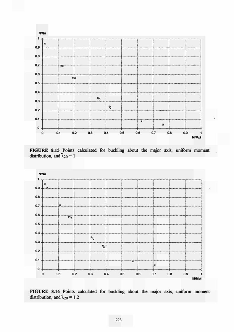
N/Nu 1 ^..

0 9 -

0.8 -

07 -

0 6 -

0 5

0 4 -

0 3

0.2 -

01

0 -

o t : i i

i 1 Î

!

m 1 1 i I

« o

: |

i

i

% 1 i % ΐ

1 9 I

1 i

• B"" ö

Φ

0.1 0.2 0.3 0.4 0.5 0.6 0.7 0.8 0.9 1

M/Mpl

FIGURE 8.15 Points calculated for buckling about the major axis, uniform moment distribution, and "λ.20 = 1

N/Nu

1 o.

Ofl

on

0 7

0 6

η*.

04

0 1

η?

01

0

o

¡o

no

%

%

—Br—

ι ί

i

: j

:

| J

t

ι 1 ! C 0.1 0.2 0.3 0.4 0.5 0.6 0.7 0.8 0.9

M/Mpl

FIGURE 8.16 Points calculated for buckling about the major axis, uniform moment distribution, and λ.20 =1.2

223

N/Nu

1 .TL

09

08

07

06

05

04

03

0.2

01

0

D

O

ι«

Jä, ,

%

%"

....Β.

ι 1 φ

0.1 0.2 0.3 0.4 0.5 0.6 0.7 0.8 0.9 1

Μ/ΜρΙ

FIGURE 8.17 Points calculated for buckling about the major axis, uniform moment

distribution, andino =1.4

N/Nu

1 ^

09

0.8

07

06

05

04

0.3

n?

01

0

0°

"ft

| %

%

Jfc

a

i 8 : | !

1 ί i Φ 0.1 0.2 0.3 0.4 0.5 0.6 0.7 0.8 0.9 1

M/Mpl

FIGURE 8.18 Points calculated for buckling about the major axis, uniform moment distribution, and"X20 =1.6

224

N/Nu 1 -_...

09 -

0.8-

07 -

08 -

05 -

04 -

03 -

n? 01 -

0 _

°» I I j '%"""T i

" %

1 ! t

ΐ i i 4 j j i

ï

i

*

%

-

o

0

Φ

0.1 0.2 0.3 0.4 0.5 0.6 0.7 0.8 0.9

M/Mpl

FIGURE 8.19 Points calculated for buckling about the major axis, uniform moment distribution, andl20 =1.8

N/Nu

1 -c

09 -

on

07

OR

0*5

04

m

η?

01

0

Ί.

J

f ç

f

j

s

'o i

i

ι i Φ 0.1 0.2 0.3 0.4 0.5 0.6 0.7 0.8 0.9 1

M/Mpl

FIGURE 8.20 Points calculated for buckling about the major axis, uniform moment distribution, and λ20 = 2

225

N/Nu

1 .

0 9

0 8

0 7

0 6

0 5

0 4

03

0?

01

0

* > , pao

<SB+:

**a <St o

i

otrtK ι·» Δ

°* o

π ï !

: i

i "Ί 0.1 0.2 0.3 0.4 0.5 0.6 0.7 0.8 0.9 1

M/Mpl

FIGURE 8.21 Points calculated for buckling about the minor axis, triangular moment distribution, and λ.20 = 0.2

N/Nu

0 9

OR

0 7

06

n*,

0 4 -

0 3

n?

m

0

HBO « S t

| « W i t t i & o

« Χ * * * * « .

< χ *

; ! : ; : i

I i ¡

1 0 '

è

0.1 0.2 0.3 0.4 0.5 0.6 0.7 0.8 0.9 1

M/Mpl

FIGURE 8.22 Points calculated for buckling about the minor axis, triangular moment

distribution, and λ20 = 0.4

226

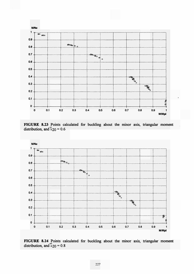
N/Nu

1 . S X .

0 9

0 8

0 7

08

05

04

03

Γ>2

01

0 J

β * _ UDO

« ■ t k l « o

'

" < α ΐ Κ *Δ""" <5

Ο

< * ο

Λ

0.1 0.2 0.3 0.4 0.5 0.6 0.7 0.8 0.9 1 M/Mpl

FIGURE 8.23 Points calculated for buckling about the minor axis, triangular moment distribution, andl.20 = 0.6

N/Nu 1 .y

0 4

on

07 -

06

η*;

0 4 -

0 3

n?

m

0

«DO

Ü55A*

0

I IjüSfc

o

i

\

£"' s if

0.1 0.2 0.3 0.4 0.5 0.6 0.7 0.8 0.9 1

M/Mpl

FIGURE 8.24 _Points calculated for buckling about the minor axis, triangular moment distribution, and λ20 = 0.8

227

N/Nu

0.9

ne

07

06

05

04

0.3

n?

0.1

0

«so

°fc»

«5 *.. * * o

* \ >»'

o 3k

\

i ¡

...i®.

>

0.1 0.2 0.3 0.4 0.5 0.6 0.7 0.8 0.9 1

M/Mpl

FIGURE 8.25 Points calculated for buckling about the minor axis, triangular moment distribution, and λ20 = 1

N/Nu

1 _y.

09

0.8

0.7

Π6

05

0.4 _

03

0?

0.1

0

EP

«ΑΧο

° ^ I i

I I I ^ »_ I

1

füU |

1 1 0.1 0.2 0.3 0.4 0.5 0.6 0.7 0.8 0.9

M/Mpl

FIGURE 8.26 Points calculated for buckling about the minor axis, triangular moment

distribution, andl20 =12

228

1 >

0 9

0 8

0 7

0 6

05

0 4

0 3

n?

01

0

Of Q?

CStXj

< * * * o

'

i 1

! j

i i

i

Skx. | _ »B !

«0 i i

X i

: ! 1

•fc,

>

0.1 0.2 0.3 0.4 0.5 0.6 0.7 0.8 0.9

M/Mpl

FIGURE 8.27 Points calculated for buckling about the minor axis, triangular moment distribution, and λ20 = 1 4

N/Nu

1 .y.

0 9

OR

0 7

0 6 1

0 5 ,

0 4

03

Π?

01

0

«9

tí

i i

i I

DO

««4 t

: t

ί

Χ .Sfc. Λ. >

Ι

: :

*%>

ι ι 1

!

j

if

0.1 0.2 0.3 0.4 0.5 0.6 0.7 0.8 0.9 M/Mpl

FIGURE 8.28 Points calculated for buckling about the minor axis, triangular moment distribution, and λ20 = 1 6

229

N/Nu 1 ->

ne

0 7

OR

OS

0 4 -

ΟΛ

η?

m

0

Ί*

[<Β<

<«κο

•ν Ι.χ_.

1

ι 1

' ^

1 -X-

t

0.1 0.2 0.3 0.4 0.5 0.8 0.7 0.8 0.9 1 M/Mpl

FIGURE 8.29 Points calculated for buckling about the minor axis, triangular moment distribution, and λ20 = 1-8

N/Nu 1 _y

n<*

OR

0 7

OR

05 -

04

(n

n?

01

0 -

\

UDO

tìaxa

• "*><; "

«t κ

¡CE* I ^ b

t "^ "5"

1 i χ

0.1 0.2 0.3 0.4 0.5 0.8 0.7 0.8 0.9 1

M/Mpl

FIGURE 8.30 Points calculated for buckling about the minor axis, triangular moment distribution, and λ20 = 2

230

WNu

1 - *

0.9

0.8

0.7

0.6

0.5

0.4

0.3

0.2

0.1

0

0.1

8 s

« 3 ^

'

it***0

ut. Λ « XO

otXxbo

6

0.2 0.3 0.4 0.5 0.6 0.7 0.8 0.9 1

M/Mpl

FIGURE 8.31 Points calculated for buckling about the major axis, triangular moment distribution, and λ20 = 0.2

N/Nu

1 .y-

0 9

0.8 -

0 7

OR

0 5 -

04

0 3

n?

01

0 -

Dpi*

I

i ί I Ι i !

i i i

j j j j j

ι 1 1 1 i 1

«y <fc>5

*X3Sa

5*

-A X

0.1 0.2 0.3 0.4 0.5 0.6 0.7 0.8 0.9 1

M/Mpl


231

N/Nu

■ >

OR

0 7

0 6

OS

0 4

0 3

n?

01

0

CS

B O »

« ζ *

ö ^

£

4 if

0.1 0.2 0.3 0.4 0.5 0.6 0.7 0.8 0.9 1

M/Mpl


N/Nu

1 _y.

n<*

na

0 7

OR

0 5

04

m

n?

m

0

X »

nap

» EXî

^

.B

i

.s..,

X

0.1 0.2 0.3 0.4 0.5 0.6 0.7 0.8 0.9

M/Mpl


232

N/Nu 1 -y

0 9 -

nn

0 7 -

0 8 J

0 5 -

0 4 -

0 3 -

n?

01

0 J

τ R

I 1

ί " ] WSõ'

i f j

1 t I

τ

j

1 1

MJ»

•

i

J

ί ¡ [ ί

i i ]

"Β* i

Lib i I

ι 1

.5

0.1 0.2 0.3 0.4 0.5 0.6 0.7 0.8 0.9 1 M/Mpl

FIGURE 8.35 Points calculated for buckling about the major axis, triangular moment distribution, and λ20 = 1

N/Nu 1 .y

0 9

OR

0 7

OR

05

04

0 3

n?

m

0 -

χ ! ix

j :

Τ"· '*w Τ

Î 1"iï&

1 i

| ■«>&

%

ι 1 i

I

i

Î

j

ï

:

i

i s j

i !

I i 1

•ja

X

0.1 0.2 0.3 0.4 0.5 0.6 0.7 0.8 0.9 1

M/Mpl

FIGURE 8.36 Points calculated for buckling about the major axis, triangular moment


233

N/Nu

1 -χ

0.9

0.8

0.7

0.6

0.5

0.4

0.3

0.2

0.1

0

Ufc

.*&··

\

X

0.9 1 M/Mpl

0.1 0.2 0.3 0.4 0.5 0.6 0.7 0.8


N/Nu 1 _y.

nq

OR

0 7

OR

05 -

04

m

02 -

m

0 -

X tx

is >

l * 5 *

1

«**

«fc. TS

! ! I * ! I i

ι 1 1 i 1

X

0.1 0.2 0.3 0.4 0.5 0.6 0.7 0.8 0.9 1 M/Mpl

FIGURE 8.38 joints calculated for buckling about the major axis, triangular moment distribution, and λ20 = 1 6

234

N/Nu

1 .y

0 9

0.8

0 7

OR

0 5

0 4

0 3

n?

m

0

\

*&

\

¡%

•

\

W'

I ¡ i

¡

1

i ι t

i t i

i 1

1 : i

í

I

ί í i

í

* & τ

\ χ

0.1 0.2 0.3 0.4 0.5 0.6 0.7 0.8 0.9

M/Mpl


distribution, and λ20 =1.8

N/Nu

1 .y

nQ

0 8

0 7

OR

OS

0 4

0 1

n?

01

0

%

1

" τι j ""«Si

i

|

ï t

i

i t

1 t

I t

i

!

¡

" ^ S s "

"f

! j i j

: : | I

1 [ %.

| |

1 i

|

i

! 1 i

1 i

!

. » i :

0.1 0.2 0.3 0.4 0.5 0.8 0.7 0.8 0.9 1

M/Mpl


distribution, and λ20 = 2

235

N/r

1

0.9

ne

07

06

05

04

03

n?

0.1

0

Ju

i

o

i

otrt·* >te> χ * » » >

δ

j

ι 1

O

1

0.1 0.2 0.3 0.4 0.5 0.6 0.7 0.8 0.9 1

M/Mpl

FIGURE 8.41 Points calculated for buckling about the minor axis, bitriangular moment distribution, and^20 = 0.2

N/r

1

0 9

nn

0 7

OR

ns

0 4

m

η ?

m

0

au

) ane +;■*£>' x x w " o"

• ; ! "o

I i i 1

« *

1

ι 4 0.1 0.2 0.3 0.4 0.5 0.6 0.7 0.8 0.9 1

M/Mpl

FIGURE 8.42 Points calculated for buckling about the minor axis, bitriangular moment


236

N/Nu 1 J . - . . . ^ . .

09 -

(18

07 -

0 8

05

04

0 3

0.2-

01

0 -

ΐ

I

i

1 t î

i

t

j ι I

î

I

j

I ι

1 1

■δ

Λ5**κ.^

■ <

.... <*%,.

Vt

ν—

ν

1 *

0.1 0.2 0.3 0.4 0.5 0.6 0.7 0.8 0.9 1

M/Mpl

FIGURE 8.43 Points calculated for buckling about the minor axis, bitriangular moment distribution, andl20 = 0.6

N/Nu

0 9

OB

0 7

OR

ns

0 4

03

n?

m

0

l j

j

I

t

ί i

t

ι i

*""■$

"■«ψχ*^ Ι ι

,ο

j ¡ j I i

j | ι i i _ 3 L

j I Ι ι

ι 1 1 1 i 1

j

if ! "O" i

ΐ

# à.

ι \ 0.1 0.2 0.3 0.4 0.5 0.6 0.7 0.8 0.9 1

M/Mpl

FIGURE 8.44 Points calculated for buckling about the minor axis, bi-triangular moment distribution, and λ20 = 0.8

237

N/Nu

1 -x-.-x-x—.

09 -

on

07 -

06 -

05 -

04 -

0.3 -

η?

01

0 -

«ί ext*

"0

i

!3k_. •è

, s

I

>

«cts

μδ

i £

0.1 0.2 0.3 0.4 0.5 0.6 0.7 0.8 0.9 1

M/Mpl

FIGURE 8.45 Points calculated for buckling about the minor axis, bitriangular moment distribution, and λ20 = 1

N/Nu

1 ΓΗ·«··

0 . 9

<stsw aatcøxx«·

0.8

0.7

0.8

0.5

0.4

0 . 3

0.2 —

. . .

0.1 I

1 h

0.1 0.2 0.3 0.4 0.5 0.6 0.7 0.8 0.9 1

M/Mpl

FIGURE 8.46 Points calculated for buckling about the minor axis, bitriangular moment distribution, and λ20 = 1.2

238

N/Nu

1

09

08

07 I

06

05

04

03

n?

01

0

r""<ä5ffo····· « K M * 0

i

1 I

I 1

i

j

I ι

i

!

i i i

í .<&, 1

ï í

:

:

1

ΐ i

ι 1

«ίο

\ te o

#

#

0.1 0.2 0.3 0.4 0.5 0.6 0.7 0.8 0.9 1 M/Mpl

FIGURE 8.47 Points calculated for buckling about the minor axis, bi-triangular moment distribution, and λ20 =1.4

N/Nu 1

0.9 - -

0.8 - - .

0 . 7 - -

0.6

0.5 4~

0.4

0.3 -|~

0.2

0.1 - Ι

Ο

üä+S" c a o * * ■»

«*· I

..«*4...

0.1 0.2 0.3 0.4 0.5 0.6 0.7 0.8 1.9 1

M/Mpl



239

N/Nu

0.9 .

0.8

0.7

0.6

0.5

0.4

0.3

0.2 ...

0.1

■ * * · «

CC κ+«

i

1

"**k Õ

\ δ

j

:

I

i

*%

" *

0.1 0.2 0.3 0.4 0.5 0.6 0.7 0.8 0.9 1

M/Mpl

FIGURE 8.49 Points calculated for buckling about the minor axis, bitriangular moment distribution, and λ20 = 1.8

N/Nu

1 )

nq

ne

0 7

OR

n*>

04

m

η?

m

0

A* røH CCHO

o !

Sfc. < c

Õ

ft

j i i i i i

ι i i i 1 i 0.1 0.2 0.3 0.4 0.5 0.6 0.7 0.8 0.9 1

M/Mpl



240

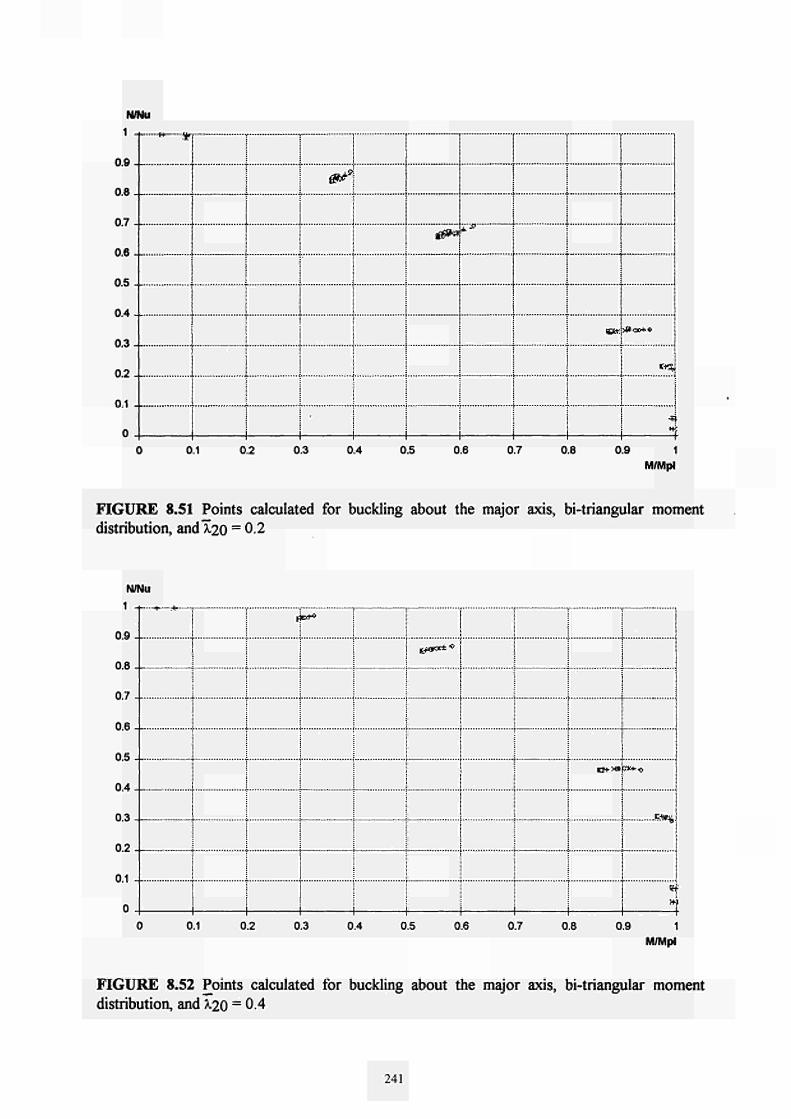
N/Nu

1 _. - XX-

09 -

OR

07

06 -

05

04

03 -

0?

01 -

0 -

w ar

1

¡

i

i

f&*\

t

■

!

: 1

ι ί

EL»* -J, ■

¡ΒΛ: 9f<x*·«

m*

0.1 0.2 0.3 0.4 0.5 0.6 0.7 0.8 0.9

M/Mpl

FIGURE 8.51 Points calculated for buckling about the major axis, bitriangular moment


N/Nu

1 _| . ._

n,9

08

07

OR

n1,

04

ni

n?

m

0

ijkO**

î tf««*-0

! · ■

i i ;

t : :

! : :

i i i

ï

: :

Of>»

i

!

I i !

rat* o

!S»x,

0.1 0.2 0.3 0.4 0.5 0.6 0.7 0.8 0.9

M/Mpl

FIGURE 8.52 Points calculated for buckling about the major axis, bitriangular moment distribution, and λ20 = 0.4

241

N/r

1

0 9

ΟΑ

0 7

06

05

04

n i

η?

m

0

«lu

UM»

tí*"*·0

cwew,..

ί

1 1

•>«s

"3; \

I Γ 0.1 0.2 0.3 0.4 0.5 0.6 0.7 0.8 0.9 1

M/Mpl

FIGURE 8.53 Points calculated for buckling about the major axis, bi-triangular moment distribution, and I20 = 0.6

N/Nu 1 _|_.^

0Q

0 8 -

0 7 -

0 6

ns

0 4 -

0 3

n?

01 -

0 -

t4a>

K** 0

i

" * *

1

f**fc"

' *·--

0.1 0.2 0.3 0.4 0.5 0.6 0.7 0.8 0.9 M/Mpl

FIGURE 8.54 Points calculated for buckling about the major axis, bi-triangular moment distribution, andX20 = 0.8

242

N/Nu

09

0.8

07

0.8

ns

04

03

0.2

m

0

1

:

1

i „. Γ î *

i

ι î

j

t

i j

i î I : : !

i j

r t

i I :

1 1 1

I ι REH*

i : t :

1 | ! 1 ! !

i i : i :

■·■ i (

i 1 i |

i ï

t :

i i

' ^

\

i

X *

ï

ι Γ

0.1 0.2 0.3 0.4 0.5 0.6 0.7 0.8 0.9 1

M/Mpl

FIGURE 8.55 Points calculated for buckling about the major axis, bitriangular moment distribution, andT20 = 1

N/Nu

1 t

0.9

0 .8

0 .7

0.6

0.5

0.4

0.3

0.2

0.1 4

0

rei*·

•Get;

$,..

0.1 0.2 0.3 0.4 0.5 0.6 0.7 0.8 0.9

M/Mpl


distribution, andX20 = 1.2

243

N/f

1

09

on

07

OR

ns

04

0 3

n?

m

0

*u

Kb»

i

m^

i I

i I

: : : j 1

■i τ»

| ï

i 0.1 0.2 0.3 0.4 0.5 0.6 0.7 0.8 0.9 1

M/Mpl

FIGURE 8.57 Points calculated for buckling about the major axis, bitriangular moment distribution, and"Ã.20 =1.4

N/Nu

1

0 3

OR

0 7

OR

05

04

0 3

n?

m

0

IXr } t£t»

ψ*»

s

i S....

1 i 0.1 0.2 0.3 0.4 0.5 0.6 0.7 0.8 0.9 1

M/Mpl


distribution, and λ20 =1.6

244

N/Nu

1 -

09

08 -

07

06 -

05 -

04

03 -

n?

01 -

0

*♦· -w ■>*+.

ι

ι

i

: : {

t

j

!

j

i

1 1

JS*_

ί

%

>$ ι

! Ι r 0.1 0.2 0.3 0.4 0.5 0.6 0.7 η.8 0.9 1

Μ/ΜρΙ

FIGURE 8.59 Points calculated for buckling about the major axis, bi-triangular moment distribution, and λ20 =1.8

1

nq nn 07

06 -

05 -i

04

0,3

n? m 0

ï i : : ι :

"<

:

t :

; ι ΐ ! : ¡

i i

i I

í 1

i I

i

κ

! i :

i i i

Ä, 1 » I

f f Τ

: : ! i

ι i i 1

1

i

i

i

!

4 i

i 1

1 Γ 0.1 0.2 n.3 n.4 0.5 0.6 0.7 0.8 0.9

M/Mpl

FIGURE 8.60 Points calculated for buckling about the major axis, bitriangular moment distribution, and Γ20 = 2

245

ANNEX9:

9. NM INTERACTION CURVES PROVIDED BY DIANA

247

DIANA 2D HEB 200 0.6 Strong

K) cx

1.00 c

0.90

0.80

0.70

0.60

0.50

0.40

0.30

0.20

0.10

nnn 0.00 0.10 0.20 0.30 o.4n n.5n

Moment

0.60 0.70 0.80 0.90 1.00

DIANA 2D HEB 200 0.6 weak

SJ

1.UU L

0.90

0.80

0.70

O.RO

« Ë 0.50 o ζ

0.40

0.30

0.20

0.10

nnn

'

0.00 0.20 0.40 0.60

moment

0.80 1.00

O-400

Δ-500

—Χ-600

O-700

Ο-800

900

1.20

ANNEX 10:

10. VALUES OF ^ FOR BUCKLING AROUND WEAK AND STRONG AXIS AND FOR THREE TYPES OF BENDING MOMENT DISTRIBUTION (UNIFORM, TRIANGULAR AND BI-TRIANGULAR)

This annex shows the values of Hy which were calculated from the results obtained numerically for a failure temperature of 400°C, so as to comply with the following equation:

My = N M , M y i S d

xäfmin A. fy " p l y *j - 1 Xrnin A fy "pl.y fy

Nsd MySd

My was calculated for buckling about the major and minor axes, with three types of moment distribution:

Uniform

Triangular

Bi-triangular

All the points calculated with LENAS are shown on FIGURE 10.1 to FIGURE 10.6, while the points obtained for both largest eccentricities were eliminated from FIGURE 10.7 to FIGURE 10.12 (we retained this assumption during the development of a simplified formula).

251

o

-1

-2

-3

-4

-5

-6

-7

-8 --

ί I

ι ι tr

0.5 1.5 2.5

FIGURE 10.1 Evolution of μ according to the slenderness ratio (buckling about minor axis uniform moment)

μ 1 -^

0.5

o --

-0.5

-1.5

0.5 1.5 2.5

FIGURE 10.2 Evolution of μ according to the slenderness ratio (buckling about minor axis triangular moment)

252

1

ΟΛ - -..

0.6 -....

0.4

02

-0.2

•0.4

-0.6

ι ί

0.5 1.5 2.5 λ«

FIGURE 10.3 Evolution of μ according to the slenderness ratio (buckling about minor axis bi-triangular moment)

μ

ι —

0 . . .

-1 --

-2 -3 ...

-4

-5

-6

-7

-β

J ! i.4 !.. 1 J.

-9 0.5 1.5 2.5

FIGURE 10.4 Evolution of μ according to the slenderness ratio (buckling about major axis uniform moment)

253

1 - Γ -

0.5 - -

•0.5

-1

-1.5

ί Ι

Ι

0.5 1.5 2.5 λ .

FIGURE 10.5 Evolution of μ according to the slenderness ratio (buckling about major axis triangular moment)

1

0.9 - -

0.8 - -

0.7

0.6-t-

0.5

0 .4 . . .

θ 3 1 1 :·■

0.3

0.2 - -

0.1

0.5 1.5 2.5

FIGURE 10.6 Evolution of μ according to the slenderness ratio (buckling about major axis bi-triangular moment)

254

μ

1 —...

0.5

0 . .

• 0 5

1

1.5.

2

2 5 .

3 _ . .

35 ...

4 . . .

4.5

Ô..

0.5 1.5 2.5

λ.

FIGURE 10.7 Evolution of μ according to the slenderness ratio (buckling about minor axis uniform moment)

μ

1 τ

0.5

0.5 .

1 . . .

15

2

0.5 1.5 2.5

FIGURE 10.8 Evolution of μ according to the slenderness ratio (buckling about minor axis triangular moment)

255

1

0.9 4-

0.8

0.7

0.6

0.5

0.4

0.3 - -

02.-

0.1

0.5 1.5 2.5

FIGURE 10.9 Evolution of μ according to the slenderness ratio (buckling about minor axis bi-triangular moment)

0.5.

0

-0.5.

-1

-1.5

-2

-2.5

-3

-3.5

-4

-4.5

I r ι ι

0.5 1.5 2.5 Κ

FIGURE 10.10 Evolution of μ according to the slenderness ratio (buckling about major axis uniform moment)

256

0 5 - .

0 ■-.

-0.5 - ...

-1.5

0.5 1.5 2.5

FIGURE 10.11 Evolution of μ according to the slenderness ratio (buckling about major axis triangular moment)

1

08

07 -

OR

05

04

03

n?

01

0 -

1.

ί ï I

8

8

1

I «'" I

!

« s

I 1

s ι ■ ·

0

g

I I Λ

i i

I \ ' i

ί i ι *

I j 0.5 1.5 2.5

"λ.

FIGURE 10.12 Evolution of μ according to the slenderness ratio (buckling about major axis bi-triangular moment)

257

ANNEX 11:

11. COMPARISON BETWEEN THE NUMERICAL SIMULATION RESULTSAND THE M-N INTERACTION FORMULA (CHAPTER 4)

A comparison between all the results obtained numerically (from 400 to 900°C) and the

analytical formulae (hereunder) is carried out in Annex 11.

Nsd , k MyxSd 1

Ain A

V» y

V^y fy,0

with:

L e i , 7 N s d b u t k , < 3 y X(ö)y A fy.6 ^


μγ = (12 ßw.y 3) λβ + 0.71 PMiy 029 with Uy < 0.8


μν = (2 ßwy 5) λβ + 0.44 ßMy + 0.29 with Uy < 0.8

and λ2ο < 1.1

The value of standard Dnumericai = (calculated numerically, FIGURE 11.1) is shown on the x

axis (proposition^), and the value of standard Danai^ = (obtained from the above defined

formula) is shown on the yaxis (LENAS). The 45° straight line represents a perfect equality

between these two values. While the straight line which is slightly above represents an error of

+10%"of the analytical value as compared to the numerical value (therefore unconservative),

the straight line which is slightly below the bisectrix represents, on the other hand, an error of

10% of the analytical value as compared to the numerical value (conservative).

259

MaMp 1 M/Mpl

FIGURE 11.1 Calculation of Dnumericai and ϋ ^ ι ^ ^

Propssitionjl 1.2

equality

1 - S

0.8

0.6 -s

0.4

0.2 conservative area

0.2 0.4 0.6 0.8 1 1.2 LENAS

FIGURE 11.2 Formula - numerical results comparison at 400°C

260

Λ.ί. ·

η ft -

2

Q.

no .

0 -

\ j î 1 S

j r

, [ ] .^Y... „ h ! 1 7^ ■y'

\ J^ fly1*'

tè&&\ J&¿Y^\

\ \ \ ! : 1 : :

ι 1 1

0.2 0.4 0.6

LENAS

0.8 1.2

FIGURE 11.3 Formula numerical results comparison at 400°C for buckling about minor axis and uniform moment distribution

0.2 0.4 0.6

LENAS

0.8 1.2

FIGURE 11.4 Formula numerical results comparison at 400°C for buckling about minor axis and triangular moment distribution

261

s

Ì.dt -

i _

η η

0.4

no -

0 i

^ I

i 0.2 0.4 0.6

LENAS

0.8 1.2

FIGURE 11.5 Formula numerical results comparison at 400°C for buckling about minor axis and bitriangular moment distribution

1.2 τ

1

0.8

c o S 0.6

2 o.

0.4

0.2

0.2 0.4 0.6

LENAS

0.8 1.2

FIGURE 11.6 Formula numerical results comparison at 400°C for buckling about major axis and uniform moment distribution

262

1.xi -

1 -

n fi -

S ( i g .

Q. n A -

no -

0 -

«ίβα 5»·*'

> ^ ΐ

i

ι ί 0.2 0.4 0.6

LENAS 0.8 1.2

FIGURE 11.7 Formula - numerical results comparison at 400°C for buckling about major axis and triangular moment distribution

0.2 0.4 0.6 LENAS

0.8 1.2

FIGURE 11.8 Formula - numerical results comparison at 400°C for buckling about major axis and bi-triangular moment distribution

263

s Q-

Ι.χέ -

1 -

0.8 -

n 9 -

0 -

&J

/^crh'

i

■■■■~^g&$

0.2 0.4 0.6

LENAS

0.8 1.2


c o s

2 o.

l . x c

1 .

0.8

0.6

0.4

0 ¿— 1

/""^jPrfS > * S ^ · ;

I ¡

0.2 0.4 0.6

LENAS

0.8 1.2


264

4 .

η ft

no i

0

¡

!

: i !

1 !

y^Y/^

¿^^

i

j r \ ^ ^ ^ ^

■ni Ull Mi» M' m i "

0.2 0.4 0.6

LENAS

0.8 1.2


1.2 r

0.2 0.4 0.6

LENAS

0.8 1.2


265

1.2 τ

1 -

0.8

0.6 --

0.4 --

0.2 -

0.2 0.4 0.6 LENAS

0.8 1.2


0.2 0.4 0.6 LENAS

0.8

1 -

η ft -

η A -

no -

0 - i

^ p ^

1.2


266

0.2 0.4 0.6 LENAS

0.8 1.2

FIGURE 11.15 Formula - numerical results comparison at 600°C for buckling about minor axis and uniform moment distribution

0.2 0.4 0.6 LENAS

0.8 1.2

FIGURE 11.16 Formula - numerical results comparison at 600°C for buckling about minor axis and triangular moment distribution

267

0.2 0.4 0.6 LENAS

0.8 1.2

FIGURE 11.17 Formula - numerical results comparison at 600°C for buckling about minor axis and bi-triangular moment distribution

1.2 τ

1 --

0.8 --

o S 0.6 -

2 O-

0.4

0.2 -

0.2 0.4 0.6 LENAS

0.8 1.2

FIGURE 11.18 Formula - numerical results comparison at 600°C for buckling about major axis and uniform moment distribution

268

0.2 0.4 0.6 LENAS

0.8 1.2


1.2 τ

0.2 0.4 0.6 LENAS

0.8 1.2


269

1.2 τ

1 --

0.8 --

% 0.6 -

0.4 --

0.2 -

0.2 0.4 0.6 LENAS

0.8 1.2


0.2 0.4 0.6 LENAS

0.8 1.2


270

i .¿

ΓΙ ft

η A

η o

0

0.2 0.4 0.6

LENAS

0.8 1.2


0.2 0.4 0.6

LENAS

0.8 1.2


271

0.2 0.4 0.6

LENAS

0.8 1.2

FIGURE 11.25 Formula numerical results comparison at 700°C for buckling about major axis and triangular moment distribution

ι ¿.

Λ .

η fi

η ß

0.4

no -

0 i i 0.2 0.4 0.6

LENAS

0.8 1.2

FIGURE 11.26 Formula numerical results comparison at 700°C for buckling about major axis and bitriangular moment distribution

272

1.2 τ

0.2 0.4 0.6 LENAS

0.8 1.2


1.2

0.8 -

% 0.6 · -

0.2

0.2 0.4 0.6 LENAS

0.8

: j

: : I : : : ΐ

| <1§M^^

^tx> ¿r Ba rfttC?^^

j r

\

ΛΥ1


273

1.2 τ

0.2 0.4 0.6 LENAS

0.8 1.2


0.2

l .x i

1 -

0.6 -

no -

0 -

y^SJF^

:

I

i 0.4 0.6

LENAS 0.8 1.2


274

λ.ί -

η ft J

η A -

no -

0 -

/ ' ¿ & Φ

i

t I

i

¡ 0.2 0.4 0.6

LENAS

0.8 1.2


2 Q.

0.2 0.4 0.6

LENAS

l . x C

1 _

0.8

η fi

η A

no

0 < ^ — i

: > : j r

j

: i

i i

0.8 1.2


275

ι . ζ

u.o

η A

no

0

βοΜ . % & ! _

/ ^ ^ JÍ&P

*&^'~

0.2 0.4 0.6

LENAS

0.8 1.2


1.2 T

0.2 0.4 0.6

LENAS

0.8 1.2


276

0.2 0.4 0.6 LENAS

0.8 1.2


0.2 0.4 0.6 LENAS

0.8 1.2


277

0.2 0.4 0.6

LENAS

0.8 1.2


c o B

0.2 0.4 0.6

LENAS

i.¿

0.8

0.6

0.4

η ο

0 ί

jf ^s^

> ^ > ^ yr ΐ j/\ ^ y j y : ι

i 0.8 1.2


278

ANNEX 12:

12. ANOTHER FORMULA FOR THE M-N INTERACTION

The M-N interaction law may also be written differently from the formulation of Eurocode 3 Part 1.2. This formulation is of the following type :

N α

Sd

VXmin A fy,6>/

M y^d

"pi.y y.e

<1 (12.1)

12.1 ANALYSIS ACCORDING TO a

The sensitiveness of this type of curves to a variation of α may be determined by drawing various curves (FIGURE 12.1) for α = 0.1, 0.2, 0.5, 1, 2, 4, 8, and 10.

N/Nu

1

0 9

08

Π7

OR

n*s

0 4

0 3

0 ,2 -

01

o

■\T""··: \ ν '··. \ \

T'\"

\ \ \ V

L \ \ \ Γ ' \ \ \ \ \ \

.5 = = Ξ " X

X

\

s

\ \

_ _ :

~ " " ■ ~ · . _ ;

— —"" ."■ .-4 ! 1 1 ;

^^-L^ T F d··-·.... 1 * v ; "*·<^ : " ~ ^ ^ :

: χ i v

* . : Ν . 1 Ν \

;

/ /

/

/

\ 1 \ \

/

Ν. v.

ι 1 1

!

* " l .

i ì

: *. _ : \ 1 : * · . ί : \ I 1 ·>. ! [ \

-f ι 1 1

alpha = 0.1

alpha = 0.2

alpha = 0.5

alpha = 1 alpha = 2

alpha = 4

alpha = 8

alpha = 10

0 0.1 0.2 0.3 0.4 0.5 0.6 0.7 0.8 0.9 1 M/Mpl

FIGURE 12.1 Evolution of the M-N interaction curve according to α

It can be noted that, for low values of α (from 0.1 to 0.2), the variation of the interaction curve is very large, while for a variation of α from 8 to 10, the difference between the curves is low.

279

12.2 FORMULA FOR EACH LOAD CASE

By solving equation 12.1, by dichotomy, α can be determined for all the points which were numerically calculated.

As previously, the values calculated for large eccentricities are conspicuous as compared to the other values (FIGURE 12.2), and they will therefore be neglected once more. For a low slenderness ratio and a uniform or triangular moment distribution, the dispersion of the points is greater than for large slenderness ratios. This phenomenon is not disturbing since, as we observed in section 12.1., the influence of α on the shape of the curve becomes lower and lower as α increases. Now, for low slenderness ratios, α varies between 1 and 2 for buckling about the minor axis and uniform moment distribution (and between 2 and 4.5 if the moment distribution is triangular).

α 2.5—

1.5

0.5

s i 0.5 1.5 2.5

FIGURE 12.2 Evolution of α according to the slenderness ratio (buckling about minor axis triangular moment) see also Annex 13

On the other hand, in the case of a bi-triangular moment distribution (FIGURE 12.3), the dispersion of the points is very high since α varies between 2 and 1200 . These very high values of α are due to the results concerning small eccentricities : in fact, the calculated value of Ν is near the ultimate value of N, which leads the interaction curve to have a very low curvature when M is small. This is obtained only if α is high.

Actually, for these points, if we take α as much smaller (2 or 3 as compared to 1200), the error is very low.

280

10

9

8

7

6

5

4

3

2

1

β

.......

? î

t "

ι

4

0.5 1.5 2.5

FIGURE 12.3 Evolution of α according to the slenderness ratio (buckling about minor axis bitriangular moment) see also Annex 13

In order to determine the curves which allow to approximate a, in a first stage, the average of the values of α is calculated for each slenderness ratio (after having first eliminated the excessively deviating values), by means of a numerical solving software; we try to find the function which best corresponds to those points.

From the evolution of the average of the points according to the slenderness ration, we try to find out a curve of the following type:

a = Ae B ^+C

These calculations lead to the development of the following formulae:

Buckling about the minor axis:

Uniform moment distribution:

α = 1.5e"2*8+0.25

Triangular moment distribution:

a = 4e~2^+0.5

Bitriangular moment distribution:

α = 2.5

(12.2)

(12.3)

(12.4)

(12.5)

281

Buckling about the major axis:

Uniform moment distribution:

a = e_2^+0.28 (12.6)

Triangular moment distribution:

a = 2e_2*9+0.56 (12.7)

Bitriangular moment distribution:

α = 2.5 (12.8)

Equations 5.27 and 5.30 may also be written under the form α = 6.5β_2λ*+2.5 and

a = 3e"2X<'+2.5 with a ^ 2.5. This does not alter the value of α but allows an easier

interpolation on factor A (equation 12.2).

12.3 FINAL EQUATION

A global formula, i.e. allowing for ßM,y, may be determined by carrying out a linear interpolation on factor A (of equation 12.2) with a function of the exponential type for the interpolation on constant C (of equation 12.2). Factor Β is immediately determined, since it is equal to 2 in all cases.

The global formulae are then as follows:

Ν f KT Λ " 'Sd

vXmin A. ty θ

+ MySd <1 (12.9) W f "'pl.y

1y.e


α = (3.57 ßHy + 2.43) e2** + 0.03 e ^ ^ " ' ^ + 0.23 but α < 2.5 (12.10)


α = (l.43 ßMy O.57) Q-2'u + 0.047 e t 2 7 7 ^ · ' " 1 ^ + 0.23 buta<2.5 (12.11)

282

ANNEX 13:

13. VALUES OF a FOR BUCKLING AROUND WEAK AND STRONG AXIS AND FOR THREE TYPES OF BENDING MOMENT DISTRIBUTION (UNIFORM, TRIANGULAR AND BI-TRIANGULAR)

The values of α which were calculated so as to comply with the following equation:

Nsd λ + My.sd _ 1

amin A fyj V\tøy fy

are shown on the x-axis on the graphs in this annex, while the slenderness ratio at failure temperature is shown on the y-axis.

The values of N ^ and My gd are derived from the results obtained with LENAS for a failure temperature of 400°C. These calculations were carried out for buckling about the major and minor axes and for three load types:

Axial force + uniform moment distribution

Axial force + triangular moment distribution

Axial force + bi-triangular moment distribution

All the calculated values of α are shown on FIGURE 13.1 to FIGURE 13.6, while the values calculated for both maximum eccentricities were eliminated from FIGURE 13.7 to FIGURE 13.12.

283

2.5

2 - .

1.5

1 - -

0.5--.

α ■

■D—

S 8 I I

0.5 1.5 2.5

λ.

FIGURE 13.1 Evolution of α according to the slenderness ratio (buckling about minor axis uniform moment)

4.5

4

3.5

3

2.5

2

1.5

1

0.5

0.5 1.5 2.5

FIGURE 13.2 Evolution of α according to the slenderness ratio (buckling about minor axis triangular moment)

284

10

β 4~

8

7 4

·§··

8 ο ο

χ » . .

τ · · » ■ ·

ι

Ι

0.5 1.5 2.5

FIGURE 13.3 Evolution of α according to the slenderness ratio (buckling about minor axis bitriangular moment)

α

1.4 _..

1.2

1

0.8

0.6

0.4

0.2

0.5 1.5 2.5

λ.

FIGURE 13.4 Evolution of α according to the slenderness ratio (buckling about major axis uniform moment)

285

α

3.5

3

2.5

2 ...

1.5

1

0.5 i i ì S o

•fl

os 1.5 2.5

λ0

FIGURE 13.5 Evolution of α according to the slenderness ratio (buckling about major axis triangular moment)

10

5

4

3

2

1 ...

Β 0

4 Θ

ι ■ * · ■

0.5 1.5 2.5

"λ.

FIGURE 13.6 Evolution of α according to the slenderness ratio (buckling about major axis bitriangular moment)

286

2.5

1.5

0.5

i ί 0.5 1.5 2.5

"λ.

FIGURE 13.7 Evolution of α according to the slenderness ratio (buckling about minor axis uniform moment)

α 2.5 - τ -

Ι.5

1 . . .

0.5

s § i s 0.5 1.5 2.5

"λ.

FIGURE 13.8 Evolution of α according to the slenderness ratio (buckling about minor axis triangular moment)

287

α 10 r

9

8 . . .

7

5

ö t

8 ,

'? 7

4..

1 _.

ΠΙ

0.5 1.5 2.5

λ.

FIGURE 13.9 Evolution of α according to the slenderness ratio (buckling about minor axis bitriangular moment)

1.4.

1 ?

1 .

on

06

04

0?

0

I

I

i

I t 1 ί ί ì â â ί

0.5 1.5 2.5

FIGURE 13.10 Evolution of α according to the slenderness ratio (buckling about major axis uniform moment)

288

3

2 .

1S

1

n*ï

0

Δ

&

I i [ I

■

α

ι ì s Ι ι i t I ι

13

0.5 1.5 2.5

Κ

FIGURE 13.11 Evolution of α according to the slenderness ratio (buckling about major axis triangular moment)

α

10,..

9 ..

8

7

β J.

5

4

3

2

1

0

Β α.

□

f

•i··

•4

0.5 1.5 2.5

FIGURE 13.12 Evolution of α according to the slenderness ratio (buckling about major axis bitriangular moment)

289

ANNEX 14:

14. COMPARISON BETWEEN THE NUMERICAL SIMULATION RESULTSAND THE N-M INTERACTION FORMULA (ANNEX 12) A comparison between all the results obtained numerically (from 400 to 900°C) and the analytical formulae (hereunder) is carried out in Annex 14.

α Nsd + My.s° ύΛ

Xrnln A fyi9J V\tøy fy.e

With:


α = (3.57 ß^y + 243) θ " 2 *» + 0:03 θ (W y " " Î + 023 but α < 2.5


α = (1.43 βΜιΥ 0.57) Θ " 2

*» + 0.047 Θ (277

^ ~ l1

8 + 023 but α < 2.5

The value of standard Dnumericai = (calculated numerically, FIGURE 14.1) is shown on the x

axis (proposition_2), and the value of standard Danica! = (obtained from the above defined

formula) is shown on the yaxis (LENAS). The 45° straight line represents a perfect equality

between these two values. While the straight line which is slightly above represents an error of

+10%"of the analytical value as compared to the numerical value (therefore unconservative),

the straight line which is slightly below the bisectrix represents, on the other hand, an error of

10% of the analytical value as compared to the numerical value (conservative).

291

MaMp .j M/Mpl

FIGURE 14.1 Calculation of Dnumericai and Dan^cai

Proposition,. 1

1.2

1 ·■··■

0.8

0.6

0.4

0.2 - ■:

equality

FIGURE 14.2 Formula - numerical results comparison at 400°C

292

0.2 0.4 0.6 LENAS

0.8 1.2


0.2 0.4 0.6 LENAS

0.8 1.2


293

\.¿ -

n A -

0 - I

y^wSssletä mìiMAg&°

i 0.2 0.4 0.6

LENAS 0.8 1.2


0.2 0.4 0.6 LENAS

0.8 1.2


294

12 τ·

0.2 0.4 0.6

LENAS

0.8 1.2


M.

0.2 0.4 0.6

LENAS

1 .£. -

η η

η R

η A

no

0

1 | V^^ISBB^^^ \ y SjlBÖfxxStSSEQmi

Yy Yy\ y*^ \ ι ι y^ y^ yc

: s ^ r *r : : : j

i : ! : ! ! ; ; ; ¡

1 1 i i i 0.8 1.2


295

1 .

0.8 -

nA -

n o -

0 -i :

I i

'^iJMfifl·'

0.2 0.4 0.6 LENAS

0.8 1.2


0.2 0.4 0.6 LENAS

0.8 1.2


296

M .

i .¿

n o ·.

0 1

Ι Ι & Α Γ * ^0

0.2 0.4 0.6

LENAS

0.8 1.2


™.

0.2 0.4 0.6

LENAS

0.8

l . x C

0.8

no -

0

! :

1 : : j

1 !

y^ ι y\s$£fos\

y'^y'*^^

yYyiser^

1 1 1 j

1.2


297

0.2 0.4 0.6

LENAS

0.8 1.2


c' o E

0.2 0.4 0.6

LENAS

1 -

nu -

0.6 -

n o -

0 -

■■■~y^^

yy^y^ i i

i i 0.8 1.2


298

1.2 -r


1.2 -r

0.2 0.4 0.6 LENAS

0.8 1.2


299

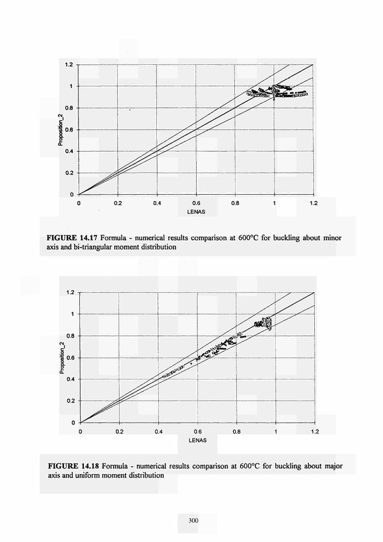
Γ".

\.£.

0.8

0.6

η Α -

no -

0

y^íijÈti5£!?*Á ,— *¿Vx*^»CHKC !

!

S

0.2 0.4 0.6

LENAS

0.8 1.2


1.2 r

0.2 0.4 0.6

LENAS

0.8 1.2


300

ί"*χ

Λ.d. -

Π Α

Π Α -

πι .

no -

0 -

y^

¿y\y^*y

i / ^y^

yr ΐ ^y^ ^ y

^y wrøyr y^

í

1 i 0.2 0.4 0.6

LENAS 0.8 1.2


0.2 0.4 0.6 LENAS

0.8 1.2


301

0.2 0.4 0.6 LENAS

0.8 1.2


1.2 τ

0.2 0.4 0.6 LENAS

0.8 1.2


302

«"f.

Ί . Ζ -

J -

Π A -

0 -

^^^ ^y : BSSAATUSD

0.2 0.4 0.6

LENAS

0.8 1.2


2 O-

0.2 0.4 0.6

LENAS

0.8

Π A -

0.6 -

0.4 -

0.2 -

0 -

:

; y ^ y ^ ^ ^

y^&y^+'y'^ y~j¿$r \ y \

\

\

\

ι 1

ι

ï

î

i 1.2


303

1.2

1 -

0.8 --

N.

'S 0.6 -

0.4 --

0.2 -

0.2 0.4 0.6

LENAS

0.8 1.2


c' o E

0.2 0.4 0.6

LENAS

1 -

0.8 -

n A

no -

0 - ■£ ί — ¡ i

j .¿jk *yl5ì \**&y

1 0.8 1.2


304

CM.

1 .¿ π

1

0.8

06

0.4

no

0

y^ëzY—

y y¿^

ï ^r y^

κ» y^

\ ΐ i

: i

: : i

î

j

! 1 1

0.2 0.4 0.6

LENAS

0.8 1.2


1.2 r

1

0.8

Ν .

% 0.6

0.4

0.2

0.2 0.4 0.6

LENAS

0.8 1.2


305

12 τ

0.2 0.4 0.6 LENAS

0.8 1.2


1.2

0.8

c o 0.6

2 O-

0.4

0.2 -··

0.2 0.4 0.6 LENAS

0.8 1.2


306

f .

Ι .«£

1

u.o

no

0 ■ ^ —

I j I

!

ι I

! y

y^

ι 1

!

ι y ι ^y \y^ .x^jiäi

¿ágy^. wy

^y^

Ι .χ***

0.2 0.4 0.6

LENAS

0.8 1.2


0.2 0.4 0.6

LENAS

0.8 1.2


307

\.¿

1

0.8

g' •s n R

α. n i

no

0

y/*^^yY_j$L,

y\3^¡É,

0.2 0.4 0.6

LENAS

0.8 1.2


1.2

1

0.8

o ¡e 0.6

2 ü

0.4

0.2

0.2 0.4 0.6

LENAS

0.8 1.2


308

1.2 τ

0.2 0.4 0.6 LENAS

0.8 1.2


1.2

1 --

0.8 -

•'S 0.6 -

2 Q.

0.4 -

0.2

0.2 0.4 0.6 LENAS

! i i : : : . — .( 'ζ j i

ί i .y.......yYnm. i i yr y \

0.8 1.2


309

<x.

Ι.χέ -

η A -

0.4 -

no -

0 - ^ 1

y^ ws£^y

0.2 0.4 0.6 LENAS

0.8 1.2


o •e

0.2 0.4 0.6 LENAS

0.8

\.Λ\ -

0.6 -

no -

0 -

j

j

: [

j

1 1.2


310

ANNEX 15:

IS. SIMPLIFICATION IN THE FORMULAE FOR CENTRALLY LOADED COLUMN FOR λ <0,8

In the formulae λ ø is dependent upon the temperature, which implies that the procedure is

iterative if the critical temperature is unknown. That's why it is interesting to study the

influence on the formula if the relative slenderness ratio λ at room temperature is considered

instead of λ Q.

If the method with λ at room temperature is applied to the database, the severity factor becomes 1,0 and it appears that method is, in an average, safe for slenderness smaller than 0,9 and unsafe for higher slenderness (see FIGURE 15.1 and FIGURE 15.2). The FIGURE 15.3

IOOÍN(Ã7)N(I)1 represents — Τ=Γ as a function of λ the slenderness at 20 °C. For small

N(A.)

slenderness (λ < 0,5), the use of λ is on the safe side for all the temperatures. If λ is

replaced by 1,2 λ, then the FIGURE 15.4 is obtained. Up to a value of 0,8 for λ, the

differences remain less than 10 %. That's why it can be concluded that λ (9) can be taken equal

to 1,2 λ for the calculation of %Q if λ is smaller than 0,8.

311

1.2

tn

'_xJ

o Tests beta = 1.00 beta = 1.60

0.0 0.5 1.5

Ν»

2.25

<3J

o FomoU lambda 20eC ) •Linear regresion

IxO

30

UI IL

¿0οΜλβ)-να)]

«η,)

30

0.00 0.50

Slenderness at 20*C

1.00 1.50

3

(Λ

2.00

UI

CÃ

30.00

20.00

U)

U.

Λ 10.00

0.00

11) 10.00 IL· or

20.00

•900.00

•800.00

•500.00

•400.00

•600.00

•700.00

30.00

y» 4k.

ANNEX 16:

16. ECCS NO 89 "FIRE RESISTANCE OF STEEL STRUCTURES" NOMOGRAM. SEPTEMBER 1995

317

ECCS Technical Committee 3 Fire Safety of Steel Structures

ECCS N° 89

Fire Resistance of Steel Structures m (On the basis of ENV 1993 part 12 "Design of steel structures Structural fire design") Sept. 1995 | | l

E C C S C E C M E K S

1. Introduction The required fire resistance of steel structures in terms of fire

resistance classes R30/R60/R90 etc. is given by national

regulations. These requirements should consider the number of

floors, the use of the building, the fire load, the number of people

and the favourable effect of active measures, such as sprinklers,

automatic fire detection, and type and proximity of the fire brigade.

The assessment of the fire resistance of structural elements is

based either on standard fire tests in furnaces or on calculation.

This Technical Note describes calculation methods for unprotected

and protected internal steelwork based on the European

prestandard ENV 199312 [1],[2].

2. Principles of Calculation

2.1 Steel temperature The increase in steel temperature is given by the following factors:

a) The section factor (A„JV): i.e. the relation between the surface

area exposed to the heat flux and the volume of the member

per unit length. Calculation methods and values of (An/V) for

common sections are given in Section 5.

b) The thermal properties of a fire protection material: i.e. thermal

conductivity λρ, its specific heat cp and its thickness dp.

Thermal properties for various protection materials are given in

Section 4. At present no European Norm is available to

determine λρ. Therefore product specifications must be

obtained in each country from approved testing laboratories, or

other expert institutes on condition that they are based on

officially approved tests (Section 10).

c) For fire protection material containing water, the evaporation of

the water causes a delay of the temperature increase of the

steel when the temperature of the steel reaches 100°C

(Example A1).

2.2 Mechanical properties of steel

at elevated temperatures Steel properties change with temperature (Fig. 1). For a member

at a uniform temperature, called critical temperature ©„ , the load

bearing capacity becomes equal to the effect of the applied loads.

Failure will then occur.

The critical temperature is determined by the level of the applied

load (action), expressed as the degree of utilisation in fire, given

by μο Efi.d / R|¡,d,o

Efi d : the design effect of actions in fire

R(l d 0 : the design resistance in fire, for time t = 0

(i.e. room temperature, γΜ = γΜ ,¡ = 1.0, support conditions

for the fire situation: 0.5 L for intermediate, 0.7 L for top storey columns)

2.3 Temperature distribution An adaptation factor κ is introduced to take account of a non

uniform temperature distribution over the height and alongside

the steel section. The value of the adaptation factor κ should be

taken as follows:

beams: • exposed on all four sides: κ = 1.0

• exposed on three sides, with a composite

or concrete slab on side four: κ = 0.7


• exposed on all four sides: κ = 0.85

• exposed on three sides, with a composite

or concrete slab on side four: κ

ke 1

ο.β

0.2

Effective yield strenght

™y,B a

'y,e ' 'y

Slope of linear

elastic range

k£,e = Ea,e / Ea

0 200 400 600 800 1000 1200

temperature [*C]

Fig. 1 : Reduction factors for steel strength and stiffness at

elevated temperatures

2.4 General assumptions The calculation of the fire resistance is based on the following

assumptions:

the temperature increase follows the standard fire curve

(ISO 834)

uniform heating of the steel 'member. A nonuniform heat

distribution is considered by the factor κ (Section 2.3)

. steel grades according to EN 10 025 (S 235, S 275, S 355) and

EN 10113 (S 420, S 460)

for member analysis, the effects of thermal expansion of the

member may be neglected

steel sections of classes 1, 2 or 3 (with Am/V > 10 m·1). For

sections of class 4 see example C.

Temperature increase curves calculated for γη , = γη c = 1.0

according to ENV 199122. (If the National Application

Document gives other values, see Section 10)

Temperature increase curves for insulated steel calculated with

φ = 0 (Modification factors for other values see Section 4)..

3. Calculation Procedure Calculate the degree of utilisation μ,, (Section 2.2).

For a preliminary design (ig may be taken as 0.6. This is

normally a conservative assumption.

The nondimensional slenderness of a column is a function of

the temperature © and has to be adapted for the calculation of

μο=

^fi,í ^fl,0 · »Ky,« ,e,max ' ^E.e.max

Stability problems (to account for lower strain level) κ

0.6

1.2

with 0m a x the steel temperature at failure

μο Ffi.d / Rfi.d.O

R«, d,o is calculated using X«¡ θ max as given above, the yield

strength fy at room temperature and buckling curve c.

The values of Vky9max / kE θ m a x are given in Table 1a.

The calculation procedure for columns is illustrated in Example D. Table 1 b gives directly the critical temperatures for intermediate columns and Table 1c for top storey columns. For a preliminary design λ,, e,max = 1 2 · λ^ο

m ay he assumed.

Determine the section factor. Am/V for unprotected steel

members and Ap/V for steel members insulated by fire

protection material (Section 5). The thermal section factor

[(Ap/V)(Ap/dp)] can be derived according to Section 4 and 7.1

Example A1.

The fire resistance time t, is assessed by making use of the

nomogram (see Section 6 and Examples in Section 7).

A series of adaptation factors κ are considered by special

curves on the left side of the nomogram.

318

For a preliminary design the increase of the fire resistance time

caused by the effects of moisture in the protection material

may be added (tr = t, + t j , if data is taken from Table 2.

Evaporation time ty = (p · ppdpz) / (5 · λρ) [min]. No increase is

allowed If the moisture is already considered implicitly in the

national ^values of the table in Section 10.

Tab. 1a Slenderness modification factor v'kye.max / ke.e.max at elevated temperatures

•teal temp.

θ.[°0]

»KyAmax» ΚΕ,θ,ητβχ

300

1.12

400

1.20

500

1.14

eoo

1.23

700

1.33

800

1.11

900

0.94

Tab. 1 b Critical steel temperature of internal columns, for ¿cr.fi.o = 0.5L,ic = 1.2

>Ve

0.30

0.35

0.40

0.45

0.50

0.55

0.60

0.20

642

eie

597

579

561

545

529

0.40

648

625

605

586

569

553

538

0.60

658

635

615

597

580

565

550

0.80

671

648

629

611

595

580

567

1.00

686

664

645

628

613

598

585

e

1.20

701

679

660

644

629

615

603

1.40

717

691

673

657

642

629

617

1.60

732

699

682

666

652

639

627

1.80

744

710

688

673

659

646

635

2.00

754

718

693

677

663

651

640

Tab. 1c Critical steel temperature of top storey columns,

¿cr,i.,o = n

7L,K = 1.2

for

"o.c

0.30

0.35

0.40

0.45

0.50

0.55

0.60

0.20

636

614

594

575

557

540

524

0.40

640

617

596

578

561

544

528

0.60

643

621

601

583

566

550

535

0.80

648

626

606

589

573

558

544

1.00

652

631

613

596

581

566

553

c

1.20

656

635

617

601

586

573

560

1.40

658

638

621

605

591

577

565

1.60

660

640

623

608

593

580

568

1.80

661

642

624

609

595

582

570

2.00

662

642

625

610

597

584

572

μ0 c = design load in fire / design buckling resistance for:

Θ = 20", 4 = 1.0 L, buckling curve c, γΜ fi = 1.0

λ^,. = non dimensional slenderness of column for 4= 1.0 L

4. Properties of Fire Protection Material

Table 2: General properties for preliminary design*. The following

material properties may be used to calculate the modified section

factor Ap λρ

~V~' dp 1 cpdppp .Ap

1 + Φ / 2 * Ca P a .V

As simplification φ may be taken equal to 0 (this leads to conser

vative results). The delay t\, caused by the moisture content of the

protection material may be considered according to Example A1.

The protection material must be fixed in such a way that it will keep

its protective function during the required fire resistance time.

Sprays mineral fibre vemilculite cement ■ perIHe

Highdensity sprays vormiculite (or perirle)

and cement vermiculite (or partite)

and gypsum

Boards vormiculite (or perlite)

and cement fibresilicate or

librecalciumsilicate fibrecement gypsum board

Compressed fibre boards fibre silicata, mineral

wool, stonewool

Concrete Light weight concrete Concrete bricks Bricks with holes Solid bricks

unit mass pp

[kg/m3]

300 350 350

550

650

800

600 800 800

150

2300

1600 2200 1000 2000

mosture

content ρ [%]

1 15 15

15

15

15

3 5

20

2

4

5 8

thermal

conductivity Ju [W7(m.k)l

0.12 0.12 0.12

0.12

0.12

0.20

0.15 0.15 0.20

0.20

1.60 0.80 1.00 0.40 1.20

specific

heatCp |J/(kgK)]

1200 1200 1200

1100

1100

1200

1200 1200 1700

1200

1000 840

1200 1200 1200

Properties obtained by national lire tests of trade products are given In Section 10 on the last page of this technical note

5. Section factors 5.1 Unprotected steel members

£ · _ « < _ . Am exposed surface area per unit length Section factor 77 = —, rrr ζ— Τ Ί — 3 L V volume of the member per unit length

concrete slab ΕΖΣ7Ζ

Y77V?777\ Examples:

surface exposed to fire cross-section area of steel profile

UZBzZZl

Τ77ΥΪ77Ά

Description

flat bar 1 — : 1—¿ί ι

b

Open section with uniform thickness

Hollow section with uniform thickness

Solid section

Sd Γ m -

Am/V

exposed to fire on all sides: " 2/t exposed to fire on one sides: - 1/ t

exposed to fire on all sides: - 2/,

exposed to fire from outside: - 1/t

exposed to fire on all sides: = 4/^

5.2 Steel members insulated by fire Protection material

<? _»· « -, Ap inner contour of encasement Section factor -^f- = ;—¡ —. V steel cross-section area

inner contour of encasement '· cross-section area of steel profile

b >

Examples:

Description Contour encasement of uniform thickness.

Hollow encasement " of unitomi thickness.

Ü—„ C2 b

Contour encasement of Hollow encasement " of uniform thickness, expo- uniform thickness, exposed to fire on three sides sed to fire on three sides.

Ap/V Contour encasement: steel perimeter

steel cross-section area

Hollow encasement:

2(b + h) 1)

steel cross-section area

Contour encasement:

steel perimeter-b steel cross-section area

Hollow encasement:

(2h + b) 1> steel cross-section area

1) The clearance dimensions c, and c, should not normally exceed h/4

Legend: i v v v v S I insulation ( with thickness dp ) V///////A steel cross section

inner contour Ap

319

5.3 Section factors AJV (resp. Ap/V)

in [m1] for hot rolled profiles

UNP

80

100

120

140

160

180

200

220

240

260

280

300

320

350

380

400

UAP

80

100

130

150

175

200

220

250

(270)

300

■:--:- -τ- -τ-

283

275

255

239

227 242

222 238

205 222

196 210

186

185

173

166

227

218

205

192

187 200

178 193

170 182

160 170

160

153

147

139

183

172

167

161

153 163

144 154

140 149

136 144

133

126

122

119

129

135

138

129

110 116

116 122

119 125

111 117

97

103

107

99

308

290

234 266

224 253

192

187

267

239

226

213

211 236

189 211

181 201

172 190

180

160

155

148

205

188

180

167

165 183

153 168

146 161

137 150

143

134

127

119

-:- -r-

60

100

120

140

160

180

200

220

240

270

300

330

360

400

450

500

550

600

750-137

147

173

196

Ι- -Ι--Τ--Τ-

430

389

359

335

329

301

278

259

370 269

335 247

310 230

290 215

309

292

269

253

240

226

210

197

268 200

254 188

234 175

221 164

235

226

215

199

184

176

167

156

204 153

197 147

187 139

174 131

185

174

163

150

145

137

129

120

162 122

152 116

143 110

132 103

140

129

113

105

124

115

140

160

180

200

220

240

270

300

330

360

400

450

500

550

600

143

134

114

102

116

109

93

83

128 101

120 95

102 81

91 72

I- -T-

408

382

354

325

313

295

270

253

354 259

331 244

308 227

282 210

298

276

265

249

231

214

205

192

259 192

240 178

222 170

208 160

228

211

200

187

178

165

158

149

199 149

182 138

175 133

165 126

172

161

147

138

129

119

152 118

143 111

131 103

-I- -τ-

INP

80

100

120

140

160

180

200

220

240

260

280

300

320

340

360

380

400

450

500

550

600

-Ι- -Ι--τ- -τ-IX X I '

401

349

309

274

321

283

250

225

345 286

301 235

268 209

238 189

252

229

211

195

205

187

173

160

219 172

200 158

184 146

171 135

183

169

158

149

150

139

130

123

160 127

148 118

138 111

131 104

140

132

124

118

115

109

103

123 99

116 94

109 88

104 85

112

100

90

84

75

94

84

76

70

64

99

89

80

75

67

-I- -τ-

ΗΕΑ

100

120

140

160

180

200

220

240

260

280

300

320

340

360

400

450

500

550

600

650

700

800

900

1000

Ι--Ι--Τ--Τ-

265

267

252

230

184 217

185 220

173 208

160 189

137

137

129

119

225

211

196

178

155 185

145 174

133 161

122 147

115

107

99

91

170

164

152

141

117 140

113 135

104 126

98 117

134

128

120

112

94 111

91 107

86 101

83 96

106

104

102

80

79

78

91

90

100

120

140

160

180

200

220

240

260

280

300

320

340

360

400

450

500

550

600

99

96

94

90

77

76

76

74

74

87

84

83

81

80

354

360

341

296

244 290

246 295

232 280

202 244

180

182

172

150

278

256

242

225

190 229

174 210

165 199

153 185

140

129

122

114

213

204

191

183

146 176

139 168

131 158

127 152

108

103

97

95

176

170

160

156

123 146

119 142

115 135

114 132

650 700

800 900

1000

134 129 121 113 108

151

142

138

112 129

107 122

106 120

104

101

97

92

90

117

113

108

101

97

I- -τ-

ΗΕΒ

100

120

140

160

180

200

220

240

260

280

300

320

340

360

400

450

500

550

600

650

700

800

900

1000

HEM

100

120

140

160

180

200

220

240

260

280

300

320

Ι--Ι--Τ--Τ-

218

201

187

153 179

141 166

130 154

117 139

115

105

97

157

147

139

130

110 130

102 121

96 115

90 107

126

123

116

109

87 104

85 102

80 95

76 91

105

102

97

91

74

73

70

68

88

85

82

77

67 76

75

74

84

82

81

7Β

77

65

65

64

65

74

72

72

70

70

116

111

103

99

85

80

75

71

96

91

88

73

68

64

62

51

79

75

73

60

340

360

400

450

500

550

600

HHD

260-54

68

93

114

142

172

225

299

320 · 74

98

127

158

198

245

300

368

451

71

70

60

59

50

49

42

42

59

58

50

50

60

60

61

43

44

45

50

50

52

62

63

64

46

48

49

50

53

54

55

56

213

170

126

104

85

71

56

44

146

117

87

72

60

50

40

32

176

140

104

86

71

59

47

37

360-134

147

162

179

196

400-187

216

237

262

287

314

347

382

421

463

509

551

592

634

677

744

818

900

990

1086

183

141

109

89

73

59

50

42

35

127

98

76

63

51

42

36

31

26

152

117

91

74

60

50

42

35

30

125

114

104

95

88

85

78

71

65

60

104

95

79

73

94

83

76

69

63

58

53

49

45

41

38

35

33

31

30

27

25

23

22

20

64

56

51

47

43

40

37

34

31

29

27

25

23

22

21

20

18

17

16

15

78

68

62

57

52

48

44

40

37

34

31

29

28

26

25

23

21

19

18

17

I-

55

55

56

56

57

96

92

85

82

65

61

57

54

51

49

47

39

38

37

32

32

108

87

65

54

46

38

31

25

UB

838 292 226 838 ■ 292 ■ 194 838 ■ 292 ■ 176

762 · 267 · 197 762 ■ 267 · 173 762 267 · 147 762 267134

686 ■ 254 · 170 686254152 686 · 254 · 140 686 254125

610 305238 610 305 179 610 ■ 305 · 149

610229140 610229 125 610229113 610229101

533210122 533210109 533 ■ 210 · 101

53321092 533 210 82

457 · 191 · 98 457 · 191 · 89 457 19182 457 191 · 74 457 · 191 · 67

I χ χ *

I χ . »

Τ' '

ν Τ' '

ν

100 115 125

100 115 135 ISO

110 120 130 150

80 105 125

120 135 145 160

125 135 145 160 180

135 145 160 175 195

80 90

100

85 95

110 120

90 95

105 115

65 80 95

95 105 115 130

95 110 115 125 140

105 115 125 135 150

90 100 110

90 105 120 135

100 110 120 130

70 95

110

105 120 130 145

110 120 130 145 160

120 130 140 155 170

70 80 90

70 80 95

105

75 85 90

100

50 70 80

80 90

100 110

85 95

100 110 120

90 100 105 115 130

95

74

58

48

39

32

28

24

20

47

42

38

35

32

30

28

25

23

22

20

19

18

17

16

15

14

13

12

11

457-152-82

457-152-74

457 · 152 · 67

457-152-60

457-152-52

406 ■ 178 · 74

406 · 178 · 67

406-178-60

406-178-54

406-140-46

406-140-39

356-171 -67

356 -171-57

356-171 -51

356 · 171 · 45

356-127-39

356 -127-33

305-165-54

305 ■ 165 · 46

305-165-40

305-127-48

305-127-42

305-127-37

305 -102 - 33

305 · 102 · 28

305 · 102 - 25

145

160

175

195

225

120

130

145

160

180

130

145

160

175

200

160

175

195

220

125 140

140 155

155 175

170 190

230

270

185

215

210

245

165

190

215

240

125 145

145 170

160 185

180 210

240

280

195

225

215

250

185

215

245

140 160

160 185

185 210

180

205

230

145 160

160 180

180 205

254-146-43

254 · 146 ■ 37

254-146-31

254 -102 - 28

254 · 102 ■ 25

UC

305 305 283 305 305 240 305305.198 305 305 158 305 · 305 · 137 305305118 305 · 305 97

254 · 254 · 167 254254132 254254 107 254 254 89 25425473

203 2 0 3 8 6

203 ■ 203 · 71

2 0 3 2 0 3 6 0

2 0 3 2 0 3 5 2

203 203 46

15215237 152152.30 15215223

245

280

320

200 220

230 255

255 285

200

230

270

150 175

170 200

200 235

255

285

200

225

225

250

-Ι-

105

115

125

140

160

105

115

130

145

160

190

105

120

135

150

165

195

115

135

150

120

140

155

175

200

225

120

140

165

175

190

-τ-

-Ι--Ι--Τ--Τ

55

65

75

95

105

120

145

40

45

50

65

70

85

100

45

55

65

75

90

100

120

75

95

115

135

160

50

65

75

90

110

65

80

95

110

135

115

135

160

185

205

80 95

110 125 140

95 115 135 150 170

60

70

80

95

105

190 240 310

135 165

160 200

210 255

100 120 155

320

15 t bare steel A m / V [ m " ' ]

1500

1200

1000

σ>

o 3 o

(Ω Û>

3

120 [minutes]

7. Worked Examples

7.1 Example A Input: degree of utilisation, thickness of fire protection and section

factor.

To determine: fire resistance time.

Example A1 Column HEA 300, encased with fibrecalciumsilicate

board (dp = 25 mm, λρ = 0.15 W/(mK), ρ = 3 %, from Table 2).

μο = 0.6. Obtained after iteration (see Example E and Section 3).

Ap/V = 104 nr1, taken from Section 5.

The thermal section factor (for φ simplified to 0.0) is calculated as:

dp 104

0.15 = 624W/(m3K)

V dp 0.025

The fire resistance time t, can be dervied from the nomogram with

Po = 0.6 and κ = 1.2, as t, = 101 minutes.

Taking into account φ:

φ = 1200 ■ 0.025 ■ 600

• 104 = 0.397 600 · 7850

the modified thermal section factor is calculated as

h... dp 1 + φ/2

1 :521W/(m3K)

The fire resistance time t. can be found from the nomogram with

μ0= 0.6 and κ = 1.2, as 117 minutes (a substantial increase

compared to the simplified assumption φ = 0).

The increase in fire resistance due to the moisture content of the

protection can be calculated as follows:

tv Ρ · Pp ■ V 3 · 600 · 0.025

2

50.15 1 minute

NB: If the influence of moisture has already been included in the

λρvalues, i^ cannot be considered again.

The protected column fulfils the R90 requirement.

Example A2 Same conditions as Example A1, but a lower degree

of utilisation (μ0= 0.4). From the nomogram the fire resistance time

is extrapolated to be t, = 121 minutes (for φ simplified to 0). t, = 140

minutes for actual value of φ = 0.397.

Note: A limitation of the steel temperature can be directly

considered using the nomogram, e.g. for class 4 sections, ©cr =

350°C, or for strengthening of concrete with epoxy bonded flat

steel reinforcement, Θ„= 90 °C.

Beam with class 4 section, Ap/V = 200, fire resistance R60, 0c r =

350 °C (see ENV 19931 2 4.2.4).

Minimal thickness of protection by fibresilicate boards:

According to the nomogram the thermal section factor

(Ap/ V)( λρ/dp) must be less then 610W7(m3K).

With Ap / V = 200 nr1 the encasement must fulfil the following

condition: A p /V 200 m2.Κ

r r r = 0.33 ,., 610 W λρ " 610

The required thickness dp of fibresilicate boards (Table 2) with the

thermal conductivity λρ = 0.15 W/(mK) results in dp > λρ · 0.33 =

0.15 · 0.33 = 0.049 m = 49 mm.

7.4 Example D Input: section factor, column length, action in fire.


Solid intermediate column 250 mm diameter, L = 4.0 m, steel

grade S 235, compression force in fire N,w= 3000 kN;

section factor: Am / V = 4 / d = 16m1, A = 49Ί 00 mm2

Assessment using Table 1 b: Non-dimensional-slenderness:

V c = <fi / (i · π · V Ea / fy) = 4000 / (62.5 · π - V 210/0.235) = 0.68 Buckling resistance for 20 °C, γΜιΠ = 1.0, buckling curve c: Buckling factor χ = 0.7370; Design buckling resistance: NRCJ = χ · fy · A = 0.7370 · 0.235 ■ 49Ί00 = 8504 kN p0 c = 3000 / 8504 = 0.35 (as defined after table 1c) Critical temperature from Table 1b (linear interpolation): Qa= 640°C. From the nomogram the fire resistance time for the section factor of 16 nr1 is found to be 63 minutes.

7.2 Example Β Input: degree of utilisation and required fire resistance time. To determine: required section factor and/or fire protection (type and thickness dp of the fire protection material). Beam IPE 300, required fire resistance R90 1. Degree of utilisation μ0 : Design bending moment (from static analysis, no lateral torsional buckling of the beam because it is stabilised by a concrete slab, steel grade S 235)

Mn d = 67.5 kNm Mfi,0,Rd = 148kNm (for γΜιΠ = 1.0)

μ0 = MBid/Ms>o,fw = 0.456 The critical temperature is 0 c r = 654 °C, derived from the nomogram for μ0 = 0.459 and κ = 0.7. 2. Encasement: Beam with a concrete or composite slab on side four, i.e. section factor Ap/V = 139 nr1

For a critical temperature of 654 °C, it is found from the nomogram that the thermal section factor should be smaller than 1150 W/(m3-K) to reach R90. For Ap/V = 139 nr1, the light and dry encasement (for simplification φ taken as 0 on safe side) must fulfil the following condition:

4 λρ

■ρ A p / V 139 : 0.121

m 2 K

1150 1150 " W

The required thickness dp of a fibre cement board encasement

(Table 2) with a thermal conductivity of λρ= 0.15 W/(mK) is:

dp 5 λρ ■ 0.121 = 0.15 · 0.121 = 0.018m = 18mm.

7.3 Example C Input: section factor, critical temperature 0cr, fire resistance time.

To determine: Insulation thickness.

7.5 Example E Input: section factor, column length, action in fire.


Solid column 250 mm diameter, L = 2.0 m, support conditions in

fire 4= 1.0 L, steel grade S 235, action in fire Nfiid = 3000 kN

Assessment using an iterative procedure:

The nondimensionalslenderness is temperature dependant

therefore the following iterative procedure must be used if the

support conditions are not covered by Tables 1 b {4 = 0.5 L) or 1 c

(4j= 0.7 L) (see Example D).

1. Step: normal temperature ky.e.max I kE,e.max =

1 0 :

Nondimensionalslenderness for 20 °C; support conditions for fire

4=1 .0L :

λ^ο = 41 (i · π · V Ea / fy) = 2000 / (62.5 π · V 210 / 0.235) = 0.34

Buckling resistance for γΜ «, = 1.0, buckling curve c: Buckling

factor χ = 0.929; Buckling resistance:

Np,d = χ · fy · A = 0.9286 · 0.235 · 49100 =10715 kN

Uo =3000/10715 = 0.28

Critical temperature from the nomogram with μ0 = 0.28 and κ = Λ 2:

Θ„=647°α

2. Step: Θ,., = 647°C = Θ ^ —> %^Jk^¡Zx = 1 28

(interpolation from Tab. 1 a) λ^ιθιηιβΧ = 1.28 · 0.34 = 0.44

Buckling resistance for γΜ n = 1.0, buckling curve c: Buckling

factor χ = 0.876; Buckling resistance:

NRd = X · fy · A = 0.876 · 0.235 · 49100 = 10108 kN

μ0= 3000/ 10108 kN = 0.30

Critical temperature from the nomogram with μ0 = 0.30 and κ = 1.2:

Θα = 640°C. The iteration process can be stopped. Fire resistance

time for the nomogram for Q„= 640°C and a section factor An/V

of. 16 nr1 is found to be 63 minutes.

322

8. Symbols and Units

8.1 Symbols A

Am

AP

V

Ea

E..e

'y.e

ΛΕ,θ

L

4 Ρ t

tr

«t

the crosssection area [ m2

the surface area of a member per unit length [ m

the area of the inner surface of the fire

protection material per unit length of the member [ m

the volume of a member per unit length [ m2

the modulus of elasticity of steel for normal tem

perature design 20°C (Ea = 210 · 103 N/mm2) [ N/mm

2

the slope of the linear elastic range for steel at

elevated temperature θ [ N/mm2

the specific heat of fire protection material [ J/(kgK)

the specific heat of steel, ca = 600 J/(kgK) [ J/(kgK)

the thickness of fire protection material [ m

the yield strength of steel at room temperature [ N/mm2

the effective yield strength of steel at elevated

temperature θ [ N/mm2

the radius of gyration [ m

the relative value for the effective yield strength,

ky,e = fy.e 'y

the relative value for the slope of the linear

elastic range, kE Θ=Ε α θ /Ε α

system length [ m ]

the buckling length in fire [ m J

the moisture content of fire protection material [ % ]

the thickness of steel [ m ]

the total fire resistance time [ min ]

the fire resistance time neglecting the influence

of the moisture content [ min ]

the increase of fire resistance time due to the

moisture content of the fire protection material [ min ]

γΜ(ι the partial material safety factor in fire design

θ the temperature [ °C ]

9c r the critical steel temperature [ °C ]

κ adaption factor

λ,ιο the non dimensional slenderness for end

conditions in fire and room temperature

Ve^the non dimensional slenderness for end

conditions in fire and steel temperature at failure

λρ the thermal conductivity of the fire protection

material [W/(mK)]

μο the degree of utilisation: μ0 = E ^ R n d 0 [ j

Φ f(Cp · Pp · dp)/(ca · pa)] · Ap/V, (see section 4)

pa the density of steel (pa = 7850 kg/m3) [ kg/m3 ]

pp the density of fire protection material [ kg/m3 ]

82 Units Slunits are generally used.

Temperatures In Celsius [°C] are marked with 0 . For conversion

temperature the following relation holds: 0 °C = 273 K, and the

conversion factor between °C and K is 1.

Between Joule [J], Watt [W] and the former unit calorie [cal] the

following relation holds: 1 W = 1 J/sec, 1 cal = 4.18 J.

9. References [1] ENV 199312 ("General rules, Structural fire design"),

CEN, Brussels 1995

[2] ECCS Technical Note 92, Explanatory Document to ECCS

No 89,Fire resistance of steel structures, Brussels 1996

10. Rules given in the National Application Document and Properties of

Proprietary Fire Protection Material According to National Test Results Information on additional rules and changes of boxed values given in the National Application Document (NAD) and the thermal properties derived from

recognised national fire tests can be ordered from the following organisations·.

Austria

Österreichischer Stahlbauverband Larochegasse 28 A1130 Wien

Belgium CRIF Section Construction métallique Université de Liège Institut du Génie Civil Quai Banning 6 B4000 Uège

Croatia Hrvatska Zajednica za Métairie Konstrukcije Janka Rakuse 1 CRO41000 Zagreb

Czech Republic Czech Steelwork Fabricators Association CSFA

Komercni 5a

CZ710 00 Ostrava

Denmark

Dansk Stalinstitut

Overgade 212

DKSOOO Odense C

Finland

Federation of Finnish Metal, Engineering and

Electrotechnical Industries

P.O. Box 10 Eteläranta 10 Fl00130 Helsinki

France

CTICM Domaine de SaintPaul BP 64

F78470 SaintRémylèsChevTBUse

Germany Deutscher StahlbauVerbund DSTV

Ebertplatz 1 D50668 Köln

Greece

Federation of Greek Industries Xenofontosstreet 5 GR105 57 Athens

Italy

Associazione fra i Costruttori

in Acciaio Italiani

Viale Abruzzi 66

120131 Milano

Luxemburg Profil ARBED Recherches 66 rue da Luxembourg / BP 141

L4221 Esch/Alzette

Netherlands TNOBouw, Centrum voor Brandveiligheid

Postbus 49

NL2600 AA Delft

Norway Den Norske Stalgruppen Postboks 7072Homansbyen N0306 Oslo 3

Spain

Empresa Nacional Siderurgica S.A. (Enskfesa) Dirección de Asistencia a Proyectos Paseo de la Castellana 91 ,la planta ES28046 Madrid

Sweden The Swedish Institute of Steel Construction

Box 27751 S11592 Stockholm

Switzerland Schweizerische Zentralstelle für Stahlbau Seefeldstrasse 25 CH8034 Zürich

Turkey Tucsa Turitish Constructional Steelwork Association

Bahariye. Sair Latiti Sokak 29

TR81310 Kadikoy Istanbul

United Kingdom The Steel Construction institute

Silwood Park

UKAscot Berks SL5 7QN

BCSA 4 Whitehall Court

UKLondonSW1A2ES

Portugal

Instituto da Construção POLO IST Departamento de Engenharia Civil Instituto Superior Tecnico

Av. Rovisco Pais PT1096 Lisboa codex

Slovenia

Institut za Metalne Konstrukcije

Menctngerjova 7

Lubljana

Republika Slovenija

323

ANNEX 17:

17. EFFECT OF THE THERMAL GRADIENT IN EXTERNAL BARE STEEL COLUMNS

17.1 INTRODUCTION In scope of an European Research project concerning buckling curves for bare steel columns numerical investigations are made into the thermal response of bare steel columns outside the facade.

Usually the thermal response of columns is calculated assuming an uniformly distributed thermal loading around the column according to the standard fire curve (ISO 384).

External columns are subjected to a lower thermal load than internal columns because the heating source is restricted to the windows. This means that external columns will warm up slower and reach lower temperatures than internal columns. But due to the asymmetrical loading an asymmetrical termperature distribution over the cross section of the column will occur introducing a thermal curvature. This curvature influences the buckling behaviour of the columns.

The aim of the research described in this report is the quantification of the temperatures and thermal gradient in external bare steel columns subjected to fire from the fire compartment.

The research is divided in two parts.

The thermal loading on the column is calculated with the aid of the thermal model of Eurocode 1 [54]. The model as well as the results are briefly described in chapter 2. In this part the dependence of the thermal load on the geometry of the fire compartment and the window size is investigated as well.

The results of the calculations with the model of Eurocode 1 are used as input for the FEM calculations for the thermal response of the column. In chapter 3 these numerical simulations are presented. The influence of the location of the column in respect to the windows on the thermal response of the column is determined.

Finally the conclusions of each chapter are summarized in chapter 4 to get an overview of the results. Moreover a proposal is given for a typical temperature gradient in fire exposed external steel columns.

17.2 THERMAL LOADING: MODEL OF EUROCODE 1

17.2.1 Introduction In 1981 in England an analytical model is set up by Margaret Law and Turlogh O'Brien to calculate the flame projection from openings of buildings facades and the heat transfer from fires to external bare steel columns [51]. This model is incorporated in Eurocode 1, which describes actions on structures exposed to fire.

325

The model calculates flame temperatures and the temperature in the fire compartment based on the geometry of the compartment, the window sizes, the fire load and draught. Moreover the model gives assumptions for the dimensions of the flames coming out of the window and the radiative properties of the flames and the fire compartment itself.

For a complete overview of the assumptions on which the calculation with the model of Eurocode 1 is based refer to [54]. 17.2.2 Description of the model With the model a steady state calculation for a bare external steel column with a uniform temperature can be made. This means that heat flux inside the column is not taken into account.

To calculate the thermal gradient over the cross section of a column a alternative approach is needed.

With the aid of the model the flame temperature and the temperature in the fire compartment can be calculated based on the fire load and the geometry of both windows and compartment. The model includes assumptions for the geometry of the flames and the emissivities of the flames, the fire compartment, the ambient air and the facade.

The main assumptions in the model are:

1. The flames come out of upper 2/3 of the window making an angle of 45° with a vertical surface.

2. The depth of the flame is 2/3 of the window height. 3. The width of the flame is equal to the window width. 4. In the window surface the temperature equal to the calculated fire compartment

temperature is assumed. 5. The emissivity of the window surface is equal to 1. 6. The emissivity of the flames depends on the thickness of the flame and the direction of

the radiation. 7. For the absorpiton of the flames holds: απ = 1- επ-8. The ambient temperature remains during fire equal to 20°C. 9. The temperature in the tip of the flame is equal to 540°C. The temperature varies linearly

along the flame axis.

With the model the following is calculated:

1. The length of the flame is calculated in the model (in most cases 2-3 metres above the window top).

2. The temperature of the flames. 3. The temperature of the fire compartment.

Input data for the calculation are:

1. Draught: For none calculations with this model through draught was assumed. 2. Length, width and height of the fire compartment. Assumed is [m]:

5.4 < length: lcom < 14.4

326

3.6 < width: Wcom< 21.6 2.4 < height: h < 3.6

3. Number and location of windows. To avoid draught all windows are assumed to be located in the same side of the compartment. In all calculations the window ledge was assumed at 800 mm above floor level. .Always just one window is assumed because two windows with a certain width result in the same calculated temperatures as one window twice as wide.

4. The window height and width: .Assumed is the window top at ceiling level. So the window height depends on the compartment height:

1.6 < height < 2.8 1.0 < width: Wx*i„< 21.0

The calculated flame and compartment temperatures in [K] are presented in TABLE 17.1.

The calculations show that the flame temperature is generally approx. 100-200 K higher than the compartment temperature. The maximum compartment temperature is about 1200-1260 K, the maximum flame temperature is about 1300-1350 K.

Moreover it can be concluded that the variation in achieved temperatures is rather small. Therefore for the calculation of the thermal gradient in bare external columns one choice is made for the flame temperature and the compartment temperature, both close to the maximum expected temperatures.

Input temperatures for the calculation of the thermal gradient:

• Compartment temperature: 1250 K • Flame temperature: 1350 K

/ 7.3 THERMAL RESPONSE: FEM MODEL USING DIANA

17.3.1 Model assumptions As a typical column size a HEB 200 is chosen. Other sizes are not investigated as they are assumed to have little influence on the thermal response, since the heat is mainly transferred due to radiation. The section size has a relatively small influence on the view factors in comparison with the position of the section. The assumptions for the flame geometry and the emissivities for the flames, the window surface, the ambient air and the facade are taken from the model of Eurocode 1.

Both 2-dimensional and 3-dimensional calculations are made. With the 2D model two different configurations are investigated, see FIGURE 17.1.

1. The column is supposed to be located right in front of a window, width 2000 mm. 2. The column is supposed to be located in between two windows, both 2000 mm wide.

Distance between the windows 600 mm.

With the 3D model only the latter configuration is used.

327

General assumptions:

• lower edge of window: 800 mm above floor level • upper edge of window: 2600 mm above floor level • distance between column and facade: varied among 100-2000 mm.

In the 2D model it is assumed that the maximum temperature difference will appear at the level of intersection of the column with the inclined flame surface. For configuration 1 this means that the inner flange is just reached by the flames. The outer flange is exposed to the ambient air.

The temperatures calculated with the model of Eurocode 1 are used as input values for the FEM model. Because the model of Eurocode 1 is only valid for steady state these temperatures are applied in several increments. The influence of the loading rate is investigated with the 2D model. The 3D calculations are made increasing the load linearly up to it's maximum value in 5 minutes.

17.3.2 Description of the model

With the FEM program DIANA [53] it is possible to calculate radiative heat exchange in convex voids [52]. Both configurations are modelled with multiple voids. For every side of the column convex voids are implemented to model the heat exchange among the heated surfaces. For a more detailed description of the modelling refer to appendix A1.

17.3.3 Results of the 2D model The main aim of the 2D model is to determine the influence of the loading rate on the thermal gradient. Only the 2D model in which the column is located in between two windows is checked with the 3D model.

The temperature differences between the inner flange (the flange nearest to the facade) and the outer flange are presented in FIGURE 17.2. The distance between the column and the facade is taken as 300 and 1200 mm. In the column located in front of the window higher temperature differences occur than in the other situation.

The time is varied in which the maximum flame and compartment temperature is reached. The results are presented in FIGURE 17.3.

As can be seen from FIGURE 17.4 the loading rate does not affect the magnitude of the temperature difference in the column. The loading speed only influences the point of time of maximum temperature difference.

17.3.4 Results of the 3D model With the 3D model the level at which the maximum temperature difference occurs is determined. Moreover the distance among the column and the facade is varied.

328

The influence of the distance between the column and the facade in the steady state is presented in FIGURE 17.5 and FIGURE 17.7, showing the thermal gradient, the inner flange temperature and the outer flange temperature respectively. For all distances within the flame depth a peak appears at the intersection of the column with the inclined flame surface.

The maximum thermal gradient is larger than the gradient in the steady state. Therefore the maximum gradient is presented in FIGURE 17.4 as well. For an impression of the temperature development in time is referred to the 2D calculation shown in FIGURE 17.3.

It can be concluded that an increasing distance enlarges the thermal gradient. Both outer flange temperature and inner flange temperature decreases at increasing distance.

Generally, the peak thermal gradient will remain below 300°C and a typical value is 200°C. Along the column axis the average thermal gradient is lower. Typical values between 100-200°C are found.

17.4 CONCLUSIONS With the model of Eurocode 1 several calculations are performed to investigate the temperatures of the flames and the fire compartment depending on the fire load and the geometry of the compartment and the windows. Within the range of the considered parameters the following conclusions are made:

• The flame temperature varies among 1100-13 50 K. • The compartment temperature varies among 840-1260 K.

With the FEM model using DIANA 2D and 3D calculations are made investigating the arising thermal gradient in external bare steel columns. Main conclusions are:

• The maximum thermal gradient is limited to approx. 300°C. The gradient increased with larger distances between the column and the facade. For a common distance of 800 mm a maximum gradient of 250°C is reached.

• Along the column axis a peak for the thermal gradient occurs near the intersection of the diagonal flame surface with the column. This peak increases for smaller distances between the column and the facade.

• The average thermal gradient along the column axis is about 100°C lower than the peak value.

• The thermal gradient depends on time as well. The thermal gradient in the steady state is generally 30°C lower than the maximum gradient.

• The loading speed does not effect the magnitude of the thermal gradient, but only the dependency on time changes, which is not relevant.

• For constructional purposes a typical value for the thermal gradient of 200°C is in reasonable accordance with the calculation results.

The results of this research can be used in a structural analysis of an external steel column. Supposed is an approach consisting of three steps. (To obtain a critical average steel temperature).

1. Put loading on member 2. Put thermal gradient of 200°C on member

329

3. Increase average temperature keeping the thermal gradient and the structural load constant.

With the DLANA programme some calculations have been made for a HEB 200 steel column to determine the M-N interaction curves at different ultimate temperatures. A bi-triangular bending moment distribution has been assumed (r = -1). The relative slenderness of the columns considered are 0.2, 0.6,1.0 and 1.6. To compare the influence of the cross section HEA 600 steel column is considered but only with a relative slenderness of 0.6.

The calculations have been made with a 2D beam model, in which the radius at the flange-web connection is neglected and the residual stresses are lefl out.

For the column with a relative slenderness of 0.6 the M-N interaction curves have been determined to see the influence of the cross section. It appears that there is not a significant influence of the cross section shape. This was also concluded for the column with a uniform temperature.

3. The M-N interaction can be predicted by the proposal in the final report for the strong and weak axis, with the assumption that the average temperature is used in the design model. The eccentricity due to the thermal gradient has to be taken into account and the correction factor for the bending moment distribution should be used according to the actual bending moment distribution. For the thermal eccentricity bending moment r = 1 should be used and for the external bending moment r = -1.

330

TABLE 17.1 Fire compartment and flame temperature [K] Eurocode 1 [54]

calculated with the model of

fire load [kg/m2]

Wcom —

3.6 m

12.6 m

i1

I Wcom —

21.6 m

Average

Wwiji

1.0 m

2.0 m

3.0 m

4.0 m

8.0 m

12.0 m

7.0 m

14.0 m

21.0 m

* compart

A window

A compartment

A window

Τ

A compartment

*■ window

A compartment

* window

Τ * compartment

A window

1 compartment

* window

I compartment

i window

Τ x compartment

A window

*■ compartment

* window

* compartment

* window

1035

1220

loom = 5.40 m

h = 2.4m

10

830

1357

826

1369

773

1315

941

1380

875

1360

786

1279

961

1384

882

1358

.

859

1350

25

1117

1293

1206

1371

1161

1417

1264

1215

1269

1340

1167

1408

1288

1214

1275

1344

.

1218

1325

h = 3.0m

10

824

1258

763

1176

-

914

1261

785

813

_

929

1261

-

-

843

1153

25

1169

1197

1149

1249

689

813

1291

1177

1167

1253

1024

1219

1308

1179

1165

1254

1017

1218

1108

1173

h = 3.6m

10

795

1173

,.

-

863

1133

-

_

873

1131

-

-

843

1145

25

1166

1141

1069

1175

947

1128

1256

1145

1062

1173

913

1114

1266

1147

1056

1144

901

1110

1070

1141

len, = 14.4 m

h = 2.4 m

10

775

1341

864

1373

894

1404

913

1239

1010

1328

1008

1399

943

1202

1037

1332

.

930

1327

25

899

1341

1105

1373

1210

1404

1052

1239

1280

1295

1350

1346

1084

1196

1311

1253

-

1161

1305

h = 3.0 m

10

817

1213

880

1243

874

1262

985

1169

1012

1248

955

1222

1021

1171

1376

1183

966

1221

949

1222

25

1004

1213

1193

1243

1245

1259

1196

1157

1353

1208

1336

1242

1234

1128

1376

1183

1344

1222

1253

1206

h = 3.6 m

10

836

1146

866

1174

830

1134

1014

1140

973

1175

833

1121

1050

1141

989

1174

889

1119

920

1147

25

1076

1146

1222

1170

1220

1174

1286

1111

1348

1154

1269

1173

1324

1091

1361

1139

1268

1165

1263

1147

331

& ■e U I HEB 200

2000 600

m m 2000

'•ίΓΓΓ,τ,τ,-ι-

ι , ι ,

.J i illif SiSl S i l i l i Itifli Hi Ili

I 'i ι ν

:

ι ι ι ι ι ι ι ι ' ι ι ι ι y~-, I t i l i I '

l i l i l í I I I I I I I I I I I I I I I I I I I ι I ι

2000

1800 Siä 20 intersection

floor level

FIGURE 17.1 Location of the column relative to the window for configuration 2.

I

t FIGURE 17.2 Approach for the structural analysis including a thermal gradient.

332

Jk ι ί \¡

¡i

^3i,_ „.

A

■ · · · . . .

" ■ .

^ L·—

I

ι ι

|

¡

front 300 nun

front 1200 mm

beside 300 mm

beside 1200 mm

20 30

TIME (MIN]

FIGURE 17.3 Thermal gradient for both configurations with 2D model. Two different

distances column facade.

r ■ r — 1 1 1

; : \ ί

i i i :

lik ^y^^^^^ ί ¡iv ι ι WA

heating time 10 sec ·

heacing time 60 sec -

heating time 300 sec -

heating tine 600 sec ■

heating time 1200 sec -

20 30 40

TIME (MINI »-««>

FIGURE 17.4 Thermal gradient for configuration 2 (distance 1200 mm) with 2D model, depending on loading rate.

333

distance 100 mm

distance 300 nm

distance BOO mm

distance 1400 mm

distance 2000 mm

distance 100 mm -*—

distance 300 mm -*>--

distance 800 mm -·>-■

distance 1400 mm -♦—

distance 2000 mm -*—

0 500 1000 1500 2000 2500 3000 3500 4000

LEVEL [MM] «■»>

FIGURE 17.5 Thermal gradient along the column axis with 3D model, maximum value and steady state, depending on distance columnfacade.

»00

700

500

400

300

200

100

0

1 1 1 f 1 1 \—

yy^-^^

¡ Â....Â ι 1 1'"J?\ Α^ϊΐϊ~~Ύ

■■y^í^i'i Τ' -, ; j j

ί , i ,, , i i ί i i i

distance 100 : distance 300 : distance BOO : distance 1400 : distance 2000 .

0 500 1000 1500 2000 2500 3000 3500 4000 LEVEL |HM] -■■->

FIGURE 17.6 Outside flange temperature along the column axis for configuration 2 in steady state with 3D model. Dependency on distance column-facade.

334

j j í ^

/ y

y/·'

/

,χ S

.·■' ! f

5e' ,, 1 /

>

1 1 1

1 i

! <-. I

| " *x * . ^

'

distance 100 t

distance 300 ι

distance 800 ι

distance 1400 ι

distance 2000 ι

0 500 1000 1500 2000 2500 3000 3500 4000

LEVEL [MM] ■■-■>

FIGURE 17.7 Inside flange temperature along the column axis for configuration 2 in steady state with 3D model. Dependency on distance column-facade.

335

Appendix A: Details concerning the FEM model

Radiative heat transfer from flame and compartment to section

With the FEM programme DIANA it is possible to model radiative heat transfer among surfaces in a void [52,53]. The use is restricted to convex voids. This means that each point is directly exposed to all other points in the void. For each void a matrix is solved every iteration taking into account emission and reflection of each incremental surface in the void.

Considering the configuration modelled in the research of this report it is obvious that it's impossible to model the complete radiative heat transfer within one convex void. Therefore several convex voids are modelled.

Imaginary surface

First an imaginary perfectly dark surface is modelled among the tip of the inner and outer flange (see fig). The void in between the flanges is now convex. Making this surface perfectly dark means that all radiation is passed through from both sides.

The sides of the section are heated by the window surface and the flame surfaces. For each side a convex void is modelled with each heated surface. For example, a separate void is made for the heat exchange between the vertical flame surface perpendicular to the facade and the surface formed by the flange tips and the imaginary surface between the flange tips (see fig). The additional surfaces to close the void are perfectly dark.

Window ....

¡■I í l l i i l í í i i |>¡ËK l l l l l l ¡¡¡lå ■ ■il MMr

I

¡Il

ι Uta » l l l l i p l i i lililí.

i . ^ il ψ

Hame

Modelling the radiation exchange in separate voids neglects the interaction between two surfaces with cannot be combined in one convex void. For example the inner flange surface radiates to the imaginary surface among the flange tips via the facade and the vertical flame surface perpendicular to the facade, (see fig).

Convex \dd But according to the Eurocode it is assumed that the facade surface and the ambient air have an emissivity equal to 1.0 reflecting nothing. Due to this assumption modelling the radiative heat flux from the all surfaces with separate convex voids can be done without loss of accuracy.

The emissivity of the flame surface depends on the thickness of the flame perpendicular to the flame surface. The absorption of the radiation of the window surface by the flames depends on the emissivity of the flame according to: af = er. This effect is taken into account reducing the emissivity of the window surface: e* = 1 af = 1 ef.

336

European Commission

EUR 18380 — Properties and in-service performance Buckling curves of hot rolled H steel sections submitted to fire

J.B. Schleich, L-G. Cajot J. Kruppa, D. Talamona W. Azpiazu, J. Unanue L. Twilt, J. Fellinger, R-J. Van Foeken J-M. Franssen

Luxembourg: Office for Official Publications of the European Communities

1998 — 336 pp. — 21 χ 29.7 cm

Technical steel research series

ISBN 92-828-4603-2

Price (excluding VAT) in Luxembourg: ECU 57

The research has lead to new formulae for the design of steel columns in case of fire:

— a new N/M interaction formula — new buckling curves instead of the buckling curve c divided by 1.2 proposed in the

present version of Eurocode 3 Part 1.2.

The formulae are presented in design tables useful for the practical engineer. These formulae were deduced and calibrated from a very large amount of numerical simulations (more than 300 000) and from a database comprising 141 test results including the 29 tests made within the framework of the research.

For the study of the axially loaded columns, 21 tests have been performed in the Laboratory of LABEIN in Bilbao and 8 tests have been made in the CTICM laboratory in Maizières-les-Metz to analyse columns subjected to a normal force and a constant bending moment distribution.

The numerical simulations were made by using the five programs available in the different organizations: CEFICOSS and SAFIR (ProfilARBED-Recherches and University of Liège), DIANA (TNO), LENAS and SISMEF (CTICM).

Venta · Salg · Verkauf · Πωλήσεις · Sales · Vente · Vendita · Verkoop · Venda · Myynti · Försäljning

BELGIQUE/BELGIË

Jean De Lannoy

Avenue du Rol 202/Konlngslaan 202 B1190 Bnjxelles/Brussel Tel. (322) 538 43 08 Fax (322) 538 08 41 Email: lean.de.lannoye inloboard.bo URL http.//www.jeande· lannoy.be

La librairie européen na/De Europea· Boekhandel

Rue de la Lol 244/Wetatraat 244 B1040 Bruxollos/Bnjssel Tel. (322) 295 26 39 Fax (322) 735 08 60 Email: mail θ libeurop.be URL: http://www.libeurop.be

Moniteur belga/Belglsch Staatsblad

Rue de Louvain 4042/Leuvenseweg 4042 B1000 Bruxollos/Bnjssel Tél. (322) 552 22 11 Fax (322) 51101 84

DANMARK

J. H. Schultz Information A/S Herstedvang 1012 DK2620 Albertslund T». (45) 43 63 23 00 Fax (45) 43 63 19 89 Email: schultzeschultz.dk URL: http://www.schultz.dk

DEUTSCHUND

Bundaaanzelger Vertag GmbH

Vertricbsabteilung Amsterdamer Straße 192 D50735 Köln Tel. (49221) 97 66 80 Fax (49221) 97 68 82 78 EMail: vertnebObundesanzelger.de URL: http://www.burxdesanzelaer.de

ΕΛΛΑΔΑ/GREECE

a C. EleftheroudaMs SA

International Bookstore Panepistimiou 17 GR10564Athlna Tel. (301 331 41 80/1/2/3/4/5 Fax (301) 323 98 21 Email: elebooksOnetor.gr

ESPAÑA

Boletín Oficial del Estado

Trafalgar, 27 E28071 Madrid Tel. (34) 915 38 21 11 (Libros)/

913 84 1715 (Suscripciones) Fax (34) 915 38 21 21 ¡Libros)/

913 841714 (Suscripciones) Email: cllentesOcom.boe.es URL: http://www.boe.es

Mundi Prensa Libros, SA

Castellò, 37 E28001 Madrid Tel. (34) 914 36 37 00 Fax (34) 915 75 39 98 Email: ilbreriaOmundlprensa.es URL: http://www.mundiprensa.com

FRANCE

Journal officiel

Service des publications des CE 26, rue Desalx F75727 Paris Cedex 15 Tél. (33) 140 58 77 31 Fax ¡33) 140 58 77 00

IRELAND

Government Supplie· Agency

Publications Section 45 Harcourt Road Dublin 2 Tel. (3531) 661 31 11 Fax (3531) 475 27 60

ITALIA

Licosa SpA

Via Duca d Calabria, 1/1 Casella postale 552 150125 Firenze Tel. (3955) 64 54 15 Fax (3955) 84 12 57 Email: licosaOftbcc.it URL· http://www.ftbcc.it/licosa

LUXEMBOURG

Messageries du livra SARL

5, rue Raüfeisen L2411 Luxembourg Tél. (352) 40 10 20 Fax ¡352) 49 06 61 Email: mdl©pt.lu URL· http://www.mdl.lu

Abonnements:

Messageries Paul Krau·

11, rue Christophe Plantin

L2339 Luxembourg Tél. (352) 49 98 888 Fax (352) 49 98 88444 Email: mpkOptlu URL· httpy/www.mpk.lu

NEDERLAND

SDU Servicecentrum Uitgevers Christoffel Plantijnstraat 2 Postbus 20014 2500 EA Den Haag Tel. (3170) 378 98 80 Fax ¡3170) 378 97 83 Email: sduOsdu.nl URL· http://www.sdu.nl

ÖSTERREICH

Manz'sche Verlags und Universitätsbuchhandlung GmbH

Kohlmarkt 16 A1014 Wien Tel. (431) 53 18 11 00 Fax ¡431) 53 16 11 67 EMail: bestellen θ manz.co.at URL' http://www.austria.EU.net:B1/manz

PORTUGAL

Distribuidora d · Livros Bartrand Ld.'

Grupo Bertrand, SA Rua das Terras dos Vales, 4A Apartado 60037 P2700 Amadora Tei. (3512) 495 90 50 Fax ¡3512) 496 02 55

Imprensa NaclonalCaea da Moeda, EP

Rua Marqués Sé da Bandeira, 16A P1050 Lisboa Codex Tei. (3511) 353 03 99 Fax ¡3511) 353 02 94 Email: del.incmOmail.telepac.pt URL' http://www.incm.pt

SUOMI/FINLAND

Akateeminen Klrjakauppa/Akademlska Bokhandeln

Keskuskatu 1/Centralgatan 1 PL/PB 128 FIN00101 Helsinki/Helsingfors PVtfn (3589) 121 44 18 FVfax (3589) 121 44 35 Sähköposti: akatilausOsfockmann.fi URL· http://www.akateeminen.com

SVERIGE

BTJAB

Traktorvägen 11 S221 82 Lund Tfn. (4646) 18 00 00 Fax ¡4646) 30 79 47 Epost: btjeupubObtj.se URL: http://www.bfj.se

UNITED KINGDOM

The Stationary Oftice Ltd

International Sales Agency 51 Nine Elms Lane London SW8 5DR Tel. (44171) 873 90 90 Fax ¡44171) 873 84 63 Email: lpaenquiriesOtheso.co.uk URL: http://www.lheslationeryoffice.co.uk

ISLAND

Bokabud Larusar Blondel Skóiavördusüg, 2 IS101 Reykjavik Tel.(354)55156 50 Fax ¡354) 552 55 60

NORGE

Swets Norge AS 0s le nj ovei e n 18 Boks 6512 Etterstad N0606Oslo Tel. (4722) 97 45 00 Fax ¡4722) 97 45 45

SCHWEIZ/SUISSE/SVIZZERA

Euro Info Center Schweiz

c/oOSEC Stampfenbachstraße 85 PF 492 CH8035 Zürich Tel. (411) 365 53 15 Fax ¡411) 365 54 11 Email: elcsOosecch URL: http://www.osec.clVeics

BÂLGARUA

Europrea· Euromedia Ltd

59, blvd Vitosha BG1000 Sofia Tel. (3592) 980 37 66 Fax ¡3592) 980 42 30 Email: Milena®mbox.cit.bg

CESKAREPUBLIKA

USIS

NISprodejna Havelkova 22 CZ130 00Praha3 Tel. (4202) 24 23 14 86 Fax ¡4202) 24 2311 14 Email: nkpospOdec.nis.cz URL· http://www.nis.cz

CYPRUS

Cyprus Chamber of Commerce and Industry

PO Box 1455 CY1509 Nicosia Tel. (3572) 66 95 00 Fax ¡3572) 6610 44 Email: infoOccci.org.cy

EESTI

Eesti KaubandusTõõstuskoda (Estonian Chamber of Commerce and Industry) ToomKool i 17 EE0001 Tallinn Tel. (372) 646 02 44 Fax ¡372) 646 02 45 Email: einfoOkoda.ee URL· http://www.koda.ee

MAGYARORSZAG

Euro Info Service

Europa Haz Margitsziget PO Box 475 H1396 Budapest 62 Tei. (361) 350 80 25 Fax ¡361) 350 90 32 Email: euroinfoOmail.matav.hu URL· http://www.euroinfo.hu/index.hlm

MALTA

Miller Distributors Ltd Malta International Airport PO Box 25 Luqa LOA 05 Tel.(356)6644 88 Fax (356) 67 67 99 Email: gwirthOusa.net

POLSKA

Ars Polona

Krakowskie Przedmiesde 7 Skr. pocztowa 1001 PLo 3950 Warszawa Tel. (4822) 826 12 01 Fax (4822) 826 62 40 Email: arsjx)IObevy.hsn.com.pl

ROMANIA

Euromedia

Str. Gral Berthelot Nr 41 RO70749 Bucuresti Tei. (401) 315 44 03 Fax ¡401) 315 44 03

SLOVAKIA

Centrum VTI SR

Nam. Slobody, 19 SK81223 Bratislava Tel. (4217) 531 83 64 Fax ¡4217) 531 83 64 Email: europOtbbl.sttk.stuba.sk URL: http://www.sllk.stuba.sk

SLOVENIA

GospodarsM Vestnlk

Dunajska cesta 5 SLO1000 Uubljana Tei. (386)611 33 03 54 Fax ¡386) 611 33 9128 Email: repansekjOgvestnlk.si URL: http://www.gvestnik.si

TURKIYE

DOnya Infotel AS 100, Yil M a hal less i 34440 TR80050 Bagdlarlstanbul Tei. (90212)62946 89 Fax ¡90212 629 4627

AUSTRALIA

Hunter Publication·

PO Box 404 3067 Abbotsford, Victoria Tel. (613) 94 17 53 61 Fax ¡613) 9419 71 54 Email: jpdavlesOozemall.com.au

CANADA

Renouf Publishing Co. Ltd

5369 Chemin Canotek Road Unit 1 KU 9J3 Ottawa, Ontario Tel. (1613) 745 26 65 Fax ¡1613) 745 76 60 Email: order.deptOrenoufbooks.com URL· httpV/www.renoufbooks.com

EGYPT

The Middle East Observer

41 Sherif Street Cairo Tel. (202) 393 97 32 Fax ¡202 393 97 32

HRVATSKA

Mediatrade Ltd Pavia Hatza 1 HR10000 Zagreb Tel. (3851) 43 03 92 Fax ¡3851) 43 03 92

INDIA

EBIC India

3rd Floor, Y. B. Chavan Centre Gen. J. Bhosale Mam. 400 021 Mumbai Tel. (9122) 282 60 84 Fax ¡9122) 285 45 64 Email: ebicOglasbm01.vsnl.neLln URL· http://www.ebicindia.com

ISRAËL

ROY International

PO Box 13056 61130 Tel Aviv Tel. (9723) 546 14 23 Fax ¡9723) 54614 42 Email: [email protected]

Subagent lor the Palestinian Authority:

Index Information Services

PO Box 19502 Jerusalem Tel. (9722) 62716 34 Fax ¡9722) 627 12 19

JAPAN

PSIJapan

Asahi Sanbancho Plaza «206 71 Sanbancho, Chiyodaku Tokyo 102 Tel. (813) 32 34 69 21 Fax ¡813) 32 34 69 15 Email: booksOpsiiapan.co.jp URL· http://www.psijapan.com

MALAYSIA

EBIC Malaysia

Level 7, Wlsma Hong Leong 18 Jalan Perak 50450 Kuala Lumpur Tel. (603) 262 62 98 Fax (603) 262 61 98 Email: ebicklOmoi.netmy

PHILIPPINES

EBIC Philippines

19th Floor, PS Bank Tower Sen. Gil J. Puyat Ave. cor. Tindalo St. Makali City Metro Manilla Tel. (632) 759 66 80 Fax (632) 759 66 90 Email: eccpcom®globe.com.ph URL· http://www.eccp.com

RUSSIA

CCEC

60letiya Oktyabrya Av. 9 117312 MOSCOW Tel. (7095)135 52 27 Fax ¡7095) 135 52 27

SOUTH AFRICA

Sarto

Salto House NO 5 Esterhyzen Street PO Box 782 706 2146 Sandten Tel. (2711)883 37 37 Fax ¡2711)883 65 69 Email: emalstarOide.co.za URL· http:/www.safto.co.za

SOUTH KOREA

Information Centre for Europe (ICE)

204 Woo Sol Parktet 395185 Seogyo Dong, Mapo Ku 121210 Seoul Tel. (822) 322 53 03 Fax ¡822) 322 5314 Email: euroinfoOshlnbiro.com

THAILAND

EBIC Thailand

29 Vanisse Bullding, 8th Floor Soi Chidlom Ploenchil 10330 Bangkok Tel. (662) 855 06 27 Fax ¡662) 655 06 28 Email: eb4cbkkOksc15.th.com URL· http:/www.ebicbkk.org

UNITED STATES OF AMERICA

Beman Assodate·

4611F Assembly Drive Lanham MD20706 Tel. ¡1800) 274 44 47 (toll free telephone) Fax (1800) 865 34 50 ¡toll free fax) Email: queryObeman.com URL· http://www.beman.com

ANDERE LANDER/OTHER COUNTRIES/ AUTRES PAYS

Bitte wanden Sie «Ich an «In Büro Ihrer Wahl / Please contact the sales office of

ur choice / Veuillez vous adresser au uraau da vanta de votre choix

your ourai

NOTICE TO THE READER

Information on European Commission publications in the areas of research and innovation can

be obtained from:

♦ CORDIS, the Community R & D Information Service

For more information, contact: CORDIS Customer Service, BP 2373, L1023 Luxembourg Tel. (352) 44 10 122240; fax (352) 44 10 122248; email: [email protected]

or visit the website at http://www.cordis.lu/

♦ Euroabstracts

The European Commission's periodical on research publications, issued every two months.

For more information, contact: RTD help desk, European Commission, DG XIII, L2920 Luxembourg Fax (352) 43 0132084; email: rtd[email protected]

o o

co co OD

O

ω

Price (excluding VAT) in Luxembourg: ECU 57 ISBN ^SflSaMLDBS

• * • OFFICE FOR OFFICIAL PUBLICATIONS * ^ * OF THE EUROPEAN COMMUNITIES

• op * • —"— •

• + • L2985 Luxembourg

9 789282"846032 >

Buckling curves of hot rolled H steel sections submitted to fire

Documents

Transcript of Buckling curves of hot rolled H steel sections submitted to fire