Book of abstracts NCR days 2017 - WUR eDepot
127
Book of abstracts NCR days 2017 i Netherlands Centre for River Studies Nederlands Centrum voor Rivierkunde Book of abstracts NCR days 2017 February 1-3, 2017 Wageningen University & Research NCR is a corporation of the Universities of Delft, Utrecht, Nijmegen, Twente and Wageningen, UNESCO-IHE, RWS-WVL and Deltares
-
Upload
khangminh22 -
Category
Documents
-
view
0 -
download
0
Transcript of Book of abstracts NCR days 2017 - WUR eDepot

Book of abstracts NCR days 2017 i
Netherlands Centre for River Studies Nederlands Centrum voor Rivierkunde
Book of abstracts
NCR days 2017 February 1-3, 2017
Wageningen University & Research
NCR is a corporation of the Universities of Delft, Utrecht, Nijmegen, Twente and
Wageningen, UNESCO-IHE, RWS-WVL and Deltares

Book of abstracts NCR days 2017 ii
The NCR days 2017 are sponsored by

Book of abstracts NCR days 2017 iii
NCR-Days 2017 The Netherlands Centre for River Studies (NCR), established in 1998, is a collaboration of eight Dutch research institutes with the goal to promote co-operation between scientific institutes in The Netherlands where river research is carried out. Members of the NCR gather during the yearly NCR days, a conference organized in rotation by the NCR member institutes. In 2016 it was decided to change the season in which the NCR Days take place from autumn to winter. This explains why 2016 was a year without NCR days. The first edition in the new winter format is organized by Wageningen University & Research, as a joint effort of the Hydrology and Quantitative Water Management Group (Tjitske Geertsema, Timo de Ruijsscher and Ton Hoitink) and the Soil Geography and Landscape Group (Jasper Cander, Jakob Wallinga and Bart Makaske). The opening speech of the conference will be delivered by Prof. Huub Rijnaarts, who is director of the Wageningen Institute for Environment and Climate Research. The theme of the conference is From Catchment to Delta, with the aim to widen the NCR perspective towards topics in hydrology and geology controlling the river boundaries. Three keynote speakers aim to stimulate the discussion focussing on these boundaries. Dr. Liviu Giosan (Woodshole Oceanographic Institution, USA) will speak about the transition from natural to design deltas, which poses problems and opportunities for scientists and engineers. Prof. Stuart Lane (Université de Lausanne, Switserland) focusses on groundwater and the engineering effects of vegetation, which may impact river morphodynamics and the associated river channel patterns. Dr. Victor Bense (Wageningen University & Research) continues to highlight the role of groundwater in driving river flow dynamics through hyporheic exchange and base flow contributions. We thank Tamara Schalkx, Koen Berends, Hedy Wessels and Monique te Vaarwerk for their impressive support in the organization of the NCR Days 2017. This book of abstract was edited by Timo de Ruijsscher, with support from Judith Poelman. The Netherlands Organisation for Scientific Research (NWO) is acknowledged for offering financial support. On behalf of the organizing committee, Ton Hoitink Wageningen, 24 January 2017

Book of abstracts NCR days 2017 iv

Book of abstracts NCR days 2017 v
Contents 1 – Long-term morphology Liselot Arkesteijn, Robert Jan Labeur & Astrid Blom
The morphodynamic equilibrium state of a river in backwater dominated reaches
2
Jasper H.J. Candel, Maarten Kleinhans, Bart Makaske, Wim Hoek, Cindy Quik & Jakob Wallinga
A palaeohydrological study of a river pattern change in the Overijsselse Vecht
5
F. Schuurman & S. Post Impact of peak discharge increase on the channel pattern and dynamics of the Upper Yellow River
7
R. Vila-Santamaria, A.L. de Jongste & E. Mosselman
Closure of offtakes in Bangladesh: use of numerical models to overcome data scarcity for the initial assessment of remedial measures
9
2 – Deltas and estuaries L. Braat & M.G. Kleinhans The influence of rivers on the morphology of
estuaries 12
Y. Huismans, C. Kuijper, W. Kranenburg, S. de Goederen, H. Haas & N. Kielen
Predicting salinity intrusion in the Rhine-Meuse Delta and effects of changing the river discharge distributions
14
K. Kästner, A.J.F. Hoitink, T.J. Geertsema & B. Vermeulen
Do distributaries in a delta plain resemble an ideal estuary? Results from the Kapuas Delta, Indonesia
16
H. Koopmans, Y. Huismans & W. Uijttewaal
The development of scour holes in a tidal area with heterogeneous subsoil under anthropogenic influence
18
3 – Ecohydraulics V. Harezlak, D.C.M. Augustijn, G.W. Geerling & R.S.E.W. Leuven
Seeking functional plant traits in 3 Dutch floodplains
22
W.K. van Iersel, M.W. Straatsma, E.A. Addink & H. Middelkoop
Monitoring vegetation height and greenness of low floodplain vegetation using UAV-remote sensing
24
A. Wetser, W.S.J. Uijttewaal, E. Mosselman, E. Penning, G. Duró & J. Yuan
Riverbank protection removal to enhance habitat diversity through bar formation
26
T.J. Geertsema, P.J.J.F. Torfs, A.J. Teuling & A.J.F. Hoitink
Backwater development by woody debris 28
Keynote Nico Bätz, Paulo Cherubini, Pauline Colombini, Mathieu Henriod, Eric Verrecchia & Stuart N. Lane
Groundwater and the engineering effects of vegetation: what does this mean for river morphodynamics and river channel pattern?
32
Book of abstracts NCR days 2017 vi
4 – Fluid mechanics F.A. Buschman Determining flow velocity near the bed in a
scour hole using ADCP observations 36
I. Niesten, A.J.F. Hoitink & B. Vermeulen Deviations from the hydrostatic pressure distribution in a deep scour retrieved from ADCP velocity data
38
E.J. van Rooijen, E. Mosselman, C.J. Sloff & W.S.J. Uijttewaal
The effect of small density differences at large confluences
40
B.W. van Linge, E. Mosselman, S. van Vuren, G.W.F. Rongen & W.S.J. Uijttewaal
Flow patterns around longitudinal training dams
42
5 – Short-term morphology T.B. Le, A. Crosato & W.S.J. Uijttewaal Longitudinal training walls: optimization of river
width subdivision 46
S. Naqshband, A.J.F. Hoitink & B. McElroy Saltation and suspension at the grain scale: implications for dune morphology and transition to upper stage plane bed
48
A.W. Baar, S.A.H. Weisscher, W.S.J. Uijtttewaal & M.G. Kleinhans
Sediment transport processes on transverse bed slopes
50
R.J. Daggenvoorde, J.J. Warmink, K. Vermeer & S.J.M.H. Hulscher
Upper stage plane bed in the Netherlands 52
6 – River management J.G. Stenfert, R.M. Rubaij Bouman, R.C. Tutein Nolthenius & S. Joosten
Flood risk Guayaquil 56
Remi M. van der Wijk, Asako Fujisaki, Jurjen de Jong & Aukje Spruyt
Discharge validation of 1D/2D models of the Rhine-Meuse delta using ADCP measurements
58
V.A.W. Beijk, M.A.G. Coonen, R.H.C. van den Heuvel & M.M. Treurniet
Smart watermanagement – case Nederrijn-Lek 60
M.W. Straatsma & M.G. Kleinhans RiverScape, the menu of river management measures
62
Poster abstracts K.D. Berends, A. Fujisaki, J.J. Warmink, S.J.M.H. Hulscher
Automatic cross-section estimation from 2D model results
66
A. Bomers, R.M.J. Schielen & S.J.M.H. Hulscher
Modelling historic floods to validate present and future design discharges: the 1926 case
68
J.A. Bonilla Porras, A. Crosato & W.S.J. Uijttewaal
Interaction between opposite river bank dynamics
70
S. Bryant & E. Mosselman Taming the Jamuna: effects of river training in Bangladesh
72
V. Chavarrias, W. Ottevanger, R.J. Labeur & A. Blom
Ill-posedness in modelling 2D river morphodynamics
74
J.A. Daniels, Y. Huismans, C. Kuijper, J.J. Noort, F. Buschman & H.H.G. Savenije
Dispersion and dynamically one-dimensional modelling of salt transport in estuaries
77

Book of abstracts NCR days 2017 vii
R.P. van Denderen, R.M.J. Schielen & S.J.M.H. Hulscher
Sediment sorting at a side channel system 79
H. Douma, M.G. Kleinhans & E.A. Addink 52 years of vegetation development in floodplains along the River Allier over half a century
80
G. Duró, W. Uijttewaal, M. Kleinhans & A. Crosato
Bank erosion processes in waterways 82
Antonios Emmanouil, Astrid Blom, Enrica Viparelli & Roy Frings
Mitigation of long-term bed degradation in rivers: set-up of research
84
S.M.M. Jammers, A.J. Paarlberg, E. Mosselman & W.S.J. Uijttewaal
Sediment transport over sills at longitudinal training dams with unaligned main flow
86
A.A. Lee, A. Crosato & A. Omer Predicting long-term river adaptation to dam removal
88
C.A. Mulatu, A. Crosato & A. Mynett Analysis of Ribb River channel migration: Upper Blue Nile, Ethiopia
90
T. Ostanek Jurina & E. Mosselman Closing secondary channels in large sand-bed braided rivers
92
T.V. de Ruijsscher, S. Dinnissen, B. Vermeulen, P. Hazenberg & A.J.F. Hoitink
Application of a line laser scanner for bed form tracking in a laboratory flume
94
M.M. Schoor, A.J. Sieben, W.M. Liefveld, L.H. Jans, P.P. Duijn, M. Dionisio Pires & W. Blaauwendraat
Innovative wood constructions for river maintenance and ecology in the Dutch Rhine
96
Meles Siele, Astrid Blom, Roy Frings & Enrica Viparelli
Causes of long-term bed degradation in rivers: setup of research
98
B.M.L. de Vries, M. Van Oorschot, L. Braat & M.G. Kleinhans
Combined effects of mud and vegetation on river morphology
100
S.A.H. Weisscher, A.W. Baar, W.S.J. Uijttewaal & M.G. Kleinhans
The effect of transverse bed slope and sediment mobility on bend sorting
102
T.G. Winkels, W.J. Dirkx, E. Stouthamer, K.M. Cohen & H. Middelkoop
Predicting piping underneath river dikes using 3D subsurface heterogeneity
104
M. Wood, S.M. de Jong & M.W. Straatsma Prototyping mapping of flood protection structures form space using SAR time series and hydrographs
106
H.A.G. Woolderink, C. Kasse, K.M. Cohen & R.T. van Balen
Next steps in palaeogeographic mapping of the Lower Meuse Valley to unravel tectonic and climate forcing
108
James Zulfan & Alessandra Crosato Vegetation channel roughness for one dimensional models
110

Book of abstracts NCR days 2017 viii
Programme Day 1: excursion 13.30-17.00u Roel Dijksma
Jasper Candel Excursion focused on hydrogeology in the Nederrijn region near Wageningen Gathering at the entrance of the Gaia and Lumen building
17.00-18.00u Drinks Day 2: presentations 9.00-9.45u Registration (day 2 or days 2/3) 9.45-10.00u Welcome and announcements 10.00-10.45u Opening
speech Prof. Huub Rijnaarts
WUR Water in Wageningen
10.45-11.15u Break and drinks 11.15-11.30u
Liselot Arkesteijn
TU Delft The morphodynamic equilibrium state of a river in backwater dominated reaches
11.30-11.45u Jasper Candel WUR A palaeohydrological study of a river pattern change in the Overijsselse Vecht
11.45-12.00u Filip Schuurman
RH-DHV Impact of peak discharge increase on the channel pattern and dynamics of the Upper Yellow River
12.00-12.15u Robert Vila-Santamaria
TU Delft Closure of offtakes in Bangladesh: use of numerical models to overcome data scarcity for the initial assessment of remedial measures
12.15-13.30u Lunch 13.30-14.15u Keynote Dr. Liviu
Giosan Woodshole Oceanographic Institution (USA)
From Natural to Design Deltas: Problems and Opportunities
14.15-14.30u Lisanne Braat Utrecht University
The influence of rivers on the morphology of estuaries
14.30-14.45u Ymkje Huismans
Deltares Predicting salinity intrusion in the Rhine-Meuse Delta and effects of changing the river discharge distributions
14.45-15.00u Karl Kästner WUR Do distributaries in a delta plain resemble an ideal estuary? Results from the Kapuas Delta, Indonesia
15.00-15.15u Hilde Koopmans
Deltares / TU Delft
The development of scour holes in a tidal area with heterogeneous subsoil under anthropogenic influence
15.15-15.45u Poster pitches 15.45-16.30u Poster market and drinks 16.30-16.45u Valesca
Harezlak University of Twente
Seeking functional plant traits in 3 Dutch floodplains
16.45-17.00u Wimala van Iersel
Utrecht University
Monitoring vegetation height and greenness of low floodplain vegetation using UAV-remote sensing
17.00-17.15u Anke Wetser Deltares Riverbank protection removal to enhance habitat diversity through bar formation
17.15-17.30u Tjitske Geertsema
WUR Backwater development by woody debris
17.30-19.00u Drinks / Meeting PC + SC (Lumen 1) 19.00-22.30u Dinner in Hotel De Wereld / Pubquiz
Sess
ion
1 Lo
ng-te
rm m
orph
olog
y Se
ssio
n 2
Del
tas
and
estu
arie
s Se
ssio
n 3
Ecoh
ydra
ulic
s

Book of abstracts NCR days 2017 ix
Day 3: presentations 8.45-9.20u Registration (day 3) 9.20-9.30u Opening and announcements 9.30-10.15u Keynote Prof. Stuart
Lane Université de Lausanne (Switserland)
Groundwater and the engineering effects of vegetation: what does this mean for river morphodynamics and river channel pattern?
10.15-10.30u
Frans Buschman
Deltares Determining flow velocity near the bed in a scour hole using ADCP observations
10.30-10.45u Iris Niesten Deltares Deviations from the hydrostatic pressure distribution in a deep scour retrieved from ADCP velocity data
10.45-11.00u Erik van Rooijen
TU Delft The effect of small density differences at large confluences
11.00-11.15u Bart van Linge TU Delft / HKV Flow patterns around longitudinal training dams
11.15-12.00u Poster market and presentation of the SandBox by Deltares 12.00-12.15u
Le Thai Binh TU Delft Longitudinal training walls: optimization of river width subdivision
12.15-12.30u Suleyman Naqshband
WUR Saltation and suspension at the grain scale: implications for dune morphology and transition to upper stage plane bed
12.30-12.45u Anne Baar Utrecht University
Sediment transport processes on transverse bed slopes
12.45-13.00u Roy Daggenvoorde
University of Twente
Upper stage plane bed in the Netherlands
13.00-14.15u Lunch 14.15-14.45u Keynote Dr. Victor
Bense WUR Groundwater as a driver for river flow
dynamics: hyporheic exchange and base flow contributions
15.00-15.30u Break and drinks 15.30-15.45u Roland Rubaij
Bouman TU Delft Flood risk Guayaquil
15.45-16.00u Remi van der Wijk
Deltares Discharge validation of 1D/2D models of the Rhine-Meuse delta using ADCP measurements
16.00-16.15u Vincent Beijk Hydrologic / RWS
Smart watermanagement – case Nederrijn-Lek
16.15-16.30u Menno Straatsma
Utrecht University
RiverScape, the menu of river management measures
16.30-17.30u Drinks, including announcement of awards for best poster
Sess
ion
4 Fl
uid
mec
hani
cs
Sess
ion
5 Sh
ort-t
erm
mor
phol
ogy
Sess
ion
6 R
iver
man
agem
ent

Book of abstracts NCR days 2017 x

Book of abstracts NCR days 2017 - 1 -
1 – Long-term morphology
Book of abstracts NCR days 2017 - 2 -
The morphodynamic equilibrium state of a river in backwater dominated reaches Liselot Arkesteijn1*, Robert Jan Labeur1, Astrid Blom1 1 Delft University of Technology, Faculty of Civil Engineering and Geosciences, Department of Hydraulic Engineering, P.O. Box 5048, 2600 GA, Delft, the Netherlands * Corresponding author; e-mail: [email protected]
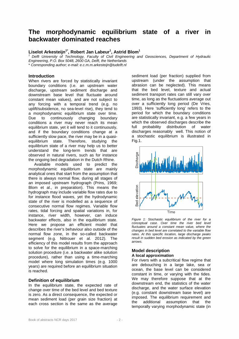
Introduction When rivers are forced by statistically invariant boundary conditions (i.e. an upstream water discharge, upstream sediment discharge and downstream base level that fluctuate around constant mean values), and are not subject to any forcing with a temporal trend (e.g. no uplift/subsidence, no sea-level rise), they tend to a morphodynamic equilibrium state over time. Due to continuously changing boundary conditions a river may never reach its mean equilibrium state, yet it will tend to it continuously, and if the boundary conditions change at a sufficiently slow pace, the river may be in a quasi-equilibrium state. Therefore, studying the equilibrium state of a river may help us to better understand the long-term trends that are observed in natural rivers, such as for instance the ongoing bed degradation in the Dutch Rhine.
Available models used to predict the morphodynamic equilibrium state are mainly analytical ones that start from the assumption that there is always normal flow, during all stages of an imposed upstream hydrograph (Prins, 1969; Blom et al., in preparation). This means the hydrograph may include variable flow rates due to for instance flood waves, yet the hydrodynamic state of the river is modelled as a sequence of consecutive normal flow regimes. Variable flow rates, tidal forcing and spatial variations in, for instance, river width, however, can induce backwater effects, also in the equilibrium state. Here we propose an efficient model that describes the river’s behaviour also outside of the normal flow zone, in the so-called backwater segment (e.g. Nittrouer et al. 2012). The efficiency of this model results from the approach to solve for the equilibrium in a space-marching solution procedure (i.e. a backwater alike solution procedure), rather than using a time-marching model where long simulation times (e.g. 1000 years) are required before an equilibrium situation is reached. Definition of equilibrium In the equilibrium state, the expected rate of change over time of the bed level and bed texture is zero. As a direct consequence, the expected or mean sediment load (per grain size fraction) at each cross section is the same as the average
sediment load (per fraction) supplied from upstream (under the assumption that abrasion can be neglected). This means that the bed level, texture and actual sediment transport rates can still vary over time, as long as the fluctuations average out over a sufficiently long period (De Vries, 1993). Here ‘sufficiently long’ refers to the period for which the boundary conditions are statistically invariant, e.g. a few years in which the observed discharges describe the full probability distribution of water discharges reasonably well. This notion of a stochastic equilibrium is illustrated in Fig.1.
Figure 1: Stochastic equilibrium of the river for a conceptual case. Over time the river bed level fluctuates around a constant mean value, where the changes in bed level are correlated to the variable flow rates. At this specific location, large discharge peaks result in sudden bed erosion as indicated by the green arrows. Model description A local approximation For rivers with a subcritical flow regime that are debouching in a large lake, sea or ocean, the base level can be considered constant in time, or varying with the tides. We may therefore suppose that at the downstream end, the statistics of the water discharge, and the water surface elevation (e.g. constant downstream base level) are imposed. The equilibrium requirement and the additional assumption that the temporally varying morphodynamic state (in

Book of abstracts NCR days 2017 - 3 -
equilibrium) can be approximated by the mean equilibrium state, then allow us to compute a local equilibrium state. This means we can compute the mean bed level, mean bed surface texture and derive all local flow variables, such as the flow depth, flow velocity, and Froude number during the various stages of the hydrograph, that on the long term facilitate the transport of exactly the average sediment load per grain size fraction. Approximation of a single branch Under the assumption that the variable flow can be treated as a sequence of steady flows (i.e. the backwater approximation), the full longitudinal equilibrium profile can be computed. We start downstream at the cross section where the equilibrium is known and compute solutions at the other cross sections by marching in upstream direction. The water surface slopes in the downstream cross section during the various stages of the hydrograph can be expressed as a function of the local friction slopes, the Froude numbers, and the mean bed slope. We note that only the mean bed slope requires information from a cross-section upstream (i.e. the bed level upstream), while the others can be estimated from the information that is available at our known (downstream) cross section. However, when we impose as equilibrium requirement that the spatial gradient of the expected sediment load (per grain size fraction) is zero, we introduce an extra set of equations which can be manipulated in such a way that they provide expressions for the approximation of the bed slope and the rate of change of bed surface texture, as a function of the local flow variables and the local domain characteristics (such as river width, friction, bed texture and porosity). This leads to a system of first order differential equations that describes the rate of change of all local hydrodynamic and
Figure 2: Convex bed profile and downstream fining in the equilibrium state.
morphodynamic variables in space. The equilibrium state can then be found by numerically integrating this system of equations along the river long-profile in upstream direction, using for instance an Euler forward method. Sufficiently far upstream of the backwater effects, the solution of our model reduces to existing analytical equilibrium models that provide expressions for the mean bed slope and mean surface texture under the assumption of normal flow. Approximation of a river system Local water or sediment extractions, variations in river width, confluences and tributaries can cause a sudden change in water and/or the required mean bed slope that is required to transport the average sediment load. Under the assumption that the water level is continuous, we can compute the mean bed level at the upstream side of the perturbation that satisfies the equilibrium requirement at the upstream reach. Please note that this can lead to a discontinuity in the bed profile, and that for tributaries and confluences there are multiple upstream branches. Once the upstream bed level(s) are known, the solution procedure can be continued (per branch). Dealing with bifurcations is less trivial and at this moment not included in the model yet. Time reconstruction When the mean equilibrium state and the hydrodynamic steady state during each discharge are known, we can compute the gradients in sediment transport during each discharge stage. After that, by ordering the erosion/deposition amounts per discharge in the order of occurrence of discharges, the bed level and bed texture fluctuations can be mimicked. This leads to an approximation of the bed level and bed texture change in time. Effect of variable flow The effect of the variable flow does not only introduce dynamic behaviour, it also leads to a different mean equilibrium state of the system in comparison to the mean equilibrium state under normal flow conditions. Fig. 2. illustrates the equilibrium state of a river section with constant width and a constant downstream base level. The alternating backwater effects lead to a mean convex upward profile, and in most cases a moderate fining of the bed surface texture in downstream direction.

Book of abstracts NCR days 2017 - 4 -
Validation and discussion In addition to the upward propagating perturbations caused by backwater effects, the local changes in river parameters also induce perturbations that are propagating in downstream direction in the ‘hydrograph boundary layer’ (e.g. Parker et al. 2004). These oscillations dampen out in streamwise direction, and the river adjusts toward a state where normal flow is prevailing during all stages of the hydrograph, while the sediment load has adjusted to the ‘normal flow load distribution’ (Blom et al., in preparation). Here the bed level does not change in time with the varying flow. A river system can therefore be considered to consist of zones where the behaviour is either best characterised as dominated by 1) downward propagating perturbations in bed level or bed texture (hydrograph boundary layer), 2) the absence of significant temporal variations in bed level and bed texture (quasi-normal flow segment), or 3) dynamic behaviour induced by backwater effects (backwater segment). Up- and downstream of each perturbation along the river section (e.g. varying width, or a tributary), a backwater segment and hydrograph boundary layer occur, which may overlap when the distance between two subsequent perturbations is too short for the oscillations to dampen out. This is illustrated in Fig. 3.
In our model, we do not incorporate the behaviour in the hydrograph boundary layer, as a solution procedure in upstream direction implies that downstream propagating information cannot be included. Also, since we formulated our model under the backwater-approximation, the morphodynamic effect of the dampening and hysteresis effect of a flood wave are not included.
The model has been validated for simple reaches where the zones do not overlap, using a numerical model that discretizes the Saint-Venant-Hirano model and that is able to predict the full dynamic behaviour as a reference
solution. For a wide range of parameter settings, our proposed model is able to capture the behaviour in the quasi-normal flow zone and backwater segment very well. Furthermore the reduction in computation time is significant. While our space-marching model requires only a few minutes, the Saint-Venant model requires a few days, dependent on the quality of the initial condition. In addition, for the latter model it is cumbersome to define whether an equilibrium state is reached. Future work aims at extending the validation to cases where the hydrograph boundary layer and backwater segment do overlap. Acknowledgements This research is part of the research programme RiverCare, supported by the Dutch Technology Foundation STW, which is part of the Netherlands Organization for Scientific Research (NWO), and which is partly funded by the Ministry of Economic Affairs under grant number P12-14 (Perspective Programme). References Blom et al. (in preparation), The equilibrium alluvial
river under variable flow, and its channel-forming discharge.
Nittrouer, J. A., Shaw, J., Lamb, M. P., & Mohrig, D. (2012). Spatial and temporal trends for water-flow velocity and bed-material sediment transport in the lower Mississippi River. Geological Society of America Bulletin, 124(3-4), 400-414.
Parker, G., 2004, Response of the gravel bed of a mountain river to a hydrograph. Proceedings, 2004 International Conference on Slopeland Disaster Mitigation, Taipei, Taiwan, October 5-6, 11 p.
Prins, A. (1969), Dominant discharge, Tech. Rep. S78-III, Waterloopkundig Laboratorium Delft.
De Vries (1993) Use of models for river problems, 85 pp., UNSECO
Figure 3: A river system in stochastic equilibrium subdivided into sections, classified as hydrograph boundary layer, quasi-normal flow segment, backwater segment, or a mixture of those.

Book of abstracts NCR days 2017 - 5 -
A palaeohydrological study of a river pattern change in the Overijsselse Vecht Jasper H.J. Candel*1, Maarten Kleinhans2, Bart Makaske1, Wim Hoek2, Cindy Quik1, Jakob Wallinga1 1 Wageningen University and Research, Soil Geography and Landscape group, P.O. Box 47, 6700AA Wageningen, The Netherlands 2 Utrecht University, Department of Physical Geography, Faculty of Geosciences, P.O. Box 80115, 3508TC Utrecht, The Netherlands * Corresponding author; e-mail: [email protected]
Introduction Re-meandering is an important measure to restore the ecology in regional rivers (Lorenz et al., 2009). However, not all regional rivers have sufficient stream power to induce lateral migration (Kleinhans and Van den Berg, 2011). Re-meander approaches are still being applied to such rivers (Kondolf, 2006), which often results in failing river restoration projects (Wohl et al., 2015). In order to gain a better understanding of channel pattern changes (Schumm, 1985), we studied the historic morphodynamics of the Overijsselse Vecht. This is a sand-bed river flowing from Germany into The Netherlands, with a length of 167 km, a catchment size of 3785 km2, a valley slope of 1.42*10-4 (Wolfert and Maas, 2007), and an average discharge and mean annual flood discharge of 22.8 and 160 m3 s-1, respectively. Before the channelization in 1914, lateral migration rates reached up to 3 m yr-1, as was observed on historical maps for several meanders (Wolfert and Maas, 2007). Some of these meanders eroded deeply into the valley sides since approximately 1500 AD (Quik, 2016). We hypothesize that the river also changed from a laterally stable river into a meandering river ca. 500 years ago. The aim of this research is to elaborate upon the changes in forcing that have caused this river pattern change. Lateral stable phase The first step was to identify the palaeochannel that was active prior to the meandering phase. In Fig. 1 this channel is indicated with an arrow. We hypothesize that this channel was longitudinally connected to the first swale of the meander bend in a period of lateral stability. A radiocarbon date (14C) of the channel bottom and an optically stimulated luminescence date (OSL) of the inner bank was taken in order to test this hypothesis (in progress). In addition, we determined the channel dimensions by coring in a transect perpendicular to the channel.
Meandering phase In the next step, we determined the channel dimensions during the meandering phase assuming the rules proposed by Hobo (2015) (Fig. 2). From the coring data reported by Quik (2016) we determined the bankfull depth (Hbf), taken from the bottom of the channel lag to the surface elevation in the swales. The transverse bed slope α was determined by using ground-penetrating radar (GPR) in a transect perpendicular to the scroll bars.
Figure 3 Digital elevation map (0.5x0.5m) of one of the studied bends in the Overijsselse Vecht. The arrow points at the palaeochannel potentially dating from the laterally stable phase. The blue dashed line shows the possible course of the channel. OSL dates are from Quik (2016).
2/3W 1/6W 1/6W
Hbf
Figure 4 Sketch of the cross-sectional flow area of a meandering channel used for the palaeo-bankfull discharge calculations (Hobo, 2015, p.122).

Book of abstracts NCR days 2017 - 6 -
Palaeodischarge The bankfull palaeodischarge was reconstructed for both phases (laterally stable and meandering) following from the reconstructed dimensions and flow resistance estimated in four different ways: 1) by applying Brownlie’s formula (Brownlie, 1983), 2) by estimating a Manning’s roughness coefficient following the procedure of Cowan (1956), 3) by determining the Chézy value for a large dataset of 127 rivers, and 4) for 29 comparable rivers with scroll bars (Kleinhans and Van den Berg, 2011). Subsequently, the potential stream power and bar regime were predicted applying relationships of Struiksma et al. (1985) and Kleinhans and Van den Berg (2011). Monte Carlo simulations allowed us to take into account the statistical uncertainty of all parameters. Our analysis suggests that the bankfull discharge increased with a factor 2 to 3 around 1500 AD, resulting in a higher potential specific stream power (Fig. 3), and a river changing from an overdamped into an underdamped regime.
We suggest that the increase of the bankfull discharge is likely the result of land use changes in the catchment. In this period, reclamation of the margins of peatland areas intensified for buckwheat cultivation (Borger, 1992), lowering the hydrological buffer capacity of these peatlands (Streefkerk and Casparie, 1987). In addition, bank instability caused by intensive use of the floodplains for cattle grazing can explain why these large meanders only formed locally (Trimble and Mendel, 1995; Quik, 2016).
Our study provides improved understanding of channel pattern transitions and associated forcings in lowland areas. Such information supports the design of sustainable river restoration. Acknowledgements This research is part of the research program RiverCare, supported by the Dutch Technology Foundation STW, which is part of the Netherlands Organization for Scientific Research (NWO), and which is partly funded by the Ministry of Economic Affairs under grant number P12-14 (Perspective Programme).
References Borger, G. J., 1992, Draining—digging—dredging; the
creation of a new landscape in the peat areas of the low countries, Fens and bogs in the Netherlands, Springer, p. 131-171.
Brownlie, W. R., 1983, Flow depth in sand-bed channels: Journal of Hydraulic Engineering, v. 109, p. 959-990.
Cowan, W. L., 1956, Estimating hydraulic roughness coefficients: Agricultural Engineering, v. 37, p. 473-475.
Hobo, N., 2015, The sedimentary dynamics in natural and human-influenced delta channel belts.
Kleinhans, M. G., and J. H. Van den Berg, 2011, River channel and bar patterns explained and predicted by an empirical and a physics‐based method: Earth Surface Processes and Landforms, v. 36, p. 721-738.
Kondolf, G. M., 2006, River restoration and meanders: Ecology and Society, v. 11, p. 42.
Lorenz, A., S. Jähnig, and D. Hering, 2009, Re-Meandering German Lowland Streams: Qualitative and Quantitative Effects of Restoration Measures on Hydromorphology and Macroinvertebrates: Environmental Management, v. 44, p. 745-754. 10.1007/s00267-009-9350-4
Quik, C., 2016, Historical morphodynamics of the Overijsselse Vecht: Extreme lateral migration of meander bends caused by drift-sand activity?, Wageningen University & Research, Wageningen.
Schumm, S., 1985, Patterns of alluvial rivers: Annual Review of Earth and Planetary Sciences, v. 13, p. 5.
Streefkerk, J., and W. Casparie, 1987, De hydrologie van hoogveen systemen: Staatsbosbeheer-rapport, v. 19, p. 1-119.
Struiksma, N., K. Olesen, C. Flokstra, and H. De Vriend, 1985, Bed deformation in curved alluvial channels: Journal of Hydraulic Research, v. 23, p. 57-79.
Trimble, S. W., and A. C. Mendel, 1995, The cow as a geomorphic agent—a critical review: Geomorphology, v. 13, p. 233-253.
Wohl, E., S. N. Lane, and A. C. Wilcox, 2015, The science and practice of river restoration: Water Resources Research, p. 5974-5997. 10.1002/2014wr016874
Wolfert, H., and G. Maas, 2007, Downstream changes of meandering styles in the lower reaches of the River Vecht, the Netherlands: Netherlands Journal of Geosciences v. 86, p. 257.
Figure 5 Stability diagram in which both river pattern phases are plotted, with the discriminators of different bed textures (Kleinhans and Van den Berg, 2011).

Book of abstracts NCR days 2017 - 7 -
Impact of peak discharge increase on the channel pattern and dynamics of the Upper Yellow River F. Schuurman*, S. Post
Royal HaskoningDHV, Dep. Rivers and Coasts, Laan 1914 No. 35, 3818 EX, Amersfoort, The Netherlands * Corresponding author; e-mail: [email protected]
Introduction The Yellow River is, with a length of nearly 5500 km, the sixth longest river in the world and it has the second largest annual sediment load of all rivers. The river, also called ‘Mother of China’, plays an important role in the Chinese history, economy and geography. The river starts in the mountainous area of western China and flows through the arid Inner Mongolia region to the Bohai Sea in the east (Fig. 1).
The discharge in the Yellow River is regulated by hydropower dams. Nevertheless, the water availability in the Yellow River is insufficient, partly due to severe water extraction for irrigation in the dry Inner Mongolia. Therefore, rerouting of discharge from the well-watered Yangtze River to the water-starved Yellow River in the upstream source area of both rivers has been considered, also called the Western route of the South-North Water Transfer Project.
However, the discharge rerouting potentially affect the Yellow River over nearly its entire length. Among others, an increase in peak discharge to flush the reservoirs in the Yellow River might change the channel pattern and dynamics of the Yellow River. Therefore, we conducted a modelling study using Delft3D to estimate the impact of the increase in peak discharge in the Yellow River.
Figure 1. Location of the study reaches in the northern part of the Yellow River (red squares) and the major hydropower dams further upstream (blue stars). Method We analysed remote sensing data and modelled the bed level change in the study reaches, including the dynamics of bars, shift
of channel branches and erosion and sedimentation on the floodplains.
Two river reaches, each with a length of about 50 km, were studied: a meandering and a braiding reach (Fig. 1). Both reaches were located in Inner Mongolia and largely unconfined. For both study reaches, we made a Delft3D schematisation using satellite images and measured cross-sectional profiles.
The period of 2015 to 2040 was simulated to predict the impact of future discharge rerouting from the Yangtze River to the Yellow River. Four scenarios with future discharge rerouting were modelled and compared, each with a peak discharge period of one month: 2000 m³/s, 3000 m³/s, 4000 m³/s and 5000 m³/s. In the remaining 11 months, the discharge had a constant magnitude of 500 m³/s.
To prevent static channels, channel and bar dynamics were stimulated by using a relatively strong bed slope effect in combination with a relatively strong spiral flow parameterization. This resulted in a significant improvement of the lateral channel shift. Sediment transport was computed using the Engelund-Hansen transport predictor, as the typical sediment in the study reaches is relatively fine with a D50 of 0.11 mm. Results The bed level of the meandering reach after 25 years with different annual peak discharges is given in Fig. 2. The initially curved reach with relatively straight sections between the bends evolved into a complicated river reach with small bends and braiding sections. In the scenario with 4000 m³/s peak discharge, many cutoffs and even avulsions occurred. This can be explained by the amount and intensity of flow over the floodplains, which depend on the peak discharge. The formation of new channels was accompanied by deposition of sand on the floodplains. At some locations, up to 2 m sedimentation occurred for the higher peak discharge scenarios.
Book of abstracts NCR days 2017 - 8 -
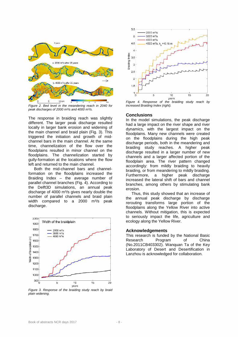
Figure 2. Bed level in the meandering reach in 2040 for peak discharges of 2000 m³/s and 4000 m³/s. The response in braiding reach was slightly different. The larger peak discharge resulted locally in larger bank erosion and widening of the main channel and braid plain (Fig. 3). This triggered the initiation and growth of mid-channel bars in the main channel. At the same time, channelization of the flow over the floodplains resulted in minor channel on the floodplains. The channelization started by gully-formation at the locations where the flow left and returned to the main channel.
Both the mid-channel bars and channel-formation on the floodplains increased the Braiding Index – the average number of parallel channel branches (Fig. 4). According to the Delft3D simulations, an annual peak discharge of 4000 m³/s gives nearly double the number of parallel channels and braid plain width compared to a 2000 m³/s peak discharge.
Figure 3. Response of the braiding study reach by braid plain widening.
Figure 4. Response of the braiding study reach by increased Braiding Index (right). Conclusions In the model simulations, the peak discharge had a large impact on the river shape and river dynamics, with the largest impact on the floodplains. Many new channels were created on the floodplains during the high peak discharge periods, both in the meandering and braiding study reaches. A higher peak discharge resulted in a larger number of new channels and a larger affected portion of the floodplain area. The river pattern changed accordingly: from mildly braiding to heavily braiding, or from meandering to mildly braiding. Furthermore, a higher peak discharge increased the lateral shift of bars and channel branches, among others by stimulating bank erosion.
Thus, this study showed that an increase of the annual peak discharge by discharge rerouting transforms large portion of the floodplains along the Yellow River into active channels. Without mitigation, this is expected to seriously impact the life, agriculture and ecology along the Yellow River. Acknowledgements This research is funded by the National Basic Research Program of China (No.2011CB403302). Wanquan Ta of the Key Laboratory of Desert and Desertification in Lanzhou is acknowledged for collaboration.

Book of abstracts NCR days 2017 - 9 -
Closure of offtakes in Bangladesh: use of numerical models to overcome data scarcity for the initial assessment of remedial measures R. Vila-Santamaria*1, A.L. de Jongste2, E. Mosselman1,3 1 Delft University of Technology, Faculty of Civil Engineering and Geosciences, Stevinweg 1, 2628 CN Delft, the Netherlands 2 Witteveen+Bos, Business Line Deltas, Coasts and Rivers, Group Hydrodynamics and Morphology, PO box 2397, 3000 CJ, Rotterdam, the Netherlands 3 Deltares, Department of river dynamics and inland water transport, PO box 177, 2600 MH, Delft, the Netherlands * Corresponding author: [email protected]
Introduction Variable flows and fast morphological changes characterize the river system of Bangladesh, which includes the downstream reaches and delta of the Ganges and Brahmaputra rivers, two of the largest rivers in the world. In contrast, fresh water supply around the country largely depends on much smaller distributaries that take off from those large rivers.
With the arrival of the dry season and the drop of water levels in the rivers, some of the distributaries become disconnected during several months from their parent rivers because of aggradation at the offtake during the monsoon season.
Analysing the evolution of such offtakes from a morphodynamic perspective is fundamental for the definition of effective measures to prevent their closure. However, bed elevation data required to perform such analyses are rarely available, and bathymetric surveys of large rivers are costly and quickly outdated by fast morphological changes.
Physics-based numerical models provide a way to fill the gap of unavailable data, while also allowing to explore river morphodynamics beyond the setting of existing rivers.
Problem analysis Four major offtakes in Bangladesh are considered in this study, each one with its own characteristics. From literature review, we determined which parameters are relevant in the closure of these offtakes.
It seems that sediment transport during the monsoon season has a dominant role in changing the morphology of the fluvial system, affecting the connection of the parent rivers with their distributaries (Delft Hydraulics and DHI, 1996). Another cause for offtake closure is the amount of flow in the parent rivers during the dry season, which in the Ganges River is reduced by operation of the Farakka Barrage in India (Mirza, 2006; CEGIS, 2012). The configuration of an offtake in relation with its
parent river seems to play an important role in the closure of these four offtakes. This depends on the location along an inner or outer bend, the bifurcation angle (see Fig. 1) and the presence of bars near the offtake.
Because of the need of fresh water, remedial measures are being considered in order to anticipate these morphologic changes. The present approach to offtake maintenance lacks a global understanding of the processes that govern the evolution of these bifurcations. We focus on one of the major offtakes in Bangladesh: the connection between the Ganges and Gorai rivers.
Figure 1. A change in the channel configuration of the Ganges River increased the bifurcation angle of the Gorai offtake, which closed during the winter of 1976. Method To overcome lack of data, we use a morphodynamic numerical model based only on the most significant characteristics of the offtake system.
We analysed the relevant physical processes for the evolution of offtakes before setting up the numerical model, concluding that processes such as helical flow, gravity pull or retarded scour need to be taken into account. The choice is for a 2-D depth-averaged model using the software Delft3D. We used a schematised geometry roughly based on the Ganges and Gorai rivers and offtake, starting with a flat bed of constant slope.
We compared the order of magnitude of model results with observations of the river system for hydrodynamic and sediment transport processes; and with satellite images for the morphological evolution of bars and

Book of abstracts NCR days 2017 - 10 -
channels. We then analysed the simulated offtake behaviour and used this as reference scenario for the assessment of different engineering measures.
Figure 2. Bed levels simulated with the numerical model and used as reference scenario for the assessment of remedial measures.
Results After the spin-up of the model, the resulting bed topography generated by the morphodynamic module presents a number of bars which migrate downstream in the parent river as well as the formation of a meandering planform at the distributary channel (Fig. 2). Fig. 3 shows the effects of a measure implemented in the model, displaying erosion and accretion after two years of simulation without any intervention, when the closure of the offtake takes place (top), and with dredging of the dry-season channel in the distributary river (bottom). This shows that dredging at the distributary river improves the flow conditions during two years. Discussion Comparison of model with real river system The model is able to reproduce the behaviour of the Gorai offtake in agreement with flow velocity measurements and discharge distributions between Ganges and Gorai available from CEGIS (2012). Bar dimensions and yearly migration rates agree with observations from satellite images. Offtake closure process Discontinuation of flow in the distributary river is observed after 4 years of simulation (with variable discharge). This discontinuation occurs because: (1) the bar upstream of the offtake reaches the bifurcation point and increases the sediment load into the distributary; and (2) the bed level of the bend crossings at the distributary river increase during peak flows whereas retarded scour after the monsoon is insufficient to erode the bed to the previous elevation. These processes were identified as potential causes of the closure of different offtakes in Bangladesh. Remedial measures
Different remedial measures are schematically introduced in the model, including dredging of the distributary channel, erodible weirs, dredging at the parent river, construction of a flow divider and longitudinal training walls. The only measure that seems effective is dredging of the distributary river.
Figure 3. Erosion and accretion after two years of simulation without any intervention (top) and after dredging at the distributary river (bottom).
Conclusions It is possible to reproduce some of the most relevant processes for the evolution of a distributary offtake using a physics-based numerical model set up with the basic characteristics of the real river system in Bangladesh. The results obtained from this model are accurate enough to analyse the general behaviour of the offtake and to assess the effectiveness of remedial measures.
Dredging of the distributary channel is effective for at least one season, and it can also influence positively the following year.
Dynamics of the rivers discourage the implementation of hard structures because they cannot adapt to changing conditions. Other remedial measures, such as submerged weirs or improved alignments of parent rivers with dredging, revealed less effectiveness and required relocation of huge amounts of sediment. This is surely more expensive and more difficult to implement than recurrent dredging.
Development of relatively cheap tools is of major importance if data are scarce. Such tools can help understand the river system and are useful for the comparison of effects of engineering interventions. References CEGIS (2012) Updated feasibility study for the Gorai River
Restoration Project; Annex A: planform analysis. Center for Environmental and Geographic Information Services (CEGIS). Dhaka, Bangladesh.
Delft Hydraulics and DHI (1996) River Survey Project (FAP24): Main volume. Prepared for Water Resources Planning Organization, Government of Bangladesh.
Mirza, M.M.Q. (ed.) (2006) The Ganges water diversion: environmental effects and implications. Water Science and Technology Library Vol. 49. Kluwer Academic Publishers. Dordrecht, the Netherland.

Book of abstracts NCR days 2017 - 11 -
2 – Deltas and estuaries

Book of abstracts NCR days 2017 - 12 -
The influence of rivers on the morphology of estuaries L. Braat*, M.G. Kleinhans
Utrecht University, Faculty of Geosciences, Department of Physical Geography, P.O. Box 80.115, 3508TC Utrecht, The Netherlands * Corresponding author; e-mail: [email protected] Introduction Alluvial estuaries are very dynamic systems which are often subjected to conflicting ecologic and economic values. Besides coastal processes, e.g., tides and waves, the river has a major influence on the morphology of an estuary Past research has shown that river discharge influences the morphology of estuaries (e.g. Guo et al., 2014), similar to deltas (Dalrymple et al., 1992). Additionally, the river supplies sediments, including mud, into the estuary from upstream sources; however mud is rarely taken into account in morphological research of estuaries.
Mud in rivers results in narrower and deeper channels with steeper banks due to a larger critical shear stress for erosion because of cohesion (e.g. van Dijk et al., 2013; Schuurman, 2016). A dynamic balance is observed between floodplain formation by cohesive sediment and floodplain erosion by channel migration. Consequently, cohesive sediment can change an unconfined braiding channel pattern into a self-confined meandering or even a laterally straight, immobile channel pattern (Makaske et al., 2002; Kleinhans and van den Berg, 2011). Until now, it was unclear whether mud flats have similar effects in estuaries.
Our objective is to understand the influence of mud supply by rivers on the morphology of estuaries on time-scales of centuries to millennia. This way we can understand influence of both the discharge and sediment supply of the river on estuary morphology. Method In this study we used the numerical modelling package Delft3D in 2DH starting from an idealised convergent estuary. The estuary was roughly based on the Dyfi, i.e. Dovey estuary, in Wales and was run for 2000 years with a morphological factor of 400.
We used three open boundaries: two cross-shore water level boundaries and one upstream discharge boundary. At the water level boundaries a M2 tide was imposed with a tidal range of 3 m. The river discharge was varied
between 0 and 150 m3/s for different models. Dry cells are freely erodible and the model will therefore develop a self-formed (alluvial) estuary shape.
In this model we use a single sand and mud fraction which we track in the bed with a bed storage layer module (van Kessel, 2012). For sand supply we used equilibrium conditions at the boundaries. Mud is supplied by the river as a concentration which we varied between 0 and 50 mg/L. Sediment transport is calculated with Engelund-Hansen for sand and Partheniades-Krone for mud.
Sand and mud interact in the bed. When the concentration of mud in the bed is above 40%, we consider the bed to be cohesive and sand fluxes are proportional to the mud erosion flux.
Results The final morphology of the run with a fluvial mud supply of 20 mg/L is flanked by mud flats that self-confine the bar-built estuary. The morphology developed towards a state of dynamic equilibrium in which average bank erosion equals sedimentation. Or in
Figure 1. Left column shows final bathymetry of model runs after 2000 yr and the right column shows mud fractions in the top layer of the bed. Run with (a,e) 150 m3/s, (b,f) 100 m3/s (default), (c,g) 50 m3/s and (d,h) 0 m3/s river discharge.
Book of abstracts NCR days 2017 - 13 -
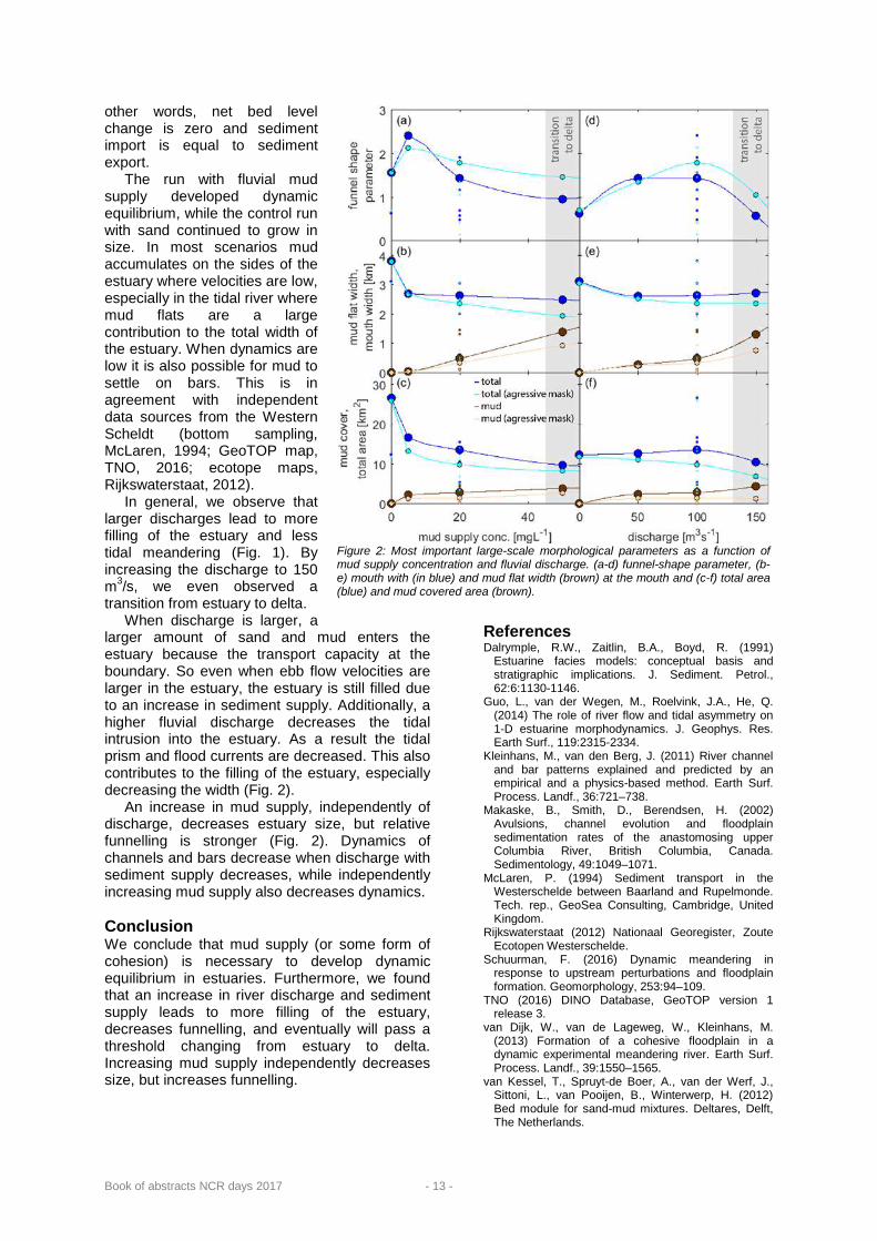
other words, net bed level change is zero and sediment import is equal to sediment export.
The run with fluvial mud supply developed dynamic equilibrium, while the control run with sand continued to grow in size. In most scenarios mud accumulates on the sides of the estuary where velocities are low, especially in the tidal river where mud flats are a large contribution to the total width of the estuary. When dynamics are low it is also possible for mud to settle on bars. This is in agreement with independent data sources from the Western Scheldt (bottom sampling, McLaren, 1994; GeoTOP map, TNO, 2016; ecotope maps, Rijkswaterstaat, 2012).
In general, we observe that larger discharges lead to more filling of the estuary and less tidal meandering (Fig. 1). By increasing the discharge to 150 m3/s, we even observed a transition from estuary to delta.
When discharge is larger, a larger amount of sand and mud enters the estuary because the transport capacity at the boundary. So even when ebb flow velocities are larger in the estuary, the estuary is still filled due to an increase in sediment supply. Additionally, a higher fluvial discharge decreases the tidal intrusion into the estuary. As a result the tidal prism and flood currents are decreased. This also contributes to the filling of the estuary, especially decreasing the width (Fig. 2).
An increase in mud supply, independently of discharge, decreases estuary size, but relative funnelling is stronger (Fig. 2). Dynamics of channels and bars decrease when discharge with sediment supply decreases, while independently increasing mud supply also decreases dynamics. Conclusion We conclude that mud supply (or some form of cohesion) is necessary to develop dynamic equilibrium in estuaries. Furthermore, we found that an increase in river discharge and sediment supply leads to more filling of the estuary, decreases funnelling, and eventually will pass a threshold changing from estuary to delta. Increasing mud supply independently decreases size, but increases funnelling.
References Dalrymple, R.W., Zaitlin, B.A., Boyd, R. (1991)
Estuarine facies models: conceptual basis and stratigraphic implications. J. Sediment. Petrol., 62:6:1130-1146.
Guo, L., van der Wegen, M., Roelvink, J.A., He, Q. (2014) The role of river flow and tidal asymmetry on 1-D estuarine morphodynamics. J. Geophys. Res. Earth Surf., 119:2315-2334.
Kleinhans, M., van den Berg, J. (2011) River channel and bar patterns explained and predicted by an empirical and a physics-based method. Earth Surf. Process. Landf., 36:721–738.
Makaske, B., Smith, D., Berendsen, H. (2002) Avulsions, channel evolution and floodplain sedimentation rates of the anastomosing upper Columbia River, British Columbia, Canada. Sedimentology, 49:1049–1071.
McLaren, P. (1994) Sediment transport in the Westerschelde between Baarland and Rupelmonde. Tech. rep., GeoSea Consulting, Cambridge, United Kingdom.
Rijkswaterstaat (2012) Nationaal Georegister, Zoute Ecotopen Westerschelde.
Schuurman, F. (2016) Dynamic meandering in response to upstream perturbations and floodplain formation. Geomorphology, 253:94–109.
TNO (2016) DINO Database, GeoTOP version 1 release 3.
van Dijk, W., van de Lageweg, W., Kleinhans, M. (2013) Formation of a cohesive floodplain in a dynamic experimental meandering river. Earth Surf. Process. Landf., 39:1550–1565.
van Kessel, T., Spruyt-de Boer, A., van der Werf, J., Sittoni, L., van Pooijen, B., Winterwerp, H. (2012) Bed module for sand-mud mixtures. Deltares, Delft, The Netherlands.
Figure 2: Most important large-scale morphological parameters as a function of mud supply concentration and fluvial discharge. (a-d) funnel-shape parameter, (b-e) mouth with (in blue) and mud flat width (brown) at the mouth and (c-f) total area (blue) and mud covered area (brown).

Book of abstracts NCR days 2017 - 14 -
Predicting salinity intrusion in the Rhine-Meuse Delta and effects of changing the river discharge distributions Y. Huismans1*, C. Kuijper1, W. Kranenburg1, S. de Goederen2, H. Haas3, N. Kielen3 1 Deltares, P.O. Box 177, 2600 MH Delft, The Netherlands 2 RWS-WNZ, Postbus 556, 3000 AN Rotterdam, The Netherlands 3 RWS-WVL, P.O Box 17. 8200 AA Lelystad, The Netherlands * Corresponding author; e-mail: [email protected]
Introduction The Rhine-Meuse Delta (RMD) is the most densely populated and intensively used area of the Netherlands. Fresh water availability is therefore of high importance. Due to climate change and several human interventions the salinity intrusion is expected to increase (Klijn et al. 2012). For current and future fresh water supply it is desirable to be able to predict and influence the salinity intrusion. For this, knowledge on how water distributes in this multi-branch system is essential. In this paper we first give insight into how the northern and southern branches interact. Based on this insight we present an improved practical formula for salinity intrusion. Secondly, the effectiveness of using hydraulic structures for reducing salinity concentrations at strategic locations is studied.
Figure1. Map Rhine-Meuse Delta (RMD). North-South interaction Since the closure of the Haringvliet in 1970 the only remaining open connection with sea is the Nieuwe Waterweg (NWW), see Fig. 1. Salinity intrusion in the northern branches is mainly governed by the river discharge and sea level elevation, caused by tide and set up (Mens 2016). Salinity intrusion in the southern branches can only occur via the northern branches. Because the difference in water level between north and south determines the amount of water transported, these differences also largely determine the salinity intrusion in the connecting branches and the southern part (Huismans 2016), as illustrated in Fig. 2. During high tide at Hoek van Holland (north), it is low tide at Moerdijk (south) and water and
salt are transported from north to south. During the second phase of the tide, the water levels are reversed and the transport is directed to the north. Under extreme conditions, like storm surges, the water level at Hoek van Holland increases. Due to the large volume of the Haringvliet and Hollandsch Diep in the south, it takes time for the water levels to respond to the increased water levels in the north and a large water level difference between north and south will occur during high tide at Hoek van Holland (Winterwerp 1982). Due to the increase in water levels in the northern part, more water will flow towards the south during high tide and less will flow back to the north during low tide, consequently transporting more salt towards the south. In extreme cases the water level at Moerdijk will remain lower than the water level at Hoek van Holland, subsequently the flow will be directed south for more than a full tidal period.
Figure 2. Illustration of the typical water levels at Hoek van Holland and Moerdijk and the resulting water motion. Predicting salinity intrusion Under the above mentioned conditions salt may reach the Haringvliet. When the Haringvlietsluices are not discharging (QRhine at Lobith < 1100 m3/s) flow velocities in the Haringvliet are low and salinity concentrations may remain high for a long time. An extreme case happened in 2005, when the fresh water intake was hampered for months (van Spijk 2006). If predicted in time, measures can be taken. Currently a prediction rule is incorporated in the “Handboek Waterwacht”, stating that for

Book of abstracts NCR days 2017 - 15 -
low river discharges (QLobith < 1100 m3/s) and large water level difference between high tide at Hoek van Holland and low tide at Moerdijk (“HL” < 1 m), salinity intrusion of the southern branches may occur. From the reported 25 occurrences of salinity intrusion in the southern branches (1990-2005, Van Spijk 2006), only 10 met the criteria. From the 15 cases which did not meet the criteria, 14 events had river discharges well exceeding the 1100 m3/s. From the previous paragraph it follows that the water level differences during the full period are normative, rather than QLobith and HL. A new prediction rule is therefore based on the average of the water level differences between Hoek van Holland and Moerdijk. As it is important how far salt intruded during the previous period, the average over two tidal periods was taken, with a weighing factor of 2 for the second period. With this new prediction rule 20 out of 25 historic events could be predicted correctly, with only 7 false positives. Influencing salinity intrusion The Hollandsche IJssel is an important branch for fresh water intake. Next we study to which extend the salinity concentrations at Krimpen a/d IJssel can be reduced by changing the operation of hydraulic structures. Through the Volkerak-locks water is taken from the Hollandsch Diep. Reducing this intake leads to more water in the RMD, discharging via the NWW, reducing the amount of salt entering from sea. With the weir at Hagestein the discharge distribution between the Lek and Waal can be regulated. By increasing the discharge through the Lek, more water will flow via the northern branches, presumably leading to lower salt concentrations at Krimpen. With SOBEK-RE a situation of near-salinization at Krimpen was simulated for a steady state river discharge (QLobith = 980 m3/s) and a cyclic tide. Three simulations were carried out: • Reference: with 50 m3/s extraction from the
Hollandsch Diep and QLek = 0 m3/s; • Stopping extraction: with 0 m3/s extraction
and QLek = 0 m3/s; • Changing discharge distribution: with
50 m3/s extraction and QLek = 50 m3/s and QWaal = 783 - 50 =733 m3/s.
Reducing the extraction with 50 m3/s at the Volkerak-locks leads to a larger reduction of the salinity concentration at Krimpen (13%) than changing the discharge distribution with 50 m3/s from the Waal to the Lek (9% reduction). The larger reduction is caused by the fact that with reducing the discharge extraction from the Hollandsch Diep the
discharges in both the NWW and Nieuwe Maas increase, while changing the discharge distribution with 50 m3/s from the Waal to the Lek only increases the discharges locally in the Lek and Nieuwe Maas, the discharge through the NWW remains unchanged. It however takes substantially longer before the salinity concentrations reduce at Krimpen when the extraction via the Volkerak-locks is reduced. Only after 8 tides 50% of the change is realized, while this is realized within 3 tides if the discharge distribution over the Lek is increased at the expense of the Waal. Due to the buffering capacity of the Haringvliet and Hollandsch Diep (Winterwerp 1982), it takes time before the water levels in these large water bodies respond to the change in extraction from the Hollandsch Diep. Only after these water levels have adjusted, the northern branches “feel” the changes at the southern branches and adjust their discharges and salinity concentrations. By changing the discharge distribution, the extra water over the Lek will quickly lead to an increase in discharge through the Nieuwe Maas and sub-sequent decrease in salinity concentrations. Conclusions and outlook In the multi-branch RMD the water level differences between the northern and southern branches largely determine the discharge and salinity distributions and response times within the system. With this knowledge a new formula is set up to predict salinity intrusion in the southern branches. This formula may be incorporated in an operational hydrodynamic model to create a warning signal for salinization. Secondly the effectiveness of reducing salinity concentrations at Krimpen with some measures has been analysed, showing that the buffering capacity of the Hollandsch Diep/Haringvliet play an important role in the response times. These insights are valuable for the operational management. References Huismans, Y. (2016). “Systeemanalyse Rijn-
Maasmonding: Analyse Relaties Noord- En Zuidrand En Gevoeligheid Stuurknoppen.” Deltares report 1230077–001. Delft, the Netherlands.
Klijn, F., E. Van Velzen, J. Ter Maat, and J. Hunink (2012). “Zoetwatervoorziening in Nederland - Aangescherpte Landelijke Knelpuntenanalyse 21e Eeuw.” Deltares report 1205970–000. Delft, the Netherlands.
Mens, M. (2016). “Karakterisering van Deelgebieden in de Rijn-Maasmonding Naar Type Verziltingsproces.” Deltares Memo 1230077–001. Delft, the Netherlands.
Spijk, A. van. 2006. “Evaluatie Verzilting En Ontzilting van Het Haringvliet Na de Storm van 24/25 November 2005.” Definitief AP/2006/03. Rijkswaterstaat Zuid-Holland.
Winterwerp, H. 1982. “Probleemanalyse van de Tijdschaaleffecten in Het Noordelijk Deltabekken.” M896-49. Waterloopkundig Laboratorium. The Netherlands.

Book of abstracts NCR days 2017 - 16 -
Do distributaries in a delta plain resemble an ideal estuary? Results from the Kapuas Delta, Indonesia K. Kästner1, A.J.F. Hoitink1, T.J. Geertsema1, B. Vermeulen2 1 Wageningen University and Research, Droevendaalsesteeg 3, 6708 PB Wageningen, The Netherlands 2 University of Twente, Drienerlolaan 5, 7522 NB Enschede * Corresponding author; e-mail: [email protected]
Coastal lowland plains under mixed fluvial-tidal influence may form complex, composite channel networks, where distributaries blend the characteristics of mouth bar channels, avulsion channels and tidal creeks. The Kapuas coastal plain exemplifies such a coastal plain, where several narrow distributaries branch off the Kapuas river at highly asymmetric bifurcations. Our goal is to increase the general understanding of physical processes in the fluvial-tidal transition. What is the typical cross sectional geometry and bed material? What consequences does the geometry have for the hydrodynamics? And how do river and tide drive the morphodynamics? We address these questions by studying the Kapuas river delta. Here we present first results of an extensive field survey and give insight into the along channel trends of cross section geometry and bed material grain size. Hydrodynamics and morphology of estuaries are often studied on hand of idealized models. In these models the estuary converges in upstream direction from a wide mouth towards a narrow river (Fig. 1). The water surface is parallel to the bed at mean flow and takes the form of a draw-down curve during high flow and that of a backwater curve at flow respectively (Fig. 2). Our results show that the Kapuas river deviates from the shape of an idealized estuary. The Kapuas distributaries all consist of short, converging reach near the sea and a non-converging reach upstream. There is a clear break of the along channel trends of geometrical scaling between the parts. Such a break in scaling was previously found in the Mahakam Delta, which suggests this may be a general characteristic in the fluvial to tidal transition. Field site The Kapuas river is a large tropical river in West Kalimantan, Indonesia. Its discharge ranges between 10^3 m^3/s in the wet and 10^4 m^3/s in the dry season. The Kapuas consists of one main distributary from which
three smaller distributaries branch off along the alluvial plain (Fig. 3). The Kapuas drains into the Karimata Strait, where it is subject to mainly diurnal tide, with average spring range of 1.5m.
Figure 1. Convergent width along an idealized estuary similar in size to the Kapuas
Figure 2. Bed and mean surface level along an idealized estuary similar in size to the Kapuas, Adopted from Lamb et. al (2012)
Figure 3. Map of the Kapuas river delta plain
Methods During October 2013 and April 2015 we surveyed the Kapuas from the sea to upstream km 300. Bankfull river width was extracted from Landsat images. Bathymetry was surveyed with a single beam each sounder. Grain size was sampled with a van Veen grabber. Results All distributaries of the Kapuas consist of a short tidal funnel where the width rapidly

Book of abstracts NCR days 2017 - 17 -
decreases. From the apex of the tidal funnel, the main distributary widens again towards the upstream end of the alluvial plain (Fig. 3). The distributaries' mouths terminate in shallow bars. The bed level reaches its maximum shortly upstream of the alluvial plain and then raises towards the upstream end of the alluvial plain (Fig. 4). During high flow the contrasting trends of width and depth cause the cross sectional area to remain approximately constant along the alluvial plain, but during low flow the cross sectional area decreases along the alluvial plain.
Figure 4. Measured bankfull width (top) and area (bottom) along the Kapuas distributaries
Figure 5. Measured bed and mean surface level along the Kapuas
The bed of the Kapuas consists mainly of sand. Bed material is downstream fining from 0.3 to 0.25mm along the alluvial plain within the main distributary. The trend of downstream fining does not break at the transition to the tidal funnel. There is a rapid downstream fining from the transition of the upstream valley to the alluvial plain. The grain size of the side distributaries differs from the main distributary and slightly increases in downstream direction (Fig. 5). Discussion and conclusion The geometry of the Kapuas distributaries differs from that of an ideal distributary. In particular the main distributary converges neither to an equilibrium width nor depth at the end of the tidal funnel.
Figure 6. Median grain size along the Kapuas distributaries
There is no simple relation between bed material grain size and channel geometry. The difference in median grain and downstream coarsening in the side distributaries can be explained by lower supply of sediment at strongly asymmetric bifurcations.
The particular geometry of the Kapuas also leads to particular hydrodynamics in the fluvial-tidal transition. Firstly, no strong drawdown curve develops during high flow (Fig. 2). Secondly the reduction of flow depth along the alluvial plain during low flow admits the tide to the upstream end of the alluvial plain without attenuation (Fig. 5). Attenuation becomes rapid at the upstream end of the alluvial plain, where the river reaches normal flow depth.
Figure 7. Tidal admittance along the Kapuas
The Kapuas river consists of an intriguing distributary network and has a particular along channel trend of cross section geometry that deviates from that of an idealised estuary. At the moment we investigate the consequences for river tide interaction, in particular propagation of the tide depending on the river discharge and the network effects. In a further step we are going to determine consequences for the morphological stability based on along channel bed shear stresses and the discharge division at bifurcations. References MP Lamb, JA Nittrouer, D Mohrig, J Shaw, Backwater and
river plume controls on scour upstream of river mouths: Implications for fluvio ‐deltaic morphodyn of Geophysical Research: Earth Surface 117 (F1)
Sassi, M. G., Discharge regimes, tides and morphometry in the Mahakam delta channel network, 2013
Hoitink, AJF and Jay, David A, Tidal river dynamics: implications for deltas, Reviews of Geophysics, 2016
K. Kästner, A.J.F. Hoitink, B. Vermeulen, T.J. Geertsema, N.S. Ningsih, Distributary channels in the fluvial to tidal transition zone, (submitted)

Book of abstracts NCR days 2017 - 18 -
The development of scour holes in a tidal area with heterogeneous subsoil under anthropogenic influence H. Koopmans*1,2, Y. Huismans1, W. Uijttewaal2 1 Deltares, P.O. Box 177, 2600 MH, Delft, the Netherlands 2 Delft University of Technology, Department Hydraulic Engineering, Faculty of Civil Engineering and Geosciences P.O. Box 5048, 2600 GA, Delft, the Netherlands * Corresponding author; e-mail: [email protected]
Introduction The Rhine-Meuse Delta is located in the most densely populated and most used part of the Netherlands. To guarantee safety it is of great importance that the dynamics of the riverbed are closely monitored. At the moment there are over 100 identified scour holes in the Rhine-Meuse delta of which some still grow, (Huismans, 2016). In the development of these holes the heterogeneity of the subsoil plays an important role, (Huismans, 2016; Sloff, 2013). The subsoil lithography is composed of alternating layers of poorly erodible clay and peat and highly erodible sand, (Berendsen, 2001; Hijma, 2009). At locations where the clay or peat layer becomes too thin due to erosion, exposure of an underlying layer of sand can result in a scour hole, see Fig. 1. Since these holes and their steep slopes may pose a risk to the stability of riverbanks, dikes and hydraulic structures, knowledge on their development is required. In this paper a thorough analysis of field data and results of a physical scale model is presented.
Figure 6. Illustration of the development of a scour hole in heterogeneous subsoil, (C. Sloff, 2013) Method The method consists of three steps: 1. Analysis of a large set of scour holes in the
field. 2. Physical scale model tests to study the
detailed growth. 3. Link the scale model results to the results
from the field data analysis. Field data analysis A tool has been developed to visualize the evolution of the deepest points of a river branch per cross section based on bathymetric surveys of the period 1976-2015 provided by Rijkswaterstaat. The result shows the overall development of the deepest parts of the entire
river and therefore the locations of the scour holes and their development. With the use of additional information on the scour hole profile, the heterogeneous subsoil, human interventions and other changes in hydrodynamics, these plots shed light on the scour hole development over time and their possible causes. Physical model To study the development of a scour hole in heterogeneous subsoil the following experiment was carried out. In the Waterlab of the Delft University of Technology a flume of 12m length, 0.8m width, 0.25m depth was constructed. The entire bottom consisted of a layer of cement except for an oval opening in the centre of 0.5m length and 0.3m width. The cement layer surrounding the oval, covers a box of sand. The flume simulates a river with a non-erodible bed and a local discontinuity in the top layer exposing an underlying sand layer. This way a scour hole could develop in the oval opening. Using scaling rules a representative water depth and flow velocity were chosen of respectively 0.13 m and 0.45 m/s and fine sand with a d50 of 260 µm. Experiments were also done using materials similar to clay partly covering the oval opening. The materials used were river clay and fine sand hardened with sprayed paint. These experiments aim at creating a better understanding of 3D effects introduced by the shape of a scour hole. Moreover, the behaviour of a poorly erodible bed can be simulated that also has the ability to fail. Results Field data analysis The Oude Maas was chosen as the first river branch to analyse. In the river a total of fifteen scour holes were identified. The developed tool shows a different development per hole in time and space, which is illustrated with three holes in Fig. 2. Typical scour hole development shows a negative exponential growth rate, with a fast initial growth and a stable end state,

Book of abstracts NCR days 2017 - 19 -
(Hoffmans, 1997). This profile is found for a part of the scour holes, showing large growth at a certain time and ending in a stable state. A sudden step in growth can possibly be related to a breakthrough of the layer of ‘Wijchen’, a clay layer which spreads over the whole delta and covers the Pleistocene sand. Its level at the location of the scour hole is also indicated in the figure with the dashed line of the same colour. Other holes which recently developed are still growing and have not reached their possible equilibrium. However, there are exceptions that behave completely different and can possibly be related to other causes.
Figure 7. Development of the deepest point of three different scour holes in the Oude Maas in the period 1976 – 2015. The dashed lines indicate the layer of ‘Wijchen’. The results show that nine out of fifteen holes already existed before 1976. In 2015 eleven holes seem stable and four are still growing. To determine the influence of river discharge a comparison will be made with high river discharges and scour hole growth. Furthermore, the slopes of the scour holes in the field will be compared with the suspected slopes from the theory. Finally, these analyses will be continued for the other river branches in the delta as well. Physical scale model Fig. 3 shows the scour after 4 hours. During the whole experiment the upstream slope appeared to have a constant value of 1:2. At the downstream edge and partly on the sides undermining occurred after a certain time. Compared to the 2D experiments, (Zuylen, 2015), the 3D experiments showed a faster growth of the scour hole. The 3D experiment did have a smoother upstream surface than the 2D experiment which could have enhanced the growth. The experiment with the spray paint layer showed the best agreement with the behaviour of clay. During the experiment the undermining process and subsequent growth in width and length could be visualized. Discussion To compare the scale model to the field the scour depth over the water depth is used. The results
are in the same order of magnitude. In the field erosion of the upstream edge of a scour hole is observed, which is not found in the scale experiment. This could be the result of the presence of a thinner clay layer upstream of the scour hole or the tide that reverses the flow direction.
Figure 8. The developed scour hole in the water flume after 4 hours. Conclusion The development of scour holes in the field is very variable, also when they are located in the same river branch. The development is therefore likely to be related to the heterogeneity of the subsoil and local phenomena in the flow conditions. The scale model shows only undermining of the downstream edge. The upstream slope stays constant and has a value of 1:2. Scour holes in the field show different behaviour which could possibly be the result of the tide or variation of the thickness of the surrounding clay layer. In future research, a comparison with the theory, the scale model and the field data will be made. Acknowledgements We would like to thank Aad Fioole (Rijkswaterstaat) for sharing the bathymetric surveys and the analysis tools, and the financial contribution from RWS NKWK-rivers pilot-B3. References Berendsen, H.J.A., E. S. (2001). Palaeogeographic
Development of the Rhine–Meuse Delta. Assen: Koninklijke Van Gorcum.
Hijma, M. (2009). From River Valley to Estuary. The Early-Mid Holocene Transgression of the Rhine-Meuse Valley. Utrecht: Utrecht University, Royal Dutch Geographical Society.
Hoffmans, G.J., H. Verheij. (1997). Scour Manual. CRC Press.
Huismans, Y., G. van Velzen, T.S.D. O’Mahoney, G.J.C.M Hoffmans, A.P. Wiersma. (2016). Scour hole development in river beds with mixed sand-clay-peat stratigraphy. Delft: ICSE.
Sloff, C., A. van Spijk, E. Stouthamer, A. Sieben. (2013). Understanding and managing the morphology of brances incising into sand-clay deposits in the Dutch Rhine Delta. Delft: International Journal of Sediment Research.
Zuylen, J. C. Sloff. (2015). Development of scour in non-cohesive sediments under a poorly erodible top layer. Delft: RCEM.

Book of abstracts NCR days 2017 - 20 -

Book of abstracts NCR days 2017 - 21 -
3 - Ecohydraulics
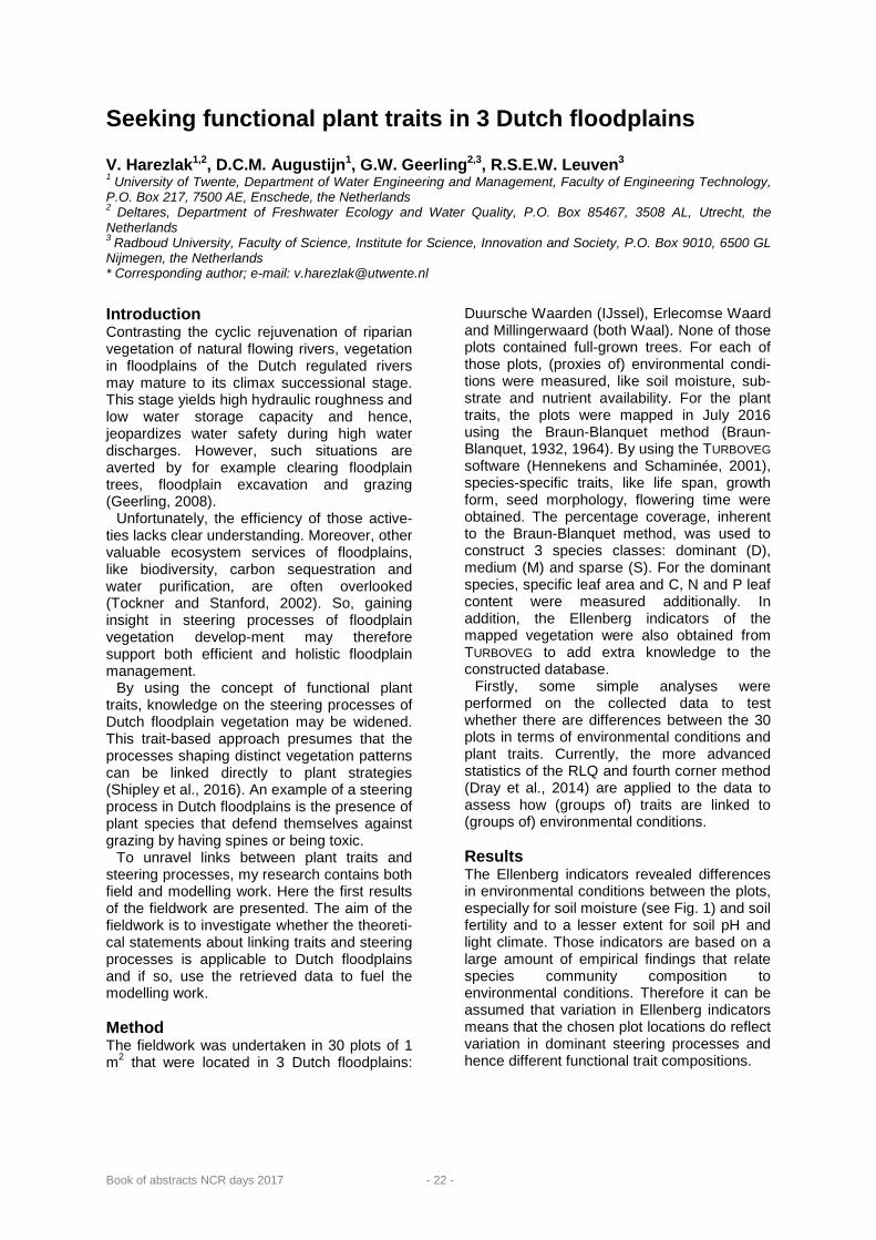
Book of abstracts NCR days 2017 - 22 -
Seeking functional plant traits in 3 Dutch floodplains V. Harezlak1,2, D.C.M. Augustijn1, G.W. Geerling2,3, R.S.E.W. Leuven3 1 University of Twente, Department of Water Engineering and Management, Faculty of Engineering Technology, P.O. Box 217, 7500 AE, Enschede, the Netherlands 2 Deltares, Department of Freshwater Ecology and Water Quality, P.O. Box 85467, 3508 AL, Utrecht, the Netherlands 3 Radboud University, Faculty of Science, Institute for Science, Innovation and Society, P.O. Box 9010, 6500 GL Nijmegen, the Netherlands * Corresponding author; e-mail: [email protected]
Introduction Contrasting the cyclic rejuvenation of riparian vegetation of natural flowing rivers, vegetation in floodplains of the Dutch regulated rivers may mature to its climax successional stage. This stage yields high hydraulic roughness and low water storage capacity and hence, jeopardizes water safety during high water discharges. However, such situations are averted by for example clearing floodplain trees, floodplain excavation and grazing (Geerling, 2008).
Unfortunately, the efficiency of those active-ties lacks clear understanding. Moreover, other valuable ecosystem services of floodplains, like biodiversity, carbon sequestration and water purification, are often overlooked (Tockner and Stanford, 2002). So, gaining insight in steering processes of floodplain vegetation develop-ment may therefore support both efficient and holistic floodplain management.
By using the concept of functional plant traits, knowledge on the steering processes of Dutch floodplain vegetation may be widened. This trait-based approach presumes that the processes shaping distinct vegetation patterns can be linked directly to plant strategies (Shipley et al., 2016). An example of a steering process in Dutch floodplains is the presence of plant species that defend themselves against grazing by having spines or being toxic.
To unravel links between plant traits and steering processes, my research contains both field and modelling work. Here the first results of the fieldwork are presented. The aim of the fieldwork is to investigate whether the theoreti-cal statements about linking traits and steering processes is applicable to Dutch floodplains and if so, use the retrieved data to fuel the modelling work. Method The fieldwork was undertaken in 30 plots of 1 m2 that were located in 3 Dutch floodplains:
Duursche Waarden (IJssel), Erlecomse Waard and Millingerwaard (both Waal). None of those plots contained full-grown trees. For each of those plots, (proxies of) environmental condi-tions were measured, like soil moisture, sub-strate and nutrient availability. For the plant traits, the plots were mapped in July 2016 using the Braun-Blanquet method (Braun-Blanquet, 1932, 1964). By using the TURBOVEG software (Hennekens and Schaminée, 2001), species-specific traits, like life span, growth form, seed morphology, flowering time were obtained. The percentage coverage, inherent to the Braun-Blanquet method, was used to construct 3 species classes: dominant (D), medium (M) and sparse (S). For the dominant species, specific leaf area and C, N and P leaf content were measured additionally. In addition, the Ellenberg indicators of the mapped vegetation were also obtained from TURBOVEG to add extra knowledge to the constructed database.
Firstly, some simple analyses were performed on the collected data to test whether there are differences between the 30 plots in terms of environmental conditions and plant traits. Currently, the more advanced statistics of the RLQ and fourth corner method (Dray et al., 2014) are applied to the data to assess how (groups of) traits are linked to (groups of) environmental conditions. Results The Ellenberg indicators revealed differences in environmental conditions between the plots, especially for soil moisture (see Fig. 1) and soil fertility and to a lesser extent for soil pH and light climate. Those indicators are based on a large amount of empirical findings that relate species community composition to environmental conditions. Therefore it can be assumed that variation in Ellenberg indicators means that the chosen plot locations do reflect variation in dominant steering processes and hence different functional trait compositions.

Book of abstracts NCR days 2017 - 23 -
Figure 1: Overview of Ellenberg moisture classes of the 30 plots, showing the median (blue diamonds) and 2x standard deviation as error bars. Classes (y-axis) are indicators of: 2 = extreme drought, 3 = drought, 4 = drought and drought/moist, 5 = drought/moist, 6 = drought/moist and moist, 7 = moist, 8 = moist/wet, 9 = wet and 10 = water species. On the x-axis are the plots, where EW stands for Erlecomse waard, MW for Millingerwaard and DW for Duursche waarden.
Figure 2: overview of life span (left) and life form (right). On the y-axis the species per dominant class (%). D, M and S represent the dominant classes. The classes in the right figure are: A = hydrophyte, B= helophyte, C=chameaphyte (herbaceous), G = geophyte, H = hemicryptophyte, L = liana, P = phanerphyte, T = therophyte, W = half parasite and Z = chameaphyte (woody). Most of the mapped species are perennial. The exceptions that occur are mainly the less dominant species (Fig. 2, left). Moreover, being a perennial means that reserves need to be stored and this is mostly done around or below ground level (class G and H respectively, Fig. 2, right). Some other life forms do exist as well, but those appear, again, by the less dominant species.
Discussion and Conclusion As most of the mapped species, especially the dominant ones, are perennial and have their remaining plant parts in winter around (mostly) or below ground level, one can conclude that no strong mechanical riverine processes (e.g. erosion and sedimentation) are steering the floodplain vegetation.
Furthermore, having reserves stored means that those plant species can kick-start their growth when the growing season starts. This indicates that biological processes, like the struggle for light, play important roles in shaping the observed vegetation patterns.
The planned data analyses are likely to disentangle traits and environmental conditions into more detail. This furthers the understan-ding of the dominant steering processes and the needed traits to handle those processes.
References Braun-Blanquet, J., 1932. Plant sociology (Transl. G.D.
Fuller and H.S. Conrad). McGraw-Hill, New York, 539pp. Braun-Blanquet, J., 1964. Pflanzensociologie: Grundzuge
der Vegetationskunde. 3te aulf. Springer-Berlag, Wein, 865 pp.
Dray, S., Choler, P., Dolédec, S., Peres-Neto, P.R., Thuiller, W., Pavoine, S., Ter Braak, C.J.F., 2014. Combining the fourth-corner and the RLQ methods for assessing trait responses to environmental variation. Ecology 95, 14–21. doi:10.1890/13-0196.1
Geerling, G.W., 2008. Changing Rivers: Analysing fluvial landscape dynamics using remote sensing. Radboud University of Nijmegen.
Hennekens, S.M., Schaminée, J.H.J., 2001. TURBOVEG, a comprehensive data base management system for vegetation date. J. of Veg. Science 12, 589-591.
Shipley, B., de Bello, F., Cornelissen, J.H.C., Laliberte, E., Laughlin, D., Reich, P.B., 2016. Reinforcing loose foun-dation stones in trait-based plant ecology. Oecologia 180, 923-933. doi:10.1007/s00442-016-3549-x
Tockner, K., Stanford, J. a., 2002. Riverine Flood Plains: Present State and Future Trends. Environ. Conserv. 29, 308–330. doi:10.1017/S037689290200022X

Book of abstracts NCR days 2017 - 24 -
Monitoring vegetation height and greenness of low floodplain vegetation using UAV-remote sensing W.K. van Iersel, M.W. Straatsma, E.A. Addink, H. Middelkoop
Utrecht University, Department of Physical Geography, Faculty of Geosciences, Heidelberglaan 2, 3584 CS Utrecht * Corresponding author; email: [email protected]
Introduction Vegetation in river floodplains has important functions for flood safety and biodiversity (Schindler et al., 2014). As a result of river restoration projects, floodplain vegetation is becoming increasingly heterogeneous (Göthe et al., 2016). This requires a more sophisticated monitoring of floodplain vegetation. Mapping of floodplain vegetation is often based on remote-sensing data from a single time step, which limits monitoring of seasonal changes. Vegetation height (VH) and greenness of pioneer, grassland and herbaceous vegetation types are highly dynamic in space and time, especially under pressures like mowing and grazing. Seasonal survey frequencies are required to monitor their functioning.
The rising availability of unmanned airborne vehicles (UAV) has a high potential to increase monitoring frequency. This study evaluated the potential of monitoring VH and greenness over one growing season with a UAV. Methods Six field surveys were performed during one year in a 100 ha floodplain. In 27 field plots VHfield was calculated per plot as the average of 30 random height measurements. Simultaneously, with each field survey we recorded true-colour and false colour imagery with a UAV. Per time step the imagery was processed into a point-based Digital Surface Model (DSM) of the floodplain using a Structure from Motion (SfM) workflow (Lucieer et al., 2014). To obtain VH from the DSMs per plot, the DSMs were normalized with the DSM of February, implicitly assuming this winter DSM represented the digital terrain model (DTM).
Next, the remote-sensed VH (VHUAV) was estimated as the 95th percentile of the z-values of the normalized DSMs (nDSM) and greenness was calculated from the false colour nDSM with Eq. (1):
BNIRBNIR
Greenness+−
= (1)
in which NIR is the average of the digital numbers (DN) in the near-infrared band and B
is the average DN in the blue band (Nijland et al., 2014).
The accuracy of the nDSMs was determined with an ordinary least squared (OLS) regression. Reed plots were excluded from the regression, because senescent reed vegetation in February prevented accurate observation of the ground surface, which resulted in high underestimations of VHfield.
In addition, we plotted per time step the VH against greenness to study the development of their relation over one year. The area of the resulting shape, if the first (Feb) and last (Jan) time step were connected, was calculated. Results Accuracy VHUAV The OLS regression of the true colour derived VHUAV (VHRGB) showed that VHRGB is estimated most accurately during leaf-on conditions (RMSE = 0.17-0.21 m) (Fig. 1). The error is in general an underestimation of VHfield. Development of VH and greenness over time VH and greenness show different developments over the seasons, resulting in hysteresis in the temporal relation between VH and greenness. Differences in this hysteresis were observed mainly between the high and low vegetation types (Fig 2). Low vegetation types (< 0.7 m) have a less clear hysteresis shape, because their VHRGB is less accurate and effected by noise. Table 1. Area of hysteresis polygon. Unit is m, since greenness is dimensionless.
Vegetation type n min max mean sd
pioneer 2 -0.01 0.03 0.01 0.02 n. grassland 5 -0.04 0.00 -0.01 0.01 p. grassland 2 0.00 0.02 0.01 0.01 l. herbaceous 11 -0.02 0.01 0.00 0.01 h. herbaceous 5 -0.01 0.22 0.12 0.08 reed 2 0.11 0.28 0.19 0.09
The areas of the resulting shapes or polygons, if the first (Feb) and last (Jan) VH-greenness pair are connected, show a similar division. The area of the high herbaceous and reed vegetation is on average a factor 10-20 larger

Book of abstracts NCR days 2017 - 25 -
than for the vegetation types < 0.7 m. However, the turquoise high herbaceous plot in Fig. 2 is an exception.
Figure 1. OLS regression of the true colour nDSMs of each time step. Reed is excluded and shown as an asterïsk.
Figure 2. Hysteresis of VHRGB and greenness per plot sorted on vegetation type. Classification was based on field observations and a simple ruleset: a) Pioneer has a vegetation cover of <25%, b) Natural and production grassland have a height limit of 0.3 m, c) The height limit for low herbaceous vegetation is 0.7 m.
Conclusion 1. Vegetation height is estimated most
accurately during leaf-on conditions (RMSE = 0.17-0.22 m);
2. Different low vegetation types show different hysteresis in temporal relations between vegetation height and greenness, which can facilitate classification of these classes.
References Göthe, E., Timmermann, A., Baattrup-Pedersen, A.,
Januschke, K., (2016) Structural and functional responses of floodplain vegetation to stream ecosystem restoration. Hydrobiologia 769, 79–92.
Lucieer, A., De Jong, S. M., & Turner, D. (2014). Mapping landslide displacements using Structure from Motion (SfM) and image correlation of multi-temporal UAV photography. Progress in Physical Geography, 38: 97–116
Nijland, W., de Jong, R., de Jong, S. M., Wulder, M. A., Bater, C. W., Coops, N. C., (2014) Monitoring plant condition and phenology using infrared sensitive consumer grade digital cameras. Agricultural and Forest Meteorology, 184: 98-106.
Schindler, S., Sebesvari, Z., Damm, C., Euller, K., Mauerhofer, V., Schneidergruber, A., Biro, M., Essl, F., Kanka, R., Lauwaars, S. G., Schulz-Zunkel, C., van der Sluis, T., Kropik, M., Gasso, V., Krug, A., Pusch, M. T., Zulka, K. P., Lazowski, W., Hainz-Renetzeder, C., Henle, K., Wrbka, T., (2014) Multifunctionality of floodplain landscapes: Relating management options to ecosystem services. Landscape Ecology 29 (2), 229–244.

Book of abstracts NCR days 2017 - 26 -
Riverbank protection removal to enhance habitat diversity through bar formation A. Wetser*1,2, W. S. J. Uijttewaal1, E. Mosselman1,3, E. Penning3, G. Duró1, J. Yuan2 1 Delft University of Technology, PO Box 5048, 2600 GA Delft, the Netherlands 2 National University of Singapore, 21 Lower Kent Ridge Rd, Singapore 119077 3 Deltares, P.O. Box 177, 2600 MH Delft, The Netherlands * Corresponding author; e-mail: [email protected]
Introduction Over the past centuries natural river banks have been transformed into banks with artificial revetments or sheet piles to protect them from erosion. Important river features for flora and fauna have disappeared and the ecological quality of the river reduced dramatically. Recently, the importance of the ecological function of rivers has been getting more attention. One river restoration measure is the removal of man-made bank protections to increase habitat diversity and biodiversity of riparian areas and the river basin. The river morphology may change due to the freely eroding banks in the restored section. Reference projects show that the removal of bank protection along rivers may lead to the formation of bars (e.g. Schirmer et al., 2014). Bars increase morphological diversity, providing specific habitats for flora and fauna (Kurth and Schirmer, 2014). There is a lack of knowledge about the formation of bars related to the length and location of the removal of bank protection. The length of river bank protection removal is usually limited, due to human activities along the riversides. Therefore, a guideline is needed for the design of bank protection removal to enhance habitat diversity through bar formation to make this a feasible river restoration method. Methodology We carried out mobile-bed flume experiments in the Fluid Mechanics Laboratory of Delft University of Technology. The experiments were focussed on how the length of bank protection removal changed the formation of bars. Furthermore, the experiment was aimed at finding geometrical changes in the setup that led to a difference in bar formation. Experimental setup Geometrical and morphodynamic characteristics were selected for the experiment having bar mode = 1 to obtain a system with alternate bars. The bar mode was calculated with the physics-based predictor of Crosato and Mosselman (2009) that estimates the number of bars in a river cross-section:
m2=0.17g(b-3)
�∆D50 B3iCQ
(1)
where: m = bar mode, b = degree of nonlinearity of the dependence of sediment transport on depth-averaged flow velocity, B = river width, C = Chézy coefficient, i = longitudinal gradient, D50 = median sediment grain size, g = gravitational acceleration, ∆ = relative sediment density under water, and Q = water discharge. The experimental flume consisted of a 6.2 metre long and 0.2 metre wide straight channel with 0.5 metre wide floodplains on the sides. On both sides of the channel, bank protection could be removed over a limited length. The channel bed and floodplain was covered by a layer of sand with a slope of 0.008. The erodible banks had a height of 2 cm above the channel bed. The mean diameter of the sediment was equal to 0.52 mm. The water discharge was kept constant at a value of 0.6 L/s. The mean water level was approximately 1 cm. A digital camera was installed above the flume that took photos at an interval of 15 minutes during the experiments. At the end of each experiment dye was added to the flow to distinguish deep channel areas from bars. The longitudinal bed profile was measured at three locations in the main channel at the end of each experiment. Experimental tests The reference case was a straight channel with fixed banks. The bank protection was removed over a length of three, six and nine times the channel width on either one or both sides. The bank protection was removed at different locations along the channel side. Tests were performed with a symmetrical flow forcing and an asymmetrical flow forcing, i.e. a groyne, upstream of the bank protection removal. Results In experiments in which the bank protection was removed, the bank eroded laterally and bars formed in the channel. A scour hole
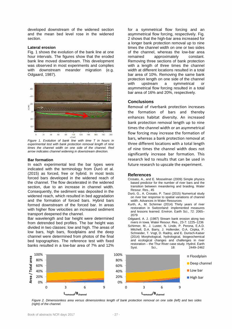
Book of abstracts NCR days 2017 - 27 -
0%20%40%60%80%
100%
0 3 6 9Lremoval/Bchannel
Floodplain
Deep channel
Low bar
High bar0%
20%40%60%80%
100%
0 3 6 9
Area
/ T
otal
are
a
Lremoval/Bchannel
Figure 2. Dimensionless area versus dimensionless length of bank protection removal on one side (left) and two sides (right) of the channel.
developed downstream of the widened section and the mean bed level rose in the widened section. Lateral erosion Fig. 1 shows the evolution of the bank line at one hour intervals. The figures show that the eroded bank line moved downstream. This development was observed in most experiments and complies with downstream meander migration (e.g. Odgaard, 1987).
Figure 1. Evolution of bank line with time T in hours in experimental test with bank protection removal length of nine times the channel width on one side of the channel. Red arrow indicates channel widening in downstream direction. Bar formation In each experimental test the bar types were indicated with the terminology from Duró et al. (2015) as forced, free or hybrid. In most tests forced bars developed in the widened reach of the channel. The flow decelerated in the widened section, due to an increase in channel width. Consequently, the sediment was deposited in the widened reach, which resulted in bed aggradation and the formation of forced bars. Hybrid bars formed downstream of the forced bar. In areas with higher flow velocities an increased sediment transport deepened the channel. Bar wavelength and bar height were determined from detrended bed profiles. The bar height was divided in two classes: low and high. The areas of low bars, high bars, floodplains and the deep channel were determined from photos of the final bed topographies. The reference test with fixed banks resulted in a low-bar area of 7% and 12%
for a symmetrical flow forcing and an asymmetrical flow forcing, respectively. Fig. 2 shows that the high-bar area increased for a longer bank protection removal up to nine times the channel width on one or two sides of the channel, whereas the low-bar area remained approximately constant. Removing three sections of bank protection with a length of three times the channel width at different locations resulted in a total bar area of 10%. Removing the same bank protection length on one side of the channel with upstream a symmetrical or asymmetrical flow forcing resulted in a total bar area of 16% and 20%, respectively. Conclusions Removal of riverbank protection increases the formation of bars and thereby enhances habitat diversity. An increased bank protection removal length up to nine times the channel width or an asymmetrical flow forcing may increase the formation of bars, whereas a bank protection removal at three different locations with a total length of nine times the channel width does not significantly increase bar formation. This research led to results that can be used in future research to upscale the experiment. References Crosato, A., and E. Mosselman (2009) Simple physics
based predictor for the number of river bars and the transition between meandering and braiding. Water Resour. Res., 45
Duró, G., A. Crosato, P. Tassi (2015) Numerical study on river bar response to spatial variations of channel width. Advances in Water Resources
Kurth, A., M. Schirmer (2014) Thirty years of river restoration in Switzerland: implemented measures and lessons learned. Environ. Earth Sci., 72: 2065–2079
Odgaard, A. J. (1987) Stream bank erosion along two rivers in Iowa. Water Resour. Res., 23-7: 1225–1236
Schirmer, M., J. Luster, N. Linde, P. Perona, E.A.D. Mitchell, D.A. Barry, J. Hollender, O.A. Cirpka, P. Schneider, T. Vogt, D. Radny, and E. Durisch-Kaiser (2014) Morphological, hydrological, biogeochemical and ecological changes and challenges in river restoration – the Thur River case study. Hydrol. Earth Syst. Sci., 18: 2449–2462

Book of abstracts NCR days 2017 - 28 -
Backwater development by woody debris in streams T.J. Geertsema*, P.J.J.F. Torfs, A.J. Teuling, A.J.F. Hoitink Wageningen University & Research, Hydrology and Quantitative Water Management Group, P.O. Box 47, 6700AA, Wageningen, Netherlands * Corresponding author; e-mail: [email protected]
Introduction Placement of woody debris is a common method for increasing ecological values in river and stream restoration (Ralph et al., 1994; Crook and Robertson, 1999) and is thus widely used in natural environments. Water managers, however, are afraid to introduce wood in channels draining agricultural and urban areas. Woody debris in streams namely, has an effect on flow deformation (Gippel et al., 1996; Piegay and Gurnell, 1997; Daniels and Rhoads, 2004 and 2007) and flow resistance (Dudley et al., 1998; Hygelund and Manga, 2003; Curran and Wohl, 2003) as a result from narrowing in the cross section. These processes provide morphological activity, both laterally through bank erosion and protection, and vertically with pool and riffle formation (Robison and Beschta, 1990; Smith et al., 1993; Piegay and Gurnell 1997; Curran and Wohl, 2003; Kail, 2003; Gurnell et al., 2006), and create backwaters upstream of the woody debris (Thomas and Nisbet, 2012). Obstruction ratio, Froude number, gradient and resistance characterize the height of the backwater according to theory, laboratory experiments and pilot studies for bridges and spur dikes. Woody debris, however, is a permeable construction and will weather over time. The purpose of this study therefore is to quantify the backwater by woody debris from in situ observation. To analyze the water level effects of woody debris, hourly water level (upstream and downstream) and discharge time series are collected for five streams in the Netherlands. Results The results are concentrated on the difference between upstream and downstream water levels over the area with woody debris. The water level difference over the woody debris relates to discharge in the streams. This relation is characterized by an increasing water level difference for an increasing discharge to a maximum for a certain discharge (Fig. 1). If the discharge increases beyond this maximum, the water level difference reduces to approximately the water level difference without woody debris. This reduction in water level difference is however depending on the blocking ratio of the woody debris (WD) as shown for the Leerinkbeek (WD mainly on the bed) and Tongelreep (WD over the whole cross section) (Fig. 1-2).
Figure 1. Relation between water level difference and discharge at Leerinkbeek. The black line indicates the water level difference before the insertion of woody debris.
Figure 2. Relation between water level difference and discharge at Tongelreep. The black line indicates the water level difference before the insertion of woody debris. Discussion These results are compared with the 1D numerical model. The numerical model solves the 1D St. Venant equations and uses a rectangular river with a width of 3.02 m, a Manning coefficient of the river of 0.04, a bed slope of 0.2*10-4 and a river length of 14.72 m. The downstream water level is equal to the normal water level, which indicates no influence from downstream. The woody debris is simulated in the middle of the stream length by decreasing the cross sectional width and/or increasing the Manning coefficient locally. The width ratio rb is defined as cross sectional area of the

Book of abstracts NCR days 2017 - 29 -
woody debris (small arrow) divided by the cross sectional area of the river (large arrow) (Fig. 3). The friction ratio rn is defined as the Manning coefficient of the woody debris divided by the Manning coefficient of the river. The results of the model are shown in Figure 4, which shows the dominance of the Manning coefficient in resulting in backwater effects and does not show the reduction in water level difference for high discharges.
Figure 3.Schematized river form in the 1D numerical model
Figure 4.Model results of decreasing cross sectional area and increasing friction coefficient as woody debris Preliminary conclusions • When the woody debris is located at the bed
of the stream, the water level gradient decreases during high discharges.
• The morphology of the stream and the wood changes in time and results therefore in smaller water level differences.
• The numerical model of woody debris is more sensitive to the friction coefficient then to the obstruction area.
• The current numerical model is not capable to simulate the reduction of the water level differences during high discharges.
Acknowledgements This research is part of the research program RiverCare, supported by the Dutch Technology Foundation STW, which is part of the Netherlands Organization for Scientific Research (NWO), and which is partly funded by the Ministry of Economic Affairs under grant number P12-14 (Perspective Programme). The authors
furthermore would like to thank Dutch water boards “De Dommel”, “Rijn en IJssel” and “Limburg” in collaboration with STOWA, Dutch Foundation of Applied Water Research, for providing discharge and water level data. References Crook, D. and A. Robertson. Relationships between
riverine fish and woody debris: Implications for lowland rivers. Marine and Freshwater Research, 50(8):941–953, 1999.
Curran, J. and E. Wohl. Large woody debris and flow resistance in step-pool channels, cascade range, washington. Geomorphology, 51(1-3):141–157, 2003.
Daniels, M. and B. Rhoads. Effect of large woody debris configuration on three-dimensional flow structure in two low-energy meander bends at varying stages. Water Resources Research, 40(11):W1130201–W1130214, 2004.
Daniels, M. and B. Rhoads. Influence of experimental removal of large woody debris on spatial patterns of three-dimensional flow in a meander bend. Earth Surface Processes and Landforms, 32(3):460–474, 2007.
Dudley, S., J. Fischenich, and S. Abt. Effect of woody debris entrapment on flow resistance. Journal of the American Water Resources Association, 34(5):1189–1197, 1998.
Gippel, C., I. O’Neill, B. Finlayson, and I. Schnatz. Hydraulic guidelines for the re-introduction and management of large woody debris in lowland rivers. Regulated Rivers: Research and Management, 12(2-3):223–236, 1996.
Gurnell, A., I. Morrissey, A. Boitsidis, T. Bark, N. Clifford, G. Petts, and K. Thompson. Initial adjustments within a new river channel: Interactions between fluvial processes, colonizing vegetation, and bank profile development. Environmental Management, 38(4):580–596, 2006.
Hygelund, B. and M. Manga. Field measurements of drag coefficients for model large woody debris. Geomorphology, 51(1-3):175–185, 2003.
Kail, J. Influence of large woody debris on the morphology of six central european streams. Geomorphology, 51(1-3):207–223, 2003.
Piegay, H. and A. Gurnell. Large woody debris and river geomorphological pattern: Examples from S.E. France and S. England. Geomorphology, 19(1-2):99–116, 1997.
Ralph, S., G. Poole, L. Conquest, and R. Naiman. Stream channel morphology and woody debris in logged and unlogged basins of western washington. Canadian Journal of Fisheries and Aquatic Sciences, 51(1):37–51, 1994.
Robison, E. and R. Beschta. Coarse woody debris and channel morphology interactions for undisturbed streams in Southeast Alaska, USA. Earth Surface Processes & Landforms, 15(2):149–156, 1990.
Smith, R., R. Sidle, P. Porter, and J. Noel. Effects of experimental removal of woody debris on the channel morphology of a forest, gravel-bed stream. Journal of Hydrology, 152(1-4):153–178, 1993.
Thomas, H. and T. Nisbet. Modelling the hydraulic impact of reintroducing large woody debris into watercourses. Journal of Flood Risk Management, 5(2):164–174, 2012.

Book of abstracts NCR days 2017 - 30 -

Book of abstracts NCR days 2017 - 31 -
Keynote lecture

Book of abstracts NCR days 2017 - 32 -
Groundwater and the engineering effects of vegetation: what does this mean for river morphodynamics and river channel pattern? Nico Bätz1, Paulo Cherubini2, Pauline Colombini1, Mathieu Henriod1, Eric Verrecchia1, Stuart N. Lane*1
1 Institute of Earth Surface Dynamics, Université de Lausanne, Lausanne, Switzerland 2 Dendroecology Research Group, Swiss Federal Institute for Forest, Snow and Landscape Research (WSL), Birmensdorf, Switzerland * Corresponding author; e-mail: [email protected]
Introduction Exogenic variables like slope and discharge influence river morphodynamics including the variability in channel planform or pattern from source to the ocean. However, we now have an alternative vision of channel pattern as being an expression of the capacity of a river to establish its own accommodation space, or floodplain width. This does not challenge the importance of exogenic hydraulic forcing. Rather it adds the importance of controls on lateral bank erosion (Murray and Paola, 1994), including bedrock, perimeter sedimentology (Van den Berg, 1995) and vegetation (Tal and Paola, 2010), that is the ability of a river to maintain its accommodation space. Here, we report upon work (Bätz et al., 2016) showing that groundwater dynamics can control river channel morphodynamics and river channel pattern, through their effects on vegetation growth rates, and hence effects of vegetation on morphological stability. Cast within the recently developed notion of biogeomorphic succession (Corenblit et al., 2007), we argue that longer term (decadal- scale) river morphodynamics are a consequence of a battle between: (a) stabilising processes associated with the engineering effects of vegetation and reductions in accommodation space; and (b) erosional and depositional processes that can reduce these effects, allowing the river to remain wider and more dynamic. Changing flood frequency and groundwater dynamics combine to modulate this balance. Geographical focus The focus of the work is the Allondon River system west of Geneva (Switzerland) (see Bätz et al., 2016), a 3km long, 200-300 m wide and 50-80 m deep floodplain valley with 1.02% slope. The floodplain comprises an active channel that is weakly sinuous and that appears to migrate laterally. Methods The methodology had 5 elements: (1) synthesis of climatological and hydrological data. (2)
Orthorectification and classification of historical imagery of the reach to quantify morphodynamic evolution over the last 60 years. (3) Dendroecological analyses to quantify plant growth, notably willow, and so the engineering effects of vegetation. (4) Non- parametric multi time-scale dendroecological analysis to quantify the level of dependence of the tree-growth rates upon climatological and hydrological variables (e.g. groundwater). (5) Quantification of the additional cohesion caused by vegetation of different ages, based upon a sample of 900 willow roots. Results Over the last 100 years, long-term climatic change has caused the basin to shift from pluvio-nival to pluvial, reducing the frequency of high flows. This change is superimposed upon a strong groundwater- depth gradient along the reach [Hottinger, 1998], with predominantly downwelling and a deep water table in the upper reach and, from 700 m downstream, the onset of upwelling and a shallower water table (Fig. 1).
Figure 1. Groundwater table depths along the studied river reach [based on GESDEC, 2015; Hottinger, 1998]. The dotted line indicates the range of fluctuations of about around the mean stage. The letters indicate the location of the dendroecological sampled zones referred to in Table 1. the reach as of 2012. Moving from upstream to downstream there is a clear gradient in morphological age. Active morphodynamics are able to maintain a young morphological age (high turnover rate) and a more braided pattern in the upper reaches, to about a

Book of abstracts NCR days 2017 - 33 -
distance downstream of 900 m. Then, the range of ages present increases, suggesting the progressive narrowing of the active zone as part of a transition from a wide and more braided state towards a single thread channel. From 2000 m downstream, the morphological age is largely binary, either being old (> 60 years) or part of the active channel.
Figure 2. Floodplain age map derived from aerial image classification. The labels on the map show the distance downstream in terms of the primary valley direction. Table 1 shows the association between hydrological variables and willow growth rates for the 4 zones in Figure 1. Upstream (e.g. A), lower mean ground water table elevation caused substantial variability in ground water elevation and associated willow growth rates, taken as a surrogate for the rate of development of their stabilising or engineering effects. Downstream (e.g. D), where the groundwater was upwelling, growth rates became more strongly forced by climate parameters and independent of groundwater and other hydrological parameters.
Figure 3. The additional willow root cohesion for the four stages of biogeomorphic succession. The geomorphological stage is that without vegetation.
Table 1. Summary of correlation indices (CorInd, CorIndw) for environmental variables along the 4 dendroecological sampled zones (A, B, C, D – Figure 1 and 5). The green gradient represents the strength of each index (max. 100).
Fig. 3 shows the additional resistance (the increase in apparent cohesion) for four stages of the biogeomorphic succession. With development of pioneer willows, there is an increase in the apparent cohesion that willow roots provide to stream banks and so the stabilising effects of vegetation. Conclusions Where groundwater was shallow, the rate of development of vegetation, and its engineering effects, was greater and controlled by broad scale climate/temperature effects. As the frequency of high flows reduced due to climate change, vegetation growth rates in these zones became great enough to engineer greater stability between floods, and a less dynamic river. This was manifest in river narrowing and the transition to a less braided pattern. Where the groundwater table was deeper, growth rates were controlled by groundwater variability, they were slower, and the engineering effect of vegetation did not increase. Even though flood frequency reduced, the river remained more active with a wandering-braiding pattern. Thus, through its control on vegetation encroachment rate groundwater influences river morphodynamics and the evolution

Book of abstracts NCR days 2017 - 34 -
of river channel pattern. With attempts to revitalize braided rivers in the face of a changing climate, consideration will have to be given to the extent to which groundwater is likely to condition river restoration success. Acknowledgements This research is based upon the Ph.D. thesis of Nico Bätz, directed by Stuart Lane and Eric Verrecchia. Please see Bätz et al. (2016) for the full set of acknowledgements. References Bätz, N. P. Columbini, P. Cherubini, and (2016), Groundwater
control on biogeomorphic succession and river channel morphodynamics, J. Geophys. Res. Earth Surf., 121, 1763-1785, doi: 10.1002/2016JF004009
Corenblit, D., E. Tabacchi, J. Steiger, and A. M. Gurnell (2007), Reciprocal interactions and adjustments between fluvial landforms and vegetation dynamics in river corridors: A review of complementary approaches, Earth Science Reviews, 84, 56-86, doi: 10.1016/j.earscirev.2007.05.004
Murray, A. B., and C. Paola (1994), A cellular model of braided rivers, Nature, 371, 54–57, doi:10.1038/371054a0
Tal, M., and C. Paola (2010), Effects of vegetation on channel morphodynamics: results and insights from laboratory experiments, Earth Surf. Process. Landf., 35, 1014–1028, doi:10.1002/esp.1908
Van den Berg, J.H. (1995), Prediction of alluvial channel patterns of perennial rivers, Geomorphology, 12, 259– 279

Book of abstracts NCR days 2017 - 35 -
4 – Fluid mechanics

Book of abstracts NCR days 2017 - 36 -
Determining flow velocity near the bed in a scour hole using ADCP observations F.A. Buschman*
Deltares, PO box 177, 2600 MH Delft * Corresponding autor; e-mail: [email protected] Introduction Flow velocity in the lowest part of the water column determines erosion and sedimentation to a large extend. At some of the scour holes in the Rhine Meuse delta erosion may result in safety problems (Huismans et al., 2014).
Rijkswaterstaat usually carries out flow velocity measurements using an Acoustic Doppler Current Profiler (ADCP) mounted on a vessel. These observations result in a flow velocity profile throughout the depth, except for the lowest part (6%) of the water column. The aim of this study was to determine whether the observed flow velocity near the bed in a scour hole is sufficient accurate to validate morphological models and to give insight in peaks of the bed shear stresses. An accuracy of 10% has been assumed to be necessary in order to validate morphological models (Buschman, 2015).
East of the eastern Scheldt storm surge barrier measurements were carried out with a vessel mounted ADCP and with an upwards looking ADCP from a frame placed on the bed simultaneously. The accuracy of the vessel mounted observations near the bed was estimated using the frame observations as a reference. Method Rijkswaterstaat delivered processed horizontal flow velocity data of both ADCP’s. The vessel sailed over a large scour hole during a flood period at 4 February 2014. Every 22 minutes the vessel passed the ADCP in the frame, which was placed at a depth of about 55 m. Both ADCP’s recorded flow velocity in cells with a height of 1 m.
Since flow direction varies in time and in the vertical, the flow velocities were analysed in the eastern (main flow direction) and northern direction (cross flow direction) separately. The vertical direction was not available in the observations from the frame. The observations from the vessel mounted ADCP were averaged over 3 ensembles of 4.6 s each, such that the observed profiles were measured within 30 m from the frame. The ADCP in the frame recorded flow velocities every minute.
Results The flow velocities from the upwards looking ADCP were averaged over an increasing time window from 1 to 30 minutes. Starting from averaging over 17 minutes the averaged flow velocity in both directions started to be smooth. This indicates that at least a duration of 17 minutes is needed to average measurement errors, small scale turbulence and large scale turbulence. Often this averaging interval is 10 minutes (Muste et al, 2004b, Szupiany et al., 2007). An explanation for the longer interval at the study site is that large scale turbulence is enhanced by the storm surge barrier (Broekema et al. 2016). Furthermore, turbulence may be generated by steep slopes (1:1) at the west the side of the scour hole.
Fig. 1 shows the flow velocity profiles averaged over 30 minutes at maximum flood and the variation within that period. The profile of the eastward flow velocity is smooth and seems a reliable estimate of the turbulence-averaged flow velocity, except for the upper 6% of the water column that is known to be affected by side lobe errors. The 0.1 and 0.9 quantiles show that 80% of the observations is within 0.2-0.5 m/s from the average, whereas 20% of the observations differs more than this range.
Considering that individual frame observations are averaged over a longer period internal in the ADCP, the 15 s averaged flow velocities from the vessel mounted ADCP are likely to have more spreading. A comparison of these profiles with 17 minutes averaged flow velocities from the frame shows that flow velocity near the bed may differ up to 1 m/s. Conclusions Analysis of observations from an uplooking ADCP in a frame east of the Eastern Scheldt storm surge barrier showed that an averaging interval of 17 minutes was necessary to obtain a turbulence-averaged velocity profile.
A passage of the vessel at the frame location was too short to average turbulence induced flow velocity variations. It is likely that turbulence-averaged flow velocity near the bed in the scour hole cannot be obtained with an

Book of abstracts NCR days 2017 - 37 -
accuracy of 10% from moving vessel observations.
Although turbulence intensities within the Rhine-Meuse delta may be lower than at the Eastern Scheldt barrier, it is expected that also at scour holes in the Rhine-Meuse delta passages of points of interest are too short to average flow velocity variation due to large scale turbulence. Recommendations • From a vessel a (multifunctional) ADCP can
be placed at the bed at several locations within a tidal cycle to get insight in the spatial variation, while observations are carried out long enough to average turbulence.
• Observations from a frame with a (multifunctional) ADCP and 6 Acoustic Doppler Velocity meters placed at the bed are able to cover almost the entire water column near the bed and monitor the variation over a spring-neap cycle.
• Bed velocity in sandy rivers can be estimated directly from the error of the bottom tracking of the ADCP from moving vessel observations (Jamieson et al., 2011). This option might have the least disturbance for shipping.
Acknowledgements Arjan Sieben, Stephany de Maaijer (Rijkswaterstaat) and Rinus Schroevers (Deltares) are acknowledged for their comments on the concept report.
References Y.B. Broekema, R.J. Labeur en W.S.J. Uijttewaal,
Observations of Flow and Turbulence at the Eastern Scheldt Storm Surge Barrier, abstract 2016.
F.A. Buschman, Hydraulische condities bij de bodem in de Rijn- en Maasmonding, rapport, Deltares kenmerk 1220038-002-ZWS-0001, 2015.
Y. Huismans, T. O’Mahoney, G. van Velzen en G. Hoffmans, Analyse ontgrondingskuilen Rijn- Maasmonding: Onderdeel van "Advies beheer rivierbodem RMM", Deltares kenmerk 1208925-000-ZWS-0017, 2014.
E.C. Jamieson, C. D. Rennie, R. B. Jacobson and R. D. Townsend, Evaluation of ADCP Apparent Bed Load Velocity in a Large Sand-Bed River: Moving versus Stationary Boat Conditions, Journal of Hydraulic Engineering, Vol. 1372011, doi 10.1061/(ASCE)HY.1943-7900.0000373, 2011.
M. Muste, K.Yu, T. Pratt and D. Abraham, Practical aspects of ADCP data use for quantification of mean river flow characteristics; Part II: fixed-vessel measurements, Flow Measurement and instrumentation, doi: 10.1016/j.flowmeasinst.2003.09.002, 2004b.
R. N. Szupiany, M.L. Amsler, J.L. Best and D.R. Parsons, Comparison of Fixed- and Moving-Vessel Flow Measurements with an aDp in a Large River, Journal of Hydraulic Engineering, Vol. 133, DOI: 10.1061/ASCE0733-94292007133:121299, 2007.
Figure 1. Flow velocity profile averaged over 30 minutes (blue) during peak flood in eastward direction (left) and in northward direction (right); The purple diamond is the location of the frame, the blue horizontal line is the water surface, the black dashed line marks the upper 6% of the profile and the red lines are the 0.1 and 0.9 quantiles of the measured flow velocity.

Book of abstracts NCR days 2017 - 38 -
Deviations from the hydrostatic pressure distribution in a deep scour retrieved from ADCP velocity data I. Niesten*1,2, A.J.F. Hoitink1, B. Vermeulen1,3 1 Wageningen University, Hydrology and Quantitative Water Management Group, Department of Environmental Sciences, Building 100, Droevendaalsesteeg 3, 6708PB WAGENINGEN, the Netherlands 2 Deltares, Department of River dynamics and inland water transport Boussinesqweg 1, 2629 HV Delft 3 University of Twente, Marine and Fluvial systems group, Water Engineering and Management, De Horst 2, 7522LW ENSCHEDE, the Netherlands * Corresponding author; email: [email protected] Introduction River bends have a profound impact on the overall river morphology; local differences in flow velocity, shear stress and bedload transport result in zones of scour and deposition. It is therefore important to increase our knowledge on flow patterns in river bends. Flow patterns are usually described with the momentum balance. A term-by-term analysis of the momentum balance is useful, as it provides insight in the driving mechanisms of flow (re)distribution and bedload transport (Blanckaert and Graf, 2004). An accurate estimate of these terms is hampered in field conditions by the quality of flow velocity data. Field flow data are commonly collected with an Acoustic Doppler Current Profiler (ADCP). Deriving flow velocity from an ADCP-signal is conventionally done under the assumption of homogeneous flow between the acoustic beams, which might be invalid in case of a) large beam spread or b) highly accelerating flow. Vermeulen et al. (2014a) proposed a processing method for which this assumption is not required. This method combines radial velocities based on spatial proximity rather than temporal proximity, reducing the volume in which homogeneous flow is assumed. Marsden and Ingram (2004) introduced a first order correction to account for inhomogeneous flow, which can be applied to both the conventional and the new processing method. As this correction involves expanding the velocity with its first order derivatives, it might well be used for improved estimates of the acceleration terms in the momentum balance. In this study, an ADCP velocity dataset is used which was obtained at a meander bend in the Mahakam river, Indonesia. The Mahakam is a tropical river, characterized by the presence of deep scour holes with depths exceeding up to four times the average river depth (Vermeulen et al., 2014b). These scours can be related to sharp bends and result in large vertical accelerations. Our study area features a sharp meander bend, with a deep scour located in front of the bend. Different ADCP processing techniques are used and compared, with the aim to give a better estimate of the vertical acceleration terms in the momentum balance and to contribute in this way
to better understanding of bend flow and the existence of deep scours related to sharp bends. Methods Velocity data were collected on six transects covering the bend (see Fig. 1) with a four-beam ADCP device. Two of these transects include measurements in the scour, which reaches a depth of 36m, exceeding twice the average depth of 15m.
Figure 9: Overview of the measuring traject (black lines). Water flows from lower left to the lower right corner. Colours indicate the depth. Estimating velocity Flow velocities are calculated from radial velocities following the conventional method (Lu and Lueck, 1999) and the more recent method by Vermeulen et al. (2014a). Both methods are applied with and without first order correction, resulting in a total of four processing methods. Comparisons are made based on flow pattern and a mass balance. Hydrostatic pressure deviation The first order correction of Marsden and Ingram (2004), initially developed to correct for inhomogeneous flow, is effectively used to deduce velocity gradients, which in turn are used to estimate the acceleration terms in the vertical momentum equation. Subsequently, the following expression is

Book of abstracts NCR days 2017 - 39 -
derived to express a deviation from hydrostatic pressure due to vertical acceleration:
(1)
where all terms have units metres. By rotating the coordinate system to align with the main flow component û, the acceleration term in normal direction has fallen out. Results The recent method was found to give the best results for flow velocity estimates, but differences in resulting discharge estimates were insignificant. Furthermore, the first order correction improved both velocity and discharge estimates. From this improvement we conclude that the use of flow acceleration calculated by a Taylor expansion around the flow velocity is justified. Velocity field For analysis of the flow field, the results from the recent processing method including first order correction were used, based on the results in the previous paragraph. In this study, the focus is on the flow around the scour hole.
The results show a plunging flow into the scour (Fig. 2, upper panel. At the entrance of the scour, the actual pressure head deviates from the hydrostatic pressure head (Fig. 2, lower panel) within a range of approximately -1.2 cm to 1.2 cm. A scaling analysis shows that pressure head deviations can mainly be attributed to the large vertical acceleration; secondly, the vertical velocity component plays a role (see also Eq. 1). A positive head deviation is caused by vertical flow deceleration and upward flow, whereas flow acceleration and downward flow cause a negative head deviation.
Conclusions This study shows that velocity estimates from ADCP data are improved by the new processing method by Vermeulen et al. (2014a), but that the difference is small for discharge estimates. The first order correction by Marsden and Ingram (2004) is found to improve velocity estimates and to provide reliable velocity gradients. An important conclusion is that under conditions of accelerating vertical flow, the assumption of a hydrostatic pressure distribution does not hold. This finding has implications for hydrodynamic models, which often assume a hydrostatic pressure distribution, and could partly explain the existence and conservation of scour holes, as the flow field is most likely influenced by the pressure distribution. The areas of lower pressure cause a plunging flow by bending the streamlines into the scour, thus conserving the existence of the scour. References Blanckaert, K., Graf, W., 2004. Momentum transport in
sharp open-channel bends. Journal of Hydraulic Engineering 130 (3), 186-198.
Lu, Y., Lueck, R., 1999. Using a broadband ADCP in a tidal channel. Part 1: Mean flow and shear. Journal of Atmospheric and Oceanic Technology 16, 1556-1567.
Marsden, R., Ingram, R., 2004. Correcting for beam spread in acoustic Doppler current profiler measurements. Journal of Atmospheric and Oceanic Technology 21, 1492-1498.
Vermeulen, B., Sassi, M.G., Hoitink, A.J.F., 2014a. Improved flow velocity estimates from moving-boat ADCP measurements. Water resources research 50 (5), 4186-4196.
Vermeulen, B., Hoitink, A.J.F., van Berkum, S.W., Hidayat, H., 2014b. Sharp bends associated with deep scours in a tropical river: the river Mahakam (East Kalimantan, Indonesia). Journal of Geophysical Research: Earth surface 119 (7), 1441-1454.
Figure 10: Upper panel: flow field in one of the cross sections. Colours indicate flow velocity (m/s) perpendicular to the plane, arrows indicate flow parallel to the flow. Lower panel: calculated deviation from the hydrostatic head (m)
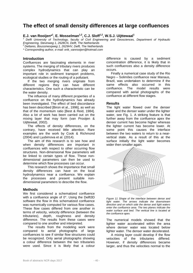
Book of abstracts NCR days 2017 - 40 -
The effect of small density differences at large confluences E.J. van Rooijen*1, E. Mosselman1,2, C.J. Sloff1,2, W.S.J. Uijttewaal1 1 Delft University of Technology, faculty of Civil Engineering and Geosciences, Department of Hydraulic Engineering, Stevinweg 1, 2628CN, Delft, The Netherlands 2 Deltares, Boussinesqweg 1, 2629HV, Delft, The Netherlands * Corresponding author, e-mail: [email protected]
Introduction Confluences are fascinating elements in river systems. The merging of tributary rivers produces complex hydrodynamics that can play an important role in sediment transport problems, ecological studies or the routing of a pollutant.
If the two merging rivers originate from different regions they can have different characteristics. One such a characteristic can be the water density.
The influence of many different properties of a confluence on the hydrodynamics has already been investigated. The effect of bed discordance has been described [Biron et al., 1996], as well as that of the momentum ratio [Best & Reid, 1984]. Also a lot of work has been carried out on the mixing layer that may form (van Prooijen & Uijttewaal, 2002).
The effects of density differences, on the contrary, have received little attention. Rare examples are the work by Cook & Richmond (2004) and Lyubimova et al. (2014).
The aim of this research is to see how and when density differences are important in confluences with respect to other occurring flow structures. Non-dimensional flow parameters will be linked to certain types of flow. These non-dimensional parameters can then be used to determine which flow processes can occur.
This research shows the importance that small density differences can have on the local hydrodynamics near a confluence. We explain the processes and present suitable non-dimensional parameters to describe the flow. Methods We first considered a schematized confluence with a confluence angle of 0°. Using the Delft3D software the flow in this schematized confluence was numerically computed for various flow cases. These flow cases differed from one another in terms of velocity, velocity difference (between the tributaries), depth, roughness and density difference. The results from these cases were compared to one another and interpreted.
The results from the modeling work were compared to aerial photographs of large confluences to see if similar flow structures could be recognized. Only aerial photographs showing a colour difference between the two tributaries were used. Since it is likely that a colour
difference is caused by a sediment concentration difference, it is likely that in such confluences also a density difference occurs.
Finally a numerical case study of the Rio Negro – Solimões confluence near Manaus, Brazil, was undertaken to determine if the same effects also occurred in this confluence. The model results were compared with aerial photographs of the confluence at different flow stages. Results The light water flowed over the denser water and the denser water under the lighter water, see Fig. 1. A striking feature is that further away from the confluence apex the denser current has become higher whereas the lighter current has become lower. At some point this causes the interface between the two waters to return to a near-vertical state. As a result of this at the surface initially the light water becomes wider then smaller again.
Figure 11 Shape of the interface between dense and light water. The arrows indicate the downstream direction and on which side the dense and light waters enter the confluence area. The two planes indicate the water surface and bed. The vertical line is located at the confluence apex. The numerical models showed that the lighter water accelerated within the area where denser water was located below lighter water. The denser water decelerated.
A mixing layer could develop if the flow velocities of the tributaries differed. However, if density differences became larger, and thus the velocities normal to the

Book of abstracts NCR days 2017 - 41 -
main direction of flow became larger, the mixing layer developed less or even not at all. In Fig. 2 a diagram shows the combinations of the non-dimensional parameters for which coherent structures could and could not develop.
Figure 2 Diagram showing combinations of non-dimensional parameters for which coherent structures may or may not occur
All results mentioned above assume that the width of the downstream river was sufficiently large. If dense or light water reached the opposite bank up- or downwelling occurred at the reached bank respectively.
Figure 12 Aerial photograph of the Irrawaddy – Chindwin confluence, 26 October 2009. Source: DigitalGlobe. Arrows indicate flow direction We found several photographs of confluences showing similar flow characteristics as those found in the numerical simulations. Fig. 3 shows the confluence of the Irrawaddy and Chindwin rivers in Myanmar. The movement of the interface at the surface can be explained using the theory derived from this research.
Similar profiles could be discerned on photographs of the Benue – Niger confluence in Nigeria. In an aerial photograph of the confluence of the Rhône and Arve rivers a similar process to the one occurring if the downstream river is rather narrow could be seen.
The numerical model runs of the Rio Negro – Solimões confluence showed similar features as the schematized model runs. The denser water flowed under the lighter water. The amount at which this happened differed for different discharge levels.
Photographs showing a profile at the surface between the lighter and denser water like in Fig. 3 lacked. This is because boils of heavier Solimões water at the Rio Negro side of the river disturbed a clear surface pattern. Since the position of these boils did not change over the years they are likely generated by permanent bed forms. Their appearance at the surface does indicate that heavier water is located below the lighter water.
On several oblique photographs of this confluence the absence of the mixing layer was visible. Sometimes floating foam was located between the two waters, indicating downwelling due to the density differences. Conclusions & recommendations The goal of this research was to identify the effects density differences could have on the flow downstream of a confluence. It is clear that density differences at a confluence affect the hydrodynamics downstream greatly. Even if these density differences are small the effects can be significant and should not be neglected.
Denser water will flow under the lighter water and lighter water over denser water. If these movements are large they hamper the development of the mixing layer.
The effects were validated using aerial photographs of several confluences. Oblique photographs of the Rio Negro – Solimões confluence were in agreement with the results.
This research shows the importance of density differences for the hydrodynamics downstream of a confluence. However many aspects are still unknown and more research into these is recommended. Especially physical model tests could give enlightening results. References Best, J.L., Reid, I., 1984, Seperation Zone at Open-
Channel Junctions, journal of hydraulic engineering 110(11) 1588-1594
Biron, P.M., Best, J.L., Roy, A.G., 1996, Effects of Bed Discordance on Flow Dynamics at Open Channel Confluences, journal of hydraulic engineering 122(12) 676-682
Cook, C.B., Richmond, M.C., 2004, Monitoring and Simulating 3-D Density Currents at the Confluence of the Snake and Clearwater Rivers, Critical Transitions in Water and Environmental Resources Management: pp. 1-9
Lyubimova, T., Lepikhin, A., Konovalov, V., Parshakova, Ya., Tiunov, A., 2014, Formation of the density currents in the zone of confluence of two rivers, Journal of Hydrology 508 328–342
Prooijen, van, B.C., Uijttewaal, W.S.J., 2002, A linear approach for the evolution of coherent structures in shallow mixing layers, Physics Of Fluids, Vol. 14, No. 12

Book of abstracts NCR days 2017 - 42 -
Flow patterns around longitudinal training dams B.W. van Linge*1,2, E. Mosselman1,3, S. van Vuren1,2, G.W.F. Rongen2, W.S.J. Uijttewaal1 1 Delft University of Technology, PO Box 5048, 2600 GA, Delft, the Netherlands 2 HKV Consultants, 8232 AC, Lelystad, The Netherlands 3 Deltares, PO Box 177, 2600 MH, Delft, the Netherlands * Corresponding author; e-mail: [email protected]
Introduction With the intention to reduce the negative effects of ongoing bed erosion, as well as to improve several other river functions such as protection against floods, provision of safe and efficient navigation and ecology, a ‘pilot project longitudinal training dams’ was initiated. The training dams have recently been implemented in the Waal between Tiel and Sind Andries. In this project, river groynes have been completely removed and replaced by dams that lie parallel to the river bank. With help of the longitudinal training dams, a two-channel river system is created in which the river is divided into a main and side channel. The dams are placed in a continuous manner with openings in between that are relatively small compared to the dam length. At the beginning and end of the dam an inlet and outlet region is situated, as shown in Fig. 1.
The combination of inlet and openings allows for water and sediment to be divided between the main and the side channel. Both inlet and openings are constructed with the help of a porous rock-layer. The crest heights can be altered by adding or removing stones. This is expected to influence the amount of water and sediment entering the side channel and can therefore be used as a regulation tool. Motivation The impact of longitudinal training dams on the different river functions is largely influenced by the flow patterns and resulting transport mechanisms of water and sediment between the main and side channel. Extensive research has been conducted on flow patterns and transport mechanisms around groynes (Uijttewaal et al., 2001). However, due to limited experience, similar research on longitudinal training dams is missing. Under the motto ‘learning by doing’, the longitudinal dams were constructed. Better understanding of the impact of regulating the inlet and opening crest heights is expected to improve the design of
river interventions using the concept of longitudinal dams. Also it should result in better regulation strategies such that various river function will be better served. In addition, insights into the flow patterns and transport mechanisms around longitudinal training dams are expected to reduce uncertainties in the modelling of the water and sediment distribution between the channels.
In current hydrodynamical models, such as Waqua and Delft3D, longitudinal training dams are modelled using sub-grid features. However, problems arise in the calculation of sediment transport over weir-like structures (Mosselman, 2001). Secondly, for more fundamental insights these models become difficult to interpret. A simple one-dimensional model could therefore provide quick and useful insights. Methodology A one-dimensional model is used to schematize the two channel system created by longitudinal training dams (schematized as shown in Fig. 1). With the help of a numerical predictor-corrector scheme as shown in Eq. (1), the water levels in both the main and side channel are calculated, where hx and hx+1 are the water level at location x and x+1, dh/dx is the water slope and dx is the space step.
dxdxdh
dxdhhh
corrpredxx )(5.01 +−=+
(1) The discharges over the inlet and openings are modelled using the standard weir equation as shown in Eq. 2, where qw is the weir discharge, CD is the weir coefficient, CS is the submergence coefficient, g is the gravitational acceleration and H is the energy head just upstream of the weir. The porous flow through the inlet and openings is modelled using the general Darcy equation for porous flow as given by Eq. 3, where vporous is the porous flow velocity, k is the permeability and I is the
Figure 1. Schematization of the inlet, openings and outlet at the longitudinal training dams.

Book of abstracts NCR days 2017 - 43 -
Figure 3. Sensitivity of the discharge distribution between the main (red) and side (blue) channel in the different river sections as shown in Figure 1 to (a) inlet crest height, (b) opening crest height and (c) channel width ratio.
hydraulic pressure gradient created by the calculated difference in water level between the two channels.
23SDw Hg2CC
32
q /= (2)
kIvporous = (3) The influence of several parameters on the discharge distribution is calculated, including the inlet crest height, opening crest heights, channel width ratio, river discharge, river bend radius and several other parameters. Basic validation tests of the model have been performed. Results Fig. 2 presents the one-dimensional model results when run with the dimensions of the longitudinal training dam near Wamel in the Waal. The top left plot shows a side view of the calculated water and bed levels in the two channels, the lower left plot the difference in water levels and the right plot a top view with the calculated weir discharges and distribution.
Figure 2. Model results of the one-dimensional model for the longitudinal training dam near Wamel in the Waal.
The influence of several parameters on the discharge distribution between the two channels has been investigated. The results for three parameters are shown in Fig. 3. Fig. 3.a shows that adjusting the inlet crest height between the minimum and maximum height results in considerable changes in the
discharge distribution. Adjusting the opening crest heights does not affect the discharge distribution much (see Fig. 3.b) whereas changes in the channel width ratio, that could for instance be caused by sedimentation of the side channel, does result in considerable changes (see Fig. 3.c). Conclusions The one-dimensional model provides useful insight in the impacts of regulating or adjusting design parameters of the longitudinal training dams. The model has not been validated for an extended range of discharges on the Waal yet. However, preliminary conclusions include: 1. Adjusting the inlet weir height could
influence the discharge distribution towards the side channel between 1% (fully closed but porous inlet) to 30% (fully open inlet).
2. The porous flow through the openings is expected to be negligible compared to the weir flow.
3. The effects of transverse slope and secondary flow in the river bend have a negligible effect on the discharge distribution.
Future work Hereafter, a schematized Delft3D model of the longitudinal dams will be developed in collaboration with another student from Delft University of Technology (Stefan Jammers). The one-dimensional model will be used to determine boundary conditions for different design choices for which the Delft3D model will be used to analyse flow patterns at the inlet and openings in more detail. References Mosselman, E. (2001), Morphological development of side
channels, IRMA-SPONGE and Delft Cluster, Delft. Uittewaal W.J.S., Lehmann D., van Mazijk, A. (2001),
Exchange processes between a riverbend and its groyne fields: model experiments, Journal of Hydraulic Engineering 127(11), 928-936.
(c) (b) (a)

Book of abstracts NCR days 2017 - 44 -

Book of abstracts NCR days 2017 - 45 -
5 – Short-term morphology

Book of abstracts NCR days 2017 - 46 -
Longitudinal training walls: optimization of river width subdivision T.B. Le*1,2, A. Crosato1,3, W.S.J. Uijttewaal1 1 Delft University of Technology, PO Box 5048, 2600 GA Delft, the Netherlands. 2 Thuy Loi University, 175 Tay Son, Dong Da, Hanoi, Vietnam. 3 UNESCO-IHE, Department of Water Engineering, PO Box 3015, 2601 GA, Delft, the Netherlands. * Corresponding author: [email protected]
Introduction Recently, engineers propose longitudinal training walls to replace traditional transverse groynes. This new intervention is expected to maintain a navigation route under low flow conditions while not hampering flow conveyance of the river channel. Navigation occurs mainly in low-land river channels where the formation of alternate bars constitutes a problem which requires mitigation measures like dredging. Le et al. (2015, 2016) found that the starting point of the longitudinal training wall with respect to a steady bar plays an important role on the stability of the bifurcating parallel channels. Starting at a location near the upstream part of the bar leads to side channel silt up. On the contrary, starting at a location near the downstream part of the bar leads to side channel erosion. The most interesting result was that when the longitudinal training wall starts near the bar top, both channels remain open for a long time. However, these results were obtained only for a specific width ratio, ratio between the width of the side and the width of the original channel, B1/B0 = 1/6, under a constant discharge. In practice, the width ratio may vary to obtain specific achievements. Wang et al. (1995) showed that the width ratio plays an important role on the stability of bifurcating channels. So, how the system behaves for different width ratios under variable discharge remains unclear and needs further investigation. Goal of the study This study analyses the long-term morphological effects of dividing a river channel with a longitudinal wall considering different channel width ratios and variable discharge. The preliminary part of the work presented here, however, analyses only the cases with constant discharge. Approach The methodology comprises both numerical simulations and laboratory experiments. The work presented here only deals with numerical simulations, which were carried out by using the Delft3D software.
This study uses the same numerical configuration as Le et al. (2015). To start with, a straight channel with geometrical (width, depth, slope) and morphodynamic (flow and sediment) characteristics is selected to reproduce alternate bars (bar mode m = 1) using Crosato-Mosselman's (2009) formula (Eq. 1).
CQiB
DΔ3bg170m
3
50
2 )(,
−= (1)
Where: m is the bar mode, b is the degree
of non-linearity of the sediment transport as a function of flow velocity, B is the river width, i is the bed slope, ∆ is the sediment relative density, D50 is the sediment mean size, C is the Chézy coefficient and Q is the river discharge.
After successfully obtaining alternate bars, the study considers 3 different starting locations of the longitudinal training wall. Location 1 is at the upstream part of a bar, location 2 near the bar top and location 3 is at the downstream part of a bar (near a pool) (Fig. 1). Starting at one of these locations, the longitudinal training wall is continuous till the end of the computational domain. The distance from the right bank to the wall varies. The following width ratios are considers: B1/B0 = 1/6, 1/3 and 1/2. The overview of the numerical simulations is given in Table 1.
Figure 1. Scenarios studied. Location 1 is at the upstream part of a bar, location 2 near the bar top and location 3 is at the downstream part of a bar (near a pool).

Book of abstracts NCR days 2017 - 47 -
Table 1. Overview of the simulations. Notation X is number 1, 2 and 3 represent locations of the upstream termination of the longitudinal training wall, depicted in Fig. 1. Run Scenario Simulation Description 1 Starting with a
flat bed Run0 Reference case
2, 3, 4 Starting with fully-developed hybrid alternate bars
Run1_X B1/B0 = 1/6 5, 6, 7 Run2_X B1/B0 = 1/3
8, 9, 10 Run3_X B1/B0 = 1/2
Preliminary results Regardless of width ratio, the starting location of the training wall plays an important role in the morphodynamic evolution of the parallel channels. Fig. 2 shows the evolution of the discharge ratio between side channel and original channel with time. In this figure, Q1/Q0=0 means that the side channel silts up, while Q1/Q0=1 means that the side channel conveys all water and the main channel silts up. Three situations can be distinguished: if the training wall starts at upstream part of a bar, all lines representing the discharge ratio finally go to zero (blue lines). When the training wall starts at the downstream part of a bar, all lines eventually approach the value of 1 (red lines). When the training wall starts near the bar top, all lines become horizontal at a value of discharge ratio between 0.5 and 0.2.
This means that if the training wall starts at the upstream part of a bar, the side channel eventually silts up completely, and this happens for all width ratios (Q1/Q0=0, blue lines). For the largest width ratio ( B1/B0=1/2), in which the channels have the same width, the silting up process takes a longer time to finish (continuous blue line).
Instead, if the training wall starts at the downstream part of a bar, the side channel eventually conveys more than 90% of the discharge, and this happens for all width ratios (red lines). For B1/B0=1/6, the process becomes extreme, because the side channel is found to eventually convey all water (Q1/Q0=1, dash red line). This means that the main channel silts up. For larger width ratios, a conveyance of more than 95% still means that both channels remain open, although with different bed levels.
When the training wall starts near the bar top, both channels remain open (black lines). If the two channels have the same width, one of the two conveys much more water than the other one, but the difference between the two channels is less marked.
Figure 2. Discharge ratio between side channel and original channel. Blue lines are training wall starting at upstream part, red lines are at downstream part, and black lines are near the bar top. Preliminary conclusions In this study, the subdivision of river channels with alternate bars in two parallel channels by means of a longitudinal training wall always results in a deeper and a shallower channel. However, the evolution depends on the starting location of the longitudinal training wall with respect to a bar. Moreover, when the width of the side channel increases, the two channels are likely to remain both open. On other words, a larger side channel seems to produce a more stable system than a relatively narrow one. Future works These preliminary simulations will be followed by simulations studying the effects of a variable discharge regime and by experiments in the laboratory of Fluid Mechanics of TU Delft. References Crosato, A. and E. Mosselman (2009), Simple physics-
based predictor for the number of river bars and the transition between meandering and braiding, Water Resour. Res., 45, W03424, doi: 10.1029/2008WR007242.
Le T.B., Crosato, A., Uijttewaal, W.S.J. (2015). Long term effects of longitudinal training wall: a numerical study. IAHR world congress 07/2015. The Hague, The Netherlands.
Le T.B., Crosato, A., Uijttewaal, W.S.J. (2016). Experimental study on the effects of longitudinal training walls. River Flow 2016. Constantinescu, Garcia & Hanes (Eds). © 2016 Taylor & Francis Group, London, ISBN 978-1-138-02913-2.
Wang, Z.B., R.J. Fokkink, M. de Vries, and A. Langerak (1995), Stability of river bifurcations in 1D morphodynamic models. J. Hydraul. Res., 33(6), 739-750.
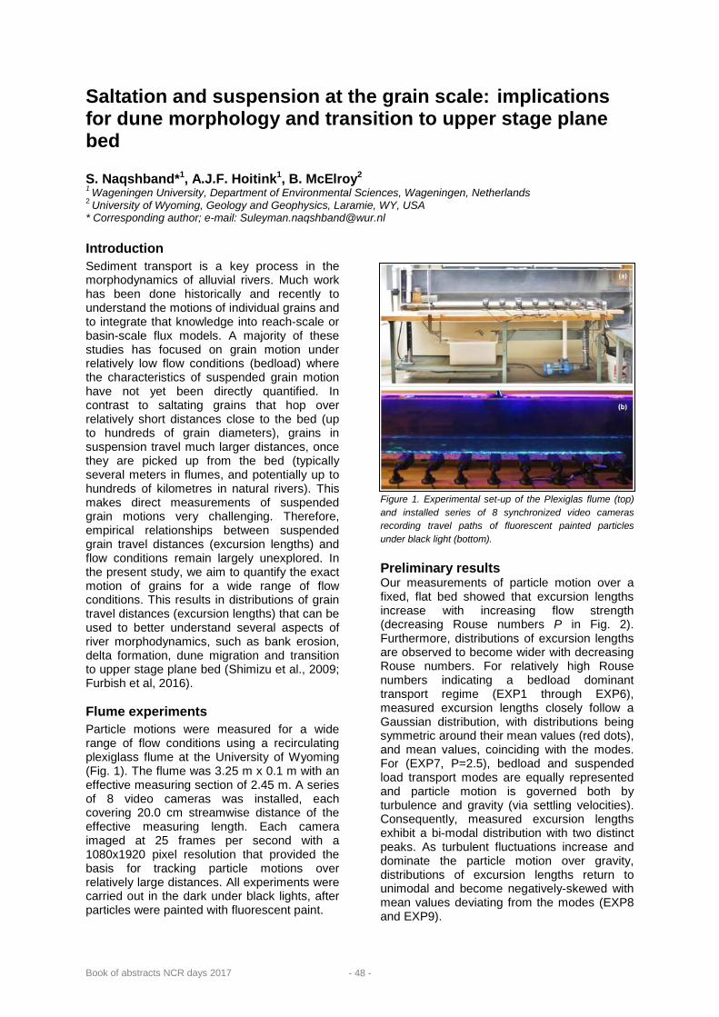
Book of abstracts NCR days 2017 - 48 -
Saltation and suspension at the grain scale: implications for dune morphology and transition to upper stage plane bed S. Naqshband*1, A.J.F. Hoitink1, B. McElroy2 1 Wageningen University, Department of Environmental Sciences, Wageningen, Netherlands 2 University of Wyoming, Geology and Geophysics, Laramie, WY, USA * Corresponding author; e-mail: [email protected] Introduction Sediment transport is a key process in the morphodynamics of alluvial rivers. Much work has been done historically and recently to understand the motions of individual grains and to integrate that knowledge into reach-scale or basin-scale flux models. A majority of these studies has focused on grain motion under relatively low flow conditions (bedload) where the characteristics of suspended grain motion have not yet been directly quantified. In contrast to saltating grains that hop over relatively short distances close to the bed (up to hundreds of grain diameters), grains in suspension travel much larger distances, once they are picked up from the bed (typically several meters in flumes, and potentially up to hundreds of kilometres in natural rivers). This makes direct measurements of suspended grain motions very challenging. Therefore, empirical relationships between suspended grain travel distances (excursion lengths) and flow conditions remain largely unexplored. In the present study, we aim to quantify the exact motion of grains for a wide range of flow conditions. This results in distributions of grain travel distances (excursion lengths) that can be used to better understand several aspects of river morphodynamics, such as bank erosion, delta formation, dune migration and transition to upper stage plane bed (Shimizu et al., 2009; Furbish et al, 2016). Flume experiments Particle motions were measured for a wide range of flow conditions using a recirculating plexiglass flume at the University of Wyoming (Fig. 1). The flume was 3.25 m x 0.1 m with an effective measuring section of 2.45 m. A series of 8 video cameras was installed, each covering 20.0 cm streamwise distance of the effective measuring length. Each camera imaged at 25 frames per second with a 1080x1920 pixel resolution that provided the basis for tracking particle motions over relatively large distances. All experiments were carried out in the dark under black lights, after particles were painted with fluorescent paint.
Figure 1. Experimental set-up of the Plexiglas flume (top) and installed series of 8 synchronized video cameras recording travel paths of fluorescent painted particles under black light (bottom). Preliminary results Our measurements of particle motion over a fixed, flat bed showed that excursion lengths increase with increasing flow strength (decreasing Rouse numbers P in Fig. 2). Furthermore, distributions of excursion lengths are observed to become wider with decreasing Rouse numbers. For relatively high Rouse numbers indicating a bedload dominant transport regime (EXP1 through EXP6), measured excursion lengths closely follow a Gaussian distribution, with distributions being symmetric around their mean values (red dots), and mean values, coinciding with the modes. For (EXP7, P=2.5), bedload and suspended load transport modes are equally represented and particle motion is governed both by turbulence and gravity (via settling velocities). Consequently, measured excursion lengths exhibit a bi-modal distribution with two distinct peaks. As turbulent fluctuations increase and dominate the particle motion over gravity, distributions of excursion lengths return to unimodal and become negatively-skewed with mean values deviating from the modes (EXP8 and EXP9).

Book of abstracts NCR days 2017 - 49 -
Figure 2. Kernel probability density functions of measured excursion lengths l* for different experiments with P the Rouse number (Naqshband et al., under review) Future research & application For modelling many unsteady morphodynamic problems knowledge of mean particle motion and travel lengths are required, as is information about the distribution of particle lengths. An examples is the class of models describing the growth and instability of bedforms, in particular regime transition from dune to upper stage plane bed [e.g., Nelson et al., 2011; Van Duin, 2015]. Non-equilibrium sediment transport is modelled within these studies by entrainment and deposition functions related to each other through a lag distance. This lag is a function of mean particle travel length and is set constant for a certain flow condition. Because information about the variation of particle travel lengths as a function of flow strength is not available, and in particular this is the case for relatively high flow conditions that are associated with substantial suspension and bedform instability, particle travel lengths have been assumed to increase linearly with increasing flow strength. As a result, a train of bedforms is modelled with similar wavelengths and natural variation in bedform scale is hardly observed. In addition, lag distances are chosen such that desired morphodynamic changes are achieved without actual details of the physical mechanisms governing particle motion and travel lengths. Measured distributions of particle excursion lengths in the present study can be used within this class of models to obtain – for a certain flow condition – distributions of lag distances between particle entrainment and deposition. This approach will allow natural variations in modelled bedform scales based on actual distributions of particle travel lengths. Furthermore, additional experiments will be carried out over mobile beds (Fig. 3) to quantify the distribution of particle travel distances and other characteristics of particle motion (e.g. particle velocity and acceleration, and particle
diffusion) to better understand bedform morphodynamics and the associated roughness to the flow.
Figure 3. Experimental set-up of a mobile dune regime with fluorescent painted sand particles under black light. Another challenge is to quantify and understand the mechanisms that give rise to the observed differences in dune morphology and dune transition under flume and field conditions (e.g. Naqshband et al., 2014). Recently, Vermeulen et al. (2014) used polystyrene granulates as a surrogate for sand to properly scale Shields parameter without compromising the Froude number. They were able to reproduce bedforms in a flume that showed similar geometrical properties as observed in the field. Whether using polystyrene granulates results in proper scaling of dune transition to upper stage plane bed still needs to be investigated. References Furbish, D. J., M. W. Schmeeckle, R. Schumer, and S. L.
Fathel (2016), Probability distributions of bed load particle velocities, accelerations, hop distances, and travel times informed by Jaynes's principle of maximum entropy, J. Geophys. Res. Earth Surf., 121, 1373–1390, doi:10.1002/2016JF003833.
Naqshband S., J. S. Ribberink, and S. J. M. H. Hulscher (2014), Using both free surface effect and sediment transport mode parameters in defining the morphology of river dunes and their evolution to upper stage plane beds, J. of Hydrauli. Eng., 140(6), 06014010. 10.1061/(ASCE)HY.1943-7900.0000873.
Naqshband, S., McElroy, B. and Mahon, R.M (under review). Validating a universal model of particle transport lengths with laboratory measurements of suspended grain motions.
Nelson, J. M., B. L. Logan, P. J. Kinzel, Y. Shimizu, S. Giri, R. L. Shreve, and S. R. McLean (2011), Bedform response to flow variability, Earth. Surf. Landforms, 36 (14), 1938-1947.
Van Duin, O.J.M. (2015), Sediment transport processes in dune morphology and the transition to upper-plane stage bed, PhD Thesis, University of Twente, Enschede, The Netherlands.
Vermeulen, B., M.P. Boersema, A.J.F. Hoitink, J. Sieben, C.J. Sloff & M. Van der Wal 2014. River scale model of a training dam using lightweight granulates. Journal of Hydro-environment Research, 8(2), pp.88–94
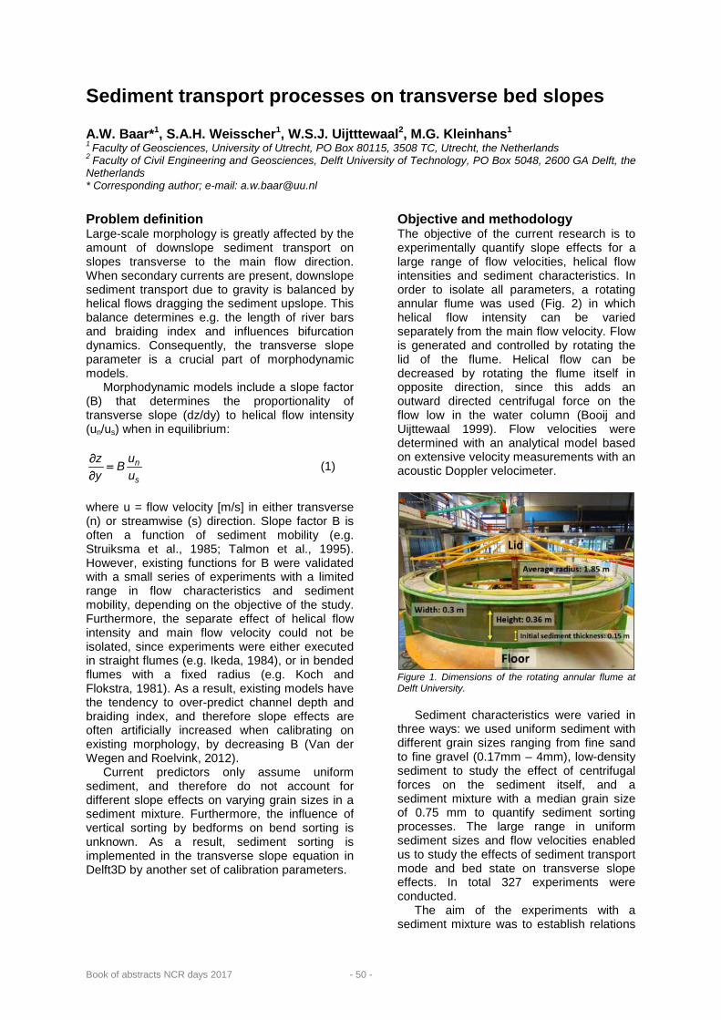
Book of abstracts NCR days 2017 - 50 -
Sediment transport processes on transverse bed slopes A.W. Baar*1, S.A.H. Weisscher1, W.S.J. Uijtttewaal2, M.G. Kleinhans1 1 Faculty of Geosciences, University of Utrecht, PO Box 80115, 3508 TC, Utrecht, the Netherlands 2 Faculty of Civil Engineering and Geosciences, Delft University of Technology, PO Box 5048, 2600 GA Delft, the Netherlands * Corresponding author; e-mail: [email protected]
Problem definition Large-scale morphology is greatly affected by the amount of downslope sediment transport on slopes transverse to the main flow direction. When secondary currents are present, downslope sediment transport due to gravity is balanced by helical flows dragging the sediment upslope. This balance determines e.g. the length of river bars and braiding index and influences bifurcation dynamics. Consequently, the transverse slope parameter is a crucial part of morphodynamic models.
Morphodynamic models include a slope factor (B) that determines the proportionality of transverse slope (dz/dy) to helical flow intensity (un/us) when in equilibrium:
s
n
uuB
yz
=∂∂ (1)
where u = flow velocity [m/s] in either transverse (n) or streamwise (s) direction. Slope factor B is often a function of sediment mobility (e.g. Struiksma et al., 1985; Talmon et al., 1995). However, existing functions for B were validated with a small series of experiments with a limited range in flow characteristics and sediment mobility, depending on the objective of the study. Furthermore, the separate effect of helical flow intensity and main flow velocity could not be isolated, since experiments were either executed in straight flumes (e.g. Ikeda, 1984), or in bended flumes with a fixed radius (e.g. Koch and Flokstra, 1981). As a result, existing models have the tendency to over-predict channel depth and braiding index, and therefore slope effects are often artificially increased when calibrating on existing morphology, by decreasing B (Van der Wegen and Roelvink, 2012).
Current predictors only assume uniform sediment, and therefore do not account for different slope effects on varying grain sizes in a sediment mixture. Furthermore, the influence of vertical sorting by bedforms on bend sorting is unknown. As a result, sediment sorting is implemented in the transverse slope equation in Delft3D by another set of calibration parameters.
Objective and methodology The objective of the current research is to experimentally quantify slope effects for a large range of flow velocities, helical flow intensities and sediment characteristics. In order to isolate all parameters, a rotating annular flume was used (Fig. 2) in which helical flow intensity can be varied separately from the main flow velocity. Flow is generated and controlled by rotating the lid of the flume. Helical flow can be decreased by rotating the flume itself in opposite direction, since this adds an outward directed centrifugal force on the flow low in the water column (Booij and Uijttewaal 1999). Flow velocities were determined with an analytical model based on extensive velocity measurements with an acoustic Doppler velocimeter.
Figure 1. Dimensions of the rotating annular flume at Delft University.
Sediment characteristics were varied in three ways: we used uniform sediment with different grain sizes ranging from fine sand to fine gravel (0.17mm – 4mm), low-density sediment to study the effect of centrifugal forces on the sediment itself, and a sediment mixture with a median grain size of 0.75 mm to quantify sediment sorting processes. The large range in uniform sediment sizes and flow velocities enabled us to study the effects of sediment transport mode and bed state on transverse slope effects. In total 327 experiments were conducted.
The aim of the experiments with a sediment mixture was to establish relations

Book of abstracts NCR days 2017 - 51 -
of sediment sorting along a cross-section as a function of transverse slope and sediment mobility, in order to determine the sedimentological and morphodynamic response to bend flow. To this end, in total 340 sediment samples of 13 experiments with varying helical flow intensity and sediment mobility were analyzed. Results: uniform sediment The equilibrium transverse slopes in the experiments with uniform sediment show a clear trend with sediment mobility and helical flow intensity. However, this trend is not a linear relation with a power function of sediment mobility, as existing predictors suggest, but are strongly influenced by bed state and sediment transport mode. For fine sand we obtained bed states from a lower plain bed, across the ripple-dune threshold and up to an upper plane bed. During the experiments with coarse sand and fine gravel, dunes developed with varying dimensions depending on the flow conditions. Therefore, the resulting trend in slope factor differs for fine sediments and coarse sediments. Surprisingly, resulting slope factors are generally comparable or higher than suggested in literature (Fig.2). A higher slope factor implies less downslope sediment transport (Eq. 1), which is in contrast with the tendency to increase slope effects in current morphodynamic models.
Figure 2. Range in slope factor of the experiments with fine and coarse sediments, compared with existing predictors that include a ratio of sediment mobility (θ) to critical sediment mobility (θc). Results: poorly sorted sediment Results of the experiments with a sediment mixture showed that mild slopes caused a gradual transition of fine sand at the inner bend to coarse sand in the outer bend. At slopes steeper than 0.15, a sharper transition was observed and all coarse sediment was located at the outer bend. Experiments with high sediment mobility resulted in higher dunes, which caused more vertical sorting and somewhat reduced the pronounced lateral sorting (Fig.3).
Figure 3. Fraction of grain sizes at several locations along the cross-section relative to flume radius (r/rc), for experiments with high and low transverse slopes, and high and low sediment mobility. Conclusions We experimentally tested the effect of a large range in helical flow intensity and sediment mobility on equilibrium transverse slopes, which resulted in a function for slope effects depending on bed state and sediment transport mode, that deviates from linear functions with sediment mobility in literature. Furthermore, we obtained basic relations for sorting patterns as a function of transverse slope and sediment mobility. References Booij, R., Uijttewaal, W.S.J. (1999) Modeling of the flow
in rotating annular flumes. Engineering Turbulence Modeling and Experiments, 4:339–348.
Ikeda, S. (1984). Closure to “Lateral Bed Load Transport on Side Slopes” by Syunsuke Ikeda (November, 1982). Journal of Hydraulic Engineering, 110(2):200-203
Koch, F. G., Flokstra, C. (1980). Bed Level Computations for Curved Alluvial Channels: Prepared for the 19th IAHR Congress, New Delhi, India, February 1981. Waterloopkundig Laboratorium
Sloff, K., Mosselman, E. (2012). Bifurcation modelling in a meandering gravel–sand bed river. Earth Surface Processes and Landforms, 37(14):1556-1566.
Struiksma, N., Olesen, K. W., Flokstra, C., De Vriend, H. J. (1985). Bed deformation in curved alluvial chan-nels. Journal of Hydraulic Research, 23(1): 57-79.
Talmon, A. M., Struiksma, N., Van Mierlo, M. C. L. M. (1995). Laboratory measurements of the direction of sediment transport on transverse alluvial-bed slopes. Journal of Hydraulic Research, 33(4):495-517.
Van der Wegen, M., Roelvink, J. A. (2012). Reproduction of estuarine bathymetry by means of a process-based model: Western Scheldt case study, the Netherlands. Geomorphology, 179:1

Book of abstracts NCR days 2017 - 52 -
Upper stage plane bed in the Netherlands R.J. Daggenvoorde*1,2, J.J. Warmink1, K. Vermeer2, S.J.M.H. Hulscher1 1 University of Twente, Faculty of Engineering Technology, Group Water Engineering and Management, PO Box 217, Enschede The Netherlands 2 HKV Consultants, PO Box 2120, 8203AC Lelystad, the Netherlands * Corresponding author; e-mail: [email protected]
Introduction Upper stage plane bed (USPB) is a river bed form where no dunes or ripples are present on the river bed. The presence of USPB results in a lower roughness, which can lead to a reduction of 0.5 m in water level under design conditions (Van Duin, 2015). It is suspected that USPB might have been present in the Meuse near Heusden (Adriaanse, 1986), however it is still unknown whether USPB can develop under design discharge in the Netherlands. This study aims to find out whether and where USPB may occur under design conditions in the Netherlands. Method To find out whether USPB can occur in the Netherlands two analyses are performed. The first analysis uses flow and sediment characteristics to calculate Froude and Suspension numbers along the Dutch river system (Eq. 1 & 2).
uFrgh
= (1)
*
s
uSuspension numberw
= (2)
Where; u is the flow velocity; g is the gravitational acceleration; h is the water depth; u* is the shear velocity and ws is the fall velocity. The flow characteristics are obtained from a WAQUA-simulation with a discharge of 16,000 m3/s at Lobith. The sediment characteristics are obtained from measurements performed by RWS (Ten Brinke, 1997).
In order to determine the most probable location for USPB we introduce the USPB-index. This index is a dimensionless indicator which allows the comparison of different locations on their probability to develop USPB, however it does not represent a quantified chance on the occurrence of USPB. The USPB-index is computed as the shortest dimensional distance to the dashed line in Fig. 1. The indices are determined for every location in the Rhine branches and the Meuse with an interval of 20 meters. Values above the
dashed in line in Fig. 1. are formulated as negative values, this allows to state that the location with the lowest USPB-index is the most-USPB-probable location.
Figure 1. Observed bed forms with Froude and Suspension numbers (Naqshband et al., 2014a).
The second analysis incorporates the dynamic behaviour of dune development, using the morphodynamic model of Van Duin et al. (2017). Firstly, the model is calibrated upon observed equilibrium dune heights in flume conditions (Coleman et al., 2005; Naqshband et al., 2014b). Secondly, the model is calibrated upon river scale with observed dune heights in the Waal in 2002 and 2003 (Sieben, 2004). This second calibration is performed on the observed dune heights, by adapting the coefficients that influence the eddy viscosity and partial slip (beta-coefficients). Because there are no observations of USPB, the dashed line in Fig. 1 is used to calibrate the moment of the transition to USPB.
The re-calibrated model of Van Duin (2017) is then applied to the location with the lowest USPB-index. The design discharge wave of 16,000 m3/s is used to create conditions which are most-likely to develop USPB. Results USPB-index The IJssel just upstream of Kampen (river kilometre 994) was found to be the most probable location for USPB. The USPB-index was above zero (0.03), which means in the dune regime in Fig. 1, so it is expected that dunes will be present. Fig. 2 shows the USPB-indices along the IJssel mouth near Kampen.

Book of abstracts NCR days 2017 - 53 -
Figure 2. USPB-indices in the IJssel river near Kampen. Results of the calibrations for field conditions Adapting the step-length-model gave good results for flume conditions (Nash-Sutcliff=0.7) and adapting the beta-coefficients to 0.245 gave reasonable results for the calibration for field conditions (NS=0.3). The simulated water depths were in range with the observations. These results were considered sufficiently accurate to have confidence in the model to predict if USPB conditions can be achieved. Upper Stage Plane Bed development under the design discharge The fully calibrated model was applied for the IJssel near Kampen. The simulated dune heights during the design discharge wave show that USPB starts to develop during day 6 (Fig. 3). This suggests that USPB can develop in the IJssel just upstream of Kampen. The second most probable location (river Waal near Tiel) did not show development of USPB.
Figure 3. Dune height evolution during the design unit discharge wave at the IJssel near Kampen Discussion The model predicts USPB where the USPB-index does not. This difference may be caused by the model application on river scale and by the uncertain roughness in the WAQUA-simulation. The model on the river scale is applied on the middle of the river while the dashed line in Fig. 1 is based upon width-averaged observations. The width-averaged
conditions required to develop USPB are higher than the conditions required in the middle of the river. The WAQUA-simulation uses the bed roughness to calibrate; this means the expected depth-discharge relation determines the bed roughness. Hence, the bed is simulated as dunes, while in the model of Van Duin (2015) the bed is dynamic allowing it to become a plane bed, resulting in other flow conditions.
The IJssel upstream of Kampen is the only assessed location found where USPB can develop according to the model and the most likely location according to the USPB-index. A detailed analysis showed that the small grain size at this location (D50 = 0.25 mm) is the main reason for USPB to develop. Therefore, USPB in the Dutch rivers is probably most likely when small grain sizes are present. Conclusion According to the model-analysis performed in this study the IJssel near Kampen may develop USPB under a design discharge wave. The dune evolution model of Van Duin et al. (2017) is applied upon a river scale and is shown to be able to predict dune heights and realistic hydrodynamic conditions. Also the exploratory analysis with the newly developed USPB-index indicated that this location is the most likely to develop USPB. Other locations scored higher on the USPB-index, indicating that USPB is less likely to develop, the dune evolution model showed that the second most probable location does not develop USPB. References Adriaanse, M. (1986). De ruwheid van de Bergsche Maas
bij hoge afvoeren, RIZA report 86.19. Dordrecht, The Netherlands.
Coleman, S. E., Zhang, M. H., & Clunie, T. (2005). Sediment-wave development in subcritical water flow. Journal of Hydraulic Engineering, 131(2), 106-111.
Naqshband, S., Ribberink, J. S., & Hulscher, S. J. M. H. (2014a). Using Both Free Surface Effect and Sediment Transport Mode Parameters in Defining the Morphology of River Dunes and Their Evolution to Upper Stage Plane Beds. Journal of Hydraulic Engineering, 140(6).
Naqshband, S., Ribberink, J. S., Hurther, D., & Hulscher, S. J. M. H. (2014b). Bed load and suspended load contributions to migrating sand dunes in equilibrium. Journal of Geophysical Research: Earth Surface, 119(5).
Sieben, J. (2004). Characterization of bed levels with statistical equivalency. Paper presented at the MARID2004, Enschede, the Netherlands.
Ten Brinke, W. B. M. (1997) De Bodemsamenstelling van Waal en IJssel in de jaren 1966, 1976, 1984 en 1995, RIZA report 97.009. Lelystad, The Netherlands.
Van Duin, O. J. M. (2015). Sediment transport processes in dune morphology and the transition to upper-stage plane bed, PhD Thesis. Enschede. The Netherlands
Van Duin, O., Hulscher S.J.M.H., Ribberink, J.S., Dohmen-Janssen, C.M., (2017), Modelling of spatial lag in sediment transport processes and its effect on dune morphology. Journal of hydraulic engineering, pp 04016084-1 04016084-12 (in press).

Book of abstracts NCR days 2017 - 54 -

Book of abstracts NCR days 2017 - 55 -
6 – River management

Book of abstracts NCR days 2017 - 56 -
Flood risk Guayaquil J.G. Stenfert1, R.M. Rubaij Bouman*1, R.C. Tutein Nolthenius1, S. Joosten1 1 Delft University of Technology, Department of Hydraulic Engineering, Faculty of Civil Engineering, Delft, The Netherlands * Corresponding author; e-mail: [email protected]
Introduction Due to climate change more severe weather conditions might be present in the future in large parts of the world (IPCC, 2013) (Cai et al., 2014). In Ecuador, the city of Guayaquil urbanized rapidly without proper planning. Therefore, the city exerts a lot of pressure on its surroundings. Nowadays, the city suffers from floods due to high precipitation rates and high water levels within the sea branches and at the Guayas river. The question is how to respond on these higher risks. Current analyses about the flooding of Guayaquil are often very pragmatic in terms of finding solutions for flood safety. Unfortunately, there is still a lack of elementary insight of the total hydrological and hydrodynamic system of Guayaquil. In that regard, an overall analysis will be executed on inundations and the following questions will be addressed: • What are the critical points within the
hydrological and hydrodynamic system of Guayaquil?
• What measures should be taken to sufficiently decrease societal risk by floods in the future?
• What are the influences of changing weather conditions?
Approach and Methodology To fully understand the processes in the area of study the total system has been analysed by means of a literature review. Amongst others, the location, topography, current state of flood defences, climate and hydrological and hydraulic conditions of the city are considered. Both GIS modelling and Delft3D-FM are used to obtain more information on the Guayas Estuary. Furthermore, different stakeholders are addressed. Last, identification and evaluations of possible measures are made. Results The Babahoyo and Daule river confluence in front of Guayaquil into the Guayas river. The convergence of the Gulf of Guayas makes this a tidal river with a spring tidal amplitude of 2 meter. With an average sea level rise of 6 mm per year (Miller, 2009), friction in the channel reduces which causes the amplitude to rise in the future (Fig. 1).
Figure 1: Tidal asymmetry elevation due to sea level rise Guayaquil is situated on the eastern side of the Pacific and is therefore directly influenced by the El Niño phenomenon. This causes the peak rainfalls during the wet season to increase even more leading to rainfall events of over 100 mm/day (INOCAR, 2016). The often high water levels in the river cause blockage of the current drainage system of the city. This in combination with a high run off and hardly any unpaved surface within the city causes inundations.
The rapid expansions of the city causes pressure on the sea branches and the Guayas river. Arc-GIS and Delft3D-FM where used to model different future scenario’s. Water levels from 3.5 to 4.1 meter above mean sea level were implemented. With Arc-GIS it was concluded that the sea branches are the weakest spot when high water is present. Over 50 km2 will be flooded when a water level of +4.1 m MSL is occurs (Fig. 2).
Figure 2: Flooded areas due to sea level rise From a political point of view the public services considering drainage are established in national planning by law by SENAGUA. Although this might sound promising, some conflicts seem to arise. The prefecture of the Guayas province and the municipality of Guayaquil do not work closely together due to

Book of abstracts NCR days 2017 - 57 -
political disagreements. In addition, flood mitigation is not a very popular topic in the political agenda. This leads to a lack of long term policy and future perspective on city planning which might cause more frequently problems. Possible measures Measures regarding the stormwater system as well as flood defence measures are considered. To reduce the run-off local collection of water might be considered. This could be obtained by large storage areas within the city or locally such as rooftops in combination with gutters. Another measure is the creation of more permeable pavement leading to an increase of infiltration and thereby temporary storage without the subsoil. The stormwater system by itself can be improved by implementing check valves at the end of the pipes. Because future discharge peaks might increase due to more extreme weather conditions, the capacity of the system has to be increased.
Protecting the city against high water levels in the sea branches is of importance nowadays. Therefore, a system of barriers and levees around the southern stretch of Guayaquil was designed. These barriers close during low tide (when high water is expected) and in this way the sea branches can function as temporary storage basins for rainwater. It is important to notice that in the coming years the river Guayas will not cause major floods and therefore no extra measures are necessary here. Conclusion The societal risk of floods in Guayaquil will increase in the near future. Due to sea level rise floods become more likely to happen adjacent to the sea branches. Nowadays, areas along the sea branches are flooded when high tide is present. More severe weather conditions may cause floods within the city due to the lack of a proper stormwater system. Several parts of the city are subject to different natural hazards, making an integral solution on reducing probabilities of failure necessary.
Most proposed solutions by local institutions will not solve short term problems and
sometimes even will not solve the problem at all on the long term. The possible measures could be divided into currently required and future measures. The required measures consider the short term problems which includes the protection of the city against flooding caused by precipitation. In addition, high tides cause floods within the southern part of Guayaquil. Constructing levees along the sea branches should increase the flood safety within this area.
Future measures are proposed to prevent inundations due to sea level rise or the increasing severity of weather conditions in the future. Recommendations First of all, it is advised that measures should be taken for improvement of the stormwater system and for flood defence in the southern part of Guayaquil. It is advised to introduce the following minor adjustments in the system on a short term: • Installing check valves on drainage outlets. • Implementing permeable pavement during
road maintenance and construction. • Using gutters and temporary storage at
houses. To achieve a proper flood defense a strategy on a nationwide level considering flood defenses might be useful. Controlling this on a national level could enhance the cooperation between municipalities and provinces. The relation between the parties of interest in the cooperation and comprehension of all parties, has to be improved. References Cai, W., Borlace, S., Lengaigne, M., van Rensch, P.,
Collins, M., Vecchi, G., Timmermann, A., Santoso, A., McPhaden, M., Wu, L., England, M., Wang, G., Guilyardi, E., and Jin, F.-F. (2014). Increasing frequency of extreme El Ni~no events due to greenhouse warming.
INOCAR (2016). Precipitation en guayaquil. http://www.inocar.mil.ec/web/index.php/precipitacion-en-guayaquil., Last accessed : Sep. 2016.
IPCC (2013). Climate change 2013: the physical science basis contribution of working group I to fifth assessment report of the intergovernmental panel on climate change. Chapter summary for policymakers. Cambridge University Press.
Miller, K. (2009). Land under Siege: Recent Variations in Sea Level through the Americas.

Book of abstracts NCR days 2017 - 58 -
Discharge validation of 1D/2D models of the Rhine-Meuse delta using ADCP measurements Remi M. van der Wijk*1, Asako Fujisaki1, Jurjen de Jong1, Aukje Spruyt1 1 Deltares, Inland Water Systems, Department of River Engineering and Inland Shipping, P.O. Box 177, 2600 MH, Delft, The Netherlands * Corresponding author; e-mail: [email protected]
Introduction In general hydraulic models require some level of validation or calibration. The models of Rijkswaterstaat of the Rhine-Meuse delta are usually validated on water level data and salinity concentrations (Zijl et al., 2011). There is not much known about the quality of the discharge computation in 1D and 2D models of Rijkswaterstaat. In the Rhine-Meuse delta (Fig. 1) processes like morphological development (Becker, 2015) and salt distribution (Kranenburg & Schueder, 2015) are directly affected by the discharge distribution. It is therefore vital to confirm the quality of the discharge reproduction on the bifurcations in the Rhine-Meuse delta (Zijl et al., 2014) in order to use these models soundly for applications like salt distribution.
The objective of the research was to validate the 1D SOBEK3 and 2D WAQUA models of the Rhine-Meuse delta (van der Wijk & Fujisaki, 2016). In order to validate the models a method had to be developed to quantify the quality of the discharge reproduction.
If the models are simulating the discharge correctly, it might be possible to create discharge distribution figures that give an understanding of the hydrodynamics of the Rhine-Meuse delta. With a better understanding of the hydrodynamics we are better suited to study long term processes in the Rhine-Meuse delta using these models.
Figure 1. River branches in the Rhine-Meuse delta
Methodology The first step in the research was to find the correct set of data to validate the models. The discharge measurements were chosen to represent different conditions at a sufficient
amount of bifurcations. Eventually two campaigns with discharge measurements were marked as suitable: • A campaign from 2003 that represents
average river discharge conditions along the Oude Maas;
• A campaign from 2011 that represents low river discharge conditions in the whole Rhine-Meuse delta.
For both campaigns the boundary conditions of the models were provided by Rijkswaterstaat and Waterschap Aa en Maas.
The discharge measurements alone are not sufficient to understand the quality of the discharge computation in the model. A large error in the reproduction of water levels could explain the inaccuracy in the reproduction of the discharge. Therefore water level measurements were obtained via the DONAR database.
Recent studies on the reproduction of the discharge in the Rhine-Meuse delta used a 3D model (Kranenburg & Schueder, 2015; Verbeek, 2015). Furthermore, the validation focussed mainly on salinity profiles. The reproduction of the discharge was based on visual inspection. It was therefore necessary to use a different methodology than these studies.
In order to quantify the reproduction over the whole tidal period the statistical bias of the discharge error could be used. However, the bias can be larger with higher discharges while the error is relatively small. It was desirable to ensure that the magnitude of the bias could be coupled to the magnitude of the discharge. This was done by expressing the bias relative to the absolute maximum and minimum discharge. Furthermore, the difference in minimum and maximum discharge was assessed.
The assessed parameters give an objective overview of the quality of the discharge reproduction. However, a visual comparison is still needed to ensure a complete overview of the trends of both the observed and simulated data.
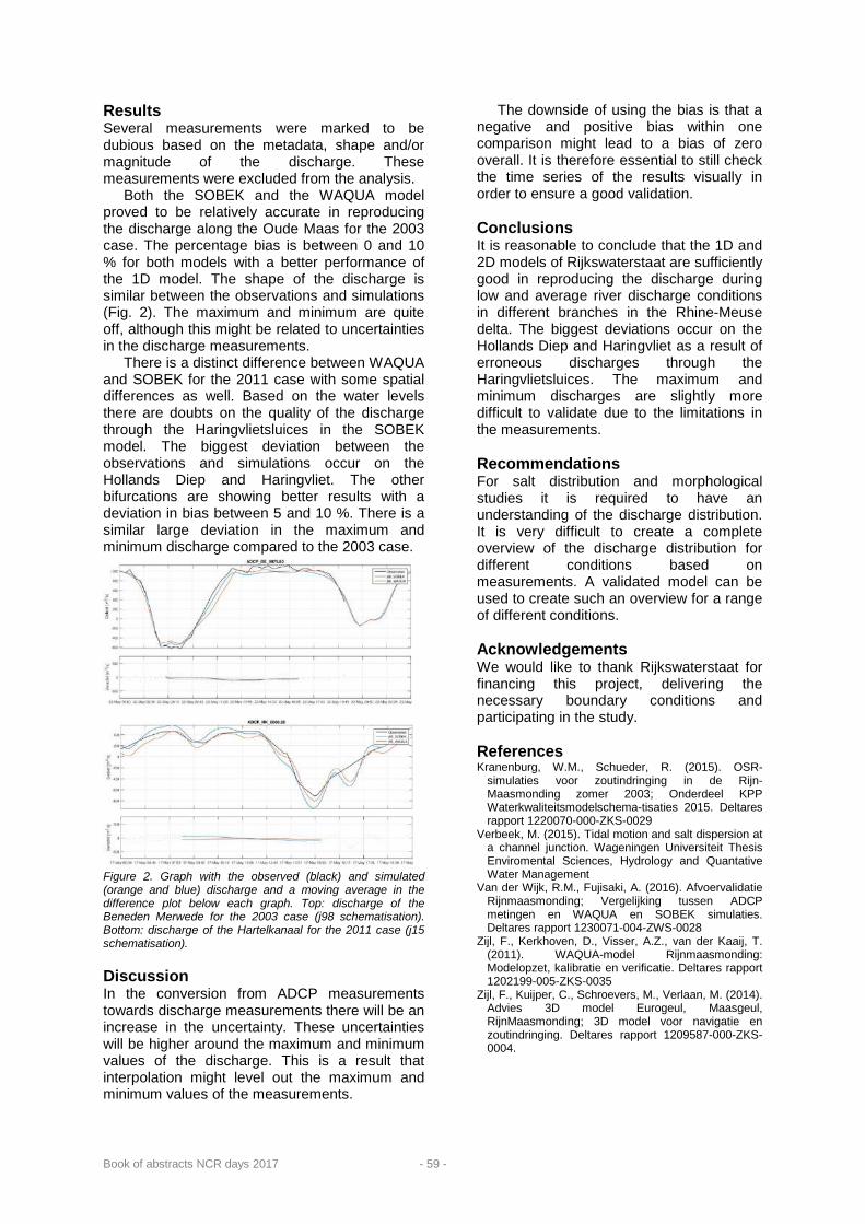
Book of abstracts NCR days 2017 - 59 -
Results Several measurements were marked to be dubious based on the metadata, shape and/or magnitude of the discharge. These measurements were excluded from the analysis.
Both the SOBEK and the WAQUA model proved to be relatively accurate in reproducing the discharge along the Oude Maas for the 2003 case. The percentage bias is between 0 and 10 % for both models with a better performance of the 1D model. The shape of the discharge is similar between the observations and simulations (Fig. 2). The maximum and minimum are quite off, although this might be related to uncertainties in the discharge measurements.
There is a distinct difference between WAQUA and SOBEK for the 2011 case with some spatial differences as well. Based on the water levels there are doubts on the quality of the discharge through the Haringvlietsluices in the SOBEK model. The biggest deviation between the observations and simulations occur on the Hollands Diep and Haringvliet. The other bifurcations are showing better results with a deviation in bias between 5 and 10 %. There is a similar large deviation in the maximum and minimum discharge compared to the 2003 case.
Figure 2. Graph with the observed (black) and simulated (orange and blue) discharge and a moving average in the difference plot below each graph. Top: discharge of the Beneden Merwede for the 2003 case (j98 schematisation). Bottom: discharge of the Hartelkanaal for the 2011 case (j15 schematisation). Discussion In the conversion from ADCP measurements towards discharge measurements there will be an increase in the uncertainty. These uncertainties will be higher around the maximum and minimum values of the discharge. This is a result that interpolation might level out the maximum and minimum values of the measurements.
The downside of using the bias is that a negative and positive bias within one comparison might lead to a bias of zero overall. It is therefore essential to still check the time series of the results visually in order to ensure a good validation. Conclusions It is reasonable to conclude that the 1D and 2D models of Rijkswaterstaat are sufficiently good in reproducing the discharge during low and average river discharge conditions in different branches in the Rhine-Meuse delta. The biggest deviations occur on the Hollands Diep and Haringvliet as a result of erroneous discharges through the Haringvlietsluices. The maximum and minimum discharges are slightly more difficult to validate due to the limitations in the measurements. Recommendations For salt distribution and morphological studies it is required to have an understanding of the discharge distribution. It is very difficult to create a complete overview of the discharge distribution for different conditions based on measurements. A validated model can be used to create such an overview for a range of different conditions. Acknowledgements We would like to thank Rijkswaterstaat for financing this project, delivering the necessary boundary conditions and participating in the study. References Kranenburg, W.M., Schueder, R. (2015). OSR-
simulaties voor zoutindringing in de Rijn-Maasmonding zomer 2003; Onderdeel KPP Waterkwaliteitsmodelschema-tisaties 2015. Deltares rapport 1220070-000-ZKS-0029
Verbeek, M. (2015). Tidal motion and salt dispersion at a channel junction. Wageningen Universiteit Thesis Enviromental Sciences, Hydrology and Quantative Water Management
Van der Wijk, R.M., Fujisaki, A. (2016). Afvoervalidatie Rijnmaasmonding; Vergelijking tussen ADCP metingen en WAQUA en SOBEK simulaties. Deltares rapport 1230071-004-ZWS-0028
Zijl, F., Kerkhoven, D., Visser, A.Z., van der Kaaij, T. (2011). WAQUA-model Rijnmaasmonding: Modelopzet, kalibratie en verificatie. Deltares rapport 1202199-005-ZKS-0035
Zijl, F., Kuijper, C., Schroevers, M., Verlaan, M. (2014). Advies 3D model Eurogeul, Maasgeul, RijnMaasmonding; 3D model voor navigatie en zoutindringing. Deltares rapport 1209587-000-ZKS-0004.

Book of abstracts NCR days 2017 - 60 -
Smart watermanagement – case Nederrijn-Lek V.A.W. Beijk*1, M.A.G. Coonen2, R.H.C. van den Heuvel1, M.M. Treurniet1 1 Ministry of Infrastructure and Environment, Directorate General Rijkswaterstaat, P.O. Box 2232, 3500 GE Utrecht, The Netherlands 2 Hydrologic BV, P.O. Box 2177, 3800CD, Amersfoort, The Netherlands * Corresponding author; e-mail: [email protected]
Introduction One of the outcomes of the Dutch Deltaprogramme (www.deltacommissaris.nl) is the introduction of smart watermanagement (SWM) (www.slimwatermanagement.nl). The objective of SWM is to reduce the effects of water shortage or floods by using the already available capacity of the Dutch watersystem to a better extent and in a more sustainable way. One of the key aspects regarding the implementation of SWM is that water-authorities are invited to work together and fine-tune the operational management to the actual situation (measurements and forecasts). Ultimately, SWM will help to avoid or reduce any damage caused by extreme events within the watersystem. Watermanagement in the Netherlands During periods of low discharge, water- management in the Netherlands is generally focused on three main goals: • Maintaining sufficient water depth for
navigational purposes. • Maintaining a minimum flow through
different river branches to provide various stakeholders (e.g. industry, drinking water agriculture) of a sufficient quantity and quality of freshwater.
• Preventing salt intrusion from the North Sea in the western part of the Dutch river system.
Nederrijn-Lek The Nederrijn-Lek is one of the tributaries of the Rhine in the Netherlands and it’s discharge is to certain extent managed by three consecutive barrages (Fig. 1)
Figure 1. Overview of the the Nederrijn-Lek with its three weirs (stuw Driel, stuw Amerongen and stuw Hagestein) Within the framework of SWM, research has been carried out to identify potential optimisation in the operation of the barrages, specifically during stages of low discharge.
During recent low discharge events of the river Rhine (e.g. 2003 and 2011) the current operational procedure of the barrages was not sufficient to meet the above mentioned objectives. This raised the question whether ‘smarter’ operation of the barrages in the Nederrijn-Lek can help to optimise the distribution of river flow in a way that the objectives are better met, specifically during times of low discharges and/or drought. Key aspect of the research was the evaluation of historical data, analytical and hydraulic computations and an assessment of the technical functionality of the barrages during stages of low discharge. Data analysis All three barrages in the Nederrijn-Lek are constructed (and operated) in a fairly similar way. They consist of two large circular, individually adjustable arches, which function as underflow gates (Fig 2).
Figure 2. Aerial photograph of the barrage at Driel. The barrages at Amerongen and Hagestein are constructed in a similar way. During low discharge of the river Rhine (<1600 m3/s at Lobith, German-Dutch border) the large gates are fully closed and discharge is controlled by a cylindrical valve. In addition the barrages consist of a lock and a fish passage which both contribute to the resulting discharge. However this contribution reduces to (nearly) zero at times of low river discharge. Consequently, the cylindrical valves are currently the main operational tools to maintain a minimum discharge of 25-30 m3/s through the Nederrijn-Lek, which is agreed to be a minimum to provide the different stakeholders of sufficient water (Rijkswaterstaat, 2016).

Book of abstracts NCR days 2017 61
However, evaluation of data during low discharge in 2003 and 2011 revealed that this objective was not always met. Further research based on hydraulic and analytical computations revealed that the most upstream barrage at Driel is the limiting structure under such circumstances, because discharge through this barrage can drop as low as 15 m3/s or even less. The key factor appears to be the declining head of water over the barrage, which severely declines the capacity of the cylindrica valve. The declining head at lower discharge is due to the fact that upstream water level is the result of natural river flow, while the downstream water level is controlled by the barrage (HydroLogic, 2013). Fig. 3 shows that at an hydraulic head of less than 1.10-1.50 meters the discharge drops below the required 25-30 m3/s. Subsequent analysis of the two downstream barrages (Amerongen and Hagestein) revealed that, during periods of low river discharge, the head of water at these locations remained more than sufficient. Hence, the solution regarding the required discharge of 25-30 m3/s lies in increasing the capacity of the barrage at Driel during periods of low river discharge (Hydrologic, 2016).
Figure 3. Relation between discharge through the cylindrical valve at Driel and the hydraulic head. A minimum discharge of 25 m3/s is required Technical analysis Because large scale infrastructural adjustments to the barrage are difficult and expensive, the goal was to find a solution within the functional boundaries of the existing structure. This resulted in the concept of allowing small openings of the main underflow gates to increase total discharge. Based on a combination of data-analysis, analytical and hydraulic computations this concept seems promising in meeting the required 25-30 m3/s The possible benefits, in terms of additional discharge, are illustrated by Fig. 4. The white columns show that opening one or two gates with 25 cm is sufficient to maintain a base flow of approximately 25m3/s at the specified low
discharge situations. The cylindrical valves can then be used for fine-tuning total discharge at the desired level.
Figure 4. Potential gain of discharge through the barrage at Driel by opening 1 or 2 main underflow gates up to 25 cm (white columns) at different discharges of the Rhine. Discussion Theoretically, a small opening of the underflow gates at Driel can have the desired effect on flow through the Nederrijn-Lek during periods of low discharge. However, this conclusion is entirely based on a theoretical analysis. Hence, in a subsequent study, a field test will be carried out in order to provide further information. This study will focus on the possible harmful effects on fish passing the gates, erosion of the riverbed downstream of the barrage and the technical construction of the gates. Furthermore, the field test will provide data for validation of both the applied hydraulic and analytical model. Future work As discussed, further research is executed in order to find out the ecological and technical feasibility of the presented solution. Additionally, an extensive stakeholder analysis will be executed in order to provide a better understanding of the various interests during low discharge events. This will result in a more refined and specific operation of the barrage under different scenario’s, specifically during events of low discharge and/or drought. Ultimately, this will contribute to the goal of smart watermanagement. References Hydrologic (2013), Analyse van de maatgevende afvoer
van de Rijn te Lobith. Hydrologic (2016), Slimwatermanagement Nederrijn-Lek,
Optimaliseren beheer hoofdwatersysteem. Rijkswaterstaat (2016), Stuwprogramma Nederrijn-Lek,
Achtrgronden bij een nieuw stuwprogramma.

Book of abstracts NCR days 2017 - 62 -
RiverScape, the menu of river management measures M.W. Straatsma*, M.G. Kleinhans Faculty of Geosciences, Department of Physical Geography, Utrecht University, PO Box 80115, 3508 TC, Utrecht, The Netherlands * Corresponding author; e-mail: [email protected] Introduction Flood risk reduction ranked high on the political agenda over the last two decades, which is warranted given the high societal cost of flooding, the anticipated ongoing climate change, and economic developments in fluvial and deltaic areas. The European Flood Directive states that it is feasible and desirable to reduce the risk of adverse consequences associated with floods, and obliges member states to create flood hazard and risk maps, and a flood risk management plan built on top of that. Consequently, river managers are confronted with large challenges in the planning of measures in and around floodplains of embanked alluvial rivers, not only due to the number of stakeholders involved, but also due to the long lasting effect on the landscape and economic development (Pinter 2005).
Accurate numerical modelling is computationally expensive, and especially generating realistic spatial input for flood hazard reduction measures and updating the input for hydrodynamic models is time consuming as it involves much manual work. Our objective was to establish relations between (1) the increase in water volume from seven landscaping measures with six increasing intensities of application, and (2) the lowering of flood hazard. Measures can be applied with different gradations and spatial extents, to which we will refer to as ‘intensities of application’. The units of this intensity vary, e.g. small and large side channels, or relocation of embankments over short or large distances. Methods The study area comprised the Waal River, which is the main distributary of the Rhine River in the Netherlands. The study area spans an 85-km-long river reach with an average water gradient of 0.10 m/km. The total area of the embanked floodplains amounts to 132 km2. The main channel is around 250 m wide and fixed by groynes. The additional conveyance capacity was created by the ‘Room for the River’ project (Klijn et al. 2013; Van Stokkom et al. 2005), which aimed at combining flood risk reduction with spatial quality, and which was finalized in 2015.
We developed RiverScape, a package written in free and open source software Python and PCRaster. RiverScape can position and parameterize landscaping measures and update spatial input for the Delft3D Flexible Mesh (DFM) hydrodynamic model (Kernkamp et al. 2011). RiverScape requires input on hydrodynamic boundary conditions, a geodatabase with layers of river attributes, and settings to determine the intensity of application for each of the measures: vegetation roughness smoothing, groyne lowering, minor embankment lowering, side channel construction, floodplain lowering, embankment relocation, and main embankment raising. All measures aimed at flood stage reduction.
Measures are automatically positioned and parameterized using a Baseline database (Fig. 1A) and the derived DFM model forced with the design discharge (Fig. 1BCD). Side channels are planned per contiguous, wide floodplain section (Fig.1E) based on a composite side channel suitability map (Fig. 1F) that consisted of land cover (main channel, floodplain, water bodies) and proximity to main channel and embankment. The centre line of the side channel was calculated as the least resistance path between start and end point of the floodplain section. The trapezoidal bathymetry was set to 2.5 m maximum below the 363 days per year flood duration level (Fig. 1G). Floodplain roughness reduction is planned based on a roughness ranking (Fig. 1H). Floodplain lowering was based on a terrain height ranking (Fig. 1I). New floodplain areas from embankment relocation were derived from alpha shapes with increasing lengths, while ignoring buildings. For each measure and intensity, we computed the required volume of transported material and related this to the flood hazard reduction.
Results The ranking of flood hazard reduction effectiveness in terms of transported material consisted of vegetation roughness smoothing, main embankment raising, groyne lowering, minor embankment lowering, side channel construction, floodplain lowering and relocating the main embankment. Water level reductions

Book of abstracts NCR days 2017 - 63 -
of more than 0.4 m could only be achieved with floodplain lowering, or embankment relocation Conclusion We applied all measures in isolation to determine the endmembers of river management options. However, the routines are flexible in their application. Spatial subsets could be used for local planning, or a combination of measures could be tested to optimize specific solutions with respect to biodiversity, dredging, or long term flood safety. Acknowledgement This research is part of the research programme RiverCare, supported by the Dutch Technology Foundation STW, which is part of
the Netherlands Organization for Scientific Research (NWO), and which is partly funded by the Ministry of Economic Affairs under grant number P12-14 (Perspective Programme). References Kernkamp, H.W.J., Van Dam, A., Stelling, G.S., & de
Goede, E.D. (2011). Efficient scheme for the shallow water equations on unstructured grids with application to the Continental Shelf. Ocean Dynamics, 61, 1175-1188
Klijn, F., de Bruin, D., de Hoog, M.C., Jansen, S., & Sijmons, D.F. (2013). Design quality of room-for-the-river measures in the Netherlands: role and assess-ment of the quality team (Q-team). International Journal of River Basin Management, 11, 287-299
Pinter, N. (2005). One Step Forward, Two Steps Back on U.S. Floodplains. Science, 308, 207
Van Stokkom, H.T.C., Smits, A.J.M., & Leuven, R.S.E.W. (2005). Flood defense in the Netherlands a new era, a new approach. Water International, 30, 76-87
Figure 1.RiverScape input and output A)Baseline data, B) water depth, C) flow velocity, D) roughness, E) floodplain width, F) side channels planning, G)side channel bathymetry, H) roughness smoothing, I) floodplain lowering, J) embankment relocation

Book of abstracts NCR days 2017 - 64 -

Book of abstracts NCR days 2017 - 65 -
Poster abstracts

Book of abstracts NCR days 2017 - 66 -
Automatic cross-section estimation from 2D model results K.D. Berends*1,2, A. Fujisaki2, J.J. Warmink1, S.J.M.H. Hulscher1 1 Department of Marine and Fluvial Systems, Twente Water Centre, University of Twente, P.O. Box 217, 7500 AE Enschede, The Netherlands 2 Department of River Dynamics and Inland Shipping, Deltares, Boussinesqweg 1, 2629 HV Delft, The Netherlands * Corresponding author; e-mail: [email protected] Introduction Both in river science and consulting practice, numerical models aid in a variety of tasks including system analysis, operational predictions and model-based design. The specific task determines which model structure is preferable. In many cases, this structure will be a detailed 2D or 3D numerical model. However, there are many applications for which 2D or 3D models are impractical, such as operational forecasting and long term analyses that are a burden on the computational budget. In such cases one-dimensional models leverage their computational speed but arguably compromise on accuracy. Although 1D models are faster, they require more assumptions and abstractions. For example, model results are known to be very sensitive to the choice of cross-section location. However, two-dimensional models contain valuable information, such as hydraulic connectivity, that can be used to improve onedimensional models. In this abstract we describe a method that constructs a 1D model from a 2D model using minimal human intervention. We aim to drastically reduce the building cost and increase the accuracy of 1D models. Once generated, the 1D model could be used as a surrogate for the preferred 2D model in computationally constrained tasks. Methodology We assume that the following information is available: • Hydraulic results of a 2D model from a
computation with slowly, monotonically rising waterlevels.
• A list of locations 𝑙𝑙𝑘𝑘 = (𝑥𝑥𝑘𝑘 ,𝑦𝑦𝑘𝑘) and distances 𝐿𝐿𝑘𝑘 between cross-sections.
Fig. 1 gives a graphical overview of the problem. For a given control volume, our aim is to match the rating curves between the 1D and 2D models: h1d(Q)=h2d(Q) (1) We aim to achieve this by two-step matching of geometry and hydraulic resistance. In this abstract, we only discuss geometry matching. The control volumes are automatically assigned to cross-sections on basis of the k-NN (nearest neighbour) classification algorithm. Geometry matching The 2D geometry within a control volume is not necessarily homogeneous – straightforward mapping to a 1D cross-section is therefore not always possible. We do not aim to construct a symmetrical cross-section that (vaguely) resembles reality, but one that replicates the lumped 2D characteristics by matching the wet volume at any given time. However, 1D cross-sections cannot reproduce the 2D water balance in the control volume if the water levels are inhomogeneous. Such conditions may occur if the floodplain is partitioned by, for example, summer-dikes. To account for such twodimensional behaviour we introduce a subgrid correction term. We model this term as a three-parameter logistic function. This function releases extra volume if a certain threshold is exceeded. The final equation for matching the geometry is:
Figure 1. Schematic overview of the problem. Modified from Berends (2015).

Book of abstracts NCR days 2017 - 67 -
𝐴𝐴𝑘𝑘�ℎ�� = 𝐿𝐿𝑘𝑘−1�∑ ℎ𝑖𝑖�ℎ��𝐴𝐴𝑖𝑖𝑛𝑛𝑖𝑖=1 + ∑ 𝐶𝐶𝑗𝑗(ℎ�)𝑚𝑚
𝑗𝑗=1 � (2) with
𝐴𝐴𝑖𝑖 ∈ 𝐴𝐴𝑤𝑤 and correction term C [m3]:
𝐶𝐶�ℎ�� = Ξ �1 + elog(𝛿𝛿)𝜏𝜏−1�ℎ�−�𝛾𝛾+𝜏𝜏2���−1
where Ak is the cross-sectional area [m2], Aw the collection of wetted 2D cells in the control volume, h the water level in a 2D cell, 𝒉𝒉� the water level at the location 𝒍𝒍𝒌𝒌 [m], n the number 2D cells in the control volume, m the number of correction terms, h the waterdepth in a computational cell [m], A the planview area [m2] of a cell, 𝜩𝜩 the required volume correction [m3], 𝝉𝝉 the transition height over which the volume become available to the 1D model [m], 𝜹𝜹 an accuracy parameter [-] and 𝜸𝜸 the water level at which the extra volume becomes available [m]. The parameters 𝝉𝝉, 𝜩𝜩 and 𝜸𝜸 are determined through minimisation of the error between the 2D and 1D volumes. To our knowledge, the only currently available software package that is able to incorporate a term like 𝑪𝑪�𝒉𝒉�� is SOBEK, albeit with a limit of m=1. Finally, we simplify the generate cross-section by line generalisation using the method proposed by Visvalingam and Whyatt (1993). Application to a simple case Case description We apply this method to a simple case of a straight, linear river channel. We modelled this river in Delft3D Flexible Mesh. The cross-section has a simple two-stage rectangular profile geometry. Part of the floodplain is partitioned by an embankment or summer dike with a crest level at approximately 51.3 m. As a result, a significant
part of the floodplain will be flooded if the water level on the main channel has well exceeded the floodplain base level. Results Fig. 2 shows the comparison between the 1D and 2D volumetric graphs. The linear segment from 47.3 to 50.8 m. is consistent with a rectangular profile. The sudden change in slope at 50.8 m results from a sudden increase in available area which, in this case, signifies the wetting of the floodplain. At 51.3 m. we observe an increase in volume at nearly nonvariant water levels. This is typical for the flooding of a floodplain compartment behind an embankment. Onedimensional cross-sections will, by definition, be unable to reproduce this behaviour unless specifically accounted for. We see that the subgrid correction term introduced above adequately reduces volume error. The step from Fig. 2 to 1D cross-sections is straightforward. Conclusion and future work In this abstract we introduced a method to automatically construct onedimensional profiles from 2D models. We demonstrated that we can use information from the 2D model to accurately generalise the cross-sectional flow area. We quantified the error of the 1D approximation and minimised it using a novel subgrid correction term. Future work will focus on validation of the method against 2D results for various cases ranging from riverine to estuarine applications and study of the applicability of 1D surrogate models in a multifidelity framework. Acknowledgements This research is part of the RiverCare research programme, supported by the Dutch Technology Foundation STW (project-number 13520), which is part of the Netherlands Organisation for Scientific Research (NWO), and which is partly funded by the Ministry of Economic Affairs under grant number P12-14 (Perspective Programme). References Berends, K.D. (2015). SOBEK 3.2-model Rijn-
Maasmonding. Deltares. Deltares rapport 1209449-004-ZWS-0008, Delft, The Netherlands.
Visvalingam, M., Whyatt, J.D. (1993) Line generalisation by repeated elimination of points. The cartographic journal 30(1), 46-51
Figure 2. Comparison of 2D and 1D graphs showing water volume in the control volume against the water level in at the cross-section location.

Book of abstracts NCR days 2017 - 68 -
Modelling historic floods to validate present and future design discharges: the 1926 case A. Bomers*1, R.M.J. Schielen1,2, S.J.M.H. Hulscher1 1 University of Twente, Department of Water Engineering and Management, Faculty of Engineering Technology, P.O. Box 217, 7500 AE, Enschede, the Netherlands 2 Rijkswaterstaat, Water, Traffic and Environment, P.O. Box 17, 8200 AA Lelystad, the Netherlands * Corresponding author; e-mail: [email protected] Introduction Floods are a major source of disasters in Europa. Recent floods of large rivers show the need for accurate design of flood defences according to an appropriate safety level. Safety levels are determined based on a statistical return period of discharges. At present, flood frequency analysis are used to estimate design discharges (Benito et al., 2004). This analysis is based on extrapolation of measured annual extreme discharges.
In the Netherlands, discharges have been measured since 1900. The largest measured discharge at Lobith equals 12.600 m3/s in 1926. This discharge was computed based on measured water levels and an estimation of the profile of the river. However, doubts exist about the reliability of this value.
Since the dataset of measured discharges is relatively short, the discharge in 1926 highly influences the flood-frequency curve and therefore the design discharges along the Dutch river branches. Therefore, the flood of 1926 will be reconstructed to study the discharge that has entered the Netherlands at Lobith. Additionally, the reconstructed 1926 discharge will be released over modern topography to investigate the consequences of such an event in modern times. The model approach developed can be used to reconstruct other historic floods (before discharge measurements were performed) to extend the dataset of observed discharges and to be able to decrease the uncertainty bandwidth of the GRADE-flood-frequency curve. which is now used in determining design discharges. Method Topography To be able to reconstruct the flood event in 1926, firstly the topography must be reconstructed. The study area stretches from Andernach up to the Dutch coastal areas. Of this area the topography in 1995 is known. This dataset will be peeled off to the situation in 1926. The largest changes between 1926 and 1995 are (Klijn and Stone, 2000; Silva et al., 1998) • Erosion summer bed • Sedimentation winter bed • Construction of weirs and sluices
• Construction of a closed dike system along the IJssel
• Bend cut off near Rheden and Doesburg (Fig. 1) of the IJssel
• Widening Pannerdensche Kop
Figure 1. Bend cut off near Doesburg in the river IJssel.(van Heezik, 2006) Hydrodynamic modelling After these changes (and possibly others, related to changes in vegetation and land use) have been implemented, the dataset can be used as input for a 2D hydrodynamic model. In our study, D-Flow Flexible Mesh will be used to carry out the two dimensional hydrodynamic calculation. Different grid types will be used to discretize the model domain. Three grid types will be compared based on model results (water levels and discharges) and computation time: • Completely curvilinear grid (traditional
method) • Completely triangular grid (fast to
develop) • Coupled curvilinear in summer bed -
triangular in winter bed grid (Fig. 2)

Book of abstracts NCR days 2017 - 69 -
Figure 2. Example of a coupled curvilinear - triangular grid in a sharp bend.
Calibration procedure After a grid type has been selected to perform the simulations, the model needs to be calibrated. For this, we use the measured water levels and if available, historic data (e.g. inundation of houses, flooding of railroads, etc.) The roughness of the summer bed and the lateral withdrawals will be used as calibration parameters. The lateral withdrawals represent the dike collapses/breaches and spillways that were present during the 1926 flood. Results The computed discharge at Lobith will be compared with measured data and possible reasons for differences will be explained. The study also reveals information about the usage of a flexible grid, with respect to accuracy and computation times.
Finally, the 1926 discharge wave will be released over modern topography to investigate the effects of such a flood event over modern topography. Additionally, this will show the consequences of measures performed in the 20th century on flood wave propagation and discharge division along the Dutch river branches. It gives information about flood patterns via the Oude IJssel which may also occur in present times at sufficiently high discharges and which may affect the discharge ratio considerably. Conclusion Reconstruction of the 1926 flood event will give insight in the occurred discharge during that event. Additionally, the modelling approach can be used to reconstruct older flood events in the same manner to be able to extend observational record of discharges. This information can be of high value since it may decrease the uncertainty bandwidth of the flood frequency curve.
Acknowledgements This study is funded by the Dutch Technology Foundation STW, Ministry of Public Works and Deltares. References Benito, G., Lang, M., Barriendos, M., Llasat, C.,
Francés, F., Ouarda, T., … Bobée, B. (2004). Use of Systematic, Palaeoflood and Historical Data for the Improvement of Flood Risk Estimation. Review of Scientific Methods. Natural Hazards, 31, 623–643. https://doi.org/10.1023/B:NHAZ.0000024895.48463.eb
Klijn, F., and Stone, K. (2000). Vroegere ruimte voor Rijntakken. WL | Delft Hydraulics report R3294.67. Delft, The Netherlands.
Silva, W., Klijn, F., and Dijkman, J. (1998). Ruimte voor Rijntakken. Wat het onderzoek ons heeft geleerd. WL | Delfts Hydraulics report R3294. Delft, The Netherlands.
van Heezik, A. (2006). Strijd om de Rivieren; 200 jaar rivierenbeleid in Nederland. Den Haag / Haarlem: HNT Historische producties Den Haag in collaboration with Rijkswaterstaat. 338 p.

Book of abstracts NCR days 2017 - 70 -
Interaction between opposite river bank dynamics J.A. Bonilla Porras*1, A. Crosato1,2, W.S.J. Uijttewaal2 1 UNESCO-IHE Institute for Water Education, Westvest 7, 2611AX Delft, The Netherlands 2 Delft University of Technology, Department of Hydraulic Engineering of the Faculty of Civil Engineering and Geosciences, P.O. Box 5048, Delft, The Netherlands * Corresponding author; e-mail: [email protected]
Introduction Although many studies regarding bank erosion and accretion can be found in the literature, it is not common to find works studying the interaction between opposite banks. Some existing morphodynamic models describe bank erosion as an event that depends on near-bank flow and bed topography, as well as on eroding bank properties. Most developed models do not include opposite bank accretion, with the exception of, e.g. Asahi et al. (2013) and Eke et al. (2014). . These models can represent opposite bank dynamics. Analyses of bank-to-bank interactions, showing for instance where the effects of depositing bank push are felt (where exactly opposite bank erosion occurs), are lacking. Observations by Nanson and Hickin (1983) on the Beatton River, in Canada, suggest that bank accretion is important for opposite bank erosion to occur, in addition to the magnitude and duration of hydrological events.
The present study focuses on the interaction between opposite river banks. The aim is to describe how bank accretion influences opposite bank erosion and whether there is a spatial lag in this interaction. This paper presents only some preliminary results. Methodology The work has three components. First, the impact of local bank accretion is analyzed, for different setups, initial and boundary conditions, in the laboratory. Second, a numerical model based on the Delft3D environment is used to integrate and interpret the laboratory results and to study some extra scenarios. Third, an analytical study is performed to further analyze the results and provide a simple mathematical description to identify the parameters governing bank-to-bank interaction.
This paper describes some laboratory observations. Laboratory experiments The laboratory experiments are carried out as a collaboration between UNESCO-IHE and Delft University of Technology (TU Delft) in the Environmental Fluid Mechanics Laboratory of TU Delft. The facility consists of a 7.00 x 1.20 m sand-bed flume with a horizontal bed (Fig. 1). A pump is recirculating the water, while the
sediment input is accomplished via a funnel-shaped sediment feeder at the upstream boundary. The depth of the flume is 0.23 m, with a 0.18 m thick sand layer. The sand is graded with values of D10, D50, and D90 of 0.27 mm, 1.0 mm, and 1.48 mm, respectively, and a density of 2365 kg/m3 (Singh, 2015). Four laser sensors are setup to record the bed topography at specified moments. Finally, a camera is located at a height of 1.50 m above the bottom of the flume to capture channel the evolution of the channel width throughout each experiment.
Figure 13. Sand-bed flume, with sediment feeder in the upstream and laser recorders. Experimental Setup and Procedure All the experiments are conducted on a straight excavated channel with a rectangular cross-section of dimensions 0.25 x 0.04 m, starting with a horizontal bed slope. The difference in the initial conditions between scenarios depends on the presence of groynes simulating local bank accretion, and the percentage of the channel width that is being obstructed by the groynes. In other proposed scenarios, opposite bank protection is present.
There are two boundary conditions to be observed. First, a constant discharge of either 0.50 l/s or 0.67 l/s. Sediment input is regulated in such a way that neither systematic erosion or deposition occurs at the upper boundary where the feeder is located

Book of abstracts NCR days 2017 - 71 -
Before starting, the initial bed topography is recorded with the laser sensors. After the discharge is released, water level and channel width is recorded at seven cross-sections. The value of average surface flow velocity is determined by measuring the time in which a floating object travels a certain distance. The measurements of water levels, channel widths, and velocity are carried out several times throughout the experiment.
The duration of the experiments is based on preliminary tests and aims at reaching a state of equilibrium, reason for which it is 16 hours. Preliminary results The experimental test that is described here is characterized by low discharge (0.5 l/s) and a single groyne obstructing 20% of the channel width.
The evolution of the longitudinal bed profile at the channel centreline is shown in Fig. 2. The groyne is located at x =150 cm. The slope evolves with time to reach an equilibrium value. A sedimentation front is observed to linearly propagate along the channel.
Figure 14. Bed topography profile after 0, 8, and 16 hours.
The test shows that opposite bank erosion does not occur right away, since it requires the formation of a bar downstream of the groyne for it to happen. Maximum bank erosion occurs at a certain distance from the groyne, showing a spatial lag in the process of bank-to-bank.
The slope is not continuous: at distance 150 cm, a scouring hole is visible, indicating the position of the groyne; between distance 160 cm and 190 cm bed aggradation is apparent, indicating the formation of a bar downstream of the groyne. Fig. 2 does not show changes in channel width, which happen during the entire experiment, as shown in Fig. 3, where traces of meandering start to become evident.
Figure 15. Channel-width evolution after 0 (left), 8 (middle), and 16 (right) hours. Conclusions Preliminary observations show that the erosion occurring at the bank opposite to a groyne occurs with a certain spatial lag and it is opposite to the deposition bar that forms downstream of the groyne.
A important limitation of the study is related to the relatively small length of the flume, in which the observed changes, and the rate at which they happen might be affected by the closeness of the boundaries. Another limitatoin that is worth mentioning is the way in which the sediment enters the flume at the upstream boundary. The results are not the same if the sediment input occurs at a point or if sediment is evenly distributed across the cross-section. References Asahi, K., Shimizu, Y., Nelson, J., and Parker, G.
(2013) Numerical simulation of river meandering with self-evolving banks. Journal of Geophysical Reserach: Earth Surface, 118: 2208-2229.
Eke, E., G. Parker, and Y. Shimizu (2014) Numerical modeling of erosional and depositional bank processes in migrating river bends with self-formed width: Morphodynamics of bar push and bank pull, J. Geophys. Res. Earth Surf., 119, 1455–1483, doi:10.1002/2013JF003020.
Nanson, G. C., and Hickin, E.J. (1983) Channel migration and incision on the Beatton River. Journal of Hydraulic Engineering, 109(3): 327-337.
Singh, U. (2015) Controls on and morphodynamic effects of width variations in bed-load dominated alluvial channels: Experimental and numerical study. Trento, Italy, University of Trento. Doctor of Philosophy: 172p.

Book of abstracts NCR days 2017 - 72 -
Taming the Jamuna: effects of river training in Bangladesh S. Bryant*1, E. Mosselman2,3 1 University of Alberta, Department of Civil Engineering, Edmonton, Alberta, Canada 2 Deltares, Delft, the Netherlands 3 Section of Hydraulic Engineering, Delft University of Technology, Delft, the Netherlands. * Corresponding author; e-mail: [email protected]
Introduction The 10 km wide Jamuna river in Bangladesh is one of the most morphologically active rivers in the world, with bank erosion rates of up to 500 m per year (Mutton and Haque 2004). Such extreme river migration in the center of Bangladesh, one of the most densely populated and impoverished regions in the world, displaces roughly 60,000 people per year (Mutton and Haque 2004). To alleviate this, the Government of Bangladesh has committed to stabilizing and narrowing it’s major rivers with the Flood and Riverbank Erosion Risk Management Investment Program (FRERMIP) (ADB 2016).
FRERMIP is investigating numerous training scenarios and final stabilized widths (4-8 km). These scenarios are combinations of works (spur dikes, dredging) at different locations and activation rates (i.e. construction schedules) which FRERMIP seeks to optimize for cost, navigation, bank erosion prevention and flood mitigation. However, little is understood about how these proposals may affect the sediment balances in Bangladesh.
The Jamuna combines with the Ganges and Upper Meghna to form the world’s second largest delta: the Bengal delta. Due to the high sediment load delivered from these Himalayan rivers, accretion rates in the delta have been in the order of 5 km2/yr (Sarker et al. 2011). Changes in the supplied sediment to the delta may reduce this accretion, amplifying the consequences of sea level rise. A better understanding of how proposed trainings will affect the sediment supply to the delta can help decision makers weigh the pros and cons of
implementation, and prepare for these impacts on the delta. Objectives This study aims to estimate the sediment balance impacts for the range of training scenarios and final stabilized widths currently under consideration by FRERMIP on the Jamuna River. This paper describes the methodology, motivation, and preliminary results of this study.
Considering the limited understanding of the current sediment balance, uncertainties in training scenarios and boundary conditions, and the time scales involved, an exact account of sediment balances is impracticable. Instead, we compare relative impacts of various scenarios against historical baselines. If these changes are significant and unavoidable, the direct impacts to the delta (e.g. accretion rates) should be assessed through further study.
Additionally, we assess model sensitivity to understand which parameters have the greatest affect on the sediment balance.
Methods To assess these impacts, we develop a simplified sediment mass balance model for the Jamuna (Fig. 1). This model uses a semi-2D discretization to apply an Exner type equation to each activated node:
(1 − 𝑒𝑒)d𝑧𝑧d𝑡𝑡
= −d𝑞𝑞d𝐿𝐿
where e is the porosity, z the bed level (m), q the sediment volume load (m2/s), and L the longitudinal dimension (m). This is not a true 2D approach as lateral nodes (x axis) in
Figure 16. Sediment mass balance schematic. Left to right objects are representations of 1D spatial nodes along the flow axis (L). Red circles represent activated nodes along the lateral axis (x). ‘dz/dt’ represents land reclamation rates. Qsi and Qso represent sediment input and output respectively.
Qsi Qso
Reclaimed Land
dz/dt

Book of abstracts NCR days 2017 - 73 -
parallel interact with hydraulic and sediment transport phenomon as a 1D cross section.
Training scenarios are simplified and categorized for inclusion into the model by activation domain (Lo,Le), activation rates (along the flow dimension (dLa/dt) and lateral dimension (dxa/dt)), and land reclamation rate (dz/dt). This allows land reclamation rates specific to the work type, and for the implementation of those activities, to better reflect proposed construction staging.
Table 1 provides an example of the simplest training scenario where dredging (from the main channel to reclaimed areas) will be implemented for land reclamation in 10 km segments along the reach each year until the entire reach (220 km) is within a dredging program (i.e. activated). These dredging programs will narrow the river 200 m/yr until the final stabilized width is achieved.
Table 1. Training scenario ‘A’ with activation parameters.
Works Location Activation Activation dz/dt Lo,Le dLa/dt dxa/dt
km km/yr km/yr Dredging 0-220 10 0.2
To establish land reclamation rates (dz/dt) for dike spur type works, we use the hyperbolic elevation functions of Hassan et al. (1999). In their study, aerial imagery and bed topography of the Jamuna from 1973-1996 were compared to estimate changes in relative land height.
This approach provides an order of magnitude approximation for land reclamation rates that may be achievable by different training works (excluding dredging). We approximate dredging rates from historical values and current project budget estimates.
SOBEK 3, a 1D physics based morphology model developed by Deltares, is used to model the progression of the sediment deficit wave, update bed levels, and calculate water depths -- as inputs for land reclamation rates. Hydraulic and sediment characteristics are taken from Delft Hydraulics and DHI (1996). Finally, we conduct a model sensitivity analysis. Preliminary Results and Discussion The scenario shown in Table 1, for a final width of 4 km, was analysed using a disconnected (from SOBEK 3) version of the sediment mass balance model. Results are shown in Fig. 2.
Fig. 2 shows the initial expected drop in sediment output from the ‘filling in’ or narrowing of the cross section as a result of land reclamation.
Figure 17. Sediment balance for Jamuna River under training scenario 'A' to a final stabilized width of 4 km.
Sediment output then reaches a minimum around year 22, when the entire reach is activated (i.e. being dredged) and land reclamation rates remain high. Finally, sediment output rises back to equilibrium as nodes ‘fill in’ and withdraw less sediment from the river.
While these results do not account for the lag in sediment output as a result of the sediment deficit wave travel time, they do demonstrate that the proposed river narrowings have the potential to impact the sediment supplied to the delta beyond annual variations (in this case on the order of 30% for 10 years).
Ultimately, the final width and trainings implemented in Bangladesh are political decisions. The approach discussed here, along with further refinements (the discussed SOBEK connection), the analysis of more scenarios, and a sensitivity analysis, combined with the broad considerations of FRERMIP, can provide a robust foundation from which to make these decisions in an informed way.
References ADB. 2016. “Flood and Riverbank Erosion Risk
Management Investment Program.” Asian Development Bank. July 25. https://www.adb.org/projects/44167-013/main#project-pds.
Delft Hydraulics, and DHI. 1996. “River Survey Project - Final Report.”
Hassan, A, TC Martin, and E Mosselman. 1999. “Island Topography Mapping for the Brahmaputra-Jamuna River Using Remote Sensing and GIS.” In Floodplains: Interdisciplinary Approaches. Vol. 163. Geological Society.
Mutton, David, and C. Emdad Haque. 2004. “Human Vulnerability, Dislocation and Resettlement: Adaptation Processes of River-Bank Erosion-Induced Displacees in Bangladesh.” Disasters 28 (1): 41–62.
Sarker, Maminul Haque, Jakia Akter, Md Ruknul Ferdous, and Fahmida Noor. 2011. “Sediment Dispersal Processes and Management in Coping with Climate Change in the Meghna Estuary, Bangladesh.” In Proceedings, ICCE Workshop, IAHS Publ. V
10 20 30 40 500
1
2
3
4
5
6
x 108
Years
Tons
of S
edim
ent
Sediment StorageSediment Output (Qso)Sediment Input (Qsi)

Book of abstracts NCR days 2017 - 74 -
Ill-posedness in modelling 2D river morphodynamics (E V. Chavarrias*1, W. Ottevanger2, R. J. Labeur1, A. Blom1 1 Faculty of Civil Engineering and Geosciences, Delft University of Technology, Delft, The Netherlands. 2 Deltares, Delft, The Netherlands. * Corresponding author; e-mail: [email protected] (E Introduction The set of equations used in modelling river morphodynamics needs to be (at least) well-posed to be representative of the real natural phenomenon. As we deal with a time dependent process the solution needs to be wave-like to be well-posed. In other words, the solution must have a domain of dependence and of influence. Otherwise, the future river state influences the present solution, which is physically unrealistic.
Based on an analysis of the system of equations to model one-dimensional river morphodynamics with unisize sediment and a Chezy-based friction term, Cordier (2011) concluded that the system is always well-posed. Stecca (2014) extended the analysis to a mixture of sediment with 2 size fractions and concluded that under degradational conditions the system may become ill-posed. This result supported the first analysis that found ill-posedness in mixed-size sediment morphodynamics conducted by RIbberink (1987) assuming a simpler model.
Here we extend these analyses by adding the effects of flow curvature which creates an intrinsically 3D flow referred to as secondary or spiral flow (Van Bendegom, 1947). In this study the flow is assumed bi-dimensional which implies that the secondary flow needs to be parameterized. Model Description The two-dimensional water flow is modelled using the Shallow Water Equations. The Exner (1920) equation accounts for the conservation of mass of bed sediment. The Hirano (1971) (or active layer) equation accounts for the conservation of mass per grain size fraction. The sediment in the topmost layer of the bed (the active layer) can be entrained and transported, and sediment can be deposited in the active layer. If the bed degrades, sediment from the substrate is transferred to the active layer and vice versa if it aggrades. The active layer has no vertical stratification, which implies that it is assumed to be fully mixed.
The parametrization of secondary flow is based on the advection and diffusion of the secondary flow intensity which is a measure of the magnitude of the velocity component normal to the depth-averaged velocity (Kalkwijk and Booij, 1986).
The system contains N+4 equations (being N the number of size fractions). The dependent
variables are the flow depth h, the water discharge per unit width in x and y direction qx and qy, the secondary flow intensity I, the bed elevation η , and the volume of sediment of size fraction k per unit of bed area in the active layer Mak. x, y and t are two space coordinates and a time coordinate. We refer the reader to Chavarrias and Ottevanger (2016) for a more detailed description of the system of equations. Model Characterization We characterize the system of equations obtaining its Monge cones (Courant and Hilbert, 1961). These cones in the x-y-t space represent the wave front of a perturbation. If the cones do not exist in the real domain the solution is not wave-like and the model is ill-posed.
We first consider the flow of water over a fixed bed (qx=1 m2/s, h=1 m, qy=0). In Fig. 1a we plot the intersection of the cones with a plane at t=1 s. Observe the two cones, one with a circular section, and a degenerated second cone related to the advection of information related to vorticity (Vreugdenhil, 1989).
When considering mobile bed with unisize sediment, an additional star-shaped cone appears (De Vriend, 1987). This cone related to morphodynamic changes is smaller, as bed perturbations propagate slower than flow perturbations (Fig. 1c-e). The consideration of two sediment size fractions introduces a new cone into the system (Sieben, 1994, and Fig. 1f-h).
We consider a two sediment size fractions case which is known to be ill-posed assuming one-dimensional flow, i.e., degradation into a substrate finer than the active layer (see Chavarrias and Ottevanger (2016) for the specific values). In two dimensions one of the cones does not exist (Fig. 1i-k) implying that the model is ill-posed. Note that not for every direction the system is ill-posed. A new cone appears when we consider a third size fraction (Fig. 1l-n).
Eventually we consider the effect of a simplified secondary flow on a case with unisize sediment. We assume no diffusion

Book of abstracts NCR days 2017 - 75 -
and we neglect the possible effects of the source terms. Note that an additional cone appears which moves at the speed of the mean flow velocity (Fig. 1p). Its size is related to the secondary flow intensity. Moreover, the cone related to morphology (Fig. 1q) is turned with respect to the situation without secondary flow (Fig. 1e) due to the change in the sediment transport direction that secondary flow induces. Interestingly, the model is ill-posed. We have tested the model for decreasing values of secondary flow and it appears to be always ill-posed. (Between paragraphs empty line Arial 10 pt) Discussion and Future Research The bi-dimensionality of the system of equations introduces an additional aspect in the study of well-posedness. While it is clear that the absence of a cone in one single direction implies that the model is mathematically ill-posed, it is not clear what are the implications of a model being ill-posed only in certain directions when numerically solving it.
The fact that the inclusion of a parameterized secondary flow induces the unisize model to be ill-posed may indicate that the neglected mechanisms (diffusion and source term) play an important role in the model. The diffusive term dampens small wavelengths (Gray and Ancey, 2011) which are the most critical ones for the ill-posedness of a system (Joseph and Saut, 1990). Yet, due to the shape of the advection-diffusion equation which models the secondary flow intensity, diffusion does not regularize the model (at least if the source term is neglected).
The source term depends on the radius of curvature which depends on the streamwise gradient of the flow velocity in transverse direction. Preliminary tests of the effect of this gradient show that it does not regularize the model if diffusion is not included. The role of diffusion needs to be studied in this case.
Eventually, the study of the role of diffusion would also be useful to assess the role of other diffusive mechanisms as the effects of bed-slope on sediment transport. (etween paragraphs empty line Arial 10 pt) Conclusions We have conducted a preliminary study of the well-posedness of a 2D model for predicting mixed-sediment river morphodynamics including the effect of secondary flow. We show that an additional cone carrying information through the domain appears for every size fraction that we include. Ill-posedness becomes a property depending on the direction. The consequences of this property need to be further assessed. A simple treatment of secondary flow seems to switch the mathematical character of the unisize model which makes it ill-posed. Further research
is required to assess the effect of the secondary flow terms that have been neglected. Acknowledgements This research is part of the research programme RiverCare, supported by the Dutch Technology Foundation STW, which is part of the Netherlands Organization for Scientific Research (NWO), and which is partly funded by the Ministry of Economic Affairs under grant number P12-14 (Perspective Programme). References Van Bendegom, L. (1947), Eenige beschouwingen
over riviermorphologie en rivierverbetering, De Ingenieur, 59, 1-11 (in Dutch).
Chavarrias V. and Ottevanger, W. (2016), Mathematical analysis of the well-posedness of the Hirano active layer concept in 2D models, Tech. Rep. 1230044-000-ZWS-0035, Deltares, Delft, The Netherlands.
Cordier, S., M. Le, and T. M. de Luna (2011), Bedload transport in shallow water models: Why splitting (may) fail, how hyperbolicity (can) help, Adv. Water Resour., 34 (8), 980-989.
Exner, F. M. (1920), Zur physic der dünen. Klasse, 129(2a) 929-952. Akad. Wiss. Wien Math. Naturwiss. (in German).
Gray, J. M. N. T. & Ancey, C. (2011) Multi-component particle-size segregation in shallow granular avalanches J. Fluid Mech., Cambridge Univ. Press, 678, 535-588.
Hirano, M. (1971), River bed degradation with armouring. Trans. Jpn. Soc. Civ. Eng. 3(2), 194-195.
Joseph, D. and Saut, J. (1990) Short-wave instabilities and ill-posed initial-value problems Theor. Comput. Fluid Mech., Springer-Verlag, 1, 191 – 227
Kalkwijk, J. P., and Booij, R. (1986), Adaptation of secondary flow in nearly-horizontal flow, J. Hydr. Res., 24(1) 19-37.
Ribberink J. S. (1987), Mathematical modelling of one-dimensional morphological changes in rivers with non-uniform sediment. Ph.D. thesis, Delft University of Technology.
Sieben, A. (1994), Notes on the mathematical modelling of alluvial mountain rivers with graded sediment, Tech. Rep. 94-3, Delft University of Technology.
Stecca, G., Siviglia, A., and Blom, A. (2014) Mathematical analysis of the Saint-Venant-Hirano model for mixed-sediment morphodynamics Water Resour. Res., 50, 7563-7589.
Vreugdenhil, C. B., (1989) Computational hydraulics, an introduction, Springer Verlag, Berlin, 182pp.
De Vriend, H. (1987), Analysis of horizontally two-dimensional morphological evolutions in shallow water, J. Geophys. Res., 92, 3877-3893.

Book of abstracts NCR days 2017 - 76 -
Figure 1. Intersection of the Monge cones at t=1 for: (a-b) the Shallow Water Equations (SW), (c-e) SW coupled to the Exner equation (SWE), (f-h) SW coupled to the Hirano equation (SWH) for 2 size fractions in aggradational conditions, (i-k) SWH for 2 size fractions in degradational conditions, (l-n) SWH for 3 size fractions in aggradational conditions, and (o-q) SWE considering secondary flow.

Book of abstracts NCR days 2017 - 77 -
Dispersion and dynamically one-dimensional modelling of salt transport in estuaries J.A. Daniels1,2, Y. Huismans*1, C. Kuijper1, J.J. Noort1, F. Buschman 1, H.H.G. Savenije2 1 Deltares, P.O. Box 177, 2600 MH Delft, the Netherlands 2 Delft University of Technology, Department of Water Management, Faculty Civil Engineering and Geosciences, P.O. Box 5048, 2600 GA Delft, the Netherlands * Corresponding author: email: [email protected] Introduction An estuary forms the transition between the ocean/sea and a river and within its boundaries fresh and salt water mix. Fresh water intake points may be located within the reach of salt intrusion. In order to justify political and managerial decisions it is thus necessary to understand and be able to predict the process of salt intrusion in estuaries.
For one-dimensional dynamic simulation of the hydrodynamics and salinity intrusion the modelling suite SOBEK is available. In the Netherlands this software is used to evaluate the impact of for example measures and climate change on salinity intrusion in the Dutch Rhine Meuse Delta (RMD). Recent validations of SOBEK have mainly focused on water levels and discharges, while less attention was payed to its capability to describe salt transport. Therefore the objective of this research is to obtain a better understanding of dynamic one-dimensional modelling of salt transport and improve the governing formulations with the newest scientific insights. Advection and dispersion The water in the estuary is rocked up and down by the tide and salt and fresh water mix. In one-dimension this is described by advection (main current) and dispersion (three-dimensional mixing processes). Many scientists like Thatcher and Harleman (1972), Savenije (2012), Kuijper and van Rijn (2011) and Gisen (2015) have studied this phenomenon and based on the underlying physics they derived dispersion formulations.
The dispersion coefficients described by those authors all have in common that they depend on the maximum flood velocity, a stratification parameter, and the relative salinity. In this research various dispersion formulations have been implemented in SOBEK and their performances have been compared with measurements. Method In this research a tidal flume experiment conducted by Rigter (1973) and measurements in real estuaries by Savenije (2016) are used to
get a better understanding of the process of salt intrusion and to validate SOBEK. By systematically changing characteristics of the system Rigter was able to investigate the response of salt intrusion. This way he investigated the effect of changing tidal amplitude, bed roughness, water depth, flume length, river discharge and density differences. Savenije did field work in many estuaries worldwide during which he obtained salt intrusion curves in the estuaries along with the corresponding hydrodynamics.
In a first step the Thatcher-Harleman dispersion formulation was evaluated by a comparison with the data form the tidal flume experiment and the real estuaries. Based on the results and recent scientific insights (Savenije, KvR, Gisen) adjustments to the dispersion formula were proposed and implemented in SOBEK. This newly implemented dispersion formula allowed to validate a wider range of dispersion formulations, including the ones referred to before. In a last step the most promising formulation has been tested for the Dutch Rhine Meuse Delta, by simulating the year 2003 and evaluating the salinity concentration at various locations. Results Below the simulation results for the tidal flume experiment (representative of a prismatic estuary), the convergent estuaries and the Dutch delta are elaborated. The dispersion formulations used are the originally implemented formulation based on Thatcher and Harleman (1972), more recent formulations based on the work of Savenije (2012), Kuijper and van Rijn (2011), Gisen (2015) and the formulation derived by Gisen adjusted for wide estuaries (Daniels, 2016). Tidal flume test For the tidal flume test the simulation results using the formulation based on Thatcher and Harleman (1972) and the dispersion formulation for prismatic channels of Kuijper and van Rijn (2011) are included. As immediately can be seen from Fig. 1 the

Book of abstracts NCR days 2017 - 78 -
results using Kuijper and van Rijn give an improved resemblance with the data. This can be attributed to certain mixing phenomena which are included in the KvR formula.
Figure 1. Maximum and minimum intrusions simulated with TH and KvR-Dispersion formulations Real convergent estuaries For the simulations considering salt intrusion in the real estuaries Table 1. shows the coefficient of determination (R2) for the maximum intrusion length, RMSE and standard deviation of the relative error for the maximum intrusion length, the bias of the salt intrusion curve and the standard deviation of the salt intrusion curves (for more details see Daniels (2016)). As one can see from those numbers there is not a dispersion formulation performing significantly better than the others.
Table 2. Quantified model results for dispersion based on Thatcher-Harleman (a), Savenije (b), Gisen (c), Gisen for wide estuaries (d) and Kuijper and van Rijn (e). a b c d e R2 0.87 0.86 0.85 0.88 0.83 RMSE 0.23 0.30 0.21 0.19 0.35 σL 0.20 0.27 0.21 0.19 0.26 Be 0.01 -1.50 0.35 1.34 -2.62 σp 3.33 3.12 2.94 3.23 3.64
The Rhine Meuse Delta (RMD) After the theoretical research on the dispersion coefficient in the tidal flume and convergent estuaries the dispersion formulation derived for prismatic channels by Kuijper and van Rijn (2011) is selected to be tested on the Dutch Delta. This is a more complex system consisting of multiple branches and side harbours. In Fig. 2 one can see that using this formulation (without calibration) the observed trend in salinity is
simulated, but that the magnitude of the variance over a tidal cycle is underestimated and peaks in salinity are not always captured. Conclusions The dispersion formulation derived for prismatic channels by Kuijper and van Rijn (2011) performed best for the tidal flume tests. For real convergent estuaries it is more difficult to select a dispersion formula which is superior to the others. This raises the question why one would need a different formula for convergent and prismatic channels.
Applying the model to the RMD it is seen that, without calibration of the coefficients, the right trends are simulated. However, the magnitude of the variance over a tidal cycle is underestimated and peaks in salinity are not always captured. Future work and acknowledgements Research in this subject should be extended using more real cases to validate the model, considering both convergent and prismatic channels. The difference between prismatic and convergence channels should be investigated, and one should find out if the tidal flume experiments are actually representative for real prismatic channels. This research was part of a thesis for the degree of Master of Science at Delft University of Technology and was carried out in collaboration with Deltares and Rijkswaterstaat. References Daniels, J.A. (2016) Dispersion and dynamically one-
dimensional modelling of salt transport in estuaries, http://repository.tudelft.nl/islandora/object/uuid%3A0043be29-6a88-419e-991d-2618f4f21c37?collection=education
Gisen, J. (2015) Prediction in ungauged estuaries, http://repository.tudelft.nl/islandora/object/uuid%3Aa4260691-15fb-4035-ba94-50a4535ef63d?collection=research
Kuijper, K. and Rijn, van L. (2011) Analytical and numerical analysis of tides and salinities in estuaries. Ocean Dynamics
Rigter, B. (1973) Minimum length of salt intrusion in estuaries. Journal of the Hydraulic division, pages 1475-1496
Savenije, H.H.G. (2012) Salinity and Tides. Delft University of Technology
Savenije, H.H.G. (2016) https://salinityandtides.com/ Thatcher, M. and Harleman, D. (1972) A mathematical
model for the prediction of unsteady salinity intrusion in estuaries. Tech. rep., Massachusetts Institute of Technology
Figure 2. Chloride concentrations at Lekhaven.
0 10 20 30 40 50
Computed intrusion length
0
10
20
30
40
50Kuijper and van Rijn
Max. Tidal amplitude
Max. Chezy
Max. Water depth
Max. Flume length
Max. River discharge
Max. Density difference
0 10 20 30 40 50
Computed intrusion length
0
10
20
30
40
50
Mea
sure
d in
trusi
on le
ngth
Thatcher and Harleman
Min. Tidal amplitude
Min. Chezy
Min. Water depth
Min. Flume length
Min. River discharge
Min. Density difference
Jan 2003 Feb 2003 Mar 2003 Apr 2003 May 2003 Jun 2003 Jul 2003 Aug 2003 Sep 2003 Oct 2003 Nov 2003 Dec 20030
2
4
6
8
10
Chl
orid
e [g
/L]
Chloride Lekhaven
MeasuredRMM SOBEK-3
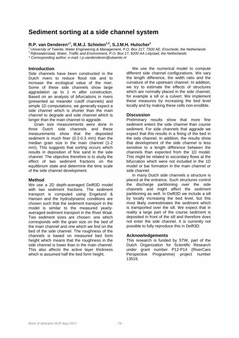
Book of abstracts NCR days 2017 - 79 -
Sediment sorting at a side channel system R.P. van Denderen*1, R.M.J. Schielen1,2, S.J.M.H. Hulscher1 1 University of Twente, Water Engineering & Management, P.O. Box 217, 7500 AE, Enschede, the Netherlands 2 Rijkswaterstaat, Water, Traffic and Environment, P.O. Box 17, 8200 AA Lelystad, the Netherlands * Corresponding author; e-mail: [email protected]
Introduction Side channels have been constructed in the Dutch rivers to reduce flood risk and to increase the ecological value of the river. Some of these side channels show large aggradation up to 1 m after construction. Based on an analysis of bifurcations in rivers (presented as meander cutoff channels) and simple 1D computations, we generally expect a side channel which is shorter than the main channel to degrade and side channel which is longer than the main channel to aggrade.
Grain size measurements were done in three Dutch side channels and these measurements show that the deposited sediment is much finer (0.2-0.3 mm) than the median grain size in the main channel (1-2 mm). This suggests that sorting occurs which results in deposition of fine sand in the side channel. The objective therefore is to study the effect of two sediment fractions on the equilibrium state and determine the time scale of the side channel development. Method We use a 2D depth-averaged Delft3D model with two sediment fractions. The sediment transport is computed using Engelund & Hansen and the hydrodynamic conditions are chosen such that the sediment transport in the model is similar to the measured yearly-averaged sediment transport in the River Waal. Two sediment sizes are chosen: one which corresponds with the grain size on the bed of the main channel and one which we find on the bed of the side channel. The roughness of the channels is based on measured bed form height which means that the roughness in the side channel is lower than in the main channel. This also affects the active layer thickness which is assumed half the bed form height.
We use the numerical model to compute different side channel configurations. We vary the length difference, the width ratio and the curvature of the upstream channel. In addition, we try to estimate the effects of structures which are normally placed in the side channel, for example a sill or a culvert. We implement these measures by increasing the bed level locally and by making these cells non-erodible. Discussion Preliminary results show that more fine sediment enters the side channel than course sediment. For side channels that aggrade we expect that this results in a fining of the bed in the side channel. In addition, the results show that development of the side channel is less sensitive to a length difference between the channels than expected from the 1D model. This might be related to secondary flows at the bifurcation which were not included in the 1D model or bar formation in the main channel or side channel.
In many Dutch side channels a structure is placed at the entrance. Such structures control the discharge partitioning over the side channels and might affect the sediment partitioning as well. In Delft3D we include a sill by locally increasing the bed level, but this most likely overestimates the sediment which is transported over the sill. We expect that in reality a large part of the course sediment is deposited in front of the sill and therefore does not enter the side channel. It is currently not possible to fully reproduce this in Delft3D. Acknowledgements This research is funded by STW, part of the Dutch Organization for Scientific Research under grant number P12-P14 (RiverCare Perspective Programme) project number 13516.

Book of abstracts NCR days 2017 - 80 -
52 years of vegetation development in floodplains along the River Allier over half a century H. Douma1, M.G. Kleinhans1, E.A. Addink1 1 Utrecht University, Department of Physical Geography, Faculty of Geosciences, Heidelberglaan 2, 3584 CS Utrecht * Corresponding author; e-mail: [email protected]
Introduction Riparian vegetation has a strong interaction with morphological processes and together they shape the habitat patterns and river patterns in the floodplain (Gurnell, 2014; Bertoldi et al., 2009). Vegetation objects affect for example the hydraulic roughness and the soil cohesion, which in turn affect sedimentation and erosion patterns. In the dynamic environment of a floodplain, this interaction leads to a complex mosaic of habitats.
To better understand this interaction, vegetation is being included as a dynamic rather than a static component in fluvial models (Van Oorschot et al. 2016). They presented a model “coupling hydraulic resistance caused by multiple vegetation types, depending on seed dispersal, colonization, growth and mortality, to a two-dimensional model that solves unsteady flow, sediment transport and morphological change at the spatial and temporal resolution appropriate for river channel-floodplain interactions”. The vegetation patterns resulting from the model correspond to patterns present in aerial photographs.
So far, however, it is not possible to compare the dynamics of these patterns, simply because there are no long records of empirical observations, either field- or image-based. The aim of this study is therefore to create a record of vegetation-object patterns with full spatial coverage and taken at discrete intervals. We collected 11 sets of aerial photographs taken in the period 1946-2002, aimed to classify them in a systematic way and to analyse the emergence and disappearance of isolated vegetation objects. Data and Methods We selected part of the River Allier between Chatel de Neuvre and Moulin as a study area (Fig. 1). All available aerial photographs were acquired. In total we had 11 sets for the period 1946-2002, mostly in black-and-white, but in later years some in true colour. The largest
time step was eight years, while the smallest was two years.
All photos were scanned, mosaicked and orthorectified to create a continuous image for each year. Pixel size varied between 19 and 30cm. For the classification we used object-based image analysis, where the pixels in an image are grouped into objects before analysis. The resulting objects correspond more closely to the vegetation objects than individual pixels. Grouping is based on spectral similarity, while taking into account textural differences. Each object was classified into the classes water, bare soil (BS), low vegetation (LV), high vegetation (HV) or isolated vegetation objects (IV).
The IV objects were tracked over time, so we could reveal when they emerged, when they disappeared or when they merged into a HV object. We grouped all objects according to age and determined their survival rate.
Figure 1. Location study area. Subset Fig. 2 in red

Book of abstracts NCR days 2017 - 81 -
Figure 2. Examples of photos and classification Results The overall composition of the area changes only slightly over time, while the spatial patterns are much more dynamic (Fig. 2). In the subset the river shifts to the east, extending the bare soil areas on its west side. These are covered by low vegetation in consecutive years. High vegetation extends from low coverage in 1946 to a more substantial coverage in 2002.
Figure 3. Isolated vegetation objects over time
Figure 4. Survival rate of isolated vegetation objects over time. Different colours correspond to emerging years.
Particularly in the west high vegetation increases strongly. The rate of newly emerged IV objects varies between 120 and 616 per year (Fig 3). Despite differences in external conditions, the disappearance rate of IV objects is relatively similar for different generations of IV objects (Fig. 4). Conclusion and Future Work The produced data set nicely captured the dynamic of this floodplain environment. Analysis of the development of isolated objects shows an exponential survival rate which is similar for different emerging years. However, the number of newly emerging isolated vegetation objects varies strongly. The data seem to provide a valuable validation set for dynamic vegetation modelling results. Next steps will be to look into the development of all vegetation classes and to link this to external factors like flooding and droughts. References Bertoldi, W., Gurnell, A., Surian, N., Tockner, K., Zanoni,
L., Ziliani, L., Zolezzi, G. (2009) Understanding reference processes: linkages between river flows, sediment dynamics and vegetated landforms along the Tagliamento river, Italy. River Research and Applications 25: 501–516.
Gurnell, A. (2014) Plants as river system engineers. Earth Surface Processes and Landforms, 39(1): 4-25.
Van Oorschot, M., Kleinhans, M., Geerling, G., Middelkoop, H. (2016) Distinct patterns of interaction between vegetation and morphodynamics. Earth Surface Processes and Landforms, 41, 791-808.
0
2000
4000
6000
1946 1976Num
ber o
f Iso
late
d Ve
geta
tion
Obj
ects
0.1
10
0 20 40 60Perc
enta
ge
rem
aini
ng o
bjec
ts
Time after seedling (in Years)

Book of abstracts NCR days 2017 - 82 -
Bank erosion processes in waterways G. Duró*1, W. Uijttewaal1, M. Kleinhans2, A. Crosato1,3 1 Delft University of Technology, Department Hydraulic Engineering, Faculty of Civil Engineering and Geosciences, P.O. Box 5048, 2600 GA, Delft, the Netherlands 2 Utrecht University, Department of Physical Geography, Faculty of Geosciences, P.O. Box 80115, 3508TC Utrecht, The Netherlands 3 UNESCO-IHE, Department of Water Engineering, PO Box 3015, 2601 GA, Delft, the Netherlands * Corresponding author; e-mail: [email protected] Natural banks Waterways serve for several functions besides transporting goods and people. The ecological importance of navigable rivers has taken much attention during recent decades bringing efforts to improve these natural corridors for fauna and flora (Boeters et al., 1997).
Following the policy of the European Water Framework Directive (WFD), many Dutch river reaches have been recently restored through the removal of bank protections in search for better riparian habitats (Florsheim et al., 2009), but they also result exposed to erosive forces. Large uncertainties generally surround the prediction of erosion rates (e.g. Samadi et al., 2009) due to complex flow characteristics in the near-bank region, variable soil properties, etc. A better understanding of bank erosion processes is then of interest to predict erosion rates and improve the design of future interventions. Case study: Meuse River The recent natural banks of a reach in the Meuse River are being monitored and analysed to have insights on the morphological and hydrodynamic processes that result in different erosion patterns. A first objective of this study is to identify the main drivers of erosion. Various mechanisms were considered as potentially active ones, namely fluvial erosion triggered during floods, piping and ship-induced erosion. Observations Two distinct patterns are identified after six years of their restoration: uniform (Fig. 1) and bay-shaped (Fig. 2). The uniform pattern has low or zero erosion rates at present, hypothetically due to the toe protection of a gravel layers, whereas the embayments are hit by ship waves, especially in areas where the base level is low enough to allow them reach the banks virtually without energy dissipation. The primary ship waves also induce shear stresses onto the banks, in particular over terraces where the wave energy dissipation occurs. It is noticeable the presence of trees along the banks that delays the erosion rates in some cases, but not in others.
Monitoring The morphology of banks is regularly being surveyed with an UAV (unmanned aerial vehicle) in order to monitor the vegetation development and quantify erosion rates. Near-bank velocities, suspended sediment concentrations and soil properties will be measured to characterize loads and bank resistances.
Figure 1. Uniform erosion pattern characterized by short grass-covered banks with gravel at the toe.
Figure 2. Bay-shaped erosion pattern characterized by high banks and contrasting erosion rates.

Book of abstracts NCR days 2017 - 83 -
Initial conclusions This case study evidences during summer time that the primary driver of erosion are ship-induced waves. There is not clear proof of piping and the role of floods will be analysed the next high-flow season. The patterns of erosion differ presumably after different soil strengths and the presence of gravel, trees and bushes seem to reduce rates by modifying erosion processes of the erosion cycle. References Boeters, Havinga, Litjens, & Verheij (1997). Ten years of
experience in combining ecology and navigation on Dutch waterways. 29th PIANC Congress. PIANC.
Florsheim, J. L., Mount, J. F., & Chin, A. (2008). Bank erosion as a desirable attribute of rivers. BioScience, 58(6), 519-529.
Samadi, A., Amiri-Tokaldany, E., & Darby, S. E. (2009). Identifying the effects of parameter uncertainty on the reliability of riverbank stability modelling. Geomorphology, 106(3), 219-230.

Book of abstracts NCR days 2017 - 84 -
Mitigation of long-term bed degradation in rivers: set-up of research Antonios Emmanouil*1, Astrid Blom1, Enrica Viparelli2, Roy Frings3 1 Delft University of Technology, Faculty of Civil Engineering and Geosciences, Department of Hydraulic engineering, P.O. Box 5048, 2600 GA, Delft, the Netherlands 2 Department of Civil and Environmental Engineering, University of South Carolina, Columbia, USA 3 Institute of Hydraulic Engineering and Water Resource Management, RWTH Aachen University, Aachen, D 52056, Germany * Corresponding author: e-mail: [email protected]
Introduction Sediment management measures are becoming increasingly popular as they are considered sustainable from both economic and environmental point of view. For example, aimed at counteracting river bed degradation, sediment nourishments have been carried out in the German reaches of the Rhine river while a nourishment pilot study has recently taken place at the Dutch Rhine and a nourishment project has been scheduled for the Danube by the Austrian water management authorities. Moreover, sediment management measures are implemented in various ecological restoration projects (e.g. Trinity river in U.S. and Nunome river in Japan) as sediments and their characteristics form the habitats of the biota, as well as in river training projects around the world.
Bed degradation is the dominant morphodynamic response of the freely flowing part of the Rhine river to past centuries’ river training focused on navigation and flood protection. It threatens almost every aspect of river management such as navigation, ecology, and existing infrastructure (Gölz 1994). Re-allocation dredging by means of by-passing and dumping of dredged sediment from shallows to deeper locations, combined with nourishments of artificial sediment have been the main mitigation practices taken on by the German river management authorities since the mid-70s to counteract this problem (Frings et al. 2014 a,b).
Such nourishments at one hand partly restore the deficit of sediment caused by its retention at upstream basins from canalization and impoundment of major tributaries. Furthermore, the relatively coarse sediment nourished –compared to the bed surface sediment- has a stabilizing effect by armouring of the bed surface, yet tends to cause degradational problems downstream (Gölz 1994, Blom 2016). This is also demonstrated by an experimental study carried out under laboratory conditions shown in Fig. 1.
A sustainable design of such mitigation measures calls for (a) an assessment of the
ongoing adjustment of the river bed and (b) the use of numerical tools. Such numerical tools need to be based on conservation laws and account for the dominant morphodynamic processes i.e., grain size selective transport and abrasion which induce sorting patterns in all directions and shape the river’s longitudinal profile (Mackin 1948, Blom et al. 2016). The validation of such numerical models is not a trivial task. Sets of measured field data are available, yet an assessment is needed on how to effectively validate such models.
Objective The main objective of the research presented here is to assess the short and long term effects of sediment management measures on the river’s profile and optimize the mitigation practices by addressing predominantly the volume, characteristics of mixtures, frequency, locations, timing and duration of nourishments. General approach The research will proceed by means of literature survey, analysis of available datasets and numerical modelling. Fig. 2 illustrates the method of the research. The first step to be taken is the identification of the current mitigation practices and a preliminary assessment of their effects based predominantly on literature survey and data analysis. Later, numerical models appropriate for simulating mitigation measures for different temporal and spatial scales will be setup and validated. These numerical tools will then be used to assess the short and long term effects of sediment management measures using cases of varying complexity. The design of such measures will be carried out with different sediment supply and water discharge scenarios as well as with the use of probabilistic analysis to address the uncertainty. Interactions of sediment management measures and other commonly implemented river management practices (e.g. Room for the River, replacement of groynes by longitudinal dams) will also be studied.

Book of abstracts NCR days 2017 - 85 -
Future work The preparation of the workplan is at its final stage, and a preliminary study on the morphodynamic temporal trends in the freely flowing Rhine has been carried out. The next step is to extend the latter step to other rivers where sediment augmentation measures have been conducted, as well as to select appropriate numerical tools. Acknowledgements This research is carried out as part of the STW (Water2015) project-C76A05: ‘Long-term bed degradation in rivers: causes and mitigation’, supported by the Technology Foundation STW, the applied science division of NWO and the technology programme of the Ministry of Economic Affairs.
References Blom, A. (2016). Bed degradation in the Rhine River.
WaterViewer, Delft University of Technology, http://waterviewer.tudelft.nl/#/bed-degradation-in-the-rhine-river-1479821439344____47.
Blom, A., E. Viparelli, and V. Chavarrías (2016), The graded alluvial river: Profile concavity and downstream fining, Geophys. Res. Lett., 43, 6285–6293, doi:10.1002/2016GL068898.
Gölz, E. (1994). "Bed degradation–nature, causes, countermeasures." Water Science and Technology 29(3): 325-333.
Frings, R. M., Döring, R., Beckhausen, C., Schüttrumpf, H., and Vollmer, S. (2014a). "Fluvial sediment budget of a modern, restrained river: The lower reach of the Rhine in Germany." Catena 122:91-102.
Frings, R.M., Gehres, N., Promny, M., H. Middelkoop, H. Schüttrumpf, H., and Vollmer, S. (2014b). "Today's sediment budget of the Rhine River channel, focusing on the Upper Rhine Graben and Rhenish Massif" Geomorpholgy 204: 573-587.
Mackin, J.H., (1948), Concept of the graded river. Geological Society of America Bulletin. v. 59, no. 5, p. 463-512
Figure 1: Laboratory experiment with nourished sediment located at x = 0 and x = 3.5 m at time 0 for two cases (nourished sediment coarser than bed surface sediment (left) and unisize compared to bed surface sediment (right). In a case of coarse nourishment degradational wave is migrating downstream considerably faster that the nourished sediment. (from Blom 2016)
Figure 2: Workplan of research project.

Book of abstracts NCR days 2017 - 86 -
Sediment transport over sills at longitudinal training dams with unaligned main flow S.M.M. Jammers*1,2,3,4, A.J. Paarlberg3, E. Mosselman1,4, W.S.J. Uijttewaal1 1 Delft University of Technology, Faculty of Civil Engineering and Geosciences, Department of Hydraulic Engineering, P.O. Box 5048, 2600 GA Delft, the Netherlands 2 National University of Singapore, Faculty of Engineering, Department of Civil and Environmental Engineering, No. 1 Engineering Drive 2, 117576, Singapore 3 HKV Consultants, P.O. Box 2120, 8203 AC Lelystad, the Netherlands 4 Deltares, P.O. Box 177, 2600 MH Delft, the Netherlands * Corresponding author; e-mail: [email protected] Introduction Longitudinal training dams (LTDs) are constructed in the River Waal in the Netherlands. They are aligned parallel to the river shore and divide the river into a main and side channel. The existing groynes are removed yielding more discharge capacity at high flows. The side channel creates possibly a sheltered environment for species compared to the traditional groyne field (Collas, 2014). Although the lay-out of the LTDs has been extensively studied using numerical models (e.g. Huthoff et al., 2011), the morphodynamic response is yet unclear and depends strongly on the dimensions (length and height) of the openings. The inlet and openings (see Fig. 1) are sill-type structures which can be changed relatively easy.
These sills are designed in such a way that they serve as a barrier for water and bed load sediment. To make long-term morphological predictions, it is necessary to understand the bed load transport processes over these sills. Suspended sediment transport is not considered in this study. We developed an analytical model to predict sediment transport paths on a slope, using a correction on the well-known critical Shields parameter.
Figure 1. Schematisation of river – top view. Correction for main flow aligned with sill If the main flow is aligned with the sill, the flow is parallel to the depth isolines of the sill. This part of the sill is schematised as a transverse slope in the main channel with main flow in x-direction, see Fig. 2.
Figure 2. Path of sediment particle on transverse slope. Shields, (1936) performed sediment transport experiments on a horizontal bed in a straight flume and derived a critical condition for the initiation of motion, the critical Shields parameter ( 0cΘ ). Dey, (2014) uses the approach of Shields, (1936), Yang, (1973) and Ikeda, (1982) to describe the sediment transport on a transverse slope in terms of an adapted critical Shields parameter. Due to gravity sediment particles tend to move towards the main (horizontal) river bed. He proposed a ‘correction factor’ ( � cαΘ ) for the critical Shields parameter (on a horizontal bed) given the situation where the flow is in downstream direction on a transverse slope (α ). Equation (1) describes this correction factor.
�0cc cααΘ ⋅ΘΘ= (1)
Correction for main flow not aligned with sill In this case the flow over the sills is not in the x-direction, but has a component in both x and y (transverse) direction, see Fig. 3. In analogy with the previous section a new correction factor ( � cγΘ ) is presented in Equation (2) (CIRIA et al., 2007). The term α is the angle the transverse slope (i.e. sill) has, tan φ is the natural angle of friction (also known as µ ), finally γ is the flow angle with respect to the x’ direction in the x’-y’-plane (see Fig. 3).
x
y
Main flow
Inlet OpeningLTD LTD
Main channel
Side channel
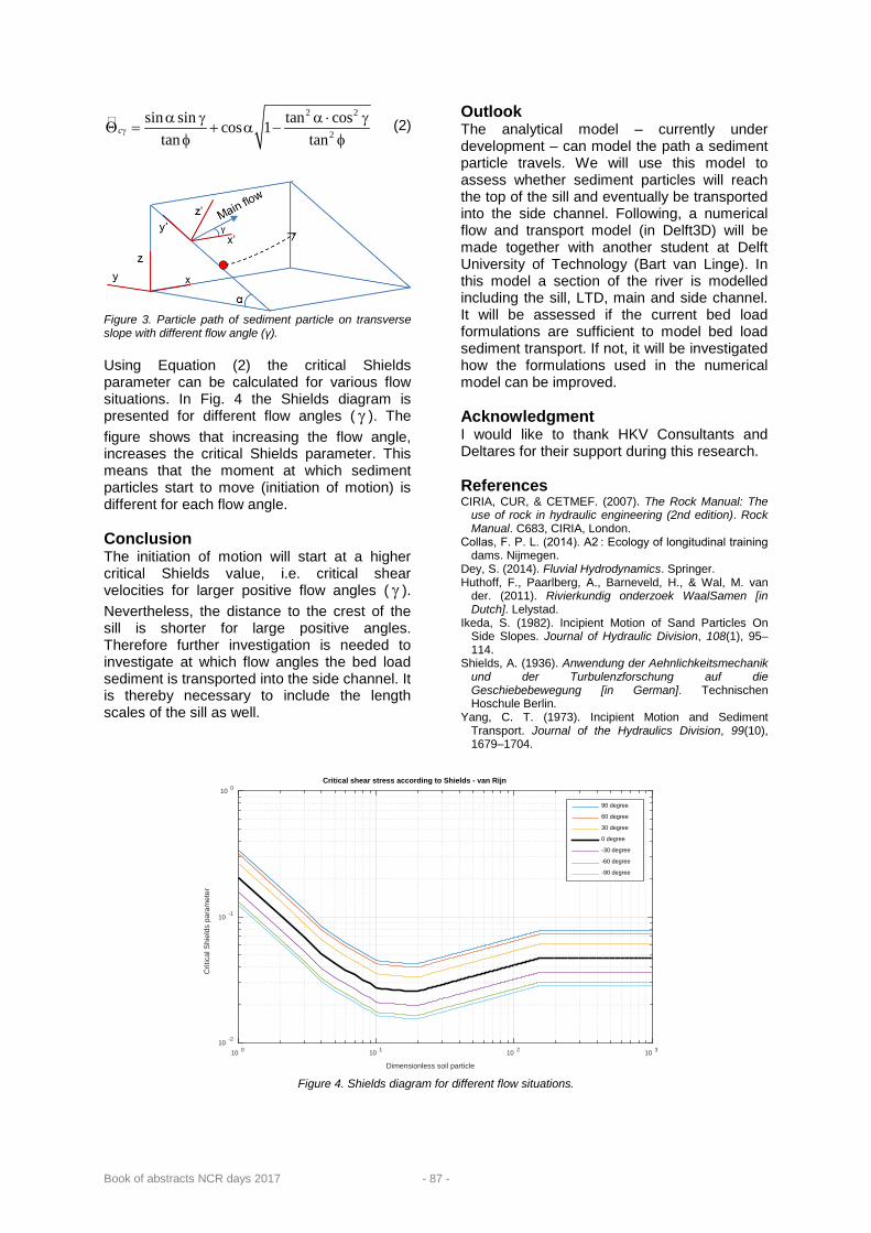
Book of abstracts NCR days 2017 - 87 -
�2 2
2
sin sin tan coscos 1tan tan
cγα γ α ⋅ γ
Θ = + α −φ φ
(2)
Figure 3. Particle path of sediment particle on transverse slope with different flow angle (γ). Using Equation (2) the critical Shields parameter can be calculated for various flow situations. In Fig. 4 the Shields diagram is presented for different flow angles ( γ ). The figure shows that increasing the flow angle, increases the critical Shields parameter. This means that the moment at which sediment particles start to move (initiation of motion) is different for each flow angle. Conclusion The initiation of motion will start at a higher critical Shields value, i.e. critical shear velocities for larger positive flow angles ( γ ). Nevertheless, the distance to the crest of the sill is shorter for large positive angles. Therefore further investigation is needed to investigate at which flow angles the bed load sediment is transported into the side channel. It is thereby necessary to include the length scales of the sill as well.
Outlook The analytical model – currently under development – can model the path a sediment particle travels. We will use this model to assess whether sediment particles will reach the top of the sill and eventually be transported into the side channel. Following, a numerical flow and transport model (in Delft3D) will be made together with another student at Delft University of Technology (Bart van Linge). In this model a section of the river is modelled including the sill, LTD, main and side channel. It will be assessed if the current bed load formulations are sufficient to model bed load sediment transport. If not, it will be investigated how the formulations used in the numerical model can be improved. Acknowledgment I would like to thank HKV Consultants and Deltares for their support during this research. References CIRIA, CUR, & CETMEF. (2007). The Rock Manual: The
use of rock in hydraulic engineering (2nd edition). Rock Manual. C683, CIRIA, London.
Collas, F. P. L. (2014). A2 : Ecology of longitudinal training dams. Nijmegen.
Dey, S. (2014). Fluvial Hydrodynamics. Springer. Huthoff, F., Paarlberg, A., Barneveld, H., & Wal, M. van
der. (2011). Rivierkundig onderzoek WaalSamen [in Dutch]. Lelystad.
Ikeda, S. (1982). Incipient Motion of Sand Particles On Side Slopes. Journal of Hydraulic Division, 108(1), 95–114.
Shields, A. (1936). Anwendung der Aehnlichkeitsmechanik und der Turbulenzforschung auf die Geschiebebewegung [in German]. Technischen Hoschule Berlin.
Yang, C. T. (1973). Incipient Motion and Sediment Transport. Journal of the Hydraulics Division, 99(10), 1679–1704.
Figure 4. Shields diagram for different flow situations.
Dimensionless soil particle
10 0 10 1 10 2 10 3
Crit
ical
Shi
elds
par
amet
er
10 -2
10 -1
10 0Critical shear stress according to Shields - van Rijn
90 degree
60 degree
30 degree
0 degree
-30 degree
-60 degree
-90 degree
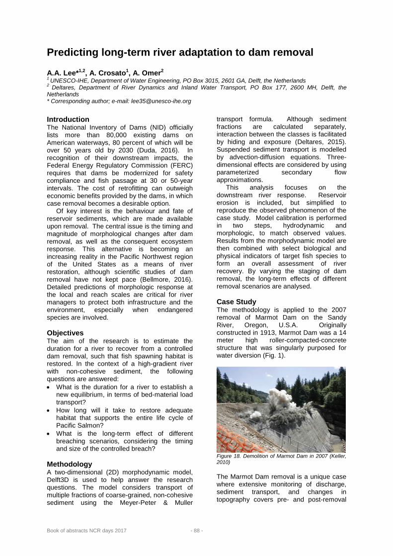
Book of abstracts NCR days 2017 - 88 -
Predicting long-term river adaptation to dam removal A.A. Lee*1,2, A. Crosato1, A. Omer2 1 UNESCO-IHE, Department of Water Engineering, PO Box 3015, 2601 GA, Delft, the Netherlands 2 Deltares, Department of River Dynamics and Inland Water Transport, PO Box 177, 2600 MH, Delft, the Netherlands * Corresponding author; e-mail: [email protected]
Introduction The National Inventory of Dams (NID) officially lists more than 80,000 existing dams on American waterways, 80 percent of which will be over 50 years old by 2030 (Duda, 2016). In recognition of their downstream impacts, the Federal Energy Regulatory Commission (FERC) requires that dams be modernized for safety compliance and fish passage at 30 or 50-year intervals. The cost of retrofitting can outweigh economic benefits provided by the dams, in which case removal becomes a desirable option.
Of key interest is the behaviour and fate of reservoir sediments, which are made available upon removal. The central issue is the timing and magnitude of morphological changes after dam removal, as well as the consequent ecosystem response. This alternative is becoming an increasing reality in the Pacific Northwest region of the United States as a means of river restoration, although scientific studies of dam removal have not kept pace (Bellmore, 2016). Detailed predictions of morphologic response at the local and reach scales are critical for river managers to protect both infrastructure and the environment, especially when endangered species are involved. Objectives The aim of the research is to estimate the duration for a river to recover from a controlled dam removal, such that fish spawning habitat is restored. In the context of a high-gradient river with non-cohesive sediment, the following questions are answered: • What is the duration for a river to establish a
new equilibrium, in terms of bed-material load transport?
• How long will it take to restore adequate habitat that supports the entire life cycle of Pacific Salmon?
• What is the long-term effect of different breaching scenarios, considering the timing and size of the controlled breach?
Methodology A two-dimensional (2D) morphodynamic model, Delft3D is used to help answer the research questions. The model considers transport of multiple fractions of coarse-grained, non-cohesive sediment using the Meyer-Peter & Muller
transport formula. Although sediment fractions are calculated separately, interaction between the classes is facilitated by hiding and exposure (Deltares, 2015). Suspended sediment transport is modelled by advection-diffusion equations. Three-dimensional effects are considered by using parameterized secondary flow approximations.
This analysis focuses on the downstream river response. Reservoir erosion is included, but simplified to reproduce the observed phenomenon of the case study. Model calibration is performed in two steps, hydrodynamic and morphologic, to match observed values. Results from the morphodynamic model are then combined with select biological and physical indicators of target fish species to form an overall assessment of river recovery. By varying the staging of dam removal, the long-term effects of different removal scenarios are analysed. Case Study The methodology is applied to the 2007 removal of Marmot Dam on the Sandy River, Oregon, U.S.A. Originally constructed in 1913, Marmot Dam was a 14 meter high roller-compacted-concrete structure that was singularly purposed for water diversion (Fig. 1).
Figure 18. Demolition of Marmot Dam in 2007 (Keller, 2010) The Marmot Dam removal is a unique case where extensive monitoring of discharge, sediment transport, and changes in topography covers pre- and post-removal
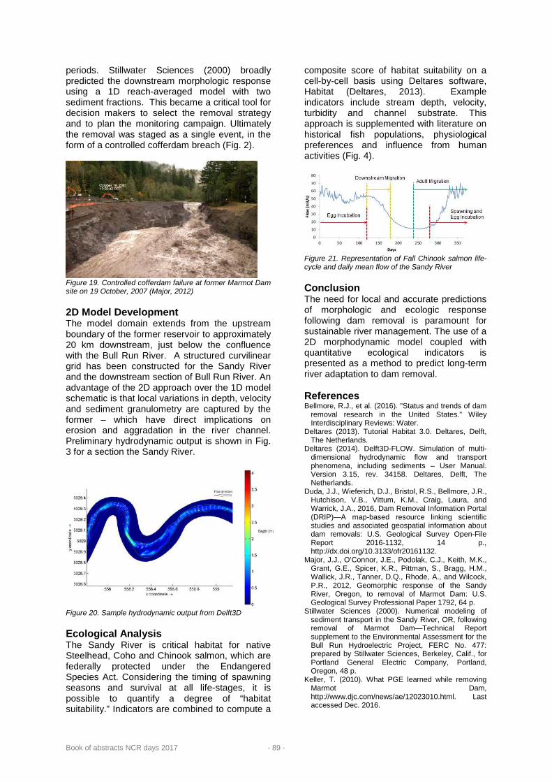
Book of abstracts NCR days 2017 - 89 -
periods. Stillwater Sciences (2000) broadly predicted the downstream morphologic response using a 1D reach-averaged model with two sediment fractions. This became a critical tool for decision makers to select the removal strategy and to plan the monitoring campaign. Ultimately the removal was staged as a single event, in the form of a controlled cofferdam breach (Fig. 2).
Figure 19. Controlled cofferdam failure at former Marmot Dam site on 19 October, 2007 (Major, 2012) 2D Model Development The model domain extends from the upstream boundary of the former reservoir to approximately 20 km downstream, just below the confluence with the Bull Run River. A structured curvilinear grid has been constructed for the Sandy River and the downstream section of Bull Run River. An advantage of the 2D approach over the 1D model schematic is that local variations in depth, velocity and sediment granulometry are captured by the former – which have direct implications on erosion and aggradation in the river channel. Preliminary hydrodynamic output is shown in Fig. 3 for a section the Sandy River.
Figure 20. Sample hydrodynamic output from Delft3D Ecological Analysis The Sandy River is critical habitat for native Steelhead, Coho and Chinook salmon, which are federally protected under the Endangered Species Act. Considering the timing of spawning seasons and survival at all life-stages, it is possible to quantify a degree of “habitat suitability.” Indicators are combined to compute a
composite score of habitat suitability on a cell-by-cell basis using Deltares software, Habitat (Deltares, 2013). Example indicators include stream depth, velocity, turbidity and channel substrate. This approach is supplemented with literature on historical fish populations, physiological preferences and influence from human activities (Fig. 4).
Figure 21. Representation of Fall Chinook salmon life-cycle and daily mean flow of the Sandy River Conclusion The need for local and accurate predictions of morphologic and ecologic response following dam removal is paramount for sustainable river management. The use of a 2D morphodynamic model coupled with quantitative ecological indicators is presented as a method to predict long-term river adaptation to dam removal. References Bellmore, R.J., et al. (2016). "Status and trends of dam
removal research in the United States." Wiley Interdisciplinary Reviews: Water.
Deltares (2013). Tutorial Habitat 3.0. Deltares, Delft, The Netherlands.
Deltares (2014). Delft3D-FLOW. Simulation of multi-dimensional hydrodynamic flow and transport phenomena, including sediments – User Manual. Version 3.15, rev. 34158. Deltares, Delft, The Netherlands.
Duda, J.J., Wieferich, D.J., Bristol, R.S., Bellmore, J.R., Hutchison, V.B., Vittum, K.M., Craig, Laura, and Warrick, J.A., 2016, Dam Removal Information Portal (DRIP)—A map-based resource linking scientific studies and associated geospatial information about dam removals: U.S. Geological Survey Open-File Report 2016-1132, 14 p., http://dx.doi.org/10.3133/ofr20161132.
Major, J.J., O’Connor, J.E., Podolak, C.J., Keith, M.K., Grant, G.E., Spicer, K.R., Pittman, S., Bragg, H.M., Wallick, J.R., Tanner, D.Q., Rhode, A., and Wilcock, P.R., 2012, Geomorphic response of the Sandy River, Oregon, to removal of Marmot Dam: U.S. Geological Survey Professional Paper 1792, 64 p.
Stillwater Sciences (2000). Numerical modeling of sediment transport in the Sandy River, OR, following removal of Marmot Dam—Technical Report supplement to the Environmental Assessment for the Bull Run Hydroelectric Project, FERC No. 477: prepared by Stillwater Sciences, Berkeley, Calif., for Portland General Electric Company, Portland, Oregon, 48 p.
Keller, T. (2010). What PGE learned while removing Marmot Dam, http://www.djc.com/news/ae/12023010.html. Last accessed Dec. 2016.

Book of abstracts NCR days 2017 - 90 -
Analysis of Ribb River channel migration: Upper Blue Nile, Ethiopia C.A. Mulatu*1, A. Crosato1,2, A. Mynett1,2 1 UNESCO-IHE, Department of Water Science Engineering, P.O. Box 3015, 2601 DA, Delft, the Netherlands 2 Delft University of Technology, Faculty of Civil Engineering and Geoscience, P.O. Box 10150, 2600 VB, Delft,
the Netherlands * Corresponding author; e-mail: [email protected] / [email protected]
Introduction The Ribb River is one of the components of the Blue Nile River system located in the North Western part of Ethiopia. It drains to Lake Tana, the source of the Blue Nile River. The Ribb has a length of 130 km, with a catchment area of 1,812 km2. The average yearly rainfall of the catchment is 1300 mm, with 80 % occurring between the months of June and September. The average and daily maximum discharge of the river are 15 m3/s and 220 m3/s, respectively. A large dam and a diversion weir 30 km downstream of the dam are under construction to irrigate 15,000 ha of Fogera flood plain (WWDSE and TAHAL, 2007). Downstream of the dam location, the Ribb is a meandering river with slope ranging from 0.18% to 0.03%. The river bed material is dominated by sand with a gravel component in its upper reaches. Intensive agriculture without any natural resources conservation, deforestation, dike construction, pump irrigation and sand mining are the most impactful activities in the Ribb watershed (Tarekegn et al., 2010; Garede and Minale, 2014). The Lake Tana level is regulated since 1995 for hydropower production, which enhances flooding along the lower river reach. During the 2006 event, 45 people died, 30,000 persons were displaced and 5371 ha of agricultural land were inundated (ENTRO, 2010). To prevent flooding, dikes have been constructed in the lower reach of the river.
This study aims to describe current river morphodynamic trends, including planimetric changes for the definition of the pre-dam conditions of the river. The first part of the work is presented here with some preliminary results, focusing on the river planimetric changes. This paper describes the initial state of the study.
Methodology The planimetric evolution of the river is assessed by means of satellite images, aerial photographs and observations complemented with field recognition. Aerial photographs of the years 1957 and 1982, SPOT satellite images of the years 2006 and 2016 and a Google Earth
image of the year 2016 are used for the study. ENVI 4.3 is used for orthorectification of aerial photographs. Ground control points, which are collected from SPOT satellite image of the year 2012 and elevations, which are collected from 30 m resolution digital elevation model are used for orthorectification of aerial photographs. ArcGIS is used to digitize the river centrelines and to visualize the super-imposed images. The one/two dimensional physics-based model, MIANDRAS, (Crosato, 1987, 2008) is applied to study the river bed topography and planimetric changes. The governing equations are derived by coupling the 2D momentum and continuity equations for water (de Saint Venant equations) to sediment transport and sediment balance equations and are linearized. To simulate the river planimetric changes, the model assumes that the lateral shift of the channel centreline is a function of near-bank velocity and water depth excess with respect to reach averaged uniform flow. The input parameters are collected from the field and derived from satellite images. The model is first used to analyse the river bed topography configuration. Hence, the model is calibrated for the bed topography (comparing the simulated and observed bed forms). The model is then also used to analyse the planimetric dynamics of the river. This part of the study is not presented here. The study river reach has a length of 77 km from the dam site to Lake Tana. It is divided in three parts: the Upper reach (from the dam to the weir), the Middle reach (from the weir to the main road to Gondar) and the Lower reach (from the main road to Gondar to Lake Tana) (Fig. 1).
Preliminary results Daily discharge data are available at the gauging station located near to Woreta-Addis Zemen Bridge. The bankfull discharge of the river has been estimated in 115 m3/s, based on the frequency analysis of the annual maximum values with a return period of 1.5. The reach-averaged river characteristics are shown in Table 1.

Book of abstracts NCR days 2017 - 91 -
Figure 1. Successive Ribb River channel centrelines.
Table 1. Reach averaged river characteristics. Reach Average river
width (m) Sinuosity
(-) Valley slope
(%) Upper 58 1.77 0.32 Middle 46 1.76 0.1 Lower 38 1.5 0.05
The analysis of satellite images shows that
the river width reduces in downstream direction. This may be due to dike construction, decree-sing natural bank erodibility and sediment inputs. A channel avulsion event occurred downstream of the weir between 1982 and 2006 when the river occupied an old channel for a length of 7.5 km. Another channel shift occurred 4 km downstream of the bridge (Fig. 1).This may be related to anthropogenic activities, since it happened during a flood event due to high discharge and backwater caused by an artificially increased level of Lake Tana (Abate et al., 2016; SMEC, 2008).
The model MIANDRAS has been used to study a 6.5 km long reach located in the Middle reach where the river is free from dike construction and flooding. The average width is 46 m (Table 1). To calibrate the model, an area having visible point bar formation is selected (Fig. 2) and the results compared to the observed bed topography (Fig. 3).
Figure 2. Part of the study reach showing river bed topography, Google Earth image of the year 2016.
The computed equilibrium bed topography resembles the observed one quite well, but does not always match it. This may be due to sand mining activities occurring during low flow conditions on bar tops.
Future work & Acknowledgements The research is a part of PhD work of the corresponding author, who is currently working at UNESCO-IHE, Delft.
Figure 3. MIANDRAS model output bed topography for calibration coefficients of σ = 2.3, E= 0.8 and α1= 0.1.The flow direction is from left to right. His work deals with the effects of dam construction on the planimetric changes of downstream rivers. He would like to thank NUFFIC for financial support. References Abate, M., J. Nyssen, M. M. Moges, T. Enku, F. A. Zimale,
S. A. Tilahun, E. Adgo & T. S. Steenhuis (2016) Long-term landscape changes in the Lalke Tana basin as evidenced by delta development and floodplain aggradation, Ethiopia. Land Degradation & Development
Crosato, A. (1987). Simulation model of meandering processes of rivers. Euromech 215-Mechanics of Sediment Transport in Fluvial and Marine Environments, European Mechanics Society, Sept. 15-19, Santa Margherita Ligure-Genoa, Italy Genoa, pp. 158-161.
Crosato, A. (2008). Analysis and modelling of river meandering, TU Delft, Delft University of Technology.
Garede, N. M. and A. S. Minale (2014). Land Use/Cover Dynamics in Ribb Watershed, North Western Ethiopia. Journal of Natural Sciences Research 4(16): 9-16.
SMEC (2008). Hydrological study of the Tana-Beles Sub-Basin: Surface water Investigation, SMEC International Pty Ltd.
Tarekegn, et al. (2010). Assessment of an ASTER-generated DEM for 2D hydrodynamic flood modeling. International Journal of Applied Earth Observation and Geoinformation 12(6): 457-465.
WWDSE and TAHAL (2007). Ribb Dam Hydrological Study (Final Report). Addis Ababa, Ethiopia, Water Works Design and Supervision Enterprise and TAHAl Consulting Engineers LTD.
ENTRO. 2010. Flood Risk Mapping Consultancy for Pilot Areas in Ethiopia. Final Report to the Eastern Nile Technical Regional Office (ENTRO). pp. 1–206. Riverside
Technology and its partners, Addis Ababa, Ethiopia
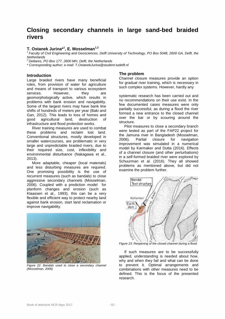
Book of abstracts NCR days 2017 - 92 -
Closing secondary channels in large sand-bed braided rivers T. Ostanek Jurina*1, E. Mosselman1,2 1 Faculty of Civil Engineering and Geosciences, Delft University of Technology, PO Box 5048, 2600 GA, Delft, the Netherlands 2 Deltares, PO Box 177, 2600 MH, Delft, the Netherlands * Corresponding author; e-mail: [email protected]
Introduction Large braided rivers have many beneficial roles, from provision of water for agriculture and means of transport to various ecosystem services. However, they are geomorphologically active, which results in problems with bank erosion and navigability. Some of the largest rivers may have bank line shifts of hundreds of meters per year (Baki and Gan, 2012). This leads to loss of homes and good agricultural land, destruction of infrastructure and flood protection works. River training measures are used to combat these problems and reclaim lost land. Conventional structures, mostly developed in smaller watercourses, are problematic in very large and unpredictable braided rivers, due to their required size, cost, inflexibility and environmental disturbance (Nakagawa et al., 2013). More adaptable, cheaper (local materials) and less disturbing measures are required. One promising possibility is the use of recurrent measures (such as bandals) to close aggressive secondary channels (Mosselman, 2006). Coupled with a prediction model for planform changes and erosion (such as Klaassen et al., 1993), this can be a very flexible and efficient way to protect nearby land against bank erosion, start land reclamation or improve navigability.
Figure 22: Bandals used to close a secondary channel {Mosselman, 2006}
The problem Channel closure measures provide an option for gradual river training, which is necessary in such complex systems. However, hardly any systematic research has been carried out and no recommendations on their use exist. In the few documented cases measures were only partially successful, as during a flood the river formed a new entrance to the closed channel over the bar or by scouring around the structure. Pilot measures to close a secondary branch were tested as part of the FAP22 project for the Jamuna river in Bangladesh (Mosselman, 2006). Partial closure for navigation improvement was simulated in a numerical model by Karmaker and Dutta (2016). Effects of a channel closure (and other perturbations) in a self-formed braided river were explored by Schuurman et al. (2016). They all showed problems as mentioned above, but did not examine the problem further.
Figure 23: Reopening of the closed channel during a flood. If such measures are to be successfully applied, understanding is needed about how, why and when they fail and what can be done to prevent it. Optimal arrangements and combinations with other measures need to be defined. This is the focus of the presented research.

Book of abstracts NCR days 2017 - 93 -
Methodology As large sand-bed braided rivers are very complex and the problem has been mostly unexplored, research will start with a simple case. A two dimensional numerical Delft3D model will be used, with pilot closure site and measures from FAP22 as reference, but with simplified geometry and length of only one bifurcation-confluence reach. A complete closure will be modelled, without taking into account possible openings to induce siltation in the channel. Applying the reference case will enable calibration of the model to reproduce the problems observed. Processes leading to reopening of the channel will be studied. A sensitivity analysis will be made, testing the effects of roughness predictors, sediment transport formulas, discharge, island height and geometry. Different positions of measures along the channel will be tested. Various factors possibly contributing to reopening, not (well) taken into account with the numerical model, will be examined and their effect assessed quantitatively or qualitatively. Examples include the effect of groundwater and sediment distribution in the water column during overbar flow. Based on the knowledge obtained, arrangements of multiple closure works combined with additional measures (artificial roughness, vegetation, increasing island height) will be designed and tested for some representative situations. A model of a larger reach will be made, to see how the proposed measures perform in a more realistic setting. Finally, recommendations for the use of recurrent measures to close secondary channels in large braided rivers will be derived. Expected results Main reason behind channel reopening downstream of the closure is expected to be the water level difference between the parallel channels. This already occurs when branches are naturally closed and cross bar channels form due to a transverse hydraulic gradient (Bristow, 1987; Schuurman and Kleinhans, 2015). It is expected that additional measures will be required to perform the closure successfully. Interesting results are anticipated from the sensitivity analysis of roughness predictors and sediment transport. Molinas and Wu (2001) made the case that common formulas are not
applicable in very large and deep rivers. Indeed, in the Jamuna river, a different power of velocity is known to perform better when computing sediment transport. Seepage probably plays a part in the erosion of the island due to a continuous water level difference from the main channel even during low flow. However the gradients are expected to be too small to make a significant difference. Not including the fact that the water flowing over the island carries only little sediment is likely more relevant. . Conclusion We address a mostly unexplored problem, which opens possibilities for useful findings and future research. Effective layouts and combinations of measures will be found and the resulting processes described. This will result in practical recommendations for effective closure of secondary channels in large braided sand-bed rivers. References Baki, A.B.M., Gan, T.Y. (2012). Riverbank migration and
island dynamics of the braided Jamuna river of the Ganges–Brahmaputra basin using multi-temporal LANDSAT images. Quaternary International, 263: 148-161.
Bristow, C. C. (1987). Brahmaputra river: channel migration and deposition. In: Ethridge, F. G., Flores, R. M., Harvey, M. D. (eds.) Recent developments in fluvial sedimentology.
Karmaker, T., Dutta, S. (2016). Prediction of short-term morphological change in large braided river using 2D numerical model. Journal of Hydraulic Engineering, 142:
Klaassen, G. J., Mosselman, E., Bruhl, H. (1993). On the prediction of planform changes in braided sand-bed rivers. In: Wang, S. S. Y., (Ed). 1st International conference on advances in hydro-science and engineering, 7-10. june 1993, Washington. 134-146.
Molinas, A., Wu, B. (2001). Transport of sediment in large sand-bed rivers. Journal of hydraulic research, 39: 135-146.
Mosselman, E. (2006). Bank protection and river training along the braided Brahmaputra–Jamuna river, Bangladesh. In: Smith, G. H. S., Best, J. L., Bristow, C.S., Petts, G., E. (ed.) Braided rivers: Process, deposition, ecology and management. Blackwell, Oxford, UK: Blackwell publishing Ltd. 277-287.
Nakagawa, H., Zhang, H., Baba, Y., Kawaike, K., Teraguchi, H. (2013). Hydraulic characteristics of typical bank-protection works along the Brahmaputra/Jamuna river, Bangladesh. Journal of flood risk management, 6: 345-359.
Schuurman, F., Kleinhans, M. G. (2015). Bar dynamics and bifurcation evolution in a modelled braided sand-bed river. Earth surface processes and landforms, 40: 1318-1333.
Schuurman, F., Kleinhans, M. G., Middelkoop, H. (2016). Network response to disturbances in large sand-bed braided rivers. Earth surface dynamics, 4: 25-45.

Book of abstracts NCR days 2017 - 94 -
Application of a line laser scanner for bed form tracking in a laboratory flume T.V. de Ruijsscher*1, S. Dinnissen1, B. Vermeulen2, P. Hazenberg1, A.J.F. Hoitink1 1 Wageningen University & Research, Department of Environmental Sciences, Hydrology and Quantitative Water Management Group, P.O. Box 47, 6700 AA, Wageningen, the Netherlands 2 University of Twente, Department of Water Engineering and Management, Faculty of Engineering Technology, P.O. Box 217, 7500 AE, Enschede, the Netherlands * Corresponding author; e-mail: [email protected]
Introduction In order to develop a measurement method that is fully non-invasive and able to capture the short timescale bed-form dynamics, tests have been performed with single-beam (Visconti et al., 2012) and multi-beam (Friedrichs and Graf, 2006; Peña González et al., 2007) laser scanners. However, these studies have only focused on a laser beam travelling vertically downward up till now. In the present study the full range of beams emitted by a multi-beam laser is taken into account, and corrections are quantified and performed in order to reduce the errors due to e.g. refraction. The applied corrections are used for measuring dunes and alternate bars under flowing water conditions. Methods The here proposed bed-form measurement method consists of a line laser and a 3D-camera with Gigabit Ethernet (SICK, 2012), both mounted on a measurement carriage that can move on fixed rails along the flume. The beam swath angle of the laser array is 50.0°, covering a width of 419 mm of the bare flume bottom. This width decreases evidently when a layer of sediment is present. The projected laser line is oriented perpendicular to the flow direction, and the camera is looking at an angle (see Fig. 1). The bed profile is measured by means of triangulation. Because of the limited width of the laser beam swath, multiple parallel (partly overlapping) tracks are used to measure the whole width of the flume (1.2 m).
Four consecutive series of experiments are performed, viz. measurement of the bottom profile of 1) an empty flume (no water, no sediment), 2) a flume with still water, 3) a flume with flowing water, and 4) a flume with a movable bed consisting of sand with a density of ρs = 2650 kg m-3
and a size of D50 = 0.719 mm and D90 = 0.962 mm.
Corrections are performed both for errors resulting from internal camera calibration and for refraction at the air-water interface.
Figure 1. a) Overview of the experimental set-up. Red lines indicate transmitted laser beams and yellow lines indicate reflected laser beams, measured by the camera. b) Side view of the flume showing the reflected laser beams. The refraction correction 𝑐𝑐 and the water depth 𝐷𝐷 are indicated.
Outliers and missing values have to be
corrected for in the moving bed experiment by applying a smoothing and interpolating algorithm. Because of the irregularly spaced nature of the retrieved data, an algorithm that does not need interpolation to a regular grid beforehand is preferred. LOESS, a robust locally weighted regression algorithm (Cleveland, 1979) appears to be an appropriate choice (Vermeulen et al., 2014). This fitting algorithm is based on a polynomial fit to the data using weighted least squares. An example of the effect of LOESS fitting to data is shown in Fig. 2, showing clearly the 3D nature of the LOESS algorithm.
Figure 2. An example of the effect of LOESS fitting. The colour plot shows the measured bed level at the end of the moving bed experiment. Black lines indicate along-track and cross-track cross-sections, which are highlighted in the bottom and right plot, respectively. Measured values are shown in blue dots and the fitted profile as a red curve.

Book of abstracts NCR days 2017 - 95 -
Results For measurement of the bare bottom with flowing water of different discharges, correlations between the mean absolute measurement error |𝜖𝜖|, coefficient of variation of the measurement error 𝜎𝜎𝜖𝜖 |𝜖𝜖|⁄ and percentage of missing values 𝑚𝑚, and both water depth 𝐷𝐷 and flow velocity 𝑢𝑢 are shown in Fig. 3. It can be seen that |𝜖𝜖| ∝ 𝑢𝑢, 𝜎𝜎𝜖𝜖 |𝜖𝜖|⁄ ∝ 𝐷𝐷 and 𝑚𝑚 ∝ 𝐷𝐷.
Besides the interpolating effect of the LOESS algorithm as shown in Fig. 2, it is also used to filter out bed forms of a specific spatial scale. Fig. 4 shows for instance the application of a LOESS algorithm with a span area of 2.0 m2, revealing an alternating bar pattern, with the bars moving downstream.
Figure 3. Flowing water correlations between absolute mean residual error |𝜖𝜖|, coefficient of variation 𝜎𝜎𝜖𝜖 |𝜖𝜖|⁄ and the percentage of missing values 𝑚𝑚, and both water depth 𝐷𝐷 and flow velocity 𝑢𝑢. Both correlation coefficient 𝜌𝜌 and the 𝑝𝑝-value are given, with the latter reflected by the background intensity.
Figure 4. Measured bed profile at three different times, after applying a LOESS filter with a span of 2.0 m2. 'H' indicates a relatively high and 'L' a relatively low bed level.
Conclusions A line laser scanner turns out to be a good replacement for existing bed form measurement techniques (acoustic techniques, single beam lasers, et cetera), resolving part of the difficulties of these widely used methods.
Flowing water conditions initiate larger measuring errors. Moreover, the relative spread of the measurement error increases with increasing water level. Despite these effects and the relatively large amount of missing values, satisfying results are obtained in a pilot with a moving sand bed. Especially when a robust locally weighted regression fit (LOESS) is applied to take outliers and missing values into account, the potential for bed form studies under laboratory conditions is huge compared to more traditional methods. Bed forms can be tracked during the experiment and there is no need to disturb the flow while measuring.
When lightweight sediment is used, like polystyrene, a decrease in the measurement error and in the percentage of missing values is expected compared to the results shown in this study, based on the limited flow velocity needed for bed forms to be created. Acknowledgements This research is part of the research programme RiverCare, supported by the Dutch Technology Foundation STW, which is part of the Netherlands Organization for Scientific Research (NWO), and which is partly funded by the Ministry of Economic Affairs under grant number P12-14 (Perspective Programme).
The numerical implementation of the LOESS algorithm in Matlab and C++ is open source and can be found on https://github.com/bartverm. References Cleveland, W.S. (1979) Robust local weighted regression
and smoothing scatterplots. Journal of the American Statistical Association, 74(368): 829-836.
Friedrichs, M., Graf, G. (2006) Description of a flume channel profilometry tool using laser line scans. Aquatic Ecology, 40: 493-501.
Peña González, E., Sánchez-Tembleque Díaz-Pache, F., Pena Mosquera, L., Puertas Agudo, J. (2007) Bidimensional measurement of an underwater sediment surface using a 3D-Scanner. Optics and Laser Technology, 39: 481-489.
SICK (2012) Ranger E/D Reference Manual – MultiScan 3D camera with Gigabit Ethernet (E), 3D camera with Gigabit Ethernet (D). SICK Sensor Intelligence.
Vermeulen, B., Boersema, M.P., Hoitink, A.J.F., Sieben, J., Sloff, C.J., Van der Wal, M. (2014) Journal of Hydro-environmental Research, 8(2): 88-94.
Visconti, F., Stefanon, L., Camporeale, C., Susin, F, Ridolfi, L., Lanzoni, S. (2012) Bed evolution measurement with flowing water in morphodynamics experiments. Earth Surface Processes and Landforms, 37: 818-827.

Book of abstracts NCR days 2017 - 96 -
Innovative wood constructions for river maintenance and ecology in the Dutch Rhine M.M. Schoor*, A.J. Sieben, W.M. Liefveld, L.H. Jans, P.P. Duijn, M. Dionisio Pires, W. Blaauwendraat
Rijkswaterstaat Oost Nederland, Postbus 25, 6200 MA Maastricht * Corresponding author; e-mail: [email protected] Introduction Traditional river maintenance in the Dutch Rhine is mainly focused on ensuring that navigation is not hampered and flood waves are rapidly discharged. Therefore, groynes have been constructed, parts of shorelines are protected by rip-rap and the river is frequently dredged. At the same time however, water managers also aim to improve the ecological functioning of rivers, especially under the Water Framework Directive (WFD). In the Netherlands, Rijkswaterstaat recently combined river maintenance and biodiversity goals by utilizing different types of wood constructions. The aim is to explore effectiveness of large wood in ecologically sound river training constructions. Two examples (Fig. 1) are discussed here below.
Figure 1. Map of the two examples Wooden screens in shallow river bend Problem and hypothesis In a shallow bend in a river, the fairway has to be maintained by frequent and expensive dredging Traditionally constructive measures like groynes have a negative impact on river ecology.
Hypothesis: Wooden screens direct the flow of suspend sediments toward the river bank. Less dredging is needed to keep the fairway navigable. Sand deposits along the river banks may have positive impacts on river ecology and screens provide shelter and natural substrate for several aquatic species. Construction and method Pilot: Four wooden screens each 30m long and 5m apart, built with logs, to a height of 2m with
8m in the sediment (Fig. 2-4). River bathymetry is measured yearly. Young fish are monitored in July and September with electrofishing and seine fishing. As a reference sites the riprap banks are included in the surveys Preliminary results The preliminary results from the first fish survey in July 2016 did not reveal significant differences in abundance between the wood structure and the reference site, but juvenile barbel (Barbus barbus) was more abundant at the wood constructions.
River depth has slightly changed, but it is unsure yet if that is due to the screens or to normal bed fluctuations.
Further monitoring will provide more data to determine the effects of these constructions.
Figure 2. Construction of the screen.
Figure 3. The wooden screen in the river.

Book of abstracts NCR days 2017 - 97 -
Figure 4. The river bend with the location of the wooden screens
Erosion protection by wood Due to bank erosion of a man-made tidal creek, there is loss of Nature 2000 grassland habitat on the river banks. To maintain the shipping fairway, the natural levee also has to be maintained. Natural river processes conflict with other uses of the river functions. (Fig. 6).
A structure of large wood can protect both the river bank and in the same time promote riverine species that live on woody substrate as well as helophytes. Fig. 5 shows the planned construction. Reed is planted between the logs. The lower logs remain for tens of years, because they are permanently submerged. When the upper and middle logs decay due to
oxidation during low tides, the reed will progressively take over their protective function.
The construction is in development and will be carried out in 2017.
Figure 5: design of the erosion protection
Figure 6: Erosion between 1996 and 2015
Book of abstracts NCR days 2017 - 98 -
Causes of long-term bed degradation in rivers: setup of research Meles Siele*1, Astrid Blom1, Roy Frings2, Enrica Viparelli3 1 Delft University of Technology, Faculty of Civil Engineering and Geosciences, Department of Hydraulic Engineering, P.O. Box 5048, 2600 GA, Delft, the Netherlands 2 Institute of Hydraulic Engineering and Water Resource Management, RWTH Aachen University, Aachen, D 52056, Germany 3 Department of Civil and Environmental Engineering, University of South Carolina, Columbia, USA * Corresponding author: [email protected]
Introduction The Dutch Rhine is one of the most intensively used river for shipping; hence ensuring navigability of its branches is one of the most important aspects of river management (e.g. Mosselman et al., 2004), in addition to flood safety. Yet, studies showed that the upper Dutch Rhine is degrading at a rate of 1 to 2 cm per year (e.g. Sieben 2009) and degradation is also observed in other European rivers e.g. the German Rhine, the Elbe River, and the Danube River (e.g. Frings et al. 14a,b). This ongoing bed degradation is problematic for (a) navigation, in the area of non-erodible layers, (b) structures (e.g. bridges, groynes and underground cables) and (c) ecology due to lowering of the ground water level in the floodplains (Gölz 1994).
The degradation in the Dutch Rhine (Fig. 1) has various causes: the 19th and 20th century large-scale river training, extensive dredging in the past, coarsening of the sediment supply from Germany, and construction of dams in its tributaries (Blom 2016). However, their relative contribution is still unclear. To minimize the negative effects of bed degradation and for optimal design of future mitigation measures, it is crucial to understand the causes of bed degradation processes and their relative contributions.
In the last decade degradation in the Bovenrijn seems to halt, which may be due to bed coarsening caused by river training and coarse sediment nourishment in Germany (Blom 2016).
Currently, degradation problems in German Rhine are dealt with through a combination of engineering works and sediment management measures such as sediment nourishment (Gölz 1994). This research will assess the causes of long-term bed degradation (human and natural changes) and their relative roles focusing on the Rhine River, the Danube, the Elbe and other degrading rivers.
As degradation is a problem, characterized by large temporal and spatial scales, climate change is expected to play a role by affecting
the water and sediment supply and sea level and this research will assess this effect. Objective The main objective of this research is to improve our understanding of the relative contribution of the causes of long-term bed degradation in Rhine and other degrading rivers. That is, the research is intended to quantify past channel adjustment processes, mainly bed degradation and bed surface coarsening over time and space, and to predict future trends, in bed elevation and bed surface texture, resulting from past interventions. General approach The research will proceed by coupling literature survey, analysis of measured datasets and numerical modelling. Fig. 2 presents the approach of the research. The relative effects of the causes of bed degradation will be first assessed using a 1D numerical research code, for quick insight on the effects of measures. The code solves the flow (1D shallow water equations or the backwater equation), bed level and bed surface texture (using the Exner and Hirano equations). The numerical modelling will involve schematic cases and river cases and will distinguish initial, transient and long-term responses. In dealing with prediction of future trends, the effects of climate change, for example on discharge and sediment supply and sea level change will be accounted for by developing scenarios. In a later stage, 2D numerical model will be setup to properly account for the presence of two river bifurcations (Pannerdens Kop and IJsselkop) and the effects of bend sorting. Future work As the preparation of the workplan is nearly finished, the next step is analysing sets of measured data for possible trends in boundary conditions, bed elevation, and bed surface texture. Numerical modelling to assess the relative effects of causes of bed degradation on schematic cases is about to start.

Book of abstracts NCR days 2017 - 99 -
Acknowledgements This study is carried out as part of the STW (Water2015: C76A05) project ‘Long-term bed degradation in rivers: causes and mitigation’, supported by the Technology Foundation STW, the applied science division of NWO and the technology programme of the Ministry of Economic Affairs. References Blom, A. (2016). Bed degradation in the Rhine River.
WaterViewer, Delft University of Technology, http://waterviewer.tudelft.nl/#/bed-degradation-in-the-rhine-river-1479821439344____47.
Gölz, E. (1994). "Bed degradation–nature, causes, counter measures." Water Science and Technology 29(3): 325-333.
Frings, R. M., Döring, R., Beckhausen, C., Schüttrumpf, H., and Vollmer, S. (2014a). "Fluvial sediment budget of a modern, restrained river: The lower reach of the Rhine in Germany." Catena 122:91-102.
Frings, R.M., Gehres, N., Promny, M., H. Middelkoop, H. Schüttrumpf, H., and Vollmer, S. (2014b). "Today's sediment budget of the Rhine River channel, focusing on the Upper Rhine Graben and Rhenish Massif" Geomorpholgy 204: 573-587.
Mosselman E., Kerssens P., van der Knaap F., Schwanenberg D. and Sloff K. (2004), Sustainable river fairway maintenance and improvement-literature survey. Technical report Q3757.00, WL Delft hydraulics, the Netherlands.
Sieben, J. (2009). "Sediment management in the Dutch Rhine branches." International Journal of River Basin Management 7(1): 43-53.
Figure 1: Bed degradation in the Upper Rhine and Waal in the last 60 Years (Blom 2016; data courtesy: Rijkswaterstaat)
Figure 2. Approach of research (numbers indicate chronology of the research)

Book of abstracts NCR days 2017 - 100 -
Combined effects of mud and vegetation on river morphology B.M.L. de Vries*, M. Van Oorschot, L. Braat, M.G. Kleinhans
Faculty of Geosciences, Universiteit Utrecht, 3508 TC Utrecht, The Netherlands * Corresponding author; e-mail: [email protected]
Introduction Both cohesive sediment (mud) and riparian vegetation interact with river morphodynamics (for review on vegetation, see Gurnell, 2014) and affect the formation of river channel patterns (Kleinhans, 2010). Mud and riparian vegetation are known to interact with each other, for example, vegetation traps sediment and particular species favour soils with either high or low mud contents (Salisbury, 1970; Gurnell et al., 2012). However, it is still unknown how the interaction between mud and riparian vegetation affects the morphological development of river systems. A better understanding of this interaction would improve predictive models for river management. The aim of this study is therefore to investigate the combined effect of mud and dynamic vegetation on the morphodynamic development of a river system over 300 years by numerical modelling. Method To investigate the combined effect of mud and dynamic vegetation on river morphology we used a numerical model loosely based on the meandering river Allier which includes both mud and dynamic riparian vegetation (Salix and Populus). Three meander bends with similar dimensions as the river Allier were used as initial bed level condition. Boundary conditions were systematically changed and we compared model outcomes to field data and literature.
The numerical modelling of the morphodynamics was conducted in Delft3D (version 4.00.01). This model interacts with a vegetation model (Van Oorschot et al., 2015) programmed in Matlab (R2014a). The vegetation model is advanced as it takes effects of hydromorphodynamics on vegetation into account and vice versa.
The total simulation time was 300 years. Two-dimensional, depth average flow was used to reduce calculation times. A recently developed module in Delft3D made it possible to incorporate the effect of bed composition (sand and mud fraction) on the erosional behaviour of the bed and hence morphological development (Van Kessel et al., 2012). An overview of vegetation parameters is given in Van Oorschot et al. (2015).
The main model scenarios are: (1) both dynamic vegetation and mud, (2) only dynamic
vegetation, (3) only mud, (4) no vegetation or mud. Table 1 gives an overview of additional boundary conditions that were tested. Table 1. Additional parameters varied in model scenarios. Parameter Low Default High Mud supply (kg/m3) 5e-3 2e-2 5e-2 & 1e-1
PmCrit* (-) 0.2 0.4 0.6 Critical shear stress for mud erosion (N/m2)
0.1 0.2 0.5
Active layer thickness (m)
- 0.03 0.1
* PmCrit is the mud fraction in the top layer above which sand is eroded proportionally with mud. Results Both mud and vegetation stabilize the river channel and interaction between vegetation and mud strengthens this effect.
Temporal and spatial patterns of mud strongly depend on presence of vegetation. When both mud and vegetation are present in the river system, mud deposition occurs at locations with vegetation near the channel margins (Fig. 1). When vegetation is absent, mud deposits far away from the active channel. Vegetation patches along the channel become more effective mud traps when they are wider than 50 m. Variations in mud cover on the floodplain also follow variations in vegetation cover on decadal timescale (Fig. 2).
Mud influences vegetation cover because it increases floodplain strength and affects channel dynamics. An increase in mud supply or critical shear stress for mud erosion can reduce migration of the active channel and hence can limit vegetation growth to near the active channel. Preliminary results of model runs in which the river channel is somewhat more dynamic do however indicate that an increase in mud supply or critical shear stress for mud erosion does not by definition cause a decrease in channel migration, at least not within 150 years. As soon as mud decreases channel dynamics it may promote vegetation development along the
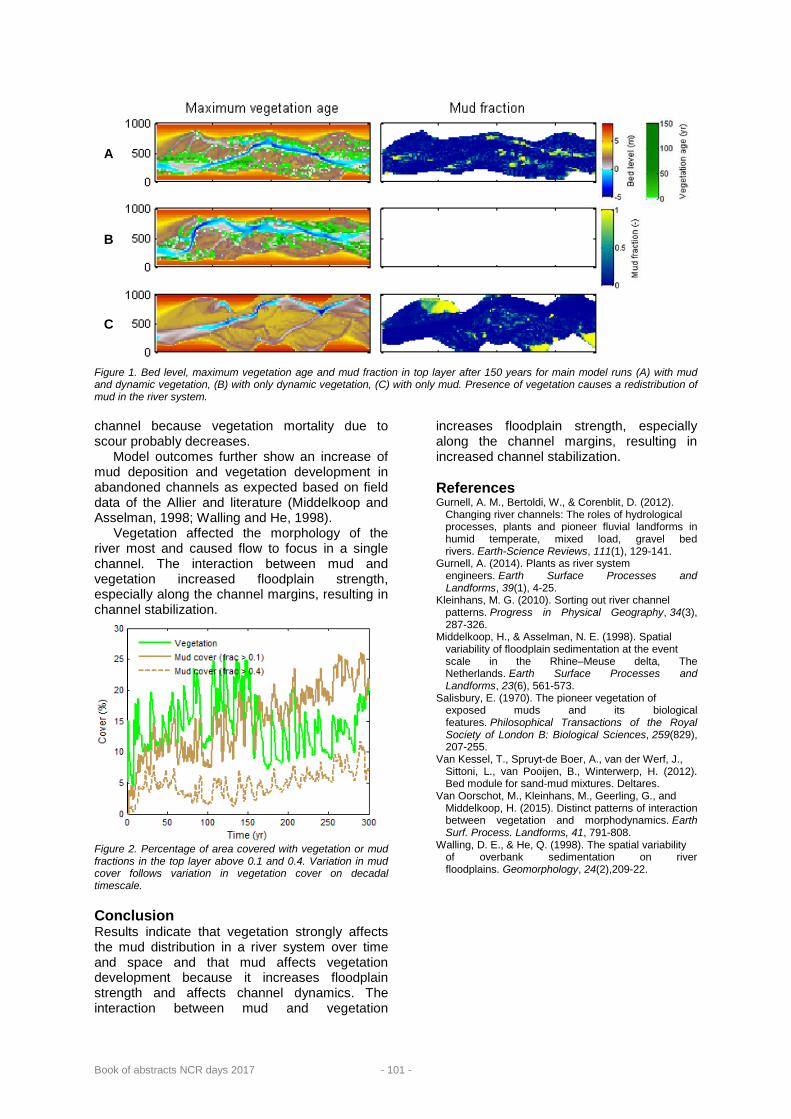
Book of abstracts NCR days 2017 - 101 -
Figure 1. Bed level, maximum vegetation age and mud fraction in top layer after 150 years for main model runs (A) with mud and dynamic vegetation, (B) with only dynamic vegetation, (C) with only mud. Presence of vegetation causes a redistribution of mud in the river system. channel because vegetation mortality due to scour probably decreases.
Model outcomes further show an increase of mud deposition and vegetation development in abandoned channels as expected based on field data of the Allier and literature (Middelkoop and Asselman, 1998; Walling and He, 1998).
Vegetation affected the morphology of the river most and caused flow to focus in a single channel. The interaction between mud and vegetation increased floodplain strength, especially along the channel margins, resulting in channel stabilization.
Figure 2. Percentage of area covered with vegetation or mud fractions in the top layer above 0.1 and 0.4. Variation in mud cover follows variation in vegetation cover on decadal timescale. Conclusion Results indicate that vegetation strongly affects the mud distribution in a river system over time and space and that mud affects vegetation development because it increases floodplain strength and affects channel dynamics. The interaction between mud and vegetation
increases floodplain strength, especially along the channel margins, resulting in increased channel stabilization. References Gurnell, A. M., Bertoldi, W., & Corenblit, D. (2012).
Changing river channels: The roles of hydrological processes, plants and pioneer fluvial landforms in humid temperate, mixed load, gravel bed rivers. Earth-Science Reviews, 111(1), 129-141.
Gurnell, A. (2014). Plants as river system engineers. Earth Surface Processes and Landforms, 39(1), 4-25.
Kleinhans, M. G. (2010). Sorting out river channel patterns. Progress in Physical Geography, 34(3), 287-326.
Middelkoop, H., & Asselman, N. E. (1998). Spatial variability of floodplain sedimentation at the event scale in the Rhine–Meuse delta, The Netherlands. Earth Surface Processes and Landforms, 23(6), 561-573.
Salisbury, E. (1970). The pioneer vegetation of exposed muds and its biological features. Philosophical Transactions of the Royal Society of London B: Biological Sciences, 259(829), 207-255.
Van Kessel, T., Spruyt-de Boer, A., van der Werf, J., Sittoni, L., van Pooijen, B., Winterwerp, H. (2012). Bed module for sand-mud mixtures. Deltares.
Van Oorschot, M., Kleinhans, M., Geerling, G., and Middelkoop, H. (2015). Distinct patterns of interaction between vegetation and morphodynamics. Earth Surf. Process. Landforms, 41, 791-808.
Walling, D. E., & He, Q. (1998). The spatial variability of overbank sedimentation on river floodplains. Geomorphology, 24(2),209-22.
A B C

Book of abstracts NCR days 2017 - 102 -
The effect of transverse bed slope and sediment mobility on bend sorting S.A.H. Weisscher*1, A.W. Baar1, W.S.J. Uijttewaal2, M.G. Kleinhans1 1 Faculty of Geosciences, Utrecht University, PO Box 80115, 3508 TC, Utrecht, The Netherlands 2 Faculty of Civil Engineering and Geosciences, Delft University of Technology, PO Box 5048, 2600 GA Delft, The Netherlands * Corresponding author; e-mail: [email protected]
Problem definition Lateral sorting (= bend sorting) is observed in natural meanders, where the inner and outer bend are fairly fine and coarse, respectively (e.g. Julien and Anthony, 2002; Clayton and Pitlick, 2007). This is caused by the mass differences between grains on a transverse slope, leading to coarser grains being dragged down net more than finer grains (Ikeda et al., 1987). The slope of the transverse bed influences the degree of bend sorting greatly.
Also vertical sorting occurs. Grainflows at the lee side of dunes result in a net fining upward trend (Kleinhans, 2005). The degree of vertical sorting depends on flow velocity and sediment mixture characteristics.
Most previous studies focused on the development of the transverse slope using small ranges of uniform sediment, so spatial sorting was absent. Yet, it was argued that there is a feedback mechanism between bend sorting and the transverse slope (Ikeda et al., 1987). So, it is of key importance to attain better understanding of how sorting in river bends comes about, which can improve current numerical models.
It is the objective of this study to examine experimentally the effect of transverse bed slope and sediment mobility on spatial sorting of bed load in a meander. Methodology A rotating annular flume was used in order to isolate all parameters (Baar et al., in prep.). A rotating lid steered the flow. Counter-rotation of the flume itself introduces a centrifugal force on the flow low in the water column, thereby weakening helical flow intensity (Booij and Uijttewaal, 1999).
A near-unimodal sediment mixture was used with a median grain size d50 = 0.75 mm and first standard deviation mass percentiles d16 = 0.53 mm and d84 = 1.49 mm. The mixture was chosen such that armouring was unlikely to occur.
A total of 34 experiments were conducted with varied helical flow intensity and sediment mobility. Bed elevation at morphodynamic equilibrium was scanned at 10 radii (Fig. 1),
using an echo sounder. 13 experiments were sampled when meeting the following criteria to acquire local grain size distributions: • Transverse slope between 0 and 0.25 • θ/θcr < 3.6 • small dune height Δ < 0.1 m where θ = dimensionless bed shear stress and θcr = dimensionless bed shear stress threshold of motion. Using these criteria, bed morphology resembled natural rivers best. In total, 340 samples were taken over the width of the flume at the dune top, in the dune trough and over the vertical deposit at the lee side of a dune (= bulk samples) (Fig. 1).
Figure 24. Sampling locations and scanned radii of bed elevation. Based on the scanned bed elevation, a mean transverse slope was computed. Lee side was removed up to the brinkpoint before sampling over the vertical. Results and conclusion Typical bed morphology at morphodynamic equilibrium was a transverse slope with dunes in the outer bend and ripples in the inner bend (Fig. 2). Generally, the outer bend was coarser than the inner bend.
Lateral separation of grain size shows clear correlation with the transverse bed slope, with coarser grains in the outer bend and finer in the inner bend; the larger the transverse slope, the more distinct bend sorting became (Fig. 3). Especially slopes larger than 0.15 caused a sharp transition, where all coarse grains were in the outer bend (Fig. 3). For smaller slopes, the transition was more gradual.
Higher sediment mobility leads to higher dunes and a thicker active layer and likely more turbulence. This resulted in slightly less

Book of abstracts NCR days 2017 - 103 -
distinct separation of grain sizes over the lateral. References Baar et al. (in prep.) Booij, R., Uijttewaal, W.S.J. (1999) Modeling of the flow in
rotating annular flumes. Engineering Turbulence Modeling and Experiments, 4:339–348.
Clayton, J.A., & Pitlick, J. (2007). Spatial and temporal variations in bed load transport in a gravel bed river bend. Water Resources Research, 43(2).
Ikeda, S., Yamasaka, M., & Chiyoda, M. (1987). Bed topography and sorting in bends. Journal of Hydraulic Engineering, 113(2), 190-204.
Julien, P. Y., & Anthony, D. J. (2002). Bed load motion and grain sorting in a meandering stream. Journal of Hydraulic Research, 40(2), 125-133.
Kleinhans, M.G. (2005). Grain-size sorting in grainflows at the lee side of deltas. Sedimentology, 52(2), 291-311.
Figure 25 Top view of a section of the bed in the annular flume. Flow was from left to right. In the outer bend, there is a dune top, followed by a coarse trough. In the inner bend, there are ripples that collapse downstream of the dune’s brinkpoint.
Figure 26. Relative median grain size over the width of the flume. d50,in = median grain size of initial, unsorted mixture, r = local radius and rc = radius at channel axis. Power of power fit increases with transverse slope, indicating a larger transition from fine to coarse.

Book of abstracts NCR days 2017 - 104 -
Predicting piping underneath river dikes using 3D subsurface heterogeneity T.G. Winkels*1, W.J. Dirkx1, E. Stouthamer1, K.M. Cohen1,2, H. Middelkoop1 1 University of Utrecht, Department of Physical Geography, Faculty of Geosciences, P.O. 80.115, 3508 TC, Utrecht, the Netherlands 2 Department of Applied Geology and Geophysics, Deltares, P.O. 85467, 3508 AL, Utrecht, the Netherlands * Corresponding author; e-mail: [email protected]
Introduction At locations where a river dike overlies a subsurface permeable sand body, seepage-pathways can emerge during flood periods, creating so called pipes, which can ultimately trigger dike destabilization (Van Beek et al., 2013). For river dikes in Dutch Rhine Meuse Delta piping is seen a as a key failure mechanism (VNK, 2015). At present, piping hazard is calculated using the 2D Sellmeijer formula (Sellmeijer 2006, Sellmeijer et al. 2011, Van Beek. 2013, Kanning 2012), that characterizes subsurface sediments by the D70 grain size values. These values are usually determined at one single depth just below the cohesive topsoil. The Dutch subsurface is however extremely heterogenic, due to the presence of multiple generations of sandy channel belts in the subsurface (Berendsen and Stouthamer, 2000). These channel belts are characterized by large scale variations in lithology and sedimentary structures, which has considerable effect on the hydraulic properties of the subsurface and hence on the pipe-forming erosion processes. Therefore, to incorporate this heterogenic subsurface in assessments of piping hazard, a shift to 3D calculations of seepage flow is essential. Sedimentary reconstruction Classic meandering river models (e.g. Allen, 1978) portray channel belts to be composed of point-bar sand bodies mostly. However, their
internal build-up is more diverse, comprising a range of elements and sedimentological structures (Bridge, 2002; Toonen et al., 2012; Miall, 1996). Although this is widely recognized, detailed reconstruction of fluvial sand bodies and their variable lithological and hydrological properties remains challenging due to the various nested scales of heterogeneity within and between fluvial deposits (Jordan and Pryor, 1992; Miall, 1996; Van de Lageweg et al., 2016; Weerts, 1996). This project aims to make a full three-dimensional reconstruction of the channel belt internal architectural elements and surrounding overbank deposits, by subdividing them into 1) cross-bedded sand deposits, 2) vertically aggraded sandy deposits (e.g. plug-bars, chute-bars), 3) overbank facies and 4) fine-grained, locally organic, laminated deposits (Fig. 1). This division is based on the distinct sedimentary characteristics between these units, caused by differences in depositional processes. This way of sedimentary reconstruction is a step to more functional hydrological character-isation of channel belts in 3D numeric subsur-face flow and piping calculations, than is available at present. Given the complexity involved, we first attempt local reconstructions using existing and new collected data (coring, CPT, geophysics) at established pilot sites from ongoing Piping investigations, and then scale up to larger areas along embanked rivers in the Netherlands.
Figure 1. Cross section of meandering river showing the different architectural elements (adapted from Erkens, 2009).

Book of abstracts NCR days 2017 - 105 -
References Allen, J.R.L. (1978). Studies in fluviatile sedimentation: an exploratory quantitative model for the architecture of
avulsion-controlled alluvial suites. Sedimentary Geology , 21: 129–147.
Bridge, J.S. (2002). Rives and Floodplains. Blackwell Publishing. 501 p.
Erkens, G. (2009). Sediment dynamics in the Rhine catchment. Quantification of fluvial response to climate change and human impact. PhD thesis Utrecht University, 278 p
Jordan, D.W. and Pryor, W.A. (1992). Hierarchical levels of heterogeneity in a Mississippi River Meander belt and application to reservoir systems. American Association of Petroleum Geologists, 76: 1601–1624.
Kanning, W. (2012). The Weakest Link, Spatial Variability in the Piping Failure Mechanism of Dikes. PhD thesis Technische Universiteit Delft, 235p.
Miall, A.D. (1996). The geology of fluvial deposits. Sedimentary facies, Basin analysis, and petroleum geology. Springer-Verlag. 582 p.
Sellmeijer, J.B. (2006). Numerical computation of seepage erosion below dams (piping). Proceedings 3rd Int. In: Conference on Scour and Erosion: 596-601.
Sellmeijer, H., de la Cruz, J.L., van Beek, V. M., Knoeff, H. (2011). Fine-tuning of the backward erosion piping model
through small-scale, medium-scale and IJkdijk experiments. European Journal of Environmental and Civil Engineering, 15(8): 1139-1154.
Stouthamer, E., Berendsen, H.J.A., (2000). Factors controlling the Holocene avulsion history of the Holocene Rhine-Meuse delta (The Netherlands). Journal of Sedimentary Research, section A, 70 (5): 1051-1064.
Toonen, W.H.J., Kleinhans, M.G. & Cohen, K.M. (2012). Sedimentary architecture of abandoned channel fills. Earth Surface Processes and Landforms, 37: 459-472.
Van Beek, V.M., Bezuijen, A., Sellmeijer, H. (2013). Backward erosion piping. In: Bonelli, N., 2013 (Ed.), Erosion in Geomechanics Applied to Dams and Levees. Wiley: 193-269.
Van de Lageweg, W.I., Schuurman, F., Cohen, K.M., Van Dijk, W.M., Shimizu, Y. and Kleinhans, M.G. (2015). Preservation of meandering river channels in uniformly aggrading channel belts. Sedimentology, 63: 586–608.
VNK (2015). De veiligheid van Nederland in kaart. Rijkswaterstaat Projectbureau VNK. Document HB 2540621, 120 p.
Weerts, H.J.T. (1996). Hydrofacies units in the fluvial Rhine-Meuse delta. In: Complex confining layers. PhD thesis Utrecht University,189 p.
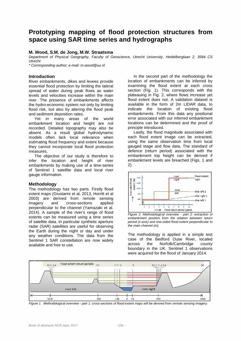
Book of abstracts NCR days 2017 - 106 -
Prototyping mapping of flood protection structures from space using SAR time series and hydrographs ( M. Wood, S.M. de Jong, M.W. Straatsma Department of Physical Geography, Faculty of Geoscience, Utrecht University, Heidelberglaan 2, 3584 CS Utrecht * Corresponding author; e-mail: [email protected]
) Introduction River embankments, dikes and levees provide essential flood protection by limiting the lateral spread of water during peak flows as water levels and velocities increase within the main river. The presence of embankments affects the hydro-economic system not only by limiting flood risk, but also by altering the flood peak and sediment deposition rates.
Yet in many areas of the world embankment location and height are not recorded. Detailed topography may also be absent. As a result global hydrodynamic models often lack local relevance when estimating flood frequency and extent because they cannot incorporate local flood protection measures.
The objective of our study is therefore to infer the location and height of river embankments by making use of a time-series of Sentinel 1 satellite data and local river gauge information. Methodology The methodology has two parts. Firstly flood extent maps (Giustarini et al, 2013, Horritt et al 2003) are derived from remote sensing imagery and cross-sections applied perpendicular to the channel (Yamazaki et al. 2014). A sample of the river’s range of flood extents can be measured using a time series of satellite data. In particular synthetic aperture radar (SAR) satellites are useful for observing the Earth during the night or day and under any weather conditions. The data from the Sentinel 1 SAR constellation are now widely available and free to use.
In the second part of the methodology the location of embankments can be inferred by examining the flood extent at each cross section (Fig. 1). This corresponds with the plateauing in Fig. 2, where flows increase yet flood extent does not. A validation dataset is available in the form of 2m LIDAR data, to indicate the location of existing flood embankments. From this data any positional error associated with our inferred embankment locations can be determined and the proof of principle introduced.
Lastly, the flood magnitude associated with each flood extent image can be extracted, using the same observation time from local gauged stage and flow data. The standard of defence (return period) associated with the embankment top height can be derived if embankment levels are breached (Figs. 1 and 2).
Figure 2. Methodological overview - part 2: extraction of embankment position from the relation between return period (x-axis) and one-sided flood extent perpendicular to the main channel (m). The methodology is applied in a simple test case of the Bedford Ouse River, located across the Norfolk/Cambridge county boundary in the UK. Sentinel 1 observations were acquired for the flood of January 2014.
Figure 1. Methodological overview - part 1: cross-sections of flood extent maps will be derived from remote sensing imagery.

Book of abstracts NCR days 2017 - 107 -
Figure 3. Left: Overlapping of Sentinel 1a flood extent images for the Bedford Ouse River, illustrating the relative frequency of inundation within the observation data. The DEM background shows elevations including the location of embankments (purple). Right: Out-of-bank flooding (blue) detected for the Bedford Ouse River, derived from Sentinel 1 data. River cross-sections used to measure flood extent at each bank are shown in red. First results Five flood extent maps were derived from a series of Sentinel 1a images at the test location for the flood of January 2014. A relative flood frequency map from these 5 data is shown in Fig. 3 (left) and indicates the areas where flood water is most often present at this location, for this particular event.
Cross-sections perpendicular to the channel were used on each of the Sentinel 1a SAR flood extent maps to examine the extent of flooding on the left and right of the main channel (Fig. 3, right).
The early results reveal the extent of flooding and suggest the location of the embankments adjacent to the river. Work is currently in progress to link the embankment location to a local water level and flow in order to estimate embankment heights. Future work Work is ongoing to link flood extent images to a return period using gauged record (Fig. 2). The final stage of work will analyse the error in embankment location and heights with respect to the validation data.
We aim to fully automate the method to enable application at selected locations around the globe. Future work could adapt the current methodology to use hydrodynamic models to associate flood extent and river flows together in the absence of gauged data. If the project is successful, there are wider applications for this methodology with the potential for use on global river systems or in data poor regions where
embankment information is not available. Future work will include testing the methodology on a larger global river network.
We expect that the information obtained on embankment location and heights will aid future work in other areas such as error assessment of embankment attributes, and the error propagation into use cases (biodiversity, flood risk, sedimentation). Acknowledgements This work has been carried out in cooperation with the Luxembourg Institute of Science and Technology. Funding for this project has been obtained from the Faculty of Geosciences, Department of Physical Geography, Utrecht University, Utrecht, the Netherlands. References Giustarini, L., Hostache, R., Matgen, P., Schumann,
G.J.P., Bates, P.D. and Mason, D.C., 2013. A change detection approach to flood mapping in urban areas using TerraSAR-X. IEEE Transactions on Geoscience and Remote Sensing, 51(4), pp.2417-2430.
Horritt, M.S., Mason, D.C., Cobby, D.M., Davenport, I.J., & Bates, P.D. (2003). Waterline mapping in flooded vegetation from airborne SAR imagery. Remote Sensing of Environment, 85, 271-281
Yamazaki, D., O'Loughlin, F., Trigg, M.A., Miller, Z.F., Pavelsky, T.M., & Bates, P.D. (2014). Development of the Global Width Database for Large Rivers. Water Resources Research, 50, 3467-3480.

Book of abstracts NCR days 2017 - 108 -
Next steps in palaeogeographic mapping of the Lower Meuse Valley to unravel tectonic and climate forcing H.A.G. Woolderink*1, C. Kasse1, K.M. Cohen2,3,4, R.T. Van Balen1,3 1 Vrije Universiteit Amsterdam, Faculty of Earth and Life Sciences, cluster Earth & climate 2 Universiteit Utrecht, Faculty of Geosciences, department of Physical Geography 3 Department of Geomodelling, TNO Geological Survey of the Netherlands, Utrecht, The Netherlands 4 Department Applied Geology and Geophysics, Deltares, Utrecht/Delft, The Netherlands * Corresponding author; e-mail: [email protected] Introduction The river Meuse flows from its headwaters in eastern France through the Paris basin and the Ardennes Massif into the horst-graben structured Roer Valley Rift System (RVRS) before entering the North Sea at the Dutch coast. The catchment of this rain-fed system is around 33.000 km2 and the river has a length of 925 km. Tectonic uplift of the Ardennes/Rhenish Massif and glacial-interglacial cyclicity has led to the formation and preservation of Meuse river terraces throughout the catchment, from the north-eastern part of the Paris Basin to below the Meuse’ delta plain in the Netherlands (Zonneveld, 1974; Van den Berg, 1996; Van Balen et al., 2000). In the Netherlands the Meuse terrace sequence has been studied in detail by, amongst many others, Pons & Schelling (1951), Pons (1954), Van Den Broek & Maarleveld (1963), Van den berg (1989,1996), Berendsen et al. (1995), Kasse et al. (1995), Huisink (1997), Tebbens et al. (1999), Cohen (2003) and Rensink et al. (2015). The youngest, lowest levels of terraces are shown to hold remnants of glacial-stage braided plains from the Weichselian Late Pleniglacial and Younger Dryas stadials, but also of meandering channel belts of Allerød interstadial and Holocene interglacial stages. Such geological-geomorphological reconstructions, in principle, allow to identify interaction between river morphology and forcing factors such as climate change and tectonics, and to explore and explain temporal and spatial changes herein. In practice, however, most of the aforementioned studies covered restricted parts of the Meuse valley and/or restricted time periods. A truly integrated reconstruction of Lower Meuse geomorphological activity since the Weichselian Last Glacial Maximum, is lacking. Because a river’s response to the same external forcing may vary along the river system, owing to both catchment and reach-specific characteristics (Erkens et al., 2009), with hindsight, some regional differences along the river Meuse may have been insufficiently
considered in the maps produced so far. In addition, a wealth of new data, mainly from archaeological exploration, has become available in the past years. For unravelling of tectonic (active and passive) from climatic controls in the Meuse valley an updated, consistent and detailed palaeogeographical reconstruction is needed, which this study aims at. Methods The production of the integrated map dataset follows similar procedures as described in Berendsen et al. (2001, 2007). First, existing information on dated geomorphological features such as meander-scar fills, pointbars and aeolian dunes is acquired from published and unpublished data (i.e. from journal papers, archaeological studies and geological surveys) and subsequently stored in a database format. Secondly, geomorphological datasets of continuous cover (e.g. AHN2 lidar data), lithological descriptions (cores, outcrops) and existing maps are digitally collected and manually (re)interpreted to geomorphological and geological maps, honouring the dating information of the first database. The polygons of the resulting geomorphological reconstruction are then digitized, coded and catalogued in dedicated format (Cohen et al., 2012), so that time-slice map series of past situations can also be generated. Results and conclusion Preliminary results indicate that synchronous river terrace fragments appear to differ in fluvial style in a longitudinal direction. Furthermore, river terraces of the Meuse are not continuous along the Meuse Valley and floodplain width varies as it crosses the horst-graben structure of the RVRS. Finally, the mapping allows to identify anomalous fluvial morphology (e.g. change in sinuosity or gradient lines) near active fault zones of the RVRS. The new steps of palaeogeographic mapping of the Lower Meuse Valley provide more insight into river response to forcing factors and will provide the basis for future research on river dynamics.

Next steps in palaeogeographic mapping of the Lower Meuse Valley to unravel tectonic and climate forcing
Book of abstracts NCR days 2017 - 109 -
References Berendsen, H., Cohen, K., Stouthamer, E. (2001) Maps
and Cross-sections. In: Berendsen & Stouthamer, 2001: Palaeogeographic development of the Rhine-Meuse delta, The Netherlands, Assen: Van Gorcum, 268 p.,
Berendsen, H., Cohen, K., Stouthamer, E. (2007). The use of GIS in reconstructing the holocene palaeogeography of the Rhine–Meuse delta, the Netherlands. International Journal of Geographical Information Science, 21(5), 589-602.
Berendsen, H., Hoek, W., Schorn, E. (1995). Late weichselian and holocene river channel changes of the rivers rhine and meuse in the netherlands (land van maas en waal). Paläoklimaforschung/Palaeoclimate Research, 14, 151-171.
Cohen, K. (2003). Differential subsidence within a coastal prism: late-Glacial-Holocene tectonics In The Rhine-Meuse delta, the Netherlands. Netherlands Geographical Studies 316, 216 pp.
Cohen, K., Stouthamer, E., Pierik, H., Geurts, A. (2012). Rhine Meuse Delta Studies’ Digital Basemap for Delta Evolution and Palaeogeography.Utrecht University.Digital Dataset.Persistent Identifier: Urn: Nbn: Nl: Ui: 13-Nqjn-Zl,
Erkens, G., Dambeck, R., Volleberg, K. P., Bouman, M. T., Bos, J. A., Cohen, K. M. (2009). Fluvial terrace formation in the northern upper rhine graben during the last 20000 years as a result of allogenic controls and autogenic evolution. Geomorphology, 103(3), 476-495.
Huisink, M. (1997). Late‐glacial sedimentological and morphological changes in a lowland river in response to climatic change: The maas, southern netherlands. Journal of Quaternary Science, 12(3), 209-223.
Kasse, C., Vandenberghe, J., Bohncke, S. (1995). Climatic change and fluvial dynamics of the maas during the late weichselian and early holocene. Paläoklimaforschung, 14, 123-150.
Pons, L. (1954). Het fluviatiele laagterras van rijn en maas. Boor En Spade, 7(97), 110.
Pons, L., Schelling, J. (1951). De laatglaciale afzettingen van de rijn en de maas. Geologie En Mijnbouw, 13, 293-297.
Rensink, E., Isarin, R., Ellenkamp, R., Heunks, E. (2015). Archeologische verwachtingskaart maasdal tussen mook en eijsden. (Report + dataset), DANS.
Tebbens, L., Veldkamp, A., Westerhoff, W., Kroonenberg, S. (1999). Fluvial incision and channel downcutting as a response to late-glacial and early holocene climate change: The lower reach of the river meuse (maas), the netherlands. Journal of Quaternary Science, 14(1), 59-75.
Van Balen, R., Houtgast, R., Van der Wateren, F., Vandenberghe, J., Bogaart, P. (2000). Sediment budget and tectonic evolution of the meuse catchment in the ardennes and the roer valley rift system. Global and Planetary Change, 27(1), 113-129.
Van den Berg, M. (1989). Toelichting op kaartblad 59–62, geomorfologische kaart van Nederland 1:50.000, DLO-Staring Centrum. WageningenrRijks Geol. Dienst, Haarlem, pp. 32.
Van den Berg, M. (1996). Fluvial sequences of the maas: A 10 ma record of neotectonics and climate change at various time-scales.
Van den Broek, J., Maarleveld, G. (1963). The late pleistocene terrace deposits of the meuse. Mededelingen Geologische Stichting NS, 16, 13-24.
Zonneveld, J. (1974). The terraces of the meuse (and rhine) downstream of maastricht (Macar, P. (Ed.) L'évolution Quaternaire de Basins Fluviaux de la mer du Nord Mérondiale. ed.). Liége: Centenaire de la société géologique de Belgique.
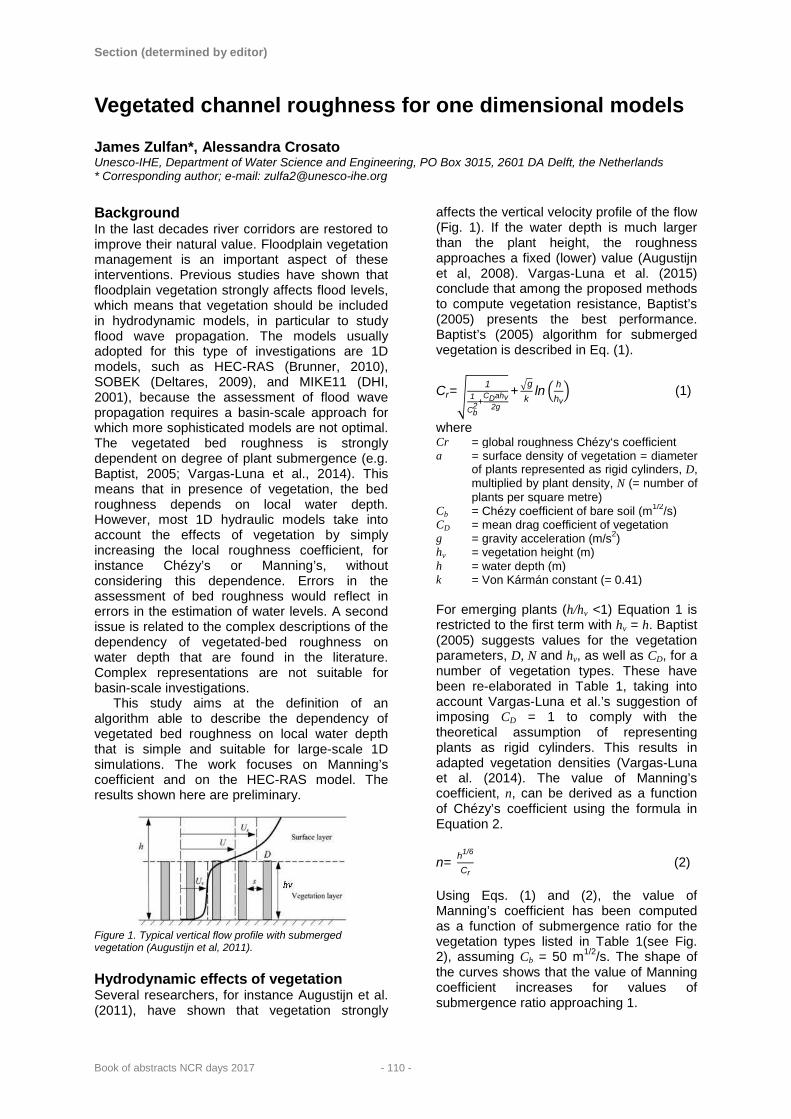
Section (determined by editor)
Book of abstracts NCR days 2017 - 110 -
Vegetated channel roughness for one dimensional models James Zulfan*, Alessandra Crosato Unesco-IHE, Department of Water Science and Engineering, PO Box 3015, 2601 DA Delft, the Netherlands * Corresponding author; e-mail: [email protected]
Background In the last decades river corridors are restored to improve their natural value. Floodplain vegetation management is an important aspect of these interventions. Previous studies have shown that floodplain vegetation strongly affects flood levels, which means that vegetation should be included in hydrodynamic models, in particular to study flood wave propagation. The models usually adopted for this type of investigations are 1D models, such as HEC-RAS (Brunner, 2010), SOBEK (Deltares, 2009), and MIKE11 (DHI, 2001), because the assessment of flood wave propagation requires a basin-scale approach for which more sophisticated models are not optimal. The vegetated bed roughness is strongly dependent on degree of plant submergence (e.g. Baptist, 2005; Vargas-Luna et al., 2014). This means that in presence of vegetation, the bed roughness depends on local water depth. However, most 1D hydraulic models take into account the effects of vegetation by simply increasing the local roughness coefficient, for instance Chézy’s or Manning’s, without considering this dependence. Errors in the assessment of bed roughness would reflect in errors in the estimation of water levels. A second issue is related to the complex descriptions of the dependency of vegetated-bed roughness on water depth that are found in the literature. Complex representations are not suitable for basin-scale investigations.
This study aims at the definition of an algorithm able to describe the dependency of vegetated bed roughness on local water depth that is simple and suitable for large-scale 1D simulations. The work focuses on Manning’s coefficient and on the HEC-RAS model. The results shown here are preliminary.
Figure 1. Typical vertical flow profile with submerged vegetation (Augustijn et al, 2011). Hydrodynamic effects of vegetation Several researchers, for instance Augustijn et al. (2011), have shown that vegetation strongly
affects the vertical velocity profile of the flow (Fig. 1). If the water depth is much larger than the plant height, the roughness approaches a fixed (lower) value (Augustijn et al, 2008). Vargas-Luna et al. (2015) conclude that among the proposed methods to compute vegetation resistance, Baptist’s (2005) presents the best performance. Baptist’s (2005) algorithm for submerged vegetation is described in Eq. (1).
Cr=�1
1
Cb2+
CDahv2g
+ �gk
ln � hhv� (1)
where Cr = global roughness Chézy‘s coefficient a = surface density of vegetation = diameter
of plants represented as rigid cylinders, D, multiplied by plant density, N (= number of plants per square metre)
Cb = Chézy coefficient of bare soil (m1/2/s) CD = mean drag coefficient of vegetation g = gravity acceleration (m/s2) hv = vegetation height (m) h = water depth (m) k = Von Kármán constant (= 0.41) For emerging plants (h/hv <1) Equation 1 is restricted to the first term with hv = h. Baptist (2005) suggests values for the vegetation parameters, D, N and hv, as well as CD, for a number of vegetation types. These have been re-elaborated in Table 1, taking into account Vargas-Luna et al.’s suggestion of imposing CD = 1 to comply with the theoretical assumption of representing plants as rigid cylinders. This results in adapted vegetation densities (Vargas-Luna et al. (2014). The value of Manning’s coefficient, n, can be derived as a function of Chézy’s coefficient using the formula in Equation 2.
n= h1/6
Cr (2)
Using Eqs. (1) and (2), the value of Manning’s coefficient has been computed as a function of submergence ratio for the vegetation types listed in Table 1(see Fig. 2), assuming Cb = 50 m1/2/s. The shape of the curves shows that the value of Manning coefficient increases for values of submergence ratio approaching 1.

Book of abstracts NCR days 2017 - 111 -
Table 1. Vegetation parameters for selected types of floodplain vegetation. Re-elaborated from Baptist (2005).
Figure 2. Manning’s value for different type of vegetation in submerged condition (Cb=50).
HEC-RAS suggests using the roughness values for vegetated beds listed in Table 2. Table 2. Vegetated-bed Manning’s coefficients suggested for HEC-RAS (Brunner, 2010).
Manning’s dependency on submergence ratio and on bare bed roughness, Cb, for a 0.05 m garden grassland is shown in Fig. 3.
Figure 3. Manning’s value for Garden grassland for different types of bed material. The constant values suggested for HEC-RAS are given by continuous horizontal lines. Fig. 3 shows that the values of Manning used in HEC-RAS do not fit the graph. They approach the computed value for large submergence ratios (h/hv > 5). Using the suggested values would therefore lead to water depth underestimation for discharges that are just above bankfull (small water depths on vegetated floodplains). Fig.3 shows also that Cb does not give any significant effects on vegetated bed roughness. The term 1/Cb
2 is very small and can be neglected from
Equation 1. The obtained expression for the roughness of vegetated beds becomes then made of two terms, a constant vegetation parameter (assuming CD = 1, the vegetation parameter becomes a function of a and hv,) plus a function of submergence ratio (h/hv).In accordance, the formula by Baptist, Eq. (1), is simplified as follows:
Cr=�2gahv
+ �gk
ln � hhv� (3)
The first term of Equation 3, � 2𝑔𝑔𝑎𝑎ℎ𝑣𝑣
, here
named Chézy’s vegetation constant, Cveg, can be computed for the different vegetation types listed by Baptist (2005), see Table 3. Table 3. Chezy’s vegetation coefficient for different types of submerged vegetation.
no type of vegetation Cveg 1 pioneer vegetation 20.14 2 garden grassland 4.90 3 natural grassland 3.01 4 herbaceous vegetation 3.29 5 softwood shrub 4.09 6 close shrub 5.04 7 reed 3.43 8 trees 28.17
Acknowledgements This research is part of an Msc thesis supported by NFP. References Augustijn, D.C.M, et al (2008). Comparison of
vegetation roughness descriptions. The 4th International Conference on Fluvial Hydraulics, River Flow 3-5 September 2008. Izmir Turkey.
Augustijn, D.C.M, et al (2011). Evaluation on flow formulas for submerged vegetation. Euromech Colloquium 523. 15-17 June 2011. France.
Baptist, M J. (2005). Modelling floodplain bio geomorphology, PhD thesis, TU Delft, The Netherlands.
Brunner, Gary W. (2010). HEC-RAS River Analysis System. Hydraulic Reference Manual.Version 4.1. Hydrologic Engineering Center Davis Ca, 2-6.
Danish Hydraulic Institute. (2001). MIKE 11 Reference manual, Appendix A. Scientific background, Danish Hydraulic Institute.
Deltares. (2009). User Manual and Theoretical Background of SOBEK model. Deltares, the Netherlands.
Vargas‐Luna, A., et al. (2014). Effects of vegetation on flow and sediment transport: comparative analyses and validation of predicting models. Earth Surface Processes and Landforms.
Vargas‐Luna,A., et al. (2015). Representing plants as rigid cylinders in experiments and models. Advances in Water Resources, 93, 205-222.
NO Vegetation typediameter
(m) density
(m-2)
a (diameter*density)
Height (m)
Drag coeff
1 Pioneer vegetation 0.0054 50 0.27 0.15 12 Garden grassland 0.0045 3000 13.50 0.05 13 Natural grassland 0.0054 4000 21.60 0.1 14 Herbaceous vegetation 0.0075 400 3 0.5 15 Close shrub 0.015 10.2 0.15 5 16 Softwood shrub 0.051 3.8 0.19 6 17 Reed 0 80 0 2.5 18 Trees 0.225 0.015 0.003 5 1
no Type of channel and description
Minimum Normal Maximum Natural streams Floodplains
a Pasture no brush 1. Short grass 0.025 0.03 0.035 2. High grass 0.03 0.035 0.05
b Cultivated areas 1. No crop 0.02 0.03 0.04 2. Mature row crops 0.025 0.035 0.045 3. Mature field crops 0.03 0.04 0.05

Book of abstracts NCR days 2017 - 112 -

Book of abstracts NCR days 2017 - 113 -
NCR-days 2017 Conference venue Gaia building (building 101) Wageningen University & Research Droevendaalsesteeg 3 6708 PB Wageningen The Netherlands Contact address NCR days 2017 organisation Mrs. Tamara Schalkx Wageningen University & Research P.O. Box 47 6700 AA Wageningen T: +31 (0) 317 481 511 E: [email protected] W: www.wur.eu/hwm Contact address NCR Mrs. Monique te Vaarwerk Netherlands Centre for River Studies (NCR) c/o University of Twente P.O. Box 217 7500 AE Enschede T: +31 (0) 53 489 4020 E: [email protected] W: www.ncr-web.org

Book of abstracts NCR days 2017 - 114 -
NCR Supervisory Board NCR Programme Committee
January 2017 January 2017
dr. J.C.J. Kwadijk, Chairman dr. R. Schielen, Chairman Deltares Rijkswaterstaat-WVL email: [email protected] email: [email protected] ir. K.D. Berends, Secretary ir. K.D. Berends, Secretary Deltares Deltares email: [email protected] email: [email protected] ir. K. van der Werff dr. G.W. Geerling Rijkswaterstaat-WVL Deltares email: [email protected] email: [email protected] prof. dr. H. Middelkoop dr. E. Stouthamer Utrecht University Utrecht University email: [email protected] email: [email protected] prof. dr. ir. H.H.G. Savenije prof. dr. ir. W.S.J. Uijttewaal Delft University of Technology Delft University of Technology email: [email protected] email: [email protected] dr. R.S.E.W. Leuven dr. H.J.R. Lenders Radboud University Nijmegen Radboud University Nijmegen email: [email protected] email: [email protected] prof. dr. ir. A.Y. Hoekstra dr. ir. D.C.M. Augustijn University of Twente University of Twente email: [email protected] email: [email protected] prof. C. Zevenbergen, PhD, MSc dr. A. Crosato UNESCO-IHE UNESCO-IHE email: [email protected] email: [email protected] dr. H. Wolfert dr. A.J.F. Hoitink Wageningen University & Research Wageningen University & Research email: [email protected] email: [email protected]


Colophon Editors: A.J.F. Hoitink (WUR, Hydrology & Quantitative Water Management group) T.V. de Ruijsscher (WUR, Hydrology & Quantitative Water Management group) T.J. Geertsema (WUR, Hydrology & Quantitative Water Management group) B. Makaske (WUR, Soil Geography & Landscape group) J. Wallinga (WUR, Soil Geography & Landscape group) J.H.J. Candel (WUR, Soil Geography & Landscape group) J. Poelman (WUR, Hydrology & Quantitative Water Management group) Design cover: T.V. de Ruijsscher Print: Zalsman Innovative Print, Kampen Number of prints: 120 To be cited as: A.J.F. Hoitink, T.V. de Ruijsscher, T.J. Geertsema, B. Makaske, J. Wallinga, J.H.J. Candel, J. Poelman (Eds.) NCR days 2017, Book of abstracts, NCR publication 41-2017.