BNR ECONOMIC REVIEW Vol. 9 - National Bank of Rwanda
146
NATIONAL BANK OF RWANDA BANKI NKURU Y’U RWANDA BNR ECONOMIC REVIEW Vol. 9 August 2016 ISSN 2410-678X
-
Upload
khangminh22 -
Category
Documents
-
view
0 -
download
0
Transcript of BNR ECONOMIC REVIEW Vol. 9 - National Bank of Rwanda

NATIONAL BANK OF RWANDABANKI NKURU Y’U RWANDA
BNR ECONOMIC REVIEW Vol. 9
August 2016
ISSN 2410-678X


i
ISSN 2410-678X
BNR ECONOMIC REVIEW Vol. 9
August 2016

iii
Disclaimer
The views expressed in this review are those of author and not the ones of the National Bank of Rwanda.
Apart from any commercial purpose whatsoever, the reprint of the review or its part is permitted.
BNR Economic Review Vol. 9
iii
iv
Foreword In acknowledgement of the importance of policy oriented studies for forward-
looking and evidence-based monetary policy, the National Bank of Rwanda
(BNR) publishes twice a year its Economic Review in which recent BNR findings
on the Rwandan economy are disseminated and shared with different economic
actors and the general public. In this ninth volume of the BNR economic review,
five research papers are published.
The first paper on financial innovation and monetary policy is aimed at
assessing whether the various financial innovation that have taken place over
the past years pose difficulties on the conduct of monetary policy in Rwanda.
In the context of the current monetary policy framework, this assessment starts
by examining whether the velocity of money and money multiplier are stable
before proceeding to test for the stability of the money demand function. The
study also examines the link between M3 and nominal GDP to verify whether
a long run relationship between the two macroeconomic variables exists.
Results show that M3 and GDP have a long run relationship though the
structural change in the relationship between the two variables as a result of
financial innovations may reduce the effectiveness of the monetary aggregate
framework. Results also show that financial innovations do not play an
important role in determining money demand in the long run and that a shock
on credit impacts real GDP and CPI. Another interesting finding is that real GDP
reacts to a shock on the treasury bills rate, implying that Rwandans consider
investment in Treasury bill as a way of alternative saving, in addition to
commercial banks’ term deposits. Thus, BNR needs to improve the use of the
central bank rate to impact money market rates, particularly the Treasury bill
interest rate as the first stage of improving the interest rate pass through.
In our last issue of February 2016, we published a paper on “Interest Rate Pass-
through in Rwanda” as part of the roadmap towards adopting the use of
interest rate as our operating target by 2018. This issue proposes another paper
that falls within the same context but extended at the EAC level. The paper
examines and compares the degree of interest rate pass-through in EAC
BNR Economic Review Vol. 9
iv
v
countries. It concludes that even with the achievements in developing our
financial sector, the interest rate pass-through is still incomplete at low levels
in all countries but varies within a country and evolves with time. The paper
offers a framework for policy makers’ discussions on key issues to address
before 2018.
In view of the current exchange rate depreciation and cognizant of the impact
of exchange rate on external sector competitiveness, the third paper assesses
the impact of exchange rate on external sector competitiveness and based on
exchange rate misalignment and Lerner-Marshal condition indicators, the paper
concludes that though exchange rate impacts on trade balance, both the
exchange rate misalignment and Lerner- Marshall condition are not substantial
to prompt loss in external sector competitiveness. The paper therefore
recommends effective monitoring of exchange rate developments to avoid higher
levels of volatility which could lead to poor performance of Rwanda’s tradable
sector as well as putting in place better and sustainable strategies to increase
production in Rwanda to avoid higher import prices induced by the exchange
rate depreciation.
Mindful of the fact that the actions of fiscal and monetary policies are
interdependent in macroeconomic management, the fourth paper examines the
effects of fiscal policy on inflation and money market interest rates in Rwanda.
This paper uses structural autoregressive models over the period from 2006Q1
to 2015Q4. Indeed, the results show that both the government spending and
government tax revenues affect positively and significantly nominal GDP and
inflation but does not significantly affect interbank rate. In both cases, the effect
on interbank rate is found less responsive to fiscal shocks in Rwanda due to
shallow financial markets. The study therefore recommends policy makers to
boost the development of financial markets to respond to changes in
macroeconomic fundamentals for efficient monetary policy transmission
mechanism.
Recognizing that economic policy in general and monetary policy in particular
needs forward-looking dimension, the fifth paper on the determinants of
aggregate demand constructs a medium-size macroeconometric model for
BNR Economic Review Vol. 9
v
vi
Rwanda and use the model to explain the main drivers of aggregate demand in
the Rwandan economy. The proposed macroeconometric model can also be
used for forecasting and simulation analysis, provide a consistent framework
to analyze the impact of exogenous shocks on the Rwandan economy, and, help
to have structured monetary policy discussions. The in-sample forecasts show
that the model tracks well the path of key demand side macroeconomic
variables (i.e. the components of domestic and external demand). However,
more sector specific analysis is needed to develop Near Term Forecasts (NTFs)
and sector-specific assumptions to help in derivation of forecasts over longer
time horizon
I wish to express my sincere appreciation to our team of researchers who have
contributed to this publication and also those whose comments have
contributed to improve the quality of the papers.
Comments and questions can be sent to the Office of The Chief Economist
([email protected], [email protected]) and/or the Monetary Policy and Research
department, KN 6 Avenue 4, P.O Box 531 Kigali-Rwanda or on
John Rwangombwa Governor
D


BNR Economic Review Vol. 9
vii
vii
Table of contents
Foreword ............................................................................ iv
Table of contents ............................................................... vii
Financial innovations and monetary policy in Rwanda ......... 1
Interest rate Pass-through in EAC ...................................... 31
Exchange Rate and External Sector Competitiveness in
Rwanda .............................................................................. 55
Effects of Fiscal Policy on Inflation and Money Market
Interest Rates in Rwanda ................................................... 83
Determinants of Aggregate Demand in the Rwandan
Economy: A Macroeconometric Approach ......................... 111
iii
vii
1
31
53
81
109


BNR Economic Review Vol. 9
1
1
Financial innovations and monetary policy in Rwanda
Thomas Kigabo RUSUHUZWA* Mutuyimana Jean Pierre †
Key words: Financial innovation, monetary policy, velocity, money multiplier, money demand function
JEL Classification Number: E41, E43, E52 and E58
* Chief economist and Director General, monetary policy and research, National Bank of
Rwanda and Associate professor, School of business and economics, University of Rwanda. † Mutuyimana Jean Pierre, Economist at National Bank of Rwanda
Financial innovations and monetary policy in Rwanda
Chief Economist and Director General, Monetary Policy and Research, National Bank of Rwanda and Associate Professor, School of Business and Economics University of Rwanda.
BNR Economic Review Vol. 9
2
2
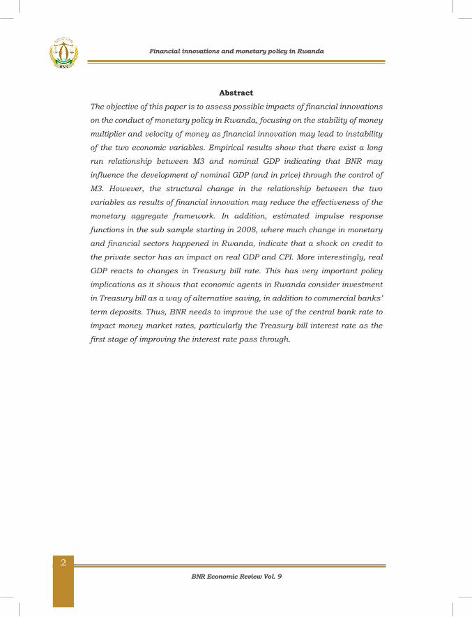
Abstract The objective of this paper is to assess possible impacts of financial innovations
on the conduct of monetary policy in Rwanda, focusing on the stability of money
multiplier and velocity of money as financial innovation may lead to instability
of the two economic variables. Empirical results show that there exist a long
run relationship between M3 and nominal GDP indicating that BNR may
influence the development of nominal GDP (and in price) through the control of
M3. However, the structural change in the relationship between the two
variables as results of financial innovation may reduce the effectiveness of the
monetary aggregate framework. In addition, estimated impulse response
functions in the sub sample starting in 2008, where much change in monetary
and financial sectors happened in Rwanda, indicate that a shock on credit to
the private sector has an impact on real GDP and CPI. More interestingly, real
GDP reacts to changes in Treasury bill rate. This has very important policy
implications as it shows that economic agents in Rwanda consider investment
in Treasury bill as a way of alternative saving, in addition to commercial banks’
term deposits. Thus, BNR needs to improve the use of the central bank rate to
impact money market rates, particularly the Treasury bill interest rate as the
first stage of improving the interest rate pass through.
Financial innovations and monetary policy in Rwanda
BNR Economic Review Vol. 9
3
3
1. Introduction The primary function of the financial system is to facilitate the optimal
allocation economic resources, both across economic sectors and across time,
in an uncertain environment. This function, in turn, involves a payment
system with a medium of exchange; the transfer of resources from savers to
users of the resources and the reduction of risk through insurance and
diversification (Merton 1992, p. 12). To operate, a financial system must incur
real resource costs generated by labor, materials and capital used by financial
intermediaries and by financial facilitators, such as stock brokers, market
makers and financial advisors. In addition, since time periods, such as
maturity of financial instruments, are an inherent characteristic of financial
activities, there are uncertainties about future states of the world that
generate risks.
Thus, financial innovation involves new and improved products, processes,
and organizational structures that can reduce costs of production, better
satisfy customer demands, and yield greater profits.
The term financial innovation refers to a wide range of changes and
developments affecting financial markets, such as the introduction of new
financial instruments, changes in the structure and depth of financial
markets, changes in the role of financial institutions, the methods by which
financial services are provided and the introduction of new products and
procedures (Esman Nyamongo et.al 2013). In a broader sense, financial
innovation can be defined as the emergence of new financial products or
services, new organizational forms, or new processes for a more developed
and complete financial markets that reduce costs and risks, or provide an
improved service that meets particular needs of financial system participants.
It is the act of creating and then popularizing new financial instruments as
well as new financial technologies, institutions and markets (Frame and
White, 2002).
The financial sector, in a broad sense, has developed an array of new financial
instruments and techniques to adopt the ever-changing global environment.
Progress in information technology affects all aspects of banking sector and
Financial innovations and monetary policy in Rwanda

BNR Economic Review Vol. 9
4
4
can be regarded as one of the main driving forces generating changes in the
sector.
Technological innovation and falling costs in computing and
telecommunications, have particularly contributed to the most recent
innovations in electronic payments. In the midst of the technological advance
in the banking industry, internet banking or online banking is considered as
one of the financial innovations that has received high popularity. The
innovation makes possible either a reduction in costs or an increase in
revenues, or both. The ATMs, which reduce banks’ operating costs by
efficiently executing much of a teller’s duty over the retail counter, is one of
the renowned innovations that has benefited from technological advances.
Technological innovation contributes to the efficiency of the financial sector,
which ultimately affects the overall growth of the economy. It reduces
significantly the costs of information management and information
asymmetries in financial transactions; it is an important strategic tool for
banks to safeguard long term competitiveness, cost efficiency and improve
their profitability. For customers, technological innovation improve the
access to banking services by introducing automated channels for supplying
and delivering various banking services and activities.
The spread of the financial innovations vary between countries, partly due to
differences in factors such as regulatory frameworks and readiness of
telecommunication infrastructure. While payment services based on the
internet and mobile phones are widely used in the advanced economies, in
some of the emerging and low-income economies, the pace and development
of e-payments is slow and uneven. However, in the recent years, mobile
technology has contributed to a remarkable development of mobile money in
some developing countries. The money transfer services are available to
millions of previously underserved people, allowing them to safely send money
and pay bills for the first time without having to rely exclusively on cash
(World Bank, 2014).
Financial innovations and monetary policy in Rwanda

BNR Economic Review Vol. 9
5
5
By affecting the structures and conditions of financial markets, financial
innovations have the potential to exert an effect on the transmission
mechanism of monetary policy. Indeed, advances in information technology
influence the structure of (financial) markets, the (financial) behavior of
economic agents and the types of (financial) products traded; that is, the
entire monetary transmission mechanism which describes the way monetary
policy actions of central banks affect aggregate demand and inflation
(Angeloni, et al, 2003; Noyer, 2008).
In addition, the transformation of the payments mechanism for goods and
services has started to have a large impact on the demand for money and its
role in the economy. Indeed, new financial products and new intermediaries
tend to blur the distinction between monetary and non-monetary assets and
to modify the financial behavior of economic agents (Noyer, 2008).
Furthermore, changes in technology which affects preferences of economic
agents in terms of financial products affects also their portfolio management
which in turn influences money multiplier (Goodhart, 1989; Kigabo; 2014).
In the above context, the objective of this paper is to assess the possible
impacts of financial innovations on the conduct of monetary policy in Rwanda.
BNR implements its monetary policy under the monetary targeting regime
which assumes that the money multiplier and money demand are stable.
However, as indicated, financial innovations may lead to instability of the two
economic variables. Instability of the money multiplier and money demand
can lead to the breakdown of the link between BNR operating target (base
money) and intermediate target (M3) on one side, and, between the
intermediate target and the final objective of monetary policy (inflation). In
other words, the instability of the money multiplier and money demand
weakens the current monetary transmission mechanism in Rwanda, which
runs from base money to inflation through M3. For BNR, the stability of
money demand is important, because if the money demand is not stable, it
becomes hard to determine the optimal level of money supply required to meet
the demand for money, which is crucial for achieving the goal of price stability.
Financial innovations and monetary policy in Rwanda

BNR Economic Review Vol. 9
6
6
The rest of the paper is structured as follow: In section 2 we present an
overview of financial innovations and monetary policy in Rwanda. Section 3
summarizes the literature review on the link between financial innovations
and monetary policy. The methodology is presented in section 4, empirical
results are presented in section 5 and thereafter, a conclusion is given.
2. Overview of financial innovations and monetary policy in Rwanda This section highlights the financial innovations that have taken place in
Rwanda during the last decade and how these have affected the financial
system and monetary aggregates. The section presents some key indicators
that can be used to measure the impact of financial innovations on monetary
aggregates.
2.1. Financial innovations and financial system development in Rwanda
In the last decade, different innovations were introduced in the banking
system in Rwanda such as the creation of new financial institutions,
extension of the banking sector network and the introduction of new financial
products. The establishment of
UMURENGE SACCOs in 2009 was one of the key recent innovations in the
financial sector in Rwanda. By enabling the establishment of least one
financial institution in each sector (UMURENGE) country-wide, this helped to
bring financial services closer to the population and thus leading to more
financial inclusion. It is important to note that before the establishment of
UMURENGE SACCOs, around 52% of sectors were without any financial
institution.
In addition, the modernization in the financial supervisory framework, high
growth in economic activities as well as conducive business environment in
Rwanda have facilitated the entry of regional banks in Rwanda as well as
the extension of the banking sector network across the country, with the
creation of bank branches and agent banking. Total network increased from
408 in 2011 to 3,085 in 2015
Financial innovations and monetary policy in Rwanda

BNR Economic Review Vol. 9
7
7
Table 1: Development in banks branches and outlets 2011 2012 2013 2014 2015 Total branches & outlets 408 438 471 515 530 BANKS' AGENTS 0 844 2,047 2,499 2,555 Total Network 408 1,282 2,518 3,014 3,085
Source: BNR, Financial Stability Directorate
These developments contributed to increased competition in the banking
sector as indicated by the Herfindahl- Hirschman Index (HHI). Developments
in the HHI indicate that the competition in the Rwandan banking sector has
been improving over time, from high concentration (between 2002 and 2009)
to moderate concentration since 2010 (Kigabo, 2014).
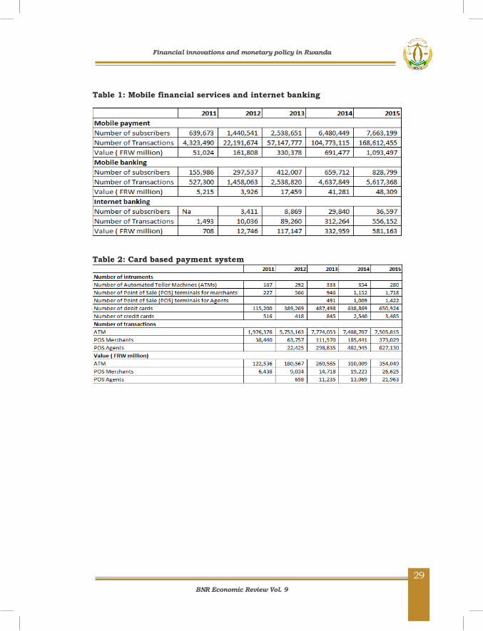
Technological innovation has also contributed to the financial sector
development with the introduction of Automated Teller machines, mobile
banking and internet banking. The number of ATMs increased from 167
machines in 2011to 280 in 2015 while the number of transactions using ATM
and POs merchants increased to 7.5 million from 1.9 million and to 373,029
from 38,440 respectively from 2011 and 2015. In the same period, the number
of transactions using mobile payments, mobile banking and internet banking
increased to 168.6 million, 5.6 million and 556,152 respectively from 4.3
million, 527,300 and 1,493 (see details in tables 1 and 2 in appendix).
These developments have contributed to deepen the banking sector in
Rwanda. Currency in circulation (CIC) as percentage of M3 has significantly
dropped from 27.3% in 2008 to 9.6% in 2015 (figure 1) which contributed to
have more deposits in the banking sector and to the increase in commercial
banks loans to the private sector.
Figure 1: Currency to M3
Source: BNR, Monetary Policy Directorate
0.0
5.0
10.0
15.0
20.0
25.0
30.0
35.0
1995 1996 1997 1998 1999 2000 2001 2002 2003 2004 2005 2006 2007 2008 2009 2010 2011 2012 2013 2014 2015
Financial innovations and monetary policy in Rwanda

BNR Economic Review Vol. 9
8
8
Both ratios of deposits and credit to private sector (CPS) to GDP increased
respectively to 23 percent and 20 percent in 2015 from 14 percent and 11
percent in 2004. The ratio of broad money (M3) to GDP which stood at 17
percent in 2006 increased to approximately 25 percent in 2015.
Figure 2: Financial depth in Rwanda
Source: BNR, Monetary Policy Directorate
Another important change in the financial system in Rwanda was the creation
of capital market in 2008. While the market remains nascent, it is becoming
progressively active since 2014 after BNR and MINECOFIN decided to issue
treasury bonds on quarterly basis. This offered an alternative way of saving
for non-bank savers. The share of retail investors in Government bonds has
increased from almost 0% in 2013 to 15% in May 2016. During the same
period, the ratio for institutional investors increased from 10% to 50.34%
while the share of commercial banks declined from 90% to 35%.
2.2. Financial innovation and monetary policy in Rwanda
The developments presented in subsection 2.1 indicate that financial
innovation in Rwanda has progressively affected the financial environment in
which BNR conducts its monetary operations as well as the financial behavior
of economic agents.
According to Fry (1988) the sign of association between the velocity of money
(which is defined as the proportion of nominal GDP to money supply, GDP/M)
and income depends on the stage of financial development. At earlier stages,
the velocity of money may fall due to high increase in the monetization of the
economy and relatively fast monetary expansion. However, at advanced stages
with financial innovation and technological progress that guarantee the
11 12 12 13 13 12 12 1315 16 17
20
14 14 1618
15 15 16 18 18 19 2023
17 17 1921
18 17 19 20 20 21 2325
2004 2005 2006 2007 2008 2009 2010 2011 2012 2013 2014 2015
% o
f GDP
CPS to GDP Deposits to GDP M3 to GDP
Financial innovations and monetary policy in Rwanda
BNR Economic Review Vol. 9
9
9
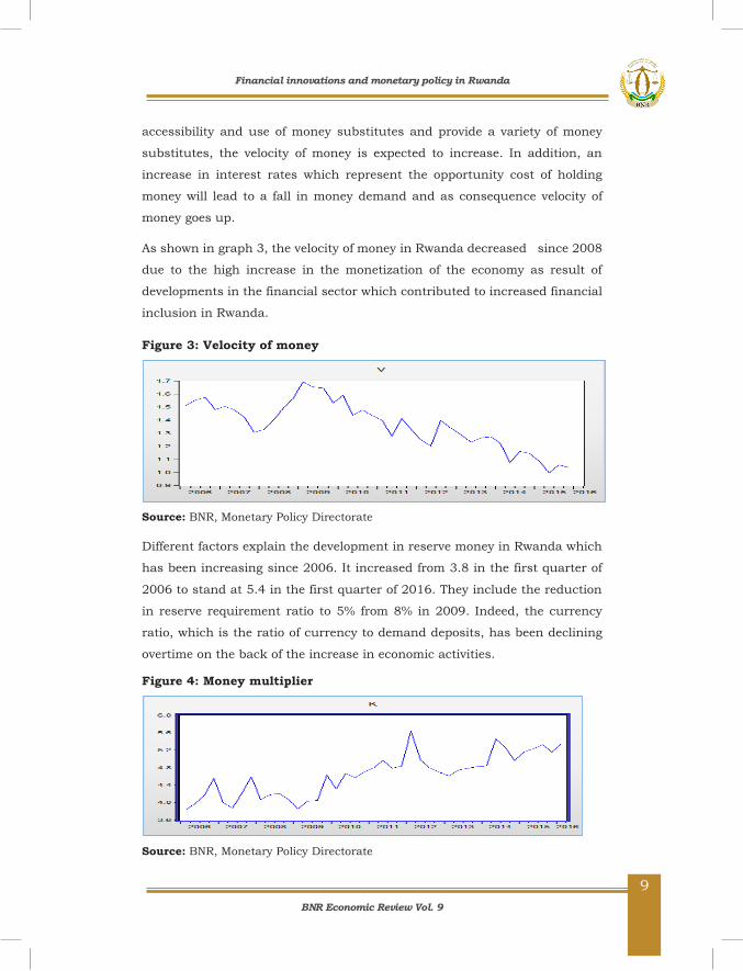
accessibility and use of money substitutes and provide a variety of money
substitutes, the velocity of money is expected to increase. In addition, an
increase in interest rates which represent the opportunity cost of holding
money will lead to a fall in money demand and as consequence velocity of
money goes up.
As shown in graph 3, the velocity of money in Rwanda decreased since 2008
due to the high increase in the monetization of the economy as result of
developments in the financial sector which contributed to increased financial
inclusion in Rwanda.
Figure 3: Velocity of money
Source: BNR, Monetary Policy Directorate
Different factors explain the development in reserve money in Rwanda which
has been increasing since 2006. It increased from 3.8 in the first quarter of
2006 to stand at 5.4 in the first quarter of 2016. They include the reduction
in reserve requirement ratio to 5% from 8% in 2009. Indeed, the currency
ratio, which is the ratio of currency to demand deposits, has been declining
overtime on the back of the increase in economic activities.
Figure 4: Money multiplier
Source: BNR, Monetary Policy Directorate
Financial innovations and monetary policy in Rwanda
BNR Economic Review Vol. 9
10
10
3. Literature Review The literature on financial innovation is still evolving as new financial
instruments and financial services continue to enter the market. The existing
literature has mainly focused on evolution of the financial system in the
developed world with few studies focusing on developing countries. Existing
studies have analyzed the linkages between general financial innovation and
monetary policy, growth and inflation and linkages between specific financial
innovation products, macroeconomic variables and monetary policy
transmission mechanisms. This section briefly presents a survey of
theoretical and empirical work with a bias towards developing economies. The
first strand of literature analyses the impact of electronic money on the central
bank’s ability to control money supply. This literature is controversial on this
aspect, with one line of thought arguing that increased usage of electronic
money would make it difficult for central banks to supervise and measure the
monetary base (Kobrin 1997, Friedman, 1999). The other strand holds a more
optimistic view and notes that the fears for the future of monetary policy may
have been overstated (Bert, 1996; Helleiner, 1998; Freedman, 2000;
Goodhart, 2000; and Woodford, 2000).
There exist an extensive literature exploring the effect of financial innovation
on the stability of the money demand function, with a general consensus that
evolution of new financial products creates instability in the traditional money
demand function. Arrau and De Gregorio (1993) examined the money demand
equations in Chile and Mexico. Their results suggested that there is an
important permanent component in the demand for money not captured by
traditional variables but by financial innovations, which is modeled as an
unobservable shock that has permanent effects on money demand.
Using the market share of credit cards as an indicator of financial innovation,
Viren (1992) empirically examined the relationship between financial
innovations and currency demand. The results showed that credit card
transactions have a strong offsetting effect on currency demand.
Financial innovations and monetary policy in Rwanda
BNR Economic Review Vol. 9
11
11
A similar study by Al-Sowaidi and Darrat (2006) examined the effects of
financial innovations in Bahrain, the UAE and Qatar on the long-run money
demand. The study found no undue shifts in the equilibrium money demand
relationship despite the fast pace of financial innovations experienced in the
three countries. The findings were robust to different measures of the money
stock.
In Korea, Cho and Miles (2007) found a downward trend in velocity which was
attributed to monetization of the economy. It is expected that velocity should
increase over time as payment systems evolve or cash management improves.
The basic argument in the perverse sign observed in the Korean case is based
on the fact that, there is increased willingness to hold money as income
increases. The coefficient of real GDP was more than unity indicating a high
level of monetization in the Korean economy.
A few number of studies exist focusing on the examination of the linkages
between financial innovation and the stability of the money demand function
in Africa. Using Granger causality and VAR methodologies, Kovanen (2004)
examined the determinants of currency demand and inflation dynamics in
Zimbabwe. The author measured financial innovation as the ratio of broad
money to currency and the results from the VAR estimation for financial
innovation are not significant. Lungu et al (2012) did a similar study using
Malawian data but in this case financial innovation has a significant effect on
the demand for money in the short run.
Sichei and Kamau (2012) conducted a similar study using Kenyan Data. They
used the number of ATMs as a proxy for financial innovations. Their results
did not indicate any significant effect of innovations on the demand for money.
The insignificant effect of financial innovations could be due to the fact that
the used measure of financial innovation is not widespread across the
country. While acknowledging that the data for other more inclusive measures
such as M-Pesa may not have been available and adequate in terms of
observations to allow plausible empirical investigation, the authors did not
explore other financial innovation measures used in previous studies. They,
however, demonstrated the instability of money demand post 2007.
Financial innovations and monetary policy in Rwanda
BNR Economic Review Vol. 9
12
12
Studies conducted on Kenya in the 1980s and 1990s (Dharat 1985; Mwega,
1990; Adam, 1990) show that money demand was stable at the time. Of
particular interest is a study by Dharat (1985), where special attention was
paid to the model specification, its dynamic structure and to its temporal
stability. Following this approach the study showed that for both conventional
definitions of money (the narrow and broad), the theoretical model fits the
Kenyan data quite well, and the variables were all statistically significant and
with the anticipated signs. Based on a battery of tests, the results suggested
that the estimated money demand equation for Kenya was temporally stable.
Turning to the open-economy nature of the money demand model, it was
found that the foreign interest rate plays a significant role in the Kenyan
money demand equations.
4. METHODOLOGY To investigate the effect of financial innovations on the conduct of monetary
policy in Rwanda we first assess the stability of money demand but before
doing this, we examine the stability of the velocity of money and the money
multiplier in Rwanda as these are key underlying assumptions of BNR
monetary policy. Second, we investigate whether or not the innovations have
impacted on money demand and the monetary policy transmission
mechanism in Rwanda.
4.1. Stability of velocity of money and money multiplier To test for the stability of the velocity of money and money multiplier, we first
use a simple model used in other recent papers on the same topic (Nyamongo
at al, 2013):
0 1t t tZ trend (1)
Where Z is either income velocity V=PY/M3 or the money multiplier k=M3/B;
B is the base money, M3 the broad monetary aggregate, P is the price and Y
is the real GDP; trend is a trend term and is the error term.
Financial innovations and monetary policy in Rwanda
BNR Economic Review Vol. 9
13
13
Considering the effects of financial innovations, 1 is expected to be negative
and significant when the dependent variable is the income velocity and
positive and significant when the dependent variable is the money multiplier.
A recent paper by Kigabo (2014) using Gregory – Hansen cointegration and
Hansen (1992) tests shows that the long-run relationship between M3 and
Reserve money holds over some period of time, and then has shifted to a new
long-run relationship after 2010 as a result of changes in monetary policy
framework and financial sector development. The paper also concluded that
the structural change in the relationship between the two variables may
reduce the efficiency of the money multiplier model and limit the
controllability of money supply by BNR using reserve money as the
operational target.
In this paper, we focus more on the stability of the velocity of money using
unit root tests and cointegration techniques which allow taking into
consideration possible structural breaks. Considering the simple quantity
theory, if the velocity V of money is stationary, M3 and nominal GDP (PY) are
either stationary or cointegrated. Non stationarity of V indicates that the long-
run relationship between M3 and PY has broken and that one of the three
variables M3, P and Y is moving separately from others.
4.2. Stability of money demand
To assess the stability of money demand, we estimate the money demand
function in line with the portfolio management theory. This allows for the
comparison of returns on alternative ways of economic agents to save their
money with returns on deposits in financial institutions. For the choice of
variables in a money demand equation, we follow Sriram (1999) and Kigabo
(2011). In order to measure the impact of financial innovations on money
demand, we augment the money demand function for Rwanda by including a
proxy for financial innovations and check if the corresponding coefficient is
statistically significant and negative.
Financial innovations and monetary policy in Rwanda

BNR Economic Review Vol. 9
14
14
Different measures of financial innovation have been used in research on the
effect of financial innovations on money demand. They include M3/M2, ATM
concentration, bank concentration and private sector credit as percentage of
GDP. For robustness of our results we will use all those variable expect ATM
concentration due to data unavailability.
The money demand function is specified as follows, with data running from
2006 quarter 1 to 2016 quarter:
0 1 2 3 4ln 3 ln ( ) (inf ) lnt t t t trm t y tb dr dr e (2)
Where lnrm3 is the natural logarithm of the broad money aggregate in real
terms, lny is the natural logarithm of real GDP, tb is the treasury bill rate
which is the opportunity cost of holding money; dr is the deposit rate which
is the return of money inf is the inflation rate, which is the expected return
from holding goods and e is the exchange rate between Rwandan franc (FRW)
and USD, defined as number of FRW for one USD. In this case, an increase
(decrease) in exchange rate corresponds to the depreciation (appreciation) of
Rwandan franc.
1 is expected to be positive, 2 and 3 are expected to be negative while 4
may be positive or negative. If 4 is positive, this means that a depreciation
of FRW leads to the substitutability of domestic currency for foreign currency
and if it is negative, a depreciation of the FRW leads to an increase in foreign
assets by domestic residents.
The level and stability of the demand for money has recently received
enormous attention in the literature because an understanding of its causes
and consequences can usefully inform the setting of monetary policy. The
demand for money is found to be a major determinant of liquidity preference.
When money demand (which is the people’s preference for cash instead of
assets) is stable, the central bank can reasonably predict the level of money
supply in the economy. Poole (1970) argued that the rate of interest should
be targeted if liquidity preference is unstable. Thus, knowing if money demand
is stable or not is necessary to select the correct monetary policy instruments.
Financial innovations and monetary policy in Rwanda

BNR Economic Review Vol. 9
15
15
A number of studies, including Bahamani-Oskooee and Bohl (2000, 2001),
Bahamani-Oskooee and Barry (2000), have examined the stability of money
demand function in the context of cointegration analysis, considering that if
money demand is cointegrated with its major determinants, then the money
demand is stable.
However, different studies have shown that the existence of cointegration is
not necessarily an evidence of the stability of money demand when other tests
are used. For example, Bahamani-Oskooee and Barry (2000), investigated the
stability of the M2 money demand function in Russia. They found evidence of
cointegration between the series in the system. While the plot of the
cumulative sum of recursive residuals (CUSUM) provided evidence of stability,
the plot of the cumulative sum of squares of recursive residuals (CUSUMSQ),
on the other hand, revealed that the demand function M2 was not stable.
In this study, we also use CUSUM and CUSUMSQ tests developed by Brown
et al. (1975) to test the stability of money demand. The CUSUM and
CUSUMSQ test statistics are updated recursively and plotted against break
points in the data. For stability of the short-run dynamics and the long run
parameters of the real broad money demand function, it is important that the
CUSUM and CUSUMSQ statistics stay within the 5 percent critical bound
(represented by two straight lines whose equations are detailed in Brown et.al,
1975).
4.3. Financial innovations and monetary policy
To investigate the effect of financial innovations on monetary policy we follow
a standard VAR framework based on 5 variables following this order: the log
of GDP; the log of the price level (CPI); the log of money supply (M3); the short-
term interest rate; the nominal exchange rate (NEER). This particular ordering
has the following implications: (i) Real GDP does not react contemporaneously
to shocks from other variables in the system; (ii) CPI does not react
contemporaneously to shocks originating from all factors except real GDP; (iii)
money stock (M3) does not react contemporaneously to real GDP but is
affected contemporaneously by short-term interest rate and nominal effective
exchange rate; (iv) the interest is affected contemporaneously by all shocks in
Financial innovations and monetary policy in Rwanda
BNR Economic Review Vol. 9
16
16
the system, except those from the nominal effective exchange rate; (v) the
nominal effective exchange rate is affected contemporaneously by all shocks
in the system.
Following Hamori (2008), we extend the traditional money demand
specification as shown in equation (2), by including financial innovation
(FINOV).
3 0 1 2 3 4ln ln ( ) (inf ) lnt t t t t t trm y tb dr dr e FINOV (3)
We use M3/M2 as of proxy measure of financial innovation, particularly for
developing economies due to data limitation.
Using the impulse response functions, the speed and effectiveness of
monetary policy is assessed in two separate periods 2000-2006 and 2006-
2016 and compare the results for the two periods. The objective is to assess
if financial innovations introduced since 2008 has contributed to improve the
transmission mechanism in Rwanda.
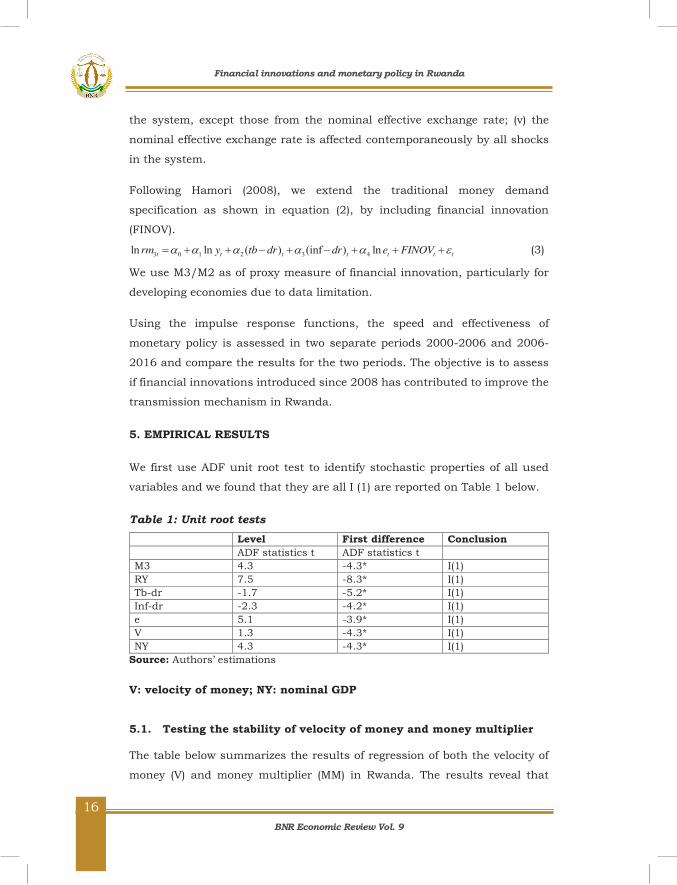
5. EMPIRICAL RESULTS We first use ADF unit root test to identify stochastic properties of all used
variables and we found that they are all I (1) are reported on Table 1 below.
Table 1: Unit root tests Level First difference Conclusion ADF statistics t ADF statistics t M3 4.3 -4.3* I(1) RY 7.5 -8.3* I(1) Tb-dr -1.7 -5.2* I(1) Inf-dr -2.3 -4.2* I(1) e 5.1 -3.9* I(1) V 1.3 -4.3* I(1) NY 4.3 -4.3* I(1)
Source: Authors’ estimations
V: velocity of money; NY: nominal GDP 5.1. Testing the stability of velocity of money and money multiplier The table below summarizes the results of regression of both the velocity of
money (V) and money multiplier (MM) in Rwanda. The results reveal that
Financial innovations and monetary policy in Rwanda
BNR Economic Review Vol. 9
17
17
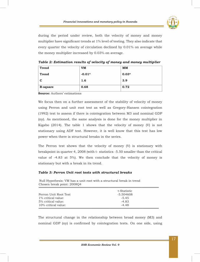
during the period under review, both the velocity of money and money
multiplier have significant trends at 1% level of testing. They also indicate that
every quarter the velocity of circulation declined by 0.01% on average while
the money multiplier increased by 0.03% on average.
Table 2: Estimation results of velocity of money and money multiplier Trend
Trend
C
VM
-0.01*
1.6
MM
0.03*
3.9
R-square 0.68 0.72
Source: Authors’ estimations
We focus then on a further assessment of the stability of velocity of money
using Perron and unit root test as well as Gregory-Hansen cointegration
(1992) test to assess if there is cointegration between M3 and nominal GDP
(ny). As mentioned, the same analysis is done for the money multiplier in
Kigabo (2014). The table 1 shows that the velocity of money (V) is not
stationary using ADF test. However, it is well know that this test has low
power when there is structural breaks in the series.
The Perron test shows that the velocity of money (V) is stationary with
breakpoint in quarter 4, 2008 (with t- statistics -5.50 smaller than the critical
value of -4.83 at 5%). We then conclude that the velocity of money is
stationary but with a break in its trend.
Table 3: Perron Unit root tests with structural breaks Null Hypothesis: VM has a unit root with a structural break in trend
Chosen break point: 2008Q4 t-Statistic Perron Unit Root Test -5.504608 1% critical value: -5.45 5% critical value: -4.83 10% critical value: -4.48
The structural change in the relationship between broad money (M3) and
nominal GDP (ny) is confirmed by cointegration tests. On one side, using
Financial innovations and monetary policy in Rwanda
BNR Economic Review Vol. 9
18
18
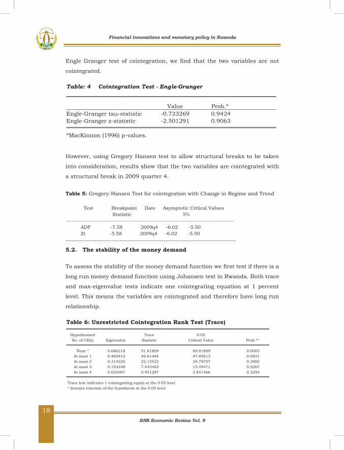
Engle Granger test of cointegration, we find that the two variables are not
cointegrated.
Table: 4 Cointegration Test - Engle-Granger
Value Prob.*
Engle-Granger tau-statistic -0.723269 0.9424 Engle-Granger z-statistic -2.501291 0.9063
*MacKinnon (1996) p-values.
However, using Gregory Hansen test to allow structural breaks to be taken
into consideration, results show that the two variables are cointegrated with
a structural break in 2009 quarter 4.
Table 5: Gregory-Hansen Test for cointegration with Change in Regime and Trend Test Breakpoint Date Asymptotic Critical Values Statistic 5% ----------------------------------------------------------------------------------------- ADF -7.58 2009q4 -6.02 -5.50 Zt -5.58 2009q4 -6.02 -5.50 ----------------------------------------------------------------------------------
5.2. The stability of the money demand
To assess the stability of the money demand function we first test if there is a
long run money demand function using Johansen test in Rwanda. Both trace
and max-eigenvalue tests indicate one cointegrating equation at 1 percent
level. This means the variables are cointegrated and therefore have long run
relationship.
Table 6: Unrestricted Cointegration Rank Test (Trace) Hypothesized Trace 0.05
No. of CE(s) Eigenvalue Statistic Critical Value Prob.** None * 0.686218 91.81809 69.81889 0.0003
At most 1 0.465912 46.61484 47.85613 0.0651 At most 2 0.314220 22.15422 29.79707 0.2900 At most 3 0.153348 7.443462 15.49471 0.5267 At most 4 0.024097 0.951287 3.841466 0.3294
Trace test indicates 1 cointegrating eqn(s) at the 0.05 level * denotes rejection of the hypothesis at the 0.05 level
Financial innovations and monetary policy in Rwanda
BNR Economic Review Vol. 9
19
19
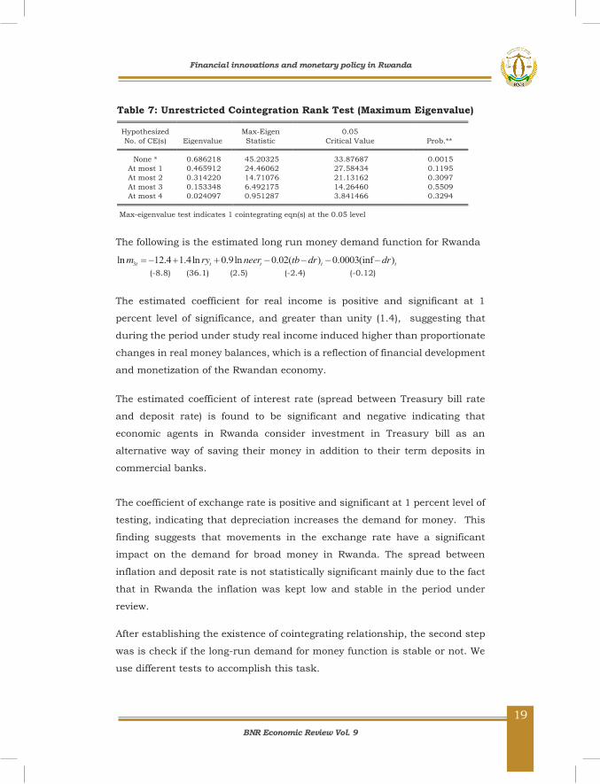
Table 7: Unrestricted Cointegration Rank Test (Maximum Eigenvalue) Hypothesized Max-Eigen 0.05
No. of CE(s) Eigenvalue Statistic Critical Value Prob.** None * 0.686218 45.20325 33.87687 0.0015
At most 1 0.465912 24.46062 27.58434 0.1195 At most 2 0.314220 14.71076 21.13162 0.3097 At most 3 0.153348 6.492175 14.26460 0.5509 At most 4 0.024097 0.951287 3.841466 0.3294
Max-eigenvalue test indicates 1 cointegrating eqn(s) at the 0.05 level
The following is the estimated long run money demand function for Rwanda
3ln 12.4 1.4ln 0.9ln 0.02( ) 0.0003(inf )t t t t tm ry neer tb dr dr (-8.8) (36.1) (2.5) (-2.4) (-0.12) The estimated coefficient for real income is positive and significant at 1
percent level of significance, and greater than unity (1.4), suggesting that
during the period under study real income induced higher than proportionate
changes in real money balances, which is a reflection of financial development
and monetization of the Rwandan economy.
The estimated coefficient of interest rate (spread between Treasury bill rate
and deposit rate) is found to be significant and negative indicating that
economic agents in Rwanda consider investment in Treasury bill as an
alternative way of saving their money in addition to their term deposits in
commercial banks.
The coefficient of exchange rate is positive and significant at 1 percent level of
testing, indicating that depreciation increases the demand for money. This
finding suggests that movements in the exchange rate have a significant
impact on the demand for broad money in Rwanda. The spread between
inflation and deposit rate is not statistically significant mainly due to the fact
that in Rwanda the inflation was kept low and stable in the period under
review.
After establishing the existence of cointegrating relationship, the second step
was is check if the long-run demand for money function is stable or not. We
use different tests to accomplish this task.
Financial innovations and monetary policy in Rwanda
BNR Economic Review Vol. 9
20
20
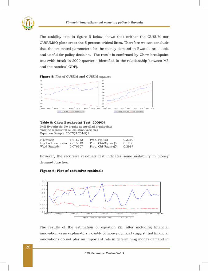
The stability test in figure 5 below shows that neither the CUSUM nor
CUSUMSQ plots cross the 5 percent critical lines. Therefore we can conclude
that the estimated parameters for the money demand in Rwanda are stable
and useful for policy decision. The result is confirmed by Chow breakpoint
test (with break in 2009 quarter 4 identified in the relationship between M3
and the nominal GDP).
Figure 5: Plot of CUSUM and CUSUM squares
Table 8: Chow Breakpoint Test: 2009Q4 Null Hypothesis: No breaks at specified breakpoints Varying regressors: All equation variables Equation Sample: 2007Q3 2016Q1
F-statistic 1.215273 Prob. F(5,25) 0.3310
Log likelihood ratio 7.615013 Prob. Chi-Square(5) 0.1788 Wald Statistic 6.076367 Prob. Chi-Square(5) 0.2989
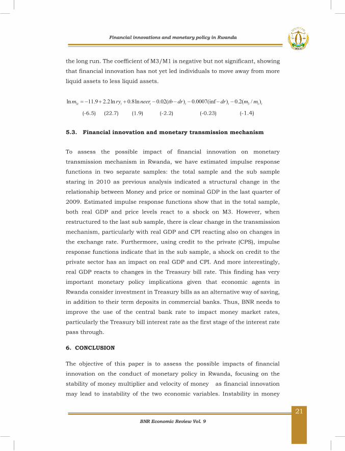
However, the recursive residuals test indicates some instability in money
demand function.
Figure 6: Plot of recursive residuals
The results of the estimation of equation (2), after including financial
innovation as an explanatory variable of money demand suggest that financial
innovations do not play an important role in determining money demand in
-16
-12
-8
-4
0
4
8
12
16
2008 2009 2010 2011 2012 2013 2014 2015 2016
CUSUM 5% Significance
-0.4
-0.2
0.0
0.2
0.4
0.6
0.8
1.0
1.2
1.4
2008 2009 2010 2011 2012 2013 2014 2015 2016
CUSUM of Squares 5% Significance
-.20
-.15
-.10
-.05
.00
.05
.10
.15
.20
2008 2009 2010 2011 2012 2013 2014 2015 2016
Recursive Residuals ± 2 S.E.
Financial innovations and monetary policy in Rwanda
BNR Economic Review Vol. 9
21
21
the long run. The coefficient of M3/M1 is negative but not significant, showing
that financial innovation has not yet led individuals to move away from more
liquid assets to less liquid assets.
3 3 1ln 11.9 2.2ln 0.8ln 0.02( ) 0.0007(inf ) 0.2( / )t t t t t tm ry neer tb dr dr m m
(-6.5) (22.7) (1.9) (-2.2) (-0.23) (-1.4)
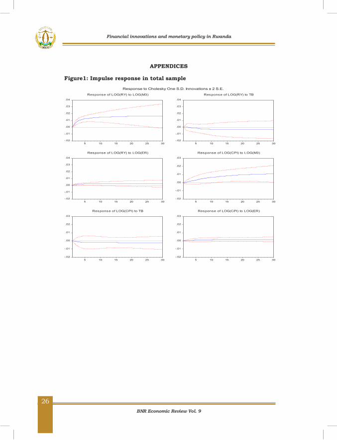
5.3. Financial innovation and monetary transmission mechanism
To assess the possible impact of financial innovation on monetary
transmission mechanism in Rwanda, we have estimated impulse response
functions in two separate samples: the total sample and the sub sample
staring in 2010 as previous analysis indicated a structural change in the
relationship between Money and price or nominal GDP in the last quarter of
2009. Estimated impulse response functions show that in the total sample,
both real GDP and price levels react to a shock on M3. However, when
restructured to the last sub sample, there is clear change in the transmission
mechanism, particularly with real GDP and CPI reacting also on changes in
the exchange rate. Furthermore, using credit to the private (CPS), impulse
response functions indicate that in the sub sample, a shock on credit to the
private sector has an impact on real GDP and CPI. And more interestingly,
real GDP reacts to changes in the Treasury bill rate. This finding has very
important monetary policy implications given that economic agents in
Rwanda consider investment in Treasury bills as an alternative way of saving,
in addition to their term deposits in commercial banks. Thus, BNR needs to
improve the use of the central bank rate to impact money market rates,
particularly the Treasury bill interest rate as the first stage of the interest rate
pass through.
6. CONCLUSION
The objective of this paper is to assess the possible impacts of financial
innovation on the conduct of monetary policy in Rwanda, focusing on the
stability of money multiplier and velocity of money as financial innovation
may lead to instability of the two economic variables. Instability in money
Financial innovations and monetary policy in Rwanda

BNR Economic Review Vol. 9
22
22
multiplier and in money demand breaks the link between BNR operating
target (base money) and intermediate target (M3) on one side, and, between
the intermediate target and the final objective of monetary policy (inflation).
In other words, instability of the money multiplier and money demand
weakens the current monetary transmission mechanism in Rwanda, which
goes from the base money to inflation through M3.
Empirical results show that both the velocity of money and money multiplier
have significant trends at 1% level of testing. They also indicate that every
quarter the velocity of circulation declined by 0.01% on average while the
money multiplier increased by 0.03% on average. In addition, Perron unit root
test indicates that the velocity of money is stationary but with break in trend.
Gregory Hansen test confirms that there is a long run relationship between
M3 and nominal GDP but with changes in the trend after 2009 in quarter 4,
mainly due to high increase in the monetization of the economy.
About the stability of money demand, the cointegration test, CUSUM test and
Chow break test indicate that money demand in Rwanda is stable. However,
recursive residuals indicate some sign of instability in the money demand.
About the impact of financial innovation on money demand, results indicate
that that financial innovation has not yet led individuals to move away from
more liquid assets to less liquid assets, though the negative sign is in line with
expected link between money demand and financial innovation. The break in
the relationship between M3 and nominal GDP is more explained by the
increase in the level of monetization of the economy as result of financial
sector development than the use of new financial products.
In terms of policy implications, the existence of the long run relationship
between M3 and nominal GDP indicates that central banks may influence the
development of nominal GDP (and in price) through the control of M3.
However, the structural change in the relationship between the two variables
as a result of financial innovation may constrain the conduct of monetary
policy and thus reduce the effectiveness of the monetary aggregate framework.
In addition, estimated impulse response functions in the sub sample starting
in 2008, where much change in monetary and financial sectors happened in
Financial innovations and monetary policy in Rwanda

BNR Economic Review Vol. 9
23
23
Rwanda, indicate that a shock on credit to the private sector has an impact
on real GDP and CPI. And more interestingly, real GDP reacts to changes in
Treasury bill rate. This result is very important in terms of policy implication
as it indicates that economic agents in Rwanda consider investment in
Treasury bill as an alternative way of saving, in addition to commercial banks’
term deposits. Thus, BNR needs to improve the use of the central bank rate
to impact money market rates, particularly the Treasury bill interest rate as
the first stage of improving the interest rate pass through.
Financial innovations and monetary policy in Rwanda
BNR Economic Review Vol. 9
24
24
References
1. Al-Sowaidi, Saif S., & Darrat, Ali F. (2006). Financial Innovations and the
Stability of Long-Run Money Demand: Implications for the conduct of monetary
policy in the GCC countries’, ERF, 13th Annual Conference, Kuwait, 16-18
December 2006.
2. Angeloni, I., Kashyap, A. K., & Mojon, B. (2003). Monetary policy transmission
in the Euro area: A study by the Eurosystem Monetary Transmission Network.
Cambridge: Cambridge University Press.
3. Arrau, P., & Gregorio, J. D. (1993). Financial Innovation and Money Demand:
Application to Chile and Mexico. The Review of Economics and Statistics, 75(3),
524-530.
4. Arrau, P., & Gregorio, J. D. (1991). Financial Innovation and Money Demand.
International Economics Department, The World Bank working paper, WPS
585.
5. Attanasio, O. P., Guiso, L., and Jappelli, T. (2002). The Demand for Money,
Financial Innovation, and the Welfare Cost of Inflation: An Analysis with
Household Data. Journal of Political Economy, 110(2), 317-351.
6. Awad, I. (2010). Measuring the stability of the demand for money function in
Egypt. Banks and Banking Systems, 5(1):71-75.
7. Bahmani-Oskooee, M., & Bohl, M. T. (2000). German monetary unification and
the stability of the German M3 money demand function. Economics Letters,
66(2), 203-208.
8. Bahmani‐Oskooee, M., & Gelan, A. (2009). How stable is the demand for money
in African countries? Journal of Economic Studies, 36(3), 216-235.
9. Dobnik, F. (2013). Long-run money demand in OECD countries: What role do
common factors play? Empir Econ Empirical Economics, 45(1), 89-113.
10. Dunne, J.P., & Kasekende, E. (2016). Financial Innovation and Money Demand:
Evidence from Sub-Saharan Africa. Economic Research Southern Africa, ERSA
working paper 583.
11. Friedman, B. (1999). The Future of Monetary Policy: The Central Bank as an
Army with Only a Signal Corps. International Finance, 2 (3), 321-328.
12. Freedman, C. (2006). Monetary Policy Implementation: Past, Present and
Future: Will the Advent of Electronic Money Lead to the Demise of Central
Banking? Future of Monetary Policy and Banking Conference, Washington D.C,
July, 11, 2006.
Financial innovations and monetary policy in Rwanda

BNR Economic Review Vol. 9
25
25
13. Kigabo, T.R. (2011). Estimation d’une Fonction de Demande de Monnaie au
Rwanda et Burundi. Editions Universitaire Européennes.
14. Kigabo, T.R. (2015). Monetary and Financial Innovations and Stability of Money
Multiplier in Rwanda. Issues in Business Management and Economics, 3 (1), 1-
8.
15. Kiptui, M. C. (2014). Some Empirical Evidence on the Stability of Money
Demand in Kenya. International Journal of Economics and Financial Issues, 4
(4), 849-858.
16. Lungu, M., Simwaka, K & Chiumia, A. (2012). Money demand function for
Malawi-implications for monetary policy conduct. Banks and Bank Systems.
7(1): 50-63.
17. Mannah-Blankson, T. & Belyne, F. (2004). The Impact of Financial Innovation
on the Demand for Money in Ghana. Bank of Ghana Working Paper.
18. Nyamongo, E. & Ndirangu L. (2013). Financial Innovations and Monetary Policy
in Kenya. MPRA Paper No. 52387. Retrieved from https://mpra.ub.uni-
muenchen.de/52387.
19. Salisu, A., Ademuyiwa, I. & Fatai, B. (2013). Modelling the Money Demand in
Sub-Saharan Africa (SSA)." Economics Bulletin, 33(1), 635-647.
20. Sichei, M. M., & Kamau, A. W. (2012). Demand For Money: Implications for The
Conduct of Monetary Policy in Kenya. International Journal of Economics and
Finance IJEF, 4(8), 72-82.
21. Sriram, S.S. (2000). A Survey of Recent Empirical Money Demand Studies. IMF
Staff Papers, 47 (3), 334-365. Retrieved from
http://www.jstor.org/stable/3867652.
22. Sriram, S.S. (1999). Survey of Literature on Demand for Money: Theortical and
Empirical Work with Special Reference to Error Correction Models. IMF working
paper P/99/64.
Financial innovations and monetary policy in Rwanda
BNR Economic Review Vol. 9
26
26
APPENDICES
Figure1: Impulse response in total sample
-.02
-.01
.00
.01
.02
.03
.04
5 10 15 20 25 30
Response of LOG(RY) to LOG(M3)
-.02
-.01
.00
.01
.02
.03
.04
5 10 15 20 25 30
Response of LOG(RY) to TB
-.02
-.01
.00
.01
.02
.03
.04
5 10 15 20 25 30
Response of LOG(RY) to LOG(ER)
-.02
-.01
.00
.01
.02
.03
5 10 15 20 25 30
Response of LOG(CPI) to LOG(M3)
-.02
-.01
.00
.01
.02
.03
5 10 15 20 25 30
Response of LOG(CPI) to TB
-.02
-.01
.00
.01
.02
.03
5 10 15 20 25 30
Response of LOG(CPI) to LOG(ER)
Response to Cholesky One S.D. Innovations ± 2 S.E.
Financial innovations and monetary policy in Rwanda

BNR Economic Review Vol. 9
27
27
Figure 2: Impulse response with sample starting in 2010
-.010
-.005
.000
.005
.010
.015
5 10 15 20 25 30
Response of LOG(RY) to LOG(M3)
-.010
-.005
.000
.005
.010
.015
5 10 15 20 25 30
Response of LOG(RY) to TB
-.010
-.005
.000
.005
.010
.015
5 10 15 20 25 30
Response of LOG(RY) to LOG(ER)
-.0050
-.0025
.0000
.0025
.0050
.0075
.0100
5 10 15 20 25 30
Response of LOG(CPI) to LOG(M3)
-.0050
-.0025
.0000
.0025
.0050
.0075
.0100
5 10 15 20 25 30
Response of LOG(CPI) to TB
-.0050
-.0025
.0000
.0025
.0050
.0075
.0100
5 10 15 20 25 30
Response of LOG(CPI) to LOG(ER)
Response to Cholesky One S.D. Innovations ± 2 S.E.
Financial innovations and monetary policy in Rwanda

BNR Economic Review Vol. 9
28
28
Figure 3: Impulse response in the sub sample, using the credit to the private sector (CPS)
-.06
-.04
-.02
.00
.02
.04
5 10 15 20 25 30
Response of LOG(RY) to LOG(CPS)
-.06
-.04
-.02
.00
.02
.04
5 10 15 20 25 30
Response of LOG(RY) to TB
-.06
-.04
-.02
.00
.02
.04
5 10 15 20 25 30
Response of LOG(RY) to LOG(ER)
-.03
-.02
-.01
.00
.01
.02
5 10 15 20 25 30
Response of LOG(CPI) to LOG(CPS)
-.03
-.02
-.01
.00
.01
.02
5 10 15 20 25 30
Response of LOG(CPI) to TB
-.03
-.02
-.01
.00
.01
.02
5 10 15 20 25 30
Response of LOG(CPI) to LOG(ER)
Response to Cholesky One S.D. Innovations ± 2 S.E.
Financial innovations and monetary policy in Rwanda
BNR Economic Review Vol. 9
29
29
Table 1: Mobile financial services and internet banking
Table 2: Card based payment system
Financial innovations and monetary policy in Rwanda

BNR Economic Review Vol. 9
31
31
Interest rate Pass-through in EAC Prof. Kigabo Thomas Rusuhuzwa* Mwenese Bruno† Key words: Interest rate, pass-through
JEL Classification Number: E43
* Prof. Kigabo Thomas Rusuhuzwa is the Chief Economist at the National Bank of Rwanda † Mwenese Bruno is a Senior Economist in the Monetary Policy and Research Department at BNR
Interest rate Pass-through in EAC

BNR Economic Review Vol. 9
32
32
Abstract
As the EAC central banks are in the process of adopting the use of interest rate
as an operating target, in this paper we examined and compared the degree of
the interest rate pass-through across EAC countries. Our analysis employed
various standard approaches in the area using macro level data. The study
reveals a limited interest rate pass-through in all countries with divergences on
whether it is the lending rate or the deposit rate that is most responsive and on
which money market rate has the most influence. The study indicates the effect
of country characteristics and time effect on the degree of the pass-through but
advancements in the financial sector have to reach a high level of integration to
be able to improve it.
Interest rate Pass-through in EAC

BNR Economic Review Vol. 9
33
33
I. Introduction
On the eve of the adoption of the inflation targeting framework by the East
African Central Banks by 2018 in which interest rate is used as operating
target, the interest rate pass-through is a subject to close scrutiny in the East
African Community economies. While these economies are getting ready, the
debate continues on whether the adoption of the inflation targeting framework
should precede a well-functioning interest rate channel or whether the
interest rate channel should first work before a monetary authority think of
using interest rate as operating target. For some scholars and practitioners
alike, the interest channel may be not working because a country is
implementing inappropriate policies (Carare et. al. 2002, Freedman and
Otker-Robe, 2010, Dabla-Norris et al. 2007).
Though central banks in EAC have generally been effective in attaining their
respective objectives within the monetary targeting framework, they have
challenges related to the breaking down of its basic assumptions necessitating
to move into using interest rate as operating target. However, there are
concerns about how these central banks are affecting the bank retail activities
before the effect propagate to the real economy. More so, there is no long time
that the EAC central banks started using the policy rate and in some cases it
is used just as a signal of monetary policy stance but without necessarily
influencing the banking pricing behavior.
The most popular channel through which monetary policy actions are
transmitted to the economy is the interest rate channel. The channel can be
divided in two stages. The first is the interest rate pass- through which
describes how markets rates (deposit and lending rates) react to changes in
the monetary policy rate. The second stage is related to the impact of nominal
interest rate changes on real economy.
This paper focuses on the first stage by analyzing the interest rate pass-
through in Rwanda. The policy interest rate pass- through is believed to be
slower and limited in Low income countries, including Rwanda due to several
factors including a low degree of monetization, underdeveloped financial
markets, a structural excess liquidity, exchange rate flexibility, the balance
sheet problems in the banking sector, and corporate sectors, institutional
Interest rate Pass-through in EAC
BNR Economic Review Vol. 9
34
34
quality and fiscal dominance (Anthoni, Udea, and Braun, 2003, Alexander
Tieman, Stephanie Medina Cas, at al, 2011). In addition, the lending policies
of banks are often found to be price inelastic with respect to interest rates in
the short run, because other, non-interest rate factors, like adjustment costs
and, sometimes, directed lending, play a substantial role (see e.g. Cottarelli
and Kourelis (1994), Schaechter, Stone, and Zelmer (2000), or Carare et. al.
(2002)).
The knowledge of the degree of the interest rate pass-through provides the
basis for policy makers to assess how they achieve their objectives. Although
there are some studies on interest rate pass-through on EAC individual
country, the principal aim of this study is to examine the regional status of
the interest rate pass-through as the six EAC countries are planning to start
using a common currency in 2024.
The rest of the paper is organized as follows: section 2 gives a brief summary
of the literature on interest rate pass through. Section 3 covers the
methodology and section 4 analyzes the empirical findings. Section 5 provide
the concluding remarks.
II. Brief Summary of the Literature
From the time the research on interest rate pass-through broke out with
Bernanke, Blinder and Gertler in 1985 to our days as part of assessing the
effectiveness of monetary transmission mechanisms, three features of the
interest rate pass-through have been researched on (Chionis and Leon, 2006).
The first tread of this research in the literature focused on providing the
theoretical explanation of interest rate stickiness. Indeed, interest rates
continue to register some rigidities in the short-run. The second one takes a
look at cross-country differences especially in a monetary union and the
degrees of pass-through and lastly, the literature centers on characteristics
of the financial system that bring about the differences in the interest rate
pass-through mechanism. This study put emphasis on the second one
analyzing the differences in interest rate pass-through among East African
Community countries.
Interest rate Pass-through in EAC
BNR Economic Review Vol. 9
35
35
The interest rate pass through has been subject of several studies,
particularly in developed countries, especially following the adoption of
inflation targeting framework for monetary policy. The empirical evidence on
features of interest rate pass-through show that the transmission of interest
rate is generally not complete and the speed of adjustment as well as the size
of pass-through in long run vary across bank products, countries, markets
and time period mainly due to differences in macroeconomic conditions and
financial market development (Tieman, 2004, Balazs at al, 2006; Nikoloz
Gigineishuli, 2011).
About macroeconomic conditions, higher interest rate pass -through to
lending and deposit rates is observed during the period of rapid economic
growth as well as in the period of high inflation. By contrast, higher interest
rate volatility, which is an indicator of macroeconomic instability and
uncertainty, weakens the interest rate pass -through (e.g. Nikoloz
Gigineishuli, 2011).
The development of financial market plays an important role in monetary
transmission. If the demand elasticity for deposits and for loans respectively
is inelastic, the pass- through may not be complete. Inelasticity of the demand
for deposits and loans may result from imperfect substitution between bank
deposits and other money market instruments of the same maturity, between
bank lending and other types of external finance due to low level of economic
development (equity or bond markets), high switching costs as well as
problems related to asymmetric information such as adverse selection and
moral hazard (Sander and Kleimeier, 2004), and the competition within the
banking sector and in financial sector.
Indeed, when banks have high market power, changes in policy rate as well
as changes in banks’costs of funds may impact spreads (difference between
lending and deposit rates) rather than market rates by maintaining fixed
lending rates when deposit rates declined as result of a reduction in the policy
rate, (Sander and Kleimeir, 2004; Catarelli and Korellis, 1994, De Bondt,
2002, Dabla Norris at al,. 2007, Stephanie Medina, at al. 2011).
Financial shallowness tends to lead to higher excess liquidity in banks which
limit the development of the interbank market and reduce the effectiveness of
Interest rate Pass-through in EAC
BNR Economic Review Vol. 9
36
36
interest rate pass –through and limit the central bank rate to opportunity cost
of holding liquidity by banks and not a cost of funds. In addition, more
developed domestic capital markets, including a secondary market for
government securities and long term domestic currency securities,
strengthens transmission (Leiderman at al,. 2006; Stephanie Medina Cas, at.
Al, 2011).
The health of the financial system may also impact the effectiveness of the
interest-rate transmission mechanism. Financially weak banks may respond
to an injection of central bank liquidity or lower policy interest rates by
building up liquidity or increasing margins in order to raise capital positions
and increase provisioning rather than extending credit (IMF, 2010). Holding
on to bad loans on the balance sheet may crowd out new loans and limit the
impact of lower interest rates (Archer and Turner, 2006).
III. Methodology
In the literature there exist two approaches to study the interest rate pass-
through. The cost of funds approach is mostly used if the analysis and focuses
on how money market rates influence the bank-retail rates. Money market
rates are taken as opportunity cost for both banks and depositors. In this
approach the maturity is an important criterion; it is better to use rates of the
same maturity to avoid mismatch; i.e. mortgage rates versus long-term
lending rates. The second approach is the monetary policy approach which is
used when the focus is on the effect of monetary policy on bank-retail rates
and includes no other explanatory variables.
Empirically, both approaches estimate the following long run function
iM = α + β. ip + ε (1)
Where iM is the market rate and IP is the policy rate.
Or an autoregressive distributed lag model:
itR = α0 + ∑ αj. it−j
Rpj=1 + ∑ βk. it−k
Mqk=0 + εt (2)
For the short-run, they both specify an error correction model (ECM) of the
form:
Interest rate Pass-through in EAC
BNR Economic Review Vol. 9
37
37
∆iR = α0 + α1. it−1R + β. it−1
M + γ(itR − α − βit
M) + μ (3)
For the cost of funds approach, studies that look at the effect of market rates
to different bank retail rates in the same model do estimate VAR models. In
some studies the term β. it−1M in the ECM is not included depending on various
reasons. For instance, when the model has to be used for forecasting this term
is dropped.
In this study we estimated both models for each single EAC country and
conducted an impulse response analysis based on a bivariate VAR to check
for robustness. We then carried out a panel analysis to assess if there are
country specificities or time effects that influence to evolution of the pass-
through.
To sum all, we estimated the following empirical models:
1. Single Equation Model
brt = α1 + α2mrt + εt (4)
Where brt is the bank-retail rate (loan and deposit rates), mrt is the policy
rate, α1 is a markup and α2 is the elasticity of market rate with respect to
policy rate, measuring the long run pass through. The short-run estimates
were obtained from estimating the following error correction model:
∆(brt) = α3 + α4dbrt−1 + α5εt + μt (5)
The coefficient α5 indicates the speed of adjustment of the short run dynamics
to the long run equilibrium relationship described by the equation (1). A high
level of α5 indicates a faster market response to the policy rate.
2. Bivariate VAR Model
For the purpose of checking the robustness of the results of the precedent
single equation model, this study estimated impulse responses from the
subsequent model based on De Bondt (2002) solved using the cholesky
decomposition:
Yt = β1 + ∑ AiYt−i2i=1 + εt (6)
With:
Interest rate Pass-through in EAC
BNR Economic Review Vol. 9
38
38
Yt = [market ratebank rate ]
t, εt = [εmr
εbr ]t, βt = [βmr
βbr ]t, Ai = [ai
mr bimr
aibr bi
br ]t brt and mrt are
defined as before.
3. The Autoregressive Distributed Lag Model (ARDL)
The Autoregressive Distributed Lag Model is normally used in case variables
of interest are integrated of order one. This study estimated the following
ARDL model akin to Mishra (2012):
yit = αiyt−1 + βiyt−2 + δixt + γixt−1 + σixt−2 + εt (7)
Where yt is the change in the bank-retail rates and xt is the change in the
money market rates. The short term effect is given by δ1 and the long-term
effect is computed as:
δi+γi+σi1−αi−βi
(8)
4. The Panel Model
In a view of exploring whether there are country-specific characteristics in
explaining differences in the degree of pass-through among EAC countries,
this study carried out a panel analysis from both the fixed effects model and
the random effects model. It starts with pooled OLS of the following form.
yit = α + Xit′ β + εit (μi = 0) (9)
μi represents country or time effect and if it is equal to zero the pooled OLS
produces efficient and consistent estimates.
The fixed-effects model is written as:
yit = (α + μi) + Xit′ β + vit (10)
And the random effects model is thus specified as:
yit = α + Xit′ β + (μi + vit) (11)
In the fixed-effects model a country and time specific effect is time invariant
and considered to be part of the intercept and thus allowed to be correlated
Interest rate Pass-through in EAC

BNR Economic Review Vol. 9
39
39
with the regressors while in the random effects model the individual effect is
assumed not to be correlated with any regressors.
Before estimations, we tested for stationarity and cointegration of all variables
and all were found to be integrated of order one. Estimations were then run
on variables that were cointegrated.
For proper comparison of all countries, Interest rates data are monthly
weighted. The bank retail rates are lending rates and deposit rates and for
money market rates, the study used the treasury bills of 91 days, 182 days
and 364 days, the interbank rate and repo rates spanning from January 2005
to January 2016.
IV. Empirical Analysis
1. Results from the single equation model
The results from this model are presented in appendix i. They indicate low
and incomplete interest rate pass through to deposit rates in all East African
countries ranging between 25% and 33% in Rwanda while it is higher in
Uganda around 56%*. In Rwanda, the treasury bills rates and the interbank
rate all affect the deposit rates while it is only the interbank that is statistically
significant in Uganda for the entire sample of the study. These findings for
Uganda are akin to those of Okello in 2013. However, the pass-through from
the 364 days treasury bills rates to deposit rates hovered around 40% before
the adoption of inflation targeting lite framework in Uganda; there are no
cointegration with deposit rates and other treasury bills rates of different
maturity. Kenya and Tanzania present similar cases of no cointegration
between the deposit rates and all the treasury bills rates.
There is evidence of incomplete interest rate pass through from money market
rates to lending rates only in Uganda using interbank rates. But even for
Uganda, the parameter has a wrong sign before the adoption of ITL. The
parameter is around 30% after but there is presence of serial correlation; thus
any inference may be biased. For other EAC countries, the parameters had
* Bank of Uganda has adopted what is called lite inflation targeting since 2012
Interest rate Pass-through in EAC
BNR Economic Review Vol. 9
40
40
negative signs or were not statistically significant. Generally, the deposit rates
seem to be reactive to changes in money market rates in the long-term but it
is not so obvious in the short-term with the pass-through effect evolving
around 10% with the speed of adjustment ranging between 60% and 80%.
2. Results from the Autoregressive Distributed Lag Model (ARDL)
We got different results when using the ARDL model (see appendix iii). The
lending rates seem to be more reactive on changes from money market rates
and the treasury bills rates has bigger effects than the interbank rates. In
Kenya, changes in interbank may explain 6% changes in lending rate in short-
run. Changes in different treasury bills rates may account for 3% to 6%
changes in deposit rates in the short-run. In Rwanda and Tanzania, the
changes in 364-days treasury bills rates may explain respectively 5% and 4%
of changes in lending rate in short-term. For Tanzania, the deposit rates may
vary by 2% and 5% from changes happened in interbank rate and the 91-days
treasury bills rates respectively in short-term. In Uganda 3% of changes in
deposit rate may be accounted for by changes in interbank rate while changes
in all treasury bills rates may explain 7% in short-term. Generally, the
findings point to even a less interest rate pass-through of around 6% in the
short-term across the region. In the long-term, the pass-through remains
below 10% and statistically significant only in Kenya and Uganda.
3. Impulse response analysis
The impulse responses are plotted in appendix ii. Except for Rwanda, the
impulse response analysis revealed a very minimal contemporaneous effects.
For Uganda, a 10% shock to interbank rate induces 0.8% changes in deposit
rate that dies out after 15 months. It is 0.4% for Kenya and 0.15% for
Tanzania but last longer about 14months and 28 months respectively. One
important conclusion from this analysis is that the changes in bank retail
rates triggered by changes in policy rates is minimal but immediate, it is in
the same range across different rates with slight differences across countries.
Interest rate Pass-through in EAC
BNR Economic Review Vol. 9
41
41
4. Results of from panel estimations
Using pooled OLS, all treasury bills rates and the interbank rate do not
statistically and significantly explain variations in deposit rates. But they are
statistically significant in explaining variations in lending rates. The 91
treasury bills rates is statistically significant in explaining the lending rate
and the fixed effects model is better. That is, the differences among countries
(such as financial development or bank competition) determine how the 91
treasury bills rates rate affects the lending rate.
The 182 and the 634 treasury bills rates are statistically significant in
explaining the lending rate and the random effects model is better. That is,
country specific characteristics may change overtime and change the effect of
the 182 and the 634 treasury bills rates on lending rate. The effects of all
treasury bills rates on lending rates is higher (around 23%) than on deposit
rates (around 20%). The effects of interbank on lending rates is higher (around
16%) than on deposit rates (around 12%). These results are in contrast with
the maturity mismatch challenge where short-term market rates are identified
as determinants of longer term bank loan rates. However, this may come from
the famous liquidity mismatch issue of financing long-term projects by short-
term deposits that is present in the banking system in the region.
5. Single Equation Model: Controlling for Financial Development and Sub-sample Results
Since the panel analysis revealed country specificities and time effect in
explaining the differences in the degree of the pass-through, the study
factored in differences in financial development (FD) in EAC economies using
the ratio of currency in circulation over money supply as a control variable
(Archer and Turner 2006, Gigineishuli 2011). This ratio may represent some
advancements realized in financial inclusion and in payment system as one
of the areas which undergone remarkable improvements in EAC countries.
In the beginning, the standard models of interest rate pass-through to bank
retail rates did not factor in other variables apart from the policy rates to
Interest rate Pass-through in EAC

BNR Economic Review Vol. 9
42
42
account for countries’ heterogeneity in bank products pricing. Indeed, though
there may be no big divergences, the EAC countries’ financial structures
present different features. To accommodate for these differences, the single
equation model was transformed as follows and was estimated at different
sample periods:
brt = α1 + α2mrt + fd + εt (12)
The estimation results (included in appendix i) of the model suggest that when
you control for the effect from the developments taking place in the financial
sector, the degree of the pass-through changes with time. In Rwanda the
changes are meaningful but the pass-through remains incomplete while in
Kenya and Uganda the changes are negligible.
6. Summary of the findings
The findings from the four models suggest some similarities and divergences.
The degree of the interest rate pass-through in all EAC economies is
incomplete and low and from some models it was found to be even below 10%.
For some countries, some models could not even find in the data any
statistically significant estimates. There is an immediate but very minor effect
of changes in money market rates to bank retail rates.
Nevertheless, some models identified the interest rate pass-through to lending
rates but failed to find it to deposit rates and vice versa. Similarly, for some
models and countries the pass-through is statistically significant from the
treasury bills rates and not from the interbank rates but for others it is the
other way around. The study indicates that country differences can explain
the different degrees of pass-through found among the EAC countries in the
region and specific characteristics within a country may change with time and
affect the degree of the pass-through in that country.
V. Conclusion
This paper sought to examine the status of the interest rate pass through at
the EAC level using different empirical methods and all point to a limited
Interest rate Pass-through in EAC

BNR Economic Review Vol. 9
43
43
degree of the interest rate pass-through. In this case, the immediate
conclusion is that other non-considered factors are more important; some
may be macroeconomic namely the level of the financial development or
microeconomic such as individual bank characteristics. This study included
the developments in the financial sector but they do not seem to improve the
degree of the pass-through per se in contrast to the conclusions of Kleimeier
and Sander (2006) that monetary policy is the main determinant. Corollary,
the study suggests that other factors especially bank-specific conditions are
key in determining the bank retail rates in all EAC countries.
Generally, EAC countries have to continue putting more efforts in developing
their financial system as it was found to have effects in Rwanda. However,
these developments have to lead to more financial integration and competition
or it may not result in higher pass-through otherwise; i.e. in Uganda and
Kenya after some financial system advancements the pass-through improved
but stagnated because financial integration was still low. Furthermore, as Tai
(2012) pointed out even Asian countries that adopted the inflation targeting
with more developed financial systems, the interest rate pass-through
remained low because the developments did not yet reach a good level of
financial integration especially offering alternative sources of funds for
households. Therefore, the EAC countries may adopt the use of interest rate
as the monetary instrument even though the degree at which its passed on to
bank retail rates is still low.
Interest rate Pass-through in EAC
BNR Economic Review Vol. 9
44
44
References
1. Bernanke, B.S. and Gertler, M., 1995. Inside the black box: the credit
channel of monetary policy transmission (No. w5146). National bureau of
economic research.
2. Archer, D., and Turner, P., (2006), “The banking system in emerging
economies: how much progress has been made,” BIS Papers No. 28.
3. De Bondt, G., (2002), “Retail bank interest rate pass-through: new evidence
at the euro area level”, ECB Working Paper, No. 136.
4. Carare, A., Schaechter, A., Stone, M.R., and Zelmer, M., (2002),
“Establishing Initial Conditions in Support of Inflation Targeting”, IMF
Working Paper, WP/02/102.
5. Chionis., D. and Leon., C., 2006. Interest rate transmission in Greece: Did
EMU cause a structural break? Journal of Policy Modeling, vol. 28, No 4,
pages 453-466
6. Cottarelli, C., and Kourelis, A., (1994), “Financial Structure, Bank Lending
Rates, and the Transmission Mechanism of the Monetary Policy”, IMF
Working Paper, WP/94/39.
7. Dabla-Norris, E., Kim, D., Zermeño, M., Billmeier, A. and V. Kramarenko,
V., (2007), “Modalities of Moving to Inflation Targeting in Armenia and
Georgia”, IMF Working Paper. 07/133.
8. Freedman, C., and Otker-Robe, I.,(2010), “Important Elements for Inflation
Targeting for Emerging Economies,” IMF Working Paper 10/113 (Washington:
International Monetary Fund).
9. Gigineishuli, N., (2011), “Determinants of Interest Rate Pass-Through: Do
Macroeconomic Conditions and Financial Structure Matter?” IMF Working
Paper, WP/11/176.
10. Mishra, P., Montiel, P.J. and Spilimbergo, A., 2012. Monetary
transmission in low-income countries: Effectiveness and policy implications.
IMF Economic Review, 60(2), pp.270-302.
Interest rate Pass-through in EAC
BNR Economic Review Vol. 9
45
45
11. Okello, J. A., (2013), “Interest Rate pass-through in Uganda”, BOU
Working Paper Series, No. 2/2013.
12. Sander, H., and Kleimeier, S., (2004), “Convergence in Euro-zone Retail
Banking? What Interest Rate Pass-through Tells Us about Monetary Policy
Transmission, Competition and Integration,” Journal of International Money
and Finance, Vol. 23, No.3, pp. 461–492.
13. Sander, H., and Kleimeier, S., (2006), "Interest Rate Pass-Through In The
Common Monetary Area Of The Sacu Countries," South African Journal of
Economics, Economic Society of South Africa, vol. 74(2), pages 215-229, 06
14. Schaechter, A., M.R. Stone, and M. Zelmer, (2000), Adoption of Inflation
Targeting”, Practical Working Paper, 136.
15. Tai., P.N., (2012), “ Interest Rate Pass-through and Monetary
Transmission In Asia”, International Journal of Economics and Finance, Vol. 4,
No. 2.
16. Tieman, A., (2004), “Interest rate-pass-through in Romania and other
Central European Economies”, IMF Working Paper, WP/04/211.
Interest rate Pass-through in EAC
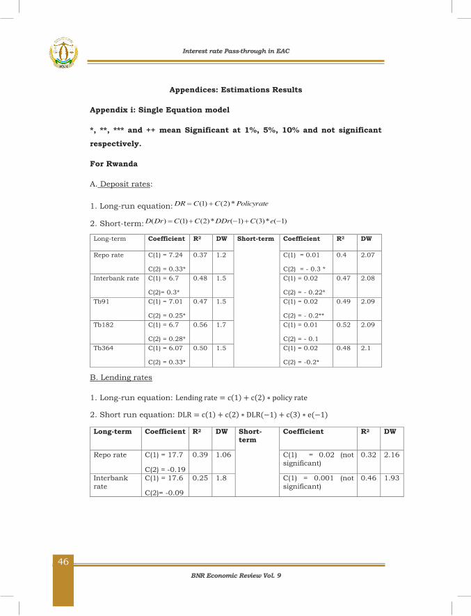
BNR Economic Review Vol. 9
46
46
Appendices: Estimations Results
Appendix i: Single Equation model
*, **, *** and ++ mean Significant at 1%, 5%, 10% and not significant respectively.
For Rwanda
A. Deposit rates:
1. Long-run equation: PolicyrateCCDR *)2()1(
2. Short-term: )1(*)3()1(*)2()1()( eCDDrCCDrD
Long-term Coefficient R2 DW Short-term Coefficient R2 DW
Repo rate C(1) = 7.24
C(2) = 0.33*
0.37 1.2 C(1) = 0.01
C(2) = - 0.3 *
C(3) = - 0.45*
0.4 2.07
Interbank rate C(1) = 6.7
C(2)= 0.3*
0.48 1.5 C(1) = 0.02
C(2) = - 0.22*
C(3) = - 0.65*
0.47 2.08
Tb91 C(1) = 7.01
C(2) = 0.25*
0.47 1.5 C(1) = 0.02
C(2) = - 0.2**
C(3) = - 0.67*
0.49 2.09
Tb182 C(1) = 6.7
C(2) = 0.28*
0.56 1.7 C(1) = 0.01
C(2) = - 0.1
C(3) = - 0.8*
0.52 2.09
Tb364 C(1) = 6.07
C(2) = 0.33*
0.50 1.5 C(1) = 0.02
C(2) = -0.2*
C(3) = - 0.7
0.48 2.1
B. Lending rates
1. Long-run equation: Lending rate = c(1) + c(2) ∗ policy rate
2. Short run equation: DLR = c(1) + c(2) ∗ DLR(−1) + c(3) ∗ e(−1)
Long-term Coefficient R2 DW Short-term
Coefficient R2 DW
Repo rate C(1) = 17.7
C(2) = -0.19
0.39 1.06 C(1) = 0.02 (not significant)
C(2) = - 0.25
C(3) = - 0.41
0.32 2.16
Interbank rate
C(1) = 17.6
C(2)= -0.09
0.25 1.8 C(1) = 0.001 (not significant)
C(2) = - 0.16
C(3) = - 0.75
0.46 1.93
Interest rate Pass-through in EAC

BNR Economic Review Vol. 9
47
48
For Kenya
A. Time deposit rates
Long-term
Coefficient R2 DW Short-tem
Coefficient R2 DW
Tb364 C(1) = 3.9
C(2) = 0.21
0.54 0.5 C(1) = 0.025 (not significant)
C(2) = 0.17 (not significant)
C(3) = -0.15
0.27 2.15
B. Lending rates
Long-term Coefficient R2 DW Short-term Coefficient R2 DW Tb364 C(1) = 13.7
C(2) = 0.27
0.50 0.51 C(1) = 0.026(not
significant)
C(2) = 0.25
C(3) = -0.15
0.25 2.06
Interest rate Pass-through in EAC

BNR Economic Review Vol. 9
48
49
For Tanzania
A. Time deposit rates
There was no cointegration with policy rates
B. Lending rates
Long-term Coefficient R2 DW Short-term
Coefficient R2 DW
Repo rate C(1) = 15
C(2) = 0.05
0.04 0.28 C(1) = 0.01(not
significant)
C(2) = -0.22
C(3) = -0.1
0.11 2.0
Interbank
rate
C(1) = 15
C(2) = 0.05
10 0.4 C(1) = 0.013(not
significant)
C(2) = -0.21
C(3) = -0.19
0.12 2.0
Tb91 C(1) = 14.3
C(2) = 0.05
0.24 0.36 C(1) = 0.012(not
significant)
C(2) = -0.2
C(3) = -0.14
0.13 2.0
Tb182 C(1) = 14.3
C(2) = 0.05
0.35 0.44 C(1) = 0.01(not
significant)
C(2) = -0.19
C(3) = -0.17
0.14 2.0
Tb364 C(1) = 13.8
C(2) = 0.129
0.35 0.48 C(1) = 0.0126(not
significant)
C(2) = -0.18
C(3) = -0.16
0.137 2.0
Interest rate Pass-through in EAC
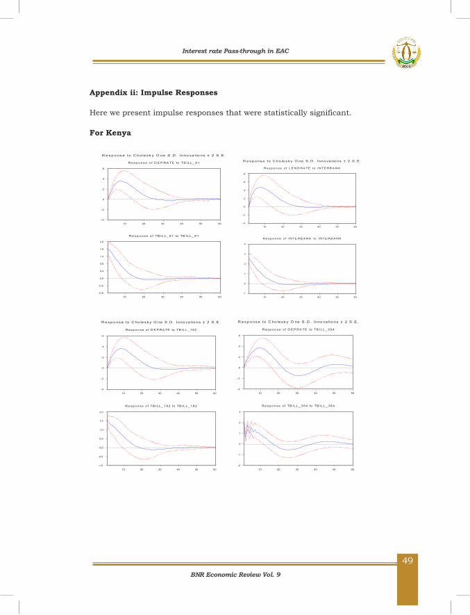
BNR Economic Review Vol. 9
49
50
Appendix ii: Impulse Responses
Here we present impulse responses that were statistically significant.
For Kenya
-.4
-.2
.0
.2
.4
.6
10 20 30 40 50 60
Respo nse o f D E P RA TE to TB ILL_91
-0.8
-0.4
0.0
0.4
0.8
1.2
1.6
2.0
10 20 30 40 50 60
Respon se o f TB ILL_9 1 to TB ILL_91
R e s p o ns e to C ho le s k y O ne S .D . Inno va t io ns ± 2 S .E .
-.4
-.2
.0
.2
.4
.6
.8
10 20 30 40 50 60
Re sp o nse o f L E ND RA TE to INTE RB A NK
-1
0
1
2
3
4
10 20 30 40 50 60
Re sp o n se o f INTE RB A NK to INTE RB A NK
R e s p o ns e to C ho le s k y O ne S .D . Inno va t io ns ± 2 S .E .
-.4
-.2
.0
.2
.4
.6
10 20 30 40 50 60
Response o f D E P RA TE to TB ILL_182
-1.0
-0.5
0.0
0.5
1.0
1.5
2.0
10 20 30 40 50 60
Response o f TB ILL_18 2 to TB ILL_182
R e s p o ns e to C ho le s k y O ne S .D . Inno va t io ns ± 2 S .E .
-.4
-.2
.0
.2
.4
.6
10 20 30 40 50 60
Response o f D E P RA TE to TB ILL_364
-2
-1
0
1
2
3
10 20 30 40 50 60
Response o f TB ILL_364 to TB ILL_364
R e s p o ns e to C ho le s k y O ne S .D . Inno va t io ns ± 2 S .E .
Interest rate Pass-through in EAC
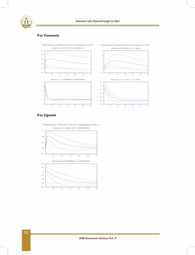
BNR Economic Review Vol. 9
50
51
For Tanzania
For Uganda
-.05
.00
.05
.10
.15
.20
10 20 30 40 50 60
Resp onse o f D E P RA TE to INTE RB A NK
-1
0
1
2
3
4
10 20 30 40 50 60
Response o f INTE RB A NK to INTE RB A NK
R e s p o ns e to C ho le s k y O ne S .D . Inno va t io ns ± 2 S .E .
-.1
.0
.1
.2
.3
.4
10 20 30 40 50 60
Response o f D E P RA TE to _91_TB ILL
-0.4
0.0
0.4
0.8
1.2
1.6
2.0
10 20 30 40 50 60
Response o f _91_TB IL L to _91_TB ILL
R e s p o ns e to C ho le s k y O ne S .D . Inno va t io ns ± 2 S .E .
-0.4
0.0
0.4
0.8
1.2
10 20 30 40 50 60
Response o f TIM E _D E P to INTE RB A NK
-0.5
0.0
0.5
1.0
1.5
2.0
2.5
10 20 30 40 50 60
Response o f INTE RB A NK to INTE RB A NK
R e s p o ns e to C ho le s k y O ne S .D . Inno va t io ns ± 2 S .E .
Interest rate Pass-through in EAC

BNR Economic Review Vol. 9
51
52
Appendix iii: The ARDL Model
* Means not significant
For Kenya
Lending rate 𝛂𝛂𝟏𝟏 𝛃𝛃𝟏𝟏 𝛅𝛅𝟏𝟏 𝛄𝛄𝟏𝟏 𝛔𝛔𝟏𝟏 𝛗𝛗𝟏𝟏 R-squared Interbank (A) 0.2 0.28 0.058 0.06 -0.027 0.38 B 0.25 0.12* 0.047 0.07 -0.02* 0.05 Tbill-91 0.16* 0.05* 0.03* 0.03* 0.09 0.21 B 0.145* 0.04* 0.03* 0.038* 0.09 0.015* 0.21 Tbill-182 0.175* 0.027* 0.021* 0.056 0.07 0.18 B - Tbill-364 0.2 0.01* 0.01* 0.065 0.05(at 10%) 0.16 B - Repo 0.327 0.07* -0.015* 0.03 0.039 0.31 Deposit rate Interbank (A) 0.08* 0.29 0.01* 0.05 0.032 0.37 B 0.07* 0.025 0.009* 0.05 0.03 0.007* 0.37 Tbill-91 0.1* 0.14* 0.06 0.02* 0.07 0.33 B 0.29* 0.07* 0.05 0.029 0.07 0.04 0.36 Tbill-182 0.1* 0.1* 0.06 0.02* 0.07 0.34 B - Tbill-364 0.09* 0.2 0.03 0.05 0.026* 0.23 B 0.03* 0.09* 0.05 0.04 0.05 0.056 0.31 Repo 0.33 0.12* 0.013 at
10% -0.001* 0.008* 0.21
B 0.265 0.12* 0.019 0.01* 0.025 0.023 0.30
For Rwanda
Lending rate 𝛂𝛂𝟏𝟏 𝛃𝛃𝟏𝟏 𝛅𝛅𝟏𝟏 𝛄𝛄𝟏𝟏 𝛔𝛔𝟏𝟏 𝛗𝛗𝟏𝟏 R-squared Interbank (A) -0.6 -0.3 -0.03* -0.03* 0.008* 0.30 B -0.6 -0.3 -0.02* -0.01* 0.01* 0.04* 0.30 Tbill-91 -0.6 -0.3 -0.04* -0.01* 0.07* 0.07 B -0.6 -0.3 -0.04* -0.0004* 0.1* 0.01* 0.32 Tbill-182 -0.6 -0.3 0.02* 0.005* 0.05 0.31 B -0.6 -0.3 0.02* 0.01* 0.06 0.03 0.32 Tbill-364 -0.6 -0.3 0.05 0.01* 0.006* 0.31 B -0.6 -0.3 0.05 0.02* 0.02* 0.06 0.35 Repo -0.6 -0.3 -0.03* -0.04* -0.05* 0.31 B -0.6 -0.3 -0.03* -0.05* -0.036* -0.068 0.32 Deposit rate Interbank (A) -0.3 0.04* 0.03* 0.01* 0.06* 0.11 B -0.3 0.03* 0.03* 0.03* 0.07* 0.04* 0.12 Tbill-91 -0.3 0.01* 0.05* 0.05* 0.1 0.14 B -0.3 0.005* 0.04* 0.05* 0.2 0.01* 0.15 Tbill-182 -03 0.01* 0.06* 0.06* 0.08* 0.14 B -0.36 0.0002* 0.07* 0.06* 0.1 0.07 0.15 Tbill-364 -0.3 0.04* 0.004* -0.1* -0.01* 0.1 B -0.3 0.04* 0.007* -0.01* -0.01* 0.02* 0.11 Repo -0.3 0.03* 0.07* -0.05* -0.01* 0.12 B -0.3 0.01* 0.08* -0.14* 0.04* -0.2 0.14
Interest rate Pass-through in EAC
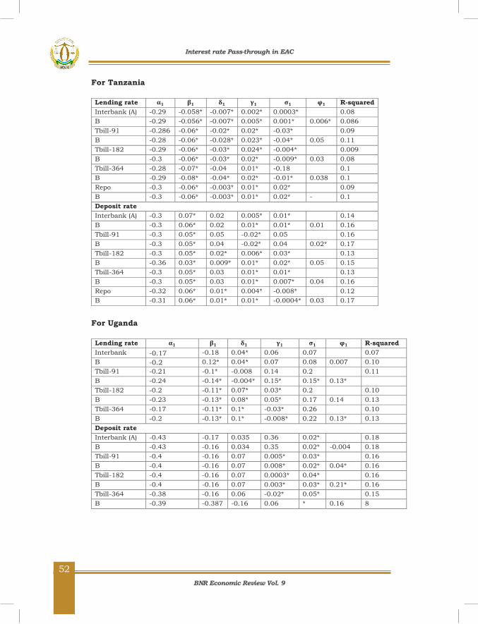
BNR Economic Review Vol. 9
52
54
53
For Tanzania
Lending rate 𝛂𝛂𝟏𝟏 𝛃𝛃𝟏𝟏 𝛅𝛅𝟏𝟏 𝛄𝛄𝟏𝟏 𝛔𝛔𝟏𝟏 𝛗𝛗𝟏𝟏 R-squared Interbank (A) -0.29 -0.058* -0.007* 0.002* 0.0003* 0.08 B -0.29 -0.056* -0.007* 0.005* 0.001* 0.006* 0.086 Tbill-91 -0.286 -0.06* -0.02* 0.02* -0.03* 0.09 B -0.28 -0.06* -0.028* 0.023* -0.04* 0.05 0.11 Tbill-182 -0.29 -0.06* -0.03* 0.024* -0.004* 0.009 B -0.3 -0.06* -0.03* 0.02* -0.009* 0.03 0.08 Tbill-364 -0.28 -0.07* -0.04 0.01* -0.18 0.1 B -0.29 -0.08* -0.04* 0.02* -0.01* 0.038 0.1 Repo -0.3 -0.06* -0.003* 0.01* 0.02* 0.09 B -0.3 -0.06* -0.003* 0.01* 0.02* -
0.003*
0.1 Deposit rate Interbank (A) -0.3 0.07* 0.02 0.005* 0.01* 0.14 B -0.3 0.06* 0.02 0.01* 0.01* 0.01 0.16 Tbill-91 -0.3 0.05* 0.05 -0.02* 0.05 0.16 B -0.3 0.05* 0.04 -0.02* 0.04 0.02* 0.17 Tbill-182 -0.3 0.05* 0.02* 0.006* 0.03* 0.13 B -0.36 0.03* 0.009* 0.01* 0.02* 0.05 0.15 Tbill-364 -0.3 0.05* 0.03 0.01* 0.01* 0.13 B -0.3 0.05* 0.03 0.01* 0.007* 0.04 0.16 Repo -0.32 0.06* 0.01* 0.004* -0.008* 0.12 B -0.31 0.06* 0.01* 0.01* -0.0004* 0.03 0.17
For Uganda
Lending rate 𝛂𝛂𝟏𝟏 𝛃𝛃𝟏𝟏 𝛅𝛅𝟏𝟏 𝛄𝛄𝟏𝟏 𝛔𝛔𝟏𝟏 𝛗𝛗𝟏𝟏 R-squared Interbank - 0.17 -0.18 0.04* 0.06 0.07 0.07 B - 0.2 0.12* 0.04* 0.07 0.08 0.007 0.10 Tbill-91 -0.21 -0.1* -0.008 0.14 0.2 0.11 B -0.24 -0.14* -0.004* 0.15* 0.15* 0.13* Tbill-182 -0.2 -0.11* 0.07* 0.03* 0.2 0.10 B -0.23 -0.13* 0.08* 0.05* 0.17 0.14 0.13 Tbill-364 -0.17 -0.11* 0.1* -0.03* 0.26 0.10 B -0.2 -0.13* 0.1* -0.008* 0.22 0.13* 0.13 Deposit rate Interbank (A) -0.43 -0.17 0.035 0.36 0.02* 0.18 B -0.43 -0.16 0.034 0.35 0.02* -0.004 0.18 Tbill-91 -0.4 -0.16 0.07 0.005* 0.03* 0.16 B -0.4 -0.16 0.07 0.008* 0.02* 0.04* 0.16 Tbill-182 -0.4 -0.16 0.07 0.0003* 0.04* 0.16 B -0.4 -0.16 0.07 0.003* 0.03* 0.21* 0.16 Tbill-364 -0.38 -0.16 0.06 -0.02* 0.05* 0.15 B -0.39 -0.387 -0.16 0.06 * 0.16 8
Interest rate Pass-through in EAC
-0.2-0.17

BNR Economic Review Vol. 9
53
55
Exchange Rate and External Sector Competitiveness in Rwanda
NUWAGIRA Wilberforce* Yves MUVUNYI†
Keywords: Exchange rate misalignment, Competitiveness, Rwanda, Cointegration
JEL Classification Numbers: F31, C13
* NUWAGIRA Wilberforce is the Manager of Balance of Payment Statistics at National Bank of Rwanda † Yves MUVUNYI is a statistician at the National Bank of Rwanda
Exchange Rate and External Sector Competitiveness in Rwanda
BNR Economic Review Vol. 9
54
56
Abstract
This paper estimates the impact of real exchange rate on external sector
competitiveness in Rwanda. The analysis focuses on two main indicators
namely exchange rate misalignment and marshall-lerner condition and the
empirical analysis builds on quarterly data from 2000Q1 to 2015Q4 and
derives a long-run Behavioral Equilibrium Exchange Rate (BEER). The
econometric analysis starts by analyzing the stochastic properties of the data
and found the variables stationary at first level of differencing. Accordingly, the
paper proceeds by estimating the cointegration and error correction models.
Regression results Show that most of the long-run behavior of the real exchange
rate could be explained by net foreign assets, terms of trade, productivity,
degree of trade openness and government expenditure. On the basis of these
economic fundamentals, alternating episodes of overvaluation and
undervaluation were identified and the antecedents characterizing the episodes
were equally traced within the review period. Among others for instance,
government expenditure on traded goods especially imports and deteriorating
terms of trade were discovered to account for undervaluation while surges in
capital flows and improved productivity in non-traded goods accounted for
overvaluation. The study also points to the fact that though exchange rate
impacts on trade balance, the marshall-lerner condition does not hold for
Rwanda. The paper therefore recommends effective monitoring of exchange rate
development to avoid higher levels of volatility which could lead to poor
performance of Rwanda’s tradable sector as well as putting in place better and
sustainable strategies to increase production in Rwanda to avoid higher import
prices induced by the exchange rate depreciation.
Exchange Rate and External Sector Competitiveness in Rwanda

BNR Economic Review Vol. 9
55
57
1. INTRODUCTION
The real exchange rate is one of the key economic indicators of the economy’s
international competitiveness, and therefore has a strong influence on a
country’s macroeconomic management particularly foreign trade
developments. A real exchange rate that is broadly aligned with its equilibrium
value is an important part of a country’s external sector competitiveness
because it improves trade balance and ensures macroeconomic stability given
that for exchange rate to be in equilibrium economic fundamentals have to be
at their sustainable levels.
However, persistently misaligned real exchange rates which is the deviation
of exchange rate from its equilibrium value can cause misallocation of
resources between tradable and non-tradable sectors and negatively impact
labor market dynamics. Reduced external competitiveness due to over-valued
exchange rate hampers exports, aggregate demand, growth and job creation.
Besides the longer-term implications, real exchange rate misalignment can
lead to inflationary pressures and even trigger speculative attacks. When
setting their exchange rate policy, countries also need to balance their goals
of reaching competitiveness and macroeconomic stability (Dornbusch, 1980)
Krugman(1979) and Frankel and Rose( 1996) argue that sustained real
effective exchange rate (REER) overvaluations constitute an early warning
indicator of possible currency crashes and they also have led to a drastic
adjustment of relative prices and to a decline in the aggregate growth rate of
the economy. On the other hand, RER movements determine production and
consumption choices between domestic and international goods,
policymakers sometimes perceive the REER as an additional tool to influence
the economy.
Some countries have tried to maintain their currencies undervalued in order
to boost the performance of the export sector and, hence, the aggregate
economic activity. For instance, academics have suggested that capital
controls and undervalued exchange rates have been key elements of an
export-oriented development strategy for Japan and Germany after World War
II and, more recently, China and other East Asian Economies (Dooley et
al.2003).
Exchange Rate and External Sector Competitiveness in Rwanda

BNR Economic Review Vol. 9
56
58
Indeed according to (World Bank, 1984, Pfefferman, 1985), exchange and
trade controls introduce large inefficiency costs and encourage the creation of
strong lobbies that compete for the rents generated by protective measures.
These types of costs can even be significant in a situation of short-term
structural misalignment if there are imperfections in local capital markets.
Exchange rate misalignment also promotes speculation and usually generates
massive capital flight out of the country. Although capital flight may be
optimal from a purely private perspective, it can substantially reduce the
social welfare of the country (Cuddington, 1986).
The existing literature suggests that maintaining the REER close to
equilibrium level is necessary for sustained growth and countries that avoided
overvaluation have been associated with sustained export-led growth and
substantial export diversification. Others have argued that undervaluation
which could be attributed to competitive devaluations may drive the exchange
rate to a level that encourages exports and promote growth. On the other
hand, overvaluations may reflect macroeconomic policy inconsistencies that
are likely to discourage growth (Razin and Collins, 1999).
Edwards (1988) and Sachs (1985) claims that the different development
experiences in East Asia, Latin America and Africa may be attributed to their
different trade regimes and exchange practices. On the one hand, unstable
and overvalued RERs hurt exports and support protectionist policies, while
persistent misaligned RERs in Africa caused a severe drop in agricultural
output (The World Bank, 1984). On the other hand, it has been argued that
outward-orientation policies and exchange rate levels that encouraged export
growth in East Asian countries generated a boost in their growth rates (Dollar,
1992). More recently, the appropriate level of the RER and its effects on
economic activity has been present in crucial debates like the performance
showed by the Chinese economy and the exchange rate policy of future
accession of countries to the Euro Area.
Government of Rwanda has embarked on economic reforms since 1995. The
foundation of the transformation of the economy is based on a process of
economic liberalization and turning away from control regulation and state
command to market policies. One of the key areas of reform were the
Exchange Rate and External Sector Competitiveness in Rwanda

BNR Economic Review Vol. 9
57
59
introduction of a more flexible exchange rate regime and fully liberalized
current account.
Rwanda is one of the African countries that demonstrate ownership of its
development programs and progress in good governance and institutional
capacity. Consequently, the country continues to receive more international
aid and other capital flows for financing the economy. However, resource
booms, such as those associated with rapid aid surges could also pose a
serious challenge for macroeconomic stability, especially with regard to the
tendency of high aid flows to be associated with disequilibrium Real Exchange
Rate (RER) appreciation because of increased and possibly unsustainable
domestic absorption.
Despite vast literature on the effects of exchange rate variation on external
sector competitiveness, little is known in the case of Rwanda. This study
therefore attempts to assess the impact of exchange rate on external sector
competitiveness in Rwanda by re-assessing exchange rate misalignment in
Rwanda as well as estimating another indicator of exchange rate-external
sector competitiveness namely Marshall-Lerner condition.
Secondly, the studies that dealt with the exchange rate movements and its
effect on external sector competitiveness have yielded mixed results. This
prompts the need to attempt to shed light on this issue by providing empirical
estimates on key indicators that link exchange rate fluctuations and external
sector competitiveness.
The objective of this paper is therefore, to estimate an equilibrium relationship
between REER and the economic fundamentals based on the theoretical
model in the spirit of Edwards (1989) identifying the impact of RER
misalignment on external sector competitiveness in Rwanda and assess
whether exchange rate movements affect trade balance in Rwanda.
The rest of the paper is organized as follows. Section 2 presents an overview
of exchange rate policies in Rwanda and external sector performance. Section
3 provides literature review and theoretical issues with emphasis on studies
that have applied the BEER approach. Section 4 presents methodology and
Exchange Rate and External Sector Competitiveness in Rwanda
BNR Economic Review Vol. 9
58
60
empirical results and discussion and Section 5 entails conclusion and
proposed policy recommendations.
2. OVERVIEW OF EXCHANGE RATE POLICIES IN RWANDA
The exchange rate policy in Rwanda is analyzed in two distinct periods; the
first period reflecting a system of fixed exchange rate and the second period,
as more flexible exchange rate system.
During the fixed exchange rate system, foreign currencies of the banking
system were held by the central bank, the later was the sole institution
authorized to carry out exchange transactions.
The exchange rate was initially pegged to the Belgian franc, then to the
American dollar and finally to the SDR. Its value did not reflect economic
reality due to lack of exchange rate flexibility (Kigabo and Nuwagira 2014).
During this period, the exchange rate seemed to be overestimated; causing a
rising of effective prices of Rwandan exports and a loss of competitiveness on
the international market. However, many reforms of exchange rate system
were undertaken since 1990 to correct the overvaluation of FRW and to
improve external competitiveness.
The statutory order n° SP 1 of 3rd March 1995 organizing the foreign exchange
market instituted a flexible system of exchange of RFW.
The objective of this flexible system aims at approaching as much as possible
the exchange rate equilibrium level; to stabilize prices and support growth.
Under this system, BNR intervenes on foreign market to smoothen the
volatility of exchange rate using its reference rate as the average of interbank
exchange rate and the BNR intervention rate.
2.1. EXTERNAL SECTOR PERFORMANCE
In the period under review, Rwanda’s external sector has been deteriorating
with current account deficit as a percentage of GDP reaching 13% in 2015.
The deterioration in the current account is due to worsening trade deficit,
Exchange Rate and External Sector Competitiveness in Rwanda
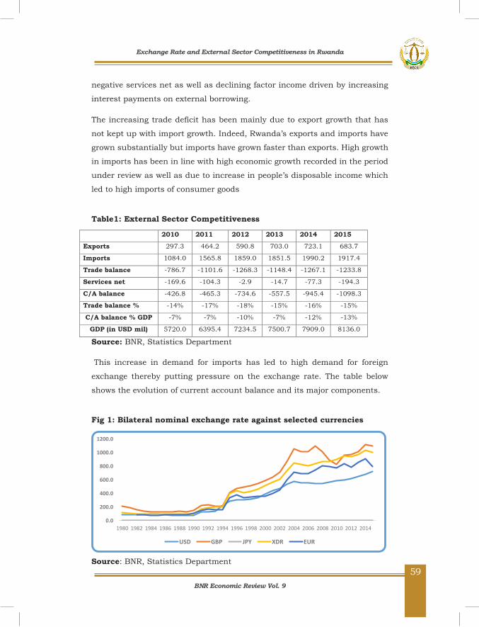
BNR Economic Review Vol. 9
59
61
negative services net as well as declining factor income driven by increasing
interest payments on external borrowing.
The increasing trade deficit has been mainly due to export growth that has
not kept up with import growth. Indeed, Rwanda’s exports and imports have
grown substantially but imports have grown faster than exports. High growth
in imports has been in line with high economic growth recorded in the period
under review as well as due to increase in people’s disposable income which
led to high imports of consumer goods
Table1: External Sector Competitiveness
2010 2011 2012 2013 2014 2015
Exports 297.3 464.2 590.8 703.0 723.1 683.7
Imports 1084.0 1565.8 1859.0 1851.5 1990.2 1917.4
Trade balance -786.7 -1101.6 -1268.3 -1148.4 -1267.1 -1233.8
Services net -169.6 -104.3 -2.9 -14.7 -77.3 -194.3
C/A balance -426.8 -465.3 -734.6 -557.5 -945.4 -1098.3
Trade balance %
GDP -14% -17% -18% -15% -16% -15%
C/A balance % GDP -7% -7% -10% -7% -12% -13%
GDP (in USD mil) 5720.0 6395.4 7234.5 7500.7 7909.0 8136.0
Source: BNR, Statistics Department
This increase in demand for imports has led to high demand for foreign
exchange thereby putting pressure on the exchange rate. The table below
shows the evolution of current account balance and its major components.
Fig 1: Bilateral nominal exchange rate against selected currencies
Source: BNR, Statistics Department
0.0
200.0
400.0
600.0
800.0
1000.0
1200.0
1980 1982 1984 1986 1988 1990 1992 1994 1996 1998 2000 2002 2004 2006 2008 2010 2012 2014
USD GBP JPY XDR EUR
Exchange Rate and External Sector Competitiveness in Rwanda

BNR Economic Review Vol. 9
60
62
2.1.1. Capital flows and Import Financing (in USD millions)
The trade deficit has been financed by capital flows particularly foreign direct
investment and both external public and private debt and occasional draw
downs on central bank reserves.
Table2. Capital flows
2010 2011 2012 2013 2014 2015 FDI inflows 250.50 119.11 254.96 257.64 458.9 471.24 PI 7.545 87.555 5.936 1.703 1.004 6.763 Debt flows 112.60 109.70 176.23 360.98 219.22 232.86
Source: BNR, Statistics Department
3. THEORETICAL AND EMPIRICAL LITERATURE REVIEW
In this section we briefly review the existing literature on the determination of
RER in the long run and the calculation of RER misalignments based on
fundamentals. The RER misalignment is conceptually defined as the deviation
of the actual RER relative to some benchmark (or equilibrium) level. Its
calculation therefore depends upon the measurement of the equilibrium level
of RER, which is unobservable. An overvalued real exchange rate indicates
that the value of current RER is above its equilibrium value, with undervalued
RER indicating the opposite.
A number of studies have found that the level of the REER relative to an
equilibrium REER, and its stability, has strong influence on exports and
private investment (Caballero and Cobra, 1989, Ghura and Grennes, 1993),
Yotopoulos and Sawada (2005) discover that systematic deviations of nominal
exchange rate from their Purchasing power parity (PPP) levels may cause
serious instabilities of the international macroeconomic system of a country.
Empirical studies on the determination of real exchange rate misalignment
have been challenging mainly due to the fact that the equilibrium real
exchange rate is unobservable and has to be estimated.
There are many approaches to determining the equilibrium exchange rate but
three of them are considered for the purpose of this study. The first is based
on purchasing power parity (PPP), which relates the nominal exchange rate to
price differentials between countries.
Exchange Rate and External Sector Competitiveness in Rwanda
BNR Economic Review Vol. 9
61
63
Lucio Sarno and Mark P Taylor (2002) assert that the nominal exchange rate
between two countries is equal to the ratio of two countries’ price level. This
suggests that the equilibrium real exchange rate remains constant with
nominal exchange rate movement offsetting relative price change between the
countries. Indeed several studies including Elbadawi & Soto (1997), Johansen
and Julius (1992) and Williamson (1994) using different empirical models
rejected PPP approach and suggested the use of approaches based on
economic fundamentals. This because a misalignment measure based on
purchasing power parity consists of the choice of a base period in which the
economy is thought to have been in equilibrium and then the RER for this
period is assumed to be in equilibrium for the rest of the sample period. The
equilibrium RER is not a static indicator and moves overtime as the economy’s
fundamentals move.
The second approach concentrates on the exchange rate that supports
sustainable internal and external macroeconomic balances over the medium
to long term. This is often referred to as the fundamental equilibrium
exchange rate (FEER) approach. Here the equilibrium exchange rate is
essentially determined by the current account balance target, which depends
on underlying sustainable equilibrium for international assets, as well as
national income base on full employment. The current account targets should
also be associated with desired levels of saving and investment.
Following FEER Approach, Terra and Valladares (2010) investigated episodes
of real exchange rate appreciations and depreciations for a sample of 85
countries from 1960 to 1998 and used a Markov Switching Model to
characterize real exchange rate misalignment series. They failed to find
evidence of misalignment in some countries while in some other countries the
evidence of misalignment was established in some states but lacked in others.
For the countries with two misalignment regimes, the appreciated regime has
higher persistence than the depreciated one.
Rajan et al. (2000) while investigating misalignment of the Baht and the crisis
in Thailand highlighted productivity (proxied by GDP per capita) as a major
fundamental influencing the equilibrium real exchange rate in any economy.
Using quarterly data spanning the period 1988 to 1999, they applied the
Exchange Rate and External Sector Competitiveness in Rwanda

BNR Economic Review Vol. 9
62
64
standard Johansen cointegration test to the natural real exchange rate model
developed by Stein (1994) and identified persistent and significant
misalignments (overvaluation) of the Thai baht against the Japanese yen.
Elbadawi and Soto (1997) used single equation cointegration methodology
and discovered that the RER for Mali was virtually in equilibrium on the
average between 1987 and 1994. Devarajan (1997) used computable general
equilibrium estimates and found that the RER for Burkina Faso was
overvalued by about 9% in 1993.
Williamson (1994), for instance, estimates the fundamental equilibrium
exchange rate of the G-7 countries given desirable current account balances
based on the potential output estimates for those countries calculated by the
IMF and the OECD. He found that in the last quarter of 1989, the actual U.S.
dollar was 14 percent overvalued, while the Japanese yen was 27 percent
undervalued.
The Fundamental equilibrium exchange rate approach is based on
macroeconomic identities; because it does not involve a theory of exchange
rate determination (Clark and MacDonald, 1998), the equilibrium exchange
rate calculated should not be viewed as normative. The equilibrium concept
is largely meant to imply the desirability of the underlying internal and
external balances rather than exchange rates per se (Bayoumi et al., 1994).
However, it is observed that this approach is less applicable as it is based on
value judgments therefore, inappropriate for meaningful and dependable
applications.
Finally, the behavioral equilibrium exchange rate (BEER) approach focuses
on the dynamic behavior of the exchange rate, including short-run
movements and deviations and taking broader macroeconomic conditions into
account. The choice of fundamentals may vary depending on the theoretical
model used. Starting with a model of risk-adjusted interest parity to construct
an equilibrium real exchange rate equation, Clark and MacDonald (1998)
include in their model as fundamentals terms of trade, the ratio of the
domestic consumer price index to the producer price index and the stock of
net foreign assets, as well as the relative supply of domestic to foreign
government debt as a risk premium factor.
Exchange Rate and External Sector Competitiveness in Rwanda

BNR Economic Review Vol. 9
63
65
Aliyu (2011) applied the Johansen’s cointegration approach and vector error
correction model to investigate RER misalignment in Nigeria. He adopted the
behavioural equilibrium exchange rate approach and included variables such
as terms of trade, crude oil volatility, monetary policy performance and
government fiscal stance in his model. His study showed that the naira was
overvalued by about 5.9 per cent.
Iossifov and Loukoianova (2007) estimated BEER model for Ghana and results
show that most of the REER’s long-run behavior can be explained by real GDP
growth, real interest rate differentials (both relative to trading-partner
countries), and the real world prices of Ghana’s main export commodities. The
REER in late 2006 was found to be very close to its estimated equilibrium
level and deviations from the equilibrium path are eliminated within two to
three years. The review of the empirical literature on the exchange rate
misalignment reveals that while much has been done on developing countries,
the studies on Rwanda are still very few.
Iimi (2006) used the BEER methodology and found that the Botswana’s pula
seems to have been undervalued in the late 1980s and overvalued by 5 to 10
percent in recent years, though the misalignment in the 1990s seems to have
been very marginal. Although the limitation of this study is that the model
included a few fundamental variables for fear of loss of degree of freedom, it
should still be recognized that these pieces of evidence were arrived at from a
sample comprising of only 19 observations (1985 – 2004).
Agu (2002) adopted a single equation procedure to estimate the time path of
the naira equilibrium exchange rate between 1970 and 1998 using
fundamentals such as trade policy, terms of trade, government consumption
expenditure, capital flows, and debt to GDP ratio. His estimates were
compared with the observed real exchange rate that prevailed during the same
period and it was discovered that real exchange rate misalignment in Nigeria
was irregular but persistent. The naira was found to be overvalued by an
average of about 1.4 per cent during the period. He confirmed that real
exchange rate misalignment and its volatility affects both the trade balance
and the capital account
Exchange Rate and External Sector Competitiveness in Rwanda
BNR Economic Review Vol. 9
64
66
Maesofernandez, Osbat and Schnatz (2001) using quarterly data from 1975
to 1998 and up to four different specifications of BEER/PEER methodology
indicate that the euro effective exchange rate was unambiguously
undervalued in 2000, although the extent largely depends on a particular
specification chosen. The driving fundamental variables in their models were
long term real interest rates differentials, productivity, net foreign assets,
relative fiscal stance, real price of oil, and relative total consumption
differentials.
Baffes, Elbadawi, and O’Connell (1999) examine misalignment for Côte
d’Ivoire and Burkina Faso using single-equation time series. They found that
for Côte d’Ivoire the actual real exchange rate was overvalued by 34 percent
on average during the period 1987–93, though Burkina Faso does not seem
to have experienced any major overvaluation. In the panel context, on the
other hand, Dufrenot and Yehoue (2005), analyzing the relationship between
real exchange rates and economic fundamentals in 64 developing countries,
found that exchange rate dynamics are less likely to be explained by
fundamentals such as productivity, terms of trade, and trade openness for
middle-income countries than for low income countries.
Using a similar approach, Elbadawi (1994), relying on an identity for nominal
domestic absorption, estimated the long-term equilibrium exchange rates for
Chile, Ghana, and India for the period 1967-1988.The fundamentals include
terms of trade, resource balances, degree of openness of the economy, share
of government expenditure in GDP, and a measure of excess money supply.
This paper employs the third approach because it seems to be a more general
method for calculating the real exchange rate and exchange rate misalignment
consistent with the concept of economic equilibrium. More important, the
analytical focus of the paper is equilibrium exchange rate behavior, including
cyclical and transitory deviations, in connection with macroeconomic
fundamentals. For Rwanda, the main factors that affect the equilibrium
exchange rate may be the terms of trade, government consumption, capital
flows, productivity and the degree of openness based on findings from studies
done in countries that have similar features like Rwanda.
Exchange Rate and External Sector Competitiveness in Rwanda

BNR Economic Review Vol. 9
65
67
4. METHODOLOGY
To estimate the indicators that link exchange rate and external sector
competitiveness namely, exchange rate misalignment and marshall-lerner
condition which are used in the context of this study, we specified different
models for each indicator. For exchange rate misalignment, the model
specified is based on behavioral equilibrium exchange rate while elasticity
approach was used in the case of Marshall-Lerner condition. Despite different
theoretical and empirical foundations, maximum likelihood method to
cointegration estimation technique was used in both cases.
4.1. Empirical model
4.1.1. Behavioral Equilibrium exchange rate model
To determine the extent of misalignment, we first need to establish the long-
run relationship between the real effective exchange rate and its
determinants. Econometrically, this paper applies a single equation approach
and uses cointegration analysis to identify the long run relationships among
variables. Meanwhile, the stochastic properties of data are assessed on the
basis of unit root tests and long run relationship is estimated as well as error
correction mechanism (ECM) to account for short run deviations from the long
run equilibrium. The cointegration parameters are used to perform a
permanent-transitory decomposition using the Hodrick and Prescott filter
(1997). Similar methodology was applied by Clark and MacDonald (1998),
Baffes, Elbadawi and O’connell (1999), recently Lim (2006) as well as Lossifov
and Loukoianova (2007).
To obtain equilibrium exchange rate we first used Hodrick-Prescot filter to
decompose the trend from the cycle to obtain permanent values of the
fundamentals. We then calculate the long run equilibrium level of REER by
multiplying the estimated coefficients obtained through BEER approach with
permanent values of the fundamentals.
For the purpose of this paper, the movements in the exchange rate of
Rwandan franc are explained by macroeconomic variables such as terms of
trade (TOT), relative productivity of home tradables proxied by GDP percapita,
government expenditure as a ratio of GDP (GOV), capital flows proxied by net
Exchange Rate and External Sector Competitiveness in Rwanda
BNR Economic Review Vol. 9
66
68
foreign assets (NFA) and the degree of economic openness (OPEN). The main
question that arises is whether the actual real exchange rate is overvalued or
undervalued in comparison with sustainable equilibrium levels. To address
this question, this paper applies the behavioral equilibrium exchange rate
(BEER) approach to determine the extent of misalignment to Rwanda
exchange rate movements over the period 2000Q1-2015Q4. The study
utilizes the traded weighted REER index while the rest of the data is
constructed and collected from various secondary data sources such as the
National Institute of Statistics of Rwanda; the Ministry of Finances and
Economic Planning and the National Bank of Rwanda.
Thus the model is specified as below;
……………(1)
Where;
The dependent variable is the real effective exchange rate. It is the CPI-based
multilateral real effective exchange rate. The REER is defined as the ratio of
the domestic consumer price index to the foreign consumer price index and
constructed as the trade-weighted average of the real exchange rate where the
weights are generated by the IMF based on both bilateral trade shares and
export similarities.
𝑅𝑅𝑅𝑅𝑅𝑅𝑅𝑅𝑖𝑖𝑖𝑖 =∑ (𝑁𝑁𝑁𝑁𝑁𝑁𝑅𝑅𝑖𝑖𝑖𝑖) (𝑝𝑝𝑖𝑖𝑖𝑖*/𝑝𝑝𝑖𝑖𝑖𝑖)…………………………………………………………..(2);
Where 𝑁𝑁𝑁𝑁𝑁𝑁𝑅𝑅𝑖𝑖𝑖𝑖 is the nominal effective exchange rate for Rwanda with respect
to the partner i, 𝑝𝑝𝑖𝑖𝑖𝑖* is the price in partner trading country, i representing the
price of tradable and 𝑝𝑝𝑖𝑖𝑖𝑖 is the CPI of home country as a proxy for price of non-
tradable.
TOT is terms of trade which is defined as the ratio of export price index to
import price index.
OPEN is the degree of openness of the economy and is computed as the ratio
of the sum of export and import to the gross domestic product (GDP).
PROD relative productivity proxied by percapita gross domestic product.
0 1 2 3 4 5log( ) log( ) log( ) log( ) log( ) log( )t t t t t t tRER TOT prod open NFA Gov
Exchange Rate and External Sector Competitiveness in Rwanda
BNR Economic Review Vol. 9
67
69
NFA is net foreign assets used as a proxy measure for capital flows; it is
computed by adding net foreign assets by monetary authority (central bank)
and net foreign assets by commercial banks.
GOV is government expenditure as a ratio of GDP less capital expenditure.
𝜀𝜀𝑡𝑡 is disturbance term that contains all other influences
Expected signs for the coefficients according to the economic theory are as
follows:
The terms of trade’s influence on the REER cannot be signed a priori, as this
depends on whether income or substitution effects dominate. The former
leads to real currency appreciation (increase in REER) while the latter to real
currency depreciation (decrease in REER).
An increase in the openness variable is assumed to be arising from a decline
in tariff rates, leading to a fall in the domestic prices of importables. This will
lead to high demand of foreign currency to take advantage of cheap imports,
and less demand for domestic currency. Hence an increase in the degree of
openness is expected to lead to the depreciation of the equilibrium real
effective exchange rate. As a result, the coefficient of openness variable is
expected to have a negative sign. Empirical researches show that there is a
negative link between trade integration and real exchange rate volatility
(Calderon and Kubota, 2009, Hau, 2002).
High government spending is likely to translate into high demand of non
tradables, which would lead to a rise in the price of non tradables. According
to the definition of REER as the ratio of the domestic consumer price index
(CPI) to the foreign consumer price index, this will lead to a real appreciation.
The effect partially depends on the extent of how RER is fully determined by
the supply side of the economy. The increase of public expenditures causes
an appreciation of RER and a permanent increase in government spending
leads to an appreciation of the equilibrium RER in the long run (Edward,
1989; Frenkel and Mussa, 1985). We expect this variable to be positively
signed.
Exchange Rate and External Sector Competitiveness in Rwanda
BNR Economic Review Vol. 9
68
70
Similarly high productivity will make the economy stronger leading to an
appreciated equilibrium RER hence we expect it to carry a positive sign.
Productivity in the traded goods sector relative to the non-traded sector. A
rapid economic growth is accompanied by real exchange rate appreciation
because of the differential productivity growth between tradable and non-
tradable sectors (Imed and Christopher, 2001, Antonia and Bara, 2006,
Samara, 2009)
Higher net foreign asset payments from abroad would lead to higher capital
inflows with a pressure on the exchange rate. We expect this variable to be
positively signed
4.1.2. Marshall-Lerner condition (Elasticity Approach)
We employ elasticity approach known in literature as imperfect substitutes
approach a kin to Bayoumi et al (2011), Chen et al (2012), Aziz and Chinoy
(2012) to estimate marshall –Lerner condition for Rwanda using quarterly
data spanning the period 2000Q1 to 2015Q4 to analyze the impact of
exchange rate on trade balance . We employ maximum likelihood method to
cointegration to estimate the both the export and import demand functions.
The models are specified as –
ln ɛ𝑒𝑒𝑒𝑒𝑡𝑡=𝛼𝛼1𝑙𝑙𝑙𝑙𝑙𝑙𝑒𝑒𝑒𝑒𝑙𝑙𝑡𝑡+𝛼𝛼2𝑙𝑙𝑙𝑙𝑙𝑙𝑙𝑙𝑙𝑙𝑙𝑙𝑡𝑡+𝜀𝜀𝑡𝑡…………….. (4)
ln ɛ𝑖𝑖𝑖𝑖𝑙𝑙𝑡𝑡=𝛼𝛼1𝑙𝑙𝑙𝑙𝑙𝑙𝑒𝑒𝑒𝑒𝑙𝑙𝑡𝑡+𝛼𝛼2𝑙𝑙𝑙𝑙𝑙𝑙𝑙𝑙𝑙𝑙𝑙𝑙𝑡𝑡+𝜀𝜀𝑡𝑡……………. (5)
Where 𝐥𝐥𝐥𝐥𝐥𝐥𝐥𝐥𝐭𝐭 is exports , lnreert is trade weighted CPI based real effective
exchange is rate, lnwgdp is foreign income as a proxy for external demand,
lnrgdp as proxy for national demand for imports and 𝜀𝜀𝑡𝑡 is the disturbance
term. All variables are transformed into natural logarithms and Real exchange
rate lagged by two quarters to allow for lags in the effect of relative price
changes.
Exchange Rate and External Sector Competitiveness in Rwanda
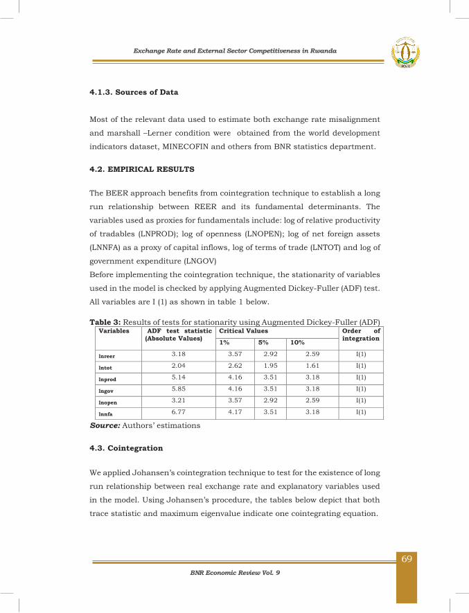
BNR Economic Review Vol. 9
69
71
4.1.3. Sources of Data
Most of the relevant data used to estimate both exchange rate misalignment
and marshall –Lerner condition were obtained from the world development
indicators dataset, MINECOFIN and others from BNR statistics department.
4.2. EMPIRICAL RESULTS
The BEER approach benefits from cointegration technique to establish a long
run relationship between REER and its fundamental determinants. The
variables used as proxies for fundamentals include: log of relative productivity
of tradables (LNPROD); log of openness (LNOPEN); log of net foreign assets
(LNNFA) as a proxy of capital inflows, log of terms of trade (LNTOT) and log of
government expenditure (LNGOV)
Before implementing the cointegration technique, the stationarity of variables
used in the model is checked by applying Augmented Dickey-Fuller (ADF) test.
All variables are I (1) as shown in table 1 below.
Table 3: Results of tests for stationarity using Augmented Dickey-Fuller (ADF) Variables ADF test statistic
(Absolute Values) Critical Values Order of
integration 1% 5% 10%
lnreer 3.18 3.57 2.92 2.59 I(1)
lntot 2.04 2.62 1.95 1.61 I(1)
lnprod 5.14 4.16 3.51 3.18 I(1)
lngov 5.85 4.16 3.51 3.18 I(1)
lnopen 3.21 3.57 2.92 2.59 I(1)
lnnfa 6.77 4.17 3.51 3.18 I(1)
Source: Authors’ estimations
4.3. Cointegration
We applied Johansen’s cointegration technique to test for the existence of long
run relationship between real exchange rate and explanatory variables used
in the model. Using Johansen’s procedure, the tables below depict that both
trace statistic and maximum eigenvalue indicate one cointegrating equation.
Exchange Rate and External Sector Competitiveness in Rwanda
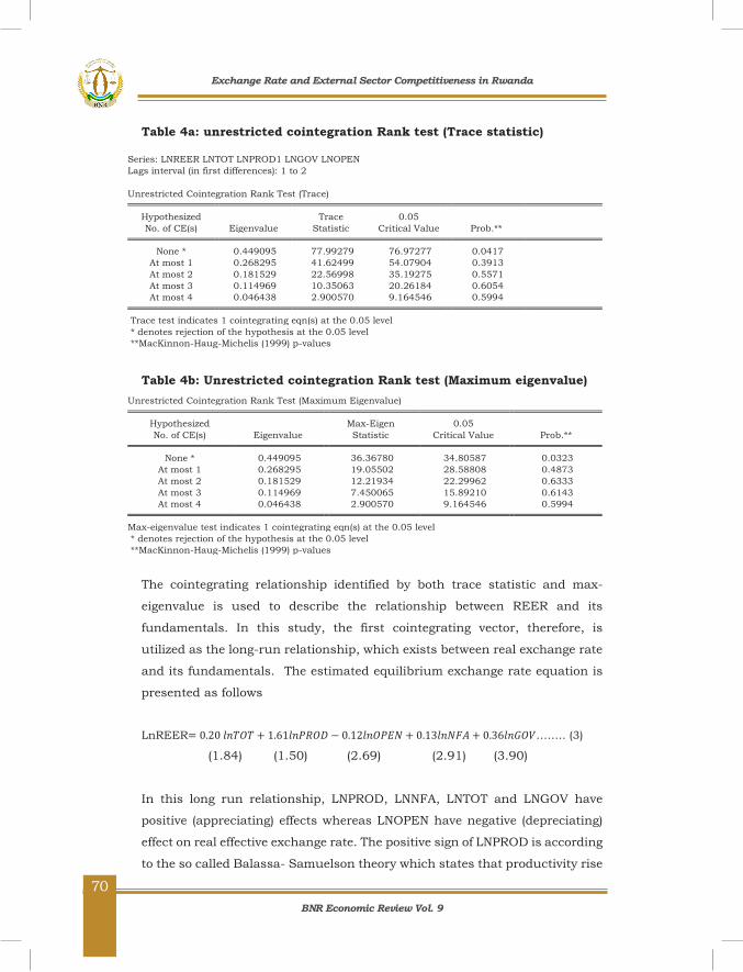
BNR Economic Review Vol. 9
70
72
Table 4a: unrestricted cointegration Rank test (Trace statistic)
Series: LNREER LNTOT LNPROD1 LNGOV LNOPEN Lags interval (in first differences): 1 to 2
Unrestricted Cointegration Rank Test (Trace) Hypothesized Trace 0.05
No. of CE(s) Eigenvalue Statistic Critical Value Prob.** None * 0.449095 77.99279 76.97277 0.0417
At most 1 0.268295 41.62499 54.07904 0.3913 At most 2 0.181529 22.56998 35.19275 0.5571 At most 3 0.114969 10.35063 20.26184 0.6054 At most 4 0.046438 2.900570 9.164546 0.5994
Trace test indicates 1 cointegrating eqn(s) at the 0.05 level * denotes rejection of the hypothesis at the 0.05 level **MacKinnon-Haug-Michelis (1999) p-values
Table 4b: Unrestricted cointegration Rank test (Maximum eigenvalue) Unrestricted Cointegration Rank Test (Maximum Eigenvalue) Hypothesized Max-Eigen 0.05
No. of CE(s) Eigenvalue Statistic Critical Value Prob.** None * 0.449095 36.36780 34.80587 0.0323
At most 1 0.268295 19.05502 28.58808 0.4873 At most 2 0.181529 12.21934 22.29962 0.6333 At most 3 0.114969 7.450065 15.89210 0.6143 At most 4 0.046438 2.900570 9.164546 0.5994
Max-eigenvalue test indicates 1 cointegrating eqn(s) at the 0.05 level * denotes rejection of the hypothesis at the 0.05 level **MacKinnon-Haug-Michelis (1999) p-values
The cointegrating relationship identified by both trace statistic and max-
eigenvalue is used to describe the relationship between REER and its
fundamentals. In this study, the first cointegrating vector, therefore, is
utilized as the long-run relationship, which exists between real exchange rate
and its fundamentals. The estimated equilibrium exchange rate equation is
presented as follows
LnREER= 0.20 𝑙𝑙𝑙𝑙𝑙𝑙𝑙𝑙𝑙𝑙 + 1.61𝑙𝑙𝑙𝑙𝑙𝑙𝑙𝑙𝑙𝑙𝑙𝑙 − 0.12𝑙𝑙𝑙𝑙𝑙𝑙𝑙𝑙𝑙𝑙𝑙𝑙 + 0.13𝑙𝑙𝑙𝑙𝑙𝑙𝑙𝑙𝑙𝑙 + 0.36𝑙𝑙𝑙𝑙𝑙𝑙𝑙𝑙𝑙𝑙…….. (3)
(1.84) (1.50) (2.69) (2.91) (3.90)
In this long run relationship, LNPROD, LNNFA, LNTOT and LNGOV have
positive (appreciating) effects whereas LNOPEN have negative (depreciating)
effect on real effective exchange rate. The positive sign of LNPROD is according
to the so called Balassa- Samuelson theory which states that productivity rise
Exchange Rate and External Sector Competitiveness in Rwanda

BNR Economic Review Vol. 9
71
73
in tradables leads to increase in demand of non-tradables, thus real exchange
rate appreciates. This is due to the fact that if productivity of traded goods
relative to non-traded goods productivity is growing faster at home than
abroad, the home currency should appreciate in real terms. As far as the
impact of NFA on REER is concerned, the results show that increase in long-
run capital inflows appreciate real exchange rate. NFA can affect equilibrium
real exchange rate through both supply and demand channels. In the supply
channel, Capital inflows increase the existing capital stock and bring spillover
effects of technology transfer and indeed Rwanda has received enormous
amounts of capital flows which in first round leads to an increase in output
and fall in prices of non-traded goods thus depreciating the real exchange rate
and in the second round, the increase in output of non-traded goods expands
disposable income and thus leads to the appreciation of Rwandan currency.
The Positive sign of terms of trade indicate that income effect dominates
insinuating that improvement in terms of trade raises demand for locally
produced goods (non-traded) hence non-traded goods prices increase relative
to traded goods, thus appreciating Rwanda’s currency. As regards to
government expenditure, the sign is positive implying that an increase in
government expenditure translates into high demand for non-traded which
leads to the rise in prices of non-traded goods thereby appreciating real
effective exchange rate.
Finally, the sign of openness is negative, implying that an increase in
openness depreciates REER because as Rwanda seeks to fully integrate within
East African community there has been a decline in tariff rates together with
the removal of non–tariff barriers, this has led to the fall in prices of
importable goods from EAC leading to expenditure switching thereby
depreciating our equilibrium real effective exchange rate.
4.4. Short-run dynamics of Exchange Rate
The appropriate mechanism for modeling the short-run real effective
exchange rate for Rwanda is an error correction mechanism (ECM). The
results from an error correction mechanism show that in the short term, only
NFA carries the burden of adjustment of real effective exchange rate. The error
Exchange Rate and External Sector Competitiveness in Rwanda
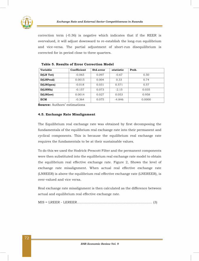
BNR Economic Review Vol. 9
72
74
correction term (-0.36) is negative which indicates that if the REER is
overvalued, it will adjust downward to re-establish the long-run equilibrium
and vice-versa. The partial adjustment of short-run disequilibrium is
corrected for in period close to three quarters.
Table 5. Results of Error Correction Model
Source: Authors’ estimations
4.5. Exchange Rate Misalignment
The Equilibrium real exchange rate was obtained by first decomposing the
fundamentals of the equilibrium real exchange rate into their permanent and
cyclical components. This is because the equilibrium real exchange rate
requires the fundamentals to be at their sustainable values.
To do this we used the Hodrick-Prescott Filter and the permanent components
were then substituted into the equilibrium real exchange rate model to obtain
the equilibrium real effective exchange rate. Figure 2, Shows the level of
exchange rate misalignment. When actual real effective exchange rate
(LNREER) is above the equilibrium real effective exchange rate (LNEREER), is
over-valued and vice versa.
Real exchange rate misalignment is then calculated as the difference between
actual and equilibrium real effective exchange rate.
MIS = LREER - LEREER…………………………………………………………... (3)
Variable Coefficient Std.error -statistic Prob.
D(LN Tot) -0.065 0.097 -0.67 0.50
D(LNProd) 0.0015 0.004 0.33 0.74
D(LNOpen) -0.018 0.031 0.571 0.57
D(LNNfa) -0.157 0.073 -2.15 0.035
D(LNGov) 0.0014 0.027 0.053 0.958
ECM -0.364 0.075 -4.846 0.0000
Exchange Rate and External Sector Competitiveness in Rwanda
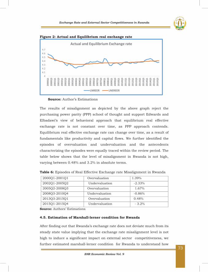
BNR Economic Review Vol. 9
73
75
Figure 2: Actual and Equilibrium real exchange rate
Source: Author’s Estimations
The results of misalignment as depicted by the above graph reject the
purchasing power parity (PPP) school of thought and support Edwards and
Elbadawi’s view of behavioral approach that equilibrium real effective
exchange rate is not constant over time, as PPP approach contends.
Equilibrium real effective exchange rate can change over time, as a result of
fundamentals like productivity and capital flows. We further identified the
episodes of overvaluation and undervaluation and the antecedents
characterizing the episodes were equally traced within the review period. The
table below shows that the level of misalignment in Rwanda is not high,
varying between 0.48% and 3.2% in absolute terms.
Table 6: Episodes of Real Effective Exchange rate Misalignment in Rwanda
2000Q1-2001Q1 Overvaluation 1.39% 2002Q1-2005Q2 Undervaluation -2.33% 2005Q2-2008Q3 Overvaluation 1.67% 2008Q3-2010Q4 Undervaluation -0.86% 2013Q3-2015Q1 Overvaluation 0.48% 2015Q1-2015Q4 Undervaluation - 3.2%
Source: Authors’ Estimations
4.5. Estimation of Marshall-lerner condition for Rwanda
After finding out that Rwanda’s exchange rate does not deviate much from its
steady state value implying that the exchange rate misalignment level is not
high to induce a significant impact on external sector competitiveness, we
further estimated marshall-lerner condition for Rwanda to understand how
44.14.24.34.44.54.64.7
2000
Q1
2000
Q3
2001
Q1
2001
Q3
2002
Q1
2002
Q3
2003
Q1
2003
Q3
2004
Q1
2004
Q3
2005
Q1
2005
Q3
2006
Q1
2006
Q3
2007
Q1
2007
Q3
2008
Q1
2008
Q3
2009
Q1
2009
Q3
2010
Q1
2010
Q3
2011
Q1
2011
Q3
2012
Q1
2012
Q3
2013
Q1
2013
Q3
2014
Q1
2014
Q3
2015
Q1
2015
Q3
Actual and Equilibrium Exchange rate
LNREER LNEREER
Exchange Rate and External Sector Competitiveness in Rwanda
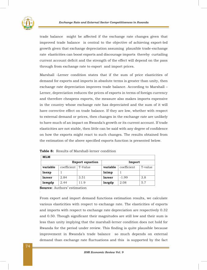
BNR Economic Review Vol. 9
74
76
trade balance might be affected if the exchange rate changes given that
improved trade balance is central to the objective of achieving export-led
growth given that exchange depreciation assuming plausible trade-exchange
rate elasticities can boost exports and discourage imports thereby curtailing
current account deficit and the strength of the effect will depend on the pass
through from exchange rate to export and import prices.
Marshall -Lerner condition states that if the sum of price elasticities of
demand for exports and imports in absolute terms is greater than unity, then
exchange rate depreciation improves trade balance. According to Marshall –
Lerner, depreciation reduces the prices of exports in terms of foreign currency
and therefore cheapens exports, the measure also makes imports expensive
in the country whose exchange rate has depreciated and the sum of it will
have corrective effect on trade balance. If they are low, whether with respect
to external demand or prices, then changes in the exchange rate are unlikely
to have much of an impact on Rwanda’s growth or its current account. If trade
elasticities are not stable, then little can be said with any degree of confidence
on how the exports might react to such changes. The results obtained from
the estimation of the above specified exports function is presented below.
Table 8: Results of Marshall-lerner condition MLM Export equation Import
Equation variable coefficient T-Value variable coefficient T-value
lnexp 1 lnimp 1 lnreer 2.84 3.51 lnreer -1.99 3.8 lnwgdp 2.44 11.9 lnrgdp 2.08 5.7
Source: Authors’ estimation Ɛfrom
From export and import demand functions estimation results, we calculate
various elasticities with respect to exchange rate. The elasticities of exports
and imports with respect to exchange rate depreciation are respectively 0.32
and 0.50. Though significant their magnitudes are still low and their sum is
less than unity implying that the marshall-lerner condition does not hold for
Rwanda for the period under review. This finding is quite plausible because
improvement in Rwanda’s trade balance so much depends on external
demand than exchange rate fluctuations and this is supported by the fact
Exchange Rate and External Sector Competitiveness in Rwanda
BNR Economic Review Vol. 9
75
77
that income elasticity which is the sum of export and import elasticities(0.86)
with respect to world gross domestic product as a proxy for external demand
and gross domestic product as a proxy for Rwanda’s demand for foreign goods
and services respectively is greater than the sum of price elasticities (0.82
<0.86). The finding broadly confirms that exchange rate changes though
significant do not have bigger impact on Rwanda’s trade balance and Taken
at face value, the response of Rwanda’s external sector to external demand
insinuates greater dependence of the Rwandan economy on external
conditions. These estimates are within the range of other studies on trade
elasticities (Goldstein and Khan, 1985, cheung, chin and Fuji, 2007). The
elasticities are presented below-
𝜀𝜀𝑒𝑒𝑒𝑒𝑒𝑒= ∆𝑙𝑙𝑙𝑙𝑒𝑒𝑒𝑒𝑒𝑒∆𝑙𝑙𝑙𝑙𝑙𝑙𝑒𝑒𝑒𝑒𝑙𝑙=0.32, 𝜀𝜀𝑖𝑖𝑖𝑖𝑒𝑒=∆𝑙𝑙𝑙𝑙𝑖𝑖𝑖𝑖𝑒𝑒
∆𝑙𝑙𝑙𝑙𝑙𝑙𝑒𝑒𝑒𝑒𝑙𝑙=0.50, 𝜀𝜀𝑦𝑦𝑒𝑒= ∆𝑙𝑙𝑙𝑙𝑒𝑒𝑒𝑒𝑒𝑒∆𝑙𝑙𝑙𝑙𝑙𝑙𝑙𝑙𝑙𝑙𝑒𝑒=0.38, 𝜀𝜀𝑦𝑦𝑖𝑖= ∆𝑙𝑙𝑙𝑙𝑖𝑖𝑖𝑖𝑒𝑒
∆𝑙𝑙𝑙𝑙𝑙𝑙𝑙𝑙𝑙𝑙𝑒𝑒=0.48
𝜀𝜀𝑒𝑒𝑒𝑒𝑒𝑒+𝜀𝜀𝑖𝑖𝑖𝑖𝑒𝑒= 0.32+0.50=0.82, 𝜀𝜀𝑦𝑦𝑒𝑒+𝜀𝜀𝑦𝑦𝑖𝑖=0.86
5. Conclusion and Policy lessons
The main objective of this paper is to evaluate the impact of REER on external
sector competitiveness. The analysis focuses on two main indicators of
external sector competitiveness namely exchange rate misalignment and
Marshall- Lerner condition.
The general finding points out to the existence of long-run relationship
between real effective exchange rate and the proposed set of economic
fundamentals. The normalized estimates confirm that productivity (balassa-
samuelson effect), openness, terms of trade, government consumption and
capital inflows are important long run determinants of the equilibrium
exchange rate in Rwanda. However, the level of misalignment taken in
absolute terms is not very high, fluctuating between 0.48% and 3.2%. This
indicates that the REER path is not a high level to prompt a significant impact
on Rwanda’s external sector competitiveness.
We also found out that Rwandan exports and imports respond more to income
than relative prices .For instance exports so much depend on external
demand than exchange rate changes and imports respond more to national
demand for imports proxied by Rwanda’s GDP confirming that exchange rate
Exchange Rate and External Sector Competitiveness in Rwanda

BNR Economic Review Vol. 9
76
78
movements have a small effect on Rwanda’s trade balance. In other words,
the income elasticity of demand for exports and imports is greater than the
price elasticity of demand for exports and imports in this respect therefore,
marshall-lerner condition doesn’t hold for Rwanda.
Despite the fact that marshall-lerner condition is not satisfied in the case of
Rwanda due to low export elasticity, both exports and import elasticities are
quite significant implying that exchange rate effect on trade balance is
becoming important and indeed the sum of the two elasticities (0.82) is close
to unity. For imports, the magnitude of responsiveness to exchange rate is
slightly higher (0.50) suggesting that the depreciation of Rwandan franc
slightly reduces imports given that most of the goods imported by Rwanda
have inelastic demand and as such their importation is less affected by
increase in prices for foreign goods. This finding calls for effective exchange
rate monitoring to avoid higher levels of exchange rate depreciation that could
make imports expensive. In view of this, the paper recommends a number of
but not limited to the following recommendations.
The government and the private sector should explore opportunities for better
and sustainable strategies to increase production in Rwanda to avoid higher
import prices induced by the exchange rate depreciation both in the short-
run and long-run. This is long-run solution and would imply for the
government to gradually proceed to expenditure switching.
Though Rwanda’s export sector is less sensitive to exchange rate movements,
effective monitoring of exchange rate developments remains vital to avoid
higher levels of volatility which could lead to poor performance of the country’s
tradable sector.
Exchange Rate and External Sector Competitiveness in Rwanda

BNR Economic Review Vol. 9
77
79
References
Agu, C. (2002). Real Exchange Rate Distortions and External Balance Position
of Nigeria: Issues and Policy Options. African Institute for Applied Economics.
Aliyu, S. U. R. (2011). Real Exchange Rate Misalignment: An Application of
Behavioural Equilibrium Exchange Rate to Nigeria. CBN Occasional paper, No.
41
Aziz, Jahangir and Sajjid Chinoy (2012): “India: More Open than You Think”,
JP Morgan note.
Baffes, J., I. Elbadawi, and S. O'Connell. (1999)."Single Equation Estimation
of the Equilibrium Real Exchange Rate."World Bank, Policy Research
Department, Washington, DC.
Balvers, R.J. and Bergstrand, J.H. (2002). “Government expenditure and
equilibrium real exchange rates’, Journal of International Money and Finance”,
vol. 21, pp. 667-692.
Bayoumi, T., P. Clark, S. Symansky, and M. Taylor, (1994). “The Robustness
of Equilibrium Exchange Rate Calculations to Alternative Assumptions and
Methodologies,” in Estimating Equilibrium Exchange Rates, ed. by J.
Williamson (Washington: Institute for International Economics).
Caballero, R., and V. Corbo, (1989). “How Does Uncertainty about the Real
Exchange Rate Affects Exports?” Policy Research Working Paper Series No.
221 (Washington: World Bank).
Clark, P. and R. MacDonald, (1998) “Exchange Rates and Economic
Fundamentals: Methodological Comparison of BEERs and FEERs,” IMF
Working Paper WP98/67 (Washington: International Monetary Fund).
Devarajan, R. (1997) Real Exchange Rate Misalignment in the CFA Zone,
Journal of African
Economies, Oxford, Vol. 6, No. 1, pp. 35 – 53.
Edwards, S. (1994). “Real and monetary determinants of real exchange rate
behavior: Theory and evidence for developing countries”. Williamson, J.
Exchange Rate and External Sector Competitiveness in Rwanda
BNR Economic Review Vol. 9
78
80
(Ed).Estimating equilibrium exchange rates, Washington D.C.: Institute for
Development Economic Research, pp. 61-92.
Edwards, S. (1995).”Why are Saving Rates so Different across Countries? An
International Comparative Analysis.” NBER Working Paper 5097
Elbadawi, I. and R. Soto. (1997). “Real Exchange Rate and Macroeconomic
Adjustment in Sub-Saharan Africa and Other Developing Countries.” in
Elbadawi, I. and R. Soto, (eds.), Foreign Exchange Market and Exchange Rate
Policies in Sub-Saharan Africa, Supplementary Edition of the Journal of
African Economies.
Elbadawi, I., (1994). “Estimating Long Run Real Exchange Rates,” in
Estimating Equilibrium
Exchange Rates, ed by J. Williamson (Washington: Institute for International
Economics).
Ghura, D. and T. J.Greenes (1993). “The Real Exchange Rate and
Macroeconomic Performance in Sub-Saharan Africa,” Journal of Development
Economics. 42: 155 – 174.
Goldstein, M. and M.S. Khan (1985), "Income and price effects in foreign
trade", in R.W.
Hinkle, L. E. and P. J. Montiel (1999). Exchange Rate Misalignment. World
Bank, New York: Oxford University Press.
Hodrick, R., and E. Prescott, (1997). “Postwar U.S. Business Cycles: An
Empirical Investigation,” Journal of Money, Credit and Banking, Vol. 29
(February), pp. 1–16.
Iossifov, P. and E. Loukoianova (2007). Estimation of a Behavioral
Equilibrium Exchange Rate Model for Ghana, IMF Working Paper WP/07/155
(Washington: International Monetary Fund).
Johansen S. and K. Juselius, (1992). “Testing Structural Hypotheses in a
Multivariate Cointegration Analysis of the PPP and the UIP for UK,” Journal
of Econometrics, Vol. 53 (July/September), pp. 211–44.
Exchange Rate and External Sector Competitiveness in Rwanda
BNR Economic Review Vol. 9
79
81
Jones and P.B. Kenen (eds.), Handbook of International Economics, North-
Holland, Amsterdam, 1041-1105.
MacDonald, R., and J. Nagayasu, (1998). “On the Japanese Yen-U.S. Dollar
Exchange Rate: A Structural Econometric Model Based on Real Interest
Differentials,” Journal of the Japanese and International Economies, Vol. 12
(March), pp. 75–102.
Maesofernandez, F.C. Osbat, B. Schnatz (2001).Determinants of the Euro
Real Effective Exchange Rate: A BEER/PEER Approach European Central
Bank (ECB) Working Paper Series, No. 85.
Rajan, R.S., Sen, R. Siregar, R. (2000). Misalignment of the Baht, Trade
Imbalances and the Crisis in Thailand. CIES Working Paper No. 00
Rodrik, Dani (1994). “King Kong Meets Godzilla: The World Bank and the East
Asian Miracle,”in Albert Fishlow, Catherine Gwin, Stephan Haggard, Dani
Rodrik and Robert Wade, eds., Miracle or Design? Lessons from East Asian
Experience, Washington, DC, Overseas Development Council, 15 – 53.
Terra, C. and Valladares, F. (2010). Real Exchange Rate Misalignment.
International Review of Economics and Finance, 19, 119-144
Williamson J. (1994). “Estimates of FEERs”, in Estimating Equilibrium
Exchange Rates, Institute of International Economics. John Williamson,
Editor.
World Bank, (1984).Toward a Sustained Development in Sub-Saharan Africa.
Washington, DC: The World Bank.
Yotopoulos A. Pan and Sawada Yasuyuki (2005). “Exchange Rate
Misalignment: A New Test of Lung-Run PPP Based on Cross-Country Data”,
CIRJE Discussion Paper, February.
Exchange Rate and External Sector Competitiveness in Rwanda

BNR Economic Review Vol. 9
80
82
APPENDICES
Appendix: 1 Permanent and transitory components
Appendix 2.misalignment
Appendix 3: Development of REER in Rwanda
Appendix 4.Descriptive Statistics
Variable Mean Maximum Minimum Std. Dev. Variance lnreer 4.35 4.58 4.21 0.07 4.35 lnprod 10.72 11.01 10.43 0.17 10.72 lnopen -2.85 -0.86 -3.27 0.56 -2.85 lntot 3.36 3.42 2.85 0.31 3.36 lngov -2.07 -1.43 -2.81 0.44 -2.07 lnnfa 5.26 6.5 3.58 0.81 5.26
-.10
-.05
.00
.05
.10
.15
4.2
4.3
4.4
4.5
4.6
5 10 15 20 25 30 35 40 45 50 55 60
LNREER Trend Cycle
Hodrick-Prescott Filter (lambda=1600)
-0.2
-0.1
0
0.1
0.2
2000
Q1
2000
Q4
2001
Q3
2002
Q2
2003
Q1
2003
Q4
2004
Q3
2005
Q2
2006
Q1
2006
Q4
2007
Q3
2008
Q2
2009
Q1
2009
Q4
2010
Q3
2011
Q2
2012
Q1
2012
Q4
2013
Q3
2014
Q2
2015
Q1
2015
Q4
LNREERGAP
405060708090
100110
Jan-
05
Jun-
05
Nov
-05
Apr-
06
Sep-
06
Feb-
07
Jul-0
7
Dec-
07
May
-08
Oct
-08
Mar
-09
Aug-
09
Jan-
10
Jun-
10
Nov
-10
Apr-
11
Sep-
11
Feb-
12
Jul-1
2
Dec-
12
May
-13
Oct
-13
Mar
-14
Aug-
14
Jan-
15
Jun-
15
Nov
-15
Apr-
16
REERm REERx REERt
Exchange Rate and External Sector Competitiveness in Rwanda
BNR Economic Review Vol. 9
81
83
Effects of Fiscal Policy on Inflation and Money Market Interest Rates in Rwanda
KARUHANGA K. Wilson* NYIRAKANANI Regine*
Key Words: Fiscal Policy, Inflation, Money Market Interest Rates, recursive SVAR
JEL Classification: E62, E31, E43, C32
* KARUHANGA K. Wilson and NYIRAKANANI Regine are Senior Economists at National Bank of Rwanda
Effects of Fiscal Policy on Inflation and Money Market Interest Rates in Rwanda
BNR Economic Review Vol. 9
82
84
Abstract
The purpose of this study is to examine the effects of fiscal policy on inflation
and money market interest rates in Rwanda using structural autoregressive
models on variables including nominal GDP, core Consumer Price Index,
interbank rate, Government spending, and government tax receipts over the
period from 2006Q1 to 2015Q4.
The results show that both the government spending and government tax
revenues affect positively and significantly nominal GDP and inflation. The
interbank rate is found less responsive to fiscal shocks. These findings show
that the effect on interest rate is not significant in Rwanda due to shallow
financial markets which could be impeding the transmission of monetary policy
signals.
Effects of Fiscal Policy on Inflation and Money Market Interest Rates in Rwanda

BNR Economic Review Vol. 9
83
85
1. Introduction
The theory suggests that fiscal policy imposes no effect on aggregate demand
and inflation as long as consumers are furnished with rational expectations.
However, the assumption seems to be utopic especially in times of high
deficits as evidenced by Perotti (2004). Indeed, Woodford (1996) had shown
that changes in fundamentals of fiscal policy affect aggregate demand and the
specification of fiscal policy matters even when the monetary policy rule is
explicitly independent. Among others, Hilbers (2004) pointed out that there
are both channels through which the actions of fiscal policy may affect
monetary policy variables. Under such posture, the effectiveness of one policy
is realized after imposing its effects on the other and therefore, this call for
macroeconomic policy coordination.
Definitely, several studies concert that fiscal policy and monetary policy are
perfect complements and their coordination is pre-requisite for achieving
sustainable economic growth. Among many others, Mishkin (2006) and
Mohammad et al. (2010) point out the interdependence of the two policies and
agree that monetary policy cannot successfully achieve its objectives unless
monetary and fiscal policies are well coordinated. Hence, being dependent to
each other, pursuing one policy without considering the other may lead to
inevitable sub-optimal outcomes such as huge budget deficits, high price
levels, exchange rate pressures and an adverse impact on aggregate demand
via their impact on monetary variables (Arby and Hanif, 2010).
Late in the 1990s, Calvo and Vegh (1999) have shown that monetary policy is
subservient to the fiscal policy in developing economies which could affect
inflation directly or indirectly. Mindful of these challenges, several
institutional reforms including the reforms reinforcing the central bank
independence have been executed in many developing countries which
certainly resulted in increased disassociation between fiscal and monetary
goals. But still, the importance of coordination of fiscal and monetary policy
for macroeconomic management rests on the fact that the two policies are
interdependent.
In Rwanda for instance, coordination between fiscal and monetary policies is
enforced through joint committees such as the Treasury Management
Effects of Fiscal Policy on Inflation and Money Market Interest Rates in Rwanda

BNR Economic Review Vol. 9
84
86
Committee (TMC) and Debt Management Committee (DMC), as well as
through the joint setting up of short and medium term Macroeconomic
framework. Among other national arrangements and policies, the
coordination of fiscal and monetary policies has yielded positive results that
include but not limited to low level of inflation and a small budget deficit as
percent of GDP. Mindful of good coordination and positive trends, this paper
aims to identify key channels through which the actions of fiscal policy may
affect monetary policy variables, namely inflation and money market interest
rates.
In fact, though the effect of fiscal policy on inflation and response of financial
market conditions has received enough attention globally, little is known for
the case of Rwanda. To the best of our knowledge, the only existing study (by
Karuhanga and Nyirakanani, 2015) has investigated the effect of shocks to
fiscal deficit and its financing components on conduct and transmission of
monetary policy. This study is different in that it examines the effect of
government spending and tax revenues on inflation and money market
interest rates.
The remainder of this paper is organized as follows. Section two presents a
brief review of the theoretical and empirical literature on different channels
through which fiscal policy can affect monetary policy. Section three lays out
the trends in Rwanda’s macroeconomic performance. Section four presents
model specification, data source and variable definition. Section five discusses
the empirical results, while section six concludes.
II. REVIEW OF THE LITERATURE
II.1 Theoretical Literature
There has been a consensus that fiscal and monetary policies are tools used
by government authorities to direct changes in the economy in order to
achieve macroeconomic stability. Theories confirm that in situations of
uncoordinated policies, fiscal policy actions may cause economic distortions
and may affect the effectiveness of the other macroeconomic policies. In this
Effects of Fiscal Policy on Inflation and Money Market Interest Rates in Rwanda
BNR Economic Review Vol. 9
85
87
section, we provide the recap of the theories behind the impact of fiscal policy
on inflation and money market interest rates.
II.1.1 Fiscal effect on inflation
In a poorly coordinated macroeconomic environment, fiscal authority takes
the first move while monetary policy remains passive to fiscal actions. This
directly affects monetary policy variables through substantial increases in
indirect tax rates which impact on prices and hence on inflation (Andrea,
1991, Hilbers, 2014). These changes in fiscal policy influence the aggregate
demand through both changes in the government spending and in household
disposable income. On this regard, the change in demand conditions
consecutively leads to a wage-price spiral and price setting behavior and
hence influences inflation and inflationary expectations. In response, the
monetary policy reacts to stabilize the overall demand at the level that
maintains inflation consistent with the target range.
The fiscal theory of the price level (Woodford, 1994 and Leeper, 1991) also
posits the importance of fiscal policy in stabilization of the economy. The
theory suggests the role of government’s inter-temporal budget constraint in
determination of the price level. Both policies vary between active and passive
behavior (Davig and Leeper, 2009). The passive policies ensure the
satisfaction of the government’s intertemporal budget constraint while the
active monetary pursues its inflation target independent of the government’s
financial position. In uncoordinated environment where fiscal discipline is not
viable, the reaction of monetary policy through aggressive increase in interest
rate cannot impact fluctuations in aggregate demand and inflation. Dixit and
Lambertini (2003) had earlier disclosed that fiscal authorities with
discretionary powers tend to constrain monetary policy commitment by
running their own policy based on rules.
Although it is currently less likely for governments to finance their deficits
with direct monetization, large dependence on domestic budget financing
through financial markets may cause crowding out effect on private sector
investment. Eventually, the economy is negatively affected leaving monetary
Effects of Fiscal Policy on Inflation and Money Market Interest Rates in Rwanda
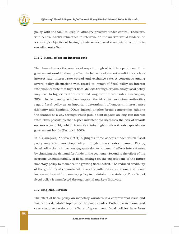
BNR Economic Review Vol. 9
86
88
policy with the task to keep inflationary pressure under control. Therefore,
with central bank’s reluctance to intervene on the market would undermine
a country’s objective of having private sector based economic growth due to
crowding out effect.
II.1.2 Fiscal effect on interest rate
The channel views the number of ways through which the operations of the
government would indirectly affect the behavior of market conditions such as
interest rate, interest rate spread and exchange rate. A consensus among
several policy discussions with regard to impact of fiscal policy on interest
rate channel state that higher fiscal deficits through expansionary fiscal policy
may lead to higher medium-term and long-term interest rates (Greenspan,
2002). In fact, many scholars support the idea that monetary authorities
regard fiscal policy as an important determinant of long-term interest rates
(Mohanty and Scatigna, 2003). Indeed, another broad compromise exhibits
the channel as a way through which public debt impacts on long-run interest
rates. This postulates that higher indebtedness increases the risk of default
on sovereign debt, which translates into higher interest rate spreads on
government bonds (Ferrucci, 2003).
In his analysis, Andrea (1991) highlights three aspects under which fiscal
policy may affect monetary policy through interest rates channel. Firstly,
fiscal policy via its impact on aggregate domestic demand affects interest rates
by changing the demand for funds in the economy. Second is the effect of the
overtime unsustainability of fiscal settings on the expectations of the future
monetary policy to monetize the growing fiscal deficit. The reduced credibility
of the government commitment raises the inflation expectations and hence
increases the cost for monetary policy to maintain price stability. The effect of
fiscal policy is manifested through capital markets financing.
II.2 Empirical Review
The effect of fiscal policy on monetary variables is a controversial issue and
has been a debatable topic since the past decades. Both cross-sectional and
case study regressions on effects of government fiscal policies have been
Effects of Fiscal Policy on Inflation and Money Market Interest Rates in Rwanda

BNR Economic Review Vol. 9
87
89
conducted. These studies show that the effects of fiscal policy on monetary
variables differ across countries even when identical approaches are used.
Consequently, this sub-section reviews both country and cross-sectional
cases seeking to review how significant the fundamentals of fiscal policy may
be influencing the monetary variables.
Indeed, Anyanwu (1993), Sheffrin (2003), Alesina and Tabelini (1990) among
others provide that fiscal policy is repeatedly subjective towards attaining
higher growth and employment even at the cost of the high inflation. The fiscal
policy makers intervene through policy activist, discretionary and
countercyclical policy in an effort to achieve the objective of macroeconomic
stability and growth.
Blinder (1982) offers that uncoordinated behavior arises when monetary
policy decides to tighten in response to loosening in fiscal policy or monetary
policy carries out loosening accompanied by tightening in fiscal policy. He
further notes that poor coordination between authorities arises from three
folds notably differences in objectives of what is best for society; adherence to
different theories about the effects of policy actions on the economy; as well
as on divergence in forecasts about the likely state of the economy in absence
of policy intervention.
Using three variables namely government expenditure, tax revenues, and the
level of output for USA, Blanchard and Perotti (1999) analyzed the effect of
fiscal policy shocks on output and consumption. They found a positive impact
of an expenditure shock on output and consumption. In contrast, an increase
in tax revenues is found to negatively affect the two variables. Höppner (2001)
adopted the same work by Blanchard and Perotti for Germany and obtained
the same findings.
In their analysis for Colombia, Lozano and Rodríguez (2011) conclude that a
positive shock on expenditure has a positive and statistically significant effect
on output, private consumption, employment, price level and short-term
interest rates. An increase in tax revenue was found less efficient because of
its impact on private investment. The results contradict with findings reported
Effects of Fiscal Policy on Inflation and Money Market Interest Rates in Rwanda
BNR Economic Review Vol. 9
88
90
by Ravnik and Žilić (2011) for Croatia where a positive expenditure shock has
an immediate and negative effect on money market interest rates.
For Sub-Saharan African countries, Baldini and Ribeiro (2008) found mixed
results with some countries dominated by fiscal regime, others by monetary
policy while the remaining did not show any clear result. The study also
reveals that changes in nominal debt could be the basis of price variability
through aggregate demand effects. Their results are consistent with the fiscal
theory of price level suggesting that the effects of fiscal actions could be direct
source of price distortions.
The analysis for Egypt and Tunisia by Slimane and Tahar (2013) found a
negative and persistent effect of revenue shock on money market interest rate
in Egypt while increase in expenditure had positive and immediate effect on
inflation and interest rate. For Tunisia, revenue shock impacts positively
inflation and interest rate while expenditure shock increases inflation with an
immediate effect and reverse for interest rate.
For the case of Italy, Giordano et al. (2007) concluded that a positive shock
on expenditure has an expansionary impact on the economic activity but with
a small and short-lived effect on inflation. The response of tax revenues to
expenditure shock is positive. For Czech Republic, the findings by Frantz
(2012) also confirm the expansionary effect of an expenditure shock on
inflation and are in line with findings by Agha and Khan (2006).
III. FISCAL AND MONETARY POLICY DEVELOPMENTS IN RWANDA
III.1 Fiscal Policy in Rwanda
Given the broad commitment of the government to achieve rapid growth and
sustainable macro-economic stability, the management of fiscal position has
been set under fiscal consolidation strategy (FCS). The program aims to
improving public revenue mobilization and prioritizing public expenditure,
with a view of reducing dependence on foreign aid.
Effects of Fiscal Policy on Inflation and Money Market Interest Rates in Rwanda
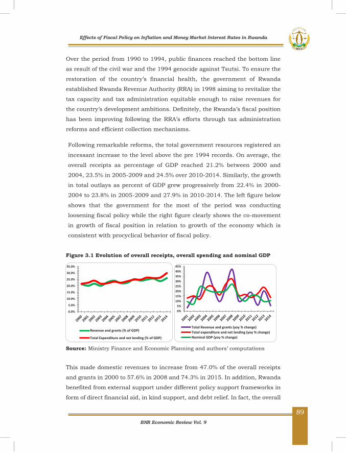
BNR Economic Review Vol. 9
89
91
Over the period from 1990 to 1994, public finances reached the bottom line
as result of the civil war and the 1994 genocide against Tsutsi. To ensure the
restoration of the country’s financial health, the government of Rwanda
established Rwanda Revenue Authority (RRA) in 1998 aiming to revitalize the
tax capacity and tax administration equitable enough to raise revenues for
the country’s development ambitions. Definitely, the Rwanda’s fiscal position
has been improving following the RRA’s efforts through tax administration
reforms and efficient collection mechanisms.
Following remarkable reforms, the total government resources registered an
incessant increase to the level above the pre 1994 records. On average, the
overall receipts as percentage of GDP reached 21.2% between 2000 and
2004, 23.5% in 2005-2009 and 24.5% over 2010-2014. Similarly, the growth
in total outlays as percent of GDP grew progressively from 22.4% in 2000-
2004 to 23.8% in 2005-2009 and 27.9% in 2010-2014. The left figure below
shows that the government for the most of the period was conducting
loosening fiscal policy while the right figure clearly shows the co-movement
in growth of fiscal position in relation to growth of the economy which is
consistent with procyclical behavior of fiscal policy.
Figure 3.1 Evolution of overall receipts, overall spending and nominal GDP
Source: Ministry Finance and Economic Planning and authors’ computations
This made domestic revenues to increase from 47.0% of the overall receipts
and grants in 2000 to 57.6% in 2008 and 74.3% in 2015. In addition, Rwanda
benefited from external support under different policy support frameworks in
form of direct financial aid, in kind support, and debt relief. In fact, the overall
0.0%
5.0%
10.0%
15.0%
20.0%
25.0%
30.0%
35.0%
Revenue and grants (% of GDP)
Total Expenditure and net lending (% of GDP)
0%5%
10%15%20%25%30%35%40%45%
Total Revenue and grants (yoy % change)Total expenditure and net lending (yoy % change)Nominal GDP (yoy % change)
Effects of Fiscal Policy on Inflation and Money Market Interest Rates in Rwanda
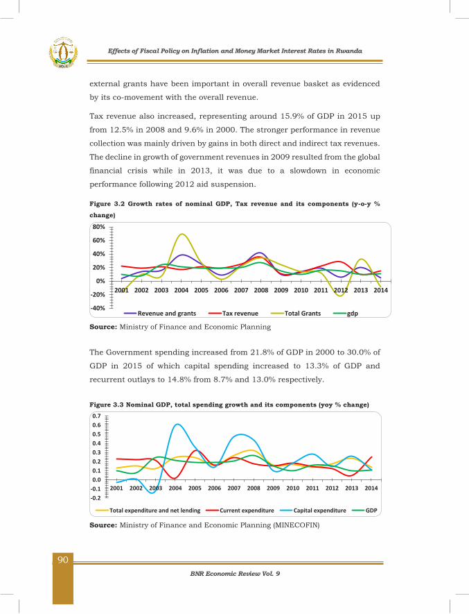
BNR Economic Review Vol. 9
90
92
external grants have been important in overall revenue basket as evidenced
by its co-movement with the overall revenue.
Tax revenue also increased, representing around 15.9% of GDP in 2015 up
from 12.5% in 2008 and 9.6% in 2000. The stronger performance in revenue
collection was mainly driven by gains in both direct and indirect tax revenues.
The decline in growth of government revenues in 2009 resulted from the global
financial crisis while in 2013, it was due to a slowdown in economic
performance following 2012 aid suspension.
Figure 3.2 Growth rates of nominal GDP, Tax revenue and its components (y-o-y % change)
Source: Ministry of Finance and Economic Planning
The Government spending increased from 21.8% of GDP in 2000 to 30.0% of
GDP in 2015 of which capital spending increased to 13.3% of GDP and
recurrent outlays to 14.8% from 8.7% and 13.0% respectively.
Figure 3.3 Nominal GDP, total spending growth and its components (yoy % change)
Source: Ministry of Finance and Economic Planning (MINECOFIN)
-40%
-20%
0%
20%
40%
60%
80%
2001 2002 2003 2004 2005 2006 2007 2008 2009 2010 2011 2012 2013 2014
Revenue and grants Tax revenue Total Grants gdp
-0.2-0.10.00.10.20.30.40.50.60.7
2001 2002 2003 2004 2005 2006 2007 2008 2009 2010 2011 2012 2013 2014
Total expenditure and net lending Current expenditure Capital expenditure GDP
Effects of Fiscal Policy on Inflation and Money Market Interest Rates in Rwanda
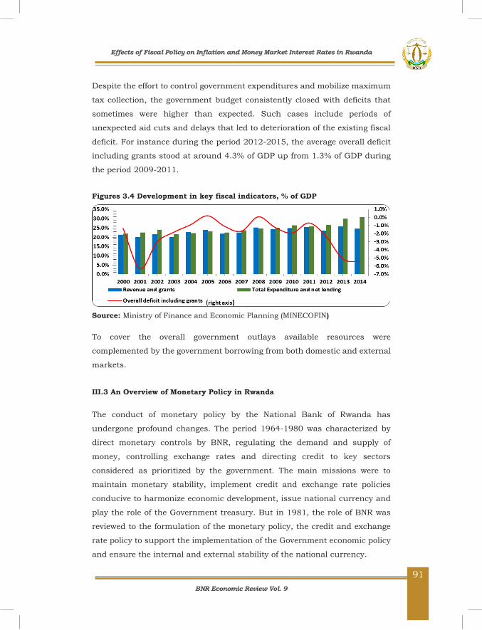
BNR Economic Review Vol. 9
91
93
Despite the effort to control government expenditures and mobilize maximum
tax collection, the government budget consistently closed with deficits that
sometimes were higher than expected. Such cases include periods of
unexpected aid cuts and delays that led to deterioration of the existing fiscal
deficit. For instance during the period 2012-2015, the average overall deficit
including grants stood at around 4.3% of GDP up from 1.3% of GDP during
the period 2009-2011.
Figures 3.4 Development in key fiscal indicators, % of GDP
Source: Ministry of Finance and Economic Planning (MINECOFIN)
To cover the overall government outlays available resources were
complemented by the government borrowing from both domestic and external
markets.
III.3 An Overview of Monetary Policy in Rwanda
The conduct of monetary policy by the National Bank of Rwanda has
undergone profound changes. The period 1964-1980 was characterized by
direct monetary controls by BNR, regulating the demand and supply of
money, controlling exchange rates and directing credit to key sectors
considered as prioritized by the government. The main missions were to
maintain monetary stability, implement credit and exchange rate policies
conducive to harmonize economic development, issue national currency and
play the role of the Government treasury. But in 1981, the role of BNR was
reviewed to the formulation of the monetary policy, the credit and exchange
rate policy to support the implementation of the Government economic policy
and ensure the internal and external stability of the national currency.
Effects of Fiscal Policy on Inflation and Money Market Interest Rates in Rwanda
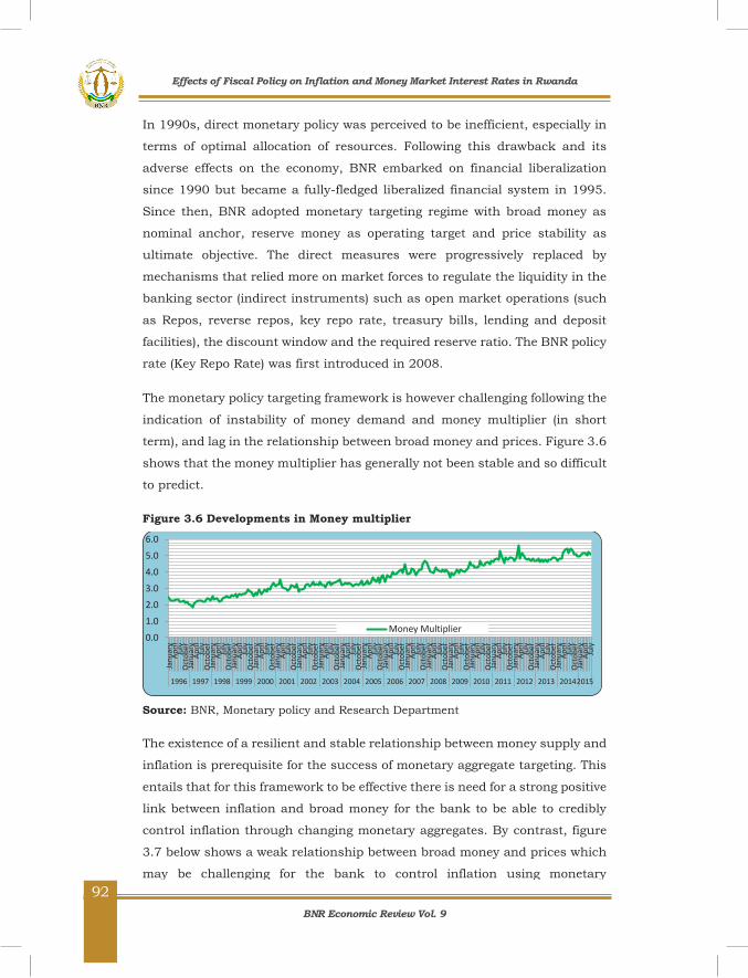
BNR Economic Review Vol. 9
92
94
In 1990s, direct monetary policy was perceived to be inefficient, especially in
terms of optimal allocation of resources. Following this drawback and its
adverse effects on the economy, BNR embarked on financial liberalization
since 1990 but became a fully-fledged liberalized financial system in 1995.
Since then, BNR adopted monetary targeting regime with broad money as
nominal anchor, reserve money as operating target and price stability as
ultimate objective. The direct measures were progressively replaced by
mechanisms that relied more on market forces to regulate the liquidity in the
banking sector (indirect instruments) such as open market operations (such
as Repos, reverse repos, key repo rate, treasury bills, lending and deposit
facilities), the discount window and the required reserve ratio. The BNR policy
rate (Key Repo Rate) was first introduced in 2008.
The monetary policy targeting framework is however challenging following the
indication of instability of money demand and money multiplier (in short
term), and lag in the relationship between broad money and prices. Figure 3.6
shows that the money multiplier has generally not been stable and so difficult
to predict.
Figure 3.6 Developments in Money multiplier
Source: BNR, Monetary policy and Research Department
The existence of a resilient and stable relationship between money supply and
inflation is prerequisite for the success of monetary aggregate targeting. This
entails that for this framework to be effective there is need for a strong positive
link between inflation and broad money for the bank to be able to credibly
control inflation through changing monetary aggregates. By contrast, figure
3.7 below shows a weak relationship between broad money and prices which
may be challenging for the bank to control inflation using monetary
0.0
1.0
2.0
3.0
4.0
5.0
6.0
Janu
ary
April
July
Oct
ober
Janu
ary
April
July
Oct
ober
Janu
ary
April
July
Oct
ober
Janu
ary
April
July
Oct
ober
Janu
ary
April
July
Oct
ober
Janu
ary
April
July
Oct
ober
Janu
ary
April
July
Oct
ober
Janu
ary
April
July
Oct
ober
Janu
ary
April
July
Oct
ober
Janu
ary
April
July
Oct
ober
Janu
ary
April
July
Oct
ober
Janu
ary
April
July
Oct
ober
Janu
ary
April
July
Oct
ober
Janu
ary
April
July
Oct
ober
Janu
ary
April
July
Oct
ober
Janu
ary
April
July
Oct
ober
Janu
ary
April
July
Oct
ober
Janu
ary
April
July
Oct
ober
Janu
ary
April
July
Oct
ober
Janu
ary
April
July
1996 1997 1998 1999 2000 2001 2002 2003 2004 2005 2006 2007 2008 2009 2010 2011 2012 2013 20142015
Money Multiplier
Effects of Fiscal Policy on Inflation and Money Market Interest Rates in Rwanda

BNR Economic Review Vol. 9
93
95
aggregates. Therefore, this growing instability of the money multiplier as well
as the weakening relationship between broad money and inflation reflect the
BNR’s plan to adopt an inflation-targeting framework by 2018.
Figure 3.7 Link between Money Supply and Inflation (YoY % changes)
Source: BNR, Statistics Department and computations by authors.
III.4 Inflation dynamics
Over the last two decades, the trend in inflation was moderate following
sustained economic performance, efficient and well-coordinated monetary
and fiscal policies as well as stable FRW exchange rate. Inflation hiked in
2007/2008 as result of commodity prices crisis. It was decelerating thereafter
as regional inflationary pressures were overcompensated by declines in prices
of domestically produced goods and falling international commodity prices.
With 2012 economic recovery, demand driven inflationary pressures were
tamed by increasing nominal interest rate on the back of monetary policy
reaction and government borrowing after the aid cut. Fiscal spending
adjustments contributed to falling aggregate demand and lower inflation in
the following years necessitating further accommodative monetary policy
stance to support the economy. Indeed, inflation averaged 1.8% in 2014 and
2.5% in 2015 due to good domestic harvest and falling international
commodity prices which add to weakening aggregate demand. The figure
below represents a co-movement between inflation and fiscal stances as well
as the interbank rate.
-20
-10
0
10
20
30
40
50
Janu
ary
July
Janu
ary
July
Janu
ary
July
Janu
ary
July
Janu
ary
July
Janu
ary
July
Janu
ary
July
Janu
ary
July
Janu
ary
July
Janu
ary
July
Janu
ary
July
Janu
ary
July
Janu
ary
July
Janu
ary
July
Janu
ary
July
Janu
ary
July
Janu
ary
July
Janu
ary
July
Janu
ary
July
Janu
ary
July
1996 1997 1998 1999 2000 2001 2002 2003 2004 2005 2006 2007 2008 2009 2010 2011 2012 2013 2014 2015
Annual Headline Inflation M3 (YoY % change)
Effects of Fiscal Policy on Inflation and Money Market Interest Rates in Rwanda

BNR Economic Review Vol. 9
94
96
Figure 3.8 Fiscal stances and Inflation Dynamics (QOQ % change)
Source: BNR, Monetary Policy and Research Department
IV METHODOLOGY
The study follows a methodology that has been used by several studies that
include Blanchard and Perotti (1999), Haug et al. (2013) as well as Kamps
and Caldara (2008) among others. The approach uses a recursive model which
draws out the dynamic effects of fiscal variations on the macroeconomic
variables. The approach imposes contemporaneous structural restrictions
based on the assumption underlying the structure of the economy.
IV.1 Model Specification
The baseline VAR model specification can be written in a reduced form as
follows:
𝑋𝑋𝑡𝑡 = 𝐴𝐴(𝐿𝐿)𝑋𝑋𝑡𝑡1 + 𝑢𝑢𝑡𝑡……………………….………………………………………….…….(1)
Where;
𝑋𝑋𝑡𝑡 = ( gt, 𝜏𝜏t, yt, πt, it, ) denotes the k-dimensional vector of endogenous
macroeconomic variables necessary to explain the effect of fiscal shocks on
inflation and money market interest rates; gt is the log of the total government
spending; yt is the log of nominal GDP; 𝜏𝜏t is the log of government tax revenue;
πt is the log of core consumer price index; it is the interbank rate.
-5.0
0.0
5.0
10.0
15.0
20.0
25.0
2006
Q1
2006
Q2
2006
Q3
2006
Q4
2007
Q1
2007
Q2
2007
Q3
2007
Q4
2008
Q1
2008
Q2
2008
Q3
2008
Q4
2009
Q1
2009
Q2
2009
Q3
2009
Q4
2010
Q1
2010
Q2
2010
Q3
2010
Q4
2011
Q1
2011
Q2
2011
Q3
2011
Q4
2012
Q1
2012
Q2
2012
Q3
2012
Q4
2013
Q1
2013
Q2
2013
Q3
2013
Q4
2014
Q1
2014
Q2
2014
Q3
2014
Q4
2015
Q1
2015
Q2
2015
Q3
2015
Q4
Inflation Total revenue, QoQ % change Total spending, QoQ % change Interbank % p.a
Effects of Fiscal Policy on Inflation and Money Market Interest Rates in Rwanda

BNR Economic Review Vol. 9
95
97
In addition, 𝐴𝐴 matrix stands for contemporaneous relationship between
endogenous variables collected in vector 𝑋𝑋𝑡𝑡. 𝐴𝐴(𝐿𝐿) is a (𝑛𝑛𝑛𝑛𝑛𝑛) the matrix
representing a lag polynomial. 𝑢𝑢𝑡𝑡= (𝑢𝑢𝑡𝑡𝑔𝑔, 𝑢𝑢𝑡𝑡,
𝜏𝜏 𝑢𝑢𝑡𝑡𝑦𝑦, 𝑢𝑢𝑡𝑡
𝜋𝜋, 𝑢𝑢𝑡𝑡𝑖𝑖 ) is the vector of the reduced
form innovations with 𝐸𝐸(𝑢𝑢𝑡𝑡) = 0, 𝐸𝐸(𝑢𝑢𝑡𝑡𝑢𝑢𝑡𝑡) = 𝛴𝛴𝑢𝑢 and 𝐸𝐸(𝑢𝑢𝑡𝑡𝑢𝑢𝑡𝑡) = 0 for 𝑠𝑠 ≠ 𝑡𝑡 -
residuals which in general have non-zero cross correlations.
To investigate the fiscal effect on inflation and money market interest rates,
we estimated a SVAR model with the abovementioned five variables. This is
done to avoid simultaneous estimation of large number of parameters. The
reason centers on the preference to follow the footsteps of both theoretical
views and on other similar empirical studies that estimated the very similar
sets of variables.
Given that the reduced form residuals have little economic significance, other
than having linear combination of the underlying structural variable shocks.
Therefore, our interest to examine the effect of shocks in government spending
and government revenue on a set of macroeconomic variables cannot be
attained. For the matter of giving the model an economic interpretation, it is
important to transform the reduced form model into a structural model that
is able to investigate the responses on the shock. Without loss of generality,
we multiply equation one by (𝑛𝑛𝑛𝑛𝑛𝑛) matrix 𝐴𝐴0 to obtain the structural form that
can be written as:
𝐴𝐴𝑋𝑋𝑡𝑡 = 𝐴𝐴∗(𝐿𝐿)𝑋𝑋𝑡𝑡𝑡𝑡−𝑡𝑡 + 𝐵𝐵𝐵𝐵𝑡𝑡 …….….…………..………………………………………….… (2)
Where 𝐴𝐴∗= 𝐴𝐴0𝐴𝐴 and 𝐵𝐵𝐵𝐵𝑡𝑡 = 𝐴𝐴0𝐵𝐵𝑡𝑡 which describes the relationship between the
reduced form residuals 𝑢𝑢𝑡𝑡 and the structural disturbances 𝐵𝐵𝑡𝑡. In the literature,
this structural representation form is called the 𝐴𝐴𝐵𝐵 model. The square (n x n) matrix B permits some shocks to affect directly more than one endogenous
variable in the model. While 𝐵𝐵𝑡𝑡 is 𝑛𝑛𝑛𝑛1 vector of structural innovations
with et~N(0, BE(etet′)B′). Both models (1) and (2) are observationally equivalent,
thus without identifying restrictions on the parameters in 𝐴𝐴 and 𝐵𝐵, no reliable
conclusions regarding the structural parameters of the true model can be
drawn from the data (Gottschalk, 2001).
Effects of Fiscal Policy on Inflation and Money Market Interest Rates in Rwanda
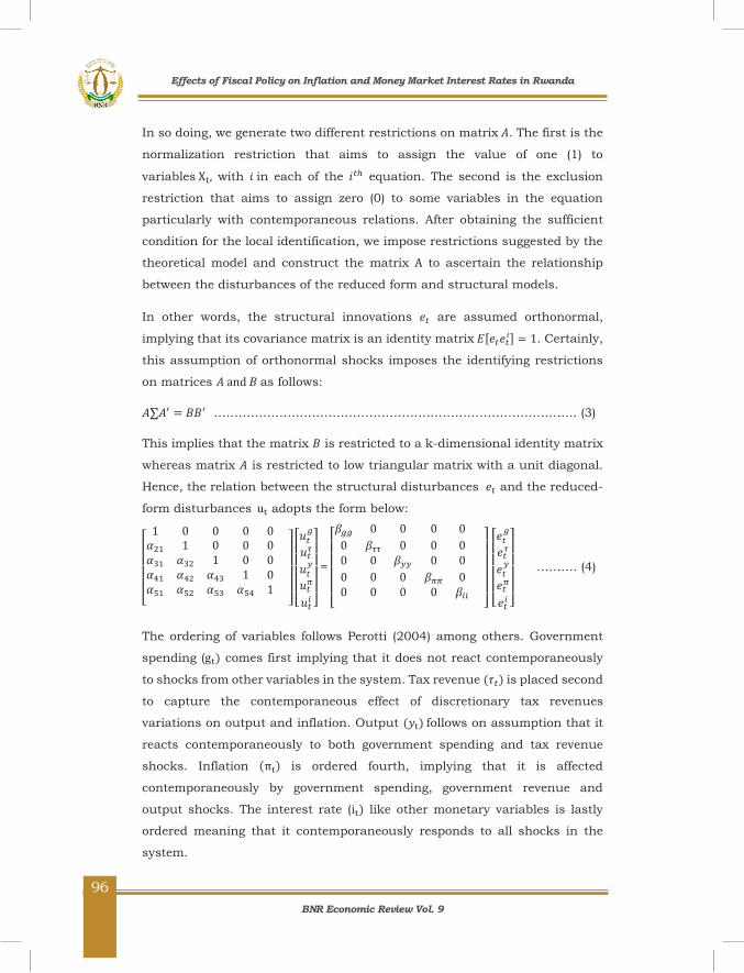
BNR Economic Review Vol. 9
96
98
In so doing, we generate two different restrictions on matrix 𝐴𝐴. The first is the
normalization restriction that aims to assign the value of one (1) to
variables Xt, with 𝑖𝑖 in each of the 𝑖𝑖𝑡𝑡ℎ equation. The second is the exclusion
restriction that aims to assign zero (0) to some variables in the equation
particularly with contemporaneous relations. After obtaining the sufficient
condition for the local identification, we impose restrictions suggested by the
theoretical model and construct the matrix A to ascertain the relationship
between the disturbances of the reduced form and structural models.
In other words, the structural innovations 𝑒𝑒𝑡𝑡 are assumed orthonormal,
implying that its covariance matrix is an identity matrix 𝐸𝐸[𝑒𝑒𝑡𝑡𝑒𝑒𝑡𝑡′] = 1. Certainly,
this assumption of orthonormal shocks imposes the identifying restrictions
on matrices 𝐴𝐴 and 𝐵𝐵 as follows:
𝐴𝐴∑𝐴𝐴′ = 𝐵𝐵𝐵𝐵′ …………………………………………………………………………….. (3)
This implies that the matrix 𝐵𝐵 is restricted to a k-dimensional identity matrix
whereas matrix 𝐴𝐴 is restricted to low triangular matrix with a unit diagonal.
Hence, the relation between the structural disturbances 𝑒𝑒𝑡𝑡 and the reduced-
form disturbances ut adopts the form below:
[ 1 0 0 0 0 𝛼𝛼21 1 0 0 0 𝛼𝛼31 𝛼𝛼32 1 0 0 𝛼𝛼41 𝛼𝛼42 𝛼𝛼43 1 0 𝛼𝛼51 𝛼𝛼52 𝛼𝛼53 𝛼𝛼54 1 ]
[
𝑢𝑢𝑡𝑡
𝑔𝑔
𝑢𝑢𝑡𝑡𝜏𝜏
𝑢𝑢𝑡𝑡𝑦𝑦
𝑢𝑢𝑡𝑡𝜋𝜋
𝑢𝑢𝑡𝑡𝑖𝑖 ]
=
[ 𝛽𝛽𝑔𝑔𝑔𝑔 0 0 0 0
0 𝛽𝛽𝜏𝜏𝜏𝜏 0 0 0 0 0 𝛽𝛽𝑦𝑦𝑦𝑦 0 0 0 0 0 𝛽𝛽𝜋𝜋𝜋𝜋 0 0 0 0 0 𝛽𝛽𝑖𝑖𝑖𝑖 ]
[
𝑒𝑒𝑡𝑡
𝑔𝑔
𝑒𝑒𝑡𝑡𝜏𝜏
𝑒𝑒𝑡𝑡𝑦𝑦
𝑒𝑒𝑡𝑡𝜋𝜋
𝑒𝑒𝑡𝑡𝑖𝑖 ]
………. (4)
The ordering of variables follows Perotti (2004) among others. Government
spending (gt) comes first implying that it does not react contemporaneously
to shocks from other variables in the system. Tax revenue (𝜏𝜏𝑡𝑡) is placed second
to capture the contemporaneous effect of discretionary tax revenues
variations on output and inflation. Output (𝑦𝑦t) follows on assumption that it
reacts contemporaneously to both government spending and tax revenue
shocks. Inflation (πt) is ordered fourth, implying that it is affected
contemporaneously by government spending, government revenue and
output shocks. The interest rate (it) like other monetary variables is lastly
ordered meaning that it contemporaneously responds to all shocks in the
system.
Effects of Fiscal Policy on Inflation and Money Market Interest Rates in Rwanda

BNR Economic Review Vol. 9
97
99
The ordering of interest rate is justified by two reasons. First, the interest rate
is a function of the output gap and inflation; and second it is non-sensitive to
the government spending and revenues.
IV.2 Data This study uses Rwandan quarterly data covering the period from 2006Q1 to
2015Q4. The data were compiled from the National Bank of Rwanda (BNR)
and from the Ministry of Finance and Economic Planning (MINECOFIN). The
key variables for the equations developed in this study include nominal GDP
(yt) and core inflation (πt) as proxies of real activities; Interbank rate (it) as
proxy of monetary variable measuring the fiscal effect on financial market
conditions; while the total government spending ( gt) and total government tax
receipts ( 𝜏𝜏t) are proxies of fiscal policy. Core inflation has been preferred for
it has more persistent behavior and less volatile and therefore serves as the
best measure that policymakers may focus on for decision making. Headline
inflation misses these properties as it includes volatile components and can
be misleading for policymakers in case of supply shock and external shock.
A part from interbank rates all variables were transformed to natural
logarithm to possess similar units.
V EMPIRICAL RESULTS V.1 Unit Root Test The study used Augmented Dickey-Fuller test to determine the order of
integration of variables. With an automatic lag length selection using Schwarz
information criterion (SIC), the results of ADF unit root test (as in table 5.1
below) show that all variables are integrated of order one ~ I(1).
Effects of Fiscal Policy on Inflation and Money Market Interest Rates in Rwanda
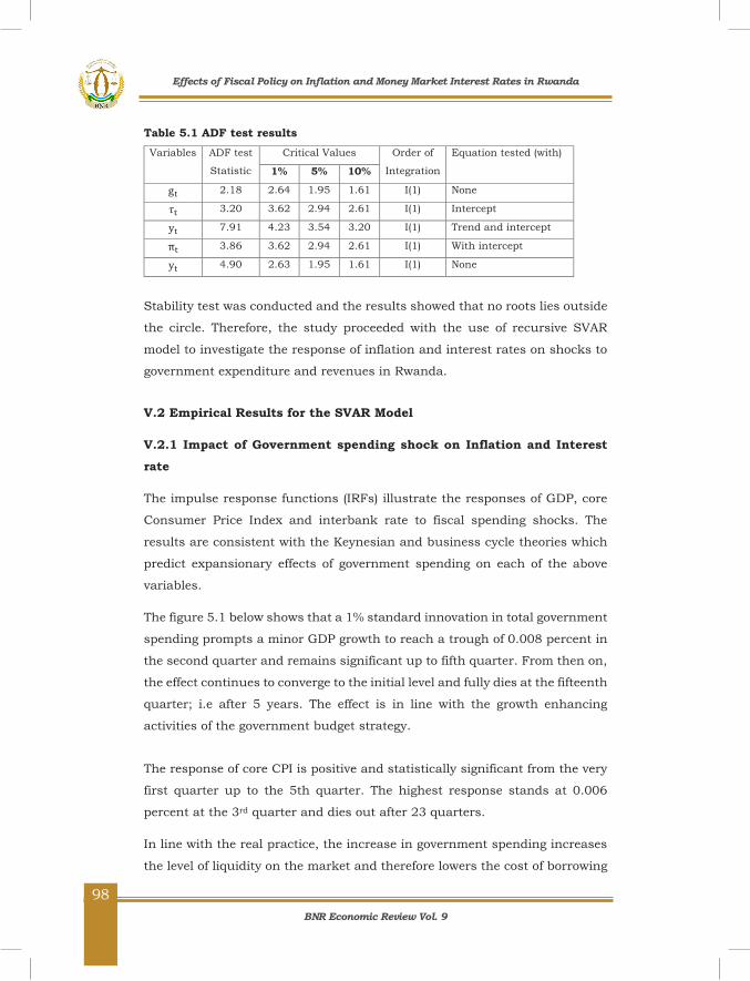
BNR Economic Review Vol. 9
98
100
Table 5.1 ADF test results Variables ADF test
Statistic Critical Values Order of
Integration
Equation tested (with)
1% 5% 10%
gt 2.18 2.64 1.95 1.61 I(1) None
𝜏𝜏t 3.20 3.62 2.94 2.61 I(1) Intercept
yt 7.91 4.23 3.54 3.20 I(1) Trend and intercept
πt 3.86 3.62 2.94 2.61 I(1) With intercept
yt 4.90 2.63 1.95 1.61 I(1) None
Stability test was conducted and the results showed that no roots lies outside
the circle. Therefore, the study proceeded with the use of recursive SVAR
model to investigate the response of inflation and interest rates on shocks to
government expenditure and revenues in Rwanda.
V.2 Empirical Results for the SVAR Model
V.2.1 Impact of Government spending shock on Inflation and Interest rate
The impulse response functions (IRFs) illustrate the responses of GDP, core
Consumer Price Index and interbank rate to fiscal spending shocks. The
results are consistent with the Keynesian and business cycle theories which
predict expansionary effects of government spending on each of the above
variables.
The figure 5.1 below shows that a 1% standard innovation in total government
spending prompts a minor GDP growth to reach a trough of 0.008 percent in
the second quarter and remains significant up to fifth quarter. From then on,
the effect continues to converge to the initial level and fully dies at the fifteenth
quarter; i.e after 5 years. The effect is in line with the growth enhancing
activities of the government budget strategy.
The response of core CPI is positive and statistically significant from the very
first quarter up to the 5th quarter. The highest response stands at 0.006
percent at the 3rd quarter and dies out after 23 quarters.
In line with the real practice, the increase in government spending increases
the level of liquidity on the market and therefore lowers the cost of borrowing
Effects of Fiscal Policy on Inflation and Money Market Interest Rates in Rwanda

BNR Economic Review Vol. 9
99
101
which translates at the end into increased households' consumption and
businesses' investment in equipment and structures pushing up prices.
Figure 5.1 Impulse Responses of GDP, Core Consumer Price Index and interbank rate
On the other side, the findings reveal that the response of interest rate to
government spending is not statistically significant. At this stage, it is worth
to conclude that GDP and inflation significantly respond to government
spending while interest rate is not responsive.
For robustness check, we also followed the ordering of variables used in
Blanchard and Perotti (2002). Tax is placed before government spending,
followed by GDP, inflation and interest rate.
5.2.2 Effect of Tax Revenue shock on Inflation and Interest rate
Impulse responses to a shock of government tax revenue show that
government spending, GDP and core inflation react positively while interbank
rate is not responsive.
The IRFs show an immediate short lived and significant effect of tax revenue
shock on government spending. The effect on GDP is significant in the third
-.020
-.015
-.010
-.005
.000
.005
.010
.015
.020
2 4 6 8 10 12 14 16 18 20 22 24 26 28 30
Response of GDP to total spending shock
-.002
.000
.002
.004
.006
.008
.010
2 4 6 8 10 12 14 16 18 20 22 24 26 28 30
Response of core inflation to total spending shock
-.6
-.4
-.2
.0
.2
.4
2 4 6 8 10 12 14 16 18 20 22 24 26 28 30
Response of Interbank to total spending shock
Effects of Fiscal Policy on Inflation and Money Market Interest Rates in Rwanda
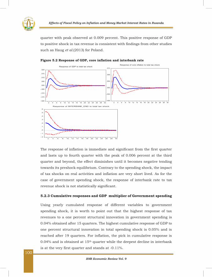
BNR Economic Review Vol. 9
100
102
quarter with peak observed at 0.009 percent. This positive response of GDP
to positive shock in tax revenue is consistent with findings from other studies
such as Haug et al.(2013) for Poland.
Figure 5.2 Response of GDP, core inflation and interbank rate
The response of inflation is immediate and significant from the first quarter
and lasts up to fourth quarter with the peak of 0.006 percent at the third
quarter and beyond, the effect diminishes until it becomes negative tending
towards its preshock equilibrium. Contrary to the spending shock, the impact
of tax shocks on real activities and inflation are very short lived. As for the
case of government spending shock, the response of interbank rate to tax
revenue shock is not statistically significant.
5.2.3 Cumulative responses and GDP multiplier of Government spending
Using yearly cumulated response of different variables to government
spending shock, it is worth to point out that the highest response of tax
revenues to a one percent structural innovation in government spending is
0.04% obtained after 15 quarters. The highest cumulative response of GDP to
one percent structural innovation in total spending shock is 0.05% and is
reached after 19 quarters. For inflation, the pick in cumulative response is
0.04% and is obtained at 15th quarter while the deepest decline in interbank
is at the very first quarter and stands at -0.11%.
-.020
-.015
-.010
-.005
.000
.005
.010
.015
.020
2 4 6 8 10 12 14 16 18 20 22 24 26 28 30
Response of GDP to total tax shock
-.008
-.004
.000
.004
.008
.012
2 4 6 8 10 12 14 16 18 20 22 24 26 28 30
Response of core inflation to total tax shock
-.2
-.1
.0
.1
.2
.3
.4
.5
.6
2 4 6 8 10 12 14 16 18 20 22 24 26 28 30
Response of INTERBANK_END to total tax shock
Effects of Fiscal Policy on Inflation and Money Market Interest Rates in Rwanda
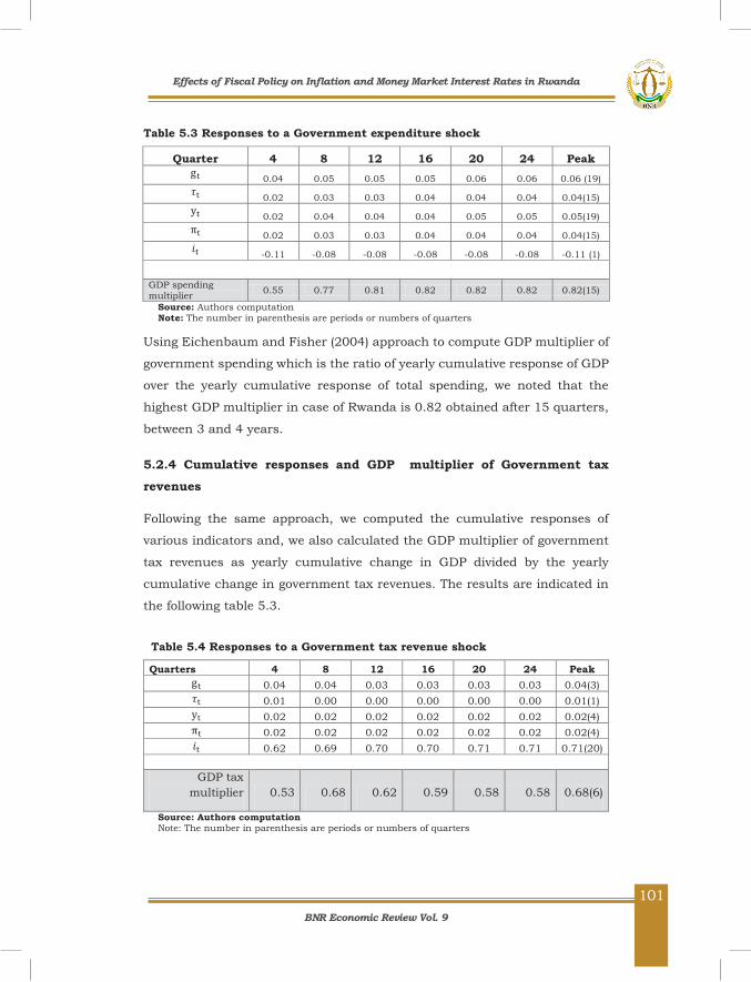
BNR Economic Review Vol. 9
101
103
Table 5.3 Responses to a Government expenditure shock
Quarter 4 8 12 16 20 24 Peak gt 0.04 0.05 0.05 0.05 0.06 0.06 0.06 (19) 𝜏𝜏t 0.02 0.03 0.03 0.04 0.04 0.04 0.04(15) yt 0.02 0.04 0.04 0.04 0.05 0.05 0.05(19) πt 0.02 0.03 0.03 0.04 0.04 0.04 0.04(15) 𝑖𝑖t -0.11 -0.08 -0.08 -0.08 -0.08 -0.08 -0.11 (1)
GDP spending multiplier 0.55 0.77 0.81 0.82 0.82 0.82 0.82(15)
Source: Authors computation Note: The number in parenthesis are periods or numbers of quarters
Using Eichenbaum and Fisher (2004) approach to compute GDP multiplier of
government spending which is the ratio of yearly cumulative response of GDP
over the yearly cumulative response of total spending, we noted that the
highest GDP multiplier in case of Rwanda is 0.82 obtained after 15 quarters,
between 3 and 4 years.
5.2.4 Cumulative responses and GDP multiplier of Government tax revenues
Following the same approach, we computed the cumulative responses of
various indicators and, we also calculated the GDP multiplier of government
tax revenues as yearly cumulative change in GDP divided by the yearly
cumulative change in government tax revenues. The results are indicated in
the following table 5.3.
Table 5.4 Responses to a Government tax revenue shock
Quarters 4 8 12 16 20 24 Peak gt 0.04 0.04 0.03 0.03 0.03 0.03 0.04(3) 𝜏𝜏t 0.01 0.00 0.00 0.00 0.00 0.00 0.01(1) yt 0.02 0.02 0.02 0.02 0.02 0.02 0.02(4) πt 0.02 0.02 0.02 0.02 0.02 0.02 0.02(4) 𝑖𝑖t 0.62 0.69 0.70 0.70 0.71 0.71 0.71(20)
GDP tax
multiplier 0.53 0.68 0.62 0.59 0.58 0.58 0.68(6)
Source: Authors computation Note: The number in parenthesis are periods or numbers of quarters
Effects of Fiscal Policy on Inflation and Money Market Interest Rates in Rwanda
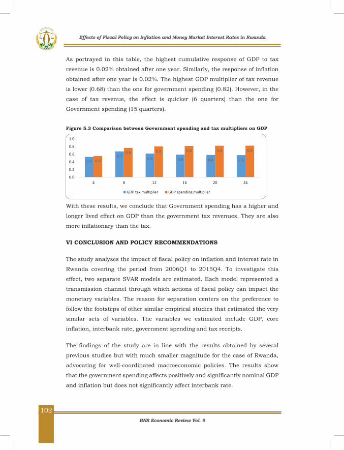
BNR Economic Review Vol. 9
102
104
As portrayed in this table, the highest cumulative response of GDP to tax
revenue is 0.02% obtained after one year. Similarly, the response of inflation
obtained after one year is 0.02%. The highest GDP multiplier of tax revenue
is lower (0.68) than the one for government spending (0.82). However, in the
case of tax revenue, the effect is quicker (6 quarters) than the one for
Government spending (15 quarters).
Figure 5.3 Comparison between Government spending and tax multipliers on GDP
With these results, we conclude that Government spending has a higher and
longer lived effect on GDP than the government tax revenues. They are also
more inflationary than the tax.
VI CONCLUSION AND POLICY RECOMMENDATIONS
The study analyses the impact of fiscal policy on inflation and interest rate in
Rwanda covering the period from 2006Q1 to 2015Q4. To investigate this
effect, two separate SVAR models are estimated. Each model represented a
transmission channel through which actions of fiscal policy can impact the
monetary variables. The reason for separation centers on the preference to
follow the footsteps of other similar empirical studies that estimated the very
similar sets of variables. The variables we estimated include GDP, core
inflation, interbank rate, government spending and tax receipts.
The findings of the study are in line with the results obtained by several
previous studies but with much smaller magnitude for the case of Rwanda,
advocating for well-coordinated macroeconomic policies. The results show
that the government spending affects positively and significantly nominal GDP
and inflation but does not significantly affect interbank rate.
0.50.7 0.6 0.6 0.6 0.60.6
0.8 0.8 0.8 0.8 0.8
0.0
0.2
0.4
0.6
0.8
1.0
4 8 12 16 20 24
GDP tax multiplier GDP spending multiplier
Effects of Fiscal Policy on Inflation and Money Market Interest Rates in Rwanda
BNR Economic Review Vol. 9
103
105
Government spending has a higher and longer-lived effect on GDP and is more
inflationary. In both cases, the effect on interbank rate is not significant, due
to shallow financial markets which could be impeding the transmission of
monetary policy signals.
Based on the above findings, there is a need for monetary authorities to
enhance the developments of the financial markets to respond to changes in
macroeconomic fundamentals for efficient monetary policy transmission
channel.
Effects of Fiscal Policy on Inflation and Money Market Interest Rates in Rwanda

BNR Economic Review Vol. 9
104
106
REFERENCES
Agha, Asif Idrees and Muhammad Saleem Khan, (2006), An Empirical Analysis of Fiscal Imbalances and Inflation in Pakistan, SBP Research Bulletin, 2(2).
Anyanwu, J. C. (1993), Monetary Economics: Theory, Policy and Institutions, Onitsha Hybrid publishers.
Arby, F. and Muhammad, N. H. (2010), Monetary and Fiscal Policy Coordination: Pakistan’s Experience, SBP Research Bulletin, Vol. 6.
Baldini, A. and Ribeiro M. P. (2008), Fiscal and Monetary Anchors for Price Stability: Evidence from Sub-Saharan Africa, IMF Working Paper.
Ben Slimane, S. and Ben Tahar, M. (2013), Is Discretionary Fiscal Policy Effective? Evidences for Tunisia and Egypt, Review of Economics & Finance, 3 (2).
Blanchard, O. and R. Perotti. (1999), An Empirical Characterization of the Dynamics Effects of Changes in Government Spending and Taxes on Output, National Bureau of Economic Research (NBER) Working Paper No. 7269.
Blinder, A. (1982), Issues in the Coordination of Monetary and Fiscal Policy, NBER Working Paper No. 982.
Caldara, D. and Kamps C. (2008), What Are the Effects of Fiscal Shocks? A VAR-based Comparative Analysis, Working Paper Series 877, European Central Bank.
Calvo, G.A and Vegh C.A., (1995), Fighting Inflation with High Interest Rates, the Small-open Economy Case Under Flexible Prices, Journal of Money, Credit and Banking, 27.
Caramazza, F. (1993), French-German Interest Rate Differentials and Time-varying Realignment Risk, IMF Staff Papers, International Monetary Fund.
Eichenbaum, M., and J.D.M. Fisher (2004), Fiscal Policy in the Aftermath of 9/11, National Bureau of Economic Research: NBER Working Paper Series n. 10430
Fatás, A. and Mihov, I. (2003). The Case for Restricting Fiscal Policy Discretion, The Quarterly Journal of Economics, 118 (4).
Feldstein, M. S. (1986), The Budget Deficit and the Dollar, in S Fischer (ed) NBER Macroeconomics 1986, Cambridge, Massachusetts: National Bureau of Economic Research.
Ferrucci, G. (2003), Empirical Determinants of Emerging Market Economies’ Sovereign Bond Spreads. Bank of England working paper no. 205
Franta, M. (2012), Macroeconomic Effects of Fiscal Policy in the Czech Republic: Evidence Based on Various Identification Approaches in A VAR Framework, Working Paper Series No. 13, the Czech National Bank.
Giordano, R., Momigliano, S., Neri, S., Perotti, R., (2007), The Effects of Fiscal Policy in Italy: Evidence from A VAR Model, European Journal of Political Economy, 23,
Effects of Fiscal Policy on Inflation and Money Market Interest Rates in Rwanda

BNR Economic Review Vol. 9
105
107
Hakkio, Craig S., (1996), The Effects of Budget Deficit Reduction on the Exchange Rate, Economic Review, Federal Reserve Bank of Kansas City 81(3).
Hamilton, J.D., (1994), Time Series Analysis, Princeton University Press.
Haug, A. A., and Smith C., (2012), Local Linear Impulse Responses for a Small Open Economy, Oxford Bulletin of Economics and Statistics 74.
Hilbers, P. (2004), Interaction of Monetary and Fiscal Policies: Why Central Banks Worry About Government Budgets? IMF European Department. Retrieved from https://www.imf.org/external/np/leg/sem/2004/cdmfl/eng/hilber.pdf
Höppner, F. (2001), A VAR Analysis of the Effects of Fiscal Policy in Germany, Institute for International Economics, University of Bonn,
International Monetary Fund (2014), Rwanda PSI Assessment, IMF Country Report No. 14/185
Koray, F. and Chan, P. (1991), Government Spending and the Exchange rate, Applied Economics
Koray, F., and Chan, P., (1991), Government Spending and the Exchange Rate, Applied Economics, 23.
Leeper, Eric (1989), Policy Rules, Information, and Fiscal Effects in a `Ricardian'
Model, Board of Governors of the Federal Reserve System, International Finance Discussion Paper No 360.
Lozano, I. and Rodríguez, K. (2011), Assessing the Macroeconomic Effects of Fiscal Policy in Colombia, Journal of Financial Economic Policy, 3 (3).
Lozano, I. and Rodriquez, K., (2008), Assessing the Macroeconomic Effects of Fiscal Policy in Colombia, Banco de la Republica, Borradores de Economia Working Paper, No. 552.
Ministry of Finance and Economic Planning (2007), Economic Development & Poverty Reduction Strategy 2008-2012, Kigali
Ministry of Finance and Economic Planning, Republic of Rwanda, available at http://www.minecofin.gov.rw/index.php?id=173 (September 08th, 2015)
Mishkin, F. S., (2006), The Next Great Globalization: How Disadvantaged Nations Can Harness Their Financial Systems to Get Rich, Princeton, N.J. Princeton University Press.
Mohanty, M. S. and Scatigna, M. (2003), Countercyclical fiscal policy and central banks. BIS Papers chapters, in: Bank for International Settlements (ed.), Fiscal issues and central banking in emerging economies, volume 20,
National Bank of Rwanda, Republic of Rwanda, available at http://www.bnr.rw/index.php?id=310 (September 15th, 2015)
National Institute of Rwanda, Republic of Rwanda, available at http://statistics.gov.rw/publications (August 28th, 2015)
Effects of Fiscal Policy on Inflation and Money Market Interest Rates in Rwanda
BNR Economic Review Vol. 9
106
108
Nordhaus, W. D. (1994), Policy games: Coordination and Independence in Monetary and Fiscal Policies, Brookings Papers on Economic Activity, Issue 2.
Perotti, R. (2004), Estimating the Effects of Fiscal Policy in OECD Countries, Centre for Economic Policy Research, Discussion Paper 168.
Ramey, V. A. and Shapiro, M. D. (1998), Costly Capital Reallocation and the Effects of Government Spending, Carnegie-Rochester Conference Series on Public Policy, 48.
Ravnik, R. and Žilić (2011), The Use of SVAR Analysis in Determining the Effects of Fiscal Shocks in Croatia, Financial Theory and Practice, 35.
Sargent, T.J. and Wallace, N. (1981), Some Unpleasant Monetarist Arithmetic, Federal Reserve Bank of Minneapolis, Quarterly Review.
Sheffrin, S. M. (2003), Economic: Principles in Action, Upper Saddle River, New Jersey 07456, Pearson Prince Hall.
Sims, C. A. (1980), Macroeconomic and Reality, Econometrica, 48 (10).
Woodford, M. (2001), Fiscal Requirements for Price Stability, National Bureau of Economic Research (NBER) Working Paper No. 8072.
Uhlig, H. (2005), What are the Effects of Monetary Policy? Results from an Agnostic Identification Procedure, Journal of Monetary Economics, 52 (2).
Effects of Fiscal Policy on Inflation and Money Market Interest Rates in Rwanda
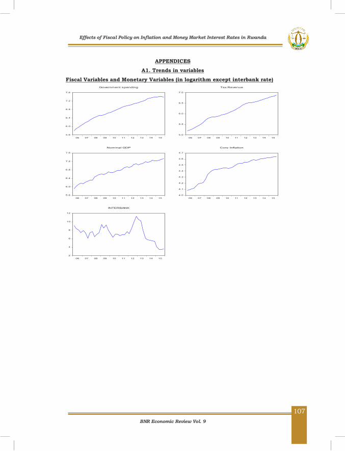
BNR Economic Review Vol. 9
107
109
APPENDICES A1. Trends in variables
Fiscal Variables and Monetary Variables (in logarithm except interbank rate)
5.6
6.0
6.4
6.8
7.2
7.6
06 07 08 09 10 11 12 13 14 15
Government spending
5.0
5.5
6.0
6.5
7.0
06 07 08 09 10 11 12 13 14 15
Tax Revenue
5.6
6.0
6.4
6.8
7.2
7.6
06 07 08 09 10 11 12 13 14 15
Nominal GDP
4.0
4.1
4.2
4.3
4.4
4.5
4.6
4.7
06 07 08 09 10 11 12 13 14 15
Core Inflation
2
4
6
8
10
12
06 07 08 09 10 11 12 13 14 15
INTERBANK
Effects of Fiscal Policy on Inflation and Money Market Interest Rates in Rwanda
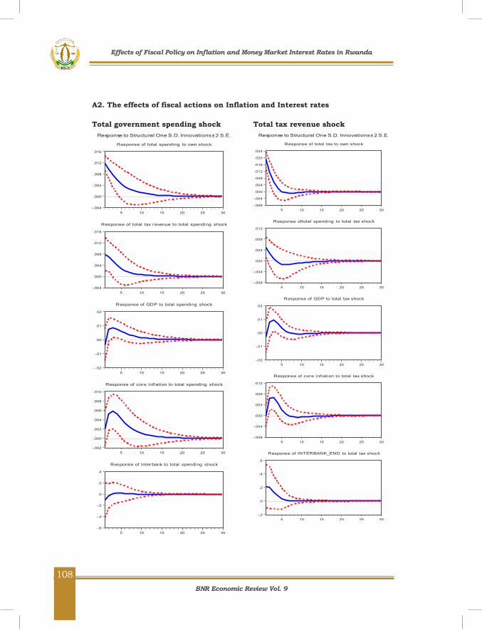
BNR Economic Review Vol. 9
108
110
A2. The effects of fiscal actions on Inflation and Interest rates
Total government spending shock
Total tax revenue shock
-.004
.000
.004
.008
.012
.016
5 10 15 20 25 30
Response of total spending to own shock
-.004
.000
.004
.008
.012
.016
5 10 15 20 25 30
Response of total tax revenue to total spending shock
-.02
-.01
.00
.01
.02
5 10 15 20 25 30
Response of GDP to total spending shock
-.002
.000
.002
.004
.006
.008
.010
5 10 15 20 25 30
Response of core inflation to total spending shock
-.6
-.4
-.2
.0
.2
.4
5 10 15 20 25 30
Response of Interbank to total spending shock
Response to Structural One S.D. Innovations ± 2 S.E.
-.008
-.004
.000
.004
.008
.012
.016
.020
.024
5 10 15 20 25 30
Response of total tax to own shock
-.008
-.004
.000
.004
.008
.012
5 10 15 20 25 30
Response oftotal spending to total tax shock
-.02
-.01
.00
.01
.02
5 10 15 20 25 30
Response of GDP to total tax shock
-.008
-.004
.000
.004
.008
.012
5 10 15 20 25 30
Response of core inflation to total tax shock
-.2
.0
.2
.4
.6
5 10 15 20 25 30
Response of INTERBANK_END to total tax shock
Response to Structural One S.D. Innovations ± 2 S.E.
Effects of Fiscal Policy on Inflation and Money Market Interest Rates in Rwanda

BNR Economic Review Vol. 9
109
111
Determinants of Aggregate Demand in the Rwandan Economy: A Macroeconometric Approach
Karangwa Mathias* MWENESE BRUNO†
Key Words: Aggregate demand, Inflation, Macroeconometric-model, Rwanda
JEL Classification: E52, E58, F47, O23
* Karangwa Mathias is the Manager of the Modelling & Forecasting division at BNR † MWENESE BRUNO is a senior Economist in the modelling & forecasting division at BNR
Determinants of Aggregate Demand in the Rwandan Economy: A Macroeconometric Approach
BNR Economic Review Vol. 9
110
112
Abstract
The National Bank of Rwanda and other EAC central banks committed to move
to an interest rate based monetary policy by December 2018. The interest rate
based regime has a lot of forward looking aspects and therefore calls for more
understanding of the economy and scaling up of modeling and forecasting
capacities (Gill Hammond et al., 2012; Roger, Scott, 2010). In this view, the
FPAS macro model, the core model of inflation as well as a set of near term
forecasting and nowcasting tools were developed for the Rwandan economy.
This paper explains the current structure of the core model of inflation and
demonstrates how it is useful for forecasting and simulation analysis. Despite
being called the core model of inflation, the model can be used to derive
forecasts for aggregate demand and its components (section 4.1) and thus serve
as a useful tool to track demand side inflationary sources. Being a macro-
model, it also provides a consistent framework to analyze the impact of
exogenous shocks on the Rwandan economy and thus helps to have structured
discussions. The in-sample forecasts show that the model tracks well the path
of key demand side macroeconomic variables (components of domestic and
external demand) and thus, the in sample forecasts for real aggregate
expenditure are quite close to the actual data.
Determinants of Aggregate Demand in the Rwandan Economy: A Macroeconometric Approach
BNR Economic Review Vol. 9
111
113
I. INTRODUCTION
1.1 GENERAL BACKGROUND
After realizing the weaknesses embedded in the monetary targeting
framework, the Governors of the East African Community (EAC) central banks
agreed to implement a price based monetary policy framework, using the
interest rate as the operating target by 2018 as stated in the report of the
Governors’ 18th ordinary meeting of the monetary affairs committee. This
decision was based on empirical evidence that the link between monetary
aggregates and the real economy (i.e. inflation and output) across the East
African economies was increasingly breaking down on the account of the
instability and unpredictability of the money multiplier, money velocity and
thus of the money demand function (Adam C., & Kessy, P., 2011; Kigabo, R.,
& Irankunda, J., 2012).
The governors of the EAC central banks also acknowledged that one of the
requirements for successful adoption of the inflation targeting framework is
to scale-up modelling and forecasting capacities to facilitate the putting in
place of both short-term and medium-term forecasting tools. In line with the
above, BNR has since 2011 put in place a suite of near term forecasting tools
such as VAR, ARMA, BVAR, and state space models. These models have been
quite useful in producing near-term forecasts but are less reliable in terms of
producing medium-term forecasts that can guide monetary policy decisions
over a relatively longer time horizon.
Thus, BNR found it necessary to embark on two projects aimed at producing
medium-term forecasting models. The first project involved cooperation
between BNR and IMF to build the “Forecasting and Policy Analysis Systems
(FPAS)” for Rwanda. This project resulted into a small Keynesian type macro-
economic model with four core equations: Aggregate demand (IS) equation,
Aggregate Supply (Phillips curve) equation, the uncovered interest rate parity
equation and the monetary policy rule (Karangwa et. al., 2015).
The second project aimed at building the core model of inflation for the
Rwandan economy. Despite being called “the core model of inflation”, the
model is generally used forecast aggregate demand and its components and
thus help to track demand-side sources of inflation.
Determinants of Aggregate Demand in the Rwandan Economy: A Macroeconometric Approach

BNR Economic Review Vol. 9
112
114
The core model of inflation was built with the help of MEFMI and the South
African Reserve Bank (SARB). The core model of inflation for Rwanda is
adapted from the one used at the SARB but tailored to the specific realities of
the Rwandan economy. Much effort has been devoted to make sure that the
set of equations describing the demand-side part of the Rwandan economy
can enable the preparation of internally consistent forecasts (i.e. the
structural interdependencies) and of externally consistent forecasts (i.e.
reflecting the actual course of the macro processes in the Rwandan economy).
In addition, the model’s structure should allow information from outside the
model (i.e. expert judgment) to be incorporated and to help in both near-term
and medium-term forecasting.
The core model of inflation is relatively big (it includes variables on
employment, balance of payments, terms of trade and price deflators) and can
therefore be more insightful in terms of understanding various inter-sectoral
linkages. This paper aims at explaining in detail the structure of the core
model of inflation for Rwanda, and demonstrating its applicability and
relevance to the Rwandan economy. However, the size of the core model of
inflation is kept at medium scale since experience shows that several
countries prefer to use both small and medium size macroeconometric models
following the fact that large ones are often too complex and not necessarily
useful (Muhammad et. al., 2011).
The rest of the paper is organized as follows: section one gives the introduction
with particular emphasis on the background, objective and theoretical basis
for the core model of inflation; section two explains the structure of the model
while section three briefly explains the estimation method used; section four
compares baseline forecasts for aggregate demand and its components with
actual and then presents the impact of selected shocks; section five covers
the conclusion.
1.2 OBJECTIVES OF THE STUDY
The main objective of this paper is to develop and explain a demand-side
macroeconometric model of inflation forecasting for the Rwandan economy,
capable of explaining the various demand-side inflationary factors.
Determinants of Aggregate Demand in the Rwandan Economy: A Macroeconometric Approach
BNR Economic Review Vol. 9
113
115
Specifically, the study aims at estimating various demand-side equations of
the economy and fit them together into a macroeconometric model.
Thereafter, the study uses the constructed macroeconometric model to derive
forecasts of key demand-side macroeconomic variables for the remaining
three quarters of 2016 and to conduct relevant simulations to analyze the
response of core inflation to some selected shocks and to approximate the
reaction of monetary policy to a supply shock (i.e. a shock to headline
inflation).
1.3 THEORETICAL FOUNDATIONS OF THE MODEL
The structure of the core model incorporates both a long-run equilibrium
based on economic theory and historical relationships, and short-run
dynamics that allow the economy to gravitate towards its long-run
equilibrium. The core model thus falls in the category described by Pagan
(2003) as a medium-sized Type II hybrid model, i.e. where the long-run
equilibrium component is explicitly modelled. In line with the expenditure
account, both domestic and external demand determine the economic growth
path. Domestic demand consists of total final consumption and gross capital
formation while external demand is simply the difference between exports and
imports.
In the long run, supply-side factors determine the economic growth rate.
Usually, the long-run economic growth is modelled by use of either a
production function or by use of a simple statistical filter. In this paper, we
use the HP filter to derive potential GDP and M3 due to data limitations.
Theoretically, the model replicates the famous “circular flow of income” that
is common in several macroeconomics textbooks (Greg Mankiw, 1997).
Households participate in the economic process by selling their labor and
receiving income in the form of remuneration as well as interest and dividend
payments and transfers from government. They pay taxes on their income
received and use their disposable income to buy goods and services and to
accumulate wealth. Business enterprises produce goods and services, which
they sell in the domestic and global market. They use production factors, i.e.
capital and labor, in the production process. They also pay taxes and make
investment decisions. Government spends revenue on consumer goods and
Determinants of Aggregate Demand in the Rwandan Economy: A Macroeconometric Approach

BNR Economic Review Vol. 9
114
116
services, and also undertakes investment. It receives taxes and makes
transfer payments.
In practice, government income and expenditure, published in the annual
Budget and Medium Term Budget Policy Statement are taken as given. The
central bank controls the level of the official nominal short-term interest rate
in order to meet the inflation target. Financial intermediaries constitute an
element of the transmission channel of monetary policy through their interest
rates on loans and deposits. The external sector contributes to the
transmission mechanism through countries that provide goods and services
to Rwanda and are, in turn, buyers of manufactured goods, commodities and
services produced domestically.
Figure 1: A simplified diagram of interdependencies between variables
Source: South African Reserve Bank (Working Paper WP/07/02, June 2007)
2. THE STRUCTURE OF THE MODEL
The core model of inflation is a demand-side representation of the Rwandan
economy. The model comprises of 17 stochastic equations (see appendix) and
a number of identities and other auxiliary equations. The model is designed
to capture developments from several economic blocks: expenditure side GDP,
exchange rates and price deflators, terms of trade, inflation, money & credit,
BOP accounts and interest rates.
Determinants of Aggregate Demand in the Rwandan Economy: A Macroeconometric Approach
BNR Economic Review Vol. 9
115
117
The expenditure side GDP is represented as:
( )................................................................................................................(1)t t t t t tY C I G X M
Where Y is expenditure-side real GDP; C is private consumption expenditure;
I is investment expenditure; G is government expenditure; X refers to
exports and M stands for imports. Measured in real terms and in line with
equation 3, the sum of private consumption expenditure ( 6tconshh ), total
investment expenditure ( 6tcap ) and government consumption ( 6tconsgg ) yields
total domestic demand ( 6tdodem ). External demand is computed as the
difference between real exports ( 6texpt ) and real imports ( 6timpt ). In turn, the
sum of external demand and domestic demand must equal to GDP as shown
in equation 2.
6 6 6 6 .....................................................................................................(2)t t t tgdp dodem expt impt
6 6 6 6 ............................................................................................(3)t t t tdodem conshh cap consgg
With the exception of government expenditure & government investment, all
domestic variables are modelled as endogenous. We also include international
commodity prices, particularly for oil and the weighted index for Rwanda’s
key exports (tea, coffee and tin). The computation of the weights for each of
these exports takes into account their respective shares in total exports. These
external variables are assumed to be exogenous, just like in many other
macroeconomic models.
2.1 BEHAVIORAL EQUATIONS
In line with equation 1, we estimate behavioral equations for private
consumption, private investment, exports and imports (from national
accounts), average salaries, private sector employment, core inflation,
bilateral exchange rate, M3, the lending rate, the interbank rate, imports and
exports (from BOP) and the key repo rate. From the national accounts, we
bifurcate GDP, exports and imports into nominal and real variables. Thus, we
also include equations for the deflators of GDP, imports and exports. The main
reference materials for this paper are the South African Reserve Bank (2007)
and Muhammad et. al., (2011).
Determinants of Aggregate Demand in the Rwandan Economy: A Macroeconometric Approach

BNR Economic Review Vol. 9
116
118
2.1.1 The consumption function
To estimate the consumption function, we consider a hybrid model combining
Milton Friedman’s permanent income hypothesis, Hall’s random walk model
and the Keynesian absolute income theory. We assume that real personal
disposable income ( 6tpdinc ) and real lending rate ( lrater ) are the main drivers
of real private consumption expenditure ( 6tconshh ). The stochastic error term
in the consumption function equation is represented by 6conshht and it is
assumed to be independently and identically distributed.
616 6 , , 6 , .............................................................................(4)conshh
t t t t tconshh f pdinc lrater conshh
In view of equation 4 and consistent with economic theory, current period real
consumption positively depends on current personal disposable income but
negatively depends on the current real lending rate. We also include the lag
of real consumption ( 16tconshh ) to capture the smoothing effect and the
assumption is that lagged consumption positively influences current period
consumption. Real personal disposable income is defined as nominal
disposable income ( 5tPdinc ) deflated with domestic headline CPI ( _ tcpi tot ).
Note that all variables, but the real lending rate, are measured in logs.
56 .........................................................................................................................(5)
_t
tt
pdincpdinccpig tot
The nominal personal disposable income is defined as the wedge between the
total personal salaries ( 5tsaltotn ) and direct personal taxes ( 5tdptax ), both
measured in nominal terms.
5 5 5 ...........................................................................................................(6)t t tpdinc saltotn dptax
Usually, the direct tax bill is always computed as the product of the personal
taxable income ( 5ttaxhh ) and the direct personal tax rate (dptaxr ). The personal
taxable income is simply the total salary ( tsaltotn5 ) earned by an individual
(formal sector) worker.
5 5 * ................................................................................................................(7)t tdptax taxhh dptaxr
Determinants of Aggregate Demand in the Rwandan Economy: A Macroeconometric Approach
BNR Economic Review Vol. 9
117
119
However, past data trends show that direct personal taxes ( 5dptax ) are on
average 30% of total tax revenue whereas 5saltotn is on average 22% of nominal
GDP ( 5tgdp ) in the 2006Q1-2016Q1 period. Thus, these assumptions are used
to simplify the computation of personal disposable income ( 5tpdinc ) as they
make it possible to overcome the problem of timely data availability for direct
personal taxes and salaries.
2.1.2 The investment function
The second important component of aggregate demand is real investment
given its usefulness in terms of fueling capital accumulation and sustained
economic growth as documented in various growth models. We model real
investment ( 6tcap ) as a function of real economic activity ( 6tgdp ), the interbank
rate ( int_ int tbank ) and the lag of real private investment ( 16tcap ). Investment is
assumed to be positively related to real GDP but inversely related to the real
interbank rate and real company taxes. The stochastic error term in the
investment function equation is represented by 6invprivt and it is assumed to be
independently and identically distributed. While gross operating surpluses
(i.e. company profits) are always important, we assume that their effect is
roughly captured by the previous level of investment ( 16tcap ). All variables,
except the interbank rate, are measured in logs.
616 6 ,int_ int , 6 , ....................................................................................(8)cap
t t t t tcap f gdp bank cap
Note that, total investment ( 6tcap ) is usually derived by summing up real
government investment ( 6tcapgov ) and real private sector investment ( 6tcappriv ).
6 6 6 ............................................................................................................(9)t t tcap capgov cappriv
However, data on real government investment and private investment are not
available for Rwanda, thus we opt to model total investment as in equation 8.
2.1.3 Total real exports of goods and services
The exports of goods and services are assumed to depend on: their own lag
( 6texpt ), the real effective exchange rate ( texreald ), domestic agricultural GDP
( 6tagr ) and foreign demand, proxied by world economic activity/GDP ( twgdp ).
Determinants of Aggregate Demand in the Rwandan Economy: A Macroeconometric Approach
BNR Economic Review Vol. 9
118
120
All variables are measured in logs. World GDP, domestic agricultural GDP,
the lag of exports and real effective exchange rate depreciation are all expected
to positively affect exports. exp 6tt is the error term assumed to be
independently and identically distributed.
exp 616 6 , , , 6 , .........................................................................(10)t
t t t t t texpt f expt exreald wgdp agr
2.1.4 Total real imports of goods and services
Total imports of goods and services are assumed to be positively affected by
their own lag ( 1m 6ti pt ) and a measure of domestic demand ( 6tdodem ) but
negatively affected by real effective exchange rate depreciation ( texreald ). All
variables are measured in logs and therefore coefficients represent elasticities.
The real effective exchange rate depreciation makes imports expensive relative
to domestically produced goods and services. Domestic demand is defined in
equation 3 above.
61m 6 m 6 , 6 , , ..............................................................................(11)impt
t t t t ti pt f i pt dodem exreald
2.1.5 Private sector employment and salaries
Due to data limitations, formal private sector employment and corresponding
salaries are approximated by considering the dataset from Rwanda Social
Security Board (RSSB) which contains information on social security
contributions, number of employees and salaries for both the private and
public sectors, with the latter assumed to be exogenous. With this
information, private sector employment ( temppriv5 ), which is simply the
number of employees working in the private sector, is assumed to be affected
by its own lag ( t-1emppriv5 ), the lag of real average private sector salaries
t-1
t-1
avspriv5
_cpig tot
and the lag of real economic activity, proxied by real GDP (t-1gdp6 ).
With all variables expressed in log form, the equation is specified as:
emppriv5t-1t t-1 t-1
t-1
5emppriv5 emppriv5 , , 6 , ...................................................................(12)
_ tavsprivf gdpcpig tot
Determinants of Aggregate Demand in the Rwandan Economy: A Macroeconometric Approach
BNR Economic Review Vol. 9
119
121
Just like in other stochastic equations, the error term, emppriv5t is included in
equation 12 and is assumed to be independently and identically distributed.
The other important equation in the employment block is for the
determination of average private sector salaries ( tavspriv5 ), which are assumed
to depend on their own lag ( t-1avspriv5 ), the smoothed CPI ( tcpitdsm ), which is a
four quarter’s moving CPI average and a measure of labor productivity
t
t
gdp6
emppriv5
, all expressed in logs. The equation is specified as:
avspriv5tt t-1 t
t
6avspriv5 , 5 , , ...........................................................(13)
emppriv5 tgdpf avspriv cpitdsm
Where avspriv5t is the error term assumed to independently and identically
distributed.
Other identities include the definition of total private salaries ( tsalprivn5 ) as a
product of average private sector salaries ( tavspriv5 ) and private sector
employment ( temppriv5 ):
t t tsalprivn5 = avspriv5 * emppriv5 ............................................................................................(14)
Likewise, total public salaries ( tsalpubn5 ) is defined as a product of average
public sector salaries ( tavspub5 ) and average public sector employment
( temppub5 ):
t t tsalpubn5 = avspub5 * emppub5 ............................................................................................(15)
Then, total salaries ( tsaltotn5 ) are defined as the sum of total private sector
salaries and public sector salaries:
t t tsaltotn5 = salprivn5 + salpubn5 ...........................................................................................(16)
The formal sector total employment ( temptot5 ) is then computed as the sum of
formal private sector employment ( temppriv5 ) and public employment
( temppub5 ):
t t temptot5 = emppub5 + emppriv5 ..........................................................................................(17)
Determinants of Aggregate Demand in the Rwandan Economy: A Macroeconometric Approach
BNR Economic Review Vol. 9
120
122
While average economy-wide salary ( tavstot5 ) is computed as the ratio of total
salaries (saltotn5 ) and total employment ( temptot5 ):
t tavstot5 = saltotn5 / emptot5 ....................................................................................................(18)
2.1.6 Inflation
Rwanda’s headline CPI has three components: core CPI, fresh products CPI
and energy CPI with a weight of 74.9%, 17.4% and 7.8% respectively. Headline
CPI is computed as a weighted sum of its components:
_ (( _ * _ ) ( _ * _ ) ( _ * _ )) /100...........(19)t t t tcpig tot cpigw core cpig core cpigw en cpig en cpigw fp cpig fp
Where _ tcpig tot is headline CPI, _cpigw core , _cpigw en and _cpigw fp are
weights for core CPI, Energy CPI and fresh products CPI, respectively and
_ tcpig core , _ tcpig en , _ tcpig fp are their corresponding price indices.
We model core CPI and assume the other components to be exogenous. Core
CPI ( _ tcpig core ) is assumed to be positively affected by its own lag (1_ tcpig core ),
imported inflation, proxied by the imports deflator ( timptd ), unit labor costs
( tulcstd ), the output gap ( ygap ) and M3 gap ( 3m gap ), all measured in logs. The
error term ( _cpig coret ) is assumed to independently and identically distributed.
_1_ _ , , , , 3 , .........................................(20)cpig core
t t t t t t tcpig core f cpig core imptd ulcstd ygap m gap
Potential Real GDP and M3 are computed using the Hodrick-Prescott (HP)
filter. Real GDP gap ( tgdpgapr ) is computed as the difference between the log of
actual non-agricultural GDP, i.e. tlog(gdpex6 ) and the log of potential non-
agricultural GDP, i.e. tlog(gdpot6 ) :
t t tgdpgapr = (log(gdpex6 )-log(gdpot6 ))*100..................................................................................(21)
Similarly, the M3 gap ( tm3gapr ) is computed as the difference between the log
of actual M3, i.e. tlog(m3 ) and the log of potential GDP, i.e. tlog(m3pot ) :
t t tm3gapr = (log(m3 )-log(m3pot ))*100............................................................................................(22)
Determinants of Aggregate Demand in the Rwandan Economy: A Macroeconometric Approach

BNR Economic Review Vol. 9
121
123
Unit labor cost is measured as the ratio between total salaries and non-
agricultural real GDP:
t
t
saltotn5.........................................................................................................................(23)
gdpex6tulcstd
2.1.7 Price deflators
As mentioned earlier, we split GDP, exports and imports into real and nominal
values. These real and nominal values are linked by their respective deflators*.
We then model the process for these deflators. First, the imports deflator
( m ti ptd ) is influenced by its own lag ( 1m ti ptd ), the nominal effective exchange
rate of the FRW ( texnomd ) and the index for foreign prices ( tforprd ), derived
from the PPP equation:
Imptd1m Im , , , ..................................................................................(24)t t t t ti ptd f ptd exnomd forprd
Secondly, the exports deflator is influenced by its own lag ( 1texptd ), the
bilateral exchange rate ( texdolld ), and the international commodity price index
( tcommdoll ), which is computed as a weighted average of international tea, tin
and coffee prices, with estimated respective shares in total exports used as
weights:
exptd1, , , ...................................................................................(25)t t t t texptd f exptd exdolld commdoll
Third, the GDP deflator is assumed to depend on its own lag ( 1tgdpd ) and on
headline CPI ( _ tcpig tot ):
gdpd1, _ , ..................................................................................................(26)t t t tgdpd f gdpd cpig tot
2.1.8 Exchange rates
In the exchange rates block, we define the nominal effective exchange rate
and the process for the bilateral (FRW/USD) exchange rate. The nominal
effective exchange rate is a trade weighted index, derived from the PPP as the
product of the real effective exchange rate ( texreald ) and the relative price,
* The deflator is defined as the ratio of nominal to real value
Determinants of Aggregate Demand in the Rwandan Economy: A Macroeconometric Approach
BNR Economic Review Vol. 9
122
124
computed as the ratio of domestic CPI ( _ tcpig tot ) to trade weighted foreign CPI
( tforprd ):
_* ....................................................................................................(27)t
t tt
cpig totexnomd exrealdforprd
Developments in the bilateral (FRW/USD) exchange rate are determined by
its own lag and by the nominal effective exchange rate:
exdolld1, , .........................................................................................(28)t t t texdolld exdolld exnomd
2.1.9 Money Supply and interest
Money demand is hypothesized to be positively linked with its lag ( 13tm ) and
nominal GDP ( 5tgdp ) but inversely related with the interbank rate ( int_ int tbank ).
The error term, has the same assumption as in the other stochastic equations.
m313 3 , 5 ,int_ int , ....................................................................................(29)t t t t tm f m gdp bank
Note that the real lending rate enters into the equation for real private
consumption while the interbank rate enters into the equations for core
inflation and M3, thus we need some kind of processes for them if not
assumed exogenous. The interbank rate ( tint_ intbank ) is assumed to positively
depend on its lag ( t-1int_ intbank ) and on the policy rate ( tint_ krepo ). Similarly,
the lending rate ( tint_ lend ) is assumed to be positively affected by its lag
( t-1int_ lend ) and the policy rate. With int_lendt and int_intbank
t defined as the
respective error terms, the interbank rate and lending rate equations are
specified as:
int_t t-1 t tint_ =f int_ ,int_krepo , ...............................................................................(30)lendlend lend
int_ intt t-1 t tint_ int =f int_ int ,int_krepo , ......................................................................(31)bankbank bank
We also specify the equation for the policy rate (Taylor rule), so as to ensure
complete definition of the interest channel of monetary policy transmission
but also to ensure the model has a closure rule that ensures the smoothing
out of short-run business cycles. A simple Taylor-type rule assumes that the
central bank sets the policy rate (KRR) in view of two main objectives: ensuring
Determinants of Aggregate Demand in the Rwandan Economy: A Macroeconometric Approach

BNR Economic Review Vol. 9
123
125
that inflation does not deviate much from the target (undershooting or
overshooting) and supporting growth such that real GDP is close enough to
its potential (i.e. a zero output gap).
Thus, we assume here that the KRR is positively affected by its lag, the output
gap and the deviation of inflation from target. The latter is set at 5% in line
with the EAC countries’ inflation objective.
int_1int_ int_ , ,inf_ , ........................................................................(32)krepo
t t t tkrepo krepo ygap dev
2.1.10 Balance of payments
In the current account of the balance of payments (BOP), we define processes
for both imports and exports. Exports ( exp torts ) are assumed to depend on
their lag ( 1exp torts ) and on the four quarters moving average of exports (
@ (exp 5 ,4)tmovav t ) from the national accounts. By analogy, imports ( timports ) in
the BOP are assumed to depend on their lag ( 1timports ) as well as on the four
quarters moving average of imports (@ ( 5 ,4)tmovav impt ) from the national
accounts. All variables are measured in log form.
exp1exp exp ,@ (exp 5 ,4), .....................................................................(33)orts
t t t torts f orts movav t
1,@ ( 5 ,4), ......................................................................(34)importst t t timports f imports movav impt
3.0 ESTIMATION METHOD
The behavioral equations of the model are estimated using the single-step
Engle Granger cointegration method, supplemented where necessary by
expert judgments/calibrations. The estimation sample is set at 2006Q1 to
2016Q1. The estimated equations are then used to form the model objects
which can be solved and used for forecasting and for conducting simulations.
As an example of the single-step Engle Granger cointegration technique,
consider the equation for real private consumption (other estimated stochastic
equations are given in the appendix). The most parsimonious (calibrated)
model is stated as:
t t t-1 t
conshh6
t t-3
dlog(conshh6 ) = - 0.69 * (log(conshh6 ) - 0.49 * log(pdinc5 / cpig_tot + .01 * (int_lend))
+ 4.4 + 0.44 * log(pdinc6 ) - 0.008 * d(int_lend + ............................t .................................(35)
Determinants of Aggregate Demand in the Rwandan Economy: A Macroeconometric Approach

BNR Economic Review Vol. 9
124
126
4.0 USING THE MODEL FOR FORECASTING AND SIMULATION ANALYSIS
The forecasting exercise helps to compare the in-sample forecasts to actual
data whereas the simulation exercise enables the assessment of how well
some key monetary policy transmission channels are functioning. We assess
the reaction of core inflation to a shock on the output gap and M3 gap,
respectively. We also assess how monetary policy reacts (i.e. the key repo rate)
to an inflation shock.
4.1 Model performance: Forecasts versus actual data
As a first step to ensure the robust performance of the model and in line with
equation 1, we compare the in sample forecasts to actual data for each
component of aggregate demand. We then compare the baseline forecast for
real GDP, which is equal to the sum of the individual components, with the
actual data. Results show that the model tracks well the historical path of real
GDP and its components.
Determinants of Aggregate Demand in the Rwandan Economy: A Macroeconometric Approach
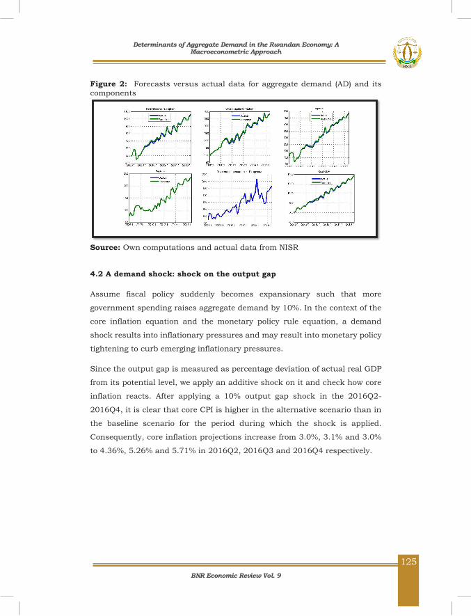
BNR Economic Review Vol. 9
125
127
Figure 2: Forecasts versus actual data for aggregate demand (AD) and its components
Source: Own computations and actual data from NISR
4.2 A demand shock: shock on the output gap
Assume fiscal policy suddenly becomes expansionary such that more
government spending raises aggregate demand by 10%. In the context of the
core inflation equation and the monetary policy rule equation, a demand
shock results into inflationary pressures and may result into monetary policy
tightening to curb emerging inflationary pressures.
Since the output gap is measured as percentage deviation of actual real GDP
from its potential level, we apply an additive shock on it and check how core
inflation reacts. After applying a 10% output gap shock in the 2016Q2-
2016Q4, it is clear that core CPI is higher in the alternative scenario than in
the baseline scenario for the period during which the shock is applied.
Consequently, core inflation projections increase from 3.0%, 3.1% and 3.0%
to 4.36%, 5.26% and 5.71% in 2016Q2, 2016Q3 and 2016Q4 respectively.
Determinants of Aggregate Demand in the Rwandan Economy: A Macroeconometric Approach
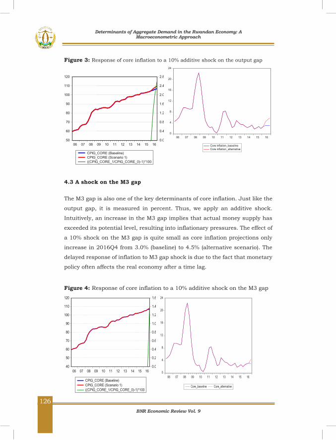
BNR Economic Review Vol. 9
126
128
Figure 3: Response of core inflation to a 10% additive shock on the output gap
4.3 A shock on the M3 gap
The M3 gap is also one of the key determinants of core inflation. Just like the
output gap, it is measured in percent. Thus, we apply an additive shock.
Intuitively, an increase in the M3 gap implies that actual money supply has
exceeded its potential level, resulting into inflationary pressures. The effect of
a 10% shock on the M3 gap is quite small as core inflation projections only
increase in 2016Q4 from 3.0% (baseline) to 4.5% (alternative scenario). The
delayed response of inflation to M3 gap shock is due to the fact that monetary
policy often affects the real economy after a time lag.
Figure 4: Response of core inflation to a 10% additive shock on the M3 gap
0
4
8
12
16
20
24
06 07 08 09 10 11 12 13 14 15 16
Core inflation_baselineCore inflation_alternative
0
4
8
12
16
20
24
06 07 08 09 10 11 12 13 14 15 16
Core_baseline Core_alternative
50
60
70
80
90
100
110
120
0.0
0.4
0.8
1.2
1.6
2.0
2.4
2.8
06 07 08 09 10 11 12 13 14 15 16
CPIG_CORE (Baseline)CPIG_CORE (Scenario 1)((CPIG_CORE_1/CPIG_CORE_0)-1)*100
40
50
60
70
80
90
100
110
120
0.0
0.2
0.4
0.6
0.8
1.0
1.2
1.4
1.6
06 07 08 09 10 11 12 13 14 15 16
CPIG_CORE (Baseline)CPIG_CORE (Scenario 1)((CPIG_CORE_1/CPIG_CORE_0)-1)*100
Determinants of Aggregate Demand in the Rwandan Economy: A Macroeconometric Approach
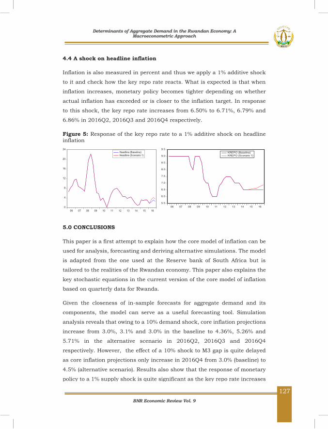
BNR Economic Review Vol. 9
127
129
4.4 A shock on headline inflation
Inflation is also measured in percent and thus we apply a 1% additive shock
to it and check how the key repo rate reacts. What is expected is that when
inflation increases, monetary policy becomes tighter depending on whether
actual inflation has exceeded or is closer to the inflation target. In response
to this shock, the key repo rate increases from 6.50% to 6.71%, 6.79% and
6.86% in 2016Q2, 2016Q3 and 2016Q4 respectively.
Figure 5: Response of the key repo rate to a 1% additive shock on headline inflation
5.0 CONCLUSIONS
This paper is a first attempt to explain how the core model of inflation can be
used for analysis, forecasting and deriving alternative simulations. The model
is adapted from the one used at the Reserve bank of South Africa but is
tailored to the realities of the Rwandan economy. This paper also explains the
key stochastic equations in the current version of the core model of inflation
based on quarterly data for Rwanda.
Given the closeness of in-sample forecasts for aggregate demand and its
components, the model can serve as a useful forecasting tool. Simulation
analysis reveals that owing to a 10% demand shock, core inflation projections
increase from 3.0%, 3.1% and 3.0% in the baseline to 4.36%, 5.26% and
5.71% in the alternative scenario in 2016Q2, 2016Q3 and 2016Q4
respectively. However, the effect of a 10% shock to M3 gap is quite delayed
as core inflation projections only increase in 2016Q4 from 3.0% (baseline) to
4.5% (alternative scenario). Results also show that the response of monetary
policy to a 1% supply shock is quite significant as the key repo rate increases
5.5
6.0
6.5
7.0
7.5
8.0
8.5
9.0
9.5
06 07 08 09 10 11 12 13 14 15 16
KREPO (Baseline)KREPO (Scenario 1)
0
4
8
12
16
20
24
06 07 08 09 10 11 12 13 14 15 16
Headline (Baseline)Headline (Scenario 1)
Determinants of Aggregate Demand in the Rwandan Economy: A Macroeconometric Approach
BNR Economic Review Vol. 9
128
130
from 6.50% in the baseline in 2016Q2-2016Q4 to 6.71%, 6.79% and 6.86%
in 2016Q2, 2016Q3 and 2016Q4 respectively. Nonetheless, the reaction of
monetary policy may depend on the source of the shock. For example,
monetary policy may not tighten if there is a temporary food supply shock.
It is worth mentioning that most of the equations in the current version of the
core model of inflation are calibrated, implying that more work is needed to
understand and accurately model the various sectors of the economy. Satellite
models are needed to help come up with near term forecasts for various blocks
in the model and this work can be effectively handled by sector experts.
Determinants of Aggregate Demand in the Rwandan Economy: A Macroeconometric Approach

BNR Economic Review Vol. 9
129
131
REFERENCES
Christopher Adam and Pantaleo Kessy, “Assessing the stability and
predictability of the money multiplier in the EAC: the case of Tanzania”, 2011.
Gill Hammond et al., “State of the art of inflation targeting”, CCBS Handbook
– No. 29, Bank of England, 2012
Gregory, N., Mankiw “Principles of Economics”, 6th Edition, 2012.
Muhammad Nadim Hanif, Zulfiqar Hyder, Muhammad Amin Khan Lodhi,
Mahmood ul Hassan Khan, Irem Batool, “A Small-Size Macroeconometric
Model for Pakistan Economy”, Technology and Investment, 2011, 2, 65-80.
South African Reserve Bank (SARB), “The core forecasting model of the South
African Reserve Bank”, Working Paper WP/07/02, June 2007.
Roger, Scott, “Inflation Targeting Turns 20”, Finance & Development, 2010,
Vol. 47, No. 1, pp. 46-49.
The Bank of England, “The Pagan Report: Report prepared by Adrian Pagan
on Modelling and Forecasting at the Bank of England, London”, 2003.
Westaway, P., “Economic models at the Bank of England”, London: Park
Communications Limited, 1999.
Karangwa Mathias and MWENESE Bruno, “The Forecasting and Policy Analysis Systems for Rwanda”, BNR economic review no. 007, 2015.
Rusuhuzwa, T.K, Irankunda J.”, “Assessing the stability of money multiplier
in Rwanda”. BNR Econ. Review, 2011, vol. 5:41-55
Determinants of Aggregate Demand in the Rwandan Economy: A Macroeconometric Approach
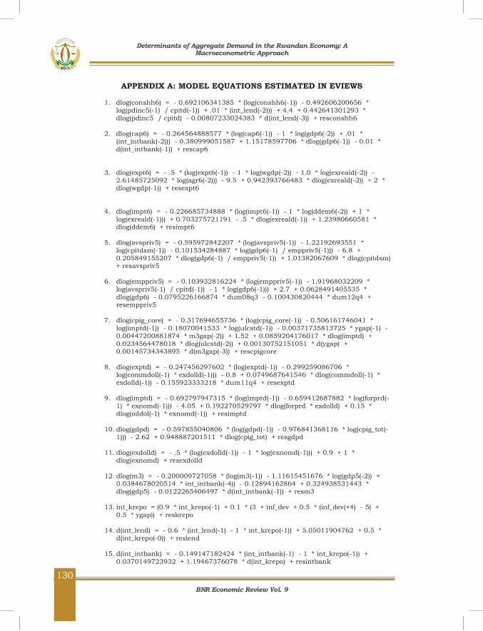
BNR Economic Review Vol. 9
130
132
APPENDIX A: MODEL EQUATIONS ESTIMATED IN EVIEWS
1. dlog(conshh6) = - 0.692106341385 * (log(conshh6(-1)) - 0.492606200656 * log(pdinc5(-1) / cpitd(-1)) + .01 * (int_lend(-2))) + 4.4 + 0.442641301293 * dlog(pdinc5 / cpitd) - 0.00807233024383 * d(int_lend(-3)) + resconshh6
2. dlog(cap6) = - 0.264564888577 * (log(cap6(-1)) - 1 * log(gdp6(-2)) + .01 *
(int_intbank(-2))) - 0.380999051587 + 1.15178597706 * dlog(gdp6(-1)) - 0.01 * d(int_intbank(-1)) + rescap6
3. dlog(expt6) = - .5 * (log(expt6(-1)) - 1 * log(wgdp(-2)) - 1.0 * log(exreald(-2)) - 2.61485725092 * log(agr6(-2))) - 9.5 + 0.942393766483 * dlog(exreald(-2)) + 2 * dlog(wgdp(-1)) + resexpt6
4. dlog(impt6) = - 0.226685734888 * (log(impt6(-1)) - 1 * log(ddem6(-2)) + 1 * log(exreald(-1))) + 0.703275721191 - .5 * dlog(exreald(-1)) + 1.23980660581 * dlog(ddem6) + resimpt6
5. dlog(avspriv5) = - 0.595972842207 * (log(avspriv5(-1)) - 1.22192693551 *
log(cpitdsm(-1)) - 0.101534284887 * log(gdp6(-1) / emppriv5(-1))) - 6.8 + 0.205849155207 * dlog(gdp6(-1) / emppriv5(-1)) + 1.01382067609 * dlog(cpitdsm) + resavspriv5
6. dlog(emppriv5) = - 0.103932816224 * (log(emppriv5(-1)) - 1.91968032209 *
log(avspriv5(-1) / cpitd(-1)) - 1 * log(gdp6(-1))) + 2.7 + 0.0628491405535 * dlog(gdp6) - 0.0795226166874 * dum08q3 - 0.100430820444 * dum12q4 + resemppriv5
7. dlog(cpig_core) = - 0.317694655736 * (log(cpig_core(-1)) - 0.506161746041 *
log(imptd(-1)) - 0.18070041533 * log(ulcstd(-1)) - 0.00371735813725 * ygap(-1) - 0.00447200881874 * m3gap(-2)) + 1.52 + 0.0859204176017 * dlog(imptd) + 0.0234564478018 * dlog(ulcstd(-2)) + 0.00130752151051 * d(ygap) + 0.00145734343895 * d(m3gap(-3)) + rescpigcore
8. dlog(exptd) = - 0.247456297602 * (log(exptd(-1)) - 0.299259086706 *
log(commdoll(-1) * exdolld(-1))) - 0.8 + 0.0749687641546 * dlog(commdoll(-1) * exdolld(-1)) - 0.155923333218 * dum11q4 + resexptd
9. dlog(imptd) = - 0.692797947315 * (log(imptd(-1)) - 0.659412687882 * log(forprd(-
1) * exnomd(-1))) - 4.05 + 0.192270529797 * dlog(forprd * exdolld) + 0.15 * dlog(oildol(-1) * exnomd(-1)) + resimptd
10. dlog(gdpd) = - 0.597855040806 * (log(gdpd(-1)) - 0.976841368116 * log(cpig_tot(-
1))) - 2.62 + 0.948887201511 * dlog(cpig_tot) + resgdpd
11. dlog(exdolld) = - .5 * (log(exdolld(-1)) - 1 * log(exnomd(-1))) + 0.9 + 1 * dlog(exnomd) + resexdolld
12. dlog(m3) = - 0.200009727058 * (log(m3(-1)) - 1.11615451676 * log(gdp5(-2)) +
0.0384678020514 * int_intbank(-4)) - 0.12894162864 + 0.324938531443 * dlog(gdp5) - 0.0122265406497 * d(int_intbank(-1)) + resm3
13. int_krepo = (0.9 * int_krepo(-1) + 0.1 * (3 + inf_dev + 0.5 * (inf_dev(+4) - 5) +
0.5 * ygap)) + reskrepo
14. d(int_lend) = - 0.6 * (int_lend(-1) - 1 * int_krepo(-1)) + 5.05011904762 + 0.5 * d(int_krepo(-0)) + reslend
15. d(int_intbank) = - 0.149147182424 * (int_intbank(-1) - 1 * int_krepo(-1)) +
0.0370149723932 + 1.19467376078 * d(int_krepo) + resintbank
Determinants of Aggregate Demand in the Rwandan Economy: A Macroeconometric Approach

BNR Economic Review Vol. 9
131
133
16. dlog(exports) = - .5 * (log(exports(-1)) - 1.20290383662 * log(@movav(expt5 (-1) , 4))) - 0.6 + 1.31954170212 * dlog(@movav(expt5 , 4)) + resexports
17. dlog(imports) = - .5 * (log(imports(-1)) - 1.14998494989 * log(@movav(impt5(-1) ,
4))) - 0.3 + 1.57345597179 * dlog(@movav(impt5 , 4)) + resimports
Determinants of Aggregate Demand in the Rwandan Economy: A Macroeconometric Approach


BNR Economic Review Vol. 9
136
National Bank of RwandaKN 6 AV. 4
P.O. Box: 531 Kigali, RwandaTel: (+250) 788 199 000
Email: [email protected]: BNRWRWRWTwitter: @CentralBankRw
Website: www.bnr.rw