BIREFRINGENT FABRY-PEROT SENSORS - VU Research ...
377
BIREFRINGENT FABRY-PEROT SENSORS A thesis submitted by Neil Raymund Yu Caranto for the degree of Doctor Of Philosophy Optical Technology Research Laboratory Victoria University of Technology 1998
-
Upload
khangminh22 -
Category
Documents
-
view
0 -
download
0
Transcript of BIREFRINGENT FABRY-PEROT SENSORS - VU Research ...

BIREFRINGENT FABRY-PEROT SENSORS
A thesis submitted
by
Neil Raymund Yu Caranto
for the degree of
Doctor Of Philosophy
Optical Technology Research Laboratory
Victoria University of Technology
1998

Page ii
Acknowledgments
Foremost, I thank my supervisor and mentor, Prof David Booth, OTRL director, for his guidance, support and
encoiuagement during my Ph.D. candidature. I thank him for being available for consultation and for demanding
the best from me. I thank him for his wisdom, simplicity and frankness, patience and understanding. I thank him
for his kindness and for anticipating and providing for all my needs while I was in Australia.
I thank Dr. Michael M. Murphy, my secondary supervisor, for his guidance during the first two years of my
research; Dr. Jakub Sazjman, Dr. Leo Cussen and Kevin Lawlor for sharing their enthusiasm and practical skills in
vacuum deposition; Dr. Andrew Stevenson and Dr. Peter Farrell, for the fruitful discussions; and Dr. Stephen
Collins, HOD Applied Physics, for his upfront support especially during my recent fellowship at VUT.
I thank the technical staff: Alex Shelamoff, for his help in the design of many of the analogue circuits and also for
simply being a great guy; Tibor Kovacs, for his assistance with the computer interface; Mark Kevinin and Donald
Emel, for their high standards of workmanship and efficiency; Hayrettin Arisoy and Durrahman Kuzucu for
making available the different components that I needed; and Umit Erturk for providing solutions to challenges in
the house and in the laboratory especially when they were most needed.
I thank Cindy Huang, Coriima Sullivan, Mikhail Vasiliev and Dr. Senyemmo Charles Kaddu for being great
housemates as well as colleagues. In particular, I thank Kaddu for his simplicity, warm smile, patience and for the
work we shared as we developed fiision-spliced sensors.
I thank Darol Garchev for his time and assistance with the fabrication of the fibre Bragg gratings I required. I
thank the other graduate students (too many to mention) for their great company.

Page iii
I thank the Australian Commonwealth Govermnent for their generous support. Without the almost-four-year
Eqtiity and Merit Scholarship, 1 could never have had the fruitful experience of my Ph.D. candidature at Victoria
University of Technology. I thank Jill Little who ensured that all went well with my scholarship.
I thank the Philippine Goverment for a five-month ESEP fellowship to complete this thesis. In particular I thank
Undersecretary Dr. Estrella P. Alabastro, Engineering and Science Education Program Director, and her staff Ester
Soils, Teody Dayoan, Ullysses Palmones for their prompt support. I thank Dr. Heruy Ramos, director of NIP, for
his endorsement of my fellowship.
I thank Fr. Bienvenido Nebres, S.J., President of the Ateneo de Manila University, for his generous support and
understanding. I thank Dr. Antonette Angeles, head of the Ateneo Faculty Developement, for her support of my
leave of absence to complete this thesis; the Deans, Dr Mart-Jo Ruiz and Dr. Assimta Cuyegkeng for their patience
and encouragement and the Physics Department chairs. Dr. Minella Alarcon, Mr. Nathaniel Libatique, Mr. Carlos
Oppus and Dr. John Holdsworth for their understanding.
I thank Fr. Jett Villarin, S.J. and in particular Dr. John L. Holdsworth for taking time to edit as well as re-edit and
proof-read my thesis.
I thank Fe Warque for her love, patience and for taking care of my needs especially diuing the final stages of this
thesis writing.
I thank my parents and my brothers who always provided the home to return to come summer breaks.
I like to especially thank Fr. Daniel J. MacNamara, S.J., for his recommendation and moral support throughout my
candidature.

Page iv
Declaration
I, Neil Raymund Yu Caranto, declare that the thesis titled,
Birefringent Fabry-Perot Sensors,
is my own work and has not, been submitted previously, in whole or in part, in respect of any
other academic award.
NeU Raymund Yu Caranto,
dated the 14* day of July, 1998

Page v
Abstract
This thesis describes the development and performance of short-cavity polarisation-maintaining (birefringent) in-
fibre Fabry-Perot interferometric sensors for the measurement of temperature or strain. By using a highly
birefringent optical fibre in their cavity, these sensors form two interferometers - one for each polarisation axis. As
in the case of other fibre interferometers, each axial interferometer is extremely sensitive to temperature and strain.
But this high sensitivity together with the periodic nature of each interferometer output yields a limited
unambiguous measurand range (UMR). However, the differential phase between the axial interferometric phase
responses of the birefringent sensors developed in this work can be exploited to provide an extended UMR.
Several approaches in obtaining a large or extended UMR of interferometric sensors are surveyed. In this work the
in-fibre birefringent Fabry-Perot sensor was the chosen sensor configuration primarily because of its high
iimnunity from perturbations in any lead-fibre and its moderately large UMR for both temperature and strain
measurements.
Long cavity birefringent fibre Fabry-Perot sensors have been previously investigated [Farahi et al., 1990] while
those with short cavity lengths have not been exploited. The main advantage of short-cavity in-fibre sensors is that
they can be deployed in hard-to-reach envirorunents to obtain localised measurements of temperature or strain.
Although the maximum possible sensitivity value of short-cavity sensors is lower than that of long-cavity sensors,
the former still offer high sensitivity to temperature and strain.
Using short-cavity in-fibre Fabry-Perot sensors involves challenges both in their fabrication and operation. Crucial
to the operation of the sensor is the alignment of the polarisation axes of the lead-in fibre with the polarization axes

^ Page vi
of the sensor. In this thesis, the fabrication of two types of short-cavity in-fibre birefringent Fabry-Perot sensors is
described. These sensors employed either fusion-spliced Ti02 in-line reflectors or in-fibre Bragg gratings and each
type of sensor exhibits different mechanical and optical properties. The expected interferometric output and the
sensitivity of the cavity phase shift to temperature and strain of the two types of sensors are also discussed.
In this work, to obtain moderately fast measurements, a pseudo-heterodyne signal processing scheme with a
modulated laser diode was implemented to detect the interferometric phase shifts of each axial interferometers of
the sensors. This scheme primarily requires that the sensors be low finesse whilst the implementation method
limits the shortest possible cavity length. Low finesse can be achieved with using low reflectance Fabry-Perot
mirrors.
Measurements made with the different sensors developed are discussed. The axial and difierential phase responses
of the birefringent sensors were found to exhibit good linear trend with temperature or strain as was expected.
However, because of the high phase resolution (LlC*) of the phase recording scheme used in this work, several
nonlinear effects were observed. Common to both types of Fabry-Perot sensors developed were effects associated
with the signal processing scheme. Observed only with the grating-based sensors, one of the nonlinear features
was subsequently attributed to the dispersion of the "grating" used with the sensor. However there was a large
disparity between the magnitude of the dispersion of the "grating" that was experimentally observed and that
predicted by coupled-mode theory. This disparity indicates that the "grating" may actually be a complicated
structure of several gratings. Such structures is not difficult to imagine since two fibre Bragg gratings have been
superimposed in the past [Xu et al., 1994].
Aside for developing an optical fibre sensing arrangement which exhibits high measurand resolution, large UMR
and moderate fast sampling rate, and can be assembled in an all-fibre form, the major contribution of this work
was the development of a method of directly measuring the dispersion of a "grating" written on optical fibres
which may be useful to others investigating the properties of different types of fibre Bragg gratings.

Page vii
Table of Contents
Acknowledgments ii
Declaration iv
Abstract v
Table of Contents vii
Chapter 1: Introduction 1-1
1.1 Research Aim and Major Activities 1-5
1.2 Thesis Overview IS
Chapter 2: Temperature Or Strain Interferometric Optical Fibre Sensing Arrangements
Exhibiting Large Unambiguous Measurand Range 2-1
2.1 Approaches in Obtaining Large Measurand Range 2-2
2.2 Reduced Sensitivity Approaches 2-5
2.2.1 Reduced Sensitivity Via Reduction of the ElTective Sensing Length; Ultra-Thin Fabry-Perot
Interferometric Sensors 2-6
2.2.2 Reduced Sensitivity Via the Reduction of the Effective Refractive Index 2-7
2.2.2.1 Polarimetric Sensors 2-7
2.2.2.2 Dual-Mode Sensors 2-8

Page viii
2.2.3 Using Direct Physical Techniques 2-9
2.3 Direct Extension of Unambiguous Phase Measurement Range Approaches 2-10
2.4 Unambiguous Measurement Approaches 2-12
2.4.1 Absolute Measurement of Optical Path Difference 2-12
2.4.1.1 Coherent Frequency-Modulated Continuous-Wave Interferometry 2-12
2.4.1.2 Low-Coherence or White-Light Interferometry 2-15
2.4.2 Measurement of Optical Path Length, Group-Delay, Dispersion of an Optical Fibre 2-17
2.4.2.1 Dispersive Optical Fourier Transform Spectroscopy 2-17
2.4.2.2 Measurement of Optical Path Length, Group-Delay, Dispersion of an Optical Fibre 2-19
2.4.3 Spectrally-Encoded Measurements 2-20
2.4.3.1 Brillouin Scattering Sensors 2-21
2.4.3.2 In-Fibre Bragg Grating Sensors 2-22
2.5 Dual-Measurement Approaches 2-25
2.5.1 Two Distinct Sensors 2-25
2.5.1.1 Schemes Not Involving Fabry-Perot Interferometric Sensors 2-26
2.5.1.2 Schemes Involving One Fabry-Perot Interferometric Sensor 2-27
2.5.1.3 Schemes Involving Effectively Two Distinct Fabry-Perot Interferometric Sensors 2-29
2.5.2 Dual Wavelength Techniques 2-30
2.5.2.1 Extending the UMR of Interferometric/Polarimetric Sensors 2-30
2.5.2.2 Extending the UMR of Dual-Evanescently-Coupled-Core Fibre Sensors 2-31
2.5.2.3 More-Than-Two-Wavelength Illumination 2-32
2.5.3 Dual In-Fibre Bragg Grating Sensors 2-33
2.5.4 Conventional Interferometry or Polarimetry Combined with Dual-Mode Interference 2-39
2.5.4.1 Extending the UMR of Interferometric Sensors 2-39
2.5.4.2 Extending the UMR of Polarimetric or Dual-Mode Sensors 2-40
2.5.5 Combined Interferometry and Polarimetry 2-41

Page ix
2,6 Overview Summary 2—43
Chapter 3: Transfer Functions of Optical Fibre Fabry-Perot Interferometers With Thin-
Film or Fibre Bragg Grating Reflectors 3-1
3.1 Intrinsic Fibre Fabry-Perot Interferometers 3-2
3.1.1 Transmission Function ofFibre Fabry-Perot Interferometers 3-6
3.1.2 Behaviour of the Airy Function, Free Spectral Range and Finesse of Fabry-Perot Interferometers.... 3-7
3.1.3 Reflection Function of Fabry-Perot Interferometers 3-10
3.1.4 Low Finesse Fabry-Perot Interferometers as a Two-Beam Interferometer 3-13
3.1.5 Fringe Visibility 3-13
3.1.6 Limitations on the Fringe Visibility 3-15
3.2 Thin-Film or Bragg-Grating Fabry-Perot Reflectors 3-16
3.2.1 Dielectric Thin Film 3-16
3.2.2 Fibre Bragg Grating 3-19
3.3 The Free Spectral Range ofFibre Fabry-Perot Interferometers With Either Thin-Film or Fibre Bragg
Grating Reflectors 3-25
3.3.1 Some Preliminary Calculations 3-25
3.3.1.1 The Case of a Dielectric Thin Film 3-25
3.3.1.2 The Case ofa Fibre Bragg Grating 3-26
3.3.2 Final Calculations 3-28
Chapter 4: Thermal and Strain Sensitivities of Single-Mode Silica Fibre Fabry-Perot
Interferometric Sensors 4-1
4,1 Thermal and Strain Sensitivities of Non-Polarisation-Maintaining Single-Mode Silica Optical Fibre
Fabry-Perot Interferometric Sensors 4-1
4.1.1 Stress and Strain Formalisms 4-3
4.1.2 Phase-Strain Sensitivity 4-4

Pagex
4.1.3 Phase-Temperature Sensitivity 4-8
4.1.4 Unified Phase-Strain-Temperature Description 4-10
4.2 Birefringence In Single-Mode Optical Fibres 4-12
4.2.1 Birefiingence Meclianisms 4-12
4.2.2 Evolution of the State-of-Polarisation 4-13
4.2.3 Mechanisms for Producing Linear Birefringence 4-13
4.2.4 Characterisation of Linear Birefringence 4-15
4.3 Thermal and Strain Sensitivities of Elliptically-cladded Birefringent Optical Fibres 4-16
4.3.1 Stress Distribution In an EUiptically Cladded Birefringent Fibre 4-16
4.3.2 Photo-elastic Effect Constants 4-19
4.3.3 Birefringence of an Optical Fibre with an Internal Elliptical Cladding 4-20
4.3.4 Phase-Strain Sensitivity 4-22
4.3.5 Phase-Temperature Sensitivity , 4-23
4.3.6 Cross-Sensitivity of Strain and Temperatme 4-25
4.4 Temperature and Strain Sensitivities of a Single-Layer Reflective Thin Film 4-27
4.5 Temperature and Strain Sensitivities of an In-Fibre Bragg Grating. 4-28
4.6 The Phase-Measurand Sensitivity of a Fibre Fabry-Perot Interferometer with Thin-Film or Bragg-
Grating Reflectors 4-29
4.7 The Unambiguous Measurand Range of a Fibre Fabry-Perot Interferometer With Thin-Film or
Bragg-Grating Reflectors 4-30
Chapter 5: Development Of Short-Cavity Fibre Fabry-Perot Interferometers 5-1
5,1 Fusion-Spliced Single-Mode Optical Fibre Fabry-Perot Sensors 5-2
5.1.1 Review of the Previous Work on the Construction of Fusion-Spliced In-Fibre Reflectors 5-2
5.1.2 Ti02 Reactive Sputter Deposition 5-3
5.1.3 Fabrication Process for Fusion-Spliced Fabry-Perot Sensors 5-12

Pagexi
5.1.4 Splice Strengthening 5-17
5.2 Fusion-Spliced Birefringent Optical Fibre Fabry-Perot Sensors 5-19
5.2.1 Fabrication Process 5-19
5.2.2 Alignment ofthe Birefringent Axes 5-20
5.3 Grating-Based Birefringent Optical Fibre Fabry-Perot Sensors 5-24
5.3.1 Single-Grating Birefringent FFPSs 5-25
5.3.2 Dual-Grating In-line FFPSs 5-29
Chapter 6: A Birefringent Optical Fibre Sensing System for the Measurement of
Temperature and Strain 6-1
6.1 The Optical Fibre Sensing Arrangement Compared With Its Closest Fore-Runner 6-1
6.2 Detailed Description of the In-Fibre Birefringent Fabry-Perot Sensor 6-^
6.3 Description of the Optical Fibre Sensing System 6-5
6.4 Jones Calculus Treatment 6-8
6.4.1 In-Fibre Sub-System 6-10
6.4.2 Launching Sub-System 6-12
6.4.3 Detection Sub-System 6-14
6.4.4 Output Electric Field and System Requirement (reflection) 6-15
6.4.5 Output Electric Field and System Requirement (transmission) 6-17
6.5 Pseudo-Heterodyne Signal Processing Scheme Implemented With A Modulated Laser Diode 6-19
6.5.1 The Technique 6-19
6.5.2 Implementation 6-22
6.5.3 Chirping of tlie Laser Diode Emission Frequency 6-22
6.6 Implementation ofthe Signal Processing and Phase Detection Scheme 6-24
6.6.1 Description of Single Channel 6-24
6.6.2 Cumulative Pliase Moniloring 6-28

Page xii
Chapter 7: Temperature and Strain Measurements With Fibre Fabry-Perot Sensors 7-1
7.1 Performance of Non-Polarisation-Maintaining Fusion-Spliced Fibre Fabry-Perot Sensors 7-2
7.1.1 Characteristics of the NPM Sensors 7-2
7.1.2 Temperature Measurements with NPM Sensors 7-4
7.1.3 Static Longitudinal Strain Measurement with NPM Sensors 7-8
7.2 Performance of Fusion-Spliced Birefringent Fibre Fabry-Perot Sensors 7-13
7.2.1 Characteristicsof the Fusion-Spliced Birefringent Sensors 7-13
7.2.2 Temperature Measurements with Fusion-Spliced Birefringent Sensors 7-14
7.3 Performance of Grating-Based Birefringent-Fibre In-Fibre Fabry-Perot Sensors 7-34
7.3.1 Description ofthe Sensor 7-34
7.3.2 The Characteristics of In-Fibre Bragg Grating 7-35
7.3.3 Temperature Measurements with Grating-Based Sensors 7-36
7.3.4 Static Longitudinal Strain Measurements with Grating-Based Sensors 7-53
7.3.5 Dynamic Strain Measurements with Grating-Based Sensors 7-64
Chapter 8: Conclusion 8-1
8.1 Synthesis 8-1
8.2 Further work 8-4
Appendix A: Measurement ofthe Group Refractive Index o fa Single-Mode Optical FibreA-1
Appendix B: Descriptions ofthe Experimental Circuits and Computer Interfaces B-1
B,l Experimental Circuits B-1
B.1.1 Savrtooth Generator Circuit B-1
B. 1.2 Laser Diode Drive Circuit B-4
B.1.3 Temperature Controller Circuit B-6

Page xiii
B. 1.4 Division Circuit B-9
B.1.5Photodiode Circuit B-9
B. 1.6 Band-pass Amplifier Circuit B-12
B.1.7 Squaring Qrcuit B-14
B. 1.8 Phase Determination Circuit B-15
B,2 Computer Interfaces B-20
B.2.I Measurand Detection Circuits B-22
B.2.1.1 Temperature Detection Circuit B-22
B.2.1.2 Electrical Strain Gauge Amplifier B-23
B.2.2 Continuous Monitoring of the Interferometric Phase Shifts B-25
Appendix C: System Noise and Limitations C-1
C.l Phase Noise Due to Intensity-Related Noise C-1
C.1.1 Detection Electronics Noise: Electrical Noise in the Photodiode Circuit C-I
C.2 Phase Error in the Detection ofthe Zero-Crossing Edges C-4
C.3 Phase Noise Due to Some ofthe Optical Components C-5
C.3.1 Fresnel Reflection From the Proximal Face of the Lead-in Fibre C-5
C.3.2 Lead-in Fibre Insensitivity C-7
C,4 Phase Noise Due to the Characteristics ofthe Laser Diode C-10
C.4.1 DC Current Characteristics and Noise C-10
C.4.2 Coherence Length ofthe Laser Diode Operated Witii A Small-Signal AC Sawtooth Current
Modulation C-12
C.4.3 AC Current Characteristics And Noise C-14
C.4.4 Temperature Sensitivity ofthe Laser Diode and Limitations ofthe LD Temperature Controller... C-20
C.5 Phase Noise Due to the Band-Pass Filter, C-23
C,6 Overall Phase Noise C-25

Page xiv
Appendix D: Publications Resulting From This Thesis D-1
Appendix E: References E-1
Appendix F: Symbols Used in This Thesis F-1
Appendix G: Abbreviations Used In This Thesis G-1

Chapter 1: Introduction
Optical fibre sensors (OFSs) have been of significant research interest over the last 20 years because of their
potential applications in highly sensitive measurements of thermal, mechanical, acoustic, magnetic, electrical or
chemical parameters [Giallorenzi et al, 1982; Jackson and Jones, 1986; Kersey, 1990; Jackson, 1994]. The
interest in OFSs is principally due to the useful material-dependent properties of optical fibres. In particular, the
good electrical isolation, high electromagnetic immunity, high tensile strength, high melting point, great
flexibility, high chemical inertness, light weight and small size [Culshaw & Dakin, 1988] of silica-fibre-based
OFSs offer the possibility of highly sensitive measurements in hazardous or hard to reach envirorunents [Yeh et
al, 1990; Inci et al., 1993]. Although OFS technology is still considered in its infancy, initial commercial
successes have been realised [Montgomery & Glasco, 1985; Crossley, 1994; Lequime, 1997]with notably strain and
temperature OFS gaining acceptance for use in various fields [Wickersheim & Hyatt, 1990; Mason et al., 1992].
For example in medicine, temperature and pressure OFSs have made a niche as promising alternatives to well-
established medical sensors [Martens et al, 1985; Baldini & Mignani, 1994; Rao et al, 1997a]. In aerospace
engineering, the development of intrinsic strain sensors has been a major research activity in the fabrication of
smart composite structures for aerospace applications [Measures, 1992]. In the operation of nuclear power plants,
a multiplexed array of fibre-optic temperature sensors can permit remote monitoring of important thermal
parameters ofa nuclear reactor with relatively high radiation damage thresholds [Meunier et al., 1994].
OFSs can basically be categorised as either intrinsic or extrinsic. In the extrinsic type, optical fibres serve merely
as optical waveguides directing light into and collecting light from a device which is external to the fibres and

Page 1-2
where a measurand can modulate one of the optical properties of this external device. In the intrinsic type, the
optical fibres are used both as the optical waveguides and the sensing elements themselves. In general, intrinsic
sensors are more attractive because they do not sxiffer from severe optical coupling losses which are conmion in
extrinsic sensors. However intrinsic sensors are limited only to measurands which affect the optical properties of
an optical fibre, e.g. refractive index, absorption length etc. Extrinsic sensors, on the other hand, allow a
convergence of optical fibre and other technologies. This convergence of technologies has given rise to several
OFSs measuring a wide variety of measurands.
OFSs can further be classified according to how a measurand affects the optical properties of a sensor. For
example a measurand can affect the intensity, the phase, the state of polarisation (SOP) or the optical spectrum of
the light beam returning from a sensor. Intensity-modulated sensors exploit the sensitivity of the fibre to
measurands which affect loss or attenuation. A measurand can interact with an optical fibre by changing its
transmission properties such as scattering loss, macro- and micro-bending loss or evanescent coupling. Phase-
modulated or interferometric sensors utilise the dependence on a measiu^nd of the relative optical phase between
the beams travelling in the arms of a fibre interferometer. Interferometric sensors can detect changes in their
optical path difference which are a fraction of a wavelength of the light source. Polarimetric or SOP-modulated
sensors exploit the susceptibility of the SOP of the light guided in an optical fibre to changes in the measurand.
For example, Kerr or Faraday effects in optical fibres have been exploited to measure electric and magnetic fields
or their related parameters {e.g. Tang et al, 1991; Ning et al, 1995]. Spectrally-encoded sensors generally
involve measiuands which affect the spectral properties of optical processes in an optical fibre. One common
example of such sensors is the fibre Bragg grating sensor. Other spectrally-encoded sensors take advantage of
nonlinear processes in an optical fibre (e.g. Stimulated Raman or Brillouin Scattering).
Of the different combinations of the type and the class of an OFS, an intrinsic interferometric sensor offers a
simple, direct and highly sensitive measurement system for temperature, strain or parameters which produce
temperature change or strain in an optical fibre. Of the various types of interferometric sensors, an intrinsic in-
fibre Fabry-Perot interferometric sensor (FFPS) offers one of the simplest and most convenient configurations for
Page 1-3
incorporation in structures. An FFPS exhibits high lead-fibre phase noise rejection because the interfering beams
travel to and from the sensor in the same optical fibre. Such high immuruty of the Fabry-Perot interferometric
phase from phase perturbations present in any lead-fibre can facilitate the successful multiplexing of several FFPSs
in the same optical fibre. An FFPS addressed in reflection naturally provides single-ended operation of the sensing
arrangement without the additional use of other fibres or optical components. Furthermore, with the use of fibre
directional couplers and other fibre-optic devices, an all-fibre system can be realised and thereby provide enormous
flexibility in deploying FFPSs. For these reasons many research groups have developed measuring systems based
on FFPSs. In this present work, FFPSs have been investigated for the measurement of temperature and strain.
FFPSs have properties which limit the variety of possible signal processing schemes that can be employed with
them. Only signal processing schemes which are compatible with a non-zero optical path difference can be
directiy employed with an FFPS. The multi-beam natiu-e of the Fabry-Perot interference implies that none of the
signal processing schemes suitable for two-beam interferometers can be applied unless the combined internal
reflectance of the two Fabry-Perot mirrors is low. Thus the reflectance of the Fabry-Perot mirrors is an important
consideration in the overall design ofa measuring system.
Like all other interferometric sensors, an FFPS interrogated with a highly coherent light source provides only
relative measurements because interferometric outputs are periodic with respect to the total round-trip cavity
optical phase difference. Hence sensing arrangements with FFPSs require re-initialisation after a system reset. On
the other hand, after such re-initialisation, the Fabry-Perot interferometric phase can be continuously monitored
such that the total phase excursion can be calculated (fringe counting) or the interferometric phase can be held
constant by some suitable feedback control (phase tracking). In either case, the interferometric phase can not
instantaneously change by more than In. k change in the measurand which produces a 2;r interferometric phase
change is known as the unambiguous measurand range (UMR).
Temperature or strain directiy affects the physical length and refractive index of an optical fibre as will be
discussed in Chapter 4. For the measurement of temperature or strain, the corresponding UMR depends on the

_ _ ^ Page 1-4
absolute length of an FFPS exposed to temperature or strain, the sensing length. On the other hand, the length of
the Fabry-Perot cavity determines the lower bound for the UMR. Both the exposure or sensing length and the
cavity length are important considerations in determining the UMR of an FFPS.
Localised measurements of temperature or strain are highly advantageous because these measurands can vary from
one location to another even within a small sensing region. Although localised temperature or strain
measurements can be achieved by exposing only a portion of an FFPS to either of these measurands, it is generally
more beneficial to expose the whole Fabiy-Perot cavity uiuformly. This preference can be understood by realising
that temperature change or strain can influence areas immediately adjacent to the sensing region {e.g. thermal
conduction along an optical fibre). The thermal and strain gradients at the ends of the sensing region determine
the magnitude of the additional temperature or strain-induced effects and consequently the effective sensing length
can vary from one measurement to another. This ambiguity in the sensing length limits the accuracy in
determining the measurand or in calibrating the sensor and may be avoided by exposing the whole cavity to the
measurand so that the Fabry-Perot cavity defines the sensing length. Exposing the entire length of a long-cavity
FFPS to a measurand yields, however, a narrow UMR sensor. Thus in order to obtain as large as possible UMR
while conveniently exposing an FFPS entirely to a measurand, a short-cavity FFPS can be used with the additional
advantage that it naturally provides localised measurements.
A short-cavity FFPS is not simple to fabricate in an optical fibre as is outiined in Chapter 6. Some of the earliest
attempts to produce these devices involved using fusion-spliced mirrors [Leilabady, 1987; Lee & Taylor, 1988]
where it was found that the fusion-splicing unavoidably degrades the tensile strength of the concatenated optical
fibres to the point that fiision-spliced FFPSs are not suitable for large strain measurements. To avoid this
limitation, FFPSs may be realised by utilising an in-fibre Bragg grating as a Fabry-Perot reflector. These fibre
Bragg gratings can be formed within the core of an optical fibre without significantiy compromising the tensile
strength of the host fibre [McGarrity & Jackson, 1998]. The thermal sensitivity, the strain sensitivity and the
limited optical reflection bandwidth of fibre Bragg gratings define the performance and limitations of grating-

Page 1-5
based FFPSs. The performance and limitations of both fiision-spIiced and grating-based FFPSs as temperature and
strain sensors are assessed and compared in Chapters 3 and 7 of this work.
1.1 Research Aim and Major Activities
This present work began (early in 1992) with the general aim of assembling and assessing the performance and
limitations of a reliable optical fibre sensing system capable of accurately measuring moderately fast variations of
temperature or strain with high resolution over as wide as possible measiuand range and in a localised region.
There were two major inter-related challenges encountered in this work. The first challenge was the fabrication of
short-cavity birefringent fibre Fabry-Perot interferometric sensors and the other challenge was the assembly of a
compact optical arrangement with associated signal processing scheme appropriate for interrogating a short-cavity
birefringent FFPS.
An FFPS can be operated with either a high-coherence or low-coherence light source. Although low-coherence or
white-light interferometry (WLI) offers absolute measurement of a measurand and subsequently a potentially
unlimited measurand range, WLI was not an option for this work because of the very slow processing time
involved limiting the whole sensing arrangement to quasi-static (< 1 Hz) temperature or sfrain measurements. In
this work, a pseudo-heterodyne signal processing scheme with a carrier of 1 kHz was implemented to extract the
Fabry-Perot interferometric phase shifts [ Jackson et al, 1982]. As a result, variations in temperatm-e or sfrain at a
rate of up to 500 Hz can be measured depending on the corresponding phase amplitude. A higher carrier
frequency may be used but a 500 Hz signal bandwidth for temperature or strain is more than adequate.
The pseudo-heterodyne signal processing scheme made use of a single-mode laser diode (LD) with a sawtooth
modulated drive current. This modulation consequentiy restricted the parameters of the Fabry-Perot interferometer
as too great an LD drive current may cause the output ofthe LD to mode-hop. A physical cavity length of at least
10 mm was found compatible with the modulated 785 nm LD as discussed in Chapter 6. This limit in the cavity
length specified the minimum vvidth ofthe sensing region for localised measurements of temperature or sfrain.

Page 1-6
Because ofthe high sensitivity of an FFPS to either temperature or strain, the temperature and strain UMR even for
the case ofa 10-mm FFPS at 785 nm are narrow: ~ 1.3 °C and ~ 25 //ffor temperature and strain respectively.
Clearly such UMR values limit the number of practical applications of an FFPS. However there are numerous
schemes that can be employed to extend the UMR of an interferometric sensor as outiined in Chapter 2. This work
used a dual FFPS arrangement using a birefringent FFPS. The two fibre Fabry-Perot interferometers (FFPIs) were
maiufested along each polarisation axis of a birefringent FFPS. These two axial interferometers were expected to
exhibit slightiy different temperature and strain sensitivities due to the birefringence of the fibre. Interestingly, the
similarity between the axial phase-measurand sensitivities was ideal for producing a birefringent FFPS with a large
dynamic range - the ratio between the UMR and the measurand resolution. A birefringent FFPS can be used such
that the phase change on one polarisation axis provides high-resolution measurements of temperature change or
sfrain whilst the polarimetric or differential phase change (the difference between the two axial phase change) the
fringe order of the chosen axis phase change. Hence the effective UMR of a birefringent FFPS is equivalent to the
UMR obtained when only the differential phase sensitivity is considered. In this work, roughly a 16-fold and
64-fold increase in the UMR were generally observed for temperature and strain measurements respectively.
By continuously monitoring the interferometric phase along the two axial interferometers, a birefringent FFPS can
still be operated over a measmand range wider than that stipulated by its UMR value. To facilitate such
continuous monitoring, the measuring system was interfaced with a personal computer programmed to calculate
the total phase excursion along each FFPS between any resetting ofthe measuring system or any re-irutialisation of
the sensor. Purpose-designed digital elecfronic circuits detected the interferometric phase shifts for each axial
interferometer and converted these phase measurements into digital signals. These circuits measured each axial
phase change with a resolution of 1/10,000* of a fringe (2n radians) at a maximmn sampling rate of 1 kHz.
In this work, the largest possible dynamic range for temperature or sfrain measurements were found to be about
1.6x10^ and 6.4x10^ respectively. The actual dynamic range was be limited by the level of phase noise in the
optical arrangement during a measurement run (Chapter 7). Nevertheless the fabrication of short-cavity
birefringent FFPSs was crucial in obtaining a sensing arrangement with extended UMR and dynamic range.

Page 1-7
Successful discrimination between the interference along each axial interferometer of a short-cavity birefringent
FFPS required a lead-in birefringent fibre whose polarisation axes had been aligned with those of the sensor.
Ensuring such ahgrunent of the polarisation axes was laborious with fusion-spliced Ti02 mirrors because the
tolerance for the angular aligrunent of the polarisation axes is < 2 °. The alignment of the polarisation axes for
grating-based FFPSs was automatic and limited only by the sfrength of any polarisation cross-coupling and the
amount of photo-induced birefringence in the gratings themselves (Chapter 5).
In this work, fusion-spliced FFPSs were initially assessed and were subsequently followed by grating-based FFPSs
as soon as fibre Bragg grating technology became available in this laboratory early in 1995. The performance of
these two kinds of FFPS to temperature or sfrain measurements were similar except in their differential phase
responses as discussed in Chapter 7.
In this work, a carefiilly designed optical arrangement was assembled to address a birefringent FFPS in reflection
with the least number of components. With minor modification, the same optical arrangement can likewise be
used to address a birefringent FFPS in transmission if desired.
By the end of this research, in late 1995, several fibre Fabry-Perot interferometric sensors were fabricated. These
FFPSs used either non-polarisation-maintaining or (birefringent) polarisation-maintaining fibres and either
employed fiision-spliced Ti02 films or in-fibre Bragg gratings as the Fabry-Perot internal mirrors of these FFPSs.
Some of these FFPSs were used as temperature or strain sensors. In the case of a birefringent FFPS, large
unambiguous measurand range, high resolution and localised measurements were realised.
Although birefringent FFPSs gave promising performance as strain or temperature sensors, these sensors still
suffer from a fimdamental drawback - both strain and temperature effects give indistinguishable phase shifts along
each axis of the sensor. Hence to effectively measure one of these measurands, the other parameter needs to be
kept constant or at least independently monitored so that the corresponding effects of these changes may be
subtracted from the total interferometric response.

Page 1-8
1,2 Thesis Overview
This thesis is the culmination of an investigation into the fabrication and the performance of fusion-spliced and
grating-based short-cavity-length birefringent fibre Fabry-Perot interferometric sensors with application to
temperature or strain measurement. The parameters of the sensors are necessarily, novel. The detailed
examination of signal phase and intensity for these sensors and others of similar type, offers a new and complete
understanding ofthe limiting parameters and thus the applicability of these sensor types as measuring devices.
The remainder of this thesis is arranged as follows. Chapter 2 presents an overview of previous work on
interferometric optical fibre sensing arrangements which exhibit a large or an extended unambiguous measurand
range. This chapter also discusses arrangements which can simultaneously measure temperature and strain
because these arrangements are almost identical and can provide single-measurand interferometric sensing
arrangements with enlarged dynamic range.
Chapter 3 provides a detailed analysis of the transmission and reflection functions of fibre Fabry-Perot
interferometers. In particular the analysis has taken into account the phase shift upon reflection from thin film
mirrors or in-fibre Bragg gratings. This analysis predicts that a fiision-spliced FFPS and a grating-based FFPS
exhibit slightiy different interferometric phase response. Chapter 4 describes the expected phase sensitivity to
temperature and strain of an FFPS fabricated with either non-polarisation-maintaining (ordinary) optical fibres and
elliptically-clad birefringent optical fibres.
Chapter 5 discusses the fabrication of fusion-spliced and grating-based Fabry-Perot interferometric sensors. The
last type of sensors fabricated were in-line birefringent FFPSs using two fibre Bragg gratings. This chapter also
describes the deposition of a Ti02 thin film onto either the entire or only around the core-region of the face of a
cleaved fibre end, possible schemes to improve or maintain the tensile sfrength of fiision-spliced fibres, the
techruque employed to align the polarisation axes of two birefringent fibres to be spliced, and the fabrication
processes used to produce fibre Bragg gratings.

Page 1-9
Chapter 6 describes in detail the optical and electronic arrangements employed to measure temperature or sfrain
using birefringent fibre Fabry-Perot interferometric sensors. The details ofthe electronic circuits implementing the
signal processing scheme are described in Appendix B.
Chapter 7 presents and discusses the different experimental temperature, static sfrain and dynanuc strain
measurements with some of the FPPSs fabricated. These evaluated sensors were either communications-fibre or
birefringent FFPSs fabricated with a fiision-spliced Ti02 dielectric mirror, or a birefringent FFPS with an in-fibre
Bragg grating reflector. These sensors were found to perform well as temperature and strain sensors. For
example, one ofthe sensors can measure slowly-varying temperature between -20 °C to 80 °C with a phase-noise-
limited resolution of 7x10" °C (after removal of systematic effects this resolution can be as high as 2x10 ' °C) and
a UMR of ~ 34 °C. In Appendix C, the possible sources of phase noise were identified to account for the deviation
ofthe experimentally observed resolution from the maximum possible resolution.
Because ofthe high resolution phase measurements obtained in this work, two distinct nonlinear features originally
believed to be noise were additionally observed in the experimental results. The first of these features was the
detection and evaluation of the highly periodic effects on the phase change on each axial interferometers. These
effects were subsequenfly attributed to a nonlinear optical frequency ramp produced by the limited thermal
response ofa modulated LD. The second feature ofthe experimental results was a simple and direct observation of
the non-linear phase shift in a low-reflectance grating. The effect is normally masked by the linear term but by
measuring the differential phase between the two polarisations the resonant part of the phase shift due to the
grating is clearly noticeable since it is a significant fraction ofthe differential phase.
Finally Chapter 8 concludes this thesis and provides suggestions for the future extension of this work.

Chapter 2: Temperature or Strain Interferometric
Optical Fibre Sensing Arrangements
Exhibiting Large Unambiguous
Measurand Range
In this chapter, techniques to ensure a large or extended unambiguous measurand range (UMR) of temperatiire or
sfrain interferometric optical fibre sensors (OFSs) are surveyed. A wide measurand range is an important
consideration for expanding the practical application of an interferometric OFS. Webb et al. [1988a] have
previously reviewed the various techniques to extend the UMR of interferometric sensors. These techniques are
either based on combining polarimetry with coherent interferometry, dual-wavelength interferometry, white-light
interferometry or coherent Frequency-Modulated-Continuous-Wave (FMCW) heterodyne interferometry. Since
then several other techniques have been developed. This chapter attempts to present an overview of various UMR-
extending techniques reported to date (1998).
An extension of the UMR does not automatically imply an increase in the dynamic range - the ratio between its
measurand range and measurand resolution. Whilst a large measurand range increases the practicality of an
interferometric sensor, a large dynamic range implies a measuring system exhibiting high precision. Obviously, a
measuring system exhibiting both a large measurand range and a high measurand resolution is generally preferred.
In this chapter UMR-extending techniques which provide an improved dynamic range receive greater attention.

Page 2-2
For this reason, techniques for simultaneous measurement of temperature and sfrain are also presented because
these simultaneous-measurement techniques can easily be adapted to extend the UMR and dynamic range of a
sensing arrangement as well.
Although this chapter focuses primarily on temperature or sfrain interferometric OFS, sensors which measure other
parameters such as pressure or displacement, are also included because these type of parameters can be interpreted
as indirect manifestations of temperature or sfrain. This chapter also presents sensors whose output can directiy or
indirectiy be considered similar to that given by an interferometer, i.e. an optical output which follows some
interference of optical beams. Furthermore, this chapter gives special attention to fibre Fabry-Perot interferometric
sensors (FFPSs) because FFPSs offer many benefits (see Chapter 1) and also because FFPSs have been chosen as
the sensor configuration for this present work.
2.1 Approaches in Obtaining Large Measurand Range
There are four possible basic approaches that can be used to obtain a large measurand range for an optical fibre
sensing arrangement based on fibre interferometric sensors. The first approach involves reducing the sensitivity of
an interferometric OFS to a measurand. In general, reducing the measurand sensitivity increases the UMR but
decreases the measurand resolution. The second approach involves directiy extending the maximum phase change
that can be measured unambiguously. Unlike the first, the second approach provides a direct extension of the
dynamic range. The third approach to obtain a large measurand range is to remove any ambiguity in determining
the measurand. Such conditions can be accomplished by deriving measurements of some parameter of the optical
output ofthe optical fibre sensor which are not periodic with temperature or strain, e.g. absolute measurements of
the optical path difference (OPD) of an interferometer. In most cases, the measurand range is essentially unlimited
and can be made exfremely wide. On the other hand the measurand resolution is limited by the resolution of the
instrument or signal processing used to determine the measurand. However if an unambiguous measurement and a
high-resolution measurement of the same measurand are combined, an exfremely large dynamic range measuring
arrangement can be obtained.

____^^___ Page 2-3
The fourth approach describes techniques involving two independent measurements which by themselves exhibit a
limited UMR. These two measurements preferably exhibit very similar or else very different sensitivities to
temperature or sfrain. The differential sensitivity of the two measurements provides a measurement with greatiy
reduced sensitivity. Essentially this dual-measurement approach is similar to the first approach because the
effective UMR is determined by the least sensitive among three measurements, the two independent measurements
and the difference between these two. Like the second approach, this dual-measurement approach also produces a
corresponding increase in the dynamic range. The measurand resolution is determined by the resolution obtained
by using the more sensitive ofthe two independent measurements.
Among these four approaches, the (fourth) dual-measurement approach is of considerable interest because it can
potentially provide a greatiy extended UMR and dynamic range compared to the others. In such an approach, the
sensitivity of the combined interferometric sensing arrangement can be characterised by a sensitivity matrix K
which relates two independent measurements, O, with temperature change AT or sfrain £ by
6 = M , Eq. 2,1
Eq. 2.2
Eq. 2.3
where K =
M =
^bT
'At
L^J
6 = '^(Pa
_^(Pb
^bE_
,and
• Eq. 2.4
Basically the matrix AT describes a sensing arrangement involving two interferometers. A(p^ and A^j refer to
the total phase change which are produced in interferometers a and b respectively when these interferometers
simultaneously experience the same temperature change Ar and sfrain £. The matrix elements K^^ {l = aor b
and M = ToT s) describe the sensitivity of each interferometer / to each measurand M while the other measurand
is kept constant. In this chapter, sfrain £ unless otherwise stated refers to axial longitudinal sfrain for surface-
mounted sensors. When a fibre sensor is embedded within a material, the four-dimensional thermo-sfrain state of
the fibre sensor depends on the composition of and on the interaction between the surrounding materials and the
sensor itseff[Sirkis, 1993a; 1993b].

Page 2-4
Moreover the same sensor configuration described by the characteristic sensitivity matrix K can be employed for
the simultaneous measurement of temperature and sfrain (SMTS). SMTS can be important in some circumstances
since both parameters (which produce indistinguishable phase change) can often vary simultaneously in practical
measurement envirorunents [Jin et al, 1996; Jones, 1997]. Eq. 2.1 can be re-arranged such that
^ = K-'^, Eq. 2.5
where K'^ is the inverse of the matrix K . Eq. 2.5 implies that SMTS needs a non-zero determinant m . In
SMTS, the effective UMR of the combined dual-parameter sensor reverts to the smaller UMR of the two
interferometers. However, for the operation expressed in Eq. 2.5 to yield an accurate SMTS, the condition number
(which is > 1) for the matrix K should approach unity [Atkinson, 1989; Vengsarkar et al, 1990; Ma et al, 1996].
Given O with its associated uncertainty, 6i>, Mean be obtained using Eq. 2.5 with uncertainty SM.
SM increases as the condition number for the matrix A increases. Mathematically, a condition number for the
matrix K that is close to unity implies that the two measurements are highly independent, i.e. the two independent
measurements are not a linear combination of one another. Physically, a low condition number means that
substantially different physical interactions or processes between the sensed parameter of the fibre sensor and the
measurand are responsible for producing the phase-measurand sensitivities of the two independent measurements.
Interestingly, most of the techniques for SMTS reported in the literature have involved similar physical
interactions or processes in obtaining both independent measurements. However these techniques have remained
suitable for extending the UMR ofthe corresponding sensing arrangement.
To compare the various UMR-extending techniques presented in this chapter, it may be useful to define a figure of
merit, Euj^^i^ which describes the ratio by which the UMR of a sensing arrangement is extended by a particular
technique compared with the UMR obtained when the technique has not been applied. The greater the value of
^UMRM > the greater is the extension ofthe effective UMR.
For techniques belonging to the dual-measiurement approach, the UMR can be extended in two possible ways
depending on K^j^, the ratio between the sensitivities of the two independent measurements to the same

measurand M Without any loss of generality, it can be assumed that
K^i^ is always greater than unity, i.e.
KaM\>
^rM = K. aM
^bM > 1,
Page 2-5
ATj j^^ and thus the sensitivity ratio
Eq. 2.6
In the exfreme case when AT w w AT, ••a A / '•fcM the measurements corresponding to the differential sensitivity.
K. aM K, bM ,can be used to extend the UMR whilst in another exfreme case when \K aM
measurements obtained with interferometer b can be used. In the case ofthe former, K^i^^l,
K rM ^UMR,M =
K aM
» K M > the
Eq. 2.7 KrM - 1 \K aM -\K bM
whilst in the case ofthe latter, Kr}^»\,
^UMR.M -^rM ~ ^oM\ Eq. 2.8
K: bMl
These two definitions gave tiie same value for ^C^^.M when K,j^ = 2. Thus the boundary for choosing which
definition to apply is chosen to be K,j^ =2. Eq. 2.7 applies for tiie case K,j^ < 2 whilst Eq. 2.8 applies when
f^rM » 2 • Furthermore, Eq. 2.7 and Eq. 2.8 show that any arrangement which involves two measurements
exhibiting different sensitivities to the same measurand will always provide at least a value of 2 for Ei;^ j ^ , i.e.
^UMR.M ^ 2. If sufficient data are available, either Eq. 2.7 or Eq. 2.8 is appropriately applied to calculate
EuMRM for the various techniques described in this chapter.
2.2 Reduced Sensitivity Approaches
The change in the interferometric phase q> can be written as
A(p "Lj^ nL^, vm M
Eq. 2,9
where n is the refractive index of a fibre interferometer and Li^ the effective physical length ofthe interferometer
exposed to the measurandM,/.e. the sensing length. InEq. 2.9
1 dcp ^M = (p dM
Eq. 2.10

Page 2-6
is the fractional phase-measurand sensitivity of a fibre interferometer. The parameter tUf^ in Eq. 2.9 tends to be
determined by the measurement situation but does not vary substantially for different measurement situations. Eq. Aw
2.9 shows that the phase-measurand sensitivity —— can be reduced by having a lower value for v, L^, n , or
AM
njj^ . Decreasing the effective optical frequency v can be obtained by simultaneously using two light sources with
slightiy different optical frequencies, Vj and Vj. Such technique exploits the beating between the phase
measurements at the two optical frequencies or wavelengths (see section 2.5.2). This beating effect implies that the
interferometer has been effectively been illuminated by an optical frequency of |v] - va] Sensing arrangements
which provide a lower value for the effective L^^ , n and TUJ^ are described in this section. These descriptions
could be found useful in section 2.5.
2,2.1 Reduced Sensitivity Via Reduction of the Effective Sensing Length: Ultra-Thin Fabry-Perot Interferometric Sensors
For fibre interferometric sensors, their measurand range can be made large by allowing only a narrow segment of
one ofthe arms of the fibre interferometer to be exposed to the measurand (short sensing length). In this regard,
only with a Fabry-Perot interferometer with short cavity length can the sensing length be assured to be both narrow
and unambiguous. Furthermore aside from providing a large UMR, a short-cavity Fabry-Perot interferometric
sensor provides remote and localised sensing of a measurand. Unfortunately, the fabrication of an intrinsic all-
silica short-cavity Fabry-Perot interferometric sensor requires highly specialized techniques [Lee et al, 1989;
Alcoz et al, 1990; Stone & Stulz, 1993; Kidd et al, 1994]. On the other hand, an extrinsic short-cavity Fabry-
Perot interferometric sensor can be realised by depositing a thin film on an end-face of a fibre [Schultheis, 1988;
Schultheis et al, 1988; Beheim et al, 1989], by attaching on to a fibre end-face a micro-cavity Fabry-Perot
fabricated with surface micro-machining techniques [Mitchel, 1989; Kim & Neikirk, 1995], by facing two fibre
ends with a short ( < 1mm) air-gap [Murphy et al, 1992; Oort & Kate, 1994; Murphy, 1996], by placing a flat
diaphragm directiy in front ofthe cleaved surface of a fibre end [Zhou & Letcher, 1995], or by fabricating an in
line fibre etalon (ILFE) [Sirkis et al, 1995]. An ILFE is a Fabry-Perot etalon assembled by fusion splicing at both
ends ofa hollow-core fibre to two solid-core fibres which have the same diameter as the hollow-core fibre. Hence a
continuous and uiuform-diameter fibre sensor is formed. Either the intrinsic or extrinsic short-cavity Fabry-Perot
interferometric sensors have performed well as temperature, strain or vibration sensors.

Page 2-7
A short Fabry-Perot cavity length limits the type of signal processing that can be used. On the other hand such
short cavity length allows the use of relatively inexpensive light emitting diodes (LED), ff the coherence length of
the LED is much greater than the optical path difference (OPD) of an FFPS, the fringe visibility of the
interferometric output is constant and thereby gives an interferometric output unambiguous only in an interval of
2n phase change. Otherwise, the fringe visibility decreases with increasing difference between the OPD of the
interferometer and the coherence length ofthe LED, i.e. white-light interferometry (WLI) [Rao & Jackson, 1996].
WLI is described with greater depth in section 2.4.1.1 since it is one ofthe possible signal processing techniques to
obtain a large UMR for an interferometric sensor. In either coherent or incoherent interrogation of a short cavity
Fabry-Perot interferometric sensor, the measurand resolution is primarily diminished by the short cavity/sensing
length ofthe interferometer.
2,2,2 Reduced Sensitivity Via the Reduction of the Effective Refractive Index
2,2,2,1 Polarimetric Sensors
Many reasonably wide measurand range temperature, sfrain, pressure and force sensors have exploited the
sensitivity ofthe state of polarisation (SOP) of a beam launched into a birefringent fibre [Eickhoff, 1981; Corke et
al, 1984; Vamham et al ,1983; Franks et al, 1985; Martinelli & De Maria, 1988; Hogg et al, 1989; Domanski et
al, 1995; Campbell et al, 1996]. A typical in-fibre polarimetric sensor involves splicing a lead-in and a sensing
birefringent fibre such that their polarisation axes are crossed at a 45° angle and the input beam is launched along
one of the polarisation axis of the lead-in fibre. A lead-out birefringent fibre can similarly be spliced with the
sensing fibre to form an in-line arrangement that can be addressed in fransmission. In such cases, the output beam
is obtained from either of the two polarisation axes of the lead-out fibre. Alternatively to address a polarimetric
sensor in reflection, the distal end of the sensing fibre is made reflective and the beam returning along the unused
polarisation axis ofthe lead-in fibre is subsequentiy monitored.
A polarimetric sensor can be considered as a two-beam interferometric arrangement. Instead of combining
amplitude-divided beams using a directional coupler in a fibre Mach-Zehnder or Michelson interferometer, a linear

Page 2-8
polariser can combine two orthogonally polarised beams guided in birefringent fibre. The relevant
"interferometric" or polarimetric phase, q}pgi, of beam leaving the output polariser is given by
9,01 = 2 ^ ^ Eq, 2.11
where X is the vacuum wavelength of the input beam and Lj^ the length of the birefringent fibre exposed to
temperature or strain. Clearly, ^^„, is proportional to the fibre's birefringence, B, which is given by
B = rifast - "slow Eq. 2,12
where w - ,and n^i^aic the refractive index along the fast and slow axis respectively. Compared with the
measurement of the phase of an interferometric sensor over the same physical sensing length Z,jy and the same
wavelength of the light source, (pp^i can be expected to vary more slowly with respect to changes in measurand
because the ratio — is typically large (/? is the usual refractive index ofa fibre interferometer). However the ratio B
between the UMR ofa polarimetric and an interferometric sensor depends on ^^ . d{BL^)ldM
2,2.2,2 Dual-Mode Sensors
In weakly-guiding single-mode optical fibres, instead of only guiding the fimdamental spatial mode, multiple
modes e.g. LP^T^ and L/'jj modes, can be guided by choosing the wavelength ofthe light source to be above the cut
off wavelength of the next higher-order modes. In a perfectiy circular core fibre, these spatial modes are
orthogonally polarised and have the same effective refractive index. However this is not the case for a birefringent
fibre. In the case of elliptical-core (e-core) birefringent fibres operated at the onset of the two-mode regime, only
the two LP^^" modes (one for each polarisation) can propagate instead ofthe usual four LP,, modes [Kim et al,
1987]. The elimination ofthe LP°f'^ modes can allow stable and well-defined interference between an IPQI ^"d
an ZP,, mode.
Just like in a polarimetric sensor, a dual-mode sensor can be considered as a two-beam interferometer whose
interferometric arms are manifested by the spatial distribution ofthe modes. The two spatial modes interfere when
their electric fields overlap in a plane transverse to the axis of the fibre. The resulting interference pattern is
characterised by their overlapping regions which exhibit an average intensity that varies as the optical phase
Page 2-9
difference between the two spatial modes changes. This phase difference can vary because the propagation
constants and the common physical path length ofthe two modes can change with temperature or strain [Wang, A.
B. et al, 1991a]. This inter-modal interference can be detected using a variety of methods [Murphy et al, 1990].
A common feature of these methods is the spatial masking of one of the lobes of the inter-modal interference.
Spatial filtering can be accomplished with a conventional pin-hole-type spatial filter [Wang G. Z. et al, 1991;
Grossman & Costandi, 1992], an elliptical-core fibre fiision-spliced with an ordinary single-mode fibre such that
their cores have a slight lateral offset [Berkoff & Kersey, 1992], or with a pair of biconically tapered fibres ftised
side-by-side [Wang, A. B. etal, 1991b].
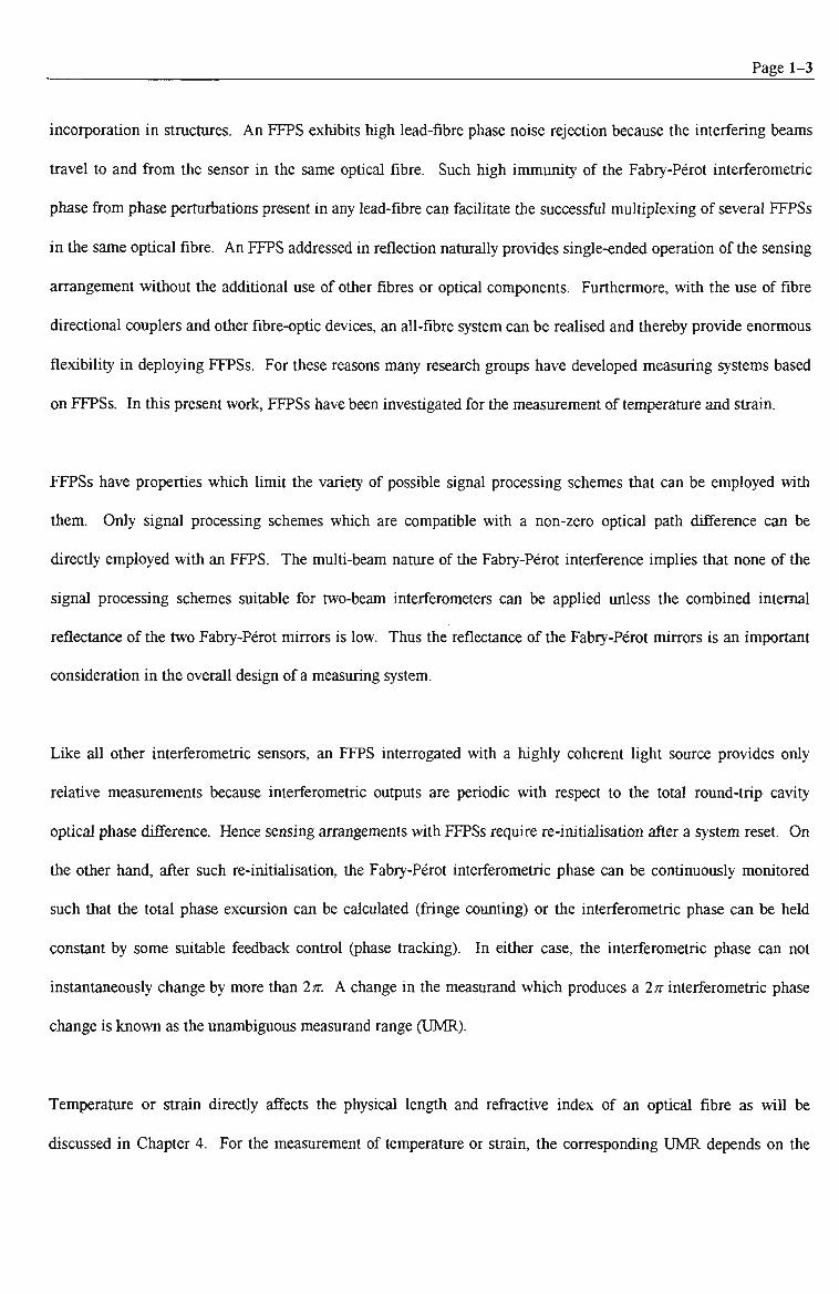
The relevant dual-mode phase, (pj^^i > is given by
( « i - W 2 ) ^ M En 2 13 <Pdual = 2 ^ -^ ^^' 2-l<»
where Li^ is the common physical sensing length of the modes exposed to a measurand. n, and /32 are the
effective refractive indices of the two spatial modes guided in the fibre. There is clearly a close similarity between
a polarimetric and a dual-mode sensor. However, because w, and «2 rc very similar and also depend on the
difference between the refractive index of core and cladding, a dual-mode sensor can be expected to exhibit lower
measurand sensitivity compared with a polarimetric sensor ofthe same sensing length and source wavelength.
2,2,3 Using Direct Physical Techniques
Physical techniques can be applied to an OFS to reduce its sensitivity. Wolinski et al [1996] reduced the
sensitivity of a polarimetric sensor by covering the sensor with a specially prepared cylindrical epoxy . This epoxy-
jacket modified the usual deformation in a highly birefringent (HiBi) fibre caused by temperature, sfrain or
pressure. In their work, Wolinski et al obtained Eyj^p s 5 for the measurement of pressure P . Their technique
can also be applied to interferometric sensors and the corresponding Euj^j^ value depends on the thermo-elastic
properties ofthe epoxy and the thermo-mechanical interaction between the epoxy and an optical fibre.
One method of reducing the sensitivity of a polarimetric sensor is to fusion splice two sections of a birefringent
fibre such that the fast and slow polarisation axes of the first section are aligned respectively with the slow and fast

Page 2-10
axes ofthe second [Farahi et al, 1988b; Bock et al, 1994]. When a lengtii Z,, ofthe first fibre and a lengtii L2 of
the second fibre are exposed to the same average amount of measurand change, the effective sensing length for
polarimetric phase change is reduced to L / =|^i -^2! • Using tiiis technique which effectively provides an
L, +L-, abrupt twist of 90° in a single birefringent fibre polarimetric sensor, E^^^ ^ =
Z,, - L2 Interestingly when
L, s 1-2' the concatenated fibre exhibits very low temperature or strain sensitivity. Such a configuration becomes
ideal in assembling a temperature- or sfrain-insensitive polarimetric sensor designed to measure other effects, e.g.
a Faraday-Effect fibre polarimetric current sensor [Noda et al, 1986; Day & Rose, 1988; Tang et al, 1991; Ning et
al, 1995].
The discussion in the preceding paragraph implies that some of the techniques intended to produce sensors
exhibiting excellent immunity to either temperature or sfrain can alternatively be considered as techniques to
obtain very large UMR since in general the resulting sensors exhibit some residual sensitivity which is ideal for
enlarging the UMR. However, these techniques are not further explored in this chapter because unless such
temperature- or strain- insensitive sensors are used in conjunction with a more sensitive same-measurand sensor,
the dynamic range of such measurand-insensitive sensors is unchanged. UMR-extending techniques which also
enlarge the dynamic range of an interferometric fibre sensor are explored in the next three sections.
2.3 Direct Extension of Unambiguous Phase Measurement Range Approaches
The UMR of an interferometric sensor can be extended if the interferometric phase change (A^) can be
unambiguously determined over a range of more than 2;r radians. For example, Chien [1992] has measured
unambiguously up to 2N7t radians phase shift in what the author refers to as an "open-loop" Sagnac fibre
gyroscope. Similarly, Turner et al. [1992] appUed the same approach to extend the UMR of a polarimetric strain
sensor.
The technique of Chien or Turner et al involves two steps. The first step is modulating the interferometric output
(which is typically proportional to cos(^)) at some carrier angular frequency co^ such that the final elecfronic
(voltage) signal is ofthe form

Page 2-11
V^g=Acos{(o,t + (p) Eq, 2,14
where A is some constant voltage amplitude, q> the interferometric phase and t time. Any one of a variety of
schemes known as "Phase-Generated-Carrier" schemes can be used to obtain an elecfronic signal described in Eq.
2.14 [see Cole et al, 1982; Jackson et al, 1982; Voges et al, 1982; Dandridge et al, 1983; Kersey et al, 1984;
Lewin et al, 1985; Martinelli & De Maria, 1988; Berkoff e al, 1990; Ono et al, 1991; Giulianelli et al, 1994].
In the work of Chien, he used a pseudo-heterodyne signal processing scheme (see Jackson et al, 1982) whilst in
the work of Turner et al, they used a "heterodyne-type" signal recovery scheme similar to that reported by Kersey
et al [1984]. The details of these two schemes are not critically important in the current discussion and are left to
the interested reader to investigate.
The second step involved in the technique of Chien or Turner et al is frequency dividing by N the electronic signal
expressed in Eq. 2.14. Both Chien and Turner et al have chosen,
AT = 2"" Eq. 2.15
where mis a positive integer. Although A can be any integer, frequency division by 2"* can easily be obtained by
observing the final output of m cascaded digital toggle flip-flop circidts, i.e. a binary counter (hence Eq. 2.15).
The result of frequency-down-shifting V^„ can be expressed as SIg
vr^ = A cos ^ t + \ Eq. 2.16 N NJ'
From the measurement of the elecfronic phase of F^g, the effective UMR corresponds to 2;r= A I — j or
2N n = A(p. For this frequency-division method, E^j^^j^^ = N.
The binary-frequency division metiiod of extending the UMR of an interferometric sensor is certainly veiy
attractive because of the exponential nature in extending the final UMR (see Eq. 2.15). However, besides the
method requiring a substantial amount of signal processing, it also reduces the fundamental angular frequency of
the sensing arrangement to—-^. This down-shifted fundamental frequency limits the frequency bandwidth of cp
(and measurand change as well) to a value reduced by a factor of —. On the other hand, the effect of this— A N
factor can be alleviated by choosing a large carrier frequency (10 MHz as in the case of Chien).

Page 2-13
difference /bg f is the product of — 2 ^ ^ the time delay between the interfering beams, and f^aw A v, the constant c
rate of change ofthe optical frequency ofthe light source; i.e.
fbea:=^fsa.^V- Eq. 2.17
/^^^ is the frequency of the sawtootii ramp, LQPD the OPD of the interferometer, and Av tiie optical frequency
ramp amplitude. Subsequently, the resulting interference beats at a frequency of 75, 1 ^nd such beating effect can
be detected by a photodetector. Clearly from Eq. 2.17, variations in LQPD can be determined from variations in the
beat frequency. Hence the measurand dynamic range is determined by the characteristics of the measuring system
for the beat frequency.
An FMCW-type signal processing scheme can be implemented with a single-longitudinal-mode LD with its drive
current modulated in a sawtooth manner [Jacobsen et al, 1982; Giles et al, 1983]. However, this current
modulation results in modulation of both the frequency and intensity ofthe LD output [Kobayashi et al, 1982].
The intensity modulation can be compensated by re-normalisation of the final interferometric output. Several
interferometric or polarimetric sensors based on a FMCW technique implemented with a modulated LD have been
demonsfrated as sfress-location [Franks et al, 1986; Zheng et al, 1996] or displacement/strain sensors [Uttam &
Culshaw, 1985b; Campbell et al, 1996]. However, because ofthe limited dynamic range in the measurement of
the beat frequency and the limitations attributed to the LD current modulation, the OPD of these sensors has been
limited to values between 0.05 m to 10 m. The upper limit is determined by the coherence length of the modulated
LD whilst the lower limit by the desired measurand resolution [Uttam & Culshaw, 1985b]. An OPD resolution in
the order of 100 |xm is not uncommon.
To achieve large dynamic range, the LD needs to be modulated with as large as possible ramp amplimde
frequency, Av. Unfortunately, an ordinary index-guided single-mode LD carmot be modulated vdth a very
large Av without driving the LD output to mode-hop [Economou et al, 1986]. Alternatively, distributed feedback
(DFB) LD can instead be used. The output ofa DFB LD is less susceptible to mode-hop and also exhibits a longer
coherence length than a conventional single-mode LD. Hence with a DFB LD, a longer OPD (~ 30 m) can be

Page 2-14
measured [Zhou et al, 1996]. A drawback with the use of a DFB LD is its relatively high cost compared with
other single-mode LDs.
Recentiy, Zhou et al [1996] demonsfrated a novel technique to extend the measurement range of an FMCW
reflectometer based on a modulated DFB LD. In their work, a uni-directional optical fibre loop was infroduced
into one of the arms of a fibre Michelson interferometer (reference arm) whilst the fibre under investigation was
placed in the other (sensing) arm. The optical fibre loop, which employed an acousto-optic modulator (AOM) and
an opto-isolator, effectively produced several reference beams for the Michelson interferometer. The A -th reference
beam was the beam which had circulated the loop A' (= 0, 1, 2, ...) times. Interestingly the A'-th reference beam OPL
experienced an optical frequency shift of A^XJFS and a relative temporal delay of N x 2L •which were due to c
the operation of the AOM and the inherent delay caused by the optical path length of the loop (OPLi ^p)
respectively, ^FS (= 85 MHz) was the single-pass frequency shift infroduced by the AOM. The relative delay OPL
N X 22L ^as Yvith respect to the zeroth-order (A =0) reference beam which did not fraverse the uni-directional c
loop.
The sensing beam which had traversed the sensing fibre interfered with the N-th reference beam only when the
OPD between these beams was less than the LD coherence length- In their arrangement, OPLi^op had been chosen
to be slightiy shorter than the coherence length ofthe LD output. Consequently, the sensing and the A -th reference
beams interfered when OPD^^re was between N x OPLio^p and (A +1) x OPLi^p. OPDj^,^^ was the optical path
difference between the sensing arm and the reference arm without the loop. Zhou et al obtained a 3-fold increase
(Euj jR] = N = 3) in the measurement range which was limited by the transmission loss of the AOM.
Nevertheless, their technique overcame the limitation imposed by the coherence length of the modulated laser by
utilising a imi-directional optical fibre loop. Unfortunately, the scheme can not be applied to a fibre Fabry-Perot
interferometer which has no spare arm in which to place an optical loop.
The resulting interferometric signal within each ramp period obtained from an interferometer illuminated with an
FMCW-type modulated LD exhibits a characteristic phase relative to the ramp. This electrical phase is practically

Page 2-15
proportional to the OPD of the interferometer and is unambiguous only for a 2;r phase change. Detecting small
changes in the OPD can be obtained from the measurements of the changes in this phase. In such instances, the
beat frequency remains essentially constant. Essentially, what has just been briefly described is the pseudo-
heterodyne phase demodulation scheme [Jackson et al, 1982]. The simultaneous measurement of the beat
frequency and phase of an FMCW interferometric signal can provided an absolute measurement of the OPD with
coarse resolution together with a high resolution measurement of OPD changes [Campbell et al, 1996].
2.4.1,2 Low-Coherence or White-Light Interferometry
Low-Coherence or White-Light interferometry (WLI) generally refers to a scheme which involves illuminating a
(sensing) fibre interferometer with a light source which has a coherence length substantially less than the OPD of
the sensing interferometer and interrogating the output of this sensing interferometer with a second (receiving or
reference) interferometer or with a specfrometer [Rao & Jackson, 1996].
The receiving or reference interferometer followed by a single photodetector may be used to analyse the output of
the sensing fibre interferometer illuminated by a low-coherence source. The photodetector detects interferometric
fringes as soon as the difference between the OPD of the receiving and sensing interferometers is similar to or less
than the coherence length ofthe light source. The signal from the photodetector is recorded while the OPD of the
receiving interferometer is scanned over a range which surrounds and includes the position of zero path unbalance
for the tandem interferometers. For high signal-to-noise ratio and low coherence length, the interferogram
recorded above contains a cenfral fringe which is reasonably easily identified. Changes in the OPD of the sensing
interferometer can be readily fracked by following the changes in the balancing position of the receiver
interferometer. For lower signal-to-noise ratios or long coherence length sources, the identification of the centre of
the low coherence fringe pattern is more difficult. The usual method is to fit an equation to the overall fringe
pattern to identify the cenfral fringe and tiien interpolate between data points to find the cenfre of this fringe. A
number of other techniques have been used for recording the low coherence fringe pattern or for enhancing the
relative size of the cenfral fringe {e.g. recording the whole fringe pattern using a charge-coupled-device (CCD)

Page 2-16
array or superimposing a number of low coherence fringe patterns at different wavelengths [Rao & Jackson, 1996])
but the principle ofthe measurement remains the same.
Sensing interferometers with short OPD are more appropriate for WLI using a scanning receiver interferometer
(the changes in OPD tend to be small). On the other hand, larger OPD sensing interferometers can still be used.
However, an OPD bias generally needs to be infroduced in the receiving interferometer and used together with the
scanning arrangement in order to cope vvith large changes in sensing interferometer OPD. Errors in determining
the value of this OPD bias limit the accuracy in measuring the OPD ofthe sensing interferometer.
A major drawback of WLI using a scarming interferometer is slow signal processing time [Kaddu, 1996].
Typically, the scanning process involved mechanical components which are generally slow [e.g. Koch & Ulrich,
1991]. On the other hand the scanning time can greatiy be reduced by expanding the output beam from the
sensing interferometer onto a wedge Fizeau interferometer which has an average OPD similar to the OPD of the
sensing interferometer. The resulting output produces an interferogram which can be projected onto a CCD array
[Murphy, 1996]. Another contributor to the slow processing time is the detemunation ofthe cenfre ofthe cenfral
fringe. Most low-coherence sources which can launch useful powers into an optical fibre have spectral bandwidths
which are much less than is desirable for WLI. Hence the fringe patterns tend to be relatively long and computer
processing is generally required to find the cenfre ofthe cenfral fringe.
The measurand range for WLI is determined by the scarming range ofthe receiver interferometer. The measurand
resolution is determined by both the scanning resolution ofthe receiver interferometer and by the signal processing
algorithm used to find the cenfre of the central fringe. Although the resulting measurand range can be exfremely
wide, the measurand resolution can not rival the best resolution determined from other interferometric signal
processing techniques. The cenfre of the cenfral fringe can be resolved to as high as 1/200 of a fringe and is
attainable by employing some intra-fringe interpolation schemes [Kaddu, 1996].

Page 2-17
On the other hand, an enhancement ofthe dynamic range can be achieved by first identifying one of the fringes of
the interferogram and following this by fracking a fixed point on this chosen fringe by some active feedback
mechanism which suitably adjusts the OPD of the receiving interferometer (enhanced white-light interferometry)
[Gerges et al, 1987; McGarrity & Jackson, 1998]. Changes in the OPD of the sensing interferometer can be
related to changes in the feedback signal. However, the measurand range in such an arrangement is limited by the
fracking range ofthe feedback system.
The intensity of resulting optical output of the sensing interferometer remains constant even though the OPD has
been modulated by a measurand such as temperature or sfrain. On the other hand the output of the sensing fibre
interferometer has an optical spectrum which can be modified by variations in the OPD. In the wavelength
domain, the output spectrum ofthe sensing interferometer exhibits regular specfral peaks which are separated by a
wavelength difference inversely proportional to the OPD ofthe interferometer, i.e. a channelled spectrum. Clearly
by employing a specfrometer, a measurement of the specfral separation between adjacent peaks is a simple and
direct measurement ofthe OPD [Egorov et al, 1995; Bhatia et al, 1996]. On the other hand, the use ofa usually
bulky specfrometer is not atfractive for practical applications, and such measurements are generally limited to
laboratory conditions. Specfrometer measurements usually involve long processing times and give measurand
resolution dictated by the spectral resolution ofthe specfrometer.
White-light interferometry is certainly very atfractive because an LED can be used as the light source. LEDs are
low cost and easy to operate compared vrith an LD. Although an LED has low output power, higher power super-
luminescence LEDs (SLEDs) can also be used.
2,4.2 Measurement of Optical Path Length, Group-Delay, Dispersion of an Optical Fibre
2.4,2.1 Dispersive Optical Fourier Transform Spectroscopy
A closely related technique to WLI is dispersive optical Fourier transform spectroscopy (DFTS). Unlike WLI
which requires a sensing interferometer and a receiving interferometer, DFTS requires only one interferometer, the
sensing interferometer. The technique involves calculating the phase information from the Fourier fransform of

Page 2-18
the resulting interferogram as the OPD of the sensing interferometer is scaimed. The sensing interferometer
effectively filters only the beams with wavelengths simultaneously falling within the spectrum of the light source
and the fransfer spectrum ofthe interferometer, i.e. a chaimelled spectrum. The sfrength of DFTS is its capabihty
to extract the information attributed to the dispersion in the sensing interferometer as the specfral spacing of the
channelled spectrum is varied.
Typically in DFTS, a sensing interferometer is illuminated by two light sources, a low-coherence source {e.g. an
LED) and a high-coherence source {e.g. a stabilised HeNe laser). While the OPD ofthe interferometer is varied to
produce the interferogram corresponding to the low-coherence source, the interference fringes corresponding to the
high-coherence source can be used to calibrate the scan of the white-light interferogram. This interferogram and
the output optical spectrum ofthe interferometer form a Fourier fransform pair.
Flavin et al [1993] have employed DFTS for the simultaneous measurement of temperature and strain (SMTS).
They obtained two simultaneous equations to discriminate temperature and strain by measuring the changes in the
difference in the group delay and in the difference in the dispersion between the two arms of the interferometer
[Flavin et al, 1994]. These differences can be extracted by fitting a cubic polynomial to the phase of the Fourier
fransform of the resulting white-light interferogram. The linear and quadratic coefficients of the fit represent the
change in the difference in the group delay and in the difference in the dispersion respectively.
DFTS was exfremely successfully in SMTS because the condition number for the corresponding sensitivity matrix
K is very close to unity. On the other hand, the technique of Flavin et al does not allow any possibility of
increasing the measurand range because the linear and quadratic coefficients of the cubic fit are not periodic with
temperature or sfrain. To increase the dynamic range ofthe measurement scheme, the dynamic range in obtaining
the interferogram needs to be similarly increased.
As in the case with WLI, the requirement to scan the OPD of an interferometer and the need to subsequentiy
calculate the Fourier transform of the interferogram limit the speed of measurement. Scanning the OPD of the

Page 2-19
interferometer generally implies mechanical components which may not be suitable in practical measurement
environments. Moreover because the OPD ofthe interferometer needs to be scanned around its zero value, optical
Fourier Transform specfroscopy is not suitable for a fibre Fabry-Perot interferometer which always has a non-zero
OPD.
2.4.2,2 Measurement of Optical Path Length, Group-Delay, Dispersion of an Optical Fibre
One ofthe techniques that can be employed for SMTS is to measure the changes in both the optical path difference
and the dispersion ofa sensing optical fibre [Gusmeroli & Martinelli, 1994]. In their arrangement, Gusmeroh &
Martinelli infroduced a sensing fibre into an arm of a nearly balanced fibre Mach-Zehnder interferometer
illuminated with 855 nm superluminescent source with a bandwidth of 17 nm. The output of the interferometer
was analysed with a bulk-optic Michelson interferometer which had an OPD very similar to that of the sensing
fibre Mach-Zehnder interferometer. To recover tiie phase of the sensing interferometer, the OPD of the Michelson
interferometer was fiirther varied in a sawtooth manner in order to produce a periodic (serrodyne) signal, i.e. a
phase-modulated receiving interferometer {c.f. Brady et al, 1995; Rao et al, 1997b).
Instead of directiy detecting the output of the Michelson interferometer with a single detector (which can also
detect variations in the OPD of the sensing interferometer), Gusmeroli & Martinelli optically filtered the
Michelson output beam into three separate beams detected by separate photodiodes. The filters were 5 nm band
pass filters whose peak wavelengths were 845 mn, 855 nm (the cenfral wavelength ofthe source) and 865 nm. The
three resulting signals varied at the same modulation (sawtooth) frequency but had different phase values because
ofthe variations ofthe OPD ofthe Mach-Zehnder interferometer with wavelength {i.e. dispersion). Gusmeroli &
Martinelli subsequently measured the relative phase of the 845-nm and the 865-nm (non-central wavelength)
signals with respect to the 855-nm (cenfral wavelength) signal. The sum of these two relative phase measurements
was found to be proportional to the optical path difference whilst the difference between them to the dispersion.
The condition number for the corresponding matrix K for tiie technique of Gusmeroli & Martinelli was far from
unity since the two differential phases were expected to have similar sensitivities. On the other hand, their sensing

______________^ Page 2-20
arrangement would provide 'UJI^T- =382 and Ejj}^^^ =4925. The relatively large E^^^j^ values compared
with the Euj^ fjiy2lm.es for the other techniques described in this chapter, can be attributed to fact that the
sensitivity of the difference between the two differential phase measurements can be ex-pected to be much less than
either of the two differential phase measurements. In a sense, the techruque of Gusmeroli & Martinelli can be
considered as a three-wavelength technique.
Incidentally, DFTS can also measure the change in optical path length of the test fibre by extracting the zeroth
order coefficient of the cubic polynomial phase fit. Compared with DFTS, the technique of Gusmeroli &
Martinelli does not require the acquisition of an interferogram. However both techniques are similarly complex in
terms ofthe amount of optical components required \c.f. Flavin, 1993; Gusmeroli & Martinelli, 1994].
Using a technique with some similarity to that of Gusmeroli & Martinelli, the mean and differential group delays
between the fast and slow axis ofa (sensing) birefringent fibre illuminated with a broadband source can be used for
SMTS [Luke et al, 1996]. In their arrangement, Luke et al analysed the beams from a sensing birefringent fibre
using a scanning Michelson interferometer. The scanning interferometer had along one of its arms a reference
birefringent fibre with a length chosen in order to balance the OPD and dispersion between the sensing and
reference fibres. From the resulting interferogram, the mean and differential group delays were calculated. Both
the mean and differential group delays unambiguously measure, with different sensitivities, the temperamre-sfrain
state ofthe sensing fibre. Such unambiguous measurements of temperature or sfrain imply that the dynamic range
ofthe sensing arrangement can only be increased by improving the resolution in the group delay measurements.
2.4,3 Spectrally-Encoded Measurements
There are several optical fibre sensors which produce an optical output with an optical spectrum that can change
with temperature or sfrain. Because temperature or sfrain is uniquely encoded with the wavelength, a potentially
unlimited measurand range can be obtained. However, the measurand resolution is limited by the resolution ofthe
specfrometer. In the subsequent discussions, several specfrally-encoded sensors which have been reported for
SMTS are described and assessed for their suitability for high-resolution and wide-range measurements. In the

Page 2-21
discussions below the two most important specfrally-encoded sensor types are discussed. These sensors involve
Brillouin scattering and in-fibre Bragg gratings.
2,4,3.1 Brillouin Scattering Sensors
One ofthe methods reported for SMTS exploits Brillouin scattering in an optical fibre [Parker et al, 1997; Izumita
et al, 1997]. The simultaneous measurement of the frequency shift and optical power of a Brillouin scattered
beam, which can have different sensitivity to temperature and sfrain, provide two independent measurements. The
determinant of the corresponding sensitivity matrix J is non-zero and hence the technique is suitable for SMTS.
However, the extension of measurand range for these sensors is not relevant as neither the scattering frequency nor
the scattered power is periodic with respect to temperature or sfrain. Although Brillouin scattering is not an
interference effect, the detection ofthe frequency shift ofa Brillouin scattered beam is obtained interferometrically
Pavis & Kersey, 1997].
Davis & Kersey [1997] detected the Brillouin scattering frequency shifts and the wavelength shifts ofa fibre Bragg
grating in a single fibre for SMTS. For ease of detection, the optical wavelength of the Brillouin beam and the
Bragg wavelength were chosen to be substantially different, 1319 nm and 1551 nm respectively. Davis & Kersey
expected different temperature and strain sensitivities for the Brillouin scattering frequency shift and the Bragg
wavelength shift because Brillouin scattering and the Bragg resonance in an optical fibre are different physical
processes. However their arrangement was quite complex because it required one set of equipment to detect Bragg
wavelength shifts and another to determine Brillouin scattering frequency shifts. The system described by Davis &
Kersey is more suited to measurements in the laboratory rather than in the field.
High resolution Bragg wavelength shift measurements can be achieved using an interferometer (see section
2.4.3.2). In such cases, the Bragg wavelength shifts can provide high resolution measurement whilst the Brillouin
scattering frequency can identify the fringe order of the phase change in the interrogating interferometer used to
measure the Bragg wavelength shift.

Page 2-22
2,4,3,2 In-Fibre Bragg Grating Sensors
In-fibre Bragg gratings (FBGs) are one of the most promising developments in optical fibre sensing technology
[Rao, 1997; Kersey et al, 1997]. FBGs are attractive because they can be illuminated by a low-coherence source
and a direct measurement of their central Bragg wavelength feature using a spectrometer can determine
unambiguously the total shift due to temperature or strain.
However shifts in the Bragg wavelength due to temperature or strain are very small. For example at a Bragg
wavelength of Aj, = 785 nm, A^jAT =s 5 pm/°C and A^fe « 0.6 pmj/js for temperature and sfrain respectively.
Hence to obtain highly resolved measurements, detection of very small shifts in the Bragg wavelength is crucial.
Unfortunately, typical optical spectrometers exhibit low wavelength resolution. Alternatively, an FBG can be
interferometrically interrogated by simply directing the reflected beam from an FBG towards an unbalanced
interferometer [e.g. Kersey et al, 1992; Weis et al, 1994]. The equivalent interferometric phase change, A<p, due
to a Bragg wavelength shift, AA^ is given by
Ap = 2n^^AA^ Eq. 2.18 ^b
where LQPJ^ is the OPD of the interrogating interferometer. Choosing a large value for Lpp,^ means a large
measurand resolution. However LQP,^ can not be longer than the equivalent coherence length of the FBG beam
otherwise no interferometric phase change can be detected. The spectral bandwidth and hence the coherence
length of the FBG beam depend on the spectrum of the illuminating light source and the reflectance spectrum of
the FBG. For a typical grating with a bandwidth of 0.2 nm, the equivalent coherence length is about 3 mm for
Af, = 785 nm. Likewise the interferometric detection of wavelength is unambiguous only for an interferometric
phase change equivalent to 2n. Eq. 2.18 shows that to achieve a UMR that is as large as possible, the OPD of the
interferometer LQPD can be chosen to be as short as possible. Hence the choice of the value of LQPQ determines
both the measurand range and resolution. Obviously issues pertinent to interferometric detection of Bragg
wavelength shift are similar to that of a fibre interferometer.

Page 2-23
The UMR for the interferometric detection of Bragg wavelength shifts can be extended using two interferometers
with OPDs Z-opD 1 and Z,OPD,2 • Assuming LQP^^ > LOPD,2 . the ratio between the equivalent Bragg-wavelength-
phase-measurand sensitivities ofthe two interferometers is given by
K^^=I:2E£^>1, Eq. 2.19
For a dual-interferometric interrogation ofwavelengtii shifts ofa single FBG, E^f^j^ is given by Eq. 2.7orEq.
2.8 depending on the value of K^j^^.
Rao et al [1996] employed a dual-cavity interferometric wavelength scanner based on the Michelson
interferometer with its OPD sawtooth-modulated [Brady et al, 1995]. The OPD ofthe interferometers, LQPP^ =
2.03 mm and LQPJ^2~ 0-71 mm, were obtained by switching between two different length values of one ofthe
arms of the Michelson interferometer during a measurement run. These OPD values gave Ejjj^j^ - 2.85.
Clearly, the response time of this arrangement was limited by the rate at which the OPD of the interferometer can
be changed.
Alternatively, the wavelength shifts of a single FBG can be detected using two cascaded interferometers with
different OPD, LQP,^ , and lopn 2 • The first interferometer is the usual interferometric wavelength scarmer
whilst the second interferometer is a phase-modulated (serrodyne) receiving interferometer [Rao et al, 1997b].
Rao et al [1997b] used Z-oro.i = 28 mm and IOPD,2 =0-7 ™^ to achieve Eyj^^ = 40. The advantage of tiiis
latter arrangement was that the phase of each interferometer can be frequency-multiplexed. Conceptually two
interferometers can also be employed in parallel.
There are alternative Bragg-wavelength-detection schemes which can rival interferometric detection of Bragg
wavelength shifts. The beam reflected from an FBG can be used as the input beam to an interferometer whose
OPD can be varied about the zero-OPD value, ff the OPD scan is calibrated with respect to the interferogram for a
reference beam {e.g. 1.319 |j.m Nd:YAG beam), the Fourier transform of the interferogram for the FBG beam can
be calculated, i.e. Fourier fransform specfrometer pavis & Kersey, 1995]. The dominant high frequency
component ofthe FBG interferogram corresponds to the Bragg wavelength of the grating. Interestingly, to obtain

Page 2-24
this high frequency component, a short scan of the FBG interferogram is sufficient. Clearly, such method can
improve the interrogation/processing time of the FBG. In addition, the method can be used to demultiplex the
signals from two FBGs which would exhibit different values for the high frequency component in their
corresponding interferograms [Flavin et al, 1997],
Recentiy Dakin et al [1997] employed a novel scheme to interrogate an FBG. Their scheme was based on pairing
the FBG with another grating with similar characteristics. The second grating was infroduced into the same fibre
to form a fibre Fabry-Perot interferometer (FFPI). In their arrangement, the FFPI was illuminated using a broad
band light source and was exposed to the measurand. The reflection from the FFPI was interrogated using a
Michelson interferometer {i.e. white-light interferometry). The sfrength ofthe technique of Dakin et al. was based
on changing the OPD of the Michelson interferometer at a fast rate. Subsequentiy as soon as the OPD of the FFPI
and the Michelson interferometer were similar, a burst of interference fringes can be observed at the output of the
Michelson interferometer. This burst of fringes was essentially a temporal version ofthe white-light interferogram
for the FFPI. This temporal interferogram manifested a dominant characteristic frequency corresponding to the
Bragg wavelength of the grating pair. Shifts in the wavelength of the grating was exhibited as shifts in the
dominant frequency of the temporal interferogram. The average velocity in displacing the scanning mirror of the
Michelson interferometer had to be high in order to obtain a large dominant frequency in the detector output so
that resolution was possible. The scheme can be used to coherentiy multiplex several gratings which had been
paired with similar gratings to form FFPIs with different OPDs. Each grating pair can be differentiated by the
different arrival times of the corresponding burst of fringes or temporal interferogram. The different arrival times
were due to tiiie different OPD of die FFPIs.
Fibre lasers based on FBGs can be used to measure temperature or strain [Ball et al, 1993; Othonos et al, 1993].
Shifts in lasing wavelength of a fibre laser with FBG reflectors can either be caused by the temperature or sfrain
sensitivity of the gratings or the laser cavity. Likewise, the output of a fibre laser can be detected
interferometrically [Koo & Kersey, 1995]. Conceptually, two fibre lasers with different sensitivities to temperature
or sfrain can be multiplexed to provide SMTS or provide an extended dynamic range single-measurand

Page 2-25
arrangement [Alavie et al, 1993; Kersey & Morey, 1993; Koo & Kersey, 1995]. The major advantage of a fibre
laser is greater signal-to-noise ratio at the detector compared with an FBG illuminated by a broad-band source.
However the need to ensure population inversion in the fibre laser cavity increases the complexity- of any sensing
artangement based on fibre lasers.
Many sensing arrangements based on two FBGs with different sensitivities to temperature and sfrain have been
exploited for SMTS. One of tihie earliest of these schemes involved two FBGs, a sensing and reference FBG.
[Morey et al, 1992b]. The reference FBG, which is configured to be protected from strain, can be used to measure
the temperature ofthe sensing FBG.
Alternatively, these dual-FBG sensing arrangements can be used to obtained a sensing arrangement with a high
measurand resolution. In such cases, these dual-FBG arrangements can either be classified as a dual sensor or a
dual-wavelength technique. However because much work has been reported in the use of FBGs for SMTS, these
FBG-based schemes are described in a separate sub-section (2.5.3) after schemes involving two distinct sensors or
light sources have been described.
2.5 Dual-Measurement Approaches
2.5.1 Two Distinct Sensors
One of the simplest methods of extending the UMR of an interferometric sensing arrangement is to employ two
interferometric sensors with either very different or very similar sensitivities. Although a birefringent fibre
interferometric sensor described in section 2.5.5 can be considered as a dual interferometer formed at the same
location, techniques employing two distinct sensors are described in this present sub-section. An extended
dynamic range is exhibited by the combined operation of the two distinct interferometric sensors which by
themselves provide a limited UMR. Unfortunately, the improvement in the performance of the combined sensor
comes at the cost of two signal demodulation schemes.

Page 2-26
2.5.1,1 Schemes Not Involving Fabry-Perot Interferometric Sensors
Chiang & Tsuchida [1988] demonsfrated a dual polarimetric sensor which exhibits an extended temperamre range.
The two polarimetric sensors employed birefringent fibres of the same type but of slightly different (sensing)
lengths, Z,i(= 520 cm) and L2 (= 500 cm), exposed to temperature. Because the same type of fibres was used,
EuMR,T = I '—i" (o'" ^UMR.T = 26). Experimentally, Chiang & Tsuchida observed slightiy higher Eyj^j
values for different pairs of sensing length and attributed their results to their under-estimation of the sensing
lengths ofthe fibre. Their underestimation may have been compounded by thermal conduction along the fibres.
Alternatively, a similar result can be obtained by employing two fibres with different characteristics. Herzog &
Meyrueis [1990] arranged pairs of single-mode fibres of different physical properties into two fibre Mach-Zehnder
interferometers. Each interferometer was fabricated from the same type of fibre and one of the arms of each
interferometer was placed in the measurement environment {e.g. pressure chamber). Herzog & Meyrueis
successfully employed this double interferometric fibre sensing arrangement to measure pressure (P) with good
performance for correcting temperature-induced effects. To extend the UMR for either pressure or temperature,
EuMR M is given by Eq. 2.7 and Eq. 2.8, depending on the sensitivity ratio ofthe two fibres interferometers. For
example, using one of their pressure measurement results, Eyj^p « 3 could be obtained.
Navarette & Bemabeu [1994] proposed a three-branch fibre interferometer based on fibre Mach-Zehnder
interferometers for tiie measurement of two parameters. Their three-branch design involved infroducing a (inner)
fibre Mach-Zehnder interferometer into one of the arms of the second (outer) Mach-Zehnder interferometer.
Essentially this novel arrangement can be considered as a system of two fibre Mach-Zehnder interferometers with a
common reference arm and two sensing arms. Navarette & Bemabeu suggested that if the sensing arms have
different sensitivities and same temperature and sfrain, then temperattire and strain can be discriminated. On the
otiier hand, as an extended-UMR single-measurand arrangement, Ey^Rj^ depends on the effective lengtiis of tiie
two arms exposed to the measurand as was the case with the technique of Chiang & Tsuchida [1988].

Page 2-27
2.5,1.2 Schemes Involving One Fabry-Perot Interferometric Sensor
Zhou & Letcher [1995] developed a fibre-optic Fabry-Perot microphone addressed in reflection. Their sensor
measured the displacement of a diaphragm caused by acoustic vibration over an extended (displacement) range.
The sensor was based on an extrinsic Fabry-Perot interferometric sensor and an intensity-modulated sensor placed
side by side in a single assembly. The surface ofthe diaphragm was placed very close and parallel to the end faces
of a single-mode and a multimode fibre. The distal end face of the single-mode fibre and the surface of the
diaphragm formed an extrinsic Fabry-Perot sensor whilst that of the multimode fibre and the diaphragm, the
intensity-modulated sensor. The intensity coupled back by the diaphragm into the multimode fibre depends
inversely proportional to the square of the separation width between the distal end of the multimode fibre and the
diaphragm. As the diaphragm vibrated, the variation in intensity received by the multimode fibre can be used to
identify the fringe order of the interferometric phase change in the extrinsic Fabry-Perot sensor. Since the received
intensity behaved monotonically with the displacement of the diaphragm, f swR.M can be large and limited by the
minimum change in the received intensity that can be detected. On the other hand, the diaphragm can also be
displaced by drifts in temperature. Hence the intensity-modulated signal may only be effective for dynamic
displacement, i.e. mechanical vibration.
In another arrangement, a fibre Bragg grating (FBG) sensor can be combined with a Fabry-Perot sensor. For the
simultaneous measurement of temperature and micro-displacement, Ferreira et al, [1996] specially designed and
fabricated a sensor head which contained a single-mode fibre protruding from one end of the sensor head. The
distal end ofthe single-mode fibre faced a mirror which could be mechanically displaced. Within the section ofthe
fibre dangling inside the sensor head, an FBG was inscripted. Effectively, the sensing arrangement consisted of
two sensors in series, an FBG sensor which is affected only by temperature change and an extrinsic Fabry-Perot
interferometer which was affected by both temperature and the displacement of the mirror (relative to the fibre
end). For dual-parameter measurements, the Bragg wavelength of the FBG can be used to measure the
temperature of tiiie extrinsic Fabry-Perot sensor. Alternatively to obtain a large dynamic range for temperature
measurements, the Bragg wavelength shift can be used to identify the fringe order of the interferometric phase of
the extrinsic Fabry-Perot sensor.

Page 2-28
Lui et al [1997] developed a similar sensor head to that of Ferreira et al [1996] which they embedded in a
composite material for SMTS. The sensor head of Lui et al involved a multimode fibre facing the end of a single-
mode fibre with an FBG. Both the single-mode and multimode fibres were fusion spliced to a hollow capillary mbe
(128/300 |a,m) such that the FBG intentionally remained sensitive only to temperature. The sensing arrangement of
Lui et al. behaved similarly to that of Ferreira et al. for simultaneous measurement of temperature and micro-
displacement/sfrain and for extended-range temperature measurements. Unlike Ferreira et al, Lui et al found that
their FBG exhibited a residual sensitivity to sfrain. This residual sensitivity can be attributed to fact that the FBG
may not be dangling completely freely inside the capillary tube as intended. The diameter of the fibre was very
similar to the inside diameter of the capillary mbe which may also had been deformed when the whole sensor was
embedded. This residual strain sensitivity of the FBG may be interferometrically detected and the resulting phase
sensitivity combined with the phase ofthe extrinsic Fabry-Perot sensor to produce an extended UMR sfrain sensor.
Instead of using a hollow capillary tube, an in-line Fabry-Perot etalon (ILFE) can be used in tandem with an FBG
[Jin et al, 1997]. The advantage of using an ILFE is that a continuous uniform-diameter fibre can be formed and
hence the resulting in-fibre sensor is ideal for embedding in composite materials. Jin et al realised that the ILFE
was only sensitive to axial strain whilst the FBG to both axial and fransverse strain. With their ILFE/FBG hybrid
sensor, they were able to simultaneously measure axial and transverse strain. Since axial and transverse sfrain can
not be separated without much difficulty within a composite material, their sensor can not be used solely to
measure axial sfrain in such circumstances. The ILFE/FBG sensor is also sensitive to temperature. A third sensor
would be necessary to simultaneously measure all three parameters {c.f. the arrangement of Udd et al. [1997]
described in section 2.5.3).
An intrinsic fibre Fabry-Perot interferometer can be combined with an FBG to measure several parameters. Rao et
al [1997c] employed an FFPI composed of FBG reflectors in tandem with another FBG sensor along the same
fibre. In their arrangement, Rao et al. were interested in simultaneously measuring temperature, strain and
vibration. To measure vibration, the change in tiie OPD of the FFPI was interferometrically detected whilst the
Bragg wavelength shifts in either of the twin FBG reflectors was used to measure temperature. The two FBG

___^_ Page 2-29
reflectors were both protected from sfrain whilst the Bragg wavelength shifts of the third FBG was employed to
discriminate sfrain. All three FBGs were placed very close to one another in order to ensure that either of the twin
FBGs can measure the temperature of the third grating. Because of the narrow bandwidth of an FBG, several
grating-based FFPIs can be wavelength-multiplexed [Henderson et al, 1997].
2.5,1,3 Schemes Involving Effectively Two Distinct Fabry-Perot Interferometric Sensors
An extrinsic in-line Fabry-Perot etalon can be followed by an intrinsic fibre Fabry-Perot interferometer to form a
dual Fabry-Perot sensor [Singh & Sirkis, 1997]. Along an optical fibre, an ILFE was first fabricated [Sirkis et al,
1995]. The distal end ofthe concatenated fibre was cleaved at some short distance from the ILFE, thereby forming
an intrinsic FFPI. The ELFE and the FFPI sensors exhibited different sensitivities to temperature and sfrain as
expected. Singh & Sirkis have interrogated both sensors with two separate interferometers and have been
successful in simultaneously measuring temperature and strain.
For extended-UMR measurements, their sensing arrangement would give E^j^j = 100 (using Eq. 2.8) and
EuMR,e = 3-8 (using Eq. 2.7) for temperature and sfrain respectively. The large value of Ey^^j had been
anticipated because the ILFE was expected to exhibit a weaker sensitivity to temperature than the silica-core FFPI.
The sensitivity of an ILFE to temperature was atttibuted to the low thermal expansion of silica (~0.5x 10'*/°C) and
tiie low thermo-optic coefficient of air (-0. Ix 10'*/°C) whilst the temperatore sensitivity ofthe FFPI was determined
by tiie large thermo-optic coefficient of silica (-12 x 10"*/°C) [Singh & Sirkis, 1997].
An FFPI with identical high-reflectance FBG reflectors which is illuminated with a broad-band source yields a
reflection spectrum which exhibits Fabry-Perot longitudinal mode structures with an amplitude envelope
corresponding to tiie reflection spectrum of tiie FBG [Shlyagin et al, 1997]. The change in the optical lengtii of
the Fabry-Perot cavity and the FBG pitch can be detected from shifts in the longitudinal mode and the spectral
envelope exhibited by the reflection spectrum of a twin-grating FFPI. Typically the shifts in the longitudinal
modes are simpler to detect. Potentially two grating-based FFPIs with different sensitivities to temperature and

Page 2-30
sfrain, either operated in parallel or in series, can be used to discriminate between these two parameters or
alternatively to obtain a large dynamic range single-measurand sensing arrangement pakin et al, 1997].
Earlier, Wosinski et al proposed [1992] and evaluated [1994] a dual Fabry-Perot sensor with two low-reflectance
Bragg grating reflectors written in both cores of a twin-core fibre. In their arrangement, the twin-core fibre was
required to have its cores sufficientiy separated to avoid any cross-talk between the cores. The two measurements
needed for SMTS were obtained by illuminating each core with slightiy different wavelength light sources. The
novelty of this dual-interferometric sensor was that the two Fabry-Perot interferometers measure practically the
same region, ff the light sources have similar wavelengths, the corresponding temperature and sfrain sensitivities
were not expected to be very different unless the materials for the two cores were intentionally chosen to be
different [Wosinski et al 1994].
2,5,2 Dual Wavelength Techniques
2,5.2.1 Extending the UMR of Interferometric/Polarimetric Sensors
One ofthe earliest techniques to extend the UMR of a fibre interferometric sensor was to excite the sensor with two
light sources with different but similar wavelengths [Farahi et al, 1988a]. The two wavelengths can be derived
from separate sources like two single-mode LDs [Kersey et al, 1986] or from a single laser output, e.g. an Argon
laser [Gauthier &. Turgeon, 1993]. Similarly two equivalent tight sources with different wavelengths can be
synthesized from the fransmission through optical band-pass filters [Webb et al, 1988b].
By using a two-wavelength illumination of a single fibre interferometric sensor, the corresponding phase at each
wavelength exhibits slightly different measurand sensitivities. For extended-UMR measurements, the
interferometric phase at each wavelength can be measured in the usual maimer and the difference between the two
interferometric phase measurements, the differential phase, can be used to identify the fringe order of the phase
change of either ofthe two phase measurements piu et al, 1991]. ff the two (closely-spaced) wavelengths are A,
and A 2, then

^UMR,M = / t i ~~ >^2
Page 2-31
Eq. 2,20
where A is the average of the two wavelengths. The smaller the wavelength difference, the greater is the value of
EuMR,M- OJ" example, by using two LDs with /i,=785nm and A2 =1^3v[m,Eu,^]^ =39Q. The
unambiguous phase range for the two wavelengths together corresponds to a 2;T phase change for an A \A 2
interferometric sensor illuminated by an effective wavelength of . The minimum wavelength difference ^\~ A2
between the light source is determined by the phase noise generated by the light sources [Meggitt et al, 1988].
Alternatively, a suitably scaled electronic version of interferometric signal for each wavelength can become the x-
and y-axis inputs of an oscilloscope and thereby fracing a Lissajous figure as the phase for each wavelength varies
[McGarrity & Jackson, 1996]. Interestingly, when either ofthe two wavelengths is not an integral multiple of their
wavelength difference, the instantaneous location and slope of the Lissajous figure on the oscilloscope monitor can
uniquely identify the relative phase (< 2;z) and fringe order (multiples of 2;r) of each wavelength-multiplexed
interferometric phase.
Similarly, the UMR of a polarimetric sensor can be extended using a dual-wavelength technique [Kersey et al,
1989; Gauthier & Turgeon, 1993]. The measurand resolution remains that obtained by simply using tiie smaller
wavelength phase measurement.
2,5.2,2 Extending the UMR of Dual-Evanescently-Coupled-Core Fibre Sensors
Provided that the cores of a dual-core fibre are close enough, optical energy in one of the cores can transfer to the
other core and back by evanescent coupling. Changes in coupting are detectable as changes in intensity ofthe light
leaving the fibres. The periodic nature of this coupling can be characterised by a beat lengtii which depends on
temperattire or strain. Since the coupting lengtii also depends on the wavelengtii of tiie light source, SMTS can be
achieved by illuminating the twin-core fibre witii two light sources with different wavelengths [Meltz & Dunphy,
1988]. For two similar wavelengUis, the corresponding coupling-measurand sensitivities are likewise similar and

Page 2-32
hence suitable for extending the UMR of a dual-core evanescent sensor. Clearly, a twin-core evanescent sensor is
an atfractive sensor configuration because both cores can measure a parameter at tiie same location.
A dual-wavelength technique is very effective in extending the UMR of an interferometric sensor but not for
SMTS. This can be expected because the total dispersion in the fibre for a small wavelength difference is
extremely small. Mathematically, employing two different but similar wavelengths simply produce two phase
measurements which are linear combination of one another unless the total dispersion between the two
wavelengths is high. Thus, dual-similar-wavelength arrangements exhibit a very large condition number for the
cortesponding sensitivity matrix K .
2,5,2,3 More-Than-Two-Wavelength Dlumination
More than two wavelength sources can also be utilised to extend the UMR of an interferometric OFS. The
effective UMR corresponds to the difference between two measurand values; at each of these values, the modulo-
271-values for the interferometric phase corresponding to each wavelength, are the same {i.e in-phase condition).
Theoretically, compared with two wavelength illumination, more-than-two-wavelength illumination can provide a
much wider UMR value for an interferometric sensor provided that the phase-measurand sensitivities of the
different wavelengths are not multiples of one another.
Gauthier & Turgeon [1993] have employed the 476 nm, 488 nm and 502 nm output of an Argon ion laser to
illuminate a polarimetric temperature sensor. For their purpose, Gauthier & Turgeon have exploited only two of
the wavelengths of the output of an Argon ion laser to obtain a large UMR with their polarimetric sensor.
Although their arrangement can potentially give a larger UMR, the use of an Argon ion laser can be considered
impractical in many circumstances.
Sharma & Posey [1995] demonstrated an extended-range multi-wavelength temperature sensor using the
interference at each wavelength between the LP02 and LP21 modes in a few-mode fibre. Instead of using
conventional light sources, Sharma & Posey generated an effective (about 5) multi-wavelength light source in a

Page 2-33
few mode fibre. Such a multi-wavelength light source was produced by Stimulated Raman Scattering (SRS) in a
few-mode fibre. The scattered beams were predominantiy manifested in the LP02 mode and exhibited different
characteristic wavelengtiis. For each wavelength, a simple microbend in the fibre coupled a fraction of the initial
LP02 mode SRS light into the LP21 mode which was subsequentiy allowed to interfere with the remaining light in
the LP02 mode. The use of high laser power and SRS in optical fibres is generally not an attractive way to produce
multiple wavelengths in a practical sensor.
2,5.3 Dual In-Fibre Bragg Grating Sensors
Many techniques employing two fibre Bragg gratings have been demonstrated for SMTS. These techniques can be
used to give an extended-UMR while providing high measurand resolution. High measurand resolution may be
achieved by detecting wavelength shifts ofthe two FBGs using two interferometers (one for each FBG). ff Kj^^ is
a wavelength-measurand sensitivity ofthe /-th FBG with Bragg wavelength Af^,, following from Eq. 2.18,
K,M=2^^Kl^ Eq. 2.21
is the equivalent phase-measurand sensitivity exhibited by an interrogating interferometer with an OPD of IQPO ,.
The ratio ofthe equivalent phase-measurand sensitivities ofthe two Bragg wavelength shifts is
^rHA~ ^\M
-rM Y ^2M
^OPD,\ f .2 \
''6,2
V ^OPD,2 / \^b,\ J
f V ^ '^\M
K^2MJ
Eq. 2.22
OPD 1
By suitably choosing the value of the ratio ^ , either the condition K^M^IOX K^^ » 1 can be obtained. ^OPD,2
However in most cases, obtaining K^j^^ s i demands less constraints on the choices for the values of Z-op ,, and
^0PD,2 which determine the un-improved UMR and the measurand resolution as in the case of interferometric
interrogation ofa single FBG (see section 2.4.3.2). The closer K^u is to its unity value, the larger is the value of
^UMR,M (using Eq. 2.7). Interestingly, Eq. 2.22 reduced to Eq. 2.20 the case of interrogating a single FBG using
two interferometers (see section 2.4.3.2).
On the other hand, the best scheme to obtain an exfremely large dynamic range and potentially unlimited UMR is
to interferometrically interrogate only one (preferable the more sensitive) of the two gratings simultaneously using

Page 2-34
the wavelength shift of the other to identify the fringe order of the interferometer. For example, an arrangement
similar to that of Brady et al. [1997] could be used to obtain large dynamic range measurements. Brady et al
[1997] used a Mach-Zehnder interferometer and a tunable acousto-optic filter to detect Bragg wavelength shifts of
two gratings.
The "price" ofthe above mentioned schemes to improve the dynamic range ofa dual-FBG arrangement is the need
to employ either two interferometers or one interferometer and a spectrometer. However, especially when the two
Bragg wavelengths of the FBGs are far apart, a single interferometer can be used if followed by appropriate
wavelength-separating optics. Certainly the use of a single interferometer is an attractive and optimised
alternative. In this present sub-section, for the sake of also defining some point of comparison with the other
techniques discussed in this chapter, the Ejjj^j^ values for the various dual-FBG arrangements are evaluated
assuming the two Bragg wavelength shifts are detected using a single interferometer. The interrogating
interferometer is preferably non-dispersive, (e.g. the interferometer is composed of air-path-arms). In such cases,
the interferometer exhibits the same effective OPD at the two Bragg wavelengths and
consequentiy £u3i jv becomes independent of LQPJ^ , the OPD of the interrogating interferometer {c.f. Eq. 2.22).
The results of the following discussions also apply for the cases when two interferometers with the same OPD are
used.
James et al [1996] fabricated a dual-FBG sensor which was assembled by fiision splicing two fibres which each
contained an FBG (spliced grating pair). The separation between the two gratings were as short as possible in
order that both gratings can be placed in essentially the same environment. To ensure the suitability of the dual-
FBG arrangement for SMTS, the composition ofthe two fibres, the diameter of the fibres (80 ^m and 125 |im) and
the Bragg wavelength of the gratings (826 nm and 837 nm) inscripted on each fibre were chosen to be different.
When the spliced grating pair was strained, the distribution of strain along the grating pair was not umform
because the fibres forming the splice had different outer diameters. In other words, the amount of sfrain on each
ofthe FBGs was different. Such difference produced an effect which modified the wavelength-strain sensitivities
ofthe FBGs. This modification enhanced the suitability ofthe arrangement for SMTS. On the other hand such a

Page 2-35
spliced grating pair when employed as a single-measurand extended-range sensor would yield an Eyj^j = 6.0
and Euj^ ^ s 2.1. The original wavelength-sfrain sensitivities of the FBGs were very similar and hence a
higher Eun^e value could have been obtained if the FBGs were not used to form the spliced grating pair.
More recentiy. Song et al [1997] formed a spliced grating pair sensor which involved two gratings written on
optical fibres of the same composition but with different diameters for SMTS. Because the Bragg wavelength of
the gratings were chosen to be very similar (1549.3 run and 1546.4 run), the wavelength shifts due to temperature
of the two gratings were found to be practically the same even for several pairs of fibres with different diameter
ratio. Hence, the difference between the Bragg wavelength shifts of the two gratings was only sensitive to sfrain.
The arrangement of Song et al was more suitable for SMTS than that the arrangement of James et al because the
differential wavelength shift measurements of Song et al. can be used to measure the sfrain on either of the two
FBGs. For extended-UMR sfrain measurements, tiieir results would give E^j^,. s 3.0 . As in the case of James et
al £HI^,£ would have been higher had the two FBGs were used without being employed in a spliced grating pair.
Since the UMR temperature measurements can not be extended, E^j^j = 1 (^o improvement). In comparison
with the sensor of James et al, the grating-pair produced by the former would exhibit£UWR,T =60 because the
FBGs were formed in two fibres with different composition.
The disadvantage of using two serial Bragg gratings is that the sensing region of the gratings are different. Xu et
al [1994] superimposed two gratings whose Bragg wavelengths were different. He chose gratings at 1300 nm and
850 nm for SMTS. The immediate disadvantage of their arrangement was the need to use two light sources. On
tiie other hand this arrangement would allow extended-range sensing with E^j^j = 2.4 and Em^^. = 3.3.
Instead of physically writing two gratings at the same location to produce a two-grating system, Brady et al
[1997] illuminated a single FBG at its first-order and second-order wavelengtii (~ 1560 nm and ~ 790 nm) using
two light sources for SMTS. This sensing arrangement would provide Ei^^j = 2.2 and Euj^^^ = 2.0.

Page 2-36
Instead of writing two gratings at the same location on a single fibre, two gratings can simultaneously be formed in
a birefringent fibre using a single physical grating. Using an optical spectrum analyser, Sudo et al [1997]
measured the Bragg wavelength shifts along the two axial gratings written in a PANDA birefringent fibre and
obtained SMTS. This birefringent grating sensor would yield E^j^j = 16.8 and ^'MI^ ^ = 162 . Interestingly,
these values were large compared with the corresponding values for the other dual grating arrangements. This
difference can be attributed to the rather high dependence of the birefringence of the fibre to variation of
temperature and its rather low dependence on sfrain.
Overlaying two gratings of different Bragg wavelengths written on a birefringent fibre produces four gratings in
the same location. Udd et al [1996] proposed and demonstrated [1997] the ability of the dual-overlaid-
birefringent sensor to determine temperature and sfrain in three directions in an optical fibre. Udd et al realised
that each grating along each polarisation axis of the fibre experiences different sfrain in the transverse direction.
Three dimensional sfrain and temperature can all be determined by solving the four equations obtained by relating
the Bragg wavelength shifts of the four gratings to these parameters. Any two of the four wavelength shifts
measurements exhibiting very similar sensitivities can be used to extend the UMR especially for temperature
measurements. On the other hand, all four wavelength shifts can be employed to produce an ex-tremely large UMR
as described in section 2.5.2.3, more-than-two-wavelengths-illumination techniques.
Instead of exploiting coupling between the forward and backward propagated modes in a single-mode grating,
polarisation coupling of the same spatial mode can be ex-ploited in an in-fibre rocking filter written in a
birefringent fibre. A rocking filter is essentially a Bragg grating which periodically couples light from one (linear)
polarisation state to another vdthin a single-mode birefringent fibre. As in the case of an FBG, a rocking filter is
characterised by a resonant coupling wavelength which corresponds to the wavelength at which the electric field of
the coupling modes are in phase with the regular spatial permrbation in the fibre, i.e. phase match condition. This
regular perturbation can be formed in a birefringent fibre by infroducing several localised linear birefringence
coupling points every beat length of the fibre. These coupling points can be photo-induced in an optical fibre

Page 2-37
piussell & Hand, 1990; Kanellopoulos et al, 1991c; 1992; Hill et al, 1991]. The grating period ofa rocking filter
is typically a couple of millimeters whilst that of an FBG, a few hundreds of nanometers.
As in the case with an FBG, the resonance wavelength of a rocking filter can sliift with temperature change or
strain. These wavelength shifts can be measured using an interferometer. However the interferometer needs to
have an OPD < 10 |i,m because of the large bandwidth {e.g. 14 nm) of the resonance wavelength exhibited by a
rocking filter. On the other hand the wavelength shifts ofa rocking filter due to temperature are large and thus the
wavelengtii shifts can be measured using an optical spectrum analyser [Kanellopoulos et al, 1994; 1995]. For
example, Kanellopoulos et al [1995] observed that tiie rocking filter they used had a temperature sensitivity of
-204 pm/°C (and resonance wavelength of 837.3 nm).
If a birefringent fibre with a rocking filter is illuminated such that the first few higher order modes can propagate,
effectively several rocking filters are manifested, one for each spatial mode. Kanellopoulos et al. [1994] utilised
the temperature and strain sensitivities ofthe spectral shifts in the resonance coupling wavelengths of the first- and
second-order spatial-modes using the same physical rocking filter for SMTS. Their measurements would yield
^UMR.T = 2.5 and ^C/MJ,^ = 2.2 .
A Bragg grating and a photo-induced rocking filter can be used simultaneously for SMTS. Kanellopoulos et al.
[1995] superimposed a Bragg grating in the cenfre of a photo-induced rocking filter on an elliptically cored D-clad
fibre. The resonance wavelengths of tiae FBG and the rocking filter were 798.1 nm and 837.3 nm. Their results
revealed that Bragg wavelength shifts of the FBG and the rocking filter with temperature were 7.3 pm/°C and
-204pm/°C respectively whilst those with strain were 0.67 pm/ixs and -1.7 pm/^s respectively. The sfrain
sensitivities were relatively similar whilst the temperature sensitivities were significantly different. The difference
in the temperature sensitivities could be attributed to the fact that the resonance wavelength of an FBG depends on
the refractive index ofthe fibre whilst tiiat ofa rocking filter depends on the birefringence ofthe fibre and tiiat the
refractive index and tiie birefringence of the fibre have substantially different rate of change with respect to
temperature (Chapter 4). Their measurement would give E^^^j = 30 and Eyj^^g = 2.8.

Page 2-38
One of the disadvantages of an arrangement involving a rocking filter is Uie need for long sensing length. This
requirement arises because a major segment ofthe rocking filter needs to be exposed to the same average change in
tiie measurand in order to maintain a uniform resonance condition across the filter and thereby avoid unnecessarily
broadening the resonance bandwidth of the rocking filter Since tiie total lengtii of tiie rocking filters are large
(-'25 to ~200 cm) compared with FBG (~1 to -20 mm), the large sensing region may not be suitable in many
applications. Furtiiermore, since a rocking filter does not exhibit a reflection spectrum (unlike an FBG), only
transmission type interrogation is possible with a rocking filter unless somehow the fransmitted light is reflected
back towards the source.
A long-period fibre grating (LPG) can also be used instead of a normal FBG. A typical LPG usually has a pitch
length of the order of 100 p.m whilst a typical FBG has a pitch length of the order of 100 nm. In fransmission, an
LPG exhibits spectral attenuation or resonance bands which correspond to the coupling between the core and
cladding modes phatia et al, 1997]. These resonance bands were found to shift with temperature and strain
although the corresponding sensitivities differed from band to band and from fibre to fibre. Nevertheless Bhatia
et al. chose two such bands of an LPG and exploited the measurand sensitivities of these bands for SMTS. Using
oneof their results, Eyj^j =14.6 and Eyj^^^ s4.1.
Instead of observing two ofthe resonance bands in a single LPG, shifts in one ofthe resonance wavelengths of an
LPG together with the shift in Bragg wavelength of an FBG can be used for SMTS [Patrick et al, 1996]. Patrick
et al have foimd that the ratio between the wavelength shifts for an LPG and FBG was about seven for
temperature whilst about one-half for strain. The difference in the wavelength-shift-to-temperature sensitivities
can be atttibuted to the fact that the resonance wavelength for an FBG depends only on the refractive index of the
core whilst that of an LPG depends on the index difference between the core and cladding [Vengsarkar et al,
1996]. As with a rocking filter, an LPG exhibits a wide resonance bandwidth and does not have a reflection
spectrum. To achieve a sensing arrangement addressed in reflection, Patrick et al fabricated an LPG followed by
two FBGs on a single fibre. The LPG was illuminated first by a broadband LED. The reflection from the two
FBGs crossed the LPG before reacliing a spectrum analyser. Because the LPG measurand-induced wavelength

Page 2-39
shifts were different from those of the FBGs, the instantaneous relative intensity at the two Bragg wavelengths
indicated the wavelength shifts of the LPG. The relatively small wavelength shift of the FBGs complicates the
analysis but the intensity ratio can still be calibrated and used to sense variations in the measurand.
To obtain an arrangement exhibiting a dynamic range which is as large as possible, the relative intensity
measurement could be used to identify the fringe order of the interferometric detection of the Bragg wavelength
shifts of one of the FBGs. The measurand range in this case would be determined by the transmission spectrum of
tiie LPG resonance.
2.5.4 Conventional Interferometry or Polarimetry Combined with Dual-Mode Interference
2.5.4.1 Extending the UMR of Interferometric Sensors
One of the arrangements to produce two effective interferometric sensors in the same location without using two
physical interferometric sensors is to exploit inter- and intra-spatial-mode interference within a single-mode e-core
fibre. An e-core fibre with its first few higher-order spatial modes excited can provide stable and well-defined
interference between an LPg, and an LP,, mode. Using a single 633 nm HeNe laser light source launched into the
major-axis of an e-core fibre, Wang G. Z. et al. [1991] have exploited the inter-modal (between two different
spatial modes ofthe same polarisation) and infra-modal (between beams ofthe same spatial mode and ofthe same
polarisation) interference for SMTS. The intra-modal interference can be formed by beams reflected from two
cleaved ends of an e-core fibre, i.e. Fabry-Perot interference. Incidentally, this dual-mode and Fabry-Perot
interferometric arrangement gave an ill-conditioned sensitivity matrix A for SMTS. On the other hand, the
sensitivity of the inter-modal interference to temperature and strain was lower than that of the intra-modal Fabry-
Perot interference. Clearly, the phase ofthe inter-mode (dual-mode) interference can be used to identify the fringe
order of the phase change in the Fabiy-Perot interference. From the results of Wang G. Z. et al [1991],
^ijMR,T =115 and Eyj^^^ = 256 could be obtained.

^ Page 2-40
2,5,4,2 Extending the UMR of Polarimetric or Dual-Mode Sensors
In an elliptical-core birefringent fibre operated in its two-mode regime, there are actually four non-degenerate
guided modes: two types of spatial modes which can be of two orthogonal polarisation states. The propagation
characteristics of these four modes are dependent on the wavelength of the light source, temperature and strain
Puang et al, 1990]. Using appropriate polarisation-sensitive optical elements, spatial filters and light sources,
polarimetric (interference between beams of the same spatial mode but different polarisation state) and spatial-
mode (same polarisation state but different spatial mode) interference can be derived from a single birefringent
fibre. A very atfractive all-fibre arrangement exploiting this single-wavelength sensing approach has been
proposed by Lefevre et al [1990]. However, the requirement for special polarisation and spatial mode splitting
fibre couplers increases the cost of an all-fibre arrangement.
Polarisation-mode and dual-spatial-mode interferences can be used for SMTS even though the corresponding
sensitivity matrix A" is usually ill-conditioned [Michie et al, 1991; Grossman & Costandi, 1992; Vengsarkar et
al, 1990, 1994; Bock & Eftimov, 1994]. On the other hand, depending on the ratio between the phase-measurand
sensitivities of polarisation-mode and dual-spatial-mode interferences, a polarimetric or a dual-mode sensor with
an extended UMR and djuamic range can be achieved.
Polarimetric and dual-mode interrogation of a birefringent fibre can be achieved using a single wavelength He-Ne
laser light source at 633 nm [Grossman & Costandi, 1992; Bock & Eftimov, 1994]. On tiie other hand preferential
excitation of each type of spatial modes can be achieved using two-wavelength interrogation. At the first
wavelength, the polarimetric information is derived from the beating LPQ^ modes using a polarisation analyser
whilst at the second wavelength, the inter-modal interference of the same polarisation can be obtained [Michie et
al, 1991; Vengsarkar et al, 1990; 1994]. Since these two sets of information are spectrally multiplexed, tiiey can
be easily separated with appropriate optics. Interestingly, the use of two different wavelength gave a sUghtiy better
condition number for the corresponding mattix K when compared with a single wavelength illumination [c.f
WangG. Z.etal, 1991; Vengsarkar e/a/., 1994].

Page 2-41
For the polarimetric and dual-mode sensor, A: , j^^ and A:j„^,j^(and hence Ey^^^j^) var>' according to the
construction of birefringent fibres. Bock & Eftimov [1994] have evaluated the practical suitability of several
birefringent fibres for LPQ, and LP,, interference ofthe same polarisation for the simultaneous measurement of
pressure and temperature (two inter-spatial-mode-interference sensors). They have concluded that Bow-Tie fibres
were more suitable to use for this type of arrangement because their corresponding pressure (hence strain) and
temperature sensitivities were relatively constant over a wide range whilst those of elliptical-core fibres varies
nonlinearly with the measurand [c.f. Kim et al, 1996]. Approximately, Ey^^j = 2 to 3 and ^'U^R.^ = 3 to 13
for an extended range dual-mode or polarimetric sensor [Michie et al, 1991; Grossman & Costandi, 1992;
Vengsarkar et al. 1990; 1994; Bock & Eftimov, 1994].
Alternatively, instead of employing two dual-mode-interference sensors as described above, a dual spatially-
multiplexed polarimetric sensor can be realised [Thursby et al, 1995]. Thursby et al employed an in-line
integrated-optic mode splitter to couple out from a birefringent fibre the LP,, modes whilst keeping the
LPQ^ modes in tiie fibre. The dual polarimetric sensor is realised by allowing the pair of polarisation modes of the
same spatial mode, LPQ^ or LP^^, to interfere after two linear analysers. The resulting matrix K for such a scheme
has exhibited a good condition number ensuring SMTS [Thursby et al, 1995]. If the same dual-polarimetric
sensing arrangement is to be employed to extend the UMR of either an LPQ^ or LP^^ polarimetric sensor,
then Euj^j = 180 and E^i^.^ = 120.
For dual-mode interference arrangements, the requirement of some spatial-filtering technique to demodulate the
two-mode interference limits the practicality of a dual-mode arrangement. Furthermore to obtain excellent
visibility, both spatial modes need to be excited equally. Unfortunately equal excitation of the spatial modes can
not be guaranteed.
2.5.5 Combined Interferometry and Polarimetry
ff a birefiingent fibre is infroduced into an arm of a fibre interferometer, effectively two fibre interferometers can
be simultaneously formed, one along each polarisation axis ofthe birefringent fibre. Such a configuration provides

Page 2-42
both interferometric and polarimetric information. By employing appropriate optical components, the
interferometric information can be obtained by determining the phase change for each axial interferometer. On the
other hand polarimetric information can be obtained by using a linear analyser or by simply calculating the
difference between the phase between the two axial interferometers. This interfero-polarimetric technique has been
applied to different fibre interferometers. Examples include a Mach-Zehnder interferometer [Newson et al, 1988],
a Michelson interferometer [Corke et al, 1985; Furstenau et al, 1992; Sirkis & Lo, 1994] or a Fabry-Perot
interferometer Peilabadye/a/., 1985; 1986a].
Dual interferometric phase shifts have also been exploited for SMTS. Farahi et al. [1990a] used a Bow-Tie
birefringent fibre (cleaved at both ends) Fabry-Perot sensor for SMTS. Instead of a fibre Fabry-Perot arrangement,
Sirkis & Lo [1994] used all-fibre Michelson interfero-polarimetric sensor to measure the axial and fransverse
strains on a length ofa highly birefringent fibre.
Chardon & Huard [1988] demonstrated a novel interferometric-polarimetric configuration for the simultaneous
measurement of pressure and temperature. Instead of using a birefringent fibre, Chardon & Huard induced
birefringence in a length single-mode fibre by wrapping a section of the fibre around a hollow copper cylinder.
When the cylinder radially expands or contracts depending on its temperature or its internal pressure, temperature
and pressure can be discriminated. Similar to Farahi et al [1990a], the ends of the fibre were cleaved and thereby
formed two low-finesse FFPIs.
With an interferometric-polarimetric sensing arrangement, an interferometric sensor with an extended
unambiguous measurand range can be obtained. In this sensing arrangement, the polarimetric information can be
used to identify the fringe order ofthe phase shift along the fast axis [Leilabady et al, 1985; 1986a; Taylor et al,
^'^^ly Eyj^j^ depends on the type of birefringent fibre used and also on the measurand. For
example E^j^j = 20 and Eyj^,. = 100 (York Bow-Tie fibre) for temperature and strain respectively peilabady
etal, 1985; 1986a; Taylor e/a/., 1987; Farahi era/., 1990a; 1990b]; Ey^p.^^, =5 and EUMR.S^ =2 for axial and
transverses sfrains ofa surface mounted sensor respectively [Sirkis & Lo, 1994].

Page 2-43
Interestingly, the E^j^j^ values obtained using an interferometer technique in a bow-tie fibre [Leilabady et al,
1985; 1986a; Taylor et al, 1987; Farahi et al, 1990a; 1990b] were comparable to those obtained from observing
the wavelength shifts along the axial gratings which were produced by a single physical grating written in a
PANDA birefiingent fibre [Sudo et al, 1997].
Compared with an interferometric-dual-mode technique to extend the UMR of an interferometric sensor, tiie
interfero-polarimetric technique provided a lower increase in the measurand range, especially for temperature.
This was expected because the birefringence of stress-induced fibres like Bow-Tie fibres is highly temperamre
dependent.
2.6 Overview Summary
Of all the possible sensing arrangements, either a short-cavity-length fibre Fabry-Perot interferometric sensor or a
fibre Bragg grating (FBG) sensor offer the best alternatives for localised, high resolution and single-ended
measurements. Unfortunately FBG technology was not available to this author at the beginning of his research
(1992). Thus FFPSs were chosen for this present work. Unless illuminated with a low-coherence source, an FFPS
exhibits a limited UMR. In such cases, its UMR can be extended in order to obtain a practical sensor.
Comparing the various techniques for obtaining a large or extended UMR, enhanced white-light interferometry,
dual-wavelength illumination, dual-spatial mode technique, combined polarimetry and interferometry, and binary-
frequency-division technique are compatible with a short-cavity FFPI. Enhanced white-light interferometry gives
tiie highest dynamic range extension whilst binary-frequency-division technique (for A <20) the lowest for either
temperature or strain measurements. A dual-FFPI configuration using a birefringent FFPS simtiar to that of Farahi
et al [1990a] can be considered to perform relatively well in many situations. Its benefits include simplicity,
immuruty from polarisation induced signal fading (inherent in the use of polarisation-maintairung fibres), the same
physical placement for the two effective FFPI, adequately large improvement in dynamic range for both
temperature or sfrain and the potential for simultaneous measurement of temperature and sfrain.

Page 2-44
This thesis concentrates on the development and evaluation of a dual FFPS based on birefringent fibres with
relatively small variation in refractive index for the two polarisations. In this way the sensor can be used to extend
the UMR. The sensor developed in this work was also designed to have a simple, computer-compatible method of
demodulating the phase information ofthe two interferometers.
The next two chapters investigate in detail the optical characteristics and the sensitivity to temperature and strain
of FFPS that were fabricated with either thin-film or fibre Bragg grating Fabry-Perot reflectors. These FFPIs were
fabricated using both non-polarisation-maintaining and elliptically-cladded birefringent fibre.

Chapter 3: Transfer Functions of Optical Fibre
Fabry-Perot Interferometers With Thin-
Film or Fibre Bragg Grating Reflectors
This chapter analyses the transmission and reflection transfer ftmctions of fibre Fabry-Perot interferometers
(FFPIs) illuminated vrith a monochromatic light source. The analyses can be considered an extension of those
found in the literature in two aspects Pom & Woff, 1980; Vaughan, 1989]. First, the analyses include the
contributions of the phase change upon fransmission through or reflection from the Fabry-Perot reflectors to the
total interferometric phase. Secondly, they use simplifications applicable to propagation of light in a single-mode
weakly-guiding optical fibre. Subsequentiy, the transfer functions obtained can be used to determine the expected
fringe visibility. Since the fringe visibility is an important consideration to achieve good signal-to-noise ratio for a
photodetector, effects which influence the fringe visibility of an FFPI are briefly discussed.
The optical properties of the Fabry-Perot mirrors fundamentally determine the behaviour of the interferometric
fransfer fimctions of an FFPI and thus these properties can influence the choice of an appropriate signal processing
scheme for the FFPI. This chapter also describes the optical properties of in-fibre dielectric mirrors and in-fibre
Bragg gratings, both of which have been used with the FFPIs fabricated in this work (Chapter 5).

Page 3-2
In the latter part of this chapter, the free spectral range (FSR) of an FFPI with in-fibre thin-film or Bragg-grating
reflectors is described in detail since the FSR is an important parameter in the pseudo-heterodyne signal processing
scheme used in this work (Chapter 6).
3.1 Intrinsic Fibre Fabry-Perot Interferometers
Fabry-Perot interferometers were first concepmalised in 1898 by Charles Fabry and Affred Perot who at that time
were interested in measuring micro-displacements with precision. They described the interference resulting from
the multiple reflections from two closely separated parallel mirrors. The region between these (Fabry-Perot)
mirrors is commonly referred to as the Fabry-Perot cavity. In a Fabry-Perot interferometer each light beam
approaching either Fabry-Perot mirror is partially transmitted by the mirror and partially recirculated back into the
Fabry-Perot cavity. The end result of this Fabry-Perot arrangement is a set of beams leaving the cavity in the
forward direction (transmitted beams) and in the backward direction (reflected beams). (The adjectives "forward"
and "backward" are defined relative to the propagation direction ofthe initial incident beam). If these transmitted
or reflected beams are temporally coherent and allowed to combine, the resulting interference varies periodically
with the total round-trip phase change in the Fabry-Perot cavity. This phase change is determined by the optical
length of the Fabry-Perot cavity, the optical frequency of the light source and the phase change introduced by the
Fabry-Perot mirrors.
Fabry-Perot interferometers can be characterised by properties describing their specfral filtering capabiHties. These
characteristics are the free spectral range (FSR), the bandwidth of each Fabry-Perot fringe and the finesse. The
wavelengths at which maximum fransmission (reflection) occur are the transmission (reflection) longitudinal
modes of the cavity. Adjacent longitudinal modes are separated in the optical frequency domain by an amount
known as tiie FSR. Each longittidinal mode can be characterised by its full width at haff maximum (FWHM)
bandwidth. This bandwidth narrows with increasing value ofthe combined internal reflectance ofthe mirrors (P).
The quality or the finesse of a Fabry-Perot interferometer is defined as the ratio between the FSR and the FWHM
bandwidth ofthe transmission longitudinal modes.

Page 3-3
In the derivations below, the ideal FSR, bandwidth and finesse are calculated for interferometric arrangements
used. These derivations include the effects of phase changes on transmission and reflection and the use of some
simplifying assumptions which are appropriate for Fabry-Perot interferometers formed in weakly-guiding optical
fibres. These assumptions are:
i. No inter-modal coupling or interference. The use of single-mode optical fibre greatiy simplifies the
resulting interferometric output (single-mode propagation). In addition, it can be safely assumed that there
is no coupling between the cladding and core (guided) modes provided that the lead-in fibre has a
substantial length or a mode-stripping jacket (as with the birefringent fibres used),
ii. No polarisation coupling effects. Coupling between the polarisation modes can be safely neglected as long
as the physical state of the fibre is not greatly perturbed or the fibre is polarisation maintaining (as in this
present work),
iii. Plane wave approximation. For weakly-guiding single-mode fibres, the propagated mode can be considered
to approximately have no electric-field component in the propagation direction [Snyder & Love, 1983].
Thus the propagated mode can be approximately described as a plane wave propagating in the optical fibre,
iv. Normal incidence. The effective transverse surface of either a fiision-spliced thin film or fibre Bragg
grating as Fabry-Perot mirrors can be made perpendicular to the propagation axis of the fibre without much
difficulty.
V. Loss-less cavity. A short cavity length fibre Fabry-Perot cavity is essentially expected not to introduce any
loss except at the mirrors, ff necessary, the effects of any absorption, diffraction or scattering losses in the
cavity can be incorporated in the reflection and fransmission coefficients ofthe mirrors,
vi. Monochromatic light source. The input beam is assumed to be highly coherent.
Figure 3.1 shows a Fabry-Perot interferometer formed within the core of an optical fibre. The two Fabry-Perot
mirrors ITli and m2 divide the core into three regions: the left-most region called region 1, is the incident region;
region 2 is the cavity region and region 3 is the fransmission region. The refractive indices of these regions are
«i, «2 and «3 respectively. ForthesimplestfibreFabry-Perot interferometer (Figure 3.1)
Eq. 3.1

Page 3-4
where n^ is the refractive index ofthe core. («3 = n^ for an in-line FFPI). Using the above convention, rrii can be
called the proximal mirror and m2 the distal mirror (with respect to the incident beam).
Figure 3.1: A Fabry-Perot interferometer formed along the core of an optical fibre.
In general, mirrors ITli and ITla can be any reflector with finite thicknesses. However in the following discussions,
rrii and 1X12 are assumed to be infinitely thin without any loss of generality. This assumption holds even with in-
fibre Bragg gratings as Fabry-Perot reflectors. Interestingly, Legoubin et al. [1995] derived the fransmission
fiinction of an FFPI composed of two identical Bragg gratings by applying coupled mode theory to the whole fibre
Fabry-Perot etalon. The results of Legoubin et al. are the same with those obtained using the freatment in this
chapter.
The time-varying electric field of the beam incident on tiie fibre Fabry-Perot etalon can be described as a plane
wave:
E<, =£„exp(-/fi)r) , Eq. 3,2
where E^ is the time-independent complex electric field, co is the angular optical frequency and / is the time. The
irradiance or the time-average intensity ofthe field E^ is given by
n [i->a> T J-T/2 J « ' '
where s^ and n are the electric permittivity and refractive index of the medium, c is the speed of light in
vacuum, r is some multiple of tiie optical period ITV/CO , and (i^)* is the complex conjugate of E^. For dielectric
materials such as optical fibres, the relation

Page 3-5
" = yfsm Eq, 3.4
can be used.
The Fabry-Perot mirrors can be described by complex electric field reflection and fransmission coefficients. The
complex electric field reflection coefficient ofthe mirror between regions b and d, 7^^ {b,d=1,2,3), is defined as
Erf (.^r\ Eq. 3.5 {<)• Eft
Ej, is the complex electric field sfrength ofthe beam incident from region b travelling towards region d and E^the
complex electric field strength of the reflected beam, r ^ is the amplitude reflection coefficient whilst 0/,'^ is the
relative phase of the reflected electric field with respect to the incident electtic field. Since the time varying
electtic field is given by Eq. 3.2, a positive value for phase, e.g. 9^^, physically corresponds to the electric field of
tiie reflected beam, i ^ , lagging that of incident beam, i j . Similarly, tiie complex transmission coefficient / ^ is
defined as
Eq. 3.6 ^ M = | ^ = ^Mexp(/^j)
E„
where i ^ is the complex electric field of tiie transmitted beam, rj, is the transmission amplittide coefficient
while ^ j ^ is the (transmission) optical phase change resulting from traversing the mirror between regions b and d.
As in tiie reflection case , 6^^ is defined relative to the phase of the incident beam at tiie proximal edge of the
mirror. Without loss of generality, r ^ and t^^ can be assumed to be positive real numbers, i.e. r,,^ = \ri,j\ and
The intensity transmission coefficient or transmittance T , and tiie intensity reflection coefficient or reflectance R ,
ofa Fabry-Perot interferometer are defined as
T = i , and Eq. 3.7
R=Zn Eq. 3.8 / *

Page 3-6
/ and / are the fransmission and reflection intensities of a Fabry-Perot interferometer, computed from their
cortesponding time-varying electric field sfrength E, and E , respectively.
3.1.1 Transmission Function of Fibre Fabry-Perot Interferometers
The fransmission electric field E, is composed of several beams. The first of these beams traverses both Fabry-
Perot mirrors and the Fabry-Perot cavity once and is described by
i ) =t^2hiEo^^i{-cot + e^2 +P + d2z)
where p = 2n-\- = 2n~^— A c
Eq. 3.9
Eq. 3.10
is the phase shift introduced by a single pass of the cavity; A and v are the wavelength and frequency of the
incident beam in vacuum; «2 \r "c) and i. are the refractive index and physical length of the optical fibre cavity
respectively. The other beams can be derived by following additional reflections from the mirrors and round trips
across the cavity. For example the second and third beams are
E, =r,2/23-^oexp
E, = r,2/23'E<, exp
i{e2^+e2^+2p)\ ,and
2
i{-(Ot + 6^2 + ^ + 23)f23''21 exp
i{-(i)t + ^2 + /? + ^3 )]('-23''21 exp[/(^3 + $2, + 2p^ )
Thus, the total transmitted electric field is
Er =/i2^23'^„exp[/(-Cyr + ^ 2 +y9 + ^ 3 ) ] Z( ' '23' '21 exp[/(^23 +^21 +2;^) ] )
Eq. 3.11
Eq. 3.12
Eq. 3.13
lm=0
which when simplified using the binomial expansion of is
E , = ^12^23^0 exp i{-C0t + e^2 +fi + ^22)
Eq. 3.14
1 - r23r2, exp /(6'23 + 021 + 2/?)
Using Eq. 3.3 to Eq. 3.7, the fransmitted irradiance and the transmittance ofa Fabry-Perot interferometer are
n-,c I t -
T = —
l ~ |2 (^12^23) ^ J
1 + ('•23''21 )^ - 2r23''21 COS(^23 + ^21 + 2/?)
(^12^23)^
' , and
. 1 + ('23''21 f - 2''23'21 COS(^23 + ^21 + 2 / ^ ,
By setting R s r23/2,,
^>rf = ^12^23 »
Eq. 3.15
Eq. 3.16
Eq. 3.17
Eq. 3.18

Page 3-7
e,^e;^+e^,,and <f>^2p + d„
Eq. 3.16 can be written as
T=T^ax^W'
" 3 where T^ax=—'
"1
rp2 ^fivd
ix-R?
Eq.
Eq.
Eq.
Eq.
3.19
3.20
3.21
3.22
is the maximum fransmittance value whilst
A{<l>) = \ Eq. 3.23 l + Fsin^{(p/2)
is a normalised function known as the (Fabry-Perot) Airy function. The Airy fiinction depends on the coefficient of
^^ Eq. 3.24 finesse F - \2
and the total round-trip cavity phase change, <p • The coefficient of finesse F approximately varies linearly for
small values of R whilst F approaches infinity as R approaches unity. The phase change <p includes the round-
trip phase shift 2/3 which is contributed only by the cavity and the phase shifts resulting from the two successive
internal reflections (within the cavity), 6^ (Eq. 3.19). It is worth noting that^^, is a combined constant ofthe
mirrors. In addition, R can be interpreted as the combined internal reflectance of the Fabry-Perot mirrors whilst
Tj^j is the combined forward transmittance ofthe mirrors.
3.1.2 Behaviour of the Airy Function, Free Spectral Range and Finesse of Fabry-Perot Interferometers
Figure 3.2 shows the behaviour of the Airy function with respect to the phase (p for different values of F. The
figure also shows that the Airy fiinction is periodic for A^ = 2mn: {m = 1,2,3,...) and that the width of each of its
modes becomes narrower with increasing value of P. This periodicity is equivalent to the FSR, Av^^ , in the
frequency domain. In tiiis domain, AvpsR is the separation between adjacent longitudinal modes. On the other
hand in the time domain, optical beams having frequencies which differ by Av^^^ overlap and therefore are
indistinguishable. Thus, AvpgRcan be interpreted as tiie range of optical frequencies tiiat a Fabry-Perot
interferometer can unambiguously address.

Page 3-8
Assuming that the refractive index of the Fabry-Perot cavity is independent of the optical frequency of the light
source v, the FSR of a Fabry-Perot interferometer can be calculated as follows. Eq. 3.20 can be differentiated
with respect to v:
dv V dv dv.
Since —^ = 27t—^— = ^ dv c V
and using Eq. 3.25,
A^ = {'IP JOc V V dv )
Av.
Eq. 3.25
Eq. 3.26
Eq. 3,27
Therefore the free spectral range (FSR) Avps^ is
2K AVxxXD = FSR = f-
^P SQc 2 — + \ V dv
Eq. 3.28
The line above the denominator in Eq. 3.28 means averaging the terms under the line over some optical frequency
interval(= AV^SR ) which includes the v.
F = 0.04 {R = 1%)
F=0.17(;? = 4 % )
F=0.5(«=10%)
F=l(;?=17.3%)
F=1600 W=95.13%)
8(R=50%)
F=80(/?=80%)
i.5 2
(l> (x2;r)
Figure 3.2: The (Fabry-Perot) Airy function as a function of the total round-trip cavity phase <t> and the
coefficient of finesse F.

Page 3-9
ff
B B 47rn2^ dO. 2 ^ = 2 - = - » ^ ,
V V c dv
Eq. 3.29
de^ for example, when ^ is independent of v {•^—^ = 0), then dv
Avp 2;rv
which is the familiar formula for the FSR.
Eq. 3.30
Each ofthe transmission longitudinal modes (plotted in the^ domain) is symmetric about its cenfre (Figure 3.2).
The (FWHM) bandwidth of the wth mode is determined from the haff-maximum points of the mode which
symmetrically occur at
^ = 2 ; T W ± ^ , / 2 »
where l + Fsin^((Z),/2/2) 2
Thus 1/2 = 2 sin"' 1
\4FJ
Hence the finesse F is
F s -A^'FSR 2n
'^^'FWHM 2^/2 = Jt 2 sin
VF.
Eq. 3.31
Eq. 3.32
Eq. 3.33
Eq. 3.34
and the FWHM frequency bandwidth AVJ^HM is
Avi FWHM = 2^1/2 • Avi FSR
2;r = 2-
Av •^sin-' ' 1 ^
n \4FJ Eq. 3.35
Figure 3.3 graphically shows the FSR and FWHM bandwidth of an FFPI.
For large values of F {F»l) the argument of the inverse sine function in Eq. 3.35 becomes small.
Consequentiy for highly reflecting Fabiy-Perot mirrors, the finesse can be approximately written as
F = 7t4R
\~R Eq. 3.36
Aside from the narrowing ofthe bandwidth when F» 1, the fransmission function around the mth mode exhibits
an interesting behaviour. Setting ^ = 2;Tm+^' where |< '| is close to zero, the fransmission function can be
approximately written as

where 5^' -
T = nS^'T^
2
S(p' 1 ' \ 2 _L.A'2
7c {S(f>'r+<f>
V?'
Page 3-10
Eq. 3.37
Eq. 3.38
The term between tiie curly brackets in Eq. 3.37 is the normalised Lorentzian function whose FWHM bandwidth
is 2S^'. Eq. 3.38 is identical to the expression for the half-bandwidth (^^2) derived from Eq. 3.33 with large F
values.
V (xAVfSR)
Figure 3.3: Graph of the free spectral range (AVPSR) and FWHM bandwidth (AVFWHM) O **•« modes of Fabry-Perot interferometer.
3.1.3 Reflection Function of Fabry-Perot Interferometers
The reflection electtic field, i ^ , can be obtained in a similar manner to the fransmitted field (Eq. 3.14) as
E^ = £„ exp(-/fijr)
r,2exp(/6',2) +
''23^12^21 e x p
Eq. 3.39
i{023 +0u +^21 +2>^]2k3'2i exp m=:0
i{02,+02X+iP)
The equation can be further simplified to

Page 3-11
E , =E„exp(-i6)t) ri2exp(/^2) + " '"23^12''21 exp ' • ( ^ 2 3 + ^ 2 + ^ 2 1 + 2 / ^
l-r23r2, exp /(^23+^2i+2y9)
which can be subsequentiy expressed as a single fraction
r,2 exp(/(^2) + 230 exp[/(623 + 2p) E , =E„exTp{-icot)
1 - ''23''21 exp /( 23 + 21 + 2>5)
where G = t^2h\ exp /(^,'2 + 21) -/•,2r2, exp / (^ , ^2+^2 l )
Eq. 3.40
Eq. 3.42 can be written as
G = -exp[/(^i2 + 02^ )]{'-i2''2i - 12 21 exp[/ ^,]}
where ^ = 0^2 + 21 ~ 12 - 2' !
is the difference between the combined transmission and reflection phase shifts ofthe proximal mirror.
Eq. 3.41
Eq. 3.42
Eq. 3.43
Eq. 3.44
Using Eq. 3.19, Eq. 3.20 and Eq. 3.43, Eq. 3.41 can be written as
\ru-r27,Ge\p^i{(l) + ^o)\ ^=E„exp [-ia)t+i0'2)
l-/-23r2,exp[/
where G = |r,2r2i - 12 21 exp[/ (pr J|, and
(pc =arg(r,2/-2i -r,2?2i exp[/<z>,]).
The reflected intensity I^ can be calculated using Eq. 3.3 and Eq. 3.45 and
J _ n,c \{r,2? +{r22Gf -2r2,r,2Gcos{^ + <PG)\
2 [ l + R^ -2Rcos{(/>) J
Hence from Eq. 3.8
(.r.jf +(^23^)^ -2r23/-i2Gcos(^ + <zb) ^ ~ l + R^-2Rcos{(/>)
Eq. 3.45
Eq. 3.46
Eq. 3.47
Eq. 3.48
Eq. 3.49
The reflectance R of a Fabry-Perot interferometer is complicated by (/>G and G. One can plot R against (/> for
different values of ^G^G and R. The general conclusions from the plots are tiiat for low-finesse Fabry-Perot
interferometers, R and T vary sinusoidalfy and are not 180° out of phase whilst for high-finesse Fabry-Perot

Page 3-12
interferometers, R is characterised by asymmetric modes. One of the cases for which asymmetric reflection modes
are evident is that of a Fabry-Perot interferometer with a metallic thin-film proximal mirror.
PZT DRIVING VOLTAGE
Ey
Ex
Figure 3.4: Reflection signals from a Fabry-Perot interferometer with a metallic thin film as its Fabry-Perot proximal mirror [Kitajima et a.L, 1990].
Figure 3.4 shows the interferometric output from an extrinsic FPS using a birefringent lead fibre, an Au thin film
proximal mirror and an air-spaced cavity [Kitajima et al, 1990]. In their work, Kitajima et al had illuminated
tiieir FPPS with two orthogonally polarised beams (along the x-and y-axis) with a 90° relative phase difference in
order to produce two competing interferometric outputs. Although Kitajima et al did not indicate it in their paper,
tiie asymmetty in the x- and y-axis signals (Figure 3.4) (as the cavity length was varied) can be attributed to the
phase change upon reflection from a metallic thin-film. Interestingly, this asymmetty can be used to determine the
direction of measurand change.
On the other hand, if the Fabry-Perot reflectors are Fresnel interfaces between two dielectrics, a single-layer
dielectric thin film or an in-fibre Bragg grating, (po =^ and subsequently Eq. 3.49 becomes
R = (rnf +(A-23G) -2r,2r23Gcos(^)
l + R^ -2Rcos{^) Eq. 3,50

__^_____ Page 3-13
3.1,4 Low Finesse Fabry-Perot Interferometers as a Two-Beam Interferometer
For low-finesse Fabry-Perot interferometers (obtained when roughly P < 0.5 or P < 10 %), the fransmission and
reflection functions of a Fabry-Perot interferometer can also be calculated by using only the first two beams
composing the entire resultant electric field. Using relations defined in previous discussions,
E Y^ = RTE„ exp i{-(ot +0^+ dn + 23 + ^\ + A)][l + ' exp(/>)], and Eq. 3.51
E'"" = E^ exp[;(-GJ/ + ,2)J{r,2 ^r2^t^2h\ exp[/(<?> + j ] } , Eq. 3.52
are the two-beam approximations of the transmission and reflection electric fields respectively. The transmittance
and reflectance for the two-beam approximations are
T,+2 = —(Pr)^fl + P^ +2P-cos(<z>)l,and Eq. 3.53
Rm =(''12)^ +(''23 12 21) +2n2''23 i2^2i cos(< + J . Eq. 3.54
These equations demonstrate sinusoidally-varying transmission and reflection transfer functions with the latter
function being out of phase from the former by (p^. Such behaviour implies that for low values of the combined
internal reflectance, signal processing schemes which are suitable for two-beam interferometers can be applied to
low-finesse Fabry-Perot interferometers.
3.1.5 Fringe Visibility
The fringe visibility of an interferometric output is defined as the ratio between the difference and sum of the
maximum and minimum intensity values ofthe interferometric output:
y = • 'max~-'mm ^ E q . 3 , 5 5
max min
The fringe visibility V can vary between 0 and 1 where a value of 1 means excellent visibility [l^^ = 0 ) .
Physically, the fiinge visibility describes the contrast or ease of identifying an interferometric fringe.
/ jg^and /^,„ may include some additional common background irradiance which conttibute only to the
denominator of the right-hand side of Eq. 3.55. Such additional intensity reduces the experimental fringe
visibility value of I . In addition, tiie experimental fringe visibility can decrease when the optical path difference
of an interferometer approaches the coherence lengtii of the light source. However, since in tlus work, a highly

Page 3-14
coherent source has been employed, such effects due to coherence degradation are ignored. In the following
discussions, the fringe visibility V is calculated with the assumption that the light source is essentially
monochromatic and that there is no background intensity signal.
The fringe visibility ofthe transmission function ofa Fabry-Perot interferometer can readily be shown to be
Vr =-^—. Eq. 3.56 ^ 2 + F
Clearly for high finesse Fabry-Perot interferometers, the transmission fringe visibility is approximately equal to I.
The reflection fringe visibility F^ for the reflection function gives a more complicated expression compared with
the transmission case (Eq. 3.56). However, the reflection fringe visibiUty becomes unity when
^\2 -^2zG' Eq. 3.57
Excellent reflection fringe visibility can be achieved because R (Eq. 3.49) can become zero at some value of
(p-^(pQ when Eq. 3.57 is satisfied. The quantity r23G can be interpreted as the effective amplitude reflectance of
the distal Fabry-Perot mirror. Hence, Eq. 3.57 implies that the reflection fringe visibility is a maximum when the
effective reflectance values of both Fabry-Perot mirrors are similar.
ff </>c = 0, Eq. 3.50 can be used to compute for the reflection fringe visibility Vp . In such case,
2^12^23^(1+ (^12)^(^23)^)-2^12%((^12)^+(%^)^) Eq. 3.58
((A-n)' +(' '23G)')(l + (/",2) '(/-23)')-4(r,2) '(r23)'G ' Vp
It can easily be shown that Vp=\ when Eq. 3.57 holds.
The fransmission fringe visibility for the two-beam approximation case is also given by Eq. 3.56 and is
approximately
V\^'- = - ^ = - ^ = 2P. Eq. 3.59 2+P l+p2
Consequently, tiie transmission fringe visibility is low since R needs to be small for the two-beam approximation
case. On the other hand, the reflection fringe visibility for the two-beam approximation case is expressed as
j/i+2 2/-i2/23/i2^2i E q . 3.60
('•12) +(''23'l2^2l)

Page 3-15
As in the multiple-beam case, Vp ^ approaches uiuty when
i.e. when the mirrors have similar effective front reflectance. In the current case, the effective reflectance of the
distal mirror is modified instead by 12 21' *e round-trip transmittance ofthe proximal mirror. Alternatively, this
result can be obtained by assuming that the transmission amplitude coefficients dominate in Eq. 3.45 to Eq. 3.47.
3.1.6 Limitations on the Fringe Visibility
The fringe visibility of a Fabry-Perot interferometer can be limited by scattering, absorption and coupling losses in
the Fabry-Perot mirrors. Light propagating within the Fabry-Perot mirrors that are either fusion-spliced thin film
or in-fibre Bragg gratings can be scattered or absorbed due to some inhomogeneity in these reflector regions. In
the case of reflective thin films, these losses arise from the impurities in the material of the film and imperfections
attributed to the deposition or fabrication process employed. Scattering loss is more pronounced near optical
boundaries because there is usually migration of ionic species across the boundaries thereby increasing the
inhomogeneity around these optical interfaces. On the other hand, scattering losses vvithin the film can be
generally neglected due to the narrow thickness ofthe film.
Absorption losses can be minimised by using a light source whose frequency is far from any resonant absorption
region in the deposited material. This implies that the thin film behaves as a dielectric at the source wavelength.
In the fabrication of in-fibre fiision-spliced dielectric reflectors, aside from the deposition and fusion processes
tiiemselves contributing to the inhomogeneity of the refractive index of the film (scattering losses), non-alignment
ofthe core ofthe fibres on either side of tiie film can give sigruficant coupling losses. In fact, this is a major loss
contribution for the fiision-spliced dielectric mirrors used in fabricating fiision-spliced fibre Fabry-Perot
interferometers (Chapter 5).
In-fibre Bragg gratings also suffer from losses due to the inefficient coupling of the incident propagating mode to
the fonvard and backward propagating beams (insertion losses) and the scattering from the ulfraviolet irradiated
regions [Krug et al, 1993]. Furthermore when the Bragg grating planes are not normal to the axis of the core.

^ Page 3-16
light can be lost into the cladding and eventually leaves the side of the fibre [St. Russell et al 1994].
Experimentally the aggregate loss in in-fibre Bragg gratings was found to be signfficantly less than that of fiision-
spliced reflectors since the core ofthe fibre is still intact. Interestingly, losses in a grating can be used to locate the
position ofthe grating along an optical fibre (Chapter 5).
The losses attributed to the Fabry-Perot mirrors can easily be incorporated in the electric field reflection Tf,^ and
ttansmission ? ^ coefficients. For the ideal case of a loss-less mirror, conservation of energy requires [Bom &
Woff, 1980]
r 7 / + ^ i 4 . r = i . Eq-^-62 \n n b
On the other hand, real mirrors which exhibit some loss deviate from this relation and for real mirrors
Ijr P 4.!1±\7 1 -1 -7- Eq. 3.63
where the term Lj^ incorporates all the energy losses in the mirror.
3.2 Thin-Film or Bragg-Grating Fabry-Perot Reflectors
In this section, the optical properties of ideal single-layer dielectric thin films and fibre Bragg gratings are
discussed.
3.2.1 Dielectric Thin Film
^1
Figure 3,6: A single-layer optical thin film sandwiched between two optical media of refractive indices n,
and n^, with refractive index «2 and physical thickness C.

Page 3-17
A single-layer thin film is essentially a Fabry-Perot etalon with Fresnel optical interfaces as the Fabry-Perot
reflectors (Figure 3.6) and hence the discussions in section 3.1 can be applied with a single-layer thin film. In the
present case, the electric field fransmission and reflection coefficients ofthe Fabry-Perot mirrors are those given by
the Fresnel formula for normal incidence:
2«, 12 =
rt, +«2 -, and
" l - " 2 ''12 = •
«1 + « 2
Also, the following replacements are used:
Eq, 3.64
Eq. 3.65
Eq. 3.66
Eq. 3.67
^ Eq. 3,68
" " " 5 - ^ " ^ Eq. 3,69
where n^ and i y are the refractive index and the physical thickness of the film respectively. Following the
discussions outlined in section 3.1 and assuming that n^ <nj-, the electric field fransmission and reflection
P-^Pf-2K ' ^
«2 - > « /
- 2n c
coefficients ofthe thin film embedded in an optical fibre are
r^exp ^film - '
% Tf exp Wf^^f)\ l-Rf exp i2p. I
,and l + Rl~2RrCo:
^film -ric-rif
\"c+"f/
2^sii{Pf]exp[i(p^ +0f +f)]
1 - Rf exp[i2Pf ]J ^l + R}-RfCoJ^2Pf]
I-exp '2Pf
Eq. 3.70
Eq. 3.71
{c.f Eq. 3.14 and Eq. 3.45) where
7> =
P .
4«c«/
n^ -n,
\"c+"f.
2 »
,and
0f =tan-RfS: 2Pf]
l-Rf coi {2Pf
Eq. 3.72
Eq. 3.73
Eq, 3,74

Page 3-18
jy and Rf are the transmittance and reflectance of the Fresnel optical interfaces. The superscript nl \n9f
indicates that 0" behaves nonlinearly with Pj- (and also with the optical frequency of the light source, the
refractive index and physical length of the film). This nonlinear behavior of / ' can be understood by realising
tiiat the fransmitted or reflected beam is the superposition of several beams which are out of phase with one
another by an integral multiple of 2>9y.
The transmittance (Eq. 3.16) and reflectance (Eq. 3.49) ofa dielecttic tiiin film embedded in an optical fibre are
'^film -(TfY
,and l + {Rfy-2Rj-cos{2Pf)
2Rj-[l-cos{2pf)]
^''"~ \ + {Rff-2Rj- cos{2pf)'
Clearly these functions are periodic witii respect to the optical thickness ofthe film. Also,
Tj- +Rf =\ , and
'^film ^'^film = 1 •
Eq. 3.75
Eq. 3.76
Eq. 3.77
Eq. 3.78
20%
15% -•
10%
Figure 3.6: The reflectance of a single-layer TiOi thin-film {nf w2.4) embedded in an optical fibre
(«£. «1.46) plotted against the round-trip phase change 2Pf associated with the film.

_ _ ^ Page 3-19
The extrema of R ^,„,, derived from differentiating the right-hand side of Eq. 3.76, occur when
2Pf=mn Eq. 3.79
where m is an integer. For odd-multiples ofthe quarter-wave optical thicknesses {m is odd), Ry;;„, is at maximum
value of
pA/4 '^ film
Un.f-{nff^ {n,f+{nffj
2 Eq. 3.80
whilst for even multiples of quarter-wave optical thickness {m is even), R^,„ is zero (minimum value). Figure
3.6 shows the reflectance ofa single-layer Ti02 thin-film embedded in an optical fibre {n^ ~ 1.46) plotted against
2pf. The refractive index of TiOi is about nf « 2.4 giving Rf = 6.0% and R ', = 21%.
From Eq. 3.70 and Eq. 3.71, the transmitted and reflected electric fields from a thin film generally exhibit a
phase shift after encountering the thin film. The total phase shifts are
0'fii. =Pf+Of , and Eq. 3.81
ar - n j.Q"i J.— Eq. 3.82
Since the optical properties of the thin film are the same whether the incident beam is travelling from the left or
from the right the film as shown in Figure 3.6, the values of ^^, G and ^c can be calculated (using Eq. 3.44, Eq.
3.46 and Eq. 3.47) from Eq. 3.81 and Eq. 3.82:
^ E.!L = -^, Eq. 3.83 ^ ' 2 2
4)Q=0 ,and Eq. 3.84
G = l- Eq. 3.85
3,2,2 Fibre Bragg Grating
Bragg gratings in optical waveguides can be formed by producing periodic variations either in the refractive index
or in tiie waveguide physical sttiicttire [Yariv & Nakamura, 1977]. Figure 3.7 illustrates a refractive-index-type
fibre Bragg grating (FBG) embedded with tiie core of an optical fibre. These variations are usually not large but

Page 3-20
extend over a section of the waveguide. The effect of these variations is a preferred reflection at a particular
wavelength. At this wavelength, the grating is on-resonance, coupling light to propagate in the opposite direction
to the incident beam. Although a Bragg grating can be considered as a multi-layer film stack, such an approach
leads to a cumbersome analysis. Alternatively, Bragg gratings resonance can be best freated by coupled-mode
theory which considers coupling between modes of an optical waveguide in the presence of some waveguide
perturbations [Yariv, 1973]. Maximum coupling occurs when the phase-matching condition is achieved. This
condition can be expressed as (the Bragg resonance condition)
h='2nbAy Eq, 3.86
where Aj is the Bragg resonance wavelength, w the average effective refractive index of the mode guided within
the grating and A the spatial period ofthe grating (pitch length).
"6 ^ M A ^
<
1 1
AAAA h
A A I\J
>
1 1
^ -7 r>v\c
fibre core's refractive index profile
fibre core region
Figure 3.7: Schematic of a fibre Bragg grating embedded along the core of an optical fibre.
Figure 3.7 shows the refractive index distribution cortesponding to a sinusoidal modulation of electric permittivity
in tiie core of a Ge-doped fibre. Such modulation of length - ^ in the electric permittivity can described as
[Yariv, 1973]
^EM
( . \ ^]/7,^+A(/7,OsiriA\ ^
V ^ b '
?0 Z Eq. 3.87 0<z<^),
n^ , z<0 or z>£j
A

Page 3-21
z is measured along the longitudinal axis of the fibre beginning from the proximal end of the grating. In Eq.
3.87, the relation n^ = [s^ was used and hence the amplitude modulation of the electric permittivity is
described as
^£EM = H"b^) = 2;7j, A«J . j,q_ 3 g9
A«J refers to the amplitude ofthe refractive index modulation (Figure 3.7).
By employing Eq. 3.87, coupled-mode theory predicts that the electric field fransmission and reflection
coefficients of an FBG are [Yariv, 1973; Yariv & Nakamura, 1977; Lam & Garside, 1981]
^6 exp Eq. 3.90
t^ = 7 V 1—T, and S,cosh(s,)-iSp,siDh(s,)
ru = ' K sinh^Sj )
S, cosh{s^)-iSpi,sinh{Si,y
Eq. 3.91
In these equations.
Sb-
sp.
Pb-
K -
--^K^-{SP,f ,
= Pb-^Pb ,
2m%i^ = ^ , a n d
KA{ni,^)?]t, nAi-ibh
2/7 , 2 A %
Eq. 3.92
Eq. 3.93
Eq. 3.94
Eq. 3.95
In the last equation, 7 , is the fraction ofthe total power of the mode guided in the core. In deriving Eq. 3.90 and
Eq. 3.91, it was assumed that no energy gain or loss occurs at the grating and that the coupling is only between the
forward and backward propagating modes of the same polarisation. In the case where cross-polarisation coupling
occurs, additional coupled equations are required. The electric field transmission and reflection coefficients of an
FBG used in this work (Eq. 3.90 and Eq. 3.91) are the complex conjugates of the corresponding expressions
typically found in tiie literattire [Yariv, 1973; Yariv & Nakamura, 1977; Lam & Garside, 1981]. This choice was
made in order to remain consistent with the convention for phase change (a positive electric field phase of the
output beam signifies a phase lag with respect to the input beam) and electric field variation (e"""').

Page 3-22
Eq. 3.90 and Eq. 3.91 can be rewritten as
5j,exp /
/ \
L 11 V ^ J)
\{5p,f sinh^(5,) + (5,) ' cosh2(5,)
/csinh(sjexp|^/(^^j+y
^((%)^sinh^(5,) + (5,) 'cosh2(5j '
,and
where 6^= tan -—-tanh| Sfc) V ^b
The transmittance and reflectance of a fibre grating can be computed as in Section 3.1:
^b =
P. =
{5P,f sinh2(5,)+(5,)' cosli'(5,) ( s , ) ' +^- sinli^(s,)
A:^sinh^(5j) K^ %\rAv^{s^
{5p,f sinh2(5,) + (5,) ' cosh^(5,) (5,) ' +^^ sinh^(5,) '
Clearly, r;,+P, =1
which confirms the conversation of energy as originally assumed.
, and
Eq. 3.96
Eq. 3.97
Eq. 3.98
Eq. 3.99
Eq. 3.100
Eq. 3.101
When the phase-matching condition
% = 0
occurs, the Bragg condition (Eq. 3.86) is obtained and
Eq. 3.102
Eq. 3.103
where/Cj, is tiie value of K at A^, .i.e. (Bragg) coupling phase. The Bragg transmittance and reflectance of an FBG
(Tj and R^ at/lj) are
r6°=sech^(/cj and Eq. 3.104
Pfc°=tanh2(Ar,).
For typical FBGs,
and thus K^ can be considered as a constant ofthe grating.
Eq. 3.105
Eq. 3.106

Page 3-23
From Eq. 3.96 the phase change upon transmission is
0' =0 +iL Eq. 3.107 * * 2
whilst from Eq. 3,97 the phase change upon reflection is
01 =0^+J. Eq. 3.108
The phase shift upon reflection or transmission across a grating thus depends on6^. It is therefore important to
determine the behaviour of 0;,. When the phase mismatch ^i, is substantially larger than the coupling phase K ,
Eq. 3.109
S.^iSp,
SPh » K ,
and iarihySi,) »i tan («% ] .
Hence when Eq. 3.109 holds, Eq. 3.98 becomes
db^SPb •
Eq. 3.110
Eq, 3.111
Eq. 3.112
Alternatively, the approximation in Eq. 3.112 can be removed such that Eq. 3.98 can be written as
01, =Sp^+0^"' Eq. 3.113
n!
where ^ can be considered as the (residual) nonlinear phase component of 0i, as opposed to the phase-mismatch
Sph which behaves linearly with the optical frequency of the light source, the refractive index and physical length ofthe grating.
Figure 3.8 shows the Pj , 0'' and 0^" of an FBG plotted against SPh for the case when /c =0.446. This value of
Ki, corresponds to that of the grating used in this work {Grating]). Bragg reflectance of Pj = 17.5% . Since the
range ofthe tan'' function is between and —, only the relative phase value of 0"^ (modulo rt) is plotted. The
exact value of 0'' requires that its haff-fringe be determined in order to unwrap its behaviour when <% is varied
by more than TT. In addition, the figure also shows that SP^ and ^^ are proportional to each other in regions far
from tiie central Bragg wavelengtii {SPi, =0) consistent with Eq. 3.112. By subtracting this linear trend from
01, 0f, is obtained. Figure 3.8 also illustrates that the behaviour of i9j," is similar to that of the anomalous
nl
dispersion in the region of an optical absorption band in a material. ^ is also referted to in this thesis as the
anomalous dispersion ofa fibre Bragg grating.

Page 3-24
SPi irad)
T O . 1 5
Figure 3.8: The reflectance (P ,), the electric field phase change upon reflection (^Jand the nonlinear
phase component of ^[ \0^'\(ii a Bragg grating plotted against the phase mismatch yfij, for the case when
K^ = 0.446 (and Bragg reflectance of R^ = 17.5%). In the figure, the values of <9[ are divided by 10 {o^ H- lo)
in order that the behaviour of 9^"' can be easily shown (when ' H- 10 and 0^"' are plotted on the same scale).
As with a thin film, an FBG exhibits reciprocal optical properties. When a fibre grating is used as the proximal
Fabry-Perot mirror of an FFPI, the value of ^ is (substituting Eq. 3.107 andEq. 3.108 into Eq. 3.44)
(pr=P^h-^ = 27rNi,-7r , Eq. 3.114
where N^ =—^ , A
Eq. 3.115
is the number of periodic refractive index (grating) planes composing the Bragg grating. Subsequently ^Q and G
(usingEq. 3.46 andEq. 3.47) are
^Q =0 ,and
G = l.
Eq. 3,116
Eq. 3.117
Therefore, as was the case with a thin film mirror, the reflection fiinction of an FFPI with a proximal FBG mirror
can be simplified and is given by equation 3.49.

Page 3-25
3.3 The Free Spectral Range of Fibre Fabry-Perot Interferometers With Either Thin-Film or Fibre Bragg Grating Reflectors
In this section, the free spectral range (FSR) of FFPIs with either thin-flim or fibre Bragg grating reflectors is
described. Eq. 3.28 can be rewritten and the chain rule for differentiation can be applied so that,
2n , P ^^m, ^Pm, ' ^m, ^/^m, Eq. 3.118 = 2 — + • ^ + -
AVfSR V ^Pm, Sv dpm^ dv
For a dielectric thin-film embedded in a fibre or an FBG reflector, "^ (A^ = ITI, or 1712 ) refers to tiiie phase
change upon reflection on either surface of the reflector {i.e. the reflector is assumed to have the same phase
change from either propagation direction). Px is the phase change associated with the optical length ofthe mirror
X. Assuming that the optical length associated with p^ does not depend on the optical frequency v.
2n P ^^m, Pm, ^^m, Pn., Eq. 3.119 • = 2 —+^rz + •
AvjrsR V dpm^ V dprn^ v
The corresponding fimctions for a thin-film or an FBG reflector, — ^ and -—7- respectively, are described in the dpf dpk
following discussions.
3.3.1 Some Preliminary Calculations
3.3.1.1 The Case of a Dielectric Thin Film
Using Eq. 3.82,
/ / ? .^"/ , ^ 1 , Eq. 3.120
dPf - dPf ~^^dPf'
On the other hand,
d0f -2Rf[Rf-cos{2Pf)] Eq. 3.121
dpf \ + {Rj.)^ - 2Rf cos{2pf)
5 sfiries exnansion of dPf
d0"' Using only the first two terms ofthe Taylor's series expansion of - r r - i n Rf about P / = 0, the right-hand side
ofEq. 3.121 yields

Page 3-26
d0"J j ^ a 2P^ cos(2;9^) + 2[2 cos' {2pf) - lJ(P^ )
for small values of Rf {Rf « 0). The maximum value of
Eq. 3.122
d0 nil
dPf is roughly
d0}'
dp, «2(P , ) '
Eq. 3.123
for films with odd-multiples of % optical thicknesses. Hence when Rf is small, this equation means that Eq.
3.120 can be expressed as
fffilr^
dpf « 1 . Eq. 3.124
3.3.1.2 The Case of a Fibre Bragg Grating
can be computed in a similar manner to the thin-film case: d0[ dPb
d0^ d_{SP,+0:'+f)_^^^d0,"'
dPb dPb &Pb Eq. 3.125
d0i d0[ Figure 3.9 shows P^ and—— for the grating shown in Figure 3.8. The maximum value of ——- occurs when
<^Pi dp.
SPb=^-
d0 nl
dPk = \-
tanh(/cj)
Ku
Figure 3.10 shows the Bragg reflectance P^ and d0 nl
dp.
Eq. 3.126
as functions of KT . The figure indicates that
de:'
dp. 0.035 when K^ < 0,32 rad or P^ < 10 %. Alternatively, expanding the right-hand side of Eq. 3.126
as a Taylor's series in Kf, about «j = 0 and using only the first two terms ofthe series yields
da nl
dp, 1 —
2>ct Eq. 3.127
For the special case when /c,, a 0 (which implies the Bragg reflectance Pj is also small), Eq. 3.125 reduces to
d0: d0. dp,K dpj
~ \ . Eq. 3.128

Page 3-27
18%
Figure 3.9: The behaviour of Pj and
for the case when K^ - 0.446 (and Bragg reflectance of Pj = 173% ).
d0l dp.
SPb irad)
of a fibre Bragg grating plotted against the phase mismatch Sp,
100.00%
10.00%
1.00% u ec u a u
n 0.10%
0.01%
- Re
Bragg flectance Ru
~~7'
\ /* \ ^ \y / ^
^ s d0:'
dp.
^ ^ h-—''^
>-~ — g .
O.I
de, nl
dp,
0.01
0.001
0.0001
0.01 0.1 1
Bragg coupling phase /r (rad) 10
Figure 3.10: The Bragg reflectance PP and d0. nl
dp, of a grating plotted against Bragg coupling phase /Cj

Page 3-28
3.3.2 Final Calculations
d0'y Eq, 3.124 and Eq. 3.128, imply that . _ » 1 when mirror A' is either an in-fibre single-layer thin-film or an
dPx
FBG with low Bragg reflectance. Hence Eq. 3.119 becomes
27U p An, Pm,
A 'FSR ~~7"
« 2 - + - + ^,or V
2KV
AVpsR V V V
/? + An, An,
Eq. 3.129
Eq. 3.130
By comparing Eq. 3.130 and Eq. 3.29, the FSR of an FFPI with either in-fibre single-layer thin-film or low-
reflectance FBG Fabry-Perot reflectors is approximately equal to an FSR cortesponding to an effective optical
cavity length measured between the middle of both Fabry-Perot reflectors. The maximum fractional ertor in
AvpsR can be expressed as
AVFSR,: max error
AvpsR
Am, V
^ <
^Am,
A •m. + -
d0t m.
dp, m.
Eq. 3.131
A Am, A • , o r
2 - + V V
•m, • + -
AVpsR, max error
A K FSR
An, ^ <
^An, + An,
^ <
^An,
Eq. 3.132
2A + An, +An,
and max
^An, are given by Eq. 3.123 or Eq. 3.126 depending on whether the mirrors are (quarter-
wave) tiun-films or FBGs. Eq. 3.132 implies that the errors in the approximation for the FSR (Eq. 3.130)
depends on Rf and P j .
In obtaining tiie FSR, — ^ a n d — - are usefiil quantities. Similarly,—^and -—7- will be found usefiil in dPf dPf, ^ dPf dp,
calculating the unambiguous measurand range (UMR) ofa fibre Fabry-Perot sensor (Chapter 4).

Page 3-29
In summary, this chapter has investigated the fransmission and reflection transfer functions of a fibre Fabrv-Perot
interferometer for both the exact and two-beam approximation cases. In addition to the phase change due to a
round-trip of the cavity, these transfer functions are also dependent on the phase change upon reflection and
transmission from the Fabry-Perot reflectors. In particular, the phase changes due to the proximal mirror can
produce asymmetric reflection longitudinal modes (high-finesse case) or modes in which the transmission and
reflection are not 180° out of phase (low-finesse case). For most reflectors, these phase changes due to the mirrors
depend on the optical frequency of the light source (v) and consequently contribute to the value of the free spectral
range of the interferometer. In the case of single-layer dielectric thin film or fibre Bragg grating reflector, the
relation between its transmission or reflection phase change and the optical frequency of the light source, has a
linear and nonlinear component. If only the linear component is considered, the FSR is constant and can be
calculated by using an effective optical cavity length measured from the cenfres of the Fabry-Perot mirrors, ff in
addition the nonlinear component is taken into account, the FSR depends on v. The FSR of the sensors developed
in this work is an important parameter for the pseudo-heterodyne signal processing scheme used with them.
ff low-reflectance (< 10 %) dielectric thin films or fibre Bragg gratings are used as Fabry-Perot reflectors, then the
two-beam approximation for the transfer functions can be applied. The phase changes due to the proximal mirror
give symmetric modes which are anti-phase with the transmission modes, and the cortesponding phase changes
upon transmission through and refiection from the mirrors essentially depend lineariy with v. These
characteristics were expected from the output of the individual interferometers of low-finesse birefringent fibre
Fabty-Perot sensors developed in this work.

Chapter 4: Thermal and Strain Sensitivities of
Single-Mode Silica Fibre Fabry-Perot
Interferometric Sensors
This chapter primarily describes the expected phase-temperature and phase-strain sensitivities of a single-mode
silica fibre Fabry-Perot interferometric sensor (FFPS). The first part of the chapter focuses on the phase-
measurand sensitivities of a non-polarisation-maintaining (NPM) FFPS. In particular, the phase-strain sensitivity
of an NPM FFPS is extremely useful in describing the birefringence and the phase-measurand sensitivities of a
polarisation-maintaining (birefringent) fibre having an internal sfress-inducing elliptical cladding similar to that
used in this work. This chapter also explores the effects of temperature and sfrain variations on the amplitude and
phase response of dielectric thin film and in-fibre Bragg gratings. In addition, the chapter discusses the
unambiguous measurand range (UMR) of an FFPS with either an in-fibre thin-film or Bragg-grating Fabry-Perot
reflectors.
4.1 Thermal and Strain Sensitivities of Non-Polarisation-Maintaining Single-Mode Silica Optical Fibre Fabry-Perot Interferometric Sensors
Butter and Hocker [1978] were the first to describe a fibre optic strain gauge which exploited the strain-optic effect
in silica optical fibres. Subsequently Hocker [1979] suggested the use of fibre optic sensors for the measurement of
temperature or pressure. In his work, Hocker used a simple fibre Mach-Zehnder interferometer composed of two

Page 4-2
fibres with their distal ends placed side by side. The emerging beams were made to interfere in the far field. One
of the arms was exposed to temperature or pressure variations which modulated the intensity of the far-field
interference. Following this pioneering work, many have produced fibre temperature or sfrain sensors using these
basic principles [e.g. Giallorenzi et al, 1982; Tseng & Chen, 1988; Measures, 1992],
The expressions for the phase-temperature and the phase-strain sensitivity of an optical fibre obtained by Hocker
apply to a fibre Fabiy-Perot interferometer (FFPI). In the case of an FFPI, the corresponding sensitivities are twice
that of a fibre Mach-Zehnder interferometer for the same sensing length. The round-trip optical phase change
contributed only by the Fabry-Perot cavity of an FFPI is
2n£ 2nt Eq. 4,1 (p = 2p = 2n = 271 V,
A c
where n and i are the effective refractive index and the physical length of the fibre-optic cavity. Furthermore,
A, V and c are the wavelength, the optical frequency and the speed of light in vacuum respectively, /? is the
(single-pass) phase shift associated with the optical length of the Fabry-Perot cavity (Eq 3,10). (To simplify the
notation, the symbol for the refractive index of the core of the fibre used in this chapter is simply n instead of
Housed in Chapter 3). Shifts in <p can be expressed as
A(p = 27r Av A{ni)\ Eq.4,2
^VpsR ^ 2
Eq. 4.2 implies that a complete fringe shift occurs whenever the optical frequency changes by an amount
equivalent to the FSR or when the cavity optical length (ni) varies by half the wavelength of the light source. In
general, the FSR depends on three factors: the optical frequency of the light source, the cavity optical length and
tiie phase change due to the Fabry-Perot mirrors (section 3.3). The relations involving the FSR in Eq. 4.2 can be
usefiil in the discussions on signal processing (Chapter 6). Variations resulting from strain or temperature change
are examined fiirther in the following sections.

Page 4-3
4.1.1 Stress and Strain Formalisms
The force per unit area or stress a and the fractional change in the dimensions ofa material, (total) sfrain s, can
be described as second-rank tensors [Timoshenko & Goodier, 1970]. Ascribing a cartesian coordinate system to an
optical fibre where the z-axis refers to the longitudinal axis of the fibre, the sfress and strain can be described as
follows:
a =
XX ^ xy ^ x2
•yx ^ yy ^ yz
= [%] =
zy ^ zz
•"xy "xz
Eq. 4.3
•"yx ^yy ^yz
•"zx ^zy
Eq. 4.4
where the indices are the coordinate values. The diagonal and off-diagonal elements of a are the normal and
shear sfresses respectively. In addition, the diagonal and off-diagonal elements of e are the longitudinal and shear
strains respectively. Since these second-rank tensors are symmetric, Voigt's confracted notation can be employed
to simplify the tensor operations to vector algebra as shown in Table 4.1 [Weber, 1986].
Old notation
Voigt's notation
Alternative Voigt's notation
ij
m
m
zz
1
z
XX
2
X
yy
3
y
xy,yx
4
xy
yz,zy
5
yz
zx,xz
6
zx
Table 4.1: Voigt's contracted index notations for symmetric tensor indices.
Using Voigt's notation, the stress and strain "vectors" are related as follows
(T, = c^jSj , and Eq. 4.5
£i = s,jaj , Eq. 4,6
where c = [c ] is the elastic comphance tensor and J = Sjj is the elastic stiffness tensor. The repeated indices
imply a summation over all their possible values (Einstein convention).

Page 4-4
The elements ofthe stiffness and compliance matrices are determined from Hooke's law. Since silica optical fibres
can be considered as isofropic material, 5 = IsA and c = [cy 1 are [Weber, 1986]
= 1 5 = —
Y
1
-M
0
0
0
z Y
(1 + / /)(!-2//)
-M 1
0
0
0
1-M
/
U
0
0
0
-M
-M 1
0
0
0
M
1-^
M
0
0
0
0
0
0
2(1 + //)
0
0
M
^
l-M
0
0
0
0
0
0
0
2(1 + //) 0
0
0
0
1-2//
2
0
0
0
0
0
0
0
2(1 + //).
,an(
0 0
0 0
0 0
0
1-2// 2
0 i
0
0
- 2 / /
Eq. 4.7
Eq. 4.8
where Y is the Young modulus and // is the Poisson's ratio Ofthe fibre.
4.1.2 Phase-Strain Sensitivity
Consider an optical fibre experiencing an externally applied tensile stress along its axis, then
(^z=sY, Eq. 4.9
wheree is the axial (or longitudinal) strain. Using Eq. 4.9, the total strain on the fibre due to the axial strain £ is
e = [ £ -M£ -MS 0 0 0]', ^^-^-l^
IS where the notation [ ]' represents the franspose matrix of [ ]. Eq. 4.10 describes changes in lateral strain which i
opposite in sign to that of the axial sfrain (Poisson's effect). Furthermore consider an axial sfrain £ affecting a
segment L^ ofthe cavity , i.e. L^<i. The phase change A(p due to s is given by [Butter & Hocker, 1978]
Aq) = • AnnL, [ \ dn dV
\£+' ^'Ar.„+-(A«)J, Eq. 4.11
A [ ndVfi,, dr,, - n ^
where F^j (Eq. 4,21) is the normalised frequency of tiie fibre with radius r,„ and (A«)^ is the elasto-optic change
in tiie effective refractive index ofthe mode. In Eq. 4.11, A{ni) = A(«Z,^) and the assumption Av= 0 were used.

Page 4-5
The first term in Eq. 4.11 is due to the physical effect of strain on the gauge length L^ . The second term allows
for the contribution to the total refractive index change by variations in the waveguide properties of the fibre
caused by changes in the radius ofthe core Ar,,. This change in the radius is due to the Poisson's effect,
'^co=-^^sr,o'
Subsequentiy Eq. 4.11 can be written as
ATtnL, Aq) = • -|f(l->"Z.o) + - ( A « ) ^ | ,
Eq. 4.12
Eq. 4.13
where %,, = rco dn dVf,,
n dVfi, dr,. Eq. 4.14
describes the waveguide effect due to Ar .
Since for weakly-guiding single-mode fibres, the core and the cladding are made from very similar materials, it can
be assumed that the elasto-optic variations in the refractive indices of the core {n,,) and cladding {n,{) are
essentially the same. Subsequently, the elasto-optic variations in the effective refractive index of the propagated
mode («) follow those of n,, and n,i. (A;?)^ can be derived from
BM-1
= A ^ 1 ^
yriloJ
Eq. 4.15
B = ''V —
r / . N "
A 1
^"coJ,
the change in the fibre's optical indicatrix tensor (which is assumed to the same as that of the core.
I.e. 1
sfrain by
' 1 ^
^"coy
) [Butter & Hocker, 1978; Weber, 1986; Bertiiolds & Dandliker, 1987]. B is related to
A = PijSj ,
where p = p^ is the fourth-rank elasto-optic tensor. For an isotropic medium like fiised silica fibre.
Eq. 4.16

Page 4-6
Eq. 4.17
P =
Pll Pl2 Pi2 0 0 0
Pl2 Pll Pl2 0 0 0
Pi2 Pi2 Pn 0 0 0
0 0 0 ;?44 0 0
0 0 0 0 /744 0
0 0 0 0 0 /P44
where P44 -——^-^ . The Pockels sfrain-optic coefficients /?,]and /?,2 completely describe the strain-optic
effect for an isotropic fibre. Using Eq. 4.17,
Bx^By =4pi2-y"(P l l+Pl2) ) -
From Eq. 4.15, the refractive index change (AW)^ perpendicular to the axial sfrain is
Eq. 4.18
M.=-^A^=-V^ 2 \n^) 2 ' Eq. 4.19
The factor Xco s determined from the normalised propagation constant bf^, and frequency Vf^, [Jeunhomme,
1990]:
btiu= —-, ; - , and 'fib "co-"cl
Eq. 4.20
Vfib=^J'co^ir^f^ll y
where k„ - — ,
Eq. 4.21
Eq, 4.22
The factor 'coCan be easily evaluated as follows:
r,, dn dVfii, _ r,, dn dbfi, dVfi,
n dVfik dr,, n dbf, di^fi, dr„ Ac ,or Eq. 4.23
^fib dbf, V,,(ni-nl,)db fib
^^^ 2n'k'rldl^ fib 2n' dV fib
Eq. 4.24
For a weakly-guiding single-mode fibre, i.e.
n,, -n I Sn = -^ ^ = 10-2 ,and
Eq. 4,25
n=n„=n,,. Eq. 4.26
Eq. 4.24 becomes

Page 4-7
„ ..r. (snf?^ Eq.4,27 Xco-^fib\^n} ^^^ .
At around the single-mode cut-off of a single-mode fibre,
y^^-^-'^'^^^ Eq,4.28
dbfi, IdVf, «0.5 [Snyder & Love, 1983]. ^^ 4^9
Thus Xco « lO"^ « 1- Eq. 4.30
Clearly Eq. 4.30 means that the waveguide effect due to a change in the radius of the fibre can be omitted in Eq.
4.13. Using this approximation together with Eq. 4.18 and Eq. 4.19, Eq. 4.13 becomes
A(p 4;r/7l^ f n^ t / J Eq. 4.31
Eq. 4.31 implies that the phase-sfrain sensitivity increases with the sensing length L^. and that its maximum value
can be obtained when the whole cavity is exposed to sfrain; i.e. L^ = i . Alternatively, Eq. 4.31 implies that the
effective Fabry-Perot cavity length during axial strain measurements is simply the gauge length L^.
A strain sensitivity expression independent of the sensing length can be obtained by normalising Eq. 4.31 with
respect to the phase change due to a round-trip ofthe gauge length L^,
^^^1jAZ.:z^ , Eq.4.32
The fractional sfrain sensitivity w^ is given by
S 1 - ^ ( P I 2 - 4 A I + P I 2 ) ) -^ ^ ^ . i _ l _ L _ „ L . „ ; i ^ Eq.4.33 <P.e
Eq, 4,33 can be called the optical gauge factor for an FFPI [Furstenau et al, 1992] similar to the definition for the
gauge factor of resistive sfrain gauges [Window, 1992], The unity value in Eq, 4.33 refers to the physical effect of
stt^n whilst the other term describes the sfrain-optic effect. In general, xu^ depends on A primarily because n can
depend on A as well.

Page 4-8
Symbol
a
n
dn dT M
Y
P\\
P\2
Description
Linear thermal expansion coefficient of silica fibre Effective core refractive index Thermo-optic coefficient Poisson's ratio
Young's modulus
Pockels sfrain-optic coefficients
Value
+5.5xlO-^/°C
1.458 1.462 (group) +10.93xlO-^/°C
0.16
64.1 GPa
+0.113
+0.252
Comments
Stiica
Ge-doped @633 nm @785nm @lnm. Bulk silica
optical fibre
optical fibre
@633 nm, fibre
@633 nm, fibre
Reference
Lagakosero/. [1981]
Lagakose/a/. [1981] Experimental results Barlow &. Payne [1983]
Bertholds & Dandliker [1988] Bertholds & Dandliker [1987] Bertholds & Dandliker [1988] Bertholds & Dandliker [19881
Table 4.2: Some relevant thermal and strain constants for silica fibres at wavelengths close to 780 nm.
Table 4.2 summarises the relevant thermal and strain related constants for silica optical fibres at wavelengths near
780 run. Using the values in the table, the strain-optic contribution has a net opposite effect compared with the
physical effect of sfrain. This condition gives an optical gauge factor less than unity (for A close to 780 run):
^<Pe
(PeS = m^ «0.80. Eq. 4,34
4,1.3 Phase-Temperature Sensitivity
If a segment Lj of the cavity is exposed to a temperature change Ar and if the cavity can freely expand, the
resulting phase change can be calculated in a manner similar to the case of sfrain measurements. Differentiating
Eq. 4.1 with respect to temperature T,
d(p ^An \d{nLj) dn d{nLj) dLj\ Eq. 4.35 dT~ A \ dn dT^ dLj dT \'
Again d{ni) = d\TiLf) are used. Subsequentiy,
A<p _^ 4mLj- jl dn iAn)^r \ dn dV dr,, 1 dLj- [ "AT" A \ii'df^ nAT ""VdV dr,, dT ^T^ dT J '
Eq. 4.36

Page 4-9
The first three terms in Eq. 4.36 involve changes in n whilst the fourth changes in i . The first term is the
fractional change in n per unit temperature change and is a result of any direct dependence of n with temperature
T. The second term involves (An)-r which is the change in n produced by thermal strain £^ (see Eq. 4.39
below). The third term describes the change in the waveguide properties of the fibre due to thermal expansion.
Finally, the fourth term is the linear thermal expansion coefficient a ofthe fibre.
Since the radius ofthe core expands thermally at the same rate as the sensing length, i.e.
^ _ J _ t _ _ L ^ ^ Eq.4.37 r,, dT Lr dT '
by using Eq, 4,23 and Eq, 4.37, Eq. 4.36 can be written as
A^_4mL^{ldn_ (An),r , J Eq, 4 38 A r " A [ndT^ nAT +«U + ^ - ; j -
As in the case of strain measurements, Xco ca i also be omitted in Eq. 4.38 for weakly-guiding fibres.
The thermal expansion ofthe fibre can be described by the following sfrain state, i.e. thermal strain:
s'^ =[aAT a AT a AT 0 0 0 ] ' , Eq. 4.39
Thus a refractive index change
{An)-T=- — a{p^^+2p^2)^T ^'
is produced via the elasto-optic effect. Thus, Eq. 4.36 can now be written (without any waveguide term) as
Acp AmLj [1 dn 1 Eq. 4.41 Ar" A \ndT^^\'
,„i,»,» ^^ ^ "^ / . T \ Eq. 4.42 where — = a[pu+2p•^^] ^
dT dT 2 ^ '
is interpreted as the total rate of change of the refractive index with temperature. Eq. 4.41 is the phase-
temperature sensitivity as derived by Butter & Hocker [1979] and Hughes & Priest [1979]. This equation is a more
practical expression because — (Eq. 4.42) can readily be measured unlike the expression—.
Defining an effective round-ttip optical phase shift similar to Eq. 4.32, Eq. 4.41 can be normalised as
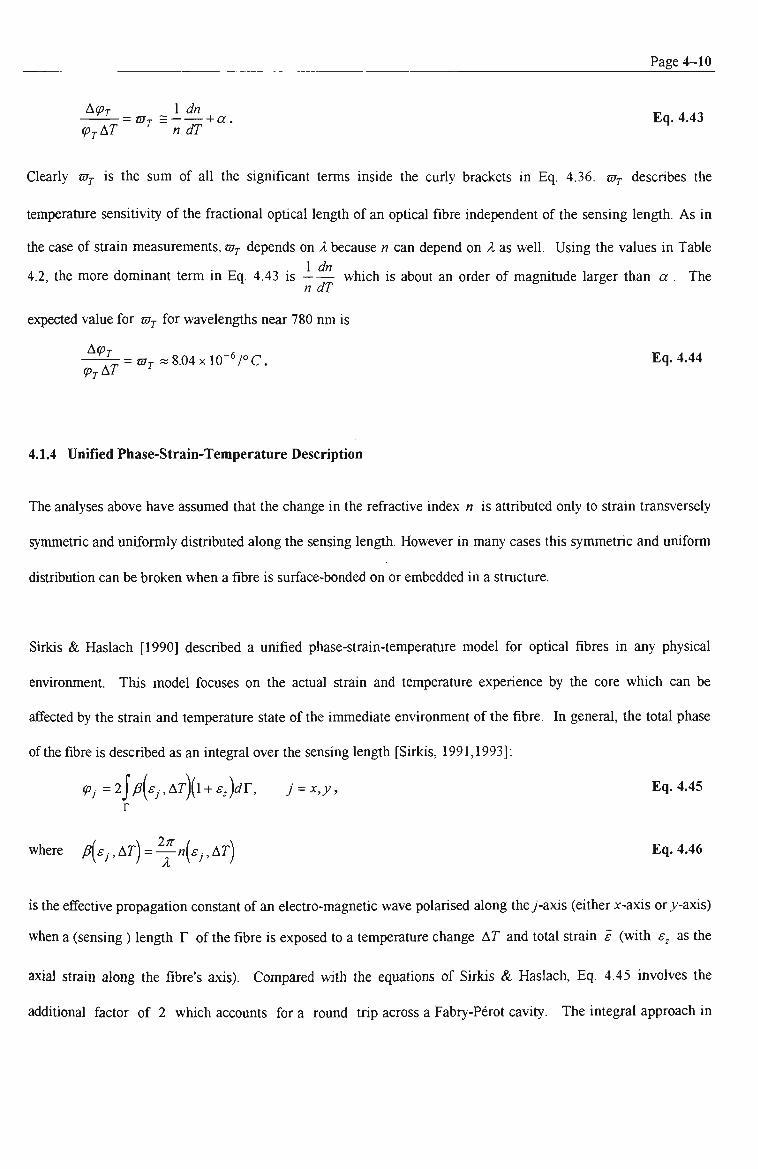
Page 4-10
-Wj^ + a . Eq.4.43 (PjAT n dT
Clearly ruj is the sum of all the significant terms inside the curly brackets in Eq. 4.36. vjj describes the
temperature sensitivity of the fractional optical length of an optical fibre independent of the sensing length. As in
the case of sfrain measurements, Wj depends on A because n can depend on A as well. Using the values in Table
4.2, the more dominant term in Eq. 4.43 is which is about an order of magnimde larger than a . The n dT
expected value for vjj for wavelengths near 780 nm is
= CTr « 8.04x10"^/°C. Eq. 4.44 (PjAT
4.1.4 Unified Phase-Strain-Temperature Description
The analyses above have assumed that the change in the refractive index n is attributed only to sfrain transversely
symmetric and uruformly distributed along the sensing length. However in many cases this symmetric and uniform
distribution can be broken when a fibre is surface-bonded on or embedded in a structure.
Sirkis & Haslach [1990] described a unified phase-sfrain-temperature model for optical fibres in any physical
enviromnent. This model focuses on the actual strain and temperature experience by the core which can be
affected by the strain and temperature state of the immediate environment of the fibre. In general, the total phase
ofthe fibre is described as an integral over the sensing length [Sirkis, 1991,1993]:
<p^ = 2Jp{£j, AT)(I + £,)dY, j = x,y, Eq. 4.45 r
where P(EJ , AT) = —n[£j, AT) Eq. 4,46
is the effective propagation constant of an elecfro-magnetic wave polarised along the y-axis (either x-axis or >'-axis)
when a (sensing) length T of the fibre is exposed to a temperature change AT and total strain £ (with s^ as the
axial strain along the fibre's axis). Compared with the equations of Sirkis & Haslach, Eq. 4.45 involves the
additional factor of 2 which accounts for a round trip across a Fabry-Perot cavity. The integral approach in

Page 4-11
Eq. 4.45 is the proper description for the change in the optical length ofthe because temperature or sfrain can vary
along the sensing region.
FoUoviing a Taylor's series expansion about some initial strain-temperature state {e.g. £ = 0 and Ar = 0) and
keeping only the first-order terms in £ and AT, the phase change is given by
A^, = 2/K0.0)j(., - ; ^ ( , , . , , , ) , ^ f ) , r . ;• = ..y , E,. 4.47
where yS(0,0) = - ^ , Eq, 4,48
In Eq. 4.47, no distinction is made between mechanical and thermal strains. Hence the sfrain £ is the algebraic
sum of these two types of sfrain. In Eq. 4.47 (and also in Eq. 4.49 below), the refractive index n is the average
value over the cross-section ofthe fibre.
Kim et al [1993a] derived an equation similar to Eq. 4,47.but employed experimentally measurable parameters.
Their final equation can be expressed as
A<p^. = 2p{0,0)jL-~p^.,{£, -s^) + ~^^]dY , E - *'*^
where i^ is the thermal strain expressed in Eq. 4.39.
Eq. 4.47 and Eq. 4.49 are two models of a unified phase-strain-temperature description of temperature or sfrain
FFPS. Clearly, these models describe the interferometric phase change for any arbifrary sfrain-temperature state of
the core. For embedded sensors, the strain state of the core is determined by the interaction between the fibre and
its host environment [Sirkis, 1993a]. However, when the stiffness ratio between the fibre and its host is greater
than 10 {e.g. surface-bonded sensors), the strain in the core is approximately that in the host material [Matthews &
Sirkis, 1990].
The two models average the effect of any asymmetry in the refractive index due to an asymmetric strain
distribution. This simplffication does not produce significant ertor with measurements which allow the fibre to

Page 4-12
experience unimpeded thermal expansion or symmetric fransverse sfrains {e.g. measurement of fransverse
pressure, axial strain) [Butter & Hocker, 1978; Sirkis & Haslach, 1990; Egalon & Rogowski, 1992]. However, the
induced birefringence as a result of asymmetric sfrain distributions in the core remains to be important especially
in the operation of polarisation-maintairung or birefringent FFPS.
4,2 Birefringence In Single-Mode Optical Fibres
To appreciate the performance of birefringent FFPS, it may be useful to describe briefly the birefiingence of a
single-mode silica fibre. Theoretically, an optical fibre with perfectly circular core and homogeneous core
refractive index distribution guides light which can be polarised either along two orthogonal directions, e.g. x- or
y-axis. Intrinsically or extrinsically induced imperfections in the fibre which produced inhomogeneity either in the
geometry or in the propagation constant can lift the (polarisation) degeneracy of the fundamental mode [Norman
etal, 1979], These effects do not poise any problem when the desired output does not depend on the state of
polarisation (SOP) of the resulting beams. On the other hand in interferometric sensors, such effects produce
unwanted polarisation-induced signal-fading or dispersion. However ff the birefringence ofa fibre is enhanced, the
light can be propagated in an optical fibre with a relatively constant SOP.
4,2,1 Birefringence Mechanisms
Birefringence mechanisms in an optical fibre can be linear, circular, elliptical or dichronic. Fibres exhibiting
linear birefringence can be considered a retarder and hence can guide linearly polarised tight throughout the fibre
if this beam is launched along one of the principal polarisation axes (polarisation-maintaining fibres). Different
methods of producing linear birefringence will be presented shortly.
Circular birefringence refers to the retardation of left- and right-circularly polarised light. The end results of such
retardation is a rotation ofthe polarisation azimuth ofthe propagating beam. Such birefringence can be produced
by twisting the fibre about its longitudinal axis [Smitii, 1980] or by immersing the fibre in a sfrong magnetic field
(Faraday effect) Pay & Rose, 1988]. Magneto-optic and also elecfro-optic properties of fibres have been exploited

Page 4-13
to measure curtent [Ren & Robert, 1989; Yu & Siddiqui, 1994], voltage [Kuroda et al, 1985; Bohnert & Nehring,
1989], magnetic field [Rashleigh, 1981; Suzuki et al, 1988] amongst others. In general fibres which exhibit both
linear and circular birefringence can be described as elliptically birefringence fibres.
Dichronism refers to a preferred propagation of a single polarisation mode regardless of the irutial state of the
input beam. The basic principle of dichronic mechanisms in fibre is to force one of the polarisation modes to
exhibit higher propagation loss than the other [Simpson et al, 1983]. Hence such fibres are referred to as single-
polarisation fibres or polarising fibres [Kaminow & Ramaswany, 1979].
4.2.2 Evolution of the State-of-Polarisation
The evolution ofthe SOP ofa light propagated in a single-mode fibre follows a complicated pattern resulting from
the interplay of linear and circular birefiingence (optical activity) in the fibre [Simon & Ulrich, 1977]. The output
SOP may appear to behave randomly since the coupling between polarisation modes may be easily induced by
internal and external perturbations in the fibre waveguide [Yariv, 1973; Okamoto et al, 1982; Tsubokawa et al,
1985, 1989; Feng et al, 1990; Shlyagin et al, 1994]. Incidentally, when externally induced birefringence is
introduced to the fibre using some feedback arrangement, the output SOP can be stabilised [Ulrich, 1979].
On tiie other hand with highly birefringent (Hi-Bi) polarisation-maintaining fibres, such feedback arrangement is
unnecessary to maintain a linear SOP. Linearly polarised beam can be propagated along one polarisation axis of
the fibre for as long as the fibre does not experience any great external perturbation [Katsuyama et al, 1983].
Twists in Hi-Bi fibres need to be minimised as well since twists can produce optical activity coupling light between
the polarisation modes [Ulrich & Simon, 1979].
4.2.3 Mechanisms for Producing Linear Birefringence
Figure 4.1 shows the different mechanisms to produce linear birefringence in fibres. Metiiods of producing linear
birefringence fall under two major forms: asymmetry in the cross-sectional geometry or stress in the core of the

Page 4—14
fibre. The common configuration of the latter form involves additional inclusions in the cladding, e.g. an inner
elliptical cladding similar to the fibres used whilst the former is an elliptical-core fibre. The inclusions usually have
higher thermal expansion coefficients compared with those of the substrate cladding and the core. Hence thermal
compressive stress is produced when the fibre cools during its drawing from the fibre preform [Rashleigh, 1983].
Otiier methods of sfress-induced birefringence are by an application of fransverse pressure or by bending [Ulrich et
al, 1980]. In general, the birefringence is directly proportional to the difference in the asymmetric sfress with the
fast-axis aligned along the direction of maximal compressive stress.
I GEOMETRICAL
NONCIRCULAR CORE
H MATERIAL
ASYMMETRICAL LATERAL STRESS
INTERNAL
(b)
17 EXTERNAL
(C)
.EXTERNAL
(d)
BENDING
FREE
(e)
TENSION TENSION a KINK
(f) (g)
|0 {EK C 0 c JJJJimM
ELECTRIC FIELD TWIST
(h) (i)
MAGNETIC FIELD
0)
Figure 4.1: Basic birefringence mechanisms in a single-mode fibre due to internal deformation or external action [Rashleigh, 1983],

Page 4-15
4.2.4 Characterisation of Linear Birefringence
The (linear) birefringence B of a fibre refers to the difference in the refractive indices of the fast-and slow-axis.
Setting the>'-axis as the fast-axis,
B = n^-ny, Eq.4.50
where n^ and ny are the slow- and fast-axis refractive indices respectively. B can be expressed as
B = B G + B ^ „ + B ^ , Eq.4.51
where BQ is the birefringence due to geometry {i.e. asymmetry in the core), B^ is the seff-induced birefringence
due to the difference in the thermal expansion of an asymmetric core and its surrounding cladding and B^ is the
sfress-induced birefringence due to the stress-applying components in the cladding [Noda et al, 1986]. In the case
of an elliptical-core fibre, B5 = 0 whilst B^ and B ^ are non-zero. BQ and B^, increase with the ellipticity ofthe
core and the difference between the refractive indices and thermal expansion coefficients of the core and cladding
[Sakai & Kimura, 1981]. In the case ofa stress-induced birefiingent fibre with a circular core, BQ » 0.
Linearly birefringent fibres are characterised by their polarisation-holding parameter h , beat length L^ and
birefringence (polarisation) coherence length L [Kaminow, 1981]. Prefers to the (intensity) cross-talk between
the polarisation modes per unit coupling length z and is related to the extinction ratio (7) between them, i.e.
{ly) _ Eq,4,52
where (ly\ and (4) are the average irradiance along each axis. LQ is the distance between two locations along
the fibre whereby the incident beam has the same SOP and is related to the birefringence B as follows
1^ = 1 = .^-., Eq,4.53 B n^-ny
whilst!^ refers to the distance within which the incident light remains polarised and depends on the optical
bandwidtii AA ofthe light source. The relative phase between the polarised beams is given by
&=^^z. Eq,4,54
( . > = ^ - ^

Page 4-16
Thus for the orthogonal beams to interfere coherentiy when they are coupled, e.g. with an analyser, the
cortesponding time delay between the modes in Eq. 4.54 must be less than the coherence timer,, of the tight
source. Hence the birefringence coherence length is
A' T,C
^ ^ " B BAA Eq, 4.55
4.3 Thermal and Strain Sensitivities of Elliptically-cladded Birefringent Optical Fibres
Figure 4.2 tilusfrates a polarisation-maintaining fibre which has an internal elliptical cladding (lEC-fibre) similar
to those used in this work. The stress distribution inside the core region needs to be established in order to
determine the refractive index and the phase-measurand sensitivities along each polarisation axis of an lEC-fibre.
It can be assumed that the components of an lEC-fibre exhibit similar elasto-optic properties but different thermal
expansion coefficients {a , a^ and a^ for the core, iimer elliptical and outer cladding respectively). The thermal
expansion coefficients can be chosen be selectiaig the doping concenfration of these components [Ramaswany
etal, 1979].
Outer circular cladding
Core
Iimer elliptical cladding
Figure 4.2: Cross-section of an elliptically-cladded birefringent fibre.
4.3.1 Stress Distribution In an Elliptically Cladded Birefringent Fibre
Assuming tiiat an lEC-fibre is an infinitely long cylinder, then the thermally induced sfress in the core is reduced
to a plane-strain problem [Timoshenko & Goodier, 1970]. The plain strain problem implies that

Page 4-17
^z =£yz=Sxz=^ £q 4 56
and hence the resulting sfress and sfrain are only a function ofthe transverse plane coordinates.
The aggregate sfress distribution inside the core is given by the sum of two contributions [Tsai et al, 1991]; i.e.
a=3 + ^&. Eq.4,57
The first contribution in Eq. 4.57 arises from the thermal stress between the core and the inner cladding whilst the
second contribution is from the thermal stress between the outer circular and the inner elliptical cladding. In the
subsequent discussions, for each contribution the inner cladding/outer cladding is assumed to radially extend to
infinity as far as the core/inner cladding is concerned. These assumptions result in a unfform sfress distribution
along each axis (x-axis and >'-axis as the case maybe).
Using Eq. 4.5, Eq. 4.8 and Eq. 4.39, the first stress contribution is given by
Y5a,(T-T,) Eq,4,58
^'=°'>'= 1-2// ' ^ ^
V , =//('cr,+'cT^), Eq,4,59
where T^ is some effective temperature when thermal stress in the fibre has began to build up and
da^=o:e-o(. Eq,4,60
T^ is difficult to determine experimentally because of the wide fransition from the viscous state to the fused state of
an optical fibre when the fibre is being drawn and allowed to cool. The other stress elements in ' a are zero.
The second stress contribution in Eq. 4.57 is given by [Eickoff, 1982; Stolen, 1983]
2 Y5a2{T-T,)r a \ Eq, 4.61
^ ' " 1-// [a+bJ'
2^ YS"2(T-T,)f b ) _ Eq.4.62 1-// Va + ft>
^ (T ,= / / (V ,+V, ) . Eq.4.63

Page 4-18
a and b are the semi-major and semi-minor axis ofthe inner cladding and
Sa2 =a,-a,. Eq. 4.64
The Other sfress elements in a are zero.
The parameters Sa-^ andt^aj depend on a , a^ and a^ (Figure 4.2). These coefficients can be estimated from the
weighted average ofthe linear expansion coefficients of its composing materials [Kaminow & Ramaswany, 1979].
Assuming that dg is the molar concentration of each doping material g, the resulting expansion coefficient can
approximately be given by
5)0, ' Eq. 4.65
where ftised siUca is the host material. Table 4.3 shows the expansion coefficients of typical dopants.
Symbol
a ^Si02
"•B^O,
"GeO^
"PlOi
T-T,
Q
c.
Description
Linear thermal expansion coefficient of silica fibre of boron oxide
of germanium dioxide of phosphate
r is on-set temperature of thermal stress Strain-optic coefficient Sfress-optic Coefficient
Values
+5.5xlO-^/°C
+10xl0-V°C
+4.5xlO"^/°C
+14xlO"^/°C 800 °C
0.2733
-3,367 xlO'V GPa
Comments
Silica
About room temperature
@850nm
@633 nm, silica
Reference
Lagakosera/, [1981]
Rashleigh & Marrone [1983]
Ballard & Browder [1986]
Rashleigh & Marrone [1983]
Rashleigh & Marrone [1983]
Rashleigh[1983]
Barlow & Payne [1983]
Table 4,3: Relevant thermal and strain constants for birefringent silica optical fibres at A near 780 nm.
Combining all the sfress contributions identified above in Eq. 4.57, the expected sfress components in the core are
a ^ = y ( r - r j D , , Eq,4,66
ay=Y{T-T)D2 »and Eq, 4.67
Eq. 4,68

_^___ Page 4-19
Sa^ 5a2 where D, = '-+—^ , and Eq, 4,69
1-2// l-fi^a+b
D2 = —+ -\ , Eq, 4.70 ^ 1-2// l - / /Va+6 '
Unforttinately, the characteristics of the different components of the EC-fibre used in this research, 3M FS-HB-
4211, were not available. To appreciate D, and D2, the following assumptions were used:
- = 3 [ for an ellipticity constant of 0.5 {c.f Eq. 4.94)], Eq, 4,71 b
Sa-^ «1X10"^ /° C [an order of magnitude estimate only] and £„ 4 72
Sa2 « -2.5 X 10~V° C [Rashleigh & Marrone, 1983]. Eq 4 73
Using these values and the values found in Table 4.2 and Table 4.3,
D, « -0,8 X 10-V° C , and Eq. 4.74
Z)2«4O.7xl0-V°C. Eq 4 75
4.3.2 Photo-elastic Effect Constants
The photo-elastic effect in an optical fibre is important in determining the refractive index along each polarisation
axis of an lEC-fibre. From Eq. 4.6, Eq. 4.7 and Eq. 4.17, the photo-elastic refractive index changes are given by
Sn,=-^p,s,,cr„ Eq.4.76
where n refers to the refractive index of mode guided in the un-sfressed core, Eq. 4.76 can be written as
^«/=Q*o-^, Eq.4.77
where C,=-!^p,s,,. Eq. 4,78
Eq. 4.77 describes the photo-elastic effect, i.e. the stress description ofthe sfrain-optic eSect.

Page 4-20
For an isofropic medium, two constants are sufficient to completely describe the photo-elastic effect [Bortelli and
Miller, 1968]:
Q = - ^ ( P u - 2 p p n ) = q,:^i = k = 1,2,3 , and Eq, 4,79
n^ C2=-J^(pn~MiPn+Pn)) = Q,:yi^k = l,2,3. Eq. 4,80
These constants are known as the photo-elastic sfress constants and their difference is called the stress-optic
(opto-elastic) constant:
Q =C, -C2 = - ^ ( l + / / ) ( A i -Pn)- ^^'^-^^
This constant describes the birefringence as well as the optical activity since
C^=C;;,:V/ = A: = 4,5,6.
The other Q^ coefficients not defined by Eq. 4.79, Eq. 4.80 and Eq. 4.82 are zero.
By using Eq. 4.58 to Eq. 4.63, Eq. 4.79 and Eq. 4.80,
2
Eq. 4.82
Using the parameters in Table 4,2,
C, « -0 .8x lO-VGPa , Eq.4.83
C2 « -4.6 X 10"V GPa, and Eq, 4.54
Q « 3 . 8 X 1 0 - V G P « . ^ Eq.4,85
These values are similar to those reported in the literature [Barlow &Payne, 1983; Namihira, 1985].
4.3,3 Birefringence of an Optical Fibre with an Internal Elliptical Cladding
Expanding Eq. 4.77, the refractive index change along the x- and^-axes of an lEC-fibre are
Sn^ =C, 0-, +C2 (7y +C2 a,, and Eq. 4.86
5ny =€2 a^ +C, (7y +C2 a,. Eq. 4.87
Sn, = -Y(T-TS)(I + M){D^{PU -M{PU + PnhD2{pn ~M(PU + Pn))} ^nd Eq, 4,88

Page 4-21
^"y=-Y(^-Ts)(l + M){D2{pu-M{pu+P^2)) + D,{p,2-M(pu+P^2))}' Eq. 4,89
These two equations show that the induced refractive index change along each polarisation axis is proportional to
temperature. Consequently this establishes the strong temperature dependence ofthe birefringence of an lEC-fibre.
The refractive index along the x-and >'-axes are
n^=n + Sn^=n +C, a^ +C2 (Ty +C2 a, , and ^^ ^^^
ny=n + Sny=n +C2 <J^ +C, Uy +C2 a, ^ ^^^j
whilst the birefringence of an EEC-fibre is
B = Sn^- Sny = (c,-C2)[a^ -ayj = C^(c7^-(7y) , or Eq. 4.92
B = Sn^-Sny=-Y(Pn-Pn)^a2{T-Ts)[j^^ Eq. 4.93
a-b where e^, = Eq. 4.94
a+b
is the ellipticity of the inner cladding. From Eq. 4.93, the strength of the birefringence B increases with the
ellipticity e^,, the thermal coefficient mismatch 5a2 and the temperature difference from the thermal stress on-set
temperature T^. Eq. 4.93 also implies that the birefringence depends only on the thermal stress produced between
the inner and outer claddings (Equation 4.58). This is because the stress between the core and the elliptical
cladding is radially symmetric. Eq. 4.93 can be rewritten as
B = Sn,- Sny =C,Sa2[T- T, ) [ ^ e„, Eq. 4.95
where C,=CJ = -'^(p,,-p,2)(\ +M) ^"^^'^^
is known as the sfrain-optic constant for an isotropic fibre.
Using the parameters in Table 4.2 and Table 4.3, tiie estimated values for Sn^, Sny and B for the EC-fibres
used are
(J«^»+L4xl0-^, Eq.4,97

Page 4-22
^n^ w -L6 X 10"^, and Eq. 4.98
B«3xlO-^. Eq,4,99
These estimates indicate that the core of the fibre experiences extensive stress parallel to the x-axis of the ellipse
and compressive stress along the y-axis. In addition, the values indicate that the -axis is clearly the fast-axis of
the fibre. The birefringence B is lower than the expected value of 4x10"^ for the birefringent fibre used.
However,
^^ * " " Eq, 4,100
is similar to those reported in the literature [Rashleigh, 1983].
4,3,4 Phase-Strain Sensitivity
The calculation for the phase-sfrain sensitivities of an FFPS employing EC-fibres is slightiy different from that of
the non-polarisation-maintaining fibre case (section 4.1.2). The different transverse stress due to an axial strain
needs to be distinguished. The additional stress caused by an axial sfrains along a lengthL^, £Y (Eq. 4.9) can be
expressed as
Ao-i=£7^fe, Eq. 4,101
where S^^ is the Kronecker delta function:
<. _ j l '* = Eq, 4.102 ' ' ^"JO ,k^z'
The axial refractive index change is given by the difference between refractive index values at two different stress
states: [cr^t+^^^fe] and[a-i] . [cr^j is the initial stress producing the birefringence. The refractive index change
can be described as
^i,^ = A(" + , ) = {" + Q(cr^ + sYS/,,))-{n + C^f,CFk) = Q,EY. Eq. 4.103
For the change along the x-and y-axis,
^x.e=^y,e=C^£Y = - — £[p^2 -M{PU + P\2))• ^' ^'^

Page 4-23
Assuming that an EC-fibre is weakly guiding then the waveguide effects can be neglected as in the NPM fibre
case. The strain-induced pliase change along each polarisation axis of a birefringent FFPS is;
Although from Eq. 4.104, the refractive index changes due to the additional sfress along each polarisation axis are
the same, the total change in the optical length ofthe slow-axis cavity would be slightly larger than that ofthe fast-
axis simply because n^ > ny. This relationship has been observed experimentally (Chapter 7).
The corresponding optical gauge factors are
^<P',e , "^ ( ( W Eq. 4.106 -r-7 = ^,.=^-Tr(Pn-M[Pn+Pn}j **
assuming no thermally induced stress effects affect the initial birefringence of the fibre. Using the values in Table
4.2 and the results in section 4,3.3,
^ ^ = e^,,= 0.7937,and Eq. 4.107 <Px,s£
^ ^ = ^ , . = 0 . 7 9 3 6 . Eq. 4.108
These values are very similar to one another and for the case of NPM FFPSs (Eq. 4.34).
4.3.5 Phase-Temperature Sensitivity
The refractive index change due to temperature of an elliptically clad fibre is given by the difference of the
refractive indices at two temperature states. This thermal refractive index change can be described as
' f tr) (''(^))' (r)l «(n-—;—Pi,s,i,ak{T) ,
{n(T + AT)Y ,„ . J f ,^, {n{T)) An^j = A ( « + ^ , . ) = n(T + AT)-- — pySj;,(7k(T + AT) 2—Pij^jk'^k^
Eq. 4.109
where n{T + AT) is tiie refractive index of the un-sfress core at temperature T + AT. a{T + AT) is tiie tiiermally-
induced sfress. Expanding Eq. 4.109 as a Taylor series in Ar and subsequently keeping only the AT terms and
adding the contribution ofthe thermal sfrain £^,

Page 4-24
dn 3«2 ] n^ da^ n^ . Eq. 4.110
The first term in Eq. 4.110 is the refractive index change due to direct dependence of «, (^-x, ) with temperature.
The last two terms are the contributions ofthe thermally induced sfress and sfrain respectively. Together they give
the elasto-optic refractive index change due to variations in temperature. From Eq. 4.58 to Eq. 4,64,
^ E l = _ £ i _ . Eq. 4.111 dT T-Z
Thus, Eq. 4.110 can be rewritten as
An,r =—-AT,
dn. dn. n / ^ \ where - ^ = - ^ - ^ ( ^ 1 + 2 A 2 J « ^ and
Eq, 4.112
Eq. 4.113
dn. dn ^ 3 dn 1 — = — + SnA +-
dT dT n dT T-T,
Eq. 4,114
Alternatively,
dn:
dT
dn
dT + Sn^ hf
nV
dn n^ , ~ \ — + — oc{Pu+2p,2) +-
T-Z Eq, 4,115
dn where — is that given by Eq. 4,42 - the total refractive index change due to temperatiire ofthe un-sfress core. Of
tiie terms inside the square brackets in Eq. 4.115, the dominant term is 1
T-r which can be interpreted as the
1 fractional change in the internal sfress experienced by tiie core (Eq. 4.111). In fact the product Sn^ YZf ^^^ *^
same order of magnitude as — . Using tiie values in Table 4.2 , Table 4.3 and the results in section 4.3.3
dn^ dT
«10.8xlO~V°C ,and Eq, 4,116
dny
~df «lLlxlO"V°C, Eq, 4.117
These are the total refractive index change due to temperature along each polarisation axis ofthe EC-fibre.
Hence from Eq. 4.11, the phase-temperature sensitivities due to temperatiire change along each polarisation axis
are:
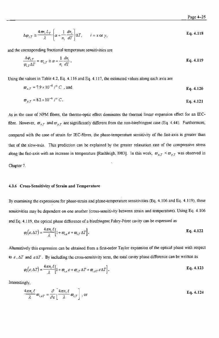
Page 4-25
imijLj 1 dn^ A<p,r=~-^-\a^-—>AT, i = xory.
and the cortesponding fractional temperature sensitivities are
Acp. T 1 dn. —^-^^^= tJUij =a+ -. (p^jAT ' «, dT
Eq. 4.118
Eq. 4.119
Using the values in Table 4.2, Eq. 4.116 and Eq. 4.117, the estimated values along each axis are
7.9 X10'^ /° C , and ta x,T
tUyj =8 .2x10"^ /°C.
Eq. 4.120
Eq. 4.121
As in tiie case of NPM fibres, the thermo-optic effect dominates the thermal linear expansion effect for an E C -
fibre. However, m^j and tUyj are significantiy different from the non-birefringent case (Eq. 4.44). Furthermore,
compared with the case of sfrain for EC-fibres, the phase-temperature sensitivity of the fast-axis is greater than
tiiat of the slow-axis. This prediction can be explained by the greater relaxation rate of the compressive sfress
along the fast-axis with an increase in temperature [Rashleigh, 1983]. In this work, tu^j < tUyj was observed in
Chapter 7.
4.3.6 Cross-Sensitivity of Strain and Temperature
By examining the expressions for phase-sfrain and phase-temperature sensitivities (Eq. 4.106 and Eq. 4.119), these
sensitivities may be dependent on one another (cross-sensitivity between strain and temperature). Using Eq. 4.106
and Eq. 4.119, tiie optical phase difference of a birefringent Fabry-Perot cavity can be expressed as
Ann. i ^i[£,AT)= ^l+aTj^E + mij-AT Eq. 4.122
Alternatively this expression can be obtained from a first-order Taylor expansion of tiie optical phase with respect
to £,AT and £AT. By including the cross-sensitivity term, tiie total cavity phase difference can be written as
<Pi{e,AT) =
Interestingly,
Ann, i 1 + c . g £• + tiTjj AT + tEr_ J- £AT Eq. 4,123
Ann, (, m i.eT d£ , or
Eq, 4,124

Page 4-26
4;r«, i m i.eT dT
Ann^ i - ^ - n r , , . Eq, 4,125
Substituting Eq. 4.106 into Eq. 4.125 and evaluating the partial derivative gives
Ann, i
A ^i.cT = • Ann, i
A ^i.E ^i,T
'3n^ dn rr' dn-
J^IT'^TT^ \{pn -M(PU + Pn))
dn dn Since for an EC-fibre, it can be shown that n. a n and —'- « —'-, Eq. 4.126 becomes
dT dT ^ dn
^i,sT « ^i.e^i.T ~"i ~^(Pn-M{Pu +Pn))
Eq. 4.126
Eq. 4.127
Using tiie values in Table 4.1 and estimates (see Eq. 4.97, Eq. 4.98, Eq, 4.107, Eq. 4.108, Eq. 4.116, Eq. 4.117,
Eq. 4.120 andEq. 4,121) of the different parameters required in Eq. 4.127,
07^,T « 3.2xlO>C,and
vjy^^r « 3.3xlO>C.
Eq. 4.128
Eq. 4.129
Farahi et al [1990b] used a Bow-Tie birefringent fibre and experimentally determined tiie cortesponding cross-
sensitivity factor for their fibre. This factor was obtained by determining the phase-temperature sensitivities at
different strain state of the fibre. Their technique can easily be appreciated from a simple rearrangement of Eq.
4.123:
^,UAr) = ^ [ l + CT,,f + {cT,_^+C7,,^f)Ar]. Eq. 4.130
For their fibre, the slow-axis sensitivity changed from 8.0 to 3.8 rad/°C as a 7 cm segment was sfretched from 0 to
30 |xm. This -50 % change gave (slow-axis) m^^^j « 4.8xlO"V°C using n=1.46 and A=633 nm. This value is
several orders of magnitade higher than the expected value for an EC-fibre similar to that used in this work {c.f
Eq. 4.128). This can only be attributed to the birefringence mechanisms in a Bow-Tie fibre although even with the
much higher birefringence of this structure, the measurements give a surprisingly large value. Others [Smith,
1980; Barlow & Payne, 1983] had indirectiy measured this cross-sensitivity effect. In characterising bend-induced
retardation and twist-induced rotation in optical fibres, they observed the temperature dependence of the sfress-
optic coefficient of — - « -4.398 x 10"'' / (GPa-° C) in the case of Bariow & Payne.

Page 4-27
Cross-sensitivity between sfrain and temperature arises because of the temperature dependence of the sfress-
induced birefringence in an optical fibre. However, this cross-sensitivity effect can be neglected when either
temperature or sfrain is kept constant or when moderate excursions in sfrain or temperature are involved.
4.4 Temperature and Strain Sensitivities of a Single-Layer Reflective Thin Film
The optical properties of the thin film introduced in an optical fibre depend on the phase change associated with
the optical thickness of a thin film (see chapter 3):
2nnfif Eq. 4.131 f^f- A '
where nf and I f are the refractive index and the (physical) thickness of the film respectively. The fractional
temperature or strain sensitivities of Pf,v}j and mf"', can be obtained as in the optical-fibre case (Eq. 4.33 and
Eq. 4.43),
Apf
bM ' ^ -p ^fii'" Eq. 4.132
where M = temperature T or strain £ The values of m^" and m^'" are expected to be of the same order of
magnitude as in the optical fibre case. (At most the order of magnitude of the values can be expected to be about
crf^^lO-^ and CTf'"«l). Thus,
^Pf ^%) fiin, n fi,^ n . ^^^^ ^ Eq. 4.133 =—^^—-xni - — IUT « —xlO rac?/°C , and
AT A ^ 2 ^ 2
APf Iniy^ jr jr Eq, 4,134 - ^ = — ^ c r f " =^^^7/"" « ^ x lO-V^^///^
for temperature change and sfrain respectively. In either case, a change of about 1,100° C or 11,000/ie change is
required to induce the equivalent of 1° phase change in pf. Hence, the optical properties of tiie thin film can be
considered invariant to moderate thermal or strain variations.

Page 4-28
4.5 Temperature and Strain Sensitivities of an In-Fibre Bragg Grating
The Bragg wavelength of a fibre grating can easily be shown to be sensitive to strain and temperature change.
Since a fibre Bragg grating (FBG) and a fibre Fabry-Perot sensor have similar refractive indices, the fractional
change in Bragg wavelength of a fibre Bragg grating with respect to strain and temperature change can be
expressed similar to those found in Eq. 4.33 and Eq. 4.43:
A^ , "b ( ( \\ , Eq. 4.135 — - = CT = 1 --Y'[Pn -M[P} 1 + Pu))> and
A ^ = ^^=±^ + a Eq, 4.136 A^AT «j dT
for sfrain and temperature change respectively.
When an FBG is used as a Fabry-Perot reflector of an FFPI, the temperature- or strain-induced change in the
reflectance and transmittance of the FBG implies changes in the fringe visibility. Such changes are important
considerations in determirung the overall measurand range ofthe Fabry-Perot sensor. These intensity variations do
not, however, directly affect the measurements of the phase shifts as long as the interferometric signals can be
detected with reasonable signal-to-noise ratio.
On tiie other hand, shifts in the spectrum of the FBG are accompanied witii a corresponding phase change. At a
fixed wavelength of the light source, the electric field reflection and transmission coefficients can vary with the
phase Pi,. As in the Bragg wavelength shifts, it can easily be shown that
1 4Pb) Eq. 4.137 P, dM " ' ^^ '
where M refers to temperature T or strain £. The phase change due to refiection from an FBG {0[) can
contribute to the interferometric phase of an FFPI ((p),
d0b ^ d0[_dp^ Eq. 4.138 dM dp^dM'
UsingEq. 3.125 andEq. 4.137

Page 4-29
d0^ ^ d0^ dp,
dM dp, dM
d0 nl\
dPi Pb^. M'
Eq. 4.139
'W
As was the case in section 3.2,3,
dM
d0 nl
dp. ,can be neglected for low Bragg reflectance values (Eq. 3.128). Hence
Eq. 4.140
4,6 The Phase-Measurand Sensitivity of a Fibre Fabry-Perot Interferometer with Thin-Film or Bragg-Grating Reflectors
The fransmittance and reflectance of an FFPS have been shown to depend on either <p or ^ + (pr (Chapter 3). For a
dielectric thin-film or an FBG, (p, is a constant. The change in 4> is given by
A^=A{<P + ^,) = A{2p) + A0,. Eq. 4,141
Using the chain rule for differentiation.
A(p = dp d0^
dM dM. AM. Eq, 4.142
6, is the sum of the phase change upon internal reflection of the cavity (Eq. 3.19). Using Eq. 4.140,
d0 \ A^= 2pmM+ „ . .
V dM. AM. Eq, 4.143
Subsequentiy similar to the steps infroduced in section 3.3, it follows from Eq. 4.143
A^ ^^m, ^Am, d0^^ dp^^ • = 2pmM+-rz r 7 ^ + -
Eq. 4,144
where ITli and m2 are the Fabry-Perot mirtors which in this work are eitiier dielectric thin films or FBGs. 0''x
refers to tiie phase change upon refiection from either surface ofthe refiector (assuming reciprocal properties) and
Px is tiie phase associated with the optical length ofthe mirror X (= ITl, or m2). Using Eq. 4.132 or Eq. 4,137,
^^m, m, ^^m. A^ '^ ''mi m, ^^m^ m, — = 2 ^ t ^ ^ + — A ^ , t ^ ^ + — / ? ^ ^ G T ^
Eq. 4,145
Using Eq, 3.120 and Eq. 3.125,
A(p
AM = 2ptnu + 1+ v. dPm,
Prt\,^M + 1 + de"^. ^
dPm Pm.^M '
Eq. 4,146
1:7

Page 4-30
dex — w 0 ff the mirrors are quarter-wave thick thin films or low-reflectance Bragg gratings (Eq. 3.123 and Eq dPx
3.127). With these types of reflectors, Eq. 4.145 becomes
^ « 2Pm^ +^^, GTS' +/9m, C • Eq. 4.147
Since the right-hand side of this equation is constant, this equation implies that the interferometric phase shift
varies linearly with measurand change AM . Strictly, slight error or nonlinear variations can be expected in A^.
This nonlinear variations are given by
A<z>"' ^^m, m, ^^m, m, Eq. 4.148 AM = dp^^ ^'"•'^^ ^ dp^^ ^'"^'^^ '
the difference between Eq. 4.146 and Eq. 4.147.
4.7 The Unambiguous Measurand Range of a Fibre Fabry-Perot Interferometer With Thin-Film or Bragg-Grating Reflectors
Using only the linear frend in A^ (Eq. 4.147), the unambiguous measurand range, AMyj^ can be estimated to be
SM « '^-^ Eq. 4.149 2pmM+Pm,^M^Pm,^M
In the case of thin-film mirrors, the temperature or strain induced variations in the reflection phase change can be
neglected since in most cases Pf m^"' « P tui^ (section 4.4). For subsequent discussions, an FPPS with two
FBGs (ITli and m2) is considered. Thus,
AU '^ or Eq. 4.150 2pj^M+Pm^^M+Pm^^M
AM '^ Eq. 4.151 'UMR /
2 m, M /TDJ Pm^
P+-:r+ 2 2 )
Eq. 4.151 implies that tiie effective optical length ofthe Fabry-Perot cavity with FBGs is equivalent to the distance
between the centres of the two FBG reflectors. This approximation assumes that the Fabry-Perot cavity and the
Fabry-Perot reflectors experience the same amount of measurand change.
In summary, this chapter has presented the expected phase-temperature and phase-strain sensitivities of fibre
Fabiy-Perot sensors fabricated with two types of fibres: non-polarisation-maintaining and polarisation-maintaining
(witii an internal elliptical stress-producing cladding) fibres. In the latter case, the phase-temperature sensitivity

Page 4-31
for the fast axis is expected to be greater than that of the slow axis whist the phase-sfrain sensitivity for the slow-
axis is expected to be greater than that of the fast axis. The temperature- and strain-induced variations to the
properties of thin-film and Bragg grating reflectors were also investigated. The intensity variations determined the
fiinge visibility. For quarter-wave thick thin films and low-reflectance Bragg gratings, the associated phase change
with these reflectors can be neglected. In addition, the phase-measurand sensitivity, the UMR and the FSR of the
sensor can be calculated by using the distance between the centres of the Fabry-Perot mirrors as the effective
optical length ofthe cavity.

Chapter 5: Development Of Short-Cavity Fibre
Fabry-Perot Interferometers
A fibre Fabry-Perot sensor (FFPS) may be easily constructed from a piece of single-mode optical fibre with cleaved
ends, however the long cavity length and ancillary bulk optics necessary for signal analyses limit the application of
this sensor in the field. An alternative is an in-fibre FFPS. It is possible to have short cavity lengths and therefore
potential for localised measurements, the incorporation of bulk optics functions into an all-fibre arrangement, the
possibility of multiplexing several sensors and the incorporation of those sensors into structures [Lee et al, 1989;
Alcoz et al, 1990; Valis et al, 1990b; Lee et al, 1992b; Mason et al, 1992].
This chapter describes the development of in-fibre FFPSs with short-cavity length and enlarged unambiguous
measurand range (UMR). The latter property is realised with the use of a birefringent FFPS which has its
polarisation axes aligned with those of a lead-in fibre forming essentially a dual-interferometer sensor. The large
UMR arises from the differential phase shift between the dual interferometers and the more-sensitive axial phase
shift to obtain high measurand resolution. In this research, in-fibre short-cavity birefringent FFPSs were developed
using eitiier reflective fiision splices [see Lee et al, 1987] or in-fibre Bragg gratings [see Morey et al, 1992a].
Initially fiision-spliced FFPSs were made with single-mode non-polarisation-maintaiiung (NPM) fibres in order to
gain familiarity with fabricating fiision-spliced devices before birefringent sensors were produced. Both the NPM
or birefringent sensors involved an in-hne (proximal) fusion-spliced titanium oxide (Ti02) nurror and a coated

Page 5-2
cleaved distal end. Unfortunately, these fiision-spliced sensors are inherentiy fragile because the regions around
the fiision splices are mechanically weak. To fabricate mechanically sfronger sensors suitable for sfrain
measurements, the fusion-spliced reflectors were replaced with in-fibre gratings. Both single-grating- and dual-
grating based birefringent FFPSs were fabricated.
5.1 Fusion-Spliced Single-Mode Optical Fibre Fabry-Perot Sensors
5.1.1 Review of the Previous Work on the Construction of Fusion-Spliced In-Fibre Reflectors
In-fibre reflective mirrors can be fabricated using various techruques. Reflective fusion spUces can be formed by
lowering the fusion cmrent such that only the cladding regions were joined whilst forming an air bubble in the core
region [Leilabady, 1987; Leilabady & Corke, 1987]. These intentionally bad splices exhibited reasonable
reflectance but were found to be weak. The tensile sfrength of the splices may be increased by using some metal
rods to brace the splice region.
To increase the reflectance of a reflective fiision splice, prior to fusion, a thin film [Lee et al, 1987; Yeh et al,
1990; Vatis et al, 1990a; Inci et al, 1992; Kaddu et al, 1993] can be coated on end-faces of eitiier NPM [Lee &
Taylor, 1988b; Inci et al, 1992; Kaddu et al, 1993] or polarisation-maintairung fibres [Mason et al, 1992; Valis
et al, 1990b]. Metallic {e.g. silver [Valis et al, 1990a], aluminium [Valis et al, 1990b]) and dielectric (titaiuum
dioxide (TiOj) [Lee & Taylor, 1988b; Inci et al, 1992]) thin films were found to survive the violent fusion-arc
process provided that the fiising current and duration were reduced. These fusion conditions gave weak tensile
sfrength, high loss and low reflectance splices. The fransmission loss can be minimised by ensuring good core-to-
core alignment whilst absorption loss by using dielectric rather than metallic films. Although the reflectance of a
single layer of dielectric thin film can be sufficient in some applications, the reflectance can be fiirther increased
with the use of multi-layer dielectric coatings incorporating silicon dioxide (Si02) and TiOj film. Seven-layer
quarter-wave Ti02/Si02 stacks were successfully used to form an in-line high-finesse Fabry-Perot sensor [Lee et
al, 1992a].

Page 5-3
Measures' group at the University of Toronto had suggested coating only the core-region ofa fibre face comprising
only 1% of the total surface area [Hogg et al, 1991; Measures, 1992]. This procedure was believed to have
enhanced the sfrength of the splice since much of the cladding can fuse without any intermediate thin film. In
their work, they coated only the core-region ofa fibre end with a thin layer of aluminum ("core-coated"). They also
reported that there was no need to reduce the ordinary fusion current with core-coated fiision splices [Hogg et al,
1991]. However in this work, fiision splicing with normal ftising parameters of core-coated TiOj fibre faces
desfroyed the Ti02 film. Thus, both (entire-)face-coated and core-coated fusion-spliced TiOj reflectors were
fabricated using reduced fiision current.
Table 5.1 summarises the reported procedures in fabricating reflective fiision splices. These splices were made at
Texas A & M University, University of Toronto, Herriot-Watt University and Victoria University of Technology.
5.1,2 TiOj Reactive Sputter Deposition
Ti02 was used in order to obtain reflective fusion splices because of its strong adherence on silica fibre faces, high
melting temperature, low absorption and high refractive index. The melting temperature Ti02 is 1820 °C [Ballard
& Browder, 1986] which is higher than the liquid-to-glass state fransition temperature of silica (1175 °C [Fleming,
1986]). It is also highly fransparent and has low-absorption at wavelengths between 0.45 .m to 6 jam, i.e. the
visible and tiie near infra-red [Weber, 1986]. Ti02 has a relatively high refractive index ranging from 2.2 to 2.6
depending on the deposition method. The refractive index of Ti02 not oiUy varies with different deposition
processes but also depends on deposition rates, subsfrate temperature, chamber conditions and operators [Bermett
et al, 1989]. An earlier study on reactive deposition of Ti02 from sputtered titanium to yield the Ti02 and Ti205
gave similar conclusions [Pulker et al, 1976].
TiOj exists in several forms: rutile, anatase, octahedite, brookite, ilmeiute and perovskite [Richardson & GangoUi,
1994], However, vacuum-deposited TiOj films are either rutile or anatase [Pulker etal, 1976]. Rutile which
exhibits a stable tefragonal structure is generally formed when pure titaiuum is used [Pulker et al, 1976] as was
the case in this work.
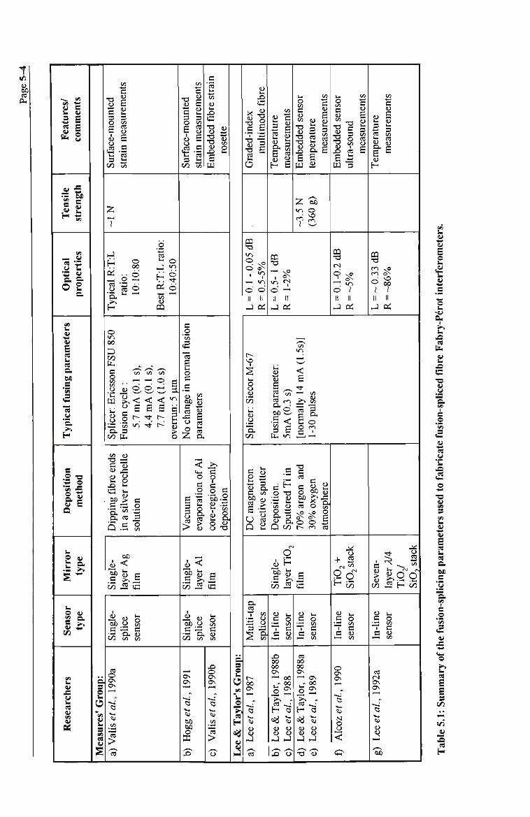
I 60 a
OH
Fea
ture
s/
com
men
ts
u ^
^ ^ SB
cal
rtie
s O
pti
|)rop
e er
s
'W
para
me
isin
g
«5
Typ
ical
a
Dep
osit
io
met
hod
£ «
u
lens
o ty
pe
(«
Res
earc
he s.
easu
res'
Gro
u
S
en
^ a ur
face
-mou
nt
rain
mea
sure
W3 GO
z T
.:T:L
lic
al R
ra
tio:
K E?
o <o
n FS
U 8
ic
sso
le:
11 CJ
plic
er:
usio
n c
(/3 tU
en aj "O "-* 3 "3 «j . a
Dip
ping
fib
re
in a
silv
er r
oc
60
Sing
l la
yer
Ji «j 60 O 3 ;3 ;'5 o. CO ter
(Q
ise/
o/.
, 19
9C
Val
CO
o 00
10:1
0:
en
e
L r
atio
: tR
:T:
en OJ
m
en en
—< O
S6 < < <
5.7
m
solu
tion
film
ns
or
ii en
4.4
m
7.7
m
o
10:4
0:
a <ri
verr
un:
o
urfa
ce-m
ount
(/3
ion
e«
orm
al f
u
3
60
No
chan
V
acuu
m
u
Sing
l le
-
60 3
W
<-H
ON ON
^gg eta
l, 1
:§
nts
a
rain
mea
sure
en
3 IBJ]
en
«J
mbe
dded
fib
r ro
sette
w
en i- i
aram
et(
o.
«4-( 3
evap
orat
ion
0 co
re-r
egio
n-o
depo
sitio
n
<
laye
r fi
lm
p. o
O . OJ en en
X5 o ON O N
Use
/a/.
, I
^
o
s* £
; Tay
lor'
s'
^
e
fib
rade
d-in
dex
mul
tim
ode
o
0.05
dB
%
0
.1-
0.5-
5
II II J 0
empe
ratu
re
leas
urem
ents
E-H fi
o
mbe
dded
sen
; m
pera
ture
w a
2 60 m o 7 -( •—'
^
0.5
-1
1-2%
11 II
H4 a;
J
M-6
7
er:
A (
1.5s
)
>:; S a 8 a ^ rc
C/2 S f O _ ^ en
Spl
icer
:
Fusi
ng p
5m
A (
0.
[non
nall
1-
30 p
ul
3 fe .« 3
DC
mag
netr
o re
activ
e sp
utt
Dep
ositi
on.
Sput
tere
d T
i i
70%
arg
on a
30
% o
xyge
n
o
O
Sing
l la
yer
film
D , « "V tn
a CJ 3 -.3
2 tn
eeta
l, 1
91
es
t j k.
3 O 12 w ~ 3 3 U M en
X> 00 OO ON
.. QO
e &
Tay
lor
eeta
l, 1
9;
<U 4J
X > CJ
4J k. 3 O • ^ t n
1 ^ S3 C dj
1—1 i n
c« 00 00 ON — ON
.. 00
e &
Tay
lor
eeta
l, 1
9
SJ SJ
"O SJ
nts
mea
sure
me
Ul O m
mbe
dded
sen
;
u
0.1-
0
11 J
atm
osph
ere
+
TiO
.
SJ
3
-Ii
3 HH
o ON ON
coz eta
l.
<
O
en • . — »
3
Itra
-sou
nd
mea
sure
me
3
II
a;
j ^
stac
l
O CO
I-I
o en 3 SJ en
nts
empe
ratu
re
mea
sure
me
H
m sP
II II J oi
Seve
i la
yer
a Q •", t n
T 3 * S 1—< en
c«
ON
eeta
l, 1
9
SJ
•60
,^ CJ
w en
O O
«J
E o
£
La
to
c "O
B
4J
^«j
.a
u ii
u a.
"3.
E E s
V2
H

«0
SJ 00 a
PH sn
tare
Fe
a
^ on e a H
Opt
ical
en U ii 4J
E
para
us
ing
Typ
ical
f D
epos
ition
M
irro
r
u
lens
o
t/2
en S>
X!
arc
GO
«S
en
men
co
m
JS
•Si) £
OS
prop
ertie
m
etho
d
ti
a.
type
roup
;
O "sB
B 5 1-5
en
SJ SJ a I-I gj
empe
ratu
m
easu
r
H
II SJ
-9N
vera
] <s <
R=
l-2
5%
A
vera
ge R
=
-12%
o^ o < "v i« a f« fe «-i S i a
Splic
er:
B
Fusi
ng P
a In
itial
: 30
2
^ *^
Frin
ge v
isib
il =
66-9
2%
(sec
ond
R=4
%)
,^v en
^ r - r
1 ? 1 cs >o 2
T Svo ^ a g® i •>* eO en
Fina
l: 10
O
verr
un: •
To
tal D
ur
8 -
20 p
ul
0.5
s
Ele
ctro
n be
am
evap
orat
ion
cs
o
Sing
l la
yer
film
SJ .^ >-i .-H SJ o 60 2 M 3 ^ 3 • — D , SJ
C/3 en en
<N (Ti ON <7 ON Ov
C3 CS
O CJ 3 3
>-N ^-N CQ . £
H I S O la
o en
JS
Boo
t
en
H S)
. T3 3
re 0
1 un
te
sure
i
Tem
pera
tu
surf
ace
mo
stra
in m
ea;
Z • a '•^
<« ii 6 O en .ts 2 ^ ^
CL,
P^ O vP —< o^
1 O
77 II II
i-~\
< O 3
f fe 2 " l a
Splic
er: B
Fu
sing
Pa
Initi
al: 3
0
DC
mag
netr
on
reac
tive
sput
ter
depo
sitio
n.
c-1
O ii H
Sing
l la
yer
film
ngle
-lic
e ns
or
••2 Cl< SJ C/3 en So
ro ON ON r^
"5 %}
•§ t 3
^ ^^«k^
re
3 2 'en 3 SJ
< P
o ) uirl
Fina
l: 10
^—s
Ove
rrun
: 2
jxm
D
urat
ion:
(0,
5 s
7-15
pul
ses
putte
red
Ti in
0%
arg
on a
nd
0 %
oxy
gen
tmos
pher
e
C/2 oo fs re
en
SJ
E £ SJ
£
re to
£
SJ
B O
re
4J
ii
re re a. 60 B
en
B
,s
o
re S S s
s B B O u
IT) ii
re H

Page 5-6
T1O2 films used in this work were formed by reactive sputter deposition. In this method relatively heavy argon
(Ar) atoms are ioiused and accelerated towards a Ti target. Subsequentiy, the Ti atoms from the target are
sputtered and can combine with other free molecules in the sputtering chamber. For example, if deposition
chamber contains oxygen, Ti02 can be synthesised. At low reactive gas partial pressure and high sputtering rate,
most of tiiie chemical reactions occur at the substrate rather than at the target [Vossen & Coumo, 1978]. The
stoichiometric ratio of the film depends on the relative arrival rates of the molecular species to compose the film.
In the case of TiOj deposited onto cleaved fibre ends, the partial pressure of oxygen (O2) is maintained at a level
such that for approximately every Ti atom arriving at the fibre a single Oj molecule is available. It is critical to
maintain this balance because it has been experimentally observed that deficiency in oxygen molecules produced a
bluish-tint film (due to a resonance absorption at 1.2 p.m [Beals, 1970]) whilst abundance is accompanied by a
decrease in the deposition rate. In the case of the latter, an increase in the partial pressure of Oj produces a more
stringent threshold condition to ionise the Ar atoms [Vossen & Coumo, 1978]. Hence the partial pressure of Oj
critically determines the composition and formation of TiOj and consequentiy the optical properties of the film as
well.
Ti02 was reactively deposited using a DC magnetron sputtering system (Figure 5.1). Prior to deposition, the
vacuum chamber was iiutially evacuated using a diSusion and rotary-vane vacuum pumps in tandem to a pressure
of ~ 1.5 X10" mbar. A liquid Nitrogen cold trap at the entrance ofthe difiusion pump reduced the partial pressure
of water vapour in the chamber. The typical ultimate pressure achieved was ~2 x 10" mbar The chamber was
filled with AT and Oj mixture with a molar ratio of 4:1 and had a US Inc. sputtering gun diode with a 99.95% Ti
target. The sputtering gun used was a circular planar magneti-on sputtering device (Figure 5.2). The gun was
operated at 108 W at a sputtering pressure of ~2 x 10" mbar. A DC potential difference was applied between an
annular anode outer ring (at ground potential) and a Ti cathode disk (the target). This difference maintained a
glow discharge which ionised the Ar atoms, at an ambient pressure of ~10~^ mbar. Permanent disk magnets
situated under the cathode formed donut-shaped magnetic field lines on top of the cathode. These anmtiar
magnetic field tines trapped the elections within the plasma discharge and hence increased the ionisation

Page 5-7
efficiency of the sputtering Ar ions. Because the sputtering ions were positive, they were accelerated towards the
negative-potential cathode, and thereby sputtered Ti upon impact.
Fibre connected to the optical thickness monitor
Fibre holder
Optical fibre faces
Sputtering gun
Liquid nitrogen cold trap
Difiiision oil vacuum pump
Top plate
Substrate platform
Glass cylinder
Deposition chamber filled with argon and oxygen
Rotary-vane vacuum pump
Figure 5,1: Schematic diagram of the sputtering chamber used to deposit TiOj on fibre end-faces.

Page 5-8
Magnetic field lines
Annular anode
South pole
North pole 12.
North pole
South pole
" < .
Titanium target (cathode)
South pole
North pole
Figure 5.2: Schematic diagram of a circular planar magnetron sputtering gun.
In this work, fibre ends facing parallel to the Ti target were coated with TiOj either only on the core-region or the
entire face. One or several (at most) fibre ends could be coated simultaneously in a single deposition run. The
fibres were arranged side-by-side in a simple aluminum holder (Figure 5.3a). During deposition, the multiple-fibre
holder sat on a platform such that the fibres were at a suitable location that ensured relatively similar thicknesses of
the deposited film on each fibre [see Waits, 1978]. For each fibre, the thickness ofthe film can be assumed to be
uniform over the core since the cross-sectional area ofthe core is very small. Figure 5.4a shows a micrograph ofa
face-coated fibre end.
Coating only the core region ofa fibre end-face was achieved by placing a 25-fim aperture directly in front ofthe
core ofa fibre (Figure 5.3b). The aperture and fibre were held fixed to a special assembly after the aperture and
tiie core had been optically aligned. The alignment was achieved by maximising the transmission of light from the
core through the aperture. The light source employed was an 840 nm LED, the same LED that was used for the
real-time morutoring of the reflectance of the deposited film (Figure 5.5). Figure 5.4b shows a nucrograph of a
core-coated fibre end.

/ -
optical fibres
% Aluminum block with tight vertical grooves
a) Whole-face coating
Optical fibre chuck
Spatial aperture
Aperture holder
Opening
b) Core-region-only coating
Page 5-9
Optical fibre
Precision XYZ translation stage
7
Figure 5.3: Schematic diagrams of the special fibre holders for a) entire-face or b) core-region-only deposition.
a) face-coated b) core-coated
Figure 5.4: Micrographs of a fibre end-face coated entirely with Ti02 or only around its core-region.

Page 5-10
Personal Computer
7^ IEEE-488 Bus
iz ANOOAQ-2J05
Optical Power Meter
Signal
ProMSflng
Unrt
^ES -»B
Chart Recorder
DIrectioiMl Coupler 2
Feedthrough
DC MAGNETRON SPUTTERING SVSTEh
\ ^ Index matehing liquid beth
Figure 5.5: Schematic diagram of an optical fibre arrangement used to monitor the reflectance of the TiO^ film during deposition [Caranto et al, 1993].
The reflectance of the TiOj film deposited onto the fibre ends was optically monitored during deposition. Figure
5.5 shows the schematic of an optical fibre monitoring system [Caranto et al, 1993]. This all-fibre optical
thickness morutoring arrangement avoided any use of optical components which can also be inadvertently coated
inside the vacuum chamber [c.f. Pitt etal, 1975; Thomas, 1986; Severin & Severijns, 1990]. Light from an
intensity-stabilised 840 nm LED was launched into one leg of a fibre directional coupler On one of the opposite
legs of the coupler, a lead fibre was fused while the other opposite leg was index-matched to avoid any reflection.
The lead fibre was introduced into the deposition chamber using a special feedthrough whilst its distal end directiy
faced the sputtering gun [Caranto et al, 1993]. During deposition, the reflectance of this end varied with thickness
of the film and a fraction of the reflected beam reached a PD coupled to the remaining unused leg of the fibre
directional coupler. The intensity of the detected beam was directiy proportional to the reflectance of the film.
Hence this return signal can be calibrated from two intensity-reflectance pair measurements.

Page S-11
30 % -r
Time ( Minutes)
Figure 5.6: Monitored reflectance of a fibre end-face deposited with TiO, film.
Figure 5.6 shows the reflectance of a fibre end as it was coated with TiOj during one of the deposition runs.
Assuming a constant deposition rate, the thickness of the film can be inferred from the deposition time. Clearly,
the reflectance varies periodically with the optical thickness of the film as expected (Chapter 3). The decaying
featare in the figure was due to the short coherence length ofthe LED (~7 )im). Figure 5.6 also shows that integral
multiples of quarter-wave optical thicknesses can be easily determined. For optical thicknesses less than a quarter-
wave, the uncertainty in determirung the physical thickness depends on the uncertainty in the refractive index of
the film used with the calculations. Unfortunately, the refractive index of the deposited TiOa film varies with the
sputtering conditions and parameters. For films of more than a quarter-wave thickness, the reflectance at the
quarter-wave condition can be used to determine the refractive index of the film. However the efiect due to the
coherence length of the light source needs to be accounted for. In this work, it was more critical to determine the
reflectance rather than the physical thickness of the film. Hence no major effort was made to determine the
refractive index. If desired, the refractive index ofthe film can be measured using other optical techniques [Stagg
& Charalampopoulos, 1992; del Pozo & Diaz, 1992; Kihara & Yokomori, 1992].

Page 5-12
5.1.3 Fabrication Process for Fusion-Spliced Fabry-Perot Sensors
Figure 5.7 describes the step-by-step procedures in fabricating fiision-spliced either for a single reflector sensor or
for an in-line sensor, if desired. The same procedures can be used for the fabrication of the birefringent sensors
with the added requirement prior to fiision splicing that the fibres have their polarisation axes aligned.
Preparing an uncontaminated fibre end is the first step for successful thin-film deposition and fusion sphcing.
Although fibre surfaces may be cleaned using solvents (acetone or isoprophyl alcohol), freshly cleaved ends placed
immediately inside the deposition chamber yield good-adhering films.
To produce low-loss fiision splices, the end faces need to be perpendicular with respect to the longitudinal axis of
the fibre so that no lateral shift in the cores occurs during splicing. Perpendicularly cleaved end faces may be
readily obtained by scribing the side of the fibre while under tension. This method is used by the YORK FXll
cleaver which applies a 2N tension along the fibre and has a vibrating diamond blade scribe the taut fibre from the
side. Highly repeatable perpendicular cleaves are obtainable and depend on the applied tension. In this work, the
tension was 210 grams (0.17 GPa) for 125 p.m communications-grade 1300-nm fibres.

Page 5-13
^
Perpendicular cleaving of a fibre end (first Fabry-Perot interface)
\ ,
Coating eitiier the core-region only or the entire face ofthe
lead-in fibre with a thin film
^
Fusion splicing (with the alignment of the
birefringent axes in the case a birefringent sensor)
\
Determining the optical properties ofthe splice
N l ' Splice strengthem'ng
Perpendicular cleaving of a fibre end (second Fabry-Perot interface)
/ Tn.linp \ ^ ^ ^ ^
f
(-Ontinnfll ^ten
Required step
\ sensor? yr ^^
NoT
: Coating the core-region only or the : entire face of the distal fibre with a
thin film
^ - - ^
Coating ofthe core-region only or the entire face of the
lead-out fibre with a thin film
N I ,
Fusion splicing (with the alignment of the
birefringent axes in the case of a birefringent sensor)
N f
Determining the optical properties ofthe splice
.4. I Srtli'^P- <:trffli<rftw=ninp
0 {
Figure 5.7: Flow diagram in the fabrication of fusion-spliced optical fibre Fabry-Perot interferometers.

Page 5-14
If only face-coated splices are desired, several fibre ends can be prepared with tiieir entire cross-section coated
simultaneously in single run. If a core-coated splice is desired, one fibre end is prepared and its core-region is
aligned with the aperture (Figure 5.3b). As expected there was no difference between the optical performance of
core-region coated fibre ends and face coated ends (Chapter 7). The ultimate strength of core-coated splice was not
evaluated because very few core-coated spUces with reasonable transmittance and reflectance were produced.
However, each ofthe core-coated splices did not break when a 0.17 GPa tension was applied during the cleaving of
the other Fabry-Perot interface. Nevertheless there is good reason to believe that core-coated splices were stronger
tiian face-coated ones based on the arguments of Measures' group [Hogg et al, 1991; Measures, 1992].
Before splicing a coated and an un-coated fibre, the core of the fibres were brought close together and aligned
using micro-positioners such that the transmission from one core to the other was maximised. The intensity of the
transmitted beam before and after fusion gave an assessment of the loss at the splice. After fiision splicing,
additional measurement ofthe properties ofthe splice can be obtained as discussed in Chapter 7.
Initially, the two available fusion-splicers in the laboratory, Siemens A30 and A71 splicers, were used to fabricate
the splices. The fusion current was set to their minimum current values (10 mA and 12 mA respectively). These
currents, while suitable for normal fiision splicing of fibres, were clearly above the currents commonly used to fiise
dielectric coated fibres to form an in-line mirror [c.f Lee & Taylor, 1988; Valis et al, 1990a; Inci et al, 1993].
Thus, as expected, after numerous attempts, the Siemens splicers proved to be unsuitable for fabricating reflective
fiision splices.
Fortunately, a BIT BFS-50 fiision splicer was available at another institution. This splicer was the same model
which Inci et al [1993] used in fabricating their reflective fusion splices. It allowed control over two phases (initial
and final) of the fiision splicing process (Table 5.1). The fiision current during each phase can be separately
programmed and can be reduced down to zero if desired. However in this work, the same fusing current was used
for both tiie irutial and final arc phases since experimentally there was no significant benefit obtained by
distinguishing between the two fusing currents.

Page 5-15
The fusion current of the BIT splicer was initially set at 5 mA, the typical value used by other researchers
(Table 5.1). However, this current did not fuse the fibres. Thus, it was increased to 10 mA, the maximum current
which would fuse the fibres without ablating the TiOa mirrors. This difference in the settings may indicate that the
built-in current meter may not be properly calibrated. The duration ofthe arc discharge was 0,5 second.
Fusion-splicing parameters
Irutial separation
Fusing current
Fusing time
Overrun
Normal
15 |j.m
20 mA
3.5 seconds
5 p.m
Fusing arc
30 nm
10 mA
0.5 second
2 ixm
Sub-arc
0 }xm
10 mA
0.5 second
0 \xm
Table 5.2: Typical fusing parameters for a BIT BFS-50 fusion splicer used in fabricating reflective fusion splices.
There were two sets of fiision-splicing parameters utilised. These parameters were similar to those used by Inci
et al [1993] and are summarised in Table 5.2. The first set (fiising arc) was used to fuse the coated and un-coated
fibre faces. Just before the arc discharged, the fibres were separated (initial separation). The fibre ends were then
brought together and compressed into each other (overrun) while the arc was stUl on. The second set were those for
subsequent arc discharges (sub-arcs). These parameters were similar to the fusing-arc parameters except that they
do not involve any mechaiucal movement ofthe fibres. The purpose of these sub-arcs was to anneal the sptice and
strengthen the bond. The techmque had been empirically developed [Inci et al, 1993] and in this case at least 10
sub-arcs were used to give adequate sptice strengthening.
The sub-arcs also generally decreased the reflectance ofthe splice. This could be monitored during the fabrication
with a 2x2 coupler arrangement similar to that used in determirung the reflectance of thin film during deposition,
and the number of sub-arcs may be varied to tune the reflectance. This decrease would suggest that the thin film
diffused into the fibre. However in other cases, there was an initial increase in the reflectance attributed to the
optical thickness of the film decreasing from an initial tluckness greater than a quarter-wave to a final thickness
less than a quarter-wave.

Page 5-16
The reflective Ti02 splices fabricated with the NPM fibres were mechanically weak. The axial tensile strength of
these splices were determined by applying tension to the fibre. To provide points of comparison, the tensile
sfrength of the NPM fibres with a section of their jacket chemically removed and standard fiision-spUced NPM
fibres were determined. The chemically stripped fibres broke at the edges of the bare section of the fibres when a
stress of-1.05 GPa (or strain of-15,600 iu£) was applied. The standard spliced fibres exhibited tensile strength of
about -0.5 GPa (-8,000 /u£) some 50% lower than the bare fibre case. The reflective Ti02 splices exhibited
strengths between -0.2 to 0.25 GPa (-3,000 //£• to -4,000 fx£), about 25 % of the original strength of the fibres.
Although these sfrength values are adequate for moderate strain applications, these strength values do not meet the
standards of some applications, e.g. a typical aerospace structure may require ± 5,000 //£• [Dunphy et al, 1993]. In
the begiiming of this work, an effort was made to determine ways of improving the tenstie strength ofthe reflective
splices. Unfortunately it was not possible to make concrete conclusions from the investigation except that the best
way not to compromise the tensile strength of the splices was to minimise the amount of handling of the fibres. A
summary of this investigation is given below in section 5.1.4.
The next step in the fabrication of an FFPS was cleaving the ftised fibre to form the surface of the second mirror.
For a single-in-line-reflector sensor, this cleaved end may be coated if desired to compensate for the high
transmission loss of the reflective splice. In addition, coating this end is important when the sensor is to be
immersed in bonding epoxy or other material used to bond the sensor on to a cantilever beam. For an in-line
sensor, which is suitable for serial multiplexing several sensors, the distal cleaved end can be fiised with a coated
end ofa (lead-out) fibre (Figure 5.7).
The fabrication process described above gave reflective fusion splices of reflectance 1 % to 10 % and a single-pass
fransmission loss of about 1 to 3.5 dB. The high transmission loss was attributed to scattering loss and to the mis
alignment of the fibre cores after fusion. Out of the 98 reflective fusion sptices made, oitiy 19 (-20%) were
successful as gauged by an adequate sptice strength, reasonable transmission and reflection properties. There was
no attempt to fabricate in-line fiision-spliced NPM FFPSs due to this poor yield determirung a likely 6% yield of
the more complex devices.

Page 5-17
5.1.4 Splice Strengthening
The mechanical weakness of reflective splices stimulated an effort to reinforce or strengthen these splices. Using
ordinary fiision splices as the test material, the techniques investigated were chemically-stripping the fibre jacket
using highly concentrated sulfiiric acid [Krause et al, 1981a], heating close and to either side ofthe sptice using
an additional fusion arc [Tacliikura & Haibara, 1985] and heating the splice using a CO2 laser beam [Kaddu et al,
1993].
As in the case of ordinary glass plates, a stressed optical fibres can easily break when cracks on its surface grow
[Michalske & Bunker, 1984], The rate of crack growth increases in the presence of water molecules [Krause et al,
1981b], Clearly avoiding any mechanical flaw can reduce the risk of any crack formation. One of the methods of
reducing mecharucal flaws is etching the surface of the fibre with hydrofluoric acid [Miyajima et al, 1981],
Alternatively the fibre jacket can be chemically stripped using highly concentrated sulfiiric acid. As high as a
three-fold improvement in the strength ofthe spliced fibre has been reported [Krause et al, 1981a].
In this work, chemically-stripped non-spliced fibres broke at the edges of the bare section of the fibres when a
stress of-1.05 GPa (or strain of-15,600 ^E) was applied. Mechanically-stripped ordinary fibres splices exhibited
tensile strength of about -0.5 GPa (-8,000 fu£) whilst chemically-stripped splices exhibited a strength of about 0.4
GPa (-6,250 //£). No obvious improvement in the strength of the spliced fibre was observed, hence chenucally
stripping was not used further.
Fibre splices fiised using the recommended parameters don't break at the splice. The weakest regions are those
about few miUimetres away from the splice [Tachikura &, Haibara, 1985]. In these regions, crystal grains which
tend to be large around contaminants {e.g. OH) can be formed and the silica devitrify. Devitrification refers to the
crystallisation of the fibre from its vitreous state and is attributed to the rapid heating and cooling of the regions
around the splice during the fusion process. Tachikura & Haibara heated about 1 mm on either side of a splice for
0.5 sec using normal fiision current in order to reverse the devitrification effect. This techruque was also
investigated in this work. However, no improvement in the sfrength of ordinary fiision splices were observed.

Page 5-18
Alternatively, the splice region can be heated in a path of a CW CO2 beam [Kaddu et al, 1993]. This novel
technique was expected to "anneal" the devitrified regions ofa spliced fibre. In this work, the splices were exposed
in the path of a 10-mm beam with different beam intensity and for different exposure time. Heating the sptices
with a 200 W beam even for 0.5 second softened the fibre enough for it to sag due to its own weight. On the other
hand, heating the splices with a lOOW for about 10 seconds gave slight improvement in the strength ofthe splice.
The suitability of this treatment with face-coated reflective fusion splices was subsequentiy investigated.
After the initial experiments with ordinary fiision splices, the strength of face-coated Ti02 reflective splices were
assessed. The initial experiments involved reflective splices which were fabricated either with 10 or 15 additional
sub-arcs after the fusing arc discharge and which were either heat-treated or not with the CO2 laser. Both the CO2-
laser treated and freated splices broke at the splice indicating the splice remains the weakest region of the spliced
fibre. The pretiminary results are presented in Table 5.3. Although the number of samples is small, the table
indicates that about 10 sub-arcs was sufficient to provide adequate splice strengths. On the other hand. Table 5.3
shows that the strength of the reflective splices did not improved with the CO2 laser treatment unlike the case of
normally sptices fibres. From these preliminary results, there was no gain in using the CO2 laser treatment with
reflective fiision splices.
Treatment of fiision splices
Untreated
Heat freated with a 100 W CO2 laser
10 Sub-arcs
0.254 GPa
0.218 GPa
15 Sub-arcs
0,220 GPa
0,224 GPa
Table 5.3: Average tensile strength of Ti02 reflective (face-coated) splices fabricated with either 10 or 15 sub-arcs and heat treated with a 100 W COj laser. The fibres were mechanically stripped. Each entry in the table is the average of 5 samples.
Of the various techniques investigated to improve the sfrength of ordinary fiision splices, only the CO2 laser
freatinent indicated the possibility of any improvement. However, the CO2 laser treatment when applied to the
reflective fiision splices did not give any improvement. Although the number of ordinary and reflective splices

Page 5-19
evaluated were not significantiy large to yield any acceptable conclusion, we observed that splices with the least
amount of handling or treatment was consistently sfronger. Thus, it was concluded that extra care in handling the
fibres rather than using any special and sometimes elaborate techruque is the most prudent method of obtaimng
maximum splice sfrength.
5.2 Fusion-Spliced Birefringent Optical Fibre Fabry-Perot Sensors
5.2.1 Fabrication Process
Birefringent fibre Fabry-Perot sensors were fabricated following the procedures similar to that of ordinary single-
mode fibres (Figure 5.7) except for the additional requirement of aligning the polarisation axes of a lead-in fibre
and sensor. The fiising parameters used were the same as that given in Table 5.2. As discussed in the previous
section, there was no significant difference observed between a face-coated and a core-coated in-line mirror m their
optical properties or possibly even in their mechanical characteristics. Thus, for simplicity, the entire end-face of
tiie birefringent fibres was coated with Ti02.
The tension of tiie York FK-11 cleaver had to be modified to 150 grams (stress of 0.29 GPa) because the 80-^m-
diameter birefringent fibre broke when the tension value recommended for 125 \xm fibre was used. This new
tension value was experimentally determined to give excellent perpendicularly cleaved ends without inadvertentiy
breaking the fibre.
After fiision, tiie polarisation axes of tiie fibres sections had to be aligned in order to simultaneously detect the
phase shifts of the individual interferometers of the sensor. The error in the angular aligmnent of the polarisation
axes must be less than 2°. In this work the alignment technique used was time-consuming because the splicer had
no provisions for rotating the fibres about its axis. Good angular alignment of the polarisation axes and excellent
alignment of the cores after fusion needed to be achieved. Unfortunately, these splice characteristics were difficult
to attain simultaneously. Consequentiy, tiie success rate in fabricating reflective splices with birefringent fibres
was low, about 11% ofthe 56 attempts. Subsequentiy, no tensile strength evaluation were made on tiie successfiil
reflective fusion splices because they were not simple to fabricate. In addition to the coupling loss due to core-to-

Page 5-20
core misalignment, the lateral misatignment of the cores after fiision can result in undesirable coupling between
polarisation modes (crosstalk) via the cladding modes [Noda et al, 1983].
The fusing arc produced very weak splices. Hence several sub-arcs were applied to the splices to fiirther sfrengthen
them. Nevertheless the splices were still weak. For this reason, the splice were not placed under tension during
the cleaving ofthe concatenated fibre to form the second distal mirror. This choice meant that the minimum cavity
length was about 35 mm in order to avoid straining the sptice.
5.2.2 Alignment of the Birefringent Axes
There are a couple of physical and optical methods of aligning the polarisation axes of birefiingent fibres. Once
the polarisation axes can be identified, e.g. as in the case of D-type birefringent fibres, the axes can appropriately
aligned. For circular cross-section birefringent fibres, the polarisation axes can be marked on the fibre by dipping
tiie fibre ends in a solution of hydrofluoric acid [Noda et al, 1983]. This method relies on the differential etching
rate of the stress-producing parts and the core of the fibre. The method involves dangerous chemicals and also
produced a fibre with a non-uniform cladding diameter since part ofthe cladding is also etched.
The simplest optical method involves laimching linearly polarised light along only one axis of the two fibres (a
proximal and a distal fibre) to be fused. The alignment is determined when maximum extinction can be obtained
after an analyser placed after the distal end of distal fibre [Watanabe et al, 1988]. The fibre ends placed inside the
fiising assembly of the splicer and the analyser can be rotated such that the maximum extinction ratio value is
obtained. The effectiveness of this method is limited by the polarisation crosstalk in the fibre and the inherent
extinction ratio ofthe analyser.
Polarisation cross-coupling can be induced by squeezing the birefringent fibres [Carrara etal, 1986; Carrara,
1990]. Interestingly if the fibre is squeezed parallel to one of its polarisation axes, no cross-coupling is induced
and this method may identify one polarisation axis.

I
Laser diode
Coated end
Page 5-21
\
/
XIO lens XIO lens
Lead-in fibre f
Polariser ^2 ^12 Analyser
Figure 5.8: Schematic diagram of the arrangement to launch linearly polarised light along one polarisation axes of the lead-in fibre.
The procedure in aligning the polarisation axes of a birefringent FFPS and its lead-in fibre is a two-step process.
These steps involve launching linearly polarised light into the two birefringent fibres to be ftised. Figure 5,8 shows
the experimental arrangement used to launch linearly polarised light from a 785 run LD into one of the
polarisation axis of one ofthe birefringent fibres. This fibre with its proximal end pre-coated with Ti02 (as shown
in Figure 5.8) eventually becomes the lead-in fibre of the sensor. Effectively the figure describes the fibre behaving
like a linearly birefiingent wave-plate between two crossed polarisers. In Figure 5.8, the polariser in front of the
LD refers to the output polariser of the opto-isolator. The half-wave plates are used to rotate the polarisation
azimuth ofthe input and output beams (Figure 5.8) such that maximum extinction through the output analyser is
achieved. When maximum extinction has been determined, the fibre is gently tapped to verify that the extinction
was not due to any destructive interference of any cross-coupled components. The gentie taps slightiy strain the
fibre and thereby slightiy change its optical length. These optical-length perturbations are manifested as intensity
variations at the output analyser if the linearly polarised light is not launched only into one ofthe polarisation axes
and this axis and the axis ofthe output polariser are not perpendicular to one another.
When linearly polarised light has been satisfactorily launched into the lead-in fibre, the output half-wave plate is
held fixed and the proximal coated end of the fibre (see Figure 5,8) is then placed on the right-hand side of the
fiision spticing assembly (Figure 5.10). Subsequentiy, another fibre with perpendicularly cleaved and uncoated
end-faces is used. The distal end ofthe fibre is placed on the left-hand side of the fusion splicing assembly whilst
the proximal end in front ofthe input half-wave plate (Figure 5.9). This fibre will become the cavity ofthe sensor.
At this stage the lead-in fibre behaved like an analyser as far as the sensing fibre was concerned. The axis of this

Page 5-22
fibre-analyser was the axis on which linearly polarised light has been previously launched. Effectively, the same
launching arrangement as in the case of the lead-in fibre is obtained with the fiinction ofthe output half-wave-plate
replaced by rotating the distal end ofthe sensing fibre at the fiision splicing assembly {c.f. Figure 5.8 and Figure
5.9). The distal end of the sensing fibre and the input haff-wave-plate are adjusted until maximum extinction is
again observed at the output analyser. These adjustments are made after the cores of the sensing and lead-in fibre
have been aligned and brought close to another. Gentie taps are applied to the sensing fibre to ensure maximum
extinction has been obtained.
\
/
XIO lens
Laser diode I
Coated end \
Fixed /
XIO lens
Polariser
Sensing fibre ''^li|||iF Lead-in fibre
\ Fibre ends which are placed inside the fiising assembly
i
X,/2 Analyser
Figure 5.9: Schematic diagram of the basic arrangement to launch linearly polarised light along one polarisation axis of a birefringent fibre.
Since the BIT splicer had no provision for rotating a fibre about its axis, a special assembly was fabricated (Figure
5,10), This assembly was placed on top ofthe splicer and supported a cylindrical fibre chuck which can be rotated.
A section of the sensing fibre was held fixed vrithin the centre of the chuck and may be rotated by rotating the
chuck. The rotation angle was determined from an angular scale marked ofthe chuck handle (Figure 5.10).
The estimated pre-ftision angular accuracy of the aligrung the birefringent axes was about ±3°. This value was
based on the measured extinction ratio of 1% for the bulk-optic analysers and polarisers. Although the chuck can
be rotated with an accuracy of ± 1°, the repeatability ofthe aligning the axes ofthe sensing and lead-in fibre was
veiy poor because the sensing fibre had to be clamped and undamped each time it was rotated. In a sense there is
some element of luck involved in obtaining a good alignment ofthe axes.

Page 5-23
1° angular markings printed on this surface
Sensing fibre
Rotation handle attached to the fibre chuck
h Special assembly
Hole for the fibre chuck
f Fibre chuck
Arc discharge electrodes
Coated end
M Lead-in fibre
Fibre clamps ofthe fiision splicer
Figure 5,10: Schematic diagram ofthe special attachment which provided controlled rotation of a fibre.
After the birefringent axes of the lead-in and sensing fibres had been aligned, the two fibres were fused. The post-
fusion extinction ratio and transmission loss were then assessed. These two parameters describes the angular
alignment ofthe polarisation axes and the lateral alignment ofthe fibre cores respectively.
The fast-axes of the lead-in and sensing fibres need not correspond to one another (Chapter 3). The fiinction of
each polarisation axis of the lead-in fibre is to guide light into and out of each polarisation axis of the Fabry-Perot
cavity (sensing fibre). In other words the relative angle between the fast axes ofthe lead-in and sensing fibres can
eitiier be 0° or 90°.
The highly coherent LD output can affect the accuracy ofthe launching parameter because any cross-coupled beam
can coherentiy interfere with the originally-guided beam on a polarisation axis. However, intrinsically-induced
polarisation cross-coupling was assmned to be negligible because of the short length of the fibres involved. The
extrinsically-induced cross-coupling can be iminimised by eliminating sharp bends and reducing the magnitude of
any external force squeezing on the fibre.

_ _ _ ^ Page 5-24
The splice strengthening treatments which depended on heating the region around tiie splice (section 5.1.4) were
believed to be un-suitable with birefringent fibres. The sudden heating and cooling of these treatments can alter the
stress state of the freated section of the fibre and in turn can alter the thermal-stress-induced birefringence of the
said section as discussed in Chapter 4.
If desired, an in-line birefringent Fabry-Perot sensor can be fabricated. In such a case, the face of another (lead-
out) fibre can be coated. A polarisation axis of this fibre is then similarly aligned with the concatenated lead-in-
sensing fibre. In this work, no in-line birefringent Fabry-Perot sensor was fabricated because fabricating one splice
was tedious and took an average of 3 hours. Additionally at this stage of the research, consideration was given to
grating-based sensors. The fabrication of this type of sensors is discussed in the next section.
5.3 Grating-Based Birefringent Optical Fibre Fabry-Perot Sensors.
Single-grating: -- Optional reflective • '••"•" - | thin film
>In-f , ix.-fibre gratings
Double-grating: y^ \ ^ I llllllll UIJIIII
Figure 5,11 Schematic diagram ofthe grating-based Fabry-Perot sensors.
In this work two types of birefringent Fabry-Perot sensors with fibre Bragg gratings (FBGs) were fabricated
(Figure 5.11). The first type involved one FBG and a coated distal end whilst the second involved two FBGs. In
the case of the single-grating sensor, after the grating has been written, the fibre is fiirther cleaved to form the
second Fabry-Perot mirror. The reflectance of this cleaved end can be increased with a deposited thin film. In the
case of the double-grating sensor, each of the FBGs needs to be written separately. One of the advantages of the
double-grating sensor is its suitabitity for serially-multiplexing several fibre Fabry-Perot sensors.

Page S-25
5.3.1 Single-Grating Birefringent FFPSs
Optical Fibre Technology Centre (OFTC) in Sydney, Australia was contracted to fabricate two gratings. Grating J
and Grating2, written on supplied 3MFS-HB-4211 birefiingent fibres. The actual fabrication method they used
was not known. Presumably they used a two-beam interference fabrication method similar to that of Meltz et al
[1989]. These gratings were initially used to develop single-grating sensors while our grating fabrication facility
was in the process of being assembled. Figure 5.12 and Figure 5.13 show the transmission spectra of these Bragg
gratings. The noise in the spectra is due to the fact that the optical signal from the Bragg grating was near the
noise fioor of an ANDO AQ3610B optical spectrum analyser (OSA). Naturally, the gratings exhibit two Bragg
resonances, one along each polarisation axis. The resonance in the lower end of the spectrum is that along the fast
axis ofthe birefringent fibre. The FWHM bandwidth ofthe axial gratings in Figure 5.12 and Figure 5.13 was about
0.17 ± 0.1 nm. The average Bragg wavelengths of Gratingl and Grating2 are 783.41 nm and 784.37 nm
respectively.
100.00%
95.00%
£ 90.00% c "5 w E
•- 85.00% -•
80.00% -•
75.00%
782.8 783 783.2 783.4 783.6
Wavelength (nm)
Experimental
Calulated (Combined Spectum)
Fast Axis (Calculated)
Slew Axis (Calculated)
783.8 784 784.2
Figure 5.12: Experimental and calculated transmission spectra of a fibre Bragg grating written in birefringent fibre single-mode at 785 nm (Gratingl). The dotted lines are the calculated spectra for each polarisation axis grating.

Page 5-26
100.00%
95.00% -•
t e o VI
E M C
c
90.00% -•
85.00% -
80.00%
Experimental
Calulated (Combined Spectum)
Fast Axis (Calculated)
Slow Axis (Calculated)
783.7 783.9 784.1 784.3
Wavelength (nm)
784.5 784.7 784,9
Figure 5,13: Experimental and calculated transmission spectra of a fibre Bragg grating written in birefringent fibre single-mode at 785 nm {Gratingl). The dotted lines are the calculated spectra for each polarisation axis grating.
The spectra shown in Figure 5.12 and Figure 5,13 describe the combined transmission spectrum ofthe two axial
grating as white light source used was unpolarised and hence excited both axes ofthe birefringent in-fibre grating
with equal intensities, the specfra in Figure 5.12 and Figure 5.13 show the 50:50 combination of tiie transmission
spectra of the axial Bragg gratings. In Chapter 7, a high-resolution spectrum of Gratingl was obtained by
employing a novel real-time method of monitoring the fringe visibility of HibiGrat, tiie sensor fabricated with
Gratingl as its proximal mirror.
The effective cavity length of HibiGrat is 15 mm. To measure this cavity length, a 637 nm LD was used to
illuminate the sensor. The 6 mm section of the sensor which subsequently glowed identified the location of the
grating. The centre of this glow was assumed to be the centre of the grating. The distance from the centre of the
grating to tiie cleaved distal end of the sensor was measured to be 15 mm. The temperature and sfrain sensitivities
ofthe sensor are presented Chapter 7.
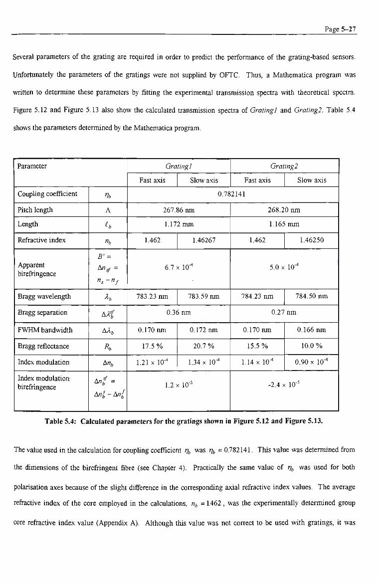
Page 5-27
Several parameters of the grating are required in order to predict the performance of the grating-based sensors.
Unfortiinately the parameters of the gratings were not supplied by OFTC. Thus, a Mathematica program was
written to determine these parameters by fitting the experimental transmission spectra with theoretical spectra.
Figure 5.12 and Figure 5.13 also show the calculated transmission spectra of Gratingl and Gratingl. Table 5.4
shows the parameters determined by the Mathematica program.
Parameter
Coupling coefficient
Pitch length
Length
Refractive index
Apparent birefringence
Bragg wavelength
Bragg separation
FWHM bandvfcidtii
Bragg refiectance
Index modulation
Index modulation birefiingence
V,
A
h "b
B' =
An^ =
h AAi
AA,
Rb
A«6
Anf =
Anl-Anl
Gratingl
Fast axis Slow axis
Gratingl
Fast axis Slow axis
0.782141
267.86 nm
1.172 mm
1.462 1.46267
6.7 X 10"
783.23 nm 783.59 nm
0.36 nm
0.170 nm
17.5 %
1.21 X 10"
0.172 nm
20.7 %
1.34 X 10-"
1.2 X 10-
268,20 nm
1.165 mm
1.462 1.46250
5.0 X 10-
784.23 nm 784.50 nm
0.27 nm
0.170 nm
15.5 %
1.14 X 10-'
0.166 nm
10.0 %
0.90 X 10-
-2.4 X 10-
Table 5.4: Calculated parameters for the gratings shown in Figure 5.12 and Figure 5.13.
The value used in the calculation for coupling coefficient % was % = 0.782141. This value was determined from
the dimensions of the birefringent fibre (see Chapter 4). Practically the same value of % was used for both
polarisation axes because of the slight difference in the corresponding axial refractive index values. The average
refractive index of the core employed in the calculations, «, = 1.462, was the experimentally determined group
core refractive index value (Appendix A). Although this value was not correct to be used with gratings, it was

Page 5-28
nevertheless believed to be the best value available to be used in tiie calculations. The actual average core
refractive index within the grating was different from that ofthe usual effective core refractive index due to the DC
photo-induced refractive index change.
The apparent birefringence of the fibre, An^f, can be inferred from the Bragg wavelength separation of the axial
gratings,. From Figure 5,12, Figure 5,13 and the theoretical calculations, An^f was about 6,7 x 10" and 5.0 x 10
for Gratingl and Gratingl respectively. These values were different from the expected value of An^ = 4 x 10
which was calculated from the beat-length of 1,6 mm at 633 nm (measured by the manufacturer).
The slow-axis Bragg grating was expected to exhibit a greater reflectance assuming that both axes experienced the
same index modulation following the couple-mode theory of FBGs. This expectation was observed in Gratingl but
not in Gratingl. The photo-induced refractive index change in germano-silicate fibre has both a DC (slowly-
varying) and an AC component, The AC component was responsible for the resonance effect whilst the DC
component and the pitch length of the grating determined the Bragg resonance wavelength. Figure 5.13 then
suggests that the slow-axis of Gratingl experienced both a greater AC and DC refractive index change than its
fast-axis compared with those of Gratingl. Clearly, the vmting conditions in the fabrication of the two Bragg
gratings(Graf/«g7 and Gratingl) were different.
Aside from illustrating tiiat tiie fast-axis grating had a greater peak reflectance value. Figure 5,12 and Figure 5,13
show that the Bragg wavelength separation ofthe axial gratings for Gratingl (0,27 nm) was shorter compared with
tiiat of Gratingl. Having different refractive index change induced on the same type of birefringent fibre implied
tiiat the photo-induced refractive index change has a birefringent character, Poirier et al [1993] had described tiie
model of the defect centres associated with 245 nm absorption band of germano-silicate fibres are preferentially
excited and bleached by UV light polarised along the dipole moment ofthe defect centres, i.e. the orientation ofthe
polarisation of the writing beam determines tiie orientation of tiie photo-induced birefringence. In addition, titis
photo-induced birefringence may enhance or relieve the intrinsic birefringence of an optical fibre [Bardal et al.

Page 5-29
1992]. This enhancement or relief of the total birefringence can explain the difference between the Bragg
wavelength separation of Gratingl and Gratingl (Figure 5.12 and Figure 5.13).
The significant difference of- 25% between the Bragg wavelength separation ofthe two gratings implies that the
photo-induced birefringence was about an order of magnitude less that the birefringence of the fibre. The
calculated the (absolute) photo-induced birefringence for Gratingl and Gratingl are 1.2x10"^ and 2.4x10"^
respectively (Table 5.4), These conclusions agreed with the results of Erdogan and Mizrahi [1994] who had
measured photo-induced birefringence between 1x10"^ to 6x10"^ in different photosensitive fibres.
5,3,2 Dual-Grating In-line FFPSs
In this work several gratings were inscripted in a birefringent fibre vrith the intention of fabricating in-line FFPSs.
This ability to write gratings in-house allowed us to determine the grating parameters and to tailor-design gratings.
The fabrication of these gratings and the in-line sensors are described in the following discussions.
Of aU the methods for fabricating FBGs (see review in Rao [1997] and Kersey et al. [1997]), the phase-mask
method is the simplest approach (Figure 5.14). It offers greater immunity from mechanical vibration and requires
less optical components to implement. This method exploits the diffraction interference pattern impressed on a
fibre produced by a UV beam through a phase mask [Anderson et al, 1993; Hill et al, 1993]. The novelty of this
scheme (Figure 5.14) is that the in-fibre grating spacing depends only on the pitch ofthe phase-mask and not on
the wavelength or the angle of incidence of the UV beam [Anderson etal, 1993]. Hence the method is less
sensitive to vibration as long as the relative position of the fibre and the mask was maintained. Long-length and
hence narrow-bandwidth gratings had been achieved by translating either the UV beam [Rourke et al., 1994] or the
fibre-phase-mask assembly [Martin & Ouellette, 1994]. On the other hand, short-length grating can be envisioned
with spatial apertures. The disadvantage of the phase-mask method was a fixed pitch length. Unfortunately the
grating spacing of the phase mask can only be slightly tuned thermally or mechanically or alternatively pre-
straining the fibre during grating inscription [Zhang et al., 1994b].
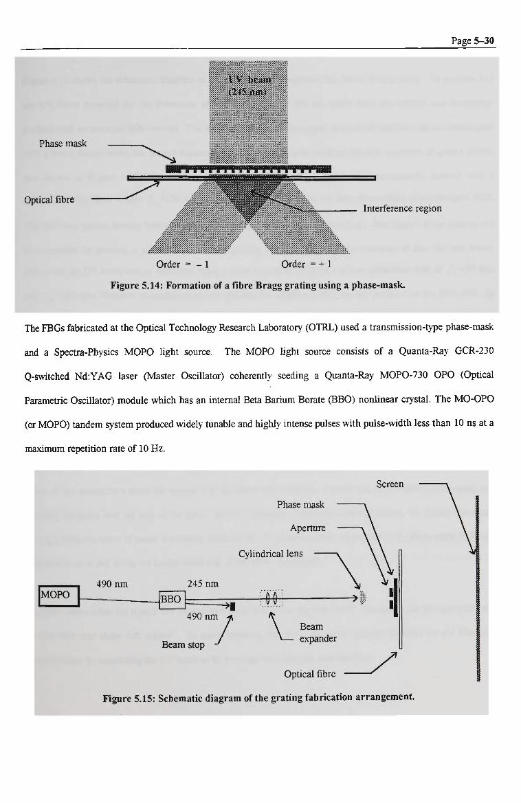
Page 5-30
Phase mask
i|ii|.i^n{miinimfniifi|MiniH|i|iii|iii|ini
Optical fibre _ Interference region
Order = - 1 Order = + 1
Figure 5.14: Formation of a fibre Bragg grating using a phase-mask.
The FBGs fabricated at the Optical Technology Research Laboratory (OTRL) used a transmission-type phase-mask
and a Spectra-Physics MOPO light source. The MOPO light source consists of a Quanta-Ray GCR-230
Q-switched Nd:YAG laser (Master Oscillator) coherently seeding a Quanta-Ray MOPO-730 OPO (Optical
Parametric Oscillator) module which has an internal Beta Barium Borate (BBO) nonlinear crystal. The MO-OPO
(or MOPO) tandem system produced widely tunable and highly intense pulses with pulse-width less than 10 ns at a
maximum repetition rate of 10 Hz,
Screen
Phase mask
Aperture
Cylindrical lens
MOPO 490 nm 245 nm
BBO
I 490 nm
Beam stop
^1 n -p Beam
expander
Optical fibre y Figure 5.15: Schematic diagram ofthe grating fabrication arrangement.

Page 5-31
Figure 5.15 shows the schematic diagram ofthe fabrication arrangement for the in-fibre grating. To produce 245
nm UV beam required for the formation of in-fibre grating, a 490 nm beam from the MOPO was frequency-
doubled with an external BBO crystal. The fiindamental-harmonic output beam ofthe BBO cystal was interrupted
with a beam dump whilst tiie second-harmoiuc was directed towards the fibre through a system of quartz prisms
(not shown in Figure 5.15). The 245 nm beam with a diameter of 3 mm was subsequentiy focused with a
cytindrical lens (focal length /j.=150 mm) into a thin optical line near the core of a section of birefringent fibre.
The fibre was placed directly behind the transmission side ofthe quartz phase-mask. The length ofthe grating can
be controlled by placing a suitable aperture for grating lengths less than the diameter of the 245 nm beam.
Otherwise the UV beam can be expanded using a beam expander composed of two cylindrical lens of fi =50 mm
and /i=100 mm. However expanding the beam reduced the effective energy density incident on the fibre core. In
practice, such reduction in the incident energy density were sometimes necessary in order the avoid the 1 J/cm^
damage threshold for the phase-mask or the fibre. The inscription was monitored by determining the transmission
spectmm ofthe fibre using an ANDO AQ3610B optical spectrum analyser whilst the fibre was illuminated with a
white-light source.
Made of thick white cardboard and placed after the phase-mask-fibre assembly (Figure 5.15), the screen served a
dual purpose. First it acted as an absorber of UV radiation not absorbed by the optical fibre. This ensured the
safety of the researchers since the unused UV radiation was captured. Second, the screen aided in focusing and
aligning the beam into the side of the fibre. As the UV beams was absorbed by the screen, the screen fluoresced
showing different types of bands depending whether the UV interferometric pattern from the phase-mask had been
projected onto or not along the longitudinal axis ofthe fibre respectively.
The fibre broke when the typical UV beam was exactiy focused on the fibre itself. The measured damage threshold
for the fibre was about 600 mJ/cm . To avoid breaking the fibre, the energy density incident on the fibre was
reduced either by expanding the UV beam or by focusing the beam just near the fibre.

Page 5-32
The photo-induced refractive index change in germanium-doped silica fibre required exposure to relatively large
energy density of UV beam. However, the photo-sensitivity ofthe fibres can be enhanced when the fibres had been
previously exposed to high pressure of hydrogen or deuterium [Lemaire et al, 1993; Mizrahi et al, 1993]. These
hydrogen-freated fibres then required much lower energy density to induce photo-refractive index change.
The birefringent fibres used were hydrogenated. They were inserted inside a specially designed capsule which was
filled with 70 atm of hydrogen. The capsule which contained the fibres was kept at a temperature of 100 °C for
about 16 hours. Subsequently the internal pressure ofthe capsule at this temperature reached about 100 atm. The
elevated temperature and pressure enhanced the penneability of hydrogen into the core of the fibres and thus
accelerated the enhancement of the photo-sensitivity of the fibre. Typically, the fibres were left inside the
pressurised capsule until the fabrication ofthe grating was about to commence.
The spectrum of one of the initial gratings written on birefringent fibres, GratingS, is shown in Figure 5.16. The
spectrum of GratingS, as expected exhibited two Bragg wavelengths as a consequence of the birefringence of the
fibre. The parameters of the grating were deduced from the theoretical fit of the spectrum. Table 5,5 summarised
the results of the fit. The phase-mask employed had grooves spaced 536.2 nm apart. This means that the grating
pitch was 268.1 nm. From the axial Bragg wavelengths, the effective core refractive indices of the fast and slow
axis are 1.4578 and 1.45845 respectively. These values imply the earlier refractive index value used in the earlier
calculations in this work, «, =1.462, gave an error of at most 0.3% and thus the previous calculations based on
«j,=1.462 were not re-calculated. The separation ofthe two Bragg wavelengths was about 0.35 nm and indicated a
birefringence AJT^ of about 6.7 x 10"^. On the other hand, the photo-induced birefringence was calculated to be
2 X10 ^ in agreement with the results from the earlier gratings.

Page 5-33
100.00%
90.00% -•
0 80.00% -
e
s I-
70.00%
60.00%
50.00%
Experimental
Calculated (Combined)
Fast Axis (Calculated)
Slow Axis (Calculated)
779.5 780 780.5 781 781.5 782 782.5 783 783.5
Wavelength (nm) 784
Figure 5.16: Transmission spectrum of a Bragg grating written on birefringent fibre (GratingS).
Figure 5.16 shows side-lobes which were not accounted for by the theoretical fit and hence their origin maybe a
result of other effects. It is most likely that coupling between the two polarised core modes may have been induced
as well. This effect is similar to the effect exploited to fabricate photo-induced rocking filters [Russel & Hand,
1990; Kanellopoulos ef a/., 1991c; 1992; HiU era/., 1991].
The calculated grating length of 0.72 mm for GratingS was about 4 times less than the diameter ofthe UV writing
beam (3 mm). This value may denote an effective beam width of the writing beam. In general the spatial intensity
distribution of the writing beam was not always uniform. In fact, on some occasions the writing beam had "hot-
spots" which broke the fibre during the initial few seconds of exposure. Certainly this condition was avoided and
only beams with good profile were used in fabricating the gratings. The non-uniform distribution may explain the
effective writing beam width lower than the diameter of the beam. This effective width implies a limited grating
length. However, for the wide-bandwidth gratings envisioned in this work, tltis apparent upper limit to the length
ofthe grating was more than adequate.

Page 5-34
Parameter
Coupling coefficient
Pitch length
Length
Refractive index
Apparent birefringence
Bragg wavelength
Bragg separation
FWHM bandwidth
Bragg reflectance
Index modulation
Index modulation birefringence
%
A
h
"b
B' =
An^ =
h
AAi
AAfc .
Rb
Artfc
Anf =
Anl-Anl
GratingS
Fast axis Slow axis
0,782141
268,1 nm
0,717 mm
1,4578 1.45845
6.5 X 10-
781.67 nm 782.02 nm
0.35 nm
0.310 nm
40.5 %
3.33 X 10"
0.3044 nm
37.0 %
3.13 X 10-'
-2.0 X 10-
Table 5.5: Calculated parameters for GratingS (Figure 5.16).
After fabricating several gratings on birefringent fibres, an in-line dual-grating birefringent FFPSs was attempted.
The ideal parameters for the in-fibre Bragg gratings are presented in Table 5.6. These parameters assume that the
average Bragg wavelength is 790.4 nm. This wavelength is the centre ofthe range of emission wavelengths which
give stable single-longitudinal output of the modulated LD, A reflectance of 3% and bandwidth of 2 nm were
desired for each axial grating. These values easily produce low-finesse interferometers along each axis of the
sensor and also give a small magnitude for the anomalous dispersion over the bandwidth of the grating. To obtain
a large bandwidth, the grating length must be very short, 0,1 mm.
The in-line sensors were produced using a double-slit aperture placed between the UV light source and the phase-
mask. The double-slit aperture was specially crafted using a 0,3 mm thick cardboard paper. The slit width and
separation were 0,2 mm and 10 mm respectively. These conditions imply grating lengths stightiy smaller than
0.2 mm and a Fabry-Perot cavity length of 10 mm. Although the ideal grating length desired was about 0,1 mm,

Page 5-35
for an initial grating length, 0.2 mm was chosen in order to lower the refractive index modulation value required to
produce some reflectance and to provide at least a bandwidth of 1 nm. The 245 nm UV beam was found not to
diverge sigiuficantiy through the 0,2 mm slits. The aperture nevertheless was placed immediately in-front of the
phase-mask to mirumise the diffraction of the UV beam (Figure 5.15).
Parameter
Coupling coefficient
Pitch length
Length
Refractive index
Apparent birefringence
Bragg wavelength
Bragg separation
FWHM bandwidth
Bragg reflectance
Index modulation
Index modulation birefringence
Vb
A
h
"b
B' =
An,f =
h
AAi
A/l,
Rb
An,
Anf =
Anl-Anl
Ideal Grating
Fast axis Slow axis
0.782141
271 nm
0.1 mm
1.458 1.45863
6.3 X 10'
790.225 nm 790.575 nm
0.35 nm
2 nm
3 %
5.864 X 10""
2 nm
3 %
5.867 X 10-
3 X 10"
Table 5.6: Ideal parameters for gratings written on a birefringent fibre to form a Fabry-Perot sensor.
There were initial attempts to write the two gratings simultaneously. The 245 nm beam was expanded to a
diameter wider than the separation of the slits. However, no grating was formed even after 30 minutes of
exposure. This may be due to the weaker energy density at the wings of the expanded UV beam compared at its

Page 5-36
cenfre. Thus, each of the grating was then written one after the other by directing the unexpanded UV beam
through each ofthe corresponding slits. Figure 5.17 shows the transmission spectra ofthe gratings which formed
an in-line fibre Fabry-Perot sensor (InLineFPl). The two gratings were each written for about 15 minutes with an
effective incident energy density of 120 mJ/cm . The spectrum ofthe first grating (Grating-Mirror 1) was obtained
at conditions near the noise fioor of the optical spectrum analyser. In hindsight, the noise in the spectrum could
have been reduced by applying some averaging routine.
Grating-Mirror 1
Grating-Mirror 2
Fabry-Perot Sensor (Grating-Mirror 1 + Grating-Mirror 2)
781,5
Wavelength (nm)
782.5 783.5 784
Figure 5.17: Transmission spectra of the two grating-mirrors written on a birefringent fibre to produce an in-line fibre Fabry-Perot sensor (InLineFPl). For clarity, each spectrum has been vertically shifted in order to separate itself from the other spectra. Each data point composing the spectrum for the in-line sensor (labeled "Fabry-Perot Sensor") is the average of 20 samples. No averaging routine was performed with the spectrum of the first grating (labeled "Grating-Mirror 1").
In Figure 5,17, the spectrum ofthe second mirror was derived by subtracting the spectrum ofthe first mirror from
combined spectiiim of the in-line sensor. Figure 5,17 shows that the spectrum of the second mirror exhibited
evidentiy two Bragg resonances unlike tiiat of tiie first mirror. This double-resonance feature was unexpected
because tiie features of tiie wide-bandwidth axial gratings are not suppose to be distinguishable when the combined
transmission spectrum ofthe axial gratings is obtained using an unpolarised white-light source. Ocular inspection
of tiie slits after the fabrication of the second grating revealed that the focused UV beam had gradually cut

Page 5-37
perpendicularly across the slits. This cut implies a longer length for the second grating and thus explains the
nartower bandvddth properties of the second grating as shown in Figure 5.17. The reflectance of the axial gratings
ofthe first mirror was about 2.5 % whtist those ofthe second mirror, about 4%. This means that the sensor is low
finesse.
Other in-line double-grating FFPSs were fabricated with an improved double-slit aperture. As in the earlier case,
the new double-slit aperture had a slit-width of 0.2 mm and a separation of 10 mm. Each of the slits consists of
two layers of cardboard paper sandwiching stainless steel razor blades. The sharp edges ofthe razor blades defined
the edges of the slits. The cardboard paper were employed primarily for safety since steel can reflect UV light.
Thus the cardboard paper absorbed the unused UV beam and thereby fluoresced.
Grating-Mirror 1
Grating-Mirror 2
Fabry-Perot Sensor (Grating-Mirror 1 + Grating-Mirror 2)
782
Wavelength (nm)
Figure 5.18: Transmission spectra of the two gratings written on a birefringent fibre to produce an in-line fibre Fabry-Perot sensor (InLineFP).
Figure 5,18 shows the transmission spectra of the gratings employed to fabricate one of the in-tine fibre Fabry-
Perot sensors using the new double-slit aperture (InLineFPl). The first grating written had an exposure time of
about 10 minutes whilst the second 20 minutes. The effective incident energy density was about 60 mJ/cm . The

Page 5-38
estimated reflectance and bandwidth ofthe axial gratings are 4 % and 1.8 nm respectively for the first mirror, 8 %
and 2.2 nm for the second mirror. The grating formation rate of InLineFPl was faster than that of InLineFPl.
This greater value can be attributed to the better focusing ofthe UV interference patterns into the core ofthe fibre.
The spectra of InLineFPl and InLineFPl show that the average Bragg wavelength of their Fabry-Perot mirrors do
not coincide. In fact Figure 5.17 and Figure 5.18 show that the spectral location of the second grating-mirror was
to the left of the first grating-mirror of the in-line sensors. This condition means the overall measurand range of
the sensor is smaller than when the averaged Bragg wavelength of their Fabry-Perot mirrors coincided. The
overall range is stiU large though because ofthe large bandwidth ofthe axial gratings.
S5 in n
E -
780 780.5 781 781.5
Wavelength (nm)
after fabrication
2 hours
783
Figure 5.19: Transmission spectra of the two gratings written on a birefringent fibre to produce an in-line fibre Fabry-Perot sensor (InLineFPl).
There is a slight complication with hydrogenating the birefringent fibres. When the combined transmission
spectiiim of the in-line Fabry-Perot sensors was recorded after fabrication, the spectrum had shifted to lower
wavelength values. For example. Figure 5.19 shows the shifts in the transmission spectrum of InLineFPl.
InLineFPl shifted by 0.1 nm after 24 hours since fabrication. This was due to the fact that when hydrogen was

Page S-39
infroduced into the core of the fibre, the effective core refractive index had increased. Thus when the hydrogen
molecules outgas themselves from the core, the refractive index of the core decreased. Hence this wavelength
shifts must be considered when the sensors are finally used.
No temperature or strain measurements were made with the in-line Fabry-Perot interferometers fabricated
including the two described in this section. This was because the LD output could not be tuned to the actual Bragg
wavelength of the gratings without causing the LD output to mode-hop. Replacing the LD with another similar
device gave similar results most probably because all the LDs were fabricated in the same batch. Had the
wavelength of the LD fallen within the spectrum of the gratings, interferometric signals would have been expected
even when the spectra of the first and second grating-mirrors did not exactly coincide because low optical signal
can still be detected (Appendix B).
The measurements made with the sensors developed in this work are discussed in the Chapter 7. In the next
chapter, the measurement arrangement used with the birefringent sensor is described.

Chapter 6: A Birefringent Optical Fibre Sensing
System for the Measurement of
Temperature and Strain
This chapter describes an optical fibre sensing arrangement employing a birefringent fibre Fabry-Perot sensor for
the measurement of temperature and sfrain. The arrangement has four major components: the sensor, optical
detection arrangement, signal processing and phase recording system. In this work, these components have been
chosen such that localised measurement of temperature or strain can be obtained vrith high-resolution, large UMR
and at a moderately fast rate.
6,1 The Optical Fibre Sensing Arrangement Compared With Its Closest Fore-Runner
In terms of operation principles, the arrangement described in this chapter (Figure 6,1) is similar to that employed
by Farahi et al [1990] (Figure 6.2), In this work, we have extended their arrangement in many aspects. A brief
comparison is worthwhile. The chosen sensor configuration of this work and that of Farahi et al was a Fabry-Perot
sensor formed in a birefringent single-mode fibre with thermally induced stress production parts. We used a fibre
with an internal elliptical cladding (EC-fibres) whilst Farahi et al used a bow-tie fibre. In both cases, two Fabry-
Perot interferometers are formed, one along each polarisation axis.

N
60 ts
U l
.•' u o ,• V H W3 "
/ X) c ^^ Vi
•...* &0 D -C 0-
b4 . 0
S£
to e
Lea
d-in
bir
efri
ngen
t fi
bre
(L> \ ~ -s sma- /
fj V 1/ . VJfc,.' , - ' * " " " ' • . ' • .
.••E
irisi
ng b
ea
r(N
PBS)
H \ ( TO u •,
• ^ • * - ' ••
0 *^ ;
0
/ 2 \ ;
J S '' '•••
u . Ksxssxssssssassssssssssa • * : " • • •
k
A A 1 • w
Ul
0 «
sol
6 Q ,
0
-4— M
a) — -ssm :-0 ^ H
\ X
in i ^ 1 « .£
J T
> 3 > J
/^
^ •
^ 1 ^ ™
2 pl
ate
«-e
i -?5 "
To DH 00 w C u • ^ U
lari;
pl
itt
0 t/i
B - ^
••^•^^•Siv
1
0 0> 0 "5 . s 0
t
ens
101
X
CO
Ole
i ><
Phot
o-di
ode
'n~ 0
cti
ti
refl
in t
his w
o ; "9 : ti
5B m
entu
ng
e 1 a
rra
enta
xp
crim
hc
e:
•*rf
0
£ « u
iag
• 0
tic
ti E ii
£ u
SO 9 u ^ £
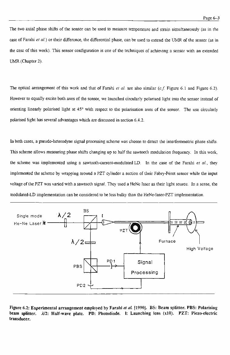
Page 6-3
The two axial phase shifts of the sensor can be used to measure temperature and strain simultaneously (as in the
case of Farahi et al) or their difference, the differential phase, can be used to extend the UMR of the sensor (as in
the case of this work). This sensor configuration is one of the techniques of achieving a sensor with an extended
UMR (Chapter 2),
The optical arrangement of this work and that of Farahi et al are also similar (c.f Figure 6,1 and Figure 6,2).
However to equally excite both axes ofthe sensor, we launched circularly polarised light into the sensor instead of
orienting linearly polarised tight at 45° with respect to the polarisation axes of the sensor. The use circularly
polarised tight has several advantages which are discussed in section 6.4.2.
In both cases, a pseudo-heterodyne signal processing scheme was chosen to detect the interferometric phase shifts.
This scheme allows measuring phase shifts changing up to half the sawtooth modulation frequency. In this work,
the scheme was implemented using a sawtooth-current-modulated LD. In the case of the Farahi et al, they
implemented the scheme by wrapping around a PZT cylinder a section of their Fabry-Perot sensor while the input
voltage ofthe PZT was varied with a sawtooth signal. They used a HeNe laser as their light source. In a sense, the
modulated-LD implementation can be considered to be less bulky than the HeNe-laser-PZT implementation.
Single mode
He-Ne Laser ^
High Voltage
Figure 6,2: Experimental arrangement employed by Farahi et al [1990], BS: Beam splitter, PBS: Polarising beam splitter. All'. Half-wave plate. PD: Photodiode. 1: Launching lens (xlO). PZT: Piezo-electric transducer.

Page 6-4
The implementation of Farahi et al is suited to a Fabry-Perot sensor with a long cavity within which only a section
of their sensor is exposed to the measurand limiting its sensitivity to reasonable values. In this work, we have
chosen to investigate short-cavity Fabry-Perot sensors. The minimum cavity length was determined by the
maximum chirp in the emission frequency of the modulated LD without any accompanying mode-hop effect.
Altiiough the phase-measurand sensitivity is proportional to the exposure length, these short-cavity sensors are still
highly sensitive to measurands like temperature or strain (Chapter 4), In addition, short-cavity sensors can provide
localised measurements which are desirable in many applications. They use a lead-in fibre which eliminates the
interference involving the cladding or leaky modes. Moreover, the lead-in fibre naturally provides the first step in
assembling an all-fibre arrangement and if desired, several sensors can be serially multiplexed on the same fibre
line.
In this work, we investigated birefiingent FFPSs either fabricated with fiision-spliced TiOa mirrors or in-fibre
Bragg gratings. The fabrication of tiiese sensors was one ofthe major challenges of this work (Chapter 5). These
fabricated sensor were designed to be low-finesse because low-finesse FFPSs approximately give sinusoidal
interferometric outputs (Chapter 3). This type of output is required by the pseudo-heterodyne signal processing
scheme.
The digital electronic circuits we employed to measure the interferometric phase shifts with a resolution of LlC
enabled us to observe effects attributed to the non-ideal adjustments of the pseudo-heterodyne signal processing
scheme and the dispersion of a Bragg grating reflector written in an optical fibre (Chapter 7).
6,2 Detailed Description of the In-Fibre Birefringent Fabry-Perot Sensor
In-fbre reflectors
< • • • . « :
..."JS^MSJ I:::-...},. » •^g|^'--v> v y '••• Ji
Lead-in birefringent fibre .^ Birefringent •^ Optional lead-out birefringent fibre ^
fibre Fabry-Perot sensor
Figure 6.3: An in-fibre birefringent Fabry-Perot sensor.

_ _ ^ Page 6-5
Figure 6.3 shows tiie in-fibre arrangement used a birefringent FFPS. The lead-in fibre waveguide and tiie Fabry-
Perot cavity are composed ofthe same type of polarisation-maintaining fibre. The polarisation axes of this lead-in
fibre are aligned with those of the birefringent Fabry-Perot cavity in order that each axial interferometer can be
independentiy addressed in reflection. Optionally, the sensor can be concatenated with a lead-out fibre which
provided a waveguide to address the sensor in transmission or to multiplexed with other Fabry-Perot sensors.
The lead-in fibre provides the simplest mechanism for remote sensing and single-ended operation of the sensor
without any additional optical components. The length of this fibre can be as long as desired to the upper timit
determined by the crosstalk between the polarisation axes of the fibre as described by the parameter h, the
coupling ratio per uitit length of the fibre. With the specifications given by the manufacturer for the polarisation-
maintaining fibre used (Table 6,1), a crosstalk of more than 1% appears only after a length of 1 km assmning no
sharp bends are present along the fibre.
To avoid any inter-modal interference, the sensor needs to be operated in the single-mode regime. This is ensured
by using a suitable light source. In this work, the LD used was chosen because its emission wavelength is greater
than that ofthe 700 nm single-mode cut-off wavelength ofthe fibre. In addition, the lead-in fibre can also act as a
mode filter. By using a sufficientiy long lead-in fibre, any initial cladding and leaky modes is dissipated and only
the fimdamental-mode beam eventually reaches the sensor. Fortunately, the fibre used is a mode-stripping acrylic
jacket. A length of about two meters is sufficient to remove any unwanted cladding modes.
6,3 Description ofthe Optical Fibre Sensing System
The optical arrangement which addresses the birefringent sensor in reflection is shown schematically in Figure 6.1.
Light from a 785 nm LD is first circularly polarised using a quarter-wave plate and is subsequentiy launched into
the lead-in fibre using a xlO microscope objective lens. With this lens, the average coupling ratio into the fibre
was about y =10%. The input beam eventually addresses the sensor and excites each axial interferometer
simultaneously. Subsequentiy, the reflected beams along each axial Fabry-Perot interferometer remm following
the reverse path taken by the initial input axial beams.

Page 6-6
Component
LD
Photodiodes
Polarisation Maintaining Fibres
Microscope objective lens Wave plates: half-wave quarter-wave
Polarisation beam splitter cube
Non-polarising beam splitter cube
Optical isolator
Manufacturer and Part Number
Hitachi HL7806G
Optex OPF480
3M FS-HB-4211
ELIZA
Melles Griot 02 WRQ021/785 02 WRQOO1/785
Newport 05FC16PB.5
Newport 05BC16NP.6
Optics for Research (OFR) IO-2-NIR2
.
Specifications
Lasing wavelength Description Lasing material Structure
Longitudinal-mode spacing Feature Monitor responsivity Maximum power Threshold current Slope efficiency Coherence length Material Collecting area Flux responsivity Rise time
Peak wavelength Type
Single-mode cut-off core/fibre/jacket radius Feature
Estimated Delta Numerical aperture Beat length Attenuation Crosstalk parameter h Proof test level Magnification Numerical aperture Type Central wavelength Aperture Retardation tolerance Operation wavelength Extinction ratio (experimental) Length of side Operation wavelength Spectral tolerance Splitting ratio Length of side Operating wavelength Transmittance Isolation Aperture
~785nm Single longitudinal mode AlGaAs Index-guided channel-substrate-planar (CSP) ~0,3nm with built-in photodiode -0,5 AAV 5mW 45 mA @ 20 °C 0,28 mW/mA (measured) ~ 2 m (modulated) Silicon 1 mm X1 mm ~ 0.5 A/W @780 nm 1 ns (VR = 15 V, RL=50n, 10%-90%) 820 nm Stress-induced elliptical cladding 700 nm 2.25/40/100 ^m Mode-stripping outer acrylic jacket 0.47 % 0.12 1.6 mm @ 633 nm 4.2 db/km @ 850 nm 10"Vm 50kpsi +10 0.25 Quartz, multi-order Designed @ 785 nm 10 mm diameter U500 620 - 1000 nm s-beam = 0,6 % (-22,2 dB) p-heam = 3,3 % (-14.8 dB) 12,7 mm (0,5 in,) 780 nm ±3% 50/50 12.7 mm (0,5 in,) 780 nm 94 % (test results) -40 dB (test results) 5 mm
Table 6.1: Specifications for the components comprising the sensing system.
Page 6-7
To prevent any reflection from this face, the proximal end ofthe lead-in fibre can be potished at an angle of about
7° with respect to the plane perpendicular to the longitudinal axis of the fibre. This reflection is not desired for
two main reasons. First, this reflection can otherwise coherentiy interfere with the returning beams and hence
exhibit another Fabry-Perot interference between this proximal face and the mirrors ofthe Fabry-Perot sensor. This
additional Fabry-Perot effect occurs only when the length of the lead-in fibre is shorter than the coherence lengtii
of input beam. Although the lead-in fibre can be chosen to be long, this approach was not implemented because of
the limited amount of the birefringent fibres available for this work. Secondly the intensity of the reflected beam
from this end is greater than that of the beam coming from the sensor, this reflection contributes to an additional
background intensity detected by the photodiodes (PDs). Thus, minimising the contribution of this reflection
improves the electronic fringe visibility.
The returning beams from the sensor are diverted towards a polarising beam splitter (PBS) cube using a non-
polarising beam splitter (NPBS) cube. The non-polarising properties of the NPBS is due to a specially designed
thin-film deposited at the reflecting interface of the NPBS cube. This film exhibits equal reflectance of the s- and
;?-polarised beams. Since the properties of the thin-film are wavelength-dependent, the NPBS was fabricated to
operate at a wavelength of about 785 nm.
The polarisation axes of the sensor were aligned with those of the PBS using a half-wave plate. In general the
combined beam returning from the birefringent FFPS is eUiptically polarised. However, the PBS conveniently
decomposed this eUiptically polarised beam into tangential beams which are the outputs of the two polarised
interferometers. The intensities of these tangential beams were detected by silicon PDs.
The tight source is a 5 mW Hitachi HL7806G LD lasing at a single longitiidinal mode of- 785 nm. This mode of
operation occurs if the LD is driven well above its lasing threshold. To prevent any undesirable optical feedback
into the laser cavity, an opto-isolator was inserted between the LD device and the quarter-wave plate. The opto-
isolator is composed of a Faraday rotator between two crossed polarisers. Hence the output beam is linearly
polarised. This linearly polarised beam was converted into a circularly polarised light using a quarter-wave plate.

^ Page 6-8
The quarter-wave and half-wave waveplates used were of the multi-order type and were designed to operate at
-785 nm with a tolerance of about 1,6 nm,
6.4 Jones Calculus Treatment
The overall optical system described in the last two sections can be analysed using Jones calculus [Jones, 1941;
Hurwitz & Jones, 1941; Klinger et al, 1990], In such an analysis, the evolution ofthe amplitude and phase ofthe
electric field of two perpendicular elecfromagnetic waves as these waves pass through a sequence optical elements
are determined. Alternatively, these waves can be treated together as a single wave with two independent
components. Hence in general the tip of the electric field of the combined wave follows an elliptical helix as the
beam propagates. The eUipticity and orientation of the ellipse describe the state of polarisation of the light beam.
Such a beam can be expressed as a Jones vector
'E, Ei„ =
LE.
Eq. 6.1
When tiie beam expressed in Eq. 6.1 travels through an optical element, the emerging beam can be expressed as
Eq. 6.2 ^out - J ' E , „ -
•^ XX • ' j y
:^yx -^yy E.
where J is the characteristic Jones matrix for tiie optical element. The diagonal elements in J can be interpreted
as direct transformation of each polarised beam whilst the off-diagonal elements the cross-coupling between the
two orthogonal input beams, Eq. 6.2 completely describes the resulting beam due to an input beam incident on
the optical element. It follows therefore that an optical system comprising of several optical elements can
equivalentiy be described as a single (total) Jones matrix J , , the matrix product of the Jones matrices of the
individual optical elements, i.e.
Eo«( = J f '^in = J n "Jn-l •••••''2 "^I " ^m
where J, and J„ are the first and last optical element encountered by the beam respectively.
Eq. 6.3
The components of the total electric field are spatially orthogonal and hence do not interfere. However, these
components can interfere when they are brought together. The light beam is said to be unpolarised if its two
orthogonal components do not interfere when brought together and polarised if they interfere. In practice no beam

Page 6-9
is perfectiy unpolarised or polarised and hence in general most beams are partially polarised. Since Jones calculus
operates only on electric fields, it is inadequate for partially polarised beams. An intensity treatment is more
appropriate and the corresponding analysis is known as Mueller calculus [Jerrard, 1982]. However since the
coherence length of the LD used in this work is much longer than the OPD of the sensors, the Jones calculus
treatment suffices.
For the optical arrangement described in Figure 6.1, the total electric field emerging either from the side {b = y) or
the straight-through (b = x) beams ofthe polarising beam sptitter can be described as follows
^out,b - ^t ' ^in - ^detection,b ' [^Fresnel + ^in-fibre ] '^launching ' ^in
where ipresnei describes the Fresnel reflection from the proximal face of the lead-in fibre while the other three
Jones matrices are the launching, in-fibre and detection sub-systems of the experimental arrangement. The input
beam in Eq. 6.4 is the output beam of the opto-isolator. This beam is linearly polarised. For the rest of the
analysis, this input beam (normalised) is defined to be along the x-axis, i.e.
E,„ = Eq. 6.5
The other three Jones matrices in Eq. 6.4 are given by
haunckins ='S.(S)-3j^, • R ( Z ) • J , „ , ^ , , • R ( 0 , E q . 6.6
iin-fibre =4r-head •^(U)-iFP 'RC^)'J/.^ , and Eq. 6.7
idetecnon.b = ip,b -RC^)" J;,.// -RCf " J^P. •R(5) • Eq. 6.8
Y is the intensity coupling efficiency into the fibre and is assumed to be equal for both polarisation axes. The
polarisation coordinate system of the left-hand side in Eq. 6.6, Eq. 6.7 and Eq. 6,8 is that of the distal optical
element (described by the first matrix element in the right-hand side of each equation). The Jones matrices are
those for the individual optical elements in the optical detection system and are presented in Table 6,2, R ( 0 , the
transformation due to an angular rotation of O, accounts for the relative angular orientation of the polarisation
axes of two adjacent optical elements and is measured anti-clockwise from the positive x-axis from the first
element. O is the angle between the x-axis of the input beam and that of the quarter-wave plate, Z between the x-
axis of quarter-wave plate and that ofthe NPBS, S between the x-axis ofthe NPBS and that ofthe lead-in fibre,

Page 6-10
U between the x-axis of the lead-in fibre and that of the Fabry-Perot sensor, W between the x-axis of the NPBS
and that ofthe half-wave plate and H between the x-axis ofthe half-wave plate and that ofthe PBS,
Eq. 6.6, Eq. 6,7 and Eq, 6,8 divides Eq, 6.4 into three major groups of optical components comprising the
entire optical arrangement. J,„_y;j„ determines the resulting electric field after an initial field has transverse the
lead-in fibre and reflected from the sensor, J launching determines the degree each polarisation axis ofthe sensor will
be excited, and J^jetectionj, determines the electric field detected by each PD b. In general these matrices can be
complicated. However, if certain assumptions and the design considerations are taken into effect, the final
expressions for the output beams are simple. These final expressions are described in the of following discussions.
6.4.1 In-Fibre Sub-System
The role of the in-fibre sub-system in the whole sensing system is to guide the incident light towards and the
subsequent reflected light from a birefringent Fabry-Perot sensor. The resulting Jones matrix for the optical
arrangement with a single in-fibre sensor in general can be complicated if the optical energy can cross-couple
between tiie polarisation axes in the lead-in fibre and the birefringent Fabry-Perot sensor. Fortunately, because the
small cross-coupling ratio of the fibre used in this research, the off-diagonal terms in J;^^ can be neglected.
Likewise, Jpp can be written to have only the diagonal terms if it is assumed that there is no cross-coupling
between the axes of the cavity and also no cross-illumination of the axes during reflections from the two Fabry-
Perot mirrors. Hence, calculating Eq. 6.7 , the Jones matrix for the in-fibre sub-system is
J-exp(i2k^z){F„cos\U) + F^sin\U)} -exp{ik^z+ikyZ)sin(2U){F^-Fyy} ^^' ^'^ ^in-fi,re = V ( ) ( -7 -y )
[ exp(ik,z+ikyZ) sin{2U)[F^ - Fyy } exp{i2kyZ)[F^ sin' (U) + Fyy cos' (f/)|
Eq. 6.9 implies that in order for F^ and Fyy to be distinguishable, the off-diagonal elements must be zero. This
condition occurs when rr AC Eq. 6.10 U = 0° ,or f/ = ±90°. Eq. 6.11

Page 6-11
Optical Element Jones Matrix Definitions/Comments
Non-polarising beam splitter: transmission 'NPt
tx 0 0 r„
t^ and ty are electric field transmission coefficients along the x- and y-axis.
Non-polarising beam splitter: reflection ^ NPr
rx 0 0 r„
r^ and r are electric field reflection coefficients along the x- and y-axis.
Polarising beam splitter
^ F , * -
^ P,x -
^P,y -
dxb +£xySy,
Syb +£yx^xb
'1
0
r^^ Lo
0 "
£yx_
0'
1_
The X- and y-axis beams emerge as straight-through (b = x) and side (b = y) beams, respectively. The diagonal elements involve the Kronecker delta fimctions 5,;. £^ and f vr are the residual electric
field extinction ratio for a polariser oriented along the y-axis and x-axis respectively.
Lead-in fibre
'/ead -'L^
w ^A ^yy\
expQk^z) xy
'yx e^{ik z)
2nn^y where k^.^= — and
'•^ A
Uxyl = l^yxl = yf^
The cross-coupling coefficients are assumed not to have any phase dependence.
h is the cross-coupling per unit length,
z is the length ofthe lead-in fibre.
Half-wave plate
Fabry-Perot sensor
Transformation matrix describing the rotation of eigen-polarisation axes
Fresnel reflection from the proximal end ofthe lead-in fibre
'half
X-axis is the fast axis.
Jpp --F^ -F, xy
F. yx
F, yy
F^ and Fyy axe the electric field interferometric reflection coefficients as derived in Chapter 4. The negative sign in the matrix accounts for the effect of reflection.
R(0 = • cos(0 sin(2) - s in(0 cos(0
Q is the angular rotation ofthe polarisation axis measured relative to the original x-axis. Positive values of Q is in the anti-clockwise direction.
' Fresnel
-Tf rf is the Fresnel reflection at normal incidence to the proximal face ofthe lead-in fibre. The negative sign accounts for mirror inversion ofthe polarisation axes.
Table 6,2: Jones matrix representation of each optical element of the sensing system.

Page 6-12
Eq. 6.10 refers to the case when the fast axis of the lead-in fibre and that of the sensor are aligned. Eq. 6.11
refers to the case when the fast axis of the lead-in fibre and tiie slow axis of the sensor are aligned. Subsequentiy
Eq, 6,9 becomes
' in-fibre
' in-fibre
4?
47
• exi>{i2k^z)F„ 0 0 exp{i2kyZ)Fy,
y ' yy. or
-ex^{i2k^z)Fyy
0 0
e\p{i2kyZ)F^^
Eq, 6,12
Eq, 6.13
after Eq. 6.10 or Eq, 6,11 has been used respectively. The negative sign in the first diagonal element in the
matrices signifies the effect of reflection. For other values of U otiier than 0° and 90°, the electric field of each
interferometer can coherentiy interfere resulting in a complicated electric field.
6.4.2 Launching Sub-System
The launching sub-system determines the intensity of light coupled into each polarisation axis of the birefringent
FFPS, The launching optical arrangement was basically designed such that circularly polarised light is launched
into the lead-in fibre using the linearly polarised light coming from an opto-isolator. However, launching
circularly polarised is not a strict requirement but rather is the simplest method to equally excite the two axial
Fabry-Perot interferometers. In general, the effect of an elliptically polarised beam incident on the lead-in fibre is
unequal excitation along the polarisation axes ofthe sensor.
Circularly polarised light can be produced from linearly polarised light using a quarter-wave plate oriented such
that the fast axis ofthe quarter-wave makes a 45° angle witii respect to the input beam, i.e.
0 = ±45°. Eq. 6.14
Because circularly polarised light has no polarisation azimuth state, it is invariant under any rotational
transformation. To maintain this rotational invariance, the electric field transnussion coefficients of the NPBS
must be equal, i.e.
t =t = r Eq. 6.15
Substitution Eq. 6.14 and Eq. 6.15 into Eq, 6.6, the resulting Jones matrix for the launching arrangement is

launching r_ \ exp(i(Z + S)) exp(- i{Z + S))
yf2[iexp{i(Z + S)) -ieKp{-i(Z + S))
Page 6-13
Eq, 6,16
Hence the beam launched into the lead-in fibre is
E;„=J t^
launching '£,„ =-j=exp(±/(Z + 5)) Eq. 6.17
is always circularly polarised and does not depend on either the angular alignment ofthe polarisation axes between
the NPBS and quarter-wave plate nor that between the NPBS and the lead-in fibre. Hence, the use of circularly
polarised light considerably simplifies the optical measuring system.
On the other hand, when the beam splitter is polarising in transmission, i.e.
t^^ty Eq. 6.18
the launching sub-system will need a half-wave plate in order to launch circularly polarised light. Figure 6.4 the
alternative arrangement which uses the half-wave plate. The quarter-wave plate converts linearly polarised light
into an elliptically polarised light of any ellipticity. Subsequentiy, the azimuth of this elliptically polarised tight is
rotated such that the resulting beam when it traverse the NPBS (which is no longer non-polarising) will be
circularly polarised.
Laser diode
XIO lens
Opto-isolator
Ordinary beam splitter (BS)
0 0 XIA plate XI2 plate
Figure 6.4: Alternative launching optical arrangement.
Besides the advantage of the rotational invariance of circularly polarised light, the launching arrangement
enhances the optical isolation between the rest of tiie experimental arrangement and the LD. In particular, the
Fresnel reflection at the proximal face ofthe lead-in fibre is effectively attenuated. This reflected beam retunung
to tiie LD passes through the launching arrangement in reverse order, i.e.
^retuming.Fresnel =" ^(.Q)' ^ quarter^(Z) • J f^f •R{S)-J p^g^^i • £ , ' „ . Eq. 6,19

Page 6-14
Evaluating Eq, 6.19,
"' returrring,Fresnel
Eq. 6.20
which is cross-polarised with respect to the input beam (Eq, 6.5). As previously mentioned, this input beam is
produced by tiie opto-isolator output linear polariser which will not allow E^g „,„g;rrei„g; to reach the LD.
Effectively, the input beam E,„ is rotated by 90° which is not surprising since the double pass through the quarter-
wave plate makes the arrangement a half-wave plate oriented at 45°. This opto-isolation property of the launching
arrangement holds for any reflection ofthe circularly polarised beam from other optical elements. This property of
the optical launching sub-system is in addition to that provided by the opto-isolator.
However, the opto-isolator is still an important component of the optical sensing system. Without its use, the LD
has been experimentally observed to be affected by back reflection from the Fabry-Perot sensor. This situation
occurs because the beam returning from the sensor and traveling towards the LD, in general can be elliptically
polarised which will not be isolated by the quarter-wave-plate-linear-polariser tandem arrangement described
above. Thus the suitable attenuation of this returning beam is depended solely on the isolation properties of the
opto-isolator.
6.4,3 Detection Sub-System
The fiinction of the detection sub-system is to effectively separate the interferometric signals along each
polarisation axis of the birefringent Fabry-Perot sensor. The Jones matrix for the detection system can be
simplified if it can be assumed that the half-wave plate is suitably adjusted such that the axes of the polarising
beam splitter and those of the in-fibre sub-system (hence those of the sensor) are aligned. This means
W = H-S or W = H-S±9Q''. Eq. 6.21
Just like with the components ofthe in-fibre sub system, the fast and slow axes ofthe PBS and those ofthe in-fibre
system do not need to correspond. Using Eq, 6,21, Eq, 6,8 becomes,
(S^ + £^Sy, ){r, cos'(5-) +r^ sin'(S)] (S^ + £^Sy,) sin(2S){r, - r^} ^ ^^' ^'^^ "* detection.b —
-iSy, ^£y,6^)sin(2S){r^ -r^} -{Sy^, +£y,5^){r, sin'(5')+r^ cos'(5)}

Page 6-15
Eq. 6.22 implies that in order for the detection arrangement to separately analyse each axial interferometer of the
sensor, the diagonal elements (in Eq, 6.22) needs to be zero. This condition means that either the axes of NPBS
and the lead-in fibre are aligned in the beginning on one hand, Le.
S = 0° or 5 = ±90°; Eq. 6.23
or the beam splitter is non-polarising in reflection, i.e.
r^=ry= r^ Eq. 6.24
on the other. The former situation though achievable can not be guaranteed always especially when the sensor
under investigation is replaced with another. Thus, the latter condition may be more practical and using the latter
condition, Eq. 6.22 becomes
{S^+£^Syi,)r^ 0
0 -{Sy,+£y,S,,)r^
Eq. 6.25 " detection,b
Interestingly, 3detection,, is not dependent on angle S as Eq. 6.22 has implied. Clearly, the condition expressed
in Eq. 6.24 simplifies the whole optical arrangement. This condition implies that NPBS needs to be effectively
non-polarising both in transmission and reflection. Eq. 6.25.depends on the fact that Eq. 6.21 andEq. 6.24 hold.
With the NPBS exhibiting the properties expressed in Eq. 6.24, Eq. 6.21 can be ensured by using a rotatable half-
wave plate between the PBS and the NPBS (Figure 6,1),
6.4.4 Output Electric Field and System Requirement (reflection)
The beam arriving at the PD has two main component beams. The first beam is the beam reflected from the
proximal end ofthe lead-in fibre and the second beam is that coming from the Fabry-Perot sensor (Eq. 6.4). The
detection sub-system cannot discriminate between these two components. Taking into consideration all the
conditions described above, the output beam can be written as
E out,b
E outjb —
-r^t^ exp(±i(Z + S))
-r^t^ exp[±i(Z+S))
S
(Sxb +£xy^yb)Y/ +Vr exp('2/:,z)F^)
± / (Syi, + £y^xS^ )\rf + 77 exp{i2kyZ)Fyy)^
(5^ •¥£^5y^)\rf +y[^exp(i2k^z)Fyyj
±i{Syk +£y^xS^f,)[rf +yl^exp(i2kyZ)F^j^
or
Eq. 6.26
Eq. 6.27
Unfortunately, the contribution of the Fresnel reflection can be as great or even greater than the retunung Fabry-
Perot beams. This situation occurs because of the intensity loss in the in-fibre sub-system especially at the

Page 6-16
proximal Fabry-Perot mirror and also because the limited value of y. When the output intensity is obtained, Eq.
6,26 and Eq. 6,27 indicate that the Fresnel reflection can interfere with the beam returning from the sensor if the
length of the lead-in fibre is less than the coherence length of the light source. Effectively this means additional
Fabiy-Perot-type effects between the proximal end of lead-in fibre and the Fabry-Perot mirrors of the sensor. To
minimise these effects either the length of the lead-in fibre is made sufficiently long or the reflection of proximal
end of the lead-in fibre is reduced. The latter was a more feasible approach in this work because of the scarcity of
birefringent fibre.
When the Fresnel beam has been eliminated, the expected electric field output beams can be expressed as
E -r*t^ exp{±i(Z + S))
out.b VI
E, -r^t"- exp(±i{Z + S))
(4fe +£xy^yb)ylr^^0^k^z)F^
±i (Syb + £y,:xS^ )yfyexp{i2kyZ)Fy
i^xb +£^5yh)^ Q>cp{i2k^z)Fyy
±i(Syb +£y^x5^)Jy exp{i2kyZ)F^_
or
The resulting intensity resulting from either Eq. 6,28 or Eq. 6.29 are given by
Lut.b "^y
I l 2 l l2
F.
hut.b ° ^ /
Eq. 6.28
Eq. 6.29
Eq. 6,30
Eq. 6.31
(4fe + ^xySyb Wxx I + i^yb + ^yx^S^b )
iS^A +£^Syb)\Fyy\ + ( ( J + ^ ^(j ) | ^ | '
respectively. The two components in either Eq. 6.28 or Eq. 6.29 do not interfere when the intensity relation is
obtained because these components are perpendicularly oriented.
For an ideal PBS, the expected intensity function detected by each PD is simply proportional to one of intensity
reflection function of one ofthe interferometers. For a real PBS which have a finite extinction ratio, the intensity
detected by the PD additionally includes the interferometric reflection function of the other axial interferometer
multiplied by the corresponding extinction ratio. Although this additional term is generally small, this term may
not be negtigible for the case when the fringe visibility of the dominant interferometer decreases whilst that of the
other interferometer increases such that their net intensity values are similar. Such conditions can occur with
grating-based birefiingent sensors.

Page 6-17
In summary, the capability of the optical arrangement to successfully interrogate separately the two axial
interferometric information from a birefringent Fabry-Perot with the least number of optical components critically
depends on the following:
1) All the optical elements should have negligible cross-coupling between the beams traveUing along each
polarisation axes. This implies the wave plates give the correct amount of retardation and the birefringent
material used in them has low cross-coupling constant.
2) The polarisation axes of the lead-in fibre and the cavity needs to be aligned in order to avoid any cross-
polarisation interference effect,
3) The beam reflected from the proximal end of the lead-in fibre needs to be minimised. This can be achieved
by coating this end with an anti-reflection film or to appropriately angle-polishing it.
4) The NPBS needs to be at least be non-polarising in reflection to be able the detection optical arrangement to
separate the two Fabry-Perot interferometers. In this minimal case, the two axes are not necessarily equally
excited since in general the lead-in fibre is excited with an elliptically polarised light. The ideal case is
when the NPBS is non-polarising both in transmission and in reflection. This further implies that circularly
polarised light at the input end ofthe system can be produced with the least number of components.
5) The use of circularly polarised light at the input end aside from exciting both axes of the sensor equally also
means that after the initial assembly of the optical detection system, the only adjustment to be made is
aligning the polarisation axes ofthe PBS and the Fabry-Perot sensor using a half-wave plate.
6.4.5 Output Electric Field and System Requirement (transmission)
If desired, the birefiingent Fabry-Perot sensor can be addressed in transmission. The transmission arrangement is
shown in Figure 6.5. This arrangement is simpler than the reflection case because the NPBS is not required. This
simplification means that the total power throughput across the system is increased at least 4 times because no
beams are unnecessary diverted as in the reflection case (c.f Figure 6.1 and Figure 6.5).

o
a> o
§ 2 C DH
J 3
60
I
cs
r +M=
U o 5«W^ ><
9 ^
^
(D
c o •r: 1)
o
Q
plat
e
s \
i
Opt
o-is
olat
oi 6 ^
cs
OH
a. en
0 O .
CO
O
><
t O 4)
II
c "K
s e
s w dc e cs u u c«
B ti
e u
w
s X
1 1 H J -a
•mm^-
1
o a; 11 CH T 3
tn
g O
X
s OS u 58
c/3
V5

Page 6-19
Inherently, the transmission arrangement does not provide single-ended operation. However if single-ended
operation is required, an (optional) lead-out fibre can be additionally concatenated with the sensor and the distal
end ofthe lead-out fibre is brought back at the receiver end as indicated in Figure 6.5. The polarisation axes of the
lead-out fibre and the cavity need to be aligned. The rest of the optical system are the same with the detection sub
system placed at the transmission end of the Fabry-Perot sensor. The elements of ipp are the complex
transmission electric field as described in Chapter 3. The optical elements presented in Figure 6,5 can be analysed
similarly as in the reflection case. The analysis will give an expression analogous to Eq. 6.28 and Eq. 6.29 with
the expression for the Fabry-Perot reflectance function replaced by the transmittance fiinction. Urtiike the reflection
case, only the beam from the Fabry-Perot sensor is incident the detection sub-system (assuming of course there are
not other reflection from other components are negligible reaching the detection sub-system).
6.5 Pseudo-Heterodyne Signal Processing Scheme Implemented With A Modulated Laser Diode
The signal processing scheme employed in this work is the pseudo-heterodyne signal processing scheme [Jackson
et al, 1982]. The scheme is suited for non-zero OPD two-beam interferometers which can be realised with low-
finesse Fabry-Perot interferometers.
6.5.1 The Technique
For a low-finesse FFPS with a proximal dielectric thin-film or FBG reflector, the reflection/transmission intensity
(Eq. 3,53 and Eq. 3.54) can be considered to be a sinusoidal fimction of tiie total round trip optical phase shift, (p
(Eq. 3.20), introduced by the cavity (Chapter 3). Altiiough the reflection fiinction involves the 4>, term inside tiie
cosine function, <z) modulo 2nis- ;r which is a constant. Without any lost of generality, the ideal interferometric
signal can be written as
/ ,=^{l+Fcos(^)} Eq. 6,32
where K is some constant of proportionality and V tiie interferometric fiinge visibtiity which is allowed take
negative values in the reflection case. From chapters 3 and 4,

, ^ ^ Av AM ^(j} = 2n{ +-
Page 6-20
Eq, 6,33
AvpsR AM, UMR
Eq. 6.33 implies that a complete fiinge shift occurs when the optical frequency (v) changes by an amount
equivalent to the FSR or when a measurand (M) which affects the interferometric phase changes by an amount
equivalent to the corresponding UMR (AM^j^^ ). The temperature and strain UMR have been described in
Chapter 4. In chapters 3 and 4, it have been shown that Avps^ and AM^^ are essentially constant for low-
finesse interferometers. However A Vpsp, and AM^^^ strictiy depends v and M since the Fabry-Perot mirrors in
general are dispersive (see chapters 3 and 4).
Optical frequency
T 2;rAv(= 2nmAvpsR ]
2;rAv, beat
Time
, ^ - _ d L^-i
2;rAvi. . , -
-^neat) -
w 1 1
f
" saw ' •
Tine
Figure 6,7: Generation of the beat frequency in a pseudo-heterodyne/FMCW-type signal.
In pseudo-heterodyne the optical frequency ofthe light source is linearly ramped periodically in a sawtooth manner
(Figure 6.7). Furthermore, the total optical frequency chirp Av is chosen such that it is an integral multiple of
the FSR ofthe interferometer, i.e.
Av=-m-AvpsR ^'l- '^"^
where m is some integer. The negative sign in Eq. 6.34 refers to a negatively sloping optical frequency ramp as
was the case in this work. The Eq. 6.34 implies that the sawtooth modulation takes the interferometer over m
number of fringes during each ramp period in time. Using Eq. 6.34, the interferometric signal can be written as
/ , =^[l+Fcos(4,-fi)„o] Eq, 6,35

where co„ = 2n T • saw
Page 6-21
m Eq, 6,36
and int s the interferometric phase less the phase change due to Av (sawtooth modulation). Eq. 6.35 impties
that the interferometric signal is now a continuous sinusoidal function of time t with an effective angular
frequency of <»„ and with an electronic phase of ^ ^ . ,„i can be measured with a phase meter. Subsequentiy,
temperature- or strain-induced shifts in (p•^^ can be measured to determine the variations in these measurands.
In this work, ^^^^ is measured from the location of the zero-crossings during each ramp period. Consequentiy in
order that the shifts in zero-crossings have the same sense as the change in temperature or strain, a negatively
sloping optical frequency ramp was chosen. Eq. 6,35 can alternatively be written as
I,=K[\+Vcos{a>„t-^^,)]. E J- 6-3^
In Chapter 4, ^ t has been established to linearly change with temperature or strain with a positive and linear rate,
Eq, 6.37 clearly indicates that when temperature or strain increases, the continuous sinusoidal function shifts to
the right in time relative to the sawtooth ramp when viewed using an oscilloscope. This situation also results in an
increase in the temporal position ofthe zero-crossings (relative to the start ofthe ramp).
The continuity of the resulting pseudo-heterodyne signal in time obviously depends on how short the fly-back
period can be made. During the fly-back period, the value of the beat frequency is larger compared with that
during the rest of the ramp (Figure 6,7). This fly-back beat frequency approaches the FSR value of the cavity and
needs to be removed to form a continuous temporal signal. However such high frequency signals are immediately
filtered out by the photodetectors which can not change quickly at this high frequency value.
For the pseudo-heterodyne scheme to be suitable for a birefringent FFPS, it is impossible for the integral condition
expressed in Eq. 6.34 be strictiy satisfied simultaneously by tiie axial interferometers. Interestingly the fraction
difference between the FSR ofthe axial interferometers is about tiie same as the fractional birefringence:
^VFSR.sr "sf

Page 6-22
where A v^r^j^ and n^ are the average FSR and refractive index along each polarisation axis. Fortunately with a
An^ -4 fractional birefringence —— of ~ 3 x 10 for the polarisation-maintaining fibre used in this work, the FSR of the
two interferometers can practically be taken to be the same. Thus a single sawtooth-modulated LD can be used to
illuminate each axial interferometer of the sensor. By optically separating the signals from each interferometer,
the axial pseudo-heterodyne signals are two sinusoidal signals which have the same angular frequency of co„ but
have different phase values.
6.5.2 Implementation
The pseudo-heterodyne signal processing scheme can be implemented by modulating the optical frequency of an
LD and can be accomplished by either modulating the current or the temperature of an LD. These various methods
are discussed in the next sub-section. Alternatively, pseudo-heterodyne signal processing can be implemented by
sttetching the Fabry-Perot cavity in a tinear sawtooth manner [Farahi et al, 1990]. This approach which does not
introduce any amplitude modulation as in the case of modulation the LD drive current. Since this implementation
is typically accomplished with a PZT cylinder, it can not be employed for short cavity Fabry-Perot sensors.
6.5.3 Chirping of the Laser Diode Emission Frequency
There are several ways to frequency-modulate the output of an LD. The frequency chirp is a consequence of
variations in the carrier density [Dandridge & Goldberg, 1982] or tiie temperature ofthe lasing region [Ohba et al,
1989; Chen et a/.,1988]. The frequency shift can be expressed as [Ito & Kimura, 1980]
Av= V ^ Ap, + ^ Ar + a ^ A r [«izj dp^ ^^ niD dF J
where v is the emission frequency and p^ the carrier density, n^^ and a^^ are the refractive index and thermal
expansion coefficient of cavity respectively.
Direa current modulation is the most convenient method of frequency modulating the output of an LD but exhibits
several drawbacks. The modulation of the LD drive current (inevitably) modulates the intensity of the LD output
as well [Peterman, 1988]. In this case the raw interferometric signal can be described as

Page 6-23
/ . . . = Kil+r(t)][l^Vcoic.J-^ . Eq, 6,40
where K' is a constant of proportionality which includes the quantum efficiency of the PD and the gain of the
trans-impedance amplifier used with the PD and r{t) is the ratio between the AC component (with respect to time
0 of the sawtooth ramp and the DC component of the ramp. The factor [l+z-f'rjjin Eq. 6.40 describes the
savrtooth modulation in the intensity of the LD output. Clearly, this additional complication needs to be addressed
before any subsequent processing can be useful.
There are two possible schemes used in this work to isolate V cosyco^t - ^^j) term in I^^w • 0"^ of t^^se schemes
involved dividing/^^j,, by the intensity ofthe LD output. This scheme can easily be implemented with an electronic
division circuit. The second scheme involves subtracting from I^^w the term K'r(t) giving
Ira..sub=K\\^vV^r{t)]cOs{cOj-<t>^;)]. ^'^' ^'^^
When r(t) « 1 , tiien Eq, 6,41 becomes similar to Eq. 6.37. Subsequentiy, /^^^^^can be band-pass filtered
about a narrow range centred at the sawtooth modulation frequency giving
The division scheme was used with grating-based birefringent FFPSs whilst the subtraction-band-pass-filtering
scheme with the fiision-spliced birefringent FFPSs.
Direct small-signal modulation of the LD current is dependent on the modulation frequency [Peterman, 1988].
The frequency response of direct small-signal current modulation can limit the performance of the pseudo-
heterodyne signal processing scheme since a sawtooth waveform is composed of (at least 10) higher harmonics
signals. Although for modulation frequencies < 1 kHz, this frequency response is expected not to introduce any
significant complication since the frequency response is relatively flat for frequency < 10 kHz (see Appendix C).
Effects associated with this frequency response have been observed in the experimental results (Chapter 7).
The temperatiire of tiie LD can be modulated to produce a frequency chirp. However, in most LD devices it is
difficult to rapidly change tiie temperattire of tiie LD cavity due to the intrinsic thermal resistance and capacitance
of the cavity and the casing for the LD. Furthermore, this approach is similarly accompanied with an intensity
modulation.

Page 6-24
Alternatively, the LD cavity can be heated preferentially by a focused beam from an external LD. [Anderson &
Jones, 1992]. Subsequentiy, the intensity of this external beam can be modulated and thereby controlling the
amount of heat introduced in the laser cavity in the technique known as opto-thermal modulation. To avoid any
instabUity in the output of the LD to be modulated, the wavelength of this heating beam is chosen to fall
substantially away from the gain spectrum of the LD. This method offers the advantage of faster modulation rate
compared with varying the temperature of the entire LD. Because only the temperature of the cavity is perturbed,
tiie method involves substantially less intensity modulation compared with either direct current or temperature
modulation. Although this method appears to be an attractive alternative, its implementation demands a high level
of mechamcal stability because of the requirement to precisely focus the modulation beam into the laser cavity
itself.
The direct-current modulation is the most practical approach despite its drawbacks of mode-hopping, temperature
dependence, coherence length, intensity-modulation, modulation frequency response, non-Unear thermal response
and line broadeiung , amplitude phase noise [Economou et al, 1986]. Some of these limitations will be discussed
in Appendix C.
6.6 Implementation of the Signal Processing and Phase Detection Scheme
6.6.1 Description of Single Channel
This subsection discusses the electronic circuits employed to implement the pseudo-heterodyne signal processing
scheme and the determination of tiie resulting interferometric phases. The details of the circuits are described in
Appendix B. In subsequent discussions, the optical beam from a Fabry-Perot birefringent sensor is assumed to has
been successfttily decomposed by the optical arrangement discussed previously into two beams which represent the
two axial interferometric signals of the sensor Signal processing of the sensor involves the simultaneous
processing of these two axial signals. However, in tiie following discussion, processing for a single axis/channel
(Channel b where A = 1 or 2) is discussed since the operation ofthe other channel is equivalent.

Page 6-25
Figure 6,8 shows the schematic of the pseudo-heterodyne signal processing scheme and the phase recording
scheme employed in this work. Figure 6,9 shows the corresponding output waveforms for a typical experimental
measurement for a birefringent FFPS addressed in reflection, A 976.5625 Hz (- 1 kHz) sawtooth generator
produces a negatively-sloping voltage ramp (similar to Figure 6.9: Divisor). This voltage ramp is generated using
a Digital-to-Analog-Converter with its input connected to a free-running 12-bit counter clocked by a 4.000 MHz
crystal oscillator. The voltage ramp is used to modulate the drive current of a temperature-controlled LD. Due to
the design of the LD drive circuit (Appendix B) , the resulting sawtooth LD current ramp yields a positively-
sloping savitooth LD intensity signal (Figure 6.9: LD Intensity). This current modulation also induces the
emission frequency ofthe LD output to decrease during the ramp.
Sawtooth generator
fr 976.5625 Hz LD drive Current msmsS^:
Start of ramp Trigger TTL pulse
High-half of a single-channel processing cycle Reference TTL fl2 square signal
Low-half of a single-channel processing cycle Reference TTL f!2 square signal
PD
Interferometric signal
XD'mtensity Division circuit
First harmonic TTL square signal
Squaring circuit
First harmonic
Simplified interferometric signal
Band-Pass amplifier
High-half TTL (phase) pulse
Phase determination
circuit
Low-half TTL (phase) pulse
•positive cycle pulse width
-10 MHz (9.8304 MHz)
Clock
Counter Negative Cycle Pulse Width
Figure 6.8: Schematic diagram ofthe pseudo-heterodyne signal processing and phase recording scheme.

Page 6-26
)\V-Half Processing Cycle Puke Train (TTL)
IGH-Half Processing Cycle Pulse Train (TTL)
-Channel b RawPD Interferometric Signal (xlO)
-LD Intensity
-Channel b Band-Pass Attqjlifier Signal ( xI/10)
-Channel b Simplified PD Inteiferometric Signal
i:hannelb Zero-Crossing TTL Signal
Sawtooth Trigger (TTL)
-Divisor (its fcrm sknilar to LD sawtooth current)
-3 TimeW)
Figure 6,9: Single-channel signal processing waveforms, NB: Channel b(b = lor 2) refers to either the fast-axis or the slow-axis signal. The thicker waveforms are TTL-compatible digital signals which have been re-scaled and were given appropriate vertical offsets in order that they do not overlap with the other analogue signals. The vertical scale refers to the voltage axis for the analogue signals.

Page 6-27
This intensity and frequency modulated LD output addresses the birefringent Fabry-Perot cavity and the resulting
interferometric outputs are detected by the PDs. As expected, these PD outputs show that the interferometric
outputs exhibit features attributed to an interference signal together with some intensity modulation (compare
Figure 6.9: Channel b Raw PD Interferometric Signal and Eq. 6.40). The intensity modulation produces
discontinuities in the PD output during the fly-back (Figure 6.9: Channel b Raw PD interferometric signal).
The intensity modulation is eliminated by dividing this raw interferometric signal by a signal proportional to LD
output intensity (Figure 6.9: Divisor) and providing a purely interferometric signal for subsequent processing
(Figure 6.9: Channel b Simplified PD Interferometric Signal), This "simplified" signal, ( Eq. 6.37) is adjusted to
behave as a continuous sinusoid by suitably adjusting the amplitude of the LD current ramp. Interestingly this
simplified signal as shown in Figure 6.9 is in anti-phase with the raw PD signal because the divisor signal had to
be restricted to negative voltage values to avoid positive feedback in the division circuit.
The simplified interferometric signal is subsequentiy band-pass filtered and amplified (Figure 6.9: Channel b
Band-Pass Amplified Signal). This filtered signal is then converted into a TTL-compatible square wave whose
edges signified its zero-crossing (Figure 6.9: Channel b Zero-Crossing TTL Signal). The amplified signal exhibits
less noise than the raw interferometric signal simply because of the narrow bandwidth of the filter. This TTL
version ofthe interferometric signal exhibits a relative phase difference with respect to the sawtooth Trigger signal
(Figure 6.9), a symmetric TTL signal witii the same frequency as the sawtooth modulation. The shifts in titis
relative phase is the same as the shifts in the interferomettic phase of the axial interferometer. Thus since phase
shift is the parameter of interest, for all practical purposes, tiie relative phase is considered to be the "phase" ofthe
corresponding axial interferometer.
The measurement of the relative phase is accomplished with a digital phase-determination processing technique.
The technique involved producing a pulse train whose width of each pulse was proportional to interferometric
phase. The rising edge of each pulse corresponds to the start ofthe ramp whilst its falling edge to the negatively-
sloping zero-crossing of the original interferomettic signal (or the positively-sloping zero-crossing of the TTL-

Page 6-28
version of the interferometric signal). The width of each pulse is measured accurately with a digital counter based
on a 9.8304 MHz (~ 10 MHz) crystal clock oscillator. The phase resolution is determined by the frequency ratio of
sawtooth modulation and the high-frequency clock. In this work, this ratio is 1:10,066 (or -1:10''). The
processing cycle for each channel involves producing two pulse trains such that the pulses of each train are
interleaved in time (HIGH- and LOW-half pulse trains). This convenient arrangement allows a computer program
to fetch the value of one counter while the other counter can be busy determining the width ofthe next pulse.
6,6.2 Cumulative Phase Monitoring
Using a computer program, the phase of each axial interferometer of a birefiingent FFPS can be continuously
monitored and the differential phase can be calculated as well. High-resolution measurement of the measurand is
obtained from the axial phase measurements. The fringe order of the axial phase measurements is determined the
value of the differential phase. The sensitivity of the differential phase determines the UMR of the sensor
(Chapter 4), ff between successive measurements, the differential phase can vary as much as 2n , then the overall
measurand range is limited to the UMR,
The overall measurand range is not limited to the UMR if it can be assumed that the differential phase varies only
up to ;T between successive measurements. For this special case, the overall measurand range can be increased as
long as the interferometric signal can be received by the PDs, The assumption of this special case is equivalent to
tiie knowing the directionality of the differential phase change. Because the direction of change is known flie
fringe order of the differential phase can be determined. In this special case, the axial phase change can be more
than 2n.
In anotiier special case, fringe order of each axial-interferometer phase change can also be inferred tf it can be
assumed that the axial phase does not change by more than ;7'between successive measurements. This was the case
with the measurements made with the sensors developed in this work and for this reason the overall measurand
range of the measurements was large than the UMR of the sensor (Chapter 7). This alternative method of
determirung the fiinge order ofthe axial phase can be vertfied with the value ofthe differential phase.

Page 6-29
Figure 6.10 shows the algorithm to calculate the fringe order of they-th interferometric phase ^ (eitiier that of the
fast-axis, slow-axis or differential phase responses) with the assumption that successive values of y do not differ
by more than n. The algorithm determines the occurrence of a fringe jump when the apparent change between two
successive modulo 2n measurements is greater than n rad. ff the current phase measurement "^^(pf current is
greater than the previous ^^(j)f previous. the interferometric fringe order (pj order has decreased and vice versa. The
aunulative phase change is simply
In. (l>j=2n(t)jorder+ <t>j-
Eq. 6.43
/fT
Decrement fringe order
Fringe order = 0
\L Read phase 2K
he TN
Incrernent fringe order
Figure 6.10: Flow diagram to determine the fringe order of thej-th interferometric phase ^

Page 6-30
The assumption that successive values of (pj do not differ by more than n implies certain properties of the
measurand-induced phase shifts A^ j^^ which can be described in general as
A<Pf^=<Pi^sv{cD,^^t). Eq. 6.44
where (pf^i^ and a»y,jw are the amplitude (depth of modulation) and angular frequency of the induced phase shifts
due to the measurand M The derivative of A(pjj^ with respect to time gives
Jf = ^},M (^j.M COS fiJy A, tj .
For the assumption described above to be valid,
Eq. 6.45
^(A^;.M)
dt
Eq. 6.46
h M ^J.M <• n
' Sampling
max
where rsampling is the sampling period. Alternatively,
^Sampling
KM Vi _ ^Nyquist
Eq. 6.47
0) 'j,M ^},M
where © i^yqunt is the angular Nyquist frequency. Since
^3,M - ^Nyquist >
the minimum
Eq. 6.48
Vi,M
approaches zero. KM
is unity for the assumption to hold. Interestingly, when the signal frequency o^j^^
increased without bound. This conclusion simply mean that the measuring system can
accommodate larger swings in the total phase excursions induced by the measurand as its maximum frequency
decreases. On the other hand, an infinite ^^^^ value is meaningless because it meant that there is no
measurand-induced phase shifts (i.e. DC case: fi)y j^/ =0). For the temperature or strain measurements obtained in
this work, (a^y^^^ast = 2nx 500 Hz was adequate that Eq. 6.47 holds.
In Chapter 7, the cumulative phase axial shifts of several short-cavity birefringent FFPSs were measured against
variations in temperature or sttain using the arrangement described in this chapter. The arrangement gave
moderately fast and high resolution measurements of temperature or strain and as weU revealed several insights on
the performance of these sensors.

Chapter 7: Temperature and Strain Measurements
With Fibre Fabry-Perot Interferometric
Sensors
This chapter discusses the temperature and sfrain performance of several fibre Fabry-Perot interferometric sensors
which were developed. The first generation of fabricated sensors employed non-polarisation-maintaining single-
mode fibres and used face-coated or core-region-ordy-coated fiision-spliced TiOj reflectors as their proximal
mirrors. The second generation of sensors were birefringent FFPSs with face-coated fiision-spliced TiOj proximal
mirrors. The third generation were birefiingent FFPSs which involved in-fibre Bragg gratings as their proximal
mirrors. Each of these FFPSs exhibited slightiy different performance characteristics. The limitations of the final
UMR-extended sensing arrangement used with birefringent FFPSs are presented.
The data from a single sensor, or from a single polarisation axis of a birefringent sensor, behaved very much as
expected. However, with the birefringent sensors, the differential phase allowed measurements with high
sensitivity and resolution. Close examination of these differential phase results showed a number of interesting
features which were not expected. A considerable part of this chapter is devoted to modeling and explaining these
features. The results reveal some problems with the LD source which arose during the experiment. The most
significant of these was a nonlinear optical frequency ramp which produced periodic phase modulation at the UMR
of the individual polarisation axis. This "noise" is not a fimdamental limitation of the sensor and could be very
greatiy reduced by careful adjustment of the LD current modulation waveform. In addition to LD-related phase

Page 7-2
effects, we also observed a fiirther phase effect which was clearly produced in the Bragg grating mirror This effect
was consistent in position and shape with an anomalous dispersion phase change associated with the Bragg
reflection peak. However the magnitude was about 0.35 fringe which is about 20 times larger than the figure for
this phase change which was calculated in Chapter 3.
7.1 Performance of Non-Polarisation-Maintaining Fusion-Spliced Fibre Fabry-Perot Sensors
The aim of fabricating sensors using NPM single-mode fibres was to gain familiarisation before fabricating
birefringent FFPSs without the need for the extta step of aligmnent of polarisation axes. Subsequentiy, these NPM
FFPSs were calibrated as either temperature or strain sensors.
7.1.1 Characteristics of the NPM Sensors
Two types of low finesse NPM FFPSs were fabricated in this work. The proximal mirror of the NPM FFPSs was
an in-fibre fiision-spliced TiOj reflector deposited eitiier on the entire cross-sectional face (face-coated) or only
around the core region (core-coated) of a fibre. In the subsequent discussions, the results from one of the face-
coated sensors (labeled "ComFace") and one of the core-coated sensors (labeled "ComCore") are presented. The
characteristics of these sensors are summarised in Table 7.1.
The proximal Fabiy-Perot mirrors were formed by fusion splicing a fibre end pre-coated with TiOj film to an
uncoated fibre end. There was no significant benefit in choosing a particular initial thickness for a film since the
ultimate thickness ofthe fiision-spliced thin film depended on how much ofthe film survived during the fiision arc
discharge. The coating thickness chosen corresponded to about a quarter-wave optical thickness at 840 run, the
wavelength of the light source used to optically monitor the thickness of the film during its deposition [Caranto
etal, 1993]. In most cases, films with an irutial thickness of 92 nm were sufficient to give useful post-fusion
reflectance ofthe spticed reflectors.
The optical properties of the fiision-spticed TiOj mirrors were obtained prior to cleaving the distal end of the
concatenated fibre to form a fibre Fabry-Perot sensor. The arrangement used to determine these parameters is

Page 7-3
schematically shown in Figure 7.1. The reflected beam from a fiision-spticed mirror was detected using a 2x2
coupler arrangement operated at 1300 nm. The light source used was an ANDO AQ-1338 intensity-stabilised
1300 nm laser diode whilst the detector was an ANDO AQ-2715 InGaAs photodiode connected to an ANDO
AQ-2105 power meter unit. Both ends of the spliced fibre were alternately fiised to one of the legs of the
directional coupler to evaluate the forward- and backward-direction properties of the spliced mirror. The unused
fibre leg of the directional coupler was immersed in a pool of index matching liquid to prevent unwanted
reflections.
The excess losses of the proximal mirrors presented in Table 7,1 allowed for all loss mechanisms including
transmission and scattering loss terms at the splice. These losses implied that the effective reflectance of the distal
mirrors was reduced by a factor of 5.5 dB and 3.4 dB for the face-coated and core-coated sensors, respectively. To
compensate for this loss, the reflectance of the distal mirror was increased. The thickness chosen was a half-wave
at 840 nm as this was very convenient for the monitoring system. This thickness gave a (fibre-film-air) reflectance
of about 30% at the measurement wavelength of 1300 nm. This reflectance was close to the maximum possible
(quarter-wave optical thickness) and this was desirable as the reflectivity was later decreased when the film was
covered with epoxy in bonding it to a cantilever. The effective (fibre-film-air) reflectance of the distal Fabry-Perot
mirror for the face-coated sensor was about 8.4 % whilst that ofthe core-coated sensor was 10.4 % (Table 7.1).
ISOOnm Laser diode
InGaAs photodiode
Power meter unit
50/50 1300 nm Directional coupler
Index matching liquid
First (forward) fusion-splice
I . 2
2 1
TiOj fiision-spliced
1 Second (reverse) fiision-splice
Index matching liquid
Figure 7.1: Schematic diagram for evaluating the optical properties of in-fibre fusion-spliced reflectors.

Page 7-4
In general the optical properties of the proximal reflectors for either the face-coated or core-coated sensors were
similar as presented in Table 7.1. This result was expected since only the film in the region of the core was
effective in reflectuig the tight. In addition Table 7.1 shows that the forward-and backward-dfrection optical
properties ofthe face-coated or the core-coated fiision-spliced mirrors were slightiy different. Both face-coated and
core-coated in-fibre fusion-spliced mirrors exhibited some non-reciprocal properties. When addressed in
transmission, the best direction to illuminate these sensors is in the direction which exhibits the least amount of
single-pass loss.
Parameters
1 |2 Reflectance (first mirror): R^^ = [A-J, |
1 |2 Transmittance (first mirror): TJ, =\(,d\
Excess loss (first mirror): L,,^ = 1- R^^ ~ bd
Reflectance (second mirror): i?23 = |'23|
Effective Reflectance (second): jrjjj |/,2 j | 2i I
Cavity length
Face-Coated Fabry-Perot ComFace
bd = 12
11.5%
52.5 %
36.0%
bd = 21
7 .0 %
53.5 %
39.5 %
- 30 %
8.4 %
5.5 mm
Core-Coated Fabry-Perot ComCore
bd = 12
3.6 %
59%
37.4 %
bd = 21
5.4 %
59%
35,6 %
- 30 %
10.4 %
5.0 mm
Table 7.1: Optical properties of a face-coated and a core-coated fibre Fabry-Perot sensor. The forward and backward direction properties are labeled bd = 12 and bd = 21 respectively [the numeric indices refer to the incident and final regions as defined in Chapter 3]. Regions 1 and 2 are the core of the fibre whilst region 3 is air.
7.1.2 Temperature Measurements with NPM Sensors
Calibrating the NPM FFPSs for temperature measurements was done using an aluminum block sitting on a hot
plate. The optical sensor was suspended at the centte of the block inside a narrow hole. A thermocouple was
mounted in another hole in such a way that the thermocouple and sensor were in close proximity. The
thermocouple was thermally contacted to the aluminum block using siticone heat-sink compound. The FFPS was
not in direct contact with the block and equilibrated via cavity radiation. The assumption made is that the block,
thermocouple and the FFPS were in thermal equilibrium at a uruform temperature.

Page 7-5
Figure 7.2 shows the experimental arrangement used. The FFPS was addressed with an arrangement similar to
tiiat shown in Figure 7.1 whilst the type-K thermocouple was read with a Fluke 52 K/J thermometer (resolution of
0.1 °C and an accuracy of ±1 °C in the range between 0 °C and 260 °C). Fringe shifts in the output of tiie FFPS
were evident from the peaks and troughs in the detected intensity as the temperature was altered.
1300 nm Laser diode Fusion-splice
50/50 1300 nm Directional coupler
'W0i0M0iM0f^MM^^^M
InGaAs photodiode
Index matching liquid
TiOj fiision-spliced
mirror
TiOs mirror
\ ,
Thermocouple
Temperature controlled region
Power meter unit
Fluke thermometer
Figure 7.2: Schematic diagram of the system used for evaluating the performance of an in-fibre fusion-spliced Fabry-Perot interferometer as a temperature sensor.
A typical experimental measurement run involved slowly increasing the temperature of the hot-plate (heating
cycle) and subsequentiy allowing the block to naturally cool to room temperature (cooling cycle). The hot-plate
was turned off to begin the cooling cycle after several fiinge shifts have been observed in the interferometric output
ofthe Fabty-Perot sensor. A heating cycle typically took about 2 hours while the cooting (tycle about 3 hours.
The linearity of FFPS interferometric fringe shifts with temperature for both ComFace and ComCore sensors may
be seen in Figure 7.3 and Figure 7.4, The points plotted in the figures are the maxima and miiuma of the
corresponding interferometric outputs. The lines of best fit in Figure 7.3 and Figure 7.4 have a 0.998 correlation
coefficient (r^). The absolute temperature sensitivities were calculated from the slopes of these lines and the
associated errors were obtained from the least squares fit.

Page 7-6
7 -|
6 -
5 •
. 4 -
X
« 3 -u c b
2 -
1 -
0 -
r 1—' ^ ^ r
O Heating
A Cooling
/^^
1 1 A r i T 1— ' r r T"
5 25 3f
-1 -L
y^*^
a^s^^'^^
45 55
^ y ^
65
^fi^
75
^ • ^
1 —! t 1 1 1
85
4& ^•J^
' 1 — 1 — ] — 1 1 — 1 — 1 — 1
95 105
Temperature (C)
Figure 7.3: Thermal Response of a 5.5 mm fibre Fabry-Perot sensor (fabricated with a face-coated fusion-spliced TiOi mirror) compared to temperature measured by a thermocouple.
The fractional phase-temperature sensitivity of the sensors was also calculated. The uncertainties in this parameter
were substantially due to a dominant contribution from the large uncertainty in determining the length of the
sensor. Nevertheless, the optical sensors exhibited an average fractional phase sensitivity of about
6,7 ±1,0x10"^ /°C which was lower than tiie expected value of 8,04xlO"^/°C (evaluated at - 780 nm, see
Chapter 4). Any difference can be attributed to the crude method of detecting the interferometric fringe shifts and
possibly to a small temperature difference between the thermocouple and the FFPS. Table 7.2 summarises the
temperature performance ofthe NPM sensors.
Hysteresis between the heating and cooling cycles is evident in Figure 7.3 and Figure 7.4 and may be explained by
a thermal lag between the radiation coupled FFPS and the direct contact thermocouple. For the purpose of taking
initial temperature measurements, however, the arrangement of the aluminum block was sufficient to demonsfrate
the performance of FFPS as temperature sensors. In the subsequent temperature measurements, improved
experimental arrangements were employed minimising thermal hysteresis.

Page 7-7
10 -1
9 -
8 -
7 -
6 -9!
2 5 -73 ex .S 4 -
3 -
2 -
1 -1
-1 -
- ^
D 40
r ^ r ^
60
KJ6^
80 100
Temperature (C)
^Heating
^Cooling
120
A j ^ J i ^
140
Figure 7.4: Fringe shifts of a 5 mm fibre Fabry-Perot sensor (fabricated with a core-coated fusion-spliced TiO: mirror) against temperature determined with a thermocouple.
Parameters
Unambiguous measurand range (heating)
Unambiguous measurand range (cooling)
Unambiguous measurand range (average)
Average fractional phase-temperature sensitivity
Free specfral range
cavity length
Units
°C/fringe
°C/fringe
°C/fringe
10"^/°C
GHz
mm
ComFace
12,4 + 0,2
12,5 ±0,1
12.4 + 0.2
6.5 ±0.5
19 ±0,7
5,5 + 0.2
ComCore
12.79 ±0.09
12.75 ±0.04
12.8 ±0.1
6.9 + 0.5
20 ± 0.8
5.0 + 0.2
Table 7.2: Experimental temperature sensitivities of fibre Fabry-Perot sensors with either a face- or core-coated spliced mirror.
In summary, there was no major difference in tibie optical performance of NPM fibre Fabty-Perot sensors with
either a face- or core-coated-spliced Ti02 mirror as temperature sensors. Botii sensors gave excellent phase-
temperature linearity over a temperature range of around 100 °C.

Page 7-8
7.1.3 Static Longitudinal Strain Measurement with NPM Sensors
The ComCore NPM FFPS was also evaluated as a sfrain sensor in an experimental arrangement shown in Figure
7.5. The sensor was surface-mounted on a stainless steel cantilever beside a similarly mounted 5-mm-long TML
(Tokyo Sokki Kenkyujo) FLA-5-11-lL resistive sttain gauge. Both tiie FFPS and the electrical strain gauge (ESG)
were glued on the cantilever using a thin layer of TML P-2 strain-gauge adhesive. The interferometric output of
the Fabty-Perot sensor was measured with the same optical arrangement as in the temperature measurements
(Figure 7.2) whilst any change in the resistance of the sttain gauge was measured with a high-resolution
Hewlett-Packard 3478A multimeter. Longitudinal sttain was induced in the sensors by placing a mass at the free
end, thereby inducing a bend as shown in Figure 7.6. To determine the extent of thermal drifts, the ambient
thermal variations were monitored using a thermocouple placed near the optical and electrical sensors. A typical
measurement run involved gradual loading followed by a gradual unloading ofthe free end ofthe cantilever.
1300 nm Laser diode
InGaAs photodiode
Power meter unit
Fusion-splice
50/50 1300 nm Directional coupler
Index matching liquid
Tia . fusion-sphced
mirror
TiOz mirror
Nearby thermocouple
Resistive electrical strain gauge
Figure 7.5: Schematic diagram of the system used for evaluating the performance of an in-fibre fusion-spliced Fabry-Perot interferometer as a strain sensor.
Although the refractive index of the cured glue used to fix the sensors on the cantilever was not measured, it was
previously observed that the reflectance of an ordinarily cleaved end embedded in cured glue was greatiy reduced
from its air value. In this circumstance, it was important for the distal end of the FFPS to be coated for high
reflectance before being glued.
Page 7-9
The resistive sfrain gauge had an average resistance of -120 Q. and a gauge factor of 2.14. The gauge factor is the
ratio between the fractional change in the resistance of the ESG and sfrain. The Hewlett-Packard 3478A
multimeter had an accuracy of ± 4 Q and a resolution of 1 mQ. This resistance resolution implied a strain
resolution of about - 3.9 ^e which was adequate for the purpose of initial sttain measurements.
Typically, a Wheatstone bridge amplifier is used to measure variations in the resistance of an ESG. Such an
amplifier involved four sttain gauges configured such that at least one of these sttain gauges can compensate for
temperature-induced drifts in the primaty ESG. However, the use of four sttain gauges was unnecessaty provided
that the strain measurements were taken in a thermally stable environment. Based on the manufacturer's test
results for the TML FLA-5-11-lL strain gauge, the worst case value for the change in the gauge factor due to
temperature is about 2 % per 4°C. The laboratoty temperature seldom changed by more than 4 °C over short
periods because ofthe built-in climate control.
Positive or tensile longitudinal sttain on the top surface of a cantilever is produced when the cantilever is bent
concave downwards (Figure 7.6). At the same time, the bottom surface of the cantilever experiences compressive
sttain. The cantilever in its unbent state is assumed to be parallel to the horizontal, i.e. perpendicular to the
influence of gravity. The sttain along the cantilever at a distance y transverse from the neuttal plane and a
distance z from the pivot point O is approximately given by [Benham & Wamock, 1976]
...y^i^gj^-^) Eq.7.1 Y I
can m
Positive (negative) y value signifies the regions above (below) the neuttal axis. L is the distance from the pivot
point where the bending weight is applied and Y^^ the Young's Modulus of the cantilever beam. /„ is the second
moment of the cross-sectional area of the cantilever about the neuttal plane, m^rr is the mass hanging from the
free end and g is the acceleration due to gravity. For a cantilever beam vrith rectangular cross-section of thickness
a^^ andofwidtii b^^,
{aeon) Kan Eq. 7.2
"" ' 12
Eq. 7.1 predicts that sfrain increases linearly along the cantilever, reaching a maximum tensile or compressive
strain near the pivot point O. This linear relationship implies that the average sttain measured by either an FFPS

Page 7-10
or an ESG is the sttain at the centte of these sensors. The error in Eq. 7.1 increases with increasing curvature of
the cantilever and in order to avoid the sensors measuring different average strain values, both the z-coordinate of
their centres and their gauge lengths need to be the same.
Strain gauge
Neuttal axis /
Pivot point O Cantilever'
Hanging weight
Figure 7.6: Bending arrangement used to induce strain in surface-mounted sensors.
In subsequent discussions, the strain measurement refers to result from ComCore and an electrical sensor whose
centtes were both located at about 95 mm from the pivot point on the top surface of the cantilever. The cantilever
had a 9 mm side square cross-section and hence the sensors 4.5 mm above the neufral axis. The cantilever was
made of iO- -type stainless steel bar which had a thermal expansion coefficient of 17.2 x 10"^/°C, a Young's
modulus of 193 GPa and a weight of 4 N. The weight of tiie cantilever provided a bending moment which gave the
cantilever an initial curvature in addition to other deformations.
Figure 7.7 shows the fringe shifts of ComCore against tiie sttain measured by tiie electrical strain gauge. The
points on the graph are the peaks and ttoughs of the interferometric outputs relative to the peak at around 50 /x£
(i.e. the chosen zero reference value). From the line of best fit ofthe data for the loading and unloading cycles, the
sttain sensitivity of ComCore at 1300 nm was about 112.8/if/fringe . Only tiie data up to 600 fj£ was used to
calculate the sttain sensitivity since above this value the temperature variations began to increase (see Figure 7.8).
The average fractional strain sensitivity (optical gauge factor) was 0.79 ± 0.06 which was in exceUent agreement
with the expected value of 0.78 (Chapter 4). The sttain sensitivities of ComCore are summarised in Table 7,3,

Page 7-11
Shift
s F
ring
e 6.5 -1
6 ;
5.5 -.
5 -. '
4.5 i
4 :
3.5 z
3 :
2.5 z
2 -.
1.5 :
1 -
0.5 -
0 -
(
. /^
) 100
^*
200
x^
300
y^
/."
400 500
Strain ( ^ )
^£ ^/!.
" * © "• 'Unloading
600 700 800
Figure 7.7: Fringe shifts of a 5.0 mm NPM fibre Fabry-Perot sensor (fabricated with a core-coated fusion-spliced TiOi mirror) placed on the top surface of a 645 \9 ^9 mm stainless steel cantilever beam against the ESG strain. The sensor was 95 mm from the pivot point
During the measurement run, no attempt was made to stabilise the temperatures of the cantilever beam and the
sensors. However, the ambient temperature of their inunediate environments was monitored using a thermocouple.
Figure 7.8 shows the ambient temperature during the measurement run described in Figure 7.7.
Parameters
Unambiguous measurand range (loading)
Unambiguous measurand range (unloading)
Unambiguous measurand range(average)
Average optical gauge factor
Free spectral range (F5K)
Cavity length
Units
H£
PS
PS
GHz
mm
ComCore
112.2 ±1.1
113.0 ±1.0
112.6 ±2.0
0.79 ± 0.06
20 ± 0.8
5.0 ±0.2
Table 7.3: Experimental strain sensitivities of an NPM fibre Fabry-Perot sensor with a core-coated splice mirror (measured at 1300 nm).

Page 7-12
Loading
100 200 300 400 500
Strain (}i£)
600 700 800
Figure 7,8: Ambient temperature of the environment near the strain gauges during the measurement run.
The average temperature during the loading run was -19 °C whUst during the unloading run -18.3 °C. For an
unbonded sensor, this temperature difference of-0.7 °C during the measurements would correspond to a shift of-
-0.05 of a fringe (using the measured temperature sensitivity of ComCore when the sensor was free to expand).
For a bonded sensor, the thermally induced sttain must also be taken into account. This thermally-induced strain
(differential thermal expansion) on the sensor was about -12 //£ which was equivalent to about -0.11 of a fringe
based on the measured phase-sttain sensitivity ofthe sensor as shown earlier in Table 7.3. Thus the aggregated
shift is expected to be about -0.16 fringe. Figure 7.7 shows that the uitioading cycle lags the loading cycle by some
0.14 of a fringe. Thus, it can be concluded that the phase difference between the cycles was predominantiy due to
the thermal expansion ofthe cantilever.
In summaty, a 5 mm NPM fiision-spliced fibre Fabty-Perot sensor has performed in a broadly comparable manner
to a 5 mm resistive strain gauge over an 800 jos range. The main advantage of the optical sensor is that it has a
small footprint compared to a typical resistive sttain gauge although the UMR of the optical sensor was small and
it was necessaty to count fringes to obtain measurements up to 800 jie. Since temperature- and sttain-induced
effects are indistinguishable in the output of an FFPS, the temperature must be kept constant or at least determined
by some other means for unambiguous sfrain measurements.

Page 7-13
7.2 Performance of Fusion-Spliced Birefringent Fibre Fabry-Perot Sensors
Following the fabrication and characterisation of NPM fiision-spticed FPPSs, the more challenging polarisation-
maintaining or birefringent fiision-spliced FFPSs were fabricated (second generation of sensors). The fabrication
ofthe latter was similar to that of NPM fiision-spliced FPPSs with the additional requirement of alignment ofthe
polarisation axes of the birefringent FFPS with those of the lead-in fibre. Accurate post-fusion alignment of the
polarisation axes was necessaty in order to obtain satisfactoty independent measurements using the two axial
interferometers.
7.2.1 Characteristics of the Fusion-Spliced Birefringent Sensors
Several birefiingent fiision-spliced fibre Fabty-Perot sensors were fabricated using 3M FS-HB-4211 birefiingent
fibre which had an internal elliptical cladding (EC-fibres). Typically, these fiision-spliced sensors had long
cavities compared to the NPM sensors. There are several reasons for this but one of the main ones was that the
construction of fiision-spliced mirrors with aligned polarisation axes was not easy and it was decided not to risk
successfiilly spliced mirrors by having them subject to tension during future cleaving to produce the second mirror
surface. These fibres had a cladding outer diameter (CD) of 80 \xm compared to 125 |j.m for the NPM fibres.
Hence they would be subjected to greater sttess than was the case with NPM fiision-spliced mirrors. The
birefiingent sensor (labeled "^HibiFace") for which subsequent data is presented had a 44 mm cavity length. The
TiOj film used in the fiision-spliced mirrors had an initial thickness of 92 nm (before splicing). The distal mirror
was simply the cleaved end ofthe fibre which had a reflectance of about 3.6 %.
The eventual performance of the sensor critically depended on the polarimetric and optical properties of the
reflective fiision splice. These properties were determined during the fabrication of the fiision-spliced TiOj mirror
(Chapter 5), For HibiFace, the post-fiision transmission along one polarisation axis was approximately 16% and
the polarisation extinction ratio was approximately 1%. This extinction value represented a good figure of merit as
it was close to the extinction ratio ofthe analyser used (0.65%). The polarisation extinction ratio value indicated
excellent post-fiision angular alignment between the polarisation axes of the lead-in fibre and the Fabty-Perot

Page 7-14
cavity. Because the core diameter of the birefringent fibres was 4.5 ^m, even a slight misalignment of the cores
can yield a high insertion loss in addition to other loss mechanisms at the splice. Since, when addressed in
reflection, the double pass ttansmission through the reflective splice would be about 2.5 %, this sensor was more
siutable for ttansmission measurements.
The high ttansmission loss prevented accurate determination of the bi-directional reflection properties of the
splice. Experimentally the reflected beam from the splice was not sufficientiy distinguishable from the beam
reflected from the other optical components. However, the reflection properties can be indirectiy obtained from the
fiinge visibility of the sensor (Chapter 3). The transmission fringe visibility of HibiFace was measured to be
V= 0.014. This low visibility impties a combined reflectance of the Fabty-Perot mirrors of R = 0.7 % (Eq. 3.58)
and thus the sensor certainly satisfies the condition for low-finesse. The reflectance of the TiOa reflective fiision
splice was estimated to be about 0.15 %.
In a tyT)ical experimental run, the ttansmitted intensity was measured to be about 40 ^W. Assuming the axes were
equally excited, about 20 |j.W was available along each polarisation axis. Even though the fringe visibtiity was
low, the peak-to-peak value of the axial interferometer signals was about 560 nW which is about two-order of
magnitude larger than the noise floor ofthe photodiode circuit (see Appendix C).
7.2.2 Temperature Measurements with Fusion-Spliced Birefringent Sensors
Figure 7.9 shows a schematic diagram of the experimental arrangement employed to determine the phase-
temperature sensitivity of each axial interferometer of HibiFace. The sensor was suspended in a dritied hole within
an aluminum block which was enclosed with a styrofoam box. The finite thickness of the styrofoam box meant
that approximately 1 cm of the Fabty-Perot cavity was suspended outside the aluminum block. This allowed the
distal end of the sensor to be brought close to a x 10 microscope objective lens which coUimated the exit beam
(Figure 7.9). Since not all of the sensor was inside the aluminum block, the effective sensing length for
temperatiu"e measurements was less than the physical sensor length. The average temperature of the sensor was
dependent on the temperature gradient along the cavity. For the temperature measurements results shown in

Page 7-15
Figure 7.11, the length suspended within the aluminum block was estimated to be 34 ± 1 mm, some 75% of the 44-
mm cavity ofthe sensor.
The temperature of HibiFace was varied using resistors embedded in the aluminum block as shown in Figure 7.10.
An AD 590 semiconductor device was used to provide independent temperature measurements.
Birefringent fibre Fabty-Perot sensor
AD 590
lead-in fibre
Heated aluminium block
L : X10 Microscopes objective lens PD : Photodiode PBS : Polarising beam splitter
PD
t
PD
Styrofoam box
Figure 7.9: Experimental arrangement used to measure the transmission output of a birefringent Fabry-Perot sensor (HibiFace).
Hole for AD 590 temperature probe
SIDE VIEW
Hole for AD 590 temperature probe
Hole for fibre sensor
Heating -resistors
3-DIMENSIONAL PROJECTION
Figure 7.10: Heating arrangement used to determine the thermal sensitivity of a birefringent Fabry-Perot sensor.

Page 7-16
The AD 590 gave an output change of about 1 /iA/° C which was converted to a voltage sensitivity of about
100 mV/°C using a ttansconductance amplifier. The accuracy ofthe AD 590 temperature readings was ± 1.5 °C
between of-55 °C to +150 °C with a repeatability of 0.1 °C. The optical sensor was tiluminated with the output of
a 785 nm LD whose drive current was modulated in a sawtooth manner to implement the pseudo-heterodyne signal
processing scheme described in Chapter 6. The resulting optical signal along each polarisation axis was detected
using the optical arrangement also described in Chapter 6.
0 T
-10
-20
W -30
£
S -40 a.
-50
-60
-70
Slow-axis phase-temperature response
Fast-axis phase-temperature response
25 35 45 55
Temperature (C)
65 75 85
Figure 7.11: The phase shifts along each polarisation axis of a 44 mm birefringent fibre Fabry-Perot sensor (HibiFace) fabricated with a fusion-spliced TiOz mirror against the temperature of an AD 590 device. Approximately 34 ± 1 mm of HibiFace was heated.
A temperature measurement run involved heating the aluminum block to some high temperature and subsequentiy
allowing the block to slowly cool. During the cooling cycle, the phase shifts of each axial interferometer of the
sensor and the temperature determined by the AD 590 were monitored and recorded. Data gathering commenced
after the block had begun to slowly cool. These circumstances were such that the temperature ofthe block and the

Page 7-17
AD 590 were expected to be vety similar. Because a fraction of HibiFace was outside the insulated aluminum
block, the average temperature along the sensor was expected to be lower than that ofthe alununum block.
The automated monitoring system recorded the fringe shifts ofthe fast- and slow-axis interferometers ofthe sensor
for evety 0.1 °C change in the temperattire of the AD 590 during cooling from 87 °C to 30 °C. The results are
displayed in Figure 7.11. The aluminum block cooled in about 3 hours and the automated system was usefiti in
monitoring such a long process. The monitoring system was essentially the same as the final measuring system
described in Chapter 6 except that the electtonic circuits which were used to process the optical signals were
different from those that were employed vrith the grating-based birefringent FFPSs. The performance of the
electtonic circuits used with HibiFace were found to significantly contribute to the phase noise in the
measurements. This phase noise is discussed later in this section.
Temperature parameter
Phase-temperature sensitivity (fringe/°C)
Unambiguous measurand range (°C)
Fractional temperature sensitivity (10'*/°C)
Linear correlation coefficient (r^)
UMR extension factor ( E m ^ j )
Fast-axis
1.1649 ±0.0009
0.8584 ± 0.006
9.2 ±0.3
0.9997
Slow-axis
1.1212 ±0.0008
0.8919 ± 0.0007
8.9 ±0.3
0.9997
Differential
0.044 ± 0.002
23 ± 1
0.35 ±0,03
0.9817
26.8
Table 7.4: The temperature sensitivities of a 44-mm birefringent fibre Fabry-Perot sensor (HibiFace) fabricated with a fusion-spliced Ti02 mirror. Approximately 34 ± 1 mm of HibiFace was directly exposed to thermal variations.
Table 7.4 summarises the phase-temperature sensitivities of HibiFace. The fractional phase-temperature
sensitivity was slightiy higher than those for NPM FFPSs (Table 7.2). The slight difference can be attributed to the
stight difference in — for the fibres and the different operation wavelengths of the sensors. The NPM sensors
were operated with a 1300 nm LD whilst the birefringent sensors used a 785 nm LD.

Page 7-18
0.5 T
-0.5 -
01
I
-1.5 -
-2 --
-2.5
-3
-3.5
-4.5
25
-Differential phase-temperature response
-Differential phase-temperature response with its linear trend ranoved (nonlinear component)
Temperature (C)
5
Figure 7.12: The differential (between the fast-axis and slow-axis) phase shifts of a 44-mm birefringent fibre Fabry-P rot sensor (HibiFace) against the temperature of an AD 590 device. Approximately 34 ± 1 mm of the sensor was heated.
The phase-temperature responses of both axial interferometers were reasonably linear as seen in Figure 7.11 and
confirmed by the correlation coefficients of 0.9997 (Table 7.4). It was expected that the differential phase-
temperature response (fast-axis response relative to that of the slow-axis) would be linear as weti. A general linear
variation was in fact observed except that the correlation coefficient for the differential phase-temperature
response, 0.9817, was lower than either ofthe fast- or slow-axis values as presented in Table 7.4, Figure 7.12
highlights this discrepancy by showing the differential phase response (left vertical scale in the figure) as the
temperatm-e ofthe centte ofthe block was varied. In addition to a linear ttend, the differential phase also exhibited
a phase noise which appears periodic with respect to temperature. To focus on this periodic feature, the general
linear behaviour in the differential phase can be removed to highlight the nonlinear component of the differential
phase (right vertical axis) as shown in Figure 7.12. This nonlinear (not linear with respect to temperature) phase
"noise" showed some high thermal-frequency periodic structure together with a periodic phase-amplitude envelope

Page 7-19
modulation. This modulation envelope is consistent with a beating effect produced when two periodic noise
signals with slightiy different thermal-frequencies are subttacted.
In Figure 7.12, the temperattire-period ofthe envelope in the differential phase-temperature response was about
23 °C whilst that of the higher thermal-frequency periodic variations was approximately 0.9 °C. Interestingly,
these values were vety similar to the unambiguous measurand (temperature) range values for the axial and
differential information summarised in Table 7.4. A detailed examination of the high frequency nonlinear
component ofthe differential phase response shows that it involved at least 10 data points per period and thus any
aliasing effects may be discounted, ff these effects are systematic rather than random, it is not strictiy correct to
refer to them as noise. However, since they are mixed with genuine noise and they represent a form of "noise" as
far as the measurements are concerned, then this term will continue to be used in the following discussion.
1.1
0.9
a, 0.7 c
s
i 0.3
« 0.1 -
-0.1 -
S -0.3 B e a I -0.5
-0.9 -_•
-1.1 --
-1.3
25 35
-Fast-asds phase-temperature response with its linear trend removed (nonlinear con^xsnent)
45
-, 1 . 1 1 —
55
Temperature (C)
— I —
65 75 85
- 1.6
1.4
1.2
-- 1
-• 0.8
0.6
-- 0.4 5
0.2
-- 0
-0.2
-0.4
-0.6
-0.8
G. E
s o Z
Figure 7.13: The phase shifts for each polarisation axis, with its linear trend removed, for a 44 mm birefringent fibre Fabry-Perot sensor (fabricated with a face-coated splice mirror) against temperature measured by an AD 590 device. Approximately 34 ± 1 mm of the sensor was heated. The fast- and slow-axis responses are presented with the same vertical scale but different vertical offset values.

Page 7-20
These effects in the differential phase prompted a more carefiil examination of the individual polarisation axis
responses shown in Figure 7.11. The linear thermal ttend ofthe fast- and slow-axis phase responses in Figure 7.11
can be removed to highlight any nonlinear effects in these individual axial responses. Figiu-e 7.13 shows the fast-
and slow-axis responses with their linear ttends removed (nonlinear component). The figure shows that the
nonlinear component of either axial response exhibits two main features, an approximately (concaved upward)
parabolic variation with a span of- 58 °C and a high frequency periodic variation with a period of- 0.9 °C.
These parabotic features were a vety small fraction of the total phase change (-1 fiinge in 60 fringes) and hence
not easily seen in Figure 7.11. They were present only in the axial responses (Figure 7.13) but not in the
differential response (Figure 7.12). This observation implies the parabolic features may have been caused by a
common source. The quadratic dependence of each axial phase-temperature response could arise from two sources.
The first of these possible sources was the first-order term in the dependence of the refractive index on
temperattire. Lee et al [1988] have measured this term using a fiision-spliced Fabty-Perot interferometer
technique over the range -200 °C to +1050 °C. They found substantial quadratic nonlinearity in the phase change
as a fimction of temperature, particularly over the range -200 °C to +100 °C. Over this range the slope of the
curve changed by a factor of 3.2. Using the data of Lee et al. to obtain estimates ofthe phase nonlinearity over the
temperature range shown in Figure 7.13 is not easy because of the way the data was presented and the limited
number of data points over the temperature range of interest. However we re-plotted their data and estimated the
phase nonlinearity to be about 3 %. While this value is not considered highly reliable it is clearly ofthe same order
of magnitude and form as the nonlinearity we have observed (-2 %). Hence the first-order term in the thermal
dependence of refractive index may well be the origin ofthe quadratic phase feature shown in Figure 7.13.
The second possibtiity which we considered for the origin of the quadratic phase nonlinearity arises from the non-
umform temperattire along the sensor length. If the temperature gradient at points along the sensor varies in a
nonlinear way with increasing aluminum block temperature, then the total phase change will include a term which
is quadratic in temperature rise above ambient. Such a nonlinear gradient could arise ff the temperature ofthe free
end of the fibre increased in a nonlinear way with aluminum block temperature or if the width of the region over

Page 7-21
which there existed a substantial temperature gradient changed with temperature. This effect while plausible is not
easy to realiably quantify. Whatever the origin of the quadratic nonlinearity in the phase change it is clear that it
arises from an effect which is common to both interferometer axes.
Figure 7.14 shows the remaining component of each axial phase-temperature response of HibiFace after the linear
and quadratic trends have been removed. Both axial responses shown in Figure 7.14 exhibit slowly varying
changes with respect to the temperature of the block. These slowly varying features were not observed in the
differential response (Figure 7,12) and so may also have been caused by a common source. Most likely, these
phase variations may have been caused by thermally induced drifts in the LD emission frequency since the
temperature measurements were taken over a long period of time. Unfortunately this effect could not be verified
because the temperature and consequentiy the wavelength changes of the LD were not recorded during the
measurement run.
1 .1 -•
0 9
I" JS
I 0.5 £ B. V)
K 0,3
« 0.1
•S -0.1 -•
a E -03 9
J -0.5
M -0.7
i -0.9 al
-1.1
-1.3
25 35 45
-Fast-axis phase-ten5>erature response with its linear and parabolic trends removed
- Slow-axis phase-ten5>erature response with its linear and parabolic trends renxjved
55
Temperature CQ
— I —
65 75 85
1.6
- 1.4
1.2
-• 0.8
-- 0.6
0.4
-- 02
s
c a S
-0.2 5 e E ei •• - 0 . 4
-06
Figure 7.14: The phase shifts of each polarisation axis with its linear and paraboUc trends removed for a 44 mm birefringent fibre Fabry-P6rot sensor (fabricated with a face-coated splice mirror) against temperature measured by an AD 590 device. Approximately 34 ± 1 mm of the sensor was heated. The fast- and slow-axis responses are presented with the same vertical scale but different vertical offset values.

Page 7-22
Figure 7.13 and Figure 7.14 confirm the presence of some periodic phase noise (spikes) on both the fast and slow
axial responses. This periodic phase noise on either axial response of the sensor was not sinusoidal but definitely
periodic. The phase-amplitudes of these periodic signals appeared to be vety similar although the phase-amptitude
for the fast axis exhibited a slightiy larger value than that of the slow axis. On average the peak-to-peak phase-
amplitude of the periodic phase noise was about 0.2 x 2n radian. A closer examination of these phase noise
features revealed their behaviour had some similarity to that of a negatively sloping sawtooth signal. Using the fast
Fourier ttansform algorithm, the fundamental harmonic variations on the fast-axis and slow-axis curves shown in
Figure 7.14 were determined to be 1.17 ± 0.01 /°C and 1.11 ± 0.01 /°C for the fast and slow axes respectively. The
corresponding thermal period of these sawtooth-type phase noise were 0.855 ± 0.009 °C and 0.901 ± 0.009 °C for
the fast and slow axes respectively. Interestingly these thermal period values were essentially the same as the
UMR for the corresponding axial interferometer of the sensor (Table 7.4). Unlike the parabolic features, the
periodic phase noise on the fast- and slow-axis responses did not cancel each other when the differential phase
response was determined. Moreover, because these periodic phase noise in the fast- and slow-axis responses had
different thermal periods, a beating effect is observed in the differential phase-temperature response (Figure 7.12).
Initially the periodic phase noise on each axial response was simply considered as unavoidable noise of the entire
measurement arrangement. However, the periodic nature and the relatively large amplitude of the periodic phase
noise along either the fast- or slow-axis response suggest it needs fiirther investigation ff the performance of this
sensor is to be fiilly understood. The possible causes of this phase noise are discussed in the following paragraphs.
The periodic phase noise in each axial response can be attributed to effects in the signal processing electtonics for
the raw interferometric output of each axial interferometer. The effectiveness of a pseudo-heterodyne signal
processing scheme implemented using a modulated LD hinges on two important characteristics of the optical
frequency ramp modulation. First, the amplittide ofthe optical frequency ramp needs to be exactiy equal to (or an
integer-multiple of) the free specttal range of the interferometer. Second, the optical frequency scan of the ramp
needs to be perfectiy linear. Deviations from the ideal adjustment of the amplitude and the linearity of the ramp
were found to contribute to the phase noise in each axial response. There is one other factor which is also

Page 7-23
involved. The modulation ofthe current through the LD produces an unwanted intensity modulation ofthe output
which also needs to be removed by the signal processing scheme. In fact that is the real reason for the difference
between the signal processing scheme used with HibiFace and that described in chapter 6 and then used with the
Bragg grating-based sensor described later in this chapter. The signal processing used with HibiFace is rather
simpler than that described in chapter 6 as the sensor length was long enough for vety small LD modulation to be
sufficient to scan the system through one FSR,
Before the HibiFace interferometric phase shifts were measured, two signal-processing-related adjustments had to
be made. The first adjustment involved choosing the amplitude of the sawtooth drive current into the LD such that
the resulting total optical frequency change in the output ofthe LD, Av, was equivalent to the average free spectral
range of the sensor, Avpsp • During each period of the linear sawtooth modulation, this adjustment produced a
signal involving a factor (c.f. the corresponding ideal expression given by Eq. 6.37)
Vo,id,coj-K^, ^^-^-^
Av Eq. 7.4 where d^ = ,
V is the fiinge visibility, co„ the angular modulation frequency and „,t is the total round-trip phase change for
the Fabty-Perot cavity (excluding changes produced by the ramp modulation). Eq. 7.3 assumes that the optical
frequency ofthe LD output varies linearly during each ramp period. The ideal adjustment requires
d^=\. Eq. 7.5
The sawtooth drive current induced a sawtooth modulation in the intensity of LD output and also of the
interferometric signals. The second adjustment is related to the scheme used to isolate the Vco^d^co„t-^^^)
term from the raw intensity-modulated pseudo-heterodyne signal I^aw (c-f the corresponding ideal expression
given by Eq, 6,40):
/ , , , = K\\+r{t)\\+Vcos[d, coj-<p^)]. ^'^- '^'^
Here K' is a constant of proportionality which includes the quantum efficiency ofthe photodiode and the gain of
its transimpedance amplifier The scheme used with HibiFace to separate Vco4^d^<Dj-(P^^) involved
subttacting from / ^^ a term proportional to r(t) followed by band-pass filtering the resulting signal about the

Page 7-24
modulation frequency, (r(t) is the AC component (with respect to time t) ofthe sawtooth ramp divided by the DC
component ofthe ramp). We can represent the action of tiie circuit elements in mathematical terms and include tiie
effects of non-ideal adjustments by expanding the discussions of Chapter 6, The amount subttacted from the raw
signal can be described by K'[l-d^]r(t) where d^ is some small number. This signal K'[\-d^]r(t) can be
derived from the output of the sawtooth generator used to modulate the LD. In these terms, the processed
interferometric signal can be readily obtained as
^a.,sub=K'{d,r{t) + v[l + r{t)\co4d^ co„t-^^,)} + K'
= K'v{dyr(t) + [l + r(t)]co{d,coJ-^^,)} + K''
where
d, Eq. 7.8 dir = .
ff the signal derived from the sawtooth generator can be adjusted such that
d^=d,=0, Eq-7.9
then the action of a narrow band-pass filter is to remove the DC term K' and the unwanted
r{t) cos(c/ G>„t - jnt) term in Eq. 7.7. This leaves a processed output proportional to V coaid^ co„t - <p^^^). ff the
band-pass filter is not sufficientiy narrow, then residual effects due to r(/)cos(j^ co„t-<p.^^) will appear in the
output even \i dy =dg=0. However ff r{t) «I these effects are expected to be small.
Unfortunately the lOOHz - lOKHz band-pass filter used with HibiFace was obviously far too wide to avoid these
effects and hence they are expected to be present in the measured data. The expected phase errors were simulated
using Mathematica. The simulation determined the positively-sloping zero-crossings of the AC component of
^'raw.sub • This was done by using the first term of Eq. 7.7 (without K') and allowing for 4)•^^ -dependent zero-
offsets arising from r{t)cos[d^ <i m'~^mt) i^ calculating the zero-crossings. The results of these simulations are
shown in Figure 7,15, The first curve plotted in the figure is the ideal phase reading obtained from the location of
the positively-sloping zero-crossings of V co^a)„t - ^-^ij (which has no dependence on d^). The second curve in
Figure 7,15 is the non-ideal phase reading sinularly obtained from the location of the positively-sloping zero-
crossings of the I'raw,sub for the case when dy =d^=0, d^=\ and the (peak-to-peak) amplitude of r(t) was
0.08 which was similar to the normalised sawtooth current ofthe LD used to obtain the temperature measurements

_ ^ Page 7-2S
with HibiFace. The titird curve in Figure 7.15 is the phase difference between the ideal and tiie non-ideal phase
readings.
The ideal phase reading shown in Figure 7.15 behaved linearly with ^^^ and lags ^^^ by 0,25 fringe because of
tiie cosine dependence. Figure 7,15 shows that tiie ideal and the non-ideal phase readings were essentially tiie
same and thereby confirming the usefulness ofthe signal processing procedures described above to give an output
which is essentially V cos(ffl„/ - ^i„t) • The phase difference between tiie ideal and tiie simulated (non-ideal) phase
readings sinusoidally varies witii <p^^ and exhibits a peak-to-peak amplittide of 0,004 of a fringe. This suiusoidal
phase error had a discontinuity at the beginning (or end) of each ramp modulation. This discontinuity can be
attributed to the step change in r{t) during flyback,
T 0.0025 2 •
1.8 -
1.6-
1.4 -
1.2 -
1 -
0.8 1
0.6 •
0 4 •
0 2 -
0 -
— Ideal
•v^ ^""Non-ideal f V.
\ Phase difference or error / \
£- 1 J
<
—1 1
' •
-
-
- •
-•
- •
0.002
-• 0.0015 S
0001
0,0005
-• -aooos g «
---0.001 S
-0.0015 I
U
-0.002
-0.0025
05 1 1.5
Interfei-ometric phase difference (fringe)
2.5
Figure 7.15: The simulated phase readings obtained from the positively sloping zero-crossing of the ideal and the processed (non-ideal) interferometric functions. The processed interferometric function is
K'V^dyr(t) +[l + r(t)]cos{d^ (Omt-<p^^j\ with dy =dg=0, d^=l whilst the ideal interferometric function
is Fcos(fi)„r-^i„j). The (peak-to-peak) amplitude of r(t) is 0.08. NB: The ideal and non-ideal curves are
almost on top of each another.

Page 7-26
ao8
5 0.06
£ 0.04 •
•5 002 -
S 0
S -0.02 V
-0.04 -•
i -0.06 -•
-0.08
0.2 0.7 1.2 17
Interferometric phase difference (fringe)
2.2 2.7
Figure 7.16: The difference in the phase readings obtained from the positively sloping zero-crossing of the ideal and the processed (non-ideal) interferometric functions. The processed interferometric function is
K'Vldyr(t)+[l+r(t)]co^d^6}„t-^^ijjwhilst the ideal interferometric function is Fcos(6?„/-^inj). The
(peak-to-peak) amplitude of r(t) is 0.08.
Although the period ofthe simulated phase noise presented in Figure 7.15 can explain the experimentally observed
period of the perioctic phase noise in the fast- and slow-axis responses of HibiFace, the results shown the figure
(for the case when Eq. 7.5 and Eq. 7.9 hold) sttil can not explain the sawtooth nature and the magnitude of the
phase-amplitude noise observed in Figure 7.13 and Figure 7.14. Similarly-behaving sawtooth-type phase noise
was subsequently simulated when dy *0 and d^ ^1. Figure 7.16 shows the difference between the non-ideal
and the ideal phase readings for the cases indicated in the figure. For all the cases shown in Figure 7.16, the
normalised ramp amplitude was 0.08. The cases presented in Figure 7.16 are believed to span the likely upper and
lower bounds in the values dy and d^ for HibiFace. Although when temperature measurements with HibiFace
were obtained, d^ was believed to be small, dy can easily become sigmficant because the transmission fringe
visibility of HibiFace was low (V= -0.014). Nevertheless, during the experiments, dy could be assumed to lie
between -1 and +1 because there was no dominant background ramp feature in the intensity of the optical signal
detected by the photodiode. Also it was believed that the maximum deviation of the optical frequency chirp of the

Page 7-27
LD differed from the free specttal range of HibiFace by no more than ± 10 %, i.e. 0.9 <d^ < LI. Deviations
larger than this would be expected to be visible in the output waveform.
Figure 7.16 illustrates that for the case when d^ > 1 the phase error behaves in a manner which is broadly similar
to a negatively sloping nonlinear sawtooth ramp whilst for the case when d^ < 1, to a positively sloping nonlinear
ramp. Furthermore examiiung each group of curves corresponding to d^ = 1.1, d^ = 1.0 and d^ = 0.9 reveals
that the phase error slopes more negatively (or less positively) as dy increases. Figure 7.16 shows that deviation
of d^ from the ideal condition of d^ =1 had a greater contribution to the phase error compared with the
contribution of the deviation of dy from the ideal condition of dy =0 . This observation impties that adjusting
the amplitude of the optical frequency ramp to equal the free spectral range of the sensor was critical in order to
effectively reduce the phase noise during the measurements.
Table 7.5 summarises the difference between the value of the phase error at the beginning and at the end of each
ramp. The value for the case when dy =d^=0 and d^ =1 is simply the value of the peak-to-peak phase error
amplitude because in such a case the phase error behaved sinusoidally as shown in Figure 7.15. Table 7.5
essentially shows that a ±0.1 change in d^ produces an error of about ±0.1 fringe whilst dy =±\ yields a
beginning-to-end-of-ramp phase error of about ±0.01 fringe. Figure 7,16 and Table 7,5 indicate within the
assumed limits on the value of dy and d^, only about 50% ofthe magnitude ofthe observed phase errors on each
axial phase response can be attributed Xo dy ^Q and d^ ^l.
dy=+\
dy=0
dy=-\
d,=\\
+0.098
+0.087
+0.076
^ ,=1 .0
+0.013
+0.004
-0.013
^ . = 0 . 9
-0.095
-0.111
-0.121
Table 7.5: The difference (as a fraction of a fringe) between the values of the phase error at the beginning and at the end of each ramp for the cases shown in Figure 7.16. The phase difference value for the case when dy =dg=0 and d^ = 1 was the peak-to-peak amplitude value for the corresponding phase error.

Page 7-28
A second possible source for the phase noise in each axial response of HibiFace is a nonlinearity in the optical
frequency ramp modulation of the LD output. This nonlinearity is produced by the slow thermal response of the
emission frequencty ofthe LD to variations in drive current (/^^). Such an effect would be most prominent during
tiie ramp flyback where —P- is relatively high. Appendix C will describe an experiment which measured tiie
dt
instantaneous optical frequency chirp of the LD as its current was varied in a linear sawtooth ramp fashion. These
measurements quantified the deviations from ideal behaviour in the optical frequency of the LD output. Figure
7.17 shows the variation in the optical frequency normalised to the amplitude of the optical frequency ramp
together with the ideal linear optical frequency ramp. The maximum optical frequency ofthe actual ramp lags that
ofthe ideal ramp by about 0.07 ofthe ramp period.
Experimental Sawtooth
Ideal Sawtooth
0 8 1 1.2
Time (x ramp period,-1 ms)
Z2
Figure 7.17: Experimentally measured (thicker line) nonlinear optical frequency ramp of an LD normalised to the free spectral range of a fibre Fabry-Perot sensor. The second curve (thinner line) represents the ideal optical frequency sawtooth ramp.
For the data presented in this section, the peak-to-peak current modulation was about 2 mA and the DC current
was about 50 mA. This sawtooth current modulation can be considered as a small-signal modulation. Hence,
Figure 7.17 can be used as the normalised transfer function from ramp current modulation to optical frequency
modulation for any ramp amplitude which satisfies the small-signal condition [Petermann, 1988].

Page 7-29
08 1 1.2
Time (x ramp period,-1 ns)
Figure 7.18: The time-varying phase produced by a nonlinear optical frequency ramp for different ratios of the optical frequency ramp amplitude and the free spectral range.
To simulate the effect of the nonlinear optical frequency ramp, the normalised transfer fiinction depicted in
Figure 7,17 was multiplied by d^ o}„ . The resulting product was used to replace the d^ co„t term in Eq. 7.6 and
Eq, 7.7 to yield nonlinear instantaneous phase variations during the ramp period, Consequentiy the actual
experimental pseudo-heterodyne signal can be described as
Ira..sub =K'v[dyr{t) + [\+r{t)]cos{^^, -K^ + K\ '*- ^-^^
where <p^^=^%+cp% EQ-7.11
describes the instantaneous time-varying phase of I'raw.sub •
<t>sig = do, 0)J Eq. 7.12
l.nl is the linear variation (with respect to time) of ^^ig whilst ^^g represents all the nonlinear components, ^^g is the
phase error fimction of ^^g with respect to ^^g . Figure 7.18 shows ^^g as a fimction of time and Figure 7,19
shows (p^g against time for several values of dg,.

Page 7-30
Figure 7.19 shows that each (p^^g function is periodic with a period equal to the sawtooth modulation period. From
tiie figure, it can be seen that the magnitude of (p^g depends on d^. When d^ = 0.85, the values of ^^g for times
(relative to the begiiming ofthe ramp) greater than 40 % ofthe ramp period are negligible. In fact for all values of
dg,, the largest value of <p^^g occurs in the first 20% of the ramp period. In hindsight, possibly a better way to
operate the sensor may involve only measuring zero-crossings occurring during the latter haff of the ramp period
and switching between positive- and negative-going crossings according to the phase ofthe signal.
d.., = 1.0
-1.1 -
Figure 7.19: The nonlinear component of the time-varying phase produced by a nonlinear optical frequency ramp for different ratios of the optical frequency ramp amplitude to the free spectral range.
Since ^ is periodic, it can be expressed as a Fourier series of harmonics of the modulation frequency, (p^g can be
interpreted as an extra phase modulation in tiie processed signal I'ra„,sub which is in addition to that inttoduced by
tiie measurand. This extra phase modulation produces higher harmonics in the power spectimn of Iray^.sub •
Because the fimdamental frequency of ^^g is the same as the sawtootii modulation frequency, the first sidebands in
tiie power spectrum of I'ray,,^, produced by the phase modulation (p^^g are at DC and at ±2fy„. Thus if /;a«,.s«6 is
band-pass filtered around tiie sawtootii modulation frequency and the bandwidth of tiie filter is narrow enough, the

Page 7-31
i.nl effect inttoduced by (p^g can be greatiy reduced. Clearly tiie characteristics of tiie band-pass amplffier play an
important role in the sfrength ofthe phase noise attributed to the nonlinear optical frequency ramp. In the case of
tiie measurements obtained with HibiFace, a band-pass amplffier with a pass-band from 100 Hz to 10 kHz was
used. This filter had littie effect on ^^g which has a fimdamental frequency of 1 kHz.
0 ; 2 2 T
fe 017
-0.03
-0.08 -•
-0,:
-0.13 -
dy =+l, dg, =U
a
e Id
ea
:; 007 • B es
13
g 0.02 • «
twe
en
th
dy= + l, dg,
dy = 0 , dg.
dy=-\, dg.
dy = 0 , dg,
dy = 0 , dg,
= 1.0
= L0
= L0
= 0.9
= 0.9
dy= 0 ,dg, = 0.9
0 5 1.5
Interferometric phase deference (fringe)
Figure 7.20: The difference in the phase readings obtained from the positively sloping zero-crossing of the ideal and the processed interferometric functions. The processed interferometric function is
K'v\dyr(t)+[l+r(t)]coddg, o)J + (p^g -^M)\ • This was subsequently filtered with a simulated 100 Hz to
10 kHz band-pass amplifier. The ideal interferometric function is assumed to be Vco^co„t-^^^). The
(peak-to-peak) amplitude of r(t) is 0.08.
Figure 7.20 shows the simulated phase noise for the same cases as presented in Figure 7.16 but including the
nonlinear phase variations due to a nonlinear optical frequency ramp. Table 7.6 summarises the peak-to-peak
phase amplitude for the phase noise corresponding to the different cases. The effect of the band-pass amplffier used
witii HibiFace was also considered. There are several similarities between the graphs shown in Figure 7.20 and
Figure 7.16. First, in general the graphs in Figure 7,20 and Figure 7,16 for tiie different cases behaved vety
broadly like periodic sawtooth signals. Second, as the value of dg, increases, the sawtooth-type phase ramp

Page 7-32
exhibits a more negative slope. Third, the magnitude of the effect due to variations in the values of dy is similar
for the case when the optical frequency ramp is linear (compare Table 7.5 and Table 7,6).
dy=+l
dy=0
dy=-\
dg, = 1.1
0.184
0.169
0.163
dg, = 1.0
0.115
0.109
0.109
c/. =0.9
0.106
0.113
0.109
Table 7.6: The peak-to-peak amplitude values (as a fraction of a fringe) of the phase noise curves for the cases shown in Figure 7.20. The optical frequency of the LD output varies in a nonlinear ramp manner.
As well as similarities, there are several differences between the graphs shown in Figure 7.20 and Figure 7.16.
First, one of the phase noise curves depicted in the figures was approximately flat for the cases when dg, = 0.9 for
tiie nonlinear ramp case whilst the same was true for dg, = 1.0 for the linear ramp case. Comparing the graphs
shown in Figure 7.20 and Figure 7.16, the contribution of the nonlinear optical frequency ramp induced the
sawtooth-type phase noise to slope more negatively by an extra peak-to-peak phase value of about 0.1 fringe. The
second main difference between the curves in Figure 7.20 and Figure 7.16 is tiiat the corresponding phase noise for
different values of dg, exhibits a phase shift in Figure 7.20 and not in Figure 7.16. This phase shift in Figure 7.20
changes by 0.1 fringe for a change in dg, of 0.1. This phase shift is simply a consequence of the fact that the zero-
crossings of COJ{dg, o}„t + ^g -<p^^ will vaty with dg,.
Examining tiie values presented in Table 7.6, the case when dg, =1.1 (and |<if/|<l) can best explain tiie
negatively-sloping sawtooth-type periodic phase noise observed on each axial response of HibiFace as shown in
Figure 7.13 and Figure 7.14. Comparing Figure 7.20 and Figure 7,16, for tiie case when d^ = 1,1, about haff tiie
magiutude of the phase noise was due to the extent of the optical frequency scan and the other haff was due to the
nonlinearity of this scan. The contribution of the latter was large because of the large bandwidtii of the band-pass
amplffier used with HibiFace. The reason for using such a large bandwidtii filter was to reduce tiie electtonic
phase shift inttoduced by the band-pass filter. In hindsight, this characteristic for tiie filter was a poor choice. In
other measurements obtained in this work, a narrower bandwidth band-pass filter was used. The phase noise

Page 7-33
shown in the simulations of Figure 7,20 has approximately the same magnitude, the same period and roughly the
same shape as the phase noise observed experimentally. The exact shape clearly varies with dg, and dy and so it
is quite conceivable that the form of the experimentally-observed phase noise can be obtained for an appropriate
combination of dg,, dy and nonlinear form ofthe optical frequency ramp.
Up to this stage, it has been assumed that the transmission interferometric functions of HibiFace behaved
sinusoidally (Eq. 7.3) and that no polarisation cross-coupling occurred The first assumption is justifiable because
HibiFace exhibited vety low combined Fabty-Perot mirror refiectance of 0.7 %. The second assumption would not
hold ff there was some nusalignment in the polarisation axes of the sensor and the lead-in fibre, nusalignment or
incomplete cross-polarisation extinction of the polarising beam splitter or misalignment of the lead-in fibre
polarisation axes with respect to the non-polarising beam splitter, ff any of these effects occur to any significant
extent, the resulting optical signal can be extremely complicated. However, in the case of the measurements made
with HibiFace, no obvious polarisation beating effect were observed in the axial interferometer responses. Some
small amount of polarisation cross-coupling may be responsible for the observed variation in the spikes in the
individual axial responses from one period to another.
Summarising this section, fusion-spliced birefringent FFPSs were constructed and have performed reasonably well
as temperature sensors. These sensors were preferentially addressed in ttansmission because of the high optical
loss at tiie splice. Over a temperature measurement range of about 60 °C, the individual axial interferometric
phase shifts depended linearly on temperature. A parabolic feature with a magnitude of about 1 fringe in 60 was
observed in both axial interferometer responses but not in the differential response. This feature appeared to be
associated with the optical fibre itseff and was consistent with the magnitude of the second-order term in —
which was observed by Lee et al. [1988]. In addition to the parabolic feature, the individual axial interferometer
responses showed other effects which were not present in the differential phase response. These effects were
attributed to drifts in the LD during the extended time required for measurements.

Page 7-34
The differential phase showed periodic phase noise features at the UMR of the individual axial interferometers
together with beating effects associated with the slight difference in UMR of the interferometers. These effects was
simulated and found to be consistent with non-ideal adjustments of the signal processing system together with a
nonlinearity in the optical frequency ramp.
No strain measurements were performed on fiision-spticed birefringent FFPSs because the sensors were fragile.
Many of these sensors were accidentally broken even with carefiti handling. To obtain sensors exhibiting greater
tensile sttength, birefringent FFPSs with in-fibre Bragg gratings were subsequentiy fabricated. Temperature or
strain measurements obtained with tiiese grating-based sensors are presented in the next section.
7.3 Performance of Grating-Based Birefringent-Fibre In-Fibre Fabry-Perot Sensors
7.3.1 Description of the Sensor
The third generation of sensors developed in this work were birefiingent fibre Fabty-Perot sensors (FPPSs) with in-
fibre Bragg grating mirrors. These sensors were subsequentiy used to measure temperature, static sttain and
dynamic (time varying) sttain. In this section, the performance of one of these grating-based birefringent FFPSs,
labelled "HibiGrat," is described. HibiGrat was fabricated with an in-fibre Bragg grating as the proximal mirror
and a cleaved end as the distal mirror. The fibre grating used with HibiGrat was Gratingl. The optical
ttansmission spectrum of Gratingl has been described in Chapter 5 (Figure 5.22). Since Gratingl was formed in a
birefiingent fibre, it exhibited effectively two gratings, one along each polarisation axis. The maximum reflectance
of each axial grating of Gratingl was approximately 17.5 % and 20.7 % for the fast and slow axis respectively.
In the case of temperature measurements, the cleaved distal end of the sensor was not coated and thus had a
Fresnel fibre-air reflectance of about 3.6 %. In the case of strain measurements, the distal end of HibiGrat was
coated with a Ti02 thin film having a quarter-wave optical thickness and a reflectance of 32.4 % at the monitoring
wavelengtii of 840 nm. Assuming tiiat tiie refractive indices of tiie TiOj film at 840 nm and 785 nm were about
tiie same, tiie reflectance of tiie film (fibre-film-air) was also about 32 % at 785 nm. The use of an optical

Page 7-35
thickness close to a quarter-wave at 785 nm meant that tiie distal cleaved end would exhibit a high reflectance for a
single-layer film. This property ofthe film was important since HibiGrat was later immersed in a bonding epoxy
which had a refractive index similar to that ofthe core ofthe fibre.
In either temperature or sttain measurements, the fast- and slow-axis interferometers of HibiGrat can be
considered as low-finesse interferometers. Furthermore, the effective cavity length of HibiGrat was measured to be
15 ± 0.2 mm - the distance from the middle of Gratingl to tiie cleaved end (Chapter 5). This cavity length is small
enough for a reasonable approximation to localised measurements in many situations.
7.3.2 The Characteristics of In-Fibre Bragg Grating
The optical, thermal and mechanical properties of fibre Bragg gratings (FBGs) were important considerations in
determining the limits ofthe fibre Fabty-Perot sensor fabricated vritii them. Prior to fonning HibiGrat, the optical
and thermal characteristics of Gratingl were first determined. Spectrally, the main features of the ttansmission
spectrum of Gratingl were two Bragg peaks witii centtal wavelengths of about 783.23 nm and 783.69 nm (at room
temperature) and each with a bandwidth of about 0.17 nm (Figure 5.22).
Temperature parameter
Bragg wavelength sensitivity
Fractional temperature sensitivity
Units
pni/°C
10" /° C
Fast-axis
6.4 ±0.2
8.2 ±0.2
Slow-axis
5.5 ±0.2
7.0 ± 0.2
Table 7.7: The temperature sensitivities of the shifts in the fast- and slow-axis Bragg wavelengths of a grating written in a birefringent fibre.
The spectrum of each axial grating can shift with temperature or sttain. Table 7,7 summarises the temperature
sensitivities of the Bragg wavelength shifts of each axial grating. These values were obtained by measuring the
axial Bragg wavelength shifts using an optical spectrum analyser, Gratingl was illuminated with a white-light
source and its temperature varied. In general the results for the wavelengtii shifts of both axial gratings as
tabulated in Table 7.7 were in agreement vrith the expected value of-0,6 nm/°C (Chapter 4). However the relative

Page 7-36
errors in the results were large because the signal-to-noise ratio was poor due to the low specttal density of the
white-tight source and the inefficient coupling of light into the birefiingent fibre which had a core-radius of 2.25
|j.m.
No sfrain measurements were performed on the fibre gratings because there were only a few gratings available at
the time the experiment was conducted, ff sttain measurements were done, there was a risk of desttoying them.
Other Bragg gratings in standard communications fibres had shown sttain sensitivities vety close to the expected
values (Chapter 4) and so it was decided that there was littie point in making such measurements.
The light source used with this sensor was an index-guided LD driven with a bias current high enough to ensure
tiiat it operated on a single-mode. For a single LD to be used for both axial interferometers, the wavelength of the
LD must fall within the reflectance spectrum of both axial gratings. Since the spectrum of each axial grating shifts
with temperature or sttain, the natural choice is a wavelength between the two Bragg wavelengths. This
wavelength shifts, together with the narrow reflection bandwidths, restricted the range of operation of HibiGrat.
Consequentiy, to obtain a sttong reflection fringe visibility of HibiGrat, the temperature change should not be more
than -30 °C or -15 °C for single-axis or dual-axes operation of HibiGrat, respectively. This is not a fimdamental
limitation with the use of Bragg grating mirrors but at the time when the sensors were made, our laboratoty was
unable to fabricate wider chirped gratings. In the measurements with HibiGrat, the signal-to-noise ratios of the
measurements were quite high and the detector gain available was also high and so we were in fact able to operate
the dual-axis sensor over a much wider range than the -15 °C mentioned above.
7.3.3 Temperature Measurements with Grating-Based Sensors
Figure 7,21 shows the schematic diagram of the experimental arrangement employed to determine the thermal
sensitivities of HibiGrat. In order for this sensor to thermally expand without any mechanical consfraints, it was
suspended within a hollow cavity in the centte of an aluminum block. The block was formed by pressing together
two 4 mm thick aluminum plates. On one side of each plate, a 3 mm wide and 1 mm deep region was mitied off

Page 7-37
such that when these milled surfaces ofthe two plates were made to face each other, an air cavity was formed. The
top plate of the block had a provision at its centre for the placement of an AD 590 which monitored the
temperature of the block. The underside of tiie bottom plate rested on two Peltier devices which were used to
conttol the temperattire of the block. The Peltier device sat on a large stainless steel table which acted as a heat
reservoir. The temperature of the block was conttoUed using a temperature conttotier sinular to that used to
conttol the temperature of the LD. The arrangement was insulated by enclosing it within a styrofoam box. By
controlling the temperature of the block and allowing adequate time for the arrangement to reach tiiermal
equilibrium, the AD 590, HibiGrat and the centte of tiie block can be assumed to have vety similar temperattires.
In-fibre Bragg grating
Lead-in birefringent fibre
Optical monitoring system
Electronic detection system
AD 590 Temperature probe
Aluminum block
TiOj coating
^ • Personal computer
Internal cavity
Temperature controller
Figure 7.21: Schematic diagram ofthe experimental arrangement for determining the thermal sensitivities of a birefringent Fabry-Perot sensor (HibiGrat) with an in-fibre Bragg grating.
A personal computer was used to regulate and monitor the temperature of tiie aluminum block. After aU tiie
initialisation procedures have been completed (see Chapter 6), a typical temperature measurement cycle involved
tiiree steps: first, tiie computer incremented tiie reference temperature for the block; second, the block was allowed
to equilibriate at tiie new temperattu-e and lastiy, tiie computer gatiiered tiie phase of each axial interferometer, tiie
temperattu-e of tiie LD and tiie temperattu-e of tiie aluminum block. In otiier measurement runs, tiie peak-to-peak
AC voltage output of tiie photodiode circuits (see Chapter 6) were also recorded. When the final desired
temperature had been reached, the data obtained were stored as computer text files.

Page 7-38
The reflectance ofthe grating-based birefringent FFPSs was at least an order of magnimde higher than tiiat ofthe
fiision-spticed birefringent FFPSs. Such high reflectance values allowed the grating-based birefringent FFPSs to
be addressed in reflection. The optical system used to address the sensors has been described in Chapter 6.
Flrsl local nonlinear phase variatioi
Second local nonlinear phase
ion
0 10
Temperature of the sensor (*C)
Figure 7.22: The axial and differential phase shifts of a birefringent fibre Fabry-Perot sensor (HibiGrat) with a fibre Bragg grating proximal reflector against the temperature of the sensor (Measurement run 1). Each data point corresponded to a 0.04°C change. The total duration of this measurement run was about 16 hours.
Figure 7.22 presents one of the irutial temperature measurement results obtained with HibiGrat (Measurement
run 1). The figure shows the phase shifts along each axial interferometer ofthe sensor as well as the differential or
polarimetric phase response as the temperature ofthe sensor was incremented in steps of 0.04 °C. The differential
phase-temperature response was the difference between the fast-axis and slow-axis phase-temperature responses.
From the figure it can be seen that the fast-axis response was stightiy more sensitive to temperature change than
that ofthe slow-axis. Both axial responses exhibited reasonable linearity with temperature. Table 7.8 summarises
the temperature sensitivities of HibiGrat calculated from the results shown in Figure 7.22. The uncertainties
quoted in the table were obtained from the least squares fits to the data.

Page 7-39
Temperature parameter
Phase-temperature sensitivity (fringe/°C)
Unambiguous measurand range (°C)
Fractional temperature sensitivity ( W^rC)
Linear correlation factor (r^)
Fast-axis
0.4637 ± 0.0002
2.157 ±0.001
8.3 ±0.2
0.9998
Slow-axis
0.4352 ±0.0003
2.298 ± 0.002
7.8 ±0.2
0.9993
Differential
0.00285 ± 0.0005
35.1 ±0.6
0.5 ± 0.02
0.7080
Table 7.8: The temperature sensitivities of a birefringent fibre Fabry-Perot sensor (HibiGrat) with a fibre Bragg grating proximal reflector (Measurement run 1).
There are several notable features of the differential response of HibiGrat as shown in Figure 7.22. First, it
exhibited a general linearity with temperature as in the case ofthe differential response of HibiFace. Second, the
differential response of HibiGrat exhibited also some high frequency features or phase noise as was the case with
HibiFace. In the case of HibiGrat, these mode structures occurred about evety 2 °C which corresponded to the
average temperature UMR of the sensor (Table 7.8). Sinular correspondence was observed in the temperature
measurements with HibiFace. However there is no obvious beating envelope in the differential phase response of
HibiGrat as was evident in HibiFace (Figure 7.12). The origin of the high frequency periodic phase noise in
HibiGrat will be discussed in the latter part of this sub-section. Third, the differential response of HibiGrat shows
two localised nonlinear phase variations as indicated in Figure 7.22. These nonlinear phase variations occurred in
tiie region of -10 °C and + 30 °C.
Altiiough it was highly improbable, tiie nonlinear behaviour in tiie differential response of HibiGrat may have been
caused by drifts in the temperature ofthe LD. Figure 7.23 shows the variations in the temperature ofthe LD and
tiie differential phase shifts of HibiGrat during measurement run 1. The figure clearly indicates tiiat the variations
in the temperattire of the LD do not coincide with tiie changes in the differential phase response. However tiie
drifts in the temperature ofthe LD could explain the deviation from linear behaviour of each ofthe individual axial
phase-temperature responses of HibiGrat. Figure 7.22 shows that tiie axial responses appeared to exhibit lower
phase-temperattu-e slope or sensitivity between 15 °C to 30 °C. This decrease in sensitivity can be attributed to the
temperattu-e rise of about 0.25 °C in the LD temperature as shown in Figure 7.23. Previous measurements on the
characteristics of the LD used in this work gave a spectral thermal sensiti-vity of 56 pm/°C or - 29 GHz/°C. The

Page 7-40
FSR of HibiGrat was measured to be about 6.4 GHz (section 7.4). Consequentiy the +0.25 °C change in the
temperature of the LD corresponded to a phase change of about -1 fringe. This observation implied the need to
better stabilise the temperature of the LD. The stabiUty requirement for the temperature of the LD is discussed in
section 7.4.
The noise in the temperature of the LD as shown in Figure 7.23 was due to some voltage noise during the
measurement and not due to the actual variations in the LD temperature which can not abruptiy change. This
voltage noise can be reduced by employing some suitable averaging techniques and the final averaged value was
limited by the 0.04 °C/bit resolution ofthe digital-to-analog conversion.
13
12.95
12.9 -•
12.85
U 12.8
2 12.75 a E
9 '2-7
12.65
12.6
12.55
12.5
-30
Differential phase shift
LD temperature
-20
- H , , . , 1 , , , • 1 .
-10 0 10
Temperature ofthe sensor (°C)
20 30
2.5
1 5 *
-- 1 S
e 5
0.5
40
Figure 7.23: The differential phase shifts of a birefringent fibre Fabry-Perot sensor (HibiGrat) with a fibre Bragg grating proximal reflector and the temperature of the laser diode plotted against the temperature of the sensor (Measurement run 1). Each data point corresponded to a 0.04<'C change. The total duration of this measurement run was about 16 hours.
Several other measurement runs with HibiGrat were obtained and in each of these runs, the drifts in the
temperature of the LD were avoided or occurred at a different point in the measurement range. All of these

Page 7-41
measurement runs revealed features similar to those in Figtire 7.22 and the major features occurred at the same
point in the measurement range. In general the nonlinear phase variations in the differential response of HibiGrat
can not be attributed to drifts in the temperature ofthe LD and the locations of these nontinear effects were always
about -10°C and +30°C.
No similar nonlinear phase variations were observed in the differential response of HibiFace. For this reason it
was suspected that the source of these nonlinear phase variations was some property of the Bragg grating. The
temperature difference between the positions ofthe nonlinear phase variations was about 40°C. Using the average
temperature sensitivity of Gratingl (Table 7.7), this temperature difference corresponded to about -0.36 nm
wavelength shift which was about the same value as the specttal separation of the Bragg wavelengths of the two
axial gratings.
In order to confirm that the nonlinear effects in the differential phase response were due to the grating, the peak-to-
peak values ofthe AC output voltage of each photodetector amplifier circuit were recorded at different values ofthe
temperatmre of HibiGrat. The fast- and slow-axis interferometers of the sensor were low finesse. From the
discussion presented in Chapter 3, it can be concluded that for a low finesse Fabty-Perot interferometer, the
amplitude ofthe reflectance ofthe interferometer is proportional to the square root of the reflectance of the Fabty-
Perot mirrors (see Eq. 3.53). Thus the square ofthe amplitude ofthe fringe signal (haff the recorded peak-to-peak
voltage values) was approximately proportional to the reflectance of Gratingl because the reflectance of the distal
TiOj thin film of HibiGrat can be assumed to be constant.
Several temperature measurement runs were made which also recorded the peak-to-peak values of the AC output
voltage of each photodiode amplffier circuit. The temperature range was wider than that shown in Figure 7.22 in
order to cover as much as possible the bandwidths of both axial gratings. Figure 7.24 shows the phase shifts
experienced by the axial interferometers of HibiGrat over an 80 °C range. Again, the individual axial phase shifts
show reasonable tinear phase-temperature responses. Table 7.9 summarises the temperature sensitivities of
HibiGrat during the measurement run shown in Figure 7.24.

Page 7-42
45 Flrsl local nonlinear phase variation High frequency
periodic itures
Second local nonlinear phase variation
T 2
10 20 30
Temperature of the sensor (°C)
1.5
DO
s £
0.5 S
a. 0 1
5 -• -0.5
-1.5
Figure 7.24: The axial and differential phase shifts of a birefringent fibre Fabry-Perot sensor (HibiGrat) with a fibre Bragg grating proximal reflector against the temperature of the sensor (Measurement run 2). Each data point corresponded to a 0.04°C change. NB: There is an offset between the differential phase shift scales of figures 7.22 and 7.24. This offset is due to a difference in the phase of the individual axial interferometers at the start of the run.
Temperature parameter
Phase-temperattire sensitivity (fiinge/°C)
Unambiguous measurand range (°C)
Fractional temperature sensitivity ( lOVC)
linear correlation factor (r )
Fast-axis
0.474 ± 0.003
2.11 ±0.01
8.5 ±0.4
0.9956
Slow-axis
0.421 ±0,002
2.37 ±0,01
7,5 ±0,2
0,9985
Differential
0.053 ± 0.003
19 ± 1
0.9 ±0.05
0.7786
Table 7.9: Temperature sensitivities of a birefringent fibre Fabry-Perot sensor (HibiGrat) with a fibre Bragg grating proximal reflector (Measurement run 2).

Page 7-43
E
a E
100000
9O0O0 --
80000
70000 --
60000
50000
4O000 -•
30000
20000 -•
10000
-30
S\<rN axis Differential phase shift
i
Temperature ofthe sensor (°C)
-• 1.5
4
0.5 S
0 S G
5 -- -05
-- -1
-1.5
70
Figure 7.25: The differential phase shifts of a birefringent fibre Fabry-Perot sensor (HibiGrat) with a fibre Bragg grating proximal reflector and the square of the intensity(/voltage) amplitude of the fast- and slow-axis interferometric signal against the temperature of the sensor (Measurement run 2). Each data point corresponded to a 0.04°C change.
Figure 7.25 shows a plot of the square of the amplitude of the interference signal and the differential phase
response of the sensor against temperature for the measurement run shown in Figure 7.24. Figure 7.25 clearly
shows that the location of each localised nonlinear phase effect occurred at the temperature when the average
wavelength ofthe LD was close to the Bragg wavelength of the corresponding axial grating. The phase features in
tiie differential phase response of tiie sensor at about -10 °C and + 30 °C appear consistent with the anomalous
dispersion of the axial gratings. The evidence for this is much clearer for the fast axis than for the slow axis. In
fact the temperature scan did not go low enough to include the centtal peak of the slow-axis grating. For this
reason and also because of the somewhat compticated reflectance of the grating in the region of -25 °C to 0 °C, it
was really not possible to make any conclusion about the differential phase in this temperature range. However,
the reflectance of the fast-axis grating was weU covered within the temperature scan and the differential phase
feattire at + 30 °C is clearly centted at tiie peak reflectance ofthe fast-axis grating. The peak-to-peak phase change

Page 7-44
of this feature was about 0.35 of a fringe. This is about 18 times the expected phase change of 0.02 of a fringe for
a grating with a reflectance of 17.5 % (calculated in a manner similar to the anomalous dispersion curve of Figure
3.8). Despite the somewhat greater than expected magnitude of the phase change, the location and shape of the
feature make it difficult not to conclude that it is due to anomalous dispersion. To highlight the essential features
ofthe differential phase effects, Figure 7.26 shows a filtered version of the differential phase with its linear ttend
removed.
0.5
-0.5 -•
e •o
-1.5
- 2 - •
-2.5
-3 -30 -20
Differential phase shift
Smoothed differential phase shift with its linear trend removed,
-10 0 10 20 30
Temperature of the sensor ("C)
40 50 60
- • I
1.5
0.5 £
0 = B
-05
- • - 1
-1.5 70
Figure 7.26: The measured differential phase shift of Figure 7.25, best fit linear trend and smoothed version of the differential phase shift with its linear trend removed.
We had not expected to see any effect due to anomalous dispersion as the rate of change of anomalous dispersion
phase with temperature was expected to be a vety small fraction ofthe total rate of phase change with temperattire.
The total rate of phase change can be calculated from Eq. 4.139 which essentially says that the total rate of phase
change is equal to CTJ. times total round-trip phase change in the cavity including the Bragg reflector. Using
approximate values of CTJ =8X10"* /°C and a total phase change of 2000 fringes in tiie Bragg grating and 53000
fringes in the rest of the cavity, this gives a total rate of phase change with temperature of about 0.44 fringe/°C.

Page 7-45
The rate of change of anomalous dispersion phase can be estimated to be about 0.0006 fiinge/°C from the expected
phase shifts of about 0.02 fringe over a bandwidtii of about 0.2 nm together with a rate of Bragg wavelength shift
with temperature of 6 pm/°C. As expected we did not see any anomalous dispersion effect in each individual axial
response. However, the differential phase provides a vety sensitive avenue for detecting small phase change
effects.
There are three main reasons why the anomalous dispersion can be observed in the differential phase response of
HibiGrat Firstly, the total phase noise in the measurement was below the magnitude of the anomalous dispersion
of each axial grating. Secondly, the phase-resolution of the phase-detection scheme used in this work was high
(10" of a fringe). Finally the sensor was short and so the difference in the total round trip phase of the two axial
interferometers was small. Hence small phase change effects such as anomalous dispersion could still give
significant fractional changes in the differential phase measurement. The issue of anomalous dispersion effects in
tiie differential phase measurements will arise again later in this chapter when sfrain measurements are reported.
E e u &
a. E
100000
90000
80000 --
70000
60000 --
50000 --
40000
30000 --
20000
10000 -•
783.3
Wavelength (nm)
783.6
Figure 7.27: Reconstructed reflection spectrum of a fibre Bragg grating at 16 °C (Gratingl).

Page 7-46
There are other comments that can be made regarding the results presented in Figure 7,25, By noting the
wavelength of the LD at the beginning of the measurement run, the reflectance-temperature spectrum shown in
Figure 7.25 can be converted into a reflectance spectrum of the grating by simply re-scaling the temperature axis
using the wavelength-temperature sensitivity of each axial grating (Table 7.7). Figure 7,27 shows the
reconstructed spectrum ofthe birefringent grating at a temperature of 16 °C, The reference wavelength ofthe LD
was 783.31 nm at a temperature of 12.2 °C.
Although the reflection spectrum of Gratingl shown in Figure 7.27 is not complete, the main features in the figure
were certainly vety similar to the ttansmission spectrum obtained using an optical spectrum analyser (Figure 5.22)
Both spectta show a FWHM bandwidth of the fast-axis grating to be 0.17 nm.
The spectrum in Figure 7.27 is in fact obtained with much higher signal-to-noise ratio and much better specttal
resolution than the previous spectrum using a white-light source and spectrum analyser. In the latter case the
specttal resolution was nominally 0.1 nm and for Figure 7.27 the spectral resolution 0.25 pm (0.04 °C x 6 pm/°C).
Figure 7.27 suggests that the Bragg grating reflection peaks are in fact more complicated than previously assumed
with a subsidiaty peak on the short wavelength side of each axial peak in the spectrum. In addition it is possible to
estimate the length of the Bragg grating using the spacing of the minima of the small ringing features in the
spectrum well away from the Bragg wavelength. The spacing of these minima can readily be shown to be given by
Al --tiL Eq. 7.13
Using tiie two spacings indicated by 17 °C and 14 °C in Figure 7.25, the length of tiie Bragg grating can be
estimated to be - 2.36 mm and -2.27 mm respectively. This is somewhat longer that the 1.2 mm estimated by
fitting the optical spectrum analyser ttace. It is not easy to estimate the magiutude of the peak reflectance in the
fast-axis spectrum of Figure 7.27 since this involves a number of different faaors including the coupting efficiency
of tight into tiie fibre, the sensitivity ofthe detectors and tiie amplffier gains and tiiese were not carefitily measured.
Nevertheless it does appear that there are grounds for believing that the Bragg grating characteristics may be
somewhat different to those obtained in Chapter 3. The reason for including the coupling efficiency in the items

Page 7-47
listed above is that this can drift during the long period required for the temperature measurement run. In fact
there is an intensity discontinuity which occurs simultaneously in the data from both axial interferometers (Figure
7.25) which we attribute to a coupling effect.
One ofthe most obvious features ofthe spectta in Figure 7.27 is the intensity modulation evident in the waveforms.
This is not simply noise. The modulation occurs at the temperature UMR (about 2 °C) of the indi-vidual axial
interferometers. This modulation is not a result of a cos(^ term but rather a modulation of intensity of the fringes
caused by the interaction of two effects. The current modulation ofthe LD sweeps the wavelength in a ramp period
by an amount which is something like a tenth of the bandwidth of the grating. This produces an intensity
modulation dependent on the slope of the grating reflectance in the operating region. Hence, in Figure 7.27, the
modulation occurs principally as one scans the region of high reflectivity ofthe grating. The modulation is fiirther
complicated by the un-removed intensity variations of the LD during each scan period. This causes a variation in
tiie peak-to-peak amplitude of the modulation which is dependent on the position of the maximum and minimum
ofthe modulation within the ramp period. Thus, for example, a maximum occurring early in the ramp period will
be littie affected by the intensity modulation of the LD and a maximum occurring late in the ramp period will be
fiulher increased because ofthe increased LD output. The interaction of these two effects produces a modulation
in the intensity of the interference signal which varies according to the interferometer phase (position of maxima
within the ramp period) and position within the grating reflectance spectrum.
Figure 7.28 shows the temperature of the LD during measurement run 2. In this case, the temperature drift
occurred at a different position in the differential phase response (c.f Figure 7.23). This re-affirms the non-
correlation between the differential phase response and the temperature of the LD. Furthermore, ff one compares
the indi-vidual axial interferometer responses for measurement runs 1 and 2 (Figure 7.22 and Figure 7,24) with
tiieir corresponding LD temperature graphs (Figure 7,23 and Figure 7.28), tiiere is a sttong suggestion tiiat tiie
kinks in linear response ofthe axial interferometers may result from temperature variations ofthe LD.

Page 7-48
12.85
12.75
12.65 --
V 12.55
a E
12.45
12.35
12.25
12.15 -30
^ . / - ' ^
Differential phase shift
-20 -10
LD temperature drift
I I I i I . I i I I . I .
10 20 30
Temperature ofthe sensor (*C)
40 50 60
T 2
- 1.5
-- 1
6 0.5 S
-- 0 =
5
-05
-1.5 70
Figure 7.28: The differential phase shifts of a birefringent fibre Fabry-Perot sensor (HibiGrat) with a fibre Bragg grating proximal reflector and the temperature of the laser diode plotted against the temperature of the sensor (Measurement run 2). Each data point corresponded to a 0.04°C change.
The differential phase-temperature response of HibiGrat as shown in Figure 7.22 and Figure 7.24 exhibited some
other high frequency noise which is not completely random and is here described as periodic phase noise. The
peak-to-peak phase-amplitude of this periodic feature was about 0.075 of a fringe. The possible origin of this high
frequency periodic phase noise will be discussed in the remainder of this section.
Polarisation cross-coupling effects can be discounted as a possible source of the periodic phase noise because the
observed temperature-period for this phase noise was similar to the UMR of either axial interferometer rather than
the UMR ofthe differential response (axial beat period) as would be expected for polarisation cross-coupling.
The possibility was also considered that this noise could arise from a non-cosine interferometer response.
Although the finesse of either the fast- or slow-axis interferometer was expected to be low, the corresponding

Page 7-49
finesse value can be significant enough that the two-beam approximation for the axial interferometer signals may
strictiy not be valid. In this situation the Fabty-Perot response looks more like an Aity fimction rather than a
cosine fimction. In fact this Aity fimction is periodic with the round-trip interferometer phase shift and the zero
crossings of this fimction (or for that matter any specific point in this fimction) still moves linearly with round-trip
phase shift. Hence the shape of the interferometer function is not important as long as it is a periodic fimction.
This assertion was verffied for a perfectiy linear LD optical frequency ramp using Mathematica.
As in the case of HibiFace, the characteristics ofthe signal processing used with HibiGrat may also be responsible
for the period phase noise in the differential phase response. The intermediate signal processing used with
HibiGrat was different from that of HibiFace. Because the FSR of HibiGrat was at least three times that of
HibiFace, a sawtooth current ramp modulation with a larger ramp amptitude was required. Consequentiy, the
corresponding sawtooth intensity modulation in the interferometric output was substantially greater than that of
HibiFace. This greater amount of intensity modulation meant that ff the ramp-subttaction technique used with
HibiFace (to isolate the interferometric fiinction from the raw interferometric signal) was also employed with
HibiGrat, a great amount of phase error or noise was to be expected. Therefore, a normalisation technique (di-vide
circuit) was used to remove the intensity modulation in the raw interferometric output of HibiGrat. The
normalisation technique was more superior than the ramp-subttaction technique because the former eUminated any
error in the determining the zero-crossing transitions due to intensity (sawtooth) variations.
As in the case of HibiFace, the nonlinear ramp optical frequency modulation produced by a tinear ramp sawtooth
current was finally believed to have caused the high frequency periodic phase noise in the differential phase
response of HibiGrat. The peak-to-peak phase-amplitude value for periodic phase noise in HibiGrat was lower
than the corresponding value observed in the results with HibiFace. This lower phase-noise amplitude value can
be atttibuted to the narrower bandwidtii ofthe 500 Hz-1500 Hz band-pass amplffier used with HibiGrat (a 100 Hz
- 10 kHz band-pass filter was used with HibiFace). As discussed in the previous section, a narrow bandwidth
reduces the effect ofthe periodic variations introduced by the nonlinear ramp optical frequency modulation.

Page 7-50
The expected AC component of a pseudo-heterodyne-type refiected intensity signal from a Fabty-Perot sensor with
properties similar to HibiGrat was simulated. To simulate as close as possible the experimental signals obtained
with HibiGrat, the simulation employed a nonlinear optical frequency ramp as depicted in Figure 7.17 and
included the effect of the 1 kHz bandwidth filter used with HibiGrat. Figure 7.29 shows tiie difference or error
between the actual (non-ideal) and ideal phase readings obtained from the positively sloping zero-crossing
transitions ofthe intensity signal. The phase error or noise was periodic with the change in ^^^ (which is the total
phase difference associated with a round-trip across the cavity).
008 T
•S- 007 --
£ O04
003
a02
S 001
-0.02
^m, = 1%
^m, = 1 5
.^m, = 1 0 % N.
% JM?
^I^JS^HT
1 1
dg, = 0.9 phase error curves
1 1 1 1 1 1
= 5%
= 1% 1 1
0.2 0 4 0 6 08 1 1,2 iDterferometric phase dltrerence A, (fringe)
1.4 1.6 1.8
Figure 7.29: The simulated difference between the phase readings obtained from the positively sloping zero-crossing of the ideal and the non-ideal pseudo-heterodyne-type signals. This phase difference or error was calculated using the reflection transfer for a Fabry-Perot interferometer. The ideal and non-ideal signals refer to the case when linearly or nonlinearly ramped optical frequency sawtooth modulation was used (see Figure 7.17). For the ideal linear-ramp signal, dg, = 1.0. The cases when dg, = 1.0 and dg, =0.9 for the
nonlinear frequency ramp are shown in the figure. The reflectance of the proximal Fabry-Perot mirror
(Rj^ ) was also varied.
Figure 7.29 shows two sets of phase error curves corresponding to dg, = LO and dg, = 0.9 (where dg, is the ratio
between the amplitude of the nortiinear optical frequency ramp modulation and the FSR of the sensor (Eq. 7.4)).

Page 7-51
The curves for dg, = 1.0 were vertically shifted by about 0.06 of a fiinge with respea to the dg, = 0.9 curves.
Incidentally, the offset value for the latter was approximately zero. This low offset can be attributed to the fact that
a nonlinear optical frequency ramp with dg, = 0.9 closely resembles the ideal optical frequency ramp (Figure 7.18).
Because the reflectance ofthe proximal grating (R^^) at tiie wavelength of tiie LD can vaty with temperattire or
sttain, different reflectance values (indicated in the figure) were used in the simulations. The simulation revealed
that the amplitude and behaviour of the phase noise were relatively independent of R^^ . However, the effect of
increasing the values of R^^ was to slightiy increase the offset value of the corresponding phase noise and to
slightiy shift the position ofthe maxima ofthe phase noise (along the ^-axis).
The peak-to-peak phase error in Figure 7,29 is about 0.03 of a fringe. This is therefore the magnitude ofthe peak-
to-peak error expected on either of the two axial interferometers of HibiGrat. The phase noise in the differential
phase response would depend on the phase difference between the two axial signals (and hence would vaty during
a temperature scan) but could be as great as 0.06 of a fiinge at places where the phase difference is 180°. This
value agrees reasonably well with the observed maximum phase noise of about 0.75 of a fringe (see Figure 7.22
and Figure 7.24).
Effects similar to the nonlinear phase variations which we have observed and which we attribute to the nonlinear
optical frequency ramp have been observed in several related papers by Brady et al. [1995], Rao et al [1996] and
Rao et al [1997b]. In each of these cases they used a pseudo-heterodyne optical detection scheme for measuring
the wavelength changes in strained Bragg grating sensors. A bulk-optic PZT-scanned Michelson interferometer
was used to produce a wavelength-modulated optical signal which illuminates sttained and unsttained Bragg
gratings. The serrodyne signals were band-pass filtered and the phase shift produced by the wavelength shift in the
reflectance spectrum of the sttained grating was obtained by measuring the phase difference of the two reflected
signals. In the third of these papers a fiirther PZT-scanned Michelson interferometer with different free spectral
range was incorporated into the detection system in order to increase the UMR of the sensor. Their pubtished
waveforms and measured phase shifts show vety similar features to the indi-vidual axial phase signals described in

Page 7-52
this thesis and they ascribe the nonlinearities in their results to a vety similar cause. In their case they associated
the phase nonlinearities to the nonlinear response of the PZT to the sawtooth voltage waveform applied. The
mechaiucal response ofthe PZT in their work was analogous to the thermal response ofthe change in the emission
frequency of the LD in this thesis. The above papers did not attempt to quantitatively analyse the observed
nonlinearities and did not report any observation of the anomalous dispersion phase shifts. This is perhaps not
surprising as anomalous dispersion effects are only made more obvious in the results of this thesis because of the
existence of two similar interferometric signals and the ability to measure differential phase shifts.
Summarising the results of this sub-section, birefringent Fabty-Perot sensors with fibre Bragg grating reflectors
were fabricated and used to measure temperature. These sensors gave reasonably linear phase-temperature
response along each polarisation axis over a range of about 90 °C. However the differential phase response
exhibited two additional features in addition to their expected linear ttend. These additional features were periodic
phase noise and localised nonlinear phase variations. The former has been established to be due to the nortiinear
ramp of the optical frequency of the LD output whilst the latter was consistent with the anomalous dispersion of
tiie Bragg grating. The method of measurement of the nonlinearity in the optical phase modulation to obtain the
results that was used in this section vrill be described in section 7.4. Table 7.10 sunmiarises the average
temperature sensitivity of HibiGrat over ten measurement runs.
Temperature parameter
Phase-temperature sensiti-vity (fiinge/°C)
Unambiguous measurand range (°C)
Fractional temperature sensiti-vity (10" /°C)
UMR extension factor
Fast-axis
0.477 ± 0.003
2.10 ±0.01
8.5 ± 0.4
Slow-axis
0.447 ± 0.002
2.24 ±0.01
8.0 ± 0.4
Differential
0.029 ± 0.003
34 ±1
0.5 ±0,1
16
Table 7.10: Temperature sensitivities of a birefringent fibre Fabry-Perot sensor (HibiGrat) with a fibre Bragg grating proximal reflector (average of 10 measurement runs).

Page 7-53
7.3.4 Static Longitudinal Strain Measurements with Grating-Based Sensors
The phase-strain sensitivities of grating-based birefringent fibre Fabty-Perot sensors were also measured. Both
static and dynamic sttain measurements were made. In this sub-section, the results of the static sttain
measurements with HibiGrat are presented whilst in tiie next sub-section dynamic sttain results are given.
A iO' -type staiitiess steel cantilever beam was used in the sttain measurements. The experimental arrangement
(c.f Figure 7.11) and the procedures were similar to those measurements with non-polarisation-maintaining fibre
Fabty-Perot sensors (Section 7.1.3). However the dimensions of tiie cantilever were different (343 x 9 x 9 mm). A
5 mm TML FLA-5-11-lL resistive sttain gauge was placed side-by-side with tiiie grating-based sensor. The centte
ofthe resistive electrical sttain gauge (ESG) was 15 mm from the pivot end and the centte ofthe effective ca-vity of
HibiGrat was 17.5 mm. This centte separation was not ideal. Ideally the sensors would have been the same
distance from pivot so that they experience tiie same average sttain. The current placement was made because
originally HibiGrat was wrongly believed to have a cavity lengtih of 10 mm. The distal end of HibiGrat had to be
coated with a reflective Ti02 film because tiie adhesive employed to attach tiie Fabty-Perot sensor would otiierwise
reduce the reflectance of this end.
The change in the resistance in the resistive sttain gauge was measured using a high-resolution Hewlett-Packard
3478A multimeter (described in section 7.1) whilst tiie optical sensor used tiie arrangement described in Chapter 6.
During the sttain measurements, the whole cantilever assembly was enclosed with air-bubble vvrapping sheets.
These sheets were exttemely usefiil in thermally insulating tiie cantilever from variations in room temperattire.
The measuring system also recorded tiie ambient temperattue near tiie cantilever, the temperature of tiie LD and
tiie (voltage) peak-to-peak amplittide ofthe interferometric intensity signals from the sensors.
The average stt-ain experienced by tiie grating was different from that experienced by the Fabty-Perot ca-vity. This
difference was because the physical centte of tiie grating was 25 mm from tiie pivot end. However, following from
Eq. 7.1, tiie average stt^n experienced by tiie grating and tiie sensor differed only by about 2 %
(-(25-17.5) mm/343 mm).

Page 7-54
Two types of static measurement were made. The first involved tensile (positive) sttain with the resistive and
optical strain gauges placed on the top surface of the cantilever whtist the second involved compressive (negative)
sttain with the sensors on the bottom surface. The cantilever beam was bent using weights hanging at the free end.
Measurements were made with mass increments of 0.05 kg until a total mass of 2.7 kg reached. For each
measurement run data was recorded during both loading and unloading.
Figure 7.30 and Figure 7.31 show the fringe shifts of typical static sttain measurements with HibiGrat for the cases
when the sttain sensors were on top or on the bottom of the cantilever respectively. After each mass increment, it
was necessaty to wait for the beam oscillations to damp out. For this reason, the complete set of loading and
unloading measurements for both tensile and compressive sttain took about 3 hours. Under these circumstances, it
would be possible for measurements to be affected by ambient temperattire changes and LD drift. However,
cantilever and LD temperatures were monitored and changes were negligible.
These results were obtained one after another in order that both axial gratings were equivalentiy scanned by the LD
light source as the sttain on HibiGrat was varied. The zero sttain value indicated in Figure 7.30 and Figure 7.31
refers to the average value ofthe unloaded ESG sttains when this sensor was on the top and on the bottom surface
of tiie cantilever The small sttain values for no added mass at the start of tiie runs are due to the weight of tiie
cantilever which produces a slight tensile or compressive sttain depending on whether the sensor is on the top or
bottom ofthe cantilever.
Figure 7.30 and Figure 7.31 show that the fast- and slow-axis responses of HibiGrat exhibited reasonably good
linearity with the sttain detected by tiie ESG. The figures show the fast- or slow-axis responses had vety similar
slopes. In addition. Figure 7.30 and Figure 7.31 show tiiat tiiere was littie difference in tiie increasing and
decreasing sttain cases. This latter observation implied negligible mechanical hysteresis between tiie loading or
imloading haff-cycles of the measurement run. Table 7.11 and Table 7.12 summarise tiie results for the
measurement run shown in Figure 7.30 and Figure 7.31 respectively. Comparing the values for the cases when tiie
sti-ain sensors were on the top and bottom of the cantilever beam in Table 7.11 and Table 7.12, the values indicate

Page 7-55
that the corresponding phase-sfrain sensitivity were different (by up to 2 %). The differences between values for
the top-surface and bottom-surface cases are explained shortly.
Figure 7.30: The phase shifts of the axial interferometers of a 15 mm birefringent Fabry-Perot sensor (HibiGrat) with one Bragg grating reflector against the strain determined with a 5 mm resistive strain gauge. The sensors were placed on the top surface of a 343 x 9 x 9 mm stainless cantilever beam. The centre of the optical sensor was 17.5 mm from the pivot end of the beam whilst that of the electrical sensor, 15 mm. Each data point corresponds to about 12 |is or a 50 g change in the mass hanging at the free end of the cantilever beam. The loading and unloading axial phase shift data are overlapping.
Parameter (tensile strain)
Phase-strain sensiti-vity (fringe/ ie)
Unambiguous measurand range (|a«)
Optical gauge factor
linear correlation coefBcient (r )
Fast-axis
0.0504 ± 0.0001
19.80 ± 0.04
0.91 ±0.07
0.9998
Slow-axis
0.0520 ± 0.0001
19.22 ±0.03
0.93 ± 0.07
0.9999
Table 7.11: Strain sensitivities of a birefringent fibre Fabry-Perot sensor (HibiGrat) for the data shown in Figure 7.30, the case when the strain gauges were on the top surface of the cantilever. The values shown in the table were calculated based on the least squares line fit for the whole data (loading and unloading).

Page 7-56
10 T
c
0 --
-5 --
• 1 0 -
i -15
-20 --
-25 --
-30
-600
Slow axis (increasing strain)
Slow axis (decreasing strain)
Fast axis (increasing strain)
Fast axis (decreasing strain)
Difi-aential (increasing strain)
-500 -400 -300
Strain (jie)
-200 -100
-07
-- -0.9
•• - 1 . 1
+ -1.3 ^\ V Sfl
J-1.5I
V -1.7 SS
a.
e 5 -- -2.1
-- -2.3
-2.5
-2.7
Figure 7.31: The phase shifts of the axial interferometers of a 15 mm birefringent Fabry-Perot sensor (HibiGrat) with one Bragg grating reflector against the strain determined with a 5 mm resistive strain gauge. The sensors were placed on the top surface of a 343 x 9 x 9 mm stainless cantilever beam. The centre of the optical sensor was 17.5 mm from the pivot end ofthe beam whilst that ofthe electrical sensor, 15 mm. Each data point corresponds to about 12 |is or a 50 g change in the mass hanging at the free end of the cantilever beam. The loading and unloading axial phase shift data are overlapping.
Parameter (compressive strain)
Phase-sttain sensitivity (fringe/us)
Unambiguous measurand range (^e)
Optical gauge factor
linear correlation coefficient (r )
Fast-axis
0.0515 ±0.0001
19.42 ± 0.04
0.92 ± 0,07
0.9997
Slow-axis
0.0508 ±0.0001
19.67 ± 0.03
0.91 ±0.07
0.9998
Table 7.12: Strain sensitivities of a birefringent fibre Fabry-Perot sensor (HibiGrat) for the data shown in Figure 7.31, the case when the strain gauges were on the bottom surface of the cantilever. The values shown in the table were calculated based on the least squares line fit for the whole data (loading and unloading).
The differential response also exhibited similar characteristics to those evident in the temperature measurements
(section 7.3.3). The differential responses shown in Figure 7.30 and Figure 7.31 exhibit some high frequency

Page 7-57
phase(-sfrain) noise structures. These structures, especially in certain segments of the differential response, appear
to be periodic with sttain and to have a period equivalent to the sttain UMR of the axial interferometers. These
sttnctures were believed to have a similar origin to those observed in the temperature measurements. However, the
period of these structures could not be measured because the incremental change in strain diuing the measurement
was comparable to the sttain-UMR of each axial interferometer.
Since the axial response exhibited linearity with sttain, the differential response was also expected to be linear with
sttain. Although some general linear ttend can be inferred, the observed differential response was predominantiy
not linear with sttain as depicted in Figure 7.30 and Figure 7.31. As was the case with the temperature
measurements, the origin of this nonlinear phase variations was suspected to be some property of the grating. In
Figure 7.32 and Figure 7.33, the variations in the square ofthe amplitude ofthe interferometric signal detected by
the photodetectors and the differential response of HibiGrat during the measurement runs shown in Figure 7.30
and Figure 7.31 are compared. The modulation evident in the squared signal amplitude curves is believed to have
the same origin as that described for the corresponding modulation ofthe curves in the temperature measurements.
Figure 7.32 and Figure 7.33 show that the inflection point of the nonlinear phase variations in the differential
response occurred vety close to the centte of the peak reflectance of both the fast- and slow-axis grating. The
results shown in Figure 7.32 and Figure 7.33 give fiirther e-vidence that indeed the nonlinear phase variations in
the differential response can be attributed to the anomalous dispersion of the axial gratings. In this case, the data
range was sufficient for both axial gratings to be covered.
The nonlinear phase variation features in the differential response ofthe sttain measurements are more pronounced
than those of the corresponding temperature measurements. This could be due to fact that the phase-sttain
sensitivities of the fast and slow axes were more similar than the phase-temperature sensitivities and hence the
linear ttend in the sttain data is less. Figure 7.30 and Figure 7,32 show that the feattires which we believed are due
to the anomalous dispersion dominated the differential response. This dominance can explain the stight difference
between the phase-sttain sensitivities of the corresponding axial interferometers shown in the results summarised
in Table 7.11 and Table 7.12. For tensile and compressive strain measurements, the LD scans through the fast-

Page 7-58
and slow-axis gratings respectively. Because the phase ofthe fast axis is affected in one scan and that ofthe slow
axis in the otiier, the slopes of corresponding axial phase changes are different in the two scans. With the linear
ttend removed from the fast-axis-grating differential phase data, the magnitude of the peak phase change across
tiie anomalous dispersion feature is about 0.4 fringe and the corresponding value for the slow-axis grating is about
0.5 fringe. Phase changes of this magnitude over a 600 ^6 range ttanslate to an average slope change of about
0,0007 - 0,0008 fringe/|j£. These numbers agree reasonably with tiie 0,0011 - 0,0012 firinge/i^s differences in the
table sensiti-vities.
80000 •
70000 •
S <s
s ^ -1 4)
1 60000 ^
pli
£ « 1 50000 • 90 *w U X
% g 40000 n o u & i u a>
^* e 1 » 30000 • £ J * 1-1 20000 -
10000 •
0 •
Differential phase shift
i - A A A ^ . f ^ - * ! ^
Fast axis B ^ T / ^f Slow axis
...o.jCt-.'^—^
-Slow axis Oncreasing strain)
-Fast axis (increasing strain)
- Slow axis (decreasing sfrain)
-Fast axis (decreasing strain)
-Differential (increasing strain)
-0.3
-0.5
-07
-- -0.9
-• -1.5
-- -1.7
-1.9
-• -2.1
-2.3
100 400 500 600
Figure 7.32: Differential phase shifts and the square of the signal amplitude of a birefringent Fabry-Perot sensor (HibiGrat) against the strain determined with a resistive strain gauge for the data shown in Figure 7.30, the case when the strain gauges were on the top surface of the cantilever.
Because of the dominance of the anomalous dispersion of the axial gratings in the differential response of
HibiGrat, and the limited scan range, the underlying linear ttend of the differential phase response can not be
easily determined from the data. In an attempt to get some idea of this frend and also to compare the behaviour of
tiie differential phase changes in the region of the two axial gratings, the differential phase response shown in

_ _ _ ^ Page 7-59
Figure 7.32 and Figure 7.33 were di-vided into three segments (left, middle and right) and tiie slopes calculated.
These segments were approximately 0 to 240 ^8, 240 to 400 ne and 400 to 630 ne for Figure 7.32; and -600 to 450
\iz, -450 to -140 \x£, -140 to 0 |as for Figure 7.33. Table 7.13 summarises tiie phase-stain sensitivities of each of
the segments.
7500 T -0.7
Figure 7.33: Differential phase shifts and the square of the signal amplitude of a birefringent Fabry-Perot sensor (HibiGrat) against the strain determined with a resistive strain gauge for the data shown in Figure 7.30, the case when the strain gauges were on the bottom surface of the cantilever.
Differential Phase-Strain Sensitivity
Right segment (10'" fringe/^e)
Middle segment (10" fiinge/fj£)
Left segment (10" fringe/fos)
Top surface
-8.9
-28.6
1.7
Bottom surface
-2
22
-8.6
Table 7.13: Phase-strain sensitivities of different segments of the differential phase response of a birefringent fibre Fabry-P6rot sensor (HibiGrat).

Page 7-60
The differential phase-sfrain sensitivity of the right segment for the bottom-surface case and tiie left segment for
the top-surface case were small. If tiiese two sets of data are put side-by-side to form a continuous record from
about - 600 us to + 600 [xe (as in Figure 7.34), then tiiese ttvo differential phase curves should be continuous.
Their average sensitivity in tiie region between the two axial grating effects was -0.14 xlO" fringe/^s which is
close enough to zero considering the uncertainties involved.
The phase-sfrain sensiti-vities in the middle segments where anomalous dispersion phase shifts dominate are also
similar in magnitude. The opposite sign of these sensiti-vities is expected since slow-axis data is subtracted from
the fast-axis data to obtain the differential phase shift.
O T
-600 -400 -200 strain (}W)
200 400 600
Figure 7.34: Combined differential phase responses (fast axis minus slow axis) of Figure 7.32 and Figure 7.33. Four separate curves are plotted for tensile and compressive strain during both loading and unloading of the cantilever.
The differential phase-strain sensitivity of the left segment for the bottom-surface case and the right segment for
the top-surface case were similar. These segments were fiirthest away from the effects ofthe axial gratings and thus
tiiese segments were less affected by the anomalous dispersion of the gratings. Their average phase-strain
sensitivity was about -8.8 x 10" fringe/foe. This value is the best estimate which can be obtained from the data of

Page 7-^1
the non-resonant differential phase-sfrain sensitivity of the fibre Fabty-Perot cavity. Since this value is negative,
the slow-axis interferometer had a greater sttain sensitivity than the fast-axis interferometer.
As mentioned earlier, a typical strain measurement took about 3 hours for both tensile and compressive strain
measurement runs. During this time it is conceivable that extraneous effects such as LD drift may have occurred
and may be responsible for the phase changes we have ascribed to anomalous dispersion. This is unlikely since
these phase changes occurred at the same point during both loading and unloading cycles. In order to fiirther
demonsttate that drifts were not tiie causes of tiiese phase changes, the LD temperature and the cantilever
temperature were morutored during the sttain runs and this data is plotted together with the differential phase shift
in Figure 7.35 and Figure 7.36. Clearly there were no significant changes in the cantilever or LD temperature
during the runs. The average temperattire ofthe LD was about 12.20 ± 0.02 °C whilst the cantilever temperattu-e
near the sttain gauges was 19.17 ± 0.02 °C. The stability of tiiese temperattires may be responsible for tiie
excellent overlap ofthe loading and unloading data.
s 2 V a S
19
18
17 -•
16
15 -
14 -•
13 -•
12
Cantilever temperature
Differential phase shift
T -0.3
-0.5
-0.7
-0.9
-1.1 to
-LD Temperature (increasing strain)
-Ambient Temperature (increasing strain)
-LD Temperature (decreasing strain)
-Ambient Temperature (decreasing strain)
- Differential (increasing strain)
- Differential (decreasing strain) LD temperature
- , , , 1 , . • : [ i • i ' 1 ' 1
100 200 300
Strain ( ^ )
-1.3
-1.5
5 -1.7
-1.9
- -2.1
-2.3
400 500 600
Figure 7.35: Differential phase shift together with cantilever temperature and the LD temperature during tensile strain measurements.

Page 7-62
20
19
18
17--
-S 16
15
1 4 -
13
12
Cantilever temperature
-LD Temperature (increasing strain)
-Ambient Temperature (increasing strain)
-LD Temperature (decreasing sfrain)
-Ambient Temperature (decreasing Srain)
-Differential (increasing strain)
-Differential (decreasing strain)
LD temperature
T -0.7
-0.9
» l » » * m* » « » —M » l * H l # M M » > l l l l » l » — » » » » > » > »
-600 -500 -400 -300
Strain (jxe)
-200
-1.1
-- -1.3
-1.5 S
- -1.7
-1.9 I
5 - -2.1
-2.3
-• -2.5
-2.7 -100
Figure 7.36: Differential phase shift together with cantilever temperature and the LD temperature during compressive strain measurements.
In summaty, static sttain measurement have been made in a birefiingent fibre Fabty-Perot sensor incorporating a
Bragg grating as one of its mirrors. Both the fast-axis and slow-axis responses were quite tinear. The differential
response of this sensor exhibited similar features to those observed in the fast axis response during temperature
measurements. In the strain case the measurement range, sensor sensitivity and system stability were such that the
features were vety clearly evident for both axial interferometers (-via the differential phase shift) and the features
could clearly be identified as due to anomalous dispersion in the gratings. This metiiod is clearly a direct
experimental approach of measuring the anomalous dispersion effects in a Bragg grating. Since it is normally
necessaty to operate a sensor in the region of reasonable reflectance of the grating, these anomalous dispersion
effects represent a limitation to the linearity which is possible with the sensor.
Table 7.14 summarises the average sttain sensitivities of HibiGrat These figures were obtained by averaging the
tenstie and compressive sttain figures.

Page 7-63
Parameter
Phase-strain sensitivity (fringe/^e)
Unambiguous measurand range (jis)
Optical gauge factor
UMR extension factor (Ejjj ^) , . - , , , ' .
Fast-axis
0.0508 ± 0.0002
19.69 ±0.05
0.91 ±0.05
Slow-axis
0.0516 ±0.0002
19.38 ±0.06
0.93± 0.05
Differential
0.0008 ± 0.0002
1250 ± 0.03
0.014 ±0.004
64.5
Table 7.14: Average strain sensitivities of a birefringent fibre Fabry-Perot sensor (HibiGrat). Average of the data of 6 strain runs.
Despite the significant difference in the details of their sensor configuration compared to that described in this sub
section, perhaps the most comparable paper reporting results for UMR extension in sttain measurements is the
recent paper by Rao et al [1997b]. The results reported in this sub-section compare favourably witii tiiose of Rao
et al and perhaps the simplest way to illusttate the sigruficance of the sttain performance we have achieved is to
look at the details of this comparison. Table 7.15 below compares the principal performance characteristics ofthe
two sensors. In terms of construction and operation, the sensor described in this thesis is more difficult to
construct as alignment of polarisation axes is involved. However the optics and electronics of the detection system
is considerably simpler than that of Rao et al In addition, the sensor described in this thesis is far more amenable
to construction in all-fibre form.
Parameter
Phase noise at constant sttain
Phase-sttain sensiti-vity
Unambiguous measurand range
Dynamic range
UMR extension factor (Euj^^.)
This thesis
- 3 °
-18°/MS
1250 |a£
6.45x10^
64.5
'Rsioetal
- 2 °
up to 9.67M£
1500^8
4x10^
40
Table 7.15: Comparison of the strain performance of the sensor described in this thesis and that of a Bragg grating sensor [Rao et aL, 1997b] which used a pseudo-heterodyne detection scheme for measuring Bragg wavelength shifts based on cascaded two-beam interferometers.

Page 7-64
In practical applications it is likely that a sensor ofthe type described in this thesis may be used in an environment
in which both temperature and sttain may vaty. Hence it is of interest to compare the temperature and strain
sensitivity. From Table 7.10 and Table 7.14, one fringe corresponds to a temperature change of approximately 2
°C or to a sttain change of about 20 le.
From Table 7.10 and Table 7.14 also show a large difference between the UMR extension factor for temperature
and sfrain. This result was of not surprising because the temperature rate of change of the linear birefringence in
elliptically clad birefringent fibres is high and so the UMR extension factor is low.
7.3.5 Dynamic Strain Measurements with Grating-Based Sensors
Temporally vaiying sttain (between 1 Hz and 10 Hz) measurements were also made with HibiGrat and were
compared with resistive sttain gauge data. The same cantilever arrangement as in the last sub-section was used
and the strain sensors were on the top surface. Since these dynanuc sttain measurements involved a relatively
small range of sfrain, a classical Wheatstone Bridge amplifier circuit was used to measure the resistance changes of
tiie ESG. The resistive bridge network was formed by two 1%-precision 120 Q resistors togetiier with a sensing
and a reference 120 Q ESG. The reference gauge was bonded near the sensing ESG but was not sttained. The
purpose of this second gauge was to provide automatic compensation whenever the ambient temperature near the
cantilever varied. The voltage output of the Wheatstone Bridge circuit was digitised and stored in the computer
using a 12-bit analogue-to-digital converter. HibiGrat was addressed and interrogated in reflection as in the
previous measurements. The average wavelength ofthe LD was set between the two axial Bragg wavelengths.
Two types of dynamic sfrain measurement are described in titis sub-section. The first type involved allowing the
free end of tiie cantilever to vibrate nattirally after this end had been initially displaced (natural damping
experiment). The second type involved a mass attached to the free end of the cantilever and to the experimental
table using two springs (coupled block experiment).

Page 7-65
The natural damping experiment began by first bending the beam to initially concave downward. This bend was
achieved by pulting the free end downward using a large mass hanging with a piece of thick soldering lead wire.
With this arrangement, reasonably repeatable vibration could be initiated by touching the solder wire with a high-
temperature iron. The whole measurement was performed inside an air-bubble wrapper bag as was done with the
static strain measurements in order to reduce variations in the cantilever temperature.
- 0
Fast axis
Slow Axis •
• -40
-60
Stra
in (
-20
-80
-100
Figure 7.37; Axial phase shifts of a birefringent Fabry-Perot sensor(HibiGrat) together with the strain measurements with a resistive strain gauge over time as the cantilever beam vibrated (natural damping). The initial phase offset between the fast- and slow-axis response is adjusted to separate the two curves.
Figure 7.37 compares the performance of a resistive strain gauge and HibiGrat over time as the free end of the
cantilever -vibrated. The initial curvature of the cantilever produced a positive strain on the optical and electrical
strain gauges. The zero for electrical strain measurements was chosen as the point of maximum strain (just before
release of cantilever). Hence, when the cantilever was allowed to vibrate, negative strain was registered by the
electrical sttain gauge. The period of the -vibrating cantilever beam was about 0.25 s.

Page 7-66
Figure 7.37 shows that the fast- and slow-axis response of HibiGrat essentially followed the response ofthe ESG.
Both sensors show that there is some small amplitude modulation of the vibration which may indicate some non-
planar -vibration. The optical and electrical sensors were about 20° out of phase and this difference could be caused
by phase shifts in the strain gauge amplifier electtonics.
The coupled-block experiment involved a 0.4 kg block of mass attached to the free end of the cantilever and also to
the experimental table using two springs with spring constants of 138 N/m. The free end, the springs and the
block were vertically aligned by eye. The block was displaced vertically by hand and when released, it vibrated
vertically but with some side-to-side wobble. The expected mechanical response was a regular oscillation with a
low-frequency modulation of its amplitude. This arrangement was chosen simply to give a more complicated
waveform than that ofthe previous figure. Figure 7.38 shows the performance ofthe optical and electrical sensors
during vibration using this coupled-block arrangement. The fimdamental period of oscillation of the free end was
0.49 second whilst the period ofthe envelope about 7.7 seconds.
g 10
Time (seconds)
Figure 7.38: The axial phase shifts of a birefringent Fabry-Perot sensor(HibiGrat) together with the strain measured with a resistive strain gauge over time as the free end of a stainless steel cantilever beam vibrated (coupled block). The offset between the fast- and slow-axis data was increased for clarity of display.

Page 7-67
It is clear from Figure 7.38 tiiat the optical and electiical sensors behaved vety similarly. However, the
unintentional wobble of the cantilever did produce a phase shift which complicates the comparison. This is
particularly evident in the region ofthe node of the amplitude modulation.
-0.5 T
-0.55 -•
3 4
Time (seconds)
Figure 7.39: The differential phase shift of a birefringent Fabry-Perot stnsor(HibiGrat) together with the strain measured with a resistive strain gauge over time as the free end of a stainless steel cantilever beam vibrated (natural damping).
Figure 7.39 and Figure 7.40 compare the differential phase response of HibiGrat with the response ofthe ESG for
the case shown in Figure 7.37 and Figure 7.38 respectively. These figures show that the peak-to-peak differential
phase amplitude was about 0.1-0.15 fringe, which is about 10% of the peak-to-peak axial phase amplitudes. It is
also evident that the differential phase shows nonlinear effects and therefore does not foUow a sinusoidal variation.

Page 7-68
Time (seconds)
Figure 7.40: The differential phase shift of a birefringent Fabry-Perot sensor(HibiGrat) together with the strain measured with a resistive strain gauge over time as the free end of a stainless steel cantilever beam vibrated (coupled block).
Figure 7,41 shows the first two seconds of data recorded during the coupled-block experiment (Figure 7,40). The
individual data points are marked with circles. This figure shows that the additional modulation seen in the
differential response was not some random noise effect but rather a regular periodic one. Furthermore, Figure 7.41
shows that the higher frequency phase-modulated structures in the differential response were regular and periodic.
The Fourier transform of this differential phase signal gave two main peaks which corresponded to the sttain-UMR
of each axial interferometer. Both the magnitude of the effect and the characteristic frequencies indicate that the
origin of these differential phase effect is the nonlinearity in the optical frequency ramp.

Page 7-69
Time (seconds)
Figure 7.41: The differential phase shift of a birefringent Fabry-Perot sensor(HibiGrat) together with the strain measured with a resistive strain gauge over time as the free end of a stainless steel cantilever beam vibrated (coupled block - first two seconds).
Figure 7.42 shows the fast- and slow-axis response of HibiGrat plotted against the strain as measured by the ESG
for the data of Figure 7.38 from /=1 s to 3 s. This axial response data was made monotonic by oitiy using the
positive sloping parts of the data. Also shown in the figure is the differential phase. The plots show some
bifiircation at higher sfrain levels since there is some variation in the amplitudes of the peaks in the figure which
arises due to the non-planar vibrations. The individual axial response plot show a sinusoidal-like variation with
ESG sfrain. This sinusoidal variation is vety clearly shown in the differential phase data. The period of this
variation agrees well with strain-UMR of the axial interferometers. This, and the differential peak-to-peak
amplitude of about 0.1 fringe provide fiirther vety sttong evidence that these features are the result of a
nonlinearity in the optical frequency ramp.

20 30 40 50
Strain (fiE)
60 70
Page 7-70
4.3 -
4 •
3.5 •
3-
& •f 2.5 •
! 2 . m «
JS
5 1-5 1 <
1 J
05 -
0 -
-0.5 -
Slow-axis phase shift ^—
\ ^
1 1
Fast-axis phase
shift .^0^t!p
1
f Differential phase shift
1 1
T 2
-• 1.95
-• 1.9
1.85 i
1.8 J
1.75
o
-• 1.7
-• 1.65
1.6
80
Figure 7.42: The axial and differential phase shift of a birefringent Fabry-Perot sensor(HibiGrat) plotted against the strain measured with a resistive strain gauge. Only the positively sloping parts of the data from ^1 s to 3 s in Figure 7.38 is plotted. The offset between the fast- and slow-axis data was increased for clarity of display.
In summaty, this sub-section has shown that in addition to the static sttain measurements reported earlier, the
grating-based sensor is also suitable for dynamic sttain measurements. To achieve its performance potential, the
sensor would need careftti adjustment and a linear optical frequency ramp. This ramp could perhaps be produced
using a nonlinear sa-wtooth current modulation for the LD. Data of the type shown in Figure 7.42 clearly reveal
the existence of any nonlinearity in the optical frequency ramp. Perhaps this type of experiment could be used
during adjustments to the current modulation to indicate when the optical frequency ramp is sufficientiy linear.

Chapter 8: Conclusion
8.1 Synthesis
In this work we have investigated an optical fibre sensing arrangement which can be operated in an all-fibre form
and can measure both temperature change and sttain with high sensitivity and large unambiguous measurand
range. The chosen sensor configuration is that of a polarisation-maintaining (birefringent) fibre Fabty-Perot
interferometer This sensor effectively has two Fabty-Perot interferometers - one for each polarisation axis. The
sensitivity of this birefiingent sensor is provided by the sensitivities of the axial interferometers whilst its UMR is
determined by the differential phase response.
A pseudo-heterodyne signal processing scheme implemented with a sawtooth-modulated LD was chosen to
determine tiie phase shifts of each axial interferometer. This scheme allows the detection of moderately fast
variations in temperature or sttain up to haff the frequency of the sawtooth modulation. The delay (relative to the
start ofthe ramp) ofthe zero-crossings of each interferometric output was determined using a high-frequency clock
signal and changes in this delay is proportional to the interferometric phase shift. The ratio of the frequencies of
the sawtooth and the clock signals was chosen to give a phase resolution of 2;r x 10"^ radian.
We have developed a range of FFPSs. Fusion-spliced non-polarisation-maintaining FFPSs were first fabricated to
provide initial measurements of the sensiti-vities of FFPSs and more importantly to perfect the technique of
producing fiision-spliced FFPSs. The NPM sensors performed well as temperature and static sttain sensors.

Page 8-2
Fusion-spliced bfrefringent FFPSs were next fabricated. These fiision-spliced sensors exhibited high loss and were
difficult to construct primarily because ofthe need to align the polarisation axes ofa lead-in fibre and those ofthe
sensor. In addition, these sensors were vety fragile and hence were not suitable for strain measurements.
Subsequentiy grating-based birefringent FFPSs were also made. These grating-based sensors exhibited high tensile
sttength and minimal ttansmission loss at the grating. Furthermore, they were easy to construct since the
polarisation axes of the lead-in fibre and those of the sensor are naturally aligned. However, there are
complications associated with the use of FBGs as Fabty-Perot mirrors. The optical length of a grating impties a
phase change between its ends. This phase change can be accounted for by using an effective cavity length of the
sensor calculated from the centres of the gratings. The grating also exhibits anomalous dispersion which is small
for low Bragg reflectance. The finite optical bandwidth of the spectrum of FBGs and their sensiti-vities to
temperature and sttain imply that the fringe visibility depends on these measurands. Consequentiy, the overall
measurand range of the sensors would be timited by intensity noise in the interferometric output as the fiinge
visibility decreases.
The fiision-spliced sensors gave reasonably linear phase responses. The magnitude of the phase sensitivities
depends on the sensing length. For a sensing length of about 34 nun, the average phase-temperature sensitivities
(in the range from 0°C to 100°C) are about 1.1649 fringe/°C and 1.1212 fringe/°C for the fast- and slow-axis
interferometers respectively. These values give a temperature-UMR of about 23 °C and a noise-free temperature
resolution of about 8.7x10' °C. The high resolution measurements have allowed the detection of other nonlinear
phase effects common to both axes ofthe sensor. These effects were slowly-vatying phase drifts, a parabolic phase
feattu-e, and a periodic phase noise effect. When the differential phase was calculated, tiie parabolic feattire and the
slowly-varying drifts in both axial responses practically canceled each other whilst tiie periodic phase noise
produced a beating waveform since the periods of tiiese phase noises were slightiy different. The parabolic feature
was attributed to the second-order dependence ofthe core refractive index with temperature and to the non-uiuform
heating ofthe ends ofthe sensor. The slowly-varying drifts were due to tiiermally-induced drifts in the LD output.

Page 8-3
In this work, the shape, magnitude and period of the periodic phase noise in each axial response were simulated
and subsequentiy the mis-adjustments in the signal processing and the nonlinear optical frequency ramp were
identified as the origin of this phase noise. These axial phase noises were not a fundamental limitation and in
principle they can be significantiy reduced by using proper signal-processing adjustments, a linearly-ramped
optical frequency sawtooth modulation and a narrow band-pass filter.
The grating-based sensors gave reasonably linear phase responses as well. For a sensing length of about 15 mm,
the average phase-temperature sensitivities (in the range from 0°C to 100°C) are about 0.477 fiinge/°C and 0.447
fnnge/°C for the fast- and slow-axis interferometers respectively whilst the average phase-strain sensitivities (in
the range from -lOOO f to +\000ju£) are about 0.0508 fringelfXE and 0.0516 fringe//i£- for the fast- and slow-axis
interferometers respectively. From these values, the temperature- and strain-UMR are about 34 °C and 1250 jU£
respectively whilst the noise-free temperature and sttain resolutions are 2.1 x 10"" °C and 2.0x 10" /u£ respectively.
As in the case of the phase measurements with the fiision-spliced sensors, periodic phase variations were also
observed in the phase responses of the grating-based sensors. These phase noises were likewise modeled and were
attributed mainly to the nonlinear optical frequency ramp. However, the magnitude of the periodic phase noises
due to the nonlinear optical frequency ramp in the grating-based sensors was less than that of the fiision-spliced
sensors because the band-pass filter used with the grating-based sensors had a narrower bandwidth compared with
tiiat employed with the fiision-spliced sensors.
In addition to the periodic phase noise in the differential phase response, additional localised nonlinear phase
variations were observed. These variations were only seen with the grating-based sensors and subsequently were
attributed to the dispersion of the axial grating-mirrors. By measuring the fiinge -visibility of each axial
interferometer as the measurand was varied, an extremely high-resolution (-0.4 pm) reflectance spectrum of the
grating was obtained. Comparing the high-resolution spectrum and the differential phase response, the position
and shape of these nonlinear variations were sinular to those of the anomalous dispersion of a grating. The high-
resolution spectrum was similar to that obtained with an optical spectrum analyser with a resolution of 0.1 nm.

Page 8-4
More importantiy the high-resolution spectrum revealed a secondaty peak in each axial grating. Although not
predicted by the coupled-mode theoty of FBGs, the presence of a secondaty peak can account for the fact that the
magnitude' of the observed dispersion effect in each axial grating was about 20 times larger than the expected
value. Clearly the exact structure of the grating needs to be further investigated. To begin with, the reflectance
spectrum of the grating can be re-measured directiy instead of indirectiy using the method described in this work.
Because effects common to both axial responses cancel one another when the differential phase is calculated,
uncommon effects like the dispersion ofthe axial gratings can be highlighted. Thus, to the best of our knowledge,
we have developed a direct method of experimentally measuring the dispersion of a grating written in an optical
fibre.
8.2 Further work
The capabtiity to obtain high resolution phase measurements using the arrangement described in this thesis can not
be fiiUy exploited because of the large phase noise due to a variety of sources. As a major improvement to ftiture
measurements with the birefringent sensors, the signal-processing-related noise can be reduced by producing a
linearly-ramped optical frequency sa- vtooth modulation witii its amplitude properly adjusted to equal the (average)
FSR of the sensor. The linearly-ramped optical frequency modulation can be produced by using an appropriate
nonlinear current ramp. As the linearity of the optical frequency ramp improves, its amplitude can be easily
adjusted to equal the FSR of the sensor with greater accuracy because the intensity-modulation-free interferometric
signals approach the ideal behaviour of continuous sinusoids.
It may not be possible to produce an optical frequency sawtooth modulation which is linearly ramped over the
whole duration ofthe ramp period because ofthe limited frequency response ofthe current-to-emission frequency
transfer fiinction. In such cases, the use of a narrow band-pass filter is fiirther suggested in order to attenuate the
effects due to deviations from the ideal sawtooth optical frequency ramp. However, the side-effect of titis filter is
that the maximum frequency ofthe measurand change is limited to roughly haff the bandwidth ofthe filter.

Page 8-5
After producing an approximately linearly-ramped optical frequency modulation, a better mode of operation of the
sensor is recommended. This involves measuring alternately the positively- and negatively-sloping zero-crossings
of the interferometric outputs occurring in the most linear region of the linearised optical frequency ramp.
Although this mode of operation requires additional circuits, it can certainly reduce the noise associated with the
nonlinearity in the optical frequency ramp.
Unless the LD temperature is stabilised, thermally-induced drifts in the LD output (-29 GHz/°C) can produced
large phase drift (-5.4 fringe/°C for a 15-nim FFPS). Since there were problems with the LD temperature
conttotier used in this work, an alternative temperature conttotier is suggested for future measurements. This
alternative conttotier is based on a proportional-integrating-differentiating (PID) feedback conttol circuit. This
controller is more suitable in regulating the current across the Peltier devices because Peltier devices require a bias
current to properly operate.
Since the LD temperature conttotier may not completely stabtiise the LD temperature, slight drifts in the average
emission frequency of the sawtooth-current-modulated LD can be fiirther reduced using a technique reported by
Tsuchida & Mitsuhashi [1987]. In their work, a fraction of the beam from their sawtooth-current-modulated LD
was diverted towards a high-finesse reference Fabty-Perot etalon which had one of its mirrors slightiy dithered at
800 Hz. A feedback control arrangement varied the DC drive current of the LD such that the minimum value of
the 800 Hz dithered signal in the interferometric output occurred at the same instant relative to the start of the
ramp period. The unused beam reflected by the non-polarising beam splitter in the arrangement shown in
Figure 6.1 is suggested to be used for the purpose of stabilising the average emission frequency of the LD.
With the above mentioned recommendations in improving the signal processing arrangement and in reducing the
LD frequency noise, there can be some usefiilness in improving the current value of the phase-resolution of
2;r X 10" radian. The phase resolution can be increased by increasing the reference clock rate, e.g. 100 MHz,
while keeping the sawtooth frequency constant.

Page 8-6
Chirped gratings which have a wider bandwidth than linearly-spaced gratings can be also used with the
birefringent sensors described in this work. A wider bandwidth implies a wider measurand range in which the
fringe -visibility remains sttong and also implies less constraints in using a single narrow linewidth source to excite
both polarisation axes of the sensor. However, the expected dispersion of the chirped grating need to be strongly
considered since they contribute to the differential phase measurements.
When extending the UMR of a birefringent sensor, its differential phase is used to identify the fringe of the more-
sensitive axial response. Unique fringe identffication, however, requires that the differential phase varies
monotonically with the measurand change. Clearly the UMR of a birefiingent sensor is limited to the measurand
range for which the differential phase varies monotonically with measurand change. Thus, the UMR of a grating-
based sensor is limited by the magnitude of the dispersion of the grating which can yield a non-monotoiuc
differential phase response as was the case with strain measurements. However the inflection points of the
dispersion of the grating can be used to self-calibrate the sensor since they correspond to uitique points in the
spectrum ofthe grating.
In the light ofthe observation ofthe dispersion ofa grating in the differential phase response ofthe grating-based
sensors developed in this work, we propose a novel method of observing the dispersion of FBGs which ordinarily
are not easily observed. In this method, two FFPIs need to be fabricated. The proximal and distal reflectors of the
first FFPI are the grating being investigated and a dielectric thin film respectively whilst those of the second FFPI
are a reflective fiision-spliced in-line mirror and a dielectric thin film respectively. These single-grating-based and
fiision-spticed FFPIs need to have equal effective ca-vity lengths. Hence when these FFPIs are exposed to the same
average amount of measurand change, the differential phase between the interferometric phase change in these
FFPIs approximately gives the dispersion ofthe grating.
The short-cavity birefringent fibre Fabty-Perot interferometric sensors developed in this work have been
demonsttated as pronusing sensors for localised measurement of temperature or strain with high measurand
resolution and large unambiguous measurand range.

Appendix A: Measurement of the Group Refractive Index of a Single-Mode Optical Fibre Neil Caranto and Alex Shelamoff (A reprint ofthe Internal Newsletter ofthe Dept. of Applied Physics, VUT, Volume 1, numbers, 11 October 1994)
Recently, in the course of developing a facility for the production of fibre Bragg gratings, we required the value of the effective refiractive index of the fundamental guided mode of particular single-mode optical fibres to an accuracy of three decimal places. Manufacturers, in general, do not devulge this figure, and, as we discovered, is diflficuh to measure. The only value manufacturers quote is the refractive index step between core and cladding.
In OTDRs, a value of "refractive index" needs to be inputted for the instrument to convert time into distance. This is the group refractive index. At communications wavelengths (1300 and 1550 nm) a nominal value of 1.47 is often used. Stated like this, to 2 decimal places, it has proven adequate for most OTDR applications. However, in our application, this figure would, firstly, not have been accurate enough, and secondly would not have been applicable to the wavelength of interest, namely 785 nm.
The relationship between effective refractive index, n, and the group refractive index, rig, is:
dn * dX
(1)
where X is the wavelength of the light source.
By measuring the value of rig at a number of closely spaced wavelengths the value of n could be derived. (See Neil for the method).
The technique we used for accurately measuring the group refractive index was from the measurement of electrical phase shifts introduced by an optical fibre when inserted in an electrical path.
When two in-phase electrical sine wave travel separately along two co-axial cables of lengths is and i, {i^ > Q and are compared at B (Figure 1), the wave arriving from \^ would lag that on the reference path by
nc.[^s-^r)f 4 , = 27t- (2)
where n^/c is the speed of propagation of an electrical signal in a co-axial cable, c the speed of light in vacuum and / is the modulation frequency. Effectively, Figure I describes a Mach-Zehnder interferometer at RF frequencies.
A piece of optical fibre can be inserted along the signal arm. In this case, E/0 (Electrical-to-Optical) and 0/E converters are employed to interface the two different media (Figure 2). The phase difference detected at B is given by
/ ««(^. o-• « . ^ +
^ ^ / O ( / ) + ^ O / E ( / ) (3)

Page A-2
where i^ is the length ofthe optical fibre and
In^e^M) and In^e^M) are the
electrical phase shifts introduced by the converters. These phase shifts are in general functions ofthe modulation frequency/
Sgnal Generator
sgnal U reference
Vector Voltmeter
Figure 1: A Schematicdiagian of an albelBCtdcalM ach-Z ehnderSitErfenn eter
E/0 0/E
signal
Sgnal Generator
optical fibre
B
Vector Voltm^er
reference
Figure 2: A Schematirdiagian of an etectdcalM ach-2 ehnder Jhter fraati eter w ilii an opticalw aveguide in^rted in -the s^nalgcm .
By subtracting the electrical phase difference measured using two different fibre lengths ix and 2, and at the same frequency/, a useful expression independent of any contributions from the co-axial cables or the converters is derived:
<l>U)=<t>2-k
= l7l- = m-f (4)
Thus, from the slope m of ^ the group refractive index is given by
« . = mc 27t[i2-ix)
(5)
The experimental arrangement employed a Wavetek 3510 signal generator capable of setting the rf frequency to within 0.001 MHz over a range of 1 GHz and a Hewlett Packard vector voltmeter capable of measuring phase -with a 0.1 degree
resolution. The E/0 converter was an OTRL light source using a Sharp LT022-PS 780 nm laser diode which was modulated by a signal from the signal generator. The O/E converter was an OTRL silicon detector module.
Figure 3 shows the aggregate phase shift di]fference against the frequency of modulation stepped from 10 MHz to 800 MHz for two set of measurements: one using a 226 mm (top line) and another using a 2854 mm (bottom line) of 3M FS-HB-4211 single-mode birefiingent optical fibre inserted in the signal arm. Stepping the frequency enables the order (multiple of 360 degrees) of (f>(f) to be determined (e.g. from the zero phase crossings) thus greatly increases the accuracy of the phase measurement. Clearly the accurate instruments used has contributed to the excellent linearity of ^ evident in Figure 3 (middle line). The coefficient of linear regression of the best fit line for ^ is r = 0.9999997!
The accuracy of measuring the group refractive index is limited by the accuracy of measuring ( 2 - ^O- In the case of the current example, the group refractive index of the birefiingent fibre is 1.476 ±0.001. Because this fibre is birefringent, this value is the average of the group refractive index along each eigen-polarisation axis. The linear birefringence of the fibre from the manufacturer's data is 0.0004 and it is hence outside the resolution of the measurement to determine the group refractive index along each axis.
Using the dispersion of pure silica, the effective refractive index was calculated to be 1.462 ± 0.002 from Equation 1.

Pages
"T 1 1 1 1 1 !—
100 200 300 400 500 600 700 800
Frequency (MHz)
Contributicm of electrical compcsients and 226 mm of birefringent fibre
Contribution of electrical components and 2854 mm of birefringent fibre
Contribution ofbirefringent fibre only (^2-^1 "2628 mm)
Figure 3: The phase shift difference as a function of frequency
The technique has also been applied to measure the group refractive index of other single-mode fibres -with an error of ± 0.001 (Table 1). The technique described can convincingly give the group refractive index of a single-mode optical fibre. However
from the group refractive index, the effective refractive index can be deduced from the dispersion ofthe core ofthe fibre. Likewise, the actual core refractive index can also be indirectly estimated although other techniques might be more appropriate.
Fibre/Manufacturer
3M FS-HB-4211 Coming Flexcor-780 Coming Flexcor-780 Sumitomo/Olex 1300
Group Refractive Index
1.476 1.477 1.463 1.465
Wavelength of source (nm)
780 780 1320 1320
Table 1: Group refractive index of different types of optical fibres.

Appendix B: Descriptions of the Experimental Circuits
and Computer Interfaces
This appendix describes in detail the experimental circuits and the computer interface used in this work. The final
circuits developed are described first followed by the computer interface.
B.l Experimental Circuits
In this work, phase shifts of two axial interferometers of a birefringent FFPS are obtained simultaneously. These
are referred to as Channel 1 and Channel 2. In this section, the experimental circuits for a single charmel/axis
(Channel b where b=\ox2) processing are described since the processing of each channel is the same. To be able
to appreciate more the relationship between the circuits, it may be usefiil to refer back to the schematic diagram
(Figure 6.8) and the corresponding intermediate waveforms (Figure 6.9) ofthe signal processing scheme and phase
determination scheme.
B.1.1 Sawtooth Generator Circuit
Figure B.l shows the schematic diagram for the sawtooth generator used in this work. An Analog Device
AD7541A 12-Bit Digital-to-Analog-Converter (DAC) was used to generate the sawtooth ramp.fThe digital inputs
ofthe DAC were derived from a continuously clocked 12-bit counter composed of three National Semiconductor
CD4520 Synchronous Up Counters. Their clock inputs were connected to a common 4.000 MHz square-wave

Page B-2
synchronous clock signal derived from an osctilating crystal. As a result the period of the sawtootii ramp was
1,024 ms (frequency = 976.5625 Hz) and was veiy stable because ofthe excellent stabitity of crystal oscillations.
Furthermore the fly-back period ofthe sawtooth generator was very short, ~ 0.5 ys. This short period was due to
the fast response ofthe output ofthe counters and the DAC. In particular the DAC was designed to quickly change
its output voltage without any ringing. Also, the generated ramp exhibited very good linear trend because the ramp
voltage was incremented by a fix amount every clock period.
A disadvantage of this method of generating a sawtooth voltage ramp was the staircase nature of the ramp
composed of 4096 voltage "steps". However this staircase feature did not introduce any undesirable effects because
tiie response of the intermediate circuit immediately after the input lead of the LD drive circuit effectively
smoothed these steps. This smoothing effect was accomplished first by the effective voltage divider circuit formed
by the variable resistor T3 and the series capacitor-resistor pair Cl and R8 and second by the frequency response of
the coupting transistor PI and diode D2 as shown in Figure B.2.
The circuit shown in Figure B.l produced three outputs of the same frequency: The first output was a sawtooth
ramp rising from 0 Volt to +5 Volts, the second a ramp decreasing from 0 Volt to - 5 Volts, and the third a
symmetiic TTL-compatible square wave. Due to the design of the LD drive circuit, the negatively sloping ramp
output was used to modulate the LD current in order to obtain a negatively-sloping sawtooth modulation of LD
emission frequency. This type of optical frequency modulation was chosen so that the sense of interferometric
phase shifts is the same as the sense ofthe measurand variations (see section 6.5). The symmetric square wave was
simply tiie behaviour ofthe most significant bit (msb) ofthe continuously running 12-bit counter. The rising edge
of this square wave signified the start ofthe sawtooth ramp. Hence, this square wave was suitable as the reference
signal for determining the temporal position of the zero-crossings of the interferometric signal during each ramp
period.

Page B-3
o e O N
•• ^ I s
o 09 V 7 r s e
Figure B.l; Schematic diagram ofthe sawtooth generator.

Page B-4
If desired the circuit shovra in Figure B.l can generate a sawtootii wave with a frequency of 488.28125 Hz,
244.140625 Hz or 122.0703125 Hz by appropriately closing tiie corresponding switches ofthe DIP switch SWl.
This feature was not necessary but was simply included to utilise the unused 4-bit counter after the 12-bit counter
was formed using two 4520 chips. Switch SI allowed or inhibited the generation of the sawtooth wave. This
feature was useful in temporarily suspending the sawtooth modulation without disconnecting the lead between the
sawtooth generator and the LD driver circuit.
The generator was powered with a different electric power source from the LD. This arrangement ensures proper
isolation of the LD drive circuit from the sawtooth generator assuming proper electrical shielding techniques have
been employed and electrical ground current loops have been avoided.
B.1.2 Laser Diode Drive Circuit
Figure B.2 shows the schematic diagram for the LD drive circuit used to operate a Hitachi HL7806G device. This
circuit diagram shows several components, however, the basic LD drive circuit consisted of two transistor current-
mirror circuits. The first (based on transistor Nl) circuit provided the primary constant DC bias current to the LD
whilst the second transistor (based on transistor N2) circuit provided secondary DC current. Dividing the source of
the DC current in such a manner allowed for coarse and fine adjustments of the bias current via the variable
resistors TI and T2. The fine adjustment was an important safety feature. Since the output-power/current
conversion ratio is high above the threshold condition, the fine adjustments avoid large increases in the LD current
which may produced an output power greater than the maximum allowed value. In addition to a DC current, the
second current-mirror provided as well an AC current proportional to the AC modulation voltage present at the
input connector B5. The sfrength of the AC current modulating the LD was primarily confroUed by the variable
resistor T3 and secondarily by T2. The resistor R8 was chosen such that the modulation voltage at the base of
tiansistor N2 was 1/5 of that present at the modulation input and thereby protecting the LD from excessive
modulation. The low-noise operational amplifier 01 (op-amp) monitored the total current across the LD and was
calibrated to give an output of -100 mV/mA.

Page B-5
I
Figure B.2: Schematic diagram of the LD drive circuit used with a Hitachi HL7806G device.

Page B-6
The HL7806G had a built-in PD directiy behind the back facet of the LD. Using a low-noise frans-impedance
amplifier, this PD determined the output the intensity ofthe LD. The output ofthe frans-impedance amplifier was
fiuther connected to two voltage amplifiers; the first of which (based on the op-amp 03) gave a direct reading of
the LD intensity whilst the output of second (based on the op-amp 04) was fiuther amplified (Figure B.2). The
variable resistor T5 ofthe trans-impedance amplifier was adjusted such that the effective output ofthe op-amp 03
was calibrated to give + 1,000 mV per 1 mW of output intensity. The (additional) amplifier (05) provided the
required signal used to remove the intensity modulation in the interferometric output. The division circuit required
that only negative voltage values are present at its divisor input in order to avoid positive feedback. It was also
important to eliminate any offset voltage at the output of the amplifier 05. This offset voltage can be canceled by
adjusting the variable resistor T8 such that the output voltage is zero when the intensity of the LD is zero. The
gain of amplifier 05 can be confrolled using the variable resistor T7 but its actual value was not a critical
parameter. The remaining unused op-amp in the quad-op-amp LF347 chip was used to assemble amplifier 06
which had similar characteristics as amplifier 05.
To avoid supply voltage noise franslating into current noise and hence phase and intensity noise in the LD output,
the whole circuit in Figure B.2 was powered from low-noise voltage-regulated supplies. In addition, low-noise
NE5532 op-amps were selected for amplifier 01 and amplifier 02 because they were directly connected to the LD
and PD of tiie HL7806G device.
B.1.3 Temperature Controller Circuit
To avoid thermally-induced drifts in the LD output, the LD temperature had to be kept constant. This constant
temperature was achieved using a temperature controller which adjusts the current flowing into some peltier
devices. One surface ofthe peltier device was in thermal contact with the case ofthe HL7806G while the other to a
large heat sink. Figure B.3 shows the schematic diagram of the temperature confroller. For "LOAD" which
involved peltier de-vices, switch SW2 was closed in order both positive and negative current can flow across the

Page B-7
peltier devices. The current driving the peltier devices were derived from a separate power source to avoid
disturbing the feedback circuitry.
The feedback circuitry involved producing a confrol voltage which was proportional to the difference between the
set (or stabilisation) temperature and the actual temperature of the LD. This control voltage in turn produced a
proportional current into the peltier device. The actual LD temperature was determined using an AD 590 device.
This device produced a current proportional to temperature. A frans-impedance amplifier with its gain adjusted
using the variable resistor VR2, produced an output of 100 mV/°C. The set temperature was determined from a
reference voltage derived from the voltage di-vider R7-VR3-R8 (Figure B.3).
There were other features of the temperature controller. The controller had a digital display which shows either
the actual or set temperature depending on tiie state of SWl. The light emitting diodes, LEDl and LED2, signaled
whether the controller was cooling or heating the LD respectively.
Although the temperature confrolled circiut was found to stabitise the temperature ofthe LD over a short period of
time, the temperature confroller circuit in its current form has a major drawback when peltier devices are used as
heating/cooling elements. Because a current is required for a peltier device to operate, the equilibrium temperature
reach was not that stipulated by the set temperature value. The equilibrium temperature exhibited a temperature
offset with respect to tiie set temperatiire such tiiat the temperature offset produced a constant current through tiie
peltier devices. The value of this current is determined by the thermal equilibrium among the LD, the peltier
device and the ambient environment. Consequentiy, tiie equilibrium temperature obtained is sfrongly dependent
on the ambient temperature as was observed in the results (Chapter 7).

Page B-8
N
Figure B.3: Schematic diagram ofthe temperature controller circuit

Page B-9
B.1.4 Division Circuit
Figure B.4 shows the schematic diagram for the di-vision circuit used in the experimental arrangement. This
circuit was simply an Analog Devices AD532 four-quadrant multiplier/divider chip configured as an analogue
divider. The interferometric signal detected by the PD (di-vidend input Z) is di-vided by a voltage proportional to
the LD intensity (di-vdsor input X) to produce an intensity-modulation-free interferometric signal (PD "simplified"
signal). The signal presented at the divisor input was limited to negative voltage values in order to avoid positive
feedback. This implied that the resulting quotient output was an inverted version of the interferometric intensity
signal (see Figure 6.9).
H> S i g n i l
LP l n t * n > i t w
Must b« n««at iwt t
Wout I 1»Z /X V o l t s
iBk
Figure B.4: Schematic diagram ofthe division circuit
B.1.5 Photodiode Circuit
Figure B.5 shows the schematic diagram for the amplifier used to convert the optical intensity signal into an
electrical voltage suitable for subsequent processing. This circuit was composed of a trans-impedance amplifier
and a negative-gain amplifier. The negative-gain amplifier ensured that the final output had the same polarity as
the optical intensity. The PD used was a silicon detector (OPTEK OPF 480) which had a quantum efficiency of
about -0.5 AAV at 785 nm. Hence the effective trans-impedance gain of the whole circuit can be varied from 0.6

Page B-10
to 6.6 mV/nW. Typically the variable resistor T2 in Figure B.5 was adjusted such that the total gain resistance of
the trans-impedance amplifier was ~250kQ, gi-ving an equivalent gain of 3 mV/nW. The use of such high
resistance did not limit the frequency response ofthe PD since the minimum overall system bandwidth requirement
was about 2 kHz. To reduce the noise in the amplifier, the whole circuit was powered from two 9 V batteries and
used low-noise NE5532 op-amps.
In general the final output voltage for the circuit in Figure B.5 was not zero even when the no optical power was
present at the PDs. This offset voltage can be generated by the input offset current, input offset voltage of the op-
amp used and by the PD dark current. Although this offset voltage can be minimised by ensuring that the op-amp
input legs encounter the same amount of impedance, this offset voltage was eliminated by introducing an
equivalent voltage at the input end of the last stage amplifier such that the total output offset voltage was zero.
This equivalent voltage was derived from a voltage divider (variable resistor TI) across two reference zener diodes.
The zener diodes was used as voltage references because over time the terminal potential difference across the
batteries gradually diminished. The need to produce a zero offset voltage was exfremely important because the
final PD output was to be divided with respect to the LD intensity which was varying in a sawtooth manner.
MCC I k H E ^ 3 Z Hi9k 0 » i n PO Ooiput
WCC = • 9 V USS = - 9 V
Figure B.5: Schematic diagram ofthe PD circuit to detect the interferometric signal from each axial interferometer of the sensor.

Page B-11
The effect of a non-zero PD output offset voltage is illusfrated in Figure B.6. The figure shows that a non-zero
output offset voltage undesirably include an additional non-linear (1/x) ramp in the time domain to the quotient
output. Clearly this additional signal will undermine the temporal position of the zero-crossing of the
interferometric signal and hence the detemunation of the actual interferometric phase as well. On the other hand.
Figure B.6 also tilusfrates that only situation when the output ofthe division circuit was a horizontal line was when
the output offset voltage of the PD circuit was zero. Thus, before the start of each experiment, the output of the
division circuit was made constant to avoid the undesirable effect of a non-zero PD output offset voltage.
s C8
3 C
S O
S
>
1.8
1.6 +
1.4
1.2
1
0.8 +
0.6
0.4 +
0.2
0
-0.2
-0.2 0.3 +
• Sawtooth-Divisor • Witii finite PD output offset • With zero PD output offset
+ + 0.8 1.3 1.8 2.3
Time (ms) 2.8 3.3
Figure B.6: The effect of a non-zero PD output offset voltage to the output of the division circuit

Page B-12
B.1.6 Band-pass Amplifier Circuit
• # -
N N OCX
A . 3
(V3
fa O
«
U
2» _ y 2 \
Hii.
HI" 2U5
Figure B.7: Schematic diagram of the band-pass amplifier and harmonic squaring circuits.

Page B-13
Figure B.7 shows the schematic diagram for the band-pass amplifier and the squaring circuits. The primary
purpose of the band-pass filter was to ampltiy only the periodic component of the ntensity-modulation-free signal
(PD "simplified' signal). The band-pass filter designed witii a cenfral frequency of ~ 1 kHz was constructed by
cascading a 3rd-order high-pass and a 3rd-order low-pass Butterwortii filters. These Butterwortii filters were
chosen for their amplitude response which exhibited the flattest response among tiie different type of filters
[Lancaster, 1975]. The components of these filters were selected using the equal-component-value Sallen-Key
circuit as building blocks. Employing 3rd-order response meant 18 dB/octave roll-off amplitude edge responses.
The -3-dB (70.7%) frequency edge ofthe filters can be selected by values ofthe capacitors C-hp and C-lp for tiie
high-pass and low-pass filters respectively. Table B.l and Table B.2 summarise the characteristic capacitance
values used in the experiments.
The entire band-pass amplifier employed three other AC-coupled amplifiers (op-amps 02, 04 and 05) interleaved
between the high-pass and low-pass filters. The first two had a gain of 11 whilst the final stage had a gain which
can be varied from 2 to 52. Thus, the effective voltage gain at the central frequency can be between 29.8 dB and
44 dB since the high-pass and low-pass filters had a voltage gain of about 2 well into their pass regions.
-3 dB Frequency
100 Hz
480 Hz
C-hp
16 nF
0.1 nF
Table B. 1: Capacitance of the characteristic capacitor for the high-pass filter.
-3 dB Frequency
10 kHz
1.6 kHz
C-lp
1.6 nF
0.01 ^F
Table B.2: Capacitance of the characteristic capacitor for the low-pass filter.
Initially, the filter was configured such that it had a pass-band from 100 Hz to 10 kHz. This filter was used with
the fusion-spliced birefringent Fabiy-Perot sensors. The idea behind such a large bandwidth was to mininuse the
elecfronic phase shift infroduced by the filter. From the initial experimental results, such a large bandvwdth was
minecessary because either the temperature or sfrain measurements were practically DC-type measurements
(< 1 Hz). Furthermore, such a large pass-bandwidth was found to contribute some periodic phase noise in the axial
response of fiision-spliced birefiingent fibre Fabry-Perot sensor (see Section 7.2). To reduce the phase noise, the
pass-band of the combined amplifier was modified to be 480 Hz to 1.6 kHz. This band-pass amplifier gave a

Page B-14
quality factor Q of ~1. Figure B.8 shows the amplitude and phase response of this unity-Q filter. The actual -3 dB
high-pass and low-pass frequency edges and the cenfral frequency ofthe filter was 530 Hz, 1530 Hz and 950 Hz
respectively. This filter response eliminated any high frequency variations expected in the interferometric signal
immediately during the flyback period ofthe savvlooth ramp (Figure 6.9).
Normalised Gain
0.01 0.1 10 Frequency (kHz)
Figure B.8: The amplitude and phase response of the band-pass amplifier
100
(unity Q).
B.1.7 Squaring Circuit
The squaring circuit was composed of an inverting Schmitt Trigger comparator and a TTL-compatible-output
transistor NOT circuit (last two stages in Figure B.7). The classic inverting Schmitt Trigger circuit was chosen as a
voltage-reference-crossing detector for its excellent noise immunity against rapid variations of the input voltage
around the reference voltage [Malvino, 1989]. The reference voltage can be adjusted with the variable resistor
VR2. The voltage reference was set to be zero in order that the phase determination procedure became
independent of the amplittide of amplified interferometric signal. This feature allowed the operation of the
measuring system even when the optical signal from the birefringent sensor was inherently low because of either
tile high loss at a fiision-spliced mirror or in the drifting of the grating reflectance spectrum away from the LD
emission wavelength.

Page B-15
Finally, the TTL-compatible-output fransistor NOT circuit converted the square wave output ofthe Schmitt Trigger
into a TTL square wave (Channel b Zero-Crossing TTL signal) which was in phase with the output of the band
pass amplifier. Effectively the rising edges of this TTL signal corresponded to the positively-sloping zero-crossing
transitions of the "simplified" PD signal and hence to the negatively-sloping zero-crossing transitions of the
unprocessed interferometric signal. The Channel b TTL signal was subsequentiy exploited to determine its relative
phase with respect to the sawtooth modulation.
B.1.8 Phase Determination Circuit
The relative temporal phase of a sinusoidal (interferometric) signal can be determined from a variety of ways. In
this work, a digital synchronous-asynchronous phase-detection (D-SAPD) technique was employed in determining
tius temporal phase. This temporal phase was inferred from the temporal position of the first positively-sloping
zero-crossing of the Channel b TTL signal. Prior to processing, a reference signal was required for each basic
(single-channel single-processing-half) phase-determination circuit. This reference signal can be of two types.
Either type can be obtained from tiie two outputs of a TTL edge-triggered Toggle Flip-Flop (FF), formed from an
ordinary D-type FF QA of a 74LS74 chip). The clock input of tiie Toggle FF was connected to the trigger signal
output of the sa-wtooth generator (Figure B.17). These outputs, labeled HIGH and LOW in Figure B.4, were
symmetric TTL square waves at half the sawtooth modulation frequency and their high value signified the two
halves of the processing cycle for each channel. These reference signals effectively allowed the simultaneously
confrol of two counters which alternately measure the width of the current pulse or to retain the width of the
recentiy concluded pulse.
The basic phase determination circuit employed another Toggle FF and an AND gate (Figure B.9). The clock
input of this edge-triggered Toggle FF was connected to the Channel b TTL signal whilst its asserted-low set input
was connected to one ofthe reference signals. (Asserted-low means that when the voltage is low at the set input of
the Toggle FF, the output ofthe FF becomes high, i.e. set state). This reference signal can be considered as an
enabling signal which allows the Toggle FF to change its state from high to low.

Page B-16
—(3lC TRAIN - 1
PHASE PULSE
ENABLine-IIEFEREHCE IC5: A 7-«74
» a 0 vt
CLK<
7-
13
CHANHELx TTL SIGNAL
Figure B.9: Schematic diagram of the basic phase determination circuit for processing a single channel or axial interferometer and for one of the t>vo possible signal processing half-cycles.
Figure B.IO and Figure B.U show the timing diagram for the phase determination algorithm applied to both
halves of the processing cycle for a single channel. Since each of the 74LS74 FFs changes state on the rising
transition of its clock input, the Q output ofthe zero-crossing Toggle FF (for each processing cycle) synchronously
changed from a high state to a low state whenever a rising edge transition of the Channel b TTL signal connected
to this Toggle FF. This arrangement describes the synchronous aspect of the phase-determination. The O output
remained low until the end of the (processing) cycle when it asynchronously returned to its high state because of
the connection to the set input described recentiy. This Q output remained high until the next rising-edge
transition of the Channel b TTL signal in tiie next enabled period of the reference signal. Effectively, the Q
output of the Toggle FF produced an asserted-low pulse train with a frequency half the sawtooth modulation
frequency and with each falling edge of each pulse signified the occurrence of a rising edge fransition of the
Channel b TTL signal during each processing half (HIGH or LOW).
Subsequently performing an AND-logic operation between the Q output of the zero-crossing Toggle FF and
corresponding enabting-reference signal (either tiie HIGH-half or LOW-half reference signals) produced a
complementary pulse train with each pulse exhibited during the high state of the enabling-reference signal. As
shown in Figure B.IO and Figure B.ll, the rising edge of each resulting pulse corresponded to the start of each
processing cycle and the falling edge, the first negatively-sloping zero-crossing of the original interferomettic
signal during each processing cycle (HIGH or LOW). The width of each pulse was proportional to the "phase" of
interferometric signal modulo 2:1.

Page B-17
- Sawtooth Trigger Signal
- Channel b Zero-Crossing TTL Signal
-HIGH-Half Reference Signal
- Zero-Crossing Toggle FF Q Output (HIGH)
"Phase Pulse Train (HIGH)
-LOW-Half Reference Signal
- Zero-Crossing Toggle FF Q Output (LOW)
•Phase Pulse Train (LOW)
3 4 5
Time (x ramp period)
Figure B.IO: Timing diagram for the phase determination circuit for the case when the width ofthe pulses is r .
less than . Channel b (b= 1 or 2) refers to each axial interferometer ofthe sensor.
• Sawtooth Trigger Signal
-Channel b Zero-Crossing TTL Signal
-HIGH-Hatf Reference Signal
- Zero-Crossing Toggle FF Q Output (HIGH)
"Phase Pulse Train (HIGH)
-LOW-Half Reference Signal
-Zero-Crossing Toggle FFQ Output (LOW)
"Phase Pulse Train (LOW)
3 4 5
Time (x ramp period)
Figure B.ll: Timing diagram for the phase determination circuit for the case when the width of the pulses is
greater than ^ ^ ^ . Channel b (b= 1 or 2) refers to each axial interferometer of the sensor.

Page B-18
The width of each pulse can be detennined in a number of ways. For example, the DC component of the pulse
frain can be measured simply with a DC voltmeter. The DC component is clearly proportional to the pulse width
of each pulse. Therefore the phase resolution and signal bandwidth is determined by the resolution and bandwidth
ofthe DC voltmeter. However in this work, the pulse width was measured using a digital counter based on a high-
frequency clock signal. This technique offered high phase resolution and large measurand signal bandwidth
compared with the low-pass filter method. In this work, a phase resolution of about 1/10,000"' of a fringe was
obtained.
An alternative method to the D-SAPD method of producing phase pulse trains described above is that of the
Exclusive-OR (XOR) method. Figure B.12 shows the schematic diagram ofthe XOR technique. In this technique,
the Channel b Zero-Crossing TTL signal and the sawtooth modulation were converted into a symmetric square
waves at half their original frequencies. The resulting signals were XOR-ed to produce a pulse frain -with each
pulse exhibiting a width proportional their relative phase. Figure B. 12 shows the schematic diagram of the XOR
technique whilst Figure B. 13 the corresponding relevant timing diagram.
Sawtooth generator
Channels zero-crossing TTL signal
start 01 ramp tngger TTL pulse / 2
circuit
/ 2 circuit
. 11 ^ ' Jl
Figure B.12: Schematic diagram for excIusive-OR (XOR) phase determination technique.
At first glance the final output of the D-SAPD and XOR techniques seemed to be equivalent. Comparing tiie
outputs of tiiese techniques (compare Figure B.12 witii Figure B.IO and Figure B.ll), the XOR output was simply
tiie combination of the HIGH and LOW processing half-cycles (for each channel) of tiie D-SAPD method.
However, it had been experimentally observed that when the Channel b TTL signal become instantaneously in
phase with the sawtooth modulation, the subsequent pulses ofthe XOR output suffered from a TTL-logic inversion
as opposed to the correct sense ofthe pulses ofthe D-SAPD outputs.

Page B-19
nj^-TLTU • Sawtootii Trigger Signal
• Sawtooth C2
• Channel b Zero-Crossing Signal (lead)
- Channel bC2 (lead)
"XOR (lead)
• Channel b Zero-Crossing Signal (lag)
• Channel bf/2 (lag)
"XOR (lag)
3 4 5
Time (x ramp period)
Figure B.13: Timing diagram for exclusive-OR (XOR) phase determination technique.
Figure B.U shows in the detail the comparison between the output pulse trains of the D-SAPD and XOR
techniques. At time index 5 and time index 14, the rising edges of the sawtooth trigger signal and the Channel b
TTL signal coincided. Between these time indices, the XOR pulses for each ramp period was the complement of
the corresponding output in either the HIGH- or LOW-half processing cycle pulses obtained using the D-SAPD
technique. On the other hand, the only effect when the rising edges of the these two signal coincided to the
D-SAPD outputs was a missing pulse at time index 5 and 14. This was not an anomaly but simply described that
the relative phase between the two signals was zero. Further examination of Figure B. 14 concluded that D-SAPD
output pulse trains do not suffer any TTL-logic and gives the correct pulse widths to describe the relative phase
shifts between the interferometric and sawtooth signals. For these properties, the D-SAPD method of producing
phase pulse trains described above was more suitable for measuring phase shifts greater than 2 ;r compared with the
simpler Exclusive-OR (XOR) method of phase determination.
The production of two pulse frains in the D-SAPD technique may seem to be a disadvantage because half of the
time of each pulse frain does not exhibit any information. If a DC voltmeter is used to measure the DC component
of these pulse frains, the sensitivity is reduced by half However in the case of measuring the width of the pulses

Page B-20
using a counter, these signals have facilitated the measurement of phase. Since an ordinary counter cannot count
and at the same memorise the count value for the last pulse, the "dead" period of each pulse train clearly allowed
the contents ofthe counter to be read by another register, e.g. a memory location in a computer, before the value of
the counter is updated.
Rj iJ i i i ruTnj^nj i j iJTr^^ ir;: "*™ " rLiriLJTiJijTniJiiJtu^^ —a^ei^z^o
Crossing TTL Signal - Channel bC2 Signal
iij-TTTinnnjTnji i i i fumjuu—
0 I 2 3 4 5 6 7 8 9 10 11 12 13 14 15 16 17 18 19 20
Time (x ramp period)
XOR
HIGH-Half Reference Signal Zero-Crossing Toggle FF Q Output (HIGH) Phase Pulse Train (HIGH) LOW-Half Reference Signal Zero-Crossing Toggle FF Q Output (LOW)
Phase Pulse Train (LOW)
Figure B.14: Comparison between D-SAPD and XOR phase determination techniques.
B.2 Computer Interfaces
In this work, tiie whole measuring system was interfaced witii an IBM-compatible AT personal computer. These
digital interface involved a multi-channel Analogue-to-Digital-Converter (ADC) interface card and a general
purpose commercial Input/Output (I/O) card. This I/O card contained 3 digital counters and programmable I/O
ports. Because four counters were required in this work, the I/O card was slightiy modified to accommodate the
additional counter.
The general-purpose I/O card used an Intel 8255, a programmable peripheral interface chip. This chip had three
programmable ports. Port A, B and C. Port A was designated to be an output port and was wired to select the
clock frequency for tiiie phase-determination counters. Table B.3 indicates bit definitions of Port A and the

Page B-21
associated clock frequency. Port B was designated to be an output port and was wired to select the gain of a sfrain
gauge amplifier and its calibration resistors. Table B.4 and Table B.5 indicate the bit definitions of Port B. Port C
was designated as an input port which allowed a computer program to poll the state of the phase-determination
circuits. The empty cells in the tables mean that the actual values ofthe corresponding bits do not matter (don't
cares).
A7
A
0
1
0
1
P
A6
INH
1
0
0
0
0
0
A5
B
0
0
1
1
R
A4
T
A3 A2
A
Al AO Clock frequency
OMHz
9.8304 MHz
2.4576 MHz
1.2288 MHz
4.9152 MHz
Table B.3: T Port A (of the 8255 PPI chip) bit definitions used to select the clock frequency for the phase determination counters.
P O R T B
A7
INH
1
0
0
0
0
0
0
0
0
A6
C
X
0
0
0
0
1
1
1
1
A5
B
X
0
0
1
1
0
0
1
1
A4
A
X
0
1
0
1
0
1
0
1
A3 A2 Al AO Calibration resistor
None connected
5.63 MQ
2.22 MQ
1.004 MQ
557 kn
219 kQ
119.8 k n
50.6 k n
11.92 k n
Table B.4: Port B bit definitions used to select the calibration resistor for the strain gauge amplifier.

Page B-22
A7
P
A6
O
A5
R
A4
T
A3 A2
B
Al
B
0
0
1
1
AO
A
0
1
0
1
Sfrain gauge gain
5 mV/)j£
10 mV/^s
50 mV/)ie
100 mV/ioE
Table B.5: Port B bit definitions used to select the gain of the strain gauge amplifier.
A7 A6
P
A5
0
A4
R
A3
LOW/2
T
A2
HIGH/2
C
Al
LOW
AO
HIGH
Table B.6: Port C bit definitions used to poll the processing cycle.
B.2.1 Measurand Detection Circuits
The performance of the birefringent FFPSs developed as temperature and strain sensors were compared with an
AD 590 device and a resistive strain gauge. The output of the sensors were digitised with an ADC and stored
togetiier with the phase measurements obtained with the FFPSs.
B.2.1.1 Temperature Detection Circuit
Figure B.15 shows schematic diagram for the temperattire detection circuit and its corresponding interface with the
ADC card via the connector CN2. The zener diodes at the output pin were include to protect the ADC from
excessive voltage. The AD 590 was a current source device which produced an output proportional to temperature
(1 ^A/°C). The voltage output ofthe trans-impedance amplifier IC4:A can be subsequently calibrated using two
known temperattire. First, the variable resistor VR4 was adjusted to remove any output offset voltage when tiie
temperattire was 0 °C. After nulling the output offset voltage, the resistor VR3 was adjusted so that tiie final
output had a gain of+100 mV/°C.

Page B-23
TEMPERATURE DETECTIOH CIRCUIT LZ
a s LH7985CT V l n •SV , ... . .T
T" 'M~ T C7 47Bu
AD2
CN2 26PIN
«D1 AD2
Z3 l e . e u Z4
• 8 . 6 U
- T 7 -
—tr
Figure B.15: Schematic diagram ofthe temperature detection circuit.
B.2.1.2 Electrical Strain Gauge Amplifier
Figure B.16 shows the schematic diagram for the classic sfrain gauge bridge amplifier circuit and its corresponding
interface with the ADC card via the connector CN2. The labels PBx, referred to connections to x-bit of Port B of
the 8255. These bits were made available using the connector CNl (Figure B.17). The overall gain of the circuit
can be selected via bits 1 and 0 of Port B ofthe 8255 chip (Table B.5). Likewise zener diodes were incorporated at
the final stage of the amplifier to protect the ADC. The circuit also had provisions for nulling the output voltage
by adjusting the variable resistor VRl.
The bridge resistors SGI to SG4 referred to the resistors of the amplifier. All of these resistors can be electrical
sfrain gauges (ESGs) connected in a variety of configurations [Neubert, 1967]. In this work, only two these
resistors were actual ESGs, SG4 and SG2. One of these ESGs was bonded on to a cantilever beam whilst the other
was placed close to the first but not sfrained. This arrangement compensated for thermal drifts in the ESGs.
The circuit shown in Figure B.16 also had provision for calibrating the amplifier. Before including into the circuit,
the resistance of one ofthe bridge resistors (SGI) was previously measured. When a resistor of known resistance is
connected in parallel to SGI, the effective resistance of the SGI changes by a calculable amount. This change
simulates the effect of strain. The calibration resistors was connected to the bridge amplifier using a CMOS 4051
8-1 analogue multiplexer which can be programmed using bits 7 to 5 of port B as defined in Table B.4.

Page B-24
K H wm b N ^
nJ 0L| E «
W U 3 ^ U
Z NN
« PC H CO
c-*—-• • fc L. b.
H 3 9 3
a « 9 S DI0MIO9
A.Ayv>v t i l l
JC
X999
L
llf^(™»TU>
NdcaeaeQc
E W t( »l l»
S - '
» » BBt0»U)
» D»*U)10 L • •
^ 1 3
e
3 S
99
J5Cl^|i
K
-wU^I,
Figure B.16: Schematic diagram of the strain gauge amplifier.
Page B-25
B.2.2 Continuous Monitoring of the Interferometric Phase Shifts
Figure B.17 shows the schematic diagram of four phase determination circuits (two axial interferometric signals
times two types of reference signal (HIGH-half or LOW-half) and the subsequent digital interface to a personal
computer. The output of these four determination circuits were subsequentiy connected to the gate input of four
separate digital counters via a wire connector (CNl).
The counters used in this work are 16-bit programmable counters available with the Intel 8253-2 chip which was
part of the general purpose I/O card. Each counter was programmed such that the content of its register was reset
to zero during the rising edge of its gate input. Subsequently the counter counted down from 0 until the falting
edge of input gate pulse. The rate at which the content of each count register was decremented was determined by
the selected clock frequency (Table B.3). After counting, the contents of its register was kept until the arrival of
the next pulse at the gate input. During this inactive "dead" period, a computer program can read the contents of
the count register. This dead period can be determine by polling the state of each reference cycle.
The clock signal for the counters was derived from a 19.6608 MHz osctilating crystals (Figure B. 17). Using a 4-bit
synchronous counter, 74LS93, the clock signal be any ofthe next 4 sub-harmonic ofthe crystal frequency. The
selection can digitally be made by controlling the INH, A and B inputs of a CMOS 4052 4-to-l analogue
multiplexers. These inputs were wired to bit 7 to bit 5 of Port A of an Intel 8255 incorporated in the general
purpose I/O card. Hence a computer program can select the clock frequency of the counters by suitable confrolling
Port A whose bit definitions are indicated in Table B.3.
In this work, the 9.8304 MHz clock signal was typically used for the counters. Since the sawtooth period was 1024
ms, this clock rate implied a resolution of 1/10,066 th of a fiinge or 0.624 mrad. This resolution defined the
accuracy of each measurement. From the phase shift measurements (Chapter 7), such resolution was more than
adequate since the total phase noise ofthe measuring system was larger than this value (Appendix C).

Page B-26
»0S X = i '*^r-2
Figure B.17: Schematic diagram ofthe phase recording and computer interface circuit

Page B-27
Figure B.18 shows the flow diagram describing the steps encompassing the continuous and simultaneous
monitoring of the interferometric phase shifts along two polarisation axis of a birefringent Fabry-Perot sensor.
Prior to the execution of the phase monitoring program, the optical and signal processing components were
adjusted such two independent interferometric signals from the sensor arrived at two PDs and that the amplitude of
the sawtooth current ramp suitably adjusted to provide the desired pseudo-heterodyne signals as described
previously (Section 6.5).
The continuous computer program begin with some initialisation routines. These routines include:
• imtialising of the ADC interface card and other components interfaced with the IBM-compatible AT
computer,
• selecting of the operation mode of Port A, Port B and Port C of the 8255 chip as described in Table B.3 to
Table B.6,
• specifying the operation mode for each counters,
• selecting the clock rate used with the counters (selected by initialising the value of Port A),
• detennirung which polling signal (one ofthe defined bits of Port C) to be used, and
• setting the program for processing either only one of both halves of the processing cycle which has been
selected by the user.
Since there are basically two types of reference signals (either having a frequency half or one-fourth of the
sawtooth modulation frequency) and either one or both halves of each reference signal can processed, the possible
sampling rate which can either be equal, half or one-fourth ofthe sawtooth frequency.
For minimal operation, only two counters were required, one for each axial chaimel. However such arrangement
reduced the sampling frequency to half the sawtooth modulation frequency. Clearly when another pair of counters
was used during the LOW-half ofthe process cycle, the combined alternate operation of botii pairs of counters gave
a data acquisition rate of equal to the ramp frequency. Since this arrangement was not difficult to produce, such a
quad-counter operation was implemented in this work.

Page B-28
Adjust signal processing and optical components
I I Required procedures
Not required
Figure B.18: Flow diagram for continuous and simultaneous monitoring ofthe phase interferometric phase from a birefringent fibre Fabry-Perot sensor.

Page B-29
With these initialisation routines completed, the program can begin to acquire data. Although not necessary, data
acquisition can be initiated by the user, e.g. depressing of a computer keyboard key. This feature may allow the
user to re-check the configuration ofthe system. The data acquisition begins with synchrorusing the program with
sawtooth wave. This is achieved by inspecting the chosen poll bit. If the initial value of the poll bit is 1, the
HIGH-half pulse are being measured and vice versa. Without any loss of generally, an initial poll bit value of 1 is
assumed in the succeeding discussions. The program proceeds and waits for the falling edge ofthe Polling signal.
This edge means that the HIGH-half counters, one fore each polarisation axis, have finished measuring the phase
of each axial interferometer. The values of the counter can now be read and the corresponding cumulative fringe
value calculated. These calculations have been described in Chapter 6.
In the case of calibration the temperature or strain sensitivities of the sensor, these parameters can be
independently measured and subsequently converted to digital format using an ADC for direct comparison with the
interferometric phase measurements. If desired other calculations can be made at this stage. These two procedures
are not required for continuous monitoring. On the other hand if such measurements and calculation would be
involved, the total time for these procedures and fetching the phase information must be less than half the period of
the reference signal. In this work, a 12-bit ADC can convert a voltage present on one of the 16 channels of the
ADC card within 0.28 ms. Hence there was plenty of time to measure temperature and strain even for the
maximum sampling rate of ~1 kHz.
ff the LOW-haff pulse widths were to be measured, the program similar waits for the rising edge of the reference
Polling signal. This transition signified the completion of the LOW-half counters pulse-width measurements,
Sinular processing follows as in the case of the HIGH-half processing. After processing the LOW-half data, the
program can measure the HIGH-haff data again. The whole data collecting process can repeated until data
acquisition was to cease, i.e. system shut down. In cases when high sampling data rate is not required, a time
delay can be incorporated into the program before acquiring the next set of measurements. During this time delay,
additional processing can be made if desired.

Appendix C: System Noise and Limitations
In chapter 7, the performance ofbirefringent fibre Fabry-Perot temperature and sfrain sensors were discussed. The
phase shifts of each axial interferometer of the sensors were found to change reasonably linear with either
temperature or sfrain. The deviation from this linear phase-measurand relationship (nonlinear phase variations)
were attributed to signal-processing-related phase noise. In the case of the grating-based sensors, the dispersion of
the axial Bragg gratings contributed as weti to the nonlinear phase noise. In this appendix, the inherent intensity
and phase noise in the components of the measuring system are discussed. These inherent noise can be associated
with the elecfronic noise at the detector and signal processing electtonics, the various optical components of the
measuring arrangement described in Chapter 6, the electronic noise in the LD drive current or the thermal drifts in
the LD output.
C.l Phase Noise Due to Intensity-Related Noise
C.1.1 Detection Electronics Noise: Electrical Noise in the Photodiode Circuit
Although the phase of the interferometric signal from each axial interferometer of a birefringent sensor was of
interest, the intensity ofthe signal must be sufficientiy sfrong so that the signal can be distinguished from any noise
signal at the detector. A complete noise analysis of the signal detection electtonics would be somewhat
uninformative and tedious because of the numerous components involved. It is sufficient to examine the noise at
the PD since this noise term is amplified the most amongst the other elecfronic noise contributions in the circuit.

Page C-2
Figure B.5 shows the schematic diagram ofthe PD circuit used in this work. There are tiiree main sources of noise
in this first stage circuit:
a) the shot noise of the PD,
b) the thermal noise of the trans-impedance gain resistors, and
c) the Root-Mean-Square (RMS) voltage V^^ and current I^^ noise per unit square root ofthe electronic signal
frequency bandwidth A/ present at the input ofthe operational amplifier.
The shot noise, which is the statistical noise associated with the photo-generated l^g and dark I^^rk currents in
the PD can be expressed as
lL,=^e{l^g+I,,,,)Af ^^-^-^
where e is the charge of an electron. The photo-generated current is given by Eq. C.2
^sjg - VPD "sig
where P^g is the optical intensity ofthe interferometric signal and rjp^ the responsivity ofthe PD. The thermal
noise which is generated by the random thermal agitation of the charge carriers in the trans-impedance gain
resistors can be expressed as 2 AkT Eq. C.3
^thrm = D ^ / gain
where k is the Boltzmann's constant, T the absolute temperature (in Kelvin) and Rgai„ the trans-impedance gain
(resistance) value. The power signal-to-noise ratio (SNR) of first stage of PD circuit can be given by
SNR = — ^-^^^^ . Eq.C.4
2e(lsig +Idarlc)^fRgain +4kTAf + ^^f^+I^,,^Rg^„Af ^gain
The noise equivalent photo-generated current (i.e. SNR =1) is
W-noise = M / - f ( e A / ) ^ 2 e / , , , , A / + i ^ A / + - ^ ^ + / L A / . Eq. C.5 y ^gain ^gain
Using the noise figures for the NE5532 op-amp provided by the manufacturer, the PD circuit is limited primarily
by the noise contribution of the amplifier and secondarily by the thermal noise for a low input power signal. The
shot noise contribution becomes significant only at high input power. Figure C.l shows the relationship of
Isig=noise with Rgain and A / . The relevant parameters are summarised in Table C. 1.

Page C-3
7;^ = 0.55 A/W
/^^i = 0.2 nA
e= 1.60217733 10"''C
F ^ ^ = 5 n V / V ^
A/ =lKHz
k= 1.380658 10- J/K
r = 293 K
/< ,^=0 .7pA/V^
Rg^„ = 50 kn to 550 kQ
Table C.l: Noise-parameters ofthe components ofthe first-stage PD circuit
1000
< 100
10
^ ' - ^
ISOyfen (Top line) \
"^'^^ = ! i ^ ^
1 S^ \
SO/
^ \
-^
> \
^- 250K
|L . - '
2 (Middle line)
5Sf) t o rRnttnm line. 1 " •
01 10 100 1000
Electronic signal rrequency bandwidtii (kHz)
Figure C.l: Dependence ofthe noise equivalent photo-generated current, /^^^^owwith the trans-impedance
gain (resistance) /?g„„ and electronic signal frequency bandwidth, A/ .
Figure C.l shows that for Rg^„ > 150 kQ, Isig=noise no longer depends on Rg^„ . For a bandwidth of A/ ~ 1 kHz
and Rg^„ = 250 kQ, Figure C.l indicates a noise equivalent photo-generated current/ g=„„; g of 22 pA which is
equivalent to 40 pW of optical RMS intensity. Experimentally, Isig=noise was determined to be 35 pA (or 63 pW of
optical power) in a bandwidth of about 1 kHz around sawtooth modulation frequency of 976.5625 Hz. Although
this experimental noise figure was about 50% higher than the expected figure depicted in Figure C.l, the
experimental noise figure agreed well with the expected noise value considering that only a partial noise analysis
was made.

Page C-4
C.2 Phase Error in the Detection of the Zero-Crossing Edges
A Schmitt Trigger Circuit (STC) can perform well in detecting the occurrence ofa zero-crossing voltage ttansition
ofthe AC component ofa voltage signal (Chapter 6). For as long as the absolute value ofthe noise voltage in the
signal was below the Trigger level voltage, the output ofthe STC does unnecessarily change its values. The trade
off of this high noise immunity meant that the STC was strictiy not a zero-crossing detector. Hence there is a
phase error between the location of the zero-crossing detected by tiie STC and the ideal zero-crossing detector.
Assuming a sinusoidal input voltage signal, this phase error can be calculated. Figure C.2 shows the absolute phase
error as a fiinction of the ratio between the Signal and Trigger voltage. As this signal-to-trigger voltage ratio
increases, the STC approximates the behavior of an ideal zero-crossing detector which determines the occurrence
of zero-crossings independent ofthe amplitude of its input signal.
0.01
O.OOI
0.0001
0.00001
10 100 1000
Ratio between the signal and the trigger voltage values
lOOOO
Figure C.2: The absolute phase introduced by the Schmitt trigger circuit due to the finite value of the trigger voltage. The x-axis in the figure is the ratio of between the signal and trigger voltage values.
For the experimental results discussed in the last two sections, the signal-to-trigger voltage ratio for the fiision-
spliced birefiingent sensors was generally low. The value of this ratio was then constant during the temperature
measurements and consequentiy the corresponding phase error was also a constant. This phase error did not
constitute as an experimental error in the measurand-induced phase measurements. On the other hand, for the
grating-based sensor, the signal-to-trigger voltage ratio changed as temperature or sfrain varied. Hence there was a

Page C-S
corresponding phase error associated with a vaiying signal-to-trigger voltage ratio. Figure C.2 shows that for as
long as the signal-to-trigger voltage ratio was greater than 160, the phase error was less than 0.001 ofa fringe. In
the case of the measurements with the grating sensors, such high Signal-to-Trigger voltage ratio was easily
obtained because ofthe minimal fransntission loss exhibited by the grating.
C.3 Phase Noise Due to Some of the Optical Components
C.3.1 Fresnel Reflection From the Proximal Face of the Lead-in Fibre
In Chapter 6, it has been established that the Fresnel reflection from the proximal end-face of the lead-in fibre
concatenated with a birefringent Fabry-Perot sensor, has to be minimised in order to avoid additional Fabry-Perot
interference between the beam reflected from this proximal end-face and the reflected beams from the sensor.
0.015 T r 0.08
-0.015
-0.0002
_ i ^
0.0002 0.0004 0.0006 0.0008
Time (sec.)
0.001 0.0012 0.0014 0.0016 0.0018
Figure C.3: The effect on the interferometric outputs of a single-grating-based birefringent fibre Fabry-Perot sensor (HibiGrat) when the Fresnel reflection from the proximal face of the lead-in fibre was not negligible. A'' : Each axial response has a different voltage scale and offset.

Page C-^
Figure C.3 shows the effect produced in the total reflected beam when the reflection from the proximal-face Fresnel
was not negligible. The two set of waveforms in the figure are the intensities detected by two PDs and
corresponded to each axis of HibiGrat (described in Chapter 5). Figure C.3 clearly indicates higher frequency
fringes which corresponded to the additional Fabry-Perot interference between reflection from this end-face and the
internal mirrors ofthe Fabry-Perot sensors. This additional Fabry-Perot effect was verified by a simple procedure -
when the lead-in fibre was stightiy sfrained, the higher frequency fringes were found to shift whilst the lower
frequency fringe remained undisturbed. Interestingly, this simple experiment also verified the excellent alignment
ofthe polarisation axes ofthe lead-in fibre and HibiGrat.
Although the additional higher frequency Fabry-Perot interference fringes caused by the Fresnel reflection can be
theoretically eliminated using a narrow-band-pass filter, this Fresnel reflection still had to be reduced. Since the
Fresnel reflected beam was not coupled into the fibre, the amplitude of these higher frequency fringes was
sometimes large enough to obscure the (lower frequency) Fabry-Perot interference fringes of the sensor or even to
saturate the output ofthe normalisation circuit. In such cases, the phase of each axial interferometer ofthe sensor
can not be suitably measured. Moreover, a real band-pass filter can still pass a fraction of signal associated with
these higher frequency fringes. Consequentiy this residual signal can contribute to the noise in determirung the
zero-crossing of the interferometric output. Several methods were used in tiiis work to eliminate the Fresnel
reflected beam from the proximal end-face ofthe lead-in fibre.
The first method employed was to coat this face with an anti-reflection thin film. Typically a quarter-wave layer of
MgF2 was used giving a reflectance of around 1%. This procedure was insufficient to remove the problem as the
residual reflectance value ofthe anti-reflection coating was ofthe same order of magnitude as the beam retunung
from sensor (Chapter 6). In many cases, the former had a greater contribution than the latter.
An alternatively method was to angle-polish the proximal end ofthe lead-in fibre. To produce such angle-potished
end, the proximal end ofthe lead-in fibre was glued within a fibre chuck which had an angled end. This end was
polished in order that the proximal face ofthe lead-in fibre had the same angle as the end face ofthe fibre chuck.

Page C-7
An angled proximal face can also be obtained by using a bad fibre cleaver. The latter procedure was implemented
more often than not since it gave the same result as the polishing technique.
The whole idea of intentionally angle-cleaving the proximal face of the lead-in fibre was to dfrect the Fresnel
reflected beam away from the optical axis of the optical arrangement of the measuring system. Subsequentiy the
Fresnel reflected beam can be blocked with an aperture which only permitted the returning beam from the sensor to
reach the PDs (Figure C.4). In this work, a circular aperture with a 1 mm diameter was used. The size of this
aperture was chosen such that most ofthe beam from the sensor passed through with minimal diffraction whilst the
Fresnel reflected beam was mostiy spatially blocked.
Towards the photo-diodes
Optical signal from / Lead-in fibre erot sensor
Optical axis
Non-polarising beam splitter
Figure C.4: Spatial blocking of the Fresnel reflection from an angled-face (proximal) of the lead-in fibre.
C.3.2 Lead-in Fibre Insensitivity
The insensitivity to environmental perturbation of the lead-in fibre is one of the most promising features of the
optical fibre sensing system described in this work Figure C.5 shows the interferomettic phase along each axis of
HibiGrat while the temperature of 10 cm of the lead-in fibre was drastically varied. This temperature variations
simulated any other effects which perturbed the optical length ofthe lead-in fibre. Figure C.5 shows that the phase

Page C-S
shifts do not resembled the ftinctional behavior ofthe change in the optical length of tiie 10 cm section of the lead-
in fibre. The slow-varying frends in the each axial response ofthe sensor shown in Figure C.5 can be attributed to
drifts in the LD temperature rather than that in the sensor temperature which was relatively constant as illustrated
in Figure C.6.
However, there was an observable effect ofthe perturbation in the lead-in fibre in the total phase noise. Prior to the
onset ofthe perturbation, the RMS phase noise on either axis was about 0.007 fiinge (x 27r) whilst during presence
of the perturbation, it was increased to 0.014 of a fringe. This RMS noise were simply the residual phase
variations after removing the slowly varying trends (due to temperature change in the LD or in the sensor) in each
axial phase measurements. The RMS phase noise contributed only by the pertuibations in optical length of the
lead-in fibre was calculated to be 0.012 ofa fringe.
0.05
•0.15 •
- -0.25
-0.3
OI
c
0.35
-0.4
Figure C.5: The phase shifts along each polarisation axis of HibiGrat as the optical length ofthe lead-in fibre was thermally perturbed. The right vertical axis corresponds to the temperature of a 10 cm section of the lead-in fibre. The left vertical axis corresponds to the interferometric phase of each axial interferometer of the sensor.

Page C-9
0.14 n
0.02-
Fast-axis phase
Temperature of the • sensor {HibiGrat): Offset: 190
--0.05
-0.1
-• -0.15 T
C
-0.2 I VI 01 in n £
-•-0.25°"
-•-0,3
-0.35
-0.4 600
Figure C.6: The phase shifts along each polarisation axis of HibiGrat as the optical length of the lead-in fibre was thermally perturbed. The right vertical axis corresponds to the temperature of the laser diode and sensor relative to their corresponding offsets. The left vertical axis corresponds to the interferometric phase of each axial interferometer of the sensor.
The additional phase noise on each axial interferometer of HibiGrat depicted in Figure C.5 can be attributed to the
effect produced by any slight mis-alignment between the polarisation axes of the different components of the
optical arrangement, the finite extinction ratio of the polarising beam splitter (Chapter 6) or photo-induced
birefringence in the grating (Chapter 5). In any one of these cases, the final intensity signal obtained by the PDs
would contain harmonics ofthe optical path lengtiis of both polarisation axes ofthe lead-in fibre and harmonics of
the sum and difference of these patii lengtiis as well. This conclusion can be elucidated by calculating tiie general
Jones Matrix ofthe sensing arrangement without any of the simplifications discussed in Chapter 6. The additional
phase noise due to perturbations in the optical length ofthe lead-in fibre can actually be interpreted as a maximum
phase noise simply because this phase effect was expected to be periodic with respect to variations in the optical
path lengtii along each axis ofthe lead-in fibre. In spite ofthe phase noise described above. Figure C.5 and Figure
C.6 shows that the interferometric phase difference of each axial interferometer of the sensor did not change
significantly. Such situations confirm the excellent alignment of the polarisation axes of the lead-in fibre and
HibiGrat.

Page C-10
C.4 Phase Noise Due to the Characteristics ofthe Laser Diode
One limitation to the use of direct current modulation was the induced phase noise due to fluctuations in the optical
frequency ofthe LD output pandridge et al, 1981]. These phase noise increases with optical path difference or
decreasing free spectral range of an interferometric sensor. The main mechanisms for tiiese phase noise were
temperature and carrier density fluctuations in the laser cavity Pandridge & Tveten, 1981; Petermann, 1988]. The
effects of these two parameters on the Hitachi HL78006G LD used in this work are investigated in order to
appreciate the limitations ofthe sensing arrangement described in Chapter 6.
C.4.1 DC Current Characteristics and Noise
Figure C.7 shows the output power of a Hitachi HL7806G LD against its drive current for different values of its
case temperature. The slope efficiency was approximately 0.27 mW/mA. Figure C.7 clearly shows the sfrong
dependence ofthe threshold current ofthe LD on the temperature ofthe LD.
Direction of increasing ten:5>era&ire
Figure C.7: The output power of a Hitachi HL78006G laser diode as a function of its drive current for different constant values of its cases temperature.

Page C-11
Figure C.8 shows the emission wavelength of a Hitachi HL7806G LD against its drive current for different
constant values of its case temperature. The figure clearly shows that as the drive current and the temperature were
varied the LD emission wavelength can abruptly change, i.e. mode-hop. Usually a mode-mop involves a pair of
adjacent longitudinal modes. For an HL7806G LD, the longitudinal mode spacing was measured to be
approximately 0.3 nm or 147 GHz (Figure C.9). Figure C.8 shows tiiat for a constant temperature, the LD
emission wavelength will typically mode-hop by about 0.3 nm. Mode-hopping limits the maximum usable optical
frequency chirp for subsequent pseudo-heterodyne signal processing. This limitation dictates the nurumum possible
cavity length of a fibre Fabry-Perot sensor that can be illuminated with a sawtooth-modulated LD. Diode laser
mode-hopping needs to be avoided during the sawtooth current ramp because of the resulting abrupt phase shift
which is proportional to the mode-hop frequency shift. In the non-mode-hop region ofthe curves shown in Figure
C.8, tiie shift in emission wavelengtii ofthe LD due to changes in tiie DC current was about -7.1 pm/mA (-3.5
GHz/mA). This sensitivity also implied that a noise current of ± I HA infroduced an RMS optical frequency noise
of ± 3.5 MHz which in turn can be exhibited as interferometric phase noise in the output ofthe sensor.
791
790
789
788
g 787
%
I 785 i E W 784 +
783
782 --
781
780
45 °C
40
\
40 "C
35 "C
30 "C
5"C
45 50 55
Drive current (mA)
60 65
Figure C.8: The emission wavelength of a Hitachi HL78006G laser diode as a function of its drive current and its case temperature.

Page C-12
Noise in the LD drive current produces some intensity and phase noise in an interferometric output [Uttam &
Culshaw, 1985; Economou et al, 1986; Petermann, 1988]. To identify all tiie sources of noise in the LD drive
circuit used in this work can be cumbersome since the LD drive circuit (Figure B.2) involved many components.
However, the most critical components are the power supply voltage and the resistors responsible of producing the
drive currents. These resistors were the series combination of T2 and R5 and TI and R4. The expected (shot and
tiiermal) noise contributions of these resistors were found to be negligible compared with the contribution of the
supply voltage. The LM337 voltage regulator which was coimected to give an output of - 12 V had a line
regulation of about ±0.6 mV. This regulation noise franslated to about ± 9 |J.A drive current noise, or ± 2 )a.W
intensity noise and ± 30 MHz optical frequency noise. Since the typical output power of the LD was in the mW
range, the ± 2 |j.W intensity noise can be neglected but the frequency noise can not. In the case of HibiGrat, this
optical frequency noise implied about ± 0.005 fringe phase noise.
SPECTRUM
- 3 5 ' 7 8 3 . 4 7 8 4 . 4 n III 7 8 5 . 4
SUP e . 2 n m / ! VS 5dB/ ! RES . In f f lTWR L WMKR LMKR
Figure C.9: The optical spectrum of a modulated Hitachi HL7806G laser diode ( 0.1 nm resolution).
C.4.2 Coherence Length of the Laser Diode Operated With A Small-Signal AC Sawtooth Current Modulation
The coherence length of the LD output was an important parameter in determining the operational characteristics
of the sensors investigated in this work. The modulation of the LD may cause its output line-width to broaden
compared with the unmodulated case. The line-broadening of the modulated LD output can infroduce

Page C-13
interferometric phase noise in addition to reducing the fringe visibility of the interferometric output of
interferometer [Economou et al, 1986]. The effect of a sawtooth current modulation to the coherence length ofthe
output beam ofthe Hitachi HL7806G LD used in this work was investigated.
First, the optical spectrum of the sawtooth-modulated LD was measured using an ANDO AQ3610B optical
spectrum analyser (OSA). Figure C.9 shows the typical spectrum obtained with the OSA. The figure tilusfrates
that even under current modulation the LD output was single-mode at ~ 785 nm and its intensity was 20 dB
(power) stronger that the immediately adjacent modes on either the blue or red end of the spectrum. Unfortunately
the OSA has a maximum resolution of the 0.1 nm which can not give the true line-width of tiie LD output.
Alternatively the LD coherence length was estimated using an interferometric technique.
Modulated 785 nm LD
Siticon photodiode
Amplifier
Cleaved end
Directional Coupler
mmmMMmmmm
Index matching liquid
Collimating lens
Variable air-path
Movable 99.9% Al mirror
Figure CIO: Schematic diagram of the experimental arrangement employed to determine the current-to-optical frequency response of a modulated Hitachi HL7806G LD.
Figure CIO shows the experimental arrangement to determine the coherence lengtii of the LD under current
modulation. The coherence lengtii was inferred from the fiinge visibility in tiie resulting optical signal from a
Fabry-Perot interferometer cavity formed by the cleaved end of a fibre and the highly reflecting and movable
aluminum (Al) plane mirror as shovm in Figure C. 10. The beam emerging from the cleaved end was coUimated in
order to minimise the re-insertion loss experienced by the beam reflected from the Al mirror. The bulk-optic
Fabry-Perot interferometer was addressed in reflection using tiie classical fibre directional coupler arrangement.

Page C-14
Light from the 785 run LD was launched into one of the legs of the coupler and excited the opposite legs one of
which was concatenated with the Fabry-Perot interferometer. The reflected beam from the interferometer was
detected using an appropriately placed PD. The unused leg of the coupler was index-matched to avoid reflections
back to the PD and the LD,
The LD current was modulated in a sawtooth manner in order to produce a set of moving fringes in time at the PD.
For the same sawtooth current modulation, the length of the Fabry-Perot cavity was varied from 40 mm to
3000 mm in order to adjust the FSR of the cavity. Subsequently tiie fringe visibtiity of tiie interference and tiie
corresponding instantaneous change in the optical frequency ofthe LD was measured. The results of latter set of
measurements are discussed in section D.4.3. Typical interferometric signals from the bulk-optic Fabry-Perot
interferometer are shown in Figure C.12 and Figure C.13.
The coherence length ofthe LD was estimated to be around 2 m when the LD was operated far from any mode-hop
region. This coherence length value implied a line-widtii of 0.15 pm or 75 MHz. An estimate was only possible
because the intensity of the beam injected back into the directional coupler was dependent on the coupling
efficiency of the collimating lens and the divergence of reflected beam from the Al mirror. An accurate
determination of any coherence length greater than 1 m was not critical because this work deals with low-finesse
and short cavity-length FFPSs.
Qtialitatively, the fringe visibility was found to decrease eitiier when the LD was operated close to a mode-mop
region or when tiie optical output power was between 1.5 and 2.0 mW. In these unstable operation regimes, phase
noise can be expected. Subsequentiy tiie pragmatic choice of operating the LD far from tiiese unstable regimes was
made.
C.4.3 AC Current Characteristics And Noise
To effectively implement the pseudo-heterodyne signal processing scheme using a modulated LD, the drive current
and the emission frequency of tiie LD needs to linearly correspond. To obtain a linear sawtooth optical frequency

Page C-15
ramp from a linear sawtooth current ramp, the frequency response of the current-to-optical-frequency transfer
function needs to be relatively flat over several harmonics of the sawtooth current ramp. Figure C. 11 shows the
typical small-signal current-to-optical-frequency response of a Channel-Substrate-Planar (CSP) LD, similar to a
Hitachi HL7806G device.
100
10
< E >>* N X
o. = • 1
ll — 0.1
0.01
t^
St-/^
Ji^^a^ •^-k. A A-**'
-I L. j L
100 IK 1G 10G 10K 100K 1M 10M 100M
MODULATION FREQUENCY (Hz] *•
Figure C.ll: Modulus of the small-signal current-to-optical frequency transfer function of a GaALAs-CSP laser diode. The dash line denotes the thermal effect whilst as the solid line the carrier effect [p. 124: Petermann, 1988].
The nonlinear (modulation) frequency response of the current-to-emission-frequency conversion is caused by the
interplay between thermal and carrier density effects. At lower modulation frequencies, tiie optical frequency chirp
is due to thermal effects whilst at higher modulation frequencies due to carrier density effects [Kobayashi et al,
1982; Jacobsen et al, 1982; Clark et al, 1982; Welford & Alexander, 1985; Petermann, 1988]. The nearly flat
response between 10 MHz and 1 GHz in Figure C. 11 is due to wide difference in the cut-off modulation frequency
for tiie thermal and carrier-density effects [Petermann, 1988].
The flat region between 10 MHz and 1 GHz is clearly an ideal region to implement tiie pseudo-heterodyne signal
processing scheme. However, tiie corresponding current-to-optical-frequency response in this region is about an
order of magnitude less than that at the lower modulation frequencies. This situation implies that tiie amplittide of
the current modulation needs to be increased substantially in order to obtain the same amount of optical frequency
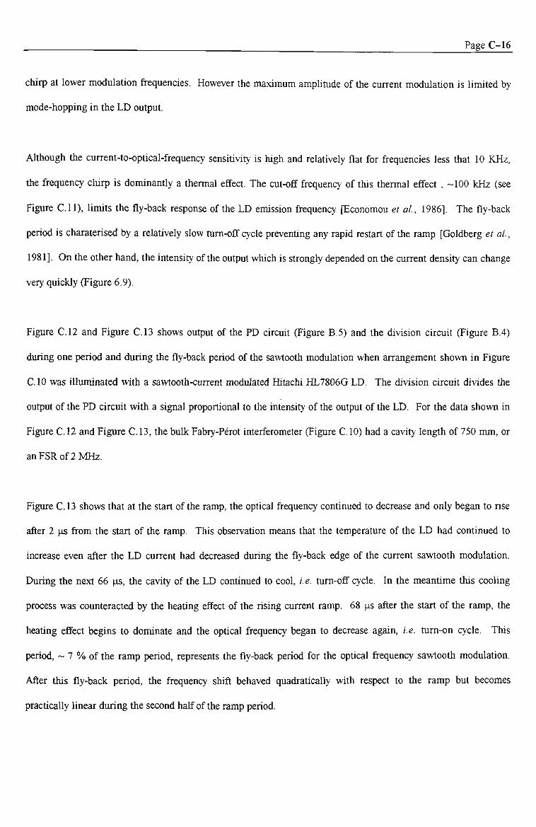
Page C-16
chirp at lower modulation frequencies. However the maximum amplimde of the current modulation is limited by
mode-hopping in the LD output.
Although the current-to-optical-frequency sensitivity is high and relatively flat for frequencies less that 10 KHz,
tiie frequency cltirp is dontinantiy a thermal effect. The cut-off frequency of this thennal effect , -100 kHz (see
Figure C.ll), limits the fly-back response ofthe LD emission frequency [Economou et al, 1986]. The fly-back
period is charaterised by a relatively slow turn-off cycle preventing any rapid restart ofthe ramp [Goldberg et al,
1981], On the other hand, the intensity ofthe output which is strongly depended on the current density can change
very quickly (Figure 6.9).
Figure C.12 and Figure C.13 shows output of the PD circuit (Figure B.5) and the division circuit (Figure B.4)
during one period and during the fly-back period of the sawtooth modulation when arrangement shovm in Figure
C.IO was tiluminated with a sawtooth-current modulated Hitachi HL7806G LD. The division circuit divides the
output ofthe PD circuit with a signal proportional to the intensity of the output of the LD. For the data shown in
Figure C.12 and Figure C.13, the bulk Fabry-Perot interferometer (Figure CIO) had a cavity length of 750 mm, or
an FSR of 2 MHz.
Figure C.13 shows that at the start ofthe ramp, the optical frequency continued to decrease and only began to rise
after 2 ^s from the start of the ramp. This observation means that the temperature of the LD had continued to
increase even after the LD current had decreased during the fly-back edge of the current sawtooth modulation.
During the next 66 |is, the cavity ofthe LD continued to cool, i.e. ttim-off cycle. In the meantime this cooting
process was counteracted by the heating effect of the rising current ramp. 68 ]xs after the start of the ramp, the
heating effect begins to dominate and the optical frequency began to decrease again, i.e. turn-on cycle. This
period, ~ 7 % of the ramp period, represents the fly-back period for the optical frequency sawtooth modulation.
After this fly-back period, the frequency shift behaved quadratically with respect to the ramp but becomes
practically linear during the second half ofthe ramp period.

Page C-17
0.5 1 End of the sawtooth ramp
0.24
Figure C.12: The unprocessed and intensity-modulation free PD signals used to measure the LD emission frequency sawtooth modulation. Air-cavity length = 750 mm.
40 60
Time (us)
Figure C.13: The unprocessed and intensity-modulation free PD signals used to measure the LD emission frequency sawtooth modulation(fly-back period). Air-cavity length = 750 mm.

Page C-18
From the measurements shown in Figure C.12 and Figure C.13, Figure C.14 shows the calculated shifts in the LD
emission frequency modulation within one sawtooth cycle. The behaviour of the LD frequency modulation clearly
deviated from a linear sawtooth. Consequently, this nonlinear optical frequency ramp produced a sinularly varying
change in the interferometric phase of an FFPS. Using the measurements presented in Figure C14, it was possible
to measure the FSR of an FFPS since the FSR ofthe bulk interferometer ui Figure CIO was known. In particular
the average FSRs of axial interferometers of HibiGrat was measured to be 6.4 GHz using titis method. This FSR
value implied a cavity length of 16 mm which was in agreement from the value inferred from the distance between
the centre ofthe grating to the cleaved end of HibiGrat (15 ± 1 mm).
S -30
TOM (us)
Figure C.14: The instantaneous optical frequency chirp within one sawtooth period of LD current modulation.
Analysis of tiie interferomettic signals shown in Figure C.12 and Figure C.13 confirmed the single-mode output of
tiie LD since no other fringe pattern was observed. Furtiiermore, tiie stability ofthe fringe pattern even for small
FSR air-path implied tiiat tiie thermally induced noise resulting from tiie limitations of tiie LD temperattu-e-
controUer was much less than tiiat previously expected. Hence the LD temperattire stabtiity can be fiirther
estimated to be about ± 0.0001°C over a period of 15 minutes. This excellent short term temperature stability

Page C-19
assured accurate phase and hence temperature or strain measurements over a very short period of time in spite of a
design flaw in the temperature confroller for the LD (Appendix B)
The same optical frequency ramp measurement described above can also provide a measurement of the AC optical-
frequency/current sensitivity. The ratio between the amplittides ofthe optical frequency and drive current sawtooth
ramps was detennined to be -2.4 GHz /mA. This AC sensitivity was similar to those measured by others for a
Hitachi HL7801E which was similar in construction to the HL7806G (Table C.2). Also, this sensitivity value was
in agreement to that depicted in Figure C.ll. The AC optical-frequency-current sensitivity was less than the
corresponding DC characteristics measured previously for the LD. This difference between the AC and DC
sensitivities was attributed to the thermal nature of the dependence of the LD optical frequency with its drive
current (Figure C11).
This high AC optical-frequency/current sensitivity ofthe LD suggested another possible source of optical frequency
noise can be due the noise in the modulation current. One possible current noise source was the staircase-type
sawtooth modulation. The RMS noise due to this staircase ramp was calculated to be 3.524 x 10' of ramp current
amplitude. Since the ramp amplitude was adjusted to correspond to the FSR of the sensor, the expected noise was
expected to be 3.524 x 10'* of a fringe. The actual noise value would be less than 3.524 x 10' ofa fringe because
the staircase steps were expected to be smoothen out by the input stage of the LD drive circuit. Nevertheless, the
3.524 X 10' of a fringe was an order of magnitude less than the resolution of the measuring system (lO"'' of a
fringe). Thus the assumption that the staircase nature of the voltage sawtooth ramp modulation signal do not
introduce any undesirable effects holds ground.
Another possible current noise source was the components of the LD drive circuit (Figure 6.12). The LM337
voltage regulator used in the circuit had a worst-case RMS noise of 360 |J.V between 10 Hz and 10 kHz which
translated to about 5 \x.k (RMS) in the same frequency range. Subsequentiy this value implied an optical frequency
noise of 12 MHz (RMS). In particular for HibiGrat, this current noise implied about 0.002 fringe (RMS) phase
noise.

Page C-20
C.4.4 Temperature Sensitivity of the Laser Diode and Limitations of the LD Temperature Controller
Figure C.15 shows the dependence of the optical output power against temperature at different constant drive
current which were greater than the threshold value. The dependence was clearly not linear. Interestingly the
output power appeared to fluctuated between 1.5 mW to 2 mW of optical power output. This instability was not
completely understood. However, it was definitely clear that the LD must be operated away from this instability
region. In the work, optical output power was preferentially chosen to be greater than 2 mW. This convenientiy
implied a lower value for relative amplitude of the sawtooth intensity modulation with respect to DC intensity
value. This condition meant the intensity modulation in the interferometric signal was less severe.
4 T
3.5
2.5
2 -•
1.5 -•
1 -•
0.5 45.4mA 47.1mA 48.6mA 50.4mA 52.2 mA 54.0mA
15 25 35 Teirperature (°C)
45 55 65
Figure C.15: The dependence of the output power of a Hitachi HL7806G LD with its case temperature for different values of its DC drive currents.
Figure C16 shows the LD emission wavelength as the case temperature of the LD was varied. The figure clearly
illustrates the mode-hopping behaviour of tiie LD output. Furthermore, The figure indicates the emission
wavelength had a greater dependence on temperature than the DC drive current. Figure C.16 shows that the most

Page C-21
stable region of operation for the LD was between 790 nm to 791 nm. In this wavelength range, the LD output
didn't not appear to mode-hop as the temperature and the drive current ofthe LD was varied.
In each ofthe non-mode-hop regions shown in Figure C.16, the wavelength(frequency)/temperature sensitivity was
measured to be about 0.06 nm/°C (or -29 GHz/°C). This sensitivity was similar to those measured by others (Table
C.2). This high sensitivity demanded excellent stabilisation of the LD temperature. In this work, the LD was
temperature-confrolled using Peltier devices with the best long-term stability (~ 3 hrs) of about ± 0.02 °C provided
that the ambient temperature was relatively constant. Unfortunately ± 0.02°C ttanslated into thermally-induced
drift of ± 0.58 GHz in tiie LD optical frequency. In tiie case of HibiGrat, this large frequency drift produced a
significantiy large phase drift of about ±0.1 of a fringe. Only for sensors with a physical cavity length less than
1.75 mm would the equivalent phase drift be less than + 1 %. Incidentally such large-FSR sensors may not be
suitably processed by the pseudo-heterodyne technique implemented with a modulated LD.
794 T
792 --
790 --
E
.1 786
784
782
780
54.0 mA
45.4 mA
52.2 mA
48.6 mA
47.1 mA
50.4 mA
10 20 30 — I —
40 50 60
Temperature (°C)
Figure C.16: The dependence of the emission wavelength of a Hitachi HL7806G LD with its case temperature for different values of its DC drive currents. Each curve in the figure was formed by connecting data points separated by 0.1 °C.

Page C-22
Figure C.l7 shows the effect of drifts in the LD output wavelength on the interferometric fringe shifts. The
polarisation axes indicated in were those of HibiGrat. Each data point in the figure was an average of 20 data
points sampled every 5 seconds. The figure shows that interferometric phase of the sensor was sfrongly affected by
the LD temperature drifts : -5.4 fringe/°C. This thermally induced phase shift was consistent with that obtained
from direct wavelength shift measurements ofthe LD (Figure C. 16). This thermal sensitivity was expected to be a
negative value because an increase in the LD temperature decreases the LD emission frequency. Figure C.17 also
shows that the total phase shifts along each polarisation axes were slightly different. Since the FSR of each axis of
the sensor was very similar, the difference was attributed to drifts in the temperature ofthe sensor itself.
0.95
^^ Sensor's temperature
-0.05 --
-0.25 -•
-0.45
LD temperature I ^^ l . i f ' r T ' i l l > i i ini i i iiiliijll i i i i i i i i< II •» - n - l i r r r ^llr II '*!•'- I * u l i ' imii
- 15.55
-• 15.05
1455
1405 I 2 a. B
-- 13.55 ""
13.05
12.55
1205
100 200 300 400 500 600 700 800 900 1000
Time (minutes)
Figure C.17: The phase drifts of each interferometer of HibiGrat due to thermally induced variations in the LD emission wavelength.
The drift in tiie LD temperature depicted in Figure C.17 was a direct consequence of a design flaw in tiie typical
temperattire controller available in the laboratory (Figure 2.13). Since the feedback current produced by the
temperature controller was proportional to tiie difference between some set (stabilisation) temperattire and tiie
acttial temperattire of tiie LD, this design was not suitable to control the Peltier devices which require a continuous
flow of current to produce the Peltier effect. Consequently the present thermal stabilisation scheme can drift as the

Page C-23
ambient temperature changes. The ratiier good temperature stabilisation reported was because the laboratory
temperattire did not change drastically during the course of the experiments. In hindsight, a more suitable
temperature controller was required.
To summarize this sub-section. Table C.2 summarises tiie different parameters of the HL7806G relevant in
defining both the operational range and limits of tiie LD when employed to implement the pseudo-heterodyne-
signal processing scheme.
Parameter
DC specfral current dependence AC spectral current dependence DC specfral temperature dependence
Coherence length
HL7806G experimental values 7.1 pm/mA (-3.5 GHz/mA)
4.9 pm/mA (-2.4 GHz/mA) at 1 kHz 0.06 nni/°C (-29 GHz/°C)
~2m
Other Hitachi laser diodes
HL7801E
HL7801E
HL7801
Values obtained by others
4.6 pm/mA (-2.3 GHz/mA)
0.07 nm/°C (-34 GHz/°C)
0.06 nm/°C (-29 GHz/°C) 10°C-30°C range
~5 m (from 20 MHz line-width)
References
Chen etal., 1988
Chen et al., 1988
Ohba etal., 1989
Maystre & Dandliker, 1989
Table C2: The measured parameters for the HL7806G laser diode used in this work compared with similar laser diodes used by others.
C.5 Phase Noise Due to the Band-Pass Filter
The band-pass filtering an electroruc signal inadvertently introduced an additional phase to the input signal.
Without lost of generality, assuming a two-beam approximation of the input optical signal, the elecfronic signal,
prior to filtering can be expressed as
^r,AC = A COs(fi)„f - (p(t) i„, ) Eq^ Q(,
where A is some voltage signal amplitude, co„ the sawtooth angular modulation frequency and t time.
^(Omt =<!^0.M+<!^iuSUl(®jV^O Eq. C.7

Page C-24
is tiie phase signal associated with the measurand M with ^Q.M as some initial time-independent phase, (p^ tiie
phase-amplittide of the signal (depth of modulation) and cOf^ angular frequency of the measurand-induced phase
shifts. Using the identity, . +00
exp(/ . (r . sin[<;>])) = J]'^g('-)Q^{i • {q •[^])) Eq. C.8
where J^(r) are the Bessel function ofthe first kind of order q. Eq. C.6 can be expanded in terms of its Fourier
components: +«
^r,AC = Z-^9te)COS[(G>„ -q0)^)1-^Q^M] Eq. C.9 g=-co
Eq. C9 indicates that the measurand-induced phase signal, < (/)int, is manifested in the side bands around the
modulation frequency. These sides bands will consequentiy encounter different electronic phase shift due to the
band-pass filter depending on its distance in the frequency domain from the modulation frequency, expressed by
(i^saw ~q<^M • Typically the first harmonic ofthe measurand-induced phase signal dominated the other harmonics
and hence usually only two major sidebands in I,.^^. were important
In a bandwidth of about 100 Hz around the centre of the pass-band of the for the uruty-Q 1-kHz band-pass
amplifier described in Chapter 6, the amount of electronic phase shift was approximately linear with changes in
frequency. The phase/frequency sensitivity for the unity Q band-pass amplifier was about 4 x 10" x 27t/Hz. The
phase shift introduced by the band-pass filter can be considered constant for as long as the frequency spectrum of
the measurand-induced phase signal was constant. Hence, when the dominant signal frequency varied from one
situation to another, additional phase error can be expected. This phase error can be below 10' of a fiinge for a
signal frequency change of up to 2 Hz. This frequency change can be more than adequate for temperature
measurements but not necessarily for strain measurements. Using a band-pass filter with a wider bandwidth and
with lower electronic-filter-order can reduced the associated phase shift. However enlarging the bandwidth
increased the noise in the photo-detector and thereby reducing the minimum detectable optical intensity (Figure
Cl).

Page C-25
C.6 Overall Phase Noise
Although the resolution ofthe phase recording scheme employed in this work was about 10" of a fiinge, the acmal
useful phase resolution was limited by phase noise. The sources of phase noise have been described above. The
amount of phase noise depends on the FSR ofthe sensor. In the case of HibiGrat, the total expected phase noise
was calculated to be 0.007 RMS of a fringe. This calculated value was obtained by assunting an RMS 0.001 °C
variation in the LD temperattire (0.005 of a fringe), moderate variation in the optical length of the lead-in fibre
(0.001 RMS ofa fringe - 10 % ofthe maximum value described in section 2), typical power supply noise in the LD
drive circuit (0.005 RMS + 0.002 RMS of a fiinge), and about 2 Hz variation in tiie dominant frequency of
measurand-induced phase variations (0.001 RMS of a fiinge). The experimentally measured phase noise varied
from 0.005 to 0.009 (RMS) of a fringe for HibiGrat and was in agreement with the expected RMS phase noise.
The typical RMS phase noise for HibiGrat recently described was predominantly due to that induced by the
elecfronic noise in the LD power supply and variations in the LD temperature. Reduced phase noise can be
achieved with low-noise LD power supply and with greater stability of the LD temperature. Achieving greater
stability in the LD temperattire over long periods of time reduced the long-term phase drifts as well.

Appendix D: Publications Resulting From This Thesis
Caranto, N. R. Y., Murphy, M. M. and Booth, D. J. (1994). A Fusion-Spliced Birefiingent Fabry-Perot Interferometric Temperature Sensor, Proc. 19th Australian Conference on Optical Fibre Technology (Melbourne, Victoria, Australia, December).
Caranto, N. R. Y., Murphy, M. M. and Booth, D. J. (1994). A Birefiingent Fabiy-Perot Interferometer for Temperature Sensing, Proc. 6th Asia Pacific Physics Conference & 11th Australian Institute of Physics Congress: BrisPhys '94 (Brisbane, Queensland, Australia, July).
Kaddu, S. C , Caranto, N. R. Y., Murphy, M. M., Collins, S. F. and Booth, D. J. (1993). Construction of Fibre Fabry-Perot Sensors for Temperature or Strain Measurement, Proc. 18th Australian Conference on Optical Fibre Technology, 245 - 248 (Wollongong, New South Wales, Australia, December).
Caranto, N. R. Y., Kaddu, S. C, Szajman, J., Murphy, M. M., Collins, S. F. and Booth, D. J. (1993). An optical fibre thin film thickness monitor. Measurement Science and Technology, 4(8), 865 -869.
Caranto, N. R. Y., Kaddu, S. C, Szajman, J., Murphy, M. M., Collins, S. F. and Booth, D. J. (1993). An optical fibre thin film thickness monitor. Engineering Optics, 6(4), 451 - 455 (1993).
Caranto, N. R. Y., Kaddu, S. C, Szajman, J., Murphy, M. M., Collins, S. F, and Booth, D. J. (1992). An optical-fibre-based thin film thickness monitor, Proc. International Conference on Physics and Technology in the 1990's (Quezon City, Philippines).

Appendix E: References
Alavie, A. T., Karr, S. E., Othonos, A. and Measures, R. M. (1993). A Multiplexed Bragg Grating Fiber Laser Sensor System, IEEE Photonics Technology Letters, 5(9), 1112-1114.
Alcoz, J. J., Lee, C. E. and Taylor, H. F. (1990). Embedded Fiber-Optic Fabry-Perot Ulfrasound Sensor, IEEE Transactions on Ultrasonics, Ferroelectrics and Frequency Control 37(4), 302-306.
An, S. and Sipe, J. E. (1992). Polarization Aspects of Two-Photon Photosensitivity in Birefringent Optical Fibers, Optics Letters, 17(7), 490-492.
Anderson, D. J. and Jones, J. D. C (1992). Optothermal Modulation of Diode Lasers, Proceedings ofthe 8th International Conference on Optical Fiber Sensors, Monterey, U.S.A., 22-25.
Anderson, D. Z., Mizrahi, V., Erdogan, T. and White, A. E. (1993). Production of In-Fibre Gratings Using a Diffractive Optical Element, Electronics Letters, 29(6), 566-588.
Atkinson, K. E. (1989). An Introduction to Numerical Analysis, 2nd edn., John Wiley & Sons, New York.
Baldini, F. and Mignani, A. G. (1994). In-Vivo Biomedical Monitoring by Fiber Optic Systems, Proceedings ofthe 10th International Conference on Optical Fiber Sensors, Glasgow, Scotland, 80-89.
Ball, G. A., Morey, W. W. and Cheo, P. K. (1993). Single- and Multipoint Fiber-Laser Sensors, IEEE Photonics Technology Letters, 5(2), 267-270.
Ballard, S. S. and Browder, J. S. (1986). Thermal Properties of Optical Crystals, CRC Handbook of Laser Science and Technology: Volume 4: Optical Materials, Part 2:Properties, Weber, M. J. (ed.), CRC Press, Florida.
Bardal, S., Kamal, A. and Russell, P. St. J. (1992). Photo-induced Birefringence in Optical Fibers: A Comparative Study of Low-Birefringence and High-Birefringence Fibers, Optics Letters, 17(6), 411-413.
Barlow, A. J. and Payne, D. N. (1983). The Sfress-Optic Effect in Optical Fibers, IEEE Journal of Quantum Electronics, QE-19(5), 834-839.

_ _ ^ Page E-2
Beals, M. D. (1970). Single-Crystal Titanates and Zirconates, High Temperature Oxides: Part II, Alper, A. M (ed.). Academic Press, New York, U. S. A.
Beheim, G., Fritsch, K., Flatico, J. M. and Massood, T. A. (1989). SiUcon-Etalon Fiber-Optic Temperature Sensor, Proceedings ofthe Society of Photo-Optical Instrumentation Engineers, 1169,504-511.
Benham, P. P. and Wamock, F. V. (1976). Mechanics of Solids and Structures, Pittman Publishing, London, U. K.
Bennett, J. M., Pelletier, E., Albrand, G., Borgogno, J. P., Lazarides, B., Camiglia, C. K, Schmell, R A., Allen, T. H., Tuttle-Hart, T., Guenther, K H. and Saxer, A. (1989). Comparison ofthe Properties of Titaiuum Dioxide Films Prepared by Various Techniques, Applied Optics, 28(15), 3303-3317.
Berkoff, T. A. and Kersey, A. D. (1992). Passive Phase Interrogation and Multiplexing of Two-Mode Fiber Sfrain Sensors for Smart Structtires Systems, Proceedings ofthe First European Conference on Smart Structures and Materials, Glasgow, Scotland, 39-43.
Berkoff, T. A., Kersey, A. D. and Moeller, R. P. (1990). Novel Analog Phase Tracker for Interferometric Fiber Optic Sensor Applications, Proceedings ofthe Society of Photo-Optical Instrumentation Engineers, 1367, 53-57.
Bertholds, A. and Dandliker, R (1987). Deformation of Single-Mode Optical Fibers Under Static Longitudinal Stress, Journal of Lightwave Technology, LT-5(7), 895-900.
Bertholds, A. and Dandliker, R (1988). Determination ofthe Individual Strain-Optic Coefficients in Single-Mode Optical Fibers, Journal of Lightwave Technology, 6(6), 17-20.
Bhatia, V., Campbell, D., Claus, R O. and Vengsarkar, A. M. (1997). Simultaneous Strain and Temperature Measurement with Long Period Gratings, Optics Letters, 22(9), 648-650.
Bhatia, V., Murphy, K. A., Claus, R O., Jones, M. E., Grace, J. L., Tran, T. A. and Greene, J. A. (1996). Optical Fibre Based Absolute Extrinsic Fabry-Perot Interferometric Sensing System, Measurement Science and Technology, 1, 58-61.
Bock, W. J. and Eftimov, T. A. (1994). Simultaneous Hydrostatic Pressure and Temperature Measurement Employing an LPoi-LPn Fiber-Optic Polarization-Sensitive Intermodal Interferometer, IEEE Transactions on Instrumentation and Measurement, 43(2), 337-340.
Bock, W. J., Urbanczyk, W., Buczynski, R and Domanski, A. W. (1994). Cross-Sensitivity Effect in Temperature-Compensated Sensors Based on Highly Birefringent Fibers, Applied Optics, 33(25), 6078-6083.
Bohnert, K. and Nehring, J. (1989). Fiber-Optic Sensing of Voltages by Line Integration ofthe Electric Field, Optics Letters, 14(5), 290-292.
Bom, M. and Wolf, E. (1980). Principles of Optics: Electromagnetic Theory of Propagation, Interference and Diffraction of Light, 6th edn., Pergamon Press.

Page E-3
Borrelli, N. F. and Miller, R A. (1968). Determination ofthe Individual Strain-Optic Coefficients of Glass by an Ulfrasonic Technique, Applied Optics, 7(5), 745-750.
Brady, G. P., Kalli, K., Webb, J. D., Jackson, D. A., Reekie, L. and Archambault, J. L. (1995). Simultaneous Interrogation of Interferometric and Bragg Grating Sensors, Optics Letters, 20(11), 1340-1242.
Brady, G. P., Kalli, K, Webb, J. D., Jackson, D. A., Reekie, L. and Archambault, J. L. (1997). Simultaneous Measurement of Sfrain and Temperature Using First- and Second-Order Diffraction Wavelengths of Bragg Gra^rig, lEE Proceedings: Optoelectronics, 144(3), 156-161.
Butter, C. D. and Hocker, G. B. (1978). Fiber Optics Sfrain Gauge, Applied Optics, 17(18), 2867-2869.
Campbell, M., Zheng G., Wallace, P. A. and Holmes-Smith, A, S. (1996). Reflectometric Birefringent Fiber Sensor for Absolute and Relative Strain Measurement, Proceedings ofthe Society of Photo-Optical Instrumentation Engineers, 2839, 254-259.
Caranto, N. R Y., Kaddu, S. C, Szajman, J., Murphy. M. M., Collins, S. F. and Booth, D. J. (1993). An Optical Fibre Thin Film Thickness Monitor, Measurement Science and Technology, 4(8), 865-869.
Carrara, S. L. A. (1990). Birefiingent-Fiber Splice Aligmnent, Proceedings ofthe Society of Photo-Optical Instrumentation Engineers, 1267, 24-28.
Carrara, S. L. A., Kim, B. Y. and Shaw, H. J. (1986). Elasto-Optic Alignment of Birefringent Axes in Polarization-Holding Optical Fiber, Optics Letters, 11(7), 470-472.
Chardon, D. and Huard, S. J. (1988). Simultaneous Measurement of Temperattire and Pressure with a Single-Mode Fiber, Proceedings ofthe 5 th International Conference on Optical Fiber Sensors, New Orleans, U.S.A., Postconference edn.. Optical Society of America Technical Digest Series, vol. 2, parts 1 & 2, 495-501.
Chen, J., Ishii, Y. and Murata, K. (1988). Heterodyne Interferometry With a Frequency-Modulated Laser Diode, Applied Optics, 27(1), 124-128.
Chiang, K- S. and Tsuchida, H. (1988). Dual-Sensor Technique for Extending the Dynamic Range of a Fiber-Optic Interferomettic Sensor, Optics Letters, 13(10), 850-852.
Chien, P. Y. (1992). Open-Loop Fiber Optic Gyroscope With Wide Dynamic Range, Review of Scientific Instruments, 63(7), 3783-3784.
Clark, G. L., Heflinger, L. O. and Roychoudhuri, C. (1982). Dynamic Wavelength Tuning of Single-Mode GaAlAs Lasers, IEEE Journal of Quantum Electronics. QE-18(2), 199-204.
Cole, J. H., Danver, B. A. and Bucaro, J. A. (1982). Syntiietic-Heterodyne Interferometric Demodulation, IEEE Journal of Quantum Electronics, QE-18(4), 694-697.

PageE-4
Corke, M., Kersey, A. D. and Jackson, D. A. (1985). Combined Michelson and Polarimetric Fibre-Optic Interferometric Sensor, Electronics Letters, 21(4), 148-149.
Corke, M., Kersey, A. D., Jackson, D. A. and Jones, J. D. C. (1983). All-Fibre 'Michelson' Thermometer, Electronics Letters, 19(13), 471-373.
Corke, M., Kersey, A. D., Jackson, D. A. and Jones, J. D. C. (1984). Remote Temperature Sensing Using Polarisation-Preserving Fibre, Electronics Letters, 20(2), 67-69.
Crossley, S. D. (1994). Commercially Available Fibre Optic Sensors - 10 Years of Progress?, Proceedings ofthe 10th International Conference on Optical Fiber Sensors, Glasgow, Scotland, 249-252.
Dakin, J. and Culshaw, B. [eds.] (1988). Optical Fiber Sensors: Principles and Components, Vol. I & II, Artech House, Boston.
Dakin, J. P., Ecke, W., Rothardt, M., Schauer, J. Usbeck, K and Willsch, R (1997). New Multiplexed Scheme for Monitoring Fiber Optic Bragg Grating Sensors in the Coherence Domain, Proceedings of the 12th International Conference on Optical Fiber Sensors, Williamsburg, Virginia, U.S.A., 31-34.
Dandridge, A. and Goldberg, L. (1982). Current-Induced Frequency Modulation in Diode Lasers, Electronics Letters, 18(7), 302-304.
Dandridge, A. and Tveten, A. B. (1981). Phase Noise of Single-Mode Diode Lasers in Interferomettic Systems, Applied Physics Letters, 38(7), 530-532.
Dandridge, A., Tveten, A. B. and Giallorenzi, T. G. (1983). Homodyne Demodulation Scheme for Fiber Optic Sensors Using Phase Generated Carrier, IEEE Journal of Quantum Electronics, QE-18(10), 1647-1653.
Dandridge, A., Tveten, A. B., Miles, R O., Jackson, D. A. and Giallorenzi, T. G. (1981). Single-Mode Diode Laser Phase Noise, Applied Physics Letters, 38(2), 77-78.
Davis, M. A. and Kersey, A. D. (1995). Application of a Fiber Fourier Transform Spectrometer to tiie Detection of Wavelength-Encoded Signals from Bragg Grating Sensors, Journal of Lightwave Technology, 13(7), 1289-1295.
Davis, M. A. and Kersey, A. D. (1997). Simultaneous Measurement of Temperature and Strain Using Fibre Grating and Bnllomn Scattenng, lEE Proceedings in Optoelectronics, 144(3), 151-155.
Day, G. W. and Rose, A. H. (1988). Faraday Effect Sensors: The State of tiie Art, Proceedings ofthe Society of Photo-Optical Instrumentation Engineers, 985, 138-150.
del Pozo, J, M. and Diaz, L. (1992). Metiiod for tiie Determination of Optical Constants of Thin FUms: Dependence on Expenmental Uncertainttes, Applied Optics, 31(22), 4474-4481.

Page lr-5
Domanski, A. W., Gorecki, A. and Swillo, M. (1995). Dynamic Sfrain Measurements by Use ofthe Polarimetric Fiber Optic Sensors, Proceedings ofthe IEEE Instrumentation/Measurement Technology Conference. Integrating Intelligent Instrumentation and Control (IMTC) Proceedings (Cat No.95CH35783), 816-819.
Dunphy, J., Ball, G., D'Amato, F., Ferraro, P., Inserra, S., Vannucci, A. and Varasi, M. (1993). Instrumentation Development in Support ofFibre Grating Sensor Arrays, Proceedings ofthe Society of Photo-Optical Instrumentation Engineers, 2071, 2-11.
Economou, G., Youngquist, R C. and Davies, D. E. (1986). Limitations and Noise in Interferometric Systems Using Frequency Ramped Stiigle-Mode Diode Lasers, Journal of Lightwave Technology, LT-4(11), 1601-1608.
Egalon, C. O. and Rogowski, R S. (1992). A Model of an Axially Sfrained Weakly Guiding Optical Fiber Modal Pattern, Optical Engineering, 31(6), 1332-1339.
Egorov, S. A., Mamaev, A. N. and Polyantsev (1995). Specfral Signal Processing in Intrinsic Interferometric Sensors Based on Birefringent Polarization-Maintaiiung Optical Fibers, Journal of Lightwave Technology, LT-3(1), 83-92.
Eickoff, W. (1981). Temperature Sensing by Mode-Mode Interference in Birefringent Optical Fibers, Optics Letters, 6(4), 204-205.
Eickoff, W. (1982). Stress-induced Single-Polarization Single-Mode Fiber, Optics Letters, 7(12), 629-631.
Erdogan, T. and Mizrahi, V. (1994). Characterization of UV-lnduced Birefringence in Photosensitive Ge-Doped Silica Optical Fibers, Journal ofthe Optical Society of America B, 11(10), 2100-2105.
Farahi, F., Jones, J. D. C. and Jackson, D. A. (1988b). An Extended Range Fibre-Optic Temperattire Sensor, International Journal of Optoelectronics, 3(3), 237-245.
Farahi, F., Newson, T. P., Leilabady, P. A., Jones, J. D. C. and Jackson, D. A. (1988a). A Multiplexed Remote Fibre Optic Fabry-Perot Sensing System, International Journal of Optoelectronics, 3(1),
79-88.
Farahi, F., Webb, D. J., Jones, J. D, C. and Jackson, D. A. (1990b). Simultaneous Measurement of Temperattire and Sfrain Using Fibre Optic Interferometric Sensors, Journal of Lightwave Technology, 8(2), 138-142.
Farahi, F., Webb, D. J., Jones, J. D. C. and Jackson, D. A. (1990a). Simultaneous Measurement of Temperattire and Strain Using Fibre Optic Interferomettic Sensors, Proceedings ofthe Society of Photo-Optical Instrumentation Engineers, 1314, 270-277.
Feng, T., YiZun, W. and PeiDa, Y. (1990). Random Coupling tiieory of Single-Mode Optical Fibers, Journal of Lightwave Technology, 8(8), 1235-1242.
Ferreira, L. A., Lobo Ribiero, A. B., Santos, J. L. and Farahi, F. (1996). Simultaneous Measurement of Displacement and Temperature Using Low Finesse Cavity and a Fiber Bragg Grating, IEEE Photonics Technology Letters, 8(11), 1519-1521.
PageE-6
Flavin, D. A., McBride, R and Jones, J. D. C (1993). Simultaneous Measurement of Temperature and Sfrain by Dispersive Fourier Transform Specfroscopy, Proceedings ofthe 9th International Conference on Optical Fiber Sensors, Florence, Italy, 333-336.
Flavin, D. A., McBride, R and Jones, J. D. C (1997). Absolute Measurement of Wavelengths From a Multiplexed In-Fibre Bragg Grating Array by Short-Scan Interferometry, Proceedings ofthe 12th International Conference on Optical Fiber Sensors, Williamsburg, Virginia, U.S.A., 24-27.
Flavin, D. A., McBride, R, Jones, J, D. C , Burnett, J. G. and Greenaway, A. H. (1994). Combined Temperature and Strain Measurement with a Dispersive Optical Fibre Fourier Transform Specfrometer, Optics Letters, 19(24), 2167-2169.
Fleming, J. W. (1986). Optical Glasses, CRC Handbook of Laser Science and Technology: Volume 4: Optical Materials, Part 2:Properties, Weber, M. J. (ed.), CRC Press, Florida.
Franks, R B., Tormellas, W. and Youngquist, R C. (1985). Birefiingent Sfress Location Sensor, Proceedings ofthe Society of Photo-Optical Instrumentation Engineers, 586, 84-89.
Franks, R B., Tormellas, W. and Youngquist, R C (1986). An Extended Fibre Optic Stress Location Sensor, Optica Acta, 33(12), 1505-1518.
Furstenau, N., Schmidt, W. and Goetting, H. C (1992). Simultaneous Interferometric and Polarimetric Strain Measurements on Composites using a Fiber-Optic Strain Gauge, Applied Optics, 31(16), 2987-2993.
Gauthier, R C. and Turgeon, S. (1993). Birefringent Sensor Enhancement by Wavelength Multiplexing, Optics and Laser Technology, 26(6), 377-381.
Gerges, A. S., Farahi, F., Newson, T. P., Jones, J. D. C. and Jackson, D. A. (1987). An Interferomettic Fiber Optic Sensor Using a Short Coherence Length Source, Electronics Letters, 23(21), 1110-1111.
Giallorenzi, T. G., Bucaro, J. A., Dandridge, A., Sigel, G. H. Jr., Cole, J. H., Rashleigh, S. C and Priest, R G. (1982). Optical Fiber Sensor Technology, IEEE Journal of Quantum Electronics, QE-18(4), 626-665.
Giles, L P., Uttam, D., Culshaw, B. and Davies, D. E. N (1983). Coherent Optical-Fibre Sensors with Modulated Laser Sources, Electronics Letters, 19(1), 14-15.
Giulianelli, L. C, Buckman, A. B., Walser, R M. and Becker, M. F. (1994). Digital Demodulation Scheme for Wide Dynamic Range Measurements of a Fiber Optic Interferometer, Proceedings ofthe Society of Photo-Optical Instrumentation Engineers, 2191, 314-323.
Goldberg, L., Taylor, H. F. and Weller, J. F. (1981). Time-Dependent Thermal Effects in Current-Modulated Semiconductor Lasers, Electronics Letters, 17(14), 497-499.
Gottlieb, M. (1986). Elastooptic Materials, CRC Handbook of Laser Science and Technology: Volume 4: Optical Materials, Part 2:Properties, Weber, M. J. (ed.), CRC Press, Florida.

Page E-7
Grossman, B. and Costandi, W. (1992). Fiber Optic Sensor for the Simultaneous Detection of Sfrain and Temperature, Proceedings ofthe Society of Photo-Optical Instrumentation Engineers, 1798, 175-185.
Gusmeroli, V. and Martinelli, M. (1994). Non-Incremental Interferometric Fiber-Optic Measurement Metiiod for Simultaneous Detection of Temperattu-e and Sfrain, Optics Letters, 19(24), 2164-2166.
Hecht, E. (1987) Optics, 2nd edn., Addison-Wesley Publishing Company, Reading, Massachusetts, U.S.A.
Henderson, P, J., G. F., Rao, Y. J., Jackson, D. A., Zhang, L. and Bennion, L (1997). Simultaneous Dynanuc-Sfrain and Temperature Monitoring Using a Wavelength Multiplexed Fibre- Fabry-Perot Array with Low-Coherence Interrogation, Proceedings ofthe 12th International Conference on Optical Fiber Sensors, Williamsburg, Virginia, U.S.A., 56-43.
Herzog, J. P. and Meymeis, P. (1990). Interferometric Optical Fiber Pressure Sensor with Temperature Compensation, Proceedings ofthe Society of Photo-Optical Instrumentation Engineers, 1267, 134-141.
Hill, K. O., Bilodeau, F., Malo, B. and Johnson, D. C (1991). Birefringent Photosensitivity in Monomode Optical Fibres: Application to External Writing of Rocking Filters, Electronics Letters, 27(11), 1548-1550.
Hill, K. C , Malo, B., Bilodeau, F., Johnson, D. C. and Albert, J. (1993). Bragg Gratings Fabricated in Monomode Photosensitive Optical Fiber by UV Exposure Through a Phase Mask, Applied Physics Letters, 62(10), 1035-1037.
Hocker, G. B. (1979). Fiber-Optic Sensing of Pressure and Temperature, Applied Optics, 18(9), 1445-1448.
Hogg, D., Janzen, D., Valis, T. and Measures, R M. (1991). Development ofa Fiber Fabry-Perot Sfrain Gauge, Proceedings ofthe Society of Photo-Optical Instrumentation Engineers, 1588, 300-307.
Hogg, W. D., Tumer, R D. and Measures, R M. (1989). Polarimetric Fiber Optic Structural strain Sensor Characterisation, Proceedings ofthe Society of Photo-Optical Instrumentation Engineers, 1170, 542-549.
Huang, S. Y., Blake, J. N. and Kim, B. Y. (1990). Perturbation Effects on Mode Propagation in Highly Elliptical Core Two-Mode Fibers, Journal of Lightwave Technology, 8(1), 23-33.
Hughes, R and Priest, R (1979). Thermally Induced Optical Phase Effects in Fiber Optic Sensors, Applied Optics, 19(9), 1477-1483.
Hurwitz, H. Jr. and Jones, R C. (1941). A New Calculus for the Treattnent of Optical Systems: I. Proof of Three General Equivalence Theorems, Journal of the Optical Society of America, 31, 493-503.
Hymans, A. J. and Lait, J. (1960). Analysis ofa Frequency-Modulated Continuous-Wave Ranging Systems, Proceedings ofthe Institute of Electrical Engineers, (Paper No. 3264 E, July), 365- 372.

PageE-8
Inci, M. N., Kidd, S. R, Barton, J. S. and Jones, J. D. C (1992). Fabrication of Single-Mode Fibre Optic Fabry-Perot Interferometers, Using Fusion Spliced Titanium Dioxide Optical Coatings, Measurement Science and Technology, 3, 678-684.
Inci, M. N., Kidd, S. R, Barton, J. S. and Jones, J. D. C (1993). High Temperature Miniature Fibre Optic Interferometric Thermal Sensors, Measurement Science and Technology, A, 382-387.
Ito, M. and Kimura, T. (1980). Carrier Density Dependence of Refractive Index in AlGaAs Semiconductor Lasers, IEEE Journal of Quantum Electronics, QE-16(9), 910-911.
Izumita, H., Horiguchi, T. and Kurashima, T. (1997). Distributed Sensing Techniques Using Brillouin Scattering, Proceedings ofthe 12th International Conference on Optical Fiber Sensors, Williamsburg, Virginia, U.S.A., 316-319,
Jackson, D. A. (1994). Fibre Optic Sensors, Measurement Science and Technology, 5, 612-638.
Jackson, D. A. and Jones, J. D. C. (1986). Fibre Optic Sensors, Optica Acta, 33(12), pl469-1503.
Jackson, D. A., Kersey, D. A., Corke, M. and Jones, J. D. C. (1982). Pseudo-Heterodyne Detection Scheme for Optical Interferometers, Electronics Letters, 18(25), 1081-1083.
Jackson, J. D. (1975). Classical Electrodynamics, 2nd edn., John Wiley and Son, Inc., New York, U.S.A.
Jacobsen, G., Olesen, H., Birkedahl, F. and Tromborg (1982). Current/Frequency-Modulation Characteristics for Directly Optical Frequency-Modulated Injected Lasers at 830 nm and 1.3 i m, Electronics Letters, 18(20), 874-876.
James, S. W., Dockney, M. L. and Tatam, R P. (1996). Simultaneous Independent Temperature and Strain Measurement Using In-Fibre Bragg Grating Sensors, Electronic Letters, 32(12), 1133-1134.
Jerrard, H. G. (1982). Modem Description of Polarized Light: Mafrix Methods, Optics and Laser Technology. 14(6), 309-319.
Jeunhomme, L. B. (1990). Single-Mode Fiber Optics: Principles and Applications, 2nd edn.. Marker Dekker, New York, U.S.A.
Jin, W., Mitchie, W. C, Thursby, G., Konstantaki, M. and Culshaw, B. (1996). Simultaneous Sfrain and Temperattire Recovery: Error Analysis, Proceedings ofthe 11th International Conference on Optical Fiber Sensors. Sapphoro, Japan, 116-119.
Jin, X. D., Sirkis, J. S. and Venkateswara. (1997). Simultaneous Measurement of Two Sfrain Components in Composite Structtires Using Embedded Fiber Sensors, Proceedings ofthe 12th International Conference on Optical Fiber Sensors, Williamsburg, Virginia. U.S.A., 44-47.
Jones,J.D. C. (1997). Review ofFibre Sensors Techniques for Temperature-Strain Discrimination, Proceedings ofthe 12th International Conference on Optical Fiber Sensors, Williamsburg, Virginia, U.S.A., 316-319.

Page E-9
Jones, R C. (1941). A New Calculus for the Treatment of Optical Systems: I. Description ofthe Calculus, Journal ofthe Optical Society of America, 31,488-493.
Kaddu, S. C. (1996). Low-Coherence Fibre Fabry-Perot Sensors Suitable for Multiplexed Sfrain Measurement, Ph. D. Thesis, Victoria University of Technology, Melbourne, Australia.
Kaddu, S. C , Caranto, N. R Y., Murphy, M. M., CoHins, S. F. and Booth, D. J. (1993). Construction ofFibre Fabry-Perot Sensors for Temperature or Strain Measurement, Proceedings ofthe 18th Australian Conference on Optical Fibre Technology, Wollongong, NSW, Australia, 245-248.
Kaminow, L P. (1981). Polarization in Optical Fibers, IEEE Journal of Quantum Electronics, QE-17(1), 15-22.
Kaminow, L P. and Ramaswany, V. (1979). Single-Polarization Optical Fibers: SlahModel, Applied Physics Letters, 34(4), 268-270.
Kanellopoulos, S. E., Handerek, V. A. and Rogers, A. J. (1994). Simultaneous Strain and Temperattire Sensing Employing a Photogenerated Polarisation Coupler and Low-Order Modes in an Elliptically Cored Optical Fibre, Electronics Letters, 30(21), 1786-77.
Kanellopoulos, S. E., Handerek, V. A. and Rogers, A. J. (1995). Simultaneous Sfrain and Temperattire Sensing with Photogenerated In-Fibre Gratings, Optics Letters, 20(3), 333-335.
Kanellopoulos, S. E., Valente, L. C. G., Handerek, V. A. and Rogers, A. J. (1991). Photorefractive Polarisation Couplers in Elliptical Core Optical Fibres , IEEE Photonics Technology Letters, 3(9), 806-809.
Katsuyama, T., Matsumura, H. and Suganuma, T. (1983). Propagation Characteristics of Single Polarization Fibers, ;7p//e<5? O/J/ZC^, 22(11), 1748-1753.
Kersey, A. D. (1990). Recent Progress in Interferomettic Fibre Sensor Technology, Proceedings ofthe Society of Photo-Optical Instrumentation Engineers, 1367, 2-12.
Kersey, A. D. and Morey, W. W. (1993). Multi-Element Bragg-Grating Based Fibre-Laser Strain Sensor, Electronics Letters, 29(11), 964-966.
Kersey, A. D., Berkoff, T. A. and Morey W. W. (1992), Fiber-Grating Based Sfrain Sensor Witii Phase Sensitive Detection, Proceedings ofthe First European Conference on Smart Structures and Materials, Glasgow, U.K., 61-67.
Kersey, A. D., Dandridge, A. and Bums, W. K (1986). Two-Wavelength Fibre Gyroscope With Wide Dynamic Range, Electronics Letters, 22(18), 935-937.
Kersey, A. D., Davis, M. A. and Marrone, M. J. (1989). Differential Polarimetric Fiber-Optic Sensor Configuration witii Dual Wavelength Operation, Applied Optics, 28(2), 204-206.
Kersey, A. D., Davis, M. A., Patrick, H. J., LeBlanc, M., Koo, K. P., Askins, C. G., Putnam, M. A. and Friebele, E. J. (1997). Fiber Grating Sensors, Journal of Lightwave Technology, 15(8), 1442-1463.

Page E-10
Kersey, A- D., Jackson, D. A. and Corke, M. (1984). Linearised Polarimetric Optical Fibre Sensor Using a 'Heterodyne-Type' Signal Recovery Scheme, Electronics Letters, 20(5), 209-211.
Kidd, S. R , Barton, J. S., Inci, M. N. and Jones, J. D. C (1994). Unsteady Gas Temperature Measurement Using an Ultra-Short Optical Fibre Fabry-Perot Interferometer, Measurement Science and Technology, 5, 816-822.
Kihara, T. and Yokomori, K (1992). Simultaneous Measurement ofthe Refractive Index and Thickness of Thin Films by s-polarized Reflectances, Applied Optics. 31(22), 4482-4487.
Kim, B. K., Yun, S. H., Hwang, L K and Kim, B. Y. (1996). Nonlinear Response of Two-Mode Fibre-Optic Interferometer to Sfrain, Proceedings ofthe 11th International Conference on Optical Fiber Sensors. Sapphoro, Japan, 112-115.
Kim, B. Y., Blake, J. N., Huang, S. Y. and Shaw, H. J. (1987). Use of Highly Elliptical Core Fibers for Two-Mode Fiber Devices, Optics Letters, 12(9), 729-731.
Kim, K., Ismail, Y. and Springer, G. S. (1993b). Measurement of Strain and Temperature with Embedded Intrinsic Fabry-Perot Optical Fiber Sensors, Journal of Composite Materials, 27(17), 1663-1677.
Kim, K-, Kollar, L. and Springer, G. S. (1993a). A Model of Embedded Fiber Optic Fabry-Perot Temperature and Strain Sensors, Journal of Composite Materials, 27(17), 1618-1662.
Kim, Y. and Neikirk. (1995). Micromachined Fabry-Perot Cavity Pressure Transducer, IEEE Photonics Technology Letters. 7(12), 1471-1473.
Kliger, D. S., Lewis, J. W. and Randall, C. E. (1990). Polarized Light in Optics and Spectroscopy, Academic Press, San Diego, U.S.A.
Kobayashi, S., Yamamoto, Y., Ito, M. and Kimura, T. (1982). Direct Frequency Modulation in AlGaAs Semiconductor Lasers, IEEE Journal of Quantum Electronics. QE-18(4), 582-595.
Koch, A. and Ulrich, R (1991). Fiber-Optic Displacement Sensor with 0.02 |am Resolution by White-Light Interferometry, Sensors and Actuators A. A25-A27, 201-207.
Koo, K. P. and Kersey, A. D. (1995). Bragg Grating-Based Laser Sensors Systems with Interferometric Interrogation and Wavelength Division MahipleyAng, Journal of Lightwave Technology, 13(7), 1243-1249.
Krause, J. T., Kurkjian, C. R and Pack, U. C. (1981a). Sfrength of Fusion Splices for Fibre Lightguides, Electronics Letters, 17(6), 232-233.
Krause, J. T., Kurkjian, C. R and Pack, U. C. (1981b). Tensile Sfrengths > 4 GPa for Lightguide Fusion Splices, Electronics Letters, 17(21), 812-813.

Page E -U
Kmg, P. A., Eggleton, B. and Coll, P. (1993). Growth of Holographically Written Optical Fibre Bragg Gratings, Proceedings ofthe 18th Australian Conference on Optical Fibre Technology, Wollongong, NSW, Ausfralia, 59-62.
Kuroda, Y., Abe Y., Kuwahara, H. and Yoshinaga K (1985). Field-Test of Fiber-Optic Voltage and Current Sensors, Proceedings ofthe Society of Photo-Optical Instrumentation Engineers. 586, 30-37.
Lagakos, N. Bucaro, J. A. and Jarzynski, J. (1981). Temperattire-Induced Optical Phase Shifts in Fibres, Applied Optics, 20(13), 2305-2308.
Lam, D. K W. and Garside, B. K. (1981). Characterisation of Single-Mode Optical Fiber Filters, Applied Optics, 20(3), 440-445.
Lancaster, D. (1975). Active Filter Cookbook, Howard W. Sams & Co., Indianapolis, U.S.A.
Lauzon, J., Gagnon, D., LaRochelle, S., Blouin, A. and Ouellette, F. (1992). Dynamic Polarization Coupling in Elliptical-Core Photosensitive Optical Fibres, Optics Letters, 17(23), 1664-1666.
Lee, C. E. and Taylor, H. F. (1988). Interferometric Sensors Using Internal Fiber Mirrors, Proceedings ofthe 5th International Conference on Optical Fiber Sensors. New Orleans. U.S.A., 48-51.
Lee, C. E., Atkins, R A. and Taylor, H. F. (1987). Reflectively Tapped Optical Fibre Transverse Filters, Electronics Letters, 23(11), 596-598.
Lee, C. E., Atkins, R A. and Taylor, H. F. (1988). Performance of a Fiber-Optic Temperature Sensor from -200 to 1500 °C, Optics Letters, 13(11), 1038-1040.
Lee, C. E., Gibler, W. N., Atkins, R A. and Taylor, H. F. (1992a). In-line Fiber Fabry-Perot Interferometer with High-Reflectance Internal Mirrors, Proceedings ofthe 8th International Conference on Optical Fiber Sensors, Monterey, U.S.A., 105-108.
Lee, C. E., Gibler, W. N., Atkins, R A., Alcoz, J. J., Taylor, H. F. and Kim, K. S. (1992b). Fiber Optic Fabry-P^rot Sensors Embedded in Metals and in a Composite, Proceedings ofthe 8th International Conference on Optical Fiber Sensors, Monterey, U.S.A., 368-371.
Lee, C. E., Taylor, H. F., Markus, A. M. and Udd, E. (1989). Optical-Fiber Fabry-Perot Embedded Sensor, Optics Letters, 14(21), 1225-1227.
Leffevre, H. C , Desforges, F. X., Martin, P. and Simonpietri, P. (1990). "Two-Mode2" Fiber Gauge for Dual Measurement of Temperature and Sfrain, Proceedings ofthe 7th International Conference on Optical Fiber Sensors, Sydney, Australia, 387-390.
Legoubin, S., Douay, M., Beraage, P., Niay, P., Boj S. and Delevaque E. (1995). Free Spectral Range Variations Fabry-Perot Filters Photowritten in Optical Fibres, Journal of Optical Society of
America A, 12(8), 1687-1694.
Leilabady, P. A. (1987). Optical Fiber Point Temperature Sensor, Proceedings ofthe Society of Photo-Optical Instrumentation Engineers, 838,231-237.

Page E-12
Leilabady, P. A. and Corke, M. (1987). All-Fiber-Optic Remote Sensing of Temperature Employing Interferometric Techrtiques, Optics Letters, 12(10), 772-774.
Leilabady, P. A., Jones, J. D. C. and Jackson, D. A. (1985). Monomode Fiber-Optic Sfrain Gauge with Simultaneous Phase- and Polarization-State Detection, Optics Letters, 10(11), 576-578.
Leilabady, P. A,, Jones, J. D. C. and Jackson, D. A. (1986a). Combined Interferometric-Polarimetric Fibre Optic Sensor Capable of Remote Operation, Optics Communications, 57(2), 77-80.
Leilabady, P. A., Jones, J. D. C and Jackson, D. A. (1986b). A Dual Interferometer Implemented in Parallel on a Single Birefringent Monomode Optical Fibre, Journal of Physics E: Scientific Instruments, 19(2), 143-146.
Lemaire, P. J., Atkins, R M., Mizrahi, R M. and Reed, W. A. (1993). High Pressure Hj Loading as a Technique for Achieving Ulfrahigh UV Photosensitivity and Thermal Sensitivity in GeOj Doped Optical Fibres, Electronics Letters, 29(13), 1191-1192.
Lequime, M. (1997). Fiber Sensors for Industrial Applications, Proceedings ofthe 12th International Conference on Optical Fiber Sensors, Williamsburg, Virginia, U.S.A.. 66-71.
Lewin, A. C, Kersey, A. D. and Jackson, D. A. (1985). Practical Sagnac Interferometer Based Fibre Optic Current Sensor, lEE Proceedings: Part J, 132(5), 271-275.
Liu, X. P., Spooncer, R C. and Jones, B. E. (1991). An Optical Fibre Displacement Sensor witii Extended Range Using Two-Wavelengtii Referencing, Sensors and Actuators A, 25-27, 197-200.
Lui, T., Femando, G. F., Zhang, L., Bennion, L, Rao, Y. J. and Jackson, D. A. (1997). Simultaneous Sfrain and Temperattire Measurement Using a Combined Fibre Bragg Grating/Exttinsic Fabry-Perot Sensor, Proceedings ofthe 12th International Conference on Optical Fiber Sensors, Williamsburg, Virginia, U.S.A., 40-43.
Luke, D. G., McBride, R, Lloyd, P., Burnett, J. G., Greenamway, A. H. and Jones, J. D, C. (1996). Strain and Temperature Measurement in Composite-Embedded Highly-Birefringent Optical Fibre Using Mean and Differential Group Delay, Proceedings ofthe 11th International Conference on Optical Fiber Sensors, Sapphoro, Japan, 200-203.
Ma, J., Tang, W. and Zhou, W. (1996). Optical-Fiber-Sensor for Simultaneous Measurement of Pressure and Temperattwe: Analysis of Cross SensiMmt^, Applied Optics, 35(25), 5206-5210.
Malvino, A. P. (1989). Electronic Principles, Ath edn., McGraw-Hill Book. Co., New York, U.S.A.
Martens, G., Helzel, T. and Kordts, J. (1985). Optical Detection of Respiration Motion and Heart Beats for Magnetic Resonance Imaging (MRI) Applications, Proceedings ofthe Society of Photo-Optical Instrumentation Engineers, 586, 250-259.

_ _ _ _ _ _ _ _ _ ^ Page E-13
Martin, J. and Ouellette, F. (1994). Novel Writing Techruque of Long and Highly Reflective In-Fiber Gratings, Electronics Letters, 30(10), 811-812.
Martinelli, M. and De Maria, L. (1988). Non-Incremental Coherent Optical Fiber Sensor, Optics Letters, 13(9), 779-781.
Mason, B., Valis, T. and Hogg, D. (1992). Commercialization of Fiber-Optic Strain Gauge Systems, Proceedings ofthe Society of Photo-Optical Instrumentation Engineers, 1795, 215-222.
Matthews, C. T. and Sirkis, J. S. (1990). The Interaction Mecharucs of Interferometric Optical Fiber Sensors Embedded in a Monolithic Structure, Proceedings ofthe Society of Photo-Optical Instrumentation Engineers, 1370, 142-153.
Maystre, F. and Dandliker, R (1989). Polarimetric Resonator Sensor with High Sensitivity and Large Dynamic Ranges, Optical Fiber Sensors, Springer Proceedings in Physics, Arditty et al (eds.), 44, 44-47.
McGarrity, C. and Jackson, D. A. (1996). Determining Quasi-Static Measurands Without a Receiving Interferometer Using a Simple Dual-Wavelength Techruque, Proceedings ofthe Society of Photo-Optical Instrumentation Engineers, 2839, 122-132.
McGarrity, C. and Jackson, D. A. (1998). A Network for Large Numbers of Interferometric Sensors and Fiber Bragg Gratings with High Resolution and E^endedRange, Journal of Lightwave Technology, 16(1), 54-65.
Measures, R M. (1992). Advances Toward Fiber Optic Based Smart Structures, Optical Engineering, 31(1), 34-47.
Meggitt, B. T., Palmer, A. W. and Grattan, K. T. V. (1988). Fibre-Optic Sensors Using Coherence Properties: Signal Processing Aspects, International Journal of Optoelectronics. 3(6), 451-464.
Meltz, G. and Dunphy, J. R (1988). Twin-Core Fiber-Optic Strain and Temperature Sensor, Proceedings ofthe 5th International Conference on Optical Fiber Sensors, New Orleans, U.S.A., paper THFF6, 142.
Meltz, G., Morey, W. W. and Glenn, W. H. (1989). Formation of Bragg Gratings in Optical Fibers by a Transverse Holographic Method, Optics Letters, 14(15), 823-825.
Meunier, C, Guerin, J. J., Lequime, M., Rioual, M., Noel, E., Eguiazabal, D., Gluery, D., Maurin, J. and Mongin R (1994). Industiial Prototype of a Fiber Optic Sensor Network for tiie Thermal Monitoring ofthe Turbogenerators ofa Nuclear Power Plant, Proceedings ofthe 10th International Conference on Optical Fiber Sensors, Glasgow, Scotland 238-244.
Michalske, T. A. and Bunker, B. C. (1984). Slow Fracttire Model Based on Sfrained Silicate Structtire, Journal of Applied Physics, 58(10), 2686-2693.
Michie, W. C, Culshaw, B., Roberts, S. S. J. and Davidson, R (1991). Fibre C^tic Technique for Simultaneous Measurement of Sfrain and Temperature Variations in Composite Materials, Proceedings ofthe Society of Photo-Optical Instrumentation Engineers, 1588, 342-355.

____^_ Page E-14
Mitchel, G. L. (1989). A Review of Fabry-Perot Interferometric Sensors, Optical Fiber Sensors, Springer Proceedings in Physics, Arditty et al (eds.), 44, 450-457.
Miyajima, Y., Ishihara, K., Kakii, T., Toda, Y and Tanaka, S. (1981). Long-Length Fibre Containing High-Sfrength Splices, Electronics Letters, 17(18), 670-672.
Mizrahi, V., Lemaire, P. J., Erdogan, T., Reed, W. A., DiGiovanni, D. J. and Atkins, R M. (1993). Ulfraviolet Laser Fabrication of Ultrasfrong Optical Fiber Gratings and of Germania-Doped Channel \^avegaides. Applied Physics Letters, 63(13), 1727-1729.
Morey, W. W., Bailey, T. J., Glenn, W. H. and Meltz, G. (1992a). Fiber Fabry-Perot Interferometer Using Side Exposed Fiber Bragg Gratings, Digest of Conference on Optical Fiber Communications. 1992 Optical Society of America Techrucal Digest Series, 5, 96.
Morey, W. W., Meltz, G. and Weiss, J. M. (1992b). Evaluation of a Fibre Bragg Grating Hydrostatic Pressure Sensor, Proceedings ofthe 8th International Conference on Optical Fiber Sensors, Monterey. U.S.A., Postdeadline paper: PD-4.
Muhs, J. D. (1989). Multiplexed, High- and Low-Sensitivity Fiber-Optic Strain/Temperature Sensor, Proceedings ofthe Society of Photo-Optical Instrumentation Engineers, 1169, 172-176.
Murphy, K. A. (1996). Practical Applications of Extrinsic Fabry-Perot Interferometric (EFPI) Sensors, Proceedings ofthe Society of Photo-Optical Instrumentation Engineers, 2839, 82-92.
Murphy, K A., Gunther, M. F., Wang, A. , Claus, R O. and Vengsarkar, A, M. (1992). Extrinsic Fabry-Perot Optical Fiber Sensor, Proceedings ofthe 8th International Conference on Optical Fiber Sensors, Monterey. U.S.A.. 193-196.
Murphy, K. A., Miller, M. S., Vengsarkar, A. M. and Claus, R O. (1990). Elliptical-Core Two-Mode Optical-Fiber Sensor Implementation Methods, Journal of Lightwave Technology, 8(11), 1688-1696.
Navarette, M. C. and Bemabeu, E. (1994). Three-Branch Optical Fibre Interferometer for Simultaneous Measurement of Two Physical Measurands, Optics Communications, 110, 55-59.
Neubert, H. K. P. (1967). Strain Gauges: Kinds and Uses, Macmillan, London.
Newson, T. P., Farahi, F., Jones, J. D. C and Jackson, D. A. (1988). Combined Interferometric and Polarimetric Temperature Sensor with a Short Coherence Length Source, Optics Communications. 68(3), 161-165.
Ning, Y. N., Wang, Z. P., Palmer, A. W. and Grattan, K T. V. (1995). Recent Progress in Optical Current Sensing Techniques, Review of Scientific Instruments, 66(5), 3097-3111.
Nishii, J., Kitamura, N., Yamanaka, H., Hosono, H. and Kawazoe, H. (1995). Ultraviolet-Radiation-Induced Chemical Reactions Through One- and Two-Photon Absorption Process in GeOj-SiOj Glasses, Optics Letters, 20(10), 1184-1186.

Page E-15
Noda, J., Okamoto, K and Sasaki, Y. (1986). Polarization-Maintairting Fibers and Their Applications, Journal of Lightwave Technology., LT-4(8), 1071-1089.
Noda, J., Shibata, N., Edahirao, T. and Sasaki, Y. (1983). Spticing of Single Polarisation-Maintaining Fibers, Journal of Lightwave Technology, LT-l(l), 61-66.
Norman, S. R , Payne, D. N., Adams, M. J. and Smith, A. M. (1979). Fabrication of Single-Mode Fibres Exhibiting Extremely Low Polarisation Birefringence, Electronics Letters, 15(11), 309-311.
Ohba, R , Kakuma, S., Yamane, H. and Uehira, L (1989). Static Sfrain Morutoring OFS Using an FM Laser Diode, Optical Fiber Sensors, Springer Proceedings in Physics, Arditty et al (eds.), 44, 400-407.
Okamoto, K., Sasaki, Y. and Shibata N. (1982). Mode Coupling Effects in Sfress-Applied Single Polarization Fibers, IEEE Journal of Quantum Electronics, QE-18(12), 1890-1899.
Ono, K., Nishiura Y. and Nishikawa M. (1991). Phase-Modulated Fiber Optic Gyroscope with Wide Dynamic Range and Linear Scale Factor, Applied Optics, 30(9), 1070-1073.
Othonos, A., Alavie, A. T., Melle, S., Karr, S. E. and Measures, R M. (1993). Fibre Bragg Grating Laser Sensors, Optical Engineering, 32(11), 2841-2846.
Parker, T. R , Farhadiroushan, M., Handerek, V. A. and Rogers, A. G. (1997). A Fully Distributed Simultaneous Strain and Temperamre Sensor Using Spontaneous Brillouin Backscatter, IEEE Photonics Technology Letters, 9(7), 979-981.
Patrick, H. J., Williams, G. M., Kersey, A. D., Pedrazzani, J. R and Vengsarkar, A. M. (1996). Hybrid Fiber Bragg Grating/Long Period Fiber Grating Sensor for Sfrain/Temperattire Discrimination, IEEE Photonics Technology Letters, 8(9), 1223-1225.
Petermann, K. (1988). Laser Diode Modulation and Noise, Kluwer Academic Publishers, Dordrecht, the Netiieriands.
Pitt, C. W., Kirk, L H. and Stevens, R J. (1975). Automatic Monitoring of Deposition Conditions During RF Sputtering of Dielectric Materials, Vacuum, 25(6), 265-271.
Poirier, M., Thibault, S., Lauzon, J. and Ouellette, F. (1993). Dynamic and Orientational Behavior of UV-Induced Luminescence in Ge-doped Silica Optical Fiber, Optics Letters, 18(11), 870-872.
Pulker, H. K., Paesold, G. and Ritter, E. (1976). Refractive Indices of TiOj Films Produced by Reactive Evaporation of Various Titanium-Oxygen Phases, Applied Optics, 15(12), 2986-2991.
Ramaswamy, V., Stolen, R H., Divino, M. D. and Pleibel, W. (1979). Birefringence in Elliptically Clad Borosilicate Single-Mode Fibers, Applied Optics, 18(24), 4080-4084.
Rao, Y. J. (1997). In-Fibre Bragg Grating Sensors, Measurement Science and Technology, 8, 355-375.

Page E-16
Rao, Y. J. and Jackson, D. A. (1996). Recent Progress in Fibre Optic Low-Coherence Interferometry, Measurement Science and Technology, 1(1), 981-999.
Rao, Y. J., Henderson, P. J., Jackson, D. A., Zhang, L. and Bennion, L (1997c). Simultaneous Strain, Temperature and Vibration Measurement Using a Multiplexed In-Fibre-Bragg-Grating/Fibre-Fabry-Perot Sensor System, Electronics Letters, 33(24), 2063-2064.
Rao, Y. J., Jackson, D. A., Zhang, L. and Bennion, L (1996). Dual-Cavity Interferometric Wavelength-Shift Detection for In-Fiber Grating Sensors, Optics Letters, 21(19), 1556-1558.
Rao, Y. J., Jackson, D. A., Zhang, L. and Bennion, I. (1997b). Extended Dynamic Range Detection System for In-Fibre Bragg Grating Sfrain Sensors Based on Two Cascaded Interferometric Wavelength Scarmers, Measurement Science and Technology, 8, 1043-1049.
Rao, Y. J., Webb, D. J., Jackson, D. A., Zhang, L. and Bennion, L (1997a). In-Fiber Bragg-Grating Temperature Sensor System for Medical Applications, Journal of Lightwave Technology. 15(5), 779-785.
Rashleigh, S. C. (1981). Magnetic Field Sensing with a Single-Mode Fiber, Optics Letters, 6(1), 19-21.
Rashleigh, S. C. (1983). Origins and Control of Polarisation Effects in Single-Mode Fibers, Journal of Lightwave Technology, LT-1(2), 312-331.
Rashleigh, S. C. and Marrone, M. J. (1983). Temperature Dependence of Stress Birefiingence in an Elliptically Clad Fiber, Optics Letters, 8(2), 127-129.
Ren, Z. B. and Robert, Ph. (1989). Discrimination Between Linear Birefringence and Faraday Rotation in Optical Fiber Current Sensors by Polarization Multiplexing, Proceedings ofthe Society of Photo-Optical Instrumentation Engineers, 1169, 226-232.
Richardson, M. L. and Gangolli, S. [eds.] (1994). The Dictionary of Substances and Their Effects, The Royal Society of Chemistry, Cambridge, U.K.
Rourke, H. N., Baker, S. R , Byron, K. C , Baulcomb, R S., Ojha, S. M. and Clements, S. (1994). Fabrication and Characterisation of Long, Narrowband Fibre Gratings by Phase Mask Scanning, Electronics
Letters, 30(16), 1341-1342.
Russell, P. St. J. and Hand, D. P. (1990). Rocking Filter Formation in Photosensitive High Birefiingence Optical Fibres, Electronics Letters, 26(22), 1846-1858.
Sakai, J. and Kimura, T. (1981). Birefringence and Polarization Characteristics of Single-Mode Optical Fibers Under Elastic Deformattons, IEEE Journal of Quantum Electronics, QE-17(6), 1041-1051.
Schultheis, L. (1988). A Simple Fiber-Optic Fabry-Perot Temperattire Sensor, Proceedings ofthe 5th International Conference on Optical Fiber Sensors, New Orleans, U.S.A., Postconference edn.. Optical Society of America Technical Digest Series, vol. 2, parts 1 & 2, 506-509.

Page E-17
Schultheis, L., Amstutz, H. and Kaufmann, M. (1988). Fiber-Optic Temperature Sensing witii Ultrathin Stiicon Etalon, Optics Letters, 13(9), 782-784.
Severin, P. J. and Severijns, A. P. (1990). In Situ Film Thickness Monitoring in CVD Processes, Journal ofthe Electrochemical Society. 137(4), 1306-1309.
Sharma, A. and Posey, R (1995). Dual-Mode Fiber-Optic Interferometer: A Novel Design, Optics Letters, 20(22), 2345-2347.
Sharma, A. and Posey, R (1996). Multiwavelengtii LP02 - LP21 Intermodal Interferometric Temperature Sensing Using Stimulated Raman Scattering, Proceedings ofthe 11th International Conference on Optical Fiber Sensors, Sapphoro, Japan., 240-243.
Shlyagin, M., Khomenko, A. and Tentori, D. (1994). Remote Measurement of Mode-Coupling Coefficients in Birefringent Fiber, Optics Letters, 19(12), 913-915.
Shlyagin, M., Miridonov, S. V., Tentori, D. and Castillo, J. (1997). Twin Grating-Based Interferometric Fiber Sensor, Proceedings ofthe 12th International Conference on Optical Fiber Sensors, Williamsburg, Virginia, U.S.A.. 472-474.
Simon, A. and Ulrich, R (1977). Evolution of Polarization Along a Single-Mode Fiber, Applied Physics Letters. 31(8), 517-520.
Simpson, J. R , Stolen, R H., Sears, F. M., Pleibel, W., Macchesney, J. B. and Howard, R E. (1983). A Single-Polarization Fiber, Journal of Lightwave Technology, LT-1(2), 370-373.
Singh, H. and Sirkis, J. S. (1997). Simultaneously Measuring Temperature and Strain Using Optical Fiber Microcavities, Journal of Lightwave Technology. LT-15(4), 647-655.
Sirkis, J. S. (1993a). Unified Approach to Phase-Strain-Temperature Models for Smart Structure Interferometric Optical Fiber Sensors: Part 1, Development, Optical Engineering. 32(4), 752-761.
Sirkis, J. S. (1993b). Unified Approach to Phase-Strain-Temperattire Models for Smart Sttiicttire Interferomettic Optical Fiber Sensors: Part 2, Applications, Optical Engineering, 32(4), 762-773.
Sirkis, J. S. (1991). Phase-Strain-Temperature Model for Structural Embedded Interferometric Optical Fiber Sfrain Sensors and Applications, Proceedings ofthe Society of Photo-Optical Instrumentation Engineers, 1588, 26-43.
Sirkis, J. S. and Haslach, H. W. Jr. (1990). Complete Phase-Sfrain Model for Structtiral Embedded Interferometric Optical Fiber Sensors, Proceedings of the Society of Photo-Optical Instrumentation Engineers, 1370, 248-259.
Sirkis, J. S. and Lo, Y. (1994). Simultaneous Measurement of Two strain Components Using 3 x 3 and 2 x 2 Coupler-Based Passive Demodulation of Optical Fiber Sensors, Journal of Lightwave Technology, 12(12), 2153-2161.

Page E-18
Sirkis, J. S., Berkoff, T. A., Jones, R T., Singh, H., Kersey, A. D., Friebele, E. J. and Putman, M. A (1995). In-Line Fiber Etalon (ELFE) Fiber-Optic Strain Sensors, Journal of Lightwave Technology, 13(7), 1256-1263.
Sirkis, J. S., Kersey, A. D., Berkoff, T. A. and Friebele, E. J. (1996). Extended Range Pseudo-Heterodyne Demodulation for Fiber Optic Sensors, Experimental Mechanics, 30(2), 135-141.
Smith, A. M. (1980). Birefringence Induced by Bends and Twists in Single-Mode Optical Fiber, Applied Optics, 19(15), 2606- 2611.
Snyder, A. W. and Love, J, D. (1983). Optical Waveguide Theory, Chapman & Hall, London.
Song, M., Lee, B., Lee, S. B. and Choi, W. S. (1997). Interferometric Temperature-Insensitive Strain Measurement with Different-Diameter Fiber Gratings, Optics Letters, 22(11), 790-792.
Stagg, B. J. and Charalampopoulos, T. T. (1992). Sensitivity ofthe Reflection Techruque: Optimum Angles of Incidence to Determine the Optical Properties of y[2Xeria\s, Applied Optics. 31(22), 4420-4429.
Stolen, R H. (1983). Calculation of Stress Birefringence in Fibers by an Infiiutesimal Element Method, Journal of Lightwave Technology, LT-1(2), 297-301.
Stone, J. and Stulz, L. W. (1993). Passively Temperature-Compensated Nontunable Fibre Fabry-Perot Etalons, Electronics Letters, 29(18), 1608-1609.
Sudo, M., Nakai, M., Himeno, K., Suzaki, S., Wada, A. and Yamauchi, R (1997). Simultaneous Measurement of Temperature and Strain Using PANDA Fiber Grating, Proceedings ofthe 12th International Conference on Optical Fiber Sensors. Williamsburg, Virginia, U.S.A., 24-27.
Suzuki, F., Kikuchi, Y., Shiota, T., Fukuda, O. and Inada, K (1988). Magnetic-Field Sensor with Polarization-Maintaining Optical Fiber, Proceedings ofthe 5 th International Conference on Optical Fiber Sensors, New Orleans. U.S.A., 292-302.
Tachikura, M. and Haibara, T. (1985). Devitrification Effect on Optical-Fiber Strength Reduction by Fusion Splicing, Journal of Lightwave Technology, LT-3(3), 662-668.
Tang, D., Rose, A. H., Day, G. W. and Etzel, S. M. (1991). Annealing of Linear Birefringence in Single-Mode Fiber Coils: Application to Optical Fiber Current Sensors, Journal of Lightwave Technology. 9(8), 1031-1037.
Taylor, R M., Webb, D. J., Jones, J. D. C. and Jackson, D. A. (1987). Extended-Range Fiber Polarimettic Strain Sensor, Optics Letters. 12(9), 744-746.
Thomas, N. L. (1986). Optical Thin Film Monitoring Using Optical Fibers, Proceedings ofthe Society of Photo-Optical Instrumentation Engineers. 678, 123-129.

Page E-19
Thursby, G., Michie, W. C, Walsh, D., Konstantaki, M. and Culshaw, B. (1995). Simultaneous Recovery of Strain and Temperature Fields by the Use of Two-Moded Polarimetry with an In-Line Mode Splitter/Analyzer, Optics Letters, 20(18), 1919-1921.
Timoshenko, S. P. and Goodier, J. N. (1970). Theory of Elasticity, 3rd edn., McGraw-Hill.
Tsai, K, Kim, K. and Morse, T. F. (1991). General Solutions for Stress-Induced Polarization in Optical Fibers, Journal of Lightwave Technology, 9(1), 7-17.
Tseng, S. and Chen, C. (1988). Optical Fiber Fabry-Perot Sensors, Applied Optics, 27(3), 547-551.
Tsubokawa, M., Higash, T. and Sasaki, Y. (1989). Measurement of Mode Couplings and Extinction Ratios in Polarization-Maintaining Fibers, Journal of Lightwave Technology, 7(1), 45-50.
Tsubokawa, M., Shibata, N. and Seikai, S. (1985). Evaluation of Polarization Mode Coupling Coefficient from Measurement of Polarization Mode Dispersion, Journal of Lightwave Technology, LT-3(4), 850-854.
Tsuchida, H. and Mitsuhashi, Y. (1987). Frequency Stabilisation of a Modulated Semiconductor Laser, Electronic Letters, 23(21), 1147-1148.
Turner, R D., Laurin, D. G. and Measures, R M. (1992). Localized Dual-Wavelength Fiber-Optic Polarimeter for the Measurement of Structural Strain and Orientation, Applied Optics, 31(16), 2994-3003.
Udd, E., Nelson, D. and Lawrence, C. (1997). Multiple Axis Sfrain Sensing Using Fiber Gratings Written onto Birefringent Single-Mode Optical Fiber, Proceedings of the 12th International Conference on Optical Fiber Sensors, Williamsburg, Virginia, U.S.A., 48-51.
Udd, E., Nelson, D., Lawrence, C, Spingam, J. R and Ferguson, B. (1996). Three Axis Strain and Temperature Sensor, Proceedings ofthe 11th International Conference on Optical Fiber Sensors. Sapphoro. Japan, 244-247.
Ulrich, R (1979). Polarization Stabilization on Single-Mode Fiber, Applied Physics Letters, 35(11), 840-842.
Ulrich, R and Simon, A. (1979). Polarization Optics of Twisted Single-Mode Fibers, Applied Optics, 18( 13), 2241 -2251.
Ulrich, R, Rashleigh, S. C. and Eickhoff, W. (1980). Bending-Induced Birefringence in Single-Mode Fibers, Optics Letters. 5(6), 273-275.
Uttam, D. and Culshaw, B. (1985). Semiconductor Lasers in Advanced Interferomettic Optical-Fibre Sensors, Proceedings ofthe Institute of Electrical Engineers J. 132(3), 184-190.
Uttam, D. and Culshaw, B. (1985b). Precision Time Domain Reflectometry in Optical Fiber Systems Using a Frequency Modulated Continuous Wave Range Techruque, Journal of Lightwave Technology, LT-3(5), 971-977.

Page E-20
Valis, T., Hogg, D. and Measures, R M. (1990a). Fiber Optic Fabry-Perot Sfrain Gauge, IEEE Photonics Technology Letters, 2(3), 227-228.
Valis, T., Hogg, D. and Measures, R M. (1990b). Composite Material Embedded Fiber-Optic Fabry-Perot Strain Rosette, Proceedings ofthe Society of Photo-Optical Instrumentation Engineers. 1370, 154-161.
van Oort, J. M. and ten Kate, H. J. (1994). A Fiber Optics Sensor for Strain and Stress Measurements in Superconducting Accelerator Magnets, IEEE Transactions on Magnetics, 30(4), 2600-2603.
Vamham, M. P., Barlow, A. J., Payne, D. N. and Okamoto, K (1983). Polarimetric Sfrain Gauges Using High-Birefringence Fibre, Electronics Letters, 19(17), 699-700.
Vaughan, J. M. (1989). The Fabry-Perot Interferometer: History, Theory, Practice and Applications, Adam Hilger Series on Optics and Optoelectronics, lOP Publishing, Bristol, England.
Vengsarkar, A. M., Michie, W. C , Jankovic, L., Culshaw, B. and Claus, R O. (1990). Fiber Optic Sensor for Simultaneous Measurement of Strain and Temperature, Proceedings ofthe Society of Photo-Optical Instrumentation Engineers, 1367, 249-260.
Vengsarkar, A. M., Michie, W. C , Jankovic, L., Culshaw, B. and Claus, R O. (1994). Fiber-Optic Dual-Technique Sensor for Simultaneous Measurement of Strain and Temperature, Journal of Lightwave Technology, 12(1), 170-177.
Vengsarkar, A. M., Michie, W. C , Jankovic, L., Culshaw, B. and Claus, R O. (1996). Fiber-Optic Dual-Techruque Sensor for Simultaneous Measurement of Strain and Temperature, Journal of Lightwave Technology. 14(1), 58-64.
Voges, E., Ostwald, O., Schiek, B. and Neyer A. (1982). Optical Phase and Amplitude Measurement by Single Sideband Homodyne Detection, IEEE Journal of Quantum Electronics. QE-18(1), 124-129.
Vossen, J. L. and Cuomo, J. J. (1978). Glow Discharge Sputter Deposition, Thin Film Processes, Vossen, J. L. and Kern, W. (eds.). Academic Press, Orlando, U. S. A.
Waits, R K. (1978). Planar Magnefron Sputtering, Thin Film Processes, Vossen, J. L. and Kern, W. (eds.). Academic Press, Oriando, U. S. A.
Wang, A. B., Wang, G. Z., Vengsarkar, A. M. and Claus, R O. (1991b). Demodulation Techniques for Two-Mode Elliptical-Core Fiber Sensors, Electronics Letters, 27(16), 1454-1456.
Wang, A. B., Wang, G. Z., Vengsarkar, A. M. and Claus, R O. (1991a). Two-Mode Elliptical-Core Fiber Sensors for Measurement of Strain and Temperature, Proceedings ofthe Society of Photo-Optical Instrumentation Engineers, 1584, 294-303.
Wang, G. Z., Wang, A. B., Murphy, K A. and Vengsarkar, A. M. (1991). Two-Mode Fabry-Perot Optical Fibre Sensors for Strain and Temperature Measurement, Electronics Letters, 27(20), 1843-1845.

Page E-21
Watanabe, T., Osaka, K-, Sasaoka, E., Tanaka, S. and Asano, Y. (1988). Splicing of Polarization-Maintaining Fibers, Optical Fiber Sensors, Springer Proceedings in Physics, Arditty et al (eds.), 44, 346-352.
Webb, D. J., Jones, J. D. C, Taylor, R M. and Jackson, D. A. (1988a). Extended Range Monomode Fibre-Optic Sensors: Spectral and Polarisation Techniques, International Journal of Optoelectronics. 3(3), 213-224.
Webb, D. J., Jones, J. D. C, Taylor, R M. and Jackson, D. A. (1988b). Extended-Range Interferometry Using a Coherence-Tuned, Synthesised Dual-Wavelength Techruque with MultimodeYihre Links, Electronics Letters, 24(18), 1173-1175.
Weber, M. J. (1986). Optical Crystals, CRC Handbook of Laser Science and Technology: Volume 4: Optical Materials, Part 2:Properties, Weber, M. J. (ed.), CRC Press, Florida.
Weis, R S., Kersey, A. D. and Berkoff, T. A. (1994). A Four Element Fiber Grating Sensor Array with Phase-Sensitive Detection, IEEE Photonics Technology Letters. 6(12), 1469-1472
Welford, D. and Alexander, S. B. (1985). Magnitude and Phase Characteristics of Frequency Modulation in Directly Modulated GaAlAs Semiconductor DiodeLasers, Journal of Lightwave Technology, LT-3(5), 1092-1099.
Wickersheim, K. A. and Hyatt, W. D. (1990). Commercial Applications of Fiber-Optic Temperature Measurement, Proceedings ofthe Society of Photo-Optical Instrumentation Engineers, 1267, 84-96.
Window, A. L. [ed] (1992). Strain Gauge Technology, 2nd edn., Elsevier Science Publishers, England.
Wolinski, T. R, Domanski, A. W. and Galazka, P. (1996). Polarimetric Fiber Optic Sensing for Smart Strucmres, Proceedings ofthe Society of Photo-Optical Instrumentation Engineers. 2839, 265-271.
Wosinski, L., Betend-Bon, J. P., Breidne, M., Sahlgren, B. and Stubbe, R (1992). Quasi-Distributed Fiber-Optic Sensor for Simultaneous Absolute Measurement of Sfrain and Temperatture, Proceedings ofthe First European Conference on Smart Structures and Materials. Glasgow. Scotland, 53-56.
Wosinski, L., Breidne, M., Sttibbe, R, Sahlgren, B. and Betend-Bon, J. P. (1994). Experimental System Considerations for Distributed Sensing vritii Grating Fabry-Perot Interferometers, Proceedings of the 10th International Conference on Optical Fiber Sensors. Glasgow, Scotland, 146-149.
Xu, M. G., Archambault, J. L., Reekie, L. and Dakin, J. P. (1994). Discrimination Between Sfrain and Temperature Effects Using Dual-Wavelength Fibre Grating Sensors, Electronics Letters, 30(13), 1085-1087.
Yariv, A. (1973). Coupled-Mode Theory for Guided-Wave Optics, IEEE Journal of Quantum Electronics. QE-9(9), 919-933.
Yariv, A. and Nakamura, M. (1977). Periodic Stiiicttires for Integrated Optics, IEEE Journal of Quantum Electronics. QE-I3(4), 233-253.

Page E-22
Yeh, Y., Lee, C. E., Atkins, R A., Gibler, W. N. and Taylor, H. F. (1990). Fiber Optic Sensor for Substrate Temperature Monitoring, Journal of Vacuum Science and Technology A, 8(4), 3247-3250.
Yeh, Y., Lee, J. H., Lee, C. E. and Taylor, H. F. (1991). In-line Fabry-Perot Interferometric Temperature Sensor with Digital Signal Processing, Proceedings ofthe Society of Photo-Optical Instrumentation Engineers, 1584, 72-78.
Yu, A. and Siddiqui, A. S. (1994). Practical Sagnac Interferometer Based Fibre Optic Current Sensor, lEE Proceedings in Optoelectronics, 141(4), 249-256.
Zhang, Q., Brown, D. A., Reinhart, L., Morse, T. F., Wang, J. Q. and Xiao, G. (1994b). Tuning Bragg Wavelength by Writing Gratings on Prestrained Fibers, IEEE Photonics Technology Letters, 6(7), 839-841.
Zheng, G., Campbell, M. and Wallace, P. (1996). Reflectometric Frequency-Modulation Continuous-Wave Distributed Fiber-Optic Sfress Sensor with Fonvard Cou-pledBeams, Applied Optics, 35(28), 5722-5726.
Zhou, C. and Letcher, S. V. (1995). Fiber-Optic Microphone Based on a Combination of Fabry-Perot Interferometry and Intensity Modulation, Journal of Acoustical Society of America. 98(2), Part 1, 1042-1046.
Zhou, X., liyama, K. and Hayashi, K. (1996). Extended-Range FMCW Reflectometry Using an Optical Loop with a Frequency Shifter, IEEE Photonics Technology Letters, 8(2), 248-250.

Appendix F: Symbols Used In This Thesis
Symbol
a
^can
arg( * )
A
A{(P)
b
bean
bfib
B
B'
B
Bi
BG
B^
Bso
Meaning of the symbol
The semi-major axis of the internal eltiptical cladding of an elliptically-cladded birefringent fibre
Thickness of a cantilever beam
Argument function: returns x in the fiinction e ' '
Constant voltage amplitude
The Fabry-Perot Airy fimction
The semi-minor axis ofthe internal elliptical cladding of an eltiptically-cladded birefringent fibre
Width ofa cantilever beam
Normalised propagation constant of an optical fibre
Birefringence of an optical fibre
Apparent birefringence of a birefiingent fibre with a Bragg grating
Change in the optical indicatrix (second-rank) tensor m of an optical fibre
/•-th element of B
Birefiingence due to geometry (i.e. asymmetry in the dimensions ofthe core of an optical fibre)
Sfress-induced birefringence due to the sfress-applying components in the cladding
Self-induced birefiingence due to the difference in the thermal expansion of an

Page F-2
Symbol
c
c
cos(x)
cosh(x)
Cl , Cj
Q
Q
de
dg
d.
dy
d[i^hM) dt
^(H.M) dt
max
Dj,D2
e
^ic
exp(x)
^UMR.M
^XJMR.P
EuMR.T
Meaning of the symbol
asymmetric core of an optical fibre and its surrounding cladding
Speed of light in free space
Elastic compliance (fourth-rank) tensor
Cosine function
Hyperbotic cosine fimction
Photo-elastic sfress constants
Strain-optic coefficient
Stress-optic coefficient
Some small number
Molar concentration ofthe doping material g
Ratio between the sawtooth optical frequency ramp amplitude and the FSR ofthe sensor
Ratio between c? and the fringe visibility V
Derivative of ^(pj^ with respect to time t
d(/^<t>j.^A Maximum absolute value of — -
dt
Some constants
= 1.60217733 X 10"' C, charge of an elecfron
Ellipticity ofthe internal elliptical cladding of an elliptically-cladded fibre
Exponential fiinction e"
UMR extension factor
UMR extension factor for the measurement of pressure
UMR extension factor for the measurement of temperature

Page F-3
Symbol
EuMR,e
Eo
Eo
(EJ*
\EO\
Eo
Efc
5;
~t Erf
E .
E ,
ir
ir
i -
ir^
E,„
E .
E .
E;„
Ecu/
Meaning of the symbol
UMR extension factor for the measurement of sfrain
Time-dependent complex electric field
Time-independent complex electric field
Complex conjugate of E „
The magiutude (absolute value) of E^
Amplitude ofthe electric field E^
Time-independent complex electric field strength ofthe beam incident from region 6 (=1,2 or 3)
Time-independent complex electric field strength ofthe reflected beam entering region c/(=1,2 or 3)
Time-independent complex electric field sfrength of the transmitted beam entering regioncf(=l,2or3)
Fabry-Perot reflection complex electric field
Fabry-Perot fransntission complex electric field
w-tii component of E;.
m-th component of E,
Two-beam-approximation Fabry-Perot reflection complex electric field
Two-beam-approximation Fabry-Perot transmission complex electric field
Normalised input electric field
Component of E,„ along the x-axis
Component of E,„ along the y-axis
Electric field launched into the lead-in fibre
Output electric field

Page F-4
Symbol
^out,b
F ^ returning,Fresnel
f
Jbeat
h
J saw
f?S
F
F
FiJ
^xx
F i yy
F ^ xy
Fy^
g
G
G
h
H
i
'LD
Meaning of the symbol
Output electric field incident on photodiode b; If all the required adjustments have been made, E„„j ^ describes tiie electtic field polarised along the *-axis (x- or y-axis) of tiie birefringent FFPS
Electtic field ofthe beam reflected from the proximal face ofthe lead-in fibre and rettirrung to the laser diode
Frequency
Characteristic beat frequency
Focal length ofa lense
Frequency ofthe sawtooth ramp
Single-pass frequency shift infroduced by an acousto-optic modulator
Finesse of a Fabry-Perot interferometer
Coefficient of finesse
Elements of the Jones matrix J pp
Fabry-P^rot reflection fransfer function along the x-axis
Fabry-Perot reflection fransfer fimction along the y-axis
Coupting the y-axis Fabry-Perot reflection fransfer fiinction into that ofthe x-axis
Coupling the x-axis Fabry-Perot reflection transfer fiinction into that of the y-axis
Acceleration due to gravity
A complex term (= / 2' i ~ ^2^1) ' sed expressing the Fabry-Perot reflectance fiinction
The magnitude of G
Polarisation holding parameter: (Intensity) cross-talk between the polarisation modes per unit coupling length z
Angle between the x-axis of the half-wave plate and that of the PBS of the sensing system
The imaginary number V-1
Drive current ofa semiconductor laser diode

Page F-5
Symbol
lo
Im
Ir
it
h
h
(^.)
(^.>
^ ans
^out,b
max
min
^ raw
•' raw.sub
J' •* raw.sub
'• raw
^dark
^sig
•'shot
•' sig=noise
Meaning of the symbol
Irradiance or time-averaged intensity ofthe electric field E^
Second moment ofthe cross-sectional area ofa cantilever about the neutral plane
Reflection irradiance ofa Fabry-Perot interferometer address by a beam with electric field i „
Transnussion irradiance of a Fabry-Perot interferometer address by a beam with electric field E^
Irradiance along the x-axis of an optical fibre
Irradiance along the y-axis of an optical fibre
Average irradiance along the x-axis of an optical fibre
Average irradiance along the y-axis of an optical fibre
Root-Mean-Square (RMS) current noise per urut square root of the elecfronic signal frequency bandwidth A/ present at the input of an operational amplifier
Intensity detected by photodiode b (derived from E u, j,), {b= x ory)
Maximum intensity value
Mirumum intensity value
Raw pseudo-heterodyne signal with the intensity-modulated associated with a current-modulated laser diode
I,aw less the background AC sawtooth modulation
I^^^ with some residual background AC sawtooth modulation
Band-pass filtered signal of Iraw,sub
Dark current in a photodiode
Photo-generated current in a photodiode
Shot-noise current
Noise equivalent current (noise current yielding an SNR =1)

Page F-6
Symbol
^ thrm
Ir.AC
M^)
^ P,b
J
^ij
Jm
Jr
Jpp
JwPr
^NPt
^half
^lead
J Fresnel
^in-fibre
" launching
" quarter
" detection))
k
K
Meaning of the symbol
Thermal-noise current
The elecfronic signal prior to filtering
Bessel fiinction ofthe first kind of order q
The Jones matrix representation for a PBS polarising along the b-axis (either x- or y-axis)
Characteristic Jones matrix representation for an optical element
Elements of J (/,/= x ory)
The Jones matrix representation for the m-th optical element
The final Jones matrix representation for an optical arrangement composed of several optical devices or interfaces
The Jones mattix representation for a birefringent fibre Fabry-Perot sensor. It elements are the Fabry-Perot reflection or fransmission functions.
The Jones matrix representation for a Non-Polarising Beam Splitter (reflection)
The Jones matrix representation for a Non-Polarising Beam Splitter (transmission)
The Jones matrix representation for a half-wave plate
The Jones matrix representation for the lead-in fibre ofthe sensing system
The Jones matrix representation for the Fresnel reflection from the proximal face ofthe lead-in fibre
The Jones matrix representation for the optical fibre components ofthe sensing system
The Jones matrix representation for the launching optical sub-system
The Jones matrix representation for a quarter-wave plate
The Jones matrix representation for the detection optical sub-system (Photodiode b)
= 1.380658 X10" ^ J / K, Boltzmann's constant
= — , wavenumber

Page F-7
Symbol
h
K
K'
K
K-'
11 ^IM
^aM
^bM
^rM
^'iM
^dual.M
^pol, M
i
h
h
L
LB
4
Ld'T
LM
Meaning of the symbol
Effective wave-number along the ^-axis (either x- or y-axis) of a birefiingent fibre
Some constant of proportionality
Constant of proportionality which includes the quantum efficiency ofthe photodiode and the gain of its transimpedance amplifier
Sensitivity matrix
Inverse ofthe matrix K
Determinant of matrix K
Phase-measurand sensitivity of interferometer / to measurand M
Phase-measurand sensitivity of interferometer a to measurand M
Phase-measurand sensitivity of interferometer b to measurand M
Ratio of the absolute values K^^^ and Kf,}^
Wavelength-measurand sensitivity ofthe /-th fibre Bragg grating to measurand M
Phase-measurand sensitivity ofa dual-mode sensor
Phase-measurand sensitivity ofa polarimetric sensor
Physical cavity length ofa Fabry-Perot interferometer
Physical length ofa fibre Bragg grating
Physical thickness of a thin film
Distance from the pivot point where the bending weight is applied
Distance between two locations along the fibre whereby the incident beam has the same SOP
Distance within which the incident light remains polarised and depends on the optical bandwidth A/l ofthe light source
Temperature sensing lengtii: segment ofthe Fabry-Perot cavity exTiosed to temperature change
Sensing lengtii

Page F-8
Symbol
Le
^1
L2
Lbd
Lij
LQPD
LQPD.X
LoPD,2
LPQ^ a n d I P i ,
^peven
LP{f
m
^WT
M
M
m,
1712
n
"i
" 2
" 3
"b
Meaning ofthe symbol
Gauge length: segment ofthe Fabiy-Perot cavity exposed to strain
Sensing length of interferometer 1
Sensing length of interferometer 2
Loss term which incorporates all the energy losses in the mirror between media b and d
The elements of matrix J ^ (i,J = x or y)
Optical path difference of an interferometer
Optical path difference of interferometer 1
Optical path difference of interferometer 2
The first few guided modes of an optical fibre
Even Z,Pj] modes
Odd IP]] modes
An integer
Mass hanging from the free end of a cantilever
Measurand, in general either temperature T or sfrain e
Measurand vector
Fabry-Perot nurror 1 (proximal mirror) which can either be a dielectric thin film or a fibre Bragg grating
Fabry-Perot mirror 2 (distal mirror) which can either be a dielectric thin film or a fibre Bragg grating
Refractive index of mode guided in the un-sfressed core; refractive index ofthe fibre
Refractive index of region 1, the incident region
Refractive index of region 2; index of refraction ofthe Fabry-Perot cavity
Refractive index of region 3, the distal region
Average effective reflective index ofthe mode guided within a fibre Bragg grating

Page F-9
Symbol
"c
"f
"x
"y
"co
"cl
"sf
"LD
"fast
"slow
N
^b
0
OPDfi,,,
OPLi,^
P
'sig
P
Pu,Pn and P44
9
Q
Q
Meaning of the symbol
Refraction ofthe core of an optical fibre
Refractive index of a thin film
Reflective index of tiie x-axis (slow-axis) of a birefringent fibre
Reflective index of the y-axis (fast-axis) ofa birefiingent fibre
Refractive index ofthe material used in the core of an optical fibre
Refractive index ofthe material used in the cladding of an optical fibre
Average refractive index between the polarisation axes ofa birefiingent FFPS
Refractive index ofthe cavity ofa semiconductor laser diode
Refractive index along the fast axis of a birefringent fibre
Refractive index along the slow axis ofa birefringent fibre
Some constant integer
Number of periodic refractive index (grating) planes composing a fibre Bragg grating
Pivot point
Optical path difference between the sensing beam and the zeroth-order beam in the fibre Michelson interferometer in the work of Zhou et al, [1996]
Optical path length of an optical fibre loop
Elasto-optic (fourth-rank) tensor
Optical intensity of an interferometric signal
Pressure
Pockels strain-optic coefficients for a homogeneous optical fibre
An integer
Quality Factor ofa band-pass filter
Angle between the x-axis of the input beam and that of the quarter-wave plate of the sensing system

Page F-10
Symbol
r
fb
' ' /
fx
^y
+ r
r(t)
''film
^co
fid
>'bd
R
R
R(0
Rb
R'b
Rf
^m,
R m
^film
Meaning of the symbol
Correlation coefficient associated with a least squares fit
Electric field reflection coefficient of a fibre Bragg grating
The electric field reflection coefficient of a Fresnel interface
The electric field reflection coefficient along tiie x-axis of an NPBS
The electtic field reflection coefficient along the y-axis of an NPBS
The electric field reflection coefBcient along the x- and y-axis of an NPBS when r^ = r
AC component (with respect to time 0 of the sawtooth ramp divided by the DC component ofthe ramp
Electric field reflection coefficient of a dielectric thin film embedded in an optical fibre
Radius of the core of an optical fibre
Complex electric field reflection coefficient ofthe interface between media b and d
Electric field reflection amplitude coefficient; amplitude of ? ^
Reflection coefficient (intensity); reflectance
Combined internal reflectance ofthe Fabry-Perot mirrors
Matrix transformation due to an angular rotation of Q
Reflectance fimction of a fibre Bragg grating
Bragg reflectance of a fibre Bragg grating
Reflectance of a Fresnel optical interface
Reflectance ofthe proximal Fabry-Perot mirror
Two-beam approximation ofthe reflectance of a Fabry-Perot interferometer
Photodiode frans-impedance gain resistance
Reflectance ofa dielectric thin film embedded in an optical fibre

Page F-11
Symbol
pA/4
Rbd
S
sech(x)
sm"' (x)
sin{x)
sinh(x)
S
Sb
SNR
t
h
tx
^y
t^
tfilm
Id
tbd
tan(x)
tan"'(x)
Meaning ofthe symbol
Reflectance ofa quarter-wave thick dielectric thin film embedded in an optical fibre
Reflectance ofthe mirror between media b and d
Elastic stifiriess (fourth-rank) tensor
Hyperbolic secant fiinction
Inverse sine function
Sine fimction
Hyperbolic sine function
Angle between the x-axis ofthe NPBS and that ofthe lead-in fibre ofthe sensing system
= y/c^ - (SPi,) , a complex term used in the fransfer fimction of a fibre Bragg grating
(coupled-mode theory solution)
Power signal-to-noise ratio
Time
Electric field fransmission coefficient of a fibre Bragg grating
The electric field fransmission coefficient along the x-axis ofa NPBS
The electric field transmission coefficient along the y-axis of a NPBS
The electric field transmission coefficient along the x- and y-axis of an NPBS when tx=ty
Electric field transmission coefficient of a dielectric thin film embedded in an optical fibre
Complex electric field transmission coefficient ofthe interface between media b and d
Electric field transmission amplitude coefficient; amplitude of / ^
Tangent fiinction
Inverse tangent fiinction

Page F-12
Symbol
tanh(x)
T
T
Tb
Tf
Ts
Tl+2
Tbd
Tffid
"^film
T
U
V
VR
Vj
vr
F;-2
V ' arts
Vfib
V '^ Slg
Meaning ofthe symbol
Hyperbolic tangent function
Transmission coefficient (intensity); fransmittance
Temperature
Transmittance fiinction ofa fibre Bragg grating
Bragg fransmittance of a fibre Bragg grating
Transmittance ofa Fresnel optical interface
Effective temperature when thermal sfress in the fibre has began to build up
Two-beam approximation ofthe fransmittance ofa Fabry-Perot interferometer
Tranantittance of the mirror between media b and d
Combined forward fransmittance ofthe Fabry-Perot mirrors
Transmittance of a dielectric thin film embedded in an optical fibre
Maximum fransmittance of an ideal Fabry-Perot interferometer
Angle between the x-axis of the lead-in fibre and of the Fabry-Perot sensor of the sensing system
Fringe visibility
Reflection fringe visibility ofa Fabry-Perot interferometer
Transmission fringe visibility of a Fabiy-Perot interferometer
Two-beam-approximation ofthe reflection fringe visibility of a Fabry-Perot interferometer
Two-beam-approximation ofthe transmission fiinge visibility ofa Fabry-Perot interferometer
RMS voltage noise per unit square root ofthe electronic signal frequency bandwidth A/ present at the input of an operational amplifier
Normalised frequency of an optical fibre
Elecfronic (voltage) signal

Page F-13
Symbol
Slg
W
y
Y
Y 'can
Z
z
a
« .
a.
^LD
^Si02
" S 2 O ,
^GeO-i,
«Pj05
fi
fi('j'^T)
fif
fib
Meaning of the symbol
Frequency-down-shifted version of F g
Angle between tiie x-axis of tiie NPBS and that of the haff-wave plate of tiie sensing system
Value ofthe regions above (below) the neufral axis(/plane) ofa cantilever
Young's modulus of an optical fibre
Young's modulus of a cantilever
coupting length along a fibre Bragg grating; represents the longitudinal axis of an optical fibre; distance along an optical fibre
Angle between the x-axis of quarter-wave plate and that of the NPBS of the sensing system
Linear thermal expansion coefficient of an optical fibre; Linear thermal expansion coefficient ofthe core of an elliptically-cladded birefringent fibre
Linear thermal expansion coefficient of the inner cladding of an elliptically-cladded birefringent fibre
Linear thermal expansion coefficient of the outer cladding of an elliptically-cladded birefiingent fibre
Thermal expansion coefficient ofthe cavity ofa semiconductor laser diode
Linear thermal expansion coefficient of silicon dioxide
Linear thermal expansion coefficient of boron oxide
Linear thermal expansion coefficient of germanium dioxide
Linear thermal expansion coefficient of phosphate
Single-pass Fabry-Perot cavity phase shift
The effective propagation constant of an electro-magnetic wave polarised along they-axis (either x-axis or y-axis) of an optical fibre
Single-pass phase change associated with the optical length of a thin film
Phase change associated witii tiie optical length of a fibre Bragg grating

Page F-14
Symbol
fil
fix
fim,
fim.
Xco
Skz
Sn
Sn^
Sny
S(p'
Sa-^
Sa^
Sfib
SU
so
A
A /
Artfc
A " /
Ant
Meaning of the symbol
/9fe evaluated at the Bragg wavelength
Phase change associated with tiie optical lengtii of tiie mirror JT (= m, or fTlj)
Phase change associated with the optical length ofthe mirror rrii
Phase change associated with the optical length ofthe mirror rPa
Waveguide effect due to Ar^^
Kronecker delta fimction
Fractional difference between the refractive indices ofthe core and cladding of an optical fibre
The sfress-induced change in the refractive index along the x-axis ofthe core of an eltiptically-cladded birefringent fibre
The sfress-induced change in the refractive index along the y-axis of the core of an elliptically-cladded birefringent fibre
Haff of the FWHM bandwidth ofa Lorentzian (line-shape) fimction
Thermal coefficient mismatch between the irmer cladding and the core of an elliptically-cladded birefringent fibre
Thermal coefficient mismatch between the outer and irmer claddings of an elliptically-cladded birefringent fibre
Bragg phase mismatch
Uncertainty ofthe vector M
Uncertainty ofthe vector O
Change
Electronic signal frequency bandwidth
Amplitude ofthe refractive index modulation of a fibre Bragg grating
Amplitude ofthe refractive index modulation along the fast axis of a birefringent Bragg grating
Amplitude ofthe refractive index modulation along the slow axis of a birefringent Bragg grating

Page F-15
Symbol
Anf
^sf
M,
{An)-r
Mij
A«x,r
hriyj
A«x.
^y.s
Ko
AM
AA^UMR
AT
^^EM
AA^
AAb,mode
AAi
Av
Ay beat
AVpsR
Meaning of the symbol
Birefiingence exhibited in the refractive index modulation
Apparent birefiingence of a birefiingent fibre with a Bragg grating
Elasto-optic change in the effective refractive index ofthe mode guided in an optical fibre
Change in n produced by thennal sfrain s^
Temperature-induced phase change along the /-th (x-ory-) polarisation axis ofa birefringent FFPS
The temperature-induced change in the x-axis refractive index of an elliptically-cladded birefiingent fibre
The temperature-induced change in the y-axis refractive index of an elliptically-cladded birefiingent fibre
The sfrain-induced change in the x-axis refractive index of an elliptically-cladded birefringent fibre
The sfrain-induced change in the y-axis refractive index of an elliptically-cladded birefringent fibre
Change in r^^
Measurand change
Unambiguous measurand range for measurand M
Temperature change
Amplitude modulation ofthe electric permittivity
Bragg wavelength shift
Approximate wavelength separation between consecutive minima ofthe reflectance transfer fimction of a fibre Bragg grating (far from tiie central Bragg wavelength)
Bragg wavelength separation of a Bragg grating written on a birefringent fibre
Amplitude of tiie laser diode emission frequency sawtooth ramp
Optical beat frequency
Free specfral range
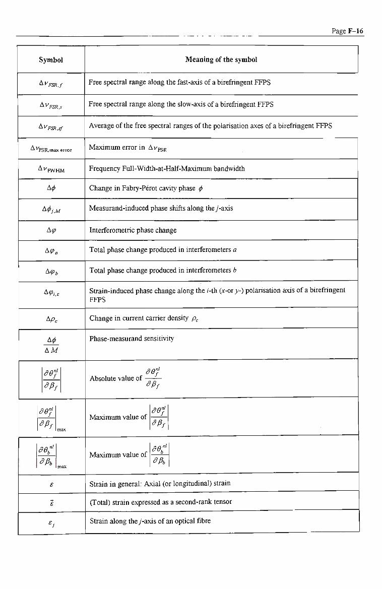
Page F-16
Symbol
Ay FSR. f
AyFSR.s
AyFSR.sf
AVpsR^maxerror
AVpwHM
A<p
A(/>jM
A(p
A(Pa
A(Pb
A(Pi,e
APc
A(p
AM
t
dfif
def dpf ^
^fib
nax
max
s
£
^J
Meaning of the symbol
Free specfral range along the fast-axis of a birefringent FFPS
Free specfral range along the slow-axis of a birefiingent FFPS
Average ofthe free spectral ranges ofthe polarisation axes of a birefringent FFPS
Maximum error in Avj;3p
Frequency Full-Widtii-at-Haff-Maximum bandwidth
Change in Fabry-Perot cavity phase <p
Measurand-induced phase shifts along the/-axis
Interferometric phase change
Total phase change produced in interferometers a
Total phase change produced in interferometers b
Sfrain-induced phase change along the i-th (x-ory-) polarisation axis ofa birefringent FFPS
Change in current carrier density p^
Phase-measurand sensitivity
Absolute value of -——-Sfif
Maximum value of
Maximum value of
69"}
dfif
dfib
Sfrain in general: Axial (or longitudinal) strain
(Total) sfrain expressed as a second-rank tensor
Sfrain along the y-axis of an optical fibre

Page F-17
Symbol
a-"
E(2)
^EM
^ib
<l>
<t>'
A"'
9
hi
<t>r
<I>G
h
"''t'i
In , Tj.current
2Jt j^ Y j , previous
^j.Order
^sig
't'sig
^M
Meaning of the symbol
Thermal strain
Sfrain along the surface of a cantilever a distance z from the pivot point 0
Electric permittivity
The ratio between the transmission along thej-axis and tiie i'-axis ofthe PBS
Total Fabry-Perot cavity phase difference, optical phase shift
Phase near the centte ofa longitudinal mode of tiie Fabry-Perot Airy fiinction A{(p)
Nortiinear measurand-induced variations in ^: ^ with its linear ttend with respect to a measurand M removed
The distance in (p -space from a longitudinal mode giving haff the maximum output for high finesse Fabry-Perot transmission output
Difference between the combined transmission and reflection phase shifts ofthe proximal imrrors
^Zyn^ix ~tnt2\ exp[/^^ 1), this phase value is determined by the properties of the
proximal mirror ofa Fabry-Perot interferometer
y-axis interferometric phase either that of the fast-axis, slow-axis or differential phase responses
Modulo 2;r value of (pj
Current value of ^''4>j
Previous value of "^"(p^
Fringe order of (pj
Instantaneous time-varying phase of I raw.sub
Linear variation (with respect to time) of ^^^
Phase term representing all the nonlinear components in (p^^
The round-trip phase change due to the Fabry-Perot cavity less the phase change due to Av

Page F-18
Symbol
^(Oint
h.M
<PM
Vj.M
KM
Q>
9
(Pj
<Ps
(PT
<PmX
<Ppol
(Pdual
(Px.T
(Py.T
(Px,.
9y,B
r
r
Meaning of the symbol
i„t explicitiy expressed as a fiinction of time; the sinusoidal phase signal associated with the measurand M
Some initial time-independent phase of tiie sinusoidal signal ^(t).^,^
(Depth of modulation) phase-amplitude ofthe sinusoidal signal (p{t)^^
Amplitude (depth of modulation) ofthe measurand-induced phase shifts along the y-axis A(t>jM
Absolute value of (p'^j^
Interferometric phase change vector
Interferometric phase (due only to the optical path difference of an interferometer)
Effective propagation constant of an electro-magnetic wave polarised along they-axis
Component ofthe Fabry-Perot phase contributed by a round-trip of the gauge length L^ (strain measurement)
Component of the Fabry-Perot phase contributed by a round-trip of the temperature sensing length Ly
The round-trip phase change due only to the optical length Fabry-Perot cavity (ni)
Phase ofa polarimetric sensor
Phase of a dual-mode sensor
Component of tiie Fabiy-Perot phase along tiie x-axis of a birefiingent fibre conttibuted by a round-trip ofthe temperature sensing length Lj
Component ofthe Fabry-Perot phase along they-axis ofa birefringent fibre contributed by a round-trip ofthe temperature sensing lengtii Lj
Component of the Fabry-Perot phase along the x-axis of a birefringent fibre conttibuted by a round-trip of the gauge length L^ (sfrain measurement)
Component ofthe Fabry-Perot phase along they-axis of a birefiingent fibre conttibuted by a round-trip ofthe gauge length L^ (strain measurement)
Intensity coupling efficiency into the lead-in fibre ofthe sensing system
(Sensing) length ofthe fibre exposed to a temperature change and total strain

Page F-19
Symbol
M
%
nPD
K
•^b
A
J
\
K
A/2
A/4
h
^b,i
Afe.i
K,i
A
M
V
V'l
^2
n'
6
Oc
Meaning of the symbol
Extinction ratio between the two polarisation mode ofa bfrefringent fibre
Fraction of the total power of the mode guided in the core of an optical fibre
Responsivity of a photodiode
(Bragg) coupling phase
Value of /r at Aj,
Optical wavelength in vacuum
Averaged wavelength value
Wavelength of light source 1
Wavelength of light source 2
Haff-wave plate
Quarter-wave plate
Bragg wavelength
Bragg wavelength of fibre Bragg grating /
Bragg wavelength of fibre Bragg grating 1
Bragg wavelength of fibre Bragg grating 2
Spatial period ofthe grating (pitch length)
Poisson's ratio of an optical fibre
Optical frequency ofa light source; laser diode emission frequency
Optical frequency oft light source 1
Optical frequency of light source 2
=3.141592654 ; ratio ofthe circumference and diameter of a circle
Characteristic phase response of a fibre Bragg grating
Phase shift due to two successive internal cavity reflections (incident from the cavity);

Page F-20
Symbol
9" b
9' b
0b
dx
^m,
^m,
^filrn
^filrn
Kd
eL
Ob
G"/
0"^
nnl
<
.9
Pc
a
'a
^a
Meaning of the symbol
Sum ofthe phase change upon internal reflections from tiie Fabry-Perot mirrors
Phase change upon reflection ofa fibre Bragg grating
Phase change upon transmission of a fibre Bragg grating
Phase change due to reflection from a fibre Bragg grating
Phase change upon reflection on either surface of tiie reflector Z(= m, or m2)
Phase change upon reflection on either surface ofthe reflector 01]
Phase change upon reflection on either surface ofthe reflector ITla
The phase shift upon reflection from a dielectric thin film
The phase shift upon transmission from a dielectric thin film
Electric field reflection phase difference; argument of / ^
Electric field transnussion phase difference; argument of T^^^
(Residual) nortiinear phase component of Gj, vrith respect to p^,
(Residual) nonlinear component of <9 ;„ with respect to Pf
(Residual) nonlinear phase component of ^^ with respect to Px (A'= rrii or m2)
(Residual) nonlinear phase component of ^m, with respect to p^^
(Residual) nonlinear phase component of 9^^ with respect to /?mj
Relative phase between the two linearly polarised beams of a birefiingent fibre
Current carrier density in a semiconductor laser diode
Sfress (force per unit area) expressed as a second-rank tensor
Thermal sfress between the core and the inner cladding of an elliptically-cladded birefiingent fibre
Thermal sfress between the outer circular and the inner elliptical cladding of an

Page F-21
Symbol
[-.]
T
^ c
^saw
^Sampling
0)
(Oc
(Om
(OM
'Oj.M
(ONyquist
tUj
^M
^e
^x,T
^y,T
^X.E
^y,E
^ET
^X,ET
^y.eT
Meaning of the symbol
elliptically-cladded birefringent fibre
Initial stress producing the birefringence
Period; multiple ofthe period 2KI(O
Coherence time ofa light source
Period ofa sawtooth modulation
Sampling period
Angular frequency
Carrier angular frequency
Angular modulation frequency: w-th order ofthe sawtooth modulation frequency
Angular frequency ofthe measurand-induced phase shifts
Angular frequency ofthe measurand-induced phase shifts along they-axis A(pji^
Angular Nyquist frequency
Fractional phase-temperature sensitivity ofa fibre interferometer
Fractional phase-measurand sensitivity ofa fibre interferometer
Fractional phase-sfrain sensitivity of a fibre interferometer
Fractional phase-temperattire sensitivity along tiie x-axis of a birefringent fibre interferometer
Fractional phase-temperamre sensitivity along they-axis of a birefiingent fibre interferometer
Fractional phase-sfrain sensitivity along the x-axis of a birefringent fibre interferometer
Fractional phase-strain sensitivity along they-axis of a birefiingent fibre interferometer
Fractional cross-sensitivity of a fibre interferometer
Fractional cross-sensitivity of a fibre interferometer along the x-axis
Fractional cross-sensitivity of a fibre interferometer along they-axis

Page F-22
Symbol
film
^E
^M
^M
^M
Meaning of the symbol
Fractional phase-temperature sensitivity ofa thin film
Fractional phase-sfrain sensitivity ofa thin film
Fractional phase-measurand sensitivity of a thin film
Fractional phase-measurand sensitivity of mirror HTli
Fractional phase-measurand sensitivity of mirror 1X12

Appendix G: Abbreviations Used In This Thesis
Notation
AC
ADC
Ag
Al
AOM
Ar
B2O3
BBO
CCD
CMOS
CO2
ComCore
ComFace
CSP
CW
DAC
DFB
DFTS
D-SAPD
Description
Alternating Current
Analog-to-Digital Converter
Silver
Aluiruruum
Acousto-Optic Modulator
Argon
Boron Dxide
Beta Barium Borate
Charge-Coupled Device
Complementary Metal-Oxide Silicon
Carbon Dioxide
A fibre Fabry-Perot (interferomettic) sensor using communications-grade fibre for its cavity and having a core-coated Ti02 fiision-spliced in-line reflector
A fibre Fabiy-Perot (interferometric) sensor using communications-grade fibre for its cavity and having a face-coated Ti02 fiision-spliced in-line reflector
Channel-Substrate-Planar
Continuous Wave
Digital-to-Analog Converter
Distributed Feedback
Dispersive Optical Fourier Transform Spectroscopy
Digital Synchronous-Asynchronous Phase-Detection

Page G-2
Notation
DC
e-core
ESG
FBG
FF
FFPI
FFPS
FM
FMCW
FSR
FWHM
Ge
GeOj
Gratingl
Grating2
GratingS
HeNe
HibiFace
HibiGrat
HiBi
I/O
lEC
ILFE
Description
Direct Current
Elliptical-core
Electrical Strain Gauge
In-fibre Bragg Grating
Flip-Flop
Fibre Fabry-Perot Interferometer
Fibre Fabry-Perot (interferomettic) Sensor
Frequency-Modulated
Frequency-Modulated-Continuous-Wave
Free Spectral Range
Full Width at Half Maximum
Germanium
Germanium Dioxide
First of two fibre Bragg gratings written on birefringent fibre fabricated at OFTC. This grating was used as the proximal Fabry-Perot mirror of HibiGrat.
Second of two FBGs written on birefringent fibre fabricated at OFTC.
One ofthe irutial FBGs written on birefringent fibre fabricated at OTRL.
Helium Neon
A fibre Fabry-Perot (interferometric) sensor using HiBi fibre for its cavity and having a face-coated Ti02 fiision-spliced in-line reflector
A fibre Fabry-Perot (interferometric) sensor using HiBi fibre for its cavity and having an in-fibre Bragg grating
Highly Birefiingent or High-Birefiingence
Input/Output
Internal Elliptical Cladding
In-line Fabry-Perot Etalon

Page G-3
Notation
InGaAs
InlineFPl
InlineFP2
LD
LED
LoBi
LPG
MgFlj
MOPO
msb
Nd:YAG
NPBS
NPM
O2
OD
OFS
OFTC
OH
op-amp
OPD
OPO
OSA
OTRL
P2O5
Description
Indium Gallium Arsenide
First ofthe two initial in-line FFPSs developed in this work. The sensor used HiBi fibre for its cavity and had two in-fibre two FBGs as Fabry-Perot nurrors.
Second ofthe two initial in-line FFPSs developed in this work. The sensor used HiBi fibre for its cavity and had two in-fibre two FBGs as Fabiy-Perot mirrors.
Laser Diode
Light-Emitting Diode
Low-Birefringence
Long-Period (Fibre) Grating
Magnesium Flouride
Master Oscillator Power Oscillator
Most signfficant bit
Neodymium Yttrium Aluminum Garnet
Non-Polarising Beam Splitter
Non-Polarisation-Maintaining
Gaseous oxygen
Outer Diameter
Optical Fibre Sensor
Optical Fibre Technology Centre
Hydroxide ion
Operational Amplifier
Optical Path Difference
Optical Parametric Oscillator
Optical Spectrum Analyser
Optical Technology Research Laboratory
Phosphate

PageG-^
Notation
PBS
PD
PID
PM
PZT
RMS
SiOj
SLED
SMTS
SNR
SOP
SRS
STC
Ti
TiA
TiO
TiOj
TML
TTL
UMR
UV
WLI
XOR
Description
Polarising Beam Splitter
Photodiode
Proportional-Integral-Derivative confroller
Polarisation-Maintaining or Phase-Modulated
Lead Zirconate Tantalate
Root-Mean-Square
Silicon Dioxide
Super-lununescence LED
Simultaneous Measurement of Temperature and Strain
Signal-to-Noise Ratio
State of Polarisation
Stimulated Raman Scattering
Schmitt Trigger Circuit
Titanium
Titanium Pentaoxide
Titanium Monoxide
Titanium Dioxide
Tol^o Sokki Kenkyuji (manufacturer of sfrain gauges)
Transistor-Transistor Logic
Unambiguous Measurand Range
Ulfraviolet
White-Light Interferometry
Exclusive-OR logic