Biomass/carbon estimation and mapping in the subtropical ...
68
Biomass/carbon estimation and mapping in the subtropical forest of Chitwan, Nepal: A comparison between VHR GeoEye satellite images and airborne LiDAR data AMADO ADALBERTO LÓPEZ BAUTISTA February, 2012 SUPERVISORS: Dr. Ir. T.A. Groen Dr. M.J.C. Weir
-
Upload
khangminh22 -
Category
Documents
-
view
0 -
download
0
Transcript of Biomass/carbon estimation and mapping in the subtropical ...

Biomass/carbon estimation and mapping in the subtropical forest of Chitwan, Nepal: A comparison between VHR GeoEye satellite images and airborne LiDAR data
AMADO ADALBERTO LÓPEZ BAUTISTA February, 2012
SUPERVISORS: Dr. Ir. T.A. Groen Dr. M.J.C. Weir

Thesis submitted to the Faculty of Geo-Information Science and Earth Observation of the University of Twente in partial fulfilment of the requirements for the degree of Master of Science in Geo-information Science and Earth Observation. Specialization: Natural Resources Management SUPERVISORS: Dr. Ir. T.A. Groen Dr. M.J.C. Weir THESIS ASSESSMENT BOARD: Chair: Dr. Y. A. Hussin External examiner: Dr. T. Kauranne (Arbonaut Oy Ltd. And Dept. of Mathematics and Physics – Lapeenranta, University of Technology, Finland)
Biomass/carbon estimation and mapping in the subtropical forest of Chitwan, Nepal: A comparison between VHR GeoEye satellite images and airborne LiDAR data
AMADO ADALBERTO LÓPEZ BAUTISTA Enschede, The Netherlands, February, 2012

DISCLAIMER This document describes work undertaken as part of a programme of study at the Faculty of Geo-Information Science and Earth Observation of the University of Twente. All views and opinions expressed therein remain the sole responsibility of the author, and do not necessarily represent those of the Faculty.

i
ABSTRACT
It is generally agreed that preservation of forest areas can contribute strongly to the mitigation of global climate change. For this purpose, international institutions such as the United Nations Framework on Climate Change (UNFCCC) have created a collaborative program in reduction emissions of carbon dioxide (REDD) to update inventories emissions from greenhouse gasses. However, studies have demonstrated that there are still uncertainties for an accurate estimation of carbon stock from forests, especially using optical remote sensing. This study aims therefore to determine which of the two sources from airborne LiDAR data or VHR GeoEye satellite images can provide more accurate information for biomass/carbon estimation in the Subtropical forest of Chitwan, Nepal. A very high resolution GeoEye satellite image provides information only in two dimensions while LiDAR data provides information in three dimensions. In the approach of this study, LiDAR data required more analysis because original information from the sensor is acquired in a cloud of points. Then, a Digital Surface Model (DSM) and a Digital Terrain Model (DTM) were derived from the cloud of points. Canopy Height Model (CHM), which is the height of trees, was calculated as the difference between DSM and DTM. The height of the trees derived from LiDAR data were compared to the height of trees measured in the field. LiDAR CHM and GeoEye images were segmented using the technique of Object Oriented Analysis (OOA) to delineate individual tree crowns and the results were compared with the manual delineation derived from the field. Then, the segments derived from both images were used to develop models to estimate the Diameter at breast height (DBH). With the most accurate DBH estimated, Above Ground Biomass (AGB) was calculated using an allometric equation that considers DBH, Height (H) and Wood specific gravity (ρ). Results show that there is no significant difference between the height of trees derived from LiDAR data and the height of trees measured in the field. However, the root mean square error (RMSE) shows a relative value of 27%. The result from segmentation implies that objects from GeoEye are oversegmented compared to those derived from LiDAR data with a difference of 14%. Segments derived from GeoEye and LiDAR images were used to develop models and shows that power model and LiDAR data is more accurate to predict DBH from CPA. Finally, the estimation of carbon stock resulted in a mean value of 1894.08 kg C/tree, which is equivalent to 181.34 Mg C ha-1. Thus, biomass/carbon estimation and mapping in the subtropical forest is practicable utilizing LiDAR data. Keywords: Crown projection area, Canopy height model, Object Oriented Analysis, Allometric equation, Regression, Carbon stock

ii
ACKNOWLEDGEMENTS
First and for most I would like to thank the almighty God for his presence, protection and guidance during the whole study period. My special thanks go to Nuffic which provided me with a fellowship to study and join with people from different countries around the world. I would like to acknowledge my institution in Guatemala, Faculty of Agronomy, San Carlos University specially Eng. MSc. Carlos Lopez and Eng. MSc. Guillermo Santos for providing any supports during my application process. My deepest gratitude and great appreciation goes to Dr. Yousif Hussin, my first supervisor Dr. Thomas Groen and my second supervisor Dr. Michael Weir for their continuous supportive feedbacks. Their comments were really constructive and I learned a lot from them. I am very thankful to the International Centre for Integrated Mountain Development (ICIMOD), Asia Network for Sustainable Agriculture and Bio-resources (ANSAB), Federation of Community Forest Users’ Nepal (FECOFUN), Forest Research Assessment (FRA) and Arbonaut of Finland for their support in filling the gaps of financial matters and providing data and any necessary information during the thesis work. My sincere thanks to Hammad Gilani of ICIMOD, Basanta Gautam of Arbonaut and Khamarrul Azahari Razak for their cooperation in providing different facilities during the analysis and thesis field work. My deepest gratitude goes to my family, especially to my parents for their prayers, encouragement and moral supports. Your presence has a great value for me. You have always special place in my heart. God bless you. Amado Adalberto López Bautista Enschede, March 2012

iii
LIST OF ACRONYMS
IPCC Intergovernmental Panel on Climate Change
UNFCCC United Nations Framework Convention on Climate Change
FAO Food Agricultural Organization
REDD Reducing Emission from Deforestation and Degradation
GHG’s Greenhouse gases
CO2 Carbon dioxide
ICIMOD International Centre for Integrated Mountain Development
ANSAB Asia Network for Sustainable Agriculture and Bio-resources
CFUG Community forest user group
GPS Geographic Position System
VHR Very high resolution
DTM Digital Terrain Model
DSM Digital Surface Model
MSS Multispectral data
AGB Aboveground biomass
CPA Crown projection area
DBH Diameter at breast height
OOA Object oriented analysis
RMSE Root Mean Square Error

iv
TABLE OF CONTENTS Abstract......................................................................................................................................................i Acknowledgements...................................................................................................................................ii List of acronyms......................................................................................................................................iii List of figures...........................................................................................................................................vi List of tables...........................................................................................................................................vii 1. Introduction ............................................................................................................................................... 1
1.1. Background ............................................................................................................................ 1 1.2. Methods for above ground biomass estimations ................................................................... 2 1.2.1. Biomass estimation using Height and Diameter at Breast Height (DBH) ................................. 3 1.3. The study area ........................................................................................................................ 3 1.4. Problem Statement ................................................................................................................. 6 1.5. Research Objectives .............................................................................................................. 7 1.5.1. The Specific Objectives .......................................................................................................................... 7 1.6. Research questions and hypothesis ........................................................................................ 7
2. Concepts and definitions ........................................................................................................................ 8 2.1. Biomass and Carbon .............................................................................................................. 8 2.2. Remote sensing approach in estimating carbon stock ........................................................... 8 2.2.1. Above-ground biomass estimation with Optical Sensor Data ....................................................... 8 2.3. Above-ground biomass estimation with Radar and LiDAR data .......................................... 9 2.4. Carbon stock from Crown Projection Area (CPA) .............................................................. 10 2.5. Allometric Equation ............................................................................................................ 10 2.6. Object Oriented Analysis (OOA) ........................................................................................ 10
3. Materials and methods.......................................................................................................................... 12 3.1. Data set ................................................................................................................................ 13 3.2. Materials .............................................................................................................................. 14 3.3. Fieldwork ............................................................................................................................. 15 3.3.1. Sampling design ..................................................................................................................................... 15 3.3.2. Data collection and analysis ............................................................................................................... 15 3.4. Canopy Height Model (CHM) ............................................................................................. 16 3.4.1. Correlation Analysis ............................................................................................................................. 18 3.5. Image Geo-registration ........................................................................................................ 18 3.6. Image filtering ..................................................................................................................... 18 3.7. Manual delineation of trees ................................................................................................. 19 3.8. Image Segmentation using OOA ......................................................................................... 19 3.8.1. Scale Parameter/Setting using ESP................................................................................................... 19 3.8.2. Multi-resolution Segmentation ........................................................................................................... 20 3.8.3. Watershed transformation ................................................................................................................... 20 3.8.4. Morphology ............................................................................................................................................. 21 3.8.5. Removal of undesired objects ............................................................................................................. 22 3.8.6. Segmentation Validation ...................................................................................................................... 22 3.9. Model validation .................................................................................................................. 23 3.9.1. Regression analysis ............................................................................................................................... 23 3.10. Biomass/Carbon Stock estimation ....................................................................................... 24

v
4. Results ..................................................................................................................................................... 25 4.1. Descriptive statistics .............................................................................................................25 4.2. Relationship between heights of trees derived from LiDAR CHM and ground data ...........27 4.3. Image segmentation ..............................................................................................................28 4.3.1. Scale parameter .................................................................................................................................... 28 4.3.2. Multi-resolution segmentation ........................................................................................................... 29 4.3.3. Accuracies of Segmentation ............................................................................................................... 30 4.4. Relationship between CPA and DBH...................................................................................31 4.4.1. Model Validation .................................................................................................................................. 33 4.5. Biomass and Carbon Estimation ..........................................................................................34
5. Discussion .............................................................................................................................................. 36 5.1. Relationship between height values .....................................................................................36 5.2. Delineation of tree crowns derived from LiDAR data and GeoEye image ..........................37 5.3. Relationship between Crown Projection Area and Diameter at Breast Height ....................39 5.4. Biomass/Carbon estimation ..................................................................................................40 5.5. Limitations of the Research ..................................................................................................41
6. Conclusion and recommendation ...................................................................................................... 42 6.1. Conclusion ............................................................................................................................42 6.2. Recommendation ..................................................................................................................43
List of references....................................................................................................................................44 Appendices..............................................................................................................................................50

vi
LIST OF FIGURES Figure 1 Theoretical framework ........................................................................................................................... 5 Figure 2 Location of the study area ..................................................................................................................... 5 Figure 3 Crown projection area .......................................................................................................................... 10 Figure 4 Flowchart for biomass/carbon estimation within GeoEye images and LiDAR data .............. 13 Figure 5 Illustration of the conceptual differences between wave form recording and discrete-return
LiDAR devices ....................................................................................................................................... 16 Figure 6 Process to derive Canopy Height Model (CHM) using cloud of pints from LiDAR data .... 18 Figure 7 Tool for estimation of Scale Parameter ............................................................................................ 20 Figure 8 Illustration of the watershed segmentation principle ..................................................................... 21 Figure 9 Image object after segmentation (a) Image object after morphology algorithm (b) ............... 22 Figure 10 Matched cases of an extracted object ................................................................................................ 22 Figure 11 Frequency of forest species ................................................................................................................. 25 Figure 12 Carbon estimation derived from field data ...................................................................................... 26 Figure 13 Distribution of tree heights .................................................................................................................. 28 Figure 14 Height values from LiDAR (Height estimated) and height values measured in the field
(Height observed) with a fitted line 1 to 1. ...................................................................................... 28 Figure 15 Estimation of scale parameter (a) LiDAR CHM, (b) GeoEye image ........................................ 29 Figure 16 Multi-resolution segmentation and watershed transformation (a) LiDAR CHM, (b) GeoEye
................................................................................................................................................................... 30 Figure 17 Segmentation derived from LiDAR CHM (a) and GeoEye (b) images .................................... 31 Figure 18 Relationship between CPA and DBH from field data ................................................................... 32 Figure 19 Relationship between DBH from field data (field data) and CPA from GeoEye (CPA
estimated) ................................................................................................................................................ 33 Figure 20 Relationship between DBH from field data (field data) and CPA from LiDAR (CPA
estimated) ................................................................................................................................................ 33 Figure 22 Map of carbon stock in the study area .............................................................................................. 35 Figure 23 Comparison of Height and mean square errors from trees ........................................................... 37 Figure 24 Comparison of segmented trees derived from LiDAR (a) and GeoEye (b) ............................. 39

vii
LIST OF TABLES Table 1 Dataset characteristics ......................................................................................................................... 14 Table 2 List of instruments used for fieldwork ............................................................................................. 14 Table 3 List of software used in the research ................................................................................................ 15 Table 4 Class codes and classification of point clouds ............................................................................... 17 Table 5 DBH and Height of species observed in the field ......................................................................... 25 Table 6 Results of t-test between tree height values from field and tree height derived from CHM 27 Table 7 “D” value from segmentation of LiDAR CHM and GeoEye image ......................................... 31 Table 8 Models to DBH estimations ............................................................................................................... 32


BIOMASS/CARBON ESTIMATION AND MAPPING IN SUBTROPICAL FOREST OF CHITWAN, NEPAL: A COMPARISON BETWEEN VHR GEOEYE SATELLITE IMAGES AND AIRBORNE LIDAR DATA
1
1. INTRODUCTION
1.1. Background
Climate change is a product of Green House Gas (GHG) emissions associated with the provision of
energy services causing the current global warming (IPCC, 2011). Gases that contribute to the
greenhouse effect are: Water vapour, Carbon dioxide (CO2), Methane (CH4), Nitrous oxide (N2O) and
Chlorofluorocarbons (CFCs) (IPCC, 1990). It is considered that annual emissions of CO2 grew by
about 80% between 1970 and 2004, while the global atmospheric concentration increased from 280
ppm to 379 ppm3 by 2005, and it has been indicated that the annual growth rate of CO2 has increased
by 1.9 ppm y-1 between 1995 and 2005 (IPCC, 2007b; McKibben, 2007). The emission of gasses is a
product of natural processes such as volcanic eruptions or mainly by human activities, including:
deforestation, land use changes, burning fossil fuels, and agriculture like soil cultivation practices.
Deforestation is one of those processes that deserve attention, given that forest can be considered as
´double´ significant in combating global warming. This is because: (1) deforestation adds CO2 to the
atmosphere when the carbon contained in the forest is burnt or decomposed, and (2) increases in forest
biomass extracts CO2 from the atmosphere and stores it. Carbon is stored by trees in their roots, trunks,
branches and leaves. The removal of 3.67 tonnes of carbon dioxide from the atmosphere results in one
tonne of carbon sequestered in trees (Hunt, 2009). In the Global Forest Resource Assessment of FAO
(2010), it is estimated that all carbon stored in above ground biomass, litter and soils of the entire
worlds’ forests is around 652 billion tonnes with an average carbon content of 161.8 tonnes per
hectare. The UN’s Intergovernmental Panel on Climate Change (IPCC, 2007a) estimated in 2007 that
deforestation, forest degradation and other changes in forests, contributes in 17.4 per cent of global
greenhouse emissions. Then, Vegetation biomass is an important ecological variable for understanding
the changes of climate and carbon sequestration in a forest (FAO, 2009). It is generally agreed that
preservation of forest areas can contribute strongly to the mitigation of global climate change. For this
purpose, the United Nations Framework on Climate Change (UNFCCC) have created a collaborative
program on 2008 called Reducing Emissions from Deforestation and Forest Degradation (REDD) to
assist developing countries to build capacity in reduction emissions to future involvement on REDD+
mechanism. Accordingly, REDD+ refers to reduce these emissions from deforestation and forest
degradation and the role of conservation, sustainable management of forests and enhancement of forest
carbon stocks (UN-REDD, 2008a). For this reason REDD+ facilitates the provision of financial
incentive to developing countries by reducing emissions from forested lands and investing in low-

BIOMASS/CARBON ESTIMATION AND MAPPING IN SUBTROPICAL FOREST OF CHITWAN, NEPAL: A COMPARISON BETWEEN VHR GEOEYE SATELLITE IMAGES AND AIRBORNE LIDAR DATA
2
carbon paths for sustainable development (UN-REDD, 2008b). In order to appropriate monitoring
systems of forest lands it is necessary to combine different data sources such as: field measurements
and observations, varieties of satellite and airborne remote sensing data with cost-efficiency to achieve
carbon reports with an accepted accuracy and precision. Remote sensing data is a crucial source of
information for monitoring the state and trends of land-use, land cover and carbon estimation in a
particular area (Holmgren, 2008).
1.2. Methods for above ground biomass estimations
Many methods have been used in forest biomass estimation. The most accurate method for estimation
of forest biomass is to harvest the trees, oven-dry them and to weigh the dry matter. However, this
direct method is normally prohibitively expensive, destructive and time-consuming (Hunt, 2009). In
recent years, many studies using satellite images with high resolution (Kosaka & Kuwata, 2006) and
radar have been investigated as alternative methods for biomass estimation (Patenaude et al., 2005).
These methods have been explored in terms of biomass and its changes to increase our understanding
of the role of forests in the carbon cycle for greenhouse gas inventories and terrestrial carbon
accounting (Muukkonen & Heiskanen, 2007). For example, as studied by Dubayah et al. (2000),
information such as canopy cover, tree size (height and crown diameter), biomass, crown volume
among others are routinely needed for sustainable resource management because it is useful
information that can help to maintain and enhance the economic, social and environmental value of all
types of forests, for the benefit of present and future generations. Despite the fact that optical images
with very high spatial resolution, such as GeoEye, can provide useful information of spectral
reflectance in objects, there is still information like vertical parameters (height of trees) that cannot be
collected with this sensor and can be useful to improve biomass estimations. In addition, weather
conditions can affect the image quality, especially in those areas that are frequently covered by clouds.
This is a situation that occurs frequently in many tropical and subtropical areas.
Recently, Light Detection and Ranging (LiDAR) is becoming more a promising technique for future
forest monitoring because of its ability to assess the 3D forest structure (Patenaude et al., 2005; van
Leeuwen & Nieuwenhuis, 2010) and to provide a good data on vertical profiles of vegetation canopies
(Balzter et al., 2007). LiDAR is an active remote sensing system which operates from aircraft by
sending laser pulses towards the ground to record the elapsed time between beam launch and return
registration. Records are a cloud of points product of pulses reflected from tree canopy, trunks,
branches, leaves, low vegetation and even reaching to the ground to create a profile in three
dimensions (Gautam & Kandel, 2010). In this way, the vertical parameters of individual trees are
calculated, giving the most feasible advantage of LiDAR to assess biomass and carbon estimation
(Kim & et al, 2010). Information of vertical profiles in individual trees can be used to validate models

BIOMASS/CARBON ESTIMATION AND MAPPING IN SUBTROPICAL FOREST OF CHITWAN, NEPAL: A COMPARISON BETWEEN VHR GEOEYE SATELLITE IMAGES AND AIRBORNE LIDAR DATA
3
from other sensors with accurate values (Balzter et al., 2007) or to estimate biomass in dense tropical
forests (Drake et al., 2002). Therefore, they have received increasing attention as new technology to
derive forest structural attributes. This can be provided and differentiated by direct retrieval (as canopy
height and crown volume), modelling (as vertical foliar diversity and layers in ecological applications)
or by fusion with other sensors (such as vegetation type). Considering these advantages, traditional
multispectral classifications in forest may be more accurately estimated when vertical component
provided by LiDAR is added (Dubayah et al., 2000).
The greatest advantage of LiDAR is its capacity to assess forest degradation when it is combined with
advanced statistical models calibrated with sample plots. Whereas other optical remote sensing only
provide the highest layer of the canopy suffering from saturation problems, while LiDAR beams
always penetrates into the deep forest and the resulting data are without being influenced by clouds
and shadows, thus providing more accurate results than any other remote sensing techniques
(ARBONAUT, 2010; Næsset, 2009).
1.2.1. Biomass estimation using Height and Diameter at Breast Height (DBH)
Different parameters can be used for above ground biomass estimation, like basal area, stand structure
and tree height. However, DBH is the widely available and is most commonly used for this estimation
(Crow & Schlaegel, 1988). Since DBH of trees cannot be derived directly from RADAR, LiDAR or
optical remote sensing data, regression models have been developed based on crown projection area
(CPA) to assess AGB (Chave et al., 2005) (See also section 2.2).
Also, canopy height provides an opportunity to model ABG and canopy volume. It has been shown in
an accurate way that is possible to determine the height of trees using remote sensing like
multiparametric interferometric radar (like Pol-InSAR) and more recently using LiDAR data. As a
comparison of these two methods, Pol-InSAR does not retrieve heights directly, but indirectly by
applying a model-based inversion (Mette et al., 2004). LiDAR data can directly retrieve tree height
data (Lim et al., 2003), offering a new way to describe a forest structure in 3D (Maier et al., 2008).
1.3. The study area
In 2008, the Nepal government submitted a note to the United Nations Framework Convention on
Climate Change (UNFCCC) Committee to be considered under REDD project and to have economical
financing on forest carbon stock. In the same year Nepal was selected as a winner for Forest Carbon
Partnership Facility (FCPF) fund, to develop the Readiness Plan -R-PLAN- (Dahal & Banskota, 2009)
to undertake activities on reducing emissions for deforestation and forest degradation in the REDD
context. The REDD context refers to establishing scenarios for emission reductions from deforestation

BIOMASS/CARBON ESTIMATION AND MAPPING IN SUBTROPICAL FOREST OF CHITWAN, NEPAL: A COMPARISON BETWEEN VHR GEOEYE SATELLITE IMAGES AND AIRBORNE LIDAR DATA
4
and forest degradation and establish scenarios in order to reduce emissions. To address international
issues to national context is becoming a challenge in Nepal, mainly by the weak governance and to be
in a process of state restructuring. Actually, this country has produced sufficient data in terms of
satellite images and field data which is required for biomass estimation to fulfil the REDD context.
This was also taken into consideration in a project by the International Centre for Integrated Mountain
Development (ICIMOD) (Dahal & Banskota, 2009), that aims to assist mountain people to understand
changes induced by climate and to adapt them to the changes and make the most of new opportunities.
Afterwards, due to the benefits mentioned above, most of the forests became managed by communities
and are considered as models of management to reduce its degradation in the Mid-hills of Nepal. This
contributes to the enhancement of carbon stock (Ministry of Forest and Soil Conservation, 2010).
As continuation of the project in Nepal, many study projects have been developed for biomass/carbon
estimation in different mountainous areas. Recently, Baral (2011) has mapped carbon stock using high
resolution satellite images in the same forest as in this study obtaining a relative error of 39%. She
concluded that subtropical regions like Chitwan are fast growing and diverse, emphasizing that
intermingling between canopies of individual trees can affect the carbon stock estimation.
LiDAR data has been also used to estimate above ground biomass in mixed species and result obtained
by Garcia, et al., (2010) shows a root mean square error (RMSE) in a range of 9.7 Mg ha-1 and 18.48
Mg ha-1, emphasizing that LiDAR data can estimate carbon content in mixed species with high
accuracy.
In the case of Nepal, it is a significant challenge to use conventional remote sensing for biomass
estimation due to the complexity of the terrain, increasing the possibility of LiDAR to assess the forest
resources. Processes of factors that are influencing the biomass/carbon stock and methods to its
estimation are presented in Figure 1. Environmental factors and policies can affect or benefit the
forests, however, analyses in forests need to be assessed to estimate the carbon stock and to contribute
to the mitigation of carbon dioxide emissions and climate change. Methods using remote sensing
techniques are common and feasible, especially in remote areas.

BIOMASS/CARBON ESTIMATION AND MAPPING IN SUBTROPICAL FOREST OF CHITWAN, NEPAL: A COMPARISON BETWEEN VHR GEOEYE SATELLITE IMAGES AND AIRBORNE LIDAR DATA
5
Environmental factors
Height
DBH
Species
Canopy
Segmentation(OOA)
VHR (GeoEye)
Above Ground Carbon Stock
REDD
Policies and Standards
Community forest Remote Sensing
+
+ -
Quality assessment
VHR-Very High ResolutionOOA-Object oriented analysis
Lidar
CO2
+-
Regression
Allometry equation
Diameter at BreastHeight
DBH-
Figure 1 Theoretical framework
This research was carried out in a study area falling in the subtropical forest located in Chitwan
District, Nepal (Figure 2). This is a forest managed by the Community (CF) and handed over to a
forest user group for its development, conservation and utilization (Ojha et al., 2009).
Figure 2 Location of the study area

BIOMASS/CARBON ESTIMATION AND MAPPING IN SUBTROPICAL FOREST OF CHITWAN, NEPAL: A COMPARISON BETWEEN VHR GEOEYE SATELLITE IMAGES AND AIRBORNE LIDAR DATA
6
1.4. Problem Statement
Many efforts have been performed using different methods to estimate biomass with high accuracy to
extract reliable structural tree information (Maier et al., 2008). Despite of this, there are still
considerable uncertainties in terms of accurate delineation of trees and regarding methods that can
standardize and precise these estimations (Nichol & Sarker, 2011). These uncertainties are causing
overestimation or underestimation of biomass/carbon, that are being attributed mainly to the
complexity of forest ecosystems that add more difficulties to derive forest parameters mainly in those
areas located in tropical and subtropical areas (Lu, 2005).
Regarding biomass estimation, Lu (2006) emphasizes the importance to integrate field data with high
resolution remote sensing which also agrees with the research of Gautam, et al (2010). Both authors
conclude that integration of data provides an accurate, precise and affordable monitoring solution for
tropical forests. However, field data is time consuming and labour intensive in remote areas (Brown,
2002; Houghton et al., 2001). Then, VHR images have been widely applied for biomass estimation
based on individual trees, demonstrating correct detection of trees for biomass estimations (Nichol &
Sarker, 2011). Despite of this, Tsendbazar (2011) found that effect of shadows using VHR optical
images can have influence to find a relationship between CPA and carbon stock of trees, because
shadow can influence in the geometry of tree crowns which makes it difficult to distinguish crowns
using remotely sensed images.
More recently, LiDAR from satellite platforms has become available and has been widely applied in
biomass estimations (Patenaude et al., 2005). Its advantage is based in its ability to provide height
values of trees that can be added to these estimations. Kim et al. (2010) was using LiDAR data to deal
with the difficulties and error on carbon storage in case of high tree density, where crown overlapping
occurs in a forest of Pinus desinflora located in South Korea. It is mentioned that error can be reduced
when height of trees are added to identify gap areas via the height information of tree stands using
LiDAR data. These advantages on LiDAR data are results of its potential in providing 3D information
to characterize forest for biomass estimation (van Leeuwen & Nieuwenhuis, 2010).
This study focuses on the biomass/carbon estimation using Object Oriented Analysis (OOA) as basis
to delineate individual trees. OOA is a technique widely discussed in processing VHR satellite images
(Heyman et al., 2003; Yu et al., 2006), used to delineate and extract individual trees inside dense
subtropical forests for biomass/carbon estimation. Considering this advantage, individual trees are
delineated inside dense subtropical forests using airborne LiDAR data and VHR GeoEye satellite
images to determine the most appropriate method in the delineation of individual trees in comparison

BIOMASS/CARBON ESTIMATION AND MAPPING IN SUBTROPICAL FOREST OF CHITWAN, NEPAL: A COMPARISON BETWEEN VHR GEOEYE SATELLITE IMAGES AND AIRBORNE LIDAR DATA
7
with the field data. Then, the most accurate data source (LiDAR or GeoEye) in the delineation of
individual trees is used for biomass/carbon estimation.
1.5. Research Objectives
This study aims to determine which of two different sources - airborne LiDAR data and VHR GeoEye
satellite images - can provide more accurate information for biomass/carbon estimation in the
Subtropical forest of Chitwan, Nepal.
1.5.1. The Specific Objectives
1. To analyze the relationship between tree height measured in the field and tree height
values derived from LiDAR data
2. To estimate the segmentation accuracy of OOA on LiDAR data compared to segmentation
of VHR GeoEye data
3. To determine the relationship between Crown Projection Area (CPA) and Diameter at
Breast Height (DBH)
4. To map the estimated biomass/carbon in the Subtropical forest of Chitwan, Nepal, using
the best performing method found from the results of objective 2.
1.6. Research questions and hypothesis
Objectives Research Questions Hypothesis
1 How strong is the relationship
between tree heights measured in
the field with height values derived
from LiDAR data?
H1. There is a strong significant relationship
between tree height values measured in the field and
tree height values derived from LiDAR data
2 Does image segmentation from
LiDAR data give an improvement
in accuracy compared to GeoEye
images?
H1. Image segmentation from LiDAR data has an
improvement compared to VHR GeoEye images
3 How strong is the relationship
between CPA and DBH?
H1. There is a strong significant relationship
between CPA and DBH

BIOMASS/CARBON ESTIMATION AND MAPPING IN SUBTROPICAL FOREST OF CHITWAN, NEPAL: A COMPARISON BETWEEN VHR GEOEYE SATELLITE IMAGES AND AIRBORNE LIDAR DATA
8
2. CONCEPTS AND DEFINITIONS
2.1. Biomass and Carbon
Biomass concerns the dry weight of the trees. Generally it includes the above ground and below
ground living mass, like trees, shrubs, vines, roots and the dead mass of fine and coarse litter
associated with the soil (Lu, 2006). To quantify biomass, the most appropriate and direct way is to
harvest all trees of a certain area, dry them and weigh the biomass (Gibbs, 2007). Then, most
commonly carbon content in a forest can be estimated by multiplying dry biomass by a fraction of 0.5
(IPCC, 2006), while after careful comparison ICIMOD (2010) has proposed to convert biomass value
of standing trees into Carbon stock multiplying by the factor 0.47 for forests in Nepal.
2.2. Remote sensing approach in estimating carbon stock
Traditional techniques, based on field measurements (Brown, 2002; Houghton et al., 2001) are most
accurate, but are time consuming and labour intensive, especially in remote areas. Also geographic
Information Systems (GIS) was used by Brown & Gaston (1995) in the tropical forest with the use of
available spatial data sets to extend limited biomass data to regional and national estimations.
Concluding that it is difficult to obtain good quality of data and that also has not been used widely for
above ground biomass (AGB) estimations. These disadvantages on GIS and traditional techniques are
providing more advantages to remote sensing techniques, increasing the attraction of scientific interest
(Foody et al., 2003; Lu et al., 2005; Santos et al., 2003; Zheng et al., 2004).
In this sense, RS has become widely used and a solution to AGB estimation (Lu, 2005; Steininger,
2000; Zheng et al., 2004). However, most of the studies related to –AGB- have been focused on
coniferous forests due to the species composition and stand structure which is relatively easy to study,
compared to moist tropical forests that become complex due to the wide species composition and
complex stand structure (Lu et al., 2005; Zheng et al., 2004).
2.2.1. Above-ground biomass estimation with Optical Sensor Data
Different approaches have been used to estimate AGB based on remote sensed data, like crown
diameter using regression analysis to estimate DBH or using canopy reflectance models (Phua &
Saito, 2003; Popescu et al., 2003). Also others, such as neural network, K nearest-neighbour (Foody et
al., 2003; Nelson et al., 2000; Zheng et al., 2004) have been less used. Thereupon, sensors from very
high to low spatial resolution have been used for AGB estimation. This section summarizes the AGB
estimation based on very high spatial resolution (VHSR) of optical remote sensing.

BIOMASS/CARBON ESTIMATION AND MAPPING IN SUBTROPICAL FOREST OF CHITWAN, NEPAL: A COMPARISON BETWEEN VHR GEOEYE SATELLITE IMAGES AND AIRBORNE LIDAR DATA
9
Very high spatial resolution data (VHSR)
VHSR also called fine spatial resolution data can be airborne such as aerial photographs or space-
borne such as Ikonos, GeoEye, Quickbird images with a spatial resolution lower than 5 meters. These
data types have been frequently used for modelling tree parameters (Levesque & King, 2003). For
applications related to forest inventory, aerial photograph has become extensively used, considering
that when using photo-interpretation technique and stereo pairs it is possible to measure various forest
parameters, like tree height, crown diameter and stand area. Nevertheless, since VHSR optical images
are providing similar information (except height) and contain a similar spatial and spectral resolution,
these have been increasingly used for forest inventory studies (Wulder et al., 2004). Culvenor (2003)
evaluates the extraction of individual trees using fine spatial resolution images and concludes that
achieving information from forest inventories is still a challenge because of the complex structure of
natural forest canopies. Nichol & Sarker (2011) improved the biomass estimation in a study located in
China using two high resolution optical sensors (Advanced Visible and Near Infrared Radiometer type
2 (AVNIR-2) and SPOT 5). They developed multiple regression models between information derived
from the images and biomass derived from field data and results show an r2 of 0.65. Tiede et al.,
(2008) combined airborne laser scanner (ALS) with optical image data to perform automated tree
crown delineation. The method was based on Cognition Network Language which is purely a
programming language. Results demonstrate correctly detected accuracies of trees (concerning the
location of trees) between 86 % for coniferous and 79 % for dead trees, but dropping to 44 % for
deciduous trees.
2.3. Above-ground biomass estimation with Radar and LiDAR data
In tropical areas, where the climatic conditions, especially clouds, are affecting most of the year, the
use of optical sensors becomes difficult. Thus, radar data become a feasible way for forest studies.
Previous work has identified the potential of Radar in estimating AGB (Hussin et al., 1991; Santos et
al., 2003). Hussin, et al., (1991) has concluded that when using L-band HV there is a strong positive
relationship with pine stand parameters (biomass, height and basal area) and Santos, et al., (2003)
found that using polarimetric P-band data can contribute significantly to develop models in tropical
areas where it is difficult to obtain information from optical remote sensing. Furthermore, the fusion of
Radar with optical remote sensing is a potential technique because it enables the possibility to have
vertical attributes of forests together with 2D information from optical data (Treuhaft et al., 2004). In
the same way, LiDAR data has shown a promising approach for biophysical parameter estimation and
AGB assessment. This is mainly due to the advantage of not being affected by clouds and its ability in
providing information in 3D (Drake et al., 2002; Hyde et al., 2005).

BIOMASS/CARBON ESTIMATION AND MAPPING IN SUBTROPICAL FOREST OF CHITWAN, NEPAL: A COMPARISON BETWEEN VHR GEOEYE SATELLITE IMAGES AND AIRBORNE LIDAR DATA
10
2.4. Carbon stock from Crown Projection Area (CPA)
CPA also known as canopy cover is defined as the area of the ground which is reflected by a vertical
projection of the tree crowns (Jennings et al., 1999). Field measurements of CPA can be difficult
because of the irregularity of the tree crown’s outline. To facilitate the measurement, the usual way is
to project the perimeter of the crown vertically to the ground and to make a diameter measurement
taking an average of two perpendicular direction of the canopy diameter (Husch et al., 2003) (Figure
3).
Figure 3 Crown projection area (Gschwantner et al., 2009)
2.5. Allometric Equation
Ketterings, et al. (2001) define allometric equation as a quantitative relationship between measurable
tree variables like DBH and height to other difficult to assess variables, like standing volume of the
tree or total biomass or carbon stock. For biomass estimations Chave, et al. (2005) emphasize that
biomass regression models may include information on diameter at breast height DBH (1.3 m from the
ground), total tree height H (in m) and wood specific gravity ρ (in g/cm3) and developed an allometric
equation for biomass estimation with these three parameters and found a bias of 0.5-6.5%. While
Brown (2002) shows that for reliable carbon estimations in highly diverse tropical forests, allometric
equations can be used that consider only DBH measurements.
2.6. Object Oriented Analysis (OOA)
OOA also called object based image analysis (OBIA) refers to the partition of an image into discrete
non overlapping units called image objects considering the homogeneity in terms of spectral or spatial
properties (Hay et al., 2005; Zhang et al., 2010).

BIOMASS/CARBON ESTIMATION AND MAPPING IN SUBTROPICAL FOREST OF CHITWAN, NEPAL: A COMPARISON BETWEEN VHR GEOEYE SATELLITE IMAGES AND AIRBORNE LIDAR DATA
11
Various OOA image classification techniques have been used successfully to find information from a
single tree crown (Hay et al., 2005). The most applicable methods are region growing and valley
following (Erikson & Olofsson, 2005). The first method is based on rule set and region grows start
from a seed point to find the boundary of segments. The second method is based on pixels with a
lower grey level values than surrounded pixels to find the boundary of objects. Yu et al. (2006)
developed a comprehensive vegetation inventory in northern California and demonstrated that the
OOA approach is better than pixel based classification. Maier et al. (2008) incorporated LiDAR
derived canopy surface models to segment individual trees using multi-resolution segmentation. He
has proved that multi-resolution segmentation can be a straight forward method to simplify complex
canopy surface with results of 82% of correct trees identified.

BIOMASS/CARBON ESTIMATION AND MAPPING IN SUBTROPICAL FOREST OF CHITWAN, NEPAL: A COMPARISON BETWEEN VHR GEOEYE SATELLITE IMAGES AND AIRBORNE LIDAR DATA
12
3. MATERIALS AND METHODS
This chapter describes the methods followed to address the research questions. The objective of this
project is to determine which of the two data sources (LiDAR data and GeoEye images) can provide
more accurate information for biomass/carbon estimations.
In order to evaluate the two sensors, the flow of the analysis is presented in Figure 4. It is observed
that the method was divided in three main steps defined by the sources of data: GeoEye images, field
data and LiDAR data.
The GeoEye Panchromatic image (0.5m) was pan-sharpened with GeoEye Multispectral bands MSS
(2m). The pansharpen technique is used to combine within images from the same sensor or by
combination with another kind of sensor to produce imagery with higher spatial, temporal or spectral
resolution. For this purpose, the low and high-resolution images must be geometrically registered prior
to be pansharpened (Section 3.5). The higher resolution image (PAN) was used as the reference to
which the lower resolution image (MSS) was registered (Schowengerdt, 2006).
LiDAR data was pre-processed to calculate the canopy height model (CHM), which is the height of
trees that was subtracted by the difference between the Digital surface model and the Digital terrain
model (DSM – DTM) (Section 3.4).
Both images were filtered (Section 3.6) to reduce the noise and facilitate the segmentation process
based on the crown projection area (CPA) of individual trees (Section 3.8). Then values of
segmentation were determined with its accuracy in comparison to the manual delineation of trees
derived from field data. For this analysis regression analysis and the root mean square error (RMSE)
was used. With these accuracy values the most accurate method for delineation crown canopies of
individual trees was determined. Then, for biomass estimation an allometric equation described in
section 3.10 which considers Diameter at breast height (DBH), Height of trees and wood specific
gravity was used.

BIOMASS/CARBON ESTIMATION AND MAPPING IN SUBTROPICAL FOREST OF CHITWAN, NEPAL: A COMPARISON BETWEEN VHR GEOEYE SATELLITE IMAGES AND AIRBORNE LIDAR DATA
13
Geo-Eye MSS (2m)
Geo-Eye Pan (50 cm)
LiDAR
Pansharpen
Field measurements
DBH, Species, Height, CPA
Allometric equation
Biomass
Conversion
Carbon
Validation
Carbon map
CHM
ABREVIATIONS
CPA = Crown Projection AreaDBH = Diameter at Breast HeightDSM = Digital Surface ModelDTM = Digital Terrain Model
Comparison
Estimated error Q1
DTMDSM
Pansharpened GeoEye (50 cm)
Image subset
Image filter
Image segmentation
CHM (study area)
Filtered image
CPA LiDAR
Manual delineation
Accuracy assessment
Image subset
Panchromatic (study area)
Image filter
Filtered image
Image Segmentation
CPA GeoEye
Image subset
GeoEye (Study area)
Manual delineation
Accuracy assessment
Regression / RMSE
Model
GeoEye analysis
LiDAR analysis
Fieldwork
LEGEND
Q2
Q3
Q2
Image georegistration
Registered image
Image georegistration
Registered image
Figure 4 Flowchart for biomass/carbon estimation within GeoEye images and LiDAR data
3.1. Data set
For the study in the Chitwan community forest, two different data were used. LiDAR data was
acquired between March and April of 2011 by the Forest Resources Assessment (FRA) project in
Nepal and data from GeoEye was acquired in November of 2009 by the ICIMOD project in Nepal.
GeoEye images with a ground resolution of 2.0 meters MSS and 0.5 meters in the panchromatic and
LiDAR data with an average of 2.4 points/m2. Other specifications are presented in Table 1.

BIOMASS/CARBON ESTIMATION AND MAPPING IN SUBTROPICAL FOREST OF CHITWAN, NEPAL: A COMPARISON BETWEEN VHR GEOEYE SATELLITE IMAGES AND AIRBORNE LIDAR DATA
14
Table 1 Dataset characteristics
Parameters Sensor LiDAR GeoEye
Costumer Forest Resource Assessment (FRA) Nepal, Ministry of Forests and Soil Conservation
International Centre for Integrated Mountain Development (ICIMOD), Nepal
Projection UTM UTM Datum WGS 84 zone 45N WGS 84 zone 45N
Altitude 2.2 kilometers 684 kilometers Aerial platform and orbit
type Helicopter (9N-AIW) Satellite sun sinchronus
Band wavelenght NA
Blue 0.45-0.51 Green 0.51-0.58 Red 0.655-0.69 NIR 0.78-0.92 PAN 0.45-0.8
Date flown 20110316 / 20110328 / 20110401 / 20110402 NA
Flying speed 80 knots NA Sensor pulse rate 52.9 khz NA
Sensor Scan speed 20.4 lines/second NA Scan FOW half-angle 20 degrees NA
NA Not Available
3.2. Materials
Additionally to the dataset, materials for the fieldwork are listed in the Table 2 and processes were
elaborated in different software’s listed in Table 3.
Table 2 List of instruments used for fieldwork
Instruments Purpose of usage iPAQ and GPS Navigation (location of plots) Suunto compass Orientation (north location) Diameter tape 5 meters Diameter measurement of trees Measuring tape 30 meters Length measurement (ratio of plots) Spherical densiometer Crown cover measurement Slope meter Slope measurement Laser range finder & Haga altimeter Tree height measurement Fieldwork datasheet Field data record

BIOMASS/CARBON ESTIMATION AND MAPPING IN SUBTROPICAL FOREST OF CHITWAN, NEPAL: A COMPARISON BETWEEN VHR GEOEYE SATELLITE IMAGES AND AIRBORNE LIDAR DATA
15
Table 3 List of software used in the research
Software Purpose of usage ArcGIS 10 GIS analysis Lastools
LiDAR data analysis SCOP++ Erdas Imagine 2011
Image processing ENVI 4.8 eCognition 8.7 Segmentation and classification R software
Statistical analysis SPSS Adobe Acrobat Professional
Thesis writing and editing Microsoft Office End note X5
3.3. Fieldwork
3.3.1. Sampling design
The sampling approach was designed prior to the fieldwork. The stratified random sampling design
was applied to collect information in circular plots of 500 m2 (radius 12.62 m) (MacDicken, 1997).
This sample design helps to ensure that a sample is spread out over the whole study area and divides
the population in different homogeneous parts to reduce the error and coefficient of variation. Data
from community and previous research projects are provided to help the stratification process. Finally
the equation to calculate the number of samples is as follow: Equation 1: n Where,
n = total number of sample units measured for all strata
t = t value derived from significance level and degrees of freedom;
Pj= Proportion of total forest area in jth stratum = Nj/N
= Variance of X for jth stratum
E = Allowable standard error in units of X (5%) (Husch et al., 2003)
3.3.2. Data collection and analysis
Circular plots with a radius of 12.62 m equivalent to an area of 500 m2 were used to measure the
forest. In case of plots located on slope, a correction of the radius based on the following equation was
applied:
Equation 2: re

BIOMASS/CARBON ESTIMATION AND MAPPING IN SUBTROPICAL FOREST OF CHITWAN, NEPAL: A COMPARISON BETWEEN VHR GEOEYE SATELLITE IMAGES AND AIRBORNE LIDAR DATA
16
Where,
re = Enlarged radius of the circular plot
r = Plot radius projected onto horizontal plane
α = Angle of slope (van Laar & Akça, 2007)
Each center of plots was geo-referenced and all trees larger than 10 cm DBH located inside of the plot
were measured. Biophysical parameters like tree height, crown cover, slope angle and aspect of the
plot were collected. Moreover, trees located within the plots and recognizable on the GeoEye image
were identified. Finally, through allometric equation the above ground tree biomass was estimated
(Section 3.10).
3.4. Canopy Height Model (CHM)
The measurement of LiDAR is a mechanism of distance between the sensor and a target surface. It
calculates the time between the emission of the laser pulse and arrival of reflection of that pulse which
is known as the return signal. The first return of pulses record only the position of the first object in the
path of the laser illumination whereas the last return is a record of the last illumination of the path by
the sensor (Figure 5).
Figure 5 Illustration of the conceptual differences between wave form recording and discrete-return LiDAR devices (Lefsky et al., 2002)
The pulses sent and received by the sensor, can be classified according to the penetration to the target
in 9 classes as presented in Table 4. Based on the code classes, extraction of ground and vegetation
was performed.

BIOMASS/CARBON ESTIMATION AND MAPPING IN SUBTROPICAL FOREST OF CHITWAN, NEPAL: A COMPARISON BETWEEN VHR GEOEYE SATELLITE IMAGES AND AIRBORNE LIDAR DATA
17
Table 4 Class codes and classification of point clouds
Class code Classification type 0 Created, never classified 1 Unclassified 2 Ground 3 Low vegetation 4 Medium vegetation 5 High vegetation 6 Building 7 Low points (noise) 8 Model key 9 Water
To find the exact locations of individual trees, a Canopy Height Model (CHM) had to be created, by
removing the effects of the topography from the raw LIDAR data. The reason for the creation of this
model is to accurately identify the actual height of each tree, without the influence of the terrain
elevation. In order to create a CHM, a Digital Terrain Model (DTM) and Digital Surface Model
(DSM) had to be created and then by subtraction of DSM - DTM was created the CHM (Figure 6).
To calculate the CHM different commands were used, and steps were developed as follows:
Step 1: Generating a DTM (blast2dem tool) Command
v blast2dem -i cloud_points.las -o chitwan_dtm.tif -v -step 0.5 -keep_class 2
Step 2: Generating a DSM (lasgrid tool) Command
v lasgrid -i cloud_points.las -o chitwan_dsm.tif -first_only -highest -step 0.5 -fill 5 -mem 2000
Step3: Generate Canopy Height Model (CHM)
Difference between DSM and DTM.
The commands for the first two steps were implemented in the command prompt to generate the
rasters, whereas the third step was implemented in the raster calculator of the ArcGis software. Finally,
a CHM with 0.5 m spatial resolution was computed which contains pixel values of the height of trees.

BIOMASS/CARBON ESTIMATION AND MAPPING IN SUBTROPICAL FOREST OF CHITWAN, NEPAL: A COMPARISON BETWEEN VHR GEOEYE SATELLITE IMAGES AND AIRBORNE LIDAR DATA
18
Cloud of points
DSM
CHM
DTM
Figure 6 Process to derive Canopy Height Model (CHM) using cloud of pints from LiDAR data
3.4.1. Correlation Analysis The height of trees collected in the field and the height of trees derived with local maxima from
LiDAR data were fitted into a regression model to determine the relationship, the kind of correlation
and differences in terms of significance. This analysis is to find out whether it is possible to predict
with an accepted accuracy, the height of trees using LiDAR data. The regression model was estimated
using excel and R software.
3.5. Image Geo-registration
To geo-register the PAN and Multispectral GeoEye images, an image-to-image transformation was
performed using the Erdas Imagine 2011. For the geo-registration root mean square error (RMSE) of
0.36 m was obtained. If the total RMSE value was larger than 0.5 m, the work was repeated until an
RMSE value less than 0.5 m was obtained. Then, after correction of the images MS and PAN images
were pansharpened to finally obtain GeoEye images with 0.5 m spatial resolution.
3.6. Image filtering
The filter is applied to reduce the noise that may cause over segmentation when individual trees are
delineated (Kim & et al, 2010). In this case Gaussian filtering was applied to decrease such
unnecessary information on the CHM image and to reduce the intensity variation on LiDAR data using
Definiens software. The Gaussian filtering is represented in the following equation:

BIOMASS/CARBON ESTIMATION AND MAPPING IN SUBTROPICAL FOREST OF CHITWAN, NEPAL: A COMPARISON BETWEEN VHR GEOEYE SATELLITE IMAGES AND AIRBORNE LIDAR DATA
19
Equation 3: g
Where, x is the distance from the origin in the horizontal axis, y is the distance from the origin in the
vertical axis, and σ is the standard deviation which determines the degree of the intensity and
emphasizes the cell value in the filtering window (Dralle & Rudemo, 1996), in this case a kernel size
of 3 was used.
On GeoEye images a low pass filter was applied to smoothen the appearance on the image with a
kernel size of 3. This method is a multiplication of each coefficient in the kernel by the corresponding
digital number (DN) in the original image and adding all the resulting products (Avgerinos, 1998).
3.7. Manual delineation of trees
After fieldwork, manual delineation of those recognized trees in the field were identified on the CHM
image and also on the GeoEye image. The delineation was performed to validate the automatic
delineation of individual trees derived from both images using Definiens software. Though 344 trees
were recognized in the field only 144 trees were delineated on LiDAR CHM and GeoEye image.
3.8. Image Segmentation using OOA
Methodologically, this technique is based on three main steps: the first step is partition of an image
into a series of non-overlapping, meaningful and homogeneous objects; the second step is the feature
set construction and optimization to remove unrelated features, while retaining the useful information
to identify the target objects; and the final step is to classify the objects into categories. The method
employed for the segmentation of the images, is conducted mainly by the Scale Parameter (SP) which
determines the object sizes by measuring the degree of heterogeneity within an image-object. The
entire segmentation process was performed with the Definiens software.
3.8.1. Scale Parameter/Setting using ESP The estimation of the scale parameter (ESP) is based on two main values to build the heterogeneity
within an image: Local Variance (LV) and Rate of Change (ROC). The ESP tool generates iterative
image objects at different scales to calculate the LV values for each scale. Then thresholds are shown
in the ROC of LV (ROC-LV) curve, which indicate the scale were the image can be segmented with
more precise values (Dragut, Tiede, & Levick, 2010). Figure 7 shows ESP tool for estimation of scale
parameter.

BIOMASS/CARBON ESTIMATION AND MAPPING IN SUBTROPICAL FOREST OF CHITWAN, NEPAL: A COMPARISON BETWEEN VHR GEOEYE SATELLITE IMAGES AND AIRBORNE LIDAR DATA
20
Figure 7 Tool for estimation of Scale Parameter
Initially only the LV was used to define the best thresholds of an image, but with the difficulty to
estimate the most appropriate scale parameter in a line which is almost constant, the ROC value was
introduced, which is more understandable. As shown on the figure above, the meaningful values are on
the levels of 21, 31, 37, 43 and 47 because they are the peaks of the ROC curve. Following this
method, scale parameter from CHM of LiDAR data and GeoEye images were estimated. This method
helped in the segmentation process to produce only minor modifications in the structure of the objects.
3.8.2. Multi-resolution Segmentation This segmentation method is a region based algorithm which applies an optimization procedure and
minimizes the average heterogeneity of image objects for a given resolution maximizing the
homogeneity within an object. The procedure for multi-resolution segmentation can be divided in four
main steps: (1) Segments start from single pixels as a starting of objects to merge pixels in series of
loops until objects are homogeneous; (2) The starting of pixels looks for its best-fitting neighbour and
assembles/merges the neighbour in it; (3) when the best fitting is not mutual, then the best candidate
image object becomes the new image object and finds its best fitting partner; (4) Whether the best
fitting is mutual, image objects are merged in each loop to proceed with another image object
(Definiens, 2007; Rejaur Rahman & Saha, 2008). After the delineation of individual trees, some trees
were observed not properly delineated. Then, to solve this problem watershed transformation was used
to correct them.
3.8.3. Watershed transformation Watershed transformation is an algorithm to separate clusters into individual trees. Refine segments on
an image considering the image to be processed as topographic surface. Individual objects are split
when individual catchment basins touch each other (watersheds) building dams to avoid merging

BIOMASS/CARBON ESTIMATION AND MAPPING IN SUBTROPICAL FOREST OF CHITWAN, NEPAL: A COMPARISON BETWEEN VHR GEOEYE SATELLITE IMAGES AND AIRBORNE LIDAR DATA
21
polygons from different catchments defining those dams as segmentation results (Figure 8)
(Derivaux et al., 2010).
Using this algorithm, big crowns and clusters of crowns were split into individual tree crowns. As a
parameter in the watershed transformation, a length factor of 8 pixels was decided to use. This size
was defined because in the field trees with 4 meters (8 pixels) were found. The outputs of this process
are segments with a minimum size of tree crowns of 4 m2, but the shapes might not be regular and
some segments might not be properly closed, and as a result is necessary to refine the segments to give
an approximation of the shape of trees. To transform it in a shape of trees, morphology operation was
used.
Figure 8 Illustration of the watershed segmentation principle (Derivaux et al., 2010)
3.8.4. Morphology Morphology is an algorithm to refine segments based on mathematical morphology to smooth the
boundaries of objects. The method is based on two basic operations: (1) remove pixels from an image
object that are irregular of shape; (2) adds surrounding pixels to an image object to fill small holes
inside the segmented area (Definiens, 2007). Modifications of segmented polygons are presented as an
example in Figure 9.

BIOMASS/CARBON ESTIMATION AND MAPPING IN SUBTROPICAL FOREST OF CHITWAN, NEPAL: A COMPARISON BETWEEN VHR GEOEYE SATELLITE IMAGES AND AIRBORNE LIDAR DATA
22
(a) (b)
Figure 9 Image object after segmentation (a) Image object after morphology algorithm (b) (Definiens, 2007)
3.8.5. Removal of undesired objects The undesired objects were removed after the morphological operation. The tiny objects with an area
less than 8 pixels (4 meters) were not considered as trees because small objects can be difficult to
identify in a dense forest. In the same way, using a filter in Definiens, objects segmented with a high
asymmetry were removed, as they are not considered as a normal shape of tree crowns.
3.8.6. Segmentation Validation Geometric relationships can be determined by a comparison of image positions. As considered by
Zhan, et al., (2005), when objects from manual delineation are overlapping by at least 50%, objects are
matching, which means that objects take position, size and shape and can be considered as
completeness and correctness (Figure 10).
Figure 10 Matched cases of an extracted object (Zhan et al., 2005)
In the figure above, the matching conditions of different objects with automatic segmented objects are
shown. (a) a more than 50% match; (b) an extracted reference object matches with the same shape and
size but a difference in position; (c) and (d ) an extracted reference object matches with the same
position but differs in its spatial extent. The reddish part is showing the overlapping of the two objects,
while green and blue are differences on the images that are not matching.

BIOMASS/CARBON ESTIMATION AND MAPPING IN SUBTROPICAL FOREST OF CHITWAN, NEPAL: A COMPARISON BETWEEN VHR GEOEYE SATELLITE IMAGES AND AIRBORNE LIDAR DATA
23
Due that measurement the shape similarity between segments and training objects has to match. Then
the “D” value was calculated to evaluate the matching of the data. This method is based onto
calculated values of OverSegmentation and UnderSegmentation, where the 0 value in both cases
define a perfect segmentation, which means that the segments match the training objects exactly
(Clinton et al., 2010).
Equation 4: D
OverSegmentation and Undersegmentation values are calculated as follow:
3.9. Model validation
3.9.1. Regression analysis
Regression analysis is to determine the relationship within dependent and independent variables,
which means that changes in the independent variable can produce changes in the dependant variable
(Husch et al., 2003). Between CPA and DBH a non-linear relationship was established, to evaluate the
degree of relation between these two variables and to estimate accuracies to estimate DBH using CPA
derived from the segmentation analysis.
For this process, only individual trees matched and recognized in the field and those derived from
LiDAR and GeoEye data were used. Out of the 144 trees recognized, only 64 were used for this
purpose. Then, the model was validated using a Root mean square error (RMSE) by dividing the data
in 70% to develop the model and the remaining values were used for the validation. To calculate the
RMSE, the values of DBH observed (field data) and DBH predicted (derived from the model) were
compared, based on the following equation.
Equation 5: RMSE
Where, RMSE = Root mean square error DBHp = Diameter at breast height predicted DBHo = Diameter at breast height observed N = Number of observations

BIOMASS/CARBON ESTIMATION AND MAPPING IN SUBTROPICAL FOREST OF CHITWAN, NEPAL: A COMPARISON BETWEEN VHR GEOEYE SATELLITE IMAGES AND AIRBORNE LIDAR DATA
24
3.10. Biomass/Carbon Stock estimation
The most common method to biomass estimation from forest is through allometric equation
(Ketterings et al., 2001). Then, the biomass by using a factor value can be converted to carbon stock.
Actually different factor values have been defined; in this case biomass is multiplied for a factor of
0.47 to estimate the carbon stock. AGB was estimated using the allometric equation that considers the
Height of trees, the Diameter at Breast Height (DBH) and the Wood Specific Gravity (ρ). The equation
is presented below.
Equation 6: AGB
Where, AGB = above-ground tree biomass [kg]; ρ = wood specific gravity [g cm-³]; D = tree diameter at breast height [cm]; and H = tree height [m]. The above equation was developed by Chave, et al. (2005) on the basis of climate and forest stand
types to improve the estimation in tropical and subtropical areas. For wood specific gravity a value of
0.88 was used (ICIMOD et al., 2010) due to the dominance of Shorea robusta.

BIOMASS/CARBON ESTIMATION AND MAPPING IN SUBTROPICAL FOREST OF CHITWAN, NEPAL: A COMPARISON BETWEEN VHR GEOEYE SATELLITE IMAGES AND AIRBORNE LIDAR DATA
25
4. RESULTS
4.1. Descriptive statistics
The forest in Chitwan is composed of five community forests. These five community forests were
studied and a total number of 1,708 trees were collected from 86 plots. In Figure 11 the eight most
abundant species are presented, representing 88% and in minor presence there are another 31 species
representing the remaining 12%.
Figure 11 Frequency of forest species
A dominance of Shorea robusta, is clearly observed, followed by Cleistocalix operculatus and
Lagestromia parviflora representing 64.7, 7.38 and 7.08 % respectively. The average Height and DBH
of trees were analysed and it was found that Dillenia pentagyna, Terminalia alata and Lannea
caromandelica are the tallest trees while Anthocephalus chinensis, Albezia procera and Lannea
caromandelica are the species with the highest DBH (Table 5).
Table 5 DBH and Height of species observed in the field
No. Species Avg. Height (m) SD=4.36
Avg. DBH (m) SD=10.2
1 Dillenia pentagyna 25.0 27.0 2 Terminalia alata 23.8 32.0 3 Lannea caromandelica 23.1 42.8 4 Anthocephalus chinensis 21.7 56.1 5 Shorea robusta 21.5 20.7 6 Syzygium cumini 21.4 21.4 7 Albezia procera 19.2 32.1 8 Terminalia chebula 19.0 23.5 9 Lagerstromia parviflora 18.0 15.4
0 10 20 30 40 50 60 70
Other species
Mallotus phillippensis
Caseria graveolens
Cassia fistula
Wrightia arborea
Semicarpous anacardium
Lagerstromia parviflora
Cleistocalyx operculatus
Shorea robusta
Frequency

BIOMASS/CARBON ESTIMATION AND MAPPING IN SUBTROPICAL FOREST OF CHITWAN, NEPAL: A COMPARISON BETWEEN VHR GEOEYE SATELLITE IMAGES AND AIRBORNE LIDAR DATA
26
10 Spondias pinnata 16.9 28.9 11 Schima Wallichii 16.9 25.8 12 Careya arborea 15.8 23.5 13 Semicarpous anacardium 14.6 20.8 14 Albizzia julibrissin 13.8 25.1 15 Cleistocalyx operculatus 13.5 15.6 16 Pterospermum lanceaefolium 12.2 18.1 17 Cassia fistula 11.6 15.3
As observed in Table 5, results in standard deviation (SD) indicate that values tend to be close to the
mean, showing a low variability from Height values and also for DBH values.
In the same way, carbon was estimated per individual tree, using =0.0509
Equation 6 and using the species specific parameters presented in Appendix 5. The results are
presented in Figure 12. It is observed that the ten highest values are the same species that present the
highest values in terms of DBH and Height. The results make sense, because DBH and Height are
used as a sole input in the allometric equation. While Casia fistula, Pterospermum lanceaefolium and
Albizzia julibrissin present the lowest values with averages of 92, 116 and 199 respectively in terms of
carbon and same species present the lowest values in terms of DBH and Height.
Figure 12 Carbon estimation derived from field data
0 500 1000 1500 2000 2500
Anthocephalus chinensis Shorea robusta
Lannea caromandelica Terminalia alata
Other species Schima Wallichii Syzygium cumini Albezia procera
Dillenia pentagyna Terminalia chebula
Lagerstromia parviflora Semicarpous anacardium
Spondias pinnata Careya arborea
Cleistocalyx operculatus Mallotus phillippensis
Albizzia julibrissin Pterospermum lanceaefolium
Cassia fistula
Carbon (kg/tree)

BIOMASS/CARBON ESTIMATION AND MAPPING IN SUBTROPICAL FOREST OF CHITWAN, NEPAL: A COMPARISON BETWEEN VHR GEOEYE SATELLITE IMAGES AND AIRBORNE LIDAR DATA
27
1015
2025
3035
LiDAR data
4.2. Relationship between heights of trees derived from LiDAR CHM and ground
data
In this regard, the height of trees derived from LiDAR data and height measured in the field were
taken and plotted to see the relationship between the two variables. The Shapiro test was calculated to
evaluate the normality of the data, presenting p-values of 0.0071 and 0.1695 respectively (Figure 13).
With the p values it is observed that LiDAR data does not present the height of trees with normal
distribution, contrary to field data. However, the Pearson correlation test was calculated to find out if
there is a significant relationship between these two values.
To evaluate if there is significant difference in the height of trees between the two data, t-test was
used. First, the F-test was used to evaluate the significance of variances between the two data. Results
show that there is no evidence of a significant difference, and then it can be assumed that variances are
equal. With this analysis, it shows that the t-test which assumes equality of variances can be used.
Result of the t-test at 95% of confidence interval demonstrates that there is a significant relationship
between heights of trees derived from LiDAR data when compared to field data, because the t-statistic
is greater than t-critical. Results of the t-test and RMSE are presented in
Table 6.
Table 6 Results of t-test between tree height values from field and tree height derived from CHM
Source Mean r R2 t Stat P-value t Crit RMSE (%)
Height_LiDAR 24.45 0.81 0.65 3.06 1.36E-03 1.98 27
Height_field 20.72
Results of the correlation analysis (Figure 14) revealed that there is a positive strong correlation
between these two values.
1015
2025
3035
Field data

BIOMASS/CARBON ESTIMATION AND MAPPING IN SUBTROPICAL FOREST OF CHITWAN, NEPAL: A COMPARISON BETWEEN VHR GEOEYE SATELLITE IMAGES AND AIRBORNE LIDAR DATA
28
Figure 13 Distribution of tree heights
Figure 14 Height values from LiDAR (Height estimated) and height values measured in the field (Height observed) with a fitted line 1 to 1.
The comparison of height values correlated in Figure 14 demonstrates that there is an overestimation of
height values derived from LiDAR CHM. Is clearly observed when line 1 to 1 is fitted (green color)
falling below the linear trend line of heights from the two datasets.
4.3. Image segmentation
Image segmentation was performed on panchromatic GeoEye image and canopy height model (CMH)
derived from LiDAR data. Multi-resolution segmentation was carried out to associate pixels into
homogeneous areas to separate objects and its results are as follows:
4.3.1. Scale parameter The result of the scale parameter is presented in Figure 15 and shows the estimation for both images.
In the case of the LiDAR image, the peaks of the ROC curve corresponding to scale levels of 17, 21,

BIOMASS/CARBON ESTIMATION AND MAPPING IN SUBTROPICAL FOREST OF CHITWAN, NEPAL: A COMPARISON BETWEEN VHR GEOEYE SATELLITE IMAGES AND AIRBORNE LIDAR DATA
29
28 and 35 were evaluated to segment the image; while on the GeoEye image scale levels of 24, 31 and
36 were evaluated. Finally, in the case of LiDAR CHM, a scale level of 17 was used and in the case of
GeoEye, a scale level of 31.
(a)
(b)
Figure 15 Estimation of scale parameter (a) LiDAR CHM, (b) GeoEye image
4.3.2. Multi-resolution segmentation Multi-resolution segmentation was done using the different scale parameters presented as peaks on the
ROC curve above. Then, the goodness of fit (D-value) was calculated for the accuracy of the
segmentation; this with the goal to evaluate the existence of over-segmentation or under-segmentation.
Figure 16 shows the output of multi-resolution segmentation.

BIOMASS/CARBON ESTIMATION AND MAPPING IN SUBTROPICAL FOREST OF CHITWAN, NEPAL: A COMPARISON BETWEEN VHR GEOEYE SATELLITE IMAGES AND AIRBORNE LIDAR DATA
30
Figure 16 Multi-resolution segmentation and watershed transformation (a) LiDAR CHM, (b) GeoEye
4.3.3. Accuracies of Segmentation
The accuracy assessment of the segmentation was analysed using the goodness of fit of the “D” value.
The analysis was in correspondence with the 148 trees that were manually delineated and located on
the GeoEye and CHM LiDAR images. For the whole study area, in the LiDAR CHM the over-
segmentation value was 0.32 and the under-segmentation was 0.14, while for the GeoEye image
values of over-segmentation and under-segmentation were 0.48 and 0.23 respectively. Also r2 was
calculated for both segmentations, results show a greater value in the LiDAR image than Geoeye, with
a 0.73 and a 0.59 respectively. Finally, the D values are presented in the Table 7.

BIOMASS/CARBON ESTIMATION AND MAPPING IN SUBTROPICAL FOREST OF CHITWAN, NEPAL: A COMPARISON BETWEEN VHR GEOEYE SATELLITE IMAGES AND AIRBORNE LIDAR DATA
31
Table 7 “D” value from segmentation of LiDAR CHM and GeoEye image
Sensor LiDAR GeoEye Scale 17 31 Over-segmentation 0.32 0.48 Under-segmentation 0.13 0.23
D-value 0.24 0.38
Results presented in Table 7 show overestimations of segments from both images, which is higher on
GeoEye image. Remain D-value indicates accuracies of 76% in the case of LiDAR and 64% in the
case of GeoEye. As comparison of results Figure 17 shows the frequency of segmented polygons per
the whole study area, clearly is observed higher estimation of segments on GeoEye image, accounting
higher frequencies for small trees in GeoEye which is reduced on LiDAR CHM image.
(a) (b) Figure 17 Segmentation derived from LiDAR CHM (a) and GeoEye (b) images
4.4. Relationship between CPA and DBH
The relationship between the crown projection area (CPA) and the diameter at breast height (DBH)
was performed to see how accurate DBH can be predicted using CPA values from segments derived
from LiDAR CHM and GeoEye images. For this purpose polynomial, logarithmic, linear and power
models were evaluated and the result is presented in Table 8. It is observed that polynomial and power
models have the lowest value of error. However, all models were developed to derive the regression
analysis and RMSE values. Finally only one model was selected for the biomass estimation based
mainly on the lowest RMSE value.

BIOMASS/CARBON ESTIMATION AND MAPPING IN SUBTROPICAL FOREST OF CHITWAN, NEPAL: A COMPARISON BETWEEN VHR GEOEYE SATELLITE IMAGES AND AIRBORNE LIDAR DATA
32
The polynomial model was tested parallel to the power model, but present difficulties to predict DBH
values for those trees with a wide CPA (>250 m2), and then the power model was selected as more
appropriate. The first analysis is a comparison of results only within the observed data to see the
relationship between CPA and DBH derived from field data (Figure 18).
Table 8 Models for DBH estimations
Data Source
Model type Model R2 RMSE (cm/tree)
% error
r
Field Logarithmic DBH (cm) = 17.746*ln(CPA) - 24.542 0.74 8.70 21.56 0.86
Polinomial DBH (cm) = -0.001*CPA2 + 0.5337*CPA + 14.374 0.79 7.45 18.48 0.90
Linear DBH (cm) = 0.2754*CPA + 24.61 0.69 8.63 21.40 0.88
Power DBH (cm) = 5.6315*CPA0.4956 0.81 7.51 18.63 0.89
GeoEye Logarithmic DBH (cm) = 22.128*ln(CPA) - 35.786 0.72 12.48 30.94 0.71
Polinomial DBH (cm) = -0.0015*CPA2 + 0.6206*CPA + 20.133 0.64 11.85 29.37 0.71
Linear DBH (cm) = 0.2595*CPA + 31.286 0.51 12.79 31.70 0.69
Power DBH (cm) = 5.1858*CPA0.5555 0.64 12.10 29.99 0.72
LiDAR Logarithmic DBH (cm) = 26.301*ln(CPA) - 58.416 0.84 9.70 24.04 0.84
Polinomial DBH (cm) = -0.0018*CPA2 + 0.7534*CPA + 7.7428 0.84 8.91 22.09 0.86
Linear DBH (cm) = 0.3621*CPA + 21.56 0.75 9.80 24.30 0.86
Power DBH (cm) = 2.679*CPA0.6835 0.79 8.54 21.17 0.86
Figure 18 Relationship between CPA and DBH from field data
In the same way, models were calculated and compared for the result of CPA from the GeoEye image
and DBH from the field data. The result shows r2=0.64, which means that 64% of DBH can be
explained by CPA estimated from GeoEye image (Figure 19) and approximately 30% of error.
0
20
40
60
80
100
120
0 50 100 150 200 250 300 350
DBH
obs
erve
d (c
m)
CPA observed (m2)
Poly. ()
Log. ()
Linear ()
Power ()
Polinomial
Logarithmic
Linear
Power

BIOMASS/CARBON ESTIMATION AND MAPPING IN SUBTROPICAL FOREST OF CHITWAN, NEPAL: A COMPARISON BETWEEN VHR GEOEYE SATELLITE IMAGES AND AIRBORNE LIDAR DATA
33
Figure 19 Relationship between DBH from field data (field data) and CPA from GeoEye (CPA estimated)
Afterward, the CPA derived from LiDAR data is contrasted with DBH observed in the field using the
same models (Figure 20), result shows that the lowest error is derived by power model with 21%
relative RMSE. It also shows that 79% of DBH can be explained by the CPA derived from the LiDAR
CHM image.
Figure 20 Relationship between DBH from field data (field data) and CPA from LiDAR (CPA estimated)
4.4.1. Model Validation
The model validation was based on the calculation of RMSE values. RMSE values were calculated
from the DBH observed in the field and the DBH estimated using the models presented in Table 8.
Results demonstrate that using LiDAR data and the power model error is 21% (rmse=8.54) while
analysis in GeoEye images is increased to 30% (rmse=12.1). This increasing in error is also producing
0
20
40
60
80
100
120
140
0 50 100 150 200 250 300 350
DBH
obs
erve
d (c
m)
CPA estimated (m2)
Poly. ()
Log. ()
Linear ()
Power ()
Polinomial
Logarithmic
Linear
Power
0
20
40
60
80
100
120
0 50 100 150 200 250
DBH
obs
erve
d (c
m)
CPA estimated (m2)
Poly. ()
Log. ()
Linear ()
Power ()
Polinomial
Logarithmic
Linear
Power

BIOMASS/CARBON ESTIMATION AND MAPPING IN SUBTROPICAL FOREST OF CHITWAN, NEPAL: A COMPARISON BETWEEN VHR GEOEYE SATELLITE IMAGES AND AIRBORNE LIDAR DATA
34
a difference in the r2 of 15% within both images; defining that using LiDAR data can be more accurate
for biomass estimation.
In search of the model validation, the DBH predicted from both equations using LiDAR and Geoeye
data, were plotted against the DBH measured in the field and calculated a linear regression (Figure 21).
The regression line was fitted through the origin for LiDAR and GeoEye derived DBH, results show
coefficient of determination of 0.63 and 0.41 while correlation values are 0.86 and 0.72 respectively.
Figure 21 Comparison between the DBH measured in the field and DBH predicted from equations (Table 8) using power models. LiDAR (a) and GeoEye (b)
4.5. Biomass and Carbon Estimation
The biomass estimation was derived using the equation developed by Chave, et al. (2005). Due, the
best result of image segmentation and accuracy in DBH estimation was more improved in LiDAR
data. This equation considers DBH, height of trees and wood specific gravity. Final equation is
presented below.
Equation 7: AGTB
Where,
AGTB = above ground tree biomass (kg/tree)
ρ = Wood specific gravity (0.88)
CPA = Crown projection area (m2) from LiDAR data
H = Height of trees (m)
The final map result for the carbon estimation is presented in Figure 22. The result estimated has a
mean value of 1894 kg C/tree equivalent to 181.34 Mg C ha-1.
(a) (b)

BIOMASS/CARBON ESTIMATION AND MAPPING IN SUBTROPICAL FOREST OF CHITWAN, NEPAL: A COMPARISON BETWEEN VHR GEOEYE SATELLITE IMAGES AND AIRBORNE LIDAR DATA
35
Figure 22 Map of carbon stock in the study area

BIOMASS/CARBON ESTIMATION AND MAPPING IN SUBTROPICAL FOREST OF CHITWAN, NEPAL: A COMPARISON BETWEEN VHR GEOEYE SATELLITE IMAGES AND AIRBORNE LIDAR DATA
36
5. DISCUSSION
5.1. Relationship between height values
Due to the capacity of LiDAR data to estimate the height of trees, it has become widely applicable in
forest studies (Naesset, 2002) particularly in forest planning (Naesset, 1997). However, the accuracy
still needs to be evaluated.
One of the objectives of this research project was to compare the relationship of tree heights between
data collected from the field and heights derived from LiDAR data. The purpose is to evaluate how
confident these values are for further analysis related to biomass estimation, which is the main
objective of this study.
The error value between LiDAR and field data (27%) is attributed to four main sources: (1) Error
derived by the instrument to calculate the height of trees in the field (Laser range finder & Haga
altimeter) (2) manipulation of the instrument (3) LiDAR data which was found with noise distributed
along the image (4) Difficulty to locate the trees on the LiDAR image, GeoEye image which
corresponds to trees on the field. This inaccuracy has caused an overestimation of values on heights
derived from LiDAR data (Figure 23) compared to the height of trees estimated in the field. The
main species with overestimation are Semicarpous anacardium, Pterospermum lanceaefolium and
Cleistocalix operculatus that are the most contributing species incrementing the RMSE.
With this analysis it is shown that heights derived from LiDAR data can affect the estimation of
biomass when it is used in the allometric equation. Results have shown that only 65 % (r2 = 0.65) of
height from trees from the field can be explained by the result of heights derived from LiDAR data,
demonstrating large residual error that can affect the estimation of biomass. However, the t-test shows
that there is a significant relationship between field and LiDAR data. Trees with the highest residual
values are labelled and presented in Figure 23.

BIOMASS/CARBON ESTIMATION AND MAPPING IN SUBTROPICAL FOREST OF CHITWAN, NEPAL: A COMPARISON BETWEEN VHR GEOEYE SATELLITE IMAGES AND AIRBORNE LIDAR DATA
37
Figure 23 Comparison of Height and mean square errors from trees
5.2. Delineation of tree crowns derived from LiDAR data and GeoEye image
Results of the accuracy obtained are 62% in the case of the GeoEye image and 76% in the case of
segments derived from the LiDAR data. Measures applied are based on Zhan, et al (2005), which
apply to objects that are matching an object in the reference by at least 50%.
In the case of LiDAR, the result accuracy achieved is similar to Wang, et al., (2004) who used a
watershed method to separate individual trees in a forest composed by species of Picea glauca,
Pseudotsuga menziesii and Abies lasiocarpa, using a high spatial resolution imagery (0.6 m) and result
obtained is 75.6%. As observed, Wang used a different type of images and the species are coniferous,
which are easier to segment compared to broadleaves. With these results it can be deduced that the
application of LiDAR in coniferous forests should improve better, increasing its potentiality for future
studies. Erikson & Olofsson (2005) compared three methods for tree crown detection and found
accuracies around 80%, which is also similar to this study. Endo Sawada (2010) presented a method
for individual tree crown delineation from point cloud derived from LiDAR data. The study is based
on triangulated irregular network (TIN) and found that the delineation of tree crowns on broadleaves
was overestimated due to the roughed surface on the same tree. It is mentioned that accuracies can be
improved with an estimation method of the tree top position and a good algorithm to determine the
search area. Comparing the values of segmented tree crowns in this study with Endo & Sawada, values
of overestimation still remain as shown in Table 7.
-5
0
5
10
15
20
25
30
35
40
Sem
icar
pous
ana
card
ium
Lage
rstr
omia
par
viflo
ra
Oth
er s
peci
es
Pter
ospe
rmum
lanc
eaef
oliu
m
Clei
stoc
alyx
ope
rcul
atus
Hei
ght
(m)
Species
Field data
LiDAR data
Residuals (height lidar vrs field)

BIOMASS/CARBON ESTIMATION AND MAPPING IN SUBTROPICAL FOREST OF CHITWAN, NEPAL: A COMPARISON BETWEEN VHR GEOEYE SATELLITE IMAGES AND AIRBORNE LIDAR DATA
38
Differences in accuracies with other studies, are due most of the methods using LiDAR data are
applied to Pine species and most of models consider the trees to have a conical shape, which is an ideal
situation especially in managed forest or plantations and does not occur in this research project
because the entire study area is covered by broadleaved species.
Possible uncertainties are considered also by Koch et al., (2006) in the study detection of individual
tree crowns using Airborne LiDAR data. Accuracies obtained was 50% on broadleaves species and
87.3% were found as correctly in the case of soft wood (Pseudotsuga menziesii). Differences in
accuracy are because the crown of trees in dense broadleaved forest tends to be merged and the
segmentation process is more difficult. The author concludes that the algorithms used perform well for
coniferous stands. However, in this research the accuracy of segmentation derived from LiDAR data
on broadleaves is greater than Koch et al., which is an advantage.
Inaccuracy was also obtained in this study. The main reason is attributed to the forest in the study area
that is complex in terms of the geometric shape of trees, the species and age of trees which are
considered with a high variation, generating an intermingling situation by the proximity of trees that
affect often into merging with surrounding crowns. Hence, the crowns of individual trees become
blurred. Another factor is that the terrain is too complex, with slopes found in the field more than 75%
especially in the Devidunga community forest. The average slope in the five community forests is
46%.
Concerning to the crown projection area (CPA) derived from both images (LiDAR and GeoEye)
compared to crown CPA measured in the field (calculated from crown diameter), results show that the
r2 of GeoEye image is 0.59 and the LiDAR r2 = 0.73. The result derived from GeoEye image is
comparable to the result obtained by Brandtberg & Walter (1998) who obtained r2 = 0.54 and mention
that a low value in r2 is due to conditions under the method that is performed with varying altitudes
and camera parameters and spatial and spectral resolution. The low values in r2 obtained in this
research can be attributed to the forest type, variation in species and the main age of trees, though in
the field big trees (maximum value in crown diameter of 17 meters) were measured and some others
are very young with a crown diameter of 2 meters. This high variation does not allow developing a
rule-set which can separate and differentiate crowns of trees with a high accuracy.
The final comparison between the segmentation result of the two images (LiDAR and GeoEye)
demonstrate that a higher over segmentation value in GeoEye exists than in LiDAR which results in a
14% accuracy of D value differences (Table 7). This implies that, while comparing this difference with

BIOMASS/CARBON ESTIMATION AND MAPPING IN SUBTROPICAL FOREST OF CHITWAN, NEPAL: A COMPARISON BETWEEN VHR GEOEYE SATELLITE IMAGES AND AIRBORNE LIDAR DATA
39
the manual segmentation, the number of crowns derived from GeoEye images are greater than those
derived from LiDAR data (See the illustration in Figure 17 and Figure 24).
Another problem found in the GeoEye image is the difficulty to separate low vegetation (below 5
meters) from trees above 5 meters, generating segments on those areas which are non-trees but are
considered another type of vegetation (shrubs). While in CHM derived from LiDAR data easily a
mask of non-trees was created to those areas with pixel values below 5 meters to avoid overestimation
of tree crowns.
Figure 24 Comparison of segmented trees derived from LiDAR (a) and GeoEye (b)
Based on the analysis above, it can be concluded that results derived from LiDAR data are more
accurate when compared to segments derived from GeoEye images. Concluding that segments derived
from LiDAR data are more appropriate to DBH estimations.
5.3. Relationship between Crown Projection Area and Diameter at Breast Height
The analysis of the relationship between CPA and DBH was tested with logarithmic, exponential,
linear and power models. The RMSE values were calculated as a main factor to decide the most
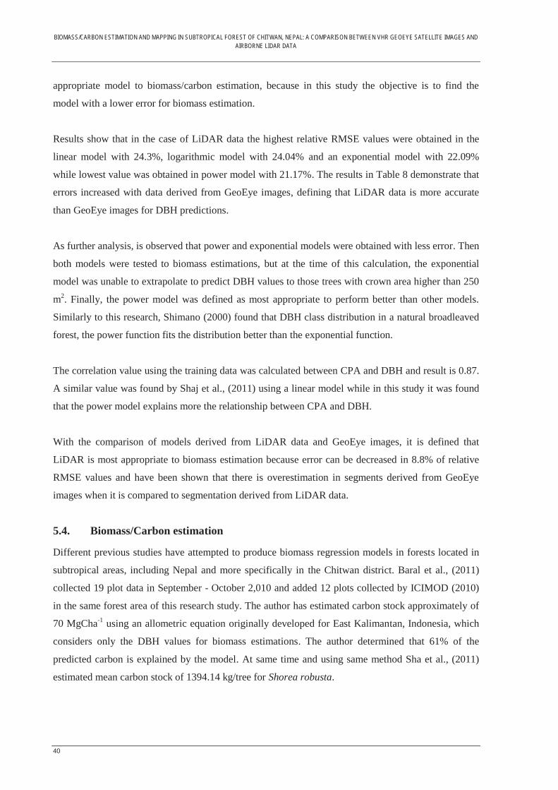
BIOMASS/CARBON ESTIMATION AND MAPPING IN SUBTROPICAL FOREST OF CHITWAN, NEPAL: A COMPARISON BETWEEN VHR GEOEYE SATELLITE IMAGES AND AIRBORNE LIDAR DATA
40
appropriate model to biomass/carbon estimation, because in this study the objective is to find the
model with a lower error for biomass estimation.
Results show that in the case of LiDAR data the highest relative RMSE values were obtained in the
linear model with 24.3%, logarithmic model with 24.04% and an exponential model with 22.09%
while lowest value was obtained in power model with 21.17%. The results in Table 8 demonstrate that
errors increased with data derived from GeoEye images, defining that LiDAR data is more accurate
than GeoEye images for DBH predictions.
As further analysis, is observed that power and exponential models were obtained with less error. Then
both models were tested to biomass estimations, but at the time of this calculation, the exponential
model was unable to extrapolate to predict DBH values to those trees with crown area higher than 250
m2. Finally, the power model was defined as most appropriate to perform better than other models.
Similarly to this research, Shimano (2000) found that DBH class distribution in a natural broadleaved
forest, the power function fits the distribution better than the exponential function.
The correlation value using the training data was calculated between CPA and DBH and result is 0.87.
A similar value was found by Shaj et al., (2011) using a linear model while in this study it was found
that the power model explains more the relationship between CPA and DBH.
With the comparison of models derived from LiDAR data and GeoEye images, it is defined that
LiDAR is most appropriate to biomass estimation because error can be decreased in 8.8% of relative
RMSE values and have been shown that there is overestimation in segments derived from GeoEye
images when it is compared to segmentation derived from LiDAR data.
5.4. Biomass/Carbon estimation
Different previous studies have attempted to produce biomass regression models in forests located in
subtropical areas, including Nepal and more specifically in the Chitwan district. Baral et al., (2011)
collected 19 plot data in September - October 2,010 and added 12 plots collected by ICIMOD (2010)
in the same forest area of this research study. The author has estimated carbon stock approximately of
70 MgCha-1 using an allometric equation originally developed for East Kalimantan, Indonesia, which
considers only the DBH values for biomass estimations. The author determined that 61% of the
predicted carbon is explained by the model. At same time and using same method Sha et al., (2011)
estimated mean carbon stock of 1394.14 kg/tree for Shorea robusta.

BIOMASS/CARBON ESTIMATION AND MAPPING IN SUBTROPICAL FOREST OF CHITWAN, NEPAL: A COMPARISON BETWEEN VHR GEOEYE SATELLITE IMAGES AND AIRBORNE LIDAR DATA
41
Results of Baral et al., (2011) and Sha et al., (2011) differ from this study, despite they were in the
same study area. Results of this study estimated a mean average carbon/tree of 1894.08 kg equivalents
to 181.34 Mg C ha-1.
Carbon estimation differs with other authors because a different number of plots were measured,
probably there is a variation for the different regression models which were affected by the number of
plots and it explains the different yield in AGB.
Another factor of variation is that in this study an allometric equation was used which considers a
Diameter at breast height (DBH), the Height of trees (H) and wood specific gravity (ρ). Brown et al.,
(1989) who proposed to include wood specific gravity (ρ) in the allometric equations, suggests that
models can lead to an important improvement when this factor is added. Also, Ogawa et al., (1965)
found that combining DBH and height (H) was a suitable predictor for AGB instead of using only
DBH. Then, in the view that H and ρ factors can improve the biomass estimation rather than using
only DBH, it is considered that results in this study are improved in comparison to the previous
studies.
5.5. Limitations of the Research
Location of trees The location of trees in the field were difficult to find due to the fact that the navigation equipment is
not precise enough (error was in meters), which carries an error in the location of trees in the images
which surely affects the biomass estimation. A Global Position System with high accuracy could be
used (like differential GPS) so the location of the trees should be more precise and improved.
Image Orthorectification Orthorectification of LiDAR data and GeoEye image is important to be used in the fusion of these two
images, which could be used to biomass estimation rather than to compare results of the separate
images.
LiDAR data Noise on LiDAR data is a limitation which cannot allow accurate biomass estimation, despite of the
fact that a filter was applied, still some pixels with wrong values remain. Hence, LiDAR data is
preferred to be corrected previous to any analysis.

BIOMASS/CARBON ESTIMATION AND MAPPING IN SUBTROPICAL FOREST OF CHITWAN, NEPAL: A COMPARISON BETWEEN VHR GEOEYE SATELLITE IMAGES AND AIRBORNE LIDAR DATA
42
6. CONCLUSION AND RECOMMENDATION
6.1. Conclusion
The main objective of this research aims to compare two methods to assess the biomass/carbon
estimation using airborne LiDAR data and VHR GeoEye satellite image in a subtropical forest located
in Chitwan, Nepal. In this regard, conclusions are based on the research questions as follows:
How strong is the relationship between tree heights measured in the field with height values
derived from LiDAR data? Regarding the relationship between the height values of LiDAR data and field data, a strong relation
was found, obtaining an r value of 0.81. Also using the correlation test, a p value of 1.36E-03 was
calculated, which means that there is a strong relationship between these two data and the same result
is derived from the t-test where the t-statistic is greater that t-critical. Despite of this, the RMSE value
demonstrates that relative error can be increased to 27% which is important to consider in the
biomass/carbon estimations.
Does image segmentation from LiDAR data give an improvement in accuracy compared to
GeoEye images? Results show that segmentation using a LiDAR CHM image is more accurate than segmentation using
the GeoEye image. LiDAR data yields an accuracy of tree crown delineation of 76% while GeoEye
image yields an accuracy of only 62%. Delineating trees in LiDAR data has the advantage that
vegetation below five meters was excluded from the analysis, a condition which does not occur in the
GeoEye image. This suggests that LiDAR is more accurate to segment tree crowns in dense
subtropical forests.
How strong is the relationship between CPA and DBH? The power model was considered to be the best as a predictor of values of DBH from CPA. Between
CPA and DBH, from field data an r2 of 0.81 was calculated. A similar value was also obtained in the
comparison of DBH from the field data and CPA derived from LiDAR data, with r2=0.79, but a weak
relationship was found from CPA delineated from GeoEye images with DBH from the field, with
r2=0.64. For the validation of the model, the RMSE value was calculated within DBH calculated for
those trees identified on LiDAR CHM and Field data. Results show a relative RMSE value of 21.17%
for LiDAR data and 29.99% for GeoEye image. This suggests that estimations of DHB derived from
CPA of LiDAR data are better than DBH estimated from CPA derived from GeoEye images.

BIOMASS/CARBON ESTIMATION AND MAPPING IN SUBTROPICAL FOREST OF CHITWAN, NEPAL: A COMPARISON BETWEEN VHR GEOEYE SATELLITE IMAGES AND AIRBORNE LIDAR DATA
43
Biomass/carbon estimation in Subtropical forest of Chitwan, Nepal Since the values of regression and RMSE were higher from segments derived from LiDAR CHM
image compared to GeoEye images, then, tree Height, wood specific gravity (ρ) and DBH values were
used in the allometric equation for biomass/carbon estimation and the result is 181.34 Mg C ha-1.
6.2. Recommendation
A high accuracy of tree crown delineation in a dense broadleaves forest is difficult to achieve. This
study has demonstrated that results in segmentation using LiDAR data are better compared to the
segmentation of GeoEye images. However, if these two sensors are fused, it is considered that results
can be further improved. This is due to the fact that tree species can be derived from the GeoEye
images. This is information that can be well complemented to LiDAR data.
Due to the problem of errors in the process of orthorectification, the combination of LiDAR data with
GeoEye image was not possible. It is therefore suggested that the correction of the images to match
pixel over pixel can have more accurate estimation.
A general allometric equation for tropical and subtropical areas was used in this study, which
introduces error. It is mentioned by the author that using this allometric equation overestimates remain,
giving a bias of 0.5-6.5%. Therefore, the development of local allometric equation is required, and if it
is possible, per individual species for better carbon stock estimation.
The use of equipment to locate trees (GPS) in the field versus images introduces an error in the
estimations. For further analysis, it is suggested to use equipment with a high precision (differential
GPS) to ensure the exact location of individual trees.

BIOMASS/CARBON ESTIMATION AND MAPPING IN SUBTROPICAL FOREST OF CHITWAN, NEPAL: A COMPARISON BETWEEN VHR GEOEYE SATELLITE IMAGES AND AIRBORNE LIDAR DATA
44
LIST OF REFERENCES ARBONAUT. (2010). Monitoring change in carbon stock and achieving REDD+ targets. Arbolidar, 8. Avgerinos, E. (1998). Remote sensing and image interpretation, 3rd edition. Geographical Analysis,
30(3), 277-279. Balzter, H., Rowland, C. S., & Saich, P. (2007). Forest canopy height and carbon estimation at Monks
Wood National Nature Reserve, UK, using dual-wavelength SAR interferometry. Remote Sensing of Environment, 108(3), 224-239.
Baral Jamarkattel, S. (2011). Mapping carbon stock using high resolution satellite images in sub - tropical forest of Nepal. University of Twente Faculty of Geo-Information and Earth Observation ITC, Enschede. Retrieved from http://www.itc.nl/library/papers_2011/msc/nrm/baral.pdf
Brandtberg, T., & Walter, F. (1998). Automated delineation of individual tree crowns in high spatial resolution aerial images by multiple-scale analysis. Machine Vision and Applications, 11(2), 64-73.
Brown, S. (2002). Measuring carbon in forests: current status and future challenges. Environmental Pollution, 116(3), 363-372.
Brown, S., & Gaston, G. (1995). Use of forest inventories and geographic information systems to estimate biomass density of tropical forests: Application to tropical Africa. Environmental Monitoring and Assessment, 38(2-3), 157-168.
Brown, S., Gillespie, A. J. R., & Lugo, A. E. (1989). Biomass estimation methods for tropical forests with applications to forest inventory. Forest Science, 35(4), 881-902.
Chave, J., Andalo, C., Brown, S., Cairns, M. A., Chambers, J. Q., Eamus, D., & Yamakura, T. (2005). Tree allometry and improved estimation of carbon stocks and balance in tropical forests. Oecologia, 145(1), 87-99.
Clinton, N., Holt, A., Scarborough, J., Yan, L., & Gong, P. (2010). Accuracy Assessment Measures for Object-based Image Segmentation Goodness. Photogrammetric Engineering and Remote Sensing, 76(3), 289-299.
Crow, T. R., & Schlaegel, B. E. (1988). A guide to using regression equations for estimating tree biomass. Northern Journal of Applied Forestry, 5, 15-22.
Culvenor, D. S. (2003). Extracting individual tree information: a survey of techniques for high spatial resolution imagery. In Remote Sensing of Forest Environments: Concepts and Case Studies, M.A. Wulder and S.E. Franklin (Eds), pp. 255–277 (Boston: Kluwer Academic).
Dahal, N., & Banskota, K. (2009). Cultivating REDD in Nepal's Community Forestry: Discourse for Capitalizing Potential? Journal of Forest and Livelihood, 8(1), 40-51.
Definiens, A. (2007). Definiens Developer 7. 195. Derivaux, S., Forestier, G., Wemmert, C., & Lef`evre, S. (2010). Supervised Image Segmentation
Using Watershed Transform, Fuzzy Classification and Evolutionary Computation. Image Sciences, Computer Sciences and Remote Sensing Laboratory, University of Strasbourg, France, 25.
Dragut, L., Tiede, D., & Levick, S. R. (2010). ESP: a tool to estimate scale parameter for multiresolution image segmentation of remotely sensed data. [Article]. International Journal of Geographical Information Science, 24(6), 859-871.
Drake, J. B., & et al. (2002). Estimation of tropical forest structural characteristics using large-footprint lidar. Remote Sensing of Environment, 79(2-3), 305-319.

BIOMASS/CARBON ESTIMATION AND MAPPING IN SUBTROPICAL FOREST OF CHITWAN, NEPAL: A COMPARISON BETWEEN VHR GEOEYE SATELLITE IMAGES AND AIRBORNE LIDAR DATA
45
Dralle, K., & Rudemo, M. (1996). Stem number estimation by kernel smoothing of aerial photos. [Article]. Canadian Journal of Forest Research-Revue Canadienne De Recherche Forestiere, 26(7), 1228-1236.
Dubayah, R. O., & et al. (2000). Land surface characterization using LiDAR remote sensing In: Hill MJ, Aspinal RJ (Eds.) Spatial information for landuse management. Gordon and Breach Science Publishers, Australia. P. 25-38.
Endo, T., & Sawada, H. (2010). Development of an individual tree crown delineation method using lidar data. International Center for Urban Safety Engineering, Institute of Industrial Science, The University of Tokyo, XXXVIII, Part 8, 4.
Erikson, M., & Olofsson, K. (2005). Comparison of three individual tree crown detection methods. Machine Vision and Applications, 16(4), 258-265.
FAO. (2009). Biomass. Assessment of the status of the development of the standards for the terrestrial essential climate variables. Global Terrestrial Observing System, Rome, Italy, Version 10, 30.
FAO. (2010). Global forest resources assessment 2010 : main report. Rome: Food and Agriculture Organization of the United Nations.
Foody, G. M., Boyd, D. S., & Cutler, M. E. J. (2003). Predictive relations of tropical forest biomass from Landsat TM data and their transferability between regions. Remote Sensing of Environment, 85(4), 463-474.
García, M., Riaño, D., Chuvieco, E., & Danson, F. M. (2010). Estimating biomass carbon stocks for a Mediterranean forest in central Spain using LiDAR height and intensity data. Remote Sensing of Environment, 114(4), 816-830.
Gautam, B. R., & et al. (2010). Integration of airborne LiDAR, satellite imagery, and field measurements using a two-phase sampling method for forest biomass estimation in tropical forests. International Symposium on “Benefiting from Earth Observation”, 7.
Gautam, B. R., & Kandel, P. N. (2010). Working paper on LiDAR mapping in Nepal. Ministry of Forests and Soil Conservation, 10.
Gibbs, H. K., Brown, S., Niles, J. O., & Foley, J. A. (2007). Monitoring and estimating tropical forest carbon stocks: making REDD a reality. Environmental Research Letters, 2(4).
Gschwantner, T., Schadauer, K., Vidal, C., Lanz, A., Tomppo, E., di Cosmo, L., . . . Lawrence, M. (2009). Common Tree Definitions for National Forest Inventories in Europe. Silva Fennica, 43(2), 303-321.
Hay, G. J., Castilla, G., Wulder, M. A., & Ruiz, J. R. (2005). An automated object-based approach for the multiscale image segmentation of forest scenes. International Journal of Applied Earth Observation and Geoinformation, 7(4), 339-359.
Heyman, O., Gaston, G. G., Kimerling, A. J., & Campbell, J. T. (2003). A per-segment approach to improving aspen mapping from high-resolution remote sensing imagery. Journal of Forestry, 101(4), 29-33.
Holmgren, P. (2008). Role of satellite remote sensing in REDD. UN-REDD Programme, 11. Houghton, R. A., Lawrence, K. T., Hackler, J. L., & Brown, S. (2001). The spatial distribution of
forest biomass in the Brazilian Amazon: a comparison of estimates. Global Change Biology, 7(7), 731-746.
Hunt, C. A. G. (2009). Carbon sinks and climate change: forests in the fight against global warming. GB: Edward Elgar Publishing Ltd.
Husch, B., Beers, T. W., & Kershaw, J. A. (2003). Forest mensuration. [Book]. New Kersey, USA, 4th. Edition, 433.

BIOMASS/CARBON ESTIMATION AND MAPPING IN SUBTROPICAL FOREST OF CHITWAN, NEPAL: A COMPARISON BETWEEN VHR GEOEYE SATELLITE IMAGES AND AIRBORNE LIDAR DATA
46
Hussin, Y. A., Reich, R. M., & Hoffer, R. M. (1991). Estimating slash pine biomass using radar backscatter. Ieee Transactions on Geoscience and Remote Sensing, 29(3), 427-431.
Hyde, P., Dubayah, R., Peterson, B., Blair, J. B., & Walker, W. (2005). Mapping forest structure for wildlife habitat analysis using waveform lidar: Validation of montane ecosystems. Remote Sensing of Environment, 96(3-4), 427-437.
ICIMOD. (2010). Forest Carbon Stock Measurement: Guidelines for measuring carbon stocks in community-managed forests. 82.
ICIMOD, ANSAB, & FECOFUN. (2010). Report on forest carbon stock in Ludikhola, Kayarkhola and Charnawati watersheds of Nepal. [Report]. [Technical reviewed by Terra Global Capital, 948 Green Street, San Francisco, CA 94123, USA]. Forest Carbon Stock in REDD+ Pilot Project Sites: Year One Measurement & Analysis, 48.
IPCC. (1990). Climate change, The IPCC scientific assessment (1990 ed.): Intergovernmental Panel on Climate Change. Cambridge University Press, Cambridge, Great Britain, New York, NY, USA and Melbourne, Australia
IPCC. (2006). Good practice guidelines for National Greenhouse gas inventories. Switzerland: Intergovernmental panel on climate change. 83.
IPCC. (2007a). Climate change 2007: Synthesis Report. Valencia, Spain: Intergovernmental Panel on Climate Change
IPCC. (2007b). Summary for Policymakers. In: Climate Change 2007: The Physical Science Basis. Contribution of Working Group I to the Fourth Assessment Report of the Intergovernmental Panel on Climate Change [Solomon, S., D. Qin, M. Manning, Z. Chen, M. Marquis, K.B. Averyt, M.Tignor and H.L. Miller (eds.)]. Cambridge University Press, Cambridge, United Kingdom and New York, NY, USA.
IPCC. (2011). IPCC Special Report on Renewable Energy Sources and Climate Change Mitigation. Prepared by Working Group III of the Intergovernmental Panel on Climate Change. (Climate change), 1075.
Jennings, S. B., Brown, N. D., & Sheil, D. (1999). Assessing forest canopies and understorey illumination: canopy closure, canopy cover and other measures. Forestry, 72(1), 59-73.
Ketterings, Q. M., Coe, R., van Noordwijk, M., Ambagau’, Y., & Palm, C. A. (2001). Reducing uncertainty in the use of allometric biomass equations for predicting above-ground tree biomass in mixed secondary forests. Forest Ecology and Management, 146(1-3), 199-209.
Kim, S. R., & et al. (2010). Estimation of carbon storage based on individual tree detection in Pinus densiflora stands using a fusion of aerial photography and LiDAR data. Science China-Life Sciences, 53(7), 885-897.
Koch, B., Heyder, U., & Weinacker, H. (2006). Detection of individual tree crowns in airborne lidar data. Photogrammetric Engineering and Remote Sensing, 72(4), 357-363.
Kosaka, N., & Kuwata, Y. (2006). Monitoring of Carbon Sink Preservation Activity for Global Warming Countermeasure Using A High-Resolution Satellite Image 2006 Ieee International Geoscience and Remote Sensing Symposium, Vols 1-8 (pp. 690-693). New York.
Lefsky, M. A., Cohen, W. B., Parker, G. G., & Harding, D. J. (2002). Lidar remote sensing for ecosystem studies. [Article]. Bioscience, 52(1), 19-30.
Levesque, J., & King, D. J. (2003). Spatial analysis of radiometric fractions from high-resolution multispectral imagery for modelling individual tree crown and forest canopy structure and health. Remote Sensing of Environment, 84(4), 589-602.

BIOMASS/CARBON ESTIMATION AND MAPPING IN SUBTROPICAL FOREST OF CHITWAN, NEPAL: A COMPARISON BETWEEN VHR GEOEYE SATELLITE IMAGES AND AIRBORNE LIDAR DATA
47
Lim, K., Treitz, P., Wulder, M., St-Onge, B., & Flood, M. (2003). LiDAR remote sensing of forest structure. [Article]. Progress in Physical Geography, 27(1), 88-106.
Lu, D. (2005). Aboveground biomass estimation using Landsat TM data in the Brazilian Amazon. International Journal of Remote Sensing, 26(12), 2509-2525.
Lu, D. S. (2006). The potential and challenge of remote sensing-based biomass estimation. [Review]. International Journal of Remote Sensing, 27(7), 1297-1328.
Lu, D. S., Batistella, M., & Moran, E. (2005). Satellite estimation of aboveground biomass and impacts of forest stand structure. Photogrammetric Engineering and Remote Sensing, 71(8), 967-974.
MacDicken, K. G. (1997). A Guide to Monitoring Carbon Storage in Forestry and Agroforestry Projects. Forest Carbon Monitoring Program. Arlington, USA. Winrock Internationl Institute for Agricultural Development. 91 p.
Maier, B., Tiede, D., & Dorren, L. (2008). Characterising mountain forest structure using landscape metrics on LiDAR-based canopy surface models
Object-Based Image Analysis. In T. Blaschke, S. Lang & G. J. Hay (Eds.), (pp. 625-643): Springer Berlin Heidelberg.
McKibben, B. (2007). Climate change 2007: The physical science basis: Summary for policymakers (vol 54, pg 44, 2007). New York Review of Books, 54(8), 58-58.
Mette, T., Papathanassiou, K., & Hajnsek, I. (2004). Biomass estimation from polarimetric SAR interferometry over heterogeneous forest terrain.
Ministry of Forest and Soil Conservation. (2010). Government of Nepal, Nepal's Readiness Preparation Proposal REDD. (Forest Carbon Partnership Facility (FCPF)), 135.
Muukkonen, P., & Heiskanen, J. (2007). Biomass estimation over a large area based on standwise forest inventory data and ASTER and MODIS satellite data: A possibility to verify carbon inventories. Remote Sensing of Environment, 107(4), 617-624.
Næsset, E. (2009). Some challenges in forest monitoring. Proposing a “research platform” for development, training, and validation of spaceborne technologies in Brazil. A Presentation. Brazilian Norwegian Workshop on Forest and Marine Monitoring, Ilhabela,SP, Brazil, March 9-12, 2009., 24 slides.
Naesset, E. (1997). Determination of mean tree height of forest stands using airborne laser scanner data. ISPRS Journal of Photogrammetry and Remote Sensing, 52(2), 49-56.
Naesset, E. (2002). Predicting forest stand characteristics with airborne scanning laser using a practical two-stage procedure and field data. Remote Sensing of Environment, 80(1), 88-99.
Nelson, R. F., Kimes, D. S., Salas, W. A., & Routhier, M. (2000). Secondary forest age and tropical forest biomass estimation using thematic mapper imagery. Bioscience, 50(5), 419-431.
Nichol, J. E., & Sarker, M. L. R. (2011). Improved Biomass Estimation Using the Texture Parameters of Two High-Resolution Optical Sensors. Geoscience and Remote Sensing, IEEE Transactions on, 49(3), 930-948.
Ogawa, H., Yoda, K., Ogino, K., & Kira, T. (1965). Comparative ecological studies on three main types of forest vegetation in Thailand II Plant biomass. Nat. Life Southeast Asia, 4:49-80.
Ojha, H., Persha, L., & Chhatre, A. (2009). Community Forestry in Nepal : A policy innovation for local livelihoods and food security. Paper presented at the International Forestry Resources and Institutions Program, School of Natural Resources and Environment, University of Michigan, 44.

BIOMASS/CARBON ESTIMATION AND MAPPING IN SUBTROPICAL FOREST OF CHITWAN, NEPAL: A COMPARISON BETWEEN VHR GEOEYE SATELLITE IMAGES AND AIRBORNE LIDAR DATA
48
Patenaude, G., Milne, R., & Dawson, T. P. (2005). Synthesis of remote sensing approaches for forest carbon estimation: reporting to the Kyoto Protocol. Environmental Science & Policy, 8(2), 161-178.
Phua, M. H., & Saito, H. (2003). Estimation of biomass of a mountainous tropical forest using Landsat TM data. Canadian Journal of Remote Sensing, 29(4), 429-440.
Popescu, S. C., Wynne, R. H., & Nelson, R. F. (2003). Measuring individual tree crown diameter with lidar and assessing its influence on estimating forest volume and biomass. Canadian Journal of Remote Sensing, 29(5), 564-577.
Rejaur Rahman, M., & Saha, S. (2008). Multi-resolution segmentation for object-based classification and accuracy assessment of land use/land cover classification using remotely sensed data. Journal of the Indian Society of Remote Sensing, 36(2), 189-201.
Santos, J. R., Freitas, C. C., Araujo, L. S., Dutra, L. V., Mura, J. C., Gama, F. F., . . . Sant'Anna, S. J. S. (2003). Airborne P-band SAR applied to the aboveground biomass studies in the Brazilian tropical rainforest. Remote Sensing of Environment, 87(4), 482-493.
Schowengerdt, R. A. (2006). Remote sensing, models, and methods for image processing. US: Academic Press.
Shah, S. K., Hussin, Y. A., van Leeuwen, L. M., & ... (2011). Modelling the relationship between tree canopy projection area and above ground carbon stock using high resolution geoeye satellite images. In: ACRS 2011 : proceedings of the 32nd Asian conference on remote sensing : sensing for Green Asia, 3-7 October 2011, Taipei, Taiwan., 6.
Shimano, K. (2000). A power function for forest structure and regeneration pattern of pioneer and climax species in patch mosaic forests. Plant Ecology, 146(2), 205-218.
Steininger, M. K. (2000). Satellite estimation of tropical secondary forest above-ground biomass: data from Brazil and Bolivia. International Journal of Remote Sensing, 21(6-7), 1139-1157.
Tiede, D., Lang, S., & Hoffmann, C. (2008). Domain-specific class modelling for one-level representation of single trees. In T. Blaschke, S. Lang & G. J. Hay (Eds.), Object-Based Image Analysis (pp. 133-151): Springer Berlin Heidelberg.
Treuhaft, R. N., Law, B. E., & Asner, G. P. (2004). Forest attributes from radar interferometric structure and its fusion with optical remote sensing. Bioscience, 54(6), 561-571.
Tsendbazar, N. E. (2011). Object based image analysis of geo - eye VHR data to model above ground carbon stock in Himalayan mid - hill forests, Nepal. University of Twente, Faculty of Geo-Information Science and Earth Observation -ITC-, Enschede. Retrieved from http://www.itc.nl/library/papers_2011/msc/nrm/tsendbazar.pdf
UN-REDD. (2008a). The UN-REDD Programme Strategy 2011-2015. The United Nations Collaborative Programme on Reducing Emissions from Deforestation and Forest Degradation in Developing Countries, 28.
UN-REDD. (2008b). UN Collaborative Programme on Reducing Emission from Deforestation and Forest Degradation in Developing Countries (UN-REDD). Framework Document.
van Laar, A., & Akça, A. (2007). Managing Forest Ecosystems,Forest mensuration. Somerset West, South Africa, 13, 377.
van Leeuwen, M., & Nieuwenhuis, M. (2010). Retrieval of forest structural parameters using LiDAR remote sensing. European Journal of Forest Research, 129(4), 749-770.
Wang, L., Gong, P., & Biging, G. S. (2004). Individual Tree-Crown Delineation and Treetop Detection in High-Spatial-Resolution Aerial Imagery. Photogrammetric Engineering & Remote Sensing, 70 (3), 351-357.

BIOMASS/CARBON ESTIMATION AND MAPPING IN SUBTROPICAL FOREST OF CHITWAN, NEPAL: A COMPARISON BETWEEN VHR GEOEYE SATELLITE IMAGES AND AIRBORNE LIDAR DATA
49
Wulder, M. A., White, J. C., Niemann, K. O., & Nelson, T. (2004). Comparison of airborne and satellite high spatial resolution data for the identification of individual trees with local maxima filtering. International Journal of Remote Sensing, 25(11), 2225-2232.
Yu, Q., Gong, P., Clinton, N., Biging, G., Kelly, M., & Schirokauer, D. (2006). Object-based detailed vegetation classification. with airborne high spatial resolution remote sensing imagery. Photogrammetric Engineering and Remote Sensing, 72(7), 799-811.
Zhan, Q. M., Molenaar, M., Tempfli, K., & Shi, W. Z. (2005). Quality assessment for geo-spatial objects derived from remotely sensed data. International Journal of Remote Sensing, 26(14), 2953-2974.
Zhang, X. Y., Feng, X. Z., & Jiang, H. (2010). Object-oriented method for urban vegetation mapping using IKONOS imagery. International Journal of Remote Sensing, 31(1), 177-196.
Zheng, D. L., Rademacher, J., Chen, J. Q., Crow, T., Bresee, M., le Moine, J., & Ryu, S. R. (2004). Estimating aboveground biomass using Landsat 7 ETM+ data across a managed landscape in northern Wisconsin, USA. Remote Sensing of Environment, 93(3), 402-411.

BIOMASS/CARBON ESTIMATION AND MAPPING IN SUBTROPICAL FOREST OF CHITWAN, NEPAL: A COMPARISON BETWEEN VHR GEOEYE SATELLITE IMAGES AND AIRBORNE LIDAR DATA
50
APPENDICES Appendix 1 Sample size for each community forest (CF)
Equation: Degrees of freedom = 59 Error allowed = 5% t = 2.009 S2 = 451 Number of samples per strata:
Strata Area No. Samples Devidhunga CF 254 24 Dharapani CF 147 14 Kalika CF 214 20 Satkanya CF 58 6 Kankali CF 92 9
Total 765 73 A total number of 73 plots were planned. However, were collected a total number of 86 plots.

BIOMASS/CARBON ESTIMATION AND MAPPING IN SUBTROPICAL FOREST OF CHITWAN, NEPAL: A COMPARISON BETWEEN VHR GEOEYE SATELLITE IMAGES AND AIRBORNE LIDAR DATA
51
Appendix 2 Locations of total collected sample plots

BIOMASS/CARBON ESTIMATION AND MAPPING IN SUBTROPICAL FOREST OF CHITWAN, NEPAL: A COMPARISON BETWEEN VHR GEOEYE SATELLITE IMAGES AND AIRBORNE LIDAR DATA
52
Appendix 3 Recording sheet used in the field
DBH Height DBH Crown(cm) (m) (cm) diam(m)
1 16
2 17
3 18
4 19
5 20
6 21
7 22
8 23
9 24
10 25
11 26
12 27
13 28
14 29
15 30
Name of recorder......................................................... Date............................................. Plot radius size.......12.62m..................
Management type:
Strata Name:
Forest type: Crown cover (%)
AspectSampling Plot No.
Coordinates X Y
Elevation Slope(%)
RemarkSpeciesCrowndiam.(m)
Remark SpeciesHeight(m)
Tree No.
Tree No.

BIOMASS/CARBON ESTIMATION AND MAPPING IN SUBTROPICAL FOREST OF CHITWAN, NEPAL: A COMPARISON BETWEEN VHR GEOEYE SATELLITE IMAGES AND AIRBORNE LIDAR DATA
53
Appendix 4 List of local tree species Species Frequency
Albezia procera 4 Albizzia julibrissin 4 Anthocephalus chinensis (Lam.) A. Rich. Ex Walp 9 Bridelia retusa (L.) Spreng 1 Careya arborea 16 Caseria graveolens 21 Cassia fistula 24 Cissus repens Lam. 1 Cleistocalyx operculatus 126 Cornus oblonga (wall.) Sojak 15 Desmodium oojeinense (Roxb.) Ohashi 3 Dillenia pentagyna 4 Ficus racemosa L. 1 Ficus religiosa L. 3 Ilex excelsa (Wall.) Hook. 3 Lagerstromia parviflora 121 Lannea caromandelica (Houtt.) Merr 9 Mallotus phillippensis 17 Manilkara zapota (L.) Van Royen 7 Myrsine semiserrata 1 Osbeckia stellata Buch. Ham. Ex D. Don 5 Pterospermum lanceaefolium Roxb. 2 Sapium insigne (Royle) Benth. Ex Hook. F 5 Schima Wallichii 10 Semicarpous anacardium 61 Shorea robusta 1105 Spondias pinnata (L.f.)Kurz 2 Stereospermum personatum (Hassk.) Chatterjee 1 Syzygium cumini 4 Terminalia alata Heyne ex. Roth 8 Terminalia chebula 6 Toona ciliata M. Roem 2 Vernacular name 79 Wrightia arborea (Dennst.) Mabberly 28 Total 1708

BIOMASS/CARBON ESTIMATION AND MAPPING IN SUBTROPICAL FOREST OF CHITWAN, NEPAL: A COMPARISON BETWEEN VHR GEOEYE SATELLITE IMAGES AND AIRBORNE LIDAR DATA
54
Appendix 5 Correlation between carbon stock derived from field and carbon stock estimated from LiDAR data

BIOMASS/CARBON ESTIMATION AND MAPPING IN SUBTROPICAL FOREST OF CHITWAN, NEPAL: A COMPARISON BETWEEN VHR GEOEYE SATELLITE IMAGES AND AIRBORNE LIDAR DATA
55
Appendix 6 Height, DBH, Biomass and carbon of standalone trees from field data
Scientific name DBH (cm)
Height (m) Biomass
Carbon Kg/tree Scientific name
DBH (cm)
Height (m) Biomass
Carbon Kg/tree
Cleistocalyx operculatus 19.6 7.6 130.78 61.46 Vernacular name 55.5 23.9 3297.50 1549.82
Shorea robusta 13.5 8.2 66.94 31.46 Shorea robusta 50 23.3 2609.13 1226.29
Shorea robusta 21.4 10.6 217.44 102.20 Shorea robusta 68 32.7 6772.77 3183.20
Shorea robusta 13.8 15.5 132.22 62.14 Lannea caromandelica 58.8 23.5 3639.34 1710.49
Shorea robusta 19.5 13.6 231.64 108.87 Shorea robusta 44.5 18.6 1649.81 775.41
Shorea robusta 17.9 11.4 163.61 76.90 Shorea robusta 46 23.5 2227.33 1046.84
Shorea robusta 81.5 31 9223.11 4334.86 Shorea robusta 66 19.8 3863.26 1815.73
Shorea robusta 75 29.5 7432.67 3493.36 Shorea robusta 58 20.8 3134.15 1473.05
Shorea robusta 77.6 24 6473.44 3042.52 Shorea robusta 51.8 20.5 2463.85 1158.01
Shorea robusta 57.9 26.5 3979.27 1870.26 Shorea robusta 57 24.6 3580.02 1682.61
Shorea robusta 68 25.4 5260.80 2472.58 Shorea robusta 91 28.8 10682.57 5020.81
Shorea robusta 65.8 29.6 5740.42 2698.00 Shorea robusta 55 24.8 3360.30 1579.34
Shorea robusta 72 25.3 5874.70 2761.11 Shorea robusta 24.8 12 330.59 155.38 Cleistocalyx operculatus 32.8 11.6 558.99 262.73
Cleistocalyx operculatus 36.8 12.8 776.44 364.93
Cleistocalyx operculatus 25.4 10.9 314.99 148.04 Shorea robusta 85.5 19 6221.37 2924.05
Shorea robusta 17.2 11.4 151.06 71.00 Shorea robusta 65 22.6 4276.96 2010.17
Shorea robusta 68 25.4 5260.80 2472.58 Shorea robusta 91 33.5 12425.91 5840.18
Shorea robusta 25.5 18.6 541.74 254.62 Shorea robusta 45 27.8 2521.57 1185.14
Shorea robusta 20 17.8 318.92 149.89 Shorea robusta 31 24.9 1071.82 503.76
Shorea robusta 21.5 16.6 343.70 161.54 Vernacular name 20 9.8 175.58 82.52
Shorea robusta 16.6 12.4 153.05 71.93 Albizzia julibrissin 28.8 14.5 538.71 253.19
Shorea robusta 19.9 16 283.81 133.39 Lagerstromia parviflora 47 20 1978.91 930.09
Shorea robusta 39.5 18.3 1278.93 601.10 Shorea robusta 81.5 28.1 8360.30 3929.34
Shorea robusta 29 21.1 794.84 373.57 Terminalia chebula 27.3 13.4 447.33 210.25
Shorea robusta 82 24.8 7469.30 3510.57 Shorea robusta 58.2 20.2 3064.77 1440.44
Vernacular name 61.5 29.6 5014.67 2356.90 Semicarpous anacardium 26.3 13 402.77 189.30
Vernacular name 39.2 23.8 1638.13 769.92 Shorea robusta 65 23.5 4447.29 2090.22
Shorea robusta 61.7 23.8 4058.33 1907.42 Shorea robusta 59 23.2 3617.37 1700.16
Shorea robusta 75.5 37.2 9498.11 4464.11 Shorea robusta 75 29.2 7357.09 3457.83
Shorea robusta 65.6 30.5 5879.06 2763.16 Terminalia alata 36.3 23.3 1375.21 646.35
Shorea robusta 73.5 30.2 7307.72 3434.63 Shorea robusta 41.3 10 764.01 359.09
Cassia fistula 21.4 11.8 242.05 113.76 Shorea robusta 38 17 1099.55 516.79
Shorea robusta 14.6 10.2 97.39 45.77 Semicarpous anacardium 41 16 1204.73 566.22
Vernacular name 21.8 10.8 229.90 108.05 Lagerstromia parviflora 40 16.8 1204.01 565.88
Shorea robusta 46.5 18.9 1830.49 860.33 Shorea robusta 49.7 22.6 2500.47 1175.22
Shorea robusta 17.8 11.6 164.63 77.37 Shorea robusta 48 18 1857.61 873.08
Shorea robusta 14.6 12.4 118.39 55.64 Lagerstromia parviflora 40 24.8 1777.35 835.35
Shorea robusta 19 12.6 203.74 95.76 Shorea robusta 36.5 19.6 1169.61 549.72

BIOMASS/CARBON ESTIMATION AND MAPPING IN SUBTROPICAL FOREST OF CHITWAN, NEPAL: A COMPARISON BETWEEN VHR GEOEYE SATELLITE IMAGES AND AIRBORNE LIDAR DATA
56
Shorea robusta 11.3 9.8 56.05 26.34 Shorea robusta 49 21 2258.46 1061.47
Shorea robusta 21.1 12.1 241.30 113.41 Shorea robusta 36 18.8 1091.35 512.93
Shorea robusta 14.5 13.7 129.02 60.64 Terminalia alata 33.8 18.4 941.57 442.54
Shorea robusta 18.5 13.5 206.96 97.27 Shorea robusta 53.5 24.2 3102.58 1458.21
Terminalia alata 55.5 28.2 3890.77 1828.66 Semicarpous anacardium 49.4 16 1748.94 822.00
Shorea robusta 74 29.8 7309.37 3435.41 Lannea caromandelica 45.5 12.2 1131.31 531.72
Shorea robusta 50 25.7 2877.89 1352.61 Terminalia alata 52.2 25.4 3100.10 1457.05
Shorea robusta 46 21.1 1999.86 939.93 Anthocephalus chinensis 78.2 26.2 7176.54 3372.97
Shorea robusta 60 23.9 3853.90 1811.33 Lannea caromandelica 10.5 25.6 126.42 59.42
Shorea robusta 55 23.4 3170.60 1490.18 Shorea robusta 51 33 3844.63 1806.98
Shorea robusta 64 26.2 4806.86 2259.23 Shorea robusta 47 26 2572.58 1209.11
Shorea robusta 56.5 22.4 3202.91 1505.37 Shorea robusta 49.2 33 3578.04 1681.68
Shorea robusta 118 29.6 18461.04 8676.69 Shorea robusta 51 25 2912.60 1368.92
Shorea robusta 40.2 20.5 1483.91 697.44 Shorea robusta 44 27 2341.37 1100.44
Shorea robusta 53 23.6 2969.37 1395.60 Shorea robusta 35 26 1426.63 670.51 Anthocephalus chinensis 83.2 19.4 6015.18 2827.14 Shorea robusta 72.5 18.7 4402.69 2069.26
Shorea robusta 65 22.8 4314.81 2027.96 Anthocephalus chinensis 51 13.7 1596.10 750.17
Shorea robusta 54 16 2089.82 982.21 Shorea robusta 102 25.7 11976.61 5629.01
Schima Wallichii 73.2 19.2 4608.12 2165.82 Vernacular name 27.7 10.35 355.71 167.19
Shorea robusta 16.9 10.4 133.05 62.53 Shorea robusta 11.9 10.8 68.50 32.20
Shorea robusta 22.8 17.2 400.50 188.23 Shorea robusta 16.5 14.6 178.04 83.68
Shorea robusta 20.9 15.5 303.27 142.54 Shorea robusta 13.7 14.4 121.06 56.90
Shorea robusta 17.2 14.2 188.17 88.44 Shorea robusta 50 8 895.84 421.04
Shorea robusta 21 13.2 260.74 122.55 Terminalia chebula 44 24.6 2133.25 1002.63
Shorea robusta 17.2 12.2 161.67 75.98 Shorea robusta 63 24 4266.71 2005.35
Shorea robusta 20.4 15.6 290.79 136.67 Lagerstromia parviflora 17.8 12 170.30 80.04
Albezia procera 40.6 19.2 1417.60 666.27 Lagerstromia parviflora 25.8 16.4 488.97 229.82
Spondias pinnata 34.8 16.9 916.74 430.87 Cassia fistula 17.1 11.4 149.31 70.18 Lagerstromia parviflora 41.1 18.2 1377.07 647.22 Vernacular name 45 16.4 1487.54 699.14
Shorea robusta 14.5 13 122.43 57.54 Lannea caromandelica 78 29.4 8011.93 3765.61
Shorea robusta 16.5 13.8 168.29 79.09 Mallotus phillippensis 29.5 11.4 444.37 208.86
Shorea robusta 72 8 1857.61 873.08 Shorea robusta 49 26.2 2817.69 1324.32
Shorea robusta 13.5 2.5 20.41 9.59 Shorea robusta 23 12.4 293.82 138.09
Shorea robusta 13.2 18.6 145.16 68.23 Shorea robusta 33.5 19.8 995.30 467.79
Shorea robusta 66.5 22.6 4476.64 2104.02 Shorea robusta 55.4 25.6 3519.33 1654.08
Shorea robusta 56.7 22 3168.03 1488.97 Shorea robusta 28 23.6 828.76 389.52
Shorea robusta 78.9 25 6970.99 3276.37 Shorea robusta 47 23.9 2364.80 1111.46
Shorea robusta 75 23.5 5920.94 2782.84 Shorea robusta 34 18.4 952.74 447.79
Shorea robusta 55.8 25.9 3612.17 1697.72 Shorea robusta 44 18 1560.91 733.63
Shorea robusta 48.4 24.4 2560.24 1203.31 Shorea robusta 50 23 2575.54 1210.50

BIOMASS/CARBON ESTIMATION AND MAPPING IN SUBTROPICAL FOREST OF CHITWAN, NEPAL: A COMPARISON BETWEEN VHR GEOEYE SATELLITE IMAGES AND AIRBORNE LIDAR DATA
57
Shorea robusta 68.7 29 6130.73 2881.44 Shorea robusta 47.5 23 2324.42 1092.48
Shorea robusta 38.5 29.2 1938.67 911.18 Shorea robusta 52 24 2906.82 1366.21
Shorea robusta 78 29.2 7957.42 3739.99 Shorea robusta 43.5 31.5 2669.87 1254.84
Shorea robusta 57.2 27 3956.91 1859.75 Shorea robusta 42 23.5 1856.81 872.70 Lagerstromia parviflora 14.1 17.8 158.51 74.50 Shorea robusta 52 33.5 4057.44 1907.00
Syzygium cumini 38.5 21.4 1420.81 667.78 Anthocephalus chinensis 27.5 21 711.35 334.34
Shorea robusta 77 29.8 7914.04 3719.60 Shorea robusta 63 32 5688.94 2673.80
Shorea robusta 66 20.8 4058.37 1907.43 Shorea robusta 99 34 14926.22 7015.32
Shorea robusta 81.5 20.4 6069.40 2852.62 Shorea robusta 50 11 1231.78 578.94
Shorea robusta 56.5 19.8 2831.15 1330.64 Shorea robusta 36 23 1335.16 627.53
Shorea robusta 75 35 8818.43 4144.66 Vernacular name 34 18 932.03 438.06
Shorea robusta 59.5 15.6 2473.77 1162.67 Shorea robusta 43 27 2236.15 1050.99 Dillenia pentagyna 35 25 1371.76 644.72 Shorea robusta 48 30 3096.02 1455.13
Shorea robusta 23 11 260.64 122.50 Shorea robusta 61 28 4666.79 2193.39
Shorea robusta 76 25.4 6571.45 3088.58 Shorea robusta 66 32 6243.65 2934.51 Lannea caromandelica 58.8 27.6 4274.29 2008.92 Shorea robusta 19.3 17 283.64 133.31
Shorea robusta 53.5 27.6 3538.48 1663.09 Cleistocalyx operculatus 17 18 233.01 109.51
Shorea robusta 51 26 3029.10 1423.68 Shorea robusta 17.8 18 255.45 120.06
Shorea robusta 43.5 27.5 2330.84 1095.49 Shorea robusta 57 33 4802.46 2257.16
Shorea robusta 36.5 20.6 1229.29 577.77 Cleistocalyx operculatus 48 11 1135.21 533.55
Shorea robusta 24 20 516.00 242.52 Shorea robusta 16.5 12 146.34 68.78
Schima Wallichii 23.1 16.2 387.20 181.99 Shorea robusta 17 16 207.12 97.35
Shorea robusta 40.5 18.4 1351.85 635.37 Cleistocalyx operculatus 21.5 19 393.40 184.90
Shorea robusta 74 25.6 6279.19 2951.22 Cleistocalyx operculatus 23 17 402.81 189.32
Schima Wallichii 34 19.2 994.17 467.26 Albizzia julibrissin 23 13 308.03 144.78
Shorea robusta 70 28.5 6255.20 2939.95 Shorea robusta 15.5 14 150.66 70.81
Shorea robusta 37.3 25.2 1570.43 738.10 Shorea robusta 17.5 15 205.76 96.71
Shorea robusta 17.8 17.9 254.03 119.40 Schima Wallichii 25 13 363.94 171.05 Lannea caromandelica 32.8 20.4 983.06 462.04 Shorea robusta 99.6 33 14663.35 6891.77
Shorea robusta 16.3 14.1 167.80 78.87 Shorea robusta 96.6 28 11703.42 5500.61
Shorea robusta 42.2 26.8 2137.77 1004.75 Shorea robusta 67.1 25 5041.80 2369.65
Careya arborea 31.6 15.8 706.69 332.15 Shorea robusta 60 30 4837.54 2273.64
Shorea robusta 45.2 24.5 2242.04 1053.76 Pterospermum lanceaefolium 10.6 9 45.30 21.29
Shorea robusta 17.8 12.8 181.66 85.38 Anthocephalus chinensis 85 24 7766.93 3650.46
Shorea robusta 39.5 24 1677.28 788.32 Shorea robusta 41 19 1430.61 672.39 Semicarpous anacardium 33.5 13.4 673.59 316.59 Shorea robusta 12 9 58.05 27.28 Pterospermum lanceaefolium 25.5 15.4 448.54 210.81
Anthocephalus chinensis 80 26 7453.39 3503.09