Biomarker Discovery and Redundancy Reduction towards Classification using a Multi-factorial...

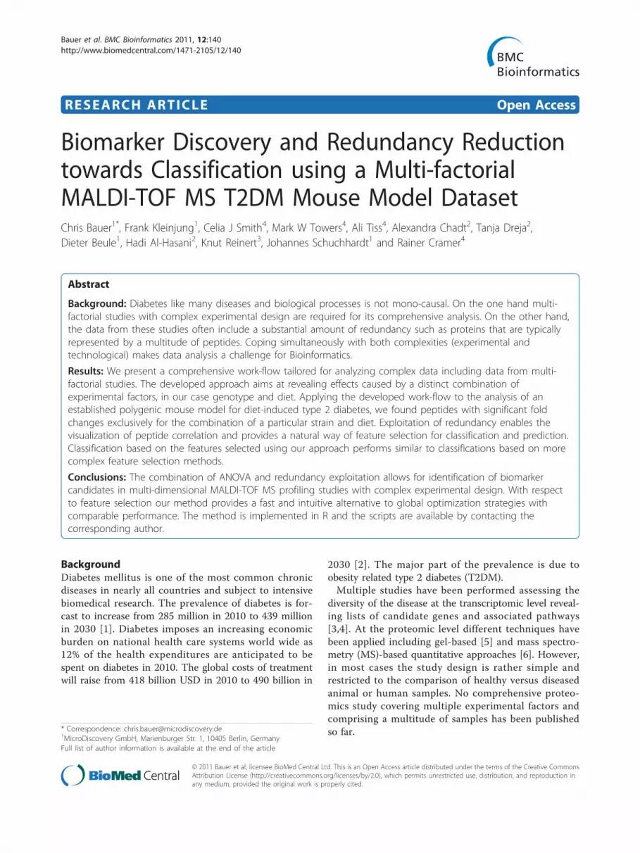
RESEARCH ARTICLE Open Access

Biomarker Discovery and Redundancy Reductiontowards Classification using a Multi-factorialMALDI-TOF MS T2DM Mouse Model DatasetChris Bauer1*, Frank Kleinjung1, Celia J Smith4, Mark W Towers4, Ali Tiss4, Alexandra Chadt2, Tanja Dreja2,Dieter Beule1, Hadi Al-Hasani2, Knut Reinert3, Johannes Schuchhardt1 and Rainer Cramer4

Abstract

Background: Diabetes like many diseases and biological processes is not mono-causal. On the one hand multi-factorial studies with complex experimental design are required for its comprehensive analysis. On the other hand,the data from these studies often include a substantial amount of redundancy such as proteins that are typicallyrepresented by a multitude of peptides. Coping simultaneously with both complexities (experimental andtechnological) makes data analysis a challenge for Bioinformatics.

Results: We present a comprehensive work-flow tailored for analyzing complex data including data from multi-factorial studies. The developed approach aims at revealing effects caused by a distinct combination ofexperimental factors, in our case genotype and diet. Applying the developed work-flow to the analysis of anestablished polygenic mouse model for diet-induced type 2 diabetes, we found peptides with significant foldchanges exclusively for the combination of a particular strain and diet. Exploitation of redundancy enables thevisualization of peptide correlation and provides a natural way of feature selection for classification and prediction.Classification based on the features selected using our approach performs similar to classifications based on morecomplex feature selection methods.

Conclusions: The combination of ANOVA and redundancy exploitation allows for identification of biomarkercandidates in multi-dimensional MALDI-TOF MS profiling studies with complex experimental design. With respectto feature selection our method provides a fast and intuitive alternative to global optimization strategies withcomparable performance. The method is implemented in R and the scripts are available by contacting thecorresponding author.

BackgroundDiabetes mellitus is one of the most common chronicdiseases in nearly all countries and subject to intensivebiomedical research. The prevalence of diabetes is for-cast to increase from 285 million in 2010 to 439 millionin 2030 [1]. Diabetes imposes an increasing economicburden on national health care systems world wide as12% of the health expenditures are anticipated to bespent on diabetes in 2010. The global costs of treatmentwill raise from 418 billion USD in 2010 to 490 billion in

2030 [2]. The major part of the prevalence is due toobesity related type 2 diabetes (T2DM).Multiple studies have been performed assessing the

diversity of the disease at the transcriptomic level reveal-ing lists of candidate genes and associated pathways[3,4]. At the proteomic level different techniques havebeen applied including gel-based [5] and mass spectro-metry (MS)-based quantitative approaches [6]. However,in most cases the study design is rather simple andrestricted to the comparison of healthy versus diseasedanimal or human samples. No comprehensive proteo-mics study covering multiple experimental factors andcomprising a multitude of samples has been publishedso far.* Correspondence: [email protected]

1MicroDiscovery GmbH, Marienburger Str. 1, 10405 Berlin, GermanyFull list of author information is available at the end of the article

Bauer et al. BMC Bioinformatics 2011, 12:140http://www.biomedcentral.com/1471-2105/12/140

© 2011 Bauer et al; licensee BioMed Central Ltd. This is an Open Access article distributed under the terms of the Creative CommonsAttribution License (http://creativecommons.org/licenses/by/2.0), which permits unrestricted use, distribution, and reproduction inany medium, provided the original work is properly cited.

mailto:[email protected]

http://creativecommons.org/licenses/by/2.0

In this manuscript we investigate a multifactorialmatrix-assisted laser desorption/ionization (MALDI) MSplasma profile data set based on a T2DM mouse model,using NZO (New Zealand Obese) and SJL (Swiss JimLambert) mouse strains. The NZO mouse is an estab-lished polygenic model for studying obesity-related dia-betes as it rapidly develops symptoms of diabetescharacterized by early onset obesity, insulin resistanceand eventually destruction of insulin-producing pancrea-tic beta cells [7]. In contrast, the lean SJL mouse strainis resistant to diet-induced obesity and diabetes, pre-sumably due to a mutation in the Tbc1d1 gene thatcauses elevated lipid use in skeletal muscle [8].MALDI MS, particularly in combination with time-of-

flight (TOF) instruments, is characterized by simplicity,good mass accuracy and high resolution [9] and hence apromising tool in proteomics [10]. It allows for proces-sing a significant number of samples in a short time andtherefore enables studies encompassing a multitude ofsamples [11-13]. MALDI-TOF MS profiling has beenused extensively for investigating different types of can-cer like breast cancer [14], lung cancer [12,15], ovariancancer [16] or colon cancer [17,18], to name a few. Bio-marker identification and classification are the typicalobjectives in MALDI profiling studies of disease models.Various different methods have been applied addressingthese two objectives. For feature selection commonlyused methods comprise the classical t-test or Wilcoxonrank sum test [19] as well as more advanced techniquessuch as genetic algorithms and swarm based intelligence[20]. With respect to classification Wu et al. [21] pub-lished a summary comparing statistical methods forovarian cancer. In 2006, Zhang et al. [22] compared theperformance of R-SVM and SVM-RFE using MALDIMS data sets and more recently, in 2009, Liu et al. [23]compared additional feature selection and classificationapproaches.In general, proteomic data has two different types of

replications, (1) biological and (2) technical, leading totwo different types of errors, and therefore requiresproper statistical analysis. The standard approach ofhandling technical replicates is to calculate a mean valuein order to reduce the technical noise. Unfortunately,this can lead to loss of information [24]. A more sophis-ticated way to handle technical replicates without loss ofinformation are mixed-effects models [25,26]. Theyincorporate fixed-effects parameters applied to the entirepopulation and random effects applied to particularexperimental units or sub-units (e.g. technical repli-cates). However, for the high number of biological repli-cates in this study the results for both methods aresimilar.Although many approaches have been developed for

biomarker identification from MALDI MS profile data,

only some studies were performed for assessing theinfluence of correlation in these datasets [27]. As corre-lation within large MS data sets can confound statisticalanalyzes, we developed statistical methods that exploitdata correlation and integrated these into a comprehen-sive work-flow designed for the analysis of multi-factor-ial experimental MALDI-TOF MS data. Mergingsimilarity and significance information our approachallows for the interpretation of complex biological datain an intuitive manner. The soundness of the statisticalmethods is demonstrated and a special plot for easyvisualization and understanding. Furthermore the pre-sented methods provide a natural way of feature selec-tion for classification and prediction. The completework-flow of the analysis is shown in Figure 1.

MethodsDataThe study design involved the experimental factors gen-otype, diet and time.GenotypeThree different mouse strains were examined: C57BL/6J(B6), NZO (New Zealand Obese) and SJL (Swiss JimLambert). The New Zealand Obese mouse strain exhi-bits polygenic obesity associated with hyperinsulinaemiaand hyperglycaemia and presents additional features of ametabolic syndrome, including hypertension, and ele-vated levels of serum cholesterol and serum triglycerides[28]. NZO mice are highly susceptible to weight gainwhen fed a high-fat diet, resulting in the development ofmorbid obesity, with fat depots exceeding 40% of totalbody weight and the development of type 2 diabetes[29]. In contrast, the Swiss Jim Lambert (SJL) mousestrain is lean and resistant to diet-induced obesity anddiabetes [30]. B6 mice represent an intermediary pheno-type between NZO and SJL at later age (> week 12)with respect to sensitivity to diet-induced obesity anddiabetes. While the genetic and molecular basis for thedifferent diabetes susceptibilities of polygenic mousestrains is largely unknown, we recently identified a natu-rally occurring loss-of-function mutation in the Tbc1d1gene in SJL mice that increases lipid oxidation in skele-tal muscle and as a result confers leanness and protectsfrom diet-induced obesity and diabetes [8].DietAfter weaning at week 3, male B6, NZO and SJL micewere raised on three different diets, a low fat diet (SD;8% calories from fat) and two different high fat diets,one containing carbohydrates (HF; 35% calories fromfat) the other one a carbohydrate-free (CHF; 72% cal-ories from fat). We have shown previously that HF dietstrongly induces insulin resistance and may lead to dia-betes, whereas CHF equally induces peripheral insulinresistance but protects from diabetes [7,31]. At week 8,


of 14

mean body weight of SJL mice was 18.81 g (+/- 1.46 g)on SD, 20.04 g (+/-0.99 g) on HF and 21.24 g (+/- 2.31g) on CHF. In contrast, mean values for NZO micewere 31.94 g (+/- 1.36 g) on SD, 33.72 g (+/- 4.39 g) on

HF and 36.6 g (+/- 4.83 g) on CHF, respectively. Meanvalues for B6 mice were 20.1 g (+/- 2.56 g) on SD, 20.54g (+/- 0.78 g) on HF and 22.32 g (+/- 1.38 g) on CHF,respectively.

Figure 1 Work-flow. Complete work-flow of the cluster-based ANOVA approach with feature selection for multi-factorial MALDI MS profilingdata in biomarker discovery.


of 14

TimeBlood samples were collected at an age of 3, 4, 6 and 8weeks from the mouse tails.Sample PreparationBlood samples were obtained by cutting the tip of themouse tail and collecting the blood from the dorsal andlateral tail veins into a Li-heparin-coated microcuvette.Immediately after blood collection each sample was cen-trifuged at 4°C for 5 min at 13,000 rpm. The bloodplasma was then transferred into 200L-microcentrifugetubes, shipped on dry ice to the mass spectrometrylaboratory and stored at - 80°C prior to further samplepreparation and MS analysis.The amount of plasma obtained at each blood collec-

tion varied between 0 and 12 μl. Essentially the sameprocedures were applied as reported previously for theMALDI sample preparation of blood serum samples[16,32], taking into account the partly lower samplevolumes available.Since 5 μl were needed for each sample preparation, it

was possible to perform up to two sample preparations.In a few cases only one or no sample preparation couldbe performed. From each sample preparation 4 replicateMALDI MS profile spectra were acquired, resulting in atotal of up to 8 technical replicates per sample. Thenumber of samples and spectra for each combination ofexperimental factors is stated in Table 1.MALDI MS spectra were obtained using an Ultraflex

MALDI-TOF/TOF mass spectrometer (Bruker Dal-tonics, Bremen, Germany). Spectra were acquired auto-matically for the m/z range of 700-10,000. MS profilepeak identification was achieved similarly to the meth-ods described in reference [33] using a Q-Tof Premiermass spectrometer (Waters, Manchester, UK).

Pre-ProcessingThe pre-processing work-flow of the MS data aims attransforming the large number of data points in rawspectral data (typically > 30, 000) into a much smaller,statistically manageable set of peaks. Mass spectrometrydata is inherently noisy due to underlying chemical pro-cesses (interference from matrix material, sample con-tamination, degradation) and the physical measurementprocess [34]. Various algorithms differing in

methodology, implementation and performance havebeen proposed to deal with the noise. Several reviews[35-38] describe and evaluate the pre-processing steps.A widely accepted standard sequence of pre-processingsteps is:

1. Log transformation2. Smoothing3. Baseline correction4. Peak alignment5. Peak picking

A multitude of software packages implementing thecomplete work-flow is available. Commonly used publicdomain software tools are R and Bioconductor [39]packages like msProcess or PROcess [40], Matlabpackages like LIMPIC [41] or Cromwell [42] and thecomprehensive C++ library OpenMS [43,44].Statistical tests such as ANOVA require intensity

data for each feature to be normally distributed andthe variance to be independent of the intensity (addi-tive error behavior). We tested different variations ofpre-processing methods and finally chose the followingprocedure leading to stabilized variance: log transfor-mation, smoothing using a median filter (windowSize= 9) and baseline correction with a tophat filter [45](see Figure 1).For peak alignment we used a heuristic approach: We

began with the identification of 43 reference peaks fromthe mean spectrum of all 1122 spectra using continuouswavelet transform (CWT) peak picking algorithm[46,47]. Peak picking was performed for each individualspectrum to be aligned. If a peak was found in an envir-onment of 30 index positions around a reference peakwe calculated their distance. The distances to referencepeaks are constant for a spectrum and thus, the finalindex shift value for a spectrum is calculated by aver-aging the corresponding distances (for detailed visualiza-tion of index shift values and a pseudo-code notation ofthe alignment algorithm see Additional file 1: Peakalignment).Peak picking was done using CWT implemented in

Bioconductor [39] package msProcess employing secondderivative of a Gaussian function (Mexican Hat Wavelet)

Table 1 MALDI Number of Samples

week 3 week 4 week 6 week 8

SD HF CHF SD HF CHF SD HF CHF SD HF CHF

B6 36/5 31/4 12/2 36/5 40/5 37/5 38/5 38/5 32/5 39/5 34/5 28/5

NZO 35/5 35/5 32/4 40/5 36/5 40/5 37/5 38/5 40/5 28/5 34/5 34/5

SJL 4/1 0/0 16/3 12/2 0/0 40/5 32/4 40/5 32/5 36/5 40/5 40/5

Number of MALDI mass spectra and biological replicates for each factor combination. The first number indicates the number of spectra, the second states thenumber of biological replicates. In total there are 1122 spectra for 155 different biological samples derived from 31 different mouse individuals.


of 14

as mother function (parameters: scale.min = 3, length.min = 7, noise.fun = “quantile”). Although CWT issomewhat complicated and slow, it is very stable againstnoise due to internal data smoothing and shows goodand reliable performance (see Bauer et al. [48] for adetailed evaluation and comparison of different peakpicking algorithms). Furthermore, the internal datasmoothing of CWT makes the whole pre-processingrobust to changes of the smoothing parameters. UsingCWT we successfully identified 261 peaks.The effects of log transformation, baseline correction

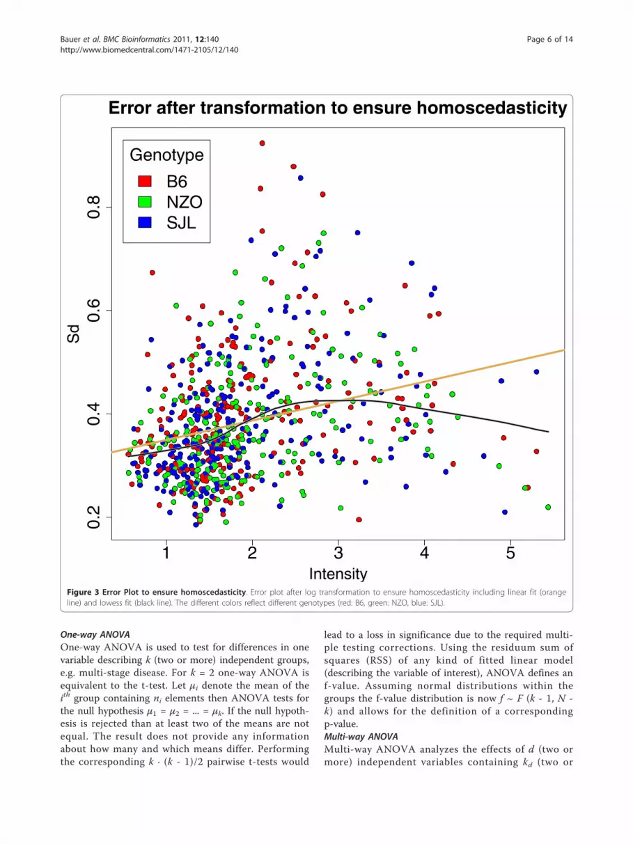
and peak matching are depicted in Figure 2. After apply-ing logarithmic transformation to the spectra the corre-lation between variance and intensity is still strong.However even the combination of log transformation,baseline correction and peak mapping does not lead to astabilization of the variance which is necessary forapplying our statistical analysis methods. Hence, inorder to assure homoscedasticity additional steps wererequired. Obviously, there is still a linear dependencybetween variance and intensity indicating a multiplica-tive error model (see Figure 2). In order to account for

this, we applied another log transformation. We added apseudo-count of 0.1 to avoid the singularity at 0. Finallywe added an offset for convenience. After this transfor-mation the data are homoscedastic (see Figure 3).While the input for the complete pre-processing

work-flow consists of 1122 continuous spectra each with32,000 data points, the output is a list comprising inten-sities for 261 discrete peak positions for all 1122 spectra(see Figure 1).Technical replicates are not independent and hence

violate an assumption of ANOVA. Because of this, tech-nical replicates were averaged prior to statistical analysis(see Figure 1). By averaging, the 1122 individual spectrawere reduced to 155 mean spectra.

ANOVAThe main idea of ANOVA (ANalysis Of VAriance) [49]is to partition the variance into subcomponents withrespect to one or more explanatory variables. The fol-lowing types can be distinguished: One-way ANOVA,Multi-way ANOVA, and ANOVA with mixed effectsmodel [50].

2000 4000 6000 8000 10000

010

0000

2500

00 Raw data

m/z

Inte

nsity

Genotype

B6NZOSJL

0 50000 100000 150000

020

000

6000

0Error of Raw Data

Intensity

Sd

2000 4000 6000 8000 10000

67

89

11

Log Transformed Data

m/z

log

Inte

nsity

Genotype

B6NZOSJL

6 7 8 9 10 11 12

0.4

0.6

0.8

1.0

Error of Log Data

Intensity

Sd

2000 4000 6000 8000 10000

01

23

Data after peak matching

m/z

log

Inte

nsity

Genotype

B6NZOSJL

0 1 2 3 40.0

0.2

0.4

0.6

0.8

Error after peak matching

Intensity

Sd

Figure 2 Preprocessing. MALDI MD profiling raw data (top), log data (middle) and after baseline correction and peak alignment (buttom). Theleft column show the effect on the spectra itself while the right column shows the corresponding standard error plots including linear fit(orange line) and lowess fit (black line). The different colors reflect different genotypes (red: B6, green: NZO, blue: SJL).


of 14

One-way ANOVAOne-way ANOVA is used to test for differences in onevariable describing k (two or more) independent groups,e.g. multi-stage disease. For k = 2 one-way ANOVA isequivalent to the t-test. Let μi denote the mean of theith group containing ni elements then ANOVA tests forthe null hypothesis μ1 = μ2 = ... = μk. If the null hypoth-esis is rejected than at least two of the means are notequal. The result does not provide any informationabout how many and which means differ. Performingthe corresponding k · (k - 1)/2 pairwise t-tests would

lead to a loss in significance due to the required multi-ple testing corrections. Using the residuum sum ofsquares (RSS) of any kind of fitted linear model(describing the variable of interest), ANOVA defines anf-value. Assuming normal distributions within thegroups the f-value distribution is now f ~ F (k - 1, N -k) and allows for the definition of a correspondingp-value.Multi-way ANOVAMulti-way ANOVA analyzes the effects of d (two ormore) independent variables containing kd (two or

1 2 3 4 5

0.2

0.4

0.6

0.8

Error after transformation to ensure homoscedasticity

Intensity

Sd

Genotype

B6NZOSJL

Figure 3 Error Plot to ensure homoscedasticity. Error plot after log transformation to ensure homoscedasticity including linear fit (orangeline) and lowess fit (black line). The different colors reflect different genotypes (red: B6, green: NZO, blue: SJL).


of 14

more) independent groups, e.g. analyzing different treat-ments and various disease states. In contrast to multipleone-way ANOVAs the RSS is calculated from a singlemodel for all variables. Thus, the degrees of freedomand the distribution of the f-values are different whichhas to be accounted for in the calculation of the corre-sponding p-values.ANOVA with mixed-effects modelANOVA with mixed-effects model looks for the effectsof several (not necessarily independent) variables andalso accounts for the effects coming from combinationsof variables, e.g. analyzing the effect of different treat-ments for various disease states. The underlying modelcan either relinquish group combinations (model 1 withp1 parameters) or include group combinations (model 2with p2 parameters). If the first model is nested withinthe second one, the f-value can be calculated as (n =sample size, RSS = Residuum Sum of Squares):

f =

(RSS1 − RSS2

p2 − p1

)(

RSS2

n − p2

) (1)

The f value is distributed as f ~ F (p2 - p1, n - p2).

Stratification and ClusteringAfter pre-processing each peak should represent a pep-tide or peptide combination (for simplification we focuson the case of one peptide only). The concentration of apeptide varies in the diverse samples (diet-genotypecombinations). The list of peptide peak intensities (N =number of samples) will be called intensity profileswithin this manuscript.Due to fragmentation/degradation each protein can

split up into multiple peptides and lead to multiplepeaks in the mass spectrum. These peaks are not inde-pendent and the corresponding intensity profiles aretherefore correlated. High correlation between intensityprofiles can indicate related peptides as in multimer for-mations or post translational modifications (PTMs).However, in order to benefit from this kind of correla-tion or any technical redundancies various methodshave been proposed [27]. For this study, we apply hier-archical clustering using average linkage [51] with 1- ras distance measure, where r denotes the Pearson-corre-lation coefficient [52]. Each node in the resulting clusterdendrogram represents several intensity profiles andsimilar intensity profiles are aggregated in closeproximity.Clustering is a standard tool in data mining but there

are only a few studies using clustering in this context (e.g. [53]). A great advantage of our approach is the com-bination of the similarity information with significance

by assigning p-values to the nodes. For the questionunder consideration the appropriate statistical test liket-test or ANOVA defines a p-value for each leaf. Foraggregated nodes based on n leafs the p-value is calcu-lated from the mean intensity profile of correspondingpeaks. For technical and biological reasons intensity pro-files are on different absolute scales. Therefore prior toaveraging intensity profiles, they have to be z-trans-formed [51].

Classification and PredictionProper feature selection is essential for building a classifierthat accomplishes good performance without overfitting.One can distinguish three kinds of feature selection meth-ods: filter methods, embedded methods and wrapper meth-ods [20,54]. Filter methods are independent of theclassification and do not consider the feature similarity ororthogonality. Embedded methods include the featureselection process in the classification training. Wrappermethods use non-linear global optimization strategies likegenetic algorithms or swarm based intelligence approaches.Wrapper methods succeed in optimizing classificationresults but they also tend to overfitting. Embedded meth-ods require complex algorithm adaptations for most classi-fiers. Filter methods are straight forward but are oftenoutperformed by the other methods [55].

ResultsANOVA with mixed effectsA major goal of this work is the analysis of the mutualinfluence of diet and genotype on blood proteins withina T2DM study. For the data presented here, a straightforward approach for this analysis was a mixed-effectANOVA of the form:

Y ∼ Genotype + Diet + time + Genotype ∗ Diet

This model investigates effects derived from all threesingle experimental factors as well as the combinationof genotype and diet (symbolized by the ‘*’). Time as afurther experimental factor was of minor biologicalinterest during this analysis. The ANOVA analysis wasperformed as described in the Methods section.

Average Linkage ClusteringIn parallel to ANOVA an average linkage clustering wasperformed. The cluster dendrogram combining corre-lated peptides and ANOVA p-values (see Figure 4) wascalculated as described in the Methods section. Theexperimental factors have different impact on the data(see Figure 4). The most significant p-values areobtained for genotype (up to 10 -91 ). The differentmouse types can be easily distinguished using the profiledata. Diet and the combination of genotype and diet


of 14

seem to have a much smaller but still substantial effecton the data (p-values of up to 10 -14 ) whereas time hasan even greater effect (p-values of up to 10 -23 ). Nearlyone third of all peaks - the whole right part of the den-drogram - is associated with the experimental factortime. On this global level the dendrogram allows anintuitive overview of the complete data set as both simi-larity and significance information are shown in a uni-fied representation.

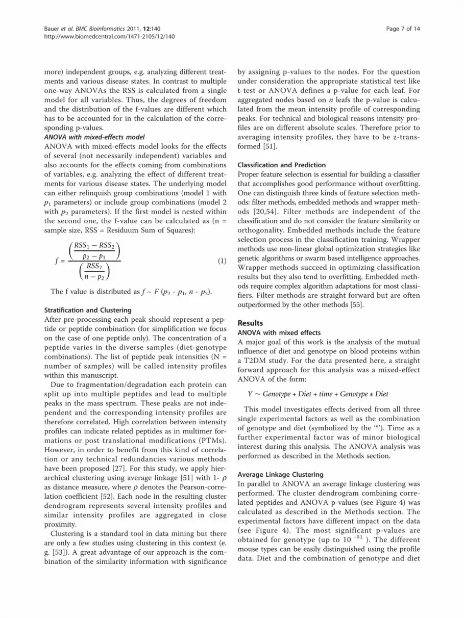
Profile Similarity for HemoglobinProtein composition of blood is typically dominated byalbumin and other highly abundant proteins such ashemoglobin. Albumin and hemoglobin are large proteinsrepresented by a multitude of peptides and thus shouldbe presented by multiple peaks in our dataset. Assumingthat many of their peptides are correlated they shouldbe located in close proximity in the dendrogram. MS-based profile peak identification revealed one albuminand three hemoglobin peptides. Mapping the threehemoglobin peptide peaks in the dendrogram showsthat they are indeed in close proximity (see Figure 5)

verifying our assumption. The peak identified as albu-min is located in the big cluster in the central part.

Identification of biomarker candidates in Multi-FactorialStudiesTable 2 provides an overview of the three clustersmarked with a red circle in Figure 4 and their corre-sponding peaks. Each cluster comprises peptide peaksthat have been partially analyzed and identified. Cluster1 comprises three peaks with a mean correlation coeffi-cient of 0.71 and is the most significant result for factordiet (p-value of 10-10). Cluster 1 has also the most sig-nificant p-value for the combination of diet and geno-type (10-14) and a p-value of 10-19 for genotype. Adetailed illustration of the intensity profile for peak m/z4075 can be seen in Figure 6. This peak shows highintensities for the combination of SJL-genotype andCHF-diet whereas it is almost constantly low for allother factor combinations. This effect is also visible withlower significance for diet or genotype only. However,only the combination of the two experimental factorsassesses the proper biological mutual influence.

Dendrogram of expression patterns

1

2 3

Diet Genotype

DietGenotype Time

P Values (− log10)

0 0

0 0

1 8

1 2

2 15

3 4

3 22

4 6

4 29

6 8

5 37

7 10

6 44

8 12

7 51

10 14

8 59

11 16

9 66

13 18

11 73

14 20

12 80

15 22

Figure 4 Cluster Dendrogram. Cluster dendrogram of all peaks identified in this dataset (see the Methods section for details). Every node ischaracterized by four ANOVA p-values shown as a color-coded box with four fields: diet (upper left), genotype (upper right), time (lower right)and combination of diet and genotype (lower left). The different -log10 p-value colorscales for the four factors are shown at the bottom. Threeclusters for further discussion (see text) are marked with red circles.


of 14

Cluster 2 consists of three peaks with a mean correla-tion coefficient of 0.94. The p-values for genotype andweek are significant: 10-31 and 10-19 respectively. Theintensity is higher in NZO mice and this effect increasesduring aging while there are only minor differencesbetween the diets.

As already mentioned the genotype has the strongesteffect in this dataset. The four peaks of cluster 3 arestrongly associated with genotype (p-value of 10-75). Themean correlation of the six peaks is 0.95 and they areonly present in SLJ genotype mice independent of dietor week. A detailed illustration of the intensity profile

Excerpt of the Dendrogram (Hemoglobin Peaks)

4011

.14

3655

.66

3664

.5

1921

.25

1809

.9

1765

.52

1995

.58

1937

.89

2893

.98

4676

.29

6989

.63

1171

.87

3790

.01

4455

.8

3903

.36

3922

.22

3943

.14

9776

.35

2342

.45

4432

.95

3524

.28

1701

.87

3838

.55

896.

33

966.

89

3514

.8

3449

.29

3455

.2

3638

.28

7371

.09

1316

.12

1696

.23

3798

.18

2020

.94

1188

.17

1582

.08

1388

.25

1024

.73

1445

.95

1080

.06

3768

.39

3881

.7

3492

.89

Figure 5 Dendrogram Hemoglobin. Excerpt of the dendrogram in Figure 4 showing the three peaks identified as hemoglobin (colored red onthe x-axis).

Table 2 Table for clusters 1-3

p values

Cluster mean cor Peak Diet Genotype Week Diet * Genotype

1 0.71 2262 1.3e-10 0.00015 2e-19 3.8e-11 0.0018 0.97 4.6e-14 1.2e-05

3618 6.7e-07 2e-08 0.004 8.8e-13

4075 2e-14 1.5e-29 3e-08 7.9e-14

2 0.94 9305 0.96 0.0019 3.3e-31 4.3e-36 2.8e-19 2.4e-17 0.12 0.013

8720 0.38 1.2e-23 2.8e-16 0.2

8735 0.57 8.2e-29 5.5e-22 0.21

3 0.95 6329 0.0012 0.022 7.5e-75 6.7e-50 0.34 0.24 0.18 0.19

4237 9.5e-05 1.1e-70 0.61 0.022

5029 0.00014 1.3e-91 0.82 0.14

5822 0.0023 5.7e-81 2.3e-07 0.82

Table for clusters 1-3 of Figure 4. For every cluster and peaks aggregated within this cluster, the correlation of the peaks and the ANOVA p-values for the threedifferent experimental factors and the factor combination of Diet and Genotype are given. P-values are given for every peak separately and for the completecluster.


of 14

for peak m/z 3388 can be seen in Additional file 2:Results for Genotype.In the middle of the dendrogram (of Figure 4) a big

cluster is visible containing 43 peaks of which one hasbeen identified as albumin. All 43 peaks in this clusterhave a mean correlation coefficient of 0.84. This clusteris not associated with any of the experimental factors.All p-values are given without multiple testing correc-

tion. Applying rigid Bonferoni multiple testing correc-tion for 261 tests, the p-value threshold of 0.05 changesto 0.05/261 = 0.0002. Hence all p-values discussedabove remain significant.

Classification and PredictionThe methods established in the previous section arealso well-suited for obtaining reliable and precise clas-sifications and predictions. This can be demonstratedby the example of diet and the classification perfor-mance can be evaluated by cross validation. Thus thetask is to predict the diet applied from the data. Theother two experimental factors are less suited for pur-pose of demonstration because genotype classificationis rather simple (c.f. Additional file 2: Results for

Genotype) and time is sampled from a continuous sup-port and less suited for formulation of a classificationtask. Using the method described above for featureselection we avoid the shortcoming of typical filtermethods as clustering incorporates information aboutsimilarity and orthogonality. We found it to be suffi-cient to use one representative feature from the clusterto achieve classification performance comparable towrapper methods.In order to demonstrate the advantages of cluster-

based ANOVA we built a classification system with adecision tree based classifier for the experimental factordiet [56]. Since the optimal feature size for classificationstrongly depends on the classifier and on feature-labeldistribution [57], we performed classification with differ-ent feature set sizes: 3, 5 and 8. The feature selectionitself was done three times by selecting top featuresfrom:

1. ANOVA analysis without clustering: Selection ofpeaks with the most significant p-values for experi-mental factor diet (Peaks m/z: 1883, 3267, 3407,4075, 4237, 5176, 5536, 8332).

B6:

CH

FD

B6:

HF

D

B6:

SD

NZ

O:C

HF

D

NZ

O:H

FD

NZ

O:S

D

SJL

:CH

FD

SJL

:HF

D

SJL

:SD

Week 3

Inte

nsity

0.0

0.5

1.0

1.5

2.0

2.5B6NZOSJL

B6:

CH

FD

B6:

HF

D

B6:

SD

NZ

O:C

HF

D

NZ

O:H

FD

NZ

O:S

D

SJL

:CH

FD

SJL

:HF

D

SJL

:SD

Week 4

Inte

nsity

0.0

0.5

1.0

1.5

2.0

2.5B6NZOSJL

B6:

CH

FD

B6:

HF

D

B6:

SD

NZ

O:C

HF

D

NZ

O:H

FD

NZ

O:S

D

SJL

:CH

FD

SJL

:HF

D

SJL

:SD

Week 6

Inte

nsity

0.0

0.5

1.0

1.5

2.0

2.5B6NZOSJL

B6:

CH

FD

B6:

HF

D

B6:

SD

NZ

O:C

HF

D

NZ

O:H

FD

NZ

O:S

D

SJL

:CH

FD

SJL

:HF

D

SJL

:SD

Week 8

Inte

nsity

0.0

0.5

1.0

1.5

2.0

2.5B6NZOSJL

Figure 6 Peak 4075. Normalized peak intensities for the peak at m/z 4075 representing cluster 1 of the dendrogram in Figure 4. Peakintensities for all 3 experimental factors are drawn as bar plots with error-of-mean error bars. Genotype and diet are given below the bars foreach week. The missing values for the SJL-HFD week 3 and 4 samples are due to the sample collection problems described in the Methodssection.


of 14

2. Ant colony optimization strategy: Using an antcolony optimization strategy [58,59], we identified aset of features with optimized classification results ina similar way to Ressom et al. [20] with 200 antsand 100 iterations (Peaks m/z: 3267, 3437, 3575,4041, 4237, 4965, 6569, 7058).3. ANOVA analysis including clustering: Selection ofclusters or peaks with the most significant p-valuesfor the experimental factor diet. For every cluster,the peak with the most significant p-value is selectedas representantive for the cluster (Peaks m/z: 1883,3267, 3407, 3556, 3943, 4075, 5176, 8332).

Confusion matrices for 10-fold cross validation areshown in Table 3 together with a p-value for the classi-fication result calculated by comparing the performanceof the selected set of features with the performance ofrandomly selected sets.Using ANOVA without clustering for feature selection

leads to a 10-fold cross validation error of 53% for 3 fea-tures (p-value: 0.0028), 52% for 5 features (p-value:0.006) and 42% for 8 features (p-value: 1 · 10-06). Asexpected the ant colony feature selection outperformsthe simple filter method with a cross validation error of40% for 3 features (p-value: 1 · 10-08), 37% for 5 features(p-value: 2 · 10-08) and 39% for 8 features (p-value: 5 ·10-07). However, our improved feature selection techni-que leads to performances comparable to wrappermethod in terms of cross validation errors (44%, 40%,38% for 3, 5 and 8 features) and p-values(1 · 10-6, 7 · 10-7, 3 · 10-7 for 3, 5 and 8 features).

DiscussionThe ANOVA model applied analyzes the effects of sin-gle experimental factors as well as the combination ofdiet and genotype. Before applying ANOVA we ensuredthat all required assumptions are fulfilled (e.g.

homoscedasticity and c2 distribution of errors). Hence,ANOVA is the perfect candidate for the statistical analy-sis and preferable to non-parametric Kruskal-Wallis testsince is has greater power.Peaks identified in the analysis of feature combination

provide valuable additional information. For instance,the most significant result found for the combination ofgenotype and diet was identical with the most significantresult for diet (see Table 2). Looking solely at the factordiet we would conclude that peak m/z 4075 is correlatedwith diabetes-protective CHF diet [7,31]. An analysis ofthe factor combination, however, shows that this corre-lation with the CHF diet only stems from the SJL geno-type (see Figure 6), which is completely invisible forsingle factor analysis.Another interesting outcome of our analysis is the fact

that the peak m/z 8735 in cluster two is associated withthe growing fat of NZO mice. First it is significantlyhigher in NZO mice then in the other genotypes thatdo not develop prominent diet-induced obesity. Sec-ondly it increases with age and thus with body weight ofthe NZO mice. Therefore the corresponding polypeptideis a candidate biomarker and a potential target towardsT2DM disease mechanism. Thus, further in-depth func-tional analysis of this marker, and its relation to diet-induced obesity and insulin resistance may provideimportant insights into the pathophysiology of diabetesand its secondary complications.As seen in the Results section, there is no direct over-

lap between the top eight features for classification ofdiet selected with ant colony optimization and the topfeatures selected with ANOVA. However, the best fea-tures of ant colony optimization are also characterizedby top ranked p-values. Both lists of top 50 featuresshow a rank correlation of 0.5 (Spearman correlation)and hence both lists are not that different. Even the bestfeatures have only low discriminative power and as a

Table 3 Confusion Matrices

CHF HF SD

nFeat Method CHF HF SD CHF HF SD CHF HF SD Error P-Value

3 ANOVA 33 14 18 17 24 24 16 16 36 0.53 0.0028

ACO 45 4 16 10 33 22 11 16 41 0.4 1e-08

Cluster ANOVA 40 12 13 15 28 22 9 16 43 0.44 1e-06

5 ANOVA 36 13 16 18 22 25 20 11 37 0.52 0.006

ACO 48 3 14 12 33 20 10 15 43 0.37 2.7e-08

Cluster ANOVA 40 13 12 15 38 12 4 24 40 0.4 6.7e-07

8 ANOVA 41 12 12 16 34 15 6 22 40 0.42 9e-06

ACO 45 5 15 12 30 23 4 18 46 0.39 5.5e-07

Cluster ANOVA 43 10 12 14 35 16 5 19 44 0.38 3.3e-07

Confusion matrix for 10-fold cross validation for experimental factor diet using random forest classifier. The feature selection was done by three differentmethods: ANOVA, ant colony optimization (ACO) and cluster-based ANOVA. The feature selection was performed three times with different number of features: 3,5 and 8. Numbers in bold print represents true positives.


of 14

result there are multiple sets of features leading to simi-lar classification results as seen in Table 3.In the middle of the cluster dendrogram (Figure 4)

there is a cluster having many very good correlatedpeaks. One possible reason for that is a large commonprotein being the common source of all those peaks. Aperfect candidate for this role would be albumin as itconsists of 608 amino acids. This hypothesis is sup-ported by the fact that one of the peaks was indeedidentified as belonging to albumin.Table 4 shows the distinctive properties of our

approach compared with other methods. Standard t-testis often the method of choice for statistical testing andthe selection of suitable features for classification andprediction. However, standard t-test is not adequate formulti-dimensional datasets since it investigates only onevariable with exact two independent groups at the sametime. F-test allows for testing multi-dimensional datasetsand ANOVA enables to investigate factor combinations.Similarity of features is not considered by any of the sta-tistical tests. Swarm intelligence or genetic algorithmsare a different group of algorithms aiming at biomarkercandidate identification. Although they are applicable tomulti dimensional datasets and take data redundancyinto account they often fail in producing deterministicresults and p-values. Our work is designed to retain allcapabilities of statistical testing while considering featuresimilarities at the same time. In addition to having simi-lar performances comparable with Swarm intelligencemethods, other great advantages of our system arereduced complexity and computational requirements.While feature selection with ant colony optimizationtook roughly 5 h with both CPUs on a Intel Core2 DuoCPU (2.66 GHz), the cluster based ANOVA took lessthan 2 seconds.Another advantage of our approach is the possibility

to use only one, representative peak from a cluster forfurther analysis. We have seen that the peaks identifiedas hemoglobin are located in close proximity in the den-drogram. Hence, we can assume that many of the sur-rounding peaks are also most likely derived fromhemoglobin. Nonetheless, it has to be kept in mind thatmany peptides originating from the same parent protein

will often behave differently. Our approach aims at iden-tifying co-occuring peptides and hence leads to a rea-sonable reduction of the data. More complex interaction(e.h. high abundance of a protein causes low abundanceof another peptide) would require other processingmethods, if predominant.

ConclusionWe have introduced a method that is suitable for identi-fication of biomarker candidates in multi-factorialMALDI-TOF MS profiling studies given an appropriatepre-processing. Applying this method to our data set wewere able to identify peaks that are characteristic for thecombination of two factors as well as peaks that are sig-nificant for single factors. These results are significanteven when applying rigid multiple testing corrections. Itis shown that ANOVA is an adequate approach for theidentification of biologically interesting biomarker candi-dates from MS profiling data based on multi-dimen-sional experimental design. Furthermore, classificationbased on features selected with our approach performsimilarly well as those generated with more complexglobal optimization methods.

Additional material

Additional file 1: Peak alignment. Visualization of the results of thepeak alignment method. The heuristic algorithm used for peak alignmentis presented in pseudo-code.

Additional file 2: Results for Genotype. Scatter plot of peak intensityvalues for peaks 3388 and 5029 and peak intensities profile for peak3388. The peaks are in the list of the most significant results for theexperimental factor genotype.

AcknowledgementsThis work is part of the Sys-Prot project funded by the EuropeanCommission, sixth framework programme for research and technicaldevelopment supported by grants from the EU (37457).

Author details1MicroDiscovery GmbH, Marienburger Str. 1, 10405 Berlin, Germany.2Department of Pharmacology, German Institute of Human NutritionPotsdam-Rehbruecke, Arthur-Scheunert-Allee 114-116, 14558 Nuthetal,Germany. 3Department Computer Science and Mathematics, Free Universityof Berlin, Berlin, Germany. 4Department of Chemistry and The BioCentre, TheUniversity of Reading, Whiteknights, Reading, RG6 6AS, UK.

Table 4 Comparison of feature selection methods

Method Deterministic Feature Selection p-Values Multi Dimensional Combinations Redundancy

t-Test ✓ ✓ ✓ ✕ ✕ ✕

F-Test ✓ ✓ ✓ ✓ ✕ ✕

ANOVA ✓ ✓ ✓ ✓ ✓ ✕

Swarm Intelligence ✕ ✓ ✕ ✓ ✓ ✓

GA ✕ ✓ ✕ ✓ ✓ ✓

This Work ✓ ✓ ✓ ✓ ✓ ✓

Comparison of different methods for biomarker candidate identification and feature selection.


of 14

http://www.biomedcentral.com/content/supplementary/1471-2105-12-140-S1.PDF

http://www.biomedcentral.com/content/supplementary/1471-2105-12-140-S2.PDF

Authors’ contributionsCB developed and implemented the described methods and drafted themanuscript. TD, AC and HA were responsible for the generation of thebiological samples. AT and CJS acquired the MALDI MS profile data. AT,MWT and RC performed the peptide identification. All authors read andapproved the final manuscript.

Received: 26 July 2010 Accepted: 9 May 2011 Published: 9 May 2011

References1. Shaw JE, Sicree RA, Zimmet PZ: Global estimates of the prevalence of

diabetes for 2010 and 2030. Diabetes Res Clin Pract 2010, 87:4-14.2. Zhang P, Zhang X, Brown J, Vistisen D, Sicree R, Shaw J, Nichols G: Global

healthcare expenditure on diabetes for 2010 and 2030. Diabetes Res ClinPract 2010, 87:293-301.

3. Tiffin N, Adie E, Turner F, Brunner HG, van Driel MA, Oti M, Lopez-Bigas N,Ouzounis C, Perez-Iratxeta C, Andrade-Navarro MA, Adeyemo A, Patti ME,Semple CA, Hide W: Computational disease gene identification: a concertof methods prioritizes type 2 diabetes and obesity candidate genes.Nucleic Acids Res 2006, 34:3067-3081.

4. Rasche A, Al-Hasani H, Herwig R: Meta-analysis approach identifiescandidate genes and associated molecular networks for type-2 diabetesmellitus. BMC Genomics 2008, 9:310.

5. Liu X, Feng Q, Chen Y, Zuo J, Gupta N, Chang Y, Fang F: Proteomics-basedidentification of differentially-expressed proteins including galectin-1 inthe blood plasma of type 2 diabetic patients. J Proteome Res 2009,8:1255-1262.

6. Rao PV, Reddy AP, Lu X, Dasari S, Krishnaprasad A, Biggs E, Roberts CT,Nagalla SR: Proteomic identification of salivary biomarkers of type-2diabetes. J Proteome Res 2009, 8:239-245.

7. Jürgens HS, Neschen S, Ortmann S, Scherneck S, Schmolz K, Schüler G,Schmidt S, Blüher M, Klaus S, Perez-Tilve D, Tschöp MH, Schürmann A,Joost HG: Development of diabetes in obese, insulin-resistant mice:essential role of dietary carbohydrate in beta cell destruction.Diabetologia 2007, 50:1481-1489.

8. Chadt A, Leicht K, Deshmukh A, Jiang LQ, Scherneck S, Bernhardt U,Dreja T, Vogel H, Schmolz K, Kluge R, Zierath JR, Hultschig C, Hoeben RC,Schurmann A, Joost HG, Al-Hasani H: Tbc1d1 mutation in lean mousestrain confers leanness and protects from diet-induced obesity. NatGenet 2008, 40:1354-1359.

9. Aebersold R, Mann M: Mass spectrometry-based proteomics. Nature 2003,422:198-207.

10. Cramer R, Gobom J, Nordhoff E: High-throughput proteomics usingmatrix-assisted laser desorption/ionization mass spectrometry. Expert RevProteomics 2005, 2:407-420.

11. McGuire J, Overgaard J, Pociot F: Mass spectrometry is only one piece ofthe puzzle in clinical proteomics. Brief Funct Genomic Proteomic 2008,7:74-83.

12. Gamez-Pozo A, Sanchez-Navarro I, Nistal M, Calvo E, Madero R, Diaz E,Camafeita E, de Castro J, Lopez JA, Gonzalez-Baron M, Espinosa E, FresnoVara JA: MALDI profiling of human lung cancer subtypes. PLoS ONE 2009,4:e7731.

13. Palmblad M, Tiss A, Cramer R: Mass spectrometry in clinical proteomics -from the present to the future. Proteomics - Clin Appl 2009, 3:6-17.

14. van der Werff MP, Mertens B, de Noo ME, Bladergroen MR, Dalebout HC,Tollenaar RA, Deelder AM: Casecontrol breast cancer study of MALDI-TOFproteomic mass spectrometry data on serum samples. Stat Appl GenetMol Biol 2008, 7:Article2.

15. Voortman J, Pham TV, Knol JC, Giaccone G, Jimenez CR: Prediction ofoutcome of non-small cell lung cancer patients treated withchemotherapy and bortezomib by time-course MALDI-TOF-MS serumpeptide profiling. Proteome Sci 2009, 7:34.

16. Timms JF, Cramer R, Camuzeaux S, Tiss A, Smith C, Burford B, Nouretdinov I,Devetyarov D, Gentry-Maharaj A, Ford J, Luo Z, Gammerman A, Menon U,Jacobs I: Peptides generated ex vivo from serum proteins by tumor-specific exopeptidases are not useful biomarkers in ovarian cancer. ClinChem 2010, 56:262-271.

17. de Noo ME, Mertens BJ, Ozalp A, Bladergroen MR, van der Werff MP, vande Velde CJ, Deelder AM, Tollenaar RA: Detection of colorectal cancerusing MALDI-TOF serum protein profiling. Eur J Cancer 2006,42:1068-1076.

18. Alexandrov T, Decker J, Mertens B, Deelder AM, Tollenaar RA, Maass P,Thiele H: Biomarker discovery in MALDI-TOF serum protein profiles usingdiscrete wavelet transformation. Bioinformatics 2009, 25:643-649.

19. Ge G, Wong GW: Classification of premalignant pancreatic cancer mass-spectrometry data using decision tree ensembles. BMC Bioinformatics2008, 9:275.

20. Ressom H, Varghese R, Drake S, Hortin G, Abdel-Hamid M, Loffredo C,Goldman R: Peak selection from MALDI-TOF mass spectra using antcolony optimization. Bioinformatics 2007, 23:619-626.

21. Wu B, Abbott T, Fishman D, McMurray W, Mor G, Stone K, Ward D,Williams K, Zhao H: Comparison of statistical methods for classification ofovarian cancer using mass spectrometry data. Bioinformatics 2003,19:1636-1643.

22. Zhang X, Lu X, Shi Q, Xu XQ, Leung HC, Harris LN, Iglehart JD, Miron A,Liu JS, Wong WH: Recursive SVM feature selection and sampleclassification for mass-spectrometry and microarray data. BMCBioinformatics 2006, 7:197.

23. Liu Q, Sung AH, Qiao M, Chen Z, Yang JY, Yang MQ, Huang X, Deng Y:Comparison of feature selection and classification for MALDI-MS data.BMC Genomics 2009, 10(Suppl 1):S3.

24. Smyth GK, Michaud J, Scott Hs: The use of withinarray replicate spots forassessing differential expression in microarray experiments.Bioinformatics 2005, 21(9):2067-2075.

25. Mercier C, Truntzer C, Pecqueur D, Gimeno JP, Belz G, Roy P: Mixed-modelof ANOVA for measurement reproducibility in proteomics. J Proteomics2009, 72:974-981.

26. Oberg AL, Vitek O: Statistical design of quantitative mass spectrometry-based proteomic experiments. J Proteome Res 2009, 8:2144-2156.

27. Carlson SM, Najmi A, Cohen HJ: Biomarker clustering to addresscorrelations in proteomic data. Proteomics 2007, 7:1037-1046.

28. Ortlepp JR, Kluge R, Giesen K, Plum L, Radke P, Hanrath P, Joost HG: Ametabolic syndrome of hypertension, hyperinsulinaemia andhypercholesterolaemia in the New Zealand obese mouse. Eur J Clin Invest2000, 30:195-202.

29. Jurgens HS, Schurmann A, Kluge R, Ortmann S, Klaus S, Joost HG,Tschop MH: Hyperphagia, lower body temperature, and reduced runningwheel activity precede development of morbid obesity in New Zealandobese mice. Physiol Genomics 2006, 25:234-241.

30. West DB, Boozer CN, Moody DL, Atkinson RL: Dietary obesity in nineinbred mouse strains. Am J Physiol 1992, 262:R1025-1032.

31. Dreja T, Jovanovic Z, Rasche A, Kluge R, Herwig R, Tung YC, Joost HG,Yeo GS, Al-Hasani H: Diet-induced gene expression of isolated pancreaticislets from a polygenic mouse model of the metabolic syndrome.Diabetologia 2010, 53:309-320.

32. Tiss A, Smith C, Camuzeaux S, Kabir M, Gayther S, Menon U, Waterfield M,Timms J, Jacobs I, Cramer R: Serum peptide profiling using MALDI massspectrometry: avoiding the pitfalls of coated magnetic beads using well-established ZipTip technology. Proteomics 2007, 7(Suppl 1):77-89.

33. Tiss A, Smith C, Menon U, Jacobs I, Timms JF, Cramer R: A well-characterised peak identification list of MALDI MS profile peaks forhuman blood serum. Proteomics 2010, 10:3388-3392.

34. Kwon D, Vannucci M, Song J, Jeong J, Pfeiffer R: A novel wavelet-basedthresholding method for the pre-processing of mass spectrometry datathat accounts for heterogeneous noise. Proteomics 2008, 8:3019-3029.

35. Pratapa P, Patz E, Hartemink A: Finding diagnostic biomarkers inproteomic spectra. Pac Symp Biocomput 2006, 279-290.

36. Norris J, Cornett D, Mobley J, Andersson M, Seeley E, Chaurand P,Caprioli R: Processing MALDI Mass Spectra to Improve Mass SpectralDirect Tissue Analysis. Int J Mass Spectrom 2007, 260:212-221.

37. Yu W, Wu B, Huang T, Li X, Williams K, Zhao H: Statistical Methods InProteomics Springer Verlag; 2006, 623-638, [Proteomics, PhysioSim].

38. Yang C, He Z, Yu W: Comparison of public peak detection algorithms forMALDI mass spectrometry data analysis. BMC Bioinformatics 2009, 10:4.

39. Gentleman RC, Carey VJ, Bates DM, Bolstad B, Dettling M, Dudoit S, Ellis B,Gautier L, Ge Y, Gentry J, Hornik K, Hothorn T, Huber W, Iacus S, Irizarry R,Leisch F, Li C, Maechler M, Rossini AJ, Sawitzki G, Smith C, Smyth G,Tierney L, Yang JY, Zhang J: Bioconductor: open software developmentfor computational biology and bioinformatics. Genome Biol 2004, 5:R80.

40. Robert Gentleman and Vince Carey and Wolfgang Huber and Rafael Irizarryand Sandrine Dudoit (Ed): Bioinformatics and Computational BiologySolutions Using R and Bioconductor Springer Verlag; 2005.


of 14

http://www.ncbi.nlm.nih.gov/pubmed/19896746?dopt=Abstract
















































































41. Mantini D, Petrucci F, Pieragostino D, Del Boccio P, Di Nicola M, Di Ilio C,Federici G, Sacchetta P, Comani S, Urbani A: LIMPIC: a computationalmethod for the separation of protein MALDI-TOF-MS signals from noise.BMC Bioinformatics 2007, 8:101.

42. Coombes K, Tsavachidis S, Morris J, Baggerly K, Hung M, Kuerer H:Improved peak detection and quantification of mass spectrometry dataacquired from surface-enhanced laser desorption and ionization bydenoising spectra with the undecimated discrete wavelet transform.Proteomics 2005, 5:4107-4117.

43. Kohlbacher O, Reinert K, Gröpl C, Lange E, Pfeifer N, Schulz-Trieglaff O,Sturm M: TOPP-the OpenMS proteomics pipeline. Bioinformatics 2007, 23:e191-197.

44. Sturm M, Bertsch A, Gröpl C, Hildebrandt A, Hussong R, Lange E, Pfeifer N,Schulz-Trieglaff O, Zerck A, Reinert K, Kohlbacher O: OpenMS - an open-source software framework for mass spectrometry. BMC Bioinformatics2008, 9:163.

45. Sauve AC, Speed TP: Normalization, baseline correction and alignment ofhigh-throughput mass spectrometry data. 2004.

46. Lange E, Gröpl C, Reinert K, Kohlbacher O, Hildebrandt A: High-accuracypeak picking of proteomics data using wavelet techniques. Pac SympBiocomput 2006, 243-254.

47. Du P, Kibbe WA, Lin SM: Improved peak detection in mass spectrum byincorporating continuous wavelet transform-based pattern matching.Bioinformatics 2006, 22:2059-2065.

48. Bauer C, Cramer R, Schuchhardt J: Evaluation of peak-picking algorithmsfor protein mass spectrometry. Methods Mol Biol 2011, 696:341-352.

49. Johnson RAaBGK: Statistics: Principles and Methods. 6 edition. John Wiley &Sons; 2009.

50. Crawley MJ: Statistics An Introduction using R New York, NY: Wiley; 2005.51. Hastie T, Tibshirani R, Friedman J: The Elements of Statistical Learning. 2

edition. New York: Springer; 2009.52. Rodgers JL, Nicewander AW: Thirteen Ways to Look at the Correlation

Coefficient. The American Statistician 1988, 42:59-66.53. Kirchner M, Renard BY, Kothe U, Pappin DJ, Hamprecht FA, Steen H,

Steen JA: Computational protein profile similarity screening forquantitative mass spectrometry experiments. Bioinformatics 2010,26:77-83.

54. Guyon I, Gunn S, Nikravesh M, Zadeh L: Feature Extraction, Foundations andApplications. 1 edition. Springer; 2006.

55. Xing EP, Jordan MI, Karp RM: Feature Selection for High-DimensionalGenomic Microarray Data. Proc 18th International Conf on MachineLearning Morgan Kaufmann, San Francisco, CA; 2001, 601-608.

56. Breiman L: Random Forests. Machine Learning 2001, 45:5-32, 32.57. Hua J, Xiong Z, Lowey J, Suh E, Dougherty ER: Optimal number of

features as a function of sample size for various classification rules.Bioinformatics 2005, 21:1509-1515.

58. Colorni A, Dorigo M, Maniezzo V: Distributed Optimization by AntColonies. European Conference on Artificial Life 1991, 134-142.

59. Dorigo M, Maniezzo V, Colorni A: Ant system: optimization by a colony ofcooperating agents. IEEE Trans Syst Man Cybern B Cybern 1996, 26:29-41.

doi:10.1186/1471-2105-12-140Cite this article as: Bauer et al.: Biomarker Discovery and RedundancyReduction towards Classification using a Multi-factorial MALDI-TOF MST2DM Mouse Model Dataset. BMC Bioinformatics 2011 12:140.

Submit your next manuscript to BioMed Centraland take full advantage of:

• Convenient online submission

• Thorough peer review

• No space constraints or color figure charges

• Immediate publication on acceptance

• Inclusion in PubMed, CAS, Scopus and Google Scholar

• Research which is freely available for redistribution

Submit your manuscript at www.biomedcentral.com/submit


of 14



















Biomarker Discovery and Redundancy Reduction towards Classification using a Multi-factorial...

Documents

Transcript of Biomarker Discovery and Redundancy Reduction towards Classification using a Multi-factorial...