A Thesis Submitted tothe Graduate School of Engineering and Sciences of

İzmir Institute of Technologyin Partial Fulfillment of the Requirements for the Degree of

MASTER OF SCIENCE

in Biotechnology

byFarid MUSA

December 2020İZMİR

BIOINFORMATIC ANALYSIS ANDBIOSTATISTICAL MODELLING OF GENETICINTERACTIONS BETWEEN MICROBIOTA AND

HOST

ACKNOWLEDGMENTS

I wish to express my sincere appreciation to my supervisor, Assoc. Prof. Dr. EfeSezgin, who always motivated and made me feel confident in my abilities. Without hispersistent help and motivation, this thesis would not have been realized. I have enjoyedevery bit of our discussions and meetings.

I would like to pay my special regards to Orkan Dal and Alper Şahin, for friend-ship, reliability, and countless moments of productive brainstorming. Without them, thePhyloMAF would not be as cool as it is now. I would like to extend my sincere thanks toOrhan Oral, who provided a warm fellowship during my research. I’m immensely gratefulto my dear girlfriend Farida Majidzade for her constant motivation and emotional supportduring my research.

I wish to thank all my friends whose support was valuable in the completion ofthis thesis. Particularly for their professional advice and support in my work, I wouldlike to thank Bertan Özdoğru, Emre Değirmenci, and Barış Çelik. For their companyand support during my research, I would like to thank Mehmet Veysel Sekendiz, MeteTokgöz, Gokhan Cihan, Ozan Ceylan, İrem Köse, Nijat Jafarov, Gökhan Demircan, DilaraYardımcı, Eren Erinanç, Özgür Acar, and Ebru Sürücüoğlu. Lastly, I would like to showmy tribute to my dear friends Erdem Öztürk and İpek Öztürk, who showed an exemplaryiron will during their tough year.

I wish to express my deepest gratitude to my dear mother Rubaba Musayeva, mydear father Dr. Hasan Musayev, and my dear brother Kamal Musa, for their unconditionallove, constant motivation, greatest encouragement, and infinite support throughout mylife.

I’m deeply indebted to 2783 souls who kept me and my family safe during thesecond Nagorno-Karabakh war.

ii

ABSTRACT

BIOINFORMATIC ANALYSIS AND BIOSTATISTICAL MODELLINGOF GENETIC INTERACTIONS BETWEEN MICROBIOTA AND HOST

Advances in genome sequencing technology have revolutionized the study of mi-croorganisms. Recent genome-wide association studies (GWAS) on gut microbiota re-vealed fascinating discoveries about the effect of microbiota on our health.

In this thesis, Drosophila Melanogaster samples were used to investigate theassociations between the host’s genotype and microbiota. The meta-analysis of microbiotadata was performed using PhyloMAF, a novel, and comprehensive microbiome meta-analysis framework. The resulting microbial abundance tables were analyzed using alphaand phylogenetic beta bio-diversity metrics, which were used in the microbiome GWASstudy. Significant variant associations were further analyzed in the post-GWAS analysis.

The results of our study show that several genomic variants are significantly as-sociated with bio-diversity estimates. Among identified variants, few were found to beassociated with more specific phenotypes. Particularly, the gene involved in folate trans-port and linked to folate malabsorption was found to be associated with Proteobacteria.The latter for its part was found to be one of the primary phyla containing the highestnumber of genes responsible for de-novo folate synthesis. Similarly, the fly gene related toimmune function with the human homologous gene linked to the inflammatory gut diseasewas found to be associated with the Acetobacter genus. This genus based on the literaturesurvey was found to be associated with an immune deficiency in a fruit fly.

In summary, this research revealed captivating findings of genetic factors associatedwith fruit fly microbiota. The limitations and future directions were stated in order toprovide the basis for future prospective studies.

iii

ÖZET

MİKROBİYOTA-KONAK GENETİK ETKİLEŞİMLERİNİNBİYOİNFORMATİK VE BİYOİSTATİSTİKSEL OLARAK

MODELLENMESİ

Genom dizileme teknolojisindeki gelişmeler, mikrobiyoloji çalışmalarında devrimyarattı. Bağırsak mikrobiyotası üzerine yapılan son genom çapında ilişkilendirme çalış-maları (GWAS), mikrobiyotanın sağlığımız üzerindeki etkisi hakkında etkileyici sonuçlarortaya koydu.

Bu tez çalışmasında, Drosophila Melanogaster örnekleri ile konağın genotipi ilemikrobiyotası arasındaki ilişkiler biyoenformatik yöntemleriyle araştırıldı. Mikrobiyotaverilerinin meta analiz süreci, yeni ve kapsamlı bir mikrobiyom meta-analiz yazılımıolarak programlanan PhyloMAF ile gerçekleştirildi. Elde edilen mikrobiyal bolluk tablo-ları, mikrobiyom GWAS çalışmasında kullanılan alfa ve filogenetik beta biyo-çeşitlilikölçümleri kullanılarak analiz edildi. Önemli varyant ilişkileri, post-GWAS aşamasındaayrıca analiz edildi.

Bu çalışmanın sonuçları, bazı genomik varyantın biyoçeşitlilik tahminleriyle önemliölçüde ilişkili olduğunu gösterdi. Tanımlanan varyantlar arasında, çok azının daha spesi-fik fenotiplerle ilişkili olduğu bulundu. Özellikle folat taşınmasında rol oynayan ve folatmalabsorpsiyonuna bağlı genin Proteobacteria ile ilişkili olduğu bulundu. Proteobacte-ria’nın;, folat sentezinden sorumlu en yüksek sayıda geni içeren birincil şubelerden biriolduğu bulundu. Benzer şekilde, iltihaplı bağırsak hastalığına bağlı insan homolog geniile bağışıklık fonksiyonuyla ile ilgili sinek geninin Acetobacter cinsiyle ilişkili olduğutespit edildi. Literatür araştırmasına dayanan bu cinsin, meyve sineğindeki bağışıklıkyetersizliğiyle ilişkili olduğu bulundu.

Özetle, bu araştırma meyve sineği mikrobiyotası ile ilişkili genetik faktörlerinilginç bulgularını ortaya çıkardı. Ek olarak, ileriye dönük çalışmalara temel olmasıaçısından bazı kısıtlamalara ve önerilere yer verilmiştir.

iv

To the memory of my grandparents, to whom joined my dear grandmotherDr. Tamilla Cavadova.

She was the jewel of our family and an angel who lived among us.Rest in peace Toma nene.

v

TABLE OF CONTENTS

ACKNOWLEDGMENTS . . . . . . . . . . . . . . . . . . . . . . . . . . . . . . . ii

LIST OF FIGURES . . . . . . . . . . . . . . . . . . . . . . . . . . . . . . . . . . x

LIST OF TABLES . . . . . . . . . . . . . . . . . . . . . . . . . . . . . . . . . . xi

CHAPTER 1. INTRODUCTION . . . . . . . . . . . . . . . . . . . . . . . . . 11.1 Microbiome Research . . . . . . . . . . . . . . . . . . . . . . . 11.2 Unveiling Omics . . . . . . . . . . . . . . . . . . . . . . . . . 21.3 Introduction to Metataxonomics . . . . . . . . . . . . . . . . . 21.3.1 Phylogenetic Marker Genes . . . . . . . . . . . . . . . . . 21.3.2 Methodology in a Nutshell . . . . . . . . . . . . . . . . . . 31.3.3 Operational Taxonomic Units (OTU) . . . . . . . . . . . . 31.3.4 Reference Taxonomy . . . . . . . . . . . . . . . . . . . . . 4

1.4 Biodiversity Analysis . . . . . . . . . . . . . . . . . . . . . . . 41.5 Genome-Wide Association Studies . . . . . . . . . . . . . . . . 51.6 Model Organism . . . . . . . . . . . . . . . . . . . . . . . . . 51.7 Microbiome Meta-Analysis . . . . . . . . . . . . . . . . . . . . 61.8 Motivation of Thesis . . . . . . . . . . . . . . . . . . . . . . . 61.9 Organization of Thesis . . . . . . . . . . . . . . . . . . . . . . 7

CHAPTER 2. BACKGROUND . . . . . . . . . . . . . . . . . . . . . . . . . . 82.1 Conducting Microbiome Study . . . . . . . . . . . . . . . . . . 82.1.1 Sample Collection . . . . . . . . . . . . . . . . . . . . . . 82.1.2 Marker Genes and Primer Selection . . . . . . . . . . . . . 92.1.2.1 Marker Genes for Archaea and Bacteria . . . . . . . . . 92.1.2.2 Marker Genes for Eukaryota . . . . . . . . . . . . . . . 9

2.1.3 Library Preparation and Sequencing . . . . . . . . . . . . . 102.1.4 Quality Control . . . . . . . . . . . . . . . . . . . . . . . . 102.1.5 OTU-Picking (OTU Clustering) . . . . . . . . . . . . . . . 112.1.6 Taxonomy Assignment . . . . . . . . . . . . . . . . . . . . 132.1.7 Reference Taxonomy Databases . . . . . . . . . . . . . . . 142.1.7.1 Greengenes - 16S rRNA Gene Database . . . . . . . . . 142.1.7.2 SILVA - rRNA Gene Database Project . . . . . . . . . . 152.1.7.3 UNITE - ITS Database for Fungal Species . . . . . . . 15

vi

2.1.7.4 RDP - The Ribosomal Database Project . . . . . . . . . 162.1.7.5 OTT - Open Tree of life Taxonomy . . . . . . . . . . . 162.1.7.6 GTDB - Genome Taxonomy Database . . . . . . . . . . 16

2.1.8 Construction of Phylogenetic Tree . . . . . . . . . . . . . . 172.1.9 Bio-Diversity Analysis . . . . . . . . . . . . . . . . . . . . 172.1.9.1 Alpha Diversity Metrics . . . . . . . . . . . . . . . . . 172.1.9.2 Beta Diversity Metrics . . . . . . . . . . . . . . . . . . 182.1.9.3 Analysis Techniques . . . . . . . . . . . . . . . . . . . 19

2.2 Conducting Genome-Wide Association Study . . . . . . . . . . 202.2.0.1 Types of GWAS . . . . . . . . . . . . . . . . . . . . . 212.2.0.2 Models in GWAS . . . . . . . . . . . . . . . . . . . . . 212.2.0.3 Data in GWAS . . . . . . . . . . . . . . . . . . . . . . 22

CHAPTER 3. DESIGN AND IMPLEMENTATION . . . . . . . . . . . . . . . 233.1 Aim and Motivation . . . . . . . . . . . . . . . . . . . . . . . 233.2 Design Strategy . . . . . . . . . . . . . . . . . . . . . . . . . . 243.3 Overview of PhyloMAF . . . . . . . . . . . . . . . . . . . . . 253.4 Module “biome” . . . . . . . . . . . . . . . . . . . . . . . . . 273.4.1 Essentials . . . . . . . . . . . . . . . . . . . . . . . . . . . 283.4.1.1 Usage Example . . . . . . . . . . . . . . . . . . . . . . 28

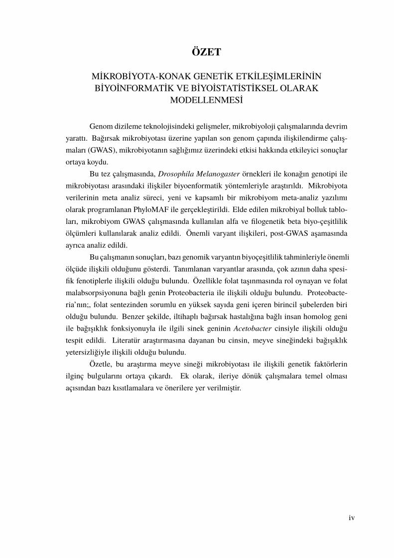
3.4.2 Assembly . . . . . . . . . . . . . . . . . . . . . . . . . . . 303.4.2.1 Usage Example . . . . . . . . . . . . . . . . . . . . . . 30

3.4.3 Survey . . . . . . . . . . . . . . . . . . . . . . . . . . . . 323.4.3.1 Usage Example . . . . . . . . . . . . . . . . . . . . . . 32

3.5 Module “database” . . . . . . . . . . . . . . . . . . . . . . . . 343.5.1 Overview . . . . . . . . . . . . . . . . . . . . . . . . . . . 353.5.2 Reconstruction of Taxonomy . . . . . . . . . . . . . . . . . 373.5.3 Storage Technicalities . . . . . . . . . . . . . . . . . . . . 383.5.4 Structure of Storage File . . . . . . . . . . . . . . . . . . . 383.5.5 The “builders” . . . . . . . . . . . . . . . . . . . . . . . . 413.5.5.1 The “parsers” - Reading and Parsing . . . . . . . . . . . 423.5.5.2 The “assemblers” - Data Transformations . . . . . . . . 433.5.5.3 The “summarizers” - Logs and Recap . . . . . . . . . . 43

3.6 Module “pipe” . . . . . . . . . . . . . . . . . . . . . . . . . . 433.6.1 Module “dockers” . . . . . . . . . . . . . . . . . . . . . . 453.6.2 Module “mediators” . . . . . . . . . . . . . . . . . . . . . 463.6.3 Module “miners” . . . . . . . . . . . . . . . . . . . . . . . 473.6.4 Module “specs” . . . . . . . . . . . . . . . . . . . . . . . . 47

3.7 Wrapper Modules . . . . . . . . . . . . . . . . . . . . . . . . . 48

vii

CHAPTER 4. MATERIALS AND METHODS . . . . . . . . . . . . . . . . . . 504.1 Sample Collection . . . . . . . . . . . . . . . . . . . . . . . . 504.2 Overall Strategy . . . . . . . . . . . . . . . . . . . . . . . . . . 524.3 Data Acquisition . . . . . . . . . . . . . . . . . . . . . . . . . 534.3.1 Microbiota Data . . . . . . . . . . . . . . . . . . . . . . . 534.3.1.1 Batch Data Fetching from MG-RAST . . . . . . . . . . 53

4.3.2 Genotype Data . . . . . . . . . . . . . . . . . . . . . . . . 544.4 Data Preparation . . . . . . . . . . . . . . . . . . . . . . . . . 544.5 Data Processing . . . . . . . . . . . . . . . . . . . . . . . . . . 584.5.1 Sample Rearrangement . . . . . . . . . . . . . . . . . . . . 584.5.2 Merging OTU-Tables and Quality Control . . . . . . . . . . 594.5.2.1 Creating Greengenes HDF5 storage file . . . . . . . . . 604.5.2.2 Reading OTU-tables into PhyloMAF . . . . . . . . . . 604.5.2.3 Complement Incomplete Taxonomy . . . . . . . . . . . 624.5.2.4 Group Essentials into Assembly . . . . . . . . . . . . . 634.5.2.5 Quality Control . . . . . . . . . . . . . . . . . . . . . . 634.5.2.6 Merging OTU-Tables . . . . . . . . . . . . . . . . . . . 644.5.2.7 Reconstructing Phylogenetic Trees . . . . . . . . . . . . 66

4.6 Bio-Diversity Analysis . . . . . . . . . . . . . . . . . . . . . . 684.6.1 Alpha-Diversity . . . . . . . . . . . . . . . . . . . . . . . . 694.6.2 Beta-Diversity . . . . . . . . . . . . . . . . . . . . . . . . 694.6.3 Abundance Analysis . . . . . . . . . . . . . . . . . . . . . 704.6.4 Secondary Analysis . . . . . . . . . . . . . . . . . . . . . . 70

4.7 Microbiome GWAS . . . . . . . . . . . . . . . . . . . . . . . . 704.7.1 Phenotype Data . . . . . . . . . . . . . . . . . . . . . . . . 714.7.2 Covariate Data . . . . . . . . . . . . . . . . . . . . . . . . 714.7.3 Genotype Data . . . . . . . . . . . . . . . . . . . . . . . . 724.7.4 Analysis of Associations . . . . . . . . . . . . . . . . . . . 72

4.8 Post-GWAS Analysis . . . . . . . . . . . . . . . . . . . . . . . 734.8.1 Explanatory Variables . . . . . . . . . . . . . . . . . . . . 744.8.2 Covariates . . . . . . . . . . . . . . . . . . . . . . . . . . . 744.8.3 Response Variables . . . . . . . . . . . . . . . . . . . . . . 754.8.3.1 Normalization . . . . . . . . . . . . . . . . . . . . . . 75

4.8.4 Regression Model . . . . . . . . . . . . . . . . . . . . . . 764.8.5 Analysis of Associations (GLM) . . . . . . . . . . . . . . . 774.8.6 Candidate Gene Analysis . . . . . . . . . . . . . . . . . . . 77

CHAPTER 5. RESULTS AND DISCUSSION . . . . . . . . . . . . . . . . . . 78

CHAPTER 6. CONCLUSION AND FUTURE DIRECTIONS . . . . . . . . . . 89viii

REFERENCES . . . . . . . . . . . . . . . . . . . . . . . . . . . . . . . . . . . . 91

APPENDICES . . . . . . . . . . . . . . . . . . . . . . . . . . . . . . . . . . . . 100

APPENDIX A. SAMPLE AND OTU TABLES . . . . . . . . . . . . . . . . . . 100

APPENDIX B. PHENOTYPE DATA TABLES . . . . . . . . . . . . . . . . . . 120

APPENDIX C. COMMUNITY ANALYSIS PLOTS . . . . . . . . . . . . . . . . 125

APPENDIX D. MANHATTAN PLOTS FOR GWAS . . . . . . . . . . . . . . . 138

APPENDIX E. TOP GWAS ASSOCIATIONS TABLES . . . . . . . . . . . . . 145

APPENDIX F. ASSOCIATION ANALYSIS RESULTS . . . . . . . . . . . . . . 151

APPENDIX G. POST-GWAS ANALYSIS RESULTS . . . . . . . . . . . . . . . 163

APPENDIX H. ADDITIONAL TABLES . . . . . . . . . . . . . . . . . . . . . . 169

ix

LIST OF FIGURES

Figure Page

Figure 2.1 Illustration of OTU clusters . . . . . . . . . . . . . . . . . . . . 12Figure 2.2 The process for GWAS analysis . . . . . . . . . . . . . . . . . . 20Figure 3.1 Relationship among metaclasses, classes and objects . . . . . . 24Figure 3.2 PhyloMAF structure in a nutshell . . . . . . . . . . . . . . . . . 26Figure 3.3 Overall structure of module “biome” . . . . . . . . . . . . . . . 27Figure 3.4 BiomeAssembly interconnecting instances of type “essentials” . 30Figure 3.5 Merging operation using BiomeSurvey . . . . . . . . . . . . . . 32Figure 3.6 Database transformation in ETL fashion . . . . . . . . . . . . . 35Figure 3.7 Overall structure of module “database” . . . . . . . . . . . . . . 36Figure 3.8 Simplified portrayal of taxonomic reconstruction . . . . . . . . 37Figure 3.9 Internal structure of HDF5 storage file . . . . . . . . . . . . . . 39Figure 3.10 Basic flow of data in “pipe” module . . . . . . . . . . . . . . . 44Figure 3.11 Overall structure of module “pipe” . . . . . . . . . . . . . . . . 45Figure 3.12 Taxonomy-to-sequence pipeline specification . . . . . . . . . . 47Figure 4.1 Overall data workflow . . . . . . . . . . . . . . . . . . . . . . . 52Figure 4.2 Overall QIIME2 pipeline for processing of Jehrke dataset . . . . 55Figure 4.3 Overall process of OTU-table merging and quality control . . . 59Figure 4.4 Process of phylogenetic tree reconstruction . . . . . . . . . . . 66Figure 4.5 Bio-diversity analysis workflow . . . . . . . . . . . . . . . . . . 68Figure 4.6 Overall workflow of GWAS analysis . . . . . . . . . . . . . . . 72Figure 4.7 Overall workflow of post-GWAS analysis . . . . . . . . . . . . 74Figure 5.1 Relative phylum abundance per datasets. . . . . . . . . . . . . . 78Figure 5.2 Relative genus abundance per datasets . . . . . . . . . . . . . . 79Figure 5.3 Overall total abundance plot per datasets by most abundant phylum 79Figure 5.4 Richness box plots per datasets . . . . . . . . . . . . . . . . . . 80Figure 5.5 Ordination plot for Dataset4(83) . . . . . . . . . . . . . . . . . 81Figure 5.6 Interdependence between bio-diversity measures for Dataset4(83). 82Figure 5.7 An UpSet plot of overlapping candidate genes. . . . . . . . . . . 83Figure 5.8 The effect of endosymbiontWolbachia on microbiota . . . . . . 88

x

LIST OF TABLES

Table Page

Table 3.1 An OTU-table example . . . . . . . . . . . . . . . . . . . . . . 29Table 3.2 Merged OTU-table . . . . . . . . . . . . . . . . . . . . . . . . . 31Table 3.3 A dummy OTU-table . . . . . . . . . . . . . . . . . . . . . . . . 33Table 3.4 Combined OTU-tables into single survey . . . . . . . . . . . . . 34Table 3.5 Fragment of real “map-rep2tid” table . . . . . . . . . . . . . . . 41Table 3.6 Taxonomy naming conventions . . . . . . . . . . . . . . . . . . 42Table 4.1 Sources for 16S microbiota data . . . . . . . . . . . . . . . . . . 51Table 4.2 DGRP lines by source . . . . . . . . . . . . . . . . . . . . . . . 51Table 4.3 Genotype and other host genomic data required for GWAS . . . . 54Table 4.4 Final rearranged sample datasets . . . . . . . . . . . . . . . . . . 59Table 4.5 Change in the number of OTUs during and after quality control . 65Table 4.6 Significance p-values of Shapiro–Wilk test for normalized response

variables used in post-GWAS anaylsis . . . . . . . . . . . . . . . 76Table 5.1 Candidate genes with prospect of further analysis . . . . . . . . . 84Table 5.2 Summary for candidate genes of interest . . . . . . . . . . . . . 85Table 5.3 Overall GWAS and post-GWAS analysis results for candidate gene

FBgn0039817 . . . . . . . . . . . . . . . . . . . . . . . . . . . 86Table 5.4 Overall GWAS and post-GWAS analysis results for candidate gene

FBgn0259241 . . . . . . . . . . . . . . . . . . . . . . . . . . . 87

xi

LISTS OF ABBREVIATIONS

API application programming interface.

ASV amplicon sequence variant.

BED binary biallelic genotype table.

BIM extended MAP file.

BIOM biological observation matrix.

BLAST basic local alignment search tool.

CD Crohn’s Disease.

CRC colorectal cancer.

CSV comma-separated values.

DGRP Drosophila melanogaster genetic reference panel.

DNA deoxyribonucleic acid.

EBI European Bioinformatics Institute.

Entrez Entrez Global Query Cross-Database Search System.

ESV exact sequence variant.

ETL extract, transform and load.

FAM sample information file.

GLM generalized linear model.

GTDB Genome Taxonomy Database.

GWAS genome-wide association study.

HDF5 hierarchical data format version 5.

I/O input/output.

IBD inflammatory bowel disease.

ID identify threshold aka sequence identity.xii

IMD immune deficiency.

INSDC International Nucleotide Sequence Database Collaboration.

ITS internal transcribed spacer.

LD linkage disequilibrium.

LSU large subunit.

MDS multidimensional scaling.

mGWAS microbiome genome-wide association study.

ML maximum-likelihood.

NBC Naive-Bayes classifier.

NCBI National Center for Biotechnology Information.

NGS next generation sequencing.

NMDS non-metric multidimensional scaling.

OOP object-oriented programming.

OTT Open Tree of life Taxonomy.

OTU operational taxonomic unit.

PC principal component.

PCA principal component analysis.

PCoA principal coordinates analysis.

PCR polymerase chain reaction.

PED text pedigree and genotype table.

PhyloMAF next generation phylogenetic microbiome analysis framework.

QC quality control.

QIIME quantitative insights into microbial ecology.

QT quantitative trait.

QTL quantitative trait locus.

xiii

R R programming language.

RAM random-access memory.

RDP Ribosomal Database Project.

REST representational state transfer.

RNA ribonucleic acid.

rRNA ribosomal RNA.

SNP single nucleotide polymorphism.

SSU small subunit.

TSV tab-separated values.

VCF variant call format.

xiv

CHAPTER 1

INTRODUCTION

Advances in DNA sequencing technology have enabled powerful yet unconven-tional means in microbial community research. Along with emerging field prospects, thecomplexity of performing microbiome research has vastly increased. A growing numberof milestones in the research of microbiota have rendered it highly dependent on computerscience and bioinformatics. As a result of aforesaid incessant and consequential mod-ernization, the microbiome research community has turned into a helter-skelter state.1

Nevertheless, since the beginning of the 21st century, the number of papers publishedin the field of microbiome and microbiota has been increasing exponentially. Moreover,advances in microbiome research have transformed our understanding of microbial com-munities in favor of symbiosis rather than commensalism. Subsequent studies have proventhat microbes living within us have a substantial effect on our health and diseases.2

1.1 Microbiome Research

Advancements in the microbiota studies have led to research outbursts and changedour understanding of human gutmicrobiota.3 Thanks to next generation sequencing (NGS),microbes that were previously impossible to culture, now can be directly sequences andanalyzed both quantitatively and qualitatively.4 It was demonstrated that the genus ofBifidobacterium living in our guts has a substantial effect on the glycan metabolism andcan indirectly affect our physiology and health.5 Furthermore, multiple studies on host-microbiome interactions have found that gut microbiota has a conspicuous effect on ourdiseases like obesity, diabetes, cancer, along with inflammatory, metabolic, and evenneurodegenerative disorders through the gut-brain axis.6,7 Moreover, another extensivestudy on the gut-brain axis has established that the microbial profile of the gut can have acausal role in the development or progression of major depressive disorder.8

1

1.2 Unveiling Omics

Omics refers to a family of disciplines in biological sciences that end with the suffix-omics. For instance, genomics, transcriptomics, proteomics and glycomics are some of theomics disciplines that refer to studies of the single whole genome, total RNA, protein, orglycome composition of the cell at some point in time, respectively. Similarly, the additionof meta- prefix to the omics disciplines indicate the study of multiple organisms, cells,or in other words sources of the data. For instance, metagenomics, metatranscriptomics,metaproteomics, and metataxonomics are some of the many fields that are concerned withthe study of multiple genomes. Likewise, but also different example is metabolomics,which refers to a study of metabolites from single or multiple organisms.9,10

In the scope of this thesis, wewill mainly focus onmetataxonomics, which is a termthat was proposedmuch later than the fieldwas established.11 Before the introduction of theterm, the scientific community often referred to the field as amplicon-basedmetagenomics,targeted metagenomics, or microbiomics.12,13

1.3 Introduction to Metataxonomics

Metataxonomics is the study of qualitative and quantitative characterization ofmicroorganisms present in an environment. Metataxonomics is also known as amplicon-based metagenomics because it focuses on sequencing and analysis of the relatively shortgenomic region rather than the whole genome as used in whole-genome or Shotgunmetagenomics. However, the amplicon-based sequencing approach is not specific onlyfor the field of metataxonomics. Subsequently, there are a few basic requirements fromthe target genomic region that must be amplified during the sequencing phase. Ideally,in metataxonomics, the amplified genomic region provides evolutionarily preserved sub-regions along with informative gist that can be used to later distinguish the sequences thatbelong to independent microorganisms within the defined environment.4,14

1.3.1 Phylogenetic Marker Genes

Taxonomic or phylogenetic marker genes refer to regions on the genome thatincorporate sufficient informative power required to construct reliable phylogeny for the

2

organisms of interest. Phylogenetic marker genes are not universal for all organisms andchoosing one is the first critical decision made in a microbiome study.15 Every markergene usually has multiple sub-regions of which at least one is used as the sequencing targetand rarely the whole region is sequenced completely. Based on the microorganisms ofinterest, marker genes can be roughly classified into three groups: prokaryotic, eukaryotic,and viral. The last one is out of the thesis scope so it will not be described at all.16,17

1.3.2 Methodology in a Nutshell

Microbiome studies have a relatively well established methodology and best-practices. Inherently, the whole process can be separated into roughly 7 stages, which mayor may not overlap depending on the preferred methodology. As in any scientific studyfirst step is to ask a question with subsequent construction of a hypothesis. Next are thesample collection and its storage so let’s call this step “Sample Collection Stage”. Thethird or “Sequencing Stage” is DNA/RNA extraction, library preparation, and sequencingprocess. At this point, the wet-lab endeavor ends and the dry-lab phase begins. Thefourth stage primarily consists of processing raw NGS sequence reads through qualityfiltering, trimming, chimera removal, demultiplexing, dereplication, etc. This step iscalled the “Quality Control Stage”. Next, quality controlled sequences are processed byeither clustering or denoising the reads into so-called operational taxonomic units (OTUs)or amplicon sequence variants (ASVs), respectively. In the literature, this step is called“OTU-picking”. Sixth is the “Taxonomy Assignment Stage” where the taxonomy is as-signed to the OTUs via classification techniques. The last and seventh stage involves usinga constructed OTU-table with the assigned taxonomy to perform a bio-diversity analysis,so let’s simply call it the “Diversity Analysis Stage”. Finally, visualization and discussionof the results with subsequent testing of the initial hypothesis takes place.1,17–20

1.3.3 Operational Taxonomic Units (OTU)

As described in the section above, OTUs are produced during the OTU-pickingstage, but because of their critical importance let’s contemplate the concept. First andforemost, the concept of OTUs is only relevant when sequences are clustered and not“denoised”, which produce ASVs. Essentially, OTU is a cluster or a group of sequences,which are similar to each other at some level. Before OTU-picking step sequences are

3

quality filtered and duplicates are removed so that non-redundant decisive sequencesare produced. During the OTU-picking process, clustering algorithm group or clusterssequences based on a certain similarity threshold called identify threshold aka sequenceidentity (ID). For instance, 97% ID results in clusters of sequences that are 97% similar or3% different. In literature, no universally accepted ID can be used in microbiome studies;rather multiple agreements are possible. For instance, there is a community consensusOTUs at 97% ID can represent taxonomic resolution up to species level. Similarly, 99%ID can identify microorganisms up to strain level.17 Recently, an alternative concept ofASVs also known as exact sequence variant (ESV) has emerged. ASVs are producedvia a process known as denoising, which takes as input minimally quality filtered rawNGS sequences. Usually, ASV’s provides higher taxonomic and phylogenetic resolutioncompared to OTUs and can be considered as a better elementary unit that should be usedin microbiome studies. However, even though ASV-based methods will prevail in usage,in the interim OTU-based methods are still considered as a gold standard.20,21

1.3.4 Reference Taxonomy

Taxonomic reference databases are also known as taxonomic classification databasesor simply taxonomies are critical components of the closed-reference OTU-picking meth-ods as described in the previous section. One could think that taxonomy of the life isestablished and well-defined but unfortunately this far not true. Before the introductionof the DNA sequencing technology, the taxonomic classification of organisms was mainlybased on the morphology of organisms and not genomes. However, introduction of mi-crobial genomics have not only transformed our understanding and changed biologicalclassification but also introduced countless new microorganisms, which were previouslycompletely unknown. Eventually, multiple papers were published that announced differenttaxonomic classification databases of varying quality and biological correctness.22–25

1.4 Biodiversity Analysis

By definition “biodiversity is the variability among living organisms.”26 In otherwords, biodiversity is a measure to describe the variability of microorganisms or theirmarker genes within the community or between communities. In his paper, Whittakerdescribed three types of biodiversity types: alpha, beta and gamma diversity.27 Alpha

4

diversity is essentially a measure of biodiversity within a single sample and beta diver-sity is a measure of biodiversity between multiple samples. Gamma diversity describesoverall diversity in the ecosystem. Alpha and beta diversity are more frequently used inmicrobiome studies compared to gamma diversity. There are many mathematical distancefunctions or so-called metrics that can be used to calculate bio-diversity with each havingdifferent applications. Moreover, there are beta-diversity metrics like UniFrac dissimilar-ity measure which incorporates taxon branch distances from the phylogenetic tree into adistance matrix. Such metrics are called phylogenetic diversity metrics and are typicallymore robust than non-phylogenetic metrics.17,27,28

1.5 Genome-Wide Association Studies

Genome-wide Association Study (GWAS) is a very powerful method of studyingassociations between a host’s genotype and phenotype. Though GWAS is not a newapproach, it only recently became feasible to perform. Genome-wide Association Studiesare the primary source of the most recent discoveries on genetic risk factors associatedwith diseases. The main power of GWAS is that it performs association analysis overthe whole-genome and runs a significance test for every single nucleotide polymorphisms(SNPs). GWAS requires two types of data, host’s genotype and phenotype. Latter, can bemany things like the disease status or the sex of the host. In addition, host’s microbiotacan also be a phenotype of interest, which can be represented in terms of alpha or betadiversity. GWAS studies between host genotype and its microbiome are calledmicrobiomegenome-wide association study (mGWAS). mGWAS is relatively new and has immenseresearch potential. However, conducting an mGWAS study can be very costly becauseit requires sequencing and data analysis of both the genome and the microbiome of thehost. Therefore, the usage of public databases and resources can be very useful for suchstudies.2,7,8,29–32

1.6 Model Organism

TheDrosophila melanogaster is one of themost preferredmodel organisms used ingenetic studies. Moreover,D.melanogaster is one of themost cost-effective animalmodelsused in microbiome research and mGWAS.33 More than 40% of all Drosophila protein-coding genes have homologs in the human genome; hence, many gene associations can

5

have direct implications in human studies.34 Besides, it is known that out of 287 humangenes associated with a diseases, 62% have homologs in the Drosophila genome.35 Insummary, Drosophila model organism can be ideal for cost-effective mGWAS studies.

1.7 Microbiome Meta-Analysis

Meta-analysis is a type of study that involves combiningmultiple independent stud-ies into a survey studywith the aim of systematic reviewing and derivation of overall strongconclusions. With a huge amount of generated microbiome data, meta-analysis studies aregradually becoming very compelling. However, performing microbiome meta-analysisrequires very tedious data selection and evaluation before moving to data analysis. Asit was previously described, the microbiome field has been through frequent transforma-tions, which essentially rendered such meta-analysis studies very challenging to performand derive trustworthy conclusions. Most of the recent meta-analysis papers, filter inde-pendent studies used in the meta-analysis based on the presence of raw sequencing datato achieve the highest overall statistical control and low bias per study. However, thisapproach ends up eliminating most of the studies, which usually contain valuable data.Moreover, using this approach directly prevents usage of OTU-tables for data merging andrapid meta-analysis.36,37

To compensate for the aforesaid issues, the microbiome research community pro-posed the concept of ASVs or ESVs, which were already described in previous sections.However, these concepts are relatively new and most of the studies are still preferring theusage of OTUs. Furthermore, most of the previously completed and published studieswould require re-analysis to transform OTUs into ASVs. To summarize, the overall prob-lem of microbiome meta-analysis has motivated us to develop a new microbiome analysisframework that would allow us to address most of the aforesaid issues.20

1.8 Motivation of Thesis

Our primary interest in this thesis study is to investigate SNPs and genes associatedwith microbial profiles of the Drosophila melanogaster Genetic Reference Panel (DGRP)lines. In other words, the purpose of this study is to investigate genetic interactionsbetween the microbiota and host, followed by the identification of host genetic factors thatinfluence the gut microbiota composition of the model organism. Our meta-analysis study

6

involves the usage of publicly available DGRP host genotype data and OTU-tables derivedfrom independent 16S microbiota DGRP studies. Due to partially missing raw ampliconsequencing data, we assume that analysis up to specie level will be impossible but highertaxonomic levels such as family or phylum level will compensate for data merging issues.Essentially, our hypothesis states that nucleotide variations in the host genome can affectthe microbial composition of the gut up to the higher taxonomic levels like phylum atwhich statistical bias of inter-study heterogeneity can be effectively ignored.

Throughout our meta-analysis study, we use DGRP lines as our primary samplesand as the main data collection criteria. As it will be described in detail later, one of thetarget phenotypes used in our mGWAS require a phylogenetic tree along with OTU-tablefor calculation. Moreover, the OTU-tables used in this study are assembled by independentstudies that have utilized different sequencing platforms and library sizes to generate OTUcounts. Further by consideringmissing data, the data typical microbiommeta-analysis wasnot possible in our study; hence, a novel platform for meta-analysis was developed duringthis thesis research. This tool practically enabled exploitation of previously unusable databased on common approach used in the literature. Our novel framework is written inPython and is used to mine missing data from relevant taxonomic classification databasesand reconstruct phylogenetic trees required for beta diversity analysis. After obtainingall data components required to perform mGWAS we use Plink, which is the commonlyused software for performing GWAS.38 Ultimately, the aim is to analyze identified geneassociation results via mGWAS to derive conclusions for the initial hypothesis.

1.9 Organization of Thesis

This introductory chapter is only meant to provide a synopsis of primary concepts,methods, mGWAS, and so forth. Also, the main issues of microbiome meta-analysis stud-ieswere stated and briefly explained. The next chapter provides a deeper introduction to theprocessing and analysis methodologies used in microbiome research like metataxonomicsand mGWAS so that the reader can better comprehend the rest of the thesis. The thirdchapter portrays the design and implementation of our novel phylogenetic microbiomemeta-analysis framework in detail. In the fourth chapter, online resources, materials,methods, and visualization techniques used in this thesis are clarified. In the fifth chapter,results are discussed and the original hypothesis is justified. Finally, in the last chapteroverall synopsis is narrated and prospects are stated.

7

CHAPTER 2

BACKGROUND

This chapter provides fundamental knowledge on how to perform microbiomestudies along with tools available in the literature. Then followed by explaining the basictheory of GWAS and describing current literature approaches used for mGWAS.

2.1 Conducting Microbiome Study

In the section 1.3.2, the methodology of conducting a microbiome study wasdescribed briefly to acquaint the reader and move on. This section provides a fundamentalbut detailed knowledge of methodology used in the literature.

2.1.1 Sample Collection

Sample collection and storage are the initial steps in any microbiota study. TheD. melanogaster samples are processed differently for host DNA extraction and microbialDNAextraction. The former is out of the scope of this thesis so it will not be described. Thelatter is mainly used to extract the genetic material of microorganisms for amplicon-basedmetagenomics study. The internal microbiota profile of laboratoryDrosophila is known tocontain relatively few observed taxa. Prior to DNA extraction, flies are typically sterilizedto remove the external microbes and contamination. Then followed by homogenizationand lysis to break the outer membrane of the cells. In some papers, DNA of Wolbachiagenus are eliminated prior to amplification, while most studies sequence the completemicrobial content. Lastly, the genetic material is isolated and amplified using polymerasechain reaction (PCR).33,39

8

2.1.2 Marker Genes and Primer Selection

Although there are many marker regions used to study different microorganism,Bacteria and Fungi are mostly studied microbes with established marker genes.

2.1.2.1 Marker Genes for Archaea and Bacteria

For most prokaryotic microorganisms from domain Archaea and Bacteria com-monly used marker gene is 16S ribosomal RNA (rRNA)subunit. The 16S small subunit(SSU) rRNA gene is part of small 30S prokaryotic ribosome subunit, consist of nine hy-pervariable regions (V1-V9) and has an approximate total length of 1600 base pairs. Thesehypervariable regions have variable phylogenetic accuracy in differentiating microorgan-isms from each other. Multiple studies have investigated which hypervariable region ismost informative from the phylogenetic and taxonomic perspectives. However, there is nodefinite rule on which should be used as amplicon. Nevertheless, regions V2-V3, V3-V4,and V4-V5 are among common preferences in literature.17,40,41

2.1.2.2 Marker Genes for Eukaryota

Compared to prokaryotes there is no established marker gene that can be used forall eukaryotic microorganisms. However, 18S SSU rRNA is one of the most promisingmarker geneswith a similar structure to 16S SSU rRNAwith hypervariable regions that canbe used as target differentiating for eukaryotes. Furthermore, 18S SSU rRNA is relativelycommonly used in the microbiome research community so it has somewhat establishedprotocols and bioinformatic means required for data analysis.42 Moreover, research onfungal communities can also profit from an additional tantamount marker gene know asan internal transcribed spacer (ITS). The ITS is a spacer sequence that is located betweenSSU and large subunit (LSU) of rRNA and is highly informative in terms of taxonomicresolution. However, ITS is not a phylogenetic marker because it is relatively unreliablefor differentiating distant taxa.17

9

2.1.3 Library Preparation and Sequencing

With the selected target hypervariable region and its “universal” primer deoxyri-bonucleic acid (DNA), the amplification is carried out. This is an important step requiredto improve the subsequent sequencing signal. However, DNA amplification by PCR isone of many factors that introduce an amplification error; hence, is an inevitable sourceof bias. Besides, late PCR cycles cause the formation of chimeric amplicons, which mustbe taken into account during quality filtering. Although decreasing the number of cyclescan reduce chimera formation, it is not always possible and primarily depends on therequirements of sequencing equipment.

Traditionally, Roche’s 454 NGS platform was the leading choice for ampliconsequencing studies. However, the introduction of novel NGS technologies like IlluminaMiSeq has rendered 454 noncompetitive and caused Roche to shut down production of theplatform. As the consequence, preference priority of the NGS platform for amplicon se-quencing has changed. At the time of writing this thesis, multiple comparative studies withaim of investigating the effect of sequencing platforms on microbial community profileshave been performed. Without any definite consensus on what sequencing platform is thebest for amplicon sequencing, the most common preference seems to be Illumina MiSeq.It is crucial to note that different sequencing platforms have a paramount effect on thequantitative aspect of microbial community profiling. However, it was also demonstratedthat depending on taxonomic rank there can also be qualitative differences.1,43,44

2.1.4 Quality Control

Quality control of raw amplicon reads is the first computational step in a typicalmicrobiome study. Quality control must be approached with caution because it is a criticalstep that affect the final OTU-table counts by introducing various types of error. Formultiple samples that were sequences at once, demultiplexing must precede OTU-pickingprocess. Similarly, sequences must be trimmed based on platform-specific adapters, andpreferably trimmed of primers oligomers. Split and trimmed sequences then must bequality filtered according to study specific criteria such as lowest base quality scores,continuous ambiguous polymers, and long homo-polymers. Based on provided criteriafiltered reads then must be checked for length thresholds and very short sequences must beremoved to normalize overall raw amplicon reads.1,17 Described quality controls can beperformed with a variety of available tools such as Trimmomatic45 or Cutadapt.46 Finally,

10

quality-filtered reads must pass chimera checks to identify and remove chimeric reads.1

This can be done using tools like UCHIME47 or DECIPHER.48

2.1.5 OTU-Picking (OTU Clustering)

Processing raw amplicon NGS data and generating OTU-tables is not a straight-forward process. The microbiota research field is evolving so rapidly that data processingtools andmethods change very often. However, somemethods havemanaged to put upwiththe looming requirements of the research community and become a part of the standardmethodology. In short, there are three methodological approaches for OTU clustering:de-novo, closed-reference, and open-reference. Reference-based clustering approachesrequire a taxonomic reference database. The main motivation for using a reference-basedapproach is to provide a clustering algorithm the ability to distinguish biologically mean-ingful sequences from irrelevant sequences. The closed-reference clustering algorithmcompares each identified OTU cluster to the database of reference sequences with knowntaxonomy and only select OTUs that are present in the database. However, using thisapproach, sequences that are not present in the reference database will be ignored and lost.Problems arise because none of the existing taxonomic reference databases is close tocompleteness in terms of representing the natural diversity of life and probably will neverbe. To compensate for this issue, the de-novo clustering approach can be used, which isessentially OTU clustering without using a reference database. This approach providesthe ability to capture all the microbes and only restricted by the algorithm itself. However,OTUs produced by the de-novo approach is only relevant within the sample or indepen-dent research. In other words, the OTUs produced by the de-novo approach do not haverepresentative taxonomy and can not be compared or combined with the OTUs producedby other researchers. As a solution to this problem, open-reference OTU clustering canbe used. Here open simply refers to the combination of closed and de-novo clusteringapproaches. That is, the open-reference clustering method first, attempts to cluster OTUsusing the closed-reference approach and then perform de-novo clustering on the remain-ing sequences that otherwise would be ignored. The process of ASV/ESV generation isdifferent from OTU clustering and is called denoising.17,19 Within the scope of this thesiswork, we focus on OTU based approaches. Moreover, unless the environmental sample iscollected from an exotic source the common way to analyze data in the literature is usinga closed-reference-based OTU-picking approach. Therefore, in this thesis work, only aclosed-reference OTU-picking approach is used.

The process of OTU generation primarily consists of two steps: dereplication

11

and clustering of sequences. The dereplication refers to grouping or marking the samesequences or replicas into a single sequence. The process of dereplication is followedby the clustering of replicas into OTUs. The clusters produced by the OTU clusteringprocess are based on the %ID threshold. The clustering algorithm as illustrated in figure2.1, attempts to form clusters of dereplicated sequences where centroids are the OTUs.The %ID threshold decree the clustering algorithm to form clusters of replicas or groupsbased on a certain level of percent similarity. In literature, OTUs clustered at 97 %IDtypically refer to taxa at the species level, while 99 %ID may refer to taxonomic resolutionup to strain level. However, interpretation of OTUs at certain %ID as taxonomic levelsis a rather putative approach. Resolution of the taxonomy associated with OTUs mainlydepends on the sequencing-depth or library-size, and the reference database used OTU-picking and taxonomy assignment. Therefore, it is not uncommon to observe OTUs at 97%ID with incomplete taxonomy without identified species level.

Figure 2.1: Illustration of OTU clusters. OTUs are cluster centroids with a radius of%ID. Depending on the algorithm clusters may or may not overlap.

The clustering algorithm minimizes the number of overlaps each cluster can havewith each other. The radius of the clusters represents %ID and centroids are sequences thatrepresent an OTU. Depending on the algorithm sequence with a certain quality(usuallythe longest) is selected as a centroid that represents all encompassed similar sequences.The sequence comparison approach used by clustering algorithms can be different. Forinstance, UCLUST49 use k-mers to compare sequence similarity, while CD-HIT50 usespairwise sequence alignment.

Among available tools for clustering reads into OTUs, VSEARCH51 and itspredecessor USEARCH/UCLUST49 are among the most commonly used. In practice,

12

VSEARCH is integrated into quantitative insights into microbial ecology (QIIME),52

which is the most commonly used tool for amplicon-based microbiome data processingand analysis. Similarly, mothur53 is another popular tool used in the microbiome analy-sis with “batteries-included”.The mothur is a powerful alternative to QIIME, which lostits popularity with the introduction of QIIME2.54 QIIME2 package also includes noveldenoising tools such as DADA255 and Deblur56 that generate ASVs or ESVs.

2.1.6 Taxonomy Assignment

In a typical microbiome data analysis pipeline, OTU-picking is followed by thetaxonomy assignment process. Representative sequences of identified OTUs are classifiedusing a taxonomic reference database. The classification is a process of predicting thecategory of input data based on the reference dataset model. There are many classifica-tion algorithms available in the literature with different computational approaches used formodel building and prediction. Within the scope of this thesis, the classification model canbe described by its accuracy and prediction time. The trade-off between two model char-acteristics is complicated and involves many parameters that may be important dependingon the input datasets. The OTU representative sequence classification methods can becategorized into three types: similarity-based, model-based, and phylogeny-based.57

Ideally, similarity-based methods involve any classification algorithm that usespairwise sequence alignment for prediction assessment. A popular sequence search toolcalled basic local alignment search tool (BLAST),49 is based on a similarity-based se-quence classification algorithm. Such algorithms are very efficient and rapid for queryinghuge databases. However, they produce a high number of false positives when queryingsequences that are not present in the reference database.57

Due to rapid prediction and longer model building time the most commonly usedclassifiers for taxonomy assignment are model-based. The Naive-Bayes classifier (NBC)is the most popular classifier used in OTU taxonomy classification because of its rela-tively rapid prediction and acceptable accuracy.58 There are many variations of the NBCsimplemented in the different taxonomy classification tools. However, probably the mostpopular and widely accepted implementation of NBC is the RDP classifier.59 Despite theintroduction of similar and sometimes improved versions of this classifier, the traditionalRDP-classifier is still commonly used in the literature.

Lastly, phylogeny-based classification approaches utilize multiple-sequence align-ment and reference phylogenetic trees. Phylogenetic classifiers assign taxonomy by fittingthe query OTU sequence into the reference tree. Although such classifiers are consid-

13

ered highly accurate, they have a relatively high computational load compared to otherapproaches.57

2.1.7 Reference Taxonomy Databases

The reference database is a critical part of closed-reference OTU-picking and thetaxonomy classifiers. It can significantly affect the results of the taxonomy assignment.The reference database is a basis for the classification of taxonomyusing defined sequences,alignments, phylogenetic trees, and so forth. In a way, NCBI is a taxonomic classificationdatabase with integrated taxonomy classifier BLAST. However, the National Center forBiotechnology Information (NCBI) contains immense genomic data of whole genomesand much more. Therefore, for the sake of narrowing down context to the scope ofthis thesis, a reference database refers to marker-gene based databases. Essentially, ataxonomic reference database is a type of relational database, where each feature hasassociated taxonomy, sequence, alignment, accession number, or a tip in the phylogenetictree. Here, feature refers to any defined reference taxon or the OTU. In practice, referencedatabases are provided in text-based file formats, where for instance taxonomy is stored ascomma-separated values (CSV)/tab-separated values (TSV) file while reference sequencesare FASTA files. In fact, despite the versatility of the NCBI database, maintainers alsoprovide a microbial subset database. In the literature, many taxonomic classificationdatabases differ by biological “correctness”, target marker-gene, usage application, and soforth.

2.1.7.1 Greengenes - 16S rRNA Gene Database

One of the oldest and most commonly used taxonomic classifications for prokary-otes is the Greengenes database.60 Greengenes is a redundant database of about 90000 16SSSU rRNA sequences associated with approximately 3000 unique Bacteria and Archaeaspecies. NCBI is the main source of both taxonomy and sequences that were used tocreate the Greengenes database. The internal public release structure of the database andits taxonomy notation has become a common standard for marker-gene databases. Thetaxonomy notation is known as Greengenes or QIIME notation.22,60 An improved versionof the Greengenes database was introduced later with “corrected” taxonomy, alignments,and phylogenetic trees.61 The QIIME package uses Greengenes as the default database

14

and provides the last public release (version 13_8) for the database. However, though theGreengenes database is still commonly used, it was not updated since the year 2013.

2.1.7.2 SILVA - rRNA Gene Database Project

Initially released in 2007, the SILVAdatabase is a vast collection of prokaryotic 16SSSU and 23S LSU, and eukaryotic 18S SSU rRNA sequences. Similar to the Greengenesdatabase, the SILVA releases contain sequence alignments, phylogenetic “guide” trees, andother complementary data such as accession numbers.62 The SILVA database is frequentlyupdated and provide different release versions like redundant and non-redundant datasets,high-quality subset datasets, and QIIME-formatted version. Public release versions con-tain separate datasets for prokaryotic and eukaryotic taxonomies, with each containing thesame internal data structure. Compared to the Greengenes database, the SILVA does notprovide taxonomic resolution lower than the genus level but contains more taxa in general.Notably, the taxonomy of the SILVA database is a well-curated collection of approximately12000 unique genera. In practice, both NCBI and SILVA databases share data; hence,have relatively common microbial taxonomies.22,62

2.1.7.3 UNITE - ITS Database for Fungal Species

Due to the complexity of eukaryotic organisms, marker genes such as 18S arenot a standard target region for microbiota analysis like 16S is for Bacteria and Archaea.Since the research on fungal communities represents a special interest in microbial studies,several marker genes were proposed in the literature. Due to its discriminatory power,the most preferred marker-region for fungal studies is ITS located between SSU and LSUof rRNA genes.17 Similarly, the most commonly used ITS-based reference database isUNITE.63 However, due to the high variability of the ITS-region, it is not well alignable.Therefore, phylogenetic studies based on this region are not recommended.64 The UNITEdatabase does not provide sequence alignments and phylogenetic trees in its public releases.However, the authors do provide various versions of the database including the QIIME-formatted release.

15

2.1.7.4 RDP - The Ribosomal Database Project

Ribosomal Database Project (RDP) database is the oldest comprehensive marker-gene database used in the analysis of microbial species. The primary source of referencesequences used in the RDP database is the International Nucleotide Sequence DatabaseCollaboration (INSDC). The total number of unique taxa available in the RDP is greaterthan 6000 and its marker-gene database is frequently updated. The RDP provides a datasetof 16S SSU rRNA for Bacteria and Archae, and more recently included 23S LSU rRNAFungi sequences. The RDP is more than a microbial dataset and it provides severalweb-services including online taxonomy classifiers. However, RDP only provides a singlerelease and does not provide a QIIME-formatted version.22,65

2.1.7.5 OTT - Open Tree of life Taxonomy

The Open Tree of life Taxonomy (OTT) project is a synthetic combination oftaxonomic classifications associated with phylogenetic trees available in the literature.66

Essentially OTT is a framework that automates the synthesis of a comprehensive phyloge-netic tree of all living organisms. The OTT utilizes available reference taxonomies such asSILVA, NCBI, and many more. Besides, OTT uses custom phylogenies found in literatureor manually provided by researchers. With over 2.5 million taxa, OTT provides the mostcomprehensive phylogeny and taxonomy database available in the literature. However,OTT does not provide any sequences or alignments, instead, it provides taxon-associatedaccession numbers to the source database.22,66

2.1.7.6 GTDB - Genome Taxonomy Database

TheGenomeTaxonomyDatabase (GTDB) is a relatively new and unique taxonomyreference database. Currently, it is the only reference database used in microbiota studiesthat provide both marker-gene sequences and whole genomes. For more than 30000Archaea and Bacteria species, GTDB provides curated taxonomic classification based onthe highly reliable phylogenetic tree. The GTDB releases contain two separate datasetsfor Bacteria and Archaea in QIIME-formatted style, with both marker-gene sequences andadditional files for whole-genome data.67,68

16

2.1.8 Construction of Phylogenetic Tree

Typical output dataset post-OTU-picking process comprises representative se-quences of OTUs and associated abundance tables with taxonomy column. However,phylogeny-based beta-diversity analysis requires a phylogenetic tree of the identifiedOTUs. A common approach to get a representative phylogenetic tree is to constructde-novo maximum-likelihood (ML) trees using various tools available in the literaturesuch as FastTree69 or RAxML.70 Although this approach is the most common choicein the literature, its reliability strongly depends on the quality of the multiple sequencealignment. Another approach to get a phylogenetic tree is to use a pruned reference tree orguide-tree with fixed topology and estimate its length values for the branches using toolslike FastTree 271 or ERaBLE.72 In general, the tree based on the second approach is morereliable as its reference topology is based on multiple sequence alignment of all databasesequences.19

2.1.9 Bio-Diversity Analysis

2.1.9.1 Alpha Diversity Metrics

Alpha diversity metrics describe the variation of microorganisms within the indi-vidual sample. The alpha-diversity can be described via species richness, evenness, orboth. Specie richness quantitatively describes the number of different species within asample. The simplest example of richness estimation is the total number of observed taxawithin the sample. In contrast, the Chao1 richness metric uses the specie counts and es-timates “true specie diversity”.19 Bio-diversity metrics for evenness take into account therelative abundances of species within the sample, hence provide more information aboutthe community. Common examples of such metrics, are Simpson and Shannon-Weiner(aka Shannon index) indices. The Simpson index (�) is the measure of evenness basedon species dominance within the community.

� =

∑B8=1 =8 (=8 − 1)# (# − 1) (2.1)

17

where:

� = Simpson IndexB = number of observed taxa=8 = number of microorganisms for a specific taxon# = total number of microorganisms for all taxa

Therefore, the value of the� is higher when diversity is low and species dominanceis high. In the literature, the most common usage of Simpson diversity is 1 − �, whichproduces higher value when the community is more even. Similarly, the Shannon-Weinerindex (�), or shortly Shannon index, is the measure of evenness based on the randomnessof the distribution.

� =

B∑8=1

=8

#ln=8

#(2.2)

where:

� = Shannon-Weiner IndexB = number of observed taxa=8 = number of microorganisms for specific a taxon# = total number of microorganisms for all taxa

Shannon index is the direct measure of diversity and its value is higher whenthe community is more even.27 Lastly, the effect of sequencing errors on alpha-diversitymetrics can be significant and must be taken into consideration.19

2.1.9.2 Beta Diversity Metrics

Beta-diversity metrics describe the variation of microbial communities betweensamples. Compared to alpha-diversity measures beta-diversity measures are less proneto be affected by sequencing and PCR errors. The beta-diversity metrics are distance

18

matrices that measure the difference between sample pairs. There are a variety of beta-diversity metrics described in the literature, which can be classified as phylogenetic andnon-phylogenetic. Similarly, beta-diversity metrics can be qualitative and quantitative.Commonly used phylogenetic and non-phylogenetic qualitative beta-diversity metrics, areunweighted UniFrac and Jaccard index, respectively. Similar to richness estimation basedon observed species, qualitative metrics only consider the presence and absence of taxa.On the other hand, quantitative beta-diversity metrics take into account the abundances oftaxa between samples. Non-phylogenetic Bray-Curtis dissimilarity metric measures thecompositional difference between sample pairs based only on taxa counts. In contrast,the weighted UniFrac metric also takes into account the phylogenetic distances betweentaxa. In general, phylogeny-based beta-diversity metrics are considered to be better atdifferentiating communities.17,19,28,73

2.1.9.3 Analysis Techniques

Analysis of community alpha-diversity involves relatively straightforward tech-niques. Richness and evenness estimates can be visualized and using simple bar-plotsor box-plots. However, beta-diversity metrics produce dissimilarity matrices of pair-wise distance values that cannot be analyzed straightforwardly. Therefore, ordinationmethods are commonly used as dimensionality reduction techniques in the analysis ofbeta-diversity dissimilarity matrices. Depending on the beta-diversity metric, ordinationmethods such as principal coordinates analysis (PCoA) aka. multidimensional scaling(MDS) or non-metric multidimensional scaling (NMDS) can be used. The sparsity ofthe initial abundance table can produce significantly different ordination results. Themost frequently used ordination method is PCoA. The PCoA works by calculating linearcombinations between sample pairs with maximum preserved variance and producingprincipal component (PC). The PCs are then visualized on a Cartesian coordinate systemfor visual inspection. However, PCoA works only with Euclidean distance matrices so arenot recommended in the analysis of sparse abundance tables. On the other hand, PCoAor MDS techniques work with any dissimilarity matrices produced by any beta-diversitymetrics. Compared to PCoA, PCoA does not produce linear PC and instead calculatenon-linear combinations. Finally, NMDS is another ordination technique, which works bya different principle than PCoA orMDS. NMDS does not calculate the linear or non-linearcombination of original variables to preserve maximum variance and instead use the it-erative approach of ordination. In general, NMDS is considered to be better at reducingdimensions while preserving relationships among variables, than MDS. However, NMDS

19

is also computationally more intensive than MDS.17,74

2.2 Conducting Genome-Wide Association Study

GWAS is an approach to study genetic associations that involves the mapping ofphenotypic traits to the sample genotypes. Here genotype refers to a complete geneticprofile of nucleotide variants among genomes from the target sample population. Phe-notype refers to any observable trait associated with samples like the host’s eye color orgut microbiota. Compared to traditional genetic association studies, which are based onlimited candidate-gene variants as a starting point, GWAS is a relatively old but only re-cently accessible novel approach that does not have such restrictions.75 The basic processdiagram for GWAS is shown in figure 2.2. In other words, GWAS is a non-candidate-based phenotype-genotype association approach that involves applying regression modelson “almost” all SNPs. Here “almost” is emphasized because GWAS does not evaluateindependent regressions for all allele frequencies but instead takes into account the link-age disequilibrium (LD).76 The LD is defined as “the non-random association of alleles atdifferent loci”. In other words, LD happens when a marker genotype “travel” along witha set of other alleles at different loci. Then again, the LD render some allele frequenciesto be dependent on each other, which is used by GWAS to derive associations.32,77

Figure 2.2: The process for GWAS analysis20

2.2.0.1 Types of GWAS

Similar to any genetic associations study, GWAS can have different experimen-tal setup strategies. The most common approaches are case-control, family-based, andquantitative trait locus (QTL) In human disease studies, the most common approach is thecase-control association study, where the genotype of the healthy and diseased populationis predefined. In case-control based GWAS, genomic allele frequencies are mapped to thedisease status, which is a phenotype. Another approach is a family-based GWAS. Here,no controls are provided initially and instead kin relationship knowledge of the samplesis used to address the effect of population stratification. Essentially, the family-basedGWAS approach uses family kinship as a control population. Finally, the last approach isquantitative trait (QT) association analysis.75,76 Here the objective is not to differentiategenotypes of the control and case populations but rather to identify QTLs associated withthe target phenotype. The QTL refers to any genomic region that can be a single nucleotideor continuous sequence of any length that is associated with the target phenotype.32,78 Themost common tool used for GWAS analysis, is “Plink”.38 While QTL is the most suitableapproach for mGWAS with only a few known specialized tools that have been developedand implemented in the literature.7 TheGWAS tool Plink and its file formats/types and datarepresentation approaches have become the gold standards in the computational GWASfield. Therefore, most of the other GWAS tools are compatible with Plink data types andwork similarly.

2.2.0.2 Models in GWAS

GWAS can be represented via the equation below.

%ℎ4=>CH?4 = �4=>CH?4 + �=E8A>=<4=C (2.3)

Typical, GWAS focuses only on finding significant associations of Phenotypeagainst Genotype. It is not uncommon to assume the Environment to be constant whensample data is produced in controlled conditions. This is common when samples aremodel organisms but is more complicated when human GWAS studies are performed.

21

A common method to find associations in GWAS is regression analysis. Linearand logistic regressions are the most common techniques used in GWAS tools like Plink.However, literature is full of different models with pros and cons depending on the data andcomputational power. The primary GWAS tool used in this thesis is factored spectrallytransformed linear mixed models or FastLMM,79 Main motivation for using this tool isdue to rapid regression analysis based on mixed models. Moreover, regressions based onlinear mixed models can handle non-normal data distribution, while plain linear or logisticregressions require normally distributed data.

2.2.0.3 Data in GWAS

Minimal data required to perform GWAS analysis is a vector of values used asphenotype data and genotype matrix with dimensions of sample size by variant number.While phenotype data can be stored in simple CSV or TSV file formats, genotype data canbe extremely large and require more efficient data storage formats. However, raw variantgenotype data is usually stored in variant call format (VCF) files which are simple text-based file formats that can be easily examined by humans. However, tools like Plink do notuse VCF files directly in GWAS and instead first transform VCF files to text pedigree andgenotype table (PED) format or binary biallelic genotype table (BED) file. In the actualanalysis, it is common to use a binary BED file instead of its text-based PED version.Moreover, along with BED files Plink also requires at least two companion files: sampleinformation file (FAM) and extended MAP file (BIM). These two file types, respectively,contain text-based sample data with pedigree data and variant metadata like position,chromosome, minor and major alleles, etc. In addition to phenotype and genotype data,covariate data can also be required for GWAS. The covariate data is stored in the basicallythe same way as phenotype data but used in a regression model as an independent variablesimilar to the sample genotypes.

22

CHAPTER 3

DESIGN AND IMPLEMENTATION

In this chapter, the design and technical implementation of a novel phylogeneticmicrobiome meta-analysis package described in detail.

3.1 Aim and Motivation

Although issues of microbiome meta-analysis were described in section 1.8 let’soverview our motivation and aim of developing a novel analysis framework. During ourstudy on this thesis, we have noticed many shortcomings that a researcher may encounterwhile conducting a microbiome meta-analysis study. The primary shortcoming is theabsence of a single framework where the researcher could perform data analysis andanswer questions rapidly. Instead, researchers are required to use multiple software,which demands from user knowledge of different working environments, programminglanguages, and much more. Moreover, various taxonomic reference databases must beparsed by using either publicly available scripts, which mostly are outdated and do notwork, or researcher must write own parsing code to make use of databases, which is time-consuming and usually intimidating for someonewith little or no programming experience.Also, most of the microbiome data analysis packages are only available in R programminglanguage (R), which is a programming language strictly developed by statisticians and forstatistical analysis. Therefore, in many ways, R lacks the typical requirements of a genericprogramming language such as Python. Important advantage of Python over R is thegentle learning curve. To conclude, in order to address the described shortcomings and tocontribute to microbiome research community we present Next Generation PhylogeneticMicrobiome Analysis Framework (PhyloMAF).

In short, PhyloMAF is a novel comprehensive microbiome data analysis toolbased on Python programming language. With memory efficient and extensible design,PhyloMAF has a wide range of applications including but not limited to: post OTUpicking microbiome data analysis, microbiome meta-analysis, taxonomy-based referencephylogenetic tree pruning, and reconstruction, cross-database data validation, taxonomy-

23

based primer design, heterogeneous data retrieval from multiple databases including localtaxonomic reference databases such as Greengenes, SILVA, GTDB and remote mega-databases like NCBI or Ensembl.

3.2 Design Strategy

PhyloMAF is designed to be flexible and extensible. Because there is no solidmethodology that can be used in microbiome studies but rather relatively standard ap-proaches of data processing and analysis. On the other hand, a meta-analysis of mi-crobiome studies essentially has no standards in literature. Therefore, making this meta-analysis package highly flexible is very important. Similarly, as it was previously describedmicrobiome field is constantly transforming with the introduction of novel methods to theresearch community. Therefore, PhyloMAF is also designed to be extensible so that newmethods or tools can be rapidly integrated into the framework. It is probably the mostimportant reason for choosing Python as the main programming language to implementour framework. Python is a very powerful programming language that supports object-oriented programming (OOP) including metaclasses. Appropriate usage of these conceptsmakes PhyloMAF very flexible and extensible.

Figure 3.1: Relationship among metaclasses, classes and objects

OOP is a programming model based on objects. Object is an encapsulated abstractdata type with internal attributes(variable) and methods(functions). In OOP, objects areinstances of classes. In other words, an object is created from a class, which describesits internal structure and functionality. Classes simply dictate how an object should workand without an instance in form of an object has no practical use. Any class can beinstantiated an unlimited number of times and each instance will produce an independentobject. Similar to how class instantiates the object, a metaclass instantiates the class. Inother words, as shown in figure 3.1, metaclasses are what define classes, and instances of

24

them are classes. In general, a metaclass is a part of a family of programming techniquesknown asmetaprogramming. Metaprogramming refers to the ways of providing a programwith knowledge of its code and functionality to manipulate itself. However, in Pythonmetaclasses do not modify the code in any way instead it simply refers to ways of definingthe rules of how classes should be structured. In other words, it is a way to dictate toa developer how to develop. Put differently, metaclasses provide an abstract interfacethrough which independent modules of PhyloMAF can interact with each other in astandardized way.

During the development, PhyloMAFwas optimized extensively andmanymoduleswere rewrittenmultiple times until it achieved its current state. Internally, some PhyloMAFmodules use external Python packages, which were selected mainly based on the strengthand reliability of the community that backs up the packages. Similar to most data analysissoftware based on Python, PhyloMAF heavily relies on packages such as Numpy andPandas. Such fundamental data analysis packages are extremely fast because internallymost of them rely on a C-based back-end. In the following sections, each module isdescribed in detail.

3.3 Overview of PhyloMAF

First and foremost PhyloMAF is not a platform but a framework. A frameworkis simply a set of functionality that limits the degree of freedom practiced by users ina flexible and concordant way. PhyloMAF is written in Python and distributed as apackage of modules that make up the whole framework. Essentially PhyloMAF can besegregated into twelve modules: “biome”, “phylo”, “classifier”, “externals”, “analysis”,”report”, “plot”, “database”, “remote”, “pipe”, “sequence”, “alignment”. Each modulehas a different responsibility but can interact with each other in coherent ways. Modulescan be grouped into four logical categories with some level of overlap as shown in figure3.2.

Modules responsible for data handling are “database”, “sequence”,“biome”, “phylo”and “externals”. These modules usually can import and transform some data into more ef-ficient data types, which can later be utilized via other modules. Modules like “database”,“pipe” and “remote” are responsible for data mining tasks like batch data fetching andpipeline design. Modules, “externals”, “biome”, “phylo”, “classifier”, “analysis” and“alignment” can be used for data transformation and statistical analysis. Lastly, moduleslike “plot” and “report” are responsible for the visualization and reporting of the results.Modules “classifier”, “analysis” and “report” are not essential for this thesis and currently

25

are under development. Therefore, these modules will not be described in the followingsections.

Figure 3.2: PhyloMAF structure in a nutshell

Due to many various taxonomic reference databases with different internal tax-onomy representation, PhyloMAF was designed to understand only 7 levels: domain,kingdom, phylum, class, order, family, and genus. Although specie level resolution ishighly desired in microbiome studies, OTU based methods can significantly vary betweendifferent taxonomic reference classifications. Therefore, for now, PhyloMAFwas designedin a way to either automatically merges species into respective genus levels or provide useroptions to do so.

Modules for data handling are completely or partially responsible for reading, pars-ing, transforming, handling, and storing different kinds of data. In this category, modulessuch as “biome”, “database” and “classifier” have properties like size and dimensions.Because OTU-tables have two dimensions, features and samples, and are the main type ofdata used in post-processing analysis, aforesaid modules have at least one such dimension.Features can typify any kind of concepts like OTUs, ASVs or ESVs. Therefore, featuresare directly related to representative taxonomy, sequence, or tips in the phylogenetic tree.In contrast to features, the sample axis only present in the “biome” module.

26

3.4 Module “biome”

This is the main module that works with raw microbiome data and is ideally themost used module by the researcher. Internally “biome” module can be divided intothree interdependent sub-modules: “essentials”, “assembly”, and “survey”. “essentials”contain essential classes that are used to import rawmicrobiome data that will be analyzed.Although each essential class can be exploited separately, “assembly” classes can combineeach essential into one single body of microbiome data that ideally intend to represent anindependent microbiome study. The “survey” refers to classes responsible to merge suchassemblies into a single study based on user-defined logic. Essentially survey is anothermerged assembly of many independent assemblies.

Figure 3.3: Overall structure of module “biome”. Dashed lines represent directories andsolid lines represent classes.

27

3.4.1 Essentials

Sub-module “essential” is a collection of classes responsible for reading and pars-ing OTU-tables provided as file formats like CSV, TSV, or biological observation matrix(BIOM). Because OTU-tables sometimes contain taxonomy data along with OTU counts,the modules provide classes to parse both separately. Similarly, module functionalityto parse OTU representative sequence data in FASTA/Q file format, a phylogenetic treeassociated with OTUs in Newick file format, and sample metadata in CSV or TSV fileformats.

To provide the maximum level of flexibility, sub-module “essentials” provideclasses for all essential kinds of microbiome data. As demonstrated in figure 3.3 thereare three types of classes based on the axes they handle. Classes placed in directory“feature” work with data that can be accessed via feature or OTU axis. For instance,each feature in RepSequence class represents a representative sequence associated withthe feature while in the RepPhylogeny features represent tips of the phylogenetic tree. Theclass SampleMetadata consist of single sample axis that represent the metadata variables(e.g. Age, Sex, Disease Status, etc.). The “composite” refers to the set of classes that haveboth axes such as OTU-table or FrequencyTable.

Each class has its own set of methods and attributes associated with the class or thedata it handles. For instance, RepTaxonomy has methods like merge_duplicated_featuresormerge_features_by_rank, which are self-explaining and used to merge taxonomy. How-ever, usually there is no point in merging taxonomy solely within an instance of RepTax-onomy class. A more reasonable action would be to merge based on taxonomy and reflectthe action of merging to FrequencyTable where OTU counts are stored. For this purpose,BiomeAssembly comes into action.

3.4.1.1 Usage Example

To demonstrate usage of the essentials module let’s consider following OTU-table3.1 as raw data input.

28

Table 3.1: An OTU-table example. Consider example OTU-table CSV file“biome/otu_table_demo.csv”.

OTU s105 s109 s908 s921 s997 s913 Taxonomy

otu1 10 0 0 0 0 0 k__Bacteria; p__Actinobacteria; ...otu2 1 10 0 0 0 0 k__Bacteria; p__Actinobacteria; ...otu3 0 2 10 0 0 0 k__Bacteria; p__Bacteroidetes; ...otu4 0 0 3 10 0 0 k__Bacteria; p__Proteobacteria; ...otu5 0 0 0 4 10 0 k__Bacteria; p__Proteobacteria; ...

To use the OTU-table in the framework it is necessary to first load the CSV fileusing the following code.

# Import classes RepTaxonomy and FrequencyTable into current namespace.

from pmaf.biome.essentials import RepTaxonomy ,FrequencyTable

# Path to OTU-table CSV file.

demo_otu_table_fp = "data/biome/otu_table_demo.csv"

# Parse taxonomy from CSV file using RepTaxonomy class.

otu_tax = \

RepTaxonomy(demo_otu_table_fp , index_col=0,taxonomy_columns=-1)

print(otu_tax) # Output: <RepTaxonomy:[N/A], Features:[5]>

# Parse OTU counts from CSV file using FrequencyTable class.

otu_freq = \

FrequencyTable(demo_otu_table_fp , index_col=0, skipcols=-1)

print(otu_freq) # Output: <FrequencyTable:[N/A], Features:[5], Samples:[6]>

Since demo OTU-table 3.1 contains both OTU read counts and associated taxon-omy as the last column, two types of data must be parsed separately. In the code above,parameter index_col is equal to 0 in both cases because the first column of our demoOTU-table represents identifiers of the OTUs. Parameter taxonomy_columns of the classRepTaxonomy is equal to -1 because the last column of the OTU-table contains taxonomydata and the rest must be ignored. Internally, RepTaxonomy will attempt to automaticallydetect the taxonomy notation of the OTU-table, which is in our case is a common Green-genes style notation with semicolons separating taxa and double underscores separatingtaxonomic rank and name of the taxon at that level. The parameter skipcols of the classFrequencyTable is equal to -1 because the last column does not contain sample countsand must be ignored. In the summary, the code above will produce two objects of type“essentials”, one is the instance of RepTaxonomy with name otu_tax and the other is theinstance of FrequencyTable with name otu_freq.

29

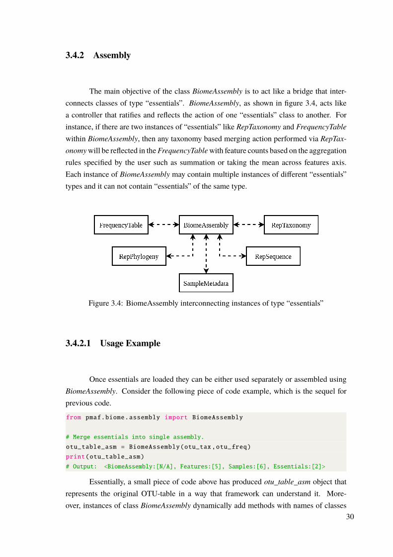
3.4.2 Assembly

The main objective of the class BiomeAssembly is to act like a bridge that inter-connects classes of type “essentials”. BiomeAssembly, as shown in figure 3.4, acts likea controller that ratifies and reflects the action of one “essentials” class to another. Forinstance, if there are two instances of “essentials” like RepTaxonomy and FrequencyTablewithin BiomeAssembly, then any taxonomy based merging action performed via RepTax-onomywill be reflected in theFrequencyTablewith feature counts based on the aggregationrules specified by the user such as summation or taking the mean across features axis.Each instance of BiomeAssembly may contain multiple instances of different “essentials”types and it can not contain “essentials” of the same type.

Figure 3.4: BiomeAssembly interconnecting instances of type “essentials”

3.4.2.1 Usage Example

Once essentials are loaded they can be either used separately or assembled usingBiomeAssembly. Consider the following piece of code example, which is the sequel forprevious code.

from pmaf.biome.assembly import BiomeAssembly

# Merge essentials into single assembly.

otu_table_asm = BiomeAssembly(otu_tax,otu_freq)

print(otu_table_asm)

# Output: <BiomeAssembly:[N/A], Features:[5], Samples:[6], Essentials:[2]>

Essentially, a small piece of code above has produced otu_table_asm object thatrepresents the original OTU-table in a way that framework can understand it. More-over, instances of class BiomeAssembly dynamically add methods with names of classes

30

of type “essentials” that internally constitute the assemblage. For instance, both “es-sentials” can now be accessed via shortcuts such as otu_table_asm.RepTaxonomy orotu_table_asm.FrequencyTable. If any instance of type “essentials” had mismatchingaxes with each other, then the assembly would have failed and produced an error. How-ever, because “essentials” were assembled successfully, it is now possible to performvarious operations like filtering, merging, and so forth. For instance, let’s merge all OTUswith the same taxonomy at the phylum level using the method of RepTaxonomy calledmerge_features_by_rank.

otu_table_asm.RepTaxonomy.merge_features_by_rank(’p’)

print(otu_table_asm)

# Output: <BiomeAssembly:[N/A], Features:[3], Samples:[6], Essentials:[2]>

As is evident from the output of otu_table_asm number of features is now reducedfrom 5 to 3. If we quickly observe original OTU-table 3.1 we can see that there are onlypresent 3 unique taxa at the phylum level. The main useful property of BiomeAssembly isthat applying any change to one of the “essentials” will reflect its action on the same axesas other “essentials”. Finally, let’s first write the merged OTU-table to the CSV file andthen see what it looks like.

# Write OTU-table to file.

otu_table_asm.write_otu_table(’data/biome/otu_table_demo_merged.csv’)

Table 3.2: Merged OTU-table. Representation of merged OTU-table file“biome/otu_table_demo_merged.csv”.

s105 s109 s908 s913 s921 s997 Taxonomy

0 11 10 0 0 0 0 k__Bacteria; p__Actinobacteria1 0 2 10 0 0 0 k__Bacteria; p__Bacteroidetes2 0 0 3 0 14 10 k__Bacteria; p__Proteobacteria

As shown in the OTU-table above (3.2) total, OTU counts are summed across thefeature axis (rows) and original identifiers are lost and replaced with new ones.

31

3.4.3 Survey

The “survey” refers to any kind of meta-analysis study that requires mergingmultiple studies into one single assembly. This is exactly what a “survey” type classdoes as shown in figure 3.5 It simply, merges multiple instances of classes with type“assembly” into one instance of type “survey”, which by itself is very similar to structureof “assembly”. The primary objective of BiomeSurvey is to execute the merging logicspecified by the user during its construction. After that, it is essentially an analogue ofBiomeAssembly and can be directly converted to an actual BiomeAssembly instance.

Figure 3.5: Merging operation using BiomeSurvey. Each input of type BiomeAssemblyrepresents different study and output is a merged survey.

3.4.3.1 Usage Example

To demonstrate usage of BiomeSurvey, at least two assemblies are required. There-fore, let’s consider another dummy OTU-table 3.3.

32

Table 3.3: A dummy OTU-table. Second dummy OTU-table file“biome/otu_table_demo2.csv”.

OTU s105 s109 s908 s921 s555 s913 Taxonomy

otu1 10 0 1 0 1 0 k__Bacteria; p__Actinobacteriaotu2 0 10 0 0 1 0 k__Bacteria; p__Bacteroidetesotu3 0 0 10 0 10 0 k__Bacteria; p__Firmicutes

Similar to the previous OTU-table loading process let’s load our second data.

from pmaf.biome.survey import BiomeSurvey

# Path to second OTU-table CSV file.

demo2_otu_table_fp = ’data/biome/otu_table_demo2.csv’

otu_tax2 = \

RepTaxonomy(demo2_otu_table_fp , index_col=0,taxonomy_columns=-1)

print(otu_tax2) # Output: <RepTaxonomy:[N/A], Features:[3]>

otu_freq2 = \

FrequencyTable(demo2_otu_table_fp , index_col=0, skipcols=-1)

print(otu_freq2) # Output: <FrequencyTable:[N/A], Features:[3], Samples:[6]>

otu_table_asm2 = BiomeAssembly(otu_tax2 ,otu_freq2)

print(otu_table_asm2)

# Output: <BiomeAssembly:[N/A], Features:[3], Samples:[6], Essentials:[2]>

Now let’s merge two different OTU-tables into a single survey and write the resultsto a CSV file.

assemblies = otu_table_asm ,otu_table_asm2

survey_study = \

BiomeSurvey(assemblies , aggfunc=’mean’, groupby=(’taxonomy’,’label’))

# Output: <BiomeSurvey:[N/A], Features:[4], Samples:[7]>

# Convert BiomeSurvey to BiomeAssembly

survey_study_asm = survey_study.to_assembly()

# Output: <BiomeAssembly:[N/A], Features:[4], Samples:[7], Essentials:[2]>

# Write OTU-table to file.

survey_study_asm.write_otu_table(’data/biome/otu_table_survey.csv’)

In the code above, aggfunc is the method of aggregation across both axes. Al-though, currently it is set to “mean” it can be customized and applied differently for eachaxis. Similarly, groupby is the parameter that dictates how to group data across differentaxes. Here, groupby=(’taxonomy’,’label’) is a Python tuple with two elements for eachaxis. First element represent grouping across feature axis by taxonomy and the secondgrouping across sample axis by sample names. Finally, the survey produces the followingaggregated OTU-table 3.4.

33

Table 3.4: Combined OTU-tables into single survey. Representation of surveyOTU-table file “biome/otu_table_survey.csv”.

s105 s109 s555 s908 s913 s921 s997 Taxonomy

0 10.5 5.0 1.0 0.5 0.0 0.0 0.0 k__Bacteria; p__Actinobacteria1 0.0 6.0 1.0 5.0 0.0 0.0 0.0 k__Bacteria; p__Bacteroidetes2 0.0 0.0 3.0 0.0 14.0 10.0 k__Bacteria; p__Proteobacteria3 0.0 0.0 10.0 10.0 0.0 0.0 k__Bacteria; p__Firmicutes

As it can be seen from the OTU-table 3.4 some values are empty because twoOTU-tables have missing samples like “s997” and “s555”, and differences in taxonomy.Such empty values can be either corrected later or considered as zeros. All other samplesand taxa which had overlaps have been merged according to the logic provided by the codeabove. BiomeAssembly is a powerful class with a flexible design that allows it to integratedifferent aggregation logics as separate functions. Therefore, even if the current state hasprimitive aggregation methods like “mean” and “sum”, different methods can be rapidlyintegrated in the future.

3.5 Module “database”

Module “database” is one of the most fundamental parts of PhyloMAF. It ismainly responsible for transforming taxonomic classification database such as Greengenes,SILVA,GTDB,RDP, and others, intomuchmore efficient data storage format. This storageformat then enables PhyloMAF to retrieve large amounts of data in a very short timeand without overloading user’s random-access memory (RAM). Essentially, the module“database” is responsible for the process commonly known as extract, transform and load(ETL) with final data storage product in hierarchical data format version 5 (HDF5) fileformat.

34

Figure 3.6: Database transformation in ETL fashion. Flow of data in “database” module.

3.5.1 Overview

Module “database” is responsible for multiple essential tasks such as the recon-struction of original reference taxonomy, transforming, analyzing, and reorganizing datalike representative sequences or phylogenetic trees into the internal storage structure.Module “database” then produce the compressed HDF580 storage file that is used in fur-ther analysis. As it was noted in the previous section, PhyloMAF can work with seventaxonomic ranks starting from domain level and ending with genera. However, most taxo-nomic classification databases do not fit into this representation except for SILVA, instead,most have species level as terminal taxonomic rank. Therefore, it is vital to standard-ize reference taxonomies to incorporate them into PhyloMAF. For instance, if referencetaxonomy (i.e. Greengenes) has species as terminal rank in its original taxonomy, thenmodule “database” will transform it and represent this taxonomy in such a way that itsterminal rank will become genera. To clarify, this transformation does not change thetaxonomy in any way but rather it agglomerates species into the respective genera accord-ing to the taxonomy of the database. Although it would be interesting to perform similartransformations based on internal phylogeny instead of using taxonomy, many databaseslack the phylogenetic tree in their repositories. Moreover, internal taxonomy ideally repre-sents the phylogeny of the reference taxonomic classification so the primary anchor of themeta-analysis approach used in PhyloMAF is the taxonomy not directly phylogeny. Usingphylogeny as a transformation method is reserved for future research.

35

Figure 3.7: Overall structure of module “database”. Directory “_parsers” and “_shared”contain no classes and only independent functions required by the module itself.

The internal code structure of the module “database” is shown in figure 3.7. Thecode in the module can be split into two parts, “builders” and “utilizers”. The “builders”is the part of code with the burden of transforming the reference database and buildingthe HDF5 storage file, while “utilizers” is the part responsible for using the storage fileand providing access to the stored data. Core classes in the directory “_core’ provideprimary functionality that gives access to the data after the storage was built. Directory“_shared” contains some code that is used by both “builders” and core classes but is notportrayed in figure 3.7. Similarly,DatabaseStorageManager is a vital class shared by both“utilizers” and “builders”, which manages the storage file by providing a low-level abstractdata access interface for every other class. The remaining code and partial classes in the“manifest” are responsible for solely the transformation and storage building process. Aspecial case is the classes in the “manifest” directory, which are the main classes that canbe directly used by the user. In other words, these classes are actual manifestations ofthe module functionality required by the specific type of classification database. Manifestclasses at the same time inherit mixin classes in “_core’ to provide necessary functionalityfrom “utilizers” and contain a set of “builders” instructions or in other words a recipeto build the storage file required for the target reference database. For instance, rawreference database Greengenes provide taxonomy, phylogeny, representative sequences,and accessions therefore respective mixin classes are inherited by DatabaseGreengenes.The actual process of raw database transformation is performed by “builders” functionswithin the manifest class, to produce proper storage file for the Greengenes database. Incontrast, fungal ITS database UNITE does not provide a phylogenetic tree so Database-UNITE does not inherit DatabasePhylogenyMixin class and lacks associated “builders”instructions. Manifest classes provide access to its “utilizers” functionality via commoninstance methods while the process of transformation and building that uses the “builders”

36

are only provided via a class method named build_database_storage. As a rule of thumb,method build_database_storage is only used once, when the database is constructed. Thisapproach makes it easy to integrate new databases in the future so that the user is onlyrequired to provide a proper recipe within a custom manifest class and the rest will simplyfit in.

3.5.2 Reconstruction of Taxonomy

The first step in database transformation is a reconstruction of taxonomy by reorga-nizing taxa into seven ranks used in PhyloMAF by producing a transformed representationof the original taxonomy as shown in figure 3.8. Primary products of reconstructionare the transformed taxonomy with novel identifiers for each taxon and the table thatmaps original identifiers to new ones. Since the data from the original database is alsokept within the final storage, this map provides a link between old and new identifiers.Within PhyloMAF identifiers that belong to original taxonomy are called reference or“refs” and identifiers associated with transformed taxonomy are called representative or“reps”. Within the internal naming convention, “refs” are known as “rid”(or “rids”) and“reps” are known as “tid”(“tids”). It is important to note that, though “rids” are associatedwith original identifiers of reference databases they are not necessarily identical. In factduring, transformation original identifiers are reindexed or renamed into integers becausesome reference databases have very long character-based identifiers, which are inefficientin terms of memory load. However, these identifiers are never lost and preserved withinthe storage files as accession numbers.

Figure 3.8: Simplified portrayal of taxonomic reconstruction

During agglomeration of original taxa into new one’s algorithm ensures that notaxon is repeated; hence, producing a non-redundant version of the original database. This

37

is crucial for the functionality of the other module that make-up PhyloMAF. It is importantto note that most of the taxonomic classification databases are redundant and many taxahave multiple duplicates with very similar but slightly different representative sequenceswithin the reference database. Similarly, duplicated taxa can be represented multiple timesin the phylogenetic tree provided by the reference database. This is compensated not bymodifying the tree during ETL but rather by a different approach, which will be explainedin the upcoming sections.

3.5.3 Storage Technicalities

Transformed database produces storage file in HDF5 format, which is essentiallyan isolated file system that can be efficiently scaled and used in the compressed state.80 TheHDF5 can be very complicated in usage and multiple Python packages can use this storageformat in its full or almost-full capacity. However, for PhyloMAF scaling of the storage fileis not necessary and once the database is transformed it can be considered immutable orfixed. To make things simpler, most of the delicate configuration complexity of an HDF5storage format can be managed by a Python package known as PyTables.81 Compared topure HDF5, PyTables does not support n-dimensional arrays but instead provides out-of-the-box label based indexing functionality. Furthermore, Pandas, which is a core packagefor the framework, provides a solid and relatively mature interface to HDF5 throughPyTables package. In summary, the previously mentioned classDatabaseStorageManageris the main abstraction layer where the actual data input/output (I/O) takes place and therest of this module is built upon it.

3.5.4 Structure of Storage File

Authors of the taxonomic classification databases provide a similar type of datain their online repositories though sometimes data can be represented in different ways.Similarly, not every reference database provides every piece of data that might be requiredin the microbiome study. To make PhyloMAF flexible and compatible with most of thereference databases that provide taxonomy, aforesaid “assemblers” process the originaldata in a certain predefined way so that DatabaseStorageManager can be more adaptive.The manager by designed provide maximum flexibility for the core base and mixin classes,which are used by “manifest” classes. In the same way, manager is designed to be most

38

restricting for the “builders”. As a consequence, to support at least most of the taxonomicclassification databases, the storage structure shown in figure 3.9 was thought-out in a waythat frequent or ideally any modifications would not be required.

Figure 3.9: Internal structure of HDF5 storage file

As shown in figure 3.9 storage file is divided into six sections or roots. Eachsection is self-describing and only contains the related data. Taxonomy data is stored in“root-taxonomy” and contains two tables “taxonomy-prior” where the original unchangedreference taxonomy is stored and “taxonomy-sheet”, which is the transformed taxonomy.Similarly, sequence data are stored in “root-sequence” and contain all original represen-tative sequences and if present alignments and accession numbers. Phylogeny data arestored in “root-tree”, which consists of three flat (not table) cells. The original unchangedphylogenetic tree in text-based Newick format is stored in “tree-prior” while the parsedtree is stored in “tree-parsed”. The parsed tree is required because some reference databaseprovides tree files that contain invalid characters and does not follow the required formatspecification by Newick format. Such files cannot be correctly read by 3rd party Pythonpackages that work with phylogenetic trees and hence, it is the responsibility of manifestclasses and “assemblers” to parse the tree and rebuild its content into a valid file format.Moreover, because original “rids” are not used for reasons described in section 3.5.2, itis the responsibility of “assemblers” to reindex tips of the phylogenetic tree and producethe final parsed version. Last but not least, “tree-object” is the binary cell that contains apickled or serialized image of the Python object with memory loaded tree. In other words,

39

it is a copy of an instance of the 3rd party Python package class responsible for workingwith phylogenetic trees. This approach of storing the tree speeds up the framework byproviding rapid loading of the pickled tree object into memory instead of re-reading “tree-parsed” whenever a phylogeny operation is requested by the user. The “root-stat” containsdata that is generated by “builders”. It consists of two tables “stat-reps” and “stat-taxs”,which contain statistical analysis results that describe “refs” and “reps”, respectively. Forexample, “stat-reps” describes representative sequences by pre-counted number of to-tal non-ambiguous and ambiguous bases, number of continuous degenerate bases, and soforth. While “stat-taxs” provide information such aswhich taxa are singletons or howmany“refs” are directly associated with the given “rep” and have a representative sequence. Twospecial sections are “root-map” and “root-metadata” so both will be described below.

The, “root-metadata” is simply the vital metadata of the storage file. It includesfour sections serving a different purpose within the storage. All the recap of the databaseis stored in “metadata-db-summary”, which contains details such as how many “refs”and “reps” are present in the storage, which of the main seven taxonomic ranks areavailable for usage, length of the shortest and longest representative sequence and so forth.Similarly, “metadata-db-stamp” contains information about the author who created thestorage file, date of creation, and similar. Two special sections are “metadata-db-history”and “metadata-db-info”. Former contains the record of the taxonomic reconstructionprocess in detail. Later or “metadata-db-info” is a basic Pandas series with boolean valuesfor every section of in every root in the figure 3.9. Each section name is a key and itsboolean state describes if it was incorporated into the storage file during creation; hence,provides the state of available data in the DatabaseStorageManager.

The unique section is “root-map” which comprises four different tables that arefrequently accessed by the “utilizers”. Two tables “map-interx-taxon” and “map-interx-repseq” are used by solely DatabaseStorageManager and are incorporated into storageat the final stage of the building process. These tables contain not many useful dataand their purpose is only to assist PyTables during indexing operations. Both tables aremade of rows, which are either “rids” or “tids” and columns that represent any sectionswithin storage that use “rids” or “tids” as indices. The name of the section is called“interx”, which stands for intermediate-index. The reason for using intermediate tablesis that PyTables, although have indexing support with internal hash maps, was found tolag without the usage of these tables. Next and one of the most important sections in thestorage database is “map-rep2tid”, which is the only table that maps “tids” to “rids”. Thistable is constructed during taxonomic reconstruction and is the most frequently accessedpiece of data by “utilizers”; hence, DatabaseStorageManager caches or loads this tableinto memory by default. The fragment of this table is shown in table 3.5. The lasttable or “map-tree” is a key-value Pandas series and represents a complete map of theparsed phylogenetic tree. After the aforesaid “tree-parsed” is formed, ideally it is passed

40

by manifest classes to make_tree_map function that can be found in “assemblers”, tomake a flat map of the tree. This function traverses the tree and produces a parent-childrelation map, which is called “map-tree”. This map is later used by “utilizers” to inferphylogenetic tree topology, which is used in other modules across PhyloMAF. Althoughit does not provide branch lengths, inferring is preferred over the common tree pruningprocess because it is much faster. The actual inferring algorithm is not described in thisthesis as it goes beyond its scope.

Table 3.5: Fragment of real “map-rep2tid” table. First column represent “rids”. Lastcolumn represent associated “tid”. Columns in the middle represent taxonomic rankswith “tids” associated with “rid”.

d k p c o f g tid

1 0 10 310 2296 593 52 1 1425 0 10 310 2296 593 52 1 1556 0 10 310 2296 593 52 1 1891 0 10 310 2296 593 52 1 11494 0 10 310 2296 593 52 1 11721 0 10 310 2296 593 52 1 11954 0 10 310 2296 593 52 1 1

3.5.5 The “builders”

As was described above, the aim of the “builders” is to transform and build thedatabase storage HDF5 file from plain text-based files of a reference taxonomic database.The term “builders” is only used in the scope of this article and merely denotes a set ofindependent Python functions that are used in the process of transformation and building.The process of the building refers to a set of “builders” instructions or recipes in themanifest class expressed via build_database_storage class method that constructs theinternal structure of the database and commits transformed data into an HDF5 file viacompositional class DatabaseStorageManager

The process of database building engraved into manifest classes in form of recipesand depends on the reference database. Manifest classes can contain custom functionsrequired to produce the final valid internal database structure. Although, such custom func-tions can also be considered as “builders”, the primary function types used in the buildingprocess can be divided into three categories: “parsers”, “assemblers”, and “summarizers”.

41

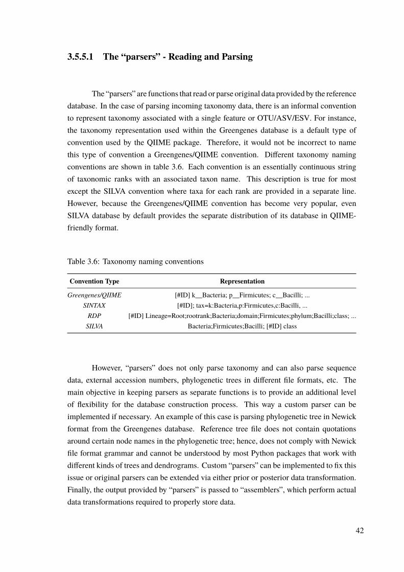
3.5.5.1 The “parsers” - Reading and Parsing

The “parsers” are functions that read or parse original data provided by the referencedatabase. In the case of parsing incoming taxonomy data, there is an informal conventionto represent taxonomy associated with a single feature or OTU/ASV/ESV. For instance,the taxonomy representation used within the Greengenes database is a default type ofconvention used by the QIIME package. Therefore, it would not be incorrect to namethis type of convention a Greengenes/QIIME convention. Different taxonomy namingconventions are shown in table 3.6. Each convention is an essentially continuous stringof taxonomic ranks with an associated taxon name. This description is true for mostexcept the SILVA convention where taxa for each rank are provided in a separate line.However, because the Greengenes/QIIME convention has become very popular, evenSILVA database by default provides the separate distribution of its database in QIIME-friendly format.

Table 3.6: Taxonomy naming conventions

Convention Type Representation

Greengenes/QIIME [#ID] k__Bacteria; p__Firmicutes; c__Bacilli; ...SINTAX [#ID]; tax=k:Bacteria,p:Firmicutes,c:Bacilli, ...RDP [#ID] Lineage=Root;rootrank;Bacteria;domain;Firmicutes;phylum;Bacilli;class; ...SILVA Bacteria;Firmicutes;Bacilli; [#ID] class

However, “parsers” does not only parse taxonomy and can also parse sequencedata, external accession numbers, phylogenetic trees in different file formats, etc. Themain objective in keeping parsers as separate functions is to provide an additional levelof flexibility for the database construction process. This way a custom parser can beimplemented if necessary. An example of this case is parsing phylogenetic tree in Newickformat from the Greengenes database. Reference tree file does not contain quotationsaround certain node names in the phylogenetic tree; hence, does not comply with Newickfile format grammar and cannot be understood by most Python packages that work withdifferent kinds of trees and dendrograms. Custom “parsers” can be implemented to fix thisissue or original parsers can be extended via either prior or posterior data transformation.Finally, the output provided by “parsers” is passed to “assemblers”, which perform actualdata transformations required to properly store data.

42

3.5.5.2 The “assemblers” - Data Transformations

After the data is parsed or read it must be transformed using either existing orcustom “assemblers” to produce final data structures that will be written into a storagefile. Similar to custom “parsers”, but more often “assemblers” are required to be extendedor customized depending on a taxonomic classification database. Data can be either pre-transformed before passing to “assemblers” or post-transformed to compensate for any dataissues that might occur during the transformation process due to differences in referencedatabases. For instance, the GTDB database provides data of two prokaryotic domainsArchaea and Bacteria in separate files. Therefore, in case if the whole database must beimplemented then it is necessary to join two datasets into a single either before or aftertransformation since in both cases it will be necessary to implement custom adjustments.

3.5.5.3 The “summarizers” - Logs and Recap

Finally, right before data is written into storage via DatabaseStorageManager allthe data transformations are logged and final datasets are analyzed to produce an overallsummary. The “overall summary” is a final recap of all stored data for easy and rapidaccess by “utilizers”. Its final storage destination is “root-metadata” and different from datastatistics, which is a part of “assemblers” with a storage destination of “root-stats”. Overallsummary, comprise the total number of taxa, number of unique taxa and duplicates, shortestand longest representative sequence, list of available taxonomic ranks in the taxonomy,and so forth. The “summarizers” generate recaps along with “assemblers” as the databaseis constructed but committed at the last step.

3.6 Module “pipe”

The module “pipe” is an extensive and well-thought-out module that providesthe main functionality required to easily construct “pipes” to allow data mining. InPhyloMAF the “pipe” module is the same as a data pipeline. Its main objective is to useone type of data to mine for other types. The type of data can be anything like taxonomy,sequence, phylogeny, accession numbers, and identifiers. The last one is the special kindof intermediate data type. Since every database, whether it is a local database such as

43

Greengenes or SILVA, or a remote database like NCBI, there are always internal identifiersused to identify any piece of data. So basically “identifier” type of data represents anidentifier used by some database. Following diagram 3.10 demonstrate a simple exampleof how the “pipe” module can mine for data.

Figure 3.10: Basic flow of data in “pipe” module

For simplicity, the intermediate “identifier” data types are not shown. However,during the real data mining process identifiers for each data type is first retrieved andonly then used to get subsequent data type. The “pipe” module has many classes eachhas a different objective and work independently. However, internally each some classes“know” how to work with other classes via the meta-class concept that was previouslydescribed. The figure 3.11 demonstrates the overall structure of the module and internalclasses. In this figure, the data types used by the “pipe” module are called “dockers”.The DockerTaxonomyMedium is a class responsible for storing taxonomy type of data.The “mediators” are classes responsible to work with databases, both remote or local.Essentially, the mediator is the primary kind of classes that provide access to the database.In contrast, “miners” comprise a single class type Miner that utilize the “mediators”. Inother words, “mediators”, mediate between the database and the Miner class.

All aforesaid classes are wrapped into a directory called “agents” since they areindeed serve as agents of the “pipe” module. The “specs” are predefined classes thatconstitute the pipeline functionality. The “specs” are specifications of pipelines thatdescribe the input data and the output data. The “factors” are simple classes that constrainthe pipeline to type of the database. For example, usage of Factor16S makes sure thatdata flowing in the pipelines are only based on 16S rRNA. Finally, the “marker” classesprovide complementary functionality that can be used to track or log the intermediate datatypes.

44

Figure 3.11: Overall structure of module “pipe”. Dashed lines represent directories andsolid lines represent classes.

3.6.1 Module “dockers”

The “dockers” are building blocks of the “pipe” module. They are used andproduced throughout the pipelines and are understood by all other classes in the “pipe”module. The instances of the “docker” class can store one or more data of the concernedtype. In other words, “docker” like DockerTaxonomyMedium can contain both single taxaassociated with a single identifier or multiple taxa associated with multiple identifiers.However, each “docker” class can also contain multiple “docker” classes of the same type.When the “docker” class does not contain elements of the same type and instead onlycontains the data it is associated with, then it is called a singleton of the “docker” type.This functionality is useful because most of the databases are usually redundant. In otherwords, a single taxon can be represented by multiple sequences or accession numbers withdifferent identifiers. Similarly, the single sequence can match multiple identifiers that areassociated with ideally closely related but different taxa.

45

3.6.2 Module “mediators”

The “mediators” are the main type of classes that are responsible for communicat-ing databases and retrieve data. The input and output data types of “mediators” are always“docker” instances. During the initialization of “mediators” proper configuration must becarried out. Both remote and local “mediators” have similar methods that can be used bytheMiner class. However, “mediators” do not necessarily have to be used viaMiner classand can be used as-is. The “mediator” classes provide following several methods for dataretrieval from connected database. To retrieve accession by identifier and search for iden-tifier by accession there are get_accession_by_identifier and get_identifier_by_accessionmethods. Similarly, for sequences there are get_sequence_by_identifier method for re-trieval and get_identifier_by_sequence method for search. Based on the same analogy,for phylogeny there are get_phylogeny_by_identifier and get_phylogeny_by_identifier, andlastly for taxonomy there are get_taxonomy_by_identifier and get_identifier_by_taxonomymethods. Each of these methods require one singleton “docker” instance and a valid“factor” instance.

Although it was stated that the “factor” is necessary to validate compatibility withdatabases, in some cases they can be used by “mediators” to mine the correct type of data.For example, Factor16Swill make sure that NCBIMediatormines only 16S data, since theNCBI database contain heterogeneous data. However, in the case of using LocalMediator,the Factor16S will check if the reference database that is being mediated is compatiblewith the “factor” type.

Despite similar methods provided by two “mediator” types, local and remote,there are clear differences in their internal organization. Firstly, the remote “mediators”are unique to the classes provided by the “remote” module and cannot mediate unrec-ognized databases. Therefore, to use the “remote” class that provides access to anyremote database, the corresponding remote “mediator” must be present. Currently, onlyNCBIMediator is present. This rigid class compatibility organization is compulsory be-cause every remote database has a very unique internal structure, internal data types,and application programming interfaces (APIs). However, local mediators are differentand much more flexible in usage. Since PhyloMAF requires every local database tobe pre-processed before usage into an HDF5 file format, they can be used in a muchmore simple way. The LocalMediator is not a class but a function that makes the classon the fly. Thanks to Python’s special type function, it is possible to generate classesduring runtime. The LocalMediator function takes only a single mandatory parameterdatabase, which corresponds to any database instance that inherits the basic meta-typeof the “database” module DatabaseBackboneMetabase. Then the function checks whichkind of data the database contains, and builds a local “mediator” class using mixin classes

46

like MediatorLocalAccessionMixin, MediatorLocalPhylogenyMixin, MediatorLocalTax-onomyMixin and MediatorLocalSequenceMixin. For example, if the target database isGreengenes, then all mixin classes will be used. However, if the target database is UNITEthen MediatorLocalPhylogenyMixin mixin class will be skipped.

3.6.3 Module “miners”

The module “miners” is essentially made of a single class Miner that requiresboth a valid “mediator” instance and a compatible “factor” instance to be initialized. Ifa “factor” is not compatible with the mediator then it will produce an error and willnot initialize. The Miner provide methods such as yield_accession_by_identifier oryield_sequence_by_identifier to retrieve a docker by identifier. Similarly, it provides asingle method yield_identifier_by_docker to retrieve identifiers by any docker. Moreover,compared to “mediators” the Miner allows mining for data using any “docker” instanceand not just singletons.

3.6.4 Module “specs”

The “specs” are not essential parts of the “pipe” module but they make the usagemuch more comfortable. The “specs” stands for specifications and are self-explanatoryin the way that they specify the collection of actions. Instead of using “dockers” with“miners” or even “mediators”, it is possible to work with “specs” in a much simplerway. Specification classes essentially describe the pipe by enforcing its inlet and outlets.Following figure 3.12 demonstrates the taxonomy to sequence pipeline specification usingboth primitive and composite “specs”.

Figure 3.12: Taxonomy-to-sequence pipeline specification

47

The primitive “specs” are self-explanatory, while composites are usually the com-bination of the primitive “specs”. In cases when there is no predefined composite “spec”then it is possible to use the ForgeSpec function to forge or compose a new specificationfrom primitives. However, when a more complicated specification is desired then thefunction ForgeSpec might not be enough. For example, SpecTSBP and SpecTSPBP areexamples of more complex specifications. Former, SpecTSBP specification uses taxon-omy to retrieve sequence alignments and then constructs a de-novo phylogenetic tree usingspecified, tree builder like FastTree.71 However, the second specification SpecTSPBP firstuses taxonomy to retrieves the phylogenetic tree topology inferred from the reference treein a database along with sequence alignments. Then it optimizes branch lengths of thetree using branch estimators like FastTree71 or ERaBLE.72

3.7 Wrapper Modules

Modules “sequence”, “phylo”, and “alignment” are essentially wrapper modules.These modules use other Python packages to provide the required functionality. The“sequence” module wraps “scikit-bio” package and provides three classes Nucleotide,MultiSequence and MultiSequenceStream. Each of these classes is recognized by otherPhyloMAFmodules and provides the basic functionality required to work with sequences.The Nucleotide class represents any single DNA or RNA sequence, can parse or writeFASTAfiles, andmore. TheMultiSequence andMultiSequenceStream are similarmodulesthat are used to work with multiple sequences. These classes can store both unalignedor aligned sequences. The former class essentially stores multiple Nucleotide classes torepresent multiple sequences of the same kind. Latter orMultiSequenceStream, is similarto the former but can work with a larger number of sequences and do not store data in theRAM and instead use PyTables81 with a simple HDF5 file structure to store sequences inthe hard drive.

The “phylo” module primarily wraps Python package ETE382 that works withphylogenomic data. The main class that provides functionality to work with phylogenetictrees is PhyloTree. However, the module also provides two other types of wrapper classescalled “branch estimators” and “tree builders”. The “branch estimators” are classes thatwrap external tools like FastTree271 or ERaBLE.72 These tools take as input Newickformatted tree topology and either sequence alignment or its Hamming distance matrixand produce branched phylogenetic tree on fixed topology. Tree builders are tools likeFastTree2,71 which are used to construct a de-novo tree from sequence alignment. Bothtype of classes simply takes required input data, and if necessary transform it, write to the

48

files, execute the tools, read the output, and returns the results. The “alignment” module isanother wrapper module that currently only provides single class MultiSequenceAligner.This class provides an alignmethod that is used to align sequences. Although any type ofsequence aligner can be configured, there is only one predefined aligner currently present,ClustalW283

Module “remote” is a wrapper module responsible for working with differentremote databases via API interface. For instance, NCBI provides a programmatic web in-terface called Entrez Global Query Cross-Database Search System (Entrez). Similarly, theEuropean Bioinformatics Institute (EBI) provides a web-based representational state trans-fer (REST) API service that can be to programmatically access the Ensembl database. The“remote” module is basically, the wrapper classes that provide the minimum functionalityrequired to access these databases. Currently, only the Entrez wrapper class is availableEntrez which wraps the popular “BioPython” Python package’s Entrez functionality.84

49

CHAPTER 4

MATERIALS AND METHODS

To recap data requirements for our mGWAS research we need D. melanogaster’sgenotype data andmicrobial profiles as our phenotype. In our analysis, we usemicrobiomedatasets of DGRP lines from credible research papers as sources for mGWAS phenotypedata. Similarly, we use publicly available DGRP host-variant datasets as target genotypesfor mGWAS.

4.1 Sample Collection

As it was described in section 1.6 the Drosophila animal model has many benefitsin microbiota studies as a model organism. Particularly for mGWAS studies, there is a veryuseful and unique library of approximately 200 inbred D. melanogaster lines collectedfrom a single population in Raleigh, North Carolina, USA. The benefits of using inbredfruit fly lines are hidden in its genome. Repeated full-sibling inbreeding over at least 20generations produces a highly homozygous genotype.85 From the research perspective,such homozygosity results in the fixation of SNPs and sets a common ground for manyindependent studies that use the same samples. For D. Melanogaster there is a publiclyavailable library known as DGRP. The online public repository contains all the genotypedata required for performing mGWAS like annotated variant calls files, per lineWolbachiainfection states, and much more.85

Our target samples used in this thesis are DGRP lines without any particularselection criteria except the presence of the microbiota data. Based on the literaturereview for microbiota studies on DGRP lines with available supplementary data, it waspossible to find two research papers, which are shown in the following table 4.1.

50

Table 4.1: Sources for 16S microbiota data

Dataset LabelUnique

DGRP LinesLibrary Size

Raw/QCReads

OTU-Table Reference

Chaston 79 669 705 No Yes (30)Jehrke 4 2 263 280 Yes No (39)

Available DGRP lines with corresponding data source are shown in the followingtable 4.1. Among 79 and 4 DGRP lines from Chaston and Jehrke data source, no sharedlines were detected.

Table 4.2: DGRP lines by source

DGRP Source DGRP Source DGRP Source DGRP Source26 Chaston 319 Chaston 441 Chaston 808 Chaston28 Chaston 321 Chaston 443 Chaston 810 Chaston45 Chaston 332 Chaston 486 Chaston 819 Chaston59 Chaston 340 Chaston 492 Chaston 837 Chaston73 Chaston 350 Chaston 513 Chaston 843 Chaston83 Chaston 352 Chaston 514 Chaston 849 Chaston85 Chaston 358 Chaston 554 Chaston 850 Chaston105 Chaston 360 Chaston 563 Chaston 852 Chaston109 Chaston 367 Chaston 584 Chaston 855 Chaston149 Chaston 371 Chaston 642 Chaston 857 Chaston161 Chaston 374 Chaston 712 Chaston 859 Jehrke176 Chaston 377 Chaston 737 Chaston 861 Chaston181 Chaston 380 Chaston 738 Chaston 879 Chaston195 Chaston 385 Chaston 750 Chaston 882 Chaston235 Chaston 393 Chaston 771 Chaston 884 Chaston237 Chaston 398 Chaston 776 Chaston 897 Chaston272 Chaston 399 Chaston 783 Chaston 900 Chaston301 Jehrke 409 Chaston 787 Chaston 907 Chaston303 Jehrke 426 Chaston 796 Chaston 908 Chaston304 Chaston 427 Chaston 801 Chaston 913 Chaston315 Jehrke 440 Chaston 805 Chaston

51

4.2 Overall Strategy

The principal objective of this study is finding and describing genetic associationsthat can affect the microbiota composition. Considering the types of available source data,missing components, target phenotypes, GWAS approach, and more, the total analysisworkflow is relatively complicated but can be represented in several overall work steps.The overall strategy for data analysis is shown in figure 4.1 and can be split into six stages.

Figure 4.1: Overall data workflow

To perform GWAS two types of data are necessary: phenotype and genotype data.WithD. melanogaster as a model organism and DGRP lines as samples, the genotype datais obtained from an online DGRP repository. Target phenotype data used in this thesis arealpha and beta bio-diversity estimates. To calculate sample alpha-diversity metrics onlyan OTU-table is required, while for UniFrac based beta-diversity calculations additionalphylogenetic tree is necessary. In either case, it is impossible to directly perform bio-diversity analysis due to the missing OTU-table from Jehrke data source. Therefore, theobtained raw microbiome data for the Jehrke dataset is first processed via the QIIME2pipeline to produce the OTU-table. Then, two OTU-tables from two independent studiesare merged using PhyloMAF and preprocessed for quality control (QC). The GWAS isthen performed using ready phenotype-genotype data with subsequent association analysisthat produces annotated most significant SNPs. Finally, these SNPs are further analyzedusing regression models for selected specific phenotypes. Lastly, the literature review isperformed for identified candidate genes and conclusions are stated.

52

4.3 Data Acquisition

There are two types of data required to acquire. First is primarily microbiota datafrom table 4.2, which is used to derive phenotypes. The other is genotype along withadditional data required in GWAS analysis.

4.3.1 Microbiota Data

Authors of the Chaston dataset provide a raw OTU-table produced using micro-biome analysis pipeline QIIME 1 against 97 %ID Greengenes reference database. TheOTU-table was obtained from supplementary files of the paper.30 However, Jehrke et al.39

used an online microbiome analysis pipeline MG-RAST,86 which does not provide thefinal OTU-table. Instead, MG-RAST provides partially quality-controlled reads availableon the public repository. Moreover, MG-RAST provides an API for batch fetching of theavailable data. Therefore, a collection of Bash scripts were used to fetch 16S rRNA readsof 4 DGRP lines from the Jehrke dataset.

4.3.1.1 Batch Data Fetching from MG-RAST

To batch fetch the QC reads using theMG-RASTAPI, it is necessary to retrieve fullsample metadata manually from MG-RAST online https://www.mg-rast.org. Keywordsused in the search were “Heinrich Heine University Duesseldorf” with initial filteringfor “Mathias Beller”. Secondary filters were “project_name”=’Basal_Microbiome’ and“env_package_name” NOT LIKE ’%axenic%’ AND "env_package_name" NOT LIKE’%L3%’. Obtained metadata was manually adjusted by removing unnecessary datacolumns and the final table is shown on A.10. Then using the following Bash scriptall the FASTQ reads of DGRP lines from the Jehrke dataset were batch downloaded fromMG-RAST servers.

sample_fp="../Step 1 - Sample Selection/SampleMetadata.csv"

i=1

while IFS=, read -r sample_name DGRP_Line sample_id metagenome_id

library_name other_cols

do

53

test $i -eq 1 && ((i=i+1)) && continue

mkdir $sample_id

wget -O $sample_id/$library_name.fastq http://api.mg-rast.org/

download/$metagenome_id?file=050.1

done < "$sample_fp"

4.3.2 Genotype Data

As previously described, the gold standard tool for GWAS analysis is Plink.38

Therefore, the required genotype data is in Plink compatible file formats. All the necessaryfiles for GWAS analysis are shown in the following table 4.3

Table 4.3: Genotype and other host genomic data required for GWAS

Data Type Variables/Columns File Type Reference

Genotype

Raw Variant Data 4 438 427 VCF

85,87

Plink Genotype Data 4 438 427 BEDPlink Sample Metadata 6 FAMPlink Variant Metadata 6 BIM

Annotations Variant Annotations 4 438 427 CSVCovariates Inversion Status 16 CSV

Wolbachia Status 1 CSV

All the data were manually downloaded from DGRP web-page http://dgrp2.gnets.ncsu.edu

4.4 Data Preparation

This section consists of data analysis steps required to generate OTU-table forJehrke dataset. Overall pipeline is shown in flowing diagram 4.2.

54

Figure 4.2: Overall QIIME2 pipeline for processing of Jehrke dataset

The 16S rRNA sequence data processing pipeline used is QIIME2 with the Green-genes database. Following Bash script was used to download the Greengenes databaseand create QIIME 2 classifier.

# Download

wget -O ./gg_13_8_otus.tar.gz "ftp://greengenes.microbio.me/

greengenes_release/gg_13_5/gg_13_8_otus.tar.gz"

# Extract Archive

tar -xzvf gg_13_8_otus.tar.gz gg_13_8_otus/taxonomy/97_otu_taxonomy.txt

gg_13_8_otus/rep_set/97_otus.fasta gg_13_8_otus/trees/97

_otus_unannotated.tree

# Create QIIME2 Greengenes classifier

source ~/miniconda3/etc/profile.d/conda.sh

conda activate qiime2

gg_root="../Step 3 - Download Greengenes/gg_13_8_otus"

forward_primer="CCTACGGGNGGCWGCAG"

reverse_primer="GACTACHVGGGTATCTAATCC"

qiime tools import --type ’FeatureData[Sequence]’ --input-path "

$gg_root/rep_set/97_otus.fasta" --output-path ref-seq-97.qza

qiime tools import --type ’FeatureData[Taxonomy]’ --input-format

HeaderlessTSVTaxonomyFormat --input-path "$gg_root/taxonomy/97

_otu_taxonomy.txt" --output-path ref-tax-97.qza

qiime feature-classifier extract-reads --i-sequences ref-seq-97.qza --p

-f-primer $forward_primer --p-r-primer $reverse_primer --o-reads

ref-seq-97-pf.qza

55

qiime feature-classifier fit-classifier -naive-bayes --i-reference -reads

ref-seq-97-pf.qza --i-reference -taxonomy ref-tax-97.qza --o-

classifier gg-97-pf-classifier.qza

Primers used for amplification of 16S rRNA reads in the Jehrke et al. study arefor V3 and V4 regions. Forward and reverse primers were CCTACGGGNGGCWGCAGand GACTACHVGGGTATCTAATCC, respectively. Although retrieved sequences werepartially quality controlled, primer oligomers were present in downloaded sequences.Hence, the following Bash script was used to trim leading 5’ forward primer sequencesand low-quality scores. The reverse 3’ primer sequences were not found in the samplereads after checking using “fuzznuc” tool from EMBOSS suite.88

sample_fp="../Step 1 - Sample Selection/SampleMetadata.csv"

samples_root="../Step 2 - Download Raw Data"

i=1

while IFS=, read -r sample_name DGRP_Line sample_id metagenome_id

library_name other_cols

do

test $i -eq 1 && ((i=i+1)) && continue

echo $"sample_name\n"

if [[ "$sample_id" =~ ^(mgs623312|mgs623315|mgs623321|mgs623351)$ ]];

then

croplen=22

else

croplen=18

fi

mkdir "$sample_id"

trimmomatic SE -phred33 -trimlog "$sample_id/trimming_results.txt" "

$samples_root/$sample_id/$library_name.fastq" "$sample_id/

$library_name.qf.fastq" HEADCROP:$croplen LEADING:30 TRAILING:30

SLIDINGWINDOW:4:15 MINLEN:36

done < "$sample_fp"

Next quality controlled raw sequences were imported into single QIIME 2 artifactfile.

#!/bin/bash

eval "$(conda shell.bash hook)"

conda activate qiime2

study_name="jehkre_basal"

sample_fp="../Step 1 - Sample Selection/SampleMetadata.csv"

samples_root="../Step 5 - Trim Primers from Raw Data"

i=1

echo "sample-id,absolute -filepath ,direction" > "$study_name -manifest.

txt"

56

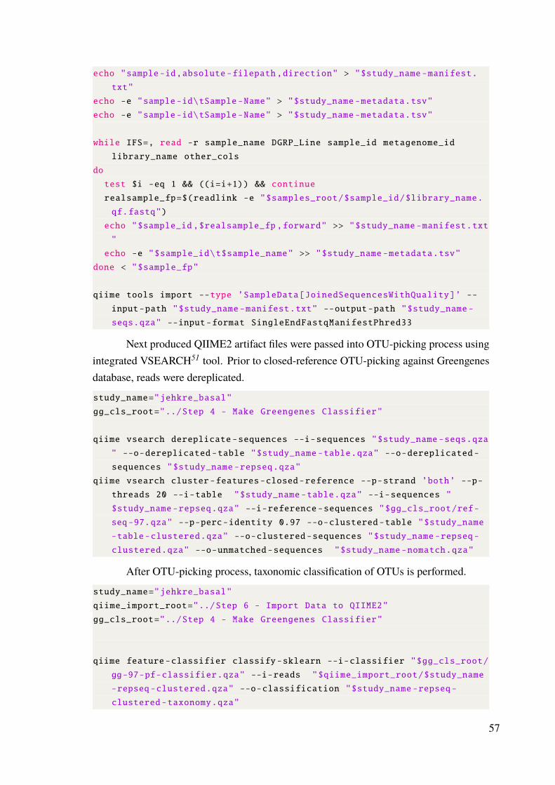
echo "sample-id,absolute -filepath ,direction" > "$study_name -manifest.

txt"

echo -e "sample-id\tSample-Name" > "$study_name -metadata.tsv"

echo -e "sample-id\tSample-Name" > "$study_name -metadata.tsv"

while IFS=, read -r sample_name DGRP_Line sample_id metagenome_id

library_name other_cols

do

test $i -eq 1 && ((i=i+1)) && continue

realsample_fp=$(readlink -e "$samples_root/$sample_id/$library_name.

qf.fastq")

echo "$sample_id ,$realsample_fp ,forward" >> "$study_name -manifest.txt

"

echo -e "$sample_id\t$sample_name" >> "$study_name -metadata.tsv"

done < "$sample_fp"

qiime tools import --type ’SampleData[JoinedSequencesWithQuality]’ --

input-path "$study_name -manifest.txt" --output-path "$study_name -

seqs.qza" --input-format SingleEndFastqManifestPhred33

Next produced QIIME2 artifact files were passed into OTU-picking process usingintegrated VSEARCH51 tool. Prior to closed-reference OTU-picking against Greengenesdatabase, reads were dereplicated.

study_name="jehkre_basal"

gg_cls_root="../Step 4 - Make Greengenes Classifier"

qiime vsearch dereplicate -sequences --i-sequences "$study_name -seqs.qza

" --o-dereplicated -table "$study_name -table.qza" --o-dereplicated -

sequences "$study_name -repseq.qza"

qiime vsearch cluster-features-closed-reference --p-strand ’both’ --p-

threads 20 --i-table "$study_name -table.qza" --i-sequences "

$study_name -repseq.qza" --i-reference -sequences "$gg_cls_root/ref-

seq-97.qza" --p-perc-identity 0.97 --o-clustered -table "$study_name

-table-clustered.qza" --o-clustered -sequences "$study_name -repseq-

clustered.qza" --o-unmatched -sequences "$study_name -nomatch.qza"

After OTU-picking process, taxonomic classification of OTUs is performed.

study_name="jehkre_basal"

qiime_import_root="../Step 6 - Import Data to QIIME2"

gg_cls_root="../Step 4 - Make Greengenes Classifier"

qiime feature-classifier classify-sklearn --i-classifier "$gg_cls_root/

gg-97-pf-classifier.qza" --i-reads "$qiime_import_root/$study_name

-repseq-clustered.qza" --o-classification "$study_name -repseq-

clustered -taxonomy.qza"

57

Finally, the OTU-table is produced from QIIME2 artifacts generated by taxonomyassignment and OTU-picking processes. Initially, artifacts are converted into BIOM fileand then into CSV file. Then, taxonomy column is added to OTU count table and finalOTU-table for Jehrke dataset is produced (tables A.7 and A.8).

study_name="jehkre_basal"

sample_fp="../Step 1 - Sample Selection/SampleMetadata.csv"

qiime_import_root="../Step 6 - Import Data to QIIME2"

qiime_classified_root="../Step 7 - Classification"

qiime tools export --input-path "$qiime_import_root/$study_name -table-

clustered.qza" --output-path .

qiime tools export --input-path "$qiime_classified_root/$study_name -

repseq-clustered -taxonomy.qza" --output-path .

biom add-metadata -i feature-table.biom -o feature-table.tax.biom --

observation -metadata-fp taxonomy.tsv --sc-separated Taxon --

observation -header "Feature ID,Taxon,Confidence"

biom convert -i feature-table.tax.biom -o otu-table.tsv --header-key

Taxon --to-tsv

4.5 Data Processing

Data processing can be split into two primary stages. First is sample rearrangement,where OTU-tables are split into four separate datasets. This step is followed by theprocessing of OTU-tables using PhyloMAF for QC, merging, and more.

4.5.1 Sample Rearrangement

The main motivation behind rearranging samples into four datasets is to test theperformance of the merging operations done by using PhyloMAF. Sample rearrangementessentially consists of randomly splitting the Chaston dataset into two separate datasets(Dataset1 and Dataset2) and one whole dataset (Dataset3) as shown in the following table4.4. The last dataset (Dataset4) consists of both Chaston and Jehrke samples. BothDataset3 and Dataset4 are produced using PhyloMAF by merging partial datasets.

58

Table 4.4: Final rearranged sample datasets

New Dataset Label SecondarySource Label Source Dataset Label Number of Sampes

Dataset1 Chaston1 Chaston 40Dataset2 Chaston2 Chaston 39Dataset3 Chaston_Asm Chaston 79Dataset4 CJ_Survey Chaston + Jehrke 83

4.5.2 Merging OTU-Tables and Quality Control

With two partial Chaston datasets and Jehrke OTU-table, PhyloMAF is used tomerge and quality filter datasets to produce the final state as shown in the table 4.4. Thefirst part of the flow diagram for data processing is shown in figure 4.3.

Figure 4.3: Overall process of OTU-table merging and quality control

The following sections describe this data flow in more detail.

59

4.5.2.1 Creating Greengenes HDF5 storage file

First and foremost, it is necessary to create a reference database compatible withPhyloMAF. Therefore, raw text-based Greengenes database is transformed into an HDF5file using class method DatabaseGreengenes.build_database_storage as shown in thefollowing piece of code.

from pmaf.database import DatabaseGreengenes

ROOT = ’MasterThesisData/’

ROOT_GG = ROOT + ’Greengenes/gg_13_8_otus/’

greengenes_hdf5_fp = ROOT + ’greengenes_138_97.hdf5’

DatabaseGreengenes.build_database_storage(storage_hdf5_fp =

greengenes_hdf5_fp ,

taxonomy_map_csv_fp = ROOT_GG + ’/taxonomy/97_otu_taxonomy.txt’,

tree_newick_fp = ROOT_GG + ’/trees/97_otus_unannotated.tree’,

sequence_fasta_fp = ROOT_GG + ’/rep_set/97_otus.fasta’,

sequence_alignment_fasta_fp = ROOT_GG + ’/rep_set_aligned/97_otus.fasta

’,

stamp_dict={’author’:’Farid MUSA’},

force = True,

compress=True)

database_gg = DatabaseGreengenes(greengenes_hdf5_fp)

While the creation of the HDF5 based database file can take some time it is a isone-time task that can be indefinitely used later.

4.5.2.2 Reading OTU-tables into PhyloMAF

Next as shown in figure 4.3 the CSV-based OTU-tables must be read using the“biome.essentials” module’s FrequencyTable and RepTaxonomy classes. Because OTU-tables contain both OTU counts and OTU taxonomy columns, two types of data are parsedseparately using the corresponding class.

60

from pmaf.biome import essentials

chaston1_otus_fp = ROOT + "OTU_Tables/Chaston/chaston_set1.csv"

chaston2_otus_fp = ROOT + "OTU_Tables/Chaston/chaston_set2.csv"

jehrke_otus_fp = ROOT + "OTU_Tables/Jehrke/jehrke-otu-table.tsv"

jehrke_metadata_fp = ROOT + "OTU_Tables/Jehrke/jehrke-sample-metadata.

csv"

chaston1_tax_inc = essentials.RepTaxonomy(chaston1_otus_fp , index_col

=0,taxonomy_columns=-1)

chaston1_freq = essentials.FrequencyTable(chaston1_otus_fp , index_col

=0, skipcols=-1)

chaston2_tax_inc = essentials.RepTaxonomy(chaston2_otus_fp , index_col

=0,taxonomy_columns=-1)

chaston2_freq = essentials.FrequencyTable(chaston2_otus_fp , index_col

=0, skipcols=-1)

jehrke_tax = essentials.RepTaxonomy(jehrke_otus_fp , index_col=0,

taxonomy_columns=-1,sep=’\t’)

jehrke_freq = essentials.FrequencyTable(jehrke_otus_fp , index_col=0,

skipcols=-1,sep=’\t’)

jehrke_meta = essentials.SampleMetadata(jehrke_metadata_fp , axis=0,

index_col=’sample_id’)

In the above, the first line imports the “essentials” sub-module from the “biome”module of the PhyloMAF package. As it was previously described, “essentials” are thebasic blocks of data that can be assembled into an “assembly”. Each starting OTU-table(Dataset1, Dataset2, and Jehrke) is processed using similar commands to parse OTUcounts and taxonomies. In each read command line, index_col=0 indicates that the firstcolumn of the table is an index column. The class RepTaxonomy, requires only taxonomydata so parameter taxonomy_columns=-1 sets the last column of the CSV/TSV file as thetarget column to be read. Likewise, for FrequencyTable, parameter skipcols=-1 sets thelast column to be ignored because it does not contain count data. In the Jehrke dataset,SampleMetadata is also defined because OTU-table produced via QIIME2 contains morethan one sample per the DGRP line. Therefore, sample metadata from table A.10 is laterused to aggregate duplicated samples like male and female flies of the same DGRP line.

61

4.5.2.3 Complement Incomplete Taxonomy

Datasets derived from Chaston data sources have incomplete taxonomy providedin the supplementary files. Consequently, Dataset1 and Dataset2 do not contain taxonomyinformation about levels above class level. Therefore, it is necessary to “complement”the missing taxonomy up to the highest level available in the database(kingdom in theGreengenes database). The “pipe”module of the PhyloMAFpackage contains a predefinedmediator configuration that can be used to complement the taxonomy against the referencedatabase.

from pmaf.pipe.specs import SpecTI,SpecIT,ForgeSpec

from pmaf.pipe.agents.mediators.local import LocalMediator

from pmaf.pipe.factors import Factor16S

mediator_gg_comp = LocalMediator(database_gg ,tax_fuzzy_mode=True,

tax_corr_method=’complement’)

f16s = Factor16S()

SpecTIT = ForgeSpec(’SpecTIT’, SpecTI,SpecIT)

stit = SpecTIT(mediator_gg_comp , f16s)

chaston1_tax = essentials.RepTaxonomy(stit.fetch(chaston1_tax_inc.data)

.to_dataframe())

chaston2_tax = essentials.RepTaxonomy(stit.fetch(chaston2_tax_inc.data)

.to_dataframe())

First 3 lines of code imports the required classes from PhyloMAF, such as basicpipes(specification), mediators, and factors. Two specifications, SpecTI and SpecIT, arepredefined “pipes” that do exactly the reverse of each other. The pipe SpecTI takes as inputa taxonomy and produces the reference database identifiers. Similarly, SpecIT takes as aninput a reference database identifier and produces the associated reference taxonomy. Thecombination of two pipes is used as a special pipe to “complement” or reassign taxonomy.This special pipe specification takes and produces a taxonomy. The function ForgeSpec isused to join the pipes and forge a new pipe, which is the taxonomy complementing pipe.The Factor16S is the simple class that is required by default for any piping operations. Theclass does not have any operational effect except that it is used to validate compatibilitybetween interconnected modules. For instance, Factor16S restricts the overall usage ofthe 16S type databases like Greengenes and not like UNITE.

In PhyloMAF, “pipes” always require themediators to communicatewith databases.Mediators can have different configurations and in the above code, LocalMediator is con-figured to match the target taxonomy to the reference taxonomy with a fuzzy approach.The reason for fuzzy matching instead of exact matching is the possible difference be-

62

tween target and reference taxonomies caused by manual author fixes or database versionvariations. Moreover, the LocalMediator is not an actual mediator class, instead, it isa function that automatically builds a valid mediator based “database” class inheritancespatterns. Lastly, themediator’s parameter tax_corr_method=’complement’ is not amanda-tory setting and instead is a predefined “smart” matching algorithm that is simply betterat “complementing” the taxonomy compared to default mode.

4.5.2.4 Group Essentials into Assembly

Prior to final merging of OTU-tables, there are few additional steps required to do.

from pmaf.biome import assembly

chaston1_asm = assembly.BiomeAssembly(chaston1_tax , chaston1_freq)

chaston2_asm = assembly.BiomeAssembly(chaston2_tax , chaston2_freq)

jehrke_asm = assembly.BiomeAssembly(jehrke_tax , jehrke_freq ,

jehrke_meta ,curb=jehrke_meta)

jehrke_asm.SampleMetadata.merge_samples_by_variable(’DGRP_Line’)

The code above first imports the “assembly” sub-module from the “biome” mod-ule. Following, two lines build an assembly from FrequencyTable and RepTaxonomyinstances. In other words, chaston1_asm and chaston2_asm are BiomeAssembly instancesthat represent a PhyloMAF version of an original OTU-table with a taxonomy column.Similarly, but with an additional component the Jehrke dataset also includes SampleMeta-data within “assembly”. Finally, as it was previously noted, DGRP samples that belong tothe same line are aggregated by taking the mean of counts across samples. To elaborate,first BiomeAssembly builds an OTU-table plus SampleMetadata configuration, where inaddition to the feature axis also sample axis is interconnected. Then, an instance methodmerge_samples_by_variable aggregates sample counts based on the “DGRP_Line” col-umn of table A.10.

4.5.2.5 Quality Control

Finally, after the assemblies are ready, quality control with the subsequent mergingof OTU-tables is performed. In the code bellow, QC is done before actual merging toproduce Dataset3 and Dataset4. However, to clarify an important point, the order does

63

not have any particular importance and data can also be first merged and then qualitycontrolled. Nevertheless, final datasets must pass the same QC processes as it is done inthe following code.

chaston1_asm.RepTaxonomy.drop_features_without_taxa()

chaston2_asm.RepTaxonomy.drop_features_without_taxa()

jehrke_asm.RepTaxonomy.drop_features_without_taxa()

chaston1_asm.RepTaxonomy.merge_duplicated_features()

chaston2_asm.RepTaxonomy.merge_duplicated_features()

jehrke_asm.RepTaxonomy.merge_duplicated_features()

chaston1_asm.RepTaxonomy.drop_features_without_ranks([’g’])

chaston2_asm.RepTaxonomy.drop_features_without_ranks([’g’])

jehrke_asm.RepTaxonomy.drop_features_without_ranks([’g’])

chaston1_asm.RepTaxonomy.merge_features_by_rank(’g’)

chaston2_asm.RepTaxonomy.merge_features_by_rank(’g’)

jehrke_asm.RepTaxonomy.merge_features_by_rank(’g’)

chaston1_asm_wolbachia_id = chaston1_asm.RepTaxonomy.

find_features_by_pattern(’Wolbachia’)

chaston1_asm.RepTaxonomy.drop_feature_by_id(chaston1_asm_wolbachia_id)

chaston2_asm_wolbachia_id = chaston2_asm.RepTaxonomy.

find_features_by_pattern(’Wolbachia’)

chaston2_asm.RepTaxonomy.drop_feature_by_id(chaston2_asm_wolbachia_id)

jehrke_asm_wolbachia_id = jehrke_asm.RepTaxonomy.

find_features_by_pattern(’Wolbachia’)

jehrke_asm.RepTaxonomy.drop_feature_by_id(jehrke_asm_wolbachia_id)

First, datasets are stripped off the OTUs that do not have any representative tax-onomies. Then duplicate OTUs are aggregated using the default sum approach that simplyadds together counts across features. Next, any OTU that does not have genus taxa likeOTUs that were classified only up-to family or class level are removed. Finally, any OTUswith Wolbachia taxon are removed from the analysis. The primary cause for removingWolbachia is because this microorganism is an endosymbiont and is not a part of naturalflymicrobiota. Moreover,Wolbachia counts are not negligible and can significantly distortthe final alpha and beta diversity estimates.

4.5.2.6 Merging OTU-Tables

Finally, after QC, OTU-tables can be merged to produce Dataset3 and Dataset4.

64

from pmaf.biome import survey

chaston_asm = survey.BiomeSurvey(chaston1_asm ,

chaston2_asm ,groupby=(’taxonomy’,’label’),

aggfunc=(’sum’,’mean’)).to_assembly()

cj_survey = survey.BiomeSurvey(chaston_asm ,

jehrke_asm ,groupby=(’taxonomy’,’label’),

aggfunc=(’sum’,’mean’)).to_assembly()

First merging operation, BiomeSurvey produces Dataset3, while second generatesDataset4. Both use grouping setup groupby=(’taxonomy’,’label’), which configure merg-ing to group the OTU or feature axis based on taxonomy, while sample labels groupthe sample axis. Similarly, aggfunc=(’sum’,’mean’) configures merger to aggregate thefeature axis by adding across feature counts and take count means across the sample axis.As it is shown in table A.9, no DGRP line is shared among datasets so aggregation acrossthe sample axis is simply not performed. Finally, both of the BiomeSurvey instances arepromptly converted into BiomeAssembly using the to_assembly. The overall change in thenumber of features during QC and after merging is shown in table 4.5.

Table 4.5: Change in the number of OTUs during and after quality control

Dataset Label# OTUs

Prior Quality Control# OTUs

Post-Aggregations# OTUs

Post-Removals

Dataset1 177 72 48Dataset2 177 72 48Dataset3 177 72 48Dataset4 870 242 151

Lastly, in the above table 4.5, it is clear that Dataset4 has a significantly highernumber of OTUs compared to the other three datasets. This is caused due to the dramaticdifference in the library sizes of Jehrke and Chaston datasets, with 2,263,280 and 669,705reads, respectively. Therefore, the OTU-table of Dataset4 is a sparse matrix, which willhave a dramatic effect on bio-diversity estimates that give more weight to rare taxa.

65

4.5.2.7 Reconstructing Phylogenetic Trees

After all the datasets from table 4.4 are prepared, the last missing component,which is required for bio-diversity analysis is the phylogenetic trees. The whole processof reconstruction of phylogenetic trees is shown in flow diagram 4.4.

Figure 4.4: Process of phylogenetic tree reconstruction. Whole process is repeated forevery dataset.

Following piece of PhyloMAF code is the implementation of the above dia-gram(4.4) that generates branched phylogenetic trees based on tree topology of referencedatabase.

from pmaf.pipe.specs import SpecTSPBP

from pmaf.phylo.branchest import BranchestFastTree2

mediator_gg_map = LocalMediator(database_gg ,

tax_fuzzy_mode = True,

tax_fuzzy_cutoff = 95,

seq_method = ’consensus’,

seq_filter_method = ’random’,

seq_filter_value=5,

seq_subs = True)

tspbp_fasttree2 = SpecTSPBP(mediator_gg_map ,

66

f16s,

branch_estimator = BranchestFastTree2())

datasets = {’chaston1’: chaston1_asm ,

’chaston2’: chaston2_asm ,

"chaston_asm": chaston_asm ,

"cj_survey": cj_survey}

rank = ’g’

for biome_asm_name , biome_asm in datasets.items():

tmp_biome_asm = biome_asm.copy()

tmp_biome_asm.RepTaxonomy.merge_features_by_rank(rank, aggfunc=’sum’)

tmp_tree_docker = tspbp_fasttree2.fetch(tmp_biome_asm.RepTaxonomy.

data)

tmp_phylo = essentials.RepPhylogeny(tmp_tree_docker.get_tree(),

annotation = tmp_biome_asm.RepTaxonomy.get_lineage_by_id())

tmp_biome_asm = assembly.BiomeAssembly(tmp_biome_asm.essentials + [

tmp_phylo], curb=’intersect’, copy=True)

tmp_biome_asm.RepPhylogeny.write(ROOT + ’OutputFinal/noWolbachia

/{}-{}.{}.tre’.format(biome_asm_name ,rank,"fasttree2_adj"),rooted=

True)

tmp_biome_asm.write_otu_table(ROOT + ’OutputFinal/noWolbachia

/{}-{}.{}.csv’.format(biome_asm_name ,rank,"fasttree2_adj"))

The above code once more begins with imports of the required classes fromPhyloMAF. Then followed by instantiation of LocalMediator that will be used to maptarget and reference taxonomies with subsequent extraction of phylogenetic tree topologyand representative sequences. Parameters tax_fuzzy_mode = True and tax_fuzzy_cutoff= 95, configure the fuzzy matching algorithm to active mode and limits the matchingratio to 95 %. Since PhyloMAF clusters feature of reference database and produce anon-redundant version of the original taxonomy database, each unique reference taxonis represented with more than one reference sequence. For example, there is always agood chance that any genus within the reference database has many (i.e. thousands)reference/representative sequences. Nevertheless, the branch estimators require only asingle representative sequence for each feature. Therefore, the mediator is configuredwith parameter seq_method = ’consensus’, which produces a consensus sequence out ofmultiple sequence alignment of representative sequences for each feature. Moreover, sincethe Greengenes database has also alignments along with representative sequences, thisprocess is relatively fast. However, due to numerous representative sequences that emergedue to parameter seq_subs = True, the time to evaluate the consensus sequence increases

67

substantially. To address this problem we set two additional parameters seq_filter_method= ’random’ and seq_filter_value=5. These parameters configure the mediator to randomlyselect 5 representative sequences out of all available, instead of retrieving the whole set. Inother words, for each target taxon that will be mapped to the reference taxon, get 5 randomsequences from potentially thousands available, retrieve reference alignment, evaluate theconsensus sequence, and produce the output.

The actual “pipe” specification that is used for phylogenetic tree reconstructionis SpecTSPBP, which stands for Taxonomy-Sequence-Phylogeny-BranchedPhylogeny. Itis a predefined specification that maps taxa, retrieves representative sequence(consensusof random reference alignments) along with reference phylogenetic tree topology, andestimates the length of branches for the tree topology. The branch estimator used inthe above code is BranchestFastTree2. This simple PhyloMAF wrapper class utilizesthe external FastTree2 tool with default branch estimation configuration based on thelikelihood approach. Generated phylogenetic trees are shown in Appendix C

4.6 Bio-Diversity Analysis

Bio-diversity analysis consists of investigating within sample alpha-diversity met-rics and between sample phylogenetic beta-diversity estimates. Simultaneously, basic andspecified OTU abundance of analysis of the samples and datasets are visualized for furtherdiscussions. Following figure 4.5 recaps the whole diversity analysis process.

Figure 4.5: Bio-diversity analysis workflow. Bio-diversity analysis is performed in Rusing mainly the microbiome analysis package “phyloseq”.

68

4.6.1 Alpha-Diversity

Alpha-diversity analysis is performed using the most commonly used microbiomeanalysis package in R called “phyloseq”.89 Estimated alpha-diversity measures are the totalnumber of observed OTUs (presence/absence), Shannon, and Simpson evenness indices.As shown in figure 4.5, the last two evenness indices are used as target phenotypes for mG-WAS analysis. Two R functions provided by the “phyloseq” package, estimate_richnessand plot_richness, are used for calculating and plotting the alpha-diversity metrics. More-over, the alpha-diversity estimates are also visualized using the “ggplot2” package90 toproduce box plots.

4.6.2 Beta-Diversity

As it was previously stated, phylogenetic beta-diversity metrics outperform otherbetween sample community analysis methods. Therefore, for beta-diversity analysis, theUniFrac distance metric was used. Although there is a weighted and unweighted versionof the UniFrac distance metric, only weighted is used in the analysis. The primary reasonfor not using the unweighted version is due to the large difference in library sizes inthe two studies. Unweighted UniFrac is sensitive to rare taxa and can contribute to theartificial distance between samples from two independent studies as shown in figure C.15.Furthermore, investigation of the effect of rare taxa on mGWAS is outside the scopeof our interest. Therefore, with the main focus on the weighted version of the UniFracmetric, the actual analysis was performed using theUniFrac function from the “phyloseq”package89 in R. However, the resulting beta-diversity distance matrix can not be directlyinterpreted and require the usage of ordination methods to analyze. Although principalcomponent analysis (PCA) is a common ordination method, it can only be used for analysisof Euclidean distance matrices. The UniFrac distance metric produces a non-Euclideandissimilarity matrix from a sparse OTU-table and requires ordination techniques such asMDS(PCoA) or NMDS. In this thesis, MDS is chosen as the main ordination methodusing the built-in R function cmdscale. Out of three dimensions calculated by MDS,the first two are used to produce Cartesian MDS plots using “ggplot2” R package.90 TheMDS plots can be found in Appendix C. Finally, the first dimension that captures the mostvariance is used as the third phenotype in mGWAS analysis.

69

4.6.3 Abundance Analysis

Abundance analysis was performed for every dataset sample wise and as wholedatasets. Relative abundance plots were generated for both phylum and genus levels. Tovisualize and compare relative abundance values per dataset, sample abundances withindatasets were aggregated by taking the mean of the counts. Relative abundance plotsfor every dataset can be found in appendix C. Relative abundance analysis dataset-wisewas performed for both phylum and genus levels. Next, total genus-level abundance plotswere produced for the most abundant phyla with removed singletons and any taxa withtotal abundance less than 3 across at least 20% of the samples. Community analysis wasperformed using the “phyloseq” package in R.89 Visualizations were produced using theR package “ggplot2”.90

4.6.4 Secondary Analysis

In addition to the primary analysis described in the previous sections, additionalanalysis and supplementary visualizations were produced. First, as shown in figure 4.5,correlation plots were generated for alpha and beta diversity estimates that were selected asphenotype. Pairwise correlation visualization between estimated alpha-diversity metricsand first dimension of MDS, was performed using the “GGally” package in R. Correlationanalysis was performed to explain the MDS1 produced by MDS analysis. Unlike PCA,the MDS does not generate any loadings that can give a descriptive hint on the PCs.

Besides, circular phylogenetic treeswere visualized using theRpackage “ggtree”.91

All the visualized trees can be found in Appendix C. Finally, for future directions, the effectof Wolbachia status on the total abundance of the most dominant phyla was investigatedand visualized using the same tools used in the previous section.

4.7 Microbiome GWAS

Initially, GWAS was performed using a public online DGRP service available athttp://dgrp2.gnets.ncsu.edu. The results of this initial GWAS was then used as a basis toconfigure and optimizemanual GWAS. The authors of the DGRP service87 use the Python-based GWAS tool FastLMM79 instead of traditional Plink38 software. Furthermore, due

70

to the non-normal distribution of the alpha-diversity and beta-diversity estimates, linearand logistic regression models provided by Plink would not be appropriate in our analysis.Consequently, FastLMMwas used to perform GWAS because it is based on mixed modelsand can handle non-normal data, used by DGRP authors, compatible with initial basisGWAS analysis, and has rapid execution time compared to other similar available toolsin the literature. Lastly, as it was previously explained, Plink is a gold standard tool forGWAS and many other similar tools use or at least compatible with Plink style file types.FastLMM is not an exception so data preparation steps described in the following sectionsprimarily consist of transforming data into Plink file types.

4.7.1 Phenotype Data

As shown in figure 4.5 the phenotypes used in GWAS are Shannon, Simpson, andthe first dimension of MDS analysis. The primary motivation for using Shannon andSimpson indices as the phenotype is because the former can detect the evenness of thesample abundance profiles while the latter is sensitive to dominant taxa and may providea hint on further analysis. The last phenotype is the first dimension of MDS which isused to detect the possible effect of phylogeny on significant associations. The phenotypedata produced in section 4.6 is generated as a CSV file type and has the per-line format“DGRP-Line, Phenotype-Value” without a header. To transform the phenotype data intoPlink style, the Bash script RunDatasetGwas (table H.2) is executed for every dataset. Allthe phenotype data can be found in appendix B.

4.7.2 Covariate Data

The covariates are independent variables similar to genotype data and may havea significant contribution to the regression model. Therefore, it is important to includecovariates into the GWAS process by supplying covariates to FastLMM as it is donein the primary script that runs GWAS, RunFastLMM (table H.2). However, as can beseen from table 4.3, DGRP provides multiple potentially covariate datasets. To reconcilewith the basis GWAS results produced via DGRP online service, it was decided to usethe same covariates as DGRP authors. Therefore, the following variables were used ascovariates in GWAS: theWolbachia infection status and fivemajor chromosome inversionsIn(2L)t, In(2R)NS, In(3R)K, In(3R)P, and In(3R)Mo. However, the six selected covariates

71

shown in table H.1 are represented as categorical variables and can not be used directlyby FastLMM, so it is necessary to transform categorical variables into binary format.To satisfy this requirement Plink provides –dummy-coding feature to dummy encodescategorical variables into binary format.

4.7.3 Genotype Data

The genotype data from table 4.3 is directly downloaded in Plink format from theDGRP web-page. Therefore, additional processing of the variant data was not performedon BED, BIM and FAM files. Although the VCF file is not required by FastLMM, whichuses directly BED file, it was nevertheless downloaded since it will be necessary forpost-GWAS analysis.

4.7.4 Analysis of Associations

The overall process for analysis of associations identified by GWAS is shown inthe following figure 4.6

Figure 4.6: Overall workflow of GWAS analysis

72

The cutoff shown in the above figure 4.6 is essentially the significance cutoff appliedto theManhattan plots shown in Appendix D. The cutoff is performed viaParseGwasAssocscript from table H.2. After the cutoff operation the most significant associations or topassociations, which can be found in appendix E, are concatenated using the full outerjoin approach. These tables are produced by ParseGwasAll script from table H.2 thatproduces a table with rows as SNPs of from top associations of all datasets and columnsare phenotypes per dataset. The overlap association tables can be found in Appendix F.Moreover, the overlap table was also annotated using an annotation file from table 4.3,which is based on Flybase92 release version 5.49. Any SNPwith no known gene annotationwasmarked as “Undefined”. Finally, the annotated overlap table was gene-wise aggregatedto produce per gene table of top associations. During aggregations, the lowest p-valuewas selected out of SNPs that were represented by the same gene annotation. Finally,both SNP and gene-based overlap tables were visualized using Venn diagrams producedby R package called “ggVennDiagram” and an UpSet diagram produced by “UpSetR” Rpackage.93 The R script that produced diagrams is MakeVennDiagrams from table H.2.These diagrams are also shown in appendix F.

4.8 Post-GWAS Analysis

After GWAS is completed and top variant associations are identified for all datasetsand phenotypes, it is now necessary to investigate the effect of specific phenotypes such astotal taxon abundance values. The primary motivation here is to investigate the secondaryassociations by regressing the top preliminary GWAS variants against the most abundanttaxa. Following diagram 4.7 summarize the whole post-GWAS process.

73

Figure 4.7: Overall workflow of post-GWAS analysis

4.8.1 Explanatory Variables

Compared to GWAS analysis using FastLMM it is aimless to analyze all genotypedata in the post-GWAS analysis. Therefore, the top SNPs associations that have passed thesignificance cutoff for all datasets and phenotypes can be found in Appendix B. In total 103SNPs (henceforth “candidate SNPs”) were used in the regression model as independentvariables. The subset of the original VCF file of DGRP genotype data was extracted using“VCFtools”.94 Similarly, to covariate encoding described previously, the VCF file alsocontains categorical values that require to be encoded. To do this dummy coding wasmanually designed and automatically performed in the script RunGlmAnalysis from tableH.2.

4.8.2 Covariates

Covariates are similar to explanatory or independent variables andmust be includedin the regression model if significant correlation with response variables are detected. Thescript RunGlmAnalysis from table H.2 was designed as shown in figure 4.7 to test andselect covariates with the most significant associations. The process first performs a

74

standard linear regression of dependent variables against potential covariate variables(table H.1) and then checks the significance values for each variable. Those variables thatare significantly associated (? < 0.05) are selected as covariates (table G.1) and used infurther analysis.

4.8.3 Response Variables

By examining the results of abundance analysis performed in section 4.6, it wasfound that the most abundant phyla are Firmicutes and Proteobacteria, while the mostabundant genera are Lactobacillus and Acetobacter. These taxa with different taxonomicranks were selected as target phenotype or response variables to be investigated in thepost-GWAS regression analysis. Besides, Comamonas was the second most abundantgenus in Proteobacteria phylum so it was also included in the analysis. Moreover, todouble-check the GWAS and post-GWAS associations, previous phenotypes, Simpsonand Shannon estimates, were re-analyzed. Lastly, the beta-diversity phenotype was notinvestigated in the post-GWAS analysis due to its significant correlation with alpha-diversity estimates. In other words, MDS1 fromMDSofweightedUniFrac distancematrixessentially captured all the variance associated with mainly alpha-diversity estimatesand not the actual phylogeny, which was the primary interest. To sum up, two mostabundant phyla Firmicutes and Proteobacteria with two corresponding most abundantgenera Lactobacillus and Acetobacter, one second most abundant genus Comamonas andtwo original alpha-diversity Simpson and Shannon estimates were selected as dependentvariables (phenotype) in the post-GWAS regression model.

4.8.3.1 Normalization

Total abundance counts for taxa selected as dependent variables have a Poissondistribution, which can not be directly used in linear regression analysis. Therefore, itwas decided to first normalize the distributions using “bestNormalize” R package, whichautomatically tests several normalization techniques and selects the best method. Thenormalization results of all datasets for every response variable are shown in figure G.1in form of histograms. Moreover, the automatically selected normalization methods bythe “bestNormalize” package are shown in table G.2. The Shapiro-Wilk test results ofnormalized response variables are shown in the following table 4.6, while results for

75

original non-normal variables are shown in table G.3. From the table below it is clearthat most variables were successfully normalized except a few that have ? < 0.05, whichmeans that some variables were significantly different from Gaussian distribution.

Table 4.6: Significance p-values of Shapiro–Wilk test for normalized response variablesused in post-GWAS anaylsis

Dataset3(79) Dataset4(83) Dataset1(40) Dataset2(39)Shannon 0.0911 0.032 0.8281 0.221Simpson 0.0405 0.0596 0.1043 1

Lactobacillus 0.9998 0.9998 0.9984 0.9984Acetobacter 0.9265 0.9188 0.0179 0.7467Comamonas 1 0 0.3067 0.0031Firmicutes 0.9999 0.9999 0.2294 0.1151

Proteobacteria 0.6362 0.2807 0.007 0.2895

4.8.4 Regression Model

The R provides several techniques to perform regression analysis but the mostcommon method is simple linear regression or lm function. However, as it was previouslystated the linear regression on non-normally distributed data can produce unreliable results.Hence, based on a few values from table 4.6 it was decided not to use linear regressionsand instead use a regression-based on the generalized linear model (GLM) for the post-GWAS. The GLM is a flexible version of the linear regression model that allows usageof distribution models other than normal Gaussian. The script RunGlmAnalysis fromtable H.2 performs GLM regression analysis for every dataset and response variableper 103 SNPs in a triple loop, where it attempts to normalize the responsive variableusing the “bestNormalize” package, tests the potential covariates, and selects the mostsignificantly associated ones. Also, the RunGlmAnalysis script produces several outputsthat are processed separately later.

76

4.8.5 Analysis of Associations (GLM)

After the post-GWAS analysis is complete, the results are processed using ThePython script MakeGwasGlmTables from table H.2 parses both overlap tables from priormGWAS and outputs of post-GWAS analysis by producing single Excel tables whereproducts of two GWAS analysis were concatenated across an axis that represent candidateSNPs.

4.8.6 Candidate Gene Analysis

Among all candidate SNPs associated with gene annotations, few genes wereselected based on Venn or UpSet93 diagrams and were further investigated by reviewingthe literature for related studies. These selected genes henceforth are called “candidategenes”. Significance results for these candidate genes from post-GWAS analysis and priormGWAS analysis are visualized in Appendix G on table G.4. Finally, table G.5 sets outsignificance levels of the former p-value table in G.4. The significance levels are definedseparately for results of mGWAS and post-GWAS analysis. Particularly, the significancelevels for former mGWAS analysis using FastLMM are defined as ∗ ∗ ∗ < 5G10−7 <

∗∗ < 5G10−6 < ∗ < 5G10−5, while levels for the latter analysis using GLM are defined as∗ ∗ ∗ < 5G10−4 < ∗∗ < 5G10−3 < ∗ < 5G10−2.

77

CHAPTER 5

RESULTS AND DISCUSSION

The microbiota of the Drosophila is known to be dominated by Firmicutes andProteobacteria phyla.33 According to figure 5.1 datasets analyzed in this study also demon-strated the expected profile with the two most dominant phyla Firmicutes and Proteobac-teria.

Figure 5.1: Relative phylum abundance per datasets.. Low abundant taxa were removedto improve visibility. See section 4.6 for details.

Similarly, based on relative abundance values per dataset in figure 5.2, the twomostabundant genus are Lactobacillus and Acetobacter, while the second most abundant taxonis Comamonas. For the total abundance, see the plot on figure C.9 from Appendix C. Dueto difference in library sizes, four samples from the Jehrke data source have significantlycontributed to the Dataset4 OTU counts.

78

Figure 5.2: Relative genus abundance per datasets. Low abundant taxa were removed toimprove visibility. See section 4.6 for details.

By further inspecting the total dataset abundance plot for the most dominant phylain figure 5.3, genera contribution per phylum can be observed. From both figures 5.2and 5.3, it is clear that overall Acetobacter is the most abundant genus across all datasets.However, compared to Lactobacillus theAcetobacter is not the only dominant genuswithinthe associated phylum. Whereas, within Firmicutes the genus Lactobacillus seems to bethe only dominant taxon essentially being almost the only contributor to the phylum.

Figure 5.3: Overall total abundance plot per datasets by most abundant phylum. Lowabundant taxa were removed to improve visibility. See section 4.6 for details.

79

The alpha-diversity estimates shown in figure 5.4, indicate very similar evennessvalues. Without a statistically significant(? > 0.05) difference between datasets, it isnot possible to have confidence in differentiating datasets based on evenness metrics.However, the slight variations are is still present among datasets shown in figures 5.4 andC.16 (appendix C). This difference in alpha-diversity is detected by mGWAS analysisand further investigated in post-GWAS to identify statistically significant differences inabundance values.

Figure 5.4: Richness box plots per datasets. Alpha-diversity richness box plot perdataset. (Diamonds indicate mean values.)

It is also important to state that Dataset2 has the lowest Shannon and Simpsonestimates according to figure 5.4. Simultaneously, based on figure 5.4 it can be seenthat Acetobacter is the most dominant genus in Dataset2, while Lactobacillus is thesecond most dominant genus. Moreover, based on figure 5.2 it is clear that Dataset1 andDataset2 have very similar total abundances of Acetobacter genus and slightly differentComamonas from Proteobacteria phylum. However, based on the same figure 5.3, thegenus Lactobacillus has a difference in abundances between Dataset1 and Dataset2. Thenagain, referring back to alpha-diversity estimates in figure 5.4, it is clear that Dataset1and Dataset2 have differences in Simpson estimates. Because alpha-diversity estimateswere calculated on genera abundance values, there should be causal genus counts forthis variation. The difference is unlikely to be caused by Comamonas, and not causedby Acetobacter. Therefore, it is safe to say that Simpson phenotype related associationsthat might be identified by mGWAS could be associated with Lactobacillus abundance.

80

Notably, it seems that the decrease in total abundance of Lactobacillus genus confides theoverall within sample dominance to the Acetobacter genus from Proteobacteria phylum.This indirectly causes the Simpson dominance index to increase and decrease the actualSimpson evenness estimate as shown on figure 5.4.

As it was previously described, the beta-diversity analysis produces MDS ordina-tion plots as shown in figure 5.5 for Dataset4 and all remaining in appendix C.

Figure 5.5: Ordination plot for Dataset4(83). Multidimensional scaling of weightedUniFrac distance matrix based on OTU-table of Dataset4(83).

According to the two-dimensional ordination plot (5.5), the first dimension ofMDS captures more than 60% of the original variance of OTU counts. It is important tostress that when using weighted UniFrac distance metric the samples from two Jehrke datasources concordantly coalesce with samples from the Chaston source, which has a muchsmaller library size. This is not the case when using the unweighted UniFrac as shown infigure C.15 in appendix C. Therefore, weighted UniFrac is more suitable as a beta-diversityphenotype. To explain the MDS1 of the MDS analysis the correlation plot was producedto inspect linear correlations with alpha-diversity estimates. Following figure 5.6 is acorrelation plot for Dataset4. The remaining figures can be found in appendix C.

81

Figure 5.6: Interdependence between bio-diversity measures for Dataset4(83).

According to figure 5.6 the MDS1 has a significant linear dependence on bothShannon and Simpson estimates. This indicates that approximately 60% variance capturedby MDS is mainly associated with alpha-diversity rather than phylogeny.

Following figure 5.7 demonstrates intersects among candidate genes for eachdataset and its phenotype. The analogous UpSet plot for candidate SNPs along withseparate Venn diagrams for every phenotype can be found in Appendix F. The UpSet andVenn diagrams were generated based on table F.1, which for its part is based on table F.2from Appendix F.

82

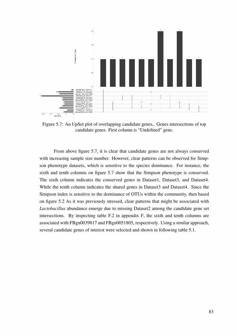
Figure 5.7: An UpSet plot of overlapping candidate genes.. Genes intersections of topcandidate genes. First column is “Undefined” gene.

From above figure 5.7, it is clear that candidate genes are not always conservedwith increasing sample size number. However, clear patterns can be observed for Simp-son phenotype datasets, which is sensitive to the species dominance. For instance, thesixth and tenth columns on figure 5.7 show that the Simpson phenotype is conserved.The sixth column indicates the conserved genes in Dataset1, Dataset3, and Dataset4.While the tenth column indicates the shared genes in Dataset3 and Dataset4. Since theSimpson index is sensitive to the dominance of OTUs within the community, then basedon figure 5.2 As it was previously stressed, clear patterns that might be associated withLactobacillus abundance emerge due to missing Dataset2 among the candidate gene setintersections. By inspecting table F.2 in appendix F, the sixth and tenth columns areassociated with FBgn0039817 and FBgn0051805, respectively. Using a similar approach,several candidate genes of interest were selected and shown in following table 5.1.

83

Table 5.1: Candidate genes with prospect of further analysis

Column Gene SNPs Phenotype D1 D2 D3 D4

6 FBgn0039817 3R_26926653_SNP Simpson y n y y10 FBgn0051805 2L_16898786_SNP Simpson n n y y9 FBgn0259241 X_10902990_SNP Shannon n n y y9 FBgn0029939 X_7038830_SNP Shannon n n y y11 FBgn0259173 3L_7145588_SNP wUF-MDS1 n n y y

2 FBgn0011746 2R_4961519_DELShannon n n y ySimpson n n y y

From above table 5.1, the gene FBgn0259173, which is associated with weightedUniFrac based MDS1, was excluded for future analysis. The reason for exclusion is due tothe necessity of a different post-GWAS analysis approach for this gene that will be statedin the final concluding section. Nevertheless, the post-GWAS analysis includes all thecandidate SNPs, and the exclusion merely indicates “not focusing” in further investigation.Similarly, but for different reasons, gene FBgn0029939 was excluded from further analysisbecause the GLM regression model discarded the genotype profile of the related SNP inthe post-GWAS analysis. The SNP with label X_7038830_SNP happened to have hassolely homogeneous sample genotypes within any of the four datasets. In other words,for each dataset, this SNP has either a set of solely missing and homologous genotypesor missing and heterozygous genotypes. Therefore, the regression model discarded theestimatorwhere all independent variables consist of are eithermissing values or categoricalvariables with a single level. Lastly, the variant 2R_4961519_DEL, which is associatedwith gene FBgn0011746, was excluded from further analysis due to missing gene ontologyand supporting papers in the literature. Therefore, further analysis is only focused on genes:FBgn0039817, FBgn0259241, and FBgn0051805. Following table 5.2 summarizes theliterature review of selected candidate genes of interest.

84

Table 5.2: Summary for candidate genes of interest. Source of annotations is FlyBaseversion FB2020_06

Gene FBgn0039817 FBgn0259241 FBgn0051805

Number of SNPs 1 1 1

GOAnnotations

MolecularFunction

-scavenger receptor

activity andpolysaccharide binding

-

BiologicalProcess

Transmembranetransport

immune responseresponse tostimulus

CellularComponent

Integral componentof membrane

- -

Associated Function Folate transport Immune responseInvolved in

wound healingHomologousHuman Gene

SLC46A1 SBSPON -

Associated DiseasesFolate (Vitamin B9)

malabsorptionInflammatoryBowel Disease

-

SuspectedPhenotype

Lactobacillus,Proteobacteria,Firmicutes

Proteobacteria -

JustificationSuspected phyla arelinked to de-novofolate production

Associated withenteric infectionsand gut disease

-

Supporting Papers (95–99) (100–102) -

From the above table 5.2, based on the FlyBase92 database, the gene FBgn0039817has the human homologous gene SLC46A1, both of which are associated with folate trans-port. Accordingly, the mutations in this gene are found to be associated with folate malab-sorption. A folate is a natural form of vitamin B9, an essential vitamin for all animals withan important role in cell growth and metabolism. In humans, folate deficiency is linkedto many health problems ranging from pregnancy-associated birth defects to neurologicalbrain diseases.97 In D. melanogaster, folate deficiency was found to be associated withslower development and worse fitness.95 The primary cause for stressing the importanceof folate is because it is not produced by the human body or D. melanogaster, and insteadit is naturally synthesized by microorganisms associated with gut microbiota. Moreover,both Firmicutes and Proteobacteria are primary phyla known to be linked to de-novo fo-late production.96 Besides, the genus Lactobacillus is a probiotic bacteria associated withvitamin production including folate.98 Therefore, all things considered, it would not be

85

absurd to presume that the aforementioned taxa are associated with folate malabsorptionor deficiency. To support the conjecture following table 5.3 summarizes the phenotypesignificance levels from both FastLMM/GWAS and GLM/post-GWAS analysis results.

Table 5.3: Overall GWAS and post-GWAS analysis results for candidate geneFBgn0039817. For complete table of candidate genes see table G.5 and G.4

Dataset1(40) Dataset2(39) Dataset3(79) Dataset4(83)

FastLMMShannon *Simpson ** ** *

GLM

Shannon *** *** ***Simpson *** *** ***

Lactobacillus *Acetobacter * *ComamonasFirmicutes * *

Proteobacteria *** * *** **

According to the results from above table 5.3, it is clear that Proteobacteria is signif-icantly associated with the variant 3R_26926653_SNP of gene FBgn0259241 in Dataset1,Dataset2, and Dataset4. In other words, statistically, the Null hypothesis is rejected, whichis stating that the sample genotype profile and abundance values of Proteobacteria withinthe datasets are from the same population. Namely, based on defined significance levels,there is high confidence that the samples with genotype 3R_26926653_SNP of the geneFBgn0259241 are significantly associated with abundance profiles of Proteobacteria phy-lum in aforesaid datasets. This finding supports the hypothesis of this thesis. To coverevery aspect, neither genus Lactobacillus nor phylum Firmicutes were not significantlyassociated with high confidence like Proteobacteria does. Based on the previous exegesisover the alpha-diversity and abundance results, the lower total abundance of Lactobacil-lus could be the main cause of low confidence associated with the Lactobacillus andFirmicutes phenotype in Dataset2 and high confidence association with Proteobacteriaphenotype in the remaining datasets in table 5.3. However, to investigate the issue further,it is necessary to have more significance confidence, which is not possible with the currentoverall sample size. Therefore, with current data, it is not unreasonable to conclude thatthe phylum Proteobacteria could be linked to folate malabsorption.

In the same manner, from table 5.2 gene FBgn0259241 was found to be associatedwith the gut disease. Particularly, the human homologous gene SBSPON or somatomedin

86

B and thrombospondin type 1 domain-containing was found to be associated with Crohn’sDisease (CD) in theAshkenazi Jewish population.101 Further, the literature review revealedthat phylum Proteobacteria and particularly Comamonas genus was associated with col-orectal cancer (CRC) and inflammatory bowel disease (IBD) such as CD.100 However,the post-GWAS analysis did not find any significant associations with the Comamonasgenus as is shown in below table 5.4. Instead, a highly confident significant associationwith genus Acetobacter was found. Although, no human studies associated with Aceto-bacter genus and gut disease was found, studies on D. melanogaster disclosed interestingfindings. It was found that both Lactobacillus and Acetobacter are linked to immunedeficiency (IMD), which is interesting since based on table 5.2 the gene of interest isassociated with an immune response function.

Table 5.4: Overall GWAS and post-GWAS analysis results for candidate geneFBgn0259241. For complete table of candidate genes see table G.5 and G.4

Dataset1(40) Dataset2(39) Dataset3(79) Dataset4(83)

FastLMMShannon ** **Simpson

GLM

Shannon * * *** ***Simpson * * ** ***

Lactobacillus * * *Acetobacter * ** ** **ComamonasFirmicutes * *

Proteobacteria * ** ***

Finally, the literature review for gene FBgn0051805 did not reveal any microbiotastudies. The overall significance results for this gene can be found in table G.5 in appendixG. Lastly, it is important to note that, though endosymbiontWolbachiawere excluded fromanalysis, it was found to have a profound effect on remaining microbiota composition as itis shown in the figure below 5.8.

87

Figure 5.8: The effect of endosymbiontWolbachia on microbiota

Moreover, the status of Wolbachia as a covariate in the post-GWAS analysis wasfound to have a highly negative regression coefficient and not infrequently had a significantassociation with the phenotype. In a few words, it is interesting to note that endosymbioticbacteria including Wolbachia could have a direct or indirect role in folate synthesis.95

88

CHAPTER 6

CONCLUSION AND FUTURE DIRECTIONS

In this thesis, host-microbiome interactions of D. melanogaster model organismswere investigated. The literature was surveyed for microbiota studies with DGRP sam-ples based on the 16S rRNA marker gene region. The problems of the meta-analysiswere addressed to use the sample data produced by independent studies, using differentsequencing technology and computational data analysis methods. Merging and data pro-cessing was performed using the novel microbiome meta-analysis framework PhyloMAFthat was developed to address shortcomings of the microbiome meta-analysis. Mergingand rearrangement of source datasets were followed by quality control and phylogenetictree reconstruction. The OTU-tables of four target datasets along with phylogenetic treeswere analyzed using alpha-diversity and beta-diversity metrics. Two Shannon and Simp-son alpha diversity indices and the first dimension of MDS based on weighted UniFracbeta-diversity distance metric were used as target phenotypes in mGWAS analysis usingthe FastLMM tool. The mGWAS identified multiple SNPs per dataset and per phenotype,which were filtered, annotated, and further analyzed. Top variant associations calledcandidate SNPs were used as the explanatory variables and further investigated in post-GWAS analysis using GLM regression models. Several specific phenotypes like genusand phylum abundance values were used as response variables in regression analysis.Among genes related to candidate SNPs, few candidate genes were selected for in-depthanalysis. The gene FBgn0039817, which is associated with folate transport, was found tobe significantly associated with the Simpson index in mGWAS analysis and the abundanceof phylum Proteobacteria. Besides, based on the literature review the latter was foundto be associated with de-novo folate synthesis. Similarly, the gene FBgn0259241 wasfound to be involved with an immune response in D. melanogaster, and its human homol-ogous gene was found to be associated with IBD. The post-GWAS analysis for this genefound a significant association with Proteobacteria and Acetobacter. The latter was alsofound to be associated with IBD in the fruit fly. In conclusion, two genes FBgn0039817and FBgn0259241 of D. melanogaster were found associated with microbiota and linkedto folate malabsorption and gut disease, respectively. Further, the meticulous analysiswas performed to rationalize the phenotype associations and provide the basis for furtherstudies.

The primary limiting factor of this research is the low sample size. Therefore, in

89

the future, using more samples from different independent studies will be useful to validatethe results. Moreover, endosymbiontWolbachiawas found to have significant associationswith candidate SNPs and has a substantial effect on microbiota profiles. Moreover, thepossibility that endosymbiont bacteria could play a role in folate synthesis makes it avery interesting subject to investigate. Therefore, further GWAS research with a focuson Wolbachia could reveal interesting discoveries. Lastly, due to the difference in librarysizes of data sources, the effect of rare taxa was not investigated in this study. Integrationof OTU-table normalization methods in PhyloMAF could address this issue.

90

REFERENCES

(1) Pollock, J., Glendinning, L., Wisedchanwet, T., and Watson, M. (2018). The Mad-ness of Microbiome: Attempting To Find Consensus “Best Practice” for 16SMicrobiome Studies. Applied and Environmental Microbiology 84, ed. by Liu,S.-J., e02627–17, /aem/84/7/e02627–17.atom.

(2) Awany, D., Allali, I., Dalvie, S., Hemmings, S., Mwaikono, K. S., Thomford,N. E., Gomez, A., Mulder, N., and Chimusa, E. R. (2019). Host and MicrobiomeGenome-Wide Association Studies: Current State and Challenges. Frontiers inGenetics 9, 637.

(3) Jovel, J., Patterson, J., Wang, W., Hotte, N., O’Keefe, S., Mitchel, T., Perry, T.,Kao, D., Mason, A. L., Madsen, K. L., and Wong, G. K.-S. (2016). Characteri-zation of the Gut Microbiome Using 16S or Shotgun Metagenomics. Frontiers inMicrobiology 7, DOI: 10.3389/fmicb.2016.00459.

(4) Wooley, J. C., Godzik, A., and Friedberg, I. (2010). A Primer on Metagenomics.PLoS Computational Biology 6, ed. by Bourne, P. E., e1000667.

(5) Sonnenburg, J. L., Xu, J., Leip, D. D., Chen, C.-H., Westover, B. P., Weatherford,J., Buhler, J. D., and Gordon, J. I. (2005). Glycan Foraging in Vivo by an Intestine-Adapted Bacterial Symbiont. Science (New York, N.Y.) 307, 1955–1959.

(6) Bercik, P., Collins, S. M., and Verdu, E. F. (2012). Microbes and the Gut-BrainAxis:Microbiota-Gut-BrainAxis.Neurogastroenterology&Motility 24, 405–413.

(7) Weissbrod, O., Rothschild, D., Barkan, E., and Segal, E. (2018). Host Genetics andMicrobiome Associations through the Lens of GenomeWide Association Studies.Current Opinion in Microbiology 44, 9–19.

(8) Zheng, P. et al. (2016). Gut Microbiome Remodeling Induces Depressive-likeBehaviors through a Pathway Mediated by the Host’s Metabolism. MolecularPsychiatry 21, 786–796.

(9) Vailati-Riboni, M., Palombo, V., and Loor, J. J. In Periparturient Diseases ofDairy Cows, Ametaj, B. N., Ed.; Springer International Publishing: Cham, 2017,pp 1–7.

(10) Marchesi, J. R., and Ravel, J. (2015). The Vocabulary of Microbiome Research:A Proposal. Microbiome 3, 31.

91

(11) Breitwieser, F. P., Lu, J., and Salzberg, S. L. (2019). A Review of Methods andDatabases for Metagenomic Classification and Assembly. Briefings in Bioinfor-matics 20, 1125–1136.

(12) Bharagava, R. N., Purchase, D., Saxena, G., andMulla, S. I. InMicrobial Diversityin the Genomic Era, Das, S., andDash, H. R., Eds.; Academic Press: 2019, pp 459–477.

(13) Morgan, X. C., and Huttenhower, C. (2012). Chapter 12: Human MicrobiomeAnalysis. PLOS Computational Biology 8, e1002808.

(14) Hiraoka, S., Yang, C.-c., and Iwasaki, W. (2016). Metagenomics and Bioinformat-ics in Microbial Ecology: Current Status and Beyond.Microbes and Environments31, 204–212.

(15) Wu, D., Jospin, G., and Eisen, J. A. (2013). Systematic Identification of GeneFamilies for Use as “Markers” for Phylogenetic and Phylogeny-Driven EcologicalStudies of Bacteria and Archaea and Their Major Subgroups. PLoS ONE 8, DOI:10.1371/journal.pone.0077033.

(16) Andersson, J. O. (2006). Microbial Phylogeny and Evolution: Concepts and Con-troversies. Systematic Biology 55, 359–361.

(17) Goodrich, J. K., Di Rienzi, S. C., Poole, A. C., Koren, O.,Walters,W.A., Caporaso,J. G., Knight, R., and Ley, R. E. (2014). Conducting a Microbiome Study. Cell158, 250–262.

(18) Comeau,A.M.,Douglas,G.M., andLangille,M.G. I. (2017).MicrobiomeHelper:A Custom and Streamlined Workflow for Microbiome Research. mSystems 2, ed.by Eisen, J., e00127–16, /msys/2/1/e00127–16.atom.

(19) Knight, R. et al. (2018). Best Practices forAnalysingMicrobiomes.Nature ReviewsMicrobiology 16, 410–422.

(20) Callahan, B. J.,McMurdie, P. J., andHolmes, S. P. (2017). Exact SequenceVariantsShould Replace Operational Taxonomic Units in Marker-Gene Data Analysis. TheISME Journal 11, 2639–2643.

(21) Bharti, R., and Grimm, D. G. Current Challenges and Best-Practice Protocols forMicrobiome Analysis. Briefings in Bioinformatics, DOI: 10.1093/bib/bbz155.

(22) Balvočiute, M., and Huson, D. H. (2017). SILVA, RDP, Greengenes, NCBI andOTT — How Do These Taxonomies Compare? BMC Genomics 18, 114.

(23) Fraix-Burnet, D. (2016). Concepts of Classification and Taxonomy PhylogeneticClassification. EAS Publications Series 77, ed. by Fraix-Burnet, D., and Girard,S., 221–257.

92

(24) Weiss, Barry D. (2004). SORT-Strength of Recommendation Taxonomy. 36, 141–143.

(25) Zuo, G., and Hao, B. In Phylogenetics, Abdurakhmonov, I. Y., Ed.; InTech: 2017.

(26) Ecosystems and Human Well-Being: Synthesis : A Report for the MillenniumEcosystem Assessment; Island Press: 2005; 137 pp.

(27) Whittaker, R. H. (1972). Evolution and Measurement of Species Diversity. Taxon21, 213–251.

(28) Lozupone, C., Lladser, M. E., Knights, D., Stombaugh, J., and Knight, R. (2011).UniFrac: An Effective Distance Metric for Microbial Community Comparison.The ISME Journal 5, 169–172.

(29) Abdul-Aziz,M.A., Cooper,A., andWeyrich, L. S. (2016). ExploringRelationshipsbetween Host Genome and Microbiome: New Insights from Genome-Wide Asso-ciation Studies. Frontiers in Microbiology 7, DOI: 10.3389/fmicb.2016.01611.

(30) Chaston, J. M., Dobson, A. J., Newell, P. D., and Douglas, A. E. (2016). HostGenetic Control of theMicrobiotaMediates the Drosophila Nutritional Phenotype.Applied and Environmental Microbiology 82, ed. by Drake, H. L., 671–679.

(31) Hua, X., Goedert, J. J., Landi, M. T., and Shi, J. (2016). Identifying Host GeneticVariants Associated with Microbiome Composition by Testing Multiple Beta Di-versity Matrices. Human Heredity 81, 117–126.

(32) Tam, V., Patel, N., Turcotte,M., Bossé, Y., Paré, G., andMeyre, D. (2019). Benefitsand Limitations of Genome-Wide Association Studies. Nature Reviews Genetics20, 467–484.

(33) Douglas, A. E. (2018). The Drosophila Model for Microbiome Research. LabAnimal 47, 157–164.

(34) Pandey, U. B., and Nichols, C. D. (2011). Human Disease Models in DrosophilaMelanogaster and the Role of the Fly in Therapeutic Drug Discovery. Pharmaco-logical Reviews 63, 411–436.

(35) Fortini, M. E., Skupski, M. P., Boguski, M. S., and Hariharan, I. K. (2000). ASurvey of Human Disease Gene Counterparts in the Drosophila Genome. TheJournal of Cell Biology 150, F23–30.

(36) Duvallet, C., Gibbons, S. M., Gurry, T., Irizarry, R. A., and Alm, E. J. (2017).Meta-Analysis of Gut Microbiome Studies Identifies Disease-Specific and SharedResponses. Nature Communications 8, 1–10.

(37) Gonzalez, A. et al. (2018). Qiita: Rapid,Web-EnabledMicrobiomeMeta-Analysis.Nature Methods 15, 796–798.

93

(38) Purcell, S., Neale, B., Todd-Brown, K., Thomas, L., Ferreira, M. A. R., Bender,D., Maller, J., Sklar, P., de Bakker, P. I. W., Daly, M. J., and Sham, P. C. (2007).PLINK:ATool Set forWhole-GenomeAssociation andPopulation-BasedLinkageAnalyses. American Journal of Human Genetics 81, 559–575.

(39) Jehrke, L., Stewart, F. A., Droste, A., and Beller,M. (2018). The Impact of GenomeVariation and Diet on the Metabolic Phenotype and Microbiome Composition ofDrosophila Melanogaster. Scientific Reports 8, 6215.

(40) Bukin, Y. S., Galachyants, Y. P., Morozov, I. V., Bukin, S. V., Zakharenko, A. S.,and Zemskaya, T. I. (2019). The Effect of 16S rRNA Region Choice on BacterialCommunity Metabarcoding Results. Scientific Data 6, 190007.

(41) Wang, F., Men, X., Zhang, G., Liang, K., Xin, Y., Wang, J., Li, A., Zhang, H.,Liu, H., and Wu, L. (2018). Assessment of 16S rRNA Gene Primers for StudyingBacterial Community Structure and Function ofAging Flue-CuredTobaccos.AMBExpress 8, DOI: 10.1186/s13568-018-0713-1.

(42) Popovic, A., and Parkinson, J. In Microbiome Analysis: Methods and Protocols,Beiko, R. G., Hsiao, W., and Parkinson, J., Eds.; Methods in Molecular Biology;Springer: New York, NY, 2018, pp 29–48.

(43) Fouhy, F., Clooney, A. G., Stanton, C., Claesson, M. J., and Cotter, P. D. (2016).16S rRNA Gene Sequencing of Mock Microbial Populations- Impact of DNAExtraction Method, Primer Choice and Sequencing Platform. BMC Microbiology16, 123.

(44) Whon, T.W., Chung,W.-H., Lim,M.Y., Song, E.-J., Kim, P. S., Hyun, D.-W., Shin,N.-R., Bae, J.-W., and Nam, Y.-D. (2018). The Effects of Sequencing Platforms onPhylogenetic Resolution in 16 S rRNA Gene Profiling of Human Feces. ScientificData 5, 180068.

(45) Bolger, A. M., Lohse, M., and Usadel, B. (2014). Trimmomatic: A Flexible Trim-mer for Illumina Sequence Data. Bioinformatics (Oxford, England) 30, 2114–2120.

(46) Martin, M. (2011). Cutadapt Removes Adapter Sequences from High-ThroughputSequencing Reads. EMBnet.journal 17, 10–12.

(47) Edgar, R. C., Haas, B. J., Clemente, J. C., Quince, C., and Knight, R. (2011).UCHIME Improves Sensitivity and Speed of Chimera Detection. Bioinformatics27, 2194–2200.

(48) Wright, E. S., Yilmaz, L. S., and Noguera, D. R. (2012). DECIPHER, a Search-Based Approach to Chimera Identification for 16S rRNA Sequences. Applied andEnvironmental Microbiology 78, 717–725.

94

(49) Edgar, R. C. (2010). Search and Clustering Orders of Magnitude Faster thanBLAST. Bioinformatics (Oxford, England) 26, 2460–2461.

(50) Huang, Y., Niu, B., Gao, Y., Fu, L., and Li, W. (2010). CD-HIT Suite: A WebServer for Clustering and Comparing Biological Sequences. Bioinformatics 26,680.

(51) Rognes, T., Flouri, T., Nichols, B., Quince, C., and Mahé, F. (2016). VSEARCH:A Versatile Open Source Tool for Metagenomics. PeerJ 4, e2584.

(52) Caporaso, J. G. et al. (2010). QIIME Allows Analysis of High-Throughput Com-munity Sequencing Data. Nature Methods 7, 335–336.

(53) Schloss, P. D., Westcott, S. L., Ryabin, T., Hall, J. R., Hartmann, M., Hollister,E. B., Lesniewski, R. A., Oakley, B. B., Parks, D. H., Robinson, C. J., Sahl,J. W., Stres, B., Thallinger, G. G., Van Horn, D. J., and Weber, C. F. (2009).IntroducingMothur: Open-Source, Platform-Independent, Community-SupportedSoftware for Describing and Comparing Microbial Communities. Applied andEnvironmental Microbiology 75, 7537–7541.

(54) Bokulich, N. A., Kaehler, B. D., Rideout, J. R., Dillon, M., Bolyen, E., Knight,R., Huttley, G. A., and Gregory Caporaso, J. (2018). Optimizing TaxonomicClassification of Marker-Gene Amplicon Sequences with QIIME 2’s Q2-Feature-Classifier Plugin. Microbiome 6, 90.

(55) Callahan, B. J., McMurdie, P. J., Rosen, M. J., Han, A. W., Johnson, A. J. A., andHolmes, S. P. (2016). DADA2: High-Resolution Sample Inference from IlluminaAmplicon Data. Nature Methods 13, 581–583.

(56) Amir, A., McDonald, D., Navas-Molina, J. A., Kopylova, E., Morton, J. T., ZechXu, Z., Kightley, E. P., Thompson, L. R., Hyde, E. R., Gonzalez, A., and Knight,R. (2017). Deblur Rapidly Resolves Single-Nucleotide Community Sequence Pat-terns. mSystems 2, ed. by Gilbert, J. A., e00191–16, /msys/2/2/e00191–16.atom.

(57) Bazinet, A. L., and Cummings, M. P. (2012). A Comparative Evaluation of Se-quence Classification Programs. BMC Bioinformatics 13, 92.

(58) Xing, Z., Pei, J., and Keogh, E. (2010). A Brief Survey on Sequence Classification.ACM Sigkdd Explorations Newsletter 12, 40–48.

(59) Wang, Q., Garrity, G. M., Tiedje, J. M., and Cole, J. R. (2007). Naive BayesianClassifier for Rapid Assignment of rRNA Sequences into the New Bacterial Tax-onomy. Applied and Environmental Microbiology 73, 5261–5267.

95

(60) DeSantis, T. Z., Hugenholtz, P., Larsen, N., Rojas, M., Brodie, E. L., Keller,K., Huber, T., Dalevi, D., Hu, P., and Andersen, G. L. (2006). Greengenes, aChimera-Checked 16S rRNA Gene Database and Workbench Compatible withARB. Applied and Environmental Microbiology 72, 5069–5072.

(61) McDonald, D., Price, M. N., Goodrich, J., Nawrocki, E. P., DeSantis, T. Z., Probst,A., Andersen, G. L., Knight, R., and Hugenholtz, P. (2012). An Improved Green-genes Taxonomy with Explicit Ranks for Ecological and Evolutionary Analysesof Bacteria and Archaea. The ISME Journal 6, 610–618.

(62) Quast, C., Pruesse, E., Yilmaz, P., Gerken, J., Schweer, T., Yarza, P., Peplies, J.,and Glöckner, F. O. (2012). The SILVA Ribosomal RNA Gene Database Project:Improved Data Processing and Web-Based Tools. Nucleic Acids Research 41,D590–D596.

(63) Nilsson, R. H., Larsson, K.-H., Taylor, A. F. S., Bengtsson-Palme, J., Jeppesen,T. S., Schigel, D., Kennedy, P., Picard, K., Glöckner, F. O., Tedersoo, L., Saar, I.,Kõljalg, U., and Abarenkov, K. (2019). The UNITE Database for Molecular Iden-tification of Fungi: Handling Dark Taxa and Parallel Taxonomic Classifications.Nucleic Acids Research 47, D259–D264.

(64) Fouquier, J., Rideout, J. R., Bolyen, E., Chase, J., Shiffer, A., McDonald, D.,Knight, R., Caporaso, J. G., and Kelley, S. T. (2016). Ghost-Tree: Creating Hybrid-Gene Phylogenetic Trees for Diversity Analyses. Microbiome 4, 11.

(65) Cole, J. R.,Wang, Q., Fish, J. A., Chai, B.,McGarrell, D.M., Sun, Y., Brown, C. T.,Porras-Alfaro, A., Kuske, C. R., and Tiedje, J. M. (2014). Ribosomal DatabaseProject: Data and Tools for High Throughput rRNA Analysis. Nucleic Acids Re-search 42, D633–D642.

(66) Rees, J., and Cranston, K. (2017). Automated Assembly of a Reference Taxonomyfor Phylogenetic Data Synthesis. Biodiversity Data Journal 5, e12581.

(67) Parks, D. H., Chuvochina,M.,Waite, D.W., Rinke, C., Skarshewski, A., Chaumeil,P.-A., and Hugenholtz, P. (2018). A Standardized Bacterial Taxonomy Based onGenome Phylogeny Substantially Revises the Tree of Life. Nature Biotechnology36, 996–1004.

(68) Parks, D. H., Chuvochina, M., Chaumeil, P.-A., Rinke, C., Mussig, A. J., andHugenholtz, P. (2020). A Complete Domain-to-Species Taxonomy for Bacteriaand Archaea. Nature Biotechnology 38, 1079–1086.

(69) Price, M. N., Dehal, P. S., and Arkin, A. P. (2009). FastTree: Computing LargeMinimum Evolution Trees with Profiles Instead of a Distance Matrix. MolecularBiology and Evolution 26, 1641–1650.

96

(70) Stamatakis, A. (2006). RAxML-VI-HPC: Maximum Likelihood-Based Phylo-genetic Analyses with Thousands of Taxa and Mixed Models. Bioinformatics(Oxford, England) 22, 2688–2690.

(71) Price, M. N., Dehal, P. S., and Arkin, A. P. (2010). FastTree 2 – ApproximatelyMaximum-Likelihood Trees for Large Alignments. PLoS ONE 5, ed. by Poon,A. F. Y., e9490.

(72) Binet, M., Gascuel, O., Scornavacca, C., P. Douzery, E. J., and Pardi, F. (2016).Fast and Accurate Branch Lengths Estimation for Phylogenomic Trees. BMCBioinformatics 17, 23.

(73) Faith, D., Lozupone, C., Nipperess, D., and Knight, R. (2009). The CladisticBasis for the Phylogenetic Diversity (PD) Measure Links Evolutionary Features toEnvironmentalGradients and Supports BroadApplications ofMicrobial Ecology’s“Phylogenetic Beta Diversity” Framework. International Journal of MolecularSciences 10, 4723–4741.

(74) Ramette, A. (2007). Multivariate Analyses in Microbial Ecology. FEMS microbi-ology ecology 62, 142–160.

(75) Lewis, C. M., and Knight, J. (2012). Introduction to Genetic Association Studies.Cold Spring Harbor Protocols 2012, pdb.top068163.

(76) Corvin, A., Craddock, N., and Sullivan, P. (2009). Genome-Wide AssociationStudies: A Primer. Psychological medicine 40, 1063–77.

(77) Rodriguez-Murillo, L., and Greenberg, D. (2008). Genetic Association Analysis:A Primer onHow ItWorks, Its Strengths and ItsWeaknesses. International journalof andrology 31, 546–56.

(78) Yang, J., Wray, N. R., and Visscher, P. M. (2009). Comparing Apples and Oranges:Equating the Power of Case-Control and Quantitative Trait Association Studies.Genetic Epidemiology, n/a–n/a.

(79) Lippert, C., Listgarten, J., Liu, Y., Kadie, C. M., Davidson, R. I., and Heckerman,D. (2011). FaST Linear Mixed Models for Genome-Wide Association Studies.Nature Methods 8, 833–835.

(80) Folk, M., Heber, G., Koziol, Q., Pourmal, E., and Robinson, D. In Proceedings ofthe EDBT/ICDT 2011 Workshop on Array Databases - AD ’11, The EDBT/ICDT2011 Workshop, ACM Press: Uppsala, Sweden, 2011, pp 36–47.

(81) Alted, F., and Fernández-Alonso,M. (2003). PyTables : ProcessingAndAnalyzingExtremely Large Amounts Of Data In Python.

97

(82) Huerta-Cepas, J., Serra, F., and Bork, P. (2016). ETE 3: Reconstruction, Analysis,and Visualization of Phylogenomic Data. Molecular Biology and Evolution 33,1635–1638.

(83) Thompson, J. D., Higgins, D. G., and Gibson, T. J. (1994). CLUSTALW: Improv-ing the Sensitivity of ProgressiveMultiple Sequence Alignment through SequenceWeighting, Position-Specific Gap Penalties and Weight Matrix Choice. NucleicAcids Research 22, 4673–4680.

(84) Cock, P. J. A., Antao, T., Chang, J. T., Chapman, B. A., Cox, C. J., Dalke, A.,Friedberg, I., Hamelryck, T., Kauff, F., Wilczynski, B., and de Hoon, M. J. L.(2009). Biopython: Freely Available Python Tools for Computational MolecularBiology and Bioinformatics. Bioinformatics 25, 1422–1423.

(85) Mackay, T. F. C. et al. (2012). The Drosophila Melanogaster Genetic ReferencePanel. Nature 482, 173–178.

(86) Keegan, K. P., Glass, E. M., and Meyer, F. (2016). MG-RAST, a MetagenomicsService for Analysis of Microbial Community Structure and Function.Methods inMolecular Biology (Clifton, N.J.) 1399, 207–233.

(87) Huang, W. et al. (2014). Natural Variation in Genome Architecture among 205Drosophila Melanogaster Genetic Reference Panel Lines. Genome Research 24,1193–1208.

(88) Rice, P. EMBOSS: The European Molecular Biology Open Software Suite., 2.

(89) McMurdie, P. J., and Holmes, S. (2013). Phyloseq: An R Package for ReproducibleInteractive Analysis and Graphics of Microbiome Census Data. PLOS ONE 8,e61217.

(90) Wickham, H., An Introduction to Ggplot: An Implementation of the Grammar ofGraphics in R.

(91) Yu, G., Smith, D. K., Zhu, H., Guan, Y., and Lam, T. T.-Y. (2017). Ggtree: Anr Package for Visualization and Annotation of Phylogenetic Trees with TheirCovariates and Other Associated Data. Methods in Ecology and Evolution 8, 28–36.

(92) Consortium, T. F. (2002). The FlyBase Database of the Drosophila GenomeProjects and Community Literature. Nucleic Acids Research 30, 106–108.

(93) Conway, J. R., Lex, A., and Gehlenborg, N. (2017). UpSetR: An R Package forthe Visualization of Intersecting Sets and Their Properties. Bioinformatics 33,2938–2940.

98

(94) Danecek, P., Auton, A., Abecasis, G., Albers, C. A., Banks, E., DePristo, M. A.,Handsaker, R. E., Lunter, G., Marth, G. T., Sherry, S. T., McVean, G., Durbin, R.,and 1000 Genomes Project Analysis Group (2011). The Variant Call Format andVCFtools. Bioinformatics 27, 2156–2158.

(95) Blatch, S. A., Meyer, K. W., and Harrison, J. F. (2010). Effects of Dietary FolicAcid Level and Symbiotic Folate Production on Fitness and Development in theFruit Fly Drosophila Melanogaster. Fly 4, 312–319.

(96) Engevik, M. A., Morra, C. N., Röth, D., Engevik, K., Spinler, J. K., Devaraj, S.,Crawford, S. E., Estes, M. K., Kalkum, M., and Versalovic, J. (2019). MicrobialMetabolic Capacity for Intestinal Folate Production andModulation of Host FolateReceptors. Frontiers in Microbiology 10, DOI: 10.3389/fmicb.2019.02305.

(97) Krishnaswamy, K., andMadhavanNair, K. (2001). Importance of Folate in HumanNutrition. The British Journal of Nutrition 85 Suppl 2, S115–124.

(98) Rossi, M., Amaretti, A., and Raimondi, S. (2011). Folate Production by ProbioticBacteria. Nutrients 3, 118–134.

(99) Sannino, D. R., Dobson, A. J., Edwards, K., Angert, E. R., and Buchon, N. (2018).The Drosophila Melanogaster Gut Microbiota Provisions Thiamine to Its Host.mBio 9, DOI: 10.1128/mBio.00155-18.

(100) Duvallet, C., Gibbons, S., Gurry, T., and Alm, E. (2017). Meta Analysis of Micro-biome Studies Identifies Shared and Disease-Specific Patterns., 46.

(101) Kenny, E. E. et al. (2012). A Genome-Wide Scan of Ashkenazi Jewish Crohn’sDisease Suggests Novel Susceptibility Loci. PLOS Genetics 8, e1002559.

(102) Yamauchi, T., Oi, A., Kosakamoto, H., Akuzawa-Tokita, Y., Murakami, T., Mori,H., Miura, M., and Obata, F. (2020). Gut Bacterial Species Distinctively ImpactHost Purine Metabolites during Aging in Drosophila. iScience 23, 101477.

99

APPENDIX A

SAMPLE AND OTU TABLES

100

Table A.1: OTU-table for Dataset1.

ID RAL_

109

RAL_

161

RAL_

181

RAL_

237

RAL_

28

RAL_

304

RAL_

321

RAL_

367

RAL_

371

RAL_

374

RAL_

380

RAL_

398

RAL_

399

RAL_

409

RAL_

426

RAL_

427

RAL_

440

RAL_

441

RAL_

443

RAL_

45

RAL_

492

RAL_

563

RAL_

584

RAL_

642

RAL_

73

RAL_

737

RAL_

750

RAL_

783

RAL_

787

RAL_

801

RAL_

805

RAL_

808

RAL_

810

RAL_

83

RAL_

843

RAL_

852

RAL_

882

RAL_

884

RAL_

897

RAL_

908

0 0 0 0 0 0 0 0 0 0 0 0 0 0 0 0 0 0 0 0 3 0 0 0 1 0 0 0 0 0 0 0 0 0 0 0 0 0 0 0 01 3 0 0 1 5 0 0 1 0 0 0 0 1 0 2 1 0 1 2 3 4 3 1 9 0 2 2 0 0 1 1 0 3 4 0 2 0 0 0 42 7 3 1 2 11 1 3 1 0 0 1 1 0 2 1 3 0 4 1 9 9 2 4 20 0 4 2 0 3 3 1 0 9 10 1 2 0 2 0 73 0 0 0 0 0 0 0 0 0 0 0 0 0 0 0 0 0 0 0 0 0 0 0 0 0 0 0 0 0 0 0 0 0 0 0 0 0 0 0 04 0 0 0 0 1 0 0 0 0 0 0 0 0 0 2 1 0 0 0 0 0 0 0 0 0 0 0 0 0 0 0 0 0 0 0 0 0 0 0 05 0 3 1 0 2 0 0 0 0 1 2 0 1 0 0 0 1 1 0 0 7 0 0 9 0 1 2 0 3 1 0 0 1 2 0 1 0 0 0 06 0 0 0 0 0 0 0 0 0 0 0 0 0 0 0 0 0 0 0 2 0 0 0 0 0 0 0 0 0 0 0 0 0 1 0 0 0 0 0 07 0 0 0 0 0 0 0 0 0 0 0 0 0 0 0 0 0 0 0 0 0 0 0 0 0 0 0 0 0 0 0 0 0 2 0 0 0 0 0 08 1 0 0 2 1 1 1 1 0 1 1 0 0 0 0 0 0 0 0 2 2 0 1 4 0 3 1 0 1 0 0 0 3 1 0 0 2 0 0 09 0 0 0 0 0 0 0 0 0 0 0 0 0 0 0 0 0 0 0 0 0 0 0 0 0 0 0 0 0 0 0 0 0 0 0 0 0 0 0 010 0 0 0 0 0 0 0 0 0 1 2 0 0 0 0 1 0 0 0 3 0 0 0 3 0 0 0 0 0 0 0 0 0 0 0 0 0 0 0 011 6 2 4 3 10 1 0 1 1 5 0 1 1 0 0 5 1 1 0 12 7 2 1 9 0 12 5 0 1 3 0 1 1 5 0 2 0 1 0 612 0 1 0 0 0 0 1 0 0 0 0 0 0 0 0 0 0 0 0 10 0 0 0 0 3 5 1 0 2 4 0 0 7 0 0 0 0 0 0 513 0 0 0 0 0 0 0 0 0 0 0 0 0 0 0 0 0 0 0 19 0 0 0 0 0 0 0 0 0 0 0 0 0 0 0 0 0 0 0 014 2806 18 19 0 0 0 0 0 0 0 1 0 15 0 0 0 0 1 0 2 0 0 0 476 0 0 46 123 0 0 0 1 32 6 0 0 40 5 0 015 570 6 0 0 0 0 0 0 0 0 0 0 3 0 0 0 0 0 0 0 0 0 0 104 0 0 0 27 0 0 0 0 3 0 0 0 5 6 0 016 0 0 0 0 0 0 0 0 0 0 0 0 0 0 0 0 0 0 0 0 0 0 0 0 0 0 0 0 0 0 0 0 0 0 0 0 0 0 0 217 0 0 0 0 0 0 0 0 0 0 0 0 0 0 0 0 0 0 0 0 2 0 0 0 0 0 0 0 0 0 0 0 0 0 0 0 0 0 0 018 0 1 0 0 0 0 0 0 0 0 0 0 0 1 0 1 1 0 0 0 0 0 0 1 0 0 0 0 0 0 0 0 2 0 0 0 0 0 0 019 1 252 1620 192 2570 122 162 2607 2887 1 3 620 2664 1771 2429 21 281 2 1330 3511 967 1768 1217 351 438 26 580 596 133 242 681 1405 3093 6533 931 582 520 2 914 230120 0 0 0 0 0 1 0 0 0 0 0 0 0 0 0 0 0 0 0 0 0 0 0 0 0 0 1 0 0 0 0 0 0 0 0 0 0 0 0 021 1 0 1 1 2 0 0 0 0 2 0 0 0 0 0 1 0 1 0 7 9 0 0 12 0 3 0 0 1 2 0 0 6 1 0 1 0 0 0 422 0 0 0 1 0 0 0 0 0 0 0 0 0 0 0 0 0 0 0 0 0 0 0 0 0 0 0 0 0 0 0 0 0 0 0 0 0 0 0 123 38 6 2 62 51 8 12 5 4 50 7 11 20 6 6 12 0 10 8 92 111 12 39 152 1 74 12 1 29 30 2 3 69 59 14 24 5 10 2 6824 5 1 2 0 0 0 0 4 0 3 2 0 0 2 1 1 5 1 0 0 2 1 0 5 0 1 4 1 0 0 4 2 0 3 0 0 0 2 0 625 4 0 3 0 0 0 0 0 0 0 0 0 0 0 0 0 0 0 0 0 0 0 0 5 0 0 12 0 0 0 0 0 2 0 0 0 0 0 0 026 3 1 0 0 3 1 0 1 1 4 2 0 2 0 0 1 1 1 0 3 13 0 1 7 0 2 1 0 1 1 0 0 5 3 0 0 0 0 0 127 0 0 0 0 0 0 0 0 0 0 0 0 0 0 0 0 0 0 0 0 0 0 0 1 0 0 0 0 0 0 0 0 0 0 0 0 0 0 0 028 488 558 2138 133 679 4900 3852 2045 2922 18 146 232 1104 1874 3864 1640 588 159 11625 2098 3001 5163 2139 1207 2348 16 499 2159 195 1022 5659 15525 2051 5380 2271 199 2878 316 1541 151029 0 0 0 1 3 0 0 0 0 0 0 0 0 0 0 1 1 0 0 1 1 0 0 0 0 0 0 0 0 0 0 0 0 0 0 0 0 0 0 030 0 0 1 0 0 0 187 2150 1 0 0 0 0 0 0 0 0 1718 267 0 0 1 631 0 0 2756 0 0 1598 565 1 0 0 0 2440 1066 0 0 0 031 0 1716 0 0 0 0 0 0 0 0 0 419 0 1 0 0 0 0 0 1 1 0 1 0 0 0 0 1 0 0 0 0 0 0 0 1003 0 0 0 032 24 0 11 0 3 0 0 0 0 0 1 0 0 0 0 0 0 0 0 1 0 0 0 7 0 0 59 1 0 0 0 1 0 0 0 0 0 0 0 133 0 0 0 0 2 0 0 0 4 0 0 0 1 0 0 0 0 0 0 3 0 1 3 4 0 0 0 0 0 0 0 0 4 1 0 0 0 0 0 134 65 15 4 50 158 15 7 17 14 40 17 13 29 8 4 23 17 23 16 121 147 20 34 257 2 69 23 4 43 32 0 2 153 79 8 22 11 14 24 10735 0 0 0 0 1 0 0 0 0 0 0 0 0 0 0 3 0 0 0 0 0 0 0 2 2 0 0 0 0 0 0 0 0 0 0 0 2 0 0 036 1 0 0 0 1 1 0 0 0 0 0 0 2 0 1 0 0 0 0 0 0 0 0 2 0 0 1 0 2 0 0 0 7 1 0 0 0 1 0 037 214 90 35 345 539 96 41 99 23 181 91 37 127 71 57 179 44 73 44 700 758 124 170 988 18 428 131 22 177 140 19 41 492 423 86 149 36 63 70 50438 17 6 4 25 38 4 1 7 1 16 12 2 17 6 1 20 2 5 6 68 66 7 16 80 2 46 19 1 10 12 1 8 38 33 8 14 3 3 5 4939 1 0 1 1 2 1 0 0 2 0 0 0 0 0 0 1 1 1 0 2 3 1 2 4 0 2 2 0 0 2 0 0 0 0 0 3 0 0 0 641 138 0 0 0 0 0 0 0 0 0 0 0 3 0 0 0 0 0 0 0 0 0 0 19 0 0 0 7 0 0 0 0 0 0 0 0 2 0 0 042 0 0 0 0 0 0 0 0 0 0 0 0 0 0 0 0 0 0 0 0 0 0 0 0 0 0 0 0 0 0 0 0 0 0 0 0 0 0 0 043 92 5 10 1 15 3 1 2 3 9 3 1 7 3 0 8 3 2 1 36 26 4 7 46 1 17 16 6 9 12 0 3 25 9 3 10 3 1 4 2744 0 0 0 0 3 1 0 1 0 1 1 0 0 0 0 1 0 0 2 2 5 2 1 3 0 7 1 0 0 1 0 0 1 3 0 1 0 0 1 245 2 1 2 1 13 2 0 3 0 2 5 0 5 5 3 5 2 1 0 21 3 5 0 26 0 10 3 0 0 2 0 1 12 14 0 0 1 0 1 1446 0 0 0 0 0 0 0 0 0 0 0 0 0 0 0 0 0 0 0 0 0 0 0 0 0 0 0 0 0 0 0 0 0 0 0 0 0 0 0 047 0 0 0 0 0 0 0 0 0 0 0 0 0 0 0 0 0 0 0 0 0 0 0 0 0 0 0 0 0 0 0 0 0 0 0 0 0 0 0 0

101

Table A.2: OTU-table for Dataset2.ID RAL_

105

RAL_

149

RAL_

176

RAL_

195

RAL_

235

RAL_

26

RAL_

272

RAL_

319

RAL_

332

RAL_

340

RAL_

350

RAL_

352

RAL_

358

RAL_

360

RAL_

377

RAL_

385

RAL_

393

RAL_

486

RAL_

513

RAL_

514

RAL_

554

RAL_

59

RAL_

712

RAL_

738

RAL_

771

RAL_

776

RAL_

796

RAL_

819

RAL_

837

RAL_

849

RAL_

85

RAL_

850

RAL_

855

RAL_

857

RAL_

861

RAL_

879

RAL_

900

RAL_

907

RAL_

913

0 0 0 0 0 0 0 0 0 0 0 0 0 0 0 0 0 0 0 0 0 0 0 0 0 0 0 0 0 0 0 1 0 0 0 0 1 0 0 01 6 1 1 1 0 1 0 0 2 2 2 1 1 7 0 0 1 0 0 1 0 2 0 0 0 2 0 0 0 0 2 1 0 0 1 0 0 0 32 11 4 1 0 1 4 0 1 4 3 4 1 4 15 0 1 1 1 0 10 1 10 0 2 3 2 1 3 0 2 6 0 4 5 4 0 3 21 73 0 0 0 0 0 0 0 0 0 0 2 0 0 0 0 0 0 0 0 0 0 0 0 0 0 0 0 0 0 0 0 0 0 0 0 0 0 0 04 0 0 0 0 0 0 0 0 0 0 0 0 0 6 0 0 0 1 0 0 0 0 0 0 0 0 0 0 0 0 2 0 0 0 0 0 0 0 05 6 4 0 0 1 0 0 0 6 1 1 1 2 6 0 0 0 0 0 3 0 13 1 0 1 1 0 0 1 0 2 0 0 0 0 0 3 5 16 0 0 0 0 0 0 0 0 1 0 0 0 0 0 0 0 0 0 0 0 1 1 0 0 0 0 0 0 1 0 0 0 0 0 0 0 1 0 07 0 0 0 0 0 0 0 0 0 0 0 0 0 0 0 0 0 0 0 0 0 0 0 0 0 0 0 0 0 0 0 0 0 0 0 0 0 0 08 1 0 0 0 0 1 0 1 2 0 5 0 2 8 0 1 0 0 1 0 0 1 0 1 1 0 1 0 0 0 1 2 2 2 1 1 0 0 09 0 0 0 0 0 0 0 0 0 0 0 0 0 0 0 0 0 0 0 0 0 0 0 0 0 0 0 0 0 0 0 0 0 0 0 0 0 0 210 0 0 0 0 0 0 0 0 0 0 0 0 1 0 0 0 0 0 0 0 0 0 0 0 0 0 0 0 0 0 0 0 0 0 0 0 0 0 011 13 1 3 2 4 11 0 0 13 3 10 0 2 12 0 1 1 5 0 4 0 6 0 0 2 0 0 0 0 3 12 0 5 0 1 0 3 0 712 0 0 12 0 0 0 0 0 0 0 0 0 0 1 0 0 0 0 0 1 0 0 0 0 0 0 0 0 0 0 0 54 0 0 0 0 0 0 013 0 0 0 0 0 0 0 0 0 0 0 0 0 0 0 0 0 0 0 0 0 0 0 0 0 0 0 0 0 0 0 0 0 0 0 0 0 0 014 1 80 0 10 5 0 1 0 3 3 0 82 4 1 0 0 0 0 0 0 13 11 0 1 0 789 0 20 0 0 0 13 0 0 0 0 0 56 015 0 18 0 0 2 0 0 0 0 0 0 11 0 0 0 0 0 0 0 0 1 5 0 0 0 273 0 3 0 0 0 8 0 0 0 0 0 15 016 0 0 0 0 0 0 0 0 0 0 0 0 0 0 0 0 0 0 0 0 0 0 0 0 0 0 0 0 0 0 0 0 0 0 0 0 0 0 017 0 0 0 0 0 0 0 0 0 0 0 0 0 0 0 0 0 0 0 0 0 0 0 0 0 0 0 0 0 0 0 0 0 0 0 0 0 0 018 0 0 0 0 0 0 0 0 0 0 0 0 0 0 0 0 0 0 0 0 0 1 0 0 0 0 0 3 0 0 0 0 0 0 0 0 0 0 019 25 1464 1841 267 42 109 2287 642 16 305 5 384 82 1582 1305 549 4 0 1561 2073 461 2016 313 116 1356 1558 1739 1798 321 743 464 70 754 195 0 432 138 377 57020 0 0 0 0 0 0 0 0 0 0 0 0 0 0 0 0 0 0 0 0 0 0 0 0 0 0 0 0 0 0 0 0 0 0 0 0 0 0 021 4 0 0 0 1 1 0 0 2 1 1 0 2 3 0 0 0 0 1 4 0 3 0 0 0 0 0 0 0 0 6 0 0 1 0 0 1 6 222 0 0 0 0 0 0 0 0 1 0 0 0 0 0 0 0 0 0 0 0 0 0 0 0 0 0 0 0 0 0 0 0 0 0 0 0 0 0 023 73 13 17 4 16 27 3 0 42 28 94 15 19 232 2 5 21 32 6 34 9 60 2 11 2 21 3 15 10 4 38 12 54 6 10 0 13 77 8924 5 0 0 1 2 3 0 0 5 0 1 1 6 6 0 0 3 0 0 1 0 7 0 0 6 5 0 1 0 2 7 0 0 1 0 0 3 5 125 0 4 0 0 0 0 0 0 0 0 0 0 0 0 0 0 0 0 0 0 0 0 0 0 0 8 0 0 0 0 0 0 0 0 0 0 0 0 026 0 1 0 0 0 0 2 2 3 0 5 0 1 5 0 0 0 2 0 1 0 0 0 0 0 2 1 1 0 2 2 1 1 0 0 0 2 2 327 0 0 0 0 0 0 0 0 0 0 0 1 0 0 0 0 0 0 0 2 0 0 0 0 0 0 1 0 0 0 0 0 0 0 0 0 0 0 028 409 6520 10327 6452 125 2456 4450 1359 5679 677 64 383 4694 1866 3631 2082 4 2254 9372 1628 1031 2690 820 294 934 977 2065 3832 1222 7971 3612 244 372 398 476 1460 1220 4193 93529 0 0 0 0 1 3 0 0 2 0 0 0 1 0 0 2 0 0 0 0 0 1 0 0 0 0 1 2 0 1 0 0 0 0 0 0 1 2 030 2 0 970 1049 0 0 0 1083 0 0 4192 0 1 2 0 0 334 0 0 0 0 0 0 0 0 0 0 0 0 0 0 0 58 0 5252 0 0 0 131 1 0 0 0 0 0 0 0 0 0 0 0 0 0 0 0 0 0 0 0 0 0 0 0 0 0 0 0 0 0 2 0 0 0 0 0 0 0 032 1 0 1 2 1 0 0 0 0 0 0 0 11 1 0 0 1 0 1 1 0 2 0 0 0 13 0 1 0 1 0 0 0 2 0 0 0 5 133 6 0 0 0 0 0 0 0 2 0 1 0 0 3 0 1 0 2 0 1 0 1 0 2 0 0 0 0 0 0 6 0 0 0 1 0 3 3 034 151 24 11 4 30 45 8 7 63 41 126 21 30 253 0 14 21 74 8 52 11 101 2 13 8 23 13 28 14 3 57 30 51 12 16 0 38 146 11435 0 0 0 0 0 0 0 0 0 0 1 1 0 0 0 0 0 0 0 0 0 1 0 0 0 0 0 0 0 0 0 2 0 0 0 0 0 0 036 1 0 0 0 0 0 0 0 0 0 0 0 0 15 0 0 0 0 0 1 0 0 0 0 0 1 0 0 0 0 2 0 0 0 1 0 0 1 037 750 97 74 39 91 313 76 25 471 154 587 148 181 1541 10 87 114 326 52 202 43 448 26 75 76 122 70 108 62 39 481 105 304 92 69 8 182 557 52438 76 9 3 5 12 23 2 10 40 9 52 15 17 152 3 7 19 25 7 16 3 31 5 4 10 8 1 8 7 5 44 3 30 7 0 1 17 33 5339 7 1 0 0 0 1 0 1 5 0 3 0 2 7 0 3 1 2 0 2 0 0 0 0 0 3 1 2 0 0 2 1 0 0 1 0 0 3 241 0 4 0 0 2 0 0 0 0 0 0 2 0 0 0 0 0 0 0 0 0 1 0 0 0 53 0 2 0 0 1 1 0 0 0 0 0 1 042 0 0 0 0 0 1 0 0 0 0 0 0 1 0 0 0 0 0 0 0 0 0 0 0 0 0 0 0 0 0 1 0 0 0 0 0 0 1 043 31 6 4 2 7 25 7 8 47 3 22 4 17 66 1 2 5 7 1 8 0 13 2 2 13 38 3 3 2 1 45 5 12 3 7 2 16 35 244 4 0 0 0 0 0 0 0 1 5 8 1 0 17 0 1 0 4 0 1 1 2 1 0 0 0 0 0 0 0 8 0 2 1 0 0 0 3 045 11 3 1 3 1 5 3 6 11 3 5 2 3 11 0 1 2 3 3 8 0 13 0 0 6 3 1 3 4 0 13 0 1 0 2 0 1 6 546 0 0 0 0 0 0 0 0 0 0 0 0 0 0 0 0 0 0 0 0 0 1 0 0 0 0 0 0 0 0 0 0 0 0 0 0 0 0 047 0 0 0 0 0 0 0 0 0 0 0 0 0 0 0 0 0 0 0 0 0 0 0 0 0 0 0 0 0 0 0 0 0 0 0 0 1 0 0

102

Table A.3: OTU taxonomy for Dataset1, Dataset2 and Dataset3

ID Taxonomy0 k__Bacteria; p__Actinobacteria; c__Actinobacteria; o__Actinomycetales; f__Corynebacteriaceae; g__Corynebacterium1 k__Bacteria; p__Actinobacteria; c__Actinobacteria; o__Actinomycetales; f__Microbacteriaceae; g__Leucobacter2 k__Bacteria; p__Actinobacteria; c__Actinobacteria; o__Actinomycetales; f__Microbacteriaceae; g__Microbacterium3 k__Bacteria; p__Actinobacteria; c__Actinobacteria; o__Actinomycetales; f__Micrococcaceae; g__Kocuria4 k__Bacteria; p__Actinobacteria; c__Actinobacteria; o__Actinomycetales; f__Micrococcaceae; g__Micrococcus5 k__Bacteria; p__Actinobacteria; c__Actinobacteria; o__Actinomycetales; f__Nocardiaceae; g__Rhodococcus6 k__Bacteria; p__Actinobacteria; c__Actinobacteria; o__Actinomycetales; f__Propionibacteriaceae; g__Propionibacterium7 k__Bacteria; p__Bacteroidetes; c__Bacteroidia; o__Bacteroidales; f__Bacteroidaceae; g__Bacteroides8 k__Bacteria; p__Bacteroidetes; c__Flavobacteriia; o__Flavobacteriales; f__Flavobacteriaceae; g__Flavobacterium9 k__Bacteria; p__Bacteroidetes; c__Flavobacteriia; o__Flavobacteriales; f__Flavobacteriaceae; g__Tamlana10 k__Bacteria; p__Bacteroidetes; c__Sphingobacteriia; o__Sphingobacteriales; f__Sphingobacteriaceae; g__Pedobacter11 k__Bacteria; p__Bacteroidetes; c__Sphingobacteriia; o__Sphingobacteriales; f__Sphingobacteriaceae; g__Sphingobacterium12 k__Bacteria; p__Firmicutes; c__Bacilli; o__Bacillales; f__Bacillaceae; g__Bacillus13 k__Bacteria; p__Firmicutes; c__Bacilli; o__Bacillales; f__Bacillaceae; g__Oceanobacillus14 k__Bacteria; p__Firmicutes; c__Bacilli; o__Bacillales; f__Paenibacillaceae; g__Brevibacillus15 k__Bacteria; p__Firmicutes; c__Bacilli; o__Bacillales; f__Paenibacillaceae; g__Paenibacillus16 k__Bacteria; p__Firmicutes; c__Bacilli; o__Bacillales; f__Planococcaceae; g__Lysinibacillus17 k__Bacteria; p__Firmicutes; c__Bacilli; o__Bacillales; f__Staphylococcaceae; g__Jeotgalicoccus18 k__Bacteria; p__Firmicutes; c__Bacilli; o__Bacillales; f__Staphylococcaceae; g__Staphylococcus19 k__Bacteria; p__Firmicutes; c__Bacilli; o__Lactobacillales; f__Lactobacillaceae; g__Lactobacillus20 k__Bacteria; p__Proteobacteria; c__Alphaproteobacteria; o__Caulobacterales; f__Caulobacteraceae; g__Caulobacter21 k__Bacteria; p__Proteobacteria; c__Alphaproteobacteria; o__Caulobacterales; f__Caulobacteraceae; g__Mycoplana22 k__Bacteria; p__Proteobacteria; c__Alphaproteobacteria; o__Rhizobiales; f__Bradyrhizobiaceae; g__Afipia23 k__Bacteria; p__Proteobacteria; c__Alphaproteobacteria; o__Rhizobiales; f__Brucellaceae; g__Ochrobactrum24 k__Bacteria; p__Proteobacteria; c__Alphaproteobacteria; o__Rhizobiales; f__Methylobacteriaceae; g__Methylobacterium25 k__Bacteria; p__Proteobacteria; c__Alphaproteobacteria; o__Rhizobiales; f__Phyllobacteriaceae; g__Mesorhizobium26 k__Bacteria; p__Proteobacteria; c__Alphaproteobacteria; o__Rhizobiales; f__Rhizobiaceae; g__Agrobacterium27 k__Bacteria; p__Proteobacteria; c__Alphaproteobacteria; o__Rhodobacterales; f__Rhodobacteraceae; g__Paracoccus28 k__Bacteria; p__Proteobacteria; c__Alphaproteobacteria; o__Rhodospirillales; f__Acetobacteraceae; g__Acetobacter29 k__Bacteria; p__Proteobacteria; c__Alphaproteobacteria; o__Rhodospirillales; f__Acetobacteraceae; g__Acidocella30 k__Bacteria; p__Proteobacteria; c__Alphaproteobacteria; o__Rhodospirillales; f__Acetobacteraceae; g__Gluconacetobacter31 k__Bacteria; p__Proteobacteria; c__Alphaproteobacteria; o__Rhodospirillales; f__Acetobacteraceae; g__Gluconobacter32 k__Bacteria; p__Proteobacteria; c__Alphaproteobacteria; o__Sphingomonadales; f__Sphingomonadaceae; g__Novosphingobium33 k__Bacteria; p__Proteobacteria; c__Alphaproteobacteria; o__Sphingomonadales; f__Sphingomonadaceae; g__Sphingomonas34 k__Bacteria; p__Proteobacteria; c__Betaproteobacteria; o__Burkholderiales; f__Alcaligenaceae; g__Achromobacter35 k__Bacteria; p__Proteobacteria; c__Betaproteobacteria; o__Burkholderiales; f__Burkholderiaceae; g__Burkholderia36 k__Bacteria; p__Proteobacteria; c__Betaproteobacteria; o__Burkholderiales; f__Burkholderiaceae; g__Lautropia37 k__Bacteria; p__Proteobacteria; c__Betaproteobacteria; o__Burkholderiales; f__Comamonadaceae; g__Comamonas38 k__Bacteria; p__Proteobacteria; c__Betaproteobacteria; o__Burkholderiales; f__Comamonadaceae; g__Delftia39 k__Bacteria; p__Proteobacteria; c__Betaproteobacteria; o__Burkholderiales; f__Oxalobacteraceae; g__Massilia41 k__Bacteria; p__Proteobacteria; c__Gammaproteobacteria; o__Enterobacteriales; f__Enterobacteriaceae; g__Enterobacter42 k__Bacteria; p__Proteobacteria; c__Gammaproteobacteria; o__Enterobacteriales; f__Enterobacteriaceae; g__Pantoea43 k__Bacteria; p__Proteobacteria; c__Gammaproteobacteria; o__Pseudomonadales; f__Moraxellaceae; g__Acinetobacter44 k__Bacteria; p__Proteobacteria; c__Gammaproteobacteria; o__Pseudomonadales; f__Pseudomonadaceae; g__Pseudomonas45 k__Bacteria; p__Proteobacteria; c__Gammaproteobacteria; o__Xanthomonadales; f__Xanthomonadaceae; g__Rhodanobacter46 k__Bacteria; p__Proteobacteria; c__Gammaproteobacteria; o__Xanthomonadales; f__Xanthomonadaceae; g__Stenotrophomonas47 k__Bacteria; p__Thermi; c__Deinococci; o__Thermales; f__Thermaceae; g__Thermus

103

Table A.4: OTU-table for Dataset4 (part 1).ID RAL_

513

RAL_

514

RAL_

554

RAL_

563

RAL_

584

RAL_

59

RAL_

642

RAL_

712

RAL_

73

RAL_

737

RAL_

738

RAL_

750

RAL_

771

RAL_

776

RAL_

783

RAL_

787

RAL_

796

RAL_

801

RAL_

805

RAL_

808

RAL_

810

RAL_

819

RAL_

83

RAL_

837

RAL_

843

RAL_

849

RAL_

85

RAL_

850

RAL_

852

RAL_

855

RAL_

857

RAL_

859

RAL_

861

RAL_

879

RAL_

882

RAL_

884

RAL_

897

RAL_

900

RAL_

907

RAL_

908

RAL_

913

0 0 0 0 0 0 0 0 0 0 0 0 0 0 0 0 0 0 0 0 0 0 0 0 0 0 0 0 0 0 0 0 1.75 0 0 0 0 0 0 0 0 01 0 0 0 0 0 0 0 0 0 0 0 0 0 0 0 0 0 0 0 0 0 0 0 0 0 0 0 0 0 0 0 0 0 0 0 0 0 0 0 0 02 0 0 0 0 0 0 1 0 0 0 0 0 0 0 0 0 0 0 0 0 0 0 0 0 0 0 1 0 0 0 0 0.75 0 1 0 0 0 0 0 0 03 0 0 0 0 0 0 0 0 0 0 0 0 0 0 0 0 0 0 0 0 0 0 0 0 0 0 0 0 0 0 0 0 0 0 0 0 0 0 0 0 04 0 0 0 0 0 0 0 0 0 0 0 0 0 0 0 0 0 0 0 0 0 0 0 0 0 0 0 0 0 0 0 0 0 0 0 0 0 0 0 0 05 0 0 0 0 0 0 0 0 0 0 0 0 0 0 0 0 0 0 0 0 0 0 0 0 0 0 0 0 0 0 0 0.25 0 0 0 0 0 0 0 0 06 0 1 0 3 1 2 9 0 0 2 0 2 0 2 0 0 0 1 1 0 3 0 4 0 0 0 2 1 2 0 0 0 1 0 0 0 0 0 0 4 37 0 10 1 2 4 10 20 0 0 4 2 2 3 2 0 3 1 3 1 0 9 3 10 0 1 2 6 0 2 4 5 0 4 0 0 2 0 3 21 7 78 0 0 0 0 0 0 0 0 0 0 0 0 0 0 0 0 0 0 0 0 0 0 0 0 0 0 0 0 0 0 0 0 0 0 0 0 0 0 0 0 09 0 0 0 0 0 0 0 0 0 0 0 0 0 0 0 0 0 0 0 0 0 0 0 0 0 0 2 0 0 0 0 0.25 0 0 0 0 0 0 0 0 010 0 0 0 0 0 0 0 0 0 0 0 0 0 0 0 0 0 0 0 0 0 0 0 0 0 0 0 0 0 0 0 167.25 0 0 0 0 0 0 0 0 011 0 0 0 0 0 0 0 0 0 0 0 0 0 0 0 0 0 0 0 0 0 0 0 0 0 0 0 0 0 0 0 0 0 0 0 0 0 0 0 0 012 0 3 0 0 0 13 9 1 0 1 0 2 1 1 0 3 0 1 0 0 1 0 2 1 0 0 2 0 1 0 0 0 0 0 0 0 0 3 5 0 113 0 0 1 0 0 1 0 0 0 0 0 0 0 0 0 0 0 0 0 0 0 0 1 1 0 0 0 0 0 0 0 0 0 0 0 0 0 1 0 0 014 0 0 0 0 0 0 0 0 0 0 0 0 0 0 0 0 0 0 0 0 0 0 0 0 0 0 0 0 0 0 0 0.25 0 0 0 0 0 0 0 0 015 0 0 0 0 0 0 0 0 0 0 0 0 0 0 0 0 0 0 0 0 0 0 0 0 0 0 0 0 0 0 0 0 0 0 0 0 0 0 0 0 016 0 0 0 0 0 0 0 0 0 0 0 0 0 0 0 0 0 0 0 0 0 0 0 0 0 0 0 0 0 0 0 0 0 0 0 0 0 0 0 0 017 0 0 0 0 0 0 0 0 0 0 0 0 0 0 0 0 0 0 0 0 0 0 0 0 0 0 0 0 0 0 0 0.25 0 0 0 0 0 0 0 0 018 0 0 0 0 0 0 0 0 0 0 0 0 0 0 0 0 0 0 0 0 0 0 0 0 0 0 0 0 0 0 0 0 0 0 0 0 0 0 0 0 019 0 0 0 0 0 0 0 0 0 0 0 0 0 0 0 0 0 0 0 0 0 0 2 0 0 0 0 0 0 0 0 0 0 0 0 0 0 0 0 0 020 0 0 0 0 0 0 0 0 0 0 0 0 0 0 0 0 0 0 0 0 0 0 0 0 0 0 0 0 0 0 0 0 0 0 0 0 0 0 0 0 021 0 0 0 0 0 0 0 0 0 0 0 0 0 0 0 0 0 0 0 0 0 0 0 0 0 0 0 0 0 0 0 0 0 0 0 0 0 0 0 0 022 0 0 0 0 0 0 0 0 0 0 0 0 0 0 0 0 0 0 0 0 0 0 0 0 0 0 0 0 0 0 0 3.25 0 0 0 0 0 0 0 0 023 0 0 0 0 0 0 0 0 0 0 0 0 0 0 0 0 0 0 0 0 0 0 0 0 0 0 0 0 0 0 0 0 0 0 0 0 0 0 0 0 024 0 0 0 0 0 0 0 0 0 0 0 0 0 0 0 0 0 0 0 0 0 0 0 0 0 0 0 0 0 0 0 19.75 0 0 0 0 0 0 0 0 025 0 0 0 0 0 0 0 0 0 0 0 0 0 0 0 0 0 0 0 0 0 0 0 0 0 0 0 0 0 0 0 0 0 0 0 0 0 0 0 0 026 0 0 0 0 0 0 0 0 0 0 0 0 0 0 0 0 0 0 0 0 0 0 0 0 0 0 0 0 0 0 0 0 0 0 0 0 0 0 0 0 027 0 0 0 0 0 0 0 0 0 0 0 0 0 0 0 0 0 0 0 0 0 0 0 0 0 0 0 0 0 0 0 0.25 0 0 0 0 0 0 0 0 028 1 0 0 0 1 1 4 0 0 3 1 1 1 0 0 1 1 0 0 0 3 0 1 0 0 0 1 2 0 2 2 0 1 1 2 0 0 0 0 0 029 0 0 0 0 0 0 0 0 0 0 0 0 0 0 0 0 0 0 0 0 0 0 0 0 0 0 0 0 0 0 0 0 0 0 0 0 0 0 0 0 230 0 0 0 0 0 0 0 0 0 0 0 0 0 0 0 0 0 0 0 0 0 0 0 0 0 0 0 0 0 0 0 0 0 0 0 0 0 0 0 0 031 0 0 0 0 0 0 0 0 0 0 0 0 0 0 0 0 0 0 0 0 0 0 0 0 0 0 0 0 0 0 0 0 0 0 0 0 0 0 0 0 032 0 0 0 0 0 0 0 0 0 0 0 0 0 0 0 0 0 0 0 0 0 0 0 0 0 0 0 0 0 0 0 0 0 0 0 0 0 0 0 0 033 0 0 0 0 0 0 0 0 0 0 0 0 0 0 0 0 0 0 0 0 0 0 0 0 0 0 0 0 0 0 0 0 0 0 0 0 0 0 0 0 034 0 0 0 0 0 0 0 0 0 0 0 0 0 0 0 0 0 0 0 0 0 0 0 0 0 0 0 0 0 0 0 0 0 0 0 0 0 0 0 0 035 0 0 0 0 0 0 0 0 0 0 0 0 0 0 0 0 0 0 0 0 0 0 0 0 0 0 0 0 0 0 0 0.5 0 0 0 0 0 0 0 0 036 0 0 0 0 0 0 3 0 0 0 0 0 0 0 0 0 0 0 0 0 0 0 0 0 0 0 0 0 0 0 0 0 0 0 0 0 0 0 0 0 037 0 4 0 2 1 6 9 0 0 12 0 5 2 0 0 1 0 3 0 1 1 0 5 0 0 3 12 0 2 5 0 0 1 0 0 1 0 3 0 6 738 0 0 0 0 0 0 0 0 0 0 0 0 0 0 0 0 0 0 0 0 0 0 0 0 0 0 0 0 0 0 0 0 0 0 0 0 0 0 0 0 039 0 1 0 0 0 0 0 0 3 5 0 1 0 0 0 2 0 4 0 0 7 0 0 0 0 0 0 54 0 0 0 0 0 0 0 0 0 0 0 5 040 0 0 0 0 0 0 0 0 0 0 0 0 0 0 0 0 0 0 0 0 0 0 0 0 0 0 0 0 0 0 0 0 0 0 0 0 0 0 0 0 041 0 0 0 0 0 0 0 0 0 0 0 0 0 0 0 0 0 0 0 0 0 0 0 0 0 0 0 0 0 0 0 0 0 0 0 0 0 0 0 0 042 0 0 0 0 0 0 0 0 0 0 0 0 0 0 0 0 0 0 0 0 0 0 0 0 0 0 0 0 0 0 0 0 0 0 0 0 0 0 0 0 043 0 0 13 0 0 11 476 0 0 0 1 46 0 789 123 0 0 0 0 1 32 20 6 0 0 0 0 13 0 0 0 0 0 0 40 5 0 0 56 0 044 0 0 1 0 0 5 104 0 0 0 0 0 0 273 27 0 0 0 0 0 3 3 0 0 0 0 0 8 0 0 0 0 0 0 5 6 0 0 15 0 045 0 0 0 0 0 0 0 0 0 0 0 0 0 0 0 0 0 0 0 0 0 0 0 0 0 0 0 0 0 0 0 0 0 0 0 0 0 0 0 2 046 0 0 0 0 0 0 0 0 0 0 0 0 0 0 0 0 0 0 0 0 0 0 0 0 0 0 0 0 0 0 0 0 0 0 0 0 0 0 0 0 047 0 0 0 0 0 0 0 0 0 0 0 0 0 0 0 0 0 0 0 0 0 0 0 0 0 0 0 0 0 0 0 0 0 0 0 0 0 0 0 0 048 0 0 0 0 0 0 0 0 0 0 0 0 0 0 0 0 0 0 0 0 0 0 0 0 0 0 0 0 0 0 0 0 0 0 0 0 0 0 0 0 049 0 0 0 0 0 1 1 0 0 0 0 0 0 0 0 0 0 0 0 0 2 3 0 0 0 0 0 0 0 0 0 8.75 0 0 0 0 0 0 0 0 050 0 0 0 0 0 0 0 0 0 0 0 0 0 0 0 0 0 0 0 0 0 0 0 0 0 0 0 0 0 0 0 0 0 0 0 0 0 0 0 0 051 0 0 0 0 0 0 0 0 0 0 0 0 0 0 0 0 0 0 0 0 0 0 0 0 0 0 0 0 0 0 0 0 0 0 0 0 0 0 0 0 052 0 0 0 0 0 0 0 0 0 0 0 0 0 0 0 0 0 0 0 0 0 0 0 0 0 0 0 0 0 0 0 27 0 0 0 0 0 0 0 0 053 0 0 0 0 0 0 0 0 0 0 0 0 0 0 0 0 0 0 0 0 0 0 0 0 0 0 0 0 0 0 0 0 0 0 0 0 0 0 0 0 05415612073 461 176812172016 351 313 438 26 11658013561558 596 133 1739 242 681 1405 309317986533 321 931 743 464 70 582 754195721.75 0 432 520 2 914 138 377 230157055 0 0 0 0 0 0 0 0 0 0 0 0 0 0 0 0 0 0 0 0 0 0 0 0 0 0 0 0 0 0 0 0 0 0 0 0 0 0 0 0 056 0 0 0 0 0 0 0 0 0 0 0 0 0 0 0 0 0 0 0 0 0 0 0 0 0 0 0 0 0 0 0 0 0 0 0 0 0 0 0 0 0104

Table A.4 (cont.)ID RAL_

513

RAL_

514

RAL_

554

RAL_

563

RAL_

584

RAL_

59

RAL_

642

RAL_

712

RAL_

73

RAL_

737

RAL_

738

RAL_

750

RAL_

771

RAL_

776

RAL_

783

RAL_

787

RAL_

796

RAL_

801

RAL_

805

RAL_

808

RAL_

810

RAL_

819

RAL_

83

RAL_

837

RAL_

843

RAL_

849

RAL_

85

RAL_

850

RAL_

852

RAL_

855

RAL_

857

RAL_

859

RAL_

861

RAL_

879

RAL_

882

RAL_

884

RAL_

897

RAL_

900

RAL_

907

RAL_

908

RAL_

913

57 0 0 0 0 0 0 0 0 0 0 0 0 0 0 0 0 0 0 0 0 0 0 0 0 0 0 0 0 0 0 0 43 0 0 0 0 0 0 0 0 058 0 0 0 0 0 0 0 0 0 0 0 0 0 0 0 0 0 0 0 0 0 0 0 0 0 0 0 0 0 0 0 0.25 0 0 0 0 0 0 0 0 059 0 0 0 0 0 0 0 0 0 0 0 0 0 0 0 0 0 0 0 0 0 0 0 0 0 0 0 0 0 0 0 0.5 0 0 0 0 0 0 0 0 060 0 0 0 0 0 0 0 0 0 0 0 0 0 0 0 0 0 0 0 0 0 0 0 0 0 0 0 0 0 0 0 0 0 0 0 0 0 0 0 0 061 0 0 0 0 0 0 0 0 0 0 0 0 0 0 0 0 0 0 0 0 0 0 0 0 0 0 0 0 0 0 0 0 0 0 0 0 0 0 0 0 062 0 0 0 0 0 0 0 0 0 0 0 0 0 0 0 0 0 0 0 0 0 0 0 0 0 0 0 0 0 0 0 16.25 0 0 0 0 0 0 0 0 063 0 0 0 0 0 0 0 0 0 0 0 0 0 0 0 0 0 0 0 0 0 0 0 0 0 0 0 0 0 0 0 0 0 0 0 0 0 0 0 0 064 0 0 0 0 0 0 0 0 0 0 0 0 0 0 0 0 0 0 0 0 0 0 0 0 0 0 0 0 0 0 0 0 0 0 0 0 0 0 0 0 065 0 0 0 0 0 0 0 0 0 0 0 0 0 0 0 0 0 0 0 0 0 0 0 0 0 0 0 0 0 0 0 0 0 0 0 0 0 0 0 0 066 0 0 0 0 0 0 0 0 0 0 0 0 0 0 0 0 0 0 0 0 0 0 0 0 0 0 0 0 0 0 0 0 0 0 0 0 0 0 0 0 067 0 0 0 0 0 0 0 0 0 0 0 0 0 0 0 0 0 0 0 0 0 0 0 0 0 0 0 0 0 0 0 0.25 0 0 0 0 0 0 0 0 068 0 0 0 0 0 0 0 0 0 0 0 0 0 0 0 0 0 0 0 0 0 0 0 0 0 0 0 0 0 0 0 0.25 0 0 0 0 0 0 0 0 069 0 0 0 0 0 0 0 0 0 0 0 0 0 0 0 0 0 0 0 0 0 0 0 0 0 0 0 0 0 0 0 2.5 0 0 0 0 0 0 0 0 070 0 0 0 0 0 0 0 0 0 0 0 0 0 0 0 0 0 0 0 0 0 0 0 0 0 0 0 0 0 0 0 40 0 0 0 0 0 0 0 0 071 0 0 0 0 0 0 0 0 0 0 0 0 0 0 0 0 0 0 0 0 0 0 0 0 0 0 0 0 0 0 0 0.25 0 0 0 0 0 0 0 0 072 0 0 0 0 0 0 0 0 0 0 0 0 0 0 0 0 0 0 0 0 0 0 0 0 0 0 0 0 0 0 0 1 0 0 0 0 0 0 0 0 073 0 0 0 0 0 0 0 0 0 0 0 0 0 0 0 0 0 0 0 0 0 0 0 0 0 0 0 0 0 0 0 16.5 0 0 0 0 0 0 0 0 074 0 0 0 0 0 0 0 0 0 0 0 0 0 0 0 0 0 0 0 0 0 0 0 0 0 0 0 0 0 0 0 0.5 0 0 0 0 0 0 0 0 075 0 0 0 0 0 0 0 0 0 0 0 1 0 0 0 0 0 0 0 0 0 0 0 0 0 0 0 0 0 0 0 0 0 0 0 0 0 0 0 0 076 1 4 0 0 0 3 12 0 0 3 0 0 0 0 0 1 0 2 0 0 6 0 1 0 0 0 6 0 1 0 1 0 0 0 0 0 0 1 6 4 277 0 0 0 0 0 0 0 0 0 0 0 0 0 0 0 0 0 0 0 0 0 0 0 0 0 0 0 0 0 0 0 0 0 0 0 0 0 0 0 0 078 0 0 0 0 0 0 0 0 0 0 0 0 0 0 0 0 0 0 0 0 0 0 0 0 0 0 0 0 0 0 0 0 0 0 0 0 0 0 0 0 079 0 0 0 0 0 0 0 0 0 0 0 0 0 0 0 0 0 0 0 0 0 0 0 0 0 0 0 0 0 0 0 0 0 0 0 0 0 0 0 1 080 0 0 0 0 0 0 0 0 0 0 0 0 0 0 0 0 0 0 0 0 0 0 0 0 0 0 0 0 0 0 0 0.5 0 0 0 0 0 0 0 0 081 6 34 9 12 39 60 152 2 1 74 11 12 2 21 1 29 3 30 2 3 69 15 59 10 14 4 38 12 24 54 6 0 10 0 5 10 2 13 77 68 8982 0 0 0 0 0 0 0 0 0 0 0 0 0 0 0 0 0 0 0 0 0 0 0 0 0 0 0 0 0 0 0 0 0 0 0 0 0 0 0 0 083 0 0 0 0 0 0 0 0 0 0 0 0 0 0 0 0 0 0 0 0 0 0 0 0 0 0 0 0 0 0 0 0.5 0 0 0 0 0 0 0 0 084 0 0 0 0 0 0 0 0 0 0 0 0 0 0 0 0 0 0 0 0 0 0 0 0 0 0 0 0 0 0 0 0 0 0 0 0 0 0 0 0 085 0 1 0 1 0 7 5 0 0 1 0 4 6 5 1 0 0 0 4 2 0 1 3 0 0 2 7 0 0 0 1 0.25 0 0 0 2 0 3 5 6 186 0 0 0 0 0 0 5 0 0 0 0 12 0 8 0 0 0 0 0 0 2 0 0 0 0 0 0 0 0 0 0 0 0 0 0 0 0 0 0 0 087 0 0 0 0 0 0 0 0 0 0 0 0 0 0 0 0 0 0 0 0 0 0 0 0 0 0 0 0 0 0 0 0 0 0 0 0 0 0 0 0 088 0 1 0 0 1 0 7 0 0 2 0 1 0 2 0 1 1 1 0 0 5 1 3 0 0 2 2 1 0 1 0 0.5 0 0 0 0 0 2 2 1 389 0 0 0 0 0 0 0 0 0 0 0 0 0 0 0 0 0 0 0 0 0 0 0 0 0 0 0 0 0 0 0 0 0 0 0 0 0 0 0 0 090 0 0 0 0 0 0 0 0 0 0 0 0 0 0 0 0 0 0 0 0 0 0 0 0 0 0 0 0 0 0 0 0.25 0 0 0 0 0 0 0 0 091 0 2 0 0 0 0 1 0 0 0 0 0 0 0 0 0 1 0 0 0 0 0 0 0 0 0 0 0 0 0 0 0 0 0 0 0 0 0 0 0 092 0 0 0 0 0 0 0 0 0 0 0 0 0 0 0 0 0 0 0 0 0 0 0 0 0 0 0 0 0 0 0 0 0 0 0 0 0 0 0 0 09393721628103151632139269012078202348 16 294499 934 977 2159 195 206510225659155252051383253801222227179713612244 199 3723985381.5 476 14602878316154112204193151093594 0 0 0 0 0 1 0 0 0 0 0 0 0 0 0 0 1 0 0 0 0 2 0 0 0 1 0 0 0 0 0 0 0 0 0 0 0 1 2 0 095 0 0 0 1 631 0 0 0 0 2756 0 0 0 0 0 1598 0 565 1 0 0 0 0 0 2440 0 0 0 1066 58 0 0 5252 0 0 0 0 0 0 0 196 0 0 0 0 1 0 0 0 0 0 0 0 0 0 1 0 0 0 0 0 0 0 0 0 0 0 2 0 1003 0 0 0 0 0 0 0 0 0 0 0 097 0 0 0 0 0 0 0 0 0 0 0 0 0 0 0 0 0 0 0 0 0 0 0 0 0 0 0 0 0 0 0 0.25 0 0 0 0 0 0 0 0 098 1 1 0 0 0 2 7 0 0 0 0 59 0 13 1 0 0 0 0 1 0 1 0 0 0 1 0 0 0 0 2 0 0 0 0 0 0 0 5 1 199 0 0 0 0 0 0 0 0 0 0 0 0 0 0 0 0 0 0 0 0 0 0 0 0 0 0 0 0 0 0 0 0 0 0 0 0 0 0 0 0 0

100 0 1 0 1 3 1 4 0 0 0 2 0 0 0 0 0 0 0 0 0 4 0 1 0 0 0 6 0 0 0 0 1.25 1 0 0 0 0 3 3 1 0101 8 52 11 20 34 101 257 2 2 69 13 23 8 23 4 43 13 32 0 2 153 28 79 14 8 3 57 30 22 51 12 0.25 16 0 11 14 24 38 146 107 114102 0 0 0 0 0 1 2 0 2 0 0 0 0 0 0 0 0 0 0 0 0 0 0 0 0 0 0 2 0 0 0 0 0 0 2 0 0 0 0 0 0103 0 1 0 0 0 0 2 0 0 0 0 1 0 1 0 2 0 0 0 0 7 0 1 0 0 0 2 0 0 0 0 4.5 1 0 0 1 0 0 1 0 0104 52 202 43 124 170 448 988 26 18 428 75 131 76 122 22 177 70 140 19 41 492 108 423 62 86 39 481 105 149 304 92 0 69 8 36 63 70 182 557 504 524105 7 16 3 7 16 31 80 5 2 46 4 19 10 8 1 10 1 12 1 8 38 8 33 7 8 5 44 3 14 30 7 0 0 1 3 3 5 17 33 49 53106 0 0 0 0 0 0 0 0 0 0 0 0 0 0 0 0 0 0 0 0 0 0 0 0 0 0 0 0 0 0 0 0 0 0 0 0 0 0 0 0 0107 0 0 0 0 0 0 0 0 0 0 0 0 0 0 0 0 0 0 0 0 0 0 0 0 0 0 0 0 0 0 0 0 0 0 0 0 0 0 0 0 0108 0 0 0 0 0 0 0 0 0 0 0 0 0 0 0 0 0 0 0 0 0 0 0 0 0 0 0 0 0 0 0 0 0 0 0 0 0 0 0 0 0109 0 0 0 0 0 0 0 0 0 0 0 0 0 0 0 0 0 0 0 0 0 0 0 0 0 0 0 0 0 0 0 0 0 0 0 0 0 0 0 0 0110 0 0 0 0 0 0 0 0 0 0 0 0 0 0 0 0 0 0 0 0 0 0 0 0 0 0 0 0 0 0 0 0 0 0 0 0 0 0 0 0 0111 0 0 0 0 0 0 0 0 0 0 0 0 0 0 0 0 0 0 0 0 0 0 0 0 0 0 0 0 0 0 0 0 0 0 0 0 0 0 0 0 0112 0 0 0 0 0 0 0 0 0 0 0 0 0 0 0 0 0 0 0 0 0 0 0 0 0 0 0 0 0 0 0 0 0 0 0 0 0 0 0 0 0113 0 0 0 0 0 0 0 0 0 0 0 0 0 0 0 0 0 0 0 0 0 0 0 0 0 0 0 0 0 0 0 0 0 0 0 0 0 0 0 0 0114 0 0 0 0 0 0 0 0 0 0 0 0 0 0 0 0 0 0 0 0 0 0 0 0 0 0 0 0 0 0 0 0 0 0 0 0 0 0 0 0 0105

Table A.4 (cont.)ID RAL_

513

RAL_

514

RAL_

554

RAL_

563

RAL_

584

RAL_

59

RAL_

642

RAL_

712

RAL_

73

RAL_

737

RAL_

738

RAL_

750

RAL_

771

RAL_

776

RAL_

783

RAL_

787

RAL_

796

RAL_

801

RAL_

805

RAL_

808

RAL_

810

RAL_

819

RAL_

83

RAL_

837

RAL_

843

RAL_

849

RAL_

85

RAL_

850

RAL_

852

RAL_

855

RAL_

857

RAL_

859

RAL_

861

RAL_

879

RAL_

882

RAL_

884

RAL_

897

RAL_

900

RAL_

907

RAL_

908

RAL_

913

115 0 0 0 0 0 0 0 0 0 0 0 0 0 0 0 0 0 0 0 0 0 0 0 0 0 0 0 0 0 0 0 0 0 0 0 0 0 0 0 0 0116 0 2 0 1 2 0 4 0 0 2 0 2 0 3 0 0 1 2 0 0 0 2 0 0 0 0 2 1 3 0 0 0 1 0 0 0 0 0 3 6 2117 0 0 0 0 0 0 0 0 0 0 0 0 0 0 0 0 0 0 0 0 0 0 0 0 0 0 0 0 0 0 0 0 0 0 0 0 0 0 0 0 0119 0 0 0 0 0 0 0 0 0 0 0 0 0 0 0 0 0 0 0 0 0 0 0 0 0 0 0 0 0 0 0 0 0 0 0 0 0 0 0 0 0120 0 0 0 0 0 0 0 0 0 0 0 0 0 0 0 0 0 0 0 0 0 0 0 0 0 0 0 0 0 0 0 5 0 0 0 0 0 0 0 0 0121 0 0 0 0 0 0 0 0 0 0 0 0 0 0 0 0 0 0 0 0 0 0 0 0 0 0 0 0 0 0 0 3.75 0 0 0 0 0 0 0 0 0122 0 0 0 0 0 0 0 0 0 0 0 0 0 0 0 0 0 0 0 0 0 0 0 0 0 0 0 0 0 0 0 3 0 0 0 0 0 0 0 0 0123 0 0 0 0 0 0 0 0 0 0 0 0 0 0 0 0 0 0 0 0 0 0 0 0 0 0 0 0 0 0 0 0 0 0 0 0 0 0 0 0 0124 0 0 0 0 0 0 0 0 0 0 0 0 0 0 0 0 0 0 0 0 0 0 0 0 0 0 0 0 0 0 0 0 0 0 0 0 0 0 0 0 0125 0 0 0 0 0 0 0 0 0 0 0 0 0 0 0 0 0 0 0 0 0 0 0 0 0 0 0 0 0 0 0 0 0 0 0 0 0 0 0 0 0126 0 0 0 0 0 0 0 0 0 0 0 0 0 0 0 0 0 0 0 0 0 0 0 0 0 0 0 0 0 0 0 4.5 0 0 0 0 0 0 0 0 0127 0 0 0 0 0 0 0 0 0 0 0 0 0 0 0 0 0 0 0 0 0 0 0 0 0 0 0 0 0 0 0 0 0 0 0 0 0 0 0 0 0128 0 0 0 0 0 1 19 0 0 0 0 0 0 53 7 0 0 0 0 0 0 2 0 0 0 0 1 1 0 0 0 1.75 0 0 2 0 0 0 1 0 0129 0 0 0 0 0 0 0 0 0 0 0 0 0 0 0 0 0 0 0 0 0 0 0 0 0 0 0 0 0 0 0 0 0 0 0 0 0 0 0 0 0130 0 0 0 0 0 0 0 0 0 0 0 0 0 0 0 0 0 0 0 0 0 0 0 0 0 0 0 0 0 0 0 5.25 0 0 0 0 0 0 0 0 0131 0 0 0 0 0 0 0 0 0 0 0 0 0 0 0 0 0 0 0 0 0 0 0 0 0 0 1 0 0 0 0 0 0 0 0 0 0 0 1 0 0132 0 0 0 0 0 0 0 0 0 0 0 0 0 0 0 0 0 0 0 0 0 0 0 0 0 0 0 0 0 0 0 0 0 0 0 0 0 0 0 0 0133 0 0 0 0 0 0 0 0 0 0 0 0 0 0 0 0 0 0 0 0 0 0 0 0 0 0 0 0 0 0 0 0 0 0 0 0 0 0 0 0 0134 0 0 0 0 0 0 0 0 0 0 0 0 0 0 0 0 0 0 0 0 0 0 0 0 0 0 0 0 0 0 0 0 0 0 0 0 0 0 0 0 0135 0 0 0 0 0 0 0 0 0 0 0 0 0 0 0 0 0 0 0 0 0 0 0 0 0 0 0 0 0 0 0 1 0 0 0 0 0 0 0 0 0136 0 0 0 0 0 0 0 0 0 0 0 0 0 0 0 0 0 0 0 0 0 0 0 0 0 0 0 0 0 0 0 0 0 0 0 0 0 0 0 0 0137 0 0 0 0 0 0 0 0 0 0 0 0 0 0 0 0 0 0 0 0 0 0 0 0 0 0 0 0 0 0 0 1.5 0 0 0 0 0 0 0 0 0138 1 8 0 4 7 13 46 2 1 17 2 16 13 38 6 9 3 12 0 3 25 3 9 2 3 1 45 5 10 12 3 0.75 7 2 3 1 4 16 35 27 2139 0 0 0 0 0 0 0 0 0 0 0 0 0 0 0 0 0 0 0 0 0 0 0 0 0 0 0 0 0 0 0 0 0 0 0 0 0 0 0 0 0140 0 0 0 0 0 0 0 0 0 0 0 0 0 0 0 0 0 0 0 0 0 0 0 0 0 0 0 0 0 0 0 1 0 0 0 0 0 0 0 0 0141 0 0 0 0 0 0 0 0 0 0 0 0 0 0 0 0 0 0 0 0 0 0 0 0 0 0 0 0 0 0 0 0 0 0 0 0 0 0 0 0 0142 0 0 0 0 0 0 0 0 0 0 0 0 0 0 0 0 0 0 0 0 0 0 0 0 0 0 0 0 0 0 0 0 0 0 0 0 0 0 0 0 0143 0 1 1 2 1 2 3 1 0 7 0 1 0 0 0 0 0 1 0 0 1 0 3 0 0 0 8 0 1 2 1 0.75 0 0 0 0 1 0 3 2 0144 0 0 0 0 0 0 0 0 0 0 0 0 0 0 0 0 0 0 0 0 0 0 0 0 0 0 0 0 0 0 0 0 0 0 0 0 0 0 0 0 0145 3 8 0 5 0 13 26 0 0 10 0 3 6 3 0 0 1 2 0 1 12 3 14 4 0 0 13 0 0 1 0 0 2 0 1 0 1 1 6 14 5146 0 0 0 0 0 1 0 0 0 0 0 0 0 0 0 0 0 0 0 0 0 0 0 0 0 0 0 0 0 0 0 2.75 0 0 0 0 0 0 0 0 0147 0 0 0 0 0 0 0 0 0 0 0 0 0 0 0 0 0 0 0 0 0 0 0 0 0 0 0 0 0 0 0 0 0 0 0 0 0 0 0 0 0148 0 0 0 0 0 0 0 0 0 0 0 0 0 0 0 0 0 0 0 0 0 0 0 0 0 0 0 0 0 0 0 0 0 0 0 0 0 1 0 0 0149 0 0 0 0 0 0 0 0 0 0 0 0 0 0 0 0 0 0 0 0 0 0 0 0 0 0 0 0 0 0 0 0 0 0 0 0 0 0 0 0 0150 0 0 0 0 0 0 0 0 0 0 0 0 0 0 0 0 0 0 0 0 0 0 0 0 0 0 0 0 0 0 0 0 0 0 0 0 0 0 0 0 0

106

Table A.5: OTU-table for Dataset4 (part 2).ID RAL_

105

RAL_

109

RAL_

149

RAL_

161

RAL_

176

RAL_

181

RAL_

195

RAL_

235

RAL_

237

RAL_

26

RAL_

272

RAL_

28

RAL_

301

RAL_

303

RAL_

304

RAL_

315

RAL_

319

RAL_

321

RAL_

332

RAL_

340

RAL_

350

RAL_

352

RAL_

358

RAL_

360

RAL_

367

RAL_

371

RAL_

374

RAL_

377

RAL_

380

RAL_

385

RAL_

393

RAL_

398

RAL_

399

RAL_

409

RAL_

426

RAL_

427

RAL_

440

RAL_

441

RAL_

443

RAL_

45

RAL_

486

RAL_

492

0 0 0 0 0 0 0 0 0 0 0 0 0 3 0.75 0 3.33 0 0 0 0 0 0 0 0 0 0 0 0 0 0 0 0 0 0 0 0 0 0 0 0 0 01 0 0 0 0 0 0 0 0 0 0 0 0 1.25 0 0 0 0 0 0 0 0 0 0 0 0 0 0 0 0 0 0 0 0 0 0 0 0 0 0 0 0 02 0 0 0 0 0 0 0 0 0 0 0 0 2.5 0.25 0 5.67 0 0 0 0 0 0 0 0 0 0 0 0 0 0 0 0 0 0 0 0 0 0 0 3 0 03 0 0 0 0 0 0 0 0 0 0 0 0 11 0 0 0 0 0 0 0 0 0 0 0 0 0 0 0 0 0 0 0 0 0 0 0 0 0 0 0 0 04 0 0 0 0 0 0 0 0 0 0 0 0 0.25 0 0 0 0 0 0 0 0 0 0 0 0 0 0 0 0 0 0 0 0 0 0 0 0 0 0 0 0 05 0 0 0 0 0 0 0 0 0 0 0 0 0 0 0 0.33 0 0 0 0 0 0 0 0 0 0 0 0 0 0 0 0 0 0 0 0 0 0 0 0 0 06 6 3 1 0 1 0 1 0 1 1 0 5 0 0 0 0 0 0 2 2 2 1 1 7 1 0 0 0 0 0 1 0 1 0 2 1 0 1 2 3 0 47 11 7 4 3 1 1 0 1 2 4 0 11 0 0 1 0 1 3 4 3 4 1 4 15 1 0 0 0 1 1 1 1 0 2 1 3 0 4 1 9 1 98 0 0 0 0 0 0 0 0 0 0 0 0 0.25 0 0 0.67 0 0 0 0 2 0 0 0 0 0 0 0 0 0 0 0 0 0 0 0 0 0 0 0 0 09 0 0 0 0 0 0 0 0 0 0 0 1 0.25 0.25 0 6 0 0 0 0 0 0 0 6 0 0 0 0 0 0 0 0 0 0 2 1 0 0 0 0 1 010 0 0 0 0 0 0 0 0 0 0 0 0 249 45.5 0 243 0 0 0 0 0 0 0 0 0 0 0 0 0 0 0 0 0 0 0 0 0 0 0 0 0 011 0 0 0 0 0 0 0 0 0 0 0 0 0 0 0 1 0 0 0 0 0 0 0 0 0 0 0 0 0 0 0 0 0 0 0 0 0 0 0 0 0 012 6 0 4 3 0 1 0 1 0 0 0 2 0 0 0 0 0 0 6 1 1 1 2 6 0 0 1 0 2 0 0 0 1 0 0 0 1 1 0 0 0 713 0 0 0 0 0 0 0 0 0 0 0 0 2.5 0.25 0 3.33 0 0 1 0 0 0 0 0 0 0 0 0 0 0 0 0 0 0 0 0 0 0 0 2 0 014 0 0 0 0 0 0 0 0 0 0 0 0 0 0 0 0 0 0 0 0 0 0 0 0 0 0 0 0 0 0 0 0 0 0 0 0 0 0 0 0 0 015 0 0 0 0 0 0 0 0 0 0 0 0 0 0 0 0.33 0 0 0 0 0 0 0 0 0 0 0 0 0 0 0 0 0 0 0 0 0 0 0 0 0 016 0 0 0 0 0 0 0 0 0 0 0 0 0.25 0 0 0.67 0 0 0 0 0 0 0 0 0 0 0 0 0 0 0 0 0 0 0 0 0 0 0 0 0 017 0 0 0 0 0 0 0 0 0 0 0 0 0 0 0 0 0 0 0 0 0 0 0 0 0 0 0 0 0 0 0 0 0 0 0 0 0 0 0 0 0 018 0 0 0 0 0 0 0 0 0 0 0 0 0 0 0 0.33 0 0 0 0 0 0 0 0 0 0 0 0 0 0 0 0 0 0 0 0 0 0 0 0 0 019 0 0 0 0 0 0 0 0 0 0 0 0 0 0 0 1 0 0 0 0 0 0 0 0 0 0 0 0 0 0 0 0 0 0 0 0 0 0 0 0 0 020 0 0 0 0 0 0 0 0 0 0 0 0 1 0 0 0 0 0 0 0 0 0 0 0 0 0 0 0 0 0 0 0 0 0 0 0 0 0 0 0 0 021 0 0 0 0 0 0 0 0 0 0 0 0 0.25 0 0 0 0 0 0 0 0 0 0 0 0 0 0 0 0 0 0 0 0 0 0 0 0 0 0 0 0 022 0 0 0 0 0 0 0 0 0 0 0 0 2.75 0.5 0 5 0 0 0 0 0 0 0 0 0 0 0 0 0 0 0 0 0 0 0 0 0 0 0 0 0 023 0 0 0 0 0 0 0 0 0 0 0 0 0 0 0 0.67 0 0 0 0 0 0 0 0 0 0 0 0 0 0 0 0 0 0 0 0 0 0 0 0 0 024 0 0 0 0 0 0 0 0 0 0 0 0 34 5.25 0 22.67 0 0 0 0 0 0 0 0 0 0 0 0 0 0 0 0 0 0 0 0 0 0 0 0 0 025 0 0 0 0 0 0 0 0 0 0 0 0 0.25 0 0 0.33 0 0 0 0 0 0 0 0 0 0 0 0 0 0 0 0 0 0 0 0 0 0 0 0 0 026 0 0 0 0 0 0 0 0 0 0 0 0 0.25 0 0 0 0 0 0 0 0 0 0 0 0 0 0 0 0 0 0 0 0 0 0 0 0 0 0 0 0 027 0 0 0 0 0 0 0 0 0 0 0 0 0.5 0.5 0 3.67 0 0 0 0 0 0 0 0 0 0 0 0 0 0 0 0 0 0 0 0 0 0 0 0 0 028 1 1 0 0 0 0 0 0 2 1 0 1 1.5 0 1 1.67 1 1 2 0 5 0 2 8 1 0 1 0 1 1 0 0 0 0 0 0 0 0 0 2 0 229 0 0 0 0 0 0 0 0 0 0 0 0 0 0 0 0 0 0 0 0 0 0 0 0 0 0 0 0 0 0 0 0 0 0 0 0 0 0 0 0 0 030 0 0 0 0 0 0 0 0 0 0 0 0 0.25 0 0 2.67 0 0 0 0 0 0 0 0 0 0 0 0 0 0 0 0 0 0 0 0 0 0 0 0 0 031 0 0 0 0 0 0 0 0 0 0 0 0 0.75 0 0 5.67 0 0 0 0 0 0 0 0 0 0 0 0 0 0 0 0 0 0 0 0 0 0 0 0 0 032 0 0 0 0 0 0 0 0 0 0 0 0 0.5 0.5 0 0 0 0 0 0 0 0 0 0 0 0 0 0 0 0 0 0 0 0 0 0 0 0 0 0 0 033 0 0 0 0 0 0 0 0 0 0 0 0 0.75 0 0 0 0 0 0 0 0 0 0 0 0 0 0 0 0 0 0 0 0 0 0 0 0 0 0 0 0 034 0 0 0 0 0 0 0 0 0 0 0 0 0 0 0 0.33 0 0 0 0 0 0 0 0 0 0 0 0 0 0 0 0 0 0 0 0 0 0 0 0 0 035 0 0 0 0 0 0 0 0 0 0 0 0 0.75 0.75 0 4 0 0 0 0 0 0 0 0 0 0 0 0 0 0 0 0 0 0 0 0 0 0 0 0 0 036 0 0 0 0 0 0 0 0 0 0 0 0 0 0 0 2.67 0 0 0 0 0 0 1 0 0 0 1 0 2 0 0 0 0 0 0 1 0 0 0 3 0 037 13 6 1 2 3 4 2 4 3 11 0 10 0 0 1 0 0 0 13 3 10 0 2 12 1 1 5 0 0 1 1 1 1 0 0 5 1 1 0 12 5 738 0 0 0 0 0 0 0 0 0 0 0 0 0 0 0 0.67 0 0 0 0 0 0 0 0 0 0 0 0 0 0 0 0 0 0 0 0 0 0 0 0 0 039 0 0 0 1 12 0 0 0 0 0 0 0 1.75 0 0 0 0 1 0 0 0 0 0 1 0 0 0 0 0 0 0 0 0 0 0 0 0 0 0 10 0 040 0 0 0 0 0 0 0 0 0 0 0 0 0 0 0 0.33 0 0 0 0 0 0 0 0 0 0 0 0 0 0 0 0 0 0 0 0 0 0 0 0 0 041 0 0 0 0 0 0 0 0 0 0 0 0 0 0 0 0 0 0 0 0 0 0 0 0 0 0 0 0 0 0 0 0 0 0 0 0 0 0 0 19 0 042 0 0 0 0 0 0 0 0 0 0 0 0 0 0 0 0.33 0 0 0 0 0 0 0 0 0 0 0 0 0 0 0 0 0 0 0 0 0 0 0 0 0 043 1 2806 80 18 0 19 10 5 0 0 1 0 0 0 0 0 0 0 3 3 0 82 4 1 0 0 0 0 1 0 0 0 15 0 0 0 0 1 0 2 0 044 0 570 18 6 0 0 0 2 0 0 0 0 0 0 0 0 0 0 0 0 0 11 0 0 0 0 0 0 0 0 0 0 3 0 0 0 0 0 0 0 0 045 0 0 0 0 0 0 0 0 0 0 0 0 0 0 0 0 0 0 0 0 0 0 0 0 0 0 0 0 0 0 0 0 0 0 0 0 0 0 0 0 0 046 0 0 0 0 0 0 0 0 0 0 0 0 0 0 0 2 0 0 0 0 0 0 0 0 0 0 0 0 0 0 0 0 0 0 0 0 0 0 0 0 0 047 0 0 0 0 0 0 0 0 0 0 0 0 0 0 0 0.33 0 0 0 0 0 0 0 0 0 0 0 0 0 0 0 0 0 0 0 0 0 0 0 0 0 048 0 0 0 0 0 0 0 0 0 0 0 0 0 0 0 0 0 0 0 0 0 0 0 0 0 0 0 0 0 0 0 0 0 0 0 0 0 0 0 0 0 249 0 0 0 1 0 0 0 0 0 0 0 0 21 1.75 0 154.33 0 0 0 0 0 0 0 0 0 0 0 0 0 0 0 0 0 1 0 1 1 0 0 0 0 050 0 0 0 0 0 0 0 0 0 0 0 0 0 0 0 0.33 0 0 0 0 0 0 0 0 0 0 0 0 0 0 0 0 0 0 0 0 0 0 0 0 0 051 0 0 0 0 0 0 0 0 0 0 0 0 0.5 0 0 0 0 0 0 0 0 0 0 0 0 0 0 0 0 0 0 0 0 0 0 0 0 0 0 0 0 052 0 0 0 0 0 0 0 0 0 0 0 0 43 3.75 0 33.67 0 0 0 0 0 0 0 0 0 0 0 0 0 0 0 0 0 0 0 0 0 0 0 0 0 053 0 0 0 0 0 0 0 0 0 0 0 0 0 0 0 0.33 0 0 0 0 0 0 0 0 0 0 0 0 0 0 0 0 0 0 0 0 0 0 0 0 0 054 25 1 1464 252 1841 1620 267 42 192 109 22872570 362.25 49852 122 33145 642 162 16 305 5 384 82 158226072887 1 1305 3 549 4 620266417712429 21 281 2 1330 3511 0 96755 0 0 0 0 0 0 0 0 0 0 0 0 0 0 0 0.33 0 0 0 0 0 0 0 0 0 0 0 0 0 0 0 0 0 0 0 0 0 0 0 0 0 056 0 0 0 0 0 0 0 0 0 0 0 0 0 0.25 0 0 0 0 0 0 0 0 0 0 0 0 0 0 0 0 0 0 0 0 0 0 0 0 0 0 0 0107

Table A.5 (cont.)

ID RAL_

105

RAL_

109

RAL_

149

RAL_

161

RAL_

176

RAL_

181

RAL_

195

RAL_

235

RAL_

237

RAL_

26

RAL_

272

RAL_

28

RAL_

301

RAL_

303

RAL_

304

RAL_

315

RAL_

319

RAL_

321

RAL_

332

RAL_

340

RAL_

350

RAL_

352

RAL_

358

RAL_

360

RAL_

367

RAL_

371

RAL_

374

RAL_

377

RAL_

380

RAL_

385

RAL_

393

RAL_

398

RAL_

399

RAL_

409

RAL_

426

RAL_

427

RAL_

440

RAL_

441

RAL_

443

RAL_

45

RAL_

486

RAL_

492

57 0 0 0 0 0 0 0 0 0 0 0 0 130.75 13.5 0 100 0 0 0 0 0 0 0 0 0 0 0 0 0 0 0 0 0 0 0 0 0 0 0 0 0 058 0 0 0 0 0 0 0 0 0 0 0 0 0.25 0 0 0 0 0 0 0 0 0 0 0 0 0 0 0 0 0 0 0 0 0 0 0 0 0 0 0 0 059 0 0 0 0 0 0 0 0 0 0 0 0 0.5 0 0 0.33 0 0 0 0 0 0 0 0 0 0 0 0 0 0 0 0 0 0 0 0 0 0 0 0 0 060 0 0 0 0 0 0 0 0 0 0 0 0 0.25 0 0 0 0 0 0 0 0 0 0 0 0 0 0 0 0 0 0 0 0 0 0 0 0 0 0 0 0 061 0 0 0 0 0 0 0 0 0 0 0 0 0.25 0 0 0 0 0 0 0 0 0 0 0 0 0 0 0 0 0 0 0 0 0 0 0 0 0 0 0 0 062 0 0 0 0 0 0 0 0 0 0 0 0 16.75 3.25 0 32.33 0 0 0 0 0 0 0 0 0 0 0 0 0 0 0 0 0 0 0 0 0 0 0 0 0 063 0 0 0 0 0 0 0 0 0 0 0 0 0.25 0 0 0 0 0 0 0 0 0 0 0 0 0 0 0 0 0 0 0 0 0 0 0 0 0 0 0 0 064 0 0 0 0 0 0 0 0 0 0 0 0 0.25 0 0 0 0 0 0 0 0 0 0 0 0 0 0 0 0 0 0 0 0 0 0 0 0 0 0 0 0 065 0 0 0 0 0 0 0 0 0 0 0 0 3.5 0 0 1.67 0 0 0 0 0 0 0 0 0 0 0 0 0 0 0 0 0 0 0 0 0 0 0 0 0 066 0 0 0 0 0 0 0 0 0 0 0 0 0 0 0 1.33 0 0 0 0 0 0 0 0 0 0 0 0 0 0 0 0 0 0 0 0 0 0 0 0 0 067 0 0 0 0 0 0 0 0 0 0 0 0 0.5 0 0 2.33 0 0 0 0 0 0 0 0 0 0 0 0 0 0 0 0 0 0 0 0 0 0 0 0 0 068 0 0 0 0 0 0 0 0 0 0 0 0 1.75 0 0 0 0 0 0 0 0 0 0 0 0 0 0 0 0 0 0 0 0 0 0 0 0 0 0 0 0 069 0 0 0 0 0 0 0 0 0 0 0 0 4 0.5 0 4.67 0 0 0 0 0 0 0 0 0 0 0 0 0 0 0 0 0 0 0 0 0 0 0 0 0 070 0 0 0 0 0 0 0 0 0 0 0 0 119 13 0 94 0 0 0 0 0 0 0 0 0 0 0 0 0 0 0 0 0 0 0 0 0 0 0 0 0 071 0 0 0 0 0 0 0 0 0 0 0 0 0 0 0 0 0 0 0 0 0 0 0 0 0 0 0 0 0 0 0 0 0 0 0 0 0 0 0 0 0 072 0 0 0 0 0 0 0 0 0 0 0 0 3.25 1 0 5.67 0 0 0 0 0 0 0 0 0 0 0 0 0 0 0 0 0 0 0 0 0 0 0 0 0 073 0 0 0 0 0 0 0 0 0 0 0 0 41.75 6 0 37.67 0 0 0 0 0 0 0 0 0 0 0 0 0 0 0 0 0 0 0 0 0 0 0 0 0 074 0 0 0 0 0 0 0 0 0 0 0 0 0.5 0.25 0 1 0 0 0 0 0 0 0 0 0 0 0 0 0 0 0 0 0 0 0 0 0 0 0 0 0 075 0 0 0 0 0 0 0 0 0 0 0 0 0 0.5 1 0 0 0 0 0 0 0 0 0 0 0 0 0 0 0 0 0 0 0 0 0 0 0 0 0 0 076 4 1 0 0 0 1 0 1 1 1 0 2 0 0 0 0 0 0 2 1 1 0 2 3 0 0 2 0 0 0 0 0 0 0 0 1 0 1 0 7 0 977 0 0 0 0 0 0 0 0 0 0 0 0 0.5 0 0 0.67 0 0 0 0 0 0 0 0 0 0 0 0 0 0 0 0 0 0 0 0 0 0 0 0 0 078 0 0 0 0 0 0 0 0 0 0 0 0 0.5 0 0 0 0 0 0 0 0 0 0 0 0 0 0 0 0 0 0 0 0 0 0 0 0 0 0 0 0 079 0 0 0 0 0 0 0 0 1 0 0 0 0 0 0 0 0 0 1 0 0 0 0 0 0 0 0 0 0 0 0 0 0 0 0 0 0 0 0 0 0 080 0 0 0 0 0 0 0 0 0 0 0 0 0 0 0 2 0 0 0 0 0 0 0 0 0 0 0 0 0 0 0 0 0 0 0 0 0 0 0 0 0 081 73 38 13 6 17 2 4 16 62 27 3 51 0.75 0 8 0 0 12 42 28 94 15 19 232 5 4 50 2 7 5 21 11 20 6 6 12 0 10 8 92 32 11182 0 0 0 0 0 0 0 0 0 0 0 0 0 0 0 0.33 0 0 0 0 0 0 0 0 0 0 0 0 0 0 0 0 0 0 0 0 0 0 0 0 0 083 0 0 0 0 0 0 0 0 0 0 0 0 0.5 0 0 1.33 0 0 0 0 0 0 0 0 0 0 0 0 0 0 0 0 0 0 0 0 0 0 0 0 0 084 0 0 0 0 0 0 0 0 0 0 0 0 0 0 0 3 0 0 0 0 0 0 0 0 0 0 0 0 0 0 0 0 0 0 0 0 0 0 0 0 0 085 5 5 0 1 0 2 1 2 0 3 0 0 0 0 0 0.67 0 0 5 0 1 1 6 6 4 0 3 0 2 0 3 0 0 2 1 1 5 1 0 0 0 286 0 4 4 0 0 3 0 0 0 0 0 0 0 0 0 0.33 0 0 0 0 0 0 0 0 0 0 0 0 0 0 0 0 0 0 0 0 0 0 0 0 0 087 0 0 0 0 0 0 0 0 0 0 0 0 0.25 0 0 0 0 0 0 0 0 0 0 0 0 0 0 0 0 0 0 0 0 0 0 0 0 0 0 0 0 088 0 3 1 1 0 0 0 0 0 0 2 3 0.75 0 1 1.67 2 0 3 0 5 0 1 5 1 1 4 0 2 0 0 0 2 0 0 1 1 1 0 3 2 1389 0 0 0 0 0 0 0 0 0 0 0 0 0 0 0 0.33 0 0 0 0 0 0 0 0 0 0 0 0 0 0 0 0 0 0 0 0 0 0 0 0 0 090 0 0 0 0 0 0 0 0 0 0 0 0 0 0 0 0 0 0 0 0 0 0 0 0 0 0 0 0 0 0 0 0 0 0 0 0 0 0 0 0 0 091 0 0 0 0 0 0 0 0 0 0 0 0 1.75 0 0 5.67 0 0 0 0 0 1 0 0 0 0 0 0 0 0 0 0 0 0 0 0 0 0 0 0 0 092 0 0 0 0 0 0 0 0 0 0 0 0 0 0 0 0.67 0 0 0 0 0 0 0 0 0 0 0 0 0 0 0 0 0 0 0 0 0 0 0 0 0 093409 488 6520 558 103272138645212513324564450 679 50722.523796.5490032249.33135938525679677 64 3834694186620452922 18 36311462082 4 2321104187438641640588 159 1162520982254300194 0 0 0 0 0 0 0 1 1 3 0 3 0 0 0 0 0 0 2 0 0 0 1 0 0 0 0 0 0 2 0 0 0 0 0 1 1 0 0 1 0 195 2 0 0 0 970 1 1049 0 0 0 0 0 0 0 0 0 1083 187 0 0 4192 0 1 2 2150 1 0 0 0 0 334 0 0 0 0 0 0 1718 267 0 0 096 1 0 0 1716 0 0 0 0 0 0 0 0 0 0 0 0 0 0 0 0 0 0 0 0 0 0 0 0 0 0 0 419 0 1 0 0 0 0 0 1 0 197 0 0 0 0 0 0 0 0 0 0 0 0 0.75 0 0 0 0 0 0 0 0 0 0 0 0 0 0 0 0 0 0 0 0 0 0 0 0 0 0 0 0 098 1 24 0 0 1 11 2 1 0 0 0 3 0.5 0 0 3.33 0 0 0 0 0 0 11 1 0 0 0 0 1 0 1 0 0 0 0 0 0 0 0 1 0 099 0 0 0 0 0 0 0 0 0 0 0 0 0 0.25 0 0 0 0 0 0 0 0 0 0 0 0 0 0 0 0 0 0 0 0 0 0 0 0 0 0 0 0100 6 0 0 0 0 0 0 0 0 0 0 2 4.25 1.75 0 37.67 0 0 2 0 1 0 0 3 0 4 0 0 0 1 0 0 1 0 0 0 0 0 0 3 2 0101151 65 24 15 11 4 4 30 50 45 8 158 1.75 0 15 0 7 7 63 41 126 21 30 253 17 14 40 0 17 14 21 13 29 8 4 23 17 23 16 121 74 147102 0 0 0 0 0 0 0 0 0 0 0 1 0 0 0 0 0 0 0 0 1 1 0 0 0 0 0 0 0 0 0 0 0 0 0 3 0 0 0 0 0 0103 1 1 0 0 0 0 0 0 0 0 0 1 8.5 0.75 1 9.67 0 0 0 0 0 0 0 15 0 0 0 0 0 0 0 0 2 0 1 0 0 0 0 0 0 0104750 214 97 90 74 35 39 91 345 313 76 539 0 0 96 0 25 41 471 154 587 148 181 1541 99 23 181 10 91 87 114 37 127 71 57 179 44 73 44 700 326 758105 76 17 9 6 3 4 5 12 25 23 2 38 0 0 4 0 10 1 40 9 52 15 17 152 7 1 16 3 12 7 19 2 17 6 1 20 2 5 6 68 25 66106 0 0 0 0 0 0 0 0 0 0 0 0 1.25 0 0 0 0 0 0 0 0 0 0 0 0 0 0 0 0 0 0 0 0 0 0 0 0 0 0 0 0 0107 0 0 0 0 0 0 0 0 0 0 0 0 0 0 0 0.67 0 0 0 0 0 0 0 0 0 0 0 0 0 0 0 0 0 0 0 0 0 0 0 0 0 0108 0 0 0 0 0 0 0 0 0 0 0 0 0.25 0 0 0 0 0 0 0 0 0 0 0 0 0 0 0 0 0 0 0 0 0 0 0 0 0 0 0 0 0109 0 0 0 0 0 0 0 0 0 0 0 0 0.25 0 0 0 0 0 0 0 0 0 0 0 0 0 0 0 0 0 0 0 0 0 0 0 0 0 0 0 0 0110 0 0 0 0 0 0 0 0 0 0 0 0 0 0 0 0.33 0 0 0 0 0 0 0 0 0 0 0 0 0 0 0 0 0 0 0 0 0 0 0 0 0 0111 0 0 0 0 0 0 0 0 0 0 0 0 0.25 0 0 0 0 0 0 0 0 0 0 0 0 0 0 0 0 0 0 0 0 0 0 0 0 0 0 0 0 0112 0 0 0 0 0 0 0 0 0 0 0 0 0 0 0 0.33 0 0 0 0 0 0 0 0 0 0 0 0 0 0 0 0 0 0 0 0 0 0 0 0 0 0113 0 0 0 0 0 0 0 0 0 0 0 0 0 0 0 0.33 0 0 0 0 0 0 0 0 0 0 0 0 0 0 0 0 0 0 0 0 0 0 0 0 0 0114 0 0 0 0 0 0 0 0 0 0 0 0 0.25 0 0 0 0 0 0 0 0 0 0 0 0 0 0 0 0 0 0 0 0 0 0 0 0 0 0 0 0 0108

Table A.5 (cont.)

ID RAL_

105

RAL_

109

RAL_

149

RAL_

161

RAL_

176

RAL_

181

RAL_

195

RAL_

235

RAL_

237

RAL_

26

RAL_

272

RAL_

28

RAL_

301

RAL_

303

RAL_

304

RAL_

315

RAL_

319

RAL_

321

RAL_

332

RAL_

340

RAL_

350

RAL_

352

RAL_

358

RAL_

360

RAL_

367

RAL_

371

RAL_

374

RAL_

377

RAL_

380

RAL_

385

RAL_

393

RAL_

398

RAL_

399

RAL_

409

RAL_

426

RAL_

427

RAL_

440

RAL_

441

RAL_

443

RAL_

45

RAL_

486

RAL_

492

115 0 0 0 0 0 0 0 0 0 0 0 0 0.5 0 0 4 0 0 0 0 0 0 0 0 0 0 0 0 0 0 0 0 0 0 0 0 0 0 0 0 0 0116 7 1 1 0 0 1 0 0 1 1 0 2 0 0 1 1.33 1 0 5 0 3 0 2 7 0 2 0 0 0 3 1 0 0 0 0 1 1 1 0 2 2 3117 0 0 0 0 0 0 0 0 0 0 0 0 0.75 0 0 0.67 0 0 0 0 0 0 0 0 0 0 0 0 0 0 0 0 0 0 0 0 0 0 0 0 0 0119 0 0 0 0 0 0 0 0 0 0 0 0 0 0 0 0.33 0 0 0 0 0 0 0 0 0 0 0 0 0 0 0 0 0 0 0 0 0 0 0 0 0 0120 0 0 0 0 0 0 0 0 0 0 0 0 13.25 1.25 0 9.67 0 0 0 0 0 0 0 0 0 0 0 0 0 0 0 0 0 0 0 0 0 0 0 0 0 0121 0 0 0 0 0 0 0 0 0 0 0 0 10.25 1.25 0 4.33 0 0 0 0 0 0 0 0 0 0 0 0 0 0 0 0 0 0 0 0 0 0 0 0 0 0122 0 0 0 0 0 0 0 0 0 0 0 0 22.25 2.25 0 14 0 0 0 0 0 0 0 0 0 0 0 0 0 0 0 0 0 0 0 0 0 0 0 0 0 0123 0 0 0 0 0 0 0 0 0 0 0 0 0.25 0 0 0 0 0 0 0 0 0 0 0 0 0 0 0 0 0 0 0 0 0 0 0 0 0 0 0 0 0124 0 0 0 0 0 0 0 0 0 0 0 0 0.25 0 0 0 0 0 0 0 0 0 0 0 0 0 0 0 0 0 0 0 0 0 0 0 0 0 0 0 0 0125 0 0 0 0 0 0 0 0 0 0 0 0 0.25 0 0 0 0 0 0 0 0 0 0 0 0 0 0 0 0 0 0 0 0 0 0 0 0 0 0 0 0 0126 0 0 0 0 0 0 0 0 0 0 0 0 5.75 1.25 0 10.67 0 0 0 0 0 0 0 0 0 0 0 0 0 0 0 0 0 0 0 0 0 0 0 0 0 0127 0 0 0 0 0 0 0 0 0 0 0 0 0.25 0 0 0 0 0 0 0 0 0 0 0 0 0 0 0 0 0 0 0 0 0 0 0 0 0 0 0 0 0128 0 138 4 0 0 0 0 2 0 0 0 0 59.5 1 0 2.67 0 0 0 0 0 2 0 0 0 0 0 0 0 0 0 0 3 0 0 0 0 0 0 0 0 0129 0 0 0 0 0 0 0 0 0 0 0 0 0 0 0 0.67 0 0 0 0 0 0 0 0 0 0 0 0 0 0 0 0 0 0 0 0 0 0 0 0 0 0130 0 0 0 0 0 0 0 0 0 0 0 0 16 3.25 0 10.67 0 0 0 0 0 0 0 0 0 0 0 0 0 0 0 0 0 0 0 0 0 0 0 0 0 0131 0 0 0 0 0 0 0 0 0 1 0 0 0 0 0 2.67 0 0 0 0 0 0 1 0 0 0 0 0 0 0 0 0 0 0 0 0 0 0 0 0 0 0132 0 0 0 0 0 0 0 0 0 0 0 0 0.25 0 0 0 0 0 0 0 0 0 0 0 0 0 0 0 0 0 0 0 0 0 0 0 0 0 0 0 0 0133 0 0 0 0 0 0 0 0 0 0 0 0 0 0 0 0.67 0 0 0 0 0 0 0 0 0 0 0 0 0 0 0 0 0 0 0 0 0 0 0 0 0 0134 0 0 0 0 0 0 0 0 0 0 0 0 0.25 0 0 0 0 0 0 0 0 0 0 0 0 0 0 0 0 0 0 0 0 0 0 0 0 0 0 0 0 0135 0 0 0 0 0 0 0 0 0 0 0 0 2.25 0.5 0 2 0 0 0 0 0 0 0 0 0 0 0 0 0 0 0 0 0 0 0 0 0 0 0 0 0 0136 0 0 0 0 0 0 0 0 0 0 0 0 0 0 0 0.33 0 0 0 0 0 0 0 0 0 0 0 0 0 0 0 0 0 0 0 0 0 0 0 0 0 0137 0 0 0 0 0 0 0 0 0 0 0 0 6 0 0 2.33 0 0 0 0 0 0 0 0 0 0 0 0 0 0 0 0 0 0 0 0 0 0 0 0 0 0138 31 92 6 5 4 10 2 7 1 25 7 15 57 1.75 3 14.67 8 1 47 3 22 4 17 66 2 3 9 1 3 2 5 1 7 3 0 8 3 2 1 36 7 26139 0 0 0 0 0 0 0 0 0 0 0 0 0 0 0 7 0 0 0 0 0 0 0 0 0 0 0 0 0 0 0 0 0 0 0 0 0 0 0 0 0 0140 0 0 0 0 0 0 0 0 0 0 0 0 2 0.25 0 2.67 0 0 0 0 0 0 0 0 0 0 0 0 0 0 0 0 0 0 0 0 0 0 0 0 0 0141 0 0 0 0 0 0 0 0 0 0 0 0 0 0.25 0 0 0 0 0 0 0 0 0 0 0 0 0 0 0 0 0 0 0 0 0 0 0 0 0 0 0 0142 0 0 0 0 0 0 0 0 0 0 0 0 0 0 0 2.67 0 0 0 0 0 0 0 0 0 0 0 0 0 0 0 0 0 0 0 0 0 0 0 0 0 0143 4 0 0 0 0 0 0 0 0 0 0 3 4.75 0.75 1 6.67 0 0 1 5 8 1 0 17 1 0 1 0 1 1 0 0 0 0 0 1 0 0 2 2 4 5144 0 0 0 0 0 0 0 0 0 0 0 0 0 0.5 0 0 0 0 0 0 0 0 0 0 0 0 0 0 0 0 0 0 0 0 0 0 0 0 0 0 0 0145 11 2 3 1 1 2 3 1 1 5 3 13 0 0 2 0 6 0 11 3 5 2 3 11 3 0 2 0 5 1 2 0 5 5 3 5 2 1 0 21 3 3146 0 0 0 0 0 0 0 0 0 0 0 0 32.75 0.25 0 6.67 0 0 0 0 0 0 0 0 0 0 0 0 0 0 0 0 0 0 0 0 0 0 0 0 0 0147 0 0 0 0 0 0 0 0 0 0 0 0 1.5 0 0 0 0 0 0 0 0 0 0 0 0 0 0 0 0 0 0 0 0 0 0 0 0 0 0 0 0 0148 0 0 0 0 0 0 0 0 0 0 0 0 0 0 0 0 0 0 0 0 0 0 0 0 0 0 0 0 0 0 0 0 0 0 0 0 0 0 0 0 0 0149 0 0 0 0 0 0 0 0 0 0 0 0 0.5 0 0 0 0 0 0 0 0 0 0 0 0 0 0 0 0 0 0 0 0 0 0 0 0 0 0 0 0 0150 0 0 0 0 0 0 0 0 0 0 0 0 0 0.25 0 0 0 0 0 0 0 0 0 0 0 0 0 0 0 0 0 0 0 0 0 0 0 0 0 0 0 0

109

Table A.6: OTU taxonomy from Dataset4 dataset.

ID Taxonomy0 k__Bacteria; p__Actinobacteria; c__Actinobacteria; o__Actinomycetales; f__Actinomycetaceae; g__Actinomyces1 k__Bacteria; p__Actinobacteria; c__Actinobacteria; o__Actinomycetales; f__Brevibacteriaceae; g__Brevibacterium2 k__Bacteria; p__Actinobacteria; c__Actinobacteria; o__Actinomycetales; f__Corynebacteriaceae; g__Corynebacterium3 k__Bacteria; p__Actinobacteria; c__Actinobacteria; o__Actinomycetales; f__Dermabacteraceae; g__Brachybacterium4 k__Bacteria; p__Actinobacteria; c__Actinobacteria; o__Actinomycetales; f__Dermacoccaceae; g__Dermacoccus5 k__Bacteria; p__Actinobacteria; c__Actinobacteria; o__Actinomycetales; f__Gordoniaceae; g__Gordonia6 k__Bacteria; p__Actinobacteria; c__Actinobacteria; o__Actinomycetales; f__Microbacteriaceae; g__Leucobacter7 k__Bacteria; p__Actinobacteria; c__Actinobacteria; o__Actinomycetales; f__Microbacteriaceae; g__Microbacterium8 k__Bacteria; p__Actinobacteria; c__Actinobacteria; o__Actinomycetales; f__Micrococcaceae; g__Kocuria9 k__Bacteria; p__Actinobacteria; c__Actinobacteria; o__Actinomycetales; f__Micrococcaceae; g__Micrococcus10 k__Bacteria; p__Actinobacteria; c__Actinobacteria; o__Actinomycetales; f__Micrococcaceae; g__Rothia11 k__Bacteria; p__Actinobacteria; c__Actinobacteria; o__Actinomycetales; f__Mycobacteriaceae; g__Mycobacterium12 k__Bacteria; p__Actinobacteria; c__Actinobacteria; o__Actinomycetales; f__Nocardiaceae; g__Rhodococcus13 k__Bacteria; p__Actinobacteria; c__Actinobacteria; o__Actinomycetales; f__Propionibacteriaceae; g__Propionibacterium14 k__Bacteria; p__Actinobacteria; c__Actinobacteria; o__Actinomycetales; f__Pseudonocardiaceae; g__Pseudonocardia15 k__Bacteria; p__Actinobacteria; c__Actinobacteria; o__Bifidobacteriales; f__Bifidobacteriaceae; g__Bifidobacterium16 k__Bacteria; p__Actinobacteria; c__Actinobacteria; o__Bifidobacteriales; f__Bifidobacteriaceae; g__Gardnerella17 k__Bacteria; p__Actinobacteria; c__Actinobacteria; o__Bifidobacteriales; f__Bifidobacteriaceae; g__Scardovia18 k__Bacteria; p__Actinobacteria; c__Coriobacteriia; o__Coriobacteriales; f__Coriobacteriaceae; g__Atopobium19 k__Bacteria; p__Bacteroidetes; c__Bacteroidia; o__Bacteroidales; f__Bacteroidaceae; g__Bacteroides20 k__Bacteria; p__Bacteroidetes; c__Bacteroidia; o__Bacteroidales; f__Paraprevotellaceae; g__Prevotella21 k__Bacteria; p__Bacteroidetes; c__Bacteroidia; o__Bacteroidales; f__Porphyromonadaceae; g__Parabacteroides22 k__Bacteria; p__Bacteroidetes; c__Bacteroidia; o__Bacteroidales; f__Porphyromonadaceae; g__Porphyromonas23 k__Bacteria; p__Bacteroidetes; c__Bacteroidia; o__Bacteroidales; f__Porphyromonadaceae; g__Tannerella24 k__Bacteria; p__Bacteroidetes; c__Bacteroidia; o__Bacteroidales; f__Prevotellaceae; g__Prevotella25 k__Bacteria; p__Bacteroidetes; c__Cytophagia; o__Cytophagales; f__Cytophagaceae; g__Dyadobacter26 k__Bacteria; p__Bacteroidetes; c__Cytophagia; o__Cytophagales; f__Cytophagaceae; g__Hymenobacter27 k__Bacteria; p__Bacteroidetes; c__Flavobacteriia; o__Flavobacteriales; f__Flavobacteriaceae; g__Capnocytophaga28 k__Bacteria; p__Bacteroidetes; c__Flavobacteriia; o__Flavobacteriales; f__Flavobacteriaceae; g__Flavobacterium29 k__Bacteria; p__Bacteroidetes; c__Flavobacteriia; o__Flavobacteriales; f__Flavobacteriaceae; g__Tamlana30 k__Bacteria; p__Bacteroidetes; c__Flavobacteriia; o__Flavobacteriales; f__Weeksellaceae; g__Chryseobacterium31 k__Bacteria; p__Bacteroidetes; c__Flavobacteriia; o__Flavobacteriales; f__Weeksellaceae; g__Cloacibacterium32 k__Bacteria; p__Bacteroidetes; c__Flavobacteriia; o__Flavobacteriales; f__Weeksellaceae; g__Elizabethkingia33 k__Bacteria; p__Bacteroidetes; c__Flavobacteriia; o__Flavobacteriales; f__Weeksellaceae; g__Wautersiella34 k__Bacteria; p__Bacteroidetes; c__Saprospirae; o__Saprospirales; f__Chitinophagaceae; g__Flavisolibacter35 k__Bacteria; p__Bacteroidetes; c__Saprospirae; o__Saprospirales; f__Chitinophagaceae; g__Sediminibacterium36 k__Bacteria; p__Bacteroidetes; c__Sphingobacteriia; o__Sphingobacteriales; f__Sphingobacteriaceae; g__Pedobacter37 k__Bacteria; p__Bacteroidetes; c__Sphingobacteriia; o__Sphingobacteriales; f__Sphingobacteriaceae; g__Sphingobacterium38 k__Bacteria; p__Firmicutes; c__Bacilli; o__Bacillales; f__Bacillaceae; g__Anoxybacillus39 k__Bacteria; p__Firmicutes; c__Bacilli; o__Bacillales; f__Bacillaceae; g__Bacillus40 k__Bacteria; p__Firmicutes; c__Bacilli; o__Bacillales; f__Bacillaceae; g__Geobacillus41 k__Bacteria; p__Firmicutes; c__Bacilli; o__Bacillales; f__Bacillaceae; g__Oceanobacillus42 k__Bacteria; p__Firmicutes; c__Bacilli; o__Bacillales; f__Listeriaceae; g__Brochothrix43 k__Bacteria; p__Firmicutes; c__Bacilli; o__Bacillales; f__Paenibacillaceae; g__Brevibacillus44 k__Bacteria; p__Firmicutes; c__Bacilli; o__Bacillales; f__Paenibacillaceae; g__Paenibacillus45 k__Bacteria; p__Firmicutes; c__Bacilli; o__Bacillales; f__Planococcaceae; g__Lysinibacillus46 k__Bacteria; p__Firmicutes; c__Bacilli; o__Bacillales; f__Planococcaceae; g__Planomicrobium47 k__Bacteria; p__Firmicutes; c__Bacilli; o__Bacillales; f__Planococcaceae; g__Staphylococcus48 k__Bacteria; p__Firmicutes; c__Bacilli; o__Bacillales; f__Staphylococcaceae; g__Jeotgalicoccus49 k__Bacteria; p__Firmicutes; c__Bacilli; o__Bacillales; f__Staphylococcaceae; g__Staphylococcus50 k__Bacteria; p__Firmicutes; c__Bacilli; o__Lactobacillales; f__Aerococcaceae; g__Aerococcus51 k__Bacteria; p__Firmicutes; c__Bacilli; o__Lactobacillales; f__Carnobacteriaceae; g__Desemzia52 k__Bacteria; p__Firmicutes; c__Bacilli; o__Lactobacillales; f__Carnobacteriaceae; g__Granulicatella53 k__Bacteria; p__Firmicutes; c__Bacilli; o__Lactobacillales; f__Enterococcaceae; g__Enterococcus54 k__Bacteria; p__Firmicutes; c__Bacilli; o__Lactobacillales; f__Lactobacillaceae; g__Lactobacillus55 k__Bacteria; p__Firmicutes; c__Bacilli; o__Lactobacillales; f__Leuconostocaceae; g__Weissella56 k__Bacteria; p__Firmicutes; c__Bacilli; o__Lactobacillales; f__Streptococcaceae; g__Lactococcus57 k__Bacteria; p__Firmicutes; c__Bacilli; o__Lactobacillales; f__Streptococcaceae; g__Streptococcus58 k__Bacteria; p__Firmicutes; c__Clostridia; o__Clostridiales; f__Clostridiaceae; g__Clostridium59 k__Bacteria; p__Firmicutes; c__Clostridia; o__Clostridiales; f__Clostridiaceae; g__Thermoanaerobacterium60 k__Bacteria; p__Firmicutes; c__Clostridia; o__Clostridiales; f__Lachnospiraceae; g__Blautia61 k__Bacteria; p__Firmicutes; c__Clostridia; o__Clostridiales; f__Lachnospiraceae; g__Coprococcus62 k__Bacteria; p__Firmicutes; c__Clostridia; o__Clostridiales; f__Lachnospiraceae; g__Oribacterium63 k__Bacteria; p__Firmicutes; c__Clostridia; o__Clostridiales; f__Lachnospiraceae; g__Roseburia64 k__Bacteria; p__Firmicutes; c__Clostridia; o__Clostridiales; f__Lachnospiraceae; g__Ruminococcus65 k__Bacteria; p__Firmicutes; c__Clostridia; o__Clostridiales; f__Tissierellaceae; g__Anaerococcus66 k__Bacteria; p__Firmicutes; c__Clostridia; o__Clostridiales; f__Tissierellaceae; g__Parvimonas67 k__Bacteria; p__Firmicutes; c__Clostridia; o__Clostridiales; f__Tissierellaceae; g__Peptoniphilus68 k__Bacteria; p__Firmicutes; c__Clostridia; o__Clostridiales; f__Veillonellaceae; g__Megasphaera69 k__Bacteria; p__Firmicutes; c__Clostridia; o__Clostridiales; f__Veillonellaceae; g__Selenomonas70 k__Bacteria; p__Firmicutes; c__Clostridia; o__Clostridiales; f__Veillonellaceae; g__Veillonella

110

Table A.6 (cont.)ID Taxonomy71 k__Bacteria; p__Fusobacteria; c__Fusobacteriia; o__Fusobacteriales; f__Fusobacteriaceae; g__Cetobacterium72 k__Bacteria; p__Fusobacteria; c__Fusobacteriia; o__Fusobacteriales; f__Fusobacteriaceae; g__Fusobacterium73 k__Bacteria; p__Fusobacteria; c__Fusobacteriia; o__Fusobacteriales; f__Leptotrichiaceae; g__Leptotrichia74 k__Bacteria; p__Proteobacteria; c__Alphaproteobacteria; o__Caulobacterales; f__Caulobacteraceae; g__Brevundimonas75 k__Bacteria; p__Proteobacteria; c__Alphaproteobacteria; o__Caulobacterales; f__Caulobacteraceae; g__Caulobacter76 k__Bacteria; p__Proteobacteria; c__Alphaproteobacteria; o__Caulobacterales; f__Caulobacteraceae; g__Mycoplana77 k__Bacteria; p__Proteobacteria; c__Alphaproteobacteria; o__Caulobacterales; f__Caulobacteraceae; g__Phenylobacterium78 k__Bacteria; p__Proteobacteria; c__Alphaproteobacteria; o__Rhizobiales; f__Aurantimonadaceae; g__Aurantimonas79 k__Bacteria; p__Proteobacteria; c__Alphaproteobacteria; o__Rhizobiales; f__Bradyrhizobiaceae; g__Afipia80 k__Bacteria; p__Proteobacteria; c__Alphaproteobacteria; o__Rhizobiales; f__Bradyrhizobiaceae; g__Bradyrhizobium81 k__Bacteria; p__Proteobacteria; c__Alphaproteobacteria; o__Rhizobiales; f__Brucellaceae; g__Ochrobactrum82 k__Bacteria; p__Proteobacteria; c__Alphaproteobacteria; o__Rhizobiales; f__Hyphomicrobiaceae; g__Devosia83 k__Bacteria; p__Proteobacteria; c__Alphaproteobacteria; o__Rhizobiales; f__Hyphomicrobiaceae; g__Pedomicrobium84 k__Bacteria; p__Proteobacteria; c__Alphaproteobacteria; o__Rhizobiales; f__Hyphomicrobiaceae; g__Rhodoplanes85 k__Bacteria; p__Proteobacteria; c__Alphaproteobacteria; o__Rhizobiales; f__Methylobacteriaceae; g__Methylobacterium86 k__Bacteria; p__Proteobacteria; c__Alphaproteobacteria; o__Rhizobiales; f__Phyllobacteriaceae; g__Mesorhizobium87 k__Bacteria; p__Proteobacteria; c__Alphaproteobacteria; o__Rhizobiales; f__Phyllobacteriaceae; g__Phyllobacterium88 k__Bacteria; p__Proteobacteria; c__Alphaproteobacteria; o__Rhizobiales; f__Rhizobiaceae; g__Agrobacterium89 k__Bacteria; p__Proteobacteria; c__Alphaproteobacteria; o__Rhodobacterales; f__Hyphomonadaceae; g__Hyphomonas90 k__Bacteria; p__Proteobacteria; c__Alphaproteobacteria; o__Rhodobacterales; f__Rhodobacteraceae; g__Amaricoccus91 k__Bacteria; p__Proteobacteria; c__Alphaproteobacteria; o__Rhodobacterales; f__Rhodobacteraceae; g__Paracoccus92 k__Bacteria; p__Proteobacteria; c__Alphaproteobacteria; o__Rhodobacterales; f__Rhodobacteraceae; g__Rhodobacter93 k__Bacteria; p__Proteobacteria; c__Alphaproteobacteria; o__Rhodospirillales; f__Acetobacteraceae; g__Acetobacter94 k__Bacteria; p__Proteobacteria; c__Alphaproteobacteria; o__Rhodospirillales; f__Acetobacteraceae; g__Acidocella95 k__Bacteria; p__Proteobacteria; c__Alphaproteobacteria; o__Rhodospirillales; f__Acetobacteraceae; g__Gluconacetobacter96 k__Bacteria; p__Proteobacteria; c__Alphaproteobacteria; o__Rhodospirillales; f__Acetobacteraceae; g__Gluconobacter97 k__Bacteria; p__Proteobacteria; c__Alphaproteobacteria; o__Sphingomonadales; f__Sphingomonadaceae; g__Kaistobacter98 k__Bacteria; p__Proteobacteria; c__Alphaproteobacteria; o__Sphingomonadales; f__Sphingomonadaceae; g__Novosphingobium99 k__Bacteria; p__Proteobacteria; c__Alphaproteobacteria; o__Sphingomonadales; f__Sphingomonadaceae; g__Sphingobium100 k__Bacteria; p__Proteobacteria; c__Alphaproteobacteria; o__Sphingomonadales; f__Sphingomonadaceae; g__Sphingomonas101 k__Bacteria; p__Proteobacteria; c__Betaproteobacteria; o__Burkholderiales; f__Alcaligenaceae; g__Achromobacter102 k__Bacteria; p__Proteobacteria; c__Betaproteobacteria; o__Burkholderiales; f__Burkholderiaceae; g__Burkholderia103 k__Bacteria; p__Proteobacteria; c__Betaproteobacteria; o__Burkholderiales; f__Burkholderiaceae; g__Lautropia104 k__Bacteria; p__Proteobacteria; c__Betaproteobacteria; o__Burkholderiales; f__Comamonadaceae; g__Comamonas105 k__Bacteria; p__Proteobacteria; c__Betaproteobacteria; o__Burkholderiales; f__Comamonadaceae; g__Delftia106 k__Bacteria; p__Proteobacteria; c__Betaproteobacteria; o__Burkholderiales; f__Comamonadaceae; g__Hydrogenophaga107 k__Bacteria; p__Proteobacteria; c__Betaproteobacteria; o__Burkholderiales; f__Comamonadaceae; g__Leptothrix108 k__Bacteria; p__Proteobacteria; c__Betaproteobacteria; o__Burkholderiales; f__Comamonadaceae; g__Methylibium109 k__Bacteria; p__Proteobacteria; c__Betaproteobacteria; o__Burkholderiales; f__Comamonadaceae; g__Paucibacter110 k__Bacteria; p__Proteobacteria; c__Betaproteobacteria; o__Burkholderiales; f__Comamonadaceae; g__Polaromonas111 k__Bacteria; p__Proteobacteria; c__Betaproteobacteria; o__Burkholderiales; f__Comamonadaceae; g__Rubrivivax112 k__Bacteria; p__Proteobacteria; c__Betaproteobacteria; o__Burkholderiales; f__Comamonadaceae; g__Schlegelella113 k__Bacteria; p__Proteobacteria; c__Betaproteobacteria; o__Burkholderiales; f__Comamonadaceae; g__Tepidimonas114 k__Bacteria; p__Proteobacteria; c__Betaproteobacteria; o__Burkholderiales; f__Oxalobacteraceae; g__Cupriavidus115 k__Bacteria; p__Proteobacteria; c__Betaproteobacteria; o__Burkholderiales; f__Oxalobacteraceae; g__Janthinobacterium116 k__Bacteria; p__Proteobacteria; c__Betaproteobacteria; o__Burkholderiales; f__Oxalobacteraceae; g__Massilia117 k__Bacteria; p__Proteobacteria; c__Betaproteobacteria; o__Burkholderiales; f__Oxalobacteraceae; g__Ralstonia119 k__Bacteria; p__Proteobacteria; c__Betaproteobacteria; o__Methylophilales; f__Methylophilaceae; g__Methylotenera120 k__Bacteria; p__Proteobacteria; c__Betaproteobacteria; o__Neisseriales; f__Neisseriaceae; g__Eikenella121 k__Bacteria; p__Proteobacteria; c__Betaproteobacteria; o__Neisseriales; f__Neisseriaceae; g__Kingella122 k__Bacteria; p__Proteobacteria; c__Betaproteobacteria; o__Neisseriales; f__Neisseriaceae; g__Neisseria123 k__Bacteria; p__Proteobacteria; c__Betaproteobacteria; o__Rhodocyclales; f__Rhodocyclaceae; g__Propionivibrio124 k__Bacteria; p__Proteobacteria; c__Deltaproteobacteria; o__Bdellovibrionales; f__Bdellovibrionaceae; g__Bdellovibrio125 k__Bacteria; p__Proteobacteria; c__Epsilonproteobacteria; o__Campylobacterales; f__Campylobacteraceae; g__Arcobacter126 k__Bacteria; p__Proteobacteria; c__Epsilonproteobacteria; o__Campylobacterales; f__Campylobacteraceae; g__Campylobacter127 k__Bacteria; p__Proteobacteria; c__Gammaproteobacteria; o__Aeromonadales; f__Aeromonadaceae; g__Aeromonas128 k__Bacteria; p__Proteobacteria; c__Gammaproteobacteria; o__Enterobacteriales; f__Enterobacteriaceae; g__Enterobacter129 k__Bacteria; p__Proteobacteria; c__Gammaproteobacteria; o__Enterobacteriales; f__Enterobacteriaceae; g__Erwinia130 k__Bacteria; p__Proteobacteria; c__Gammaproteobacteria; o__Enterobacteriales; f__Enterobacteriaceae; g__Escherichia131 k__Bacteria; p__Proteobacteria; c__Gammaproteobacteria; o__Enterobacteriales; f__Enterobacteriaceae; g__Pantoea132 k__Bacteria; p__Proteobacteria; c__Gammaproteobacteria; o__Legionellales; f__Legionellaceae; g__Legionella133 k__Bacteria; p__Proteobacteria; c__Gammaproteobacteria; o__Methylococcales; f__Methylococcaceae; g__Methylomonas134 k__Bacteria; p__Proteobacteria; c__Gammaproteobacteria; o__Oceanospirillales; f__Halomonadaceae; g__Halomonas135 k__Bacteria; p__Proteobacteria; c__Gammaproteobacteria; o__Pasteurellales; f__Pasteurellaceae; g__Actinobacillus136 k__Bacteria; p__Proteobacteria; c__Gammaproteobacteria; o__Pasteurellales; f__Pasteurellaceae; g__Aggregatibacter137 k__Bacteria; p__Proteobacteria; c__Gammaproteobacteria; o__Pasteurellales; f__Pasteurellaceae; g__Haemophilus138 k__Bacteria; p__Proteobacteria; c__Gammaproteobacteria; o__Pseudomonadales; f__Moraxellaceae; g__Acinetobacter139 k__Bacteria; p__Proteobacteria; c__Gammaproteobacteria; o__Pseudomonadales; f__Moraxellaceae; g__Alkanindiges140 k__Bacteria; p__Proteobacteria; c__Gammaproteobacteria; o__Pseudomonadales; f__Moraxellaceae; g__Enhydrobacter141 k__Bacteria; p__Proteobacteria; c__Gammaproteobacteria; o__Pseudomonadales; f__Moraxellaceae; g__Perlucidibaca142 k__Bacteria; p__Proteobacteria; c__Gammaproteobacteria; o__Pseudomonadales; f__Moraxellaceae; g__Psychrobacter143 k__Bacteria; p__Proteobacteria; c__Gammaproteobacteria; o__Pseudomonadales; f__Pseudomonadaceae; g__Pseudomonas

111

Table A.6 (cont.)ID Taxonomy144 k__Bacteria; p__Proteobacteria; c__Gammaproteobacteria; o__Xanthomonadales; f__Xanthomonadaceae; g__Pseudoxanthomonas145 k__Bacteria; p__Proteobacteria; c__Gammaproteobacteria; o__Xanthomonadales; f__Xanthomonadaceae; g__Rhodanobacter146 k__Bacteria; p__Proteobacteria; c__Gammaproteobacteria; o__Xanthomonadales; f__Xanthomonadaceae; g__Stenotrophomonas147 k__Bacteria; p__Thermi; c__Deinococci; o__Deinococcales; f__Deinococcaceae; g__Deinococcus148 k__Bacteria; p__Thermi; c__Deinococci; o__Thermales; f__Thermaceae; g__Thermus149 k__Bacteria; p__Verrucomicrobia; c__Verrucomicrobiae; o__Verrucomicrobiales; f__Verrucomicrobiaceae; g__Prosthecobacter150 k__Bacteria; p__Wwe1; c__Cloacamonae; o__Cloacamonales; f__Cloacamonaceae; g__W22

Table A.7: OTU-table from Jehrke dataset.39

ID mgs623312

mgs623315

mgs623318

mgs623321

mgs623327

mgs623330

mgs623333

mgs623336

mgs623345

mgs623348

mgs623351

mgs623354

mgs623363

mgs623366

mgs623369

020470027486420962225677848118671471012853447758329 80228 24911292872339525991 79091 0 0 0 0 0 0 0 0 0 0 0 0 0 5 02 0 0 0 0 0 0 0 0 0 0 0 0 0 1 03 0 0 0 0 0 1 2 0 0 0 0 0 0 0 04 0 0 0 0 0 0 0 0 0 0 0 0 0 2 05 0 0 0 0 0 0 0 0 0 0 0 0 0 1 06 0 0 0 0 1 0 0 0 0 0 0 0 0 0 07 1 1 0 5 4 4 3 1 1 2 0 0 3 6 18 0 0 0 0 1 0 4 0 0 0 0 0 0 0 09 1 0 2 0 5 5 0 0 0 1 0 0 0 15 210 0 0 0 0 0 0 44 0 0 0 0 0 0 0 011 0 0 0 0 1 0 0 0 0 0 0 0 0 0 012 0 0 1 0 0 0 0 0 0 0 0 0 0 1 013 0 0 0 0 0 0 3 0 0 0 0 0 0 0 014 1 0 0 0 1 0 0 0 0 0 0 0 0 1 015 0 0 0 0 0 0 0 0 0 0 0 0 1 0 016 0 0 0 0 0 0 1 0 0 0 0 0 0 2 017 0 1 0 0 1 0 0 0 1 0 0 0 0 18 018 168 188 91 222 492 307 157 40 44 110 5 23 289 349 9119 0 0 0 0 0 0 0 0 0 0 0 0 0 3 020 0 0 0 0 0 1 0 0 0 0 0 0 0 0 021 3 0 3 0 0 1 1 0 0 0 0 0 0 0 022 0 0 0 0 6 4 0 0 0 1 0 0 4 4 223 0 0 1 0 0 0 0 0 0 0 0 0 0 0 024 0 0 0 0 1 0 0 0 0 0 0 0 0 0 025 0 0 0 0 0 0 0 0 0 0 0 0 0 1 026 0 0 0 0 1 0 0 0 0 0 0 0 0 2 027 0 0 1 0 0 0 0 0 0 0 0 0 0 0 028 0 0 0 0 0 0 0 0 0 0 0 0 0 0 129 0 0 0 0 0 2 0 0 0 0 0 0 0 0 030 0 0 0 0 0 0 0 0 0 0 0 0 0 2 131 0 0 0 0 4 0 0 0 0 0 0 0 0 0 032 0 0 0 0 1 0 0 0 0 0 0 0 0 0 033 8 3 1 1 0 6 3 2 0 2 0 0 7 8 034 0 0 0 0 0 0 0 0 0 0 0 0 0 2 035 20 20 12 27 65 38 29 4 6 12 0 3 29 24 1536 0 0 0 0 0 0 0 0 0 0 0 0 4 0 037 0 0 0 0 0 0 1 0 0 0 0 0 1 0 038 0 0 0 0 1 0 0 0 0 0 0 0 0 0 039 2 0 0 1 3 0 0 0 0 0 0 0 0 1 040 1 0 0 0 0 2 0 0 0 2 0 0 8 3 041 0 0 0 0 4 2 0 0 0 0 0 0 1 4 042 0 0 0 0 1 4 0 0 0 0 0 1 3 2 043 0 0 0 0 1 0 0 0 0 0 0 0 3 5 044 0 0 0 0 0 3 0 0 0 0 0 0 11 6 045 0 0 0 0 2 0 0 0 2 0 0 0 0 0 046 0 0 0 0 0 3 0 0 0 0 0 0 0 0 047 0 0 0 0 1 1 0 0 0 0 0 0 0 5 048 0 0 0 0 0 0 0 0 0 0 0 0 0 0 149 0 0 0 2 0 1 2 0 3 0 0 0 2 8 250 0 0 0 0 0 0 0 0 2 0 0 0 0 1 051 0 0 0 0 0 0 0 0 0 0 0 0 7 1 052 0 0 1 0 0 0 0 0 0 1 0 0 0 0 053 0 0 0 0 2 0 0 0 0 0 0 0 0 0 054 0 0 0 0 0 1 0 0 0 0 0 0 0 0 055 1 0 0 7 11 26 0 0 1 21 0 0 136 6 156 0 0 0 0 1 0 0 0 0 0 0 0 0 0 057 0 0 0 0 0 0 1 0 0 0 0 0 0 0 058 0 0 1 0 1 0 1 2 2 1 0 0 1 5 059 0 0 0 0 1 1 2 0 0 1 0 0 0 0 060 0 0 0 0 0 0 0 0 0 0 0 0 0 2 061 0 0 0 0 2 4 1 0 0 0 0 0 0 0 062 0 0 0 0 0 0 0 0 0 0 0 0 1 0 063 0 0 0 0 0 0 0 0 0 0 0 0 1 0 064 0 0 0 0 0 0 0 0 0 0 0 0 0 1 0

112

Table A.7 (cont.)

ID mgs623312

mgs623315

mgs623318

mgs623321

mgs623327

mgs623330

mgs623333

mgs623336

mgs623345

mgs623348

mgs623351

mgs623354

mgs623363

mgs623366

mgs623369

65 0 0 0 0 0 0 0 0 0 0 0 0 0 6 066 0 0 0 0 0 0 0 0 0 0 0 0 0 1 067 16 7 7 5 49 18 15 2 2 5 0 0 30 429 468 0 0 0 0 0 0 0 0 0 0 0 0 0 1 069 1 0 0 1 1 3 4 1 2 2 0 0 3 6 070 20 23 10 10 80 37 15 1 7 7 2 1 44 38 1471 0 0 0 0 2 0 0 0 17 43 0 31 5 8 272 0 0 0 0 0 0 0 0 0 0 0 0 1 0 073 0 0 0 0 0 2 0 0 0 0 0 0 0 0 074 35 18 19 36 82 52 29 9 8 7 0 0 57 32 1275 0 0 0 0 0 0 0 0 0 0 0 0 0 1 076 7 3 221 5 811 1130 1946 777 1250 1741 22 727 450 465 22177 1226 610 112 939 473 755 167 54 67851105003 7910 1864435063504751389778 0 0 0 0 0 1 0 0 0 0 0 0 0 0 079 0 0 0 0 0 0 0 0 0 0 0 0 1 0 080 0 0 0 0 0 0 0 0 0 1 0 0 0 0 081 43 38 41 50 272 166 72 13 18 32 1 3 120 145 3582 0 0 0 0 4 0 0 0 0 0 0 0 0 0 083 0 0 1 0 0 1 0 0 0 0 0 0 0 0 084 0 1 0 1 0 2 0 0 0 0 0 0 0 0 185 0 1 0 0 0 3 3 1 1 0 0 0 0 6 086 0 0 0 0 0 1 0 0 0 0 0 0 0 0 087 0 0 0 0 1 0 0 0 0 0 0 0 0 0 088 16 20 13 16 27 22 14 4 5 6 0 2 42 43 1289 0 0 0 0 0 1 0 0 0 0 0 0 0 0 090 0 0 0 0 1 0 0 0 0 0 0 0 0 0 091 0 0 0 0 0 0 1 0 0 0 0 0 0 0 092 0 0 0 0 2 12 0 0 0 0 0 0 2 3 093 0 0 0 0 0 0 0 0 0 0 0 0 0 4 094 0 1 0 0 0 2 0 0 0 0 0 0 1 5 195 0 0 0 0 0 0 0 0 0 0 0 0 1 0 096 0 0 0 1 7 0 0 0 0 0 0 0 0 0 097 1 2 7 0 10 2 3 1 2 0 0 0 4 10 098 39 46 41 34 266 141 49 20 12 35 0 5 110 141 3199 0 0 0 0 0 1 0 0 0 0 0 0 0 0 0

100 0 0 0 0 1 0 0 0 0 0 0 0 0 0 0101 0 0 1 0 0 0 0 0 0 0 0 0 0 0 0102 3 0 0 1 3 4 4 2 2 1 0 1 3 13 1103 18 16 11 21 66 68 21 12 7 15 0 2 50 52 11104 0 0 0 0 0 0 1 0 0 0 0 0 0 0 0105 0 0 0 0 0 0 1 0 0 0 0 0 0 0 0106 1 0 0 0 0 0 0 0 0 0 0 0 0 4 0107 0 0 0 0 0 0 0 2 0 0 0 0 0 0 0108 0 1 1 0 2 2 5 1 0 0 0 1 2 6 0109 0 0 1 0 1 0 0 0 0 0 0 0 1 0 0110 0 0 0 0 0 0 3 0 0 0 0 0 28 3 2111 1 0 0 1 0 0 2 0 0 1 0 0 0 3 0112 0 0 0 0 0 0 0 0 0 0 1 1 0 0 0113 0 0 0 0 2 0 0 0 0 0 0 0 0 2 0114 0 0 1 0 0 0 0 1 0 5 0 0 0 9 0115 0 0 0 0 0 0 0 0 0 0 0 0 1 0 0116 0 0 0 0 2 0 0 0 0 0 0 0 0 0 0117 0 0 0 0 0 0 0 0 0 0 0 0 0 1 0118 0 2 0 0 0 0 0 0 0 0 0 0 2 2 2119 0 0 0 0 0 3 0 0 0 0 0 0 0 0 0120 0 0 0 0 0 0 0 0 0 0 0 0 0 1 0121 2 0 0 0 0 1 0 1 0 0 0 0 0 4 0122 0 0 0 0 0 0 0 0 0 0 0 0 2 7 0123 0 0 0 0 0 0 0 0 0 0 0 0 3 0 0124 0 1 0 0 0 0 0 0 0 0 0 0 1 0 1125 0 0 0 1 6 0 0 0 1 1 0 0 0 7 0126 0 0 0 0 0 0 0 0 0 0 0 0 1 0 0127 0 0 0 0 0 0 0 0 0 0 0 0 0 0 1128 0 0 0 0 1 0 0 0 0 0 0 0 0 0 0129 0 0 0 0 3 0 0 0 0 0 0 0 0 0 0130 0 2 0 0 1 2 0 0 0 0 0 0 3 1 1131 0 0 0 0 0 0 0 0 0 0 0 0 0 1 0132 0 0 1 0 0 0 0 0 0 0 0 0 0 0 0133 0 0 0 0 6 0 1 0 0 0 0 0 17 0 0134 0 0 0 0 0 0 0 0 0 0 0 0 2 0 0135 8 0 18 2 310 318 638 151 214 279 0 55 6 21 2136 7411 7516 2256 4343 4922247807 83872 2198935223 47914 2569 9480 395574632810863137 0 1 1 0 0 1 0 0 0 2 0 0 0 4 1138 0 0 0 0 0 0 0 0 0 2 0 0 4 0 0139 21 33 1553 24 2 29 0 1 2 7 0 0 3 1 0140 0 0 0 0 1 4 0 0 0 0 0 0 2 0 0141 0 0 0 0 0 0 0 0 2 0 0 0 1 0 0142 0 0 0 0 0 1 0 0 0 0 0 0 0 3 0143 0 0 1 0 3 0 0 0 0 0 0 0 0 0 0

113

Table A.7 (cont.)

ID mgs623312

mgs623315

mgs623318

mgs623321

mgs623327

mgs623330

mgs623333

mgs623336

mgs623345

mgs623348

mgs623351

mgs623354

mgs623363

mgs623366

mgs623369

144 0 0 0 0 1 1 0 0 0 0 0 0 8 2 0145 0 0 0 0 0 0 0 0 0 0 0 1 0 0 0146 0 1 3 1 8 3 6 0 6 1 0 0 109 3 1147 0 0 0 0 3 1 1 0 0 1 0 0 0 7 0148 0 0 0 0 0 1 0 0 0 0 0 0 0 0 0149 0 0 0 0 2 0 0 0 2 0 0 0 0 0 0150 0 0 0 0 0 0 0 0 0 1 0 0 0 0 0151 0 0 0 1 4 2 1 0 0 0 0 0 0 0 0152 0 0 0 0 0 0 0 0 0 0 0 0 0 1 0153 6 1 3 8 17 12 2 3 0 3 0 0 10 15 4154 3 0 2 0 7 8 1 0 1 0 0 0 4 4 0155 0 0 0 0 3 2 0 0 0 0 0 0 0 0 0156 0 0 0 0 0 0 0 0 0 0 0 0 1 1 0157 0 0 0 0 1 0 0 0 0 0 0 0 0 0 0158 0 0 0 0 0 1 0 0 0 0 0 0 0 0 0159 0 0 0 0 0 0 0 0 0 0 0 0 0 1 0160 0 0 0 0 1 0 0 0 0 0 0 0 0 0 0161 0 0 0 0 0 0 0 0 0 0 0 0 1 0 0162 0 0 0 0 0 0 0 0 0 0 0 0 1 0 0163 0 0 0 0 0 3 0 0 0 0 0 0 0 0 0164 0 0 0 0 0 1 0 0 0 0 0 0 0 0 0165 0 0 0 0 1 0 1 0 0 0 0 0 12 0 0166 0 0 0 0 0 0 0 0 0 0 0 0 2 2 0167 0 0 0 0 3 0 0 0 0 0 0 0 0 2 0168 0 0 0 0 0 0 0 0 0 0 0 1 0 0 0169 0 0 0 0 1 0 0 0 0 0 0 0 0 0 0170 0 0 0 0 0 0 0 0 0 0 0 0 1 0 0171 0 0 0 0 0 0 0 0 0 0 0 0 0 1 0172 0 0 0 0 2 3 0 0 0 0 0 1 0 0 0173 2 8 4 6 33 8 8 4 2 3 0 0 5 20 4174 4 6 2 3 9 25 4 3 3 2 0 0 9 0 4175 3 5 2 2 45 25 10 9 1 5 1 2 21 17 4176 0 0 0 0 1 0 0 0 0 0 0 0 0 0 0177 0 0 0 0 1 0 0 0 0 0 0 0 0 0 0178 0 0 0 0 0 0 0 0 0 0 0 1 0 1 0179 0 0 0 0 0 0 0 0 0 0 0 0 0 3 0180 0 0 0 0 0 0 0 1 0 0 0 0 0 0 0181 1 11 3 3 16 5 2 0 3 2 0 0 13 11 8182 0 0 1 0 0 1 0 0 1 0 0 0 0 0 0183 0 0 0 0 0 1 1 0 0 0 0 0 0 0 0184 0 0 0 0 0 0 0 1 0 0 0 0 0 0 0185 0 0 0 0 1 6 0 0 0 0 0 0 1 3 0186 1 5 0 1 7 228 3 0 0 4 0 0 8 0 0187 0 0 0 0 0 0 0 0 0 0 0 0 0 2 0188 3 1 2 15 2 52 2 8 8 5 0 0 0 29 3189 0 0 0 0 0 0 0 0 0 0 0 0 8 0 0190 0 0 0 0 0 1 0 0 0 0 0 0 0 0 0191 0 0 0 0 0 0 0 0 0 0 0 0 0 2 0192 0 0 0 0 0 0 0 1 0 0 0 0 0 0 0193 0 0 0 0 1 0 0 0 0 0 0 0 0 0 0194 0 1 0 3 0 8 1 0 1 0 0 1 1 4 1195 0 0 0 0 0 0 0 0 0 0 0 0 0 1 0196 2 1 1 2 16 7 0 1 0 0 0 0 4 2 1197 1 0 1 1 4 2 222 0 1 5 0 1 11 32 1198 0 0 0 0 0 0 0 0 0 0 0 0 21 0 0199 1 0 1 2 4 3 1 0 0 1 0 0 3 5 0200 0 0 0 0 0 0 0 0 0 1 0 0 0 0 0201 0 0 0 0 0 0 0 0 0 0 0 0 8 0 0202 1 2 0 0 7 2 8 2 1 2 0 0 17 2 1203 0 0 0 0 1 0 0 0 0 0 0 0 1 0 0204 0 0 0 0 0 0 0 0 0 1 0 1 0 0 0205 1 6 0 4 15 17 99 0 0 0 0 1 4 11 5206 0 0 0 0 1 0 0 0 0 0 0 0 0 0 0207 0 0 0 0 0 6 0 0 0 0 0 0 0 0 0208 0 0 0 0 0 4 0 1 0 0 0 0 0 0 0209 0 0 0 0 0 0 0 0 0 0 0 0 0 4 0210 0 0 0 0 1 0 0 0 0 0 0 1 0 0 0211 0 0 0 0 2 0 0 0 0 0 0 0 0 0 0212 0 0 0 0 0 0 0 0 0 1 0 0 0 0 0

¯Table A.8: OTU taxonomy from Jehrke dataset.

ID Taxonomy0 k__Bacteria1 k__Bacteria; p__Acidobacteria; c__Acidobacteria-52 k__Bacteria; p__Acidobacteria; c__Acidobacteria-6; o__Iii1-153 k__Bacteria; p__Acidobacteria; c__Da052; o__Ellin6513

114

Table A.8 (cont.)ID Taxonomy4 k__Bacteria; p__Actinobacteria; c__Acidimicrobiia; o__Acidimicrobiales5 k__Bacteria; p__Actinobacteria; c__Acidimicrobiia; o__Acidimicrobiales; f__C1116 k__Bacteria; p__Actinobacteria; c__Actinobacteria; o__Actinomycetales7 k__Bacteria; p__Actinobacteria; c__Actinobacteria; o__Actinomycetales; f__Actinomycetaceae; g__Actinomyces8 k__Bacteria; p__Actinobacteria; c__Actinobacteria; o__Actinomycetales; f__Brevibacteriaceae; g__Brevibacterium9 k__Bacteria; p__Actinobacteria; c__Actinobacteria; o__Actinomycetales; f__Corynebacteriaceae; g__Corynebacterium10 k__Bacteria; p__Actinobacteria; c__Actinobacteria; o__Actinomycetales; f__Dermabacteraceae; g__Brachybacterium11 k__Bacteria; p__Actinobacteria; c__Actinobacteria; o__Actinomycetales; f__Dermacoccaceae; g__Dermacoccus12 k__Bacteria; p__Actinobacteria; c__Actinobacteria; o__Actinomycetales; f__Gordoniaceae; g__Gordonia13 k__Bacteria; p__Actinobacteria; c__Actinobacteria; o__Actinomycetales; f__Intrasporangiaceae14 k__Bacteria; p__Actinobacteria; c__Actinobacteria; o__Actinomycetales; f__Microbacteriaceae15 k__Bacteria; p__Actinobacteria; c__Actinobacteria; o__Actinomycetales; f__Micrococcaceae16 k__Bacteria; p__Actinobacteria; c__Actinobacteria; o__Actinomycetales; f__Micrococcaceae; g__Kocuria17 k__Bacteria; p__Actinobacteria; c__Actinobacteria; o__Actinomycetales; f__Micrococcaceae; g__Micrococcus18 k__Bacteria; p__Actinobacteria; c__Actinobacteria; o__Actinomycetales; f__Micrococcaceae; g__Rothia19 k__Bacteria; p__Actinobacteria; c__Actinobacteria; o__Actinomycetales; f__Mycobacteriaceae; g__Mycobacterium20 k__Bacteria; p__Actinobacteria; c__Actinobacteria; o__Actinomycetales; f__Nocardiaceae21 k__Bacteria; p__Actinobacteria; c__Actinobacteria; o__Actinomycetales; f__Nocardioidaceae22 k__Bacteria; p__Actinobacteria; c__Actinobacteria; o__Actinomycetales; f__Propionibacteriaceae; g__Propionibacterium23 k__Bacteria; p__Actinobacteria; c__Actinobacteria; o__Actinomycetales; f__Pseudonocardiaceae; g__Pseudonocardia24 k__Bacteria; p__Actinobacteria; c__Actinobacteria; o__Actinomycetales; f__Streptomycetaceae25 k__Bacteria; p__Actinobacteria; c__Actinobacteria; o__Bifidobacteriales; f__Bifidobacteriaceae; g__Bifidobacterium26 k__Bacteria; p__Actinobacteria; c__Actinobacteria; o__Bifidobacteriales; f__Bifidobacteriaceae; g__Gardnerella27 k__Bacteria; p__Actinobacteria; c__Actinobacteria; o__Bifidobacteriales; f__Bifidobacteriaceae; g__Scardovia28 k__Bacteria; p__Actinobacteria; c__Coriobacteriia; o__Coriobacteriales; f__Coriobacteriaceae; g__Atopobium29 k__Bacteria; p__Actinobacteria; c__Thermoleophilia; o__Gaiellales; f__Gaiellaceae30 k__Bacteria; p__Bacteroidetes; c__Bacteroidia; o__Bacteroidales; f__Bacteroidaceae; g__Bacteroides31 k__Bacteria; p__Bacteroidetes; c__Bacteroidia; o__Bacteroidales; f__Paraprevotellaceae; g__Prevotella32 k__Bacteria; p__Bacteroidetes; c__Bacteroidia; o__Bacteroidales; f__Porphyromonadaceae; g__Parabacteroides33 k__Bacteria; p__Bacteroidetes; c__Bacteroidia; o__Bacteroidales; f__Porphyromonadaceae; g__Porphyromonas34 k__Bacteria; p__Bacteroidetes; c__Bacteroidia; o__Bacteroidales; f__Porphyromonadaceae; g__Tannerella35 k__Bacteria; p__Bacteroidetes; c__Bacteroidia; o__Bacteroidales; f__Prevotellaceae; g__Prevotella36 k__Bacteria; p__Bacteroidetes; c__Cytophagia; o__Cytophagales; f__Cytophagaceae37 k__Bacteria; p__Bacteroidetes; c__Cytophagia; o__Cytophagales; f__Cytophagaceae; g__Dyadobacter38 k__Bacteria; p__Bacteroidetes; c__Cytophagia; o__Cytophagales; f__Cytophagaceae; g__Hymenobacter39 k__Bacteria; p__Bacteroidetes; c__Flavobacteriia; o__Flavobacteriales; f__Flavobacteriaceae40 k__Bacteria; p__Bacteroidetes; c__Flavobacteriia; o__Flavobacteriales; f__Flavobacteriaceae; g__Capnocytophaga41 k__Bacteria; p__Bacteroidetes; c__Flavobacteriia; o__Flavobacteriales; f__Flavobacteriaceae; g__Flavobacterium42 k__Bacteria; p__Bacteroidetes; c__Flavobacteriia; o__Flavobacteriales; f__Weeksellaceae43 k__Bacteria; p__Bacteroidetes; c__Flavobacteriia; o__Flavobacteriales; f__Weeksellaceae; g__Chryseobacterium44 k__Bacteria; p__Bacteroidetes; c__Flavobacteriia; o__Flavobacteriales; f__Weeksellaceae; g__Cloacibacterium45 k__Bacteria; p__Bacteroidetes; c__Flavobacteriia; o__Flavobacteriales; f__Weeksellaceae; g__Elizabethkingia46 k__Bacteria; p__Bacteroidetes; c__Flavobacteriia; o__Flavobacteriales; f__Weeksellaceae; g__Wautersiella47 k__Bacteria; p__Bacteroidetes; c__Saprospirae; o__Saprospirales; f__Chitinophagaceae48 k__Bacteria; p__Bacteroidetes; c__Saprospirae; o__Saprospirales; f__Chitinophagaceae; g__Flavisolibacter49 k__Bacteria; p__Bacteroidetes; c__Saprospirae; o__Saprospirales; f__Chitinophagaceae; g__Sediminibacterium50 k__Bacteria; p__Bacteroidetes; c__Sphingobacteriia; o__Sphingobacteriales51 k__Bacteria; p__Bacteroidetes; c__Sphingobacteriia; o__Sphingobacteriales; f__Sphingobacteriaceae; g__Pedobacter52 k__Bacteria; p__Chloroflexi; c__Anaerolineae; o__Caldilineales; f__Caldilineaceae53 k__Bacteria; p__Chloroflexi; c__Tk17; o__Mle1-4854 k__Bacteria; p__Cyanobacteria; c__4c0d-2; o__Mle1-1255 k__Bacteria; p__Cyanobacteria; c__Chloroplast; o__Streptophyta56 k__Bacteria; p__Fbp57 k__Bacteria; p__Firmicutes58 k__Bacteria; p__Firmicutes; c__Bacilli59 k__Bacteria; p__Firmicutes; c__Bacilli; o__Bacillales60 k__Bacteria; p__Firmicutes; c__Bacilli; o__Bacillales; f__Bacillaceae; g__Anoxybacillus61 k__Bacteria; p__Firmicutes; c__Bacilli; o__Bacillales; f__Bacillaceae; g__Bacillus62 k__Bacteria; p__Firmicutes; c__Bacilli; o__Bacillales; f__Bacillaceae; g__Geobacillus63 k__Bacteria; p__Firmicutes; c__Bacilli; o__Bacillales; f__Listeriaceae; g__Brochothrix64 k__Bacteria; p__Firmicutes; c__Bacilli; o__Bacillales; f__Paenibacillaceae65 k__Bacteria; p__Firmicutes; c__Bacilli; o__Bacillales; f__Planococcaceae; g__Planomicrobium66 k__Bacteria; p__Firmicutes; c__Bacilli; o__Bacillales; f__Planococcaceae; g__Staphylococcus67 k__Bacteria; p__Firmicutes; c__Bacilli; o__Bacillales; f__Staphylococcaceae; g__Staphylococcus68 k__Bacteria; p__Firmicutes; c__Bacilli; o__Bacillales; f__Thermoactinomycetaceae69 k__Bacteria; p__Firmicutes; c__Bacilli; o__Gemellales70 k__Bacteria; p__Firmicutes; c__Bacilli; o__Gemellales; f__Gemellaceae71 k__Bacteria; p__Firmicutes; c__Bacilli; o__Lactobacillales72 k__Bacteria; p__Firmicutes; c__Bacilli; o__Lactobacillales; f__Aerococcaceae; g__Aerococcus73 k__Bacteria; p__Firmicutes; c__Bacilli; o__Lactobacillales; f__Carnobacteriaceae; g__Desemzia74 k__Bacteria; p__Firmicutes; c__Bacilli; o__Lactobacillales; f__Carnobacteriaceae; g__Granulicatella75 k__Bacteria; p__Firmicutes; c__Bacilli; o__Lactobacillales; f__Enterococcaceae; g__Enterococcus76 k__Bacteria; p__Firmicutes; c__Bacilli; o__Lactobacillales; f__Lactobacillaceae77 k__Bacteria; p__Firmicutes; c__Bacilli; o__Lactobacillales; f__Lactobacillaceae; g__Lactobacillus78 k__Bacteria; p__Firmicutes; c__Bacilli; o__Lactobacillales; f__Leuconostocaceae79 k__Bacteria; p__Firmicutes; c__Bacilli; o__Lactobacillales; f__Leuconostocaceae; g__Weissella80 k__Bacteria; p__Firmicutes; c__Bacilli; o__Lactobacillales; f__Streptococcaceae; g__Lactococcus81 k__Bacteria; p__Firmicutes; c__Bacilli; o__Lactobacillales; f__Streptococcaceae; g__Streptococcus82 k__Bacteria; p__Firmicutes; c__Clostridia; o__Clostridiales; f__Clostridiaceae83 k__Bacteria; p__Firmicutes; c__Clostridia; o__Clostridiales; f__Clostridiaceae; g__Clostridium84 k__Bacteria; p__Firmicutes; c__Clostridia; o__Clostridiales; f__Clostridiaceae; g__Thermoanaerobacterium85 k__Bacteria; p__Firmicutes; c__Clostridia; o__Clostridiales; f__Lachnospiraceae86 k__Bacteria; p__Firmicutes; c__Clostridia; o__Clostridiales; f__Lachnospiraceae; g__Blautia87 k__Bacteria; p__Firmicutes; c__Clostridia; o__Clostridiales; f__Lachnospiraceae; g__Coprococcus88 k__Bacteria; p__Firmicutes; c__Clostridia; o__Clostridiales; f__Lachnospiraceae; g__Oribacterium89 k__Bacteria; p__Firmicutes; c__Clostridia; o__Clostridiales; f__Lachnospiraceae; g__Roseburia90 k__Bacteria; p__Firmicutes; c__Clostridia; o__Clostridiales; f__Lachnospiraceae; g__Ruminococcus91 k__Bacteria; p__Firmicutes; c__Clostridia; o__Clostridiales; f__Ruminococcaceae92 k__Bacteria; p__Firmicutes; c__Clostridia; o__Clostridiales; f__Tissierellaceae; g__Anaerococcus93 k__Bacteria; p__Firmicutes; c__Clostridia; o__Clostridiales; f__Tissierellaceae; g__Parvimonas94 k__Bacteria; p__Firmicutes; c__Clostridia; o__Clostridiales; f__Tissierellaceae; g__Peptoniphilus95 k__Bacteria; p__Firmicutes; c__Clostridia; o__Clostridiales; f__Veillonellaceae96 k__Bacteria; p__Firmicutes; c__Clostridia; o__Clostridiales; f__Veillonellaceae; g__Megasphaera97 k__Bacteria; p__Firmicutes; c__Clostridia; o__Clostridiales; f__Veillonellaceae; g__Selenomonas98 k__Bacteria; p__Firmicutes; c__Clostridia; o__Clostridiales; f__Veillonellaceae; g__Veillonella99 k__Bacteria; p__Firmicutes; c__Clostridia; o__Halanaerobiales; f__Halanaerobiaceae

115

Table A.8 (cont.)ID Taxonomy100 k__Bacteria; p__Firmicutes; c__Clostridia; o__Sha-98101 k__Bacteria; p__Fusobacteria; c__Fusobacteriia; o__Fusobacteriales; f__Fusobacteriaceae; g__Cetobacterium102 k__Bacteria; p__Fusobacteria; c__Fusobacteriia; o__Fusobacteriales; f__Fusobacteriaceae; g__Fusobacterium103 k__Bacteria; p__Fusobacteria; c__Fusobacteriia; o__Fusobacteriales; f__Leptotrichiaceae; g__Leptotrichia104 k__Bacteria; p__Gn02; c__Bd1-5105 k__Bacteria; p__Od1106 k__Bacteria; p__Od1; c__Sm2f11107 k__Bacteria; p__Od1; c__Zb2108 k__Bacteria; p__Proteobacteria109 k__Bacteria; p__Proteobacteria; c__Alphaproteobacteria110 k__Bacteria; p__Proteobacteria; c__Alphaproteobacteria; o__Caulobacterales; f__Caulobacteraceae111 k__Bacteria; p__Proteobacteria; c__Alphaproteobacteria; o__Caulobacterales; f__Caulobacteraceae; g__Brevundimonas112 k__Bacteria; p__Proteobacteria; c__Alphaproteobacteria; o__Caulobacterales; f__Caulobacteraceae; g__Caulobacter113 k__Bacteria; p__Proteobacteria; c__Alphaproteobacteria; o__Caulobacterales; f__Caulobacteraceae; g__Phenylobacterium114 k__Bacteria; p__Proteobacteria; c__Alphaproteobacteria; o__Rhizobiales115 k__Bacteria; p__Proteobacteria; c__Alphaproteobacteria; o__Rhizobiales; f__Aurantimonadaceae116 k__Bacteria; p__Proteobacteria; c__Alphaproteobacteria; o__Rhizobiales; f__Aurantimonadaceae; g__Aurantimonas117 k__Bacteria; p__Proteobacteria; c__Alphaproteobacteria; o__Rhizobiales; f__Bradyrhizobiaceae118 k__Bacteria; p__Proteobacteria; c__Alphaproteobacteria; o__Rhizobiales; f__Bradyrhizobiaceae; g__Bradyrhizobium119 k__Bacteria; p__Proteobacteria; c__Alphaproteobacteria; o__Rhizobiales; f__Brucellaceae; g__Ochrobactrum120 k__Bacteria; p__Proteobacteria; c__Alphaproteobacteria; o__Rhizobiales; f__Hyphomicrobiaceae; g__Devosia121 k__Bacteria; p__Proteobacteria; c__Alphaproteobacteria; o__Rhizobiales; f__Hyphomicrobiaceae; g__Pedomicrobium122 k__Bacteria; p__Proteobacteria; c__Alphaproteobacteria; o__Rhizobiales; f__Hyphomicrobiaceae; g__Rhodoplanes123 k__Bacteria; p__Proteobacteria; c__Alphaproteobacteria; o__Rhizobiales; f__Methylobacteriaceae124 k__Bacteria; p__Proteobacteria; c__Alphaproteobacteria; o__Rhizobiales; f__Methylobacteriaceae; g__Methylobacterium125 k__Bacteria; p__Proteobacteria; c__Alphaproteobacteria; o__Rhizobiales; f__Methylocystaceae126 k__Bacteria; p__Proteobacteria; c__Alphaproteobacteria; o__Rhizobiales; f__Phyllobacteriaceae127 k__Bacteria; p__Proteobacteria; c__Alphaproteobacteria; o__Rhizobiales; f__Phyllobacteriaceae; g__Mesorhizobium128 k__Bacteria; p__Proteobacteria; c__Alphaproteobacteria; o__Rhizobiales; f__Phyllobacteriaceae; g__Phyllobacterium129 k__Bacteria; p__Proteobacteria; c__Alphaproteobacteria; o__Rhizobiales; f__Rhizobiaceae130 k__Bacteria; p__Proteobacteria; c__Alphaproteobacteria; o__Rhizobiales; f__Rhizobiaceae; g__Agrobacterium131 k__Bacteria; p__Proteobacteria; c__Alphaproteobacteria; o__Rhodobacterales; f__Hyphomonadaceae; g__Hyphomonas132 k__Bacteria; p__Proteobacteria; c__Alphaproteobacteria; o__Rhodobacterales; f__Rhodobacteraceae; g__Amaricoccus133 k__Bacteria; p__Proteobacteria; c__Alphaproteobacteria; o__Rhodobacterales; f__Rhodobacteraceae; g__Paracoccus134 k__Bacteria; p__Proteobacteria; c__Alphaproteobacteria; o__Rhodobacterales; f__Rhodobacteraceae; g__Rhodobacter135 k__Bacteria; p__Proteobacteria; c__Alphaproteobacteria; o__Rhodospirillales; f__Acetobacteraceae136 k__Bacteria; p__Proteobacteria; c__Alphaproteobacteria; o__Rhodospirillales; f__Acetobacteraceae; g__Acetobacter137 k__Bacteria; p__Proteobacteria; c__Alphaproteobacteria; o__Rickettsiales138 k__Bacteria; p__Proteobacteria; c__Alphaproteobacteria; o__Rickettsiales; f__Mitochondria139 k__Bacteria; p__Proteobacteria; c__Alphaproteobacteria; o__Rickettsiales; f__Rickettsiaceae; g__Wolbachia140 k__Bacteria; p__Proteobacteria; c__Alphaproteobacteria; o__Sphingomonadales141 k__Bacteria; p__Proteobacteria; c__Alphaproteobacteria; o__Sphingomonadales; f__Erythrobacteraceae142 k__Bacteria; p__Proteobacteria; c__Alphaproteobacteria; o__Sphingomonadales; f__Sphingomonadaceae143 k__Bacteria; p__Proteobacteria; c__Alphaproteobacteria; o__Sphingomonadales; f__Sphingomonadaceae; g__Kaistobacter144 k__Bacteria; p__Proteobacteria; c__Alphaproteobacteria; o__Sphingomonadales; f__Sphingomonadaceae; g__Novosphingobium145 k__Bacteria; p__Proteobacteria; c__Alphaproteobacteria; o__Sphingomonadales; f__Sphingomonadaceae; g__Sphingobium146 k__Bacteria; p__Proteobacteria; c__Alphaproteobacteria; o__Sphingomonadales; f__Sphingomonadaceae; g__Sphingomonas147 k__Bacteria; p__Proteobacteria; c__Betaproteobacteria148 k__Bacteria; p__Proteobacteria; c__Betaproteobacteria; o__A21b; f__Eb1003149 k__Bacteria; p__Proteobacteria; c__Betaproteobacteria; o__Burkholderiales150 k__Bacteria; p__Proteobacteria; c__Betaproteobacteria; o__Burkholderiales; f__Alcaligenaceae151 k__Bacteria; p__Proteobacteria; c__Betaproteobacteria; o__Burkholderiales; f__Alcaligenaceae; g__Achromobacter152 k__Bacteria; p__Proteobacteria; c__Betaproteobacteria; o__Burkholderiales; f__Burkholderiaceae153 k__Bacteria; p__Proteobacteria; c__Betaproteobacteria; o__Burkholderiales; f__Burkholderiaceae; g__Lautropia154 k__Bacteria; p__Proteobacteria; c__Betaproteobacteria; o__Burkholderiales; f__Comamonadaceae155 k__Bacteria; p__Proteobacteria; c__Betaproteobacteria; o__Burkholderiales; f__Comamonadaceae; g__Hydrogenophaga156 k__Bacteria; p__Proteobacteria; c__Betaproteobacteria; o__Burkholderiales; f__Comamonadaceae; g__Leptothrix157 k__Bacteria; p__Proteobacteria; c__Betaproteobacteria; o__Burkholderiales; f__Comamonadaceae; g__Methylibium158 k__Bacteria; p__Proteobacteria; c__Betaproteobacteria; o__Burkholderiales; f__Comamonadaceae; g__Paucibacter159 k__Bacteria; p__Proteobacteria; c__Betaproteobacteria; o__Burkholderiales; f__Comamonadaceae; g__Polaromonas160 k__Bacteria; p__Proteobacteria; c__Betaproteobacteria; o__Burkholderiales; f__Comamonadaceae; g__Rubrivivax161 k__Bacteria; p__Proteobacteria; c__Betaproteobacteria; o__Burkholderiales; f__Comamonadaceae; g__Schlegelella162 k__Bacteria; p__Proteobacteria; c__Betaproteobacteria; o__Burkholderiales; f__Comamonadaceae; g__Tepidimonas163 k__Bacteria; p__Proteobacteria; c__Betaproteobacteria; o__Burkholderiales; f__Oxalobacteraceae164 k__Bacteria; p__Proteobacteria; c__Betaproteobacteria; o__Burkholderiales; f__Oxalobacteraceae; g__Cupriavidus165 k__Bacteria; p__Proteobacteria; c__Betaproteobacteria; o__Burkholderiales; f__Oxalobacteraceae; g__Janthinobacterium166 k__Bacteria; p__Proteobacteria; c__Betaproteobacteria; o__Burkholderiales; f__Oxalobacteraceae; g__Massilia167 k__Bacteria; p__Proteobacteria; c__Betaproteobacteria; o__Burkholderiales; f__Oxalobacteraceae; g__Ralstonia168 k__Bacteria; p__Proteobacteria; c__Betaproteobacteria; o__Ellin6067169 k__Bacteria; p__Proteobacteria; c__Betaproteobacteria; o__Methylophilales; f__Methylophilaceae170 k__Bacteria; p__Proteobacteria; c__Betaproteobacteria; o__Methylophilales; f__Methylophilaceae; g__Methylotenera171 k__Bacteria; p__Proteobacteria; c__Betaproteobacteria; o__Mnd1172 k__Bacteria; p__Proteobacteria; c__Betaproteobacteria; o__Neisseriales; f__Neisseriaceae173 k__Bacteria; p__Proteobacteria; c__Betaproteobacteria; o__Neisseriales; f__Neisseriaceae; g__Eikenella174 k__Bacteria; p__Proteobacteria; c__Betaproteobacteria; o__Neisseriales; f__Neisseriaceae; g__Kingella175 k__Bacteria; p__Proteobacteria; c__Betaproteobacteria; o__Neisseriales; f__Neisseriaceae; g__Neisseria176 k__Bacteria; p__Proteobacteria; c__Betaproteobacteria; o__Rhodocyclales; f__Rhodocyclaceae; g__Propionivibrio177 k__Bacteria; p__Proteobacteria; c__Deltaproteobacteria; o__Bdellovibrionales; f__Bdellovibrionaceae; g__Bdellovibrio178 k__Bacteria; p__Proteobacteria; c__Deltaproteobacteria; o__Myxococcales179 k__Bacteria; p__Proteobacteria; c__Deltaproteobacteria; o__Myxococcales; f__Om27180 k__Bacteria; p__Proteobacteria; c__Epsilonproteobacteria; o__Campylobacterales; f__Campylobacteraceae; g__Arcobacter181 k__Bacteria; p__Proteobacteria; c__Epsilonproteobacteria; o__Campylobacterales; f__Campylobacteraceae; g__Campylobacter182 k__Bacteria; p__Proteobacteria; c__Gammaproteobacteria183 k__Bacteria; p__Proteobacteria; c__Gammaproteobacteria; o__Aeromonadales; f__Aeromonadaceae184 k__Bacteria; p__Proteobacteria; c__Gammaproteobacteria; o__Aeromonadales; f__Aeromonadaceae; g__Aeromonas185 k__Bacteria; p__Proteobacteria; c__Gammaproteobacteria; o__Enterobacteriales; f__Enterobacteriaceae186 k__Bacteria; p__Proteobacteria; c__Gammaproteobacteria; o__Enterobacteriales; f__Enterobacteriaceae; g__Enterobacter187 k__Bacteria; p__Proteobacteria; c__Gammaproteobacteria; o__Enterobacteriales; f__Enterobacteriaceae; g__Erwinia188 k__Bacteria; p__Proteobacteria; c__Gammaproteobacteria; o__Enterobacteriales; f__Enterobacteriaceae; g__Escherichia189 k__Bacteria; p__Proteobacteria; c__Gammaproteobacteria; o__Enterobacteriales; f__Enterobacteriaceae; g__Pantoea190 k__Bacteria; p__Proteobacteria; c__Gammaproteobacteria; o__Legionellales; f__Legionellaceae; g__Legionella191 k__Bacteria; p__Proteobacteria; c__Gammaproteobacteria; o__Methylococcales; f__Methylococcaceae; g__Methylomonas192 k__Bacteria; p__Proteobacteria; c__Gammaproteobacteria; o__Oceanospirillales; f__Halomonadaceae193 k__Bacteria; p__Proteobacteria; c__Gammaproteobacteria; o__Oceanospirillales; f__Halomonadaceae; g__Halomonas194 k__Bacteria; p__Proteobacteria; c__Gammaproteobacteria; o__Pasteurellales; f__Pasteurellaceae; g__Actinobacillus195 k__Bacteria; p__Proteobacteria; c__Gammaproteobacteria; o__Pasteurellales; f__Pasteurellaceae; g__Aggregatibacter

116

Table A.8 (cont.)ID Taxonomy196 k__Bacteria; p__Proteobacteria; c__Gammaproteobacteria; o__Pasteurellales; f__Pasteurellaceae; g__Haemophilus197 k__Bacteria; p__Proteobacteria; c__Gammaproteobacteria; o__Pseudomonadales; f__Moraxellaceae; g__Acinetobacter198 k__Bacteria; p__Proteobacteria; c__Gammaproteobacteria; o__Pseudomonadales; f__Moraxellaceae; g__Alkanindiges199 k__Bacteria; p__Proteobacteria; c__Gammaproteobacteria; o__Pseudomonadales; f__Moraxellaceae; g__Enhydrobacter200 k__Bacteria; p__Proteobacteria; c__Gammaproteobacteria; o__Pseudomonadales; f__Moraxellaceae; g__Perlucidibaca201 k__Bacteria; p__Proteobacteria; c__Gammaproteobacteria; o__Pseudomonadales; f__Moraxellaceae; g__Psychrobacter202 k__Bacteria; p__Proteobacteria; c__Gammaproteobacteria; o__Pseudomonadales; f__Pseudomonadaceae; g__Pseudomonas203 k__Bacteria; p__Proteobacteria; c__Gammaproteobacteria; o__Xanthomonadales; f__Xanthomonadaceae204 k__Bacteria; p__Proteobacteria; c__Gammaproteobacteria; o__Xanthomonadales; f__Xanthomonadaceae; g__Pseudoxanthomonas205 k__Bacteria; p__Proteobacteria; c__Gammaproteobacteria; o__Xanthomonadales; f__Xanthomonadaceae; g__Stenotrophomonas206 k__Bacteria; p__Sr1207 k__Bacteria; p__Thermi; c__Deinococci; o__Deinococcales; f__Deinococcaceae; g__Deinococcus208 k__Bacteria; p__Tm7; c__Tm7-1209 k__Bacteria; p__Tm7; c__Tm7-3210 k__Bacteria; p__Tm7; c__Tm7-3; o__Ew055211 k__Bacteria; p__Verrucomicrobia; c__Verrucomicrobiae; o__Verrucomicrobiales; f__Verrucomicrobiaceae; g__Prosthecobacter212 k__Bacteria; p__Wwe1; c__Cloacamonae; o__Cloacamonales; f__Cloacamonaceae; g__W22

117

Table A.9: DGRP lines by dataset.

DGRP D1 D2 D3 D4 DGRP D1 D2 D3 D4 DGRP D1 D2 D3 D4513 No Yes Yes Yes 783 Yes No Yes Yes 358 No Yes Yes Yes514 No Yes Yes Yes 272 No Yes Yes Yes 360 No Yes Yes Yes26 No Yes Yes Yes 787 Yes No Yes Yes 367 Yes No Yes Yes28 Yes No Yes Yes 796 No Yes Yes Yes 879 No Yes Yes Yes554 No Yes Yes Yes 801 Yes No Yes Yes 882 Yes No Yes Yes45 Yes No Yes Yes 805 Yes No Yes Yes 371 Yes No Yes Yes563 Yes No Yes Yes 808 Yes No Yes Yes 884 Yes No Yes Yes59 No Yes Yes Yes 810 Yes No Yes Yes 374 Yes No Yes Yes584 Yes No Yes Yes 301 No No No Yes 377 No Yes Yes Yes73 Yes No Yes Yes 303 No No No Yes 380 Yes No Yes Yes83 Yes No Yes Yes 304 Yes No Yes Yes 385 No Yes Yes Yes85 No Yes Yes Yes 819 No Yes Yes Yes 897 Yes No Yes Yes105 No Yes Yes Yes 315 No No No Yes 900 No Yes Yes Yes109 Yes No Yes Yes 319 No Yes Yes Yes 393 No Yes Yes Yes642 Yes No Yes Yes 321 Yes No Yes Yes 907 No Yes Yes Yes149 No Yes Yes Yes 837 No Yes Yes Yes 908 Yes No Yes Yes161 Yes No Yes Yes 843 Yes No Yes Yes 398 Yes No Yes Yes176 No Yes Yes Yes 332 No Yes Yes Yes 399 Yes No Yes Yes181 Yes No Yes Yes 849 No Yes Yes Yes 913 No Yes Yes Yes195 No Yes Yes Yes 850 No Yes Yes Yes 409 Yes No Yes Yes712 No Yes Yes Yes 340 No Yes Yes Yes 426 Yes No Yes Yes737 Yes No Yes Yes 852 Yes No Yes Yes 427 Yes No Yes Yes738 No Yes Yes Yes 855 No Yes Yes Yes 440 Yes No Yes Yes235 No Yes Yes Yes 857 No Yes Yes Yes 441 Yes No Yes Yes237 Yes No Yes Yes 859 No No No Yes 443 Yes No Yes Yes750 Yes No Yes Yes 861 No Yes Yes Yes 486 No Yes Yes Yes771 No Yes Yes Yes 350 No Yes Yes Yes 492 Yes No Yes Yes776 No Yes Yes Yes 352 No Yes Yes Yes

118

Table A.10: Sample metadata for Jehrke dataset39 from MG-RAST.

sample_name DGRP_Line sample_id metagenome_id library_name env_package_id library_id project_id sequence_count_raw average_length_raw bp_count_raw collection_date25175_male_a RAL_301 mgs623327 0167db4f606d676d343736383034372e33 11_S10_L001_R.join mge623328 mgl623329 mgp82581 217286 446.457 47281604 2015-06-1725175_female_b RAL_301 mgs623336 62a421f5466d676d343736383034312e33 20_S19_L001_R.join mge623337 mgl623338 mgp82581 105306 451.665 27126995 2015-06-1725175_female_a RAL_301 mgs623333 51924b2ae16d676d343736383032362e33 19_S18_L001_R.join mge623334 mgl623335 mgp82581 105904 451.695 88756179 2015-06-1725175_male_b RAL_301 mgs623330 fa8a9926c26d676d343736383032312e33 12_S11_L001_R.join mge623331 mgl623332 mgp82581 167405 449.647 55776935 2015-06-1725176_male_a RAL_303 mgs623345 6c7b034b156d676d343736383034342e33 13_S12_L001_R.join mge623346 mgl623347 mgp82581 139987 458.334 76727481 2015-06-1725176_male_b RAL_303 mgs623348 258c5d49f26d676d343736383033332e33 14_S13_L001_R.join mge623349 mgl623350 mgp82581 60060 457.32 111331468 2015-06-1725176_female_a RAL_303 mgs623351 ed79bf23746d676d343736383032352e33 21_S20_L001_R.join mge623352 mgl623353 mgp82581 285966 461.294 16635633 2015-06-1725176_female_b RAL_303 mgs623354 131351aae46d676d343736383032342e33 22_S21_L001_R.join mge623355 mgl623356 mgp82581 34612 456.703 27620493 2015-06-1725181_male_a RAL_315 mgs623363 63f97eaacd6d676d343736383034382e33 15_S14_L001_R.join mge623364 mgl623365 mgp82581 268415 448.167 47194659 2015-06-1725181_male_b RAL_315 mgs623366 0d9b86b1b16d676d343736383034332e33 16_S15_L001_R.join mge623367 mgl623368 mgp82581 243443 439.291 61495021 2015-06-1725181_female_b RAL_315 mgs623369 f21338ebe96d676d343736383033352e33 24_S22_L001_R.join mge623370 mgl623371 mgp82581 196496 450.713 15600066 2015-06-1725210_male_a RAL_859 mgs623312 711f9b11df6d676d343736383034392e33 9_S8_L001_R.join mge623313 mgl623314 mgp82581 36063 440.752 95769166 2015-06-1725210_male_b RAL_859 mgs623315 5968d4ecd76d676d343736383033372e33 10_S9_L001_R.join mge623316 mgl623317 mgp82581 60478 440.501 125968432 2015-06-1725210_female_b RAL_859 mgs623321 fe51d430306d676d343736383033342e33 18_S17_L001_R.join mge623322 mgl623323 mgp82581 217813 441.106 118399401 2015-06-1725210_female_a RAL_859 mgs623318 e2ef2f43ff6d676d343736383032332e33 17_S16_L001_R.join mge623319 mgl623320 mgp82581 124046 439.957 95828359 2015-06-17

119

APPENDIX B

PHENOTYPE DATA TABLES

120

Table B.1: Dataset1(40) Diversity Estimates

DGRP Shannon Simpson wUF_MDS1 DGRP Shannon Simpson wUF_MDS1109 1.333283251 0.5767945214 0.4491659601 492 1.263557927 0.6007924157 -0.0115800321161 1.098915794 0.5383230514 -0.2063943063 563 0.7078725304 0.4115338654 -0.09177633745181 0.8419019022 0.516694701 0.06779063193 584 1.252944043 0.6437422946 -0.02472772503237 1.564597053 0.7308027748 0.2728947485 642 1.966514036 0.8006842058 0.178622353828 1.199774591 0.5631696023 0.44908215 73 0.5014845988 0.2800185507 -0.1909210749304 0.2628659737 0.09626838843 -0.2888634206 737 0.8363221314 0.356901969 -0.2043724563321 0.4362730136 0.1815913396 -0.2877232526 783 0.8129252822 0.4212744726 -0.1042374807367 1.194668271 0.6762452981 0.02696318841 787 1.041465457 0.4572718226 -0.1914167221371 0.7545331626 0.5091275522 0.1273324715 801 1.386488235 0.6645934098 -0.1417574753374 1.559918789 0.6630929757 0.1673563261 805 0.3740737496 0.1990854439 -0.2383007562380 1.467779386 0.6559760774 -0.02737894086 808 0.3142714175 0.1584717388 -0.2593558082399 0.8881248329 0.4796642159 0.3490252028 810 1.213676057 0.6118781322 0.2677424618409 0.8367408581 0.52685952 0.1215471592 83 0.9296462406 0.5456351372 0.1908224869426 0.7384804568 0.4867198012 0.01949360948 843 1.126451316 0.6389970026 -0.172609024427 0.6525387641 0.2681357179 -0.2192756816 852 1.515895953 0.7319721201 -0.1090958636440 0.9865510283 0.52489585 -0.001881140474 882 0.6028388277 0.3039088073 -0.181443969441 0.6069383197 0.2580093407 -0.2841101939 884 0.9697981558 0.4257863299 -0.166018756443 0.4654457538 0.2258356755 -0.2425862416 897 0.8495693701 0.5101041402 0.0220334134445 1.245863505 0.6191679049 0.2953459524 908 1.268505459 0.6332529217 0.277290446

121

Table B.2: Dataset2(39) Diversity Estimates

DGRP Shannon Simpson wUF_MDS1 DGRP Shannon Simpson wUF_MDS1105 1.624921967 0.6985614184 0.1900056172 59 1.188720171 0.6108385597 0.1427318739149 0.665449692 0.3443161451 -0.1158252046 712 0.7549415945 0.438633531 -0.03156022283176 0.71908617660.3693663062 -0.1672527372 738 1.223779249 0.6085946746 0.05627238464195 0.60357218150.3038255823 -0.2596243821 776 1.572658871 0.730755903 0.3843135878235 1.833088174 0.7711769876 0.1741639917 796 0.81385178590.5204838922 0.124630430226 0.769421957 0.32969541 -0.1574519168 819 0.81424179260.47301071310.004430373926319 1.161355279 0.6527156618-0.09351491695 837 0.78973260750.4078089758 -0.0765162926332 0.52798539960.2116431636 -0.2104080125 849 0.34262578940.1680420782 -0.2188061816340 1.28595753 0.6230748954 0.07619014244 85 0.95251337810.4178449672 -0.1044139189350 0.77145310650.3325906067 -0.1880300719 850 1.696575214 0.7365421488 0.1561942118352 1.537847671 0.7192694083 0.2803459925 855 1.500995997 0.7020189226 0.368213566358 0.40734588650.1452582217 -0.2339051919 857 1.197838697 0.6075155578 0.08086883273360 1.613346181 0.7480184618 0.264315283 861 0.40260467890.1847160681 -0.2939934879377 0.6008450997 0.392907779 -0.0605050455 879 0.57827650930.3605087255 -0.09203487747385 0.728102669 0.3885900877-0.08438158735 900 0.97893822060.4305647625 -0.1017202141486 0.67137675120.3071526406 -0.1737264452 907 0.98246851090.4140846767 -0.1138601129513 0.45826790270.2555592525 -0.167706462 913 1.509351739 0.7222411402 0.1900728554

122

Table B.3: Dataset3(79) Diversity Estimates

DGRP Shannon Simpson wUF_MDS1 DGRP Shannon Simpson wUF_MDS1 DGRP Shannon Simpson wUF_MDS1105 1.624921967 0.6985614184 -0.1310488288 380 1.467779386 0.6559760774 0.008449770165 796 0.8138517859 0.5204838922 -0.1175207228109 1.333283251 0.5767945214 -0.4362294712 385 0.728102669 0.3885900877 0.0985589527 801 1.386488235 0.6645934098 0.1218805044149 0.665449692 0.3443161451 0.130472373 399 0.8881248329 0.4796642159 -0.3670751855 805 0.3740737496 0.1990854439 0.2162803944161 1.098915794 0.5383230514 0.1868672799 409 0.8367408581 0.52685952 -0.14588713 808 0.3142714175 0.1584717388 0.238220418176 0.7190861766 0.3693663062 0.1828989781 426 0.7384804568 0.4867198012 -0.04435417252 810 1.213676057 0.6118781322 -0.2862457435181 0.8419019022 0.516694701 -0.09253695054 427 0.6525387641 0.2681357179 0.2050295282 819 0.8142417926 0.4730107131 0.006878377781195 0.6035721815 0.3038255823 0.275413391 440 0.9865510283 0.52489585 -0.01961231954 83 0.9296462406 0.5456351372 -0.2132673757235 1.833088174 0.7711769876 -0.1212560742 441 0.6069383197 0.2580093407 0.2679643906 837 0.7897326075 0.4078089758 0.09113478293237 1.564597053 0.7308027748 -0.2883396841 443 0.4654457538 0.2258356755 0.2207787337 843 1.126451316 0.6389970026 0.147405471926 0.769421957 0.32969541 0.176690097 45 1.245863505 0.6191679049 -0.3119692723 849 0.3426257894 0.1680420782 0.233730608928 1.199774591 0.5631696023 -0.4592087132 486 0.6713767512 0.3071526406 0.1955932285 85 0.9525133781 0.4178449672 0.1232373065304 0.2628659737 0.09626838843 0.2699130611 492 1.263557927 0.6007924157 -0.007948402774 850 1.696575214 0.7365421488 -0.115932505319 1.161355279 0.6527156618 0.109725217 513 0.4582679027 0.2555592525 0.1828416867 852 1.515895953 0.7319721201 0.08752177669321 0.4362730136 0.1815913396 0.2677212727 563 0.7078725304 0.4115338654 0.0681558039 855 1.500995997 0.7020189226 -0.3461929512332 0.5279853996 0.2116431636 0.2280097774 584 1.252944043 0.6437422946 0.001073908591 857 1.197838697 0.6075155578 -0.06295749398340 1.28595753 0.6230748954 -0.05612547593 59 1.188720171 0.6108385597 -0.1303979894 861 0.4026046789 0.1847160681 0.3046430718350 0.7714531065 0.3325906067 0.205065738 642 1.966514036 0.8006842058 -0.1989289548 879 0.5782765093 0.3605087255 0.1045019911352 1.537847671 0.7192694083 -0.2597693851 712 0.7549415945 0.438633531 0.04466043852 882 0.6028388277 0.3039088073 0.1588471895358 0.4073458865 0.1452582217 0.25075539 73 0.5014845988 0.2800185507 0.1679110998 884 0.9697981558 0.4257863299 0.1499605162360 1.613346181 0.7480184618 -0.22486432 737 0.8363221314 0.356901969 0.1909209644 897 0.8495693701 0.5101041402 -0.04599046482367 1.194668271 0.6762452981 -0.0536853285 738 1.223779249 0.6085946746 -0.03452901899 900 0.9789382206 0.4305647625 0.1225100307371 0.7545331626 0.5091275522 -0.1512093334 776 1.572658871 0.730755903 -0.3889831191 907 0.9824685109 0.4140846767 0.1342945357374 1.559918789 0.6630929757 -0.1617295358 783 0.8129252822 0.4212744726 0.08094614313 908 1.268505459 0.6332529217 -0.2945313703377 0.6008450997 0.392907779 0.07290212258 787 1.041465457 0.4572718226 0.1761069323 913 1.509351739 0.7222411402 -0.1522369523

123

Table B.4: Dataset4(83) Diversity Estimates

DGRP Shannon Simpson wUF_MDS1 DGRP Shannon Simpson wUF_MDS1 DGRP Shannon Simpson wUF_MDS1105 1.624921967 0.6985614184 -0.02121720216 377 0.6008450997 0.392907779 -0.03271751009 801 1.386488235 0.6645934098 -0.1318716862109 1.333283251 0.5767945214 0.4042860388 380 1.467779386 0.6559760774 -0.1048457667 805 0.3740737496 0.1990854439 -0.2033405274149 0.665449692 0.3443161451 -0.107659865 385 0.728102669 0.3885900877 -0.07868184707 808 0.3142714175 0.1584717388 -0.2304584911161 1.098915794 0.5383230514 -0.1870463679 399 0.8881248329 0.4796642159 0.4037017152 810 1.213676057 0.6118781322 0.302551772176 0.7190861766 0.3693663062 -0.1645416918 409 0.8367408581 0.52685952 0.1959067355 819 0.8142417926 0.4730107131 0.03193652732181 0.8419019022 0.516694701 0.1434583179 426 0.7384804568 0.4867198012 0.09522785571 83 0.9296462406 0.5456351372 0.2558034729195 0.6035721815 0.3038255823 -0.2800385551 427 0.6525387641 0.2681357179 -0.2405024806 837 0.7897326075 0.4078089758 -0.07525903216235 1.833088174 0.7711769876 0.03835759097 440 0.9865510283 0.52489585 0.0436637615 843 1.126451316 0.6389970026 -0.1294250378237 1.564597053 0.7308027748 0.1968610934 441 0.6069383197 0.2580093407 -0.2902124448 849 0.3426257894 0.1680420782 -0.226163996326 0.769421957 0.32969541 -0.2093402202 443 0.4654457538 0.2258356755 -0.2096987419 85 0.9525133781 0.4178449672 -0.143710171628 1.199774591 0.5631696023 0.4501936467 45 1.245863505 0.6191679049 0.3212960507 850 1.696575214 0.7365421488 0.07096435757301 0.3069281854 0.09287037319 -0.2989564113 486 0.6713767512 0.3071526406 -0.2392993422 852 1.515895953 0.7319721201 -0.0753020883303 0.6530481426 0.437554516 0.3947735065 492 1.263557927 0.6007924157 -0.01159460918 855 1.500995997 0.7020189226 0.327238223304 0.2628659737 0.09626838843 -0.2801956712 513 0.4582679027 0.2555592525 -0.1634815106 857 1.197838697 0.6075155578 0.06131456809315 0.8846300285 0.5301751823 0.2254863439 563 0.7078725304 0.4115338654 -0.03617651667 859 1.202706525 0.5239392918 -0.02865947606319 1.161355279 0.6527156618 -0.08382594991 584 1.252944043 0.6437422946 0.02536725101 861 0.4026046789 0.1847160681 -0.3183130533321 0.4362730136 0.1815913396 -0.2722804898 59 1.188720171 0.6108385597 0.1478899159 879 0.5782765093 0.3605087255 -0.07057476938332 0.5279853996 0.2116431636 -0.2597011229 642 1.966514036 0.8006842058 0.1129385521 882 0.6028388277 0.3039088073 -0.1405202515340 1.28595753 0.6230748954 0.04781146762 712 0.7549415945 0.438633531 -0.01219699288 884 0.9697981558 0.4257863299 -0.2004205557350 0.7714531065 0.3325906067 -0.2480723358 73 0.5014845988 0.2800185507 -0.1464128244 897 0.8495693701 0.5101041402 0.08576845463352 1.537847671 0.7192694083 0.2512787938 737 0.8363221314 0.356901969 -0.2355894063 900 0.9789382206 0.4305647625 -0.1494514787358 0.4073458865 0.1452582217 -0.2688587374 738 1.223779249 0.6085946746 0.02263644385 907 0.9824685109 0.4140846767 -0.1614999583360 1.613346181 0.7480184618 0.1759495642 776 1.572658871 0.730755903 0.4054953279 908 1.268505459 0.6332529217 0.3015652395367 1.194668271 0.6762452981 0.09970418978 783 0.8129252822 0.4212744726 -0.05233273787 913 1.509351739 0.7222411402 0.1139884207371 0.7545331626 0.5091275522 0.2074514857 787 1.041465457 0.4572718226 -0.1985076256374 1.559918789 0.6630929757 -0.0248640486 796 0.8138517859 0.5204838922 0.1677134846

124

APPENDIX C

COMMUNITY ANALYSIS PLOTS

125

Phylogenetic Trees

Figure C.1: Phylogenetic Tree for Dataset1 dataset. Circular phylogenetic tree forDataset1(40) dataset, where taxa are in format “Class; Genus”

126

Figure C.2: Phylogenetic Tree for Dataset2 dataset. Circular phylogenetic tree forDataset2(39) dataset, where taxa are in format “Class; Genus”

127

Figure C.3: Phylogenetic Tree for Dataset3 dataset. Circular phylogenetic tree forDataset3(79) dataset, where taxa are in format “Class; Genus”

128

Figure C.4: Phylogenetic Tree for Dataset4 dataset. Circular phylogenetic tree forDataset4(83) dataset, where taxa are in format “Class; Genus”

129

Abundance

Figure C.5: Relative abundance of Dataset1(40) dataset

Figure C.6: Relative abundance of Dataset2(39) dataset

130

Figure C.7: Relative abundance of Dataset3(79) dataset

Figure C.8: Relative abundance of Dataset4(83) dataset

131

Figure C.9: Total genus abundance per datasets

Figure C.10: Total genus abundance per datasets for Firmicutes phylum

132

Figure C.11: Total genus abundance per datasets for Proteobacteria phylum

Multidimensional Scaling

Figure C.12: Ordination plot for Dataset1 dataset. Multidimensional scaling of weightedUniFrac distance matrix of Dataset1(40) OTU-table.

133

Figure C.13: Ordination plot for Dataset2 dataset. Multidimensional scaling of weightedUniFrac distance matrix of Dataset2(39) OTU-table.

Figure C.14: Ordination plot for Dataset3 dataset. Multidimensional scaling of weightedUniFrac distance matrix of Dataset3(79) OTU-table.

134

Figure C.15: Ordination plot for Dataset4 dataset. Multidimensional scaling ofunweighted UniFrac distance matrix of Dataset4(83) OTU-table.

Alpha-Diversity Estimates

Figure C.16: Alpha-diversity estimates for each dataset

135

Correlation Plots

Figure C.17: Pairwise correlations for target phenotype bio-diversity estimates forDataset1(40). Plot by R package “GGally”

136

Figure C.18: Pairwise correlations for target phenotype bio-diversity estimates forDataset2(39). Plot by R package “GGally”

Figure C.19: Pairwise correlations for target phenotype bio-diversity estimates forDataset3(79). Plot by R package “GGally”

137

APPENDIX D

MANHATTAN PLOTS FOR GWAS

Phenotype - Shannon

Figure D.1: Manhattan plot for Dataset1(40) Shannon phenotype

138

Figure D.2: Manhattan plot for Dataset2(39) Shannon phenotype

Figure D.3: Manhattan plot for Dataset3(79) Shannon phenotype

139

Figure D.4: Manhattan plot for Dataset4(83) Shannon phenotype

Phenotype - Simpson

Figure D.5: Manhattan plot for Dataset1(40) Simpson phenotype

140

Figure D.6: Manhattan plot for Dataset2(39) Simpson phenotype

Figure D.7: Manhattan plot for Dataset3(79) Simpson phenotype

141

Figure D.8: Manhattan plot for Dataset4(83) Simpson phenotype

Phenotype - wUniFrac MDS1

Figure D.9: Manhattan plot for Dataset1(40) weighted UniFrac MDS1 phenotype

142

Figure D.10: Manhattan plot for Dataset2(39) weighted UniFrac MDS1 phenotype

Figure D.11: Manhattan plot for Dataset3(79) weighted UniFrac MDS1 phenotype

143

Figure D.12: Manhattan plot for Dataset4(83) weighted UniFrac MDS1 phenotype

144

APPENDIX E

TOP GWAS ASSOCIATIONS TABLES

145

Table E.1: Top hit annotations for Dataset1(40) dataset with Shannon phenotype

SNP Chr ChrPos PValue SnpWeight SnpWeightSE SnpFractVarExpl Gene2R_8988998_SNP 2.0 8988998.0 1.5277993483165027e-06 -0.3404816457791875 0.054445693062772915 0.7810442944337064 Undefined

Table E.2: Top hit annotations for Dataset1(40) dataset with Simpson phenotype

SNP Chr ChrPos PValue SnpWeight SnpWeightSE SnpFractVarExpl Gene3R_26926653_SNP 4.0 26926653.0 7.282340779433084e-07 -0.1316841715225932 0.020096446369398804 0.7949907926725638 FBgn00398173R_25526181_SNP 4.0 25526181.0 1.3556657896687364e-06 -0.1424957739051795 0.02261272435045046 0.7833645531546207 Undefined3R_21957954_SNP 4.0 21957954.0 2.11646920479903e-06 -0.1402076337666479 0.0228974632084761 0.7745743069966624 FBgn00394152R_8988998_SNP 2.0 8988998.0 2.6357693769815707e-06 -0.1510450105624624 0.025024322638507162 0.7700966171472533 Undefined2L_19059735_SNP 1.0 19059735.0 3.093686547009968e-06 -0.1567973549439974 0.026253916080345014 0.7667639882511703 FBgn00327493R_24415449_SNP 4.0 24415449.0 3.7851859582254724e-06 -0.13605830646629286 0.023090169221843416 0.7624885809162547 FBgn02627413R_24433055_SNP 4.0 24433055.0 3.874277211085113e-06 -0.1375376453149421 0.023377705773616468 0.7619898101592687 FBgn00395892R_6299587_SNP 2.0 6299587.0 5.608582619633968e-06 -0.15388304617673634 0.026820787737135497 0.7538952936539087 FBgn0261698X_18429680_SNP 5.0 18429680.0 5.775464687734007e-06 -0.13892670337233687 0.024262745583473997 0.7532403549666742 FBgn0265598X_10431347_SNP 5.0 10431347.0 6.381917866701345e-06 -0.13006211839905488 0.022871274159871488 0.7509949249578488 FBgn00854433R_17320894_SNP 4.0 17320894.0 8.116238336440463e-06 -0.13029911694691146 0.02329907038778764 0.7454916475423269 Undefined2R_4916164_SNP 2.0 4916164.0 9.841962761559143e-06 -0.1200382962436462 0.02175761454863368 0.7409766102283006 FBgn0033365

Table E.3: Top hit annotations for Dataset1(40) dataset with weighted UniFrac MDS1 phenotype

SNP Chr ChrPos PValue SnpWeight SnpWeightSE SnpFractVarExpl Gene3L_2002367_SNP 3.0 2002367.0 4.3274519683291036e-07 0.1535306301445328 0.02269443576408029 0.8041936237030163 FBgn02620303R_25565889_SNP 4.0 25565889.0 1.7442369765132527e-06 -0.15295403125598928 0.024667850219918814 0.7784398331591272 FBgn00396903L_4019527_SNP 3.0 4019527.0 2.8947457171634656e-06 0.15949286721491612 0.02658787572571659 0.7681533997994177 FBgn00048953L_4019528_SNP 3.0 4019528.0 2.8947457171634656e-06 0.15949286721491612 0.02658787572571659 0.7681533997994177 FBgn00048953L_4019525_SNP 3.0 4019525.0 2.894745717163481e-06 0.15949286721491598 0.02658787572571658 0.7681533997994175 FBgn00048952L_12356111_INS 1.0 12356111.0 3.350939117313009e-06 -0.1917644289903276 0.03227981899846257 0.7650816803240486 FBgn02624753L_2002343_SNP 3.0 2002343.0 4.577892198587761e-06 0.1469533057288676 0.025260952668964456 0.7583767111131618 FBgn02620302L_9685981_SNP 1.0 9685981.0 5.3378880008379755e-06 0.14965336054138595 0.025995418423579032 0.7549957452271079 FBgn00002732L_9685982_SNP 1.0 9685982.0 5.337888000838001e-06 0.1496533605413858 0.02599541842357901 0.7549957452271078 FBgn00002732L_9685975_SNP 1.0 9685975.0 5.337888000838019e-06 0.14965336054138567 0.025995418423578998 0.7549957452271077 FBgn00002732L_9685986_SNP 1.0 9685986.0 5.337888000838054e-06 0.1496533605413863 0.02599541842357912 0.7549957452271076 FBgn00002732L_16388651_SNP 1.0 16388651.0 5.948068366472829e-06 0.17402652001031846 0.030454280225286137 0.7525805606366102 Undefined2L_16388639_SNP 1.0 16388639.0 5.948068366472847e-06 0.1740265200103183 0.030454280225286123 0.7525805606366099 Undefined2L_16388658_SNP 1.0 16388658.0 5.948068366472887e-06 0.17402652001031818 0.03045428022528612 0.7525805606366099 Undefined3R_14624160_SNP 4.0 14624160.0 8.603667919486614e-06 0.14023259270249186 0.025178052396768555 0.7441354467681509 FBgn00386533R_16633261_SNP 4.0 16633261.0 9.360923530474173e-06 -0.1745114417898489 0.03151931404019853 0.7421590532803322 FBgn00388263L_7705263_SNP 3.0 7705263.0 9.69291483733953e-06 -0.17318211277927462 0.03135634696007183 0.7413373543750921 FBgn0052373146

Table E.4: Top hit annotations for Dataset2(39) dataset with Shannon phenotype

SNP Chr ChrPos PValue SnpWeight SnpWeightSE SnpFractVarExpl GeneX_8949044_SNP 5.0 8949044.0 3.478475050308975e-07 0.3544249187963656 0.04856758324823498 0.8468698147685833 FBgn00300772R_13932114_SNP 2.0 13932114.0 4.899697480660093e-07 0.3837576188601913 0.053784238200011485 0.8414087669987682 FBgn00342912R_13212976_SNP 2.0 13212976.0 6.397273427402421e-07 0.3194243264785425 0.04556811432983876 0.8370116599236817 FBgn02654872R_13213406_SNP 2.0 13213406.0 7.506661842384007e-07 0.31773037339939075 0.04581450662746702 0.8343118324504596 FBgn02654873L_721148_DEL 3.0 721148.0 9.003725085904557e-07 0.33688550746228124 0.04917569836505265 0.8311826779946055 Undefined3L_721196_SNP 3.0 721196.0 9.003725085904676e-07 0.33688550746228096 0.04917569836505265 0.8311826779946053 Undefined3L_721171_SNP 3.0 721171.0 9.003725085904676e-07 0.33688550746228124 0.04917569836505268 0.8311826779946053 Undefined3L_721238_SNP 3.0 721238.0 9.003725085904712e-07 0.3626210141237887 0.052932350060732415 0.8311826779946052 UndefinedX_6329781_SNP 5.0 6329781.0 9.164916348909826e-07 0.3722559627418926 0.05440407134028511 0.8308739185339066 FBgn02592423R_12149306_SNP 4.0 12149306.0 9.237982893612816e-07 0.3288968370863895 0.04809311914954005 0.8307355462719256 FBgn00384143L_721213_SNP 3.0 721213.0 9.42341137735966e-07 0.31335621435903177 0.045882417178469546 0.8303886993821982 Undefined3L_16691743_SNP 3.0 16691743.0 9.94799250711523e-07 0.3835263368403703 0.0563636920655267 0.8294392937783094 FBgn00634853R_1331531_INS 4.0 1331531.0 1.0101860405097451e-06 0.3273560842877553 0.04815900987079543 0.8291692514055296 Undefined3L_2815393_SNP 3.0 2815393.0 1.096507141361628e-06 0.3386383909496604 0.0500976613019273 0.8277187438251118 FBgn02633923R_5319909_SNP 4.0 5319909.0 1.601114490964204e-06 0.33185380449758545 0.050387917410249575 0.8208453349200179 FBgn00376983L_989005_SNP 3.0 989005.0 1.904814138742164e-06 0.3457658465444041 0.05313808595446709 0.8175920296281215 FBgn02645743R_5489497_SNP 4.0 5489497.0 1.99023532080852e-06 -0.3753395142898516 0.05786006348526807 0.8167601222307469 FBgn0037726X_11167397_SNP 5.0 11167397.0 2.5253148531245733e-06 0.3272866590453825 0.05130403566235097 0.8121713562894274 FBgn0265595X_17652507_SNP 5.0 17652507.0 3.1720403903885176e-06 0.3084156421422825 0.04913528949773726 0.8076586001537069 Undefined3L_1011527_SNP 3.0 1011527.0 3.776180233849874e-06 0.3645885211162847 0.058815104609099236 0.8041274356503276 FBgn00242773L_1011554_SNP 3.0 1011554.0 3.7761802338498804e-06 0.3645885211162845 0.05881510460909922 0.8041274356503276 FBgn00242773L_13845358_SNP 3.0 13845358.0 3.808151636253303e-06 0.3315148747764992 0.05351217163385444 0.8039548630819496 FBgn00291672R_13213180_SNP 2.0 13213180.0 4.173461100494633e-06 0.3294334166717022 0.053528970704897406 0.8020689978755295 FBgn02654872R_13213182_SNP 2.0 13213182.0 4.173461100494633e-06 0.3294334166717022 0.053528970704897406 0.8020689978755295 FBgn02654872L_7886804_SNP 1.0 7886804.0 4.344696937414557e-06 0.3673327558073956 0.059861211353300164 0.8012348293341536 FBgn0031961X_21931828_SNP 5.0 21931828.0 4.601591544552707e-06 0.3120353545299172 0.05106232916364152 0.800036337412511 FBgn02628662L_4349883_SNP 1.0 4349883.0 6.036048925539912e-06 0.297243844181278 0.049617392865728485 0.7942658365719718 FBgn02659102R_8721568_DEL 2.0 8721568.0 6.3574018872730725e-06 0.33936473296386765 0.056865631995283175 0.7931418270287928 Undefined3L_1186186_SNP 3.0 1186186.0 6.6559456776255225e-06 0.34265191536530154 0.057611676783491814 0.7921416884258045 Undefined3R_19833650_SNP 4.0 19833650.0 7.405284690974725e-06 0.3162317746368167 0.05359244081795832 0.7897957574868288 FBgn00206473L_1011542_SNP 3.0 1011542.0 7.732219738740746e-06 0.3422667056186943 0.05819175952971335 0.7888373717388629 FBgn00242772R_13213177_DEL 2.0 13213177.0 7.733879953506218e-06 0.3070847496402156 0.052211003774579184 0.7888325969252545 FBgn02654873R_26174152_DEL 4.0 26174152.0 8.383781218258587e-06 0.3799764649420262 0.06499525374292674 0.7870294876164974 FBgn00101132L_8352415_SNP 1.0 8352415.0 8.901093860720726e-06 -0.36181982599879 0.062168395398023366 0.7856803631011255 FBgn00519012R_9524078_SNP 2.0 9524078.0 9.934018767466973e-06 0.3281929021771301 0.056859482264699286 0.7831816105596213 FBgn0000633

147

Table E.5: Top hit annotations for Dataset2(39) dataset with Simpson phenotype

SNP Chr ChrPos PValue SnpWeight SnpWeightSE SnpFractVarExpl GeneX_8949044_SNP 5.0 8949044.0 1.6715385453048494e-06 0.14765152939206974 0.02248607195770517 0.8200450267519488 FBgn00300773L_2815393_SNP 3.0 2815393.0 3.7240180708179115e-06 0.1409992726040014 0.022723120256879614 0.8044117865763436 FBgn02633923L_16691743_SNP 3.0 16691743.0 4.2530551736407236e-06 0.15881640547964315 0.02584106693469664 0.8016775665194575 FBgn00634852R_17125652_SNP 2.0 17125652.0 4.7603127755048505e-06 -0.13553305155432524 0.02223378848373565 0.7993250970694786 FBgn00346062R_8721568_DEL 2.0 8721568.0 6.416493753893198e-06 0.1460256765760136 0.024485519354898136 0.7929406209841441 Undefined3R_21525727_SNP 4.0 21525727.0 8.03162660134656e-06 0.14435893487440482 0.024613491559313392 0.7879905545017886 FBgn00510922L_8352415_SNP 1.0 8352415.0 9.026001074065383e-06 -0.15601705743461974 0.026835189764304046 0.7853650009051326 FBgn0051901

Table E.6: Top hit annotations for Dataset2(39) dataset with weighted UniFrac MDS1 phenotype

SNP Chr ChrPos PValue SnpWeight SnpWeightSE SnpFractVarExpl GeneX_6802552_INS 5.0 6802552.0 1.5776067221160147e-06 0.13230287837777227 0.020068000521713585 0.8211194373489651 FBgn0029922X_8949044_SNP 5.0 8949044.0 1.6913232869086285e-06 0.13434453386813436 0.02047624652991652 0.8198255724306978 FBgn00300772R_13363494_SNP 2.0 13363494.0 1.994421168821793e-06 0.12684223512436466 0.019556102480367425 0.8167201755633049 FBgn00342243L_3533376_SNP 3.0 3533376.0 2.819041413779154e-06 0.11888812244531713 0.01878221770474429 0.8100083509680133 FBgn0005640X_14458205_SNP 5.0 14458205.0 2.844769267492121e-06 0.1430695380563299 0.02261704412792653 0.8098285339967731 Undefined2R_8721568_DEL 2.0 8721568.0 3.059870560940069e-06 0.1356817192032812 0.02156070192144664 0.808379032738881 Undefined2R_14475427_SNP 2.0 14475427.0 4.464746463554567e-06 0.13843402127298224 0.02260410384747426 0.8006671776684875 FBgn00501152R_13895882_SNP 2.0 13895882.0 4.909029052016271e-06 -0.12718879708876007 0.020911762013723384 0.7986774622617051 FBgn0034286

Table E.7: Top hit annotations for Dataset3(79) dataset with Shannon phenotype

SNP Chr ChrPos PValue SnpWeight SnpWeightSE SnpFractVarExpl Gene3L_10287406_SNP 3.0 10287406.0 1.341593127178228e-06 0.22094892742368008 0.04106445353161823 0.5737298059035231 UndefinedX_7038830_SNP 5.0 7038830.0 1.7429992746315746e-06 0.22154052337389388 0.04172053459667355 0.5686590292576739 FBgn00299392R_10607652_SNP 2.0 10607652.0 4.0399039420552335e-06 0.2186656144400509 0.04302773929588672 0.5517806153184837 UndefinedX_10902990_SNP 5.0 10902990.0 4.814549237659734e-06 0.21051767430049576 0.04181957493673622 0.5481386870000401 FBgn02592413L_10741790_SNP 3.0 10741790.0 5.260505956365872e-06 -0.21951236782670114 0.04381795350465315 0.5462832022558597 Undefined2R_10607645_SNP 2.0 10607645.0 5.2858662233930526e-06 0.21613650268274406 0.04315545763553527 0.5461821496106609 Undefined3L_7220939_SNP 3.0 7220939.0 7.933936626831212e-06 0.261355088515779 0.05337741258547255 0.5375285133223948 Undefined2R_4961519_DEL 2.0 4961519.0 8.23477141099046e-06 0.22998337240698466 0.04706932472757104 0.5367233726547529 FBgn00117463R_2285727_SNP 4.0 2285727.0 9.56542803361758e-06 0.20738937630254173 0.04280922191077308 0.5334617340819962 Undefined3L_4734179_SNP 3.0 4734179.0 9.62382218022142e-06 0.22896145857710765 0.047278625238700515 0.5333284902414632 FBgn00355743R_10164736_SNP 4.0 10164736.0 9.860171781118334e-06 0.20704188958471856 0.0428120331158029 0.5327967589111707 FBgn0024321148

Table E.8: Top hit annotations for Dataset3(79) dataset with Simpson phenotype

SNP Chr ChrPos PValue SnpWeight SnpWeightSE SnpFractVarExpl Gene3L_10741790_SNP 3.0 10741790.0 2.245184786775977e-07 -0.1099756021927992 0.018782204318580974 0.6062401862573679 Undefined3R_26926653_SNP 4.0 26926653.0 7.425312020901372e-07 -0.108984234849633 0.01967658629961043 0.5848854663335553 FBgn00398172L_4803632_SNP 1.0 4803632.0 4.379002999593101e-06 -0.09954902812915184 0.019674014114853568 0.5501125875818521 UndefinedX_3907145_SNP 5.0 3907145.0 4.5288871541573505e-06 -0.10651196592760216 0.021088510704572672 0.5494134236456834 Undefined2R_4961519_DEL 2.0 4961519.0 4.853534405809613e-06 0.10595712509931952 0.02105775294018253 0.5479702215897713 FBgn00117462R_10607652_SNP 2.0 10607652.0 5.216806515856014e-06 0.0977233712318579 0.019498132266705995 0.5464584012715523 Undefined2R_10607645_SNP 2.0 10607645.0 6.426990858096086e-06 0.09679541533468088 0.01953669835252816 0.5420469341182609 Undefined2R_10251238_SNP 2.0 10251238.0 7.275124963024913e-06 -0.09964859942998218 0.020252403019048057 0.5393959471219171 FBgn00339292L_16898786_SNP 1.0 16898786.0 7.416315068041829e-06 -0.09800286008581986 0.01993945281557977 0.5389828435438575 FBgn00518052R_14586562_SNP 2.0 14586562.0 9.336115705802177e-06 -0.09453013046572194 0.0194857565072253 0.5339924069158821 FBgn0262103

Table E.9: Top hit annotations for Dataset3(79) dataset with weighted UniFrac MDS1 phenotype

SNP Chr ChrPos PValue SnpWeight SnpWeightSE SnpFractVarExpl Gene3L_10741790_SNP 3.0 10741790.0 1.514921737498106e-06 0.10721363417063184 0.020047883526710268 0.57138644470395 Undefined3L_4785064_SNP 3.0 4785064.0 4.874282243742567e-06 -0.10780635756599308 0.02143024826199745 0.5478810784958231 FBgn00355743L_7145588_SNP 3.0 7145588.0 6.126865701357874e-06 -0.10793487616925786 0.021727249139368958 0.5430637273300399 FBgn02591732L_19392900_SNP 1.0 19392900.0 7.697363159922064e-06 -0.10775196578932936 0.02196895740257888 0.5381818870234446 FBgn00327752L_20328945_SNP 1.0 20328945.0 8.098023318418486e-06 -0.097839200135813 0.02000517730877996 0.5370859050038828 FBgn0003475X_8617865_SNP 5.0 8617865.0 8.628568120039363e-06 -0.09674158811372788 0.0198521205333598 0.5357098425643407 FBgn02629892L_20365990_SNP 1.0 20365990.0 9.760698680463746e-06 -0.09614267162398757 0.0198687599429333 0.5330190894070198 FBgn0015803

Table E.10: Top hit annotations for Dataset4(83) dataset with Shannon phenotype

SNP Chr ChrPos PValue SnpWeight SnpWeightSE SnpFractVarExpl GeneX_7038830_SNP 5.0 7038830.0 7.1593145106701e-07 0.21924282073760365 0.039808134299597314 0.5700819428587236 FBgn00299393L_10287406_SNP 3.0 10287406.0 1.04723073999601e-06 0.2156982537439681 0.03988563633464786 0.5630634356362669 Undefined3L_7220939_SNP 3.0 7220939.0 1.4498474535203285e-06 0.2620652557677897 0.04923909095732763 0.5569293356452835 Undefined3L_4734179_SNP 3.0 4734179.0 2.558105844920887e-06 0.2264082273145695 0.043777619802051713 0.5459204183364652 FBgn00355743L_10741790_SNP 3.0 10741790.0 3.1868278793193765e-06 -0.2125675058714236 0.04157289377063795 0.5415522760383915 Undefined3R_2285727_SNP 4.0 2285727.0 3.7554948519073298e-06 0.20585350331096264 0.0406090685971038 0.538248093644466 UndefinedX_10902990_SNP 5.0 10902990.0 4.770996740953946e-06 0.20361961239874296 0.04068483175023449 0.5333682706257499 FBgn02592413L_8323379_SNP 3.0 8323379.0 5.2431058430356245e-06 0.2197367981167412 0.044129593494125666 0.5314232721893595 FBgn00854912L_8354915_SNP 1.0 8354915.0 5.6726049057374904e-06 0.2264666257074259 0.045676289591093946 0.5297910526461226 FBgn0051901X_21931828_SNP 5.0 21931828.0 5.913330503953548e-06 0.20156295639612531 0.04074584145110685 0.5289260339219725 FBgn02628663L_7221082_SNP 3.0 7221082.0 6.920222454400603e-06 0.20473810823906435 0.041747414882809614 0.5256316616333077 Undefined2R_4961519_DEL 2.0 4961519.0 8.021850705305679e-06 0.21876895474611988 0.04497682294185242 0.5225049734819694 FBgn0011746X_21910670_SNP 5.0 21910670.0 9.339990854223686e-06 0.23069706462475484 0.04783735133592383 0.5192521238191358 FBgn0027279149

Table E.11: Top hit annotations for Dataset4(83) dataset with Simpson phenotype

SNP Chr ChrPos PValue SnpWeight SnpWeightSE SnpFractVarExpl Gene3L_10741790_SNP 3.0 10741790.0 1.712929740437477e-07 -0.10571144758499308 0.01798572366080376 0.5951015261064534 Undefined2L_4803632_SNP 1.0 4803632.0 2.212576731493798e-06 -0.0985056202614098 0.01890563351010048 0.5487714004206774 Undefined3R_26926653_SNP 4.0 26926653.0 6.14378617380493e-06 -0.09803792113244464 0.01985986901046401 0.5281281898599128 FBgn00398172L_16898786_SNP 1.0 16898786.0 8.938756770513191e-06 -0.09445322837719787 0.01953723467418556 0.5201943882081229 FBgn00518052R_4961519_DEL 2.0 4961519.0 9.171872669409763e-06 0.0984588688214711 0.020395445254241185 0.5196422521974194 FBgn0011746

Table E.12: Top hit annotations for Dataset4(83) dataset with weighted UniFrac MDS1 phenotype

SNP Chr ChrPos PValue SnpWeight SnpWeightSE SnpFractVarExpl Gene3L_10741790_SNP 3.0 10741790.0 9.182550859170851e-07 -0.1078674426179312 0.01981986956455379 0.565507203200885 Undefined2L_2891800_SNP 1.0 2891800.0 9.507225969403653e-07 -0.11808559651300045 0.021733749819311917 0.5648630256482536 FBgn00411113L_7145588_SNP 3.0 7145588.0 2.349908730056981e-06 0.11266082792065055 0.02168900143843529 0.5475914592693543 FBgn02591733L_14002353_SNP 3.0 14002353.0 5.788424486647457e-06 0.10716213822630033 0.021637500246259128 0.5293706768871573 FBgn00363982R_14127188_SNP 2.0 14127188.0 7.123568703348399e-06 0.10720526049994268 0.021894959023395527 0.5250211108619336 Undefined2R_12180575_SNP 2.0 12180575.0 7.84025382402157e-06 0.0997426584684661 0.02047989089974861 0.5229916698821909 FBgn0034109X_21880696_SNP 5.0 21880696.0 9.939863756913033e-06 0.09719859841036198 0.02022650344463601 0.5179114756125739 FBgn0031190

150

APPENDIX F

ASSOCIATION ANALYSIS RESULTS

151

Variant-Dataset Union Tables

Table F.1: Overlap table for significance levels for mGWAS associations. Significance levels are: ∗ ∗ ∗ < 5G10−7 < ∗∗ < 5G10−6 < ∗ < 5G10−5

gene D1_shannon D1_simpson D1_wUF.MDS1 D2_shannon D2_simpson D2_wUF.MDS1 D3_shannon D3_simpson D3_wUF.MDS1 D4_shannon D4_simpson D4_wUF.MDS12R_8988998_SNP Undefined * *3R_2285727_SNP Undefined * *X_17652507_SNP Undefined *2R_8721568_DEL Undefined * * *3L_1186186_SNP Undefined *3L_10287406_SNP Undefined * *3L_10741790_SNP Undefined * ** * * ** **2R_10607645_SNP Undefined * *3L_7220939_SNP Undefined * *2L_4803632_SNP Undefined * *3L_721213_SNP Undefined **X_3907145_SNP Undefined *3L_7221082_SNP Undefined *2L_16388651_SNP Undefined *2L_16388639_SNP Undefined *2L_16388658_SNP Undefined *X_14458205_SNP Undefined *2R_14127188_SNP Undefined *3R_1331531_INS Undefined *2R_10607652_SNP Undefined * *3L_721238_SNP Undefined **

3R_25526181_SNP Undefined *3L_721171_SNP Undefined **

3R_17320894_SNP Undefined *3L_721148_DEL Undefined **3L_721196_SNP Undefined **2L_4349883_SNP FBgn0265910 *X_18429680_SNP FBgn0265598 *X_11167397_SNP FBgn0265595 *2R_13213180_SNP FBgn0265487 *2R_13213406_SNP FBgn0265487 **2R_13213182_SNP FBgn0265487 *2R_13213177_DEL FBgn0265487 *2R_13212976_SNP FBgn0265487 **3L_989005_SNP FBgn0264574 *3L_2815393_SNP FBgn0263392 * *X_8617865_SNP FBgn0262989 *X_21931828_SNP FBgn0262866 * *3R_24415449_SNP FBgn0262741 *2L_12356111_INS FBgn0262475 *2R_14586562_SNP FBgn0262103 *3L_2002367_SNP FBgn0262030 **152

Table F.1 (cont.)gene D1_shannon D1_simpson D1_wUF.MDS1 D2_shannon D2_simpson D2_wUF.MDS1 D3_shannon D3_simpson D3_wUF.MDS1 D4_shannon D4_simpson D4_wUF.MDS1

3L_2002343_SNP FBgn0262030 *2R_6299587_SNP FBgn0261698 *X_6329781_SNP FBgn0259242 **X_10902990_SNP FBgn0259241 * *3L_7145588_SNP FBgn0259173 * *3L_8323379_SNP FBgn0085491 *X_10431347_SNP FBgn0085443 *3L_16691743_SNP FBgn0063485 ** *3L_7705263_SNP FBgn0052373 *2L_8352415_SNP FBgn0051901 * *2L_8354915_SNP FBgn0051901 *2L_16898786_SNP FBgn0051805 * *3R_21525727_SNP FBgn0051092 *2R_14475427_SNP FBgn0050115 *2L_2891800_SNP FBgn0041111 **3R_26926653_SNP FBgn0039817 ** ** *3R_25565889_SNP FBgn0039690 *3R_24433055_SNP FBgn0039589 *3R_21957954_SNP FBgn0039415 *3R_16633261_SNP FBgn0038826 *3R_14624160_SNP FBgn0038653 *3R_12149306_SNP FBgn0038414 **3R_5489497_SNP FBgn0037726 *3R_5319909_SNP FBgn0037698 *3L_14002353_SNP FBgn0036398 *3L_4734179_SNP FBgn0035574 * *3L_4785064_SNP FBgn0035574 *2R_17125652_SNP FBgn0034606 *2R_13932114_SNP FBgn0034291 **2R_13895882_SNP FBgn0034286 *2R_13363494_SNP FBgn0034224 *2R_12180575_SNP FBgn0034109 *2R_10251238_SNP FBgn0033929 *2R_4916164_SNP FBgn0033365 *2L_19392900_SNP FBgn0032775 *2L_19059735_SNP FBgn0032749 *2L_7886804_SNP FBgn0031961 *X_21880696_SNP FBgn0031190 *X_8949044_SNP FBgn0030077 ** * *X_7038830_SNP FBgn0029939 * **X_6802552_INS FBgn0029922 *

3L_13845358_SNP FBgn0029167 *X_21910670_SNP FBgn0027279 *3R_10164736_SNP FBgn0024321 *3L_1011542_SNP FBgn0024277 *3L_1011554_SNP FBgn0024277 *3L_1011527_SNP FBgn0024277 *3R_19833650_SNP FBgn0020647 *2L_20365990_SNP FBgn0015803 *2R_4961519_DEL FBgn0011746 * * * *3R_26174152_DEL FBgn0010113 *3L_3533376_SNP FBgn0005640 *3L_4019528_SNP FBgn0004895 *153

Table F.1 (cont.)gene D1_shannon D1_simpson D1_wUF.MDS1 D2_shannon D2_simpson D2_wUF.MDS1 D3_shannon D3_simpson D3_wUF.MDS1 D4_shannon D4_simpson D4_wUF.MDS1

3L_4019527_SNP FBgn0004895 *3L_4019525_SNP FBgn0004895 *2L_20328945_SNP FBgn0003475 *2R_9524078_SNP FBgn0000633 *2L_9685975_SNP FBgn0000273 *2L_9685981_SNP FBgn0000273 *2L_9685982_SNP FBgn0000273 *2L_9685986_SNP FBgn0000273 *

Table F.2: Overlap table for significance values for mGWAS associations

gene D1_shannon D1_simpson D1_wUF.MDS1 D2_shannon D2_simpson D2_wUF.MDS1 D3_shannon D3_simpson D3_wUF.MDS1 D4_shannon D4_simpson D4_wUF.MDS12R_8988998_SNP Undefined 1.53E-06 2.64E-06 1.81E-03 4.90E-01 4.80E-01 4.29E-01 4.51E-02 6.87E-02 3.33E-01 5.78E-02 6.37E-02 3.60E-013R_2285727_SNP Undefined 2.62E-02 6.75E-02 1.01E-01 1.63E-03 2.16E-03 2.74E-03 9.57E-06 1.06E-04 2.41E-03 3.76E-06 5.15E-05 3.58E-02X_17652507_SNP Undefined 3.44E-01 2.88E-01 4.95E-01 3.17E-06 1.73E-05 3.70E-03 6.04E-03 2.11E-02 2.61E-01 3.23E-03 1.63E-02 3.83E-012R_8721568_DEL Undefined 8.89E-01 9.41E-01 6.51E-01 6.36E-06 6.42E-06 3.06E-06 1.05E-01 1.00E-01 6.37E-02 5.59E-02 6.31E-02 1.06E-013L_1186186_SNP Undefined 1.72E-01 4.17E-01 7.90E-01 6.66E-06 8.78E-05 1.07E-02 2.09E-04 7.67E-04 4.41E-02 1.31E-04 4.28E-04 1.30E-013L_10287406_SNP Undefined 7.42E-03 4.93E-02 6.06E-02 1.00E-04 1.56E-03 4.23E-03 1.34E-06 1.66E-04 1.91E-03 1.05E-06 2.24E-04 4.94E-023L_10741790_SNP Undefined 5.65E-03 1.80E-03 1.63E-03 4.55E-04 4.46E-05 1.94E-04 5.26E-06 2.25E-07 1.51E-06 3.19E-06 1.71E-07 9.18E-072R_10607645_SNP Undefined 6.34E-02 5.65E-02 6.89E-01 1.88E-04 2.74E-04 1.04E-03 5.29E-06 6.43E-06 7.29E-03 3.26E-05 6.28E-05 2.45E-023L_7220939_SNP Undefined 2.74E-02 3.22E-02 6.50E-01 9.85E-04 7.56E-04 1.50E-02 7.93E-06 3.57E-05 3.32E-02 1.45E-06 1.22E-05 1.26E-012L_4803632_SNP Undefined 4.42E-03 9.69E-04 1.31E-02 2.33E-01 1.31E-01 1.63E-01 4.60E-04 4.38E-06 9.63E-05 2.50E-04 2.21E-06 7.94E-053L_721213_SNP Undefined 6.14E-01 3.88E-01 3.71E-02 9.42E-07 3.65E-05 1.18E-04 1.34E-01 2.34E-01 9.86E-01 2.07E-01 3.75E-01 4.93E-01X_3907145_SNP Undefined 5.56E-03 1.30E-03 7.82E-03 1.48E-01 1.08E-01 1.56E-01 8.45E-05 4.53E-06 1.56E-04 1.28E-04 1.04E-05 6.15E-043L_7221082_SNP Undefined 2.08E-02 6.18E-02 1.03E-02 2.11E-04 2.63E-03 1.11E-03 1.92E-05 1.12E-03 1.89E-04 6.92E-06 7.78E-04 1.98E-022L_16388651_SNP Undefined 4.19E-01 2.51E-01 5.95E-06 5.61E-01 4.33E-01 2.70E-01 3.96E-01 3.45E-01 3.22E-03 2.40E-01 2.56E-01 5.41E-032L_16388639_SNP Undefined 4.19E-01 2.51E-01 5.95E-06 3.88E-01 3.48E-01 2.37E-01 3.20E-01 2.87E-01 1.59E-03 2.33E-01 2.22E-01 2.41E-032L_16388658_SNP Undefined 4.19E-01 2.51E-01 5.95E-06 5.63E-01 4.34E-01 2.72E-01 3.97E-01 3.46E-01 3.25E-03 2.41E-01 2.56E-01 5.45E-03X_14458205_SNP Undefined 2.80E-01 1.56E-01 4.30E-01 2.16E-04 8.90E-05 2.84E-06 3.24E-04 2.07E-04 2.18E-03 4.20E-04 2.48E-04 4.07E-032R_14127188_SNP Undefined 4.09E-01 4.62E-02 6.27E-03 2.78E-02 3.85E-02 1.60E-02 2.72E-02 1.48E-03 1.96E-04 2.86E-02 1.05E-03 7.12E-063R_1331531_INS Undefined 3.58E-01 3.48E-01 9.06E-01 1.01E-06 2.31E-05 5.52E-05 5.01E-02 5.96E-02 6.13E-02 4.33E-02 5.22E-02 9.36E-022R_10607652_SNP Undefined 2.71E-02 2.65E-02 3.97E-01 2.59E-04 2.72E-04 9.35E-04 4.04E-06 5.22E-06 3.91E-03 3.04E-05 6.10E-05 1.55E-023L_721238_SNP Undefined 1.71E-01 9.28E-02 1.24E-02 9.00E-07 2.14E-05 6.03E-05 3.91E-01 5.90E-01 6.70E-01 5.49E-01 8.11E-01 3.44E-01

3R_25526181_SNP Undefined 2.69E-05 1.36E-06 8.47E-02 3.60E-01 5.21E-01 7.90E-01 1.45E-03 4.31E-04 4.69E-01 4.21E-03 2.23E-03 6.39E-013L_721171_SNP Undefined 2.17E-01 8.01E-02 3.62E-03 9.00E-07 2.14E-05 6.03E-05 2.68E-01 4.50E-01 7.23E-01 3.83E-01 6.53E-01 3.42E-01

3R_17320894_SNP Undefined 1.14E-04 8.12E-06 5.95E-04 9.61E-01 1.00E+00 8.25E-01 4.38E-02 1.12E-02 4.25E-02 8.34E-02 2.08E-02 4.46E-023L_721148_DEL Undefined 2.04E-01 7.48E-02 3.43E-03 9.00E-07 2.14E-05 6.03E-05 2.45E-01 4.12E-01 7.90E-01 3.55E-01 6.10E-01 3.91E-013L_721196_SNP Undefined 7.47E-01 9.95E-01 1.53E-01 9.00E-07 2.14E-05 6.03E-05 5.40E-02 8.06E-02 6.53E-01 8.68E-02 1.46E-01 7.48E-012L_4349883_SNP FBgn0265910 2.02E-01 4.98E-02 7.88E-01 6.04E-06 2.80E-04 1.61E-03 1.12E-03 2.11E-03 1.31E-01 1.06E-03 2.15E-03 3.89E-01X_18429680_SNP FBgn0265598 5.22E-05 5.78E-06 3.04E-03 9.42E-01 8.37E-01 8.81E-01 5.58E-02 5.14E-02 1.99E-02 2.56E-02 2.79E-02 5.68E-02X_11167397_SNP FBgn0265595 6.14E-01 4.90E-01 5.50E-01 2.53E-06 2.20E-05 8.32E-04 2.80E-02 6.34E-02 1.91E-01 3.34E-02 7.65E-02 3.01E-012R_13213180_SNP FBgn0265487 4.08E-01 7.71E-01 4.41E-01 4.17E-06 1.76E-05 3.67E-03 2.10E-01 2.33E-01 8.18E-01 2.15E-01 2.35E-01 7.80E-012R_13213406_SNP FBgn0265487 3.20E-01 3.67E-01 2.08E-01 7.51E-07 2.74E-05 2.87E-04 8.06E-05 1.59E-03 5.90E-03 4.96E-05 7.82E-04 2.63E-022R_13213182_SNP FBgn0265487 4.08E-01 7.71E-01 4.41E-01 4.17E-06 1.76E-05 3.67E-03 2.10E-01 2.33E-01 8.18E-01 2.15E-01 2.35E-01 7.80E-012R_13213177_DEL FBgn0265487 4.05E-01 6.03E-01 4.39E-01 7.73E-06 1.05E-04 2.43E-03 5.13E-04 1.45E-02 5.03E-02 4.54E-04 1.07E-02 2.26E-012R_13212976_SNP FBgn0265487 4.05E-01 6.03E-01 4.39E-01 6.40E-07 2.24E-05 3.15E-04 9.35E-05 4.46E-03 1.89E-02 8.98E-05 3.33E-03 1.24E-013L_989005_SNP FBgn0264574 1.12E-01 1.25E-01 2.08E-01 1.90E-06 5.84E-05 8.16E-04 9.91E-05 2.73E-04 1.15E-02 3.12E-05 1.26E-04 2.70E-023L_2815393_SNP FBgn0263392 5.12E-01 7.25E-01 3.98E-01 1.10E-06 3.72E-06 1.02E-05 2.03E-02 1.26E-02 2.35E-01 7.44E-03 6.61E-03 2.50E-01X_8617865_SNP FBgn0262989 2.48E-01 2.07E-01 1.57E-04 8.60E-02 7.71E-02 8.63E-02 1.64E-02 1.23E-02 8.63E-06 1.89E-02 9.63E-03 3.45E-05X_21931828_SNP FBgn0262866 2.36E-02 5.99E-02 5.00E-01 4.60E-06 1.58E-04 4.17E-05 1.47E-05 1.80E-04 3.95E-03 5.91E-06 1.49E-04 2.40E-023R_24415449_SNP FBgn0262741 1.77E-05 3.79E-06 1.12E-04 8.18E-01 6.13E-01 9.94E-01 7.36E-04 1.44E-04 4.72E-03 1.07E-03 3.49E-04 2.41E-02154

Table F.2 (cont.)gene D1_shannon D1_simpson D1_wUF.MDS1 D2_shannon D2_simpson D2_wUF.MDS1 D3_shannon D3_simpson D3_wUF.MDS1 D4_shannon D4_simpson D4_wUF.MDS1

2L_12356111_INS FBgn0262475 2.56E-03 3.65E-04 3.35E-06 6.91E-01 7.09E-01 7.26E-01 6.78E-01 5.45E-01 3.45E-01 6.78E-01 5.32E-01 2.75E-012R_14586562_SNP FBgn0262103 2.75E-03 6.51E-04 3.19E-02 1.93E-02 7.06E-03 1.18E-02 5.92E-05 9.34E-06 1.29E-04 5.53E-05 1.85E-05 4.01E-033L_2002367_SNP FBgn0262030 9.38E-02 5.28E-02 4.33E-07 4.48E-01 4.13E-01 5.71E-01 4.31E-01 3.12E-01 2.38E-03 2.75E-01 1.84E-01 3.54E-033L_2002343_SNP FBgn0262030 8.89E-02 7.83E-02 4.58E-06 5.07E-01 4.18E-01 5.43E-01 3.48E-01 3.09E-01 2.91E-03 2.13E-01 1.80E-01 5.74E-032R_6299587_SNP FBgn0261698 3.50E-05 5.61E-06 1.08E-03 5.19E-01 5.21E-01 7.55E-01 5.68E-05 3.73E-05 5.35E-03 7.17E-05 9.05E-05 6.18E-02X_6329781_SNP FBgn0259242 7.63E-02 1.06E-01 1.21E-01 9.16E-07 2.12E-05 5.54E-05 2.61E-04 9.42E-04 5.23E-03 3.81E-04 7.03E-04 1.10E-02X_10902990_SNP FBgn0259241 4.42E-03 4.79E-02 5.33E-01 1.92E-03 1.23E-02 5.06E-02 4.81E-06 1.07E-03 1.37E-01 4.77E-06 1.10E-03 7.95E-013L_7145588_SNP FBgn0259173 1.61E-01 1.02E-01 2.60E-04 3.70E-01 3.25E-01 6.42E-02 7.67E-02 4.39E-02 6.13E-06 7.67E-02 3.00E-02 2.35E-063L_8323379_SNP FBgn0085491 2.37E-03 2.20E-02 1.98E-01 1.06E-03 1.44E-03 4.67E-03 1.79E-05 2.90E-04 2.31E-02 5.24E-06 1.35E-04 9.68E-02X_10431347_SNP FBgn0085443 7.04E-05 6.38E-06 5.01E-03 9.51E-01 6.88E-01 9.28E-01 2.80E-02 1.57E-02 1.55E-01 1.35E-02 6.49E-03 1.60E-013L_16691743_SNP FBgn0063485 8.32E-01 9.08E-01 7.82E-01 9.95E-07 4.25E-06 1.38E-03 8.34E-02 5.96E-02 1.67E-01 1.04E-01 5.26E-02 8.01E-023L_7705263_SNP FBgn0052373 5.49E-03 1.46E-03 9.69E-06 8.82E-01 7.46E-01 7.20E-01 1.62E-01 9.94E-02 4.35E-02 9.39E-02 4.04E-02 1.08E-022L_8352415_SNP FBgn0051901 4.84E-01 4.71E-01 3.89E-01 8.90E-06 9.03E-06 5.32E-03 1.55E-03 4.90E-03 3.83E-02 7.89E-04 2.88E-03 6.83E-022L_8354915_SNP FBgn0051901 1.04E-02 1.28E-02 7.49E-02 2.68E-03 1.39E-03 7.35E-03 1.37E-05 2.64E-05 1.19E-03 5.67E-06 1.30E-05 4.32E-032L_16898786_SNP FBgn0051805 1.97E-03 3.86E-04 3.71E-02 1.40E-01 1.16E-01 1.02E-01 6.66E-05 7.42E-06 1.40E-03 7.91E-05 8.94E-06 2.01E-033R_21525727_SNP FBgn0051092 9.52E-01 6.23E-01 9.55E-01 6.57E-05 8.03E-06 2.47E-05 4.17E-03 6.87E-04 1.13E-02 3.97E-03 3.83E-04 7.61E-032R_14475427_SNP FBgn0050115 4.89E-01 5.27E-01 3.50E-01 6.54E-04 4.20E-04 4.46E-06 3.72E-03 1.44E-02 1.21E-02 2.51E-03 1.27E-02 1.04E-012L_2891800_SNP FBgn0041111 4.96E-01 1.04E-01 3.33E-03 5.69E-02 7.81E-02 1.68E-01 6.37E-02 5.34E-03 2.30E-05 6.99E-02 4.67E-03 9.51E-073R_26926653_SNP FBgn0039817 1.61E-04 7.28E-07 4.20E-05 1.21E-01 1.30E-01 1.12E-01 2.06E-05 7.43E-07 2.16E-05 5.57E-05 6.14E-06 6.54E-043R_25565889_SNP FBgn0039690 3.82E-02 1.25E-02 1.74E-06 9.43E-01 9.67E-01 6.47E-01 1.01E-01 6.43E-02 8.66E-03 7.49E-02 5.29E-02 8.79E-033R_24433055_SNP FBgn0039589 8.55E-05 3.87E-06 9.77E-04 6.62E-01 5.90E-01 3.71E-01 1.93E-03 3.31E-04 4.58E-04 5.04E-03 9.88E-04 4.88E-043R_21957954_SNP FBgn0039415 1.47E-04 2.12E-06 3.25E-03 4.02E-01 2.79E-01 3.80E-01 4.72E-03 2.63E-04 3.63E-03 3.74E-03 2.17E-04 4.94E-033R_16633261_SNP FBgn0038826 3.91E-02 2.30E-02 9.36E-06 6.35E-01 7.80E-01 8.66E-01 2.80E-01 4.56E-01 2.72E-01 1.80E-01 2.75E-01 2.33E-013R_14624160_SNP FBgn0038653 1.10E-01 5.94E-02 8.60E-06 7.24E-01 9.57E-01 5.23E-01 6.60E-01 5.44E-01 8.35E-02 5.17E-01 3.55E-01 6.20E-023R_12149306_SNP FBgn0038414 1.00E+00 1.00E+00 1.00E+00 9.24E-07 2.02E-05 4.67E-05 4.32E-04 2.17E-03 4.97E-02 3.39E-04 1.59E-03 9.68E-023R_5489497_SNP FBgn0037726 8.85E-01 8.99E-01 8.82E-01 1.99E-06 2.29E-05 1.98E-03 9.61E-02 1.40E-01 3.20E-01 4.26E-02 8.25E-02 4.73E-013R_5319909_SNP FBgn0037698 4.69E-01 6.30E-01 2.94E-01 1.60E-06 2.49E-05 1.11E-04 3.30E-03 1.13E-02 1.31E-02 1.03E-02 3.42E-02 7.28E-023L_14002353_SNP FBgn0036398 3.81E-02 4.61E-03 4.47E-04 2.65E-02 2.71E-02 1.48E-02 4.25E-03 4.50E-04 1.31E-05 2.12E-03 2.05E-04 5.79E-063L_4734179_SNP FBgn0035574 2.50E-02 2.49E-02 5.14E-01 1.26E-04 5.87E-04 2.26E-03 9.62E-06 4.77E-05 4.55E-02 2.56E-06 3.14E-05 2.98E-013L_4785064_SNP FBgn0035574 4.25E-01 3.79E-01 9.15E-04 2.71E-01 1.50E-01 6.68E-02 8.94E-02 3.85E-02 4.87E-06 2.30E-01 1.08E-01 3.43E-052R_17125652_SNP FBgn0034606 6.84E-01 6.35E-01 5.22E-01 9.14E-05 4.76E-06 2.72E-05 4.57E-03 2.32E-03 3.13E-03 2.04E-03 7.04E-04 1.21E-032R_13932114_SNP FBgn0034291 4.63E-01 3.14E-01 3.86E-01 4.90E-07 1.04E-05 3.10E-04 1.13E-03 1.32E-03 3.96E-03 9.74E-03 1.57E-02 2.00E-022R_13895882_SNP FBgn0034286 5.82E-01 3.95E-01 6.53E-01 1.77E-03 3.14E-04 4.91E-06 2.02E-01 1.82E-01 2.58E-02 1.37E-01 1.30E-01 2.08E-022R_13363494_SNP FBgn0034224 5.45E-01 4.92E-01 6.82E-01 1.08E-03 1.31E-04 1.99E-06 2.74E-01 1.89E-01 1.79E-01 3.76E-01 3.07E-01 3.18E-012R_12180575_SNP FBgn0034109 2.10E-01 6.23E-02 1.85E-05 4.85E-01 4.84E-01 3.29E-01 2.26E-01 7.06E-02 1.44E-05 2.03E-01 6.20E-02 7.84E-062R_10251238_SNP FBgn0033929 6.53E-02 5.46E-02 3.15E-01 2.76E-03 5.17E-04 2.02E-04 3.77E-05 7.28E-06 4.84E-04 2.94E-04 5.15E-05 2.50E-032R_4916164_SNP FBgn0033365 1.72E-04 9.84E-06 2.86E-03 4.25E-01 4.80E-01 9.48E-02 1.67E-02 4.02E-03 1.20E-01 4.32E-02 8.00E-03 1.21E-012L_19392900_SNP FBgn0032775 1.02E-01 1.01E-01 5.73E-05 7.59E-01 9.28E-01 9.40E-01 8.37E-02 4.76E-02 7.70E-06 4.17E-02 3.56E-02 5.91E-052L_19059735_SNP FBgn0032749 7.06E-04 3.09E-06 3.04E-04 2.23E-01 2.40E-01 3.10E-01 1.48E-02 1.54E-03 9.81E-03 1.52E-02 2.12E-03 1.59E-022L_7886804_SNP FBgn0031961 1.58E-01 3.62E-01 8.00E-01 4.34E-06 3.04E-05 7.58E-05 9.01E-04 6.37E-03 4.23E-02 3.13E-04 4.71E-03 3.38E-01X_21880696_SNP FBgn0031190 2.84E-01 1.20E-01 7.75E-03 1.28E-02 1.59E-02 1.01E-02 6.07E-03 1.17E-03 1.48E-05 3.85E-03 6.31E-04 9.94E-06X_8949044_SNP FBgn0030077 5.40E-01 3.80E-01 2.12E-01 3.48E-07 1.67E-06 1.69E-06 1.81E-02 3.30E-02 3.13E-01 4.96E-02 1.09E-01 5.37E-01X_7038830_SNP FBgn0029939 9.91E-05 2.66E-03 1.90E-02 3.23E-03 9.57E-03 1.07E-02 1.74E-06 2.87E-04 1.63E-03 7.16E-07 1.55E-04 5.47E-02X_6802552_INS FBgn0029922 2.64E-01 2.25E-01 2.81E-01 3.90E-04 2.08E-04 1.58E-06 7.26E-03 7.83E-03 1.62E-02 6.59E-03 6.99E-03 3.99E-02

3L_13845358_SNP FBgn0029167 4.45E-01 2.51E-01 2.33E-01 3.81E-06 9.24E-05 1.74E-05 4.34E-03 3.56E-03 2.16E-03 1.62E-03 2.12E-03 5.77E-03X_21910670_SNP FBgn0027279 7.03E-05 1.10E-03 5.94E-02 6.21E-03 1.74E-02 3.60E-02 2.38E-05 5.26E-04 1.04E-02 9.34E-06 3.49E-04 5.38E-023R_10164736_SNP FBgn0024321 6.98E-03 1.14E-02 3.26E-01 4.79E-03 4.61E-03 7.37E-02 9.86E-06 1.22E-05 2.30E-02 9.70E-05 3.41E-04 3.08E-013L_1011542_SNP FBgn0024277 1.30E-01 7.83E-02 2.18E-01 7.73E-06 1.35E-04 6.16E-04 2.00E-01 5.63E-01 9.19E-01 1.77E-01 4.85E-01 9.22E-013L_1011554_SNP FBgn0024277 5.55E-01 5.18E-01 7.56E-01 3.78E-06 8.76E-05 7.11E-05 2.09E-01 3.30E-01 2.92E-01 2.05E-01 2.95E-01 2.86E-013L_1011527_SNP FBgn0024277 5.55E-01 5.18E-01 7.56E-01 3.78E-06 8.76E-05 7.11E-05 2.09E-01 3.30E-01 2.92E-01 2.04E-01 2.94E-01 2.89E-013R_19833650_SNP FBgn0020647 5.70E-01 9.11E-01 4.80E-01 7.41E-06 2.07E-04 1.72E-03 7.15E-03 4.12E-02 6.31E-01 4.66E-02 1.41E-01 8.77E-012L_20365990_SNP FBgn0015803 2.09E-01 1.50E-01 2.10E-04 3.87E-01 2.52E-01 2.25E-01 4.45E-02 1.19E-02 9.76E-06 3.68E-02 8.60E-03 1.46E-052R_4961519_DEL FBgn0011746 4.01E-03 4.38E-03 4.72E-01 7.09E-03 2.12E-02 5.34E-02 8.23E-06 4.85E-06 2.05E-02 8.02E-06 9.17E-06 1.23E-01155

Table F.2 (cont.)gene D1_shannon D1_simpson D1_wUF.MDS1 D2_shannon D2_simpson D2_wUF.MDS1 D3_shannon D3_simpson D3_wUF.MDS1 D4_shannon D4_simpson D4_wUF.MDS1

3R_26174152_DEL FBgn0010113 2.62E-01 3.02E-01 4.89E-01 8.38E-06 3.56E-05 1.27E-05 4.77E-04 3.21E-03 1.02E-02 3.53E-03 2.14E-02 1.50E-013L_3533376_SNP FBgn0005640 2.85E-01 5.40E-01 2.74E-01 1.76E-03 3.80E-04 2.82E-06 8.99E-03 2.01E-02 6.92E-03 1.03E-02 3.41E-02 4.46E-023L_4019528_SNP FBgn0004895 7.80E-02 1.33E-01 2.89E-06 5.66E-01 6.34E-01 3.13E-01 3.92E-01 4.16E-01 1.36E-03 5.44E-01 6.82E-01 4.02E-023L_4019527_SNP FBgn0004895 7.80E-02 1.33E-01 2.89E-06 5.66E-01 6.34E-01 3.13E-01 3.92E-01 4.16E-01 1.36E-03 5.44E-01 6.82E-01 4.02E-023L_4019525_SNP FBgn0004895 7.80E-02 1.33E-01 2.89E-06 5.25E-01 5.68E-01 2.72E-01 4.10E-01 4.41E-01 1.58E-03 5.64E-01 7.12E-01 4.50E-022L_20328945_SNP FBgn0003475 1.05E-01 7.99E-02 4.51E-04 1.89E-02 4.52E-02 6.19E-02 6.23E-04 7.67E-04 8.10E-06 9.20E-04 5.49E-04 3.59E-052R_9524078_SNP FBgn0000633 5.15E-01 5.43E-01 4.64E-02 9.93E-06 1.83E-04 1.50E-03 9.80E-03 3.96E-02 3.82E-02 1.17E-02 2.90E-02 3.67E-022L_9685975_SNP FBgn0000273 1.40E-01 1.61E-01 5.34E-06 2.44E-01 2.77E-01 5.71E-01 3.25E-01 2.37E-01 3.34E-01 3.25E-01 2.24E-01 2.68E-012L_9685981_SNP FBgn0000273 1.40E-01 1.61E-01 5.34E-06 3.21E-01 2.18E-01 4.64E-01 4.36E-01 6.01E-01 6.84E-03 5.00E-01 7.14E-01 5.47E-022L_9685982_SNP FBgn0000273 1.40E-01 1.61E-01 5.34E-06 3.21E-01 2.18E-01 4.64E-01 4.36E-01 6.01E-01 6.84E-03 6.48E-01 7.95E-01 5.11E-022L_9685986_SNP FBgn0000273 1.40E-01 1.61E-01 5.34E-06 3.21E-01 2.18E-01 4.64E-01 4.36E-01 6.01E-01 6.84E-03 6.48E-01 7.95E-01 5.11E-02

156

Venn Diagrams

Overlaps for Shannon Phenotype

Figure F.1: Overlapping SNPs for Shannon phenotype

157

Figure F.2: Overlapping genes for Shannon phenotype

Overlaps for Simpson Phenotype

Figure F.3: Overlapping SNPs for Simpson phenotype

158

Figure F.4: Overlapping genes for Simpson phenotype

Overlaps for Weighted UniFrac MDS1 Phenotype

Figure F.5: Overlapping SNPs for weighted UniFrac MDS1 phenotype

159

Figure F.6: Overlapping genes for weighted UniFrac MDS1 phenotype

160

Figure F.7: Full UpSet diagram for overlapping SNPs identified by mGWAS(FastLMM) for every dataset and its corresponding phenotype161

Figure F.8: Full UpSet diagram for overlapping genes identified by mGWAS(FastLMM) for every dataset and its corresponding phenotype162

APPENDIX G

POST-GWAS ANALYSIS RESULTS

163

Table G.1: Significance p-values for auto-selected covariates, tested using linearregression models for post-GWAS analysis

In_2L_tIn_2R_NSIn_3R_PIn_3R_KIn_3R_Mo wolbaDataset1(40)-Acetobacter NA NA NA NA NA NADataset1(40)-Comamonas NA NA NA NA NA 4.105E-02Dataset1(40)-Firmicutes NA NA NA NA NA 7.239E-05

Dataset1(40)-Lactobacillus NA NA NA NA NA 1.103E-03Dataset1(40)-Proteobacteria NA NA NA NA NA 4.359E-02

Dataset1(40)-Shannon NA NA NA NA NA NADataset1(40)-Simpson NA NA NA NA NA NA

Dataset2(39)-Acetobacter NA NA NA NA 9.252E-01 NADataset2(39)-Comamonas NA NA NA NA NA NADataset2(39)-Firmicutes NA NA NA NA 3.919E-02 3.919E-02

Dataset2(39)-Lactobacillus NA NA NA NA 1.177E-01 NADataset2(39)-Proteobacteria NA NA NA NA NA NA

Dataset2(39)-Shannon NA NA NA NA NA NADataset2(39)-Simpson NA NA NA NA NA NA

Dataset3(79)-Acetobacter NA NA NA NA 5.653E-02 NADataset3(79)-Comamonas NA NA NA NA NA 7.723E-03Dataset3(79)-Firmicutes NA NA NA NA NA 2.825E-02

Dataset3(79)-Lactobacillus NA NA NA NA NA 4.718E-02Dataset3(79)-Proteobacteria NA NA NA NA NA 4.881E-02

Dataset3(79)-Shannon NA NA NA NA NA NADataset3(79)-Simpson NA NA NA NA NA NA

Dataset4(83)-Acetobacter NA NA NA NA 2.835E-02 2.835E-02Dataset4(83)-Comamonas NA NA NA NA NA NADataset4(83)-Firmicutes NA NA NA NA NA 2.137E-02

Dataset4(83)-Lactobacillus NA NA NA NA NA 4.129E-02Dataset4(83)-Proteobacteria NA NA NA NA 2.546E-02 2.546E-02

Dataset4(83)-Shannon NA NA NA NA NA NADataset4(83)-Simpson NA NA NA NA NA NA

Table G.2: Normalization methods for post-GWAS phenotypes identified by“bestNormalize” R package

Dataset3(79)Dataset4(83)Dataset1(40)Dataset2(39)Shannon no_transform log_x no_transform log_xSimpson no_transform boxcox no_transform orderNorm

Lactobacillus orderNorm orderNorm orderNorm orderNormAcetobacter boxcox boxcox sqrt_x boxcoxComamonas orderNorm arcsinh_x arcsinh_x sqrt_xFirmicutes orderNorm orderNorm sqrt_x sqrt_x

Proteobacteria boxcox arcsinh_x sqrt_x arcsinh_x

164

Table G.3: Shapiro–Wilk test significance p-values for original post-GWAS phenotypesprior to normalization

Dataset3(79)Dataset4(83)Dataset1(40)Dataset2(39)Shannon 0.0911 0.0829 0.8281 0.0346Simpson 0.0405 0.0505 0.1043 0.0401

Lactobacillus 0 0 0 0.0001Acetobacter 0 0 0 0.0001Comamonas 0 0 0 0Firmicutes 0 0 0 0.0001

Proteobacteria 0 0 0 0.0036

165

Figure G.1: Original and normalized phenotype histograms for GLM analysis

166

Table G.4: Phenotype significance p-values for candidate genes of interest from both mGWAS/FastLMM and post-GWAS/GLM analysis

FBgn0039817 FBgn0051805Dataset1(40)Dataset2(39)Dataset3(79)Dataset4(83)Dataset1(40)Dataset2(39)Dataset3(79)Dataset4(83)

FastLMM Shannon 1.61E-04 1.21E-01 2.06E-05 5.57E-05 1.97E-03 1.40E-01 6.66E-05 7.91E-05Simpson 7.28E-07 1.30E-01 7.43E-07 6.14E-06 3.86E-04 1.16E-01 7.42E-06 8.94E-06

GLM

Shannon 2.11E-07 1.47E-01 8.36E-06 3.51E-05 2.57E-04 1.80E-02 2.41E-05 1.63E-04Simpson 2.74E-08 3.68E-01 2.32E-06 2.38E-05 6.41E-04 4.11E-03 4.74E-06 4.53E-05

Lactobacillus 8.77E-02 1.78E-02 8.61E-01 6.71E-01 9.50E-01 7.38E-01 3.98E-01 2.07E-01Acetobacter 1.70E-01 2.22E-02 7.77E-03 5.33E-02 4.26E-02 5.74E-02 2.24E-02 1.89E-01Comamonas 1.62E-01 3.13E-01 5.92E-02 1.83E-01 1.78E-01 8.66E-01 2.55E-01 5.62E-01Firmicutes 1.92E-02 1.84E-02 6.40E-01 9.33E-01 8.28E-01 7.14E-01 2.61E-01 1.15E-01

Proteobacteria 1.47E-04 1.85E-02 5.57E-05 4.31E-03 1.78E-02 7.69E-03 1.81E-03 9.30E-02FBgn0259241 FBgn0011746

Dataset1(40)Dataset2(39)Dataset3(79)Dataset4(83)Dataset1(40)Dataset2(39)Dataset3(79)Dataset4(83)

FastLMM Shannon 4.42E-03 1.92E-03 4.81E-06 4.77E-06 4.01E-03 7.09E-03 8.23E-06 8.02E-06Simpson 4.79E-02 1.23E-02 1.07E-03 1.10E-03 4.38E-03 2.12E-02 4.85E-06 9.17E-06

GLM

Shannon 1.38E-02 2.70E-02 9.98E-05 7.07E-05 1.66E-03 1.38E-01 1.10E-03 5.76E-04Simpson 1.13E-02 5.94E-03 1.51E-03 4.33E-04 5.44E-04 6.88E-02 8.41E-04 6.54E-04

Lactobacillus 4.91E-02 5.73E-02 1.86E-02 1.37E-02 5.06E-01 6.22E-01 1.57E-01 5.93E-01Acetobacter 1.48E-02 3.49E-03 1.59E-03 9.27E-04 2.59E-01 1.05E-01 4.98E-01 3.15E-02Comamonas 1.10E-01 7.24E-01 3.99E-01 2.33E-01 5.57E-02 6.17E-01 2.56E-01 2.00E-02Firmicutes 6.02E-02 9.34E-02 3.80E-02 2.48E-02 4.39E-01 6.47E-01 1.28E-01 4.85E-01

Proteobacteria 5.99E-02 3.23E-02 3.56E-03 6.23E-05 1.65E-01 3.12E-01 6.51E-01 3.23E-02167

Table G.5: Phenotype significance levels for candidate genes of interest from both mGWAS/FastLMM and post-GWAS/GLM analysis

FBgn0039817 FBgn0051805Dataset1(40)Dataset2(39)Dataset3(79)Dataset4(83)Dataset1(40)Dataset2(39)Dataset3(79)Dataset4(83)

FastLMM Shannon *Simpson ** ** * * *

GLM

Shannon *** *** *** *** * *** ***Simpson *** *** *** ** ** *** ***

Lactobacillus *Acetobacter * * * *ComamonasFirmicutes * *

Proteobacteria *** * *** ** * * **FBgn0259241 FBgn0011746

Dataset1(40)Dataset2(39)Dataset3(79)Dataset4(83)Dataset1(40)Dataset2(39)Dataset3(79)Dataset4(83)

FastLMM Shannon ** ** * *Simpson ** *

GLM

Shannon * * *** *** ** ** **Simpson * * ** *** ** ** **

Lactobacillus * * *Acetobacter * ** ** ** *Comamonas *Firmicutes * *

Proteobacteria * ** *** *168

APPENDIX H

ADDITIONAL TABLES

Table H.1: Covariates per sample for GWAS

DGRP In_2L_t In_2R_NS In_3R_P In_3R_K In_3R_Mowolba100 INV/ST ST ST INV ST y101 INV/ST ST ST ST ST n105 ST ST ST INV ST n109 INV/ST ST ST ST ST n129 ST ST ST ST ST n136 ST ST ST INV/ST ST y138 ST ST INV ST ST n142 ST ST ST ST ST y149 ST ST ST ST ST y153 ST ST ST ST ST y158 ST ST ST ST ST n161 INV ST ST ST ST n176 ST ST ST ST ST y177 ST ST ST ST ST n181 ST ST ST ST ST y189 ST ST INV ST ST y195 ST ST ST ST ST n208 ST ST ST ST ST n21 ST ST ST ST ST y217 ST ST ST ST ST n223 ST ST ST ST ST y227 ST ST ST ST ST y228 ST ST ST ST ST n229 ST ST ST ST ST n233 INV ST ST ST ST n235 ST ST ST ST ST n237 INV/ST INV/ST ST ST ST y239 ST ST ST ST ST n256 ST ST ST ST ST y26 INV ST ST ST ST n28 ST INV ST ST ST n280 ST ST ST ST ST y287 ST ST ST ST ST y301 INV/ST ST ST ST ST n

169

Table H.1 (cont.)DGRP In_2L_t In_2R_NS In_3R_P In_3R_K In_3R_Mowolba303 INV/ST INV/ST ST ST ST n304 ST INV ST ST ST y306 ST ST ST ST ST y307 ST ST ST ST ST n309 ST ST ST INV/ST ST n31 ST ST ST INV/ST ST n310 ST ST ST ST ST y313 INV ST ST ST ST n315 ST ST ST ST ST n317 ST ST ST ST INV/ST y318 ST ST ST ST ST y319 ST ST ST ST ST y32 INV ST ST ST INV n320 ST ST ST ST ST y321 ST ST ST ST ST y324 ST ST ST ST INV n325 ST ST ST ST ST n332 ST ST ST ST ST n335 ST ST ST ST INV/ST y336 INV/ST INV/ST ST ST ST y338 INV/ST INV/ST ST ST ST y340 ST ST ST ST ST y348 INV ST ST ST INV n350 INV ST ST ST INV n352 INV/ST ST ST ST INV y354 ST ST ST ST ST n355 ST ST ST ST ST y356 ST ST ST ST ST y357 ST ST ST ST ST n358 INV ST ST ST INV n359 INV ST ST ST ST n360 ST ST ST ST ST y361 ST ST INV/ST ST ST y362 ST ST ST ST ST y365 ST ST ST ST ST y367 ST ST ST ST ST n370 ST ST ST ST ST y371 ST ST ST ST ST n373 ST ST INV/ST ST ST n374 ST ST ST ST INV y375 ST ST ST ST ST n377 INV/ST INV/ST ST ST ST n379 ST ST ST ST ST n38 ST ST ST INV/ST ST n380 ST ST ST ST ST y

170

Table H.1 (cont.)DGRP In_2L_t In_2R_NS In_3R_P In_3R_K In_3R_Mowolba381 INV/ST ST ST ST ST n382 ST ST ST ST ST y383 INV ST ST ST ST y385 ST ST ST ST ST n386 INV ST ST ST ST n390 INV ST ST ST INV/ST n391 ST ST ST ST ST n392 ST ST ST ST ST n395 ST ST ST ST ST n397 ST ST INV/ST ST ST y399 ST ST ST ST ST n40 ST ST ST ST ST y405 INV/ST ST ST ST ST y406 INV ST ST ST ST n409 ST INV ST ST INV y41 ST ST ST ST ST n42 ST ST ST ST ST n426 INV/ST INV/ST ST ST ST n427 ST ST ST ST ST n437 ST ST ST ST INV n439 ST ST ST ST ST n440 ST ST ST INV/ST ST y441 ST ST ST ST ST y443 INV/ST ST ST ST ST n45 ST ST ST ST ST n461 ST ST ST ST ST y48 ST ST ST INV/ST ST y486 ST ST ST ST ST y49 ST ST ST ST ST y491 ST ST ST ST ST n492 INV/ST ST ST ST INV/ST n502 INV/ST ST ST ST ST n505 ST ST ST ST ST y508 ST ST ST ST ST n509 ST ST ST ST ST n513 ST ST ST ST ST y517 ST ST ST ST ST n528 INV/ST INV/ST ST ST ST y530 ST ST ST ST ST y531 ST ST ST ST ST y535 ST ST ST ST ST y551 ST ST ST ST INV/ST y555 ST ST ST ST INV y559 ST ST ST INV/ST INV/ST n563 INV/ST INV/ST ST ST ST n

171

Table H.1 (cont.)DGRP In_2L_t In_2R_NS In_3R_P In_3R_K In_3R_Mowolba566 ST ST ST ST INV/ST n57 ST ST ST ST ST n584 INV ST ST ST ST y589 ST ST ST ST ST y59 ST ST ST ST ST n595 INV/ST ST ST ST ST y596 ST ST ST ST ST n627 INV ST ST ST ST n630 INV ST INV/ST ST ST n634 ST ST INV/ST ST ST y639 ST ST ST ST ST y642 ST INV ST ST ST n646 ST ST ST INV ST y69 ST INV ST ST ST y703 ST ST ST ST ST n705 ST ST ST ST ST y707 ST ST ST ST INV y712 ST ST ST ST INV y714 ST ST ST ST INV n716 ST ST ST ST ST y721 ST ST ST ST ST y727 ST ST ST ST ST y73 ST ST ST ST ST y730 ST ST ST ST ST y732 ST ST ST INV/ST ST n737 ST ST ST ST ST y738 ST ST ST ST INV/ST y748 INV ST ST ST ST y75 ST ST ST ST ST y757 ST ST ST ST ST n761 ST ST ST ST ST y765 ST ST ST ST ST n774 ST ST ST ST ST n776 ST ST INV ST ST y783 ST ST ST ST ST y786 ST ST INV ST ST y787 ST ST ST ST ST y790 ST ST ST ST ST y796 ST ST ST ST ST y799 ST ST ST ST ST n801 ST ST ST ST ST y802 INV/ST ST ST INV/ST ST y804 ST ST ST ST ST y805 ST ST ST ST ST y808 ST ST ST ST ST n

172

Table H.1 (cont.)DGRP In_2L_t In_2R_NS In_3R_P In_3R_K In_3R_Mowolba810 ST ST ST ST INV n812 INV/ST INV ST ST ST n818 ST ST ST ST ST y819 ST ST ST ST ST y820 ST ST ST ST INV y821 ST INV/ST ST ST ST y822 ST ST ST ST ST y83 ST ST ST ST ST n832 ST ST ST ST ST y837 INV ST ST ST ST y843 ST ST ST ST ST n849 INV/ST ST ST ST ST n85 INV/ST ST ST ST ST n850 ST ST ST ST ST y852 ST INV ST ST ST y853 ST ST ST ST ST y855 ST ST ST ST INV/ST y857 ST INV/ST ST ST ST n859 ST ST ST ST ST y861 ST ST ST ST INV y879 ST ST ST ST ST y88 INV/ST ST ST ST ST n882 ST ST ST ST ST y884 ST ST INV/ST ST ST y887 ST ST ST ST ST y890 ST ST ST ST ST y892 ST ST ST ST ST y894 INV/ST ST ST ST ST n897 ST ST ST ST ST y900 ST ST ST ST ST n907 ST ST ST ST ST n908 ST ST ST ST INV n91 ST ST ST ST ST n911 ST ST ST ST ST n913 ST ST ST INV/ST ST y93 INV ST ST ST ST n

173

Table H.2: Directory for the main scripts in the supplementary disk (CD/DVD)

Script Label Filename Description Location (/cdroot)

DataProcessingScript BIOM_THESIS_MERGE_main.py Merging, QC, phylogenetic treereconstruction using PhyloMAF /QC_Merging

DataProcessingScript(Jupyter) MS_DATA_PROCESSING.ipynb Same as DataProcessingScript

but as Jupyter notebook /QC_Merging

MakeAlphaPhenotype MAKE_alpha_datasets.R Generate alpha-diversity estimatesfor each dataset and phenotype /DataAnalysis/Analysis/

MakeBetaPhenotype MAKE_beta_dataset.R Generate MDS1 of beta-diversityestimates for each dataset /DataAnalysis/Analysis/

RunOverallGwas run_mgwas_all.sh Automated Bash script to run GWASfor all datasets and phenotypes /DataAnalysis/Analysis/

RunDatasetGwas run.sh Bash script to run GWAS for single dataset /DataAnalysis/Analysis/Scripts/RunFastLMM run_fastlmm.py Python script to run

FastLMM based GWAS analysis /DataAnalysis/Analysis/Scripts/

ParseGwasAssoc MAKE_top_assoc.py Parse GWAS output by producingtop associations with annotations /DataAnalysis/Analysis/

ParseAssocAll MAKE_overlay_tables.py Produce concatenated overlap tablefor top GWAS associations /DataAnalysis/Analysis/

MakeVennDiagrams venn_diagram_PLOTS.R Produce Venn and UpSet diagramsfor top GWAS assocations /DataAnalysis/Analysis/

MakeManhattanPlots manhattan_PLOTS.R Produce Manhattan plotsfor GWAS assocations /DataAnalysis/Analysis/

RunGlmAnalysisANALYZE_target_snp_regression.R Run complete Post-GWAS analysis scheme. /DataAnalysis/Analysis/MakeGwasGlmTables MAKE_comparison_tables.py Parse post-GWAS results and make

GWAS-GLM comparison tables /DataAnalysis/Analysis/MakeAlphaPlots make_alpha_datasets_PLOTS.R Produce alpha-diversity and abundance plots /DataAnalysis/Analysis/MakeBetaPlots make_beta_dataset_PLOTS.R Produce beta-diversity MDS plots /DataAnalysis/Analysis/MakeTreePlots make_tree_dataset_PLOTS.R Produce phylogenetic tree visualizations /DataAnalysis/Analysis/MakeFDPlots make_wolbachia_PLOTS.R Produce plots for “Future Directions” section. /DataAnalysis/Analysis/

174