Big Temporally-Detailed Graph Data Analytics - Digital ...

Big Temporally-Detailed Graph Data Analytics

A THESIS

SUBMITTED TO THE FACULTY OF THE GRADUATE SCHOOL

OF THE UNIVERSITY OF MINNESOTA

BY

Venkata Maruti Viswanath Gunturi

IN PARTIAL FULFILLMENT OF THE REQUIREMENTS

FOR THE DEGREE OF

DOCTOR OF PHILOSOPHY

Prof. Shashi Shekhar

June, 2015

c© Venkata Maruti Viswanath Gunturi 2015

ALL RIGHTS RESERVED

Acknowledgements

There are many people who have earned my gratitude for their contribution to my time

in graduate school. First, I would like to thank my adviser, Prof. Shashi Shekhar, for

his mentorship, support and guidance through my PhD. I am sincerely grateful for all

the learning opportunities he gave me which not only helped me develop my skills as

a research scholar, but also to be a good team player and a mentor. I thank all the

professors who have guided me over the years in my research and course work, some of

whom also served on my thesis committee: Prof. Vipin Kumar, Prof. Ravi Janardan,

Prof. William Northop, Prof. Arindam Banerjee and Prof. Henry Liu.

I extend my gratitude to my collaborators Prof Kathleen Carley and Kenneth Joseph

at the Carnegie Mellon University for their open mindedness and patience in exploring

the applications of my work in the domain of social network analysis. I would also like

to thank Andrew Kotz for patiently exploring the next directions of my work. I also

deeply appreciate the feedback given by Kim Koffolt towards improving the presentation

of ideas in my papers.

And last (but not the least), I would like to extend my special thanks to Prof.

Shekhar’s spatial computing research group and my friends at UMN. Their peer feedback

helped me uncover several aspects of my research and their warmhearted nature made

my stay at UMN a true delight. As I prepare to move forward in life, I must say that I

have many sweet memories of this place which will last a lifetime.

i

Abstract

Increasingly, temporally-detailed graphs are of a size, variety, and update rate that

exceed the capability of current computing technologies. Such datasets can be called Big

Temporally-Detailed Graph (Big-TDG) Data. Examples include temporally-detailed

(TD) roadmaps which provide typical travel speeds experienced on every road segment

for thousands of departure-times in a typical week. Likewise, we have temporally-

detailed (TD) social networks which contain a temporal trace of social interactions

among the individuals in the network over a time window. Big-TDG data has trans-

formative potential. For instance, a 2011 McKinsey Global Institute report estimates

that location-aware data could save consumers hundreds of billions of dollars annually

by 2020 by helping vehicles avoid traffic congestion via next-generation routing services

such as eco-routing.

However, Big-TDG data presents big challenges for the current computer science

state of the art. First, Big-TDG data violates the cost function decomposability assump-

tion of current conceptual models for representing and querying temporally-detailed

graphs. Second, the voluminous nature of Big-TDG data can violate the stationary-

ranking-of-candidate-solutions assumption of dynamic programming based techniques

such Dijsktra’s shortest path algorithm. This thesis proposes novel approaches to ad-

dress these challenges.

To address the first challenge, this thesis proposes a novel conceptual model called,

“Lagrangian Xgraphs”, which models non-decomposability through a series of over-

lapping (in space and time) relations, each representing a single atomic unit which

retains the required semantics. An initial study shows that Lagrangian Xgraphs are

more convenient for representing diverse temporally-detailed graph datasets and com-

paring candidate travel itineraries. For the second challenge, this thesis proposes a novel

divide-and-conquer technique called “critical-time-point (CTP) based approach,” which

efficiently divides the given time-interval (over which over non-stationary ranking is ob-

served) into disjoint sub-intervals over which dynamic programming based techniques

can be applied. Theoretical and experimental analysis show that CTP based approaches

outperform the current state of the art.

ii

Contents

Acknowledgements i

Abstract ii

List of Tables vi

List of Figures vii

1 Introduction 1

1.1 Challenges of Big-TDG Data . . . . . . . . . . . . . . . . . . . . . . . . 2

1.2 Limitations of current related work . . . . . . . . . . . . . . . . . . . . . 3

1.3 Summary of Contributions . . . . . . . . . . . . . . . . . . . . . . . . . . 5

1.4 Thesis Organization . . . . . . . . . . . . . . . . . . . . . . . . . . . . . 5

2 Lagrangian Xgraphs 6

2.1 Description of STN Datasets . . . . . . . . . . . . . . . . . . . . . . . . 9

2.2 Lagrangian Xgraphs . . . . . . . . . . . . . . . . . . . . . . . . . . . . . 12

2.2.1 Desired routing-related concepts to be modeled . . . . . . . . . . 12

2.2.2 Proposed Logical Model . . . . . . . . . . . . . . . . . . . . . . . 14

2.2.3 Sample Lagrangian Xgraph . . . . . . . . . . . . . . . . . . . . . 16

2.3 Conclusion . . . . . . . . . . . . . . . . . . . . . . . . . . . . . . . . . . 17

3 All-start-time Lagrangian Shortest Path Problem 18

3.1 Basic Concepts and Problem Definition . . . . . . . . . . . . . . . . . . 22

3.2 Computational structure of the ALSP problem . . . . . . . . . . . . . . 25

iii

3.3 Critical Time-point based ALSP Solver (CTAS) . . . . . . . . . . . . . . 28

3.3.1 CTAS Algorithm . . . . . . . . . . . . . . . . . . . . . . . . . . . 29

3.4 Correctness and Completeness CTAS algorithm . . . . . . . . . . . . . . 32

3.5 Experimental evaluation . . . . . . . . . . . . . . . . . . . . . . . . . . . 34

3.6 Conclusions . . . . . . . . . . . . . . . . . . . . . . . . . . . . . . . . . . 38

4 Bi-directional algorithm for the ALSP problem 39


4.2 Computational structure of the ALSP problem . . . . . . . . . . . . . . 48

4.2.1 Forward Search Basic Concepts . . . . . . . . . . . . . . . . . . . 49

4.2.2 Trace Search Basic Concepts . . . . . . . . . . . . . . . . . . . . 50

4.3 Proposed Temporal Bi-directional Search for ALSP problem . . . . . . . 52

4.3.1 BD-CTAS Algorithm . . . . . . . . . . . . . . . . . . . . . . . . . 54

4.4 Correctness and Completeness of BD-CTAS algorithm . . . . . . . . . . 60

4.5 Asymptotic complexity of Critical-Time-Point based approaches . . . . 66

4.5.1 Comparison with related work and dominance zone . . . . . . . . 69

4.6 Experimental evaluation . . . . . . . . . . . . . . . . . . . . . . . . . . . 72

4.7 Conclusions and Future work . . . . . . . . . . . . . . . . . . . . . . . . 77

5 Temporally Detailed Social Network Analytics 79


5.1.1 Background on Representational models . . . . . . . . . . . . . . 83

5.2 Computational Structure of TD social network analytics . . . . . . . . . 85

5.3 Epoch based Betweenness Centrality . . . . . . . . . . . . . . . . . . . . 89

5.3.1 Basic Concepts of Temporal Betweenness Centrality Metrics . . . 92

5.3.2 Epoch-point based BETweenness centrality Solver . . . . . . . . 93

5.3.3 Execution trace . . . . . . . . . . . . . . . . . . . . . . . . . . . . 98

5.4 Analytical Evaluation . . . . . . . . . . . . . . . . . . . . . . . . . . . . 101

5.5 Experimental Evaluation . . . . . . . . . . . . . . . . . . . . . . . . . . . 104

5.6 Temporal Betweenness Centrality vs Traditional Betweennness Centrality 108

5.7 Conclusion . . . . . . . . . . . . . . . . . . . . . . . . . . . . . . . . . . 112

iv

6 Conclusions and Future Directions 113

6.1 Summary of results . . . . . . . . . . . . . . . . . . . . . . . . . . . . . . 113

6.2 Potential future research directions . . . . . . . . . . . . . . . . . . . . . 115

References 118

Appendix A. Appendix 127

A.1 Illustration of different algorithms on the University-Airport ALSP instance127

A.2 Execution trace of CTAS algorithm . . . . . . . . . . . . . . . . . . . . . 131

v

List of Tables

1.1 Current literature and novelty of this thesis. . . . . . . . . . . . . . . . . 3

2.1 Access operators for Lagrangian Xgraph. . . . . . . . . . . . . . . . . . . 15

5.1 Priority Queue vs Temporally-Detailed Priority Queue. . . . . . . . . . 88

6.1 Potential future directions of this thesis. . . . . . . . . . . . . . . . . . . 116

vi

List of Figures

1.1 Eco-routing supports sustainability (Best in color). . . . . . . . . . . . . 2

2.1 Coordinated traffic signals [1] (best is color). . . . . . . . . . . . . . . . 7

2.2 Related work and our approach for holistic travel-time shown in Figure 2.1. 9

2.3 Sample TD roadmap and traffic signal data. . . . . . . . . . . . . . . . . 10

2.4 Conceptual model of a transportation network with spatial pictograms. 11

2.5 Taxonomy of concepts. . . . . . . . . . . . . . . . . . . . . . . . . . . . . 12

2.6 Taxonomy of Xedges. . . . . . . . . . . . . . . . . . . . . . . . . . . . . . 14

2.7 First and last Xnodes for journey through a series of coordinated signals. 16

3.1 Problem illustration. . . . . . . . . . . . . . . . . . . . . . . . . . . . . . 19

3.2 Application Domain and related work. . . . . . . . . . . . . . . . . . . . 20

3.3 Total travel time of candidate paths. . . . . . . . . . . . . . . . . . . . . 21

3.4 Snapshot model of spatio-temporal network. . . . . . . . . . . . . . . . . 22

3.5 Time aggregated graph example. . . . . . . . . . . . . . . . . . . . . . . 23

3.6 Time expanded graph example. . . . . . . . . . . . . . . . . . . . . . . . 24

3.7 Output of ALSP problem. . . . . . . . . . . . . . . . . . . . . . . . . . . 25

3.8 Illustrating Non-stationarity . . . . . . . . . . . . . . . . . . . . . . . . . 27

3.9 Execution trace of CTAS algorithm. . . . . . . . . . . . . . . . . . . . . 32

3.10 Network for Lemma 7 . . . . . . . . . . . . . . . . . . . . . . . . . . . . 33

3.11 Experimental setup . . . . . . . . . . . . . . . . . . . . . . . . . . . . . . 35

3.12 Re-computations saved . . . . . . . . . . . . . . . . . . . . . . . . . . . . 35

3.13 Effect of Lambda on Speed-up . . . . . . . . . . . . . . . . . . . . . . . 37

3.14 Effect of travel time on Speed-up . . . . . . . . . . . . . . . . . . . . . . 37

4.1 Preferred routes between the University and Airport [2]. . . . . . . . . . 40

4.2 Comparison of Related work and our critical-time based approaches. . . 41

vii

4.3 Exploration space of forward-only and bi-directional searches. . . . . . . 43

4.4 ST network represented as a TAG. . . . . . . . . . . . . . . . . . . . . . 46

4.5 Sample input and output of ALSP problem. . . . . . . . . . . . . . . . . 47

4.6 Forward critical-time points and path functions. . . . . . . . . . . . . . 49

4.7 Illustration of Trace Critical-time points. . . . . . . . . . . . . . . . . . . 50

4.8 Arrival times corresponding to first and last departure-times. . . . . . . 52

4.9 Illustration of impromptu rendezvous condition. . . . . . . . . . . . . . . 53

4.10 Execution trace of the BD-CTAS algorithm. . . . . . . . . . . . . . . . . 58

4.11 Sample cases for correctness. . . . . . . . . . . . . . . . . . . . . . . . . 60

4.12 Effect of length of departure time interval (|λ|) . . . . . . . . . . . . . . 73

4.13 Effect of total travel time of path. . . . . . . . . . . . . . . . . . . . . . 74

4.14 Number of re-computations saved. . . . . . . . . . . . . . . . . . . . . . 75

4.15 Comparison with allFP algorithm. . . . . . . . . . . . . . . . . . . . . . 76

4.16 Experiments on synthetic datasets. . . . . . . . . . . . . . . . . . . . . . 77

5.1 Sample Temporally-Detailed Social Network (best in color). . . . . . . . 80

5.2 Explicit flow-path models (best in color). . . . . . . . . . . . . . . . . . 84

5.3 Time aggregated graph . . . . . . . . . . . . . . . . . . . . . . . . . . . . 85

5.4 Shortest path tree rooted at node W for different times. . . . . . . . . . 86

5.5 Sample temporally-detailed social network. . . . . . . . . . . . . . . . . 89

5.6 Path functions for all the singleton edges. . . . . . . . . . . . . . . . . . 90

5.7 Path function computation for modeling information flows. . . . . . . . 91

5.8 EBETS Execution trace: Start of Step 1 . . . . . . . . . . . . . . . . . . 97





5.13 Sample network for Lemma 7 and Lemma 8 . . . . . . . . . . . . . . . . 102

5.14 Effect of length of time interval (|λ|). . . . . . . . . . . . . . . . . . . . . 105

5.15 Effect of Network size. . . . . . . . . . . . . . . . . . . . . . . . . . . . . 106

5.16 Effect Maximum Wait allowed for |λ| = {2000, 3000, 7000}. . . . . . . . 107

5.17 Traditional betweenness centrality vs Temporal betweenness centrality. . 111

A.1 Preferred routes between the University and the Airport [2]. . . . . . . . 127

viii

A.2 Illustration of non-stationary ranking of candidate paths. . . . . . . . . 128

A.3 Schedule on candidate paths for different departure times . . . . . . . . 129

A.4 Illustration of Naive approach and 2S-LTT [3] . . . . . . . . . . . . . . . 130

A.5 Illustration of CTAS and BD-CTAS on UMN-MSP ALSP instance . . . 130

A.6 Execution trace of CTAS algorithm on ST network shown in Figure 4.5(a).131

ix

Chapter 1

Introduction

Increasing proliferation of technology and internet has given us an unprecedented op-

portunity to observe and collect data on network phenomena at a fine temporal scale.

Examples include, study of variation in traffic congestion and route preferences on ur-

ban transportation network made possible through GPS enabled mobile phones, in-car

navigation devices, location based services (e.g. Waze) and loop detectors major road

segments. Similarly, the study of evolving social roles of individuals in social networks

has been made possible due to the ever-increasing adoption of mobile and online social

networking platforms.

However, increasingly, the data collection platforms in the domains of transporta-

tion and social networks generate network datasets which are of a volume, variety and

update rate that exceed the capabilities of current graph data analytics. This thesis

refers to these datasets as Big Temporally-Detailed Graph (Big-TDG) Data. Exam-

ples of Big-TDG data include temporally-detailed (TD) roadmaps which provide typical

travel speeds experienced on every road segment for thousands of departure-times in

a typical week. Likewise, by assembling time-stamped social events from several types

of social interactions such as emails, phone calls, post-comment interactions and co-

location pairs, we can construct temporally-detailed (TD) social network which would

contain a temporal trace of social interactions among the individuals in the network

over a time window. TD social networks can help in answering time-aware questions

(e.g., “How did the betweenness centrality of an individual vary over the past year?”)

on the underlying social systems.

1

2

Big Temporally-Detailed Graph Data has transformative potential. For instance, in

the domain of transportation networks, a recent McKinsey Global Institute report [4]

estimates that personal location data could save consumers hundreds of billions of dollars

annually by 2020 by helping vehicles avoid traffic congestion via next-generation routing

services such as eco-routing [5, 6]. Where todays route finding services are based on

shortest historical average travel time or distance, eco-routing may leverage various

forms of Big-TDG Data to allow commuters to compare alternative routes by typical

travel-speed, fuel consumption or greenhouse gas emissions for a precise departure-

time(s) of interest. Preliminary evidence of this value proposition is the experience

of UPS, which saved three million gallons of fuel annually [7] by using routes that

avoided left turns (see Figure 1.1(a)). Such savings can be multiplied many times over

when eco-routing services become available for consumers and other fleet owners (e.g.,

public transportation). It may also significantly reduce US consumption of petroleum,

the dominant source of energy for transportation (see Figure 1.1(b)). But, a number

hurdles must be overcome before we can exploit Big-TDG data.

(a) UPS avoids left-turns tosave fuel [7].

91 %

(b) Petroleum is dominant energy source for US Trans-portation (2014 data) [8].

Figure 1.1: Eco-routing supports sustainability (Best in color).

1.1 Challenges of Big-TDG Data

Big-TDG Data presents two main challenges: First, Big-TDG Data captures several

properties of n-ary relations which cannot be completely decomposed into properties of

3

binary relations without losing their semantic meaning. Thus, it violates the assump-

tions of current conceptual models for representing and querying temporally-detailed

graphs, which assume that properties recorded in the data are completely decompos-

able.

Secondly, the voluminous nature of Big-TDGData can violate the stationary-ranking-

of-candidate-solutions assumption of dynamic programming (DP) based techniques. In

other words, both TD roadmaps and TD social networks show a non-stationary ranking

of alternate candidate paths across time points. This makes it non-trivial to general-

ize the current single-time-point only DP literature on shortest paths and betweenness

centrality for computing optimal solutions across time-points while retaining both cor-

rectness and computational efficiency.

Current Literature New ContributionsChapter in

Thesis

Conceptual

Time aggregated

graphs [9--14] and Time

expanded graphs [13,15]

Lagrangian Xgraphs Chapter 2 and

Section 3.1 in

Chapter 3Frame of reference:

Eulerian

Frame of reference:

Lagrangian

Logical

Physical

Algorithms for single

start time Shortest

path [15--28] on a TD

roadmap

Algorithms for all

start-time shortest

paths on a TD roadmap

Chapter 3 and

Chapter 4

Algorithms for a

single time-point

betweenness centrality

[13, 14, 29, 30]) on a TD

social network

Betweenness centrality

over a time-interval in

a TD social network

Chapter 5

Table 1.1: Current literature and novelty of this thesis.

1.2 Limitations of current related work

Table 1.1 summaries the current literature in the area of temporal-detailed graph data

analytics. This literature can be divided into contributions at the Conceptual, Logical

and Physical levels of a data analytics system (rows in Table 1.1). At the conceptual

level, the goal is to design a representative model of the data which balances the trade-

offs between expressive power and support for computationally scalable algorithms. An

4

expressive model is able to capture a number of concepts in the data. For instance,

the current approaches in this area (second row in Table 1.1), Time aggregated graphs

(TAG) [9–14] and Time expanded graphs (TEG) [13,15], are able to model the concepts

of connectivity and temporal variance of edge costs (e.g., variation in travel-time on a

road segment across rush and non-rush hours). Connectivity is modeled using binary

edges which connect two nodes which were considered as immediate neighbors. Each

edge is associated with a list of attributes (e.g, travel-time and distance in the case of

roadmaps and social interactions in the case of social networks). Temporal variation in

these attributes is modeled either by a time series of values or a systematic replication

of node connectivity information across multiple time points (more details in Section

3.1 of Chapter 3 and Section 5.1 of Chapter 5). Amongst TAG and TEG, TAG has

been shown to be more conducive for computationally scalable algorithms [16] due to

its brevity. However, both TAG and TEG are limited for Big-TDG data as they assume

complete decomposability of properties of n-ary relations (e.g., delay observed across a

series of coordinated traffic signals). More details are presented in Chapter 2.

At the physical level of data analytics, the goal is to design query algorithms and

storage models for temporally-detailed graph data. The current literature on storage

models includes temporally-detailed graph partitioning techniques such as [31]. Like-

wise, the literature on query algorithms for temporally-detailed graphs includes flow,

minimum spanning tree and shortest path algorithms [32]. My thesis focuses only on

shortest path algorithms. Research to date in this area [15–28] has mostly considered

only single start-times. However, Big-TDG allows us to compute a shortest path (and

centrality metrics) for thousands of time points in a given time interval. A naive ap-

proach to harness this potential could use algorithms developed for single start-times to

repeatedly compute the shortest path (and centrality metrics such as betweenness and

closeness) for each desired time point. However, such an approach would incur redun-

dant re-computation across time points sharing a common solution, thereby limiting its

scalability for analysis on long time intervals (more details in Chapter 3, 4 and 5). Note

that due to non-stationary ranking of candidates in a TD roadmap (or in a TD social

network), we cannot use just one instance of a Dynamic Programming (DP) based tech-

nique to compute optimal solutions across all time points. Thus to enure correctness,

the naive approach resorts to a repeated instantiation of a DP based technique [15–28].

5

1.3 Summary of Contributions

To address the first challenge, this thesis proposes a novel representation model called

Lagrangian Xgraphs [33] (Chapter 2). Lagrangian Xgraphs addresses the non-decomposability

challenge by modeling the non-decomposable properties of n-ary relations in Big-TDG

Data as a series of overlapping (in space and time) relations, each representing a sin-

gle atomic unit which retains the required semantics. To address the second chal-

lenge, this thesis proposes a novel divide-and-conquer strategy called critical-time-point

(CTP) based approaches [34, 35]. A CTP based approach addresses the challenge of

non-stationary-ranking-of-candidates by dividing the given time-interval over which one

desires to compute the shortest path (or betweenness centrality) into a set of disjoint

sub-intervals over which ranking is stationary (while ensuring both correctness and

computational efficiency). One can now use a single instance of DP based technique

to compute the shortest path (or betweenness centrality) inside this sub-interval (more

details in Chapter 3, 4 and 5).

1.4 Thesis Organization

The rest of the thesis is organized as follows. Chapter 2 describes the proposed concep-

tual model of Lagrangian Xgraphs which addresses the challenge of non-decomposable

nature of certain properties of n-ary relations captured in Big-TDG data. Chapter 3 pro-

poses the concept of critical-time-points to address the non-stationary ranking challenge

in TD roadmaps and develops a forward-only search algorithm based on this concept

for the all start-time shortest path problem. Chapter 4 proposes a bi-directional search

algorithm for a critical-time-point based solution to the all start-time shortest path

problem. In Chapter 5, the notion of critical-time-points (referred to as epoch points in

this chapter) is used to develop an algorithm to compute betweenness centrality in TD

social networks. Finally, in Chapter 6, a summary of the results is presented followed

by a brief discussion on potential future research directions.

Chapter 2

Lagrangian Xgraphs

Increasingly a variety of spatial-temporal datasets representing diverse properties of a

transportation network over space and time (STN datasets) are becoming available.

Examples include temporally detailed (TD) roadmaps [5] that provide travel-time for

every road-segment at 5 minute granularity, traffic signal timings and coordination

[36], map-matched GPS tracks annotated with engine measurement data (e.g., fuel

consumption) [5,28], etc. Given a collection of such STN datasets and a set of use-case

queries, the aim is to build a unified logical data-model across these datasets which

can express a variety of travel related concepts explicitly while supporting efficient

algorithms for given use-cases. The objective here is to explore the trade-off between

expressiveness and computational efficiency. Such a unified logical data-model would

enable richer results by allowing query algorithms to access and compare information

from multiple datasets simultaneously.

Value of STN datasets: Collectively, STN datasets capture a wide assortment

of travel-related information, e.g., historic traffic congestion patterns, “fuel efficiency

index” of different road segments, emerging commuter driving preferences, etc. Such

information is not only important for routing related use-cases, e.g., comparison of

alternative itineraries and navigation, but also valuable for several urban planning use-

cases such as traffic management and analysis of transportation network. According to

a 2011 McKinsey Global Institute report, annual savings of about $600 billion could be

achieved by 2020 in terms of fuel and time saved [4] by helping vehicles avoid congestion

and reduce idling at red lights or left turns. Preliminary evidence on the potential of STN

6

7

B C

DS

SG 1

SG1 SG2

SG 2

Signal IDFor Traffic in-coming from

Duration ofred-light

<S B>

<B C>

90 sec

90 sec

E

SG3

SG 3 <C E> 90 sec

SG1 SG2, SG3 areCoordinated

S

B

C

E

D

SG1

SG2

SG3Source: Google Maps

Red-len90 sec

Red-len90 sec

Red-len90 sec

Road segment along Hiawatha

RoadIntersection

Legend

83 55<travel-time in mins>

Figure 2.1: Coordinated traffic signals [1] (best is color).

datasets include the experience of UPS which saves millions of gallons of fuel by simply

avoiding left turns and associated engine-idling when selecting routes [7]. Similarly,

other pilot studies with TD roadmaps [27] and congestion information derived from GPS

traces [28] showed that indeed, travelers can save up to 30% in travel time compared

with approaches that assume a static network. Thus, it is conceivable that immense

savings in fuel-cost and green-house gas emissions are possible if other consumers avoided

hot spots of idling, low fuel-efficiency, and congestion, potentially leading towards ‘eco-

routing’ [5].

Challenges: Modeling a collection of STN datasets is challenging due to the con-

flicting requirements of expressive power and computational efficiency. In addition, the

growing diversity of STN datasets requires modeling a variety of concepts accurately.

For instance, it should be convenient to express all the properties of a n-ary relation

in the model. A route with a sequence of coordinated traffic signals is a sample n-ary

relation. Properties measured over n-ary relations cannot always be decomposed into

properties over binary relations. Consider the following scenario of signal coordination

on a portion of Hiawatha Ave in Minneapolis (shown in Figure 2.1). Here, the traffic

signals SG1, SG2 and SG3 control the incoming traffic from segments S-B, B-C, and

C-E (and going towards D) respectively. Now, the red-light durations and phase gap

among traffic signals SG1, SG2 and SG3 are set such that a typical traveler starting

at S and going towards D (within certain speed-limits) would typically wait only at

8

SG1, before being smoothly transferred through intersections C and E with no waiting

at SG2 or SG3. In other words, in this journey initial waiting at SG1 renders SG2

and SG3 wait free. If the effects of immediate spatial neighborhood are referred to

as local-interactions, e.g. waiting at SG1 delaying entry into segment B-C, then we

this would be referred to as a non-local interaction as SG1 is not in immediate spatial

neighborhood of C-E (controlled by SG2) and E-D (controlled by SG3).

Travel-time measured on a typical journey with non-local interactions (e.g. a journey

from S to D in Figure 2.1) cannot be decomposed to get typical experiences on individual

segments. Consider again the above sample journey from S to D in Figure 2.1. Here,

the total travel-time measured on a typical journey from S to D would not include any

waiting at intersections C (signal SG2) and E (signal SG2). This is, however, not true

as a traveler starting intersection C (or E) would typically wait for some time SG2 (or

SG3). We refer to this kind of behavior, where properties (e.g. travel-time) measured

over larger instances (e.g. a route) loose their semantic meaning on decomposition, as

holism. For our previous example, we say that the total travel-time measured over the

route S-B-C-E-D was behaving like a holistic property.

Limitations of Related work: Current approaches for modeling STN datasets

such as time aggregated graphs [37], time expanded graphs [15], and [10, 11] are most

convenient when the property being represented can be completely decomposed into

properties of binary relations. In other words, they are not suitable for representing the

previously described holistic properties of n-ary relations. Consider again our previous

signal coordination scenario. The related work would represent this using following two

data structures: one containing travel-time on individual segments (binary relations)

S-B, B-C, C-E, and E-D; the second containing the delays and the traffic controlled by

signals SG1, SG2, and SG3 (also binary). However, this is not convenient as non-local

interactions affecting travel-times on some journeys (e.g. S-B-C-E-D) are not expressed

explicitly. Note that this representation would have been good enough if SG1, SG2 and

SG3 were not coordinated.

Our approach: In contrast, our approach can support n-ary relations better by

modeling non-local interactions on journeys more explicitly. Figure 2.2(b) illustrates the

spirit of our logical data-model for the previous signal coordination scenario. The first

entry in the figure corresponds to travel-time experienced on a journey containing road

9

Road

S-B

B-C

C-E

E-D

3mins

8mins

5mins

5mins

SG1

SG2

SG3

S-B

B-C

C-E E-D

B-C

C-E

TypicalTravelTime Signal

Incoming Traffic

Outgoing Traffic

MaxDelay

90secs

90secs

90secs

(a) Related Work

Typical travel-time Experienced

S-B +delay at SG1 3 mins --- 4 mins 30 sec

S-B +SG1+ B-C +SG2 11 mins -- 12 mins 30 sec

S-B +SG1+ B-C +SG2+C-E +SG3

16 mins -- 17 mins 30 sec

Journeys withnon-local interactions

(b) Our approach

Figure 2.2: Related work and our approach for holistic travel-time shown in Figure 2.1.segment S-B (3 mins) and delay at SG1 (max delay 90 secs). This would be between 3

mins and 4 mins 30 secs (no non-local interactions in this case). Next we would store

travel-time experienced on the journey containing road segment S-B (3mins) , delay

at SG1 (max delay 90secs), segment B-C (8mins) and delay at SG2 (max 90secs) as

between 11 mins and 12 mins 30 secs. Notice that we did not consider the delay caused

by SG2 due to non-local interaction from SG1. This process continues until all the

possible non-local interactions are covered.

Contributions: This chapter makes the following contributions: (1) Elucidate valuable

routing-related concepts, e.g. reference frame and type of properties, captured in STN

datasets, (2) Propose a logical data-model called Lagrangian Xgraphs for these concepts,

(3) Propose an abstract data type for Lagrangian Xgraphs, and (4) Illustrate Lagrangian

Xgraphs through a sample scenario.

Scope and Outline: The scope of the chapter is limited to routing-related use-cases

(e.g. comparison of travel itineraries and navigation) only. The rest of the chapter is

organized as follows: Section 2.1 describes the STN datasets considered in this chapter.

Section 2.2.1 presents the routing-related concepts captured in these datasets. Our

proposed logical data-model, Lagrangian Xgraph model, and its abstract data types are

described in Section 2.2.2. Lagrangian Xgraphs are illustrated in Section 2.2.3. Finally,

Section 2.3 concludes this chapter.

2.1 Description of STN Datasets

Consider the sample transportation network shown in Figure 2.3 (on the left). Here, the

arrows represent road segments and labels (in circles) represent an intersection between

two road segments. Location of traffic signals are also annotated in the figure. On

10

B C

D

A F

S

Legend:

SG 1

RM1

SG1 SG2

RM1RM2

SG 2

Signal ID Duration of Red light

RM2

6:00--11:00am [90 sec]

6:00--11:00am [2-1/2 min]

6:00--11:00am [90 sec]

[1min]

E

SG3

SG 3 6:00--11:00am [90 sec]

5 <Non-rush hourTravel time>

87

3 58 5

CoordinatedTraffic Signals

A-F

F-D

Road Segment Rush hours Travel Time

7:00--11:00am [11min]

7:00--11:00am [9 min]

S-A 7:00--11:00am [7 min]

Signal ID Duration of Red light

Figure 2.3: Sample TD roadmap and traffic signal data.

this network, we consider three types of STN datasets: (a) temporally detailed (TD)

roadmaps [5], (b) traffic signal data [36], and (c) annotated GPS traces [5, 28]. These

datasets record either historical or evolving aspects of certain travel related phenomena

on our transportation network. TD roadmaps store historical travel-time on road seg-

ments for several departure-times in typical week [5]. For simplicity, TD roadmap data

is illustrated in Figure 2.3 by highlighting the morning (7:00am – 11:00am) travel-time

only on segments A-F, F-D and S-A. The travel-times of other road segments in the

figure are assumed to remain constant. The figure also shows the traffic signal delays

during the 7:00am – 11:00am period. Additionally, traffic signals SG1, SG2 and SG3

are coordinated for a journey from S to D.

Another type of STN dataset considered in this paper are the map-matched and pre-

processed [38] GPS traces. These are typically also annotated with data from engine

computers to get richer datasets illustrating fuel economy of the route. We refer to them

as annotated GPS traces. Each trace in this dataset is represented as a sequence of road-

segments traversed in the journey along with its corresponding schedule denoting the

exact time when the traversal of a particular segment began. GPS traces can potentially

capture the evolving aspect of our system. For instance, if segment E-D (Figure 2.3) is

congested due to an event (a non-equilibrium phenomenon), then travel-time denoted

by TD roadmaps may no longer be accurate. In such a case, a traveler may prefer to

follow another route (say C-F-D) which other commuters may be taking to reach D.

Figure 2.4 provides a conceptual model of the transportation network using pic-

togram enhanced ER diagram [39, 40]. Our model primarily contains streets, road

segments and traffic signals as entity types. Additionally, we have turns, traffic signal

coordination and GPS traces as weak entity types. One may observe that the attributes

11

Road Segment

Traffic Signal

Traffic Signal Coordination

InTraffic

Streetn

Part of1M

Sequence of

Sequence of

Sequence of

Turns

Map MatchedGPS Trace

1

M

1 M

M

1

<Spatial Pictograms>

Point typeLine type

Lagrangian Xgraphs

TypicalTravel-time

Turn Delay Fuel consumption

TypicalStop Delay

travel-timeexperienced

OutTraffic

Figure 2.4: Conceptual model of a transportation network with spatial pictograms.

of these weak entity types form our previously described STN datasets. More detailed

conceptual models for transportation networks (containing many more entity types and

relations) have been proposed in the literature [41]. We have simplified our model in

order to focus on the previously mentioned weak entity types.

Usually entities like road segments, traffic signals and streets are modeled using

basic shapes like lines, points and line-strings (see spatial pictograms in Figure 2.4).

These basic shapes are then queried using a logical data implemented through Open

Geodata Interchange Standard (OGIS) operators. However, this approach is not suitable

for use-cases that involve comparing candidate routes or itineraries (e.g. fastest path

queries). As a solution, spatial [10, 11] and spatial-temporal [37] network models were

developed which implement these concepts through graphs where each edge contains

only two entities (a binary relation). However, as described earlier, this approach is not

suitable for modeling holistic properties of n-ary relations, although they can represent

decomposable properties of n-ary relations. To this end, we propose a novel logical

data-model called Lagrangian Xgraphs which is capable of modeling both holistic and

decomposable properties.

12

2.2 Lagrangian Xgraphs

2.2.1 Desired routing-related concepts to be modeled

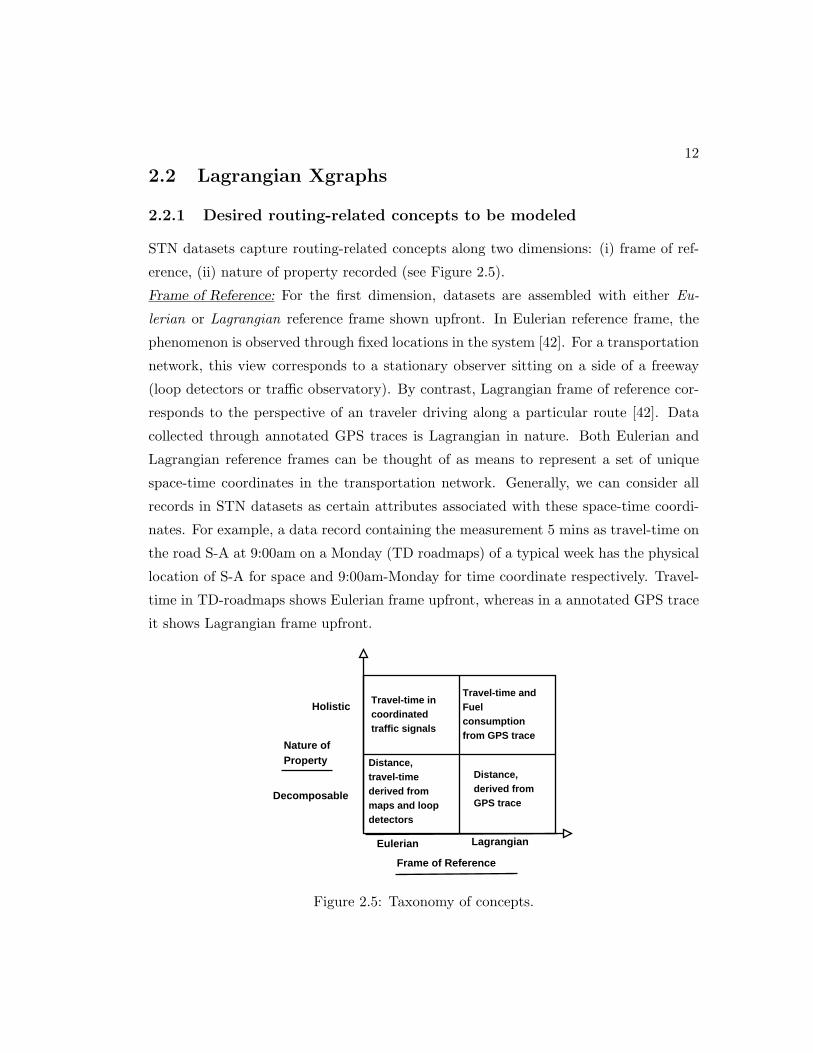
STN datasets capture routing-related concepts along two dimensions: (i) frame of ref-

erence, (ii) nature of property recorded (see Figure 2.5).

Frame of Reference: For the first dimension, datasets are assembled with either Eu-

lerian or Lagrangian reference frame shown upfront. In Eulerian reference frame, the

phenomenon is observed through fixed locations in the system [42]. For a transportation

network, this view corresponds to a stationary observer sitting on a side of a freeway

(loop detectors or traffic observatory). By contrast, Lagrangian frame of reference cor-

responds to the perspective of an traveler driving along a particular route [42]. Data

collected through annotated GPS traces is Lagrangian in nature. Both Eulerian and

Lagrangian reference frames can be thought of as means to represent a set of unique

space-time coordinates in the transportation network. Generally, we can consider all

records in STN datasets as certain attributes associated with these space-time coordi-

nates. For example, a data record containing the measurement 5 mins as travel-time on

the road S-A at 9:00am on a Monday (TD roadmaps) of a typical week has the physical

location of S-A for space and 9:00am-Monday for time coordinate respectively. Travel-

time in TD-roadmaps shows Eulerian frame upfront, whereas in a annotated GPS trace

it shows Lagrangian frame upfront.

Lagrangian

Decomposable

Eulerian

Holistic

Frame of Reference

Nature ofProperty

Distance,derived fromGPS trace

Distance,travel-timederived frommaps and loopdetectors

Travel-time andFuel consumptionfrom GPS trace

Travel-time in coordinatedtraffic signals

Figure 2.5: Taxonomy of concepts.

13

Nature of Property: Under Eulerian or Lagrangian frame of reference, the property be-

ing recorded can be either decomposable or holistic. A decomposable property when

re-constructed for a larger instance (e.g. route) by joining values for smaller instances

(at appropriate space-time coordinates) retains its correctness. Distance measured from

a GPS trace (Lagrangian frame) or as measured through maps (Eulerian frame) is a

decomposable property. Other examples include, travel-time obtained from loop de-

tectors, signal delays (red light duration) at individual traffic signals as set by traffic

managers.

Decomposable properties can be further classified as deterministic or non-deterministic.

Properties which can be expressed clearly from a start-point are termed as determinis-

tic. Travel-time as captured in TD roadmaps is deterministic as given a departure-time

(in a typical week), TD roadamps will provide a unique travel-time for a road-segment.

In contrast, traffic signal delays are non-deterministic unless the absolute start-time of

their cycles is known. In other words, given a departure-time on a route, we cannot

determine (at least in current datasets) the precise delay to be experienced at a signal.

On the other hand, holistic properties are properties when measured over a large in-

stance cannot be broken down into corresponding values for smaller instances through

space-time decomposition. This is due to presence of non-local interactions. Apart

from our earlier example with coordinated traffic signals, travel-time (and fuel consump-

tion) experienced by a commuter on a road-segment, as derived from his/her annotated

GPS trace, is holistic in nature. Here, the travel-time experienced would depend on

his/her initial velocity gained before (a non-local interaction) entering the particular

road-segment under consideration. Travel-time of the commuter is deterministic as we

can exactly measure its value from start of journey. By contrary, travel-time through a

series of coordinated traffic signals is non-deterministic.

It is important to note that ‘data-collection’ reference frame may be different from

‘querying’ reference frame. For instance, travel-time recorded in TD roadmaps shows

Eulerian frame upfront. Whereas, routing queries on the same TD roadmaps (and

other STN datasets) would be more meaningful through Lagrangian frame of reference

[34]. The interoperability of Eulerian and Lagrangian frame of reference allows for the

‘querying’ and ‘data-collection’ reference frames to be different. In other words, data

recorded in one frame can be easily queried from (or converted to) another reference

14

frame [42].

2.2.2 Proposed Logical Model

Given a collection of STN datasets measured over a time horizon H, we formally define

a Lagrangian Xgraph (LaX ) as an ordered set of Xnodes (X v), Xedges (X e) and a time

horizon parameter H, i.e., LaX = (X v,X e,H).

Xnodes: For any network system under consideration, Xnodes X vi ∈ X v represent the

underlying entities at specific space-time coordinates.

Xedges: are used to express a ‘as-traveled’ or ‘typical-experience-in-travel’ relation-

ship among a set of Xnodes. More formally, X ei = {X vs,X v1, . . . ,X vk, X vd1,X vd2,

. . . ,X vdj}. Here, the first Xnode (X vs) and the last set of Xnodes (X vd[1...j]) corre-

spond to the instance of the first and the last entities participating in the relation and

are marked separately for ease.

Xedge for with first and last Xnodes from entites

Stem-Xedge

R1 and R2 are immediate neighbors

Shoot-Xedge

Flower-Xedge

property Pt

R1 and R2

YES NO

Pt is deterministic Pt is deterministic

YES NO YES NO

Bush-Xedge

Figure 2.6: Taxonomy of Xedges.

Taxonomy of Xedges: Xedges as defined above are further categorized according to: (a)

spatial relationship between the first (X vs) and last set of Xnodes (X vd[1 j]) and (b)

property being modeled is deterministic or non-deterministic. Figure 2.6 shows the

proposed classification. Primarily, we classify an Xedge as: (i) shoot-Xedge, (ii) flower-

Xedge, (iii) stem-Xedge or, (iv) bush-Xedge. The first and last Xnodes in both shoot-

Xedges and flower-Xedges belong to entities which are spatially immediate neighbors.

15

Thus, they would be used for modeling decomposable properties. In a shoot-Xedge,

each entity is present for a single time and thus, can model deterministic properties.

Flower-Xedges allow one entity to be represented for multiple time coordinates and thus,

can be used to model non-deterministic properties (e.g. individual signal delays).

By contrast, both stem-Xedges and bush-Xedges allow the first and last Xnode(s)

to be separated physically. This physical separation allows both stem and bush-Xedges

to represent holistic properties. Bush-Xedges are useful for non-deterministic properties

since they allow one entity to be represented at multiple time coordinates. Stem-Xedges

are employed for deterministic properties since each entity is present only for one time

coordinate.

Abstract Data Type: Access operators for Lagrangian Xgraphs define the basic logi-

cal units of work during information retrieval for queries. Table 2.1 shows an illustrative

set of access operators for Xnodes and Xedges. In the table we use (s,t) to denote the

Xnode representing an entity at a particular space-time coordinates.

Access operators for Xnodes retrieve information on Xedges which are incident on

a particular Xnode. For example, the operation Xnode.decom successors (Xnode(s,t),

property) retrieves all the Xedges whose first Xnode is Xnode(s,t) and represent a

decomposable property. Similarly, get holistc successors(Xnode(s,t), property) returns

Xedges representing a given holistic property from Xnode(s,t).

Access operators for Xedges require the following parameters for retrieval: (1) the

first Xnode (Xnode(s1,t) in Table 2.1); (2) the last Xnode; (3) the property. Here,

the time coordinate of the last Xnode (Xnode(s2) in Table 2.1) may not always be

precisely defined before hand. Based on the information retrieved, we would know the

time coordinate of last Xnode(s2). Lastly, we also have an operator Xroute which can

successively join Xedges to create a route as would be experienced by a person traveling

on that route.

Table 2.1: Access operators for Lagrangian Xgraph.Category Decomposable Holistic

XnodeXnode.decom successors

(Xnode(s,t), property)

Xnode.holistc successors

(Xnode(s,t), property)

XedgeXedge.get decom

(Xnode(s1,t),Xnode(s2),property)

Xedge.get telecon

(Xnode(s1,t),Xnode(s2),property)

Xroute Xroute.glue(an Xedge)

16

FD0

SB0

AF0

BC0

t=0Signals In-coming

Max Waiting Time

SG1

SG2

SG3

S-B

B-C

C-E

[90sec]

[90sec]

[90sec]

CE0

Departure time7:00:00

ED0S-B +SG1+ B-C +SG2+C-E +SG3

AF22

t=22

FD22

SB22

BC22

CE22

ED22

AF23

t=23

FD23

SB23

BC23

CE23

ED23

S-B + SG1 + B-C + SG2

S-B + SG1

AF32

t=32

FD32

SB32

BC32

CE32

ED32

Bush-Xedge Legend:

30sec temporal granularity. Some departure-times are omitted to retain clarity.

FD6

SB6

AF6

BC6

t=6

CE6

ED6

FD7

SB7

AF7

BC7

t=7

CE7

ED7

FD8

SB8

AF8

BC8

t=8

CE8

ED8

FD9

SB9

AF9

BC9

t=9

CE9

ED9

AF24

t=24

FD24

SB24

BC24

CE24

ED24

AF25

t=25

FD25

SB25

BC25

CE25

ED25

7:03:30 7:04:307:11:30 7:12:30

AF33

t=33

FD33

SB33

BC33

CE33

ED33

AF34

t=34

FD34

SB34

BC34

CE34

ED34

AF35

t=35

FD35

SB35

BC35

CE35

ED35

7:16:30 7:17:30Coordinated 7:16:00

Figure 2.7: First and last Xnodes for journey through a series of coordinated signals.

2.2.3 Sample Lagrangian Xgraph

We now describe an instance of Lagrangian Xgraphs modeling STN datasets for routing

applications. Here, Xnodes represent the road segments at multiple departure-times

and Xedges express the experience of a traveler among a sequence of Xnodes. Here,

each Xnode is associated with information such as: (a) start and end point of the road-

segment, (b) departure-time, (c) typical travel-time on segment for the departure-time

(from TD roadmaps), (d) lower bound on travel-time, and other information depending

on application requirements. Due to space limitation we only illustrate Xedges for

travel-time experienced in a sequence of coordinated traffic signals.

Coordinated traffic signals: Consider again our previous example of coordinated signals

SG1, SG2 and SG3 in Figure 2.3. Here, we will represent typical experiences of journeys

through these signals starting from S at 7:00:00am. Given that signal delays are non-

deterministic and travel-time experienced in a sequence of coordinated traffic signals is

holistic, we would use bush-Xedges. Figure 2.7 illustrates bush-Xedges for some journeys

at 30secs temporal granularity. We have bush-Xedges for following journeys: (a) start

at S and travel to the beginning of segment B-C (after SG1), (b) start at S and travel

to the beginning of segment C-E (after SG2), (c) start at S and travel to the beginning

of segment E-D (after SG3).

For case (a), the bush-Xedge would include (SB0) and (BC6, BC7, BC8 and, BC9)

as Xnodes for the first (X vs) and last Xnodes (X vd[1 j]). Intuitively, this Xedge means

that a typical journey starting from S at 7:00am along S-B (SB0 in the Figure) can start

traversing road segment B-C at times 7:03:00 (no wait at SG1, BC6 in Figure), 7:03:30

17

(30secs wait at SG1, BC7 in the Figure), 7:04:00 or 7:04:30 (90secs wait at SG1, BC9 in

the Figure). Similarly, in case (b), we would have SB0 and (CE22, CE23, CE24, CE25)

as the first and last Xnodes. Internally, this would include the Xnodes (BC6, BC7, BC8

and, BC9) (not shown in Figure to maintain clarity). Other bush-Xedges can be defined

in a analogous way. Similarly, there would be other bush-Xedges representing journeys

starting at beginning of B-C (after SG1).

Discussion: Other related work for modeling STN data includes literature on con-

ceptual models for spatio-temporal data [43], moving objects [44, 45] and hypergraphs

[46,47]. Studies focusing on conceptual models alone [43] do not model routing-related

concepts such as Lagrangian reference frame. Though, studies done on moving ob-

jects represent the Lagrangian history of an object. They are not suitable for modeling

TD roadmaps and traffic signal data. Furthermore, Lagrangian Xgraphs differ from

both general hypergraphs [47], which represent subsets of nodes without any reference

frame and directed hypergraphs [46] which directly connect a set of sources to a set of

destinations.

2.3 Conclusion

Modeling STN datasets is important for societal applications such as routing and nav-

igation. It is however challenging to do so due to holistic properties increasingly being

captured in these datasets. The proposed Lagrangian Xgraphs addresses this challenge

at logical level by expressing the non-local interactions causing these holistic proper-

ties more explicitly. Initial study shows that the proposed Lagrangian Xgraphs can

express the desired routing-related concepts in a manner which is amenable to routing

frameworks.

Chapter 3

All-start-time Lagrangian

Shortest Path Problem

Given a spatio-temporal (ST) network, a source, a destination, and a start-time inter-

val, the All-start-time Lagrangian shortest paths problem (ALSP) determines a path

set which includes the shortest path for every start time in the interval. The ALSP

determines both the shortest paths and the corresponding set of time instants when the

paths are optimal. For example, consider the problem of determining the shortest path

between the University of Minnesota and the MSP international airport over an interval

of 7:00AM through 12:00 noon. Figure 3.1(a) shows two different routes between the

University and the Airport. The 35W route is preferred outside rush-hours, whereas

the route via Hiawatha Avenue is preferred during rush-hours (i.e., 7:00AM - 9:00AM)

(see Figure 3.1(b)). Thus, the output of the ALSP problem may be a set of two routes

(one over 35W and one over Hiawatha Avenue) and their corresponding time intervals.

Application Domain: Determining shortest paths is a key task in many societal ap-

plications related to air travel, road travel, and other spatio-temporal networks [48].

Ideally, path finding approaches need to account for the time dependent nature of the

spatial networks. Recent studies [27,28] show that indeed, such approaches yield short-

est path results that save upto 30% in travel time compared with approaches that

assume static network. These savings can potentially play a crucial role in reducing

delivery/commute time, fuel consumption, and greenhouse emissions.

18

19

(a) Different routes between Uni-versity and Airport.

(b) Optimal times.

Figure 3.1: Problem illustration.

Another application of spatio-temporal networks is in the air travel. Maintaining the

shortest paths across destinations is important for providing good service to passengers.

The airlines typically maintain route characteristics such as average delay, flight time

etc, for each route. This information creates a spatio-temporal network, allowing for

queries like shortest paths for all start times etc. Figure 3.2(a) shows the Delta Airlines

flight schedule between Minneapolis and Austin (Texas) for different start times [49]. It

shows that total flight time varies with the start time of day.

Challenges: ALSP is a challenging problem for two reasons. First, the ranking of

alternate paths between any particular source and destination pair in the network is not

stationary. In other words, the optimal path between a source and destination for one

start time may not be optimal for other start times. Second, many links in the network

may violate the property of FIFO behavior. For example, in Figure 3.2(a), the travel

time at 8:30AM is 6 hrs 31mins whereas, waiting 30mins would give a quicker route with

9:10AM flight. This violation of first-in-first-out (FIFO) is called non-FIFO behavior.

Surface transportation networks such as road network also exhibit such behavior. For

example, UPS [7,50] minimizes the number of left turns in their delivery routes during

heavy traffic conditions. This leads to faster delivery and fuel saving.

Related work and their limitations: The related work can be divided on the basis

of FIFO vs non-FIFO networks as shown in see Figure 3.2(b). In a FIFO network, the

flow arrives at the destination in the same order as it starts at the source. A* based

approaches, generalized for non-stationary FIFO behavior, were proposed in [21,51] for

20

(a) Minneapolis - Austin (TX) Flight schedule (b) Related work

Figure 3.2: Application Domain and related work.

solving the shortest path problem in FIFO networks. However, transportation networks

are known to exhibit non-FIFO behavior (see Figure 3.2(a)). Examples of Non-FIFO

networks include multi-lane roads, car-pool lanes, airline networks etc. This paper

proposes a method which is suitable for both FIFO and non-FIFO networks.

Proposed approach: A naive approach for solving the non-FIFO ALSP problem

would involve determining the shortest path for each start time in the interval. This

leads to redundant re computation of the shortest path across consecutive start times

sharing a common solution. Some efficiencies can be gained using a time series general-

ization of a label-correcting algorithm [52]. This approach was previously used to find

best start time [16], and is generalized for ALSP in Section 3.5 under the name modified-

BEST. However, this approach still entails large number of redundant computations.

In this paper, we propose the use of critical time points to reduce this redundancy. For

instance, consider again the problem of determining the shortest path between Univer-

sity of Minnesota and MSP international airport over a time interval of 7:30am through

11:00am. Figure 3.1(b) shows the preferred paths at some time instants during this

time interval, and Figure 3.3 shows the travel-times for all the candidate paths during

this interval.

As can be seen, the Hiawatha route is faster for times in the interval [7:30am 9:30am)

1 , whereas 35W route is faster for times in the interval [9:30am 11:00am]. This shows

that the shortest path changed at 9:30am. We define this time instant as critical time

point. Critical time points can be determined by computing the earliest intersection

1 Note: an interval (a,b) does not include the end points a and b, [a,b] includes the endpoints a andb, and [a,b) includes a but not b

21

18

20

22

24

26

28

30

32

34

7:30am-8:30am 8:31am-9:30am 9:31am-10:30am 10:31am-11:00am

Tra

vel t

ime

Hiwatha route35W route

Figure 3.3: Total travel time of candidate paths.

points between the functions representing the total travel time of paths. For example,

the earliest intersection point of Hiawatha route was at 9:30am (with 35W route func-

tion). Therefore, it would be redundant to recompute shortest paths for all times in

interval (7:30am 9:30am) and (9:30am 11:00am] since the optimal path for times within

each interval did not change. This approach is particularly useful in case when there

are a fewer number of critical time points.

Contributions: This chapter proposes the concept of critical time points, which are

the time points at which the shortest path between a source-destination pair changes.

Using this idea, a novel algorithm, Critical-Time-point-based-ALSP-Solver (CTAS), is

proposed for solving the ALSP problem. The correctness and completeness of the CTAS

is presented. The CTAS algorithm is experimentally evaluated using real datasets.

Experiment results show that the critical time point based based approach is particularly

useful in cases when the number of critical times is small.

Scope and Outline of the Chapter: This paper models the travel time on any

particular edge as a discrete time series. Turn restrictions are not considered in the ST

network representation. The paper uses a Dijkstra-like framework. A*-like framework

are beyond the scope of the paper. Moreover, we focus on computing the critical time

points on the fly rather than precomputing them. The rest of the chapter is organized

as follows. A brief description of the basic concepts and a formal problem definition

is presented in Section 3.1. A description of the computational structure of the ALSP

problem is presented in Section 3.2. The proposed CTAs algorithm is presented in

22

Section 3.3. Sectionctas-cor presents the correctness and completeness proof of the

CTAS algorithm. Experimental analysis of the proposed methods is presented in Section

3.5. Finally, Section 3.6 concludes this chapter.

3.1 Basic Concepts and Problem Definition

Spatio-temporal Networks: Spatio-temporal networks may be represented in a num-

ber of ways. For example, snapshot model, as depicted in Figure 3.4, views the spatio-

temporal network as snapshots of the underlying spatio network at different times. Here,

each snapshot shows the edge properties at a particular time instant. For example, travel

times in all the edges ((A,B),(A,C),(B,D),(B,C)) at time t = 0 is represented in the

top left snapshot in Figure 3.4. For the sake of simplicity, this example assumes that

(B,C) and (C,B) have the same travel time. The same network can also be represented

as a time-aggregated graph (TAG) [37] as shown in Figure 3.5(a). Here, each edge is

associated with a time series which represents the total cost of the edge. For example,

edge (A,B) is associated with the time series [3 3 1 1 2 2 2 2]. This means that the

travel time of edge (A,B) at times t = 0, t = 1, and t = 2 is 3, 3 and 1 respectively.

Figure 3.4: Snapshot model of spatio-temporal network.

Both TAG and snapshot representations of our sample transportation network use

a Eulerian frame of reference for describing moving objects. In the Eulerian frame of

reference, traffic is observed as it travels past specific locations in the space over a period

23

of time [42]. It is similar to sitting on the side of a highway and watching traffic pass a

fixed location.

(a) Time aggregated graph. (b) Transformed TAG.

Figure 3.5: Time aggregated graph example.

Traffic movement can also described using a Lagrangian frame of reference, in which

the observer follows an individual moving object as it moves through space and time [42].

This can be visualized as sitting in a car and driving down a highway. The time-

expanded graph (TEG) described later corresponds to this view.

Both Eulerian and Lagrangian-based views represent the same information and one

view can be transformed into another view. The choice between the two depends on the

problem being studied. In our problem context, it is more logical to use a Lagrangian

frame of reference for finding the shortest paths because the cost of the candidate paths

should be computed from the perspective of the traveler. TAG can also be used to

view the network in Lagrangian frame of reference, however we use TEG for ease of

communication. We now define the concept of a Lagrangian path.

Lagrangian Path: A Lagrangian path Pi is a spatio-temporal path experienced by the

traveler between any two nodes in a network. A Lagrangian path may be viewed as a

pair of traditional path in a graph and a schedule specifying arrival time at each node.

During traversal of a Lagrangian path, the weight of any particular edge e = (x, y)

(where e ∈ Pi) is considered at the time of arrival at node x. For instance, consider

the path <A,C,D> for start time t = 0. Here, we would start at node A at time t = 0.

Therefore, the cost of edge (A,C) would be considered at t = 0, which is 1 (see Figure

3.5(a)). Following this edge, we would reach node C at time t = 1. Now, edge (C,D)

would be considered at time t = 1 (because it takes 1 time unit to travel on edge (A,C)).

24

A0 A1 A2 A3

B0 B1 B2 B3

C0 C1 C2 C3

D0 D1 D2 D3

A

B

C

D

0 1 2 3Time Step

A4 A5 A6

B4 B5 B6

C4 C5 C6

D4 D5 D6

A7

B7

C7

D7

A8

B8

C8

D8

4 5 6 7 8

Figure 3.6: Time expanded graph example.

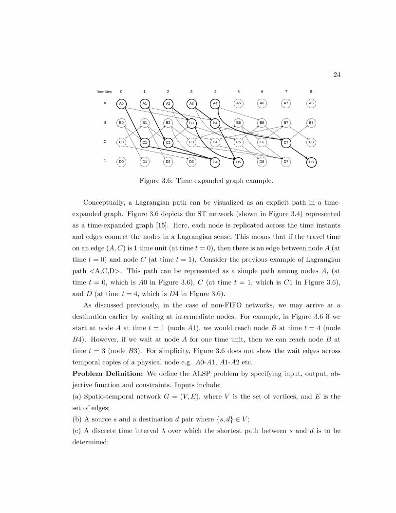
Conceptually, a Lagrangian path can be visualized as an explicit path in a time-

expanded graph. Figure 3.6 depicts the ST network (shown in Figure 3.4) represented

as a time-expanded graph [15]. Here, each node is replicated across the time instants

and edges connect the nodes in a Lagrangian sense. This means that if the travel time

on an edge (A,C) is 1 time unit (at time t = 0), then there is an edge between node A (at

time t = 0) and node C (at time t = 1). Consider the previous example of Lagrangian

path <A,C,D>. This path can be represented as a simple path among nodes A, (at

time t = 0, which is A0 in Figure 3.6), C (at time t = 1, which is C1 in Figure 3.6),

and D (at time t = 4, which is D4 in Figure 3.6).

As discussed previously, in the case of non-FIFO networks, we may arrive at a

destination earlier by waiting at intermediate nodes. For example, in Figure 3.6 if we

start at node A at time t = 1 (node A1), we would reach node B at time t = 4 (node

B4). However, if we wait at node A for one time unit, then we can reach node B at

time t = 3 (node B3). For simplicity, Figure 3.6 does not show the wait edges across

temporal copies of a physical node e.g. A0-A1, A1-A2 etc.

Problem Definition: We define the ALSP problem by specifying input, output, ob-

jective function and constraints. Inputs include:

(a) Spatio-temporal network G = (V,E), where V is the set of vertices, and E is the

set of edges;

(b) A source s and a destination d pair where {s, d} ∈ V ;

(c) A discrete time interval λ over which the shortest path between s and d is to be

determined;

25

(d) Each edge e ∈ E has an associated cost function, denoted as δ. The cost of an edge

represents the time required to travel on that edge. The cost function of an edge is

represented as a time series.

Output: The output is a set of routes, Psd, from s to d where each route Pi ∈ Psd is

associated with a set of start time instants ωi, where ωi is a subset of λ.

Objective function: Each path in Psd is a shortest commuter-experienced travel time

path between s and d during its respective time instants.

We assume the following constraints: The length of the time horizon over which the ST

network is considered is finite. The weight function δ is a discrete time series.

Figure 3.7: Output of ALSP problem.

Example: Consider the sample spatio-temporal network shown in Figure 3.5(a). An

instance of the ALSP problem on this network with source A destination D and λ =

[0, 1, 2, 3], is shown in Figure 3.7. Here, path A-C-D is optimal for start times t = 0 and

t = 1, and path A-B-D is optimal for start times t = 2 and t = 3.

3.2 Computational structure of the ALSP problem

The first challenge on solving the ALSP problem involves capturing the inherent non-

stationarity present in the ST network. Due to this non-stationarity, traditional al-

gorithms developed for static graphs cannot be used to solve the ALSP problem be-

cause the optimal sub-structure property no longer holds in case of ST networks [16].

On the other hand, algorithms developed for computing shortest paths for a single

start time [3, 15, 16, 22, 53] are not practical because they would require redundant re-

computation of shortest paths across the start times sharing a common solution.

This paper proposes a divide and conquer based approach to handle network non-

stationarity. In this approach we divide the time interval over which the network exhibits

non-stationarity into smaller intervals which are guaranteed to show stationary behavior

26

2 . These intervals are determined by computing the critical time points, that is, the

time points at which the cost functions representing the total cost of the path as a

function of time intersect. Now, within these intervals, the shortest path can be easily

computed using a single run of a dynamic programming (DP) based approach [16].

Recall our previous example of determining the shortest paths between the university

and the airport over an interval of [7:30am 11:00am]. Here, 9:30am was the critical time

point. This created two discrete sub-intervals [7:30 9:30) and [9:30 11:00]. Now, we can

compute the ALSP using two runs of a DP based algorithm [16] (one on [7:30 9:30) and

another on [9:30 11:00]).

Our second challenge for solving ALSP is capturing the non-FIFO behavior of the

network. We do this by converting the travel information associated with an edge into

earliest arrival time (at destination) information [22, 54]. This is a two step process.

First, the travel time information is converted into arrival time information. Second, the

arrival time information is converted into earliest arrival time information. The second

step captures the possibility of arriving at an end node earlier by waiting (non-FIFO

behavior). For example, in the ST network shown in Figure 3.5(a), the travel time series

of edge (A,B) is [3 3 1 1 2 2 2 2]. First, we convert it into arrival time series. This is done

by adding the time instant index to the cost. For example, if we leave node A at times

t = 0, 1, 2, 3 . . ., we would arrive at node B at times t = 3+0, 3+1, 1+2, 1+3, 2+4 . . ..

Therefore, the arrival time series of (A,B) is [3 4 3 4 6 7 8 9]. The second step involves

comparing each value of the arrival time series to the value to its right in the arrival

time series. A lower value to its right means we can arrive at the end node earlier by

waiting. Consider the arrival time series of (A,B) = [3 4 3 4 6 7 8 9]. Here, the arrival

time for t = 1 is 4 (which is less than the arrival time for t = 2). Therefore, the earliest

arrival time on edge (A,B) for time t = 1 is 3 (by waiting for 1 time unit at node

A). This process is repeated for each value in the time series. The earliest arrival time

series of edge (A,B) is [3 3 3 4 6 7 8 9]. The earliest arrival time series of the edges are

precomputed. Figure 3.5(b) shows the ST network from Figure 3.5(a) after the earliest

arrival time series transformation.

There are two ways to determine the stationary intervals, either by precomputing all

2 By stationarity, we mean that ranking of the alternate paths between a particular source-destination pair does not change within the interval i.e, there is a unique shortest path

27

the critical time points, or by determining the critical time points at run time. The first

approach was explored in [55] for a different problem. Precomputing the critical time

points involves computing intersection points between cost functions of all the candidate

paths. Now, in a real transportation network there can be exponential number candidate

paths. Therefore, this paper follows the second approach of determining the critical time

points at run-time. In this approach only a small fraction of candidate paths and their

cost functions are actually considered while computation. Now, we define and describe

our method of determining the critical time points.

Figure 3.8: Illustrating Non-stationarity

Critical time point: A start time instant when the shortest path between a source and

destination may change.

Consider an instance of the ALSP problem on the ST network shown in Figure 3.8,

where the source is node A, the destination is C, and λ = [0 1 2 3 4]. Here, start time

t = 2 is a critical time point because the shortest path between node A and C changes

for start times greater that t = 2. Similarly, t = 2 is also a critical time point for the

network shown in Figure 3.5(a), where the source node is A and the destination node

is D (see Figure 3.7). Now, in order to determine these start time instants, we need

to model the total cost of the path. This paper proposes using a weight function to

capture the total cost of a path. This approach, which associates a weight function to a

path, yields a path-function which represents the earliest arrival time at the end node

of the path. A formal definition of the path-function is given below.

Path Function: A path function represents the earliest arrival time at the end node of

a path as a function of time. This is represented as a time series. A path function is de-

termined by computing the earliest arrival times on its component edges in a Lagrangian

28

fashion.

For example, consider the path <A,B,C> in Figure 3.8. This path contains two

edges, (A,B) and (B,C). The earliest arrival time (EAT) series of edge (A,B) is [3 4

5 6 7], while the EAT of edge (B,C) is [1 2 3 4 6 8 10 12]. Now, the path function of

<A,B,C> for start times [0, 4] is determined as follows. If we start at node A at t = 0,

the arrival time at node B is 3. Now, arrival time at node C through edge (B,C) is

considered for time t = 3 (Lagrangian fashion), which is 4. Thus, the value of the path

function of <A,B,C> for start time t = 0 is 4. The value of the path-function for all

the start times is computed in similar fashion. This would give the path function of

<A,B,C> as [4 6 8 10 12]. This means that if we start at node A at times t = 0, 1, 2, 3, 4

then we will arrive at end node C at times t = 4, 6, 8, 10, 12. Similarly, the path function

of path <A,C> is [5 6 7 8 9] (since it contains only one edge). By comparing the two

path-functions we can see that path <A,B,C> has an earlier arrival time (at destination)

for start times t = 0 and t = 1 (ties are broken arbitrarily). However, path <A,C>

is shorter for start time t ≥ 2. Thus, start time t = 2 becomes a critical time point.

In general, the critical time points are determined by computing the intersection point

(with respect to time coordinate) between path functions. In this case, the intersection

point between path functions <A,C> and <A,B,C> is at time t = 2. Computing this

point of intersection is the basis of the CTAS algorithm.

3.3 Critical Time-point based ALSP Solver (CTAS)

This section describes the critical time point based approach for the ALSP problem.

This approach reduces the need to re-compute the shortest paths for each start time by

determining the critical time points (start times) when the shortest path may change.

Although Lagrangian paths are best represented by a time-expanded graph (TEG),

these graphs are inefficient in terms of space requirements [16]. Therefore, this paper

uses TEG model only for visualizing the ST network. For defining and implementing

our algorithm we use TAG [16]. Recall that since the optimal substructure property is

not guaranteed in a ST network, the given time interval is partitioned into a set of dis-

joint sub-intervals, where the shortest path does not change. The Sub-interval Optimal

Lagrangian Path denotes this shortest path.

29

Sub-interval optimal Lagrangian path: is a Lagrangian path, Pi, and its corre-

sponding set of time instants ωi, where ωi ∈ λ. Pi is the shortest path between a source

and a destination for all the start time instants t ∈ ωi.

The Lagrangian path <A,C,D> shown in Figure 3.7 is an example of sub-interval Op-

timal Lagrangian Path and its corresponding set ω = 0, 1.

3.3.1 CTAS Algorithm

The algorithm starts by computing the shortest path for the first start time instant in

the set λ. Since the optimal substructure property is not guaranteed in a ST network,

the choice of the path to expand at each step made while computing the shortest path for

a particular start time may not be valid for later time instants. Therefore, the algorithm

stores all the critical time points observed while computing the shortest path for one

start time in a data structure called path-intersection table. As discussed previously,

the critical time point is determined by computing the time instants where the path

functions of the candidate paths intersect. The earliest of these critical time points

represents the first time instant when the current path no longer remains optimal. The

algorithm re-computes the shortest paths starting from this time instant. Since the

path functions represent the earliest arrival time (at end node of path) for a given start

time, the intersection points represent the start times (at the source) when there is a

change in relative ordering of the candidate paths.

The pseudocode for the CTAS algorithm is shown in Algorithm 1. The outer loop

of ALSP ensures that a shortest path is computed for each start time instant in the set

λ. The inner loop computes a single sub-interval optimal Lagrangian path. There may

be several sub-interval optimal Lagrangian paths for the set λ. First, a priority queue is

initialized with the source node. The inner loop determines the shortest path for start

times greater than the earliest critical time points stored in the path intersection table

(tmins). For the first iteration, this would just be the first start time instant of our

set λ. In each iteration, the algorithm expands along the path which has the minimum

weight for time t = tmin. After a path is expanded the last node of the path is closed

for start time t = tmin. For example, if a path s − x − y is expanded for start time

t = tmin, then node y is closed for start time t = tmin. This means there cannot be any

30

Algorithm 1 CTAS Algorithm

1: Determine the earliest arrival time series of each edge2: Initialize the path intersection table with the first start time in λ3: while a shortest path for each time t ∈ λ waits to be determined do4: Select the minimum time instants among all time instants at which a shortest path might

change and clear path intersection table5: Initialize a priority queue with the path functions corresponding to the source node and

its neighbors6: while destination node is not expanded do7: Choose the path with the minimum weight to expand8: Determine the intersection points among the path functions in the priority queue9: Delete all the paths ending on that node from the priority queue

10: Save the time coordinate of the intersection point in the path intersection table11: Determine the path functions resulting from expansion of the chosen path12: Push the newly determined path functions into the priority queue13: end while14: end while

other shorter path from node s to node y for the start time t = tmin.

Before expanding a path, the algorithm computes the intersecting points among the

path functions available in the priority queue. The earliest intersection point (consid-

ering intersection points in the increasing order of their time coordinate) involving the

path with minimum weight is the time instant when the stationary ordering among the

candidate paths change. After that the path is expanded and path functions to all its

neighbors are computed and added to the priority queue. The inner loop terminates

when it tries to expand a source-destination path. In the next iteration of the outer

loop, the shortest path computation starts from the earliest of the optimal route change

times in path intersection table. Now, the path determined in the previous iteration is

closed for all the start times earlier than earliest of the critical time point (and greater

than tmin of previous iteration). In a worst case scenario, the value of the earliest crit-

ical time point could be the next time start time instant in the set λ (one more than

previous tmin). In such a case, the inner loop would have determined the shortest path

only for a single start time instant. The algorithm terminates when the earliest of the

path-order change times is greater than the latest start time instant in the set λ.

Execution Trace: Figure 3.9 gives an execution trace of the CTAS algorithm on the

ST network shown in Figure 3.5(b). The first iteration of the outer loop starts with

31

initializing the priority queue with the source node. The inner loop builds a shortest

path starting from the earliest critical time point. For the first iteration, this would be

time t = 0 (the first start time instant in λ). First, the source node is expanded for

time t = 0. Path functions for its immediate neighbors (path <A,B> and <A,C>) are

computed and added them to the priority queue. In this case, the path functions just

happen to be their edge weight functions.

In the first iteration of the inner loop, the algorithm chooses the path whose path

function has minimum weight at the start time instant chosen in step 4 of the algorithm.

This would be t = 0 for the first case. At this point the algorithm has two choices, path

function <A,C> and <A,B>(see Figure 3.9). The algorithm chooses <A,C> because

it has lowest cost for t = 0. This path is expanded and path functions for its neighbors,

<A,C,D> and <A,C,B>, are computed and added to the priority queue. Again the

choice of path <A,C> may not be valid in later times, therefore, the algorithm closes

the node C only for the start time t = 0. The algorithm stores the intersection point

between the path <A,B> and <A,C> (which is at t = 2) in the path intersection table.

The next iteration expands path <A,C,B>. There is no intersection between the

path functions of <A,C,D> and <A,C,B> (in our interval λ). Again, node B is closed

only for t = 0. At this point, all the paths which end in node B are deleted from the

priority queue. Now, the priority queue contains two paths, <A,C,D> and <A,C,B,D>.

This time the algorithm tries to expand along path <A,C,D> because it has least

cost. Again the intersection point between the path functions is computed. Here,

paths <A,C,D> and <A,C,B,D> do not intersect 3 . This time a complete source to

destination path was expanded. This is the terminating condition of the inner loop.

This completes one iteration of the outer loop. Next iteration of the outer loop builds

the shortest path starting at the earliest of the critical time points stored in the previous

iteration. This happens to be t = 2 for our example. The next iteration of the inner

loop starts for start time t = 2. At this point the path intersection table is cleared. We

see that the algorithm did not compute the shortest path for start time t = 1. Figure

3.6 also showed that the shortest path did not change start time t = 1 (shortest paths

between node A and node D for start-times t = 0, 1, 2, 3 are shown in bold). The fact

that the next iteration of the CTAS algorithm starts with t = 2 shows that it saves

3 Note that here path <A,C,B,D> may also be expanded

32

Figure 3.9: Execution trace of CTAS algorithm.

computation. The algorithm terminates when shortest paths of all time instants in the

set λ have been determined. Figure 3.7 shows the final result of the algorithm.

3.4 Correctness and Completeness CTAS algorithm

The CTAS algorithm divides a given departure-time interval into a set of disjoint sub-

intervals. Within these intervals, the shortest path does not change. The correctness

of the CTAS algorithm requires the path returned for a particular sub-interval to be

optimal and the completeness of the algorithm guarantees that none of the critical time

points are missed. The correctness of the CTAS can be easily argued on the basis greedy

nature of the algorithm. Lemma 7 shows that the CTAS algorithm does not miss any

critical time point. Using Lemma 7, Theorem 4 proves the completeness of the CTAS

algorithm.

33

Lemma 1. The CTAS algorithm recomputes the shortest path for all those departure

times ti ∈ λ, where the shortest path for previous departure time ti−1 can be different

from the shortest path for departure time ti.

Proof. Consider the sample network shown in Figure 5.13, where a shortest path has

to be determined between node s and d for discrete time interval λ = [1, 2 . . . T ]. First,

the source node is expanded for the time instant t = 1. As a result, path functions

for all the neighbors <s,2>, <s,1>, <s,xi> are added to the priority queue. With loss

of generality assume that path <s,1> is chosen in the next iteration of the inner loop.

Also assume that the earliest intersection point between path functions <s,xi > and

<s,1> is at t = α between <s,1> and <s,2>. Now, the queue contain paths <s,1,d>,

<s,2>, <s,xi>. Here we have two cases. First, path <s,1,d> has lower cost for start

time t = 1. Second, path <s,2> has lower cost for start time t = 1.

Figure 3.10: Network for Lemma 7

Considering the first case, without loss of generality assume that the earliest inter-

section point between the path functions <s,1,d> and <s,2> is at t = β. Note that

both t = α and t = β denote the departure times at the source node. Consider the

case when β ≤ α (Note that β cannot be greater than α as all the edges have posi-

tive weights). In such a case the shortest path is recomputed for starting time t = β

and the path <s,1,d> is closed for all start times 1 ≤ t < β. Assume for the sake

of contradiction, that there is a shortest path Px from source to destination that is

different from path <s,1,d> which is optimal for departure time tx ∈ [1, β). Assume

that Px =< s, x1, x2, x3, . . . , d >. This means that path < s, x1 > had least for time

t = tx. However, by the nature of the algorithm, this path would have been expanded

instead of path < s, 1 > (a contradiction). Moreover, as all the travel times positive,

34

if sub path <s,x1 > was not shorter than <s,1,d> for start times earlier than t = β.

Any positive weight addition to the path function (through other edges) cannot make

Px shorter than <s,1,d>. Consider the second case when <s,2> had lower cost for start

time t = 1. Now, path <s,2> would be expanded and path function <s,2,d> would

be added to priority queue. Again, assume that path functions <s,1,d> and <s,2,d>

intersect at time t = β. A similar argument can be given for this case as well.

Corollary 1. (Corollary to Lemma 7) Given a instance of forward search which started

from node S at time td and terminated when node D was closed. Now, if the earliest

forecasted forward critical time point was tminctp , then shortest path determined between

S and D is optimal from all departure-times td through tminctp − 1.

Theorem 1. CTAS algorithm is complete.

Proof. There may be several sub-interval optimal Lagrangian paths Pi over set λ. Each

Pi is associated with a set of time instants ωi, where⋃

∀i∈|Psd|ωi = λ. The completeness

proof of the CTAS algorithm is presented in two parts. First, using Lemma 7 we can

conclude that the CTAS algorithm does not miss any departure time instant when the

shortest path changes. Secondly, the outer loop iterates until the algorithm determines

a shortest path for all the time instants in set λ. This happens when the earliest of the

forecasted CTPs tmin falls outside λ. This proves the completeness of the algorithm.

3.5 Experimental evaluation

Experiments were conducted to evaluate the performance of CTAS algorithm as differ-

ent parameters were varied. The experiments were carried on a real dataset containing

the highway road network of Hennepin county, Minnesota, provided by NAVTEQ [56].

The dataset contained 1417 nodes and 3754 edges. The data set also contained travel

times for each edge at time quanta of 15mins. Figure 3.2 shows the speed profiles for

a particular highway segment in the dataset over a period of 30days. As can be seen,

the speed varies with the time of day. For experimental purposes, the travel times were

converted into time quanta of 1mins. This was done by replicating the data inside time

interval. The experiments were conducted on an Intel Quad core Linux workstation

with 2.83Ghz CPU and 4GB RAM. The performance of CTAS algorithm was compared

35

against a modified version of the existing BEST start time algorithm proposed in [16].

Modified-BEST (MBEST) algorithm: The MBEST algorithm consists of two main

parts. First, the shortest path between source and destination is determined for all the

desired start time instants. Second, the computed shortest paths are post-processed

and a set of distinct paths is returned. The MBEST algorithm uses a label correcting

approach similar to that of BEST algorithm, proposed in [16] to compute the shortest

paths between source and destination. The algorithm associates two lists viz, the arrival

time list and ancestor list, with each node. The arrival time array, Cv[t], represents the

earliest arrival time at node v for the start time t at the source. The ancestor array,

Anv[t], represents the previous node in the path from source for time t. These lists are

updated using Equation 3.1, where γuv represents the earliest arrival time series of the

edge (u, v). The algorithm terminates when there are no more changes in the arrival

time list of any node.

Cv[t] = min{Cv[t], γuv[Cu[t]]}, uv ∈ E (3.1)

Figure 3.11: Experimentalsetup

60

80

100

120

140

160

180

200

T-time=30Non-Rush

T-time=40Non-Rush

T-time=30Rush

T-time=40Rush

#Re-

com

puta

tions

sav

ed

lambda = 100lambda = 200

Figure 3.12: Re-computationssaved

Experimental setup: The experimental setup is shown in Figure 3.11. The first step

of the experimental evaluation involved combining the travel time information along

with the spatial road network to represent the ST network as a Time-aggregated graph.

A set of different queries (each with different parameters) was run on the CTAS and

the MBEST algorithms. The following parameters were varied in the experiments: (a)

36

length of the time interval over which shortest paths were desired (|λ|), (b) total travel

time of the route, (c) time of day (rush hour vs non-rush hours). A speedup ratio, given

by Equation 3.2, was computed for each run. The total number of re-computations

avoided by CTAS was also recorded for each run. In worst case, the shortest paths

may have to be re-computed for each time instant in the interval λ. The total number

of re-computations saved by CTAS is the difference between |λ| and re-computations

performed.

speed− up ratio =MBEST runtime

CTAS runtime(3.2)

Number of re-computations saved in CTAS : Figure 3.12 shows the number of re-

computations saved by the CTAS algorithm. The experiments showed that more saving

was gained where paths were shorter. Similarly, fewer number of re-computations were

performed in case of Non-rush hours. This is because there were fewer intersections

among the path-functions.

Effect of length of start time interval (|λ|): This experiment was performed to

evaluate the effect of length of start time interval (λ) over which the shortest path was

desired. Figure 3.13(a) shows the speed-up ratio for Non-rush hours and Figure 3.13(b)

shows the speed-up ratio for Rush hours. The speed ratio was calculated for paths with

travel time 30 and travel time 40. These travel times indicate the time required to

travel on these paths during non-rush hours when there is no traffic. The experiments

showed that run-time of both CTAS and MBEST increased with increase in the lambda.

Runtime of MBEST increases steadily whereas CTAS increases very slowly with lambda

for a travel time of 30. However, the run-time of CTAS increases rapidly for travel time

of 40.

Effect of total travel time of a path: This experiment was performed to evaluate the

effect of total travel time of a path on the candidate algorithms. Figure 3.14 shows the

speed-up ratio as the total travel time of the path was varied. The experiments showed

that the runtime of CTAS algorithm increased with a corresponding increase in the total

travel time of the path, whereas the runtime of the MBEST algorithm remained the

same. This is because, CTAS algorithm follows a Dijkstra’s like approach and expands

the paths, but MBEST is follows a label correcting approach and terminates when there

37

2

4

6

8

10

12

14

Lambda=60 Lambda=100 Lambda=200 Lambda=300

Spe

ed-u

p R

atio

Non-Rush hours

travel-time 30travel time 40

(a)

1

1.5

2

2.5

3

3.5

Lambda=60 Lambda=100 Lambda=200 Lambda=300

Spe

ed-u

p R

atio

Rush hours

travel-time 30travel time 40

(b)

Figure 3.13: Effect of Lambda on Speed-up

no more changes in the arrival time array of any node.

1

2

3

4

5

6

Traveltime=20

Traveltime=30

Traveltime=40

Traveltime=50

Spe

ed-u

p R

atio

Rush hours

lambda 100lambda 200

(a)

4

5

6

7

8

9

10

11

12

Traveltime=20

Traveltime=30

Traveltime=40

Traveltime=50

Spe

ed-u

p R

atio

Non-Rush hours

lambda 100lambda 200

(b)

Figure 3.14: Effect of travel time on Speed-up

Effect of different start times: Experiments showed that better speed-up was ob-

tained for Non-rush hours than the rush hours (see Figure 3.14 and Figure 3.13). This

is because there are fewer number of intersection points in case of non-Rush hours.

38

3.6 Conclusions

The All-start-time shortest Lagrangian shortest path problem (ALSP) is a key compo-

nent of applications in transportation networks. ALSP is a challenging problem due

to the non-stationarity of the spatio-temporal network. Traditional A* and Dijkstra’s

based approaches incur redundant computation across the time instants sharing a com-

mon solution. The proposed Critical Time-point based ALSP Solver (CTAS), reduces

this redundant re computation by determining the time points when the ranking among

the alternate paths between the source and destination change. Theoretical and experi-

mental analysis show that this approach is more efficient than naive particularly in case

of few critical time points.

Chapter 4

Bi-directional algorithm for the

ALSP problem

Given a spatio-temporal (ST) network, a source, a destination, and a discrete departure-

time interval, the All-departure-time Lagrangian shortest paths problem (ALSP) deter-

mines a path set which includes the shortest path for every departure time in the inter-

val. The ALSP determines both the shortest paths and the corresponding set of time

instants when the paths are optimal. For example, consider the problem of determining

the shortest path between the University of Minnesota and the MSP international air-

port over the departure-time interval of 7:30am through 9:15am. Figure 4.1 (on the left)

shows three different routes between the University and the Airport. The I-35W route

is preferred outside rush-hours, whereas the route via Hiawatha Avenue is preferred

during rush-hours (i.e., 7:30am - 8:30am). Thus, the output of the ALSP problem may

be a set of these two routes and their corresponding preferred departure time intervals.

Application Domain: Determining shortest paths is a key task in many societal

applications related to air travel, road travel, eco-routing and other spatio-temporal

network applications [48, 57, 58]. Ideally, path finding approaches need to account for

the time dependent nature of the spatial networks. Recent studies [27, 28] show that

indeed, such approaches yield shortest path results that save up to 30% in travel time

compared with approaches that assume static network. These savings can potentially

play a crucial role in reducing delivery/commute time, fuel consumption, and greenhouse

39

40

Preferred Route

Departure Time

via Hiawatha

via Hiawatha

via Hiawatha

via Hiawatha

via Hiawatha

via I35W

via I35W

via I35W

7:30am

7:45am

8:00am

8:15am

8:30am

8:45am

9:00am

9:15am

1

2

3

4

5

6

7

8

ID

I-35W Hiawatha Ave

36th St

Figure 4.1: Preferred routes between the University and Airport [2].

emissions leading to ‘eco-routing’ [5].

Challenges: The ALSP problem is challenging because of multiplicity of departure

times. In addition, the ranking among candidate paths between any particular source

and destination pair in the network is not stationary across departure times. In other

words, the optimal path between a source and destination for one departure time may

not be optimal for other departure times. This lack of stationarity in ST networks makes

it non-trivial to use classic algorithms developed for static graphs (e.g. Dijkstra’s and

A*) for solving the ALSP problem. On the other hand, it would be computationally

redundant to re-compute the shortest path for each distinct departure-time when the

ranking changes only few times. For example, in our previous University-Airport ALSP

instance, it would be redundant to re-compute for all the departure-times in the interval

of 7:30am through 9:15am when the shortest path changes only at 8:45am.

Limitations of Related work: Few studies have investigated ways to reduce re-

dundant computations across consecutive departure times sharing a common solution.

Figure 4.2(a) shows a classification of these approaches. These methods attempt to re-

duce the redundant computations by closing nodes for several departure instants during

a single iteration of the algorithm. A node is said to be closed when the algorithm

has found a shortest path (from the source) to that node. So, in these algorithms, an

attempt is made to find the shortest path to a node for several departure-times (at the

41

Discrete allFP [Kanoulas et.al.]

Our Critical-time pointsbased approaches(CTAS, BD-CTAS)

Discrete 2S-LTT [Ding et.al.]

Use complete information at hand to close intermediate nodes

YESNO

Use only a fractionof complete information for closing

YESNO

(a) Related work classification

Naive Approach, e.g., SP-TAG

Discrete 2S-LTT [Ding et. al.]

CTAS Chapter 3

Bi-Directional-CTAS (this chapter)

#Recomputations

8

6

3

2

(b) #re-computations on UMN-Airport ALSP in-stance

Figure 4.2: Comparison of Related work and our critical-time based approaches.

source) in a single iteration. Figure 4.2(b) shows the number of re-computations that

would be required by different methods which close intermediate nodes on our previous

University-Airport ALSP instance illustrated in Figure 4.1. A naive approach (first row

in Figure), referred to as SP-TAG in this paper, computes a shortest path for each of

the 8 time instants shown in Figure 4.1. Therefore, methods which reduce redundant

work aim to perform less than 8 re-computations. However, they do this using only a

fraction of the available information at hand. For instance, discrete version of [3] (re-

ferred to as Discrete 2S-LTT in this paper) compares the time series of arrival times at

an intermediate node against a single (scalar) lowest feasible cost along other candidate

paths to that node leading to 6 re-computations (second row in Figure 4.2(b)). How-

ever, this can be further improved as the shortest path changes only once (at 8:45am)

in our ALSP instance.

Another discrete version of approach [51] (referred to as Discrete allFP in this paper)

does not close any intermediate nodes. Consequently all paths between a source and a

destination whose destination arrival time is less than the optimal arrival time for the

last desired departure-time are enumerated. As there can be a huge number of candidate

paths between a source and a destination, it usually results in significant computational

bottlenecks. This limitation was also highlighted by other works [3, 17]. Running time

ramifications of this limitation are shown in our experimental analysis.

Proposed Approach: In contrast, we propose to use all of the available information

by comparing the entire available time series of arrival times along candidate paths at

42

each intermediate node before destination is closed. As a result, nodes are likely to

be closed for a longer range of departure times, and hence incur fewer redundant re-

computations. The last two rows in Figure 4.2(b) illustrate the superior performance

of our critical-time-points based approaches which use all of the available information

to reduce the re-computations to just 3 or 2. Note that reducing the number of re-

computations to less than 2 is not possible for our problem instance as the shortest

path does change at 8:45am (see Figure 3.1). Appendix A.1 provides a detailed trace

of all the above mentioned algorithms on this University-Airport ALSP instance.

We propose to operationalize the use of complete information through the our con-

cept of critical-time-points. This helps in reducing the redundant computations across

departure times sharing a common solution. For instance, consider again our previous

University-Airport ALSP instance. As Figure 4.1 shows, the Hiawatha route is faster

for times in the interval [7:30am 8:30am], whereas I-35W route is faster for times in the

interval [8:45am 9:15am]. This shows that the shortest path changed at some instant be-

tween 8:30am and 8:45am. For the sake of convenience we assume it changed at 8:45am.

We define this time instant as a critical time point (CTP), i.e., a departure time before

which optimal path is guaranteed not to change. Critical time points can be determined

by computing the earliest intersection points between functions representing the total

travel time of paths. For example, the earliest intersection point of the Hiawatha route

would be at 8:45am (with the I-35W route function).

A candidate way to compute the critical-time points for a given ALSP problem

instance would be to first enumerate the costs (as a function of departure-time) of all

the possible candidate paths between the source and destination and, then compute the

lower envelope of these cost functions to give us the critical time points for the given

problem. However, this would be computational intensive as in a real road network,

there can be huge number of candidate paths. Thus, we propose to use a expand

and refine search strategy (similar to Dijkstra’s) to enumerate paths for determining

their cost functions. As mentioned earlier, due to non-stationarity in the ST network,

we would not have a clear ranking of candidates across departure-times. To this end,

we propose to use the ranking for a particular departure-time (which is stationary) to

conservatively forecast only the next time departure-time (forcasted critical-time point)

when the ranking is expected to change (while maintaining correctness). The same

43

procedure is repeated for this departure-time as well, and continued until all the desired

departure-times in the given ALSP instance are covered.

It is important to note that due to the expand and refine nature of the search strat-

egy, we would not be enumerating all the possible candidate paths (and their cost func-

tions) between source and destination. In other words, we would computing critical-time

points based on partial paths itself which might lead to forecasts which are irrelevant to

our source-destination pair. Figure 4.3 (on the left) illustrates this conceptually. Here,

the search started from S (for a specific departure-time) and terminated at node D.

The shaded region shows the area covered by the search, i.e., the enumerated candidate

paths belong to this region. Now, our forecasted critical-time point might come due

to an intersection between cost functions of paths S V and S D. It is necessary

to consider this because there might be a path through V which might be optimal for

the departure-time corresponding to the intersection. But at the same time it might be

irrelevant as the cost on the V D portion was not considered while computing the

intersection point.

DSV

S

Paths in the shaded region influence the forcasted critical time point;

D

Forward-only search Bi-directional search

Figure 4.3: Exploration space of forward-only and bi-directional searches.

Our previous algorithm CTAS (Section 3.3 in Chapter 3) focused on this kind of

search strategy which started from the source and terminated when shortest path to

destination was found. But, as mentioned before, it can lead to irrelevant critical-time

points due to large search space. This was specifically true when the shortest path

turned out to be long. This was primarily because a larger search area was explored

in these cases making it more likely to encounter an irrelevant critical-time point. In

44

this paper, we propose to use a bi-directional search which starts at both source and

destination. This allows us to do a more focused search for paths to the desired des-

tination. Figure 4.3 (on the right) illustrates this conceptually. As the figure shows,

due to the focused nature we would have much less number of irrelevant critical-time

points (formal argument in Theorem 3 in Section 4.5) making it computationally more

efficient even for long paths (Section 4.6).

New Contributions in this chapter: In our previous chapter on the ALSP problem

(Chapter 3), we proposed the concept of critical time points. Using this idea, we de-

signed a forward search only algorithm called Critical Time point based ALSP Solver

(CTAS) (Section 3.3 in Chapter 3). We also provided rigorous correctness and com-

pleteness proof of our algorithm and evaluated it experimentally using real datasets.

This chapter makes the following additional contributions.

• (a) We propose temporal bi-directional search for the ALSP problem. This tech-

nique takes advantage of lower bounded arrival times at a destination to facilitate

searches from both the source and the destination. A bi-directional search allows

us to pursue a more focused search.

• (b) We propose a novel termination condition called the impromptu rendezvous for

our temporal bi-directional search which guarantees correctness without degrading

the performance.

• (c) Based on temporal bi-directional search and impromptu rendezvous condition,

we propose a new algorithm called Bi-Directional CTAS (BD-CTAS) for the ALSP

problem. This approach addresses the computational bottlenecks of CTAS by

reducing the number of irrelevant critical time points.

• (d) We provide correctness and completeness proof of the BD-CTAS algorithm

• (e) We also present asymptotic complexity analysis for our new BD-CTAS algo-

rithm and previous CTAS algorithm.

• (f) We compared our approaches with related work based on asymptotic time

complexity

45

• (g) Finally, we also evaluated our proposed methods using real and synthetic

datasets.

Scope and Outline: This chapter models the travel time on any particular edge as

a discrete time series. Continuous models for ST networks [17] are not considered here

and would be explored in the future. Also, we are limiting the scope of the paper to

strong fifo networks, where an earlier departure on any route strictly implies an earlier

arrival at its terminal node. Turn restrictions are not considered in the ST network

representation. Comparisons with single departure time algorithms, bi-directional (with

reverse search done on the underlying static graph) and other forward search algorithms

(e.g. Hierarchical and A*) are beyond the scope of the paper.

The rest of the paper is organized as follows. A brief description of the basic con-

cepts and a formal problem definition is presented in Section 4.1. A description of the

computational structure of the ALSP problem is presented in Section 4.2. The proposed

temporal bi-directional CTAS algorithm (BD-CTAS) is presented in Section 4.3. Cor-

rectness and completeness of the proposed BD-CTAS algorithm is presented in Section

4.4. Section 4.5 presents an analytical evaluation our critical-time based approaches.

Experimental evaluation of the algorithms is presented in Section 4.6. Finally, this

chapter concludes in Section 4.7.


Spatio-temporal (ST) Networks are spatial networks (e.g. road networks) whose

properties (e.g. typical travel-time on the road segments) change with time. Typically

in a ST-network, nodes represent the road intersections, whereas edges represent road

segments between the intersections. A ST network can be represented in several ways

as discussed in [37]. In this paper, we choose to represent it using a time-aggregated

graphs (TAG) due its simplicity and less storage overhead over others [16, 37]. Figure

4.4 illustrates a sample ST network represented as a TAG [37]. Here, each edge is

associated with a time series which represents the travel-time of the edge as a function

of time. For example, edge (S,B) is associated with the travel time series [1 1 6 6]. This

means that the travel time of edge (S,B) at departure times t = 0, t = 1, and t = 2

is 1, 1 and 6 respectively. Travel time information can also be represented in terms of

46

arrival times. In order to get this, the travel time of the edge is added to the departure

times. For instance, the arrival time series of the edge (S,B) in our previous example

would be: [1+0 1+1 6+2 6+3], which is, [1 2 8 9]. This means that a journey departing

from node S at times t = 0, t = 1, t = 2, and t = 3 would arrive at node B at times

1,2,8 and 9 respectively. In this paper, we choose to use TAG with arrival time series

(right side of Figure 4.4) for ease of communication.

B

E

D

S

C

[1 2 8 9]

[4 5 6 7]

[2 3 4 6]

[7 8 10 11]

[3 4 5 6 10 11 12]

[2 4 5 6 7..]

t=0 1 2 3

[2 4 5 7 8 ...] t =0 1 2 3...

t = 0 1 2 ...

B

E

D

S

C

[1 1 6 6]

[4 4 4 4]

[2 2 2 3]

[7 7 8 8]

[3 3 3 3 6 6 6]

[2 3 3 3 3..]

t=0 1 2 3

[2 3 3 4 4...] t =0 1 2 3...

t = 0 1 2 ...

Transformed TAG with Arrival Time SeriesTAG with Travel time series

Figure 4.4: ST network represented as a TAG.

Lagrangian vs Eulerian frame of reference: ST networks can be queried through

either Lagrangian or Eulerian frame of reference. In Eulerian frame of reference, the

traffic (or typical travel-time) is observed from specific locations in the space over a

period of time [42]. It is similar to sitting on the side of a highway and watching traffic

pass a fixed location. In contrast, the Lagrangian frame of reference corresponds to an

observer driving along a particular route [42]. It is important to that the total cost

of a candidate path would be different across these reference frames. For example,

consider the cost of path B-C-D for a departure time t = 0 in Figure 4.4. In an Eulerian

reference frame, this would be sum of times travel-times of edges (B,C) and (C,D) for

t = 0, which is 4 time units. However, one may note that, after departing from B at

t = 0, it takes 2 time units to travel along the edge (B,C). Thus, we should consider

the cost of (C,D) for time t = 2 and not at t = 0 as done in the Eulerian frame of

reference. This kind of view, where the cost of the edge is considered for the time when

the traveler arrives at its starting point, is known as the Lagrangian frame of reference.

Routing queries over ST networks would be more meaningful through Lagrangian frame

of reference. This was also pointed in other literature in this area [16, 17, 34]. In this

paper, paths whose cost is viewed through Lagrangian frame of reference are referred

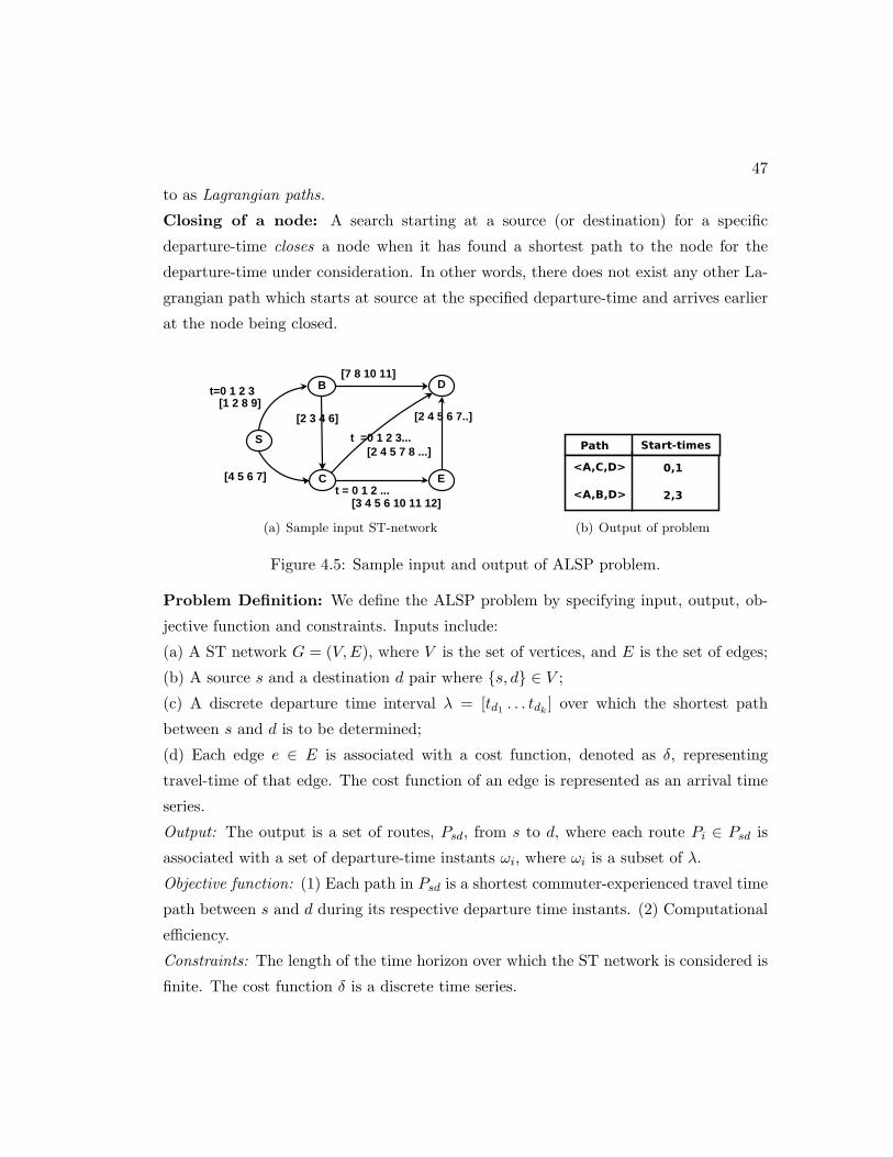
47

to as Lagrangian paths.

Closing of a node: A search starting at a source (or destination) for a specific

departure-time closes a node when it has found a shortest path to the node for the

departure-time under consideration. In other words, there does not exist any other La-

grangian path which starts at source at the specified departure-time and arrives earlier

at the node being closed.

B

E

D

S

C

[1 2 8 9]

[4 5 6 7]

[2 3 4 6]

[7 8 10 11]

[3 4 5 6 10 11 12]

[2 4 5 6 7..]

t=0 1 2 3

[2 4 5 7 8 ...] t =0 1 2 3...

t = 0 1 2 ...

(a) Sample input ST-network (b) Output of problem

Figure 4.5: Sample input and output of ALSP problem.

Problem Definition: We define the ALSP problem by specifying input, output, ob-

jective function and constraints. Inputs include:

(a) A ST network G = (V,E), where V is the set of vertices, and E is the set of edges;

(b) A source s and a destination d pair where {s, d} ∈ V ;

(c) A discrete departure time interval λ = [td1 . . . tdk ] over which the shortest path

between s and d is to be determined;

(d) Each edge e ∈ E is associated with a cost function, denoted as δ, representing

travel-time of that edge. The cost function of an edge is represented as an arrival time

series.

Output: The output is a set of routes, Psd, from s to d, where each route Pi ∈ Psd is

associated with a set of departure-time instants ωi, where ωi is a subset of λ.

Objective function: (1) Each path in Psd is a shortest commuter-experienced travel time

path between s and d during its respective departure time instants. (2) Computational

efficiency.

Constraints: The length of the time horizon over which the ST network is considered is

finite. The cost function δ is a discrete time series.

48

Example: A sample ST network is shown in Figure 4.5(a). Figure 4.5(b) shows the

output of an ALSP problem instance on this network with source S, destination D, and

λ = [0, 1, 2, 3]. Here, the path S-B-C-D is optimal for departure times t = 0 and t = 1,

and the path S-C-D is optimal for departure times t = 2 and t = 3.

4.2 Computational structure of the ALSP problem

Given (a) a source, (b) destination and (c) a departure-time, the basic computational

unit in our scheme computes: (1) a shortest path between the source and destination

for the given departure-time and, (2) a forecasted critical-time point, which serves as

the next departure-time for re-computation. We refer to this as the sub-interval optimal

lagrangian path, defined formally as follows:

A Sub-interval optimal Lagrangian path is a pair of Lagrangian path, Pi, and its

corresponding set of departure time instants ωi, where ωi ∈ λ. Pi is a shortest path

between the source and the destination for all the departure times t ∈ ωi.

The Lagrangian path S-B-C-D and its corresponding ω = 0, 1 (shown in Figure

4.5(b)) is an example of a sub-interval optimal Lagrangian path. Output of any ALSP

problem instance can be considered as a set of several sub-interval optimal lagrangian

paths. Given a sub-interval optimal Lagrangian path Pi with ωi = [tdi , tdi+1, . . . , tdnt

] ∈

λ, the departure-time tdnt+1∈ λ forms the forecasted critical-time point at which re-

computation starts.

Our proposed bi-directional search consists of a forward search and a trace search.

The forward search starts exploring the candidate paths from the source (given in the

ALSP problem instance) for a particular departure-time. Whereas the trace search

starts from the destination (given in the ALSP problem instance) for a particular time

in estimated arrival time interval at the destination (described later in Section 4.3).

The proposed temporal bi-directional approach employs the forward and trace search

along with the our novel impromptu rendezvous condition (described later) to determine

successive sub-interval optimal lagrangian paths forming a solution to the ALSP problem

instance.

49

B

D

[1 2 3 6 7 8]

Ct=0 1 2 3....

[3 4 5 6 7]

t=0 1 2 3....

departure Time t=0

DC

B

<3 4 5 6>

D <2 3 6 7>Ct=0 1 2 ...

[1 2 3 4]

Forward Path Function

Departure time of 2 is the Forward CTP

[1 2 3 6 7 8] t=0 1 2 3....t=0 1 2 ...

[1 2 3 4]

Arrival time series on C-B

Arrival time series on B-D

<2 3 6 7> t=0 1 2 3....

Path Function C-B-Dfor departure-times

Depart from Cat time t=0

Arrive at D at Cat time t=2

Figure 4.6: Forward critical-time points and path functions.

4.2.1 Forward Search Basic Concepts

The goal of the forward search is to explore candidate paths from the source node for

a specific departure-time in the given departure-time interval (λ). The forward search,

while exploring paths for a departure-time, maintains some information to forecast the

critical time point (forward critical time point) at which the search needs to re-start the

exploration.

Forward Critical time point: A departure-time instant at the source (as determined

by the forward search) when the shortest path between the source and a destination

changes.

In order to determine these critical time points (CTPs), we need to model the total

cost of the path. This is achieved through forward path-function, a time-series which

represents the earliest arrival time at the end node of the path for different departure-

times at the source. A formal definition of a path-function is given below.

Forward Path Function: A forward path function represents the arrival time at the

end node of a path as a function of time (representing the departure-times at the start

node). This is represented as a time series. A path function is determined by composing

the arrival times on its component edges in a Lagrangian fashion.

Figure 4.6 illustrates the construction of forward path function for the path C-B-

D. The Figure also illustrates the forward CTPs for a search with C as the source,

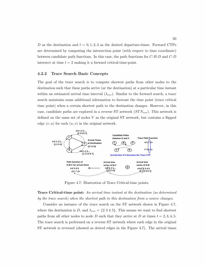
50

D as the destination and t = 0, 1, 2, 3 as the desired departure-times. Forward CTPs

are determined by computing the intersection point (with respect to time coordinate)

between candidate path functions. In this case, the path functions for C-B-D and C-D

intersect at time t = 2 making it a forward critical-time-point.

4.2.2 Trace Search Basic Concepts

The goal of the trace search is to compute shortest paths from other nodes to the

destination such that these paths arrive (at the destination) at a particular time instant

within an estimated arrival time interval (λrev). Similar to the forward search, a trace

search maintains some additional information to forecast the time point (trace critical

time point) when a certain shortest path to the destination changes. However, in this

case, candidate paths are explored in a reverse ST network (STNrev). This network is

defined on the same set of nodes V as the original ST network, but contains a flipped

edge (v, u) for each (u, v) in the original network.

{2 3 4 5}

B

D

[1 2 3 5 6 7]

C

t=0 1 2 3....[3 4 5 6 7]

t=0 1 2 3....

Arrival Times at Destination

DC

B

<* 0 1 2>

D <0 1 * 2>Ct=0 1 2 3....[1 2 3 4]

Trace Path Function

Arrival time of 4 becomes the Trace CTP

Candidate Paths between D and C

[1 2 3 5 6 7] t=0 1 2 3 4 5t=0 1 2 3....

[1 2 3 4]

Arrival time series of B-C

Arrival time series of D-B

t=2 3 4 5<0 1 * 2>

Path function ofD-B-C for arrival times

Figure 4.7: Illustration of Trace Critical-time points.

Trace Critical-time point: An arrival time instant at the destination (as determined

by the trace search) when the shortest path to this destination from a source changes.

Consider an instance of the trace search on the ST network shown in Figure 4.7,

where the destination is D, and λrev = {2 3 4 5}. This means we want to find shortest

paths from all other nodes to node D such that they arrive at D at times t = 2, 3, 4, 5.

The trace search is performed on a reverse ST network where each edge in the original

ST network is reversed (showed as dotted edges in the Figure 4.7). The arrival times

51

series in the original network are interpreted as an inverse-mapping from arrival times

to departure-times. For instance, in Figure 4.7, consider the original edge (C,D) (shown

in bold) and its corresponding reverse (shown using a dotted arrow). The arrival time

series of the original edge was [3 4 5 6 7], which means that a departure at t = 0 at node

C would have an arrival at D at t = 3. Since this is a trace search, we would read this

time series as: If need to arrive at D at t = 3, what is the latest departure time at C?.

Similar to forward CTPs, in order to determine trace CTPs, we model the total cost

of the path using a cost function. This cost function, which we call trace path function,

is defined formally below.

A Trace Path Function represents the latest departure times at the end node as a time

series. Each item in this time series represents the latest departure at the end node for

the corresponding arrival time at the start node of the path.

Similar to a forward path function, a trace path function is determined by combining

the arrival times on its component edges in a Lagrangian fashion. The only difference

is that, due to inverse mapping, we look backwards while composing the time series.

Figure 4.7 illustrates the construction of a trace path function for the path D-B-C for a

trace search with destination D and λrev = [2 3 4 5]. While composing the arrival time

series for the component edges, we consider only the latest departure time that incurs

no waiting. Note that in some cases, the arrival times cannot be mapped backwards.

For instance, in our previous example of D-B-C, the arrival time 4 at D cannot be

mapped back along edge (D,B). In other words, there does not exist a departure-time

at B such that its corresponding arrival time (with no waiting) at D is 4. Note that

a departure-time of 2 at B would not be considered as it would arrive at D early and

wait. Cases like these are represented using ‘*’ in the trace function (and implemented

as −∞). Figure 4.7 also illustrates the arrival time t = 4 as a trace critical time point

because the shortest path to D from C changes for arrival times greater that t = 4.

We now begin our discussion on our proposed temporal bi-directional search for the

ALSP problem. During the discussion, we may sometimes drop the prefix “trace” or

“forward” from critical-time-points and path functions when the context is clear.

52

4.3 Proposed Temporal Bi-directional Search for ALSP

problem

Designing an efficient bi-directional search for the ALSP problem poses two challenges.

First, unlike the forward search which explores over a given set of departure-times, ap-

propriate “departure-times” for the trace search at the destination are not known in

advance. Second, designing a suitable termination condition which gives good perfor-

mance while ensuring correctness is non-trivial.

“Departure-times” for trace search: To address the first challenge, we compute a

bound on the arrival times at the destination. These bounds are computed by executing

a single start-time shortest path algorithm developed for ST networks [16] for the first

and the last departure-time in λ. Given the fifo nature of our network, we can claim

that arrival times for all the other departure-times in λ would fall inside the interval

defined by the arrival times corresponding to the first and last departure-times. The

range defined by these arrival times at the destination form the set of “departure-times”

(denoted by λrev) for the trace search. To avoid ambiguity, we use the term trace-times

instead of “departure-times” when discussing the trace search 1 . We use the term

departure-times in context of the forward search or the problem instance (λ). Figure

4.8 shows the upper and lower bounds defining the range λrev for our ALSP instance in

Figure 4.5.

B

E

D

S

C

1

3

7

6

Shortest path tree rooted at S for t=0

Lower Boundon arrival time: 7

B

E

D

S

C

9

7

11

13

Shortest path tree rooted at S for t=3

Upper Boundon arrival time: 11

Figure 4.8: Arrival times corresponding to first and last departure-times.

impromptu rendezvous condition: Our second challenge for bi-directional search

1 trace-times refer to time points in λrev, while departure-times refer to time points in λ (in theALSP instance)

53

was designing an appropriate termination which gives good performance while ensuring

correctness. Current termination conditions for bi-directional searches work only when

the trace search is done on the underlying static graph [17, 23–26] and thus cannot be

applied in our case. The trace search in these studies is used to prune the search space

for the forward search to continue efficiently until destination node is closed. In contrast,

our trace search is executed on the ST network itself, thus, allowing us to avoid visiting

the nodes already closed by the trace search. We now describe our novel impromptu

rendezvous condition on our previous ST network in Figure 4.5(a).

B

E

D

S

C

B

E

D

S

C

[1 2 8 9]

[4 5 6 7]

[2 3 4 6]

[7 8 10 11]

[3 4 5 6]

[..5 6 7..]

t=0 1 2 3

[2 4 5 7]

Arrival time series

start time =0

1

3

7

6

Forward search tree rooted at S for t=0

B

E

D

S

C

trace start time =7

0

3 4

Trace search tree from D at t=7 Done on graph with rev edges

1

1

Node B is closed by bothforward and trace search with same label 1

t=3 4

Figure 4.9: Illustration of impromptu rendezvous condition.

Consider again the ST network illustrated in Figure 4.5(a) (replicated in top left

of Figure 4.9). Suppose we want to determine the shortest path between S and D

which departs S at time t = 0. A bi-directional search for this problem would involve

a forward search from node S and a trace search from node D. Clearly, the forward

search from S would start at time t = 0. By contrast, the choice of trace-time for the

trace search is non-trivial and is discussed next with an intuitive explanation of the

termination condition.

Figure 4.9 contains a forward search tree (explored until node D was closed) from

node S for time t = 0 (top right). This can be considered as a instance of forward

54

search algorithm with departure time t = 0 run until node D was closed. The Figure

also contains a trace search tree from node D which starts at time t = 7. This can be

considered as instance of trace search being executed from D on reverse ST network

until node S was closed. The numbers written beside the nodes in the figure represent

their respective distance labels when they were closed. For instance, the forward search

closed the node E at time 6, i.e, the shortest path to E from S arrives at time 6. On

the other hand, the trace search closed node E at time t = 4. This means we need to

depart node E at the latest by t = 4 in order to arrive at D by t = 7. A comparison

of these two trees shows that nodes B and C happen to be closed with the same label

by both the forward and the trace search. In other words, both the forward (starting

at S at t = 0) and the trace search (starting at D at t = 7) “agree” on node B and C

along the path S-B-C-D, which happens to be the shortest path between S and D for

the departure-time t = 0. This shows that when the trace-time of a trace search at the

destination is correct (shortest path to D from S indeed arrives at t = 7), both forward

and trace searches close the nodes on the shortest path with the same labels.

If the trace search does not start at the optimal time, there are only two other

possibilities: it started earlier or later than the optimal time. A trace search starting

earlier would close all the nodes at an earlier time than the forward search. In other

words, there would be no “agreement” between the forward and trace search on any

node. On the other hand, a trace search starting later (e.g. t = 9) might lead to an

agreement between the two searches on a node which does not lie on the shortest path.

This leads our proposed termination condition, called the impromptu rendezvous, which

states: it is sufficient to terminate when both the forward and trace search close a node

with the same label, provided the trace-time is not an over-estimate of the optimal

arrival time. This is formally stated as Lemma 4 in Appendix 4.4.

4.3.1 BD-CTAS Algorithm

In this section we describe our proposed temporal Bi-Directional based Critical-Time-

point Alsp Solver (BD-CTAS). The forward and the trace search along with the im-

promptu rendezvous condition form the key parts of this algorithm. In the algorithm,

the forward and the trace search start from the source and the destination respectively.

The priority queue for the forward search is sorted in ascending order on the values

55

in the path functions, while the priority queue in the trace search is sorted (also in

ascending order) on the difference between the trace-time at the destination and the

values in the trace function. This kind of ordering in the trace search ensures that the

closest node (to the destination) is closed first, an essential requirement for correctness

as discussed later.

The impromptu rendezvous condition is only used as a sufficiency condition for

terminating the algorithm. It is possible for the algorithm to run without meeting this

condition. This happens when the trace-time of the trace search is earlier than the

optimal arrival time of the shortest path (Lemma 3 in Appendix 4.4). In such cases, the

algorithm terminates only when the destination node is closed by the forward search

(similar to the CTAS algorithm, Section 3.3 in Chapter 3).

In order to integrate impromptu rendezvous termination into the BD-CTAS algo-

rithm, we need to ensure that the trace-time is never an overestimate of the optimal

arrival time at the destination (had the forward search been allowed to proceed until

the destination). To this end, the algorithm employs an incremental strategy for de-

termining the next times of the trace and forward search. Given the correctness of the

trace-time of a trace search (i.e., it is not an overestimate), a pair of forward and trace

searches explore the ST network to determine a single sub-interval optimal lagrangian

path and determine the time instants for the next pair of searches. We refer to this unit

of work as one iteration of BD-CTAS algorithm. Here, the algorithm simply ensures

that the next trace-time for the trace search is not an overestimate of the optimal arrival

time. This process starts at the first departure-time in λ and continues until shortest

paths for all the departure-times given in λ are determined. To ensure the correctness

for the first departure-time in λ, the algorithm uses the first time point in the range

defined by λrev (described earlier in the section) as the trace-time of the trace search.

Recall that, by construction this trace-time is guaranteed not be an overestimate; in

fact, it is the correct destination arrival time. This means that the algorithm does more

work for the first departure time in λ. However, this extra cost is usually compensated

by the savings generated by the impromptu rendezvous.

We now describe our approach for determining the next times after a pair of forward

and trace searches. Assuming that the trace-time of the trace search in the previous

56

instance was not an overestimate, one of the following two cases can be encountered dur-

ing the execution. Case (a): the algorithm terminated because impromptu rendezvous

condition was met. Which means both the trace and forward search closed a node with

same label. Case (b): the algorithm terminated because the forward search closed the

destination node.

Case (a): Impromptu rendezvous was satisfied: The impromptu rendezvous condition

guarantees that whenever a node v is closed by both forward and trace search with

the same label, the combined path from source to v and v to destination is optimal for

its respective departure-time (of the forward search) at source. However, for a more

efficient solution for the ALSP problem, we need to forecast a minimum duration for

which this path remains optimal. In the CTAS algorithm [34] this was done by choos-

ing the earliest of the intersection points as the forecasted critical-time-poin (CTP),

the next departure-time for re-computation. In other words, the path was guaranteed

to be optimal for all departure-times between these two departure-times at the source.

A natural extension of such an approach to a temporal bi-directional search would be

to take the minimum of forward and trace critical time points to determine the next

departure and trace times. Note that the trace critical time points would be in terms

of arrival times at destination and would generally be higher than the forward CTPs.

In order circumvent this, we need to take the minimum over the mutual distance (in

time) between CTPs and their “reference time points” (departure-times of forward and

trace-time of trace searches).

In order to guarantee the correctness of the above approach in a general case, we need

to incorporate the notion of lagrangian agreement duration into the process of finding

the minimum of the forward and trace CTPs. The lagrangian agreement duration is

duration for which both the forward and trace path functions (ending at the common

node) have same values. In order to compute the next departure and trace times, we

take the minimum of the lagrangian agreement duration, and the forward and trace

CTPs (after subtracting their respective departure and trace times). This minimum,

referred to as γmap, is added to the current departure-time of forward search and the

trace-time of trace search to get the next times for the searches. Correctness of this

case is presented in Lemma 5 (Section 4.4).

57

Case (b): Forward search closed the destination node: In this case, the algorithm ig-

nores the data collected by the trace search and sets the next forward search departure-

time to the earliest of observed intersection points (same as done by CTAS). The next

trace-time of the trace search is set to one more than the current shortest path ar-

rival time found by the forward search. Correctness of this case is argued in Lemma 6

(Appendix 4.4).

Algorithm 2 Bi-Directional CTAS AlgorithmInput: a ST network STN , source S, destination D, a departure-time interval λ =[td1 . . . tdk ]

1: Build a reverse ST network STNrev with each edge in STN reversed.2: Set ta1

and tamto the arrival times (at D) of a shortest path between S and D for times td1 , and tdk

3: Set the trace-time interval for the trace search λrev = [ta1. . . tam

]4: Set the current departure-time of forward search forst = td1 and of trace search trast = ta1

5: while a shortest path for each time t ∈ λ waits to be determined do

6: Initialize priority queues for forward (PQfor) and trace search (PQtra)7: FPmin ← min weight path function from PQfor

8: TPmin ← min weight path function from PQtra

9: Add the tail node of FPmin and TPmin to set of closed nodes10: Test the impromptu rendezvous condition11: while D is not closed by forward search or impromptu rendezvous condition is not satisfied do

12: Determine the earliest intersection point of FPmin with other path functions in PQfor and save inPinterfor

13: Expand FPmin and push the newly determined path functions into PQfor and delete paths endingon tail of FPmin

14: Determine the earliest intersection point of TPmin with other trace functions in PQtra and save inPintertra

15: Expand TPmin and push the newly determined trace functions into PQtra and delete paths endingon tail of TPmin

16: FPmin ← min weight path function from PQfor and TPmin ← min weight path function from TQfor

17: Add the tail node of FPmin and TPmin to set of closed nodes18: Test the impromptu rendezvous condition19: end while

20: Compute γmap

21: if impromptu rendezvous condition was satisfied then

22: forst = forst + γmap + 123: trast = trast + γmap + 124: else

25: forst = min{Pinterfor} {earliest intersection point in path intersection table.}26: trast = 1+ arrival time of shortest path found for time t = (min{Pinterfor} − 1)27: end if

28: end while

Pseudocode of the BD-CTAS algorithm is given in Algorithm 2. The algorithm

starts by computing a shortest path between the given source and destination for the

first and the last departure-time in λ (line 2). We use algorithms developed for single

departure-time [16] for this purpose. As described earlier, the range defined by the

arrival times of these shortest paths form the trace-time interval for the trace search

(line 3). Initially, the departure-time of the forward and trace-time of the trace search

58

are set to the first time points in λ and λrev respectively (line 4). The outer while loop

(lines 5-28) ensures that a shortest path for each departure-time in λ = [td1 . . . tdk ] is

determined. The loop begins by initializing the priority queues for forward and trace

search (line 6). The forward search priority queue, PQfor, is initialized with the path

functions of the source and its neighbors. The trace search priority queue, PQtra, is

initialized with the trace functions of the destination and its neighbors. Using the inner

while loop (11-19) the algorithm then runs a pair of forward and trace searches to

compute a single sub-interval optimal Lagrangian path. Conditions described earlier in

case (a) and case(b) are used to terminate the loop. Inside this loop the forward search

executes on the input ST network, whereas the trace search executes on the reverse

ST network, where all the edges of the original ST network are reversed. Finally, the

next departure-time of the forward search and the trace-time of the trace search are

computed in lines 20-27 for the next pair of searches.

E

D

S

C

B

E

D

S

C

[1 2 8 9]

[4 5 6 7]

[2 3 4 6..]

[7 8 10 11..]

[3 4 5 6 10 11 12]

[...5 6 7 8 9 10 11..]

t=0 1 2 3

[..5 7 8 9 10..]

{1 2 8 9}

Forward search from S; departure-time interval: [0 1 2 3]

t =2 3 4 5 6...

Optimal path

S-B-C-D

S-C-D

Departure Times

t=0,1

t=2,3

t = 0 1 2 3 4..

{8 9 ....}

{3 4 ....}

{7 8 ....}

B

E

D

C

Trace search from D; trace-time interval: [7 8 9 10 11]

Node C is closed by both Trace and ForwardSearch with same label

<0 1 2 3 4>

<3 4 5 6 7>

B

S

C

departure time =0

{1 2 8 9}

{4 5 6 7}

B

S

C

{1 2 8 9}

{4 5 6 7}

Forward CTPsPaths TimeS-C and S-B t=2

D

{8 9 ....}

B

B

{3 4 ....}

B

E

D

C

trace time =7<0 1 * 3 4>

<3 4 5 6 7>

B

E

D

C

<0 1 2 3 4>

<3 4 5 6 7>

t=2 3 4 5 6 7

<4 5 6 7 8>

<4 5 6 7 8>

Trace CTPsPaths TimeD-E and D-B t=9

<1 2 3 *>

<4 5 6 7 8>

Forward CTPsPaths TimeS-C and S-B t=2S-C and S-B-C t=2

Trace CTPsPaths TimeD-E and D-B t=9D-E-C and D-C t=10

STEP ONE

STEP TWO

STEP THREE

departure time =0

departure time =0

trace time =7

trace time =7

Forward Search Closes

Node: S Via Path S

Label 0PFunc {0 1 2 3}

Trace Search Closes

Node: D Via Path D

Label 7PFunc <7 8 9 10 11>


Node: B Via Path S-B

Label 1 PFunc {1 2 8 9}

Trace Search Closes

Node: E Via Path D-E

Label 4PFunc <4 5 6 7 8>


Node: C Path S-B-C

Label 3 PFunc {3 4...}

Trace Search Closes

Node: C Via Path D-C

Label 3PFunc <3 4 5 6>

Figure 4.10: Execution trace of the BD-CTAS algorithm.

Execution Trace of BD-CTAS algorithm: Figure 4.10 illustrates an execution trace

59

of the BD-CTAS algorithm on the ALSP instance shown in Figure 4.5. In the figure,

forward search is shown in green and trace search is shown in blue. Nodes which are

closed by either search have shaded background. In order to keep the figure clear and

simple, we have not shown the inner details of the priority queue. As noted earlier, the

priority queue of forward search is similar to that of CTAS. The trace search priority

queue is ordered on the difference between the trace-time at the destination and the

trace function values. We are only giving a high-level conceptual trace of BD-CTAS

algorithm for the first iteration for the ALSP instance shown in Figure 4.5. Here, a pair

of forward (from node S with departure-time t = 0) and trace searches start (from D

with trace-time t = 7) to compute a single sub-interval optimal Lagrangian path.

In the first step (after closing S and D) the forward and trace searches add the path

functions to their corresponding neighbors to their respective priority queues. Path

functions are indicated using {} or (< >) next to the node. For instance, the forward

path function of S-B is {1 2 8 9} and the trace path function of D-B is < 0 1 ∗ 3 4 >.

In the second step, the forward search closes node B, and the trace search closes

node E. The intersection points (among the path functions) encountered at this stage

are shown in Figure 4.10. Figure 4.10 (on the right) also shows the optimal paths and

their corresponding path functions for all the closed nodes in every step. Now, paths

S-B and D-E are expanded to include the neighbors.

In the next step both searches close node C with the same label 3. This is the im-

promptu termination condition. At this stage, the BD-CTAS algorithm would compare

the forward and the trace path functions for node C, which are {3 4 . . .} (forward) and

< 3 4 5 6 7 > (trace) to determine the lagrangian agreement duration to be 2. Com-

bined with the forecasted forward and trace CTP information, the next departure-time

of the forward search would be t = 2 (0+2) and the next trace-time of the trace search

would be t = 7 + 2 = 9. Thus, the algorithm has computed one sub-interval optimal

Lagrangian path, S-B-C-D with ω = 0, 1. This process continues until shortest paths

for all departure-times are found. A brief comparison with the execution trace of the

CTAS algorithm (Figure A.6 in Appendix A.2) on the same input shows that BD-CTAS

was able to skip the departure time of t = 1 (an irrelevant CTP forcasted by the CTAS

algorithm).

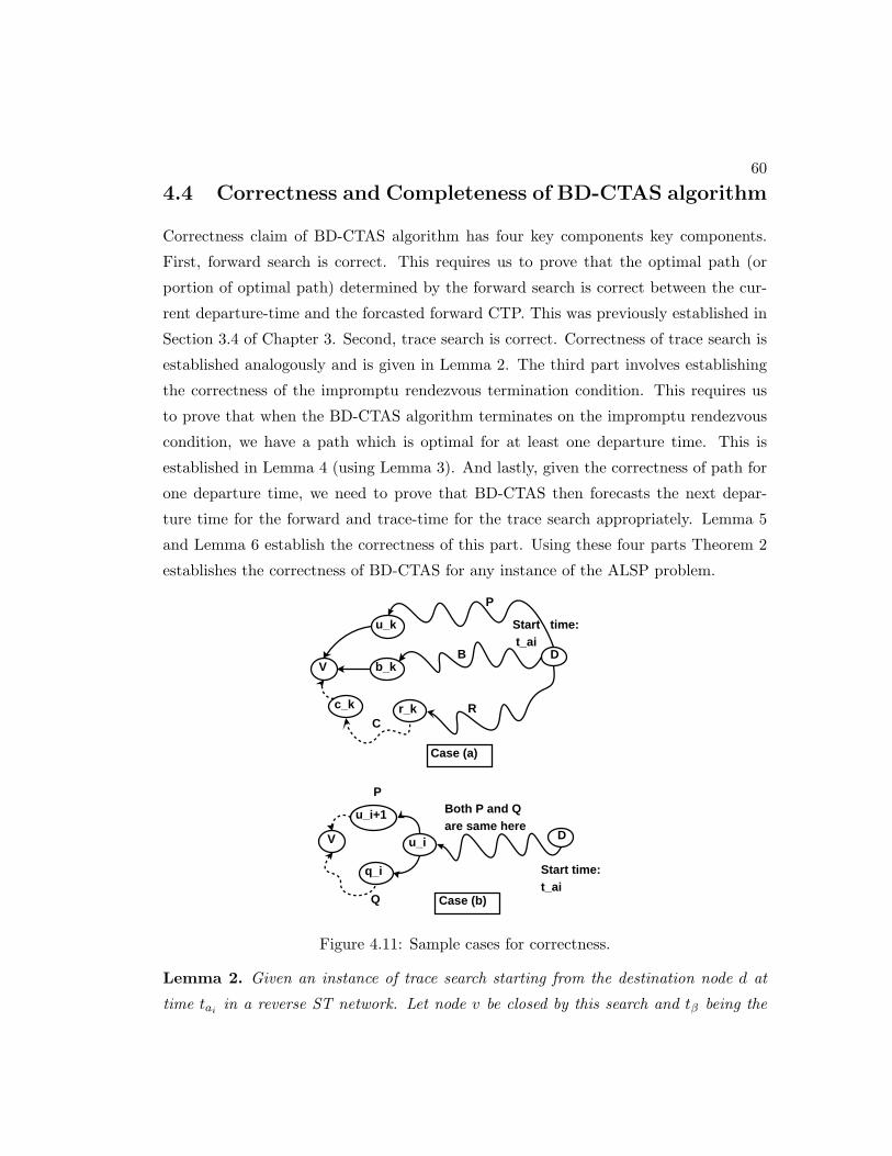
60

4.4 Correctness and Completeness of BD-CTAS algorithm

Correctness claim of BD-CTAS algorithm has four key components key components.

First, forward search is correct. This requires us to prove that the optimal path (or

portion of optimal path) determined by the forward search is correct between the cur-

rent departure-time and the forcasted forward CTP. This was previously established in

Section 3.4 of Chapter 3. Second, trace search is correct. Correctness of trace search is

established analogously and is given in Lemma 2. The third part involves establishing

the correctness of the impromptu rendezvous termination condition. This requires us

to prove that when the BD-CTAS algorithm terminates on the impromptu rendezvous

condition, we have a path which is optimal for at least one departure time. This is

established in Lemma 4 (using Lemma 3). And lastly, given the correctness of path for

one departure time, we need to prove that BD-CTAS then forecasts the next depar-

ture time for the forward and trace-time for the trace search appropriately. Lemma 5

and Lemma 6 establish the correctness of this part. Using these four parts Theorem 2

establishes the correctness of BD-CTAS for any instance of the ALSP problem.

DV

Start time: t_ai

u_k

b_k

r_k

P

B

Rc_k

Case (a)

C

Case (b)

DV

Start time: t_ai

u_i

Both P and Q are same here

q_i

Q

u_i+1

P

Figure 4.11: Sample cases for correctness.

Lemma 2. Given an instance of trace search starting from the destination node d at

time tai in a reverse ST network. Let node v be closed by this search and tβ being the

61

earliest trace critical time point observed so far. Let P : d-u1-. . .-uk-v be path found by

this search and P ′ be the path with edges in P reversed. We have the following

• P ′ is the shortest path between v to d for all arrival times in t′ ∈ [tai (tβ + tai)]

at d. By shortest we mean, P ′ has latest departure among all paths for the same

arrival time t′.

Proof. The proof for this lemma consists of two parts. First part involves proving that

P (or P ′) is optimal for time tai . Whereas, the second parts concerns itself with proving

the optimality for the entire time interval [tai (tβ + tai)]. We begin with the first part.

Given the greedy nature, similar concepts of expanding and closing a node in trace

search, its basic correctness can be borrowed from Dijkstra‘s. Here, we would just prove

that the trace search has gathered sufficient information when node v is closed for arrival

time tai . Consider the case (a) in Figure 4.11 (top part), which shows that candidate

paths to node v through its neighbors uk, bk and ck. Clearly, one of these would be the

predecessors of the optimal path. Also, optimal path leading to v would be composed

of optimal paths leading to one of these nodes followed by the edge to node v. Without

loss of generality assume that when node v was closed, the priority queue had trace

functions P : <D,. . .,uk,v >, B:<D,. . .,bk,v > and R:<D,. . .,rk−1,rk >. This means

that nodes uk, bk, and rk−1 were closed. According to the given case in Lemma, at this

stage the algorithm would have picked P and closed the node v. Now assume (for sake

of argument) that there exists another path through ck (D–rk via path R–v via path

C) which was optimal for arrival time tai . Given that all the travel times are positive,

path R which was not picked now, any positive additions (edges in path C) to it cannot

make it smaller that path P . This proves the optimality of path P for time tai at d.

The second part of the Lemma is proved using contradiction (case (b) in Figure 4.11).

Assume that there exists a path Q between d and v such that, path its edges reversed

(i.e, edges in Q are reversed) Q′ is shorter than P ′ for a certain tα (tai < tα ≤ (tβ+ tai))

at d. The trace search would order the priority queue on the value of trace functions at

time tai . This is because tai is the starting time of trace search according to the given

condition in Lemma. Without loss of generality assume that ui (ui 6= v) be the node

upto which both Q and P agree. This implies that path between ui and d (in P ′ and Q′)

was optimal for tα. Therefore, the portion between ui and v in Q must be shorter than

62

in P . After closing node ui, the algorithm would include trace functions of its neighbors

qi and ui+1 and continue the process of closing the closest node in a greedy fashion.

After closing a node, the algorithm always computes the earliest intersection point of

its trace function with others. Now as portion between ui and v in Q is shorter than in

P for tα, this process will create a trace critical time point at tα. This contradicts the

assumption that tβ was the earliest trace critical time point (tα ≤ (tβ + tai)).

Lemma 3. Given any instance of a temporal bi-directional search on a ST network

with a forward search starting from source S at time td, and trace search starting from

destination D at time ta, the searches can close a node v with the same distance label

iff ta ≥ aopt, where aopt is the optimal arrival time of the forward search.

Proof. (By contradiction) Consider a case where the trace search starts at time ta < aopt.

This means that the trace search starts earlier than the optimal arrival time aopt. Further

assume that, the trace search and forward search close a node v with same distance label

(for sake of contradiction). Now, consider the path resulting after combining: (a) the

path determined by the forward search from S to v; (b) path determined by trace search

from D to v with its edges reversed. Now, this is a valid path in our ST network which

departs from S at time td and arrives at D at time ta, which is a contradiction as the

aopt (> ta) was considered to the optimal arrival time of the forward search starting at

td.

Lemma 4. Given any instance of a temporal bi-directional search on a ST network

with a forward search starting from source S at time td, and a trace search starting

from destination D at time ta, it is sufficient to terminate as soon as both searches

close a node u with the same distance label, iff ta ≤ aopt, where aopt is the optimal

arrival time of the forward search.

Proof. (By contradiction) Consider a case where the trace search (starting at ta) and

the forward search (starting at td) closes a node u with the same distance label. Now,

we have following three cases: (1) ta < aopt; (2) ta = aopt or; (3) ta > aopt. Consider

the first case. Using Lemma 3 we know that the trace and forward searches can close

a node with same distance label, iff ta ≥ aopt. This contradicts our original assumption

that both trace and forward search have closed the node u with the same distance label.

63

Now, we consider the second case when ta = aopt (which is allowed as per Lemma

3). This implies that we have valid path between S and D which consists of path S

through u followed by u through D. Any other path which arrives at D earlier than ta

would contradict our original condition of aopt being optimal for td.

The third case ta > aopt can be easily shown via examples to lead to sub-optimal

paths. This proves the Lemma.

Lemma 5. Given an instance of the BD-CTAS algorithm with a forward search starting

from source S with a departure-time tdi; a trace search starting from destination D at

tai, where tai is guaranteed not to be an overestimate; and termination on impromptu

rendezvous condition with γmap = x (x ≥ 1),

1. BD-CTAS correctly determines the shortest path for departure-times tdi through

tdi + x− 1;

2. A trace-time of tai +x is not an overestimate of optimal arrival time for a forward

search starting at time t = tdi + x.

Proof. (By contradiction) We prove this Lemma using the properties of the strong FIFO

networks, where an earlier departure strictly implies earlier arrival. We first prove item

1 followed by item 2. Using Lemma 3 and Lemma 4, we know that when BD-CTAS

terminates with impromptu rendezvous condition, we have a shortest path between the

source and the destination for the corresponding departure-time at source. Without

loss of generality assume that both the searches closed node v with the same label. This

implies that, the path P obtained by combining S to v of forward search and D to v of

trace search is optimal for departure-time t = tdi . Given, γmap = x we know that path

found by forward search from S to v is guaranteed not to change between times tdi and

tdi +x− 1 (by construction of γmap and correctness of CTAS). Similarly, path found by

trace search betweenD and v is guaranteed not to change between times tai and tai+x−1

(by construction of γmap and correctness of trace search). Further, a γmap = x also

implies that lagrangian agreement duration between forward and trace functions at v

was at least x time units long. This proves the existence of the path P . The optimality of

this path for departure-times (at S) t ∈ [tdi tdi+x−1] is now proved using contradiction.

Note by nature of construction of path P and strong FIFO networks, there would be a

64

bijective mapping between the departure times [tdi tdi + x − 1] and the arrival times

[tai tai+x−1]. Let this function be DMapP : [tdi+1 tdi+x−1] → [tai+1 tai+x−1].

For example, DMapP (tdi) = tai and so on.

Now, Assume for sake of contradiction that there exists a path Q between S and D

which is shorter that P for a departure-time tdα ∈ [tdi tdi +x−1]. Wlg. assume that its

corresponding arrival time at destination is Qα. This implies that Qα < DMapP (tdα)

(by assumption). Given that our original ST network is strong FIFO, arrival time along

Q for the tdα −1 would be < Qα−1. However, DMapP (tdα −1) = DMapP (tdα)−1 (By

nature of construction of γmap), thus making Q shorter for tdα − 1 as well. Recursively

proceeding this we would have the following: the arrival time along Q for time tdi

would be less tai . This contradicts the given condition that tai was not an overestimate

of arrival time for departure-time tdi .

Proof for item 2 can also be given in similar fashion. Assume for sake of contradiction

that tai + x is an overestimate of arrival time for a forward search starting at time t =

tdi+x. This means that there exists a path R whose arrival time at destination Qdi+x <

tai + x. As above, using the properties of strong FIFO, we can recursively construct a

case where arrival time along R for time tdi would be less tai (a contradiction).

Lemma 6. Given an instance of BD-CTAS algorithm with a forward search starting

from source S with a departure-time tdi; a trace search starting from a destination D

at tai, termination with destination node being closed and tdi + x being the forecasted

forward CTP,

1. BD-CTAS correctly determines the shortest path for departure-times tdi through

tdi + x− 1;

2. A departure-time of PFunP (tdi +x− 1)+1 is not an overestimate of arrival time

for a forward search starting at time t = tdi + x. Here, PFunP (tdi + x − 1) is

the arrival time at the destination along the current shortest path P found by the

forward search for time t = tdi + x− 1

Proof. Whenever BD-CTAS terminates with forward search closing the destination,

information collected by the trace search (e.g. trace CTPs) is ignored. In this case, the

next start-time of forward and trace search is determined solely on the basis of earliest

65

forward CTP. Thus, the correctness of the first item in the Lemma can be ensured using

the argument presented in the correctness proof of the CTAS algorithm (Lemma 7 in

Section 3.4 of Chapter 3). On the other hand, the second item can be proved using the

properties of the strong FIFO networks.

Assume for sake of contradiction that PFunP (tdi + x − 1) + 1 is an overestimate.

This implies that there exists another path U between S and D, whose arrival time for

t = tdi + x, Udi+x at destination is less than PFunP (tdi + x − 1) + 1. This implies

that the arrival time at destination along U is at most PFunP (tdi + x− 1), which also

happens to the arrival time along P for time t = tdi+x−1. Now, given the properties of

the strong FIFO network, we know that the arrival time along the same path U for time

t = tdi +x−1 would be at most PFunP (tdi +x−1)−1. This is contradiction as path P

was optimal for start-times tdi through tdi+x−1. Or in other words, PFunP (tdi+x−1)

was the optimal arrival time (or shortest distance) for departure-time t = tdi+x−1.

Theorem 2. Given a source S; a destination D and; a discrete departure-time interval

(at S) λ = [td1 td2 td3 . . . tdk ], the BD-CTAS algorithm correctly computes a solution to

the all-departure-time Lagrangian Shortest paths (ALSP) problem.

Proof. The correctness of the BD-CTAS algorithm implies that it gives an optimal

shortest path for each departure-time tdi ∈ λ. The algorithm starts by computing the

shortest path between S and D for departure-times t = td1 and t = tdk . Assume that the

arrival times of these shortest paths at D are ta1 and tam . Using this information, the

trace-time interval for the trace search from D is now set to λrev = [ta1 . . . tam ]. We now

prove the correctness of the BD-CTAS in an incremental fashion over all departure-times

tdi ∈ λ.

Initial Step (tdi = td1): We have used known algorithms [16] in this step to compute the

arrival time ta1 and hence its correctness is trivially established. Following this, the

algorithm starts a forward search from S with departure-time td1 and a trace search

from D with a trace-time ta1 . This iteration can either terminate on impromptu termi-

nation condition or the forward search closing D. The correctness in case of impromptu

rendezvous termination is established through the fact that ta1 was the actual arrival

time at the destination (thus guaranteed not to be an overestimate). Correctness of the

second case (forward search closing node D) is established through the correctness of

66

CTAS algorithm [34].

General case (tdi ∈ [td2 td3 . . . tdk ]): Without loss of generality assume that the above

initial step gave us a shortest path between S and D for times td1 through tdi − 1.

Let the next departure-time of forward and trace-time of trace search be tdi and tai

respectively. Using Lemma 5 and Lemma 6 we know that trace-time tai is not an

overestimate. Thus, the correctness of the next iteration of the BD-CTAS algorithm is

guaranteed. This process continues until all the tdi ∈ λ are covered. This proves the

correctness of the algorithm.

4.5 Asymptotic complexity of Critical-Time-Point based

approaches

In this section, we provide detailed asymptotic complexity analysis for CTP based ap-

proaches (both BD-CTAS and CTAS algorithms). We also compare the complexity of

proposed algorithms with related work and provide an intuitive explanation of our dom-

inance zone. Additionally, we also provide a formal argument (Theorem 3) for superior

performance of BD-CTAS over CTAS algorithm [34] for the ALSP problem.

Space Complexity: The total space complexity of BD-CTAS (or CTAS) consists of

two key components. First, space required for storing the ST network for the use of

algorithms. In this work, we used time-aggregate graph [16] representation for storing

the ST network. The space complexity of this data structure is O(m+ n)H [16], where

n and m are the number of nodes and edges in the underlying spatial network. H is

number of distinct departure-times for which travel-time information (of each edge) is

available in the dataset.

The second component in the total space complexity comes from space required for

storing the priority queue. At any instant during the execution of the inner loop in

BD-CTAS (lines 11–19 of Algorithm 2) or CTAS (lines 3–13 of Algorithm 1 in [34]),

there can be at most indegree(v) paths terminating at node v. Now, if path ending on

v, P v, is expanded, v is closed for the current departure-time and P v is expanded (if

it is not the destination node). Following this at most indegree(v)− 1 paths would be

deleted from the priority queue. Thus, we can say at any instant during the execution,

the total number of paths in the priority queue would at most be∑|V |

i=1 degree(vi)

67

(degree(vi) ≤ indegree(vi)), which is O(m). Now, each of these O(m) paths would

have a path function represented as a time series of length #departure− times, which

in worst case can have O(H) items. Therefore, the total space of priority queue would

be O(mH). Combining with the space complexity of time-aggregate graph, the total

space complexity would be O(m+ n)H.

Time Complexity: The total running time cost of CTAS and BD-CTAS algorithms

can be presented in terms of the following: (a) #forecasted − CTPs, i.e., the num-

ber of re-computations performed for a particular instance of the ALSP problem and;

(b) cost of one iteration, i.e., the cost of determining a single sub-interval optimal

lagrangian path. Both CTAS and BD-CTAS algorithms determine the solution of an

ALSP problem instance by finding series of sub-interval optimal lagrangian paths (a

dyad of a path Pi and set of time instants ωi). The next departure-time outside ωi

being the forecasted critical time point. Thus, the overall cost incurred while solving a

particular instance would be #forecasted− CTPs× cost of one iteration

Cost of computing one sub-interval optimal lagrangian path is of the same order

in both CTAS and BD-CTAS algorithms. The difference in performance of the algo-

rithms is due to #forecasted − CTPs during the run-time. The BD-CTAS algorithm

encounters much less number of CTPs during run-time due to its bi-directional nature.

The bi-directional nature of BD-CTAS algorithm allows it to explore much less (and

potentially more relevant) search space, creating fewer irrelevant critical time points (as

also seen in experimental analysis, Section 4.6). We now provide a detail description of

cost of finding one sub-interval optimal lagrangian path.

The inner most loop in CTAS algorithm (lines 3–13 of Algorithm 1 in [34]) and BD-

CTAS algorithm (lines 11–19 in of Algorithm 2) computes a single sub-interval optimal

lagrangian path. In CTAS algorithm, this loop is characterized by the following: (1)

extract path function (Pfmin) with the least value of arrival time (for the current

departure-time) from the priority queue, assume this corresponds to a path P v with

the terminal node v; (2) compute the earliest intersection of Pfmin with other path

functions present in the priority queue, (3) expand the path P v to create path functions

to its open neighbors and, (d) delete paths ending on node v from the priority queue.

The inner most loop of the BD-CTAS algorithm also performs the same steps once for

each of forward and the trace search respectively. we now describe the cost of each

68

of these operations and number of times they are performed during computation of a

single sub-interval optimal lagrangian path. These costs are for a binary heap-based

implementation of the priority queues.

1. Extracting Pfmin (path function in P v: For a binary-heap implementation, this

cost would be O(logm) (since there can be O(m) paths in the queue). Since there

can be at most n extract mins (when destination is discovered last), the total cost

of extracting all the Pfmins would be O(n logm).

2. Compute earliest intersection of Pfmin: For a path function with T values (#depature−

times in ALSP instance (λ)=T ), computing earliest intersection with any particu-

lar path function can take O(T ) in worst case. Total cost of computing earliest in-

tersection of a single Pfmin would be O(T )×sizeof−priority−queue ≈ O(mT ).

Overall, for n such operations the cost would be O(nmT ).

3. Expand P v to create path functions to v’s neighbors: This would correspond to at

most outdegree(v) inserts into the priority queue. In worst case, there can be O(n)

expands which would lead to∑|V |

i=1 outdegree(vi) (≈ O(m) as outdegree(vi) ≤

degree(vi)) inserts into the priority queue. Thus, the total cost of expanding P vs

would be O(m logm) (with O(logm) as cost of single insert key).

4. Delete paths ending on v: When a path ending at node v is extracted, at most

indegree(v) paths would be deleted from the priority queue. Thus, in worst

case there would be O(m) deletes from the priority queue with a total cost of

O(m logm).

Thus, the cost of computing one sub-interval optimal lagrangian path for CTAS

and BD-CTAS would be sum of all above cost, which is O(n logm +m logm + nmT ).

Combined with the number of CTPs, the total cost of CTAS (and BD-CTAS) would

be #forecasted − CTPs × O(n logm + m logm + nmT ). Now, in worst case both

#forecasted− CTPs and #depature− times in ALSP instance could be O(H). This

could happen when the given ALSP instance required an re-computation for each of the

H time instants available in the ST network dataset. This would make the total worst

case time complexity to be H×O(n logm+m logm+ nmH).

69

4.5.1 Comparison with related work and dominance zone

Before we delve into the details of the actual comparison, it is important to note the

difference in the worst case complexity of discrete and continuous versions of the ALSP

problem. In the discrete version of the problem, the travel-times of edges are modeled

as a discrete time series. And, between two distinct departure-times the travel-time is

assumed to remain constant. On the other hand, in the continuous version, the travel-

time is modeled using continuous functions e.g., piece-wise linear functions. Depending

on the nature of problem (discrete vs continuous) the worst case complexity changes. In

case of discrete version, the number of re-computations are bounded by #departure−

times (λ) desired in the problem instance which, as mentioned before, in worst case

can be H. This means that in worst case, we just need to compute shortest path

H times. Whereas, in case of continuous functions, the same worst case complexity

becomes nΘ(logn) (where n is the number nodes in the graph) [59]. In other words, we

may have to re-compute the shortest path nΘ(logn) times, which is clearly prohibitive

for real graphs of large sizes.

The worst case run-time complexity of 2S-LTT [3] is O((n logn +m)α(H)), where

α() is the cost of maintaining the piece-wise linear function over a time interval of length

H. For a discrete case, where edge costs are represented as time-series (this paper), this

complexity becomes O((n logn +m)H). Time complexity of allFP was not mentioned

in [51] and thus comparison with it is limited to experiments.

As can be seen critical time point (CTP) based approaches (CTAS and BD-CTAS)

have higher worst case time complexity (H × O(n logm + m logm + nmH)). This is

because both CTAS and BD-CTAS do more amount of additional work in terms of

book-keeping and comparing entire times-series of arrival time information to eliminate

all knowable redundant re-computation. The performance gained by reducing redun-

dant work and its associated additional cost creates a trade off, making CTP based

approaches more expensive when several of them are forecasted during the execution

of the algorithms. Among CTAS and BD-CTAS algorithms, BD-CTAS can be shown

(Theorem 3 in Section 4.5) to perform less re-computations than CTAS algorithm.

Theorem 3. Given an ALSP instance on a ST network G = (V,E), the number of

critical-time points forcasted by the BD-CTAS algorithm does not exceed that of the

70

CTAS algorithm.

Proof. For simplicity, we assume that the travel time function δe associated with every

edge e ∈ E maps each departure time to either 1 or ∞, i.e., δe) : t → {1,∞}. For an

equitable comparison between BD-CTAS and CTAS, we make two assumptions: First,

δe exhibits a strong fifo property. This means each edge e ∈ E has a travel time of 1

time unit up to a certain departure time and then changes to ∞ and remains that way.

Second, the shortest path between any nodes in the ST network is unique for any given

departure time.

Consider an ALSP instance with source s, destination d and departure-time interval

λ = [td1 td2 td3 . . . tdk ]. Without loss of generality assume that a shortest path between

s and d exists and is of finite length for all departure times in λ.

Both BD-CTAS and CTAS would start from the departure-time td1 and forecast the

next critical time point, tdnt∈ λ, for re-computation. Here, we argue that tdnt

− td1

for BD-CTAS would not be lower than that for CTAS algorithm. It would be exactly

the same if the BD-CTAS terminates with the forward search closing the destination,

in which case it behaves exactly like CTAS. Thus, wlg., we assume that the BD-CTAS

algorithm terminated on the impromptu rendezvous condition. Let v be the common

node closed by both forward and trace searches with the same label. Let d(s, d)for denote

the shortest travel time distance from s as determined by forward search, and d(v, d)tra

be the distance to d from v as determined by the trace search. Also, let d(s, d)CTAS

be the distance computed by CTAS. Using the correctness of the BD-CTAS algorithm

(Theorem 2) we have the following equation: d(s, d)CTAS = d(s, v)for + d(v, d)tra.

Now given the construction of our ST network (edge costs can only be 1 or ∞), the

number of nodes closed during the search would have a direct relation (e.g. monoton-

ically increasing) to the shortest distance d(s, d)CTAS (d(s, v)for and d(v, d)tra in the

case of forward and trace searches) computed by the CTAS algorithm. Let F be a

function which maps this distance onto the number of nodes closed during the search

before setting this optimal distance label. Note that F would be the same for the for-

ward, trace and CTAS algorithm as they share the same candidate path enumeration

style 2 . We assume that this function is super-linear (nx, x > 1) in nature for our

ST network. This assumption is intuitive since the search space of forward, trace and

2 extract min from priority queue and expand the terminal node using δ of its neighbors

71

CTAS algorithm are likely to be “circular” around the origin as we do not use A* based

heuristics. Also, the codomain of F would only consist of positive integers (trivially).

On applying F to both sides of the above equation, we have:

F(

d(s, d)CTAS

)

? F(

d(s, v)for + d(v, d)tra)

Given that F is a super-linear.

F(

d(s, d)CTAS

)

≥ F(

d(s, v)for)

+ F(

d(v, d)tra)

Let G be a function which maps the number of nodes closed onto the difference

between the current departure time and the forecasted CTP (tdnt− td1 in this case).

These entities are conceived to have an inverse relation (e.g. monotonically decreasing)

between them, which means that as more nodes are closed, the more likely the search

will forecast a CTP very close to current departure time. This is intuitive since a direct

relation would not be feasible unless the edge weights were negative. We assume that

G is not sub-linear, i.e., it is at least linear. Applying G to both sides of the previous

equation, we have:

G(

F(

d(s, d)CTAS

)

)

≤ G(

F(

d(s, v)for)

+ F(

d(v, d)tra)

)

Given that G is monotonically decreasing and the codomain of F consists only of

positive integers (discrete nature of time),

G(

F(

d(s, d)CTAS

)

)

≤ min

{

G(

F(

d(s, v)for)

)

,G(

F(

d(v, d)tra)

)

}

Recall that BD-CTAS takes the minimum among, forward CTP, trace CTP and

lagrangian agreement duration (lag − dur), for determining the next departure and

trace time. This is done to determine the maximum length of time for which there is

agreement between forward and trace search. So the above equation becomes:

G(

F(

d(s, d)CTAS

)

)

? min

{

G(

F(

d(s, v)for)

)

,G(

F(

d(v, d)tra)

)

, lag − dur

}

Given that shortest path is assumed to be unique, a min (in above equation) coming

from lag − dur would imply that shortest path does indeed change for departure time

lag−dur+1. Under the correctness claim of the CTAS algorithm this would mean that

G(

F(

d(s, d)CTAS

)

)

= lag − dur. Thus,

72

G(

F(

d(s, d)CTAS

)

)

≤ min

{

G(

F(

d(s, v)for)

)

,G(

F(

d(v, d)tra)

)

, lag − dur

}

Applying this argument repeatedly over all of λ would show that the number of

CTPs forecasted by BD-CTAS algorithm would not exceed the number forecasted by

CTAS.

4.6 Experimental evaluation

Experimental setup: The overall goal of the experimental evaluation was to char-

acterize the dominance zone of the proposed BD-CTAS algorithm. To this end, the

following parameters were varied in the experiments: (a) length of the departure-time

interval over which shortest paths were desired (|λ|), (b) length of the route in terms of

its total travel time in minutes, and (c) time of day (rush hour vs non-rush hours). The

experiments were carried on one real and two synthetic datasets over the road network

of Hennepin county, Minnesota. The real dataset (provided by NAVTEQ [56]) contained

1481 nodes and 4510 edges. Travel-time information on all these edges was available at

a time quanta of 15mins. For experimental purposes, travel-times were converted into

time quanta of 1 min. This was done by replicating the data inside time interval. To

maintain the correctness of the BD-CTAS algorithm, we extracted only those sets of

departure-times where the edge followed the strong fifo property. One of the synthetic

dataset contained 54593 nodes and 166970 edges, whereas the other had 102709 nodes

and 302380 edges. Both of these datasets were created by first extracting the road

network from open street map [60] and then adding a variation to the static travel-time

of the edges to mimic its increase in the rush hour. This was done by increasing the

travel-time after a randomly chosen departure-time during the rush hour.

In our experiments, we first randomly choose a set of different queries (each with

different parameters) and then executed them on BD-CTAS, CTAS [34], Discrete version

of 2S-LTT [3], Discrete version of allFP [51] and a naive approach of computing shortest

path for each departure-time using SP-TAG [16]. Comparison against the A* versions

of the related work algorithms is out scope of this paper. For each of these queries, we

measured the total run-time in seconds. The total number of re-computations saved by

73

0

0.5

1

1.5

2

100 200 300 400 500

Run

-tim

e (s

ecs)

#departure-times (|Lambda|)

Path Length 20min, Non-Rush hours, 1481 Nodes, 4510 Edges

CTAS

SP-TAG

Discrete 2S-LTT

BD-CTAS

(a)

0.5

1

1.5

2

2.5

3

100 200 300 400 500

Run

-tim

e (s

ecs)


Path Length 20min, Rush hours, 1481 Nodes, 4510 Edges

CTAS

SP-TAG

Discrete 2S-LTT

BD-CTAS

(b)

0.01

0.1

1

10

100 200 300 400 500

Run

-tim

e (s

ecs)

(lo

gsca

le)


Path Length 40min, Non-Rush hours, 1481 Nodes, 4510 Edges

CTAS

SP-TAG

Discrete 2S-LTT

BD-CTAS

(c)

1

10

100 200 300 400 500

Run

-tim

e (s

ecs)

(lo

gsca

le)


Path Length 40min, Rush hours, 1481 Nodes, 4510 Edges

CTAS

BD-CTAS

SP-TAG

Discrete 2S-LTT

(d)

Figure 4.12: Effect of length of departure time interval (|λ|)

CTAS, BD-CTAS and Discrete 2S-LTT was also recorded for each run. The number

of re-computations saved is defined as the difference between #departure-times and

#forecasted-CTPs for the given ALSP problem instance. Experiments were conducted

on an Intel Quad Core Linux workstation with a 3.40GHz CPU and 16GB RAM. We

now discuss our results starting with our real dataset and followed by synthetic datasets.

Comparison with CTAS algorithm Effect of length of departure time interval (|λ|):

We evaluated the effect of length of departure-time interval (|λ|) over which the shortest

path was desired. Figure 4.12(a) and Figure 4.12(b) show the run-times for a route of

length (total travel time) of 20mins. Figure 4.12(c) and Figure 4.12(d) show the run-

times for a route of length 40mins. Here, the length of the route refers to the time

required to travel through these routes during non-rush hours (e.g. midnight). The

experiments showed that run-times of both the algorithms increase with |λ|, but the

run-time of BD-CTAS algorithm rises much more slowly than CTAS. This is because

74

BD-CTAS uses a bi-directional based search space, creating a much smaller number of

irrelevant CTPs. Experiments also showed that more saving occurred during non-rush

hours.

Effect of total travel time of path: We also evaluated the effect of length of the path

(in terms of its total travel time) on the candidate algorithms. Figure 4.13 shows the

execution time as the total travel time of the path was varied. As can be seen, the

runtime of both the algorithms increased with increasing path length. However, the

run-time of BD-CTAS rises much more slowly.

0 0.2 0.4 0.6 0.8

1 1.2 1.4

20 30 40 50

Run

-tim

e (s

ecs)

Path length (mins)

#departure-times 100, Non-Rush hours, 1481 Nodes, 4510 Edges

CTAS

SP-TAG

Discrete 2S-LTT

BD-CTAS

(a)

0.2

0.4

0.6

0.8

1

1.2

1.4

20 30 40 50

Run

-tim

e (s

ecs)

Path length (mins)

#departure-times 100, Rush hours, 1481 Nodes, 4510 Edges

CTAS

SP-TAG

Discrete 2S-LTT

BD-CTAS

(b)

0.01

0.1

1

20 30 40 50

Run

-tim

e (s

ecs)

(lo

gsca

le)

Path length (mins)

#departure-times 200, Non-Rush hours, 1481 Nodes, 4510 Edges

CTAS

SP-TAG

Discrete 2S-LTT

BD-CTAS

(c)

0.5 1

1.5 2

2.5 3

3.5 4

4.5

20 30 40 50

Run

-tim

e (s

ecs)

Path length (mins)

#departure-times 200, Rush hours, 1481 Nodes, 4510 Edges

CTAS

SP-TAG

Discrete 2S-LTT

BD-CTAS

(d)

Figure 4.13: Effect of total travel time of path.

Number of re-computations saved in BD-CTAS: Figure 4.14 shows that BD-CTAS

algorithm performed much less number of re-computations than CTAS.

Effect of time of the day (rush hour vs non-rush hours) Experiments showed that

better performance was obtained for non-rush hours than rush hours (see Figure 4.13,

Figure 4.12 and Figure 4.14). This is because there were fewer intersections among the

path-functions.

75

50

100

150

200

250

300

Path-Length=20mins

Path-Length=30mins

Path-Length=40mins

Path-Length=50mins

#Re-

com

puta

tions

sav

ed

Non-Rush Hours, #departure-times = 300, N=1481, M=4510

BD-CTAS2S-LTT

CTAS

(a) During Non-Rush hours

50

100

150

200

250

Path-Length=20mins

Path-Length=30mins

Path-Length=40mins

Path-Length=50mins

#Re-

com

puta

tions

sav

ed

Rush Hours, #departure-times = 300, N=1481, M=4510

BD-CTAS2S-LTT

CTAS

(b) During Rush hours

Figure 4.14: Number of re-computations saved.

Comparison with Naive algorithm: In general, BD-CTAS performed better than

the naive approach. However, for routes lengths greater than 40mins and |λ| ≥ 200,

SP-TAG started giving quicker response time during rush-hours (see Figure 4.12(d) and

Figure 4.13(d)). A similar observation was made for non-rush hours as well, but for

|λ| > 500. This is because, longer routes and departure-time intervals create a large

number of forecasted CTPs and thus, it is much faster to simply instantiate the SP-

TAG algorithm for all the departure-times. Recall that both BD-CTAS and CTAS

achieve their performance benefits by making conservative estimates of the departure-

times which can be skipped. This is achieved through additional book-keeping and

processing over a common label setting algorithm like SP-TAG. Thus, it is conceivable

that computational costs associated with additional book-keeping and processing may

start to outweigh the gains obtained by skipping some departure-times when the number

of critical time points is large.

Comparison with the Discrete 2S-LTT algorithm During rush hours, on longer

paths (greater than 40mins), 2S-LTT was able to save more re-computations than BD-

CTAS algorithm (Figure 4.14(b)) on ALSP instance with |λ| ≥ 300 usually resulting

in better run-time (Figure 4.12(d)). This is because, in our approach, when a path

is expanded, we compute the intersection point with all the other paths (possible ter-

minating on different nodes) present in the priority queue to ensure correctness. This

sometimes forecasts CTPs which are irrelevant to the ALSP instance. Whereas, 2S-LTT

compares the cost of current path against the earliest feasible cost to the same terminal

node (as the current path) along other paths. This approach, though may not be able to

76

close the node for longer times (as discussed earlier), but might forecast fewer irrelevant

CTPs.

Comparison with Discrete allFP algorithm: Our experimental analysis shows that

the run-time of the allFP algorithm rises sharply with length (i.e., total travel time) of

the route (see Figure 4.15). In contrast, our approach was much less sensitive to length of

the route. Due to this limitation allFP was not included in further experiments. Figure

4.15 shows that the BD-CTAS algorithm is faster than allFP algorithm by several orders

of magnitude.

0

10

20

30

40

50

60

5 10 15 20

Run

-tim

e (s

ecs)

Path length (mins)

Non-Rush hours, 1481 Nodes, 4510 Edges

Discrete allFP #departure-times 100

Discrete allFp #departure-times 300

BD-CTAS #departure-times 100


(a)

0

10

20

30

40

50

60

5 10 15 20

Run

-tim

e (s

ecs)

Path length (mins)

Rush hours, 1481 Nodes, 4510 Edges

allFP #departure-times 100

allFp #departure-times 300



(b)

Figure 4.15: Comparison with allFP algorithm.

Experiments synthetic datasets: Figure 4.16 illustrates the results on synthetic

datasets. This experiment revealed trade-offs similar to the ones observed in the real

datasets, i.e., both BD-CTAS and CTAS gain performance by skipping some departure-

times. However, the additional cost of book-keeping and processing starts to out-weigh

the benefits for cases with longer path-length and more #departure−times due to more

CTPs. Further, our experiments also highlighted that the algorithms were in general

slightly slower on larger datasets due to the larger size of TAG data-structure.

Discussion: A naive approach for solving the ALSP problem involves computing a

shortest path for each departure time using a time-generalized version of Dijkstra’s

[15–22]. However, this leads to redundant re-computation of the shortest path across

consecutive departure times sharing a common solution, creating an computational

bottleneck for ALSP instances with long departure time intervals. For instance, in our

77

0.05 0.1

0.15 0.2

0.25 0.3

0.35 0.4

0.45 0.5

100 200 300 400 500

Run

-tim

e (s

ecs)


Path Length 20min, 54593 Nodes, 166970 Edges

CTAS

SP-TAG

Discrete 2S-LTT

BD-CTAS

(a)

0

1

2

3

4

5

100 200 300 400 500

Run

-tim

e (s

ecs)



CTAS

SP-TAG

BD-CTAS

Discrete 2S-LTT

(b)

0.1

0.2

0.3

0.4

0.5

0.6

0.7

100 200 300 400 500

Run

-tim

e (s

ecs)



CTAS

SP-TAG

Discrete 2S-LTT

BD-CTAS

(c)

0.5

1

1.5

2

2.5

100 200 300 400 500

Run

-tim

e (s

ecs)



CTAS

SP-TAG

Discrete 2S-LTT

BD-CTAS

(d)

Figure 4.16: Experiments on synthetic datasets.

earlier University-Airport ALSP instance (Figure 3.1), it would have been computation-

ally redundant to compute shortest path for departure-times 7:45, 8:00, 8:15 and 8:30

as the solution does not change.

4.7 Conclusions and Future work

The All-departure-time shortest Lagrangian shortest path problem (ALSP) is a key com-

ponent of applications in transportation networks. ALSP is a challenging problem due to

non-stationarity of the spatio-temporal network. A naive approach of re-computing the

shortest path for each departure time incurs redundant computation across time instants

sharing a common solution. The proposed critical-time-point based approaches (CTAS

and BD-CTAS) reduces this redundancy by determining the departure times when the

ranking among the alternate paths between the source and destination changes. Theo-

retical and experimental analysis show that this approach is more efficient particularly

78

when the number of critical time points is small.

In the future we plan to extend the BD-CTAS algorithm by developing an A* based

approach on continuous models [17]. We also plan to generalize the proposed algorithm

to non-FIFO networks. Further, we plan to explore alternative approaches similar to [61]

for solving ALSP. Performance of CTAS and BD-CTAS will also be evaluated on larger

real datasets. We also plan to extend critical-time point based approaches to other

problems on ST networks.

Chapter 5

Temporally Detailed Social

Network Analytics

Given the ever-increasing proliferation of mobile and online social networking platforms,

social interactions can increasingly be observed and studied at a fine temporal scale.

Data from these platforms typically consists of time-stamped social events. These social

events can represent several types of social interactions such as emails, phone calls,

post-comment interactions, co-location pairs, etc. A time-stamped social event can be

described as a relational tuple <Ai,Aj ,T>, where Ai and Aj are the two individuals

(or agents) who were interacting, and T is the time-stamp when this was observed.

Such an event creates a temporary link between Ai and Aj , which can then be used

in a time-aware analysis. A time-aware analysis can either consider the social events

individually (e.g. change detection in streams) or could first create a set of frames

containing interactions among members of a specific social system (e.g., employees of a

university). Here, each frame would either contain events that occurred at a specific time

point or comprise of all the events spread over a certain time duration (e.g., hour, day,

week, etc.). A collection of all such frames (over a time window) recording interactions

among the members of the same social system is referred to as a Temporally Detailed

(TD) social network in this paper. Figure 5.1 illustrates a sample TD social network

among W,X,A,C,D,U,U and Y. Here, an edge between two individuals denotes a social

interaction.

79

80

Figure 5.1: Sample Temporally-Detailed Social Network (best in color).

In this chapter, given a TD social network, we explore the computational challenges

underlying a potential realization of what we refer to as temporally-detailed (TD) social

network analytics. TD social network analytics can answer novel time-aware questions

on the underlying social system. Examples include: “How did the betweenness centrality

of an individual vary over past year?” “How is the closeness centrality of a person

changing over time?” Etc. To this end, several pilot studies [13, 14, 29, 30, 62] have

extended the traditional centrality metrics such as Betweenness and Closeness for TD

social networks. These extended metrics capture the dynamics of the underlying social

system and thus provide a better opportunity to understand its evolutionary behavior.

However, a TD social network still poses significant challenges for a computationally

scalable realization of TD social network analytics. For instance, the shortest path

between any two individuals in a TD social network–a key component in the extended

versions of Betweenness and Closeness [13, 14, 29, 30]–is not stationary across time. As

an example, in our previous TD social network shown in Figure 5.1, the shortest path

between W and U passes through A for times t = 1,t = 2 and t = 3. Whereas, the same

passes through C for times t=4 and t=5. Note that for sake of simplicity, we did not

consider the temporal order of edges in this example, which is important while analyzing

a TD social network as noted by other works as well [13,14,29,30]. It is important to note

81

that non-stationarity can be seen when we consider temporal order of edges as well. If we

consider the temporal order of the edges in Figure 5.1, then the shortest path between

W and U passes through A only for times t = 1 and t = 2. This non-stationarity

present in TD social networks violates the stationary ranking assumptions [63, 64] of

classical dynamic programming (DP) based techniques (e.g. Dijkstras and its variants),

and thus, makes it non-trivial to use them for computing the temporal extensions of

shortest-path-based centrality metrics such as Betweenness and Closeness.

Current works [13, 14, 29, 30] intrinsically resort to re-computing the shortest paths

(using a DP based technique) for all the times (for which the network is desired to

be analyzed) while calculating the temporal extensions of Betweenness and Closeness.

This approach yields a correct answer as given a particular time point, the ranking

among paths is stationary. One could indeed use a DP based technique to re-compute

the shortest paths (or the shortest path tree) and the centrality metric for each time

point individually (as done in the related work). While such an approach provides a

correct answer, it performs redundant work across times sharing a common solution.

For instance, in our previous sample shown in Figure 5.1, the shortest path tree rooted

at W does not change across t = 1,t = 2 and t = 3. Thus, it would be computationally

redundant to re-compute the shortest path tree for t = 2 and t = 3 as the solution did

not change. Such redundant work becomes a major computational bottleneck in case

of large TD social networks observed for a long time-interval.

In this chapter, we propose to reduce this redundant re-computation through our

novel approach of epoch-points. Epoch-points are the time points when the shortest path

tree rooted a node changes. For example, in our previous sample shown in Figure 5.1,

t = 1 (trivially), t = 4 and t = 6 form the epoch-points for the shortest path tree rooted

at W. Epoch-points can be computed using one of the two strategies, pre-computing

or lazy. In a pre-computing based method, all the candidate solutions (spanning trees)

are enumerated and compared to determine the best tree for each time. This approach,

however, would become a bottleneck in case of a large TD social network. To this end,

we propose to use the lazy technique which computes epoch-points on-the-fly. The key

insight in a lazy approach is that immediately after the computation of the shortest path

tree for the earliest (nth) time, one has adequate information to forecast the first (nth)

epoch-point. Epoch-point based algorithms for computing the temporal extensions of

82

shortest-path-based centrality metrics such as Betweenness [13, 14, 29, 30] show better

scalability by reducing the work across time-points sharing a common solution.

Contributions: This chapter makes following contributions:

1. We introduce epoch-point based approaches as a computational technique for tem-

porally detailed analytics on TD social networks.

2. We propose a novel data structure called temporally-detailed priority queue helps

in computing epoch-points on the fly (the lazy approach of computing epoch-

points).

3. We propose an epoch-point based algorithm called EBETS for computing temporal

extensions of Betweenness centrality. Note that EBETS can be easily modified

to compute temporal extensions of closeness centrality as well. For purposes of

brevity, we chose not to include that extension in the paper.

4. We prove the correctness and completeness of our proposed approach.

5. We evaluate EBETS experimentally via real datasets.

6. We provide an empirical comparison of temporal extension of betweenness cen-

trality and traditional betweenness centrality on a real dataset.

The rest of the paper is organized as follows. Section 5.1 describes the basic con-

cepts (e.g., representation models for TD social networks) and defines the problem of

temporally-detailed social network analytics. In Section 5.2, we propose the concept

of epoch-points for the problem of temporally-detailed social network analytics and de-

scribe our temporally-detailed priority queue to compute them on-the-fly. We propose

an epoch-point based algorithm called EBETS for computing the temporal extension

of betweenness centrality in Section 5.3. In Section 5.4, we prove the correctness and

completeness our epoch-point based algorithm. The experimental evaluation of our

algorithm is given in Section 5.5. Empirical comparison of temporal extension of be-

tweenness centrality and traditional betweenness centrality in given in Section 5.6. We

conclude this chapter in Section 5.7.

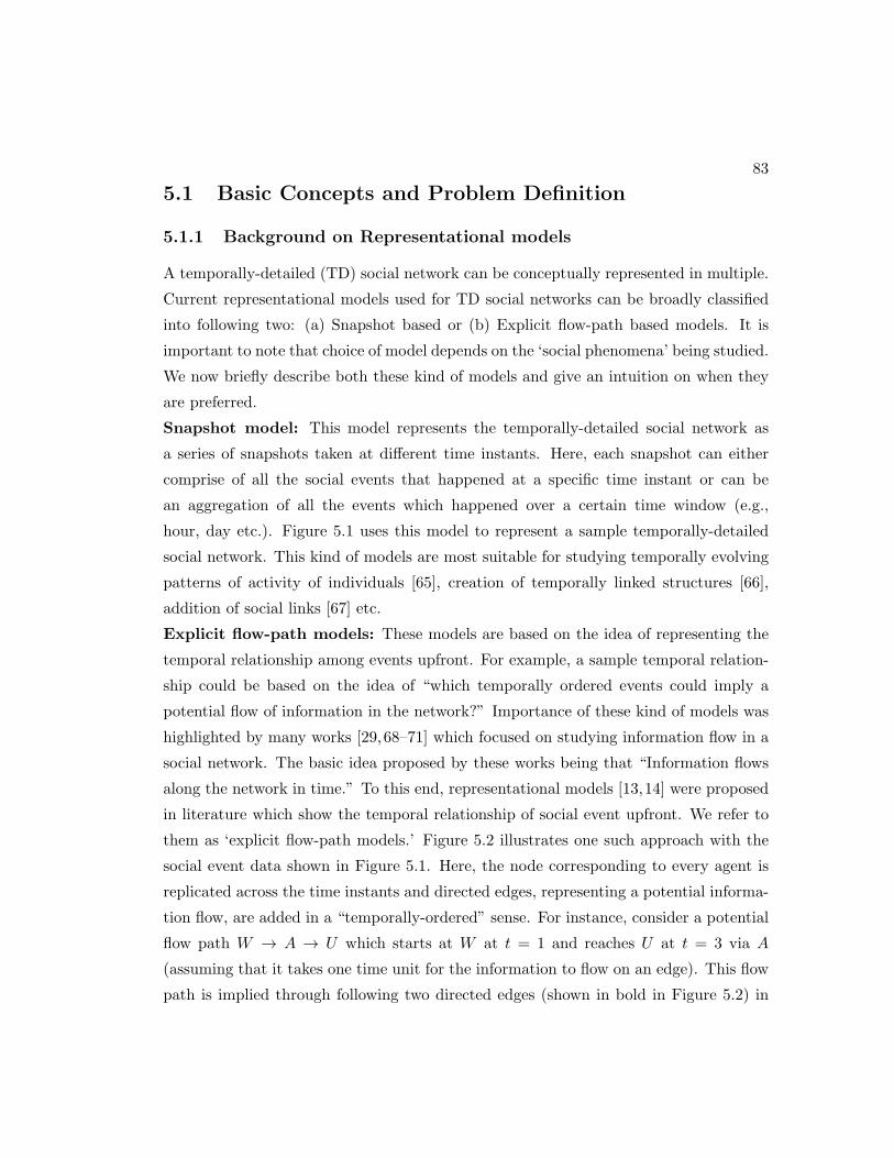
83


5.1.1 Background on Representational models

A temporally-detailed (TD) social network can be conceptually represented in multiple.

Current representational models used for TD social networks can be broadly classified

into following two: (a) Snapshot based or (b) Explicit flow-path based models. It is

important to note that choice of model depends on the ‘social phenomena’ being studied.

We now briefly describe both these kind of models and give an intuition on when they

are preferred.

Snapshot model: This model represents the temporally-detailed social network as

a series of snapshots taken at different time instants. Here, each snapshot can either

comprise of all the social events that happened at a specific time instant or can be

an aggregation of all the events which happened over a certain time window (e.g.,

hour, day etc.). Figure 5.1 uses this model to represent a sample temporally-detailed

social network. This kind of models are most suitable for studying temporally evolving

patterns of activity of individuals [65], creation of temporally linked structures [66],

addition of social links [67] etc.

Explicit flow-path models: These models are based on the idea of representing the

temporal relationship among events upfront. For example, a sample temporal relation-

ship could be based on the idea of “which temporally ordered events could imply a

potential flow of information in the network?” Importance of these kind of models was

highlighted by many works [29,68–71] which focused on studying information flow in a

social network. The basic idea proposed by these works being that “Information flows

along the network in time.” To this end, representational models [13,14] were proposed

in literature which show the temporal relationship of social event upfront. We refer to

them as ‘explicit flow-path models.’ Figure 5.2 illustrates one such approach with the

social event data shown in Figure 5.1. Here, the node corresponding to every agent is

replicated across the time instants and directed edges, representing a potential informa-

tion flow, are added in a “temporally-ordered” sense. For instance, consider a potential

flow path W → A → U which starts at W at t = 1 and reaches U at t = 3 via A

(assuming that it takes one time unit for the information to flow on an edge). This flow

path is implied through following two directed edges (shown in bold in Figure 5.2) in

84

W1

Time t=1 t=2 t=3 t=4 t=5 t=6

A1

C1

U1

V1

W2

A2

C2

U2

V2

W3

A3

C3

U3

V3

W4

A4

C4

U4

V4

W5

A5

C5

U5

V5

W6

A6

C6

U6

V6

t=7

W7

A7

C7

U7

V7

Figure 5.2: Explicit flow-path models (best in color).

the graph: (a) an edge between the copy of node W at t = 1 and A at t = 2, and (b)

an edge between the copy of node A at t = 2 and U at t = 3.

Snapshot models vs Explicit flow-path models: Both snapshot and explicit flow-

path models represent the same social event data but in two different ways. Further,

one representation can be easily converted into another, i.e, snapshot based models

can also be used to study flow based questions (by considering events across snapshots).

And similarly, explicit flow-path based models can be used to study temporally evolving

patterns, potentially seen upfront in a snapshot based model.

In this paper, we will use a compressed version of snapshot based models to describe

our work. These are called as Time aggregated graphs [37]. In this model, we assign a

time series, called an interaction time series, to each edge. This time series captures the

time instants at which interactions have occurred. Figure 5.3 illustrates this model with

the TD social network shown in Figure 5.1. Here, edge (W,A) is associated with an

interaction time series [1 1 1 X X X X]. This implies that W interacted with A at times

t = 1, 2, 3. Using this model, the information flow paths can also be easily retrieved

by following the edges in a temporally-ordered fashion. Figure 5.3 also illustrates our

previous information flow path W → A → U which starts at W at t = 1 and reaches U

at t = 3 via A.

Problem Definition: The problem of temporally-detailed social network analytics

85

Figure 5.3: Time aggregated graph

(TDSNA) is defined as follows:

Input: (a) Temporally-detailed social network; (b) Shortest path based centrality met-

rics (e.g., betweenness and closeness)

Output: An algorithm design paradigm for computing these metrics over an discrete

interval of time.

Objective: Computational scalability.

Constraints: Correctness and completeness of the solution.

5.2 Computational Structure of TD social network ana-

lytics

A nave approach for the TDSNA problem could be to repeatedly re-compute the short-

est path tree using a DP based algorithm for each time. However, this would incur

redundant re-computation across times sharing a common solution, leading to a severe

computational bottleneck in case of long time-intervals for large TD social networks. To

reduce this computational cost, we propose the notion of epoch-points which divide the

given time-interval into a set of disjoint sub-intervals in which the ranking among alter-

native candidate paths is stationary. Within these intervals, the shortest path tree can

now be computed using a single run of a dynamic programming (DP) based algorithm.

The advantage of such an approach is that we would not compute the shortest path tree

for many times in the given interval. We would re-compute only at the epoch-points

without missing any time instant in the given time-interval where the shortest path tree

can change. Note that the shortest path tree rooted at any node is not unique. It just

86

Figure 5.4: Shortest path tree rooted at node W for different times.

represents ‘a’ shortest path to the internal and leaf nodes of the tree from its root. To

this end, we define epoch-points in terms of the maximum duration of ‘optimality’ of

the current shortest path tree. Epoch-points are formally defined in Definition 1.

Definition 1. Epoch-Points Given a shortest path tree STree(v) for a time t = tcur

which is rooted at node v and contains nodes U = {u1, u2, . . . , uk}. The earliest time

instant tepoch > tcur is a epoch-point with respect to STree(v) if one of the following

holds:

1. There is a path P (at t = tepoch) from v to some ui ∈ U which is shorter than the

current path in STree(v).

2. The current path to some ui ∈ U in STree(v) no longer exists at t = tepoch.

3. There is a node w /∈ U which is reachable from v at time t = tepoch.

Figure 5.4 illustrates the proposed idea of epoch-points for the shortest path tree

rooted at W for the TD social network shown in Figure 5.1. The figure shows that the

shortest path tree rooted at node W changes at t = 1 (trivially), t = 4, and t = 6 making

them the epoch-points in this case. Note that the trees represented in Figure 5.1 are

constructed based on the snapshot model where the temporal order of edges was not

considered. Basically, each shortest path tree in Figure 5.4 corresponds to an instance

of Dijsktra’s (from node W) on each of the 6 snapshots in Figure 5.1. These trees would

be slightly different if we consider temporal order of edges (for modeling flows). We did

87

not consider them in this example for ease of communication. Note, that the concept

of Epoch-Points is valid for both snapshot and flow-path based studies. Just “what

constitutes a shortest path?” changes across snapshot and flow-path based studies. In

a flow-path based study, the edges must be considered in a temporally-ordered fashion.

A key challenge in designing an epoch-point based algorithm for the TDSNA prob-

lem is to minimize the amount of time needed to compute the epoch-points while

ensuring correctness and completeness. Epoch-points can be computed in two ways,

pre-computing strategy or a lazy strategy. In a pre-computing based method, all the

candidate solutions (spanning trees) are enumerated and compared to determine the

best tree for each time. This approach, however, may become a computational bottle-

neck in the case of a temporally-detailed social network, as there can be large number

of candidate spanning trees. In this paper, we investigate the lazy technique, which

computes epoch-points on-the-fly while exploring candidate paths. The key insight in

a lazy approach is that immediately after the computation of the shortest path tree for

the first (nth) time, one has adequate information to forecast the first (nth) epoch-point.

In our previous example of shortest path tree of node W, this would mean that, after

computing the shortest path at t = 1 we could forecast t = 4 as the next epoch-point for

the re-computation to start. In other words, a single logical work-unit of the proposed

algorithm would be: “compute the shortest path tree for one time and forecast the next

epoch-point for re-computation.”

An epoch-point is forecasted through the use of a modified priority queue, which

we call as a temporally-detailed (TD) priority queue. Table 5.1 illustrates its

properties in contrast the regular priority queues. Unlike a regular priority queue,

whose elements are scalar values, a TD priority queue is composed of time-series of

values. For our shortest path tree problem, a time-series in this queue would contain

the cost along a path to a node in the open list for the times under consideration.

The queue is ordered on the current time (tord in Table 5.1) under consideration. For

instance, in our previous example of shortest path tree of node W over the time interval

[1 6], we would order the queue based on costs for t = 1 for the first logical work-unit

and then for the forecasted epoch-point for the second work unit, and so on. Apart

from the standard priority queue operations such as insert, extract-min, update-key,

we have a new operation called “forecast-epoch-point.” This new operation is called

88

Properties/operationsPriority

Queue

Temporally-Detailed

Priority Queue

KeysScalar

valuesTime-series of values

OrderingAscending or

Descending

Ascending or Descending on

a time index tord

Insert operationInserts

scalar valueInserts a time-series

Update-Key operationUpdates a

scalar value

Updates an entire

time-series

Extract-Min

Returns a

scalar with

lowest cost

Returns a time-series with

least value of tord

Forecast-Epoch-Point--Not

Available--

Maximum time tept(> tord)for which the previous

extract-min has least value

among all keys in the queue

Table 5.1: Priority Queue vs Temporally-Detailed Priority Queue.

at the end of each extract-min, at that stage it compares the time-series corresponding

to the extract-min with the other time-series in the queue to determine the maximum

time duration (beyond tord) for which the chosen time-series has the lowest value. This

value is stored in an auxiliary data-structure as a “potential epoch-point.” At any stage

during the execution, we have the following loop invariant:

Proposition 1. The choices (i.e., extract-mins from the TD priority queue) made

during execution hold their validity for all the times between the time for which the

queue is ordered (trivially) and the min{potential epoch-points observed so far}.

Using this loop invariant and exploring the paths in a greedy fashion (similar to

Dijkstra’s enumeration style), when we expand (extract-min + forecast-epoch-point) a

node v, we have a shortest path between the root of the tree to v which is optimal for all

the times between tord (on which the queue was ordered) and the min{potential epoch-

points observed so far}. This min{potential epoch-points} then becomes the forecasted

epoch-point when the re-computation starts.

89

5.3 Epoch based Betweenness Centrality

Figure 5.5: Sample temporally-detailed social network.

This section describes a general epoch-point based algorithm for computing temporal

extension of betweenness centrality on a temporally-detailed social network. A key

component of this computation would be to determine shortest paths between all pairs

of nodes for either all the times or for a given range of time instants. As mentioned

previously, these shortest paths could change with time. As soon as the optimal shortest

path to a node in the tree changes, we deem the shortest path tree to has changed

(ref Definition 1). The time points where these changes happen are termed as the

epoch-points (ref Definition 1). These epoch-points need to be determined in order to

efficiently compute a temporal extension of betweenness centrality [13, 14, 29, 30] for

several time points in a TD social network. Note that, even if the shortest path tree

changes according to Definition 1, the overall betweenness centrality value may not

change. However, in order to ensure correctness, we re-compute the shortest path tree

(and the betweenness centrality) for all the epoch-points as defined in Definition 1.

In order to determine the epoch-points using a temporally-detailed (TD) priority

queue, we need to model the total cost of a path for different time instants which would

be inserted in the TD priority queue as keys. We propose to do this via–what we refer

to–as a path-function. A formal definition of the path-function is given below.

Definition 2. Path-function: A path function is a time series that represents the total

cost of the path from the root of the tree to the end node of path as a function of time.

A path function is determined by combining the interaction time series of its component

edges in a suitable fashion, e.g., in a time-ordered way for modeling information flow.

For instance, consider the path <W ,A,U> in the TD social network shown in Figure

90

5.5. This path contains two edges, (W,A) and (A,U). The interaction time series of edge

(W,A) is [1 1 1 1 X X], while that of (A,U) is [1 1 1 1 X X]. Depending on the nature of

the ‘social phenomena’ being studied, these interaction time-series can be combined in

multiple ways. If the ‘social phenomena’ of interest is preferable via a snapshot model,

then these can be simply added (interpreting ‘X’ as +∞) to create the path function of

<W ,A,U> over time instants [1 6] as [2 2 2 2 X X]. This means that length of the path

<W ,A,U> for times t = 1, 2, 3, 4 . . . is two edges, and the path is undefined for times

t = 5, 6.

On other hand, if the ‘social phenomena’ being studied requires modeling informa-

tion flows then we need to consider the temporal order of interaction events on the

edges [29, 68–71]. Further, the cost of the path is noted in terms of the arrival time

at the end node of the path [14]. In other words, cost of a path, e.g. S-X-Y, for time

t = α is interpreted as “If I start at S at time t = α and traverse S-X-Y, then when

(a time t > α) can I take an outgoing edge from Y?” This boils down to considering

following two aspects: (a) How much time does it take for the information to flow on an

edge? and (b) Is information allowed to wait at a node? Depending on our choices for

item (a) and item (b), the resulting path-function may be different. We now illustrate

the procedure for constructing path-function for modeling flows under following design

decisions: For item (a), we assume it takes 1 time unit for the information to travel

on an edge. And for item (b), we assume that the information is not allowed to wait.

Note that these assumptions are only for illustration purposes, and are not constraints

on our epoch-point based approaches. Usually, these design decisions would depend on

nature of the ‘social phenomena’ being studied.

Figure 5.6: Path functions for all

the singleton edges.

Consider the interaction time series of edge

(W,A): [1 1 1 1 X X] which denotes that W and

A interacted at times t = 1, 2, 3 and 4. Following

our previous assumptions for item (a) and item

(b), we interpret this interaction time series in fol-

lowing way: If we start at W at time t = 1, 2, 3, 4,

we can take the next outgoing edge from A at

times t = 2, 3, 4, 5. Note that ‘X’ is interpreted

as “cannot follow this edge” (implemented as +∞). This gives the path-function [2 3

91

Figure 5.7: Path function computation for modeling information flows.

4 5 X X] for the edge (W,A). Similarly, we would get the path-function [2 3 4 5 X X]

for the edge (A,U). Figure 5.6 shows the path-functions computed in this way for all

the singleton edges ((W,A), (W,C), (A,U), etc.) in the TD social network illustrated

in Figure 5.5. Now consider the case of determining the path function of <W,A,U>.

Figure 5.7 illustrates this process. If we take the edge W-A at time t = 1, we would

be able to edge (A-U) at time t = 2 and then take the next outgoing edge from node

U at time t = 3. Thus, the value of path-function of <W,A,U> for t = 1 would be

3. Following this process, the complete path-function of <W,A,U> for t = 1, 2, 3, 4, 5

(under the previous assumptions for item (a) and item (b)) would be [3 4 5 X X]. Note

that a path function for <W,A,U> modeling flows cannot be defined for t = 6 for the

network shown in Figure 5.5 because the network was not ‘observed’ for t = 7 which is

needed if a flow has to modeled for t = 6.

As mentioned previously, different path-functions would be obtained if waiting is

allowed or it takes more than 1 time unit for the information to travel on a edge. For

instance, consider the case when waiting is allowed. Waiting is a natural consequence

when the goal is to model the notion of “lifetime” of an information unit [72–74] flowing

through the network. Waiting can be implemented by incorporating the notion of

maximum wait allowed into the path-function construction. For example, consider

the interaction time series of (C,V) [X X X 1 1 X]. Under the no waiting scheme, this

translated to the path-function: [X X X 5 6 X] (see Figure 5.6). Now, consider the

case when an information unit is allowed to wait for a maximum of 2 time units at

any node. This means if the information has to flow through the edge (C,V) it must

92

arrive at node C (or V as this is an undirected edge) by times t = 2, 3, 4 or 5. Case

of t = 4 and t = 5 is trivial as C and V interacted at these times. However, t = 2

and t = 3 imply that the information waits at C (or V) for two and one time units

respectively. In this case, we would get the following path-function for (C,V): [X 5 5 5

6 X]. Note the value 5 for times t = 2 and t = 3 in this path-function, these capture

the notion of maximum wait allowed to be 2 time units. It is important to note that

our proposed epoch-based approaches are transparent to the way the path-functions

are constructed. It retains correctness across both snapshot style and information flow

style paths. However, waiting does play a role on the computational performance of the

proposed algorithm. To this end, we vary this parameter in our experiments (Section

5.5).

Given path-functions of candidate paths, epoch-points are determined by computing

the earliest intersection point between the path functions and ‘X’ is interpreted as +∞.

5.3.1 Basic Concepts of Temporal Betweenness Centrality Metrics

Several works [13,14,29,30] have defined temporal extensions of betweenness centrality.

Although they slightly vary in their formal definition, they share the common underlying

structure given in Equation 5.1. Here, CB(v)[t] denotes the betweenness centrality of a

node v at time t. In the equation, σsd[t] refers to the number of shortest paths between

node s and node d at time t, and σsd(v)[t] refers to the number of shortest paths between

node s and node d that pass through node v at time t. Here, the concept of “shortest

path between node s and node d at time t” was interpreted according to Definition 3.

This interpretation is close to what we refer as “modeling information flows” in this

paper.

CB(v)[t] =∑

∀s 6=v 6=d∈V

σsd(v)[t]

σsd[t](5.1)

Definition 3. Temporal Shortest Path: A path Psd = s, x1, x2, x3 . . . , xk, d between

s and d, where s and x1 interacted at time t, is considered to be a shortest path for time

t if it has following two properties.

• All the nodes in Psd should be visited in a temporally ordered sense. This means

that if (xi, xj) and (xj,xk) are two consecutive edges in Psd corresponding to the

93

interactions at times txixjand txjxk

, then txixj< txjxk

.

• If there is another path Qsd = s, y1, y2, y3 . . . , d between s and d, where s and x1

interacted at time t, then the interaction time of the edge (yk,d) is not less than

that of (xk,d), i.e, tykd ≥ txkd.

In order to study the betweenness centrality of an individual over an time inter-

val, Equation 5.1 was computed repeatedly for all the times in the time-interval of

interest [13, 14, 29, 30]. Internally they used a temporal generalization of path counting

technique proposed in [75]. More specifically, the notion of pair-dependencies in [75] was

generalized to a temporal case. Equation 5.2 shows this generalization for the metric

given in Equation 5.1. Here, δsd(v)[t] denotes the temporal pair-dependencies on node

v at time t.

CB(v)[t] =∑

∀s 6=v 6=d∈V

σsd(v)[t]

σsd[t]

=∑

s 6=v 6=d∈V

δsd(v)[t] where δsd(v)[t] =σsd(v)[t]

σsd

=∑

∀s∈V

δs·(v)[t] where δs·(v)[t] =∑

∀d∈V

δsd(v)[t]

(5.2)

Here, a single δs·(v)[t] is computed using Equation 5.3. This is a temporal general-

ization of Theorem 6 in [75]. This equation is computed using recursive fashion (using

stacks), starting with the last node in a shortest path whose δs·() is initialized to zero.

δs·(v)[t] =∑

w:v∈Ps(w)[t]

σsv(v)[t]

σsw[t]· (1 + δs·(w)[t])

where Ps(w) = {u ∈ V : u is predecessor to w in a shortest path

(According to Definition 3) from s for time t}

(5.3)

5.3.2 Epoch-point based BETweenness centrality Solver

Our proposed Epoch-point based BETweenness centrality Solver (EBETS) efficiently

computes the epoch points on the fly without enumerating all the possible candidate

94

paths. We do this by using a search and prune strategy (similar to Dijkstra’s algorithm)

coupled with our temporally-detailed priority queues. This ensures bounded exploration

of the space of possible candidate paths while ensuring correctness at the same time.

EBETS employs the previously mentioned temporal generalization of the path counting

technique proposed in [75] to count the number paths passing through any particular

node. The input and output of EBETS are formally defined next.

Input: The input EBETS consists of (a) temporally-detailed social network dataset

over V individuals observed for H time steps and; (b) a time interval λ ⊂ H represented

as discrete time instants

Output: Temporal betweenness centrality (as defined in Equation 5.1) of all individu-

als v ∈ V for all the time instants t ∈ λ.

Note that the proposed EBETS algorithm can be easily adapted to other variations

of temporal betweenness centrality (apart from Equation 5.1) and temporal shortest

paths (apart from Definition 3).

As mentioned previously, the spirit of an epoch based approach is to efficiently deter-

mine the time points (i.e, the epoch points) when the shortest path changes (according

to Defnition 1). Epoch-points would partition the given time interval λ into a set of dis-

joint sub-intervals, over which the shortest path tree does not change. The sub-interval

SPtree denotes this shortest path tree.

Definition 4. sub-interval SPtree (SPTv): A pair of a tree rooted at v and a set of

time instants ωv such that the path from v to any of the nodes in SPTv is the temporal

shortest path (according to Definition 3) for all the time instants in ωv. In other words,

the shortest path tree SPv is guaranteed not to change during ωv.

The key idea of EBETS is compute successive sub-interval SPtree’s for each node

v ∈ V until all the time instants in the input time-interval λ are covered. For each

sub-interval SPtree, the temporal generalization of pair-dependency (Equation 5.3) is

computed to for the times ωv. These are also summed up during the execution to obtain

the centrality given by Equation 5.1. While computing a sub-interval SPtree, EBETS

95

maintains following two tables:

Path Intersection Table: Stores the potential epoch points returned from Forecast-

Epoch-Point operation of the temporally-detailed priority queue. This table is referred

while determining the next epoch-point for re-computation.

Predecessor Table: Stores all the possible predecessor(s) of a node across possible

temporal shortest paths from the root of tree. This is used to compute Equation 5.3.

Algorithm 3 Epoch-point based BETweenness centrality Solver (EBETS) Algorithm

1: for all nodes s ∈ V do

2: cur-time ← first time instant in λ

3: upper-time ← last time instant in λ

4: while cur-time ≤ upper − time do

5: Initialize a temporally-detailed priority queue TDPQ

6: Insert path functions corresponding to neighbors of s into TDPQ

7: while TDPQ is not empty do

8: pfmin ← Extract-Min operation on TDPQ

9: mintail ← Tail node of path corresponding to pfmin

10: tmin ← Forecast-Epoch-Point operation on TDPQ

11: Save tmin in the path intersection table12: if multiple paths in TDPQ end on mintail then

13: for all time instants t in interval cur − time through tmin − 1 do

14: Set the second last node of all the paths (including pfmin) which have the same costpfmin for time t as predecessor mintail

15: end for

16: else

17: Set the second last node in pfmin as the predecessor of mintail for all times cur-time

through tmin

18: end if

19: Delete all the paths ending on pftail from TDPQ

20: Determine the path functions resulting from expansion of the chosen path21: Insert the newly determined path functions into TDPQ

22: end while

23: cur-time ← min{tmin in path intersection table}24: Clear path intersection table25: Re-initialize the predecessor table for times greater than cur-time

26: Compute the dependency of s on each vertex for times between the previous and the cur-time

27: end while

28: end for

We now provide a detailed description of the EBETS algorithm and illustrative

execution trace on the temporally-detailed social network shown in Figure 5.5. A

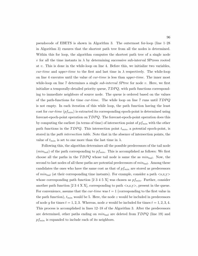
96

pseudocode of EBETS is shown in Algorithm 3. The outermost for-loop (line 1–28

in Algorithm 3) ensures that the shortest path tree from all the nodes is determined.

Within this for loop, the algorithm computes the shortest path tree of a single node

v for all the time instants in λ by determining successive sub-interval SPtrees rooted

at v. This is done in the while-loop on line 4. Before this, we initialize two variables,

cur-time and upper-time to the first and last time in λ respectively. The while-loop

on line 4 executes until the value of cur-time is less than upper-time. The inner most

while-loop on line 7 determines a single sub-interval SPtree for node v. Here, we first

initialize a temporally-detailed priority queue, TDPQ, with path functions correspond-

ing to immediate neighbors of source node. The queue is ordered based on the values

of the path-functions for time cur-time. The while loop on line 7 runs until TDPQ

is not empty. In each iteration of this while loop, the path function having the least

cost for cur-time (pfmin) is extracted its corresponding epoch-point is determined using

forecast-epoch-point operation on TDPQ. The forecast-epoch-point operation does this

by computing the earliest (in terms of time) of intersection point of pfmin with the other

path functions in the TDPQ. This intersection point tmin, a potential epoch-point, is

stored in the path intersection table. Note that in the absence of intersection points, the

value of tmin is set to one more than the last time in λ.

Following this, the algorithm determines all the possible predecessors of the tail node

(mintail) of the path corresponding to pfmin. This is accomplished as follows: We first

choose all the paths in the TDPQ whose tail node is same the as mintail. Now, the

second to last nodes of all these paths are potential predecessors ofmintail. Among these

candidates the ones who have the same cost as that of pfmin are stored as predecessors

of mintail (at their corresponding time instants). For example, consider a path <s,x,y>

whose corresponding path function [2 3 4 5 X] was chosen as pfmin. Further, consider

another path function [2 3 4 X X], corresponding to path <s,z,y>, present in the queue.

For convenience, assume that the cur-time was t = 1 (corresponding to the first value in

the path function), tmin would be 5. Here, the node z would be included in predecessors

of node y for times t = 1, 2, 3. Whereas, node x would be included for times t = 1, 2, 3, 4.

This process is accomplished in lines 12–18 of the Algorithm 3. After the predecessors

are determined, other paths ending on mintail are deleted from TDPQ (line 19) and

pfmin is expanded to include each of its neighbors.

97

Figure 5.8: EBETS Execution trace: Start of Step 1

The newly determined path functions (line 21) are inserted into TDPQ. This process

continues until TDPQ is empty. Note that when pfmin is expanded, mintail is closed for

cur-time. This means that there cannot be any other path leading to mintail from the

root with a shorter length. After exiting from the inner while loop on line 7, we have a

sub-interval SPtree rooted at node s (as per Line 1) whose optimality is guaranteed for

all times between cur-time and the minimum of tmins stored in the path intersection

table. Following this EBETS performs following three tasks. First, cur-time (next time

for re-computation) is set to the minimum of tmins stored in the path intersection table

(line 23 in Algorithm 3). In a worst case scenario, this value could just be the next time

instant in λ. In such a case, the sub-interval SPtree determined by the inner most while

loop would be valid for only one time in λ. Second, the predecessor table is reinitialized

for times greater than the new cur-time. Third, the dependency (given by Equation

5.3) of each of the nodes in the sub-interval SPtree is computed for times between the

previous and the new cur-time.

98

5.3.3 Execution trace

We now provide an execution trace of the EBETS on the temporally-detailed social

network shown in Figure 5.5. Here, the set λ = 1, 2, 3, 4, 5. For brevity, we only show

the computation of a single sub-interval temporally-ordered SPtree with source W .

For this execution trace, we have the following: (a) Our path-functions are modeling

information flows, (b) It takes 1 time unit for the information to flow on an edge, (c)

Waiting is not allowed.

In the first iteration of the while-loop on line 4 the value of cur-time would be 1 (first

time instant in λ). The inner while-loop on line 7 begins with a temporally-detailed

priority queue initialized with the path functions corresponding to immediate neighbors

of W (see Figure 5.8). Now, the path function having the lowest cost at t = 1 would be

chosen as pfmin on line 8. In this case, the path <W,A> has the lowest cost for t = 1.

The path-function of <W,A> intersects with that of <W,C> at time t = 5 which be

the value of tmin. In other words, forecast-epoch-point would return t = 5, which is

stored in the path intersection table. Now, since there are no other paths ending on

node A in queue, W would be set as the predecessor of A for times 1, 2, 3, 4 (all times

between cur-time and tmin − 1). Lines 20-21 would expand the path <W,A> to insert

the path-function corresponding to <W,A,U> and <W,A,V> (see Figure 5.9) into the

queue.


For the second iteration of the while loop on line 7, the algorithm would select the

path <W,C> as pfmin and node C would be closed for time t = 1. Forecast-epoch-point

would consider the intersection of the path function of <W,C> with <W,A,U> at t = 3

99

(see Figure 5.9). This intersection point would be stored in the path intersection table.

Now, since there are no paths ending with node C in the queue (see Figure 5.9), W

would be set as the predecessor of C for times t = 1, 2. The algorithm then expands

the path <W,C> and the path-functions corresponding to <W,C,U> and <W,C,V>

are inserted into the queue.


In the third iteration of the while loop on line 7, the algorithm would select the

path <W,C,U> as pfmin (ties broken arbitrarily) and node U would be closed for time

t = 1. Forecast-epoch-point would return t = 3 as there is an intersection of the path

function of <W,C,U> with <W,A,U> at t = 3 (see Figure 5.10). This intersection

point is stored in the path intersection table. Now, there are two paths, <W,C,U> and

<W,A,U>, in the queue which end on node U and have the same cost of t = 1 and

t = 2. Thus, both A and U would be set as predecessors of U for times t = 1 and t = 2.

<W,C,U> is not expanded further as it does not have any unclosed neighbors. At line

19, the algorithm deletes both <W,C,U> and <W,A,U> from the queue.

In the fourth iteration of the while loop on line 7, the algorithm would select the

path <W,A,V> as pfmin and node V would be closed for time t = 1. Forecast-epoch-

point would return t = 3 as <W,A,V> ceased to exist at t = 3 (see Figure 5.11). This

intersection point is stored in the path intersection table. Now, there are no other two

paths ending on V for times t = 1 and t = 2. Thus, only A is set as a predecessor of V

for times t = 1 and t = 2. <W,A,V> is not expanded further as it does not have any

unclosed neighbors. At line 19, the algorithm deletes both <W,C,V> and <W,A,V>

from the queue.

100



For the fifth iteration of the while loop on line 7, the priority queue would be empty.

This is the termination condition of the while-loop on line 7. After the the termination

of this loop, the next cur-time is determined by selecting the earliest of the tmins stored

in the path intersection table. This happens to be t = 3 for this example (see Figure

5.12). Thus effectively, the algorithm has now determined a sub-interval SPtree with

source W valid for times t = 1 and t = 2. Note that we did not compute the shortest

path tree for t = 2 separately. The above process of computing a sub-interval SPtree

will now repeat for t = 3. Before proceeding to the next iteration of the while-loop

on line 4, the algorithm re-initializes the predecessor table for times t = 3 and greater.

After that partial dependencies of all the nodes in this sub-interval SPtree are computed

for times t = 1 and t = 2 using Equation 5.3.

101

5.4 Analytical Evaluation

The EBETS algorithm divides a given interval (over which shortest path trees have to

be determined) into a set of disjoint sub-intervals. Within these intervals, the tree does

not change. The correctness of EBETS algorithm requires that the set of predecessors

determined for any particular node (lines 12-18 of Algorithm 3) be comprehensive.

On the other hand, the completeness of the algorithm guarantees that none of the

epoch-points are missed. Lemma 8 and Corollary 3 are used to show that the set of

predecessors determined by EBETS is comprehensive, i.e., the algorithm records all the

potential predecessors of a node while building an sub-interval SPtree. On the other

hand, Lemma 7 shows that the EBETS algorithm does not miss any epoch-point. These

lemmas are used to prove the correctness and completeness of the EBETS algorithm.

Lemma 7. The EBETS algorithm re-computes the shortest path tree (for any particular

node s ∈ V ) for all those times ti ∈ λ, where the tree for previous time ti−1 can be

different from that of ti.

Proof. The shortest path tree of a node s ∈ V is considered to have changed if the

shortest path to any node t (from s) in the tree is different across times ti and ti−1 or

there is node w outside of tree which is now reachable. For the sake of brevity, we only

give the proof for case when the shortest path to a single node t in the tree has changed.

This can be easily generalized for case of w and the whole tree.

Consider the network shown in Figure 5.13(a) where a shortest path tree of the node

s is to be determined for each time instant in λ = [1, 2 . . . T ]. In this proof we focus on the

shortest path to node d instead of the whole tree. First, the source node is expanded

for the time instant t = 1. As a result, path functions for all the neighbors <s,u>,

<s,x1>, <s,x2>, . . . <s,xi> are added to the priority queue. Without loss of generality,

assume that the path <s,u> is chosen in the next iteration of the innermost loop. Also

assume that the earliest intersection point between <s,u> and the path functions in the

priority queue is at t = α (between <s,u> and <s,x1>). After expanding <s,u> the

queue would contain paths <s,u,d>, <s,x1>, . . ., <s,xi>. Here we can have two cases.

First, path <s,u,d> has lower cost for time t = 1. Second, path <s,x1> has lower cost

for time t = 1.

Consider the first case, again without loss of generality assume that the earliest

102

intersection point between the path functions <s,u,d> and <s,x1> is at t = β. Note

that both t = α and t = β denote the times at the source node. Now, β ≤ α (note

that β cannot be greater than α as all the edges have positive weights). In such a

case the shortest path is recomputed for time t = β and the path <s,u,d> is closed for

all times 1 ≤ t < β. Assume for the sake of argument, that there is a shortest path

Px =< s, x2, . . . , d > from s to d that is different from path <s,u,d> and is optimal for

a time tx ∈ [1, β). This means that path < s, x2 > should have had least cost for time

t = tx. In other words, the earliest intersection point between functions in the priority

queue and < s, u, d > should have been at t = tx rather than at t = β (a contradiction).

Moreover, as all the edge costs are positive, if sub path <s,x2> was not shorter than

<s,u,d> for times t ∈ [1, β). Any positive weight addition to the path-function (through

other edges) cannot make Px shorter than <s,u,d> for t ∈ [1, β)

Now we consider the second case when <s,x1> had lower cost for time t = 1. Now,

path <s,x1> would be expanded and path function <s,x1,d> would be added to priority

queue. A similar argument as above can be given for this case as well.

(a) (b)

Figure 5.13: Sample network for Lemma 7 and Lemma 8

Corollary 2. The EBETS algorithm correctly computes the shortest path tree (for any

particular node s ∈ V ) for any particular time instant t ∈ λ.

Lemma 8. The set of predecessors determined for a node v for a time t ∈ λ is complete.

Proof. Let P (v) = Pu1(v), Pu2

(v), Pu2(v), . . . , Puk

(v) denote the set of paths currently

in the priority queue whose tail node is v. Here, Pui, where i ∈ [1, k], denotes the path

103

whose second-to-last node is ui (and last node being v) and cost(Pui(v)) denotes the

cost of path Pui(v) for time t = α. Without loss of generality assume that the node v is

being closed for time t = α (see Figure 5.13(b)) through the path Pu1, i.e., Pu1

is found

to be a shortest path for node v. Now, the EBETS algorithm assigns a node ux as a

predecessor of node v based on the following cases;

Case 1: ux is the second-to-last node in the shortest path found, i.e., ux = u1.

Case 2: ux ∈ U , where U = {ui|cost(Pui(v)) = cost(Pu1

(v))&i 6= 1}.

In order to prove the lemma, we show that the above two cases are correct and

complete. We first show the correctness followed by completeness. Using Corollary 2

we know that when a node v is closed by the EBETS algorithm for any particular time

t, it has correctly determined the shortest path for v. Therefore, the node preceding

v in this path is clearly a predecessor of time t. This proves the correctness of Case

1. Correctness of Case 2 can be also guaranteed in similar fashion as we include the

second-to-last nodes of only those paths whose cost is same as that of the shortest path

found by EBETS.

In order to show the completeness, we need to prove that there cannot be any

other path Q, not currently in the priority queue, with cost(Q) = cost(Pu1). For sake

of argument assume that there exists a path Q =< s, . . . , x, v >, not currently in

TDPQ, and x is valid predecessor of v for time t = α. By definition the distance

of x from s should be less than that of v (as we have only positive weights). This

means that node x should be closed before v. Now, whenever a node is closed by the

algorithm, path functions corresponding to its neighbors are added to the priority queue.

This contradicts our original assumption that path Q was not present in the priority

queue.

Corollary 3. The set of predecessors determined for a node v for all times t ∈ λ is

complete.

Proof. Using Lemma 7, we know that EBETS does not miss any epoch point. Now,

during the time interval between two consecutive epoch-points, Lemma 8 can be used

to conclude that the predecessors are correctly determined for all time time instants

104

within the interval. Using these two arguments we can conclude that EBETS correctly

determines the predecessors of a node v for all times t ∈ λ.

Theorem 4. EBETS algorithm is correct and complete.

Proof. For any particular node v, there can be several sub-interval SPtrees, SPTv =

{SPT 1v , SPT 2

v , . . . , SPT kv }, over the λ, where each SPT i

v is associated with a set of

time instants ωiv and

⋃

∀i∈|SPTv |ωiv = λ. The correctness of the algorithm is shown by

Lemma 8 and Corollary 3. The completeness proof is presented in three parts. First,

using Lemma 7 we can conclude that the EBETS algorithm does not miss any epoch

point. Secondly, the loop on line 4 of the algorithm ensures that all time instants in λ

are considered. Finally, the outer most loop on line 1 ensures that all the nodes v ∈ V

are processed. This proves the completeness of the algorithm.

Discussion: The EBETS algorithm would perform less computation than a naive

approach which determines the shortest path tree of a node for each time in the user

specified time interval λ. However, this happens only when the ratio of the number

of epoch-points to that of time instants in λ is low. This ratio can be denoted as the

change probability shown by Equation 5.4.

change probability =#epoch points

#time instants in λ(5.4)

When the change probability is nearly 1, there would be a different shortest path

tree (of a node) for each time in the interval λ. In this worst case scenario, the EBETS

approach would also have to recompute the shortest path tree for each time.

5.5 Experimental Evaluation

The overall goal of experimental evaluation was to characterize the performance of

epoch-point based betweenness centrality algorithms. To this end, the performance of

EBETS algorithm was compared against a baseline algorithm which involved comput-

ing the shortest path tree for each time in the given time interval of interest (input

parameter λ). For comparison, both algorithms computed the temporal extension of

105

1000

1000 2000 3000 4000 5000

Run

time

(sec

s) (

logs

cale

)

Length of interval (|Lambda|)

Maximum Wait allowed=120mins

EBETS-runtimeBaseline-runtime

1000

1000 2000 3000 4000 5000

Run

time

(sec

s) (

logs

cale

)




1000

1000 2000 3000 4000 5000

Run

time

(sec

s) (

logs

cale

)



EBETS-runtimeBaseline-runtime 1000

1000 2000 3000 4000 5000

Run

time

(sec

s) (

logs

cale

)




Figure 5.14: Effect of length of time interval (|λ|).

betweenness centrality given in Equation 5.1 and followed the temporal shortest path

definition given in Definition 3. Both EBETS and the baseline algorithms were imple-

mented in C++ language. The experiments were carried out on a real dataset containing

email communications spread over 83 days in early 2004 from a large European univer-

sity. This dataset recorded about 161227 email communications among approximately

2000 individuals. Events in this dataset (email communications) were recorded in the

following format: <A,B,t>, where A and B are two individuals in the University and t

denotes the time-stamp (in minutes) of the interaction. Experiments were carried out

on a Linux workstation with Intel Xeon Processor and 8GB RAM.

The first step of the experimental evaluation involved creating a time aggregated

graph out of the social event data. Since the dataset contained emails communications,

these translated into directed edges in the time aggregated graph. Then, a set of dif-

ferent queries (each with a different set of parameters) was run on the EBETS and the

baseline algorithm. The following parameters were varied in the experiments: (a) |λ|:

Length of the time interval over which the centrality metric was computed, (b) Network

106

size, and (a) Maximum wait allowed. In each of the experiments the total execution

time of both the algorithms was recorded.

1000

Dataset1 Dataset2 Dataset3

Exe

cutio

n tim

e (m

ins)

Maximum Wait allowed = 120mins, |Lambda| = 3000


1000


Exe

cutio

n tim

e (m

ins)



1000


Exe

cutio

n tim

e (m

ins)



1000


Exe

cutio

n tim

e (m

ins)

Maximum Wait allowed = 240, |Lambda| = 7000


Figure 5.15: Effect of Network size.

Effect of Length of time interval (|λ|): This experiment evaluated the effect of

length of time interval (λ) on the candidate algorithms. The results, shown in Figure

5.14, indicate that execution time of both the algorithms increased linearly with increase

in |λ|. However, for any particular value of |λ| and maximum allowed wait, EBETS was

faster than the baseline by an order of magnitude.

Effect of Network size: We tested the algorithms on three different size networks. To

create the networks, we removed some nodes and their edges from our original dataset

(referred to as Dataset3) to created two smaller datasets called Dataset1 and Dataset2.

Dataset1 had 1095 nodes and 18000 edges, whereas Dataset2 had 1300 nodes and 21000

edges. In both the smaller datasets the length of the time series was approximately

107

100,000. The algorithms were tested on all the three datasets. We also varied the max-

imum wait allowed and length of lambda. Figure 5.15 shows the effect of the Network

size on the performance of the algorithms. As can be seen the execution of time of both

the algorithms increased with the increase in network size, but EBETS still outperforms

the baseline.

Effect of Maximum Wait allowed: We also tested the effect of increasing the max-

imum wait allowed parameter on the candidate algorithms. As shown in Figure 5.16,

run-time for both the algorithms increased with a longer waits. However, run-time of

EBETS increased at a slower rate than that of baseline algorithm. Moreover, for any

particular value of maximum allowed wait parameter, the EBETS algorithm was faster

than the baseline algorithm by several orders of magnitude.

500

1000

1500

2000

2500

100 150 200 250 300

Run

time

(sec

s)

Maximum Wait allowed (mins)

Length of interval (|Lambda|) = 2000


670

1200

2000

3000

100 150 200 250 300

Run

time

(sec

s) (

logs

cale

)




1690

3200

4800

8000

50 100 150 200 250

Run

time

(sec

s) (

logs

cale

)




Figure 5.16: Effect Maximum Wait allowed for |λ| = {2000, 3000, 7000}.

108

5.6 Temporal Betweenness Centrality vs Traditional Be-

tweennness Centrality

In this section, we present an empirical comparison of temporal betweenness centrality

(Equation 5.1) based on temporal shortest paths (Definition 3) against the traditional

betweenness centrality computed on aggregated snapshots. The data we use in this

study is a set of email communications spread over eighty three days in early 2004 from a

large European university. The dataset has been used in several previous studies [76–79],

with a focus on both the prevalence of dynamic triads [76] and on characterizing the in-

ter event dynamics of users (i.e. the time between two consecutive email sends) [77–79].

Though we will utilize findings from these works extensively, it is important to note

that this dataset does contain several nodes which appear to be mail servers as well as

several people who do not communicate often enough (as also noted in [76–78]). We

choose to remove such nodes from the study.

How does temporal betweenness centrality compare with the traditional be-

tweenness centrality calculated on aggregated panels?

[76] notes, when studying the data utilized in this case study, that “temporal

dynamics create coherent space-time structures that...will in general be very different

from the fixed ones that appear in the static network”. However, [76] is in this quote

referring to the network created by aggregating all the events into a single panel, i.e., the

network comprised of all eighty three days of interaction data. In contrast, our interest

here is in comparing the results of temporal betweenness centrality (based on temporal

shortest paths) to the traditional betweenness centrality computed over panels obtained

by aggregating over shorter time intervals.

One disadvantage to our approach is that, while it is straightforward to determine

which agent is the most central at any given time instant (a minute, in this case study),

it is not immediately obvious how one should determine which agent is the most central

over an entire time interval. This is because at each time instant, all agents may be

on some number of temporal shortest paths, and thus have some non-zero betweenness

centrality score. Therefore, if we wish to determine which agent was the most central

109

on a given day, we must somehow aggregate over all temporal betweenness values, for

all agents, for each minute in that day. Though our approach was not geared towards

such an cumulative notion of centrality, a quantitative comparison between our method

and the aggregated panel is necessary and thus some calculation of the ranks of different

agents for betweenness over a given aggregation must be computed.

The manner in which we choose to do this is used for its simplicity and explainability,

though others no doubt exist which may be more powerful along one or both of these

dimensions. In order to determine which agent is most central over a given period

of interval, we first determine the most central agent (i.e. the one with the highest

temporal betweenness score) at each time instant (minute), and then aggregate over

the desired time period (e.g. a day) to produce a count, for each agent, of the number

of time instants he/she was most central for. The rank of a node (e.g. most central,

second most central, etc.) for the given time interval is then determined by his or her

rank in this list of counts.

Before we can compare to some betweenness metric on aggregated panels of the

network, we must also determine what representation of the network each panel will

have. [80] considers different meanings of an edge in an email network, including remov-

ing mass emails to get a more social view of the network. Here, because we consider

betweenness as an information flow metric, we choose to keep mass emails in the data.

On a different note, [77] sees that most users receive more emails than they send, sug-

gesting further that, of course, agents thus receive far more emails than they respond

to. This finding suggests email communication may be particularly susceptible to dif-

ferences in directed versus undirected measures of betweenness, and hence we use a

directed approach in order to compare best with our algorithm.

Having operationalized the notion of an agent being “most central” over any given

time interval across both methods, we now may compare the results of our metric with

the traditional betweenness centrality on aggregated panel. We compare across five

different levels of aggregation: one hour, two hours, ten hours, one day and three days.

In full, the process for comparing the metric at a single level of aggregation (e.g. a day)

can be described in three steps. We first aggregate the interaction data into panels and

then compute the traditional weighted, directed betweenness centrality [81,82] for agents

in each using the igraph package in R [83]. Note of this step, the traditional betweenness

110

centrality would ignore the the temporal order of interactions on the edges. We then use

the method described in Section 5.3 to compute the centrality of each agent within the

time-aggregated graph representation of each of the panels for the temporal betweenness

centrality metric (we consider the temporal order here). Finally, we utilize one of three

comparison metrics, first introduced by [84] and later used by [85], to compare agreement

between the two approaches for each set of aggregated interactions.

The three comparison metrics we use are “Top 1”, “Top 3” and “Top 10%” (the

original names provided by [84]. “Top 1” refers to the percentage of panels over which

the most central node is the same across both techniques. “Top 3” refers to the per-

centage of panels that the top node using the traditional approach on aggregated panel

is one of the top three nodes utilizing our metric. “Top 10%” refers, similarly, to the

percentage of panels in which the top node in the traditional approach on aggregated

panel approach is one of those in the top ten percent using our metric. We choose these

metrics over other similar metrics [86] because they are straightforward to understand

while still providing depth for intuition. In collecting results, we only consider as input

those panels where at least one node was central using both approaches and where there

were no ties as to the most central node in the aggregated panel network. It is also

important to note that at lower maximum allowed wait values and aggregations, be-

cause often less than 30 nodes have some non-zero centrality value, our results suggest

the counter-intuitive finding that in some cases, “Top 3” shows a higher percentage of

agreement across the two algorithms than “Top 10%”. Also, because larger aggregation

levels naturally have fewer data points, the reader will notice that confidence intervals

surrounding the point estimates for these metrics naturally increase with aggregation.

Figure 5.17 shows the results for each of the three comparison metrics, where points

represent the point estimate and error bars give the 95% confidence intervals using

Wilson’s formula [87]. The figure plots of the percentage of aggregation sets (on Y

axis) where the most central agent according to traditional betweenness centrality is in

the top one (top set of plots), top three (middle set) or top 10% (bottom set) of most

central agents using temporal betweenness centrality. The values on the X-axis represent

different maximum allowed wait values our algorithm was run with, while the values

in the grey bars above each graph represent the level of aggregation, in minutes, over

which the interactions were split. In considering the “Top 1” and “Top 3” metrics (the

111

60 120 600 1440 4320

0%

20%

40%

60%

80%

100%

15 30 60 120 15 30 60 120 15 30 60 120 15 30 60 120 15 30 60 120

60 120 600 1440 4320

0%

20%

40%

60%

80%

100%

15 30 60 120 15 30 60 120 15 30 60 120 15 30 60 120 15 30 60 120

60 120 600 1440 4320

0%

20%

40%

60%

80%

100%

15 30 60 120 15 30 60 120 15 30 60 120 15 30 60 120 15 30 60 120

Figure 5.17: Traditional betweenness centrality vs Temporal betweenness centrality.

top two plots), we see that although there is reasonably high variance across individual

combinations of maximum allowed wait and aggregation level, there are several general

patterns. First, agreement between the two methods is slightly higher at lower levels of

aggregation. This finding is not particularly surprising; at lower levels of aggregation,

there are fewer emails and less time to be aggregated over; resulting in fewer invalid

temporal paths and fewer unrealistic durations for which information is held at a given

node. However, at these levels, we do see that higher maximum allowed wait values have

much lower levels of agreement. This, also, has a fairly obvious explanation in that these

values consider data far outside the boundaries of the aggregation, and thus will likely

112

present different pictures of the network. This explanation is further supported by the

fact that this difference appears to slow at higher levels of aggregation.

Figure 5.17 thus suggests following conclusions. First, the agreement between the

two metrics on the most central nodes (Top 1 comparison metric) is not more than

60%. Second, there is very high agreement between the two metrics in case of Top

10% over long periods of aggregation. This shows that temporal betweenness centrality

does measure something which does not entirely agree with what is being measured

by the traditional betweenness centrality. In other words, these results do show an

inclination towards the fact time agnostic based techniques may consider paths which

are not feasible for information flow.

5.7 Conclusion

Temporally-detailed Social network Analytics (TDSNA) has value addition potential

due to its potential to answer time-aware questions about the underlying social system,

e.g., “How is the betweenness centrality of an individual changing over time?” However,

designing scalable algorithms for TDSNA is challenging because of the non-stationary

ranking of shortest path between any two nodes in a TD social network. This non-

stationary ranking violates the assumptions of dynamic programming underlying the

common shortest path algorithms such as Dijkstra’s used by current techniques. To this

end, we proposed the concept of epoch-point based approaches which divide the given

time interval–over which observe non-stationarity–into a set of disjoint time intervals

which show stationary ranking. Based on the concept of epoch-points, we developed a

novel algorithm, called EBETS, for computing the temporal extension of betweenness

centrality. EBETS saves computation over the baseline algorithm which re-computes

the solution for every time instant. Experimental evaluation showed that EBETS out

performs the baseline algorithm. In future, we plan to extend our concept of epoch-based

algorithms to adapt floyd warshall’s algorithm for all-pair shortest paths. This would

be useful in developing more scalable algorithms for temporal extensions of closeness

centrality. We also plan to extend our approach to centrality metrics in multiplex

networks and networks where interaction among a group of people are recorded through

hyperedges.

Chapter 6

Conclusions and Future

Directions

This chapter presents a summary of results obtained in this thesis followed by a brief

discussion on potential future directions.

6.1 Summary of results

Big Temporally-Detailed Graph (Big-TDG) data is an emerging trend. Sample Big-

TDG data such as temporally-detailed (TD) roadmaps have value-adding potential is

societal use-cases such as eco-routing. Likewise, TD social networks could help in an-

swering time-aware questions on the underlying social system (e.g, “How is the between-

ness centrality of an individual changing over time?”). However, both TD roadmaps

and TD social networks pose challenges to the state of the art in computer science.

TD roadmaps capture several properties of n-ary relations which cannot be completely

decomposed into properties of binary relations without losing its semantic value. This

challenge was formulated as follows:

• Given emerging diverse spatio temporal network (STN) datasets, e.g., GPS tracks,

temporally detailed roadmaps and traffic signal data, the aim was to develop a

data-model which achieves a seamless integration of these datasets for routing

113

114

related use-cases (queries) and supports efficient algorithms. This problem is im-

portant for travel itinerary comparison and navigation applications. However, this

was challenging due to the conflicting requirements of expressive power and com-

putational efficiency as well as the need to support ever more diverse STN datasets,

which now record non-decomposable properties of n-ary relations. Examples in-

clude travel-time and fuel-use during a journey on a route with a sequence of

coordinated traffic signals and turn delays. Current data models for STN datasets

are limited to representing properties only of binary relations, e.g., distance on

individual road segments. In contrast, Chapter 2 proposed a novel data-model,

called Lagrangian Xgraphs, which can express properties of both binary and n-ary

relations. Initial study shows that Lagrangian Xgraphs are more convenient for

representing diverse STN datasets and comparing candidate travel itineraries.

Both TD roadmaps and TD social networks show non-stationary ranking of alternate

candidate paths across different time points. In other words, the shortest path between

any two nodes in a TD roadmap or a TD social network changes with time. In a TD

roadmap this variation is due to changing traffic congestion across rush and non-rush

hours; in a TD social network it is caused due to variation in activity levels of individuals.

This non-stationary ranking of alternate candidate paths violates the assumptions of

dynamic programming shortest path algorithms such as Dijkstra’s algorithm. This

challenge was formulated through the following:

• Given a spatio-temporal network, a source, a destination, and a desired departure

time interval, the All-departure-time Lagrangian Shortest Paths (ALSP) prob-

lem determines a set which includes the shortest path for every departure time

in the given interval. ALSP is important for critical societal applications such

as eco-routing. However, ALSP is computationally challenging due to the non-

stationary ranking of the candidate paths across distinct departure-times. Current

related work for reducing redundant computation across consecutive departure-

times sharing a common solution exploits only partial information e.g., the earliest

feasible arrival time of a path. In contrast, our approach uses all available informa-

tion, e.g., the entire time series of arrival times for all departure-times. This allows

elimination of all knowable redundant computation based on complete information

115

available at hand. This idea was operationalized through the concept of critical-

time-points (CTP), i.e., departure-times before which ranking among candidate

paths cannot change. Chapter 3 proposed a CTP based forward search strat-

egy, and Chapter 4 proposed a CTP based temporal bi-directional search for the

ALSP problem via a novel impromptu rendezvous termination condition. Theo-

retical and experimental analysis showed that the proposed approach outperforms

the related work approaches particularly when there are few critical-time-points.

• The increasing proliferation of mobile and online social networking platforms has

given us unprecedented opportunity to observe and study social interactions at

a fine temporal scale. A collection of all such social interactions among a group

of individuals (or agents) observed over an interval of time is referred to as a

temporally-detailed (TD) social network. TD social networks open up the oppor-

tunity to explore temporally-detailed questions on the underlying social system,

e.g., “How is the betweenness centrality of an individual changing with time?”

To this end, related work has proposed temporal extensions of centrality metrics

(e.g., betweenness and closeness). However, scalable computation of these metrics

for long time-intervals is challenging. This is due to the non-stationary ranking

of shortest paths (the underlying structure of betweenness and closeness) between

a pair of nodes which violates the assumptions of classical dynamic program-

ming based techniques. To this end, Chapter 5 proposed a novel computational

paradigm called epoch-point based techniques for addressing the non-stationarity

challenge in a TD social network. Using the concept of epoch-points, this chapter

proposed a novel algorithm for computing shortest path based centrality metric

such as betweenness on a TD social network. Correctness and completeness of

the proposed algorithm were established. Experimental analysis showed that the

proposed algorithm outperforms the alternative by a wide margin.

6.2 Potential future research directions

Table 6.1 lists the current literature for shortest path and betweenness centrality algo-

rithms in the area of temporal-detailed graphs (second column), contributions made by

this thesis (third column) and a few potential future directions (last column) which are

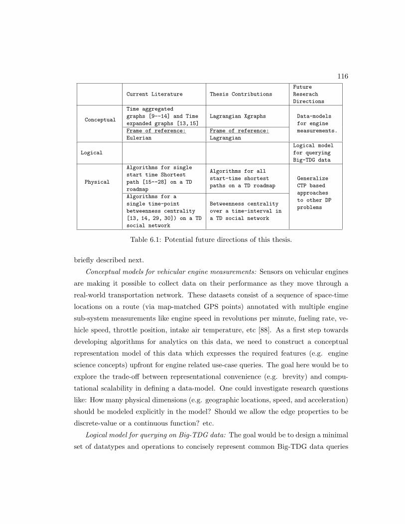
116

Current Literature Thesis Contributions

Future

Reserach

Directions

Conceptual

Time aggregated

graphs [9--14] and Time

expanded graphs [13,15]

Lagrangian Xgraphs Data-models

for engine

measurements.Frame of reference:

Eulerian

Frame of reference:

Lagrangian

Logical

Logical model

for querying

Big-TDG data

Physical

Algorithms for single

start time Shortest

path [15--28] on a TD

roadmap

Algorithms for all

start-time shortest

paths on a TD roadmap

Generalize

CTP based

approaches

to other DP

problems

Algorithms for a

single time-point

betweenness centrality

[13, 14, 29, 30]) on a TD

social network

Betweenness centrality

over a time-interval in

a TD social network

Table 6.1: Potential future directions of this thesis.

briefly described next.

Conceptual models for vehicular engine measurements: Sensors on vehicular engines

are making it possible to collect data on their performance as they move through a

real-world transportation network. These datasets consist of a sequence of space-time

locations on a route (via map-matched GPS points) annotated with multiple engine

sub-system measurements like engine speed in revolutions per minute, fueling rate, ve-

hicle speed, throttle position, intake air temperature, etc [88]. As a first step towards

developing algorithms for analytics on this data, we need to construct a conceptual

representation model of this data which expresses the required features (e.g. engine

science concepts) upfront for engine related use-case queries. The goal here would be to

explore the trade-off between representational convenience (e.g. brevity) and compu-

tational scalability in defining a data-model. One could investigate research questions

like: How many physical dimensions (e.g. geographic locations, speed, and acceleration)

should be modeled explicitly in the model? Should we allow the edge properties to be

discrete-value or a continuous function? etc.

Logical model for querying on Big-TDG data: The goal would be to design a minimal

set of datatypes and operations to concisely represent common Big-TDG data queries

117

and support traversal of the graph. This task is challenging due to the conflicting

goals of concise representation and support for computationally efficient algorithms.

Table 2.1 in Chapter 2 presented a set of preliminary operations, but several research

questions remain unanswered. For instance, is the set of proposed Lagrangian Xgraph

data-types and operations (Table 2.1 in Chapter 2) closed, i.e., can operation results be

represented within the set? Is this set expressive enough to represent spatio-temporal

routing queries about a traveler’s experience relevant to eco-routing? Does it facilitate

in design of computationally efficient algorithms? How should the set be refined to

address the conflicting needs of expressive power and support for efficient algorithms?

Generalize critical-time-points to a broader set of DP problems: Critical-time-points

(CTPs) could be investigated for their generalizability in a larger set of computational

problems. For illustration, consider the All-pair All start-time Lagrangian Shortest path

Problem (AALSP). Given a temporally-detailed roadmap and a departure-time interval,

the AALSP problem determines a route collection which includes the shortest path,

for every departure-time in the given interval, for every possible (start, destination)

pair. CTP may adapt the traditional All-pair Shortest Path (ASP) algorithms (e.g.,

Floyd Warshall’s, Johnson’s) to reduce redundant computation across departure-times

sharing a common solution. However, this task is much harder than adapting Dijkstra’s

algorithm for ALSP, since we do not know the departure-times for the sub-paths being

combined in the recurrence step. This issue invalidates even a naive approach of invoking

the ASP algorithm for all distinct departure-times. The applicability of CTP based

approaches could be further investigated for other dynamic programming use-cases such

as maximum likelihood decoding techniques (e.g. Viterbi algorithm) for hidden Markov

models, optimal policy determination techniques for Markov decision processes (e.g.

Value iteration algorithm for finite horizon problems), and Selinger’s algorithm for query

optimization and other discrete-time optimization problems.

References

[1] Peter Koonce and et al. Traffic signal timing manual. Technical Report FHWA-

HOP-08-024, US Dept of Trans. Federal Higway Admin., June 2008.

[2] Bing maps. http://www.bing.com/maps/.

[3] Bolin Ding, Jeffrey Xu Yu, and Lu Qin. Finding time-dependent shortest paths

over large graphs. In Proc. of the Intl. Conf. on Extending database technology

(EDBT), pages 205–216, 2008.

[4] J. Manyika et al. Big data: The next frontier for innovation, competition and

productivity. McKinsey Global Institute http://goo.gl/AA8DS, May 2011.

[5] Shashi Shekhar, Viswanath Gunturi, Michael R. Evans, and KwangSoo Yang. Spa-

tial big-data challenges intersecting mobility and cloud computing. In MobiDE,

pages 1–6. ACM, 2012.

[6] A Community Whitepaper resulting from the 2012 Spatial Computing 2020 Work-

shop funded by the Computing Community Consortium. From gps and vir-

tual globes to spatial computing - 2020: The next transformative technology.

www.cra.org/ccc/visioning/visioning-activities/spatial-computing.

[7] J. Lovell. Left-hand-turn elimination. NY Times, December 9th, 2007.

[8] Us energy information administration. http://www.eia.gov/totalenergy/data/monthly/.

[9] Betsy George and Shashi Shekhar. Time-aggregated graphs for modeling spatio-

temporal networks. J. Data Semantics, 11:191–212, 2006.

118

http://goo.gl/AA8DS

www.cra.org/ccc/visioning/visioning-activities/spatial-computing

119

[10] Erik G. Hoel, Wee-Liang Heng, and Dale Honeycutt. High performance multimodal

networks. In Advances in Spatial and Temporal Databases, volume 3633 of LNCS,

2005.

[11] Ralf Hartmut Guting. Graphdb: Modeling and querying graphs in databases. In

Proc. of the 20th International Conference on Very Large Data Bases, pages 297–

308, 1994.

[12] Betsy George and Shashi Shekhar. Modeling spatio-temporal network computa-

tions: A summary of results. In GeoSpatial Semantics, Second International Con-

ference, GeoS 2007, Mexico City, Mexico, November 29-30, 2007, Proceedings,

pages 177–194. Springer. LNCS 4605.

[13] Hyoungshick Kim and Ross Anderson. Temporal node centrality in complex net-

works. Physcial Review E, 85(2), 2012.

[14] Habiba, Chayant Tantipathananandh, and Tanya Y. Berger-Wolf. Betweenness

centrality measure in dynamic networks. Technical Report 2007-19, Center for

Discrete Mathematics and Theoretical Computer Science, 2007.

[15] Ekkehard Khler, Katharina Langkau, and Martin Skutella. Time-expanded graphs

for flow-dependent transit times. In Algorithms ESA 2002, volume 2461, pages

49–56. 2002.

[16] Betsy George, Sangho Kim, and Shashi Shekhar. Spatio-temporal network

databases and routing algorithms: A summary of results. In Symposium on Spatial

and Temporal Databases (SSTD), pages 460–477, 2007.

[17] Ugur Demiryurek, Farnoush Banaei-Kashani, Cyrus Shahabi, and Anand Ran-

ganathan. Online computation of fastest path in time-dependent spatial networks.

In Proc. of the 12th intl. conf. on Advances in spatial and temporal databases,

SSTD’11, pages 92–111. Springer-Verlag, 2011.

[18] Daniel Delling and Dorothea Wagner. Landmark-based routing in dynamic graphs.

In Experimental Algorithms, pages 52–65. Springer Berlin Heidelberg, 2007.

120

[19] Daniel Delling. Time-dependent sharc-routing. In Proc. of the 16th annual Euro-

pean symposium on Algorithms, pages 332–343, 2008.

[20] Daniel Delling and Dorothea Wagner. Time-dependent route planning. In Robust

and Online Large-Scale Optimization, volume 5868 of Lecture Notes in Computer

Science, pages 207–230. Springer Berlin Heidelberg, 2009.

[21] Ismail Chabini and Shan Lan. Adaptations of the a* algorithm for the computation

of fastest paths in deterministic discrete-time dynamic networks. IEEE Trans. on

Intel. Trans. Systems, 3(1):60–74, 2002.

[22] Ariel Orda and Raphael Rom. Shortest-path and minimum-delay algorithms in

networks with time-dependent edge-length. J. ACM, 37(3):607–625, July 1990.

[23] Giacomo Nannicini, Daniel Delling, Dominik Schultes, and Leo Liberti. Bidirec-

tional a* search on time-dependent road networks. Networks, 59(2):240–251, 2012.

[24] Giacomo Nannicini, Daniel Delling, Leo Liberti, and Dominik Schultes. Bidirec-

tional a* search for time-dependent fast paths. In Experimental Algorithms, pages

334–346. Springer Berlin Heidelberg, 2008.

[25] Daniel Delling and Giacomo Nannicini. Bidirectional core-based routing in dynamic

time-dependent road networks. In Algorithms and Computation, pages 812–823,

2008.

[26] Giacomo Nannicini. Point-to-point shortest paths on dynamic time-dependent road

networks. 4OR, 8(3):327–330, 2010.

[27] Ugur Demiryurek, Farnoush Kashani, and Cyrus Shahabi. A case for time-

dependent shortest path computation in spatial networks. In Proc. of the SIGSPA-

TIAL Intl. Conf. on Advances in GIS, GIS ’10, pages 474–477, 2010.

[28] Jing Yuan and et. al. T-drive: driving directions based on taxi trajectories. In

Proc. of the ACM SIGSPATIAL, pages 99–108, 2010.

121

[29] John Tang, Mirco Musolesi, Cecilia Mascolo, Vito Latora, and Vincenzo Nicosia.

Analysing information flows and key mediators through temporal centrality met-

rics. In Proceedings of the 3rd Workshop on Social Network Systems, SNS ’10,

pages 3:1–3:6, 2010.

[30] John Tang, Mirco Musolesi, Cecilia Mascolo, and Vito Latora. Temporal distance

metrics for social network analysis. In Proceedings of the 2Nd ACM Workshop

on Online Social Networks, WOSN ’09, pages 31–36, New York, NY, USA, 2009.

ACM.

[31] KwangSoo Yang, M.R. Evans, V.M.V. Gunturi, J.M. Kang, and S. Shekhar. La-

grangian approaches to storage of spatio-temporal network datasets. Knowledge

and Data Engineering, IEEE Transactions on, 26(9):2222–2236, 2014.

[32] Dan Sha and C. K. Wong. Time-Varying Network Optimization. International

Series in Operations Research and Management Science, Vol. 103, Springer, 2007.

[33] VenkataM.V. Gunturi and Shashi Shekhar. Lagrangian xgraphs: A logical data-

model for spatio-temporal network data: A summary. In Marta Indulska and

Sandeep Purao, editors, Advances in Conceptual Modeling, volume 8823 of Lec-

ture Notes in Computer Science, pages 201–211. Springer International Publishing,

2014.

[34] Venkata M. V. Gunturi, Ernesto Nunes, KwangSoo Yang, and Shashi Shekhar. A

critical-time-point approach to all-start-time lagrangian shortest paths: a summary

of results. In Proc. of 12th intl. conf. on Adv. in spatial and temporal databases,

pages 74–91, 2011.

[35] Venkata M. V. Gunturi and et. al. A critical-time-point approach to all-start-time

lagrangian shortest paths. Accepted in IEEE Transactions on Knowledge and Data

Engineering, 2015.

[36] Henry Liu and Heng Hu. Smart-signal phase ii: Arterial offset optimization using

archived high-resolution traffic signal data. Technical Report CTS 13-19, Intel.

Trans. Sys. Inst., Center for Transportation Studies, Univ. of Minnesota, Apr-2013.

122

[37] B. George and S. Shekhar. Time-aggregated graphs for modelling spatio-temporal

networks. J. Semantics of Data, XI:191, 2007.

[38] Yu Zheng and Xiaofang (Eds.) Zhou, editors. Computing with Spatial Trajectories.

Springer, 2011.

[39] Shashi Shekhar and et al. Spatial pictogram enhanced conceptual data models

and their translation to logical data models. In Intl. Works. on Integrated Spatial

Databases, Digital Inages and GIS, pages 77–104. Springer-Verlag, 1999.

[40] Yvan Bedard. Visual modeling of spatial databases: Towards spatial PVL and

UML. Geoinformatica, 53(2), 1999.

[41] Shashi Shekhar and et al. Data models in geographic information systems. Com-

mun. ACM, 40(4), April 1997.

[42] G.K. Batchelor. An introduction to fluid dynamics. Cambridge Univ. Press, 1973.

[43] Christine Parent and et al. Spatio-temporal conceptual models: Data structures

+ space + time. In Proc. of the Intl. Symp. on Adv. in GIS, pages 26–33. ACM,

1999.

[44] Erlend Tssebro and Mads Nygrd. Representing topological relationships for spa-

tiotemporal objects. GeoInformatica Springer US, 15(4):633–661, 2011.

[45] Renato Fileto and et al. Baquara: A holistic ontological framework for movement

analysis using linked data. In Conceptual Modeling, pages 342–355. Springer, 2013.

[46] G. Gallo, G. Longo, S. Pallottino, and S. Nguyen. Directed hypergraphs and

applications. Elsevier, Discrete applied mathematics, 42(2):177–201, 1993.

[47] C. Berge. Graphs and Hypergraphs. Elsevier Science Ltd, 1985.

[48] Michael R. Evans and et. al. A lagrangian approach for storage of spatio-temporal

network datasets: a summary of results. In Proc. of the ACM SIGSPATIAL, pages

212–221, 2010.

[49] Delta airlines. http://www.delta.com/.

123

[50] C.H. Deutsch. Ups embraces high-tech delivery methods. NY Times, July 12, 2007.

[51] Evangelos Kanoulas, Yang Du, Tian Xia, and Donghui Zhang. Finding fastest

paths on a road network with speed patterns. In Proc. of the 22nd Intl. Conf. on

Data Engineering (ICDE), page 10, 2006.

[52] Jon Kleinberg and Eva Tardos. Algorithm Design. Pearson Education, 2009.

[53] David E. Kaufman and Robert L. Smith. Fastest paths in time-dependent networks

for intelligent vehicle-highway systems application. I V H S Journal, 1(1):1–11,

1993.

[54] B. George, S. Shekhar, and S. Kim. Spatio-temporal network databases and routing

algorithms. Technical Report 08-039, Univ. of Minnesota - Comp. Sci. and Engg.,

2008.

[55] Viswanath Gunturi, Shashi Shekhar, and Arnab Bhattacharya. Minimum spanning

tree on spatio-temporal networks. In Proc. of the 21st Intl. Conf. on Database and

expert systems applications: Part II, DEXA’10, pages 149–158, 2010.

[56] Navteq. http://www.navteq.com/.

[57] Lıvia A. Cruz, Mario A. Nascimento, and Jose Antonio Fernandes de Macedo. k-

nearest neighbors queries in time-dependent road networks. JIDM, 3(3):211–226,

2012.

[58] Ugur Demiryurek, Farnoush Banaei-Kashani, and Cyrus Shahabi. Efficient k-

nearest neighbor search in time-dependent spatial networks. In Proc. 21st Intl.

Conf. on Database and Expert Systems Applications: Part I, pages 432–449, 2010.

[59] Luca Foschini, John Hershberger, and Subhash Suri. On the complexity of time-

dependent shortest paths. In SODA, pages 327–341, 2011.

[60] Openstreetmap. http://www.openstreetmap.org/.

[61] Daniel Delling and et. al. Phast: Hardware-accelerated shortest path trees. Journal

of Parallel and Distributed Computing, 73(7):940 – 952, 2013.

124

[62] Hyoungshick Kim, John Tang, Ross Anderson, and Cecilia Mascolo. Centrality

prediction in dynamic human contact networks. Computer Networks, 56(3):983 –

996, 2012.

[63] S. Russel and P. Norwig. Artificial Intelligence: A Morden Approach. Prentice-Hall,

Upper Saddle River, NJ, 1995.

[64] Dimitri P. Bertsekas. Dynamic Programming: Deterministic and Stochastic Models.

Prentice-Hall, Englewood Cliffs, NJ, 1987.

[65] Dan Braha and Yaneer Bar-Yam. From centrality to temporary fame: Dynamic

centrality in complex networks. Complexity, 12(2):59–63, 2006.

[66] Jean-Pierre Eckmann, Elisha Moses, and Danilo Sergi. Entropy of dialogues creates

coherent structures in e-mail traffic. Proceedings of National Academy of Sciences

(2004), 101(40), 143330–14337.

[67] Gueorgi Kossinets and Duncan J. Watts. Empirical analysis of an evolving social

network. Science, 311(5757), 2006.

[68] R. Nia, C. Bird, P. Devanbu, and V. Filkov. Validity of network analyses in open

source projects. In 2010 7th IEEE Working Conference on Mining Software Repos-

itories (MSR), pages 201–209, May 2010.

[69] James Howison, Andrea Wiggins, and Kevin Crowston. Validity issues in the use

of social network analysis with digital trace data. Journal of the Association for

Information Systems, 12(12), December 2011.

[70] Gueorgi Kossinets, Jon Kleinberg, and Duncan Watts. The structure of information

pathways in a social communication network. In Proceeding of the 14th ACM

SIGKDD international conference on Knowledge discovery and data mining, KDD

’08, pages 435–443, 2008.

[71] Kristina Lerman, Rumi Ghosh, and Jeon-hyung Kang. Centrality metric for dy-

namic network analysis. In Proceedings of KDD workshop on Mining and Learning

with Graphs (MLG), July 2010.

125

[72] L. Weng, A. Flammini, A. Vespignani, and F. Menczer. Competition among memes

in a world with limited attention. Scientific Reports, 2, 2012.

[73] Dashun Wang, Zhen Wen, Hanghang Tong, Ching-Yung Lin, Chaoming Song, and

Albert-Lszl Barabsi. Information spreading in context. In Proceedings of the 20th

international conference on World wide web, WWW ’11, page 735?744. ACM, 2011.

[74] F. Wu and B. A. Huberman. Novelty and collective attention. Proc. Natl. Acad.

Sci. USA, 104(45):17599–17601, 2007.

[75] Ulrik Brandes. A faster algorithm for betweenness centrality. Journal of Mathe-

matical Sociology, 25(2):163–177, 2001.

[76] Jean-Pierre Eckmann, Elisha Moses, and Danilo Sergi. Entropy of dialogues cre-

ates coherent structures in e-mail traffic. Proceedings of the National Academy of

Sciences of the United States of America, 101(40):14333–14337, October 2004.

[77] Albert-Laszlo Barabasi. The origin of bursts and heavy tails in human dynamics.

Nature, 435(7039):207–211, May 2005.

[78] R. Dean Malmgren, Jake M. Hofman, Luis A.N. Amaral, and Duncan J. Watts.

Characterizing individual communication patterns. In Proceedings of the 15th ACM

SIGKDD international conference on Knowledge discovery and data mining, KDD

’09, pages 607–616, New York, NY, USA, 2009. ACM.

[79] R. Dean Malmgren, Daniel B. Stouffer, Adilson E. Motter, and Lus A. N. Amaral.

A poissonian explanation for heavy tails in e-mail communication. Proceedings of

the National Academy of Sciences, November 2008.

[80] Rebeka Johnson, Balzs Kovcs, and Andrs Vicsek. A comparison of email networks

and off-line social networks: A study of a medium-sized bank. Social Networks,

pages –, 2012.

[81] L.C. Freeman. Centrality in social networks conceptual clarification. Social net-

works, 1(3):215–239, 1979.

126

[82] J. M. Anthonisse. The rush in a directed graph. CWI Technical Report Stichting

Mathematisch Centrum. Mathematische Besliskunde-BN 9/71, Stichting Mathe-

matisch Centrum, 1971.

[83] Gabor Csardi and Tamas Nepusz. The igraph software package for complex network

research. InterJournal, Complex Systems:1695, 2006.

[84] Stephen P. Borgatti, Kathleen M. Carley, and David Krackhardt. On the robust-

ness of centrality measures under conditions of imperfect data. Social Networks,

28(2):124–136, May 2006.

[85] Terrill L. Frantz, Marcelo Cataldo, and Kathleen M. Carley. Robustness of central-

ity measures under uncertainty: Examining the role of network topology. Comput.

Math. Organ. Theory, 15(4):303–328, December 2009.

[86] P.-J. Kim and H. Jeong. Reliability of rank order in sampled networks. The

European Physical Journal B - Condensed Matter and Complex Systems, 55(1):109–

114, 2007.

[87] Alan Agresti and Brent A. Coull. Approximate is better than ”Exact” for interval

estimation of binomial proportions. The American Statistician, 52(2), May 1998.

[88] V. Gunturi, S. Shekhar, W. Northrop, and A. Kotz. Big spatio-temporal

network data analytics for smart cities: Research needs. Proceedings of

the NSF workshop on Big Data and Urban Informatics Workshop 2014

(http://urbanbigdata.uic.edu/proceedings/).

Appendix A

Appendix

A.1 Illustration of different algorithms on the University-

Airport ALSP instance

This section provides a detailed trace of the related work and our proposed critical time

point approaches on our previous University-Airport ALSP instance for the 8 departure

times listed in Figure 4.1 of Chapter 4 (replicated as Figure A.1 in this Chapter).

Specifically, we provide details on the number of re-computations performed by the

related and our proposed work on this ALSP instance.

Preferred Route

Departure Time

via Hiawatha

via Hiawatha

via Hiawatha

via Hiawatha

via Hiawatha

via I35W

via I35W

via I35W

7:30am

7:45am

8:00am

8:15am

8:30am

8:45am

9:00am

9:15am

1

2

3

4

5

6

7

8

ID

I-35W Hiawatha Ave

36th St

Figure A.1: Preferred routes between the University and the Airport [2].

Figure A.2 illustrates the UMN-MSP airport ALSP problem instance (Figure A.1)

using a simplified graph to represent the underlying road network (Figure A.2(a)). The

127

128

nodes A, D, H and, I in the Figure represent University, Airport and, an intermediate

transit node on Hiawatha and I-35 route. The Hiawatha Ave. route to the airport is

represented by the pair of edges (A,H) and (H,D), and the I-35 route is represented by

the pair (A-I) and (I,D). The edge (I,H) in the Figure A.2(a) represents the 36th St.

section of a third route to the airport via I35W-36th St-Hiawatha.

A

D

HI

A-- University

H--node on Haiwatha route.

I-- node on I35W route

D--MSP airport

(I-H) -- 36th St.

(a) Graph representation ofnetwork

(b) Total cost of candidate paths (best incolor)

Figure A.2: Illustration of non-stationary ranking of candidate paths.

Figure A.2(b) represents the total cost of the 3 candidate paths to Airport. Here,

A-H-D, A-I-D and, A-I-H-D represent the Hiawatha, I35W and, the 35W-36th ST-

Hiawatha routes respectively. A schedule along these three routes and cost of edge

D-I is given in Figure A.3 for different departure-times 1 . In the Figure, the time

written inside the circle represents the arrival time at that node. For instance, the

Hiawatha route between UMN and airport for a departure time of 7:30am is shown as

A7:30→H7:42→D7:54. This means that a journey starting at UMN (node A) at 7:30

would reach an intermediate node on Hiawatha (node H) at 7:42 and, finally arrive at

airport (node D) by 7:55. The cost of the edge between two consecutive departure-times

is assumed to remain constant. For example, cost of the edge A-H is assumed to remain

13 mins between 7:45am and 8:00am. Thus, a journey departing from A at 7:47am

would arrive at H by 8:00am.

For purpose of comparison, we define and use the work-unit alsp-iteration. An alsp-

iteration is characterized by enumerating and pruning of candidate paths starting from

1 Due to space constraints we illustrate the cost only those routes which are most relevant to thealgorithms

129

t=7:30am A 7:30 I 7:47D 7:54 A 7:30H 7:42 D 8:00

A 7:45 I 8:02D 8:10 A 7:45H 7:58 D 8:15t=7:45am

A 8:00 I 8:17D 8:25 A 8:00H 8:13 D 8:30t=8:00am

A 8:15 I 8:32D 8:40 A 8:15H 8:28 D 8:45t=8:15am

A 8:30 I 8:47D 8:55 A 8:30H 8:43 D 9:00t=8:30am

A 8:45 H 9:03 D 9:18 A 8:45 I 9:02 D 9:15t=8:45am

A 9:00 H 9:18 D 9:33 A 9:00 I 9:17 D 9:30t=9:00am

Arrival time via Hiawatha Ave Arrival time via I35W

A 7:30

A 7:45

A 8:00

A 8:15

A 8:30

A 8:45 H 9:13

A 9:00 H 9:28

D 8:08

D 8:24

D 8:39

D 8:54

D 9:09

D 9:28

D 9:43

Shortest path changes between 8:30am and 8:45am

H 7:56

H 8:12

H 8:27

H 8:42

H 8:57

A 9:15 H 9:44 D 9:59 A 9:15 I 9:32 D 9:45t=9:15am A 9:15 H 9:43 D 9:58

I 7:47

I 8:02

I 8:17

I 8:32

I 8:47

I 9:02

I 9:17

I 9:32

D 7:54

D 8:10

D 8:25

D 8:40

D 8:55

D 9:18

D 9:33

D 9:59

I 8:00

I 8:16

I 8:31

I 8:46

I 9:01

I 9:24

I 9:39

10:05

Figure A.3: Schedule on candidate paths for different departure times

the source node (for a particular departure-time) or from both source and destination (in

case of BD-CTAS) until a termination condition is met. In each alsp-iteration nodes are

closed for either one (naive approach) or multiple time instants ( [3] and our approach)

to reduce redundant re-computation across departure times sharing a common solution.

Clearly, if more nodes are closed in a single alsp-iteration, fewer would be the number

of re-computations. Figure A.4(a) illustrates the nodes closed by a naive approach

which re-computes shortest path for each departure time. Here, each row represents

nodes with their corresponding optimal distance labels for a particular departure-time.

A solution to our University-Airport ALSP instance would require all of these to be

computed by the naive algorithm. As the Figure shows, in any particular alsp-iteration

the naive approach can only compute labels of nodes belonging to a single row. Thus,

it would take 8 re-computations for the entire University-Airport ALSP instance. We

use this as a baseline for comparing partial information based approaches (e.g. Discrete

version of 2S-LTT in [3]) and our complete information based approaches (CTAS and

BD-CTAS) proposed in this paper.

Figure A.4(b) illustrates the labels computed by 2S-LTT [3] in different alsp-iterations.

As as can be seen, 2S-LTT uses only partial information to close nodes and thus requires

a more number (6) of re-computations (as shown in Figure 4.2(b) in Chapter 4). For

instance, in the first alsp-iteration (departure-time: 7:30am) time series of arrival times

at node H, [7:42 8:00 . . .] is compared against 7:56 (arrival along A-I-H for a departure

of 7:30am). Consequently, label of node H is computed only for 7:42am.

130

t=7:30am A 7:30 D 7:54H 7:42

A 7:45 D 8:10H 7:58t=7:45am

A 8:00 D 8:25H 8:13t=8:00am

A 8:15 D 8:40H 8:28t=8:15am

A 8:30 I 8:47 D 8:55H 8:43t=8:30am

A 8:45 H 9:03I 9:02 D 9:15t=8:45am

A 9:00 H 9:18I 9:17 D 9:30t=9:00am

I 7:47 ALSP-Iteration 1

ALSP-Iteration 2

ALSP-Iteration 3

ALSP-Iteration 4

A 9:15 H 9:44I 9:32 D 9:45t=9:15am

.

.

.

.

I 8:02

I 8:17

I 8:32

(a) Nodes closed (shaded) by Naive approach

t=7:30am A 7:30 D 7:54H 7:42

A 7:45 D 8:10H 7:58t=7:45am

A 8:00 D 8:25H 8:13t=8:00am

A 8:15 D 8:40H 8:28t=8:15am

A 8:30 D 8:55H 8:43t=8:30am

A 8:45 H 9:03 D 9:15t=8:45am

A 9:00 H 9:18 D 9:30t=9:00am

I 7:47 ALSP Iteration 1

ALSP Iteration 2

ALSP Iteration 3

ALSP Iteration 4

A 9:15 H 9:44 D 9:45t=9:15am

I 9:02

I 9:17

I 9:32

ALSP Iteration 5

I 8:02

I 8:17

I 8:32

I 8:47

ALSP Iteration 6

(b) Nodes closed (shaded) by Discrete 2S-LTTapproach

Figure A.4: Illustration of Naive approach and 2S-LTT [3]

t=7:30am A 7:30 D 7:54H 7:42

A 7:45 D 8:10H 7:58t=7:45am

A 8:00 D 8:25H 8:13t=8:00am

A 8:15 D 8:40H 8:28t=8:15am

A 8:30 D 8:55H 8:43t=8:30am

A 8:45 H 9:03 D 9:15t=8:45am

A 9:00 H 9:18 D 9:30t=9:00am

I 7:47

ALSP Iteration 1

ALSP Iteration 2

ALSP Iteration 3A 9:15 H 9:44 D 9:45t=9:15am

I 9:02

I 9:17

I 9:32

I 8:02

I 8:17

I 8:32

I 8:47

(a) Nodes closed (shaded) by CTAS

t=7:30am A 7:30 D 7:54H 7:42

A 7:45 D 8:10H 7:58t=7:45am

A 8:00 D 8:25H 8:13t=8:00am

A 8:15 D 8:40H 8:28t=8:15am

A 8:30 D 8:55H 8:43t=8:30am

A 8:45 H 9:03 D 9:15t=8:45am

A 9:00 H 9:18 D 9:30t=9:00am

I 7:47

ALSP Iteration 1

ALSP Iteration 2

A 9:15 H 9:44 D 9:45t=9:15am

I 9:02

I 9:17

I 9:32

I 8:02

I 8:17

I 8:32

I 8:47

(b) Nodes closed (shaded) by BD-CTAS

Figure A.5: Illustration of CTAS and BD-CTAS on UMN-MSP ALSP instance

In contrast, the proposed critical time point based approaches (CTAS and BD-

CTAS) use complete information available at hand to compute labels. Figure A.5(a)

illustrates the labels computed by CTAS algorithm in different alsp-iterations. The

Figure highlights the benefit of using complete information, as CTAS performed only 3

re-computations. Our temporal bi-directional approach, BD-CTAS performs even fewer

re-computations (only 2 as shown in Figure A.5(b)) as it avoids irrelevant CTPs. The

iteration 3 of CTAS (Figure A.5(a)) was due to a irrelevant CTP created by intersection

of path functions of A-H and A-I-H. Here, though the optimal path to node H changes

(from A-H to A-I-H) at 9:15am, it does not effect the optimal path to destination which

is A-I-D.

131

B

E

D

S

C

[1 2 8 9]

[4 5 6 7]

[2 3 4 6..]

[7 8 10 11..]

[3 4 5 6 10 11 12]

[...5 6 7 8 9 10 11..]

t=0 1 2 3

[..5 7 8 9 10..] t =2 3 4 5 6...

Optimal path

S-B-C-D

S-C-D

Start Times

t=0,1

t=2,3

t = 0 1 2 3 4..

B

S

C

t=2 3 4 5 6 7

STEP 1

Path

S-B

S-C


{1 2 8 9}

{4 5 6 7}

Priority Queue Path Intersection Table

NULL

ALSP problem instanceSource: SDestination: DLambda = [0 1 2 3]

S

C

STEP 2

Path

S-B-C

S-C


{3 4 11 12}

{4 5 6 7}

Priority Queue Path Intersection Table

B

S-B-D {8 9 ...}

t=2 S-C and S-B

STEP 3Path

S-B-C-E

S-B-C-D


{6 10 ....}

{7 8 15 16}

Priority Queue

Path Intersection Table

S-B-D {8 9 11 12}

t=2 S-C and S-B

D

S

B D

EC

t=2 S-C and S-B-C

STEP 4

Path

S-B-C-D


{7 8 15 16}

Priority Queue

Path Intersection Table

S-B-D {8 9 11 12}

t=2 S-C and S-B

S

B D

C

t=2 S-C and S-B-C

E

S-B-C-E-D {9 .....}

t=1 S-B-C-E and S-B-C-D

In the next iteration we close the destinationnode along the path S-B-C-D. We will have oneintersection at t=2 with S-B-D

Next start for CTAS is t=1 but is Irrelavant Critical time point

Figure A.6: Execution trace of CTAS algorithm on ST network shown in Figure 4.5(a).

A.2 Execution trace of CTAS algorithm

An execution trace of the CTAS algorithm on sample ST network shown in Figure

4.5(a) (Section 4.1 in Chapter 4) is given in Figure A.6. The Figure shows that CTAS

algorithm forecasts a irrelevant CTP at t = 1, which was avoided by the bi-directional

approach as shown in Figure 4.10 (Section 4.3 in Chapter 4.

Big Temporally-Detailed Graph Data Analytics - Digital ...

Documents

Transcript of Big Temporally-Detailed Graph Data Analytics - Digital ...