Best practice stochastic facies modeling from a channel-fill turbidite sandstone analog (the Quarry...

AUTHORS

Oriol Falivene � Geomodels-3D GeologicalModeling CER-Group of Geodynamics and BasinAnalysis, Facultat de Geologia, Universitat de Barce-lona, Barcelona, Spain; [email protected]

Oriol Falivene received his degree in geology in2002 from the Universitat de Barcelona. Currently,he is finishing his Ph.D. dissertation dealing withreservoir-scale modeling of outcrop analogs in theGeomodels–Geodynamics and Basin Analysis Group(Universitat de Barcelona). His areas of study in-clude turbidite and alluvial-fan reservoir analogs.

Pau Arbues � Geomodels-3D Geological Model-ing CER-Group of Geodynamics and Basin Analysis,Facultat de Geologia, Universitat de Barcelona,Barcelona, Spain

Pau Arbues received his degree in geology in 1987from the Universitat Autonoma de Barcelona. He hasworked as an independent consultant for 11 years,contracting research for the Servei Geologic deCatalunya and various oil companies. For the last7 years, he has been working as a researcher in sedi-mentology for the Geomodels– Geodynamics andBasin Analysis Group (Universitat de Barcelona).

Andy Gardiner � Institute of Petroleum Engi-neering, Heriot-Watt University (Edinburgh), Edin-burgh, Scotland, United Kingdom

Andy Gardiner graduated in 1974 from ChurchillCollege, Cambridge, before undertaking Ph.D. re-search on fluviodeltaic sedimentology at the Univer-sity of Leeds. From 1978 to 1984, he taught inthe Universities of Swansea and Liverpool, beforespending 13 years with Robertson Research Interna-tional, where he worked on a wide range of explo-ration and development studies. In 1997, Andymoved to Heriot-Watt University, where his researchinterests include reservoir modeling, using bothoutcrop-derived and generic reservoir geometries,with the aim of examining the impact of geologicalheterogeneity on hydrocarbon recovery.

Gillian Pickup � Institute of Petroleum Engineer-ing, Heriot-Watt University (Edinburgh), Edinburgh,Scotland, United Kingdom

Gillian Pickup gained her B.Sc. degree and Ph.D. inastrophysics from Edinburgh University, but sincethen has worked on more down-to-earth subjects.She joined the Department (now Institute) of Pe-troleum Engineering at Heriot-Watt University in1990 to work on a project assessing the effect ofgeological heterogeneity on oil recovery. Her mainresearch interest is in upscaling, i.e., taking account offine-scale structures in coarse-scale models. Re-cently, she has also started investigating the effects ofuncertainty in reservoir models at different scales.

Best practice stochastic faciesmodeling from a channel-fillturbidite sandstone analog(the Quarry outcrop, EoceneAinsa basin, northeast Spain)Oriol Falivene, Pau Arbues, Andy Gardiner,Gillian Pickup, Josep Anton Munoz, and Lluıs Cabrera

ABSTRACT

Using data from an outcrop characterization of a sandstone-rich

turbidite channel fill (the so-called ‘‘Quarry outcrop’’ in the Ainsa

basin), several stochastic facies models were constructed at bed-

scale resolution (cells 2.5 m [8 ft] wide and 0.05 m [2 in.] thick).

Several industry-standard reservoir-modeling algorithms were em-

ployed: truncated Gaussian simulation, sequential indicator simu-

lation, multiple-point geostatistics, and object-based methods with

varying degrees of complexity. The degree of similarity (i.e., re-

alism) between realizations and the outcrop characterization was

quantified through the use of several responses: (1) static connec-

tivity, (2) effective permeability, and (3) recovery efficiency from

waterflood simulations.

Differences in the responses measured from the outcrop and

facies models were observed: these are mostly algorithm related,

instead of caused by soft data or different stochastic realizations. Dif-

ferences increase greatly when the permeability of the heterolithic

packages and mudstone beds (Ht-M) decreases and reflect the

methods’ ability to model the inclined and undulating Ht-M pack-

ages and beds that occur in the outcrop. These packages and beds

can drape scours and sandstone beds with depositional topography

and pinch-outs, producing sandstone thinning and dead ends.

Object-based methods capable of introducing highly undulat-

ing Ht-M beds provided themost realisticmodels. Variogram-based

and simple object-based methods failed to capture and reproduce

the whole length of undulating beds. Multiple-point geostatistics

GEOHORIZONS

AAPG Bulletin, v. 90, no. 7 (July 2006), pp. 1003–1029 1003

Copyright #2006. The American Association of Petroleum Geologists. All rights reserved.

Manuscript received July 18, 2005; provisional acceptance December 1, 2005; revised manuscriptreceived January 16, 2006; final acceptance February 7, 2006.

DOI:10.1306/02070605112

provided realizations with responses intermediate between vario-

gram-based and simple object-based methods and the more suc-

cessful advanced object-based methods. The conditioning-to-hard-

data capabilities of multiple-point geostatistics are higher than those

of the object-based methods, which give them an added advantage.

INTRODUCTION

Technical Context

Reservoir facies models improve appraisal and development wher-

ever petrophysics can be correlated with facies. Following initial

development during appraisal phase, the reservoir facies model

becomes the foundation of the reservoir management workflow

designed for efficient recovery of reserves. Generally, seismic data

provide a deterministic architectural framework, and well data al-

low detailed facies and petrophysical description at discrete lo-

cations, whereas the interwell scale of heterogeneity remains the

objective of facies modeling (e.g., Krum and Johnson, 1993; Hurst

et al., 1999; Slatt and Weimer, 1999). Facies modeling is typically

achieved bymeans of stochastic methods. These methods are useful

tools to build realistic equiprobable facies distributions when hard

data (i.e., well data) are not enough to capture the detailed facies

distribution (e.g., Haldorsen and Damsleth, 1990; Srivastava, 1994;

Koltermann and Gorelick, 1996; Dubrule, 1998; Webb and Davis,

1998; Deutsch 1999). Within a cycle of execution of the reservoir

management workflow, facies modeling is followed by petrophys-

ical modeling, upscaling, and flow simulation. Production decisions

are made using the results of this modeling and simulation cycle.

Therefore, it is important to construct realistic facies models, with

realism being judged by the ability of the model to predict the flow-

related responses of the reservoir.

Uncertainties in Facies Models

Uncertainties involved in stochastic facies modeling can be grouped

into three types (Dubrule, 1994): (1) algorithm related, derived

from the mathematical parameterization, assumptions, and simpli-

fications of the modeling algorithm chosen; (2) soft data related,

derived from a poor knowledge of the values of parameter for

input to the modeling algorithm; dealing with uncertainties re-

lated to soft data commonly involves the use of outcrop analogs

and the consideration of several geological scenarios (e.g., Dreyer

et al., 1993; Cossey, 1994; Mijnessen, 1997; Satur et al., 2000; Dal-

rymple, 2001; Johnson et al., 2001; Larue, 2004; Larue and Friedmann,

2005); and (3) stochastic related, derived from the stochastic

nature of the algorithms, which incorporate random numbers to

generate equiprobable realizations because heterogeneity in the

facies distribution cannot be totally constrained by hard data.

Josep Anton Munoz � Geomodels-3D GeologicalModeling CER-Group of Geodynamics and BasinAnalysis, Facultat de Geologia, Universitat deBarcelona, Barcelona, Spain

Josep Anton Munoz is a professor of structural ge-ology at the Universitat de Barcelona. He receivedhis Ph.D. in 1985 from the Universitat de Barcelonaand worked for the Servei Geologic de Catalunyafrom 1985 to 1990, when he joined the Universitatde Barcelona. His research interests include thestructure of thrust and fold belts, tectonosedimentaryrelationships, tectonics of collisional orogens, andconstruction of three-dimensional structural models.He is, at present, the director of the GeomodelsResearch Center.

Lluıs Cabrera � Geomodels-3D GeologicalModeling CER-Group of Geodynamics and BasinAnalysis, Facultat de Geologia, Universitat de Bar-celona, Barcelona, Spain

Lluıs Cabrera is a professor of stratigraphy at theUniversitat de Barcelona, where received his Ph.D. in1983 and is, at present, the head of the SpecialResearch Center (CER) of 3D Geological Modeling.His research interests include the application ofclastic sedimentology, sequence stratigraphy, andthe three-dimensional reconstruction and modelingof sedimentary bodies to the exploration, develop-ment, and production of coal and oil.

ACKNOWLEDGEMENTS

This research was conducted in the Geomodels In-stitute. This institute is sponsored by Generalitat deCatalunya (DURSI) and Instituto Geologico y Minerode Espana (IGME) and includes the 3-D GeologicalModeling CER (University of Barcelona). Financialsupport from the Ministerio de Educacion y Ciencia(Proyectos COMODES GGL 2004-05816-C02-01/BTEand MARES CGL 2004-05816-C02-02/BTE) and fromthe Generalitat de Catalunya (Grup de Recerca deGeodinamica i Analisi de Conques, 2005 SGR 00397)is acknowledged. Research by O. Falivene is fundedby a predoctoral grant from the Spanish government(MEyC). Roxar is thanked for providing the IRAPRMS1 reservoir modeling software. Eclipse1 flowsimulations were conducted during the O. Falivene’sstay at Heriot-Watt University. O. Falivene is indebtedto H. Lewis, J. M. Questiaux, G. Carvajal, and S. Nealfor their support. The original manuscript has beenimproved thanks to the comments by M. Sweet,T. Good, W. Parcell, and E. Mancini.

1004 Geohorizons

Collecting and using more hard data to build facies

models can reduce stochastic-related uncertainties.

Regarding algorithm-related uncertainties, a varie-

ty of algorithms are available in the arena of stochastic

modeling (e.g., Deutsch, 2002). Consequently, the choice

of the optimal modeling strategy is crucial in reservoir

management. The optimalmodeling strategy is, of course,

a balance between the amount of realism desired and

practical constraints (such as the time available, computa-

tion capabilities, simplicity of the method, and costs).

Aims and Workflow

This article is focused exclusively on the scientific part

of the balance, namely, realism. Assessment of real-

ism is achieved by comparing several responses from

a well-known example of reservoir analog geometry

(an outcrop of a sandstone-filled turbidite channel)

with the responses from several realizations produced

using diverse stochastic modeling algorithms. This

procedure enabled us to establish which algorithm pro-

duces themost realistic bed-scalemodels of the outcrop.

Both pixel-based and object-based modeling methods,

implemented in the industry-standard reservoir model-

ing packages, were compared. Soft data-related uncer-

tainties could be neglected because soft data were ex-

tracted directly from the outcrop, and stochastic-related

uncertainties were reduced to a minimum by averaging

responses from 10 realizations for each modeling ap-

proach. Therefore, most of the differences observed in

the responses were algorithm related.

Some studies comparing several algorithms to re-

produce fluvial depositional systems at several hetero-

geneity scales have already been presented (Journel et al.,

1998; Scheibe and Murray, 1998; Seifert and Jensen,

2000). We chose an outcrop of a sandstone-filled tur-

bidite channel, the Quarry outcrop in the Ainsa basin,

to guide our comparison because these types of res-

ervoirs are increasingly important in the petroleum

industry (Weimer et al., 2000). This outcrop has been

widely used as analog for slope channel deposits such

as those located offshore in west Africa, Brazil, the

Gulf of Mexico, and the North Sea, as well as other

areas (Schuppers, 1995). Thick-bedded sandstone beds

commonly dominate this type of channel fill, although

other facies (e.g., gravels, conglomerates, heterolithics,

and shales) also occur. The presence of nonreservoir

facies exerts important effects on the flow-related pat-

terns in these bodies. It is therefore of primary impor-

tance to reproduce them in the construction of realistic

facies models with stochastic modeling algorithms for

improved oil recovery predictions. The results pre-

sented here will be applicable to similar facies archi-

tectures elsewhere.

The workflowwe used involved the following steps

(Figure 1): (1) detailed characterization of the out-

crop; (2) resampling of outcrop characterization into

a two-dimensional (2-D) grid; (3) extraction of soft

data from the outcrop characterization and the gridded

outcrop; (4) extraction of hard data from the gridded

outcrop by selecting five vertical logs across the out-

crop; (5) building of facies models using the stochastic

algorithms; (6) computation of several flow-related re-

sponses (static connectivity, effective permeability using

single-phase upscaling, and recovery efficiency from

waterflood simulations) for both the gridded outcrop

and the faciesmodels; and (7) comparison of the results

of the responses derived from the gridded outcrop

(which we assume is reality) with the averaged results

of the responses predicted by the facies models. The

more complex responses (single-phase upscaling and

waterflood simulations) required the assignation of sev-

eral additional parameters, including rock and fluid

properties. Because the outcrop is not at reservoir con-

ditions, typical reservoir values were used, and diverse

scenarios were assumed for the petrophysical values.

Results obtained demonstrate that not all the stochastic

methods produce facies distributions with responses

similar to those derived for the outcrop characteriza-

tion; and magnitude of the differences (but not the rela-

tive ordering) was largely affected by the petrophysical

scenario.

GEOLOGICAL SETTING

The outcrop selected for this study occurs in the Ainsa

basin, in the southern Pyrenees, northern Spain. The

Ainsa basin is the slope part of a lower Eocene fore-

deep, which developed in the footwall of the Montsec

thrust sheet western oblique ramp (Figure 2a). East-

ward, the Ainsa basin was fed from a fluviodeltaic

complex deposited piggyback on top of the Montsec

thrust sheet. Westward, it grades into the more basinal

part of the foredeep (referred as the Jaca basin). During

the middle Eocene, the basin was incorporated into

the hanging wall of the Gavarnie–Sierras Exteriores

thrust sheet and evolved into a piggyback setting as the

thrust front propagated toward the foreland (Munoz

et al., 1998; Fernandez et al., 2004). Several turbidite

systems are preserved in the Ainsa basin slope complex,

among them the Ainsa turbidite system, which has a

Falivene et al. 1005

preserved width of 8 km (5 mi) and length of 9 km

(5.6 mi), and a maximum thickness of 305 m (1000 ft).

The bottom of the system corresponds to an angular

unconformity, and the top is a gradual facies transition

into a mudstone unit. The system has been subdivided

into three cycles of channel-complex development and

abandonment (Figure 2b) (Arbues et al., in press).

Facies and Architecture of the Quarry Outcrop

The Quarry outcrop was chosen for this study because

of the infill characteristics and the quality and extent of

the exposure. This exposure corresponds to a basal part

of the lowermost cycle of channel-complex develop-

ment and abandonment in the Ainsa turbidite system

(Figure 2b, c). Detailed inspection of the channel-fill

deposits is possible along a road cut and quarry face

(Figures 2c; 3a, b). The exposed section is approximately

40m (130 ft) thick and 750m (0.5mi) long and oriented

oblique (south-southeast–north-northwest) to the mean

paleoflow (west-northwest).Mutti andNormark (1987),

Schuppers (1993, 1995),Clark andPickering (1996), and

Arbues et al. (in press) have presented sedimentological

descriptions and interpretations for this outcrop.

The outcrop characterization by Arbues et al. (in

press) was used as the starting point for this study

Figure 1. Flowchartshowing the steps under-taken in this study. See textfor detailed description.

1006 Geohorizons

(Figure 4a). In the characterization, five facies have

been distinguished:

1. Gravelly mudstones: soft-sediment deformed ma-

terial with a mudstone-dominated composition, but

including lesser amounts (generally less than 5%) of

other coarser grained sediment. This facies classifies as

F1 on Mutti’s (1992) scheme and, on account of its

disorganized character and mudstone-dominated com-

position, has been interpreted as cohesive debris-flow

deposits.

2. and 3. Conglomerates and mudstone-clast con-

glomerates: two facies that are clast supported, very

poorly to poorly sorted, with clast size up to cobbles,

and include a matrix of sand. Pebble and cobble-size

clasts include rounded to subrounded limestone clasts

with extrabasinal provenance and mudstone clasts. Both

facies correspond to facies F3 of Mutti (1992) and

represent the deposits left behind from hyperconcen-

trated flows that were experiencing a transformation

into high-density turbidity currents.

4. Thick-bedded sandstones: consist of sandstone

beds thicker than 10 cm (4 in.); most sandstones are

medium or coarse grained. The thicker beds are erosively

based, whereas others have sharp soles but nonerosive

bases. These strata correspond to F5 and F9b facies of

Figure 2. (a) Location of the Ainsa basin (boxed area) in the Pyrenean context. (b) General architecture of the Ainsa turbidite systemrestored to paleodepositional state; the system comprises three cycles of channel-complex development and abandonment (A1, A2, andA3), and view is from the southeast. Arrows indicate paleocurrent direction. Approximate stratigraphic position of the Quarry outcrop isshown. Vertical exaggeration is 12�, and the vertical coordinates datum corresponds to a paleodepositional surface in the Ainsa turbiditesystem (Fernandez et al., 2004; Arbues et al., in press). Heights increase with depth. Horizontal coordinates are in meters in UniversalTransverse Mercator (UTM) zone 31. (c) Geological map of the Quarry outcrop and surrounding areas (from Arbues et al., in press).


Figure 3. Photographs showing parts of the Quarry outcrop. The limits of the intervals identified in the outcrop characterization in Figure 4a are shown. Positions of the photographedparts in the outcrop characterization are shown in Figure 4a. Lengths of the outcrop faces shown in (a) and (b) are nearly 80 and 100 m (262 and 328 ft), respectively.

10

08

Geohorizons

Figure 4. (a) Quarry outcrop characterization (from Arbues et al., in press; used with permission from AAPG). (b) Schematicbedding architecture of the C2 interval (from Arbues et al., in press). (c) Gridded and simplified characterization corresponding onlyto the C2 architectural interval used as the starting point for this study. (d) Hard data used to condition the facies models.


Mutti (1992), which are interpreted as deposits of both

high- and low-density turbidity currents.

5. Heterolithic packages and mudstone beds: com-

posed of packages of layered mudstones and sandstone

beds up to 10 cm (4 in.) thick; thicker mudstone beds are

also included in this facies. The elements of this facies can

be described in terms of the Bouma sequence and include

representatives of facies F9a and F9b of Mutti (1992),

which correspond mostly to the deposits of low-density

turbidity currents; some mudstones may also have been

deposited by pelagic settling.

The outcrop can be subdivided into three archi-

tectural intervals (C1–C3, Figure 4a). Interval C1 is

composed of laterally stacked channel forms domi-

nated by nonsandstone facies. Interval C2 corresponds

to a mixed erosional to depositional channel fill (sensu

Mutti andNormark, 1987). It is dominated bymedium-

to coarse-grained thick-bedded sandstones, which were

deposited above a stepped erosional surface. Interval C2

is overlain by a truncation at the base of C3, which rep-

resents an episode of cannibalistic rejuvenation. The

infill of interval C3 mainly consists of gravelly mud-

stones, although it includes lenses of other coarse-grained

facies.

Only the sandstone-rich interval C2 was consid-

ered for this study (Figure 4a). Following the work of

Arbues et al. (in press), this interval can be further sub-

divided into C2.1 andC2.2 channel forms, separated by

a relatively minor erosive surface. C2.1 and C2.2 are

both characterized by a multistory bedding architec-

ture. Sandstone beds show different architectures: ero-

sionally confined (onlapping to the channel base), un-

confined within the outcrop extension (layered), with

depositional terminations (depositional lobe geom-

etry), and depositionally confined in the topograph-

ic low alongside a lobe (accommodation geometry)

(Figure 4b).

This geometry, with the presence of minor chan-

nels, oblique erosive surfaces with or without shale

drapes, and local bed pinch-out, is also found in sev-

eral other turbidite systems in the Ainsa basin slope

complex (e.g., Gerbe and Morillo turbidite systems)

and may therefore be common in sandstone-rich chan-

nel fills. Many of the features observed in the Quarry

outcrop occur at a scale below seismic resolution, and

their presence may not always be discernible in core.

It is therefore not clear to what extent this geometry

may occur in channelized turbidite reservoirs. An

understanding of the potential impact of the lateral

variation of sandstone and shale geometry may there-

fore be important if we are to understand the range

of possible reservoir behaviors of such sandstone-rich

bodies.

STOCHASTIC FACIES MODELING

Input Data and General Setup

The outcrop characterization was constructed from a

photomosaic and several closely spaced field-measured

stratigraphic logs reporting on facies (texture, compo-

sition, geometry, sedimentary structures, and fossil

content). A widespread shale layer located in the mid-

dle of C2 was used as a datum to correlate the logs.

This enabled us to consider the general bedding in C2

parallel to the horizontal for facies modeling purposes.

The characterization (Figure 4a), originally recorded by

means of digitized polygons in a CAD (computer-aided

design) environment, was resampled onto a 2-D rect-

angular grid, with cells oriented parallel to the horizon-

tal. Cell dimensions were 2.5 m (8 ft) wide and 0.05 m

(2 in.) high (256 columns and 512 rows), covering an

area that is 640m (0.4mi) wide and 25.6m (84 ft) high

(Figure 4c). To optimize the modeling procedure, the

original genetic facies in the gridded characterization

were transformed into three modeling facies based on

genetic and petrophysical criteria (Figure 4c):

1. thick-bedded sandstone facies (Ss), with the assumed

highest porosity and permeability

2. conglomerate facies (Cc); grouping the facies that

represent the highest energy levels in the system

(mainly gravellymudstones, conglomerates, andmud-

stone clast conglomerates), with assumed low po-

rosity and permeability

3. heterolithic packages and mudstone beds (Ht-M);

comprising the lowest energy deposits, with the as-

sumed lowest porosity and permeability, consider-

ing the presence of beds and laminae of silt and shale

Selected hard data consisted of five, regularly

spaced, vertical logs extracted from the gridded char-

acterization (Figure 4d). These logs conditioned the

modeling (except in one algorithm) and were intended

to reproduce an extremely well-known subsurface set-

ting. Soft data required for conditioning the modeling

algorithms were extracted from the outcrop charac-

terization. These include facies proportions, variograms

(Figure 5), indicator variograms (Figure 6), object

parameters (Table 1), and indirectly, training images

1010 Geohorizons

(Figure 7). In terms of facies modeling, conditioning is

about posing restrictions to the modeling algorithms;

for example, honoring hard data or soft data in the fa-

cies model (Deutsch, 2002). Because soft data were

directly derived from the outcrop characterization, un-

certainties need not be considered, except for the case of

Ht-M undulations because their capture from the out-

crop is not straightforward. All the algorithms were set

up to reach the facies proportions obtained from the

gridded outcrop (7% for Cc, 63% for Ss, and 30% for

Ht-M). No facies trends were set up because not all the

modeling methods are able to handle them.

Modeling Procedure

The modeling grid had the same geometry and dimen-

sions as the gridded outcrop. This discretization was

fine enough to capture detailed bed geometries and

allowed reasonable computing times when performing

facies modeling and response measurement. Different

modeling algorithms, with variants, were used to gen-

erate facies distribution models (Figure 8). To obtain

average results of the responses considered and reduce

the effect of ergodic fluctuations (i.e., variations be-

tween the different stochastic realizations), 10 realiza-

tions for each algorithm were built.

Some of the modeling algorithms were pixel-based

methods (truncated Gaussian simulation [TGS], se-

quential indicator simulation [SIS], and multiple-point

geostatistics [MPG]), whereas other methods were ob-

ject based (Ellipsim: Deutsch and Journel, 1998; and an

advanced object-based algorithm based on Lia et al.,

1997).Most of the algorithms (TGS, SIS, and Ellipsim)

used the code available in Geostatistical Software Li-

brary (GSLIB) (Deutsch and Journel, 1998). TheMPG

algorithm used Snesim (single normal equation simu-

lation) code (Strebelle, 2002), and advanced object-

based modeling was achieved using the implementa-

tion in the facies:composite module in Reservoir

Modeling System (RMS) (by Roxar, AS).

Pixel-Based Methods

All the pixel-based methods applied correspond to

stochastic, sequential, geostatistical-based facies mod-

eling algorithms (Deutsch, 2002). These algorithms

are fast and allow direct hard data conditioning, avoid-

ing iterative time-consuming solutions. Common to

these algorithms is the fact that to obtain a simulated

field or realization, a value (category) is assigned to

each cell according to a probability distribution func-

tion (PDF). The assignation proceeds sequentially,

following a preset path visiting the grid nodes. At

each node, the PDF is calculated considering both

hard data, previously simulated node values, and soft

data (variograms in the case of TGS and SIS and

training images in the case of MPG). Commonly, the

visiting paths are not completely random to improve

on soft data integration (Tran, 1994). The pixel-based

methods used herein differ in the assumptions made to

deal with facies categories and to compute the PDF.

Truncated Gaussian Simulation

A prerequisite for TGS (Figure 8a) (Deutsch, 2002) is

the ordering of the facies, which was done following

grain size criteria (Cc, Ss, and Ht-M). The algorithm

starts by calculating the thresholds between facies; as-

suming a Gaussian distribution, the areas between thresh-

olds correspond to the proportions measured in the

outcrop. The next step is to assign to each facies a value

between their thresholds; constant values located in the

center of each category were used. The values assigned

to the outcrop characterization and the hard data were

used toderive experimental variograms, and standardized

sills were used. The theoretical variogram models were

adjusted to the experimental ones (Figure 5). Because

the facies distribution in the outcrop is not completely

stationary, the variogram sill did not reach the stan-

dard deviation of the population (Kupfersberger and

Deutsch, 1999; Gringarten and Deutsch, 2001). This

trend effect was considered using nested variogram struc-

tures, one of them with a very large range (Figure 5).

Then, a simulated field, conditioned by the theoretical

variograms (Figure 5) and the transformed hard data

(Figure 4c) was built using sequential Gaussian simu-

lation with the code provided in GSLIB (Deutsch and

Journel, 1998). The sequential Gaussian simulation al-

gorithm uses kriging (Cressie, 1990) to obtain the PDF

in each node. To assure that the simulated field repro-

duces the input variogram, the simulation was conducted

over a larger grid, with the hard data located in the center.

Dimensions of the larger grid were set to at least 10 times

the variogram range in each direction. After cropping

the area of interest, the final step of the algorithmwas to

truncate the simulated field with the thresholds be-

tween facies categories to obtain the facies distribution.

The TGS has several limitations when compared

to the other geostatistical algorithms presented here

(i.e., SIS and MPG) because of its simplicity. This sim-

plicity is induced by the transformation of the facies

categories to a single continuous variable and imposes

(1) continuous facies ordering, (2) dependence on the


procedure used to assign values to the categories be-

tween thresholds (W. Xu and A. G. Journel, 1993, per-

sonal communication), and (3) use of only one vario-

grammodel to characterize the spatial variability. Facies

ordering is not a prerequisite when using SIS and MPG

because these are not based on transforming facies cat-

egories into a continuous variable.

Sequential Indicator Simulation

The code provided in GSLIB (Deutsch and Journel,

1998)was used to generate SIS realizations (Figure 8b).

Sequential indicator simulation is based on the indi-

cator approach (Journel, 1983; Gomez-Hernandez and

Srivastava, 1990). When dealing with categorical vari-

ables like facies, the indicator approach transforms

each facies into a new variable, and the value of each

variable corresponds to the probability of finding the

related facies at a given position.Where hard data exist,

the value of the variable corresponding to the facies

present is set to 1, whereas the values of the other var-

iables are set to zero. The transformed outcrop char-

acterization and hard data were used to estimate in-

dicator variograms for each facies (Figure 6). Some

variograms (Cc and Ht-M) did not reach the standard

deviation of the variables because of the presence of

areal trends (Figure 6) (Kupfersberger and Deutsch,

1999; Gringarten and Deutsch, 2001), as observed in

the variograms used for TGS. This trend effect was

accounted for using nested variogram structures for

each indicator variogram, one of themwith a very large

range. A simulated field was built, which was condi-

tioned by hard data and the theoretical variograms. In

this case, and differing from TGS, the PDF involves

kriging of new variable category. As in the case of TGS,

and to assure that the simulated facies distribution re-

produces the variograms, the simulation grid extended

well beyond the limits of the area of interest, with the

hard data located in the center. In this case, the di-

mensions of the larger grid were set to at least 20 times

the variogram range in each direction. The final simu-

lated facies distribution was obtained by cropping the

area of interest; it reproduced the original variograms

and the targeted facies proportions.

Multiple-Point Geostatistics

This is a recently developed algorithm (Caers, 2001;

Strebelle, 2002; Caers and Zhang, 2004; Liu et al.,

2004), which is not yet widely available in standard

industry reservoir modeling packages (Figure 8c, d).

We used the Snesim code, introduced in Strebelle

(2002). At each grid node, the PDF is now obtained

by considering hard data, previously simulated nodes,

and training images. A training image is a template

from which to find spatial configurations of facies re-

sembling the one around the node to be simulated.

From each of the spatial configurations found in the

training image (which resembles the one around the

node to be simulated), the facies of the corresponding

homologous node is recorded. Facies records are used

to construct the PDF corresponding to the node to be

simulated. Multiple-point geostatistics should repre-

sent an improvement with respect to the classical

variogram-based geostatistical methods (i.e., TGS and

SIS) because it characterizes the spatial structure by

considering more than two data points each time (it

searches for spatial configurations, whereas variograms

Figure 5. Variograms for the transformed Gaussian variable.Black dots correspond to the experimental variogram derivedfrom the log data, the dashed curve to the experimental vario-gram derived from outcrop data, and the continuous curve tothe theoretical model fitted:

g(h) ¼ 0:82 � Exp (Rh ¼ 120 m, Rv ¼ 0:6 m)þ 0:18 � Exp (Rh ¼ 1000 m, Rv ¼ 5 m)

Note that only the experimental vertical variogram can be ap-proximated when using the hard data. Rh and Rv stand forhorizontal and vertical variograms, respectively.

1012 Geohorizons

only account for measures between pairs of points),

enabling the reproduction of more complex patterns.

The training image represents a conceptual image

of the heterogeneity to be reproduced. Although it

could be drawn by a geologist or directly input from an

outcrop characterization, training images have been

generally derived from object-based realizations (e.g.,

Strebelle, 2002; Caers and Zhang, 2004). In ourmodel-

ing, we used training images extracted from advanced

object-based unconditioned realizations with differ-

ent degrees of Ht-M bed undulations (low and high

degree [see below]; Figure 7a, b). Because the modeled

elements are, in many cases, longer than the modeling

grid, a training image four times the modeling grid

width was used to assure the reproduction of large-

scale correlations (Caers and Zhang, 2004). Training

images derived directly from the outcrop characteriza-

tion could not be used because their width was insuf-

ficient to assure reproduction of large-scale correlation

patterns.

Figure 6. Variograms for the indicator variables. Black dots correspond to the experimental variograms derived from the logdata, dashed curves to the experimental variograms derived from outcrop data, and continuous curves to the theoretical variogrammodels fitted:

g (h) Cc facies ¼ 0:04 � Exp (Rh ¼ 112 m, Rv ¼ 0:75 m) þ 0:025 � Exp (Rh ¼ 500 m, Rv ¼ 2:5 m)g (h) Ss facies ¼ 0:23 � Exp (Rh ¼ 115 m, Rv ¼ 0:46 m)g (h) Ht-M facies ¼ 0:16 � Exp (Rh ¼ 112 m, Rv ¼ 0:46 m) þ 0:05 � Exp (Rh ¼ 400 m, Rv ¼ 0:5 m)

Note that only the experimental vertical variograms can be approximated when using the hard data. Rh and Rv stand for horizontal andvertical variograms, respectively.


Object-Based Methods

The generalmodeling operationwith object-basedmeth-

ods consists of the introduction of objects replacing

a background, which commonly represents the most

laterally extensive facies. The introduced objects can

have different geometries and dimensions, reproduc-

ing the variability of elements in the depositional model

(e.g., Haldorsen and Chang, 1986; Clementsen et al.,

1990; Tyler et al., 1994; Deutsch and Wang, 1996;

Deutsch and Tran, 2002). The objects are discretized

according to the grid geometry; thus, each object may

span several cells. Objects are introduced until a set

of conditions is met. Among these, facies propor-

tions are generally considered to be the most criti-

cal. In addition, conditioning to hard data is frequently

achieved through the implementation of iterative pro-

cedures. Object-based methods allow the reproduc-

tion of more sharply bounded elements than pixel-

based ones.

Among the many available object-based algorithms,

we have used two different ones with different mod-

eling capacity. In both algorithms, a background of Ss

was used because it is themost laterally extensive facies

into which objects of the Cc and Ht-M facies were

introduced. In addition, outcrop observations indicate

that Cc beds have a lenticular shape and Ht-M beds are

commonly planar and undulated, and it is much easier

to model these geometries if Cc and Ht-M are modeled

as objects placed into a background of Ss facies.

Ellipsim

This method only handles elliptical objects with con-

stant orientation of their main axes, and it is not capa-

ble of conditioning to hard data (Deutsch and Journel,

1998) (Figure 8e). It can only introduce objects of a

single facies in each run, so the modeling was split into

three steps: (1) modeling of Ht-M facies in a back-

ground of Ss facies; (2) modeling of Cc facies in a

background of Ss facies; and (3) merging of the two re-

alizations into a single one. The criteria used for merg-

ing is that the Cc facies replaces Ht-M facies. Ellipses

were considered to have their long axis parallel to the

horizontal grid axis, which is parallel to bedding.

Dimensions and proportions for the ellipses were de-

rived from the outcrop characterization (Table 1).

Advanced Object-Based Algorithm

Here, we refer to the facies:composite module in the

RMS package, which contains an algorithm to repro-

duce complex geometries (Figure 8f–h) (Lia et al.,

1997). In addition to the basic setups for object-based

facies modeling (different shapes, dimensions, and cor-

relation factors between dimensions), simulated Gaus-

sian fields can be used to introduce undulations of

the object center plane and to add roughness to the top

and base of each object, yielding a more realistic object

shape geometry. The simulation algorithm allowed con-

ditioning to hard data, which is achieved via an iter-

ative routine based on simulated annealing.

Figure 7. Training images used in multiple-point geostatistics. Both correspond to unconditioned realizations derived from anadvanced object-based method with a low degree of undulations for Ht-M beds (a) and with a high degree of undulations (b). Notethe change of scale with respect to Figures 4c, d, and 8.

1014 Geohorizons

The basic shape for the Cc elements was set up as

ellipses, aimed at reproducing their general lenticular ex-

ternal geometry. In addition, the center plane and rough-

ness were set up to mimic the more detailed concave-

convex nature of the erosive bounding surfaces observed

in the outcrop. In the case of the Ht-M elements, rect-

angles were used as the basic shape. Ht-M center plane

undulations were not directly extracted from the out-

crop characterization; these are difficult to derive from

outcrop data and traditionally have not been consid-

ered for facies modeling. However, in our case, we con-

sidered it useful to compare different degrees of un-

dulations, aimed at reflecting the overall erosive and

depositional geometry of these elements: low (Figure 8f),

medium (Figure 8g), and high degree (Figure 8h).

Roughness was set at low values because small-scale

erosive features are generally absent.Object dimensions

were also derived from the outcrop characterization.

STATIC CONNECTIVITY

Static connectivity is generally used to estimate drain-

able volumes (King, 1990; Mijnessen, 1997; Larue and

Legarre, 2004), and several definitions exist (e.g.,

Deutsch, 1998; Pardo-Iguzquiza and Dowd, 2003;

Jackson et al., 2005; Knudby and Carrera, 2005). We

have used measures of this parameter to compare the

outcrop and the facies distribution models. More spe-

cifically, we adopted the connectivity definition given

by Pardo-Iguzquiza and Dowd (2003) because it is

more sensitive to facies distribution variation than

others. In this definition, two cells of the same facies are

connected if a continuous path of cells with the same

facies exists, this path can be relatively straightfor-

ward or tortuous. Then, connectivity is defined as the

percentage of pairs of connected cells for a particular

facies, direction, and separation.Wemeasured the con-

nectivity of the Ss facies in the horizontal and vertical

directions considering only face connections, both for

the outcrop and the models. Each connectivity curve

derived from a facies modeling method is the average

of the connectivity curves measured from 10 realiza-

tions, whichwas required to avoid ergodic fluctuations

(Figure 9).

Results

The vertical connectivity measured from the outcrop

decreases to zero at 6-m (20-ft) separation (Figure 9a),

which is a relatively high value considering that the

mean Ss bed thickness is less than 1 m (3 ft), and that

the most apparent bedding architecture is layered.

This relatively high value is caused by local amalgam-

ation of Ss beds. The horizontal connectivity mea-

sured from the outcrop shows a smoother decreasing

slope toward values of 52% at 500-m (0.3-mi) sepa-

ration (Figure 9b). Factors responsible for horizontal

disconnection are bedding geometries displaying un-

dulations and intersections of Ht-M beds. Connectivity

curves obtained from facies distribution models, either

horizontal or vertical, are always higher than those mea-

sured from the outcrop characterization (Figure 9).

The largest differences in connectivity between

outcrop and models correspond to TGS. Sequential

indicator simulation also yields large differences. In the

vertical direction, differences at 10-m (33-ft) separa-

tion reach up to 79 percentage points for connectivity

predicted by models built using TGS and 55 percent-

age points for connectivity predicted by models built

using SIS (Figure 9a). These large differences are re-

lated to the presence of undulating Ht-M beds in the

outcrop. These beds are not seen as laterally continu-

ous by the standard sampling methods used to derive

the experimental horizontal variograms; this has the

effect of underestimating horizontal variogram ranges.

Table 1. Dimensions and Proportions of the Ellipses Used in Ellipsim*

Facies Proportion Horizontal Radius Vertical Radius

Ht-M** 30 + 2% 225 m 0.16 m

Type 1 5% 25 m 0.23 m

Ccy Type 2 7% 5% 20 m 0.21 m

Type 3 90% 52 m 0.43 m

*Deutsch and Journel (1998).**Ht-M proportions were increased to account for the erosion after merging with Cc facies.yThree types of different Cc geometries were considered.

f f


Figure 8. Example realizations for each of the facies modeling algorithms compared.

1016 Geohorizons

Underestimated horizontal variogram ranges may re-

sult in the reproduction of unrealistically narrow Ht-M

beds and, thus, vertically overconnected Ss beds.

In the horizontal direction, differences at 500-m

(0.3-mi) separation reach up to 31 percentage points

for connectivity predicted by models built using TGS

and 27 percentage points for connectivity predicted by

models built using SIS (Figure 9b). This significant over-

estimation derives in part from the fact that the code

used for TGS and SIS fails in both cases to reproduce

undulatingHt-M beds because the dip of the variogram

is constant along the simulation grid. Another factor

causing increased connectivity in TGS and SIS models

is the tendency of the algorithm to produce small-scale

noise (Journel andDeutsch, 1993; Strebelle, 2002). The

problem with constant variogram dip might be ap-

proached by introducing a variable variogram dip, as

has been shown by Xu (1996).

Figure 9. Sandstone facies connectivity curves derived from the outcrop and the stochastic methods compared. Each curve for thestochastic methods corresponds to the average of 10 realizations.


In contrast to TGS and SIS, MPG models tend to

yield connectivity curves closer to those obtained from

the outcrop. In vertical direction and at a separation of

10 m (33 ft), differences between connectivity mea-

sured at the outcrop characterization and connectiv-

ity predicted by models built using MPG reach up

to 64 percentage points for a training image with low

Ht-M bed undulations and to 53 percentage points

for a training image with high undulations (Figure 9a).

In the horizontal direction and at a separation of 500 m

(0.3 mi), differences between the connectivity mea-

sured in the outcrop and the connectivity predicted

by models built using MPG are 26 percentage points

for a training image with low Ht-M bed undulations

and 24 percentage points for a training image with

high undulations (Figure 9b). The general improve-

ment of the connectivity predictions by models built

using MPG (compared to predictions by models using

SIS and TGS) is obviously related to the fact that MPG

captures the spatial facies distribution from multiple-

point observations, instead of from a simple two-point

variogram. However, connectivity values are still far

from the outcrop. The facies models obtained with the

training image incorporating a high degree of undu-

lations for Ht-M beds gave connectivities that were

closer to thosemeasured in the outcrop than themodels

constructed using a training image with a low degree of

undulation. This reveals that MPG is sensitive to the

presence of undulations in the training images.

In general, object-based models reproduce con-

nectivities that better fit the outcrop connectivity

(Figure 9c, d). The Ellipsim models present a rea-

sonably good match to the outcrop connectivity in the

vertical direction (differences at 10-m [33-ft] separa-

tion are reduced to only 6 percentage points, Figure 9c).

However, differences in connectivity in the horizontal

direction are much larger (differences at 500-m [0.3-mi]

separation reach up to 41 percentage points, Figure 9d).

The differences in horizontal connectivity are, as in the

case of TGS and SIS, caused by the fact that the algo-

rithm does not reproduce the undulations of Ht-M

beds.

In the vertical direction and at 10-m (33-ft) sepa-

ration, differences in the connectivity predicted by the

advanced object-based modeling algorithm are be-

tween 7 and 19 percentage points depending on the

degree of undulation used for Ht-M beds (Figure 9c).

These differences are similar to the ones measured for

the Ellipsim models. However, the horizontal connec-

tivity from advanced object-based modeling is much

closer to outcrop connectivity than the predictions ob-

tained from the other algorithms, and the differences

decrease as undulation of Ht-M beds increases from

low to high. The differences at 500-m (0.3-mi) separa-

tion are 20, 19, and 11 percentage points for the low,

medium, and high degree of undulation, respectively

(Figure 9d).

EFFECTIVE PERMEABILITY

The effective permeability is the permeability of a ho-

mogeneous coarse cell, which gives rise to the same

flow as a heterogeneous fine-scale model, when the

same pressure gradient is applied (Christie, 1996; Renard

and de Marsily, 1997). The calculation of effective per-

meability is commonly referred as upscaling and is

generally aimed at lowering the number of cells in a

model and, thus, reducing computing time for full-

field reservoir-flow simulation. Effective permeability

is strongly dependent on facies distribution and was used

as a response to compare outcrop and facies models.

The permeability and porosity of rocks in the out-

crop may be very different from those properties in

actual reservoirs (Schuppers, 1993; Schuppers, 1995).

To produce realistic results, typical reservoir values

for the different lithologies were used for the base

case: 1000 md for facies Ss and 1 md for facies Cc and

facies Ht-M (e.g., Slatt and Weimer, 1999; Slatt et al.,

2000; Stephen et al., 2001; Larue, 2004). Lower per-

meability values for the Ht-M facies were also con-

sidered (e.g., Dewhurst et al., 1999; Larue, 2004). For

the sake of simplicity, isotropic and uniform perme-

ability values for each facies were used.

Eight scale-up factors were considered (i.e., eight

different sizes for coarse grid cells). Starting from the

cell size of the original outcrop and facies models,

each successive coarser grid doubled the dimensions

of the cells in both the horizontal and vertical direc-

tions and, thus, reduced the total number of cells by a

factor of 4. Effective permeabilities were calculated for

each scale-up factor using the diagonal tensor single-

phase upscaling algorithm implemented in the RMS

package, which is based on King andMansfield (1999).

For each scale-up factor, the mean effective perme-

ability was obtained by arithmetically averaging the

corresponding effective permeability values found in all

the grid cells. For each facies modeling method, the

average results from 10 realizations were, in turn, aver-

aged to avoid ergodic fluctuations.

Because of the irregular shape of the gridded out-

crop (Figure 4c), upscaling from the characterization

1018 Geohorizons

should be restricted to a more regular area in the out-

crop, reducing the number of coarse cells available for

calculation and giving rise to a biased mean effective

permeability (too high),measured just from the central

and lower part of the outcrop, where amalgamated

beds of the Ss facies dominate. These problems were

resolved by the interpretive extrapolation of facies into

the void cells beyond the irregular boundaries of the

C2 interval to complete a rectangular grid coincident

with the modeling grid (Figure 10a). The irregular

boundaries of the interval are partly caused by the

outcrop discontinuity and partly by onlap and trunca-

tion relationships with other architectural intervals

(Figure 4a). Beds of the different facies were extended

from the gridded outcrop across the boundaries, with

trends overall parallel to bedding, and mimicking bed-

ding geometries observed in the outcrop. Facies pro-

portions and connectivity were kept equal to the origi-

nal gridded outcrop characterization (Figure 10b). The

added portion represents one-third of the total area of

the extended outcrop.

Results

The comparison between the extended outcrop char-

acterization and models in terms of effective perme-

ability was conducted by examining normalized mean

effective permeability. This parameter is defined as the

percentage ratio between upscaled mean effective per-

meability, measured for each scale-up factor, and non-

upscaled mean effective permeability. It is not affected

by small differences in Ss percentage and corresponds

to the effective permeability decrease in percent, as the

scale-up factor increases. Effective normalized perme-

ability was evaluated in vertical (Kveff) and horizontal

(Kheff) directions (Figure 11a–d).

Figure 10. (a) Completed outcrop characterization to reach rectangular boundaries. The black line encircles the original charac-terization. (b) Vertical and horizontal connectivity match of the completed rectangular characterization (dashed lines) to the originalone (solid lines).


Figure 11. Normalized mean effective permeability along the vertical (Kveff) and the horizontal direction (Kheff). Apart from theoriginal outcrop and facies models scale (denoted as O and M scale), eight scale-up factors were used (denoted as Coarse 2 � 2, Coarse4� 4, etc.), cell sizes for each scale are shown in brackets. Each curve for the stochastic modeling methods corresponds to the average of10 realizations. Line styles are the same as in Figure 9. Note the different scales used for the vertical axis of Kveff and Kheff.

1020 Geohorizons

Both pixel-based and object-basedmodelingmeth-

ods provide higher normalized mean effective perme-

ability than the extendedoutcrop (exceptTGS andKvefffrom SIS). Most differences are comprised between 1

and 5 percentage points in Kheff and 1 and 10 percent-

age points in Kveff. Although these differences are

small, they are enough to rank the different methods.

TheTGS andSISmodelingmethods provide thepoorest

reproductions of outcrop heterogeneity in terms of ef-

fective permeabilities (Figure 12).

The maximum differences in Kveff are located at

intermediate scale-up factors (Coarse 4 � 4 to Coarse

16 � 16, Figure 11a, c). These differences decrease

toward the largest scale-up factors because Kvefffrom facies models and the outcrop both decrease

toward the harmonic average of the original perme-

ability values (2–4 md) as expected for layered systems

(Figure 11a, c).

Regarding Kheff, values obtained from the upscaled

outcrop deviate from the arithmetic average perme-

ability calculated from the gridded outcrop (which

correspond to 100% in terms of normalized mean ef-

fective permeability), demonstrating that the system

is not perfectly layered (Figure 11b, d). The differ-

ences in Kheff between the outcrop and the facies

models increase with the scale-up factor. The best fits

are achieved by the algorithms capable of reproduc-

ing Ht-M beds that deviate from the mean layering

direction (Figures 11d, 12), i.e., the advanced object-

based modeling method with a high degree of undula-

tions for Ht-M beds.

Sensitivity of Kheff Permeability to Ht-M Permeability

Being aware that Ht-M beds may present substan-

tial differences in permeability in subsurface settings

(Haldorsen and Lake, 1984; Dewhurst et al., 1999;

Larue, 2004), we tested the sensitivity of effective per-

meability to variations of Ht-M permeability. This anal-

ysis was restricted to Kheff because Kveff tends to the

harmonic average when the scale-up factor increases,

independently of the applied modeling method. Only

MPG, Ellipsim, and the advanced object-basedmethod

were considered because these are the methods yield-

ing the best predictions of Kveff.

The sensitivity analysis was conducted for the fifth

scale-up factor (Coarse 32� 32). At this scale, cells are

80 m (262 ft) long and 1.6 m (5.2 ft) thick, well in the

ranges of typical geological and simulation cell sizes.

We foresee that the resulting tendencies will be simi-

lar for other scale-up factors. The considered perme-

ability scenarios for Ht-M beds ranged between 1 and

10�5 md (which means that Ss/Ht-M permeability

ratios are between 103 and 108). Permeability assign-

ment for other facies was kept the same as in the base

case.

Results show that the difference between outcrop

and models is strongly dependent on Ht-M perme-

ability values assigned at the outset. In the lowest Ht-

M permeability scenario, differences reach up to two

times the base case differences (Figure 13).

FLOW SIMULATION

The Eclipse simulator was used to predict two-phase

flow results for the outcrop and facies models; pre-

dictions of recovery efficiency and water saturation

distributions were used to compare the outcrop and

facies models (Figures 14, 15). Horizontal water flood-

ing was chosen because it is a common driving mecha-

nism for producing subsurface turbidite reservoirs.

Two-phase flow simulations were conducted on

the finely gridded extended outcrop characterization

Figure 12. Differences in the normalized mean effective per-meability for each modeling method with respect to the outcrop-derived results. To obtain a single representative value, all theabsolute differences for the scale-up factors considered wereaveraged.


and on the finely gridded facies models obtained from

Ellipsim and the advanced object-based algorithm.

Facies models derived from TGS, SIS, and MPG were

discarded for two-phase flow simulation because of

their limited performance in the previously compared

responses. Because of computing time restrictions, only

one realization was simulated from each facies model-

ing method. Therefore, the uncertainty range linked to

ergodic fluctuations of each stochastic facies modeling

method could not be statistically averaged. To choose a

representative realization, one-phase streamline-based

flow simulation was previously conducted on all the

realization sets.

Once again, the permeability of Ht-M facies varied

between 10�5 and 1 md. The porosity was 25% for

Ss and 1% for the Cc and Ht-M facies. Relative per-

meability curves were derived using typical Corey-type

functions (for formulations, see Pickup et al., 2000).

The Corey exponent was set to 3. The initial oil sat-

uration was 0.895 for Ss facies and 0.4 for Ht-M and

Cc facies. Residual oil saturation was 0.3 for all facies.

Oil and water viscosity was 1 cp, simulating a highly

favorable displacement. Other oil and rock properties

and pressures were set to common reservoir values.

An injector was located on the left edge of the

extended gridded outcrop and the facies models, and a

producer was located on the right. Only the central

layer of the outcrop (12.8 m [42 ft] thick) was sub-

jected to waterflood simulation, which was again in-

tended tomake computing times reasonable. This layer

was selected because it corresponds to the best exposed

and characterized area.

Results

For the highest Ht-M permeability scenario (1 md),

which corresponds to a low Ss/Ht-M permeability

ratio (103), all the simulations conducted on the fa-

cies models predict recovery efficiencies similar to

the outcrop; differences are less than 1 percentage

point (Figure 14a). This means that the relatively

thin-bedded character of Ht-M beds and their relative

high permeability makes them act as baffles instead

of barriers (Figure 15a, c, e, g). In this case, recovery

efficiency is independent of the stochastic modeling

method used.

When the Ht-M permeability decreases toward

the lowest values (10�5 md), which corresponds to

very high Ss/Ht-M permeability ratio (108), the simu-

lations conducted on the facies models predict recov-

ery efficiencies differing from the outcrop by as much

as 13 percentage points. The facies model that pre-

sents recovery efficiency closest to the outcrop values

is the one built with the advanced object-based algo-

rithm with highly undulating Ht-M beds (difference is

less than 4 percentage points, Figure 14b). The high

sensitivity of the predicted recovery efficiencies to the

presence of undulating and intersecting Ht-M beds is

now caused by their very low assigned permeability,

which makes them act as effective barriers for oil and

water displacement, capable of completely isolating Ss

beds, although Ht-M beds are thin (Figure 15b, d, f, h).

Recovery efficiencies simulated from the outcrop

and facies models decrease with permeability as ex-

pected. These changes are not linear and occur mostly

in the Ht-M permeability range of 10�2–10�4 md

(Figure 14c).

SUMMARY AND DISCUSSION

Summary

The results show that there are differences between

the responses measured from the outcrop and facies

models. These differences occur despite the presence

of closely spaced hard data, which would not normally

be available for a real reservoir. Differences are inter-

preted as algorithm related, instead of caused by soft

Figure 13. Evolution of normalized mean effective perme-ability measured along the horizontal direction for different Ht-Mpermeability scenarios. Results correspond to Coarse 32 � 32scale-up factor (see Figure 11). Each curve for the facies mod-eling methods corresponds to the average of 10 realizations.Line styles are the same as in Figure 9.

1022 Geohorizons

data or stochastic realizations because most soft data

used for the facies modeling (except for Ht-M bed

undulations) were directly extracted from the outcrop,

and ergodic fluctuations were averaged. Although the

differences between responses measured from the out-

crop and responses related to facies models are a small

percentage (in some cases, less than 1 percentage point),

they are sufficient to provide a ranking of how well

the modeling algorithms reproduce the outcrop. This

ranking is fairly consistent, independent of both the re-

sponse measured and the permeability scenario consid-

ered (where applicable), which reinforces the algorithm-

related origin of the measured differences.

The responses produced by models built with ad-

vanced object-based algorithms are the closest to the

outcrop responses. Among these, best fits are for mod-

els built by introducing a high degree of undulation

for Ht-M beds and when the response is measured in

the horizontal direction (horizontal connectivity, hori-

zontal effective permeability, and horizontal water

flooding). Ellipsim models yield very small differences

for responses measured in the vertical direction (ver-

tical connectivity and vertical effective permeability),

with values similar to those of responses related to

advanced object-basedmodels.However, Ellipsimmod-

els show the largest differences for responses mea-

sured in the horizontal direction, even compared to

results related to pixel-based algorithms. Responses

related to models built with MPG provide intermedi-

ate differences from the outcrop responses, which de-

crease slightly when the training image used accounts

for Ht-M beds with a high degree of undulation. Fol-

lowing in the rank are SIS models, with responses de-

parting slightly fromMPG responses, and TGSmodels,

which give the largest differences from the outcrop.

Although different permeability scenarios were

considered for the comparison of dynamic responses

(effective permeability and water flooding), they did

Figure 14. (a) Recovery efficiency versus pore volumesinjected considering a 1-md permeability for Ht-M beds; notethat differences between the different modeling methods andthe outcrop are not significant. (b) Recovery efficiency versuspore volumes injected considering a 10�5-md permeability forHt-M beds. (c) Recovery efficiency at 0.6 pore volumes injectedfor different scenarios of Ht-M permeability beds. Both theoutcrop and the models are at breakthrough and producingmore than 95% water, and thus, the recovery efficiency at thispoint is very close to the total recovery efficiency; frames (a)and (b) represent extreme situations in this plot.


not alter the ordering of the methods but did alter the

magnitude of the differences in the responses mea-

sured. These differences increase as Ht-M permeability

decreases.

Ht-M Permeability

Generally, the permeability of Ht-M beds in a sub-

surface setting will be influenced by the permeability

of the fine-grained fraction. This will, in turn, depend

largely on its origin. If the fine-grained fraction was

deposited from low-density turbidity currents, it

would show relatively high permeability. Conversely,

pelagic settling would give rise to the lowest perme-

ability because of the lowest mean grain size, lowest

porosity, high preferred grain orientation, and the low-

est degree of bioturbation (Ethridge, 2004). As the

percentage of shale originated by pelagic settling in-

creases distally, Ht-M permeability will be influenced

by their proximal or distal position in the turbidite

system, with the lowest permeability values occurring

Figure 15. Water satu-ration at 0.33 pore vol-ume injected for twopermeability scenariosof the outcrop and ex-ample realizations. Notethe change of verticalscale with respect toFigures 4c, 8, and 10a.

1024 Geohorizons

in distal settings. Detailed attention should be paid to

the measurement of Ht-M permeability in reservoir

successions, to establish whether the use of advanced

object-based algorithms, capturing Ht-M undulations,

is needed to predict effective permeability and water-

flooding results, or whether simpler algorithms are

sufficient.

Ht-M Modeling and Undulations Origin

Several classical studies have addressed the importance

of considering the presence of shales to upscale and

simulate sandstone-dominated reservoirs (Haldorsen

and Lake, 1984; Begg and King, 1985; Haldorsen and

Chang, 1986; Desbarats, 1987; Thomas, 1990). The

facies models in these studies used planar and perfectly

horizontal shale beds. Recently, some authors working

in deltaic deposits have shown that although shale beds

should be included in the facies model, the shale-

modeling parameters are not critical to obtaining re-

alistic models if the shale continuity is not sufficient

to compartmentalize the reservoir (Novakovic et al.,

2002; Li and White, 2003). However, other authors

have noticed that differences in sweep efficiency by

water flooding can be significant when shales have in-

clined geometries with respect to the draining front,

intersect with other shales, and spread over large areas

(Jackson and Muggeridge, 2000; Willis and White,

2000; Larue, 2004).

The Quarry outcrop corresponds to a turbidite

channel fill, with Ht-M beds displaying large-scale

continuity, compared to the above-cited deltaic exam-

ples. Because of the presence of a fine-grained fraction

in the Ht-M beds, these should not be considered dif-

ferent in terms of heterogeneity from the shales in the

above examples. In the outcrop studied, realism of the

facies model largely depends on the possibility of re-

producing undulations in the Ht-M beds.

The Ht-M undulations and crosscutting relation-

ships, causing sandstone thinning and dead ends that

can be observed in the outcrop, are caused by the sedi-

mentological processes of (1) scouring by bypassing

turbidity currents or construction of subtle reliefs by

depositional pinch-outs of Ss beds and (2) subsequent

draping by finer grained sediments, which were de-

posited from low-density turbidity currents and pelagic

settling.

As pointed out by the comparisons made, object-

based methods that are capable of introducing highly

undulating Ht-M beds are the best approaches for

realistic facies modeling of this outcrop. However, it is

important to bear in mind their major drawbacks:

1. Object-basedmethods generally are not conditioned

to hard data by construction and require iterative

procedures to be conditioned. This contrasts with

pixel-basedmethods,which are conditioned sequen-

tially during the modeling. The use of iterative pro-

cedures to achieve conditioning renders object-based

methods considerably slower, especially when a high

number of conditioning data are used, and the objects

to be placed are large compared with data spacing.

Moreover, if the input parameters provide too many

constraints so that the algorithm does not converge,

artifacts may be produced, with nonrealistic discon-

tinuities near hard data. This effect can be observed

in the realizations obtainedwith the advanced object-

based modeling algorithm using different degrees of

undulation for Ht-M beds (Figure 8f–h). Abrupt

lateral facies changes near hard data are most abun-

dant in the realizations considering a high degree of

undulations forHt-M beds. Tests using the advanced

object-based algorithmwithout conditioning to hard

data were also conducted to compare measured re-

sponses from conditioned realizations with responses

from nonconditioned realizations. The measured re-

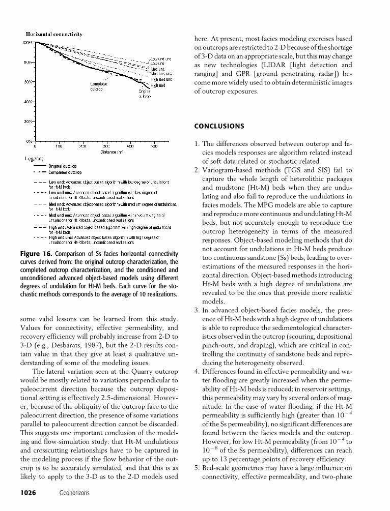
sponses (see horizontal connectivity in Figure 16)

did not change significantly, and the obtained rank-

ings remained the same, indicating that the artifacts

observed in the conditioned realizations (Figure 8f–h)

did not significantly affect the measured responses

and the validity of the comparison.

2. Advanced object-based methods also need a large

number of parameters to obtain reliable reproduc-

tions of heterogeneity.

The predictions obtained by MPG were not as

good as the ones obtained by object-based methods

with highly undulating shales because of difficulties in

reproducing large-scale continuous structures (Liu et al.,

2004). However, future implementations of the MPG

method cannot be discarded for modeling this deposi-

tional setting because of its ability to generate realistic

conditioned realizations when data density is high.

Limitations

Although the comparison of the models was in 2-D

(limited by the 2-D nature of the outcrop) and reality

is three-dimensional (3-D), we are of the opinion that


some valid lessons can be learned from this study.

Values for connectivity, effective permeability, and

recovery efficiency will probably increase from 2-D to

3-D (e.g., Desbarats, 1987), but the 2-D results con-

tain value in that they give at least a qualitative un-

derstanding of some of the modeling issues.

The lateral variation seen at the Quarry outcrop

would be mostly related to variations perpendicular to

paleocurrent direction because the outcrop deposi-

tional setting is effectively 2.5-dimensional. Howev-

er, because of the obliquity of the outcrop face to the

paleocurrent direction, the presence of some variations

parallel to paleocurrent direction cannot be discarded.

This suggests one important conclusion of the model-

ing and flow-simulation study: that Ht-M undulations

and crosscutting relationships have to be captured in

the modeling process if the flow behavior of the out-

crop is to be accurately simulated, and that this is as

likely to apply to the 3-D as to the 2-D models used

here. At present, most facies modeling exercises based

on outcrops are restricted to 2-Dbecause of the shortage

of 3-D data on an appropriate scale, but thismay change

as new technologies (LIDAR [light detection and

ranging] and GPR [ground penetrating radar]) be-

comemore widely used to obtain deterministic images

of outcrop exposures.

CONCLUSIONS

1. The differences observed between outcrop and fa-

cies models responses are algorithm related instead

of soft data related or stochastic related.

2. Variogram-based methods (TGS and SIS) fail to

capture the whole length of heterolithic packages

and mudstone (Ht-M) beds when they are undu-

lating and also fail to reproduce the undulations in

facies models. The MPGmodels are able to capture

and reproducemore continuous andundulatingHt-M

beds, but not accurately enough to reproduce the

outcrop heterogeneity in terms of the measured

responses. Object-based modeling methods that do

not account for undulations in Ht-M beds produce

too continuous sandstone (Ss) beds, leading to over-

estimations of the measured responses in the hori-

zontal direction. Object-based methods introducing

Ht-M beds with a high degree of undulations are

revealed to be the ones that provide more realistic

models.

3. In advanced object-based facies models, the pres-

ence of Ht-M beds with a high degree of undulations

is able to reproduce the sedimentological character-

istics observed in the outcrop (scouring, depositional

pinch-outs, and draping), which are critical in con-

trolling the continuity of sandstone beds and repro-

ducing the heterogeneity observed.

4. Differences found in effective permeability and wa-

ter flooding are greatly increased when the perme-

ability of Ht-M beds is reduced; in reservoir settings,

this permeability may vary by several orders of mag-

nitude. In the case of water flooding, if the Ht-M

permeability is sufficiently high (greater than 10�4

of the Ss permeability), no significant differences are

found between the facies models and the outcrop.

However, for lowHt-M permeability (from 10�4 to

10�8 of the Ss permeability), differences can reach

up to 13 percentage points of recovery efficiency.

5. Bed-scale geometries may have a large influence on

connectivity, effective permeability, and two-phase

Figure 16. Comparison of Ss facies horizontal connectivitycurves derived from: the original outcrop characterization, thecompleted outcrop characterization, and the conditioned andunconditioned advanced object-based models using differentdegrees of undulation for Ht-M beds. Each curve for the sto-chastic methods corresponds to the average of 10 realizations.

1026 Geohorizons

flow, as demonstrated here. Results presented here-

in will apply during the process of building facies

models to upscale petrophysical properties from

lamina scale to geological cell scale, and for building

field-scale reservoir models if sufficiently fine (i.e.,

able to reproduce bed-scale geometries) grids are

considered.

REFERENCES CITED

Arbues, P., D. Mellere, O. Falivene, O. Fernandez, J. A. Munoz,M. Marzo, and J.M.deGibert, inpress,Context and architectureof the Ainsa-1-quarry channel complex, Ainsa basin, Spain, inT. H. Nilsen, R. D. Shew, G. S. Steffens, and J. R. J. Studlick,Atlas of deep-water outcrops: AAPG Studies in Geology 56.

Begg, S. H., and P. R. King, 1985, Modeling the effect of shales onreservoir performance: Calculation of effective vertical per-meability: Society of Petroleum Engineers Paper 13529, 15 p.

Caers, J., 2001, Geostatistical reservoir modelling using statisticalpattern recognition: Journal of Petroleum Science and Engi-neering, v. 29, p. 177–188.

Caers, J., and T. Zhang, 2004, Multiple-point geostatistics: A quan-titative vehicle for integrating geologic analogs into multiplereservoir models, inM. Grammer, P. M. Harris, and G. P. Eberli,eds., Integration of outcrop and modern analogs in reservoirmodeling: AAPG Memoir 80, p. 383–394.

Christie, M. A., 1996, Upscaling for reservoir simulation: Journal ofPetroleum Technology, v. 48, p. 1004–1010.

Clark, J. D., and K. T. Pickering, 1996, Submarine channels:Processes and architecture: London, Vallis Press, 231 p.

Clementsen, R., A. Hurst, R. Knarud, and H. Omre, 1990, Acomputer program for evaluation of fluvial reservoirs, in A. T.Buller, E. Berg, O. Hjemeland, J. Kleppe, O. Torsaeter, andJ. O. Aasen, eds., North Sea oil and gas reservoirs II: London,Graham and Trotham, p. 373–385.

Cossey, S. P., 1994, Reservoir modeling of deepwater clastic se-quences: Mesoscale architectural elements, aspect ratios, andproducibility, in P. Weimer, A. H. Bouma, and B. F. Perkins,eds., Submarine fans and turbidite systems: Gulf Coast SectionSEPM 15th Annual Research Conference, p. 83–93.

Cressie, N., 1990, The origins of kriging: Mathematical Geology,v. 22, p. 239–252.

Dalrymple, M., 2001, Fluvial reservoir architecture in the StratfjordFormation (northern North Sea) augmented by outcrop analogstatistics: Petroleum Geoscience, v. 7, p. 115–122.

Desbarats, A. J., 1987, Numerical estimation of effective perme-ability in sand-shale formations: Water Resources Research,v. 23, p. 273–286.

Deutsch, C. V., 1998, Fortran programs for calculating connectivityof three dimensional numerical models and for ranking multi-ple realizations: Computers and Geosciences, v. 24, p. 69–76.

Deutsch, C. V., 1999, Reservoir modeling with publicly availablesoftware: Computers and Geosciences, v. 25, p. 355–363.

Deutsch, C. V., 2002, Geostatistical reservoir modeling: AppliedGeostatistics Series: NewYork, OxfordUniversity Press, 376 p.

Deutsch, C. V., and A. G. Journel, 1998, GSLIB: Geostatisticalsoftware library and user’s guide, 2d ed.: Oxford, OxfordUniversity Press, 350 p.

Deutsch, C. V., and T. T. Tran, 2002, FLUVISIM: A program forobject-based stochastic modeling of fluvial depositional sys-tems: Computers and Geosciences, v. 28, p. 525–535.

Deutsch, C. V., and L. Wang, 1996, Hierarchical object-basedstochastic modeling of fluvial reservoirs: Mathematical Geol-ogy, v. 28, p. 851–880.

Dewhurst, D. N., Y. Yang, and A. C. Aplin, 1999, Permeability andfluid flow in natural mudstones, in A. C. Aplin, A. J. Fleet, andJ. H. S. Macquaker, eds., Muds and mudstones: Physical andfluid flow properties: Geological Society (London) SpecialPublication 158, p. 23–43.

Dreyer, T., L. M. Falt, T. Hoy, R. Knarud, R. Steel, and J. L.Cuevas, 1993, Sedimentary architecture of field analogues forreservoir information (SAFARI): A case study of the fluvialEscanilla Formation, Spanish Pyrenees, in S. Flint and I. D.Bryant, eds., The geological modelling of hydrocarbon reser-voirs and outcrop analogues: International Association of Sedi-mentologists Special Publication 15, p. 57–80.

Dubrule, O., 1994, Estimating or choosing a geostatistical model?,in R. Dimitrakopoulos, ed., Geostatistics for the next century:Dordrecht, Holland, Kluwer Academic Publishers, p. 3–14.

Dubrule, O., 1998, Geostatistics in petroleum geology: AAPGCourse Note Series 38, 52 p.

Ethridge, F. G., 2004, Sealing capacity and petrographic character-istics of Eocene marine mudrocks, south-central Pyreneanforeland basin, Spain (abs.): AAPGAnnual Meeting, April 18–21, Dallas, Texas, v. 13, p. A42.

Fernandez, O., J. A. Munoz, P. Arbues, O. Falivene, and M. Marzo,2004, 3-D reconstruction of geological surfaces: An exampleof growth strata and turbidite systems from the Ainsa basin(Pyrenees, Spain): AAPG Bulletin, v. 88, p. 1049–1068.

Gomez-Hernandez, J., and R. M. Srivastava, 1990, ISIM 3D: AnANSI-C three-dimensional and multiple indicator conditionalsimulation program: Computers and Geosciences, v. 16, p. 355–410.

Gringarten, E., and C. V. Deutsch, 2001, Variogram interpreta-tion and modeling: Mathematical Geology, v. 33, p. 507–535.

Haldorsen, H. H., and D. M. Chang, 1986, Notes on stochasticshales— From outcrop to simulation model, in L. W. Lakeand H. B. Carroll, eds., Reservoir characterization: Orlando,Academic Press, p. 445–485.

Haldorsen, H. H., and E. Damsleth, 1990, Stochastic modeling:Journal of Petroleum Geology, v. 42, p. 404–412.

Haldorsen, H. H., and L. Lake, 1984, A new approach to shalemanagement in field-scale models: Society of Petroleum Engi-neers Journal, v. 24, p. 447–457.

Hurst, A., I. Verstralen, B. Cronin, and A. Hartley, 1999, Sand-richfairways in deep-water clastic reservoirs: Genetic units, cap-turing uncertainty, and a new approach to reservoir modeling:AAPG Bulletin, v. 83, p. 1096–1118.

Jackson, M. D., and A. H. Muggeridge, 2000, The effects ofdiscontinuous shales on reservoir performance during horizon-tal waterflooding: Society of Petroleum Engineers Journal, v. 5,p. 446–455.

Jackson, M. D., S. Yoshida, A. H. Muggeridge, and D. Johnson,2005, Three-dimensional reservoir characterization and flowsimulation of heterolithic tidal sandstones: AAPG Bulletin,v. 89, p. 507–521.

Johnson, S. D., S. Flint, D. Hinds, and H. D. V. Wickens, 2001,Anatomy geometry and sequence stratigraphy of basin floor toslope turbidite systems, Tanqua Karoo, South Africa: Sedi-mentology, v. 48, p. 987–1023.

Journel, A. G., 1983, Nonparametric estimation of spatial distribu-tions: Mathematical Geology, v. 15, p. 445–468.

Journel, A. G., and C. V. Deutsch, 1993, Entropy and spatialdisorder: Mathematical Geology, v. 25, p. 329–355.

Journel, A. G., R. Gundeso, E. Gringarten, and T. Yao, 1998, Sto-chastic modelling of a fluvial reservoir: A comparative review


of algorithms: Journal of Petroleum Science and Engineering,v. 21, p. 95–121.

King, M. J., and M. Mansfield, 1999, Flow simulation of geologicmodels: Society of Petroleum Engineers Reservoir Evaluationand Engineering, v. 2, p. 351–367.

King, P. R., 1990, The connectivity and conductivity of overlappingsand bodies, in A. T. Buller, E. Berg, O. Hjemeland, J. Kleppe,O. Torsaeter, and J. O. Aasen, eds., North Sea oil and gasreservoirs II: London, Graham and Trotham, p. 353–362.

Knudby, C., and J. Carrera, 2005, On the relationship betweenindicators of geostatistical, flow and transport connectivity:Advances in Water Resources, v. 28, p. 405–421.

Koltermann, C. E., and S. M. Gorelick, 1996, Heterogeneity insedimentary deposits: A review of structure-imitating, process-imitating, and descriptive approaches: Water Resources Re-search, v. 32, p. 2617–2658.

Krum, G. L., and C. R. Johnson, 1993, A 3-D modelling approachfor providing a complex reservoir description for reservoirsimulations, in S. S. Flint and I. D. Bryant, eds., The geologicmodelling of hydrocarbon reservoirs and outcrop analogues:International Association of Sedimentologists Special Publica-tion 15, p. 253–258.

Kupfersberger, H., and C. V. Deutsch, 1999, Methodology forintegrating analog geologic data in 3-D variogram modeling:AAPG Bulletin, v. 83, p. 1262–1278.

Larue, D., 2004, Outcrop and waterflood simulation modeling ofthe 100-foot channel complex, Texas and the Ainsa II channelcomplex, Spain: Analogs to multistory and multilateralchannelized slope reservoirs, in M. Grammer, P. M. Harris,and G. P. Eberli, eds., Integration of outcrop and modernanalogs in reservoir modeling: AAPGMemoir 80, p. 337–364.

Larue, D., and F. Friedmann, 2005, The controversy concerningstratigraphic architecture of channelized reservoirs and recoveryby waterflooding: Petroleum Geoscience, v. 11, p. 131–146.

Larue, D., and H. Legarre, 2004, Flow units, connectivity, and res-ervoir characterization in a wave-dominated deltaic reservoir:Meren reservoir, Nigeria: AAPG Bulletin, v. 88, p. 303–324.

Li, H., and C. D. White, 2003, Geostatistical models for shales indistributary channel point bars (Ferron Sandstone, Utah): Fromground-penetrating radar to three-dimensional flow modelling:AAPG Bulletin, v. 87, p. 1851–1868.

Lia, O., H. Tjelmeland, and L. E. Kjellesvik, 1997, Modeling offacies architecture by marked point model in E. Y. Baafi andN. A. Schofield, Geostatistics Wollongong ’96: 5th Interna-tional Geostatistics Congress inWollongong, Dordrecht, KluwerAcademic, v. 1, p. 386–398.

Liu, Y., A. Harding, W. Abriel, and S. Strebelle, 2004, Multiple-point simulation integrating wells, three-dimensional seismicdata, and geology: AAPG Bulletin, v. 88, p. 905–921.

Mijnessen, F. C. J., 1997, Modelling of sandbody connectivity in theSchooner field, in K. Ziegler, P. Turner, and S. R. Daines, eds.,Petroleum geology of the southern North Sea: Future po-tential: Geological Society (London) Special Publication 123,p. 169–180.

Munoz, J. A., P. Arbues, and J. Serra-Kiel, 1998, The Ainsa basinand the Sobrarbe oblique thrust system: Sedimentological andtectonic processes controlling slope and platform sequencesdeposited synchronously with a submarine emergent thrustsystem, in A. Melendez Hevia and A. R. Soria, eds., Field tripguidebook of the 15th International Association of Sedimen-tologists International Congress of Sedimentology, p. 213–223.

Mutti, E., 1992, Turbidite sandstones: AGIP-Istituto di Geologia,Universita di Parma, 275 p.

Mutti, E., and W. R. Normark, 1987, Comparing examples ofmodern and ancient turbidite systems: Problems and concepts,

in J. K. Legget and G. G. Zuffa, eds., Deep water clastic de-posits:Models and case histories: London,GrahamandTrotham,p. 1–38.

Novakovic, D., C. D. White, R. Corbeanu, W. S. Hammon III,J. Bhattacharya, and G. A. McMechan, 2002, Hydraulic effectsof shales in fluvial-deltaic deposits: Ground-penetrating radar,outcrop observations, geostatistics and three-dimensional flowmodeling for the Ferron Sandstone, Utah: Mathematical Ge-ology, v. 34, p. 857–893.

Pardo-Iguzquiza, E., and P. A. Dowd, 2003, CONNEC3D: Acomputer program for connectivity analysis of 3D random setmodels: Computers and Geosciences, v. 29, p. 775–785.

Pickup, G. E., P. S. Ringrose, and S. Ahmed, 2000, Steady-stateupscaling: From lamina-scale to full-field model: Society ofPetroleum Engineers Journal, v. 5, p. 208–217.

Renard, P., and G. de Marsily, 1997, Calculating equivalent perme-ability: A review: Advances in Water Resources, v. 20, p. 237–278.

Satur, N., A. Hurst, B. Cronin, G. Kelling, and K. Gurbuz, 2000,Sand body geometry in a sand-rich, deep-water clastic system,Miocene Cingoz Formation of southern Turkey: Marine andPetroleum Geology, v. 17, p. 239–252.

Scheibe, T. D., and C. J. Murray, 1998, Simulation of geologicpatterns: A comparison of stochastic simulation techniques forgroundwater transport modeling, in G. S. Fraser and J. M.Davis, eds., Hydrogeologic models of sedimentary aquifers:Concepts in Hydrogeology and Environmental Geology, v. 1,p. 107–118.

Schuppers, J. D., 1993, Quantification of turbidite facies in areservoir-analogous submarine-fan channel sandbody, south-central Pyrenees, Spain, in S. S. Flint and I. D. Bryant, eds.,The geologic modelling of hydrocarbon reservoirs and outcropanalogues: International Association of Sedimentologists Spe-cial Publication, p. 99–112.

Schuppers, J. D., 1995, Characterization of deep-marine clasticsediments from foreland basins: Outcrop-derived concepts forexploration, production and reservoir modelling: Ph.D. thesis,Delft University of Technology, Netherlands, 272 p.

Seifert, D., and J. L. Jensen, 2000, Object and pixel-based reservoirmodeling of a braided fluvial reservoir: Mathematical Geology,v. 32, p. 581–603.

Slatt, R. M., and P. Weimer, 1999, Turbidite systems: Part 2.Subseismic-scale reservoir characteristics: The Leading Edge,v. 18, no. 5, p. 562–567.

Slatt, R., H. Al-Siyabi, C. VanKirk, and R. Williams, 2000, Fromgeologic characterization to ‘reservoir simulation’ of a turbiditeoutcrop, in A. Bouma and C. Stone, eds., Fine-grained turbi-dite systems: AAPG Memoir 72/SEPM Special PublicationNo. 68, p. 187–194.

Srivastava, R. M., 1994, An overview of stochastic methods forreservoir characterization, in J. M. Yarus and R. L. Chambers,eds., Stochastic modeling and geostatistics: Principles, methodsand case studies: AAPG Computer Applications in Geology 3,p. 3–16.

Stephen, K. D., J. D. Clark, and A. R. Gardiner, 2001, Outcrop-based stochastic modelling of turbidite amalgamation and itseffects on hydrocarbon recovery: Petroleum Geoscience, v. 7,p. 163–172.

Strebelle, S., 2002, Conditional simulation of complex geologicalstructures using multiple-point statistics: Mathematical Geol-ogy, v. 34, p. 1–22.

Thomas, J. M. D., 1990, The movement of oil initially bypassedbehind stochastic shale barriers: North Sea oil and gas res-ervoirs: II. Proceedings of the North Sea Oil and Gas Reser-voirs Conference, p. 437–444.

Tran, T. T., 1994, Improving variogram reproduction on dense

1028 Geohorizons

simulation grids: Computers and Geosciences, v. 20, p. 1161–1168.

Tyler, K., A. Henriquez, and T. Svanes, 1994, Modeling heterogene-ities in fluvial domains, a review on the influence on productionprofile, in J. M. Yarus and R. L. Chambers, eds., Stochasticmodeling and geostatistics: Principles, methods and case studies:AAPG Computer Applications in Geology 3, p. 77–89.

Webb, E. K., and J. M. Davis, 1998, Simulation of the spatialheterogeneity of geologic properties: An overview, in G. S.Fraser and J. M. Davis, eds., Hydrogeologic models ofsedimentary aquifers: Concepts in Hydrogeology and Environ-mental Geology, v. 1, p. 1–24.

Weimer, P., R. M. Slatt, P. Dromgoole, M. Bowman, and A.Leonard, 2000, Developing and managing turbidite reservoirs:Case histories and experiences: Results of the 1998 EuropeanAssociation of Geoscientists and Engineers–American Associ-ation of Petroleum Geologists Research Conference: AAPGBulletin, v. 84, p. 453–465.

Willis, B. J., and C. D. White, 2000, Quantitative outcrop data forflow simulation: Journal of Sedimentary Research, v. 70,p. 788–802.

Xu, W., 1996, Conditional curvilinear stochastic simulation usingpixel-based algorithms: Mathematical Geology, v. 28, p. 937–950.


Best practice stochastic facies modeling from a channel-fill turbidite sandstone analog (the Quarry...

Documents

Transcript of Best practice stochastic facies modeling from a channel-fill turbidite sandstone analog (the Quarry...