A szécsényi seregszék jegyzőkönyve (1656-1661) ed. Szabó András Péter

Turbidite Event History—Methods and Implications for Holocene Paleoseismicity of the Cascadia Subduction Zone
Asto
ria C
hann
el
-130° -128° -126° -124° -122°
-
AstoriaFan
Hydrate RidgeBasin West
Juan
de F
uca
Ridg
e
JUAN DE FUCA PLATE
Cascad
ia Cha
nnel
Blanco Fracture Zone
Gord
a Ri
dge
GORDAPLATE
Mendocino Escarpment
Tufts AbyssalPlain
OREGON
WASHINGTON
42°
44°
46°
48°
BarkleyCanyon
Juan de FucaCanyon
QuinaltCanyon
GraysCanyon
WillapaCanyon
AstoriaCanyon
RogueCanyon
SmithCanyon
KlamathCanyon
TrinidadCanyon
EelCanyon
MendocinoChannel
Noyo Canyon
Nitinat Fan
San Andreas Fault
40°
Port Alberni
Willapa Bay
NetartsBay
SalmonRiver
Yaquina Bay
Alsea Bay
Lagoon Creek
Sixes RiverCoquille River
Humboldt Bay
Johns River
Bradley Lake
Coos Bay
Discovery Bay
Stanley LakeEcola Creek
CALIFORNIA
Astoria Channel
GuideCanyon
QuillayuteCanyon
08/09 PC06/07 PC
05 PC
11/12 PC
13 PC14/15 PC
01/03 PC
16 PC
17/18/19/20/21 PC
26/28 PC 27/29 PC
30/31 PC
33 PC
34 PC
35/36/37 PC
41/42 PC39/40 PC
47/51 PC BX 144/45 PC
48/49 PC
22/23 PC
10 PC
02/56 PC01 KC
55 KC
38 BC
24 BC
04 BC
6509-15
6502 PC-1
6705-5
6609-1
6609-12
6609-24
6508 K1
6705-6
53-18
Vancouver Sea Valley
U.S. Department of the InteriorU.S. Geological Survey
Professional Paper 1661–F

COVERCascadia study area, including major features and core locations (see fig. 2 for complete figure).

i
Turbidite Event History—Methods and Implications for Holocene Paleoseismicity of the Cascadia Subduction Zone
By Chris Goldfinger, C. Hans Nelson, Ann E. Morey, Joel E. Johnson, Jason R. Patton, Eugene Karabanov, Julia Gutiérrez-Pastor, Andrew T. Eriksson, Eulàlia Gràcia, Gita Dunhill, Randolph J. Enkin, Audrey Dallimore, and Tracy Vallier
Earthquake Hazards of the Pacific Northwest Coastal and Marine Regions Robert Kayen, Editor
COVERCascadia study area, including major features and core locations (see fig. 2 for complete figure).
Professional Paper 1661–F
U.S. Department of the InteriorU.S. Geological Survey

ii
U.S. Department of the InteriorKEN SALAZAR, Secretary
U.S. Geological SurveyMarcia K. McNutt, Director
U.S. Geological Survey, Reston: Virginia 2012
For product and ordering information: World Wide Web: http://www.usgs.gov/pubprod Telephone: 1-888-ASK-USGS
For more information on the USGS—the Federal source for science about the Earth, its natural and living resources, natural hazards, and the environment: World Wide Web: http://www.usgs.gov Telephone: 1-888-ASK-USGS
Suggested citation: Goldfinger, C., Nelson, C.H., Morey, A.E., Johnson, J.R., Patton, J., Karabanov, E., Gutierrez-Pastor, J., Eriksson, A.T., Gracia, E., Dunhill, G., Enkin, R.J., Dallimore, A., and Vallier, T., 2012, Turbidite event history—Methods and implications for Holocene paleoseismicity of the Cascadia subduction zone: U.S. Geological Survey Professional Paper 1661–F, 170 p, 64 figures, available at http://pubs.usgs.gov/pp/pp1661/f
Any use of trade, product, or firm names is for descriptive purposes only and does not imply endorsement by the U.S. Government.
Although this report is in the public domain, permission must be secured from the individual copyright owners to reproduce any copyrighted material contained within this report.

iii
Contents
Conversion Factors .......................................................................................................................................ixAcronyms, Initializations, Abbreviations ...................................................................................................xAbstract ...........................................................................................................................................................1Introduction.....................................................................................................................................................2
Significance of Turbidite Paleoseismology ......................................................................................3Cascadia Subduction Zone and Great Earthquake Potential ...............................................4
Methods..................................................................................................................................................5Bathymetric Analysis of Turbidite Pathways and Core Siting ..............................................5Coring Tools and Techniques .....................................................................................................7Core Siting .....................................................................................................................................8
Stratigraphic Correlation .....................................................................................................................9Lithostratigraphic Correlation ....................................................................................................9Numerical Signal Correlation .................................................................................................12
Age Control .........................................................................................................................................15Radiocarbon Dates ....................................................................................................................15Radiocarbon Date Reporting ...................................................................................................16Reservoir Correction .................................................................................................................17
Sedimentation Rates, Hemipelagic-Thickness Dates, and Refinements and Corrections to the Dates ..............................................................................................22
Hemipelagic Thickness and the Turbidite Tail-Hemipelagic Boundary ............................22Basal Erosion and Erosion Corrections .................................................................................23Sample Thickness Correction and Sedimentation Rates ....................................................23Hemipelagic Turbidite Dates ....................................................................................................23OxCal Analysis ............................................................................................................................24Event Ages and Potential Biases ............................................................................................24210Pb Activity ................................................................................................................................25Core Imaging and RGB Imagery ..............................................................................................26CT and X-Radiography ..............................................................................................................26Bioturbation Depth as a Time Indicator .................................................................................26Bioturbation and Its Effect on Radiocarbon Dating
of Interseismic Hemipelagic Sediments ...................................................................28Stratigraphic Datum Ages .................................................................................................................28
Late Quaternary Stratigraphy in Cascadia Basin .................................................................28Mazama Ash Datum ..................................................................................................................29Pleistocene-Holocene Faunal Boundary ...............................................................................31First Turbidite in the 10-k.y. Sequence (T18) ..........................................................................32Relative Dating Tests .................................................................................................................32
Results ...........................................................................................................................................................34Cascadia Turbidites, Stratigraphic Sequences, and Stratigraphic Correlation .......................34
General Description of Relevant Features of the Deposits ................................................34Mineralogy ..................................................................................................................................36Cascadia Turbidite Systems .....................................................................................................36
Barkley Canyon .................................................................................................................37

iv
Barkley Canyon Turbidite Sequence .............................................................................37Juan de Fuca Canyon and Channel ...............................................................................37Juan de Fuca Turbidite Sequence .................................................................................42Grays, Quinault, Guide, and Willapa Canyons and Channels ....................................42Willapa Channel Turbidite Sequence ............................................................................42Cascadia Deep-Sea Channel ..........................................................................................42Cascadia Channel Turbidite Sequence .........................................................................44Astoria Fan, Channel, and Base of Slope Channel ......................................................47Astoria Fan Turbidite Sequence .....................................................................................47Hydrate Ridge Basin West ..............................................................................................53Hydrate Ridge Basin West Turbidite Sequence ..........................................................53Rogue Apron ......................................................................................................................53Rogue Apron Turbidite Sequence ..................................................................................56Smith and Klamath Canyons and Aprons .....................................................................62Smith and Klamath Turbidite Sequences ......................................................................62Trinidad Canyon, Plunge Pool, and Sediment Wave Turbidite System ....................62Trinidad Turbidite Sequence ...........................................................................................64Eel Canyon Pool, Sediment Wave, Channel, and Lobe Turbidite System ................64Eel Canyon Pool, Sediment Wave, and Channel Turbidite Sequence ......................64Mendocino Channel .........................................................................................................70Mendocino Channel Turbidite Sequence .....................................................................70
Regional Stratigraphic Correlation .........................................................................................72Radiocarbon-Age Series .................................................................................................76Correlation of Derivative Parameters ............................................................................76Limitations ..........................................................................................................................77Regional Erosion Analysis ...............................................................................................77
Discussion ............................................................................................................................................79Cascadia Turbidite Summary ...................................................................................................79What Triggered the Turbidity Currents? .................................................................................84Sedimentological Examination ................................................................................................84
Multiple Pulses, Sedimentology, and Areal Extent .....................................................84Hyperpycnal Flow .............................................................................................................84Sedimentological Summary ...........................................................................................86
Synchronous Triggering ............................................................................................................86Spatial Extent .....................................................................................................................86Numerical Coincidence and the Confluence Test .......................................................87Stratigraphic Correlation .................................................................................................87
Applicability of Triggering Mechanisms to Cascadia ..........................................................88Triggering by Storm or Tsunami Waves ........................................................................88Liquefaction Caused by Wave Loading .........................................................................89Sediment Erosion Caused by Combined Current and Storm Wave Conditions ......89Geostrophic and Surface Currents ................................................................................91Cascadia Physiography and Turbidite Deposition.......................................................91
Frequency of Triggering Mechanisms ....................................................................................92Cascadia Turbidite Frequency—Earthquakes Versus Storms and Other
Phenomenon ........................................................................................................92

v
Tsunami Waves, Historical Evidence ............................................................................93Crustal and Slab Earthquakes ........................................................................................94Triggering Summary .........................................................................................................94
Cascadia Paleoseismic Record ...............................................................................................96Integrating the Onshore and Marine Paleoseismic Records ....................................96Discovery Bay..................................................................................................................102Willapa Bay, Grays Harbor, Columbia River, Southwest Washington
and Northern Oregon .......................................................................................102Bradley Lake, Coquille River, and Sixes River, Southern Oregon ..........................103Saanich and Effingham Inlets, Western Vancouver Island .....................................104
Constrained Time Series .........................................................................................................106Variability of Turbidite Deposition along the Southern Cascadia Margin ......................108Magnitude Sensitivity .............................................................................................................109Margin Segmentation ............................................................................................................110Full or Nearly Full Margin Ruptures ......................................................................................110Segmented Ruptures ...............................................................................................................112Recurrence Intervals of Cascadia Earthquakes .................................................................112
Segment A ........................................................................................................................115Hemipelagic Thickness Based Recurrence Intervals for Segment A ..................115Segment B ........................................................................................................................116Segment C ........................................................................................................................116Segment D .......................................................................................................................116Additional Segments? ....................................................................................................117
Structural and Sediment-Thickness Controls on Cascadia Earthquakes ......................117Implications for Earthquake Hazards in Cascadia Basin
and the Northern San Andreas Fault ...............................................................................119Earthquake Relative Magnitudes ..........................................................................................122Clustering ..................................................................................................................................123
Are the Clusters Statistically Significant? .................................................................125Recurrence Model for Cascadia Earthquakes ...................................................................126
Relation Between Earthquake Size and Recurrence Interval .................................128Segment-Based Probabilities for Cascadia Great Earthquakes ......................................129Temporal Coincidence with and Possible Triggering
of Northern San Andreas Fault Earthquakes .........................................................133Implications of Turbidite Paleoseismology Beyond Cascadia Basin ..............................133Implications of Stratigraphic Correlation ............................................................................134
A Simple Experiment ......................................................................................................135Variability of the Source ...............................................................................................135Time Resolution .....................................................................................................................136
Conclusions........................................................................................................................................136Lessons Learned ...............................................................................................................................138
Applicability to Other Settings ...............................................................................................138Future Directions .....................................................................................................................139
Acknowledgments .....................................................................................................................................139References Cited........................................................................................................................................140Appendixes .................................................................................................................................................159

vi
Figures 1. Turbidite-channel and canyon-system types along the Cascadia margin .................................2 2. Cascadia margin turbidite canyons, channels, and 1999–2002 core locations .........................6 3. Photographs of coring equipment .....................................................................................................8 4. Image showing 100-m-resolution shaded swath bathymetry of a portion
of Astoria Canyon, northern Oregon, Cascadia subduction zone ........................................9 5. Example of typical turbidite stratigraphy from Cascadia Basin,
showing events T1–T3 in core M9907-25PC in Cascadia Channel .....................................11 6. Photograph showing detail from core M9907-25TC event T4,
Cascadia subduction zone (see fig. 2 for location) ...............................................................12 7. Detailed stratigraphic diagrams showing examples of physical property traces
versus grain size .........................................................................................................................13 8. Diagrams showing correlation details from two representative pairs of cores
on the Cascadia margin .............................................................................................................14 9. Graphs showing sedimentation rate curves for Cascadia Basin core sites,
Cascadia subduction zone ........................................................................................................1810. Plots showing calibration examples and OxCal example ............................................................2111. Diagram showing Mazama-ash correlation in Cascadia Basin .................................................3012. Shipboard core photograph showing color changes at the approximate
Pleistocene to Holocene boundary in the central core section .........................................3113. Synchroneity test at a channel confluence as applied where multiple
Washington channels merge into the Cascadia Deep Sea Channel, indicated by the green outline .................................................................................................33
14. Lithologic, magnetic, and density data for event T5 in Cascadia Channel ...............................3515. Heavy-mineral composition diagram showing Columbia River-Cascade Range
source of Astoria and Cascadia Channel sands and Rogue River-Klamath terrane source of Rogue Apron sands ....................................................................................36
16. Perspective view of shaded-relief bathymetry of the Barkley Canyon system and apron, Vancouver Island margin ......................................................................................38
17. Site-correlation diagram for Barkley and No Name Canyon cores (see figs. 2 and 16 for core locations) ....................................................................................38
18. Perspective views of shaded-relief bathymetry of the northern Juan de Fuca Channel system and upper Nitinat Fan, Washington margin ..............................................40
19. Site-correlation diagram for the Juan de Fuca Channel key site (see figs. 2 and 18 for core locations) .....................................................................................43
20. Summary core logs and digital photographs of all sections of Juan de Fuca Channel core M9907-12PC (see figs. 2 and 18B for location). .............................................44
21. Perspective view of shaded-relief bathymetry of the Willapa Canyon system and lower Nitinat Fan, Washington margin ............................................................................45
22. Site-correlation diagram for Willapa Channel cores (see figs. 2 and 21 for core locations) .....................................................................................46
23. Perspective view of shaded-relief bathymetry of the Cascadia Channel system and surrounding Cascadia abyssal plain ................................................................................48
24. Site-correlation diagram for Cascadia Channel cores (see figs. 2 and 23 for core locations) .....................................................................................48
25. Summary core logs and digital photographs of all sections of Cascadia Channel core M9907-25PC ........................................................................................................................50

vii
26. Perspective view of shaded-relief bathymetry of the lower Astoria Canyon system and upper Astoria Fan, Oregon margin ...........................................................................................51
27. Site-correlation diagram for Northern Astoria Channel cores (see figs. 2 and 26 for core locations) .....................................................................................52
28. Perspective view of shaded-relief bathymetry of Hydrate Ridge Basin West and the lower Astoria Channel system, Oregon margin ......................................................54
29. Site-correlation diagram for south Astoria Channel cores (see figs. 2 and 28 for core locations) .....................................................................................55
30. Perspective view of shaded-relief bathymetry of Hydrate Ridge Basin West (HRBW) on the central Oregon margin ...................................................................................................56
31. Site-correlation diagram for Hydrate Ridge Basin West (HRBW) cores (see figs. 2 and 30 for core locations) ....................................................................................57
32. Perspective view of shaded-relief bathymetry of the Rogue Canyon system and apron, southern Oregon margin .......................................................................................58
33. Site-correlation diagram for Rogue Apron cores (see figs. 2 and 32 for core locations) ......5934. Summary core logs and digital photographs of all sections of Rogue Apron core
M9907-31PC (see figs. 2 and 32 for location) .........................................................................6035. A, Details of events from the surface to T4, Rogue Apron and Klamath Channel,
emphasizing small events T2a and T3a ...................................................................................6136. Perspective view of shaded-relief bathymetry of the Smith and Klamath Canyon systems
and aprons, southern Oregon/northern California margin ..................................................6337. Site-correlation diagram for Smith Canyon cores (see figs. 2 and 36 for core locations) .....6538. Site-correlation diagram for Klamath Canyon cores (see figs. 2 and 36 for core locations) 6639. Perspective view of shaded-relief bathymetry of the Trinidad, Eel, and Mendocino
canyon/channel systems and plunge pools, northern California margin ..........................6640. Site-correlation diagram for Trinidad Channel cores
(see figs. 2 and 39 for core locations) .....................................................................................6841. Site-correlation diagram for Eel Channel cores (see figs. 2 and 39 for core locations) ........6942. Site-correlation diagram for Mendocino Channel cores
(see figs. 2 and 39 for core locations) .....................................................................................7043. Correlation examples .........................................................................................................................7244. Core-lithology diagram and physical properties from key core sites
along the Cascadia margin, shown at true scale ..................................................................7545. Core-lithology diagram and physical properties from the Hydrate Ridge
and Rogue Apron core sites, central-southern Cascadia margin ......................................7946. Correlation plot of marine turbidite records and 14C ages along the Cascadia margin
from Barkley Channel to Eel Channel for the past ~10,000 years .......................................8147. Correlation of vertical series of coarse fraction pulses per turbidite
for Juan de Fuca (JDF), Cascadia (Casc.), Hydrate Ridge (HR), and Rogue cores ..........8148. Holocene hemipelagic sediment-drape thickness in cores from Cascadia Basin .................8349. Idealized stratigraphy resulting from hyperpycnal flow, characterized by
a coarsening-upward sequence followed by a fining-upward sequence, attributed to a waxing, then waning, hydrographic profile during a storm event ...........85
50. Schematic representation of a typical Cascadia Canyon system showing effective maximum credible depth of wave resuspension of sediments (~500 m) and input from the nearshore and cross-shelf transport .....................................................95
51. Summary of the number of observed post-Mazama and Holocene turbidites in Cascadia Basin turbidite systems from this study and archive cores of Duncan (1968), Griggs (1969), and Nelson, C.H., (1968) that were used in Adams (1990) compilation .................98

viii
52. Space-time diagram for the Cascadia margin showing Holocene marine radiocarbon data and stratigraphic correlations ..................................99
53. Preliminary correlations between Cascadia Channel core M9907-23PC and core MD02-2494 from Effingham Inlet, western Vancouver Island, Canada (see fig. 2 for core locations) ...................................................................................106
54. OxCal-constrained 14C time series of Cascadia turbidites .......................................................................10755. Holocene rupture lengths of Cascadia great earthquakes from marine
and onshore paleoseismology ................................................................................................11156. Subduction of lower-plate features along the southern Cascadia margin ................................................ 11857. Sedimentary section thickness on the incoming Juan de Fuca Plate ....................................11958. Fit of distributions to the northern-central margin recurrence intervals ................................12059. Fit of distributions to the southern margin recurrence intervals ...................................................12160. Time series of Cascadia turbidite emplacement for the northern
and central Cascadia margin .................................................................................................................12461. Relation between turbidite mass per event at Juan de Fuca and Cascadia Channels,
and preceding interseismic time, northern Cascadia margin ...........................................12662. Plot of interseismic intervals versus mass per event for the northern
and central Cascadia margin ..................................................................................................12763. Probability of failure for the northern-central Cascadia margin population
of recurrence intervals ..................................................................................................................13164. Hypothetical rupture distribution along the Cascadia margin, consisting
of two patches of greater slip .................................................................................................132
Tables 1. Core locations and depths, Cascadia subduction zone .................................................................7 2. Bioturbation depth, turbidite mass, and interevent time, Cascadia subduction zone ............27 3. Pearson correlation matrix for bioturbation depth, turbidite mass,
and interevent time, Cascadia subduction zone ...................................................................27 4. Datum ages from 14C probability distribution function peaks, Cascadia subduction zone ....31 5. Rogue 210Pb activity, core tops ..........................................................................................................60 6. Calculation of hemipelagic-drape thickness from representative Cascadia Basin cores ....82 7. Cascadia canyon (listed north to south), shelf width, time of turbidite
frequency shifts, and canyon-head depths during the Holocene ......................................82 8. Magnitude estimated from time interval, plate motion,
and rupture-zone dimensions, Cascadia subduction zone. .................................................90 9. Potential turbidite-triggering mechanisms and their frequencies,
Cascadia subduction zone ........................................................................................................9510. Turbidite age averages and OxCal “combines” and 2s ranges,
Cascadia subduction zone ........................................................................................................9711. Rupture limits (limiting core sites and core numbers) from turbidite correlation,
Cascadia subduction zone ......................................................................................................11312. Turbidite mass versus interevent time, Cascadia subduction zone.........................................11513. Pearson correlation matrix: Turbidite mass versus prior and following interevent time .....122
ix
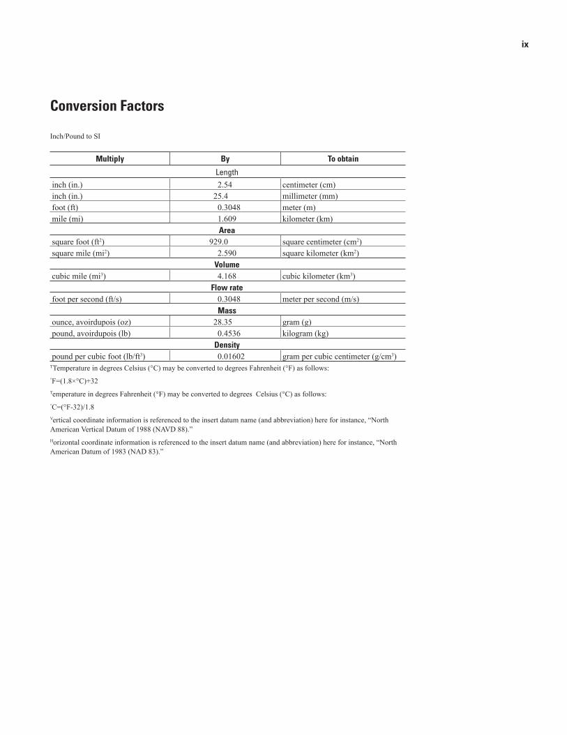
Conversion Factors
Inch/Pound to SI
Multiply By To obtain
Lengthinch (in.) 2.54 centimeter (cm)inch (in.) 25.4 millimeter (mm)foot (ft) 0.3048 meter (m)mile (mi) 1.609 kilometer (km)
Areasquare foot (ft2) 929.0 square centimeter (cm2)square mile (mi2) 2.590 square kilometer (km2)
Volumecubic mile (mi3) 4.168 cubic kilometer (km3)
Flow ratefoot per second (ft/s) 0.3048 meter per second (m/s)
Massounce, avoirdupois (oz) 28.35 gram (g) pound, avoirdupois (lb) 0.4536 kilogram (kg)
Densitypound per cubic foot (lb/ft3) 0.01602 gram per cubic centimeter (g/cm3)
TTemperature in degrees Celsius (°C) may be converted to degrees Fahrenheit (°F) as follows:°F=(1.8×°C)+32Temperature in degrees Fahrenheit (°F) may be converted to degrees Celsius (°C) as follows:°C=(°F-32)/1.8Vertical coordinate information is referenced to the insert datum name (and abbreviation) here for instance, “North American Vertical Datum of 1988 (NAVD 88).”Horizontal coordinate information is referenced to the insert datum name (and abbreviation) here for instance, “North American Datum of 1983 (NAD 83).”

x
Acronyms, Initializations, AbbreviationsADCP acousitc Doppler current profilerAVHR advanced very high resolutionAVHRR advanced very high resolution radiometerAMS accelerator mass spectrometryapd average wave periodBBL bottom boundary layerBC box coreCALIB 14C calibration programcc cubic centimeterCCD carbonate compensation depthCSZ Cascadia subduction zoneCT computed tomographyCUC California Undercurrent∆R, delta-R, DR local reservoir correction related to locationdpd dominant wave periodETS episodic tremor and slipGIS geographic information systemGLORIA Geological Long-Range Inclined AsdicHR Hydrate RidgeIODP Integrated Ocean Drilling ProgramJDF Juan de FucaKC kasten coreLORAN Long Range Navigation system; letter (LORAN A, LORAN C) MS magnetic susceptibilityMSCL mult-sensor core loggerNGDC National Geophysical Data CenterNOAA National Oceanic and Atmospheric AdministrationNOS National Oceanic ServiceNM nautical mileNSAF northern San Andreas FaultODP Ocean Drilling ProgramOSU Oregon State UniversityOxCal radiocarbon calibration softwarePC piston coreRC radiocarbonPDF/PDFs probability density function(s)RGB red, green, blueRMS root mean squareSI Systeme InternationaleSST sea surface temperatureTC trigger coreXBT expendable bathythermograph

Turbidite Event History—Methods and Implications for Holocene Paleoseismicity of the Cascadia Subduction Zone
Chris Goldfinger1, C. Hans Nelson2, Ann E. Morey1, Joel E. Johnson1, Jason R. Patton1, Eugene Karabanov3, Julia Gutiérrez-Pastor2, Andrew T. Eriksson1, Eulàlia Gràcia4, Gita Dunhill5, Randolph J. Enkin6, Audrey Dallimore7, and Tracy Vallier8
AbstractTurbidite systems along the continental margin of Cascadia
Basin from Vancouver Island, Canada, to Cape Mendocino, California, United States, have been investigated with swath bathymetry; newly collected and archive piston, gravity, kasten, and box cores; and accelerator mass spectrometry radiocarbon dates. The purpose of this study is to test the applicability of the Holocene turbidite record as a paleoseismic record for the Cascadia subduction zone. The Cascadia Basin is an ideal place to develop a turbidite paleoseismologic method and to record paleoearthquakes because (1) a single subduction-zone fault underlies the Cascadia submarine-canyon systems; (2) multiple tributary canyons and a variety of turbidite systems and sedimentary sources exist to use in tests of synchronous turbidite triggering; (3) the Cascadia trench is completely sediment filled, allowing channel systems to trend seaward across the abyssal plain, rather than merging in the trench; (4) the continental shelf is wide, favoring disconnection of Holocene river systems from their largely Pleistocene canyons; and (5) excellent stratigraphic datums, including the Mazama ash and distinguishable sedimentological and faunal changes near the Pleistocene-Holocene boundary, are present for correlating events and anchoring the temporal framework.
Multiple tributaries to Cascadia Channel with 50- to 150-km spacing, and a wide variety of other turbidite systems with different sedimentary sources contain 13 post-Mazama-ash and 19 Holocene turbidites. Likely correlative sequences are found
in Cascadia Channel, Juan de Fuca Channel off Washington, and Hydrate Ridge slope basin and Astoria Fan off northern and central Oregon. A probable correlative sequence of turbidites is also found in cores on Rogue Apron off southern Oregon. The Hydrate Ridge and Rogue Apron cores also include 12–22 interspersed thinner turbidite beds respectively.
We use 14C dates, relative-dating tests at channel confluences, and stratigraphic correlation of turbidites to determine whether turbidites deposited in separate channel systems are correlative—triggered by a common event. In most cases, these tests can separate earthquake-triggered turbidity currents from other possible sources. The 10,000-year turbidite record along the Cascadia margin passes several tests for synchronous triggering and correlates well with the shorter onshore paleoseismic record. The synchroneity of a 10,000-year turbidite-event record for 500 km along the northern half of the Cascadia subduction zone is best explained by paleoseismic triggering by great earthquakes. Similarly, we find a likely synchronous record in southern Cascadia, including correlated additional events along the southern margin. We examine the applicability of other regional triggers, such as storm waves, storm surges, hyperpycnal flows, and teletsunami, specifically for the Cascadia margin.
The average age of the oldest turbidite emplacement event in the 10–0-ka series is 9,800±~210 cal yr B.P. and the youngest is 270±~120 cal yr B.P., indistinguishable from the A.D. 1700 (250 cal yr B.P.) Cascadia earthquake. The northern events define a great earthquake recurrence of ~500–530 years. The recurrence times and averages are supported by the thickness of hemipelagic sediment deposited between turbidite beds. The southern Oregon and northern California margins represent at least three segments that include all of the northern ruptures, as well as ~22 thinner turbidites of restricted latitude range that are correlated between multiple sites. At least two northern California sites, Trinidad and Eel Canyon/pools, record additional turbidites, which may be a mix of earthquake and sedimentologically or storm-triggered events, particularly during the early Holocene when a close connection existed between these canyons and associated river systems.
The combined stratigraphic correlations, hemipelagic analysis, and 14C framework suggest that the Cascadia margin has three rupture modes: (1) 19–20 full-length or nearly
1 Oregon State University, Corvallis, OR2 Instituto Andaluz de Ciencias del la Tierra, Universidad de Granada, Granada, Spain3 Institute of Geochemistry, Siberian Branch of Russian Academy of Sciences, Irkutsk, Russia; Chevron Energy Technology Company, Houston, TX4 Centre Mediterrani d’Investigacions Marines i Amvientals Unitat de Tecnologia Marina, Barcelona, Spain5 Department of Earth and Environmental Sciences, California State University, East Bay, Hayward, CA 6 Geological Survey of Canada—Pacific, Sydney, B.C., Canada7 Geological Survey of Canada—Pacific, Sydney, B.C., Canada; Royal Roads University, Victoria, B.C., Canada8 U.S. Geological Survey, Menlo Park, CA

2 Turbidite Event History—Methods and Implications for Holocene Paleoseismicity of the Cascadia Subduction Zone
full length ruptures; (2) three or four ruptures comprising the southern 50–70 percent of the margin; and (3) 18–20 smaller southern-margin ruptures during the past 10 k.y., with the possibility of additional southern-margin events that are presently uncorrelated. The shorter rupture extents and thinner turbidites of the southern margin correspond well with spatial extents interpreted from the limited onshore paleoseismic record, supporting margin segmentation of southern Cascadia. The sequence of 41 events defines an average recurrence period for the southern Cascadia margin of ~240 years during the past 10 k.y.
Time-independent probabilities for segmented ruptures range from 7–12 percent in 50 years for full or nearly full margin ruptures to ~21 percent in 50 years for a southern-margin rupture. Time-dependent probabilities are similar for northern margin events at ~7–12 percent and 37–42 percent in 50 years for the southern margin. Failure analysis suggests that by the year 2060, Cascadia will have exceeded ~27 percent of Holocene recurrence intervals for the northern margin and 85 percent of recurrence intervals for the southern margin.
The long earthquake record established in Cascadia allows tests of recurrence models rarely possible elsewhere. Turbidite mass per event along the Cascadia margin reveals a consistent record for many of the Cascadia turbidites. We infer that larger turbidites likely represent larger earthquakes. Mass per event and magnitude estimates also correlate modestly with following time intervals for each event, suggesting that Cascadia full or nearly full margin ruptures weakly support a time-predictable model of recurrence. The long paleoseismic record also suggests a pattern of clustered earthquakes that includes four or five cycles of two to five earthquakes during the past 10 k.y., separated by unusually long intervals.
We suggest that the pattern of long time intervals and longer ruptures for the northern and central margins may be a function of high sediment supply on the incoming plate, smoothing asperities, and potential barriers. The smaller southern Cascadia segments correspond to thinner incoming sediment sections and potentially greater interaction between lower-plate and upper-plate heterogeneities.
42°
40°
44°
46°
48°
130° 128° 126° 124°
42°
44°
46°
48°
130° 128° 126° 124°
WAS
HIN
GTO
NO
REG
ON
CAL
IFO
RN
IA
0 km 1000 miles 100
TURBIDITESYSTEM TYPES
RogueApron
Cascadia
Deep-Sea C
hannel
Asto
ria C
hann
elTrinidadPool andWaves
Eel Channeland Wave Field
Mendocino Channel
NitinatFan
AstoriaFan
BlancoFracture Zone
TuftsAbyssal
Plain
PacificOcean
Figure 1. Turbidite-channel and canyon-system types along the Cascadia margin. Dashed portion of Astoria Channel currently has no surface expression, but it is mapped in the subsurface (Wolf and others, 1999).
The Cascadia Basin turbidite record establishes new paleoseismic techniques utilizing marine turbidite-event stratigraphy during sea-level highstands. These techniques can be applied in other specific settings worldwide, where an extensive fault traverses a continental margin that has several active turbidite systems.
IntroductionCascadia Basin includes the deep ocean floor over the
Juan de Fuca and Gorda Plates and extends from Vancouver Island, Canada, to the Mendocino Escarpment off northern California, United States (figs. 1, 2). Cascadia Basin contains a variety of Quaternary turbidite systems that exhibit different patterns of channel development and an extensive Holocene

Introduction 3
history of turbidite deposition (fig. 1). It has long been known that submarine channels along the Cascadia convergent margin have recorded a Holocene history of turbidites, and recent work suggests that these turbidites are linked to great earthquakes along the Cascadia subduction zone (Adams, 1990; Nelson, C.H., and others, 2000; Goldfinger and others, 2003a,b; Goldfinger and others, 2003a,b, 2008).
Cascadia Basin is an ideal location to examine the link-ages between earthquakes and turbidites because the turbidite systems and turbidite history have been studied extensively for the past 40 years, resulting in a large suite of archive cores and associated data and analyses (Duncan, 1968; Duncan and others, 1970; Nelson, C.H., 1968, 1976; Griggs, 1969; Griggs and Kulm, 1970; Carlson and Nelson, 1969). The Holo-cene stratigraphy of submarine channels along the Cascadia margin includes excellent turbidite marker beds that contain Mazama ash from the eruption of Mount Mazama that formed Crater Lake, Oregon (Nelson, C.H., and others, 1968). The calendar age of the eruption of Mount Mazama has recently been redated at 7,627±150 cal yr B.P. from the GISP-2 ice core (Zdanowicz and others, 1999). Airfall from the Mount Mazama eruption was distributed northeastward from southern Oregon, mainly over the Columbia Basin drainage and some of the coastal rivers. It also is found in the Puget lowland, Brit-ish Columbia (Hallett and others, 1997), and in inlets on the west coast of Vancouver Island (Dallimore and others, 2005b). From these rivers, Mazama ash was transported to temporary depocenters in canyon heads of the Cascadia continental mar-gin, much as Mount St. Helens ash was transported following the 1980 eruption (Nelson, C.H., and others, 1988). Turbidity currents subsequently transported the ash into Cascadia Basin canyon and channel-floor depocenters. The first occurrence of a tuffaceous turbidite dated to the Mount Mazama erup-tion at each channel site provides a stratigraphic marker to anchor the turbidite sequence and provide opportunities to test for synchronous triggering of turbidity currents for extensive distances along the margin.
We designed our investigation, in part, to test Adams’ (1990) hypothesis of a near one-to-one correlation between Holocene great earthquakes and the turbidite-event record in Cascadia Basin channels. Adams observed that 13 post-Mazama turbidites existed at widely separated sites in the Cascadia Basin, that such a coincidence was unlikely, and that the most plausible explanation is that turbidity currents were generated synchronously by subduction-zone earthquakes affecting the entire Cascadia margin. Adams made a convinc-ing case for seismic triggering versus other possible mecha-nisms, relying on the numerical coincidence and an elegant relative-dating test that established clear synchroneity for part of the margin. Adams used only archive core descriptions, with no age dating or modern sedimentological or stratigraphic techniques. We have tested this hypothesis using new cores collected in 1999 and 2002, accelerator mass spectrometry (AMS) radiocarbon dates, visible and X-ray imagery, and stratigraphic correlation using continuous physical-property measurements to extend the turbidite record in space and time
to the earliest Holocene. During the process, we developed a new turbidite paleoseismic method that tests for synchroneity of turbidite events along strike on convergent and transform margins characterized by single primary faults. Using this method, we evaluate potential triggers of turbidity currents against the time, space, and physical requirements imposed by various mechanisms and develop a paleoseismic record for the Cascadia subduction zone from the turbidite record, where other nonearthquake turbidites can, in many cases, be excluded. Mapping the spatial extent and timing of correlated events can also illustrate segmentation, relative earthquake magnitudes, and spatio-temporal relations that allow testing of recurrence models and stress triggering of margin segments and adjacent fault systems.
We (1) outline the types of turbidite systems found along the Cascadia margin and analyze the channel pathways where the best turbidite event records are preserved; (2) describe the turbidite sequences found in each system; (3) present the radiocarbon, X-ray, computed tomography (CT), visible image, and physical-property data from the core sites; (4) examine the evidence for triggering mechanisms of the Holo-cene Cascadia turbidites for synchroneity and for stratigraphic correlation of individual events over large distances; (5) pres-ent evaluation of the turbidite record as a paleoseismic record for the Cascadia subduction zone; (6) assess the combined onshore and offshore paleoseismic record and propose recur-rence intervals and rupture lengths for Holocene great earth-quakes in Cascadia; (7) discuss earthquake probabilities and possible recurrence models; and (8) discuss implications of the correlation records for the potential recording of paleoearth-quake-source information.
Testing and verification of the turbidite-event paleoseis-mic technique in Cascadia Basin will help develop fundamen-tal methods that can be applied to other continental-margin systems where an extensive, single, active fault traverses a continental margin that contains several active turbidite sys-tems. Two notable examples are the San Andreas Fault system along the continental margin of northern California (Nelson, C.H., and others, 2000; Goldfinger and others, 2007a, 2008) and the Sunda subduction margin offshore Sumatra (Patton and others, 2007, 2009, 2010).
Significance of Turbidite Paleoseismology
Subduction earthquakes generate some of the largest releases of energy on Earth. Quantifying the mechanisms and patterns of these great events remains elusive, because our observations commonly span only part of a seismic cycle and because the ability to measure the associated strain directly has only recently been developed. Recent rapid advances in Global Positioning System (GPS) technology now make it possible to measure crustal motion associated with elastic-strain accumulation at plate boundaries with a high degree of certainty (for example, McCaffrey and others, 2007; d’Alessio and others, 2005). However, real-time strain measurements

4 Turbidite Event History—Methods and Implications for Holocene Paleoseismicity of the Cascadia Subduction Zone
in subduction zones typically represent only a fraction of one strain cycle. Fundamental questions, such as the utility of the seismic-gap hypothesis, clustering, and the applicability of recurrence models, remain largely unanswered because we rarely have a long enough record of earthquake recurrence. Characteristic earthquake models assume that stress buildup is proportional to the time since the last earthquake. The seismic-gap hypothesis follows directly from this assumption and is the basis for probabilistic predictions of seismicity (Nishenko, 1991; Kagan and Jackson, 1995). Characteristic earthquake models and their derivatives have been challenged recently by new models of stress triggering and fault interaction (Stein and others, 1992; Toda and others, 1998; Ward and Goes, 1993; Weldon and others, 2004; Goldfinger and others, 2008). Stress-transfer models have been highly successful where the complex interaction of fault systems can be documented. In these models, strain recharge following an earthquake is sup-plied only indirectly by the underlying motion of the plates, and the stress on each fault segment is controlled by the action and history of the surrounding segments. What is most needed to address earthquake recurrence and fault interaction is data on spatial and temporal earthquake recurrence for more fault systems over longer spans of time, so that meaningful statisti-cal conclusions may be drawn.
Paleoseismology has the potential to address these ques-tions directly using the geologic record and precise dating during a longer time span than is available to geodesists or seismologists. The use of paleoseismology in active tectonic settings is now advancing rapidly. In the past two decades, dis-covery of rapidly buried marsh deposits (for example, Atwater and Hemphill-Haley, 1997) and associated tsunami sands (Clague and others, 2000; Kelsey and others, 2005) along the northern Pacific coast of North America, from Vancouver Island to northern California, has led to the recognition that the Cascadia subduction zone, once thought aseismic owing to low instrumental seismicity, likely has generated great (Mw 8–9) earthquakes in the past. The questions of how large and how frequent the megathrust earthquakes are and how these events occur spatially and temporally are now active areas of research in Cascadia and elsewhere (for example, Goldfinger and others, 2008; Nelson, A.R., and others, 2008; Kelsey and others, 2005).
Two avenues for addressing these questions at active con-tinental margins are coastal paleoseismology and investigation of the turbidite-event history. Neither technique uses fault outcrops because the faults are inaccessible, and both tech-niques must demonstrate that the events they are investigat-ing are generated by earthquakes and not some other natural phenomenon. Nevertheless, these problems can be overcome, and both techniques can be powerful tools for deciphering the earthquake history along an active continental margin (Goldfinger, 2009, 2011a). These methods are complementary; the onshore record provides temporal precision for the most recent events by using radiocarbon dating, coral chronology, and dendrochronology (tree-ring dating), whereas the turbidite record extends farther back in time, at least 10,000 years in
Cascadia, which is long enough to encompass many earth-quake cycles. In recent years, turbidite paleoseismology has been attempted in Cascadia (Adams, 1990; Goldfinger and others, 2003a,b, 2008; Nelson, C.H., and others, 1996; Nelson, C.H., and Goldfinger, 1999; Blais-Stevens and Clague, 2001), Puget Sound (Karlin and Abella, 1992; Karlin and others, 2004), Japan (Inouchi and others, 1996), the Mediterranean (Anastasakis and Piper, 1991; Kastens, 1984; Nelson, C.H., and others, 1995b), the Dead Sea (Niemi and Ben-Avraham, 1994), northern California (Field and others, 1982; Field, 1984; Garfield and others, 1994; Goldfinger and others, 2007a, 2008), Lake Lucerne (Schnellmann and others, 2002), Taiwan (Huh and others, 2006), the southwest Iberian margin (Gràcia and others, 2010), the Chile margin (Blumberg and others, 2008; Völker and others, 2008), the Marmara Sea (McHugh and others, 2006; Beck and others, 2007), the Sunda margin (Patton and others, 2007, 2009, 2010), and the Arctic ocean (Grantz and others, 1996). Results from these studies suggest the turbidite paleoseismologic technique is evolving as a use-ful tool for seismotectonics.
Cascadia Subduction Zone and Great Earthquake Potential
The Cascadia subduction zone is formed by the subduc-tion of the oceanic Juan de Fuca and Gorda Plates beneath the North American Plate off the coast of northern Califor-nia, Oregon, Washington, and Vancouver Island (fig. 2). The convergence rate is ~35–38 mm/yr directed N. 60° E. at the latitude of Oregon (0.4 m.y. interpolation in Mazotti and others, 2003, depending on models and reference frames). Juan de Fuca-North American convergence is oblique, with obliquity increasing southward along the margin. The subma-rine forearc widens from 60 km off southern Oregon to 150 km off the northern Olympic Peninsula of Washington, where the thick Pleistocene Astoria and Nitinat Fans presently are being accreted to the margin (fig. 2). The active accretionary thrust faults of the lower slope are characterized by mostly seaward-vergent thrusts on the Oregon margin from lat 42° N. to lat 44°55′ N. and north of lat 48°08′ N. off Vancouver Island and by landward-vergent thrusts between lat 44°55′ N. and lat 48°08′ N., on the northern Oregon and Washington margins. The landward-vergent province of the northern Oregon and Washington lower slope may be related to subduction of rapidly deposited and overpressured sediment from the Nitinat and Astoria Fans (Seely, 1977; MacKay, 1995; Goldfinger and others, 1997; Adam and others, 2004). Off Washington and northern Oregon, the broad accretionary prism is characterized by a low wedge taper and widely spaced landward-vergent accretionary thrusts and folds (which scrape off virtually all of the incoming sedimentary section). Sparse age data suggest that this prism is Quaternary in age and is building westward at a rate similar to the orthogonal component of plate conver-gence (Westbrook, 1994; Goldfinger and others, 1996). This young wedge abuts a steep slope break that separates it from

Introduction 5
the continental shelf. Much of onshore western Oregon and Washington and the continental shelf of Oregon is underlain by a basement of Paleocene to middle Eocene oceanic basalt with interbedded sediments known as the Crescent or Siletzia terrane. This terrane may have been accreted to the margin (Duncan, 1982) or formed by in-situ rifting and extension parallel to the margin (for example, Wells and others, 1984). Much of the Oregon and Washington shelf is underlain by a moderately deformed Eocene through Holocene forearc-basin sequence.
The earthquake potential of Cascadia has been the subject of major paradigm changes in recent years. First thought to be aseismic owing to the lack of historical seismicity, great thick-ness of subducted sediments, and low uplift rates of marine terraces (Ando and Balazs, 1979; West and McCrumb, 1988), Cascadia is now thought capable of producing great subduc-tion earthquakes on the basis of paleoseismic and tsunami evidence (for example, Atwater, 1987; Atwater and others, 1995; Darienzo and Peterson, 1990; Nelson, A.R., and others, 1995; Satake and others, 1996, 2003), geodetic evidence of elastic strain accumulation (for example, Mitchell and oth-ers, 1994; Savage and Lisowski, 1991; Hyndman and Wang, 1995; Mazotti and others, 2003; McCaffrey and others, 2000), and comparisons with other subduction zones (for example, Atwater, 1987; Heaton and Kanamori, 1984). Despite the presence of abundant paleoseismic evidence for rapid coastal subsidence and tsunamis, the Cascadia plate boundary remains the quietest of all subduction zones, with only one significant interplate thrust event ever recorded instrumentally (Oppen-heimer and others, 1993). Cascadia represents an end mem-ber of the world’s subduction zones in both seismic activity (Acharya, 1992) and temperature. The Cascadia plate interface is among the hottest subduction thrusts, because of its young subducting lithosphere and thick blanket of insulating sedi-ments (McCaffrey, 1997).
With the past occurrence of great earthquakes in Casca-dia now well established, attention has turned to magnitude, recurrence intervals, and segmentation of the margin. Geodetic leveling surveys across the onshore Cascadia forearc show that some areas are tilting landward on a time scale of 70 years. These data indicate that tilting is occurring parallel to the arc. Mitchell and others (1994) calculated tectonic uplift rates from the leveling data using ties to tide gauges. The uplift signal is highly variable along strike in Cascadia; central Oregon and central Washington are apparently undergoing no tectonic uplift, whereas other areas are rising at rates of 1–4 mm/yr. The geodetic uplift rates in the fast-rising areas greatly exceed the geologically determined rates of marine-terrace uplift and have thus been attributed to elastic-strain accumulation preceding a future subduction zone earthquake (Mitchell and others, 1994; Hyndman and Wang, 1995; Burgette and others, 2009). Elastic-dislocation models based on thermal and GPS data indicate that the locked plate boundary must lie off-shore (Hyndman and Wang, 1995; Mitchell and others, 1994; McCaffrey and others, 2000, 2007); however, the meaning and existence of the high variability in rates is controversial.
Hyndman and Wang (1995) attribute the variability to arti-facts in data processing, whereas Mitchell and others (1994) consider them the real products of a locked zone of varying width. Goldfinger and McNeill (2006) and Priest and oth-ers (2009) suggest that structural evidence offshore supports long-term asperities underlying uplifted submarine structural highs offshore that coincide with areas of rapid uplift onshore. In contrast, Wells and others (2003) proposed a forearc-basin-centered asperity model for Cascadia and elsewhere. Recent evidence of episodic tremor and slip (ETS) events downdip of the locked interface (Brudzinski and Allen, 2007) also may reveal evidence of segmentation. The significance of the debate about the configuration of the Cascadia locked zone is that there may or may not be seismic segments controlled by the thermal or structural boundaries and which, thus, control slip distribution and tsunami generation. Segmented- and whole-margin ruptures should leave distinctly different strati-graphic records in both the coastal marshes and the offshore turbidite-channel systems, which we discuss below.
Methods
Bathymetric Analysis of Turbidite Pathways and Core Siting
Before our 1999 cruise, we integrated all available swath bathymetry and archive core datasets from Cascadia Basin into a geographic information system (GIS) database for channel-pathway analysis that included physiography, axial gradi-ents, and slope-stability/slumping assessments. We included numerous seismic-reflection profiles that were used to evaluate turbidite pathways and recency of activity from Wolf and oth-ers (1999). During the R/V Melville cruise (1999) and three prior cruises, we collected ~9,000 km2 of new multibeam data off the Vancouver Island, Washington, Oregon, and northern California margins using the SeaBeam 2000, SeaBeam Clas-sic, and Hydrosweep systems. Data were edited and corrected for water velocity using velocity profiles calculated from temperature data collected using daily expendable bathyther-mograph (XBT) casts. Integration of the Washington data presented considerable difficulty because no publicly available multibeam data existed. Not having adequate ship time to sur-vey the entire Washington margin, we found that combining the new multibeam data with sparse soundings was inadequate to define modern sediment-transport pathways clearly. We have attempted to better define these pathways by developing a new bathymetric grid for the Washington continental slope. The grid was composed of areas with and without modern multibeam data. For areas without multibeam data, we hand-contoured the existing soundings in a GIS, while using the GLORIA regional sidescan dataset (EEZScan-84, 1986) to define the detailed morphology of the accretionary prism. This allowed us to interpret the map pattern of canyons, anticlines, and synclines in considerable detail, while honoring the height

6 Turbidite Event History—Methods and Implications for Holocene Paleoseismicity of the Cascadia Subduction Zone
Asto
ria C
hann
el
-130° -128° -126° -124° -122°
-
AstoriaFan
Hydrate RidgeBasin West
Juan
de F
uca
Ridg
e
JUAN DE FUCA PLATE
Cascad
ia Cha
nnel
Blanco Fracture Zone
Gord
a Ri
dge
GORDAPLATE
Mendocino Escarpment
Tufts AbyssalPlain
OREGON
WASHINGTON
42°
44°
46°
48°
BarkleyCanyon
Juan de FucaCanyon
QuinaltCanyon
GraysCanyon
WillapaCanyon
AstoriaCanyon
RogueCanyon
SmithCanyon
KlamathCanyon
TrinidadCanyon
EelCanyon
MendocinoChannel
Noyo Canyon
Nitinat Fan
San Andreas Fault
CanadaU.S.A.
yelkraB
dnuoS
PACIFIC OCEAN
VA
VictoriaStra i t of
Juan de Fuca
VancouverIsland
EffinghamInlet
40°
Port Alberni
Willapa Bay
NetartsBay
SalmonRiver
Yaquina Bay
Alsea Bay
Lagoon Creek
Sixes RiverCoquille River
Humboldt Bay
Johns River
Bradley Lake
Coos Bay
Discovery Bay
Stanley LakeEcola Creek
CALIFORNIA
Astoria Channel
GuideCanyon
QuillayuteCanyon
NSubmarine canyons and channels
2002 cores 1960s OSO cores1999 cores
Additional archive coresPrimary 1999 cores
08/09 PC06/07 PC
05 PC
11/12 PC
13 PC14/15 PC
01/03 PC
16 PC
17/18/19/20/21 PC
26/28 PC 27/29 PC
30/31 PC
33 PC
34 PC
35/36/37 PC
41/42 PC39/40 PC
47/51 PC BX 144/45 PC
48/49 PC
22/23 PC
10 PC
02/56 PC01 KC
55 KC
38 BC
24 BC
04 BC
6509-15
6502 PC-1
6705-5
6609-1
6609-12
6609-24
6508 K1
6705-6
53-18
Vancouver Sea Valley
0 100
Kilometers
0 50
Miles
Figure 2. Cascadia margin turbidite canyons, channels, and 1999–2002 core locations. Major canyon/channel systems are outlined in dark blue. Bathymetric grid was constructed from multibeam data collected in 1999, Gorda Plate swath bathymetry collected in 1997 (Dziak and others, 2001), and archive data available from National Geophyscial Data Center. Primary core sites shown gray with yellow rim; all other 1999–2002 cores are gray. White core numbers, preceded by cruise number M9907, collected on R/V Melville. Yellow numbers, preceded by cruise designation RR0207, collected on the R/V Roger Revelle. Core EW9504-16PC shown in red. Earlier Oregon State University core numbers shown in gray. BC, box core; GC, gravity core; KC, kasten core; PC, piston core. Trigger cores are omitted for clarity. Inset of Effingham Inlet shows collection site of Pacific Geoscience Centre collected piston cores.

Introduction 7
data represented by soundings available from the National Oceanic and Atmospheric Administration (NOAA) National Geophysical Data Center (NGDC) and National Ocean Service (NOS). These data were then combined with the new multi-beam survey data to provide the bathymetric grid used through-out this study (fig. 2).
Coring Tools and TechniquesWe collected sediment cores along the Cascadia mar-
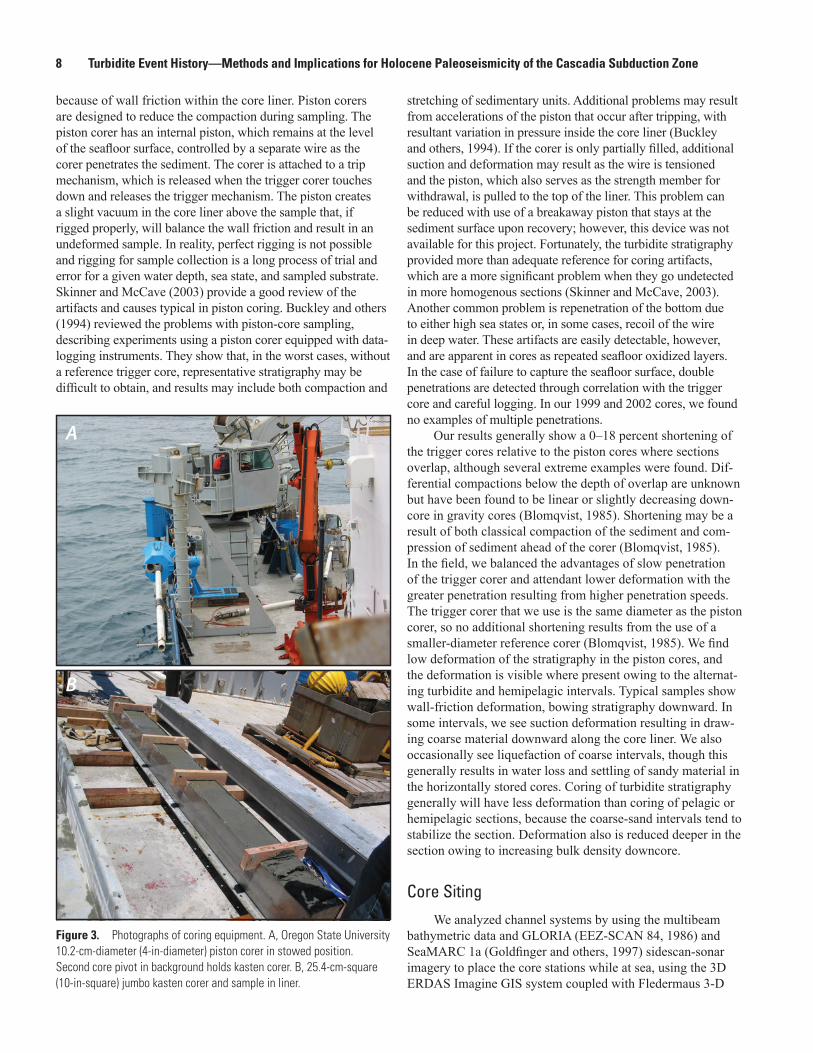
gin during two coring cruises—the 1999 R/V Melville cruise (prefix M9907) and the 2002 R/V Roger Revelle cruise (prefix RR0207). One additional core collected in 2009 at Rogue Apron also was used. During both cruises, we employed the Oregon State University (OSU) 10.16-cm-diameter (4-in-diameter) piston/trigger combination coring gear. During the 1999 R/V Melville cruise, we collected 44 piston cores of 6–8 m length (fig. 3A), 44 companion trigger cores of ~2–3 m length, and 8 box cores (50 x 50 x ~50 cm). Core locations are shown in figure 2 and listed in table 1. During the 2002 R/V Roger Revelle cruise, we collected an additional two pairs of piston and trigger cores from Hydrate Ridge (west basin), as well as two jumbo 25-cm2 kasten core, 3 m in length, from Hydrate Ridge (west basin) and Rogue Apron. This larger corer was designed specifically for capturing large sample volumes needed for radiocarbon dating of the latest Holocene and to minimize coring disturbance (Skinner and McCave, 2003; fig. 3B). These cores were excellent in both respects, although somewhat difficult to predict in terms of weight required for good penetration.
The box corers collected samples of 0.045 m2 and 0.35 m2 and typically recovered 20–50 cm of material of excel-lent quality, penetrating the youngest one to two turbidites. These cores were excavated to reveal stratigraphic details and were subsampled with 10.16-cm-diameter liners by push-ing the tubes vertically into the sample while still in the box liner. These subsamples were treated as other cores and were split, logged, and scanned for physical properties by using the Geotek core-logging system; they are further described in a subsequent section.
The OSU piston corer has a variable weight stand that allows the total weight of the system to be varied between ~1,000 and 2,200 kg. This system normally could penetrate the entire Holocene and latest Pleistocene sections with minimal to modest disturbance of the stratigraphy. The large-diameter corers reduce deformation relative to smaller-diameter systems. The trigger cores are gravity cores that touch down gently on the bottom and trigger the free-falling piston corer. The trigger core also acts as a reference core to compare to the piston core, which may be distorted under some circumstances and which may lose parts of the uppermost section owing to the shock-wave of water pressure ahead of the free-falling piston corer. The piston core and trigger core are ~1 m apart.
The piston corer penetrates to a greater depth, using a variable weight as much as 2,200 kg, depending on the sediment conditions. Gravity cores generally are compacted
Table 1. Core locations and depths, Cascadia subduction zone. [Cascadia (M9907; R/V Melville, 1999) and San Andreas (RR0207; R/V Roger Revelle, 2002) paleoseismicity cruises, Chris Goldfinger, Chief Scientist]
Core locations and depths
Core ID Latitude LongitudeWater depth
(m)M9907-01PC 45° 58.7311′ 125° 16.9806′ 1,763M9907-02PC 45° 57.9970′ 125° 17.0887′ 1,869M9907-03PC 45° 58.4975′ 125° 16.7471′ 1,818M9907-04BC 45° 58.5030′ 125° 16.7510′ 1,813M9907-05PC 47° 37.6461′ 126° 20.5062' 2,376M9907-06PC 48° 06.9613′ 126° 36.2189′ 2,528M9907-07PC 48° 06.2781′ 126° 35.5844′ 2,505M9907-08PC 48° 14.1040′ 126° 42.7710′ 2,552M9907-09PC 48° 14.3960′ 126° 43.3260′ 2,546M9907-10PC 47° 29.5895′ 125° 54.1828′ 1,471M9907-11PC 46° 46.3720′ 126° 04.8670′ 2,658M9907-12PC 46° 46.3783′ 126° 04.8664′ 2,665M9907-13PC 46° 25.9809′ 125° 23.9758′ 2,255M9907-14PC 46° 15.1301′ 125° 56.9189′ 2,680M9907-15PC 46° 15.1336′ 125° 56.9103′ 2,677M9907-16PC 45° 44.6588′ 125° 39.8950′ 2,323M9907-17PC 45° 30.6990′ 125° 44.9740′ 2,495M9907-18PC 45° 27.5088′ 125° 44.7039′ 2,547M9907-19PC 45° 26.1037′ 125° 52.6140′ 2,567M9907-20PC 45° 22.7817′ 125° 43.5268′ 2,622M9907-21PC 45° 22.9150′ 126° 00.9100′ 2,587M9907-22PC 44° 09.6000′ 127° 11.4970′ 3,208M9907-23PC 44° 09.6023′ 127° 11.4970′ 3,211M9907-24BC 44° 09.6023′ 127° 11.4970′ 3,211M9907-25PC 44° 14.7330′ 127° 11.4135′ 3,205M9907-26PC 44° 06.7783′ 125° 50.1230′ 3,043M9907-27PC 44° 00.8664′ 125° 33.0034′ 3,054M9907-28PC 44° 05.4180′ 125° 47.7750′ 3,029M9907-29PC 43° 58.2280′ 125° 23.5679′ 2,858M9907-30PC 42° 25.1685′ 125° 13.1174′ 3,112M9907-31PC 42° 24.5932′ 125° 11.9863′ 3,107M9907-32BC 42° 24.5916′ 125° 11.9888′ 3,106M9907-33PC 41° 44.7292′ 125° 11.6328′ 3,093M9907-34PC 41° 29.5977′ 125° 12.3887′ 3,118M9907-35PC 41° 05.2309′ 125° 01.1744′ 3,045M9907-36PC 41° 05.2304′ 125° 01.1762′ 3,050M9907-37PC 41° 05.0843′ 125° 00.9514′ 3,049M9907-38BC 41° 05.2302′ 125° 01.1756′ 3,054M9907-39PC 40° 37.8544′ 124° 50.8182′ 2,656M9907-40PC 40° 37.3101′ 124° 54.1751′ 2,675M9907-41PC 40° 44.5927′ 125° 23.1285′ 2,940M9907-42PC 40° 45.0467′ 125° 24.2605′ 2,957M9907-43BC 40° 45.0460′ 125° 24.2560′ 2,934M9907-44PC 40° 31.0422′ 126° 58.1289′ 3,221M9907-45PC 40°.31.0404′ 126° 58.1233′ 3,224M9907-46BC 40° 24.9407′ 125° 12.4901′ 2,578M9907-47PC 40° 25.3191′ 125° 15.8993′ 2,620M9907-48PC 39° 05.7553′ 124° 33.6661′ 3,373M9907-49PC 39° 09.2943′ 124° 36.8141′ 3,332M9907-50BC 39° 09.2912′ 124° 36.8135′ 3,330M9907-51PC 40° 25.3167′ 125° 15.8993′ 2,621M9907-52BC 40° 25.3170′ 125° 15.9000′ 2,617RR0207-02PC 44° 38.6806′ 125° 15.0006′ 2,311RR0207-56PC 44° 38.6600′ 125° 15.8100′ 2,250RR0207-01KC 44° 40.0239′ 125° 17.0616′ 2,110RR0207-55KC 42° 25.16900′ 126° 13.1200′ 3,090
8 Turbidite Event History—Methods and Implications for Holocene Paleoseismicity of the Cascadia Subduction Zone
Figure 3. Photographs of coring equipment. A, Oregon State University 10.2-cm-diameter (4-in-diameter) piston corer in stowed position. Second core pivot in background holds kasten corer. B, 25.4-cm-square (10-in-square) jumbo kasten corer and sample in liner.
because of wall friction within the core liner. Piston corers are designed to reduce the compaction during sampling. The piston corer has an internal piston, which remains at the level of the seafloor surface, controlled by a separate wire as the corer penetrates the sediment. The corer is attached to a trip mechanism, which is released when the trigger corer touches down and releases the trigger mechanism. The piston creates a slight vacuum in the core liner above the sample that, if rigged properly, will balance the wall friction and result in an undeformed sample. In reality, perfect rigging is not possible and rigging for sample collection is a long process of trial and error for a given water depth, sea state, and sampled substrate. Skinner and McCave (2003) provide a good review of the artifacts and causes typical in piston coring. Buckley and others (1994) reviewed the problems with piston-core sampling, describing experiments using a piston corer equipped with data-logging instruments. They show that, in the worst cases, without a reference trigger core, representative stratigraphy may be difficult to obtain, and results may include both compaction and
stretching of sedimentary units. Additional problems may result from accelerations of the piston that occur after tripping, with resultant variation in pressure inside the core liner (Buckley and others, 1994). If the corer is only partially filled, additional suction and deformation may result as the wire is tensioned and the piston, which also serves as the strength member for withdrawal, is pulled to the top of the liner. This problem can be reduced with use of a breakaway piston that stays at the sediment surface upon recovery; however, this device was not available for this project. Fortunately, the turbidite stratigraphy provided more than adequate reference for coring artifacts, which are a more significant problem when they go undetected in more homogenous sections (Skinner and McCave, 2003). Another common problem is repenetration of the bottom due to either high sea states or, in some cases, recoil of the wire in deep water. These artifacts are easily detectable, however, and are apparent in cores as repeated seafloor oxidized layers. In the case of failure to capture the seafloor surface, double penetrations are detected through correlation with the trigger core and careful logging. In our 1999 and 2002 cores, we found no examples of multiple penetrations.
Our results generally show a 0–18 percent shortening of the trigger cores relative to the piston cores where sections overlap, although several extreme examples were found. Dif-ferential compactions below the depth of overlap are unknown but have been found to be linear or slightly decreasing down-core in gravity cores (Blomqvist, 1985). Shortening may be a result of both classical compaction of the sediment and com-pression of sediment ahead of the corer (Blomqvist, 1985). In the field, we balanced the advantages of slow penetration of the trigger corer and attendant lower deformation with the greater penetration resulting from higher penetration speeds. The trigger corer that we use is the same diameter as the piston corer, so no additional shortening results from the use of a smaller-diameter reference corer (Blomqvist, 1985). We find low deformation of the stratigraphy in the piston cores, and the deformation is visible where present owing to the alternat-ing turbidite and hemipelagic intervals. Typical samples show wall-friction deformation, bowing stratigraphy downward. In some intervals, we see suction deformation resulting in draw-ing coarse material downward along the core liner. We also occasionally see liquefaction of coarse intervals, though this generally results in water loss and settling of sandy material in the horizontally stored cores. Coring of turbidite stratigraphy generally will have less deformation than coring of pelagic or hemipelagic sections, because the coarse-sand intervals tend to stabilize the section. Deformation also is reduced deeper in the section owing to increasing bulk density downcore.
Core SitingWe analyzed channel systems by using the multibeam
bathymetric data and GLORIA (EEZ-SCAN 84, 1986) and SeaMARC 1a (Goldfinger and others, 1997) sidescan-sonar imagery to place the core stations while at sea, using the 3D ERDAS Imagine GIS system coupled with Fledermaus 3-D
A
B

Introduction 9
visualization software. Together, these systems enabled us to “fly through” the site data and visualize backscatter data draped over shaded-relief bathymetry to locate core sites pre-cisely. This technique, coupled with P-code GPS and dynamic positioning, allowed us to pinpoint cores on the Cascadia mar-gin to within tens of meters in areas that were surveyed only hours before. Continuous 3.5 kHz subbottom profiling was done using a Knudsen 320 B/R series chirp system and was recorded digitally in SEG-y format. The 3.5 kHz profiles were invaluable in refining site selections based on the reflectivity of Holocene turbidite sequences, and feedback from coring helped refine the optimum reflection profile to target. Naviga-tion for all core locations and multibeam and 3.5 kHz data was based on P-code GPS, with nominal 2-D root-mean-square (rms; ~95%) error circles of 12 m or better. Dynamic position-ing of the vessel allowed for precise core siting within a few meters or better of the selected site. Older data were navigated with a variety of technologies. GLORIA was navigated with LORAN C, with a 95-percent accuracy of 0.25 NM given good estimation of local offset (Culbertson and Roeber, 1975). Archive cores collected by OSU in the 1960s were navigated using LORAN A, with accuracy ranging from 1 to 5 nautical mile (NM) depending on weather, distance from stations, and other factors (Culbertson and Roeber, 1975). Older datasets were registered to newer, better navigated data using common control points in the GIS.
Core sites were chosen to take advantage of known depositional segments of channels versus nondepositional or erosional segments. Analysis of these data proved essential to successfully capturing the turbidite-event record while avoid-ing difficulties, such as channel-gravel lag and erosive effects, that can complicate and bias the record. Proximal sites, for example, required avoidance of amalgamated gravel deposits and associated erosion, whereas distal sites required seeking depositional pools and channel segments likely to decelerate currents to capture fine sands and silts and, thus, a complete and expanded record (fig. 4).
ASTORIA CANYON
point bar
Thalweg
0
0 5 Miles
5 Kilometers
M990704BC
Figure 4. Image showing 100-m-resolution shaded swath bathymetry of a portion of Astoria Canyon, northern Oregon, Cascadia subduction zone. Siting of turbidite cores at sea is facilitated by using three-dimensional visualization of canyon/channel morphology. To obtain the most complete turbidite record in proximal settings, we avoided erosive channel thalwegs and coarse-grained frontal point bars. We found nonerosive complete records in the lee of point bars and on terrace risers, such as this site for core M9907-04BC.
Forty-six piston-trigger core pairs, two kasten cores, and eight box cores were collected in every major and many minor canyon/channel systems from Barkley Canyon near the north-ern limit of the Cascadia subduction zone to Cape Mendocino at its southern terminus. These systems include (from north to south) Barkley, Juan de Fuca, and Willapa Channels; Astoria Fan; Astoria Canyon; Astoria Channel; Rogue Apron; and Smith, Klamath, Trinidad, Eel, and Mendocino canyon/chan-nel systems (fig. 2). We also collected cores in Hydrate Ridge (west basin) off central Oregon and an unnamed midslope basin off Washington (fig. 2).
Stratigraphic Correlation
Lithostratigraphic CorrelationWe carried out analysis of the physical properties of the
cores to establish detailed lithologic and geophysical stratig-raphy in greater detail than is available through visual core logging. Stratigraphic correlation between sites is the founda-tion of land-based paleoseismology (for example, Scharer and others, 2007), and we use it similarly among cores at given sites. This approach has allowed us to identify characteristic stratigraphic “fingerprints” for turbidite sequences that are a result of the grain-size distribution of individual events and the sequences of events. The stratigraphic signatures extend beyond individual sites, allowing stratigraphic correlation over considerable distances.
While at sea, all cores were scanned using a GEOTEK multisensor core logger (MSCL), collecting P-wave velocity, gamma-ray density, and loop-sensor magnetic-susceptibility (MS) data from the unsplit cores. Calibration of the MSCL was carried out using an aluminum and water standard. Cores were then split for visual description and to collect high-reso-lution line-scan imagery. Subsequently, high-resolution point MS data were collected from each core using a point sensor (Bartington MS2E high-resolution surface sensor) at 1-cm

10 Turbidite Event History—Methods and Implications for Holocene Paleoseismicity of the Cascadia Subduction Zone
intervals and were imaged with X-radiography (for example, figs. 5–8). Later analyses included higher resolution MS, at 5-mm intervals for selected cores, and collection of Computed Tomography (CT) data from the cores. CT volume density data were acquired using a Toshiba Aquillon 64 slice system with 3-D voxel resolution of 0.35 mm. We also employed an enhanced resolution MS method for a few cores with weak turbidite intervals. This method consisted of zeroing the magnetic susceptibility meter on a hemipelagic sediment standard, rather than in air, resulting in greater dynamic range. Selected grain-size analyses were done with the laser diffrac-tion method using a Beckman-Coulter LS13-320 laser counter (Blott and Pye, 2006). We primarily use MS and density as grain-size proxies and for stratigraphic correlation. P-wave velocity also is useful; however, the data typically contain artifacts from air in the core liner and from poor contact with the liner, making the data noisy and less useful. We also found the P-wave data to be more strongly influenced by air gaps and coring artifacts that resulted from slanted or distorted strata, reducing the fit of these data to the observed stratigra-phy (fig. 5). An additional problem with velocity data is that they can be strongly affected by core compaction and exten-sion owing to the coring process. Density and magnetic data are locally much less affected by many of these problems. For this reason, our use of velocity data was limited to single events, where it was apparent that these effects were minimal by comparison to other data and visual inspection. See figures 5 and 7 for examples including the P-wave data. Additionally, we logged MS at a higher resolution using a Bartington MS2 system, using the narrow MS2E sensor (3.8-mm width). These samples were at intervals ranging from 3 mm to 2 cm and varied according to the local sedimentation rate.
Sediment color-variability measurements were extracted from the high-resolution line-scan imagery and offered a high-resolution measure of compositional variability to support visual and magnetic and density measurements. X-radiography and CT were used to examine detailed stratigraphic relations and to test individual events for basal erosion and were found to correlate well with the other physical-property measure-ments (fig. 7). In many cases, the X-ray and CT imagery revealed internal details of the turbidites and could sometimes be used to differentiate two turbidites that are closely spaced from two coarse pulses within a single turbidite.
Physical-property data does an excellent job of represent-ing properties of the sedimentary units within the core (for example, Weber and others, 1997). Initially, the combined geophysical data were used to correlate stratigraphy between cores at single sites, which typically have four to six cores. This technique makes use of the trigger cores (collected 1 m away from the companion piston cores) and helps identify missing upper sections, an occasional problem with pis-ton cores. Correlating among the local group of cores also captures much of the variability at each site. The correlation was done primarily using MS and gamma density (Weber and others, 1997; Wetzel and Balson, 1992), similar to e-log correlation in the oil industry (McCubbin, 1982; Lovlie and
Van Veen, 1995). We plot the physical-property data in some of the figures with variable vertical scales to align the turbi-dites horizontally for visual inspection (Thompson and others, 1975). Physical-property correlations of this type also are common practice with academic and ODP/IODP cores (for example, Fukuma, 1998) and have recently come into use for paleoseismology (Karlin and others, 2004; Abdeldayem and others, 2004; St-Onge and others, 2004; Hagstrum and others, 2004; Iwaki and others, 2004; Schnellmann and others, 2002). Individual event signatures at a given site are established by multiple cores at each site: a minimum of four cores and as many as seven in some cases. This reduces the possibility of correlating an unrepresentative example of a given event. Gamma density and MS data are collected on horizontal and vertical axes, respectively, relative to a half-round core on the scanner track. This yields a good cross-check that signatures of a given interval are not the result of local 3-D effects within the core. In some cases, such 3-D effects result in mismatching density and MS logs.
In addition to local site correlations, we have found that it is possible to correlate unique physical-property signatures of individual turbidites between distant sites (fig. 8). This correla-tion suggests that the processes controlling deposition of the turbidite maintain consistency for some considerable distance within a channel. We also have found it possible to correlate event signatures, not only down individual channels and past confluences, but between channel systems separated by con-siderable distance, some of which never meet. These turbidite fingerprints form the basis of along-strike correlations, closely supported by 14C dates. Such stratigraphic correlations are beginning to be recognized and used for regional correlation in a variety of settings, including Lake Baikal (Lees and oth-ers, 1998), off Morocco (Wynn and others, 2002), Cascadia and northern California (Goldfinger and others, 2007a, 2008), Sumatra (Patton and others, 2010), and the Laptev Sea, Rus-sian Arctic (Rivera and others, 2006). Recently, the event sig-natures of Cascadia turbidites have been linked to coastal fjord records on Vancouver Island (Dallimore and others, 2005b, 2008; Goldfinger and others, 2006).
Figures 5–8 show several representative turbidites, illustrating the multiple fining-upward sequences (Bouma A–C) that compose each turbidite. Typically, these sequences have only one fine tail (Bouma D) associated with waning of the turbidity current. The signatures we are correlating are composed of these stacked coarse pulses. These figures show in detail that the MS, density, and grain-size trends within each event are closely correlated. This relation is straightforward but important, because we can, in most cases, use the high-resolution density and magnetic data as grain-size proxies, at least for lithologies along the Cascadia and northern San Andreas Fault systems and other localities where this rela-tion can be established (Goldfinger and others, 2003a, 2007a, 2008; Wynn and Masson, 2003). In detail, the MS signal is associated with terrestrial, silt-sized magnetic minerals, but often we see sand at the turbidite base. The sand may be nonmagnetic quartz grains, so the MS peak does not always

Introduction 11
-10
-20
-30
-40
-50
-60
-70
-80
-90
-100
-110
-120
-130
-140
-150
-160
-0
0 2001,4501,650
1.02.0 0 80
Silt
Sand
Very fine sand
Very fine sand/silt
Hemipelagic clay
Turbidite silty mud
Burrows
EXPLANATION
LITHOLOGY
Density (g/cm3)
Magnetic susceptibility (SI units)
P-wave velocity (m/s)
M9907-25PC
H
T1
T2
T3
density (g/cm)
high-resolution magnetic susceptibility (SI units)
low-resolution magnetic susceptibility (SI units)
core break/end cap artifact
core break/end cap artifact
p-wave velocity (m/s)
H
H
H
Figure 5. Example of typical turbidite stratigraphy from Cascadia Basin, showing events T1–T3 in core M9907-25PC in Cascadia Channel. Magnetic susceptibility, gamma density, and P-wave velocity are shown to illustrate the response of these parameters to the turbidites, hemipelagic intervals, and bioturbation. Hemipelagic sediment in this core is very light in color, making stratigraphic relations clear. Grain-size analysis and mineralogy are not ideal for discriminating the turbidite tail-hemipelagic boundary owing to low resolution and bioturbation. The limits of bioturbation and the tail-hemipelagic boundary commonly can be observed in the physical property data, but these typical events illustrate that definition of these boundaries can be problematic. Abbreviations: g/cm3, grams per cubic centimeter; m/s, meters per second; SI, Systeme Internationale.

12 Turbidite Event History—Methods and Implications for Holocene Paleoseismicity of the Cascadia Subduction Zone
multiple�ning-upwardcoarse subunits
intereventhemipelagic
bioturbation
underlyingturbiditetail
M9907-25TC
�ningupwardtail
200 cm
210 cm
220 cm
190 cm
180 cm
Low-resolution magneticsusceptibility (SI units)
Density (g/cm3)
P-wave velocity (m/s)
2.0 1.5 1.0
preferred 14C sampleinterval
Low-resolution magnetic susceptibility (SI units)
P-wave velocity (m/s)
Density (g/cm3)
1,4501,650
10 50
EXPLANATION
Figure 6. Photograph showing detail from core M9907-25TC event T4, Cascadia subduction zone (see fig. 2 for location). Turbidite tail/hemipelagic boundary commonly is distinct visually and variably disturbed by bioturbation. Because turbidite bases can be erosive, planktic foraminifers were used to date the upper hemipelagic boundary as the least problematic option. A typical sample location is shown, with a small gap above the sample. Erosion was evaluated visually in the cores by comparison to hemipelagic thickness in nonchannel cores and by intersite comparisons between multiple cores. P-wave velocity and low-resolution loop magnetic susceptibility shown in this figure were not as instructive as density and high-resolution magnetics for revealing detailed turbidite structure (see fig. 7 for comparison.) Abbreviations: g/cm3, grams per cubic centimeter; m/s, meters per second; SI, Systeme Internationale.
precisely correlate with a maximum of grain size. In thick turbidite beds, separation of grains according to specific grav-ity (or mineral density) can dominate, resulting in fine-silt heavy-mineral lamina below medium quartz silt or sand. Edge effect and biasing of the measurements, even at 5-mm spacing, further alters the geophysical signatures. We find, however, that the proxy approximation is reasonable in most cases (for example, Stupavsky and others, 1976; King and others, 1982). Using density, MS, and CT together reduces this problem, and the differences are not typically critical to observing a rec-ognizable fingerprint for many turbidites. These fingerprints represent detailed depositional characteristics of each turbidite.
On close inspection of physical-property logs, we some-times see a remarkable similarity between correlative turbi-dites that are separated by as much as 500 km in Cascadia and 280 km in the northern San Andreas Fault. Figure 8 shows several typical examples of correlative events in detail along strike over a distance of 480 km. We see a general correspon-dence of relative turbidite size downcore that is reflected in separate channels, as well as correlatable details, such as the number of coarse sandy pulses (density and magnetic peaks) per event. For example, Cascadia turbidite events T10 and T12 are small single-pulse events in all cores; T11 and T16 are large events in all cores. Not only do individual size comparisons hold across several channel systems, but verti-cal sequences comprise trends that also extend across chan-nel systems. We observe similar patterns along the northern
San Andreas Fault margin, where size trends and individual characteristics persist over large distances (Goldfinger and others, 2007a, 2008). We use these characteristics to establish correlations between channels through both visual correlation and numerical tests. The visual correlation method typically involves testing potential sequence matches between sites by using the magnetic- and density-data traces used as grain-size proxies, as described above. As sedimentation rates vary, we pin the vertical scales to one site and allow the others to extend or compress as needed to match the event bases in the reference core (fig. 8 and subsequent correlation figures). This allows for sedimentation-rate differences between sites, changes in the proportion of tail material per event, and basal erosion, which is evident in some intervals. The correlation tests are constrained by 14C dates and the Mazama ash datum, supported by RGB color data, P-wave velocity data, and CT and X-ray imagery. Together, these factors limit the possible correlation matches significantly and allow for rigorous test-ing of stratigraphic correlation. In addition, three methods of numerical testing of potential correlations are used.
Numerical Signal Correlation Two classical approaches are commonly used in strati-
graphic correlation; visual correlation and signal correlation of quantifiable parameters. The simplest approach is visual, using corresponding remarkable features of both cores (for example,

Introduction 13
H?
1.21.6 1.4 0 200
EventT6
H
H
EventT3
M9907-12PC M9907-25PC
0 150
60
70
80
90
100
110
120
130
90
8010 50 20 100
A B
1,0681,650 1,4501,650
1.22.0
H
LITHOLOGYEXPLANATION
Hemipelagic clay
Turbidite silty mud Sand
Very �ne sand
Silt Mottled clay
BurrowsP-wave velocity (m/s)Gamma density (g/cm3)Magnetic susceptibility (SI units)Mean grain size (µm)
P-wave velocity (m/s)P-wave velocity (m/s) Mean grain size (µm) Mean grain size (µm)
Gamma density (g/cm3) Magnetic susceptibility (SI units)Gamma density (g/cm3) Magnetic susceptibility (SI units)
bioturbation
coringartifact
Figure 7. Detailed stratigraphic diagrams showing examples of physical property traces versus grain size. A, Event T6 in Juan de Fuca Channel, showing a typical proximal event. Note similarities and differences between density, magnetic susceptibility, and grain-size plots. B, Event T3 in Cascadia Channel, showing typical distal event, with generally closer correspondence between grain-size and physical-property plots. X-ray, lithologic logs, and density and magnetic traces show both of these typical events to be composed of three fining-upward sequences. The lower two sequences are truncated by the overlying ones. Grain-size determinations are shown (Coulter laser counter method, 1-cm interval), showing correlated relation between grain size, density, and magnetic susceptibility. No hemipelagic sediment exists between coarse subunits, indicating the three coarse subunits were deposited in a short time during a single current (a coring artifact may exist between upper and middle subunits in A). Only the last subunit has a fine tail, indicating final waning of the turbidity current. We interpret these signatures as resulting from a single multipulse turbidity current. P-wave velocity traces shown in A and B typically are nondiagnostic of grain size for these lithologies. Abbreviations: g/cm3, grams per cubic centimeter; m/s, meters per second; μm, micrometers; SI, Systeme Internationale.
Prell and others, 1986). Although its simplicity is appealing, this method may give subjective results and may be arbitrary. The second method uses a mathematical measure of the similarity between both signals—for example, a correlation coefficient—and then optimizes this measure when adjusting the age-depth relation (Martinson and others, 1987). This procedure gives a more objective result, but the fit is not always as good as that with the simple visual correlation. A mathematical measure, such as a correlation coefficient, will give more weight to the large-timescale signal fluctuations (low-frequency variations), whereas much of the variance is in the higher frequencies. With this method, the sharp events are not exactly in phase, as they should be according to the underlying simultaneity hypothesis. This second approach is, therefore, more objective but is often less precise and lacking in geological judgment.
Because we had good results from stratigraphic cor-relation, indicating a genetic link between widely separated turbidites, we also tested numerical correlation of the physical-property traces by using simple correlation of individual events and more sophisticated correlation of series of events. The correlation of single events was done by calculating a Pearson correlation (parametric) and Spearman rank (non-parametric) coefficient between events at multiple sites. The Pearson coefficient is a measure of the relation of two vari-ables (in this case two sites) obtained by dividing the covari-ance of the two variables by the product of their standard deviations (Cohen, 1988). The Spearman rank coefficient is a measure of how one series varies relative to the other. The Spearman rank is a more restrictive variant of the Pearson that does not require normal distribution of the variables (nonpara-metric). The distribution of grain size within all the turbidites

14 Turbidite Event History—Methods and Implications for Holocene Paleoseismicity of the Cascadia Subduction Zone
H
Density (g/cm3)
Radiocarbon sample location
EXPLANATION LITHOLOGY
H
Core break
Correlation lines, dashed if uncertain
High-resolution point magnetics
Sample # AMS 14C age and 2σ range
Reversed AMS 14C age and 2σ range
CASC 11: 7,290 (7,220–7,380)
Holocene/Pleistocene boundary
Oldest Mazama ash bearing turbidite
Hemipelagic age and estimated 2σ range
Erosion corrected AMS 14C age and 2σ range
Hemipelagic clay
Turbidite silty mud
Sand
Silt
Mottled clay
Burrows
Pleistocene
Very �ne sand
Shell
Wood fragment
Hemipelagicbasal boundary
CASC 11: 7,290 (7,220–7,380)
H/P
7,290 (7,220–7,380)
CASC 11: 7,290 (7,220–7,380)
CASC 107, 2324,140 (4,000–4,290)
CASC 4, 1167,100
(7,000–7,210)
CASC 110, 117 7,580
(7,470–7,690)CASC 109, 234, 1145,760 (5,640–5,830)
CASC 108,113 4,760 (4,630–4890)
A
1.31.6
Juan de Fuca11/12PC
0 100
Cascadia23/25PC
-10 400 1.31.7 -10 400
BJuan de Fuca
11/12PCRogue31PC
10001.21.61.21.7
4.0
5.0
4.0
notcorrelated
CASC 108,113 4,760
CASC 109, 234, 1145,760 (5,640–5,830)
(4,630–4,890)
2.0
1.52.0
H
H
H
H
H
H
H
H
H
H
H
H
H
H
H
H
H
T11
T8
T9
T10
T11
T12
T13
T14
T10 T10f
CASC 131 3,490
(3,310–3,660)
CASC 1324,160
(3,980–4340)
CASC 115 6,440
(6,280–6,570)
CASC 32, 7,100(6,980–7,260)
CASC 9, 7,670(7,530–7,820)
CASC 47 3,500 (3,340–3,680)
6,000(5,870–6,120)
5,850(5,700–5,990)
6,900(6,780–7,030)
T12a
6,630(6,440–6,810)
6,090(5,910–6,290)
5,790(5,630–5,934)
5,790(5,630–5,934)
4,740(4,560–4,930)
Depth(m)
Depth(m)
Depth(m)
Depth(m)
Figure 8. Diagrams showing correlation details from two representative pairs of cores on the Cascadia margin. Lithologic logs are shown: left traces along each log are raw gamma density (g/cm3); right traces are magnetic susceptibility (SI units). Note correspondence of size, spacing, number of peaks, and trends of physical-property traces between cores. A, Events T8–T11 in cores from Juan de Fuca Channel (left) and Cascadia Channel (right). Cores in A are part of the same channel system; distance along channel is 475 km. B, Events T10–T14 in Juan de Fuca Channel (left) and in Rogue Channel (right). Cores in B are in channels that do not meet; separation distance is 500 km. Note that correlation of longer sections and 14C data show that T10f and T10 do not correlate in B. Similarly, Mazama ash appears in T14, but not in T13 in Rogue apron. See text for discussion. 14C ages in cal yr B.P., including 2s-error ranges. Abbreviations: AMS, accelerated mass spectrometry; g/cm3, gram per cubic centimeter; m, meter; SI, Systeme Internationale.

Introduction 15
is not known well enough to determine whether parametric or nonparametric techniques are most appropriate.
We applied these methods to a series of turbidites at different sites, both as individual events and as series. For individual events, we used MS as a grain-size proxy (see above) and compared the variability within individual events and across sites. We also applied the same techniques to numerical series extracted from the entire Holocene sequence. For example, turbidite mass, number of sandy pulses in each event, and other characteristics can be extracted as series and compared between sites to test the overall series correlation.
We tested the use of least-squares search for optimal fit of stratigraphic sections represented by multiparameter physical-property data. This method compares multiple fits and seeks those that minimize the difference between the tested pairs of traces. We used multiparameter (gamma density and MS as grain-size proxies) correlations using the Vector Transfer code as described in Hofmann and others (2005). This method allows pure signal correlation or allows input of key tie points, such as known stratigraphic ties and recomputation of best fit and a transfer function based on the constrained dataset. One can examine the transfer function to see where the most distortion of one record was needed to match the others. Multiple parameters and multiple cores can be fitted; we used P-wave amplitude, travel time, gamma density, and MS, although, in practice, the velocity parameters proved unreliable in terms of data quality. This method closely mimics the process of visual correlation, adjusting the vertical scale of one core iteratively to match a reference core and minimizing the distance between superimposed traces, given known tie points. This method cannot replace the geologic knowledge of a good stratigrapher; however, such information can be included in limited ways, for example, by setting tie points to account for known core artifacts that throw off the algorithm. These numerical methods are purely signal-processing methods and have in common the disassociation of the signal trends from the absolute value of the data, as do visual and other methods. Correlation by such methods does not verify causality but, even without knowledge of causality, it can indicate significant relations. Possible explanations for the correlation signatures are discussed in a subsequent section.
Age Control
Radiocarbon DatesTo date the turbidites, we extracted the calcium carbonate
shells of planktic foraminifers preserved in the hemipelagic sediment below each turbidite (fig. 6). We sampled below each turbidite, because the boundary between the top of the turbidite tail and the hemipelagic sediment is difficult to identify reliably and because bioturbation is concentrated at this boundary, possibly because the organic material brought down in the turbidite tail results in a benthic bloom (figs. 5–7; Thomson and others, 1988; Smith and others, 1993). Sediment
samples were removed from the cores while avoiding the 1 cm of material nearest the core walls to avoid visible or undetected deformation and friction drag along the core walls. In some cases, highly irregular bases resulted in sampling an interval below the basal irregularities and applying a correction to the hemipelagic thickness called “gap” (appendix 1). Hemipelagic sediment samples were freeze dried to separate clay particles to improve rinsing through a sieve, washed in a dilute calgon (sodium hexametaphosphate) solution to keep the fine particles in suspension, sieved through a 63-µm stainless steel sieve, and then dried in a warm oven. Typically 600–1,000 individual planktic foraminifers (depending on size/weight) were identified (estimated) to species level (data included in appendix 2) and then removed from this dried >63-µm-size fraction using a fine sable brush moistened with distilled water. Benthic foraminifers also were used in rare cases, as discussed below (run separately if a planktic sample was unavailable). Foraminiferal samples were dated using accelerator mass spectrometry (AMS) methods at the Lawrence Livermore Laboratory AMS facility with the assistance of Michaele Kashgarian. Some additional samples were analyzed at the Keck AMS facility at the University of California, Irvine, in collaboration with John Southon. Radiocarbon data are given in appendix 1.
The radiocarbon dates are reported with 1 standard deviation in lab error (Stuiver and Polach, 1977), and these values averaged ±42 radiocarbon years for the entire dataset. Lab errors were generally much lower from the U.C. Irvine lab, averaging ±20 radiocarbon years. Lab errors with radiocarbon dating are straightforward and based on counting statistics from the laboratory. All dates are calibrated (as described in the next section) and, in many cases, we made additional corrections to the raw and calibrated dates, including the reservoir correction, sediment sample thickness correction, and a correction for differential erosion in some cases. We also calculated dates based on hemipelagic thickness above and below undated turbidites, introducing observational error at that stage. For individual dates, we propagated these uncertainties using rms calculations using estimates of the uncertainties at each step. This calculation included the lab uncertainties and resulted in the final reported 2σ range for each radiocarbon age. The fully propagated 2σ-error ranges averaged +140/-170 calibrated years (calculations given in appendix 1). In later sections, we use marginwide-mean event ages to calculate various parameters. For these mean ages, we averaged the ages and again applied rms calculations to the averaged error ranges to produce the 2σ-rms ranges for each averaged age. These steps are included in appendix 1, so the reader may follow the error propagation.
To evaluate the effect of foraminifer shell size on the radiocarbon date from a single sample, we did a sensitivity test on a sample by dividing the foraminifers into large (>~350 µm) and small (<~350 µm) groups. The resulting dates were within 45 radiocarbon years of each other, suggesting foraminifer test size is most likely not a factor, although similar tests for all channel systems and latitudes are not

16 Turbidite Event History—Methods and Implications for Holocene Paleoseismicity of the Cascadia Subduction Zone
available. We rarely had enough sediment to do monospecific assemblage dating, which may be preferable. Sensitivity tests for species-specific biases are presented in Goldfinger and others (2007a). Faunal data were collected from planktic sample assemblages and are included in appendix 2. We expect some bias in sampling toward species that are physically larger owing to the large volume of samples to be processed and the ease with which large individuals brought the sample weight to the required minimum. The close match in dates between land and marine events observed in both Cascadia Basin and the northern San Andreas Fault suggests that, on the whole, neither bioturbation (Wheatcroft, 1992; Smith and others, 1993; Thomson and Weaver, 1994; Thomson and others, 1995) nor basal erosion significantly biases 14C dates derived from planktic foraminifers following this procedure. A small number of events were not dated or had reversed and (or) incongruous dates, likely owing to excessive erosion and (or) bioturbation.
Not all intervals were directly datable by this method. Because foraminifer abundance is much lower in the latest Holocene (in some cases, we found abundances as low as five individuals per cubic centimeter), samples representing times younger than ~2,000 cal yr B.P. were difficult to date. The total volume of material available was limited by the hemipelagic sediment deposited between turbidites, thus shorter recurrence intervals (in southern Cascadia) also reduced the chances of obtaining one or more successful 14C dates. In the age range of ~2,000–300 cal yr B.P., it was sometimes necessary to combine samples from piston and trigger cores and, rarely, from multiple localized pairs of piston and trigger cores to collect the required minimum of ~1.0 mg carbon (~600–1,000 specimens) for a successful date. In some cases, we collected multiple cores and a jumbo kasten or box core for this purpose in anticipation of dating difficulties. Mixing in this way requires perfect correlation between the local core sets. In the early phases of this study, when no age control was available, some early mixed samples were from miscorrelated cores, and these samples were either not run or not used in this report, although they are included in appendix 1.
In several rare cases, however, mixed but miscorrelated samples could be used when the intervals were off by only one event and enough supporting data allowed calculation of the dates of both events from the mixed sample. For example, if the carbon weights of both mixed samples were known and the age of one of the two events also was well known from other dating, the age of the second sample in the mixture could be calculated reliably. This was tested with several events where both dates were known, and it proved to be a successful strategy for obtaining an age when other methods were exhausted. The final dataset shown in our figures does not include these dates, which nevertheless served a useful purpose as a methods check.
In several cases in the Barkley, Rogue, Trinidad, Smith, and Klamath systems, we dated benthic foraminifers where planktic foraminifers were not abundant enough to obtain a result. These dates were calibrated using the additional reservoir difference between benthic and planktic samples
established locally for those cores for a given time range. This method is similar to that used to establish the modern reservoir value (for example, Hughen and others, 2004). Subsequent sections describe the reservoir issue in more detail.
Radiocarbon Date ReportingAll dates reported were calibrated using Calib 5.0.2
software unless otherwise noted (Stuiver and Reimer, 1993; Stuiver and others, 2005), using the calibration database of Reimer and others (2004) and the marine reservoir database of Hughen and others (2004). Dates are reported as calendar years before 1950, unless otherwise noted, and appear in the text as “cal yr B.P.” All previously published marine data used in this report were recalibrated using Calib 5.0.2, unless otherwise noted. No lab multipliers were applied to the data. Modern radiocarbon-dating laboratories generally report an uncertainty for each date. For example, 3,000±30 yr B.P. indicates a standard deviation of 30 radiocarbon years. Traditionally, this included only the statistical counting uncertainty. However, some laboratories supplied an error multiplier that could be multiplied by the uncertainty to account for other sources of error in the measuring process. More recently, laboratories try to quote the overall uncertainty, which is determined from control samples of known age and verified by international intercomparison exercises (Scott, 2003). The AMS dates, the calibrated 1σ and 2σ ranges, the reservoir correction applied to each sample, and the associated error ranges, as well as the lab number, sample weights, isotopic fractionation (δ13C), and other processing information, are presented in appendix 1.
Radiocarbon dates are calibrated to calendar years, which are convolved from the laboratory counting statistics of 14C from the sample and the calibration curve for the appropriate time for that sample (Bennett, 1994). Although the AMS results have an analytical error with a Gaussian distribution about the mean, calibrated dates are represented by a probability density function (PDF) with irregular shape based on the irregularities in 14C production in the atmosphere, uncertainties in the data used to create the curve, and other factors (Christen, 1994). This density function is known as a posterior function that represents the probabilities implied by factors that make up the prior set of information (which may include other factors in addition to the 14C age and calibration curve). The probability-density functions (PDFs) may be simple to interpret in terms of the peak, mode, or median probability and ranges when the probability peaks and the mean and median of the 2σ range are nearly coincident, which is a common occurrence in our data. Some PDFs, however, show multimode peaks of probability, making it more difficult to interpret the age of a dated event. A single point age may be prohibited by the data in the case of multimode peaks, where large probability areas under the density function are widely separated, which is fortunately a rare occurrence limited largely to plateaus of the calibration curve. The issue of multimode peaks is more prevalent in land data using the

Introduction 17
atmospheric curves, whereas the marine-calibration curve is smoothed by using an oceanographic-circulation model that effectively smooths the entire curve.
Despite these caveats, it is useful to summarize dates as a single value with appropriate error ranges for some purposes. There is no precise consensus on how to handle dates with multimode peaks or the more general case of how to represent the PDF when age estimates are required for a dated event. For example, reporting the 2σ range of the PDF is a conservative approach, however the calculation of recurrence intervals and probabilities for earthquakes does not lend itself well to the use of ranges.
The peak probability of the PDF is by definition the maximum likelihood point age for a calibrated radiocarbon age (Telford and others, 2004). The peak can be considered the most likely age of the event of interest in an ideal case (Buck and others, 2003; Telford and others, 2004; Goslar and others, 2005) and would be a straightforward way to represent a calibrated age as a point age with an error range, as raw 14C dates are reported (Stuiver and Polach, 1977). In many cases, however, simply choosing the peak age from the PDF is unwarranted and, in the case of multimode peaks, problematic and (or) misleading (Buck and others, 2003). Nevertheless, the probability distribution is significant, and the conservative use of ranges alone may represent a considerable loss of information about the age of an event.
We present both the ranges and a preferred single age for each event, which are used throughout this report and given for all 14C dates in appendix 1. For use in calculations that require averaging of event dates and calculation of recurrence intervals, probabilities, hemipelagic dates, and so forth, we also use a point-age estimate derived from the PDF. Goslar and others (2005) and Goldfinger and others (2007a) show the strong tendency for the probability peaks to lie along the age-model sedimentation rate. Goslar and others (2005) and Walanus (2008) make the case for using the simplest possible sedimentation-rate curve and the rates to assist in resolving ambiguities in the multimodal peaks of radiocarbon dates in difficult parts of the calibration curve. In the marine environment, deep-water pelagic sedimentation rates are relatively constant (discussed further in a subsequent section), and this property can be used to constrain problematic 14C dates. Walanus (2008) makes the general case that the multimode ambiguity can be reduced or resolved by constraining the dates based on fitting a simple sedimentation rate curve to them. Parts of the PDF that require rapid changes in sedimentation rate are not preferred, whereas those that are consistent with a smoothly varying rate are preferred. Goslar and others (2005) make a similar case using specific examples, comparing the required rate curves for multiple scenarios for ambiguous dates and constraining these dates by maintaining a simple rate curve, thereby eliminating some of the multiple peaks.
Several tests with well-constrained events (discussed below) suggest that ambiguous dates can be constrained with prior information on sedimentation rates, as shown by Goslar and others (2005). The hemipelagic intervals (calculated using
smoothed rates) represent times during which earthquakes are precluded and restrict the time intervals in which earthquakes could have occurred.
Following these principles, the dates cited and used in this report are based on the following procedure:1. Central-point dates are reported as the average of the
mean 2σ range, midpoint 2σ range, and peak, where these are nearly coincident. This is the most common mode for our dates. For cases with simple single-mode peaks that are skewed from the midpoint, we give preference to the peak, similar to the weighted mean method of Telford and others, (2004).
2. For PDFs of radiocarbon dates where multimode peaks make the above method sufficiently ambiguous, we resolve the ambiguity and, if possible, restrict the range by using prior information on sedimentation rates (fig. 9) and thicknesses to narrow the region of highest probability. We then derive the date as in (1) above.
3. For dates where (1) and (2) cannot be applied, we use the midpoint of the 2σ range. Method (1) is shown graphically in figure 10A. The
methods used in (2) are shown in figure 10B and are further discussed in subsequent sections.
Reservoir CorrectionWe apply the reservoir-correction value, representing
the age of the seawater populated by microfossils, to correct the turbidite dates. The reservoir correction value is a published, spatially varying value specific to west coast sites (Reimer and Reimer, 2001). The standard correction is ~400 years, and an additional local amount (ΔR, delta-R, or DR) is added depending on location. The published value is derived usually from paired shell/wood dates that establish the age of the water in which some shelled animals lived with stratigraphically correlated terrestrial material. The published values are almost exclusively from the 20th century, although these values change through time (Kovanen and Easterbrook, 2002). In our age series, we apply a reservoir correction that is interpolated linearly between the nearest points available in the Marine04 database (Reimer and others, 2004): western British Columbia and Puget Sound (ΔR 398±50); Yaquina Bay, Oregon (ΔR 390±50); Sunset Bay, Oregon (ΔR 437±50); and San Francisco, California (ΔR 271±50). We note that the AMS age of the uppermost turbidite in our sample BX1 (Mendocino Channel, fig. 1) gives a zero age after reservoir correction and conversion to calendar years. This sample has unsupported 210Pb activity, indicating a maximum age of less than ~100–150 years (Faure, 1986; C. Nittrouer, University of Washington, oral commun., 1997) and suggesting that the applied reservoir correction is correct within at least 150 years in the latest Holocene. Our ages for the uppermost turbidite in much of Cascadia is within a decade or two of A.D. 1700, further supporting this correction in the latest Holocene.

18 Turbidite Event History—Methods and Implications for Holocene Paleoseismicity of the Cascadia Subduction Zone
Figure 9. Graphs showing sedimentation rate curves for Cascadia Basin core sites, Cascadia subduction zone. Rates calculated for available pairs of turbidites after corrections for sample thickness and either removal or correction for eroded intervals.
y = 0.0101x+2.4823R2 = 0.9965
0.0
20.0
40.0
60.0
80.0
100.0
120.0
0 2,000 4,000 6,000 8,000 10,000 12,000Calibrated years B.P. (1950)
0 2,000 4,000 6,000 8,000 10,000Calibrated years B.P. (1950)
0 2,000 4,0003,000 6,0005,0001,000 7,000Calibrated years B.P. (1950)
0 2,000 4,000 6,000 10,000 12,0008,000Calibrated years B.P. (1950)
0 2,000 4,000 6,000 8,000 10,000 12,000Calibrated years B.P. (1950)
0 2,000 4,000 6,000 8,000 10,000 12,000Calibrated years B.P. (1950)
y = 0.0044x–4.8426 R2 = 0.9834
y = 0.0085x–30.431 R2 = 0.9832
Sedimentation rate 0–4,000 cal yr BPSedimentation rate 4,000–10,000 cal yr BPLinear (sedimentation rate 0–4,000 cal yr BP)Linear (sedimentation rate 4,000–10,000 cal yr BP)
Sedimentation rate 0–2,000 cal yr BPSedimentation rate 2,000–4,500 cal yr BPSedimentation rate 4,500–7,200 cal yr BPLinear (sedimentation rate 0–2,000 cal yr BP)Linear (sedimentation rate 2,000–4,500 cal yr BP)Linear (sedimentation rate 4,500–7,200 cal yr BP)
Sedimentation rate 0–900 cal yr BPSedimentation rate 1,000–3,000 cal yr BPSedimentation rate 3,000–5,000 cal yr BPSedimentation rate 5,000–10,000 cal yr BPLinear (sedimentation rate 0–900 cal yr BP)Linear (sedimentation rate 1,000–3,000 cal yr BP)Linear (sedimentation rate 3,000–5,000 cal yr BP)Linear (sedimentation rate 5,000–10,000 cal yr BP)
Sedimentation rate 0–10,000 cal yr BPLinear (sedimentation rate 0–10,000 cal yr BP)
Sedimentation rate 0–1,500 cal yr BPSedimentation rate 2,000–6,300 cal yr BPSedimentation rate 6,300–10,000 cal yr BPLinear (sedimentation rate 0–1,500 cal yr BP)Linear (sedimentation rate 2,000–6,300 cal yr BP)Linear (sedimentation rate 6,300–10,000 cal yr BP)
Sedimentation rate 0–1,500 cal yr BPSedimentation rate 2,000–5,000 cal yr BPSedimentation rate 5,000–10,000 cal yr BPLinear (sedimentation rate 0–1,500 cal yr BP)Linear (sedimentation rate 2,000–5,000 cal yr BP)Linear (sedimentation rate 5,000–10,000 cal yr BP)
y = 0.024x-2.0628
R2 = 0.9784
y = 0.0154x+3.8138
R2 = 0.9995
y = 0.0072x+42.382R2 = 0.9363
y = 0.0299x-4.4993
R2 = 0.9766
y = 0.0087x+21.049R2 = 0.8689
y = 0.0149x+2.3858R2 = 0.9975
y = 0.0074x+32.861R2 = 0.9894
y = 0.0207x+6.9391R2 = 0.9834
y = 0.0165x+4.4922R2 = 0.9972
y = 0.0084x+47.495
R2 = 0.9568
y = 0.0236x+0.3064
R2 = 0.883
y = 0.0139x+24.896R2 = 0.9798
y = 0.0109x+44.049R2 = 0.9799
Juan De Fuca Sedimentation Rate CurveBarkley Channel Sedimentation Rate Curve
Astoria Sedimentation Rate Curve
Cascadia Channel Sedimentation Rate Curve
Hydrate Ridge Sedimentation Rate Curve
Rogue Apron Sedimentation Rate Curve
0.0
10.0
20.0
30.0
40.0
50.0
60.0
Cum
ulat
ive
hem
ipel
agic
thic
knes
s (c
m)
0.0
20.0
40.0
80.0
100.0
60.0
Cum
ulat
ive
hem
ipel
agic
thic
knes
s (c
m)
0.0
40.0
60.0
20.0
80.0
120.0
140.0
100.0
160.0
Cum
ulat
ive
hem
ipel
agic
thic
knes
s (c
m)
0.0
20.0
40.0
60.0
80.0
100.0
120.0
0.0
20.0
40.0
60.0
80.0
100.0
120.0
140.0
160.0

Introduction 19
Figure 9. Graphs showing sedimentation rate curves for Cascadia Basin core sites, Cascadia subduction zone. Rates calculated for available pairs of turbidites after corrections for sample thickness and either removal or correction for eroded intervals—continued.
y = 0.0168x+2.5442
R2 = 0.845
y = 0.002x+36.327R2 = 1
y = 0.0213x-0.0464
R2 = 0.9748
y = 0.0161x+0.2462R2 = 0.9828
y = 0.0322x-5.4426
R2 = 0.9345
y = 0.0223x+5.9397R2 = 0.9967
y = 0.0458x+12.398R2 = 0.9917
y = 0.0205x+72.368R2 = 0.9894
0 2,0001,000 4,0003,000 6,0005,000 8,0007,000
Smith Apron Sedimentation Rate Curve
Trinidad Pool Sedimentation Rate Curve Eel Channel Sedimentation Rate Curve
0.0
10.0
20.0
30.0
40.0
50.0
60.0
Cum
ulat
ive
hem
ipel
agic
thic
knes
s (c
m)
0.0
20.0
40.0
60.0
80.0
100.0
120.0
Cum
ulat
ive
hem
ipel
agic
thic
knes
s (c
m)
0.0
20.0
40.0
60.0
80.0
100.0
120.0
140.0
160.0
Calibrated years B.P. (1950)0 2,0001,000 4,0003,000 6,0005,000
Klamath Apron Sedimentation Rate Curve
0.0
20.0
40.0
60.0
80.0
100.0
Calibrated years B.P. (1950)
0 2,000 2,500500 1,000 1,500 4,000 4,5003,000 3,500
Calibrated years B.P. (1950)
0 2,000 2,500500 1,000 1,500 3,000 3,500
Calibrated years B.P. (1950)
Sedimentation rate 0–1,200 cal yr BPSedimentation rate 1,200–3,000 cal yr BPLinear (sedimentation rate 0–1,200 cal yr BP)Linear (sedimentation rate 1,200–3,000 cal yr BP)
Sedimentation rate 0–1,500 cal yr BPSedimentation rate 1,500–5,200 cal yr BPLinear (sedimentation rate 0–1,500 cal yr BP)Linear (sedimentation rate 1,500–5,200 cal yr BP)
Sedimentation rate 0–1,500 cal yr BPSedimentation rate 1,500–4,200 cal yr BPLinear (sedimentation rate 0–1,500 cal yr BP)Linear (sedimentation rate 1,500–4,200 cal yr BP)
Sedimentation rate 0–2,000 cal yr BPSedimentation rate 4,000–7,500 cal yr BPLinear (sedimentation rate 0–2,000 cal yr BP)Linear (sedimentation rate 4,000–7,500 cal yr BP)
Because the reservoir database is largely limited to the 20th century, time variation of the reservoir age usually is ignored because little data on the time history is available (Stuvier and others, 1998). We have observed probable time- and space-variant mismatches between land and marine dates for the same earthquake events; for earlier periods of time, observations also have been made elsewhere (for example, Deo and others, 2004; Ingram, 1997; Southon and others, 1990). We have attempted to map the variability using the numerous dates from the land and marine earthquake record as part of an ongoing separate investigation. A preliminary version of this mapping is presented by Goldfinger and others (2008) and revised here in appendix 3. The time-variant reservoir model also makes use of the difference between benthic and planktic dates, mapped through time and space. Although this reservoir model remains a work in progress, we have applied it in selected cases where it is well constrained.
We tentatively detect three significant shifts in marine reservoir ages (appendixes 1, 3) that can be linked through faunal analysis to oceanographic causes. Two other partial reservoir curves from Southon and others (1990), for British Columbia, and from Russell and others (2004), for central California, show a broadly similar pattern. These earlier studies show a general correspondence of the trend we find for Cascadia. Comparisons of the computed reservoir ages with planktic foraminiferal species abundances in the same samples allow us to assess possible oceanographic mechanisms for changing reservoir ages, as follows:
1. ~5,000–3,000 yr B.P.: Marine-reservoir ages are anoma-lously high (1,000+95/-75 yr relative to modern values of 800 yr) resulting in several marine events with anomalously young dates (by 200–300 years) in comparison to onshore correlatives and other unaffected marine sites. During this time interval, Neogloboquadrina pachyderma (left coiling) reaches approxi-

20 Turbidite Event History—Methods and Implications for Holocene Paleoseismicity of the Cascadia Subduction Zone
Simple calibration Calibration after constraints applied
most recent earthquakeA.D. 1700
T1
T2
date of collectionA.D. 1999
Estimating Calendar Ages: Four Methods to Estimate the Age of a Known Event(example from Juan de Fuca Channel, 1700 earthquake)
1. Calibrate the RC date for the upper-most event (AD):
2. Date of coring (1999) minus 'H1' (=266):
3. Age of calibrated T2 event [A.D. 1485 (1400–1565)] plus H2 (=248):
4. OxCal Sequence with all available data (preferred option):
1680 (1590–1770)
1680
1730 (1630–1840)
1690 (1640–1710)
This example shows four options for estimating the age of the 1700 AD Cascadia earthquake using the age of the event below and hemipelagic constraints. The upper-most event can be dated using the following methods:
Historical Data: Collected in A.D. 1999 (-49BP)
M9907 11–12 PC
H1: 4.5 cm = 266 yrs
H2: 3.5 cm = 207 yrs*
T2:RC Date (B.P.) =1,410 ±40**,calibrated age = 470 yr B.P. (2-sigma range = 260–520)
T1 (1700?):RC Date (B.P.) = 1,130 ±40**,calibrated age =270 yr B.P. (2-sigma range = 180–370)
Available Data:
*Using sedimentation rate of 16.9 cm/kyr. **Sedimentation rate corrected for sample thickness and gap. (OxCal modeled gaps include sample interval, erosion if any, and basal gap).
T1
T2
T3
B.
OxCal v4.1.3 Bronk Ramsey (2009); r:5 Marine04 marine curve (Hughen and others, 2004)
V_Sequence Cascadia 1700 example [Amodel:102]
R_Date T2 [A:85]
Gap 343 30
R_Date T1 [A:115]
Gap 395 10
C_Date date of collection [A:100]
020040060080010001200
Modelled date (B.P.)
Sample ID CASC 45 2,310 ± 40Delta R398 ± 25Cal curve:marine04.14c1 and 2 sigma
0.00001,300 1,400 1,500
Calibrated years B.P.1,600 1,700 2,000 2,100 2,200 2,300 2,400 2,500 2,600
Calibrated years B.P.
0.0010
0.0020
0.0030
0.0040
0.0050
0.0060
0.0070 Normalized Probability
Sample ID CASC 111 3,020 ± 40Delta R398 ± 25Cal curve:marine04.14c1 and 2 sigma
0.0000
0.0010
0.0020
0.0030
0.0040
0.0050
0.0060
0.0070
0.0080
0.0090 Normalized Probability
2 sigma 95.4%
1 sigma 68.3%
midpoint of 2σ is 1,454midpoint of 1σ is 1,456peak is 1,450–1,460, or 1,455
A.
2 sigma 95.4%
1 sigma 68.3%
midpoint of 2σ is 2,292midpoint of 1σ is 2,298peak is 2,305

Introduction 21
Figure 10 (left). Plots showing calibration examples and OxCal example. A, Calibration examples. Samples CASC 45 and CASC 111 are shown, calibrated with Calib. 5.02, showing the probability density function (PDF) and 1s and 2s ranges. The CASC 45 graph reflects many samples in our dataset, where the peak PDF and midpoint of 1s and 2s ranges were indistinguishable, as shown by the vertical lines indicating these parameters. The CASC 111 graph shows a skewed peak and minor multimodal peak. For samples with this type of distribution, minor modes were rejected, and the peak was selected when point representation of the age is required. More complex cases with multimodal peaks were constrained with prior data when possible, as illustrated in B. Where prior constraints were not available, the midpoint of the 2s range was used. B, An OxCal methods example using the well-constrained A.D. 1700 earthquake and associated paleoseismic data onshore and offshore. The age of this event is well known through 14C dating, tree-ring data, and historical records (Atwater and Hemphill-Haley, 1997; Atwater and others, 2003; Jacoby and others, 1997; Satake and others, 2003). The CASC 45 graph (A) shows the hemipelagic (H) data determined from visual observation, physical-property data, smear-slide mineralogy, and X-radiography. H data is then input to OxCal with raw 14C ages converted to time through sedimentation-rate curves developed for each site. The CASC 111 graph shows four ways to calculate the age of the A.D. 1700 earthquake, with the preferred method being the use of underlying and overlying hemipelagic intervals and historical data (none for this example). This method commonly reduces the ambiguities inherent in radiocarbon dating where PDFs have multiple peaks or broad distributions owing to the slope or complexity of the calibration curve. In this example, the overlying ~300 years of hemipelagic sediment in Cascadia restricts the PDF to the earlier of three peaks. Such constraints typically are not as strong for events deeper in the core section, because the present-day upper-boundary layer is absolute for the uppermost layer. Abbreviations: JDF, Juan de Fuca; RC, radiocarbon.
mately 50 percent of the foraminiferal fauna, and Globorotalia scitula reaches a maximum of 5 percent. At present, both of these deep-dwelling species (Ortiz and others, 1995) are rela-tively rare offshore but appear in abundance within ~100 km of the coast when strong coastal upwelling events bring subsur-face water masses to the surface (Ortiz and others, 1997). This suggests that the high marine-reservoir ages may be caused by strong coastal upwelling, which may vary as the mean annual position of the Subpolar Transition Zone shifts north and south during the Holocene.
2. 3,000–1,100 yr B.P.: Marine-reservoir age drops to near or slightly below modern values; Neogloboquadrina dutertrei (here a tracer of well-stratified California Current offshore; Ortiz and others, 1995) increases to approximately 60 percent of the fauna. We infer conditions roughly similar to modern at this time.
3. 1,200–400 yr B.P.: Marine-reservoir age below modern values, 579+236/–170 yr. (Two of the five land dates have errors of +300 yr, inflating this estimate of error; standard deviation of the five mean dates is 14.) Globigerina ruber (a subtropical species that occurs today offshore and tracks incur-sions of warm subtropical waters between upwelling events in summer and El Niño; Ortiz and others, 1995) is present in most samples. These data are shown in appendix 3. We suggest that anomalously low reservoir ages could
reflect expansion of subtropical waters in the region and reduced upwelling. The reservoir age variations we (tentatively) observe track changes in faunal assemblages—in this case a tradeoff between N. pachyderma (left coiling), which tracks upwelling of subsurface waters as noted above, and the combined abundance of Globigerina bulloides, Globigerina quinqueloba, and Globigerinita glutinata, which also are characteristic of a productive upwelling system but with a warmer system with shallower source waters (Ortiz and others, 1995, 1997). Although our conclusions based on work thus far on onshore and offshore 14C dates are somewhat limited by statistical
significance, the signal clearly is present, and we are encouraged that the patterns of variation in the two regions are compatible. The relations of faunal variations to marine-reservoir ages make oceanographic sense in both regions. With the work reported here, the range of statistical errors will narrow, and a more refined view of changing reservoir ages and their oceanographic causes will emerge in both the northern and southern regions.
Within our regional dataset, apparent reservoir ages vary systematically between key sites: Rogue, Klamath, Juan de Fuca, Cascadia, Barkley, and Astoria. In particular, the southern margin events represented in the Rogue, Smith, and Klamath systems vary with greater amplitude than the northern and western sites. This variability could be because the Rogue Apron site is presently in the core of the coastal upwelling system (because the California Current is deflected to the southwest by Heceta Bank, causing enhanced upwelling in the lee of the bank), whereas the Juan de Fuca site is presently in the California Current, but not in the coastal upwelling zone (appendix 3). This condition may have been quite different in the past, related to latitudinal movement of the divergence zone relative to the present, similar to its seasonal north-south shift. Regardless of the explanation, the spatial variability between our sites shows that reservoir values vary both temporally and spatially.
We have applied the new reservoir correction in limited instances to the Rogue system, where a clear excursion in event dates is observed. For example, in the time range 4,500–3,000 cal yr B.P., the dates for correlated events at Rogue Apron (T7, T8, T9) differ from dates for likely correlative events in other systems and onshore in a consistent fashion. In this case, T7 is consistently too old, whereas T8 and T9 are consistently too young, based on repeated dating of these events at Rogue Apron compared to other sites. The dates of these events, individually calculated from a smooth sedimentation-rate curve from well-correlated and dated events above and below this excursion (see below for method), do not show the excursion, yielding ages that closely

22 Turbidite Event History—Methods and Implications for Holocene Paleoseismicity of the Cascadia Subduction Zone
match other sites; thus we attribute it to a reservoir excursion as opposed to miscorrelation or other dating artifact. The Rogue Apron is in a position highly influenced by the mean position of the California Current upwelling, which varies through time. It is this sensitivity to which we attribute the apparent reservoir variability at Rogue Apron.
Sedimentation Rates, Hemipelagic-Thickness Dates, and Refinements and Corrections to the Dates
Hemipelagic Thickness and the Turbidite Tail-Hemipelagic Boundary
Determining hemipelagic thickness between turbidite events was critical to the age models for our cores. This value was used in the sedimentation-rate curves, the sample corrections, the calculation of dates of undatable events using Bayesian analysis, and the redundant calculation of dates for events also dated with 14C. To establish the hemipelagic-sediment thickness between turbidite pairs, we defined the boundary between the gradational turbidite tail and the overlying hemipelagic sediment as precisely as possible. Determination of the turbidite tail-hemipelagic boundary is a key factor that is uniquely difficult and that may not be accomplished at the base level of visual and geophysical core logging. The differences between the very fine grained turbidite tail and the overlying hemipelagic sediment may be nearly nonexistent, and finding techniques to identify the boundary can be difficult. In Cascadia basin, cores that are either relatively distal or more northerly tend to have obvious boundaries that are clearly visible to the eye as a color change (for example, fig. 6). This color difference, which is due to biogenic CaCO3 content, renders the hemipelagic sediment a light-tan color, while the turbidite tail is olive green (Nelson, C.H., 1968; Lyle and others, 1999). For more proximal and southerly sites, this distinction diminishes, becoming very subtle.
Many attempts have been made to find universal methods for defining this boundary, including examining the coarse fraction for high microfauna content (hemipelagic) vs. high plant fragment and mica content in the tail (Nelson, C.H., 1968, 1976) clay-fabric orientation (O’Brien and others, 1980; Azmon, 1981), color (Rogerson and others, 2006), hydraulic sorting of microfossils (for example, Brunner and Ledbetter, 1987), X-ray fluorescence (XRF) and X-ray diffraction (XRD) (for example, Bernd and others, 2002), grain size (the most common method; for example, Brunner and Ledbetter, 1987; Joseph and others, 1998; St-Onge and others, 2004), resistivity, and other methods. Although these methods may work in specific cases, there is no universally applicable technique. Additionally, many methods are limited to small numbers of events by logistics; our application precluded labor-intensive methods because of the large numbers of turbidites, ~900 in all. Grain-size analyses, for example, would require ~8–10 samples per event, at a minimum, or ~7,000–9,000 samples for this
project. XRF was generally not applicable in this project, because XRF techniques were not widely available before many of the radiocarbon samples were removed from the cores, making new continuous techniques inapplicable to the existing Cascadia cores. Resistivity measurements made with probes in contact with the sediment, at 2-mm spacing downcore, also proved effective in defining the tail boundary; high resistance from lower porosity definitively marked the boundary. Resistivity did not prove superior to density or MS, however, and was not used beyond the testing phase.
Ultimately, we determined hemipelagic thickness and tail boundaries by using visual observations of color change, X-radiography (including CT), and high-resolution physical-property data (figs. 5–8) augmented with smear-slide photomicrograph transects across key boundaries. High-resolution gamma density, point magnetics, and CT imagery proved to be the most sensitive and reliable methods, acting as proxies for grain size, as previously described; however, this method must be checked for applicability with specific lithologies. In ideal cases, both density and MS values declined upward in the fining-upward tail and reached an inflection point where constant values continued upward to the base of the overlying turbidite, reflecting a homogenous, uniform grain size and lithology in the hemipelagic sediment. In some cases, the grain size of the hemipelagic material was greater than the finest tail owing to the inclusion of relatively large biogenic material. The density and susceptibility curves were verified by grain-size analyses to confirm this relation. In numerous examples, many hemipelagic-tail boundaries could be identified accurately by this method, which was corroborated with color-change observations for the northern cores. The primary difficulty with this method proved to be bioturbation, which in reality blurs the tail boundary, and this effect was clearly evident in the physical-property and CT-image data. In such cases, a measured boundary would be problematic regardless of the method used but was best determined with CT imagery.
We also used sequences of smear slides of sediment, examined under a petrographic microscope, to augment other methods. In the slides, the relative amounts of terrigenous (turbidite tail) and biogenous (hemipelagic) grains were estimated to determine the boundary between the two sediment types. This was not as straightforward as one might hope, because the turbidite tails and the body of some of the small mud turbidites are likely to mobilize material substantially the same as the hemipelagic material. Smear-slide transects were used in the identification of these most subtle boundaries, enabling the counting of intact versus fragmented biologic forms and heavier lithic grains, such as hornblende. Using this method, hemipelagic sediment typically has a biogenous content of >25–95 percent, and the turbidite tail sand/silt fraction more typically is dominated by platy mica minerals and terrigenous plant fragments of >25–100 percent (Nelson, C.H., 1976). This general relation was consistent within the study area, though the proportions varied considerably. We also tested XRD techniques but found that bioturbation rendered them less effective than other methods.

Introduction 23
Using the methods described, we determined hemipelagic-sediment thickness between each turbidite pair, with sufficient data from trigger and piston cores in all cores, and calculated sedimentation rates locally for these pairs (fig. 9). Although there is a variable amount of differential compaction between piston and trigger cores, we did not attempt to correct for differential compaction because of the high degree of variability. We also did not correct for compaction downcore in general, because the purposes for which we use the sedimentation rates (primarily correction of 14C dates for sample thickness and calculation of undated intervals) do not require absolute rates but can be calculated accurately with locally derived uncorrected rates.
Basal Erosion and Erosion CorrectionsBasal erosion is the primary concern when dating
turbidites below their bases. To mitigate this problem, we examined all turbidite bases to estimate the degree of basal erosion. An erosional index (EI; appendix 4) was created by examining the morphology of the turbidite bases for the degree of roughness and obvious truncations, which can tell us that erosion may have occurred (although erosion may occur without such evidence). We then examined the underlying hemipelagic sediment for thickness variations between cores, assuming that erosion is likely the primary cause of such variability. We determined the best hemipelagic thickness (appendix 5; discussed further in the next section) among the two to six intervals available for each turbidite pair from the two to seven cores at each site. Typically, several of these intervals are greater than the others, and, if differential erosion is the most likely explanation for the variability, we can use these observations to estimate the degree of basal erosion. We average the thickest layers and assume that the thinner intervals are most likely eroded. By averaging, we attempt to reduce the effect of variance in observations, which ranges over ±0.5–1.0 cm. The EI was used to assist in the analysis of erosion for individual events. The amount of erosion could then be estimated from the difference between the thickest and the other intervals. This method obviously underestimates erosion where all intervals are eroded. These “best thickness” values are used throughout this report to establish sedimentation rates.
In some cases, we found that 14C dates were obtained from eroded intervals, biasing their dates older than the time of deposition. If the dated interval was found to wholly or partially come from an interval suspected of erosion, and other dating options were exhausted, we calculated a corrected age based on the full hemipelagic thickness represented in the nearby cores. This correction applies to a number of samples in this study, and the calculations and criteria used to apply these corrections are given in appendix 1 in the Erosion Correction section. If more than one sample was used for the anomalous age, the correction was weighted by the proportion of the sample weights. See Gutiérrez-Pastor and others (2009) for additional discussion of these methods.
Sample Thickness Correction and Sedimentation Rates
To correct dates for the thickness of a radiocarbon sample, it was necessary to subtract the time representing half the sample thickness from the 14C age. This correction attempts to bring the age as close as possible to the age of the deposition of the turbidite, barring basal erosion, discussed previously.
Once the tail boundaries were identified in as many intervals as possible, sedimentation rate curves were constructed for each site by using the interval thicknesses and radiocarbon data (fig. 9). We did not correct for compaction or differential compaction between piston and trigger cores because compaction was not of interest in this study. The rate curves, thus, are uncorrected and do not represent true accumulation rates. Attempting to correct for compaction, given the variability we observed, would have added a new source of error without clear benefit. Using uncorrected rates had no effect on the dates and corrections that use the rates, because corrections that were applied are unique to a particular interval in the core and, thus, are unaffected by overall compaction or stretching of the core. We found that differential effects between the two core types, typically expressed as the trigger core being somewhat compressed relative to the piston core, proved inconsistent; therefore, no individual corrections were attempted. We used data from the same core type whenever possible to reduce potential error. Using a moving-window average sedimentation rate for each site, we corrected the original AMS dates by subtracting the time corresponding to half the thickness of the sample interval from the calibrated radiocarbon age. In some cases, there was a “gap” remaining between the bases of the turbidites and the tops of the samples owing to irregularity of the bases or uncertainty about the boundaries (see fig. 6). We corrected dates for this gap in the same way by using the local sedimentation rates. Sample thickness and gap corrections are calculated and given in appendix 1, and all applied corrections are shown in appendix 5. Because the corrected dates affected the sedimentation rates and are, thus, interdependent, the calculations cannot be solved directly and were iterated (a Gauss-Seidel method; for example Heath, 2002) until values stabilized.
Hemipelagic Turbidite DatesWe determined the best hemipelagic sediment thickness
between turbidites at each site, where we had multiple cores, as the thickest or average of the two thickest intervals for each turbidite pair (Gutiérrez-Pastor and others, 2009; appendix 1). This approach mitigates the effects of erosion, bioturbation, observational error, and rare and unexplained thick layers found in one of the multiple cores at one key site. Such anonymously thick layers may be an artifact of core stretching caused by the coring process (Skinner and McCave, 2003),

24 Turbidite Event History—Methods and Implications for Holocene Paleoseismicity of the Cascadia Subduction Zone
though we found no obvious evidence of this in our cores, apart from overall distortion in a few cases. Nevertheless, such stretching would be difficult to differentiate from erosion of intervals in neighboring cores.
The hemipelagic intervals are used throughout to establish sedimentation rates, to test for eroded intervals, and to calculate the dates of turbidites that cannot be dated by other methods. To calculate the age of an undated turbidite, we calculated the age based on a dated turbidite below or above (or both when possible) the undated turbidite. The reference age above or below must be well dated in the core and at other nearby sites to provide a stable reference. We then calculated the age of the undated event by adding the hemipelagic time to, or subtracting it from, the reference age to establish a calculated age for the event. This also can be done with OxCal radiocarbon calibation software (Ramsey, 2001), although the Bayesian calculation provides weaker constraints than those of the analytical solution using the full hemipelagic time constraint. We have included dates corrected by these methods, where the erosion correction and the calculated-age methods produce similar results (significant overlap at the 1σ level). These dates are indicated in all core figures, with symbology indicated in the legends. The calculations are given in appendix 1.
Gutiérrez-Pastor and others (2009) present additional analysis of hemipelagic-age calculations with hemipelagic intervals treated as a semi-independent event timeline.
OxCal AnalysisOxCal is radiocarbon calibration software that includes
multiple methods to allow the use of external age constraints, multiple 14C dates, and geological constraints, such as sedimentation rates to constrain radiocarbon dates (Ramsey, 1995, 2001). In general, the software uses Bayesian statistics to combine multiple dates, trim probability-density functions, and handle overlapping probabilities. We used the Bayesian methods within OxCal to take advantage of multiple dates (if within analytical error of one another) and other stratigraphic and historical constraints to refine some of our dates. The external constraints include (1) the time represented by sediment deposited between events; (2) historical information; (3) stratigraphic ordering; and (4) other external stratigraphic constraints such as dated ashes, pollen, or other biostratigraphic markers (Biasi and others, 2002; Goldfinger and others, 2007a). Where age data are missing, sedimentation rates alone can be used to model event dates in OxCal. We have used this method for several events in our time series owing to scarcity of foraminifers in certain intervals.
Hemipelagic thickness was converted to time for input into OxCal (Ramsey, 1995, 2001). A sedimentation-rate regression analysis was employed to flag erosion at a given interval and to provide a check for consistency downcore, because sudden hemipelagic sedimentation-rate changes in the marine environment are rare (see fig. 9 for site/rate curves). Outliers in this analysis most likely are caused by
basal erosion, because dates appear to be older and sediment thickness between events is less than expected. Erosion is treated in more detail in subsequent sections.
Figure 10 illustrates the main steps used to combine 14C age and hemipelagic-sedimentation constraints. Because the calculated sedimentation rates also are dependent on the radiocarbon dates and on basal erosion, there is some unavoidable circularity in this process; however, analysis of multiple cores at each key site can address these issues and is discussed in subsequent sections (see also Gutiérrez-Pastor and others, 2009). In this example of the method, we use hemipelagic-sedimentation and historical constraints for the A.D. 1700 Cascadia earthquake and for the 1906 and penultimate northern San Andreas Fault earthquakes. Using these well-known events, the time constraints provided by the hemipelagic sediment deposited in the interseismic period are strong, and OxCal returns a probability peak corresponding to the calendar age of the 1906 and 1700 Cascadia earthquakes to within a few years (fig. 10). The penultimate northern San Andreas Fault event similarly is constrained to a narrower time window than that obtained by simple calibration.
The age constraints provided by uniform sedimentation between events are strong, in fact somewhat too strong, because the interevent hemipelagic sediment can account for nearly 100 percent of the time between events (the turbidites representing zero time). Although this is good in a statistical sense, there is no temporal “room” left for the PDF required to describe the 14C event age. For this reason, we presently relax the hemipelagic constraint to 75 percent of the time represented to allow for overlap of the hemipelagic time interval with the PDF for each turbidite age in OxCal.
Event Ages and Potential BiasesThe question of how well the radiocarbon dates represent
the time the turbidite event was deposited is complex. In land paleoseismology, dates commonly represent maximum or minimum dates when dated using sample material below or above the event. Typically, the best one can do is to collect material from as close below and as close above an event as possible and refer to these dates as “close maximum” and “close minimum” dates (for example, Nelson, A.R., and others, 2006, 2008). These dates commonly are reported in the literature and usually are indicated on space-time diagrams with arrows pointing upward or downward for maximum and minimum dates, respectively. Marine dates in this report are taken only below events owing to the high level of bioturbation above the turbidite tails and, thus, would be expected to have a similar relation to the “close maximum” age reporting commonly used in onshore studies. However, the sedimentation-rate corrections, erosion analyses, and OxCal analyses using hemipelagic intervals used in this study attempt to remove this bias. These tools are unavailable in most land settings owing to the absence of continuous sedimentation, although they are used when other constraints are available (Kelsey and others, 2005). Several opportunities to evaluate

Introduction 25
the techniques are available, including the 1906 San Andreas earthquake, the Cascadia A.D. 1700 earthquake (T1), and our T14 earthquake, which are all well dated independently, as discussed in subsequent sections.
For the 1906 earthquake, Goldfinger and others (2007a) calculated the age of the event by using the 14C data and hemipelagic constraints. The peak PDF age from that study was 1902 (range 1845–1910), within a few years of the 1906 earthquake. For the Cascadia A.D. 1700 event (our T1), our four best dates (Juan de Fuca Channel, 270±94; Cascadia Channel, 270±115; Trinidad Pool, 250±150; and Eel Channel, 270±103) average 265±115 cal yr B.P., 15 years older than the age of this event known from tsunami records (Satake and others, 1996). In a subsequent section, we show that our event T14 is likely to have occurred within ~1 year of the eruption of Mount Mazama. Primary deposits of the Mazama ash have been dated in numerous localities, most recently in the GISP2 ice core at 7,627±150 cal yr B.P. by Zdanowicz and others (1999). Our dates and ranges for T14 include Barkley Canyon, 7,610±170; Juan de Fuca Channel, 7,580±105; Cascadia Channel, 7,650±130; and Rogue Apron, 7,670±135; and a hemipelagic age estimate of 7,650±168 at Hydrate Ridge. The average age is 7,630±140, indistinguishable from the ice-core age of Zdanowicz and others (1999). These three independently dated events and the close correspondence of peak dates lends support to the inference that the peak PDF dates have meaning and are valuable reference points when comparing event dates and calculating recurrence intervals.
These data also suggest that we may have been reasonably successful in removing systematic bias. Nevertheless, the event ages reported here are most likely slightly biased toward older ages even after sample thickness gap and erosion corrections are made, because the known sources of error that would yield a systematic younger bias are few and numerous factors could yield a systematic older bias. These known sources of error include basal erosion, bioturbation, foraminifera reworking, undetected turbidite-tail mixing with hemipelagic sediment, and undetected turbidite tail contamination during sampling. Nevertheless, there are a few dates that are inexplicably younger than expected for a given event and for some datums, such as the ~170 cal yr B.P. age of T1 in one sample from Cascadia Channel, which is (we believe) correctly dated at ~270 cal yr B.P. in another sample likely below and slightly older than the A.D. 1700 Cascadia earthquake. Several other anomalously young dates were found that may reflect unmodeled reservoir variability. Through analysis of all the radiocarbon data, including removal of rare reversed dates that usually occur because of turbidite tail contamination, we find a similar number of dates that appear anomalously young as we do dates that appear anomalously old; although, without additional stable datums, this inference cannot be tested thoroughly. In later sections and figures, we consider events that have applied erosion corrections to be maximum event ages, and most others likely are close to event ages, barring undetected basal erosion. A greater concern is unmodeled reservoir variation, which has a
time and space variability that is potentially much greater than the difference between the actual age of turbidite emplacement and the radiocarbon age of the event.
210Pb ActivityThe 210Pb method was used to determine whether or
not piston cores had captured the youngest material at the seafloor. The free-falling piston corer sometimes does not sample the interface, which is blown away by the force of the falling core barrel and piston face, whereas the slowly lowered trigger corer almost always includes the seafloor. Stratigraphic correlation between the paired trigger and piston cores almost always resolves this issue, but, in several cases, 210Pb-activity rates were used to determine either the age of the uppermost sediment or whether the uppermost material was older than the maximum typical age at which 210Pb reached background levels (~150 years; Robbins and Edgington, 1975).
We know that there is some degree of basal erosion associated with many of our turbidites. Several questions that need to be addressed relate to how much (if any) time loss this erosion represents when we date the youngest part of the remaining hemipelagic section. Numerous observations from multicore samples and submersibles show that there is a very low density material near the nepheloid layer at the seafloor. This layer usually is not recovered in piston and gravity cores but is easily observed in multicore samples, which push slowly into the sediment and capture the sediment-water interface with little loss of material. We imagine that this layer cannot survive passage of even a small turbid flow, based on the inability of most coring devices to capture it and on direct observations from submersibles. Nittrouer (1978) did closely spaced 210Pb dating of the upper sedimentary section of the Washington continental shelf. The upper layer, termed the “mixed layer,” proved to have uniform 210Pb activity and, therefore, is modern at the resolution of the 210Pb dates. The logarithmic decay of 210Pb began below the mixed layer, and the inflection point between flat and decaying 210Pb curves was determined to be the point at which the sediments are recording accumulation. The mixed layer on the Washington shelf was ~10 cm thick. Observations in deep water in Cascadia suggest that the mixed layer is generally ~2–5 cm thick, although it may be highly variable. We make the assumption that the mixed layer is entrained in any turbid flow and is removed completely from the record that we observe in sediment cores. This apparently presents no significant problem; there is no time lost by removing the mixed layer because its 210Pb age is constant and near zero on the seafloor before the deposition of each turbidite (Nittrouer, 1978).
Because the youngest Cascadia earthquake is known to have occurred in the year A.D. 1700 (Satake and others, 1996), 210Pb and other short half-life radiometric methods were not otherwise applicable to this study. 210Pb analyses that were completed to determine missing core tops were performed in Rob Wheatcrofts’ lab at Oregon State University.

26 Turbidite Event History—Methods and Implications for Holocene Paleoseismicity of the Cascadia Subduction Zone
Core Imaging and RGB ImageryAll key cores were imaged with a Geotek Geoscan IV
linescan digital camera. This device became available in 2002, several years after many of the cores were sampled, and thus most imagery shows radiocarbon sample voids. Sediment color likely is oxidized and inaccurate for these 1999 cores. Cores collected in 2002 (02PC, 56PC) were imaged onboard immediately after splitting. The Geoscan IV collects digital images using a linescan camera linked to the MSCL core-conveyor stepper motor to generate synchronous output of image data. Three individual interference filters are in front of each of three 1024 (or 2048) charge-coupled-device line arrays inside the camera body, and each camera is supplied with a white ceramic calibration tile. This ensures that color from each charge-coupled-device array is calibrated and nonoverlapping.
CT and X-RadiographyAt least one core from each key site was imaged with
conventional X-radiography to assist in visualizing turbidite structure and hemipelagic intervals, bioturbation, coring disturbances, and other core features. Subsequently, most cores were imaged with an Aquilion 64 CFX Computer Tomographic (CT) imager. This device uses a 64-row Quantum detector for simultaneous 64-slice scanning with voxel spatial resolution of 0.35 mm and volume-imaging capabilities. The Toshiba Aquilion 64 CT system is optimized for low-contrast medical applications, making it ideal for subtle stratigraphic relations in soft sediment. We have used the imagery to improve understanding of the stratigraphic sequence, because it easily images the smallest details of turbidite structure and also reveals coring artifacts, liquefaction, and boundaries between hemipelagic sediment and turbidite-tails bioturbation. CT imagery provides as many slices of the core volume, in any orientation, as needed to interpret the stratigraphy and depositional sequence. It allows the user to avoid coring artifacts and to view each deposit from enough angles that most difficulties can be resolved. The system is in every way analogous to 3-D seismic imaging, uses similar software, and allows similar detailed investigation of the stratigraphy at submillimeter scale.
Bioturbation Depth as a Time IndicatorBioturbation depth in Cascadia cores has been suggested
as a possible correlation tool, as well as an indicator of the passage of time (Griggs and others, 1969; Adams, 1990). Griggs and others (1969) used bioturbation intensity and depth as a tool for local correlation, in addition to the deposition of the Mazama ash, for turbidites in the Cascadia Channel. The bioturbation depths are greatest in Cascadia Channel and are less in both the proximal sites at Juan de Fuca and Rogue Apron, suggesting less bioturbation at proximal sites. All channels show less bioturbation in the early Holocene, perhaps
because of lower productivity or greater terrigenous input. Comparing the average bioturbation depth per event between channels (table 2), we notice only a modest relation between the 1969 Griggs cores and our 1999 cores in Cascadia Channel at nearly the same location, with a correlation coefficient of 0.65. Little or no relation is found between the Griggs core 24 in Cascadia Channel and our 1999 Juan de Fuca cores (M9907-11PC, M9907-12PC). A moderately good relation is found between our 1999 data from Juan de Fuca and Cascadia Channels, with a coefficient of 0.72. Rogue Apron follows an independent bioturbation-depth trend compared to Juan de Fuca Channel and Cascadia Channel, with coefficients of 0.26–0.39 between Rogue Apron and Cascadia Channel and 0.27 between Rogue Apron and Juan de Fuca Channel. In general, we find that most of the bioturbation data shows little consistency when comparing the same event at different sites, except for the relation between Juan de Fuca Channel and Cascadia Channel, which are part of the same system. Even then, reproducibility is poor when comparing our 1999 data to Griggs 1969 data. Furthermore, table 3 indicates a very weak or no relation between interevent times (prior or following), mass of the turbidites, and bioturbation depth, with Pearson correlation coefficients for the numerical series of -0.49–0.34 for Cascadia Channel bioturbation depth versus prior and following interevent times. For Juan de Fuca Channel, the coefficients are 0.20–0.38 for prior and following interevent times. For Rogue Apron, the values are 0.22–0.21 for prior and following interevent times. Turbidite mass versus bioturbation coefficients are equally poor, ranging from -0.36 to 0.02 for Cascadia Channel, from 0.27 to 0.22 for Juan de Fuca Channel, and from 0.20 to 0.15 for Rogue Apron.
It is perhaps not surprising that our results are inconsistent. Numerous studies suggest that bioturbation is a complex process that involves sediment and carbon flux and the timing and distribution of periodic events that remove or introduce particles of food to a given site. In general, marine sediments have an active mixed layer in which most of the bioturbation activity occurs, and this depth globally averages ~8–10 cm (Boudreau, 1998). About 90 percent of bioturbation is accomplished by deposit feeders, such as polychaete worms, active in the mixed layer (Miller and others, 2000). With increased time and continued sedimentation, this mixed layer migrates upward with the sediment surface; in the absence of major sedimentation events or other local changes, all sediment would move into and out of the mixed layer with time, and the depth of bioturbation would remain constant relative to the seafloor.
With dramatic changes, such as the rapid deposition of a turbidite, the steady-state mixed layer is covered almost instantly by the turbidite. In our cores, we observe intense bioturbation at the boundary between the turbidite tail and the overlying hemipelagic sediment, an observation also made in turbidites elsewhere (Stow and Piper, 1984; Howe, 1996; Wynn and Masson, 2003; Haughton, 2000). These investigators observe that bioturbation diminishes downward through the multiple sandy pulses of turbidites, similar to our observations
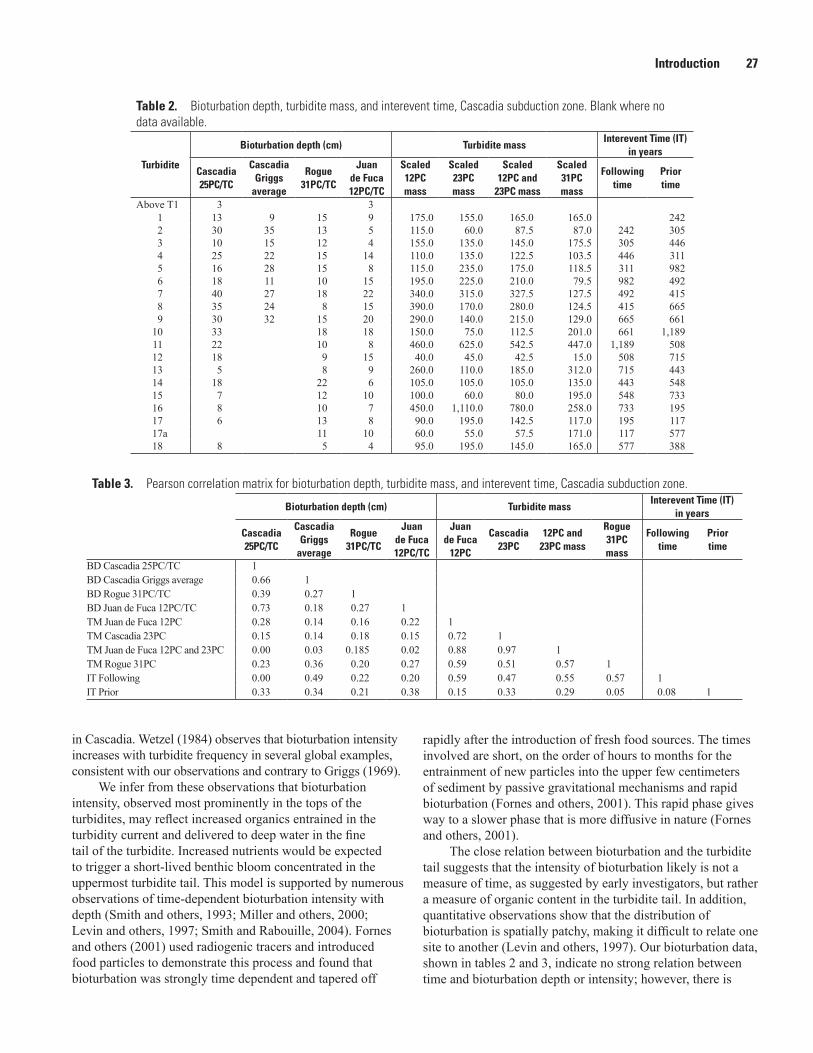
Introduction 27
Table 2. Bioturbation depth, turbidite mass, and interevent time, Cascadia subduction zone. Blank where no data available.
Turbidite
Bioturbation depth (cm) Turbidite massInterevent Time (IT)
in years
Cascadia 25PC/TC
Cascadia Griggs
average
Rogue 31PC/TC
Juan de Fuca 12PC/TC
Scaled 12PC mass
Scaled 23PC mass
Scaled 12PC and
23PC mass
Scaled 31PC mass
Following time
Prior time
Above T1 3 31 13 9 15 9 175.0 155.0 165.0 165.0 2422 30 35 13 5 115.0 60.0 87.5 87.0 242 3053 10 15 12 4 155.0 135.0 145.0 175.5 305 4464 25 22 15 14 110.0 135.0 122.5 103.5 446 3115 16 28 15 8 115.0 235.0 175.0 118.5 311 9826 18 11 10 15 195.0 225.0 210.0 79.5 982 4927 40 27 18 22 340.0 315.0 327.5 127.5 492 4158 35 24 8 15 390.0 170.0 280.0 124.5 415 6659 30 32 15 20 290.0 140.0 215.0 129.0 665 661
10 33 18 18 150.0 75.0 112.5 201.0 661 1,18911 22 10 8 460.0 625.0 542.5 447.0 1,189 50812 18 9 15 40.0 45.0 42.5 15.0 508 71513 5 8 9 260.0 110.0 185.0 312.0 715 44314 18 22 6 105.0 105.0 105.0 135.0 443 54815 7 12 10 100.0 60.0 80.0 195.0 548 73316 8 10 7 450.0 1,110.0 780.0 258.0 733 19517 6 13 8 90.0 195.0 142.5 117.0 195 11717a 11 10 60.0 55.0 57.5 171.0 117 57718 8 5 4 95.0 195.0 145.0 165.0 577 388
Table 3. Pearson correlation matrix for bioturbation depth, turbidite mass, and interevent time, Cascadia subduction zone.
Bioturbation depth (cm) Turbidite massInterevent Time (IT)
in years
Cascadia 25PC/TC
Cascadia Griggs
average
Rogue 31PC/TC
Juan de Fuca 12PC/TC
Juan de Fuca
12PC
Cascadia 23PC
12PC and 23PC mass
Rogue 31PC mass
Following time
Prior time
BD Cascadia 25PC/TC 1 BD Cascadia Griggs average 0.66 1BD Rogue 31PC/TC 0.39 0.27 1BD Juan de Fuca 12PC/TC 0.73 0.18 0.27 1TM Juan de Fuca 12PC 0.28 0.14 0.16 0.22 1TM Cascadia 23PC 0.15 0.14 0.18 0.15 0.72 1TM Juan de Fuca 12PC and 23PC 0.00 0.03 0.185 0.02 0.88 0.97 1TM Rogue 31PC 0.23 0.36 0.20 0.27 0.59 0.51 0.57 1IT Following 0.00 0.49 0.22 0.20 0.59 0.47 0.55 0.57 1IT Prior 0.33 0.34 0.21 0.38 0.15 0.33 0.29 0.05 0.08 1
in Cascadia. Wetzel (1984) observes that bioturbation intensity increases with turbidite frequency in several global examples, consistent with our observations and contrary to Griggs (1969).
We infer from these observations that bioturbation intensity, observed most prominently in the tops of the turbidites, may reflect increased organics entrained in the turbidity current and delivered to deep water in the fine tail of the turbidite. Increased nutrients would be expected to trigger a short-lived benthic bloom concentrated in the uppermost turbidite tail. This model is supported by numerous observations of time-dependent bioturbation intensity with depth (Smith and others, 1993; Miller and others, 2000; Levin and others, 1997; Smith and Rabouille, 2004). Fornes and others (2001) used radiogenic tracers and introduced food particles to demonstrate this process and found that bioturbation was strongly time dependent and tapered off
rapidly after the introduction of fresh food sources. The times involved are short, on the order of hours to months for the entrainment of new particles into the upper few centimeters of sediment by passive gravitational mechanisms and rapid bioturbation (Fornes and others, 2001). This rapid phase gives way to a slower phase that is more diffusive in nature (Fornes and others, 2001).
The close relation between bioturbation and the turbidite tail suggests that the intensity of bioturbation likely is not a measure of time, as suggested by early investigators, but rather a measure of organic content in the turbidite tail. In addition, quantitative observations show that the distribution of bioturbation is spatially patchy, making it difficult to relate one site to another (Levin and others, 1997). Our bioturbation data, shown in tables 2 and 3, indicate no strong relation between time and bioturbation depth or intensity; however, there is

28 Turbidite Event History—Methods and Implications for Holocene Paleoseismicity of the Cascadia Subduction Zone
a somewhat better relation between bioturbation thickness and turbidite thickness, with correlation coefficients ranging from 0.16 to 0.65. This lends weak support to the hypothesis that larger events supply more organic material to support a benthic bloom following turbidite emplacement. Turbidite-thickness between sites correlates moderately well, with Pearson coefficients ranging from 0.43 to 0.73, from which we infer that turbidite size may affect bioturbation more than just locally (thickness correlations are discussed in subsequent sections). We conclude that bioturbation is not useful for correlation or time passage, except perhaps for local sites, and we are unable to verify a bioturbation depth and time connection suggested by Griggs and others (1969) and Adams (1990) and reiterated in Atwater and Hemphill-Haley (1997). All values here are given assuming T5b does not extend to the Juan de Fuca system; however, inclusion of this event changes the outcome little.
We note that bioturbation is more severe in smaller turbidites, suggesting that smaller events do not kill the resident infauna, which are able to dig their way through the turbidite and continue feeding. Large events appear to kill off the fauna, which typically do not burrow up through the multiple sand layers to the surface. In many instances, bioturbation is difficult to measure at all because it may continue downward through a small event with no way to distinguish the boundaries related to each event. Also common is the presence of large-diameter helical zoophycos burrows that sweep through the section with individual extents of a meter or more. These burrows likely have no relation to individual events (for example, below T8 in M9907-25PC in subsequent figures).
Bioturbation and Its Effect on Radiocarbon Dating of Interseismic Hemipelagic Sediments
A number of attempts have been made to test the dependence of vertical rates of mixing during bioturbation on various parameters. Our interest is the vertical mixing of foraminifers and what effect particle size has on vertical mixing rates. This information is needed to evaluate uncertainties for radiocarbon dates and the radiocarbon-date results in terms of foraminifer size within samples, as well as any effect such rate changes may have toward biasing 14C dates in either direction. When considering single species, it has been shown that rates can be dependent on temperature, particle size, and particle shape (Wheatcroft, 1992, and references therein). Abyssal-plain temperatures are constant and, therefore, are unlikely to contribute to variable bioturbation.
The process of bioturbation is highly complex. Experimental results from several settings suggest, however, that bioturbation in the deep sea is dominated by deposit feeders and that deposit feeders, in turn, preferentially ingest and retain fine particles (Thomson and others, 1988, 1995; Wheatcroft, 1992). The impact of this in the context of this study is that large particles, such as foraminifers, used for dating are not selected by deposit feeders for
retention and apparently are not mixed vertically as much as the finer fractions of material. Evidence for this is found in studies that compare the vertical mixing of sand-sized particles or foraminifers to those based on radionuclides, which are associated with smaller particle sizes. Thomson and others (1988, 1995) show that vertical mixing of foraminifers is less by a factor of 1–3 than that estimated from 210Pb and 230Th. Radionuclides associated with finer particle sizes also show greater biodiffusivity than those associated with larger grain sizes. For dating of turbidites or other stratigraphic horizons, these results are important and may help explain the surprising consistency we see in dating correlative turbidites when other variables, such as reservoir age, basal erosion, and contamination, are minimized. The presence of color contrast between the hemipelagic sediment and turbidite tails in most cores in Cascadia Basin suggests even less bioturbation in cores that primarily are turbidite stratigraphy than in pelagic cores. This is most likely because the sediments are loaded instantaneously with thick and barren turbidites that extinguish the infauna at the former seafloor and require recolonization and reestablishment of a mixed layer following each turbidite emplacement. A stable mixed-layer profile is ephemeral in this context.
Stratigraphic Datum Ages
Late Quaternary Stratigraphy in Cascadia BasinChanges in climate, sea level, and glaciation in addition
to Cascade volcanic eruptions have acted as primary controls in late Quaternary stratigraphy of Cascadia Basin deposits. Before the onset of deposition of Holocene turbidites, glacial marine deposits dominated and are found in the levees of Astoria Channel (Nelson, C.H., 1976). These silty clays with ice-rafted dropstones and a coarse-sand, coarse-fraction composition represent deposition during the last glacial maximum. Turbidites overlying the glacial marine deposits represent times of glacial melting and significant input of turbidite sediment into Cascadia Basin (figs. 11, 12). In addition, from 16,000 to 12,000 yr B.P., 22 or more ice-dam outbursts from glacial Lake Missoula (for example, Baker and Bunker, 1985) deposited ~2,100 km3 of turbidites on Astoria Fan (Normark and Reid, 2003). As a result, the frequency and volume of turbidite deposition was much greater (as much as 1 per 180 years from Lake Missoula outbursts, in addition to earthquake-triggered turbidites) during the late Pleistocene compared to the interglacial Holocene record. During the time of intense turbidity-current activity in the late Pleistocene, extensive erosion of turbidite-channel pathways also took place, because we often find only a partial record of early Holocene and older turbidite deposits in proximal settings in Astoria and Eel Canyons. Many systems continued to be energetic into the Holocene and, as a result, the most complete history of turbidite deposition is found in Holocene deposits distal from the submarine canyon mouths.

Introduction 29
In addition to the local glacial effect of Lake Missoula, worldwide glacial meltwater pulses, such as the Bölling-Allerød (14,000–12,800 cal yr B.P.) interval and episodes of rapidly rising sea levels (10–20 m/1,000 years; for example, Fairbanks, 1989; Lohmann and Schultz, 2000), affected the stratigraphy of the Cascadia Basin and other turbidite systems. At the end of the Bölling-Allerød rapid rise of sea level in Cascadia Basin turbidite systems and other deep-sea fans such as the Mississippi, Bryant, Amazon, and Indus fans, the composition (for example, clay, carbonate) and color of hemipelagic sediment changed (fig. 12; Nelson, C.H., 1968, 1976; Griggs and others, 1969; Duncan and others, 1970; Nelson, C.H., and others, 1992, 2009; Maslin and others, 2005; Kessarkar and others, 2005; Damuth and others, 2006).
Mazama Ash DatumIn Cascadia, the widespread deposition of ash sourced from
the eruption of Mount Mazama (now Crater Lake) provides a clear datum throughout most of the Cascadia Basin system. The ash is observed in marine cores as brown basaltic-glass shards with little alteration, and it may constitute as much as 50 percent of sand-fraction samples at some sites. The ash was deposited as airfall on land and was dispersed primarily to the north and east from the eruptive site. With one possible exception (Royse, 1967), airfall ash has not, to our knowledge, been observed in marine cores, because it is mixed with other river sediment carried by the ash-bearing turbidity currents (Nelson, C.H., and others, 1968, 1988). The ash apparently was transported to the shelf by rivers as bed and suspended load, where it most likely was deposited. The next subduction earthquake following ash deposition triggered turbidity currents that entrained the ash, depositing it with the turbidites in the Cascadia Basin submarine-canyon systems, including Juan de Fuca, Quinault, Willapa, Grays, Astoria, Cascadia, and Rogue canyon/channel systems (Griggs, 1969; Nelson, C.H., and others, 1968, 1988; our Mazama ash data are given in appendix 6). Airfall Mazama ash also has been identified as far north as Kootnay Lake (British Columbia; Hallett and others, 1997) and in Effingham Inlet (Vancouver Island), where it is dated at 7,570±70 cal yr B.P. (Ivanochko and others, 2008). However, we found no Mazama ash in Barclay Canyon, a canyon that may have connected to Effingham Inlet during the Pleistocene but is now isolated by a sill and a wide continental shelf (Dallimore and others, 2005a). We find no Mazama ash in Hydrate Ridge (west basin), a lower slope basin off Oregon that is isolated from land-sediment sources by the accretionary-wedge ridge and basin physiography, or in the Smith, Klamath, Trinidad, or Eel systems. We also note that Mazama ash has not been found in cores outside abyssal-plain channels, further suggesting airfall was most likely not significant.
The age of the cataclysmic Mazama eruption is well constrained by recent work, yielding 7,627±150 cal yr B.P. (Zdanowicz and others, 1999) from Greenland ice cores and 7,610±29 cal yr B.P. in British Columbia lake sediments (calibrated from Hallett and others, 1997). Throughout
Cascadia Basin, the first turbidite containing the Mazama ash is identified easily and has been dated in numerous localities, with an average age of 7,180±120 cal yr B.P. The presence of the Mazama ash establishes a strong temporal anchor in the Cascadia stratigraphic sequence (fig. 11). The age of the eruption and the age of the first turbidite containing Mazama ash establish that the ash was present in the canyon systems for nearly 500 years before a turbidity current delivered it to the abyssal channels. Earlier work identified this Mazama ash-bearing turbidite as the 13th event down from the surface in many Cascadia Basin cores (Adams, 1990; Nelson, C.H., and others, 2000; Goldfinger and others, 2003a,b). In most channel systems, Mazama ash content tapers off in events T12–T9, indicating that upper canyon sources were tapped repeatedly during subsequent turbidity currents.
Subsequent work supports Adams’ (1990) conclusion for northern Cascadia Basin cores, but for the Rogue Apron system, we modify the earlier stratigraphy and note additional age control provided by this revision. Earlier cores used by Adams and by us were missing upper sections, a fact that became apparent when a new core (RR0207-55KC), collected in 2002, revealed previously missing shallow turbidites. Careful correlation and further dating subsequent to Goldfinger and others (2003a,b) demonstrated that Rogue Apron beds could be well correlated, both locally and to other Cascadia Basin sites (Goldfinger and others, 2008; see below), and that the first appearance of Mazama ash was in the 14th marginwide turbidite down from the surface at Rogue Apron (T14), not the 13th, as in other systems. These correlations are discussed in detail in subsequent sections; however, we note here that the occurrence of Mazama ash in T14 rather than T13 provides a possible additional datum. The average age of T14 is 7,630±140 cal yr B.P. (four sites), indistinguishable from the ice core and lake sediment dates for the Mazama eruption (table 4). The Rogue River, the sediment source for Rogue Canyon, has headwaters on the flanks of Crater Lake, the former Mount Mazama. Ash flows and lahars extended for 75 km down the Rogue River valley from Mount Mazama (Nelson, C.H., and others, 1988). For this reason, we suggest that Mazama ash most likely was delivered to the Rogue system immediately after the eruption (T14 contains 80 percent Mazama ash glass shards from our Rogue Apron cores), which must have choked the river with ash, much as the 1980 Mount St. Helens eruption choked the Toutle River with ash. We suggest that, because it carries the first Mazama ash, the T14 event occurred closely spaced in time with the Mazama eruption. Because the ash was not included in T14 at any other site, the time between the Mazama eruption and T14 is probably limited to ~1 year, and possibly much less, which is the time required for ash from Mount St. Helens to be delivered to Washington canyon heads (Healy Ridge and Carson, 1987). We infer that these strong constraints make T14 essentially coeval with the Mazama eruption, independent of the marine 14C dates that also support this timing. If correct, T14 acts as a second Mazama-based stratigraphic datum with well-constrained timing.

30
Turbidite Event History—M
ethods and Implications for Holocene Paleoseism
icity of the Cascadia Subduction Zone
00 200200
0 150 3000 150 300
400
300
200
250
�500
600
500
600
400
1.31.6 1.21.8
1.31.9
0
80
15
20
15
0 50
0.5
0.5
20
30
40
15
0 50
0 65
95
5
1
40
35
20
0 80
T10
T10b
T10f
T11
T13
T14
T12
T15
T12
T11
T14
T10
T13
T15
T12?
T10c
T10a
T10
T11
T12
T13
T14
T15
CASC 113: 4,700 (4,590–4,830)
CASC 109+234+114: 5,760 (5,530–5,740)
CASC 115: 6,430 (6,280–6,570)
CASC 116+4: 7,100 (6,990–7,250)
CASC 117+110: 7,580 (7,470–7,690)
CASC 57: 6,820 (6,670–6,990)
CASC 181+134: 6,580 (6,470–6,720)
CASC 182+135: 7,160 (7,040–7,260)
CASC 147+69: 5,230 (5,090–5,370)
CASC 70: 7,020 (6,910–7,150)
8,050 (7,900–8,200)
4,740 (4,560–4,940)
6,090 (5,910–6,280)
CASC 136: 7,650 (7,510–7,770)
CASC 137: 8,250 (8,140–8,350)
4,740 (4,570–4,910)
5,180 (5,010–5,380)
5,930 (5,800–6,060)
CASC 31+167: 4,850 (4,710–4,960)
5,400 (5,250–5,580)
5,810 (5,670–5,950)
6,000 (5,870–6,120)
6,590 (6,410–6,770)
CASC 32: 7,100 (6,980–7,260)
5,220 (5,090–5,380) CASC 176B: 5,070 (4,860–5,260)
15
Magnetic susceptibility (SI units),high-resolution point sensorDensity (gm/cm3)
EXPLANATION
Percentage of Mazama ashCASC 113: 4,715 (4,662–4,877) Radiocarbon age, in cal yr B.P.
and 2σ range, purple if erosion corrected, gray if reversed
First occurrence of Mazama ash >1.0%First occurrence of Mazama ash (inferred)
Correlation Summary
Calculated hemipelagic age in cal yr B.P. and 2σ range
M9907-31PC
M9907-12PC M9907-23PC
0 200 4001.21.41.61.8
T11
T10
T10b
T13
T15
T14?
T10f
HRW-10: 5,330 (5,210–5,430)
HRW-13: 5,680 (5,560–5,810)
HRW-11: 7,220 (7,140–7,310)
HRW-12: 8,650 (8,470–8,820)
RR020756PCHydrate Ridge Basin
Cascadia Channel Juan de Fuca Canyon
Rogue Canyon
coring artifact
T12
T14
T13
12PC 23PC 56PC 31PC
T11
T10c
CASC 9: 7,670 (7,530–7,820)
No Mazama Ashat HRBW
T10aHRW-09: 5,160 (5,080–5,310)
CASC 72: 8,250 (8,150–8,350)
Figure 11. Diagram showing Mazama-ash correlation in Cascadia Basin. Four cores, including representatives from Juan de Fuca, Cascadia, Hydrate Ridge, and Rogue Apron systems, are shown. The heavy red line is the first appearance of Mazama ash in Cascadia Basin cores, but it is dashed in Hydrate Ridge Basin core, where only a very subdued mud turbidite is present in the stratigraphic position of T14. The numbered diamonds and the associated dashed curve are the
percentage of glass in the sand fraction of corresponding turbidites. The inset shows correlation details of magnetic susceptibility curves closely spaced for comparison. Regionally, the first Mazama ash appearance is in T13, but the first Rogue appearance is in T14, ~500 years earlier. No Mazama ash is found in Hydrate Ridge Basin, and T14 is weak or absent. See text for discussion. Abbreviations: gm/cm3, gram per cubic centimeter; HRBW, Hydrate Ridge Basin West.
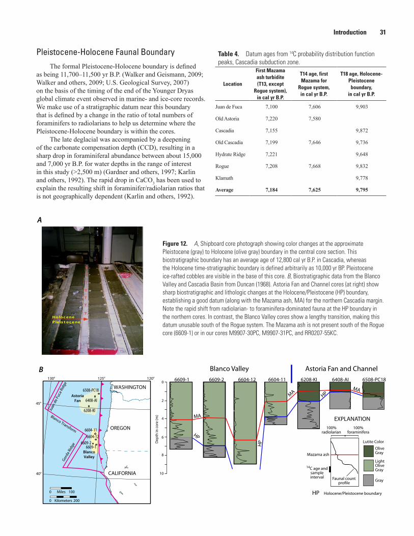
Introduction 31
Table 4. Datum ages from 14C probability distribution function peaks, Cascadia subduction zone.
Location
First Mazama ash turbidite (T13, except
Rogue system), in cal yr B.P.
T14 age, first Mazama for
Rogue system, in cal yr B.P.
T18 age, Holocene- Pleistocene boundary,
in cal yr B.P.
Juan de Fuca 7,100 7,606 9,903
Old Astoria 7,220 7,580
Cascadia 7,155 9,872
Old Cascadia 7,199 7,646 9,736
Hydrate Ridge 7,221 9,648
Rogue 7,208 7,668 9,832
Klamath 9,778
Average 7,184 7,625 9,795
Pleistocene-Holocene Faunal BoundaryThe formal Pleistocene-Holocene boundary is defined
as being 11,700–11,500 yr B.P. (Walker and Geismann, 2009; Walker and others, 2009; U.S. Geological Survey, 2007) on the basis of the timing of the end of the Younger Dryas global climate event observed in marine- and ice-core records. We make use of a stratigraphic datum near this boundary that is defined by a change in the ratio of total numbers of foraminifers to radiolarians to help us determine where the Pleistocene-Holocene boundary is within the cores.
The late deglacial was accompanied by a deepening of the carbonate compensation depth (CCD), resulting in a sharp drop in foraminiferal abundance between about 15,000 and 7,000 yr B.P. for water depths in the range of interest in this study (>2,500 m) (Gardner and others, 1997; Karlin and others, 1992). The rapid drop in CaCO3 has been used to explain the resulting shift in foraminifer/radiolarian ratios that is not geographically dependent (Karlin and others, 1992).
6609-1 6609-2 6604-12 6604-11 6208-KI 6408-AI 6508-PC18
MA
MA
HP
HP
Lutite Color
OliveGray
LightOliveGray
Gray
Mazama ash
Holocene/Pleistocene boundaryHP
Faunal countpro�le
14C age andsampleinterval
EXPLANATION
HP
MA
Blanco Valley Astoria Fan and Channel
100%radiolarian
100%foraminifera
Dep
th in
cor
e (m
)
0
2
4
6
8
10
45°
125° 120°130°
40°
0 Kilometers 200
0 Miles 100
OREGON
CALIFORNIA
WASHINGTON
Juan
de
Fuca
Rid
ge
Blanco Transform
Gorda
Rid
ge
AstoriaFan
BlancoValley
6508-PC18
6208-KI
6604-116604-12
6609-26609-1
6408-AI
B
A
Figure 12. A, Shipboard core photograph showing color changes at the approximate Pleistocene (gray) to Holocene (olive gray) boundary in the central core section. This biostratigraphic boundary has an average age of 12,800 cal yr B.P. in Cascadia, whereas the Holocene time-stratigraphic boundary is defined arbitrarily as 10,000 yr BP. Pleistocene ice-rafted cobbles are visible in the base of this core. B, Biostratigraphic data from the Blanco Valley and Cascadia Basin from Duncan (1968). Astoria Fan and Channel cores (at right) show sharp biostratigraphic and lithologic changes at the Holocene/Pleistocene (HP) boundary, establishing a good datum (along with the Mazama ash, MA) for the northern Cascadia margin. Note the rapid shift from radiolarian- to foraminifera-dominated fauna at the HP boundary in the northern cores. In contrast, the Blanco Valley cores show a lengthy transition, making this datum unusable south of the Rogue system. The Mazama ash is not present south of the Rogue core (6609-1) or in our cores M9907-30PC, M9907-31PC, and RR0207-55KC.

32 Turbidite Event History—Methods and Implications for Holocene Paleoseismicity of the Cascadia Subduction Zone
This drop in CaCO3 and increase in biogenic components of hemipelagic sediments is reflected by a sharp color change from gray to olive green at the same time in this transitional sediment (Duncan, 1968; Nelson and others, 1968; fig. 12). The foraminifer-to-radiolarian change is regional, but the sediment-color change may vary with geography and does fade southward (Duncan, and others, 1970), as we observed in our Cascadia Basin cores. The foraminifer/radiolarian ratio, however, is an indicator of the most rapid CCD transition from 13,000 to 11,000 yr B.P., which correlates with the worldwide Bölling-Allerød event (fig. 12) (for example, Lohmann and Schultz, 2000).
Not all of our cores penetrate deep enough to reach the Pleistocene-Holocene boundary; however, a number of our new and archive cores do show this faunal and color change (fig. 12). This boundary provides a solid stratigraphic datum and allows a comparison of Holocene hemipelagic-sediment thickness in Cascadia Basin interchannel cores with that found at our key channel core locations to test for net erosion between channel sites and undisturbed abyssal-plain sites.
We combine radiocarbon dates from our cores with new data from the archive cores of Duncan and others (1970) to determine the best age estimate of the distinct Pleistocene-Holocene faunal boundary in Cascadia Basin (Gutiérrez-Pastor and others, 2009). We define the boundary as the maximum gradient in foraminifer/radiolarian shift at the point where the ratio is ~1:1. In core M9907-30PC on Rogue Apron, where the foraminifer/radiolarian ratios reach 1:1 at a depth in the core of 781 cm, we obtain an age of 12,750±50 cal yr B.P. (2σ range, 12,880–12,530). We have used foraminifers from archive core 6609-1 (Duncan, 1968) to date the same stratigraphic interval at another location on Rogue Apron with nearly the same result of 13,000 cal yr B.P., giving a sample-depth-corrected age of 12,800±80. In core RR0207-49PC in Noyo Channel, about 350 km to the south, we determined an age of 12,840 cal yr B.P. for this boundary, giving a sample depth corrected age of 12,800±40 (2σ, 12,930–12,580). Ivanochko and others (2008) also observe the transition to stable Holocene conditions using multiproxies as initiating at ~12,700 cal yr B.P. at the start of the Younger Dryas and reaching completion by 10,700 cal yr B.P. Our data show that the best estimated age for the Pleistocene-Holocene faunal boundary (as defined above) along the base of the continental slope in abyssal Cascadia Basin is ~12,800 cal yr B.P. In Cascadia Channel, 140 km west of the base of the continental slope, the faunal boundary occurs at a later time, ~10,200 cal yr B.P. (the age of T19), based on the foraminifer/radiolarian ratio at the base of our core M9907-25PC and the data from the Griggs (1969) core 6609-24 at the same location.
We note that the timing of the abrupt shift in sedimentation associated with the Pleistocene-Holocene boundary (likely related to sea-level rise) generally postdates the 12,800 cal yr B.P. faunal boundary by ~3,000 years. The faunal color-change shift is more abrupt than we would expect and also may be related to a loss of glacially derived sediments to the shelf after the Bölling-Allerød rapid
meltwater events and prior to the depth-related river cutoff. In addition, the abrupt change to a much colder Younger Dryas climate and different deep-ocean circulation immediately after the Bölling-Allerød events also may contribute to the rapid change in hemipelagic sediment (Gardner and others, 1997; Karlin and others, 1992).
First Turbidite in the 10-k.y. Sequence (T18)We use turbidite T18 as a reliable datum because
it commonly marks the first distinct well-dated and stratigraphically correlatable turbidite in the 10-k.y. sequence. The average 14C dates for T18 at six sites are moderately well clustered within a 115-yr standard deviation, averaging 9,800+180/-230 cal yr B.P. (table 4). T18 was deposited following an abrupt change from thicker, sandy Pleistocene turbidites to a Holocene regime dominated by thinner and finer grained sand-silt turbidites and hemipelagic interbeds. This event also is slightly younger than a prominent plateau in the radiocarbon calibration curve (Goslar and others, 2000) that makes distinguishing the dates of marine events ~11,000–10,000 cal yr B.P. problematic. Event T19 is close to this time and is affected by this calibration curve anomaly, thus the age of this bed is uncertain. Physical property and lithologic logs show an abrupt increase in turbidite mass, grain size, and possibly event frequency before the deposition of regional T18 for some proximal Cascadia sites, particularly those with narrow continental shelves. The most likely reason for this is that at the Pleistocene-Holocene transition, sea level was ~40–45 m below present and rising (for example, Peltier and Fairbanks, 2006). As sea level rose, connections between rivers and canyons began to be severed as the transgression proceeded rapidly across the shelf—earlier for systems with wide shelves (Juan de Fuca, Willapa, Grays, Quinault, and Barkley Canyons) and later for those with narrower shelves (Smith, Klamath, Astoria, Eel, and Trinidad Canyons). Turbidite frequency at distal sites appears unaffected by this event (Underwood and others, 2005).
Relative Dating TestsGriggs and Kulm (1970) used the Mazama ash to
calculate a mean recurrence of 410–510 years for post-Mazama turbidites in Cascadia Channel. They speculated on, but did not explicitly publish, the idea that these events were generated by earthquakes (L. Kulm, oral commun., 1999). Following the first discovery of coeval buried-marsh sequences on land, Adams (1990) assessed this hypothesis. He examined core logs for the Cascadia Basin channels and determined that many had 12 turbidites overlying the Mazama ash, which was included in the 13th turbidite. Adams observed that cores from Juan de Fuca, Willapa, Grays, and Quinault Canyons all contain 13–16 turbidites above the Mazama ash. The correlative turbidites in Cascadia Channel lie downstream from the confluence of those channels (fig. 13). If these events

Introduction 33
0Kilometers200 Miles 100
13–15 13–15
13
13
13
13
1313
Barkley Canyon
Juan de Fuca Canyon
Quinault CanyonGrays Canyon
Willapa Canyon
Astoria Canyon
Rogue Canyon
Base
of S
lope
Cha
nnel
Casc
adia
Cha
nnel
Chan
nel
Ast
oria
Klamath Canyon
Trinidad Canyon
Eel Canyon
Noyo Canyon
Mendocino Channel
13/19
16
13/19
16/19
)
13/18
130° 128° 126° 124° 122°
CALIFORNIA
OREGON
WASHINGTON
VancouverIsland
Nitanat Fan
Astoria Fan
Blanco Fracture Zone
48°
47°
46°
45°
44°
43°
42°
41°
40°
39°
Columbia
River
GordaPlate
Mendocino Escarpment
Gor
da R
idge
Tufts AbyssalPlain
Juan de FucaPlate
Juan
de
Fuca
Rid
ge
EXPLANATION1990–2002 Core locationsSubmarine canyons and channelsResults from Adams (1990)Post-Mazama/Holocene turbidite events
Figure 13. Synchroneity test at a channel confluence as applied where multiple Washington channels merge into the Cascadia Deep Sea Channel, indicated by the green outline. The number of events downstream should be the sum of events in the tributaries, unless the turbidity currents were triggered simultaneously. Remarkable similarity of records in northern Cascadia support the initial conclusion of Adams (1990) that these events are likely of earthquake origin. The number of events present above the Mazama ash remains constant between tributaries and the main stem. The internal structure and number of coarse pulses also remains constant after passage through the confluence.
had been independently triggered, with more than a few hours separation in time, the channels below the confluence should contain between 26 and 32 turbidites, not 13 as observed. This simple observation demonstrates synchronous triggering of turbidity currents in tributaries, the headwaters of which are separated by 50–150 km. Similar inferences about regionally triggered synchronous turbidites, in separate channels elsewhere, have been reported (Pilkey, 1988; Nakajima and Kanai, 2000; Shiki and others, 2000b; Gorsline and others, 2000). The one to three extra turbidites (fig. 13) in some proximal upper canyons of Washington may have been generated by other mechanisms, discussed below.
This key test of synchronous triggering has become known as the “confluence test” and has now been applied successfully along the northern San Andreas Fault, where
there are eight major confluences applicable to ~6,000 years of turbidite record observed in multiple systems (Goldfinger and others, 2007a). In the northern San Andreas Fault system, three heavy-mineral suites enabled us to distinguish the various dominant sources of the stratigraphy within turbidites upstream and downstream from confluences and to test for synchronous or asynchronous arrival at confluences by observing the stacking of turbidites and their provenance components. As in the original confluence test, a sequence of turbidites should show little change in stratigraphy downstream of confluences if the multiple-source canyons were triggered simultaneously, but may show the arrival and blending of the separate provenance components.
In Cascadia, we have only one robust confluence test as described above. Unfortunately, Astoria Channel, which

34 Turbidite Event History—Methods and Implications for Holocene Paleoseismicity of the Cascadia Subduction Zone
could meet Rogue “channel” off southern Oregon (fig. 2), has such subdued, if any, surface morphology that we are unable to determine whether these systems meet. Rogue Apron also has no topographically expressed channel leading away from the canyon mouth that we can resolve with existing data. Additionally, the southern margin has a different event history, further complicating the picture.
Results
Cascadia Turbidites, Stratigraphic Sequences, and Stratigraphic Correlation
General Description of Relevant Features of the Deposits
The textural and mineralogical details of the turbidites in Cascadia Channel (Griggs, 1969), Astoria Fan (Carlson, 1967; Nelson, C.H., 1968, 1976; Carlson and Nelson, 1969), and regionally (Duncan, 1968; Duncan and Kulm, 1970) are well described by previous investigators. We briefly summarize the most relevant features for this report (see core details in figs. 14–42). Cascadia turbidites are characterized by normally graded sequences of sand, silt, and clay and many have multiple-stacked amalgamated pulses, sharp bases, and normal grading of individual sand/silt pulses when present. Cascadia turbidites include sparse, reworked foraminifera displaced from continental-shelf environments (Nelson, C.H., 1968; Duncan, 1968; Griggs, 1969). These deposits are turbidites in the classic sense (Bouma, 1962), exhibiting Ta-Te divisions, although rarely are all divisions present in a single deposit. Mud turbidites are observed, primarily along the southern Cascadia margin, which commonly include further subdivisions of Piper (1978): laminated silt (D), laminated mud (E1), graded mud (E2), and ungraded mud (E3). The mud turbidites are distinguished from other fine deposits, such as contourites, by their sharp bases, organized internal structure, and fining-upward sequences. They are well characterized using the schemes of Bouma (1962) and Piper (1978). Muddy contourites, on the other hand, generally lack consistent internal structure, although they may have laminae. Transitions from silt to mud within contourites tend to be gradual, reflecting changes in the strength of slow-moving bottom currents (Stow and others, 1986; Nelson, C.H., and others, 1993). Fine contourites also show pervasive bioturbation, which is sparse in the Cascadia mud turbidites (Gonthier and others, 1984).
Mud rip-up clasts are scarce, and cross-laminated and parallel-laminated units are common. Shell and wood fragments in the coarse fraction occasionally are present. Basal erosion sometimes is indicated by fluted bases and
slanted contacts in the core; however, load features also are apparent in many turbidite bases and can be difficult to distinguish from erosive contacts. Loading features occasionally inject hemipelagic sediment from below the basal contact through breaches in the turbidite base and into an overlying weak zone, sometimes causing confusion in interpretation. Proximal cores may include limited reverse grading and cutouts, which typically are found in narrow bands internal to the multiple pulses of individual turbidites. The internal fining-upward grading between coarse pulses typically reaches silt size and rarely can reach nearly clay-size particles. The tail typically consists of 30–80 percent of the deposits (thickening downstream in Cascadia Channel, Griggs, 1969) and exhibits a classic Bouma E, massive or gradually fining upward to clay and capped by massive bioturbated hemipelagite.
Soft deformation of the turbidites and hemipelagites is common and includes coring deformation, loading deformation, and possibly other forms. Coring deformation includes wall drag, commonly expressed as doming upward of the turbidites, and suction or compression deformation. Suction deformation can occur in piston cores when the adjustment of the free-fall scope (wire allotted to the free fall of the piston corer relative to the trigger corer) system is too long, resulting in a lag of the piston and compression of the sediments. Suction of the sediments may result from the scope being too short, resulting in the piston starting up the liner tube before the core nose touches down. Such suction artifacts, known as “slurps” can result in the coarse fraction being pulled downward along the liner wall, the hemipelagic sediment being pulled up along the liner, or both. (See events T6 in fig. 7, T1 in fig. 5, and T4 and T7 in Cascadia Channel core M9907-25PC in fig. 24).
Soft sediment deformation not related to coring also is apparent in some cores, most notably in the Rogue system. The Rogue Apron cores and, to a lesser extent, other cores, occasionally show evidence of loading and injection features. The Rogue Apron site has a somewhat higher hemipelagic sedimentation rate compared to our other primary sites and also is a proximal site at the foot of a steep continental slope. We suspect that the thicker hemipelagic units, combined with high velocity of the turbidity currents as they accelerate downslope to the Rogue Apron site, may account for the more common evidence of loading and injection. In several cases, we observe clear loading structures and intermixing of the turbidite base and hemipelagic sediment. In other cases, we observe wedges of hemipelagic material injected into the tail of the overlying silty, fining-upward turbidite tails. These wedges contain scattered silt and sand stringers and appear to have some flow-banding structures consistent with extrusion from the underlying hemipelagic unit through a breach in the turbidite. In one case, our large kasten corer captured an extrusion site, where hemipelagic sediment had been squeezed upward through a breach in the overlying coarse sand and had formed a sill in the overlying fining-upward silt. Although the nature of these extrusions is apparent,

Results 35
their origins are less so. They may have occurred during emplacement of the turbidite or, possibly, during ground shaking from some later earthquake. In some cases, they may have occurred during coring. Examples of this can be seen in Rogue Apron cores RR0207-55KC at T8 (complete breach) and in core M9907-30TC above T5 and above T7 (fig. 33), where the breaches occurred close to, but not exactly at, the core site. The best alternative explanation for these tongues of hemipelagic material embedded within a turbidite is subdivision of the turbidites into multiple events, separated by normal hemipelagic sediment. This would require some unusual relations, including at least one turbidite consisting of a coarse-sand base only, with no other units (bypassing of finer fractions and no tail). Given that the RR0207-55KC example shows a clear breach with a dike and a sill, we favor the extrusion/injection explanation.
Apparent reverse-grading artifacts sometimes are observed in the physical-proxy data. An apparent reverse-grading signature appears in some Cascadia turbidites, notably in the distal cores of Cascadia Channel and in several other localities. An example can be seen clearly in the physical-property data for core M9907-23PC (fig. 14). The physical-property logs for this turbidite show an apparent
Figure 14. Lithologic, magnetic, and density data for event T5 in Cascadia Channel. T5 is an example of a turbidite showing apparent “reverse” grading in the density and magnetic signatures. Lithologic logs and the grain-size profile, however, show stacked multiple coarse pulses that are normally graded. In this case, more robust pulses overlie weaker pulses, giving a superficial appearance of reverse grading that is reinforced by the physical-property signatures. Coring artifacts, such as the doming of the stratigraphy visible in this event, also can create or enhance the false reverse-grading signature. Nevertheless, this is a counter example of correlation between grain size, magnetic susceptibility, and gamma-density plots. Abbreviations: g/cm3, grams per cubic centimeter; μm, micrometers; SI, Systeme Internationale.
H
EXPLANATION
LITHOLOGY
Hemipelagicclay Turbidite silty mud
Sand
Silt
Mottled clay
Burrows
1.01.5
180
190
200
210
220
-10 190Gamma density (g/cm3) Magnetic susceptibility (SI units)
Core M9907-23PC
Event T5
H
230
170
390 530
20 40 60 80Mean grain size (µm)
Magnetic susceptibility(SI units)
Gamma density (g/cm3)
Mean grain size (µm)
Very fine sand
reverse grading when the turbidite is viewed as a whole, with the largest density and MS spikes at the top of the unit. For such cases, however, careful examination indicates that the stratigraphy is made up of multiple fining-upward coarse pulses, which vary in thickness, sometimes with the thickest or coarsest unit in the uppermost position. The variability in thickness of the coarse units gives the illusion of a coarsening upward unit, when the turbidite is composed simply of a stack of increasingly thick fining-upward units.
The number and form of the multiple pulses persist over wide areas and are the basis for correlation of individual turbidites. We observe cases in which the stacking of pulses changes along strike for likely correlative events, thus giving the appearance of a shift from fining upward to coarsening upward, when only the grain size or thickness of individual pulses has changed. We see examples of similar apparent reverse grading in the northern San Andreas Fault system (Goldfinger and others, 2007a). Similar artifacts can also be generated in the physical-property proxy data by distortion during coring, typically an upward doming of the stratigraphy, which weakens the density and magnetic response from the coarse basal layer and extends the response from the upper transitional layer.

36 Turbidite Event History—Methods and Implications for Holocene Paleoseismicity of the Cascadia Subduction Zone
MineralogyThe heavy-mineral mineralogy of the turbidites shows
affinities to the Klamath Mountains for southern cores (Rogue Apron, Smith, Klamath, Trinidad, and Eel channel/canyon systems) and to Cascade Range and Columbia River sources for some of the northern cores (Cascadia and Astoria Channels) (fig. 15). Excellent descriptions of the lithology, mineralogy, distribution, and other details of Cascadia Basin sediments are given by Griggs (1969), Griggs and others, (1970), Nelson, C.H. (1968, 1976), Duncan (1968), and Duncan and others (1970).
Cascadia Turbidite SystemsThe continental slope of Cascadia Basin is traversed by
numerous submarine canyons delivering an abundant sediment supply to the filled trench from the high-rainfall coastal region and continental interior (fig. 2). The Columbia River, one of the largest rivers in North America, has delivered about 20 million metric tons of sediment per year during the late Holocene (Sternberg, 1986; Wolf and others, 1999). During the Pleistocene lowstands, when much of the Columbia River drainage basin was glaciated, a greater sediment load was delivered directly to the Cascadia Basin floor turbidite systems, constructing systems such as the broad Astoria and Nitinat Fans that filled the subduction-zone trench (Nelson, C.H., and others, 1968, 1987; Normark and Reid, 2003; Goldfinger and others, 1997). During the Holocene, sediments from Cascadia rivers were deposited mostly in nearly full shelf basins and upper canyons (Goldfinger and others, 1992; McNeill and others, 2000), with only limited input to many of the canyon heads (Sternberg, 1986; Wolf and others, 1999).
A wide variety of modern turbidite systems are found in present-day oceans and lakes and can also be found within a single basin system such as Cascadia Basin. No single fan model describes this variety of turbidite systems; however, basic end-member types of modern siliciclastic turbidite systems have been outlined, and a nomenclature assigned,
Rogue RiverKlamath
River
Eel River
Columbia River
8910
11
1213
20
Turbidite Sand Heavy-Mineral Composition
Cascade RangeNorthernSegment Source
Klamath MountainsSouthernSegment Source
Rogue Apron CORE 1, Turbidite Event 1313
Cascadia Channel (Griggs, 1969)Astoria Channel (Nelson, 1968)Astoria Canyon(Carlson, 1968)Normark, andothers, (1994)
Amphibole
Epidote Pyroxene
Decreasing Mount M
azama Influence (except Rogue)
Figure 15. Heavy-mineral composition diagram showing Columbia River-Cascade Range source of Astoria and Cascadia Channel sands and Rogue River-Klamath terrane source of Rogue Apron sands.
which we will use throughout this report (Nelson, C.H., and others, 1991, 2000). Base-of-slope sand-rich aprons, such as Rogue Apron, are defined as those small-scale (<10 km), wedge-shaped turbidite systems abutting the base of a slope. They do not have significant channel development detectable in seismic profiles, side-scan mosaics, or swath-bathymetry at the resolution of presently available data (Wolf and Hamer, 1999). Submarine fans, such as Nitinat and Astoria Fans, are defined as those turbidite systems with significant channel development that funnel sediment into outer-fan depositional lobes. Another turbidite system type commonly found in active-margin settings is the extensive, tectonically controlled, deep-sea or mid-ocean channel system. Deep-sea channel systems, such as Cascadia Channel, are fed by multiple tributary canyons, extend for hundreds to thousands of kilometers across basin floors, and eventually connect with abyssal-plain fans (Carter, 1988; Nelson, C.H., and others, 2000). A wide variety of feeding canyons, connecting axial channels, and channel-levee complexes, such as Mendocino Channel, also are parts of turbidite systems or may make up a partially developed turbidite system itself. Large-scale sediment-wave or dune fields associated with canyon mouths and proximal channels, such as those of the Trinidad and Eel systems, also have been observed in swath-bathymetric and sidescan mosaics of basin floors.
In a tectonically active setting like Cascadia Basin, folding, faulting, and extensive sediment failures can disrupt canyon and channel pathways of turbidite systems. Using our GIS database, sub-bottom profiles, and core lithologic correlation for Cascadia Basin (fig. 2), we have attempted to determine which are the open and active pathways and which have been disrupted. Marker beds, such as the Mazama ash (Nelson, C.H., and others, 1968, 1988), are important for determining whether a complete sequence of Holocene turbidite beds is present and an active turbidite channel pathway has been active to the present. Irregular axial gradients of channels, caused by fault offsets and mass transport deposits, together with missing turbidite sequences

Results 37
are evidence of a disrupted channel system (Nelson, C.H., and others, 2000). As individual Cascadia turbidite systems are described, these pathway features will be pointed out.
In the following sections we describe the site localities and turbidite sequences along the Cascadia margin. Individual turbidite numbers shown and discussed are those assigned following regional stratigraphic correlation presented in a subsequent section. Core positions and water depths are given in table 1. Radiocarbon data, correlations, and hemipelagic calculations can be found in appendix 1.
Barkley CanyonBarkley Canyon is our northernmost site along the Cascadia
margin, exiting the continental slope at lat ~48°10′ N. Its source is the Barkley Sound along western Vancouver Island, from which it is presently separated by a ~80-km-wide shelf. We sampled this site near the canyon mouth and also sampled a smaller, unnamed canyon ~12 km to the south (fig. 16). Barkley Canyon records turbidity currents triggered along the middle-southern Vancouver Island margin. Our data coverage does not include the northernmost corner of the Cascadia subduction zone between Barkley Canyon and the Nootka Fault, a distance of ~130 km, assuming that the subduction zone terminates at the Nootka Fault. The Barkley Canyon thalweg is interrupted by an active fault in its lowermost reach before exiting into a small apron at the canyon mouth. The fault, imaged in multibeam bathymetry, appears to offset the thalweg ~50 m, west side up, creating a sediment pond just upstream from the canyon mouth. This partial blockage may be reflected in the turbidite sequence in cores M9907-08PC and M9907-09PC from the Barkley system. An alternate path for Barkley Canyon turbidites exits over a 50-m sill and directly downslope, instead of the northward swing to the better defined canyon mouth. This alternate exit, informally called No Name Canyon, also was cored, but the turbidite sequence appears less complete than at Barkley Canyon. Barkley Canyon has a partially correlated turbidite record with some anomalies, and is not one of our primary sites.
Barkley Canyon Turbidite SequenceThe Barkley Canyon cores (M9907-08PC, M9907-08TC,
M9907-09PC, M9907-09TC) and No Name Canyon cores (M9907-06PC, M9907-06TC, M9907-07PC, M9907-07TC) contain 35 turbidites. The faunal event approximating the Pleistocene-Holocene boundary (hereafter referred to as the faunal Pleistocene-Holocene boundary) is found at a depth of 470 cm at event T23 in M9907-09PC. The closest 14C age is 11,650 (12,010–11,210) cal yr B.P. at event T21, which is ~70 cm above the core base and two turbidites above the faunal Pleistocene-Holocene boundary (fig. 17). The best Holocene record is found in M9907-09PC, although this and all of the Barkley Canyon cores are anomalous in several ways.
Above local bed T5, dated in M9907-09PC at 1,550 cal yr B.P. (2σ 1,810–1,280 cal yr B.P.), the turbidites are subdued and are little more than thin silt and mud stringers. The same is true for all cores at this site, including cores M9907-06PC and
M9907-07PC at No Name Canyon 12 km to the south. There appear to be four thin events above T5, suggesting that four beds (local T1–T4) may be present in Barkley Canyon. We cannot correlate these events reliably to other sites with the available data. Between two robust, dated events locally called T6 and T9, events T7 and T8 may be present as fine silt/mud turbidites. Another anomaly in this core is that the bed that we correlate regionally with event T11, which is a very large event marginwide, has an exceptionally long (45 cm) tail in all Barkley Canyon cores, reflected in the magnetic and density signatures as a very gradual upward taper. This unusual feature makes Barkley Canyon cores visually distinct and straightforward to correlate, but this feature generally is not observed elsewhere. A similar pattern is noted in both Barkley Canyon cores. The extensive mud tails may result from the primary distribution of mud from the Juan de Fuca Strait and the Columbia River, which is northward (Wolf and others, 1999) and feeds into the northern Cascadia canyons. Good dates were obtained from events locally named (and later interpreted to be regional): T5, T6, T9, T13, T14, T15, T16, T17, T17a, and T18. Fewer dates were obtained from Barkley Canyon than from other sites owing to the thin, undatable upper section and the initial difficulty in establishing good ties with other sites. Barkley Canyon cores do not contain Mazama ash and have 0–2 percent glass shards present in the section examined from 70 cm to the core base (fig. 17; appendix 6).
No Name Canyon, an alternate Barkley Canyon outlet, lies ~12 km to the south of the mouth of Barkley Canyon (figs. 16, 17). Core M9907-07TC is broadly similar to cores M9907-08 and M9907-09, most likely containing events T1–T11, but not enough age data are available to link this core positively to the site sequence at Barkley Canyon. Cores M9907-07PC, M9907-06PC, and M9907-06TC seem to have recovered parts of the section but likely are missing substantial parts of Holocene stratigraphy.
Juan de Fuca Canyon and ChannelJuan de Fuca Canyon is a complex system that originates at
the Juan de Fuca Strait and, to a lesser extent, likely received input from coastal rivers in northern Washington. Juan de Fuca Canyon has a low gradient and meanders through the growing anticlines of the broad continental slope. Two branches of the Juan de Fuca Canyon exit the continental slope separately and join as a base-of-slope channel off northern Washington at the head of the Nitinat Fan (fig. 18). Juan de Fuca Channel then bends to the southwest as part of the Nitinat Fan, which apparently has only one primary active Holocene distributary channel in the upper fan system. Cores M9907-05PC and M9907-05TC are near the fan apex, and cores M9907-11PC, M9907-11TC, M9907-12PC, and M9907-12TC were collected 94 km to the south in the main channel (figs. 1, 2, 18). Juan de Fuca channel is the northern tributary to Cascadia Channel and is thus part of the confluence test discussed previously. The channel gradient increases at the upper slope break and is interrupted at several points where it meanders around active anticlines and over active thrust faults on the lower slope, becoming more uniform on the Nitinat Fan (fig. 18). There is no change in gradient for this channel as it exits the slope onto the fan.

38 Turbidite Event History—Methods and Implications for Holocene Paleoseismicity of the Cascadia Subduction Zone
-2,500
-2,000
-1,500
-1,000
09PC/TCN
-500
Barkley Canyon
08PC/TC
06PC/TC07PC/TC
No Name Canyon
Barkley Canyon
Distance (km)
Dep
th (m
)
0 50 1003,000
2,500
2,000
1,500
1,000
500
0
08PC/TC09PC/TC
AstoriaFan
Juan
de F
uca R
idge
Juan de FucaPlate
Casc
adia
Cha
nnel
Blanco Fracture Zone
Gord
a Ridg
e
GORDAPLATE
Mendocino Escarpment
Tufts AbyssalPlain
Nitinat Fan
08/09 PC
06/07 PC
05 PC
11/12 PC
13 PC14/15 PC
01/03 PC
16 PC
17/18/19/20/21 PC
26/28 PC
27/29 PC
30/31 PC
33 PC
34 PC
35/36/37 PC
41/42 PC
39/40 PC
47/51 PC
44/45 PC
48/49 PC
22/23 PC
10 PC
02/56 PC 01 KC
55 KC
38 BC
24 BC
04 BC
6509-15
6502 PC-1
6705-5
6609-1
6609-12
6609-24
6508 K1
6705-6
53-18
130° 128° 126° 124° 122°
-
Hydrate RidgeBasin West
42°
44°
46°
48°
BarkleyCanyon
VancouverIsland
Juan de FucaCanyon
QuinaltCanyon
Grays Canyon
Willapa Canyon
Astoria Canyon
RogueCanyon
SmithCanyon
Klamath Canyon
Trinidad Canyon
EelCanyon
MendocinoChannel
Noyo Canyon
San Andreas Fault
40°
OREGON
WASHINGTON
CALIFORNIA
North
Am
erica
n Pl
ate
0 100
Kilometers
0 50
Miles
contours in metersactive channel pathways shown by thick gray lines
Figure 16. Perspective view of shaded-relief bathymetry of the Barkley Canyon system and apron, Vancouver Island margin. Multiple canyon tributary pathways are shaded gray. No Name Canyon (dashed pathway) appears to be a former Barkley pathway, now partially blocked by a sill. Sites for 1999 cores at the mouth of Barkley and No Name Canyons are shown by yellow symbols. Yellow outline on core location map shows approximate location of perpective view. Axial gradient for Barkley Canyon is shown.
Figure 17 (right). Site-correlation diagram for Barkley and No Name Canyon cores (see figs. 2 and 16 for core locations). Barkley Canyon correlation is tentatively based on physical-property signatures and limited 14C ages. Mazama ash is not found in Barkley Canyon cores. The characteristic large sand event is interpreted to be T11, which appears to have an exceptionally long tail in these cores. T8 has a recognizable signature, also assisting in this interpretation. Barkley Canyon cores are strikingly similar to Willapa Channel cores M9907-14PC and M9907-14TC (fig. 22). The upper six events are very subdued in these cores. The long gap between inferred T6 and T8 in cores M9907-08PC, M9907-08TC, M9907-09PC, and M9907-09TC suggests that T7 is missing or very weak. 14C ages in cal yr B.P., including 2s-error ranges; see appendix 1 for radiocarbon age data. (See Methods section.) Abbreviations: AMS, accelerator mass spectrometry; g/cm3, grams per cubic centimeter; SI, Systeme Internationale.

Results 39
100 cm
200 cm
300 cm
400 cm
500 cm
600 cm
0 cm
5.0
1.0
0.0
3.0
4.0
2.0
1.0
2.0
1.0
3.0
4.0
2.0
1.0
2.0
1.0
0.0
2.0
1.0
0.00.0
1.02.5 1.21.4 1.52.01.02.01.21.5 1.21.8 1.41.91.01.60 100
0 15030 700 4000 150 0 200 60 120 100 4000 250
0 1000 100
Barkley Canyon Barkley Canyon No Name Canyon
H/P
Hemipelagic clay
Turbidite silty mud
Sand
Silt
Mottled clay
Burrows
Pleistocene
Very fine sand
ShellWood fragment
LITHOLOGY
H
1.0
0.0
H/P
M9907-08PC M9907-09TC M9907-09PC M9907-06PC M9907-07PCM9907-07TCM9907-06TCM9907-08TC
Density (g/cm 3)
Radiocarbon sample location
EXPLANATION
Core break
Correlation lines, dashed if uncertain
Percentage of Mazama ash
High-resolution point magnetic susceptibility (SI units)
Low-resolution magnetic susceptibility (SI units)
Sample number: AMS 14C age and 2 σ range
Sample number: reversed AMS 14C age and 2 σ range
CASC 11: 7,290 (7,220–7,380)
CASC 11: 7,290 (7,220–7,380)
H/P Holocene/Pleistocene boundary
Oldest Mazama ash bearing turbidite
Hemipelagic age and estimated 2 σ range7,290 (7,220–7,380)
Sample number: erosion corrected AMS 14C age and 2 σ rangeCASC 11: 7,290 (7,220–7,380)
*Asterisk indicates Benthic age
CASC 24: 9,250 (8,950–9,520)
CASC 1: 2,590 (2,350–2,830)
CASC 191: 1,530 (1,260–1,800)
CASC 55+B: 7,610 (7,440–7,780)
CASC 52: 4,180 (3,910–4,430)
CASC 2: 11,650 (11,210–12,010)
CASC 236: 2,520 (2,360–2,650)
CASC 237: 8,150 (7,980–8,450)
CASC 238: 9,080 (8,870–9,290)
CASC 239: 6,790 (6,620–6,950)
CASC 240: 4,040 (3,870–4,220)
CASC 241: 8,870 (8,660–9,080)
CASC 242: 7,580 (7,380–7,720)*
CASC 243: 4,190 (3,950–4,470)
7,220 (7,070–7,370)
9,760 (9,540–10,000)
6,000 (5,860–6,140)
H
H
H
H
H
H
H
H
H
H
H
H
H
H
H
H
H
0
0
10
0.50
0
0
.5
% MA0 50
0
0
0.5
1
0
0
0
0
0.5
% MA0 50
0
0
0
0
0
10.5
% MA0 50
0.5
0
2
1
0
0
0
0
0
0
0.5
0.5
% MA0 50
00
0
0
% MA0 50
0
01
00.5
% MA0 50
0
0
% MA0 50
0
0
1
0
0
0
0
1
% MA0 50
0
0
0.5
0.5
T25
T24
T23
T24
T25
T6
T9
T11
T5
T9
T11
T12
T6
T14
T15
T16
T5
T6
T9
T11
T14T14
T16
T17
T21
T22
T23
T12
T15T15
T17aT17a
T20
T5
T24
T6
T5
T6
T11
T15T15
T17
T17a
T24
T19
T21
T22
T23
T12
T16T16
T18T18
T5
T14T14
T2?T1?
T3?
T7
T9
T8
T10
T13T13
T20
T6
T9
T12
T11
T5
T13
T4?
T2?
T1?
T3?
T4?
T13
T13
T7?
T12
T18T18
T19

40 Turbidite Event History—Methods and Implications for Holocene Paleoseismicity of the Cascadia Subduction Zone
AstoriaFan
Juan
de F
uca
Ridg
e
Juan de FucaPlate
Cas
cadi
a C
hann
el
Blanco Fracture Zone
Gord
a Ri
dge
GORDAPLATE
Mendocino Escarpment
Tufts AbyssalPlain
Nitinat Fan
08/09 PC
06/07 PC
05 PC
11/12 PC
13 PC14/15 PC
01/03 PC
16 PC
17/18/19/20/21 PC
26/28 PC
27/29 PC
30/31 PC
33 PC
34 PC
35/36/37 PC
41/42 PC
39/40 PC
47/51 PC
44/45 PC
48/49 PC
22/23 PC
10 PC
02/56 PC 01 KC
55 KC
38 BC
24 BC
04 BC
6509-15
6502 PC-1
6705-5
6609-1
6609-12
6609-24
6508 K1
6705-6
53-18
130° 128° 126° 124° 122°
-
Hydrate RidgeBasin West
42°
44°
46°
48°
BarkleyCanyon
VancouverIsland
Juan de FucaCanyon
QuinaltCanyon
Grays Canyon
Willapa Canyon
Astoria Canyon
RogueCanyon
SmithCanyon
Klamath Canyon
Trinidad Canyon
EelCanyon
MendocinoChannel
Noyo Canyon
San Andreas Fault
40°
OREGON
WASHINGTON
CALIFORNIA
North
Am
eric
an P
late
0 100
Kilometers
0 50
Miles
M9907-05PC-1,500
-2,000
Juan de Fuca
Chan
nelN
Distance (km)
Dept
h (m
)
0 100 200 3003,000
2,500
2,000
1,500
1,000
500
0
05PC/TC11-12PC/TC
A contours in metersactive channel pathways shown by thick gray lines
Figure 18A. Perspective views of shaded-relief bathymetry of the northern Juan de Fuca Channel system and upper Nitinat Fan, Washington margin. Multiple canyon tributary pathways are shaded gray; core sites are shown by yellow symbols. Yellow outlines on core location maps show approximate locations of detailed figures. Axial gradients for Juan de Fuca Channels are shown. A, Core site M9907-05PC/TC at Juan de Fuca. B, Core sites M9907-11PC/TC and M9907-12PC/TC on lower Nitinat Fan.

Results 41
NM9907-11PC/TC
Juan de Fuca Channel
M9907-12PC/TC
-2,600
-2,500
-2,000
-1,500
Distance (km)
Dep
th (m
)
0 100 200 3003,000
2,500
2,000
1,500
1,000
500
0
05PC/TC11-12PC/TC
B
AstoriaFan
Juan
de F
uca
Ridg
e
Cas
cadi
a C
hann
el
Blanco Fracture Zone
Gord
a Ri
dge
GORDAPLATE
Mendocino Escarpment
Tufts AbyssalPlain
Nitinat Fan
Juan de FucaPlate
08/09 PC
06/07 PC
05 PC
11/12 PC
14/15 PC
01/03 PC
16 PC
17/18/19/20/21 PC
26/28 PC
27/29 PC
30/31 PC
33 PC
34 PC
35/36/37 PC
41/42 PC
39/40 PC
47/51 PC
44/45 PC
48/49 PC
22/23 PC
10 PC
02/56 PC 01 KC
55 KC
38 BC
24 BC
04 BC
6509-15
6502 PC-1
6705-5
6609-1
6609-12
6609-24
6508 K1
53-18
130° 128° 126° 124° 122°
-
Hydrate RidgeBasin West
42°
44°
46°
48°
BarkleyCanyon
VancouverIsland
Juan de FucaCanyon
Willapa Canyon
Astoria Canyon
RogueCanyon
SmithCanyon
Klamath Canyon
Trinidad Canyon
EelCanyon
MendocinoChannel
Noyo Canyon
San Andreas Fault
40°
OREGON
WASHINGTON
CALIFORNIA
North
Am
eric
an P
late
0 100
Kilometers
0 50
Miles
13 PC6705-6
QuinaltCanyon
Grays Canyon
Figure 18B. Perspective views of shaded-relief bathymetry of the northern Juan de Fuca Channel system and upper Nitinat Fan, Washington margin. Multiple canyon tributary pathways are shaded gray; core sites are shown by yellow symbols. Yellow outlines on core location maps show approximate locations of detailed figures. Axial gradients for Juan de Fuca Channels are shown. A, Core site M9907-05PC/TC at Juan de Fuca. B, Core sites M9907-11PC/TC and M9907-12PC/TC on lower Nitinat Fan.

42 Turbidite Event History—Methods and Implications for Holocene Paleoseismicity of the Cascadia Subduction Zone
Juan de Fuca Turbidite SequenceCores M9907-11PC and M9907-12PC extend well
into the Pleistocene, distinguished by massive sands, high abundance of foraminifers, and gray color with dropstones (figs. 19–20). The Holocene section is compressed in these cores, fitting completely in the upper 3 m of section in M9907-12PC, but otherwise these cores have an excellent turbidite record with distinct stratigraphic boundaries and easily distinguishable hemipelagic intervals. Core M9907-11PC was found to be missing the upper five events when correlated with the other three cores at that site. The first Mazama ash appearance is in T13, as in most Cascadia Basin cores, with ash content tapering upward in events T12–T9. Correlation and dating of Juan de Fuca turbidite beds is straightforward, making the Juan de Fuca Channel (cores M9907-11PC, M9907-11TC, M9907-12PC, M9907-12TC) one of our primary sites that has no missing events relative to other sites. Cores M9907-05PC and M9907-05TC, at the more proximal Nitinat Fan apex, contain an excellent record of turbidites that we tentatively interpret to include T4–T15 on the basis of physical-property correlation. The stratigraphic boundaries in these cores are less distinct and are problematic for dating, as is common for very proximal sites. Core M9907-05PC is highly distorted by the coring process in its lower section, and it contains a large liquefied sand unit in the upper section. This core is not useful for dating or correlation, except for the upper 30 cm, which includes three turbidites that may be correlative with regional T1, T2, and T3. We focused our efforts on dating events in cores M9907-11PC, M9907-11TC, M9907-12PC, and M9907-12TC but have included tentative correlation to cores M9907-05PC and M9907-05TC in the correlated figures, although without age corroboration. One core, M9907-12PC, contains a distorted interval of hemipelagic sediment within what we believe is regional T6 by comparison to other cores. We interpret this hemipelagic sediment as most likely a coring artifact, but it alternatively could define another event, though the lower unit would be missing most elements of a typical turbidite. If it is an additional event, it would be designated T5b locally.
Grays, Quinault, Guide, and Willapa Canyons and Channels
The Washington continental margin is characterized by five major submarine canyons (Juan de Fuca, Quinault, Grays, Guide, and Willapa) that follow irregular pathways through the folds of the accretionary prism to the deformation front along the continental slope (figs. 1, 2). Quinault, Guide, and Grays Canyons join at a low point in the accretionary prism, which has a reversed surface taper along much of the Washington slope, with ridge tops and basin depths becoming deeper landward. This causes the merged systems to travel southward, parallel to the margin. They meet Willapa Canyon and meander westward, exiting the slope at the southern end of Nitinat Fan on the continental rise (fig. 21). Together, these systems monitor 120 km of margin length. During the
Holocene, these systems largely receive sediments from the Columbia River rather than their Pleistocene river sources in Washington (Sternberg, 1986), although much of this material is deposited on the Washington shelf (Wolf and others, 1999; Sternberg, 1986). Willapa Channel is the southern major tributary to Cascadia Channel and is part of the confluence test discussed previously.
Willapa Channel Turbidite SequenceCores M9907-14PC, M9907-14TC, M9907-15PC,
and M9907-15TC were collected in Willapa Channel, approximately at the same location as an older core (6705-5) collected by OSU in the 1960s (Griggs, 1969). Core 6705-5 was used later by Adams (1990), and it contained Mazama ash, as well as 13 post-Mazama turbidites. Our cores, M9907-14PC and M9907-15PC, extend reliably down to event T13, with Mazama ash present in this event in core M9907-14PC. The Mazama ash-bearing turbidite is likely regional T13, and reasonable stratigraphic correlation can be done from T1–T13. The best core in this sequence is M9907-14TC. The newer cores generally proved to be inferior to the older cores because they contained less datable hemipelagic material and had incomplete records (fig. 22), most likely owing to local variability in preservation or deposition. Additional cores taken in proximal Willapa Channel (M9907-13PC, M9907-13TC) recovered only Pleistocene clay, suggesting nondeposition or scouring of this channel floor in proximal areas. An older core taken in the head of Willapa Canyon (Brown Bear core 326-36) recovered Mazama ash and was not overlain by turbidites observable visually or in X-radiographs (Royse, 1967).
Cascadia Deep-Sea ChannelJuan de Fuca and Willapa Channels (also comprising the
input from Grays, Guide, and Quinault Canyons) meet on the southwestern part of Nitinat Fan to form Cascadia Channel. Cascadia deep-sea channel crosses Cascadia Basin, then enters the Blanco Fracture Zone (fig. 2) and continues hundreds of kilometers into Tufts Abyssal Plain (Griggs, 1969; fig. 2). This turbidity-current pathway traverses ~1,000 km of Cascadia Basin and has remained open throughout the late Quaternary to the present. This continuity is shown by the presence of 20 beds during the past 10 k.y. and 13 post-Mazama ash turbidite beds in cores we have collected and in those previously examined by Griggs (1969), Griggs and Kulm (1970), and Adams (1990). The active pathway also is verified by the occurrence of the youngest turbidite, with an age of 270 (360–180) cal yr B.P. likely corresponding to the A.D. 1700 Cascadia subduction zone earthquake. Griggs (1969) estimated the flow velocities in Cascadia Channel ranging from 5.8 m/s in the upper channel to 3.3 m/s in the lower channel. Griggs (1969) described the Cascadia Channel turbidites and turbidite system in considerable detail, and some of the data from the archive cores from Griggs’ thesis are included in our analysis. Griggs (1969) discussed the depositional histories of three

Results 43
0 cm
100 cm
200 cm
300 cm
400 cm
500 cm
600 cm
slurp
M9907-12PCM9907-12TCM9907- 11PCM9907- 11TC
Juan de Fuca Canyon/Channel
smalluncorrelatedevent
smalluncorrelatedevent
M9907-05PCM9907-05TC
smalluncorrelatedevent?
H
H
H
H
H
H
H
H
H
H
H
H
H
H
H
H
H
7
0 50% MA
40
45
25
2
500 % MA
6
45
32
0.5
0.5
2
0.5
0.5
1
2
15
35
45
40
0 50% MA
2
0.5
% MA
0
0
0
0.5
0 25% MA
0.5
0.5
10
0.5
0.5
0
0 50% MA
0.5
0
0
0.5
0 50
10
40
35
20
0 65
5 9
5
1
1
% MA7
CASC 107: 4,180 (4,020–4,310)
CASC 108: 4,820 (4,660–4,970)
CASC 110: 7,550 (7,430–7,670)
CASC 121:10,850 (10,620– 11,000)
CASC 113: 4,700 (4,590–4,830)
CASC 114: 5,810 (5,680–5,960)CASC 115: 6,440 (6,280–6,570)
CASC 116: 7,120 (6,990–7,250)CASC 117: 7,610 (7,490–7,710)
CASC 118: 8,990 (8,860–9,140)CASC 119: 9,330 (9,230–9,410)
CASC 120: 9,900 (9,680–9,980)
CASC 122: 10,690 (10,500–10,940)
CASC 123: 11,730 ( 11,480– 11,860)
CASC 4: 7,080 (6,970–7,190)
CASC 3: 270 (180–360)
CASC 43: 870 (770–990)
CASC 45: 1,210 (1,090–1,330)
CASC 46: 2,500 (2,340–2,600)
CASC 109: 5,690 (5,530–5,740)
CASC 44: 470 (390–550)
CASC B 111: 1,580 (1,460–1,720)*
CASC 234: 5,780 (5,660–5,910)
8,,050 (7900–8,200)
3,440 (3,280–3,610)
9,460 (9,270–9,700)
CASC 232: 4,090 (3,970–4,200)
6,600 (6,470–6,740)
5,750 (5,590–5,890)
CASC 112: 3,070 (2,920–3,190)
CASC 47: 3,500 (3,340–3,680)
noit
amr
ofed
er o
c er
eves
5,790 (5,630–5,930)
0 1000 100
0 80
0 150
0 400 0 50 100 100 20001.01.81.21.81.02.01.21.8
1.01.0
2.0
1.0
2.0
3.0
4.0
1.0
2.0
3.0
4.0
1.0
2.0
1.0 H
H
HT12
T15
T4
T4T5
T6
T11
T14
T7
T8
T9
T10
T13
T3
T2
T1
2.0 0.5
H
H
H
H
1.8 1.0
H
H
H
H
20 100
0 100 200 300
H/P
H/P
Gamma Density (g/cm 3)
Radiocarbon sample location
EXPLAN ATION
Core break
Correlation lines, dashed if uncertain
Percentage of Mazama ash
First occurrence, Mazama ash
High-resolution point magnetic susceptibility (SI units)
Low-resolution magnetic susceptibility (SI units)
Sample number: AMS 14C age and 2 σ range
CASC 11: 7,298 (7,220–7,377)
Sample number: reversed AMS 14C age and 2 σ rangeCASC 11: 7,298 (7,220–7,377)
H/P Holocene/Pleistocene boundary
Hemipelagic age and estimated 2 σ range7,298 (7,220–7,377)
Sample number: erosion corrected AMS 14C age and 2 σ range
CASC 11: 7,298 (7,220–7,377)
Hemipelagic clay
Turbidite silty mud
Sand
Silt
Mottled clay
Burrows
Pleistocene
Very fine sand
Shell
Wood fragment
LITHOLOGYH
*Asterix indicates Benthic age
0.5
T18
T12
T16T17
T4
T5
T6
T11
T14
T7
T8
T9
T10
T13
T3
T2
T1
T20
T19
T4
T5
T6
T11
T14
T7
T8
T9
T10
T13
T3
T2
T1
6
T15
T17a
T12
T17a
T15
Figure 19. Site-correlation diagram for the Juan de Fuca Channel key site (see figs. 2 and 18 for core locations). Mazama ash first appears in T13 in these cores. The characteristic large sand event has been interpreted to be T11. Core M9907-12PC contains a complete Holocene sequence for the northern Cascadia margin and extends well into the Pleistocene. Core M9907-11PC is missing events T1–T7. 14C ages in cal yr B.P., including 2s-error ranges; see appendix 1 for radiocarbon age data. (See Methods section.) Abbreviations: AMS, accelerator mass spectrometry; g/cm3, grams per cubic centimeter; SI, Systeme Internationale.
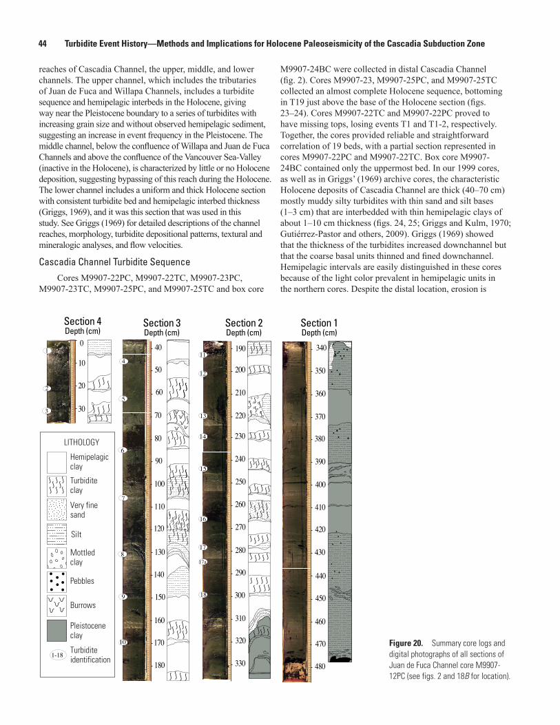
44 Turbidite Event History—Methods and Implications for Holocene Paleoseismicity of the Cascadia Subduction Zone
LITHOLOGY
Section 4Depth (cm)
Section 3Depth (cm)
Section 2Depth (cm)
Section 1Depth (cm)
0
10
20
30
50
70
90
100
110
120
130
140
150
160
170
180
190
200
210
220
230
240
250
260
270
280
290
300
310
320
330
340
350
360
370
380
390
400
410
430
420
440
450
460
470
40
60
80
480
Hemipelagic clay
Turbidite clay
Silt
Very fine sand
Mottled clay
Pebbles
Burrows
Pleistocene clay
Turbiditeidentification
1
2
3
4
5
6
11
12
13
16
17
18
7
8
9
10
14
15
1-18
17a
Figure 20. Summary core logs and digital photographs of all sections of Juan de Fuca Channel core M9907-12PC (see figs. 2 and 18B for location).
reaches of Cascadia Channel, the upper, middle, and lower channels. The upper channel, which includes the tributaries of Juan de Fuca and Willapa Channels, includes a turbidite sequence and hemipelagic interbeds in the Holocene, giving way near the Pleistocene boundary to a series of turbidites with increasing grain size and without observed hemipelagic sediment, suggesting an increase in event frequency in the Pleistocene. The middle channel, below the confluence of Willapa and Juan de Fuca Channels and above the confluence of the Vancouver Sea-Valley (inactive in the Holocene), is characterized by little or no Holocene deposition, suggesting bypassing of this reach during the Holocene. The lower channel includes a uniform and thick Holocene section with consistent turbidite bed and hemipelagic interbed thickness (Griggs, 1969), and it was this section that was used in this study. See Griggs (1969) for detailed descriptions of the channel reaches, morphology, turbidite depositional patterns, textural and mineralogic analyses, and flow velocities.
Cascadia Channel Turbidite SequenceCores M9907-22PC, M9907-22TC, M9907-23PC,
M9907-23TC, M9907-25PC, and M9907-25TC and box core
M9907-24BC were collected in distal Cascadia Channel (fig. 2). Cores M9907-23, M9907-25PC, and M9907-25TC collected an almost complete Holocene sequence, bottoming in T19 just above the base of the Holocene section (figs. 23–24). Cores M9907-22TC and M9907-22PC proved to have missing tops, losing events T1 and T1-2, respectively. Together, the cores provided reliable and straightforward correlation of 19 beds, with a partial section represented in cores M9907-22PC and M9907-22TC. Box core M9907-24BC contained only the uppermost bed. In our 1999 cores, as well as in Griggs’ (1969) archive cores, the characteristic Holocene deposits of Cascadia Channel are thick (40–70 cm) mostly muddy silty turbidites with thin sand and silt bases (1–3 cm) that are interbedded with thin hemipelagic clays of about 1–10 cm thickness (figs. 24, 25; Griggs and Kulm, 1970; Gutiérrez-Pastor and others, 2009). Griggs (1969) showed that the thickness of the turbidites increased downchannel but that the coarse basal units thinned and fined downchannel. Hemipelagic intervals are easily distinguished in these cores because of the light color prevalent in hemipelagic units in the northern cores. Despite the distal location, erosion is

Results 45
M9907-14PC/TC
-2500W
illapa Channel
N
M9907-15PC/TC
WillapaCanyon
Distance (km)
Dep
th (m
)
0 50 100 150 2003,500
3,000
2,500
2,000
1,500
1,000
500
0
14-15PC/TC
-2,000
-2,500
-2,600
-1,500
Abyssal Plain
Accretionary Prism
AstoriaFan
Juan
de F
uca
Ridg
e
Cas
cadi
a C
hann
el
Blanco Fracture Zone
Gord
a Ri
dge
GORDAPLATE
Mendocino Escarpment
Tufts AbyssalPlain
Nitinat Fan
Juan de FucaPlate
08/09 PC
06/07 PC
05 PC
13 PC14/15 PC
01/03 PC
16 PC
17/18/19/20/21 PC
26/28 PC
27/29 PC
30/31 PC
33 PC
34 PC
35/36/37 PC
41/42 PC
39/40 PC
47/51 PC
44/45 PC
48/49 PC
22/23 PC
10 PC
02/56 PC 01 KC
55 KC
38 BC
24 BC
04 BC
6509-15
6502 PC-1
6705-5
6609-1
6609-12
6609-24
6508 K1
6705-6
53-18
130° 128° 126° 124° 122°
-
Hydrate RidgeBasin West
42°
44°
46°
48°
BarkleyCanyon
VancouverIsland
Juan de FucaCanyon
QuinaltCanyon
Willapa Canyon
Astoria Canyon
RogueCanyon
SmithCanyon
Klamath Canyon
Trinidad Canyon
EelCanyon
MendocinoChannel
Noyo Canyon
San Andreas Fault
40°
OREGON
WASHINGTON
CALIFORNIA
North
Am
eric
an P
late
0 100
Kilometers
0 50
Miles
11/12 PC
Grays Canyon
contours in metersactive channel pathways shown by thick gray lines
Figure 21. Perspective view of shaded-relief bathymetry of the Willapa Canyon system and lower Nitinat Fan, Washington margin. Canyon pathway is shaded gray. Axial gradient for Willapa Canyon is shown. Core sites for 1999 cores at Willapa are shown by yellow symbols. Yellow outline on location map shows approximate location of detailed figure. White areas indicate no multibeam bathymetry data.

46 Turbidite Event History—Methods and Implications for Holocene Paleoseismicity of the Cascadia Subduction Zone
Figure 22. Site-correlation diagram for Willapa Channel cores (see figs. 2 and 21 for core locations). Willapa correlation is tentatively based on physical-property signatures, because there currently are no 14C ages for this site. Mazama ash content peaks in a turbidite we infer to be T13. The characteristic large sand event just above is interpreted to be margin-wide T11. T8 also has a recognizable signature, assisting in this interpretation. Cores M9907-14TC and M9907-14PC are strikingly similar to Barkley Canyon cores M9907-08PC, M9907-08TC, M9907-09PC, and M9907-09TC. The upper six events are subdued in these cores. The long gap in cores M9907-14TC and M9907-14PC between inferred T6 and T8 suggests T7 is missing in these cores but possibly is present in cores M9907-15TC and M9907-15PC. 14C ages in cal yr B.P., including 2s-error ranges; see appendix 1 for radiocarbon age data. (See Methods section.) Abbreviations: AMS, accelerator mass spectrometry; g/cm3, grams per cubic centimeter; SI, Systeme Internationale.
M9907-15PCM9907-15TCM9907-14TC M9907-14PC
Willapa Channel
mostly missing;liquefied fine tomedium sand with turbidite clay
1.0
2.0
3.0
4.0
1.0 1.0
2.02.0
1.0
0 cm
100 cm
200 cm
300 cm
400 cm
1.02.01.02.01.02.02.0 1.00 300 50 150 0 2000 600
0 200
2
7
2
35
0
1
0
1
0.5
0
0
1
2
0 50% MA
0.5
3
5
0 50% MA
30
35
0 50% MA
T3?
T2?
T4?
T12
T5?
T9
T8
T11
T10
T6
T7
T2?
T5?
T6
T3?
T4?
T8
T9
T10
T11
T12?
T13?T14?
T6
T7
T4?
T5?
T8
T9
T10
T11
T4?
T5?
T1?T2?
T6
T3?
T9
T8
T10
T11
T13
T12
Hemipelagic clay
Turbidite silty clay
Sand
Silt
Mottled clay
Burrows
Pleistocene
Shell
Wood fragment
LITHOLOGY
H
H
H
H
H
H
H
Density (g/cm3)
Radiocarbon sample location
EXPLANATION
Core break
Correlation lines, dashed if uncertain
Percentage of Mazama ash
High-resolution point magnetic susceptibility (SI units)
Low-resolution magnetic susceptibility (SI units)
Sample number: AMS 14 C age and 2σ range
Sample number: reversed AMS 14 C age and 2 σ range
CASC 11: 7,298 (7,220–7,377)
CASC 11: 7,298 (7,220–7,377)
H/P Holocene/Pleistocene boundary
Oldest Mazama ash bearing turbidite
Hemipelagic age and estimated 2 σ range7,298 (7,220–7,377)
Sample number: erosion corrected AMS 14 C age and 2 σ rangeCASC 11: 7,298 (7,220–7,377)
2

Results 47
present in many of the event bases. A detailed description of the erosion analysis is found in the Erosion Analysis section. The 13 post-Mazama ash events, without other input, suggest a Holocene history dominated by channel deposition, with cyclic generation of muddy turbidity currents (Griggs, 1969). In contrast, intermittent deposits of thick (as much as 2 m), late Pleistocene graded gravel-to-sand beds (Griggs and others, 1970; Griggs and Kulm, 1970) suggest that stronger, more frequent turbidity currents with channel erosion, nondeposition, and sediment bypassing occurred during glacial times. Additional cores discussed in Griggs (1969), collected from the middle reach of Cascadia Channel from lat 45° N. to lat ~46° N. (cores 6609-28, 6609-30, and 6705-13), mostly are Pleistocene sand units, indicated by dropstones and foraminifer-dominated fauna, with a thin Holocene section of mostly hemipelagic clay and thin silt turbidites (Griggs, 1969). This suggests erosion or bypassing of this channel reach during the Holocene, with coherent deposition farther downchannel at the sites for our cores, as well as the site for the older Griggs core 6609-24. Cascadia Channel is fed by primary tributaries Willapa Channel and Juan de Fuca Channel (previously discussed), which form an important confluence of these systems and provide a valuable relative-dating test. One major and several minor tributaries to the upper and middle reach of Cascadia Channel were investigated by Griggs (1969). Vancouver Sea Valley, the major tributary, proved to be largely inactive in the Holocene, containing thin, Holocene hemipelagic sections with a few thin, silty turbidites (Griggs, 1969). Other tributaries on the Nitinat fan contain up to 10 Holocene turbidtes, such as core 6705-10 (see Griggs, 1969). The possible bed T5b, mentioned in M9907-12PC at Juan de Fuca Channel, does not appear in Cascadia Channel downstream of the Juan de Fuca Channel cores.
Astoria Fan, Channel, and Base of Slope ChannelAstoria Fan can be divided into the typical morphological
subdivisions of a proximal inner fan with a few large channels, a middle fan with numerous channel bifurcations or splays, and an outer fan with distal depositional lobes (Nelson, 1976). The fan has a single Astoria Canyon source that feeds two main upper fan channels, the slope base channel and Astoria Channel (figs. 1, 2, 26). Astoria Channel on the middle-fan region has a continuous gradient down the main channel (fig. 26). The pathway down the slope base channel is blocked by a lower slope slump and then a fault offset (fig. 26; Goldfinger and others, 1997; Nelson, C.H., and others, 2000). This can be shown in the axial gradient of the slope base channel that is disrupted at both features, and by the presence of post-Mazama ash turbidites upstream but not downstream from these channel-gradient disruptions (Goldfinger and others, 1992). Consequently, the slope base channel does not provide a reliable turbidite event record, whereas the main Astoria Channel does.
Astoria Channel and its splays show the classic U-shaped fan valley floor and levee morphology. Several splay channels are cut off by the active channel leaving upslope-facing
hanging valleys. Although the surface morphology of Astoria Channel ends abruptly at lat 44° N., in seismic profiles we can trace a major subsurface continuation of this channel near the base of the slope southward to about lat 42° N. (figs. 1, 2; Wolf and Hamer, 1999) and through the Blanco Gap. There, the Astoria Channel turns to the southwest across south Cascadia Basin and again at lat 40°30′ N. emerges on the surface near Escanaba Trough as a channel 1,000 m wide with ~100 m relief.
The southern portion of Astoria Channel from lat 44° N. to lat 42° N. has infilled in part because mega-landslides from the central Oregon continental slope have blocked and (or) disrupted the channel gradients (Goldfinger and others, 2000). First, at about 130–108 ka, the giant Heceta slide displaced an 80-km block of the margin onto the base-of-slope region (fig. 1). About 11,000–13,000 years ago, based on sedimentation rates (Goldfinger and others, 2000, and this study), a second 25-km block (fig. 1, see lat 44° N. slump) from the lower continental slope slid into Astoria Channel at lat 44° N. on the northern end of the Heceta megaslide, breaking up and spreading a debris apron over the channel path (Goldfinger and others, 2000). Likely as a result of these slides, and the partially blocked pathways in some Astoria Fan channels, Astoria Channel southward of lat 44° N. does not have surface expression or contain a significant turbidite record. Cores M9907-44PC and M9907-45PC in southernmost Astoria Channel (fig. 1) have a basal age of ~13,000 cal yr B.P. at 5.5 m and only rare turbidites, suggesting blockage by the lat 44° N. slide at ~16,000–13,000 cal yr B.P. (Nelson, C.H., and others, 2009). The faunal Pleistocene-Holocene boundary is found at ~30 cm depth in these cores, which otherwise consist of uniform gray clay. This history of blockage of Astoria Channel is verified by a seismic profile showing 10 m of hemipelagic drape covering the emergent channel floor near Escanaba Trough (fig. 1; Wolf and Hamer, 1999). Southern Astoria Channel is not discussed further in this report.
Astoria Fan Turbidite SequenceA variable record of ash-bearing Holocene turbidites is
found in the thalwegs of Astoria Channel and fan distributary channels (fig. 27; Nelson, C.H., and others, 1968, 1988). Astoria Channel has variable turbidite-bed continuity, particularly in the channel floors of the canyon mouth and inner fan. In some canyon mouth locations, the entire post-Mazama ash turbidite sequence is missing, whereas in other sites, part or all of the sequence is present. The best preservation of the Holocene turbidite sequence is found in lower canyon walls (Carlson, 1967) or channel-floor terraces that are slightly elevated above the deepest thalweg. These data show that cut and fill processes are very active in the canyon-mouth region and that lateral-bedding continuity in channel floors is poor. Preservation of bed continuity is better slightly downstream from the canyon-mouth area, with the best sequence preserved in cores M9907-16PC and M9907-16TC (fig. 27), which extends reliably to event T10 in cores M9907-16PC, M9907-16TC, M9907-17PC, and

48 Turbidite Event History—Methods and Implications for Holocene Paleoseismicity of the Cascadia Subduction Zone
Distance (km)
Dept
h (m
)
0 50 100 150 2005,000
4,000
3,000
2,000
1,000
0
6609-2425PC/TC
22-23PC/TC
Cascadia Channel
N
Gorda Plate
-3,000
M9907-22PC/TCM9907-23PC/TC, 24BC
M9907-25PC/TC
-2,500
Cascadia Abyssal Plain
Accretionary Prism
Blanco Fracture Zone
6609-24
AstoriaFan
Juan
de F
uca
Ridg
e
Juan de FucaPlate
Gord
a Ri
dge
GORDAPLATE
Mendocino Escarpment
Tufts AbyssalPlain
Nitinat Fan
Cas
cadi
a C
hann
el
Blanco Fracture Zone
08/09 PC
06/07 PC
05 PC
11/12 PC
13 PC14/15 PC
01/03 PC
16 PC
17/18/19/20/21 PC
27/29 PC
30/31 PC
33 PC
34 PC
35/36/37 PC
41/42 PC
39/40 PC
47/51 PC
44/45 PC
48/49 PC
22/23 PC
10 PC
02/56 PC 01 KC
55 KC
38 BC
24 BC
04 BC
6509-15
6502 PC-1
6705-5
6609-1
6609-12
6609-24
6508 K1
6705-6
53-18
130° 128° 126° 124° 122°
-
Hydrate RidgeBasin West
42°
44°
46°
48°
BarkleyCanyon
VancouverIsland
Juan de FucaCanyon
QuinaltCanyon
Grays Canyon
Willapa Canyon
Astoria Canyon
RogueCanyon
SmithCanyon
Klamath Canyon
Trinidad Canyon
EelCanyon
MendocinoChannel
Noyo Canyon
San Andreas Fault
40°
OREGON
WASHINGTON
CALIFORNIA
North
Am
eric
an P
late
0 100
Kilometers
0 50
Miles
26/28 PC
contours in metersactive channel pathways shown by thick gray lines
Figure 23. Perspective view of shaded-relief bathymetry of the Cascadia Channel system and surrounding Cascadia abyssal plain. Core sites for 1999 cores at Cascadia Channel are shown by yellow symbols. Core 6609-24 (Griggs, 1969) shown with gray symbol. Channel pathway is shaded gray. Axial gradient for Cascadia Channel is shown. Yellow outline on location map shows approximate location of detailed figure.
Figure 24 (right). Site-correlation diagram for Cascadia Channel cores (see figs. 2 and 23 for core locations). Cascadia Channel turbidites are more generic in their simpler structure, as expected at a distal site. Individual coarse pulses in these turbidites are not as well defined as in more proximal settings, such as Juan de Fuca and Hydrate Ridge. Hemipelagic color contrast with turbidite tails is definitive at this site, making it the most reliable site for determining time between events by using hemipelagic thickness. 14C ages in cal yr B.P., including 2s-error ranges; see appendix 1 for radiocarbon age data. (See Methods section.) Abbreviations: AMS, accelerator mass spectrometry; g/cm3, grams per cubic centimeter; SI, Systeme Internationale.

Results 49
0 cm
100 cm
200 cm
300 cm
400 cm
500 cm
600 cm
700 cm
800 cm
900 cm
1000 cm
H
H
H
H
H
H
H
H
H
H
H
H
H
H
H
H
H
H
H0 2000 125 0 2500 100 0 20050 250
0 2000 2000 150
20 701.8 1.0 2.0 1.02.0 1.0 1.02.0 1.02.0 2.0 1.0 2.0 1.0
20
3.0
4.0
2.0
1.0
7.0
8.0
6.0
5.0
3.0
4.0
2.0
1.0
7.0
8.0
6.0
5.0
2.0
1.0
3.0
4.0
2.0
1.0
1.0
0 50
10
20
40
0.5
% MA 0 50
6
3
5
6
12
0.5
0
0
% MA0 50
5
20
15
40
30
20
0.5
0.5
% MA
T1
T2
T3
T4
T5
T6
T1
T2
T3
T4
T7
T6
T5
T4
T3
T8
T9
T10
T11
T12
T13
T14
T1
T7
T6
T5
T4
T3
T2
T8
T9
T10
T11
T12
T13
T14
T15
T18
T16
T17
T17a
T6
T8
T9
T10
T11
T12
T13
T7
T1
T2
T3
T4
T14
T15
T16
T17
T18
T5
T17a
T2
T3
T4
T5
T6
CASC 135+B: 7,150 (7,030–7,250)
CASC 136: 7,650 (7,510–7,770)
CASC 137+B: 8,250 (8,140–8,350)
CASC 138+B: 9,080 (8,930–9,200)
CASC 139: 9,870 (9,670–9,970)
CASC 132: 4,160 (3,980–4,340)
CASC 133: 5,190 (5,050–5,330)
CASC 131: 3,490 (3,310–3,660)
CASC 130: 2,550 (2,400–2,710)
CASC 129+B: 3,210 (3,130–3,320)
CASC 126: 1,160 (900–1,420)
CASC 183: 2,230 (2,120–2,330)
CASC 128B: 1,300 (1,190–1,410)
CASC 181: 6,530 (6,400–6,700)
CASC 134: 6,630 (6,490–6,800)
CASC 182+135+b: 7,150 (7,030–7,270)
CASC 126: 1,160 (900–1,420)
CASC 178: 270 (190–360)
CASC 96-4: 9,740 (9,420–10,070)(projected from Griggs core 24)
CASC 96-3: 7,180 (7,030–7,330)(projected from Griggs core 24)
CASC 96-2: 4,660 (4,460–4,840)(projected from Griggs core 24) 4,740 (4,560–4,930)
470 (370–600)
3,070 (2,920–3,220)
1,610 (1,500–1,740)
6,420 (6,290–6,550)
6,090 (5,910–6,280)
8,910 (8,710–9,050)
CASC 127+B: 1,280 (1,140–1,410)
CASC 128: 1,470 (1,340–1,590)
860 (760–950)
CASC 6: 170 (20–270)
CASC 26: 2,550 (2,420–2,680)
CASC 26: 2,550 (2,420–2,680)
CASC 126B+C: Too Few
CASC 126D: Too Few
CASC 179+B: No Data
No CASC #: Not Run
No CASC #: Not Run
CASC 180: Too Few
Hemipelagic clay
Turbidite silty mud
Sand
Silt
Mottled clay
Burrows
Pleistocene
Very fine sand
ShellWood fragment
LITHOLOGY
H
Density (g/cm3)
Radiocarbon sample location
EXPLANATION
Core break
Correlation Lines, dashed if uncertain
Percentage of Mazama ash
High-resolution point magnetic susceptibility (SI units)
Low-resolution magnetic susceptibility (SI units)
Sample number: AMS 14C age and 2σ range
Sample number: reversed AMS 14C age and 2σ range
CASC 11: 7,298 (7,220–7,377)
CASC 11: 7,298 (7,220–7,377)
H/P Holocene/Pleistocene boundary
Sample number: erosion corrected AMS 14C age and 2σ range CASC 11: 7,298 (7,220–7,377)
Sample number: AMS 14C age and 2σ range(projected from Griggs core 24)
CASC 11: 7,298 (7,220–7,377)
Hemipelagic age and estimated 2σ range 7,298 (7,220–7,377)
Oldest Mazama ash bearing turbidite
0
M9907-25PCM9907-23PCM9907-23TCM9907-22TC M9907-25TCM9907-22PC
Cascadia Channel
H/P
slurp
turbiditeslantedin core
slurp
slurp
slurp - can'ttake sample
slurpartifact
anomalous biogenic layer
M9907-24BC
data loss

50 Turbidite Event History—Methods and Implications for Holocene Paleoseismicity of the Cascadia Subduction Zone
88
98
108
118
128
138
148
158
168
178
188
218
298
208
78
228
10
20
30
40
50
60
70
0
240
250
260
270
280
290
300
310
320
330
340
350
360
370
380
228
390
400
410
420
430
440
450
460
470
480
490
500
510
520
530
380
540
550
560
570
580
590
600
610
620
630
640
530
650
660
670
680
690
700
710
720
730
740
750
760
770
780
790
640
796
Silt
Sand
Very fine sand
Very fine sand/silt
Hemipelagic clay
Turbidite silty clay
Mottled mud
Zoophycos
Burrows
Turbidite identification
Rad/foramsample
1
2
3
4
5
6
7
8
9
10
11
12
13
14
15
16
17
18
18
17a
Section 6Depth (cm)
Section 5Depth (cm)
Section 4Depth (cm)
Section 3Depth (cm)
Section 2Depth (cm)
Section 1Depth (cm)
LITHOLOGY
Figure 25. Summary core logs and digital photographs of all sections of Cascadia Channel core M9907-25PC. See figure 2 for location.
M9907-17TC. Below that, interpretation becomes difficult owing to somewhat generic physical-property signatures and thin hemipelagic sediment. Core M9907-17PC improves somewhat in its lower section and likely records all 18 Holocene turbidites, although age control below T12 presently is lacking. Mazama ash first appears at event T13 in core M9907-17PC. Core M9907-20PC may contain a similar record; it has reasonable stratigraphic correlation, but lacks age control outside of the first Mazama ash appearance at T11 (fig. 27). We attribite the difficulty of correlating turbidites on the fan to channel switching and cutoffs on the complex fan and also to an insufficient number of cores.
The characteristics of turbidites change between early and late Holocene deposits of Astoria Channel, at approximately T10 time, or ~5,000 cal yr BP. The finer grained, thin coarse silt turbidites of
late Holocene time in Astoria Channel (post-Mazama ash) evolve downcore to progressively thicker and coarser grained turbidite sand beds of early Holocene time (fig. 27; Nelson, C.H., 1976). Pleistocene-age deposits are penetrated in Astoria Channel cores M9907-16PC, M9907-17PC, and M9907-20PC. Early Holocene deposits were eroded by robust, first post-Mazama ash turbidity currents in M9907-16PC (fig. 27; Nelson, C.H., and others, 1968, 1988). At these locations, consolidated, gray, glacial-marine pebbly clays with silt laminations are the typical Pleistocene deposits we found in our 1999 cores and previous cores (fig. 27; Carlson and Nelson, 1969; Nelson, C.H., 1976).
We also collected cores from Astoria Channel, near lat 44° N. Cores M9907-26PC, M9907-26TC, M9907-28PC, and M9907-28TC were collected just upstream of the slump blockage (figs. 28, 29). These cores ultimately proved to be poor recorders

Results 51
Distance (km)
Dept
h (m
)
0 50 100 150 2003,500
3,000
2,500
2,000
1,500
1,000
500
0
16PC/TC 17PC/TC19PC/TC
Astoria Channel
N
-2,000
M9907-16PC/TC M9907-17PC/TC
M9907-18PC/TC
M9907-19PC/TC
M9907-20PC/TC
-2,000
-1,500
base of s lope c hannel
Mt. Hood Mt. Jefferson
slide blocks
channel wall failures
hanging valley6905-3
Astoria Fan
-2,400
Three Sisters
AstoriaFan
Juan
de F
uca
Ridg
e
Juan de FucaPlate
Cas
cadi
a C
hann
el
Blanco Fracture Zone
Gord
a Ri
dge
GORDAPLATE
Mendocino Escarpment
Tufts AbyssalPlain
Nitinat Fan
08/09 PC
06/07 PC
05 PC
11/12 PC
13 PC14/15 PC
01/03 PC
16 PC
17/18/19/20/21 PC
26/28 PC
27/29 PC
30/31 PC
33 PC
34 PC
35/36/37 PC
41/42 PC
39/40 PC
47/51 PC
44/45 PC
48/49 PC
22/23 PC
10 PC
02/56 PC 01 KC
55 KC
38 BC
24 BC
04 BC
6509-15
6502 PC-1
6705-5
6609-1
6609-12
6609-24
6508 K1
6705-6
53-18
130° 128° 126° 124° 122°
-
Hydrate RidgeBasin West
42°
44°
46°
48°
BarkleyCanyon
VancouverIsland
Juan de FucaCanyon
QuinaltCanyon
Grays Canyon
Willapa Canyon
RogueCanyon
SmithCanyon
Klamath Canyon
Trinidad Canyon
EelCanyon
MendocinoChannel
Noyo Canyon
San Andreas Fault
40°
OREGON
WASHINGTON
CALIFORNIA
North
Am
eric
an P
late
0 100
Kilometers
0 50
Miles
Astoria Canyon
contours in metersactive channel pathways shown by thick gray lines
Figure 26. Perspective view of shaded-relief bathymetry of the lower Astoria Canyon system and upper Astoria Fan, Oregon margin. Multiple canyon tributary pathways are shaded gray. Base of slope channel is blocked by slide debris (Goldfinger and others, 1997). Core sites for 1999 cores at Astoria Channel are shown by yellow symbols. Axial gradient for Astoria Canyon is shown. Yellow outline on location map shows approximate location of detailed figure.

52
Turbidite Event History—M
ethods and Implications for Holocene Paleoseism
icity of the Cascadia Subduction Zone
0 cm
100 cm
200 cm
300 cm
400 cm
500 cm
600 cm
700 cm
6
10
20
40
0 50% MA
4
5
15
0 50% MA
20
30
55
60
0.5
0.5
0.5
0.5
0.5
0
0 100% MA0 50% MA
2
3
15
13
20
0
0.5
25
65
15 98
2
0 100% MA
30
5
10
20
97
0.5
0 100% MA
0.5
30
25
9
0
0
0
0
0
0
6
0 50% MA
1.21.6 1.22.0 1.02.0 1.02.0 1.22.0 1.01.751.02.00 100
0 100 0 150
20 60 0 2000 200 0 200
?
Mazama Ash
1.01.0
2.0
1.0
2.0
3.0
4.0
5.0
1.0
2.0
3.0
4.0
1.0
2.0
1.0
2.0
3.0
4.0
5.0
1.0
2.0
3.0
4.0
5.0
Hemipelagic clay
Turbidite silty mud
Sand
Silt
Mottled clay
Burrows
Very fine sand Shell
Wood Fragment
LITHOLOGY
H
PleistoceneDensity (g/cm3)
Radiocarbon sample location
EXPLANATION
Core break
Correlation lines, dashed if uncertain
Percentage of Mazama ash
High-resolution point magnetic susceptibility (SI units)
Low-resolution magnetic susceptibility (SI units)
Sample number: AMS 14C age and 2σ range
Sample number: reversed AMS 14C age and 2σ range
CASC 11: 7,298 (7,220–7,377)
CASC 11: 7,298 (7,220–7,377)
H/P Holocene/Pleistocene boundary
Oldest Mazama ash bearing turbidite
Hemipelagic age and estimated 2σ range7,298 (7,220–7,377)
Sample number: erosion corrected AMS 14C age and 2σ rangeCASC 11: 7,298 (7,220–7,377)
30
HH
H
H
H
H
H
H
HH
H
H
H
HH
H
H
H
H
H
H
H
H
H
H
HH
H
T5b
T4
T8
T11
T14
T13
T6
T5
T9
T7
T10
T12
T4
T5
T6
T7
T9
T8
T3
T10
T2
T1
T10b
T5b
T7
T11
T4
T6
T8
T9
T5T5b
T10
T8
T5
T6T7
T5b
T10
T9
T11
T7
T11
T1
T2
T3
T4
T6
T8
T9
T5
T10
T2
T5
T6T7
T8
T10
T9
T11
T5b
T3
T4
T1
T12?T13?
T15?
T16?T17?T17a?T18?
dropstone
T13
T16
T14T15
T13
T16
T14
T15
T9a
T9a
T9a
T9aT12
T5b
T8a or b?
CASC 192:1,280 (1,150–1,420)
CASC 5B: 6,380 (6,260–6,520)
CASC 193: 740 (620–840)
CASC 229: 5,220 (4,980–5,360)
CASC 58: 4,430 (4,250–4,570)
CASC 227: 3,500 (3,380–3,600)
CASC 231: 1,580 (1,480–1,700)
CASC 260: 4,540 (4,420–4,670)
CASC 264: 8,660 (8,510–8,770)
CASC 233: 250 (170–330)
2,060 (1,910–2,210)
3,000 (2,860–3,150)
1,200 (1,090–1,320)
CASC 58: 4,390 (4,250–4,570)
4,760 (4,580–4,960)
5,990 (5,830–6,130)
230 (170–280)
480 (370–600)470 (360–590)
2,590 (2,410–2,770)
4,080 (3,910–4,260)
3,560 (3,370–3,760)
7,200 (7,040–7,350)
M9907-16PCM9907-16TC
H/P
M9907-20TC M9907-20PC M9907-17TC M9907-17PCM9907-19PC
Northern Astoria Fan
0 400 0 500
Figure 27. Site-correlation diagram for Northern Astoria Channel cores (see figs. 2 and 26 for core locations). Astoria Fan channels splay from the main channel and contain a variable turbidite record. Cores M9907-17PC, M9907-17TC, M9907-16PC, and M9907-16TC have good turbidite records correlatable to other sites from T1 to T11 for M9907-16PC and M9907-16TC and from T1 to T18 for M9907-17PC and M9907-17TC. Cores M9907-18PC, M9907-19PC, and M9907-20PC have subdued and partial records. These sites are in channel splays that were cut off by younger channel development (fig. 26). Core M9907-20PC has the best of these records and lies in the late Holocene channel thalweg. Cores M9907-18PC and M9907-18TC (not shown) missed the channel thalweg and have a poor record. Cores M9907-19PC and M9907-19TC lie in a hanging valley with a 35-m step up to the south, which mostly likely is responsible for the weak turbidite record in this core (see fig. 26). 14C ages in cal yr B.P., including 2s-error ranges; see appendix 1 for radiocarbon age data. (See Methods section.) Abbreviations: AMS, accelerator mass spectrometry; g/cm3, grams per cubic centimeter; SI, Systeme Internationale.

Results 53
of Holocene turbidites and are difficult to correlate regionally, likely owing to a progressive downstream loss of the turbidite sequence with the increasing number of Astoria Channel splays and blockage of the channel pathways by slumps and cutoffs (Nelson, C.H., and others, 2000, 2009). The Astoria Channel turbidite record points out the difference in reliability of turbidite records between the channel-splay depositional system of Astoria Fan, compared to the consistent record of the deep-sea channel system of Cascadia Channel.
Hydrate Ridge Basin WestHydrate Ridge is a composite thrust ridge formed from
seaward and landward vergent thrust faults (Johnson, 2004) within the lower slope of the Cascadia accretionary wedge on the central Oregon continental margin (figs. 28–31). It is flanked on the east and west by slope basins. The isolation of the western slope basin from any canyon or channel system sourced to the east indicates that sedimentation in the slope basin may only be local submarine slope failures of the surrounding bathymetric highs (Hydrate Ridge itself). The most likely sediment-transport pathway into the basin is a small submarine canyon that cuts into the western flank of Hydrate Ridge; however, several other smaller potential pathways exist around the basin toward the east and to the north. Hydrate Ridge West Basin is isolated from all terrestrial and shallow-water sediment sources and thus provides an independent environment in which Cascadia turbidites have been recorded.
Hydrate Ridge Basin West Turbidite SequenceThe Holocene stratigraphic record of slope failures,
preserved as turbidites in the slope basin west of Hydrate Ridge, was studied at three core sites west of the submarine canyon cut into the western flank of Hydrate Ridge (fig. 30). The most proximal (furthest east) site to the canyon contains a late Holocene (~3,000 years ago to modern) record in piston and trigger cores RR0207-02PC and RR0207-02TC. The midbasin site to the west (RR0207-56PC, RR0207-56TC) contains a complete Holocene record starting at ~11,000 cal yr B.P. The distal kasten core site (RR0207-01KC) may contain a partial Holocene record; however, radiocarbon dating to confirm Holocene stratigraphy was not possible owing to the poor preservation of hemipelagic clay intervals. The only dates obtained from this core are from the base of the section and are late Pleistocene in age (see below). Measured excess 210Pb activity from the core tops confirms that the most recent (<~100 years) sediments are preserved. No Mazama ash is present in any of the Hydrate Ridge cores, confirming the isolation of the Hydrate Ridge site from fluvial sources. This site shows among the best resolution of individual sand units within individual turbidites in our cores, most likely because of its proximal location. With little transport distance and time during transport for distinct inputs to mix following the initiating event, individual coarsening-upward pulses remain more distinct (Goldfinger and others, 2007a). This expanded resolution is similar to that observed in the Trinidad system
cores, possibly for similar reasons. Piston and trigger cores RR0207-56PC and RR0207-56TC are well correlated, although the uppermost bed is missing from the piston core. Because of the distinct separation of coarse units within the turbidite, it is less clear than at other sites whether multiple fining-upward sequences are separated by thin hemipelagic intervals, indicating separate events, or whether they are part of the same event with some brief time separation. In cores RR0207-02PC and RR0207-02TC, the most proximal core at the base of Hydrate Ridge, the upper two units in the trigger core are not observed in the piston core, where a single unit occupies the same position. In the trigger core, there is hemipelagic sediment between the units, but in the piston core, no hemipelagic sediment is present in the 40-cm single turbidite. X-radiography, however, reveals that the single unit in RR0207-02PC is two separate units, each consisting of parallel laminations overlying lightly crossbedded fine sand laminae, with the lower unit deposited on an unlevel eroded surface. These same units appear in the trigger core with hemipelagic separation, but in the piston, the upper unit clearly has eroded the hemipelagic and tail of the lower unit, leaving them in contact. This relation, of a larger unit eroding into a smaller underlying unit, is also observed for T1 and T2 in Rogue Apron cores and in some cases where the large T11 unit has eroded through or into the thinner T12 below. Fortunately, this scenario was rare in our cores and generally identified through correlation of multiple cores that commonly reveals the presence of the missing unit in at least one core.
Originally, the Hydrate Ridge cores were collected with the intention of investigating possible failures of the ridge flanks from gas hydrate destabilization. However, core RR0207-56PC proved, after several years of investigation, to include a near complete turbidite record correlative with other margin sites and with excellent resolution (Johnson, 2004). Radiocarbon ages and stratigraphic correlation suggest that all but one marginwide event likely are present. We note that cor-related marginwide T14 is either missing or very weak in this core for unknown reasons. A number of thin mud turbidites are also present in all Hydrate Ridge cores, indicated by density and magnetic excursions, X-radiography and CT data, and color data (fig. 31). All Hydrate Ridge cores contain a rela-tively high silt content that we find disseminated throughout even the hemipelagic units, making the distinction of mud tur-bidites somewhat more difficult. We attribute this to the steep, sandy-silty cliffs exposed immediately to the east by seaward-vergent thrust faulting that uplifts Hydrate Ridge itself. These poorly consolidated cliffs were observed in several Alvin dives (L.D. Kulm, unpub. data from ALVIN dive 2044, 1988). We suggest these noncohesive cliffs input a steady rain of silty-sandy material to the proximal basin floor.
Rogue ApronThe continental slope off the mouth of the Rogue River
in southern Oregon has a well-developed submarine canyon with multiple tributaries (figs. 1, 2, 32). On the Cascadia Basin floor in front of the canyon mouth, no channels are

54 Turbidite Event History—Methods and Implications for Holocene Paleoseismicity of the Cascadia Subduction Zone
-500-1,000
-2,500
-2,000
-3,000
Hydrate Ridge
Heceta Bank
44N Slide
Astoria Channel
base of slope channel
ve = 3.0
-3,000
-1,500
Distance (km)
Dep
th (m
)
0 5 10 15 203,200
2,200
1,200
200
Distance (km)
Dep
th (m
)
0 50 100 150 200 2503,300
2,800
2,300
1,800
56PC/TC02PC/TC 01KC
28PC/TC26PC/TC
RR0207-01KCRR0207-02PCRR2007-56PC
M9907-26PC
M9907-27PC
M9907-28PC
M9907-29PC
AstoriaFan
Juan
de F
uca
Ridg
e
Juan de FucaPlate
Cas
cadi
a C
hann
el
Blanco Fracture Zone
Gord
a Ri
dge
GORDAPLATE
Mendocino Escarpment
Tufts AbyssalPlain
Nitinat Fan
08/09 PC
06/07 PC
05 PC
11/12 PC
13 PC14/15 PC
01/03 PC
16 PC
17/18/19/20/21 PC
26/28 PC
27/29 PC
30/31 PC
33 PC
34 PC
35/36/37 PC
41/42 PC
39/40 PC
47/51 PC
44/45 PC
48/49 PC
22/23 PC
10 PC
02/56 PC 01 KC
55 KC
38 BC
24 BC
04 BC
6509-15
6502 PC-1
6705-5
6609-1
6609-12
6609-24
6508 K1
6705-6
53-18
130° 128° 126° 124° 122°
-
42°
44°
46°
48°
BarkleyCanyon
VancouverIsland
Juan de FucaCanyon
QuinaltCanyon
Grays Canyon
Willapa Canyon
RogueCanyon
SmithCanyon
Klamath Canyon
Trinidad Canyon
EelCanyon
MendocinoChannel
Noyo Canyon
San Andreas Fault
40°
OREGON
WASHINGTON
CALIFORNIA
North
Am
eric
an P
late
0 100
Kilometers
0 50
Miles
Astoria Canyon
Hydrate RidgeBasin West
contours in metersactive channel pathways shown by thick gray lines
Figure 28. Perspective view of shaded-relief bathymetry of Hydrate Ridge Basin West and the lower Astoria Channel system, Oregon margin. Astoria Channel, foreground, loses topographic expression to the south and right side of the image, likely because of burial by the lat 44° N. slide shown in the center of the figure. Core sites for the 1999 and 2002 cores at Hydrate Ridge Basin and southern Astoria Channel are shown by yellow symbols. Axial gradient for primary Astoria Channel and Hydrate Ridge Canyon are shown. Yellow outline on location map shows approximate location of detailed figure.

Results 55
0 cm
100 cm
200 cm
300 cm
400 cm
500 cm
600 cm
700 cm
Density (g/cm3)
Radiocarbon sample location
EXPLANATION
Core break
Correlation lines, dashed if uncertain
Mazama ash: white text equals percentage of ash
Fine silt layers
High-resolution point magnetic susceptibility (SI units)
Low-resolution magnetic susceptibility (SI units)
Sample number: AMS 14C age and 2σ range
Sample number: reversed AMS 14C age and 2 σ range
CASC 11: 7,298 (7,220–7,377)
CASC 11: 7,298 (7,220–7,377)
H/P Holocene/Pleistocene boundary
4H/P?
H/P?
2.0
1.0
0.0
2.0
1.0
0.0
1.0
2.0
0.0
1.0
0.0
1.0
2.0
0.0
2.0
3.0
4.0
5.0
1.0
0.0
6.0
0.5
0.5
0 50% MA
6
0.5
0.5
0.5
1
1
0.5
0.5
0.5
0 50% MA
60
6
4
0 100% MA
35
1
0.5
0 50% MA
1.02.0
1.21.61.21.4 1.251.751.21.61.251.51.21.6
368–
453
cm
empt
y
note scale change!
note scale change!
South Astoria Channel and Adjacent Abyssal Plain
M9907-26TC M9907-26PC M9907-27TC M9907-27PCM9907-28TC M9907-28PC
T13?
T13?
5 1055 105
0 1500 150
10 50 0 50 10 40 5 2525 75 0 150
1.82.8
CASC 27: 492–496 cm
South Astoria Channel Abyssal Plain near South Astoria Channel
Figure 29. Site-correlation diagram for south Astoria Channel cores (see figs. 2 and 28 for core locations). These sites proved to be poor paleoseismic sites but are included here for completeness. Astoria Fan channels splay from the main channel, and most splays die out on the fan; however, several coalesce into a well-defined main channel at the southern base of the fan. Cores M9907-26PC, M9907-26TC, M9907-28PC, and M9907-28TC are in the main channel, but have poor turbidite records, suggesting little coherent sediment transport to the southern edge of Astoria Fan. Mazama ash is present, indicating some limited passage of turbidites from the upper fan channels and suggesting the T1–T13 record may be thin and compressed in the upper meter of section. M9907-27PC and M9907-27TC are interchannel cores closer to the base of the slope, and core M9907-29PC (not shown) is on top of the lat 44° N. slide debris. 14C ages in cal yr B.P., including 2s-error ranges. Abbreviations: AMS, accelerator mass spectrometry; g/cm3, grams per cubic centimeter; SI, Systeme Internationale.

56 Turbidite Event History—Methods and Implications for Holocene Paleoseismicity of the Cascadia Subduction Zone
evident at the surface in swath bathymetry or 3.5-kHz high-resolution seismic profiles (fig. 32; Wolf and Hamer, 1999). A morphologic apron of about 5–10 m thickness and 2 km diameter, however, is found in front of the canyon mouth. The apron has seismic reflectors wedging and onlapping toward the base of the continental slope. This geometry, lack of significant channel development, and presence of turbidites containing Klamath terrane heavy minerals (fig. 15; Nelson, C.H., and others, 1996) all suggest that a small sand-rich, base-of-slope apron has developed off the mouth of the Rogue Canyon and is supplied by sediment from the Rogue River drainage.
Rogue Apron Turbidite SequenceThe echo character of 3.5-kHz profiles, correlatable
core stratigraphy, and the turbidite bed lithology, all suggest that good lateral-bed continuity is developed throughout the Rogue Apron. Our two 1999 cores, 2002 kasten core, one 2009 core, and two previous archive cores contain excellent stratigraphic sequences of Holocene turbidites (figs. 33–35).
-2,500
-2,000
-1,500
-1,000
-500
Hydrate Ridge
-1,000
HRBW
02PC56PC01KC
VE=4
N
contours in meters
Figure 30. Perspective view of shaded-relief bathymetry of Hydrate Ridge Basin West (HRBW) on the central Oregon margin. The basin is protected on all sides from terrestrial input. On the north, access to the basin is blocked by a sill with a height of ~500 m. The continuous sill grows to 1,800 m in height to the east and decreases to 1,200 m in the south. The Hydrate Ridge Basin West record from cores RR0207-02PC, RR0207-02TC, RR0207-56PC, and RR0207-56TC, thus, is shielded from storm-, hyperpycnal-, and tsunami-resuspended sediments.
The Rogue Apron turbidite record includes the Mazama ash, which anchors the stratigraphic sequence. The stratigraphy is correlatable between the eight cores at this site and likely other key Cascadia cores, notably the Hydrate Ridge cores which have the most similar event stratigraphy. The Rogue Apron contains, in addition to the large marginwide turbidites discussed by Adams (1990) and Goldfinger and others (2003a,b), a number of smaller silt/mud turbidites that reflect a higher turbidite frequency that is prevalent throughout the southern Cascadia cores. Rogue Apron, which has the best record and the greatest number of cores, is the key site upon which interpretation of the southern Cascadia turbidite record is based.
Earlier publications discussed the presence of 13 post-Mazama turbidites in older and 1999 cores from the Rogue Apron (Adams, 1990; Goldfinger and others, 2003a,b). Subsequent investigation has shown that this earlier conclusion was incorrect. As noted by Goldfinger and others (2008), 1999 cores M9907-30PC and M9907-31PC proved to have missing sections at their tops. Inability to fully correlate

Results 57
0 cm
100 cm
200 cm
300 cm
400 cm
500 cm
600 cm
800 cm
700 cm
0100200
H
H
H?
Lighter Graysilty Clay
H
H
H
H
H
H
H
H
H
H
H
H
H
H
H
H
H
H
Density (g/cm 3)
Radiocarbon sample location
EXPLANATION
Core break
Correlation lines, dashed if uncertain
Percentage of Mazama ash
High-resolution point magnetic susceptibility (SI units)
Low-resolution magnetic susceptibility (SI units)
Sample number: AMS 14C age and 2σ range
Sample number: reversed AMS 14C age and 2σ range
HRW-11: 7,298 (7,220–7,377)
HRW-11: 7,298 (7,220–7,377)
H/P Holocene/Pleistocene boundary
Hemipelagic age and 2σ range7,298 (7,220–7,377)
Sample number: erosion corrected AMS 14C age and 2σ range CASC 11: 7,290 (7,220–7,380)
CT density (gray value)
0.5
210 Pb(excess)210 Pb(excess) 210 Pb(excess)
1.8 1.01.01.8 1.01.61.01.8
T1a?T1a?
T1
T3
T4
T3
T1
T2
T5
T12?
T4a
T3a
T10dor small uncorrelated event ?
T19
T10
T13
T15
T17
T18
T10b
T10c
T3
T4
T7
T8
T4a?
T5
T6
T5aT5b
T10f
T11
T2
T9
T10a
T16
T14?
T17a
T3a
T9a?
T5c
T6a?
T1
T2
HRW-10: 5,330 (5,210–5,430)
HRW-01: 11,010 (10,790–11,110)
HRW-17: 9,650 (9,460–9,860)
HRW-12: 8,650 (8,470–8,820)
HRW-11: 7,220 (7,140–7,310)
HRW-13: 5,,690 (5570–5,810)
HRW-09: 5,160 (5,080–5,320)
HRW-07+B+C: 3,470 (3,280–3,640)
HRW-03: 800 (700–910)
HRW-04: 2,700 (2,,610–2810)
HRW-06+B+C: 2,960 (2,820–3,070)
HRW-15: 10,040 (9,960–10,180)
HRW-16: 9,340 (9,260–9,410)
HRW-24: 300 (230–410)
HR W-19: 800 (700–1,000)
HR W-25:No age
HRW-21: 920 (810–1040)
HRW-26: 24,360 (24,030–24,710)
HRW-27: 24,600 (24,320–25,020)
1,060 (950–1,180)
4,160 (4,000–4,330)
4,460 (4,290–4,620)
4,740 (4,570–4,910)
5,,920 (5790–6,050)
5,700 (5,560–5,830)
3,470 (3,330–3,650)
2,550 (2,410–2,720)
1,210 (1,100–1,340)
1,470 (1,330–1,620)
1,650 (1,490–1,810)
7,,650 (7480–7820)
8,150 (7,940–8,360)
5,290 (5,120–5,490)
320 (220–420)
510 (410–610)
HRW-18: too few
0 4000 400 0 3000 4002000
1.0
2.0
3.0
4.0
5.0
6.0
7.0
8.0
1.0
2.0
3.0
4.0
5.0
1.0
2.0
1.0
2.0
RR0207-02PC
Hydrate Ridge Basin WestRR0207-02TC
slurp effect
RR0207-01KC RR0207-56TC RR0207-56PC
slurp artifact
RGB color reflectance (rgb value)
Hemipelagic clay
Turbidite silty clay
Sand
Silt
Mottled clay
Burrows
Pleistocene
Very fine sand
ShellWood fragment
LITHOLOGY
Figure 31. Site-correlation diagram for Hydrate Ridge Basin West (HRBW) cores (see figs. 2 and 30 for core locations). Hydrate Ridge Basin West correlation with Rogue is striking and helps define the northerly extent of several smaller turbidites. No Mazama ash is present in Hydrate Ridge Basin West cores, illustrating the lack of terrestrial input to this system. Individual coarse pulses in these turbidites, especially in cores RR0207-02PC and RR0207-02TC, are well defined and consistent with their proximal setting. The light, high-density interval (second pulse of T3) in cores RR0207-56PC and RR0207-56TC is very unusual and may have carbonate content related to fluid venting and slope failure on Hydrate Ridge. 14C ages in cal yr B.P., including 2s-error ranges; see appendix 1 for radiocarbon age data. (See Methods section). Abbreviations: AMS, accelerator mass spectrometry; g/cm3, grams per cubic centimeter; RGB, color reflectance; SI, Systeme Internationale.

58 Turbidite Event History—Methods and Implications for Holocene Paleoseismicity of the Cascadia Subduction Zone
Coos Bay
Cape Blanco
M9907-31PCM9907-30PCRR0207-55KC
Rogue River
Juan de Fuca Plate
-500
-1,000
-1,500
-2,500
-2,000
-3,000
ve = 3.0
TT0909-01PC
Distance (m)
Dep
th (m
)
0 20 40 60 803,500
3,000
2,500
2,000
1,500
1,000
500
0
Distance (km)
Dep
th (m
)
0 10 20 30 40 503,500
3,000
2,500
2,000
1,500
1,000
500
0
Distance (km)
Dep
th (m
)
0 20 40 60 803,500
3,000
2,500
2,000
1,500
1,000
500
0
Buried Astoria Channel
30-31PC/TC 55KC
30-31PC/TC 55KC
30-31PC/TC 55KC
AstoriaFan
Juan
de F
uca
Ridg
e
Juan de FucaPlate
Cas
cadi
a C
hann
el
Blanco Fracture Zone
Gord
a Ri
dge
GORDAPLATE
Mendocino Escarpment
Tufts AbyssalPlain
Nitinat Fan
08/09 PC
06/07 PC
05 PC
11/12 PC
13 PC14/15 PC
01/03 PC
16 PC
17/18/19/20/21 PC
26/28 PC
27/29 PC
30/31 PC
33 PC34 PC
35/36/37 PC
41/42 PC
39/40 PC
47/51 PC
44/45 PC
48/49 PC
22/23 PC
10 PC
02/56 PC 01 KC
55 KC
38 BC
24 BC
04 BC
6509-15
6502 PC-1
6705-5
6609-1
6609-12
6609-24
6508 K1
6705-6
53-18
130° 128° 126° 124° 122°
-
42°
44°
46°
48°
BarkleyCanyon
VancouverIsland
Juan de FucaCanyon
QuinaltCanyon
Grays Canyon
Willapa Canyon
Klamath Canyon
Trinidad Canyon
EelCanyon
MendocinoChannel
Noyo Canyon
San Andreas Fault
40°
OREGON
WASHINGTON
CALIFORNIA
North
Am
eric
an P
late
0 100
Kilometers
0 50
Miles
Astoria Canyon
Hydrate RidgeBasin West
RogueCanyon
SmithCanyon
contours in metersactive channel pathways shown by thick gray lines
Figure 32. Perspec-tive view of shaded-relief bathymetry of the Rogue Canyon system and apron, southern Oregon margin. Mul-tiple canyon tributary pathways are shaded gray. No topographic expression of a channel leading from the Rogue Canyon is apparent at the resolution of the multibeam bathym-etry. Similarly, the buried Astoria Channel, (foreground) has no bathymetric expression at this latitude. Axial gradients for the north, middle, and south forks of Rogue Canyon are shown. Core sites for the 1999 and 2002 cores on Rogue Apron are shown by yellow symbols. Yellow outline on location map shows approximate location of detailed figure.

Results 59
050100150200 060120
0306090120150
100 cm
200 cm
300 cm
400 cm
500 cm
600 cm
700 cm
800 cm
0 cm
0
10
20
30
40
50
60
70
80
90
100
110
120
130
140
150
160
170
180
190
200
210
220
230
240
250
260
270
280
290
0 25 0 40
0 120M . S . ( S .I. )
10 50
M . S . ( S .I. )
Hemipelagic clay
Turbidite silty mud
Sand
Silt
Mottled clay
Burrows
Pleistocene
Very fine sand
Shell
Wood Fragment
LITHOLOGY
H
H/P
H/P
Gamma density (g/cm 3)
Radiocarbon sample location
EXPLANATION
Core break
Correlation lines, dashed if uncertain
Percentage of Mazama ash
First occurrence, Mazama ash
High-resolution point magnetic susceptibility (SI units)
Low-resolution magnetic susceptibility (SI units)
CASC 11: 7,298 (7,220–7,377)
Sample number: Reversed 14C age and 2σ range CASC 11: 7,298 (7,220–7,377)
H/P Holocene/Pleistocene boundary
Hemipelagic age and estimated 2σ range 7,298 (7,220–7,377)Sample number: erosion corrected AMS 14C age and 2σ range
Sample number: AMS 14C age and 2σ range
CASC 11: 7,298 (7,220–7,377)
CT density (gray level)
* Asterisk indicates Benthic age
1.8 1.21.8 1.2 1.6 1.2
10 30
deformedH-clay
H
H
H
H
H
H
H
H
H
H
H
H
H
H
H
H
H
H
H
H
H
H
H
H
H
H
H
H
H
H
H
H
H
H
H
HH
H
H
H
H
H
Light
Dark
H
CP13-7099MCP03-7099MCT03-7099MRR0207-55KC
Rogue ApronM9907-31TC
reconstructed from nose cone
reconstructed from upperflange and weight stand
ss ol at ad
M9907-32BC
ss ol at adss ol at ad
-30 120 -20 350 -30 170 00401-0 120
1.21.6 -30 120
% MA0 50
0.5
1
% MA% MA0 50
1
0.5
0.5
15
15
15
85
15
0.5
0.5
0.5
% MA0 50
15
20
15
80
0
100% MA% MA
0 50 100
T2
T1
T3
T4
T5
T6
T7
T8
T9
T10
T2a
T3a
T4a
T5a
T5b
T6a
T4
T5
T6
T7
T8
T9
T10
T11
T13
T14
T15
T16
T17
T17a
T18
T3
T19
T20
T21
T22
T23
T24
T25
T26
T10b
T10d
T10a
T9a
T5a
T5b
T7a
T6a
T15a
T10f
T8a
T10c
T12
T16a
T2
T1
T3
T4
T5
T6
T7
T8
T8a
T5b
T2a
T3a
T4a
T5a
T7a
T1
T3
T4
T5
T6
T7
T8
T2
T2a
T3a
T4a
T5a
T5b
T6a
T7a
T12a
T4
T5
T6
T7
T8
T9
T10
T11
T13
T14
T15
T16
T17
T17a
T18
T10a
T10c
T10d
T25
T7a
T8a
T10b
T6a
T5a
T5b
T4a
T9a?
T10f
T12
T14a
T16a
T19
T20
T21
T22
T23
T24
T12a
T15a
T10b
T7a
T8a
T9a
T8b
T8bT8b
T6a
T10a
T4a
T3a
T5cT5cT5c
T9b?
T5c
T5c
120150 90
T26
1.0
2.0
3.0
4.0
5.0
6.0
7.0
8.0
1.0
2.0
0.0
1.0
2.0
1.0
2.0
3.0
4.0
5.0
6.0
7.0
1.0
2.0
3.0
0.0
CASC 141B: 1,590 (1,420–1,750)
CASC 184: 1,590 (1,420–1,760)
CASC 187+B: 2,560 (2,490–2,710)
CASC 189: 3,500 (3,310–3,670)
CASC 145: 3,530 (3,360–3,710)
CASC 190+B: 4,250 (4, 110–4,490)
CASC 146: 3,960 (3,780–4,130)
CASC 31: 4,850 (4,630–5,030)
CASC 147: 5,240 (5,090–5,370)
CASC 70: 7,020 (6,910–7,150)
CASC 71: 6,590 (6,430–6,750)
CASC 32: 7,100 (6,980–7,260)
CASC 9: 7,670 (7,530–7,820)
CASC 148: 8,400 (8,260–8,550)
CASC 149: 9,150 (8,990–9,260)
CASC 88: 9,190 (9,070–9,300)
CASC 89: 9,830 (9,640–9,990)
CASC 90: 10,200 (10,180–10,330)
CASC 91: 10,280 (10,130–10,390)
CASC 92: 10,470 (10,350–10,650)
CASC 93: 10,950 (10,870–11,050)
CASC 94: 10,960 (10,820–11,080)
CASC 95: 10,940 (10,790–11,280)
CASC 155: 11,530 ( 11,290– 11,730)
CASC 158+B: 1.280 ( 1.180–1.390)
CASC 160: 740 (680–810)
CASC 161+B+C: 1,760 (1,520–1,990)
CASC 162: 2,730 (2,640–2,840)
CASC 163: 2,670 (2,580–2,780)
CASC 164: 3,240 (3,010–3,380)
CASC 165: 3,590 (3,410–3,760)
CASC 167: 4,840 (4,680–5,070)
CASC 166: 5,690 (5,540–5,840)
CASC 168: 490 (380–590)
CASC 169: 1,400 (1,220–1,560)
CASC 170: 1,,200 1,100–1,290)
CASC 172+B: 3,330 (3,230–3,450)
CASC 173+B+C: 3,060 (2,860–3,220)
CASC 174: 3,590 (3,400–3,820)
CASC 175+B: 4,180 (3,990–4,400)
CASC 176+B: 5,070 (4,860–5,260)
CASC 7: 12,590 (12,500–12,650)
CASC 72: 8,250 (8,150–8,350)
CASC 9: 7,670 (7,530–7,820)
CASC 70: 7,020 (6,910–7,150)
CASC 185: 2,490 (2,340–2,570)*
CASC 69: 5,220 (5,070–5,350)
550 (440–670)
1,070 (970–1,200)
1,370 (1,260–1,500)
1,760 (1,570–1,920)
2,020 (1,850–2,180)
2,730 (2,590–2,880)
3,890 (3,720–4,080)
4,320 (4,140–4,510)
5,050 (4,870–5,250)
5,390 (5,240–5,590)
5,740 (5,590–5,880)
5,850 (5,700–5,990)
6,000 (5,870–6,120)
6,900 (6,780–7,030)
7,940 (7,800–8,080)
8,460 (8,270–8,600)
8,850 (8,660–8,990)
CASC 69: 5,220 (5,070–5,350)
CASC 32: 7,100 (6,980–7,260)
CASC 253: 12,730 (12,680–12,780)
890 (790–990)
3,330 (3,190–3,490)
210Pb(excess) 210Pb(excess)
CASC 143+B: 2,610 (2,570–2,700)*
CASC 144: 3,330 (3,170–3,510)CASC186+188:3,550 (3,260–3,850)
CASC 156: 11,400 ( 11,180– 11,600)
CASC 157: 11,870 ( 11,750–12,050)
CASC 252: 12,710 (12,620–12,780)
CASC 150+142: 1,670 (1,530–1,790)
CASC186+188:3,550 (3,260–3,850)
CASC 31: 4,850 (4,630–5,030)
CASC 72: 8,250 (8,150–8,350)
2,320 (2,190–2,470)
2,820 (2,680–2,990)
3,160 (3,020–3,320)
3,600 (3,440–3,760)
6,630 (6,440–6,810)
9,070 (8,910–9,230)
250 (200–300)
4,540 (4,360–4,730)
CASC 152: 2,590 (2,540–2,680)*
1.21.4
0.5
Figure 33. Site-correlation diagram for Rogue Apron cores (see figs. 2 and 32 for core locations). 210Pb analysis demonstrated that cores M9907-30PC and M9907-31PC were missing their upper sections. Correlation is shown with trigger cores which have oxidized tops and consistent 210Pb activity in their tops. Rogue Apron stratigraphy correlates well with Hydrate Ridge Basin West. The first appearance of Mazama ash is observed in marginwide event T14, not T13, as found at other Cascadia Basin sites (fig. 11). Additional smaller events were recognized first at Rogue, which is at or near a segment boundary for several southern events. Excellent physical-property records from kasten core RR0207-55KC illustrate the improved data available from these large-volume cores. 14C ages in cal yr B.P., including 2s-error ranges; see appendix 1 for radiocarbon age data. (See Methods section). Abbreviations: AMS, accelerator mass spectrometry; g/cm3, grams per cubic centimeter; SI, Systeme Internationale.

60 Turbidite Event History—Methods and Implications for Holocene Paleoseismicity of the Cascadia Subduction Zone
these cores with their trigger cores, and later with a 2002 kasten core, suggested missing section which was then confirmed with 210Pb analysis (fig. 33). Original logging of cores M9907-30PC and M9907-31PC indicated incorrectly that they had oxidized tops, resulting in the earlier incorrect interpretation. Coincidental presence of 13 post-Mazama turbidites compounded the error. The final correlation (fig. 33) shows that M9907-30PC is missing the uppermost three turbidites, whereas M9907-31PC is missing the uppermost two events by comparison with the trigger cores. 210Pb data confirmed the loss of M9907-30PC and M9907-31PC core tops, with no activity in the uppermost section, and 210Pb activity confirms the presence of very
Section 6Depth (cm)
Section 5Depth (cm)
Section 4Depth (cm)
Section 3Depth (cm)
Section 2Depth (cm)
Section 1Depth (cm)
Hemipelagic clay
Turbidite clay
Sand
Silt
Mottled clay
Burrows
Pleistocene
1-18
Shell
Wood fragment
Very fine sand
Turbidite identification
LITHOLOGY00
1010
20
3030
4040
50
60
70
80
90
100
110
120
130
140
150
160
170
180
190
200
210
220
230
240
250
260
270
280
290
300
310
320
330
340
350
360
370
380
390
400
410
420
440
450
460
480
490
430
470
500
510
520
530
540
550
560
570
580
590
600
610
620620
630630
640640
650650
660660
670670
680680
690690
700700
710710
720720
730730
740740
750750
760760
3
4
5
6
7
8
9
10
10b
10f
11
12
13
14
15
16
17
17a
18
19
20
21
26
25
24
23
22
H
Figure 34. Summary core logs and digital photographs of all sections of Rogue Apron core M9907-31PC (see figs. 2 and 32 for location).
young sediments in the tops of M9907-30TC and M9907-31TC (fig. 33; table 5). The companion trigger cores captured the upper section, as did kasten core RR0207-55KC, collected in 2002, and cores TN0909-01JC and TN0909-01TC, collected in 2009. We can conclude only that the older archive cores must have similarly lost their upper sections to yield a count of 13 post-Mazama turbidites, as there are actually 15 major turbidites logged above the Mazama ash in the 1999–2009 cores. Another late discovery was that a thin mud/silt bed existed below the likely regional T11 in all cores at the Rogue Apron site, and this initially was missed in earlier interpretations. Further complicating the issue was the discovery that the first Mazama ash-bearing turbidite likely was not
Table 5. Rogue 210Pb activity, core tops. [dpm, disintegrations per minute]
46.5 KeV, Pb-210 63.3 KeV, Th-234 352 KeV, Pb-214 661.6 KeV, Cs-137
File ID Sample name
Depth (cm)
Pb-210 dpm at time of collection
Sigma dpm
Th-234dpm
Sigma dpm dpm Sigma
dpmSigmadpm
Sigma dpm
Excess Pb-210 (dpm/g)
Error (dpm/g)
Core top? Notes
GF1_1 RR0207_55KC 0-1 2.34 0.12 2.43 0.14 3.93 0.13 -0.01 0.01 0.00 0.25 noGF1_2 M9907_31PC 0-1 6.86 0.25 2.31 0.22 5.99 0.20 -0.03 0.03 0.86 0.45 noGF1_3 M9907_30PC 0-1 9.70 0.42 1.84 0.33 6.53 0.29 -0.07 0.06 3.16 0.71 noGF1_4 M9907_31TC 0-1 38.22 0.68 2.10 0.22 7.57 0.21 -0.03 0.03 30.65 0.89 yes
GF1_5 M9907_30PC 322-323 2.67 0.18 2.38 0.20 3.34 0.15 -0.02 0.02 0.00 0.32 no background level
GF1_6 M9907_30TC 0-1 57.22 1.35 1.74 0.22 7.67 0.22 -0.03 0.03 49.55 1.58 yes

Results 61
020406080100120140
04080120
1.0
CASC 276: 490 (420–550)*
M9907-34TC Klamath Channel
1.6
T1
T2
T3
T2a
0
10
20
30
40
50
60 H
H
M9907-31TCM9907-30TC
TN0909-01TCRogue Apron
1.21.5
RR0207-55KCRogue Apron
0 60
550(430–670)
850(740–970)
70
*
sample void
3678
210 Pb (excess)
H
H
H
30TC 31TC
600(510–700)
H
H
H
HT1
T2
T3
T2a
T4
T3a70
80
90
H
T4
T5
01TC
1,140 (1,030–1,250)
1,510(1,390–1,640)
-30
CASC 168 490 (380–590)
1,070(970–1,200)
250 (200–300)
CASC 170 1,200 (1,100–1,290)
CASC 160740 (680–810)
sample void
0
10
20
30
40
A
B
T1
T2
T3
T2a
lithic5–7%
lithic5–7%
lithic35–40%
lithic50–60%
lithic20–30%
lithic45–55%
lithic60–70%
TT0909-01TC
% Lithics80 70 60 50 40 30 20 10
Depth (cm)
1.3
102030405060
Grain size
30 TC)(µm, M9907-
1,4501,650
1,4501,650
H Hemipelagic clay
Turbidite silty mud
Sand
Silt
Mottled clay
Burrows
Pleistocene
Very fine sand
ShellWood fragment
LITHOLOGY
CASC 11: 7298 (7220-7377)
Gamma density (g/cm3 )
Radiocarbon sample location
EXPLANATION
Core break
Correlation Lines, dashed if uncertain
Percentage of Mazama ash
First occurrence, Mazama ash
High-resolution magnetic suscepibility (SI units)
Low-resolution magnetic susceptibility (SI units)
Sample number: AMS 14 C age and 2σ rangeCASC 11: 7,298 (7,220–7,377)
14C age and 2σ range14C age and 2σ range
CASC 11: 7,298 (7,220–7,377)
H/P Holocene/Pleistocene boundary
Hemipelagic age and estimated 2 σ range7,298 (7,220–7,377)
Sample number: erosion corrected AMS 14C age and 2σ range
CASC 11: 7,298 (7,220–7,377)
CT Density (gray level)
*Asterisk indicates benthic age
0.5
Figure 35. A, Details of events from the surface to T4, Rogue Apron and Klamath Channel, emphasizing small events T2a and T3a. These turbidites are representative of the smallest of the southern Oregon events tentatively correlated in this study. Detailed magnetic susceptibility, gamma density and p-wave velocity records, and CT imagery reveal fine-grained mud turbidites between T2 and T3, and T3 and T4, which were originally logged as “dark” clay, although it was thought to be hemipelagic sediment. Closer inspection revealed silt stringers and turbidite mud in these intervals and, similarly, for a significant number of small mud turbidites in cores from Rogue Apron (fig. 33). Similarity of small turbidite grain-size patterns between cores (magnetic and density proxies), consistent appearance at the same intervals in multiple cores, and the observed silt/turbidite mud stringers supports interpretation of them as small mud/silt turbidites. Lithologic detail is summarized from cores RR0207-55KC, M9907-30TC, M9907-31TC, and TN0909-01TC (Rogue) and M9907-34TC (Klamath). Hemipelagic ages and ranges are calculated from hemipelagic thickness and sedimentation rates between adjacent 14C ages. T1 apparently has eroded into T2 in core M9907-30TC (center) but remains distinct in the kasten core (left) and in M9907-34TC with hemipelagic sediment between them. CT imagery for M9907-30TC, M9907-31TC, and TN0909-01TC, “flattened” on major horizons in M9907-30TC, are shown for comparison. B, Detail of CT and smear-slide data from core TN0909-01TC. Smear slides taken in a transect across T2a show the lithic content from hemipelagic material consisting of ~30 percent clay, 5–7 percent lithics, and ~65 percent biogenic material. T2a is 50–60 percent lithics, the thin bioturbated interval of hemipelagic sediment below is 20–30 percent lithics, and the tail of T3 is 30–70 percent lithics. The biogenic material in the tail of T2a is rich in heterogeneous patches of glass-sponge spicules transported from shallower water. The grain-size plot across T2a in M9907-30TC is shown and “flattened” to the lithology in TN0909-01TC in B. Abbreviations: AMS, accelerator mass spectrometry; g/cm3, grams per cubic centimeter; m/s, meters per second; SI, Systeme Internationale.

62 Turbidite Event History—Methods and Implications for Holocene Paleoseismicity of the Cascadia Subduction Zone
marginwide T13. Based on stratigraphic correlation and 14C evidence, the Mazama ash appears first in regional bed T14. The proposed explanation for this was discussed in a preceding section.
The Rogue Apron site was the first at which we could confirm that turbidites that did not correlate marginwide were present, and that they could be correlated locally to other southern Cascadia sites. Two of these, now known as T10b and T10f, are sandy beds that were logged visually. An additional 20 beds are interpreted to be mud/silt turbidites that originally were noted as darker intervals in what otherwise was thought to be hemipelagic sediment in the shipboard logs of the 1999 cores. However, further examination revealed that these dark intervals sometimes had silty bases, noted in the original logs, they were in consistent stratigraphic position across multiple cores, and all had density and magnetic peaks in physical-property logs, as well as being imaged as dense bodies in X-radiographs and CT imagery (figs. 33, 35). The originally logged hemipelagic intervals furthermore were far too thick for reasonable sedimentation rates, and thus were likely not uniform hemipelagites. As noted by Goldfinger and others (2008), we now interpret these small events to be mud/silt turbidites that are found at intervals between the thicker and coarser regional turbidites. Two examples, T2a and T3a, are shown in figure 35. We retain the original 18 event numbers to maintain consistency with earlier publications and to distinguish those events with regional extent along strike. The mud/silt beds in southern Cascadia are designated using the overlying event number (for example T5a for a small event between T5 and T6). In figure 35B, we show the upper part of 2009 core TN0909-01TC. Event T2a in this more distal core is shown in detail. This event shows the shift from biogenic material to lithic fragments in this mud turbidite. The biogenic material included in this interval is rich in glass sponge spicules, which must have been transported to this site at ~3,100 m from the shallower depths of 150–1,300 m in which this species lives (fig. 35B; Bett and Rice, 1992; Tunnicliffe and others, 2008). The mean grain size across this distal event is not diagnostic of the mud turbidite because of the biogenic material included in it, which is actually larger in most cases than the silt matrix. We show a lithic grain-size profile determined from microscopy. Events T8a and T9a have coarse silt bases in this core, coarser than their more proximal counterparts in 1999 cores M9907-30PC, M9907-30TC, M9907-31PC, and M9907-31TC.
Some of these fine-grained beds are not presently datable by 14C methods because there is either not enough hemipelagic material available in the thin intervals below them, or the bioturbation that commonly disrupts the smaller events to a greater extent makes definition of top and bottom boundaries too irregular. For such cases, where we can define hemipelagic intervals, we have calculated their ages based on hemipelagic intervals above or below well-dated larger events, as described above.
Smith and Klamath Canyons and ApronsSmith and Klamath Canyons share characteristics as
smaller, poorly developed canyon and turbidite systems. Both Smith and Klamath Canyons meander around growing folds of the upper and mid-slope accretionary prism, rather than cutting through them as the larger canyons do. On the lower slope, the grade of these systems has been at least partially defeated by growth of these folds, and some and perhaps much of their flow becomes nonchannelized, spilling over anticlinal ridges on the steep lower slope and onto small aprons at the base of the continental slope (fig. 36). Smith Canyon becomes difficult to map on the lower slope and appears to disgorge over a recent submarine landslide before reaching the abyssal plain.
Smith and Klamath Turbidite SequencesSmith and Klamath Aprons each have one piston/trigger
pair of cores, M9907-33PC, M9907-33TC, M9907-34PC, and M9907-34TC, respectively (figs. 37, 38). The cores off the Smith and Klamath Canyons appear to penetrate the faunal transitional zone where there is an erratic switching back and forth of the foraminifer/radiolarian ratio. The turbidite record from these cores is, nevertheless, a good one, and appears to include both marginwide events and smaller southern margin turbidites similar to those at Rogue Apron. Many of the thinner turbidites observed are thicker and coarser in Smith, Klamath, and Trinidad system cores, suggesting that if they are correlative with Rogue Apron, that site may be near the northern termination of these events. Smith and Klamath Apron sites correlate well with the Rogue Apron key site for events younger than marginwide T11 (~5,700–5,600 cal yr B.P.). The correlation deteriorates during the earlier Holocene with an abrupt increase in turbidite frequency about the time of T10–T11. The few 14C dates in Smith and Klamath Apron cores reflect both difficulty in defining hemipelagic intervals and limited resources that were focused on more productive sites.
Trinidad Canyon, Plunge Pool, and Sediment Wave Turbidite System
Trinidad Canyon feeds into a turbidite system and has an unusual morphology and setting for a Cascadia Basin system (figs. 1, 2). The canyon is fed by a set of radially oriented gullies that drain the shelf and slope, feeding the canyon. Spinelli and Field (2001) have shown that these gullies were formed during lowstand conditions and have been infilling with sediment, likely from the Eel River, in postglacial time (Mullenbach and Nittrouer, 2000). Spinelli and Field (2001) also show that even during lowstand conditions, these feeder gullies likely never were connected directly to the local sediment source, the Mad River.
The Eel River has a small drainage area, but a high sediment load, greater than that of the Columbia River. Recent detailed studies show that 35 percent of the Holocene mud from the Eel River is transported obliquely northwest to be
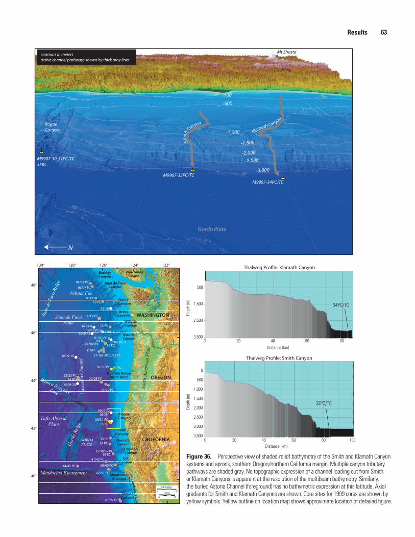
Results 63
Klamath Canyon
N
M9907-34PC/TC
M9907-33PC/TC
Smith
CanyonRogueCanyon
Gorda Plate
M9907-30-31PC/TC55KC
Mt Shasta
-2,000
-2,500
-1,500
-500-100
-1,000
-3,000
Distance (km)
Dept
h (m
)
0 20 40 60 80 1003,500
3,000
2,500
2,000
1,500
1,000
500
0
Distance (km)
Dept
h (m
)
0 20 40 60 803,500
2,500
1,500
500
34PC/TC
33PC/TC
AstoriaFan
Juan
de F
uca
Ridg
e
Juan de FucaPlate
Cas
cadi
a C
hann
el
Blanco Fracture Zone
Gord
a Ri
dge
GORDAPLATE
Mendocino Escarpment
Tufts AbyssalPlain
Nitinat Fan
08/09 PC
06/07 PC
05 PC
11/12 PC
13 PC14/15 PC
01/03 PC
16 PC
17/18/19/20/21 PC
26/28 PC
27/29 PC
30/31 PC
33 PC34 PC
35/36/37 PC
41/42 PC
39/40 PC
47/51 PC
44/45 PC
48/49 PC
22/23 PC
10 PC
02/56 PC 01 KC
55 KC
38 BC
24 BC
04 BC
6509-15
6502 PC-1
6705-5
6609-16609-12
6609-24
6508 K1
6705-6
53-18
130° 128° 126° 124° 122°
-
42°
44°
46°
48°
BarkleyCanyon
VancouverIsland
Juan de FucaCanyon
QuinaltCanyon
Grays Canyon
Willapa Canyon
EelCanyon
MendocinoChannel
Noyo Canyon
San Andreas Fault
40°
OREGON
WASHINGTON
CALIFORNIA
North
Am
eric
an P
late
0 100
Kilometers
0 50
Miles
Astoria Canyon
Hydrate RidgeBasin West
RogueCanyon
SmithCanyon
Klamath Canyon
Trinidad Canyon
contours in metersactive channel pathways shown by thick gray lines
Figure 36. Perspective view of shaded-relief bathymetry of the Smith and Klamath Canyon systems and aprons, southern Oregon/northern California margin. Multiple canyon tributary pathways are shaded gray. No topographic expression of a channel leading out from Smith or Klamath Canyons is apparent at the resolution of the multibeam bathymetry. Similarly, the buried Astoria Channel (foreground) has no bathymetric expression at this latitude. Axial gradients for Smith and Klamath Canyons are shown. Core sites for 1999 cores are shown by yellow symbols. Yellow outline on location map shows approximate location of detailed figure.

64 Turbidite Event History—Methods and Implications for Holocene Paleoseismicity of the Cascadia Subduction Zone
deposited across the shelf and on the slope, but 65 percent is transported down upper Trinidad and Eel Canyons (Austin and Nittrouer, 2001). The combined effect of the mud deposited in Trinidad Canyon and of the structural setting has resulted in slope instability and erosion of a 50-km-wide amphitheater-shaped upper to middle canyon (fig. 39; Wolfe and Hamer, 1999). This morphology contrasts with the other Cascadia margin canyons that are narrow (10–20 km) and incised across the slope (fig. 1). The upper Trinidad Canyon funnels downstream into a narrow canyon of a few kilometers width that crosses an unusually steep lower-continental slope (12.5°; fig. 39). At the base of the continental slope, the canyon feeds into a plunge pool that is 5.5 km in diameter and 50–80 m deep (fig. 12 in Nelson, C.H., and others, 2000). Radiating out from the plunge pool, a sediment-wave field that extends for about 17 km exhibits wave lengths of 3–5 km and wave heights of 20–50 m. No channel-levee complexes are formed or connected to the canyon mouth. Studies of some other smaller canyons on the Cascadia and New Jersey continental margins suggest that when slope steepness exceeds 4°, plunge pools form at the base of the continental slope in the canyon mouth region (Lee, and others, 2002).
Trinidad Turbidite SequenceThe Trinidad plunge pool and sediment-wave field
complex is also a turbidite system, because graded sand turbidite beds are found in both the plunge pool and sediment waves (fig. 40). The apron-like geometry of the Trinidad turbidite system is somewhat like the Rogue system. 3.5-kHz chirp subbottom records indicate excellent bed continuity between the pool and sediment-wave field. Cores M9907-35PC, M9907-35TC, M9907-36PC, M9907-36TC, M9907-37PC, and M9907-37TC and box core M9907-38BC all were collected within the Trinidad plunge pool, and all three cores include nine major Holocene turbidites (fig. 40). Because the plunge pool at the Trinidad Canyon mouth appears to trap most of the turbidite deposition during the Holocene, the pool provides the best record of turbidite events and is expanded in comparison to other systems. The expanded record provides increased resolution and detail of some turbidites and a record of hemipelagic material between some of the smaller events that is absent or difficult to distinguish elsewhere. Hemipelagic sediment is rare between the larger events; we suspect this is because of the higher energy of deposition in the plunge pool and greater basal erosion. Gradational very fine sand to silt turbidite-bed thicknesses of 5–10 cm are characteristic of the turbidites in all environments at the Trinidad site. Individual turbidites from the plunge pool exhibit unusual double or triple sand/coarse silt pulses within each bed, not unlike the multiple basal sand/coarse silts found in turbidites of the other Cascadia Basin turbidite systems. The difference is that there is greater separation between the coarser units, much like Hydrate Ridge, which we attribute to the proximal location. Alternatively, there could be internal reflections of the turbidity currents within the plunge pool. The turbidites in the Trinidad system typically have two or rarely three distinct cleaner sand or coarse
silt pulses that are 1–3 cm thick and separated by several centimeters of muddy silt with little hemipelagic sediment.
No Mazama ash is found south of the Rogue River and, consequently, we rely on AMS radiocarbon dates and stratigraphic correlation. Because little hemipelagic sediment is available in these cores, we were able to date only 11 turbidites in the Trinidad system, while the stratigraphic correlation is reasonably good (fig. 40).
Eel Canyon Pool, Sediment Wave, Channel, and Lobe Turbidite System
The morphology of the Eel pool/channel turbidite system in the proximal region is similar to the Trinidad system (fig. 39; Nelson and others, 2000). At the base of the continental slope, the steep (10°), narrow (<10 km) canyon feeds into an irregular plunge pool that is about 5 km in diameter and 50 m deep (fig. 39). Radiating out from the plunge pool, an asymmetric sediment-wave field extends for about 25 km, exhibiting wave lengths of 2.5–5.5 km and wave heights of 30–80 m. This sediment-wave field has larger waves and is longer than that in the Trinidad pool and wave system. An irregular channel threads its way through the sediment waves and is connected downstream to a well-developed channel-levee complex that has a channel floor width of 1.8 km and a relief of 25 m on the higher right-hand levee (Wolf and Hamer, 1999). This channel-levee complex extends for 25 km beyond the sediment-wave field and forms a ponded lobe in a local graben structure on the Gorda Plate (Chaytor and others, 2004).
Eel Canyon Pool, Sediment Wave, and Channel Turbidite Sequence
The sand-rich Eel Channel turbidite system has numerous, thin, graded-sand turbidite beds in all canyon-mouth, plunge-pool, sediment-wave, channel, and lobe environments (fig. 41). The thin-bedded units in the proximal cores mostly lack hemipelagic sediment, making it difficult to distinguish multibed turbidites from smaller single-bed deposits.
The thickest Eel Channel turbidite beds (10–15 cm) are found in cores M9907-39PC, M9907-M9907-40PC, and M9907-40TC in the canyon-mouth floor. The proximal-pool turbidites are thicker and more sand-rich than those in more distal environments. The lateral continuity of late Holocene turbidite beds is consistent across different geomorphic environments in the Eel Channel turbidite system. The proximal canyon mouth and plunge-pool floor of the Eel Channel system show excellent turbidite-bed continuity in both the cores (fig. 41) and 3.5-kHz reflection records. The 14C data show that the distal cores, M9907-41PC and M9907-41TC, extend to ~3,800 cal yr B.P. We dated intervals from these cores, rather than the proximal cores, because the hemipelagic sediment was better defined in the distal cores. The proximal cores M9907-30PC, M9907-40PC, and M9907-40TC are correlated tentatively to M9907-41PC and M9907-41TC on the basis of physical-property correlation shown in

Results 65
100 cm
200 cm
300 cm
400 cm
500 cm
600 cm
700 cm
800 cm
0 cm 5 15
Hemipelagic clayTurbidite silty mud
Sand
Silt
Mottled clayBurrows
Pleistocene
Very fine sand
ShellWood fragment
LITHOLOGY
CASC 79: 490 (430–570)
CASC 81: 1,480 (1,310–1,610)
CASC 220: 500 (420–590)
CASC 83: 7,190 (7,080–7,280)
CASC 84: 7,740 (7,620–7,850)
CASC 82: 4,160 (3,960–4,350)
CASC 80: 1,220 (1,120–1,350)
CASC 291: 3,880 (3,750–4,010)
CASC 292: 7,160 (7,000–7,300)
CASC 274: 4,010 (3,850–4,120)*
1.31.6 1.6 1.20 30
0 50 100 150 200
0 50 100 150 200
M9907-33PCM9907-33TCSmith Apron
10 50
Hoxidized
H
H
H
H
H
H
H
H
H
H
H
H
H
H
H
H
H
H
H
H
H
H
H
H
H
H
H
H
H
1.0
2.0
1.0
2.0
3.0
4.0
5.0
6.0
7.0
8.0
% MA0 50
0.5
0
0
0.5
0.5
0.5
0
0.5
0.5
0.5
0
T1
T2
T3
T2a
T4
T5
T6
T8
T7?
T5a
T5b
T3
T4
T5
T6
T9
T8
T7
T5a
T5b
T2
T13
T14
T2a
T9a
T10
T11
T10d
T10c
T10a
T10b
T12?
T13a
T12a?
T5c T5c
T8a
T8b
T10f
180 (90–280)
1,180 (1,000–1,350)
1,840 (1,660–2,020)
CASC 11: 7298 (7220-7377)
Gamma density (g/cm3 )
Radiocarbon sample location
EXPLANATION
Core break
Correlation Lines, dashed if uncertain
Percentage of Mazama ash
First occurrence, Mazama ash
High-resolution magnetic suscepibility (SI units)
Low-resolution magnetic susceptibility (SI units)
Sample number: AMS 14 C age and 2σ rangeCASC 11: 7,298 (7,220–7,377)
14C age and 2σ range14C age and 2σ range
CASC 11: 7,298 (7,220–7,377)
H/P Holocene/Pleistocene boundary
Hemipelagic age and estimated 2 σ range7,298 (7,220–7,377)
Sample number: erosion corrected AMS 14C age and 2σ range
CASC 11: 7,298 (7,220–7,377)
CT Density (gray level)
*Asterisk indicates benthic age
0.5
Figure 37. Site-correlation diagram for Smith Canyon cores (see figs. 2 and 36 for core locations). Mazama ash is not present in Smith Canyon cores. Numerous additional small turbidites are apparent in some southern Cascadia cores, including Smith Canyon earlier than ~T9 or ~4,200 cal yr B.P. (see discussion). 14C ages in cal yr B.P., including 2s-error ranges; see appendix 1 for radiocarbon age data. (See Methods section.) Abbreviations: AMS, accelerator mass spectrometry; g/cm3, grams per cubic centimeter; SI, Systeme Internationale.

66 Turbidite Event History—Methods and Implications for Holocene Paleoseismicity of the Cascadia Subduction Zone
1.0
2.0
1.0
2.0
3.0
4.0
5.0
6.0
7.0
100 cm
200 cm
300 cm
400 cm
500 cm
600 cm
700 cm
0 cm
CASC 221: 3,360 (3,210–3,500)
CASC 75: 3,380 (3,220–3,540)
CASC 276: 490 (420–550)*600 (510–700)
850 (740–970)
1,140 (1,030–1,260)
1,510 (1,390–1,640)
2,610 (2,440–2,750)
3,120 (2,970–3,280)
CASC 223: 4,210 (4,070–4,340)
CASC 224: 4,740 (4,610–4,900)
CASC 219: 3,330 (3,160–3,510)
CASC 76: 5,990 (5,880–6,130)
CASC 78: 9,780 (9,530–9,960)
CASC 222: 5,400 (5,300–5,490)
H
H
H
H
Light
Dark, mottled
Medium
Medium
Light
Light
Medium
Dark
Dark
Medium
Light
Medium
Medium
Light
Medium
Dark
Light
Dark
Dark
H
H
H
H
H
H
H
H
H
H
H
H
H
H
H
Light
Dark
Light-Medium
Dark
Medium
Light
Light
Dark
Light
Dark
Medium
Medium
Medium
Dark
Medium
Medium
Medium
Medium
Medium
Dark
Medium
Light
Dark
Dark
Light
Dark
Dark
Light
Light
Dark
Dark
Light
Dark
Light with dark mottles
Medium
Medium
Dark
Light
Medium
Medium
Medium
Medium
Medium
Dark
Medium
Medium
Light
Dark
Light
Dark
Light
Dark
Medium
Medium
H
H
H
H
H
H
H
H
H
H
H
H
H
M9907-34PCM9907-34TC
Klamath Apron1.6 1.2 1.6 1.2
8 18 5 15
% MA0 50
0
0
0
0
0
0
0
0
0.5
0.5
0.5
0.5
0
0180
0180
T9
T10
T10b
T10d
T10a
T9a
T10f
T10c
T5
T6
T8
T7
T5a
T10e
T8a
T5b
T3
T5c
T8b
T4
T1
T2
T3
T2a
T4
T5
T6?
T7
T5aT5b
T8
T5c
T1a
Y
Hemipelagic clayTurbidite silty mud
Sand
Silt
Mottled clayBurrows
Pleistocene
Very fine sand
ShellWood fragment
LITHOLOGY
H
CASC 11: 7298 (7220-7377)
Gamma density (g/cm3 )
Radiocarbon sample location
EXPLANATION
Core break
Correlation Lines, dashed if uncertain
Percentage of Mazama ash
First occurrence, Mazama ash
High-resolution magnetic suscepibility (SI units)
Low-resolution magnetic susceptibility (SI units)
Sample number: AMS 14 C age and 2σ rangeCASC 11: 7,298 (7,220–7,377)
14C age and 2σ range14C age and 2σ range
CASC 11: 7,298 (7,220–7,377)
H/P Holocene/Pleistocene boundary
Hemipelagic age and estimated 2 σ range7,298 (7,220–7,377)
Sample number: erosion corrected AMS 14C age and 2σ range
CASC 11: 7,298 (7,220–7,377)
CT Density (gray level)
*Asterisk indicates benthic age
0.5
Figure 38. Site-correlation diagram for Klamath Canyon cores (see figs. 2 and 36 for core locations). Mazama ash is not present in Klamath cores. Numerous additional small turbidites are apparent in some southern Cascadia cores, including Klamath Canyon earlier than ~T10b or ~5,000 cal yr BP. 14C ages in cal yr B.P., including 2s-error ranges; see appendix 1 for radiocarbon age data. See Discussion and Methods sections for additional information. Abbreviations: AMS, accelerator mass spectrometry; g/cm3, grams per cubic centimeter; SI, Systeme Internationale.
Figure 39 (right). Perspective view of shaded-relief bathymetry of the Trinidad, Eel, and Mendocino canyon/channel systems and plunge pools, northern California margin. Multiple canyon tributary pathways are shaded gray. No topographic expression of a channel leading out from Trinidad plunge pool is apparent at the resolution of the multibeam bathymetry. The buried Astoria Channel (foreground) has bathymetric expression at this latitude. Axial gradients for Trinidad and Eel Canyons are shown. Core sites for 1999 cores are shown by yellow symbols. Yellow outline on location map shows approximate location of detailed figure.

Results 67
Eel Canyon
M9907-47PC/TC
M9907-41PC/TC
Trin
idad
Can
yon
Gorda Plate
M9907-35PC/TC36 PC/TC, 37 PC/TC38BC
Mt Shasta
M9907-51PC/TC
M9907-39PC/TCM9907-40PC/TC
Mendocino Channel
-2,000-2,500
-1,500
-500
-100
-1,000
-3,000
Distance (km)
Dept
h (m
)
0 20 40 60 803,500
3,000
2,500
2,000
1,500
1,000
500
0
35-37PC/TC
Distance (km)
Dept
h (m
)
0 50 1003,000
2,500
2,000
1,500
1,000
500
0
47-51PC/TC52BC
Distance (km)
Dept
h (m
)
0 50 1003,500
3,000
2,500
2,000
1,500
1,000
500
0
39-40PC/TC41PC/TC
AstoriaFan
Juan
de F
uca
Ridg
e
Juan de FucaPlate
Cas
cadi
a C
hann
el
Blanco Fracture Zone
Gord
a Ri
dge
GORDAPLATE
Mendocino Escarpment
Tufts AbyssalPlain
Nitinat Fan
08/09 PC
06/07 PC
05 PC
11/12 PC
13 PC14/15 PC
01/03 PC
16 PC
17/18/19/20/21 PC
26/28 PC
27/29 PC
30/31 PC
33 PC34 PC
35/36/37 PC
41/42 PC
39/40 PC
47/51 PC
44/45 PC
48/49 PC
22/23 PC
10 PC
02/56 PC 01 KC
55 KC
38 BC
24 BC
04 BC
6509-15
6502 PC-1
6705-5
6609-1
6609-12
6609-24
6508 K1
6705-6
53-18
130° 128° 126° 124° 122°
-
42°
44°
46°
48°
BarkleyCanyon
VancouverIsland
Juan de FucaCanyon
QuinaltCanyon
Grays Canyon
Willapa Canyon
Noyo Canyon
San Andreas Fault
40°
OREGON
WASHINGTON
CALIFORNIA
North
Am
eric
an P
late
0 100
Kilometers
0 50
Miles
Astoria Canyon
Hydrate RidgeBasin West
RogueCanyon
SmithCanyon
Klamath Canyon
Trinidad Canyon
EelCanyon
MendocinoChannel
Mendocino Escarpm
entcontours in metersactive channel pathways shown by thick gray lines

68 Turbidite Event History—Methods and Implications for Holocene Paleoseismicity of the Cascadia Subduction Zone
100 cm
200 cm
300 cm
400 cm
500 cm
600 cm
700 cm
0 cm
CASC 210:250 (70–380)
CASC 65: not picked
CASC 211: 750 (610–870)CASC 212:830 (710–990)
CASC 10+10B: not picked
CASC 230: not picked
CASC 36: too few
CASC 216:1,560* (1,430–1,690)
CASC 217: 690 (610–800)*
CASC 215: 780 (640–920)*
CASC 66: 2,440 (2,280–2,620)
CASC 11+B: not picked
CASC 12: > modern
CASC 214: 540 (480–620)
CASC 218: 1,440 (1,320–1,560)*
CASC 213: 800 (660–940)
CASC 66 (37PC): 2,440 (2,280–2,620)
CASC 284: 1,510 (1,380–1,650)*
CASC 282:620 (520–700)*
CASC 283: 1,230 (1,080–1,280)*
CASC 288: not run
CASC 281:560 (500–630)*
CASC 280:460 (360–590)*
CASC 278:800 (690–900)*
CASC 286: 2,090 (1,950–2,250)*
CASC 287: 2,680 (2,500–2,770)*
CASC 33: 1,870 (1,740–2,010)*
H
H
H
H
H
H
H
H?
H?
H?
H?
H
H?
H?
H?
H?
H?
H?
H?
H?
HH
H
H
H
H
H
H
H
0 2010 20
0 20 10 25 10 17 0 20 10 140 1001.31.61.21.21.6
1.21.6 1.52.0 1.21.6 1.21.81.8
T6
T3
T4
T5a
T7
T5
T5b
T1
T5c
T3a
T4a
T6a
T3b
T1
T4b
T4b
T4b
Trinidad PoolM9907-36PCM9907-36TC M9907-37PCM9907-37TCM9907-35PCM9907-35TC M9907-38BC
01200120
1.0
2.0
1.0
2.0
3.0
4.0
5.0
6.0
7.0
1.0
2.0
1.0
2.0
3.0
4.0
5.0
6.0
1.0
2.0
1.0
2.0
3.0
4.0
5.0
6.0
7.0
Hemipelagic clayTurbidite silty mud
Sand
Silt
Mottled clayBurrows
Pleistocene
Very fine sand
ShellWood fragment
LITHOLOGY
H
CASC 11: 7298 (7220-7377)
Gamma density (g/cm3 )
Radiocarbon sample location
EXPLANATION
Core break
Correlation Lines, dashed if uncertain
Percentage of Mazama ash
First occurrence, Mazama ash
High-resolution magnetic suscepibility (SI units)
Low-resolution magnetic susceptibility (SI units)
Sample number: AMS 14 C age and 2σ rangeCASC 11: 7,298 (7,220–7,377)
14C age and 2σ range14C age and 2σ range
CASC 11: 7,298 (7,220–7,377)
H/P Holocene/Pleistocene boundary
Hemipelagic age and estimated 2 σ range7,298 (7,220–7,377)
Sample number: erosion corrected AMS 14C age and 2σ range
CASC 11: 7,298 (7,220–7,377)
CT Density (gray level)
*Asterisk indicates benthic age
0.5
Figure 40. Site-correlation diagram for Trinidad Channel cores (see figs. 2 and 39 for core locations). Mazama ash is not present in Trinidad cores. Numerous additional small turbidites are apparent in Trinidad plunge pool. We observe four turbidites above what may be margin-wide event T1, similar to Eel and Mendocino channels. Our interpretation and correlation of turbidites for Trinidad Canyon and Eel Canyon cores is assisted by correlating low-resolution magnetics, which effectively filters smaller turbidites from the record. 14C ages in cal yr B.P., including 2s-error ranges; see appendix 1 for radiocarbon age data. (See Discussion and Methods sections for additional information.) Abbreviations: AMS, accelerator mass spectrometry; CT, computed tomography; g/cm3, grams per cubic centimeter; SI, Systeme Internationale.

Results 69
M9907-41PCM9907-41TC
Eel Channel/Plunge Pool
1.0
2.0
3.0
4.0
1.0
Hemipelagic clay
Turbidite silty mud
Sand
Silt
Mottled clay
Burrows
Pleistocene
Very fine sand
Shell
Wood fragment
LITHOLOGY
Gamma density (g/cm 3)
Radiocarbon sample location
EXPLANATION
Core break
Correlation Lines, dashed if uncertain
Percentage of Mazama ash
First occurrence, Mazama ash
High-resolution magnetic suscepibility (SI units)
Low-resolution magnetic susceptibility (SI units)
Sample number: AMS 14C age and 2 σ rangeCASC 11: 7,298 (7,220–7,377)
Sample number: reversed AMS 14C age and 2 σ rangeCASC 11: 7,298 (7,220–7,377)
H/P Holocene/Pleistocene boundary
Hemipelagic age and estimated 2 σ range7,298 (7,220–7,377)
Sample number: erosion corrected AMS 14C age and 2 σ rangeCASC 11: 7,298 (7,220–7,377)
CT Density (gray level)
Asterisk indicates benthic age
0.5
CASC 39: 30 (0–150)
CASC 38:270 (180–370)
CASC 37: 1,430 (1,300–1,580)
CASC 40: 2,780 (2,640–2,970)
CASC 104: 3,420 (3,300–3,550)
CASC 105: 3,280 (3,130–3,430)
CASC 106: 2,860 (2,720–3,010)
CASC 13: 3,800 (3,630–3,950)
CASC 265: 190 (0–280)*
CASC 266: 500 (450–600)*
CASC 267: 1,660 (1,530–1,790)
H
H
H
H
H
H
H
H
H
H
H
H
H
H
H
H
H
H
H
H
H
H
H
H
1.8 1.2
1.0
2.0
3.0
H
H
H
HH
H
H
H
1.8 1.2 20 4024 34
M9907-39PC
1.8 1.3 5 15 5 2010 40 1.8 1.22.0 1.3
M9907-40PC M9907-40TC
T2
T3
T2a
T3a
T4
T5?
T6?
T8?
T7?
100 cm
200 cm
300 cm
400 cm
500 cm
600 cm
0 cm
T1
T4a?
T3b
T3c
Figure 41. Site-correlation diagram for Eel Channel cores (see figs. 2 and 39 for core locations). Mazama ash is not present in Eel Channel cores. Numerous additional small turbidites are apparent in Eel Channel stratigraphy. We observe four turbidites above what may be margin-wide T1. Our interpretation and correlation of turbidites for Trinidad and Eel Canyon cores is assisted by correlating low-resolution magnetics, which effectively filters smaller turbidites from the record. 14C ages in cal yr B.P., including 2s-error ranges; see appendix 1 for radiocarbon age data. (See Discussion and Methods sections for additional information). Abbreviations: AMS, accelerator mass spectrometry; CT, computed tomography; g/cm3, grams per cubic centimeter; SI, Systeme Internationale.

70 Turbidite Event History—Methods and Implications for Holocene Paleoseismicity of the Cascadia Subduction Zone
figure 41. We interpret that the proximal core M9907-40PC contains approximately 2,000 years of Holocene section, on the basis of correlation to the dated turbidite core M9907-41PC (fig. 41).
We interpret 51 turbidites in M9907-41PC, the distal core. With a dated event at the core base yielding an age of 3,800 (3,950–3,630) cal yr B.P., this yields a turbidite frequency of one per 60 years. We tentatively correlate the basal turbidite with marginwide T8, which has an average age of 3,475±170 cal yr B.P., somewhat younger than the Eel Channel age. The recurrence interval for Eel Channel (using the T8 age) is ~70 years. The large number of thin turbidite beds in the Eel Channel system, like the Trinidad-system cores, may be related to input from the Eel River, additional seismic sources, or a mixture of sources. Recent detailed studies of the fluvial-sediment budgets for the Eel River Basin show that ~40 percent of the sediment input is deposited on the continental shelf and slope (Austin and Nittrouer, 2001). The remaining 60 percent of the sediment appears to be transported by sediment gravity flows downslope into upper Eel Canyon, one of the largest sediment sources on the U.S. west coast. In addition, both Eel and Mendocino Canyon heads erode close to the shoreline where the canyon heads may intersect the littoral-drift sediment that can be funneled downcanyon by storms (fig. 2). The distance from the canyon heads to the coast is only 12 km, by far the narrowest shelf width in Cascadia. The head of Mendocino Canyon, which has the highest frequency of turbidite events, comes within 1 km of the shoreline.
We note that the largest events, clearly separable from the numerous small events, are possible stratigraphic and temporal turbidite correlatives with other Cascadia sites. However, an event we tentatively correlate with the A.D. 1700 earthquake is not the uppermost turbidite; rather it is overlain by three younger turbidites, as is in the Trinidad system cores (fig. 40).
To attempt to test correlations with more northerly cores, we low-pass filtered the smaller high-frequency events from the magnetic records used for correlation by using a loop magnetic sensor with a lower resolution. This technique effectively images only the thicker beds. We note that the thicker beds, clearly separable from the numerous thinner ones, are moderately good stratigraphic and temporal correlatives with other Cascadia sites. The Eel, Trinidad, and Mendocino system cores, however, are far from ideal and require further work to correlate the local cores and apply tests of origin beyond those presented here.
Mendocino ChannelThe Mendocino Canyon feeds Mendocino Channel that
lies at the base of the Mendocino Escarpment (figs. 1, 2, 39). The escarpment topography and the meandering channel pathway have been controlled by the extensive tectonic activity of the Mendocino Triple Junction (Cacchione and others, 1996; Wolf and Hamer, 1999). Even with the extensive tectonic disruption, this turbidite pathway has been more active than any other Cascadia Basin turbidite system, likely because its proximal canyon head erodes to within 1 km of the shoreline. After meandering along the escarpment for 50 km, the distal
end of the channel turns northwest into the Gorda Basin, where it may coalesce with the Eel Channel turbidite system. The Mendocino Channel does not exhibit proximal plunge pools or distal lobe development in any of the 3.5-kHz profiles downstream (Cacchione and others, 1996; Wolf and Hamer, 1999); thus, it is a connecting channel-levee-complex type of turbidite system. We have sampled this narrow channel (0.5 km width) in its central area of tight meanders, approximately 55–60 km downstream from the canyon mouth.
Mendocino Channel Turbidite SequenceThe sand-rich Mendocino Channel has the highest
frequency of deposition of turbidite beds in Cascadia Basin. No Mazama-ash turbidite bed or faunal Pleistocene-Holocene boundary datum was penetrated by our 5-m cores (M9907-51PC, M9907-51TC). The stratigraphy of two archive 1986 box cores (LH-86-NC/Box 1 and LH-86-NC/Box 5; Cacchione and others, 1996) reveals six turbidite beds, four of which were deposited during the past 260 years (fig. 42). These dates show that, during the latest Holocene, the average turbidite frequency in the central channel was one per ~65 years, similar to Eel Channel, although with a higher overall sedimentation rate. In piston core M9907-51PC, a few kilometers downstream from LH-86-NC/Box 1, an age of ~800 (950–650) cal yr B.P. was obtained for the fifteenth turbidite down at 4-m depth in hemipelagic sediment. The deep young age indicates a highly expanded section in Mendocino Channel, with a turbidite frequency of 1 per ~34 years during the past ~800 years (fig. 42).
The penultimate turbidite (labeled T0a) in our core M9907-51TC has ~8 cm of hemipelagic sediment overlying it and is in turn capped by an organic-debris blanket consisting of 2–4 cm of twigs, roots, and plant fragments, representing T0. The likely correlative unit is sandy in LH-86-NC/Box 1 and overlain by 7 cm of hemipelagic sediment. The total hemipelagic thickness in LH-86-NC/Box 5 above T1 is ~25 cm, yielding a sedimentation rate of ~84 cm/1,000 yr (adding 36 years to the B.P. 1950 calibrated age to correspond to the 1986 date of collection). Overlying T0, LH-86-NC/Box 1 and
Figure 42 (right). Site-correlation diagram for Mendocino Channel cores (see figs. 2 and 39 for core locations). LH-86-NC/Box 1 and LH-86-NC/Box 5 were collected in 1986 (Cacchione and others, 1996, and unpublished logs and photographs). Location map and GLORIA image were modified after Cacchione and others (1996). Mazama ash is not present in Mendocino Channel cores. High-frequency turbidite record in Mendocino Channel includes four events younger than the ~260±60 ca yr B.P. age of T4, which may correlate to marginwide A.D. 1700 earthquake on the basis of similarity of the 14C ages. Correlation of box- and piston-core stratigraphy reveals hemipelagic sediment between multiple events in the box cores that is not as apparent in the piston core stratigraphy. 14C ages in cal yr B.P., including 2s-error ranges; see appendix 1 for radiocarbon age data. (See Methods section.) Abbreviations: AMS, accelerator mass spectrometry; g/cm3, grams per cubic centimeter; SI, Systeme Internationale.

Results 71
0 cm
80 cm
20 cm
40 cm
60 cm
CASC 23: 820 (670–970)
510
1520
25
0 101.21.8
0 cm
100 cm
200 cm
300 cm
400 cm
500 cm
M9907-51PCM9907-51TC
Gamma density (g/cm
3)
Radiocarbon sample location
EXPLANATION
Core break
Correlation Lines, dashed if uncertain
Percentage of Mazama ash
First occurrence, Mazama ash
High-resolution magnetic suscepibility (SI units)Low-resolution magnetic susceptibility (SI units)
Sample number: AMS 14C age and 2 σ rangeCASC 11: 7,298 (7,220–7,377)
Sample number: reversed AMS 14C age and 2 σ rangeCASC 11: 7,298 (7,220–7,377)
H/P Holocene/Pleistocene boundary
Hemipelagic age and estimated 2 σ range7,298 (7,220–7,377)
Sample number: erosion corrected AMS 14C age and 2 σ rangeCASC 11: 7,298 (7,220–7,377)
0.5
Hemipelagic clay
Turbidite silty mud
Sand
Silt
Needles, small leaves and roots
Burrows
Very fine sand
Shell
Wood fragment
LITHOLOGY
H
CASC 270: 230 (90–310)
CASC 271: 470 (380–540)*
CASC 272: 710 (640–830)*
CASC 269* 160 (30–250)
0 15
* Asterisk indicates benthic age
?
?
?
Mendocino Channel
LH-86-NCBOX 5 M9907-51TC M9907-51PC
LH-86-NCBOX 1
1.01.5
H
H
H
H
H
H
H
H
H
Modern
130 (0–264)
260 (59–406)
10 km
Mendocino Channel
Mendocino Ridge
Modified from Cacchione and others, 1996
Trace of transform fault
Gorda Basin
Sonar look direction
BX 1
Mendocino Channel
Location
Mendocino Channel
51PC
BX 1
BX 5
310 (111–500)
1.0
2.0
3.0
4.0
5.0
CASC 273: 830 (720–910)
CASC 269 140 (10–240)
1
2
9
10
11
8
8a
7
6a
6
5
4
3
11a
12
13
14
16
17
18
17a
19
20
21
22
23
24
25
26
27
28
29
30
31
3233343536
15
9a
8b
18a
19a
27a
72 Turbidite Event History—Methods and Implications for Holocene Paleoseismicity of the Cascadia Subduction Zone
LH-86-NC/Box 5 have 7–8 cm of hemipelagic sediment, suggesting an age of T0 of 80–95 years prior to collection in 1986, corresponding to a calendar age of ~A.D. 1890–1910 (2σ 1830–1940, including 14C range and H thickness range). This turbidite could correlate to the 1906 earthquake on the nearby San Andreas Fault. The next event downward, T0a, is separated by ~8 cm of hemipelagic sediment (with one thin stringer of silt, a possible burrow) representing ~95–120 years below T0, or an event age of ~A.D. 1790–1810. T0b is dated at A.D. 1820+60 and T1 at A.D. 1710+60 (fig. 42).
Regional Stratigraphic CorrelationBuilding on the original work of Adams (1990), we
observed from our earliest shipboard examination of the cores that some obvious regional marker horizons existed in addition to the Mazama ash contained in T13. For example, the eleventh event down in most cores is a very large sandy event, as is the sixteenth event down. We have explored regional correlations in the Holocene turbidite section extensively to test for regional event continuity or lack thereof along the Cascadia margin. In figure 43 we show several representative examples from Cascadia Basin channels of stratigraphic correlation of key stratigraphic horizons supported by radiocarbon dates. Radiocarbon data, reservoir corrections, sample thickness, erosion corrections, and sedimentation-rate curves used in this compilation are given in their entirety in appendix 1. Appendix 1 also includes calculation of ages based on hemipelagic thickness for undated events, as well as for comparison to dated events. Hemipelagic dates, when used in the correlation, are shown with a color code in figures 43–46.
The correlated horizons in figures 43–46 are the foundation for regional correlations; they are supported by radiocarbon data but represent independant primary stratigraphic ties. The regional stratigraphic framework correlations among Cascadia channels in figures 43–46 are modified and extended in time from those of Goldfinger and others (2008) to ~10 k.y. Figure 44 shows the margin correlations at true scale; however, it is difficult to evaluate the quality of the stratigraphic correlation using this type of diagram because it is complex and difficult to see the details of individual events side by side with those of other sites. To allow the reader to view the data in a common framework, figures 45 and 46 are “hung” in the vertical framework of Rogue Apron core M9907-31PC with event bases “flattened” to those of the Rogue Apron core. This is done so that individual turbidites line up horizontally across the figures for visual comparison and is a primary aid to correlation (Thompson and others, 1975). Rogue Apron core M9907-31PC is chosen because it contains nearly all of the smaller southern Cascadia events, is interpretable down to the Pleistocene-Holocene boundary, and has no significant distortions or gaps, although it is missing several events at its top, which are included in the trigger core M9907-31TC. The vertical scales of other cores are adjusted to match M9907-31PC.
The correlated horizons were determined through iterative visual correlation, which proved superior to least squares and other numerical methods. Although we attempted numerical analyses, as described previously, the results ultimately were compatible with visual correlation, but offered little added value. The reasons that numerical methods were inferior include the inability to include all data simultaneously (for example, X-ray, CT, visible imagery, logs, physical properties, and radiocarbon) and the inability of algorithms to recognize core artifacts, distortions, and explicable variability, which were readily apparent to a human interpreter when all the data were used. This commonly caused automatic methods to fail, even when every horizon was dated and well correlated. Thus, we were unable to achieve good results using purely numerical methods in whole-core series; however, we used correlation techniques with individual turbidites and with other derivative parameters, and these are discussed in subsequent sections.
We note that in addition to the Mazama ash, a number of turbidites provided unique horizons that served to strengthen the stratigraphic framework significantly. These include events T5, T7, T11, and T16, in particular. T5 is notable for its unusual stacking of coarse fining-upward units within the turbidite (fig. 14). This odd signature persists at many (but not all) sites, including Effingham Inlet, further discussed below. T7, in several channels, consists of three major units, but can be subdivided into as many as seven units, an unusual feature that persists in the Juan de Fuca and Cascadia Channel cores. T11 and T16 are distinguished by their great thickness at all sites but also have very distinctive three-unit and five-unit structures respectively, at nearly all sites as well. While some were more obvious than others, as we processed the data we
Figure 43 (right). Correlation examples. Correlation details from representative pairs of cores on the Cascadia margin. A, Events T5–T10 in cores from Rogue Channel (left) and Cascadia Channel (right). B, Events T9–T15 from Hydrate Ridge (left) and Rogue Channel (right). C, Events T11–T20 in Rogue Channel (left) and Juan de Fuca Channel (right). Note the strong similarity between event T11 in Hydrate Ridge (B), Rogue Channel (B, C) and Juan de Fuca Channel (C). This event has a distinctive shape that is recognizable marginwide, and it is characterized by a thick deposit with a broad, somewhat flat excursion in physical properties. Also note the multiple pulses reflected by the physical properties in event T16 in Rogue and Juan de Fuca Channels (C). Radiocarbon ages are calibrated using Calib 5.0.2. D, E, and F show CT imagery pairs for T9 and T7 and T6, respectively, in both Juan de Fuca and Cascadia Channels. The Juan de Fuca imagery is “flattened” to the upper and lower sand contacts of the corresponding Cascadia Channel units. These examples show the relatively unchanged internal structure of these typical events after passing the confluence at Willapa Channel and ~350 km of transport. Juan de Fuca channel imagery is degraded significantly by numerous small gas evolution voids, but the structural similarity is still evident. The primary structure of two pulses and three pulses for T9 and T6, respectively, is matched by density and magnetic peaks. T7 shows more pulsing (~7) than is resolvable with the geophysical data, but it is apparent in both cores.

Results
73
D. E. F.
T9 Cascadia Channel T9 Juan de Fuca Channel T7 Cascadia Channel T6 Cascadia ChannelT7 Juan de Fuca Channel T6 Juan de Fuca Channel
Hydrate RidgeRR0207-56PC
1.6 1.2
M9907-31PC-10 150
T9
T10
T11
T13
T14
T15
T10b
T10d
T10a
T9a
T15a
T10f
T10c
T12
T12a
Rogue Channel Rogue Channel Juan de Fuca ChannelM9907-12PC
0 1001.31.8
T18
T12
T16
T17
T11
T14
T13
T19
T15
T17a
RR0207-55KC0 120
T5aT5b
T6a
CASC 184 (30TC): 1,520(1,380–1,670)
CASC 163: 2,670 (2,580–2,780)
CASC 167: 4,840(4,680–5,070)
CASC 175+B: 4,180(3,990–4,400)
CASC 176+B: 5,070(4,860–5,260)
Rogue Channel
0 2001.7 1.2
� �
� �
� �
T7
T6
T5
T8
T9
T10
M9907-22PC
Cascadia ChannelA. T5–T10
1.11.6 1.11.6 0 200
slurp effect
4.0
5.0
6.0
B. T9–T15 C. T11–T20
1.6 1.2M9907-31 PC
10 150% MA
0 50
20
15
80
0
T20
T15a
T16a
T19a
T12a
4.0
5.0
6.0
2.0
3.0
4.0
% MA0 50
35
20
0 65
5 9
5
1
1
T14a
T5c
T14a
H
H
H
H
H
H
H
H
H
H
H
H
H
H
H
2.0T7a
T8a
T9a
T10a
1.0
2.0
3.0
3.0
HRW-09: 5,160(5,080–5,320)
CASC 70: 7,070(6,960–7,210)
CASC 71: 6,590(6,440–6,750)
CASC 148: 8,400(8,260–8,550)
CASC 149: 9,150(8,990–9,260)
CASC 88: 9,190(9,070–9,300)
CASC 89: 9,830(9,640–9,990)
CASC 90: 10,200(10,180–10,330)
CASC 91: 10,280(10,130–10,390)
CASC 92: 10,470(10,350–10,650)
CASC 114: 5,810 (5,680–5,960)
CASC 115: 6,440 (6,280–6,570)
CASC 116: 7,120(6,990–7,250)
CASC 117: 7,610(7,490–7,710)
CASC 118: 8,990 (8,860–9,140)
CASC 119: 9,330 (9,230–9,410)
CASC 120: 9,900 (9,680–9,980)
CASC 122: 10,690 (10,500–10,940)
T8b
CASC 130 (25PC): 2,550 (2,400–2,710)
CASC 131 (25PC): 3,490 (3,310–3,660)
CASC 132 (25PC): 4,160 (3,980–4,340)
4,740(4,600–4,970)
3,070(2,920–3,220)
4,160(4,000–4,330)
CASC 176+B: 5,070(4,860–5,270)
6,000(5,870–6,120)
7,940(7,800–8,080)
8,850(8,660–8,990)
9,070(8,910–9,230)
8,050(7,900–8,200)
9,530(9,340–9,770)
CASC 174: 3,590(3,400–3,820)
1,610(1,500–1,740)
CASC 173+B: 3,060(2,860–3,220)
CASC 146: 3,960(3,780–4,130)
CASC 31: 4,850 (4,630–5,030)
CASC 9: 7,670(7,530–7,820)
CASC 72: 8,280(8,190–8,390)
CASC 69: 5,220(5,080–5,350)
4,320(4,140–4,510)
5,390(5,240–5,590)
5,740(5,590–5,880)
6,900 (6,780–7,030)
7,940 (7,800–8,080)
8,460 (8,270–8,600)
CASC 32: 7,140(7,020–7,300)
4,540(4,360–4,730)
% MA0 50
15
20
15
80
0
H
H
H
H
H
H
H
H
H
H
H
H
H
H
H
H
HH
H
H
H
H
H
H
H
?
T9b
5,810(5,670–5,950)
6000(5,870–6,120)
HRW-10: 5,330 (5,210–5,430)
HRW-12: 8,650(8,470–8,820)
HRW-11: 7,220 (7,140–7,310)
HRW-13: 5,700 (5,560–5,830)
4,460 (4,290–4,620)
4,740(4,570–4,910)
5,920(5,790–6,050)
5,700(5,560–5,830)
7,650(7,480–7,820)
8150 (7,940–8,360)
5,290(5,120–5,490)
CASC 71: 6,590(6,440–6,750)
CASC 9: 7,670(7,530–7,820)
CASC 72: 8,280(8,190–8,390)
6,900 (6,780–7,030)
8,460 (8,270–8,600)
CASC 32: 7,140(7,020–7,300)
Hemipelagic clay
Turbidite silty mud
Sand
Silt
Mottled clay
Burrows
Pleistocene
Very fine sand
Shell
Wood Fragment
LITHOLOGY
H
Samp. #: Erosion corr. 14C age & 2σ rangeCASC 11: 7298 (7220-7377)
Gamma Density (g/cm3)
EXPLANATION
Core break
Correlation Lines, dashed if uncertain
Percentage of Mazama ash
First occurrence, Mazama ash
High-resolution point mag. susc. (SI)
Sample #: 14C age & 2σ rangeCASC 11: 7298 (7220-7377)
Samp. #: Reversed 14C age & 2σ rangeCASC 11: 7298 (7220-7377)
Hemipelagic age & est. 2σ range7298 (7220-7377)
Sample #: 14C age & 2σ range, erosion corr.CASC 11: 7298 (7220-7377)
0.5

74
Turbidite Event History—M
ethods and Implications for Holocene Paleoseism
icity of the Cascadia Subduction Zone
0 cm
100 cm
200 cm
300 cm
400 cm
500 cm
600 cm
700 cm
800 cm
?
H
H
H
H
H
H
H
H
H
H
H
H
H
H
H
H
H
F
H
H
H
H
H
H
H
H
H
H
H
H
H
H
H
H
H
H
HH
HH
HH
HH
H
H
H
H
H
HH
H
H
H
H
H
H
H
H
H
H
HH
H
H
H
0 1000 100
5
20
15
40
30
20
0.5
0.5
% MA% MA0 500 50
10
40
35
20
0 65
5 9
5
1
1
% MA% MA
-30 170
1.0
2.0
0.0
1.0
2.0
3.0
4.0
5.0
0.0
6.0
7.0
CASC 145:3,560 (3,310–3,710)
CASC 146
3,960 (3,780–4,130)
CASC 167
4,840 (4,680–5,070)
CASC 147
5,240 (5,090–5,370)
CASC 327,100 (6,980–7,260)CASC 97,670 (7,530–7,820)
CASC 149
9,150 (8,990–9,260)
CASC 88
9,190 (9,070–9,300)
CASC 89
9,830 (9,640–9,990)CASC 90
10,200 (10,180–10,330)CASC 91
10,280 (10,130–10,390)CASC 92
10,470 (10,350–10,650)CASC 93
10,950 (10,870–11,050)CASC 94
10,960 (10,820–11,080)CASC 95
10,940 (10,790–11,280)
CASC 155
11,530 (11,290–11,730)
210Pb(excess)
CASC 173+B (55KC)
3,060 (2,860–3,220)
CASC 156
11,400 (11,180–11,600)
CASC 157
11,870 (11,750–12,050)
CASC 72
8,250 (8,150–8,350)
T6a
T2T1
T3
T4
T5
T6
T7
T8T8a
T5b
T2a
T3a
T4a
T5a
T7a
T5c
CASC 141(30PC):
1,590 (1,420–1,750)
CASC 160 (55KC)
740 (680–810)
CASC 168 (55KC)
480 (370–580)
CASC 170 (55KC)
1,200 (1,100–1,290)
CASC 187 (30PC)
2,560 (2,490–2,710)
6,000 (5,870–6,120)
6,630 (6,440–6,810)6,900 (6,780–7,030)
7,940 (7,800–8,080)
T4
T5
T6
T7
T8
T9
T10
T11
T13
T14
T15
T16
T17
T17a
T18
T3
T19
T20
T21T22
T23
T24T25
T26
T10b
T10d
T10a
T9a
T5aT5b
T7a
T6a
T15a
T10f
T8a
T10c
T12
T16a
T19a
T12a
T8b
T4a
T3a
T5c
T9b
T14a
8,460 (8,270–8,600)
T8a or b
1.0
2.0
3.0
4.0
5.0
0.0
6.0
7.0
8.0
0.0-10 400
H
H
H
H
H
H
H
H
H
H
H
H
H
H
H
H
H
H
H
H
H
HH
H
H
H
H
H
Light
Dark
0 4000 2500 100
CASC 138+B (25PC):9,080 (8,930–9,200)
CASC 137+B (25PC):8,250 (8,140–8,350)
CASC 139 (25PC):9,870 (9,670–9,970)
CASC 131(25PC): 3,490 (3,310–3,660)
CASC 132 (25PC): 4,160 (3,980–4,340)
CASC 136 (25PC):7,650 (7,510–7,770)
CASC 130 (25PC): 2,550 (2,400–2,710)
CASC 178 (23TC): 270 (190–360)
CASC 182+135+b (23PC):7,150 (7,030–7,270)
CASC 128B (23PC): 1,300 (1,190–1,410)
HRW-10: 5,330 (5,210–5,430)
HRW-01: 11,010 (10,790–11,110)
HRW-17: 9,650 (9,460–9,860)
HRW-12: 8,650 (8,470–8,820)
HRW-11: 7,220 (7,140–7,310)
HRW-07+B+C: 3,470 (3,280–3,640)
HRW-03: 800 (700–910)
HRW-06+B+C: 2,960 (2,820–3,070)
HRW-16: 9,340 (9,260–9,410)
slurp
CASC 113 (12PC):4,700 (4,590–4,830)
CASC 114 (12PC):5,810 (5,680–5,960)CASC 115 (12PC):6,440 (6,280–6,570)CASC 116 (12PC):7,120 (6,990–7,250)CASC 117 (12PC):7,610 (7,490–7,710)
CASC 118 (12PC):8,990 (8,860–9,140)
CASC 119 (12PC):9,330 (9,230–9,410)
CASC 3 (12TC):270 (180–360)CASC 44 (12TC):
470 (390–550)CASC 43 (12TC):870 (770–990)CASC 45 (12TC):1,210 (1,090–1,330)
CASC B111 (12TC):1,580 (1,460–1,720)*
CASC 47 (12TC):3,500 (3,340–3,680)
CASC 46 (12TC):2,500 (2,340–2,600)
CASC 112 (12TC):3,070 (2,920–3,190)
CASC 120 (12TC):
9,900 (9,680–9,980)
CASC 107 (11TC):4,180 (4,020–4,310)
CASC 181+134 (23+25PC):6,580 (6,470–6,720)
HRW-24: 300 (230–410)
3,440 (3,280–3,610)
470 (370–600)
840 (750–940)
4,740 (4,560–4,930)
6,090 (5,910–6,280)
8,910 (8,710–9,050)
1,060 (950–1,180)
2,550 (2,410–2,720)
4,160 (4,000–4,330)
4,740 (4,570–4,910)
5,290 (5,120–5,490)
5,920 (5,790–6,050)
CASC 236 (09PC):2,520 (2,360–2,650)
CASC 240 (09PC):4,040 (3,870–4,220)
CASC 191 (08TC):1,530 (1,260–1,800)
CASC 1 (08TC):2,590 (2,350–2,830)
1,610 (1,500–1,740)
3,070 (2,920–3,220)
6,000 (5,860–6,140)
8,850 (8,660–8,990)
550 (440–670)
1,070 (970–1,200)
1,370 (1,260–1,500)
1,760 (1,580–1,930)2,020 (1,850–2,180)
2,320 (2,190–2,470)
2,730 (2,590–2,880)
3,160 (3,020–3,320)
3,600 (3,440–3,760)3,890 (3,720–4,080)
4,320 (4,140–4,510)4,540(4,360–4,730)
CASC 176+B
5,070 (4,860–5,260)
5,390 (5,240–5,590)
5,740 (5,590–5,880)
5,850 (5,700–5,990)
9,070 (8,910–9,230)
CASC 239 (08TC):6,790 (6,620–6,950)
CASC 55+B (09TC):7,610 (7,440–7,780)
7,220 (7,070–7,370)
9,760 (9,540–10,000)
CASC 237 (09PC):8,150 (7,980–8,450)
CASC 241 (09PC):8,870 (8,660–9,080)
CASC 238 (09PC):9,080 (8,,870–9290)CASC 24 (09PC):9,250 (8,950–9,520)
CASC 2: 11,650 (11,210–12,010)
CASC 243 (08TC):4,190 (3,950–4,470)
8,050 (7,900–8,200)
1,210 (1,100–1,340)
1,470 (1,330–1,620)
1,650 (1,490–1,810)
4,460 (4,290–4,620)
5,700 (5,560–5,830)
250 (200–300)
1.0
2.0
3.0
4.0
0.0
1.0
2.0
3.0
4.0
0.0
T1
T7
T6
T5
T4
T3
T2
T8
T9
T10
T11
T12
T13
T14
T15
T18
T16
T17
T17a
T18
T12
T16T17
T4
T5
T6
T11
T14
T7
T8
T9
T10
T13
T3
T2T1
T20
T19
T15
T17a
20
30
55
60
0.5
0.5
0.5
0.5
0.5
0
T8
T11
T14
T13
T6
T9
T7
T10
T12
T15?
T16?T17?T17a?T18?
dropstone
T9a
CASC 5B: 6,380 (6,260–6,520)
CASC 260: 4,540 (4,420–4,670)
4,760 (4,580–4,960)
5,990 (5,830–6,130)
4,080 (3,910–4,260)
3,560 (3,370–3,760)
7,200 (7,040–7,350)
M9907-17PC/TC
T19
T10
T13
T15
T17
T18
T10b
T10c
T3
T4
T7
T8
T4a?
T5
T6
T5a
T5b
T10f
T11
T2
T9
T10a
T16
T1
T5c
T17a
1.0
2.0
3.0
4.0
5.0
0.0
0.0
small uncorrelated event
CASC 229: 5,220 (4,980–5,360)
0 50% MA
T4
T5
T3
T2
T1
CASC 193: 740 (620–840)
230 (170–280)
470 (360–590)
CASC 192:1,280 (1,150–1,420) CASC 231 (16TC): 1,580 (1,480–1,700)
3,000 (2,860–3,150)
2,590 (2,410–2,770)
330 (280–380)
510 (410–610)
Hemipelagic clay
Turbidite silty mud
Sand
Silt
Mottled clay
Burrows
Pleistocene
Very fine sand
Shell
Wood fragment
LITHOLOGY
HSamp. #: Erosion corr. 14C age & 2σ rangeCASC 11: 7298 (7220-7377)
Gamma density (g/cm3)
Radiocarbon sample location
EXPLANATION
Core break
Correlation Lines, dashed if uncertain
Percentage of Mazama ash
First occurrence, Mazama ash
High-resolution magnetic suscepibility (SI units)
Low-resolution magnetic susceptibility (SI units)
Sample number: AMS 14C age and 2σ rangeCASC 11: 7,298 (7,220–7,377)
Sample number: reversed AMS 14C age and 2σ rangeCASC 11: 7,298 (7,220–7,377)
H/P Holocene/Pleistocene boundary
Hemipelagic age and estimated 2σ range7,298 (7,220–7,377)
Sample number: erosion corrected AMS 14C age and 2σ rangeCASC 11: 7,298 (7,220–7,377)
CT Density (gray level)
Asterisk indicates benthic age
0.5
� �
coringartifact
slurp
M9907-23PC M9907-31PC/TC, RR0207-55KC
Key Sites: Barkley to Rogue
RR0207-56PC/TCM9907-12PC
5.0
3.0
4.0
2.0
0.0
1.0
0 400
H
H
H
H
H
H
H
H
H
H
H
% MA% MA0 500 50
0.5
0
2
1
0
0
0
0
0
0
0.5
0.5
T6
T11
T15T15
T17
T17a
T24
T19
T21
T22
T23
T12
T16T16
T18T18
T5
T14T14
T2?T1?
T3?
T7
T9T8
T10
T13T13
T20
T4?
M9907-09PC
��
��
��
��
��
��
��
5.0
�
�
�
6.0
7.0
TCPCTC
PC
CASCADIA ROGUEHYDRATE RIDGEJUAN DE FUCA ASTORIABARKLEY
0 60
1.8
0 401.2 1.6 1.21.01.8 1.01.8
0 200
1.02.00 100
1.01.81.22.0
20 601.8 1.2
0 100
A
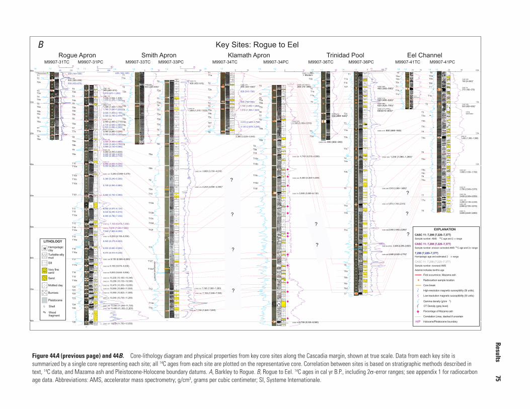
Results
75
Figure 44A (previous page) and 44B. Core-lithology diagram and physical properties from key core sites along the Cascadia margin, shown at true scale. Data from each key site is summarized by a single core representing each site; all 14C ages from each site are plotted on the representative core. Correlation between sites is based on stratigraphic methods described in text, 14C data, and Mazama ash and Pleistocene-Holocene boundary datums. A, Barkley to Rogue. B, Rogue to Eel. 14C ages in cal yr B.P., including 2s-error ranges; see appendix 1 for radiocarbon age data. Abbreviations: AMS, accelerator mass spectrometry; g/cm3, grams per cubic centimeter; SI, Systeme Internationale.
1.0
2.0
1.0
2.0
3.0
4.0
5.0
6.0
7.0
1.0
2.0
Hemipelagic clayTurbidite silty mud
Sand
Silt
Mottled clay
Burrows
Pleistocene
Very fine sand
Shell
Woodfragment
LITHOLOGY
H
Gamma density (g/cm 3)
Radiocarbon sample location
EXPLANATION
Core break
Correlation Lines, dashed if uncertain
Percentage of Mazama ash
First occurrence, Mazama ash
High-resolution magnetic suscepibility (SI units)
Low-resolution magnetic susceptibility (SI units)
Sample number: AMS 14C age and 2 σ rangeCASC 11: 7,298 (7,220–7,377)
Sample number: reversed AMS CASC 11: 7,298 (7,220–7,377)
H/P Holocene/Pleistocene boundary
Hemipelagic age and estimated 2 σ range7,298 (7,220–7,377)
Sample number: erosion corrected AMS 14C age and 2σ rangeCASC 11: 7,298 (7,220–7,377)
CT Density (gray level)
Asterisk indicates benthic age
0.5
M9907-41TC
1.0
24 34
Eel ChannelM9907-41PC
1.0
2.0
3.0
4.0
20 40
CASC 37:1,430 (1,300–1,580)
CASC 40: 2,780 (2,640–2,970)
CASC 105: 3,280 (3,130–3,430)
1.8 1.2
coringdeformation
CASC 266:500 (450–600)*
CASC 267: 1,660 (1,530–1,790)
H
H
H
H
H
H
H
H
H
H
H
H
H
H
H
H
H
H
H
H
H
CASC 104: 3,420 (3,300–3,550)
CASC 106: 2,860 (2,720–3,010)
CASC 13: 3,800 (3,630–3,950)
0 401.8 1.6 1.2
H
H
H
H
H
H
H
H
H
H
H
H
H
H
H
H
H
H
H
H
H
HH
H
H
H
H
H
Light
Dark
M9907-31PCM9907-31TC
-30 170 -10 200
1.0
2.0
1.0
2.0
3.0
4.0
5.0
6.0
7.0
CASC 146: 3,960 (3,550–3,830)
CASC 31: 4,850 (4,620–5,030)
CASC 147: 5,240 (5,090–5,370)
CASC 32: 7,100 (6,970–7,260)
CASC 9: 7,670 (7,530–7,820)
CASC 149: 9,150 (8,990–9,260)
210Pb(excess)
CASC 72: 8,250 (8,150–8,350)
CASC 141B:1,590 (1,420–1,750)
CASC 173+B+C:3,060 (2,860–3,220)
CASC 187+B:
2,560 (2,490–2,710)
CASC 189:3,500 (3,300–3,660)
3,890 (3,720–4,080)3,600 (3,440–3,760)
4,320 (4,140–4,510)
5,050 (4,880–5,250)
5,390 (5,240–5,590)
5,740 (5,590–5,880)
5,850 (5,700–5,990)
6,000 (5,870–6,120)
6,900 (6,780–7,030)
6,630 (6,440–6,810)
4,540 (4,360–4,730)
7,940 (7,800–8,090)
8,460 (8,270–8,600)
8,850 (8,660–8,990)
9,070 (8,910–9,230)
CASC 88: 9,190 (9,070–9,300)
CASC 89: 9,830 (9,640–9,990)
CASC 90: 10,200 (10,180–10,340)CASC 91: 10,280 (10,130–10,390)
CASC 92: 10,470 (10,350–10,650)CASC 93: 10,950 (10,880–11,050)
CASC 94: 10,960 (10,820–11,080)
CASC 95: 10,940 (10,790–11,280)
CASC 155: 11,530 (11,290–11,730)CASC 156: 11,400 (11,180–11,600)
CASC 157: 11870 (11,750–12,050)
0 601.2
??dr
ocer
devl
oser
nu
?
?
?
?
?
?
?
201.21.6
Trinidad PoolM9907-36PCM9907-36TC
1.0
2.0
1.0
2.0
3.0
4.0
5.0
6.0
7.0
CASC 33: 1,870 (1,740–2,010)
CASC 12 (38BC): > Modern
CASC 217 (37PC): 690(610–800)*
CASC 210 (35TC):250 (70–380) CASC 280:
460 (360–590)*
CASC 214:540 (480–620)*CASC 282:620 (520–700)*
CASC 38: 270 (180–370)
CASC 75: 3,380 (3,220–3,540)
CASC 79:
490 (430–570)
CASC 81:1,480 (1,310–1,620)
CASC 83: 7,190 (7,080–7,280)
CASC 84: 7,740 (7,620–7,850)
CASC 291: 3,880 (3,750–4,010)
CASC 292: 7,150 (7,000–7,300)
CASC 274: 4,250 (4,090–4,390)*
CASC 276: 490 (420–550)*
CASC 283: 1,230 (1,080–1,280)*
CASC 284: 1,510 (1,380–1,650)*
CASC 286: 2,090 (1,950–2,250)*
CASC 287: 2,680 (2,500–2,770)*
CASC 66 (37PC): 2,440 (2,280–2,620)
CASC 213: 800 (660–940)
CASC 265: 190 (0–280)*
550 (430–670)
1,070 (970–1,200)
1,760 (1,580–1,930)2,020 (1,850–2,180)
2,730 (2,590–2,880)
2,320 (2,180–2,470)
2,820 (2,680–2,990)
250 (150–350)
CASC 160: 740 (680–810)
CASC 170: 1,230 (1,180–1,300)1,370 (1,270–1,500)
3,160 (3,020–3,320)
220 (140–320)
600 (510–700)
840 (740–960)
1,140 (1,030–1,260)
1,510 (1,390–1,640)
2,610 (2,440–2,750)
3,120 (2,970–3,280)
CASC 220:
500 (420-590)*
CASC 214:540 (480–620)*
CASC 278: 800 (660–940)
CASC 76: 5,990 (5,880–6,130)
CASC 78: 9,790 (9,530–9,960)
CASC 222: 5,400 (5,300–5,490)
CASC 224: 4,740 (4,610–4,900)
CASC 219: 3,330 (3,160–3,510)
H
H
H
H
H
H
H
H?
H?
H?
H?
H
H?
H?
H?
H?
H?
H?
H?
H?
H
HH
H
H
H
H
H
H
H
H
H
H
H
H
H
H
H
Light
Dark
Dark
Medium
Light
Light
Dark
Light
Dark
Medium
Medium
Medium
Dark
Medium
Medium
Medium
Medium
Medium
Dark
Medium
Light
Dark
Dark
Light
Dark
Dark
Light
Light
Dark
Dark
Light
Dark
Light with dark mottles
Medium
Medium
Dark
Light
Medium
Medium
Medium
Medium
Medium
Dark
Medium
Medium
Light
Dark
Light
Dark
Light
Dark
Medium
Medium
H
H
H
H
H
H
H
H
H
H
H
H
H
H
H
H
H
Light
Dark, mottled
Medium
Medium
Light
Light
Medium
Dark
Dark
Medium
Light
Medium
Medium
Light
Medium
Dark
Light
Dark
Dark
H
H
H
H
H
H
H
Hoxidized
H
H
H
H
H
H
H
H
H
H
H
H
H
H
H
H
H
H
H
H
H
H
H
H
H
H
H
H
CASC 78: 755-761cm
?
?
?
?
M9907-34PCM9907-34TCKlamath ApronSmith ApronRogue Apron
coring deformation
5 151.6 1.2
5 158 18 1.2 1.8 1.21.6 1.21.31.6 1.8 10 200 25
0 10010 50
% MA0 50
0
0
0
0
0
0
0
0
0.5
0.5
0.5
0.5
0
T4
T5
T6
T7
T8
T9
T10
T11
T13
T14
T15
T16
T17
T17a
T18
T3
T19
T20T21T22
T23
T24
T25
T26
T10b
T10d
T10a
T9a
T5aT5b
T7a
T6a
T15a
T10f
T8a
T10c
T12
T16a
T19a
T12a
T8b
T4a
T3a
T6
T3
T4
T5a
T7
T5
T5b
T5c
T3a
T4a
T6a
T3
T1
T0
T0b
T3a
T1
T1a
T2
T3
T3a
T4a
T5
T6
T8
T7
T5a
T5b
T5c
T6a
T7a
T4
T3b
T3c
T1
T2
T3
T2a
T4T5
T6?
T7
T5aT5b
T8
T5c
T8b
1.6 1.2
M9907-33PCM9907-33TC
1.0
2.0
1.0
2.0
3.0
4.0
5.0
6.0
7.0
8.0
T9
T10
T10b
T10d
T10a
T9a
T10f
T10c
T8a
T2a
T3
T4
T5
T6
T9
T8
T7
T5a
T5b
T2
T13
T14
T3a
T9a
T10
T11
T10f
T10d
T10c
T10a
T10b
T12?
T13a
T12a?
T5c
T1
T2
T3
T4
T5
T6
T8
T7?
T5aT5b
T2a
T5c
T3a
T5c
T6a
T2T1
T3
T4
T5
T6
T7
T8T8a
T5b
T2a
T3a
T4a
T5a
T7a
T5c
T6b
T4b
T6c
T6d
T3b
T3c
T1b
T1a
T2?
T2c
T1
6.0m
7.0m
8.0m
0.0m
1.0m
2.0m
3.0m
4.0m
5.0m
0.0m
1.0m
2.0m
3.0m
T5b
T4
T5c
T5
T6
T8
T7
T5a
T3
T8b
T8a
T14a
CASC 168:500 (390–590)
T0
T0bT0a
T0c
T1
T0
T0bT0a
T0c
T1aT1a
T1b
T1a
T2
T1b
T1c
Key Sites: Rogue to Eel B

76 Turbidite Event History—Methods and Implications for Holocene Paleoseismicity of the Cascadia Subduction Zone
recognized that most of the turbidite events had individual characteristics that could be recognized between sites.
A notable feature we observe is the lack of significant change in the structure of the turbidite series and the coarser parts of many of the individual turbidites from proximal (Juan de Fuca) to distal (Cascadia) channels. The transport distance is ~300 km between these two sites, and the turbidity currents pass through the confluence with Willapa Channel, which drains most of the Washington margin with multiple canyon systems. Nevertheless, individual turbidites are remarkably similar in the number of fining upward units in each, and in their geophysical signatures. We see no evidence of stacking of units downstream, resulting in a downstream increase in the number of coarse units as might be expected from the input of Willapa Channel.
Figure 45 shows a detailed comparison of Hydrate Ridge cores RR0207-56PC and RR0207-56TC and Rogue Apron cores M9907-31PC, M9907-31TC, TN0909-01JC, and TN0909-01-TC. These two sites are ~250 km apart and represent an isolated slope basin (Hydrate Ridge) and a typical canyon-channel system near its mouth on the abyssal plain (Rogue Apron). Figure 45 shows these two key sites side by side, with all data in the Hydrate Ridge site “flattened” on the major turbidite-base horizons present in the Rogue Apron core. Figure 45 also represents a typical working-correlation diagram used to test for correlations between key core sites. This plot is significant because it allows close examination of both the major events that we interpret as correlative between the two sites, and the smaller mud turbidites that are ubiquitous along the southern Cascadia margin. Although these smaller mud events generally lack the distinctiveness of geophysical signatures used to assess stratigraphic correlation of the larger turbidites, they appear in the stratigraphic record with notable similarity at these two sites. Mud events are present in a similar sequence, notably the presence of single mud events between T3 and T4, T4 and T5, T7 and T8, T9 and T10, T12 and T13, T14 and T15, and T16 and T17. We observe three mud events between T5 and T6 identical to the Rogue Apron cores. In the 1,000-year gap between T10 and T11, both cores have two sandy-silty events and two mud events. The Rogue Apron core has one more mud event in this interval. Mud events interpreted at Rogue Apron but not at Hydrate Ridge are found between T2 and T3, T6 and T7, T7 and T8, T8 and T9 (one missing), and T9 and T10 (one missing).
Radiocarbon-Age SeriesStratigraphic correlations are linked closely to
the radiocarbon dates, which constrain the options for correlation. We could not date every turbidite in every core, but the framework of dates is quite strong, with most events dated at at least three sites, and as many as eight dates were obtained for some events. Appendix 1 contains the radiocarbon results, which are summarized
in the Land-Marine Compilation tab. The dates for each correlated event are tabulated and averaged across sites that are correlated stratigraphically, excluding reversed and anomalous dates. The standard deviation of these averaged age groups averaged 62 years, with a range of 3–167 years. The 2σ error ranges for all data used in the marginwide event dates average +150 and -160 years, including rms-propagated error. Turbidite frequency for the northern part of the margin is ~530 years (500 years if T5b is included), more than five times the standard deviation of the averaged individual dates for all events (and more than twice the maximum) and more than three times the mean 2σ error range, indicating that miscorrelation is highly unlikely. For the southern margin, the turbidite frequency is ~240 years, which is nearly four times the average standard deviation for all events and twice the mean 2σ error range. Miscorrelation of turbidites along the southern margin is, therefore, not very likely, although not always precluded by the radiocarbon data. In cases where errors were large and a particular interevent time was short, the error ranges have significant overlap and, thus, do not place strong constraints on the correlation for that event. Several such events can be seen in the Rogue Apron correlation diagram (fig. 33), particularly between T10 and T11, where significant uncertainty in our correlation remains. See appendix 1 for further details.
Correlation of Derivative ParametersTo test the visual correlation series, we tested signal
correlation between individual turbidite physical properties and analyzed several derivative parameters from individual turbidites as numerical series downcore. The derivatives included turbidite mass, derived from the density records, and the number of coarse fraction units in each turbidite. Turbidite mass was estimated from the area under the gamma-density plot multiplied by the cross-sectional area of the core liner for each event (we omit units and use this parameter as a dimensionless relative measure of mass). For a vertical series of turbidites without a common origin, these parameters should be uncorrelated between sites. In figure 47, we show correlation between multiple sites based on the number of coarse fining-upward units, turbidite mass, and the results of the signal correlation.
Pearson correlation coefficients for Juan de Fuca, Cascadia, Hydrate Ridge Basin West, and Rogue Apron range from 0.84 to 0.92 for the number of coarse pulses per event, and the average value for combinations of all four primary sites is 0.90, a quite consistent result, though the self similarity of turbidites limits the number of possible combinations and artificially improves this value. Correlation of the mass per event series at the same four sites shows more variability, ranging from 0.43 to 0.72. The strongest fits are found between Juan de Fuca and Cascadia Channels, parts of the same system, though hundreds of kilometers apart. Coefficients of 0.68–0.72 are found between Juan de Fuca, Cascadia, and the Hydrate Ridge Basin West site, our isolated control site. The lowest values, 0.43–0.59 are found

Results 77
for Rogue Apron vs. Juan de Fuca, Cascadia, and Hydrate Ridge sites. The average value for all combinations at the four primary sites is 0.67. Although by no means definitive, these values suggest that the Holocene turbidite series present at these four sites are likely related, and therefore unlikely to be generated by independent processes.
Figure 47C shows the results of signal correlation of turbidites at Juan de Fuca and Cascadia Channels. Signal correlation compares individual magnetic and density traces (vertical grain-size distributions) to all distributions from other sites. Pearson matrix values show strong correlations between turbidites correlated visually, with three exceptions (of 11 shown), where the next event above or below stratigraphically was as good or better fit numerically. The nonparametric equivalent, the Spearman rank coefficient, yielded similar results for these parameters (not shown). This type of correlation tests the robustness of the signal from the depositional history of each event between sites. High scores further support the stratigraphic correlation, with alternative fits receiving mostly lower or negatively correlated scores (fig. 47).
LimitationsThe correlation method used in this report, like all
methods, has limitations. Although in general the Holocene sequence correlates remarkably well between sites, we find a number of equivocal events for which interpretation is problematic. For example, the uppermost event in Rogue Apron core RR0207-55KC appeared to have hemipelagic mud between two fining-upward sequences, whereas the other cores at that site did not. Closer examination confirmed the hemipelagic mud, and thus we reinterpreted the upper sequence in all Rogue Apron cores as two events. Similarly, the same sequence and observations occurred in Hydrate Ridge cores RR0207-02PC and RR0207-56PC, where the upper two events were resolved in one core, but appeared to be a single unit in other cores. Another such example was T17, which in northern cores appeared to be a single two-pulse deposit, although most southern cores revealed hemipelagic mud between the two coarse intervals. Finally, in most cores event T6 is a three-pulse event, with no hemipelagic mud between coarse intervals. Core M9907-12PC, however, has 3 cm of hemipelagic mud between the lower two coarse intervals and an upper one, which appears to be a separate event. We consider the most likely explanation for this is localized core deformation and injection of hemipelagic material along a weakness in the turbidite itself. We have observed several other such instances of apparent injection of hemipelagic mud into weak intervals between coarse units, leaving an odd sequence. This hemipelagic interval does not appear in the trigger core, or in adjacent cores M9907-11PC and M9907-11TC. In the case of T6, we are not able to resolve the discrepancy, and we use the base and dates for T6 for the regional correlation. The upper small event conceivably could be a northern continuation of event 5b, which we interpret to extend to at least Astoria
Channel. There could be similar undetected instances in other Cascadia Basin cores. The ability to resolve many of these inconsistencies depends critically on a regional sampling of all events and multiple cores at each site, so as not to rely heavily on any single core.
Regional Erosion AnalysisWe observe several indicators of basal erosion: (1)
irregular thicknesses of hemipelagic sediment below correlative turbidites in multiple cores; (2) irregular erosive bases for some of the turbidites (appendix 4), and (3) occasional mud rip-ups (rarely light hemipelagic mud, otherwise dark clay or silt). Typical minor basal erosion is commonly visible at the core bases (for example, fig. 6). Differential erosion between cores at each site is detected and corrected for as described in the Methods section. What we cannot determine easily is to what degree basal erosion may have affected all cores at a given site and therefore remained undetected.
To evaluate the overall impact of basal erosion regionally, we evaluated the overall hemipelagic thickness summed from the interseismic intervals and compared that to background values at nearby hemipelagic-core sites. This assessment is in addition to the individual per-event analyses of differential erosion used for hemipelagic-thickness determination and sedimentation rates. For this comparison, we compare total thickness of the hemipelagic sediment during the 10-k.y. record at Cascadia Channel with thickness variation of the hemipelagic drape layer in nearby interchannel cores. Numerous interchannel cores exist on which to base this comparison, all of which are described in detail by Duncan (1968), Nelson, C.H. (1968, 1976), and Griggs (1969). Figure 48 shows the core locations for comparison, their sources, and Holocene hemipelagic-sediment thickness at those sites. The data are presented in table 6. The thickness determination uses the faunal shift from foraminifer- to radiolarian-dominated hemipelagic sediment associated with an olive green to Pleistocene gray color change (fig. 12). The age of this boundary is ~12,800 cal yr B.P. along the base of the continental slope, but ~10,200 cal yr B.P. at the Cascadia Channel site in our cores and Griggs’ (1969) cores, as discussed previously. In table 6 we correct for the percentage of turbidite material reported in several of these otherwise hemipelagic cores that may have captured a small amount of turbidite overbank deposition (Nelson, C.H., 1976). The differential compaction between our piston and gravity (trigger) cores was accounted for in the compilation of hemipelagic thickness among the six 1999 Cascadia Channel cores (appendix 1). The archive cores were collected with a 5.08-cm-diameter piston-core system, whereas our 1999 and 2002 cores were collected with a 10.16-cm-diameter piston corer. We expected significant compaction differences between these two systems, but found that our core M9907-25PC and Griggs’ core 6609-24 were nearly identical in terms of depth to the Mazama ash and depth to the faunal Holocene-Pleistocene boundary. Neither core lost much, or any, of its top, judging from trigger correlations

78 Turbidite Event History—Methods and Implications for Holocene Paleoseismicity of the Cascadia Subduction Zone
100 cm
200 cm
300 cm
400 cm
500 cm
600 cm
700 cm
800 cm
0 cmM . S . ( S . I . )
M . S . ( S . I . )
g/cc g/cc
H/PHemipelagic clay
Turbidite silty mud
Sand
Silt
Mottled clay
Burrows
Pleistocene
Very fine sand
Shell
Wood fragment
LITHOLOGYH
EXPLANATION
First occurrence, Mazama ash
Radiocarbon sample location
Core break
High-resolution magnetic suscepibility (SI units)
Low-resolution magnetic suscepibility (SI units)
Gamma density (g/cm3)
CT Density (gray level)
Percentage of Mazama ash
Correlation Lines, dashed if uncertain
Holocene/Pleistocene boundary
Sample number: AMS 14C age and 2s rangeCASC 11: 7,298 (7,220–7,377)
Sample number: reversed AMS 14C age and 2σ rangeCASC 11: 7,298 (7,220–7,377)
H/P
Hemipelagic age and estimated 2s range7,298 (7,220–7,377)
Sample number: erosion corrected AMS 14C age and 2s rangeCASC 11: 7,298 (7,220–7,377)
*Asterisk indicates benthic age
0.5
1.8 1.2
CASC 146: 3,960 (3,780–4,130)
CASC 9: 7,670 (7,530–7,820)
CASC 149: 9,150 (8,990–9,260)
CASC 88: 9,190 (9,070–9,300)
CASC 89: 9,830 (9,640–9,990)
CASC 168 (55KC): 490 (380–590)
CASC 176+B: 5,070 (4,860–5,260)
550 (430–670)
1,070 (970–1,200)
1,370 (1,260–1,500)
1,760 (1,580–1,930)
2,020 (1,850–2,180)
2,730 (2,590–2,880)
3,890 (3,720–4,080)
4,320 (4,140–4,510)
6,900 (6,780–7,030)
7,940 (7,800–8,090)
8,460 (8,370–8,600)
8,850 (8,660–8,990)
CASC 147: 5,240 (5,090–5,370)
CASC 72: 8,280 (8,190–8,390)
2,320 (2,190–2,470)
3,160 (3,020–3,320)
3,600 (3,440–3,760)
6,630 (6,440–6,810)
9,070 (8,910–9,230)
250 (200–300)
4,540 (4,360–4,730)
CASC 170 (55KC): 1,200 (1,100–1,290)
CASC 160 (55KC): 740 (680–810)
CASC 141B (30PC): 1,590 (1,420–1,750)
CASC 187 (30PC): 2,560 (2,490–2,710)
CASC 173+B+C (55KC): 3,060 (2,860–3,220)
CASC 145 (31PC): 3,530 (3,360–3,710)*
CASC 167 (55KC): 4,840 (4,680–5,070)
6,000 (5,870–6,120)
5,850 (5,700–5,900)
5,740 (5,590–5,880)
5,390 (5,240–5,590)
CASC 32: 7,100 (6,980–7,260)
M9907-31PC/TCRogue Apron
TN0909-01JC/TC
-10 400
% MA0 50
15
20
15
80
0
100
T4
T5
T6
T7
T8
T9
T10
T11
T13
T14
T15
T16
T17
T17a
T18
T3
T19
T10b
T10d
T10a
T9a
T5a
T5b
T7a
T6a
T15a
T10f
T8a
T12
T16a
T12a
T14a
T8b
T4a
T3a
T5c
T9b?
T10c
1.0
2.0
3.0
4.0
5.0
6.0
7.0
210Pb(excess)
Hydrate Ridge Basin WestRR0207-56PC/TC
T1T2
T2a
210Pb(excess)0100200
0 4000100200Grey Level Grey Level
100 100
T4
T5
T6
T7
T8
T9
T10
T11
T13
T14
T15
T16
T17
T17a
T18
T3
T19
T10b
T10d
T10a
T9a
T5a
T5b
T7a
T6a
T15a
T10f
T8a
T12
T16a
T12a
T14a
T8b
T4a
T3a
T5c
T9b?
T10c
T1T2
T2a
7,650 (7,480–7,820)
HRW-10: 5,330 (5,210–5,430)
HRW-17: 9,650 (9,460–9,860)
HRW-12: 8,650 (8,470–8,820)
HRW-11: 7,220 (7,140–7,310)
HRW-13: 5,690 (5,570–5,810)
HRW-09: 5,160 (5,080–5,310)
HRW-07+B+C: 3,470 (3,280–3,640)
HRW-06+B+C: 2,960 (2,820–3,070)
HRW-15: 10,040 (9,960–10,180)
HRW-16: 9,340 (9,260–9,410)
HR W-19: 800 (700–1,000)
510 (410–610)
1,060 (950–1,180)
4,160 (4,000–4,330)
4,460 (4,290–4,620)
4,740 (4,570–4,910)
5,920 (5,790–6,050)
5,700 (5,560–5,830)
3,470 (3,330–3,650)
2,550 (2,410–2,720)
1,210 (1,100–1,340)
1,470 (1,330–1,620)
1,650 (1,490–1,810)
8,150 (7,940–8,360)
5,290 (5,120–5,490)
HRW-24: 300 (230–410)320 (220–420)
1.01.8
1.31.4 0
CASC 90: 10,200 (10,180–10,330)
CASC 91: 10,280 (10,130–10,390)
CASC 92: 10,470 (10,350–10,650)
CASC 93: 10,950 (10,880–11,050)
CASC 94: 10,960 (10,820–11,080)
CASC 95: 10,940 (10,790–11,280)
CASC 155: 11,530 (11,290–11,730)
CASC 156: 11,400 (11,180–11,600)
CASC 157: 11,870 (11,750–12,050)
1.6

Results 79
Figure 45 (left). Core-lithology diagram and physical properties from the Hydrate Ridge and Rogue Apron core sites, central-southern Cascadia margin. Data from Hydrate Ridge cores RR0207-56PC and RR0207-56TC and Rogue cores M9907-31PC and M9907-31TC are summarized with a single core composite of piston and trigger cores, and all 14C ages from each site are plotted on the representative core. These two core composites are flattened on all turbidite base horizons, with the Rogue core at true scale. Undated Rogue Apron core TN0909-01JC is shown flattened to cores M9907-31PC and M9907-31TC. Correlation between sites based on stratigraphic methods described in the text, 14C data, and Mazama ash and Pleistocene-Holocene boundary datums. This site correlation between two sites 250 km apart, and isolated from each other, strengthens the correlation of major events and supports the correlation of smaller events based on similar numbers, stratigraphic positioning, and calculated ages. Abbreviations: AMS, accelerator mass spectrometry; g/cm3, grams per cubic centimeter; SI, Systeme Internationale.
and brown oxidation at the core tops (exact loss, if any, could not be determined). On this basis we have not made any corrections to the thicknesses based on the two core types, and we compare our cores to the older piston cores directly.
Near Cascadia Channel, the total hemipelagic thickness from interchannel cores, measured to the faunal Holocene-Pleistocene boundary, is 60–127 cm, averaging ~92 cm for those cores near the M9907-25PC site (fig. 48; table 6; Duncan, 1968; Nelson, C.H., 1968, 1976; Griggs, 1969). The equivalent sum of hemipelagic intervals, from the surface to the top of event T19, from the compilation of all 1999 Cascadia Channel cores (M9907-22PC, M9907-22TC, M9907-23PC, M9907-23TC, M9907-25PC, M9907-25TC, and M9907-24BC), is 105±9 cm, assuming a cumulative maximum ±0.5 cm thickness measurement error for each interval owing to bioturbation. We find the interchannel hemipelagic-thickness average and the Cascadia Channel value are similar. Rather than finding material missing, hemipelagic thickness is ~10 percent greater than expected, although within the error bounds for the thick-ness measurements. The total hemipelagic thickness observed in a single core, for example M9907-25PC, is 73 cm, and the observed erosion in that core totals 24 cm from the surface to T18, yielding a consistent value for the overall missing section on one core compared to the complete set.
This is not to say that there is no basal erosion of hemipe-lagic sediment by turbidity currents in Cascadia Channel, but rather that this result is a measure of the effectiveness of the differential erosion corrections applied locally. These correc-tions appear to capture the majority of erosive effects, with erosion of all cores likely quite minor. The age consistency among events around Cascadia Basin after erosion corrections also supports a minor role for undetected basal erosion. We suspect that the greater hemipelagic thickness from the reli-able set of 1999 cores in Cascadia Channel represents either error in converting thicknesses from archive cores, or lower interchannel sedimentation rates. In either case, the constraint upon erosion is not particularly strong.
We note that more proximal cores in our dataset, such as those collected in Willapa Canyon (M9907-13PC) and Astoria Canyon (M9907-01-03PC, M9907-04BC) clearly have missing sections, with the entire Holocene section missing from proximal Willapa Canyon. This contrast indicates that the longitudinal and cross-channel position of a core site in a channel system can be critical to recovery of a representative turbidite section.
Discussion
Cascadia Turbidite SummaryThe combined record of 1999, 2002, 2009 and archive
cores represents a wide spatial sampling of the Cascadia mar-gin. All cores are in channel systems of the continental rise, with the exception of Cascadia Channel, a distal system, and Hydrate Ridge, a lower slope piggyback basin. It is important to note that depositional processes limited to the shelf and upper slope would not be expected to be represented in most of our cores. Erosion is extensive in several proximal canyon cores in Willapa and Astoria Canyons, but modest in most other systems.
The Cascadia turbidite record shows considerable variabil-ity along strike, with the number of turbidites during the past 10 k.y. increasing southward along the margin. The northern group of sites, including Barkley Canyon, Juan de Fuca, Wil-lapa, and Cascadia Channels, represent a correlated series of 19 turbidites on the basis of the stratigraphic correlations and 14C data (20 if T5b is present at Juan de Fuca Channel) and a recur-rence interval of 530 years (500 years if T5b is included). We observe little variability in the northern record, the only cases being several small uncorrelated events in Juan de Fuca Chan-nel, the partial record at Willapa Channel (a better archive-core record was published previously in Adams, 1990), and the subdued appearance of T1–T4 in Barkley Canyon. From Asto-ria Canyon southward, the number of turbidites throughout the past 10 k.y. steps upward, first to 23 events in the Astoria Chan-nel area, adding T5b, T9a, T8a (or T8b), and T10b, resulting in a recurrence interval of ~430 years. Farther south, the Hydrate Ridge cores show a further increase to 31 or 32 events, yield-ing a recurrence interval of ~320 years. At Rogue Apron, the number increases to 41 events in 10 k.y., a recurrence interval of 240 years. South of Rogue Apron, the record becomes more complex yet, with 44 events younger than ~7,800 cal yr B.P. at Smith Apron, an interval of 180 years, and 80 events younger than 9,750 cal yr B.P. at Klamath Apron, a recurrence interval of 125 years. The southernmost margin, represented by the Trinidad, Eel, and Mendocino systems, continues the trend of increasing frequency, with 44 events in Trinidad Pool younger than 3,100 cal yr B.P., an interval of 72 years. Eel Channel has 51 events in ~3,470 years, an interval of 70 years (similar to the Trinidad recurrence interval). Mendocino Channel has an interval of 34 years in the past ~800 years.
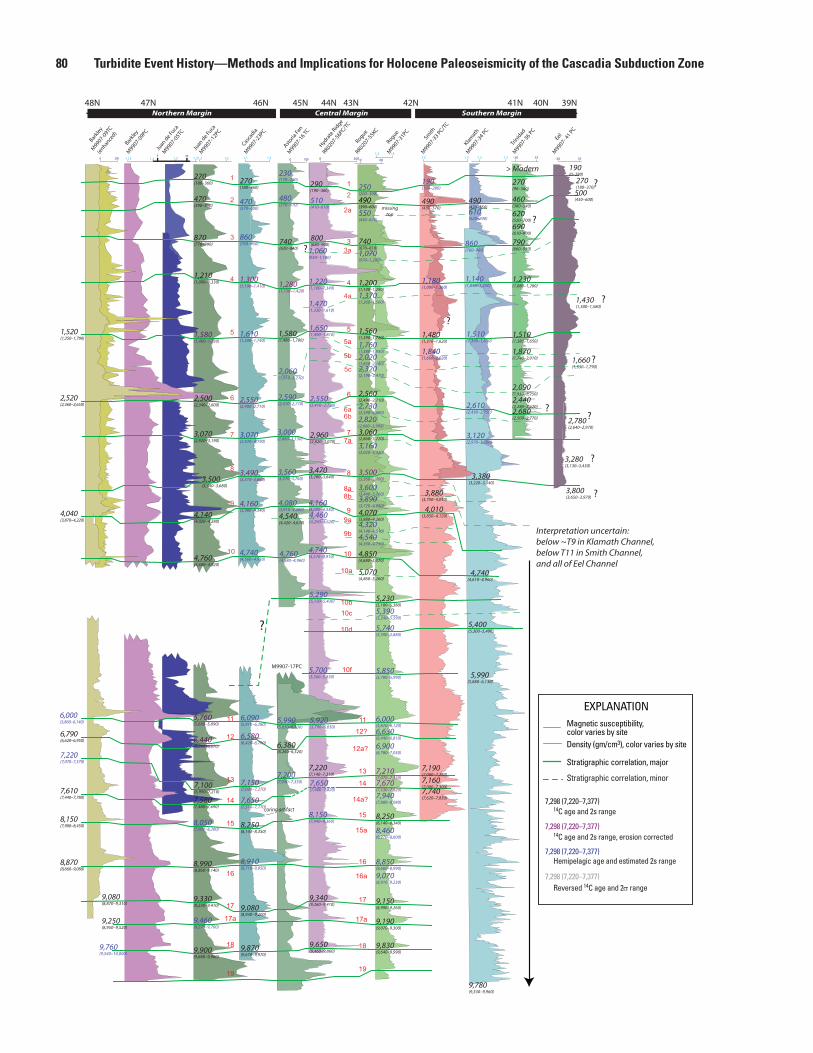
80 Turbidite Event History—Methods and Implications for Holocene Paleoseismicity of the Cascadia Subduction Zone
Magnetic susceptibility, color varies by siteDensity (gm/cm3), color varies by site
Stratigraphic correlation, major
EXPLANATION
Stratigraphic correlation, minor
?
?
??
?
?
2
1
3
4
5
6
7
8
9
10
11
12
13
14
15
16
17
17a
18
19
coring artifact
21
3
4
5
6
7
8
9
5a
2a
3a
4a
5b
6a
5c
7a
10
10a
10b
10d
10f
11
12?
13
14
15
15a
16
17
17a
18
19
16a
9a
12a?
14a?
10c
8a
9b
8b
6b
-20 35 0 90
Eel
M9907- 4
1 PC
Rogue
RR0207-55KC
Astoria
Fan
M9907-1
6 TC
Hydra
te R
idge
RR0207-56PC/T
C
Smith
M9907-3
3 PC/T
C
Klam
ath
M9907-3
4 PC
Trin
idad
M9907-3
6 PC
Casca
dia
M9907-2
3PC
Juan
de Fu
ca
M9907-1
2PC
1.2 1.5 1.1 1.5 0 200
1.2 1.4
0 601.3 1.51.3 1.5 -20 35
RogueM
9907-31PC
Barkl
ey
M9907-0
9PC
missingtop
Juan
de Fu
ca
M9907-0
5TC
Barkl
ey
M9907-0
9TC
(enhan
ced)
Interpretation uncertain:below ~T9 in Klamath Channel, below T11 in Smith Channel, and all of Eel Channel
2000 1.15 1.2
48N 47N 46N 45N 44N 43N 42N 41N 40N 39N
1.2 1.3
M9907-17PC
0 100
Northern Margin Central Margin Southern Margin
740(670–810)
1,200(1,100–1,290)
1,560(1,390–1,720)
2,560(2,490–2,710)
3,060(2,860–3,220)
3,500(3,360–3,700)
4,070(3,880–4,260)
4,850(4,680–5,070)
5,070(4,860–5,260)
490(430–570)
3,880(3,750–4,010)
7,190(7,080–7,280)
790(660–930)
1,510(1,380–1,650)
190(0–280)
290(190–360)
800(680–900)
2,960(2,820–3,070)
3,470(3,280–3,640)
7,220(7,140–7,310)
9,650(9,460–9,860)
740(620–840)
1,280(1,150–1,420)
1,580(1,480–1,700)
4,540(4,420–4,670)
6,380(6,260–6,520)
270(180–360)
470(390–550)
870(770–990)
1,210(1,090–1,330)
1,580(1,460–1,730)
2,500(2,340–2,600)
3,070(2,920–3,190)
3,500(3,340–3,680)
4,140(4,020–4,280)
4,760(4,600–4,920)
5,760(5,680–5,890)
6,440(6,280–6,570)
7,100(6,990–7,210)
7,580(7,480–7,690)
8,990(8,860–9,140)
9,900(9,680–9,980)
270(180–360)
3,490(3,310–3,660)
4,160(3,980–4,340)
6,580(6,420–6,700)
7,150(7,030–7,270)
7,650(7,510–7,770)
8,250(8,140–8,350)
9,080(8,930–9,200)
9,870(9,670–9,970)
1,520(1,250–1,790)
2,520(2,360–2,650)
4,040(3,870–4,220)
7,610(7,440–7,780)
8,150(7,980–8,450)
8,870(8,660–9,080)
9,080(8,870–9,310)
9,250(8,950–9,520)
6,000(5,860–6,140)
8,050(7,900–8,200)
9,460(9,270–9,700)
2,060(1,910–2,210)
5,990(5,830–6,130)
510(410–610)
2,550(2,410–2,720)
4,160(4,000–4,330)
4,740(4,570–4,910)
5,920(5,790–6,050)
470(370–600)
860(760–950)
4,740(4,560–4,930)
6,090(5,910–6,280)
8,910(8,710–9,050)
490(390–600)
1,070(970–1,200)
1,370(1,260–1,500)
1,760(1,580–1,930)2,020(1,850–2,180)2,320(2,190–2,470)
2,730(2,590–2,880)
3,160(3,020–3,320)
3,600(3,440–3,760)3,890(3,720–4,080)
4,320(4,140–4,510)
4,540(4,360–4,730)
5,230(5,100–5,380)
7,210(7,070–7,330)7,670(7,530–7,820)
8,250(8,140–8,340)
8,850(8,660–8,990)
9,150(8,990–9,260)
9,190(9,070–9,300)
9,830(9,640–9,990)
5,390(5,240–5,590)
5,740(5,590–5,880)
5,850(5,700–5,990)
6,000(5,870–6,120)
6,630(6,440–6,810)
6,900(6,780–7,030)
7,940(7,800–8,080)
8,460(8,270–8,600)
9,070(8,910–9,230)
6,790(6,620–6,950)
9,760(9,540–10,000)
7,220(7,070–7,370)
1,300(1,190–1,410)
1,610(1,500–1,740)
230(170–280)
3,000(2,860–3,150)
4,760(4,580–4,960)
4,460(4,290–4,620)
5,700(5,560–5,830)
9,340(9,260–9,410)
550(440–670)
1,230(1,080–1,280)
2,090(1,950–2,250)
3,280(3,130–3,430)
1,480(1,310–1,620)
4,010(3,850–4,120)
> Modern
270(90–360)
460(380–540)
620(520–700)
690(610–800)
1,870(1,740–2,010)
2,440(2,280–2,620)
270(180–370)500(450–600)
1,430(1,300–1,580)
1,660(1,530–1,790)
2,780(2,640–2,970)
9,330(9,230–9,410)
3,070(2,920–3,190)
2,550(2,400–2,710)
480(370–610)
2,590(2,410–2,770)
4,080(3,910–4,260)
3,560 (3,370–3,760)
7,200(7,040–7,350)
1,060(950–1,180)
1,220(1,100–1,340)
1,470(1,330–1,610)
1,650(1,490–1,810)
5,290(5,120–5,430)
250(200–300)
190(100–280)
1,180(1,000–1,360)
1,840(1,660–2,020)
610(520–700)
5,400(5,300–5,490)
9,780(9,530–9,960)
490(420–550)
3,380(3,220–3,540)
4,740(4,610–4,900)
5,990(5,880–6,130)
860(760–980)
1,140(1,040–1,250)
1,510(1,390–1,630)
2,610(2,430–2,750)
3,120(2,970–3,280)
7,160(7,000–7,300)7,740(7,620–7,850)
2,680(2,500–2,770)
7,650(7,480–7,820)
8,150(7,940–8,360)
14C age and 2s range7,298 (7,220–7,377)
Reversed 14C age and 2σ range7,298 (7,220–7,377)
Hemipelagic age and estimated 2s range7,298 (7,220–7,377)
14C age and 2s range, erosion corrected7,298 (7,220–7,377)
2,820(2,680–2,990)
?
?
?
?
?
3,800(3,650–3,970)

Results 81
Figure 46 (left). Correlation plot of marine turbidite records and 14C ages along the Cascadia margin from Barkley Channel to Eel Channel for the past ~10,000 years. All cores are in this figure are “hung” on an event-based vertical scale to match Rogue core M9907-31PC, which is at true scale. Turbidite ages are averaged where multiple ages at one site are available. Turbidites linked by stratigraphic correlations are shown by connecting lines. Near-full-margin events correlated by using stratigraphy and 14C ages are shown with thicker ties. Local southern Cascadia events are thinner and dashed. Sparse dating of southernmost cores reflects low abundance of foraminifera and thin hemipelagic intervals. Ages revised after Goldfinger and others (2003a,b: 2008), Johnson (2004), and Gutiérrez-Pastor and others (2009) by using additional data and analyses. Core M9907-09TC is shown with original and enhanced magnetic data. Stratigraphic correlation allows resolution of some of the ambiguities pointed out by Nelson, A.R., and others (2006) for southern Cascadia paleoseismic events. 14C ages in cal yr B.P., including 2s-error ranges; see appendix 1 for radiocarbon age data. Abbreviation: g/cm3, grams per cubic centimeter.
Figure 47 (above). A, Correlation of vertical series of coarse fraction pulses per turbidite for Juan de Fuca (JDF), Cascadia (Casc.), Hydrate Ridge (HR), and Rogue cores. Table and chart show the number of fining-upward coarse units per turbidite for events observed at all four sites. The correlation matrix shows the Pearson correlation coefficient for the four series. Four line plots are offset slightly for visibility. The number of coarse pulses per event remains quite constant among widely separated core sites. B, Correlation of turbidite mass for Cascadia and Juan de Fuca Channels, Hydrate Ridge, and Rogue Apron. Mass (dimensionless here) is derived from gamma density traces (see Methods section for details). C, Pearson correlation coefficient for gamma density data for individual turbidites T3–T13 from Juan de Fuca and Cascadia Channels. This correlation is a numerical measure of the goodness of fit between the gamma density “fingerprints” among all turbidites at two sites. Dark green cells indicate those correlated visually and the best fit for 14C data. Yellow cells are one turbidite above or below the best stratigraphic fit and are the only values that could be matches if one turbidite was miscorrelated, and remaining cells are unlikely fits given the stratigraphy and 14C data. Orange cells are those that indicate a superior numerical fit but are an inferior fit based on visual correlation and 14C data. Light green cells are excluded by age data, although several are good numerical fits.
23PC T3 23PC T4 23PC T5 23PC T6 23PC T7 23PC T8 23PC T9 23PC T10 23PC T11 23PC T12 23PC T1312PC T3 0.7394 0.7765 0.8555 0.5660 0.0841 0.5790 0.5684 0.4228 0.6632 0.7481 0.441412PC T4 0.5599 0.7290 0.6260 0.6137 -0.0305 0.6000 0.4960 0.2750 0.6070 0.5730 0.482812PC T5 0.5393 0.7701 0.8010 0.4643 0.2079 0.2149 0.6604 0.6705 0.7680 0.5473 0.002812PC T6 0.3390 0.6400 0.4089 0.3277 -0.0325 -0.0614 -0.3643 -0.3891 0.4111 -0.1717 0.500312PC T7 0.8080 0.6674 0.5328 -0.0143 0.7786 -0.0728 0.3005 0.0456 0.1135 0.3903 0.281212PC T8 0.4256 0.2234 0.2276 -0.2901 0.7445 0.1667 0.1601 0.2036 -0.0716 0.2368 0.534512PC T9 0.4931 0.7050 0.6576 0.2648 -0.2524 0.4746 0.6100 0.0784 0.7797 -0.1748 0.283712PC T10 0.1580 -0.0378 0.5636 0.7427 -0.2168 0.7303 0.4836 0.7894 0.4770 0.6343 -0.161612PC T11 0.4769 0.6352 0.5957 0.5483 -0.2204 0.1846 0.7349 0.1713 0.8810 -0.2749 -0.087212PC T12 0.6994 0.4378 0.4748 0.3347 -0.3492 0.5236 0.3711 0.2778 0.2471 0.8241 -0.221012PC T13 0.1132 0.5389 0.3567 0.2467 -0.0551 0.4801 -0.1384 -0.1150 0.4129 -0.0530 0.7731
C
A BNumber fining upward units per event, primary sites.
Even
t num
ber
Turbidite mass per event, key sites(dimensionless) 0 400 800
Even
t Num
ber
1
2
3
4
5
6
7
8
9
10
11
12
13
14
15
16
17
17a
18
12PC scaled mass23PC scaled mass
12PC and 23PC avg. mass scaled mass31PC scaled mass56PC scaled mass
12PC 23PC 12PC and 23PC 31PC 56PCscaled scaled average scaled scaledmass mass mass mass mass
12PC scaled mass 1
23 scaled mass 0.724113 1
12PC/23PC scaled mass 0.874762 0.967614 1
31PC scaled mass 0.586783 0.505279 0.569769223 1
56PC scaled mass 0.681114 0.683977 0.729845579 0.426721 1
Turbidite 12PC 23PC12PC/23PC 31PC 56PC
Number scaled mass scaled massaverage
mass
1 175 155 165 165 742 115 60 88 87 333 155 135 145 176 1914 110 135 123 104 2015 115 235 175 119 1086 195 225 210 80 1687 340 315 328 128 1268 390 170 280 125 1809 290 140 215 129 5710 150 75 113 201 4811 460 625 543 447 23412 40 45 43 15 4513 260 110 185 312 11414 105 105 105 135 1815 100 60 80 195 4516 450 1110 780 258 24317 90 195 143 117 66
17a 60 55 58 171 3618 95 195 145 165 99
Pearson coefficient,mass per event
Pearson coefficient, pulses per event
Number fining upward units per event, primary sitesJDF Casc. HR Rogue
T1 2 2 2 2T2 1 1 1 1T3 2 3 2 3T4 2 3 2 2T5 3 3 3 3T6 3 3 3 3T7 3 3 3 3T8 3 3 3 3T9 3 3 3 3T10 2 2 2 2T11 3 3 3 3T12 1 1 1 1T13 2 2 2 3T14 1 2 1 2T15 1 1 2 2T16 5 5 5 5T17 2 3 2 2T17a 1 1 2 2T18 2 2 2 2
JDF Casc. HR RogueJDF 1Casc. 0.916523 1HR 0.952831 0.835546 1Rogue 0.898984 0.857597 0.918994 1
T1
T2
T3
T4
T5
T6
T7
T8
T9
T10
T11
T12
T13
T14
T15
T16
T17
T17a
T18
0 1 2 3 4 5 6
Juan de FucaCascadiaHydrate RidgeRogue
Number of fining upward units per turbidite at four sites along the Cascadia margin.
Mass per turbidite at four sites along the Cascadia margin.
Numerical correlation of density traces for 13 turbidites in Juan de Fuca and Cascadia Channels.
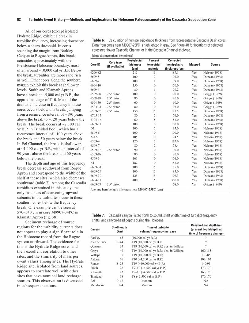
82 Turbidite Event History—Methods and Implications for Holocene Paleoseismicity of the Cascadia Subduction Zone
Table 6. Calculation of hemipelagic-drape thickness from representative Cascadia Basin cores. Data from cores near M9907-25PC is highlighted in gray. See figure 48 for locations of selected cores near lower Cascadia Channel or in the Cascadia Channel thalweg. [dpm, disintegrations per minute]
Core IDCore type
(if available)
Postglacial thickness
(cm)
Percentterrestrial material
Corrected hemipelagic
thickness (cm)Mapped Source
6206-KI 215 13 187.1 Yes Nelson (1968)6609-5 100 7 93.0 Yes Duncan (1968)6609-7 100 1 99.0 Yes Duncan (1968)6604-10 150 0 150.0 Yes Duncan (1968)6609-4 80 1 79.2 Yes Duncan (1968)6509-28 2.5" piston 100 0 100.0 Yes Griggs (1969)6509-29 2.5" piston 80 0 80.0 Yes Griggs (1969)6504-30 2.5" piston 60 0 60.0 Yes Griggs (1969)6504-31 2.5" piston 80 0 95.0 Yes Griggs (1969)6509-25 2.5" piston 150 15 127.5 Yes Duncan (1968)6705-17 80 5 76.0 Yes Duncan (1968)6705-16 60 5 57.0 Yes Duncan (1968)6609-11 100 0 100.0 Yes Duncan (1968)D3 100 5 95.0 Yes Nelson (1968)6509-5 100 0 100.0 Yes Nelson (1968)A-4A 105 10 94.5 Yes Nelson (1968)6509-4 120 2 117.6 Yes Nelson (1968)6509-7 80 2 78.4 Yes Nelson (1968)6509-16 2.5" piston 90 0 90.0 Yes Nelson (1968)6509-9a 80 0 80.0 Yes Nelson (1968)6509-3 101 0 101.0 Yes Nelson (1968)K1 182 0 182.0 Yes Nelson (1968)6609-31 100 15 85.0 Yes Duncan (1968)6609-29 100 15 85.0 Yes Duncan (1968)6609-30 125 15 106.3 Yes Duncan (1968)6604-11 400 5 380.0 Yes Duncan (1968)6609-24 2.5" piston 68.0 Yes Griggs (1969)Average hemipelagic thickness near M9907-25PC (cm)
All of our cores (except isolated Hydrate Ridge) exhibit a break in turbidite frequency, increasing downcore below a sharp threshold. In cores spanning the margin from Barkley Canyon to Rogue Apron, this break coincides approximately with the Pleistocene-Holocene boundary, most often around ~10,000 cal yr B.P. Below the break, turbidites are more sand rich as well. Other cores along the southern margin exhibit this break at shallower levels. Smith and Klamath Aprons have a break at ~5,000 cal yr B.P., the approximate age of T10. Most of the dramatic increase in frequency in these cores occurs below this break, jumping from a recurrence interval of ~190 years above the break to ~120 years below the break. The break occurs at ~2,300 cal yr B.P. in Trinidad Pool, which has a recurrence interval of ~100 years above the break and 50 years below the break. In Eel Channel, the break is shallower, at ~1,400 cal yr B.P., with an interval of 90 years above the break and 60 years below the break.
The depth and age of this frequency break decrease southward from Rogue Apron and correspond to the width of the shelf at these sites, which also decreases southward (table 7). Among the Cascadia turbidites examined in this study, the only instances of coarsening-upward subunits in the turbidites occur in these southern cores below the frequency break. One example can be seen at 570–540 cm in core M9907-34PC in Klamath Apron (fig. 38).
Sediment recharge of source regions for the turbidity currents does not appear to play a significant role in the Holocene record from the Rogue system northward. The evidence for this is the Hydrate Ridge cores and their excellent correlation to other sites, and the similarity of mass per event values among sites. The Hydrate Ridge site, isolated from land sources, appears to correlate well with other sites that have nominal land recharge sources. This observation is discussed in subsequent sections.
Table 7. Cascadia canyon (listed north to south), shelf width, time of turbidite frequency shifts, and canyon-head depths during the Holocene.
CanyonShelf width
(km)Time of turbidite
volume/frequency increase
Canyon-head depth (m) (present depth/depth at
time of frequency change)Barkley 65 (10,000 cal yr B.P.) ?Juan de Fuca 17–44 T19 (10,000 cal yr B.P. ?Quinault 34 T19 (10,000 cal yr B.P.) obs. in Willapa ?Grays 49 T19 (10,000 cal yr B.P.) obs. in Willapa 160/115Willapa 35 T19 (10,000 cal yr B.P.) 130/85Astoria 16 T10 (~4,200 cal yr B.P.) 103/103Rogue 18–25 T19 (~10,000 cal yr B.P.) 140/95Smith 22 T9–10 (~4,500 cal yr B.P.) 170/170Klamath 22 T9–10 (~4,500 cal yr B.P.) 160/170Trinidad 18 T8 (~3,500 cal yr B.P.) 170/170Eel 9–12 Modern NAMendocino 1–4 Modern NA

Results 83
Barkley Canyon
Ju an de FucaCanyon
Astoria Canyon
Willapa Canyon
Rogue Canyon
Sm ith Canyon
Klamath Canyon
Trinidad Canyon
Eel Canyon
Mendocino Channel
Noyo Canyon
Nitinat F
t F
an
As toria Fan
Grays Canyon
Quinault Canyon
131 130 129 128 127 126 125 124 123 122
39
40
41
42
43
44
45
46
47
48
Columbia
River
VancouverIsland
NorthCascadia
Basin
-200
3,100
2,700
6609-5 93 (D) 6604-11
380(G)
6604-10150 (D)
6609-472.9 (D)
6509-9a80 (N)
327 (A)
Duncan, 1968 (D); Griggs, 1969 (G); Nelson, C.H., 1968 (N); Adams 1990 (A)
110 cm Holocene Hemipelagic interval
25 PC
PacificPlate
Gorda PlateGord
a Ri
dge
Mendocino Fracture Zone
Mendocino Fault
Juan
de F
uca
Ridg
e
Juan de Fuca Plate
North
Am
eric
anPl
ate
SouthCascadiaBasin
6509-30106.3 (D)
A-4A94.5 (N)
D395 (N)
Vanc
ouve
r Va
lley
6509-1690 (N)
Astoria Channel
Casca
dia C
hann
el
WASHINGTON
OREGON
CALIFORNIA
0Kilometers100 Miles 100
1999 Core locations PC: Piston cores
Submarine canyons and channels
Delormation front of the Cascadia Subduction Zone
Contour interval 100 m
6509-28100 (G)
6604-3060 (G)
6509-2980 (G)
6604-31
95 (G)
6609-2985 (D)
6609-31
85 (D)
6609-25127.5 (G)
6705-1776 (D)
6705-1657 (N)
6609-11100 (D)
6609-799 (D)
6208-KI212 (N)
6509-4117.6 (N)
6509-778.4 (N)
6509-5100 (D)
6509-3101 (N)
Figure 48. Holocene hemipelagic sediment-drape thickness in cores from Cascadia Basin. Archive cores contain a good regional record of hemipelagic thickness in interchannel areas on Astoria Fan and in Cascadia Basin. Older archive core data are corrected for differential compaction and a different basal datum to compare directly to our data (calculations are given in table 6). Interchannel cores near M9907-25PC record a turbidite-free Holocene hemipelagic thickness averaging 93 cm, comparable to the sum of 102 cm summed from interseismic intervals in our channel cores.

84 Turbidite Event History—Methods and Implications for Holocene Paleoseismicity of the Cascadia Subduction Zone
What Triggered the Turbidity Currents?The turbidite sequences we observe in Cascadia Basin
represent slope failures triggered either by some mechanism, or randomly through sediment accumulation, loading, and (or) oversteepening. The crux of the problem with using turbidites as paleoseismic recorders lies in testing for earthquake origin. Adams (1990) suggests four plausible mechanisms for turbidity current triggering: (1) storm wave loading; (2) earthquakes; (3) tsunamis; and (4) sediment loading. To these we add: (5) hyperpycnal floods; (6) tsunami generated by distant earthquakes; (7) volcanic explosions; and (8) bolide impacts. Other factors, such as gas hydrate destabilization, sea-level change, and tectonic steepening, are factors that reduce seafloor stability, but do not generally trigger submarine mass movements. For example, the Storegga slide generated a large tsunami and occurred because of the massive deposition of glacial sediments and associated gas hydrate disassociation that destabilized the region, likely multiple times (for example, Solheim and others, 2005). The slide itself was most likely triggered by an earthquake (Bryn and others, 2005). Factors reducing slope stability may eventually lead to failure without other triggers; however, such failures are random and are unlikely to be regional and synchronous with other failures. We limit our discussion to triggering mechanisms only and do not consider the range of other factors that may reduce slope stability over time.
As the listed mechanisms may trigger turbidity currents, and are inherently difficult to distinguish, how can earthquake-generated turbidites be distinguished from other turbidites? Two methods can be used to differentiate earthquake-generated turbidites from those originating from other processes: (1) sedimentological examination; and (2) tests for synchronous triggering of multiple turbidite systems that can eliminate nonearthquake origins.
In the following sections we discuss these two methods and their global application, followed by specific applications to Cascadia. We then compare the Cascadia record to the expected frequencies of these triggers, a third circumstantial approach. An open question addressed here is whether shelf and nearshore processes of sediment transport can contribute to the Holocene deep-water turbidite record in Cascadia Basin and, if so, under what circumstances.
Sedimentological ExaminationInvestigators have attempted to distinguish seismically
generated turbidites (seismo-turbidites) from storm, tsunami, and other deposits. Nakajima and Kanai (2000), Nakajima (2000), Shiki (1996), and Shiki and others (2000a,b) argue that seismo-turbidites may be distinguished sedimentologically in some circumstances.
Multiple Pulses, Sedimentology, and Areal ExtentShiki and others (2000b) examined known seismo-turbidites
in Lake Biwa, Japan, including the A.D. 1185 Lake Biwa/Kyoto earthquake (M=~7.4; Inouchi and others, 1996). These deposits are characterized by wide areal extent, multiple coarse-fraction
pulses, variable mineralogical provenance (from multiple or line sources), greater organic content, and greater depositional mass and coarser grain size than the barely visible storm-generated events. They also concluded that defining the triggering mechanism of even known deposits was problematic, and that further study was needed. Nakajima and Kanai (2000) observe that a known earthquake caused multiple slump events in many tributaries of a canyon system, resulting in multiple coarser sediment pulses in a single turbidite. In the Japan Sea, the stacked multipulsed turbidites are found deposited in order of travel time to their lithologic sources, demonstrating synchronous triggering of multiple parts of the canyon system (Nakajima and Kanai, 2000). Goldfinger and others (2007a) found a similar relation with vertical stacking of separate mineralogical sources along the northern San Andreas Fault. For a more complete discussion of stacked and multipulsed tubidites, see Nelson, C.H., and others (in press). Gorsline and others (2000) find that complexity, thickness, and areal extent also serve to distinguish Holocene seismo-turbidites in the Santa Monica and Alfonso Basins of the California borderland and Gulf of California, respectively. In the Santa Monica Basin, both flood-generated and earthquake generated turbidites are present. The flood turbidites are one-tenth to one-fifth the volume of the earthquake-generated events, which are more widespread. Similarly, turbidites in the Alfonso Basin were found to be thicker and greater in aerial extent when earthquake generated. Gorsline and others (2000) argued that reasonable estimates of discharge, sediment input, and source area can be used to constrain the sediment budget for flooding episodes to define the upper bound for sediment available for nonseismic turbidites.
In our cores, we find that Adams’ (1990) “confluence test” can be extended down to the structure of individual turbidites. The Juan de Fuca Channel turbidites can be compared directly to the Cascadia Channel equivalents on a detailed level with surprising results. Not only does the confluence test apply to the gross number of units above the Mazama ash, but it also applies to the internal structure of individual events, which for the most part pass through the confluence and travel 300–350 km with little change in structure. We have discussed the correlation using physical properties and their meaning, but at an even more detailed level, revealed by CT imagery, the comparisons can be striking and suggest a common origin at multiple sites, as opposed to a randomly generated sequence. Three graphic examples are shown in fig. 43.
Hyperpycnal FlowHyperpycnal flow is the density-driven underflow from storm-
flood discharge of rivers into marine or lacustrine systems and has been proposed as a link to deep-water turbidity currents in a variety of settings. Documentation of hyperpycnal flows into lakes and shelf basins is abundant; however, evidence of such flows entering canyon systems and moving into deep water is scant. Most, if not all examples involve short distances between the river mouth and canyon head, either during Pleistocene low-stand conditions, or in systems that have very narrow shelves during highstand conditions. Hyperpycnal flows extend farther from river mouths with high discharge (Alexander and Mulder, 2002), but documentation is limited. Wright and others (2001) observe that hyperpycnal flow

Results 85
is affected strongly by ambient currents, and it generally delivers sediment to the slope only upon relaxation of longshore currents. Most investigators cite Pleistocene examples or examples with little or no shelf when referring to flows reaching the abyssal plain or lower fan reaches (for example, Mulder and others, 2003; Normark and others, 1998; Normark and Reid, 2003; Piper and others, 1999). This is an expected result of sea-level change, when during lowstand conditions there are direct connections between rivers and offshore canyons in areas where the shelf is narrow. Under lowstand conditions, therefore, hyperpycnal flows that transform into turbidity currents that transport material into deep water may occur. An example of highstand hyperpycnal flow has been reported for the Var River, France, in which the canyon and river mouth are less than 1 km apart (Klaucke and others, 2000; Mulder and others, 1998). Many large river systems deposit most of their load in river mouth bars, with lesser quantities making it past such bars and into a delta-front slope (for example, Yellow River, China; Li and others, 1998). Many canyon systems on continental margins, including those in Cascadia, were largely incised during Pleistocene sea-level lowstands (for example, Curray and others, 2002; LeRoux and others, 2005; Evans and others, 2005; McNeill and others, 2000).
Hyperpycnites are reported to have reverse-then-normal grading stemming from the waxing, then waning, nature of flood events. The literature includes several reported cases and compares them to failure deposits that are graded normally, such as those in the Var system (Mulder and others, 2001) and at Lake Biwa (Shiki
and others, 2000a). The dynamics of longitudinal and temporal variability and their effects have been discussed in detail by Kneller and McCaffrey (2003) and Mulder and others (2003).
In an early study, a major river flood during the 1969 El Niño input ~25 million tons of sediment (five times the present yearly Columbia River sediment load; Sherwood and others, 1990) to the Santa Ana River in southern California in a 24-hour period, in close proximity to nearby canyon heads (Drake and others, 1972). Sediment from this extreme flood did not continue down canyons as hyperpycnal flow, but was deposited as a distinct yellow unit on the shelf and upper slope. During the next 10 years, this Santa Ana flood sediment moved downslope as turbid-layer transport caused by storm-wave resuspension, and it was deposited as yellow layers between varves of the Santa Barbara Basin (Drake and others, 1972). In a recent study along the Hikurangi margin of New Zealand, no Holocene hyperpycnites out of a total of ~70 likely seismo-turbidites were found in a setting very similar to Cascadia. The source of New Zealand turbidites was determined to be the upper slope based on foraminiferal assemblages (Pouderoux, in press).
In some proximal settings, such as large lakes, shelf basins, and fjords, records of both earthquakes and flood deposits have been found. In one of the best comparisons, St-Onge and others (2004) show that details of both seismic and hyperpycnal deposition in the Saguenay Fjord in eastern Canada are diagnostic, and they argue that hyperpycnal deposits are distinguished by reverse grading at the base, followed by normal grading. The diagnostic
Dept
h (c
m)
flowvelocityincrease
homogeneous silty clay Hemipelagic
laminated silty clay
possible erosive or sharp contact
cross-laminated silt orfine sand, maximum flow velocity
laminated silt
laminated silty clay
homogeneous silty clay
Grain size (mm)
flowvelocitydecrease
0
20
31 63 125 250 0
30
multiple flowvelocity increases and decreases
H
A B
Figure 49. A, Idealized stratigraphy resulting from hyperpycnal flow, characterized by a coarsening-upward sequence followed by a fining-upward sequence, attributed to a waxing, then waning, hydrographic profile during a storm event (after Mulder and others, 2001). Other events with similar hydrographs, such as a gradual dam breaching, may produce similar stratigraphy. B, Typical stratigraphic sequence from a turbidite with multiple fining-upward pulses from core M9907-12PC in Juan de Fuca Channel. This turbidite and nearly all others in the Holocene Cascadia Basin turbidite sequence exhibit multipulsed stratigraphy, with no waxing phase. Multiple fining-upward sequences are capped by a fine mud tail, signaling the final waning of the turbidity current.

86 Turbidite Event History—Methods and Implications for Holocene Paleoseismicity of the Cascadia Subduction Zone
reverse-then-normal grading for hyperpycnal deposits has been reported widely and is attributed to waxing and then waning flow associated with the storm, although the waning portion may later be eroded during later peak flows (Guyard and others, 2007). In the Saguenay Fjord, six events have normal grading alone and are inferred to be earthquake generated. Four other events have similar basal units, but are topped by a reverse-graded unit and then a normally graded unit, with no evidence of hemipelagic sediment between the multiple units. These events are interpreted as an earthquake, followed by a hyperpycnite that resulted from the breaching of a landslide dam caused by the original earthquake (St-Onge and others, 2004). Dam breaching is a variant of the more common hyperpycnal scenario involving waxing and waning depletive flow (Kneller, 1995), but likely would result in a similar flow hydrograph (fig. 49; St-Onge and others, 2004).
Hyperpycnites commonly are organic-rich, as compared to seismic turbidites, having their sources in floods rather than in resuspension of older canyon-wall material, as in earthquake triggering (Mulder and others, 2001; Shiki, 1996; Shiki and others, 2000b; Nakajima and Kanai, 2000). It has been suggested that this distinction may be used as a basis for distinguishing earthquake and storm deposits by using optically stimulated luminescence (OSL) dating (Shirai and others, 2004). However, we suspect that this generalization may be easily violated, as in the case of floods in very arid regions or earthquakes in heavily vegetated areas. Because the river drainage basins feeding Cascadia Basin are heavily vegetated, the Holocene turbidite tails linked to earthquake origins through a variety of methods (Goldfinger and others, 2008) are characterized by significant quantities of plant fragments (Nelson, C.H., 1976). The high organic content may also be related to events such as the cataclysmic volcanic eruption of Mount Mazama and other volcanic events. The Mazama eruption decimated forests throughout much of the million square kilometers of the Columbia River drainage basin, similar to the forest destruction observed for the 1980 Mount St. Helens eruption (for example, Nelson, C.H., and others, 1988). The Mount Mazama eruption, however, was about 100 times larger than the St. Helens eruption. Consequently, large quantities of forest material washed out of the Columbia River drainage basin to be incorporated into the turbidites. The most interesting example of this effect was our discovery of a first post-Mazama ash turbidite, T13, in the proximal Astoria Channel that consisted of a 0.5-m-thick graded turbidite composed mostly of wood. This turbidite correlates along the length of the margin, where it is mostly devoid of organic material at other sites, illustrating the lack of broader utility of this distinction.
In our cores, we observe that the turbidites of Cascadia Basin are complex, with cutouts and normal and rare reverse grading including multiple coarse-grained pulses within a single turbidite bed, consistent with observations of earthquake-generated turbidites globally (Shiki and others, 2000a; Nakajima and Kanai, 2000). Within the mulipulse events, the subevents can be in any stacking order. This
sometimes gives the false appearance of a coarsening-upward sequence in the density and magnetic data if a larger pulse is at the top of a multipulse sequence (fig. 14). True examples of coarsening-upward intervals are uncommon in the Cascadia turbidites, with the exception of several such events in southern margin cores below the previously described frequency breaks.
Sedimentological Summary In summary, the Cascadia turbidite sequences are
consistent with those of seismic origin observed elsewhere. We find few examples of fining-upward sequences, a characteristic commonly cited as evidence of storm related deposits. The few examples we do find are in southern channel systems with narrow shelves and therefore short distances between canyon heads and their associated rivers. They also are found deeper in the sections at southern sites, representing pre-middle Holocene time when sea level was significantly lower. This observation suggests that the frequency breaks observed in the southern cores may be the result of sea-level change, and this will be discussed further in a subsequent section.
Whether hyperpycnal flows can reach deep water (in this case, the abyssal plain) during the Holocene through canyon systems incised during the Pleistocene appears to be a function of shelf width, steepness, peak storm discharge of rivers, Holocene aggradation, and the wave and current climate during peak storm discharge. However, the requirements for, and evidence of, hyperpycnal flows to the deep ocean under highstand conditions (excepting very narrow shelves) remain poorly known at best (Mulder and others, 2001). In cases of narrow shelves, a turbidite record in an offshore basin or abyssal plain may well contain a mixture of hyperpycnal, sediment failure, and earthquake-generated turbidites. For systems that minimize these effects, those with wide continental shelves, or topographic barriers isolating the slope and abyssal plain, the turbidite record is more likely to contain a dominantly earthquake record (Nakajima and Kanai, 2000; Abdeldayem and others, 2004).
In general, we view the sedimentological determination of turbidite origin as difficult with few definitive criteria, except in a small number of documented cases that may be site specific. Nevertheless, the sedimentological criteria offer one set of tools that may be used in conjunction with other techniques to form a more robust and comprehensive set of criteria.
Synchronous Triggering
Spatial ExtentThere are relatively few definitive sedimentological
studies linking earthquakes directly with turbidites on the basis of the deposits themselves. Most studies have focused on aspects of earthquake processes that are unique, and therefore eliminate most or all of the turbidite triggering mechanisms other than earthquakes. One primary characteristic that can

Results 87
be distinguished in sediment cores is spatial extent. When turbidite deposits can be correlated among widely spaced sites, synchronous deposition can be established or inferred, and if the spatial extent exceeds that which is reasonable for other mechanisms, then earthquake triggering is likely. Virtually all studies that make the linkage between earthquake triggering and turbidites invoke this test in some fashion, including those studies cited previously under sedimentological examination (Adams, 1990; Nakajima and Kanai, 2000; Gorsline and others, 2000; Goldfinger and others, 2003a,b, 2007a, 2008).
Numerical Coincidence and the Confluence TestIn his synthesis of Cascadia Basin turbidite events, Adams
(1990) observed that at Juan de Fuca Canyon, and below the confluence of Willapa, Grays, and Quinault Canyons, cores contain 14–16 turbidites above the Mazama ash. Below the Juan de Fuca and Willapa Channel tributaries, cores in the main Cascadia Channel contain 13 post-Mazama turbidites (figs. 19, 24). Adams (1990) reasoned that these events must have been synchronously triggered, because if these events had been independently triggered with more than a few hours separation in time, cores taken below the confluence should contain from 26 to 31 turbidites, not 13, as observed. The only alternative is that 13 turbidites coincidentally dropped out of the sequence owing to the more distal position of the downstream core, and that the 13 events in the other tributary is also a coincidence. The importance of this simple observation is that it demonstrates synchronous triggering of turbidity currents in tributaries, the headwaters of which are separated by 50–150 km. The synchroneity demonstrated by this “confluence test” also is supported by the similar numbers of events alone, without the existence of the confluence. Noncorrelative “extra” events are found in the most proximal cores in the Washington accretionary wedge and could represent smaller interplate events, upper plate earthquakes, or nonseismically triggered deposits. Off the California margin, Goldfinger and others, (2007a) demonstrate that turbidites adjacent to the San Andreas Fault converge at channel confluences and remain constant in number above and below the confluence, following the Cascadia pattern. The San Andreas turbidites also show the vertical stacking by provenance affinity as mentioned previously.
Adams (1990) makes a convincing case for synchroneity of the Washington margin turbidites and reports that 13 post-Mazama events also are present at the mouth of Astoria Canyon and in the Rogue Apron off southern Oregon. In our 1999 cores, we observe the same record of 13 post-Mazama turbidites in the Juan de Fuca and Cascadia Channel systems, confirming Adams’ observation and strengthening it with 14C and stratigraphic correlation. In Willapa Channel, our 1999 cores are similar to, but not as complete as, the earlier core 6705-5 used by Adams (1990). Our cores either are missing event T7, or this event is very subdued. For the post-Mazama confluence test we therefore rely partially on the earlier core.
We extend the regional synchrony to include 19 correlative turbidites above the faunal Pleistocene-Holocene boundary datum along the northern Cascadia margin (although the test
does not include Willapa Channel for events older than the Mazama eruption). We also extend the record of numerical similarity northward to include Barkley Canyon.
In pre-1999 cores, we initially found only three post-Mazama events in lower Astoria Channel in older archive cores, which appeared to contradict Adams’ (1990) hypothesis for 13 events. In the 1999 cores, however, we find a complete record in cores M9907-16PC and M9907-17 PC from the main trunk channel. The more distal cores M9907-18PC through M9907-21PC proved to be incomplete records, most likely owing to imperfect core siting and less active splay channels that proved to be hanging valleys with 10–30-m barriers to entry. This downchannel loss of events in the distributary fan channels explains the previous contradiction and illustrates the consistency of the post-Mazama turbidite record along the northern margin. In Astoria Channel cores M9907-17PC and M9907-17TC, we also observe four additional thinner turbidites without regional correlatives above the Mazama ash. The additional events, T5b, T8a, T9a, and T10b, are interpreted as additional events not present in the Juan de Fuca, Barkley or Cascadia Channel systems. This tentative interpretation is based on correlation to sites farther south, discussed below.
Extending the tests for synchroneity southward to other sites is somewhat more complex. Goldfinger and others (2003a,b) support Adams’ observation that the record of 13 post-Mazama ash turbidites extended to Rogue Apron off southern Oregon. However, we have since recognized that some of the older cores (those used by Adams and two 1999 cores in this study) were missing portions of their upper record as discussed previously. Adams’ (1990) inference that marginwide synchroneity can be tested at Rogue Apron, based on the simple coincidence of 13 post-Mazama events, is therefore not supported by our work.
Stratigraphic Correlation The detailed stratigraphic correlations shown in figures
43–46 are supported by 14C dates and hemipelagic dates to form a robust stratigraphic framework. In figures 43–46, solid correlation lines link events that we interpret as the same stratigraphic units on the basis of detailed stratigraphy and age control. Lighter and dashed lines indicate interpreted correlations that have less robust data to support them, are less robust correlations, or have fewer diagnostic criteria available. The primary result of the resulting stratigraphic framework is that we find few turbidites that are clearly isolated to a single site (not correlated) in our cores between Rogue Apron and Barkley Canyon. There are two uncorrelated events in the Juan de Fuca Channel site and two in the Hydrate Ridge site. Sites south of Rogue Apron, including Smith, Klamath, Trinidad, Eel, and Mendocino Channel sites, each have deeper sections that we are unable to correlate with existing data, as previously discussed. We have correlated events above these breaks and find reasonable correlation of the upper units at these sites with the exception of Mendocino Channel, which has only tentative linkages to the other sites.

88 Turbidite Event History—Methods and Implications for Holocene Paleoseismicity of the Cascadia Subduction Zone
The detailed geological/geophysical “fingerprinting” of turbidites, through their grain size distributions and proxy measurements, has direct implications for synchronous origins of the deposits. Because we are correlating grain-size distributions (density and magnetic susceptibility as proxies) among multiple sites, we find that the persistence of the event “fingerprints” among sites at both local (site) and regional scales makes a compelling case for synchronous deposition. Considerable variability exists, and we find that only by comparison of a large number of sites along the margin can we identify the characteristic fingerprints. Nevertheless, these fingerprints sometimes retain a remarkable similarity at sites along strike, but they also commonly evolve somewhat along strike in subtle ways that can be traced from one site to another.
If the grain-size fingerprints are robust as we suggest, the triggering mechanisms that produced them, or the hydrodynamics of the separate canyon systems, must have some commonality; producing matching grain-size patterns in multipulse turbidites by coincidence is unlikely. Not only must the same pattern be reproduced in multiple canyon/channel systems, it also must be reproduced at Hydrate Ridge, which not only has no sources of fluvial input, it has no significant canyon system delivering material to the basin, thus it has limited opportunity for hydrodynamic evolution of the flow. Detailed stratigraphic fingerprinting also may provide an extension to the original confluence test. We observe that turbidites at Juan de Fuca and Cascadia Channels are among the best correlation series in Cascadia Basin (figs. 43–46), yet Juan de Fuca Channel is upstream and Cascadia is downstream of the Willapa Channel confluence. The original confluence test only examined numbers of events above the Mazama ash; however, the detailed stratigraphic correlation matches each event in detail, above and below the confluence. Not only is the total number of events the same, but the number of coarse-fraction pulses remains the same in nearly all cases. This occurs despite the addition of input from Quinault, Guide, Grays, and Willapa Canyons at the confluence. The preservation of the individual fingerprints above and below the confluence further supports a synchronous and common origin, which is best attributed to earthquakes, though why the turbidite elements are not stacked as previously discussed for other margins is not clear.
We also note that, as this report was in final preparation, new data were acquired along the Cascadia margin in 2009. These data will be the subject of new work focused on the southern part of the margin, where existing data are sparse and problematic. One outcome of cruise TN0909 was that hundreds of kilometers of 3.5-kHz chirp subbottom profiles were collected parallel to and along the entire length of the Cascadia margin. Although analysis of these data has not yet occurred, one obvious conclusion from them is that individual turbidites were clearly imaged in the records and can be linked to the core sites through which they pass. These individual units are traceable for long distances along the margin, demonstrating that while distal turbidites are channelized (for example, Cascadia Channel), proximal turbidites exist as sheet deposits
along the base of the continental slope (Goldfinger, 2009, 2010, 2011a). We find that the correlated reflectors are not strongly linked to canyon/channel systems but apparently have been derived from sheet flows from the continental slope, as well as from the channelized flows we focused on in this study. We view this as strong support for earthquake origin of these units, as stratigraphic correlation along the base of the continental slope is possible in areas that are remote from slope canyons as well as areas near canyons, with no significant change in the stratigraphy.
Applicability of Triggering Mechanisms to Cascadia
Although synchronous triggering is the primary tool used in this study to distinguish earthquake-related turbidites from those with other triggering mechanisms, we can make relevant observations about how other triggering mechanisms might or might not operate in the specific case of Cascadia. A variety of triggering mechanisms for downslope sediment transport have been mentioned in the literature. As many as 12 triggering mechanisms have been suggested (for example, Shanmugam, 2008); however, here we distinguish between factors that reduce slope stability over time and those that actually trigger slope failures. Because triggering mechanisms that might explain the Cascadia evidence must be regional and synchronous in addition to being applicable to Cascadia, we eliminate sediment oversteepening and loading as plausible triggers because there is no reason to expect such events to be regional and synchronous; they should be random events in single canyon systems. We eliminate volcanic activity because onshore volcanism is too distant in Cascadia to have a direct and regional effect on canyon systems offshore, although high ash loads certainly accumulate in systems that drain each Cascadia volcano and are expected to promote isolated sediment failures in affected systems. The remaining triggers that can be both regional and at least semisynchronous (spanning days or weeks) are discussed in the following sections with specific reference to the Cascadia physiography and canyon-channel systems.
Triggering by Storm or Tsunami WavesA triggering mechanism for slope failures that is
potentially widespread and approximately synchronous is wave loading from either tsunami or storm waves. Both types of waves cause a cyclical loading and unloading of surficial sediments that can generate a moment couple that both shears and displaces sediments (Wright and Rathje, 2003). Teletsunami waves are likely to be smaller than extreme storm waves in Cascadia, so we discuss them together with emphasis on extreme storm waves.
Wave-related failure results from two processes: (1) liquefaction caused by cyclic loading and (2) shear failure in cohesive or noncohesive sediments and subsequent resuspension and transport of sediments. Maximum significant

Results 89
wave heights in the open ocean in Cascadia are ~20 m, based on models incorporating 40 years of observations, Topex data, and a 100-year extreme return model (Caires and Sterl, 2005). The maximum wave period probably is limited to ~20–25 seconds by shallow water, calculated using the method of the Coastal Engineering Research Center (1984). We adopt these values for the following discussion of wave-induced sediment transport and failure.
Liquefaction Caused by Wave LoadingThe passage of large waves, either by storms or tsunami,
induces oscillatory fluctuation in the loading condition, as well as progressive increase in pore pressure after repeated wave cycles (for example, Cheng and others, 2001). As successive waves pass, an undrained loading condition occurs, increasing pore-fluid pressures and potentially bringing a slope closer to its static failure condition. Seed and others (1988) report that a submarine landslide off the port of Nice, France, generated a tsunami that triggered a slope failure by passage of the leading trough, which is believed to have occurred owing to undrained flow liquefaction and a 1–2 percent increase in shear stress caused by the passage of the wave. Another commonly cited example of wave loading in the literature is the failure of sediments around drilling platforms in the Mississippi River Delta during Hurricane Camille in 1969 (Bea and others, 1983).
It is not generally agreed that this is a common or important mechanism for slope failure, even in shallow water. Chillarige and others (1997) calculate that wave loading could not be the cause of observed sediment failures on the Frazier River delta, British Columbia. Spontaneous flow liquefaction there remains a poorly explained phenomenon, possibly linked to free gas (Christian and others, 1997). Luternauer and Finn (1983) also conclude that wave loading does not cause sufficient sustained or transient pore-pressure changes needed to initiate slope failure. Cyclic loading also can strengthen sediments that do not reach a failure criterion. Boulanger and others (1998) and Boulanger (1999) have shown, through a series of cyclic loading-drainage tests using an earthquake source rather than waves, that with a period of drainage between events, the void space decreased and shear strength increased from exposure to many cycles. Locat and Lee (2002) termed this condition “seismic strengthening” and suggest that it may explain the paucity of shallow landslides in Cascadia and elsewhere relative to passive margins (Lee and others, 2004; Nelson and others, 2011). The same may be true for periods of wave loading and draining between storms (Sassa and others, 2003; Homa Lee, oral commun., 2005), and it has been modeled as resistance to liquefaction (Chang and others, 2004). Chang and others modeled 3-D liquefaction potential in saturated, sandy nearshore sediments of Taiwan under wave-loading conditions from typhoons and winter northeast monsoon waves. Both weather systems generate maximum waves of 7-m height and periods of 9–12 s. The modeled liquefaction from these waves did not extend below 15 m water depth. These types of liquefaction analyses are complex and
not well correlated with field experience (Nataraja and Gill, 1983).
The question relevant to this work is whether wave loading on the shelf or upper slope could generate turbidity currents that reach deep water. On the shelf near the uppermost Eel Canyon, Puig and others (2003, 2004) infer that fluidization in storm-wave conditions is the likely cause of sediment fluid flows recorded at a study site in the Eel Canyon head in 120 m of water. They infer that shear-failure erosion of the sediment (discussed below) is unlikely and that fluidization is a viable alternative, although they do not calculate the potential. These authors cite the rapid development of sediment flows with increased wave height, and reach the conclusion that the short time interval would be insufficient for erosive entrainment of material in the bottom boundary layer, but is more consistent with the near instantaneous fluidization on arrival of storm waves. Using multiyear in-place sea-floor-monitoring equipment, Puig and others (2004) found that 1998 El Niño flood sediment from the Eel River was first deposited in the shelf mud blanket and then for several years was progressively transported by storm-resuspension processes into the upper Eel Canyon, but not to the deep canyon. Fan and others (2004) also discuss the Holocene stratigraphy of the northern California (southern Cascadia) shelf in detail. They conclude that river-flood and storm-sediment resuspensions largely are confined to the shelf and, as observed on the Washington margin, are transported to the north, away from the nearby Eel Canyon head. Nevertheless, Mullenbach and others (2004) show a clear connection between storm events and deposition in upper Eel Canyon at depths above ~900 m.
Sediment Erosion Caused by Combined Current and Storm Wave Conditions
The potential for sediment erosion, given wave and current conditions, is commonly made by calculating wave orbital velocity and combining it with tidal or other current measurements or estimates to arrive at a combined estimate of shear stress in the bottom boundary layer (BBL; Madsen, 1994). Puig and others (2004) have used this method to estimate the erosion potential in the head of Eel Canyon at 120-m water depth during two storms in January and March 2000. At Eel Buoy 46030 on January 31, 2000, the maximum significant wave height was 8.57 m. The dominant wave period (dpd) was 20 s, the average wave period (apd) was 13.2 s (data from NOAA buoy 40630 in 82-m water depth near the canyon head). Puig and others (2004) calculate a shear stress of 0.17–0.2 Pa, 30 cm above the bottom, greater than the critical shear value of 0.07 for the top few centimeters of fluidized sediment, but below the value of 0.27 Pa estimated for shallow subsurface sediments by Thomsen and others (2002). They further conclude from this analysis that the observed sediment resuspension during the two storms is more likely caused by sediment fluidization (as discussed above), because calculated shear stresses do not reach the critical value estimated for shallow sediments. Cheng and others (1999), however, have

90 Turbidite Event History—Methods and Implications for Holocene Paleoseismicity of the Cascadia Subduction Zone
shown that the calculations are highly dependent on the value of the “roughness length” of the seafloor (z0). Although the value of z0 is estimated or assumed as an input parameter to the frequently used shear-stress calculations, it is also an unknown. This unknown value has been cited as a function of grain size, but various published “rules of thumb” vary over several orders of magnitude. As the calculation of near-seabed shear stress is sensitive to this value, we conclude that explicit calculation of erosion potential is problematic without further detailed information about roughness of the seabed and further refinement of the techniques for calculating erosion potential.
For our purposes, we calculate the erosion potential from theoretical extreme waves of 20-m significant height, and 20-s period at canyon-head depths, similar to Puig and others (2004), using the methods of Madsen (1994). We include the combined
shear velocity from currents, which in this case are primarily the bidirectional tidal component, measured at ~20 to 30 cm/s, and the contribution from wave orbital velocity in the BBL. If we assume that the bed roughness parameter, z0, is equal to grain size for the sediment (9 µm for the Eel Canyon head, Puig and others, 2004), a minimum value from the literature, and assuming no bedforms to increase drag, we estimate that such waves should have erosive power to a depth of ~450 m, including tidal downflow, or ~300 m from the waves alone. Larger values of z0, or consideration of bedforms or slopes, will increase this depth, as would adding the effects of storm-driven inshore Davidson Current. Calculations and other details are given in appendix 7. This condition exists only during downcanyon tidal flow (or perhaps during offshore storm-surge return flow). As the flow reverses during the tidal cycle,
Table 8. Magnitude estimated from time interval, plate motion, and rupture-zone dimensions, Cascadia subduction zone.
Turbidite number Mean age
Northern margin
following interval, in
years
Northern margin
slip from following time, in meters
Southern margin
interval, in years
Southern margin slip from time, in meters
Average northern and
southern slip, in meters
Segment name
Rupture length, in
kilometers
Rupture width, in
kilometersMw Seismic
moment
1 250 16.0 A 1,000 83 9.00 398.4E+272 482 232 8.9 232 8.3 8.4 A 1,000 55 8.70 138.3E+272a 550 57 2.1 2.1 D 222 40 8.19 23.8E+273 798 305 11.2 248 8.9 10.0 A 1,000 83 8.87 250.2E+273a 1,077 279 10.0 10.0 C 444 50 8.34 40.1E+274 1,243 446 16.3 167 6.0 11.2 A 1,000 83 8.90 277.9E+274a 1,429 186 6.7 6.7 C 444 50 8.25 29.9E+275 1,554 311 11.4 125 4.5 7.9 A 1,000 83 8.80 197.4E+275a 1,820 266 9.6 9.6 C 444 50 8.41 51.9E+275b 2,036 216 7.8 7.8 B 660 60 8.66 122.5E+275c 2,323 286 10.3 10.3 C 444 50 8.41 51.1E+276 2,536 982 35.9 213 7.7 21.8 A 1,000 83 9.09 542.7E+276a 2,730 194 7.0 7.0 D 222 40 8.24 28.7E+277 3,028 492 18.0 298 10.7 14.4 A 1,000 83 8.97 358.2E+277a 3,157 129 4.6 4.6 D 222 40 8.23 27.5E+278 3,443 415 15.2 286 10.3 12.7 A 1,000 83 8.94 317.2E+278a 3,599 442 5.6 0.0 B 660 60 8.67 124.4E+278b 3,890 447 10.5 10.5 D 222 40 8.15 21.0E+279 4,108 665 24.4 218 7.9 16.1 A 1,000 83 9.01 401.1E+279a 4,438 548 11.9 0.0 B 660 60 8.35 41.4E+279b 4,535 426 3.5 3.5 D 222 40 8.17 22.5E+2710 4,770 661 24.2 235 8.5 16.3 A 1,000 83 9.01 406.6E+2710a 5,062 292 10.5 10.5 C 444 50 8.39 47.6E+2710b 5,260 198 7.1 7.1 B 660 60 8.43 55.7E+2710c 5,390 130 4.7 4.7 C 444 50 8.55 82.7E+2710d 5,735 344 12.4 12.4 C 444 50 7.90 9.0E+2710f 5,772 37 1.3 1.3 C 444 50 8.37 44.8E+2711 5,959 1189 43.5 187 6.7 25.1 A 1,000 83 9.13 625.5E+2712 6,466 508 18.6 508 18.3 18.4 A 1,000 55 8.93 304.0E+2712a 6,903 437 15.7 15.7 D 222 40 8.22 26.7E+2713 7,182 715 26.2 278 10.0 18.1 A 1,000 83 9.04 450.7E+2714* 7,625 443 16.2 443 16.0 16.1 A 1,000 83 9.01 400.7E+2714a 7,943 318 11.4 11.4 D 222 40 8.17 22.1E+2715 8,173 548 20.1 230 8.3 14.2 A 1,000 83 8.97 353.0E+2715a 8,459 286 10.3 10.3 D 222 40 8.36 42.9E+2716 8,906 733 26.8 447 16.1 21.4 A 1,000 83 9.09 534.1E+2716a 9,074 169 6.1 6.1 D 222 40 7.54 2.6E+2717 9,101 195 7.2 27 1.0 4.1 A 1,000 55 8.49 67.0E+2717a 9,218 117 4.3 117 4.2 4.2 A 1,000 55 8.50 70.1E+2718 9,795 577 21.1 577 20.8 20.9 A 1,000 83 9.08 521.2E+27
Results 91
downcanyon orbital motion and tidal flow oppose each other, and deposition is likely to occur. Such transport is likely to result in deposition within the canyon at depths of 200–500 m following extreme storms. We calculated similar values for local Cascadia tsunami, and Weiss (2008) calculated that the extreme tsunami formed during the December 2004 Sumatra rupture (maximum slip ~25–30 m) would be capable of moving fine sand in a maximum depth of 985 m locally in the rupture zone. Cascadia ruptures, with maximum slips that could approach 30 m, are more frequently in the 15–18 m range (table 8; Priest and others, 2009) with correspondingly smaller tsunami.
Geostrophic and Surface CurrentsIn this report we mainly focus on triggering mechanisms
for turbidity currents that could be compatible with the observed turbidite frequency in Cascadia. Annual or continuous phenomenon, such as geostrophic or surface currents, do not meet this criteria; however, they should be mentioned because the long-term periodicity of major geostrophic “storms” (Gross and Nowell, 1990) and outlier current events is unknown. Surface currents are generated primarily by wind stress and decrease in velocity downward, making them unlikely to transport sand-sized material at upper canyon-head depths of 100–200 m. In Cascadia, the shallow California Current flows southward at typical surface velocities that reach ~30 cm/s in spring and summer months (Chereskin and others 2000; Strub and James, 2000). The California Undercurrent (CUC) flows poleward farther inshore and deeper than the California Current, along with the winter inshore current, known as the Davidson Current (Hickey, 1998). Studies of the velocity field of the CUC suggest typical mean and maximum velocities of ~7 and 16 cm/s, respectively, at depths of 100–500 m (Garfield and others, 2001), decreasing from peak values at ~200 m depth to near zero at 1,000 m for observed and geostrophic flow (Collins and others, 2000). Using Madsen’s (1994) shear-velocity/shear-stress formulation, implemented in the code SEDX (http://woodshole.er.usgs.gov/staffpages/csherwood/sedx_equations/sedxinfo.html), we calculate that these maximum current velocities are less than half of that needed to erode noncohesive fine sand from the seafloor, ignoring the logarithmic decrease in velocity in the bottom boundary layer. Geostrophic currents of sufficient velocity (0.5–1 m/s), however, are known from other localities (for example, Osiński and others, 2003); therefore, such currents cannot be ruled out as sources of sediment erosion at canyon-head depths on a theoretical basis. Nevertheless, there are no examples of such currents initiating turbidity currents in the literature that we are aware of, and the literature that cites deposits related to geostrophic currents is thin with respect to linkages to sediment deposits. Since these currents are seasonal or continuous, and the frequency of reported “benthic storms” is unknown, we cannot evaluate this mechanism further. We can only refer the reader to rather speculative distinctions made between geostrophic deposits, which are described as lacking clear structure, and autosuspending turbidites with clear erosive bases and fining-upward sequences (for example, Michels, 2000; Lewis and Pantin, 2002). Many of these speculations refer to ancient deposits and are difficult to verify or test.
Cascadia Physiography and Turbidite DepositionIn the Pacific Northwest of the United States, large storms
both increase river discharge and produce strong southerly winds that disperse sediment northward on the shelf by way of the Davidson Current (Sternberg, 1986; Wheatcroft and others, 1997; Sommerfield and Nittrouer, 1999; Wolf and others, 1999). Sediment plumes are also observed to extend hundreds of kilometers seaward as evidenced by satellite imagery (Wheatcroft and others, 1997). In the previous sections, we have shown that both tsunami and storm waves can easily resuspend and transport sand-size material at canyon-head water depths throughout Cascadia, evidence supported at least for the Eel system by observations. But does this sediment disturbance result in delivery of turbidity currents to the deep sea?
An important consideration is the distance and position of canyon heads relative to their potential sediment sources. On the Cascadia margin the major canyon systems have Holocene shelf widths of 9–65 km separating the modern canyon heads from the coast. Several of these systems have narrow shelves, including Eel Canyon (9–12 km; table 7), Astoria Canyon (16 km), Trinidad Canyon (18 km), and Mendocino Canyon (~1–5 km). The rest of the systems are 20 km or greater in present width. The Eel River system, with its narrow 12-km shelf width, is the best candidate in Cascadia for delivering hyperpycnal flows and (or) storm-related sediment transport by any mechanism to the canyon head. Puig and others (2004) saw no evidence of hyperpycnal flow into the Eel Canyon, although they did observe cross-shelf sediment transport owing to wave loading into the canyon head. Other observations of high turbidity at depths of 280 m and 900 m in upper Eel Canyon also were linked to storms, with wave loading being the inferred mechanism. Mullenbach and Nittrouer (2006) estimated that ~12 percent of sediment mobilized during storms could be accounted for in the Eel Canyon head, but that over ~100-year timescales, 2–3 percent of the Eel system sediment budget accumulated in the canyon head, the difference likely being distributed by downslope movement. Unfortunately, the extensive work in Eel Canyon under the STRATAFORM project dealt only with the upper canyon, and the ultimate fate of these sediments was beyond the scope of the project.
The observations of sediment input to Eel Canyon head hardly are surprising considering the extremely short distance between the river mouth and canyon head, and the high sediment load of the Eel River. Similar observations have been made at Monterey Canyon, with a near-zero shelf width (Paull and others, 2005), and we observed continuous sand deposition in Viscaino Channel, fed by littoral drift into Viscaino Canyon with less than 1 km of shelf width (Goldfinger and others, unpub. data).
Delivery of sediment transported across the shelf to Cascadia canyon heads is made somewhat more difficult by the modern Holocene physiography. Given that high discharge occurs during winter storms when southerly currents prevail, net sediment transport (river flood plumes or hyperpycnal) is northerly or northwesterly from the coast, limiting input to the canyon heads to a small percentage of the total load (Sternberg,

92 Turbidite Event History—Methods and Implications for Holocene Paleoseismicity of the Cascadia Subduction Zone
1986; Wolf and others, 1999). The Eel Canyon head is somewhat to the south of the modern river mouth, reducing the potential for storm-related plumes to enter the canyon. In all systems, the late Pleistocene transgression and subsequent sediment infill and aggradation have erased much or all topographic canyon or channel expression across the Cascadia shelf, further widening the distance otherwise created by sea-level rise alone (Carlson, 1967; Twitchell and Cross, 2001).
Core BB 326-36, on a terrace in the head of Willapa Canyon at a water depth of ~370 m, contains the Mazama ash at a depth of 240 cm in the core. Above the possible airfall ash, no turbidites were detected texturally or in X-radiographs (Royse, 1967). The significance of this and other canyon-head cores is that they do not reveal deposition of turbidites that are well recorded downchannel, suggesting that the source is not likely to be upstream of the canyon head, though bypassing of such sites remains a possibility.
For north and central Cascadia systems, we find no evidence of Holocene storm-generated turbidites in Barkley Canyon, Juan de Fuca, Cascadia, Willapa, and Astoria Channels, or Rogue Apron, nor in the Hydrate Ridge west basin. During that period, when sea level was at or near present levels, these systems correlate remarkably well stratigraphically, with strong 14C-age support. Few differences are found, except for the notable presence of the suite of thinner southern Cascadia correlative mud-silt turbidites described previously.
The Trinidad, Eel, and Mendocino systems, our southern-most three sites, all have canyon heads close to the shoreline and contain a Holocene turbidite frequency higher than that of the remainder of the margin. The breaks in turbidite frequency observed at all sites suggest rapid change in the mechanisms that deliver turbidity currents either near the Holocene-Pleis-tocene boundary or during the Holocene; such a rapid change is unlikely to be of tectonic origin and is more likely related to sea-level rise.
As noted previously, we observe a turbidite character and frequency break at all sites, except Hydrate Ridge. The frequency break occurs at Barkley Canyon, Juan de Fuca, Willapa, and Cascadia Channels, and Rogue Apron sites and coincides with a shift from silt-sand turbidites to thicker, more coarse-grained deposits accompanied by a color change from olive green to gray clay in most cores at these sites. For many sites, including Barkley Canyon, Juan de Fuca, Cascadia, and Astoria Channels, and Rogue Apron, this change corresponds approximately to the Pleistocene-Holocene temporal (not faunal) boundary at ~10,000 yr B.P. As noted previously, the downcore frequency increase is abrupt and is found at different times in the southern cores. In Smith and Klamath Aprons, the shift occurs at T10 time, or around 5,000 cal yr B.P. At Trini-dad Pool, the shift occurs at ~2,300 cal yr B.P. The break is at ~1,400 cal yr B.P. for Eel Channel, and Mendocino Channel has a very high frequency record throughout. The time at which this change in turbidite frequency took place correlates well with shelf width. The narrower the shelf, and shallower the canyon head, the later the frequency change took place (table 7). We interpret this as an expected result of sea-level change
and the gradual cutoff of rivers from their Pleistocene canyon heads. The infilling of late Pleistocene canyon heads during and following the transgression has subsequently increased the separation between sediment sources and submarine canyons.
We observe a small number of reversely graded turbi-dites below the frequency breaks at these sites, suggestive of hyperpycnal origin; however, the majority of turbidites below the breaks, and nearly all of the events above the breaks, do not show this character, precluding a clear interpretation of nonseismic origin for the events that are responsible for the frequency increase. Similar observations have been made from cores in the Chile trench, where turbidite frequency is reduced greatly during highstand periods. The Chilean turbidite record likely is complicated and may not represent a complete earth-quake record during highstand times owing to low sediment supply and poorly located cores on the outer trench wall for some of the cores (Blumberg and others, 2008).
We also observe that the Hydrate Ridge record is unaf-fected by the lithologic or frequency change observed at other sites; such a change would not be expected at Hydrate Ridge which is isolated from fluvial or storm-related input and has only a single local deep-water sediment source.
In summary, Cascadia physiography does not favor trans-port of fluvial, littoral, or storm-related sediments to the abys-sal plain during Holocene sea-level highstands at northern and central Cascadia sites. The wide shelf at these sites, combined with the northwestward transport direction during storm condi-tions, favors deposition on the shelf, with modest contribution to the canyon heads (Sternberg, 1986; Wolf and others, 1999). Exceptions to this are the Smith, Klamath, Trinidad, Eel, and Mendocino systems, with narrow shelves, which have changes in frequency at times that correspond to their associated shelf widths. We interpret the frequency breaks to be the result of Holocene cutoff of nearshore sediment as sea level rose during the early Holocene.
Finally, greater turbidite frequency in southern Cascadia may be attributed to additional input from storm-generated turbidites, greater earthquake frequency, additional Cascadia rupture segments (see Carver, 2000), multiple seismic sources near the Mendocino Triple Junction, or a mixture of these sources. We cannot distinguish these hypotheses in this study.
Frequency of Triggering Mechanisms
Cascadia Turbidite Frequency—Earthquakes Versus Storms and Other Phenomenon
Storm-flood events that may trigger significant cross-shelf transport or hyperpycnal flow occur frequently in lake settings, where any inflow with suspended sediment becomes a hyper-pycnal underflow. In Crater Lake, Oregon, hyperpycnal events occur every year with snowmelt runoff, and major storm floods happen every few years; yet there are only 3–18 turbidites per thousand years in Crater Lake Basins (Nelson, C.H., and others, 1991, 1994). In Lake Baikal, Russia, where any fluvial

Results 93
input would create a hyperpycnal flow down the steep (~30°), deep (1,200 m) basin slopes, only seven turbidites have been deposited on the floor of the North Basin during the past ~12,000 years (Nelson and others, 1995a). In contrast, nearly annual catastrophic debris flows and floods from the Lake Bai-kal border fault scarp (2,500 m relief) enter the lake. The flood debris apparently deposits on the Gilbert deltas of the upper lake slope, and other less frequent processes (every 1,000 yrs or more) generate the large turbidity currents that deposit Holocene turbidites on the lake floor.
In sum, there are orders of magnitude fewer turbidites than the thousands of Holocene hyperpycnal flow events in these well-known lakes. Even in lakes where there is no shelf development or Pleistocene to Holocene water-level change (Colman and others, 2003), because of stratigraphic frequency, basin-floor turbidites cannot be linked to generation by hyper-pycnal flows in Holocene or Pleistocene times.
Along the Cascadia margin, the frequency of great storms is high, with two to three storms per year reaching more than 100 knots wind speed and 10- to 15-m wave height, or roughly 600–900 large storms since the last Cascadia earthquake in A.D. 1700. The turbidite frequency along the northern margin, however, where the strongest winds and largest waves occur, is the lowest at 500–530 years. Moving southward along the Cascadia coast (toward better weather) the turbidite frequency increases, the opposite of what would be expected from storm severity and frequency in Cascadia. In parallel, the onshore paleoseismic record shows that earthquake frequency also increases southward, and closely matches the turbidite fre-quency (Goldfinger and others, 2008; Kelsey and others, 2005; Nelson, A.R., and others, 2006). Crossing the triple junction into the northern California margin, the turbidite frequency remains high, matching the earthquake frequency of the north-ern San Andreas Fault (Goldfinger and others, 2007a, 2008), even though sediment supply, storm frequency, and storm severity are reduced. Only at the Eel, Trinidad, and Mendocino systems, where there is well-documented sediment input from the nearshore, a narrow shelf, and the very large Eel River sediment source, do we see a high-frequency turbidite record suggestive of fluvial- or storm-related input. Otherwise, the frequency is ~240 years for southern Cascadia Basin.
Even for canyon systems known to collect large volumes of nearshore sand, such as Monterey Canyon (shelf width ~10 m), there is a well-known disparity between sediment input to the canyon head (Smith and others, 2005) and ultimate deposi-tion in lower fan channels. Paull and others (2005) observe that material accumulating rapidly in upper Monterey Canyon is subject to frequent downslope movements, otherwise the canyon head would fill completely in ~500 years. Despite high frequencies in the canyon head area, the youngest turbidite on the lower fan is likely from the 1906 earthquake, and the frequency of turbidite deposition is on the order of one every 230 years, similar to the northern San Andreas Fault earth-quake frequency (Johnson and others, 2005, 2006; Goldfinger and others, 2007a; Piper and Normark, 2009). Furthermore, the fill accumulating in the canyon is not sufficient to account
for the volume deposited on the fan in major events, thus the material must not be escaping the canyon, but rather residing in the canyon-floor reservoir for considerable periods of time. Paull and others (2005) conclude that upper canyon reaches stage sediments for later dispersal to the lower Monterey Fan in large and infrequent events, a conclusion also drawn by Piper and Normark (2001) for other turbidite systems.
Apparently, the last time that significant hyperpycnal flows occurred in Cascadia Basin was during the catastrophic Lake Missoula floods from 16,000 to 12,000 cal yr. B.P. (for exam-ple, Baker and Bunker, 1985; Normark and Reid, 2003). In our cores, we find no evidence for turbidites in sediments overlying the uppermost turbidite generated by the A.D. 1700 Cascadia earthquake (Eel, Trinidad, and Mendocino systems excepted, which each have three events above T1). Although we see a rea-sonable opportunity for storm waves to both erode and fluidize sediments in the upper 500 m of Cascadia canyon heads, we see no evidence of such flows reaching the abyssal plain, except for these narrow-shelf sites. We also have found no evidence of the El Niño flood events from the great 1964 and 1998 storms in our cores from Cascadia Basin.
If storm-wave-induced flows from extreme storms have occurred during the past 300 years, they either have not reached the abyssal plain channels we sampled, or they cannot be dis-tinguished from hemipelagic sediments without more detailed analysis. During the Holocene, input to canyon heads from cross-shelf transport or wave-loading resuspension appears not to generate autosuspension flows of the type required to tra-verse the continental slope and 100–500 km of channel length on the abyssal plain.
We conclude that although storms represent an important mechanism for delivery of sediments to the shelf and upper canyons, the evidence shows this delivery is not sufficient to ensure downslope delivery to the abyssal plain or fan channels in Cascadia Basin during the Holocene. Similarly, storm input is also not sufficient to reach the fan and abyssal plain in the Monterey system, despite nearly continual sediment input to the Monterey Canyon head. The turbidite frequency data clearly do not reflect the hundreds of great storms that occur between Cascadia earthquakes, though it may make a contribution to southern Cascadia Channels, particularly below the observed turbidite-frequency breaks.
Tsunami Waves, Historical EvidenceTsunami waves, because of their extreme wavelengths,
cannot cause either liquefaction or erosion at middle to lower slope depths using any reasonable parameterization; however, they have the ability to liquefy and resuspend sediments at upper canyon and shelf depths, as do large storm waves. They can also bring sediment plumes to the shelf through backwash and from erosion or fluidization in shallow water (Bondevik and others, 1997; Fujiwara and others, 2000; van den Bergh and others, 2003). Most likely, such sediments are deposited on the nearshore shelf, but they could conceivably reach canyon heads. If present, tsunami washback deposits should behave much the same as surficial sediment plumes from rivers and

94 Turbidite Event History—Methods and Implications for Holocene Paleoseismicity of the Cascadia Subduction Zone
might reach upper canyons in the absence of strong longshore currents; however, the literature is very sparse on this topic.
We note, as did Adams (1990), that no evidence of a turbidite from the 1964 Alaskan tsunami has been found in earlier Cascadia cores, or in our more extensive set of cores, nor has evidence been found from any of the 50 other teletsunami reported in the National Geophysical Data Center database along the Cascadia margin from lat 40° N. to lat 50° N. (several of them were local to Cascadia, including the 1992 Petrolia and 1949 British Columbia earthquakes; http://www.ngdc.noaa.gov/, years 1854–2008). The 1964 tsunami waves mainly disturbed specific shallow-water areas in coastal plain estuary settings (C.H. Nelson, personal observations, 1964), which is the same pattern paleoseismologists have observed for ancient tsunami deposits along the Cascadia coast (Hemphill-Haley, 1995; Hutchinson and others, 2000; Kelsey and others, 2000, 2005). Of the 49 other reported tsunami, only a few were significant, including two in the highly amplified Alberni Bay, B.C., from the 1964 Alaska earthquake and the 1949 British Columbia earthquake with runup heights of 9 m and 6.5 m, respectively. Additionally, three tsunami were 4–5 m in runup height and five others were between 1 and 3 m in runup height. The remaining 39 events averaged 25 cm in height. Despite the common occurrence of teletsunami in the Northeast Pacific, most are too small to have any significant effect. The remainder, which occur at a rate of about one every 20 years for events exceeding 1 m (~15 since 1700), should have left some evidence in deep water if this mechanism is capable of deep water transport; however, no evidence of such transport is observed. In contrast, local Cascadia tsunami have been modeled with runup heights ranging from about 10 to 25 m (Geist, 2005; Priest and others, 2009).
Tsunami from rarer sources, such as impacts, volcanic explosions, or submarine megalandslides, could be much larger and may generate greater effects in upper slope water depths. Such deposits have been observed in a few cases (Bondevik and others, 1997; Fujiwara and others, 2000; van den Bergh and others, 2003). The frequency of these events is not well known and remains controversial. Recurrence is estimated to be hundreds of years to 500,000 years or more for impacts (Abbott and others, 2007; Masse and others, 2006, disputed by Pinter and Ishman, 2008) and hundreds of thousands of years for the known Pacific megalandslides (Cascadia: Goldfinger and others, 2000; Hawaii: McMurtry and others, 2004); however, there are more sources yet to be discovered. Although triggering by such events cannot be ruled out, and their frequency is probably underestimated, the frequency of turbidites in both the Cascadia and the northern San Andreas Fault systems during the latter half of the Holocene is much higher than current estimates of event frequency for these tsunami and also closely matches the earthquake frequency onshore (Goldfinger and others, 2007a, 2008). The mismatch in frequency makes these triggers a poor fit for the Cascadia Basin turbidite record.
Crustal and Slab EarthquakesCrustal or slab earthquakes also have potential to trigger
turbidity currents. To investigate this possibility, we resampled the location of a 1986 box core in Mendocino Channel, where the uppermost event is suspected to be related to the 1906 San
Andreas earthquake. Since collection of that core, the Mw 7.2 Petrolia earthquake occurred in 1992, either on the plate interface or lowermost accretionary wedge immediately landward of the Mendocino canyon head (Oppenheimer and others, 1993). Despite the epicentral distance of only a few kilometers from the canyon head, and the abundant sediment input to the Eel and Mendocino Canyon heads, we were surprised to find no surface sand in the 1999 box core, nor was surface sand clearly present in nearby Eel Channel (Nelson, C.H., and others, 2000; figs. 39, 41). However, our analysis does not definitively rule out a turbidity current from this event because of limited core coverage of the area. In addition, three other crustal earthquakes in the Mendocino Channel vicinity during the past 21 years have had estimated magnitudes of Mw 6.9–7.4 (Dengler and others, 1992), yet no turbidites are present in the top hemipelagic layer of cores in this study that sedimentation rates indicate is 50–70 years old. These data are similar to observations made in Japan (Inouchi and others, 1996; Nakajima and Kanai, 2000; Shiki and others, 2000b) suggesting that earthquake magnitudes greater than Mw =7.4 may be required to trigger turbidity currents in “seismically strengthened” regions. Triggering is highly sensitive to ground acceleration and pore pressure fluctuations, which are related only indirectly to earthquake magnitude. Nevertheless, this high threshold may limit the possibility of triggering earthquakes to those of higher magnitudes, which are unlikely to be slab or upper-plate events. Observations from the repeating 1952 and 2003 Tokachi-oki earthquakes suggest the triggering threshold there may be ~Mw 8.3. Both generated turbidity currents, but the slightly smaller Mw ~8.3 2003 event did not result in a deep-water turbidite observed in cores, while the 1952 event did (Mikada and others, 2006; Noda and others, 2008; sediment supply could also have been related to this observation).
Triggering SummaryAlthough presently there are not (and may never be)
unequivocal global, regional, or local criteria to distinguish between turbidity current generation processes (Piper and Normark, 2009), the combined evidence from sedimentology, tests of synchroneity, stratigraphic correlation, and analysis of nonearthquake triggers leads to the inference of earthquakes as the triggering mechanism for most Cascadia Holocene turbidites. The available sedimentological criteria generally support, or at least do not preclude, earthquake triggering in Cascadia Basin systems. The lack of evidence in the turbidite record of recent major tsunami, storms, and floods, the most likely alternative triggers, also supports earthquake triggering. Although there is evidence of sediment input to canyon heads from storms (and inferred for the largest teletsunami), and wave resuspension from extreme storm waves may occur to a depth of several hundred meters, these materials apparently settle in the upper- to mid-canyon until dislodged by an earthquake. The flood tidal cycle during storm transport can stop or reverse the current direction, resulting in deposition of material that has reached the upper canyons. In addition, active-margin canyon thalwegs do not have smooth axial gradients (see axial profiles in all site figures). Figure 50 shows a schematic simple model that incorporates a typical channel thalweg on an accretionary prism that is actively deformed by growing folds. This results in abundant areas for sediment storage and

Results 95
Earthquake shaking and canyon wall failuresSHELF
0
3,000 m
Wave resuspension and river discharge
500 m
Cross-shelf transport
40–100 km canyon length
Locked interface
Accretionary prism
Downdip transition
Updip transition
Typical canyon thalweg
pooling, rather than a steeply inclined depocenter. In map view, the canyons commonly meander along strike in response to fold growth, providing additional barriers to downslope movement.
The most powerful tool available to test the hypothesis of earthquake generation is synchroneity as a primary discriminator between earthquake and nonearthquake sources. For this reason, we have used the spatial and temporal pattern of event correlations and the synchroneity test at the confluence of Willapa, Juan de Fuca, and Cascadia Channels to establish a regional correlation that is highly unlikely to be the result of triggers other than earthquakes. We confirm Adams’ (1990) results from the channel confluence of 13 post-Mazama events both above and below the confluence and further extend the confluence test to 19 events during the past 10 k.y.. Because turbidity currents deposit their coarse loads in a matter of hours to days at most, they are excellent relative-dating horizons, with age-resolution far superior to radiometric-dating techniques. The synchroneity of turbidite records established at the
confluence effectively eliminates nonearthquake triggers because other possible mechanisms are extremely unlikely to trigger slides in separate canyons less than a few hours apart. This would have to have occurred 19 consecutive times to produce the turbidite record we observe. The correlation is strengthened by lengthening Adams’ (1990) original test to 19 correlative turbidites during the past 10 k.y. at all key locations in Barkley Canyon, Juan de Fuca, Cascadia, and Astoria Channels, Hydrate Ridge, and Rogue Apron, but with the noted addition of local southern Cascadia events. In addition, the uncertainty as to whether these are the same turbidites has been greatly reduced by 14C dating and stratigraphic correlation.
From the recurrence intervals of the turbidites versus distant tsunami and storms, bolide impacts, and volcanic eruptions, we can infer that these mechanisms cannot be responsible for the observed record (table 9). Bolide impacts significant enough to generate tsunami are rare, and submarine and nearshore volcanoes are not present along the Cascadia margin. Crustal and slab earthquakes are too frequent and too small to be responsible for the deep-water turbidite record. The combined lines of evidence indicate that other nonearthquake mechanisms, as unlikely as it may seem, simply do not add significantly to the Holocene turbidite record of local paleoseismic events. We have found only a very small number of turbidites in any canyon channel system that do not have correlatives in other systems; instead, what we observe is a strongly correlative turbidite record that defines margin segments by their turbidite frequency and along-strike terminations. There are a few instances of poor sampling locations, blocked channels, and small numbers of uncorrelated events that add modest complexity to the record.
Table 9. Potential turbidite-triggering mechanisms and their frequencies, Cascadia subduction zone.
TriggerFrequency
per 500 yearsTeletsunamis ~ 20Major storms ~ 1,000–1,500Crustal and slab earthquakes ~ 50–75Bolide impacts 0Forearc volcanic eruptions 0–1Pacific megalandslides 0Megathrust earthquakes 1–3
Figure 50. Schematic representation of a typical Cascadia Canyon system showing effective maximum credible depth of wave resuspension of sediments (~500 m) and input from the nearshore and cross-shelf transport. The typical canyon thalweg rarely is a normally graded profile, but it usually is deformed by active folds of the accretionary wedge (see channel profiles in figs. 16, 18, 21, 23, 26, 28, 32, 36, and 39). Active folding also forces channels to meander around growing folds, lengthening the canyon system and reducing the gradient. These active deformation effects provide abundant temporary sinks for sediments received from the shelf edge, which are later released in a great earthquake. Full canyon length is underlain by locked-plate interface in most cases, providing multiple steep failure surfaces to provide input to the main canyon (indicated by small arrows).

96 Turbidite Event History—Methods and Implications for Holocene Paleoseismicity of the Cascadia Subduction Zone
Although other mechanisms certainly exist, each is problematic in terms of triggering competence, frequency, synchroneity, or the sustainability of transport of sand-size material to the abyssal plain. During great earthquakes, on the other hand, the entire canyon system is affected, a length of the canyon that can exceed 100 km in Cascadia. The rupture zone also underlies the full length of all of the Cascadia canyons at a shallow depth, making a near ideal setting for causing slope failures. During a great earthquake, the hypocentral distance to a locked fault is never more than 2–10 km from the canyon walls (slab model of McCrory and others, 2006), which likely fail in nearly continuous wall failure during the severe ground shaking of a large earthquake. Peak ground accelerations at such short hypocentral distances are unknown, but can be estimated using the attenuation relations of Atkinson and Boore (1997) and Youngs and others (1997). Using a source-to-site distance of 10 km and Mw =9.0, spectral acceleration can approach 2 g (Youngs and others, 1997, soil site) or 3.5 g (Atkinson and Boore, 1997, rock site only). This represents a tremendous suspension and liquefaction force far greater than anything possible from surface waves and has been recently confirmed by the March 11, 2011, Tohoku earthquake, in which ground acceleration along the coast exceeded 2.7 g as much as 75 km from the fault (http://nsmp.wr.usgs.gov/ekalkan/Tohoku/index.html).
Another key piece of evidence that can be used to address multiple triggering mechanisms is the data from Hydrate Ridge. As previously noted, the Hydrate Ridge west basin is completely isolated from land and shallow water sources of sedimentation. It is a lower slope basin at a depth of ~2,275 m, and the only sediment source is the western flank of Hydrate Ridge, a seaward-vergent anticline. The ridge rises 1,800 m above the basin floor, and the basin is guarded on all sides by structural ridges that prevent downslope transport into the basin from any source other than the flanks of the ridge itself. The surrounding ridges are 500 m high on the north, 1,800 m on the east, and 1,200 m on the south (fig. 29). The west side is bounded by a low sill. The direct downslope transport path to the core sites is clearly visible in the high-resolution deep-towed sidescan-sonar data presented by Johnson and others (2004). The physiography and great depth of the basin eliminate input from storms, tsunami, hyperpycnal flow, and other external sources, as evidenced by the absence of Mazama ash at Hydrate Ridge. There are also no large rivers along the central Oregon coast and no canyon systems between Astoria Canyon (lat 46° N.) and Rogue Canyon (lat 42.2° N.), a distance of 420 km.
Given the exclusion of river, tsunami, or storm-derived material, Hydrate Ridge acts as a control site, limiting the number of potential triggers for turbidity currents to earthquakes (both regional and local), gas hydrate destabilization, and sediment self-failure. The turbidite record at Hydrate Ridge, however, closely matches that of the nearest core sites at Rogue Apron. Stratigraphic correlation between these two sites is good, and 14C age matches also are good, with some exceptions (fig. 45). The turbidite records at these two sites both contain large events (T14 is very subdued at Hydrate Ridge), most of which are close stratigraphic (physical-property trace) matches. We infer that the close stratigraphic
correlation, permissive 14C data, and the identical number of large events in the Hydrate Ridge cores make nonregional earthquake sources unlikely, with the possible exception of one uncorrelated event observed in the most proximal core (fig. 30).
Finally, the recurrence intervals of Cascadia Basin offshore turbidites (Trinidad, Eel, and Mendocino systems excepted) closely match that of the onshore paleoseismic record where temporal overlap exists (Goldfinger and others, 2003a, 2007a, 2008), further discussed in the following section. From the preceding discussion, we conclude that great earthquakes are the best explanation for the observed turbidite record in Cascadia Basin and that uncorrelated turbidites are few. Within this constrained dataset, in the following sections, we discuss the marine turbidite and onshore paleoseismic record and the implications of a long-term earthquake history along the Cascadia margin.
Cascadia Paleoseismic RecordGiven the strong evidence for earthquake triggering of the
Cascadia marine-turbidite record, with the exceptions discussed previously, we examine the results of this record in terms of the temporal history and margin segmentation of Cascadia paleoearthquakes. The turbidite record in each channel system is summarized in figure 51, and the event time series is given in table 10. Table 10 gives averaged ages for events we interpret as correlative, as well as 2σ-rms error ranges, constrained ages, and 2σ ranges combined and modeled with OxCal. OxCal output is shown in appendix 8, and OxCal input code is included as appendix 9. Because the extensive onshore paleoseismic record exists and provides a strong complimentary dataset for the late Holocene, we first discuss the potential for integration of the onshore and marine paleoseismic records.
Integrating the Onshore and Marine Paleoseismic RecordsCoseismic subsidence in the last few thousand years has
been well documented in coastal bays and estuaries in the form of rapidly subsided marsh deposits and tsunami sand sheets along the Cascadia coastline (for example, Atwater, 1987, 1992; Clague and Bobrowsky, 1994a,b; Williams and others, 2005; Darienzo and Peterson, 1990; Atwater and others, 1995; Nelson, A.R., and others, 1995, 2006, 2008; Kelsey and others, 2005; Witter and others, 2003). These events indicate sudden coseismic submergence, inundation of coastal lowlands, and burial of the former land surface. Subsidence results from the sudden elastic rebound of the land surface during the earthquake, following gradual uplift during the interseismic period, but the sign of the motion at the coast differs in different subduction zones. Such elastic rebound of land surfaces also has been documented following the 1960 Chilean and 1964 Alaskan subduction earthquakes (Plafker, 1969, 1972). Coastal evidence also includes tsunami runup or washover deposits of thin marine-sand layers with diatoms that are interbedded within estuarine or lake muds (Hemphill-Haley, 1995; Hutchinson and others, 2000; Kelsey and others, 2005; Nelson, A.R., and others, 2006). The tsunami deposits are found several kilometers inland from the coast up river estuaries or in low-lying freshwater lakes near sea level, but above the reach of storm surges. A ~3,500-yr

Results 97
Table 10. Turbidite age averages and OxCal “combines” and 2s ranges, Cascadia subduction zone. Turbidite age averages and OxCal “combines” and 2s ranges, Cascadia subduction one.
Event number
Mean turbidite
age, in yearsRMS 2s +
RMS 2s-
Standard deviation
OxCal combined event ages, in years
T1 265 106 126 11 268 339 200T2 481 92 97 83 494 548 448T2a 548 114 122 Single age 601 728 466T3 796 109 117 55 801 840 760T3a 1,066 110 123 4 1,076 1,211 947T4 1,243 105 124 42 1,228 1,278 1,178T4a 1,422 126 137 84 1,386 1,520 1,246T5 1,554 177 170 32 1,578 1,650 1,510T5a 1,820 169 158 61 1,853 1,997 1,721T5b 2,040 158 157 28 2,071 2,244 1,889T5c 2,317 139 149 Single age 2,294 2,493 2,087T6 2,536 137 147 22 2,563 2,617 2,506T6a 2,730 139 149 Single age 2,767 3,059 2,483T6b 2,822 143 171 Single age 2,825 3,119 2,529T7 3,028 134 163 61 3,041 3,127 2,951T7a 3,157 136 165 Single age 3,182 3,481 2,881T8 3,443 153 156 68 3,473 3,553 3,392T8a 3,599 156 159 Single age 3,613 3,958 3,274T8b 3,890 173 193 Single age 3,891 4,265 3,521T9 4,108 170 190 52 4,111 4,187 4,038T9a 4,438 160 168 115 4,498 4,634 4,376T9b 4,535 174 194 Single age 4,533 4,789 4,266T10 4,770 170 191 51 4,761 4,864 4,666T10a 5,062 258 291 16 5,050 5,223 4,884T10b (T10R1) 5,260 148 201 38 5,273 5,342 5,202T10c 5,390 152 204 Single age 5,389 5,671 5,107T10d 5,735 146 143 Single age 5,769 6,059 5,480T10e Undated 0 0 0T10f (T10R2) 5,772 141 138 106 5,808 6,007 5,609T11 5,959 141 135 111 5,893 5,989 5,796T12 6,466 146 133 102 6,445 6,542 6,348T12a 6,903 127 125 Single age 6,877 7,125 6,625T13 7,182 122 120 44 7,169 7,217 7,121T14 7,625 138 138 39 7,608 7,668 7,547T14a 7,943 141 141 Single age 7,946 8,229 7,665T15 8,173 183 135 95 8,181 8,292 8,070T15a 8,459 187 139 Single age 8,449 8,780 8,123T16 8,906 160 145 62 8,936 9,103 8,775T16a 9,074 166 151 Single age 9,055 9,374 8,744T17 9,101 259 291 38 9,088 9,215 8,962T17a 9,218 211 229 39 9,192 9,355 8,997T18 9,795 184 232 94 9,758 9,913 9,629
record of such tsunami events is found in Willapa Bay, Washington (Atwater and Hempill-Haley, 1997). A 7,300-yr record of lake disturbances is found in Bradley Lake, Oregon (Kelsey and others, 2005). A 5,500-yr record is found in Sixes River estuary, Oregon (Kelsey and others, 1998, 2002). Similar evidence has been found at virtually all bays and estuaries along the Cascadia margin.
Correlation of coseismic subsidence events from site to site is dependent on age control with sufficient precision to distinguish between separate events. Recently, AMS and high-precision radiocarbon and dendrochronology dates for several sites have significantly reduced errors to ±10–20 years or less (Nelson, A.R., and others, 1995; B. Atwater, oral commun., 1997), but suitable material is often unavailable or is stratigraphically positioned above or below the event of interest. The most abundant high-precision data are available for the most recent subsidence event, which probably occurred within a few decades of A.D. 1700, ~311 years ago. Dendrochronology of western red cedar in Washington and in northern Oregon estuaries shows death occurred between summer A.D. 1699 and spring A.D. 1700 (Jacoby and others, 1997; Yamaguchi and others, 1997), and less precise dates bracket these dates. The age of this event is supported by evidence of a far-field tsunami in Japan on January 26, A.D. 1700, which has been attributed to a subduction earthquake on the Cascadia subduction zone (Satake and others, 1996, 2003). The A.D. 1700 event is widespread, with evidence found from northern California to Vancouver Island. For older events, error bars for numerical dates are significantly larger, and the difficulty in identifying anomalous local subsidence events increases.
We have compiled all published and available land paleoseismic data in appendix 10. To compare the extensive onshore data with the marine record, we summarize both datasets in figure 52A–C and refer the reader to compilations of both in appendixes 1 and 10. This figure shows the spatial and temporal Holocene earthquake data and our interpreted relations between coastal and marine sites.
The onshore events have been investigated during a period of more than 25 years, and techniques have evolved considerably in that time. Details of the tests applied to individual sites to test for earthquake origin also vary and are contained in the original literature. Early studies tended to use bulk peat samples from below and sometimes above the tsunami or subsidence-event deposits, with conventional
14C dates (for example, Peterson and Darienzo, 1996). As techniques evolved, close maximum or close minimum dates were determined through more careful selection of individual rhizomes or seeds, needles, and twigs close to the event interface, and dating was done using AMS radiocarbon techniques (for example, Nelson, A.R., and others, 2008). Most dates reported were close maximums (dated underneath the events), and thus, like the marine dates, are likely biased somewhat older than the event age (for example, Nelson, A.R., and others, 2008). We favor the most recent work in which origin tests and sampling methods are more robust than in the earlier works; and we favor sites that have multiple well-constrained dates for each event and dates that use seeds and needles over those that use peat and detrital plant

98 Turbidite Event History—Methods and Implications for Holocene Paleoseismicity of the Cascadia Subduction Zone
material. Event records vary somewhat in their preservation of events and in natural variability that comes from segmented margin ruptures. In figure 52 and the following discussion, we present our preferred correlation between coastal and marine paleoseismic records and discuss in detail the issues that arise from such comparisons, with emphasis on the discrepancies. These data also are found in the Land-Marine compilation section of appendix 1. For the most part, the onshore data are presented as published, with several exceptions. In cases where single preferred dates were available in 14C years, we recalibrated these data using Calib 5.0.2 both for consistency and to extract the PDF information. Where these data were unavailable or where published data were combinations of multiple dates from OxCal, but PDF information was unavailable, we use the midpoint of the 2σ range for plotting purposes in figure 52.
The differences between dates at onshore sites are great enough in many cases that many onshore events cannot be correlated reliably on the basis of 14C dates, a proposition that is problematic even with much more precise data (for example, Biasi and others, 2002; Scharer and others, 2007). Event 3, for example, is discussed as a possible segmented event by Nelson, A.R., and others (2008) because of this age disparity, whereas offshore, the stratigraphic correlation and tighter age spread suggest it was most likely a single marginwide event. Alternatively, there could be two events, closely spaced in time, that the marine record does not resolve. A similar situation exists along the northern margin with a number of sites reporting a tsunami and earthquake subsidence around 2,000 cal yr B.P., a time for which no marine correlative is found offshore and for which we have no explanation. The space-time diagram of figure 52 relies primarily on the marine record, using stratigraphic correlation to address a number of lesser disparities that radiocarbon dating cannot resolve. Here we discuss primarily the notable unresolved conflicts between the datasets.
CANADAUSA
Victoria
MountSt. Helens
Portland
Willapa
Astoria
Grays
Quinault
Juan de Fuca
16
14
1413
15
Casc
adia
13
1344°
CapeBlanco Rogue
River
Extent of airfall Mazama Tephra
Crater Lake-Mt. Mazama
Asto
ria
46°
13
48°
Kilometers
126° 124°W
15
3
Rogue
?
14
33/41
13/19
13/19
26/31
?/19
13/?
17/23
This study
13 Adams, 1990
13/19
CapeMendocino
Barkley
HydrateRidge
Smith
Klamath
Trinidad
Eel
Mendocino
42°
40°
13/19
13/?
17/?
13
GORDAPLATE
Gord
a Ri
dge
Mendocino Escarpment
Blanco FractureZone
Number of post-Mazama/Holocene turbidites
Base of continental slope
200 m
OREGON
CALIFORNIA
WASHINGTON
Seattle
Columbia River
0 100
Figure 51. Summary of the number of observed post-Mazama and Holocene turbidites in Cascadia Basin turbidite systems from this study and archive cores of Duncan (1968), Griggs (1969), and Nelson, C.H., (1968) that were used in Adams (1990) compilation.

Results 99
T1
T2
T3
T4
T5
T6
T7
T11
T10
T9
T8
T12
T13
T14
T15
T16
T17
T18
T17a
? ?
?
Juan
de Fu
ca
Casca
dia
Astoria
Hydrate
Ridg
e
Rogu
eSm
ithKla
mathTrin
idad
Eel
Barkle
y
0
500
1,000
1,500
2,000
2,500
3,000
3,500
4,000
4,500
5,000
5,500
6,000
6,500
7,000
7,500
8,000
8,500
9,000
9,500
10,00039.540.541.542.543.544.545.546.547.548.549.5
Barclay Canyon
Barkley Hemipelagic
Juan de Fuca
Juan de Fuca Hemipelagic
Cascadia Channel
Cascadia Hemipelagic
Cascadia 199648
Astoria Channel
Astoria Hemipelagic
Astoria 199648
Hydrate Ridge
Hydrate Ridge Hemipelagic
Rogue Apron
Rogue Hemipelagic
Smith Apron
Smith Hemipelagic
Klamath Canyon
Klamath Hemipelagic
Trinidad Plunge Pool
Eel Channel
Marine Data
Calib
rate
d ye
ars
B.P
. (19
50)
Latitude (N)
A
T16a
T3a
T5b
T4a
T2a
T5a
T6a
T10f
T9a
T8a
T7a
T5c
T10a
T10c
T12a
T14a
T15a
T8b
T6b
T9b
T10b
T10dFigure 52. A, Space-time diagram for the Cascadia margin showing Holocene marine radiocarbon data and stratigraphic correlations. Filled symbols are marine 14C ages, smaller filled symbols are hemipelagic calculated ages. Marine data are plotted as 2s midpoints and 2s ranges. Plotted ages correspond to the land-marine compilation tab in appendix 1. Dashed lines show stratigraphic correlation of the turbidite data, which show deviations from the preferred age range where correlation overrules an individual 14C age. Up arrows are shown for marine data where sitewide erosion suggests a maximum age. Marine error ranges are 2s-rms propagated errors. Smaller southern Cascadia events are indicated with thinner dashed lines. Green bars are best fitting offshore-onshore age trends for Cascadia earthquakes. B, As in A, with high-precision land data added. Land data are plotted as published, with some sites revised as discussed in text. Preference among land sites is given to recent publications that use well-constrained ages. Down arrows indicate minimum ages as published (land only). Two-sided arrows are shown where maximum and minimum ages are averaged (land sites only). C, As in B, with additional lower precision land data, including early bulk peat ages. Superscript numerals in the legend are keyed to publications cited in the References tab of appendix 1 (marine data) and appendix 10 (terrestrial data). Marine 14C data are given in appendix 1; onshore data are given in appendix 11.

100 Turbidite Event History—Methods and Implications for Holocene Paleoseismicity of the Cascadia Subduction Zone
Figure 52. A, Space-time diagram for the Cascadia margin showing Holocene marine radiocarbon data and stratigraphic correlations. Filled symbols are marine 14C ages, smaller filled symbols are hemipelagic calculated ages. Marine data are plotted as 2s midpoints and 2s ranges. Plotted ages correspond to the land-marine compilation tab in appendix 1. Dashed lines show stratigraphic correlation of the turbidite data, which show deviations from the preferred age range where correlation overrules an individual 14C age. Up arrows are shown for marine data where sitewide erosion suggests a maximum age. Marine error ranges are 2s-rms propagated errors. Smaller southern Cascadia events are indicated with thinner dashed lines. Green bars are best fitting offshore-onshore age trends for Cascadia earthquakes. B, As in A, with high-precision land data added. Land data are plotted as published, with some sites revised as discussed in text. Preference among land sites is given to recent publications that use well-constrained ages. Down arrows indicate minimum ages as published (land only). Two-sided arrows are shown where maximum and minimum ages are averaged (land sites only). C, As in B, with additional lower precision land data, including early bulk peat ages. Superscript numerals in the legend are keyed to publications cited in the References tab of appendix 1 (marine data) and appendix 10 (terrestrial data). Marine 14C data are given in appendix 1; onshore data are given in appendix 11—continued.
T1
T2
T3
T4
T5
T6
T7
T11
T10
T9
T8
T12
T13
T14
T15
T16
T17
T18
T17a
? ?
?
T16a
T3a
T5b
T4a
T2a
T5a
T6a
T10f
T9a
T8a
T7a
T5c
T10a
T10c
T12a
T14a
T15a
T8b
T6b
T9b
T10b
T10d
Effingham11,45
Saanich Inlet6
Saanich Varves6
Discovery Bay41
Copalis River2
Grays Harbor3
Willapa Bay2,3,4,7
Columbia River3
Ecola 200744
Salmon River29
Alsea Bay14,31
Coquille River43
Coos Bay30,27,28
Bradley Lake23
Sixes River43
Land Data
Juan
de Fu
ca
Casca
dia
Astoria
Hydrat
e Ridg
e
Rogue
SmithKlam
athTri
nidad
Eel
Barkley
Barclay Canyon
Barkley Hemipelagic
Juan de Fuca
Juan de Fuca Hemipelagic
Cascadia Channel
Cascadia Hemipelagic
Cascadia 199648
Astoria Channel
Astoria Hemipelagic
Astoria 199648
Hydrate Ridge
Hydrate Ridge Hemipelagic
Rogue Apron
Rogue Hemipelagic
Smith Apron
Smith Hemipelagic
Klamath Canyon
Klamath Hemipelagic
Trinidad Plunge Pool
Eel Channel
Marine Data
B
39.540.541.542.543.544.545.546.547.548.549.5Latitude (N)
0
500
1,000
1,500
2,000
2,500
3,000
3,500
4,000
4,500
5,000
5,500
6,000
6,500
7,000
7,500
8,000
8,500
9,000
9,500
10,000
Calib
rate
d ye
ars
B.P
. (19
50)
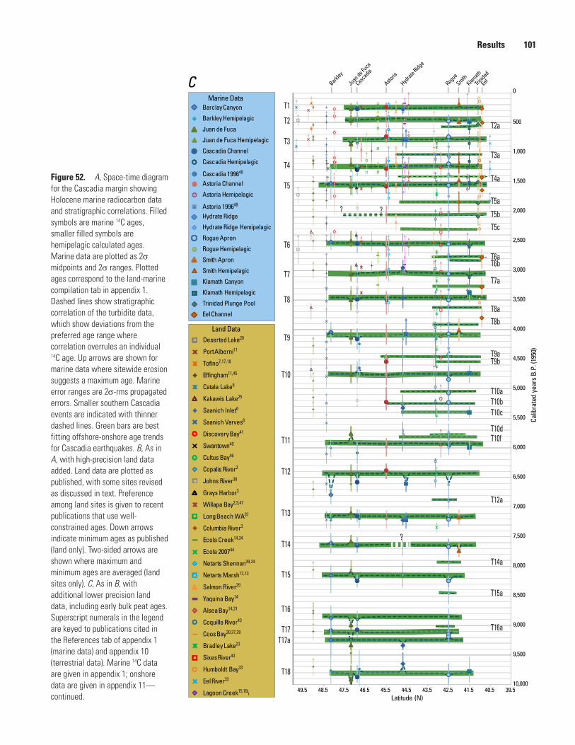
Results 101
Figure 52. A, Space-time diagram for the Cascadia margin showing Holocene marine radiocarbon data and stratigraphic correlations. Filled symbols are marine 14C ages, smaller filled symbols are hemipelagic calculated ages. Marine data are plotted as 2s midpoints and 2s ranges. Plotted ages correspond to the land-marine compilation tab in appendix 1. Dashed lines show stratigraphic correlation of the turbidite data, which show deviations from the preferred age range where correlation overrules an individual 14C age. Up arrows are shown for marine data where sitewide erosion suggests a maximum age. Marine error ranges are 2s-rms propagated errors. Smaller southern Cascadia events are indicated with thinner dashed lines. Green bars are best fitting offshore-onshore age trends for Cascadia earthquakes. B, As in A, with high-precision land data added. Land data are plotted as published, with some sites revised as discussed in text. Preference among land sites is given to recent publications that use well-constrained ages. Down arrows indicate minimum ages as published (land only). Two-sided arrows are shown where maximum and minimum ages are averaged (land sites only). C, As in B, with additional lower precision land data, including early bulk peat ages. Superscript numerals in the legend are keyed to publications cited in the References tab of appendix 1 (marine data) and appendix 10 (terrestrial data). Marine 14C data are given in appendix 1; onshore data are given in appendix 11—continued.
T1
T2
T3
T4
T5
T6
T7
T11
T10
T9
T8
T12
T13
T14
T15
T16
T17
T18
T17a
? ?
?
Deserted Lake20
Port Alberni11
Tofino7,17,18
Effingham11,45
Catala Lake9
Kakawis Lake25
Saanich Inlet6
Saanich Varves6
Discovery Bay41
Swantown40
Cultus Bay46
Copalis River2
Johns River38
Grays Harbor3
Willapa Bay2,3,47
Long Beach WA37
Columbia River3
Ecola Creek14,34
Ecola 200744
Netarts Shennan39,24
Netarts Marsh12,13
Salmon River29
Yaquina Bay14
Alsea Bay14,31
Coquille River43
Coos Bay30,27,28
Bradley Lake23
Sixes River43
Humboldt Bay33
Eel River33
Lagoon Creek15,16\
Land Data
T16a
T3a
T5b
T4a
T2a
T5a
T6a
T10f
T9a
T8a
T7a
T5c
T10a
T10c
T12a
T14a
T15a
T8b
T6b
T9b
T10b
T10d
Juan
de Fu
ca
Casca
dia
Astoria
Hydrat
e Ridg
e
Rogue
SmithKlam
athTri
nidad
Eel
Barkley
Barclay Canyon
Barkley Hemipelagic
Juan de Fuca
Juan de Fuca Hemipelagic
Cascadia Channel
Cascadia Hemipelagic
Cascadia 199648
Astoria Channel
Astoria Hemipelagic
Astoria 199648
Hydrate Ridge
Hydrate Ridge Hemipelagic
Rogue Apron
Rogue Hemipelagic
Smith Apron
Smith Hemipelagic
Klamath Canyon
Klamath Hemipelagic
Trinidad Plunge Pool
Eel Channel
Marine Data
C
39.540.541.542.543.544.545.546.547.548.549.5Latitude (N)
500
0
1,000
1,500
2,000
2,500
3,000
3,500
4,000
4,500
5,000
5,500
6,000
6,500
7,000
7,500
8,000
8,500
9,000
9,500
10,000
Calib
rate
d ye
ars
B.P
. (19
50)

102 Turbidite Event History—Methods and Implications for Holocene Paleoseismicity of the Cascadia Subduction Zone
We observe some systematic age differences between coastal and marine age sequences that otherwise appear likely to represent correlatable events. The basis for this statement is that both datasets have passed independent tests of earthquake origin, and thus the chances of having separate earthquake sequences, one recorded onshore but not offshore, and vice versa, must be considered very low. Offshore dates can be biased in time by unmodeled marine-reservoir variability, which we suspect may account for some age disparities. Onshore dates also may be biased in time, including offsets from dating of detrital material and contamination from younger material, such as roots from a higher stratigraphic level. In several cases, the variability does not appear systematic and may simply be scatter owing to unidentified errors. In cases of clear systematics, we use these differences to model temporal and spatial reservoir variability, along with the difference in benthic and planktic foraminiferal dates, as discussed previously.
For a given time range where overlap exists and a given latitude range, the total number of events, whether onshore or offshore, is similar, with a few differences noted below. The nearly identical recurrence values support our inference that both records are most likely recording the same earthquake series. We suggest that the thinner, spatially limited turbidites offshore are, in many cases, the same events recorded at the more sensitive sites onshore, such as Bradley Lake. Considering the offshore record alone, these turbidites do not have the benefit of the same variety of synchroneity tests that the marginwide events do.
Some of the smallest turbidites offshore appear to be represented by spotty or no record onshore. Although this reduces our confidence in these events to some degree, it is consistent with a reasonable scenario in which smaller earthquakes would be expected to leave a more discontinuous geologic record onshore and offshore. For example, potential correlatives for marine event T2 are observed at many but not all onshore sites (Tofino, Ucluelet, Johns River, Discovery Bay, Netarts Bay, and Ecola Creek; see fig. 2). Where coseismic subsidence data are available for this earthquake, they suggest minimal subsidence relative to other events (Shennan and others, 1998). We also note that the smaller turbidites of limited latitudinal extent correspond reasonably well in age to the local southern Oregon events, where they have been dated or their approximate ages calculated. These earthquakes have limited rupture length in both onshore and offshore records, suggesting a first-order compatability between offshore turbidite size, shaking intensity or duration (controlling turbidite mass) and rupture length. The offshore rupture limits discussed in subsequent sections are derived from our interpretation of the combined coastal/marine data shown in figure 52.
Discovery BayIn a few cases, dated events onshore were interpreted as
upper plate earthquakes because they did not appear in the existing coastal paleoseismic record (events 2 and 3 in Discovery Bay; Williams and others, 2005). However, these events are included in figure 52 because the original interpretations
were based on the interpreted fit, or lack thereof, to existing paleoseismic data, rather than any independent metric of origin. Some of these events appear nonetheless to be a reasonable fit to the Cascadia earthquake time series offshore, which seems to better capture smaller earthquakes than the onshore paleoseismic sites. Resolution of such discrepancies is beyond the scope of this report and will require further research.
Willapa Bay, Grays Harbor, Columbia River, Southwest Washington and Northern Oregon
One of the best documented land paleoseismic sites is the Willapa Bay, Wash., area (Atwater and Hemphill-Haley, 1997; Atwater and others, 2003). These sites (including Grays Harbor and the Columbia River) have a paleoseismic record spanning ~3,500 years that reveals seven probable earthquake events (Atwater and others, 2003); the turbidite record for the same interval and same region offshore includes eight events. The difference is that marine event T2 apparently was not observed at Willapa Bay (or many coastal sites). By comparison, virtually all onshore and offshore sites recorded the A.D. 1700 earthquake, with a tight grouping of dates spanning the margin. The smaller T2 event may have been recorded at Discovery Bay and other land sites (fig. 52); thus we suspect that T2 is simply below a recording or preservation threshold at some land sites.
We would expect to find less age scatter among the later, higher precision studies, and although the error ranges are smaller, there remains considerable scatter among even the best quality dates. For example, event T3, a marginwide event in the turbidite record, is well dated, with an average age of 810±115 cal yr B.P. in the marine record and an average age of 860±100 cal yr B.P. for the most likely correlative onshore event. However, two dates at Willapa Bay and the Salmon River skew the average age older. The age of the likely correlative event (“W”) is given as 980±200 cal yr B.P. by Atwater and others (2004) at Willapa Bay, more than 100 years older than the onshore average and 150 years older than the marine average. This was a single age of very low precision, however. (In appendix 1 and figure 52, we have broken out the correlated and combined dates from Atwater and others (2004), grouped them into dates collected at Willapa Bay, Grays Harbor, and Columbia River, and recombined them in OxCal. This had virtually no effect on the age means. At the Salmon River (Nelson, A.R., and others, 2004), the likely correlative event was dated as 1,040±140 cal yr B.P., although just as at Willapa Bay, this was a single low-precision peat age. If these dates are not included, the onshore average would be 800±100 cal yr B.P., identical to the marine average. Nevertheless, onshore age means range from 990 to 700 cal yr B.P., nearly a 300-year spread as compared to ~120 years in the marine age record. The difference between the land and marine age ranges could be because several old dates are included in the land average or to an unmodeled marine reservoir effect if these data represent the same earthquake. The likely correlative dates for T4, T5, and T6 at Willapa Bay and Grays Harbor are very close to the marine averages; however,

Results 103
the dates for likely T7 and T8 equivalents are well constrained and slightly younger than the marine dates. This ~100 year difference is seen at other sites, as well, and suggests a possible unmodeled reservoir effect in this time range that is applicable marginwide (as opposed to just the southern Cascadia region).
Bradley Lake, Coquille River, and Sixes River, Southern Oregon
Bradley Lake is a coastal lake in southern Oregon that contains a tsunami record of marine sands that inundated the lake. Kelsey and others (2005) established the requirements for such inundation in detail, and they concluded that the tsunami record there was attributable to local, rather than distant, tsunami. Bradley Lake however, had an event time series for which reconciliation with the offshore record initially was problematic. Several of the tsunami sands that occur in Bradley Lake seemed to be poor temporal matches for other land paleoseismic sites and for the offshore turbidite record. For example, Bradley Lake events DE3 and DE4 occur with closely spaced reported dates at about the time of small marine event T3a at ~1,000 cal yr B.P. At the same time, there is no record in Bradley Lake of temporal correlatives of marginwide T3 and T4, which likely were much larger earthquakes. Below that, another Bradley Lake event occurs at the time of small marine event T4a, rather than at the time of the larger T4 or T5 turbidites that bracket this time. Other differences include several closely spaced pairs of events in Bradley Lake, where the most likely correlative marine turbidite is interpreted as a single event. In these cases, it is possible that the marine record would be unable to resolve closely spaced events and may be missing several small events that the Bradley Lake record resolves.
The Bradley Lake record, however, may include a systematic error, which shifts the reported dates older than the event age. This is because the Bradley Lake dates, like many onshore sites, come from detrital plant material. Unlike most other sites, the material comes from a thick post-tsunami mud deposit on the bottom of the lake that overlies the tsunami sands that were swept into the lake. The massive mud deposits likely include a range of materials swept into the lake, from live plant material to detrital material that could be hundreds to thousands of years older than the event. The multiple Bradley Lake dates reported in Kelsey and others (2005) were subjected to a chi2 test to determine which of them were grouped and therefore represented good statistical prospects for representing the event age. Because this test was done on random plant fragments with an age range of hundreds of years for each event, the test likely did not select for the best event age but rather dates that grouped statistically. The reported dates are likely biased older than the event dates because of inclusion of old detrital material. Because material that is younger than the detrital deposit is unlikely in a lake bottom setting (Kelsey and others, 2005), we have investigated using an alternate representation of the Bradley Lake dates that makes use of the youngest age from the sample group from each disturbance event in the lake. Using the youngest valid samples is common in paleoseismic investigations, where sampling represents a maximum age for the event and where
contamination by young material is precluded or unlikely, as in the Bradley Lake samples (McAlpin, 2009; Kelsey and others, 2005). The youngest sample from a group in the massive detrital deposits should represent the age closest to the event time in the lake setting. We also recalibrated the data using IntCal04 to be consistent with the marine data. As with the marine data, we found that recalibration with IntCal04 (Reimer and others, 2004) resulted in shifts of dates of 0–80 years, but more importantly, the PDFs from recalibration were, in many cases, more distinct in terms of the probability peaks, reducing the effect of multiple peaks. Presumably this results from improvements to the calibration database.
In figure 52, we plotted the Bradley Lake data using the youngest age from each event, as described here. We find this refinement of the Bradley Lake data resolves many of the discrepancies between these data and the marine turbidite record, as well as other land data, bringing many of the shifted Bradley Lake dates into closer agreement with other paleoseismic sites. Kelsey and others (2005) also used varves and sedimentation rates to estimate event dates independently, and the results of their analysis are consistent with the radiocarbon dates. The modifications we propose here (all <200 years) are within the range of 16–20 percent error in the sedimentation-rate dates given by Kelsey and others (2005, their table DR2).
The Bradley Lake record is based on tsunami-deposited sands for 12 events and on lake-sediment disturbances (possible local turbidites?) for 4 others (Kelsey and others, 2005). The Bradley Lake record exhibits a greater number of events per unit time than nearby estuary records, including 12 events that require a tsunami height of >5.5 m to reach the lake (Kelsey and others, 2005). The Bradley Lake tsunami stratigraphy includes maximum (960 yr) and minimum (22 yr) repeat times (Kelsey and others, 2005), comparable to the offshore minimum and maximum intervals of 1,190 years and 40 years, respectively).
Bradley Lake may be one of the few onshore sites that has evidence of the smaller class of earthquakes inferred at Rogue Apron, Hydrate Ridge, and other southern Cascadia offshore sites. The mean Bradley Lake recurrence interval is 390 years (<4,600 cal yr B.P.; Kelsey and others, 2005), considerably shorter than other onshore paleoseismic localities and somewhat higher than the offshore average of 220 years for 20 turbidites during the same ~4,600-year period that Bradley Lake was a good paleoseismic recorder (T1–T9a). Bradley Lake appears to be missing T2, as are other land sites, and likely is missing several of the smaller events represented in Rogue Apron cores. The temporal record at Bradley Lake exhibits clusters of events and large time gaps similar to those evident in the offshore record. For the time between T3 and T5 (~1,550–800 cal yr B.P.), the offshore record contains five turbidites and Bradley Lake includes the same number of tsunami sands. For this period, both records have a recurrence interval of ~190 years. From T5 to T6 time (~2,550–1,550 cal yr B.P.), onshore and offshore records include major events bounding this time. The offshore record also includes three very small mud turbidites, T5a, T5b, and T5c, representing events not recorded at any onshore paleoseismic site (with the possible exception of one of these recorded at the Coquille
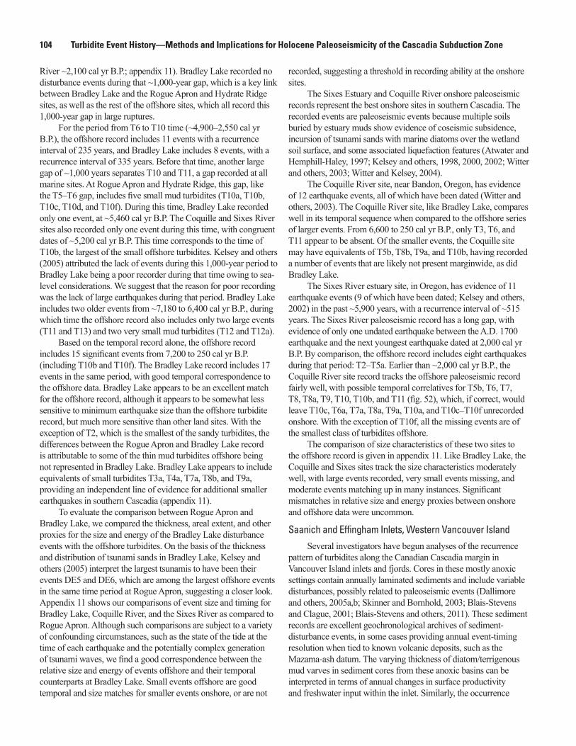
104 Turbidite Event History—Methods and Implications for Holocene Paleoseismicity of the Cascadia Subduction Zone
River ~2,100 cal yr B.P.; appendix 11). Bradley Lake recorded no disturbance events during that ~1,000-year gap, which is a key link between Bradley Lake and the Rogue Apron and Hydrate Ridge sites, as well as the rest of the offshore sites, which all record this 1,000-year gap in large ruptures.
For the period from T6 to T10 time (~4,900–2,550 cal yr B.P.), the offshore record includes 11 events with a recurrence interval of 235 years, and Bradley Lake includes 8 events, with a recurrence interval of 335 years. Before that time, another large gap of ~1,000 years separates T10 and T11, a gap recorded at all marine sites. At Rogue Apron and Hydrate Ridge, this gap, like the T5–T6 gap, includes five small mud turbidites (T10a, T10b, T10c, T10d, and T10f). During this time, Bradley Lake recorded only one event, at ~5,460 cal yr B.P. The Coquille and Sixes River sites also recorded only one event during this time, with congruent dates of ~5,200 cal yr B.P. This time corresponds to the time of T10b, the largest of the small offshore turbidites. Kelsey and others (2005) attributed the lack of events during this 1,000-year period to Bradley Lake being a poor recorder during that time owing to sea-level considerations. We suggest that the reason for poor recording was the lack of large earthquakes during that period. Bradley Lake includes two older events from ~7,180 to 6,400 cal yr B.P., during which time the offshore record also includes only two large events (T11 and T13) and two very small mud turbidites (T12 and T12a).
Based on the temporal record alone, the offshore record includes 15 significant events from 7,200 to 250 cal yr B.P. (including T10b and T10f). The Bradley Lake record includes 17 events in the same period, with good temporal correspondence to the offshore data. Bradley Lake appears to be an excellent match for the offshore record, although it appears to be somewhat less sensitive to minimum earthquake size than the offshore turbidite record, but much more sensitive than other land sites. With the exception of T2, which is the smallest of the sandy turbidites, the differences between the Rogue Apron and Bradley Lake record is attributable to some of the thin mud turbidites offshore being not represented in Bradley Lake. Bradley Lake appears to include equivalents of small turbidites T3a, T4a, T7a, T8b, and T9a, providing an independent line of evidence for additional smaller earthquakes in southern Cascadia (appendix 11).
To evaluate the comparison between Rogue Apron and Bradley Lake, we compared the thickness, areal extent, and other proxies for the size and energy of the Bradley Lake disturbance events with the offshore turbidites. On the basis of the thickness and distribution of tsunami sands in Bradley Lake, Kelsey and others (2005) interpret the largest tsunamis to have been their events DE5 and DE6, which are among the largest offshore events in the same time period at Rogue Apron, suggesting a closer look. Appendix 11 shows our comparisons of event size and timing for Bradley Lake, Coquille River, and the Sixes River as compared to Rogue Apron. Although such comparisons are subject to a variety of confounding circumstances, such as the state of the tide at the time of each earthquake and the potentially complex generation of tsunami waves, we find a good correspondence between the relative size and energy of events offshore and their temporal counterparts at Bradley Lake. Small events offshore are good temporal and size matches for smaller events onshore, or are not
recorded, suggesting a threshold in recording ability at the onshore sites.
The Sixes Estuary and Coquille River onshore paleoseismic records represent the best onshore sites in southern Cascadia. The recorded events are paleoseismic events because multiple soils buried by estuary muds show evidence of coseismic subsidence, incursion of tsunami sands with marine diatoms over the wetland soil surface, and some associated liquefaction features (Atwater and Hemphill-Haley, 1997; Kelsey and others, 1998, 2000, 2002; Witter and others, 2003; Witter and Kelsey, 2004).
The Coquille River site, near Bandon, Oregon, has evidence of 12 earthquake events, all of which have been dated (Witter and others, 2003). The Coquille River site, like Bradley Lake, compares well in its temporal sequence when compared to the offshore series of larger events. From 6,600 to 250 cal yr B.P., only T3, T6, and T11 appear to be absent. Of the smaller events, the Coquille site may have equivalents of T5b, T8b, T9a, and T10b, having recorded a number of events that are likely not present marginwide, as did Bradley Lake.
The Sixes River estuary site, in Oregon, has evidence of 11 earthquake events (9 of which have been dated; Kelsey and others, 2002) in the past ~5,900 years, with a recurrence interval of ~515 years. The Sixes River paleoseismic record has a long gap, with evidence of only one undated earthquake between the A.D. 1700 earthquake and the next youngest earthquake dated at 2,000 cal yr B.P. By comparison, the offshore record includes eight earthquakes during that period: T2–T5a. Earlier than ~2,000 cal yr B.P., the Coquille River site record tracks the offshore paleoseismic record fairly well, with possible temporal correlatives for T5b, T6, T7, T8, T8a, T9, T10, T10b, and T11 (fig. 52), which, if correct, would leave T10c, T6a, T7a, T8a, T9a, T10a, and T10c–T10f unrecorded onshore. With the exception of T10f, all the missing events are of the smallest class of turbidites offshore.
The comparison of size characteristics of these two sites to the offshore record is given in appendix 11. Like Bradley Lake, the Coquille and Sixes sites track the size characteristics moderately well, with large events recorded, very small events missing, and moderate events matching up in many instances. Significant mismatches in relative size and energy proxies between onshore and offshore data were uncommon.
Saanich and Effingham Inlets, Western Vancouver IslandSeveral investigators have begun analyses of the recurrence
pattern of turbidites along the Canadian Cascadia margin in Vancouver Island inlets and fjords. Cores in these mostly anoxic settings contain annually laminated sediments and include variable disturbances, possibly related to paleoseismic events (Dallimore and others, 2005a,b; Skinner and Bornhold, 2003; Blais-Stevens and Clague, 2001; Blais-Stevens and others, 2011). These sediment records are excellent geochronological archives of sediment-disturbance events, in some cases providing annual event-timing resolution when tied to known volcanic deposits, such as the Mazama-ash datum. The varying thickness of diatom/terrigenous mud varves in sediment cores from these anoxic basins can be interpreted in terms of annual changes in surface productivity and freshwater input within the inlet. Similarly, the occurrence

Results 105
of unlaminated mud units (homogenites) intercalated amongst the laminated sediments can be interpreted in terms of oceanic and climatic changes (Dallimore and others, 2005b, 2008; Hay and others, 2009; Chang and Patterson, 2005; Chang and others, 2003). However, the sedimentary record also contains massive and graded mud units believed to arise from debris flows and turbidity currents. Some of these units probably were initiated by seismic events (seismites) corresponding to crustal and plate boundary earthquakes. These units have organic properties with a strong terrestrial signature, as opposed to other mud units in the cores that have marine affinities (Hay and others, 2009).
A large (50 cm) unit has been found in the most recent sediments of Effingham Inlet (giant Calypso core MD02-2494; Dallimore and others, 2009), as well as in other inlets farther to the north on the central mainland British Columbia coast. This deposit has been correlated to the large (magnitude 7.3) central Vancouver Island earthquake that occurred on June 23, 1946 (Dallimore and others, 2005b, 2008; Hay and others, 2009). Liquefaction of sediments, resulting in significant terrestrial and submarine slumps and slides, was initiated on both coasts of Vancouver Island by the seismic shaking associated with this earthquake, which was one of the most damaging in British Columbia’s history (Rogers, 1980). This regionally recognized event bed provides a rare modern analogue for the nature of coastal marine-sediment disturbance resulting from large (Mw ~7) earthquakes and, hence, provides a proxy for the identification of other large earthquakes expressed in the sediment record.
Other paleoseismic events from the Effingham inner-basin core are interpreted as such because, like the 1946 deposit, they have wall-rock signatures from the surrounding highlands and because they show characteristics more closely resembling true turbidites than other disturbance events attributed to climate events in the cores. The deposit from the 1946 earthquake is, while much larger than the other events because of its very local source, similar in character to the events suggested as Cascadia great earthquakes (Dallimore and others, 2005b, 2008).
Similarly, cores collected in Saanich Inlet, on the eastern side of Vancouver Island, reveal a remarkably similar record of debris-flow events interspersed with varved sedimentation (Blais-Stevens and Clague, 2001; Blais-Stevens and others, 2011). Cores from ODP leg 169S and older cores established a record of synchronous deposition of debris-flow deposits at sites separated by several kilometers. Figure 52 includes the interpreted records of debris flows from Effingham and Saanich Inlets. Both records show potentially good correspondence to the marine-turbidite record and land-paleoseismic events. Saanich and Effingham cores both have potential time correlatives for a number of plate boundary earthquakes recorded by onshore and offshore paleoseismic data during the Holocene, except T8, T13, and T14, which may be represented at Saanich but not at Effingham. Events T15, T16, T17, and T18 may be present at Effingham, but data are not available for Saanich. There are a greater number of debris-flow events in Saanich Inlet than are present in the land or marine paleoseismic records for northern Cascadia. In addition to the likely correlatives, a number of other events are interspersed in the record. These events generally are thinner deposits, suggesting smaller
earthquakes or nonseismic sources. Given the known record of at least one debris-flow deposit attributable to a crustal earthquake, it is reasonable to assume that many of the smaller events originate from crustal earthquake sources, though this remains unknown at present. The recurrence intervals for all events in Saanich Inlet (1946 excepted) is very similar to that of southern Cascadia, averaging ~290 years for 24 events between our T13 at ~7,100 cal yr B.P. and A.D. 1700, as compared to 240 years for all events at Rogue Apron. The frequency of events capable of generating debris flows in Saanich Inlet is similar to all recorded seismic events in southern Cascadia.
As an alternative correlation test of the Effingham seismite record, we compared the physical property records of 11 candidate turbidites interpreted as Cascadia earthquakes to possible correlatives in offshore turbidite records. (Data from the upper four turbidites have not been collected because this section is a “freeze core” which cannot be removed from its storage freezer, creating some difficulties for making magnetic measurements). Six of these comparisons are shown in figure 53, which includes magnetic and density traces and radiocarbon dates for Effingham and Cascadia Channel turbidites. A strong stratigraphic physical-property signature common to both onshore and offshore cores is apparent, as is an approximate compatibility between 14C dates for events T5, T6, T7, and T16 and corresponding Effingham ages. For events T10 and T11, the Effingham ages are considerably older. Four other potential correlatives have rather generic turbidite signatures that are not diagnostic, though all are compatible in age. One event is a poor radiocarbon and stratigraphic match. Dated material from the Effingham core is plant and wood material and likely represents maximum limiting ages for these events. In all but one instance (T6), the Effingham ages are older than the offshore turbidite ages.
Although many turbidites are similar, and some parameters may be somewhat autocorrelated by their fining-upward nature, several independent characteristics of the offshore deposits also are evident in the Effingham deposits. Event T5, which appears in some cores with an unusual stacking of sand units, has a density and magnetic signature that appear inverted from the normally declining-upward density and MS pattern. The Effingham signature for the potentially correlative event has a similar inverted appearance (fig. 53). The pattern of turbidite thickness for Effingham is also similar to Cascadia Channel, with events 11 and 16 being large, multipulse events in both sequences; event 10 is a small single pulse event in both sequences, and events 5, 6, 7, and 9 are moderately sized 2- or 3-pulse events in both sequences. We suggest that this evidence lends significant support to an earthquake “signature” as the common link between the onshore and offshore cores, further explored in a subsequent section. This preliminary comparison will require further study.
The record at Effingham inlet is important for advancing understanding of the Cascadia earthquake and tsunami record. At present, the coastal and marine records have much in common; however, head-to-head comparisons between onshore and marine radiocarbon dates are hindered by several issues, including reservoir correction for marine dates. The Effingham turbidites have been dated using terrestrial materials, yielding onshore dates directly comparable to onshore dates elsewhere in Cascadia,

106 Turbidite Event History—Methods and Implications for Holocene Paleoseismicity of the Cascadia Subduction Zone
and potentially helping to bridge the onshore-offshore gap. The stratigraphic physical-property fingerprints at Effingham may also represent an important “missing link” between the northern Cascadia onshore and offshore paleoseismic records.
Constrained Time SeriesFigure 54A shows the OxCal-constrained time series
for all 41 correlated events along the Cascadia margin, with segmentation indicated by symbology. These events are shown as PDFs, constrained with the Combine function in OxCal. The 2σ limits generally are narrower than shown in figure 52 owing to the Bayesian combination of multiple PDFs for events linked
by stratigraphic correlation. The events used in each combine operation are those averaged in appendix 1 (Land-Marine Compilation), and they are used elsewhere in this report where averaged regional event dates are employed for recurrence and other calculations. OxCal model inputs and outputs are given in appendixes 8 and 9. Segment D PDFs also include hemipelagic dates for events not radiocarbon dated. These computed PDFs use the Date function of OxCal inputting the calculated hemipelagic age data. The 2σ limits are generally narrower than shown in figure 52, although the simulated dates have rather broad 2σ ranges. These PDFs do not include constraints available from interevent hemipelagic intervals. Figure 54B shows the past ~7,000 years of record from the turbidite time series, compared
Effingham E5(246–272cm)1636 (±32)cal yr B.P.
Effingham E6(424–434cm)2351 (±17)cal yr B.P.
Effingham E10(1050–1058cm)5290 (±29)cal yr B.P.
Effingham E11(1405–1416cm)6639 (±23)cal yr B.P.
Effingham E16(1974–2070cm)9060 (±37)cal yr B.P.
Effingham E7(625–627cm)3210 (±44)cal yr B.P.
8,000
8,0006,000
0 200 400 600
10,000
9,000
M9907-23 PCCascadia ChannelOxCal combined age 1580 (±70)cal yr B.P.
M9907 22PC“T6”CascadiaChannelOxCal comb. age 2560 (±60) cal yr B.P.
M9907 23 PC“T7”Cascadia ChannelOxCal comb. age 3040 (±90)cal yr B.P.
M9907 23PC“T10” CascadiaChannelOxCal comb. age 4760 (±100)cal yr B.P.
M9907 23PC“T11” CascadiaChannelOxCal comb. age 5890 (±100)cal yr B.P.
M9907 23PC“T16” CascadiaChannelOxCal comb. age 8940 (±160)
0
10
Depth (centimeters)
0
10
0
10
0
10
0
10
0
10
Gamma density (cps) Cascadia Magnetic susceptibility (SI units) Cascadia
Magnetic susceptibility
Gamma density (cps) Cascadia
Magnetic susceptibility
Gamma density (cps) Cascadia
Magnetic susceptibility (SI units) Cascadia
Magnetic susceptibility
Magnetic susceptibility (SI units) Cascadia
Depth (centimeters)
Depth (centimeters)
Depth (centimeters)
Depth (centimeters)
Depth (centimeters)
Figure 53. Preliminary correlations between Cascadia Channel core M9907-23PC and core MD02-2494 from Effingham Inlet, western Vancouver Island, Canada (see fig. 2 for core locations). Each plot shows the magnetic-susceptibility record (blue) from an Effingham Inlet (inner basin) turbidite, and a magnetic-susceptibility or gamma-density record from our 1999 cores in Cascadia Channel (purple). These events were interpreted as seismites by Dallimore and others (2005b), on the basis of wall-rock signature from the adjacent fiord walls (gray) and by comparison to the historical turbidite triggered by the1946 Vancouver Island earthquake. The records show a striking similarity in general size, number of sandy pulses (magnetic and density peaks), and, in some cases, detailed trends. Radiocarbon ages also are first-order compatible but have separations of 100–200 years in some cases. Offshore ages are the OxCal combined ages in appendix 8 with 2s ranges. The combined age data and stratigraphic correlation suggest that the Effingham turbidites and the Cascadia Basin turbidite signatures are recording the same earthquakes. Effingham data from Dallimore and others (2009). Abbreviations: cps, counts per second; SI, Systeme Internationale.

Results 107
Figure 54. A, OxCal-constrained 14C time series of Cascadia turbidites. Probability density functions (PDFs) computed from the best 14C ages and hemipelagic ages for each event. The 2 sigma ranges and median values are shown. Each PDF is computed with the “combine” function of OxCal from multiple 14C ages that are correlated stratigraphically between core sites, where possible. Hemipelagic-based PDFs are generated from hemiplelagic ages calculated in appendix 1. These PDFs are generated by the “age” function in OxCal and have normal distributions applied, based on error ranges given in appendix 1. Vertical scale is arbitrary. OxCal model-agreement indices are shown for the overall model and for each “combine” function where appropriate. Ages used in this figure are taken from appendix 1 and generally are those ages used to calculate event averages in appendix 1. Events are assigned to segments on the basis of latitudinal extents shown in figure 52. Highly uncertain extents exist for T5b, T6a, T6b, T8a, T8b, and for all events south of Rogue Apron. B, OxCal time series for the offshore turbidites compared to Bradley Lake, the Coquille River, and Sixes River onshore paleoseismic sites. Long ruptures are shown by red bars, others shown gray. Colored PDFs use same color scheme as in A.
Combine CSZ-T1 [Amodel:163 Acomb:127]
Combine CSZ-T2 [Amodel:163 Acomb:52]
Combine CSZ-T2a [Amodel:163 Acomb:133]
Combine CSZ-T3 [Amodel:163 Acomb:125]
Combine CSZ-T3a [Amodel:163 Acomb:134]
Combine CSZ-T4 [Amodel:163 Acomb:114]
Combine CSZ-T4a [Amodel:163 Acomb:135]
Combine CSZ-T5 [Amodel:163 Acomb:124]
Combine CSZ-T5a [Amodel:163 Acomb:140]
Combine CSZ-T5b [Amodel:163 Acomb:138]
Combine CSZ-T5c [Amodel:163 Acomb:121]
Combine CSZ-T6 [Amodel:163 Acomb:85]
Rogue event T6a H age [Amodel:163]
Rogue event T6b H age [Amodel:163]
Combine CSZ-T7 [Amodel:163 Acomb:129]
Rogue event T7a H age [Amodel:163]
Combine CSZ-T8 [Amodel:163 Acomb:129]
Rogue event T8a H age [Amodel:163]
Rogue event T8b H age [Amodel:163]
Combine CSZ-T9 [Amodel:163 Acomb:107]
Combine CSZ-T9a [Amodel:163 Acomb:102]
Combine CSZ-T9b [Amodel:163 Acomb:122]
Combine CSZ-T10 [Amodel:163 Acomb:102]
Combine CSZ-T10a [Amodel:163 Acomb:139]
Combine CSZ-T10b [Amodel:163 Acomb:120]
Rogue event T10c H age [Amodel:163]
Rogue event T10d H age [Amodel:163]
Combine CSZ-T10f [Amodel:163 Acomb:117]
Combine CSZ-T11 [Amodel:163 Acomb:87]
Combine CSZ-T12 [Amodel:163 Acomb:93]
Rogue event T12a H age [Amodel:163]
Combine CSZ-T13 [Amodel:163 Acomb:119]
Combine CSZ-T14 [Amodel:163 Acomb:130]
Rogue event T14a H age [Amodel:163]
Combine CSZ-T15 [Amodel:163 Acomb:68]
Rogue event T15a H age [Amodel:163]
Combine CSZ-T16 [Amodel:163 Acomb:115]
Rogue event T16a H age [Amodel:163]
Combine CSZ-T17 [Amodel:163 Acomb:136]
Combine CSZ-T17a [Amodel:163 Acomb:117]
Combine CSZ-T18 [Amodel:163 Acomb:135]
01,0002,0003,0004,0005,0006,0007,0008,0009,00010,000
Calibrated years B.P. (1950)
EXPLANATION
A
Probability Density Function (PDF), Segment A
Probability Density Function (PDF), Segment B
Probability Density Function (PDF), Segment C
Probability Density Function (PDF), Segment D2 σ range and median values are shown
Combine CSZ-T14 [Amodel:163 Acomb:130]
Overall OcCal model agreement index, and combine agreement index

108 Turbidite Event History—Methods and Implications for Holocene Paleoseismicity of the Cascadia Subduction Zone
to Bradley Lake, the Coquille River, and the Sixes River onshore paleoseismic sites.
Variability of Turbidite Deposition along the Southern Cascadia Margin
As the turbidite record shows, there is a progressive increase in turbidite frequency south of Astoria Fan and substantial evidence for correlated turbidites that appear to affect only the southern Cascadia margin (figs. 43–46). The observed turbidite frequency increase in central and southern Oregon is best defined by Hydrate Ridge west basin, which has
only deep-water sediment sources and Rogue Apron. Figure 45 compares the Hydrate Ridge and Rogue Apron sites, with all core data flattened to the turbidite bases of M9907-31PC at Rogue Apron. The consistency of the smaller turbidites among the Rogue Apron cores and the similar sequence at Hydrate Ridge is apparent; there are virtually identical sequences of major turbidites and similar patterns of mud-silt turbidites interspersed between the larger events. The smaller turbidites show variability in thickness, grain size, and physical-property signatures similar to the larger events, but with finer grain size and more subdued signatures. Several of the mud turbidites at Rogue Apron are coarser in the more distal 2009 core TN0909-01JC. Three events have coarse silty to very fine sand bases, whereas their more proximal
Calib
rate
d ye
ars B
.P.
III
IV
VI
VII
sand i
VIII
IX
X
XI
V
XII
sand m
sand g
I
II
III
IV
VI
VII
VIII
IX
X
XI
V
XII
I
II
Bradley LakeB Turbidite Coquille River Sixes River
DE1
DE2DE3
DE4
DE5/6
DE7
DE8
DE9
DE10
DE11DE12
DE13
DE14
DE15
DE16
T1
T2
T4
T6
T5
T4a
T3a
T2a
T3
T5aT5b
T5c
T6a
T7T7a
T8a
T8b
T8
T9
T9aT9b
T10
T10a
T10bT10c
T10dT10fT11
T12
T6b
0
500
1,000
1,500
2,000
2,500
3,000
3,500
4,000
4,500
5,000
5,500
6,000
6,500
7,000
Figure 54. A, OxCal-constrained 14C time series of Cascadia turbidites. Probability density functions (PDFs) computed from the best 14C ages and hemipelagic ages for each event. The 2 sigma ranges and median values are shown. Each PDF is computed with the “combine” function of OxCal from multiple 14C ages that are correlated stratigraphically between core sites, where possible. Hemipelagic-based PDFs are generated from hemiplelagic ages calculated in appendix 1. These PDFs are generated by the “age” function in OxCal and have normal distributions applied, based on error ranges given in appendix 1. Vertical scale is arbitrary. OxCal model-agreement indices are shown for the overall model and for each “combine” function where appropriate. Ages used in this figure are taken from appendix 1 and generally are those ages used to calculate event averages in appendix 1. Events are assigned to segments on the basis of latitudinal extents shown in figure 52. Highly uncertain extents exist for T5b, T6a, T6b, T8a, T8b, and for all events south of Rogue Apron. B, OxCal time series for the offshore turbidites compared to Bradley Lake, the Coquille River, and Sixes River onshore paleoseismic sites. Long ruptures are shown by red bars, others shown gray. Colored PDFs use same color scheme as in A.

Results 109
correlatives are finer grained. Several proposed correlatives at Hydrate Ridge, T5c, and T10c, also have silty bases as compared to mud bases for these events at Rogue Apron.
Though correlative criteria are weaker, we interpret these smaller events as likely correlative (fig. 45) on the basis of radiocarbon data (T10b), calculated hemipelagic ages bracketed by radiocarbon data (T3a, T4a, T10f), similar stratigraphic number and ordering of small events between dated and correlated larger ones, and physical-property stratigraphic correlation. Event ages are calculated for the smaller undated events using sedimentation rates during hemipelagic intervals. Because the sequences at Hydrate Ridge west basin and Rogue Apron are so similar, and because of the complete isolation of Hydrate ridge basin west, we tentatively interpret the correlation of these events as shown in figure 45 as evidence of earthquake origin. The ~250-km distance between the Hydrate Ridge and Rogue Apron sites suggests that correlated events likely ruptured at least this distance along strike.
If our correlations and preferred interpretations are correct, the earthquake event frequency is higher from Astoria Channel southward, with a second significant increase from Hydrate Ridge southward. For the region between Astoria Fan and Rogue Apron, the most likely source of the increase is margin segmentation, because there are no other known major seismic sources and no significant river or canyon systems on that part of the Oregon coast and continental margin that might complicate the record with nonearthquake input.
From Rogue Apron southward, another significant turbidite frequency increase is observed. There are several possible explanations for an increase in turbidite frequency south of the Rogue system. The region from Rogue Apron to Mendocino Channel is coincident with the increasing seismicity near the Mendocino Triple Junction, from the Blanco and Mendocino Fracture Zones, from faults internal to the Gorda Plate, and from the northern San Andreas Fault. Additionally, the canyon systems are fed by numerous rivers with increasingly narrow adjacent shelf widths (Trinidad, Eel, and Mendocino Canyons), suggesting greater connectivity between coastal rivers and offshore canyon systems.
For the Trinidad system, we postulate that the multiple tributary canyon heads that are spaced as much as 50 km apart (figs. 1, 2, 40; Wolf and Hamer, 1999) may contribute to the unusual multipulsed turbidites. Travel distances to a pool or sediment-wave depositional site from the various tributary canyon heads are different, and triggering times vary as the earthquake waves travel along the subduction zone. Thus, several turbidite pulses may arrive at each depositional site caused by the combination of different travel distances and sequential earthquake triggering from each canyon source. The coarse pulses in the cores also may have greater separation owing to their proximal setting in the plunge pool and overall higher sedimentation rate and expanded section. Additional small turbidites in Trinidad plunge pool may be related to additional storm/river input superimposed on the regional paleoseismic turbidite stratigraphy. We are presently unable to distinguish between these mechanisms using sedimentological evidence; however, we favor the expanded section hypothesis because the physical property signatures of
the main Trinidad Pool turbidites correlate reasonably well to other sites when they are compared side by side (fig. 46). T4, for example, is fundamentally a two-pulse turbidite at nearly all sites. At Trinidad Pool, the physical properties and core logs also show T4 to be two coarse pulses, although several very thin silt stringers also are logged in the tail of T4 that are not resolvable (or not present) at most other sites (Nelson, C.H., and others, 2000).
For all of the southern sites, but particularly Eel and Mendocino Channels, resolution of the high-frequency issue requires further investigation. We correlate the thicker turbidites, where possible, to test for along-strike continuity, but we cannot distinguish between hypotheses for the origin of the numerous small turbidites recorded in our cores.
Magnitude SensitivityGoldfinger and others (2007a) show that the offshore
turbidite record of northern San Andreas Fault earthquakes likely is complete, at least down to the level of Mw ~8. Another important observation is that the youngest T1 event in Mendocino Channel is overlain by a deposit of 7–8 cm of hemipelagic sediment in LH-86-NC/Box 1 and LH-86-NC/Box 5. Correlation of these box cores to our piston and trigger cores indicates that this overlying hemipelagic sediment was not recovered in cores M9907-51PC and M9907-51TC (fig. 42). The box cores were taken in 1986, before the 1992 Petrolia earthquake (Oppenheimer and others, 1993), making it impossible to test the sensitivity of Mendocino Channel to this Mw 7.2 earthquake. We had previously attempted to test the sensitivity of this site to the Petrolia earthquake (Nelson, C.H., and others, 2000), but further analysis in this report shows that there are insufficient data to make this test. We, therefore, can say only that we have observed the Mw 7.9 1906 earthquake at multiple sites near the northern terminus of the northern San Andreas Fault, as well as along its length (Goldfinger and others, 2007a).
The ~7–8 cm of hemipelagic surface sediment in Mendocino Channel indicate that ~80–95 years have passed between deposition of the youngest turbidite bed in Mendocino Channel (T0, fig. 42) and 1986. Because LH-86-NC/Box 1 was collected in 1986, the approximate age of this turbidite would be A.D. 1891–1906; thus we infer that T0 could be linked to the 1906 northern San Andreas Fault earthquake. Furthermore, the T1 event, dated at 260+60 cal yr B.P., is consistent with the A.D. 1700 earthquake and is overlain by three turbidites (T0, T0a, T0b; similar to the records at the Eel and Trinidad sites). The frequency of the Mendocino Channel turbidites corresponds to the combined northern San Andreas Fault and Cascadia record for T1 and above, suggesting this site may record earthquakes from both faults in that time range. The overall event frequency from M9907-51PC is too high in the long term for this explanation. The T0a or T0b turbidites could be linked to an early 1800s event observed onshore in Humboldt County (Carver, 2000; Goldfinger and others, 2007a). This event is suggested to have occurred on an additional southern Cascadia segment not observed elsewhere on the Cascadia margin. Our Mendocino Channel data is compatible with this proposed segment, but alternative scenarios are numerous. Turbidite

110 Turbidite Event History—Methods and Implications for Holocene Paleoseismicity of the Cascadia Subduction Zone
T1 also could be the penultimate northern San Andreas Fault event, which is dated at A.D. 1720 (A.D. 1650–1820) (Goldfinger and others, 2007a).
In summary, we believe that the limited available evidence suggests wthat the turbidite record is likley to be fairly complete to a magnitude level of ~Mw 8.0.
Margin Segmentation The correlated turbidite record gives a positive
stratigraphic method of determining rupture length, limited by the spatial core coverage and the uncertainty in the distance a turbidity current could be triggered beyond a segment end. In figure 55 we present the rupture segmentation we infer from latitude limits of the marine and onshore paleoseismic record. In terms of the accuracy of the limits shown in figure 55, Goldfinger and others (2007a) estimated the maximum distance from an earthquake rupture to a triggered turbidity current to be less than ~90 km for full-margin Cascadia events and almost certainly less for smaller events. Uncertainties in correlation also are a factor. Onshore, the constraints are weaker because individual events cannot be correlated stratigraphically. The links between onshore events are based mostly on 14C dates, with some additional constraints from the stratigraphic sequences at the onshore sites. In no cases do we find onshore events extending beyond the latitude limits of the marine record. In most cases, latitude limits are similar, but in a few cases, such as T2, the marine correlatives extend to greater latitude limits. Several of the smaller events in the marine record apparently have no coastal equivalents (T2a and T6a). These are the smallest of the marine events, with narrow latitude limits, thus, we suggest that the marine record is more sensitive to these small events. Limited rupture lengths and, presumably, magnitudes for these events may lack sufficient stress drop to generate significant tsunami or coastal subsidence, although they generate small correlatable marine turbidites. Alternatively, these small offshore events may not correlate as we infer and would then be uncorrelated local events of unknown origin. Although the correlation evidence and limited 14C age control for these events make them less robust than the larger events, their appearance at the same intervals in numerous cores from isolated environments in Cascadia Basin channels and slope basin cores makes such a coincidence unlikely.
Full or Nearly Full Margin RupturesOn the basis of stratigraphic correlations, supporting
radiocarbon dates, and the synchroneity tests discussed above, we define correlative sequences along the Cascadia margin that most likely represent individual earthquakes. The correlation length between offshore core sites then represents the approximate segment length for these ruptures (figs. 44–46, 52).
We can now define a full or nearly full margin segment, termed Segment A, extending approximately from Barkley Canyon (lat 48.2° N.) to Eel Canyon (lat 41° N., assuming T1 extends to Mendocino Channel). We use turbidite-event numbering T1–T19 to designate these full-margin events and to remain consistent with the nomenclature published in Nelson and others (2000) and Goldfinger and others (2003a,b). Only one change from the previous publications has been made: the division of T17 into two separate events, T17 and T17a, yielding 19 regional turbidites during the past 10 k.y., rather than 18. Of these regional turbidites, four ruptures can likely be traced from Barkley Canyon to Eel Channel (T5–T8) and eight ruptures can be traced from Juan de Fuca Channel to Eel Channel (T1–T8). For events older than T9, we observe 11 full-margin events that have southern limits defined by the limitations of the core data. Cores from the Trinidad and Eel Channel systems penetrate no farther than T8 (~3,800 cal yr B.P.); thus no record exists for earlier times. Events T10–T14 are probably recorded as far south as Smith and Klamath Aprons, though highly uncertain below T10. The Smith Apron cores do not penetrate to earlier times, and the Klamath Apron cores, which do penetrate the full Holocene section, reveal a high-frequency record of small turbidites, making them difficult to date or interpret below ~5,000 cal yr B.P. Mendocino Channel cores penetrate only to ~800 cal yr B.P., approximately the time of marginwide T3. Pre-Mazama turbidites T15–T19 are present from Barkley Canyon to Rogue Canyon. Rupture south of Rogue Apron is suggested by the robust appearance of events T15–T19 in Rogue Apron, from which we infer it unlikely that Rogue Apron was near a southern rupture limit and that these earthquakes ruptured well to the south of Rogue Canyon.
The Barkley Canyon turbidite record can be correlated with the Juan de Fuca and Cascadia Channel, Hydrate Ridge, and Rogue Apron sites for T5–T19, although sparse 14C dates from Barkley Canyon make this link somewhat less robust than for other sites. T13 is very weak at Barkley Canyon, but most other marginwide events appear to be represented. The thin beds interpreted as T1–T4 in Barkley cores are subdued and uncertain. The full-margin segment most likely ruptured at Barkley Canyon for all events older than T4, and rupture along the Barkley Canyon segment is likely for T1–T4 as well. This conclusion is based on the presence of the A.D. 1700 earthquake and other coastal paleoseismic events onshore that likely correlate with the marine record on Vancouver Island (Hughes, 2000; Hutchinson and others, 2000). We note a lack of evidence in our cores for an overlap of events that would be expected near a northern segment boundary with a different rupture history. However, our turbidite record does not extend farther north than Barkley Canyon, leaving ~150 km of the margin without an offshore record and presenting the possibility that a small segment with a separate rupture history could exist there.
Segment A has a minimum rupture length of 800 km. Events T1–T8, included in the Eel Channel cores, extend this length an additional 60 km (860 km total length).

Results
111
Figure 55. Holocene rupture lengths of Cascadia great earthquakes from marine and onshore paleoseismology. Four images showing rupture modes inferred from turbidite stratigraphic/14C correlation, supported by onshore radiocarbon data. Marine core sites controlling rupture-length estimates are shown as yellow dots. A, Full or nearly full rupture, represented at most sites by 19 events. B, Mid-southern rupture, represented by 3–4 events. Northern extents of T8a and T8b are uncertain, although one of them likely is present at Astoria. T5b is present at Astoria, but most likely does not reach Juan de Fuca (JDF). C, Southern rupture from central Oregon southward represented by 10–12 events. Northern extents of Segment C events break into two groups, one terminating south of Hydrate Ridge (HR), as indicated by dashed line. The second group extends north of Hydrate Ridge but is not observed at Astoria. D, Southern Oregon/northern California events, represented by a minimum of 7–8 events. Northern extents of Segment D events break into two groups, one terminating south of Rogue, as indicated by dashed lines. The second group extends north of Rogue, but is not observed at Hydrate Ridge. Southern rupture limits are poorly known for all events indicated by query, are limited by temporal coverage, and are probable nonseismic events in the early Holocene. See table 11 for details of limiting criteria and text for additional constraints applied. Recurrence intervals for each segment are shown in A. Rupture terminations are located approximately between three forearc structural uplifts, Nehalem Bank (NB), Heceta Bank (HB) and Coquille Bank (CB). Approximate updip and downdip limits from Goldfinger and others (1992, 1996, 2007a), Clarke and Carver (1992b), Oleskevich and others (1999), and Priest and others (2009). Paleoseismic segmentation shown also is compatible with latitudinal boundaries of episodic tremor and slip (ETS) events proposed for the downdip subduction interface (Brudzinski and Allen, 2007) and shown by white dashed lines. A northern segment proposed from ETS data at approximately lat 48° N. does not appear to have a paleoseismic equivalent.
A B CT1T2T3T4T5T6T7T8T9T10T11T12T13T14T15T16T17T17aT18
T5bT9aT8a or b?T10b
T3aT4aT5aT5cT8a or bT10aT10cT10dT10f
T2aT8a or bT15a
NB
HB
CB
NB
HB
CB
NB
HB
CB
NB
HB
CB
500–530years(110–1,150)
410–500years(110–1,150)
220–240 years(40–600)
300–380years(40–1,150)
? ? ? ?<200 years
T6aT6bT7aT9bT12aT14aT16aAdditionalunresolved events
Barkley
JDF
Astoria
HR
Rogue
Barkley
JDF
Astoria
HR
Rogue
Barkley
JDF
Astoria
HR
Rogue
Barkley
JDF
Astoria
HR
Rogue
SmithKlamathTrinidad
Eel
SmithKlamathTrinidad
Eel
SmithKlamathTrinidad
Eel
D129 128 127 126 125 124 123 122 121 129 128 127 126 125 124 123 122 121 129 128 127 126 125 124 123 122 121 129 128 127 126 125 124 123 122 121
128 127 126 125 124 123 122 128 127 126 125 124 123 122128 127 126 125 124 123 122 128 127 126 125 124 123 122
48
47
46
45
44
43
42
41
40
48
47
46
45
44
43
42
41
40
48
47
46
45
44
43
42
41
40
48
47
46
45
44
43
42
41
40
48
47
46
45
44
43
42
41
40
48
47
46
45
44
43
42
41
40
48
47
46
45
44
43
42
41
40
48
47
46
45
44
43
42
41
40

112 Turbidite Event History—Methods and Implications for Holocene Paleoseismicity of the Cascadia Subduction Zone
Segmented RupturesInvestigators onshore have postulated for some time that there
are segmented ruptures that affect southern Cascadia on the basis of mismatching 14C data along strike and the higher recurrence frequency from southern Cascadia sites (Kelsey and others, 2002, 2005; Nelson, A.R., and others, 2006, 2008; Witter and others, 2003). We suggest that there is significant commonality between the onshore and offshore paleoseismic records and that along strike correlation of the offshore turbidites can help resolve some of the unknowns. The evidence for correlated turbidites of limited spatial extent is fairly robust and, in many instances, is consistent with the onshore paleoseismic data.
We observe two classes of thinner turbidites, a larger class and a smaller class. The larger class includes T10b and T10f, which are similar in thickness to the marginwide events. These two turbidites are best observed in Rogue Apron and Hydrate Ridge cores (fig. 45), where they have well-defined sandy bases and fining-upward sequences and are dated (figs. 30, 33, 45). The smaller class of southern Cascadia turbidites, 20 in all, is composed of thinner, mud-silt turbidites, subdued in their physical-property signatures, more bioturbated, and limited in strike length. In many cases these beds are undatable with 14C methods owing to bioturbation and thin, poorly defined hemipelagic intervals. Our initial interpretation, including these smaller events from 3,000 to 0 cal yr B.P. is given by Goldfinger and others (2008). Here we extend the southern Cascadia record to 10,000 years, with additional data pertinent to the thinner southern Cascadia turbidites. These mud turbidites were noted in the original core logs as darker intervals within what was logged as hemipelagic sediment between major turbidites. The origin of the darker intervals was initially unknown; however, the physical property, color data, smear slides, grain-size analysis, and CT imagery indicate that they are fine-grained mud turbidites. The original logging of these intervals as hemipelagic sediment would have required high and extremely variable sedimentation rates. For example, event T2a, is shown in figure 35. Although these mud-silt turbidites commonly cannot be dated and have weak physical-property signatures, they are observed persistently at the same intervals in cores between Hydrate Ridge and Eel Channel and occur in approximately the same frequency and at approximately similar times to many smaller events recorded onshore at the Bradley Lake, Sixes River, and Coquille River coastal paleoseismic sites. In particular, the good correlation between Hydrate Ridge and Rogue Apron (fig. 45) supports the interpretation of the smaller mud events as earthquake generated, and significant coincidence would be required to generate the two similar sequences by some other method.
The 20 correlated thin turbidites represent an average recurrence interval of ~500 years. The long interval suggests that alternative triggers, such as major storm events, are unlikely for many of the same reasons as for larger events. The recurrence interval of several hundred years also approximately matches the onshore earthquake recurrence interval for segmented ruptures, further discussed in the next section. The small events are best explained by smaller earthquakes of limited rupture length, though with more caveats than the marginwide events. In addition to the
intersite correlation, the preferred interpretation of the presence of these smaller events at Hydrate Ridge places an additional constraint on possible origins in that shallow-water origins, such as storm or tsunami triggering, are excluded at this isolated site. Further details and analysis of the series of mud turbidites a the Rogue Apron site are given in Goldfinger and others (in press).
Our preferred interpretation of the along-strike limits of the segmented southern ruptures is shown in figure 55. The primary observation is that segmented earthquake ruptures occur primarily in southern Cascadia, with variable northern (and probably southern) limits. Ten ruptures are interpreted to terminate at or near Rogue Apron: T2a, T6a, T6b, T7a, T8a (or T8b), T9b, T12a, T14a, T15a, and T16a. These events are among the faintest in our records. Eight ruptures likely terminate near Hydrate Ridge: T3a, T4a, T5a, T5c, T10a, T10c, T10d, and possibly T10f. These ruptures are interpreted to appear in both Rogue Apron and Hydrate Ridge cores but do not appear in Astoria Channel cores. Four ruptures that may extend north of Hydrate Ridge include T5b, T9a, T8a or T8b, and T10f, but we are unable to determine the limits for these beyond Hydrate Ridge with confidence. More events exist to the south of Rogue Apron. As of this writing, correlation and testing of these numerous events for earthquake origin is underway.
The southern limits of many of the correlated mud turbidites also are difficult to determine with existing data. Core M9907-41PC in Eel Channel has a large number of smaller turbidites that may include storm input from the Eel River. We have filtered these out of the magnetic record shown in figure 41 by using the loop-magnetic record rather than the point-source record (see Methods section). This effectively captures only the larger turbidites but also filters the detail and smaller events of interest. New cores collected in 2009 will help clarify the southern Cascadia record.
In summary, we can tentatively define three southern Cascadia segments in addition to the full-margin ruptures represented by T1–T18 (fig. 55). Our preferred northern and southern limits and defining core numbers are given in table 11. Northern limits for T1–T4 are uncertain in Barkley Canyon. Southern limits for events older than T8 vary by site and are limited by lack of data south of Klamath Apron. Events older than T14 are limited by lack of data south of Rogue Apron (table 11).
Recurrence Intervals of Cascadia EarthquakesFigure 55 shows the rupture limits of four modes of
Cascadia great earthquake rupture that we model from the offshore paleoseismic data, the event numbers for each segment, and the average recurrence value and range for each segment. Table 11 gives the average age for each event marginwide and the standard deviation for the dates used in the averages. For table 9 we use the best available dates for each event for both averaged and OxCal solutions. We exclude reversed dates and dates with coring deformation, or other sampling problems, and include dates calculated from well-constrained hemipelagic thicknesses. The data used for table 9 are reproduced and simplified from appendix 1, which contains the raw data, all corrections, and averaging selections used for table 10.

Results 113
Table 11. Rupture limits (limiting core sites and core numbers) from turbidite correlation, Cascadia subduction zone. Marine turbidite number
North limit Supporting data source South limit Supporting
data source Robustness at limiting site Notes
T1 Vancouver Island
Cores 05PC/TC, possible in 09PC/TC
Mendocino Channel/Eel
Cores 51PC/TC,41PC
T2
Juan de Fuca Canyon, Barkley?
Cores 05PC, 11–12 PC/TC, possible in 09PC/TC
Eel Canyon Core 41PC Weak in Trinidad and Klamath, likely present in Eel, though undated.
T2a Rogue Apron
Cores 30–31PC-TC, 55KC, 01JC
Eel Canyon Core 41PC Strong at Rogue, absent at HR Present at Hydrate Ridge, uncertain in Astoria. Not present in JDF. Possibly present in Eel.
T3 Vancouver Island
Cores 05PC/TC, possible in 08–09 PC-TC
Eel Canyon Core 41PC
T3a Hydrate Ridge
Cores 56 PC/TC, 02PC/TC
Trinidad Canyon. Possible in Eel
Cores 35-37PC
This event very weak in 56PC. 02TC has small density blip at the stratigraphic position, and silt stringers present, with overlying hemipelagic between it and base of T3. Robustness slightly weaker than Rogue. This event probably reached HR and died out greater than 90 km south of Astoria.
T4 Vancouver Island
Cores 05PC/TC, 08–09 PC/TC possible
Eel Canyon Core 41PC
T4a Hydrate Ridge
Cores 56 PC/TC, 02PC/TC
Trinidad Canyon, Eel?
Cores 35-37PC
This event signature similar to Rogue, very weak at both sites. This event probably died between HR and Astoria, but must be more than 90 km from Astoria.
T5 Vancouver Island
Cores 08–09PC-TC Eel Canyon Core 41PC
T5a Hydrate Ridge
Cores 56 PC/TC, 02PC/TC Eel Canyon Core 41PC
Weak, thin event at HR, but also obscured by core break. This event must terminate between HR and Astoria, greater than 90 km south of Astoria.
T5b Astoria Canyon?
Cores 02, 56PC-TC, 16 and 17 PC
Eel Canyon Core 41PCSmall, thin event in 16TC, but similar in thickness, mag and density to adjacent T5 and T6 in 16PC. Heavily bioturbated in 17TC, obscured by core break in 17PC. Very weak if present in the non-diagnostic cores 19 and 20 PC-TC.
Hemipelagic ages suggest this is T5b as opposed to T5a or T5c. Weak in Eel, but likely present
T5c Hydrate Ridge Core 56 PC Eel Canyon Core 41PC
Robust in HR, not present at Astoria. Must terminate between HR and Astoria, but must be greater than 90 km south of Astoria.
Weak in Eel, but likely present.
T6 Vancouver Island
Cores 08–09PC-TC Eel Canyon Core 41PC Extension to Eel likely.
T6aRogue Apron? Uncertain
Cores 30–31PC-TC, 55KC, 01JC
Eel Canyon Core 41PC Core disturbance of lower part of T6 precludes determination at HR
T6b Rogue Apron?
Cores 30–31PC-TC, 55KC 01JC
Rogue Apron
Cores 30–31PC-TC, 55KC 01JC
Possible very faint appearance at Rogue, event must terminate south of Rogue.
Event poorly correlated along strike; extent and origin uncertain.
T7 Vancouver Island
Cores 05PC/TC, possible in 08–09PC-TC
Eel Canyon Core 41PC Possibly present in Barkley, certainly in JDF.
T7a RogueCores 30–31PC-TC, 55KC, 01JC
Eel Canyon Core 41PC Possible but doubtful presence at HR. Likely died between Rogue and HR.
Weakens mid margin, HR uncertain, Could terminate between Rogue and HR.
T8 Vancouver Island
Cores 08–09PC-TC Eel Canyon Core 41PC
T8a
One of T8a or T8b may reach Astoria
Core 17PC only Klamath Canyon 34PC-TC
One small event at this position present at HR and in 17PC only at Astoria. If this is correlative to Rogue, it is not clear whether this is T8a or T8b. Physical properties and H thickness not diagnotsic. CT may resolve. Northern limit near Astoria slightly favored, but very uncertain.
T8b
One of T8a or T8b may reach Astoria
Core 17PC only Trinidad?Cores 35, 36, 37 PC/TC
One small event at this position present at HR and in 17PC only at Astoria. If this is correlative to Rogue, it is not clear whether this is T8a or T8b. Physical properties and H thickness not diagnotsic. CT may resolve. Northern limit near Astoria slightly favored, but very uncertain.
T9 Vancouver Island
Cores 08–09PC-TC Eel Canyon Core 41PC
T9a Astoria Canyon
Cores 16–17 PC-TC
Klamath Canyon 34PC-TC
This event is a very robust event similar to T10 and T9 at Astoria, although there is some ambiguity of the correlation. Event is weak at HR.
Minimum southern limit defined by Klamath as Smith, Trinidad, and Eel do not penetrate to this depth.
T9b Rogue Apron
Cores 30–31PC-TC, 55KC 01JC
Klamath Canyon 34PC-TC
Minimum southern limit defined by Klamath as Smith, Trinidad, and Eel do not penetrate to this depth.

114 Turbidite Event History—Methods and Implications for Holocene Paleoseismicity of the Cascadia Subduction Zone
Table 11. Rupture limits (limiting core sites and core numbers) from turbidite correlation, Cascadia subduction zone—continued. Marine turbidite number
North limit Supporting data source South limit Supporting
data source Robustness at limiting site Notes
T10 Vancouver Island
Cores 08–09PC-TC
Klamath Canyon 34PC-TC
Minimum southern limit defined by Klamath as Smith, Trinidad, and Eel do not penetrate to this depth.
T10a Hydrate Ridge Core 56PC Klamath
Canyon 34PC-TCWeakly present at HR, similar to Rogue in thickness and physical property signature. Probably dies out between HR and Astoria. Not well constrained.
Minimum southern limit defined by Klamath as Smith, Trinidad, and Eel do not penetrate to this depth.
T10b Astoria Canyon
Cores 16–17 PC-TC
Klamath Canyon 34PC-TC Robust at Astoria, dies between Astoria and JDF.
Minimum southern limit defined by Klamath as Smith, Trinidad, and Eel do not penetrate to this depth.
T10c Hydrate Ridge Core 56PC Klamath
Canyon 34PC-TC Robust at HR, dies between HR and Astoria, greater than 90 km south of Astoria.
Minimum southern limit defined by Klamath as Smith, Trinidad, and Eel do not penetrate to this depth.
T10d Hydrate Ridge Core 56PC Klamath
Canyon 34PC-TC Weakly present at HR, similar to Rogue in thickness and physical property signature. Dies between HR and Astoria.
Minimum southern limit defined by Klamath as Smith, Trinidad, and Eel do not penetrate to this depth.
T10eBetween Smith and Rogue
Cores 30–31PC-TC, 55KC 01JC, 34PC-TC
Klamath Canyon 34PC-TC
Minimum southern limit defined by Klamath as Smith, Trinidad, and Eel do not penetrate to this depth.
T10funcertain, may extend north of HR
Core 56PC Klamath Canyon 34PC-TC Very robust at HR, not present at Astoria, but correlation and
age contril below T10 less certain.
Minimum southern limit defined by Klamath as Smith, Trinidad, and Eel do not penetrate to this depth. T10b or T10F may extend to Astoria, T10f most likely.
T11 Vancouver Island
Cores 08–09PC-TC
Klamath Canyon 34PC-TC
Minimum southern limit defined by Klamath as Smith, Trinidad, and Eel do not penetrate to this depth.
T12 Vancouver Island
Cores 08–09PC-TC
Klamath Canyon 34PC-TC
Minimum southern limit defined by Klamath as Smith, Trinidad, and Eel do not penetrate to this depth.
T12a Rogue Apron
Cores 30–31PC-TC, 55KC 01JC
Klamath Canyon 34PC-TC
Minimum southern limit defined by Klamath as Smith, Trinidad, and Eel do not penetrate to this depth.
T13 Vancouver Island
Cores 08–09PC-TC
Klamath Canyon 34PC-TC
Minimum southern limit defined by Klamath as Smith, Trinidad and Eel do not penetrate to this depth
T14 Vancouver Island
Cores 08–09PC-TC
Klamath Canyon 34PC-TC
Minimum southern limit defined by Klamath as Smith, Trinidad and Eel do not penetrate to this depth
T14a Rogue Apron
Cores 30–31PC-TC, 55KC 01JC
Klamath Canyon 34PC-TC
Minimum southern limit defined by Klamath as Smith, Trinidad and Eel do not penetrate to this depth
T15 Vancouver Island
Cores 08–09PC-TC
Rogue Apron
Cores 30–31PC-TC, 55KC 01JC
Minimum southern limit defined by Rogue, as Klamath difficult to interpret below T14 and Smith, Trinidad and Eel do not penetrate to this depth
T15a Rogue Apron
Cores 30–31PC-TC, 55KC 01JC
Rogue Apron
Cores 30–31PC-TC, 55KC 01JC
Minimum southern limit defined by Rogue, as Klamath difficult to interpret below T14 and Smith, Trinidad and Eel do not penetrate to this depth
T16 Vancouver Island
Cores 08–09PC-TC
Rogue Apron
Cores 30–31PC-TC, 55KC 01JC
Minimum southern limit defined by Rogue, as Klamath difficult to interpret below T14 and Smith, Trinidad and Eel do not penetrate to this depth
T16a Hydrate Ridge
Cores 30–31PC-TC, 55KC 01JC
Rogue Apron
Cores 30–31PC-TC, 55KC 01JC
Presence possible at HR, may corelate to Rogue T16a. Minimum southern limit defined by Rogue, as Klamath difficult to interpret below T14 and Smith, Trinidad and Eel do not penetrate to this depth
T17 Vancouver Island
Cores 08–09PC-TC
Rogue Apron
Cores 30–31PC-TC, 55KC 01JC
Minimum southern limit defined by Rogue, as Klamath difficult to interpret below T14 and Smith, Trinidad and Eel do not penetrate to this depth
T17a Vancouver Island
Cores 08–09PC-TC
Rogue Apron
Cores 30–31PC-TC, 55KC 01JC
Minimum southern limit defined by Rogue, as Klamath difficult to interpret below T14 and Smith, Trinidad and Eel do not penetrate to this depth
T18 Vancouver Island
Cores 08–09PC-TC
Rogue Apron
Cores 30–31PC-TC, 55KC 01JC
Minimum southern limit defined by Rogue, as Klamath difficult to interpret below T14 and Smith, Trinidad and Eel do not penetrate to this depth
T19 Vancouver Island
Cores 08–09PC-TC
Rogue Apron
Cores 30–31PC-TC, 55KC 01JC
Minimum southern limit defined by Rogue, as Klamath difficult to interpret below T14 and Smith, Trinidad and Eel do not penetrate to this depth

Results 115
For Segments B, C, and D, northern terminations are broken into two groups terminating either north or south of the controlling core site. The approximate northern terminations are established using thickness trends of the individual turbidites and the distance beyond which earthquake triggering is unlikely (estimated to be ~90 km; Goldfinger and others, 2007a). For example, in Segment B, events T9b and T10b are robust events in Astoria Channel cores, equal or greater in thickness than at other sites, suggesting they do not terminate near the Astoria Channel core sites. These two events are not observed at the Juan de Fuca Channel site, indicating they probably terminate between these two core sites. The minimum triggering distance further restricts their northern terminations to greater than 90 km south of Juan de Fuca Channel. Events that are faintly present, as compared to other sites, are assumed to have terminated within 90 km of the controlling core site, between the controlling site and other robust sites.
Segment AFor the north-central Cascadia margin and full-margin
ruptures (Segment A, fig. 55), the turbidite-based recurrence interval for the 10-k.y. record is ~530 years for the 19 events listed in figure 55 (T5b has an uncertain northern limit; thus the Segment A recurrence interval is 500 years if T5b is included). Because the southern and northern limits are less certain for some periods of time, as described above, the recurrence interval for nearly full margin ruptures applies between lat 48° N. and lat 42° N. and could be different farther north and farther south. The best available onshore comparison for the northern margin is found at Willapa Bay (Atwater and others, 2003). The onshore earthquake record there includes seven events in ~3,500 years, and the offshore record includes eight events at that latitude, the difference being T2, which is not observed onshore. The Willapa Bay recurrence interval is then 530 years,
whereas the offshore interval is 460 years for the same ~3,500-year period. If T2 is included in the onshore average (possibly recorded at Discovery Bay; Williams and others, 2005) the onshore and offshore recurrence intervals would be the same. For areas to the north, along Vancouver Island, there presently is not enough onshore data for meaningful comparison.
Hemipelagic Thickness Based Recurrence Intervals for Segment A
Throughout this report, we use hemipelagic sediment thicknesses to calculate sedimentation rates, to check and correct for erosion, and to correct for sample interval thickness. We can also calculate hemipelagic dates and intervals as a check on the distribution of time intervals. Because radiocarbon dates can be in error, the interevent times also can be driven by inaccurate or biased data. Hemipelagic sedimentation theoretically provides an independent timeline; however, we generally do not know its deposition rate independent of the radiocarbon data, with the exception of T1 and T14, which anchor the deposition time independently. We use this information as a semi-independent indicator of time. Hemipelagic thicknesses that yield significantly different interevent times than the 14C data can flag intervals for which the inconsistency is suggestive of bad radiocarbon data, or undetected erosion.
Using the best hemipelagic thickness for each interval between turbidites and above T1, we calculate the interevent time intervals based on the hemipelagic thickness and moving-window average sedimentation rates. The average recurrence interval during the most recent 10 k.y. is the same as the radiocarbon result. The individual intervals are given in table 12. The interevent times are consistent with those calculated from the 14C dates, with several exceptions, including T12, T17, T17a, and T18, which have unresolved inconsistencies between the marginwide average
Table 12. Turbidite mass versus interevent time, Cascadia subduction zone.
Turbidite number
Mean age,in years
Standard deviation of mean ages
Margin average
following interevent,
in time, years
Margin average
prior interevent,
in time, years
Hemipelagic interevent
following time (Cascadia Channel)
Hemipelagic interevent prior time (Cascadia Channel)
12PC scaled mass
23PC scaled mass
12PC and 23PC
average mass
31PC scaled mass
56PC scaled mass
1 250 232 227 432.3 382.9 407.6 165.0 73.52 482 83 232 316 227 368 284.1 148.2 216.1 87.0 33.03 798 58 316 446 368 290 382.9 333.5 358.2 175.5 190.54 1,243 42 446 311 290 486 271.7 333.5 302.6 103.5 201.05 1,554 32 311 982 486 617 284.1 580.5 432.3 118.5 108.06 2,536 22 982 492 617 472 481.7 555.8 518.7 79.5 168.07 3,028 61 492 415 472 487 839.8 778.1 808.9 127.5 126.08 3,443 68 415 665 487 593 963.3 419.9 691.6 124.5 180.09 4,108 52 665 661 593 810 716.3 345.8 531.1 129.0 57.010 4,770 51 661 1,189 810 899 370.5 185.3 277.9 201.0 48.011 5,959 111 1,189 508 899 449 1,136.2 1,543.8 1,340.0 447.0 234.012 6,466 102 508 715 449 705 98.8 111.2 105.0 15.0 45.013 7,182 44 715 443 705 465 642.2 271.7 457.0 312.0 114.014 7,625 39 443 548 465 560 259.4 259.4 259.4 135.0 18.015 8,173 95 548 733 560 675 247.0 148.2 197.6 195.0 45.016 8,906 62 733 195 675 614 1,111.5 2,741.7 1,926.6 258.0 243.017 9,101 38 195 117 614 454 222.3 481.7 352.0 117.0 66.017a 9,218 39 117 577 454 130 148.2 135.9 142.0 171.0 36.018 9,795 94 577 388 130 234.7 481.7 358.2 165.0 99.0

116 Turbidite Event History—Methods and Implications for Holocene Paleoseismicity of the Cascadia Subduction Zone
event dates and the hemipelagic-sediment thickness in Cascadia Channel. We calculate these values for Cascadia Channel because the hemipelagic data there is the best quality and has the lowest degree of uncertainty. The average difference between the radiocarbon and hemipelagic-based intervals is small, although deviations for the above-mentioned events are as great as 440 years for several outlier events. The value of the semi-independent time line is that it serves to support the overall suite of recurrence intervals derived from the radiocarbon data, as well as to draw attention to problem intervals. This allows more confident use of the intervals and their frequencies in seismic and tsunami hazard assessments (Priest and others, 2009) and for comparisons to the paleoseismic history of other neighboring faults (Goldfinger and others, 2008).
Earlier investigators hypothesized that the recurrence intervals were regular, using the turbidite record at Cascadia Channel (Adams, 1990). This inference was based on the apparently uniform thickness of hemipelagic intervals and turbidite spacing in these early cores. Our data do not support this conclusion and include interevent times that range from ~400 years to more than 1,000 years. We suspect the apparent similarity of hemipelagic thickness is partly an artifact of preservation in that basal erosion, particularly in Cascadia Channel, affects these observations, and only through analysis of numerous cores can values approaching the true thickness be obtained. Our range of hemipelagic thickness in Cascadia Channel cores ranges from 2 to 10 cm (appendix 1), which is far from uniform. The visual appearance of regularity in the cores is striking, nonetheless, and is due to the uniform overall thickness of the turbidites, which make up almost all of the section.
Segment BFor the segment bounded at approximately lat 46° N.,
near offshore Nehalem Bank, Oregon (Segment B, fig. 55), the offshore turbidite record suggests a reduced recurrence time owing to the presence of four turbidites not oberved to the north. Our tentative correlation suggests the presence of T5b, T9a, the probable presence of T10b, and possible presence of either T8a or T8b. The corresponding recurrence interval for this segment is 430 years, if we include the less certain T8a or T8b. Onshore, Netarts Bay has a paleoseismic record with recurrence intervals of 540 years during the past 2,500 cal yr B.P. (Shennan and others, 1996, 1998) and 470 years in the past 3,500 cal yr B.P. (Darienzo and Peterson, 1995). Although these less precise bulk-peat dates are problematic in terms of event correlation, the overall frequency is not affected. These sites corroborate the increased event frequency in this segment, but they do not include all events recorded in the Astoria Channel offshore cores. The northern terminations of T9b, T10b and T8a or T8b are closely constrained by their robust presence at Astoria Channel and absence at Juan de Fuca Channel. This restricts their northern limit to ~90 km or more from the Juan de Fuca Channel site. T5b likely
terminates between Astoria Channel and Juan de Fuca Channel, with the possibility of extending farther north, as previously discussed.
Segment CFor the segment bounded at lat ~44° N., near Heceta Bank
in central Oregon (Segment C, fig. 55), the offshore turbidite record suggests a recurrence time further reduced by the inclusion of events that reach this latitude and are recorded at Hydrate Ridge: T3a, T4a, T5a, T5c, T8a or T8b, T10a, T10c, T10d, and T10f. The northern limit of T8a or T8b is uncertain, and it could lie between Hydrate Ridge and Astoria Channel. The corresponding recurrence interval for this segment is ~350 years during the past 10 k.y. The onshore rate is ~485 years recorded at Salmon River (<2,200 cal yr B.P.; Nelson and others, 2004), 580 years at Alsea Bay (<2,500 cal yr B.P.; Nelson, Sawai, and others, 2008), 425 years at Siletz Bay (<2,800 cal yr B.P.), and 530 years at Netarts Bay (<2,900 cal yr B.P.; Darienzo and Peterson, 1995). Like Willapa Bay, these sites do not include the small T2 event and likely do not include any of the smaller mud turbidites. Some other large events appear to be missing from the onshore record as well, including T3 from Yaquina and Siletz Bays and T4 from earlier Alsea Bay work (Peterson and Darienzo, 1996); however, temporal correlation to these sites, which utilized bulk-peat dating is problematic. Coos Bay, with a recurrence interval of 620 years (<4,600 cal yr B.P.; Nelson, A.R., and others, 1996a, 2006) would appear to be missing several significant events, as well as a number of smaller ones. Termination estimates suggest that many of the segment C events extend beyond Hydrate Ridge, on the basis of their robust appearance at that site, and terminate between Hydrate Ridge, and Astoria Channel, but not closer than 90 km south of Astoria Channel.
Segment D The most difficult segment to resolve is the southernmost
segment, Segment D (fig. 55). In the offshore records, Rogue Apron is the only southern site that reliably contains the entire Holocene, apparently without influence from nearshore storm or river input that affects other southern Cascadia sites at various times during the Holocene. Rogue Apron includes 41 events that correlate some distance along strike (fig. 46). These yield a recurrence interval during the past 10 k.y. of ~240 years for Segment D turbidites. Onshore, Bradley Lake is located about 75 km north of the Rogue River (fig. 2) and includes 17 tsunami and lake-disturbance events in ~7,400 years. Together, Bradley Lake, Coquille River, and Sixes River form a suite of onshore sites that are collectively in good agreement with the turbidite record for major events. These sites appear to record some of the smaller offshore events but are probably below the threshold for recording many of them. A number of these smaller turbidites do not extend to the Hydrate Ridge site, or any northern site, defining Segment D (fig. 52). These events include T2a, T6a, T6b, T7a, T8a or T8b, T9b, T12a, T14a, and T16a. These smallest mud turbidites generally are not recorded at any

Results 117
onshore site. Many of the smaller events that do have tentative correlatives at Hydrate Ridge and, therefore, are likely to be larger events (T3a, T4a, T5a, T5b, T5c, T8a or T8b, T9a, T10a, T10b, T10d, and T10f) have potential correlatives at Bradley Lake, as well as having more evidence of greater energy and therefore longer potential strike length (appendix 11).
Additional Segments?There may be, as suggested by Carver (2000), one or two
additional short segments at the extreme southern end of the Cascadia subduction zone. Radiocarbon dates from a tree-ring series from subsided and buried trees in the Eel River delta indicate the last rupture on the northern of the two segments occurred in the early 1800s. The 1992 Petrolia earthquake may have occurred on the southern segment (Carver, 2000). Two turbidites in Mendocino Channel between the A.D. 1700 Cascadia earthquake and the 1906 northern San Andreas Fault earthquake may represent earthquakes on these short segments. The older of these two earthquakes has a peak PDF age of ~170 cal yr B.P. (260–0), loosely consistent with the age reported by Carver (2000). The younger turbidite is undated, but approximately 40 years younger on the basis of the local sedimentation rate (fig. 42).
In prior sections we discussed the turbidite sequences in the southern Cascadia canyon channel systems, including the Smith, Klamath, Trinidad, Eel, and Mendocino systems. These systems each present difficulty in interpretation owing to the increased event frequency, which could potentially come from storm and or river input, additional earthquake sources, or both. Hyperpycnal input was discussed previously, but the potential for more frequent earthquake triggering also increases progressively toward the triple junction. Early in the past century, the Mw 7.9 San Francisco earthquake of 1906 (Song and others, 2008) and another unlocated event of Mw 7.3–7.6 (1922; Dengler and others, 1992) may relate to the youngest one or two turbidite events of the Trinidad, Eel, and Mendocino systems. Three other earthquakes of Mw 6.9–7.4 have occurred in the past 21 years in the triple junction area. At present we are unable to determine the origins of the additional turbidites found in our southern cores. For the late Holocene, we have confidence that cores in the Smith, Klamath, Trinidad, and Eel systems have recorded the same correlatable events we see in Rogue Apron, although smaller turbidites are interspersed between the larger regional ones, including the 3–4 events above the likely A.D. 1700 regional turbidite in the Trinidad and Eel systems.
Structural and Sediment-Thickness Controls on Cascadia Earthquakes
The question of whether there are universal controls on the genesis and maintenance of large slip and moment patches along strike on subduction megathrusts has proved elusive, in part owing to the short temporal records of great earthquakes around the globe. Many great earthquakes in the past century are poorly constrained,
and many subduction zones have only one or a few events available for comparison.
The offshore paleoseismic evidence from 41 Cascadia earthquakes presented here and the onshore evidence discussed by Nelson, A.R., and others (2006) and Kelsey and others (2005) strongly suggest that structural segmentation plays a role primarily along the southernmost Cascadia margin. These data do not directly lead to estimates of seismic moment or slip distribution, but do place some constraint on rupture lengths and segment boundaries (fig. 55). Rupture lengths constrained by the paleoseismic data show that there is apparently no observed Holocene segmentation for the northern margin at the completeness level of the onshore and offshore paleoseismic records (the data do not preclude the small northern segment north of Barkley Canyon).
The Cascadia paleoseismic record is long enough to suggest that the segmentation pattern is persistent and thus must be controlled by characteristics of the plate boundary that persist longer than the length of the Holocene. Such features might include plate dip, sediment supply, subducting lower-plate seamounts or fracture zones, and embedded forearc features. There are several persistent features, such as the Blanco Fracture Zone and two associated pseudofaults (Wilson, 1989), that are subducting along the southern margin near the Rogue Canyon. In addition, the Blanco Fracture Zone itself defines a lower-plate offset of ~1–1.5 km (up to the south) between the Juan de Fuca and Gorda Plates (visible in seismic data of EEZ-SCAN, 1986) and an age contrast of ~7 m.y. (Wilson, 1993). The projections of the Blanco Fracture Zone (fig. 56A) and the two pseudofaults beneath the margin are in approximately the right locations to influence the apparent segment boundary in the Rogue-Cape Blanco-Coquille Bank region (fig. 56A). One of the pseudofaults (pseudofault B) exhibits 0.55 second (two-way time) of basement relief at the point it subducts (figs. 56B,C), representing ~500 m of basement relief. At the same location, a significant reentrant in the deformation front (at the location of the Rogue Apron cores) and westward step of the frontal thrust attest to the likely interaction of these basement structures with the upper plate (fig. 56). The southern limit of the embedded Siletzia forearc terrane (for example, Wells and others, 1998) also is near the Blanco Fracture Zone projection and may represent a significant rheologic boundary between Siletzia and the Klamath terranes to the south, influencing seismic segmentation.
Another regional characteristic of Cascadia that may influence the observed rupture patterns is sediment thickness on the incoming plate. Cascadia is characterized by the massive Astoria Channel and Nitinat fans that are accreting to the northern and central margin, with incoming sedimentary sections of 3–4-km thickness that taper both southward and northward (fig. 57). These thick sections promote high fluid pressure and weak interplate coupling, but they also tend to smooth the plate interface with respect to structures in both the downgoing and upper plates. A smooth plate interface has long been thought to promote long ruptures and high moment release (Ruff, 1989), even if the shear stress per unit area is low (Wang and others, 1995). We observe that the long ruptures and recurrence intervals in northern and central Cascadia are consistent with the greater sediment supply there, and we suspect

118 Turbidite Event History—Methods and Implications for Holocene Paleoseismicity of the Cascadia Subduction Zone
Figure 56. Subduction of lower-plate features along the southern Cascadia margin. A, Blanco Fracture Zone and two pseudofaults extend beneath the lower slope, shown by dashed lines. The structures themselves, and an underlying ~1-km step up in basement level on the Gorda Plate, may play a role in the apparent paleoseismic segment boundary near Cape Blanco and the Rogue Canyon. B, Migrated multichannel reflection profile showing subducting pseudofault B beneath a landward-vergent initial thrust ridge (Western Geco Line 552a, U.S. Geological Survey, 2009). C, Migrated multichannel reflection profile showing subducting basement without pseudofault B beneath a landward-vergent initial thrust ridge (Western Geco Line 544a, U.S. Geological Survey, 2009). Net basement relief is ~500 m at 1,900 m/s average velocity.
Blanco Fracture Zone
Cape Blanco
Rogue Canyon
Pseudofault APseudofault B
Gorda Plate
Juan de Fuca PlateSiletzia Terrane
Coqu
ille B
ank
126.0126.5
43.0
42.5
42.0
125.5 125.0 124.5 124.0 123.5
128° 126° 124° 122°
CALIFORNIA
OREGON
WASHINGTON
VancouverIsland
Blanco Fracture Zone
48°
47°
46°
45°
44°
43°
42°
41°
40°
39°
Columbia
River
GordaPlate
Mendocino Escarpment
Gord
a Rid
ge
Tufts AbyssalPlain
Juan
de F
uca R
idge
CapeBlanco
A
B
C

Results 119
Figure 57. Sedimentary section thickness on the incoming Juan de Fuca Plate (from Adam and others, 2004; Goldfinger and others, 1997; Gulick and others, 1998). Incoming thickness decreases to the south, potentially controlling interaction with upper and lower plate structures and, thus, segment size of subduction earthquakes.
3–4 km
1–2 km1
km
Nitinat Fan
Astoria Fan
CALIFORNIA
OREGON
WASHINGTON
IslandVancouver
Columbia
River
that northern Cascadia may be prone to longer ruptures owing to the masking of upper and lower plate structures by large influxes of sediment on the subducting plate. By comparison, the thin subducted-sediment section along the southern margin clearly fails to mask lower and upper plate structures and allows them to interact with the decollement or to play a role in rupture limits (fig. 57).
The Sumatran subduction zone has parallels to Cascadia (Goldfinger and McNeill, 2006) and, in a general way, follows the same pattern of a northern influx of sediments from the Bengal and Nicobar fans that accrete to the margin in the Andaman-Nicobar and northern Sumatra regions (Curray, 2005; Goldfinger and McNeill, 2006; Goldfinger and others, 2007b).
Sediment supply thins southward along Sumatra to Java. Similarly, initial reports of the paleoseismic record from the region of the great Mw 9.2 Sumatra-Andaman earthquake of 2004 suggest long (700–1,000 yr) recurrence intervals (Jankaew and others, 2007; Patton and others, 2009) for large earthquakes in northern Sumatra and along the Andaman-Nicobar region. The frequency of large earthquakes decreases southward along Sumatra to 100–200 years where lower-plate structures may play a role in rupture limitation in that system as well (fig. 57; Natawidjaja and others, 2004; Zachariasen and others, 1999). Further work on long-term paleoseismology is underway in Sumatra and may illuminate this issue (Patton and others,
2009, 2010). The Nankai trough (Ike and others, 2002), with thinner incoming-sediment section (~700–1,500 m), may similarly allow structural boundaries to play a greater role in rupture propagation and moment release, yielding well-defined structural segment boundaries (Sugiyama, 1994; Wells and others, 2003).
Implications for Earthquake Hazards in Cascadia Basin and the Northern San Andreas Fault
Using the turbidite data presented here, we propose a seismic segmentation for the Cascadia margin that is based on past occurrence and inferred rupture limits of great paleoearthquakes. Previous work onshore and offshore has focused on what we now recognize as the primary mode of full-rupture earthquakes with an average recurrence interval of ~500 years for the northern and central margin. In contrast, in the southern Cascadia Basin where segmented earthquakes are common, the average recurrence interval is ~240 years and the minimum recurrence time is ~20–50 years. Onshore, this pattern is mirrored, with longer average recurrence times most likely owing to lower sensitivity of land sites to the smaller southern Cascadia earthquakes. The best onshore sites document an average recurrence of ~390 years and a minimum interval of ~22 years, supported by varve counting between events 5 and 6 in Bradley Lake (Kelsey and others, 2005). Our data suggest that the minimum time between full-rupture great earthquakes is ~300 years (discounting the poorly constrained ~120-year interval between T17 and T17a), and the minimum time between smaller earthquakes from segmented ruptures in southern Cascadia Basin is a few decades.
The long paleoseismic records offshore, supported by onshore data, allow the recurrence intervals to be binned and assessed for the frequency of interval ranges, as shown in figures 58 and 59. If the earthquakes are not random, then

120 Turbidite Event History—Methods and Implications for Holocene Paleoseismicity of the Cascadia Subduction Zone
Figure 58. Fit of distributions to the northern-central margin recurrence intervals. Upper graph shows the visual fit of binned intervals. Lower graph is a quantile-quantile (Q-Q) plot, which compares the data (Y axis) with the quantiles of a cumulative probability distribution function (X axis). A good fit is represented by closeness to the straight line. Error ranges are 2s ranges from Oxcal analysis (see fig. 54). Also shown are tabular goodness-of-fit results and alternative-distribution fit results.
10
17
1
4 27
16
3
1311
5
186
14
17a
9
8
15
12
Histogram for Recurrence Segment A
0 200 400 600 800 1,000 1,200Recurrence Segment A
0
1
2
3
4
5
6
Freq
uenc
y
DistributionGammaGamma (3-parameter)Largest extreme valueLognormal (3-parameter)Weibull (3-parameter)
Quantile-Quantile plot
0 200 400 600 800 1,000 1,200Weibull 3 distribution
0
200
400
600
800
1,000
1,200
Recu
rrenc
e Se
gmen
t A
DistributionGammaGamma (3-parameter)Largest extreme valueLognormal (3-parameter)Weibull (3-parameter)
0.09441560.1069170.1069170.981644
0.111340.08989720.111340.972567
0.1115230.09082780.1115230.972138
0.0924550.1112510.1112510.972774
DPLUSDMINUSDNP-Value
Goodness-of-fit tests for Recurrence Segment A.Kolmogorov-Smirnov Test
GammaGamma
(3-parameter)Largest
extreme value Lognormal
(3-parameter)Weibull
(3-parameter)0.1104790.09924470.1104790.974528
P-values less than 0.05 would indicate that recurrence Segment A does not come from the selected distribution with 95 percent confidence.
Comparison of alternative distributions.Estimated
parametersLog
likelihood KS DDistribution
Lognormal (3-parameter) 33
32
2222222222211
-130.387 0.11134Gamma (3-parameter)Largest extreme valueWeibull (3-parameter)GammaLaplaceWeibullLoglogisticLogisticNormalLognormalBirnbaum-SaundersUniformInverse GaussianSmallest extreme valueExponentialPareto
0.1115230.1069170.1104790.1112510.1207220.1230280.1031370.1304130.1540020.1454930.1631560.2966510.1662580.1945760.3370630.534832
-130.407-130.48-130.489-130.559-130.562-130.601-130.781-130.971-131.347-131.499-131.786-131.883-131.959-134.792-138.337-170.696

Results 121
Figure 59. Fit of distributions to the southern margin recurrence intervals. Upper graph shows the visual fit of binned intervals. Lower graph is a quantile-quantile (Q-Q) plot, which compares the data (Y axis) with the quantiles of a cumulative probability-distribution function (X axis). A good fit is represented by closeness to the straight line. Error ranges are 2s ranges from Oxcal analysis (see fig. 54). Also shown are tabular goodness-of-fit results and alternative-distribution fit results.
Histogram for Recurrence Segment D
Segment D intervals0 200 400 600 800
0
2
4
6
8
10
12
Freq
uenc
y
DistributionGammaLargest extreme valueLoglogisticNormalWeibull
Quantile-Quantile plot
0 100 200 300 400 500 600Gamma distribution
0
100
200
300
400
500
600
Segm
ent D
inte
rval
s
DistributionGammaLargest extreme valueLoglogisticNormalWeibull
Goodness-of-fit tests for southern intervals.Kolmogorov-Smirnov Test
Gamma Largestextreme value
Loglogistic Normal Weibull
0.1084570.05969450.1084570.720429
0.1304020.07298160.1304020.499754
0.08116640.06987830.08116640.949915
0.07329750.06280210.07329750.980265
0.07897890.06455180.07897890.960174
DPLUSDMINUSDNP-Value
P-values less than 0.05 would indicate that southern intervals do not come from the selected distribution with 95 percent confidence.
Comparison of alternative distributions
Distribution Estimatedparameters
Loglikelihood KS D
Largest extreme value -251.326 0.0732975GammaWeibullLoglogisticLognormalLogisticNormalBirnbaum-SaundersLaplaceInverse GaussianUniformSmallest extreme valueExponentialPareto
1
2
1817a
1716a
16
15a
15
14a
14
13
12a
12 11
10f
10c
10b
10a 9b
9a
10
9
8b
8a
8
7a
7
6b
6a
6
5b
5a5
4a
4
3a
32a
10d
5c
-251.39-251.625-252.324-253.129-253.239-253.527-253.895-254.133-254.258-259.225-261.064-267.536-331.78
0.07897890.1084570.08116640.09781710.08507540.1304020.1143350.09680680.1181780.3054690.1905370.2961990.546655
22222222222211

122 Turbidite Event History—Methods and Implications for Holocene Paleoseismicity of the Cascadia Subduction Zone
they probably fit some sort of distribution. For full-margin events, we test the distribution of recurrence intervals first for a normal distribution. By using multiple goodness-of-fit tests, the recurrence data are determined to be a good fit for a normal distribution, as shown in figure 58. A preferred test for normality is the Shapiro-Wilk W statistic, which for full-margin rupture intervals is 0.9741 (p=0.8704, values closer to 1.0 indicate a good fit; Shapiro and others, 1968); the Kolmogorov-Smirnov statistic also can indicate a moderate fit to a normal distribution (fig. 58). The fit to a normal distribution cannot be rejected at the 95-percent confidence level. For full-margin events, we fit a number of distributions to the recurrence-interval data. Good fits include lognormal, largest extreme value, gamma, and Weibull 3 parameter distributions, all with p-values of 0.972 or better (fig. 58).
The southern margin presents additional difficulties in that fewer turbidites have good age control and are represented by calculated dates. Given these caveats, we investigate the distribution of interevent times by using hemipelagic estimates where 14C dates are lacking. We find the distribution of intervals is a reasonable fit to a gamma, loglogistic, largest extreme value, and Weibull 3 parameter distribution for segment C/D, yielding a Kolmogorov-Smirnov statistic of 0.11 or lower. Searching possible distributions yields better fits for gamma, loglogistic, and largest extreme value distributions, with p-values of 0.94 or greater for these distributions, respectively (fig. 59). We make use of these distributions in subsequent sections.
Earthquake Relative MagnitudesAlthough there are few direct indicators of earthquake
magnitude from off-fault paleoseismologic techniques such as those described here, there are several indirect clues that suggest a method to estimate relative magnitudes. First, we note a strong relation between the correlated rupture length and turbidite thickness and turbidite mass, as well as the strong correlation of mass per event between sites. This indicates that longer ruptures are associated with greater shaking and offers a method to place some constraints on relative magnitudes for the Cascadia earthquake series.
To estimate magnitude, we use rupture lengths from figure 55 and assume an average width of 83 km for full-margin ruptures, 60 km for segment B ruptures, 50 km for segment C ruptures, and 40 km for segment D ruptures. These values are derived from a recent tsunami-source study that included geological and geodetic constraints on the locked portion of the subduction zone (Priest and others, 2009; Witter and others, 2011). We convert interevent time intervals to fault slip, using a convergence rate of 36.6 mm/yr for the northern margin, by using the full convergence rate uncorrected for obliquity (poles of McCaffrey and others, 2007). For the southern margin we use a rate of 18 mm/yr for North America-Juan de Fuca convergence at lat 42° N. This value is derived from the Juan de Fuca-North America convergence rate at lat 42° N. from the MORVEL 2010 model (DeMets and others, 2010). To this we add the 18-mm/yr convergence value that results from average northwestward forearc block rotation in southern Cascadia (McCaffrey and others, 2007). The approximately equal contributions of these two components result in nearly northward motion of GPS stations along the southern Cascadia coast (McCaffrey and others, 2000). We assume that all interplate convergence is released in coseismic slip (Priest and others, 2009), an obvious simplification. Real fault slips likely are smaller owing to the oblique component, some of which drives anelastic deformation (Goldfinger and others, 1997), and to a coupling ratio that is typically less than 1.0 for most subduction zones (McCaffrey, 1997). However, the approximation provides a simple test of potential first-order relations. These seismic-moment values cannot realistically model the moment contributed by transitional zones or nonuniform slip distributions, which are presently unknown. The calculation is made with the recognition that slip per event must taper southward for full-margin ruptures to accommodate the additional slip represented by the series of small southern Cascadia earthquakes. Otherwise, total slip would exceed plate motion for a given time interval. For this reason we use the average slip calculated for both northern and southern time intervals for full-margin events. Table 13 gives these results for T1–T17, using the time following each event to represent the slip for that event (see subsequent sections for discussion of this selection). The calculated
Table 13. Pearson correlation matrix: Turbidite mass versus prior and following interevent time. [T5b not included]
Following time Prior time
Hemipelagic following
time
Hemipelagic prior time
12PC scaled mass
23PC scaled mass
12PC and 23PC
average mass
31PC scaled mass
56PC scaled mass
Following time 1.00000 Prior time 0.07465 1.00000 Hemipelagic follow time 0.60685 0.27946 1.00000 Hemipelagic prior time 0.33524 0.60685 0.37283 1.00000 12PC scaled mass 0.59378 -0.14833 0.52446 0.12908 1.00000 23PC scaled mass 0.46621 -0.32765 0.38539 0.05514 0.72411 1.00000 12 & 23PC avg mass 0.54499 -0.28449 0.46283 0.08547 0.87476 0.96761 1.00000 31PC scaled mass 0.56815 -0.04909 0.61079 -0.09396 0.58678 0.50528 0.56977 1.00000 56PC scaled mass 0.47358 -0.29027 0.20732 -0.10975 0.68111 0.68398 0.72985 0.42672 1.00000

Results 123
Mw values are not realistic, considering that we have no knowledge of strain accumulation or slip for each event, nor do we know if strain is accumulated over cycles longer than each seismic cycle, which is a distinct possibility.
The largest turbidites are associated, for the most part, with the longest time intervals and largest values of Mw and include T6, T10, T11, T13, T16, and T18, all exceeding Mw =9.0. Several events are not compatible in terms of the time interval, turbidite size, and estimated Mw. T12, for example, is a small turbidite marginwide, yet its calculated Mw is 8.9, driven by the long time interval (~500 years) between T11 and T12. Several other similarly mismatched intervals include many of the smaller turbidites. Such disparities could be artifacts of the radiocarbon dates, yet the hemipelagic sediment thickness supports this long interval between T12 and T11, as it does for many of the smaller turbidites. On the basis of this observation, we suspect that many of the smaller earthquakes slipped less than the available stored energy from plate motion, storing stress for future earthquakes, and the larger events likely expended the excess stored stress. Another anomaly is T1, the A.D. 1700 earthquake. Table 13 gives 16 m of slip for this event; however, the slip calculated from the following time is not available because we are still in the interseismic period following this earthquake. Instead, we inserted the value of 16 m to force Mw to be 9.0, as estimated from calculation based on tsunami heights in Japan that year (Satake and others, 1996, 2003). T1, however is not among the largest turbidites; it ranks only ninth in turbidite mass, although the tsunami-based magnitude places it among the top four in Mw. T1 occurred only ~160 years after the previous marginwide earthquake, albeit one represented by a thin turbidite of low relative mass (T2, ranking thirty-first in slip and sixth lowest in relative mass; table 12). We suspect that the A.D. 1700 earthquake was likely not among the largest events on the basis of turbidite thickness and mass and that its magnitude from the Japanese tsunami modeling may have been somewhat overestimated. It also may be that the slip of the small southern Cascadia events could be significantly less than larger events in terms of seismic slip ratio, and the remaining strain could be released in the larger events.
Although calculation of moment and magnitudes should not be taken as representing realistic values, given all the unknowns, we suggest that, at a minimum, the relative magnitudes have significance. In the family of Holocene Cascadia earthquakes shown in table 13, we note that only one of them, T1, has an independent estimate of magnitude. However, T1 is in the grouping of “average” events from the turbidite perspective, despite the independent estimate of this event of Mw ~9.0 (Satake and others, 2003). If we compare sites that appear unaffected by long-term sedimentation-rate changes (Juan de Fuca Channel, Rogue Apron, Hydrate Ridge, and Cascadia Channel), we conclude that turbidite mass and following time correlations imply there were almost certainly events larger than the A.D. 1700
earthquake, such as T8, T11, and T16, a group of events of about the same magnitude (T3, T4, T5, T6, T7, T9, and T13), and numerous events that were smaller (T2, T10, T12, T14 and all the southern shorter-length ruptures).
ClusteringThe long Cascadia earthquake record provides evidence
of several long gaps in the earthquake series and suggests clustering (Goldfinger and others, 2004). Clustering also has been proposed by Kelsey and others (2005) and considered by Mazotti and Adams (2004). Figure 60 shows the temporal pattern of recurrence intervals for the northern-central margin through the Holocene. Along the northern margin, earthquakes T1–T5 form a series with recurrence times significantly shorter than the mean, averaging ~330 years. Before T5, a gap of ~980 years separates this group from a second cluster that includes T6–T10 and averages ~560 years between earthquakes. The problematic small event, T5b, may interrupt this gap, but its presence at northern sites such as Juan de Fuca Channel remains uncertain north of Astoria Fan. Before T10, another gap of ~1,190 years separates it from T11. The apparent groupings are less obvious from T11 to T18. One possibility is that T11 and T12 form a cluster of two events. Before T12, another gap of ~720 years separates the T11–T12 pair from a cluster of three events, T13, T14, and T15. Alternatively, T11–T15 could form a cluster with a fourth gap of ~730 years separating this group from T16–T18, which form the earliest cluster and which could extend to earlier events. Figure 60 shows the range of intervals included in each gap and the range for each gap, including 2s error on low and high ends.
The record suggests clusters of earthquakes, each followed by gaps of 730–1,190 years. There appears to be a tendency for these clusters to be terminated by a large event, a phenomenon noted also for Sumatra (Sieh and others, 2008), the southern San Andreas (Sieh and others, 1989), and the Denali Fault (Carver and others, 2004). Two of the long gaps were preceded by the deposition of the thickest and coarsest turbidites (T16 and T11), whereas the other two were preceded by average events (T13 and T6).
On the southern margin, the smaller class of earthquakes represented by 22 spatially limited turbidites fills the long gaps present on the northern margin. The southern margin record is significantly more uniform in terms of time intervals, with a mean recurrence time of 240 years and a standard deviation of 130 years, as compared to a mean of 500–530 years and a standard deviation of 210 years for the northern margin. Most pairs of larger earthquakes have one or several smaller earthquakes between them (T2a, T3a, T4a, T6a, T6b, T7a, T8a, T8b, T9a, T12a, T14a, T15a, and T16a). During the long gaps on the northern margin, additional small events are found filling the gaps on the southern margin; the 1,150-year gap between T5 and T6 is filled by T5a, T5b, and T5c; the 1,200-year gap between T10 and T11 is filled by six small events, T10a–f. Although the temporal gaps disappear in southern

124 Turbidite Event History—Methods and Implications for Holocene Paleoseismicity of the Cascadia Subduction Zone
05001,0001,5002,0002,5003,0003,5004,0004,5005,0005,5006,0006,5007,0007,5008,0008,5009,0009,500
Turb
idite
mas
s (s
cale
d)
0
200
400
600
800
1,000
T1
T2T3
T4T5T6
T7
T8
T9
T10
T11
T12
T13
T14T15
T16
T17
T17a
T18
cluster avg. = 330 yr(150–510)
clusterclusterclustercluster avg. = 560 yr
(340–740)cluster avg. = 510 yr
(330–690)
cluster
Gap 980
(800–1,130)years
Gap 1190
(1,020–1,380) years
cluster
Gap720
(570–870)years
Gap730
(540–910)years
cluster avg. = 500 yr(320–580)
cluster avg. = 300 yr(120–480)
A
B
C
Calibrated years B.P. (1950)
05001,0001,5002,0002,5003,0003,5004,0004,5005,0005,5006,0006,5007,0007,5008,0008,5009,0009,50010,000
Turb
idite
mas
s (s
cale
d)
0
200
400
600
800
1,000
T1
T2T3
T4T5T6
T7
T8
T9
T10
T11
T12
T13
T14T15
T16
T17
T17a
T18
cluster avg. = 330 yr(150–510)
clusterclusterclustercluster avg. = 560 yr
(340–740)
clustercluster avg. = 550 yr
(370–730)cluster avg. = 300 yr
(120–480)
3.00
2.25
1.50
0.75
0.00
Diss
imila
rity
1 2 3 4 5 6 7 8 9 10 11 12 13 14 15 16 17 17a18
DendrogramVariables C2 Clustering method: Complete linkage (furthest neighbor) Distance type: Euclidean Scale type: Standard deviation
Cophenetic correlation: 0.809855 Delta(0.5): 0.393080 Delta(1.0): 0.445 917
Event number
Gap 980
(800–1,130)years
Gap 1,190
(1,020–1,380) years
Gap730
(540–910)years
Cluster 1 Cluster 2 Cluster 3 Cluster 4
Figure 60. A, Time series of Cascadia turbidite emplacement for the northern and
central Cascadia margin. Bars are scaled with height representing turbidite mass (taller bars are larger turbidites).
Bar widths are the 2s error range from OxCal combines for each event. Turbidite mass is calculated from gamma density data for
cores M9907-12PC (Juan de Fuca Channel) and M9907-23PC (Cascadia Channel) (data given in table 12). The time series suggests a history of clusters of earthquakes (average repeat times shown) separated by gaps of ~750–1,150 years. Gaps appear to have a tendency to conclude with a large event. B, Four cluster models. C, Clustering dendrogram for the north-central Cascadia turbidite time series, model B.

Results 125
Cascadia, the size correlations along strike and the differences in turbidite size between large and small events suggests that if the energy of the events is considered in addition to just the time series, the clusters also are present in southern Cascadia, but as “moment clusters” rather than temporal ones.
Are the Clusters Statistically Significant? Three of the four gaps have longer minimums than the
maximum interval for adjacent clusters. The earliest cluster has some overlap with the minimum gap length, although this is controlled by the age of the poorly constrained T17a and, therefore, the longest interval may be shorter or longer. A full analysis of the Cascadia time series for clustering is beyond the scope of this report; however, we performed several simple tests of the northern-central time series to test for clustered behavior. Many simple tests assume a normal distribution, and although not the best fit, a normal distribution cannot be rejected for this dataset. If we apply the Grubbs test and the Dixon’s test for outliers (for example, Barnett and Lewis, 1984), neither test confirms that the longest gaps are significant at the 95-percent level. We performed three tests to determine whether or not the event time series is a random sequence of numbers. A time series of random numbers often is called white noise, since it contains equal contributions at many frequencies. The first test counts the number of times the sequence was above or below the median. The number of such runs equals 2, as compared to an expected value of 10.0 if the sequence were random. Because the p-value for this test is less than 0.05, we can reject the hypothesis that the series is random at the 95.0-percent confidence level. The second test counts the number of times the sequence rose or fell. The number of such runs equals 1, as compared to an expected value of 12.3 if the sequence were random. Because the p-value for this test is less than 0.05, we can reject the hypothesis that the series is random at the 95.0-percent confidence level. The third test is based on the sum of squares of the first 24 autocorrelation coefficients. Because the p-value for this test is less than 0.05, we can reject the hypothesis that the series is random at the 95.0-percent confidence level. Because the three tests are sensitive to different types of departures from random behavior, failure to pass any test suggests that the time series may not be completely random.
We also performed a simple agglomerative hierarchical cluster analysis (Everitt and others, 2001). In this type of analysis, each event time is considered a cluster, and it is joined successively to its most similar neighbor using some measure of similarity. Common measures include nearest neighbor, furthest neighbor, cluster centroid, cluster median, Ward’s criteria, and k-Means. Cluster-centroid and cluster-median clustering use measures of the average similarity of observations between two groups as the measure between the two groups. Farthest neighbor or complete linkage clustering uses the farthest pair of observations between two groups to determine the similarity of the two groups. Nearest neighbor clustering, on the other hand, computes the similarity between two groups as the similarity of the closest pair of observations between the two groups. Ward’s linkage is distinct from all the other methods because it
uses an analysis-of-variance approach to evaluate the distances between clusters. It attempts to minimize the sum of squares of any two clusters that can be formed at each step. Distance is then computed using Euclidean, squared Euclidean, or Manhattan distance to form the next level up in the cluster “dendrogram.” This method is suitable here because the order of the earthquake series is known, and each event need only be compared to its neighbors in an expanding series of branches, rather than comparing each event independently to every other event.
The agglomerative clustering analysis reproduces the clustering in figure 60 when four clusters are specified. We performed this analysis using all of the above methods, including a “fuzzy” method that does not require exclusive membership in only one cluster, and reproduced the clustering in figure 60B with each method. The resulting dendrogram is shown in figure 60C. A measure of the goodness of fit of agglomerative clustering models is called the cophenetic correlation coefficient, which ranges from 0.71 to 0.81 for the range of models tested. The cophenentic correlation coefficient (rc) is the product-moment correlation coefficient between the elements of the distance matrix and the cophenetic matrix (C). The null hypothesis (that the entities belong to a single multivariate normal distribution) typically is rejected when rc >0.80, however, a dendrogram may not serve as a sufficiently good summary of the group relations even when rc >0.90 (Farris, 1969). In this case, with only one variable, we do not compare group relations and compare only distances, so the limitation of the methods mostly do not apply. Figure 60A shows an alternate five-cluster scheme with more viability in number of members, although this scheme was not suggested by any statistical methods.
We also computed classes and probabilities using the Bayesian algorithm AutoClass developed by NASA Intelligent Systems Division (Cheesman and Stutz, 1996; Achcar and others, 2009). AutoClass is an unsupervised Bayesian classification system that tests clustering by using values that can be either real numbers, normally representing a measurement of the attribute, or discrete numbers, one of a countable attribute-dependent set of such values normally representing some aspect of the attribute. AutoClass models the data as a mixture of conditionally independent classes. Each class is defined as a probability distribution incorporating the uncertainties using Gaussian distributions for real-valued attributes and Bernoulli distributions for discrete attributes. This analysis then finds the set of classes from the data with maximized probability. Using the northern-central-margin time series, the Bayesian analysis did not identify the five classes shown in figure 60. Instead, two classes were identified, comprising T1–T10 and T11–T18, with the break at the ~1,000-yr gap between T10 and T11 with a high probability. Although the analysis performed by AutoClass is sophisticated, it does not take stratigraphic ordering into account, and thus, as with similar approaches, is unlikely to classify earthquake clusters from an unordered dataset. The same analyses were performed on the Segment D time series with negative results.
These analyses suggest that stringent statistical criteria cannot demonstrate that the pattern is not random; however, they also do not preclude the pattern from being a real phenomenon, because there is no requirement that physical systems pass statistical tests.

126 Turbidite Event History—Methods and Implications for Holocene Paleoseismicity of the Cascadia Subduction Zone
01 2 3 4 5 6 7 8 9 10 11 12 13 14 15 16 17 1817a
1 2 3 4 5 6 7 8 9 10 11 12 13 14 15 16 17 1817a
200
400
600
800
1,000
1,200
1,400
Scal
ed tu
rbid
ite m
ass
Event number
Turbidite mass versus prior interevent time
23PC mass per event12PC mass per event12 and 23PC avg massSlip from prior timeHemipelagic thickness(following time)
0.0
200
400
600
800
1,000
1,200
1,400
Scal
ed tu
rbid
ite m
ass
Event number
Turbidite mass versus subsequent interevent time23PC mass per event12PC mass per event12 and 23PC avg massSlip from following timeHemipelagic thickness(following time)
A
B
Figure 61. A, Relation between turbidite mass per event at Juan de Fuca and Cascadia Channels, and preceding interseismic time, northern Cascadia margin. B, As in A, but comparing subsequent interevent time. For both plots, mass values for each turbidite from two cores (M9907-12PC from Juan de Fuca Channel and M9907-23PC from Cascadia Channel) are plotted separately and also as their average mass. Local turbidite mass determined from gamma-density traces and scaled by an arbitrary factor to plot at the same scale with interevent time in years (see Methods section). Time (Y axis) is the interevent time between turbidites taken from the mean ages of the turbidites marginwide (appendix 1). Also plotted are the hemipelagic time equivalents from core M9907-25PC. Error ranges shown for interevent times are the 2s ranges from OxCal analysis (fig. 54).
Further analysis will be required to test models of recurrence in Cascadia. As Biasi and others (2002) note, estimating parameters of recurrence from a time series is straightforward, but it is difficult to test models because of the scatter and uncertainties in the data and the weakness of the tests available to prove or disprove them.
Nevertheless, the apparent filling of the long gaps along the northern margin, with a regular series of smaller earthquakes in the south, suggests to us that the Cascadia megathrust system
may be operating in a systematic way, influenced by physical factors or perhaps by interactions with other fault systems.
Recurrence Model for Cascadia EarthquakesWe have observed in preceding sections that primary
turbidite stratigraphic signatures, including turbidite mass and thickness per event, correlate locally and regionally, regardless

Results 127
A
B
R² = 0.3989
0.1
1.0
10.0
100.0
1,000.0
Mas
s per
eve
nt
Following time (years)
R² = 0.3136
R² = 0.0828
R² = 0.0626
8.0
80.0
800.0
Mas
s per
eve
nt
Prior time (years)
0 200 400 600 800 1,000 1,200
0 200 400 600 800 1,000 1,200
14 C IntervalsHemipelagic intervals
14 C intervalsHemipelagic intervals
Figure 62. Plot of interseismic intervals versus mass per event for the northern and central Cascadia margin. A, Time-predictable model. B, Slip-predictable model. Time intervals based on hemipelagic sediment thickness and sedimentation rates also are shown.
of local sedimentation rate. We infer that the magnitude of the source earthquake is likely a primary control on the quantity of sediment deposited in each turbidite. If we make the assumption that thicker turbidites represent the stronger or longer shaking expected during larger earthquakes, we can use the relative sizes and interevent times to explore earthquake-recurrence models.
To examine relations between earthquake size (using turbidite mass as a proxy) and time intervals between earthquakes, we compare the mass-versus-time values using a Pearson correlation matrix. Table 12 summarizes the time/mass relation for cores from Juan de Fuca, Cascadia, Hydrate Ridge Basin West, and Rogue for both the preceding and following
interevent time intervals for each earthquake. For both table 11 and figure 61, we scale turbidite mass with an arbitrary scale factor to plot on the same scale as interevent time in years. Table 12 shows the data values, and table 13 shows the Pearson correlation matrix for these variables; figure 61 shows the graphical representation. Figure 61 shows only the northern margin sites, because the comparison is less meaningful at southern sites where smaller events are interspersed in the record. As previously discussed, the correlation of turbidite relative mass between sites is good, with a coefficient of 0.72 for the Juan de Fuca Channel and Cascadia Channel sites, and moderately good between Cascadia Channel and Rogue

128 Turbidite Event History—Methods and Implications for Holocene Paleoseismicity of the Cascadia Subduction Zone
Apron (0.51), Juan de Fuca Channel and Rogue Apron (0.59), Hydrate Ridge and Juan de Fuca Channel (0.68), and Hydrate Ridge and Cascadia Channel (0.68). The correlation between Hydrate Ridge and Rogue Apron is weakest at 0.43. Although comparison of the Juan de Fuca Channel and Cascadia Channel sites is partly a measure of consistency within two arms of the same channel system, the Hydrate Ridge site has no physical connection to the other systems, thus the good correlations there support a common origin for the Holocene turbidite series.
Relation Between Earthquake Size and Recurrence Interval
Figure 61 shows the relations between turbidite mass per event and following and preceding time intervals. The lower three plot lines in the figure are turbidite mass per event for Juan de Fuca and Cascadia Channels and the Juan de Fuca-Cascadia Channel average. The upper plot lines are preceding interevent times (A) and subsequent interevent times (B) using marginwide OxCal combined 14C data and 2s ranges. Both plots include hemipelagic thickness (scaled to plot at the same scale) for preceding and subsequent interevent times for A and B, respectively. The plots in figure 61 do not include the equivocal T5b in the time series. Although this event is clearly present in Astoria Channel, its presence farther north remains uncertain owing to conflicting evidence. These plots also omit T9b and T10f, which are also uncertain. They both likely terminate somewhere between the Astoria Channel and Juan de Fuca Channel sites, but their role in northern margin ruptures, like T5b, is uncertain.
It can be seen from the figure 61B plots that subsequent time intervals, both hemipelagic and radiocarbon based, generally track turbidite mass reasonably well, suggesting a possible relation. Figure 61A shows that the preceding intervals are out of phase with turbidite mass.
Using the Pearson coefficient, we find a weak relation between earthquake size (mass proxy) and the time following its deposition before the next turbidite, with a correlation coefficient of 0.51 (0.42–0.57) between the averaged mass and the following interevent time for Juan de Fuca-Cascadia (table 12) and an average coefficient of 0.59 (0.49–0.69) for averaged mass versus the following time calculated with hemipelagic sedimentation rates. (These values improve if T5b is included). Mass and following-time correlation values are 0.56 for Rogue Apron and 0.47 for Hydrate Ridge. The preceding interevent time is correlated negatively, with an average value of –0.23 (–0.07 to 0.31) for averaged Juan de Fuca-Cascadia Channel, and similar values of 0.08 and –0.29 for Rogue Apron and Hydrate Ridge, respectively.
The moderate correlation between turbidite mass and the following interevent time, and the good correlation of mass between sites, supports the inference that the relative size relation has physical meaning. Furthermore, the temporal correspondence supports a link between turbidite size, earthquake size, and time between earthquakes. This relation has several important exceptions. T16, the second
largest event by mass, only weakly follows the trend. T16 is one event for which there is uncertainty about whether it is a single event or an amalgam of two or even three events. The thickness of T16 tapers to the north and south of the central margin sites, suggesting that the source earthquake may have had reduced slip in those areas. T12 does not follow the trend, with a very low mass and long (~500 year) following time. Similarly, T13 is an event of only moderate mass, but it has a long following time of ~720 years. The ~1,220-year interval between events T13 and T11 represents ~42 m of orthogonal plate motion, yet only the very thin T12 turbidite was deposited during that period. We suspect that much of that strain was released during the very large T11 event. Turbidite T2 also is quite thin, and the associated earthquake left little record of subsidence or tsunami deposits in coastal estuaries. Turbidite T2 was followed ~200 years later by the A.D. 1700 Mw ~9 event, but only ~6–8 m of interplate motion had occurred during that time. This suggests that much of the plate motion between T3 and T1 (~530 years) was released in the A.D. 1700 earthquake, little influenced by T2. Finally, the presence or absence of T5b in the Juan de Fuca Channel record has a significant impact on the correspondence between mass and following times.
An earthquake model in which the time after an event is related to the size of the event is known as a “time predictable” model because the time of the next event (but not its size) can be predicted from the size of the preceding event (Shimazaki and Nakata, 1980). Our data suggest that Cascadia may weakly follow a time-predictable model. The negative correlation with preceding time intervals suggests that the slip predictable model of Shimazaki and Nakata does not fit the Cascadia data.
In figure 62 we plot mass per event versus interevent time for following and preceding time intervals. These regression plots show that the relation between following interevent time and the turbidite mass magnitude proxy (time-predictable model) is poor to nonexistent (r2=0.25 for radiocarbon intervals, 0.39 for hemipelagic intervals; fig. 62A). If T5b is included, these 14C-based fits increase to 0.31. Comparing mass per event and preceding interevent time (a slip-predictable model), we find no relation for either radiocarbon or hemipelagic data (fig. 62B). This result suggests that although the trends based on a Pearson statistic shown in figure 61 are moderately good, a direct numerical relation is weak at best. The Pearson statistic examines trends in compared series above and below the mean and probably is a better comparison because any relation between earthquake size and turbidite size is most likely nonlinear. The regression fit in figure 62 also is strongly influenced by the outliers discussed previously, which in turn may result from flawed radiocarbon data or other factors. We infer that the most likely interpretation is that Cascadia data may at times have a weak tendency to follow a time-predictable model.

Results 129
Segment-Based Probabilities for Cascadia Great Earthquakes
Frequently, fault systems do not have long enough records to make a reasonable estimate of appropriate distributions from which probability estimates can be made. With the long Cascadia earthquake record, we have the rare opportunity to make such calculations, given the record of 19–41 events available (depending on the segment), which are sufficient to make good estimations. For even the most basic statistics, such as the mean and sigma, there are often not enough intervals for reliable values. In this report, the data exceed the minimum required to estimate the mean and sigma values with 95-percent confidence (the minimum is n=18 for the average rms error and estimated sigma for intervals in this study).
We estimate probabilities for earthquakes in the next 50 years after 2010 for two margin segments. Not enough data exist to differentiate segments C and D, or A and B unequivocally; thus we focus on probabilities for segment A (full or nearly full margin) and segment C/D (including all southern margin and full-margin events combined). Calculation of earthquake probabilities has been discussed by Sykes and Nishenko (1984), Sieh and others (1989), Rundle and others, (2005), and many others. Mazzotti and Adams (2004) considered probabilities partially based on a preliminary version of the turbidite data for the northern Cascadia margin.
In the simplest case, that of a time-independent Poisson model (Epstein and Lomnitz, 1966), any time interval has the same probability of an earthquake as any other, given the mean recurrence interval and standard deviation (Stein and Wysession, 2003). This type of probability calculation has no assumptions beyond the inevitability of another earthquake, and the time of the previous earthquake has no effect. We calculated the recurrence intervals, standard deviations, and probabilities of occurrence for the period 2010–2060 for the two segments. For the Poisson case, Segment A, a full or nearly full margin rupture represented by events assigned to Segment A in figure 55, has a recurrence interval of 530 years, with a standard deviation of 260 years. These values yield a time-independent probability of 7–11 percent in 50 years using gamma and log-normal distributions. This range is similar to that reported by Petersen and others (2008) who used only the onshore dates from Willapa Bay (Atwater and others, 2003), a ~3,500 year record. For segment B, with an average recurrence of ~430 years and standard deviation of ~220 years, the Poisson probability in 50 years is ~12 percent. For Segment C, the average recurrence is ~350 years, with a standard deviation of 230 years, and the Poisson probability for 50 years is 17 percent. For Segment D, including all correlated Cascadia events (n=41), the recurrence interval is 240 years, and the standard deviation is 120 years. We calculate the time-independent probability for segment D for the next 50-year period to be ~21 percent.
By using a very long earthquake record and a large number of correlated events, we can improve on the Poisson model approach by using a time-dependent calculation that takes into account the passage of 310 years between 2010 and the
A.D. 1700 earthquake, the last known event (with the possible exception of the southernmost margin, represented by the Trinidad and Eel systems which have several uncorrelated events after A.D. 1700).
The choice of distributions is a topic of considerable debate in earthquake science. Commonly, not enough recurrence intervals are known for a meaningful analysis, therefore, analysis centers around selection of a recurrence model or distribution based on other arguments. Various studies have argued for log-normal (for example, Jackson and others, 1995; Working Group on California Earthquake Probabilities, 1988, 1990), Brownian passage-time (Matthews and others, 2002; Working Group on California Earthquake Probabilities, 2003), Weibull (Rikitake 1991, 1999), and other distributions, or employed simulations with their own set of assumptions to simulate a longer time series (Abaimov and others, 2008). Arguments for Weibull and B.P.T (also known as Inverse Gaussian) models have been made on the basis of these being better representations of physical behavior of earthquakes (Ellsworth and others, 1999; Rundle and others, 2005; Abaimov and others, 2008). We agree with Rundle and others (2005) that the Weibull distribution is preferred (assuming a good fit to the actual recurrence data) because it, unlike many distributions including B.P.T, predicts continuously increasing probability as time since the last earthquake increases.
Using the same recurrence estimates, time-dependent probabilities for the next 50 years, ending in 2060, are ~7–12 percent for Segment A, 11–17 percent for Segment B, 15–21 percent for Segment C, and 37–43 percent for Segment D.
Because the number of events in the Cascadia record is relatively large, our dependence on model-based assumptions is low, and we may also take the approach used in engineering applications for analysis of failed structures. Weibull analysis, also known as “reliability analysis,” is a common engineering practice used to analyze failure data of structures and systems to predict reliability, failure rates with time, and probability of failure at a given time. This type of analysis uses the earthquake interseismic intervals, which represent an actuarial population of times to failure of the Cascadia megathrust, much as materials are treated in engineering analysis of failure. This type of analysis (for example, Nelson, W., 1982) first seeks to find a probability function that fits the dataset well and estimates its key parameters. Then, using this fitted distribution, “reliability” may be estimated for a point in time, or the time to failure for a target reliability value may be estimated by fitting a regression line to the dataset. In this case reliability is the probability that a failure will have occurred at or before a specified time, given the failure population. With n=19 for the full margin, and n=41 for the southern margin, there are enough events available for good distribution fits and application of this method.
For earthquake data with uncertainties (called “interval data” in reliability engineering), this estimation is difficult because there may be overlaps in the intervals. We typically know that the event occurred between times A and B, and we have the probability function of these radiocarbon data to estimate the probability of occurrence during that interval. In our case, we have used the time difference between probability
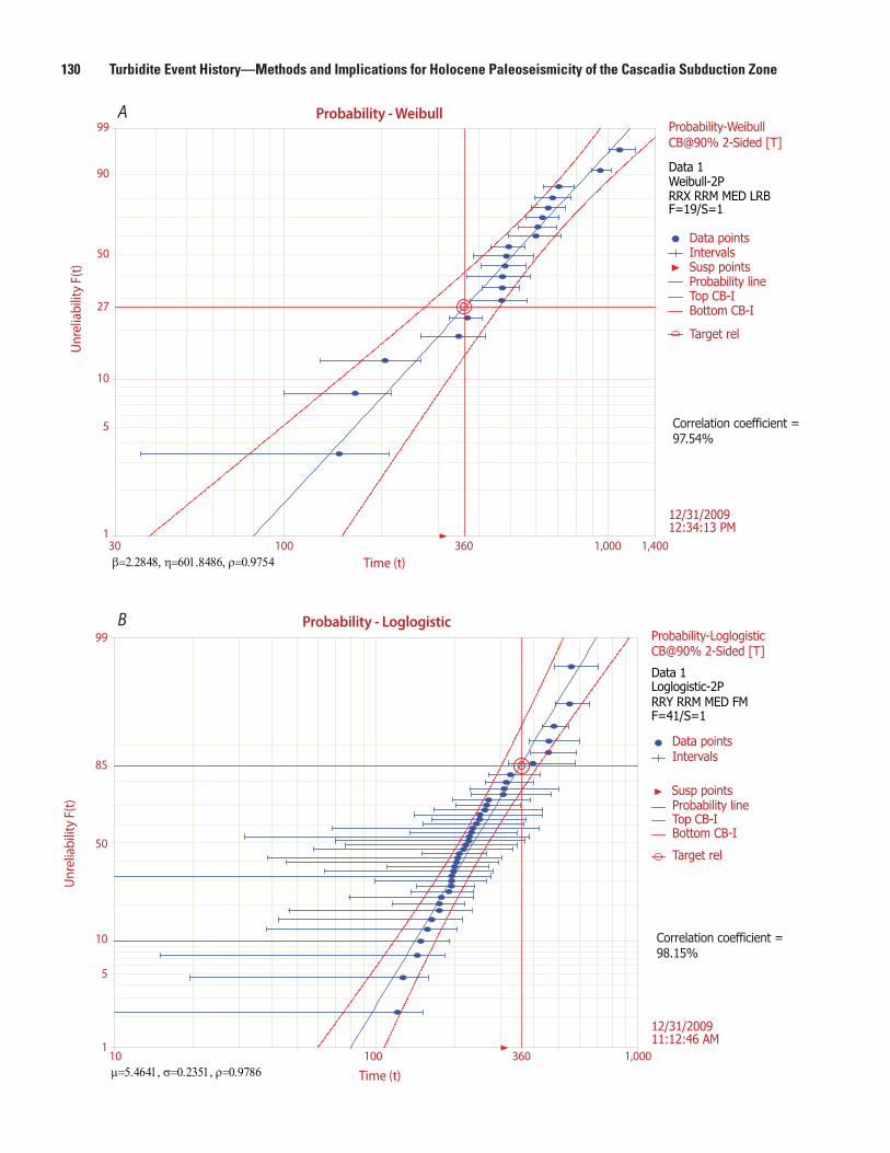
130 Turbidite Event History—Methods and Implications for Holocene Paleoseismicity of the Cascadia Subduction Zone
A
B Probability - Loglogistic
µ=5.4641, σ=0.2351, ρ=0.978610 1,000100 360
1
5
10
50
99
85
Probability-LoglogisticCB@90% 2-Sided [T]
Data 1Loglogistic-2PRRY RRM MED FMF=41/S=1
Data pointsIntervals
Probability lineTop CB-IBottom CB-I
Target rel
12/31/200911:12:46 AM
Probability - Weibull
β=2.2848, η=601.8486, ρ=0.9754 Time (t)
Time (t)
Unr
elia
bilit
y F(
t)U
nrel
iabi
lity
F(t)
30 1,400100 1,0003601
5
10
50
90
99
27
Probability-WeibullCB@90% 2-Sided [T]
Data 1Weibull-2PRRX RRM MED LRBF=19/S=1
Data pointsIntervalsSusp pointsProbability lineTop CB-IBottom CB-I
Target rel
12/31/200912:34:13 PM
Susp points
Correlation coefficient =97.54%
Correlation coefficient =98.15%

Results 131
means for each event based on radiocarbon probability-density functions to mitigate this problem. Since we have multiple radiocarbon dates for many of the intervals, and hemipelagic time constraints for many of them as well, we believe that the average constrained age computed using the Bayesian Combine function of OxCal is a good representation of the interevent time, particularly considering the close correspondence between the onshore and offshore event dates where the records overlap. The previously discussed biases toward turbidite dates slightly older than the earthquake dates have no systematic effect on the recurrence intervals, because these biases are in the same direction for all events. When fitting earthquake (or any) interval data, ambiguities and misinterpretations can result from binning the data, so we rely on cumulative probability distributions. Goodness-of-fit tests then use the maximum likelihood and Kolmogorov-Smirnov nonparametric criterion when comparing different distributions.
For the northern-margin earthquake series, reasonably good fits are found for gamma, Weibull, lognormal, and loglogistic distributions. Although the lognormal distribution is a slightly better fit, we prefer the Weibull distribution because of its theoretical advantages, better fit in the analysis, and because the logistic and loglogistic distributions start at negative infinity. This can result in negative values not appropriate for failure analysis. The Weibull distribution has been used widely for failure analysis (Meeker And Escobar, 1991; Weibull, 1951) and has unique properties that make it suitable for failure analysis. Abaimov and others (2008) discuss these properties, which center around the fact that the Weibull distribution is the only one in which the probability (hazard function) continues to increase with time into the tail of the distribution. Lognormal and Brownian passage-time and many other distributions have hazard functions that reach a constant value, not increasing with time as one would expect in a tectonic system driven by plate motions.
We adopt the Weibull distribution for the recurrence intervals along the northern margin, (Segment A) with a mean recurrence
of 530 years, n=19, and a standard deviation of 260 years. The Weibull analysis shown in figure 63 shows that by the target year 2060, the Cascadia Fault will have exceeded ~27 percent (90-percent bounds are 14–42 percent) of known recurrence intervals (fig. 63). The value represents the actuarial value, based on the Cascadia time series, since time T0, the A.D. 1700 Cascadia earthquake. In other words, the number of events with intervals shorter than 360 years is ~27 percent of the population. The failure analysis is not particularly sensitive to the distribution details for analysis of times near or less than the mean as shown by Ellsworth and others (1999). For other reasonable distribution fits, a normal distribution yields a 23-percent probability in the same period (2σ 8–38 percent), and the other high-scoring distributions yield similar results. Petersen and others (2008) report a probability of 14 percent in 50 years, again using the Willapa Bay record and a Brownian passage-time model to estimate aperiodicity in the paleoseismic record, the difference primarily being that this value reports the conditional probability for the next 50 years, whereas we are reporting the cumulative value since the last event. Our estimate of the conditional probability for the time 2010–2060 is 12 percent.
On the southern Cascadia margin (Segment D), good fits to the population of southern Cascadia recurrence intervals include lognormal, loglogistic (2p) gamma, Weibull, and largest extreme value (see fig. 59, log-likelihood and KS test, as well as the quantile-quantile plot). If we adopt the loglogistic distribution (loglogistic provided a more stable calculation than the slightly higher ranked distribution fits, and negative values and tail fits are not a factor for the southern analysis) for the southern-margin population of earthquake recurrence intervals (fig. 59), we can then calculate that the actuarial value is ~85 percent (90 percent confidence bounds are 77–93 percent). That is, the Cascadia fault will have exceeded 85 percent of known recurrence times by the target date of 2060 (fig. 63). Although different distributions have theoretical advantages and disadvantages, the reliability analysis in this case is not sensitive to the choice between the top ranked distributions for these data. Tests using all of the five best-ranked distributions yield a maximum 5-percent difference in the ranges. Ellsworth and others (1999) show that for intervals of interest near the mean, the differences between these distributions are small. The theoretical advantages of the Weibull distribution primarily apply to intervals greater than 1.5 times the mean. For both plots shown in figure 63, 95-percent ranges for the recurrence intervals are defined by adding and subtracting the one-sided 2σ range for each of the two radiocarbon-age combines from OxCal (see fig. 54).
We note that each of the two plots in figure 63 has outliers in the population of recurrence intervals. On the full-margin plot (fig. 63A), the shortest interval is ~110 years. This short interval, between T17 and T17a, is quite poorly constrained, and the poor fit to the probability line is not likely significant. Removing this point improves the fit to the Weibull line from 0.975 to 0.991 using the Weibull distribution. For the normal distribution, however, the fit is slightly better with this value retained at 0.992 versus 0.987 without this interval. For the southern margin, possible outliers include the shortest and longest intervals; both of these intervals, rounded to 40 years and 600 years, respectively, are poorly constrained. The former is constrained
Figure 63 (left). A, Probability of failure for the northern-central Cascadia margin population of recurrence intervals. This plot uses a Weibull 2 parameter probability-density function determined by fitting the recurrence data to a family of distributions (fig. 58). Points plotted are the midpoints of recurrence intervals; bars include interval and 2s confidence bounds based on OxCal analysis (fig. 54). Red curves indicate 90-percent confidence bounds for the analysis. Time-dependant probability of failure for a target time of 50 years from time of writing (360 years from last earthquake, A.D. 2060) is ~27 percent (90-percent confidence bounds are 14–41 percent). B, Probability of failure for the southern Cascadia margin population of recurrence intervals. This plot uses a loglogistic probability-density function determined by fitting the recurrence data to a family of distributions (fig. 59). Loglogistic provided a more stable calculation than the slightly higher ranked distribution fits. Intervals and confidence bounds as in A, except 1s ranges are used for several short intervals to prevent negative values for the low-extreme range. Probability of failure for a target time of 50 years from time of writing (360 years from last earthquake, A.D. 2060) is ~85 percent (90-confidence bounds are 77–93 percent).

132 Turbidite Event History—Methods and Implications for Holocene Paleoseismicity of the Cascadia Subduction Zone
H
70
80
90
H
70
80
90
Rupture direction
N
Figure 64. Hypothetical rupture distribution along the Cascadia margin, consisting of two patches of greater slip. Insets show hypothetical turbidites at two sites generated by a large rupture with a source time of several minutes. We infer the result at both sites would be turbidites with two fining-upward intervals closely stacked and capped by a single fining-upward tail terminating in clay-size material. The relative coarseness and thickness of the two pulses may reflect proximity to the areas of strong shaking, as shown in this example with north–south directivity.

Results 133
only by lower precision hemipelagic estimates of age, and the latter is bounded by the difficult-to-date T17a event. Fits to the preferred loglogistic distribution improve from 0.982 to 0.991 with the removal of the shortest interval; no improvement is realized if the 600-year interval is removed from the dataset.
If the clustering of earthquakes shown in figure 60 repeats in the future, and if the repetition is similar to past clusters of 2–5 earthquakes followed by a gap, the next event could be a gap 750–1,000 years long for the northern and central margin. The mean repeat time within clusters for the northern margin is ~440 years, with a standard deviation of ~90 years, yielding a cumulative probability since A.D. 1700 of 18 percent, and a conditional probability in 50 years of 13 percent for the next event, if the event is in a cluster. If the next event is a gap, with a mean of 940 years and standard deviation of 240 years, these values drop to <1 percent.
The southern margin, however, appears to be unaffected by temporal clustering, with smaller earthquakes filling each gap between long ruptures with an event of limited strike length. Thus we suspect that the next event would most likely be in southern Cascadia. The general pattern of at least one smaller event between the larger events holds true for 17 of the 19 northern margin intervals, suggesting a 90-percent chance of the next event being a southern-margin earthquake.
Temporal Coincidence with and Possible Triggering of Northern San Andreas Fault Earthquakes
Another significant implication from this study has been the recognition that great earthquakes on the southern Cascadia subduction zone occur at a frequency very similar to that of earthquakes on the northern San Andreas Fault along the northern California continental margin. Goldfinger and others (2008) reported that onshore and offshore paleoseismic records in Cascadia suggest that marginwide and segmented southern Cascadia earthquakes occur at similar times to earthquakes on the northern San Andreas Fault, possibly preceding northern San Andreas Fault events by ~25–45 years for 13 of 15 occurrences during the past 3,000 years. Modeling of the static coseismic and viscoelastic- and afterslip-induced postseismic stress changes suggests that coseismic stress changes from Cascadia earthquakes are more than sufficient to trigger northern San Andreas Fault events, if they nucleate along the northernmost section of the fault near Point Delgada. On the other hand, northern San Andreas Fault events precede Cascadia earthquakes on average by ~150–200 years, most likely too long for a stress-change effect.
The inclusion of additional data in this study leaves the conclusions of Goldfinger and others (2008) unchanged for 12 of 15 earthquake pairs. The potential triggering of the northern San Andreas Fault by Cascadia great earthquakes is significant for seismic hazards in northern California and San Francisco in that it implies north-south directivity for such events, increasing hazards for northern California (Goldfinger and
others, 2008). It also suggests the possibility of two damaging earthquakes on the west coast, closely spaced in time.
Implications of Turbidite Paleoseismology Beyond Cascadia Basin
The study of turbidite paleoseismology highlights several implications for earthquake-hazards and turbidite-system research. The primary implication is that detailed offshore data supported by correlative onshore data in Cascadia Basin dem-onstrate the validity of turbidite paleoseismologic techniques. The methods can be used in a number of other active tectonic continental-margin areas to provide paleoseismic histories over long time spans that commonly cannot be achieved with onshore paleoseismic studies. As a result, improved hazard analyses and a better understanding of plate-boundary pro-cesses can be developed in regions prone to great earthquakes. Recently, the methods of turbidite paleoseismology, combined with sedimentary structures, have been extended to inland lakes to define earthquake hazards in noncoastal areas (for example, Schnellmann and others, 2002).
The recent Mw=9 superquake off Tohoku, Japan, and the 2004 Sumatra-Andaman earthquake have called into question long-held earthquake recurrence models. Neither region was thought capable of earthquakes exceeding Mw ~8.4. Appeal-ing proposed relations, such as that between plate age and convergence rate and plate coupling based on anchored slabs, at least have many exceptions and may not be valid. Both those earthquakes occurred where the plate age was quite old, ~50–130 m.y. Clearly much remains to be learned about these great events, so much so that most subduction plate boundar-ies should now be considered suspect, and perhaps other fault systems as well. Short instrumental records have hampered the development of models of earthquake recurrence, so much so that events like the March 2011 Mw ~9 event in Japan were totally unexpected, though it should not have been. Long paleoseismic records are revealing that such behavior occurs elsewhere and that major fault systems have much more variability in earthquake behavior than previously thought. Goldfinger and others (2010) have proposed a new model of earthquake recurrence based on the 10,000-year Cascadia paleoseismic record. They suggest that the long-term energy state of the megathrust can be evaluated with paleoseismic data and that the Cascadia record suggests supercycles with lengths of several thousand years. They propose a model of energy management for the Cascadia megathrust, inferring long-term cyclic increases and decreases in overall potential energy that may also be applicable to northeast Japan and other fault systems.
The estimation of fault-segment boundaries typically is made by evaluating structural elements of fault systems and making assumptions about what elements may hypothetically constitute barriers to rupture. Paleoseismology can, in some cases, be used to locate segment boundaries when radiocarbon data can resolve them; but submarine paleoseismology offers the alternative method of stratigraphic correlation to determine

134 Turbidite Event History—Methods and Implications for Holocene Paleoseismicity of the Cascadia Subduction Zone
rupture extents independent of radiocarbon error ranges. In addition, long-term paleoseismic records offer the opportunity to evaluate long-term rupture models, clustering, and stress triggering between fault systems, fundamental tectonic issues best addressed by long earthquake time series.
The turbidite paleoseismic studies along the Cascadia and northern California continental margins also demonstrate clearly that earthquakes are the dominant triggering mecha-nism for turbidity currents in active continental margins when physiography is favorable. Earthquake generation of turbidity currents has been postulated for decades, but there has never been a direct link between the onshore and offshore paleo-seismic record. In both the Cascadia and northern California systems, nearly all Holocene turbidites have most likely been triggered by great earthquakes. Preliminary evidence from ODP drill sites in northern Cascadia Basin suggest that the same general periodicity of turbidites has occurred during the past ~100,000 years (Underwood and others, 2005), and thus it appears that earthquake triggering has dominated during Pleistocene time, even during lower sea levels. In addition, the turbidite frequency from seismic generation is significantly different in Cascadia (~250–500 yr) and the San Andreas Fault (~200 yr) margins (Goldfinger and others, 2008). These data (and the body of evidence presented here) strongly support the earthquake-trigger mechanism and show that frequency of turbidite generation in each active tectonic margin will vary, depending on the characteristics of the fault system.
Implications of Stratigraphic CorrelationThe physical-property-based stratigraphic correlations
observed in Cascadia, along with radiocarbon dates and ash and faunal datums, have allowed regional links between turbidites that would otherwise be difficult to make or test. Physical-property (grain size proxy) correlations revealed detailed correlatable patterns that were unexpected. Although the correlations are well supported for many events, the causality is less clear. The magnetic-density turbidite signatures we see are created by sand-rich layers, mostly in the base of the turbidites, and include heavy (dark) minerals, such as magnetite and hematite, which are largely responsible for the signatures. This is clear from the high-resolution imagery CT and X-rays, which show an obvious correlation between density, MS, and the coarse stringers in the turbidites (Goldfinger and others, 2007a, 2008; fig. 7). The correlation of these signatures indicates that the pattern of coarse-fraction deposition is maintained to some extent over time and distance during the life of a turbidity current downstream, as shown by the strong correlation between Juan de Fuca and Cascadia Channels, and also in the San Andreas system (Goldfinger and others, 2007a).
Turbidity currents are fundamentally different from those driven by fluid-density differences, because the suspended particles that contribute to the high density are continuously settling out of the flow as it evolves (Harris and others, 2002). In most models and numerical work to date, three important assumptions commonly are made. First, it is assumed that settling
velocity is constant; second, turbulence is ignored; and third, the initiation of the current is a simple impulsive release, assuming either no source function, or a uniform injection of dense fluid. With respect to the first assumption, settling velocity, a single velocity is a considerable simplification and in real settings there is a continuum of particle sizes and settling velocities. In fact, it is the presence of fine particles that extends propagation of particle-driven currents (for example, Harris and others, 2001). Typical turbidites are composed of a range of grain sizes and, therefore, of settling velocities, and they generally are observed to grade both downstream and vertically (for example, Wynn and others, 2002) in nature, as well as in numerical and physical models (for example, Harris and others, 2002; Gladstone and others, 1998; Felix, 2002). Numerical models can now simulate the variation of the deposit vertically and with streamwise distance (for example, Harris and others, 2002). Such models can predict the total thickness of each class, but also the variation of the composition of the deposit with depth and its deposition with time.
Recent model results suggest that at early times, the density difference between the current and the ambient fluid is relatively constant, and the effect of particle sizes is minimal. As the current evolves, particle sedimentation begins to reduce the overall density, and the effects of the distribution of grain sizes and settling velocities primarily is observed in later stages, controlled by the variance of the initial distribution relative to the square of the mean settling velocity (Harris and others, 2002; Gladstone and Woods, 2000; Bonnecaze and others, 1996). Harris and others (2002) compute the vertical and streamwise grain distribution from a well-mixed intrusion of a polydisperse (range of grain sizes) suspension. Because model predictions are in reasonable agreement with field observations of turbidite deposits, it seems that the limits of both numerical models and physical experiments do not significantly affect the pattern of expected deposition. Similarly, numerical models, which generally do not consider spanwise flow, and physical experiments, which are in confined tanks, apparently do not seriously compromise simulations. This may be because most turbidity currents are channelized flows to begin with, simulating the experimental boundary conditions.
The success of simplified models indicates that the governing processes of deposition are more sensitive to the particle-size distribution and settling velocities than to processes within the turbid flow. This suggests that internal turbulence in the turbidity current serves to maintain the flow by keeping particles in suspension, and thus maintaining the density contrast required for self-sustained flow, but that it has little effect on the depositional sequence that results.
With respect to the third assumption, that of impulsive and (or) uniform start to the turbidity current, there is little basis for this in nature. The assumption is commonly made owing to the lack of information about the initiation process and to the assumption that depositon is controlled by hydrodynamics, making the reasoning circular. Fundamentally, the vertical sequence of deposition of any stratigraphic unit, including a turbidite, represents a time-history of deposition, barring unusual circumstances. The vertical time

Results 135
series, in the case of a turbidity current, represents a longitudinal structure present in the turbidity current that results in deposition as the current flows past a fixed site. Several experimental treatments have examined the time history of deposition as a function of the evolution of the turbidity current and its longitudinal flow structure. The most recent of these (Baas and others, 2005) provides detailed evidence of direct temporal linkage between the grain-size deposition and the internal longitudinal-flow structure of experimental turbidity currents.
A Simple Experiment
Because our turbidites are well correlated and include considerable structure and multiple fining-upward sequences, we suspect that something other than hydrodynamics is driving their depositional sequence. To address the third assumption, that of uniform initial conditions, we performed several simple experiments to test an alternative hypothesis—that the turbidite depositional sequences are linked to initial conditions. We first generated a small sediment gravity flow in a small tank of fresh water by using two grain-size samples of different colors, mixed before the experiment. The bimodal sample was 50 percent very fine sand, color coded yellow, and 50 percent slightly coarser sand, color coded black. The slide was initiated with a well-mixed sample introduced on a sloping ramp into the water tank. We released several inputs of sand, each with a single rapid impulse to the sand container. We then ran several others inputs with multiple pulses with ~1-s separation between the pulses. This was intended to simulate both single-pulse and heterogeneous multipulse input sources.
The resulting deposit at the base of the ramp consisted of single fining-upward graded sequences of coarse material for single-pulse inputs and multiple fining-upward sequences for multipulse inputs. The relative grain-size distribution from the unconsolidated deposits was determined (approximately) from analysis of image color from five megapixel images taken through the glass tank. These results indicate that, even with very little runout distance, the deposit had self-organized according to grain size and that each input pulse resulted in a corresponding fining-upward sequence. This simple, unscaled experiment demonstrates that pulses of coarse material, triggered with very close temporal spacing, result in separable fining-upward coarse units in the deposit (Goldfinger and others, 2004). Further experiments using ranges of scaling, larger tanks, and instrumentation have also been conducted, and more are underway as of this writing. Preliminary results suggest similarly that input perturbations are well recorded in experimentally generated turbidity currents and their deposits (see Goldfinger, 2011b).
Results from these experiments suggest that the stratigraphic details of turbidites that are preserved over large distances spanning proximal to distal sites could represent a longitudinal time history of not just the current, but of the source input as well, a supposition commonly absent in most turbidity current experiments. This concept has been discussed by Myrow and Southard (1996), Mulder and others (2003), and others for storm-generated turbidity currents, and by St-Onge and others
(2004), who compared flood and earthquake signatures. Kneller and McCaffrey (2003) discuss the consequences of unsteady flow in turbidity currents and conclude that such unsteadiness can result in variations in deposition and erosion during the life of the current. They also discuss unsteadiness owing to surging of the source, resulting in waxing and waning deposition from the longitudinal velocity structure, as we observed in our simple experiment. Our initial experiments did not ideally simulate conditions of turbidity-current deposition in Cascadia, because they were unscaled and the runout distance was too short to establish a turbulence-supported turbidity current; however, subsequent experiments have explored the parameter spaces in scaling and with longer runouts with similar results (Goldfinger, 2011b). We conclude that it is likely that multiple input pulses self-organize into fining-upward depositional sequences that correspond to a variety of source variability inputs, though much further work is required to test this concept and alternative explanations in nature.
Variability of the Source
If source variation may be reflected in turbidity currents and their deposits, one might expect that a relevant factor would be how the turbidity current initiated in the canyon system. An earthquake, unlike other triggers for submarine landslides, is likely to trigger multiple failures along the length of a canyon. Thus, the turbidity current could contain multiple inputs, each containing a coarse-fraction pulse, which coalesce downchannel (this also could be due to retrograde landsliding). This would, in effect, be multiple catastrophic failures and turbidity currents triggered within perhaps minutes of each other, rather than a waxing and waning unsteady source. This could explain the persistent pattern we see within channels as reflecting an original multiple-source input, but we are still left with the problem, Why do the observed event signatures appear to correlate beyond individual channel systems to other channels and slope basins with different pathways? This commonality (if correct) requires a different explanation.
The fact that the turbidites correlate at all is strong evidence that the turbidity currents were earthquake generated, because the commonality within multiple-channel systems along hundreds of kilometers of the margin cannot be explained by multiple wall failures (nor by other triggering mechanisms) unless they were nearly identical in separate canyons. We conclude that the only plausible commonality between correlative turbidites in separate channels is a common earthquake source. In the case of Cascadia, we find that turbidites correlate across channels where the geology, mineralogy, physiography, channel gradients and morphology, sediment sources, and transport mechanisms are different. To explain the similarity across environments, we postulate that the depositional signatures may record elements of the unique shaking signal imparted to the sediment-failure region by the earthquake itself; in effect, the physical-property signatures may be crude “paleoseismograms,” imparting some information about magnitude, source character, or aftershocks

136 Turbidite Event History—Methods and Implications for Holocene Paleoseismicity of the Cascadia Subduction Zone
to the depositional history of each turbidite (Goldfinger and others 2007a, 2008). In the case of a subduction zone such as Cascadia, the source may last 3–6 minutes and may consist of multiple rupture patches, linked together but separated in time by several minutes (for example, the 2004 Sumatra earthquake; Chlieh and others, 2007). Rupture of these source patches imparts a waxing and waning shaking signal to the canyon systems and may result in multiple turbidity currents initiated within minutes of each other traveling the canyon-channel system to depocenters in the distal channels (fig. 64).
We suggest that a complex source may explain why the northern Cascadia turbidites not only pass the confluence test in number of events deposited above the Mazama ash (fig. 13), but also in stratigraphic detail, resulting in similar depositional sequences within individual turbidites in tributaries and downstream. It also can potentially explain the observed relation between Effingham Inlet magnetic signatures and our offshore cores, as well as recently observed similar linkages to southern Cascadia lakes (Morey and others, 2011). Generally, turbidite beds are observed to be more complex in proximal settings and less so in distal ones (Kneller and McCaffrey, 2003; Shiki and others, 2000b). We observe similar downstream merging and simplification of northern San Andreas Fault turbidite beds (Goldfinger and others, 2007a) and, to a lesser extent, in Cascadia. Despite this trend, the multiple fining-upward sequences are preserved over transport distances exceeding 400 km in Cascadia Basin, indicating that these are primary features of the longitudinal flow that are modified during transport by flow variability and other factors.
This may be a controversial interpretation, but we are led to it out of a need to explain the observed data. This topic is the focus of a current study involving the northern San Andreas Fault, Sumatra and Cascadia turbidites, and continuing experimental work (Garrett and others, 2011).
Time ResolutionIf turbidites that have passed other tests of earthquake origin
can be thought of as recorders of earthquake-source details, what sort of time resolution might they have? The question is important whether or not the origin is earthquakes because the multiple fining-upward sequences could result from earthquakes closely spaced in time, retrogressive faulures over days, or other complexities. In a general way, the time represented from the base of the turbidite to the base of the fine tail that represents postevent settling of the fine clay fraction should be proportional to the source time of the initiating event(s). Given the minor differences between deposits from Juan de Fuca Channel to Cascadia Channel, a distance of 480 km, we suggest that modification by hydrodynamic processes is probably not of primary significance.
Although we cannot know precisely the amount of time required for deposition of the coarse fraction of the Cascadia turbidites, we observe that, between the fining-upward pulses, it is rare to find mud particles at the tops of the individual units. The finest material usually is fine sand and silt. Not until the uppermost sand/silt pulse is deposited do we observe the final sequence of
fining-upward mud typical of a waning turbidity current. As the current passes a fixed site, the time frame for deposition is roughly minutes to hours for deposition of coarse fractions. The short time requirement imposed by the lack of clay particles between coarse pulses implies that a series of mainshock-aftershock inputs from multiple earthquakes, or failures spread over hours to days, is not favored as a source event series. The aftershock sequence would have to take place over a span of minutes after the mainshock, which is uncommon for major aftershocks. Other explanations would be spread over even longer periods, and require mud deposition between them. A source comprising a series of rupture patches is a better fit to the observed stratigraphy, implied time constraints, and minimum magnitudes previously discussed.
Our observations of Cascadia and northern San Andreas Fault turbidites suggest that it may be possible to resolve details of seismic energy inputs that take place during a span of several minutes typical of the Mw 8–9 earthquakes known to occur in the Cascadia and San Andreas systems. If correct, interpretation of paleorupture patterns may be possible from a dense set of paleoseismic records in marine and lacustrine systems.
Conclusions
Cascadia Basin contains a variety of types and scales of turbidite systems on the continental margin from Vancouver Island, Canada, to Cape Mendocino, Calif., United States. These systems include multiple canyon sources on the Washington margin that funnel turbidites into Cascadia Channel (1,000 km length): Astoria Canyon, on the northern Oregon margin, that feeds Astoria Fan (300 km diameter) containing channel splays with depositional lobes; Rogue, Smith, and Klamath Aprons, on the southern Oregon and northern California margins, that feed small (<5 km) base-of-slope aprons; and Trinidad, Eel, and Mendocino Canyons (30–100 km length) on the northern California margin that feed into plunge pools, sediment-wave fields, and channels.
Cascadia Basin turbidite systems are an ideal place to develop a turbidite paleoseismologic method and record, because (1) a single Cascadia subduction-zone fault underlies the margin; (2) multiple tributary canyons and a variety of turbidite systems and sedimentary sources and basins exist to test for synchronous triggering of turbidity currents; (3) the presence of an excellent Mazama-ash marker provides a stratigraphic anchor in the northern two thirds of the basin; (4) during highstands of sea level, Cascadia margin physiography exerts a strong control on sediment input to canyon heads, limiting most storm/river input, except for those localities with narrow shelves; and (5) the Cascadia trench is filled, thus channel systems flow away from the margin, remaining isolated rather than merging in the trench. Detailed swath bathymetric data and core sampling procedures verify that key turbidite-channel pathways of Cascadia Basin are open and provide a good turbidite-event record. Proximal canyon-mouth and inner-fan channel areas have erratic turbidite-event records because of extensive cut-and-fill episodes in turbidity currents; however, even in these difficult locations, complete records can be found in some point bars, terraces, and canyon walls that are slightly elevated

Results 137
above the channel thalweg. The most consistent turbidite event records occur in distal locations of continuous deep-sea channel systems, such as Cascadia Channel.
The similarity of the turbidite time series and good stratigraphic correlation of the turbidite event record along the northern two thirds of the Cascadia subduction zone is best explained by paleoseismic triggering of great earthquakes. Turbidites in this region pass several tests of synchronous triggering, including the “confluence test” that requires passage of multiple-source turbidites past a channel confluence in a span of a few hours, 19 consecutive times during the Holocene. Stratigraphic correlation of individual event signatures, correlation of series characteristics, such as mass and number of coarse-fraction pulses, as well as 14C dates, further support synchronous triggering. Sediment supply to canyon sources appears not to be a significant controlling factor in the Holocene, partly because highstand deposition is concentrated on the shelf, and because strong ground shaking probably is sufficient to overcome variability in sediment input to the canyons.
The mismatch between the turbidite record and the frequency of teletsunami and local storms, as well as the good match in frequency and dates with earthquake and tsunami evidence onshore, also support the conclusion that the Holocene Cascadia-turbidite record primarily records earthquakes. The lack of turbidites overlying the most recent turbidite, dated to within a decade of the A.D. 1700 Cascadia earthquake, indicates that no other triggering mechanism has produced an observable turbidite in the last 300 years, except in some of the northern California channels adjacent to narrow shelves. Several sites in southern Cascadia may record a mixed storm and earthquake signal in their early Holocene sections owing to a lowered sea level. The lack of turbidite triggering in Cascadia Basin by El Niño storm and flood events (1964, 1998–99), and the 1964 Alaskan earthquake tsunami suggest that storm events and tsunami, whether or not sediment is transported to canyon heads, generally do not result in correlative abyssal-plain turbidites, except where the shelf is narrow. A small number of uncorrelated turbidites may represent crustal earthquakes or other sources.
The mean AMS age of 270 (170–390) cal yr B.P. from four channel systems for the youngest turbidite event in Cascadia Channel, T1, differs by only 15–20 years from (1) the coastal paleoseismic dates that center consistently at 250 cal yr B.P. (A.D. 1700; Nelson, A.R., and others, 1995) and (2) tsunami evidence from Japan suggesting a date of January 26, 1700, for the youngest great earthquake on the Cascadia subduction zone (Satake and others, 1996, 2003). This further validates the synchronous turbidite-event record and associated high-resolution AMS radiocarbon dates as a method to provide a long-term paleoseismic record.
The temporal correspondence between the onshore and offshore paleoseismic records along the Cascadia margin is good, despite a variety of methods and lines of evidence onshore. Within the time ranges that the two records overlap, there are few significant discrepancies. The ties between onshore and offshore paleoseismic data remain limited to radiocarbon timing for most sites, but three more direct links have emerged. Effingham Inlet on Vancouver Island contains turbidites with possible stratigraphic correlatives offshore, and Bradley Lake appears to have a reasonable correlation based on event-size characteristics in addition to radiocarbon
evidence. Other lakes onshore likely also contain earthquake turbidite stratigraphy. All three links represent more direct linkages than those available through radiocarbon dating alone.
AMS radiocarbon dates downcore for individual turbidite events show that the average recurrence interval for full-margin paleoseismic events (900–1,100 km in length) is ~500–530 years, with a variance ranging from ~200 to 1,200 years. A series of smaller ruptures, represented by thinner turbidites of lesser areal extent, can be correlated among southern Cascadia cores and has moderately good correspondence with the presence of events of limited extent at coastal paleoseismic sites. These smaller events define three other margin segments that have recurrence intervals of 410–500, 300–380, and 220–240 years for segments with northern terminations at approximately lat 46° N. (Nehalem Bank), lat 44° N. (Heceta Bank), and lat 43° N. (Coquille Bank). For full-margin ruptures, the Holocene time series implies a probability during the next 50 years of 7–11 percent of a Cascadia earthquake by using either a Poisson or time-dependent calculation. Conditional probabilities for the next 50 years are similar. Using failure-analysis statistics, the Cascadia megathrust will have exceeded ~25 percent of known recurrence intervals by a target date of 2060. For the southern segment, with a recurrence of ~240 years, probability of an earthquake occuring in the next 50 years rises to 18 percent for a Poisson distribution and 32–43 percent for a time-dependent model. Failure analysis indicates that, by the year 2060, ~85 percent of recurrence intervals will have been exceeded along the southern margin. It is also highly likely that the next event will be a southern-margin event because these occur between all known pairs of longer ruptures.
We find a strong correspondence between turbidite mass among separate margin sites, suggesting that mass of the turbidites may crudely represent earthquake magnitude and shaking duration or strength. We further find a moderate correspondence between turbidite mass and the time following each event. We conclude that there is a reasonable possibility that if the turbidite mass represents a proxy for magnitude, then the central and northern Cascadia margin may weakly follow a “time-predictable” model of recurrence. The long paleoseismic record also indicates a repeating pattern of clustered earthquakes that includes four Holocene cycles of two to five earthquakes separated by unusually long intervals of 700–1,200 years. Two of the four cycles terminated with what were likely very large earthquakes. We suggest that the good correlation of stratigraphic details along strike for many individual beds implies a common source, which may be the heterogeneity of the rupture of the initiating earthquake.
We find that the pattern of long recurrence intervals and long ruptures along the northern and central Cascadia margin is consistent with the thick sediment supply along that part of the margin. Where sediment supply thins along the southern margin, recurrence intervals and rupture lengths shorten, consistent with a model of greater interaction between lower plate and forearc structures in those areas, providing barriers to rupture propagation as well as points of nucleation not present along most of the northern margin.
Finally, Cascadia Basin investigations establish new paleoseismic techniques using marine-turbidite event stratigraphy during sea-level highstands. These investigations can be applied

138 Turbidite Event History—Methods and Implications for Holocene Paleoseismicity of the Cascadia Subduction Zone
in other specific settings worldwide, where an extensive fault traverses a continental margin that has several active turbidite systems and favorable physiography.
Lessons Learned
An important consideration for investigations using turbidites to develop a paleoseismic record along a major submarine fault system is an adequate number of samples and good areal coverage. In the case of Cascadia, the sample cruise was 30 sea days, and more than 102 new cores were used, along with ~60 older cores. A similar number of cores were collected for the San Andreas work (Goldfinger and others, 2007a) and the Sumatra work that is just getting underway (Patton and others, 2009). During the analysis of these data, we began with cores and locations that were well known from previous work and, therefore, had some of the details worked out. Over time, as we gained confidence in the methods, we extended the analysis to more difficult sites, finally working with cores that we initially had rejected as not being useful for turbidite stratigraphy and (or) paleoseismology. We learned, by studying the cores, which sites made good recorders of earthquakes and which did not. This led to a better understanding of the sensitivity of each site to the earthquake record: some sites being too sensitive, as evidenced by gravel lag and missing sediment section, and others with low sensitivity, as shown by thin mud turbidites and subdued log signatures. With only a few cores, we could possibly have developed a partial record: but much of the evidence for correlation, rupture lengths, and relations between time and turbidite characteristics requires broad areal sampling and replicate cores to improve the robustness of interpretations. A reduced number of samples could lead to biased or incorrect conclusions based on the biases inherent in a smaller dataset.
Blumberg and others (2008) discussed the turbidite paleoseismology of the Chile margin using two existing cores; their study may illustrate some of the issues involved with sparse data. Neither core was sited with earthquake turbidites in mind, and one ODP site was chosen as a paleoceanographic site specifically to avoid turbidites. The primary site used was on the outer trench wall, well above the trench floor, and was designed to be elevated above the influence of turbidites that would have to travel across the trench floor and central channel and up the outer trench wall to reach the site. Nevertheless, the cores from Site 1232 had more than 600 turbidites in the 64-m core, spanning ~138,000 years. During highstands, the turbidite frequency was less than one per 1,000 years, much lower than the recent onshore earthquake record. During lowstand times, the frequency increased to one every 200–300 years, similar to the earthquake record onshore. With only a single core located poorly for the purpose, we infer that the record at Site 1232 likely underestimates the number of earthquakes during all times and may include a mixed record of flood events during lowstand intervals. Without additional data from a number of sites, however, conclusions about earthquakes and climate are, at best, difficult to resolve.
Applicability to Other SettingsAs we have gained experience with marine
paleoseismology, we have come to realize that Cascadia is a highly favorable locality for the turbidite technique. It has a shallow plate dip and filled trench, which promote development of fan systems and discrete channel systems leading away from the margin, rather than merging on the trench floor as is more common in subduction settings. Cascadia also is in a region of upwelling and high productivity, as well as high sediment input from rivers. The hemipelagic sediment between turbidites is a mix of biogenic and extremely fine material from river plumes accumulating at a rate of ~1 m/10,000 years in Cascadia Basin. This yields just enough datable material and separation between turbidites for good stratigraphic discrimination and correlation. Cascadia Basin is mostly above the CCD, allowing good preservation of datable calcareous microfossils. Most importantly, Cascadia has large-magnitude (Mw ~9?) events at fairly regular intervals with long recurrence times, enough to allow accumulation of datable foraminifers between most events.
Few other settings have as many favorable factors, such that modification of the techniques used here is needed for most other settings. For example, the northern San Andreas Fault lies adjacent to a margin that shares many of the favorable conditions for turbidite distribution and dating that we found in Cascadia; however, the earthquake source is more distant, partly because the fault is vertical and because the shelf is wider. Earthquakes on the northern San Andreas Fault are smaller (maximum of Mw ~8, limited by crustal thickness), and the sedimentation rates are lower, factors that make the northern San Andreas Fault turbidite record more difficult to define than the Cascadia record. In Sumatra, we have started a new study to help define segments and paleoseismic recurrence along the Sumatra margin; however, many of the favorable features found in Cascadia are absent. The trench is not filled along Sumatra, the plate dip is steeper, and the trench depth ranges from 4,000 to 6,500 m, below the CCD. This means that there is no datable material in the Sumatra trench. Moreover, channels leading from the margin all merge and travel southward in the well-expressed trench. Many trench systems are more similar to Sumatra than to Cascadia, so it is worth considering alternate strategies to deal with these issues. In Sumatra, as in Cascadia, we have found that well-selected slope basins are a good alternative. They can be selected to be above the CCD and in more productive shallower waters to increase the sedimentation rate and provide datable microfossils. With dating and stratigraphic correlation, it is possible to link sites and test for earthquake origin, although without the elegant confluence test. The trench is divided by subducting fracture zones into compartments that do not communicate with each other, somewhat relieving the problem of turbidity currents merging in the trench. This is common in the world’s trenches and can be used to isolate seismic segments of the margin, which may also be controlled by subducting lower-plate structures.

Acknowledgments 139
Future Directions The utility of turbidite stratigraphy has now allowed robust
determination of long earthquake histories along the Cascadia margin and the northern San Andreas margin, and work is underway in Japan, along the Sumatra margin, on the southwest Iberian margin, and elsewhere. The difficulties are somewhat greater than for onshore paleoseismology, but once overcome, the rewards are significant. Because marine sedimentation is continuous, along-strike stratigraphic correlation is possible, as well as development of very long records critical to the understanding of plate-boundary processes and earthquake probabilities. At present, dating of individual events is hindered slightly by the lack of regional reservoir models for the worlds’ oceans that cover time periods older than the 20th century. Such models will be needed for both paleoseismic and paleoclimatic studies and are under development in some areas.
In addition to dating past earthquakes, the correlation results presented here, and by Goldfinger and others (2007a, 2008), suggest that more information can be gleaned from the turbidites than just the dates of past earthquakes. The success of the physical-property-based correlation methods and the presence of independent “fingerprint” records in settings, such as Hydrate Ridge and Effingham Inlet, suggest that turbidites may be crude recorders of the original earthquake-rupture sequence, rather than just random sediment deposition controlled by each canyon and the hydrodynamics of transport. If this is the case, information about magnitude, rupture pattern, and perhaps directivity, may be obtained from turbidite records in the future. Testing of this hypothesis can be done in the laboratory and on deposits from the 1906 San Andreas earthquake, the 2004 and 2005 Sumatra earthquakes, the 2011 Tohoku earthquake, and other instrumental events that can be sampled in lacustrine or offshore environments. Lastly, long records may yield clues to fundamental models of earthquake recurrence based on actual occurrence over long time spans rather than inferred from short instrumental records.
AcknowledgmentsWe thank the investigators who have contributed to this
research. Richard Boettcher analyzed and picked planktic foraminifera for radiocarbon dates. Michaele Kashgarian and John Southon ran the majority of the AMS radiocarbon dates and assisted with many radiocarbon issues. Rob Wheatcroft ran 210Pb samples. We acknowledge Rob Witter and Harvey Kesley for detailed discussion of the Bradley Lake 14C ages and possible modifications presented here. We also are grateful for the following students, graduate students, and their sponsoring universities, whose assistance was invaluable for the success of the 1999 and 2002 cruises: Mike Winkler, Pete Kalk, Antonio Camarero, Clara Morri, Gita Dunhill, Luis Ramos, Alex Raab, Nick Pisias, Jr., Mark Pourmanoutscheri, David Van Rooij, Lawrence Amy, Churn-Chi “Charles” Liu, Chris Moser, Devin Etheridge, Heidi Stenner, Chris Popham, Claire McKee, Duncan
McMillan, Chris Crosby, Susanne Schmid, Eulalia Gràcia, Suzanne Lovelady, Chris Romsos, Vincent Rinterknecht, Rondi Robison, David Casas, Francois Charlet, Britta Hinrichsen, Jeremiah Oxford, Miquel Marin, Marta Mas, Sergio Montes, Raquel Villalonga, Alexis Vizcaino, Santiago Jimenez, Mayte Pedrosa, Silvia Perez, Jorge Perez, Andreu Turra, David Lamas, Himar Falcon, and Andres Baranco. Captain Tom Desjardins and the officers and crews of the R/V Melville and R/V Roger Revelle provided excellent ship handling and coring logistics for the field work. The coring techniques of Pete Kalk, Chris Moser, Bob Wilson, and Chuen-Chi “Charles” Liu provided the superb piston cores that are necessary for paleoseismic analysis. We also thank Kat Crane, Suzanne Lovelady, Beth Myers, Abi Stephen, Cheryl Hummon, Trent Carmichael, Kaileen Amish, Morgan Erhardt, Jeff Beeson, Amy Garrett, and Rachel King for help with graphics, grain size, and a variety of things. We thank Linda Lamb, Crystal Barnes, and Dave Reinert at Oregon State University for the extensive copy edit on the final manuscript.
We thank the many investigators who have provided insightful conversations, advice, and suggestions during the long course of this project, including Mary Lou Zoback, Harvey Kelsey, Alan Nelson, Kerry Sieh, Rich Briggs, David Schwartz, Rob Witter, Bill McCaffrey, Peter Houghton, Russ Wynn, Takeshi Nakajima, Ken Ikehara, Brian Atwater, Kenji Satake, Tsunemasa Shiki, Keith Kelson, Keith Knudsen, Paul Spudich and many others. We thank Ivan Wong and Ram Kulkarni for insightful discussions of earthquake probabilities.
The initial funding for this study was provided by the Coastal and Marine Geology Team of the U.S. Geological Survey. The primary funding for field work and subsequent research has been provided by NSF Awards EAR 9803081, EAR-0001074, EAR-0107120, EAR-0440427, and OCE-0550843 (reservoir model development) and OCE 0850931 (2009 cruise). The U.S. Geological Survey substantially supported this study through Cooperative Agreements 6-7440-4790, 98HQAG2206, and 99HQAG0192, and the U.S. Geological Survey National Earthquake Hazard Reduction Program grants 02HQGR0019, 03HQGR0037, 06HQGR0149, and 07HQGR0064 to Goldfinger and 02HQGR0043, 03HQGR0006, and 06HQGR0020 to Nelson. The American Chemical Society awarded support to Ph.D. student Joel Johnson for core collection and analysis at Hydrate Ridge under ACS PRF 37688-AC8.
The manuscript has benefited from thoughtful reviews by Brian Atwater and David Twitchell. The authors also greatly benefited from comments and discussion at a workshop convened at Oregon State University on November 18–19, 2010, for the purpose of reviewing turbidite paleoseismic data discussed in this report. The participants in this workshop were Arthur Frankel, John Vidale, Ray Weldon, Alan Nelson, Brian Atwater, Brian Sherrod, Craig Weaver, Ned Field, Gary Carver, C. Crouse, Ivan Wong, Mark Petersen, Roland LaForge, Vicki McConnell, Tim Walsh, Ian Madin, Rob Witter, Harvey Kelsey, Paul Johnson, Larry Phillips, Ben Sheets, Joanne Bourgeois, Chesley Williams, Jake Covault, Gordon Seitz, Paul Bodin, Robert Yeats, Guillaume St-Onge, Yumei Wang, and Ray Wells.

140 Turbidite Event History—Methods and Implications for Holocene Paleoseismicity of the Cascadia Subduction Zone
References Cited
Abaimov, S.G., Turcotte, D.L., Shcherbakov, R., and 4 others, 2008, Earthquakes—Recurrence and interoccurrence times: Pure and Applied Geophysics, v. 165, p. 777–795.
Abbott D., Bryant T., Gusiakov V., and Masse, W., 2007, Megat-sunami of the world ocean—Did they occur in the recent past?: Eos, Transactions of the American Geophysical Union, v. 88, no. 23, Joint Assembly Supplement, Abstract PP42A-04.
Abdeldayem, A.L., Ikehara, K., and Yamazaki, T., 2004, Flow path of the 1993 Hokkaido-Nansei-oki earthquake seis-motrubidite, southern margin of the Japan sea north basin, inferred from anisotropy of magnetic susceptibility: Geo-physical Journal International, v. 157, p. 15–24.
Abramson, H.F., Garrison-Laney, C.E., Carver, G.A., and Anonymous, 1998, Evidence for earthquakes and tsunamis during the last 3500 years from Lagoon Creek, a coastal freshwater marsh, northern California: Geological Society of America, Abstracts with Programs, v. 30, p. 2.
Achcar, F., Camadro, J.-M., and Mestivier, D., 2009, Auto-Class@IJM—A powerful tool for Bayesian classification of heterogeneous data in biology: Nucleic Acids Research, doi:10.1093/nar/gkp430.
Acharya, H., 1992, Comparison of seismicity parameters in different subduction zones and its implications for the Cas-cadia subduction zone: Journal of Geophysical Research, v. 97, p. 8831–8842.
Adam, J., Klaeschen, D., Kukowski, N., and Flueh, E., 2004, Upward delamination of Cascadia Basin sediment infill with landward frontal accretion thrusting caused by rapid glacial age material flux: Tectonics, v. 23, p. TC3009.
Adams, J., 1990, Paleoseismicity of the Cascadia subduction zone—Evidence from turbidites off the Oregon-Washington margin: Tectonics, v. 9, p. 569–583.
Alexander, J., and Mulder, T., 2002, Experimental quasi-steady density currents: Marine Geology, v. 186, no. 3–4, p. 195–210.
Anastasakis, G.C., and Piper, D.J.W., 1991, The character of seismo-turbidites in the S-1 sapropel, Zakinthos and Stro-fadhes basins, Greece: Sedimentology, v. 38, p. 717–733.
Ando, M., and Balazs, E.I., 1979, Geodetic evidence for aseismic subduction of the Juan de Fuca plate: Journal of Geophysical Research, v. 84, p. 3023–3027.
Atkinson, G.M., and Boore, D.M., 1997, Stochastic point-source modeling of ground motions in the Cascadia region: Seismological Research Letters, v. 68, no. 1, p. 74–85.
Atwater, B.F., 1987, Evidence for great Holocene earthquakes along the outer coast of Washington State: Science, v. 236, p. 942–944.
Atwater, B.F., 1992, Geologic evidence for earthquakes during the past 2,000 years along the Copalis River, southern coastal Washington: Journal of Geophysical Research, v. 97, p. 1901–1919.
Atwater, B.F., and Hemphill-Haley, E., 1997, Recurrence intervals for great earthquakes of the past 3,500 years at northeastern Willapa Bay, Washington: U.S. Geological Survey Professional Paper, v. 1576, 108 p.
Atwater, B.F., Nelson, A.R., Clague, J.J., and 13 others, 1995, Summary of coastal geologic evidence for past great earthquakes at the Cascadia subduction zone: Earthquake Spectra, v. 11, p. 1–18.
Atwater, B.F., Tuttle, M.P., Schweig, E.S., and 3 others, 2003, Earthquake recurrence inferred from paleoseismology, in Gillespie, A.R., Porter, S.C., and Atwater, B.F., eds., The Quaternary period in the United States, Volume 1: Amsterdam, The Netherlands, Elsevier Ltd., Developments in Quaternary Sciences, p. 331–350.
Austin, J.A., and Nittrouer, C.A., 2001, Conference investigates formation and preservation of continental margin stratigraphic record: Eos, Transactions of the American Geophysical Union, v. 82, p. 485, 488.
Azmon, E., 1981, Use of clay fabric to distinguish turbidites from hemipelagic siltstone: Sedimentology, v. 28, p. 733–735.
Baas, J.H., McCaffrey, W.D., Haughton, P.D.W., and Choux, C., 2005, Coupling between suspended sediment distribution and turbulence structure in a laboratory turbidity current: Journal of Geophysical Research, v. 110, p. 20.
Baker, V.R., and Bunker, R.C., 1985, Cataclysmic Late Pleistocene flooding from glacial Lake Missoula—A review: Quaternary Science Reviews, v. 4, p. 1–41.
Barnett, V., and Lewis, T., 1984, Outliers in statistical data (2nd ed.): New York, John Wiley & Sons, 463 p.
Bea, R.G., Wright, S.G., and Niedoroda, A.W., 1983, Wave-induced slides in South Pass Block 70, Mississippi Delta: Journal of Geotechnical Engineering, v. 109, no. 4, p. 619–644.
Beck, C., Mercier de Lépinay, B., Schneider, J.-L., and 23 others, 2007, Late Quaternary co-seismic sedimentation in the Sea of Marmara’s deep basins: Sedimentary Geology, v. 199, p. 65–89.
Bennett, K.D., 1994, Confidence intervals for age estimates and deposition times in late Quaternary sediment sequences: The Holocene, v. 4, p. 337–348.
Benson, B.E., Clague, J.J., and Grimm, K.A., 1999, Relative sea-level change inferred from intertidal sediments beneath marshes on Vancouver Island, British Columbia: Quaternary International, v. 60, p. 49–54.

References Cited 141
Benson, B.E., Grimm, K.A., and Clague, J.J., 1997, Tsunami deposits beneath tidal marshes on northwestern Vancouver Island, British Columbia: Quaternary Research, v. 48, p. 192–204.
Bernd, Z., Jens, M., van der Gaast, S., Jansen, J., and Nau-mann, R., 2002, Sediment logging techniques, in Last, W.M., and Smol, J.P., eds., Tracking environmental change using lake sediments, Volume 1—Basin analysis, coring, and chronological techniques: New York, Kluwer Academic Pub-lishers, p. 137–153.
Bett, B.J., and Rice, A.L., 1992, The influence of hexactinellid sponge (Pheronema carpenteri) spicules on the patchy dis-tribution of macrobenthos in the Porcupine Seabight (bathyal NE Atlantic): Ophelia, v. 36, p. 217–226.
Biasi, G.P., Weldon, R.J., Fumal, T.E., and Seitz, G.G., 2002, Paleoseismic event dating and the conditional probability of large earthquakes on the southern San Andreas fault, Califor-nia: Bulletin of the Seismological Society of America, v. 92, p. 2761–2781.
Blais-Stevens, A., and Clague, J.J., 2001, Paleoseismic sig-nature in late Holocene sediment cores from Saanich Inlet, British Columbia: Marine Geology, v. 175, p. 131–148.
Blais-Stevens, A., Rogers, G.C., and Clague, J.J., 2011, A revised earthquake chronology for the last 4,000 years inferred from varve-bounded debris-flow deposits beneath an inlet near Victoria, British Columbia: Bulletin of the Seismo-logical Society of America, v. 101, p. 1–12.
Blomqvist, S., 1985, Reliability of core sampling of soft bot-tom sediments—An in situ study: Sedimentology, v. 32, p. 605–612.
Blott, S.J., and Pye, K., 2006, Particle size distribution analysis of sand-sized particles by laser diffraction—An experimen-tal investigation of instrument sensitivity and the effects of particle shape: Sedimentology, v. 53, p. 671–685.
Blumberg, S., Lamy, F., Arz, H.W., and 4 others, 2008, Turbid-itic trench deposits at the South-Chilean active margin—A Pleistocene–Holocene record of climate and tectonics: Earth and Planetary Science Letters, v. 268, p. 52–539.
Bondevik, S., Svendsen, J.I., Mangerud, J., 1997, Tsunami sedimentary facies deposited by the Storegga tsunami in shallow marine basins and coastal lakes, western Norway: Sedimentology, v. 44, p. 1115–1131.
Bonnecaze, R.T., Huppert, H.E., and Lister, J.R., 1996, Patterns of sedimentation from polydisperse turbidity currents: Pro-ceedings of the Royal Society of London, A, v. 452, p. 2247–2261.
Boudreau, B.P., 1998, Mean mixed depth of sediments—The wherefore and the why: Limnology and Oceanography, v. 43, no. 3, p. 524–526.
Boulanger, E., 1999, Comportement cyclique des sédiments de la marge continentale de la rivière Eel—Une explication posible pour le peu de glissements sous-marins superficiels dans cette region: Sainte-Foy, Quebec, Laval University, M.S. thesis, 145 p.
Boulanger, E., Konrad, J.M., Locat, J., and Lee, H.J., 1998, Cyclic behavior of Eel River sediments—A possible expla-nation for the paucity of submarine landslide features: Eos Abstracts, American Geophysical Union, v. 79, p. 254.
Bouma, A.H., 1962, Sedimentology of some flysch deposits—A graphic approach to facies interpretation: Amsterdam, The Netherlands, Elsevier, 168 p.
Brudzinski, M.R., and Allen, R.A., 2007, Segmentation in episodic tremor and slip all along Cascadia: Geology, v. 35, p. 907–910.
Brunner, C.A., and Ledbetter, M.T., 1987, Sedimentological and micropaleontological detection of turbidite muds in hemipelagic sequences—An example from the late Pleisto-cene levee of Monterey Fan, central California continental margin: Marine Micropaleontology, v. 12, p. 223–239.
Bryn, P., Berga, K., Forsberg, C.F., Solheim, A., and Kvalstada, T., 2005, Explaining the Storegga slide: Marine and Petro-leum Geology, v. 22, p. 11–19.
Buck, C.E., Higham, T.F.G., and Lowe, D.J., 2003, Bayesian tools for tephrochronology: Holocene, v. 13, p. 639.
Buckley, D.E., MacKinnon, W.G., Cranston, R.E., and Christian, H.A., 1994, Problems with piston core sampling—Mechanical and geotechnical diagnosis: Marine Geology, v. 117, p. 95–106.
Burgette, R.J., Weldon, R.J. II, and Schmidt, D.A., 2009, Inter-seismic uplift rates for western Oregon and along-strike vari-ation in locking on the Cascadia subduction zone: Journal of Geophysical Research, v. 114, doi:10.1029/2008JB005679.
Cacchione, D.A, Drake, D.E., and Gardner, J.V., 1996, A meandering channel at the base of the Gorda Escarpment, in Gardner, J.V., Field, M.E., and Twichell, D.C., eds., Geol-ogy of the United States’ seafloor: New York, Cambridge University Press, p. 181–192.
Caires, S., and Sterl, A., 2005, 100-year return value estimates for ocean wind speed and significant wave height from the ERA-40 data: Journal of Climate, v. 18, no. 7, p. 1032–1048.
Carlson, P.R., 1967, Marine geology of Astoria submarine canyon: Corvallis, Oregon State University, Ph.D. dissertation, 259 p.
Carlson, P.R., and Nelson, C.H., 1969, Sediments and sedi-mentary structures of Astoria Canyon-Fan system: Journal of Sedimentary Petrology, v. 39, no. 4, p. 1269–1282.
Carter, R.M.,1988, The nature and evolution of deep-sea chan-nel systems: Basin Research, v. 1, p. 41–54.

142 Turbidite Event History—Methods and Implications for Holocene Paleoseismicity of the Cascadia Subduction Zone
Carver, G.A., 2000, Paleoseismic geology of the southern part of the Cascadia subduction zone Penrose conference—Great Cascadia Earthquake Tricentennial Program summary and abstracts: Seaside, Oregon Department of Geology and Mineral Industries, p. 38–39.
Carver, G.A., Plafker, G., Metz, M., and 5 others, 2004, Surface rupture on the Denali fault interpreted from tree damage during the 1912 Delta River Mw 7.2–7.4 Earthquake—Implications for the 2002 Denali fault earthquake slip distribution: Bulletin of the Seismological Society of America, v. 94, p. S58–S71.
Chaytor, J.D., Goldfinger, C., Dziak, R.P., and Fox, C.G., 2004, Active deformation of the Gorda plate—Constraining deformation models with new geophysical data: Geology, v. 32, p. 353–356.
Chang, C.H., Chien, L.K., and Chang, Y.H., 2004, 3-D liquefaction potential analysis of seabed at nearshore area: Journal of Marine Science and Technology, v. 12, no. 3, p. 141–151.
Chang, A.S., and Patterson, R.T., 2005, Climate shift at 4400 years BP—Evidence from high-resolution diatom stratigraphy, Effingham Inlet, British Columbia, Canada: Palaeogeography, Palaeoclimatology, Palaeoecology, v. 226, p. 72–92.
Chang, A.S., Patterson, R.T., and McNeely, R., 2003, Seasonal sediment and diatom record from late Holocene laminated sediments, Effingham Inlet, British Columbia, Canada: PALAIOS, v. 18, p. 477–494.
Cheeseman, P., and Stutz, J., 1996, Bayesian Classification (AutoClass)—Theory and results, in, Fayyad, U., Piatelsky-Shapiro, G., Smyth, P., and Uthurusamy, R., eds., Advances in knowledge discovery and data mining: Cambridge, Mass., AAAI Press/MIT, p. 153–180.
Cheng, L.B., Sumer, B.M., and Freds, J., 2001, Solutions of pore pressure build up due to progressive waves: Inter-national Journal of Numerical and Analytic Methods in Geomechanics, v. 25, p. 887–907.
Cheng, R.T., Ling, C.H., and Gartner, J.W., 1999, Estimates of bottom roughness length and bottom shear stress in south San Francisco Bay, California: Journal of Geophysical Research, v. 104, no. C4, p. 7715–7728.
Chereskin, T.K., Morris, M.Y., Niiler, P.P., and 5 others, 2000, Spatial and temporal characteristics of the mesoscale circulation of the California Current from eddy-resolving moored and shipboard measurements: Journal of Geophysi-cal Research, v. 105, p. 1245–1269.
Chillarige, A.V., Morgenstern, N.R., Robertson, P.K., and Christian, H.A., 1997, Seabed instability due to flow lique-faction in the Fraser River Delta: Canadian Geotechnical Journal, v. 34, p. 520–533.
Chlieh, M., Avouac, J.-P., Hjorleifsdottir, V., and 8 others, 2007, Coseismic slip and afterslip of the great (Mw9.15) Sumatra-Andaman earthquake of 2004: Bulletin of the Seismological Society of America, v. 97, p. S152–S173.
Christen, J.A., 1994, Summarizing a set of radiocarbon determinations—A robust approach: Applied Statistics, v. 43, p. 489–503.
Christian, H.A., Woeller, D.J., Robertson, P.K., and Courtney, R.C., 1997, Site investigations to evaluate flow liquefaction slides at Sand Heads, Fraser River delta: Canadian Geotechnical Journal, v. 34, p. 384–397.
Clague, J.J., and Bobrowsky, P.T., 1994a, Tsunami deposits beneath tidal marshes on Vancouver Island, British Columbia, with Supplementary Data 9421: Geological Society of America Bulletin, v. 106, p. 1293–1303.
Clague, J.J., and Bobrowsky, P.T., 1994b, Evidence for a large earthquake and tsunami 100–400 years ago on western Vancouver Island, British Columbia: Quaternary Research, v. 41, p. 176–184.
Clague, J.J., Bobrowsky, P.T., and Hutchinson, I., 2000, A review of geological records of large tsunamis at Vancouver Island, British Columbia, and implications for hazard: Quaternary Science Reviews, v. 19, p. 849–863.
Clague, J.J., Hutchinson, I., Mathewes, R.W., and Patterson, R.T., 1999, Evidence for late holocene tsunamis at Catala Lake, British Columbia: Journal of Coastal Research, v. 15, p. 45–60.
Clague, J.J., Naesgaard, E., and Nelson, A.R., 1997, Age and significance of earthquake-induced liquefaction near Vancouver, British Columbia, Canada: Canadian Geotechnical Journal, v. 34, p. 53–62.
Clarke, S.H., and Carver G.A., 1992a, Late Holocene tectonics and paleoseismicity, southern Cascadia subduction zone: Science, v. 255, p. 188–192.
Clarke, S.H., and Carver, G.A., 1992b, Breadth of interplate coupling in the southern Cascadia subduction zone—implications for earthquake magnitudes: Geological Society of America, Cordilleran Section, 88th annual meeting, 1992, v. 24, p. 15.
Coastal Engineering Research Center, 1984, Shore protection manual (4th ed.), U.S. Army Corps of Engineers, Waterways Experiment Station, Vicksburg Mississippi: Washington, D.C., U.S. Government Printing Office, 1,088 p.
Cohen, J., 1988, Statistical power analysis for the behavioral sciences (2nd ed.): Hillsdale, N.J., Lawrence Erlbaum Associates, 567 p.

References Cited 143
Collins, C.A., Garfield, N., Rago, T.A., Rischmiller, F.W., and Carter, E., 2000, Mean structure of the inshore countercurrent and California undercurrent off Point Sur, California: Deep Sea Research Part II, Topical Studies in Oceanography, v. 47, p. 765–782.
Colman, S.M., Karabanov, E.B., and Nelson C.H., 2003, Quaternary sedimentation and subsidence history of Lake Baikal, Siberia, based on seismic stratigraphy and coring: Journal of Sedimentary Research, v. 73, no. 6, p. 941–956.
Culbertson, J.F., and Roeber, J.F., 1975, Loran-C expansion impact on offshore technology: Houston, Tex., May 5–8, 1975, Offshore Technology Conference.
Curray, J.R., 2005, Tectonics and history of the Andaman Sea region: Journal of Asian Earth Science, v. 25, p. 187–232.
Curray, J.R., Emmel, F.J., and Moore, D.G., 2002, The Bengal Fan—Morphology, geometry, stratigraphy, history, and processes: Marine and Petroleum Geology, v. 19, no. 10, p. 1191–1223.
d’Alessio, M.A., Johansen, I.A., Bürgmann, R., Schmidt, D.A., and Murray, M.H., 2005, Slicing up the San Francisco Bay Area—Block kinematics and fault slip rates from GPS-derived surface velocities: Journal of Geophysical Research, v. 110, B06403, doi 10.1029/2004JB003496.
Dallimore, A., Enkin, R.J., Baker, J., and Peinitz, R., 2009, Stratigraphy and late Pleistocene-Holocene history of Effingham Inlet, B.C.—Results from MONA Core MD02-2494 and GSC freeze cores: Geological Survey of Canada Open-File Report 5930.
Dallimore, A., Enkin, R.J., Peinitz, R., and 6 others, 2008, Post-glacial evolution of a Pacific coastal fjord in British Columbia, Canada—Interactions of sea-level change, crustal response, and environmental fluctuations—Results from MONA core MD02-2494: Canadian Journal of Earth Sciences, v. 45, p. 1345–1362.
Dallimore, A., Enkin, R.J., and Southon, J.R., 2005a, Post-glacial and paleo-environmental history of the west coast of Vancouver Island: American Geophysical Union Annual General Meeting, San Francisco, December 2005.
Dallimore, A., Thomson, R.E., and Bertram, M.A., 2005b, Modern to late Holocene deposition in an anoxic fjord on the west coast of Canada—Implications for regional oceanography, climate, and paleoseismic history: Marine Geology, v. 219, p. 47–60.
Damuth, J.E., Nelson, C.H., and Olson, H.C., 2006, Gulf Interslope Basins Project Phase 2 Atlas—Unpublished technical report: Austin, University of Texas, Institute of Geophysics, 189 p.
Darienzo, M.E., and Peterson, C.D., 1990, Episodic tectonic subsidence of late Holocene salt marshes, northern Oregon central Cascadia margin: Tectonics, v. 9, p. 1–22.
Darienzo, M.E., and Peterson, C.D., 1995, Magnitude and frequency of subduction-zone earthquakes along the northern Oregon coast in the past 3,000 years: Oregon Geology, v. 57, no. 1, p. 3–12.
Darienzo, M.E., Peterson, C.D., and Clough, C., 1994, Stratigraphic evidence for great subduction-zone earthquakes at four estuaries in northern Oregon: Journal of Coastal Research, v. 10, no. 4, p. 850–876.
DeMets, C., Gordon, R.G., and Argus, D.F., 2010, Geologically recent plate motions: Geophysical Journal International, v. 181, p. 1–80, doi:10.1111/j.1365-246X.2010.04491.x.
DeMets, C., Gordon, R.G., Argus, D.F., and Stein, S., 1994, Effect of recent revisions to the geomagnetic reversal time scale on estimates of current plate motions: Geophysical Research Letters, v. 21, p. 2191–2194.
Dengler, L., Carver, G.A., and McPherson, R., 1992, Sources of north coast seismicity: California Geology, v. 45, p. 45–53.
Deo, J.N., Stone, J.O., and Stein, J.K., 2004, Building confidence in shell—Variations in the marine radiocarbon reservoir correction for the northwest coast over the past 3,000 years: American Antiquity, v. 69, p. 771–786.
Drake, D.E., Kolpack, R.L., and Fischer, P.J., 1972, Sediment transport on the Santa Barbara-Oxnard Shelf, Santa Barbara Channel, California shelf sediment transport—Process and pattern: Stroudsburg, Penn., Dowden, Hutchinson and Ross, p. 307–331.
Duncan, J.R., 1968, Late Pleistocene and postglacial sedimentation and stratigraphy of deep-sea environments off Oregon: Corvallis, Oregon State University, Ph.D. dissertation, 222 p.
Duncan, J.R., Fowler, G.A., and Kulm, L.D., 1970, Planktonic foraminiferan-radiolarian ratios and Holocene-late Pleistocene deep-sea stratigraphy off Oregon: Geological Society of America Bulletin, v. 81, p. 561–566.
Duncan, J.R., and Kulm, L.D., 1970, Mineralogy, provenance, and dispersal history of late Quaternary deep-sea sands in Cascadia Basin and Blanco Fracture Zone: Journal of Sedimentary Petrology, v. 40, p. 874–887.
Duncan, R.A., 1982, A captured island chain in the Coast Range of Oregon and Washington: Journal of Geophysical Research, v. 87, p. 10,827–10,837.
144 Turbidite Event History—Methods and Implications for Holocene Paleoseismicity of the Cascadia Subduction Zone
Dziak, R.P., Fox, C.G., Bobbitt, A., and Goldfinger, C., 2001, Bathymetric map of the Gorda Plate—Structural and geomorphological processes inferred from mulitbeam surveys: Marine Geophysical Researches, v. 22, p. 235–250.
EEZ-SCAN 84 Scientific Staff, 1986, Atlas of the Exclusive Economic Zone, western conterminous United States: U.S. Geological Survey Miscellaneous Investigations Series I-1972, 1:500,000, 152 p.
Ellsworth, W.L., Matthews, M.V., Nadeau, R.M., and 3 others, 1999, A physically based earthquake recurrence model for estimation of long-term earthquake probabilities: U.S. Geological Survey Open-File Report, 99-522, 22 p.
EPICA Community Members, 2006, One-to-one coupling of glacial climate variability in Greenland and Antarctica: Nature, v. 444, p. 195–198, doi:10.1038/nature05301.
Epstein, B., and Lomnitz, C.,1966, A model for the occurrence of large earthquakes: Nature, v. 211, p. 954–956.
Evans, D., Laberg, J.S., Nielsen, T., and 11 others, 2005, Palaeoslides and other mass failures of Pliocene to Pleistocene age along the Atlantic continental margin of northwestern Europe: Marine and Petroleum Geology, v. 22, no. 9–10, p. 1131–1148.
Everitt, B.S., Landau, S., and Leese, M., 2001, Cluster analysis (4th ed.): London, Edward Arnold Publishers Ltd., 248 p.
Fairbanks, R.G., 1989, A 17,000-year glacio-eustatic sea level record—Influence of glacial melting rates on the Younger Dryas event and deep-ocean circulation: Nature, v. 342, p. 637–642.
Fan, S., Swift, D.J.P., Traykovski, P., and 4 others, 2004, River flooding, storm resuspension, and event stratigraphy on the northern California shelf—Observations compared with simulations: Marine Geology, v. 210, p. 17–41.
Farris, J.S., 1969, On the Cophenetic Correlation Coefficient: Systematic Zoology, v. 18, p. 279–285.
Faure, G., 1986, Principles of isotope geology (2nd ed.): New York, John Wiley and Sons, p. 374–377.
Felix, M., 2002, Flow structure of turbidity currents: Sedimentology, v. 49, p. 397–419.
Field, M.E., 1984, The submarine landslide of 1980 off Northern California: U.S. Geological Survey Circular 938, p. 65–72.
Field, M.E., Gardner, J.V., Jennings, A.E., and Edwards, B.D., 1982, Earthquake-induced sediment failures on a 0.25 degree slope—Klamath River Delta, California: Geology, v. 10, p. 542–546.
Fornes, W.L., DeMaster, D.J., and Smith, C.R., 2001, A par-ticle introduction experiment in Santa Catalina Basin—Test-ing the age-dependent mixing hypothesis: Journal of Marine Research, v. 59, p. 97–112.
Fujiwara, O., Masuda, F., Sakai, T., Irizuki, T., and Fuse, K., 2000, Tsunami deposits in Holocene bay mud in southern Kanto region, Pacific coast of central Japan: Sedimentary Geology, v. 135, p. 219–230.
Fukuma, K., 1998, Origin and applications of whole-core magnetic susceptibility of sediments and volcanic rocks from Leg 152: Proceedings for the Ocean Drilling Program, Scientific Results, v. 152, p. 271–280.
Gardner, J.V., Dean, W.E., and Dartnell, P., 1997, Biogenic sedimentation beneath the California current system for the past 30 kyr and its paleoceanographic significance: Pale-oceanography, v. 12, p. 207–226.
Garfield, N., Maltrud, M.E., Collins, C.A., Rago, T.A., and Paquette, R.G., 2001, Lagrangian flow in the California Undercurrent, an observation and model comparison: Jour-nal of Marine Systems, v. 29, p. 201–220.
Garfield, N., Rago, T.A., Schnebele, K.J., and Collins, C.A., 1994, Evidence of a turbidity current in Monterey Subma-rine Canyon associated with the 1989 Loma Prieta earth-quake: Continental Shelf Research, v. 14, no. 6, p. 673–686.
Garrett, A., Goldfinger, C., Patton, J., Morey, A., 2011, Paleo-seismograms—Testing a hypothesis of source-time func-tion recording of paleoearthquakes: American Geophysical Union, 2011 Fall Meeting, San Francisco, Calif., December 5–9, abstract T51F-2421.
Garrison-Laney, C.E., Abramson, H.F., and Carver, G.A., 2002, Late Holocene tsunamis near the southern end of the Cascadia subduction zone: Seismological Research Letters, v. 73, p. 248.
Garrison-Laney, C.E., Abramson-Ward, H.F., and Carver, G.A., 2006, A 3,000 year record of tsunami deposition from the south-ern end of the Cascadia subduction zone, in Hemphill-Haley, M.A., McPherson, R., Patton, J.R., and 4 others, eds., Pacific Cell Friends of the Pleistocene field trip guidebook—The triangle of doom: Arcata, Calif., Signatures of Quaternary Crustal Deforma-tion in the Mendocino Deformation Zone (MDZ), p. 309–323.
Geist, E.L., 2005, Local tsunami hazards in the Pacific Northwest from Cascadia subduction zone earthquakes, U.S. Geological Survey Professional Paper 1661-B, 21 p.
Gladstone, C., Philips, J.C., and Sparks, R.S.J., 1998, Experiments on bidisperse, constant-volume gravity currents—Propagation and sediment deposition: Sedimentology, v. 45, p. 833–843.
Gladstone, C., and Woods, A.W., 2000, On the application of box-models to particle-driven gravity currents: Journal of Fluid Mechanics, v. 416, p. 187–195.

References Cited 145
Goldfinger, C., 2009, Subaqueous paleoseismology, in McAlpin, J.P., ed., Paleoseismology, Volume 95: Amsterdam, Elsevier, International Geophysics Series, p. 119–170.
Goldfinger, C., 2010, Cascadia segmentation—Sediment supply, structural influences, and a pinchout of the locked interface: 2010 Fall Meeting, San Francisco, Calif., December 13–17, American Geophysical Union, abstract T11D-2130.
Goldfinger, C., 2011a, Submarine paleoseismology based on turbidite records: Annual Reviews of Marine Science, v. 3, p. 35–66.
Goldfinger, C., 2011b, Possible turbidite records of earthquake source characteristics—A small scale test: National Earthquake Hazards Reduction Program (NEHRP) Annual Report, v. 34, 18 p.
Goldfinger, C., Grijalva, K., Burgmann, R., and 8 others, 2008, Late Holocene rupture of the northern San Andreas Fault and possible stress linkage to the Cascadia subduction zone: Bulletin of the Seismological Society of America, v. 98, p. 861–889.
Goldfinger, C., Kulm, L.D., and McNeill, L.C., 2000, Super-scale slumping of the southern Oregon continental margin: Pure and Applied Geophysics, special volume on landslides, v. 157, p. 1189–1226.
Goldfinger, C., Kulm, L.D., Yeats, R.S., and 3 others, 1992, Transverse structural trends along the Oregon convergent margin—Implications for Cascadia earthquake potential: Geology, v. 20, p. 141–144.
Goldfinger, C., Kulm, L.D., Yeats, R.S., McNeill, L.C., and Hummon, C., 1997, Oblique strike-slip faulting of the central Cascadia submarine forearc: Journal of Geophysical Research, v. 102, p. 8217–8243.
Goldfinger, C., and McNeill, L.C., 2006, Cascadia and Sumatra—Parallels explored: Eos, Transactions of the American Geophysical Union, Fall Meeting Supplement, v. 87, no. 52, abstract U44A-06.
Goldfinger, C., McNeill, L.C., Kulm, L.D., and Yeats, R.S., 1996, Width of the seismogenic plate boundary in Cascadia—Structural indicators of strong and weak coupling: Geological Society of America Abstracts with Programs, v. 28, p. 69. Page nos. do not always synch. with report posted on web.
Goldfinger, C., Morey, A., Black, B., and Patton, J., in press, Spacially limited mud turbidites on the Cascadia margin; segmented earthquake ruptures, in, Pautosti, D., Gracia, E., Lamarche, G., Nelson, C.H., and Tinti, S., eds., Research Conference Submarine Paleoseismology; The offshore search of large Holocene earthquakes: Obergurgl, Austria, Natural Hazards and Earth System Sciences, v. 12.
Goldfinger, C., Morey, A., Erhardt, M., and 4 others, 2006, Cascadia great earthquake recurrence—Rupture lengths, correlations, and constrained OxCal analysis of event ages: Proceedings of the U.S. Geological Survey Tsunami Sources Workshop, April 21–22, 2006, abstracts available at http://walrus.wr.usgs.gov/tsunami/workshop/.
Goldfinger, C., Morey, A.E., Nelson, C.H., and 5 others, 2007a, Rupture lengths and temporal history of significant earthquakes on the offshore and north coast segments of the northern San Andreas fault based on turbidite stratigraphy: Earth and Planetary Science Letters, v. 254, p. 9–27.
Goldfinger, C., and Nelson, C.H., 1999, Holocene recurrence of Cascadia great earthquakes based on the turbidite event record: Eos, Transactions of the American Geophysical Union, v. 80, p. 1024.
Goldfinger, C., Nelson, C.H., and Johnson, J.E., 2003a, Deep-water turbidites as Holocene earthquake proxies—The Cascadia subduction zone and northern San Andreas fault systems: Annali Geofisica, v. 46, p. 1169–1194.
Goldfinger, C., Nelson, C.H., and Johnson, J.E., 2003b, Holocene earthquake records from the Cascadia subduction zone and northern San Andreas fault based on precise dating of offshore turbidites: Annual Reviews of Earth and Planetary Sciences, v. 31, p. 555–577.
Goldfinger, C., Nelson, C.H., Morey-Ross, A., and Johnson, J.E., 2004, Cascadia great earthquake recurrence—Correlation evidence for repeated margin wide rupture: Eos, Transactions of the American Geophysical Union, Fall Meeting Supplement, v. 85, abstract T12B-03.
Goldfinger, C., Wang, K., Witter, R., and 6 others, 2007b, Interplay of structure and sediment supply may influence subduction zone rupture patches and propagation: Eos, Transactions of the American Geophysical Union, Fall Meeting Supplement, abstract U53A-0026.
Goldfinger, C., Witter, R., Priest, G.R., Wang, K., and Zhang, Y., 2010, Cascadia supercycles—Energy management of the long Cascadia earthquake series: Seismological Society of America 2010 Annual Meeting, Portland, Oreg., Seismological Research Letters, v. 81, p. 290.
Gonthier, E.G., Faugeres, J.C., and Stow, D.A.V., 1984, Contourite facies of the Faro Drift, Gulf of Cadiz, in Stow, D.A.V., and Piper, D.J.W., eds., Fine-grained sediments—Deep water processes and facies: London, Geological Society, Special Publications, v. 15, p. 275–292.
Gorsline, D.S., De Diego, T., and Nava-Sanchez, E.H., 2000, Seismically triggered turbidites in small margin basins—Alfonso Basin, western Gulf of California and Santa Monica Basin, California borderland: Sedimentary Geology, v. 135, p. 21–35.

146 Turbidite Event History—Methods and Implications for Holocene Paleoseismicity of the Cascadia Subduction Zone
Goslar, T., Arnold, M., Tisnerat-Laborde, N., Czernik, J., and Wieckowski, K., 2000, Variations of Younger Dryas atmospheric radiocarbon explicable without ocean circulation changes: Nature, v. 403, p. 877–880.
Goslar, T., van der Knaap, W.O., Hicks, S., and 5 others, 2005, Radiocarbon dating of modern peat profiles—Pre- and post-bomb 14C variations in the construction of age depth models: Radiocarbon, v. 47, p. 115–134.
Gràcia, E., Vizcaino, A., Escutia, C., and 5 others, 2010, Holocene earthquake record offshore Portugal (SW Iberia)—Applying turbidite paleoseismology in a slow-convergence margin: Quaternary Science Reviews, v. 29, p. 1156–1172.
Grant, W.D., and Madsen, O.S., 1986, The continental shelf bottom boundary layer, in Van Dyke, M., ed., Annual Review of Fluid Mechanics: Annual Reviews, v. 18, p. 265–305, at http://www.annualreviews.org/.
Grantz, A., Phillips, R.L., Mullen, M.W., and 4 others, 1996, Character, paleoenvironment, rate of accumulation, and evidence for seismic triggering of Holocene turbidites, Canada abyssal plain, Arctic Ocean: Marine Geology, v. 133, p. 51–73.
Griggs, G.B., 1969, Cascadia Channel—The anatomy of a deep sea channel: Corvallis, Oregon State University, Ph.D. dissertation, 183 p.
Griggs, G.B., Carey, A.G., and Kulm, L.D., 1969, Deep-sea sedimentation and sediment-fauna interaction in Cascadia Channel and on Cascadia Abyssal Plain: Deep-Sea Research, v. 16, p. 157–170.
Griggs, G.B., and Kulm, L.D., 1970, Sedimentation in Cascadia deep-sea channel: Geological Society of America Bulletin, v. 81, p. 1361–1384.
Griggs, G.B., Kulm, L.D., Waters, A.C., and Fowler, G.A., 1970, Deep-sea gravel from Cascadia Channel: Journal of Geology, v. 78, p. 611–619.
Gross, T.F., and Nowell, A.R.M., 1990, Turbulent suspension of sediments in the deep sea: Philosophical Transactions of the Royal Society of London, Series A, Mathematical and Physical Sciences, v. 331, p. 167–181.
Guilbault, J.-P., Clague, J.J., and Lapointe, M., 1996, Foraminiferal evidence for the amount of coseismic subsidence during a late Holocene earthquake on Vancouver Island, west coast of Canada: Quaternary Science Reviews, v. 15, p. 913–937.
Gulick, S.P.S., Meltzer, A.M., and Clarke, S.H., 1998, Seismic structure of the southern Cascadia subduction zone and accretionary prism north of the Mendocino triple junction: Journal of Geophysical Research, v. 103, no. B11, p. 27,207–27,222.
Gutiérrez-Pastor, J., Nelson, C.H., Goldfinger, C., and 4 others, 2009, Earthquake control of Holocene turbidite frequency confirmed by hemipelagic sedimentation chronology on the Cascadia and northern California active continental margins, in Kneller, B., Martinsen, O.J., and McCaffrey, W., eds., External controls on deep-water depositional systems: Society for Sedi-mentary Geology Special Publication, v. 92, p. 179–197.
Guyard, H., St-Onge, G., Chapron, E., Anselmetti, F., and Francus, P., 2007, The AD 1881 earthquake-triggered slump and late Holocene flood-induced turbidites from progla-cial Lake Bramant, Western French Alps, in Lykousis, V., Sakellariou, D., and Locat, J., eds., Submarine mass move-ments and their consequences: Dordrecht, The Netherlands, Springer, p. 279–286.
Hagstrum, J.T., Atwater, B.F., and Sherrod, B.L., 2004, Paleo-magnetic correlation of late Holocene earthquakes among estuaries in Washington and Oregon: Geochemistry Geo-physics Geosystems, v. 5, doi: 10.1029/2004GC000736.
Hallett, D.J., Hills, L.V., and Clague, J.J., 1997, New accelerator mass spectrometry radiocarbon ages for the Mazama tephra layer from Kootenay National Park, British Columbia, Canada: Canadian Journal of Earth Sciences v. 34, p. 1202–1209.
Harris, T.C., Hogg, A.J., and Huppert, H.E., 2001, A math-ematical framework for the analysis of particle-driven grav-ity currents: Proceedings of the Royal Society London, A, v. 457, p. 1241–1272.
Harris, T.C., Hogg, A.J., and Huppert, H.E., 2002, Polydis-perse particle-driven gravity currents: Journal of Fluid Mechanics, v. 472, p. 333–371.
Haughton, P.D.W., 2000, Evolving turbidite systems on a deforming basin floor, Tabernas, southeast Spain: Sedimen-tology, v. 47, p. 497–418.
Hay, M.B., Calvert, S.E., Pienitz, R., and 3 others, 2009, Geo-chemical and diatom signatures of bottom water renewal events in Effingham Inlet, British Columbia, Canada: Marine Geology, v. 262, p. 50–61.
Healy Ridge, M.J., and Carson, B., 1987, Sediment transport on the Washington continental shelf—Estimates of dis-persal rates from Mount St. Helens ash: Continental Shelf Research, v. 7, p. 759–772.
Heath, M.T., 2002, Scientific Computing: New York, McGraw-Hill Companies, Inc., 563 p.
Heaton, T.H., and Kanamori, H., 1984, Seismic potential associ-ated with subduction in the northwestern United States: Bulletin of the Seismological Society of America, v. 74, p. 993–941.
Hemphill-Haley, E., 1995, Diatom evidence for earthquake induced subsidence and tsunami 300 yr ago in southern coastal Washington: Geological Society of America Bul-letin, v. 107, p. 367–378.

References Cited 147
Hemphill-Haley, E., 2003, Diatom data from Bradley Lake, Oregon—Downcore analyses: U.S. Geological Survey Open-File Report 03–190 at http://geopubs.wr.usgs.gov/open-file/of03-190/.
Hickey, B.M., 1998, Coastal oceanography of western North America from the tip of Baja to Vancouver Island, in Robinson, A.R., and Brink, K.H., The sea, Volume 11—The global coastal ocean—Regional studies and syntheses: New York, Wiley, p. 345–393.
Hofmann, D.I., Fabian, K., Schmieder, F., Donner, B., and Bleil, U., 2005, A stratigraphic network across the Subtropi-cal Front in the central South Atlantic—Multi-parameter correlation of magnetic susceptibility, density, X-ray fluorescence and δ18O records: Earth and Planetary Science Letters, v. 240, p. 694–709.
Howe, J.A., 1996, Turbidite and contourite sediment waves in the northern Rockall Trough, North Atlantic Ocean: Sedi-mentology, v. 43, p. 219–234.
Hughen, K.A., Baillie, M.G.L., Bard, E., and 25 others, 2004, Marine04—Marine radiocarbon age calibration, 26–0 ka BP: Radiocarbon, v. 46, p. 1059–1086.
Hughes, J.F., and Mathewes, R.W., 2003, A modern analogue for plant colonization of palaeotsunami sands in Cascadia, British Columbia, Canada: Holocene, v. 13, p. 877–886.
Huh, C.-A., Su, C.-C., Wang, C.-H., Lee, S.-Y., and Lin, I.-T., 2006, Sedimentation in the southern Okinawa Trough—Rates, turbidites, and a sediment budget: Marine Geology, v. 231, p. 129–139.
Huntley, D.J., and Clague, J.J., 1996, Optical dating of tsunami-laid sands: Quaternary Research, v. 46, p. 127–140.
Hutchinson, I., Clague, J.J., and Mathewes, R.W., 1997, Reconstructing the tsunami record on an emerging coast—A case study of Kanim Lake, Vancouver Island, British Columbia: Canada Journal of Coastal Research, v. 13, p. 545–553.
Hutchinson, I., Guilbault, J.P., Clague, J.J., and Bobrowsky, P.T., 2000, Tsunamis and tectonic deformation at the north-ern Cascadia margin—A 3000-year record from Deserted Lake, Vancouver Island, British Columbia, Canada: Holo-cene, v. 10, p. 429–439.
Hyndman, R.D., and Wang, K., 1995, The rupture zone of Cascadia great earthquakes from current deformation and the thermal regime: Journal of Geophysical Research, v. 100, p. 22,133–22,154.
Ike, T., Park, J., Moore, G., and Kaneda, Y., 2002, Variations in basement topography and sediment thickness on the Philippine Sea plate subducting along the Nankai Trough: Eos, Transactions of the American Geophysical Union, Fall Supplement, v. 83, abstract T52B-1195.
Ingram, L., 1997, Holocene climate change recorded in radio-carbon age differences between shell and charcoal from a shell mound near San Francisco Bay: Eos, Transactions of the American Geophysical Union, v. 78, no. 46, p. F367.
Inouchi, Y., Kinugasa, Y., Kumon, F., and 3 others, 1996, Turbidites as records of intense palaeoearthquakes in Lake Biwa, Japan: Sedimentary Geology, v. 104, p. 117–125.
Ivanochko, T.S., Calvert, S.E., Southon, J.R., and 4 others, 2008, Determining the post-glacial evolution of a north-east pacific coastal fjord using a multiproxy geochemical approach: Canadian Journal of Earth Sciences, v. 45, p. 1331–1344.
Iwaki, H., Hayashida, A., Kitada, N., and 3 others, 2004, Stratigraphic correlation of samples from the Osaka Bay off Kobe based on magnetic properties and its implica-tion for tectonic activity of the Osaka-wan fault for the last 6300 years: Eos, Transactions of the American Geophysical Union, v. 84, p. GP41C-0053 F554.
Jackson, D.D., Aki, K., Cornell, C.A., and others, 1995, Seis-mic hazards in southern California—Probable earthquakes, 1994 to 2024: Bulletin of the Seismological Society of America, v. 85, no. 2, p. 379–439.
Jacoby, G.C., Bunker, D.E., and Benson, B.E., 1997, Tree-ring evidence for an A.D. 1700 Cascadia earthquake in Washing-ton and northern Oregon: Geology, v. 25, p. 999–1002.
Jankaew, K., Atwater, B.F., Charoentitirat, T., and 5 others, 2007, Thai evidence for recurrent Indian Ocean tsunamis of the last 3,000 years: Eos, Transactions of the American Geo-physical Union, Fall Supplement, v. 88, abstract S24A-04.
Johnson, J.E., 2004, Deformation, fluid venting, and slope failure at an active margin gas hydrate province, Hydrate Ridge, Cascadia accretionary wedge: Corvallis, Oregon State University, Ph.D. dissertation, 145 p.
Johnson, J.E., Paull, C.K., Normark, W., and Ussler, W., 2005, Late Holocene turbidity currents in Monterey Canyon and fan channel—Implications for interpreting active margin turbidite records: Eos, Transactions of the American Geo-physical Union, v. 86, no. 52, abstract OS21A-1521.
Johnson, J.E., Paull, C.K., Normark, W., and Ussler, W., 2006, The extent and recurrence of Holocene turbidity currents in Monterey Canyon and fan channel, offshore California [abs.]: Eos, Transactions of the American Geophysical Union, v. 87, Fall Meeting Supplement, abstract OS14A-06.
Joseph, L.H., Rea, D.K., and van der Pluijm, B.A., 1998, Use of grain size and magnetic fabric analyses to distinguish among depositional environments: Paleoceanography, v. 13, p. 491–501.
Kagan, Y.Y., and Jackson, D.D., 1995, New seismic gap hypothesis—Five years after: Journal of Geophysical Research, v. 100, no. B3, p. 3943–3959.

148 Turbidite Event History—Methods and Implications for Holocene Paleoseismicity of the Cascadia Subduction Zone
Karlin, R.C., and Abella, S.E.B., 1992, Paleoearthquakes in the Puget Sound region recorded in sediments from Lake Wash-ington, U.S.A.: Science, v. 258, p. 1617–1620.
Karlin, R.C., Lyle, M., and Zahn, R., 1992, Carbonate variation in the northeast Pacific during the Late Quaternary: Pale-oceanography, v. 7, p. 43–62.
Karlin, R.E., Holmes, M., Abella, S.E.B., and Sylwester, R., 2004, Holocene landslides and a 3500-year record of Pacific Northwest earthquakes from sediments in Lake Washington: Geological Society of America Bulletin, v. 116, p. 94–108.
Karlin, R.C., Lyle, M., and Zahn, R., 1992, Carbonate variation in the northeast Pacific during the late Quaternary: Pale-oceanography, v. 7, p. 43–62.
Kastens, K.A., 1984, Earthquakes as a triggering mechanism for debris flows and turbidites on the Calabrian Ridge: Marine Geology, v. 55, p. 13–33.
Kelsey, H.M., Nelson, A.R., Hemphill-Haley, E., and Wit-ter, R.C., 2005, Tsunami history of an Oregon coastal lake reveals a 4600 yr record of great earthquakes on the Cascadia subduction zone: Geological Society of America Bulletin, v. 117, p. 1009–1032.
Kelsey, H.M., Witter, R.C., and Hemphill-Haley, E., 1998, Response of a small Oregon estuary to coseismic subsidence and postseis-mic uplift in the past 300 years: Geology, v. 26, p. 231–234.
Kelsey, H.M., Witter, RC., and Hemphill-Haley, E., 2000, Sub-duction zone earthquakes and associated tsunamis of the past 5,500 years, Sixes River estuary, southern Oregon, in Clague, J.J., Atwater, B.F., Wang, K., Wang, Y., and Wong, I., eds., Proceedings of the GSA Penrose conference Great Cascadia Earthquake tricentennial: Oregon Department of Geology and Mineral Industries, Special Paper 33, p. 51–52.
Kelsey, H.M., Witter, R.C., and Hemphill-Haley, E., 2002, Plate-boundary earthquakes and tsunamis of the past 5,500 yr, Sixes River estuary, southern Oregon, Geological Society of America Bulletin, v. 114, p. 298–314.
Kessarkar, P.M., Rao, V.P., Ahmad, S.M., and 5 others, 2005, Chang-ing sedimentary environment during the Late Quaternary—Sedi-mentological and isotopic evidence from the distal Bengal Fan: Deep-Sea Research, Part I, v. 52, no. 9, p. 1591–1615.
King, J., Banerjee, S.K., Marvin, J., and Özdemir, Ö., 1982, A comparison of different magnetic methods for determin-ing the relative grain size of magnetite in natural materi-als—Some results from lake sediments: Earth and Planetary Science Letters, v. 59, p. 404–419.
Klaucke, I., Savoye, B., and Cochonat, P., 2000, Patterns and processes of sediment dispersal on the continental slope off Nice, southeast France: Marine Geology, v. 162, no. 2–4, p. 405–422.
Kneller, B., 1995, Beyond the turbidite paradigm—Physical models for deposition of turbidites and their implications for reservoir prediction, in Hartley, A.J., and Prosser, D.J., eds., Characterization of deep marine clastic systems: Geological Society of London Special Publication 94, p. 31–49.
Kneller, B.C., and McCaffrey, W.D., 2003, The interpretation of vertical sequences in turbidite beds—The influence of longitudinal flow structure: Journal of Sedimentary Research, v. 73, no. 5, p. 706–713.
Kovanen, D.J., and Easterbrook, D.J., 2002, Paleodeviations of radiocarbon marine reservoir values for the northeast Pacific: Geology, v. 30, p. 243–246.
Lee, H.J., Orzech, K., Locat, J., Konrad, J.M., and Boulanger, E., 2004, Seismic strengthening, a conditioning factor influencing submarine landslide development: Proceedings, 57th Canadian Geotechnical Conference, p. 8–14, CD-ROM.
Lee, S.E., Talling, P.J., Ernst, G.G.J., and Hogg, A.J., 2002, Occurrence and origin of submarine plunge pools at the base of the U.S. continental slope: Marine Geology, v. 185, p. 363–377.
Lees, J.A., Fowler, R.J., and Appleby, P.G., 1998, Mineral magnetic and physical properties of surficial sediments and onshore samples from the southern basin of Lake Baikal, Siberia: Journal of Paleolimnology, v. 20, p. 175–186.
Le Roux, J.P., Fenner, J., Middleton, H., and 8 others, 2005, Neogene-Quaternary coastal and offshore sedimentation in north central Chile—Record of sea-level changes and implications for Andean tectonism: Journal of South American Earth Sciences, v. 19, p. 83–98.
Levin, L., Blair, N., DeMaster, D., and 4 others, 1997, Rapid subduction of organic matter by maldanid polychaetes on the North Carolina slope: Journal of Marine Research, v. 55, p. 595.
Lewis, K.B., and Pantin, H.M., 2002, Channel-axis, overbank and drift sediment waves in the southern Hikurangi Trough, New Zealand: Marine Geology, v. 192, p. 123–151.
Li, G., Wei, H., Yue, S., Cheng, Y., and Han, Y., 1998, Sedimentation in the Yellow River delta, part II—Suspended sediment dispersal and deposition on the subaqueous delta: Marine Geology, v. 149, no. 1–4, p. 113–131.
Locat, J., and Lee, H., 2002, Submarine landslides—Advances and challenges: Canadian Geotechnical Journal, v. 39, p. 193–212.
Lohmann, W., and Schultz, P., 2000, Reconciling Boelling warmth with peak glacial meltwater discharge: Paleoceanography, v. 15, p. 537–554.

References Cited 149
Long, A.J., and Shennan, I., 1998, Models of rapid relative sea-level change in Washington and Oregon, USA, late Quaternary coastal records of rapid change—Application to present and future conditions: The Holocene, v. 8, p. 129–142.
Lopez, G.I., and Bobrowsky, P.T., 2001, A 14,000 year-old-record from a coastal freshwater lake—Sedimentological evidence for tsunamigenic events on the west coast of Vancouver Island, British Columbia, Canada: Proceedings of the International Tsunami Society 2001 meeting, Seattle, Wash., National Oceanic and Atmospheric Administration, p. 491–500.
Lovlie, R., and Van Veen, P., 1995, Magnetic susceptibility of a 180 m sediment core—Reliability of incremental sampling and evidence for a relation between susceptibility and gamma activity, in Turner, P., and Turner, A., eds., Palaeomagnetic applications in hydrocarbon exploration and production: London, Geological Society, Special Publication 98, p. 259–266.
Luternauer, J., and Finn, W.D.L., 1983, Stability of the Fraser River Delta front: Canadian Geotechnical Journal, v. 20, p. 603–616.
Lyle, M., Gallaway, P.J. , Liberty, L.M., and others, 1995, Data submission W9406 and EW9504, site surveys of the California margin proposed drilling sites, leg 167, Volume 2: Seismic profiles, submitted to JOIDES 01 July 1995, Boise State University, Technical Report BSU CGISS 95-12, p. 242.
Lyle, M.E., Mix, A., Ravelo, C., and 3 others, 1999, Millenial scale CaCO3 and Corg events along the northern and central California margin—Stratigraphy and origins: Ocean Drilling Program Revision for Proceedings of the Ocean Drilling Program Science Results Paper 167S-214.
MacKay, M.E., 1995, Structural variation and landward vergence at the toe of the Oregon accretionary prism: Tectonics, v. 14, p. 1309–1320.
Madsen, O.S., 1994, Spectral wave-current bottom boundary layer flows: American Society of Civil Engineers, Coastal Engineering Research Council, Proceedings of 24th International Coastal Engineering Conference, v. 1, p. 384–398.
Martinson, D.G., Pisias, N.G., Hays, J.D., and 3 others, 1987, Age dating and orbital theory of ice ages—Development of high-resolution 0 to 300,000-year chronostratigraphy: Quaternary Research v. 27, p. 1–29.
Maslin, M., Vilela, C., Mikkelsen, N., and Grootes, P., 2005, Causes of catastrophic sediment failures of the Amazon Fan: Quaternary Science Reviews, v. 24, p. 2180–2193.
Masse, W., Bryant, E., Gusiakov, V., and 7 others, 2006, Holocene Indian Ocean cosmic impacts—The megatsunami chevron evidence from Madagascar: Eos, Transactions of the American Geophysical Union, Fall Meeting Supplement, v. 87, no. 52, abstract PP43B-1244.
Matthews, M.V., Ellsworth, W.L., and Reasenberg, P.A., 2002, A Brownian model for recurrent earthquakes: Bulletin of the Seismological Society of America, v. 92, no. 6, p. 2233–2250.
Mazzotti, S., and Adams, J., 2004, Variability of near-term probability for the next great earthquake on the Cascadia subduction zone: Bulletin of the Seismological Society of America, v. 94, p. 1954–1959.
Mazzotti, S., Dragert, H., Henton, J., and 5 others, 2003, Current tectonics of northern Cascadia from a decade of GPS measurements: Journal of Geophysical Research, v. 108, no. B12, doi:10.1029/2003JB002653.
McAlpin, J.P., 2009, Paleoseismology: Amsterdam, Elsevier, 613 p.
McCaffrey, R., 1997, Influences of recurrence times and fault zone temperatures on the age-rate dependence of subduction zone seismicity: Journal of Geophysical Research, v. 102, p. 22,839–22,854.
McCaffrey, R., Long, M.D., Goldfinger, C., and 4 others, 2000, Rotation and plate locking at the southern Cascadia subduction zone: Geophysical Research Letters, v. 27, p. 3117–3120.
McCaffrey, R., Qamar, A., King, R.W., and 6 others, 2007, Fault locking, block rotation and crustal deformation in the Pacific Northwest: Geophysical Journal International, doi:10.1111/j.1365-246X.2007.03371.x.
McCrory, P.A., Blair, J.L., Oppenheimer, D.H., and Walter, S.R., 2006, Depth to the Juan de Fuca slab beneath the Cascadia subduction margin—A 3-D model for sorting earthquakes: U.S. Geological Survey Data Series 91, v. 1.2.
McCubbin, D.G., 1982, Barrier-island and strand-plain facies, in Scholle, P.A., and Spearing, D., eds., Sandstone depositional environments: American Association of Petroleum Geologists, Memoir 31, p. 247–258.
McHugh, C.M.G., Seeber, L., Cormier, M.-H., and 5 others, 2006, Submarine earthquake geology along the North Anatolia Fault in the Marmara Sea, Turkey—A model for transform basin sedimentation: Earth and Planetary Science Letters, v. 248, p. 661–684.
McMurtry, G.M., Watts, P., Fryer, G.J., Smith, J.R., and Imamura, F., 2004, Giant landslides, mega-tsunamis, and paleo-sea level in the Hawaiian Islands: Marine Geology, v. 203, p. 219–233.

150 Turbidite Event History—Methods and Implications for Holocene Paleoseismicity of the Cascadia Subduction Zone
McNeill, L.C., Goldfinger, C., Kulm, L.V.D., and Yeats, R.S., 2000, Tectonics of the Neogene Cascadia forearc basin—Investigations of a deformed late Miocene unconformity: Bulletin of the Geological Society of America, v. 112, no. 8, p. 1209–1224.
Meeker, W.Q., and Escobar, L.A., 1991, Statistical methods for reliability data: New York, John Wiley, 712 p.
Meyers, R.A., Smith, D.G., Jol, H.M., and Peterson, C.D., 1996, Evidence for eight great earthquake-subsidence events detected with ground-penetrating radar, Willapa barrier, Washington: Geology, v. 24, p. 99–102.
Michels, K., 2000, Inferring maximum geostrophic current velocities in the Norwegian-Greenland Sea from settling-velocity measurements of sediment surface samples—Methods, application, and results: Journal of Sedimentary Research, v. 70, p. 1036–1050.
Mikada, H., Mitsuzawa, K., Matsumoto, H., and 7 others, 2006, New discoveries in dynamics of an M8 earthquake-phenomena and their implications from the 2003 Tokachi-oki earthquake using a long term monitoring cabled observatory: Tectonophysics, v. 426, p. 95–105.
Miller, R.J., Smith, C.R., Demaster, D.J., and Fornes, W.L., 2000, Feeding selectivity and rapid particle processing by deep-sea megafaunal deposit feeders—A 234Th tracer approach: Journal of Marine Research, v. 58, p. 653.
Mitchell, C.E., Vincent, P., Weldon, R.J.I., and Richards, M.A., 1994, Present-day vertical deformation of the Cascadia margin, Pacific northwest, U.S.A.: Journal of Geophysical Research, v. 99, p. 12,257–12,277.
Miyamoto, J., Sassa, S., and Sekiguchi, H., 2002, Wave-induced liquefaction and changes in void ratio profile with depth: International Conference on Physical Modeling in Geotechnics-ICPMG 02, St. Johns, July 2002.
Morey, A.E., Goldfinger, C., Brilés, C.E., Gavin, D.G., Columbaroli, D., and Kusler, J., in press, Potential lacustrine records of Cascadia great earthquakes, in, Pantosti, D., Gracia, E., Lamarche, G., Nelson, C.H., and Tinti, S., eds., Research Conference Submarine Paleoseismology—The offshore search of large Holocene earthquakes; Obergurgl, Austria, Natural Hazards and Earth System Sciences, v. 12.
Morris B., Pozza, M., and Boyce, J., 2001, Enhancement of magnetic data by logarithmic transformation: The Leading Edge, v. 20, p. 882–885.
Mulder, T., Migeon, S., Savoye, B., and Jouanneau, J.M., 2001, Twentieth century floods recorded in the deep Mediterranean sediments: Geology, v. 29, no. 11, p. 1011–1014.
Mulder, T., Savoye, B., Piper, D.J.W., and Syvitski, J.P.M., 1998, The Var submarine sedimentary system—Understand-ing Holocene sediment delivery processes and their impor-tance to the geological record: London, Geological Society, Special Publications, v. 129, p. 145–166, doi:10.1144/GSL.SP.1998.129.01.10.
Mulder, T., Syvitski, J.P.M., Migeon, S., Faugeres, J.C., and Savoye, B., 2003, Marine hyperpycnal flows—Initiation, behavior and related deposits—A review: Marine and Petro-leum Geology, v. 20, no. 6–8, p. 861–882.
Mullenbach, B.L., and Nittrouer, C.A., 2000, Rapid deposition of fluvial sediment in the Eel Canyon, northern California: Continental Shelf Research, v. 20, p. 2191–2212.
Mullenbach, B.L., and Nittrouer, C.A., 2006, Decadal record of sediment export to the deep sea via Eel Canyon: Continental Shelf Research, v. 26, p. 2157–2177.
Mullenbach, B.L., Nittrouer, C.A., Puig, P., and Orange, D.L., 2004, Sediment deposition in a modern submarine canyon—Eel Canyon, northern California: Marine Geology, v. 211, p. 101–119.
Myrow, P.M., and Southard, J.B., 1996, Tempestite deposition: Journal of Sedimentary Research, v. 66, p. 875–887.
Nakajima, T., 2000, Initiation processes of turbidity cur-rents—Implications for assessments of recurrence intervals of offshore earthquakes using turbidites: Bulletin of the Geological Survey of Japan, v. 51, no. 2–3, p. 79–87.
Nakajima T, and Kanai, Y., 2000, Sedimentary features of seismoturbidites triggered by the 1983 and older historical earthquakes in the eastern margin of the Japan Sea: Sedimentary Geology, v. 135, p. 1–19.
Nataraja, M.S., and Gill, H.S., 1983, Ocean wave-induced liquefaction analysis: Journal of Geotechnical Engineering, v. 109, no. 4, p. 573–590.
Natawidjaja, D.H., Sieh, K., Ward, S.N., and 4 others, 2004, Paleogeodetic records of seismic and aseismic subduction from central Sumatran microatolls, Indonesia: Journal of Geophysical Research, v. 109, doi:1029/2003JB002398.
Nelson, A.R., Asquith, A.C., and Grant, W.C., 2004, Great earthquakes and tsunamis of the past 2000 years at the Salmon River estuary, central Oregon coast, USA: Bulletin of the Seismological Society of America, v. 94, no. 4, p. 1276–1292.
Nelson, A.R., Atwater, B.F., Brobowski, P.T., and 9 others, 1995, Radiocarbon evidence for extensive plate-boundary rupture about 300 years ago at the Cascadia subduction zone: Nature, v. 378, p. 371–374.

References Cited 151
Nelson, A.R., Jennings, A.E., and Kashima, K., 1996a, An earthquake history derived from stratigraphic and microfossil evidence of relative sea-level change at Coos Bay, southern coastal Oregon: Geological Society of America Bulletin, v. 108, p. 141–154.
Nelson, A.R., Kelsey, H.M., Hemphill-Haley, E., and Witter, R.C., 2000, Oxcal analyses and varve-based sedimentation rates constrain the times of 14C-dated tsunamis in southern Oregon, in Clague, J., Atwater, B., Wang, K., Wand, M.M., and Wong, I., eds., Proceedings of the GSA Penrose conference great Cascadia earthquake tricentennial: Oregon Deptartment of Geology and Mineral Industries, p. 71–72.
Nelson, A.R., Kelsey, H.M., and Witter, R.C., 2006, Great earthquakes of variable magnitude at the Cascadia subduction zone: Quaternary Research, v. 65, p. 354–365.
Nelson, A.R., Ota, Y., Umitsu, M., Kashima, K., and Matsushima, Y., 1998, Seismic or hydrodynamic control of rapid late-Holocene sea-level rises in southern coastal Oregon, USA?: The Holocnene, v. 8.3, p. 287–299.
Nelson, A.R., and Personius, S.F., 1996, Great earthquake potential in Oregon and Washington—An overview of recent coastal geologic studies and their bearing on segmentation of Holocene ruptures, central Cascadia subduction zone, in Roger, A.M., Walsh, T.J., Kockelman, W.J., and Priest, G.R., eds., Assessing earthquake hazards and reducing risk in the Pacific Northwest: U.S. Geological Survey Professional Paper 1560, p. 91–114.
Nelson, A.R., Sawai, Y., Jennings, A.E., and 5 others, 2008, Great-earthquake paleogeodesy and tsunamis of the past 2000 years at Alsea Bay, central Oregon coast, USA: Quaternary Science Reviews, v. 27, p. 747–768.
Nelson, A.R., Shennan, I., and Long, A.J., 1996b, Identifying coseismic subsidence in tidal-wetland stratigraphic sequences at the Cascadia subduction zone of western North America: Journal of Geophysical Research, v. 101, p. 6115–6135.
Nelson, C.H., 1968, Marine geology of Astoria deep-sea fan: Corvallis, Oregon State University, Ph.D. dissertation, 289 p.
Nelson, C.H., 1976, Late Pleistocene and Holocene depositional trends, processes, and history of Astoria deep-sea fan, northeast Pacific: Marine Geology, v. 20, p. 129–173.
Nelson, C.H., Bacon, C.R., Robinson, S.W., and 5 others, 1994, The volcanic, sedimentologic and paleolimnologic history of the Crater Lake caldera floor, Oregon—Evidence for small caldera evolution: Geological Society of America Bulletin, v. 106, p. 684–704.
Nelson, C.H., Baraza, J., and Maldonado, A., 1993, Mediterranean undercurrent sandy contourites, Gulf of Cadiz, Spain: Sedimentary Geology, v. 82, p. 103–131.
Nelson, C.H., Carlson, P.R., and Bacon, C.R., 1988, The Mt. Mazama climactic eruption (7626 B.P.) and resulting convulsive sedimentation on the continent, ocean basin, and Crater Lake caldera floor in Clifton, H.E., ed., Sedimentologic consequences of convulsive geologic events: Geological Society of America Special Paper 229, p. 37–56.
Nelson, C.H. Escutia, C., Damuth, J.E., and Twichell, D.C., 2011, Interplay of mass-transport and turbidite-system deposits in different active tectonic and passive continental margin settings—External and local controlling factors, in Shipp, C., Weimer, P., and Rosimentier, H., eds., Mass Transport Deposits, Society for Sedimentary Geology (SEPPM) Special Publication 96, p. 39 –66.
Nelson, C.H., Escutia, C., Goldfinger, C., and 3 others, 2009, External controls on modern clastic turbidite sytems—Three case studies, in Kneller, B., Martinsen, O.J., and McCaffrey, W., eds., External controls on deep-water depositional systems: Society for Sedimentary Geology Special Publication, v. 92, p. 57–76.
Nelson, C.H., and Goldfinger, C., 1999, Turbidite event stratigraphy and implications for Cascadia Basin paleoseismicity: Eos, Transactions of the American Geophysical Union, v. 80, p. 733.
Nelson, C.H., Goldfinger, C., Johnson, J.E., and Dunhill, G., 2000, Variation of modern turbidite systems along the subduction zone margin of Cascadia Basin and implications for turbidite reservoir beds, in Weimer, P.W., Nelson, C.H., and others, eds., Deep-water reservoirs of the world: Houston, Tex., Gulf Coast Section Society of Economic Paleontologists and Mineralogists Foundation 20th Annual Research Conference, 31 p.
Nelson, C.H., Goldfinger, C. Vallier, T.L. McGann, M.L., and Kashgarian, M., l996, North to south variation in Cascadia Basin turbidite event history—Implications for paleoseismicity: Geological Society of America Abstracts with Programs, v. 28, no. 5, p. 95.
Nelson, C.H., Gutiérrez-Pastor, J., Goldfinger, C., Escutia, C., in press, Great earthquakes along the Western United States Continental Margin; Implications for hazards, stratigraphy, and turbidite lithology in, Pantosti, D., Gracia, E., Lamarche, G., Nelson, C.H., and Tinti, S., eds., Research Conference Submarine Paleoseismology: The offshore search of large Holocene earthquakes: Obergurgl, Austria, Nathral Hazards and Earth System Sciences, v. 12.
Nelson, C.H., Hampton, M.A., Karl, H.A., and Barber, J.H.J., 1987, Astoria Fan, a trench-filling elongate deep-sea fan, in Schymiczek, H., and Suchsland, R., eds., Tectonics, sedimentation, and evolution of the Eel River and associated coastal basins of Northern California: San Joaquin Geological Society, Miscellaneous Publication 37, p. 113–120.

152 Turbidite Event History—Methods and Implications for Holocene Paleoseismicity of the Cascadia Subduction Zone
Nelson, C.H., Karabanov, E.B., and Colman, S.M., 1995a, Late Quaternary Lake Baikal turbidite systems, Russia, in Pickering, K.T., Lucchi, F.R., Smith, R., Hiscott, R.N., and Kenyon, N., eds., An atlas of deep-water environments: London, Chapman and Hall, p. 29–33.
Nelson, C.H., Kulm, L.D., Carlson, P.R., and Duncan, J.R., 1968, Mazama ash in the northeastern Pacific: Science, v. 161, p. 47–49.
Nelson, C.H., Maldonado, A., Barber, J.H., Jr., and Alonso, B., 1991, Modern sand-rich and mud-rich silic-clastic aprons, alternative base-of-slope turbidite systems to submarine fans, in Weimer, P., and Link, M.H., eds., Seismic facies and sedimentary processes of modern and ancient submarine fans: New York, Spring-Verlag, p. 171–190.
Nelson, C.H., Savoye, B., Rehault, J.P., and Escutia, C., 1995b, Interfingering of western Corsican margin aprons with the Var Fan lobe and an apparent Late Quaternary Corsican paleoseismic event: International Association of Sedimentologists, 16th Regional European Meeting, Aix-les-Bains, Savoie, France, Abstracts Volume, p. 113.
Nelson, C.H., Twichell, D.C., Schwab, W.C., Lee, H.J., and Kenyon N.H.,1992, Upper Pleistocene turbidite sand beds and chaotic silt beds in the channelized, distal, outer-fan lobes of the Mississippi Fan: Geology, v. 20, p. 693–696.
Nelson, W., 1982, Applied life data analysis: New York, John Wiley and Sons, 656 p.
Niemi, T.M., and Ben-Avraham, Z., 1994, Evidence for Jericho earthquakes from slumped sediments of the Jordan River delta in the Dead Sea: Geology, v. 22, p. 395–398.
Nishenko, S.P., 1991, Circum-Pacific seismic potential, 1989–1999: Pure Applied Geophysics, v. 135, p. 169–259.
Nittrouer, C.A., 1978, Detrital sediment accumulation in a continental shelf environment of the Washington shelf: Seattle, University of Washington, Ph.D. dissertation, 243 p.
Noda, A., TuZino, T., Furukawa, R., Joshima, M., and Uchida, J., 2008, Physiographical and sedimentological characteristics of submarine canyons developed upon an active forearc slope—The Kushiro Submarine Canyon, northern Japan: Geological Society of Americal Bulletin, v. 120, p. 750–767.
Normark, W.R., Piper, D.J.W., and Hiscott, R.N., 1998, Sea level controls on the textural characteristics and depositional architecture of the Hueneme and associated submarine fan systems, Santa Monica Basin, California: Sedimentology, v. 45, no. 1, p. 53–70.
Normark, W.R., and Reid, J.A., 2003, Extensive deposits on the Pacific Plate from late Pleistocene North American glacial lake outbursts: Journal of Geology, v. 111, p. 617–637.
O’Brien, N.R., Nakazawa, K., and Tokuhashi, S., 1980, Use of clay fabric to distinguish turbiditic and hemipelagic siltstones and silts: Sedimentology, v. 27, p. 47–61.
Oleskevich, D.A., Hyndman, R.D., and Wang, K., 1999, The updip and downdip limits to great subduction earthquakes—Thermal and structural models of Cascadia, south Alaska, southwestern Japan, and Chile: Journal of Geophysical Research, B, Solid Earth, v. 104, p. 14,965–14,991.
Oppenheimer, D., Eaton, J., Jayko, A., and 17 others, 1993, The Cape Mendocino, California, earthquakes of April, 1992—Subduction at the triple junction: Science, v. 261, p. 433–438.
Ortiz, J.D., Mix, A.C., and Collier, R.W., 1995, Environmental control of living symbiotic and asymbiotic foraminifera of the California Current: Paleoceanography, v. 10, p. 987–1009.
Ortiz, J.D., Mix, A.C., Hostetler, S., and Kashgarian, M., 1997, The California Current of the last glacial maximum: Reconstruction at 42°N based on multiple proxies: Paleoceanography, v. 12, p. 191–205.
Ortiz, J.D., Mix, A.C., Rugh, W., Watkins, J.M., and Collier, R.W., 1996, Deep-dwelling planktonic foraminifera of the northeastern Pacific Ocean reveal environmental control of oxygen and carbon isotopic disequilibria: Geochimica et Cosmochimica Acta, v. 60 , p. 4509–4523.
Osiński, R., Wieczorek, P., Beszczyńska-Möller, A., and Goszczko, I., 2003, ADCP-referenced geostrophic velocity and transport in the West Spitsbergen Current: Oceanologia, v. 45, no. 3, p. 425–435.
Ota, Y., Nelson, A.R., Umitsu, M., Kaoru, K., and Matsushima, Y., 1995, Interpreting an earthquake history from the stratigraphy of late Holocene intertidal deposits in South Slough, Coos Bay, Oregon, U.S.A.: Journal of the Geographical Society of Japan, v. 104, p. 94–106.
Ota, Y., and Unitsu, M., 1995, Stratigraphic, radiocarbon, and diatom indicators of sudden submergence along the Naselle River mouth, Washington, USA: Journal of Geography, v. 104, p. 107–112.
Patterson, R.T., Prokoph, A., Dallimore, A., and 3 others, 2001, Impact of abrupt Holocene climate change and solar cyclicity on fish population dynamics in the northeastern Pacific: Geological Society of America Abstracts with programs, Paper No. 65-0.
Patton, J.R., Goldfinger, C., Morey, A., and 5 others, 2009, 7.5 ka earthquake recurrence history in the region of the 2004 Sumatra-Andaman earthquake: Geological Society of America Abstracts with Programs, v. 41, p. 408.

References Cited 153
Patton, J.R., Goldfinger, C., Morey, A., and 5 others, 2010, Tempo-ral clustering and recurrence of Holocene paleoearthquakes in the region of the 2004 Sumatra-Andaman earthquake: Seismo-logical Society of America Annual Meeting, v. 41, p. 408.
Patton, J.R., Goldfinger, C., Morey, A., and 8 others, 2007, Possible earthquake generated turbidites along the Sumatra margin: Eos, Transactions of the American Geophysical Union, v. 88, Fall Meeting Supplement, Abstract S24A-05.
Patton, J.R., and Witter, R.W., 2006, Late Holocene coseismic subsidence and coincident tsunamis, southern Cascadia sub-duction zone, Hookton Slough, Wigi (Humboldt Bay), Cali-fornia, in Hemphill-Haley, M.A., McPherson, R., Patton, J.R., and 4 others, eds., The triangle of doom—Signatures of Quaternary crustal deformation in the Mendocino Defor-mation Zone (MDZ): Arcata, Calif., Pacific Cell, Friends of the Pleistocene field trip guidebook, p. 181–193.
Paull, C.K., Mitts, P., Ussler, W., III, Keaten, R., and Greene, H.G., 2005, Trail of sand in upper Monterey Canyon—Off-shore California: Geological Society of America Bulletin, v. 117, p. 1134–1145.
Peltier, W.R., and Fairbanks, R.G., 2006, Global glacial ice volume and last glacial maximum duration from an extended Barbados sea level record: Quaternary Science Reviews, v. 25, p. 3322–3337.
Petersen, M.D., Frankel, A.D., Harmsen, S.C., and 11 others, 2008, Documentation for the 2008 update of the United States National Seismic Hazard Maps: U.S. Geological Survey Open-File Report 2008–1128, 127 p.
Peterson, C.D., and Darienzo, M.E., 1996, Discrimination of climatic, oceanic, and tectonic mechanisms of cyclic marsh burial, Alsea Bay, Oregon, in Rogers, A.M., Walsh, T.J., Kockelman, W.J., and Priest, G., eds., Assessing and reducing earthquake hazards in the Pacific Northwest: U.S. Geological Survey Professional Paper 1560, p. 115–146.
Peterson, C.D., Darienzo, M.E., Burns, S.F., and Burris, W.K, 1993, Field trip guide to Cascadia paleoseismic evidence along the northern Oregon coast—Evidence of subduction zone seismicity in the central Cascadia margin: Oregon Geology, v. 55, no. 5, p. 99–114.
Peterson, C.D., Darienzo, M.E., Doyle, D., and Barnett, E., 1996, Evidence for coseismic subsidence and tsunami depo-sition during the past 3,000 years at Siletz Bay, Oregon, in Priest, G.R., ed., Oregon Department of Geology and Mineral Industries Open-File Report 0-95-5, 25 p.
Pilkey, O.H., 1988, Basin plains—Giant sedimentation events: Geological Society of America Special Paper 229, p. 93–99.
Pinter, N., and Ishman, S.E., 2008, Impacts, mega-tsunami, and other extraordinary claims: GSA Today, v. 18, p. 37–38.
Piper, D.J.W., 1978, Turbidite muds and silts on deepsea fans and abyssal plains, in Stanley, D.J., and Kelling, G., eds., Sedimentation in submarine canyons, fans and trenches: Stroudsburg, Pa., Dowden, Hutchinson, and Ross, p. 163–175.
Piper, D.J.W., Hiscott, R.N., and Normark, W.R., 1999, Outcrop-scale acoustic facies analysis and latest Quaternary development of Hueneme and Dume submarine fans, offshore California: Sedimentology, v. 46, p. 47–78.
Piper, D.J.W., and Normark, W.R., 2001, Sandy fans—From Amazon to Hueneme and beyond: American Association of Petroleum Geologists Bulletin, v. 85, p. 1407–1438.
Piper, D.J.W., and Normark, W.R., 2009, Processes that initiate turbidity currents and their influence on turbidites—A marine geology perspective: Journal of Sedimentary Research, v. 79, p. 347–362.
Piper, D.J.W., Pirmez, C., Manley, P.L., and 4 others, 1997, Mass-transport deposits of the Amazon fan: College Station, Tex., Proceedings of the Ocean Drilling Program, Scientific Results, v. 155, p. 109–145.
Plafker, G., 1969, Tectonics of the March 27 Alaskan earthquake: U.S. Geological Survey Professional Paper 543–I, 74 p.
Plafker, G., 1972, Alaskan earthquake of 1964 and Chilean earthquake of 1960—Implications for arc tectonics: Journal of Geophysical Research, v. 77, p. 901–925.
Pouderoux, H., Lamarche, G., and Proust, J.-N., 2012 in press, Building and 18,000 long paleo-earthquake record from detailed deep-sea turbidite characterization in Poverty Bay, New Zealand in Pantosti, D., Gracia, E., Lamarche, G., Nelson, C.H., and Tinti, S., eds., Research Conference on Submarine Paleoseismology; the offshore search of large Holocene earthquakes: Obergurgl, Austria, Natural Hazards and Earth System Sciences, v. 12.
Prell, W.L., Imbrie, J., Martinson, D.G., and 4 others, 1986, Graphic correlation of oxygen isotope stratigraphy—Application to the late Quaternary: Paleoceanography, v. 1, p. 137.
Priest, G.R., Goldfinger, C., Wang, K., and 3 others, 2009, Confidence levels for tsunami-inundation limits in northern Oregon inferred from a 10,000-year history of great earthquakes at the Cascadia subduction zone: Natural Hazards, v. 54, p. 27–73.
Puig, P., Ogston, A.S., Mullenbach, B.L., and 3 others, 2004, Storm-induced sediment gravity flows at the head of the Eel submarine canyon, northern California margin: Journal of Geophysical Research, v. 109, p. C03019.
Puig, P., Ogston, A.S., Mullenbach, B.L., Nittrouer, C.A., and Sternberg, R.W., 2003, Shelf-to-canyon sediment-transport processes on the Eel continental margin (northern California): Marine Geology, v. 193, p. 129–149.

154 Turbidite Event History—Methods and Implications for Holocene Paleoseismicity of the Cascadia Subduction Zone
Ramsey, C.B., 1995, Radiocarbon calibration and analysis of stratigraphy—The OxCal program: Radiocarbon, v. 37, no. 2, p. 425–430.
Ramsey, C.B., 2001, Development of the radiocarbon program OxCal: Radiocarbon, v. 43, p. 355–363.
Reimer, P.J., Baillie, M.G.L., Bard, E., and 26 others, 2004, IntCal04 Terrestrial radiocarbon age calibration, 26–0 ka BP: Radiocarbon, v. 46, p. 1029–1058.
Reimer, P.J., Baillie, M.G.L., Bard, E., and 25 others, 2009, IntCal09 and Marine09 radiocarbon age calibration curves, 0–50,000 years cal BP: Radiocarbon, v. 5, p. 1111–1150.
Reimer, P.J. and Reimer, R.W., 2001, A marine reservoir correction database and on-line interface: Radiocarbon, v. 43, p. 461–463 (supplemental material at http://www.calib.org).
Rikitake, T., 1991, Assessment of earthquake hazard in the Tokyo area, Japan: Tectonophysics, v. 199, no. 1, p. 121–131.
Rikitake, T., 1999, Probability of a great earthquake to recur in the Tokai district, Japan—Reevaluation based on newly-developed paleoseismology, plate tectonics, tsunami study, micro-seismicity and geodetic measurements: Earth Planets Space, v. 51, p. 147–157.
Rivera, J., Karabanov, E., Williams, D.F., Buchinskyi, V., and Kuzmin, M., 2006, Lena River discharge events in sediments of Laptev Sea, Russian Arctic: Estuarine, Coastal and Shelf Science, v. 66, p. 185–196.
Robbins, J.A., and Edgington, D.N., 1975, Determination of recent sedimentation rates in Lake Michigan using Pb-210 and Cs-137: Geochimica et Cosmochimica Acta, v. 39, p. 285–304.
Rogers, G.C., 1980, A documentation of soil failure during the British Columbia earthquake of 23 June, 1946: Canadian Geotechnical Journal, v. 17, p. 122–127.
Rogerson, M., Weaver, P.P.E., Rohling, E.J., and 3 others, 2006, Colour logging as a tool in high-resolution palaeoceanography, in Rothwell, R.G., and Rack, F.R., eds., New techniques in sediment core analysis: London, UK, Geological Society of London, Special Publication 267, p. 99–112.
Royse, C.E., 1967, Mazama ash from the continental slope off Washington: Northwest Science, v. 41, p. 103–109.
Ruff, L.J., 1989, Do trench sediments affect great earthquake occurrence in subduction zones?: Pure and Applied Geophysics, v. 129, p. 263–282.
Rundle, J.B., Rundle, P.B., Donnellan, A., and 11 others, 2005, A simulation-based approach to forecasting the next great San Francisco earthquake: Proceedings of the National Academy of Sciences of the United States of America, v. 102, p. 15,363–15,367.
Russell, A.D., Kennedy, M.A., and Guilderson, T.P., 2004, Changes in upwelling along the Northern California coast based on 14C reservoir ages: Pacific Grove, Calif., Proceedings of the Paclim Conference, p. 31.
Sassa, S., Miyamoto, J., and Sekiguchi, H., 2003, The dynamics of liquefied sediment flow undergoing solidification: Dordrecht, The Netherlands, Kluwer Academic Publishers, p. 95–102.
Satake, K., Shimazaki, K., Tsuji, Y., and Ueda, K., 1996, Time and size of a giant earthquake in Cascadia inferred from Japanese tsunami records of January, 1700: Nature, v. 379, p. 246–249.
Satake, K., Wang, K., and Atwater, B.F., 2003, Fault slip and seismic moment of the 1700 Cascadia earthquake inferred from Japanese tsunami descriptions: Journal of Geophysical Research, B, Solid Earth and Planets, v. 108, p. ESE 7-1.
Savage, J.C., and Lisowski, M., 1991, Strain measurements and potential for a great subduction earthquake off the coast of Washington: Science, v. 252, p. 101–103.
Scharer, K.M., Weldon, R.J., II, Fumal, T.E., and Biasi, G.P., 2007, Paleoearthquakes on the southern San Andreas fault, Wrightwood, California, 3000 to 1500 B.C.—A new method for evaluating paleoseismic evidence and earthquake horizons: Bulletin of the Seismological Society Of America, v. 97, p. 1054–1093.
Schlichting, R., and Peterson, C., 2006, Mapped overland distance of paleotsunami high-velocity inundation in back-barrier wetlands of the central Cascadia margin, U.S.A: The Journal of Geology, v. 114, p. 577–592.
Schnellmann, M., Anselmetti, F.S., Giardini, D., and Ward, S.N., 2002, Prehistoric earthquake history revealed by lacustrine slump deposits: Geology, v. 30, p. 1131–1134.
Scott, E.M., 2003, The Fourth International Radiocarbon Intercomparison (FIRI): Radiocarbon, v. 45, p. 135–285.
Seed, H.B., Seed, R.B., Schlosser, F., Blondeau, F., and Juran, I. 1988, The landslide at the Port of Nice on October 16, 1979: Berkeley, University of California, Earthquake Engineering Research Center, Report No. EERC 88-10.
Seely, D.R., 1977, The significance of landward vergence and oblique structural trends on trench inner slopes, in Talwani, M., and Pitman, W.C., III, eds., Island arcs, deep sea trenches and back-arc basins: Washington, D.C., American Geophysical Union, Maurice Ewing Series I, p. 187–198.
Shanmugam, G., 2008, The constructive functions of tropical cyclones and tsunamis on deep-water sand deposition during sea level highstand—Implications for petroleum exploration: American Association of Petroleum Geologists Bulletin, v. 92, p. 443–471.

References Cited 155
Shapiro, S.S., Wilk, M.B., and Chan, H.J., 1968, A comparative study of various tests for normality: Journal of the American Statistical Association, v. 63, p. 1343–1372.
Shennan, I., Innes, J.B., Green, F.M., and 3 others, 1998, Tidal marsh stratigraphy, sea-level change and large earthquakes, II—Submergence events during the last 3500 years at Netarts Bay, Oregon, USA: Quaternary Science Reviews, v. 17, p. 365–393.
Shennan, I., Long, A.J, Rutherford, M.M., and 5 others, 1996, Tidal marsh stratigraphy, sea-level change and large earthquakes, I—A 5000 year record in Washington, USA: Quaternary Sciences Review, v. 15. p. 1023–1059.
Shennan, I., Long, A.J., Rutherford, M.M., and 4 others, 1998, Tidal marsh stratigraphy, sea-level change and large earthquakes II—Submergence events during the last 3500 years at Netarts Bay, Oregon, USA: Quaternary Science Reviews, v. 17, p. 365–393.
Sherwood, C., 2007 [last modified], Java applet implementations of current and wave transport calculations in package SEDX: U.S. Geological Survey, Woods Hole Field Center, accessed 07/08/2011 at http://woodshole.er.usgs.gov/staffpages/csherwood/sedx_equations/sedxinfo.html.
Sherwood, C.R., Jay, D.A., Harvey, R.B., Hamilton, P., and Simenstad, C.A., 1990, Historical changes in the Columbia River estuary: Progress in Oceanography, v. 25, p. 299–352.
Shiki, T., 1996, Reading of the trigger records of sedimentary events—A problem for future studies: Sedimentary Geology, v. 104, p. 249–255.
Shiki, T., Cita, M.B., and Gorsline, D.S., 2000a, Sedimentary features of seismites, seismo-turbidites and tsunamiites—An introduction: Sedimentary Geology, v. 135, p. vii–ix.
Shiki, T., Kumon, F., Inouchi, Y., and 5 others, 2000b, Sedimentary features of the seismo-turbidites, Lake Biwa, Japan: Sedimentary Geology, v. 135, p. 37–50.
Shimazaki, K., and Nakata, T., 1980, Time-predictable recurrence model for large earthquakes: Geophysical Research Letters, v. 7, p. 279–282.
Shirai, M., Tsukamoto, S., Ujiie, Y., and 5 others, 2004, A possibility Of OSL-dating as an indictor of transportation history of turbidites: American Geophysical Union Fall Meeting Abstracts, p. C1370.
Sieh, K., Natawidjaja, D.H., Meltzner, A.J., and 7 others, 2008, Earthquake supercycles inferred from sea-level changes recorded in the corals of West Sumatra: Science, v. 322, p. 1674–1678.
Sieh, K., Stuiver, M., and Brillinger, D., 1989, A more precise chronology of earthquakes produced by the San Andreas fault in southern California: Journal of Geophysical Research, v. 94, p. 603–623.
Skinner, L.C., and McCave, I.N., 2003, Analysis and modeling of gravity and piston coring based on soil mechanics: Marine Geology, v. 199, p. 181–204.
Skinner, M.R., and Bornhold, B.D., 2003, Slope failures and paleoseismicity, Effingham Inlet, Southern Vancouver Island, British Columbia, Canada, in Locat, J., and Mienert, J., eds., Submarine mass movements and their consequences: Dordrecht, The Netherlands, Kluwer Academic Publishers, p. 375–382.
Smith, C.R., Pope, R.H., DeMaster, D.J., and Magaard, L., 1993, Age-dependent mixing of deep-sea sediments: Geochimica et Cosmochimica Acta, v. 57, p. 1473–1488.
Smith, C.R., and Rabouille, C., 2004, Reply to comment by Boudreau on what controls the mixed-layer depth in deep-sea sediments?—The importance of POC flux: Limnology and Oceanography, v. 49, no. 2, p. 623–624.
Smith, D.P., Ruiz, G., Kvitek, R., and Iampietro, P.J., 2005, Semiannual patterns of erosion and deposition in upper Monterey Canyon from serial multibeam bathymetry: Geological Society of America Bulletin, v. 117, p. 1123–1133.
Solheim, A., Bryn, P., Sejrup, H.P., Mienert, J., and Berg,K., 2005, Ormen Lange—An integrated study for the safe development of a deep-water gas field within the Storegga Slide Complex, northeastern Atlantic continental margin—Executive summary: Marine and Petroleum Geology, v. 22, p. 1–9.
Sommerfield, C.K., and Nittrouer, C.A., 1999, Modern accumulation rates and a sediment budget for the Eel shelf—A flood-dominated depositional environment: Marine Geology, v. 154, no. 1–4, p. 227–241.
Song, S.G., Beroza, G.C., and Segall, P., 2008, A unified source model for the 1906 San Francisco earthquake: Bulletin of the Seismological Society of America, v. 98, p. 823–831.
Southon, J.R., and Fedje, D.W., 2003, A post-glacial record of 14C reservoir ages for the British Columbia coast: Canadian Journal of Archaeology, v. 27, no. 1, p. 95–111.
Southon, J.R., Nelson, D.E., and Vogel, J.S., 1990, A record of past ocean-atmosphere radiocarbon differences from the northeast Pacific: Paleoceanography, v. 5, no. 2, p. 197–206.
Spinelli, G.A., and Field, M.A., 2001, Evolution of continental slope gullies on the northern California margin: Journal of Sedimentary Research, v. 71, p. 237–245.

156 Turbidite Event History—Methods and Implications for Holocene Paleoseismicity of the Cascadia Subduction Zone
Stein, R.S., King, G.C.P., and Lin, J., 1992, Change in failure stress on the southern San Andreas fault system caused by the 1992 M 7.4 Landers earthquake: Science, v. 258, p. 1325–1328.
Stein, S., and Wysession, M., 2003, Introduction to seismology, earthquakes, and earth structure: Boston, Blackwell Publishing, 498 p.
Sternberg, R.W., 1986, Transport and accumulation of river-derived sediment on the Washington continental shelf, USA: Journal of Geological Society of London, v. 143, p. 945–956.
St-Onge, G., Mulder, T., Piper, D.J.W., Hillaire-Marcel, C., and Stoner, J.S., 2004, Earthquake and flood-induced turbidites in the Saguenay Fjord (Québec)—A Holocene paleoseismicity record: Quaternary Science Reviews, v. 23, p. 283–294.
Stow, D.A.V., Faugeres, J., and Gonthier, E., 1986. Facies dis-tribution and textural variation in Faro Drift contourites—Velocity fluctuation and drift growth: Marine Geology, v. 72, p. 71–100.
Stow, D.A.V., and Piper, D.J.W., 1984, Deep water fine grained sediments—Facies models, in Stow, D.A.V., and Piper, D.J.W., eds., Fine grained sediments, deep-water processes and facies: Geological Society of London Special Publication, v. 15, p. 611–646.
Strub, P.T., and James, C., 2000, Altimeter-derived variability of surface velocities in the California Current System—2. Seasonal circulation and eddy statistics: Deep-Sea Research Part II, Topical Studies in Oceanography, v. 47, p. 831–870.
Stuiver, M., and Polach, H.A., 1977, Discussion—Reporting of 14C data: Radiocarbon, v. 19, p. 355–363.
Stuiver, M., and Reimer, P.J., 1993, Extended 14C data base and revised CALIB 3.0 14C age calibration programme: Radiocarbon, v. 35, no. 1, p. 215–231.
Stuiver, M., Reimer, P.J., and Braziunas, T.F., 1998, High-precision readiocarbon age calibration for terrestrial and marine samples: Radiocarbon, v. 40, p. 1127–1151.
Stuiver, M., Reimer, P.J., and Reimer, R.W., 2005, CALIB 5.0: WWW program and documentation at http://calib.qub.ac.uk/calib/calib.html.
Stupavsky, M., Gravenor, C.P., and Dumala, R., 1976, Technique for measurement of isotropic magnetic susceptibility of till: Geological Society of America Bulletin, v. 87, p. 818–820.
Sugiyama, Y., 1994, Neotectonics of southwest Japan due to the right-oblique subduction of the Philippine Sea Plate: Geofisica Internacional, v. 33, p. 53–76.
Sykes, L., and Nishenko, S., 1984, Probabilities of occurrence of large plate rupturing earthquakes for the San Andreas, San Jacinto, and Imperial faults, California, 1983–2003: Journal of Geophysical Research, v. 89, p. 5905–5928.
Takada, K., and Atwater, B.F., 2004, Evidence for liquefac-tion identified in peeled slices of Holocene deposits along the lower Columbia River, Washington: Bulletin of the Seismological Society of America, v. 94, p. 550.
Telford, R.J., Heegaard, E., and Birks, H.J.B., 2004, The intercept is a poor estimate of a calibrated radiocarbon age: The Holocene, v. 14, p. 296–298.
Thompson, R., Battarbee, R.W., O’Sullivan, P.E., and Old-field, F., 1975, Magnetic susceptibility of lake sediments: Limnology and Oceanography, v. 20, p. 697–698.
Thomsen, L., vanWeering, T., and Gust, G., 2002, Benthic boundary layer characteristics at the Iberian continental margin: Progress in Oceanography, v. 52, p. 315–329.
Thomson, J., Colley, J.S., and Weaver, P.P.E., 1988, Bioturbation into a recently emplaced deep-sea turbidite as revealed by 210Pbexcess,
230Thexcess, and planktonic foraminifera distributions: Earth and Planetary Science Letters, v. 90, p. 157–173.
Thomson, J., Cook, G.T., Anderson, R., and 3 others, 1995, Radiocarbon age offsets in different-sized carbonate components of deep-sea sediments: Radiocarbon, v. 7, no. 2, p. 91–103.
Thomson, J., and Weaver, P.P.E., 1994, An AMS radiocarbon method to determine the emplacement time of recent deep-sea turbidites: Sedimentary Geolology, v. 89, p. 1–7.
Toda, S., Stein, R.S., Reasenberg, P.A., Dieterich, J.H., and Yoshida, A., 1998, Stress transferred by the 1995 Mw=6.9 Kobe, Japan, shock—Effect on aftershocks and future earthquake probabilities: Journal of Geophysical Research, B, Solid Earth and Planets, v. 103, p. 24,543–24,565.
Tunnicliffe, V., Chapman, R., Yahel, G., and Wilmut, M., 2008, Environmental impacts of air-gun surveys on glass sponges: Final report submitted to the Canadian Ministry of Energy and Mines, 36 p.
Twitchell, D.C., and Cross, V.A., 2001, Holocene evolution of the southern Washington and northern Oregon shelf and coast—Geologic discussion and GIS data release: U.S. Geological Survey Open-File Report 01–176.
Ujiie, H., Nakamura, T., Miyamoto, Y., and 3 others, 1997, Holocene turbidite cores from the southern Ryukyu Trench slope—Suggestions of periodic earthquakes: The Journal of the Geological Society of Japan, v. 103, no. 6, p. 590–603.

References Cited 157
Underwood, M.B., Hoke, K.D., Fisher, A.T., and 4 others, 2005, Provenance, stratigraphic architecture, and hydrogeologic influence of turbidites on the mid-ocean ridge flank of northwestern Cascadia Basin, Pacific Ocean: Journal of Sedimentary Research, v. 75, p. 149–164.
U.S. Geological Survey, 2007, Divisions of geologic time—Major chronostratigraphic and geochronologic units: U.S. Geological Survey Fact Sheet 2007–3015, 2 p.
U.S. Geological Survey, 2009, Geophysical data of field activity W-9-78-NC in EEL RIVER FILL-IN 1978 from 00/00/1978 to 00/00/1978: U.S. Geological Survey, Coastal and Marine Geology, USGS CMG W-9-78-NC Seismic database at http://walrus.wr.usgs.gov/infobank/w/w978nc/html/w-9-78-nc.seis.html and metadata at http://walrus.wr.usgs.gov/infobank/programs/html/definition/meta.html.
Vallance, J.W., 1999, Postglacial lahars and potential hazards on the southwest flank of Mount Adams, Washington: U.S. Geological Survey Bulletin 2161, 49 p.
van den Bergh, G.D., Boer, W., de Haas, H., van Weering, T.C.E., and van Wijhe, R., 2003, Shallow marine tsunami deposits in Teluk Banten (NW Java, Indonesia), generated by the 1883 Krakatau eruption: Marine Geology, v. 197, p. 13–34.
Völker, D., Reichel, T., Wiedicke, M., and Heubeck, C., 2008, Turbidites deposited on southern Central Chilean seamounts—Evidence for energetic turbidity currents: Marine Geology, v. 251, p. 15–31.
Walanus, A., 2008, Drawing the optimal depth-age curve on the basis of calibrated radiocarbon dates: Geochronometria, v. 31, p. 1–5.
Walker, J.D., and Geissman, J.W., comps., 2009, Geologic time scale: Geological Society of America, April/May 2009, doi:10.1130/2009.CTS004R2C.
Walker, M., Johnsen, S., Rasmussen, S.O., and 16 others, 2009, Formal definition and dating of the GSSP (Global Stratotype Section and Point) for the base of the Holocene using the Greenland NGRIP ice core and selected auxiliary records: Journal of Quaternary Science, v. 24, p. 3–17.
Wang, K., Mulder, T., Rogers, G.C., and Hyndman, R.D., 1995, Case for very low coupling stress on the Cascadia subduction fault: Journal of Geophysical Research, v. 100, p. 12,907–12,918.
Ward, G.K., and Wilson, S.R., 1978, Procedures for comparing and combining radiocarbon age determinations—A critique: Archaeometry, v. 20, p. 19–34.
Ward, S.N., and Goes, S.D.B., 1993, How regularly do earthquakes recur? A synthetic seismicity model for the San Andreas Fault: Geophysical Research Letters, v. 20, no. 19, p. 2131–2134.
Weber, M.E., Niessen, F., Kuhn, G., and Wiedicke, M., 1997, Calibration and application of marine sedimentary physical properties using a multi-sensor core logger: Marine Geology, v. 136, p. 151–172.
Weibull, W., 1951, A statistical distribution function of wide applicability: Journal of Applied Mechanics, v. 18, no. 3, p. 293–297.
Weiss, R., 2008, Sediment grains moved by passing tsunami waves—Tsunami deposits in deep water: Marine Geology, v. 250, p. 251–257.
Weldon, R.J, Scharer, K.M., Fumal, T.E., and Biasi, G.P., 2004, Wrightwood and the earthquake cycle—What a long recurrence record tells us about how faults work: Geological Society of America Today, v. 14, no. 9, p. 4–10.
Wells, R.E., Blakely, R.J., Sugiyama, Y., Scholl, D.W., and Dinterman, P.A., 2003, Basin-centered asperities in great subduction zone earthquakes—A link between slip, subsidence, and subduction erosion: Journal of Geophysical Research, v. 108, doi:10.1029/2002JB002072.
Wells, R.E., Engebretson, D.C., Snavely, P.D., and Coe, R.S., 1984, Cenozoic plate motions and the volcano-tectonic evolution of western Oregon and Washington: Tectonics, v. 3, p. 275–292.
Wells, R.E., Weaver, C.S., and Blakely, R.J., 1998, Fore-arc migration in Cascadia and its neotectonic significance: Geology, v. 26, p. 759–762.
West, D.O., and McCrumb, D.R., 1988, Coastline uplift in Oregon and Washington and the nature of Cascadia subduction zone tectonics: Geology, v. 16, p. 169–172.
Westbrook, G.K., 1994, Growth of accretionary wedges off Vancouver Island and Oregon, in Westbrook, G.K., Carson, B., and Musgrave, R.J., and others, eds., Proceedings of the Ocean Drilling Program, Initial Reports, v. 146, pt. 1, p. 381–388.
Wetzel, A., 1984, Bioturbation in deep-sea fine-grained sediments—Influence of sediment texture, turbidite frequency and rates of environmental change: London, Geological Society, Special Publications, v. 15, p. 595–608.
Wetzel, A., and Balson, P., 1992, Sedimentology of fine-grained turbidites inferred from continuously recorded physical properties data source: Marine Geology, v. 104, p. 165–178.
158 Turbidite Event History—Methods and Implications for Holocene Paleoseismicity of the Cascadia Subduction Zone
Wheatcroft, R.A., 1992, Experimental tests for particle size-dependent bioturbation in the deep ocean. Limnology and Oceanography, v. 37, p. 90–104.
Wheatcroft, R.A., Borgeld, J., Born, R.S., and 4 others, 1996, The anat-omy of an oceanic flood deposit: Oceanography, v. 9, p. 158–162.
Wheatcroft, R.A., Sommerfield, C.K., Drake, D.E., Borgeld, J., and Nittrouer, C.A., 1997, Rapid and widespread dispersal of flood sediment on the northern California margin: Geology, v. 25, no. 2, p. 163–166.
Williams, H., and Hutchinson, I., 2000, Stratigraphic and microfossil evidence for late Holocene tsunamis at Swantown marsh, Whidbey Island, Washington: Quaternary Research, v. 54, p. 218–227.
Williams, H., Hutchinson, I., and Nelson, A.R., 2005, Multiple sources for late-Holocene tsunamis at Discovery Bay, Washington State, USA: The Holocene, v. 15, p. 60–73.
Wilson, D.S., 1989, Deformation of the so-called Gorda Plate: Jour-nal of Geophysical Research, v. 94, p. 3065–3075.
Wilson, D.S., 1993, Confidence intervals for motion and deforma-tion of the Juan de Fuca Plate: Journal of Geophysical Research, v. 98, p. 16,053–16,071.
Witter, R.C., 2008, Prehistoric Cascadia tsunami inundation and runup at Cannon Beach, Oregon: Oregon Department of Geology Mineral Industries technical report to the Cannon Beach Rural Fire Protec-tion District, Oregon Department of Geology Mineral Industries Open-File Report O-08-12
Witter, R.C., and Kelsey, H.M., 2004, Middle to Late Holocene earthquake chronologies for the Cascadia subduction zone from two estuaries in southern Oregon—Collaborative research with William Lettis & Associates, Inc., and Humboldt State University: final technical report submitted to the U.S. Geological Survey National Earthquake Hazard Reduction Program, 40 p.
Witter, R.C., Kelsey, H.M., and Hemphill-Haley, E., 2003, Great Cascadia earthquakes and tsunamis of the past 6,700 years, Coquille River estuary, southern coastal Oregon: Bulletin of the Geological Society of America, v. 115, p. 1289–1306.
Witter, R.C., Peterson, C.D., Cruikshank, K.M., and 3 others, 2008, Prehistoric Cascadia tsunami inundation and runup at Cannon Beach, Clatsop County, Oregon: Oregon Department of Geology and Mineral Industries, OFR O-08-12, 49 p.
Witter, R.C., Zhang, Y., Wang, K., and 5 others, 2011, Simulating tsu-nami inundation at Bandon, Coos County, Oregon, using hypotheti-cal Cascadia and Alaska earthquake scenarios: Oregon Department of Geology and Mineral Industries, Special Paper 43, 57 p.
Wolf, S.C., and Hamer, M.R., 1999, Turbidite pathways in Cas-cadia Basin and Tufts abyssal plain—Part A, Astoria Chan-nel, Blanco Valley, and Gorda Basin: U.S. Geological Survey Open-File Report 99–0157.
Wolf, S.C., Nelson, C.H., Hamer, M.R., Dunhill, G., and Phillips, R.L., 1999, The Washington and Oregon mid-shelf silt deposit and its relation to the late Holocene Columbia River sediment budget: U.S. Geological Survey Open–File Report 99–173.
Wood, C.A., and Kienle, J., 1990, Volcanoes of North America—United States and Canada: Cambridge University Press, 354 p.
Working Group on California Earthquake Probabilities, 1988, Probabilities of large earthquakes occurring in California on the San Andreas Fault: U.S. Geological Survey Open-File Report 88–398.
Working Group on California Earthquake Probabilities, 1990, Prob-abilities of Large Earthquakes in the San Francisco Bay Region, California: U.S. Geological Survey Circular 1053.
Working Group on California Earthquake Probabilities, 2003, Earth-quake probabilities in the San Francisco Bay region, 2002–2031: U.S. Geological Survey Open-File Report 2003–214.
Wright, L.D., Friedrichs, C.T., Kim, S.C., and Scully, M.E., 2001, Effects of ambient currents and waves on gravity-driven sediment transport on continental shelves: Marine Geology, v. 175, no. 1–4, p. 25–45.
Wright, S.G., and Rathje, E.M., 2003, Triggering mechanisms of slope instability and their relationship to earthquakes and tsuna-mis: Pure and Applied Geophysics, v. 160, no. 10–11, p. 1865.
Wynn, R.B., and Masson, D.G., 2003, Canary Islands landslides and tsunami generation—Can we use turbidite deposits to interpret landslide processes?, in Lykousis, V., Sakellariou, D., and Locat, J., eds., Submarine mass movements and their consequences: Dordrecht, The Netherlands, Kluwer Academic Publishers, p. 325–332.
Wynn, R.B., Weaver, P.P.E., Masson, D.G., and Stow, D.A.V., 2002, Turbidite depositional architecture across three interconnected deep-water basins on Northwest African margin: Sedimentology, v. 49, p. 661–695.
Yamaguchi, D.K., Atwater, B.F., Bunker, D.E., Benson, B.E., and Reid, M.S., 1997, Tree-ring dating the 1700 Cascadia earthquake: Nature, v. 389, p. 922–923.
Youngs, R.R., Chiou, S.-J., Silva, W.J., and Humphrey, J.R., 1997, Strong ground motion attenuation relationships for subduction zone earthquakes: Seismological Research Letters, v. 68, no. 1, p. 58–73.
Zachariasen, M., Sieh, K., Taylor, F.W., Edwards, R.L., and Hantoro, W.S., 1999, Submergence and uplift associated with the giant 1833 Sumatran subduction earthquake—Evidence from coral microatolls: Journal of Geophysical Research, v. 104, p. 895–919.
Zdanowicz, C.M., Zielinski, G.A., and Germani, M.S., 1999, Mount Mazama eruption—Calendrical age verified and atmospheric impact assessed: Geology, v. 27, p. 621–624.

Appendixes 1–11

This page left intentionally blank

Appendixes 1–11 161
Appendix 1. Marine Radiocarbon data Appendix 1 is provided separately as a table in spread-
sheet format at http://pubs.usgs.gov/pp/pp1661f/. The 18 worksheet labels (bold) are explained below:1. Land-Marine compilation—Radiocarbon data, sedimen-
tation rate curves, corrections, and calculated dates
2. RC data—R/V Melville and R/V Roger Revelle Cascadia Turbidite Coring Cruises 1999–2002, Radiocarbon sample data
3. Barkley Sed rate curve—Barkley sedimentation rate calculation
4. JDF Sed rate curve—Juan de Fuca sedimentation rate calculation
5. Astoria Sed Rate Curve—Astoria sedimentation rate calculation
6. HR Sed rate curve—Hydrate Ridge sedimentation rate calculation
7. Cascadia Sed rate curve—Cascadia sedimentation rate calculation
8. Rogue Sed rate curve—Rogue sedimentation rate calcu-lation
9. Smith Sed Rate curve—Smith sedimentation rate calcu-lation
10. Klamath Sed Rate curve—Klamath sedimentation rate calculation
11. Trinidad Sed rate curve—Trinidad sedimentation rate calculation
12. Eel Sed rate curve—Eel sedimentation rate calculation
13. Mendocino Sed rate curve—Mendocino sedimentation rate calculation
14. H calc and rates—Hemipelagic age and rate calculations
15. Datum Ages—Datum ages from 14C probability density function (PDF) peaks
16. Bioturbation—Bioturbation depth correlation with time
17. Modern Reservoir Interpolation—Modern regional reservoir interpolation
18. References—Figure 52A,B,C references
Appendix 2. Faunal Data for Cascadia 14C Samples
Appendix 2 provides sampling data for foraminifera dated in this study and is provided separately as a table in spreadsheet format at http://pubs.usgs.gov/pp/pp1661f/.
Appendix 3. Variability in Reservoir Age as Determined by Deposits Dated in Concurrent Land and Marine Earthquake Records
We attempt to establish marine reservoir ages for the Northeast Pacific, where substantial variations in reservoir ages probably occurred during the past 15,000 years. We propose to refine reservoir ages by dating materials that represent terrestrial events and surface- and deep-ocean conditions for events in a latitude and depth transect of existing sediment cores. This study capitalizes on the recent discovery that submarine channels along the Cascadia margin have recorded a Holocene turbidite history of great earthquakes. Many of the events appear to be synchronous from Barclay Canyon (Vancouver Island) to Rogue Canyon (southern Oregon) and thus provide precise chronostratigraphic markers with an average recurrence interval of ~500 years across a broad region that spans the transition zone between the subpolar and subtropical gyres and the important coastal upwelling system of the California Current. We use the 19 distinct turbidites in the Holocene that can be uniquely “fingerprinted” and correlated among Cascadia sites using several independent lines of evidence. A similar record along the northern San Andreas Fault system provides additional constraints from lat 37° to 40° N.
These turbidite events are linked tentatively, through radiocarbon dating of planktic and benthic foraminifera to well-dated terrestrial earthquakes onshore in trenches and coastal marshes overlain by tsunami sands. Offshore inter-site correlations effectively reduce the chance that turbidites are not earthquake related, and recurrence patterns and temporal correlation show a strong correlation to the onshore record. Systematic apparent 14C age differences between marine and terrestrial materials reflect the variable reservoir ages of the water masses at the offshore core sites. Within a single water mass, the benthic dates provide an independent measure of nearsurface reservoir variability, as well as an important check of synchroneity of turbidite events through the broad region.

162 Turbidite Event History—Methods and Implications for Holocene Paleoseismicity of the Cascadia Subduction Zone
Reservoir Correction
This value, representing the age of the seawater popu-lated by microfossils we use to date the turbidites, is a published, spatially varying value specific to west coast sites. The standard correction is 400 years, and an additional local amount (delta-R or ΔR) is added depending on location. The published value usually is derived from paired shell/wood dates that establish the age of the water in which some shelled animals lived with stratigraphically correlated terrestrial mate-rial. The published values are almost exclusively from the 20th century, though it is known that these values change through time (Kovanen and Esterbrook, 2002). In our age series, we apply a reservoir correction that is interpolated linearly between the nearest points available in the Marine04 database (Reimer and others, 2004), which are western British Columbia and Puget Sound average (ΔR 398±50), Yaquina Bay Oregon (ΔR 390±50), Sunset Bay Oregon (ΔR 437±50), and San Francisco (ΔR 271±50). We note that the AMS age of the uppermost turbidite in our BX1 (Mendocino Channel; fig. 42) gives a zero age after reservoir correction and conversion to calendar years. This sample has unsupported 210PB activity, indicating a maximum age of less than ~100–150 years (Faure, 1986; C. Nittrouer, University of Washington, oral commun., 1997) and suggesting that the applied reservoir correction is correct within at least 150 years in the latest Holocene.
Methodology and Analytical Methods
To determine the variability in reservoir age through time, we compared well-dated terrestrial event ages from the published literature to radiocarbon dates derived from planktic foraminifers extracted from deep-sea sediment cores for each event. Benthic foraminifers extracted from the same samples were radiocarbon dated to evaluate if the difference between benthic and planktic ages could account for the observed marine-terrestrial variability. This method requires that the events represented by the turbidite deposits are earthquake triggered and that the marine and terrestrial events are corre-lated accurately so the deposits represent the same earthquake.
Benthic-Planktic DifferencingWe have pursued two parallel approaches to constrain-
ing reservoir variability. The first is based on the notion that benthic foraminifera should exhibit only slow changes in age related to reservoir variability, based on low ventilation rates of bottom waters. We dated 180 benthic samples split from our existing samples and compared the benthic-planktic vari-ability. We subtracted the raw (uncalibrated) planktic radio-carbon determinations from the benthic radiocarbon deter-minations and plotted them through time (in radiocarbon years, fig. 1) for all Cascadia and northern San Andreas sites. These data show high-amplitude variability through time over short time scales (more than ±500 radiocarbon years),
relative to the modern value we estimate to be approximately 1,200 radiocarbon years. To use these data to correct planktic radiocarbon determinations, we need to determine how much of the variability in the benthic-minus-planktic radiocar-bon data are a result of changes in the age of carbon in the surface water. We observe that, for the most part, benthic-planktic variability is similar to (but in several cases, greater in amplitude than) the land- versus marine-derived data. The amplitude exceeds what is allowable in just the surface waters alone on the basis of land-marine correlations; thus we conclude, contrary to expectations, that the benthics are contributing significantly to the variability and, generally, with the same sign. For this reason we make only limited use of the benthic-planktic differencing method.
Differencing of Earthquake Ages Among Marine and Land Sites
In 2008, we compiled and partially revised the extensive onshore paleoseismic record. Event records vary somewhat in their preservation of events and in natural variability that comes from segmented-margin ruptures. For events interpreted to be full-margin events on the basis of the joint land-marine data, we use the best ages from sites along the margin to constrain event ages. For southern Cascadia events, we follow Kelsey and others (2005) and Nelson, A.R., and others (2006) in attempting to clarify segmented ruptures through addition of the marine turbidite record. However, in our collaboration with Nelson, A.R., and others (2006), we discovered an issue with some of the land data that required additional effort to refine event ages at three southern Oregon sites. In particu-lar at Bradley Lake (Kelsey and others, 2005), an excellent ~4,600 year earthquake tsunami record seemed anomalous with respect to other nearby paleoseismic sites at the Coquille and Sixes Rivers and the turbidite record. This resulted in speculation about a potential segment boundary based on these age mismatches. In the original publication, the authors used a chi2 test to evaluate groups of ages, rejecting the high and low values and averaging the rest. In some cases, all investiga-tors felt in retrospect that choosing the youngest detrital ages would be a more appropriate representation of the earthquake event, when younger contaminated material could be ruled out. Bradley Lake is a key land site at which this could be done because the Bradley ages, like many onshore sites, come from detrital plant material. Unlike most other sites, the material comes from a thick post-tsunami mud deposit on the bottom of the lake that overlies the tsunami sands that were swept into the lake.
The massive mud deposits likely include a range of materials swept into the lake, ranging from live plant mate-rial to detrital material that could be quite old. The multiple Bradley Lake ages reported by Kelsey and others (2005) were subjected to a chi2 test to determine which of them were grouped and represent good statistical prospects for repre-senting the same event. However, because this test was done

Appendixes 1–11 163
on apparently random plant fragments with an age range of hundreds of years for each event, the test likely did not select for the best event age, but rather ages that grouped statistically. The reported ages are thus likely biased older than the event ages because of inclusion of old detrital material. Because material that is younger than the detrital deposit is unlikely in a lake bottom setting (Kelsey and others, 2005), we have investigated using an alternate representation of the Bradley ages that makes use of the youngest age from the sample group from each disturbance event in the lake. Using the youngest valid samples is common in paleoseismic investiga-tions, where sampling represents a maximum age for the event and where contamination by young material is precluded or unlikely as in the Bradley samples (McAlpin, 1996; Kelsey and others, 2005). The youngest sample from a group in the massive detrital deposits should represent the age closest to the event time in the lake setting. We also recalibrated the data using IntCal04 to be consistent with the marine data. As with the marine data, we found that recalibration with IntCal04 resulted in shifts of ages of 0–80 years, but more importantly, the PDFs from recalibration were, in many cases, more distinct in terms of the probability peaks, presumably resulting from improvements to the calibration database. We find this refine-ment of the Bradley data resolves many of the discrepancies between these data and the marine turbidite record, as well as other land data, bringing many of the apparently shifted Brad-ley ages into closer agreement with other paleoseismic sites. We note that Kelsey and others (2005) also carefully used varves and sedimentation rates to estimate event ages inde-pendently, and the results of this analysis are consistent with the radiocarbon ages. The modifications we propose here (all <200 years) are well within the range of 16–20 percent error in the partial varve sedimentation rate ages given in Kelsey and others (2005, their table DR2).
Following refinement and recalibration of much of the land database (appendix 2) with a consistent calibration, the refinement of the Bradley data resolves many of the discrep-ancies between these data, other land sites, and the marine turbidite record. The earthquake records spanning 3,350 years from Willapa Bay, Washington, reveal six probable earthquake events (Atwater and others, 2003), while the marine record for the same interval and same region offshore includes seven events. The difference is that marine event T2 apparently was not observed at Willapa Bay (or at most coastal sites). Marine event T2 is one of several small, but nonetheless marginwide turbidites that appear sporadically in the coastal record. We suggest that this may be owing to these events being smaller in magnitude and, thus, not represented at some sites by coastal subsidence or tsunami deposits. By comparison, virtually all sites both onshore and offshore recorded the A.D. 1700 earthquake, with a tight grouping of ages spanning the margin. The reported ages for marine events T1, T4, T5, T6, and T7 have good matches at Willapa Bay, though ~80 years younger than the marine average, while event T3 is notably different. The age of T3 at Willapa Bay (Atwater, 1987, event W) also is problematic because it has a very broad error range spanning
~400 years. T2, the event we interpret as missing from the Willapa Bay record, may be represented at Johns River, Discovery Bay, and Lagoon Creek onshore, all of which have possible age-equivalent paleoseismic events between ~400 and 450 cal yr B.P. (fig. 52).
The Reservoir Model
Differences in raw 14C ages between correlative events on land and sea provide an estimate of the marine reservoir-age variations through time, under the assumption that the land dates have no local reservoir age relative to the atmosphere. Here we show the preliminary results of this study thus far. Analytical uncertainties for combinations of dates are propa-gated using standard methods (least squares). This method is conservative and in most cases probably overestimates true errors. Age ranges are reported as ±1 standard deviation. Our preliminary results reveal no systematic differences in land ages for events between the northern and southern regions; however, the data show significant changes in the marine reservoir age through time.
Results
We (tentatively) detect three significant shifts in marine reservoir ages (fig. 2) that can be linked by faunal analysis to oceanographic causes. Two other partial reservoir curves from Southon and others (1990) for British Columbia and from Russell and others (2004) for central California show a broadly similar pattern. These earlier studies show a general correspondence to the trend we find for Cascadia. Compari-sons of the computed reservoir ages with planktic foraminif-eral species abundances in the same samples allow us to assess possible oceanographic mechanisms for changing reservoir ages, as follows:1. ~5,000–3,000 years B.P.: Marine reservoir ages are
anomalously high (1,000+95/-75 yr relative to modern values of 800 yr), resulting in several marine events with ages anomalously young by 200–300 years in comparison to onshore correlatives and other unaffected marine sites. We use both marine sites that appear stable with respect to each other and likely correlative land sites to establish this value. The sharp reservoir swings during this period are corroborated at the Rogue site by calculation of ages for events T7, T8, and T9, based on hemipelagic sedimenta-tion rates. These ages were calculated from stable points outside the reservoir variations at T6 and T10 and are consistent with marginwide and land-event averages for these events. (Compare these hemipelagic ages and the 14C ages for the same events in appendix 1.) During this time interval, Neogloboquadrina pachyderma (left coil-ing) reaches approximately 50 percent of the foraminiferal fauna, and Globorotalia scitula reaches a maximum of 5 percent. At present, both of these deep-dwelling species (Ortiz and others, 1996) are rare offshore, but appear

164 Turbidite Event History—Methods and Implications for Holocene Paleoseismicity of the Cascadia Subduction Zone
in abundance within ~100 km of the coast when strong coastal upwelling events bring subsurface watermasses to the surface (Ortiz and others, 1995). This suggests the high marine-reservoir ages would be caused by strong coastal upwelling, which may vary as the mean annual position of the Subpolar Transition Zone shifts north and south during the Holocene.
2. 3,000–1,200 yr B.P.: Marine reservoir age drops to near or slightly below modern values; Neogloboquadrina dutertrei (here a tracer of well stratified California Current offshore; Ortiz and others, 1995) rises to approximately 60 percent of the fauna. We infer conditions roughly simi-lar to modern at this time.
3. 1,100–400 years B.P.: Marine reservoir age below mod-ern, 579+236/-170 yr. (Two of the five land ages have errors of +300 yr, inflating this estimate of error; the stan-dard deviation of all five mean ages is 14). Globigerina ruber (a subtropical species that occurs today offshore and tracks incursions of warm subtropical waters, that is, between upwelling events in summer and El Niño; Ortiz and others, 1995) is present in most samples. These data are shown in appendix 1. We suggest that anomalously low reservoir ages could
reflect expansion of subtropical waters in the region and reduced upwelling. The reservoir-age variations we (tenta-tively) observe track changes in faunal assemblages—in this case a tradeoff between N. pachyderma (left coiling), which tracks upwelling of subsurface waters, as noted above, and the combined abundance of Globigerina bulloides, Globigerina quinqueloba, and Globigerinita glutinata, which also are char-acteristic of a productive upwelling system, but with a warmer system with shallower source waters (Ortiz and others, 1995, 1996). Although our conclusions based on work thus far on land-sea 14C ages are limited by statistical significance, the signal is present, and we are encouraged that the patterns
of variation in the two regions are compatible and that the relations of faunal variations to marine-reservoir ages make oceanographic sense in both regions. With future work, the range of statistical errors will narrow and a more refined view of changing reservoir ages and their oceanographic causes will emerge in both the northern and southern regions.
Within our regional dataset, apparent reservoir ages vary systematically between key sites: Rogue, Klamath, Juan de Fuca, Cascadia, Barkley, and Astoria. In particular, the southern margin events represented by Rogue, Smith, and Klamath events vary with greater amplitude than the northern and western sites. This variability could be because the Rogue site and all sites to the south presently are in the core of the coastal upwelling system (because the California Current is deflected to the southwest by Heceta Bank, causing enhanced upwelling in the lee of the bank), whereas the Juan de Fuca site is presently in the California Current, but not in the coastal upwelling zone (fig. 3). This condition may have been quite different in the past, related to latitudinal movement of the divergence zone relative to the present, similar to its seasonal north-south shift. Regardless of the explanation, the spatial variability between our sites shows that reservoir values vary both temporally and spatially.
We have applied the new reservoir correction in limited instances to the Rogue system, where a clear excursion in event ages is observed. For example, in the time range 4,500–3,000 cal yr B.P., the ages for correlated events at Rogue (T7, T8, T9) differ from ages for these events in other systems and onshore in a consistent fashion. In this case, T7 is consistently too old, while T8 and T9 are consistently too young, based on repeated dating of these events at Rogue. The ages of these events, calculated from a smooth sedimentation-rate curve (see below for method), do not show this excursion; thus we attribute it to a reservoir excursion. The Rogue apron sits in a position highly influenced by the mean position of the California Current upwelling, which varies through time. It is this sensitivity to which we attribute the apparent reservoir variability at Rogue.
Figure 1. Benthic-planktic differences compared to other vari-ables and the land-minus-marine results. A, Benthic minus planktic data for all Cascadia and Noyo Channel (northern California) sites through the Holocene and latest deglacial (planktic radiocarbon yr B.P.). B, Benthic minus planktic data for the same period (cal yr B.P.) for the southern Cascadia sites at Rogue and Noyo, with site 1019 alkenone sea surface temperature (SST) estimates and land minus marine data (for all sites and just Rogue) superimposed for comparison. C, Benthic minus planktic data as in B, but with the EPICA (European Project for Ice Coring in Antarctica) DML (Dronning Maud Land) ice core data superimposed (0–10 k.y. on the EDML05 (EPICA Dronning Maud Land 2005) age model, >10 k.y. on the GICC05 (Greenland Ice Core Chronology 2005) age model (EPICA Community Members, 2006) through time (cal yr B.P.).

Appendixes 1–11 165

166 Turbidite Event History—Methods and Implications for Holocene Paleoseismicity of the Cascadia Subduction Zone
Figure 2. Subset of benthic minus planktic data as in figure 1, with final variable reservoir model. Light purple band shows low reser-voir variability that characterizes most of the Cascadia-margin sites. Darker purple band shows higher variability inferred for southern Cascadia sites based on consistency of three independent datasets: (1) differencing of Rogue site ages with correlated events at other sites; (2) differencing of Rogue and land sites thought to be correlative; and (3) benthic planktic differencing for the southern margin where variability is low and consistent with alkenone SST results from ODP Site 1019. See appendix 1 for model table.
Figure 3. A, 1-km AVHRR SST plot 08/08/02. Typical summer upwelling conditions place the Rogue site within the upwelled core, which widens southward owing to the southwestward deflection of the California Current by Heceta Bank. B, AVHR SST image from 08/98 showing Juan de Fuca and Cascadia core sites in the California Current (red colors) in summer condi-tions, while Rogue and all sites south-ward lie in the upwelling jet. Barkley, Astoria, and Hydrate Ridge sites also lie inside the California Current.
Ben
thic
min
us P
lank
tic (y
r B
.P.)

Appendixes 1–11 167
Appendix 4. Erosional Index Values for Cascadia Turbidite Bases from Visual Inspection
Appendix 4 is provided separately as a table in spread-sheet format at http://pubs.usgs.gov/pp/pp1661f/. See explana-tions below for criteria used.
Notes on Core EI Data
Erosional Index Values (EI) are recorded on a scale of 1 to 5. These numbers refer to the amount of erosion at the base of turbidites, where 1 indicates no visible erosion and 5 indi-cates a very rough, sharp, erosive base. EI values are provided for each turbidite event and are added up for each meter of core (EI per meter) and for each entire core (Total EI).
The EI numbers for turbidite bases marked as disturbed or highly bioturbated were not added into the EI totals or EI per meter intervals. Turbidites marked as not having visible bases have no lower contacts to calculate an EI number for.
The turbidites marked as reinterpreted are either not recorded in the original logs or their base depth was changed
from that recorded in the original logs. Their EI values are included.
Double- and triple-coring contact locations are also mentioned.
Explanation for EI per Meter Data
The recorded turbidites between 0 m and 1 m are added into the meter interval labeled “1,” the recorded turbidites between 1 m and 2 m are added into the meter interval labeled “2,” and so on for measured turbidites.
EI values are added up within each meter interval (EI per meter). EI values are also averaged for each meter interval by dividing the “EI per meter” value by the number of events within the corresponding meter interval. The resulting value is referred to as the “average EI per meter.”
Explanation for Average EI per Core
The “average EI per core” numbers are calculated by dividing the “total EI” value of a core by the number of events in that core.

168 Turbidite Event History—Methods and Implications for Holocene Paleoseismicity of the Cascadia Subduction Zone
Appendix 5. Event-Age Calculation from Radiocarbon DatesCorrections to radiocarbon dates used to determine event ages in Cascadia Subduction Zone cores used in this paper.
2.8 2.3
H
M9907-31PC
T7
T7a
CASC 144: 3,310
(3,160-3,490)
1.3
1.5
120 cm
150 cm
140 cm
sample thickness is 3 cm
-10 195 gap between top of sample and turbidite base is 0.5 cm
estimated thickness ofmaterial eroded is 0.9 cm
Radiocarbon determination from this sample is 4,095 50, or
3,613 (3,455-3,780) cal yrs BP (2-sigma range)
RC determinationrepresents midpoint
3,495 (3,338 - 3,672) cal yrs BP minus (((0.5*3 cm) + 0.5 cm + 0.9 cm)*(1000 yrs/19.4 cm)) = 3314.8 (3155.0-3494.2), rounded to 3310
half-sample thickness
estimate of amount erodedamount of hemipelagic
sediment remaining between top of sample and turbidite
sedimentation rateused to convert sediment thickness to time
Final age calculation from the calibrated age:
Appendix 5. Event-Age Calculation from Radiocabon Dates.
Corrections to radiocarbon dates used to determine event ages in Cascadia Subduction Zone cores used in this paper.
B. Corrections to radiocarbon dates shown here include correcting for the sample thickness, estimated erosion, (from A) gap between turbidite and sample. Corrections are converted to time using the local sedimentation rate.
Hcore 1
T1
T2
Core 1
T1
T2
Core 2
T1
T2
Core 3
T1
T2
Core 4
Hcore 3>Hcore 1>Hcore 4>Hcore 2
Hcore 2Hcore 3 Hcore 4
(Hcore 3+Hcore 1)/2 = BT between T1 and T2
A. To correct for erosion, sediment thicknesses are compared between correlated events within a site. Theaverage of the thickest intervals is called “best thickness” and is used in the calculation in B.
Calculation of differential basal erosion from multiple cores. Differential erosion is detected as missing hemipelagic section in one or more cores relative to the thickest hemipelagic interval observed at a given site. In this example, the similar intervals measured in cores 1 and 3 are averaged as the “best thickness” (BT). Hemipelagic thickness for cores 2 and 4 are then corrected for this missing section when these intervals are used to calculate event ages using either radiocarbon dates or calculation based on sedimentation rates. Erosion of all intervals is not detected by this method.
Typical calculation of event age from a single radiocarbon date. To get the age of the turbidite deposit, one must subtract the time represented by the time elapsed between the time sediment was deposited at the midpoint of the sample and the base of the turbidite. This age includes a correction for sample thickness, a correction for the “gap” between the top of the sample and the base of the turbidite, and a correction for differential erosion, estimated as shown in A. An assumption is that the foramini-fers analyzed for radiocarbon are distributed equally throughout the sample with respect to depth, and that there is no preferen-tial transport of forminifera up or down because of bioturbation. The effects of bioturbation are not explicitly known. The Radiocarbon determination, therefore, reflects the average age (or midpoint) of the sample.
+−
T# = turbidite number in sequenceH = hemipelagic thickness (cm)
Explanation
BT = average of the thickest intervals “best thickness”
gamma density magnetic susceptibility
(3,160-3,490)
Computed Tomographyimagery
LithologicInterpretation

Appendixes 1–11 169
Appendix 6. Mazama Ash in M9907 Cores
Appendix 6 is provided separately as a table in spread-sheet format at http://pubs.usgs.gov/pp/pp1661f/. It was com-piled by C. Hummon, 3/8/04. In the file, 0.5 percent is used for <1 percent or trace.
Appendix 7. Analysis of Canyon Head Erosion by Storm Waves, Cascadia Margin
Note: Analysis of liquefaction is more complex. Puig and others (2004) show that it occurs on the Eel shelf and upper canyon.
We estimate using a 100-year wave of 20 m as predicted (though not yet measured) from the literature (Caires and Sterl, 2005). What is the wave-induced oscillatory shear stress?
First we calculate wave orbital velocities and compare them to observations for a known case. At Eel Buoy 46030 on January 31, 2000, the peak wave height was 8.57 m. The period at that time was dominant wave period (dpd), 20 s; average wave period (apd), 13.2 s. This is the storm used by Puig and others (2004). Water depth of observations at the Eel Canyon tripod is 120 m. Calculations of orbital velocity are based on the software package SedX, accessed at: http://woodshole.er.usgs.gov/staffpages/csherwood/sedx_equations/RunWav-eCalcs.html. For these waves, orbital velocity is 73 cm/s using a 20-s period, 25 cm/s using an average period of 13 s.
Puig and others (2004) measured a velocity of 20–25 cm/s at their tripod, corresponding to the calculated velocity from the average (not peak) wave period. Calculations are as described in SedX documentation, referenced above.
We estimate the orbital velocities for a maximum wave condition, wave height 20 m, period 30 s. Although the period of this hypothetical wave is unknown, the calculation is not that sensitive to period. Using a 30-s period yields 2.34 m/s. A 20-s period yields 1.8 m/s. Using a period of 40 s yields 2.5 m/s. Calculations (as described in SedX documentation, referenced above), suggest that the period is water-depth limited at 120 m to about 21 s, nearly the same as measured for storm waves at the Blunt Reef buoy. If so, then the near-bottom orbital velocity should peak at ~1.8 m/s.
Critical shear stress from noncohesive fine sand (2.5 phi), calculated as described in SedX documentation referenced above, is ~0.17 Pa. Critical shear stress for fin-grained sedi-ments from Puig and others (2004) was 0.27 Pa. We use the method of Grant and Madsen (1986) to estimate shear stress from orbital velocity. The calculations can be done as per
calculation below from the combined wave and current shear velocity. We use the current velocity at 30 cm above the sea-bed reported by Puig and others (2004). This is a tidal velocity that is then combined with the wave orbital velocity as noted by Madsen (1994).
For the test case from Puig and others (2004) data (wave data from the National Buoy Data Center), height 8.6 m, peak period 20 s, average period 13 s, we get a maximum shear velocity of.0.04951 m/s. From notes in SedX documentation, referenced above, u* = (τ o/ρ)
½. Rearranged, this is u*2ρ = τ o. Shear stress in this example is 0.01266322ρ = 0.16 n/m2, in agreement with Puig and others (2004), although they used smaller than peak values in their solution. [ρ = seawater den-sity (we use 1,026 kg/m3); τ o= shear stress in Pascals.]
Estimating shear stress from extreme waves of 20 m with 20 s period, we get τ o=8.4, greater than the 0.27 critical shear stress. We then calculate the depth below which the combined wave-tidal current velocity would fall below the critical shear stress of 0.27 Pa. The critical shear stress is reached at a depth of ~440 m during this hypothetical extreme storm event. We conclude that such extreme storms are capable of moving sediment from shelf depths down to 440 m during times of tidal downflow only. During neutral or tidal upflow, sediments could not be moved in the canyon head at all. Erosion is pos-sible when oscillatory wave motion is aligned downcanyon with tidal downflow.
The above calculations are sensitive to the bed roughness term zo, which is variously referenced as D/12, and 30D, or D (D is diameter). This parameter is not well constrained and should be considered an unknown. A good discussion of this is presented in Cheng and others (1999). Based on detailed ADCP measurements in San Francisco Bay, Cheng and others estimate zo required to satisfy the conventional equations “law of the wall,” the logarithmic decrease in velocity in the bottom boundary layer (bbl). They find that several orders of magni-tude variation in zo are computed when fitting the logarithmic solution. They then estimate zo by another method. Therefore, zo cannot be estimated or retrieved from the literature, yet it completely controls the outcome of the erosion estimate.
Appendix 8. OxCal Model Output DataAppendix 8 is provided separately as a table in spread-
sheet format at http://pubs.usgs.gov/pp/pp1661f/.
Appendix 9. OxCal Model Input DataAppendix 9 is provided only as an OxCal file at http://
pubs.usgs.gov/pp/pp1661f/.

170 Turbidite Event History—Methods and Implications for Holocene Paleoseismicity of the Cascadia Subduction Zone
Appendix 10. Land Radiocarbon DataAppendix 10 is provided separately as a table in spread-
sheet format at http://pubs.usgs.gov/pp/pp1661f/. The 31 worksheet labels (bold) are explained below:
1. CSZ all data for OxCal combine—These data are pasted into OxCal to determine terrestrial mean ages
2. references—References for terrestrial radiocarbon data in Appendix 10
3. csz sites and references—Ages cited in text
4. Clague and Bobrowsky, 1994—Port Alberni and Tofino, British Columbia, age interpretations (Clague and Bobrowsky, 1994a)
5. Williams, etal., 2005—Discovery Bay age interpretations (Williams and others, 1995)
6. Shennan, etal., 1996—John’s River age interpretations (Shennan and others, 1996)
7. atwater, etal., 2003—Willapa Bay age interpretations (Atwater and others, 2003)
8. darienzo, etal. 1994 stanley—Stanley Lake age interpre-tations (Darienzo and others, 1994)
9. peterson, etal. 1993 neawanna—Neawanna Creek age interpretations (Peterson and others, 1993)
10. darienzo 1993 ecola—Ecola Creek age interpretations-Peterson and others, 1993, reported age interpretations
11. darienzo, etal. 1995 ecola—Ecola Creek age interpreta-tions (Darienzo and others, 1995)
12. Witter, P.C. 2007 ecola—Ecola Creek age interpretations (Witter, 2007)
13. Peterson 1993 netarts—Netarts Bay age interpretations (Peterson and others, 1993)
14. Darienzo 1993 nestucca—Nestucca Bay age interpreta-tions (Peterson and others, 1993)
15. Darienzo, etal. 1995 nestucca—Nestucca Bay age inter-pretations (Darienzo and others, 1995)
16. Nelson, etal. 2004 salmon—Salmon River age interpreta-tions (Nelson, A.R., and others, 2004)
17. Peterson et al., 1993 siletz—Siletz Bay age interpreta-tions (Peterson and others, 1993)
18. Darienzo, etal. 1995 siletz—Siletz Bay age interpreta-tions (Darienzo and Peterson, 1995, table 1)
19. darienzo, ptrsn 1996 alsea—Alsea Bay age interpreta-tions (Darienzo and Peterson, 1996)
20. Nelson etal. 2008 alsea—Alsea Bay age interpretations (Nelson, A.R., and others, 2008)
21. darienzo, ptrsn 1995 coos—Coos Bay age interpretations (Darienzo and Peterson, 1995)
22. Nelson, personius 1996 Coos—Coos Bay age interpreta-tions (Nelson, A.R., and Personius, 1996)
23. Nelson, et al. 1996 Coos—Coos Bay age interpretations (Nelson and others, 1996a)
24. Nelson, et al. 1998 Coos—Coos Bay age interpretations (Nelson and others, 1998)
25. kelsey, etal. 2005—Bradley Lake age interpretations (Kelsey and others, 2005)
26. kelsey, etal. 2002 sixes—Sixes River age interpretations (Kelsey and others, 2002)
27. witter, etal. 2004 sixes—Sixes River age interpretations (Witter and others, 2004)
28. Witter, etal. 2003 coq—Coquille River age interpreta-tions (Witter and others, 2003)
29. Witter, etal. 2004 coq—Coquille River age interpreta-tions (Witter and others, 2004)
30. Garrison-Laney, etal. 2006—Lagoon Creek age interpre-tations (Garrison-Laney and others, 2006)
31. patton etal., 2006—Hookton Slough age interpretations (Patton and others, 2006)
Appendix 11. Southern Oregon Size Proxies
Appendix 11 is provided separately as three tables in spreadsheet format at http://pubs.usgs.gov/pp/pp1661f/. The three worksheet labels are explained below:1. Table1BradleyLk—Characteristics of disturbance event
facies in cores from Bradley Lake.
2. Table2Coquille—Characteristics of stratigraphic evi-dence for Cascadia earthquakes at Coquille estuary.
3. Table3Sixes—Characteristics of stratigraphic evidence for Cascadia earthquakes at Sixes River.


Goldfinger and others—Turbidite Event History—
Methods and Im
plications for Holocene Paleoseismicity of the Cascadia Subduction Zone—
Professional Paper 1661–F
Copyright © 2022 FDOKUMEN