
Balasuriya, Sumitha (2006) A computational model of space ...
236
Glasgow Theses Service http://theses.gla.ac.uk/ [email protected] Balasuriya, Sumitha (2006) A computational model of space-variant vision based on a self-organised artificial retina tessellation. PhD thesis http://theses.gla.ac.uk/4834/ Copyright and moral rights for this thesis are retained by the author A copy can be downloaded for personal non-commercial research or study, without prior permission or charge This thesis cannot be reproduced or quoted extensively from without first obtaining permission in writing from the Author The content must not be changed in any way or sold commercially in any format or medium without the formal permission of the Author When referring to this work, full bibliographic details including the author, title, awarding institution and date of the thesis must be given.
-
Upload
khangminh22 -
Category
Documents
-
view
2 -
download
0
Transcript of Balasuriya, Sumitha (2006) A computational model of space ...

Glasgow Theses Service http://theses.gla.ac.uk/
Balasuriya, Sumitha (2006) A computational model of space-variant vision based on a self-organised artificial retina tessellation. PhD thesis http://theses.gla.ac.uk/4834/ Copyright and moral rights for this thesis are retained by the author A copy can be downloaded for personal non-commercial research or study, without prior permission or charge This thesis cannot be reproduced or quoted extensively from without first obtaining permission in writing from the Author The content must not be changed in any way or sold commercially in any format or medium without the formal permission of the Author When referring to this work, full bibliographic details including the author, title, awarding institution and date of the thesis must be given.

A Computational Model of Space-Variant Vision
Based on a Self-Organised Artificial Retina
Tessellation
Sumitha 8alasuriya
Department of Computing Science
University of Glasgow
UNIVERSITYof
GLASGOW
Submitted for the Degree of Doctor of Philosophy
at the University of Glasgow
March 2006

To my parents.

Abstract
This thesis presents a complete architecture for space-variant VISIOnand fully automated
saccade generation. The system makes hypotheses about scene content using visual
information sampled by a biologically-inspired self-organised artificial retina with a non-
uniform pseudo-random receptive field tessellation. Saccades direct the space-variant
sampling machinery to spatial locations In the scene deemed 'interesting' based on the
hypothesised visual stimuli and the system's current task.
Chapter I of this thesis introduces the author's work and lists his motivation for conducting
this research. The self-imposed constraints on this line of research are also discussed. The
chapter contains the thesis statement, an overview of the thesis and outlines the contributions
of this thesis to the current literature.
Chapter 2 contains details about the self-organisation of a space-variant retina with a pseudo-
random receptive field tessellation. The self-organised retina has a uniform foveal region
which seamlessly merges into a space-variant periphery. In this chapter, concepts related to
space-variant sampling are discussed and related work on space-variant sensors is reviewed.
The chapter contains experiments on self-organisation and concludes with the retina
tessellation which was used for space-variant vision.
Chapter 3 explains the feature extraction machinery implemented by the author to extract
space-variant visual information from input stimuli based on sampling locations given by the
self-organised retina tessellation. Retina receptive fields with space-variant support regions
based on local node density extract Gaussian low-pass filtered visual information. The author
defines cortical filters which are able to process the output of retina receptive fields or other
cortical filters to perform hierarchical feature extraction. These cortical filters were are to

extract space-variant multi-resolution low-pass and band-pass visual information USIng
Gaussian and Laplacian of Gaussian retina pyramids.
Chapter 4 describes how the information in the Laplacian of Gaussian retina pyramid is used
to extract local representations of visual content called interest point descriptors. Interest
points are extracted at stable extrema in the scale-space built from Laplacian of Gaussian
pyramid responses. Local gradients within the interest point's support region are accumulated
into the scale and rotation invariant descriptor using Gaussian support regions. The chapter
concludes with matching interest point descriptors and the accumulation of visual evidence
into a Hough accumulator space.
Chapter 5 details the machinery for generating saccadic exploration of a scene based on high
level visual evidence and the system's current task. The evidence of visual content in the
scene is mediated with information from the current task of the system to generate the next
fixation point. Three different types of high-level object-based saccadic behaviour is defined
based on targeting influence. Visual object search tasks are used to demonstrate different
types of saccadic behaviour by the implemented system. The convergence of the hypothesis
of high level visual content as well as the difference between bounded and unbounded search
are quantitatively demonstrated.
Chapter 6 concludes this thesis by discussing the contributions of this work and highlighting
further directions for research.
The author believes that this thesis is the first reported work on the extraction of local visual
reasoning descriptors from non-uniform sampling tessellations and as well as the first
reported work on fully automated saccade generation and targeting of a space-variant sensor
based on hypotheses of high-level visual scene content.
11

The work presented in this thesis has appeared in the following papers:
An Architecture for Object-based Saccade Generation using a Biologically Inspired Self-
organised Retina, Proceedings of the International Joint Conference on Neural Networks,
Vancouver (submitted)
Hierarchical Feature Extraction using a Self-Organised Retinal Receptive Field Sampling
Tessellation, Neural Information Processing - Letters & Reviews (submitted)
Scale-Space Interest Point Detection using a Pseudo-Randomly Tessellated Foveated Retina
Pyramid, International Journal of Computer Vision (in revision)
Balasuriya, L. So& Siebert, J. Po, "A Biologically Inspired Computational Vision Front-end
based on a Self-Organised Pseudo-Randomly Tessellated Artificial Retina," Proceedings of
the International Joint Conference on Neural Networks, Montreal, August 2005
Balasuriya, L. So & Siebert, 1. Po, "Space-Variant Vision using an Irregularly Tessellated
Artificial Retina," Biologically-Inspired Models and Hardware for Human-like Intelligent
Functions, Montreal, August 2005
Balasuriya, L. So& Siebert, 1. Po,"Generating Saccades for a Biologically-Inspired Irregularly
Tessellated Retinal Sensor," Proceedings for the Biro-Net Symposium, Essex, September
2004
Balasuriya, L. So& Siebert, J. Po, "Saccade Generation for a Space-Variant Artificial Retina,"
Early Cognitive Vision Workshop, Isle of Skye, May 2004
Balasuriya, L. So & Siebert, J. Po, "A low level vision hierarchy based on an irregularly
sampled retina," Proceedings of the International Conference on Computational Intelligence,
Robotics and Autonomous Systems, Singapore, December 2003
Balasuriya, L. So& Siebert, J. Po, "An artificial retina with a self-organised retinal receptive
field tessellation," Proceedings of the Biologically-inspired Machine Vision, Theory and
Application symposium, Artificial Intelligence and the Simulation of Behaviour Convention,
Aberystwyth, April 2003
III

Acknowledgements
I thank the following individuals who contributed to the realisation of this thesis.
My PhD supervisor, Paul Siebert. I travelled down this particular path to my computer science
PhD solely because of Paul. From igniting a spark of interest in biologically-inspired
computer vision and space-variant vision to guiding my PhD to its end, Paul has been a friend
and captain during these last four years and I am grateful for the enthusiasm, energy and time
Paul devoted to my work.
Other members of my PhD supervisory team, Keith van Rijsbergen and Joemon Jose. They
kept me grounded, stopping me from going off on tangents, away from developing a concrete
system that worked in the real world. Keith, with his incredible background in computer
science and mathematics and Joemon, with his experience in image retrieval, were constant
companions during my PhD.
My external examiner, Bob Fisher, for his interest in my research and for taking the time to
exhaustively study this thesis and provide valuable input which improved this work.
The past and present staff and students of the Glasgow information retrieval group who
provided a warm and welcoming social climate for research. During the many long hours in
the lab it was nice to know that I wasn't alone in the trenches.,
The past and present members of the Glasgow computer vision and graphics group. Research
was never more fun and fascinating than when I was discussing it with you.
My flatmates through the years, too numerous to mention individually, who made Glasgow a
home away from home. The flat was never a lonely place as long as you were around.
My family back home, who although were far from sight were never far from mind.
Especially my parents, Lal and Shiranee, for opening my eyes to the world.
IV

Table of Contents
Abstract i
Acknowledgements iii
Table of Figures x
Chapter 1 Introduction 11.1. Introduction 1
1.1.1. Space-variant vision 2
1.1.2. Vision Tasks 3
1.2. Motivation 4
1.3. Constraints 6
1.4. Thesis Statement 7
1.5. Overview of the modeI 7
1.5.1. Retinal Sampling 9
1.5.2. Feature Extraction 9
1.5.3. Saccadic Targeting 10
1.5.4. Reasoning II
1.6. Contributions 11
1.7. Thesis Outline 13
1.8. References 15
Chapter 2 Retina Tessellation 162.1. Introduction 16
2.2. Concepts 18
2.2.1. Dimensionality reduction 18
2.2.2. Attention 19
2.2.3. Frequency shift and uniform processing machinery 19
2.2.4. Ensemble of messages 20
2.2.5. Topological mapping 20
2.3. Related Work 21
2.3.1. Hardware retinae 21
v

2.3.2. Foveated Pyramid 22
2.3.3. Log-polar transform 24
2.3.4. The log(z+a) transform 28
2.3.5. Uniform fovea retina models 30
2.3.6. Conclusion 32
2.4. Self-Organised Retina Tessellation 33
2.4.1. Introduction ···· 33
2.4.2. Self-Similar Neural Networks 34
2.5. Experiments 35
2.5.1. Vertical and horizontal translations 36
2.5.2. Translation in a radial direction .40
2.5.3. Translations in the vertical, horizontal and radial directions .42
2.5.4. Random translation 45
2.6. Discussion and Conclusion 49
2.7. References · ·················· 51
Chapter 3 Feature Extraction 54
3.1. Introduction 54
3.2. Concepts ······················ 57
3.2.1. Invariance 57
3.2.2. Modality ····················· 58
3.2.3. Dimensionality reduction ·· 58
3.2.4. Discrimination ······················ 59
3.2.5. Psychophysics evidence 59
3.2.6. Illusions 61
3.3. Feature extraction in the biological visual pathway 62
3.3.1. The Retina ·..························· 62
3.3.2. Lateral Geniculate Nucleus 63
3.3.3. Visual Cortex 64
3.3.4. Evidence of hierarchical processing in the primate visual pathway 66
3.4. Background 67
3.4.1. Functions used for image processing 67
3.4.2. Multi-scale feature extraction 70
3.4.3. Space-variant image processing 72
VI

3.5. Retina receptive fields 76
3.5.1. Adjacency in the retina tessellation 77
3.5.2. Space-variant receptive field sizes 79
3.5.3. Retina receptive fields 82
3.6. Processing irregular visual information 87
3.6.1. Cortical filter support region 90
3.6.2. Cortical filter response 90
3.7. Retina pyramid 92
3.7.1. Gaussian retina pyramid 92
3.8. Laplacian of Gaussian retina pyramid 98
3.8.1. Increasing granularity of Laplacian of Gaussians pyramid 100
3.8.2. Normalising Laplacian of Gaussian scale trace ······················ 101
3.8.3. Visualising the responses from the Laplacian of Gaussian retina pyramid 104
3.9. Conclusion 109
3.10. References 111
Chapter 4 Interest Points 1144.1. Introduction 114
4.1.1. Overview of algorithm for interest point descriptor extraction 115
4.2. Related work 117
4.2.1. Interest Points 117
4.2.2. Interest point descriptor 119
4.2.3. Distance metrics ····.·.········································· 121
4.2.4. Hough Transform 124
4.2.5. Affine Transformation ············ 125
4.3. Interest points on the self-organised retina 126
4.3.1. Laplacian of Gaussian scale-space extrema detection 127
4.3.2. Corner detection 130
4.3.3. Interest point spatial stability 133
4.4. Interest point descriptor 135
4.4.1. Interest point support 135
4.4.2. Interest point orientation ·················· 138
4.4.3. Descriptor sub-region orientation histograms 141
VII

4.4.4. Interest point descriptor 143
4.5. Interest point matching 144
4.5.1. Invariance to rotation and scaling 146
4.5.2. Voting into the Hough accumulator space 149
4.5.3. Affine Transformation 150
4.6. Conclusion 152
4.7. References 154
Chapter 5 Saccadic Vision 1565.1. Introduction 156
5.2. Concepts 158
5.2.1. Attention 158
5.2.2. Saliency 159
5.2.3. Saccades 160
5.3. Background 161
5.4. Model for space-variant vision 165
5.4.1. Retinal sampling 165
5.4.2. Feature extraction 166
5.4.3. Saccadic targeting ·..·· 166
5.4.4. Reasoning 167
5.4.5. Processing pathways in the model... 168
5.5. Bottom-up saliency 170
5.5.1. Saliency based on low level features 170
5.5.2. Bottom-up saliency based on interest points 175
5.6. Top-down saliency 178
5.6.1. Covert attention 179
5.6.2. Type I object appearance based saccade 180
5.6.3. Type II object appearance based saccade 181
5.6.4. Type III object appearance based saccade 182
5.6.5. Overview of the algorithm for object appearance based saccades 183
5.7. Top-down object visual search 184
5.7.1. Comparison with unbounded visual search 190
5.7.2. Top-down and bottom-up saliency 193
VIlJ

5.8. Conclusion 194
5.9. References 196
Chapter 6 Conclusion 1986.1. Introduction 198
6.2. Contributions 201
6.2.1 Fully automated space-variant vision and saccade generation 201
6.2.2 Completely flexible visual processing machinery 202
6.2.3 Sampling visual stimuli with a self-organised retina 203
6.2.4 Retina pyramid 203
6.2.5 Space-variant continuous scale-space 204
6.2.6 Saliency calculations using interest points 204
6.2.7 Fully automated object-based and task-based saccadic behaviour 205
6.3. Future Work 206
6.3.1 System parameter optimisation 206
6.3.2 Saccade generation 208
6.3.3 Retina tessellation 209
6.3.4 High level reasoning and contextual information 209
6.3.5 Interest point descriptors 210
6.3.6 Covert attention 211
6.3.7 Hardware 211
6.3.8 Video 211
6.3.9 Perception 213
6.4. References 213
Bihiliography 215
IX

Table of Figures
Figure 1-1. Feed-forward model for space-variant vision and saccade generation 8Figure 2-1. Foveated vision chips 22Figure 2-2. A foveated pyramid 23Figure 2-3. Log-polar retina tessellation and cortical image 25Figure 2-4. log(z+a) retina tessellation and cortical image 29Figure 2-5. Retina with a uniform rectilinear foveal region 30Figure 2-6. Retina tessellation with a hexagonal receptive field tiling and uniform foveal
region and associated cortical image 31Figure 2-7. Learning rate during self-organisation 36Figure 2-8. Retina tessellation with 4096 nodes self-organised for 5000 iterations with
translations made in horizontal and vertical directions 37Figure 2-9. Retina tessellation with 4096 nodes self-organised for 250000 iterations with
translations made in horizontal and vertical directions 38Figure 2-10. The inverse of mean distance to a node's neighbours for all nodes of the
retina tessellation self-organised with translations made in horizontal and verticaldirections 38
Figure 2-11. Magnified areas of a self-organised retina topology 39Figure 2-12. Retina tessellation with 4096 nodes self-organised for 20000 iterations and
translations made in a radial direction away from the centre of the retina 40Figure 2-13. The inverse of mean distance to a node's neighbours for nodes along a cross
section of the retina tessellation self-organised with translations made in a radialdirection 41
Figure 2-14: A magnified view of the fovea from the retina illustrated in Figure 2-12 41Figure 2-15: A retina tessellation with 4096 nodes self-organised for 20000 iterations and
translations made in horizontal, vertical directions and radially away from the centreof the retina 42
Figure 2-16. The inverse of mean distance to a node's neighbours for all nodes of theretina tessellation self-organised with translations made in a vertical, horizontal andradial directions 43
Figure 2-17. A magnified view of the fovea from the retina generated with vertical,horizontal and radial translations 44
Figure 2-18 Standard deviation of the distance to a node's immediate neighbours for allthe nodes in the self-organised retina tessellation with translations made inhorizontal, vertical directions and radially away from the centre of the retina 44
Figure 2-19. A retina tessellation with 4096 nodes self-organised for 20000 iterationswith a random translation 45
Figure 2-20. The inverse of mean distance to a node's neighbours for all nodes of theretina tessellation self-organised with a random translation 46
Figure 2-21. Standard deviation of the distance to a node's immediate neighbours for allthe nodes in the self-organised retina tessellation with a random translation 46
x

Figure 2-22. A retina tessellation with 1024 nodes self-organised for 20000 iterationswith a random translation and/=0.2 47
Figure 2-23. A retina tessellation with 256 nodes self-organised for 20000 iterations witha random translation and.t-=0.2 47
Figure 2-24. A retina tessellation with 8192 nodes self-organised for 20000 iterationswith a random translation and.f=0.2 48
Figure 2-25. The inverse of mean distance to a node's neighbours for all nodes in retinatessellations within a retina pyrmiad 49
Figure 3-1. Marroquin's figure 60Figure 3-2. The Kanizsa triangle 61Figure 3-3. A mosaic of cone photoreceptors in the human retina 63Figure 3-4. Lateral Geniculate Nucleus body from a macaque monkey 64Figure 3-5. Map of the Macaque brain 65Figure 3-6. Mapping of node coordinates to a cortical image 73Figure 3-7. The connectivity graph for a log-polar sensor 75Figure 3-8. Voronoi diagram for a retina tessellation 78Figure 3-9. Cortical graph by Delaunay triangulation ofa retina tessellation 78Figure 3-10. Responses of a Gaussian retinal receptive field 81Figure 3-11. Space-variant sizes of Gaussian receptive fields in a self-organised retina. 82Figure 3-12. Calculating the centre of a kernel for even and odd sized kernels 83Figure 3-13. Kernel coefficients of a Gaussian receptive field 84Figure 3-14. Imagevector with the responses of retina receptive fields 85Figure 3-15. Responses of Gaussian retina receptive fields on a retina 85Figure 3-16. Back-projected Gaussian retinal receptive field responses from a retina 87Figure 3-17. Support regions of cortical filters 89Figure 3-18. Convolution operation on non-uniformly tessellated visual information 91Figure 3-19. Sampling of the retina pyramid 93Figure 3-20. Responses from layers of an octave separated Gaussian retina pyramid 96Figure 3-21. Back-projected responses from the octave-separated Gaussian retina
pyramid 97Figure 3-22. Gaussian and associated Laplacian of Gaussian retina pyramids 101Figure 3-23. The scale trace for responses of the Laplacian of Gaussian cortical filters in
the retina pyramid 103Figure 3-24. Responses from layers of an octave separated Laplacian of Gaussian retina
pyramid 105Figure 3-25. Attenuation of the back-projected response from Laplacian of Gaussian
cortical filters 106Figure 3-26. Back-projected responses from layers within a Laplacian of Gaussian retina
pyramid 106Figure 3-27. Back-projected Laplacian of Gaussian responses within an octave of the
retina pyramid 107Figure 3-28. Back-projected Laplacian of Gaussian responses within an octave of the retina
pyramid 108Figure 4-1. Overview of the interest point descriptor extraction algorithm 116Figure 4-2. Locations of fiducial points registered on to a face image with different pose
orientations and the Elastic Bunch Graph representation of a face 120
Xl

Figure 4-3. Keypoint descriptor 121Figure 4-4. The feature descriptor extracted during training of an objects appearance .. 124Figure 4-5. The feature descriptor extracted during testing 124Figure 4-6. Accurate Laplacian of Gaussian scale-space extrema localisation within an
octave of the Laplacian of Gaussian retina pyramid 129Figure 4-7 : Laplacian of Gaussian scale-space extrema found in the retina pyramid 132Figure 4-8 : Laplacian of Gaussian scale-space extrema found on greyscale images 133Figure 4-9. The percentage of repeatedly detected interest points as a function of the
variance of additive Gaussian noise 134Figure 4-10. An interest point's support and the assignment of a local gradient vector to a
node within the support 136Figure 4-11. Calculating the standard deviation of the support of the interest point
descriptor 137Figure4-12. Discrete responsesof a descriptororientationhistogramH 140Figure 4-13. Placement of descriptor sub-regions on the descriptor support 142Figure 4-14. Interest point descriptor containing sub-region orientation histograms 143Figure 4-15. Canonical orientation and scales of interest point descriptors extracted from
two objects 144Figure 4-16. Log-likelihood ratio statistic for a typical interest point descriptor 145Figure 4-17. A rectilinear uniform resolution vision system and frontal view images of
the objects in the SOIL database............................................................................. 146Figure 4-18. Matched percentage of test image interest points as a function of the
counter-clockwise rotation from the training image 147Figure 4-19. Matched percentage of test image interest points as a function of scaling
from the training image........................................................................................... 148Figure 4-20. Scene hypothesis of the space-variant vision system 151Figure 5-1. Eye movements of a subject viewing an image of the bust of Nefertiti 160Figure 5-2. Feed-forward model for space-variant vision and saccade generation 165Figure 5-3. Saccade generation based on bottom-up saliency 169Figure 5-4. Saccade generation based on top-down saliency 169Figure 5-5. Conventional bottom-up saliency based saccade generation 174Figure 5-6. Saliency values during the saccadic exploration of the Mandrill image 174Figure 5-7. Saccadic exploration during the extraction of interest point descriptors 177Figure 5-8. Flow chart for object appearance based saccadic exploration of a scene 183Figure 5-9. Convergence of target Ovaltine object's hypothesised pose parameters to the
estimated ground truth with saccadic exploration 184Figure 5-10. Saccadic behaviour of the implemented space-variant vision system in the
visual search task for the Ovaltine object 186Figure 5-11. Saliency information driving the next type II object appearance based
saccade.................................................... 187Figure 5-12. Convergence of target Bean object's hypothesised pose parameters to the
estimated ground truth with saccadic exploration 189Figure 5-13. Saccadic behaviour of the implemented space-variant vision system in the
visual search task for the Beans object 189Figure 5-14. Unbounded visual search 190Figure 5-15. Unbounded visual search for the Beans object. 191
Xll

Figure 5-16. The hypothesised spatial location of the Beans object using bounded andunbounded visual search 192
Figure 6-1. Implemented computational model for space-variant vision and saccadegeneration 199
Figure 6-2. The sampling of scale-space by a multi-resolution space-variant visionsystem 212
XIII

Chapter 1
Introduction
The first chapter of this thesis begins with a brief introduction to space-
variant vision and the task of a vision system. The author justifies the
rationale for undertaking the research contained in this thesis and summarises
the contribution of this thesis to the current literature. The chapter also
contains the thesis statement for this work as well as an overview of the
space-variant vision and saccade generation model described and
implemented as part of this thesis. The chapter will conclude with an outline
of the contents of the thesis.
1.1. Introduction
This thesis presents a complete architecture for space-variant vision using a biologically-
inspired artificial retina with a non-uniform pseudo-random receptive field tessellation. The
author believes that this is the first reported work on the extraction of local visual reasoning
descriptors from non-uniform sampling tessellations, as well as the first reported work on
fully automated saccade generation and targeting of a space-variant sensor based on
hypotheses of high-level visual scene content.

Introduction 1.1 Introduction
1.1.1. Space-variant vision
There is an interest in biologically-motivated information processing models because of the
undisputed success of these models in nature(Srinivasan and Venkatesh, 1997). Biological
vision systems have evolved over millions of years into efficient and extremely robust entities
with a level of perception and understanding that greatly surpasses the creations of modem
machine vision. Vision systems found in nature are quite different from those developed in
conventional machine vision. One of the striking differences between biological and
conventional machine vision systems is the space-variant processing of visual information.
The term space-variant is used to refer to the non-uniform spatial allocation of sampling and
processing resources to an information processing system's input stimulus, specifically to the
smooth variation of visual processing resolution in the human visual system (Schwartz et al.,
1995).
In human retinae, the highest acuity central region in the foveola has a diameter of
about 1Y2degrees around the point of fixation in our field-of-view. This corresponds to about
lcm at arms length. The rest of our field-of-view is sampled at reduced acuity by the rest of
the fovea (with a diameter of 5 degrees) and at increasingly reduced detail in the large
periphery (up to a diameter of 150 degrees). This reduction in sampling density with
eccentricity isn't just because of the difficulty of tightly packing biological sensor elements in
our retinae. The visual information extracted by our retinae undergoes extensive processing in
the visual cortex. Based on the biological computational machinery dedicated to the human
fovea, our brains would have to weigh about 60kgs if we were to process our whole field-of-
view at foveal resolution!
When a space-variant sampling strategy which allocates sampling resources unevenly
across the system's input is used, an effective system for dispensing precious resources is
essential to efficiently extract all 'necessary' visual information for the task that the system is
trying to achieve. In vision, this whole process of allocating limited sampling and processing
2

Introduction 1.1 Introduction
resources is referred to as attention. Humans use ballistic eye movements, saccades, to
allocate sampling resources to the scene by targeting the high resolution foveal region of our
retinae on different visual regions such that we perceive a seamless integrated whole and are
rarely consciously aware that our visual system is based on a space-variant sensor.
There seems to be an apparently intractable discrepancy between the representations
and sampling strategies found within biological vision systems and those available with
modern computational techniques. In this thesis the author demonstrates that it is viable to
implement a complete vision system that samples, represents, processes and reasons with
visual information extracted with a biologically-inspired retina that has similar space-variant
characteristics to primate retinae. The author will describe the generation of a space-variant
retina tessellation with a local non-uniform pseudo-random hexagonal-like pattern, with a
smooth global variation between a central high density foveal region and a surrounding space-
variant periphery. Processing machinery that can operate upon visual information extracted
with a non-uniform sampling will be developed as part of a complete vision system capable of
task-based visual reasoning behaviour.
1.1.2. Vision Tasks
It seems that biology provides us with the only existential proof that the general vision
problem can be solved. If not for the fact that humans and other animals survive in the general
environment, proficiently using their vision systems, one would be tempted to conclude that
the general vision problem was impossible to unravel. How can a biological or machine
system which just captures a two dimensional visual projection of a view of a cluttered visual
field even attempt to reason with and function in the environment? An accurate detailed
spatial model of the environment is difficult to compute and the whole problem of scene
analysis is ill-posed (Hadamard, 1902).
3
Introduction 1.2 Motivation
However, biological systems have not solved the general vision problem. This deals
with understanding all phenomena that gave rise to the two-dimensional stimulus on a vision
system's sensor ~ from the spatial position, scale, pose and reflectance of objects in the scene
to illumination sources and inter-reflection. Biological systems use visual perception to
perform a certain limited set of tasks, from pursuing prey to finding a mate. Therefore, the act
of vision must not be disassociated from the (current) task the system is trying to perform.
Nature has evolved to perform only the bare minimum of visual processing to efficiently
execute these tasks necessary for survival. Domain knowledge and information about the
current task are used to constrain the vision problem in relation to the system's current task,
providing the vital contextual information that finally makes vision and understanding
possible.
The author will demonstrate the implemented space-variant vision system exhibiting
task-specific saccadic targeting behaviours. Hypotheses about the high-level visual content of
a scene, such as the label, scale and pose of objects will be constructed and pursued by the
system depending on its current task.
1.2. Motivation
This section outlines the author's rationale for conducting the research described in this thesis.
• While an exhaustive simulation of the exact chemical interactions in neural
projections and other minutiae of a biological vision system may not be appropriate to
solve real-world computer vision problems using current computational machinery, a
qualitative model resembling vision systems in nature may provide us with new
insight and a valuable approach to problems we have been trying to solve for decades.
• Space-variant visual processing, similar to that found in biology, reduces the
dimensionality of a sensor's extracted visual information, exhaustively processing
4

Introduction 1.2 Motivation
information in the central (foveal) region of the field-of-view while constraining the
processing resources dedicated to peripheral regions. The focusing of processing
resources at a single temporal instant to a region of fixation controls the complexity
and reduces the combinatorial explosion of information processing in a vision system.
A computational system capable of space-variant processing of visual information
would benefit from the advantages biological vision has reaped from this approach.
While many retina models have been reported in the literature (Section 2.3) and used
in computer vision tasks, none of the implemented models have solved the problem of
having a retina with a uniform central foveal region which seamlessly merges into an
increasingly sparse periphery. There was clearly a dearth in the literature worthy of
investigation.
• The processing machinery used in conventional computer vision is based upon a
uniform rectilinear array representation. Visual information in the form of images or
video is stored, manipulated and reasoned with using this representation. There is a
wide body of work dealing with image processing routines available for this array
representation of visual stimuli. However, the uniform rectilinear array does not have
the flexibility to represent and manipulate information output at constant confidence
from any arbitrary (sampling) visual source (Section 3.4.3.1). Providing such
computational machinery, capable of storing and reasoning with visual descriptors
from any arbitrary sampling sensor or visual representation would be a useful tool for
future research as we no longer need to be tied to a fixed rectilinear array for
performing computer vision.
• The saccadic targeting of the foveal region of a space-variant sensor based on high-
level coarse cues observed in peripheral regions of the system's field-of-view is still
unsolved. Recent advances in computer vision in representing visual content using
local interest point descriptors holds much promise and saccade generation using
5

Introduction 1.3 Constraints
• high-level groupings such as visual objects may now be possible, yet has not been
reported in the computer vision literature.
1.3. Constraints
Because of the wide scope of the challenge encouraged by the previous section, the author
decided upon the following constraints to focus the work on an achievable goal.
• The implemented system and model shall only perform feed-forward processing in
connections between processing layers. Feed-back processing may help the
convergence of visual reasoning (Grossberg, 2003) but is outside the scope of this
thesis.
• The implemented vision system shall only be presented with a single (monocular)
image (without any explicit depth or stereo cues). Issues raised by the targeting of a
binocular space-variant system and vergence of a pair of sensors shall not be
addressed (Siebert and Wilson, 1992).
• The implemented system shall only process static visual stimuli contained in
conventional images. While temporal information may have interesting processing
implications for space-variant vision (Traver, 2002), this shall not be considered in
this thesis.
• Only visual images previously captured using conventional imaging techniques shall
be used as stimuli for the system. The system will not directly capture the visual
scene using hardware sensor (van der Spiegel et al., 1989).
• The space-variant vision and saccade generation model and all computational
machinery shall be implemented in software. While models and algorithms developed
6

Introduction 1.4 Thesis Statement
• in this thesis may be highly suitable for parallel hardware implementation, the author
shall implement all algorithms in software for flexibility and financial cost benefits.
• Training appearance views of known objects shall be presented to the system and the
system's domain shall be restricted to occurrences of the specific known visual
content. The system shall not be required to generalise to a class of objects and shall
perform recognition not categorisation (Leibe and Schiele, 2003) tasks.
• The implemented system must be fully automated and receive no manual intervention
or cues regarding object segmentation, object location, fiducial locations on the
object, saliency biasing etc.
• All internal operations in the system shall be performed on the space-variant visual
information extracted using the artificial retina. No other external sources of visual
information shall be provided to the system.
1.4. Thesis Statement
"A computer vision system based on a biologically-inspired artificial retina with a non-
uniform pseudo-random receptive field tessellation is capable of extracting a useful space-
variant representation of visual content observed in its field-of-view, and can exhibit task-
based and high-level visual content-based saccadic targeting behaviour."
1.5. Overview of the model
In this section the author gives the reader a brief outline of the space-variant vision and
saccade generation model described in this thesis.
7

Introduction 1.5 Overview of the model
The implemented computational model extracts visual information at several scales
and generates a space-variant continuous scale-space representation for the extracted local
visual descriptors reflecting the continuum of scales present in visual scenes. Besides this
scale hierarchy within the implemented system, there is also an abstraction hierarchy of
processing resulting in the feature extraction of less spatially instantiated and more abstract
concepts as information travels from the retinal sampling component of the model to the
reasoning component (Figure 1-1). Retinal responses at a certain spatial location in the retinal
sampling component, are encapsulated into a descriptor with a large support region in the
feature extraction component, and may finally contribute to a hypothesis of the presence of an
object in the reasoning component of the model.
The model that is being presented conceptually resembles the human visual pathway
with generic space-variant visual components (retinal sampling and feature extraction)
resembling the human retina and lower visual cortex, a spatial component (saccadic targeting)
representing world or scene coordinates for targeting the space-variant components and
resembling the superior colliculus structure, as well as a high level abstract reasoning
component which would conceptually resemble the frontal lobe in humans (Felleman and Van
Essen, 1991). The implementation of the model is completely automated and the reasoning
component is the only component which inserts a (external) task dependent bias.
RetinalSampling
Space-variantvisual ,----------, Interest point r---------,
infonnation I Feature descriptors--~, Ii ~., Extraction Reasoning
'\. '~:;~~':.~:1Next fixation ""
SaccadicTargeting
~ownbiasing
Figure 1-1. Feed-forward model for space-variant vision and saccade generation.
8

Introduction 1.5 Overview of the model
1.5.1. Retinal Sampling
This component of the model will extract space-variant visual information from the input
visual stimulus based on the fixation location provided by the saccadic targeting mechanism.
The visual information extracted from this component is reasoned with and stored as
imagevectors (Section 3.6) which correspond to a coordinate domain in relation to the retina
tessellation and independent of world (scene) coordinates. Multi-resolution space-variant low
pass filtering operations on the input visual stimuli, as well as contrast detection using
isotropic centre-surround receptive fields are performed in this component.
Because of the non-uniform pseudo-random sampling locations of the retinal
sampling component, all constituent visual processing machinery units are uniquely
(pre)computed to conform to the connectivity and scale of the unit's position in the retina.
This approach is used throughout the author's space-variant vision model and is analogous to
biological vision systems where the same computational feature extraction processing unit
does not operate on the whole field-of-view but has a specific limited spatial receptive field.
1.5.2. Feature Extraction
The feature extraction component processes the output of the retinal sampling component,
extracting scale and orientation invariant local interest point descriptors for higher level
reasoning operations. As before, all visual machinery is uniquely defined for the specific
spatial location and connectivity of its spatial support. The interest point information
extracted in this component is more abstract than that from the retinal sampling component.
The spatial descriptiveness of the interest point descriptors are not as accurate as the
imagevectors extracted by the retinal sampling. However, the visual information contained in
interest point descriptors has increased invariance and is therefore more suitable for being
transmitted to the saccadic targeting and higher level reasoning components in the model.
9

Introduction 1.5 Overview of the model
The feature extraction component sparsifies the visual information extracted by the
ViSIOnsystem, reducing redundant information (with respect to the system's typical task
repertoire). While the visual information input into the feature extraction component is in the
form of imagevectors, the output interest point descriptors are located as discrete locations on
the field-of-view (however still on a coordinate frame related to the retina tessellation and
independent of world coordinates).
1.5.3. Saccadic Targeting
A saccadic targeting component of the model generates the space-variant system's next
saccadic fixation location on the visual scene and also serves as the system's only spatial
visual memory and only representation in world (visual scene) coordinates. The saccadic
targeting component receives visual information in the form of interest point descriptors from
the feature extraction component as well as top-down (task-biased) information from the
high-level reasoning component. The top-down information from the reasoning component
and bottom-up information from the feature extraction component is represented as scalar
weightings on a single global saliency map using world (scene) coordinates.
The saccadic targeting component orientates the space-variant retinal sampling
machinery so the central high acuity foveal region inspects important or salient regions in the
scene. The only output of this part in the space-variant vision model is a spatial location for
the next fixation location by the retina. Generating this location is not a trivial task. It is not
possible to know a priori with confidence whether a visual region is useful before looking at
it in detail with the fovea. Only a hypothesis or guess can be made about visual content before
high resolution analysis is performed by targeting the visual region with the fovea of the
space-variant machinery.
In this thesis the author will generate saccadic targeting mechanisms based on high-
level visual concepts such as the grouping of low-level features into semantic objects. The
10

Introduction 1.7 Thesis Outline
saccade generation will exhibit serialised saccadic behaviour depending on the
current hypothesised visual content in the scene and the system's current task.
1.5.4. Reasoning
The reasoning component is the only part of the model which inserts a task bias into the
perception-action cycle of the system's behaviour. This component is the most abstract in the
model, with reasoning structures having no direct or very limited spatial relationship to
locations in the system's field-of-view. The reasoning component will make associations
between incoming interest point descriptors and descriptors from previously observed known
object appearances. The only output from the reasoning component is to the saccadic
targeting system. This output would contain information about unknown (from current
fixation) and known (from a previous training example) interest point descriptor matches as
well as object labels for spatial reasoning and task based fixations by the saccadic targeting
component.
1.6. Contributions
This thesis distinguishes itselfby making the following original contributions to the literature.
• The description of an overall architecture for and implementation of a completely
automated space-variant vision system capable of fully automated saccadic
exploration of a scene biased by fixation-independent object appearance targets. The
integration of space-variant feature extraction, higher level reasoning decisions and
saccade generation mechanisms into a theoretical, as well as implemented, working
computational system.
11

Introduction 1.7 Thesis Outline
• Generation of an artificial retina sampling mechanism based on a non-uniform
irregular self-organised retina tessellation. The retina receptive field density is
uniform in the central foveal region and seamlessly merges into a space-variant
periphery with a hexagonal-like pseudo-random local organisation.
• Construction of visual processing machinery capable of extracting local interest point
descriptors based on the sampling density of a vision system or sensor with any
arbitrary sampling tessellation including non-uniform irregular tessellations. The
visual machinery is used to extract descriptors from information sampled by the self-
organised retina yet is fixation independent and represented in world-coordinates.
• The description and construction of a multi-resolution space-variant Gaussian and
associated Laplacian of Gaussian retina pyramid. This enables the efficient extraction
of multi-resolution information at several discrete scales at each spatial location of
field-of-view on the self-organised retina. The multi-resolution visual information
extracted near the foveal region is at a higher spatial frequency than that from more
peripheral areas of the same retina pyramid layer.
• Construction and reasorung with local visual descriptors on a space-variant
continuous scale-space. Visual information is present in a continuum of scales, yet
space-variant systems previously reported in the literature have extracted and
reasoned with visual information only at discrete scales for a single fixation location
(Sun, 2003). The author extracted local space-variant visual descriptors at continuous
scale and spatial locations, as well as detected feature orientations at continuous
orientation angles.
• Top-down and bottom-up saliency calculations based on interest point descriptors.
Interest point descriptors have been used for image retrieval (Schmid et al., 2000),
object recognition (Lowe, 2004) and robot navigation (Se et al., 2002) tasks yet have
12

Introduction 1.7 Thesis Outline
not yet been used for computing saliency and performing space-variant vision. The
local representation of visual content is a powerful visual reasoning approach and is
used for targeting the author's space-variant machinery based on high-level (abstract)
visual content such as objects.
• Fully automated fixation-independent object appearance based saccade generation
using a space-variant system has not been previously reported in the literature. The
author's space-variant vision system is attentive to spatial locations in the visual
scene corresponding to stimuli that form high level (abstract) visual object concepts.
• The author demonstrates fully automated saccadic behaviour based on the current
task that the space-variant system is attempting to perform and the hypothesised high-
level visual content present in the visual scene.
1.7. Thesis Outline
The thesis consists of six chapters:
Chapter 1: Introduction. This chapter contains the author's motivation for conducting the
research contained in this thesis, as well as the self-imposed constraints on the research. The
chapter also contains the thesis statement, an overview of the thesis and the significance of
this thesis in relation to the current literature.
Chapter 2: Retina tessellation. This chapter contains details about the design and
construction of a space-variant retina with a pseudo-random receptive field tessellation.
Concepts related to space-variant sampling are discussed and related work previously
reported in the literature is reviewed. The Self-Similar Neural Network model for self-
organisation is introduced and the author details experiments for the construction of a retina
tessellation for space-variant vision.
13

Introduction 1.7 Thesis Outline
Chapter 3: Feature Extraction. In this chapter the author defines space-variant receptive
fields based on the local node density of the self-organised retina tessellation. These receptive
fields will be used to extract low pass visual information which is stored in a structure
referred to as an imagevector with each location in the structure having a spatial association
with a location on the non-uniform pseudo-random retina tessellation. Cortical filters which
can process visual information stored in imagevectors are defined, and are used to efficiently
extract space-variant multi-resolution visual information at discrete scales using a Gaussian
and Laplacian of Gaussian retina pyramid.
Chapter 4: Interest Points. The information in the Laplacian of Gaussian retina pyramid is
used to extract interest point descriptors. Interest points are detected at space-variant
Laplacian of Gaussian extrema on a continuous scale-space. An interest point descriptor
invariant to rotation and scale is computed with a space-variant support region surrounding
the interest point location. The chapter concludes with a description of a mechanism for
matching interest point descriptors and voting of visual evidence into a Hough accumulator
space.
Chapter 5: Saccadic Vision. This chapter is about the saccade generation mechanism that
targets the space-variant visual machinery on 'interesting' areas in a scene depending on the
system's current task. The evidence of visual content in the scene (encapsulated in Hough
space) is mediated with information from the current task of the system to generate the next
fixation point. The author divided the object appearance based saccadic behaviour of the
implemented system into three types: type I (targeting of the hypothesised object centre), type
II (targeting of the hypothesised object's expected constituent parts) and type III (targeting of
interest points which contributed to the object hypothesis). The different saccadic behaviour
of the space-variant vision system when performing visual tasks is demonstrated and the
convergence of the system's interpretation of a visual scene with saccadic exploration is
shown.
14

Introduction I.X References
Chapter 6: Conclusion. In this chapter the author overviews the contribution of this thesis
and its significance to the current literature. The chapter concludes with directions for further
work based on this thesis.
1.8. References
Felleman, D. J. and Van Essen, D. C. (1991). "Distributed hierarchical processing in theprimate cerebral cortex." Cerebral Cortex 1: 1-47.
Grossberg, S. (2003). "How Does the Cerebral Cortex Work? Development, Learning,Attention, and 3-D Vision by Laminar Circuits of Visual Cortex." BehaviouralCognitive Neuroscience Reviews 2(1): 47 - 76.
Hadamard, J. (1902). "Sur les problemes aux derivees partielles et leur significationphysique." Princeton University Bulletin 13: 49-52.
Leibe, B. and Schiele, B. (2003). Analyzing Appearance and Contour Based Method sforObject Categorization. CVPR.
Lowe, D. (2004). "Distinctive image features from scale-invariant keypoints." InternationalJournal of Computer Vision 60(2): 91-110.
Schmid, C., Mohr, R. and Bauckhage, C. (2000). "Evaluation of Interest Point Detectors."International Journal of Computer Vision 37(2): 151 - 172.
Schwartz, E., Greve, D. and Bonmassar, G. (1995). "Space-variant active vision: Definition,overview and examples." Neural Networks 8(7/8): 1297-1308.
Se, S., Lowe, D. G. and Little, J. (2002). Global localization using distinctive visual features.International Conference on Intelligent Robots and Systems, Lausanne, Switzerland.
Siebert J. P. and Wilson, D. (1992). Foveated vergence and stereo. 3rd InternationalConference on Visual Search, Nottingham, UK.
Srinivasan, M. V. and Venkatesh, S., Eds. (1997). From Living Eyes to Seeing Machines,Oxford University Press, UK.
Sun, Y. (2003). Object-based visual attention and attention-driven saccadic eye movementsfor machine vision. University of Edinburgh, Edinburgh.
Traver, V. 1. (2002). Motion Estimation Algorithms in Log-Polar Images and Application toMonocular Active Tracking. Departament de Llenguatges i Sistemes Informatics.Universitat Jaume I,Castello, Spain.
van der Spiegel, 1., Kreider, G., Claeys, c., Debusschere, I., Sandini, G., Dario, P., Fantini, F.,Belluti, P. and Sandini, G. (1989). A foveated retina-like sensor using CCDtechnology. Analog VLSI implementation of neural systems. Mead, C. and Ismail, M.Boston, Kluwer Academic Publishers: 189-212.
15

Chapter 2
Retina Tessellation
The objective of this chapter is to detail the design and construction of a
space-variant retina tessellation that can be used as a basis to construct an
artificial retina. The author will introduce the space-variant sampling of a
vision system's field-of-view based on a foveated retina tessellation.
Conventional retina models will be reviewed and the need for self-organising
a retina tessellation will be justified. The Self-Similar Neural Networks
model will be described and the chapter will conclude with the author's
experiments in self-organisation and the selection of self-organisation
parameters to generate a plausible retina tessellation for space-variant vision.
2.1. Introduction
The vision of all higher order animals is space-variant. Unlike most conventional computer
vision systems, in these animals, sampling and processing machinery are not uniformly
distributed across the animal's angular field-of-view. The term space-variant was coined to
refer to (visual) sensor arrays which have a smooth variation of sampling resolution across
their workspace similar to that of the human visual system (Schwartz et aI., 1995). In the
human retina and visual pathway, visual processing resources are dedicated at a much higher
16

Retina Tessellation 2.1 Introduction
density to the central region of the retina called the fovea. The retina regions surrounding the
fovea (which will be referred to as the periphery) are dedicated increasing less processing
resources, with resources reducing with distance from the fovea. There is a smooth, seamless
transition in the density of the processing machinery between the central dense foveal region
and the increasingly sparse periphery. The size and shape of the foveal region in an animal's
retinae will vary depending on its particular evolutionary niche. While vertically or
horizontally stretched foveal regions can be found in nature (Srinivasan and Venkatesh,
1997), the human (and primate) foveal region is a roughly circular region in the centre of the
retina. Sensors with a central dense (foveal) sampling region are referred to as foveated to
reflect their similarity with space-variant biological retinae.
A retina comprises of receptive fields which sample visual information from the
scene within a visual system's field-of-view. A receptive field is defined as the area in the
field-of-view which stimulates a neuron in (esp) the visual pathway (Levine and Shefner,
1991). This stimulation may be inhibitory or excitatory. As this thesis is concerned with
constructing a software vision system with processing inspired from biology, the physical
location of the artificial neuron (which is stimulated by a particular receptive-field) in
computer memory is not a functional issue. The neuron's location in memory can be
independent of its receptive field's sampling location in the field-of-view. However the
location of the visual stimulatory region of the neuron, i.e. the location of its receptive field
in the retina, is a crucial element in the design of a space-variant vision system as it affects
the entire internal representation of visual information in the vision system. As a hardware
retina is not physically present in this work, the retina of the implemented vision system is
essentially its constituent receptive-fields which sample visual information. The field-of-
view of the system is governed by the point in the scene targeted by the retina. This chapter
will deal with the design decisions made in calculating the locations of the receptive fields
on the artificial software retina. As the receptive fields that make up the retina consist of
17

Retina Tessellation 2.2 Concepts
overlapping support regions that tile the entire field-of-view, the term retina tessellation will
be used to refer to the pattern or mosaic of the spatial locations of a retina's receptive fields.
The scale and profile of receptive field spatial supports will be discussed in Chapter
Three. In this chapter, the locations of receptive fields in the retina tessellation will be
completely described by the spatial locations of the centre of the receptive-field spatial
support region.
2.2. Concepts
2.2.1. Dimensionality reduction
Vision tasks tend to involve the processing of a huge flood of information from input visual
stimuli. Even modern computational machinery has very limited processing capabilities when
dealing with vision processing tasks. When the whole field-of-view of a vision system is
given equal processing emphasis there is a combinatorial explosion of information and
processing operations throughout the processing hierarchy of a vision system. A sensor with a
foveated, space-variant retina tessellation reduces the dimensionality and bandwidth of visual
data that is being sampled and processed by concentrating on the region in the scene on which
the retina is fixated. The region in the scene examined with the central foveal region of the
retina is sampled with a very high sampling density. Sufficient information must be extracted
to process and reason with to perform the system's current task. At the same time, since the
vision system considered in this thesis will be sampling image data, the foveal region of the
retina must not sample an image with a super-Nyquist sampling density and thereby extract
redundant, highly correlated information which needlessly increases the dimensionality of the
information processed and represented internally in the vision system.
18

Retina Tessellation 2.2 Concepts
2.2.2. Attention
The visual information extracted at the peripheral regions of the retina is of a much coarser
resolution than that from the fovea. This information may not be directly used to perform
task-based reasoning, but instead will be used to select areas in the visual scene which are
potential targets for future retinal fixations. Tentative hypotheses may be made about scene
objects which lie in the peripheral regions of the current field-of-view which could be verified
by a subsequent saccadic fixation. The peripheral regions of the retina tessellation must be
detailed enough for a space-variant vision system to extract coherent information for attention
behaviour and not neglect potential salient areas in the scene, while minimising the density of
processing machinery outside the fovea to reduce computational workload.
2.2.3. Frequency shift and uniform processing machinery
It is conceptually and functionally elegant to have uniform processing machinery to operate
on visual stimuli to simplify the design and analysis of visual processing operations. The
primate primary visual cortex comprises uniform parallel units of neurological machinery that
process visual information from the whole visual field-of-view (Hubel and Wiesel, 1979).
Since the retina has sampled the field-of-view with a space-variant sampling, a frequency
shift takes place in the sampled visual information. The continuous space of incoming visual
stimuli is sampled only at discrete space-variant intervals. The frequency shift results in
uniform 'cortical' radial spatial frequencies for exponentially increasing retinal radial spatial
frequencies with respect to the point of fixation. Hubel (1987) commented on the remarkable
uniform topography of ocular-dominance columns in the visual cortex and the decidedly non-
uniform magnification in the cortex. Magnification is defined by the linear cortical
magnification function (Daniel and Whitteridge, 1961), as the distance over the cortical
surface corresponding to a 'distance' of a degree in the visual field parameterised by visual
eccentricity. In primates, the cortical magnification in the fovea is about 36 times that in the
periphery.
19

Retina Tessellation 2.2 Concepts
2.2.4. Ensemble of messages
Wilson (1983) showed that retinal structures could extract information such that the uniform
cortical machinery would output an 'ensemble of messages' that does not change with
differences in the scale and orientation of an object for a given point of fixation. In order to
achieve image coding uniformity, it is necessary to implement a retina tessellation model that
similarly preserves sampling continuity to avoid artefacts in the extracted 'ensemble of
messages' caused by discontinuities in the sampling retina's receptive field tessellation.
2.2.5. Topological mapping
In the primate visual pathway the responses of retinal receptive-fields (captured by retinal
ganglion cells) are projected along the optic nerve to a neural structure called the Lateral
Geniculate Nucleus. This mapping has motivated the development of many conventional
artificial retina models found in the literature (Schwartz, 1977, 1980; 1989). The mapping or
projection is topological and conformal. Nearby points in the visual hemisphere (i.e. the
retina) are mapped to adjacent neural locations and local angles in the visual hemisphere are
preserved in the mapped structure. This mapping is also called a retinotopic mapping, as it is
a topological mapping based on the retinal structure. Topological mappings can be found in
all neural projections of sensory information. For example, the somatosensory cortex in the
brain processes information related to touch, pain and muscle/joint movement. This neural
structure in our brains spatially resembles a small deformed human body, and is sometimes
called the Homunculus which means 'little man.' This distortion is due to biased processing
giving priority to areas such as the hands and tongue. Similarly, in the Lateral Geniculate
Nucleus, the neural area that processes the foveal region of the visual hemisphere is much
20

Retina Tessellation 2.3 Related work
larger than the neural area that processes the periphery. These topological mappings have
evolved as an efficient way of wiring neural circuitry. Since sensory stimuli are related
spatially (or even temporally) to other adjacent stimuli, it makes sense to map these to
adjacent cortical regions where they could be processed together. Most neural connections are
local with neurons in a single layer in (for example) the visual pathway being highly
connected and interacting with each other, and long axons projecting the result of these
computations to the next level in the visual (cortical) pathway.
2.3. Related Work
2.3.1. Hardware retinae
The work presented in this thesis does not use a space-variant electronic sensor to capture
vision information from the environment. Researchers such as Giulio Sandini in van der
Spiegel et al. (1989) and Ferrari et al. (1995) used Charge-Coupled Devices (CCD) and
Complementary Metal-Oxide Semiconductor (CMOS) chips respectively, varying the
placement of photo detectors to capture a space-variant representation of a scene. Recently
the work in Sandini's LIRA-Lab has matured to use hardware-based artificial retinae in their
Babybot robot (Orabona et al., 2005). The robot was shown to be capable of learning object
descriptions and performing fixation and grasping actions. Babybot uses an attention
mechanism for fixation based on color regions or color texture regions. A conventional
complex-log (Schwartz, 1977) type retina sensor, sometimes with a uniform fovea region,
was used to extract visual information. Their approach suffers only slightly from the
problems of using a sensor based on the complex-log transform (Section 2.3.3 and 2.3.5)
because the sensor directly samples light from the visual scene and not from a pre-captured,
bandwidth limited image. While their attention model is robust because it uses color blob
21

Retina Tessellation 2.3 Related work
regions for cues, there have been many advances in computer vision, especially in interest
point based object recognition, which the author believes can be used for top-down object
attention.
Since the author of this thesis was working with digital images that had already been
captured using conventional techniques, a computational system to extract a space-variant
representation of visual information in images had to be researched and implemented. This
approach is much more flexible than using hardwired chips, although a host of convoluted
issues arise from sampling a rectilinear uniform image with a simulated (software) space-
variant sensor.
(a) (b)
Figure 2-1. Foveated Vision chips (a) reprinted from Van der Spiegel et. al. (1989) who
used a CCD chip and (b) reprinted from Ferrari et. al.(1995) who used a CMOS chip.
2.3.2. Foveated Pyramid
Multi-resolution analysis of images using Gaussian and Laplacian of Gaussian pyramids (Burt
and Adelson, 1983) has become an integral part of computer vision within the last twenty
years. Image pyramids divide visual information into spectral low-pass (Gaussian) or band-
pass (Laplacian or Difference of Gaussian) layers, allowing the researcher to process visual
information 'independently' at several scales, reflecting the intrinsic multi-scale property of
22
Retina Tessellation 2.3 Related work
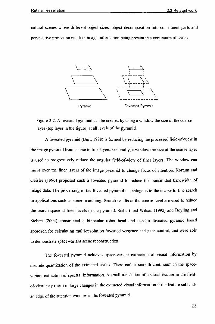
natural scenes where different object sizes, object decomposition into constituent parts and
perspective projection result in image information being present in a continuum of scales.
\ ~
\ \\ \
Pyramid
\ \.. .
,-j-----,\\ \\~:_.----:- .... _\.
,---"':':'---~_;--\\ : .,\ \ \ "\ ,
.... -------------~Foveated Pyramid
Figure 2-2. A foveated pyramid can be created by using a window the size of the coarse
layer (top layer in the figure) at all levels of the pyramid.
A foveated pyramid (Burt, 1988) is formed by reducing the processed field-of-view in
the image pyramid from coarse to fine layers. Generally, a window the size of the coarse layer
is used to progressively reduce the angular field-of-view of finer layers. The window can
move over the finer layers of the image pyramid to change focus of attention. Kortum and
Geisler (1996) proposed such a foveated pyramid to reduce the transmitted bandwidth of
image data. The processing of the foveated pyramid is analogous to the coarse-to-fine search
in applications such as stereo-matching. Search results at the coarse level are used to reduce
the search space at finer levels in the pyramid. Siebert and Wilson (1992) and Boyling and
Siebert (2004) constructed a binocular robot head and used a foveated pyramid based
approach for calculating multi-resolution foveated vergence and gaze control, and were able
to demonstrate space-variant scene reconstruction.
The foveated pyramid achieves space-variant extraction of visual information by
discrete quantization of the extracted scales. There isn't a smooth continuum in the space-
variant extraction of spectral information. A small translation of a visual feature in the field-
of-view may result in large changes in the extracted visual information if the feature subtends
an edge of the attention window in the foveated pyramid.
23

Retina Tessellation 2.3 Related work
2.3.3. Log-polar transform
The topological mapping of biological retina afferents to the Lateral Geniculate Nucleus has
inspired the mathematical projection of visual stimuli at coordinates in the input image to
those in an image structure often referred to as the cortical image. These analytic projections
are often called retina-cortical transforms, and the most widely used is the log(z), complex-
log or log-polar transform (Schwartz, 1977), which is claimed to approximate the space-
variant mapping in primates from the retina to Lateral Geniculate Nucleus (and higher visual
areas in the primary visual cortex).
In the log-polar transform, if the ~2 coordinate (x, y) in the input image can be also
given by the following metric preserving mapping
z = x+iy
= Izl[ cos (8) + i sin (8) ] (Equation 2-1)
where O=arctan(ylx) and n c 71.. The retino-cortical projection into the cortical image
is given by log(z).
log (z) = log (Izlei(8+2nJr))
= log(lzl)+i8= log(eccentricity)+ i(ang/e)
(Equation 2-2)
While Schwartz (1977) directly projected the pixel intensities from input coordinates
(x, y) to associated cortical coordinates (lz], 8), a better approach is to reduce aliasing by
sampling the input coordinates with (overlapping) receptive fields (Chapter 3).
24

Retina Tessellation 2.3 Related work
y
(a)
[z]
x 8(b)
Figure 2-3. (a) Log-polar retina tessellation (input image sampling locations) for a
retina based on the log-polar transform. (b) Cortical image generated by the log-polar
transform of the standard greyscale Lena image. The cortical image was created by
placing overlapping Gaussian receptive fields on the log-polar retina tessellation.
The log-polar mapping results in a cortical image representation which is biased
towards the foveal region of the field-of-view (Figure 2-3b). All higher level processing
operations are conducted on the cortical image resulting in space-variant processing in the
image domain. The log-polar mapping has interesting properties. Rotation or scaling in the
input image results in a translation in the cortical image. Therefore, researchers such as
Tunley and Young (1994) have found log-polar representations useful for the computation of
first order optical flow.
2.3.3.1. Space-complexity of a sensor
Rojer and Schwartz (1990) defined what they called the space-complexity ofa sensor or FIR
quality as the ratio of a sensor's field-of-view to its maximum resolution.
sensor field-of -viewSpace-complexity = - _ _.;;___ ,--_-maximum resolution
(Equation 2-3)
25

Retina Tessellation 2.3 Related work
The FIR ratio of a sensor gives an indication of the compression or bandwidth
reduction achieved by a sensor. The FIR ratio of conventional space-invariant sensors scale
quadratically with the rank of the sensor matrix while space-variant log(z) sensors' space-
complexity scale logarithmically (Schwartz et aI., 1995). Space-complexity is also a measure
of the spatial dynamic range of a sensor. Schwartz et al.( 1995) estimated that if humans were
to achieve the same dynamic range we have using space-variant vision (i.e. coarse wide angle
vision and high acuity centre) with space-invariant vision (uniform acuity across the field-of-
view), our brains would have to weigh between 5000-300001bs to process the extracted visual
information.
In the author's opinion the space-complexity measure is lacking in that it does not
take into account that, unlike a space-invariant sensor, a space-variant sensor must change its
focus of attention (i.e. point of fixation on the scene) to absorb a complete representation of
visual information in the continuum of scale-space (Chapter 4). The overhead of these
saccadic fixations (Chapter 5) will be related to the spatial complexity of the visual
information in the scene.
The space-complexity measure also does not reflect the tapering of the sampled
resolution of a space-variant sensor with eccentricity. A very sharp rate of change of
resolution would give an optimal space-complexity as the sensor will have a wide field-of-
view for a given high maximum resolution. However the author believes that saccadic search
for objects with such a sensor would suffer from the reduction of visual information density at
intermediate scales between the coarse periphery (which generates hypothesises for future
fixations) and the maximum resolution fovea. This results in the space-variant sensor needing
more fixations to target and home in on a feature observed in the periphery.
26

Retina Tessellation 2.3 Related work
2.3.3.2.Nyquist criterion
The Shannon-Nyquist sampling theorem states that when sampling an input analog signal, the
sampling rate must be greater than twice the bandwidth of the input signal in order to
accurately reconstruct the input signal. Assuming the input signal has been low-pass filtered,
which is justified for natural images, the Nyquist criterion is that the sampling frequency w,
must be greater than twice the input image's maximum frequency wmax•
(Equation 2-4)
The frequency WN is known as the Nyquist rate. If a signal is sampled at lower than
its Nyquist rate, input frequencies greater than w, / 2 will generate artefacts in the sampled
information in a process called aliasing. Sampling at a frequency much higher than the
Nyquist rate results in the sampled signal containing highly correlated (redundant)
information. This is an inefficient use of finite sampling resources referred to as super-
Nyquist sampling.
In this thesis the author processes digital images which are limited to a maximum
frequency of half a cycle per pixel. Because an image has an underlying minimum spatial
frequency, any attempts to sample an image at higher spatial frequencies would result in a
highly correlated output. Therefore sampling a digital image at much higher than a sample per
pixel will result in super-Nyquist sampling.
There is always super-Nyquist sampling In the foveal region of the log-polar
transform of a digitised image as the sampling rate of the transform approaches a singularity
at the centre. Large areas of redundant information can be observed in the cortical image in
Figure 2-3b. A large percentage of the cortical image is highly correlated information and the
log-polar sampling process has not optimally reduced the dimension of the extracted visual
information. As the cortical image is the internal representation of visual information
processed by higher order machinery in a space-variant vision system, there has been a sub-
optimal allocation of limited processing resources on redundant visual data. The author
27

Retina Tessellation 2.3 Related work
therefore concludes that the log-polar transform is not a suitable basis for space-variant vision
systems that extract visual information from pre-digitised media such as digital images or
digital cinema.
2.3.4. The log(z+a) transform
The processing of the visual pathway in vertebrates is divided between the two lobes of the
brain. The visual cortex in the right lobe processes the left visual hemisphere from both left
and right eyes, and the cortex in the left lobe processes the right visual hemisphere from both
eyes. Schwartz (1980) proposed a log(z+a) model which would split the cortical image along
the vertical meridian into two visual hemispheres and which would also try to address the
problem of the super-Nyquist sampling in the fovea of the log-polar transform.
In the log(z+a) model, a real parameter a is added to the image space complex
coordinate as follows
z+a=x+iy+a
= I~(x+a)'+ y' I(cot:a )+iSi{:a)) (Equation 2-5)
I~ 2 21 {arcta{:a )+2nJr )= (x+a)+y e
The resulting coordinate is projected into cortical space (the cortical image) using the
log-polar transform,
(Equation 2-6)
= 109(I~(x+a)2+ll)+iarctan(x:a)The real a term has in effect sliced off a central vertical (corresponding to the real
axis) slice in the log(z) retina tessellation. The super-Nyquist central sampling region in the
pure log-polar model can be reduced or removed completely depending on the chosen value
for a.
28

Retina Tessellation 2.3 Related work
In the log(z+a) model, the two visual hemispheres in the input image are processed
separately. The ex term is positive for the right hemisphere and negative for the left
hemisphere.
y
(a)
e
x(b)
Figure 2-4. (a) log(z+a) retina tessellation. (b) Cortical image generated by the log(z+a)
transform of the standard greyscale Lena image. The cortical image is split along the
vertical meridian. Overlapping Gaussian receptive fields were used to sample the input
image.
2.3.4.1. Distorted sampling tessellation
While the exparameter avoids the singularity in the centre of the logfz) model and reduces
oversampling in the foveal region, it distorts the isotropic retina tessellation sample locations,
vertically elongating the central fovea. Values for ex which do not drastically distort the
topology of the associated retina (such as in Figure 2-4) result in super-Nyquist sampling in
the fovea.
29

Retina Tessellation 2.3 Related work
2.3.5. Uniform fovea retina models
To solve the super-Nyquist sampling problem in the centre of space-variant retinae,
researchers have attempted to use a different sampling topology or representation in the fovea.
Bolduc and Levine (1996) sampled the foveal region of their input uniformly and projected
the visual information to a separate image structure while maintaining a mapping of the
peripheral region of the retina to a log(z) cortical image (Figure 2-5).
y
x
(b)
RF fowa;11111111111111111111111111111111 0-
e(a) (c)
Figure 2-5. (a) Receptive fields of a retina with a uniform rectilinear foveal region.
(b) Structure containing information mapped from the foveal region, this is a copy of
the foveal data in the retina. (c) Cortical image with the log(z) transformed data from
the periphery. Reprinted from Bolduc and Levine (1996).
Gomes (Gomes, 2002) used a retina with a hexagonal receptive field tessellation and
uniform foveal region. Both the hexagonally tessellated fovea and periphery were mapped to
a single rectilinear cortical structure based on a coordinate lookup (Figure 2-6). The
rectilinear cortical image was not completely populated with projected data but instead
tapered towards the foveal region as the angular receptive field density reduced in the log(z)
transform.
30

Retina Tessellation 2.3 Related work
y
........... . . . ..
[z]
x 8. . ... . .
Figure 2-6. (a) Retina tessellation with a hexagonal receptive field tiling and uniform
foveal region. (b) Cortical image created by mapping receptive fields with a uniform
foveal region (reprinted from Gomes (2002».
2.3.5.1. Discontinuities in representation and topology
Separating the processing of foveal and peripheral regions as in Bolduc and Levine (1996)
creates a discontinuity in the internal representation of visual information in a space-variant
system. There are difficulties in reasoning with features that cross the foveal and peripheral
representations. Although creating a tapering cortical image as in (Gomes, 2002) solved the
problem of storing the space-variant visual information in a single structure, this approach
necessitates a lookup calculation to map coordinates into the rectilinear cortical image. Higher
order processing of the rectilinear array containing the cortical image would have to deal with
border problems where visual data is not present in the tapered cortical image. The sudden
change in the topological structure of the retina tessellation (Figure 2-6) between the fovea
and periphery will disrupt the continuum in sampled scale-space because the approach does
not maintain a seamless merging of the foveal topology to the peripheral topology.
31

Retina Tessellation 2.3 Related work
2.3.6. Conclusion
Biological retinae appear to exhibit an almost uniform hexagonal receptor packing structure in
the fovea that transforms seamlessly into an exponential sampling structure (resembling log-
polar) towards the peripheral field. The log(z) and other similar mappings (Johnston, 1989)
attempt to approximate the retino-cortical transform in primates. The author has not found any
analytic or geometric mapping reported in the literature with a closed form solution that can
describe the change in topography of the receptive field centres between the fovea and periphery
of a retina tessellation. These reported retino-cortical transform approaches do not address the
question of the actual ~2 locations (retina tessellation coordinates) where a computer vision
system should extract visual information from an image or video. The work in the literature is
based on the projection of the radial component of retinal coordinates (with respect to the point
of fixation) to a cortical space and does not effectively deal with the angular relationships
between the coordinates in the input retinal plane when performing the projection. This failing
results in images being over-sampled in the foveal region during the construction of plausible
retinae that sample pre-digitised media.
The exponential sampling strategy of the log(z) retina periphery appears to have many
desirable properties, capable of ameliorating some subsequent visual information processing tasks.
But the topology of the periphery must transform into a uniform fovea without generating
discontinuities to allow a single set of uniform 'coding units' to be constructed for higher order
processing in the cortex (Wilson, 1983). These coding units would then be able to represent
Wilson's "ensemble of messages" which are generated across a continuum in scale-space aiding
visual search. Researchers have not been able to define a retina with the properties of a space-
variant peripheral retina topology that searnlessly merges into a uniform foveal region with a
hexagonal tessellation that will optimally tile 20 space (Hales, 200 1) without over-sampling the
image or creating discontinuities in the retina tessellation. Solving the problem of generating a
viable retina model will allow biologically motivated space-variant vision to progress,
32

Retina Tessellation 2.4 Self-organised retina tessellation
circumventing the mentioned limitations and driving attentional structures which are part of an
overall space-variant vision system.
2.4. Self-Organised Retina Tessellation
2.4.1. Introduction
During his search for a retinal tessellation that would be space-variant and sample 20 space,
the author questioned the need to base the retina on a closed form retino-cortical transform. It
is not possible to generate a continuous regular retina tessellation with a uniform density in
the foveal region and a log-polar density in the peripheral region using a purely analytic
transform based on image plane coordinate eccentricity. If a researcher were not concerned
with projecting the afferents of a retina to a topological cortical image, the positions of the
retina receptive fields (retina tessellation) could be independently determined to satisfy the
criterion of a uniform fovea region and space-variant periphery.
This section describes the design, implementation and evaluation of a space-variant,
continuous, regular retinal tessellation generated using self-organisation. Self-organisation is
a form of unsupervised learning where neural systems are trained without a target output
pattern or class. Self-organisation was able to mediate between the influences of the
constraints for the retinal tessellation (uniform fovea and space-variant periphery) and to
generate a seamless transition between these two influences in the retinal mosaic. A self-
organisation technique similar to Kohonen Feature Maps (Kohonen, 1995) called Self-Similar
Neural Networks (Clippingdale and Wilson, 1996) generated retinal tessellations that best
33

Retina Tessellation 2.4 Self-organised retina tessellation
merged the foveal and peripheral regions of a retina. However the retinal tessellations
generated usmg self-organisation do not have an explicit associated cortical image data
structure found in conventional artificial retinae based on retino-cortical transforms. Chapter 3
will describe visual processing machinery that can reason with the information extracted
using a self-organised artificial retina.
2.4.2. Self-Similar Neural Networks
This approach's main distinction from Kohonen Feature maps and other self-organising
techniques is that the stimulatory input for the network is derived by applying a composite
transformation to the network weights themselves. The network weights Xi in the model
represent the coordinates of (in our case) receptive fields in R2 space.
For a network of N units, each characterised by a two dimensional network weight
vector x,{n), the input stimulus y,{n) at iteration n is calculated by the following,
Yi(n) = T(n) xi(n -I) (Equation 2-7)
where Xi (n - I) is the i th network unit at iteration n - I and I ::::;i::::; N. To generate a space-
variant retina with a uniform fovea the following (ordered) composite transform T similar to
that in Clippingdale and Wilson (1996) can be used
1. A random rotation about the centre of the coordinate space between 0 and 2n.
2. A dilation (increase in eccentricity from the centre of the coordinate space) of the
exponent of a dilation factor which is random between 0 and log(8). This results
in network units in the periphery being transformed more than those in the fovea.
3. A random translation between 0 and f, where f is associated with the required
foveal percentage of the resultant retina.
(Equation 2-8)
Any input stimuli Yi(n) which lie outside the bounds of the coordinate space are culled before
the network weights Xi (n - 1) are stimulated to calculate Xi (n) . In this model's training
34

Retina Tessellation 2.5 Experiments
methodology the final configuration of the network weights are governed by the composite
transformations T. Clippingdale and Wilson (1996) list other composite transformation to
generate networks with regular lattice, circle, disc, toroidal and other configurations.
The network is initialised with a random weight configuration and recursively iterated
with the described composite transformation T and the following learning rule to find the
updated weight vector xln):
Xi(n)=Xi(n-I)+a(n) L (Yi(n)-X;(n-I»iEA;(n)
(Equation 2-9)
{i: IIYI(n) - xi(n -1)11 }
i\j(n) =< IIYi(n)-Xk(n-I)II,k:t:. j
(Equation 2-10)
Ai(n) contains the indices to the input stimuli yln) to which Xi (n - 1) is the closest
network vector. a(n) is a learning parameter which controls the stimulation of the network
weights. The learning parameter a is linearly reduced (annealed) throughout the self-
organisation to increase the speed of convergence of the network weights to a stable
configuration, although Clippingdale and Wilson (1996) proved the convergence of Self-
Similar Neural Networks in a circle network configuration even with a constant learning
parameter. Intuitively, one can visualise the effect of the learning rule as each network weight
Xi (n - 1) being updated individually by the input stimuli y;(n) that are closer to that weight
than any other in the network.
2.5. Experiments
In this section of the thesis, the author will present the results of self-organising retina
tessellations with different self-similar neural network composite transformations T. The goal
of the self-organisation is to converge onto a retina tessellation with a circular uniform central
35

Retina Tessellation 2.5 Experiments
foveal topology that smoothly transitions into a surrounding space-variant peripheral
topology. The first and second steps in the composite transformation in Equation 2-8 will be
retained and the variation of the third step in the composite transformation T will be
investigated in this section.
In all self-organisation experiments, the radius of the coordinate frame for self-
organisation was unity and the learning rate a was annealed from 0.1 to 0.0005 between
iterations. The initial value for a was retained for the first quarter of the total number of
iterations to induce large updates in topography before being linearly reduced to the final
value at the end of the self-organisation. Figure 2-7 contains a plot of the learning rate during
a self-organisation with 20000 iterations.
Leaming Rate a
0.11--------,
0.12
000
0.04
0.02
7500 10000 12500 15000 17500 20000iteration
Figure 2-7. The learning rate u was reduced (annealed) during self-organisation.
2500 5000
2.5.1. Vertical and horizontal translations
The author generated the retina tessellation in Figure 2-8 by using vertical and horizontal
translations in the composite transformation T as indicated in Equation 2-8 for self-organising
a network of weights using Self-Similar Neural Networks. Therefore a node at (x, y) in the
coordinate frame will be translated to (x+lx, y+/y) where lx, /y -+ 1./ The horizontal Ix and
vertical r, translations were random up to 20% (/ = 0.2) of the radius of the coordinate space
36

Retina Tessellation 2.5 Experiments
r.e. 20% of the radius of the resulting retina field-of-view. The network comprises of 4096
nodes and was self-organised for 5000 iterations.
Figure 2-8. A retina tessellation with 4096 nodes self-organised for 5000 iterations and
generated with translations made in horizontal and vertical directions up with.f-=0.2.
The topology of the resultant retina tessellation has a central foveal region that
seamlessly coalesces into a space-variant peripheral region without any major first or second
order discontinuities in node density.
The spacing between nodes in the tessellation can be subjectively seen to be irregular
in some regions of the retina mosaic. The next figure (Figure 2-9) contains the result of a self-
organisation over a very high number of iterations in comparison to other tessellations in this
thesis (250000 iterations) to demonstrate the effect of a high iteration count on the resulting
weight configuration mosaic.
37

Retina Tessellation 2.5 Experiments
............. .;., ".. . ......... .
.. . . ..
. . .
• ••••• ': •• •• t. t.: :.,..: .Figure 2-9. A retina tessellation with 4096 nodes self-organised for 250000 iterations
and translations made in horizontal and vertical directions withf-=0.2.80
~660..Clx:ClQ)co 50.9IDuc£l 40isc(UID._E3J..-
- Translations made horizontally and vertically~ Ideal
20
10L- __ -L ~ ~ __~~--~--~L---~-----L--~L---~o 0.1 0.2 0.3 0.4 0.5 0.6 0.7 0.8 0.9
eccentri City
Figure 2-10. The inverse of mean distance to a node's neighbours for all nodes of the
retina tessellation self-organised with translations made in horizontal and vertical
directions plotted against the node's eccentricity (Figure 2-9). The highest value
corresponds to the retina tessellation's space-complexity. The ideal curve with
exponential decay of the mean distance to a node's neighbours in the periphery and
with a uniform foveal region with radius 0.2 is also displayed.
38

Retina Tessellation 2.5 Experiments
The weight configuration of the self-organisation has converged into a very regular
tessellation with a local topology approaching a regular hexagonal tiling. Slight deviations
from the hexagonal packing may be observed at some nodes on the tessellation (Figure 2-11).
These occur at the region between the foveal and peripheral regions of the tessellation.
The vertical and horizontal translation components of the composite transformation T
have had a strong influence on the convergent tessellation. The size of the uniform central
fovea-like region roughly corresponds to the f parameter used in the translations (Figure
2-10). The highest value in Figure 2-10 corresponds to the space-complexity (Equation 2-3)
of the retina tessellation. The foveal region of the tessellation has a distinctly square shape
which the author hypothesises was caused by performing the translations in the vertical and
horizontal directions. Therefore in the next section a different translation methodology will be
used in an attempt to generate a more plausible retina tessellation with a circular central
foveal region.
003-0.14
• •• •0025·
-0.150.02
•0.015· • •• • -0.16
0.01·
-0.17 •0.005
•o· • •-0.125 -012 -0;15 -011 -0;05 -oci9s
-018-01 -o.Q3 -0.02 -001
(a) (b)
•
•
001
Figure 2-11. Magnified areas of a self-organised retina that show different packing
mosaics. The area in figure (b) is from a region in the tessellation where the foveal
topology merges into the peripheral.
39

Retina Tessellation 2.5 Experiments
2.5.2. Translation in a radial direction
The author obtained the following retina tessellation by changing the translation. in the
composite transformation T, from a random vertical and a random horizontal translation to a
random translation in the radial direction away from the centre of the coordinate space.
Therefore a node at (r, 8) In polar coordinates frame will be translated to (r+/r. 0) where
/r ---4 1./ As with previous experiments, the translation in a radial directionj, was random up
to 20% (j = 0.2) of the radius of the coordinate space. The network consisted of 4096 nodes
and was self-organised for 20000 iterations.
Figure 2-12. A retina tessellation with 4096 nodes self-organised for 20000 iterations
and translations made in a radial direction away from the centre of the retina (FO.2).
Unlike previous retina tessellations, that resulting from a translation m a radial
direction (Figure 2-12) has a central circular fovea like region. However this approach
resulted in a mosaic with a higher packing density in the fovea for the same f parameter as the
40

Retina Tessellation 2.5 Experiments
experiment in Section 2.5.1. The density of the foveal region increases sharply towards the
centre of the coordinate space (Figure 2-13) but the foveal topology does not reach singularity
(Figure 2-14).
180
160
140e'"0.0 120x:OlIDc.9 100(l)uc
~ 80
isc(U 60(l)
~~40
20
00 0.1
- Translations made In the radial direction~ Ideal
0.2 0.3 0.4 0.5eccentncrty
0.6 0.7 0.8 0.9
Figure 2-13. The inverse of mean distance to a node's neighbours for all nodes of a
retina tessellation self-organised with translations made in a radial direction
(Figure 2-12) plotted against the node's eccentricity. The highest value corresponds to
the retina tessellation's space-complexity. The ideal curve with exponential decay of
the mean distance to a node's neighbours in the periphery and a uniform foveal region
with radius 0.2 is also displayed.
. . .
o .' . : . : :.:.::..:.:.: .. :".'. '. ' ' .:
.....0.1. . . .
0.05 . . ' . . . . .. , .. . "
. .. . . . , .. . . . .. . . . .. ' '.. . ....
-0.05 .......... . '. . . .....
-01" : .. ~ '.'
.. ' . ' : : .. : ..-0.1 -0.05 o 0.05 0.1
Figure 2-14: A magnified view of the fovea from the retina illustrated in Figure 2-12
(the radius of the retina is I unit).
41

Retina Tessellation 2.5 Experiments
In the next section of this thesis, a self-organisation experiment will be conducted that
combines the influences translations in the vertical/horizontal and the radial directions.
2.5.3. Translations in the vertical, horizontal and radial directions
Here the composite transformation T contains translations in the vertical, horizontal and radial
directions. First a node at (x, y) in the coordinate frame will be translated to (x+.fx, y+f,.) where
Ix,f,. ~ 1./ Then the polar coordinate of the node (r, 8) will be translated to (r+/r, 0) where
/r ~ l.f As earlier, f,was random up to 20% (f-=0.2) of the radius of the coordinate space,
while Ix and f,. were random up to 6.6% (f-=0.066). The network consisted of 4096 nodes and
was annealed for 20000 iterations.
Figure 2-15: A retina tessellation with 4096 nodes self-organised for 20000 iterations
and translations made in horizontal (f-=0.066), vertical (f-=0.066) directions and radially
away from the centre of the retina (f-=0.2).
42

Retina Tessellation 2.5 Experiments
The tessellation resulting from self-organising with vertical, horizontal and radial
translations (Figure 2-15) has a circular central uniform foveal region(Figure 2-17). The size
of the fovea roughly corresponds to the vertical and horizontal translations (f=0.066). The
node density of the retina was uniform in the central foveal region and gradually reduced
pseudo-logarithmically in the periphery. Very slight increases and first order irregularities in
the node density can be observed between the fovea and periphery and in the edge of the
retina tessellation (Figure 2-16).
100
so~ 80:::J0.Ds:
700)
(j)c.8 60(J)uc 50ro.....(f)
'6c 40ro(J)
~ 30.....20
100
- Translations made vertically, horizontally and radially~ Ideal
0.1 0.2 0.3 0.4 0.5 0.6 0.7 O.S 0.9
eccentricity
Figure 2-16. The inverse of mean distance to a node's neighbours for all nodes of the
retina tessellation self-organised with translations made in a vertical, horizontal and
radial directions (Figure 2-15). The ideal curve with exponential decay of the mean
distance to a node's neighbours in the periphery and a uniform foveal region with
radius 0.2 is also displayed.
43

Retina Tessellation 2.5 Experiments
-0.2 o 0.2 0.4
Figure 2-17. A magnified view of the fovea from the retina generated with vertical,
horizontal and radial translations (the radius of the complete retina is 1 unit).
007 ~~e::IC)
0.06.J:>oJ::.2>~£ 0.05
8c::-£I 0.04
:sc::<U 0.03Cl>E
E 0.02
.~
eccentricity
Figure 2-18 Standard deviation of the distance to a node's immediate neighbours for all
the nodes in the self-organised retina tessellation with translations made in horizontal,
vertical directions and radially away from the centre of the retina sorted on eccentricity.
The standard deviation of the distances between nodes in the retina tessellation
(Figure 2-18) increases in the foveal region and also drops sharply in the edge of the
coordinate space. The author hypothesises that the increase in the fovea region is caused by
conflicting affects of a space-variant periphery and uniform central fovea. The low variation
at the far periphery may be because these peripheral nodes are not completely surrounded by
adjacent neighbours.
44

Retina Tessellation 2.5 Experiments
While the generated retina topology has a uniform dense central foveal region
surrounded by a sparse, space-variant periphery, the transition between the densities of the
two regions is not completely seamless. In the next and final section of results in this chapter
the author will demonstrate retina tessellations with a smooth transition between foveal and
peripheral topographies.
2.5.4. Random translation
The author obtained the following retina tessellation by changing the translation, in the
composite transformation T, to a random translation in a random direction in the coordinate
space. Therefore a node at (x, y) in the coordinate frame will be translated to (x+cos(O)xJH,
y+sin(O)xJH) where JH ~ 1./and O~ 1..21t, The radial translation JH was random up to 20%
(f = 0.2) of the radius of the coordinate space (i.e. radius of the retina) and the direction of
the translation 0 was random from 0 to 21t. A network with 4096 nodes was self-organised for
20000 iterations,
'. '.
' .... . . .
···0 '0 '.'.'.'.. . '., : ':'.': .'::: >:->::': :':'::-:::::.::, : .' .,0,0. :. '0 '0 •••••• " •• •
•:,' .' •• '0 ••• '. ' .' • eo': . '.' ... '. :.:.:.::: '0 :' .'. 0 : .' •
• •••••• 0 ... 0 •• 0 •• °. '0 .'........... ·0· .. 0.· ... 0 ..",
o ••••. ' ... . . . .. . . .. . . . .. .. . . ..... .. ' .. -.';: .. '.
'0· ••
• ,0 ••
• '0' •••••••• ,0',
o •• '.
" .. . " .. ' .''.' .
•• :: '0'.' . ·0···0··· ".. : ,0. '0' . : : '.' .: ,0.: .
• '0 '0", '0.0 ..... ·0··.. '. . .' .Figure 2-19. A retina tessellation with 4096 nodes self-organised for 20000 iterations
with a random translation andf=O,2,
45

Retina Tessellation 2.5 Experiments
90- Random translation~ Ideal
20
100~--~0~1--~0~2--~0~3--~OL.4--~0~.5--~O~.6~~0~.7~~0~8--~0~.9~~sccentncrty
Figure 2-20. The inverse of mean distance to a node's neighbours for all nodes of the
retina tessellation self-organised with a random translation plotted against node
eccentricity (Figure 2-19). The ideal curve with exponential decay of the mean distance
to a node's neighbours in the periphery and a uniform foveal region is also displayed.
The space-complexity of the retina tessellation is given by the maximum of the curve .
• IO-l'5~---'-----r----'-----'----'-----'-----'----'-----r-----~i! •.0-a 35·iic 3s~ 25C
~ ,'6~ 1 se.€ 1.g, 05·iii
~~"' ,""WWW\°O~--~Ol----~O~2----~03~--~O~'----~O~5--~O~6----~O~7----~08~--~O~9----~
eccentricity
Figure 2-21. Standard deviation of the distance to a node's immediate neighbours for
all the nodes in the self-organised retina tessellation with a random translation sorted on
eccentricity (Figure 2-19).
The node density of the retina tessellation generated using a random translation has a
smooth seamless transition between foveal and peripheral regions (Figure 2-20). The
maximum density of nodes in the fovea is approximately that of the tessellation generated in
Section 2.5.3 which had vertical, horizontal and radial translations. The standard deviation of
the distance to a nodes neighbours (Figure 2-21) for the tessellation is also much lower than
previously (Figure 2-18).
46

Retina Tessellation 2.5 Experiments
The retinal topology self-organised with a random translation was used for saccadic
vision and other experiments in this thesis. As a multi-resolution pyramid of retinae will be
used to extract visual information from images in this thesis, the author generated retina
tessellations with differing number of nodes.
. "... ' .
• ',' 0'·· •. . ' .. , .. . . . :... :. ' ... '. '. .
··..WiCL<. .. '..... ....
. .... ' .
. . . . . . .
Figure 2-22. A retina tessellation with 1024 nodes self-organised for 20000 iterations
with a random translation andj=0.2.
. .. . ..
Figure 2-23. A retina tessellation with 256 nodes self-organised for 20000 iterations
with a random translation and.f-=0.2.
47

Retina Tessellation 2.5 Experiments
A space-variant retina pyramid based on retina tessellations with 4096 (Figure 2-19),
1024 (Figure 2-22) and 256 (Figure 2-23) nodes will extract approximately octave-separated
space-variant visual information. To efficiently implement the retina pyramid, a 8192 node
retina (with tessellation illustrated in Figure 2-24) was also generated. Only this layer of the
retina pyramid sampled the input image, all others sampled low-pass filtered information
from immediately higher frequency layers in the retina pyramid (Chapter 3).
Figure 2-24. A retina tessellation with 8192 nodes self-organised for 20000 iterations
with a random translation and.t=0.2.
48

Retina Tessellation 2.6 Discussion and Conclusion
so- 4096 nodes
1024 nodes- 256 nodes
80
°0~--~0~.1----~0.2~--~O~.3--~O~.4~--~O.~5--~O~.6--~O~.7~--~O.~8--~O~.g~~eccentri city
Figure 2-25. The inverse of mean distance to a node's neighbours for all nodes in retina
tessellations with 4096, 1024 and 256 nodes self-organised with a random translation
plotted against the node's eccentricity. The retina pyramid based on these tessellations
will extract approximately octave separated visual information.
2.6. Discussion and Conclusion
The principle achievement in this chapter is the creation of a self-organised retina receptive
field tessellation. Researchers (Schwartz, 1977, 1980; Wilson, 1983; Gomes, 2002) have tried
to use an analytical retino-cortical transform that maps locations in the field-of-view to a
continuous cortical image, thereby creating a data structure that can store extracted visual
information. However the actual retinal tessellations or locations of retinal receptive fields
that are needed to generate these continuous cortical images are inadequate, exhibiting
singularities and over-sampling the fovea or having discontinuities and distortions in the
sampling mosaic. No analytic approach or geometric mapping that can describe the gradual
49

Retina Tessellation 2.6 Discussion and Conclusion
change in topography of the retina between a uniform fovea and space-variant periphery has
been reported in the computer vision literature.
The author used a self-organisation methodology (Clippingdale and Wilson, 1996) to
generate retinal tessellations that, while foregoing a defining closed form analytic mapping,
had continuity in sampling density between a uniform fovea and space-variant periphery. The
retina has a uniform foveal region which seamlessly coalesces into a space-variant periphery
and the tessellation does not have a singularity in the fovea.
The tiling structure of the retina locally resembles a hexagonal lattice with occasional
deviations in the hexagonal topology in some locations where there is a transition between the
dominant influences on the local network topology. These deviations enable the retina
tessellation to maintain a sampling density continuum at a macroscopic level and regularity in
node positions, while the retina's uniform foveal region seamlessly coalesces into a space-
variant periphery. At the transition between the foveal and peripheral topological influences
there is an increase in entropy in the system, observable as an increase in the variance of
neighboring intra-node distances at 0.03 and 0.95 of the radius of the retina in Figure 2-21.
The author surmises that this is caused by the retina tessellation trying to maintain regularity
in its mosaic while being subject to increased contradictory forces from foveal (uniform) and
peripheral (space-variant) topological influences.
The hexagonal lattice structure of the self-organised retina is interesting but expected.
A hexagonal tessellation is the approximate pattern in which receptive fields are found in
biological retinae (Polyak, 1941) and is a pattern commonly found throughout nature
(Morgan, 1999). Retina receptive fields placed on this tessellation would be equidistant from
their immediate neighbours and Dudgeon and Mersereau (1984) showed that such a
hexagonal tessellation is the optimal sampling (tiling) scheme for a 2D space.
The non-uniform, almost pseudo-random sampling locations generated by self-
organisation have properties that help reduce aliasing artefacts in their associated retina's
50

Retina Tessellation 2.7 References
extracted visual information. Pharr and Humphreys (2004) discussed how the random
jittering of sampling locations turns aliasing artefacts into noise. It is possible that
biologically retinae have similarly benefited by the non-uniform locations of visual
machinery.
A retina tessellation is not yet a retina. To prevent aliasing, visual information must
be gathered over a large support region around each coordinate in the retina tessellation. In
the next chapter the author will define the receptive fields that will extract features at
locations indicated by the space-variant retina tessellation.
An explicit closed form analytic mapping from the retina tessellation coordinates to a
retinotopic cortical image data structure that could be used to store and manipulate extracted
image information is not available for the self-organised retina. In the next chapter the author
will describe processing structures that can operate on space-variant visual information
extracted using a retina with a self-organised or in fact any arbitrary receptive field
tessellation.
2.7. References
Bolduc, M. and Levine, M. D. (1996). "A real-time foveated sensor with overlapping
receptive fields." Real'Iime Imaging.
Boyling, T. A. and Siebert, J. P. (2004). Foveated Vision for Space-Variant Scene
Reconstruction. 35th International Symposium on Robotics, Nord Villepinte, Paris,
France.
Burt, P. J. (1988). Algorithms and architectures for smart sensing. DARPA Image
Understanding Workshop.
Burt, P. J. and Adelson, E. H. (1983). "The Laplacian Pyramid as a Compact Image Code."
IEEE Transactions on Communications 31(4): 532-540.
51

Retina Tessellation 2.7 References
Clippingdale, S. and Wilson, R. (1996). "Self-similar Neural Networks Based on a Kohonen
Learning Rule." Neural Networks 9(5): 747-763.
Daniel, P. M. and Whitteridge, D. (1961). "The representation of the visual field on the
cerebral cortex in monkeys." Journal of Physiology 159: 203-221.
Dudgeon, D. E. and Mersereau, R. M. (1984). Multidimensional Digital Signal Processing.
Englewood-Cliffs, NJ, Prentice-Hall, Inc.
Ferrari, F., Nielsen, J., Questa, P. and Sandini, G. (1995). "Space variant imaging." Sensor
Review 15(2): 17-20.
Gomes, H. (2002). Model Learning in /conic Vision. University of Edinburgh.
Hales, T. C. (2001). "The Honeycomb Conjecture." Discrete Computational Geometry 25: 1-
22.
Hubel, D. H. (1987). Eye, Brain and Vision, Scientific American Library.
Hubel, D. H. and Wiesel, T. N. (1979). "Brain mechanisms of vision." Scientific American
241: 150-162.
Johnston, A. (1989). "The geometry of the topographic map in striate cortex." Vision
Research 29: 1493-1500.
Kohonen, T. (1995). Self-Organizing Maps, Berlin: Springer-Verlag.
Kortum, P. and Geisler, W. (1996). " Implementation of a foveated image coding system for
image bandwidth reduction." SPIE Proceedings 2657: 350-360.
Levine, M. W. and Shefner, 1. M. (1991). Fundamentals of sensation and perception. Pacific
Grove, CA, Brooks/Cole.
Morgan, F. T. (1999). "he hexagonal honeycomb conjecture." Transactions of the American
Mathematical Society 351(1753).
Orabona, F., Metta, G. and Sandini, G. (2005). Object-based Visual Attention: a Model for a
Behaving Robot. 3rd International Workshop on Attention and Performance in
Computational Vision, San Diego, CA, USA.
Pharr, M. and Humphreys, G. (2004). Physically Based Rendering: From Theory to
Implementation, Morgan Kaufmann.
Polyak, S. L. (1941). The Retina. Chicago, University of Chicago Press.
52

Retina Tessellation 2.7 References
Rojer, A. S. and Schwartz, E. L. (1990). Design considerations for a space-variant visual
sensor with a complex-logarithmic geometry. 10th International Conference on
Pattern Recognition.
Schwartz, E., Greve, D. and Bonrnassar, G. (1995). "Space-variant active vision: Definition,
overview and examples." Neural Networks 8(7/8): 1297-1308.
Schwartz, E. L. (1977). "Spatial mapping in primate sensory projection: Analytic structure
and relevance to perception." Biological Cybernetics 25: 181-194.
Schwartz, E. L. (1980). "Computational Anatomy and functional architecture of the striate
cortex." Vision Research 20: 645-669.
Siebert, 1. P. and Wilson, D. (1992). Foveated vergence and stereo. 3rd International
Conference on Visual Search, Nottingham, UK.
Srinivasan, M. V. and Venkatesh, S., Eds. (1997). From Living Eyes to Seeing Machines,
Oxford University Press, UK.
Tunley, H. and Young, D. (1994). Dynamic fixation of a moving surface using log polar
sampling. 5th British Machine Vision Conference.
van der Spiegel, J., Kreider, G., Claeys, c., Debusschere, I., Sandini, G., Dario, P., Fantini, F.,
Belluti, P. and Sandini, G. (1989). A foveated retina-like sensor using CCD
technology. Analog VLSI implementation of neural systems. Mead, C. and Ismail, M.
Boston, Kluwer Academic Publishers: 189-212.
Wilson, S. W. (1983). "On the retino-cortical mapping." International Journal of Man-
Machine Studies 18(4): 361-389.
53

Chapter 3
Feature Extraction
The objective of this chapter is to describe the feature extraction operations
performed by a vision system based on the self-organised retina tessellation
implemented as part of this thesis. The primate visual pathway will be
reviewed by the author as inspiration for biologically motivated computer
vision. Relevant conventional image processing approaches and reported
work on space-variant image processing will also be investigated in this
chapter. Computational machinery to extract features generated from a
pseudo-random sampling tessellation will be developed and the feature
extraction hierarchy of the implemented vision system, from processing of
retinal receptive fields, to multi-resolution space-variant Gaussian and
Laplacian of Gaussian retina pyramids, and the detection of Laplacian of
Gaussian scale-space extrema will be described.
3.1. Introduction
In the previous chapter the author described the self-organisation of a retina tessellation.
However, a retina tessellation does not a retina make. Visual information from input stimuli
must be sampled at the space-variant locations indicated by the retina tessellation. This
54

Feature Extraction 3.1 Introduction
information cannot be gathered by point sampling the locations indicated by the tessellation.
The sampling frequency of the retina tessellation (inverse of the interval between retina
sampling locations) is frequently lower than the spatial frequencies contained in the visual
scene or image (especially in the periphery of the retina). Therefore point sampling intensities
in the visual information would cause aliasing in the extracted visual information as higher
spatial frequencies in the image cause artefacts at the lower sampling rate. To avoid aliasing,
visual information is extracted using a large support region around each sampling location.
The support regions will have profiles which will low pass or band pass the information to
approximately half the (local) Nyquist rate of the space-variant retina tessellation.
The support region around the sampling locations given by the retina tessellation will
be referred to as the retinal receptive field in this thesis. This reflects the definition of a
receptive field used in neuroscience, where the receptive field of a nerve cell (in the visual
pathway) is the area in the field-of-view in which the cell is stimulated. This stimulation may
be excitatory or inhibitory. Feature extraction machinery found in biology and in machines
generally consists of a hierarchy of operations which progressively extract more complex (and
eventually potentially abstract) features with progressively larger receptive fields from the
input. Connectivity need not be restricted to adjacent layers in the processing hierarchy. The
features generated at the terminal stage of the processing hierarchy are used for higher level
reasoning such as object recognition and tracking.
The idea of a hierarchy of feature detectors assembling progressively more complex
or abstract features and concepts has existed in the computer vision community for
surprisingly long. In his seminal work, Vision, (Marr, 1982) described a "primal sketch"
image representation comprising of image primitives such as blobs, edges and corners. It is
generally regarded that the Pandemonium model (Selfridge, 1959) was the first well reported
approach for the hierarchical extraction of iconic features for pattern recognition. The work
arose at a time where experimental probe recordings were beginning to reveal the receptive
55

Feature Extraction 3.1 Introduction
fields of neurons in the biological visual pathway, from the relatively crude centre-surround
receptive fields in retinal ganglion cells (Barlow et al., 1957), to the orientated receptive fields
of simple cell in the lower visual cortex (Hubel and Wiesel, 1959). The Pandemonium model
consists of many processing units with limited capability called demons. In the first layer of
the model, there is a single image demon which observes the world (analogous to an imaging
sensor). The output of the image demon was processed by a multitude oifeature demons each
looking out for the presence of a specific pattern. The output of the feature demons were in
tum processed by cognitive demons. Cognitive demons would become active depending on
their connectively to and stimulation from feature demons. Because of their pooling of feature
demon afferents, cognitive demons would detect complex features of an object class over a
large receptive field. Processing in the Pandemonium model terminates with the decision
demon which decides the content of the world by the activity of the cognitive demons.
Recently similar models have been reported (Riesenhuber and Poggio, 1999) with advances,
such as the non-linear pooling of units responses, validating the general approach of the
hierarchical extraction of progressively complex/abstract features.
Most of the feature extraction hierarchies found in modem computer vision have
feed-forward pathways with processing unit afferents being projected to higher levels in the
processing hierarchy. Experimental findings have revealed that a large percentage of cortical
connections are in fact feedback pathways (Felleman and Van Essen, 1991). These feedback
connections can include a task or top-down bias to the operations of the processing units in a
feature extraction hierarchy. Theories in visual psychology also support a more holistic
approach to vision than simple feed-forward processing. Furthermore, it has also been
suggested that vision machinery should not be regarded in isolation without other sensory and
motor information from the environment in which the vision system behaving. Therefore
Granlund (Granlund, 1999) proposed a hierarchical processing model with feedback
connections between layers of visual processing units, down from a high level task/goal, as
well as connections from other modalities. Feedback connections based on hypothesis goals
56

Feature Extraction 3.2 Concepts
or hypothesis feature configurations will constrain the reasoning within a processing
hierarchy providing contextual task information that helps prevent the combinatorial
explosion of active connections.
3.2. Concepts
Some form of feature extraction can be seen in almost all computing applications dealing with
the analysis and reasoning of data as diverse as images, video, audio to text documents. Effort
is made to detect certain 'interesting' patterns in the data or map the data into another space
before higher level reasoning. But why can't the data be analysed directly in its original form?
For example, why aren't image pixels processed directly without a convoluted feature
extraction process? Why do we need feature extraction?
3.2.1. Invariance
Information which is considered to belonging to intrinsically the same data item, class or
entity can be observed in the environment. For example, the same cup object may be observed
under different noise conditions, positions, pose orientations, spatial scales, etc., resulting in
different stimulated image pixel arrays. The pixel intensities of the cup object image are not
invariant under many of the transformations to which the cup object may be exposed in the
environment. Invariance refers to a quantity or measure which remains unchanged under
certain classes of transformations of the object or entity. In a vision system, the features
extracted from an object may be invariant to noise in the image or the rotation and scaling of
the objects in the scene. Almost all feature extraction (or even signal processing) operations in
a vision system can be viewed in the context of increasing the invariance of the extracted
feature information.
57

Feature Extraction 3.2 Concepts
The formal definition of invariance shall be given as follows, where function (or
measure) f is invariant under transformation T if the following holds
f(T(x)) = T(f(x)) (Equation 3-1 )
However, general usage of the term invariance in computer vision literature implies a
relaxed interpretation of the above equation. Stability under the transformation T instead of
strict equality in the above equation is desired for measure! Furthermore, f(T(x)) == f(x)
or even f(T(x)) == S(f(x)) is frequently implied by the term invariance in computer vision
where S is a closed form function related to T. For example, the log(z) transform is considered
to be invariant to rotation of the image centred around the point of fixation because a specific
rotation in the retinal image corresponds to an associated translation in the cortical image.
3.2.2. Modality
The feature extraction operations applied in the analysis of data are intimately related to the
modality of the data. The stable, characteristic features extracted from video, images, audio,
text documents, etc., may be quite different from one another. This form of feature extraction
regularly falls under the domain of general signal processing. For example, in most signal
processing hierarchies there is an initial low-pass filtering feature extraction step which
prevents aliasing in the data. Without this step, the data will lack any invariance whatsoever
to even slight transformations such as a translation of a single pixel.
3.2.3. Dimensionality reduction
Many feature extraction approaches involve reduction in the dimension of input data. Since
processing and internal memory resources are limited even in modem computers
dimensionality reduction benefits the efficacy of their operating machinery. There are a
couple of other benefits of dimensionality reduction which enhances the extracted features:
58

Feature Extraction 3.2 Concepts
(1) Sparsification - Much of the content in data vectors may be redundant, correlated
information. Reducing the data to its minimal essential elements while retaining most of
its information content aids higher level reasoning operations in the system.
(2) Increase variance - The high dimensional data input into a computational system may be
highly correlated. In a classification task, the inter-class variance of the data classes may
be low in the high dimensional input data resulting in classification errors. It is possible to
use statistical techniques such as PCA, LOA, etc. to project the data into a lower
dimensional basis space to increase the variance between data points.
3.2.4. Discrimination
Information from the input data after feature extraction must still contain sufficient
information to perform the task at hand. As the feature or measurement of data becomes more
invariant to transformations, a computational system is able to generalise from the specific
data example to the entire class of objects. For example, in a highly utopian situation, the
invariant features from an image of a red cup will enable a machine vision classifier to
generalise to the category of all cup images.
As features become more invariant they lose the ability to discriminate between
specific examples of the data. At an extreme, the features that a classifier uses will become so
invariant that all input data will appear to be the same. There is an inherent dichotomy
between the invariance of a feature and its discrimination ability. If a feature generalises too
much, all data will appear the same; if the features are too descriptive and discriminate, they
can't generalise to new examples of the data or other items in the data class.
3.2.5. Psychophysics evidence
Psychophysics is a branch of psychology dealing with the perception of physical stimuli. The
field conducts experiments using the human body as the measuring instrument in the hope of
59

Feature Extraction 3.2 Concepts
inferring the inner working of our perceptual and cognitive processing machinery. A leading
theory in visual psychology was proposed by Wertheimer (Wertheimer, 1923), Koftka
(Koffka, 1922) and Kohler (Kohler, 1925), who identified certain fundamental principles
called the Gestalt Principles of Perceptual Organization. The approach encourages a holistic
view to perception which complements the simple feed-forward aggregation of visual
precepts to a whole. Paraphasing Wertheimer, " ... what takes place in each single part already
depends upon what the whole is." The following are considered to be some of the Gestalt
Laws of Organisation
(I) Proximity - Similar parts that are close together In time or space appear to belong
together and tend to be perceived together.
(2) Similarity - Parts that are similar in some respect tend to be perceived together.
(3) Good Continuity - There is a tendency to perceive contiguous parts following a
continuous direction.
(4) Closure - Parts are perceived together if they tend to complete some entity and there
is a tendency in our perception to complete the entity.
(5) Figure and Ground segmentation - Perceptions tend to be organised by distinguishing
between a figure and a background
Figure 3-1. Marroquin's figure (Marroquin, 1976) demonstrates the perception of
Gestalt structure and relationships. Different holistic structures emerge as our attention
shifts between details in the figure.
60
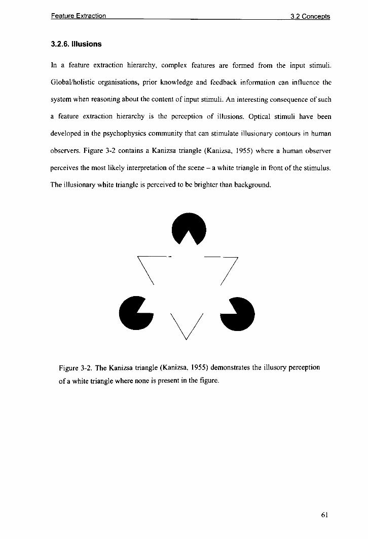
Feature Extraction 3.2 Concepts
3.2.6. Illusions
In a feature extraction hierarchy, complex features are formed from the input stimuli.
Global/holistic organisations, prior knowledge and feedback information can influence the
system when reasoning about the content of input stimuli. An interesting consequence of such
a feature extraction hierarchy is the perception of illusions. Optical stimuli have been
developed in the psychophysics community that can stimulate illusionary contours in human
observers. Figure 3-2 contains a Kanizsa triangle (Kanizsa, 1955) where a human observer
perceives the most likely interpretation of the scene - a white triangle in front of the stimulus.
The illusionary white triangle is perceived to be brighter than background.
7v
Figure 3-2. The Kanizsa triangle (Kanizsa, 1955) demonstrates the illusory perception
of a white triangle where none is present in the figure.
61

Feature Extraction 3.3 Biological visual pathway
3.3. Feature extraction in the biological visual pathway
This section provides a brief overview of the human visual pathway to give the reader an
insight into a feature extraction hierarchy operating in biology relevant to this thesis. While
amazing insight into human visual perception has been gained by recording the structure and
processing of our visual pathway, it is striking how much is as yet unknown.
3.3.1. The Retina
The vision of most primates is tri-chromatic. There are three types of cone photoreceptors in
the primate retina: those sensitive to red, green and blue light. However the terms red, green
and blue are in fact misnomers, as these cone photoreceptors are sensitive to a wide chromatic
range of light. Based on their response curves it has been experimentally found that out of the
6 to 7 million cones in the retina, 64% of the cones are sensitive to "yellowish-red" (L-cones),
32% are sensitive to "yellowish-green" (M-cones) and just 2% sensitive to "blue" (S-cones)
(Hecht, 1975). However because of interactions between horizontal and bipolar cells in the
retina and more importantly retinal ganglion cells with spatially opponent centre-surround
receptive fields (Barlow et al., 1957), colour intensity information is not directly transferred
from the retina to higher processing structures (Ratliff, 1965).
Retinal ganglion cells with centre-surround isotropic receptive fields project an
achromatic contrast channel, based on spatial contrast in L and M cones responses, and
chromatic contrast channels, based on red (L cone) and green (M cone) colour opponency
and on blue (S cone) and yellow colour opponency, from the retina (Hering, 1964). Here
'yellow' is the aggregation of the responses from L and M cones. The few S cones in the
retina are mainly distributed outside the fovea, where we have high acuity vision. Therefore
these do not constitute much visual information and are not used to compute the achromatic
channel.
62

Feature Extraction 3.3 Biological visual pathway
Figure 3-3. A mosaic of cone photoreceptors in the (A) foveal, and (B) peripheral
regions of the human retina. The scale bar in (B) is 1Ourn. (reprinted from Curcio et al.,
1990). Cone photoreceptors human retinae vary in size between the fovea and
periphery. These are larger in the periphery and spaced farther apart than in the fovea.
The gaps between cones in the periphery are filled by rod photoreceptors.
3.3.2. Lateral Geniculate Nucleus
Nerve afferents from the primate retina carry retinal ganglion cell responses to a mass in the
thalamus called the Lateral Geniculate Nucleus (LGN). The LGN contains distinct layers with
cells which have been categorised into two separate pathways. The parvocellular (P) pathway
primarily processes visual information related to form, colour and texture. Processing is
comparatively slow and is regarded to be the pathway which tells us "what" we are seeing.
This is in contrast to the magnocellular (M) pathway, which is responsible for the quick
processing of motion and flicker, and contains information regarding "where" something is
(Livingstone and Rubel, 1988). Because the author has constrained this thesis to static visual
stimuli, the magnocellular pathway shall not be investigated further. The LGN projects its
neural afferents to the lower visual cortex from which it also receives many strong feedback
connections from other cortical areas.
63

Feature Extraction 3.3 Biological visual pathway
Figure 3-4. Section of a left Lateral Geniculate Nucleus body from a macaque monkey
cut parallel to the monkey's face. There are six layers of cells stacked upon each other
like, using Hubel's analogy, a club sandwich. The layers are folded over each other and
alternate between cells stimulated by the left and the right eye. The direction
perpendicular to the layers is indicated by the dashed line. Taken from Hubel (1987).
3.3.3. Visual Cortex
The author shall give a very brief outline of the processing of the parvocelluar pathway in the
visual cortex. The achromatic information in the P pathway is processed by simple cells
(Hubel and Wiesel, 1959) in the striate cortex (VI). These simple cells have been found to
have anisotropic receptive fields. The receptive fields are elongated and are thought to be
used to extract edge (and end-stop) information from the isotropic centre-surround receptive
field responses emitted from the retina. The simple cells have orientated receptive fields at
different angles and scales and perform a great deal of processing on the visual information
from the retina. Output of simple cells is processed by complex cells. These consist of almost
~ of the cells in the striate cortex and have receptive fields which are larger than simple cells
resulting in the detection of features over a larger region of the field-of-view. Complex cells
seem to be optimally stimulated by orientated edges (similar to simple cells), but these stimuli
64

Feature Extraction 3.3 Biological visual pathway
must be swept across the cells respective field in a selected direction (Hubel, 1987). It is
thought that chromatic information in the parvocellular pathway is processed by double
opponent cells (Hubel, 1987). These are circularly symmetric centre-surround cells found in
the "blob" regions of the primary visual cortex and are believed to help provide colour
constancy to human vision.
Visual and other sensory information proceed from dedicated low-level feature
extraction neural structures in the rear of the brain to frontal areas where higher level
reasoning and memory associations are computed.
Figure 3-5. Map of the Macaque brain, taken from Felleman and Van Essen (1991).
Areas in the brain predominantly associated visual activities are coloured. The visual
cortex lies at the back of the brain with VI, the lower visual cortex at the rear. The
processing machinery of the visual hierarchy generally proceeds from the rear to the
front of the brain where higher level reasoning and memory associations take place.
65

Feature Extraction 3.3 Biological visual pathway
3.3.4. Evidence of hierarchical processing in the primate visual pathway
Evidence from physiological studies of the visual pathway complement psychophysics
theories for the hierarchical organisation of the feature extraction in vision. Centre-surround
receptive fields in retinal ganglion cells evolve into orientated receptive fields in the striate
cortex (V I). There are direct feed-forward connections from V I and feedback connections to
VI originating from V2(complex features), V3(orientation, motion, depth), MT(motion),
MST(motion), and FEF(saccades spatial memory) parts of the visual cortex, as well as pure
feedback connections to V I originating from LIP (saccade planning) and IT (recognition)
(Schrnolesky, 2005). Receptive fields of units in the feature extraction hierarchy get larger,
more complex as one ascends the hierarchy. At higher layers in the primate visual pathway
one may expect direct spatial relationships to have been absorbed into a group of processing
units (perhaps also related to memory) which represent abstract concepts or labels such as a
human face (Bruce and Young, 1986).
Therefore, paraphrasing Hubel (1987), once we have garnered sufficient knowledge
of the processing mechanisms in the human brain we may not need the word mind at all. And
the author of this thesis hypothesises that implementing similar machinery in artificial brains
may result in the immergence of behaviour normally associated with biological
consciousness.
66

Feature Extraction 3.4 Background
3.4. Background
This section contains a brief review of the computer vision literature relevant to the feature
extraction and space-variant image processing operations implemented by the author.
3.4.1. Functions used for image processing
Computer vision researchers have attempted to discover closed-form functions which
resemble receptive fields in the biological visual pathway.
Image processing filters based on the Gaussian function are used for blurring
operations. The Gaussian filter has smooth low-pass characteristics and is therefore useful for
dampening high-frequency noise and aliasing artefacts in images. The normalised 1-
dimensional Gaussian function over t with standard deviation (1 and zero mean is given below.
g(t)1 (-2~~)
--==e(jJ2i (Equation 3-2)
The Fourier transform of the Gaussian function is as follows, where w is circular
frequency (W=27Cf)
G(m) = e (Equation 3-3)
In his seminal work, Vision, Marr (1982) identified the second derivative of the
Gaussian (V2G) or Laplacian of Gaussian filter (Marr and Hildreth, 1980) as resembling the
centre-surround receptive-fields of retinal ganglion cells. The following is the Laplacian of
Gaussian (LoG) function centred around zero, with Gaussian standard deviation (1 in the
spatial domain.
n2 ()_(t2_(j2J 1 (-2~2)V g t - 4 r::;-::_ ea (j,,2:r
(Equation 3-4)
67

Feature Extraction 3.4 Background
The Laplacian of Gaussian in the frequency domain is given by the following where
ro is the circular frequency,
-~-V2G(w) = _w2 e 2 (Equation 3-5)
The peak circular frequency of a Laplacian of Gaussian is given by,
(Equation 3-6)
Marr (1982) stated that the Laplacian of Gaussian may be approximated by the
difference of Gaussian function when the ratio r between the standard deviation of the
excitory and inhibitory Gaussians is 1.6. The following is the un-normalised difference of
Gaussian (DoG) spatial domain function centred around zero and with standard deviations (I~
and a, for the constituent excitatory and inhibitory Gaussian functions.
( r' ) ( r' )I -2a' I -1a'dog(t) = e" - e ->,
a,.fii a, .fii(Equation 3-7)
ar=-' =1.6
a,.(Equation 3-8)
The Fourier transform of the difference of Gaussian gives its frequency domain
function, where cois the circular frequency.
_ 0/0/ _ W101:!
DOG ( ro) = e 2 - e 2 (Equation 3-9)
At the peak circular frequency WI'<!lJA of the difference of Gaussians,
d (DOG( Wl'fak )) = 0dw
Differentiating and simplifying Equation 3-9 at W,I<'ak gives the following,
1-a; e
- ,_ WI't'<lka,-
2 =0
68

Feature Extraction 3.4 Background
Simplifying the above results in
Taking the natural logarithm on both sides
Which gives the peak circular frequency of a di fference of Gaussians function
OJ = ±peak
4 In[ (ji)v. (Equation 3-10)
Response of difference of Gaussians at peak circular frequency,
DOG (peak (0) = exp -
Substituting with Equation 3-8,
2In(r) 2In(r) 2
DOG (peak (l)) = e- (,2 - J) _ e-R' (Equation 3-11 )
Image processing filters based on Laplacian of Gaussian and difference of
Gaussian functions have band-pass characteristics and are therefore useful for extracting
sparse contrast information from an image.
Oaugman (1985) and Granlund (1978) independently proposed the two dimensional
Gabor wavelet to minimise uncertainly for the localisation of a feature in space and
frequency. Oaugman (1985) additionally showed that the 20 Gabor wavelet resembles the
receptive fields of simple cells in the striate cortex. A Gabor wavelet pair consists of a sine
and a cosine function localised with a Gaussian envelope. The formulation of a Gabor wavelet
69

Feature Extraction 3.4 Background
with an asymmetric Gaussian envelope as given in Kyrki (2002) follows. This formulation
aids steering the orientation of the wavelet along the sine/cosine wave propagation direction
by modulating the angle e, while y and" are the standard deviations of the Gaussian envelope
along the direction of propagation and perpendicular to the direction of propagation
respectively.
lI'(x, y)= (Equation 3-12)
x'= xcosO+ ysinO (along direction of wave propagation)
y'= -xsinO+ ycosO (Equation 3-13)
The Fourier transform of the Gabor wavelet formulation in Equation 3-12 follows,
!r( , " ')-~ r(U'-/"f+TP'-\II(u, v) = e t.. (Equation 3-14)
u' = u cos 0+ vsin 0 (along direction of wave propagation)
v'= -usinO+vcosO (Equation 3-15)
3.4.2. Multi-scale feature extraction
Features are present in images at a continuum of scales. Therefore, it useful to analyse an
image at several scales and extract features at their associated intrinsic scale. Witkin (1983)
proposed considering scale as a continuous parameter, sowing the seeds of modem scale-
space theory. Koenderink (1984) showed that scale-space must satisfy the diffusion equation
which led to the use of the Gaussian function for the construction of Gaussian scale-space.
The multi-scale representation of the image is extracted by convolving the image with
Gaussian kernels with differing standard deviations.
70

Feature Extraction 3.4 Background
Because it satisfies the diffusion equation, extrema (maxima or minima) will not be
found within a Gaussian scale-space. Therefore researchers have used scale-normalised
Laplacian of Gaussian (Lindeberg, 1994; Mikolajczyk, 2002) and difference of Gaussian
(Lowe, 2004) scale-space for the detection of scale-space extrema. These normalised
Laplacian of Gaussian extrema positions in scale-space will be used in Chapter 4 for the
detection of interest point locations. Un-normalised Laplacian of Gaussian kernels are not
suitable for the detection of scale-space extrema because the amplitude of a Laplacian of
Gaussian filter generally decreases with scale. Lindeberg (1994) and Mikolajczyk (2002)
showed that the scale-normalised derivative D of order m centred on (x, y) with standard
deviation (scale) a is given by
(Equation 3-16)
The am term helps to somewhat normalise the image derivative L; response to scale.
Therefore for the Laplacian (second derivative) ofa Gaussian we get
(Equation 3-17)
Instead of generating a continuous scale-space it is possible to compute Gaussian
filter responses at discrete scales within scale-space. Furthermore, instead of repeatedly
filtering the original image as several spatial scales it is possible to filter the immediately finer
discrete scale reducing computation load. As the coarser scales contain redundant correlated
visual information it is possible to sub-sample and low-pass filter in a single operation
creating a Gaussian pyramid (Burt and Adelson, 1983). Subtracting adjacent layers in the
Gaussian pyramid gives a difference of Gaussian pyramid which approaches a Laplacian
pyramid (Burt and Adelson, 1983).
Greenspan et al. (1994) extended Burt and Adelson's (1983) work by constructing an
orientated Laplacian pyramid through the formation of a Filter-Subtract-Decimate Laplacian
pyramid and modulating each level of the pyramid with oriented sine waves. The resulting
log-Gabor kernel was used for rotation invariant texture classification.
71

Feature Extraction 3.4 Background
3.4.3. Space-variant image processing
This section will review prior work on processing visual stimuli that has been extracted using
a space-variant sensor or sampling technique. The reader must note that this does not refer to
the extraction of responses from the scene using retinal receptive fields. but rather to the
subsequent processing of the retinal responses to perform operations such as blurring or the
extraction of gradients.
Most conventional space-variant approaches are based on projecting and representing
space-variant responses in a conventional continuous rectilinear array (i.e. the cortical image).
Image processing operations are performed uniformly on the array resulting in space-variant
processing in the retina domain. Operations such as optical flow computation (Tistarelli and
Sandini, 1993; Traver, 2002), edge detection and saliency calculation (Bernardino, 2004) are
computed on the cortical image. Because the extracted space-variant visual information is
represented as a conventional rectilinear image, conventional image processing operations can
be used to operate on the structure. While this approach enable researchers working on space-
variant vision to use the huge library of image processing machinery implemented for image
array representations, they are shackled by the previously discussed shortcomings of the
retino-cortical transform based approaches that generate continuous rectilinear cortical images
(Section 2.3).
Gomes (2002) used a coordinate mappmg to represent and store the responses
extracted using a retina within a rectilinear array structure which was discontinuous in the
fovea. Interestingly, he also learnt visual features using a neural network to process contrast
normalised responses of a retina with a uniform fovea and a local hexagonal organisation. An
iconic feature subsumed the support region of a retinal receptive field and its immediate
neighbouring 18 receptive fields on the hexagonal tessellation (geodesic distance of two
nodes away from the centre of the iconic feature). Principal Component Analysis was then
used to derive an iconic vector which increased variation between the receptive field
72

Feature Extraction 3.4 Background
responses for classification with the neural network. The system was trained with blob, edge
and end-stop features presented to the retina over each feature's support region.
While learning the distinctive features extracted from a retina is a promising
approach, it is not straightforward to structure a fast learning process that learns distinctive
features directly from natural images themselves. It is also not possible to interpolate between
the responses of the learnt features as there is no explicit relationship between the features
unlike, for example, the Gabor wavelets orientated at different predefined angles in a Gabor
jet. Games (2002) normalised his features for orientation invariance but there were no scale
invariant properties described.
Out-fovea
log-polar
I,YtSl't.:IlIP,) 1.11'.114.11
~.JO l.IIU 10
I.. 2.8,,8 4.X
I. 2.7.-.74.7
L 1.63,(.4.6
0.0 I. 2.5 . .l.5, 4.5
1.1 2.4.l.4 4.4
I. 23.'34,3
2.2 J.2 4.2
2.1 3.1 .t.l
2.U .l.u 4.0
Figure 3-6. Mapping of node coordinates from a 5 ring retina with a 3 ring fovea to a
cortical image. Reprinted from Gomes (2002)
Wallace et. al. (1994) considered image processing using space-variant structures in a
paper titled 'Space-variant image processing.' They used connectivity graphs to encode
adjacency relations between nodes in the retina sensor, where graph nodes represent sensor
pixels and graph edges represent adjacency relations between pixels. This work primarily
dealt with retinal tessellations and sensors based on analytical retina-cortical transforms
(Schwartz, 1977, 1980) and therefore connectivity was based on the associated analytic
transform. Conventional cortical image data structures were used to store the extracted visual
information. Image transformations, pyramid operations and connected components analysis
73

Feature Extraction 3.4 Background
(also in Montanvert et a1.(l99 I)) were conducted on the cortical images based on the
connectivity graph. They also performed simple contrast detection operations by subtracting
the pixel value of adjacent nodes from the pixel value of a node, as well as simple pyramidal
operations such as adaptive local binarisation.
The approach by Wallace et. al. (1994) was a significant contribution to the
processing of visual information extracted using a space-variant retina. Yet there are several
advances to this approach which the author shall make within this thesis. While Wallace et. al.
defined neighbourhood support regions, they failed to define receptive fields with an analytic
profile function. Therefore image processing operations such as the space-variant filtering of
visual information with a given kernel were not discussed. For example, a simple vertical
Sobel operator filtering responses extracted from a space-variant retina will detect very fine
vertical edges near the foveal region, and coarse vertical edges at the peripheral region of the
retina.
An important aspect of the approach by Wallace et. al. is that connectivity IS
determined by adjacency in the retina and not adjacency in the cortical image. Similar
mechanisms govern the formation of retino-tectal connections (Willshaw and von der
Malsburg, 1976) and cortical receptive fields (Zhang et al., 2005) within the visual pathway.
It is adjacency and neighbourhood relationships in the retina that govern the formation of
filter coefficients and connectivity in a feature extraction hierarchy and not the structure that
the visual information is stored (i.e. the cortical image), although retinotopic organisation
causes a convergence in relationships between nodes in the retina and between associated
projected nodes in the cortical image. Since processing operations are governed by spatial
relationships in the retina, from a computer vision standpoint, the reader must question the
need for a uniform array cortical image representation of visual data. After all, since space-
variant vision is going to be implemented in software, why do we need the retinotopic cortical
image at all? The author of this thesis proposes that the responses extracted by the retina can
74

Feature Extraction 3.4 Background
be stored in any arbitrary structure (even a one-dimensional vector), as long as the addressing
mechanism into this structure is consistent. All spatial relationships between nodes in the
structure are determined by adjacency of associated retinal receptive fields in the retina.
Figure 3-7. The connectivity graph for a log-polar sensor taken from Wallace et al.
(1994). Connectivity based on retina nodes neighbourhoods (Left) are represented as
relationships between nodes on the cortical image (Right).
3.4.3.1 Normalised convolution
In many signal processing applications data may be missing or have low confidence at some
locations in the sampling array. Knutsson and Westin (1993) and Piroddi and Petrou (2003)
described the normalised convolution which was able to convolve data from a pseudo
irregular tessellation or with varying confidence better than conventional convolutions. If fit)
generates regularly spaced samples of a signal with associated confidence values c(t) and the
required conventional convolution kernel is given by get), then the normalised convolution
output h(t) which has a regular tessellation is given by
het) = J(t) * g(t)e(t) * get) (Equation 3-18)
75

Feature Extraction 3.5 Retina receptive fields
For an irregular tessellation the missing values inf(t) have a zero associated value in
c(t). This approach for signal analysis is suitable for a regularly tessellated sensor with
outputs which have dynamically changing associated confidence values, but is not appropriate
for a sensor with a fixed irregular tessellation. The normalised convolution approach attempts
to resample the irregular data into a regular grid. In a feature extraction hierarchy the ensuing
regular data would then be used for higher level processing. However there is a waste of
processing and storage resources in this approach by creating regularly spaced data with low
confidence. The resulting regular data will have a much higher dimensionality than the
irregularly (retinally) sampled data and will be highly correlated in many regions.
After reviewing relevant work in vision literature the reader must be aware that
performing feature extraction operations on visual data extracted by the self-organised non-
uniformly tessellated retina in this thesis is not trivial. In this chapter the author will describe
the formulation of space-variant retina receptive fields, as well as space-variant cortical filters
in higher layers in the feature extraction hierarchy that can (re)sample and analyse irregularly
sampled visual data.
3.S. Retina receptive fields
In the previous chapter the author described the generation of an irregular, self-organised
retina tessellation which characterised the locations for space-variant sampling of visual
information from an image. As discussed earlier (Section 3.1) the locations described in the
retina tessellation must be sampled over a support region to prevent aliasing artefacts. The
size of the sample support region (receptive field size) could also have been self-organised
together with sample location (Clippingdale and Wilson, 1996) but this would have created
retinae with receptive fields without sampling continuity in Gaussian scale-space. While such
76

Feature Extraction 3.5 Retina receptive fields
a retina capable of multi-resolution sampling within a single irregularly spaced node layer (in
space and scale) may seem elegant, performing hierarchical feature extraction operations on
the responses extracted using such a retina would exceed the scope of this thesis. Therefore
the author adopted self-organisation only to establish receptive field positions. Receptive field
support sizes were determined based on local receptive field density.
A single retinal layer is restricted to extracting visual information at a single narrow
frequency range from a particular location in the scene at a single retinal fixation. Multi-
resolution space-variant feature extraction was performed by using a pyramid of retinae that
efficiently extracted visual information at several scales.
3.5.1. Adjacency in the retina tessellation
The self-organised retina tessellation IS a mosaic of coordinate locations without any
accompanying adjacency information. In order to define retina receptive field sizes and
compute support regions for feature extraction operations, it is useful to define adjacency and
neighbourhood regions about nodes (receptive fields) on the retina tessellation. These
adjacency criteria will be based on a structure which will be referred to as the cortical graph
which will be formed by Delaunay triangulation of the retinal tessellation.
If P = [Ph Pz, ... , Pn] are the set of 'sites' (i.e. retinal tessellation nodes) in a two-
dimensional Euclidean plane, it is possible to assign every point x in the plane to its nearest
site. The Voronoi region of site pi, given by V(pJ, consists of all points at least as close to Pi
as to any other site (O'Rourke, 1994).
V(p,) ={x: Ipi -xl Slpi -xl, vi= i} (Equation 3-19)
The set of points in V(Pi) for T:;f i that have more than one nearest neighbour form the
Voronoi diagram V(P) for the set of sites P.
77

Feature Extraction 3.5 Retina receptive fields
Figure 3-8. Voronoi diagram for a retina tessellation with 256 receptive fields. The
receptive field centres are plotted as dots in their associated Voronoi region.
The dual graph G for a Voronoi diagram V (P) is constructed by connecting node
sites with an arc if the sites' corresponding Voronoi regions share a Voronoi edge in the
Voronoi diagram. Delaunay showed drawing straight lines in the dual graph results in the
planar triangulation of the Voronoi sites P if no four sites are co-circular. The resulting
structure is called the Delaunay triangulation 9)(P) of P.
Figure 3-9. Cortical graph constructed by Delaunay triangulation of a retina tessellation
with 256 receptive fields. The vertices in the graph are receptive field centres.
The cortical graph structure is created by Delaunay triangulation of the associated
retina tessellation. The length of a graph edge on the cortical graph is defined as unity.
78

Feature Extraction 3.5 Retina receptive fields
Therefore the cortical graph has the useful property that graph distance on the cortical graph
results in space-variant distances in the image plane. The graph distance is defined as the
shortest path or graph geodesic between two nodes in the graph. Distance is measured as the
number of graph edges along a path between two graph vertices.
3.5.2. Space-variant receptive field sizes
Node positions on the retina tessellation were defined during self-organisation on a coordinate
frame which spans from -I to + I, vertically and horizontally. The node positions on the retina
tessellation have to be scaled up to the dimensions of the input image stimuli which the retina
receptive fields will be sampling. There are two criteria governing the scaling
I) Minimum spacing (in pixels) between adjacent retinal receptive fields
2) Required field-of-view of the retina
A value Dmin for the minimum distance between adjacent receptive fields in the retina
which samples the image was chosen mediating these two criteria. This may be sub-optimal
for larger images where the constraint of a large field-of-view necessitates a foveal sampling
well below the Nyquist limit of the rectilinear image. A value for Dmin of 1.5 pixels was used
for this work to generate retinae with a field-of-view of 360 pixels on a conventional array
image. This was the width of images in the SOIL (Koubaroulis et al., 2002) object database.
If dmin is the minimum distance between adjacent nodes (receptive fields) in the retina
tessellation after self-organisation, Ai.) is the Euclidean distance matrix for the retinal
tessellation sorted along rows, (Xi, Yi) are the coordinates of nodes on the retina tessellation
and (Xi, Y;) are the coordinates of receptive field centres on the retina that samples the image,
the following was defined,
d.~A,J·=2,Vimm 1,/
(Equation 3-20)
79

Feature Extraction 3.5 Retina receptive fields
(Equation 3-21)
Y=D _li_ ~(-l +1)i min d . ,~Vi ..mm
A retinal tessellation is not yet a retina. To prevent aliasing, visual information must
be gathered over a large support region around each sampled retinal coordinate. To avoid
super-Nyquist sampling, the standard deviation (and in turn size) of low-pass filter support
regions is related to the local spatial sampling rate of retinal receptive fields. Basing a retinal
receptive field's size on local node density also results in space-variant retinal receptive
fields. At the foveal region, where visual information is densely sampled, receptive fields will
have a narrow spatial support, while large receptive fields will be placed at the periphery with
its widely spaced sampling points. If Gaussian receptive fields were used to low-pass filter
visual stimuli before space-variant (sub )sampling, the following was used to determine the
standard deviation a, of the Gaussian support region of retina receptive field i.
k,
"A.~ 1.,1
a = A _E___ pixelsI k -1
I
(Equation 3-22)
k, is the neighbourhood size for determining local retina tessellation receptive field
density. The author determined k, as the number of nodes (receptive fields) in the cortical
graph with a graph distance equal to one. In the above equation the standard deviation of the
retinal receptive field is assigned to the average distance to the receptive field's immediate
neighbours scaled by A.. The fixed scaling constant A. expands the retina receptive field's
standard deviation to prevent aliasing of the sub-sampled extracted retinal responses.
The sampling rate of a conventional image can be considered as one sample per
pixel(width). Space-variant retinal sampling of the image with the self-organised retina
changes the sampling rate to one sample per graph edge on the cortical graph. The scaling
factor A. is chosen to reduce aliasing caused by retinal sub-sampling by locally blurring the
input image to reduce frequencies above the local retinal sampling Nyquist limit.
80

Feature Extraction
, "
09 -
OB
07
06
~II>.:0 05Q.II>~Cl::
0'
03
, 1.:2
0'
0'
00 05
3,5 Retina receptive fields
1.=O.5
'5 2 25 35
Circular frequency (radians per graph edge)45
Figure 3-10. Responses of a Gaussian retinal receptive field at different values for A.
The preceding figure contains the plots of the response of low-pass Gaussian retinal
receptive fields for different values for A.. Circular frequency is defined over the cortical graph
assuming the local sampling rate (node density) on the retina tessellation is constant. The
Nyquist limit after retinal sampling is half the sampling rate f resulting in a circular frequency
(w=27if) of 1C radians per graph edge on the cortical graph.
If the signal-to-noise ratio is defined as follows,
SNR= 2010 Signalglo N .oise
I= 20 log., ---------Response at Nyquist limit
(Equation 3-23)
a value of ,l. = 0.5 results in a Gaussian receptive field with a significant response at the
Nyquist limit with a SNR of 10.72dB, causing aliasing artefacts. At ,l. = 2, the Gaussian
receptive fields do not have a significant response at the Nyquist limit with a SNR of
171.45dB, but this value will result in very large spatial receptive fields. At,l. = I the Gaussian
receptive field's response at the Nyquist limit is 0.0072 with a signal-to-noise ratio of
42.85dB.
81

Feature Extraction 3.5 Retina receptive fields
Figure 3-11. Space-variant sizes of Gaussian receptive fields for a self-organised retina
tessellation with 256 nodes. Spatial support at the standard deviation is displayed for
each Gaussian receptive field (A=I).
The support region of a continuous Gaussian function is infinite. However the kernel
used for image processing is discrete with a limited spatial support. The above figure
indicates the support region of Gaussian receptive fields with a support region radius at one
standard deviation. Only 68.27% of the Gaussian support is within one standard deviation. In
this thesis Gaussian kernels with a support region radius of two standard deviations (95.45%
of Gaussian support) or three standard deviations (99.73% of Gaussian support) were used to
approach the ideal Gaussian kernel with its infinite spatial support.
3.5.3. Retina receptive fields
The calculated receptive field centres (Xi, Yi) are generated at floating point coordinates.
Sampling discrete image pixels (x, y) with an square image processing kernel based on the
receptive fields centred at (Xi. Y,,) requires the calculation of the horizontal and vertical sub-
pixel offset (Pi, Q,) of the receptive field centre floating point position from the actual kernel
integer location. The equation for a symmetric un-normalised two-dimensional Gaussian
82

Feature Extraction 3.5 Retina receptive fields
kernel with standard deviation a., used to place Gaussian receptive field support regions on an
image with sub-pixel accuracy is given below
G(X,y,Xi,Y"lTi,P;,Q) = e
(x-rQund(X, )+1\)' +(y-round(Y, )+Q, )'
2a? (Equation 3-24)
The computation of the sub-pixel offset (Pi, Qi) differs depending on whether the
rounded integer size of the support region (with diameter 4a or 6a) is odd or even. This is
because the change (error) in position of a receptive field centre by the rounding operation is
quite different when the resulting kernel is even or is odd.
(x.y) -,'0~
dry))(rounc (X),roUI
I
Even sized kernel
PixeI
Grid
.(ro ~nd(x)/1puq\(X,) )
nd(y))
Odd sized kernel• Position of centre of kernel on image pixel grido Floating point position of centre of receptive field~ Rounded position of centre of receptive field
(even sized kernel, .in odd sized kernel)
Figure 3-12. Calculating the centre ofa kernel for even and odd sized kernels
[
P, =round(X,)-Xiodd: Q = round(Y,) - Y,
(Equation 3-25)
(P; = round (X; )+sign( Xi +round (Xi ))xO.5-Xi
even:Q = round(Y,) + sign( Y, +round (Y,) )XO.5 - Y,
The filter coefficients of the Gaussian support region G(x,y'x;,Yi,ai,Pi,Qi) were
normalised to sum to unity to satisfy the following equation
L G(x,y,Xp Y"lTi,P"Q) = 1'Vx.\;/y
(Equation 3-26)
83

Feature Extraction 3.5 Retina receptive fields
2 4 6 8 10 12
Figure 3-13. Kernel coefficients of a Gaussian receptive field spanning 12xl2 image
pixels. Note the slight sub-pixel offset of the filter coefficients to reflect the error in the
integer position of the kernel.
The response of receptive field R(i) was generated by multiplying the underlying
image pixels with the co-located Gaussian filter coefficients Gi as indicated by the following
equation. The parameter a is the scaling of the kernel support region radius to 2 or 3 Gaussian
standard deviations a;
'Vm.'7n
(Equation 3-27)
The resulting retinal receptive field responses R(i) do not have an associated cortical
image data structure. Therefore the author stored these as a one dimensional vector R(i) which
will be referred to as an imagevector. The allocation of a location on the imagevector for a
particular retinal receptive field response is not important as long as the allocation is
consistent. A variable in the imagevector corresponds to the response of one retinal receptive
field. In this thesis the author allocated responses to the vector based on the magnitude of the
associated receptive field's eccentricity (distance from the centre of the tessellation).
84

Feature Extraction 3.5 Retina receptive fields
ImageRetinal
receptivefieldsrY'I'"'"
Receptive fieldresponses
Figure 3-14. The responses of retina receptive fields are represented and stored as a
one-dimensional vector which will be referred to as the imagevector. Each receptive
field is allocated a consistent location on the vector.
Figure 3-15. Responses of Gaussian retina receptive fields on a retina with 8192 nodes,
displayed based on the receptive field's associated Voronoi region on the cortical
graph. The retina was fixated upon the centre of the standard greyscale Lena image.
CA = 1).
85

Feature Extraction 3.5 Retina receptive fields
3.5.3.1 Visualising receptive field responses
The one dimensional imagevector containing retinal receptive field responses is not an
intuitive representation of the retinal sampling for visualisation. However, variables on the
imagevector have a spatial relationship with associated receptive fields and nodes on the
retina tessellation. The author used the Voronoi region (Section 3.5.1) of the associated node
for visualisation; pixels within the node's Voronoi region were displayed with the receptive
field's response (Figure 3-15).
3.5.3.2 Back-projecting receptive field responses
It is also possible to visualise the responses of the space-variant sampling by back-projecting
the responses through the receptive field to the image plane. This action is equivalent to the
probe mapping of receptive fields in the biological visual pathway by neurophysiologists.
Except instead of measuring the responses of a neuron for a certain visual stimuli, the author
reconstructed the visual stimuli that would cause the stimulation of a particular neuron. This
approach will be used throughout this chapter to map the receptive fields of layers of units in
the feature extraction hierarchy. The response of the retinal receptive field at (Xi, Y;) is back-
projected to the image domain as indicated in the following assignment operation.
I (round{ Xi)+ m,round{ Y;)+ n):= I (round{ Xi)+ m.round i Y;)+ n) +
R(i)xGi (m,n,Xi,Y;,0'"P;,Q,)x(2a)2, m.n -+ -aO' ..+aO', m.n e Z, Vi
(Equation 3-28)
The sampling operation of the whole retina is visualised by aggregating the back-
projected responses of all the retina's constituent receptive fields. A scaling factor equal to the
area of the Gaussian receptive field's support, (2ai, was used to prevent the decay in the
intensity of the backprojected image with eccentricity. In the following figure, Gaussian
support regions were implemented with a kernel with radius of three standard deviations. The
minimum distance between receptive fields (kernels) on the retina was chosen at Dmin = 1.5
pixels so the retina had a field-of-view with a diameter of approximately 360 pixels.
86

Feature Extraction 3.6 Processing irregular visual information
Figure 3-16. Back-projected Gaussian retinal receptive field responses from a retina
tessellation with 8192 nodes (2 = 1). The retina was fixated upon the centre of the standard
greyscale Lena image.
3.6. Processing irregular visual information
The internal representation of visual information in the described system (which processes
information extracted using a self-organised space-variant retina) is quite different from the
representation used in conventional vision systems. Most current systems give equal
processing emphasis to the whole field of view of the camera or image frame, and work with
visual information which can be stored in a uniform rectilinear data structure. For example,
greyscale information extracted by a conventional CCO imager in a digital camera can be
stored in a rectilinear two dimensional array structure. Image processing operations for
analysis and feature extraction can be easily applied to this array. Convolution operations are
simple to implement by raster scanning a mask or kernel over the array and performing the
87

Feature Extraction 3.6 Processing irregular visual information
necessary multiply and accumulate operations. Similarly the visual information can be easily
sub-sampled to reduce its resolution. Rotation and other translation operations are also trivial.
This simply is because the local connectivity between adjacent nodes of information in the
array is uniform. Pixels have equidistant neighbours above, below and to their left and right
(except on the border of the array).
However the described space-variant imaging system does not process all visual
information equally. The central or foveal region of the retina has a very high acuity. The
image is finely sampled by filters in this retinal region, generating many retinal responses. As
we increase eccentricity and move away from the central area of the retina, the acuity of the
retina gradually reduces to the periphery where the image is only coarsely sampled,
generating few retina responses for a given spatial area.
Connectivity in the self-organised retinal tessellation is not uniform. While most
receptive fields have six adjacent neighbours (determined by connectivity after Delaunay
triangulation) some have five or even seven adjacent neighbours. The local connectivity of a
given node in the tessellation to its neighbours cannot be effectively predicted before self-
organisation. The tessellation lacks geometric regularity and only maintains sampling density
continuity. Because of this non-uniform connectivity of nodes in the tessellation, a fixed
convolution kernel cannot be used for filtering operations as in image processing operations
on conventional images.
While the imagevector is one dimensional, each location on the vector has a
consistent spatial semantic relationship with an associated location on the retinal tessellation.
This is akin to a pixel's spatial location on the image being related to the spatial location of
the related area in the scene. With the irnagevector, spatial relationships between regions
aren't as explicit as in a conventional image array. Therefore the author implemented
computational machinery within the space-variant vision system which was able to reason
88

Feature Extraction 3.6 Processing irregular visual information
with the imagevector visual information by maintaining internal lookup tables of the spatial
relationships between nodes in the retina tessellation.
Cortical filter near fovea
Retinal receptive fieldsupport Cortical filter
Input image
Figure 3-17. Support regions of cortical filters
Processing machinery in the implemented space-variant vision system that accept
imagevectors as input and output imagevectors shall be referred to as cortical filters. Because,
as discussed, the local topography of the retina tessellation is non-uniform, a fixed kernel
cannot be used for image processing operations such as convolutions. Convolution operations
on the imagevector necessitates the pre-computing of the unique filter kernel coefficients (and
associated lookup addresses) for each location on the image vector.
Unlike most computer vision approaches, in biology a fixed kernel is not raster
scanned over the field-of-view. A biological neuron in the visual cortex has inter-cortical or
retina-cortical connections that result in a single receptive field in the field-of-view. A similar
approach had to be used by the author because of the non-uniform fixed retina tessellation
that was used to sample images.
89

Feature Extraction 3.6 Processing irregular visual information
3.6.1. Cortical filter support region
The nodes in any retina tessellation Vi are within the neighbourhood Q( v,) of the cortical filter
centred on VC' on the same or even another tessellation if the following is satisfied
(Equation 3-29)
r, is the diameter of the cortical filter support. As before, the cortical filter support
region was made space-variant by making the size of the support related to the local node
density of the cortical filter's (vc's) tessellation.
(Equation 3-30)
Ai.! is the Euclidean distance matrix for vc's retinal tessellation from Equation 3-20
and k, is the neighbourhood size for determining local retina tessellation receptive field
density. )" is a scaling constant. Because Ai.! has been sorted in ascending order, the summation
from 2 to k; and division by k,-l will give the mean distance to cortical filter vc's neighbours
with a neighbourhood size of k.,
3.6.2. Cortical filter response
The response of the cortical filter O(c) centred on VC' in the form of an imagevector is
computed by the following equation. The computation is applied for all elements in the
imagevector from I to N. The number of elements N in the output imagevector could be
different to that in the input imagevector.
M
O(c) = IR(pc (m»)xF;. (m),c = I..Nm=1
(Equation 3-31)
R is the input in the form of an imagevector. F, are the 1xM filter kernel coefficients
over the neighbourhood Q( vC> for the cortical filter kernel on v,. Whereas p, is the 1xM
indices of elements in the imagevector R with which F,'s are multiplied in the local
convolution operation. The filter coefficients F, are calculated based on a particular filter
90

Feature Extraction 3.6 Processing irregular visual information
support profile based on the spatial positions on the field-of-view of the elements P, in the
input imagevector.
Inputimagevector
R
Kernelc
Outputimagevector
o
O(c)
CoefficientsFe
IndicesPc
2
M
Figure 3-18. Computation involved in a convolution operation on visual information on
a non-uniform tessellation.
The author visualised the output imagevector using Voronoi regions (Section 3.5.3.1)
and by back-projecting all associated responses in 0 back to the R(i) using a similar
methodology as described in 3.5.3.2. Back-projection was performed using the same Fc(m)
coefficients as in Equation 3-31 to visualise the stimuli that would cause the stimulation of a
particular neuron. The reader should note that in instances, such as pyramidal decomposition,
o and R may be based on different (retina) tessellations.
R(i):=R(i)+ IO(c)F:.(m) ,c=l..N,ViE pc(m)'ric
(Equation 3-32)
91

Feature Extraction 3.7 Retina pyramid
The back-projection computation in Equation 3-32 may be repeated back down the
space-variant feature extraction hierarchy until the retinal receptive field responses (Section
3.5.3.2) can be back-projected to the image.
The ability of operating on visual information stored as imagevectors enables the
system to perform feature extraction operations on the responses sampled by the space-variant
retina receptive fields. Blurring operations for a multi-resolution pyramid (Section 3.7), edge
responses based on neighbourhood differences (Chapter 4) or Gabor wavelet filters
(Balasuriya and Siebert, 2003) can be computed. It is no longer necessary to represent and
deal with data as rectilinear frame arrays to perform processing in a feature extraction vision
hierarchy.
3.7. Retina pyramid
Sampling with a space-variant retina extracts visual information from the field-of-view with
information density and spatial frequency varying with eccentricity. However, at a single
location in the field-of-view, visual information is extracted only as a single central
frequency. As scene content may be present at many intrinsic scales in the scene, multi-
resolution image analysis becomes an important component of vision. The author was
motivated by pyramidal decomposition in conventional image processing to create a space-
variant retina pyramid.
3.7.1. Gaussian retina pyramid
The multi-resolution processing of an image using a Gaussian retina pyramid is more efficient
than placing ever larger Gaussian filters on the image to extract coarse features. The
construction of the Gaussian retina pyramid of cortical filters necessitates the pre-computing
of a large number of kernel coefficients Fe and associated sampling indices pC' This overhead
92

Feature Extraction 3.7 Retina pyramid
is justified by the reduction in dimensionality of data being processed at coarser layers. In an
octave decomposition (where the central frequency of the next coarse layer in the pyramid is
half that of the current layer), the dimensionality reduction in the next (coarse) layer will be
N/4, where N is the number of nodes in the retina tessellation associated with the current
layer.
Cortical filterreceptive field -.,.--
supports
Cortical filters
Cortical filtersupport region
Cortical filters
Cortical filtersupport region
Retinal.. . Retinal
receptive fields
Input image
Figure 3-19. Sampling of the retina pyramid. Only the retina receptive field layer
samples the image. Visual information is processed by cortical filters in the form of
image vectors.
The filter-subsample operations by retinal receptive fields and cortical filters reduces
the dimensionality of the visual information as the content get coarser, maintaining a constant
intrinsic blurring in the visual content. In the case of the self-organised retina tessellation,
Gaussian layers in the pyramid should blur the input image vector (or input image) so that
after filter-subsampling the output imagevector has the same blur as the input.
93

Feature Extraction 3.7 Retina pyramid
If p is the sub-sample factor (p=2' for octave sub-sampling), a, the (constant)
Gaussian blurring of visual information at each layer, and a, and a,., the intrinsic blurring of
imagevectors in layers iand i-I in the pyramid, the following holds
g(pai) = g(ai_,)® g(a,)
The symbol ® indicates the convolution operation and g denotes a Gaussian function
in the spatial domain. The above equation can be simplified in the Fourier domain
Expanding out the Gaussian function and simplifying gives,
Taking the logarithm of both sides leads to the follow result
I~' ,a =- a +aI pI-I ( (Equation 3-33)
a, = O"i-' = O"init for constant blurring in the pyramid equal to the initial visual input.
(Equation 3-34)
For octave sub-sampling within the retina pyramid p=2 the applied constant blurring
in each layer of the Gaussian pyramid,
(Equation 3-35)
Therefore, assuming the intrinsic blurring in the responses from the retina receptive
fields is 1 graph edge on the space-variant retina tessellation (the blurring in the input image
not being significant in most of the field-of-view in comparison to the large Gaussian
receptive field size), the constant blurring (standard deviation) of the Gaussian retina pyramid
layers is 0", = 1.7321x 1 graph edges = 1_7321 graph edges. Therefore)' = 1.7321 in Equation
3-30_ The reader should remember that basing the applied blurring on the above equation
results in space-variant standard deviations of receptive fields in a layer in the Gaussian retina
pyramid.
94

Feature Extraction 3.7 Retina pyramid
The retinal tessellations for coarser layers in the octave-separated space-variant retina
pyramid were created by self-organising N/4 nodes where N is the number of nodes (receptive
fields) in the immediately preceding (finer) layer in the retina pyramid (the author empirically
found that decimation of the N node layer to create coarser layer did not generate regular
retinae). The retina tessellations of the coarser layers (Xi, y,) were scaled up to the size of the
image by multiplying with Dmim the minimum distance between adjacent retina receptive
fields (in the finest retina pyramid layer which samples the input image) and dividing by dmin,
the minimum distance between adjacent retina receptive fields (in the finest later). Only the
Gaussian retina receptive field layer directly samples the input image. All other layers operate
on imagevectors which are generated by previous layers in the Gaussian retina pyramid. The
imagevector at layer N was obtained from layer N-I using Equation 3-31.
The following equation was used to determine the F", the profile of the two
dimensional Gaussian cortical filter centred over vertex v,. The reader should note that in the
Gaussian retina pyramid n(vJ will be defined over the preceding finer retina tessellation.
(/1 J1 .2IT 1 2 2 2 •
gc(t,o-._) = --2 e ',t = X +Y ,(X,Y)E Q(vc) (Equation 3-36)2lra,
A multi-scale hierarchy of Gaussian retina pyramid layers with 4096, 1024, 256, 64
and 16 filters were created for the following results (Figure 3-20). A 8192 retina receptive
field layer was created to sample the input image and the resulting imagevector was used for
pyramidal decomposition. The need for the additional 8192 node layer will become apparent
in the next section where a Laplacian pyramid is constructed using the imagevectors from the
Gaussian retina pyramid. A 8192 node layer was self-organised because implementation
limitations prevented the self-organisation of a 16384 node retina tessellation.
As before, retina pyramid sampling results are visualised based on associated
Voronoi regions (Figure 3-20) and by back-projecting filter responses to the rectilinear array
image plane (Figure 3-21). Slight variations in the back-projected image's pixel values may
95

Feature Extraction 3.7 Retina pyramid
be observed because small variations in the retina tessellation's local node density result in
• t920 ......... toy ..
changes in the overlap of the neighbouring receptive field supports .
Figure 3-20 : Responses from layers of an octave separated Gaussian retina pyramid
with (upper left) 8196, (upper right) 4096, (lower left) 1024 and (lower right) 256 node
layers displayed based on the response's associated Voronoi region (J. = 1 for retina
receptive fields, A. = 1.7321 for cortical filters). The retina was fixated upon the centre
of the standard greyscale Lena image.
The space-variant nature of the processing of the retina pyramid can be observed.
The pyramid was fixated upon Lena's right eye, which has been sampled at a higher
96

Feature Extraction 3.7 Retina pyramid
spatial frequency at all retina layers than more peripheral regions of the image. The multi-
resolution (space-variant) decomposition is apparent with the increasingly blurred (Figure
3-21) and spatially separated (Figure 3-20) responses in the coarser layers of the retina
pyramid.
8196 Gaussian layer
1024 Gaussian layer
4096 Gaussian layer
256 Gaussian layer
Figure 3-21: Back-projected responses from an octave-separated Gaussian retina
pyramid from the (upper left) 8196, (upper right) 4096, (lower left) 1024 and (lower
right) 256 node layers. The retina was fixated upon the centre of the standard greyscale
Lena image.
The system has a restricted field of view which can be altered by changing the
Gaussian filter spacing in the retina receptive field (finest) layer. When implemented only this
97

Feature Extraction 3.8 Laplacian of Gaussian retina pyramid
layer needs to be fixated upon the image at a given salient fixation point as other
layers in the retina pyramid sample the output of the retina receptive field layer. The cortical
filters in the retina pyramid hierarchy extract increasingly coarser, low-pass filtered visual
information from the input. The term cortical filter is a slight misnomer in this context as
analogous low-pass processing in biology occurs in the retina and not the visual cortex.
However in the described software implementation, cortical filters process the output of the
retina receptive fields to extract coarse scale low-pass visual information.
3.8. Laplacian of Gaussian retina pyramid
The Laplacian of Gaussian (LoG) filter is of interest in biologically motivated computer
vision due to the filter's resemblance to the profile of biological retinal ganglion cell receptive
fields (Marr and Hildreth, 1980). The LoG filter is a spatial frequency band pass filter, able to
detect contrast in visual information. Because of the Laplacian of Gaussian filter's band-pass
characteristics it is not possible to create a multi-resolution Laplacian pyramid in isolation
without a parallel low-pass pyramid. The author sampled the imagevector responses from the
Gaussian retina pyramid to create a space-variant Laplacian of Gaussian retina pyramid.
The following equation was used to compute the cortical filter coefficients Fe for a
Laplacian of Gaussian cortical filter centred over vertex Vc that samples the imagevector from
a higher spatial frequency layer in the Gaussian retina pyramid within the neighbourhood
Q( v.). Because of the irregular support of the cortical filter, positive subfields of the Laplacian
of Gaussian cortical filter must be scaled to equate the negative subfield so the response of the
cortical filters to a uniform stimulus is zero.
98

Feature Extraction 3.8 Laplacian of Gaussian retina pyramid
, . \
[/2 a2J I I . ...:._I- 'l(1'~ i, 1 1
Lit.tr; = --. - --, e - " r = x- +~'-,(X,Y)E Q(V)if 2~- , (Equation 3-37)
Since the imagevector input to the LoG cortical filter has already been blurred by the
Gaussian pyramid, the effective blurring of the LoG, crolT, will be different to that of the
applied blurring in the Laplacian of Gaussian cr. If the sub-sampling by the Laplacian of
Gaussian cortical filters of the imagevector is by a factor of p, and the blurring of the
Gaussian layer that was sub-sampled by the Laplacian of Gaussian cortical filter was crg, the
following holds
L (t, patll ) = L (t, a) ®G(=.)Expanding in the Fourier domain,
tJJ (pat'lf )2 al(j~ _ aJa/
-oj e 2 = -ol e 2 x e 2
And simplifying gives the required blurring of the Laplacian of Gaussian, G, to
achieve the effective blurring G,lf.
(Equation 3-38)
For an effective Laplacian of Gaussian blurring equal to that of the Gaussian
pyramid, Gel] = Gg , and in turn Gg = Ginit. Therefore the following applied blurring for the
Laplacian of Gaussian cortical filter is obtained.
(Equation 3-39)
This is similar to the result for the Gaussian pyramid cortical filters. p=2 for an
octave change in sampling rate between the Laplacian of Gaussian layer and the sampled
Gaussian layer in the pyramid.
a = I. 7321ainit (Equation 3-40)
With Gintl = I graph edge as with the Gaussian pyramid gives, G = 1.7321 graph
edges and )_= 1.7321 for the Laplacian of Gaussian cortical filters (Equation 3-30).
99

Feature Extraction 3.8 Laplacian of Gaussian retina pyramid
3.8.1. Increasing granularity of laplacian of Gaussians pyramid
To increase the granularity of sampling scale by the pyramid, Laplacian of Gaussian
cortical filters with different effective blurring standard deviations were used on the same
retina tessellation. The blurring was changed to extract contrast information with retina
pyramid layers with central frequencies spanning the octave decomposition. The visual
information in the resulting imagevectors will contain different intrinsic blurring (because the
sub-sampling was constant for different blurring) but this is a computationally efficient
approach to space-variant contrast detection at many finely separated spatial scales.
The effective blurring (standard deviation) for the i th Laplacian of Gaussian layer in
the octave is given by
a.>.a si, i-t-l..n-2I 0
(Equation 3-41)
where a; is the effective blurring of the finest layer in the octave. s is a scaling factor
for the blurring. Since for the detection of Laplacian of Gaussian extrema in the octave
requires two additional retina layers (one finer and one coarser), the scaling factor s for a
Laplacian of Gaussian retina pyramid with n-2 layers per octave is
(Equation 3-42)
100

Feature Extraction 3.8 Laplacian of Gaussian retina pyramid
Gaussian Retina Pyramid Laplacian of GaussianRetina Pyramid
256 nodes
256 nodes___ 1074 nodes
Figure 3-22 : Gaussian and associated Laplacian of Gaussian retina pyramids. Each
layer sub-samples the immediately finer Gaussian layer. Only the finest Gaussian retina
layer (with 8192 receptive fields in the figure) is fixated upon the input image and
samples input image pixels.
3.8.2. Normalising Laplacian of Gaussian scale trace
The responses of a filter as its standard deviation (blurring) is changed is referred to as its
scale trace. The scale traces of un-normalised Laplacian of Gaussian responses rarely contain
extrema. As discussed in Section 3.4.2, the amplitude of a Laplacian of Gaussian filter
generally decreases with scale. A normalising multiplier of the effective blurring squared, if
(Equation 3-17), is used to reduce the attenuation in the response of the filter with scale.
101

Feature Extraction 3.8 Laplacian of Gaussian retina pyramid
While the (J 2 term helps to somewhat normalise the Laplacian of Gaussian cortical
filter's response with scale, the author found that this normalisation was not sufficient to
generate scale-space extrema equitably on retina layers within an octave of the retina
pyramid. Table 1 contains the number of discrete scale-space extrema (greater or less than all
its adjacent neighbours in space and scale) detected on Laplacian of Gaussian cortical filter
layers in the retina pyramid within each octave. As indicated in the table, most extrema are
found in coarser scales of an octave of the retina pyramid even after normalising with (J 2.
4096 octave LoG 1024 octave LoG 256 octave LoGlayers layers I<!yers
Scaling of supportSO Si S2 3 S4 SO Si S2 S3 S4 SO Si S2 S3 S4region s
No. of (J2V' 2g 18 0 0 0 0 0 0 0 0 0 0 0 I 0 0scale-space extrema
No. of (J2V' 'sextrema after 55 52 38 31 34 19 11 13 10 6 I 7 5 4 Inormalising withrandom response
Table I : Number of Laplacian of Gaussian discrete scale-space extrema in the retina
pyramid when fixated upon the centre of the standard greyscale Lena image. Discrete
peaks locations cannot be found for Laplacian of Gaussian retina layers S-I and S5 as
peaks are located using finite differences.
Extrema were detected equitably across scales by normalising each Laplacian of
Gaussian cortical filters in the retina pyramid with its mean response to random stimuli. The
retina pyramid was repeatedly fixated upon many examples of random dot stimuli. It was
assumed that the random dot stimulus (on average) contains all spatial frequencies above the
Nyquist limit. Normalising by the random stimulus response increases the scale invariance of
the cortical filter by normalising the dynamic range of its responses.
102

Feature Extraction 3.8 Laplacian of Gaussian retina pyramid
If [(00, V" a) contains the mean of the absolute responses to random dot stimuli for a
Laplacian of Gaussian cortical filter at node v" the normalised responses L",wm (I, vc' er) of
the cortical filter is given by the following
L I L(l,v,a-)(va-) - (norm ' c' - L(oo V ), e,a-
(Equation 3-43)
The following figure contains the scale trace (responses across scale) of scale
normalised Laplacian of Gaussian cortical filters on the retina pyramid octave with 1024
filters. The cortical filters are collocated on the centre of the retina tessellation and fixated
upon the standard greyscale Lena image. Seven Laplacian of Gaussian layers were computed
for each octave in the retina pyramid and the responses from layer a,s-1 to layer 17,,/ are
plotted.
Scale trace over 1024 filter LoG layel"$0.• r-----.----~---r---.-----:---,.--__,
0.1
035 ~
0.3 ~
"'"
112
"108
w'"c~ 106
'"Cl'10~
10.~
10
s' 9S ..
0.J5IDon
g_ OJon'"er
0.15
o ns
SO s'leyer
s' s'.'
Scale trace over 1024 filter normalised LoG Iayers11 4
s' s·," s'layer
Figure 3-23 : Responses of the Laplacian of Gaussian cortical filters in the retina
pyramid when fixated at the centre of the standard greyscale Lena image. The scale
traces are for the filter at centre of the retina tessellation before (Left) and after (Right)
normalising its response with [(00, ve,a).
Although scale normalising the LoG responses with a 2 did reduce the variation of the
filter with respect to scale, it is only after normalising the LoG cortical filter with its mean
response to random stimuli that the scale trace effectively is able to detect extrema in scale.
The authors also investigated Gamma normalisation of the LoG responses (Mikolajczyk,
103

Feature Extraction 3.8 Laplacian of Gaussian retina pyramid
2002), but this had little impact on the scale trace. Extrema were only effectively detected
after normalising with the response to random stimuli.
Without normalising most extrema are detected in the coarse layers of each octave
while after normalising, extrema are detected more equitably across the octave. The mean
response to random stimuli for each filter in the entire retina pyramid was obtained after
presenting the system with 1000 independently generated random dot images. All extrema
were detected between LoG layers SO and S4 in the normalised scale trace. No extrema were
detected in the un-normalised scale trace. This was typical of almost all scale traces in the
retina pyramid.
3.8.3. Visualising the responses from the Laplacian of Gaussian retina pyramid
Responses of the Laplacian of Gaussian cortical filter layers were visualised using similar
methodologies to that for Gaussian retina layers. The Voronoi regions of the tessellation
associated with the Laplacian of Gaussian layer was used for visualising responses (Figure
3-24). All Laplacian of Gaussian responses will be displayed with a colour map that spans the
dynamic range of the image.
The Laplacian of Gaussian responses were also visualised by back-projecting to the
immediately finer Gaussian layer using Equation 3-32, progressively back to the 8192
Gaussian receptive field layer (Equation 3-32), and then to the rectilinear array image plane
(Equation 3-28). A further scaling of the Lnorm (I, Vc' a) LoG responses was used to reduce the
attenuation (Figure 3-25) of the reconstructed Image with eccentricity.
L.,,,m(/' v"a)1 [(00, vc,a) was used as the value that was back-projected down the feature
extraction hierarchy to the image plane (Figure 3-27). The following figures contain
visualisation of the Laplacian of Gaussian retina pyramid.
104

Feature Extraction 3.8 Laplacian of Gaussian retina pyramid
Figure 3-24. Responses from layers
of an octave separated Laplacian of
Gaussian retina pyramid with (top)
4096, (middle) 1024 and (bottom)
256 node layers displayed based on
the cortical filter's associated
Voronoi region The retina was
fixated upon the centre of the
greyscale Lena image. (A=1 for the
Gaussian layers and A=1.7321 for the
Laplacian of Gaussian layers).
105

Feature Extraction 3.8 Laplacian of Gaussian retina pyramid
4096 LoG layer S5 1024 LoG layer S5
Figure 3-25. Attenuation of the back-projected LnormU,vc,a) response from Laplacian
of Gaussian cortical filters.
4096 loG layer s5
256 LoG layer S5
1024 LoG layer s5
Figure 3-26. The back-projected
responses from Laplacian of Gaussian
layer, S5, in each octave of a three
octave (4096, 1024 and 256 cortical
filters) retina pyramid (A.=l for the
Gaussian layers and A.=1.7321 for the
Laplacian of Gaussian layers).
106

Feature Extraction 3.8 Laplacian of Gaussian retina pyramid
1024 too layer S-I
1024 teo layer Sl
1024 teo layer S3
1024 loG layer SO
1024 LoG layer i
1024 teo layer S4
Figure 3-27. The back-projected Laplacian of Gaussian responses within an octave of
the retina pyramid, ;'=1 for the Gaussian layer and 2=1.7321 for the Laplacian of
Gaussian layer. Layers from S-1 to S4 are shown (Equation 3-41). Aliasing can be
observed in the back-projected responses from high frequency layers in the octave.
107

Feature Extraction 3.8 Laplacian of Gaussian retina pyramid
1024 LoG layer S-I 1024 LoG layer SO
1024 too layer Si
1024 teo layer S3
1024 LoG layer s2
1024 teo layer S4
Figure 3-28. The back-projected Laplacian of Gaussian responses within an octave of the
retina pyramid, 2=1.25 for the Gaussian layer and 2=2.1651 for the Laplacian of Gaussian
layer. Layers from S-I to S4 are shown (Equation 3-41). Obvious signs of aliasing cannot be
found but the extracted visual contrast information is at a coarse spatial frequency.
108

Feature Extraction 3.10 References
3.9. Conclusion
This chapter analysed the construction of a feature extraction hierarchy that is based on the
sampling of an irregularly tessellated multi-resolution retina pyramid. A Gaussian retina
pyramid was used to extract multi-resolution space-variant low-pass information from the
input stimulus while an associated Laplacian of Gaussian retina pyramid extracted multi-
resolution contrast visual information.
By placing space-variant retina receptive fields on the retina tessellation, the author
extracted space-variant, Gaussian low-pass filtered visual information from an input image.
Calculating retinal receptive field size based on local node density resulted in space-variant
filters that varied in size in parallel with the topological changes of the self-organised
tessellation. Retinal filters with small spatial supports were produced in the central dense
foveal region and the widely spaced filters at the retina's coarse periphery had large spatial
supports. The resulting visual information was represented as a one-dimensional imagevector.
The puzzle of representing and operating on visual information extracted using a non-
uniform sampling tessellation was solved using the non-intuitive imagevector representation
and associated operating machinery. The author demonstrated the construction of multi-
resolution space-variant pyramidal sub-sampling operations and Laplacian of Gaussian
filtering operations. A cortical graph was introduced, based on the Delaunay triangulation of
the retina tessellation, which enabled the author to define cortical filters that had receptive
fields with space-variant spatial support regions. The coefficients for cortical filters were
calculated for nodes within the cortical filter's spatial support on the cortical graph. The
methodology used for processing the irregular space-variant tessellation can be extended to
other filtering operations such as orientated processing, feature abstraction hierarchies that
extract complex visual features and other non-uniform sampling tessellations.
109

Feature Extraction 3.10 References
Multi-resolution image analysis has become a mainstay of computer vision and is
used in a variety of automated tasks from object recognition to stereo matching. The
pyramidal sub-sampling of Gaussian retina filters was an efficient approach to construct a
multi-resolution space-variant representation of the visual information extracted using the
retina with the self-organised tessellation. By avoiding having to repeatedly sample the input
image to generate responses for the coarser layers in the Gaussian retina pyramid it becomes
possible to drastically reduce the computational cost of multi-resolution retinal filtering. In
this chapter, the filters in the retina pyramid were allocated such that decomposition would
approximate octave separation. Each layer in the Gaussian retina pyramid approximately
filters a spatial frequency twice that of the preceding layer.
If the Gaussian retina pyramid is considered to be analogous to the photoreceptors in
biological retinae, the derived Laplacian of Gaussian retina pyramid resembles the processing
of retina ganglion cells. These band-pass 'cortical' filters extracted space-variant, foveated,
contrast information from the irregularly tessellated Gaussian retina pyramid. To increase the
granularity of sampling in scale, the octave separated Gaussian retina pyramid was processed
at several scales using Laplacian of Gaussian cortical filters on the retina pyramid. For
experiments in this thesis, each octave was allocated seven Laplacian of Gaussian layers
containing cortical filters with increasing spatial support. When these cortical filter responses
are used for discrete scale-space extrema detection, only five retina layers produce extrema.
The seven Laplacian of Gaussian layers were organised such that there were five layers within
octave separation, with one finer and one coarser retina layer.
Each cortical filter in the Laplacian of Gaussian pyramid was normalised by its
response to random stimuli. This caused Laplacian of Gaussian scale-space extrema along the
scale trace to be equitably distributed among the retina pyramid layers; reflecting reality
where the intrinsic scale of visual stimuli are distributed in a continuum across scale. The
110

Feature Extraction 3.10 References
location of these scale-space extrema, in both scale and space, are stable visual regions in
which to extract feature information for higher-level task-based reasoning.
This chapter has achieved the multi-resolution extraction of space-variant contrast
information from visual stimuli contained in images sampled with a non-uniformly tessellated
retina. In the next chapter the author will describe detection of interest points in the space-
variant visual output of the Laplacian of Gaussian retina pyramid and the formulation of a
feature descriptor based on visual information in the interest point's area of spatial support.
3.10. References
Balasuriya, L. S. and Siebert, 1. P. (2003). A low level vision hierarchy based on anirregularly sampled retina. CIRAS, Singapore.
Barlow, H. B., FitzHugh, R. and Kuffler, S. W. (1957). "Dark adaptation, absolute thresholdand Purkinje shift in single units of the eat's retina." Journal of Physiology 137: 327-337.
Bernardino, A. 1. M. (2004). Binocular Head Control with Foveal Vision: Methods andApplications. Instituto Superior Tecnico. Universidade Tecnica de Lisboa, Lisbon,Portugal.
Bruce, V. and Young, A. (1986). "Understanding face recognition." British Journal ofPsychology 77: 305-327.
Burt, P. 1. and Adelson, E. H. (1983). "The Laplacian Pyramid as a Compact Image Code."IEEE Transactions on Communications 31(4): 532-540.
Clippingdale, S. and Wilson, R. (1996). "Self-similar Neural Networks Based on a KohonenLearning Rule." Neural Networks 9(5): 747-763.
Daugman, 1. G. (1985). "Uncertainty relation for resolution in space, spatial frequency, andorientation optimized by two-dimensional visual cortical filters." Journal of theOptical Society of America A 2: 1160-1169.
Felleman, D. 1. and Van Essen, D. C. (1991). "Distributed hierarchical processing in theprimate cerebral cortex." Cerebral Cortex 1: 1-47.
Gomes, H. (2002). Model Learning in Iconic Vision. University of Edinburgh.
Granlund, G. H. (1978). "In search of a general picture processing operator." ComputerGraphics and Image Processing 8(2): 155-178.
Granlund, G. H. (1999). "The Complexity of Vision." Signal Processing 74(1): 101-126.
III

Feature Extraction 3.10 References
Greenspan, H., Belongie, S., Perona, P., Goodman, R., Rakshit, S. and Anderson, C. H.(1994). Overcomplete steerable pyramidfilters and rotation invariance. CVPR.
Hecht, E. (1975). Optics, McGraw-HilI.
Hering, E. (1964). Outlines of a theory of the light sense. Cambridge, MA, HarvardUniversity Press.
Hubel, D. H. (1987). Eye, Brain and Vision, Scientific American Library.
Hubel, D. H. and Wiesel, T. N. (1959). "Receptive fields of single neurons in the eat's striatecortex." Journal of Physiology 148: 574-591.
Kanizsa, G. (1955). "Margini quasi-percettivi in campi con stimulazione omogenea." Rivistadi Psicologia 49: 7-30.
Knutsson, H. and Westin, C.-F. (1993). Normalized and differential convolution: MethodsforInterpolation and Filtering of incomplete and uncertain data. Computer Vision andPattern Recognition.
Koenderink, 1. J. (1984). "The structure of images." Biological Cybernetics 50: 363-396.
Koffka, K. (1922). "Perception: and introduction to the Gestalt-theorie," PsychologicalBulletin 19: 531-585.
Kohler, W. (1925). Mentality of apes. London, Routledge & Kegan Paul.
Koubaroulis, D., Matas, J. and Kittler, 1. (2002). Evaluating colour object recognitionalgorithms using the SO/L-47 database. Asian Federetion of Computer VisionSocieties, Melbourne.
Kyrki, V. (2002). Local and Global Feature Extraction for Invariant Object Recognition.Lappeenranta University of Technology, Lappeenranta, Finland.
Lindeberg, T. (1994). Scale-Space Theory in Computer Vision, Kluwer Academic Publishers.
Livingstone, M. S. and Hubel, D. H. (1988). "Segregation of form, color, movement, anddepth: Anatomy, physiology, and perception." Science 240: 740-749.
Lowe, D. (2004). "Distinctive image features from scale-invariant keypoints." InternationalJournal of Computer Vision 60(2): 91-110.
Marr, D. (1982). Vision, W. H. Freeman and Co.
Marr, D. and Hildreth, E. (1980). "Theory of edge detection." Proceedings of the RoyalSociety of London 8(207): 187-217.
Marroquin, 1. L. (1976). Human Visual Perception of Structure. Deptartment of ElectricalEngineering and Computer Science. MIT, Massachusetts.
Mikolajczyk, K. (2002). Detection of local features invariant to affine transformations, PhDThesis, Institute National Polytechnique de Grenoble, France.
Montanvert, A., Meer, P. and Rosenfeld, A. (1991). "Hierarchical image analysis usingirregular tesselations." IEEE Transactions on Pattern Analysis and MachineIntelligence 13(4): 307-316.
O'Rourke, J. (1994). Computational Geometry in C. New York, Cambridge University Press.
112

Feature Extraction 3.10 References
Piroddi, R. and Petrou, M. (2005). "Normalized Convolution: A Tutorial," Ci/online. Fisher,R. (ed).http://homepages.inf.ed.ac.ukJrbf/CVonline/LOCAL COPIES/PIROD DII INormConvlNormConv.html.
Ratliff, F. (1965). Mach Band ..: Quantitative studies on neural networks in the retina. SanFrancisco, Holden Day Inc.
Riesenhuber, M. and Poggio, T. (1999). "Hierarchical Models of Object Recognition inCortex." Nature Neuroscience 2: 1019-1025.
Schmolesky, M. (2005). "The Primary Visual Cortex," Webvision. Kolb, H., Fernandez, E.and Nelson, R. (ed). http://webvision.med.utah.eduiVisuaICortex.html.
Schwartz, E. L. (1977). "Spatial mapping in primate sensory projection: Analytic structureand relevance to perception." Biological Cybernetics 25: 181-194.
Schwartz, E. L. (1980). "Computational Anatomy and functional architecture of the striatecortex." Vision Research 20: 645-669.
Selfridge, O. (1959). Pandemonium: A paradigm for learning. Symposium on theMechanization of Thought Processes, London, Her Majesty's Stationery Office.
Tistarelli, M. and Sandini, G. (1993). "On the Advantages of Polar and Log-Polar Mappingfor Direct Estimation of Time-To-Impact from Optical Flow." IEEE Transactions onPattern Analysis and Machine Intelligence 15(4): 401-410.
Traver, V. J. (2002). Motion Estimation Algorithms in Log-Polar Images and Application toMonocular Active Tracking. Departament de Llenguatges i Sistemes Informatics.Universitat Jaume I, Castello, Spain.
Wallace, R. S., Ong, P. W., Bederson, B. B. and Schwartz, E. L. (1994). "Space-VariantImage-Processing." International Journal of Computer Vision 13( I): 71-90.
Wertheimer, M. (1923). Principles of perceptual organization. Readings in Perception.Beardslee, D. C. and Wertheimer, M. Princeton NJ: van Nostrand.: 115-135.
Willshaw, D. J. and von der Malsburg, C. (1976). "How patterned neural connections can beset up by self-organization." Proceedings of the Royal Society of London. Series B:Biological Sciences 194: 431-445.
Witkin, A. P. (1983). Scale-space filtering. 8th International Joint Conference on ArtificialIntelligence, Karlsruhe, Germany.
Zhang, B., Bi, H., Sakai, E., Maruko, I., Zheng, J., Smith, E. L. and Chino, Y. M. (2005)."Rapid plasticity of binocular connections in developing monkey visual cortex (VI)."Proceedings of the National Academy of Sciences of the United States of America102(25): 9026-31.
113

Chapter 4
Interest Points
Interest points are stable locations on the image which can be reliably and
robustly detected under variable imaging conditions and object deformations.
This chapter will describe the detection of interest points based on the space-
variant visual information extracted by the self-organised artificial retina as
described in the previous chapter on feature extraction. A feature descriptor
that is invariant to scale and rotation will be extracted at interest point
locations in scale-space to represent the support region of the interest point.
Interest point matching and the accumulation of evidence from interest point
matching based on the Hough transform will be described and the chapter
will conclude with results of the described processing machinery.
4.1. Introduction
In the previous chapter the author described a feature extraction hierarchy that was able to
extract space-variant multi-resolution Laplacian of Gaussian contrast information from the
artificial retina. The extracted information was represented as imagevectors. Information in
this form is not ideal for high level visual reasoning operations such as object recognition and
visual search. A global representation of visual information from the whole field-of-view
(albeit couched in a space-variant representation) is not optimal for reasoning. Instead, the
encoding of visual information in local regions in the field-of-view around interest point
locations will be used in this thesis.
114

Interest Points 4.1 Introduction
Representing visual content based on interest points falls under the auspices of
appearance-based vision. The descriptors extracted at interest point locations are matched to
those extracted during training from a specific appearance, view or deformation of the object
related to the degrees of freedom that the object's projection to the view plane such as
translation, rotation or articulation angle. These specific, discrete appearances of the object
are determined during the system's training stage. The appearance-based approach contrasts
with the model-based vision approach where the specific appearance or pose of the object
matched to the test stimulus is determined during the test stage itself. Typically a geometric
model of the object is captured during training and the model is transformed during test and
matched to the test stimulus (Stein and Medioni, 1992.). Recent work in image retrieval
(Schmid and Mohr, 1997) and robotics (Se et aI., 2002) have demonstrated that appearance-
based vision approaches using interest points can be used in real-world applications under
robust conditions. The representation of local object view appearances for visual reasoning is
a significant advance in computer vision. Experiments on monkeys by Logothetis et al. ( 1995)
have shown that the appearance based approach to object recognition may also be biologically
plausible. When monkeys were trained on novel paperclip or amoeba-like objects (with
unfamiliar geometry), cells in their inferior temporal cortex were found to be tuned to specific
views of the objects.
4.1.1. Overview of algorithm for interest point descriptor extraction
In this chapter the visual information contained in the Laplacian of Gaussian retina pyramid
(Section 3.8) will be used to extract invariant interest point descriptors that shall represent
space-variant visual content. The following figure contains a diagrammatic overview and
algorithm pseudo-code for the operations which the author shall describe in this chapter.
115

Interest Points 4.1 Introduction
Scale-space Scale-space,------, extrema .-------, extrema at ,-------,
corners Interest PointDescriptor -+ Interest Point
descriptors
Laplacian of Gaussian Scale-spaceRetina Pyramid -+ extrema
detection
Cornerdetection extraction
Algorithmic overview of interest point descriptor extraction operations:
Scale-space extrema detection (Section 4.3.1)
1. Detect discrete scale-space extrema locations
2. Accurate scale-space extrema location by fitting scale-space polynomial Lnorm
Corner detection (Section 4.3.2)
1. Compute determinant and trace of the Hessian matrix of Lnorm
2. Detect whether scale-space extrema is at a comer location
Interest point descriptor extraction (Section 4.4)
1. Determine interest point support region in LoG retina pyramid around spatial
position and scale of interest point (Section 4.4.1)
2. Calculate magnitude and angel of local orientation vectors within the interest
points support (Section 4.4.2)
3. Compute descriptor orientation histogram H by binning local orientation
vectors over a discrete set of orientations (Section 4.4.2.1)
4. Find the discrete peaks in the descriptor orientation histogram (Section 4.4.2.2)
5. Fit a polynomial to H and find accurate peak which is the interest point's
canonical orientation (Section 4.4.2.2)
6. Place descriptor sub-regions bins on interest point support region orientated to
canonical orientation and scaled to interest point scale (Section 4.4.3).
7. Compute descriptor sub-region orientation histograms Hhin by weighted
aggregation of local orientation vectors into sub-regions (Section 4.4.3).
8. Generate interest point descriptor by concatenating information in descriptor
sub-region orientation histograms Hhin. Interest point spatial location, scale and
canonical orientation information are also included in the descriptor.
Figure 4-1. Overview of the interest point descriptor extraction algorithm
116

Interest Points 4.2 Related work
4.2. Related work
This section contains a review of the computer vision literature relevant to the interest point
detection and feature descriptor extraction.
4.2.1. Interest Points
Representing objects in a scene based on local features extracted at characteristic, stable
locations, referred to as interest (or fiducial) points has proven to be a successful approach for
recognition tasks in the recent computer vision literature such as image retrieval and object
recognition (Schmid and Mohr, 1997; Lowe, 2004), even though local interest points were
first used in stereo matching over two decades ago (Moravec, 1981). The local appearance of
parts of objects extracted at interest points is far more invariant to occlusion and object
transformation than the object's appearance as a whole. Interest points need to be extracted
reliably, robust to low levels of noise and moderate object transformation in the scene.
Therefore interest points tend to be found in areas in the image where there is strong bi-
directional variation and not on edges or lines where variation in only a single direction leads
to poor two-dimensional localisation and stability.
Comers in images are stable locations for the detection of interest points. (Beaudet,
1978) used the determinant of the Hessian matrix H of the image intensity surface I as a
rotation invariant measure of 'comemess'.
d2/ d2
/
H=dx2 dxdy
d2/ d2
]
dydx dy2
(Equation 4-1 )
(Equation 4-2)
117

Interest Points 4.2 Related work
A similar approach using the autocorrelation matrix later led to the widely used
Harris comer detector (Harris and Stephens, 19R8). The Harris comer detector uses the
Plessey operator applied to a local image region weighted by a centred Gaussian G
IGXdl dldxdy
IGx(~~J(Equation 4-3)
where dx and dy are derivatives of the local image patch (window) in the x and y directions
respectively. If 0. and fJ are the first and second eigenvalues of M, the following formulation
avoids explicitly computing the eigenvalue decomposition of M.
(dI)2 (dI)2Tr(M)=a+/3= dx + dy (Equation 4-4)
(Equation 4-5)
Tr(M) and Det(M) are the trace and determinant of M. Note that the determinant (afl)
must be positive to avoid saddle points in I. In the following Harris comer detector R, a comer
is detected when R is positive. A value of 0.06 for the k parameter has been advised based on
empirical evidence (Schmid et al., 2000).
R = Det{M)-k(Tr( M))2 (Equation 4-6)
Lowe(2004) used a similar measure for eliminating SIFT keypoint descriptors
detected at edges from his system, where r is the ratio between the principal curvatures of the
intensity surface (approximated by the two eigenvectors of M).
(Tr(M)t = (a+/3)2 _ (r/3+/l)2 = (r+l)2Det(M) a/3 - r/32
(Equation 4-7)r
The interest point is over an image area with bi-directional curvature in the intensity
surface if the following inequality holds. Lowe (2004) advised a value ofr=lO.
11R

Interest Points 4.2 Related work
( Tr (M) f (r + 1)2....:....___ -,--<....:....__...:...._
Det(M) r(Equation 4-X)
Extrema of scale-space have also been used for the detection of stable interest point
locations. The detection of interest point locations based on scale-space extrema enables the
extraction of features not only at salient spatial locations in the image but also at the
characteristic scale of the particular salient feature. Since extrema (maxima or minima) are
not found within Gaussian scale-space, scale-normalised Laplacian of Gaussian (Lindeberg,
1994; Mikolajczyk, 2002) and difference of Gaussian (Lowe, 2004) scale-space have been
used for the detection of scale-space extrema.
4.2.2. Interest point descriptor
The previous section described the detection of interest points at stable spatial positions and
scales in visual stimuli. A representative description of the content in the visual stimuli can be
obtained by encoding invariant visual content at (and around) interest point locations. The
resulting descriptor can be stored (with associated location, scale and orientation information)
during a system training stage and matched against when performing tasks such as object
recognition, visual search, and image/video retrieval.
Wiskott et al. (1997) used Gabor jets at interest points or 'node' locations determined
by Elastic Bunch Graph matching for a face recognition task. A Gabor jet comprises of
responses of local visual content to scaled and rotated versions of a 'mother' Gabor wavelet
(Section 3.4.1). The approach fared well when tested on the FERET database (Phillips et al.,
2000) of faces with different expressions and poses. Face recognition is a more constrained
and well-defined task in comparison to general object recognition or information retrieval
where a wide spectrum of content may be represented and queried. Simple Gabor jets may
therefore not perform robustly in less well-constrained domains.
119

Interest Points 4.2 Related work
Figure 4-2. (Left) Locations of fiducial points registered on to a face image with
different pose orientations. (Right) Elastic Bunch Graph representation of a face with
Gabor jet responses at different orientations and scales centred at fiducial points. Taken
from Wiskott et aI.(1997)
Descriptors for the iconic region around an interest point have been developed in the
image retrieval and object recognition communities which display a degree of invariance to
rotation and scaling. Schmid and Mohr (1997), in their seminal paper 'Local Greyvalue
Invariants for Image Retrieval,' used a tensor derived from differential invariants of Gaussian
derivatives. These comprise measures such as average luminance, square of the gradient
magnitude and Laplacian of Gaussian. The Harris comer detector was used to detect interest
points in a multi-scale approach.
A robust local feature descriptor called the SIFT feature (Scale Invariant Feature
Transform) was recently proposed by Lowe (2004) and has proved to be effective in real-
world vision applications in robotics (Se et al., 2002). A descriptor motivated by Lowe's
which can process space-variant visual information extracted from arbitrary tessellations,
such as that of a self-organised retina, will be used to encode interest point iconic regions in
this thesis. Lowe's descriptor resembles the previous work discussed in this section in that
local gradients around an interest point are grouped into the descriptor. However, as indicated
in Figure 4-3, the descriptor region is divided into subparts which independently aggregate
120

Interest Points 4.2 Related work
gradients within sub-region supports. First, a canonical orientation of the descriptor is
computed by aggregating gradients within the whole descriptor. The descriptor is made
invariant to rotation by rotating the gradients, as well as the descriptor sub-regions to the
canonical orientation of the underlying iconic image region. Gradients are weighted by a
Gaussian window to reduce the influence of gradients at the extremity of the descriptor
support. This reduces aliasing-like effects as gradients fall within or outside an interest point's
limited support region with even a small translation. The gradients were aggregated into the
sub-regions of the descriptor using tri-linear interpolation to equitably distribute the local
orientation responses to the descriptor sub-regions.
f, :¥**I
Image gradients Keypoint descriptor
Figure 4-3. Keypoint descriptor taken from Lowe (2004) created by aggregating image
gradient magnitudes and orientations weighted by a Gaussian window. Gradients are
binned into orientation histograms over sub-regions in the descriptor (right).
4.2.3. Distance metrics
Vision systems based on interest points recognise known physical objects in the scene by
matching feature descriptors obtained from the scene to descriptors extracted during training.
A winner-take-all match could be made or confidences or distances assigned to descriptors
based on a metric. A metric is defined as a non-negative function that describes the 'distance'
121

Interest Points 4.2 Related work
between points and satisfies the triangle inequality, positivity and symmetry conditions. The
following distance metrics are frequently used in computer vision applications.
4.2.3.1 Euclidean distance
The Euclidean distance between the unknown descriptor a and the known (labelled)
descriptor b is the root sum of the squared differences between variables in the descriptor
vectors.
(Equation 4-9)
The Euclidean distance can be heavily prejudiced by variables with large values (i.e.
large variances). Therefore the cosine distance is used to ignore the influence of a descriptor
vector's magnitude.
4.2.3.2 Cosine distance
The cosine distance measures the relative scalar differences between vectors assuming that
scale is uniform. While this solves the problem of the metric being biased by large variables,
the descriptiveness of the metric is lower since vector magnitude is ignored completely.
Cos(a,b)=I- ~ I~>~~~>~i i
(Equation 4-10)
4.2.3.3 Mahalanobis distance
The Mahalanobis distance is superior to Euclidean distance because it takes the distribution of
the variables (correlations) of the descriptor vectors into account when computing the metric.
The distance between two descriptors is scaled by the statistical variation in each variable.
(Equation 4-1 1)
(( is the covariance matrix of the variables, obtained from the known descriptor (b;).
The Mahalanobis distance is able to mediate the influence of the different statistical variation
122

Interest Points 4.2 Related work
of variables by weighting the Euclidean distance with the covariance matrix. However, in
many applications such as in this thesis, many examples of the known vector (descriptor) are
not available to compute the covariance matrix ([ required for the Mahalanobis distance.
4.2.3.4 l- distance
The x: distance, resembles the Euclidean distance, but each term in the metric is weighted by
the inverse of the variable in the known descriptor b. The metric thereby attempts to achieve
variance standardisation without having to compute the statistical variance of the variables in
the descriptors. The X2distance was used as a distance metric in this thesis.
(Equation 4-12)
4.2.3.5 Log-likelihood ratio
The log-likelihood ratio is used as a statistic to reject a null hypothesis. In the context of
matching descriptors, the hypothesis H would be that unknown descriptor a and known
descriptor b come from the same interest point. The null hypothesis is that the unknown
descriptor a and known descriptor b are not from the same interest point, i.e. a is close to
another interest point extracted during training. Therefore the log-likelihood ratio is given as
follows where the null hypothesis Ho is rejected for larger values of the log-likelihood ratio.
L(b / a) = _log_H = _Iog-=-p___:.(a___;/_b)___:.Ho ~ p(a/b)
(Equation 4-13)
The log-likelihood ratio therefore is able to encapsulate the confidence of an
unknown interest point descriptor's match with that from training.
123

Interest Points 4.2 Related work
4.2.4. Hough Transform
Besides the identification of object label by matching feature descriptors, it is also possible to
make a hypothesis of the unknown object's (appearance) pose in the scene by the spatial
configuration of the matched interest point feature descriptors. The Hough transform (Ballard,
1981) identifies clusters of features that have a consistent interpretation of an object
hypothesis. This object hypothesis in the scene is not only the object label but also its
position, scaling and rotation. Other degrees of freedom such as soft body deformations may
also be included. The Hough transform is especially useful when there are a high proportion
of outliers in the matched feature descriptors (i.e. most feature descriptor matches are
incorrect).
When feature descriptors (j) are extracting during view-based training of an object
appearance (Section 4.2.2) the x, y position of the features, the canonical angle of the feature 0
and the scale of the feature s are stored with the extracted feature vector along with the known
object label.
label x y f) s fi h h 14 Is It, .h /8 h fio fil fi2
Figure 4-4. The feature descriptor extracted during training of an objects appearance.
The object label and feature descriptor location, canonical angle and scale information
are appended to feature measurement data r,
During testing, when an image is presented to the vision system, feature vectors (j)
are extracted with associated spatial position, canonical angle and scale information.
x' y' 0' s' r. r. /'3 f4 r, f6 f7 f8 r. /'10 fll fl2
Figure 4-5. The feature descriptor extracted during testing with an image with unknown
content. Feature descriptor location, canonical angle and scale information are
appended to feature measurement dataj",
The descriptors extracted during training and testing are matched by computing the X2
distance between measurements / and f', This match may be a winner take all match or an
124

Interest Points 4.2 Related work
associated matching score may also be computed between all feature pairs. These matches
maybe consistent with several objects being present within the image at many different poses
and locations. Given the well known ill-posed nature of vision problems, many perhaps even
most, of the matches between feature descriptors extracted during training and during testing
will be incorrect. The Hough transform maps descriptor matches from spatial coordinates in
the visual scene to a hypothesis voting accumulator space to weed out outlying object,
position or pose hypotheses which accumulate fewer votes. Feature descriptor matches vote
into the Hough accumulator space which is parameterised by the underlying degrees of
freedom considered within the problem domain. Since in this thesis visual objects were
considered to translate (in plane), rotate (in plane) and scale in size, the Hough accumulator
space has four dimensions.
The Hough accumulator space is discrete and therefore quantised along its
dimensions (if a contiguous Hough space is implemented). This quantisation must be coarse
enough to tolerate noise in the object hypothesis, reduce computational complexity and
storage requirements. Feature descriptor matches (or match scores) may be allocated in a
winner-take-all manner to a single Hough space cell or distributed among neighbouring cells
using a spread function such as a Gaussian to reduce aliasing in the vote distribution.
4.2.5. Affine Transformation
Hough accumulator space is evaluated to find peaks in object hypothesis using a threshold
and/or region shrinking. Because of the coarse quantisation of Hough space, the resulting
object hypothesis is not accurate. Lowe (2004) demonstrated that accurate object parameters
may be obtained by analysing the parameters of the feature descriptor matches if, /') that
contributed to peaks in the Hough space. This will reduce outliers as only matches which
consistently contributed to a strong object hypothesis are considered.
If ./{x,y) and f'(x ',y ') are the feature descriptors from training and test respectively, the
transformation of the object from the training image to the test image may be accurately given
125

Interest Points 4.3 Interest points on the self-organised retina
as follows
(Equation 4-14)
where m i mz- m3.m, and In II" are the parameters of the affine transformation of the object
from the training appearance view to the test scene. These may determined by solving the
following least squares system where a single match f{x,y) and f'(x ',y ') is indicated. Many
such matches may be included in the system. As there are 6 unknowns at least 3 match pairs
(6 equations) will be needed to determine transformation parameters.
ml
x' x y 0 0 1 0 m2
y' 0 0 X Y 0 1 m)(Equation 4-15)
...................... m4
...................... It
ty
4.3. Interest points on the self-organised retina
This section will describe the detection of interest point locations in visual information
extracted by the space-variant feature extraction hierarchy. The reader is reminded that visual
information extracted by the hierarchy is stored in imagevectors which have an associated
spatial relationship with an area (receptive field) in the field-of-view. Separate imagevectors
contain contrast visual information extracted at different levels of the Laplacian of Gaussian
retina pyramid.
126

Interest Points 4.3 Interest points on the self-organised retina
4.3.1. Laplacian of Gaussian scale-space extrema detection
The scale traces of the normalised Laplacian of Gaussian responses in the retina pyramid were
demonstrated to have extrema in the previous chapter. These (discrete) extrema locations on
the retina pyramid were detected using finite differences by comparing the normalised
response of the Laplacian of Gaussian receptive fields Lnorm (I, v" 0') in the retina pyramid
with their neighbouring receptive fields' responses. The classification of a Laplacian of
Gaussian receptive field (vc, rr') in the pyramid at the /h level in an octave of layers, centred at
retina tessellation coordinate vertex VI is given by the following
{
extrema: (ve,ai) > V(v*,ai ),j = i-1...i + 1: vk E N(v,)
(v" er') = extrema: (v" a' ) < V (vk .a' ),j = i-1...i + I : vk E N (v, )
not extrema: otherwise
(Equation 4-16)
Node Vk is a neighbour of node v,, in space and scale (d) in the Laplacian of Gaussian
retina pyramid. The neighbourhood ~(v,.) is unique for each receptive field in the retina
pyramid and was pre-computed based on adjacency in the Delaunay triangulated retina
tessellation.
4096 octave layers 1024octave layers 256 octave layers
No. of discrete Laplacian of Gaussian 417 132 33scale-space extrema
Table 4-1. The number of Laplacian of Gaussian scale-space extrema detected at the
discrete locations within separate octaves of the retina pyramid. Data was generated
from an example retina pyramid fixation on the centre of the standard greyscale Lena
Image.
Extrema detected on the retina tessellation are present only at the discrete locations
and scales where there are sampling cortical filters. However features in visual stimuli are not
bound to certain preferred discrete scales or locations but are present in a continuous scale-
space.
127

Interest Points 4.3 Interest points on the self-organised retina
Because of the space-variant nature of the sampling in the self-organised retina,
receptive fields in far peripheral regions of the retina are widely spaced from each other. The
localisation of scale-space extrema in a continuous scale-space based on the responses on the
retina pyramid will be especially inaccurate in the far periphery of the retina's field-of-view
where receptive fields are widely spaced from one another. Therefore the author found the
accurate location of extrema in scale and then in space by fitting quadratics to the Laplacian
of Gaussian responses from the retina pyramid. While ideally the location of extrema in scale
and space should be optimised within a single system, these were solved separately to reduce
the order of the system to a quadratic polynomial.
The offset of the accurate extrema location from v, in scale was determined by fitting
the quadratic Lnorm (I, vc' 0) = aa' +ba+ c. Since a scale offset is being calculated, the
absolute value of (J is not required. Therefore, the scale values (1;.) = -1, (J;.) = 0, (J;.) = 1 were
used to solve the following determined system.
(Equation 4-17)
The offset of the extrema in scale is therefore the zero-crossing of the first derivative
of the quadratic, -b/2a, and the Laplacian of Gaussian response at the scale extrema is given
by -b2/4a+c. The extrema location in scale is given by the following.
a -a - blextrema - I /2a (Equation 4-18)
128

Interest Points 4.3 Interest points on the self-organised retina
Scale extrema(solve quadratic)
Neighbouring responsesin same scale
(solve quadratics)
I Scale space extrema
: I"'~ b"q,"rn'"I
~__,..........,...~--~
Discrele extrema locationI II II
Figure 4-6. Accurate Laplacian of Gaussian scale-space extrema localisation within an
octave of the Laplacian of Gaussian retina pyramid. The retina mosaic tessellation
within an octave is constant and is indicated by blue dots.
The Laplacian of Gaussian response of all Vk e ~(vc) are computed at (Je.xtrema.the scale
extrema of Vc, using Equation 4-18 and solving for (Jextrema"giving Lnorm(l, v*,O'extremJ.
Lnorm (I, {vc, Vk}, 0'extrema) is then solved for the accurate scale-space location of the extrema.
The bi-quadratic Lnorm(l,x,y,O' extrema)= a +bx+cx' + dy + ey2 + fxy is solved where x and
yare the spatial positions of {vc, vd, At least six equations (a receptive field surrounded by
five neighbours in the self-organised retina tessellation) are needed to solve this system. The
self-organisation most often caused more than five neighbours to surround a node resulting in
over-determined bi-quadratics Lnorm (l, {vc' vk}, 0'extrema)' Therefore the solution to the
following system was determined using Gaussian elimination (Press et aI., 1992).
a
y l (Equation 4-19)
e
f
129

Interest Points 4.3 Interest points on the self-organised retina
If v e {vn vd, at the spatial extrema of L"orm (I,x, Y, CYerlremJ '
dLnorm (/, x, y,<:» I dx = 0
b+ 2Cxntrema + hextn'ma = 0 (Equation 4-20)
and, dLnorm(I,x'Y'CYextremJI dy = 0
d + 2eYextremll + jXntremll = 0 (Equation 4-21)
Solving the above gives the accurate spatial location of the extrema (x('xtr('m",Y,'xtr('mll)'
Note that this may be a maxima, a minima or a saddle point in Lnorm(l,x,Y,CY.,rtremJ.
2be- fdx =--=--~extrema [2 -4ec
2cd- jhY"tI"'mu = r' 4- ec
(Equation 4-22)
The over-determined system in Equation 4-19 sometimes resulted in extrema (xntremm
Yextrema) being inaccurately detected outside the neighbourhood support region ~(vJ of the
system. Such scale-space extrema were rejected as interest points as these were probably
caused by extrema generated by very small inflections in the scale-space function.
4096 octave layers 1024 octave layers 256 octave layers
No. of discrete Laplacian of Gaussian417 132 33
scale-space extrema
No. of Laplacian of Gaussian extrema 411 118 32detected on a continuous scale-space
Table 4-2. Reduction in the number of generated Laplacian of Gaussian scale-space
extrema after rejecting extrema lying outside the support of the bi-quadratic for each
interest point. Data was generated from an example retina pyramid fixation on the
centre of the standard greyscale Lena image.
4.3.2. Corner detection
The previous section described the detection of interest points by locating Laplacian of
Gaussian continuous scale-space extrema in the extracted visual information. Although
interest points were detected at local extrema, these might not be well localised if the interest
130

Interest Points 4.3 Interest points on the self-organised retina
points were detected along a global edge in the image. There will also be ambiguity in the
spatial location of the interest point caused by similarity of the associated feature descriptors
along the edge. Therefore the detected scale-space extrema were checked for being co-located
with a corner in the extracted Laplacian of Gaussian visual features. Extrema not located at
corners were rejected and not considered as locations for interest points.
The determinant and trace of the Hessian matrix (Equation 4-1) of the Laplacian of
Gaussian information at the extrema location and scale was obtained from the coefficients of
the solution to Lnorm (/, x, Y, (Yet/n'm,) (Equation 4-19).
Del (H) = d2
Lnorm d2
Lnorm _ ( d2
Lnorm J2dx' dy' dxdy
=4ce- f2
(Equation 4-23)
Tr (H) = d2Lnorm + d
2Lnorm
dx: dy'
=2c+2e
(Equation 4-24)
Equation 4-8 was used as a comer detector and r=10 was used as in Lowe (2004).
(Tr(M))2 (r+l)2-'-----'-- < ...:.__~-Del(M) r
(2c+2e)2 (r+l)2-'-----':- < -'-----'-4ce- f2 r
(Equation 4-25)
To avoid detecting interest points at saddle points in Lnflrm (I,x, y, aa/remll) the
following must also hold (Equation 4-5).
4ce- f2 >0
131

Interest Points 4.3 Interest points on the self-organised retina
4096 octave layers 1024 octave layers 256 octave layers
No. of discrete Laplacian of Gaussian417 132 33scale-space extrema
No. of Laplacian of Gaussian extrema411 118 32detected on a continuous scale-space
No. of Laplacian of Gaussian maxima orminima detected at comers on a 192 50 17
continuous scale-space
Table 4-3 : Reduction in the number of generated Laplacian of Gaussian scale-space
extrema after removing extrema detected at edge locations and saddle points. Data was
generated from an example retina pyramid fixation on the centre of the standard
greyscale Lena image.
All Extrema in 4096 LoG Retina Octave All Extrema in 1024 LoG Retina Octave
Figure 4-7 : Laplacian of Gaussian scale-space extrema found in the retina pyramid in
layers in the 4096 (Left) and 1024 (Right) filter octaves. The extrema are displayed on
the back-propagated retina filter responses from the 4096 and 1024 Gaussian layers
respectively. The retina pyramid was fixated upon on the centre of the standard
greyscale Lena image.
132

Interest Points 4.3 Interest points on the self-organised retina
4.3.3. Interest point spatial stability
The Laplacian of Gaussian extrema detected at corners were used as interest point locations in
scale-space. The spatial locations of these interest points on objects are clearer in Figure 4-8
which illustrates interest points on two objects from the SOIL collection (Koubaroulis et aI.,
2002) captured in front of a uniform black background. It is apparent that some interest points
have poor localisation caused by a large support region or have been generated by noise on
the image, as the background in SOIL image is not exactly uniform. While the field-of-view
of the retina pyramid spans the width of the SOIL images, interest points were not detected
near borders of the image because of the large support regions of the interest point descriptor.
Figure 4-8 : Laplacian of Gaussian scale-space extrema found on greyscale images of
two objects from the SOIL collection for a fixation in the centre of the image. Interest
point spatial locations are indicated by a dot.
The stability of interest points was measured as the percentage of interest points
repeatedly detected at the same spatial location (±20 pixels), scale (greater than or less than
1.5 times training object appearance) and canonical angle (± 1[/5) with the same feature
descriptor (Section 4.4). The stability of the extracted interest points for a fixation at the
centre of a subset of eight objects from the SOIL image collection against the variance of
additive Gaussian noise can be found in Figure 4-9. Variance of the Gaussian noise is
133

Interest Points 4.3 Interest points on the self-organised retina
expressed as the percentage of the maximum possible intensity, resulting in noise invariant to
the intensity scaling of the input image. The number of repeatedly detected interest points can
be clearly seen to reduce with the addition of Gaussian noise.
60
~l! 75c:.[1;;•.! 70.5
"~..•i'650::
~L'----~02----~O~3----~O~4----~O~5----~O~6----~O~7----~O~8-----70~9----~
Gaussian noise variance %
60,-----,-----,------,-----,,-----,-----,------,-----,------,
55
50
JJ
~,L----~----~L-----7-----~5~----~6----~~----~----~-----7,,0Gaussian noise variance %
Figure 4-9. The percentage of repeatedly detected interest points for the same retina
pyramid fixation on the centre of the image as a function of the variance of additive
Gaussian noise for a subset of objects from the SOIL object collection (Koubaroulis et
al.,2002).
134

Interest Points 4.4 Interest point descriptor
4.4. Interest polnt descriptor
In the preceding section of this thesis the author described the detection of interest point
locations in the visual information output by the space-variant feature extraction hierarchy.
These interest point locations can be robustly detected in the scene. Therefore interest points
can be used as locations for encoding visual information which can be reliably detected and
matched for higher level reasoning tasks. The visual information encoded at interest point
locations is extracted over a wide spatial support region around the interest point to create an
interest point descriptor that provides a detailed representation of the information around the
interest point location. The interest point has been detected at a stable location and scale in the
space-variant Laplacian of Gaussian visual information contained in an imagevector.
Therefore, the match to its associated descriptor will be invariant to changes in the interest
point's detected scale. Additionally the descriptor is created such that it is also invariant to
rotation by rotating the descriptor to the canonical orientation of the interest point's support
region.
4.4.1. Interest point support
The support region around an interest point should reflect the detected scale of the interest
point in scale-space. Interest points generated near the retina's point of fixation will tend to
have a small spatial support with respect to the field of view while those generated in the
periphery will have a large support.
The author defined the support of an interest point based on adjacency in the
associated retina layer's Delaunay triangulation (Section 3.5.1). Nodes on the retina layer
with a graph geodesic less than or equal to j away from the interest point's associated discrete
extrema v, (Section 4.3.1) were considered to be within the interest point's space-variant
support. This will be denoted as VN e ~j (vJ, where ~j (vc) is the set of nodes within graph
135

Interest Points 4.4 Interest point descriptor
geodesic j of vc' A value of j=4 was used for experiments in this thesis to give a support
region with approximately 60 nodes in the retina tessellation except near the periphery.
The responses of the cortical filters within the interest point's spatial support region
VN€ Nj(vc), at the scale (Jextremawas determined by solving Equation 4-18 for VN and (Jextrema
giving Lnorm(I,vN,fJextrema)' Since the author has to assign a local gradient vector to node(s)
VN, the response Lnorm(I, Vi,fJextrema) at immediately adjacent neighbours Vi e N(VN) was
calculated at (Jextrema using Equation 4-18.
0.1
o.ce • • • • •0.00 • • • • ••0.1J.4 • • •• • • •0.02 • • • •• •• •
v~• • v. •* . •~.02 exextrema- .Yexrl'cma) •
• • • •.(J1J.4 •
• • •-(l.OO ••
• • • •.(Jre ••
.(J.l -0.05 0 0.05 0.1
Figure 4-10. An interest point's (xextrema, Yextrema) support VN e NJCvc) and the assignment
of a local gradient vector to a node in VN using its immediately adjacent neighbours v,
Local gradients are assigned to all VN'
When aggregating local orientation gradients at VN, a Gaussian weighting was used to
reduce the influence of local gradient vectors at the extremes of the interest point's support.
Varying numbers of interest points may fall inside or outside the interest point's support
region as a result of even a small change in the location of the scale-space extrema and
therefore would cause aliasing and instability in the descriptor values with a lack of spatial
sampling continuity.
136

Interest Points 4.4 Interest point descriptor
The spatial standard deviation \jI of the Gaussian' for an interest point descriptor's
support region was based on the size of the co-located cortical filter on the retina pyramid
(Equation 3-41). This resulted in a space-variant standard deviation. As the scale-space
extrema is detected on a continuous scale-space, receptive field size is modulated with the
offset of the scale extrema on the octave on the retina pyramid (Equation 4-18).
If j is the graph geodesic size of the support region on the retina tessellation, a, as
given in Equation 3-41 is the standard deviation of the collocated cortical filter on the retina
pyramid, '1 the number of nodes in the support region VN and s as given in Equation 3-42, the
standard deviation for the interest point's Gaussian support region ",(vc) is given below where
VN e ~j (vc) and Vc is the closest node on the retina pyramid to the interest point location
(Xextremw Yextrema, aextrema) given in Equations 4-18 and 4-22. s(;o,- is therefore the scale offset of
the interest point from the closest discrete Laplacian of Gaussian retina pyramid layer.
(Equation 4-26)
Scale
Figure 4-11. Calculating the standard deviation of the support of the interest point
descri ptor Gaussian ",(vc). The star indicates the (continuous) scale-space location of
(xextrema, Yextrema> aextrema). The value generated for aextrema, ranging from -1 to +1 is used
to generate the actual scale blurring ",(vc) in Equation 4-26.
The weights within the Gaussian support region encompassing nodes VN are
calculated relative to the continuous scale-space location of the interest point (xe:arema, Yextrema,
137

Interest Points 4.4 Interest point descriptor
(Jextrema)' If X and y give the spatial location of nodes in the retina pyramid, the interest point's
support weights using an un-normalised Gaussian support is given below
( , "~ (III·., )~ ,,,,,,.•,, )- +( ,~,., )~I·,.,,,,_,,t ..'
G( 'P( ») 2'1'(1, ) IVs , Xl'Xlrl'ma ' .YnlrtOma ' Vc = e (Equation 4-27)
The Gaussian weighting will be used to aggregate local gradient vectors within the
interest point support. The next section will describe the creation of local gradient vectors.
4.4.2. Interest point orientation
Local orientation vectors are calculated for VN€ ~ _AvJ with response Lnorm (I,VN ' antr!'m') based
on contrast with immediately adjacent neighbours Vi with response Lnorm (I, v" a"'trl'ma) .
Because the self-organisation results in the non-uniform placing of nodes Vi around VN.
gradients were calculated based on the gradient orientation and the gradient contrast between
nodes. Therefore the resulting vertical and horizontal components of the local gradient at VN
after combining the square roots in the denominator are:
o (v I V (J' ) =I(x( V ) _ x( V )) Lnorm (I, Vi' (J'extrl'ma) - Lnorm (I, VN' (J'l'.arl'm,).r N" c' eXlremai. N (X(V,)-X(VN))2 +(Y(Vi)- Y(VN»)2
o (V, I V (J' )=I(y(V.)-y(V ))Lnorm(I,vi,(J'ex,rema)-Lnorm(I,v",(J'"x,rema)y t..', c: extrema i I N (x(v,}-X(VN»)2+(Y(V,)-Y(VN))2
(Equation 4-28)
where x( v,) and y( v;) are functions that return the spatial coordinate of node Vi. The magnitude
and orientation of the local gradient at VN are as follows
(Equation 4-29)
( )-I a v ( VN , I,vc' al!Xlrt'ma) .
aangle vN,I, v",aexlrema = tan a (v I V a ) (Equation 4-30)of N" (" extrema
138

Interest Points 4.4 Interest point descriptor
The calculations for achromatic local gradients 0, and O, can be extended to
chromatic gradients (simultaneously extracting spatial and chromatic contrast information) by
sampling Lnorm(I, Vi,l1"xlremJ and Lnorm(I,vN,l1,'xlrcmJ from separate chromatic channels.
For example, sampling Lnorm (I, Vi' O"nlrcmJ from a red channel LoG retina pyramid and
Lnorm(I, v"" l1exlrema) from a green channel LoG retina pyramid would result in a gradient with
spatial and red-green Laplacian of Gaussian opponent contrast.
4.4.2.1 Descriptor orientation histogram
A canonical orientation for the local descriptor was obtained by binning the local gradient
vectors, represented by Omag(VN) and Oang/e(VN), over a discrete set of orientations () separated
by /).0. The author used eight orientations: () = 0, 1tI4, 7[/2, 37t14, 7[, 57t14, 67t14, 77t14 (/10 = 7[/4)
for experiments in this thesis. Redundant representation of local gradient vector components
within the descriptor orientation histogram Gaussian support region was prevented by only
binning the positive cosine component of a local gradient vector. Failure to do so would
encode correlated information (positive and negative directions of the same gradient) in the
descriptor orientation histogram. Therefore the descriptor orientation histogram at interest
point (Xnlremm Yexlrem", ae>lrem,,)is as follows:
H (I, Xnlrt'nw' Y('tlrl'ma' O"'X'Tt'f7UI ' '¥ (v(. ), 8) = LG( v:v ,xt'xln'mtl 'Yt'xtrt'mu ' 'f' (VI"» X 0 mull.(Vi'" , I, Vc' G"'Xlrt'mu)N
X COS( 0anKle (V N ' I, Vc' CYetlrema) - 0),COS( 0unKle (V\, ) - 0) ~ 0
(Equation 4-31 )
139

Interest Points 4.4 Interest point descriptor
..' - ---_._-------,--------------.------
21
/
/\ /~ /''''v "',,-.__1
19 __l~_._ . L_ _ L _o 2 J • 5
Angle (radillns)
Figure 4-12. Discrete responses of a descriptor orientation histogram H with orientations 0 at 0,
ro'4, 7rl2, 3ro'4, 1[, 5ro'4, 67rl4, 77rl4. The canonical orientations (orientation peaks) of the interest
point are between 7ro'4 and 7rl4as well as the lower response canonical orientation between 3ro'4
and 57rl4. The next section describes calculating the exact continuous canonical orientation(s) of
the interest point descriptor (-0.3602 and 2.7552 radians in the above example).
25
4.4.2.2 Canonical orientation
The canonical orientation(s) Op~akof the descriptor was found by computing the peaks over the
discrete orientations in the descriptor orientation histogram H( I, Xt!Wtm:l> Y~ (JL'<1MPkl> Ip(v,.),O).
B",.ClIc E B, H (I, X",f/n'mu 'Yt'.tlrf'ma ,G":Clrf'tna ,V'(v(. ),0pt'uk) > H (I, X,>.tlrt'ma ,Y, -.nrf'mu 'O',';t/rt'ma ,'I'(vc )'(}pt'uJc - flBpt'tlk)
/\ H(I, Xex/m",,' Yew-emu ' (J'~'/"mu ' V'(Vc ), () fWUk ) > H(I, X"f/rem.' Y"f/n-mu ' (Term'mu ' V'( v,_ ), () "..uk + !l(),,,,,,. )(Equation 4-32)
The largest peak in the orientation histogram will be ()mcupeukwhere
(Jmaxpeak : H (I, xe.rlrema' Yexlre"",' (jexlremu' 'II( vc), (Jp) s H (I, xexlrema' Yexlrema' (jexlrema' 'II( vc), (Jmcupeak)'
v (Jp E (Jpeak
(Equation 4-33)
To reduce the affect of noise and increase stability in the descriptor, only orientation
peaks of a magnitude over a pre-defined threshold are used for further processing. Orientation
peaks with a magnitude of over 0.4 x ()muxpeuk were used in experiments in this thesis.
(J > OAx(J _peak maxpeak (Equation 4-34)
Separate interest point descriptors (orientated differently) were created for each
canonical orientation Opeak The exact canonical orientation of the descriptors were determined
140

Interest Points 4.4 Interest point descriptor
by fitting the quadratic polynomial H(l,x,'xlrem",Yexlremal7erllemm'l'(v,),O) = aff+hO+c at ()",'ar/l.{),
(8pl'llk - ~8f 8"..ak - ~88 2 8peak prak (
aJ [H(! ,X"xlrema' Y"llremu' <:». 11/(V,.), 8"t'lIk - ~8)Jb = H (!,X,'xlrema ' Yellrem(/ , O'l'xlrl'ma ' 11/(V, ), 8"I'(/k )
C H(!, Xexlrt'ma' Ynlrl'm(/' O'n/n'ma' 11/(V('), 8''''(/k +~8)(Equation 4-35)
The canonical orientation of the descriptor will be given by
8 =_blcanonical 12a (Equation 4-36)
4.4.3. Descriptor sub-region orientation histograms
In the previous section the author described the calculation of the canonical orientation
Omnoni(ul of a descriptor located at (Xt'xlremuoYt'xtrema,lT"xlrema) with a spatial space-variant support
region of '1'( v.) on the retina pyramid. Based on the canonical orientation and support region
of the descriptor it is possible to divide the descriptor into sub-regions. Encoding orientation
information subsumed by sub-regions of the descriptor increases the acuity of the descriptor
to represent spatial variation. However the dimensionality of the descriptor increases from
21t//l.e as in H(I,x,'x,remu,Yexlrt'ma,r7exrremuo'l'(v,.},fJ) to 21tnl/l.e where n is the number of sub-regions
in the descriptor.
The spatial locations of the sub-region centres within the descriptor were chosen as
indicated in the figure below. Nine sub-regions were placed as a rectilinear grid separated by
k'l'(v,) and orientated with the canonically orientation of the descriptor. A value of k = 0.4 was
chosen for experiments in this thesis. The standard deviation of the spatial support of the
Gaussian centred at each sub-region centre was also chosen as k'l'( v,.}.
141

Interest Points 4.4 Interest point descriptor
Canonical orientation
Gaussianweighting ofgradients based on distanceto interest point location Gaussian weighting and accumulation
into descriptor sub-regions based on the',,- /canonical orientation .and scale of the\Y Interest point
\
)
Figure 4-13. Placement of descriptor sub-regions on the descriptor support A
descriptor with nine sub-regions is illustrated, with the spatial support at one standard
deviation indicated. Local gradient vectors are aggregated into the sub-regions using
Gaussian weighting.
If Xbin and Ybin are the X and Y coordinates of the descriptor sub-region bin, its
associated orientation histogram Hbin is given below:
H bin (1, XexlremCJ' Yextrema' Uexlrema , '¥ (v.), ()canonical' Xbin, Y bin' 8) =L G(VN,Xbin'Ybin' k'l'(vc »X G(VN ,X""trema 'Yextrema' '¥(VJ) X Omog (VN, I, Vc' aextremu)XN
cos(Oangle( VN' I,Vc,(j extrema) - 8), coS(Oangle(VN) - 8) ~ 0
(Equation 4-37)
The reader should note that the local gradients are weighted by the Gaussian
G(VN' Xexlrema,Yexlrema. IfI(vc)) before being aggregated into the sub-region orientation histogram
Hbin to avoid aliasing in the allocation of local gradients near the edge of the support region of
the descriptor. As previously in Equation 4-31, only the positive cosine orientation
components of the local gradient vector are binned into the orientation histogram. Failure to
do so would unnecessarily encode correlated information in the descriptor orientation
histogram (positive and negative directions of the same gradient).
142

Interest Points 4.4 Interest point descriptor
4.4.4. Interest point descriptor
The author used the orientation histograms from the (nine) descriptor sub-regions described in
the previous section as a representation of the iconic visual content at the interest point's
location in scale-space. The sub-region orientation histograms Hhin were concatenated to form
an interest point descriptor that was used to represent content in images. The interest point
location in scale (xeX1rt'mu, Yexlremu), size of support region (",(VC» and canonical angel OcunoniC'tlI
are attached to the descriptor for high-level reasoning operations after interest point matching.
With chromatic gradients, while both red-green and blue-yellow spatial and chromatic
contrast was extracted and is represented in the interest point descriptor, O,unoniml is determined
only by the canonical orientation of the red-green local gradients.
Xextrema Yexln'ma 1jI(vJ 8('{}mmh'lJl HI H2 H3 H4 H5 H6 H7 H/I H9
Figure 4-14. The interest point descriptor containing sub-region orientation histograms
The orientation histograms in the interest point descriptor are normalised to unity
magnitude to increase invariance of the descriptor to contrast changes. Influence of large
orientation histogram values in the normalised descriptor were reduced by clipping the value
at 0.2, which was experimentally determined by Lowe(2004). The features of the resulting
global descriptor (HI"') was once again normalised to unity magnitude.
All visual reasoning and visual information representation in this thesis will be using
interest point descriptors. These provide a representation of iconic visual information at stable
Laplacian of Gaussian extrema in the space-variant information extracted by the retina
pyramid. When calculating interest point descriptors, the author economised processing
resources of the space-variant vision system by only making computations at nodes on the
retina pyramid which had significant responses. The strategy of sparsifing the visual
information to significant responses resulted in the emergence of interest point descriptors at
distinctive interest points or locations where there is substantial activity in the data-driven
visual information stream.
143

Interest Points 4.5 Interest point matching
Figure 4-15. The canonical orientation and scales of interest point descriptors extracted from
two objects from the SOIL object database. Arrow direction indicates canonical orientation
()canonical and arrow size is proportional to scale l.fI(ve).
4.5. Interest point matching
The interest point descriptors extracted during a retinal fixation on an image can be matched
with others extracted during training of an object appearance. The X2distance (Section 4.2.3.4)
was used as a distance metric between interest points extracted from the current retinal
sampling and those extracted during training. If the interest point descriptor Hlesl extracted
from the retina sampling of an image with unknown content has the closest X2 distance to
descriptor Hlralna extracted during training, followed by descriptor Hlrain!3 also extracted during
training, the log likelihood ratio statistic testing the hypothesis that Hlesl and Hlraina are from
the same iconic visual content is as follows
L(H . IH ) = _IOg(X2(H,es' ,H,ra;no)J
irama test X2 (H H.)lest' tramp
(Equation 4-38)
144

Interest Points 4.5 Interest point matching
The log-likelihood ratio L(Ht~,tIHtmim') is a useful statistic that encapsulates the
confidence of interest point descriptor Htes/s match with Htminll by USIng the
discriminativeness of Hte.lt. The distribution for the hypothesis is approximated by the ldistance from the unknown descriptor Hte.,t to its closest descriptor Htminll in the training
dataset. The distribution for the null hypothesis, placed in the denominator, is approximated
by the X2 distance from the unknown descriptor Hle.'1 to the second closest descriptor in the
training set Htrain/i' The author also used the 'l distance to the mean feature descriptor for the
null hypothesis. A highly discriminant descriptor which is very different to all others in the
training set will generate a high log-likelihood ratio statistic when matched with similar visual
stimuli.
xv.-----~----~,_----._----_,------._----_.------,_----_,
°O~----~O~5----~--~==~15~~==~2==~==~25~~~~=---~3~5~~~Log- Likelihood ratio statistic
180
150
~ 00::>Z 50
40
20
Figure 4-16. Log-likelihood ratio statistic for a typical interest point descriptor Hlesl•
The static is low for most descriptors Hlruin/i with a high value (close match) registering
for only a few interest points Hlraina'
In the next section of this thesis that author will investigate the invariance of the interest
point extraction and matching systems to the rotation (in an axis perpendicular to the image
plane) and scaling of an object in front ofa uniform background.
145

Interest Points 4.5 Interest point matching
4.5.1. Invariance to rotation and scaling
The author investigated the invariance of the interest point extraction and matching mechanisms
by implementing a uniform density rectilinear version of the previously described space-variant
vision machinery. The rectilinear version of the vision system isolated the system's interest
point extraction and matching performance from effects from the space-variant sampling of
visual information and the saccadic targeting of the retina sensor. The rectilinear system
consisted of an octave separated 4-layer pyramid with a 1OOxl00 receptive field image sampling
layer and a field-of-view of 100 pixels by 100 pixels. Interest points were detected on a scale-
space continuum and extracted at canonical scales and orientations using the methodology
described in Sections 4.3 and 4.4. Rotated and scaled versions of the frontal-view image of the
47 objects m the SOIL database (Koubaroulis et aL, 2002) were used in the interest point
matching experiments using a winner-take-all match. A 70 pixel by 70 pixel down-sampled
version of the object's frontal-view image was used for training by extracting interest points
using the rectilinear visual machinery .
............................................................................................••...........•..•......•....••••...........................••......................•••...•••••.••••••••.••..............................................................................................••...•••••••.•.•......•••.••..•.••••....•••.......•••..•..•••..•.••••••••••........•....•.....•••••••....•.....•.....•....................................••..........•..•..........••.•••..•..•••••.••.••••••..••...•.•......•....•...............................•.........•......•.••••••••.••..••.•••••..••.••.........•...........•...............••.............................................••......•••...••..•••••........••••••..........••....•••..•...•••...••.••••••...........•.....•••••..•••.....••••.•••............................•..........•••••..........••.............•.•....••..••.•...••.•••..•.••••............•..•...............................••••....••.•...•...•••••....•••....•••••..•......•••..•........•••.....•.................................•.....••..•.............•••••.•••.••..•••••...•.................•.•...............................•••...•..•................•........•.•.•••..•.•............................................................................................••............••..........••.••.........•................••••...........•...••.•....•.....•...••••••...•...........•...........•..............................................................•••.•••...••.•••....•.......................................................•.•...................•....•.......•••.•••.•.••.•.•.............•.....•....•..•••••.•.••••.••••............................................•...••.•.•••.•...••.•••...•••....................•.....•.....................•.•.•.•......•..•...............................................•...............................................................................•...........••••.••••••••••••••••••.................................................................................................•••..........•••..•...•.••..••.....•••..•••.••••...••...................................................•......•••••.......••••.•......••.•.•.••••••.•••.............................................................................................•...............•..••..•............••••••••.••••••••••.••.••...•••••••.••••.•...•......•.•.•....•••.................•................................•.......••••••••••••••••• ++ •••••••••••••••••••••••••••••••
~ e :: ~.. '" F.... Iff.:"i ~ .. ~, r~hlWt!'I! .... r: ~~'I;. '.! .-
~ ~
~ -- ,"ITl 'Ii' •U,IU .;iDI;':'1' .' ~ r~ .~,
•.. • , ... .,.:"i !~ \- 2i .. I ~tf'
~.:;
s: ~ :,\ J - '. ..:.t
<Cr.
~~
I.. ~,ttl ~ i .f, tJ.,.
f! i i e ~;:
Figure 4-17. (Left) The rectilinear uniform resolution vision system sampling locations
with a field-of-view of 100 pixels by 100 pixels. (Right) Frontal view images of the 47
objects in the SOIL database (Koubaroulis et al., 2002).
146

Interest Points 4.5 Interest point matching
100
so(J)c 00(50.tiQ) 70IDC'0 60Q)
OltUC 50Q)vQj0. 40"DQ)
s:utu 3)~
20
100
Figure 4-18.
20 40 60 00 100 120 140 160 100Counter clockwise rotation angle (degrees)
Matched percentage of test image interest points as a function of the
counter-clockwise rotation from the training image.
Invariance of the interest point extraction and matching mechanism to rotation of the
object in an axis perpendicular to the image plane was investigated by rotating the training
image from the SOIL database an angle of 0, I, 2, 5, 10, 20, 45, 90 and 180 degrees in a
counter-clockwise direction, and extracting and matching interest points from the resulting (test)
image.
The percentage of correctly matched test interest points (Section 4.3.3) reduces sharply
from a rotation of zero to 10 degrees from the training image's orientation. The matched
percentage then levels off with approximately 11% of the interest points being correctly
matched even when the object is completely inverted (180 degrees rotation). The rectilinear
vision system could not extract interest points for the frontal view training image of the 41 SI
object in the SOIL database (the yellow watering can in Figure 4-17) causing the slight
reduction in matching performance observable in Figure 4-18 even with a zero degrees rotation.
147

Interest Points
100
so(f)
C 80(5Q.-(f) 70Cl
2c 60'0Cl
50OlEcCl 40uQ;Q."'0 :llCls:
¥ 20L
10
005 06 0.7
4.5 Interest pOint matching
0.8 09 1.1
Training Image scaling12 1.3 14 1.5
Figure 4-19. Matched percentage of test image interest points as a function of scaling
from the training image
Invariance to the scaling of the object was investigated by scaling the frontal-view
training image by a scaling factorofO.5, 0.6, 0.7, 0.8,0.9, l(no scaling), 1/0.9, 110.8and 1/0.7.
Interest points were extracting and matching from the resulting scaled (test) image and the
percentage of correctly matched test interest points (Section 4.3.3) was computed (Figure 4-19).
The percentage of correctly matched interest points to the training image's interest points drops
sharply as the object is scaled away from the trained size. Correctly matched interest points
using a winner-take-all mechanism can be found only with a scaling of the object between 0.6
and 1.5.
By matching test image interest points to those from a known object labelled training
image it is possible to assign an object label to previously unclassified interest points generated
from a retina sampling. The Hough transform (Section 4.2.4) is able to also assign an object
scale and pose hypothesis based on the spatial arrangement of the extracted (and matched)
interest points. Matches between test and training interest point descriptors are used as evidence
that votes into a discrete Hough accumulator space. The Hough transform is able to reason with
visual evidence, even coping with the low percentage of correctly matched interest points
between test and training object examples. The next section of this thesis will describe the
methodology for the allocation of votes into Hough accumulator space cells.
148

Interest Points 4.5 Interest point matching
4.5.2. Voting into the Hough accumulator space
The decision of which cell(s) in the discrete Hough accumulator space receive the vote from a
match between known (training) and unknown (test) feature descriptors depends upon the
spatial location, angle and scale parameters of the matched interest point descriptors. The
problem may be formulated as: if during training descriptor H,rain was found at location X,rlllm
Y'min at scale 'IIlmin( v,.} with canonical angle B,mi", what rotation R, scaling S and translation Tis
consistent with finding descriptor H,el" (which was matched with H,min) at location XICS!> Yr.", at
scale 'l'le."'<V') and canonical angle B'el'r in the scene?
[XI!'I'I ] = SR [Xlram ] + TYlt'.\"t Ytram
(Equation 4-39)
Homogenous coordinates were not used in the above equation so translation is not a
multiplication and therefore the equation can be simply solved for T.
T = [X'''''' ] _ SR [Xlram ]Y,el" Y,ram
(Equation 4-40)
The scaling and rotation parameters may be determined based on the match between
interest point descriptors:
[
'Ple"r (V()~ . V 0 ]S = ftp Imm( c)
o \f'es' (vc)//'P 'rain (v.)
(Equation 4-41 )
(Equation 4-42)
From Equations 4-40 to 4-42, the translation T of the object from the training image
to the test image is as follows:
T [Tx ] [x '-"1scos (B '- B) x-"1s sin (B '- B) Y] (Equation 4-43)
= T, = y'+"1s sin(8'-8)x-"1s cos(8'-8)y
149

Interest Points 4.5 Interest point matching
The vote is accumulated at continuous coordinate [object, T" T", VJI<'SI(v.)/ VJlmin( v), Olnl - Olrain]
in the Hough accumulator space. The author used the log-likelihood ratio statistic between the
training and test descriptors as the vote. As Hough space is quanti sed into discrete cells that
span a certain parameter range (for example, image width for T", and 21t for Oft." - (Jlrain) the
continuous coordinate in Hough space is divided by its associated parameter range and
multiplied by associated cell quantisation to give the required discrete Hough accumulator
space cell. In this thesis the author used a coarsely quanti sed Hough space that could
accumulate sparse evidence from the periphery of the space-variant vision system's field-of-
view. A quantisation of 7 cells for vertical T, and horizontal T" spatial translation Hough
space dimensions, 5 cells for scaling and 5 cells for rotation Hough space dimensions was
used for experiments in this thesis.
4.5.3. Affine Transformation
The Hough transform was able remove outlier interest point descriptor matches that were not
constant with a stable object hypothesis in the test image. As discussed in Section 4.2.5 it is
possible to create an affine transformation of the training interest points to the test interest
points based on the system in Equation 4-15. As the author has calculated a log-likelihood
ratio score L(HlminIHlel'l) for the interest point matches this was also used to bias the Gaussian
elimination (Press et al., 1992) when solving Equation 4-15 by multiplying both sides of the
equation with the associated confidence of the interest point descriptor match as indicated by
the log-likelihood score. The affine transformation parameters mi. m], m3. m, and In tv are
obtained by solving the system and are used to perform a geometric transform of the pixels in
the training image to render a scene hypothesis for the current retina sampling.
rn,
[
UH ••,.III""IXX",,] [/,(I1"",.III."IXX""" L(H"".IH~,lxy".. 0 0L(H.",.I ff"" Ix""" = 0 0 L(H"",.I H.,,1 x x,,",. L(II,,,,," III." Ixy"".
: :
o ] rn,rn,L(II"".I H"" I
: m .., I,
I,
(Equation 4-44)
150

Interest Points 4.5 Interest point matching
Training image. The retina pyramid was
fixatated on the centre of the image.
Responses from the 4096 node Gaussian
retina pyramid layer indicating the vision
system's space-variant sampling.
Test image (training image rotated by 45°)
The retina pyramid was once again
fixatated on the centre of the image.
Affine transformation of the (vertical)
training image based on matched interest
point descriptors from a fixation at the
centre of the image.
Figure 4-20. Scene hypothesis of the space-variant vision system generated by affine
transformation of the training image based on matched interest point descriptors. As
most descriptors are generated near the high resolution foveal region there is not
enough evidence to correctly determine the length of the Oval tine container object.
Time limitations caused testing the pose estimation of the system for a single fixation
on a larger number of objects to be outside the scope of this thesis.
151

Interest Points 4.6 Conclusion
4.6. Conclusion
In this chapter, the author described how Laplacian of Gaussian space-variant contrast
information was used to compute interest point descriptors located at stable scale-space
extrema locations within a non-uniformly tessellated space-variant architecture. Spatial
locations in scale-space and gradient orientations of descriptors were computed on a
continuous domain reflecting the intrinsic continuum of visual stimuli in nature. The interest
point descriptors contained information based on local spatial contrast (and chromatic
contrast) gradients on a support region modulated by a Gaussian window centred on the
interest point. An effort was made to create interest point descriptors which were invariant to
the orientation and spatial scale of visual stimuli by rotating the descriptor to a canonical
orientation and extracting interest points only at scale-space extrema. Methodologies to match
interest points and generate a hypothesis for the vision system on the content of the scene
were also presented.
The significant contribution of this chapter is the description of computational
machinery that can extract a visual representation based on local interest point descriptors
from any arbitrary visual information sampling, applicable to any vision system from that
based on an internal representation of a conventional rectilinear array to that of a non-uniform
pseudo-randomly tessellated retina. The only constraint is that sampling locations are
organised as layers.
The visual information from which scale-space extrema and interest point descriptors
were calculated were in the form of imagevectors (Chapter 3). Imagevector variables had an
associated spatial relationship with associated receptive fields in the retina pyramid. Because
of the non-uniform tessellation of the retina, extracting local gradient orientations or even the
location of scale-space extrema was not trivial unlike conventional image processing using
rectilinear arrays of pixels. All reasoning and analysis was done based on fitting local
152

Interest Points 4.6 Conclusion
polynomials on the sampled visual information, extracting the spatial location of scale-space
extrema and local gradient orientation on a continuous domain. While a great deal of
associated (pre-computed) computational machinery is required for these operations on non-
uniformly sampled data, the author is able to now construct a complete two-dimensional
appearance based vision system for any arbitrary uniform or non-uniform sampling
tessellation or sensor. From the extraction of low pass information from visual stimuli to the
generation of local descriptors of visual content, a vision system with any arbitrary sampling
tessellation can now extract and represent the visual content it 'sees.'
It is interesting that machinery found in biological vision systems have evolved a
similar approach in which computational machinery is wired to a specific a receptive field, as
opposed to the same computational unit operating on the whole field-of-view. This approach
is quite unlike conventional image processing (for example convolutions) or even
conventional computing science applications (iterative algorithms). The author did not set out
to build these large computational machinery structures when he started on this work, but
almost unknowingly converged to a biologically plausible approach of having unique
machinery for each processing unit because of the common problem of operating on non-
uniformly sampled visual stimuli.
A space-variant vision system that samples visual information at high acuity in its
central foveal region and at coarser resolutions in surrounding peripheral regions of its field-
of-view is incomplete without a machinery to target the sensor on interesting or salient
regions in the scene. The benefits of space-variant vision, such as data reduction and clutter
suppression based on the point of fixation, implies that a visual scene is searched by directing
the sensor to important areas.
Without such an attention mechanism, the vision system will not sample a complete
scale-space of the visual stimuli from the scene. In this chapter the space-variant vision
system was shown to extract evidence of visual content and make a hypothesis about the pose
153
Interest Points 4.7 References
and position of an object in its field-of-view. In the next chapter the author will
demonstrate the targeting of the vision system's sampling mechanism based on bottom-up and
top-down attention. The system will perform saccades, examining images and performing
behaviours depending upon the task it is trying to achieve.
4.7. References
Ballard, D. H. (1981). "Generalizing the Hough transform to detect arbitrary patterns."Pattern Recognition 13(2): 111-122.
Beaudet, P. R. (1978). Rotationally invariant image operators. 4th International JointConference on Pattern Recognition, Tokyo.
Harris, C. and Stephens, M. (1988). A Combined Corner and Edge Detector. Proceedings ofThe Fourth Alvey Vision Conference, Manchester.
Koubaroulis, D., Matas, J. and Kittler, J. (2002). Evaluating colour object recognitionalgorithms using the SOIL-47 database. Asian Federetion of Computer VisionSocieties, Melbourne.
Lindeberg, T. (1994). Scale-Space Theory in Computer Vision, Kluwer Academic Publishers.
Logothetis, N., Pauls, J. and Poggio, T. (1995). "Shape representation in the inferior temporalcortex of monkeys." Current Biology 5: 552-563.
Lowe, D. (2004). "Distinctive image features from scale-invariant keypoints." InternationalJournal of Computer Vision 60(2): 91-110.
Mikolajczyk, K. (2002). Detection of local features invariant to affine transformations, PhDThesis, Institute National Poly technique de Grenoble, France.
Moravec, H. (1981). Rover visual obstacle avoidance. International Joint Conference onArtificial Intelligence, Vancouver, Canada.
Phillips, P. J., Moon, H., Rauss, P. J. and Rizvi, S. (2000). "The FERET evaluationmethodology for face recognition algorithms." IEEE Transactions on PatternAnalysis and Machine Intelligence 22(10).
Press, W. H., Teukolsky, S. A., Vetterling, W. T. and Flannery, B. P. (1992). NumericalRecipes in C. New York, Cambridge University Press.
Schmid, C. and Mohr, R. (1997). "Local Grayvalue Invariants for Image Retrieval." PAMI19(5): 530-535.
154

Interest Points 4.7 References
Schmid, C,Mohr, R. and Bauckhage, C (2000). "Evaluation of Interest Point Detectors."International Journal of Computer Vision 37(2): 151 - 172.
Se, S., Lowe, D. G. and Little, J. (2002). Global localization using distinctive visualfeatures.International Conference on Intelligent Robots and Systems, Lausanne, Switzerland.
Stein, F. and Medioni, G. (1992.). "Structural Indexing: Efficient 2D Object Recognition."IEEE Transactions on Pattern Analysis and Machine Intelligence 14( 12): 119X-1204.
Wiskott, L., Fellous, 1.M., Kruger, N. and von der Malsburg, C (1997). "Face Recognitionby Elastic Bunch Graph Matching." IEEE Transactions on Pattern Analysis andMachine Intelligence 19(7): 775-779.
ISS

Chapter 5
Saccadic Vision
A saccade is the change in the point of fixation of a space-variant sensor in a
biological or machine vision system as it explores a visual scene. This
chapter will contain information about the mechanisms that the author used to
target the self-organised retina pyramid and associated feature extraction
machinery on 'interesting' regions in images. The concepts of attention and
salience will be introduced, bottom-up and top-down attention mechanisms
will be discussed and used to change the behaviour of the implemented
space-variant vision system. Demonstrations of the saccadic behaviour of the
vision system under different environments and tasks will be provided
throughout the chapter. The attention mechanisms will use the interest point
feature descriptors extracted by the hierarchical processing described in
previous chapters to find salience, not only in low-level visual stimuli such as
stable comers in the scene, but also in higher level conceptual groupings of
features such as specific objects or specific object poses depending on the
task that the implemented vision is currently performing.
5.1. Introduction
In the previous chapters the author described the extraction of interest point feature
descriptors based on the sampling of a self-organised space-variant artificial retina.
Information was extracted at a high resolution in the foveal region near the point of fixation
156

Saccadic Vision 5.1 Introduction
and at coarser resolutions in the surrounding periphery. Thus far space-variant sampling
machinery, in the form of the retina pyramid, has been targeted only at the centre of the input
image stimulus. Visual information spatially distant from the centre of the image was not
sampled at a high resolution. In this chapter the vision system will decide where to 'look' or
fixate upon on the image based on (especially) the coarse resolution cues presented from
visual evidence gathered at the peripheral region of its field of view.
The problem of targeting a space-variant sensor so that the central high acuity foveal
region inspects 'interesting' or important regions in the scene is not a trivial task. It is not
possible to definitely know a priori with confidence that a spatial region is useful before
looking at it in detail with the fovea. The regions in the scene which are important to the
system will differ depending not only on the visual content in these regions but also by the
task that the system is currently trying to achieve.
The approach of considering feature extraction processing machinery involved with
perception (specifically vision) as isolated entities may not be beneficial. This machinery
exists in the context of a processing system which is attempting to perform a specific (current)
task (Granlund, 1999). Furthermore, biological systems continually generate overt responses
to visual stimuli, from saccadic fixation to the mechanical manipulation of physical scene
contents. Perhaps a biological or machine system's perception or consciousness cannot be
separated from the task it is trying to achieve and the overt responses (output) it is generating.
Many systems, especially space-variant vision systems, exist within a perception-action cycle
which is used to constrain the operation of internal processing machinery, preventing the
combinatorial explosion of processing outcomes of unconstrained reasoning.
157

Saccadic Vision 5.2 Concepts
5.2. Concepts
The author has listed the following general principles relevant to a machine vision
implementation for targeting of a space-variant sensor on regions in a visual scene.
5.2.1. Attention
Many information processing systems are subjected to a very high dimensional input.
overloading limited sampling capability and resulting in a combinatorial explosion of the
system's possible processing outcomes. Attention can be defined as a mechanism that deals
with the allocation or regulation of limited system resources to the afferent data in the system.
In many systems, performance is limited by a restricted input bandwidth. This is
called the von Neumann bottleneck in computing and specifically is refers to the bottleneck
between a large memory and a powerful CPU processor within a computer (Backus. 1978).
Attention should efficiently allocate a system's limited sampling resources to a subset of the
afferent data depending on the system's current task, thereby improving the performance of
that specific task (potentially at the expense of performing other tasks). Such an approach in
vision, where a space-variant sensor is explicitly targeted at a region in the visual scene, is
defined as overt attention.
The limited sampling resources of a vision system may still result in afferents to
operating machinery that cause a combinatorial explosion of processing outcomes. Covert
attention is defined as the allocation of system processing resources to afferents to reduce the
uncertainty of a system's reasoning and aid its convergence to a stable processing outcome or
hypothesis by suppressing some of the incoming (noise) afferent information.
These attention mechanisms work in space-variant vision by targeting system
sampling resources towards and allocating processing resources to salient regions in the
visual scene.
158

Saccadic Vision 5.2 Concepts
5.2.2. Saliency
Saliency deals with the conspicuousness or importance of regions In the visual field.
Computations involving saliency based on bottom-up attention are defined as data driven and
are completely independent of the task that the system is trying to achieve. These involve
dimensionality reduction, sparsification and feature extraction operations that suppress
extraneous visual information such as noise or redundant stimuli retaining only salient data. In
biological vision systems, saliency based on bottom-up attention may be based on centre-
surround spatial receptive fields, chromatic contrast, orientated edges, etc. Saliency
computations based on bottom-up attention may be considered to be involuntary in
organisation because these operate without any conscious effort of the machine or biological
system.
A goal-directed system may also find afferent data particularly salient because of the
current task that the system is performing. In a vision system this may simply be the
chromatic features corresponding to a face in a face detection task or the characteristic spatial
configuration of edge features of an object appearance in an object recognition task. These
regions are found salient because of top-down attention, in which the current task of the
system biases the saliency determination mechanism.
The saliency information of a machine vision system may be encoded in a saliency
map which is a topographic encoding of scene saliency value in world coordinates. A scalar
value is used to represent the saliency of the visual region, combining the result of bottom-up
and top-down attention mechanisms in one single representation. As a vision system explores
the scene and gathers more visual evidence, new saliency information can be aggregated into
the saliency map and saliency from temporally older evidence may be atrophied.
159

Saccadic Vision 5.2 Concepts
5.2.3. Sacca des
Space-variant sensors have a wide field of view but a spatially limited high resolution foveal
centre. The movement which changes the fixation target of the sensor so the high resolution
foveal region is directed at a salient visual region is called a saccade. In humans, these
ballistic saccadic eye movements target different scene locations such that we perceive a
seamless integrated whole and are rarely consciously aware that our visual system is based on
a space-variant retina.
Yarbus (1967) showed that the location and sequence of the saccadic exploration of a
scene is not random and is related to the task the user is trying to perform. Space-variant
machine vision systems should similarly target highly salient locations in the visual scene in a
serial process represented by high value areas in the saliency map. While exploring high
saliency regions in the visual field, a vision system would simultaneously gather more visual
evidence for saliency calculations, potentially spawning further saccadic behaviour.
Figure 5-1. Eye movements of a subject viewing an image of the bust of Nefertiti from
Yarbus (1967).
160

Saccadic Vision 5.3 Background
Besides voluntary (often large) saccadic movements, human and other primates
exhibit small, pseudo-erratic, involuntary eye movements called micro-saccades. The reason
for the existence of micro-saccades in humans is still unclear. Suggestions from their affect in
stabilising the extracted visual information by changing the stimulated cortical receptive
fields, correcting retinal drift to stopping the retina image from fading have been proposed
(Martinez-Conde et aI., 2004).
A space-variant machine vision system that examines a static image will not gain any
information sampling advantages by fixating upon previously visited locations in the scene.
While the largest value on the saliency map can be used to determine the next point of
fixation, an inhibition of return map is used to identify and inhibit visual regions which have
been previously visited. The size of this inhibitory region will depend on the foveal size of the
vision system's space-variant sensor. The inhibition of return map will resemble the saliency
map in that it is expressed in world coordinates.
5.3. Background
Recent work in machine vision has spawned many models for saliency calculation and
attention. The author will review and critique a selection of this work relevant to the
development of a space-variant vision system that uses bottom-up and top-down attention
priming to modulate its behaviour.
The unification of separate visual feature channels into a single structure representing
saliency was addressed by Treisman and Gelade (1980) with their Feature Integration
Theory. While separate spatial feature maps represent visual information such as colour,
orientation, spatial frequency, brightness or direction of movement, these are synthesised
together by focus of attention which binds the features present in a fixation into a single
object. Quoting Treisman and Gelade (1980), "focal attention provides the glue which
161

Saccadic Vision 5.3 Background
integrates the initially separable features into unitary objects." Koch and Ullman (19H5) and
later Itti et al. (1998) proposed and implemented a computational model based on this
approach by using centre-surround processing of the separate feature maps followed by a
linear combination into a single saliency map which was used for attention. Locations for
fixation were chosen in a winner-take-all manner and inhibition-of-return was used to prevent
revisiting previously explored visual regions.
While this model is currently widely used in computer vision it may be considered
lacking as a model for space-variant attention. A space-variant sampling or sensor was not
used to extract visual formation for saliency calculation. Therefore their attention mechanism
would previously know the visual contents of an unattended region in the scene before
fixating upon it with a focus of attention spotlight, negating the benefit and justification of
having an overt attention mechanism. This may be considered to be a computational
simulation of covert attention, but the author is yet to be convinced that there is justification
in implementing covert attention as a serial spatial process instead of using feedback or serial
top-down approaches. ltti et al. (1998) only considered bottom-up saliency and did not
introduce any top-down, task-based biasing into their system's attention behaviour.
The top-down priming of features for object search is reported in the literature by
Swain et al. (1992). They used low resolution colour histogram cues to drive the saccades of
their system in an object search task. A coarse resolution, down-sampled version of the input
image was used to mimic the low resolution periphery of a retina. Saliency information based
on colour cues in the coarse image was used to modulate the search for an object. This was an
early implementation of top-down biasing of a multi-resolution search which did not use a
space-variant sensor with sampling density continuity between foveal and peripheral regions.
The primitive colour cues used for top-down attention in that study are not robust and their
visual representation was not descriptive of the spatial configuration of features on objects.
162

Saccadic Vision 5.3 Background
Schiele and Crowley (1996) presented a fixation model based on their work on
probabilistic object recognition using a local appearance visual representation called
'multidimensional receptive field histograms' which is somewhat similar to that in
Lowe(2004). However, this representation generated features at salient locations on an image
based on the discriminability of the local feature for object classification. This credible
approach which enabled the top-down generation of object hypothesis was however not based
on a space-variant extraction of visual information and therefore did not address the problems
of extraction and reasoning with space-variant information and the construction of hypotheses
about objects based on low resolution, sparse visual evidence.
Rao( 1994) presented work on top-down gaze targeting based on a cortical Image
generated by the space-variant log-polar transform (Schwartz, 1977). Visual content was
represented by the responses of regions in the cortical image to Gaussian derivatives at five
different scales. A goal or target image was used to create a saliency map in an object search
task. The work is lacking because the system needed to be provided with a 'scaling
correction' to reason between visual information extracted in its fovea and its periphery. The
top-down search algorithm was not effective without this external scaling correction input
which occurs when one naively extracts visual content using a space-variant sensor. This
early work also did not use a local, interest point based visual representation which would
increase robustness and efficiency, but instead the system processed the whole cortical image
for saliency.
Recently Sun (2003) presented an hierarchical attention model based on object
groupings in visual stimuli. Visual information was extracted using a space-variant retina
(Gomes, 2002) and low-level saliency information was computed based on intensity, colour
and orientation responses. Overt and covert attention was modelled as a serial process with
focus attended to plausible regions in the visual scene corresponding to groupings of visual
features into objects. The author questions whether there is computational justification for
163

Saccadic Vision 5.3 Background
implementing covert attention as a spatially serial process. Overt attention, the targeting of a
space-variant sensor, is obviously serial, as the sensor can only fixate upon a single point on
the view sphere at a time. However, covert attention is an internal mechanism within a vision
system. Therefore a vision system may implement covert attention in parallel between spatial
receptive fields. This must be contrasted with the testing of high-level hypotheses, which
anecdotally seems to occur in series. Covert attention may be useful in preventing the
combinatorial explosion of visual processing by a coarse-to-fine search for bottom-up or top-
down primed features. Sun's (2003) work may not be considered a fully automated machine
vision system as the top-down hierarchical grouping of features into objects was performed
manually.
There are relatively few examples of complete vision systems that classify or conduct
recognition tasks with information extracted from a space-variant retina. Smeraldi and Bigun
(2002) developed a facial landmark detection and face authentication system based on low-
level features extracted using multi-scale Gabor filters placed on a coarse retina-like sampling
grid. They used Support Vector Machine (Vapnik, 1998) classifiers to detect facial landmarks
comprising of two eyes and the mouth. The search for facial landmarks was conducted by
centring their retina on the sampling point that resulted in a local maximum of SVM output.
This appears to be the most complete attempt reported in the literature to date where an active
space-variant retina has been used for a high-level vision task. However the Smeraldi and
Bigun(2002) retina contained just 50 receptive fields. They did not develop a biologically
plausible feature extraction hierarchy and instead steered anisotropic (Gabor) filters and other
complex filters on the retina itself which is inefficient. Smeraldi and Bigun (2002) have
shown the efficacy of space-variant processing in a well-defined vision task dealing with face
Images.
The author believes in this chapter he is attempting to address a dearth in the current
machine vision literature on a complete fully automated space-variant vision system using
164

Saccadic Vision 5.4 Model for space-variant vision
bottom-up and top-down saliency evidence for attention behaviour and capable of performing
generic object search tasks.
5.4. Model for space-variant vision
The model the author presents for space-variant vision and saccade generation is a simple
modular feed-forward system integrating the retinal sampling and feature extraction hierarchy
mentioned in previous chapters in this thesis (Chapters 3 and 4) with higher-level reasoning
and saccadic targeting subsystems. Figure 5-2 contains an abstract overview of the
implemented model indicating the feed-forward flow of visual information between
component modules.
RetinalSampling
Space-variantvisual ...--------, Interest point ,....- --,
information Feature descriptors---~) Extraction ) Reasoning
Intere~t pOintdescriptors
Next fixa
SaccadicTargetting
.:biasingFigure 5-2. Feed-forward model for space-variant vision and saccade generation.
5.4.1. Retinal sampling
The retinal sampling component of the model implements the space-variant extraction of
multi-resolution visual information from the input scene using an artificial retina. As
described in Chapters 2 and 3, this would comprise of circularly symmetric (retinal) receptive
165

Saccadic Vision 5.4 Model for space-variant vision
fields which densely populate the central foveal region of the retina and are increasingly
sparse in peripheral regions of the system's field-of-view. The space-variant visual output of
the retinal sampling is projected to the feature extraction component of the model which
reduces the dimensionality and increases the invariance of the visual information. Optionally
the output of the retinal sampling may also be projected to the saccadic targeting component
for low latency overt attention behaviours using primitive visual information.
5.4.2. Feature extraction
The retina output is processed by the feature extraction module which, as described
previously in this thesis (Chapter 4), can extract invariant visual features in the form of
interest point descriptors. The descriptors can optionally also contain additional visual feature
modalities such as motion vectors, seamlessly integrated into a single representation. Later
processing operations in the implemented space-variant vision model solely use these interest
point descriptors. Descriptors are projected together with associated spatial, scale and
orientation information to the saccadic targeting and reasoning components using simple
feed-forward efferent connections.
5.4.3. Saccadic targeting
The saccadic targeting component of the model contains spatial information (memory) about
salient and previously fixated regions in the scene. The space-variant visual information from
the feature extraction component is used to generate saliency information represented in the
saliency map. The saccadic targeting component transforms the coordinate domain of the
visual information from the space-variant retinotopic spatial domain extracted by the retinal
sampling and feature extraction components to a spatial world coordinate system
corresponding to the visual scene. Conceptually all accurate spatial reasoning should be done
in the saccadic targeting module; therefore the Hough accumulator space representation
described in the previous chapter is placed in this component of the model.
166

Saccadic Vision 5.4 Model for space-variant vision
The saccadic targeting component integrates bottom-up (generic, data-driven)
saliency information from the feature extraction component and top-down (specific, task-
biased) saliency information from the reasoning component into a single world coordinate
spatial saliency map that represents the importance or usefulness of locations in the scene.
The next spatial location in the visual scene for fixation by the retina sensor is determined by
the saccadic targeting component based on high saliency locations in the saliency map.
Besides integrating different sources of saliency information, the saccadic targeting
component also continually accumulates visual saliency information from different saccadic
fixations as the space-variant sensor explores the scene. The inhibition-of-retum mechanism
functions in this module, preventing the space-variant sensor fixating upon information which
has already been sampled and processed.
5.4.4. Reasoning
The reasoning component is the only part of the implemented space-variant model which
introduces a task bias into the system. The generation of hypotheses and the biasing of visual
features based on the space-variant vision system's current task are conducted in this
component. The spatial reasoning conducted in the reasoning component will only manipulate
very coarse (perhaps even only relative) spatial knowledge. Accurate spatial knowledge is
contained only in the saccadic targeting component. The reasoning component of the model
should only be capable of manipulating abstract concepts such as object labels or coarse
object spatial locations and orientations.
The reasoning component introduces the influence of the system's task into the
system's processing cycle. Potential goal states, a priori information and the context of the
visual information are used in this module to bias the currently available visual information to
the task. The output from the reasoning component comprises matched pairs of interest point
descriptors (unknown from current fixation matched to known from training) which are
167

Saccadic Vision 5.4 Model for space-variant vision
diagnostic to the system's current task and the desired pursued hypothesis. This information is
projected to the saccadic targeting component.
The reasoning component also generates hypotheses based on the semantic grouping
of features discovered by the saccadic exploration of the scene and makes task specific
judgements such as the high level interpretation of visual contents in the scene. Besides visual
information from the current fixation and past fixations, the reasoning engine will use other
contextual information for its reasoning. This may include previous reasoning judgements
generated from previous fixations, domain specific knowledge and optionally even spatial
information from the saccadic targeting component for the detailed spatial examination of the
scene, which is outside the scope of this thesis. Once the task-biased saliency information is
incorporated into the saliency map, the space-variant vision system will be attentive to and
will saccade to scene locations that may help solve the current task.
5.4.5. Processing pathways in the model
There are three potential types of processing pathways from which visual stimuli extracted by
retinal sampling could result in a saccade generated to a new fixation location.
(1) Saccade generation based solely on bottom-up saliency information.
It is possible to generate task independent saccadic fixations by implementing (pre-attentive)
saccade generation without any biasing from the reasoning component. This naive approach
finds salient regions and the next overt fixation location in the scene using only bottom-up
(data-driven) saliency information. Image regions with high levels of activity or entropy of
low-level image features such as edges and colour are considered salient and will be fixated
upon by the space-variant sensor. Unbounded visual search (Tsotsos, 1989) for target stimuli
would be based solely on the available visual data. The overall target or goal state of such
vision systems does not provide any influence to the search process and may only be used as a
cost function for computing a match or reasoning decision output.
168

Saccadic Vision 5.4 Model for space-variant vision
Space-variant,--------, visual ,---------,
information)
RetinalSampling
FeatureExtraction
Ne~flX.~ Ilnterest pointdescriptors
SaccadicTargetting
Figure 5-3. Saccade generation based on bottom-up saliency.
(2) Saccade generation based on top-down saliency information.
A more advanced approach is to use top-down (task/goal directed) saliency to drive saccade
generation. Influences from the goal of the vision system and context of the system's task are
used to bias the saliency information and provide the saccade generation component with
locations in the visual scene which are specifically diagnostic to the current task. Bounded
visual search (Tsotsos, 1989) will be performed where saccades are generated and the sensor
will only explore areas in the visual scene which are determined to be useful by top-down
biasing.
Space-variant,-- --, visual ,-------, Interest point
information Feature descriptors ~
---~) Extraction ) ~Retinal
Sampling
~down~ ':-asing
SaccadicTargetting
Figure 5-4. Saccade generation based on top-down saliency.
169

Saccadic Vision 5.5 Bottom-up saliency
(3) Saccade generation based on top-down and bottom-up saliency in/ormation.
The processing pathways in the complete saccade generation model combine top-down and
bottom-up saliency information in a single saliency map in the saccadic targeting component.
In the author's implementation, increased scaler saliency values are given to scene regions
resulting from top-down saliency. Focus of attention is allocated to visual regions salient due
to bottom-up attention only when the current top-down salient visual regions have been
visited. Saccadic fixation on bottom-up salient visual regions could then potentially spawn
new top-down salient regions depending on the system's current task.
Therefore, the combination of bottom-up and top-down saliency information for
saccade generation constrains the search space for a stimuli useful for the current task while
providing a robust, efficient means of exploring visual content.
5.5. Bottom-up saliency
In this section the author will demonstrate the saccadic behaviour of the space-variant vision
system solely using naive bottom-up information based first on low-level feature activity and
later based on the interest point descriptors described in the Chapter 4.
5.5.1. Saliency based on low level features
The responses from cortical filters (Chapter 3) with centre-surround receptive fields
extracting achromatic spatial contrast, chromatic contrast, double opponent chromatic contrast
and achromatic orientated receptive fields (Balasuriya and Siebert, 2003) were utilized as
bottom-up saliency information from the space-variant sensor's current fixation. Saliency
information S(c) from the current retina fixation was obtained by standardising responses
from the different feature modalities O,{c) by subtracting the population mean and dividing
by population standard deviation from a series of retina fixations on several input images. The
saliency information S(c) and feature responses O,{c) are represented in the vision system as
170

Saccadic Vision 5.5 Bottom-up saliency
one-dimensional imagevectors as described in Chapter 3. If the standardisation is represented
by N, the saliency information at node c generated by cortical filters corresponding to a retina
layer with N nodes is given below
S(c) = IN(OF (c»), I <S: c <S: NF
(Equation 5-1)
5.5.1.1. Saliency Map
The saliency map represents the usefulness or importance of the visual scene (i.e, input
image) that the space-variant vision system was fixating upon and has the same dimensions
(domain) as the input image. However bottom-up saliency information from the current
fixation is in the form of a one-dimensional imagevector. The saliency information from the
current fixation S(e) was mapped to a rectilinear domain representation S(x, y) corresponding
to the input image using the back-projection of cortical filters methodology presented in
Section (3.5.3.2) and reproduced below for convenience.
S(round(x,) +m,round(y,) + n):= S(round(x,) +m,round(y,) + n) +
S( c) x G, (m - aa; ,n - aa, ,O""p,.,Q,) x (2a)2, m, n ~ -aO",...+aa; Tic(Equation 5-2)
The standard deviation (1; of the Gaussian G; was chosen corresponding to the spatial
support of the cortical filter at node i. The back-projection of saliency values reflected not
only the degree or significance of the saliency value but also the spatial scale (related to retina
eccentricity) of the represented region in the saliency map Sex, y) for the current fixation.
Therefore, space-variant saliency values S(x,y) have been generated for the current fixation.
5.5.1.2. Aggregating saliency values from multiple retinal fixations
As the space-variant retina explores the visual scene, saliency information Sex, y) will be
continually generated at each fixation. The accumulated saliency map sex. y) for the scene is
171

Saccadic Vision 5.5 Bottom-up saliency
calculated by aggregating saliency values from the current retina fixation using the following
equation where height and width are the dimensions of the input image stimulus.
{. .
• S(X, v) if S(x, v) ~ S(x, v)S(x,y) = . .' " 1:-:;; x:-:;; width, 1:-:;; y:-:;;height (Equation 5-3)
S(x,y) if S(x,y) < S(x,y)
The accumulated saliency map S(x, y) is used to decide the next location in the visual
scene for fixation by the space-variant sampling machinery.
5.5.1.3. Inhibition-of-return map
There is no direct sampling advantage in the space-variant retina re-inspecting locations on a
static image. An inhibition-of-return map was implemented to prevent the vision system
repeatedly re-fixating upon highly salient locations on the image by suppressing the saliency
of visual regions visited by the retina's central fovea. The continually evolving inhibition-of-
return map In was calculated by placing two-dimensional Gaussians with standard deviation
a (corresponding to the foveal size of the retina) and problem specific scaling factor A at
each saccadic fixation point (xI, YI)' The inhibition-of-retum map for the (n+ I )th fixation is
(Equation 5-4)
It is possible to optionally temporally decay the inhibition-of-retum map to encourage
the retina to re-fixate upon previously discovered highly salient locations on the image after
exploring other regions.
5.5.1.4. Saccade generation
The saccade to the next point of fixation was generated based on the maximum location on
the difference between the accumulated saliency map and the inhibition-or-retum map.
Therefore the next fixation point (xI, Yj) for the space-variant sensor satisfies the following
(Equation 5-5)
172

Saccadic Vision 5.5 Bottom-up saliency
The space-variant VISIOn system explored the visual scene until the following
equation was satisfied for the next point of fixation (i.e. there are no unvisited regions in the
scene which have high saliency).
S(Xf,Y!)- In(xf'Yf) < 0 (Equation 5-6)
Figure 5-5 displays the result of saccade generation based solely on bottom-up
saliency from low-level features. A 4096 receptive field artificial retina was initially targeted
on the centre of the colour mandrill image and the space-variant system explored the image
until Equation 5-6 was satisfied at 17th fixation. As the radius of the foveal region of the retina
(Chapter 2) was approximately 30 pixels, this was used as the standard deviation of the
Gaussian in the inhibition-of-retum map.
The retina almost spans the whole mandrill image when fixated upon the centre of the
Image. Space-variant saliency information, detailed and high frequency in the fovea and
coarse in the periphery, has been extracted and can be clearly observed in the saliency map
for the fixation on the centre of the image.
It is interesting to note that high saliency values were assigned to the eyes of the
mandrill and the space-variant system immediately fixated upon these locations. These
regions have a strong spatial and chromatic contrast which may have caused the high bottom-
up saliency values.
While only a single retina layer, instead of a multi-resolution pyramid of retinae, was
used for this demonstration, because of the space-variant structure of the retinal sampling and
the different fixation locations on the image, the accumulated saliency map L~(X, y) contains
saliency information from different spatial frequencies at co-located salient locations on the
saliency map.
173

Saccadic Vision 5.5 Bottom-up saliency
Figure 5-5. Conventional bottom-up saliency based saccade generation (Top-left) First
five saccades on the standard colour mandrill image based on bottom-up saliency from
low level features. (Top-right) Inhibition-of-return map after 17 retina fixations on the
mandrill image. (Bottom-left) Saliency information Sex,y) from retina fixation on the
centre of the Mandrill image. (Bottom-right) Accumulated saliency map sex, y) after
16 saccades.
3J 3J
25c25~ 0
~20 ~'-. ~20
~ ...IS 0
-S 1:"0 15, ...~ 10 1;;;::....~ 10..::.
~ 5 Iii~'V') UI 5
0
·5 6 B 10 12 14 16 1600 8 '0 '2 ,. 16 18
0Fixation Fixation
Figure 5-6. Saliency values during the saccadic exploration of the colour Mandrill
image. (Left) A plot of S(Xf,Yf)- In(xf,Yf) where (xf,Yj) is the prospective next fixation
point. (Right) Saliency value S(xf,Yf) at the point of fixation.
174

Saccadic Vision 5.5 Bottom-up saliency
When exploring an image, the space-variant vision model can not determine the true
salience of a location until it is examined with the fovea. Therefore the salience value at the
point of fixation may not monotonically decrease as the retina examines the image. Figure 5-6
contains the maximum value of the accumulated saliency map inhibited by the inhibition-of-
return map ,(;(x.y)-In(x. y). This value corresponds to the location of the retina's next fixation
point (Xj.Yj) and even determines whether the model should continue saccadic exploration. It
is interesting to observe that even these values do not monotonically decrease during
exploration as a new highly salient region may be discovered causing the sudden peaks in
S(x/.y/)-ln(xj.Yj) seen in the third and 14thfixation.
5.5.2. Bottom-up saliency based on interest points
Saliency mechanisms in the machine vision literature have been based on the excitation or
entropy of low-level visual features (ltti et aI., 1998). These low-level features may not be the
best internal representation for visual information in a vision system. The encoding of local
appearance of objects using interest points has proven to be revolutionary in machine vision
for reasoning with visual content (Chapter 4). The author has not revealed any reported work
where sparsely encoded interest point descriptors of local visual information that were
internal to a vision system being used for saliency calculations.
In the previous chapter the author demonstrated the detection of interest points and
extraction of interest point descriptors for a retina pyramid fixation at the centre of a stimulus
image (Section 4.3.3). Interest point descriptors were extracted and labelled with associated
spatial location on the image (xextrema, Yextremu), spatial scale ",(vc) and canonical angle ()canonical.
The (accumulated) saliency map of the visual scene was computed using saliency from
interest point descriptors using the following equation for all interest points.
175

Saccadic Vision 5.5 Bottom-up saliency
S(round (x~\tr~ma ), round (Y~xtr~ma )) := S(round (X,'xtmna ), round (Yntrmlll )) + '1'(v)(Equation 5-7)
Interest points with large support regions ",(vC> (Equation 4-26) were assigned higher
scalar saliency values than those with a smaller support. Saccade generation based on values
in this saliency map would be attentive to dominant coarse scale interest points in the visual
scene. As the internal visual representation of the vision system is based on interest point
descriptors, it is more effective for the extraction of visual information if the space-variant
sensor is targeted at interest point locations. Interest points with large support regions would
often be found in the coarse resolution, peripheral regions of the retina pyramid's field-of-
view. Saccading to these locations would often result in the discovery of new visual content in
the form of fine resolution interest point descriptors. Inhibition-of-retum was used with a
similar saccade generation strategy (Equation 5-5) to explore an input stimulus image based
on bottom-up interest point locations. Instead of Gaussian suppression regions (Equation 5-4),
a uniform suppression region with a radius equal to the foveal radius was used to generate the
evolving inhibition-of-retum map.
The methodology of saccade generation based on bottom-up saliency based on
interest points was used for the training of (known) appearances of objects as indicated in
Figure 5-7.
176

Saccadic Vision 5.5 Bottom-up saliency
The first five saccades during training of a
colour appearance view of an object from
the SOIL database. The initial fixation
was at the centre of the image.
Interest point locations found after 24
fixations. Saccadic exploration of the
scene terminated when Equation 5-6 was
satisfied
Chromatic responses from the 4096 node
Gaussian retina pyramid layer at the initial
fixation indicating the vision system's
space-variant sampling and resolution.
Accumulated saliency map suppressed by
the Inhibition-of-return map (S-In) at the
is" fixation. Saliency generated by
(unvisited) interest points can be observed
as the discrete white dots. Saliency in
areas previously visited by the fovea has
been nullified.
Figure 5-7. Saccadic exploration during the extraction of 348 interest point descriptors
from a 288x320 pixel appearance view of an SOIL object in a using bottom-up
attention based on interest point locations. The fovea of the retina has a radius of 15
pixels.
177

Saccadic Vision 5.6 Top-down saliency
During the saccadic exploration during training of an object appearance, redundant
visual information in scale-space may be continually extracted by the retina pyramid
machinery. Therefore, new interest points extracted at the same location in scale-space, with
the same canonical angle and descriptor features were disregarded from the feature extraction
process. Furthermore, to ensure that stable locations in scale-space had been represented by
the system, a single micro-saccade type movement of 5 pixels in a random direction was used
to generate another fixation location. Only interest points which were stable between the
micro-saccade (similar descriptor features, canonical angle and as well as location in scale-
space) were extracted to represent the appearance view of the training object.
The interest point descriptors associated with a known appearance of an object are
used for high-level interpretation and visual reasoning tasks in the next section. The space-
variant sensor will not naively explore a visual scene but instead target visual regions spatially
corresponding to the hypothesis location of a high-level visual cue.
5.6. Top-down saliency
The reasoning component of the model for space-variant vision and saccade generation
(Figure 5.2) combines the interest point descriptors into high-level semantic groupings such
as object appearances in the visual scene. The author uses the term high-level to distinguish
this abstract interpreted visual content (such as object labels, poses) from the low-level iconic
spatial visual features (for example, contrast responses) operated on by retinal sampling and
feature extraction components of the model.
The Hough transform described in Section 4.2.4 provides a mechanism for mapping
local visual low-level evidence to form high-level hypotheses about the content of a visual
scene. If the cells of a discrete Hough accumulator space, with considered degrees of freedom
of object label, horizontal and vertical translation, scaling and in plane rotation are given by
178

Saccadic Vision 5.6 Top-down saliency
Hough(obj, dx, dy, ds, d8), a particular high-level reasoning visual concept (such as the
presence of a particular object in the scene) will result in high votes in a cell or subset of cells.
Cells with high number of votes will correspond to the vision system's hypotheses about
scene content. Depending on the current task that the vision system is attempting to perform.
a subset of these hypotheses may be pursued. Hypotheses about visual content (probably
discovered in the wide, coarse resolution periphery) are investigated by performing a saccade
that targets the high-level abstract concept's associated spatial visual area in the scene with
the fine resolution foveal region of the space-variant vision system.
5.6.1. Covert attention
The evidence accumulated within the Hough transform may frequently be pathological with
high spatial frequency evidence contributing a large percentage of the Hough vote without
any low spatial frequency evidence in support. This is analogous to deciding that a face is
being perceived with only the evidence of observing lots of skin pores. A form of covert
attention heuristic that rewards interest point matches (or rather a Hough space cell) which
contribute to a single consistent visual hypothesis at several scales was needed. Because
visual stimuli can be found in a continuum of scale, instead of using absolute values, the
covert attention heuristic was based on the variance and mean of the contributing evidence in
a discrete Hough space cell. The following heuristic is calculated for every Hough
accumulator space cell at every fixation as evidence is gathered during saccadic exploration.
H(obj, dx,dy, ds,d8) := H(obj,dx,dy,ds,d8)x var(V/(vlrain »x var(V/(vlrsl))mean(V/( vlrain »x mean(V/( v/es/)
(Equation 5-8)
'II( V/rain) and 'II( vle,,/) are the spatial scale of the training and test interest point descriptors which
contributed to Hough(obj, dx, dy, ds, dB). The assignment in Equation 5-8 penalises visual
evidence with low spatial support bandwidth.
179

Saccadic Vision 5.6 Top-down saliency
5.6.2. Type I object appearance based saccade
An affine transformation (Section 4.2.5) of the visual evidence (matched interest point
descriptors in Section 4.5) in the discrete Hough accumulator space cell associated with the
pursued high-level hypothesis is used to determine the accurate spatial location (and pose) of
the object in the scene (Xohj, Yohj)' As in the author's implementation. the centre of the object is
assumed to be the centre of the training appearance image, the centre of the object in the test
image (Xohj, Yohj) is given by the following equation.
[XOhj
] = [rnl rn2l[Wi~lh /2 ] +[I.x]Yohj m, m, height /2 t ,.
(Equation 5-9)
where mi. m}, m3. m, and t.; Iy are solved the parameters of the affine transformation from
Equation 4-46 and width and height are the dimensions of the training object appearance
image. The author stresses that the spatial location (Xohj, Yohj) in the visual scene corresponds
to the hypothesised central location of the high-level object concept, not the necessarily the
centre of the object's constituent low-level features in the scene.
This approach should be contrasted with that by other top-down attention approaches
reported in the literature (Swain et al., 1992; Rao, 1994) which increase the saliency of a
pursued hypothesis' associated low-level features. They are not top-down attentive to the
spatial location of high-level visual semantic groupings in scene content such as objects.
A saccade to the hypothesised location of the object centre (Xohj' Yohj) in the author's
approach will focus the space-variant machinery on the hypothesised object's associated low-
level features, generating new visual evidence for reasoning and saccadic targeting. This
corresponds to processing pathways identified in the space-variant vision and saccade
generation model and achieves fully automated object appearance based attention based on
high-level visual content.
180

Saccadic Vision 5.6 Top-down saliency
The saliency information c""1 (corresponding to an hypothesis confidence) for a top-
down generated object spatial location (x"hi' Y"h/) is aggregated into a global saliency map
S(X. y). The author used a value for Cohl greater than all other values in the saliency map to
prioritise saliency information from the target object's spatial location (x""I' Y""/)'
S(round( xohl ),round (Y"hl)):= S(round (xohl), round (YOI'!)) +<; (Equation 5-10)
Saccadic targeting to a next fixation at the maxima location on the saliency map will
result in the system actively searching for the target object appearance based on its current
hypothesis and shall be referred to as a type I object appearance based saccade. As previously,
with saccade generation using bottom-up saliency based on interest points, the retina is
prevented from revisiting visual content previously sampled with the high resolution fovea by
an inhibition-of-retum map which suppressed the saliency map with a uniform circular region
the size of the retina's fovea.
5.6.3. Type II object appearance based saccade
If the space-variant vision system had previously visited the hypothesis location of a pursued
hypothesis object centre (and therefore all type I object appearance based saliency
information is suppressed by the inhibition-of-retum mechanism), a type II object appearance
based saccade was used to generate saccadic exploration of the spatial location of top-down
hypothesised or expected constituent parts of the object in the unknown test image.
These expected object feature spatial locations (xexf1,.cr~d, Yexf1~(,/t'd) in the unknown
image are generated by transforming all the training interest point locations (X/raim Y/rain) of the
known object appearance using the solved affine transformation parameters (Equation 4-44).
(Equation 5-11)
181

Saccadic Vision 5.6 Top-down saliency
The saliency information from the expected training object feature locations
(Xexpnl~d, y~<f"'(led) is temporarily aggregated into a saliency map based on the spatial support of
the training interest point 'I'(vJ.
s (round ( xexpecled), round (Yex"ecle" )) := S(round (xt"'l"'clcd), round (Yt","'I/Cd )) + 'II( vc)
(Equation 5-12)
By using type I and type II top-down object appearance based saccade exploration,
the space-variant system will initially fixate upon the scene to determine the spatial location
of a hypothesised object and then examine the top-down expected constituent parts of the
object in the test image to determine an accurate object scale and pose.
5.6.4. Type III object appearance based saccade
Besides type I and type II object appearance based saccade generation which are based on a
top-down hypothesis of an object position, scale and pose, conventional (Swain et al., 1992;
Rao, 1994) top-down saliency information by priming the spatial location of test interest point
descriptors which contributed to the object hypothesis can also be given increased weighting
in a temporary saliency map resulting in what shall be referred to as type III object
appearance based saccades. If (xleSI>Ylesl" 'I'(Vlesl), Oles" Hlt'sll, ....... ) are the interest point
descriptors from the (unknown) scene which matched with (Xlrain. Ylruin" 'I'(Vlrain), Olrain.HlrtJinl,
....... ) from a training appearance view with log-likelihood ratio L(Hlmin .Hle'/) to contribute
votes to the Hough cell that generated the pursued hypothesis, the visual scene's saliency map
is updated as follows for all test
s(round (s.; ),round (Ylesl ) ) := S(round (Xlt-,11 ) , round (Yle,,1 ) ) + L( Hlmin IHlesl)
(Equation 5-13)
182

Saccadic Vision 5.6 Top-down saliency
5.6.5. Overview of the algorithm for object appearance based saccades
By allocating increased scalar values to saliency from top-down object appearance based
(high-level) attention Coh; (Equation 5-10 and 5-11) than that from top-down feature based
(Equation 5-12) or bottom-up attention processing (Equation 5-7), the author caused the
system to be biased towards spatial regions which are strongly associated with the system's
current task. Once all available object appearance based top-down saliency spatial regions in
the visual scene had been explored (and suppressed by the inhibition-of-return map), the
saccadic vision system would be attentive to unexplored salient visual regions generated by
top-down feature-based saliency or bottom-up processing.
Compute type I objectbased saccadic 1+------------<fixation location
YES-<;
~on location::----~< rcviouslyvisit~//
NO
Compute type IIobject based saccadicfixation location(s)
YES
NO cached maximumumber of li\ati(~,>'
/'./
NO
Saccade tocomputed next
fixation
Have matched testinterest points"!
NO Compute bottom-upsaliency based
saccadic fixationlocation(s)
YESCompute type III
object based saccadic 1----+<fixation location(s)
NO
L..-- ....NO
YES
Halt saccadicexploration
Fixation location~viously visit~ YES
~//
Figure 5-8. Flow chart for object appearance based saccadic exploration of a scene.
183

Saccadic Vision 5.7 Top-down object visual search
5.7. Top-down object visual search
The following demonstrations of object appearance based visual search uses top-down and
bottom-up saliency mechanisms to generate saccadic behaviour. The space-variant system
was presented with a scene with multiple objects taken from the SOIL database (Koubaroulis
et aI., 2002) and given the task of finding the Ovaltine object which the space-variant vision
system observed previously (during training) using bottom-up attention based saccade
generation. The images have been captured under real-world conditions, have a high intrinsic
noise and there are lighting differences, occlusions and pose variations occurring between the
instance of the training appearance view of the target object and the object in the test
composite scene. In all saccadic explorations, space-variant machinery was initially fixated
upon the centre of the image and the high-resolution foveal region of the self-organised space-
variant retina is approximately the size of the X on the SAXA salt object.
_ 1.2C
.~ m1 ground truth for m,.m.~ 1~~-~-=-~~------------------------~~<I> <,
o '\o ".... 0.8 - _<I>a;~ 0.6IIICoC 0.4o~E 0.2
.2 _._._._._._._ ground truth lor m2.m3~ O~~-=~~~----~~~---------------]l~ -0.2~«
-0.40!------5~----1:':-0-----:';15----~20,-----~25;--------;;30·
Saccadic fixation
Figure 5-9. (Left) Training appearance of the Ovaltine container target object and test
composite scene. (Right) Convergence of target object's hypothesised pose parameters
to the (estimated) ground truth with the saccadic exploration of the composite image.
184

Saccadic Vision 5.7 Top-down object visual search
The graph in Figure 5-9Error! Reference source not found. illustrates convergence
of the Ovaltine object's hypothesised pose parameters m, ..mol from Equation 4-44 to the
ground truth with object appearance based saccadic exploration of the scene. As the accurate
ground truth for the composite scenes were not available from the SOIL object database
(Koubaroulis et al., 2002), the ground truth for the pose of the Oval tine object was estimated
as the object being vertical as the same scale as in the training appearance (m,=l, m:=O, mJ=I,
mol=O). The interest point database for matching comprised of descriptors extracted during
bottom-up training of the three objects in the scene. The increase in the accuracy of the
estimation of the object pose with saccadic exploration of the scene can be confirmed with the
hypothesis being asymptotic to its final state by the zo" saccadic fixation.
Note the sudden improvement in the pose estimation at the sixth fixation resulting in
the accurate localisation of the target object with a type I object appearance based saccade to
the seventh fixation location. This location in the test image approximately corresponds to the
centre of the Ovaltine object appearance (Figure 5-9). Note that the Ovaltine object is slightly
below the centre of the image in the training appearance from the SOIL database.
IRS

Saccadic Vision 5.7 Top down object visual search
Retina responses Hypothesis Retina responses Hypothesis Retina responses Hypothesis
Figure 5-10. Saccadic behaviour of the Implemented space-variant vision system in a
visual search task for the Ovaltine container. The responses of the 4096 retina pyramid
layer Gaussian receptive fields and the hypothesised target the scene at each fixation
are illustrated. The size of the high resolution foveal region of the system roughly
corresponds to the size of' the X on the SAXA salt object in the composite size.
IR6

Saccadic Vision 5.7 Top-down object visual search
Figure 5-10 illustrates the space-variant system's fixation locations and evolving
hypothesis of the target Ovaltine object as top-down object appearance based visual search for
the target is performed. The fixation number is indicated above the Gaussian layer responses
of each targeting and a white cross indicates the fixation location. Visual evidence is
continually aggregated into Hough space driving high-level visual content based saccadic
exploration. The reader is encouraged to note the fixations based on type I saccades. The
system decided to use type I saccades for only the second and seventh fixations (based on top-
down saliency information at the initial and sixth fixation). All other fixations were targeted
based on the type II object appearance based saccade generation machinery which inspected
the expected spatial locations of the constituent parts (features) of the pursued object. A type I
saccade tends to occur when there is a large change in the hypothesised object location (to an
unattended region in the scene). Type II saccades explore the spatial locations in the scene
where parts of the target object are expected to be found, improving the system's
interpretation of the target object's position, pose and scale hypothesis. The system did not
have to resort to type III saccades or bottom-up saliency information based saccades in the
visual search for the Ovaltine container object
Figure 5-11. Saliency information driving the next type II object appearance based
saccade at the fifth and the seventh fixation. The transformed training interest point
locations are illustrated as dots with the calculated location of the next fixation
(Equation 5-12) indicated with a cross.
187

Saccadic Vision 5.7 Top-down object visual search
The saccadic behaviour of the implemented space-variant system given the same
visual stimulus from the SOIL database but with the visual search task of finding the Beans
object is illustrated in Figure 5-13. The evolving pose hypothesis for the target Beans object
can be found in Figure 5-12. The pose of the object has not converged to the estimated ground
truth, most probably because of the partial occlusion of the Beans object by the Saxa salt
object in the scene. However the spatial location of the object is close to the ground-truth and
the visible upper section of the hypothesised Beans object roughly corresponds to that in the
scene.
Studying the behaviour of the system during the initial few saccades gives interesting
insights into its visual reasoning mechanism (Figure 5-13). At the initial fixation. the system
discovered several possible hypotheses for the location, scale and pose of the Beans object.
Unfortunately, the hypothesis with the maximum confidence was completely wrong. A
saccade to this location (2nd fixation) did not contribute any significant visual evidence and
the saliency in this visual region (in Hough space) was reduced by the covert attention
heuristic (Equation 4-8). Therefore the space-variant vision system made a type I object
appearance based saccade to the new maximum confidence hypothesis which resulted in a
line of visual reasoning close to the ground truth. The space-variant system only needed type I
and II saccades for the visual search for the Beans object.
Section 5.7.1 compares the performance of the author's space-variant vision system
given the exact same task, finding the Beans object, without top-down biasing of saccade
generation. Section 5.7.2 demonstrates a task where the system resorted to bottom-up saliency
based saccade generation, thereby exhibiting the space-variant vision system combining top-
down and bottom-up attention to solve visual reasoning problems.
188

Saccadic Vision 5.7 Top-down object visual search
10 15 20
Saccadic fixation25 30
Figure 5-12. (Left) Training appearance of the Beans target object and the test
composite scene. (Right) Convergence of target object's hypothesised pose parameters
to the (estimated) ground truth with the saccadic exploration of the composite image.
Retina responses Hypothesis Retina responses Hypothesis Retina responses Hypothesis
Figure 5-13. Saccadic behaviour of the implemented space-variant vision system in the
visual search task for the Beans object in the same multiple object scene. The
responses of the 4096 retina pyramid layer Gaussian receptive fields and the
hypothesised target the scene at each fixation are illustrated.
189

Saccadic Vision 5.7 Top-down object visual search
s.7.1. Comparison with unbounded visual search
The use of top-down information in saccade generation optimises the sampling of the visual
scene scale-space with respect to the task that the vision system is attempting to perform. This
is sometimes referred to as bounded visual search in contrast to unbounded visual search
where only data-driven, bottom-up information is used to perform search as envisioned by
Marr (1982). Tsotsos (1989) proved that unbounded visual search is NP-complete, yet
bounded visual search has a time-complexity linear in the number of test image pixel
locations.
The author forced the space-variant architecture to perform unbounded visual search
by disconnecting the saccadic targeting component from the reasoning component (Figure
5-14). Therefore all top-down biasing to saccade generation has been removed. The reasoning
component is still functioning yet does not drive search. Figure 5-15 illustrates the saccadic
behaviour and the hypothesised iocation, scaie and pose of the target beans object using
unbounded visual search.
Space-variantr--------, visual r--------, Interest point
information Feature descriptors ~
---~) Extraction ) L::JRetinalSampling
Intere~t pOin1descriptors
Next f1xa
SaccadicTargeting
Figure 5-14. The space-variant vision and saccade generation model is modified by
disconnecting the saccadic targeting component from the reasoning component to
force unbounded visual search.
190

Saccadic Vision 5.7 Top-down object visual search
Figure 5-15. Unbounded visual search for the Beans object. The same space-variant
machinery was used on the same stimulus, and given the same task as before, except
the saccadic targeting component was disconnected from the reasoning component.
Saccade generation was based only on bottom-up saliency information.
191

Saccadic Vision 5.7 Top-down object visual search
The continually generated visual evidence in the form of interest point descriptors
gathered using unbounded search has not contributed to a stable, correct hypothesis for the
location of the Beans object. While at the second fixation the object hypothesis was close to
the ground truth, this evidence was not used to target the retina resulting in a competing
incorrect object hypothesis emerging and becoming dominant.
350
ground truth for x300
Co
bounded y
unbounded y- ~-- ~----------I
ground trUUllofy
%'~------~~------~10~------~15~-------~20~------~25~---~OSaccadic fixation
Figure 5-16. The hypothesised spatial location of the Beans object using bounded and
unbounded visual search. The accuracy of the result, as well as converge to the final
hypothesis is superior with bounded visual search.
The hypothesised target object position using bounded visual search almost
monotonically approaches the ground truth while that from unbounded visual search is not
well behaved, with the unbounded hypothesis continually changing until an (incorrect)
dominant hypothesis for the object location is constructed.
192

Saccadic Vision 5.7 Top-down object visual search
5.7.2. Top-down and bottom-up saliency
The proposed and implemented model supports the interaction between top-down and
bottom-up information for saccade generation. This scenario does not occur often as saliency
information from top-down biasing supersedes that from bottom-up processes. A bottom-up
saliency based saccadic fixation will only be made when there are no significant hypotheses
for top-down bounded visual search to pursue.
The task of searching for the Saxa salt object using the same input stimulus as
previous demonstrations gives an insight into the working of the saccadic targeting system
with respect to bottom-up attention. The Saxa salt object (which is near the lower edge of the
image) was not detected with an accurate pose hypothesis, potentially because of the lack of
evidence of the object's pose caused by the large spatial support region of interest point
descriptors falling outside the domain of the image. Padding the SOIL database image with
zeros may solve this problem, but fortunately this particular visual search task reveals
interaction between bottom-up and top-down saliency mechanisms for saccadic targeting
(Figure 5-15).
At the first and second saccadic fixations the vision system was not able to construct
a significant hypothesis about Saxa salt object. The Hough accumulator space cells would
contain visual evidence from no more that a single match of known training and unknown test
interest point descriptors, i.e. the system was unable to extract consistent visual evidence for
the presence of the Saxa salt object at a given location, scale and orientation. In such a
situation, bottom-up saliency drove saccadic exploration of the visual scene (for two
fixations) until there was a reliable top-down hypothesis of the pursued object for a type I
object appearance based saccade followed by type II object appearance based saccadic
exploration of the visual scene.
193

Saccadic Vision 5.8 Conclusion
Equation 5-14. Saccadic behaviour of the implemented space-variant vision system in
the visual search task for the Saxa salt object in the same multiple object scene. The
responses of the 4096 retina pyramid layer Gaussian receptive fields and the
hypothesised target pose, position and scale at each fixation are illustrated.
5.8. Conclusion
In this chapter, the space-variant visual processing machinery implemented in Chapters Two,
Three and Four was targeted on salient locations on the visual scene based on high-level
194

Saccadic Vision 5.8 Conclusion
visual content hypotheses and the system's current task. The author rendered the evolving
visual hypothesis of the system during saccadic exploration and demonstrated the
convergence of target hypotheses to the ground truth with saccadic exploration, as well as the
difference between bounded and unbounded visual search for a visual object target
The author demonstrated targeting of the space-variant machinery using previously
un-reported top-down attention mechanisms. The saccadic targeting component used type I
object appearance based saccades to fixate upon spatial regions in the visual scene which
correspond to the centre of a hypothesised target object, and type II object appearance based
saccades to fixate upon spatial regions where target object constituent parts are expected to be
found based on the pursued hypothesis. Type III object appearance based saccades which use
conventional top-down priming of target object features and well as bottom-up attention
based saccades were defined based on interest point descriptors.
Top-down saliency information was generated by a fully automated reasoning process
based on interest point descriptors extracted from previously learnt (known) object
appearances. Computing top-down and bottom-up saliency information for space-variant
vision using interest point descriptors has not been previous reported in the literature.
The accumulation of visual evidence gathered by matching (known) training and
(unknown) test interest point descriptors into a discrete Hough space parameterised by object
label, horizontal and vertical translation, rotation (in image plane) and scaling, is able to
remove the large number of outlier evidence with respect to a target hypothesis and the
remaining consistent evidence is used to generated a location, pose and scale hypothesis for
the target object.
During experiments with the composite scene from the SOIL database, the size of the
high resolution foveal region of the space-variant machinery had a diameter of only 15 pixels
195

Saccadic Vision 5.9 References
which approximately corresponds to the size of the X on the SAXA salt object in the
scene. Therefore the hypothesis for the location of the next saccadic fixation was cued by the
coarse, wide-angle visual evidence computed by machinery in the space-variant vision
system's large peripheral area.
The test stimuli from the SOIL database may not be optimally suited for test space-
variant vision. The angle subtended by visual objects in the database in the space-variant
machinery's field-of-view is very large compared to typical scenarios in human vision.
Images with smaller objects may be more suitable as visual stimuli for space-variant vision.
The visual information extracted by the space-variant machinery using scale and abstraction
hierarchies result in the loss of spatial detail in the retina. A retina tessellation with the same
field of view and a higher resolution fovea region, may improve object appearance based
saccade generation and the space-variant system's visual perception.
The author believes work presented in and implemented as part of this chapter is a
useful tool for the future investigation of space-variant vision and saccade generation and
provides a foundation for the construction of complete computer vision systems capable of
task based attention behaviour.
5.9. References
Backus, J. (197X). "Can Programming be liberated from the von Neumann Style? AFunctional Style and its Algebra of Programs." Communications ofthe ACM 21(8):hl3-64 I.
Balasuriya, L. S. and Siebert, J. P. (2003). A low level vision hierarchy based on anirregularly sampled retina. ClRAS, Singapore.
196

Saccadic Vision 5.9 References
Gomes, H. (2002). Model Learning in Iconic Vision. University of Edinburgh.
Granlund, G. H. (1999). "The Complexity of Vision." Signal Processing 74( I): 101-126.
Itti, L., Koch, C. and Niebur, E. (1998). "A Model of Saliency-Based Visual Attention forRapid Scene Analysis." IEEE Transactions on Pattern Analysis and MachineIntelligence 20(11): 1254-1259.
Koch, C. and Ullman, S. (1985). "Shifts in selective visual attention: towards the underlyingneral circuitry." Human Neurobiology 4(4): 219-227.
Koubaroulis, D., Matas, J. and Kittler, J. (2002). Evaluating colour object recognitionalgorithms using the SOIL-47 database. Asian Federetion of Computer VisionSocieties, Melbourne.
Lowe, D. (2004). "Distinctive image features from scale-invariant keypoints." InternationalJournal of Computer Vision 60(2): 91-110.
Marr, D. (1982). Vision, W. H. Freeman and Co.
Martinez-Conde, S., Macknik, S. L. and Hubel, D. H. (2004). "The role of fixational eyemovements in visual perception." Nature Reviews Neuroscience 5: 229-240.
Rao, R. P. N. (1994). Top-Down Gaze Targeting for Space-Variant Active Vision. ARPA.
Schiele, B. and Crowley, J. (1996). Where to look next and what to look for. IntelligentRobots and Systems (lROS), Osaka.
Schwartz, E. L. (1977). "Spatial mapping in primate sensory projection: Analytic structureand relevance to perception." Biological Cybernetics 25: 181-194.
Smeraldi, F. and Bigun, 1. (2002). "Retinal vision applied to facial features detection and faceauthentication." Pattern Recognition Letters 23: 463 - 475.
Sun, Y. (2003). Object appearance based visual attention and attention-driven saccadic eyemovements for machine vision. University of Edinburgh, Edinburgh.
Swain, M. J., Kahn, R. E. and Ballard, D. H. (1992). Low Resolution Cues For GuidingSaccadic Eye Movements. CVPR.
Treisman, A. and Gelade, G. (1980). "A feature integration theory of attention." CognitivePsychology 12: 97-136.
Tsotsos, J. K. (1989). The Complexity of Perceptual Search Tasks. IJCAI, Detroit, Michigan.
Vapnik, V. (1998). Statistical Learning Theory. New York, Wiley-Interscience.
Yarbus, A. L. (1967). Eye Movements and Vision. New York, Plenum Press.
197

Chapter 6
Conclusion
This chapter summarises the author's research undertaken as part of this
thesis and indicates the significance of the work in light of the current
literature. The chapter concludes with potential directions for research
initiated by this thesis.
6.1. Introduction
In this thesis the author presented a fully automated complete computational model for space-
variant vision and high-level visual content based saccade generation. This research addressed
and computationally demonstrated fundamental concepts in visual perception including
space-variant sampling, hierarchical feature extraction, retinotopic processing, attention and
recognition. Many inadequacies in the literature were addressed, resulting in contributions to
the study of computer vision and perception. Similar work on fully automated space-variant
vision and high-level object based saccade generation using local interest points can not be
found in the literature.
198

Conclusion 6.1 Introduction
RetinalSampling
Space-variantvisual ,---------, Interest point r-------,
information Feature descriptors
---~) Extraction ) Reasoning
Intere~t pOintdescriptors
Next fixa
SaccadicTargetting
h~nbiasing
Figure 6-1. Implemented computational model for space-variant visron and
saccade generation
Revisiting the thesis statement that began this journey ...
"A computer vision system based on a biologically-inspired artificial retina with a non-
uniform pseudo-random receptive field tessellation is capable of extracting a useful space-
variant representation of the observed visual content in its field-of-view, and can exhibit task-
based and high-level visual content-based saccadic targeting behaviour."
The research conducted by the author verified the hypothesis underlying this thesis by
extending the known literature with descriptions and computational implementations of the
following
(I) The implemented space-variant vision system is based on a sclf-organised retina
tessellation with a central uniform density foveal region which seamlessly merges into a
space-variant periphery, with a local pseudo-random hexagonal-like receptive field
tessellation.
199

Conclusion 6.1 Introduction
(2) Receptive fields are placed, with space-variant spatial support depending on local node
density, upon the self-organised retina tessellation and Gaussian low-pass filtered space-
variant visual information was extracted from visual images and stored as imagevectors.
(3) Cortical filters which perform image processing operations on imagevectors are
constructed enabling the author to create Gaussian and Laplacian of Gaussian retina pyramids
which efficiently extract multi-resolution low-pass and band-pass filtered space-variant visual
information from the input image stimulus.
(4) Interest points are detected at Laplacian of Gaussian retina pyramid scale-space extrema
to extract scale and orientation invariant local visual descriptors. These form a robust visual
representation of observed space-variant visual content in the system's field-of-view. Interest
point descriptors are used for higher-level visual reasoning by matching descriptors from the
(current) retina fixation upon unknown visual content with those previously gathered from
known (training) object appearances.
(5) High-level visual evidence, in the form of high-level object labels and associated
position, scale and pose information, is calculated based on interest point matches and
accumulated into a discrete Hough space which helps to remove inconsistent, outlier visual
evidence.
(6) Hypotheses about the high-level spatial content in the unknown visual scene are formed
based on the visual evidence in gathered Hough space. The current task of the vision system
combined with hypothesis about observed visual content generates fully automated top-down
task and object-based bounded saccadic exploration of an unknown visual scene.
200

Conclusion 6.2 Contributions
6.2. Contributions
6.2.1 Fully automated space-variant vision and saccade generation
Visual perception based on fully automated space-variant vision and saccade generation was
achieved by combining the author's research on self-organised retina tessellations (Chapter
2), feature extraction on irregular sampling schemes (Chapter 3), scale-space extrema
detection and interest point descriptor extraction (Chapter 4), and high-level visual content
based and task based saccade generation (Chapter 5) into a single, integrated computational
model and implemented system (Chapter 6). The processing machinery within the vision
system operated only upon space-variant information extracted by the self-organised retina.
The sole other influence on the system's behaviour (besides the input visual stimulus) was its
current visual task.
Similar work on a fully automated space-variant vision system can not be found in the
current literature. The space-variant version of the top-down gaze targeting system presented
by Rao (1994) based on the log(z) retina (Schwartz, 1977) needed to be manually provided
with a 'scaling correction' to reason between visual evidence gathered in the fine resolution
foveal and coarse resolution peripheral regions. The object based attention model in Sun
(2003) required manual pre-processing of the input providing the system with top-down
grouping and saliency information. Grove and Fisher (1996) used blob and bar detectors on a
log-polar representation of an image to create a world coordinate interest map. However they
only demonstrated saccadic exploration based on bottom-up attention. This work was
extended in Fisher and MacKirdy (1998), where an iconic human face was represented by
eye, nose, mouth and full face models. In this work, models were registered to an iconic
image feature that may attract the space-variant system's attention. Therefore the approach is
incomplete as top-down attention based on tentative target hypotheses formed by matches to
models which are not fixated upon by the vision system cannot be implemented. In Fisher and
MacKirdy (1998) saccadic exploration was based on the bottom-up attention mechanism
201

Conclusion 6.2 Contributions
described in Grove and Fisher (1996) as well as predicted model positions based on observed
image parts. An automated approach for training the space-variant system was also not
described.
The space-variant computer vision system described in this thesis used interest point
descriptors to construct high-level visual groupings into visual concepts such as object
appearances (Chapter 4). By training the system on (known) object appearances it was
possible to perform visual search tasks based on high-level visual concepts resulting in the
top-down directed bounded saccadic exploration of an unknown test image with the space-
variant machinery (Chapter 5). The author believes no other fully automated space-variant
vision system reported in the literature is capable of such behaviour.
6.2.2 Completely flexible visual processing machinery
A vision system based on the self-organised retina was constructed by implementing visual
processing machinery (Chapters 3 and 4) capable of extracting interest point descriptors from
any arbitrary sampling tessellation. The machinery needs only to be provided with multi-
resolution visual sampling locations in several laminar layers. Receptive field and interest
point descriptor spatial support sizes are automatically calculated based on the local density of
the sampling. The only constraint to the multi-resolution sampling locations is that they are
organised as layers (even space-variant layers which are curved in scale-space are
permissible ).
Other approaches such as the normalised convolution (Piroddi and Petrou, 2003)
transform irregularly sampled visual information into a rectilinear grid for image processing.
Their approach is suitable for irregular sampling locations which are continually changing
spatial locations or have varying degrees of associated confidence. When visual information
is generated from ajixed sensor array or sampling tessellation, the visual information can not
be optimally extracted with the normalised convolution without reducing the local Nyquist
202

Conclusion 6.2 Contributions
limit of the visual information. Information from a space-variant retina processed by the
normalised convolution would lose the high resolution foveal visual information or over-
represent the sparse periphery depending on the granularity of the convolution.
The author's approach of uniquely defining each receptive field on the (potentially)
irregular sampling (Chapter 3) is biologically plausible and provides a mechanism for
extracting features an arbitrary irregular sampling. Hierarchical feature extraction (Chapter 3)
as well as the detection and extraction of interest point descriptors (Chapter 4) demonstrated
the versatility of the imagevector to visual analysis. The penalty for such a processing
architecture is the necessity to pre-compute coefficients for a large number of processing units
in the system because of the unique local support of each unit. The analogy of this
architecture with biological neurons in the visual pathway is appropriate because of the
unique connectivity and coefficients of retina receptive field and cortical filters (neuron
weights).
6.2.3 Sampling visual stimuli with a self-organised retina
The self-organisation methodology in Clippingdale and Wilson (1996) enabled the author to
generate a non-uniform space-variant retina tessellation with a uniform density in the central
foveal region which seamlessly merged into a space-variant periphery. The tessellation had a
local hexagonal-like pseudo-random organisation which optimally sampled space-variant
visual information (Dudgeon and Mersereau, 1984). While Clippingdale and Wilson (1996)
self-organised similar retina tessellations, the literature contains no previous work on retinae
that can sample images and whole vision systems based on self-organised retina tessellations.
6.2.4 Retina pyramid
Multi-resolution image analysis using image pyramids (Burt and Adelson, 1983) is wide
spread in computer vision. While multi-resolution analysis on cortical images has been
previously reported in the literature (Sun, 2003; Bernardino, 2004), prior to this thesis, no
203

Conclusion 6.2 Contributions
reported work can be found for the efficient multi-resolution extraction of space-variant visual
information from the input stimulus image itself. The octave separated Gaussian retina
pyramid and associated Laplacian of Gaussian retina pyramid described in this thesis
efficiently extracted multi-resolution space-variant low-pass and band-pass filtered visual
information from the input image using hierarchical layers of irregularly places retina
receptive fields and cortical filters (Section 3).
6.2.5 Space-variant continuous scale-space
The space-variant visual information was calculated on a continuous domain reflecting the
continuum of scales present in visual stimuli. While a global scale-space function was not
used to generate the continuous visual information, quadratic polynomials were fit between
the discretely sampled space-variant visual locations in space and scale to generate and
localise visual information such as Laplacian of Gaussian scale-space extrema (Chapter 4).
Interest point descriptor orientations were detected at continuous angles.
By constructing machinery that extracted visual information on a continuous domain
it was possible to extract visual information from irregular (non-rectilinear) sampling
schemes.
6.2.6 Saliency calculations using interest points
Since top-down visual reasoning was conducted based on visual information gathered at
interest points, the implemented vision system was biased towards looking for these interest
points during bottom-up training of a known object appearance (Chapter 5). Interest points
with a large spatial support were found more salient using bottom-up saliency than those with
a small support, encouraging the system to discover large visual structures and visual content
in its coarse periphery. When presented with unknown visual stimuli, the system would find
spatial grouping of interest points which contribute to a target hypothesis salient. By using
interest points for top-down saliency, manual grouping (or segmentation) of visual features
204

Conclusion 6.2 Contributions
(Sun, 2003) was not needed, and the system could independently decide to whether to fixate
upon high-level (abstract) visual content such as objects in the scene.
6.2.7 Fully automated object-based and task-based saccadic behaviour
The author implemented a saccadic targeting component which explored spatial regions in
input stimuli corresponding to high-level visual content depending on the current task of the
vision system. Saccadic behaviour was divided into the following hierarchy of fixation types
depending on targeting influence.
(1) Type I object based saccade. This mechanism generated a saccade to the hypothesised
spatial location of the centre of the pursued object in the visual scene.
(2) Type II object based saccade. This saccade targeted the spatial visual regions where
constituent parts of the target object were expected to be found based on the
hypothesised location, pose and scale parameters of the target object. Most top-down
object based saccades used this mechanism.
(3) Type III object based saccade. This conventional top-down saccade targeted interest
points in the visual scene which contributed to the object hypothesis (Swain et aI., 1992;
Rao, 1994).
(4) Bottom-up saliency based saccade. The conventional saccadic targeting of data-driven
visual information independent of any task bias (ltti et aI., 1998).
Saliency generated for visual regions in the static scene was suppressed by an
inhibition-of-return mechanism before the next fixation location was calculated. Saccadic
influences higher in the above hierarchy dominated those at lower levels. Therefore, if there is
a valid target object hypothesis, a fixation would be made to the spatial region corresponding
to the hypothesised object centre using a type I object based saccade unless this region is
205

Conclusion 6.3 Future work
suppressed by the inhibition-of-return mechanism causing other saccadic influences (type II.
type III and bottom-up saliency) to come to the fore.
When given the bounded search task of searching for a target object, top-down
influences help constrain the visual search, preventing distracting visual evidence leading the
system astray as was demonstrated with unbounded visual search (Section 5.7.1). Because of
the high number of outlier evidence inherent in vision tasks, unbounded visual search results
in potentially incorrect paths of visual reasoning to emerge based on the accumulation of
erroneous evidence into Hough space. In contrast bounded visual search resulted in the well-
behaved convergence of the target object hypothesis to a solution which was frequently close
to the ground truth.
6.3. Future Work
The author proposes the following directions for further investigation based on the research in
this thesis.
6.3.1 System parameter optimisation
With this thesis the author concentrated on implementing and integrating individual
components into a complete working model for space-variant vision and saccade generation.
Many of the design decisions made during the construction of the system were motivated by
prior work, especially that by Lowe (2004). These parameters may not be optimal for the
implemented system. The author identifies the following parameters which should be
prioritised for optimisation. The optimisation could be based on matched interest point
percentage under additive noise.
206

Conclusion 6.3 Future work
• Scale separation between layers in the Gaussian retina pyramid (Section 3.7.1) and
the granularity of sampling scale in the Laplacian of Gaussian pyramid (Section
3.8.1). The author implemented an octave separated Gaussian retina pyramid which
was sampled by the Laplacian of Gaussian retina pyramid at many scales within an
octave to extract multi-resolution space-variant contrast information. Investigation
into half-octave or alternate pyramidal decomposition factors, as well as finding the
optimum number of layers in the Laplacian of Gaussian pyramid will improve the
detection of scale-space extrema.
• The comer detector that removed interest points detected at areas in the visual scene
with high bi-directional spatial variation depended on an r parameter threshold
(Section 4.3.2). The efficacy of the corner detector may be improved by finding the
optimum r for the space-variant system.
• Interest point descriptors needed a large support region on the retina pyramid. The
neighbourhood j of an interest point on the retina pyramid and the spatial scale of the
interest point's Gaussian support region (Section 4.4.1) should be minimised to
reduce computational complexity, increase spatial acuity and reduce the need to pad
input stimuli.
• Local gradient vectors were accumulated into the interest point descriptor depending
on their magnitude and orientation. The number of orientation bins in orientation
histograms (Section 4.4.2.1) should be optimised to mediate between the need for
constructing a robust representation of visual content and reducing the dimensionality
of the descriptor.
• The number, spatial scale and spatial layout of the sub-regions of the interest point
descriptor (Section 4.4.3) can be studies to determine the best configuration for the
space-variant system.
207

Conclusion 6.3 Future work
• The implemented system conducted higher-level top-down reasoning based on the
visual evidence gathered in a quanti sed Hough space (Section 4.5.1). The number of
discrete cells and degrees of freedom in the Hough accumulator space has a
significant effect on the behaviour of the system and should be investigated.
6.3.2 Saccade generation
The fully automated saccadic exploration of the implemented space-variant system may be
compared to that from psychophysics results on the saccadic path of humans for different
visual stimuli and visual search tasks (Rao et al., 200 I). A more plausible saccading strategy
close to human vision may be devised based on eye-tracking data. Mechanisms such as
Gaussian weighting could visual focus search to local regions in the field-of-view preventing
the space-variant machinery making repeated saccades across the whole visual scene
(especially during bottom-up saliency based saccade generation).
The saccadic exploration and path of an overt attention system should be related to
the space-variant nature of the sampling sensor and associated space-variant processing
machinery. Novel research into different optimal saccadic strategies for various retina
configurations could be undertaken to study the relationship between these two factors in
space-variant vision.
The visual objects contained in images from the SOIL database (Koubaroulis et al.,
2002) and used as test stimuli in this thesis subtend a very large angle on the retina's field-of-
view. Visual stimuli with high-level spatial content which subtend smaller visual angles may
be more plausible.
The large support region of interest point descriptors resulted in the inability to
represent visual content near the borders of the SOIL database image. Padding the images
with zeros would prevent interest point descriptors exceeding the dimensions of the image
when extracting local gradients (Section 4.4.1).
208

Conclusion 6.3 Future work
6.3.3 Retina tessellation
The composite transform T which generated the self-organised retina tessellation (Section
2.4.2) contained an exponential dilation component which resulted in the space-variant
organisation. Johnston (1989) has fit an analytic function to primate cortical magnification
function data which could be used to develop a more biologically plausible self-organised
retina tessellations. The learning rule from the Self-Similar Neural Network (Clippingdale and
Wilson, 1996) self-organisation methodology can be used regularise retina tessellation
generated based on any arbitrary cortical magnification function. The composite transform T
can only contain a rotation, evenly distributing the sampling locations on the retina
tessellation (Section 2.4).
A retinotopic rectilinear cortical data structure to store retina receptive field responses
from the self-organised retina would be an interesting visualisation and storage representation.
Generative Topographic Mapping (Bishop et al., 1998) could be used to find a topological
mapping from locations on the irregular self-organised retina to that in (any arbitrary) cortical
structure.
6.3.4 High level reasoning and contextual information
Object recognition with multiple objects in a composite scene can be formulated by extending
the implemented top-down visual object search mechanism. Target hypotheses are generated
by the system based on evidence in Hough space. These hypotheses are pursued using top-
down visual search with a terminating criterion which halts the pursuit of a hypothesis when
its pose parameters are stable, causing the system to pursue another target hypothesis.
The top-down pose hypotheses of objects in the visual scene were determined without
any constraints. Constraints on the degrees of freedom based on prior knowledge about visual
objects, as well as occlusion information, can improve the pose hypothesis generated by the
system. This will reduce the generation of implausible poses such as the skewed Beans
209
Conclusion 6.3 Future work
container (Section 5.7). Constraints were not used in thesis to isolate the interaction between
the saccade generation and interest point matching mechanisms.
Besides optimising the quantisation and degrees of freedom of Hough space (Section
6.3.1), mechanisms for the construction of visual hypothesis from Hough space needs to be
researched, including the thresholding of Hough space, Hough space hypothesis peak
localisation, and visual evidence vote allocation.
The visual evidence gathered during bounded visual search may not have uniform
confidence with respect to saccadic fixation. Evidence gathered during saccadic exploration
could be temporally decayed to remove potential outliers gathered during the initial fixations
of bounded visual search.
6.3.5 Interest point descriptors
The visual information extracted in the implemented system and stored as interest point
descriptors will be highly correlated. Matching interest points on a PCA subspace will
increase matching performance. Visual evidence (interest point matches) could also be
explicitly weighted based on the entropy of contributing interest point descriptors (Schiele,
1997). In the currently implemented system, the log-likelihood ratio statistic is used to
encapsulate the informativeness of a interest point match.
The interest point support region grouped local gradients into a scale and orientation
invariant descriptor. Local spatial relationships between interest point descriptors could be
used to create an even higher level of grouping of visual information before accumulating
evidence into the Hough space. Granlund and Moe (2004) described a methodology for
encoding triplets of local spatial descriptors for 3D object recognition.
The experiments In this thesis only used a subset of the whole SOIL database
(Koubaroulis et al., 2002). To store and efficiently access the multi-dimensional data
210

Conclusion 6.3 Future work
contained in interest point descriptors from many object classes and appearances, efficient
(with regards to computational complexity and storage) indexing schemes such as k-d trees
should be used to access the visual data.
6.3.6 Covert attention
The author's research concentrated on the overt orientating of space-variant visual processing
machinery. More research needs to be conducted on an improved covert attention mechanism
that will help to further improve system performance under robust environments such as
visual stimuli with cluttered backgrounds and high noise levels.
6.3.7 Hardware
The author's implemented model conceptually resembles biological hardware with dedicated
processing units for each spatial receptive field in the field-of-view. Such a model may be
highly suitable for a DSP hardware implementation and acceleration. This would enable near
real-time operation of the system in applications such as robotics.
The only overt responses of the implemented space-variant system were saccades to
highly salient visual regions in the scene. In a robotics scenario, the mechanical manipulation
of the environment could be absorbed into the model for space-variant vision and saccade
generation.
6.3.8 Video
Space-variant vision using a fixed retina-based sampling mechanism evolved in nature to
reason with a dynamic changing visual environment (i.e. video). Animal eyes are bombarded
with an ever changing visual environment as the animal navigates in its surroundings or the
environment itself changes. If a vision system was analysing a static scene, such as that
depicted in an image, a Quadtree-type decomposition where the sampling topology morphs
211

Conclusion 6.3 Future work
depending on the visual stimuli, would be more appropriate. During saccadic exploration, a
space-variant vision system would extract redundant areas in scale-space (Figure 6-2).
However, if the visual environment is always changing it isn't temporally feasible to
transform the sampling topology to match the particular scene in the field-of-view resulting in
a fixed space-variant sensor being the optimal sampling strategy for many vision systems
found in nature. The extension of the author's implemented system to video processing would
spawn many interesting research challenges.
The spatia-temporal differences from temporally adjacent video frames could drive
the space-variant system to be attentive to motion. Dealing with dynamic visual content
involves interesting problems such as a global saliency map for the ever changing visual
world of the space-variant system. Issues related to the tracking of multiple moving objects in
a dynamic visual scene while being restricted to reasoning with a single attentional spotlight
at the point of fixation is worthy of investigation.
initial fixation saccadeinput image
bIDrnUen
x
igure 6-2. The sampling of scale-space by a multi-resolution space-variant
vi ion y tern. The curved line indicates the maximum sampled spatial
frequencies of the vision system for a point of fixation.
212

Conclusion 6.4 References
6.3.9 Perception
The extraction of visual information in the author's implemented system resembles the
processing of the biological ventral pathway. Gauthier et al.(2002) showed that the biological
ventral visual pathway is used for view-point dependant object recognition while the dorsal
visual pathway is used for mental manipulation of visual objects such as rotation. The
integration of the processing of the dorsal and ventral pathways in a computer vision system
could potentially join the two fields of appearance based and model based object recognition.
The computer vision research conducted as part of this thesis has been inspired by
numerous fields from psychology to neuroscience. It is hoped that in the future the models
developed by computer scientists will in tum help psychologists and neuroscientists in their
investigations into nature. We can then close the interaction loop between these three fields
which can so easily complement each other in a symbiosis that results in the deep
understanding of how machines and animals can see.
6.4. References
Bernardino, A. J. M. (2004). Binocular Head Control with Foveal Vision: Methods andApplications. Instituto Superior Tecnico. Universidade Tecnica de Lisboa, Lisbon,Portugal.
Bishop, C. M., Svensn, M. and Williams, C. K. I. (1998). "GTM: The GenerariveTopographic Mapping." Neural Computation 10(1): 215-235.
Burt, P. J. and Adelson, E. II. (19X3). "The Laplacian Pyramid as a Compact Image Code."IEEE Transactions on Communications 31(4): 532-540.
Clippingdale, S. and Wilson, R. (1996). "Self-similar Neural Networks Based on a KohonenLearning Rule." Neural Networks 9(5): 747-763.
Dudgeon, D. E. and Mersereau, R. M. (19X4). Multidimensional Digital Signal Processing.Englewood-Cliffs, NJ, Prentice-Hall, Inc.
213

Conclusion 6.4 References
Fisher, R. B. and MacKirdy, A (1998). Integrating iconic and structured matching. EuropeanConference on Computer Vision, Freiburg, Germany.
Gauthier, I., Hayward, W. G., Tarr, M. J., Anderson, A, Skudlarski, P. and Gore, J. C. (2002)."BOLD activity during mental rotation and viewpoint-dependent object recognition?"Neuron 34(1): 161-171.
Granlund, G. H. and Moe, A (2004). "Unrestricted recognition of 3D objects for roboticsusing multilevel triplet invariants." AI Magazine 25(2): 51-67.
Grove, T. D. and Fisher, R. B. (1996). Attention in Iconic Object Matching. British MachineVision Conference, Edinburgh.
ltti, L., Koch, C. and Niebur, E. (1998). "A Model of Saliency-Based Visual Attention forRapid Scene Analysis." IEEE Transactions on Pattern Analysis and MachineIntelligence 20(11): 1254- I259.
Johnston, A. (1989). "The geometry of the topographic map in striate cortex." VisionResearch 29: 1493-1500.
Koubaroulis, D., Matas, J. and Kittler, J. (2002). Evaluating colour object recognitionalgorithms using the SOIL-47 database. Asian Federetion of Computer VisionSocieties, Melbourne.
Lowe, D. (2004). "Distinctive image features from scale-invariant keypoints." InternationalJournal a/Computer Vision 60(2): 91-110.
Piroddi, R. and Petrou, M. (2005). "Normalized Convolution: A Tutorial," CVonline. Fisher,R. (ed).http://homepages. infoed.ac.uklrbf/CVonline/LOCAL _COP IES/PIRO 0 0 I IlNormConvlNormConv.html.
Rao, R. P. N. (1994). Top-Down Gaze Targeting/or Space-Variant Active Vision. ARPA
Rao, R. P. N., Zelinsky, G. J., Hayhoe, M. M. and Ballard, D. H. (2001). "Eye movements iniconic visual search." Vision Research 42: 1447-1463.
Schiele, B. (1997). Object Recognition using Multidimensional Receptive Field Histograms.I.N.P.Grenoble.
Schwartz, E. L. (1977). "Spatial mapping in primate sensory projection: Analytic structureand relevance to perception." Biological Cybernetics 25: 18 I-194.
Smeraldi, F. and Bigun, J. (2002). "Retinal vision applied to facial features detection and faceauthentication." Pattern Recognition Letters 23: 463 - 475.
Sun, Y. (2003). Object-based visual attention and attention-driven saccadic eye movementsfor machine vision. University of Edinburgh, Edinburgh.
Swain, M. 1., Kahn, R. E. and Ballard, D. H. (1992). Low Resolution Cues For GuidingSaccadic Eye Movements. CVPR.
214

Bibliography
Bibliography
Backus, J. (1978). "Can Programming be liberated from the von Neumann Style? AFunctional Style and its Algebra of Programs." Communications of the ACM 21(8):613-641.
Balasuriya, L. S. and Siebert, J. P. (2003). A low level vision hierarchy based on anirregularly sampled retina. ClRAS, Singapore.
Ballard, D. H. (1981). "Generalizing the Hough transform to detect arbitrary patterns."Pattern Recognition 13(2): 111-122.
Barlow, H. B., FitzHugh, R. and Kuffler, S. W. (1957). "Dark adaptation, absolute thresholdand Purkinje shift in single units of the eat's retina." Journal of Physiology 137: 327-337.
Beaudet, P. R. (1978). Rotationally invariant image operators. 4th International JointConference on Pattern Recognition, Tokyo.
Bernardino, A. J. M. (2004). Binocular Head Control with Foveal Vision: Methods andApplications. Instituto Superior Tecnico. Lisbon, Portugal, Universidade Tecnica deLisboa.
Bishop, C. M., Svensn, M. and Williams, C. K. I. (1998). "GTM: The GenerariveTopographic Mapping." Neural Computation 10(1): 215-235.
Bolduc, M. and Levine, M. D. (1996). "A real-time foveated sensor with overlappingreceptive fields." ReaiTime Imaging.
Boyling, T. A. and Siebert, J. P. (2004). Foveated Vision for Space-Variant SceneReconstruction. 35th International Symposium on Robotics, Nord Villepinte, Paris,France.
Bruce, V. and Young, A. (1986). "Understanding face recognition." British Journal ofPsychology 77: 305-327.
Burt, P. 1. (1988). Algorithms and architectures for smart sensing. DARPA ImageUnderstanding Workshop.
Burt, P. J. and Adelson, E. H. (1983). "The Laplacian Pyramid as a Compact Image Code."IEEE Transactions on Communications 31(4): 532-540.
Clippingdale, S. and Wilson, R. (1996). "Self-similar Neural Networks Based on a KohonenLearning Rule." Neural Networks 9(5): 747-763.
Daniel, P. M. and Whitteridge, D. (1961). "The representation of the visual field on thecerebral cortex in monkeys." Journal of Physiology 159: 203-221.
Daugman, J. G. (1985). "Uncertainty relation for resolution in space, spatial frequency, andorientation optimized by two-dimensional visual cortical filters." Journal of theOptical Society of America A 2: 1160-1169.
Dudgeon, D. E. and Mersereau, R. M. (1984). Multidimensional Digital Signal Processing.Englewood-Cliffs, NJ, Prentice-Hall, Inc.
215

Bibliography
Felleman, D. 1. and Van Essen, D. C. (1991). "Distributed hierarchical processing in theprimate cerebral cortex." Cerebral Cortex 1: 1-47.
Ferrari, F., Nielsen, J., Questa, P. and Sandini, G. (1995). "Space variant imaging." SensorReview 15(2): 17-20.
Fisher, R. B. and MacKirdy, A. (1998). Integrating iconic and structured matching. EuropeanConference on Computer Vision, Freiburg, Germany.
Gauthier, I., Hayward, W. G., Tarr, M. J., Anderson, A., Skudlarski, P. and Gore, J. C. (2002)."BOLD activity during mental rotation and viewpoint-dependent object recognition?"Neuron 34(1): 161-171.
Gomes, H. (2002). Model Learning in Iconic Vision, University of Edinburgh.
Granlund, G. H. (1978). "In search of a general picture processing operator." ComputerGraphics and Image Processing 8(2): 155-178.
Granlund, G. H. (1999). "The Complexity of Vision." Signal Processing 74( I): 101-126.
Granlund, G. H. and Moe, A. (2004). "Unrestricted recognition of 3D objects for roboticsusing multilevel triplet invariants." AI Magazine 25(2): 51-67.
Greenspan, H., Belongie, S., Perona, P., Goodman, R., Rakshit, S. and Anderson, C. H.(1994). Overcomplete steerable pyramid filters and rotation invariance. CVPR.
Grossberg, S. (2003). "How Does the Cerebral Cortex Work? Development, Learning,Attention, and 3-D Vision by Laminar Circuits of Visual Cortex." BehaviouralCognitive Neuroscience Reviews 2(1): 47 - 76.
Grove, T. D. and Fisher, R. B. (1996). Attention in Iconic Object Matching. British MachineVision Conference, Edinburgh.
Hadamard, J. (1902). "Sur les problernes aux derivees partielles et leur significationphysique." Princeton University Bulletin 13: 49-52.
Hales, T. C. (2001). "The Honeycomb Conjecture." Discrete Computational Geometry 25: 1-22.
Harris, C. and Stephens, M. (1988). A Combined Comer and Edge Detector. Proceedings ofThe Fourth Alvey Vision Conference, Manchester.
Hecht, E. (1975). Optics, McGraw-Hill.
Hering, E. (1964). Outlines of a theory of the light sense. Cambridge, MA, HarvardUniversity Press.
Hubel, D. H. (1987). Eye, Brain and Vision, Scientific American Library.
Hubel, D. H. and Wiesel, T. N. (1959). "Receptive fields of single neurons in the eat's striatecortex." Journal of Physiology 148: 574-591.
Hubel, D. H. and Wiesel, T. N. (1979). "Brain mechanisms of vision." Scientific American241: 150-162.
lui, L., Koch, C. and Niebur, E. (1998). "A Model of Saliency-Based Visual Attention forRapid Scene Analysis." IEEE Transactions on Pattern Analysis and MachineIntelligence 20(11): 1254-1259.
216

Bibliography
Johnston, A. (1989). "The geometry of the topographic map in striate cortex." VisionResearch 29: 1493-1500.
Kanizsa, G. (1955). "Margini quasi-percettivi in campi con stimulazione omogenea." Rivistadi Psicologia 49: 7-30.
Knutsson, H. and Westin, C.-F. (1993). Normalized and differential convolution: Methods forInterpolation and Filtering of incomplete and uncertain data. Computer Vision andPattern Recognition.
Koch, C. and Ullman, S. (1985). "Shifts in selective visual attention: towards the underlyingneral circuitry." Human Neurobiology 4(4): 219-227.
Koenderink, J. 1. (1984). "The structure of images." Biological Cybernetics 50: 363-396.
Koffka, K. (1922). "Perception: and introduction to the Gestalt-theorie," PsychologicalBulletin 19: 531-585.
Kohler, W. (1925). Mentality of apes. London, Routledge & Kegan Paul.
Kohonen, T. (1995). Self-Organizing Maps, Berlin: Springer-Verlag.
Kortum, P. and Geisler, W. (1996). " Implementation of a foveated image coding system forimage bandwidth reduction." SPIE Proceedings 2657: 350-360.
Koubaroulis, D., Matas, 1. and Kittler, J. (2002). Evaluating colour object recognitionalgorithms using the SOIL-47 database. Asian Federetion of Computer VisionSocieties, Melbourne.
Kyrki, V. (2002). Local and Global Feature Extraction for Invariant Object Recognition.Lappeenranta, Finland, Lappeenranta University of Technology.
Leibe, B. and Schiele, B. (2003). Analyzing Appearance and Contour Based Methods forObject Categorization. CVPR.
Levine, M. W. and Shefner, J. M. (1991). Fundamentals of sensation and perception. PacificGrove, CA, Brooks/Cole.
Lindeberg, T. (1994). Scale-Space Theory in Computer Vision, Kluwer Academic Publishers.
Livingstone, M. S. and Hubel, D. H. (1988). "Segregation of form, color, movement, anddepth: Anatomy, physiology, and perception." Science 240: 740-749.
Logothetis, N., Pauls, J. and Poggio, T. (1995). "Shape representation in the inferior temporalcortex of monkeys." Current Biology 5: 552-563.
Lowe, D. (2004). "Distinctive image features from scale-invariant keypoints." InternationalJournal of Computer Vision 60(2): 91-110.
Marr, D. (1982). Vision, W. H. Freeman and Co.
Marr, D. and Hildreth, E. (1980). "Theory of edge detection." Proceedings of the RoyalSociety of London B(207): 187-217.
Marroquin, J. L. (1976). Human Visual Perception of Structure. Deptartment of ElectricalEngineering and Computer Science. Massachusetts, MIT.
Martinez-Conde, S., Macknik, S. L. and Hubel, D. H. (2004). "The role of fixational eyemovements in visual perception." Nature Reviews Neuroscience 5: 229-240.
217

Bibliography
Mikolajczyk, K. (2002). Detection of local features invariant to affine transformations, PhDThesis, Institute National Poly technique de Grenoble, France.
Montanvert, A., Meer, P. and Rosenfeld, A. (1991). "Hierarchical image analysis usingirregular tesselations." IEEE Transactions on Pattern Analvsis and MachineIntelligence 13(4): 307-316. .
Moravec, H. (1981). Rover visual obstacle avoidance. International Joint Conference onArtificial Intelligence, Vancouver, Canada.
Morgan, F. T. (1999). "The hexagonal honeycomb conjecture." Transactions ofthe AmericanMathematical Society 351(1753).
Orabona, F., Metta, G. and Sandini, G. (2005). Object-based Visual Attention: a Model for aBehaving Robot. 3rd International Workshop on Attention and Performance inComputational Vision, San Diego, CA, USA.
O'Rourke, J. (1994). Computational Geometry in C. New York, Cambridge University Press.
Pharr, M. and Humphreys, G. (2004). Physically Based Rendering: From Theory toImplementation, Morgan Kaufmann.
Phillips, P. 1., Moon, H., Rauss, P. 1. and Rizvi, S. (2000). "The FERET evaluationmethodology for face recognition algorithms." IEEE Transactions on PatternAnalysis and Machine Intelligence 22( 10).
Piroddi, R. and Petrou, M. (2005). "Normalized Convolution: A Tutorial," CVon/ine. Fisher,R. (ed).http://homepages.inf.ed.ac.uklrbf/CVonline/LOCAL _COPIES/PIRODDI IlNormConvlNormConv.html.
Polyak. S. L. (1941). The Retina. Chicago, University of Chicago Press.
Press, W. H., Teukolsky, S. A., Vetterling, W. T. and Flannery, B. P. (1992). NumericalRecipes in C. New York, Cambridge University Press.
Rao, R. P. N. (1994). Top-Down Gaze Targeting for Space-Variant Active Vision. ARPA.
Rao, R. P. N., Zelinsky, G. J., Hayhoe, M. M. and Ballard, D. H. (2001). "Eye movements iniconic visual search." Vision Research 42: 1447-1463.
Ratliff, F. (1965). Mach Bands: Quantitative studies on neural networks in the retina. SanFrancisco, Holden Day Inc.
Riesenhuber, M. and Poggio, T. (1999). "Hierarchical Models of Object Recognition inCortex." Nature Neuroscience 2: 10 19-1025.
Rojer, A. S. and Schwartz, E. L. (1990). Design considerations for a space-variant visualsensor with a complex-logarithmic geometry. 10th International Conference onPattern Recognition.
Schiele, B. (1997). Object Recognition using Multidimensional Receptive Field Histograms,I.N.P.Grenoble.
Schiele, B. and Crowley, 1. (1996). Where to look next and what to look for. IntelligentRobots and Systems (IROS), Osaka.
Schmid. C. and Mohr, R. (1997). "Local Grayvalue Invariants for Image Retrieval." PAM!19(5): 530-535.
218

Bibliography
Schmid, C., Mohr, R. and Bauckhage, C. (2000). "Evaluation of Interest Point Detectors."International Journal of Computer Vision 37(2): 151 - 172.
Schmolesky, M. (2005). The Primary Visual Cortex. Webvision. R. Nelson. 2005.
Schwartz, E., Greve, D. and Bonmassar, G. (1995). "Space-variant active vision: Definition,overview and examples." Neural Networks 8(7/8): 1297-1308.
Schwartz, E. L. (1977). "Spatial mapping in primate sensory projection: Analytic structureand relevance to perception." Biological Cybernetics 25: 181-194.
Schwartz, E. L. (1980). "Computational Anatomy and functional architecture of the striatecortex." Vision Research 20: 645-669.
Se, S., Lowe, D. G. and Little, J. (2002). Global localization using distinctive visual features.International Conference on Intelligent Robots and Systems, Lausanne, Switzerland.
Selfridge, O. ~19~9). Pandemonium: A paradigm for learning. Symposium on theMechanization o/Thought Processes, London, Her Majesty's Stationery Office.
Siebert, J. P. and Wils~n, D. (1992). Foveated vergence and stereo. 3rd InternationalConference on Visual Search, Nottingham, UK.
Srneraldi, F. an? B~gu~: J. (2002). "Retinal vision applied to facial features detection and faceauthentication. Pattern Recognition Letters 23: 463 - 475.
Srinivasan, M. V. and Venkatesh, S., Eds. (1997). From Living Eyes to Seeing Machines,Oxford University Press, UK.
Stein, F. and Medioni,. G. (1992.). "Structur~l Indexing: Efficient 2D Object Recognition."IEEE Transactions on Pattern Analysis and Machine Intelligence 14(12): 1198-1204.
Sun, Y. (2003). ?bje~t~based ~isual atten~ion ~nd attention-driven saccadic eye movementsfor machme VISIOn.Edinburgh, University of Edinburgh.
Swain, M. J., Kahn, R. E. and Ballard, D. H. (1992). Low Resolution Cues For GuidingSaccadic Eye Movements. CVPR.
Tistarelli, M. and Sandini, G. (1993). "On the Advantages of Polar and Log-Polar Mappingfor Direct Estimation of Time- To-Impact from Optical Flow." IEEE Transactions onPattern Analysis and Machine Intelligence 15(4): 401-410.
Traver, V. 1. (2002). Motion Estimation Algorithms in Log-Polar Images and Application toMonocular Active Tracking. Departament de Llenguatges i Sistemes Informatics.Castello, Spain, Universitat Jaume I.
Treisman, A. and Gelade, G. (1980). "A feature integration theory of attention." CognitivePsychology 12: 97-136.
Tsotsos, J. K. (1989). The Complexity of Perceptual Search Tasks. IJCAI, Detroit, Michigan.
Tunley, H. and Young, D. (1994). Dynamic fixation of a moving surface using log polarsampling. 5th British Machine Vision Conference.
van der Spiegel, J., Kreider, G., Claeys, C., Debusschere, I., Sandini, G., Dario, P., Fantini, F.,Belluti, P. and Sandini, G. (1989). A foveated retina-like sensor using CCDtechnology. Analog VLSI implementation of neural systems. C. Mead and M. Ismail.Boston, Kluwer Academic Publishers: 189-212.
219

Bibliography
Vapnik, V. (1998). Statistical Learning Theory. New York, Wiley-Interscience.
Wallace, R. S., Ong, P. W., Bederson, B. B. and Schwartz, E. L. (1994). "Space-VariantImage-Processing." International Journal of Computer Vision 13( I): 71-90.
Wertheimer, M. (1923). Principles of perceptual organization. Readings in Perception. D. C.Beardslee and M. Wertheimer. Princeton NJ: van Nostrand.: 115-135.
Willshaw, D. 1. and von der Malsburg, C. (1976). "How patterned neural connections can beset up by self-organization." Proceedings of the Royal Society of London. Series B:Biological Sciences 194: 431-445.
Wilson, S. W. (1983). "On the retino-cortical mapping." International Journal of Man-Machine Studies 18(4): 361-389.
Wiskott, L., Fellous, 1. M., Kruger, N. and von der Malsburg, C. (1997). "Face Recognitionby Elastic Bunch Graph Matching." IEEE Transactions on Pattern Analysis andMachine Intelligence 19(7): 775-779.
Witkin, A. P. (1983). Scale-space filtering. 8th International Joint Conference on ArtificialIntelligence, Karlsruhe, Germany.
Yarbus, A. L. (1967). Eye Movements and Vision. New York, Plenum Press.
Zhang, B., Bi, H., Sakai, E., Maruko, I., Zheng, J., Smith, E. L. and Chino, Y. M. (2005)."Rapid plasticity of binocular connections in developing monkey visual cortex (V I)."Proceedings of the National Academy of Sciences of the United States of America102(25): 9026-31.
220