Axelle Dany Juliette Pochet Modeling of Geobodies
128
Axelle Dany Juliette Pochet Modeling of Geobodies: AI for seismic fault detection and all-quadrilateral mesh generation Tese de Doutorado Thesis presented to the Programa de Pós–graduação em Infor- mática of PUC-Rio in partial fulfillment of the requirements for the degree of Doutor em Ciências – Informática. Advisor : Prof. Marcelo Gattass Co-advisor: Prof. Hélio Côrtes Vieira Lopes Rio de Janeiro September 2018
-
Upload
khangminh22 -
Category
Documents
-
view
1 -
download
0
Transcript of Axelle Dany Juliette Pochet Modeling of Geobodies
Axelle Dany Juliette Pochet
Modeling of Geobodies: AI for seismic faultdetection and all-quadrilateral mesh generation
Tese de Doutorado
Thesis presented to the Programa de Pós–graduação em Infor-mática of PUC-Rio in partial fulfillment of the requirements forthe degree of Doutor em Ciências – Informática.
Advisor : Prof. Marcelo GattassCo-advisor: Prof. Hélio Côrtes Vieira Lopes
Rio de JaneiroSeptember 2018
DBD
PUC-Rio - Certificação Digital Nº 1413519/CA
Axelle Dany Juliette Pochet
Modeling of Geobodies: AI for seismic faultdetection and all-quadrilateral mesh generation
Thesis presented to the Programa de Pós–graduação em Infor-mática of PUC-Rio in partial fulfillment of the requirements forthe degree of Doutor em Ciências – Informática. Approved by theundersigned Examination Committee.
Prof. Marcelo GattassAdvisor
Departamento de Informática – PUC-Rio
Prof. Hélio Côrtes Vieira LopesCo-advisor
Departamento de Informática – PUC-Rio
Prof. Waldemar Celes FilhoDepartamento de Informática – PUC-Rio
Prof. Luiz Fernando Campos Ramos MarthaDepartamento de Engenharia Civil – PUC-Rio
Prof. Aristófanes Corrêa SilvaUFMA
Prof. Paulo Cezar Pinto CarvalhoFGV
Prof. Márcio da Silveira CarvalhoVice Dean of Graduate Studies
Centro Técnico Científico da PUC-Rio
Rio de Janeiro, September 28th, 2018
DBD
PUC-Rio - Certificação Digital Nº 1413519/CA
All rights reserved.
Axelle Dany Juliette Pochet
Graduated in Geology at the Ecole Nationale Supérieure deGéologie (ENSG) in Nancy, France, in 2013. The same year,she obtained a master degree in Numerical Geology from theInstitut National Polytechnique de Lorraine (INPL) in Nancy,France.
Bibliographic dataPochet, Axelle Dany Juliette
Modeling of Geobodies: AI for seismic fault detectionand all-quadrilateral mesh generation / Axelle Dany JuliettePochet; advisor: Marcelo Gattass; co-advisor: Hélio CôrtesVieira Lopes. – 2018.
128 f: il. color. ; 30 cm
Tese (doutorado) - Pontifícia Universidade Católica doRio de Janeiro, Departamente de Informática, 2018.
Inclui bibliografia
1. Informática – Teses. 2. Falhas Sísmicas;. 3. RedesNeurais Convolucionais;. 4. Transferência de aprendizado;.5. Geração de Malha;. 6. Quadtree.. I. Gattass, Marcelo.II. Côrtes Vieira Lopes, Hélio. III. Pontifícia UniversidadeCatólica do Rio de Janeiro. Departamento de Informática. IV.Título.
CDD: 004
DBD
PUC-Rio - Certificação Digital Nº 1413519/CA

Acknowledgments
First, I would like to express my sincere gratitude to my advisor, Prof. MarceloGattass, for his continuous support and precious advices all along my Ph.D.Those years of inspiring research and study in this beautiful city would nothave been possible without him. I would also like to give a special thanks tomy co-advisor, Prof. Hélio Cortes Vieira Lopes, for his endless optimism andfor giving me motivation whenever I needed it.
I would also like to thank my committee members, Prof. Waldemar CelesFilho, Prof. Luiz Fernando Campos Ramos Martha, Prof. Aristófanes CorrêaSilva and Prof. Paulo Cezar Pinto Carvalho, for their insightful comments andsuggestions. Thanks to their kindness and sincere interest in my research, mydefense was an enjoyable moment that I will not forget.
My thanks also go to my colleagues and friends at the Tecgraf Instituteand PUC-Rio. Especially, thanks to Jeferson Coelho, Pedro Henrique BandeiraDiniz and William Paulo Ducca Fernandes for their help, their kind andmotivating words, and their support in my research. Thanks to Erwan Renaultand Murillo Santana for their mental support and good time we spent in Rio.
I would like to thank my family and friends for their long distance supportand for visiting me many times. A special thanks goes to my parents whosehappiness, humor and optimism are priceless. Thanks also to my long distancesisters all over the world: Inus, la Gaga, Rorchal la Rogette, Khakha, Lanlan,Hélène, Tatchianaou and Polypolya.
Last but not least, I would like to thank my beloved husband RémyJunius for being the real MVP.
This study was financed in part by the Coordenação de Aperfeiçoamentode Pessoal de Nível Superior – Brasil (CAPES) – Finance Code 001.
DBD
PUC-Rio - Certificação Digital Nº 1413519/CA

Abstract
Axelle Dany Juliette Pochet; Marcelo Gattass (Advisor). Mode-ling of Geobodies: AI for seismic fault detection and all-quadrilateral mesh generation. Rio de Janeiro, 2018. 128p. Tesede Doutorado – Departamento de Informática, Pontifícia Universi-dade Católica do Rio de Janeiro.
Safe oil exploration requires good numerical modeling of the subsur-face geobodies, which includes among other steps: seismic interpretation andmesh generation. This thesis presents a study in these two areas. The firststudy is a contribution to data interpretation, examining the possibilitiesof automatic seismic fault detection using deep learning methods. In parti-cular, we use Convolutional Neural Networks (CNNs) on seismic amplitudemaps, with the particularity to use synthetic data for training with the goalto classify real data. In the second study, we propose a new two-dimensionalall-quadrilateral meshing algorithm for geomechanical domains, based on aninnovative quadtree approach: we define new subdivision patterns to effici-ently adapt the mesh to any input geometry. The resulting mesh is suitedfor Finite Element Method (FEM) simulations.
KeywordsSeismic fault; Convolutional Neural Network; Transfer Learning;
Mesh generation; Quadtree.
DBD
PUC-Rio - Certificação Digital Nº 1413519/CA
Resumo
Axelle Dany Juliette Pochet; Marcelo Gattass. Modelagem deobjetos geológicos: IA para detecção automática de falhase geração de malhas de quadriláteros. Rio de Janeiro, 2018.128p. Tese de Doutorado – Departamento de Informática, PontifíciaUniversidade Católica do Rio de Janeiro.
A exploração segura de reservatórios de petróleo necessita uma boa mo-delagem numérica dos objetos geológicos da sub superfície, que inclui entreoutras etapas: interpretação sísmica e geração de malha. Esta tese apresentaum estudo nessas duas áreas. O primeiro estudo é uma contribuição parainterpretação de dados sísmicos, que se baseia na detecção automática de fa-lhas sísmicas usando redes neurais profundas. Em particular, usamos RedesNeurais Convolucionais (RNCs) diretamente sobre mapas de amplitude sís-mica, com a particularidade de usar dados sintéticos para treinar a rede como objetivo final de classificar dados reais. Num segundo estudo, propomosum novo algoritmo para geração de malhas bidimensionais de quadrilateraispara estudos geomecânicos, baseado numa abordagem inovadora do métodode quadtree: definimos novos padrões de subdivisão para adaptar a malhade maneira eficiente a qualquer geometria de entrada. As malhas obtidaspodem ser usadas para simulações com o Método de Elementos Finitos(MEF).
Palavras-chaveFalhas Sísmicas; Redes Neurais Convolucionais; Transferência de
aprendizado; Geração de Malha; Quadtree.
DBD
PUC-Rio - Certificação Digital Nº 1413519/CA
Table of contents
1 Introduction 131.1 Motivations 131.2 Goals 141.3 Contributions 151.4 Document layout 15
I Seismic fault detection using Convolutional Neu-ral Networks 17
2 Concepts 182.1 Seismic Data 182.1.1 Acquisition 182.1.2 Processing 202.1.3 Interpretation 212.1.4 Synthetic data 232.2 Convolutional Neural Networks 292.2.1 Artificial neural networks 292.2.2 Learning mechanism 312.2.3 CNN architecture 362.2.4 Network’s performance 43
3 Related works 47
4 Fault detection in synthetic amplitude maps using CNNs 504.1 Synthetic dataset generation 504.2 Patch extraction 514.3 CNN training 534.4 CNN classification and post-processing 544.5 Results 54
5 Fault detection in real seismic data 565.1 Applying the synthetic classifier to real data 565.1.1 Synthetic and real data comparison 565.1.2 Automatic patch size extraction 575.1.3 Best architecture 585.2 Using Transfer Learning 605.2.1 Building the real dataset 615.2.2 TL strategies 625.2.3 Results 63
6 Conclusions for Part I 666.1 Summary 666.2 Conclusions 666.3 Suggestions for further research 67
DBD
PUC-Rio - Certificação Digital Nº 1413519/CA
II Adaptive all-quadrilateral FEM mesh generation 69
7 Concepts 707.1 FEM meshes 707.2 Quality metrics 727.2.1 The distortion factor 727.2.2 The Jacobian 737.2.3 Aspect ratio 757.3 Data structures 757.3.1 The quadtree 757.3.2 The half-edge mesh 787.3.3 Half-edge versus quadtree 787.4 Mesh smoothing 79
8 Related works 81
9 The extended quadtree 84
10 Adaptive mesh generation using the extended quadtree 8610.1 Overview 8610.2 Tree geometry deformation 8710.2.1 Destination points 8710.2.2 The attraction zone 8810.2.3 Tree construction algorithm 8910.3 Application of patterns S1 and S2 9210.4 Curve approximation accuracy 9410.5 Node quality improvement 9610.6 From the extended quadtree to the conform mesh 9710.7 Mesh smoothing 9810.8 The final algorithm 99
11 Results 10011.1 Mesh quality on three hand-made models 10011.2 Complex geometries 10411.3 Method’s performances 10711.4 Limitations 10911.5 Application: full-automatic mesh generation for the SABIAH software 111
12 Conclusions for Part II 11512.1 Summary 11512.2 Conclusions 11512.3 Suggestions for further research 116
13 Final words 118
Bibliography 119
DBD
PUC-Rio - Certificação Digital Nº 1413519/CA
List of figures
Figure 2.1 Seismic acquisition 19Figure 2.2 Seismic trace, section and cube 21Figure 2.3 Rock configuration around oil and gas reservoirs 21Figure 2.4 Simple marking on seismic section 22Figure 2.5 Theory on compressional tectonics 22Figure 2.6 Convolutional model 24Figure 2.7 Random reflectivity 25Figure 2.8 Synthetic section, flat 25Figure 2.9 Synthetic section with shearing 26Figure 2.10 Synthetic section with folding 26Figure 2.11 Relation between fault angle θ and normal 27Figure 2.12 Synthetic section with faulting 28Figure 2.13 Synthetic section, complete 29Figure 2.14 Popular activation functions 30Figure 2.15 Neural network layer 31Figure 2.16 Multilayer Perceptron 31Figure 2.17 Dropout example 35Figure 2.18 Architecture of a CNN 37Figure 2.19 Convolutional layer 38Figure 2.20 Pooling layer 39Figure 2.21 Support Vector Machine for two linearly separable classes 40Figure 2.22 Example of mapping from 2D to 3D feature space 42Figure 2.23 Receiver Operating Characteristic (ROC) space 45
Figure 4.1 Synthetic section and corresponding mask 51Figure 4.2 Three existing patch types 52Figure 4.3 Example of patches in synthetic seismic image 52Figure 4.4 Example of patches in synthetic seismic image 55
Figure 5.1 Frequency content of real and synthetic datasets 56Figure 5.2 Comparaison patches real and synthetic 57Figure 5.3 Multi dimensional scaling results 58Figure 5.4 Classification results for synthetic classifier applied on
real data 60Figure 5.5 Transfer learning overview 61Figure 5.6 Real seismic section marking and binary mask 62Figure 5.7 Results of TL on time section 924 65Figure 5.8 Results of TL on time section 1736 65
Figure 7.1 Example of 2D mechanical domain 71Figure 7.2 Valence of a vertex related to the ideal angle of adjacent
elements corners 72Figure 7.3 Jacobian: transformation from reference space to real,
distorted space 73
DBD
PUC-Rio - Certificação Digital Nº 1413519/CA
Figure 7.4 Relation between deformation and ordering of a squarecorners 74
Figure 7.5 Quadtree graph structure 76Figure 7.6 Node corners in a quadtree 76Figure 7.7 Spatial structure of the quadtree 76Figure 7.8 Quadtree: relative position of children in parent nodes 77Figure 7.9 Transition patterns for conforming a quadtree 77Figure 7.10 Half-edge mesh structure 78
Figure 9.1 Patterns S1 and S2 of the extended quadtree 84Figure 9.2 Extended quadtree patterns children neighborhood 85Figure 9.3 Extended quadtree transition patterns 85
Figure 10.1 Mesh construction workflow 87Figure 10.2 Tree deformation: destination points 88Figure 10.3 Tree deformation: Attraction zone 89Figure 10.4 Pseudo code for tree construction, step 1 90Figure 10.5 Pseudo code for tree construction, step 2 90Figure 10.6 Pseudo-code for function MoveCorners 91Figure 10.7 Two local deformation configurations 91Figure 10.8 Refinement restrictions when moving tree corners 92Figure 10.9 The curve-curve intersection problem 93Figure 10.10Solution to the curve-curve intersection problem 94Figure 10.11Process to handle curvature 95Figure 10.12Detecting fake intersections 96Figure 10.13Node quality improvement process 97Figure 10.14Process to make the extended quadtree conform 98Figure 10.15Algorithm for the proposed all-quadrilateral mesh gen-
eration method 99
Figure 11.1 Smooth star mesh 101Figure 11.2 Olympics rings mesh 102Figure 11.3 Brazil map mesh 103Figure 11.4 Mesh on multiple curve intersections 104Figure 11.5 Models built from real horizons and fault interpretation 105Figure 11.6 Mesh generated on Model 1 106Figure 11.7 Mesh generated on Model 2 107Figure 11.8 Test case and efficiency results 108Figure 11.9 Test case and efficiency results 109Figure 11.10Preferential orientations for mesh automatic adaptation 110Figure 11.11Structural model with several horizons and a single
reservoir in its center 111Figure 11.12Generated mesh for model of Figure 11.11 113Figure 11.13Mesh generated above a model of a single reservoir view
from the top 114
DBD
PUC-Rio - Certificação Digital Nº 1413519/CA
List of tables
Table 2.1 Kernels used in this thesis 42Table 2.2 Confusion matrix 43
Table 4.1 Best architecture for synthetic classification 55
Table 5.1 Best architecture for synthetic classifier on real data 59Table 5.2 Quantitative results of transfer learning strategies 64
Table 7.1 Quadtree structure versus half-edge mesh structure entities 79
Table 11.1 Quality results for meshes on hand-made models 101Table 11.2 Quality results for models 1 and 2 106Table 11.3 Parameters used to generate the different extended
quadtrees 108Table 11.4 Details of the computation time for the different parts of
our workflow 109
DBD
PUC-Rio - Certificação Digital Nº 1413519/CA

List of Abreviations
AUC – Area Under the CurveCNN – Convolutional Neural NetworkFE – Feature ExtractorFEM – Finite Element MethodFFT – Full Fine-TuningFN – False NegativeFP – False PositiveHE – Half EdgeMDS – Multi-Dimensional ScalingMLP – Multi-Layer PerceptronRBF – Radial Basis FunctionRC – Reflectivity CoefficientROC – Receiver Operating CharacteristicSVM – Support Vector MachineTL – Transfer LearningTN – True NegativeTP – True Positive
DBD
PUC-Rio - Certificação Digital Nº 1413519/CA
1Introduction
1.1Motivations
The exploitation of oil and gas reservoirs is a process facing manyuncertainties. Reservoirs are located kilometers under the ground surface,where the presence and quantity of resources can only be estimated. Complexgeological structures react to resource extraction in ways that can cause severeenvironmental damages, as well as huge economic losses. The only availabledirect observation at such depth is through well drilling, a process extremelyexpensive, which only gives local information on areas that extend over severalcubic kilometers.
Experts thus extensively rely on indirect methods to assess informationon the sub-surface. Among them, seismic reflection allows building imagescovering the entire volume of interest, in which the important geologicalfeatures, called here geobodies, can be interpreted. Horizons delimit differenttypes of rocks; faults can block flow or on the contrary be preferential fluidpaths, breaking the continuity of horizons; salt domes and channels can alsobe important to locate hydrocarbon traps.
The manual interpretation of geobodies in seismic data is a tedious task.In the past decades, the amount of data have increased from hundreds ofmegabytes to hundreds of gigabytes and seldom even terabytes today (Wanget al, 2018). The majority of recent seismic surveys are three-dimensional, com-prising hundreds of seismic images organized in seismic cubes. For that reason,computational tools that allow automating or even assisting interpretation areof great value in the industry. Such tools face challenges related to the qualityof the processed seismic signal and the complexity of the geological structuresinvolved (Figueiredo, 2007).
The finality of the interpretation step is to build numerical models ofthe sub-surface, in which geobodies are represented as separation lines in2D and surfaces in 3D models. Numerical simulations in those models aimat understanding the mechanical, hydraulic and thermal behavior of rocks indifferent scenarios, helping experts to take strategic decisions for production.
DBD
PUC-Rio - Certificação Digital Nº 1413519/CA
Chapter 1. Introduction 14
One important decision is, for example, the number and location of injectionand production wells. Simulations are carried out using numerical methodsthat require the subdivision of the domains in small elements, forming a meshover the interest area. Methods like the Finite Element Method imply a setof constraints on the mesh generation, including restrictions on the number ofelements, their arrangement and their quality.
Data interpretation and mesh construction are thus two crucial steps forreservoir characterization. The accuracy of both processes as respect to thein-place geobodies is essential to reduce environmental and economical risksduring reservoir production, overall allowing for a safe reservoir exploitation.In this thesis we propose a work in each of these two fields.
1.2Goals
The first study presented in this work focuses on seismic faults. Weinvestigate the use of Convolutional Neural Networks (CNNs) for automaticinterpretation of fault location. CNN is a deep learning method that has beenrecently growing in interest due to its high performances in a great varietyof object detection tasks (Rawat et al, 2017; Zhiqiang and Jun, 2017). Worksapplying such technique recently achieved state-of-the art results for faultsand salt domes detection (Wang et al, 2018). One of the obstacles of using thismethod in the seismic area is the difficulty of obtaining a significant number ofwell-interpreted data to train the networks. To face this issue, we propose towork with a synthetic dataset, however our final goal remains the classificationof real data.
In a second work, we try to develop a mesh generator adapted to anygeobody configuration, and suited for Finite Element Method simulations.Mesh generation remains until today a challenge in both 2D and 3D, especiallyfor quadrilateral (resp. hexahedral) elements, which are usually preferred in theindustry (Zienkiewicz et al, 2008). We tackle the problem in two-dimension andtry to develop an automatic tool which produces meshes of good quality evenin complex geological domains. For clarity, we note here that this work doesnot imply any method related to artificial intelligence.
Both works aim at reducing the manual effort for building models of thesub-surface, through process automation.
DBD
PUC-Rio - Certificação Digital Nº 1413519/CA
Chapter 1. Introduction 15
1.3Contributions
The first study, on automatic seismic fault detection, presents an inno-vative method, where a CNN trained with synthetic seismic images is used toclassify real seismic images through the use of Transfer Learning techniques.This method presents an interesting solution for two common problems re-searchers face when applying CNNs to seismic data: the obtention of a greatnumber of well-annotated data for training, along with the generalizability ofthe method to different types of seismic data. This contribution is presentedin two articles submitted in 2018: (Pochet et al, 2018b) and (Pochet et al,2018a).
The second study, on all-quadrilateral mesh generation for FEM simu-lations, proposes an algorithm based on a new data structure, the extendedquadtree. This new structure allows the division of a quadrilateral elementinto six quadrilaterals, giving more flexibility than the classical quadtree forthe adaptation to the domain geobodies. The application of the technique isnot bounded to geological domains and is also interesting for meshing curvesrepresenting human-made objects. We published an article to present this in-novation: (Pochet et al, 2017).
1.4Document layout
This thesis is divided into two parts.Part I includes chapters 2 to 6 and investigates the use of CNNs for
seismic fault detection in seismic images. We base our redaction on the contentof two articles submitted in 2018: (Pochet et al, 2018b) and (Pochet et al,2018a).
In Chapter 2, we present the concepts needed for the understanding ofthe proposed methodology. First, we introduce the basics of seismic imageryand describe the method we use to build synthetic seismic data. Second, weexplain the principles of deep learning and the specificities of CNNs. Chapter3 presents the related works: we focus on fault detection in seismic images, anddo not treat other geobodies or other types of seismic data. In Chapter 4, wedescribe our methodology to build a fault classifier on synthetic seismic data,and show examples on test images where we apply a post-process to extractthe exact fault locations. In Chapter 5, we present, test and discuss differentstrategies to apply the synthetic classifier to real data. Finally, Chapter 6 drawsthe conclusions of this first part and proposes potential lines of research forfuture works.
DBD
PUC-Rio - Certificação Digital Nº 1413519/CA

Chapter 1. Introduction 16
Part II includes chapters 7 to 12 and details an innovative algorithm foradaptive all-quadrilateral mesh generation suited for Finite Element Methodsimulations. It is based on the content of a published article: (Pochet et al,2017).
Similarly to Part I, we begin by introducing important concepts inChapter 7, describing some aspects of quadrilateral meshes and the datastructures we use to develop our meshing method. Chapter 8 then presentsan overview of the works related to quadrilateral mesh generation. Chapter9 describes our extended quadtree, a new data structure at the core of ourmesh construction method. Then, in Chapter 10, we detail the mesh generationalgorithm. In Chapter 11, we present and discuss results on a set of models, andexamine the performances and the limitations of the method. We also presentan application of the algorithm as part of a software currently in development.We conclude on the method in Chapter 12, and give suggestions for furtherresearch.
Finally, we close this thesis with a few general words on our work inChapter 13.
DBD
PUC-Rio - Certificação Digital Nº 1413519/CA
Part I
Seismic fault detection usingConvolutional Neural Networks
DBD
PUC-Rio - Certificação Digital Nº 1413519/CA
2Concepts
2.1Seismic Data
Seismic reflection is a technique widely used in the oil and gas reservoirexploration industry. It is an indirect method that permits the construction ofimages of the sub-surface, based on the study of the seismic waves’ traveltime, frequency and waveform (Sheriff and Geldart, 1995; Goldner, 2014).Compared to direct methods like well drilling, seismic reflection allows to coverlarge volumetric areas at a lower cost. The acquisition and processing of theseismic signal in the interest area result in the visualization of the sub-surfacewhere geologists and geophysicists can interpret the principal geobodies, suchas faults, horizons, channels or salt domes, in order to further construct a 3Dmodel of the exploration volume.
In this section we briefly describe the steps of seismic imagery in order toestablish the notation used in this thesis and provide some understanding ofthe overall process in which our automatic fault detection method is inserted.For a deeper understanding we suggest (Robinson and Treitel, 2000; Gerhardt,1998; Yilmaz and Doherty, 1987).
2.1.1Acquisition
Seismic acquisition begins with the emission of elastic waves from a sourcethat can be a dynamite explosion for terrestrial surveys or an airgun detonationwhen performed in the sea. A wave propagates with a velocity depending onthe medium it is passing through. In fluids, such as air or water, there is onlya compression wave that is an oscillatory movement in the direction of thewave propagation. In solids, there is also a shear wave that is an oscillation inthe direction perpendicular to the propagation. Here we will consider only thecompression wave which, for simplicity, will be referred as seismic wave.
At the interface between two different mediums, part of the seismic waveis reflected to the surface and is registered by a receiver, while the other
DBD
PUC-Rio - Certificação Digital Nº 1413519/CA
Chapter 2. Concepts 19
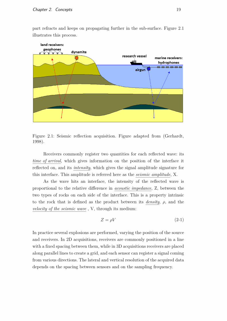
part refracts and keeps on propagating further in the sub-surface. Figure 2.1illustrates this process.
Figure 2.1: Seismic reflection acquisition. Figure adapted from (Gerhardt,1998).
Receivers commonly register two quantities for each reflected wave: itstime of arrival, which gives information on the position of the interface itreflected on, and its intensity, which gives the signal amplitude signature forthis interface. This amplitude is referred here as the seismic amplitude, X.
As the wave hits an interface, the intensity of the reflected wave isproportional to the relative difference in acoustic impedance, Z, between thetwo types of rocks on each side of the interface. This is a property intrinsicto the rock that is defined as the product between its density, ρ, and thevelocity of the seismic wave , V, through its medium:
Z = ρV (2-1)
In practice several explosions are performed, varying the position of the sourceand receivers. In 2D acquisitions, receivers are commonly positioned in a linewith a fixed spacing between them, while in 3D acquisitions receivers are placedalong parallel lines to create a grid, and each sensor can register a signal comingfrom various directions. The lateral and vertical resolution of the acquired datadepends on the spacing between sensors and on the sampling frequency.
DBD
PUC-Rio - Certificação Digital Nº 1413519/CA
Chapter 2. Concepts 20
2.1.2Processing
Signal processing aims at minimizing the signal noise and distortions,removing artifacts or unwanted seismic events in order to provide a visualresult where the position of the geobodies is the most accurate as possible.
One important step in the process is the seismic migration that trans-forms recorded amplitudes to simulate an explosion where the source and re-ceiver are at the same location. We can then consider that the signal prop-agated in the vertical direction and associate the reflected wave arrival timewith depth. This vertical signal is called the seismic trace, and its maximal am-plitude values (positive or negative peaks) correspond to the reflection events.It is important to this study to note that the actual value of the seismic ampli-tude is dependent of decisions made in the seismic migration step. The samedata can be processed from different interpreters, yielding amplitudes in dif-ferent scales. For this reason, when comparing different seismic images, it isbetter to put them in the same amplitude range. If the data is kept with floatthis may be values in the range between -1.0 and 1.0. If it is converted to asmall integer (0 to 255) one must be carefull with the quantization procedure.The noise in the data may artificially increase the amplitude range, yieldingmany classes with no elements.
Figure 2.2(a) shows an example of a seismic trace. Its amplitude can becoded with color. By stacking seismic traces represented in a color scale alongthe acquisition lines, the seismic image appears. Figure 2.2(b) and 2.2(c)show the visual results for a 2D acquisition line (seismic section) and a 3Dacquisition grid (seismic cube). All voxels of the grid (2D or 3D) contain avalue of the trace amplitude, here painted with a grayscale. We assess thecoordinates of each voxel through the in-line, cross-line and time (or equivalentdepth) positions in the grid.
DBD
PUC-Rio - Certificação Digital Nº 1413519/CA

Chapter 2. Concepts 21
Figure 2.2: (a) Seismic trace; (b) seismic section; (c) seismic cube.
2.1.3Interpretation
Theory on rock deformation and deposit behavior allows performingstructural interpretation of the seismic image features. Figure 2.3 shows anexample of the common organization of rocks and fluids around oil and gasreservoirs. Rock deformations are consequent to natural compression andtraction forces applying in the Earth’s crust, and can eventually result inbreak surfaces called seismic faults. Faults can trap the resources if filled witha sealing material, or on the contrary let them leak by opening a path throughthe surrounding rocks. The interface between rocks are called seismic horizons.As faults, sealing horizons can trap resources by blocking their natural upwardpropagation.
Figure 2.3: Common rock configuration around oil and gas reservoirs. Figurefrom (Robinson and Treitel, 2000).
DBD
PUC-Rio - Certificação Digital Nº 1413519/CA
Chapter 2. Concepts 22
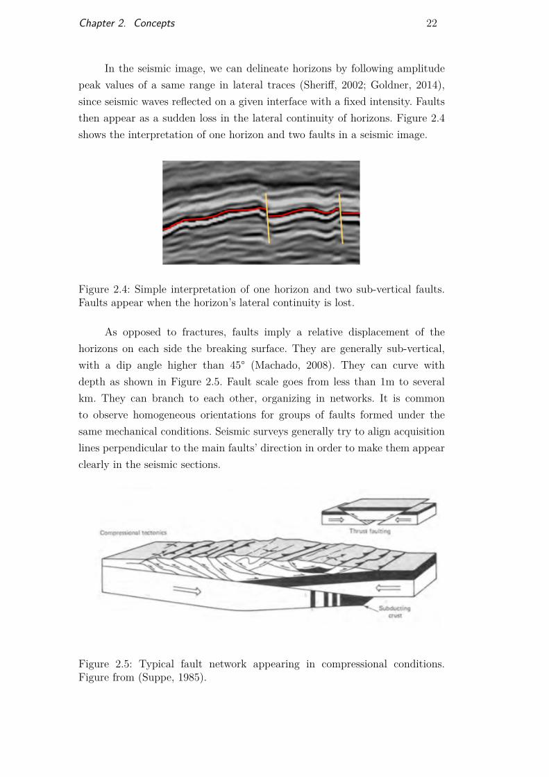
In the seismic image, we can delineate horizons by following amplitudepeak values of a same range in lateral traces (Sheriff, 2002; Goldner, 2014),since seismic waves reflected on a given interface with a fixed intensity. Faultsthen appear as a sudden loss in the lateral continuity of horizons. Figure 2.4shows the interpretation of one horizon and two faults in a seismic image.
Figure 2.4: Simple interpretation of one horizon and two sub-vertical faults.Faults appear when the horizon’s lateral continuity is lost.
As opposed to fractures, faults imply a relative displacement of thehorizons on each side the breaking surface. They are generally sub-vertical,with a dip angle higher than 45° (Machado, 2008). They can curve withdepth as shown in Figure 2.5. Fault scale goes from less than 1m to severalkm. They can branch to each other, organizing in networks. It is commonto observe homogeneous orientations for groups of faults formed under thesame mechanical conditions. Seismic surveys generally try to align acquisitionlines perpendicular to the main faults’ direction in order to make them appearclearly in the seismic sections.
Figure 2.5: Typical fault network appearing in compressional conditions.Figure from (Suppe, 1985).
DBD
PUC-Rio - Certificação Digital Nº 1413519/CA
Chapter 2. Concepts 23
Because of noise and events location uncertainties in seismic images, asame input can result in many different interpretations: real seismic imageshave no ground truth.
2.1.4Synthetic data
In our automatic fault detection method, part of the input are syntheticseismic data. We present here the basic concepts behind their construction.
There are two main possibilities when it comes to generating syntheticseismic images. The first approach is to simulate the seismic wave acquisitionprocess: artificial source and receivers are placed upon a simplified sub-surfacemodel made of rock layers with realistic properties, and the wave propagationis simulated using ray tracing (Fagin, 1991) or full waveform modeling (Hilter-man, 1970; Kelly et al, 1976). The generated synthetic signal has to passthrough all the seismic processing steps in order to produce a seismic section(or cube). Generating realistic seismic images with such technique requiressubstantial time and effort for both the acquisition simulation process and theseismic processing steps.
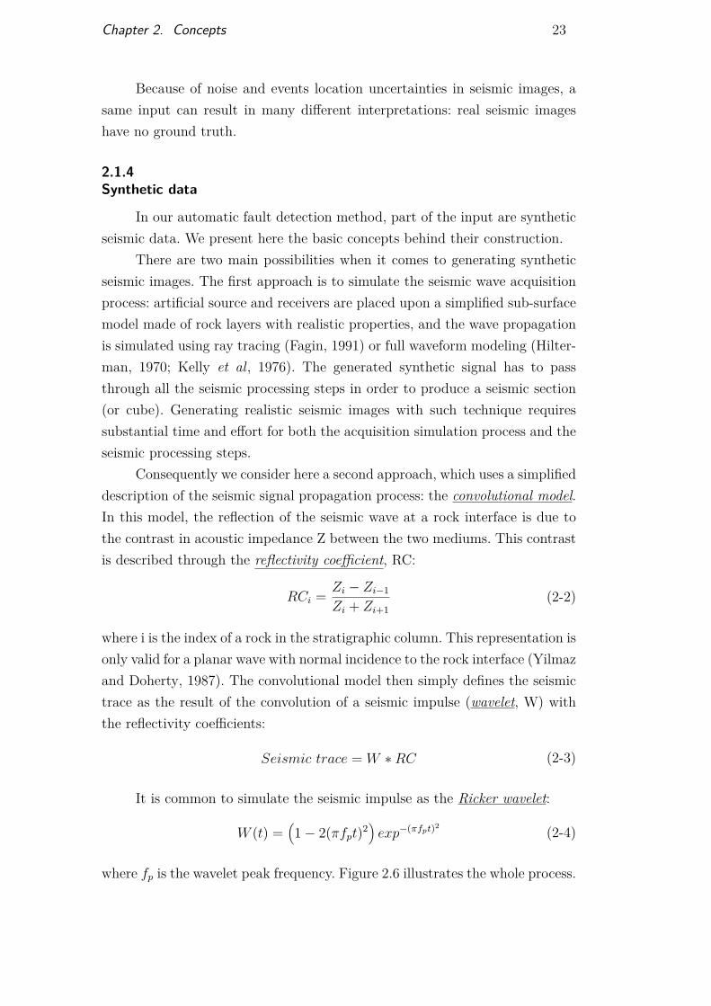
Consequently we consider here a second approach, which uses a simplifieddescription of the seismic signal propagation process: the convolutional model.In this model, the reflection of the seismic wave at a rock interface is due tothe contrast in acoustic impedance Z between the two mediums. This contrastis described through the reflectivity coefficient, RC:
RCi = Zi − Zi−1
Zi + Zi+1(2-2)
where i is the index of a rock in the stratigraphic column. This representation isonly valid for a planar wave with normal incidence to the rock interface (Yilmazand Doherty, 1987). The convolutional model then simply defines the seismictrace as the result of the convolution of a seismic impulse (wavelet, W) withthe reflectivity coefficients:
Seismic trace = W ∗RC (2-3)
It is common to simulate the seismic impulse as the Ricker wavelet:
W (t) =(1− 2(πfpt)2
)exp−(πfpt)2 (2-4)
where fp is the wavelet peak frequency. Figure 2.6 illustrates the whole process.
DBD
PUC-Rio - Certificação Digital Nº 1413519/CA
Chapter 2. Concepts 24
Figure 2.6: Convolutional model. Figure adapted from (Gerhardt, 1998).
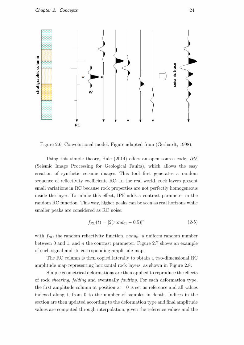
Using this simple theory, Hale (2014) offers an open source code, IPF(Seismic Image Processing for Geological Faults), which allows the easycreation of synthetic seismic images. This tool first generates a randomsequence of reflectivity coefficients RC. In the real world, rock layers presentsmall variations in RC because rock properties are not perfectly homogeneousinside the layer. To mimic this effect, IPF adds a contrast parameter in therandom RC function. This way, higher peaks can be seen as real horizons whilesmaller peaks are considered as RC noise:
fRC(t) = [2(rand01 − 0.5)]n (2-5)
with fRC the random reflectivity function, rand01 a uniform random numberbetween 0 and 1, and n the contrast parameter. Figure 2.7 shows an exampleof such signal and its corresponding amplitude map.
The RC column is then copied laterally to obtain a two-dimensional RCamplitude map representing horizontal rock layers, as shown in Figure 2.8.
Simple geometrical deformations are then applied to reproduce the effectsof rock shearing, folding and eventually faulting. For each deformation type,the first amplitude column at position x = 0 is set as reference and all valuesindexed along t, from 0 to the number of samples in depth. Indices in thesection are then updated according to the deformation type and final amplitudevalues are computed through interpolation, given the reference values and the
DBD
PUC-Rio - Certificação Digital Nº 1413519/CA
Chapter 2. Concepts 25
Figure 2.7: Random reflectivity for n = 5, with 100 samples. (a) discrete signal,corresponding to the amplitude map of the reflectivity signal, painted in greyscale from black = -1 to white = 1. (b) Corresponding continuous signal.
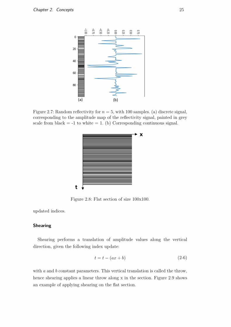
Figure 2.8: Flat section of size 100x100.
updated indices.
Shearing
Shearing performs a translation of amplitude values along the verticaldirection, given the following index update:
t = t− (ax+ b) (2-6)
with a and b constant parameters. This vertical translation is called the throw,hence shearing applies a linear throw along x in the section. Figure 2.9 showsan example of applying shearing on the flat section.
DBD
PUC-Rio - Certificação Digital Nº 1413519/CA
Chapter 2. Concepts 26
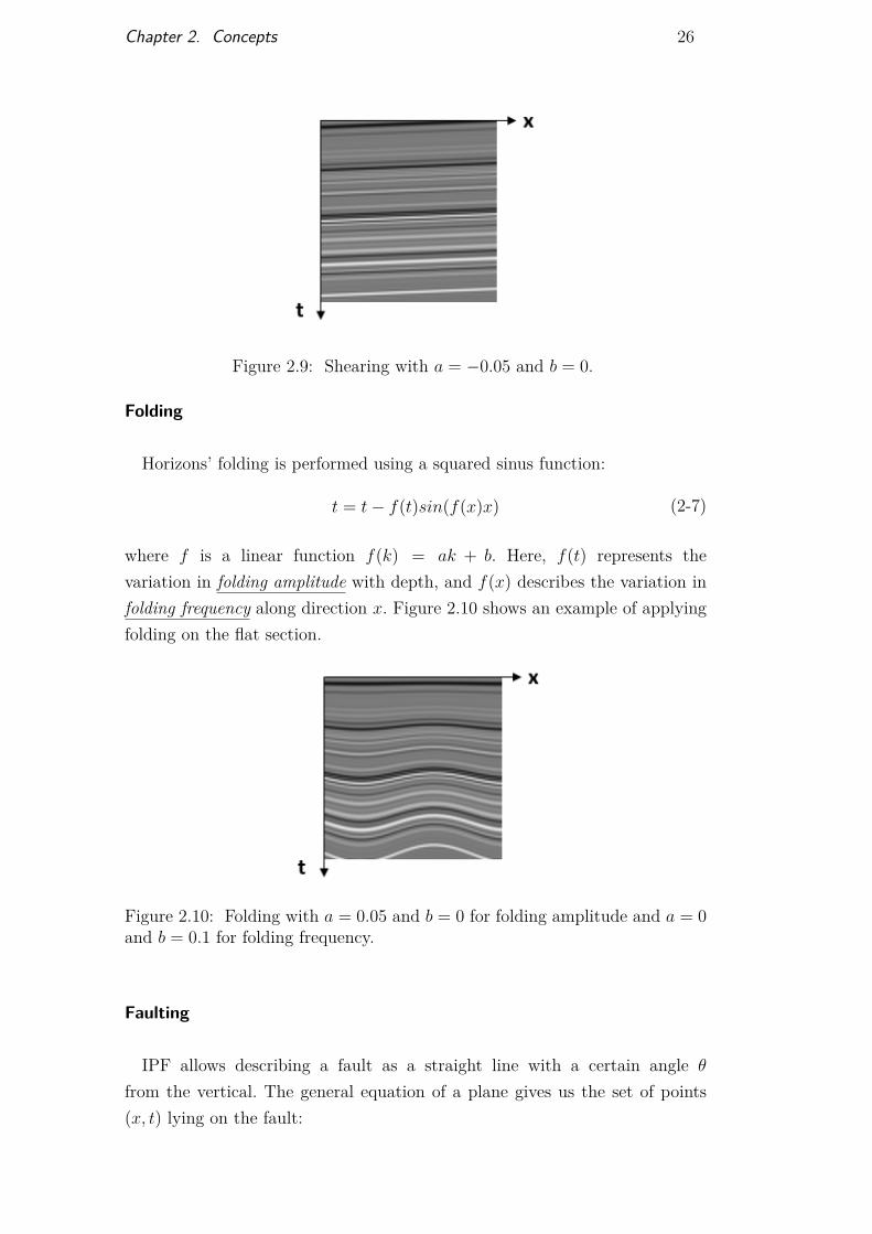
Figure 2.9: Shearing with a = −0.05 and b = 0.
Folding
Horizons’ folding is performed using a squared sinus function:
t = t− f(t)sin(f(x)x) (2-7)
where f is a linear function f(k) = ak + b. Here, f(t) represents thevariation in folding amplitude with depth, and f(x) describes the variation infolding frequency along direction x. Figure 2.10 shows an example of applyingfolding on the flat section.
Figure 2.10: Folding with a = 0.05 and b = 0 for folding amplitude and a = 0and b = 0.1 for folding frequency.
Faulting
IPF allows describing a fault as a straight line with a certain angle θ
from the vertical. The general equation of a plane gives us the set of points(x, t) lying on the fault:
DBD
PUC-Rio - Certificação Digital Nº 1413519/CA

Chapter 2. Concepts 27
xnx + tnt + d = 0 (2-8)
with nx, nt the two components of the fault’s normal vector, and d the distanceto the origin. Using simple trigonometry we can find the expression of thenormal ~n: Figure 2.11 shows the relation between angle θ and normal ~n.
Figure 2.11: Relation between fault angle and normal on the unit circle. Thickblue line is the fault.
We can deduce that:
~n = (cosθ,−sinθ) (2-9)
From Equation 2-8, we need one point (x, t) on the fault to obtain thedistance to the origin, d. This point is an input parameter of the faultingprocess. To perform the index updates, the code first compares Equation 2-8to 0: if the result is positive, the point is on the right side of the fault, and athrow is applied, constant along x but linear along t:
throwfault = at+ b (2-10)
with a and b constant parameters. Figure 2.12 shows an example of applyingfaulting on the flat section.
After all deformations were performed, the synthetic sub-surface struc-ture appears and the convolutional model can be applied. In order to maintainthe validity of the convolution operation, the code keeps track of the hori-zons’ normal along the deformation process. This way, the convolution can beperformed considering the normal incidence of the synthetic seismic signal.
Finally, noise is added to make the resulting image more realistic.The amount of noise is controlled through a constant C which modifies thesignal-to-noise ratio (SNR):
SInoise = SI + InoiseSNR(SI, Inoise)C (2-11)
DBD
PUC-Rio - Certificação Digital Nº 1413519/CA

Chapter 2. Concepts 28
Figure 2.12: Faulting with reference point (50, 0), θ = 10◦, and throwparameters a = 0, b = 4.
where SI is the seismic image and Inoise is an image of equal dimensioncontaining random values of high frequency between -1 and 1. SNR representsa way to scale the noise values with the image values, and is computed usingthe root mean square (RMS) of both images. Given a signal f with n values,the RMS is defined as:
RMS(f(x)) =√√√√ 1n
n∑i=1
x2i (2-12)
and the SNR is:
SNR(SI, Inoise) = RMS(SI)RMS(Inoise)
(2-13)
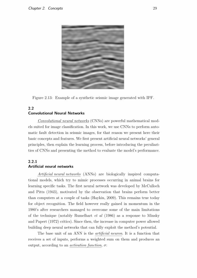
Figure 2.13 shows an example of the final image. In this synthetic sectionwe applied the shearing, folding and faulting of Figures 2.9, 2.10 and 2.12, aRicker wavelet with peak 0.5 and noise with C = 0.5.
This method presents the great advantage of being simple and fast. Asevery step of the process is parameterizable, we can create many seismic imagesautomatically in few minutes. However, generated images only present simpleconfigurations: faults are straight lines crossing the image entirely, it is difficultto generate more than a few faults per image, and other geobodies like channelsor salt domes cannot be created. The code also lacks in documentation.
However, deep learning techniques used in this thesis for automaticseismic fault detection require large amounts of data where the position ofthe faults is known a priori: IPF remains thus a powerful tool to use with suchmethods, which concepts are presented in the next section.
DBD
PUC-Rio - Certificação Digital Nº 1413519/CA
Chapter 2. Concepts 29
Figure 2.13: Example of a synthetic seismic image generated with IPF.
2.2Convolutional Neural Networks
Convolutional neural networks (CNNs) are powerful mathematical mod-els suited for image classification. In this work, we use CNNs to perform auto-matic fault detection in seismic images, for that reason we present here theirbasic concepts and features. We first present artificial neural networks’ generalprinciples, then explain the learning process, before introducing the peculiari-ties of CNNs and presenting the method to evaluate the model’s performance.
2.2.1Artificial neural networks
Artificial neural networks (ANNs) are biologically inspired computa-tional models, which try to mimic processes occurring in animal brains forlearning specific tasks. The first neural network was developed by McCullochand Pitts (1943), motivated by the observation that brains perform betterthan computers at a couple of tasks (Haykin, 2009). This remains true todayfor object recognition. The field however really gained in momentum in the1980’s after researchers managed to overcome some of the main limitationsof the technique (notably Rumelhart et al (1986) as a response to Minskyand Papert (1972) critics). Since then, the increase in computer power allowedbuilding deep neural networks that can fully exploit the method’s potential.
The base unit of an ANN is the artificial neuron. It is a function thatreceives a set of inputs, performs a weighted sum on them and produces anoutput, according to an activation function, σ:
DBD
PUC-Rio - Certificação Digital Nº 1413519/CA
Chapter 2. Concepts 30
f(x) = σ(n∑i=1
xiwi + b) (2-14)
with xi the input i, wi the weight associated with xi, n the number of inputsand b a bias term.
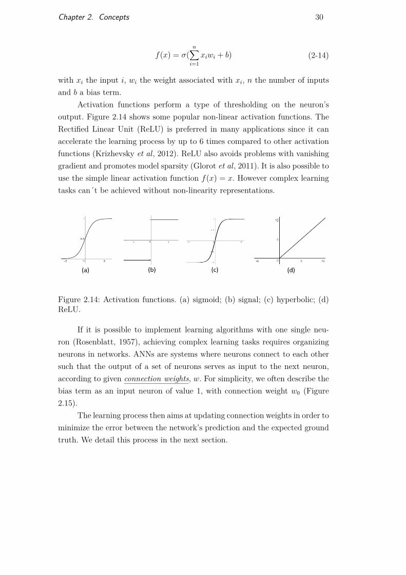
Activation functions perform a type of thresholding on the neuron’soutput. Figure 2.14 shows some popular non-linear activation functions. TheRectified Linear Unit (ReLU) is preferred in many applications since it canaccelerate the learning process by up to 6 times compared to other activationfunctions (Krizhevsky et al, 2012). ReLU also avoids problems with vanishinggradient and promotes model sparsity (Glorot et al, 2011). It is also possible touse the simple linear activation function f(x) = x. However complex learningtasks can´t be achieved without non-linearity representations.
Figure 2.14: Activation functions. (a) sigmoid; (b) signal; (c) hyperbolic; (d)ReLU.
If it is possible to implement learning algorithms with one single neu-ron (Rosenblatt, 1957), achieving complex learning tasks requires organizingneurons in networks. ANNs are systems where neurons connect to each othersuch that the output of a set of neurons serves as input to the next neuron,according to given connection weights, w. For simplicity, we often describe thebias term as an input neuron of value 1, with connection weight w0 (Figure2.15).
The learning process then aims at updating connection weights in order tominimize the error between the network’s prediction and the expected groundtruth. We detail this process in the next section.
DBD
PUC-Rio - Certificação Digital Nº 1413519/CA
Chapter 2. Concepts 31
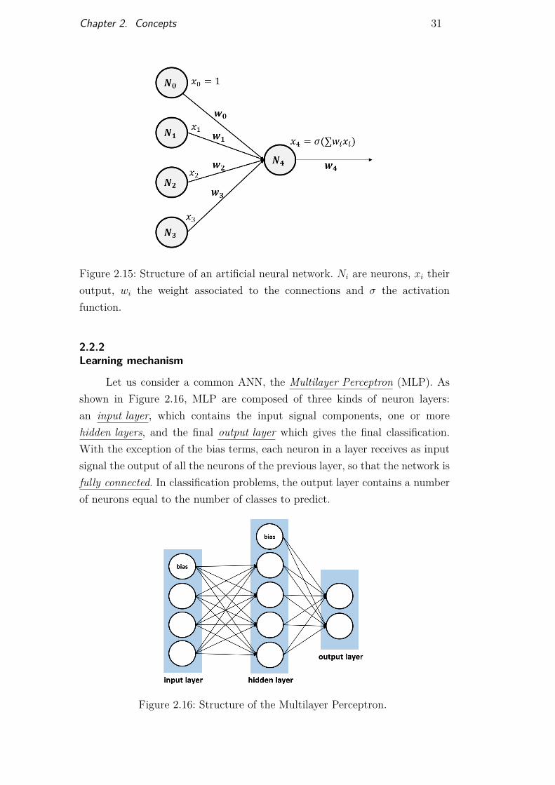
Figure 2.15: Structure of an artificial neural network. Ni are neurons, xi theiroutput, wi the weight associated to the connections and σ the activationfunction.
2.2.2Learning mechanism
Let us consider a common ANN, the Multilayer Perceptron (MLP). Asshown in Figure 2.16, MLP are composed of three kinds of neuron layers:an input layer, which contains the input signal components, one or morehidden layers, and the final output layer which gives the final classification.With the exception of the bias terms, each neuron in a layer receives as inputsignal the output of all the neurons of the previous layer, so that the network isfully connected. In classification problems, the output layer contains a numberof neurons equal to the number of classes to predict.
Figure 2.16: Structure of the Multilayer Perceptron.
DBD
PUC-Rio - Certificação Digital Nº 1413519/CA
Chapter 2. Concepts 32
Given a set of training examples (x(i), y(i)), where x(i) represents the inputsignal and y(i) the expected output, the network performs classification in thefollowing way.
First, all connection weights are initialized randomly. The input signalx(i) propagates forward in the network until reaching the output layer. Thegiven output, called the prediction, is compared to the expected ground truthy(i) through an error calculated with a loss function. The error then propagatesbackward in the network and weight values are adjusted consequently. Thenetwork learns by repeating this process a number of times through all trainingexamples, until reaching the desired minimal error. Connection weights arehence called learnable parameters, as opposed to a set of fixed parameters whichdescribe the learning algorithm.
To explain those steps more in details, let us introduce some notations:
− i is the training example index, with Ni the total number of examples;
− c denotes the index of a neuron in the current layer, with Nc the numberof neurons in that layer;
− p denotes the index of a neuron in the previous layer, with Np the numberof neurons in that layer;
− wab is the weight connection between neurons a and b. Bias terms haveindex 0.
− as the output of a layer is the input of its next layer, we denote by x theoutput of a neuron.
For the input layer, output x(i)c are the components of the input signal.
For the output layer:
x(i)c = y(i)
c (2-15)
with · denoting the prediction. For the intermediate layers, Figure 2.15 shows:
x(i)c = σ(
Np∑p=0
x(i)p wpc) (2-16)
Loss function
In this work we use the popular cross-entropy loss. To calculate it, weset the last layer activation function as the Softmax function, which outputsa normalized probability for each class (hence for each output neuron):
DBD
PUC-Rio - Certificação Digital Nº 1413519/CA
Chapter 2. Concepts 33
x(i)c = y(i)
c = exp∑Np
p=0 x(i)p wpc∑Nc
k=1 exp∑Np
p=0 x(i)p wpk
∈ [0, 1] (2-17)
The cross-entropy loss for training example i is then computed as follows:
L(i) = −Nc∑k=1
y(i)k log(y(i)
k ) (2-18)
with y(i) the ground truth vector. The cross-entropy loss for a set of k examplesis assessed through the mean:
L = 1Nk
Nk∑i=1
L(i) (2-19)
Weight update
Updates of connection weights aim at minimizing the loss value. Thecommon method to perform this optimization in neural networks is to use theGradient descent algorithm coupled with backpropagation.
Gradient descent exploits the fact that a function’s gradient reaches 0 atits optima. The gradient of a function is the vector of its partial derivatives.Given our loss function:
grad L(i) ={∂L(i)
∂w0,∂L(i)
∂w1, ...
∂L(i)
∂wNw
}(2-20)
with Nw the total number of weights in the network, initialized with randomvalues. Gradient descent tries to reach the null gradient by taking smallnegative steps for all weights j:
wj = wj − α(∂L(i)
∂wj
)(2-21)
with α the learning rate, a fixed parameter controlling the convergence speed.Negative steps ensure that the method converges to a minimum. If the lossfunction is convex (which is desirable), the gradient will find the unique (henceglobal) minimum of the function.
One problem with neural networks is that the loss of training example iis computed in the last layer, knowing only the output of its previous layer: itis not straightforward to access to the derivatives for all connection weights.The backpropagation method resolves this issue through the computation ofneurons’ local error δc, which can be seen as the contribution of each neuron
DBD
PUC-Rio - Certificação Digital Nº 1413519/CA
Chapter 2. Concepts 34
to the global loss, and defined as:
δc = ∂L(i)
∂(∑Np
p=0 x(i)p wpc)
(2-22)
Details on the computation of δc for each neuron can be found in (Haykin,2009). We note here that computing such local error in layer l involves knowinglocal errors of all neurons in layer (l + 1), so that the errors propagate layerby layer, backward in the network. Given the local error of a neuron in thecurrent layer, the derivative of the loss function regarding this neuron’s inputweights can be computed as :
∂L(i)
∂wpc= δcx
(i)p (2-23)
Backpropagation hence allows using the gradient descent algorithm inany neural network. In practice, weights are updated only after a set of trainingexamples have passed through the network (forward and backward). Thesesets are called batches, and the update occurring after each batch is called aniteration. With this method, one iteration only estimates the gradient on asubset of training examples. As batches do not represent the entire datasetand can contain a varying number of data outliers, this gradient estimatemay provide poor gradient steps. Adding a momentum term in the gradientupdate helps preventing this effect (Rumelhart et al, 1986; Qian, 1999). Whenall training examples have passed through the network once, an epoch wasconcluded. For example, a dataset of 2000 training examples with a batch sizeof 500 would result in 4 iterations per epoch. The process reaches convergenceafter several epochs. Batch size and number of epochs are fixed parameters.
Deep learning
The depth of a network is related to the number of non-linear opera-tions it performs (Bengio, 2009). Deep networks consequently contain moreneurons and more layers than shallow networks. The strength of neural net-works is to extract new information dynamically during training through theuse of the hidden layers. Each neuron corresponds to a feature, which canbe seen as a puzzle piece used for building class discrimination. In neuralnetworks, shallow features contain general information, while deep featuresare insights specific to the task. For example, in image classification, a shallowfeature would allow recognizing edges, while a deep feature would hold forexample the information of a particular stripe pattern on an animal’s back.
DBD
PUC-Rio - Certificação Digital Nº 1413519/CA
Chapter 2. Concepts 35
The capacity of deep neural networks to dynamically learn features at differentlevels of abstraction allows the network to map complex inputs to the outputdirectly from the data, without the need to manually select the features,as it would be the case with other learning techniques. This is particularlyinteresting for data with a high level of abstraction, like images, where it isdifficult to specify features in terms of raw sensory input (Bengio, 2009).
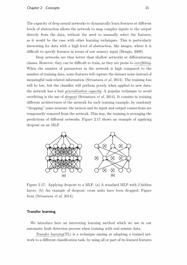
Deep networks are thus better than shallow networks at differentiatingclasses. However, they can be difficult to train, as they are prone to overfitting.When the number of parameters in the network is high compared to thenumber of training data, some features will capture the dataset noise instead ofmeaningful task-related information (Srivastava et al, 2014). The training losswill be low, but the classifier will perform poorly when applied to new data:the network has a bad generalization capacity. A popular technique to avoidoverfitting is the use of dropout (Srivastava et al, 2014). It consists in trainingdifferent architectures of the network for each training example, by randomly“dropping” some neurons: the neuron and its input and output connections aretemporarily removed from the network. This way, the training is averaging thepredictions of different networks. Figure 2.17 shows an example of applyingdropout on an MLP.
Figure 2.17: Applying dropout to a MLP. (a) A standard MLP with 2 hiddenlayers. (b) An example of dropout: cross units have been dropped. Figurefrom (Srivastava et al, 2014).
Transfer learning
We introduce here an interesting learning method which we use in ourautomatic fault detection process when training with real seismic data.
Transfer learning(TL) is a technique aiming at adapting a trained net-work to a different classification task, by using all or part of its learned features
DBD
PUC-Rio - Certificação Digital Nº 1413519/CA
Chapter 2. Concepts 36
to train a new network. Here again, TL researches are based on the observa-tion of a biological process: the presence of a knowledge learned previouslycan help solving new problems faster and / or better (Pan and Yang, 2010).For example, it may be simpler to learn playing the piano if we already knowhow to play the electric organ. In the neural network context, this translatesas follows: the connection weights in the new network are not initialized ran-domly but come from a first training process. This initial network is called thepre-trained model. It can be any network trained on any classification task, butthe method is more efficient if the two networks share a similar task.
In practice, there are many ways to apply TL, depending on eachparticular situation. First, part of the weights of the pre-trained model canbe frozen, meaning that they will not be updated in the new training session.This makes sense if we consider that some features (neurons) already holdrelevant information for the current classification task. The more similar thetasks are, the more pre-trained model weights can be frozen. Second, it ispossible to use only a part of the pre-trained model’s architecture: some layerscan be removed, new ones can be added. This is particularly interesting whenthe pre-trained model is deep but the new network dataset is small. In thiscase some pre-trained model layers are removed to avoid overfitting.
TL is hence particularly suited for building powerful classifiers with smalldatasets. In addition, the drop in number of learnable parameters due tothe freezing of parts of the network weights allows for fast training. Transferlearning is often used with CNNs, as the different layers of such networks havea rather good interpretability.
2.2.3CNN architecture
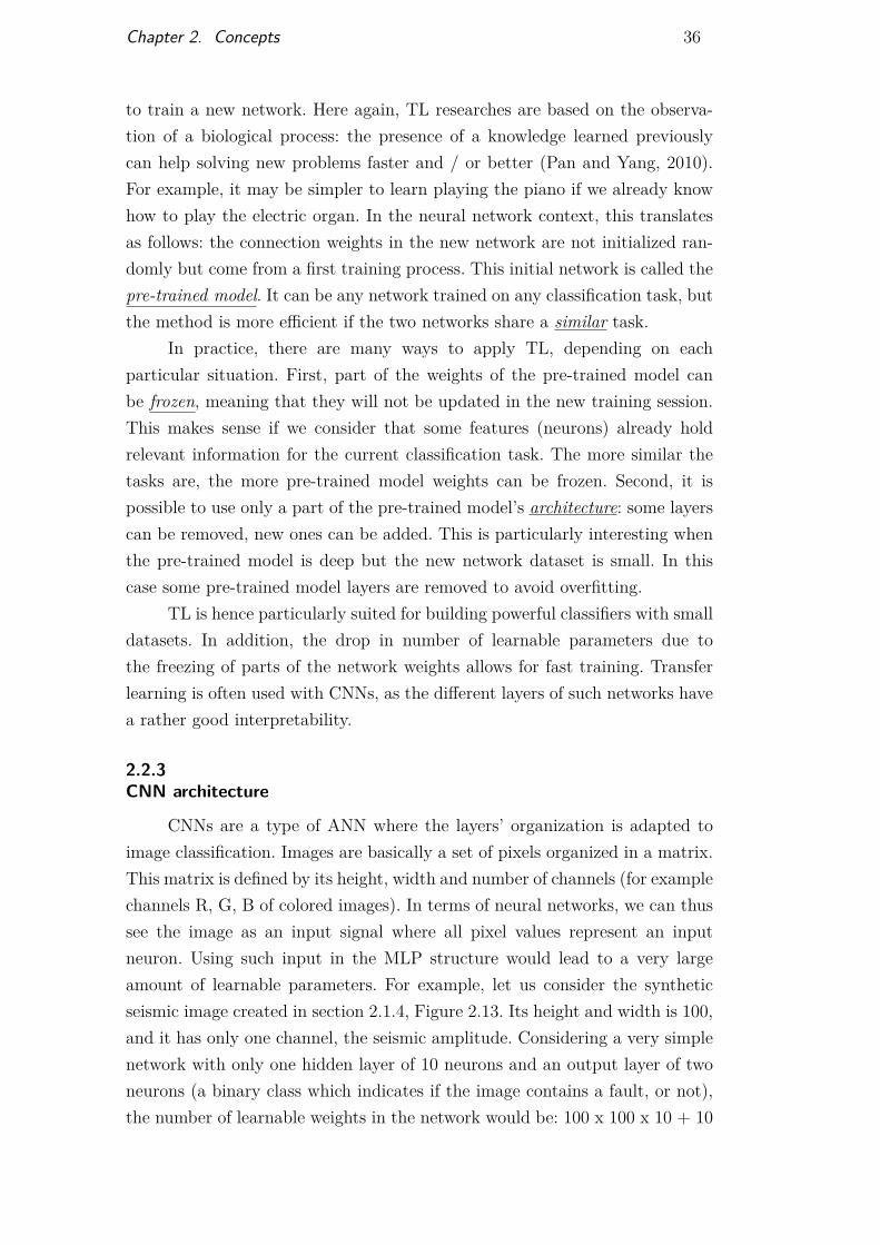
CNNs are a type of ANN where the layers’ organization is adapted toimage classification. Images are basically a set of pixels organized in a matrix.This matrix is defined by its height, width and number of channels (for examplechannels R, G, B of colored images). In terms of neural networks, we can thussee the image as an input signal where all pixel values represent an inputneuron. Using such input in the MLP structure would lead to a very largeamount of learnable parameters. For example, let us consider the syntheticseismic image created in section 2.1.4, Figure 2.13. Its height and width is 100,and it has only one channel, the seismic amplitude. Considering a very simplenetwork with only one hidden layer of 10 neurons and an output layer of twoneurons (a binary class which indicates if the image contains a fault, or not),the number of learnable weights in the network would be: 100 x 100 x 10 + 10
DBD
PUC-Rio - Certificação Digital Nº 1413519/CA

Chapter 2. Concepts 37
x 2 = 100 020. In practice, we want to train with deeper networks.CNNs exploits the spatial organization of the image to reduce the number
of parameters while efficiently extracting relevant features. It does so througha sequence of specific layers illustrated in Figure 2.18.
Figure 2.18: Architecture of a CNN, with: [@] = learnable filters; [w] =learnable weights. The example input is a seismic image, the output could bea binary class with value 1 if the image contains a seismic fault, 0 otherwise.
The first part of the network performs feature extraction through aseries of convolution and pooling layers. In this part, layers are organized infeature maps, which are sets of neurons that share sets of weights called filters.Neurons in feature maps are connected to only a small region of the previouslayer. Layer outputs are here again controlled by activation functions. At theend of the feature extraction part, neurons are flatten into a single vector andserve as input to a fully connected network. Here we describe in details eachlayer for the case of two-dimensional images (i.e with only one channel), whichare the kind of images used in this thesis.
Convolutional layers
Convolutional layers are at the core of the feature extraction process.The convolution operation computes a weighted sum on a small region of theinput neurons, as shown in Figure 2.19(a). The weight matrix, called filter, isapplied throughout the input at different locations and outputs a feature map,where neurons’ location roughly corresponds to their input region location(Figure 2.19(b)). Weights and bias are hence shared by all neurons of thefeature map.
DBD
PUC-Rio - Certificação Digital Nº 1413519/CA
Chapter 2. Concepts 38
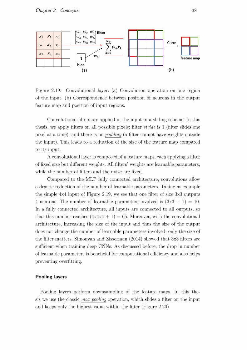
Figure 2.19: Convolutional layer. (a) Convolution operation on one regionof the input. (b) Correspondence between position of neurons in the outputfeature map and position of input regions.
Convolutional filters are applied in the input in a sliding scheme. In thisthesis, we apply filters on all possible pixels: filter stride is 1 (filter slides onepixel at a time), and there is no padding (a filter cannot have weights outsidethe input). This leads to a reduction of the size of the feature map comparedto its input.
A convolutional layer is composed of n feature maps, each applying a filterof fixed size but different weights. All filters’ weights are learnable parameters,while the number of filters and their size are fixed.
Compared to the MLP fully connected architecture, convolutions allowa drastic reduction of the number of learnable parameters. Taking as examplethe simple 4x4 input of Figure 2.19, we see that one filter of size 3x3 outputs4 neurons. The number of learnable parameters involved is (3x3 + 1) = 10.In a fully connected architecture, all inputs are connected to all outputs, sothat this number reaches (4x4x4 + 1) = 65. Moreover, with the convolutionalarchitecture, increasing the size of the input and thus the size of the outputdoes not change the number of learnable parameters involved: only the size ofthe filter matters. Simonyan and Zisserman (2014) showed that 3x3 filters aresufficient when training deep CNNs. As discussed before, the drop in numberof learnable parameters is beneficial for computational efficiency and also helpspreventing overfitting.
Pooling layers
Pooling layers perform downsampling of the feature maps. In this the-sis we use the classic max pooling operation, which slides a filter on the inputand keeps only the highest value within the filter (Figure 2.20).
DBD
PUC-Rio - Certificação Digital Nº 1413519/CA
Chapter 2. Concepts 39
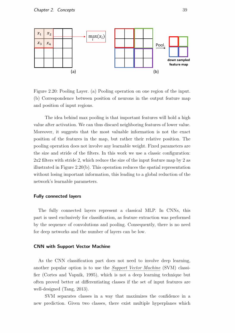
Figure 2.20: Pooling Layer. (a) Pooling operation on one region of the input.(b) Correspondence between position of neurons in the output feature mapand position of input regions.
The idea behind max pooling is that important features will hold a highvalue after activation. We can thus discard neighboring features of lower value.Moreover, it suggests that the most valuable information is not the exactposition of the features in the map, but rather their relative position. Thepooling operation does not involve any learnable weight. Fixed parameters arethe size and stride of the filters. In this work we use a classic configuration:2x2 filters with stride 2, which reduce the size of the input feature map by 2 asillustrated in Figure 2.20(b). This operation reduces the spatial representationwithout losing important information, this leading to a global reduction of thenetwork’s learnable parameters.
Fully connected layers
The fully connected layers represent a classical MLP. In CNNs, thispart is used exclusively for classification, as feature extraction was performedby the sequence of convolutions and pooling. Consequently, there is no needfor deep networks and the number of layers can be low.
CNN with Support Vector Machine
As the CNN classification part does not need to involve deep learning,another popular option is to use the Support Vector Machine (SVM) classi-fier (Cortes and Vapnik, 1995), which is not a deep learning technique butoften proved better at differentiating classes if the set of input features arewell-designed (Tang, 2013).
SVM separates classes in a way that maximizes the confidence in anew prediction. Given two classes, there exist multiple hyperplanes which
DBD
PUC-Rio - Certificação Digital Nº 1413519/CA
Chapter 2. Concepts 40
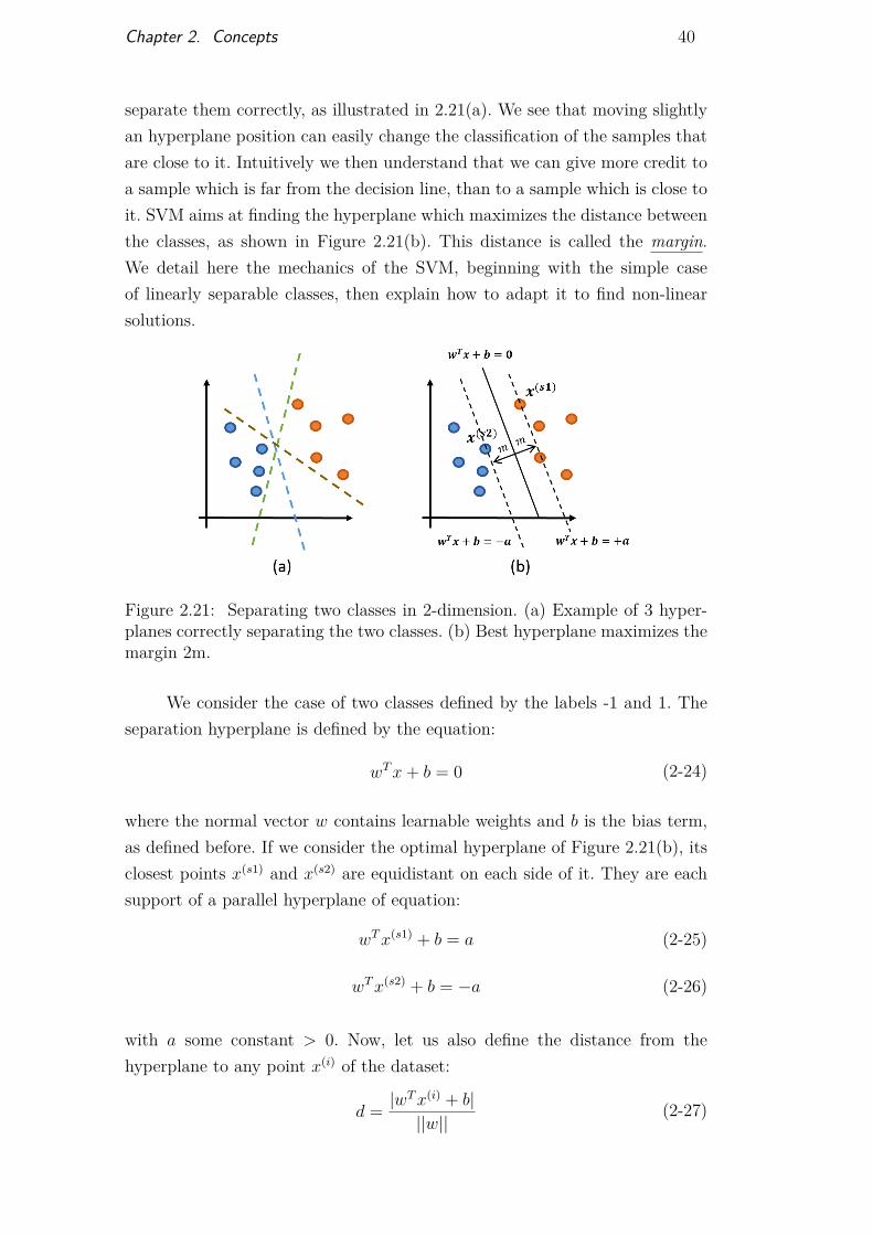
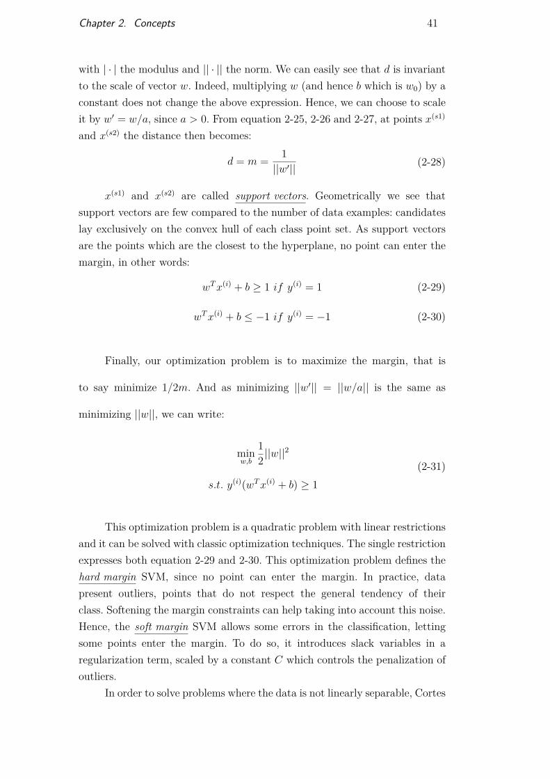
separate them correctly, as illustrated in 2.21(a). We see that moving slightlyan hyperplane position can easily change the classification of the samples thatare close to it. Intuitively we then understand that we can give more credit toa sample which is far from the decision line, than to a sample which is close toit. SVM aims at finding the hyperplane which maximizes the distance betweenthe classes, as shown in Figure 2.21(b). This distance is called the margin.We detail here the mechanics of the SVM, beginning with the simple caseof linearly separable classes, then explain how to adapt it to find non-linearsolutions.
Figure 2.21: Separating two classes in 2-dimension. (a) Example of 3 hyper-planes correctly separating the two classes. (b) Best hyperplane maximizes themargin 2m.
We consider the case of two classes defined by the labels -1 and 1. Theseparation hyperplane is defined by the equation:
wTx+ b = 0 (2-24)
where the normal vector w contains learnable weights and b is the bias term,as defined before. If we consider the optimal hyperplane of Figure 2.21(b), itsclosest points x(s1) and x(s2) are equidistant on each side of it. They are eachsupport of a parallel hyperplane of equation:
wTx(s1) + b = a (2-25)
wTx(s2) + b = −a (2-26)
with a some constant > 0. Now, let us also define the distance from thehyperplane to any point x(i) of the dataset:
d = |wTx(i) + b|||w||
(2-27)
DBD
PUC-Rio - Certificação Digital Nº 1413519/CA
Chapter 2. Concepts 41
with | · | the modulus and || · || the norm. We can easily see that d is invariantto the scale of vector w. Indeed, multiplying w (and hence b which is w0) by aconstant does not change the above expression. Hence, we can choose to scaleit by w′ = w/a, since a > 0. From equation 2-25, 2-26 and 2-27, at points x(s1)
and x(s2) the distance then becomes:
d = m = 1||w′|| (2-28)
x(s1) and x(s2) are called support vectors. Geometrically we see thatsupport vectors are few compared to the number of data examples: candidateslay exclusively on the convex hull of each class point set. As support vectorsare the points which are the closest to the hyperplane, no point can enter themargin, in other words:
wTx(i) + b ≥ 1 if y(i) = 1 (2-29)
wTx(i) + b ≤ −1 if y(i) = −1 (2-30)
Finally, our optimization problem is to maximize the margin, that is
to say minimize 1/2m. And as minimizing ||w′|| = ||w/a|| is the same as
minimizing ||w||, we can write:
minw,b
12 ||w||
2
s.t. y(i)(wTx(i) + b) ≥ 1(2-31)
This optimization problem is a quadratic problem with linear restrictionsand it can be solved with classic optimization techniques. The single restrictionexpresses both equation 2-29 and 2-30. This optimization problem defines thehard margin SVM, since no point can enter the margin. In practice, datapresent outliers, points that do not respect the general tendency of theirclass. Softening the margin constraints can help taking into account this noise.Hence, the soft margin SVM allows some errors in the classification, lettingsome points enter the margin. To do so, it introduces slack variables in aregularization term, scaled by a constant C which controls the penalization ofoutliers.
In order to solve problems where the data is not linearly separable, Cortes
DBD
PUC-Rio - Certificação Digital Nº 1413519/CA
Chapter 2. Concepts 42
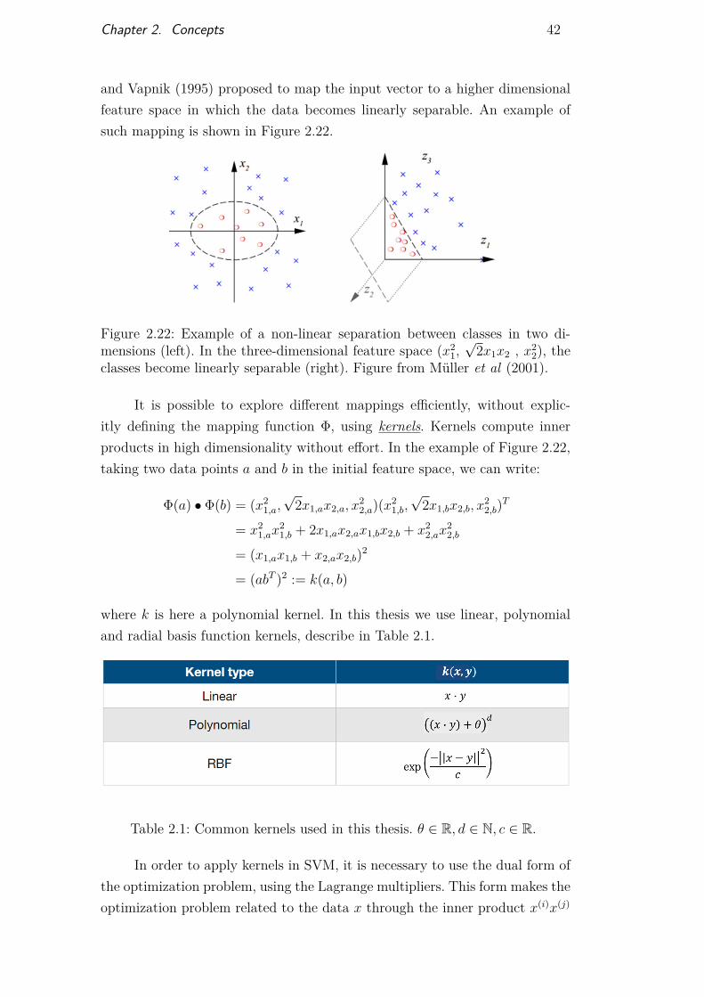
and Vapnik (1995) proposed to map the input vector to a higher dimensionalfeature space in which the data becomes linearly separable. An example ofsuch mapping is shown in Figure 2.22.
Figure 2.22: Example of a non-linear separation between classes in two di-mensions (left). In the three-dimensional feature space (x2
1,√
2x1x2 , x22), the
classes become linearly separable (right). Figure from Müller et al (2001).
It is possible to explore different mappings efficiently, without explic-itly defining the mapping function Φ, using kernels. Kernels compute innerproducts in high dimensionality without effort. In the example of Figure 2.22,taking two data points a and b in the initial feature space, we can write:
Φ(a) • Φ(b) = (x21,a,√
2x1,ax2,a, x22,a)(x2
1,b,√
2x1,bx2,b, x22,b)T
= x21,ax
21,b + 2x1,ax2,ax1,bx2,b + x2
2,ax22,b
= (x1,ax1,b + x2,ax2,b)2
= (abT )2 := k(a, b)
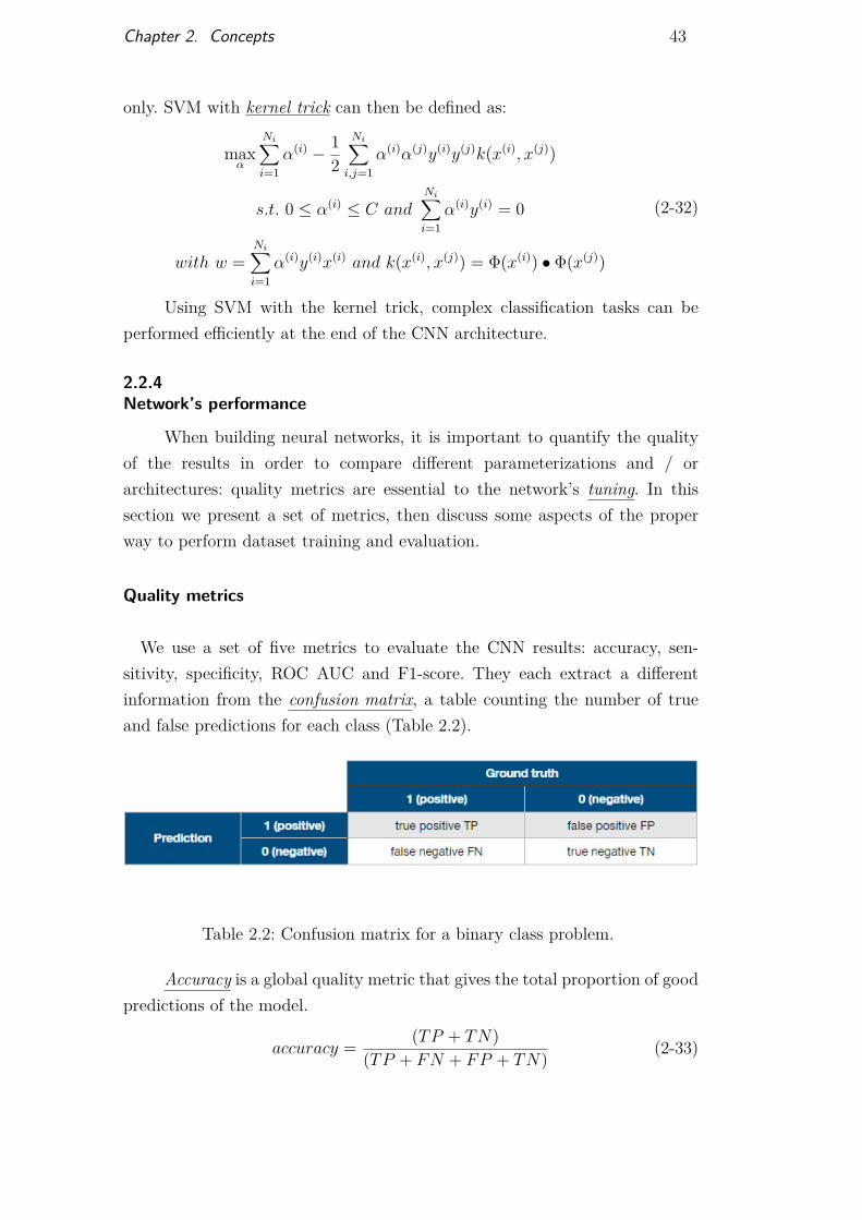
where k is here a polynomial kernel. In this thesis we use linear, polynomialand radial basis function kernels, describe in Table 2.1.
Table 2.1: Common kernels used in this thesis. θ ∈ R, d ∈ N, c ∈ R.
In order to apply kernels in SVM, it is necessary to use the dual form ofthe optimization problem, using the Lagrange multipliers. This form makes theoptimization problem related to the data x through the inner product x(i)x(j)
DBD
PUC-Rio - Certificação Digital Nº 1413519/CA
Chapter 2. Concepts 43
only. SVM with kernel trick can then be defined as:
maxα
Ni∑i=1
α(i) − 12
Ni∑i,j=1
α(i)α(j)y(i)y(j)k(x(i), x(j))
s.t. 0 ≤ α(i) ≤ C andNi∑i=1
α(i)y(i) = 0
with w =Ni∑i=1
α(i)y(i)x(i) and k(x(i), x(j)) = Φ(x(i)) • Φ(x(j))
(2-32)
Using SVM with the kernel trick, complex classification tasks can beperformed efficiently at the end of the CNN architecture.
2.2.4Network’s performance
When building neural networks, it is important to quantify the qualityof the results in order to compare different parameterizations and / orarchitectures: quality metrics are essential to the network’s tuning. In thissection we present a set of metrics, then discuss some aspects of the properway to perform dataset training and evaluation.
Quality metrics
We use a set of five metrics to evaluate the CNN results: accuracy, sen-sitivity, specificity, ROC AUC and F1-score. They each extract a differentinformation from the confusion matrix, a table counting the number of trueand false predictions for each class (Table 2.2).
Table 2.2: Confusion matrix for a binary class problem.
Accuracy is a global quality metric that gives the total proportion of goodpredictions of the model.
accuracy = (TP + TN)(TP + FN + FP + TN) (2-33)
DBD
PUC-Rio - Certificação Digital Nº 1413519/CA
Chapter 2. Concepts 44
It allows quickly evaluating the model, as a high accuracy is desirable.However, it does not provide details on the performance of each class, conse-quently it should not be used alone.
Sensitivity is the probability for the model to predict class 1, knowingthe ground truth is 1. This corresponds to the proportion of good predictionsfor the positive class:
sensitivity = TP
(TP + FN) = TP
Number of positive samples(2-34)
A high sensitivity ensures the validity of negative predictions (FN arescarce). However, it does not guarantee that a positive prediction is true,because it does not take into account the FP samples. If the model predictsall samples as class 1, it will have a 100% sensitivity while being always wrongabout class 0 samples.
Specificity is the counterpart of sensitivity, for the negative class. Itcorresponds to the probability to predict class 0 knowing that the groundtruth is 0.
specificity = TN
(TN + FP ) = TN
Number of negative samples(2-35)
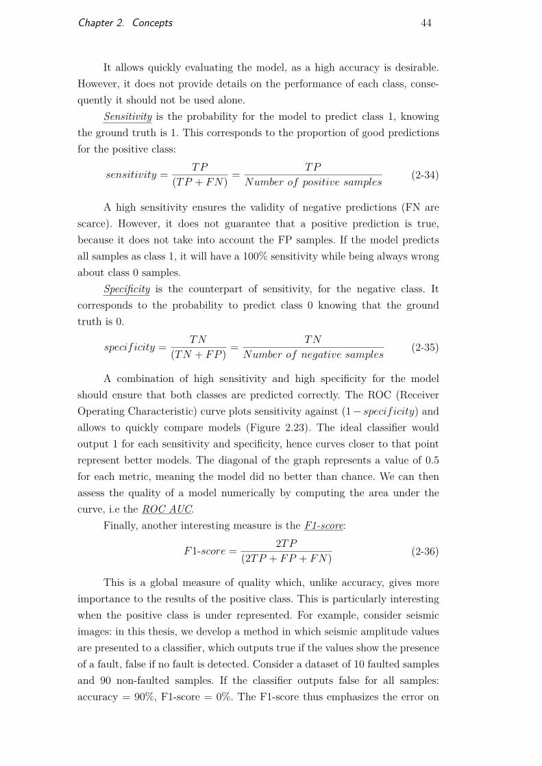
A combination of high sensitivity and high specificity for the modelshould ensure that both classes are predicted correctly. The ROC (ReceiverOperating Characteristic) curve plots sensitivity against (1− specificity) andallows to quickly compare models (Figure 2.23). The ideal classifier wouldoutput 1 for each sensitivity and specificity, hence curves closer to that pointrepresent better models. The diagonal of the graph represents a value of 0.5for each metric, meaning the model did no better than chance. We can thenassess the quality of a model numerically by computing the area under thecurve, i.e the ROC AUC.
Finally, another interesting measure is the F1-score:
F1-score = 2TP(2TP + FP + FN) (2-36)
This is a global measure of quality which, unlike accuracy, gives moreimportance to the results of the positive class. This is particularly interestingwhen the positive class is under represented. For example, consider seismicimages: in this thesis, we develop a method in which seismic amplitude valuesare presented to a classifier, which outputs true if the values show the presenceof a fault, false if no fault is detected. Consider a dataset of 10 faulted samplesand 90 non-faulted samples. If the classifier outputs false for all samples:accuracy = 90%, F1-score = 0%. The F1-score thus emphasizes the error on
DBD
PUC-Rio - Certificação Digital Nº 1413519/CA
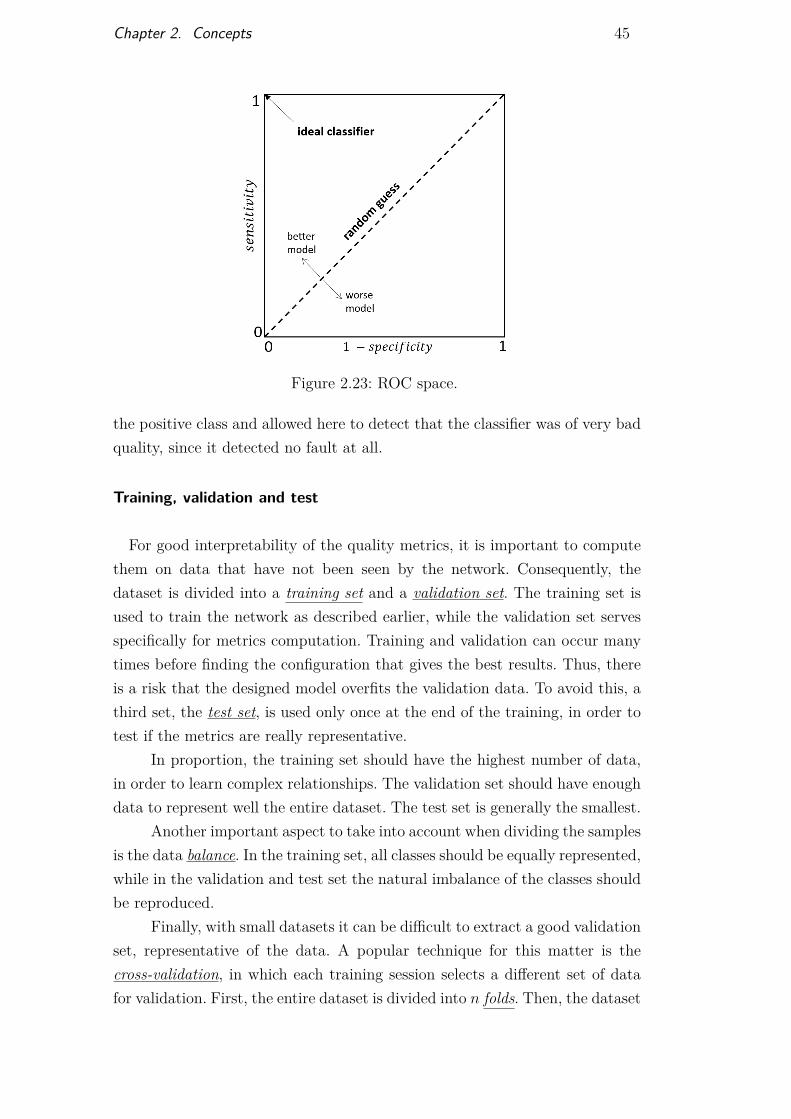
Chapter 2. Concepts 45
Figure 2.23: ROC space.
the positive class and allowed here to detect that the classifier was of very badquality, since it detected no fault at all.
Training, validation and test
For good interpretability of the quality metrics, it is important to computethem on data that have not been seen by the network. Consequently, thedataset is divided into a training set and a validation set. The training set isused to train the network as described earlier, while the validation set servesspecifically for metrics computation. Training and validation can occur manytimes before finding the configuration that gives the best results. Thus, thereis a risk that the designed model overfits the validation data. To avoid this, athird set, the test set, is used only once at the end of the training, in order totest if the metrics are really representative.
In proportion, the training set should have the highest number of data,in order to learn complex relationships. The validation set should have enoughdata to represent well the entire dataset. The test set is generally the smallest.
Another important aspect to take into account when dividing the samplesis the data balance. In the training set, all classes should be equally represented,while in the validation and test set the natural imbalance of the classes shouldbe reproduced.
Finally, with small datasets it can be difficult to extract a good validationset, representative of the data. A popular technique for this matter is thecross-validation, in which each training session selects a different set of datafor validation. First, the entire dataset is divided into n folds. Then, the dataset
DBD
PUC-Rio - Certificação Digital Nº 1413519/CA

Chapter 2. Concepts 46
is trained n times using (n−1) folds for training and 1 fold for validation. Thefinal metrics are the mean of all n results. With this method, it is importantto respect the proportion of each class in each fold.
DBD
PUC-Rio - Certificação Digital Nº 1413519/CA
3Related works
The past decades have seen the development of many tools for computer-aided fault detection in migrated seismic data. The vast majority of methods isbased on the use of seismic attributes, which can be defined as « the quantitiesthat are measured, computed or implied from the seismic data » (Subrah-manyam and Rao, 2008). They mainly consist in a set of mathematical opera-tions highlighting a certain type of information in the seismic image. Fault at-tribute maps allow visually enhancing possible fault location by looking at thelocal continuity of the seismic signal (coherence (Bahorich and Farmer, 1995;Luo et al, 1996), semblance (Marfurt et al, 1998), variance (Van Bemmel andPepper, 2000), chaos (Randen et al, 2001), edge detection (Di and Gao, 2014)),or at the geometry of the reflectors (curvature (Lisle, 1994; Roberts, 2001; Al-Dossary and Marfurt, 2006), flexure (Gao, 2013)). Among them, the coherenceis the best known attribute for highlighting faults (Wang et al, 2018). An al-ternative to seismic attributes is to use the information of interpreted horizonsto find fault locations (horizons dip and azimuth maps, (Rijks and Jauffred,1991)).
Each seismic attribute has its pros and cons, and fails at enhancing faultsonly; numerous artifacts remain, other structures appear. Seismic attributesusually require massive computation, and, alone, are not suited for efficientfault identification: a human interpreter must spend time finalizing the studymanually. Consequently, many authors propose to post-process the attributemaps to extract fault location automatically, usually using some kind of imageprocessing technique. For example, Pedersen et al (2002) used Artificial Antstracking on one or more attribute cubes to extract fault surfaces. Gibson etal (2005) used semblance to extract a set of high faultiness points that theyjoin in a multi-resolution scheme to build fault surfaces. Hale (2013) builtsurface meshes by connecting a selection of high fault likelihood points. Wanget al (2014) performed color transformations on semblance maps, followed bya skeletonization of the highlighted fault regions. Recently the same authorsproposed the combination of the Hough Transform and tracking vector toextract faults from binarized coherence maps (Wang and AlRegib, 2017). Thosemethods generally fall into two categories: faults are well extracted but many
DBD
PUC-Rio - Certificação Digital Nº 1413519/CA
Chapter 3. Related works 48
artifacts remain, or the result is clean, but not all faults are detected (Wanget al, 2018; Di and Gao, 2017).
Another approach is to combine attributes using machine learning al-gorithms. Supervised methods extract meaningful information from a set ofinputs (the features) and observations (here, the fault location), then applyacquired knowledge to predict new samples. Such methods allow building com-plex relationships within large amounts of seismic data. One of the first worksin this direction is a study from Tingdahl et al (2005), where they used aset of 12 seismic attributes as input features of an Artificial Neural Network,generating fault probability maps that can be seen as a new attribute. Morerecently, Support Vector Machine (SVM) achieved promising results when ap-plied on a selection of seismic attributes (Di et al, 2017) or image textureattributes (Guitton et al, 2017). These techniques imply a tedious step of at-tribute selection and computation, an operation which can be avoided withdeep learning methods.
Compared to standard machine learning techniques, deep networks canlearn new features dynamically during training, explaining their success insolving complex tasks (Voulodimos et al, 2018). Among them, image-orientedmethods like CNNs are especially promising as they recently achieved state-of-the-art results in automatic fault detection (Wang et al, 2018). The use ofCNNs is recent in the seismic field, as the first work for fault detection wasby Huang et al (2017), in which the authors built many CNNs in parallelon a set of 9 seismic attribute cubes, then fed the extracted features to asingle MLP. In other words, they did not take advantage of the ability ofCNNs to automatically extract features from the data: as seismic attributesare derived from the seismic amplitude, a CNN should be able to computerelevant attributes from the amplitude input automatically during training. Inthis direction, Di et al (2018) proposed to classify amplitude patches on a realcube and showed promising results. Overall, despite very encouraging results,deep learning techniques present some drawbacks. As supervised learningmethods, they require a large amount of marked seismic data as input; thegeneralizability of the proposed networks to other seismic cubes is hard toassess, as studies generally train and classify in the same field; building a CNNmodel on new data involves a long tuning step, due to the substantial amountof hyper-parameters to adjust.
In this thesis, we propose a two-step scheme to build a good faultclassifier, addressing each of the aforementioned CNN drawbacks. First, webuild a classifier on a set of synthetic data: a huge amount of error-free labeleddata is thus easy to obtain. Second, we apply TL methods to adapt the classifier
DBD
PUC-Rio - Certificação Digital Nº 1413519/CA

Chapter 3. Related works 49
to real data. In this step, only a small number of marked data is needed, andthe number of parameters to tune is also greatly reduced. TL methods alsoensure the generalizability of the technique, by providing a way to adapt toany seismic cube.
DBD
PUC-Rio - Certificação Digital Nº 1413519/CA
4Fault detection in synthetic amplitude maps using CNNs
Compared to real data, synthetic seismic data present several advantagesfor deep networks training. First, they allow total control of the groundtruth and thus avoid marking errors. Second, the marking being automaticand fast, synthetic data provide an easy scaling regarding the number oftraining examples. Finally, they avoid problems with data privacy, allowingfree distribution.
We propose a methodology in four steps. First, we generate syntheticseismic images where we control the location of the faults. Second, we extractFault and Non-fault patches from the generated dataset. Then, we train andfine-tune different CNN architectures focusing on maximizing quality metrics.Finally, we classify pixels in new synthetic images and post process the resultsfor fault segmentation.
4.1Synthetic dataset generation
The open source code IPF from Hale (2014) allowed us to reproducethe results of migrated seismic data. Beginning with a randomly generatedreflectivity model extended along the section, simple image transformationsrecreate sequential rock deformations along time: shearing, folding and fault-ing. We can then apply convolution with a Ricker wavelet and add randomnoise. Each step of the process can be parameterized. We built a dataset of500 images of 572x572 pixels, all containing one straight fault crossing thesection entirely, modifying randomly fault angle, position and throw, shearingslope, folding amplitude and frequency, wavelet peak and amount of noise.Resulting images present amplitude values between -1 and 1. Along with theseismic amplitude information, we generated for each image its correspondingbinary mask, indicating in white the location of the fault. Figure 4.1 shows anexample of such a pair.
DBD
PUC-Rio - Certificação Digital Nº 1413519/CA
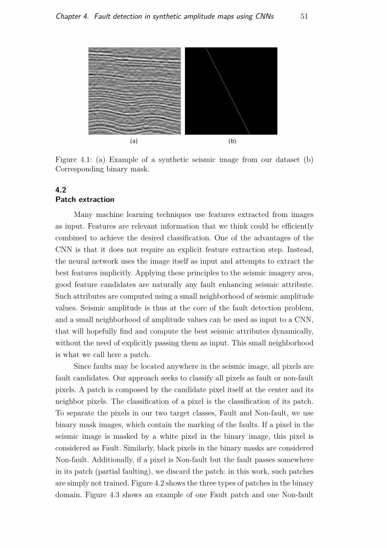
Chapter 4. Fault detection in synthetic amplitude maps using CNNs 51
Figure 4.1: (a) Example of a synthetic seismic image from our dataset (b)Corresponding binary mask.
4.2Patch extraction
Many machine learning techniques use features extracted from imagesas input. Features are relevant information that we think could be efficientlycombined to achieve the desired classification. One of the advantages of theCNN is that it does not require an explicit feature extraction step. Instead,the neural network uses the image itself as input and attempts to extract thebest features implicitly. Applying these principles to the seismic imagery area,good feature candidates are naturally any fault enhancing seismic attribute.Such attributes are computed using a small neighborhood of seismic amplitudevalues. Seismic amplitude is thus at the core of the fault detection problem,and a small neighborhood of amplitude values can be used as input to a CNN,that will hopefully find and compute the best seismic attributes dynamically,without the need of explicitly passing them as input. This small neighborhoodis what we call here a patch.
Since faults may be located anywhere in the seismic image, all pixels arefault candidates. Our approach seeks to classify all pixels as fault or non-faultpixels. A patch is composed by the candidate pixel itself at the center and itsneighbor pixels. The classification of a pixel is the classification of its patch.To separate the pixels in our two target classes, Fault and Non-fault, we usebinary mask images, which contain the marking of the faults. If a pixel in theseismic image is masked by a white pixel in the binary image, this pixel isconsidered as Fault. Similarly, black pixels in the binary masks are consideredNon-fault. Additionally, if a pixel is Non-fault but the fault passes somewherein its patch (partial faulting), we discard the patch: in this work, such patchesare simply not trained. Figure 4.2 shows the three types of patches in the binarydomain. Figure 4.3 shows an example of one Fault patch and one Non-fault
DBD
PUC-Rio - Certificação Digital Nº 1413519/CA
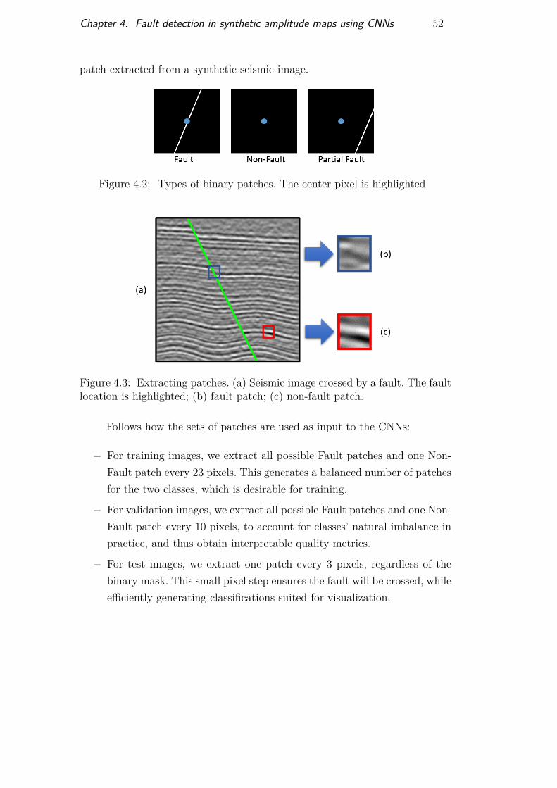
Chapter 4. Fault detection in synthetic amplitude maps using CNNs 52
patch extracted from a synthetic seismic image.
Figure 4.2: Types of binary patches. The center pixel is highlighted.
Figure 4.3: Extracting patches. (a) Seismic image crossed by a fault. The faultlocation is highlighted; (b) fault patch; (c) non-fault patch.
Follows how the sets of patches are used as input to the CNNs:
− For training images, we extract all possible Fault patches and one Non-Fault patch every 23 pixels. This generates a balanced number of patchesfor the two classes, which is desirable for training.
− For validation images, we extract all possible Fault patches and one Non-Fault patch every 10 pixels, to account for classes’ natural imbalance inpractice, and thus obtain interpretable quality metrics.
− For test images, we extract one patch every 3 pixels, regardless of thebinary mask. This small pixel step ensures the fault will be crossed, whileefficiently generating classifications suited for visualization.
DBD
PUC-Rio - Certificação Digital Nº 1413519/CA
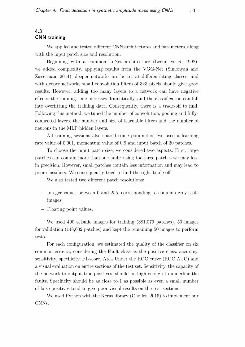
Chapter 4. Fault detection in synthetic amplitude maps using CNNs 53
4.3CNN training
We applied and tested different CNN architectures and parameters, alongwith the input patch size and resolution.
Beginning with a common LeNet architecture (Lecun et al, 1998),we added complexity, applying results from the VGG-Net (Simonyan andZisserman, 2014): deeper networks are better at differentiating classes, andwith deeper networks small convolution filters of 3x3 pixels should give goodresults. However, adding too many layers to a network can have negativeeffects: the training time increases dramatically, and the classification can fallinto overfitting the training data. Consequently, there is a trade-off to find.Following this method, we tuned the number of convolution, pooling and fully-connected layers, the number and size of learnable filters and the number ofneurons in the MLP hidden layers.
All training sessions also shared some parameters: we used a learningrate value of 0.001, momentum value of 0.9 and input batch of 30 patches.
To choose the input patch size, we considered two aspects. First, largepatches can contain more than one fault: using too large patches we may losein precision. However, small patches contain less information and may lead topoor classifiers. We consequently tried to find the right trade-off.
We also tested two different patch resolutions:
− Integer values between 0 and 255, corresponding to common grey scaleimages;
− Floating point values.
We used 400 seismic images for training (381,079 patches), 50 imagesfor validation (148,632 patches) and kept the remaining 50 images to performtests.
For each configuration, we estimated the quality of the classifier on sixcommon criteria, considering the Fault class as the positive class: accuracy,sensitivity, specificity, F1-score, Area Under the ROC curve (ROC AUC) anda visual evaluation on entire sections of the test set. Sensitivity, the capacity ofthe network to output true positives, should be high enough to underline thefaults. Specificity should be as close to 1 as possible as even a small numberof false positives tend to give poor visual results on the test sections.
We used Python with the Keras library (Chollet, 2015) to implement ourCNNs.
DBD
PUC-Rio - Certificação Digital Nº 1413519/CA
Chapter 4. Fault detection in synthetic amplitude maps using CNNs 54
4.4CNN classification and post-processing
Once a good model is obtained, new images can be classified. Dependingon the image size and fault scale, one can choose to classify all pixels or justa subset. In any case, the result will be a binary image with sets of whitepixels at the predicted fault location. Extracting the fault thus requires apost-processing. We chose a simple sequence of morphological operations:
− Dilation adds white pixels to the boundary of detected objects. It tendsto close holes and join adjacent parts of the objects: this operation aimsat reducing the number of false negatives (pixels wrongly classified asNon-Fault).
− Erosion removes white pixels from the boundary of detected objects. Ittends to clean the object’s boundary and erase isolated white pixels: thisoperation aims at reducing the number of false positives (pixels wronglyclassified as Fault).
− Thinning extracts the skeleton of the object. It reduces the number ofFault pixels without losing information.
Those steps clean the image and result in smaller Fault point sets. Wethen apply the Hough Transform (Hough, 1962) to finally extract the faults:the method allows detecting alignments of white pixels in our post-processedclassification images. The method is here restricted to straight lines and wealso give a restriction on fault angles, which should be sub-vertical.
4.5Results
The network architecture which gave the highest metrics is described inTable 4.1. Input are patches of size 45x45, with a floating point precision. Thenetwork gave an accuracy of 0.98, a sensitivity of 0.95, a specificity of 0.99,F1-score of 0.97 and ROC AUC of 0.99.
Figure 4.4 shows the classification and fault extraction of sections fromthe test set. Classification is performed every three pixels. The fault is clearlyhighlighted, but still coarse because patches of type Partial fault are presentand mainly classified as Fault. Since the training step did not include suchpatches, as stated in section 4.2, those results are unsurprising. Note also thatsuch patches did not enter in the calculation of the quality metrics, over-estimating all values except sensitivity since the number of false positives wasunderestimated.
DBD
PUC-Rio - Certificação Digital Nº 1413519/CA
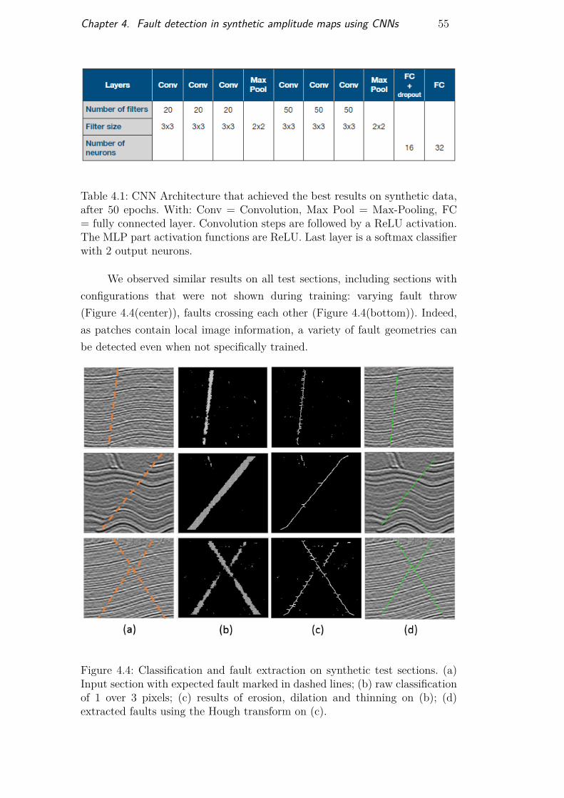
Chapter 4. Fault detection in synthetic amplitude maps using CNNs 55
Table 4.1: CNN Architecture that achieved the best results on synthetic data,after 50 epochs. With: Conv = Convolution, Max Pool = Max-Pooling, FC= fully connected layer. Convolution steps are followed by a ReLU activation.The MLP part activation functions are ReLU. Last layer is a softmax classifierwith 2 output neurons.
We observed similar results on all test sections, including sections withconfigurations that were not shown during training: varying fault throw(Figure 4.4(center)), faults crossing each other (Figure 4.4(bottom)). Indeed,as patches contain local image information, a variety of fault geometries canbe detected even when not specifically trained.
Figure 4.4: Classification and fault extraction on synthetic test sections. (a)Input section with expected fault marked in dashed lines; (b) raw classificationof 1 over 3 pixels; (c) results of erosion, dilation and thinning on (b); (d)extracted faults using the Hough transform on (c).
DBD
PUC-Rio - Certificação Digital Nº 1413519/CA

5Fault detection in real seismic data
5.1Applying the synthetic classifier to real data
5.1.1Synthetic and real data comparison
We use as case study a real data from the North Sea, the F3 cube (Opend-Tect, 1987). It contains 650 in-lines, 950 cross-lines and 462 time sections. Weassessed the frequency content of the data by performing the Fourier trans-form on seismic traces. We compared with the frequencies of our syntheticdataset. It appears that our synthetic dataset does not match real data: whilereal seismic signal ranges between 20 and 50 Hz, the synthetic dataset doesnot present patches with a higher frequency than 20 Hz, as shown in Figure5.1.
Figure 5.1: (a) Frequency range of the F3 cube; (b) frequency range of thesynthetic dataset. Unit is Hz.
As a result, patches of size 45x45 present different amplitude patterns inthe real and synthetic data. Figure 5.2 shows an example of patch extractedin both cases.
However, a proper scaling of real patches allows minimizing this differ-ence: indeed, selecting smaller patches in the real data and resizing them tothe proper input size of 45x45 should naturally lower their frequency content.
DBD
PUC-Rio - Certificação Digital Nº 1413519/CA
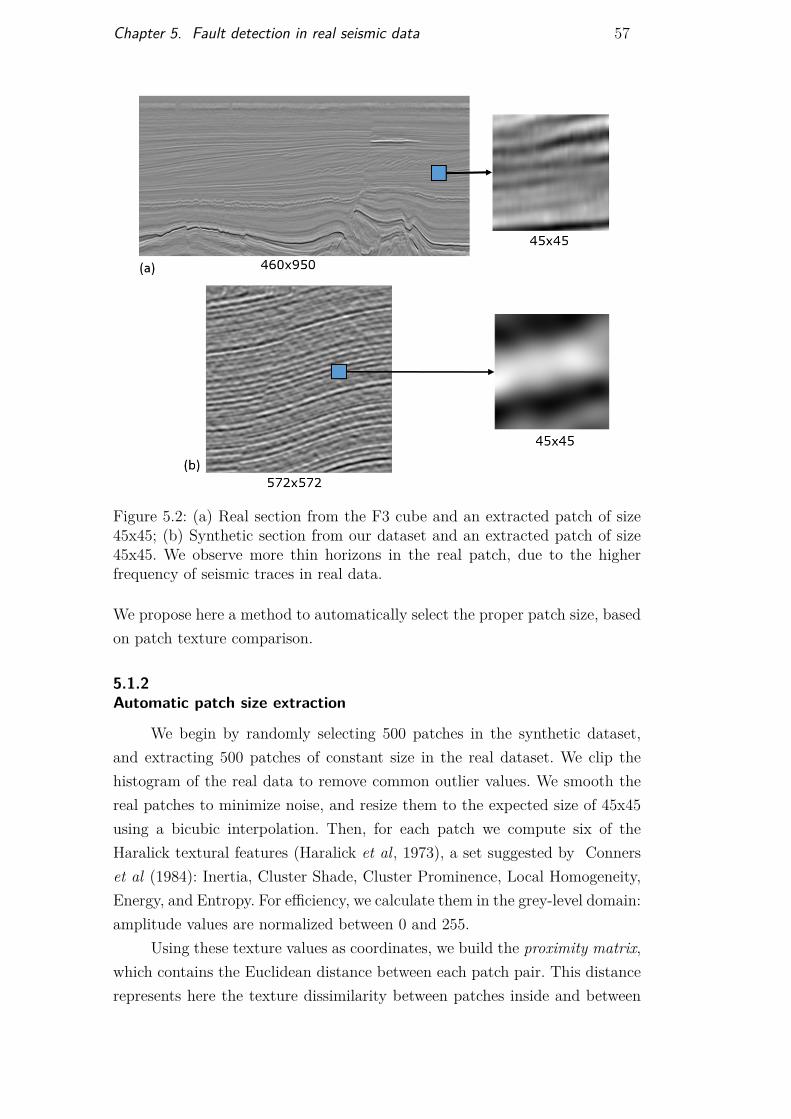
Chapter 5. Fault detection in real seismic data 57
Figure 5.2: (a) Real section from the F3 cube and an extracted patch of size45x45; (b) Synthetic section from our dataset and an extracted patch of size45x45. We observe more thin horizons in the real patch, due to the higherfrequency of seismic traces in real data.
We propose here a method to automatically select the proper patch size, basedon patch texture comparison.
5.1.2Automatic patch size extraction
We begin by randomly selecting 500 patches in the synthetic dataset,and extracting 500 patches of constant size in the real dataset. We clip thehistogram of the real data to remove common outlier values. We smooth thereal patches to minimize noise, and resize them to the expected size of 45x45using a bicubic interpolation. Then, for each patch we compute six of theHaralick textural features (Haralick et al, 1973), a set suggested by Connerset al (1984): Inertia, Cluster Shade, Cluster Prominence, Local Homogeneity,Energy, and Entropy. For efficiency, we calculate them in the grey-level domain:amplitude values are normalized between 0 and 255.
Using these texture values as coordinates, we build the proximity matrix,which contains the Euclidean distance between each patch pair. This distancerepresents here the texture dissimilarity between patches inside and between
DBD
PUC-Rio - Certificação Digital Nº 1413519/CA
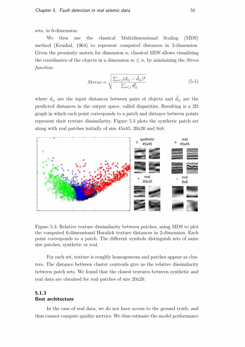
Chapter 5. Fault detection in real seismic data 58
sets, in 6-dimension.We then use the classical Multidimensional Scaling (MDS)
method (Kruskal, 1964) to represent computed distances in 2-dimension.Given the proximity matrix for dimension n, classical MDS allows visualizingthe coordinates of the objects in a dimension m ≤ n, by minimizing the Stressfunction:
Stress =
√√√√∑i<j(dij − dij)2∑i<j d
2ij
(5-1)
where dij are the input distances between pairs of objects and dij are thepredicted distances in the output space, called disparities. Resulting is a 2Dgraph in which each point corresponds to a patch and distance between pointsrepresent their texture dissimilarity. Figure 5.3 plots the synthetic patch setalong with real patches initially of size 45x45, 20x20 and 8x8.
Figure 5.3: Relative texture dissimilarity between patches, using MDS to plotthe computed 6-dimensional Haralick texture distances in 2-dimension. Eachpoint corresponds to a patch. The different symbols distinguish sets of samesize patches, synthetic or real.
For each set, texture is roughly homogeneous and patches appear as clus-ters. The distance between cluster centroids give us the relative dissimilaritybetween patch sets. We found that the closest textures between synthetic andreal data are obtained for real patches of size 20x20.
5.1.3Best architecture
In the case of real data, we do not have access to the ground truth, andthus cannot compute quality metrics. We thus estimate the model performance
DBD
PUC-Rio - Certificação Digital Nº 1413519/CA
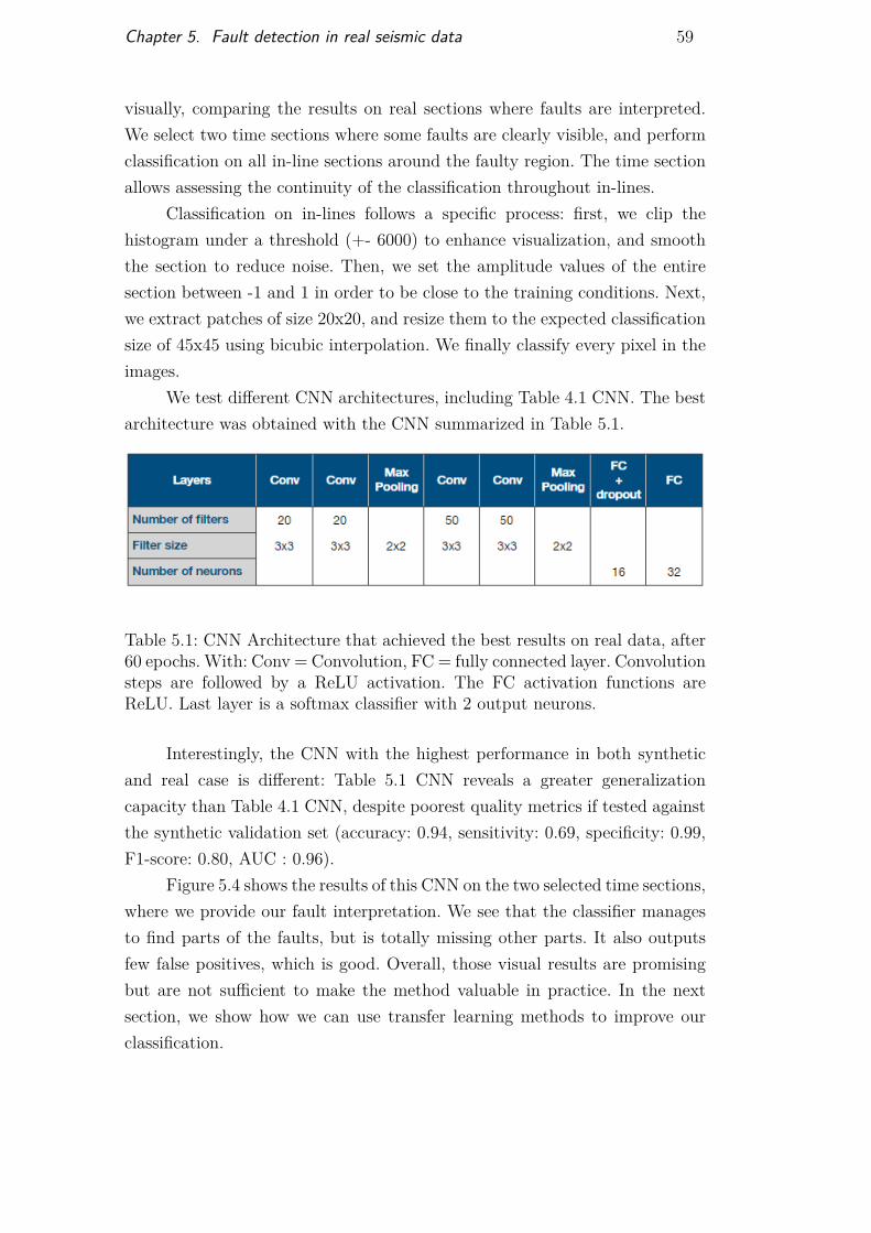
Chapter 5. Fault detection in real seismic data 59
visually, comparing the results on real sections where faults are interpreted.We select two time sections where some faults are clearly visible, and performclassification on all in-line sections around the faulty region. The time sectionallows assessing the continuity of the classification throughout in-lines.
Classification on in-lines follows a specific process: first, we clip thehistogram under a threshold (+- 6000) to enhance visualization, and smooththe section to reduce noise. Then, we set the amplitude values of the entiresection between -1 and 1 in order to be close to the training conditions. Next,we extract patches of size 20x20, and resize them to the expected classificationsize of 45x45 using bicubic interpolation. We finally classify every pixel in theimages.
We test different CNN architectures, including Table 4.1 CNN. The bestarchitecture was obtained with the CNN summarized in Table 5.1.
Table 5.1: CNN Architecture that achieved the best results on real data, after60 epochs. With: Conv = Convolution, FC = fully connected layer. Convolutionsteps are followed by a ReLU activation. The FC activation functions areReLU. Last layer is a softmax classifier with 2 output neurons.
Interestingly, the CNN with the highest performance in both syntheticand real case is different: Table 5.1 CNN reveals a greater generalizationcapacity than Table 4.1 CNN, despite poorest quality metrics if tested againstthe synthetic validation set (accuracy: 0.94, sensitivity: 0.69, specificity: 0.99,F1-score: 0.80, AUC : 0.96).
Figure 5.4 shows the results of this CNN on the two selected time sections,where we provide our fault interpretation. We see that the classifier managesto find parts of the faults, but is totally missing other parts. It also outputsfew false positives, which is good. Overall, those visual results are promisingbut are not sufficient to make the method valuable in practice. In the nextsection, we show how we can use transfer learning methods to improve ourclassification.
DBD
PUC-Rio - Certificação Digital Nº 1413519/CA
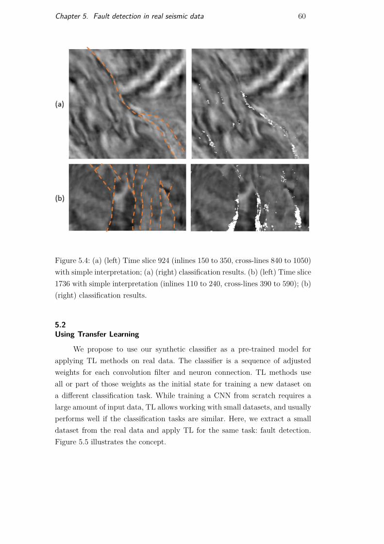
Chapter 5. Fault detection in real seismic data 60
Figure 5.4: (a) (left) Time slice 924 (inlines 150 to 350, cross-lines 840 to 1050)with simple interpretation; (a) (right) classification results. (b) (left) Time slice1736 with simple interpretation (inlines 110 to 240, cross-lines 390 to 590); (b)(right) classification results.
5.2Using Transfer Learning
We propose to use our synthetic classifier as a pre-trained model forapplying TL methods on real data. The classifier is a sequence of adjustedweights for each convolution filter and neuron connection. TL methods useall or part of those weights as the initial state for training a new dataset ona different classification task. While training a CNN from scratch requires alarge amount of input data, TL allows working with small datasets, and usuallyperforms well if the classification tasks are similar. Here, we extract a smalldataset from the real data and apply TL for the same task: fault detection.Figure 5.5 illustrates the concept.
DBD
PUC-Rio - Certificação Digital Nº 1413519/CA
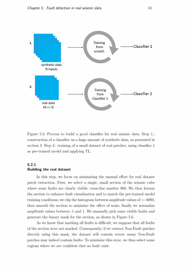
Chapter 5. Fault detection in real seismic data 61
Figure 5.5: Process to build a good classifier for real seismic data. Step 1.:construction of a classifier on a huge amount of synthetic data, as presented insection 3. Step 2.: training of a small dataset of real patches, using classifier 1as pre-trained model and applying TL.
5.2.1Building the real dataset
In this step, we focus on minimizing the manual effort for real datasetpatch extraction. First, we select a single, small section of the seismic cubewhere some faults are clearly visible: cross-line number 900. We then formatthe section to enhance fault visualization and to match the pre-trained modeltraining conditions: we clip the histogram between amplitude values of +- 6000,then smooth the section to minimize the effect of noise, finally we normalizeamplitude values between -1 and 1. We manually pick some visible faults andgenerate the binary mask for the section, as shown in Figure 5.6.
As we know that marking all faults is difficult, we suppose that all faultsof the section were not marked. Consequently, if we extract Non-Fault patchesdirectly using this mask, the dataset will contain errors: many Non-Faultpatches may indeed contain faults. To minimize this error, we thus select someregions where we are confident that no fault exist.
DBD
PUC-Rio - Certificação Digital Nº 1413519/CA
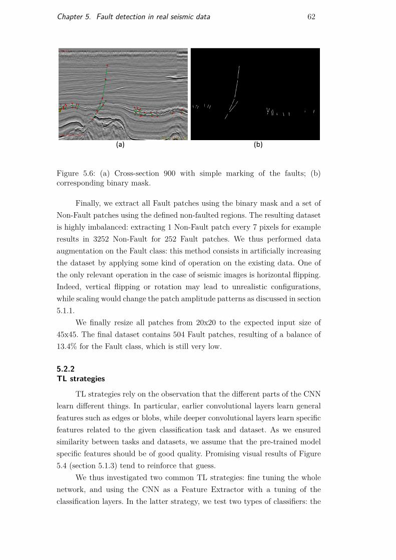
Chapter 5. Fault detection in real seismic data 62
Figure 5.6: (a) Cross-section 900 with simple marking of the faults; (b)corresponding binary mask.
Finally, we extract all Fault patches using the binary mask and a set ofNon-Fault patches using the defined non-faulted regions. The resulting datasetis highly imbalanced: extracting 1 Non-Fault patch every 7 pixels for exampleresults in 3252 Non-Fault for 252 Fault patches. We thus performed dataaugmentation on the Fault class: this method consists in artificially increasingthe dataset by applying some kind of operation on the existing data. One ofthe only relevant operation in the case of seismic images is horizontal flipping.Indeed, vertical flipping or rotation may lead to unrealistic configurations,while scaling would change the patch amplitude patterns as discussed in section5.1.1.
We finally resize all patches from 20x20 to the expected input size of45x45. The final dataset contains 504 Fault patches, resulting of a balance of13.4% for the Fault class, which is still very low.
5.2.2TL strategies
TL strategies rely on the observation that the different parts of the CNNlearn different things. In particular, earlier convolutional layers learn generalfeatures such as edges or blobs, while deeper convolutional layers learn specificfeatures related to the given classification task and dataset. As we ensuredsimilarity between tasks and datasets, we assume that the pre-trained modelspecific features should be of good quality. Promising visual results of Figure5.4 (section 5.1.3) tend to reinforce that guess.
We thus investigated two common TL strategies: fine tuning the wholenetwork, and using the CNN as a Feature Extractor with a tuning of theclassification layers. In the latter strategy, we test two types of classifiers: the
DBD
PUC-Rio - Certificação Digital Nº 1413519/CA
Chapter 5. Fault detection in real seismic data 63
Multi-Layer Perceptron (MLP) and the Support Vector Machine (SVM).
Full fine tuning (FFT)
We train the entire network with initial weights the pre-trained modelweights instead of random ones. In this context, the learning rate should below in order to avoid a sudden change in weights during back-propagation.The number of epochs should also be low to avoid overfitting.
Feature extractor with MLP (FE-MLP)
We freeze the weights of the whole convolutional part of the CNN, inorder to extract fixed features that we feed in the fully connected layers. Wefix the number of hidden layers to 2 with dropout between layers, and thelearning rate to 0.01. We tune the number of neurons in each layer, and thenumber of epochs.
Feature extractor with SVM (FE-SVM)
In many deep learning applications, SVM proved better than MLP atpredicting classes, given good input features (Tang, 2013). To find a goodSVM classifier, we tune the SVM kernel type (linear, polynomial and RBF)and the value of constant C controlling the penalization of outliers and thusthe softness of the SVM margins.
5.2.3Results
We use as benchmark the pre-trained model applied on real data withoutTL, presented in section 5.1.3, Table 5.1. Table 5.2 shows the parameters andthe numerical performances of each model. Benchmark metrics were calculatedover the entire real dataset. For TL models, due to the small size and highimbalance of the dataset, metrics were averaged over a 5-fold cross-validation,respecting in each fold the class proportions. We considered the Fault class asthe positive class.
The benchmark model shows a high specificity, confirming our visualconclusions that it outputs few false positives: it is good at discarding faults.However, it has a very low sensitivity, indeed as we saw it misses a lot of faultsin practice.
DBD
PUC-Rio - Certificação Digital Nº 1413519/CA
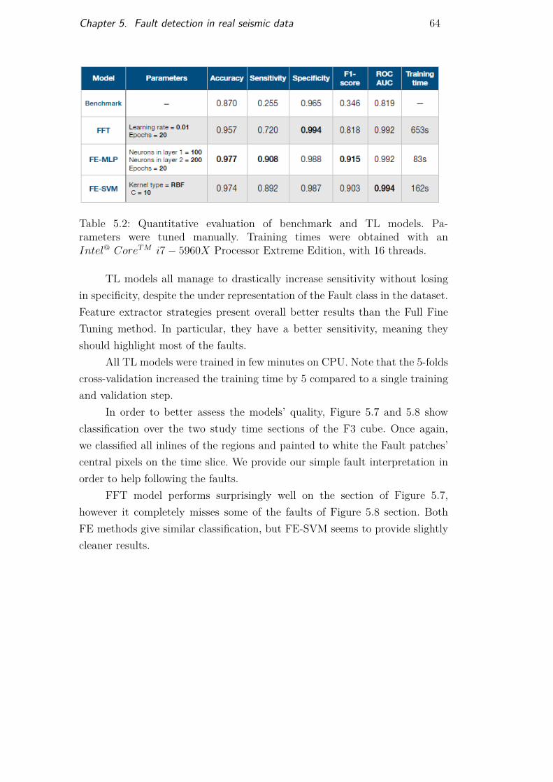
Chapter 5. Fault detection in real seismic data 64
Table 5.2: Quantitative evaluation of benchmark and TL models. Pa-rameters were tuned manually. Training times were obtained with anIntel@ CoreTM i7− 5960X Processor Extreme Edition, with 16 threads.
TL models all manage to drastically increase sensitivity without losingin specificity, despite the under representation of the Fault class in the dataset.Feature extractor strategies present overall better results than the Full FineTuning method. In particular, they have a better sensitivity, meaning theyshould highlight most of the faults.
All TL models were trained in few minutes on CPU. Note that the 5-foldscross-validation increased the training time by 5 compared to a single trainingand validation step.
In order to better assess the models’ quality, Figure 5.7 and 5.8 showclassification over the two study time sections of the F3 cube. Once again,we classified all inlines of the regions and painted to white the Fault patches’central pixels on the time slice. We provide our simple fault interpretation inorder to help following the faults.
FFT model performs surprisingly well on the section of Figure 5.7,however it completely misses some of the faults of Figure 5.8 section. BothFE methods give similar classification, but FE-SVM seems to provide slightlycleaner results.
DBD
PUC-Rio - Certificação Digital Nº 1413519/CA
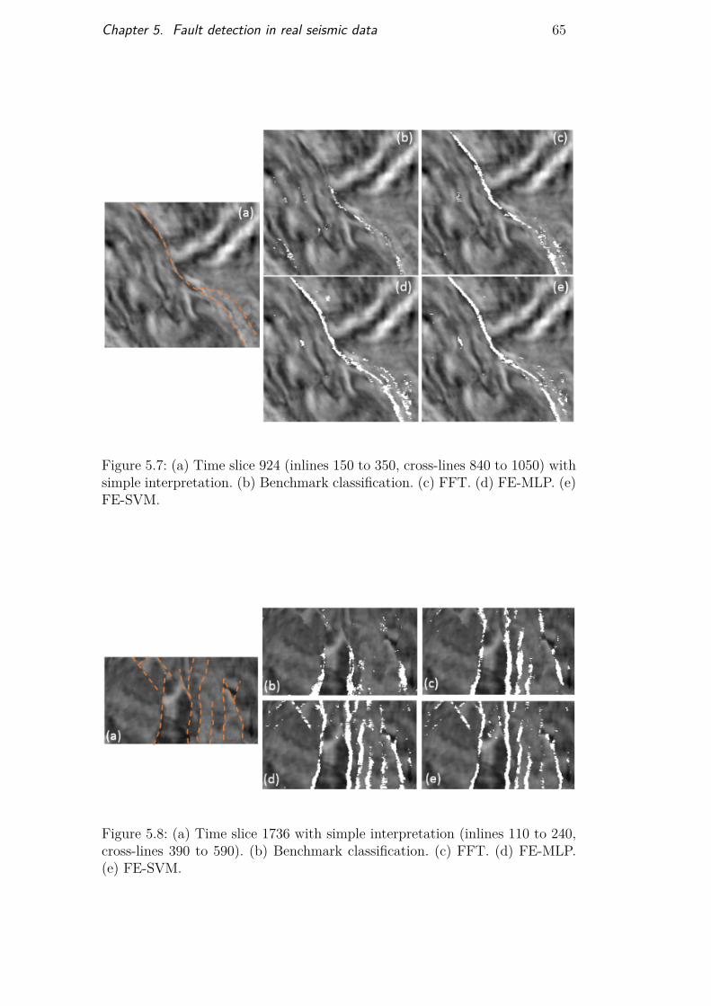
Chapter 5. Fault detection in real seismic data 65
Figure 5.7: (a) Time slice 924 (inlines 150 to 350, cross-lines 840 to 1050) withsimple interpretation. (b) Benchmark classification. (c) FFT. (d) FE-MLP. (e)FE-SVM.
Figure 5.8: (a) Time slice 1736 with simple interpretation (inlines 110 to 240,cross-lines 390 to 590). (b) Benchmark classification. (c) FFT. (d) FE-MLP.(e) FE-SVM.
DBD
PUC-Rio - Certificação Digital Nº 1413519/CA
6Conclusions for Part I
6.1Summary
This part presented a methodology for the detection of faults in seis-mic amplitude images, using a patch-based CNN approach for training andclassification. CNNs were first trained with synthetic data only and yieldedgood results when applied to new synthetic data, with a perfect match of thepredicted and ground truth fault after applying the Hough Transform post pro-cess. They also revealed promising when classifying pre-processed real data,leading us to use our best CNN architecture as base model to TL processes inorder to adapt the classifier to our real data case study. With a small datasetgenerated by marking only some of the faults on a single cross-section, we wereable to build a satisfying classifier trained in a few minutes on CPU.
6.2Conclusions
The use of CNN allowed us to train with the seismic amplitude mapas the only input feature: explicit feature extraction through computationand selection of seismic attributes was unnecessary. However, we highlightedthe large number of empirical parameters used in CNNs, which makes modelfine-tuning difficult. We were able to overcome this drawback with the use ofTL. Detecting real faults using TL from the synthetic seismic data classifiershowed powerful despite the naturally high imbalance of classes in real data.The proposed strategies implied a tuning of a small number of parameters, theFeature Extractor with SVM model being the easiest to adjust. Using a CNNtrained with synthetic data, this work shows that it is not necessary to havea large amount of well-marked real data to build a good fault detector withsupervised techniques. However, results tend to mimic the interpretation andtheir quality thus depends on the quality of the marking.
DBD
PUC-Rio - Certificação Digital Nº 1413519/CA
Chapter 6. Conclusions for Part I 67
6.3Suggestions for further research
There are several research directions we can suggest to improve this workand go further.
First, we could improve the synthetic dataset by generating data withthe commonly seen frequencies in real seismic signals. With this new data, wecould investigate multi-scale CNNs, as in Schlegl et al (2015).
Second, we could improve the synthetic classifier in different ways.Patches of the type Partial Fault could be added as a new class during train-ing. One idea could also be to assign a value of the distance of a patch to thefault instead of a fixed class. Patches far from the fault would receive a higherpenalization if classified as Fault, taking as, for example, the work from Araya-Polo et al (2017). Also, the architecture of the CNN could be improved: wecould try to visualize and better understand the generated features, for exam-ple using the Layer-Wise Relevance Propagation (LRP) method (Bach et al,2015). We could also use evolutionary or other optimization algorithms to findthe best architecture automatically (for example, see the work from Yamasakiet al (2017)).
Concerning TL results, a straightforward test to improve the classifica-tion is to increase the size of the real dataset, for example by classifying anothersection. Also, we could test other balance between the two classes. Other pre-trained models could also be studied. As shown in (Wang et al, 2018), thereare many ways to build the main classifier, using synthetic or real data andeven non-migrated data. Powerful pre-trained classification models like VGG-Net (Simonyan and Zisserman, 2014) are readily available online, and it wouldbe interesting to compare the TL performances using such models, trained on atremendous amount of images from the ImageNet database (Deng et al, 2009),with TL from models designed explicitly for fault detection as presented here.
Another line of research to improve the method is to work on the post-processing step used to extract the exact fault location from the classificationresults. In the synthetic case, faults are straight lines and simple morphologicaloperations coupled with the Hough transform were enough to obtain a perfectmatch between predictions and ground truth. With real data, this processshould be adapted to faults with any geometry, for example in the fashionproposed by Wang and AlRegib (2014).
One interesting research direction is also the exploitation of the three-dimensional information contained in seismic cubes. A simple way to do thiswould be to classify not only in-line sections but also cross-line sections: thisshould help us detecting some false positives, and faults in various directions.
DBD
PUC-Rio - Certificação Digital Nº 1413519/CA
Chapter 6. Conclusions for Part I 68
More interesting, the IPF code used to generate synthetic data allows building3D cubes: we could develop a CNN taking as input 3D patches.
Finally, during the few months of writing this thesis, many articlesand expanded abstracts have been published on seismic fault detection usingdeep learning, showing the interest of the community in this approach. Twoconferences in particular present many works which directions seem verysimilar to our CNN, patch-based approach: the 80th EAGE Annual Conferenceand Exhibition (June 2018) and the SEG International Exposition and 88thAnnual Meeting, which will be held in October 2018. All those works canindeed be an excellent source of inspiration for future research in our field. Wealso wish to cite two interesting published articles during this period. Xiong etal (2018) trained a CNN with seven annotated synthetic and real seismic cubesto compute fault probability maps which showed better results than coherencemaps: the number and the diversity of their data ensure the generalizationcapacity of their method, but require a considerable effort for preparing thedata. Lu et al (2018) proposed a pre-process based on a Generative AdversarialNetworks (GAN) to enhance the performances of an existing fault detectionnetwork: this is an interesting alternative to our TL method for improving theresults of a pre-existing CNN.
DBD
PUC-Rio - Certificação Digital Nº 1413519/CA
Part II
Adaptive all-quadrilateral FEMmesh generation
DBD
PUC-Rio - Certificação Digital Nº 1413519/CA
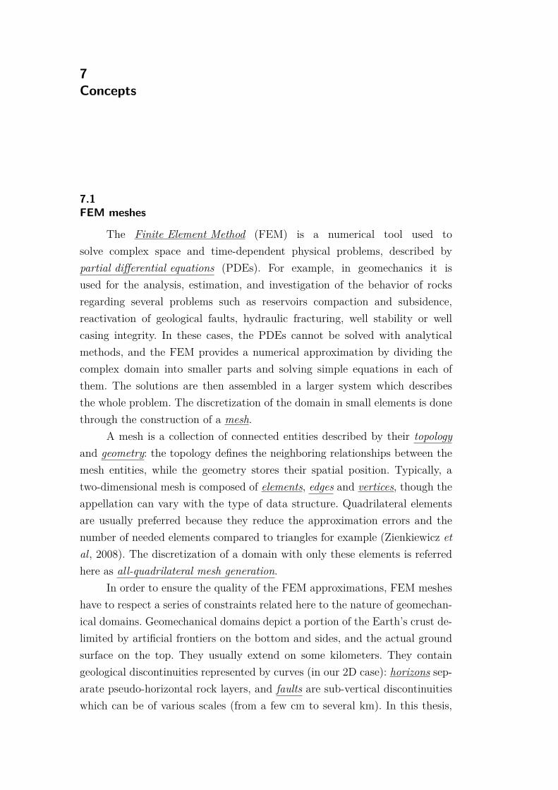
7Concepts
7.1FEM meshes
The Finite Element Method (FEM) is a numerical tool used tosolve complex space and time-dependent physical problems, described bypartial differential equations (PDEs). For example, in geomechanics it isused for the analysis, estimation, and investigation of the behavior of rocksregarding several problems such as reservoirs compaction and subsidence,reactivation of geological faults, hydraulic fracturing, well stability or wellcasing integrity. In these cases, the PDEs cannot be solved with analyticalmethods, and the FEM provides a numerical approximation by dividing thecomplex domain into smaller parts and solving simple equations in each ofthem. The solutions are then assembled in a larger system which describesthe whole problem. The discretization of the domain in small elements is donethrough the construction of a mesh.
A mesh is a collection of connected entities described by their topologyand geometry: the topology defines the neighboring relationships between themesh entities, while the geometry stores their spatial position. Typically, atwo-dimensional mesh is composed of elements, edges and vertices, though theappellation can vary with the type of data structure. Quadrilateral elementsare usually preferred because they reduce the approximation errors and thenumber of needed elements compared to triangles for example (Zienkiewicz etal, 2008). The discretization of a domain with only these elements is referredhere as all-quadrilateral mesh generation.
In order to ensure the quality of the FEM approximations, FEM mesheshave to respect a series of constraints related here to the nature of geomechan-ical domains. Geomechanical domains depict a portion of the Earth’s crust de-limited by artificial frontiers on the bottom and sides, and the actual groundsurface on the top. They usually extend on some kilometers. They containgeological discontinuities represented by curves (in our 2D case): horizons sep-arate pseudo-horizontal rock layers, and faults are sub-vertical discontinuitieswhich can be of various scales (from a few cm to several km). In this thesis,
DBD
PUC-Rio - Certificação Digital Nº 1413519/CA

Chapter 7. Concepts 71
we call all curves the domain boundaries. Figure 7.1 shows an example of sucha domain.
Figure 7.1: Example of a two-dimensional geomechanical domain.
Inside a rock layer, properties such as porosity or permeability are consid-ered constant. Consequently, any flow or pressure propagation simulation willpresent the highest variability at the vicinity of faults and at the discontinuitybetween rock layers: the horizons. Those facts allow understanding some of therestrictions a FEM mesh has to respect in order to produce a good solution:
− alignment with the discontinuities: properties have to be constant at thescale of each finite element, so it cannot cross any curve in the domain.An element can touch a curve by a vertex or an entire edge only;
− precision: alignment with the discontinuities have to be as precise aspossible in order to minimize the approximation errors at their vicinity;
− adaptivity: the size of the elements should be small enough near thediscontinuities to catch the variations of the studied field. Far from them,they can be larger since properties vary less. Varying the size of theelements throughout the domain also allows for creating less elements,thus minimizing the FEM computational effort.
Additionally, any FEM mesh should respect some topological and geo-metrical constraints:
− conformity: neighboring elements must share entire edges and vertices;− element’s quality: the quality of the solution depends on the elements’
quality, related to their shape. Ideally, elements must be close to perfectsquares, as local deformations lower the method’s accuracy and can evenbe a blocker to calculations if any element presents a null or negativearea.
DBD
PUC-Rio - Certificação Digital Nº 1413519/CA
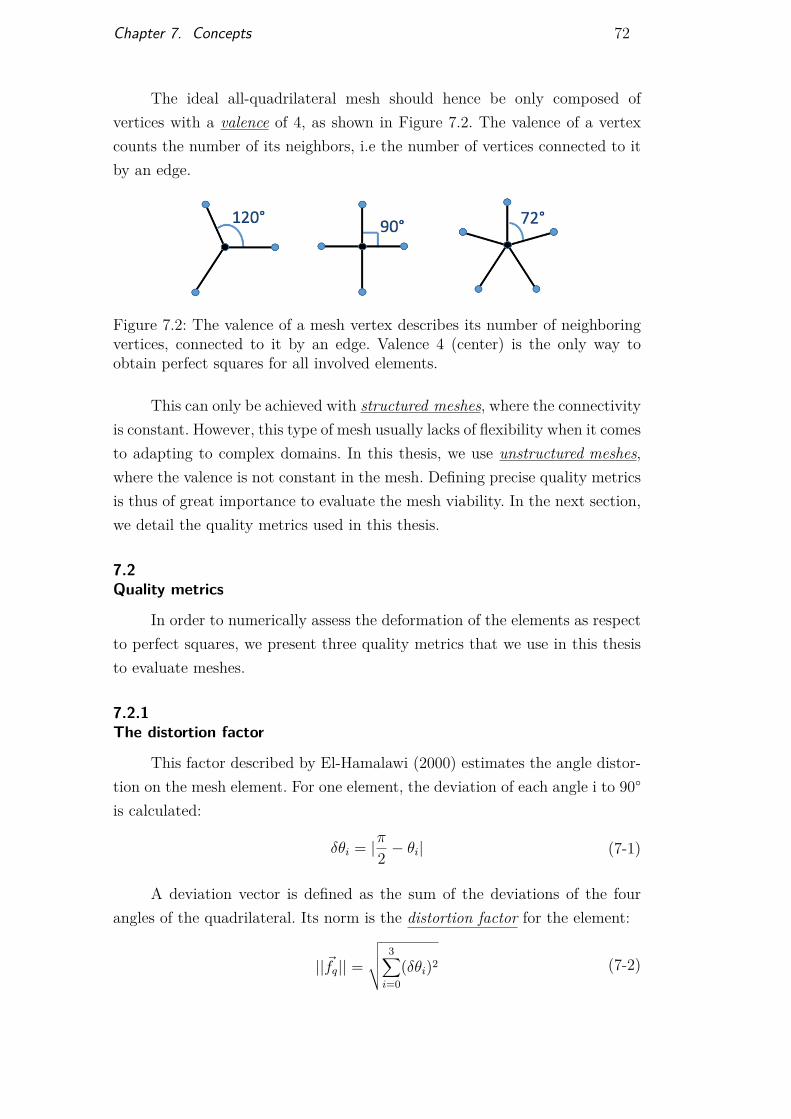
Chapter 7. Concepts 72
The ideal all-quadrilateral mesh should hence be only composed ofvertices with a valence of 4, as shown in Figure 7.2. The valence of a vertexcounts the number of its neighbors, i.e the number of vertices connected to itby an edge.
Figure 7.2: The valence of a mesh vertex describes its number of neighboringvertices, connected to it by an edge. Valence 4 (center) is the only way toobtain perfect squares for all involved elements.
This can only be achieved with structured meshes, where the connectivityis constant. However, this type of mesh usually lacks of flexibility when it comesto adapting to complex domains. In this thesis, we use unstructured meshes,where the valence is not constant in the mesh. Defining precise quality metricsis thus of great importance to evaluate the mesh viability. In the next section,we detail the quality metrics used in this thesis.
7.2Quality metrics
In order to numerically assess the deformation of the elements as respectto perfect squares, we present three quality metrics that we use in this thesisto evaluate meshes.
7.2.1The distortion factor
This factor described by El-Hamalawi (2000) estimates the angle distor-tion on the mesh element. For one element, the deviation of each angle i to 90°is calculated:
δθi = |π2 − θi| (7-1)
A deviation vector is defined as the sum of the deviations of the fourangles of the quadrilateral. Its norm is the distortion factor for the element:
||~fq|| =
√√√√ 3∑i=0
(δθi)2 (7-2)
DBD
PUC-Rio - Certificação Digital Nº 1413519/CA
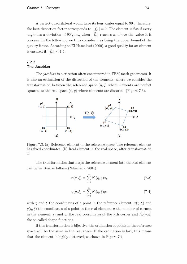
Chapter 7. Concepts 73
A perfect quadrilateral would have its four angles equal to 90°; therefore,the best distortion factor corresponds to ||~fq|| = 0. The element is flat if everyangle has a deviation of 90°, i.e., when ||~fq|| reaches π; above this value it isconcave. In the following, we thus consider π as being the upper bound of thequality factor. According to El-Hamalawi (2000), a good quality for an elementis ensured if ||~fq|| < 1.5.
7.2.2The Jacobian
The jacobian is a criterion often encountered in FEM mesh generators. Itis also an estimation of the distortion of the elements, where we consider thetransformation between the reference space (η, ξ) where elements are perfectsquares, to the real space (x, y) where elements are distorted (Figure 7.3).
Figure 7.3: (a) Reference element in the reference space. The reference elementhas fixed coordinates. (b) Real element in the real space, after transformationT.
The transformation that maps the reference element into the real elementcan be written as follows (Nikishkov, 2004):
x(η, ξ) =n∑i=1
Ni(η, ξ)xi (7-3)
y(η, ξ) =n∑i=1
Ni(η, ξ)yi (7-4)
with η and ξ the coordinates of a point in the reference element, x(η, ξ) andy(η, ξ) the coordinates of a point in the real element, n the number of cornersin the element, xi and yi the real coordinates of the i-th corner and Ni(η, ξ)the so-called shape functions.
If this transformation is bijective, the ordination of points in the referencespace will be the same in the real space. If the ordination is lost, this meansthat the element is highly distorted, as shown in Figure 7.4.
DBD
PUC-Rio - Certificação Digital Nº 1413519/CA

Chapter 7. Concepts 74
Figure 7.4: Taking p1 as reference point: (a) corners are ordered anti-clockwise;(b) a slight deformation does not affect the corners ordination; (c) when theelement is highly distorted the ordination is lost as p3 comes in second in theincreasing angle θ sequence.
The local bijectivity of the transformation can be assessed throughthe determinant of its Jacobian matrix: if the transformation is bijective,the determinant should be strictly positive. The Jacobian matrix of thetransformation and its determinant can be written as follows:
J =∂x∂ξ ∂y
∂ξ∂x∂η
∂y∂η
=∂N1
∂ξ. . . ∂Ni
∂ξ. . . ∂Nn
∂ξ∂N1∂η
. . . ∂Ni
∂η. . . ∂Nn
∂η
x1 y1... ...xi yi... ...xn yn
=J11 J12
J21 J22
(7-5)
det J = J11J22 − J12J21 (7-6)
In the case of a quadrilateral, the shape function and its derivative aregiven as:
[N ]T = 14
(1− ξ)(1− η)(1 + ξ)(1 + η)(1 + ξ)(1 + η)(1− ξ)(1 + η)
(7-7)
[∂N
∂ξ
]T= 1
4
−(1− η)
1− η1 + η−(1 + η)
(7-8)
[∂N
∂η
]T= 1
4
−(1− ξ)−(1 + ξ)
1 + ξ1− ξ
(7-9)
In practice, the Jacobian factor corresponds to a single value for each
DBD
PUC-Rio - Certificação Digital Nº 1413519/CA
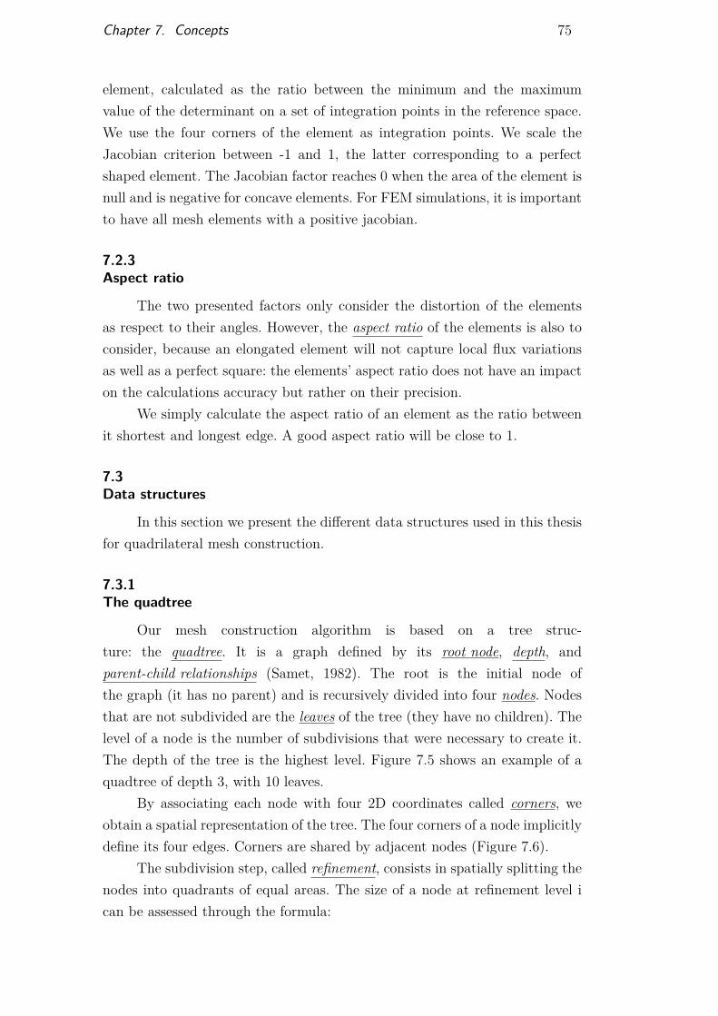
Chapter 7. Concepts 75
element, calculated as the ratio between the minimum and the maximumvalue of the determinant on a set of integration points in the reference space.We use the four corners of the element as integration points. We scale theJacobian criterion between -1 and 1, the latter corresponding to a perfectshaped element. The Jacobian factor reaches 0 when the area of the element isnull and is negative for concave elements. For FEM simulations, it is importantto have all mesh elements with a positive jacobian.
7.2.3Aspect ratio
The two presented factors only consider the distortion of the elementsas respect to their angles. However, the aspect ratio of the elements is also toconsider, because an elongated element will not capture local flux variationsas well as a perfect square: the elements’ aspect ratio does not have an impacton the calculations accuracy but rather on their precision.
We simply calculate the aspect ratio of an element as the ratio betweenit shortest and longest edge. A good aspect ratio will be close to 1.
7.3Data structures
In this section we present the different data structures used in this thesisfor quadrilateral mesh construction.
7.3.1The quadtree
Our mesh construction algorithm is based on a tree struc-ture: the quadtree. It is a graph defined by its root node, depth, andparent-child relationships (Samet, 1982). The root is the initial node ofthe graph (it has no parent) and is recursively divided into four nodes. Nodesthat are not subdivided are the leaves of the tree (they have no children). Thelevel of a node is the number of subdivisions that were necessary to create it.The depth of the tree is the highest level. Figure 7.5 shows an example of aquadtree of depth 3, with 10 leaves.
By associating each node with four 2D coordinates called corners, weobtain a spatial representation of the tree. The four corners of a node implicitlydefine its four edges. Corners are shared by adjacent nodes (Figure 7.6).
The subdivision step, called refinement, consists in spatially splitting thenodes into quadrants of equal areas. The size of a node at refinement level ican be assessed through the formula:
DBD
PUC-Rio - Certificação Digital Nº 1413519/CA
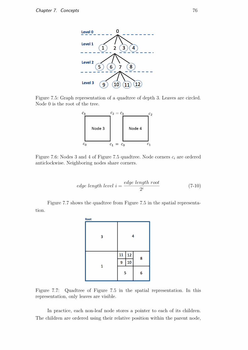
Chapter 7. Concepts 76
Figure 7.5: Graph representation of a quadtree of depth 3. Leaves are circled.Node 0 is the root of the tree.
Figure 7.6: Nodes 3 and 4 of Figure 7.5 quadtree. Node corners ci are orderedanticlockwise. Neighboring nodes share corners.
edge length level i = edge length root
2i (7-10)
Figure 7.7 shows the quadtree from Figure 7.5 in the spatial representa-tion.
Figure 7.7: Quadtree of Figure 7.5 in the spatial representation. In thisrepresentation, only leaves are visible.
In practice, each non-leaf node stores a pointer to each of its children.The children are ordered using their relative position within the parent node,
DBD
PUC-Rio - Certificação Digital Nº 1413519/CA
Chapter 7. Concepts 77
defined by the frontiers they have in common with the parent, using thefour cardinal directions (Figure 7.8). The pointer list is always ordered asfollows: {SW, SE, NW, NE}. The distinctive advantage of this structure is thatthe neighboring information between nodes is quickly recovered. As explainedby Samet (1982), to find a horizontal or vertical neighbor to a node, a commonancestor is found by going up in the tree, then following a backtracking pathmirroring the axis formed by the common boundary of the two nodes.
Figure 7.8: Parent-children relationship in a quadtree. (a) Orientation ofparent frontiers; (b) Position of children correspond to the parent frontier theyare in contact with.
The spatial quadtree can be seen as a quadrilateral mesh, howeveradjacent nodes of different refinement level present hanging corners and thisis hence not a conform structure. Schneiders et al (1996) proposed a set oftransition patterns shown in Figure 7.9 to conform the tree.
Figure 7.9: (a) Transition patterns from (Schneiders et al, 1996); (b) usualrefinement pattern is also involved in the tree conformation; (c) unconformtree; (d) conform tree.
The conventional quadtree structure does not have the flexibility to in-clude those patterns, since the children position and implicit neighborhoodrelationships are not preserved. However, in this thesis we develop a modifica-
DBD
PUC-Rio - Certificação Digital Nº 1413519/CA
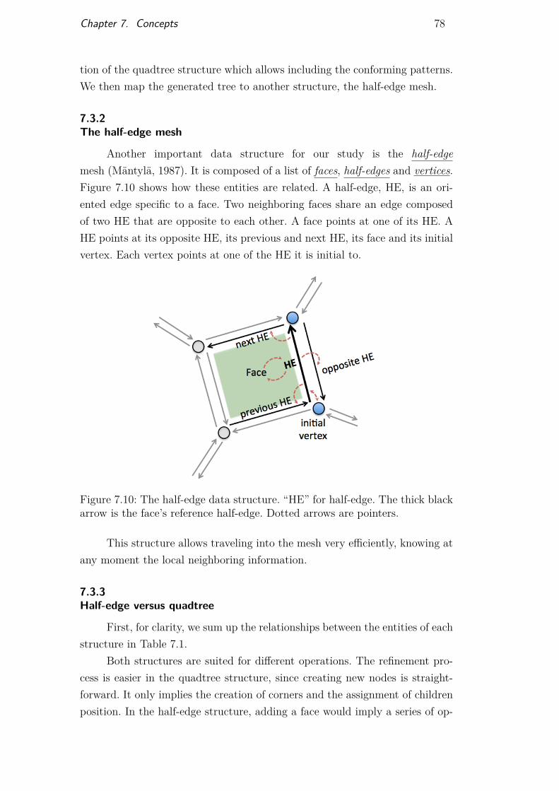
Chapter 7. Concepts 78
tion of the quadtree structure which allows including the conforming patterns.We then map the generated tree to another structure, the half-edge mesh.
7.3.2The half-edge mesh
Another important data structure for our study is the half-edgemesh (Mäntylä, 1987). It is composed of a list of faces, half-edges and vertices.Figure 7.10 shows how these entities are related. A half-edge, HE, is an ori-ented edge specific to a face. Two neighboring faces share an edge composedof two HE that are opposite to each other. A face points at one of its HE. AHE points at its opposite HE, its previous and next HE, its face and its initialvertex. Each vertex points at one of the HE it is initial to.
Figure 7.10: The half-edge data structure. “HE” for half-edge. The thick blackarrow is the face’s reference half-edge. Dotted arrows are pointers.
This structure allows traveling into the mesh very efficiently, knowing atany moment the local neighboring information.
7.3.3Half-edge versus quadtree
First, for clarity, we sum up the relationships between the entities of eachstructure in Table 7.1.
Both structures are suited for different operations. The refinement pro-cess is easier in the quadtree structure, since creating new nodes is straight-forward. It only implies the creation of corners and the assignment of childrenposition. In the half-edge structure, adding a face would imply a series of op-
DBD
PUC-Rio - Certificação Digital Nº 1413519/CA
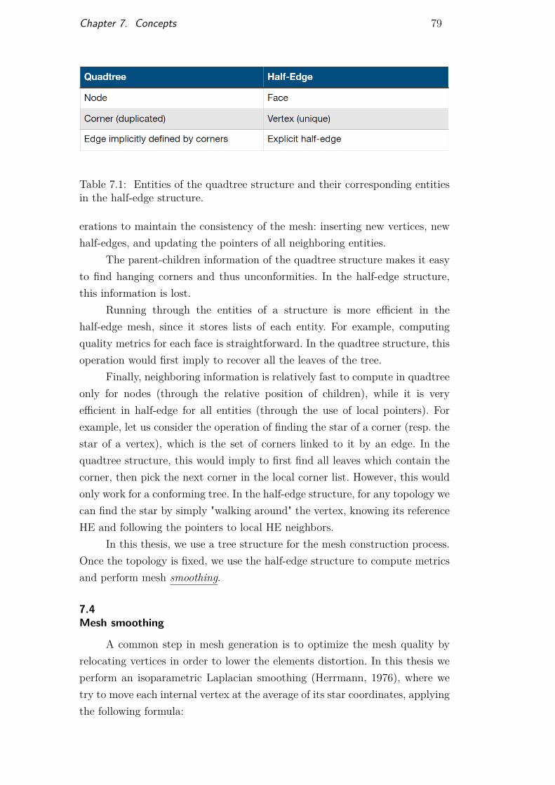
Chapter 7. Concepts 79
Table 7.1: Entities of the quadtree structure and their corresponding entitiesin the half-edge structure.
erations to maintain the consistency of the mesh: inserting new vertices, newhalf-edges, and updating the pointers of all neighboring entities.
The parent-children information of the quadtree structure makes it easyto find hanging corners and thus unconformities. In the half-edge structure,this information is lost.
Running through the entities of a structure is more efficient in thehalf-edge mesh, since it stores lists of each entity. For example, computingquality metrics for each face is straightforward. In the quadtree structure, thisoperation would first imply to recover all the leaves of the tree.
Finally, neighboring information is relatively fast to compute in quadtreeonly for nodes (through the relative position of children), while it is veryefficient in half-edge for all entities (through the use of local pointers). Forexample, let us consider the operation of finding the star of a corner (resp. thestar of a vertex), which is the set of corners linked to it by an edge. In thequadtree structure, this would imply to first find all leaves which contain thecorner, then pick the next corner in the local corner list. However, this wouldonly work for a conforming tree. In the half-edge structure, for any topology wecan find the star by simply "walking around" the vertex, knowing its referenceHE and following the pointers to local HE neighbors.
In this thesis, we use a tree structure for the mesh construction process.Once the topology is fixed, we use the half-edge structure to compute metricsand perform mesh smoothing.
7.4Mesh smoothing
A common step in mesh generation is to optimize the mesh quality byrelocating vertices in order to lower the elements distortion. In this thesis weperform an isoparametric Laplacian smoothing (Herrmann, 1976), where wetry to move each internal vertex at the average of its star coordinates, applyingthe following formula:
DBD
PUC-Rio - Certificação Digital Nº 1413519/CA

Chapter 7. Concepts 80
v′i = 1N
N∑j=1
vj (7-11)
where v′i is the new location of vertex vi, N is the number of vertices in thestar and vj the coordinates of the j-th neighbor. This process is performedon each vertex of the mesh iteratively. This method is straightforward andefficient, the computation time varying linearly with the number of vertices inthe mesh. However it can generate bad and even inverted quadrilaterals aftera few iterations, and tends to make the elements size uniform. In our case itshould hence be used with few iterations.
DBD
PUC-Rio - Certificação Digital Nº 1413519/CA
8Related works
There are two categories of techniques to generate unstructured all-quadrilateral meshes: indirect and direct methods.
Indirect methods first create a triangle mesh and then convert it intoa quadrilateral mesh. The triangle mesh is usually generated using the con-strained Delaunay triangulation (Chew, 1987). Methods then differ in the stepof converting the triangles into quadrilaterals. A common strategy is to subdi-vide the triangles as introduced by Catmull and Clark (1978): one triangle isdivided into three quadrilaterals by adding a vertex at the centroid of the tri-angle and at the middle of each edge. Generated quadrilaterals tend to have apoor aspect ratio, and Liu et al (2011) improved the resulting mesh by propos-ing a post-processing method based on local topological operations. Anotherstrategy to convert triangles into quadrilaterals is to combine them. Borouchakiand Frey (1998) joined pairs of triangles and divided the remaining ones us-ing the Catmull subdivision. The Q-morph method (Owen et al, 1999) guidesthe combination of triangles using an advancing front strategy. Lee et al(2003) extended the Q-morph method to include open boundaries. Ebeida et al(2010b) introduced the Q-tran method, which joins a combination of triangleswith a new subdivision scheme to generate good-quality quadrilaterals. Re-cently, Araújo and Celes (2014) proposed an algorithm to obtain good-qualitymesh for complex crossing boundaries using a deferred constraint insertionstrategy coupled with a new triangle mesh generation scheme. In general, in-direct methods generate good-quality elements, but meshes suffer from a largenumber of vertices with a valence different from 4.
Direct methods generate quadrilaterals directly. We can group the directmethods into three categories: advancing front, domain decomposition, andgrid-based methods.
Advancing front algorithms generate a first set of elements on theboundaries of the domain and then recursively project the elements towardthe interior, moving the elements front until the domain is totally covered. Asan example, the paving method by Blacker et al (1991) successfully generatesmeshes with good quality. However, advancing front methods tend to lackstability for complicated regions, especially at the meeting of the fronts, and
DBD
PUC-Rio - Certificação Digital Nº 1413519/CA
Chapter 8. Related works 82
usually require post cleanup operations.Domain decomposition techniques subdivide the domain into a set of
simple regions where conventional mapping methods can be applied to generatequadrilaterals. Talbert and Parkinson (1990) proposed a recursive algorithmthat subdivides the complex domain until only basic shaped regions remain; thealgorithm was then improved by Chae and Jeong (1997) and Nowottny (1997).Medial axis decomposition was introduced by Tam and Armstrong (1991)and uses the center of a maximal circle rolled through the area to subdividethe domain. Miranda and Martha (2013) proposed a template strategy fordomain decomposition. These methods generate good-quality meshes butusually require heavy user intervention for complex domains.
Grid-based methods superimpose a grid to the domain and try to adaptit to the boundaries by modifying the grid geometry. It can be any type ofgrid, but quadtrees are often used because they allow a control on the localrefinement, with a smooth size transition. To increase the refinement levelaround domain boundaries, Frey and Marechal (1998) proposed a simple sizecriterion. Ebeida et al (2010a) used a criterion based on the boundary curva-ture, assessed through an initial boundary discretization. The main challengein such methods remains to adapt the grid points to the domain boundaries.For example, Yerry and Shephard (1983) intersected quadtree leaves with theboundaries, allowing the formation of non-quadrilateral elements. This is nota limitation to them since they aim at building a triangle mesh: they simplytriangulate the elements at the end of the process. Rushdi et al (2015) recentlypresented a similar idea to create all-quadrilateral meshes: they first repel somequadtree grid points based on their distance to the boundary to guarantee aclean intersection; then they apply local midpoint subdivisions to turn ele-ments into quadrilaterals. Another method is to remove all elements crossingthe boundary and then reconstruct the missing layer with a post process. Thiscan be done simply with a projection technique (Schneiders and Bünten, 1995)or using some reconstruction patterns (Liang et al, 2009). However, as stressedby Liang et al (2009), these techniques present some difficulties when the bufferlayers face each other and must conform. In any case quadtrees have to undergoa conforming step before being usable as meshes (Schneiders et al, 1996). Thesemethods are easy to implement and generate meshes of good quality. They alsousually allow to bound maximum and minimum angles (Rushdi et al, 2015;Atalay et al, 2008). However, they can easily generate inverted elements andtend to gather lower quality elements on the boundaries.
All those methods tend to be dependent of the domain geometricalcomplexity. In the present work we aim at developing a method that would
DBD
PUC-Rio - Certificação Digital Nº 1413519/CA

Chapter 8. Related works 83
be robust for all kinds of boundaries. Moreover, the method should beusable in the industry and consequently have to be efficient and user-friendly.The quality of the resulting mesh should be adapted to FEM calculationsrequirements. We opted for a grid-based method using a new quadtree-basedhierarchical data structure: the extended quadtree.
DBD
PUC-Rio - Certificação Digital Nº 1413519/CA
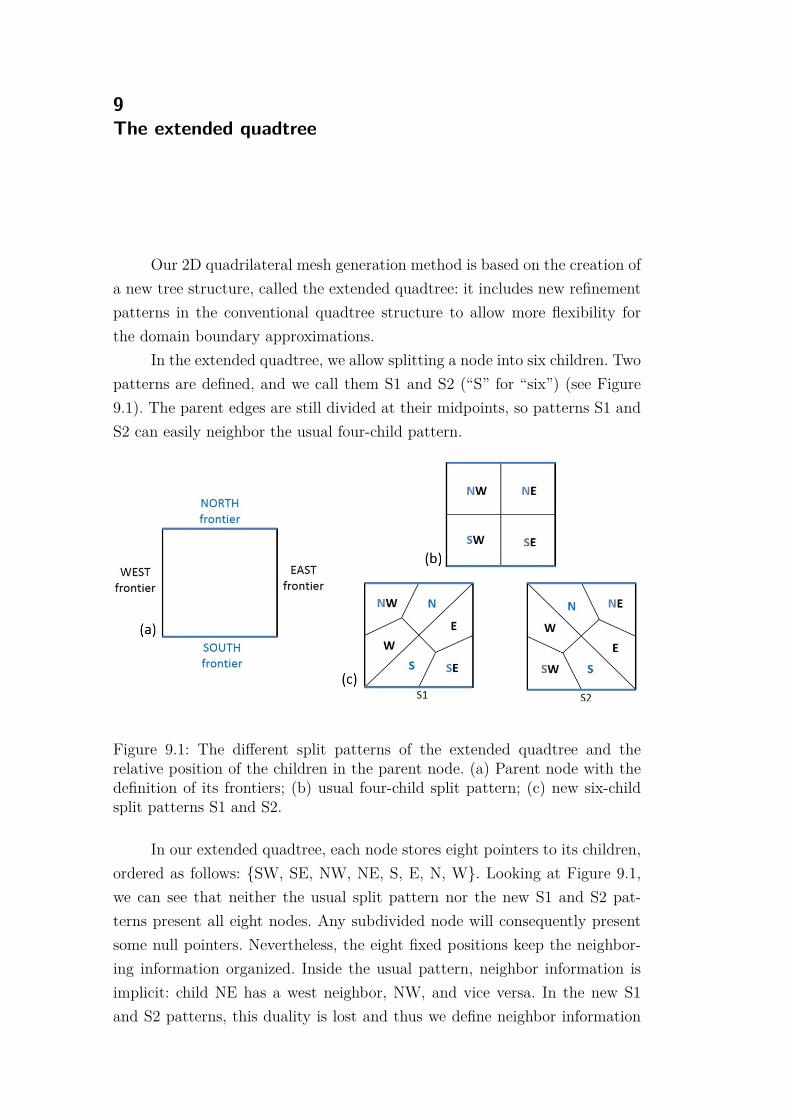
9The extended quadtree
Our 2D quadrilateral mesh generation method is based on the creation ofa new tree structure, called the extended quadtree: it includes new refinementpatterns in the conventional quadtree structure to allow more flexibility forthe domain boundary approximations.
In the extended quadtree, we allow splitting a node into six children. Twopatterns are defined, and we call them S1 and S2 (“S” for “six”) (see Figure9.1). The parent edges are still divided at their midpoints, so patterns S1 andS2 can easily neighbor the usual four-child pattern.
Figure 9.1: The different split patterns of the extended quadtree and therelative position of the children in the parent node. (a) Parent node with thedefinition of its frontiers; (b) usual four-child split pattern; (c) new six-childsplit patterns S1 and S2.
In our extended quadtree, each node stores eight pointers to its children,ordered as follows: {SW, SE, NW, NE, S, E, N, W}. Looking at Figure 9.1,we can see that neither the usual split pattern nor the new S1 and S2 pat-terns present all eight nodes. Any subdivided node will consequently presentsome null pointers. Nevertheless, the eight fixed positions keep the neighbor-ing information organized. Inside the usual pattern, neighbor information isimplicit: child NE has a west neighbor, NW, and vice versa. In the new S1and S2 patterns, this duality is lost and thus we define neighbor information
DBD
PUC-Rio - Certificação Digital Nº 1413519/CA
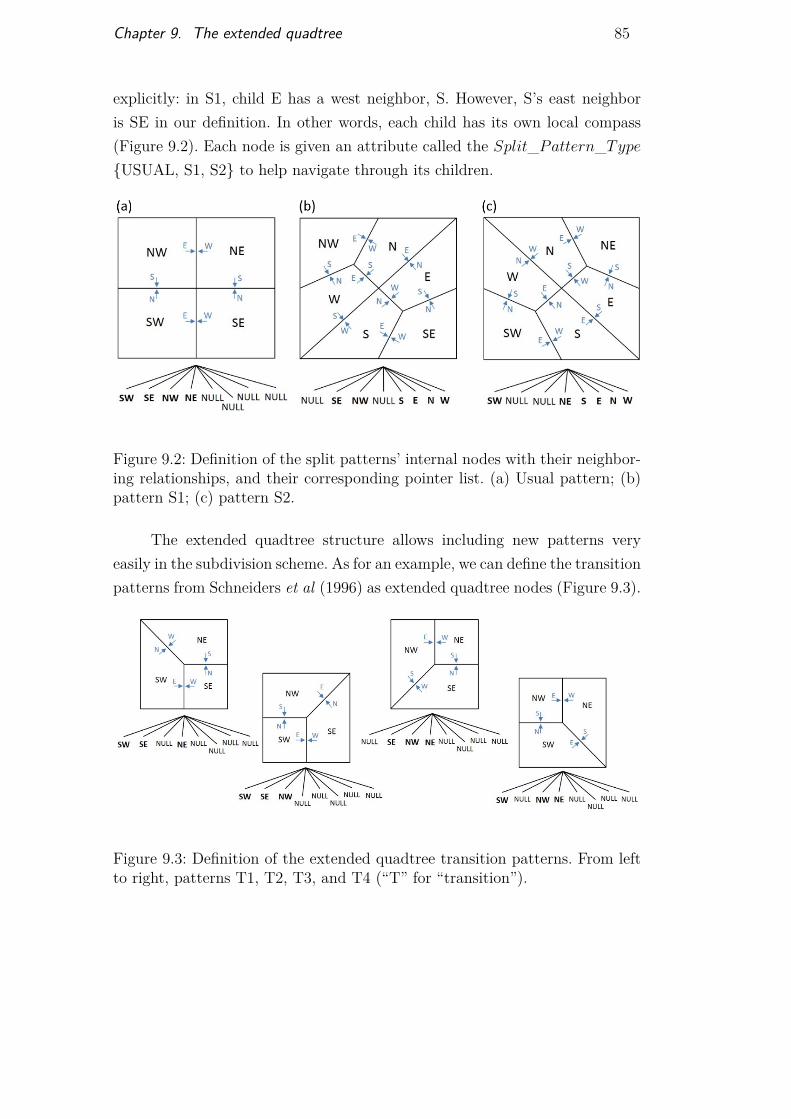
Chapter 9. The extended quadtree 85
explicitly: in S1, child E has a west neighbor, S. However, S’s east neighboris SE in our definition. In other words, each child has its own local compass(Figure 9.2). Each node is given an attribute called the Split_Pattern_Type{USUAL, S1, S2} to help navigate through its children.
Figure 9.2: Definition of the split patterns’ internal nodes with their neighbor-ing relationships, and their corresponding pointer list. (a) Usual pattern; (b)pattern S1; (c) pattern S2.
The extended quadtree structure allows including new patterns veryeasily in the subdivision scheme. As for an example, we can define the transitionpatterns from Schneiders et al (1996) as extended quadtree nodes (Figure 9.3).
Figure 9.3: Definition of the extended quadtree transition patterns. From leftto right, patterns T1, T2, T3, and T4 (“T” for “transition”).
DBD
PUC-Rio - Certificação Digital Nº 1413519/CA
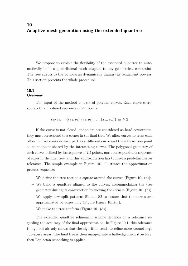
10Adaptive mesh generation using the extended quadtree
We propose to exploit the flexibility of the extended quadtree to auto-matically build a quadrilateral mesh adapted to any geometrical constraint.The tree adapts to the boundaries dynamically during the refinement process.This section presents the whole procedure.
10.1Overview
The input of the method is a set of polyline curves. Each curve corre-sponds to an ordered sequence of 2D points:
curvei = {(x1, y1), (x2, y2), . . . , (xm, ym)},m ≥ 2
If the curve is not closed, endpoints are considered as hard constraints:they must correspond to a corner in the final tree. We allow curves to cross eachother, but we consider each part as a different curve and the intersection pointas an endpoint shared by the intersecting curves. The polygonal geometry ofeach curve, defined by its sequence of 2D points, must correspond to a sequenceof edges in the final tree, and this approximation has to meet a predefined errortolerance. The simple example in Figure 10.1 illustrates the approximationprocess sequence:
− We define the tree root as a square around the curves (Figure 10.1(a));− We build a quadtree aligned to the curves, accommodating the tree
geometry during its construction by moving the corners (Figure 10.1(b));− We apply new split patterns S1 and S2 to ensure that the curves are
approximated by edges only (Figure Figure 10.1(c));− We make the tree conform (Figure 10.1(d)).
The extended quadtree refinement scheme depends on a tolerance re-garding the accuracy of the final approximation. In Figure 10.1, this toleranceis high but already shows that the algorithm tends to refine more around highcurvature areas. The final tree is then mapped into a half-edge mesh structure,then Laplacian smoothing is applied.
DBD
PUC-Rio - Certificação Digital Nº 1413519/CA
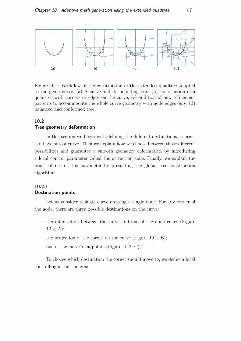
Chapter 10. Adaptive mesh generation using the extended quadtree 87
Figure 10.1: Workflow of the construction of the extended quadtree adaptedto the given curve. (a) A curve and its bounding box; (b) construction of aquadtree with corners or edges on the curve; (c) addition of new refinementpatterns to accommodate the whole curve geometry with node edges only; (d)balanced and conformed tree.
10.2Tree geometry deformation
In this section we begin with defining the different destinations a cornercan have onto a curve. Then we explain how we choose between those differentpossibilities and guarantee a smooth geometry deformation by introducinga local control parameter called the attraction zone. Finally, we explain thepractical use of this parameter by presenting the global tree constructionalgorithm.
10.2.1Destination points
Let us consider a single curve crossing a single node. For any corner ofthe node, there are three possible destinations on the curve:
− the intersection between the curve and one of the node edges (Figure10.2, A);
− the projection of the corner on the curve (Figure 10.2, B);
− one of the curve’s endpoints (Figure 10.2, C);
To choose which destination the corner should move to, we define a localcontrolling attraction zone.
DBD
PUC-Rio - Certificação Digital Nº 1413519/CA

Chapter 10. Adaptive mesh generation using the extended quadtree 88
Figure 10.2: All considered destination points for a given corner onto a curvecrossing a node.
10.2.2The attraction zone
In order to ensure a smooth deformation of the tree geometry at eachrefinement step, we define a local parameter based on each node dimensionsto control the movement of its corners. Indeed, the deformation of a node istransmitted to all of its children, and, thus, we must not allow big deformationsat low refinement levels.
For each node corner, we define an area called the attraction zone: if thecorner’s destination point is inside the attraction zone, then the corner canmove to its new position. This area corresponds to a proportion of the totalnode area around the corner: it is a quadrilateral which dimensions are givenby a proportion of the two edges adjacent to the corner (Figure 10.3). Thisproportion is given by the ratio parameter:
ratio = ratiomax −reflevel(ratiomax − ratiomin)
refmax(10-1)
where ratiomax is the maximum value of ratio, defined by the user and superiorto ratiomin; ratiomin is the minimum value of ratio and is fixed to 2, which cutsthe edge at its mid length; reflevel is the node’s current refinement level; andrefmax is the user-defined refinement level from which ratio reaches ratiomin.
ratiomax defines the smallest proportion of the attraction zone, whichwill be considered at the lowest refinement level. The attraction zone thenincreases smoothly at each refinement step, reaching its maximum proportionfor the refinement level refmax. At this stage, the total area of the node iscovered by its four corners’ attraction zones. This means that, for any curvecrossing the node, at least one corner should be able to move onto it. It isimportant to use the real length of the edges in the definition of the attractionzone to account for node deformation and avoid building an area that exceedsthe limits of the node. Above the user-defined value of parameter refmax, ratiois maintained to ratiomin.
DBD
PUC-Rio - Certificação Digital Nº 1413519/CA
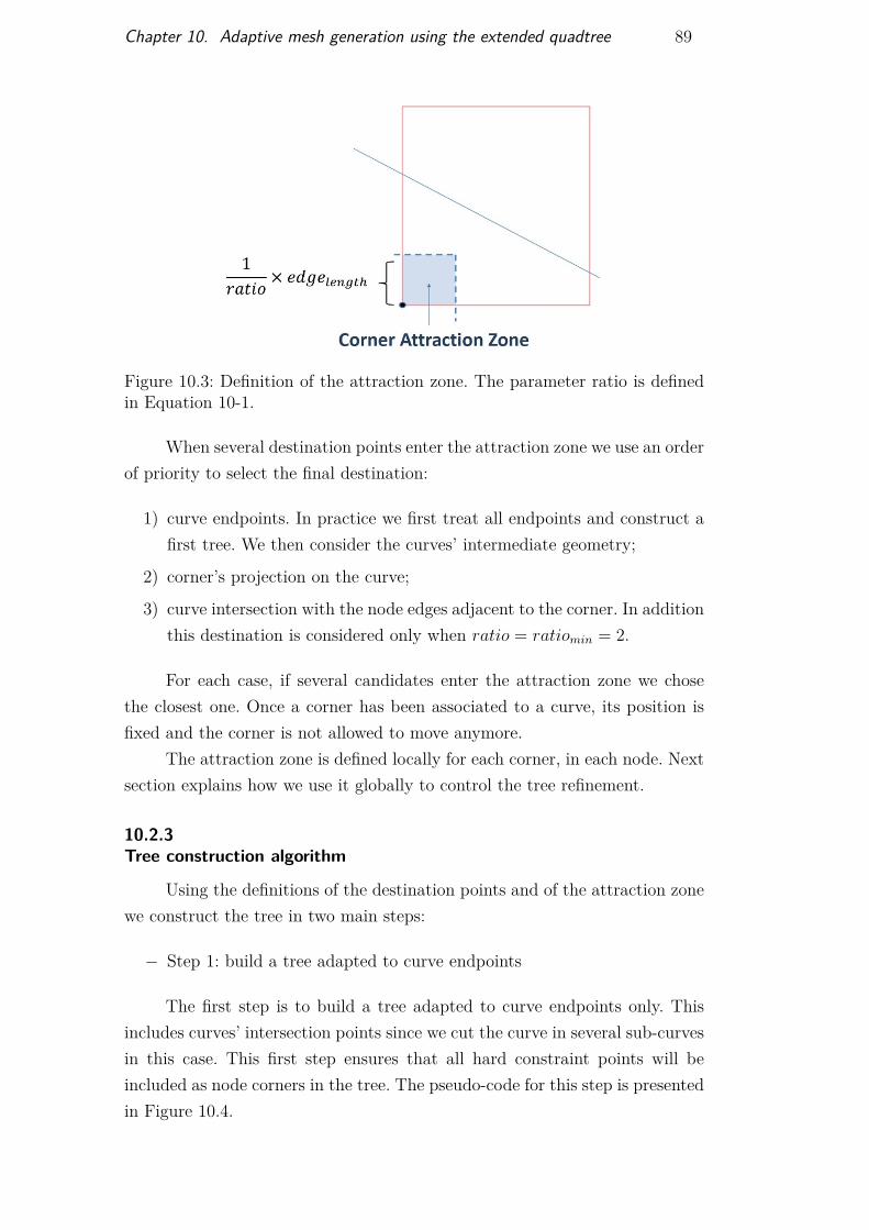
Chapter 10. Adaptive mesh generation using the extended quadtree 89
Figure 10.3: Definition of the attraction zone. The parameter ratio is definedin Equation 10-1.
When several destination points enter the attraction zone we use an orderof priority to select the final destination:
1) curve endpoints. In practice we first treat all endpoints and construct afirst tree. We then consider the curves’ intermediate geometry;
2) corner’s projection on the curve;
3) curve intersection with the node edges adjacent to the corner. In additionthis destination is considered only when ratio = ratiomin = 2.
For each case, if several candidates enter the attraction zone we chosethe closest one. Once a corner has been associated to a curve, its position isfixed and the corner is not allowed to move anymore.
The attraction zone is defined locally for each corner, in each node. Nextsection explains how we use it globally to control the tree refinement.
10.2.3Tree construction algorithm
Using the definitions of the destination points and of the attraction zonewe construct the tree in two main steps:
− Step 1: build a tree adapted to curve endpoints
The first step is to build a tree adapted to curve endpoints only. Thisincludes curves’ intersection points since we cut the curve in several sub-curvesin this case. This first step ensures that all hard constraint points will beincluded as node corners in the tree. The pseudo-code for this step is presentedin Figure 10.4.
DBD
PUC-Rio - Certificação Digital Nº 1413519/CA
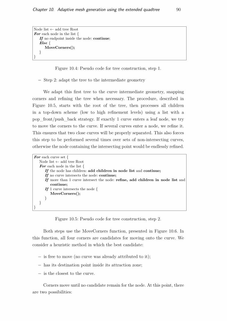
Chapter 10. Adaptive mesh generation using the extended quadtree 90
Node list ← add tree RootFor each node in the list {
If no endpoint inside the node: continue;Else {
MoveCorners();}
}
Figure 10.4: Pseudo code for tree construction, step 1.
− Step 2: adapt the tree to the intermediate geometry
We adapt this first tree to the curve intermediate geometry, snappingcorners and refining the tree when necessary. The procedure, described inFigure 10.5, starts with the root of the tree, then processes all childrenin a top-down scheme (low to high refinement levels) using a list with apop_front/push_back strategy. If exactly 1 curve enters a leaf node, we tryto move the corners to the curve. If several curves enter a node, we refine it.This ensures that two close curves will be properly separated. This also forcesthis step to be performed several times over sets of non-intersecting curves,otherwise the node containing the intersecting point would be endlessly refined.
For each curve set {Node list ← add tree RootFor each node in the list {
If the node has children: add children in node list and continue;If no curve intersects the node: continue;If more than 1 curve intersect the node: refine, add children in node list and
continue;If 1 curve intersects the node {
MoveCorners();}
}}
Figure 10.5: Pseudo code for tree construction, step 2.
Both steps use the MoveCorners function, presented in Figure 10.6. Inthis function, all four corners are candidates for moving onto the curve. Weconsider a heuristic method in which the best candidate:
− is free to move (no curve was already attributed to it);
− has its destination point inside its attraction zone;
− is the closest to the curve.
Corners move until no candidate remain for the node. At this point, thereare two possibilities:
DBD
PUC-Rio - Certificação Digital Nº 1413519/CA
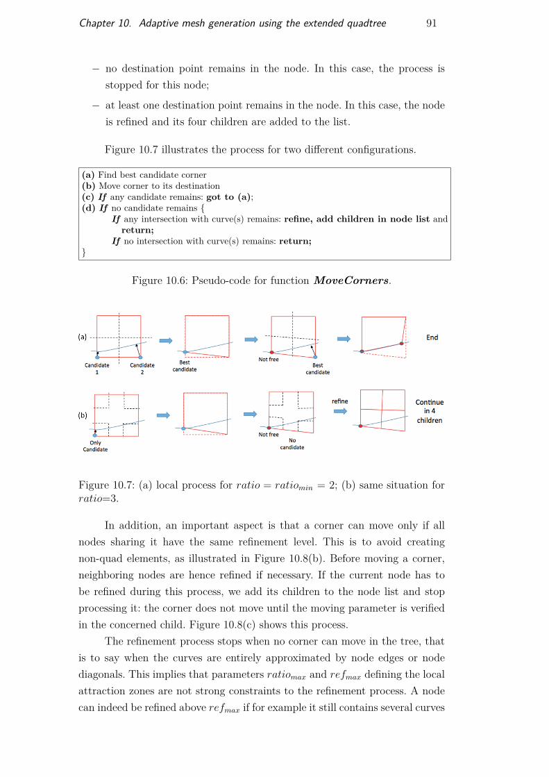
Chapter 10. Adaptive mesh generation using the extended quadtree 91
− no destination point remains in the node. In this case, the process isstopped for this node;
− at least one destination point remains in the node. In this case, the nodeis refined and its four children are added to the list.
Figure 10.7 illustrates the process for two different configurations.
(a) Find best candidate corner(b) Move corner to its destination(c) If any candidate remains: got to (a);(d) If no candidate remains {
If any intersection with curve(s) remains: refine, add children in node list andreturn;
If no intersection with curve(s) remains: return;}
Figure 10.6: Pseudo-code for function MoveCorners.
Figure 10.7: (a) local process for ratio = ratiomin = 2; (b) same situation forratio=3.
In addition, an important aspect is that a corner can move only if allnodes sharing it have the same refinement level. This is to avoid creatingnon-quad elements, as illustrated in Figure 10.8(b). Before moving a corner,neighboring nodes are hence refined if necessary. If the current node has tobe refined during this process, we add its children to the node list and stopprocessing it: the corner does not move until the moving parameter is verifiedin the concerned child. Figure 10.8(c) shows this process.
The refinement process stops when no corner can move in the tree, thatis to say when the curves are entirely approximated by node edges or nodediagonals. This implies that parameters ratiomax and refmax defining the localattraction zones are not strong constraints to the refinement process. A nodecan indeed be refined above refmax if for example it still contains several curves
DBD
PUC-Rio - Certificação Digital Nº 1413519/CA
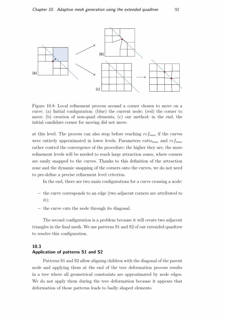
Chapter 10. Adaptive mesh generation using the extended quadtree 92
Figure 10.8: Local refinement process around a corner chosen to move on acurve. (a) Initial configuration: (blue) the current node; (red) the corner tomove; (b) creation of non-quad elements; (c) our method: in the end, theinitial candidate corner for moving did not move.
at this level. The process can also stop before reaching refmax if the curveswere entirely approximated in lower levels. Parameters ratiomax and refmax
rather control the convergence of the procedure: the higher they are, the morerefinement levels will be needed to reach large attraction zones, where cornersare easily snapped to the curves. Thanks to this definition of the attractionzone and the dynamic snapping of the corners onto the curves, we do not needto pre-define a precise refinement level criterion.
In the end, there are two main configurations for a curve crossing a node:
− the curve corresponds to an edge (two adjacent corners are attributed toit);
− the curve cuts the node through its diagonal.
The second configuration is a problem because it will create two adjacenttriangles in the final mesh. We use patterns S1 and S2 of our extended quadtreeto resolve this configuration.
10.3Application of patterns S1 and S2
Patterns S1 and S2 allow aligning children with the diagonal of the parentnode and applying them at the end of the tree deformation process resultsin a tree where all geometrical constraints are approximated by node edges.We do not apply them during the tree deformation because it appears thatdeformation of those patterns leads to badly shaped elements.
DBD
PUC-Rio - Certificação Digital Nº 1413519/CA
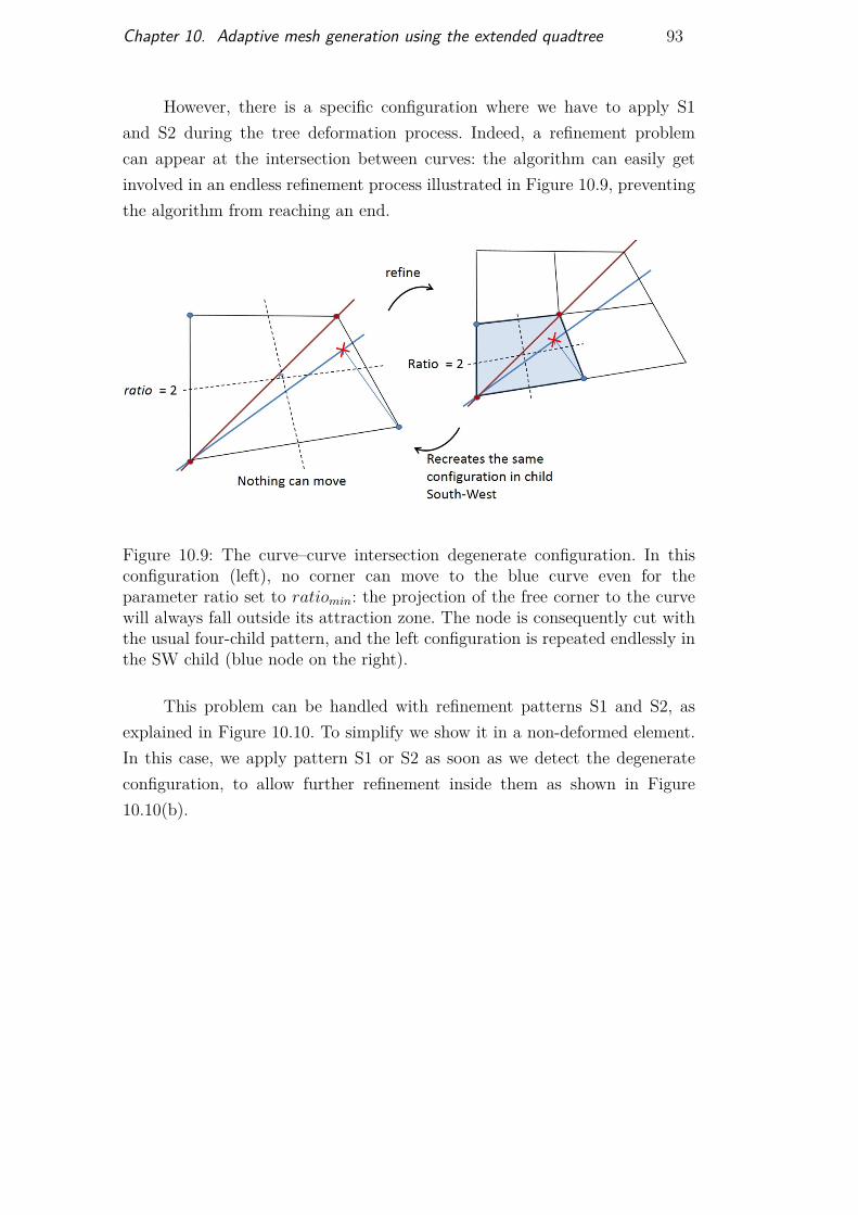
Chapter 10. Adaptive mesh generation using the extended quadtree 93
However, there is a specific configuration where we have to apply S1and S2 during the tree deformation process. Indeed, a refinement problemcan appear at the intersection between curves: the algorithm can easily getinvolved in an endless refinement process illustrated in Figure 10.9, preventingthe algorithm from reaching an end.
Figure 10.9: The curve–curve intersection degenerate configuration. In thisconfiguration (left), no corner can move to the blue curve even for theparameter ratio set to ratiomin: the projection of the free corner to the curvewill always fall outside its attraction zone. The node is consequently cut withthe usual four-child pattern, and the left configuration is repeated endlessly inthe SW child (blue node on the right).
This problem can be handled with refinement patterns S1 and S2, asexplained in Figure 10.10. To simplify we show it in a non-deformed element.In this case, we apply pattern S1 or S2 as soon as we detect the degenerateconfiguration, to allow further refinement inside them as shown in Figure10.10(b).
DBD
PUC-Rio - Certificação Digital Nº 1413519/CA
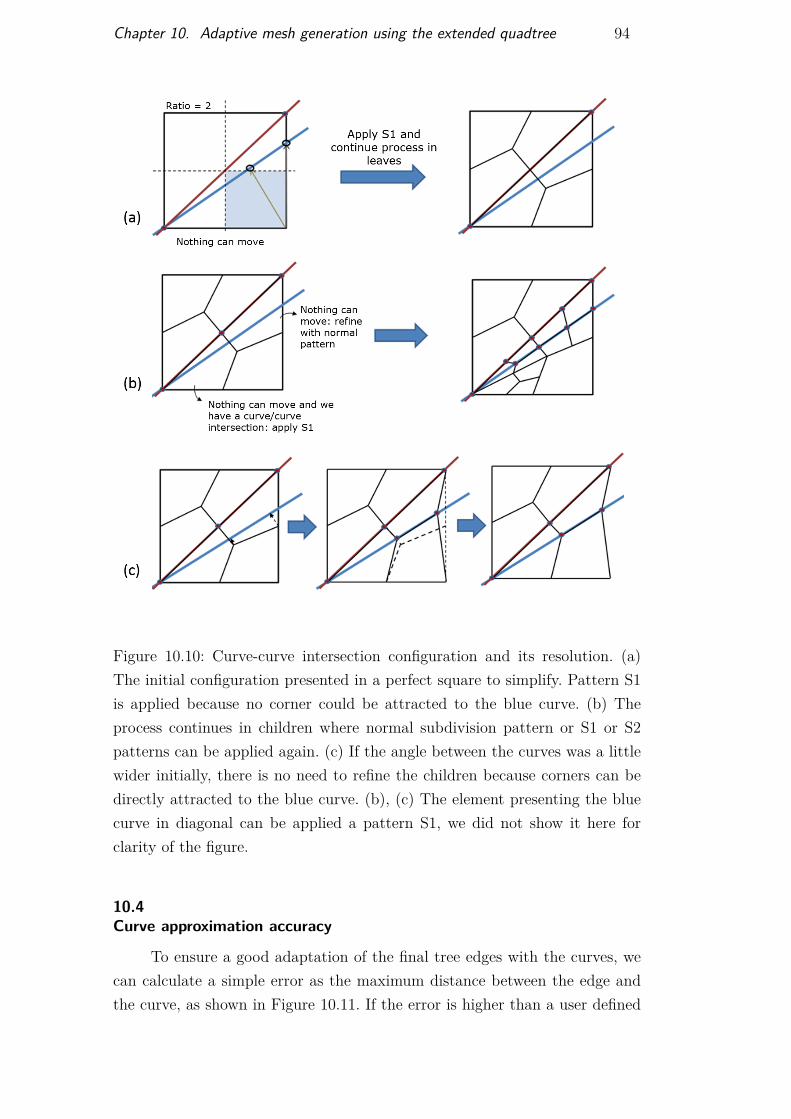
Chapter 10. Adaptive mesh generation using the extended quadtree 94
Figure 10.10: Curve-curve intersection configuration and its resolution. (a)The initial configuration presented in a perfect square to simplify. Pattern S1is applied because no corner could be attracted to the blue curve. (b) Theprocess continues in children where normal subdivision pattern or S1 or S2patterns can be applied again. (c) If the angle between the curves was a littlewider initially, there is no need to refine the children because corners can bedirectly attracted to the blue curve. (b), (c) The element presenting the bluecurve in diagonal can be applied a pattern S1, we did not show it here forclarity of the figure.
10.4Curve approximation accuracy
To ensure a good adaptation of the final tree edges with the curves, wecan calculate a simple error as the maximum distance between the edge andthe curve, as shown in Figure 10.11. If the error is higher than a user defined
DBD
PUC-Rio - Certificação Digital Nº 1413519/CA
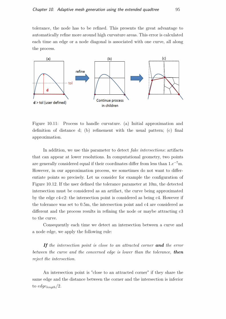
Chapter 10. Adaptive mesh generation using the extended quadtree 95
tolerance, the node has to be refined. This presents the great advantage toautomatically refine more around high curvature areas. This error is calculatedeach time an edge or a node diagonal is associated with one curve, all alongthe process.
Figure 10.11: Process to handle curvature. (a) Initial approximation anddefinition of distance d; (b) refinement with the usual pattern; (c) finalapproximation.
In addition, we use this parameter to detect fake intersections: artifactsthat can appear at lower resolutions. In computational geometry, two pointsare generally considered equal if their coordinates differ from less than 1.e−7m.However, in our approximation process, we sometimes do not want to differ-entiate points so precisely. Let us consider for example the configuration ofFigure 10.12. If the user defined the tolerance parameter at 10m, the detectedintersection must be considered as an artifact, the curve being approximatedby the edge c4-c2: the intersection point is considered as being c4. However ifthe tolerance was set to 0.5m, the intersection point and c4 are considered asdifferent and the process results in refining the node or maybe attracting c3to the curve.
Consequently each time we detect an intersection between a curve anda node edge, we apply the following rule:
If the intersection point is close to an attracted corner and the errorbetween the curve and the concerned edge is lower than the tolerance, thenreject the intersection.
An intersection point is "close to an attracted corner" if they share thesame edge and the distance between the corner and the intersection is inferiorto edgelength/2.
DBD
PUC-Rio - Certificação Digital Nº 1413519/CA
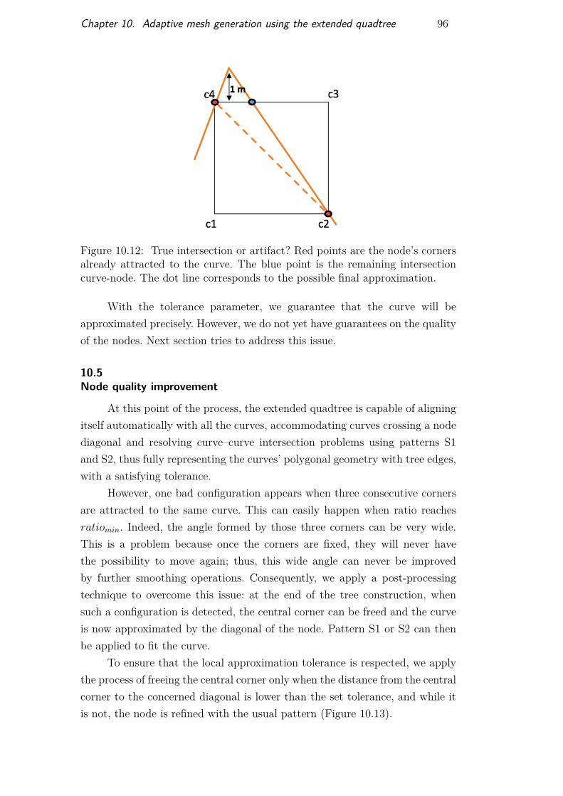
Chapter 10. Adaptive mesh generation using the extended quadtree 96
Figure 10.12: True intersection or artifact? Red points are the node’s cornersalready attracted to the curve. The blue point is the remaining intersectioncurve-node. The dot line corresponds to the possible final approximation.
With the tolerance parameter, we guarantee that the curve will beapproximated precisely. However, we do not yet have guarantees on the qualityof the nodes. Next section tries to address this issue.
10.5Node quality improvement
At this point of the process, the extended quadtree is capable of aligningitself automatically with all the curves, accommodating curves crossing a nodediagonal and resolving curve–curve intersection problems using patterns S1and S2, thus fully representing the curves’ polygonal geometry with tree edges,with a satisfying tolerance.
However, one bad configuration appears when three consecutive cornersare attracted to the same curve. This can easily happen when ratio reachesratiomin. Indeed, the angle formed by those three corners can be very wide.This is a problem because once the corners are fixed, they will never havethe possibility to move again; thus, this wide angle can never be improvedby further smoothing operations. Consequently, we apply a post-processingtechnique to overcome this issue: at the end of the tree construction, whensuch a configuration is detected, the central corner can be freed and the curveis now approximated by the diagonal of the node. Pattern S1 or S2 can thenbe applied to fit the curve.
To ensure that the local approximation tolerance is respected, we applythe process of freeing the central corner only when the distance from the centralcorner to the concerned diagonal is lower than the set tolerance, and while itis not, the node is refined with the usual pattern (Figure 10.13).
DBD
PUC-Rio - Certificação Digital Nº 1413519/CA
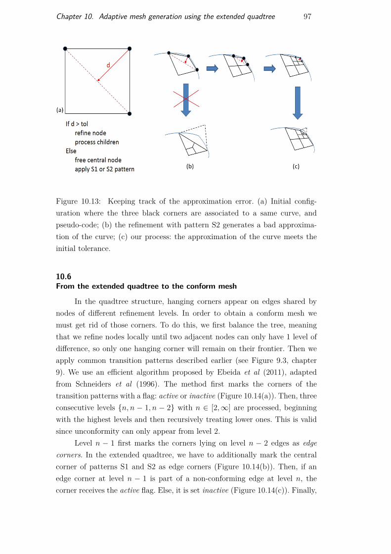
Chapter 10. Adaptive mesh generation using the extended quadtree 97
Figure 10.13: Keeping track of the approximation error. (a) Initial config-uration where the three black corners are associated to a same curve, andpseudo-code; (b) the refinement with pattern S2 generates a bad approxima-tion of the curve; (c) our process: the approximation of the curve meets theinitial tolerance.
10.6From the extended quadtree to the conform mesh
In the quadtree structure, hanging corners appear on edges shared bynodes of different refinement levels. In order to obtain a conform mesh wemust get rid of those corners. To do this, we first balance the tree, meaningthat we refine nodes locally until two adjacent nodes can only have 1 level ofdifference, so only one hanging corner will remain on their frontier. Then weapply common transition patterns described earlier (see Figure 9.3, chapter9). We use an efficient algorithm proposed by Ebeida et al (2011), adaptedfrom Schneiders et al (1996). The method first marks the corners of thetransition patterns with a flag: active or inactive (Figure 10.14(a)). Then, threeconsecutive levels {n, n − 1, n − 2} with n ∈ [2,∞] are processed, beginningwith the highest levels and then recursively treating lower ones. This is validsince unconformity can only appear from level 2.
Level n − 1 first marks the corners lying on level n − 2 edges as edgecorners. In the extended quadtree, we have to additionally mark the centralcorner of patterns S1 and S2 as edge corners (Figure 10.14(b)). Then, if anedge corner at level n − 1 is part of a non-conforming edge at level n, thecorner receives the active flag. Else, it is set inactive (Figure 10.14(c)). Finally,
DBD
PUC-Rio - Certificação Digital Nº 1413519/CA
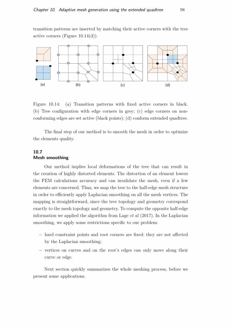
Chapter 10. Adaptive mesh generation using the extended quadtree 98
transition patterns are inserted by matching their active corners with the treeactive corners (Figure 10.14(d)).
Figure 10.14: (a) Transition patterns with fixed active corners in black.(b) Tree configuration with edge corners in grey; (c) edge corners on non-conforming edges are set active (black points); (d) conform extended quadtree.
The final step of our method is to smooth the mesh in order to optimizethe elements quality.
10.7Mesh smoothing
Our method implies local deformations of the tree that can result inthe creation of highly distorted elements. The distortion of an element lowersthe FEM calculations accuracy and can invalidate the mesh, even if a fewelements are concerned. Thus, we map the tree to the half-edge mesh structurein order to efficiently apply Laplacian smoothing on all the mesh vertices. Themapping is straightforward, since the tree topology and geometry correspondexactly to the mesh topology and geometry. To compute the opposite half-edgeinformation we applied the algorithm from Lage et al (2017). In the Laplaciansmoothing, we apply some restrictions specific to our problem:
− hard constraint points and root corners are fixed: they are not affectedby the Laplacian smoothing;
− vertices on curves and on the root’s edges can only move along theircurve or edge.
Next section quickly summarizes the whole meshing process, before wepresent some applications.
DBD
PUC-Rio - Certificação Digital Nº 1413519/CA

Chapter 10. Adaptive mesh generation using the extended quadtree 99
10.8The final algorithm
Figure 10.15 shows the algorithm for the proposed automatic all-quadrilateral mesh generation method.
1. Approximate hard constraint points onlyInput:
- all hard constraint points- refmax, ratiomax: specific for endpoints
Output: a first extended quadtree2. Separate curves in groups of non-intersecting curves3. For each group {
Add curve intermediate geometryInput:
- current group point sequence- refmax, ratiomax: specific for intermediate geometry
Output: updated extended quadtree4. Apply local node quality improvement5. Apply patterns S1 and S2 on all nodes where a curve corresponds to a
diagonal6. Conform the tree7. Map the extended quadtree into a half-edge mesh structure8. Apply global Laplacian smoothing (10 iterations)
Figure 10.15: Algorithm for the proposed all-quadrilateral mesh generationmethod.
Steps 1 to 5 correspond to the construction of the tree. In step 2, wemanually separate the curves into groups following this rule: curves in the samegroup do not intersect each other; curves from different groups can intersecteach other. In step 3, we construct the extended quadtree by iterativelyupdating it, adding new constraints to the grid. We apply patterns S1 andS2 at the end of the tree construction for nodes where the curve correspondsto a diagonal (step 5). In steps 6 we conform the extended quadtree, beforemapping it into a half-edge mesh structure in step 7. Finally step 8 applies aLaplacian smoothing to improve global element quality.
Next chapter presents and discusses our results.
DBD
PUC-Rio - Certificação Digital Nº 1413519/CA
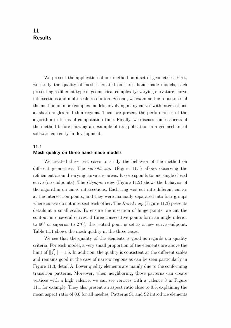
11Results
We present the application of our method on a set of geometries. First,we study the quality of meshes created on three hand-made models, eachpresenting a different type of geometrical complexity: varying curvature, curveintersections and multi-scale resolution. Second, we examine the robustness ofthe method on more complex models, involving many curves with intersectionsat sharp angles and thin regions. Then, we present the performances of thealgorithm in terms of computation time. Finally, we discuss some aspects ofthe method before showing an example of its application in a geomechanicalsoftware currently in development.
11.1Mesh quality on three hand-made models
We created three test cases to study the behavior of the method ondifferent geometries. The smooth star (Figure 11.1) allows observing therefinement around varying curvature areas. It corresponds to one single closedcurve (no endpoints). The Olympic rings (Figure 11.2) shows the behavior ofthe algorithm on curve intersections. Each ring was cut into different curvesat the intersection points, and they were manually separated into four groupswhere curves do not intersect each other. The Brazil map (Figure 11.3) presentsdetails at a small scale. To ensure the insertion of hinge points, we cut thecontour into several curves: if three consecutive points form an angle inferiorto 90° or superior to 270°, the central point is set as a new curve endpoint.Table 11.1 shows the mesh quality in the three cases.
We see that the quality of the elements is good as regards our qualitycriteria. For each model, a very small proportion of the elements are above thelimit of ||~fq|| = 1.5. In addition, the quality is consistent at the different scalesand remains good in the case of narrow regions as can be seen particularly inFigure 11.3, detail A. Lower quality elements are mainly due to the conformingtransition patterns. Moreover, when neighboring, those patterns can createvertices with a high valence: we can see vertices with a valence 8 in Figure11.1 for example. They also present an aspect ratio close to 0.5, explaining themean aspect ratio of 0.6 for all meshes. Patterns S1 and S2 introduce elements
DBD
PUC-Rio - Certificação Digital Nº 1413519/CA
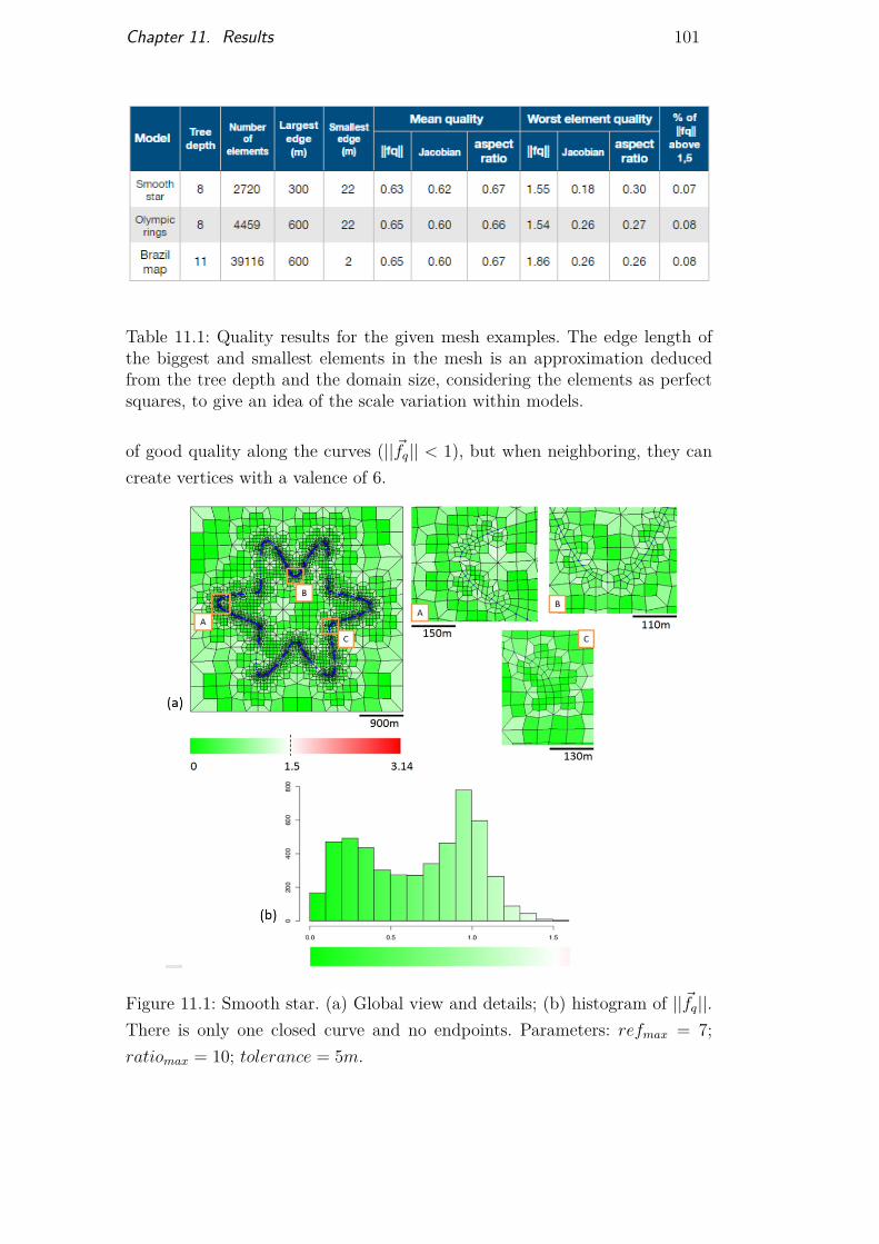
Chapter 11. Results 101
Table 11.1: Quality results for the given mesh examples. The edge length ofthe biggest and smallest elements in the mesh is an approximation deducedfrom the tree depth and the domain size, considering the elements as perfectsquares, to give an idea of the scale variation within models.
of good quality along the curves (||~fq|| < 1), but when neighboring, they cancreate vertices with a valence of 6.
Figure 11.1: Smooth star. (a) Global view and details; (b) histogram of ||~fq||.There is only one closed curve and no endpoints. Parameters: refmax = 7;ratiomax = 10; tolerance = 5m.
DBD
PUC-Rio - Certificação Digital Nº 1413519/CA
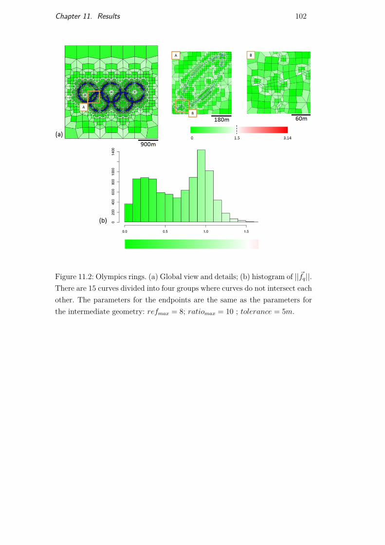
Chapter 11. Results 102
Figure 11.2: Olympics rings. (a) Global view and details; (b) histogram of ||~fq||.There are 15 curves divided into four groups where curves do not intersect eachother. The parameters for the endpoints are the same as the parameters forthe intermediate geometry: refmax = 8; ratiomax = 10 ; tolerance = 5m.
DBD
PUC-Rio - Certificação Digital Nº 1413519/CA
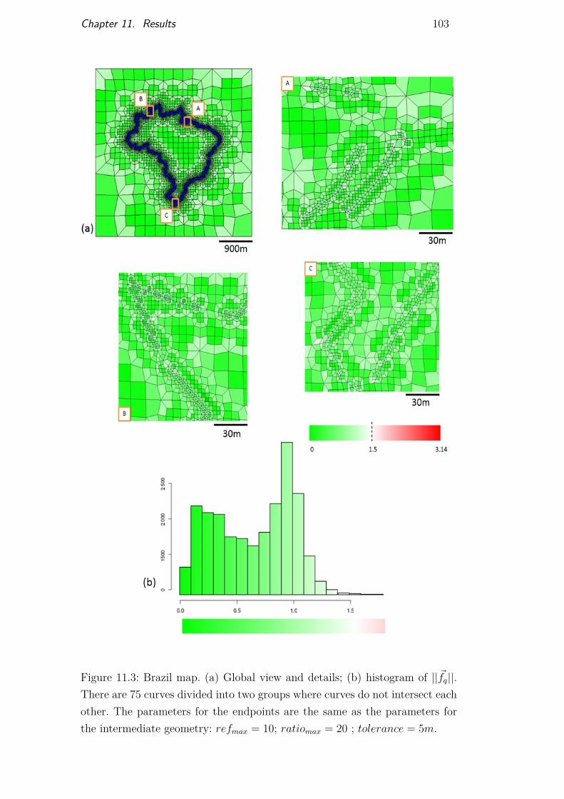
Chapter 11. Results 103
Figure 11.3: Brazil map. (a) Global view and details; (b) histogram of ||~fq||.There are 75 curves divided into two groups where curves do not intersect eachother. The parameters for the endpoints are the same as the parameters forthe intermediate geometry: refmax = 10; ratiomax = 20 ; tolerance = 5m.
DBD
PUC-Rio - Certificação Digital Nº 1413519/CA
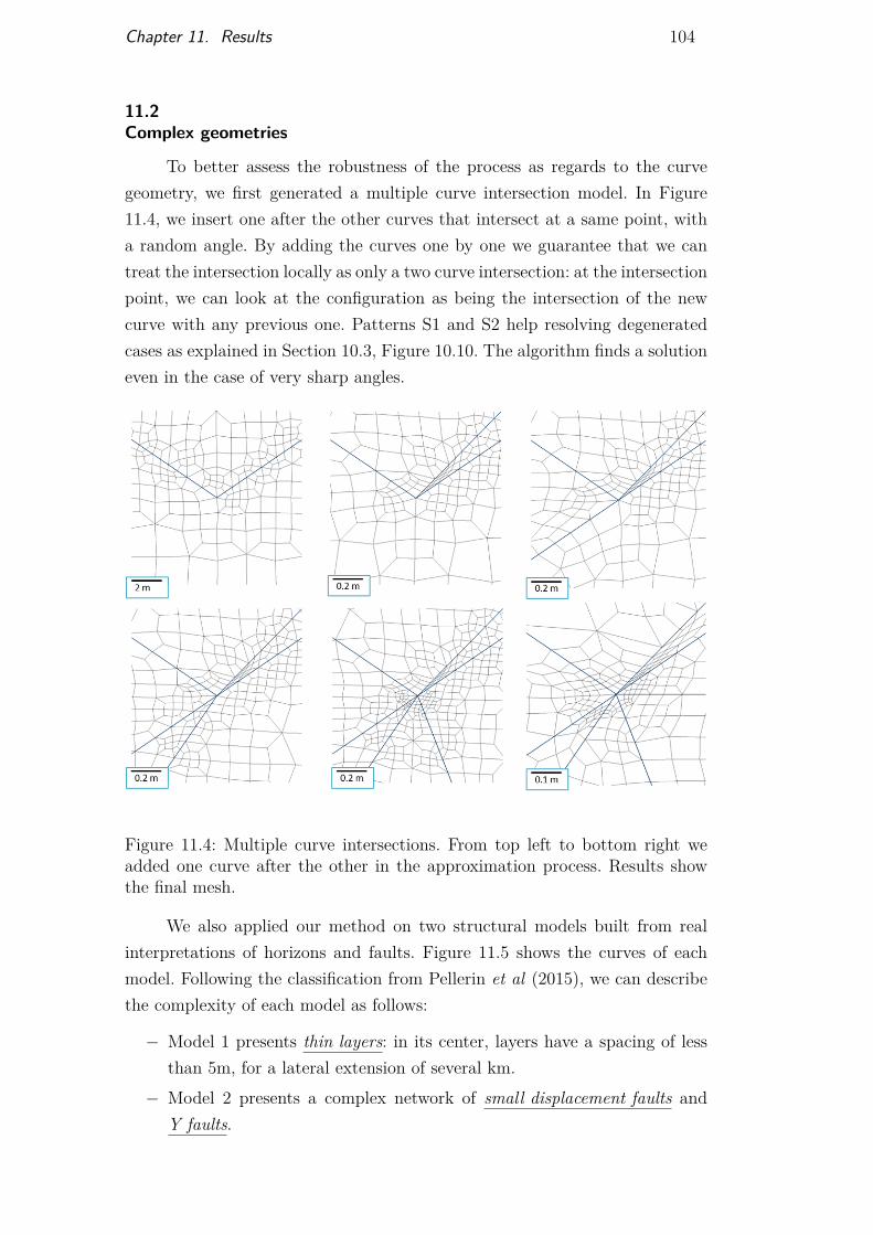
Chapter 11. Results 104
11.2Complex geometries
To better assess the robustness of the process as regards to the curvegeometry, we first generated a multiple curve intersection model. In Figure11.4, we insert one after the other curves that intersect at a same point, witha random angle. By adding the curves one by one we guarantee that we cantreat the intersection locally as only a two curve intersection: at the intersectionpoint, we can look at the configuration as being the intersection of the newcurve with any previous one. Patterns S1 and S2 help resolving degeneratedcases as explained in Section 10.3, Figure 10.10. The algorithm finds a solutioneven in the case of very sharp angles.
Figure 11.4: Multiple curve intersections. From top left to bottom right weadded one curve after the other in the approximation process. Results showthe final mesh.
We also applied our method on two structural models built from realinterpretations of horizons and faults. Figure 11.5 shows the curves of eachmodel. Following the classification from Pellerin et al (2015), we can describethe complexity of each model as follows:
− Model 1 presents thin layers: in its center, layers have a spacing of lessthan 5m, for a lateral extension of several km.
− Model 2 presents a complex network of small displacement faults andY faults.
DBD
PUC-Rio - Certificação Digital Nº 1413519/CA
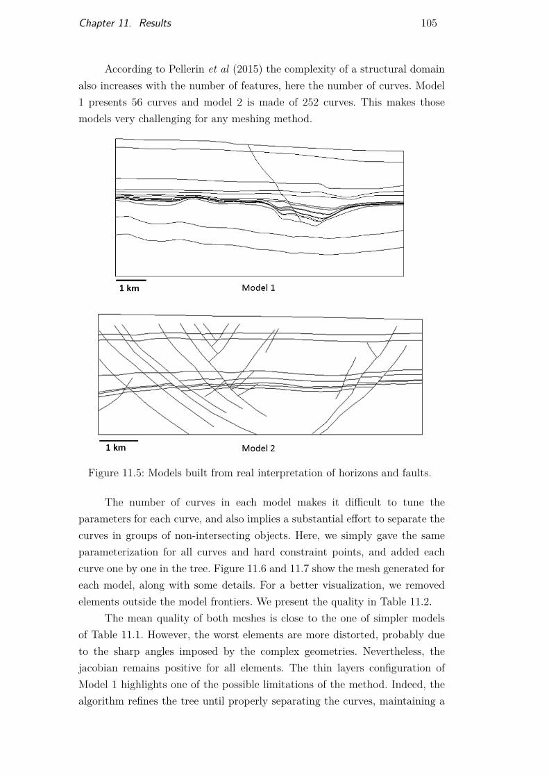
Chapter 11. Results 105
According to Pellerin et al (2015) the complexity of a structural domainalso increases with the number of features, here the number of curves. Model1 presents 56 curves and model 2 is made of 252 curves. This makes thosemodels very challenging for any meshing method.
Figure 11.5: Models built from real interpretation of horizons and faults.
The number of curves in each model makes it difficult to tune theparameters for each curve, and also implies a substantial effort to separate thecurves in groups of non-intersecting objects. Here, we simply gave the sameparameterization for all curves and hard constraint points, and added eachcurve one by one in the tree. Figure 11.6 and 11.7 show the mesh generated foreach model, along with some details. For a better visualization, we removedelements outside the model frontiers. We present the quality in Table 11.2.
The mean quality of both meshes is close to the one of simpler modelsof Table 11.1. However, the worst elements are more distorted, probably dueto the sharp angles imposed by the complex geometries. Nevertheless, thejacobian remains positive for all elements. The thin layers configuration ofModel 1 highlights one of the possible limitations of the method. Indeed, thealgorithm refines the tree until properly separating the curves, maintaining a
DBD
PUC-Rio - Certificação Digital Nº 1413519/CA
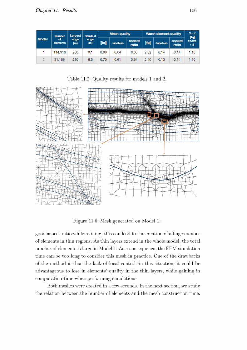
Chapter 11. Results 106
Table 11.2: Quality results for models 1 and 2.
Figure 11.6: Mesh generated on Model 1.
good aspect ratio while refining: this can lead to the creation of a huge numberof elements in thin regions. As thin layers extend in the whole model, the totalnumber of elements is large in Model 1. As a consequence, the FEM simulationtime can be too long to consider this mesh in practice. One of the drawbacksof the method is thus the lack of local control: in this situation, it could beadvantageous to lose in elements’ quality in the thin layers, while gaining incomputation time when performing simulations.
Both meshes were created in a few seconds. In the next section, we studythe relation between the number of elements and the mesh construction time.
DBD
PUC-Rio - Certificação Digital Nº 1413519/CA
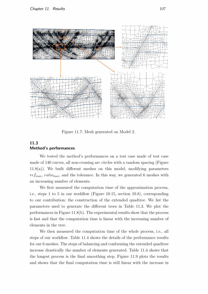
Chapter 11. Results 107
Figure 11.7: Mesh generated on Model 2.
11.3Method’s performances
We tested the method’s performances on a test case made of test casemade of 140 curves, all non-crossing arc circles with a random spacing (Figure11.8(a)). We built different meshes on this model, modifying parametersrefmax, ratiomax, and the tolerance. In this way, we generated 6 meshes withan increasing number of elements.
We first measured the computation time of the approximation process,i.e., steps 1 to 5 in our workflow (Figure 10.15, section 10.8), correspondingto our contribution: the construction of the extended quadtree. We list theparameters used to generate the different trees in Table 11.3. We plot theperformances in Figure 11.8(b). The experimental results show that the processis fast and that the computation time is linear with the increasing number ofelements in the tree.
We then measured the computation time of the whole process, i.e., allsteps of our workflow. Table 11.4 shows the details of the performance resultsfor our 6 meshes. The steps of balancing and conforming the extended quadtreeincrease drastically the number of elements generated. Table 11.4 shows thatthe longest process is the final smoothing step. Figure 11.9 plots the resultsand shows that the final computation time is still linear with the increase in
DBD
PUC-Rio - Certificação Digital Nº 1413519/CA
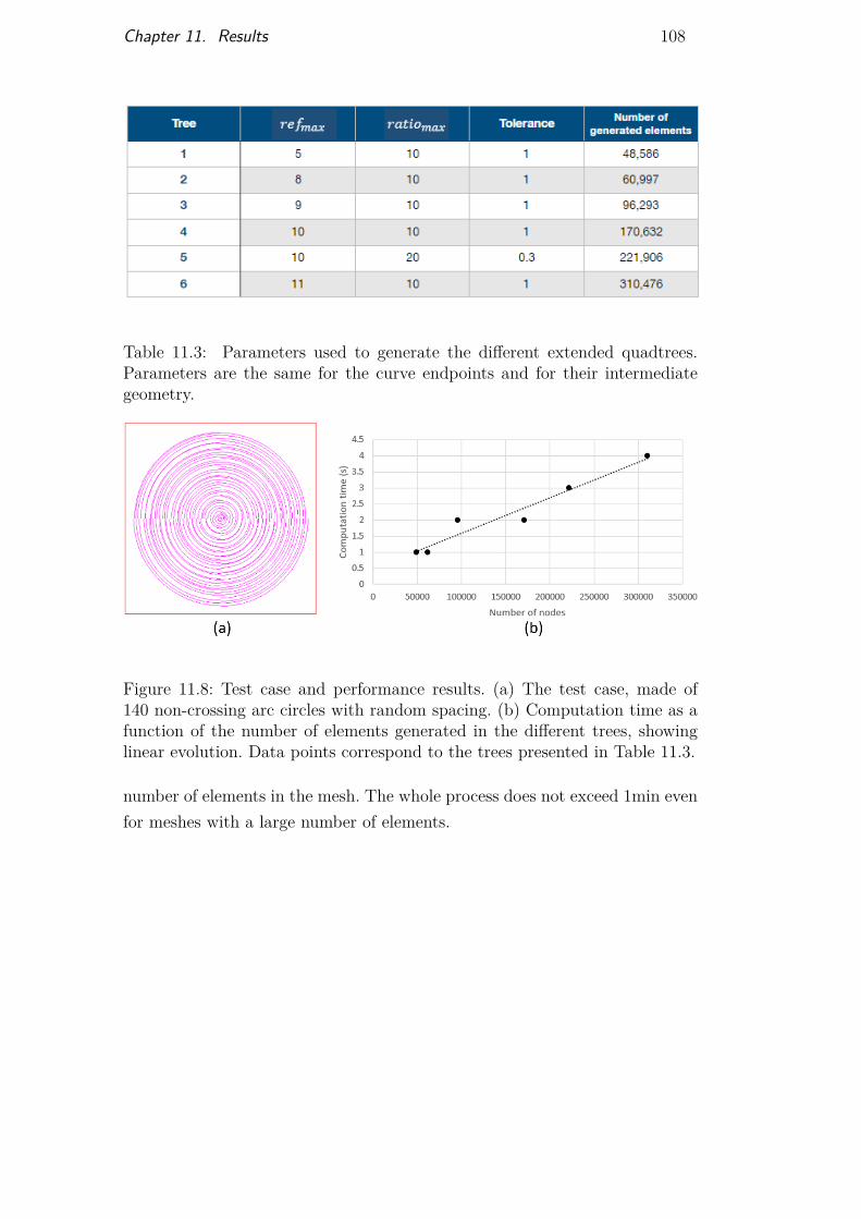
Chapter 11. Results 108
Table 11.3: Parameters used to generate the different extended quadtrees.Parameters are the same for the curve endpoints and for their intermediategeometry.
Figure 11.8: Test case and performance results. (a) The test case, made of140 non-crossing arc circles with random spacing. (b) Computation time as afunction of the number of elements generated in the different trees, showinglinear evolution. Data points correspond to the trees presented in Table 11.3.
number of elements in the mesh. The whole process does not exceed 1min evenfor meshes with a large number of elements.
DBD
PUC-Rio - Certificação Digital Nº 1413519/CA
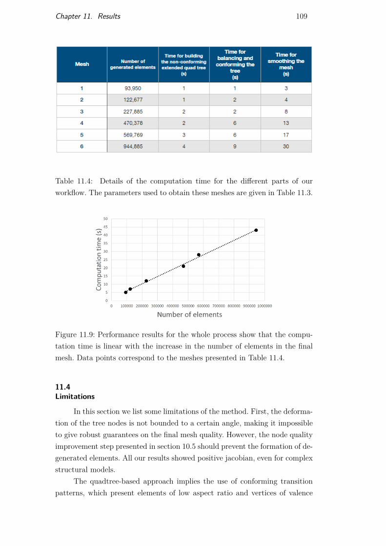
Chapter 11. Results 109
Table 11.4: Details of the computation time for the different parts of ourworkflow. The parameters used to obtain these meshes are given in Table 11.3.
Figure 11.9: Performance results for the whole process show that the compu-tation time is linear with the increase in the number of elements in the finalmesh. Data points correspond to the meshes presented in Table 11.4.
11.4Limitations
In this section we list some limitations of the method. First, the deforma-tion of the tree nodes is not bounded to a certain angle, making it impossibleto give robust guarantees on the final mesh quality. However, the node qualityimprovement step presented in section 10.5 should prevent the formation of de-generated elements. All our results showed positive jacobian, even for complexstructural models.
The quadtree-based approach implies the use of conforming transitionpatterns, which present elements of low aspect ratio and vertices of valence
DBD
PUC-Rio - Certificação Digital Nº 1413519/CA
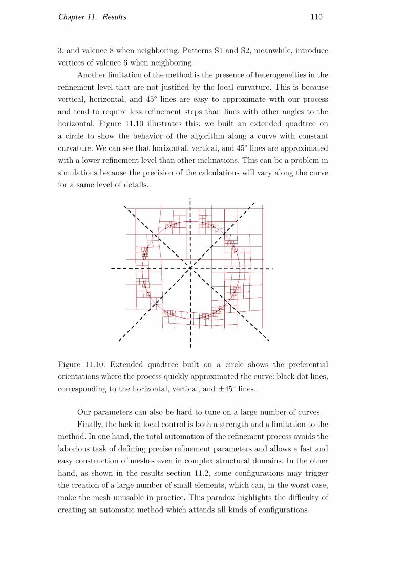
Chapter 11. Results 110
3, and valence 8 when neighboring. Patterns S1 and S2, meanwhile, introducevertices of valence 6 when neighboring.
Another limitation of the method is the presence of heterogeneities in therefinement level that are not justified by the local curvature. This is becausevertical, horizontal, and 45° lines are easy to approximate with our processand tend to require less refinement steps than lines with other angles to thehorizontal. Figure 11.10 illustrates this: we built an extended quadtree ona circle to show the behavior of the algorithm along a curve with constantcurvature. We can see that horizontal, vertical, and 45° lines are approximatedwith a lower refinement level than other inclinations. This can be a problem insimulations because the precision of the calculations will vary along the curvefor a same level of details.
Figure 11.10: Extended quadtree built on a circle shows the preferentialorientations where the process quickly approximated the curve: black dot lines,corresponding to the horizontal, vertical, and ±45° lines.
Our parameters can also be hard to tune on a large number of curves.Finally, the lack in local control is both a strength and a limitation to the
method. In one hand, the total automation of the refinement process avoids thelaborious task of defining precise refinement parameters and allows a fast andeasy construction of meshes even in complex structural domains. In the otherhand, as shown in the results section 11.2, some configurations may triggerthe creation of a large number of small elements, which can, in the worst case,make the mesh unusable in practice. This paradox highlights the difficulty ofcreating an automatic method which attends all kinds of configurations.
DBD
PUC-Rio - Certificação Digital Nº 1413519/CA
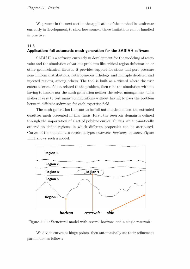
Chapter 11. Results 111
We present in the next section the application of the method in a softwarecurrently in development, to show how some of those limitations can be handledin practice.
11.5Application: full-automatic mesh generation for the SABIAH software
SABIAH is a software currently in development for the modeling of reser-voirs and the simulation of various problems like critical region deformation orother geomechanical threats. It provides support for stress and pore pressurenon-uniform distributions, heterogeneous lithology and multiple depleted andinjected regions, among others. The tool is built as a wizard where the userenters a series of data related to the problem, then runs the simulation withouthaving to handle nor the mesh generation neither the solver management. Thismakes it easy to test many configurations without having to pass the problembetween different softwares for each expertise field.
The mesh generation is meant to be full-automatic and uses the extendedquadtree mesh presented in this thesis. First, the reservoir domain is definedthrough the importation of a set of polyline curves. Curves are automaticallyordered to define regions, in which different properties can be attributed.Curves of the domain also receive a type: reservoir, horizons, or sides. Figure11.11 shows such a model.
Figure 11.11: Structural model with several horizons and a single reservoir.
We divide curves at hinge points, then automatically set their refinementparameters as follows:
DBD
PUC-Rio - Certificação Digital Nº 1413519/CA

Chapter 11. Results 112
− ratiomax is fixed to 10, this value was found empirically to always givesatisfying results;
− refmax is deduced from the default expected length of elements along thecurves: 50m for reservoirs, 300m for others. We remind here the equationgiving the size of an edge length in a quadtree as a function of its depth:
edge length level i = edge length root
2i (7-10)
We can invert the equation to find level i, given the edge length:
i = log2(edge length root
edge length level i
)(11-1)
We then set refmax = i;
− the tolerance is set to the relatively high value of tolerance =expected edge length/2. Doing this, the refinement process is driven bythe expected edge length and not by a tight tolerance to the curve, whichwould in many cases refine more than expected;
− the parameters for the curve endpoints are the same as the parametersfor the intermediate geometry.
With this method, we can set all parameters for all curves in thedomain very quickly. The mesh is expected to refine until refmax. However,as explained, the algorithm makes local decisions that can lead to refining alittle more, or a little less. The large tolerance should prevent the algorithmto refine a lot more, except in high curvature areas, which is good. To ensurethat the process refines at least to the expected depth, we add a post-processin the tree construction: all nodes touching a curve with a refinement depthlower than the curve refmax are refined until meeting refmax.
We also give the possibility to make the refinement uniform along a curve.To do so, in the tree, we find the smallest refinement level along a curve andthen refine all the elements touching the curve to this level. In the same fashion,we can make the refinement uniform for all elements in a region.
In the curve approximation process, curves are added one by one in orderto avoid the step of building groups of non-intersecting objects.
Figure 11.12 shows the resulting mesh for the domain presented in Figure11.11. The refinement along the reservoir curve is forced uniform. For this typeof mesh, if horizons create thin layers, our process will generate a lot of smallelements. We plan on detecting such configurations in a pre-processing.
DBD
PUC-Rio - Certificação Digital Nº 1413519/CA
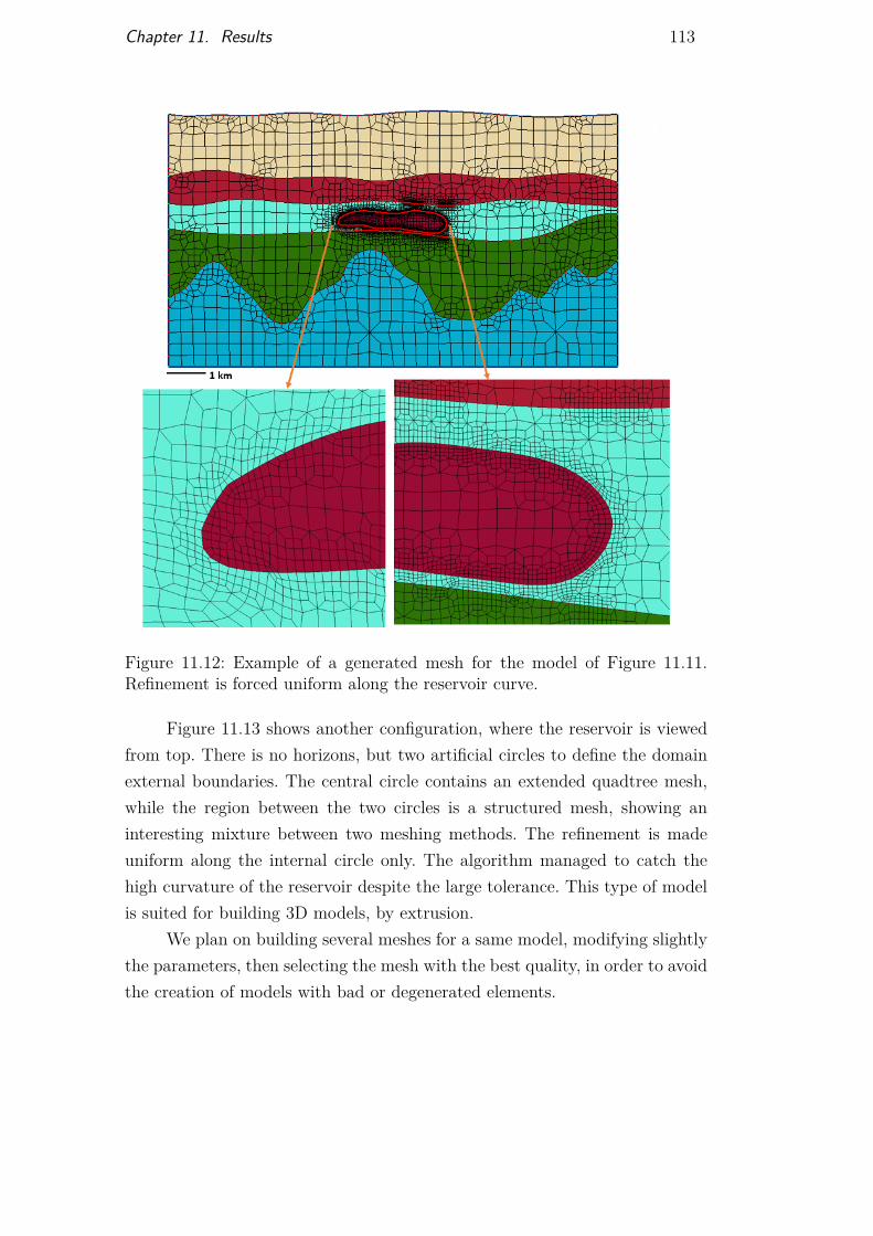
Chapter 11. Results 113
Figure 11.12: Example of a generated mesh for the model of Figure 11.11.Refinement is forced uniform along the reservoir curve.
Figure 11.13 shows another configuration, where the reservoir is viewedfrom top. There is no horizons, but two artificial circles to define the domainexternal boundaries. The central circle contains an extended quadtree mesh,while the region between the two circles is a structured mesh, showing aninteresting mixture between two meshing methods. The refinement is madeuniform along the internal circle only. The algorithm managed to catch thehigh curvature of the reservoir despite the large tolerance. This type of modelis suited for building 3D models, by extrusion.
We plan on building several meshes for a same model, modifying slightlythe parameters, then selecting the mesh with the best quality, in order to avoidthe creation of models with bad or degenerated elements.
DBD
PUC-Rio - Certificação Digital Nº 1413519/CA
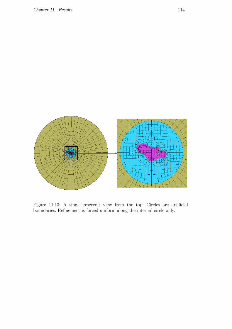
Chapter 11. Results 114
Figure 11.13: A single reservoir view from the top. Circles are artificialboundaries. Refinement is forced uniform along the internal circle only.
DBD
PUC-Rio - Certificação Digital Nº 1413519/CA
12Conclusions for Part II
12.1Summary
In this work, we presented a new method for 2D all-quadrilateral meshgeneration. The method is based on our extended quadtree structure, whichallows building a simple algorithm for the domain adaptation around anycurve geometry, with few parameters involved and automatic refinement inhigh curvature areas. The key to this process was the inclusion of two newsubdivision patterns, which we call S1 and S2, in the quadtree node refinementoperation. The final mesh is obtained after a conforming step, followed bysmoothing. The process proved efficient, building trees of over 400,000 elementsin less than 5s, and generated meshes of reasonable quality even for complexstructural domains.
12.2Conclusions
The presented method is a fast and user-friendly mesh generator whichfinds a solution for any curve configuration. Local adaptation processes allowadaptive refinement without the need to define precise refinement criteria.Compared to other meshing methods, the extended quadtree mesh thus avoidsheavy pre-processing of the input geometry and complex parameterization.In return, the user does not have control on local decisions such as, forexample, the number of elements along the curves. To some extent, localcontrol is possible through the underlying tree structure, which allows easyand fast refinement for local adjustments in a post-processing step. This can beadvantageous in situations where the refinement must be uniform along curvesor in specific mesh regions. However, coarsening is much more difficult thanrefining because of the tree corners adaptation to the curves. Thus, a problemappears in configurations where the extended quadtree tends to generate manyelements, for example in the presence of thin layers extended throughout thedomain. This situation remains the main limitation to the method, since itcan generate unusable meshes. Another limitation of the method is the lack
DBD
PUC-Rio - Certificação Digital Nº 1413519/CA
Chapter 12. Conclusions for Part II 116
in robust quality guarantees, as the elements can deform freely. However, thegeneration of a degenerated element can be easily detected by quality metricssuch as the jacobian, and the mesh can be reconstructed in few seconds withother parameters in order to attempt reaching a better quality.
12.3Suggestions for further research
As discussed, the two main limitations of the method are the behaviorof the algorithm in thin layer configurations and the lack of robust qualityguarantees for the elements.
The first problem could be handled by detecting the configuration anddefining a specific refinement scheme in the concerned nodes. For example, iftwo curves with a given spacing cross one node, we could snap corners directlywithout having to first separate the curves in different children.
The lack of quality guarantees could lead to locally bad shaped elements.We could investigate processes based on local topological operations to locallyimprove the mesh, taking as example the works from Kinney (1997), Canannet al (1998) and Anderson et al (2008).
Finally, a natural continuation to this work is the adaptation of themethod to the 3D case: we could try to develop an extended octree. However,two major problems arise that have to be treated in parallel in the 3D case.First, the dynamic adaptation of tree corners to the geometrical constraints ismuch more complex in 3D. The number of configurations with which a surfacecan cross a cube is finite (Lorensen and Cline, 1987), however the subdivision ofan hexahedron into smaller hexahedron aligned with the crossing surface andwith a good quality for each child may be a real challenge. Second, supposinga set of subdivision patterns provides the desired adaptation, neighboringhexahedron will have to conform not only by matching edges and vertices, butalso by matching faces, which is not trivial. Some authors have investigated3D transition patterns (Mitchell, 1999; Yamakawa and Shimada, 2002). Noneof them guarantees the quality of the created elements, and transition patternstend to create many small elements, overall presenting techniques which arenot adapted to the FEM mesh constraints. The interesting work of Schneiderset al (1996) proposes octree conforming patterns in the case of a 27-childrenscheme octree, consisting in cutting a node in 27 hexahedron instead of 8(resp. 9 quadrilateral instead of 4 in the 2D case). Owen et al (2017) adaptedit to the usual 8-children pattern octree. These works may be interestingfor mesh extrusion. Mesh extrusion allows easily creating 3D meshes from2D meshes by projecting elements in the third dimension. In the case of
DBD
PUC-Rio - Certificação Digital Nº 1413519/CA

Chapter 12. Conclusions for Part II 117
geomechanical reservoirs, conformation to the geometrical constraints can bediscarded in certain regions. 3D transition patterns could help reduce thenumber of elements in those regions by coarsening the mesh, without havingto handle mesh alignment with boundaries.
DBD
PUC-Rio - Certificação Digital Nº 1413519/CA

13Final words
This thesis is part of a research that aims to generate simulation modelsdirectly from the seismic data. The final goal is to construct the first modelof a digital twin of the oil field as soon as the exploration begins to improvethe safety of the operation. As one of the early work, we did not achieve thisgoal. Both parts of this thesis discuss relevant aspects of the problem. Theuse of a 2D model was enough to reveal challenges that automatic tools haveto face to replace humans in tedious activities that are heavily dependent oninterpretation and experience.
In the future, we hope to join the two parts of this work in a generaltool. First, we could couple our fault detector with other geobodies’ automaticextractors, like horizons or salt domes for example. Clean delineation of faults,horizons and salt domes would then build a structural model that could be theinput to our mesh generator.
Merging the different steps of a complex workflow in a single tool isalways of great value to reduce the accumulated errors and give the users aclear and general view of their models.
DBD
PUC-Rio - Certificação Digital Nº 1413519/CA
Bibliography
AL-DOSSARY, S.; MARFURT, K. J.. 3d volumetric multispectral esti-mates of reflector curvature and rotation. GEOPHYSICS, 71(5):P41–P51, 2006.
ANDERSON, B. D.; SHEPHERD, J. F.; DANIELS, J. ; BENZLEY, S. E.. Quadri-lateral mesh improvement. Research Note, 17th International MeshingRoundtable, 2008.
ARAYA-POLO, M.; DAHLKE, T.; FROGNER, C.; ZHANG, C.; POGGIO, T. ;HOHL, D.. Automated fault detection without seismic processing.The Leading Edge, 36(3):208–214, 2017.
ARAÚJO, C.; CELES, W.. Quadrilateral mesh generation with deferredconstraint insertion. Procedia Engineering, 82:88 – 100. 23rd InternationalMeshing Roundtable, 2014.
ATALAY, F. B.; RAMASWAMI, S. ; XU, D.. Quadrilateral meshes withbounded minimum angle. In: PROCEEDINGS OF THE 17TH INTERNA-TIONAL MESHING ROUNDTABLE, p. 73–91. Springer, 2008.
BACH, S.; BINDER, A.; MONTAVON, G.; KLAUSCHEN, F.; MÜLLER, K.-R.; SAMEK, W.. On pixel-wise explanations for non-linear classifierdecisions by layer-wise relevance propagation. PLOS ONE, 10(7):1–46, 2015.
BAHORICH, M.; FARMER, S.. 3-d seismic discontinuity for faultsand stratigraphic features: The coherence cube. The Leading Edge,14(10):1053–1058, 1995.
BENGIO, Y.. Learning deep architectures for AI. Foundations and Trendsin Machine Learning, 2(1):1–127, Jan. 2009.
BLACKER, T. D.; STEPHENSON, M. B.. Paving: A new approach toautomated quadrilateral mesh generation. International Journal forNumerical Methods in Engineering, 32(4):811–847, 1991.
DBD
PUC-Rio - Certificação Digital Nº 1413519/CA
Bibliography 120
BOROUCHAKI, H.; FREY, P. J.. Adaptive triangular–quadrilateral meshgeneration. International Journal for Numerical Methods in Engineering,41(5):915–934, 1998.
CANANN, S. A.; MUTHUKRISHNAN, S. ; PHILLIPS, R.. Topological im-provement procedures for quadrilateral finite element meshes. En-gineering with Computers, 14(2):168–177, 1998.
CATMULL, E.; CLARK, J.. Recursively generated b-spline surfaces onarbitrary topological meshes. Computer-Aided Design, 10(6):350 – 355,1978.
CHAE, S.-W.; JEONG, J.-H.. Unstructured surface meshing using oper-ators. In: PROC. 6TH INT. MESHING ROUNDTABLE, p. 281–291, 1997.
CHEW, L. P.. Constrained delaunay triangulations. In: PROCEEDINGSOF THE THIRD ANNUAL SYMPOSIUM ON COMPUTATIONAL GEOME-TRY, SCG ’87, p. 215–222, 1987.
CHOLLET, F.. Keras. https://keras.io, 2015.
CONNERS, R. W.; TRIVEDI, M. M. ; HARLOW, C. A.. Segmentation ofa high-resolution urban scene using texture operators. ComputerVision, Graphics, and Image Processing, 25(3):273 – 310, 1984.
CORTES, C.; VAPNIK, V.. Support-vector networks. Machine Learning,20(3):273–297, Sept. 1995.
DENG, J.; DONG, W.; SOCHER, R.; LI, L.; LI, K. ; FEI-FEI, L.. Imagenet: Alarge-scale hierarchical image database. In: 2009 IEEE CONFERENCEON COMPUTER VISION AND PATTERN RECOGNITION, p. 248–255, June2009.
DI, H.; GAO, D.. Gray-level transformation and canny edge detectionfor 3d seismic discontinuity enhancement. Computers & Geosciences,72:192 – 200, 2014.
DI, H.; GAO, D.. Fault detection: Methods, applications and technol-ogy. chapter Seismic attribute aided fault detection in petroleum industry: Areview, p. 53–80. Nova Science Publishers, 2017.
DI, H.; SHAFIQ, M. A. ; ALREGIB, G.. Seismic-fault detection based onmultiattribute support vector machine analysis. In: SEG TECHNICALPROGRAM EXPANDED ABSTRACTS 2017, p. 2039–2044, 2017.
DBD
PUC-Rio - Certificação Digital Nº 1413519/CA
Bibliography 121
DI, H.; WANG, Z. ; ALREGIB, G.. Seismic fault detection from post-stack amplitude by convolutional neural networks. In: 80TH EAGECONFERENCE AND EXHIBITION 2018, 2018.
EBEIDA, M. S.; DAVIS, R. L. ; FREUND, R. W.. A new fast hybrid adaptivegrid generation technique for arbitrary two-dimensional domains.International Journal for Numerical Methods in Engineering, 84(3):305–329,2010.
EBEIDA, M. S.; KARAMETE, K.; MESTREAU, E. ; DEY, S.. Q-tran: A newapproach to transform triangular meshes into quadrilateral mesheslocally. In: PROCEEDINGS OF THE 19TH INTERNATIONAL MESHINGROUNDTABLE, p. 23–34. Springer Berlin Heidelberg, 2010.
EBEIDA, M. S.; PATNEY, A.; OWENS, J. D. ; MESTREAU, E.. Isotropicconforming refinement of quadrilateral and hexahedral meshesusing two-refinement templates. International Journal for NumericalMethods in Engineering, 88(10):974–985, 2011.
EL-HAMALAWI, A.. A simple and effective element distortion factor.Computers & Structures, 75(5):507–513, 2000.
FAGIN, S.. Seismic Modeling of Geologic Structures. Society of Explo-ration Geophysicists, 1991.
FIGUEIREDO, A. M.. Mapeamento automático de horizontes e falhasem dados sísmicos 3d baseado no algoritmo de gás neural evolutivo.Master’s thesis, Pontifícia Universidade Católica do Rio de Janeiro, 2007.
FREY, P. J.; MARECHAL, L.. Fast adaptive quadtree mesh generation.In: 7TH INTERNATIONAL MESHING ROUNDTABLE, p. 211–224. Citeseer,1998.
GAO, D.. Integrating 3d seismic curvature and curvature gradientattributes for fracture characterization: Methodologies and inter-pretational implications. Geophysics, 78(2):O21–O31, 2013.
GERHARDT, A. L. B.. Aspectos da visualização volumétrica de dadossísmicos. Master’s thesis, Pontifícia Universidade Católica do Rio de Janeiro,1998.
GIBSON, D.; SPANN, M.; TURNER, J. ; WRIGHT, T.. Fault surface detec-tion in 3-d seismic data. IEEE Transactions on Geoscience and RemoteSensing, 43(9):2094–2102, Sept 2005.
DBD
PUC-Rio - Certificação Digital Nº 1413519/CA
Bibliography 122
GLOROT, X.; BORDES, A. ; BENGIO, Y.. Deep sparse rectifier neuralnetworks. In: PROCEEDINGS OF THE FOURTEENTH INTERNATIONALCONFERENCE ON ARTIFICIAL INTELLIGENCE AND STATISTICS, p. 315–323. PMLR, 2011.
GOLDNER, E. L.. Avaliação de algoritmos de menor caminho em ras-treamento de horizontes sísmicos. Master’s thesis, Pontifícia UniversidadeCatólica do Rio de Janeiro, 2014.
GUITTON, A.; WANG, H. ; TRAINOR-GUITTON, W.. Statistical imaging offaults in 3d seismic volumes using a machine learning approach.In: 2017 SEG INTERNATIONAL EXPOSITION AND ANNUAL MEETING, p.24–29. Society of Exploration Geophysicists, 2017.
HALE, D.. Methods to compute fault images, extract fault surfaces,and estimate fault throws from 3d seismic images. Geophysics,78(2):O33–O43, 2013.
HALE, D.. Seismic image processing for geologic faults. https://github.com/dhale/ipf,2014, 2014.
HARALICK, R. M.; SHANMUGAM, K. ; OTHERS. Textural features forimage classification. IEEE Transactions on systems, man, and cybernetics,(6):610–621, 1973.
HAYKIN, S.. Neural Networks and Learning Machines. Prentice Hall,2009.
HERRMANN, L. R.. Laplacian-isoparametric grid generation scheme.Journal of the Engineering Mechanics Division, 102(5):749–907, 1976.
HILTERMAN, F. J.. Three-dimensional seismic modeling. Geophysics,35(6):1020–1037, 1970.
HOUGH, P.. Method and means for recognizing complex patterns.,1965. US Patent 3069654A.
HUANG, L.; DONG, X. ; CLEE, T. E.. A scalable deep learning platformfor identifying geologic features from seismic attributes. The LeadingEdge, 36(3):249–256, 2017.
KELLY, K. R.; WARD, R. W.; TREITEL, S. ; ALFORD, R. M.. Syntheticseismograms: A finite-difference approach. Geophysics, 41(1):2–27,1976.
DBD
PUC-Rio - Certificação Digital Nº 1413519/CA
Bibliography 123
KINNEY, P.. Cleanup: Improving quadrilateral finite element meshes.In: 6TH INTERNATIONAL MESHING ROUNDTABLE, p. 437–447, 1997.
KRIZHEVSKY, A.; SUTSKEVER, I. ; HINTON, G. E.. Imagenet classificationwith deep convolutional neural networks. In: PROCEEDINGS OFTHE 25TH INTERNATIONAL CONFERENCE ON NEURAL INFORMATIONPROCESSING SYSTEMS - VOLUME 1, NIPS’12, p. 1097–1105, 2012.
KRUSKAL, J. B.. Multidimensional scaling by optimizing goodness offit to a nonmetric hypothesis. Psychometrika, 29(1):1–27, Mar 1964.
LAGE, M.; MARTHA, L. F.; DE ALMEIDA, J. M. ; LOPES, H.. Ibhm: index-based data structures for 2d and 3d hybrid meshes. Engineering withComputers, 33(4):727–744, 2017.
LECUN, Y.; BOTTOU, L.; BENGIO, Y. ; HAFFNER, P.. Gradient-basedlearning applied to document recognition. Proceedings of the IEEE,86(11):2278–2324, Nov 1998.
LEE, K.-Y.; KIM, I.-I.; CHO, D.-Y. ; WAN KIM, T.. An algorithm forautomatic 2d quadrilateral mesh generation with line constraints.Computer-Aided Design, 35(12):1055 – 1068, 2003.
LIANG, X.; EBEIDA, M. S. ; ZHANG, Y.. Guaranteed-quality all-quadrilateral mesh generation with feature preservation. In: PRO-CEEDINGS OF THE 18TH INTERNATIONAL MESHING ROUNDTABLE, p.45–63. Springer, 2009.
LISLE, R.. Detection of zones of abnormal strains in structures usinggaussian curvature analysis. AAPG Bulletin, 78(12), 1994.
LIU, Y.; XING, H. L. ; GUAN, Z.. An indirect approach for automaticgeneration of quadrilateral meshes with arbitrary line constraints.International Journal for Numerical Methods in Engineering, 87(9):906–922.
LORENSEN, W. E.; CLINE, H. E.. Marching cubes: A high resolution3d surface construction algorithm. In: ACM SIGGRAPH COMPUTERGRAPHICS, volumen 21, p. 163–169. ACM, 1987.
LU, P.; MORRIS, M.; BRAZELL, S.; COMISKEY, C. ; XIAO, Y.. Usinggenerative adversarial networks to improve deep-learning faultinterpretation networks. The Leading Edge, 37(8):578–583, 2018.
DBD
PUC-Rio - Certificação Digital Nº 1413519/CA
Bibliography 124
LUO, Y.; HIGGS, W. G. ; KOWALIK, W. S.. Edge detection and strati-graphic analysis using 3d seismic data. In: SEG TECHNICAL PROGRAMEXPANDED ABSTRACTS 1996, p. 324–327, 1996.
MACHADO, M. D. C.. Determinação de Malhas de Falhas em DadosSísmicos por Aprendizado Competitivo. PhD thesis, Pontifícia Univer-sidade Católica do Rio de Janeiro, 2008.
MÄNTYLÄ, M.. An Introduction to Solid Modeling. Computer SciencePress, Inc., 1987.
MARFURT, K. J.; KIRLIN, R. L.; FARMER, S. L. ; BAHORICH, M. S.. 3-dseismic attributes using a semblance-based coherency algorithm.Geophysics, 63(4):1150–1165, 1998.
MCCULLOCH, W. S.; PITTS, W.. A logical calculus of the ideas immanentin nervous activity. The bulletin of mathematical biophysics, 5(4):115–133,1943.
MINSKY, M.; PAPERT, S.. Perceptrons: An Introduction to Computa-tional Geometry. Mit Press, 1972.
DE OLIVEIRA MIRANDA, A. C.; MARTHA, L. F.. Quadrilateral meshgeneration using hierarchical templates. In: PROCEEDINGS OF THE21ST INTERNATIONAL MESHING ROUNDTABLE, p. 279–296. Springer,2013.
MITCHELL, S. A.. The all-hex geode-template for conforming a dicedtetrahedral mesh to any diced hexahedral mesh. Engineering withComputers, 15(3):228–235, 1999.
MÜLLER, K. .; MIKA, S.; RATSCH, G.; TSUDA, K. ; SCHOLKOPF, B.. Anintroduction to kernel-based learning algorithms. IEEE Transactionson Neural Networks, 12(2):181–201, March 2001.
NIKISHKOV, G. P.. Introduction to the finite element method. Universityof Aizu, p. 1–70, 2004.
NOWOTTNY, D.. Quadrilateral mesh generation via geometricallyoptimized domain decomposition. In: PROC. 6TH INT. MESHINGROUNDTABLE, p. 309–320, 1997.
OPENDTECT. Netherland offshore f3 block complete. https://www.opendtect.org/osr/Main/NetherlandsOffshoreF3BlockComplete4GB.,1987.
DBD
PUC-Rio - Certificação Digital Nº 1413519/CA

Bibliography 125
OWEN, S. J.; STATEN, M. L.; CANANN, S. A. ; SAIGAL, S.. Q-morph: anindirect approach to advancing front quad meshing. InternationalJournal for Numerical Methods in Engineering, 44(9):1317–1340, 1999.
OWEN, S. J.; SHIH, R. M. ; ERNST, C. D.. A template-based approachfor parallel hexahedral two-refinement. Computer-Aided Design, 85:34– 52, 2017.
PAN, S. J.; YANG, Q.. A survey on transfer learning. IEEE Transactionson Knowledge and Data Engineering, 22(10):1345–1359, Oct. 2010.
PEDERSEN, S. I.; RANDEN, T.; SONNELAND, L. ; ØYVIND STEEN. Au-tomatic fault extraction using artificial ants. In: SEG TECHNICALPROGRAM EXPANDED ABSTRACTS 2002, p. 512–515, 2002.
PELLERIN, J.; CAUMON, G.; JULIO, C.; MEJIA-HERRERA, P. ; BOTELLA, A..Elements for measuring the complexity of 3d structural models:Connectivity and geometry. Computers & Geosciences, 76:130–140, 2015.
POCHET, A.; CELES, W.; LOPES, H. ; GATTASS, M.. A new quadtree-basedapproach for automatic quadrilateral mesh generation. Engineeringwith Computers, 33(2):275–292, 2017.
POCHET, A.; CUNHA, A.; LOPES, H. ; GATTASS, M.. Seismic faultdetection in real data using transfer learning from a convolutionalneural network pre-trained with synthetic seismic data. Submittedto Computers & Geosciences, July 2018.
POCHET, A.; DINIZ, P. H. B.; LOPES, H. ; GATTASS, M.. Seismic faultdetection using convolutional neural networks trained on syntheticpost-stacked amplitude maps. Submitted to IEEE GRSL, April 2018.
QIAN, N.. On the momentum term in gradient descent learningalgorithms. Neural Networks, 12(1):145–151, Jan. 1999.
RANDEN, T.; PEDERSEN, S. I. ; SØNNELAND, L.. Automatic extractionof fault surfaces from three-dimensional seismic data. In: SEGTECHNICAL PROGRAM EXPANDED ABSTRACTS 2001, p. 551–554, 2001.
RAWAT, W.; WANG, Z.. Deep convolutional neural networks for im-age classification: A comprehensive review. Neural Computation,29(9):2352–2449, 2017.
DBD
PUC-Rio - Certificação Digital Nº 1413519/CA
Bibliography 126
RIJKS, E. J. H.; JAUFFRED, J. C. E. M.. Attribute extraction: Animportant application in any detailed 3-d interpretation study.The Leading Edge, 10(9):11–19, 1991.
ROBERTS, A.. Curvature attributes and their application to 3dinterpreted horizons. First Break, 19(2):85–100, 2001.
ROBINSON, E.; TREITEL, S.. Geophysical Signal Analysis. Society ofExploration Geophysicists, 2000.
ROSENBLATT, F.. The Perceptron, a Perceiving and RecognizingAutomaton. Project Para. Cornell Aeronautical Laboratory, 1957.
RUMELHART, D. E.; HINTON, G. E. ; WILLIAMS, R. J.. Parallel distributedprocessing: Explorations in the microstructure of cognition, vol. 1.chapter Learning Internal Representations by Error Propagation, p. 318–362.MIT Press, 1986.
RUSHDI, A. A.; MITCHELL, S. A.; BAJAJ, C. L. ; EBEIDA, M. S.. Robustall-quad meshing of domains with connected regions. Procediaengineering, 124:96–108, 2015.
SAMET, H.. Neighbor finding techniques for images represented byquadtrees. Computer Graphics and Image Processing, 18(1):37 – 57, 1982.
SCHLEGL, T.; WALDSTEIN, S. M.; VOGL, W.-D.; SCHMIDT-ERFURTH, U. ;LANGS, G.. Predicting semantic descriptions from medical imageswith convolutional neural networks. Information processing in medicalimaging : proceedings of the conference, 24:437–48, 2015.
SCHNEIDERS, R.; BÜNTEN, R.. Automatic generation of hexahedralfinite element meshes. Computer Aided Geometric Design, 12(7):693–707,1995.
SCHNEIDERS, R.; SCHINDLER, R. ; WEILER, F.. Octree-based generationof hexahedral element meshes. In: IN PROCEEDINGS OF THE 5THINTERNATIONAL MESHING ROUNDTABLE, p. 205–215, 1996.
SHERIFF, R.. Encyclopedic Dictionary of Applied Geophysics. Societyof Exploration Geophysicists, fourth edition, 2002.
SHERIFF, R.; GELDART, L.. Exploration Seismology. Cambridge UniversityPress, 1995.
DBD
PUC-Rio - Certificação Digital Nº 1413519/CA
Bibliography 127
SIMONYAN, K.; ZISSERMAN, A.. Very deep convolutional networks forlarge-scale image recognition. CoRR, abs/1409.1556, 2014.
SRIVASTAVA, N.; HINTON, G.; KRIZHEVSKY, A.; SUTSKEVER, I. ;SALAKHUTDINOV, R.. Dropout: A simple way to prevent neural net-works from overfitting. Journal of Machine Learning Research, 15(1):1929–1958, Jan. 2014.
SUBRAHMANYAM, D.; RAO, P. H.. Seismic attributes-a review. In:7TH HYDERABAD INTERNATIONAL CONFERENCE AND EXPOSITION ONPETROLEUM GEOPHYSICS, p. 398–403, 2008.
SUPPE, J.. Principles of Structural Geology. Prentice-Hall, 1985.
TALBERT, J. A.; PARKINSON, A. R.. Development of an automatic,two-dimensional finite element mesh generator using quadrilateralelements and bezier curve boundary definition. International Journalfor Numerical Methods in Engineering, 29(7):1551–1567, 1990.
TAM, T.; ARMSTRONG, C. G.. 2d finite element mesh generation bymedial axis subdivision. Advances in engineering software and workstations,13(5-6):313–324, 1991.
TANG, Y.. Deep learning using support vector machines. CoRR,abs/1306.0239, 2013.
TINGDAHL, K. M.; DE ROOIJ, M.. Semi-automatic detection of faults in3d seismic data. Geophysical Prospecting, 53(4):533–542, 2005.
VAN BEMMEL, P.; PEPPER, R.. Seismic signal processing and apparatusfor generating a cube of variance values, 2000. UUS Patent 6151555.
VOULODIMOS, A.; DOULAMIS, N.; DOULAMIS, A. ; PROTOPAPADAKIS, E..Deep learning for computer vision: A brief review. Computationalintelligence and neuroscience, 2018, 2018.
WANG, Z.; ALREGIB, G.. Fault detection in seismic datasets usinghough transform. In: ACOUSTICS, SPEECH AND SIGNAL PROCESSING(ICASSP), 2014 IEEE INTERNATIONAL CONFERENCE ON, p. 2372–2376,2014.
WANG, Z.; ALREGIB, G.. Interactive fault extraction in 3-d seismic datausing the hough transform and tracking vectors. IEEE Transactionson Computational Imaging, 3(1):99–109, March 2017.
DBD
PUC-Rio - Certificação Digital Nº 1413519/CA
Bibliography 128
WANG, Z.; TEMEL, D. ; ALREGIB, G.. Fault detection using color blendingand color transformations. In: 2014 IEEE GLOBAL CONFERENCE ONSIGNAL AND INFORMATION PROCESSING (GLOBALSIP), p. 999–1003, Dec2014.
WANG, Z.; DI, H.; SHAFIQ, M. A.; ALAUDAH, Y. ; ALREGIB, G.. Successfulleveraging of image processing and machine learning in seismicstructural interpretation: A review. The Leading Edge, 37(6):451–461,2018.
XIONG, W.; JI, X.; MA, Y.; WANG, Y.; BENHASSAN, N. M.; ALI, M. N. ;LUO, Y.. Seismic fault detection with convolutional neural network.Geophysics, p. 1–28.
YAMAKAWA, S.; SHIMADA, K.. Hexhoop: modular templates for con-verting a hex-dominant mesh to an all-hex mesh. Engineering withcomputers, 18(3):211–228, 2002.
YAMASAKI, T.; HONMA, T. ; AIZAWA, K.. Efficient optimization ofconvolutional neural networks using particle swarm optimization.In: 2017 IEEE THIRD INTERNATIONAL CONFERENCE ON MULTIMEDIABIG DATA (BIGMM), p. 70–73, April 2017.
YERRY, M. A.; SHEPHARD, M. S.. A modified quadtree approach to fi-nite element mesh generation. IEEE Computer Graphics and Applications,3(1):39–46, 1983.
YILMAZ, Ö.; DOHERTY, S.. Seismic Data Processing. Investigations ingeophysics. Society of Exploration Geophysicists, 1987.
ZHIQIANG, W.; JUN, L.. A review of object detection based on convolu-tional neural network. In: 2017 36TH CHINESE CONTROL CONFERENCE(CCC), p. 11104–11109, July 2017.
ZIENKIEWICZ, O.; TAYLOR, R. ; ZHU, J.. The Finite Element Method:Its Basis and Fundamentals. Elsevier Butterworth-Heinemann, 2008.
DBD
PUC-Rio - Certificação Digital Nº 1413519/CA