SWAT MODELING OF SEDIMENT, NUTRIENTS AND ...

SWAT MODELING OF SEDIMENT, NUTRIENTS AND PESTICIDES

IN THE LE-SUEUR RIVER WATERSHED, SOUTH-CENTRAL MINNESOTA

A DISSERTATION SUBMITTED TO THE FACULTY OF THE GRADUATE SCHOOL

OF THE UNIVERSITY OF MINNESOTA BY

SOLOMON MULETA FOLLE

IN PARTIAL FULFILLMENT OF THE REQUIREMENTS FOR THE DEGREE OF

DOCTOR OF PHILOSOPHY

January 2010

i

ACKNOWLEDGEMENTS

I owe thanks to many people whose assistance was indispensable from the inception of

my life in grad school to this point of completing my research. First, I thank my advisor

Dr. David J. Mulla for accepting me as his student, for his wonderful guidance, endless

freedom on my work, thoroughness and promptness in reviewing my work. Without his

patience, constructive comments and feedback, it would have been impossible to handle

a research work of this kind. I would also like to extend my sincere thanks to my

committee members Dr. William Koskinen, Dr. Gary Sands, Dr. Pam Rice, Dr. Bruce

Willson and Dr. Adam Birr, for their participation in my dissertation committee and

their valued feedbacks.

Great thanks goes to the Minnesota Department of Agriculture for financially

supporting this research. In particular, I would like to thank Dr. Joseph Zachmann, Ron

Struss, Dr. Khalil Ahmad, VanRyswyk Bill, Scott Matteson, Pat Baskfield , Heidi

Peterson, Joel Nelson , David Ruschy, Dr. Srinivasan, R., and Dr. Manoj Jha for their

technical support, data provision and enriching ideas on my study.

Many friends have helped me stay sane during my stay at grad school. I greatly value

their friendship and I deeply appreciate their belief in me. Debela Dinka, Teshome

Negussie, Afework Hailu, Mulugeta W/Tsadik (In Ethiopia); Brent Dalzell, Jose

Hernandez, Jake Galzki, Silvano Abreu and Sandera, Burka Edie, Bulla Atomssa,

Zerihun Oda, Bizuwork Zewde, Menbere Kidanu, Brian Ashman, Fredda Scobey,

Mesfin Tesfaye, Bullo, Atlawu Michael and his wife Aster here in USA.

I am also grateful to my mom Aregash Konde and my late father Muleta Folle, whom I

owe everything I am today. Emama and Aba, I will never forget the love, motivation

and encouragement you gave me.

Finally, I would like to say special thanks to my wife Askale Z. Chibssa and my two

kids Deedee and Hemen. I am deeply indebted to the sacrifices you three paid. None of

this would have been possible without your love and patience.

ii

DEDICATION

This dissertation is dedicated to my wife, Askale Z. Chibssa,

and to our children Edom (Deedee) and Hemen.

iii

ABSTRACT

The Le Sueur River Watershed (LRW) of South-Central Minnesota drains 2,850 km² in

the Minnesota River Basin. The watershed has an annual discharge of 230 mm and

generates significant sediment and chemical pollution. The objective of this study was

to quantify the spatial and temporal patterns of sediment, nutrient (nitrate-nitrogen,

phosphorus) and pesticide (atrazine, acetochlor and metolachlor) losses from the LRW

using the Soil and Water Assessment Tool (SWAT) model. The SWAT model was

calibrated and validated from 2000-2006 in the Beauford sub-watershed. The calibrated

model was applied to the entire LRW mainly to identify critical pollutant contributing

areas and to evaluate effectiveness of alternative best management practices to reduce

the loadings. The study has five major parts. The first part deals with hydrologic

simulation. The second part identifies the relative contribution of upland and channel

sediment sources. The third part deals with water quality impacts of land use and

management alternatives on phosphorus and nitrogen losses to the LRW. The fourth

part deals with pesticide losses. The fifth part deals with impacts of various biofuel

production options on water quality. The LRW has estimated annual loadings of 1.0 kg

TP/ha, 18 kg NO3-N/ha and 302,000 t/yr of sediment that contribute to water quality

impairments in Lake Pepin and the Mississippi River. Alternative management

practices are predicted to reduce upland sediment yield by up to 54%, nitrate-N losses

by 22%, and phosphorus loadings by 64%. Overall, the SWAT model was able to

accurately simulate the hydrology and transport of chemical pollutants under the land

use systems, climate, hydrologic and physiographic settings of South-Central

Minnesota.

iv

TABLE OF CONTENTS

ACKNOWLEDGEMENTS ............................................................................................ i

ABSTRACT ................................................................................................................... iii

LIST OF TABLES ....................................................................................................... viii

LIST Of FIGURES ......................................................................................................... x

CHAPTER 1 : GENERAL INTRODUCTION ........................................................... 1

CHAPTER 2 : SWAT MODELING OF LE SUEUR RIVER WATERSHED

HYDROLOGY ...................................................................................... 3

SYNOPSIS ....................................................................................................................... 4

2.1. INTRODUCTION .............................................................................................. 5

2.1.1. Historical Overview of Watershed Models .......................................................... 5 2.1.2. The Soil and Water Assessment Tool (SWAT) Model ........................................ 6 2.1.3. Groundwater Flow/ Baseflow Hydrology .......................................................... 11 2.1.4. Snowmelt Hydrology .......................................................................................... 12 2.1.5. Surface Runoff Hydrology and Critical Contributing Areas (CCAs) ................ 13 2.2. MATERIALS AND METHODS ..................................................................... 15

2.2.1. The Study Area ................................................................................................... 15 2.2.2. Model Setup and Input Data Acquisition ........................................................... 19 2.2.3. Modeling Assumptions ....................................................................................... 23 2.2.4. Identifying Critical Contributing Areas .............................................................. 24 2.2.5. Baseflow Separation ........................................................................................... 28 2.2.6. Model Sensitivity Analysis, Calibration and Validation .................................... 29 2.3. RESULTS AND DISCUSSION ....................................................................... 31

2.3.1. Identifying Critical Contributing Areas (CCAs) ................................................ 31 2.3.2. Modeling LRW Hydrology ................................................................................ 33 2.4. SUMMARY AND CONCLUSIONS ............................................................... 49


SEDIMENT SOURCE AREAS AND TRANSPORT PROCESSES

............................................................................................................... 50

SYNOPSIS ..................................................................................................................... 51

3.1. INTRODUCTION ............................................................................................ 52

3.1.1. Problem Statement .............................................................................................. 52 3.1.2. Objectives ........................................................................................................... 53

v

3.1.3. Soil Erosion and Sedimentation Processes ......................................................... 53 3.1.4. Models of Soil Erosion and Sediment Transport ............................................... 56 3.1.5. Soil Erosion and Sediment Transport in SWAT model ..................................... 59 3.2. MATERIALS AND METHODS ..................................................................... 62

3.2.1. Description of the Study Area ............................................................................ 62 3.2.2. Data Collection and Analysis ............................................................................. 63 3.2.3. Sensitivity Analysis, Calibration and Validation ............................................... 63 3.2.4. Representation of Erosion and Sediment Control BMPs ................................... 66 3.3. RESULTS AND DISCUSSION ....................................................................... 69

3.3.1. Sediment Input Parameters ................................................................................. 69 3.3.2. Sensitivity Analysis ............................................................................................ 69 3.3.3. Calibration and Validation of Sediment ............................................................. 70 3.3.4. Temporal and Spatial Distribution of LRW Sediment Yields ............................ 74 3.3.5. Sediment BMPs .................................................................................................. 81 3.4. SUMMARY AND CONCLUSIONS ............................................................... 85


PHOSPHORUS DYNAMICS ............................................................ 86

SYNOPSIS ..................................................................................................................... 87

4.1. INTRODUCTION ............................................................................................ 88

4.1.1. Problem Statement .............................................................................................. 89 4.1.2. Objectives ........................................................................................................... 90 4.1.3. Models of Phosphorus Transport and Fate ......................................................... 91 4.1.4. Phosphorus Simulation Processes in SWAT Model .......................................... 93 4.2. MATERIALS AND METHODS ..................................................................... 94

4.2.1. The Study Area ................................................................................................... 94 4.2.2. Data Collection and Analysis ............................................................................. 94 4.2.3. Selection of Phosphorus BMPs .......................................................................... 97 4.3. RESULTS AND DISCUSSION ....................................................................... 98

4.3.1. Sensitivity Analysis ............................................................................................ 98 4.3.2. Calibration and Validation of Phosphorus ......................................................... 99 4.3.3. Phosphorus Yield and Source Areas ................................................................ 103 4.3.4. Phosphorus Budget ........................................................................................... 106 4.3.5. Phosphorus BMPs ............................................................................................ 107 4.4. SUMMARY AND CONCLUSIONS ............................................................. 110


NITROGEN DYNAMICS ................................................................ 111

vi

SYNOPSIS ................................................................................................................... 112

5.1. INTRODUCTION .......................................................................................... 113

5.1.1. Problem Statement ............................................................................................ 114 5.1.2. Objectives ......................................................................................................... 115 5.1.3. Models of Nitrogen Dynamics ......................................................................... 116 5.1.4. Nitrogen Simulation Processes in SWAT Model ............................................. 117 5.2. MATERIALS AND METHODS ................................................................... 118

5.2.1. Study Area .......................................................................................................... 118 5.2.2. Data Collection and Analysis ............................................................................. 118 5.3. RESULTS AND DISCUSSION .......................................................................... 125

5.3.1. Sensitivity Analysis of Nitrogen Parameters ...................................................... 125 5.3.2. Calibration and Validation of Nitrogen .............................................................. 127 5.3.3. Impacts of Hydrology on Nitrate-N Flux ........................................................... 129 5.3.4. Nitrogen Budget ................................................................................................ 131

5.3.5. Spatial and Temporal Distribution of Nitrate-N Losses ..................................... 132 5.3.6. Nitrate-N BMPs .................................................................................................. 135 5.4. SUMMARY AND CONCLUSIONS .................................................................. 138

CHAPTER 6 : SWAT MODELING OF LRW PESTICIDE DYNAMICS .......... 139

SYNOPSIS ................................................................................................................... 140

6.1. Introduction .................................................................................................... 141

6.1.1. Problem Statement ............................................................................................ 142 6.1.2. Objectives ......................................................................................................... 143 6.1.3. Models of Pesticide Dynamics ......................................................................... 143 6.1.4. Pesticide Simulation Processes in SWAT Model ............................................. 144 6.2. Materials and Methods .................................................................................. 146

6.2.1. Study Area ........................................................................................................ 146 6.2.2. Data Collection and Analysis ........................................................................... 146 6.3. Results and Discussion ................................................................................... 149

6.3.1. Calibration and Validation ............................................................................ 149

6.3.2. LRW Estimated Pesticide Losses ..................................................................... 151 6.3.2.1. Acetochlor ..................................................................................................... 151 6.3.2.2. Atrazine ......................................................................................................... 152 6.3.2.3. Metolachlor .................................................................................................... 153 6.3.3. Acetochlor Best Management Practices (BMPs) ............................................. 154 6.4. SUMMARY AND CONCLUSIONS ............................................................. 160

vii

CHAPTER 7 : SWAT MODELING OF SURFACE WATER QUALITY

IMPACTS OF ALTERNATIVE BIOFUEL CROPS AND CROP

RESIDUE REMOVAL ..................................................................... 161

SYNOPSIS ................................................................................................................... 162

7.1. INTRODUCTION .......................................................................................... 163

7.1.1. Problem Statement ............................................................................................ 165 7.1.2. Objectives ......................................................................................................... 165 7.1.3. Models of Crop Growth .................................................................................... 166 7.2. MATERILAS AND METHODS ................................................................... 167

7.2.1. Study Area ........................................................................................................ 167 7.2.2. Data Collection and Analysis ........................................................................... 167 7.2.2.1. Crop Growth Simulation Processes in SWAT Model ................................... 169 7.3. RESULTS AND DISCUSION ....................................................................... 172

7.3.1. Baseline Crop Production Scenario .................................................................. 172 7.3.2. Water Quality Impacts of Shifting from a Corn-Soybean to a Corn-Corn-

Soybean Rotation .............................................................................................. 179 7.3.3. Water Quality Impacts of Planting Switchgrass ............................................... 182 7.3.4. Water Quality Impacts of Corn Residue Removal for Cellulosic Ethanol

Production ......................................................................................................... 183 7.4. SUMMARY AND CONCLUSIONS ............................................................. 187

CHAPTER 8 : GENERAL CONCLUSIONS .......................................................... 188

BIBLIOGRAPHY ....................................................................................................... 190

viii

LIST OF TABLES

Table 2-1: Soil types in the Le Sueur watershed ............................................................ 18

Table 2-2: Distribution of slope steepness in the Le Sueur watershed ........................... 18

Table 2-3: Data sources for the Le Sueur watershed SWAT modeling ......................... 20

Table 2-4: LRW monitoring stations .............................................................................. 22

Table 2-5: LRW land use ............................................................................................... 22

Table 2-6: SWAT model parameters for the sensitivity analysis ................................... 30

Table 2-7: CCA soils in the Beauford sub-watershed .................................................... 31

Table 2-8: CCA soils in LRW ........................................................................................ 32

Table 2-9: SWAT model hydrology parameters sensetivity .......................................... 36

Table 2-10: Basin level calibrated parameters for the Beauford and Le Sueur watersheds. .................................................................................................. 39

Table 2-11: Calibration of parameters governing surface and subsurface hydrology .... 40 Table 2-12: Water budget components of the LRW (1994-2006).................................. 45

Table 2-13: Water yield versus areal coverage .............................................................. 45 Table 2-14: Average monthly and annual stream flow using standard HRU and the

modified CCA-HRU ..................................................................................... 47

Table 2-15: Average annual water balance components for the standard HRU and the modified CCA-HRU approach ..................................................................... 47

Table 2-16: SWAT modeling study water budget results for the region ....................... 48 Table 3-1: Erosion and sediment transport models ....................................................... 58

Table 3-2: Imet used for sensitivity analysis .................................................................. 64

Table 3-3: Sediment calibration parameters used by SWAT modelers ......................... 64

Table 3-4: Sediment parameter bounds for calibration .................................................. 65

Table 3-5: Management operations associated with sediment ....................................... 69

Table 3-6: Average annual hydrology and sediment yield of LRW .............................. 76

Table 3-7: Summary of sediment yield Vs contributing areas of LRW ......................... 78

Table 3-8: Predicted and measured sediment loads from the LRW and its major tributaries in the 2006 growing season. ........................................................ 80

Table 3-9: Sediment loss under different tillage BMP scenarios ................................... 82

Table 3-10: Sediment loss under different VFS BMP scenarios .................................... 83

Table 3-11: Effects of planting rye as a cover crop in reducing sediment loss .............. 84 Table 4-1: Summary of calibrated phosphorus parameters in the LRW SWAT model .......................................................................................................... 102

Table 4-2: Annual Phosphorus Loss in the LRW (kg/ha) ............................................ 104

Table 4-3: Phosphorus loss in the major sub-watersheds of LRW .............................. 105

Table 4-4: LRW Phosphorus Budget ........................................................................... 107

Table 4-5: Relative effects of application of different BMPs in reducing P losses in the LRW ........................................................................................................... 108

ix

Table 5-1: Baseline scheduled management operations for corn-soybean rotation ..... 125 Table 5-2: Input parameters associated with nitrogen .................................................. 126

Table 5-3: Nitrogen inputs to the LRW ........................................................................ 132

Table 5-4: Nitrogen outputs from the LRW ................................................................. 132

Table 5-5: Nitrogen losses from the sub-watersheds of the LRW ............................... 133

Table 5-6: Annual Nitrogen loss in the LRW (kg/ha) .................................................. 134

Table 5-7: Relative effects of application of different BMPs in reducing N loss in the LRW ........................................................................................................... 136

Table 6-1: Pesticide models .......................................................................................... 145

Table 6-2: Physico-chemical properties of selected pesticides .................................... 149

Table 6-3: Baseline scheduled herbicide applications .................................................. 149

Table 6-4: Proportion of pesticide losses in solution and adsorbed forms ................... 151

Table 7-1: Scheduled management operations for baseline corn-soybean rotation ..... 172 Table 7-2: PHU for crops in the LRW ......................................................................... 173

Table 7-3: Measured and predicted corn grain yield at Beauford sub-watershed ........ 177

Table 7-4: Measured and predicted soybean grain yield at Beauford sub-watershed .. 178 Table 7-5: Corn and Soybean grain and biomass yield under different rotations in the

LRW ........................................................................................................... 179

Table 7-6: Water quality impacts of shifting from a C-S to a C-C-S rotation ............. 181 Table 7-7: Switchgrass production potential in the LRW ............................................ 182

Table 7-8: Water quality effects of planting switchgrass in the LRW ......................... 183

Table 7-9: Water quality impacts of residue removal under C-S rotation ................... 185

Table 7-10: Water quality impacts of residue removal under C-C-S rotation ............. 186

x

LIST Of FIGURES

Figure 2-1: Location map of Le Sueur River Watershed (LRW) ................................... 15

Figure 2-2: Le Sueur watershed Cross Section A-B ...................................................... 17

Figure 2-3: Le Sueur River watershed major tributaries ................................................ 19

Figure 2-4: Input data layers to build the LRW SWAT model ...................................... 21

Figure 2-5: Stream flow, water quality and weather monitoring stations in LRW ........ 23 Figure 2-6: Compound Topographic Index (CTI) .......................................................... 31

Figure 2-7: Stream power Index (SPI) ........................................................................... 31

Figure 2-8: Critical contributing areas In the Beauford sub-watershed ......................... 32

Figure 2-9: CCAs in the LRW ........................................................................................ 33

Figure 2-10: Average daily streamflow and baseflow in the Beauford sub-watershed . 34 Figure 2-11: Le Sueur River average daily streamflow and baseflow ........................... 35

Figure 2-12: Cumulative precipitation for the period 2000-2005 .................................. 37

Figure 2-13: Calibration year precipitation vs normal year precipitation ...................... 37 Figure 2-14: Calibration of monthly stream flow ........................................................... 38

Figure 2-15: Validation of monthly flow in the Beauford sub-watershed ..................... 41

Figure 2-16: Validation of monthly flow in the LRW ................................................... 41

Figure 2-18: Annual flow in the LRW ........................................................................... 42

Figure 2-17: Annual flow in Beauford sub-watershed ................................................... 42

Figure 2-19: Average annual water budget .................................................................... 43

Figure 2-20: Average monthly distribution of the water balance components (1994-2006) ........................................................................................................... 44

Figure 2-21: Spatial variation in water yield in the LRW .............................................. 46

Figure 3-1: Sensitivity of sediment related parameters .................................................. 70

Figure 3-2: Calibration of sediment load in Beauford sub-watershed (Year 2000) ....... 71 Figure 3-3: Validation of annual sediment yield in the Beauford watershed ................. 72 Figure 3-4: Average annual sediment yield from LRW uplands ................................... 73

Figure 3-5: Validation of annual sediment yield in the LRW ........................................ 73

Figure 3-6: Average monthly sediment yield of LRW (1994-2006) .............................. 74

Figure 3-7: Sediment yield runoff relationship .............................................................. 75

Figure 3-8: Sediment yield versus precipitation ............................................................. 75

Figure 3-9: HRU based spatial distribution of sediment yield in the LRW ................... 77 Figure 3-10: Cumulative sediment yield vs contributing watershed area of LRW ........ 78 Figure 3-11: Sub-watershed based spatial distribution of sediment yield ...................... 79 Figure 3-12: Average annual upland sediment yield of LRW major sub-watersheds ... 79 Figure 3-13: Comparison of different BMP sediment loss reduction potentials ............ 81 Figure 4-1: SWAT phosphorus pools and phosphorus cycle processes ......................... 94

Figure 4-2: Relative sensitivity of P related parameters ................................................ 98

xi

Figure 4-3: Phosphorus calibration in the Beauford Sub-watershed. ............................. 99

Figure 4-4: Monthly Phosphorus loss validation in the Beauford sub-watershed ........ 100

Figure 4-5: Average monthly Phosphorus loss validation in the Beauford sub-watershed ................................................................................................................... 100

Figure 4-6: Monthly Phosphorus loss validations in the LRW .................................... 101

Figure 4-7: Monthly Phosphorus loss validation in the LRW (2000-2006) ................. 101

Figure 4-8: Monthly average phosphorus concentration in the LRW .......................... 103

Figure 4-9: Monthly average phosphorus load in the LRW ......................................... 104

Figure 4-10: Phosphorus contributing area vs load. ..................................................... 105

Figure 4-11: Spatial distribution of phosphorus loss in the LRW ................................ 106

Figure 4-12: BMP scenarios potential to reduce the total P losses of the LRW .......... 108 Figure 5-1: SWAT soil nitrogen processes .................................................................. 118

Figure 5-2: Relative sensitivity of nitrogen related parameters ................................... 127

Figure 5-3: Nitrate-Nitrogen calibration in the Beauford sub-watershed. ................... 128

Figure 5-4: Average monthly Nitrogen loss validation in the Beauford sub-watershed ................................................................................................................... 129

Figure 5-5: Monthly Nitrogen Loss Validations in the LRW ...................................... 129

Figure 5-6: Relationship between rainfall and snowfall with tile loss of Nitrate-N .... 130 Figure 5-7: Water yield Vs Nitrate-N losses ................................................................ 130

Figure 5-8: Tile flow Vs Nitrate-N losses .................................................................... 131

Figure 5-9: Relationships between water yield and tile flow with Nitrate-N losses .... 131

Figure 5-10: Average monthly Nitrogen loss validation in the LRW (2000-2006) ..... 133 Figure 5-11: Contributing area vs Nitrogen loss .......................................................... 134

Figure 5-12: Nitrogen contributing areas in the LRW ................................................. 135

Figure 6-1: Pesticide calibration results in the Beauford sub-Watershed .................... 150 Figure 6-2: Annual loss of Acetochlor in the LRW ..................................................... 151

Figure 6-3: Average monthly cumulative losses of acetochlor in the LRW ................ 152

Figure 6-4: Average monthly loss of Atrazine in the LRW ......................................... 152 Figure 6-5: Annual loss of Atrazine in the LRW ......................................................... 153

Figure 6-6: Annual loss of Metolachlor in the LRW ................................................... 153

Figure 6-7: Average monthly loss of Metolachlor in the LRW ................................... 154 Figure 6-8: Effect of changing application rate of Acetochlor in the Beauford

watershed. ................................................................................................. 155

Figure 6-9: Effect of watershed application area on Acetochlor losses. ...................... 156

Figure 6-10: Acetochlor losses in response to application date and rate. .................... 157

Figure 6-11: Effect of Acetochlor incorporation on Acetochlor losses........................ 158

Figure 6-12: Effect of buffer strips on Acetochlor losses. ........................................... 158

Figure 6-13: Relative importance of Acetochlor management practices in the LRW..159 Figure 7-1: Optimum temperature to grow corn-soybean and switchgass in the LRW 174

Figure 7-2: PHU in the LRW 1990-2006 ..................................................................... 174

xii

Figure 7-3: Cumulative average annual PHU in the LRW ........................................... 175

Figure 7-4: Corn LAI calibration ................................................................................. 176

Figure 7-5: Soybean LAI calibration ............................................................................ 176

Figure 7-6: Calibration of corn grain yield ................................................................... 177

Figure 7-7: Calibration of soybean grain yield in the Beauford sub-watershed ........... 178 Figure 7-8: Corn acreage and production in LRW ....................................................... 180

Figure 7-9: Soybean acreage and production in LRW ................................................. 180

Figure 7-10: Sediment yield response to residue removal and changes in crop rotation ................................................................................................................... 184

1

Chapter 1 : GENERAL INTRODUCTION

The water quality of Mississippi River and its watersheds have been impacted by

sediment and nutrient pollutants from crop lands that cover 58% of its area (Committee

on the Mississippi River and the Clean Water Act., 2008). The increased transport of

nutrients from the basin contributes to enlargement of the hypoxic zone in the Gulf of

Mexico (Rabalais et al., 1996). Several reaches of the river and its tributaries have been

listed as impaired under CWA sections 303(d) (Committee on the Mississippi River and

the Clean Water Act., 2008). The Minnesota River Basin, one of the head waters of the

Mississippi River, has 336 impaired rivers and lakes listed in the 2008 303(d). The Le

Sueur River Watershed (LRW), in the Minnesota River Basin, has 14 lakes and rivers

included in the list (MRBDC, 2009).

The Minnesota River Basin in general and the LRW in particular require a better

understanding of the type, extent and sources of pollutant loadings, and the effects of

alternative management practices to mitigate water quality problems. Physically based

distributed watershed modeling approaches are needed that have the capacity to analyze

the quantity and quality of water resources, and identify existing and potential

watershed stressors or pollutants as well as the relative importance of best management

options (Muttiah and Wurbs, 2002). One such model that is recommended by US EPA

for TMDL studies is the Soil and Water Assessment Tool Model (SWAT). The SWAT

model has the ability to adequately simulate hydrology and the sediment, nutrient and

pesticide losses under different management conditions in agricultural watersheds.

Major components of the model include hydrology, weather, erosion, soil temperature,

crop growth, nutrients, pesticides and agricultural management practices (Neitsch et al.,

2005).

This study was conducted in one of the major watersheds of the Minnesota River Basin,

namely the LRW. The LRW covers a total area of about 2,850 km2, which represents

7% of the area in the Minnesota River Basin. According to the estimates of Mulla

(1997) and data from Minnesota State University at Mankato, this watershed contributes

2

53% of the sediment load, 20% of the nitrate-nitrogen load, 31% of the phosphorus load

to the Minnesota River Basin. The pesticides acetochlor, atrazine and metolachlor are

frequently detected in the LRW (Minnesota River Basin Data Center MRBDC., 2004).

Thus, it is imperative to conduct research that can contribute towards mitigating the

contaminant loads from this watershed. For this purpose, the Soil and Water

Assessment Tool (SWAT) model developed by USDA-ARS was selected to study the

watershed. The contributions of this research study will be:

• Test applicability of the SWAT hydrologic model under the climate, farming

systems, hydrologic and physiographic conditions of Minnesota

• Improve the runoff simulation of the SWAT model by including the concept

of Critical Contributing Areas (CCAs)

• Identify factors that influence the process of mobilization and transport of

surface and sub-surface runoff, sediment and agricultural chemicals

• Quantify sediment, nutrient (nitrate-nitrogen, phosphorus) and pesticide

(atrazine, acetochlor and metolachlor) losses from the watershed

• Estimate the spatial and temporal patterns of water quality pollutants in the

LRW and prioritize critical sub-watersheds

• Evaluate the effectiveness of alternative best management practices (BMPs)

at reducing pollutant loads from the LRW

• Overall, the study is expected to contribute to the future development of

TMDL studies in the LRW.

This dissertation is organized with the first and last chapters focusing on the general

introduction and conclusions, respectively. The remaining five chapters discuss the

LRW hydrology (chapter 2), sediment (chapter 3), phosphorus (chapter 4), nitrate-N

(chapter 5), and the herbicides acetochlor, atrazine and metolachlor (chapter 6), and

water quality impacts of producing alternative biofuel crops (chapter 7). Each of the

chapters discuss the study area, problem statements, specific objectives, modeling

approaches, and results with a focus on input parameters sensitivity analysis, calibration

and validation, spatial distribution of pollutant source areas and impacts of alternative

BMPs.

3

Chapter 2 : SWAT MODELING OF LE SUEUR RIVER

WATERSHED HYDROLOGY

4

SYNOPSIS

The Le Sueur River watershed (LRW), HUC 07020011, is one of twelve major

watersheds in the Minnesota River Basin located in South Central Minnesota. It covers

2,850 km2, and agricultural land use accounts for 87% of the available area. The LRW

is impaired for sediment and nutrients in several locations. Investigation of the LRW

hydrology is vital for the planning, and management of its water resources. The

objective of this study was to evaluate the hydrologic components of the LRW using the

Soil and Water Assessment Tool (SWAT) model. Simulation of surface and sub-surface

hydrologic processes was performed based on input data for soils, land use, elevation,

drainage, climate, and management practices in the LRW. The ability of the SWAT

model to predict hydrologic processes in the LRW was evaluated through sensitivity

analysis, calibration and validation. The model was calibrated and validated from 2000-

2006 in the Beauford sub-watershed, located near the center of the LRW. The calibrated

model parameters were transferred to the entire LRW region.

SWAT simulation results showed that the model predicted monthly total discharge in

the LRW with high accuracy. The Nash-Sutcliffe efficiency (NSE) values for monthly

flow in the Beauford sub-watershed were 0.77 and 0.88, respectively, during the

calibration and validation periods. Validation of flow for the entire watershed over the

years from 1994-2006 gave an NSE value of 0.73. The annual water budget of the LRW

was made up of 71% evapotranspiration, 13% tile flow and 11% surface runoff.

Baseflow contributes 49% of the annual 230 mm water yield in the watershed.

The simulated monthly and annual water yields showed a 2% improvement in model

simulation efficiency (NSE) after including the critical contributing area (CCA-HRU)

concept in the SWAT model. This improvement in the simulated hydrology of the LRW

is important for an accurate assessment of the fate and transport of sediment and

agricultural pollutants from the watershed. Overall, the SWAT model was found to be

an effective tool for describing hydrologic processes in the LRW.

5

2.1. INTRODUCTION

The quantity and quality of surface water, subsurface water and ground water constitute

the water resources continuum of a watershed. Effective management of watersheds

necessitates basic understandings of the numerous processes and interactions between

the water resources continuum of a watershed, pollutant loadings, the receiving water

bodies and effects of management practices. Watershed models are cost effective tools

to analyze the quantity and quality of water resources, in the planning, design, and

operation of water use, distribution systems, and management activities (Wurbs, 1998;

Muttiah and Wurbs, 2002).

2.1.1. Historical Overview of Watershed Models

According to Singh and Woolhiser (2002), the origin of mathematical modeling dates

back to the rational method developed by Mulvany (1850) and an event model relating

storm runoff peak to rainfall intensity by Imbeau (1892). This was followed by the

development of the unit hydrograph concept developed by Sherman in 1932, infiltration

theory by Horton in 1933 and the Penman theory of evaporation in 1948 (Singh and

Woolhiser, 2002).

Most of the modeling efforts prior to 1950 primarily focused on one component of the

hydrologic cycle. Integration of hydrologic cycle components in watershed hydrologic

modeling started after the development of Crawford and Linsley’s (1966) Stanford

Watershed Model (SWM), which became the foundation for the current Hydrological

Simulation Program FORTRAN (HSPF) model (Ahmadi et al., 2006; DeBarry and

Quimpo, 1999a; Sherman, 1932). After the SWM model, a number of lumped models

that consider the catchment as a lumped whole were created (Dawdy and O’Donnell,

1965a; DeBarry and Quimpo, 1999b; Ewen et al., 2000; Singh and Frevert, 2002).

Further research and improvement of watershed models led to the development of

contemporary distributed process based models. Popular models include the

Agricultural Non-Point Source Pollution Model (AGNPS) (Young, 1987), Soil and

Water Integrated Model (SWIM) (Krysanova et al., 2000), HSPF (Bicknell et al., 1997),

6

Soil and Water Assessment Tool (SWAT) (Arnold et al., 1998; Srinivasan et al., 1998),

and the Dynamic Watershed Simulation Model (DWSM) (Borah et al., 2004) .

Physically based distributed hydrologic models, where watershed processes are linked

through surface and subsurface flow routing, are an important tool to address the water

quality decision making processes (Bouraoui et al., 1997; Srinivasan et al., 1998; Wurbs

et al., 1994). Compared to the lumped conceptual models, physically based process

models are better suited for the accurate simulation of spatial and temporal patterns in

surface runoff, sediment, chemicals, and nutrients and their associated transport

pathways. Distributed models rely on the spatial variability of model input parameters,

while lumped hydrologic models simulate a spatially averaged hydrologic system

(Arnold et al., 1999; Chow et al., 1988.; Mehta et al., 2004; Muttiah and Wurbs, 2002;

Sherman, 1932; Singh and Frevert, 2002).

The importance of physically based, distributed and continuous time model like SWAT

has increased with the advent of computationally efficient computers, GIS software and

availability of spatial input data (Borah and Bera, 2003; Muttiah and Wurbs, 2002;

Singh, 1995b). The extensive input data for the distributed watershed models are often

generated from Geographic Information Systems (GIS) and regional or local surveys

(Ewen et al., 2000; Refsgaard, 1997; Srinivasan et al., 1998).

2.1.2. The Soil and Water Assessment Tool (SWAT) Model

SWAT is a physically-based continuous watershed simulation model that operates on a

daily time step and for long-term simulations. It was created in the early 1990s by the

USDA-ARS Grassland, Soil and Water Research Laboratory in Temple, Texas. It has

undergone a continual review and expansion of capabilities since it was created (Arnold

et al., 1998; Neitsch, et al., 2002; Neitsch et al., 2005).

SWAT is used to support the Total Maximum Daily Load (TMDL) analyses performed

for impaired waters by the different states as mandated by the 1972 U.S. Clean Water

Act (Borah et al., 2006; Shirmohammadi et al., 2006; USEPA, 2006b). The U.S.

7

Environmental Protection Agency’s BASINS (Better Assessment of Science Integrating

Point & Nonpoint Sources) software has included SWAT as one component of its

modeling framework. The USDA has used SWAT within the Conservation Effects

Assessment Project. In the Hydrologic Modeling of the United States Project

(HUMUS), SWAT was used to analyze water management scenarios (Arnold et al.,

1999). SWAT has the functionality to model water quality parameters including

sediments, nutrients and pesticides in agricultural watersheds. More recently the use of

the SWAT model has been expanded worldwide. Gassman et al. (2007) and Williams et

al. (2008) have described the historical development of the SWAT model.

Major components of the SWAT model include hydrology, weather, erosion, soil

temperature, crop growth, nutrients, pesticides and agricultural management practices

(Neitsch et al., 2005). This model has the ability to predict changes in sediment, nutrient

and pesticide loads with respect to the different management conditions in watershed.

The modeling approach in SWAT subdivides a watershed into multiple sub-watersheds,

and the sub-watersheds further into Hydrologic Response Units (HRUs) that consist of

homogeneous land use, soils, slope, and management (Gassman et al., 2007; Neitsch et

al., 2005; Williams et al., 2008). The water balance of each HRU in the watershed is

represented by four storage volumes: snow, soil profile (0–2m), shallow aquifer (2–

20m) and deep aquifer (>20m). The hydrologic components of the SWAT model have

incorporated routines to simulate evapotranspiration, snowmelt, surface runoff,

infiltration, percolation, return flow, groundwater flow, channel transmission losses,

pond and reservoir storage, channel routing, tile drainage and plant water use processes

(Arnold et al., 1999).

According to L'vovich (1979), 57% of the total precipitation in North America is

returned to the atmosphere through evapotranspiration (ET). Irmak et al. (2005)

described ET as an important component of watershed hydrologic cycle that needs

accurate quantification in order to develop best management practices to protect surface

and ground water quality. The fact that direct measurement of actual ET (AET) is

8

difficult requires estimation of AET based on potential ET (PET). Grismer et al., (2002)

indicated that there are over 50 methods of estimating PET.

The SWAT model uses three different methods for estimating PET and AET; namely,

Hargreaves, Priestley-Taylor, and Penman-Monteith. Wang et al.,(2006) tested the

appropriateness of the three methods in the Wild Rice River watershed, located in

northwestern Minnesota. The SWAT model simulation of the monthly, seasonal, and

annual mean discharges was found to be satisfactory with all three methods. However,

the Hargreaves method was slightly superior to the other two models in estimating

evapotranspiration.

The SWAT simulation of surface runoff is made for each HRU using a modification of

the SCS curve number method or the Green & Ampt infiltration method (Green and

Ampt, 1911). The peak runoff rate is predicted using a modification of the rational

formula. The model calculates the difference between the amount of rainfall and surface

runoff to represent the amount of infiltration into the soil profile. Optionally, the sub-

daily precipitation based Green & Ampt infiltration method is included in the SWAT

model to directly model infiltration.

The continued movement of water through each soil layer in the soil profile after

infiltration, also called redistribution, is calculated in SWAT using a storage routing

technique. When field capacity of a soil layer is exceeded and the layer below is not

saturated, the SWAT model percolation routine starts. The flow rate is governed by the

saturated conductivity of the soil layer. Redistribution is affected by soil temperature. If

temperature in a particular layer is 00C or below, no redistribution is allowed from that

layer. Once the water content throughout the entire profile is uniform, redistribution

ceases.

Lateral subsurface flow, or interflow in the soil profile (0-2m) is calculated

simultaneously with redistribution using the kinematic storage model (Sloan and

Moore, 1984). This method is based on a mass continuity equation along a hill slope

9

segment used as a control volume and assumes that the lines of flow in the saturated

zone are parallel to the impermeable boundary and the hydraulic gradient equals the

slope of the bed.

The lateral flow prediction equation is:

=

L

KSWq

d

satlat φ

αsin**2024.0 (2.1)

Where, q

lat = lateral flow (mm/ day); SW = drainable volume of soil water per unit area

of saturated thickness (mm/day), Ksat = saturated hydraulic conductivity (mm/h); L =

flow length (m); α = slope of the land: φd = drainable porosity

SW is given by:

2

***1000 LHSW odφ= (2.2)

Where, dφ is the drainable porosity of the soil layer (mm/mm) and is calculated as:

fcsoild φφφ −= (2.3)

Where, soilφ is the total porosity of the soil layer (mm/mm), and fcφ is the porosity of

the soil layer at field capacity water content (mm/mm). In HRUs without subsurface drainage tiles, lateral flow travel time (TTlag) is calculated

based on kinematic storage model:

mxsat

hilllag K

LTT

.

*4.10= (2.4)

Where, TTlag is the lateral flow travel time (days), Lhill is the hillslope length (m), and

Ksat,mx is the highest layer saturated hydraulic conductivity in the soil profile (mm/hr).

For watersheds with subsurface drainage, the SWAT model has a tile drainage routine

to drain soil water in excess of the soil field capacity. Estimation of tile drainage is a

function of the depth of drains, time required for the tile drains to bring the soil layer to

field capacity and a drainage lag parameter (Neitsch, et al.., 2002).

10

−−−

−=

drainwtbl

drainwtblwtr t

FCSWh

hhtile

24exp1*)(* (2.5)

Where, tilewtr, is the amount of water removed from the layer on a given day by tile

drainage (mm H20), hwtbl is the height of the water table above the impervious

zone (mm), hdrain is the height of the tile drain above the impervious zone (mm),

SW is the water content of the profile on a given day (mm H20), FC is the field

capacity water content of the profile (mm H20), and tdrain is the time required to

drain the soil to field capacity (hrs).

The model calculates lateral flow travel time or utilizes a user-defined travel time.

The lag time of water in tile system is given by:

laglag TTtile *24= (2.6)

The SWAT model water balance is simulated in two major divisions, the land phase and

the routing phase. Once runoff has reached the stream channel of a watershed, the

routing phase controls all the processes to the outlet. Runoff routing through the

channels is based on the variable storage coefficient method (Williams, 1969). The

method developed by Arnold et al. (1995) is used to adjust the transmission losses,

evaporation, diversions, and return flow is used to compute flow based on Manning’s

equation. In this method, flow is not routed between HRUs, but routing is used for flow

in the channel network. The fact that a large number of HRUs can be continuously

simulated using SWAT makes this model applicable to large watersheds.

The hydrologic cycle is simulated by the water balance equation given by:

∑=

−−−−+=t

iiiiiit QRPETQRSWSW

10 )( (2.7)

Where, SWt is the final soil water content (mm H20), SWo is the initial soil water content

on day i (mm H20), t is the time (days), Ri is the amount of precipitation on day i (mm

H20), Qi is the amount of surface runoff on day i (mm H20), ET, is the amount of

11

evapotranspiration on day i (mm H20), Pi is the amount of water entering the vadose

zone from the soil profile on day i (mm H20), and QRi is the amount of return flow on

day i (mm H20).

2.1.3. Groundwater Flow/ Baseflow Hydrology

The continuous interaction of groundwater with surface water sustains streamflow

during periods of low flow, moderates water level fluctuations of groundwater-

connected lakes, and maintains wetlands. Understanding this interconnection is very

essential for the development of effective water resources management and policy

(Smakhtin, 2001; Winter, 1998). More importantly, the shallow flow component of

ground-water flow systems, termed baseflow, affects the overall water budget of a

watershed. The USGS glossary of hydrologic terms defines baseflow as that part of the

stream discharge that is not attributable to direct runoff from precipitation or melting

snow; it is usually sustained by groundwater discharge.

It is often important to minimize the risk of contamination of shallow aquifers from

both point sources and nonpoint sources (Pye and Patrick, 1983; Moody, 1990). Careful

consideration of the overall water budget and management of stream flow requires the

separation of the baseflow component from surface runoff. There are numerous

baseflow separation analysis techniques for estimating the groundwater component of

streamflow. These techniques make use of the time-series record of stream flow to

derive the baseflow signature, either graphically defining the points where baseflow

intersects the rising and falling limbs of the quick flow response, or by applying a

filtering procedure where the entire stream hydrograph is used to derive a baseflow

hydrograph. Automated baseflow separation and recession analysis techniques of

Arnold et al. (1995), and the Web-based Hydrograph Analysis Tool (WHAT) are

common tools for baseflow separation (Lim and Engel, 2004; Lim et al., 2005b).

The separation of baseflow is an important task to facilitate calibration of many current

hydrologic watershed models, including SWAT and HSPF. These models make use of

12

the outputs from baseflow separation to obtain the ratio of baseflow to surface runoff,

and to estimate the baseflow recession constant (Arnold et al., 1998; Tallaksen, 1995).

SWAT model uses the following routines to estimate baseflow:

)exp1(*exp* )*()*(1

trchrg

tgwjgwj

gwgw WQQ ∆−∆−− −+= αα

(2.8)

Where, Q

gwj = groundwater flow into the main channel on day j; α

gw = base flow

recession constant; and ∆t = time step. Wrchrg is the amount of recharge entering the

shallow aquifer on day i (mm H20)

2.1.4. Snowmelt Hydrology

Snowmelt and snow formation parameters are important hydrology calibration

parameters in the SWAT model. Snowmelt events are considered in the same way as

rainfall events. Wang and Melesse (2005) have evaluated the snowmelt algorithm of

SWAT in western Minnesota where the average annual snowfall is 146 mm. They

reported satisfactory monthly performance of the model. Zhang et al. (2008) in their

study of the Yellow River in China have shown good performance of the snowmelt

algorithms of the SWAT model.

Snowfall accumulation and snowmelt are a function of the daily mean air temperature.

The parameters that control the snowpack accumulation and melt are defined at the

watershed scale. Heterogeneity between different HRUs that can influence the melt

dynamics can be accounted for through the following SWAT model parameters.

• The snowpack temperature lag factor TIMP, that dictates how quickly the

snowpack temperature is affected by air temperature;

• The snowmelt base temperature SMTMP, above which the snowpack melts;

• The maximum and minimum temperature-index snowmelt factors SMFMX and

SMFMN;

13

• The snowfall temperature threshold SFTMP, below which the total precipitation

is taken as solid;

• The areal snow coverage thresholds at 50% and 100%, SNO50COV and

SNOCOVMX, that together control the areal depletion curve accounting for

variable snow coverage.

2.1.5. Surface Runoff Hydrology and Critical Contributing Areas (CCAs)

Identifying the hydrological processes generating runoff is central to developing

watershed management strategies for protecting water quality. The two primary

hydrological mechanisms that generate overland flow are infiltration excess and

saturation excess. The infiltration excess, often called Hortonian flow after R. E.

Horton, occurs when the application of water to the surface soil exceeds the

infiltration capacity of the soil. Soil type, land use and vegetation cover are major

factors controlling the generation of infiltration excess runoff (Betson, 1964, Dickinson

and Whiteley, 1970). Saturation excess runoff, on the other hand, is generated in

locations where the soil is saturated to the surface. Apart from infiltration excess,

differences in local topography, landscape position and the depth to water table are

factors that control saturation excess runoff. In most watersheds, both Hortonian and

saturation excess processes contribute to runoff generation; however, one or the other

often dominates (Mehta et al., 2003; Betson, 1964; Dickinson and Whiteley, 1970).

The infiltration excess approach can be useful at a field scale, but may not be good enough

to simulate hydrologic processes at a watershed scale, especially in areas where significant

saturation excess runoff occurs (Mehta et al., 2003). Betson (1964) and Moldenhauer et

al. (1960) hypothesized that only relatively small portion of watershed areas

contribute to the direct runoff flow. Therefore, appropriate spatial and temporal

representation of infiltration excess and saturation excess runoff is the most important

task in hydrologic modeling studies.

14

Models such as SWAT and AGNPS make use of curve number methods for runoff

estimation. Hence, they do not identify discrete saturated areas in the landscape. These

models estimate the runoff potential of each portion of the landscape based on infiltration

excess (Mehta et al., 2004). Kinnell (2005) has shown the inability of the USLE to

estimate soil erosion for individual storm events and large areas. The USLE accuracy

can be improved by coupling it with a hydrological rainfall-excess model (Novotny &

Olem, 1994).

The size and location of saturation excess areas within watersheds affect the

amount of runoff generated and pollutant transport. This is the fundamental

source of the concept behind "critical contributing areas (CCAs)" in this and

previous studies. Walter et al. (2000) have defined Variable source area (VSA)

hydrology as a watershed runoff process whereby saturated areas are the primary

sources of runoff. In watersheds dominated by VSA hydrology, runoff production is

independent of rainfall intensity. The VSA areas within the watershed are more

susceptible to produce runoff than the rest of non-runoff generating areas. (Srinivasan et

al., 2002; Needelman et al., 2004).

A quantifiable description of CCAs can provide the basis for water quality risk

assessment and developing water quality management practices for non-point source

pollution. The challenge is how to incorporate the CCA hydrology so as to capture the

role of saturation excess runoff areas in models that usie CN runoff methods, like

SWAT. This project seeks to develop methods for identifying and representing

CCAs in watersheds to provide a more physically realistic simulation of runoff than one

involving simply infiltration excess runoff applied in a uniform fashion.

15

2.2. MATERIALS AND METHODS

2.2.1. The Study Area

The study was conducted in one of the twelve major watersheds of the Minnesota River

Basin, the Le Sueur River Watershed (LRW). The LRW is designated using an 8-Digit

Hydrologic Unit Code (HUC) of 7020011. It is located in south central Minnesota

covering a total area of about 2,850 km2 in the counties of Blue Earth (33%), Waseca

(31.8%), Faribault (22%), Freeborn (9.7%), Steele (3.2%), and Le Sueur (0.3%) (Figure

2-1).

Figure 2-1: Location Map of Le Sueur River Watershed

The total human population of LRW is about 56,100. Agriculture is the primary land

use in the watershed, accounting for approximately 87% of the available area. A two-

year corn/soybean rotation comprises approximately 93% of cropped lands within the

watershed; small grains, hay, grasslands, and lands enrolled in the Conservation

Reserve Program (CRP) make up the rest (USDA-NRCS, 2006). The total number of

16

livestock in the LRW is about 1.1 million, of which 59.3% are swine, 28.2% turkey,

4.2% beef and dairy cattle and 8.3% chicken and other animals (USDA, 2008).

The Le Sueur Watershed has a continental climate with cold dry winters and warm wet

summers. Based on long term weather averages between 1971 and 2000 recorded at the

Southern Research and Outreach Center of Waseca, the average monthly temperatures

range from 11°F in January to 71°F in July. The average annual precipitation ranges

from 737 mm to 838 mm (USDA, 2008).

Surface relief of the Le Sueur River Watershed converges from the east, west, and south

toward the central portion of the watershed. Elevation in the watershed ranges from 233

to 418 m a.s.l. The highest values occur in the eastern and southeastern portions of the

watershed, while the lowest are found across the central and western part towards its

outlet. The elevation difference along the cross section AB (Figure 2-2) that goes from

the southeastern side of the watershed to its outlet over 65 km away is 185m. As shown

in the profile graph of Figure 2-2, the streams flow through rolling landscapes in the

headwaters and then they flow in very deep incised stream channels near the outlet.

The western half of the watershed lies primarily within the Rolling Moraine

agroecoregion, where the topography is a complex mixture of gently sloping (2-6%)

well drained loamy soils and nearly level (0-2%) poorly drained loamy soils. The

landscape at the lower reach of the Le Sueur River watershed is a region of high stream

bluffs where the river flows through deeply incised channels. The center of the

watershed was formed in glacial Lake Minnesota, and has flat (0-2% slope) landscapes

with clay deposits on top of glacial till. The Le Sueur watershed has about 115 soil

series types. The most prevalent 8 soil series in LRW (Table 2-1) cover 147,693 ha or

51% of the total watershed area. Many of these soils are poorly drained fine textured

mollisols which have to be tile drained for optimum crop production.

17

Figure 2-2: Le Sueur Watershed Cross Section A-B

A

B

18

Table 2-1: Soil Types in the Le Sueur Watershed

# Soil Types

Wshed area (%)

HYD_ GRP Texture

SOL_BD (g/cc)

SOL_ AWC (mm/mm)

SOL_K (mm/hr)

1 Marna 8.75 C SICL-SIC-CL 1.25 0.2 2.9

2 Webster 8.66 B CL-CL-L 1.38 0.19 31

3 Nicollet 7.59 B CL-CL-CL 1.2 0.19 29

4 Glencoe 7.22 B L-SICL-CL-CL 1.4 0.2 15

5 Clarion 5.37 B L-CL-L 1.42 0.17 30

6 Beauford 4.98 D C-C-C 1.2 0.16 0.47

7 Guckeen 4.96 C SICL-SIC-CL 1.25 0.21 0.83

8 Lester 3.74 B L-CL-L 1.35 0.16 23

9 102 others

48.73

Where: HYD_GRP is the soil hydraulic group, SOL_BD is the soil bulk density,

SOL_AWC is the available water capacity of soils and SOL_K is the saturted

hydraulic conductivity of soils.

Table 2-2: Distribution of Slope Steepness in the Le Sueur Watershed

Percent Slope Area [ha] % Watershed Area

0-2 231,254 80.3

2-6 48,042 16.7

6-12 6,826 2.3

> 12 1,901 0.7

TOTAL 288,023 100

The Le Sueur River drainage network has three major tributaries, including the Maple

River, Big Cobb River, and the Upper Le Sueur River. The drainage network also

includes several smaller streams, public and private drainage systems, lakes, and

wetlands. The watershed has a 1,933 km long stream network, of which 41% is

perennial (Minnesota State University, October, 2000).

19

Figure 2-3: Le Sueur River Watershed Major Tributaries

2.2.2. Model Setup and Input Data Acquisition

The SWAT model configuration procedure subdivides a watershed into spatial units

consisting of sub-basins. The LRW sub-basin delineation was made following the

Minnesota Department of Natural Resources (DNR) subdivisions and matches the

available flow and water quality monitoring stations. A 30m DEM was used to

determine the slope and flow direction, which is used to determine sub-basin outlets and

areas contributing discharge to the outlets. The Le Sueur River watershed was

subdivided into a total of 84 sub-basins.

Further discretization of the sub-basins was made using areas with the same soil types,

land use and slope to create the SWAT model computational units that are assumed to

be homogeneous in hydrologic response, also called Hydrologic Response Units

(HRUs). The soil types were delineated based on SSURGO soils data base with a

modification made to adjust the available water capacity of saturation excess area soils

20

identified by using terrain attributes. Each HRU has its own unique parameters that are

utilized in the simulation process. In each sub-basin, each land use representing over

10% of the subbasin area was included in the model; also included were each soil

representing 2% or more of that land use area and each land slope representing 5% or

more of that land use area. Accordingly, the LRW was subdivided in to 4,818 HRUs.

All the necessary spatial datasets and database input files for the LRW SWAT model

were organized following the guidelines of Neitsch et al. (2004 and 2007). GIS data

layers used to build the model included USGS 30 m Digital Elevation Model (DEM),

the most detailed soils data from SSURGO, land use/land cover data of the USDA and

the stream network from the Minnesota River Basin Data Center (MRBDC). (Table 2-3

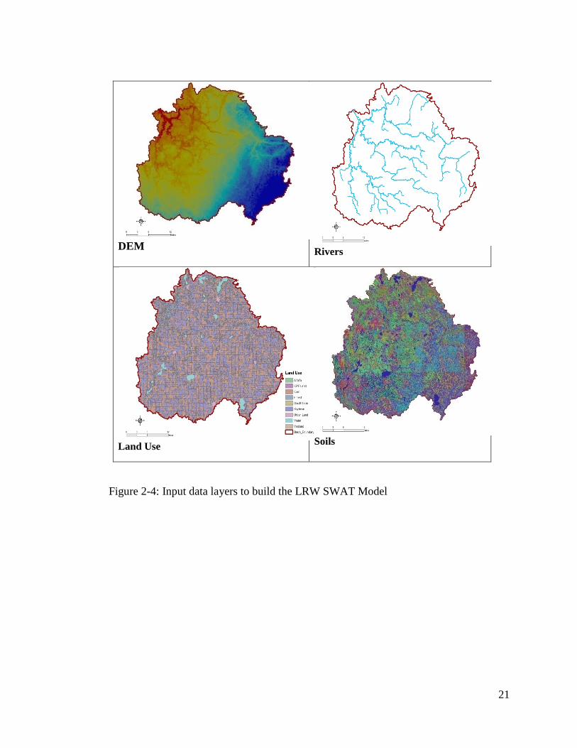
and Figure 2-4).

Table 2-3: Data sources for the Le Sueur Watershed SWAT modeling

Data Type

Source Digital Elevation Model (DEM)

http://seamless.usgs.gov USGS

SSURGO soil http://www.ftw.nrcs.usda.gov USDA

Land use http://datagateway.nrcs.usda.gov USDA

Stream network http://mrbdc.mnsu.edu/gis/lesueur MRBDC

Weather http://climate.umn.edu U of M

Point Sources MPCA

21

DEM Rivers

Land Use Soils

Figure 2-4: Input data layers to build the LRW SWAT Model

22

Table 2-4: LRW monitoring stations Station ID Water Body

Drainage Area, ha Record period

Recording Agency

S003-860 Upper Le Sueur river 117,707 9 months/2006 DNR, MPCA S003-446 Big Cobb 80,019 2004-2006 DNR, MPCA

S000-340 Le Sueur River nr Rapidan, MN66 284,499 1990-2006 USGS, MDA

S002-427 Maple 88,167 2004-2006 DNR, MPCA

S003-574 Little Cobb 34,065 1998-2006

USGS, MetCouncil, MDA

S001-210 Beauford Dtch 2,096 1998-2006 MetCouncil, MDA

The other SWAT model input database files that were not in GIS Layers were the

management operations, stream water quality, point sources and weather data. Weather

data for the LRW SWAT modeling was taken from nine different gauging stations of

the MN State Climatology Office. The selected stations are distributed all over the

watershed to effectively capture the spatial variability of LRW precipitation. The

Thiessen Polygon method was used to define the LRW precipitation data discretization.

Measurements of stream flow and water quality recorded by USGS, MN Metropolitan

Council, MPCA, DNR and MDA (Table 2-4) were used for model simulation,

calibration and validation. The most detailed USDA crop land data (CLD) for the year

2006 was used for the LRW SWAT model land use data input (Figure 2-4 & Table 2-5).

Table 2-5: LRW land use in the year 2006

Land Use % Alfalfa 0.3 CRP Land 2.6 Corn 44.8 Forest 3.9 Small Grain 0.3 Soybean 37.0 Urban Land 7.1 Water 2.1 Wetland 1.8 Total 100.0

23

Figure 2-5: Stream flow, Water Quality and Weather Monitoring Stations in LRW

2.2.3. Modeling Assumptions

The following basic assumptions pertaining to hydrology (surface runoff, snow

hydrology, surface and subsurface flow) were used during SWAT modeling of LRW.

• Tile drained lands in the LRW were identified based on the following

assumptions:

o No subsurface tile drainage exists in crop land with slopes greater than

6%

o All crop land with slopes less than 2% are tile drained

o Crop land with slopes of 2-6% and hydrologic soil group “C” or “D” are

tile drained

• A two year rotation of corn and soybean was used as the baseline scenario, and

as the framework for management operations over the simulation period.

• The maximum or peak rainfall intensity during a storm is calculated assuming

the peak rainfall intensity is equivalent to the rainfall intensity used to calculate

the peak runoff rate.

• The peak runoff rate from snow melt is estimated assuming uniformly melted

snow over a 24 hour duration.

24

• The hydraulic gradient of stream-bed and subsurface flow is assumed to be

equal to the land-surface slope.

• The average flow velocity was estimated from Manning’s equation assuming a

trapezoidal channel with 2:1 side slopes and a 10:1 bottom width-depth ratio.

• The hourly solar radiation was calculated by assuming that solar noon occurs at

12:00 pm local standard time.

• The depth distribution of the evaporative demand for soil layers assumed a total

soil evaporation demand of 100 mm

2.2.4. Identifying Critical Contributing Areas

Soil water content is an important variable that defines the surface runoff impacts of

watersheds (Hassan et al., 2007). Saturated soils within a watershed have quick

response to surface runoff generation and potentially large losses of soil by erosion

(Mehta et al., 2003; Betson, 1964).

The most commonly used methods for estimating soil water content can only provide

point measurements due to the amount of work required to process field samples. Field

measurements of soil water content are insufficient to provide continuous spatial

coverage needed for land-management applications (Hassan et al., 2007). As an

alternative to field measurement of soil water content, topographic indices of wetness

can be used to generate spatially continuous soil water information for identifying

saturation excess areas (Western et al., 1999). The compound topographic index (CTI)

and stream power index (SPI) were the two hydrologic based indices that were used to

estimate relative soil wetness in the LRW.

Compound Topographic Index (CTI)

The Compound Topographic Index (CTI) is a steady state wetness index, also called

Topographic Wetness Index. It is a function of the slope and upstream contributing area

per unit width orthogonal to the flow direction. CTI has proven to be highly correlated

with several soil attributes such as horizon depth, silt percentage, organic matter content

25

and phosphorus (Moore et al., 1993). It is a parameter which shows the tendency of

runoff dispersion in the watershed, and represents the ratio between upstream area and

slope. Areas with high values for CTI tend to be depositional and are sites with

saturated soil (Moore et al., 1993; Gessler et al., 1995).

CTI is calculated with the formula:

=

βtanln sA

CTI (2.9)

Where: - As is the specific catchment area expressed as m2 per unit width orthogonal to

the flow direction, and

- β is the slope angle expressed in radians (Gessler et al. 1995).

Stream Power Index (SPI) Stream power index is a measure of the erosive power of overland flow based on the

assumption that discharge (q) is proportional to specific catchment area (As) and the

slope. As specific catchment area increases, there will be concentrated surface water

flow, which increases the velocity of water flow, this in turn increases the stream power

index and then the erosion risk (Moore et al., 1993). The SPI is given by:

( )βtan*ln AsSPI = (2.10)

A 30m Digital Elevation Model (DEM) was used to derive the primary terrain attributes

of slope and specific catchment area using the TAUDEM approach in ARCGIS

(Tarboton, 2002). These primary attributes were used to calculate the secondary terrain

attributes of CTI and SPI. Finally, all CTI values over 10.5 and SPI values over 7 were

used for the delineation of critical contributing areas (CCAs). These threshold values

were selected as the best fit to define CCA areas after field cross checking of the

developed CTI and SPI maps with the actual land features (depressional areas,

wetlands, riparian areas etc).

26

Once the CCAs are created and the CCA soils are delineated, the threshold values of

2% land use, 1% soil and 10% slope of the sub-watershed area were used as criteria of

homogeneity to incorporate CCA-HRUs into the SWAT model.

The incorporation of the CCA concept in the SWAT model was made by calibrating the

available water capacity (AWC) of the soils represented by CCAs. In this process the

CCA-AWC was reduced, and the effect of this reduction increased the initial curve

number values in saturated areas. The changes made to AWC directly affect the runoff

generated through its effect on the maximum retention parameter used in estimating the

curve number.

The USDA-SCS (1972) curve number method to estimate watershed runoff is:

)(

)( 2

SIP

IPQ

a

a

+−

−= (2.11)

Where: - Q is the accumulated runoff or rainfall excess (mm H20)

- P is the rainfall depth for the day (mm H20)

- Ia is the initial abstraction which includes surface storage, interception and

infiltration prior to runoff (mm H20), and

- S is the retention parameter (mm H20).

The runoff estimates increase with increasing curve number condition, and with

increasing antecedent soil moisture. The initial abstraction, Ia, is commonly

approximated by the empirical relationship Ia= 0.2S. Substituting in Eq. (1) gives:

)8.0(

)2.0( 2

SP

SPQ

+−

= (2.12)

Runoff will only occur when P > Ia

The retention parameter varies spatially due to changes in soils, land use, management

and slope and temporally due to changes in soil water content. The retention parameter

is defined as:

−= 101000

4.25CN

S (2.13)

Where: CN is the curve number for the day.

27

The potential maximum retention S increases exponentially as the curve numbers

decrease from 100 down to 30.

The daily curve number value adjusted for moisture content was calculated by

rearranging Eq. (2.13) and inserting the retention parameter calculated for that moisture

content:

+

=254

25400

SCN (2.14)

In the SCS-curve number procedure, the overall impact of land use, management and

cover conditions, and antecedent moisture conditions are represented by the initial

abstraction (Ia = 0.2S).

The curve number estimation method of Eq. (2.14) is a spatially averaged value, and

cannot describe the quick surface runoff response of CCA areas. This decreases the

ability of the SWAT model to accurately estimate daily time-step surface runoff from

CCA areas.

The initial rate of infiltration depends on the moisture content of the soil. The maximum

storage capacity, S in Eq. (14) reflects the effect of AWC prior to rainfall. Therefore,

proper simulation of saturated excess areas of CCAs can be captured by adjusting the

AWC of CCA soils. For this, the CTI and SPI cutoff values that represent the saturation

excess areas of the LRW were determined and an adjustment to the spatial distribution

of the runoff response was made by calibrating the AWC of CCA soils. The AWC of

these soils was calibrated until the SWAT predicted water yield closely matched the

measured water yield.

Incorporating CCAs in the LRW SWAT model was hypothesized to improve model

efficiency and accuracy.

28

2.2.5. Baseflow Separation

Baseflow discharge to streams is an important concept in many current watershed

models. Baseflow recession coefficients can be used to route recharge to the stream

(Arnold et al., 1995, Leavesley et al., 1983). SWAT model output results can be

significantly improved by estimating the correct average annual ratio of surface runoff

to baseflow. Hence, application of some type of separation techniques is essential for

calibration of the SWAT model.

The baseflow separation method make use of the time-series record of stream flow to

derive the baseflow signature. The separation method can be graphical, in which the

points where baseflow intersects the rising and falling limbs of the quickflow response

are defined, or the entire stream hydrograph can be used to derive a baseflow

hydrograph through filtering. The baseflow recession constant, also called alpha factor,

can be derived from the baseflow separation process. The alpha factor is one of the

input parameters to the SWAT model shallow ground water simulation routine. A large

alpha value is an indication of steep recession, which is indicative of rapid drainage and

little storage. Conversely, a small alpha value shows very slow drainage (Arnold et al.,

1995).

In the case of LRW, baseflow separation was achieved using Eckhardt's (2004)

automated recursive digital filter method applied in the Web-based Hydrograph

Analysis Tool (WHAT). The WHAT method application was preferred due to the fact

that this system was extended to include GIS capabilities for WI, MN, OH, IL, MI, and

SC (Lim and Engel, 2004; Lim et al., 2005ab) . An estimate of baseflow was made for

the Beauford sub-watershed and the entire LRW. The estimated baseflow was used to

calibrate the shallow groundwater flow component against measured streamflow,

through adjusting the ALPHA BF factor. This analysis was performed prior to setting

up and calibration of the LRW SWAT model.

29

2.2.6. Model Sensitivity Analysis, Calibration and Validation

The heterogeneity of environmental variables such as soil types, land uses, topographic

features, and weather parameters need to be considered for the effective simulation of

spatially varying properties of a watershed. Spatially discrete and temporally continuous

data are often not available. Satisfactory physical representation of physically based

spatially distributed models, like SWAT, is limited by the amount of information

available. Thus, the application of complex distributed models over large areas using

insufficient input data has led to the inclusion of model sensitivity analysis, calibration

and validation as methodological frameworks of the models. Muleta et al. (2005) has

suggested a procedural approach of parameter screening, spatial parameterization, and

parameter sensitivity analysis to reduce the SWAT model calibration parameters

(Muleta and Nicklow, 2005;,Vachaud and Chen, 2002).

The most sensitive input parameters were identified using the SWAT model inbuilt

procedures (van Griensven, 2005). This procedure employs a One-factor-At-a-Time

(OAT) sensitivity analysis methods and Latin-Hypercube (LH) random sampling. The

Nash–Sutcliffe efficiency (NSE) was used as an objective function while analyzing the

sensitivity of 26 flow sensitive input parameters included in the model (Table 2-6).

Once the parameters to be optimized were identified through the sensitivity analysis, the

model was calibrated. Model calibration was made on a single site using a single

objective function, namely, the Nash–Sutcliffe efficiency measure (Nash and Sutcliffe,

1970). A sub-watershed of the LRW, called Beauford sub-watershed, that has many

years of gauged data and relatively homogeneous land use and site characteristics was

used for calibration. The calibration year (year 2000) was selected based on an analysis

of cumulative annual precipitation to find a year with nearly normal annual

precipitation. Calibration of the parameters was made manually based on the SWAT

model upper and lower boundary limits. A number of iterations were made to obtain

good parameter value estimation. This was justified by validating the model over a four

year period in the Beauford sub-watershed and at three major tributaries of the LRW,

namely the Maple, Big Cobb and Upper Le Sueur watersheds.

30

Table 2-6: SWAT model parameters for the sensitivity analysis

# PARAMETER LOWER BOUND

UPPER BOUND imet

1 Alpha_Bf 0 1 1 2 Biomix 0 1 1 3 Blai 0 1 1 4 Canmx 0 10 1 5 Ch_K2 0 150 1 6 Ch_N 0 1 1 7 Cn2 -25 25 2 8 Epco 0 1 1 9 Esco 0 1 1 10 Gw_Delay -10 10 2 11 Gw_Revap -0.036 0.036 1 12 Gwqmn -1000 1000 1 13 Revapmin -100 100 1 14 Sftmp 0 5 1 15 Slope -25 25 2 16 Slsubbsn -25 25 2 17 Smfmn 0 10 1 18 Smfmx 0 10 1 19 Smtmp -25 25 2 20 Sol_Alb -25 25 2 21 Sol_Awc -25 25 2 22 Sol_K -25 25 2 23 Sol_Z -25 25 2 24 Surlag 0 10 1 25 Timp 0 1 1 26 Tlaps 0 50 1

Note: Imet is the variation method during sensitivity analysis. The value of 1 indicates

replacement of initial parameters by new value and 2 means adding to the initial value.

The SWAT model parameter estimation, calibration and validation procedures followed

those recommended by Neitsch et al. (2002). The accuracy of the SWAT model output

was examined by comparing the time series outputs with monitored data over both the

calibration and validation periods.

31

2.3. RESULTS AND DISCUSSION

2.3.1. Identifying Critical Contributing Areas (CCAs)

2.3.1.1. CCAs in the Beauford Sub-Watershed

Based on the percent watershed area threshold values for land use (2%), soil (1%) and

slope (10%) as criteria to establish homogeneous HRUs, a total of 357 HRUs were

created for the Beauford sub-watershed. About 29 % (559 ha) of the Beauford sub-

watershed, encompassing 152 of the 357 HRUs were identified as CCA HRUs (Figures

2-6, 2-7 and 2-8).

The Beauford sub-watershed CCA-HRUs have a total of 34 soil series types, of which

eight soil types accounted for 86% of the CCA area.

Table 2-7: CCA soils in the Beauford sub-watershed

HRU Soils Area, ha CCA - Lura 143.15 CCA - Minnetonka 88.56 CCA - Waldorf 84.78 CCA - Caron 52.90 CCA - Shorewood 46.07 CCA - Lester 27.29 CCA - Marna 24.32 CCA - Muskego 24.12

Figure 2-2: Stream power Index (SPI)

Figure 2-1: Compound Topographic

Index (CTI)

32

2.3.1.2. CCAs in the LRW

LRW has 28% (79,868 ha) of its area in the CCAs. About 73% of the CCAs are on

three soil series types: Lura, Minnetonka and Waldorf. These soils are very deep and

poorly drained soils that were formed in clayey glacial lacustrine sediments on glacial

lake plains, and ground moraines. They have slopes of 0 to 2 percent and a saturated

hydraulic conductivity of 0.15 to 0.51 cm per hour. They have seasonal saturation

during the months of November to June in normal years.

Table 2-8: CCA soils in LRW

Soil Series % CCA - Lura 25.1 CCA - Minnetonka 15.5 CCA - Waldorf 14.9 CCA - Caron 9.3 CCA - Shorewood 8.1 CCA - Lester 4.8 CCA - Marna 4.3 CCA - Muskego 4.2

Figure 2-3: Critical contributing Areas In the Beauford Sub-Watershed

33

Figure 2-9: CCAs in the LRW

2.3.2. Modeling LRW Hydrology

The movement of surface water and associated pollutants are governed by hydrologic

processes. Therefore, understanding hydrological processes is very important for

assessing the environmental and economical well-being of the LRW and all receiving

water bodies downstream. The Le Sueur River drains an area of 2,850 km2, and has an

annual mean flow of 21 m3/sec. The three months of April to June are the peak flow

season, and low flows occur during the months of Dec-Jan.

There are a number of processes controlling the spatial and temporal variability of the

LRW hydrology. Baseflow separation was the primary task for separating surface and

subsurface hydrological processes. This was followed by a sensitivity analysis of

SWAT model input parameters.

34

2.3.2.1. Baseflow Separation

Baseflow separation for the Beauford sub-watershed showed that 49% of the total

stream flow was contributed by baseflow. Eighty seven percent of the total baseflow

occurred in the five months from March to July, which account for 84% of the annual

stream flow. The month of May has the largest baseflow (28%), while the month of

August has the smallest (0.28%)(Figure 2-10).

The baseflow contribution to the LRW is about 66% of the total flow (Figure 2-11). In

the period from March to July, baseflow represented 71% of the streamflow. The same

period accounts for 72% of the total stream flow. The month of April has the largest

baseflow (19%), while the month of January has the smallest (0.28%). The monthly

distribution of baseflow in the LRW is more consistent from month to month than in

small sub-watersheds like Beauford. This is what sustains flow in the LRW throughout

the year. The high baseflow of the LRW, compared to the Beauford sub-watershed is

due to the large contributing area that increases baseflow, as well as snowmelt that

increases hydrostatic pressure.

Figure 2-10: Average daily streamflow and baseflow in the Beauford sub-watershed

0

500

1000

1500

2000

2500

3000

3500

4000

4500

Av

era

ge

d

ail

y f

low

, m

3

Streamflow Baseflow

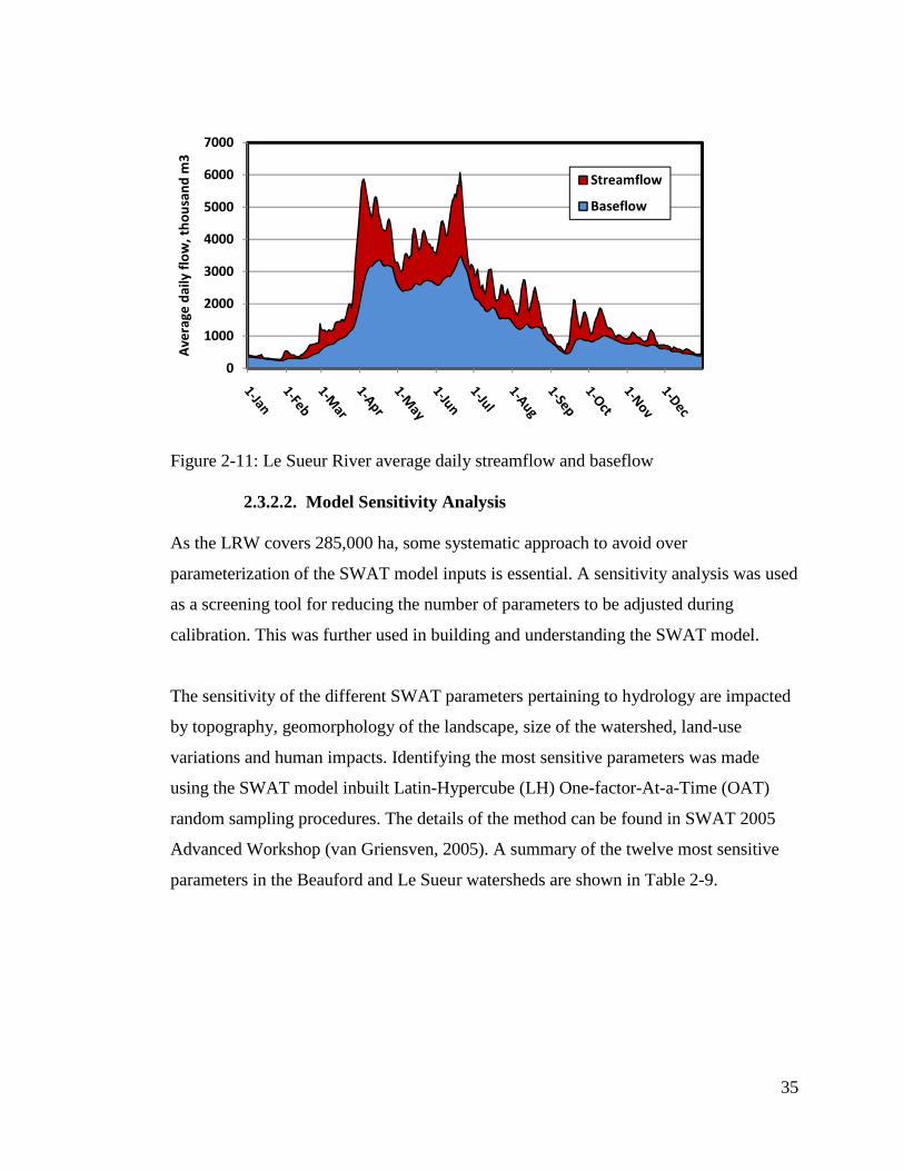
35

Figure 2-11: Le Sueur River average daily streamflow and baseflow

2.3.2.2. Model Sensitivity Analysis

As the LRW covers 285,000 ha, some systematic approach to avoid over

parameterization of the SWAT model inputs is essential. A sensitivity analysis was used

as a screening tool for reducing the number of parameters to be adjusted during

calibration. This was further used in building and understanding the SWAT model.

The sensitivity of the different SWAT parameters pertaining to hydrology are impacted

by topography, geomorphology of the landscape, size of the watershed, land-use

variations and human impacts. Identifying the most sensitive parameters was made

using the SWAT model inbuilt Latin-Hypercube (LH) One-factor-At-a-Time (OAT)

random sampling procedures. The details of the method can be found in SWAT 2005

Advanced Workshop (van Griensven, 2005). A summary of the twelve most sensitive

parameters in the Beauford and Le Sueur watersheds are shown in Table 2-9.

0

1000

2000

3000

4000

5000

6000

7000

Av

era

ge

da

ily

flo

w,

tho

usa

nd

m3

Streamflow

Baseflow

36

Table 2-9: SWAT model hydrology parameters sensetivity

Parameter UNIT Description Rank

Ch_K2 mm/hr Effective hyd. cond. in the main channel

1 Surlag days Surface lag coefficient

2

Alpha_Bf decimal Baseflow alpha factor 3

Esco fraction Soil evaporation compensation factor

4

Ch_N [ ] Manning coefficient for channel

5

Sol_Awc mm/mm Available soil water capacity

6

Blai [ ] Leaf area index for crop

7

Sol_Z mm Soil depth

8

Timp [ ] Snow pack temperature lag factor 9

Canmx [ ] Maximum canopy index

10

Cn2 [ ] SCS curve number, antecedent moisture

condition II,

11

Epco fraction Plant evaporation compensation factor

12

2.3.2.3. Model Calibration

To minimize the complexity of model calibration, the Beauford sub-watershed was

selected as a representative small sub-watershed of the LRW. Beauford sub-watershed

is located at the center of the LRW and has an area of 2,096 ha. The land use in the

Beauford sub-watershed is dominantly (89%) agricultural, with a two year rotation of

corn and soybean. Tile drainage is extensively used on the flat 0-2% slope lands that

cover 92% of the sub-watershed. The fact that this sub-watershed has no significant

channel erosion and no bluffs or ravines is very important for calibration of upland

hydrological and sediment transport processes in the SWAT model.

SWAT model calibration was made in the year 2000. This year was selected for having

precipitation very similar to that in a normal year as shown in Figures 2-12 and 2-13.

37

Figure 2-12: Cumulative precipitation for the period 2000-2005

Figure 2-13: Calibration Year Precipitation vs Normal Year Precipitation

The estimated average monthly stream flow for the Beauford sub-watershed is about

0.14 m3/s/month. The monthly flow ranges from zero in the low flow season, to 1.58 m3/s during

the high flow season. Timing of occurrence of both low and peak flows as predicted by the

SWAT model generally agreed with observed data. The total simulated annual flow

volume for the calibration year (2000) was less than the observed by 14%, with an NSE

0

200

400

600

800

1000

1200

Cu

mu

lati

ve

Pre

cip

ita

tio

n,

mm

Date

2000

2001

2002

2003

2004

2005

Average

38

value of 0.77. Overall, model predictions showed very good agreement with field

measured data (Figure 2-14).

Figure 2-14: Calibration of monthly stream flow

The calibration result in Figure 2-14 was achieved after an adjustment to the twelve

most sensitive model input parameters. The adjustments were made based on available

measured data, knowledge about the watershed and an extensive literature review of

SWAT model applications.

Calibration of Parameters governing the entire watershed hydrology

The calibrated basin level hydrology parameters include:

• The snow hydrology parameters

• The surface runoff lag time (SURLAG)

• Channel hydraulic conductivity (CH_K2)

• The soil evaporation compensation factor(ESCO)

• The plant evaporation compensation factor(EPCO)

0

200

400

600

8000.0

0.2

0.4

0.6

0.8

1.0

1.2

Dec-99 Mar-00 Jun-00 Oct-00 Jan-01

Pre

cipita

tion

, mm

Dis

cha

rge

, (m

3/s

)

Precipitation Measured Predicted

39

Table 2-10: Basin level calibrated parameters for the Beauford and Le Sueur

watersheds.

SWAT variable

Description min max Default Value

Calibrated Value

SFTMP Snowfall temperature [◦C] −5 +5 1 0.0 SMTMP Snow melt base temperature [◦C] −5 +5 0.5 4.0 TIMP Snow pack temperature lag

factor [–] 0 1 1 0.85

SMFMN Melt factor for snow on December 21st [mm H2O/◦C day]

0 10 4.5 2

SMFMX Melt factor for snow on June 21st [mm H2O/◦C day]

0 10 4.5 4

SNOCOVMX Minimum snow water content that corresponds to 100% snow cover [mm]

0 500 1 40

SNO50COV Fraction of snow volume represented by SNOCOVMX that corresponds to 50% snow cover [–]

0 1

0.5 0.3

ESCO Soil evaporation coefficient 0 1 0.95 0.87 EPCO Plant evaporation coefficient 0 1 1 0.89 SURLAG The surface runoff lag time 1 24 4 1

CH_K2 Channel hydraulic conductivity

-0.01

500 0.05

The snow pack temperature lag factor, TIMP, that controls the previous day snow pack

temperature effect on the current day's snow pack temperature is the most sensitive

parameter of all the snow hydrology parameters. The final calibrated value of TIMP

was 0.85. This indicates that snow pack temperature is mostly influenced by current day

air temperature. The calibrated values for the rest of the snow parameters and basin

level inputs are shown in Table 2-10.

40

Table 2-11: Calibration of Parameters governing Surface and Subsurface Hydrology

2.3.2.4. Model Validation

Validation of stream flow was conducted both in the Beauford and the entire LRW. The

calibrated model parameters for the Beauford watershed were considered transferable to

the LRW due to the fact that model performance in the Beauford sub-watershed was

good.

Validation of monthly flow over the years 2001 - 2006 in the Beauford watershed gave

an NSE of 0.89. Validation in the LRW from 1994 to 2006 showed good agreement

between measured and predicted monthly flow, with an NSE of 0.73. These results

indicate that the SWAT model can accurately simulate the hydrology of the LRW

(Figure 2-15 and Figure 2-16).

Parameter Range Default Value

Final Calibrated Value

Curve Number (CN) ±10 - -6

Soil available water capacity (SOIL_AWC) 0-1 - variable

Base-flow alpha factor, days (ALPHA_BF) 0.1-1.0 0.025 0.2

Groundwater revap. coefficient, (GW_REVAP)

0.02-0.2 0.02 0.02

Groundwater delay time, days (GW_DELAY) 0-100 40 20

Time to drain soil to field capacity, hours (TDRAIN)

24 48

Drain tile lag time, hours (GDRAIN) - 96 96

Depth to subsurface drain, mm (DDRAIN) - 1200 1200

41

Figure 2-15: Validation of monthly flow in the Beauford sub-watershed

Figure 2-16: Validation of monthly flow in the LRW

The predicted average annual flows in the Beauford (Figure 2-17) and Le Sueur (Figure

2-18) watersheds were very accurate. The model over predicted annual flow by 10% in

the Beauford sub-watershed. Over the simulation period from 1994 to 2006, there was a

6% under prediction in some years and a 7% over prediction in other years, indicating

no systematic error. The predicted annual flows in the Beauford and LRW have NSE

values of 0.93 and 0.7, respectively (Figures 2-17 & Figure 2-18).

0.0

0.5

1.0

1.5

2.0

Dis

cha

rge

, (m

3/s

)

Measured Predicted

0

50

100

150

200

250

Flo

w,

M3/s

ec

Meaured Predicted

42

Figure 2-18: Annual flow in the LRW

2.3.2.5. Water Budget

The principle of conservation of mass was applied to compute the annual water budget

in the LRW.

∆�� (15)

0

5

10

15

20

25

30

35

Flo

w,

M3

/Se

c

Measured Predicted

0.00

0.05

0.10

0.15

0.20

0.25

0.30

2001 2002 2003 2004 2005 Average

Flo

w,

M3

/Se

c

Measured Predicted

Figure 2-4: Annual flow in Beauford sub-watershed

43

Where ∆SW is the change in soil water storage, P is the total annual precipitation, ET

the evapotranspiration, tileQ is the tile flow, surfQ is the surface runoff flow, gwQ is the

groundwater flow and daqQ is the deep aquifer recharge.

ET accounts for 71% of the water budget, the largest of all components. Tile flow is the

second largest component, accounting for 13% of the water budget. Surface runoff

accounts for another 11% of the water budget. Available water holding capacity of the

LRW soils varies considerably, the average annual soil water storage is estimated at

about 245 mm. The average soil water content ranges from 227 mm to 273 mm over the

whole year, except the three months of July, August and September. In those three

months the soil water content gets as low as 172 mm due to the high evapotranspiration

(Figure 2-19 and 2-20 and Table 2-12).

The annual water yield of LRW is 230 mm. About 47% of the water yield is

contributed by tile drainage, 38% is from surface runoff, 11% is groundwater flow and

4% is lateral flow. The months of March to June are the period in which over 70% of

the surface runoff, tile flow and total water yield of LRW occurs. April is the month in

which the water yield, surface runoff and tile flow reach the maximum peak point

(Figure 2-20).

Figure 2-19: Average annual water budget

44

Figure 2-20: Average monthly distribution of the water balance components

(1994-2006)

0

10

20

30

40

50

60

Flo

w,

mm

SURQ

LATQ

GWQ

TILE Q

WATER YIELD

0

50

100

150

200

250

300

Wa

ter

con

ten

t, m

m

Precipitation Soil water ET

45

Table 2-12: Water budget components of the LRW (1994-2006).

YEAR PREC SURQ LATQ GWQ TILEQ SW ∆ SW

ET WYLD 1994 854.7 60.8 11.1 25.6 111.1 262.1 0 641.3 207.3 1995 868.1 56.9 12.2 32.5 157.1 265.3 3.2 597.4 256.9 1996 799.9 48.8 9.8 17.6 69 262 -3.3 597.8 144.6 1997 687 64.3 10.1 21.1 100.4 225.3 -36.7 574.3 195 1998 809.8 69.8 8.4 20.4 81.6 253.4 28.1 598.3 178.8 1999 897.9 99.6 11.4 31.9 154.6 234.8 -18.5 607.2 296.2 2000 923.4 144.8 8.7 27.6 87.2 224.6 -10.3 596.6 267.1 2001 866.1 159 9.8 24.1 145.9 236 11.4 561.7 337.1 2002 805.9 64.4 8.4 22.7 79.3 255 19.1 609.5 173.6 2003 589.5 22.8 6.6 17.2 64.6 149 -106 567 110.7 2004 980.7 127.4 7.8 32.5 74.9 264.6 115.6 619.1 241.3 2005 1001.8 136.9 11 29.1 132 281.8 17.2 634.5 307.5 2006 845.1 91.8 11.1 20.4 155 276 -5.7 591.9 276.5 Avg 840.8 88.2 9.7 24.8 108.7 245.4 1.1 599.7 230.2

Note:

PRECP= Precipitation, SURFQ= Surface runoff, LATQ= Lateral flow, GWQ=

groundwater flow, TILEQ= Tile flow, SW= Soil water storage, ET=

Evapotranspiration, WYLD= Water yield

The major water yielding areas of the LRW are concentrated in the western portion of

the LRW. About 36% of the watershed area has an annual water yield of over 250 mm,

and the rest less than 250 mm. The source areas and their relative contributions are

shown in Table 2-13 and Figure 2-21 below.

Table 2-13: Water yield versus areal coverage

WYLD, mm Area coverage, % WYLD Contribution, %

> 350 2 3

250-350 34 41

200-250 45 43

131-200 17 13

< 131 2 0

46

Figure 2-21: Spatial Variation in Water Yield in the LRW

2.3.2.6. Evaluation of Effects of CCA-HRUs on Watershed Hydrology

HRUs delineated using the concept of critical contributing areas (CCA-HRUs) had NSE

values that were 2% better for monthly and annual water yield than the non-CCA

model. The CCA-HRU approach had a 7 mm increase in the overall water yield, a 5.3%

increase in surface runoff and a 2.8% increase in groundwater flow. Tile Q and lateral

flow decreased by 4.7% and 0.7%, respectively, with the CCA model. These results

show that the two modeling approaches produced roughly similar results (Table 2-14 &

Table 2-15). As measured data for each hydrologic component are not available for

these watersheds, further research is recommended to further evaluate the utility of the

CCA modeling approach.

47

Table 2-14: Average monthly and annual stream flow using standard HRU and the

modified CCA-HRU

Table 2-15: Average annual water balance components for the standard HRU and the

modified CCA-HRU approach

Water balance component Default HRU Modified HRU Depth, mm

PRECIP + SNOW MELT 840.8 (100%) 840.8 (100%)

ET 612.8 (72.9%) 599.7 (71.3%)

TILE Q 148.1 (17.6%) 108.7 (12.9)

SURFACE RUNOFF Q 60.2 (7.2%) 88.2 (10.5%)

GROUNDWATER (SHAL AQ) Q 1.67 (0.2%) 24.8 (3.0%)

LATERAL SOIL Q 16.35 (1.9%) 9.7 (1.2%)

DEEP AQ RECHARGE 0.1 (0.01%) 0.4 (0.1%)

CHANGE IN SOIL STORAGE 0.7 (0.1%) 8 (1.0%)

Water budgets for other SWAT studies in the Midwestern US are presented here for

comparison (Table 2-16). Green et al. (2006) found that 80% of the water yield in a tile

drained watershed in north central Iowa was from tile flow and subsurface flow. Studies

by Gassman et al. (2006) and Jha et al. (2007) are in good agreement with the Le Sueur

SWAT model results. However, Jha et al. (2007) underestimate tile flow, although 51%

of their watershed is under tile drainage.

Time

Average Stream Flow, mm Measured

Simulated HRU Based

NSE CCA-HRU Based

NSE

Monthly 20.33 20.39 0.70 20.84 0.72

Annual 269.49 264.36 0.66 270.71 0.68

48

Table 2-16: SWAT modeling study water budget results for the region

Note

*1 Boone River watershed in North-Central Iowa. (Gassman et al., 2006)

*2 Racoon River watershed West-Central Iowa. (Jha et al., 2007)

*3 South Fork watershed in North-Central Iowa. (Green et al., 2006)

** Percent of the water yield

***Percent of the precipitation

Component

Depth (mm)

*1 *2 *3 LRW

Precipitation 812.7 840.2 768 840.8

**Surface Runoff 118.6 (49%)

104.6 (45%)

38.1 (20%)

87 (37.8%)

**Tile Flow 89.9 (37%)

21.2 (9%)

136.4 (71%)

108.67 (47.2%)

**Groundwater & lateral subsurface flow

34.1 (24%)

112.5 (48%)

17.9 (9%)

34.54 (15%)

***Evapotranspiration 562.3 (69%)

598.3 (71%)

569.2 (74%)

599.7 (71.3%)

***Water Yield 241.0 (29.7%)

235.1 (28%)

192.4 (25.1%)

230.21 (27.4%)

49

2.4. SUMMARY AND CONCLUSIONS

The LRW SWAT hydrologic model has two major components, a surface water

component, and a subsurface component which simulates water flow in the soil water

continuum that includes tile flow, lateral flow and groundwater flow. The study

involved sensitivity analysis, parameterization and calibration of model input

parameters in a selected sub-watershed of the LRW, called the Beauford sub-watershed.

The calibrated input parameters were transferred to the LRW, and the SWAT model

outputs were validated over the years 1994-2006. In order to test model efficiency, the

goodness of fit between the measured and simulated water yield were evaluated using

the Nash–Sutcliffe model efficiency coefficient.

SWAT predicted monthly discharge from 1994-2006 has high accuracy with NSE

values of 0.77 and 0.73 in the Beauford sub-watershed and LRW, respectively. The

average annual water yield of LRW during this period was 230 mm. About 47% of the

water yield is contributed by tile drainage, 38% from surface runoff, 11% groundwater

flow and 4% lateral flow. The calibrated hydrology parameters at the scale of the

Beauford sub-watershed were transferred to the entire LRW. The incorporation of

critical contributing areas (CCA-HRUs) produced slightly better model efficiencies than

the non CCA model in both the monthly and annual water yield.

The months of March to June are the period in which over 70% of the surface runoff,

tile flow and the total water yield occurs in the LRW. April is the month in which the

water yield, surface runoff and tile flow reach maximum peak values. ET accounts for

71% of the water budget, the largest of all components. Tile flow is the second largest

component, accounting for 13% of the water budget. Surface runoff accounts for

another 11% of the water budget. The average annual soil water storage of the LRW is

estimated at about 245 mm. The average soil water content ranges from 227 mm to 273

mm in all months, except the months of July, August and September. In those three

months months the soil water content gets as low as 172 mm due to the high

evapotranspiration.

50


WATERSHED SEDIMENT SOURCE AREAS AND

TRANSPORT PROCESSES

51

SYNOPSIS

The Le Sueur River Watershed (LRW) generates 302,000 t/yr of sediment which has

resulted in turbidity impairment of several river reaches in the watershed. Unless some

mitigation measures are taken, the current excessive sediment flux from LRW can

destroy aquatic habitats, biotic communities and aesthetic qualities of the LRW itself

and all receiving water bodies downstream, including Lake Pepin. Our objective in this

research was to use the Soil and Water Assessment Tool (SWAT) to quantify the spatial

and temporal sediment loadings of the LRW. The ability of the model to represent soil

erosion, sediment transport and deposition processes in the LRW was assessed through

the calibration and validation processes.

The Beauford sub-watershed, at the center of LRW, was selected as a representative

watershed for calibration because it sediment loss arises only from upland erosion

processes – there are no eroding streambanks, bluffs or ravines. Upland hydrologic and

sediment variables obtained by calibrating SWAT in the Beauford sub-watershed could

be transferred to all other upland sub-watersheds in the LRW. In contrast, SWAT model

sediment channel parameters such as the peak rate adjustment factor for sediment

routing in the main channel (PRF) and the linear parameter for calculating the channel

sediment routing (SPCON) were found to be very different in the Beauford and Le

Sueur River mainstem watersheds. A sensitivity analysis of SWAT channel sediment

parameters in combination with upland hydrology and sediment parameters from the

calibrated model showed that sediment contributions from upland regions of the LRW

range from 13% to 30%, the remaining 70% to 87% is from channel sources. The

effectiveness and water quality impacts of best management practices (BMPs) was also

evaluated so as to identify the best ones for conservation planning and water quality

improvement. Implementation of conservation tillage, filter strips and rye cover crop

BMPs decreased upland sediment losses from 8% to 54%.

52

3.1. INTRODUCTION

3.1.1. Problem Statement

The Minnesota River is impaired for suspended solids which affects turbidity. The

annual average load of suspended solids transported by Minnesota River to the

Mississippi River is estimated to be about 625 million kg (Senjem et al., 1996).

According to the estimates of Kelley et al. (2000), sediment loadings of the Minnesota

River to the Mississippi River and Lake Pepin have increased annually by an average

increment of 8% over the last 160 years. Roughly 85% of the sediment entering Lake

Pepin arises from the Minnesota River Basin. The annual sedimentation rate in the

upper portion of Lake Pepin in recent years is about 40 mm. The excessive sediment

loadings, mainly from the Minnesota River basin, have impacted water quality in Lake

Pepin. Consequently, the lake has been listed as being impaired for nutrients and

turbidity since 2004 (MPCA, 2009).

The Le Sueur River watershed accounts for about 7% of the area, but 53% of the TSS

leaving the Minnesota River Basin (Water Resources Center, 2008). The Le Sueur

River Watershed transports over 200 mg/L of sediment to Minnesota River, higher than

all other major watersheds in the basin . Because the Le Sueur River watershed is

impaired for sediment, a Total Maximum Daily Load is being established, and the

sources of sediment are being evaluated.

Sekely et al. (2002) showed that the Blue Earth River watershed, which is adjacent to

the LRW and has very similar geology, soils and landscapes, generates roughly 44% of

its sediment load from slumping river bluffs. Based on this research, we hypothesize

that sediment loads in the LRW are dominated by channel sources of sediment,

including bluffs, eroding stream banks and ravines. Also there is a wide range of

reported data on channel erosion contributions; a study of the sediment source areas for

the LRW is an important task to be conducted as part of this modeling study. Studies in

the Midwestern United States have reported large sediment contributions from channel

sources: Odgaard (1987) has shown 30- 40% of sediment in the East Nishnabotna and

53

Des Moines Rivers of Iowa are contributed by channel sources, 50% in two Illinois

streams (Wdlun and Hebel 1982), and 65% in the Lawrence River (Rondeau et al.,

2000).

3.1.2. Objectives

The general objective of the sediment modeling component of the LRW study was to

use the Soil and Water Assessment Tool (SWAT) to estimate the spatial and temporal

patterns of soil erosion in the Le Sueur River Watershed. The contribution of upland

areas to sediment loads at various locations within the LRW was quantified. Estimation

of the contributions from channel sources of sediment, including river bluffs, ravines

and stream banks were made.

Specific study objectives include:

i. Evaluate ability of SWAT model to simulate erosion, deposition and

sediment transport dynamics in the LRW

ii. Identify factors that influence erosion processes

iii. Evaluate spatial patterns of upland sources of sediment

iv. Simulate seasonal and long term sediment yields

v. Evaluate relative importance of different best management practices to

reduce sediment loss

3.1.3. Soil Erosion and Sedimentation Processes

Soil erosion and sedimentation are two separate, but interrelated processes at different

stages in the loss of soil from upland regions. Soil erosion is the removal of soil by

water, wind, ice, or gravity. Soil erosion by water involves the detachment, transport

and deposition of soil particles by the erosive forces of rainfall and snowmelt runoff.

This can be in the form of splash, sheet, rill, or gully erosion (Summer et al., 1998).

54

Soil particles will detach and then splash into the air as raindrops strike the soil. Rain

water infiltrates into the soil at a rate controlled by the intensity of the water hitting the

surface and infiltration capacity of the soil profile. When soil becomes saturated,

surface ponding of water will be initiated. When surface accumulated water is

sufficiently deep, it induces surface runoff or overland flow that transports dissolved or

suspended soil particles, causing the process of sediment entrainment or transport to the

outlet of a watershed (Nichols et al., 2003; Julien, 1998).

Changes in stream channel factors, such as stream geometry (width, depth, slope etc),

can reduce flow velocity causing some of the soil particles to be deposited as flows lose

their capacity to carry the sediment. Transport capacity is the maximum amount of

sediment that a given flow can carry without net deposition. Detachment capacity and

transport capacity are interrelated, and it is their interaction that controls the patterns

and magnitudes of both erosion and deposition (Slaymaker, 2003). In any given

watershed, one of the two dominant processes (transport or detachment), will become

the limiting factor for soil erosion. When sediment production or detachment capacity is

lower, there will be transport of available sediment which is generally referred to as

“detachment-limited erosion” (Van Rompaey et al., 2003). In contrast, if detachment

capacity is significantly greater than transport capacity, then the amount and magnitude

of soil erosion is limited by the sediment transport capacity of runoff, referred to as

“transport-limited erosion” (Harmon and Doe, 2001).

Sediment-transport rates are a function of flow hydraulics, bed composition, and

upstream sediment supply. Sediment yield and sediment load are the most commonly

used terms to describe the watershed response to soil erosion. Sediment yield is the

amount of eroded soil that is delivered to a point in the watershed that is usually remote

from the origin of the detached soil particles. It includes the erosion from slopes,

channels, and mass wasting (slumping, sliding, falling soils), minus the sediment that is

deposited after it is eroded but before it reaches the point of interest (Renard et al.,

1997). Sediment yield is not available as a direct measurement but can be estimated by

55

using a sediment delivery ratio (SDR), which is the ratio of sediment delivered at a

location in the stream system to the gross erosion from the drainage area above that

point.

SDYLD = SDR*Eg (3.1)

Where: SDYLD is the sediment yield (tons)

SDR is the sediment delivery ratio (fraction)

Eg = Gross erosion (tons)

The SDR generally decreases with increasing watershed area. The estimation of SDR

can be site specific using the relationship of sediment rating curve to flow duration.

This method can be used for small sub-watersheds. In the case of large watersheds there

are commonly used empirical relationships which relate SDR to the watershed area.

Vanoni (1975) suggested the use of an area power function (Vanoni, 1975).

SDR = 0.42S-0.125 (3.2)

where A is the watershed area in square miles.

Old versions of the Soil and Water Assessment Tool (SWAT) model estimated SDR

using a runoff factor (Arnold et al., 1996; Ouyang and Bartholic, 1997). The primary

form of the SWAT-SDR model was:

SDR = ((qp / rp)/ (0.782845 + 0.217155 Q / R )) 0.56 (3.3)

where q p = the peak runoff rate in mm/hr.

rp = the peak rainfall rate in mm/hr

R = the rainfall in mm.

Q = the runoff volume in mm.

The amount of sediment carried per unit time is called the sediment load. Hewlett,

(1982) divided sediment load into three categories:

i. Suspended Load: Containing organic and inorganic particulate matter that is

suspended in and carried by moving water.

56

ii. Dissolved Load: All organic and inorganic material carried in solution by

moving water.

iii. Bed load: Coarse materials such as gravel, stones, and boulders that move along

the bottom of the channel.

3.1.4. Models of Soil Erosion and Sediment Transport

Nearing (1994) defined soil erosion modeling as a process of mathematically describing

soil particle detachment, transport and deposition on land surfaces (Nearing and Lane ,

1994; and Lopes, 1994). Modeling soil erosion and sediment transport of a watershed

can be used for three basic reasons (Jain and Kothyari, 2000):

i. To assess soil loss for conservation planning and regulation. Application of

watershed models can provide a quantitative and consistent approach to estimate

soil erosion and sediment yield under the conditions of applications of different

management practices or changes in land use.

ii. To understand erosion processes and their interactions and for setting research

priorities

iii. Physically based models can predict where and when erosion is occurring, thus

helping to target efforts to reduce erosion

The most important difference among soil erosion models that estimate soil erosion and

sedimentation is the level of complexity in which they represent the processes of soil

erosion, entrainment, detachment and transport of soil particles . Watershed models that

can simulate soil erosion and sediment yield can be grouped into three broad categories:

empirical, conceptual and physically-based models.

The empirical soil erosion models are statistical in nature and usually establish

relationships between annual soil erosion and precipitation, vegetation cover, soil types,

topography, land use types, tillage styles and conservation measures. Due to the

57

simplicity in their structure, those models are easy to apply (Merritt et al., 2003).

However, the fact that the model coefficients are developed by calibrating on

measurements taken on specific localized areas, they fail to fully simulate in other areas

(Nearing and Lane, 1994; and Lopes, 1994). Models of this category include Universal

Soil Loss Equation (USLE) (Wischmeier and Smith, 1965), the Modified Universal Soil

Loss Equation (MUSLE) (Williams, 1975), or the Revised Universal Soil Loss

Equation (RUSLE)(Renard et al., 1997).

Conceptual models employ the continuity equation and make use of grid cells to

describe spatial variations in erosion and deposition. Many of the conceptual models

developed in the 1970's, including CREAMS (USDA, 1980), ANSWERS (Beasley et

al., 1980) overcame the limitations of the USLE. Nevertheless, these models make use

of USLE factors. Since USLE factors, such as C and K, do not change with time to

accommodate differences in season, models that use static values of C and K are limited

to average annual erosion estimates. The main weakness of conceptual models is their

poor physical description of basic sediment processes (Elliot, et al., 1994).

Modeling efforts over the last two decades have focused on the development of

physically based erosion models that have the required routines to capture spatial

variability of soil erosion processes. Among those type of models are the Water Erosion

Prediction Equation, WEPP (Nearing et al., 1989), European Soil Erosion model,

EUROSEM (Morgan et al., 1998) and Soil and Water Assessment Tool, SWAT

(Neitsch et al., 2005).

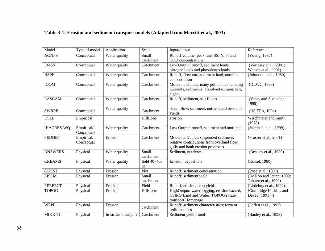
Table 3-1: Erosion and sediment transport models (Adapted from Merritt et al., 2003)

Model Type of model Application Scale Input/output Reference AGNPS Conceptual Water quality Small

catchment Runoff volume; peak rate, SS, N, P, and COD concentrations

(Young, 1987)

EMSS Conceptual Water quality Catchment Low Output: runoff, sediment loads, nitrogen loads and phosphorus loads

(Vertessy et al., 2001; Watson et al., 2001)

HSPF Conceptual Water quality Catchment Runoff, flow rate, sediment load, nutrient concentration

(Johanson et al., 1980)

IQQM Conceptual Water quality Catchment Moderate Output: many pollutants including nutrients, sediments, dissolved oxygen, salt, algae.

(DLWC, 1995)

LASCAM Conceptual Water quality Catchment Runoff, sediment, salt fluxes (Viney and Sivapalan, 1999)

SWRRB Conceptual Water quality

Catchment streamflow, sediment, nutrient and pesticide yields

(US EPA, 1994)

USLE Empirical Hillslope erosion Wischmeier and Smith (1978)

IHACRES-WQ Empirical/ Conceptual

Water quality Catchment Low Output: runoff, sediment and nutrients (Jakeman et al., 1999)

SEDNET Empirical/ Conceptual

Erosion Catchment Moderate Output: suspended sediment, relative contributions from overland flow, gully and bank erosion processes

(Prosser et al., 2001)

ANSWERS Physical Water quality Small catchment

Sediment, nutrients (Beasley et al., 1980)

CREAMS Physical Water quality field 40–400 ha

Erosion; deposition (Knisel, 1980)

GUEST Physical Erosion Plot Runoff; sediment concentration (Rose et al., 1997) LISEM Physical Erosion Small

catchment Runoff; sediment yield (De Roo and Jetten, 1999;

Takken et al., 1999) PERFECT Physical Erosion Field Runoff, erosion, crop yield (Littleboy et al., 1992) TOPOG Physical Erosion Hillslope HighOutput: water logging, erosion hazard,

CSIRO Land and Water, TOPOG solute transport Homepage

(Gutteridge Haskins and Davey (1991), )

WEPP Physical Erosion catchment

Runoff; sediment characteristics; form of sediment loss

(Laflen et al., 1991)

MIKE-11 Physical In-stream transport Catchment Sediment yield, runoff (Hanley et al., 1998)

58

59

3.1.5. Soil Erosion and Sediment Transport in SWAT model

The SWAT model soil erosion algorithm uses the Modified Universal Soil Loss

Equation (MUSLE) equation to estimate the total amount of sediment delivered to the

stream network within a watershed (Williams, 1975). The MUSLE model was

developed by modifying the Universal Soil Loss Equation (USLE) developed by

Wischmeier and Smith ( 1965). Therefore, a clear understanding of MUSLE and its

components is needed for appropriate parameterization of the LRW sediment modeling.

The SWAT model calculates sediment yield for each HRU and every single day with

rainfall and runoff using the following MUSLE equation:

�� 11.8*(Qsurf * qp)0.56*K * LS *C * P*CFRG (3.4) where SYLD is the sediment yield to the stream network in metric tons, Qsurf is the

surface runoff volume in mm, qp is the peak flow rate in m3/s, K is the soil erodibility

factor which is a soil property available from the Soil Survey Geographic (SSURGO)

data, LS is the slope length and gradient factor, C is the cover management factor and

can be derived from land cover data, P is the erosion control practice factor which is a

field specific value and CFRG is the coarse fragment factor. The SWAT model no

longer uses a sediment delivery ratio to calculate sediment yield at the HRU level.

In the MUSLE equation, the peak surface runoff rate, total volume of runoff and the

USLE-C factor can vary over time as a result of changes in the watershed to be

modeled. SWAT is a continuous simulation model, so it constantly updates antecedent

soil moisture and the curve number to capture temporal and spatial variations in surface

runoff, and eventually to predict the sediment yield. Details of the surface runoff (Qsurf)

calculation methods used in SWAT model were explained in Chapter 2.

60

Sediment Channel Routing

The SWAT model applies Bagnold’s (1977) stream power concept as modified by

Williams (1980) for sediment routing (Bagnold, 1977);(Williams, 1980). The routing of

sediment involves channel deposition and re-entrainment, and bed degradation. The

continuity equation is applied to volumes and concentrations of inflow and outflow.

Bed degradation is adjusted with USLE soil erodibility and cover factors, and

deposition depends on particle fall velocity. Details of each process are shown below:

Flow rate (qch) and Velocity (Vch) in a channel,

The rate and velocity of flow in a channel is calculated by using Manning's equation.

�� !"# !$/&"'() !*/$+ (3.5)

,�� # !$/&"'() !*/$+ (3.6)

where, qch is the rate of flow in the channel (m3/s),

Ach is the cross-sectional area of flow in the channel (m2),

Rch is the hydraulic radius for a given depth of flow (m),

slpch is the slope along the channel length (m/m),

n is Manning's "n" coefficient for the channel, and

Vch is the flow velocity (m/s).

SWAT calculates the peak runoff rate using the peak channel velocity (Vpk) , and the

peak flow rate (qpk). These two important factors of the sediment transport are given by

the following equations:

Peak channel flow velocity, Vpk

Vpk = qpk/Ach (3.7)

Peak flow rate, qch.pk

qch.pk = CIA/3.6 (3.8)

Where, C is the runoff coefficient,

61

I is the rainfall intensity (mrn/hr),

A is the subbasin area (krn2) and 3.6 is a unit conversion factor.

Peak flow velocity (qpk)is affected by the uncertainty in channel dimensions (slope,

length, width and depth) estimated from the 30m DEM. Peak flow can be calibrated

using an adjustment factor for peak flow, PRF, using

qpk = PRF . qch (3.9)

PRF = is the peak rate adjustment factor.

Once these two factors are known, the maximum amount of sediment that can be

transported from a reach segment is calculated using:

Sedmx=SPCON*Vpkspexp (3.10)

Where:- SPCON, is a coefficient for the max amount of sediment that can be re-

entrained, as defined by the user,

- SPEXP is used to calculate sediment re-entrained during channel sediment

routing

Sediment Deposition

Sediment deposition occurs when the initial concentration of sediment in the reach

(Sedi) is more than the maximum amount of sediment transported to the reach (Sedmx).

Under this circumstance, the net amount of sediment deposited is calculated by:

Seddep=(sedi-sedmx)*V ch (3.11)

Where Vch is the volume of water in the reach segment

Sediment re-entrained

If Sedi < Sedmx degradation is the dominant process in the reach segment, and the net

amount of sediment re-entrained is calculated as:

62

Sedre=(sedmx-sedi)*V ch*K ch*Cch (3.12)

Where Kch is the channel erodibility factor (cm/hr/Pa), and Cch is the channel cover

factor.

Once the amount of deposition and degradation has been calculated, the final amount of

sediment in the reach is determined by:

Sed susp=sedi-seddep+seddeg (3.13)


3.2.1. Description of the Study Area

The texture of LRW soils for the most part is clay and silt that have slow settling

characteristics and are often carried long distances causing turbidity problems. Payne

(1994), estimated that TSS in the Minnesota river basin is 86% silt and clay. Similarly,

MPCA has reported that the Minnesota River carries more suspended sediment than

most of the State’s rivers (Senjem, 1997).

There are four principal sources of sediment from the LRW, namely soil erosion in

upland areas, head-cut and knick point migration of ravines, stream bank erosion and

river bluff slumping. The streams of the LRW flow through glacial till or lacustrine

plains, cutting deep down into the soils and working upstream into the agricultural

lands. This has resulted in head cut and nick point migration that initiates the

development of ravines and slumping of river bluffs. Sekely et al. (2002) in their study

of slumping streams in Blue Earth River, adjacent to LRW, reported average annual

bluff erosion rates of 2,154 t /ha, contributing up to 44% of the TSS load. This suggests

that bluffs are an important source of sediment in the LRW.

The LRW is impaired for turbidity in several river reaches in the watershed. Unless

some mitigation measures are taken, excessive sediment flux from the LRW can destroy

aquatic habitats and biotic communities, increase the cost of water treatment, and

reduce the aesthetic qualities of not only the LRW, but also all receiving water bodies

downstream, including Lake Pepin.

63

3.2.2. Data Collection and Analysis

The LRW SWAT model setup procedures and objective functions used to evaluate

model performance were described in Chapter 2 of this study. Detailed descriptions of

sources for primary input data required to build the model, (weather, topography, soils,

land use, stream network etc) were also described. SWAT sediment modeling has

additional requirements including information about tillage management practices and

measured Total Suspended Solid (TSS) levels . These data were obtained from MDA

field surveys and USGS monitoring stations in the watershed (Table 2-4).

3.2.3. Sensitivity Analysis, Calibration and Validation

The transport and deposition of sediment along a stream reach is known to be impacted

by the amount and velocity of the stream flow. Thus, accurate prediction of discharge

(Chapter 2 of this study) is very important for accurate simulation of sediment loads.

Migliaccio and Chaubey (2008) studied the Illinois River watershed in Northwest

Arkansas and found that a small uncertainty in flow predictions may lead to high

uncertainty in predicted sediment values. Sensitivity analysis, calibration and validation

work for sediment was started after calibration and validation of the SWAT model for

discharge.

There are several parameters that can affect SWAT sediment predictions. Some of these

parameters are known to affect the flow component, too. Sediment predictions are more

sensitive to some parameters than others and it might be feasible to exclude the

insensitive ones. Parameters that are known to strongly affect sediment include PRF,

SPCON, SPEXP, CH_N, CH_K2, CH_Cov, USLE-C and USLE-P (Bingner et al.,

1997; Jha et al., 2004; Kirsch et al., 2004; Migliaccio and Chaubey, 2008; Muleta and

Nicklow, 2005; Santhi et al., 2001; White and Chaubey, 2005)(Table 3-1).

A sensitivity analysis of the LRW sediment parameters was made using Latin

Hypercube One factor At a Time (LH-OAT) routine which is built into the SWAT

model. It combines LH sampling and OAT design for simulation. This method is based

64

on Monte Carlo simulations. The procedure starts by generating random values of the

parameters and subdividing the distribution of each parameter into n ranges of 1/n equal

probability of occurrence, each range being sampled only once. Then, the model is run

n times, with random combinations of the parameters. The change in model output for

each model run, made after changing a single input parameter, is evaluated and the

result is explicitly attributed to the changes made in the selected parameter.

The sensitivity analysis of LRW sediment used 10 intervals. OAT parameter changes of

0.05 were made for a random seed number of 2001. The parameter bounds and the

variation method (imet) used are shown in Tables 3-2 & 3-3 below:

Table 3-2: Imet used for sensitivity analysis

imet Description

1 Replacement of initial parameter by value

2 Adding value to initial parameter

3 Multiplying initial parameter by value (in percentage)

Table 3-3: Sediment calibration parameters used by SWAT modelers

Parameter Description Min Max Source SPCON A linear parameter used in

channel sediment routing 0.0001 0.01 1,2,4

SPEXP An exponent parameter used in channel sediment routing

1 1.5 1,2,4

PRF Adjustment factor for sediment routing in the main channel

0.001 2 2,4

CH_N Manning’s n value 0.01 0.15 2,4 CH_K2 Channel erodibility factor -0.05 0.06 3,4 CH_Cov Channel cover factor -0.001 1 3,4 USLE-C 3 USLE-P 3,4

1.(Santhi et al., 2001) 2. (White and Chaubey, 2005) 3. (Kirsch et al., 2002) 4. (Muleta and Nicklow, 2005)

65

Table 3-4: Sediment parameter bounds for calibration

PARAMETER LOWER BOUND

UPPER BOUND imet

1 Ch_Cov 0 1 1 2 Ch_Erod 0 1 1 1 Ch_K2 0 150 1 4 Ch_N 0 1 1 5 Cn2 -25 25 3 6 Epco 0 1 1 7 Esco 0 1 1 8 Sol_Awc -25 25 3 9 Sol_K -25 25 3 10 Sol_Z -25 25 3 11 Spcon 0.0001 0.01 1 12 Spexp 1 2 1 11 Surlag 0 10 1 14 Timp 0 1 1 15 Usle_C -25 25 3 16 Usle_P 0 1 1

The most sensitive sediment related parameters PRF, SPCON, SPEXP, CH_N, and

CH_K2 cannot be directly estimated from topographic or soil characteristics. The

values for theses parameters are rarely available to fully support the SWAT sediment

modeling. They are typically identified using sensitivity analysis, and their values were

determined based on similar research conducted in the nearby area or through

calibration procedures.

The Beauford sub-watershed was selected as a representative watershed expected to

have relatively homogeneous parameter values for sediment input factors. Calibration

of the sensitive sediment variables in the Beauford sub-watershed allows extrapolation

of sediment input parameters to all other sub-watersheds in the LRW.

Sediment calibration was made manually using the year 2000 as a calibration year.

Calibration started using SWAT model default values and then adjusting sensitive

parameters based on available data and knowledge about the LRW. Calibration was

66

made by changing one variable at a time and then comparing the fitness of simulated

monthly sediment outputs against measured loads based on the NSE efficiency index.

The calibrated model was validated for sediment on a monthly basis for the years 2001-

2006 in the Beauford sub-watershed and for the years 1999-2006 for the entire LRW.

SWAT model sediment validation provides a measure of model accuracy in years

different from the calibration year and at locations different than the watershed where

the model was calibrated.

3.2.4. Representation of Erosion and Sediment Control BMPs

Once the spatial location of sources of sediment in the LRW are known, best

management practices (BMPs) that can minimize erosion and sediment transport are

selected and evaluated. Since the focus of this study is sediment from upland regions of

the LRW, application of the BMPs will also focus on those areas.

Tillage BMPs

The level of residue cover on the soil surface is affected by the type of tillage operation

and implements used. Reduced tillage leaves residue on the surface, thereby reducing

sediment losses. The LRW is characterized by a cropping rotation of corn and soybeans.

Reduced tillage of corn residue helps reduce sediment losses in the soybean crop year.

Two basic tillage BMPs, conservation tillage and no till, were evaluated.

Conservation tillage

Conservation tillage is a tillage system in which over 30 percent of the soil surface is

covered with crop residue after planting. Three different scenarios of conservation

tillage were tested on the corn residue from the year before soybeans were planted in

the LRW:

• On all fields going from corn to soybean

• Corn going into soybeans on land steeper than 2% slope.

• On half of fields planted to corn

67

No-till

No-till is a tillage system that leaves the soil undisturbed from harvesting to planting.

Planting and fertilization are done with row cleaners and slits in the soil for placing seed

and nutrients. Weeds are controlled with herbicides, except when doing emergency

weed control.

Filter Strips (VFS)

Vegetative filter strips (VFS) also called 'buffer strips' are land areas of either planted or

indigenous vegetation that are established between a potential pollutant-source area and

a surface-water body that receives runoff. VFS can protect water-quality by reducing

the amount of sediment in runoff at the edge of the field, and before the runoff enters

the surface-water body. The provision of soil cover by the VFS gives localized erosion

protection. The effects of VFS in trapping sediment can be enhanced if applied in

conjunction with other land management practices, such as contour plowing,

conservation tillage, crop rotations and strip cropping.

Often constructed along stream, lake, pond or sinkhole boundaries, filter strips installed

on cropland not only help remove pollutants from runoff, but also serve as habitat for

wildlife, and provide an area for field turn rows and haymaking. In some instances, a

filter strip could be used as pasture in a controlled-grazing, livestock management

system, if livestock are kept fenced out of the stream or lake. Additionally, filter strips

may provide increased safety by moving machinery operations away from steep stream

and ditch banks.

VFS are one of the most effective methods to trap sediment effectively. Establishing

VFS at the edge of agricultural fields or adjacent to streams or drainage ditches has

been shown to be effective in removing sediment loss from upland runoff.

The SWAT model algorithm for VFS sediment trapping efficiency is given by:

��-.// � 0.367��5filtstrip)0.2967 (3.14)

68

where trapeff is the fraction of the constituent loading trapped by the filter strip, and

widthfiltstrip is the width of the filter strip (m).

This equation has some limitations. Even though there are many factors affecting

sediment trapping efficiency, such as runoff volume, soil properties, and vegetative

properties, the SWAT model algorithm to simulate VFS effects on sediment reduction

is set only as a function of width. Despite this limitation, two different alternative

scenarios of VFS were tested in the LRW.

• on all corn-soy land steeper than 2% slope

• on all corn-soy CCAs.

Cover Crops

Erosive rain storms can induce substantial soil loss following soybeans, because of the

low residue production and rapid decomposition. The erosion rate following soybeans has

been reported to be up to seven fold greater than following corn (Laflen and Colvin, 1981).

Cover crops may be effective at controlling erosion from harvested soybean fields. The

SWAT model was used to evaluate the impacts on sediment loss of planting rye

immediately after soybean harvest in early October. Cover crops were harvested the 3rd

week of April.

69


3.3.1. Sediment Input Parameters

The LRW SWAT model requires numerous input parameters. Most of the input

parameters were generated using ARCGIS during model development, and several

others were developed for the purpose of LRW hydrology modeling. Inputs that are

specific to sediment were developed during management input data organization and

during parameter optimization through sensitivity analysis and calibration procedures

described in sections 3.3.2 and 3.3.3.

Tillage operations have a major impact on sediment loss. Tillage management

operations for baseline conditions are shown in Table 3-5.

Table 3-5: Management operations associated with sediment

Year Crop type Management operation Date

Year 1 Corn - Secondary tillage Cultivation (Field Cultivator)

28-Apr

- Planting corn 1-May - Harvest/kill 20-Oct - Primary Tillage (Chisel Plow)

25-Oct

Year 2 Soybean - Secondary tillage Cultivation (Field Cultivator)

12-May

- Planting soybean 15-May - Harvest/kill 7-Oct - Primary Tillage (Chisel Plow) 12-Oct

3.3.2. Sensitivity analysis

As shown in Figure 3-1, the most sensitive parameters for sediment load predictions

during calibration and parameterization are peak rate adjustment factor for sediment

routing in the main channel (PRF), linear parameter for calculating the maximum

amount of sediment that can be re-entrained during channel sediment routing (SPCON),

exponent parameter for calculating sediment re-entrained in channel sediment routing

70

(SPEXP), USLE cover factor (USLE-C), Manning’s “n” value for the tributary channels

(CH_N), effective hydraulic conductivity of main channel (CH_K2), soil available

water capacity (AWC) and soil evaporation compensation factor (ESCO). Calibration of

other sensitive parameters that affect SWAT hydrologic processes such as SURLAG,

ESCO and AWC are described in Chapter 2. Most of the parameters important for

simulation of sediment losses control upland sediment transport and deposition

processes. Since channel degradation was not simulated, the two parameters, CH_N and

CH_K2, that affect channel sediment processes were not calibrated.

Figure 3-1: Sensitivity of Sediment Related Parameters

3.3.3. Calibration and Validation of Sediment

The calibration results showed good agreement between measured and predicted

sediment load at the mouth of the Beauford sub-watershed with an NSE of 0.71 (Figure

3-2). The predicted sediment load was less than the measured by about 12%, which

0 1 2 3 4 5 6 7 8 9 10 11 12 13 14 15 16 17

Spcon

PRF

Ch_N

Ch_K2

Spexp

Surlag

Sol_Awc

Esco

Sol_Z

Timp

Epco

Cn2

Usle_P

Usle_C

Sol_K

Ch_Cov

Ch_Erod

Rank

Pa

ram

ete

rs

71

could be the contribution from ditch bank slumping or near ditch sources of

concentrated flow.

Figure 3-2: Calibration of Sediment Load in Beauford Sub-watershed (Year 2000)

The predicted sediment load in the Beauford sub-watershed for the validation years of

2001-2006 was satisfactory, with NSE values of 0.61 and 0.75 for monthly and annual

loads, respectively (Figure 3-3 & Figure 3-4 ). Overall, the time to peaks of the

simulated sediment yield consistently matched the time to measured peaks of sediment

yield in different seasons. Since the model only predicts upland sediment sources, the

predicted sediment load was consistently under predicted at the mouth of the LRW.

Validation of sediment load in the Beauford sub-watershed from 2001-2005 was

satisfactory, with an NSE value of 0.81 (Figure 3-3). Measured (961 t/yr) and predicted

(994 t/yr) sediment loads were very close. Sediment losses during these years average

0.47 t/ha.

0

500

1000

1500

2000

2500

3000

Se

dim

en

t Y

ield

,

ton

s

Measured Predicted

72

Figure 3-3: Validation of Annual Sediment Yield in the Beauford Watershed

Not all calibrated sediment parameters for the SWAT model in the Beauford sub-

watershed were directly transferrable to the entire LRW. Calibration at the HRU level in

the Beauford watershed involves channel length and time of concentration parameters

which fail to represent hydrologic processes occurring at the scale of the LRW. This

results in over prediction of peak runoff rate. As scale increases, there is an increasing

uncertainty for SWAT estimated channel dimensions (width, depth and channel slope).

In Iowa, Jha et al. (2004) found that increasing the number of HRUs causes sediment

yield to be over predicted. To overcome these nuances of the SWAT model, it was

decided to estimate the sediment yield for any given year using a range of PRF values

(peak runoff rate) taken over equal intervals from 0.35 to 1, in order to capture the

uncertainties in channel dimensions. The maximum value 1 was obtained from

calibration in the Beauford sub-watershed, and a PRF value of 0.35 was assumed to be

the minimum value under extreme weather conditions.

The predicted annual sediment yield of the LRW for PRF values ranging from 0.35 to 1

varied from 13% to 30% of the total measured sediment load at the mouth of the LRW

(306,318 t/yr). This indicates that 70% to 87% of the sediment loss from the LRW was

0

500

1000

1500

2000

2500

2001 2002 2003 2004 2005

Se

dim

en

t Lo

ad

, to

ns

Year

Measured Predicted

73

contributed by channel sources, which could include slumping stream bluffs and

ravines. The average upland sediment losses occurring at a PRF value of 0.65 was 21%

of the total sediment yield. Therefore, the long term annual average sediment yield from

channel sources of the LRW is about 79%.

Figure 3-4: Average annual sediment yield from LRW uplands

Figure 3-5: Validation of Annual Sediment Yield in the LRW

0

5

10

15

20

25

30

35

1 0.95 0.85 0.75 0.65 0.55 0.45 0.35

Pe

rce

nt

of

To

tal

SY

LD

PRF

Sediment Yield from Uplands Average

0

100000

200000

300000

400000

500000

600000

700000

800000

1999 2000 2001 2002 2003 2004 2005 2006

Se

dim

en

t Lo

ad

, to

ns

Year

Measured Maximum Minimum Average

74

3.3.4. Temporal and Spatial Distribution of LRW Sediment Yields

The annual sediment yield in major tributaries of the LRW (Big Cobb, Maple and

Upper Le Sueur) exhibited remarkable spatial and temporal differences. The variability

is attributed to differences in contributing area, hydrology, soils, topography and

climate, mainly rainfall intensity and timing. Analysis of the monthly distribution of

sediment yield shown in Figure 3-6, indicates that 67% of the sediment yield occurs in

the three months from April to June. There is no substantial sediment yield in the four

months from November to February. The average annual sediment yield in the LRW

was 1.6 t/ha (Table 3-6).

Figure 3-6: Average monthly sediment yield of LRW (1994-2006), ton/ha

Annual sediment yield in the LRW was below average in 8 of the 13 years of

simulation. Annual sediment yield was 38% less than the average for the years 1994-

1998. Sediment yield doubled during the years from 1998 to 2006 considering the year

1998 as a base year. Correlation coefficients of the linear regression of average

sediment yield to surface runoff over the years 1994 to 2006 (Figure 3-7) suggest that

the increase in sediment yield was primarily due to increases in surface runoff.

Increased surface runoff is related to increased total amounts of precipitation received in

those years. The minimum surface runoff (22.8 mm) occurred in the dry year of 2003,

0

5

10

15

20

25

30

Jan Feb Mar Apr May Jun Jul Aug Sep Oct Nov Dec

Se

dim

en

t Y

ield

, %

75

when the precipitation was 590 mm, leading to a sediment yield of only 0.4 t/ha. In

contrast, 923 mm of rainfall in the wet year of 2000 caused 145 mm of surface runoff

flow that generated sediment yield of 3.9 t/ha. The sediment yield response to amount

of annual precipitation was not as strong as the response to the surface runoff. Changes

in precipitation only explained 62% of the variation in sediment yield, while surface

runoff explained 86% of the variation (Figure 3-7 and Figure 3-8).

Figure 3-7: Sediment yield runoff relationship

Figure 3-8: Sediment yield versus precipitation

y = 0.0187x

R² = 0.86

0

0.5

1

1.5

2

2.5

3

3.5

4

0 50 100 150 200

SY

LD,

ton

/ha

Surf. Runoff, mm

y = 0.032e0.0044x

R² = 0.6242

0.0

0.5

1.0

1.5

2.0

2.5

3.0

3.5

4.0

500 700 900 1100

Se

dim

en

t Y

ield

, to

n/h

a

Precipitation , mm

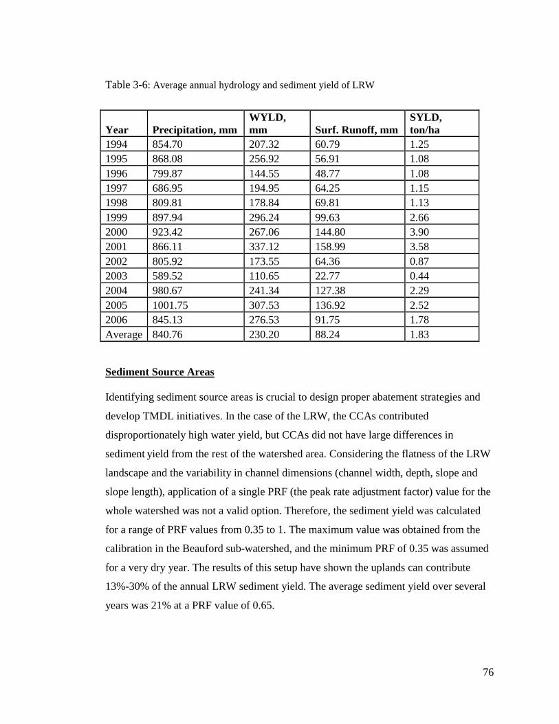
76

Table 3-6: Average annual hydrology and sediment yield of LRW

Sediment Source Areas

Identifying sediment source areas is crucial to design proper abatement strategies and

develop TMDL initiatives. In the case of the LRW, the CCAs contributed

disproportionately high water yield, but CCAs did not have large differences in

sediment yield from the rest of the watershed area. Considering the flatness of the LRW

landscape and the variability in channel dimensions (channel width, depth, slope and

slope length), application of a single PRF (the peak rate adjustment factor) value for the

whole watershed was not a valid option. Therefore, the sediment yield was calculated

for a range of PRF values from 0.35 to 1. The maximum value was obtained from the

calibration in the Beauford sub-watershed, and the minimum PRF of 0.35 was assumed

for a very dry year. The results of this setup have shown the uplands can contribute

13%-30% of the annual LRW sediment yield. The average sediment yield over several

years was 21% at a PRF value of 0.65.

Year Precipitation, mm WYLD, mm Surf. Runoff, mm

SYLD, ton/ha

1994 854.70 207.32 60.79 1.25 1995 868.08 256.92 56.91 1.08 1996 799.87 144.55 48.77 1.08 1997 686.95 194.95 64.25 1.15 1998 809.81 178.84 69.81 1.13 1999 897.94 296.24 99.63 2.66 2000 923.42 267.06 144.80 3.90 2001 866.11 337.12 158.99 3.58 2002 805.92 173.55 64.36 0.87 2003 589.52 110.65 22.77 0.44 2004 980.67 241.34 127.38 2.29 2005 1001.75 307.53 136.92 2.52 2006 845.13 276.53 91.75 1.78 Average 840.76 230.20 88.24 1.83

77

SWAT estimated higher sediment loss rates at the HRU scale than at the sub-watershed

level. Thus, scale of analysis had an important impact on sediment losses. At the HRU

scale analysis, 91% of the upland areas of the LRW delivered less than 5 t/ha and 9%

delivered over 5 t/ha on average (Figure 3-9 & 3 -10). Roughly 25% of the LRW

generated half of the upland sediment losses (Figure 3-10). In contrast, at the sub-

watershed scale, there was no area in the LRW that yielded over 5 t/ha and 94% of the

watershed had less than 3 t/ha sediment yield.

Figure 3-9: HRU Based Spatial Distribution of Sediment yield in the LRW

78

Figure 3-10: Cumulative Sediment Yield vs Contributing Watershed Area of LRW

Table 3-7: Summary of Sediment Yield Vs Contributing Areas of LRW

SYLD, ton/ha HRU Based Analysis Sub-watershed Based Analysis

Area, ha Area, % Area, ha Area, % < 1 152945 54 145276 46

1 - 2 46324 16 81799 26

2 - 3 32651 11 71577 22

3 - 4 16550 6 8782 3

4 - 5 10223 4 10698 3

5 to 10 19000.6 7 0 0

10 to 20 7512.59 3 0 0

> 20 470.72 0 0 0

Total 285676 100 318132 100

Figure 3-11: Sub-watershed Based Spatial Distribution of Sediment yield

Evaluation of the spatial distribution of the average upland sediment yield from the

three major sub-watersheds, the Upper Le Sueur, the Big

watersheds over the years from 1994

the upland sediment load from each watershed (Figure 3

Figure 3-12: Average annual upland sediment yield of LRW major sub

18

24

watershed Based Spatial Distribution of Sediment yield


watersheds, the Upper Le Sueur, the Big-Cobb and Maple major

watersheds over the years from 1994-2006 showed 58%, 18% and 24%, respectively, of

sediment load from each watershed (Figure 3-12).

: Average annual upland sediment yield of LRW major sub-

58

Upper Le Sueur

Big-Cobb

Maple

79

watershed Based Spatial Distribution of Sediment yield


Cobb and Maple major-sub-

2006 showed 58%, 18% and 24%, respectively, of

-watersheds

80

The relative contributions of predicted upland and inferred channel sediment sources

during the 2006 growing season are shown in Table 3-8 for each of the three major sub-

watershed outlets and the LRW outlet. The measured sediment yield of the LRW in

2006 was about 230,502 tons. The SWAT model predicted 32,893 tons at the LRW

outlet, which means that the upland contribution to total sediment load was 14%. By

inference, most of the sediment (86%) was generated from channel sources, including

river bluffs, stream banks and ravines. Based on HRU level sediment loss estimates for

the entire LRW, only about 9% of the sediment loss at the HRU scale reaches the outlet

of the LRW. About 93% of the sediment losses in the LRW occur during the growing

season/months of April to September. At scales finer than the entire LRW, the SWAT

model predicted that agricultural uplands in the Big Cobb, Maple and Upper Le Sueur

sub-watersheds contributed 38%, 22% and 12% of the sediment loads measured during

2006, respectively, at their outlets. By inference, the Big Cobb, Maple and Upper Le

Sueur sub-watersheds generate 62, 78 and 88% of their sediment from channel sources,

respectively. These differences in sediment sources can be explained in terms of

differences in upland slope steepness class distributions and differences in the

frequency of river bluffs and ravines.

Table 3-8: Predicted and measured sediment loads from the LRW and its major

tributaries in the 2006 growing season. :

Sub-watershed

Predicted Upland Sed. Load

Channel Erosion (estimated by difference)

Measured Total Sediment Load

Average Sed. Yield

tons % tons % tons tons/ha

Beauford 178 83 36 27 214 0.10

Big Cobb 8998 38 14785 62 23783 0.30

Maple 11047 22 39290 78 50337 0.57

Upper Le Sueur

20019 12 146462 88 166481 1.44

LRW 32893 14 197609 86 230502 0.81

81

3.3.5. Sediment BMPs

Over 70% of the sediment load of the LRW originates from channel sources, and

upland agricultural areas contribute a maximum of 30%. Reduction of sediment yield

requires application of BMPs on both agricultural and in channel areas. Evaluating

BMPs to reduce channel sources of sediment is beyond the scope of this modeling

effort. Thus, we have focused on alternative BMPs to reduce the upland sediment loads

only.

Upland sediment erosion, transport and deposition in the LRW can be reduced through

a variety of measures, including reduced tillage, crop rotation, waterways and terraces,

grassed buffers at the field edge, and catch basins. The impact of selected BMPs to

reduce the upland sediment loadings of the LRW and its tributaries were evaluated

using the SWAT model. The BMPs were tested for specific land use and potential

sediment source areas.

Tillage BMPs

Management of the surface residue cover through applying reduced tillage is considered

the primary means of sediment reduction for the Minnesota River Basin (Senjem et al.,

1996). Maintaining over 30% residue cover can significantly reduce upland sediment

losses. Even under conditions where secondary BMPs are required, residue

management makes them less costly, more effective, and longer lasting (Senjem et al.,

1996).

Three different scenarios of conservation tillage were tested in the corn residue from the

year before soybeans were planted:

• On all fields under corn residue going from corn to soybean

• Corn going into soybeans on land over 2% slope.

• On 50% of corn fields

Each scenario resulted in sediment load reductions of 13% in the LRW compared to the

baseline scenario of conventional tillage. Application of conservation tillage on 50% of

randomly selected fields (73,852 ha) decreased the sediment yield by 9%. Application

82

of no-till on the same randomly selected 50% fields decreased the sediment yield by

31% (Table 3-9).

Table 3-9: Sediment Loss Under Different Tillage BMP Scenarios

Year

Baseline Scenario

Conservation tillage No till

All Corn land Land > 2% slope 50% Corn land

50% Corn land

Sed. load, tons (% of baseline)

1994 351623 309445(85.6) 309846(85.7) 323940(89.8) 228480(65.5)

1995 289349 253626(83.6) 255653(84.2) 270498(89.8) 204231(60.2)

1996 329939 284724(90.2) 285448(90.4) 304293(93.3) 220709(72)

1997 330432 282700(88.6) 283078(89) 296739(97.1) 216413(69.6)

1998 318872 266662(86.4) 268522(86.5) 286298(91.1) 191940(66.7)

1999 680854 614465(84.2) 615686(84.4) 635388(89.5) 490084(66.7)

2000 992003 878960(92.3) 882518(92.4) 963282(98.5) 690503(79.2)

2001 988949 854127(84.8) 855280(85) 900747(90.6) 659891(67.3)

2002 230289 193831(90.4) 194270(90.5) 206115(93.5) 153680(78.8)

2003 113424 104710(84.3) 104765(84.4) 111703(88.6) 89849(61.9)

2004 621019 526314(87.2) 527603(87.5) 562554(92.4) 417805(68.6)

2005 677579 309445(85.6) 309846(85.7) 323940(89.8) 228480(65.5)

2006 486717 253626(83.6) 255653(84.2) 270498(89.8) 204231(60.2)

Average 493158 284724(90.2) 285448(90.4) 304293(93.3) 220709(72)

Filter Strips

Dillaha et al., (1989) defined vegetative filter strips (VFS) as areas of vegetation

designed to remove sediment and other pollutants from surface water runoff by

filtration, deposition, infiltration, adsorption, absorption, decomposition, and

volatilization. VFS separate a nonpoint pollution source land area from a water body.

They are effective at reducing runoff volume and peak velocity primarily because of the

filter’s hydraulic roughness, and subsequent augmentation of infiltration. Establishing

VFS at the edge of agricultural fields or adjacent to streams or drainage ditches has

been shown to be effective in removing sediment loss from upland runoff (Dillaha et al.,

1989; Munoz-Carpena et al., 1999).

83

Despite the limitations of the SWAT algorithms discussed in the methodology (section

3.2.3.), two different alternative scenarios of VFS were tested in the LRW (Table 3-10).

The simulation results revealed that application of VFS on all fields steeper than 2%

slope reduced sediment losses by 56%, while VFS installation on all corn-soy CCAs

reduced sediment losses by about 20% as compared to the baseline scenario.

Table 3-10: Sediment Loss Under Different VFS BMP Scenarios

Year

Baseline On CS land > 2% slope On all CS CCAs

Sed. load, tons (% of baseline)

1994 351623 121382(34.5) 276936(78.8)

1995 289349 106761(36.9) 234533(81.1)

1996 329939 139655(42.3) 261836(79.4)

1997 330432 139791(42.3) 264995(80.2)

1998 318872 137301(43.1) 252456(79.2)

1999 680854 277106(40.7) 550127(80.8)

2000 992003 458741(46.2) 784208(79.1)

2001 988949 450535(45.6) 809755(81.9)

2002 230289 97497(42.3) 164468(71.4)

2003 113424 49782(43.9) 98725(87)

2004 621019 287666(46.3) 488343(78.6)

2005 677579 340709(50.3) 557473(82.3)

2006 486717 208850(42.9) 384537(79)

Average 493158 216598(43.9) 394492(80)

Cover Crops

The vegetative biomass of rye as a cover crop increases the amount of transpiration and

decreases the impact of rain drops that can detach soil aggregates. As a result of this,

there is an increase in water infiltration and decrease in surface runoff and runoff

velocity. Planting rye after the harvest of soybeans in the LRW reduces sediment loss

into streams by an average of 32% (Table 3-11).

84

Table 3-11: Effects of planting rye as a cover crop in reducing sediment loss

Year Baseline

Rye as cover crop Sed. load, tons (% of baseline) 1994 351623 233265(66.34)

1995 289349 197150(68.14) 1996 329939 263284(79.8) 1997 330432 192726(58.33) 1998 318872 196497(61.62) 1999 680854 453698(66.64) 2000 992003 768043(77.42) 2001 988949 609187(61.6) 2002 230289 163233(70.88) 2003 113424 84193(74.23) 2004 621019 459333(73.96) 2005 677579 484285(71.47) 2006 486717 257258(52.86) Average 493158 335550(67.95)

Figure 3-13: Comparison of Different BMP Sediment Loss Reduction Potentials

0

10

20

30

40

50

60

VFS on land

>2% slope

Rye as cover

crop

No Tillage on

50% corn land

VFS on all

CCAs

CT on all corn

land

CT on land

>2% slope

CT on 50%

corn land

Pe

rce

nt

red

uct

ion

of

sed

. Y

ield

BMPs

85


This study has used the strength of the SWAT model; namely its ability to predict

sediment losses from upland agricultural regions, to estimate the proportion of total

measured sediment loads in the Le Sueur River watershed that arise from upland

agricultural regions. The SWAT model was calibrated and validated in a small

representative sub-watershed (Beauford) without significant channel sources of

sediment, and was found to be very accurate at predicting discharge and sediment loads.

At the scale of the LRW, predicted sediment loads were much smaller than measured

sediment loads, indicating that upland sediment sources are a small fraction of the total

sediment losses at these large scales. Based on the SWAT model simulation results,

about 21% of the LRW sediment arises from upland agricultural areas, while 79% arises

from river bluffs, ravines and eroding stream channels.

The effectiveness and water quality impacts of best management practices (BMPs),

were evaluated for conservation planning and targeting. Conservation tillage, filter

strips and rye as a cover crop decreased upland sediment losses from 8% up to 54%.

Implementation of sediment BMPs in upland regions of the LRW can only reduce

sediment losses by at most a quarter of the total sediment yield. Sediment losses from

channels and stream banks, which account for about 79% of the sediment yield, are

another important source of turbidity impairment. Measures are needed to reduced

sediment losses from these sources. More research is needed to identify and implement

interventions that can mitigate sediment losses coming from channel sources.

86


WATERSHED PHOSPHORUS DYNAMICS

87

SYNOPSIS

The Minnesota River is noted for its high P flux to the Mississippi River and Lake Pepin.

The LRW is among the top three highest contributors for phosphorus in all the major

watersheds of the Minnesota River Basin. The SWAT model was calibrated and validated

for hydrology and sediment transport processes and used to simulate the P dynamics of

the LRW. The major objectives of the study were to investigate the level of P

contamination, P source areas and best management practices that can minimize P losses

and improve water quality.

SWAT model calibration for P in the Beauford sub-watershed ( 2000) and validation over

the entire LRW (1999-2006) were accurate with NSE values of 0.77 and 0.67,

respectively. Total P loss in the LRW was correlated with total sediment yield with an R2

value of 0.69, and there was also a weak relationship with water discharge. Organic P

losses showed a strong linear relationship (R2 value of 0.79) with sediment flux.

Estimated mean annual total P loss in the LRW from 1994-2006 was 1.02 kg/ha. Steeply

sloping lands in the northern and eastern parts of the watershed have the highest annual P

yield, exceeding 2 kg/ha/year. Those areas are situated in the Upper Le Sueur major sub-

watershed, where 64% of the total LRW P loss arises. Application of vegetative filter

strips on targeted areas of the LRW reduced P losses by 64%. P losses in the LRW were

reduced by 25-30% relative to baseline conditions by reducing P application rates by

34% or implementing no tillage on 50% of corn fields, or planting rye as a cover crop. P

losses were reduced by 15% with conservation tillage on 50% of corn fields.

88

4.1. INTRODUCTION

Phosphorus (P) is an essential element for plant and animal production. Compared to

other macronutrients, it is the least mobile element in plant and soils (Khan et al., 2001).

P has high affinity to quickly combine with Ca, Fe, and Al ions to form insoluble

compounds that precipitate out of solution, causing build-up near the soil surface and

ready transport in surface runoff (Broberg and Persson, 1988). Enrichment of fresh water

resources with P leads to eutrophication, which involves the increased growth of

undesirable organisms such as cyanobacteria (blue-green algae), Pfiesteria piscicida and

other aquatic weeds. The increase in the density of algae lowers the penetration of

sunlight. Consequently, the algae begin to die and decompose thereby consuming

dissolved oxygen, which in turn causes the death of aquatic organisms, including fish

(Carpenter et al., 1998; Sharpley et al., 2000).

Agricultural nonpoint sources of P are primarily runoff from farm-fields and concentrated

animal-feeding sites. These sources have contributed to eutrophication of surface waters,

throughout the United States (Lemunyon and Daniel, 1998; Sharpley, 2003; USEPA,

1996a). Although both nitrogen and phosphorus contribute to eutrophication, phosphorus

is the most limiting nutrient for the growth of aquatic organisms and thus the primary

factor that must be controlled to prevent eutrophication of fresh water bodies (Lemunyon

and Daniel, 1998; Lemunyon and Daniel, 1998).

The increase in eutrophication of fresh waters can be controlled through decreasing P

inputs to surface waters (Shigaki et al., 2006). Establishment of economically and

environmentally sound P management systems requires adoption of local management

strategies that consider soil test phosphorus, P application methods, and transport factors

such as hydrology and erosion (Mallarino et al., 2002). Since the buildup of P is most

prevalent in areas where P from fertilizer and manure is applied in excess of crop needs,

the problems of P losses are most severe in areas where soil P levels are highest and

where water movement from soil to surface water is greatest (Sharpley et al., 1994).

Interest in reducing P loadings to surface waters via implementation of Total Maximum

Daily Loads (TMDLs) has increased the urgency for information on the impacts of

89

agricultural best management practices (BMPs) on P loss. Soil test P data may give

information about the spatial distributions of high P source areas, but provide no

information about hydrologic or management factors important for P transport to surface

waters (Sims et al., 1998). In this regard, the US EPA recommends the application of

process based P models that link watershed data, P source areas and land uses so as to

evaluate alternative management practices to reduce watershed P loadings and maintain

water quality standards ((U.S. USEPA, 2000). EPA has evaluated 65 currently available

models for their capabilities and applicability to TMDL development and related

watershed management activities. The US EPA designated two of the most widely used

water quality models, SWAT and HSPF, for simulation of hydrology and water quality

nationwide (Di Luzio et al., 2002; Shoemaker et al., 2005).


Phosphorus loadings from the Mississippi River Basin to the hypoxic zone in the

northern Gulf of Mexico are about 0.1 million tons/year. Much of this load arises from

the headwaters of the Upper and Lower Mississippi (Goolsby et al., 1999). James et al.

(1997) reported 45% of the P flux to Lake Pepin is from Minnesota River Basin. Total P

flux to Lake Pepin, a natural widening in the Mississippi River south of St. Paul, MN, is a

result of increases in applied P fertilizer and hydrologic discharge from the Minnesota,

Upper Mississippi and St. Croix River basins (Mulla and Sekely, 2009). Engstrom and

Almendinger (2009) showed that the P load in Lake Pepin increased roughly seven fold

over the past two centuries. The most drastic increases occurred after 1940 (Engstrom et

al., 2009). The concentration of TP in the Minnesota River along the reach from Judson

to Fort Snelling averaged 0.34 mg/L over the years from 2000 - 2005 (Water Resources

Center, 2007). Birr and Mulla (2001) reported that the total P concentration of stream

water quality samples in the Minnesota River Basin routinely exceeded 0.25 mg/L.

The P yield of the LRW is the highest of all the major tributaries of the Minnesota River

Basin. Mulla and Mallawatantri (1998) estimated that two thirds of the total Minnesota

River P load originated from three of its major watersheds, namely the Lower Minnesota,

Blue Earth and Le Sueur River watersheds. Total P concentrations and yield in the Le

90

Sueur River averaged 0.47 mg/L and 1.15 kg/ha, respectively, over the years from 2000-

2005 (Water Resources Center, 2007). Sekely et al. (2002) in their study of the Blue

Earth River estimated the total P contribution of stream bank slumping to be 7%-10% .

The last 40 mile reach of the Minnesota River had soluble phosphorus concentrations of

only 0.0115 mg/L, while the particulate P concentration was 66% of the total P load

(James and Larson, 2008). Generally, the mean P concentration of the Minnesota and Le

Sueur Rivers was far above the EPA’s desired goal of 0.1 mg/L, indicating the need for P

load reductions through application of improved management measures.

Randall et al. (1997) showed long term increases in soil test P values in South Central

Minnesota due to excess application of P fertilizers and animal manure. Soil test P levels

for about 65% of the soil samples in South Central Minnesota were low to medium in

1956. In the early 1990’s, 69% of the soil samples from the same area had soil test P

values that exceeded 21 ppm . Thus, more application of P in these areas will increase the

potential for P losses without providing any agronomic benefits (Randall et al., 1997).

Field assessment of soil test P values to understand P transport, loss processes and best

management options requires a huge expenditure of financial resources, technical

personnel and time (Sharpley et al., 2000). Application of models is a more efficient and

feasible means towards the same end. A modeling study that could contribute towards

mitigating the high levels of P loss from watersheds in South Central Minnesota, and

severe contamination of water resources from Lake Pepin to the Gulf of Mexico is very

timely.

4.1.2. Objectives

The LRW phosphorus modeling study was initiated in response to the phosphorus

enrichment and contamination of water resources in the region with the following

objectives:

• Evaluate the applicability of the SWAT model to simulate P transport and loss

processes under the local climate, topography, and farming systems of South

Central Minnesota

• Understand major processes of P transport and loss

• Evaluate spatial and temporal trends of phosphorus loss

91

• Identify and target parts of the watershed with high P loss

• Develop mitigation strategies for P loss by evaluating the relative importance of

different best management practices.

4.1.3. Models of Phosphorus Transport and Fate

Several phosphorus models of different spatial and temporal scales, from risk-based P-

index models to complex and dynamic models such as the Soil Water Assessment Tool

were developed after 1980 (Radcliffe et al., 2009). The lack of detailed parameterization

data on soil physical, chemical, and biological properties as well as crop management and

tillage data are common limitations for accurately modeling P (Sharpley et al., 2000). The

invention of graphic user interfaces and the use of geographic information system layers

and databases for developing input files have contributed to the advancement of model

input data management (Radcliffe and Cabrera, 2006).

The most comprehensive process based P models include the Agricultural Nonpoint

Pollution Source (AGNPS) (Young et al., 1989), Areal Nonpoint Source Watershed

Environment Response Simulation (ANSWERS) (Beasley et al., 1980), Hydrologic

Simulation Program - Fortran (HSPF) (Bicknell et al., 1997; Johanson et al., 1984),

Agricultural Runoff Model (ARM) (Donigian and Davis, 1978), Erosion Productivity

Impact Calculator (EPIC), the lumped parameter model Generalized Watersheds Loading

Functions (GWLF) (Haith and Shoemaker, 1987), and the Soil and Water Assessment

Tool (SWAT) (Luzio et al., 2001). These models are capable of simulating the most

important processes governing P dynamics, can integrate information over different

scales and spatial resolutions, emphasize appropriate best management practices (BMPs),

and identify critical source areas where BMPs are most likely to affect watershed scale P

losses (Radcliffe and Cabrera, 2006). Modeling approaches used to simulate dissolved

and particulate P losses in these models are explained by Sharpley et al., (2002).

Dissolved P in most non-point source models such as AnnAGNPS, EPIC, and SWAT is

simulated using an extraction coefficient, available soil P and overland flow volume. The

sediment bound particulate P is a product of total soil P, sediment concentration, P

enrichment ratio and overland flow volume (Sharpley et al., 2002).

92

The SWAT model has been applied in several studies of P transport and management

studies. Lin et al. (2009) estimated SWAT model P input parameters related to soils and

in -stream processes . They calibrated and applied the SWAT model for changes in land

use in the Lake Allatoona Watershed of Georgia. Gitau et al. (2004) used SWAT to

predict the spatial distribution of P losses and to target critical source areas in the

Cannonsville Reservoir watershed. Santhi et al. (2001) validated the SWAT model for the

Bosque River watershed. Kirsch et al. (2002) applied the SWAT model to quantify P

source areas and effects of applying watershed level BMPs. Despite some limitations of

the SWAT model, it has the potential to significantly improve the effectiveness of

existing water quality programs through identifying watershed target areas for

implementation of conservation measures (White et al., 2009).

The simulation of applied manure for tilled systems where manure is well mixed into soil

is adequately simulated in most models. However, surface application of manures or

direct transfer of P from broadcast manure to runoff is still not dealt with adequately in

most models (Pierson et al., 2001; Sharpley et al., 2002).

Strategies to combat P losses include general measures focusing on reducing the net input

of P to agricultural land or targeted measures implemented in areas of the landscape with

a high risk of P losses by interrupting the transport pathway and reduce the mobility of P

with practices that include reduced tillage, direct injection of manure, of grass filter strips

(Withers et al., 2000). Kronvang et al. (2003) described targeted measures to mitigate P

losses from agricultural areas to surface waters, as well as the effect, requirements,

uncertainties, obstacles, and possible side effects of these measures. The identification of

areas that contribute disproportionately high P loads is essential to efficiently manage

phosphorus losses at the watershed scale (Gburek et al., 2002). Reducing P inputs to

lower soil available P has little or no immediate effect on actual P losses unless excess P

buildup is prevented (Sharpley et al., 2000).

93

4.1.4. Phosphorus Simulation Processes in SWAT Model

SWAT phosphorus modeling is based on point sources of P, soil applied organic and

inorganic P fertilizers, and cycling of P in crop residue and microbial biomass. P cycling

accounts for transformations in six soil P pools; three are organic (fresh organic, active

and stable organic P) and another three are inorganic pools (labile/solution, active, and

stable pools). The major P transformation processes include mineralization of fresh

organic P and soil organic matter, and decomposition and immobilization. SWAT

requires estimates for the initial mineral P and organic P concentrations in the upper soil

layers for phosphorus simulation (Neitsch et al., 2005a).

Phosphorus transport processes simulated in SWAT include surface runoff in solution,

losses of P attached to sediment and leaching of soluble P. The amount of soluble P

removed in runoff is predicted using solution P concentration in the top 10 mm of soil,

the runoff volume and a partitioning factor. Sediment transport of P is simulated with a

loading function as described in the SWAT theoretical documentation (Neitsch et al.,

2005b). Plant use of phosphorus is estimated using the supply and demand approach.

Losses of P in base flow and subsurface losses are considered in calculating total loads.

The in-stream P transformation and routing processes of SWAT are taken from QUAL2E

– The Enhanced Stream Water Quality Model (Brown and Barnwell, 1987). The various

pools of phosphorus its transport and transformation processes modeled by SWAT are

shown in Figure (4-1).

94

Figure 4-1: SWAT phosphorus pools and phosphorus cycle processes


4.2.1. The Study Area

The LRW is one of twelve major watersheds in the Minnesota River Basin. It is part of

the Western corn-belt of the USA, where corn-soybean production is the predominant

land use. The soils are dominated by fine textured clay and silt mollisols that are formed

in very flat lacustrine landscape that is now extensively tile drained. The LRW has been

chosen for this study based on P concentrations that routinely exceed the EPA desired

goal of 0.1 mg/L. In addition, the watershed has soils with high organic matter content

(over 3%) coupled with a long history of excess applications of P from fertilizer and

animal manure, making it an area at high risk of P loss.


Simulation of P losses was made after calibration and validation of SWAT’s hydrology

and sediment components. Organization of input data specific to P including the

management operations file (time, rate and sources of P fertilizer applied, application

methods and tillage operations) was made based on data from previous studies and water

quality monitoring stations in the area, knowledge about the watershed and a farm survey

made by the Minnesota Department of Agriculture. P discharges from 16 point-source

95

facilities were identified within the 6 counties of the LRW, out of which four within the

LRW had monthly discharge monitoring reports used for SWAT modeling.

Monitoring results for P collected by the Met Council and the Minnesota Department of

Agriculture for the period from 1994 to 2006 were used to calibrate and validate the

model. Monthly calibration was made on the Beauford sub-watershed for the year 2000.

Validation of the model occurred over the years 2001-2006 in the Beauford sub-

watershed, and from 1994 -2006 in the LRW. Procedures similar to those used in

hydrology and sediment predictions were applied for sensitivity analysis, and calibration

and validation of P.

The soil test P values to initialize the labile P in the first soil layer were adopted from

studies by Schmitt et al. (2001). Initial organic P was calculated from total N using the

procedures of Sharpley et al. (1984). Once the initial concentration setup was completed,

the model uses different algorithms to calculate the various pools and their interactions in

the soil matrix.

SWAT model P mineralization, decomposition, and immobilization processes are

represented by procedures developed by Jones et al. (1984). Mineralization of P from

crop residue and microbial biomass is regulated by variations in temperature and water

availability. Major processes of P dynamics include P uptake by plants, transport in

surface runoff and in-stream P cycles (Jones et al., 1984; Neitsch et al., 2005a).

Mineral Pools of P

SWAT initializes the active and stable mineral pools of P based on labile P.

i. Solution Pool: also known as the labile pool provides P for plant uptake,

soluble P in surface runoff, and P leaching. Mineralized organic matter P and

inorganic fertilizer P enter this pool. The initial value for this pool is a user

defined concentration. The initial Solution pool value, which is an input, sets

both the active and stable P pools via fixed ratios.

ii. Active mineral pool: Interacts slowly with the stable pool and quickly with the

solution pool. This pool represents P which is reversibly precipitated or

96

adsorbed, but is less active than Solution P. It is about 1.5 times larger than

the solution pool.

Active mineral pool (Pact. min. pl ) concentrations (mg/kg) are given by:

P act.min.pl � Psol " 71 � PAI

PAI8 �4.1�

Where Psol is the amount of labile P (mg/kg) and PAI is the P availability index.

PAI is estimated using the method outlined by Sharpley et al. (1984).

iii. Stable mineral pool: is the pool that is not readily available for plant uptake

and reaches equilibrium very slowly with the active pool. This is the largest of

the mineral P pools, about four times larger than the active pool.

Stable mineral pool\(Pst.min.pl) concentrations (mg/kg) are given by:

P st.min.pl � 4 " ;Pact.min.pl< (4.2) Organic Pools of P

i. Phosphorus in the fresh organic pool is the sum fresh Organic P from animal

manure added to the solution pool and organic P from crop residue set to

0.03% of the initial amount of residue on the soil surface. The SWAT model

assumes animal manures are composed of relatively soluble mineral and

readily degradable organic forms.

ii. Organic P concentration (Phum) in mg/kg is calculated with the assumption of

an 8:1 N to P ratio in humic substances using:

Organic P hum � 0.125 " �Nhum� �4.3�

Where Nhum is the concentration of humic organic nitrogen in the soil layer (mg /kg).

iii. Active Organic P( Organic Pact) is given by:

Organic P act � Organic Phum " 7 Organic Nact

Organic Nact=Organic Nst8 (4.4)

iv. Stable organic P (Organic Pst) is given by:

Organic P st � Organic Phum " 7 Organic Nst

Organic Nact=Organic Nst8 (4.5)

97

4.2.3. Selection of Phosphorus BMPs

Identifying phosphorus best management practices that can maintain a balance between

water quality protection and agricultural production of LRW is very important. The

following four categories of BMPs have been evaluated to optimize the P fertilizer use

efficiency and reduce P losses.

A. P application methods:

The P application rate was reduced by 34% from the baseline application rate of 84 kg/ha

P2O5 from both animal manure and applied DAP fertilizer.

B. Tillage systems

Cropping systems that maintain at least 30 percent of the soil surface cover with residue

after planting can help to reduce soil erosion and the associated P loss. Two alternative

tillage BMPs have been tested:

i. Conservation tillage on 50% of the corn residue in the year before soybean

planting.

ii. Direct seeding of soybean into corn residue without tillage

C. Vegetative filter strips (VFS)

Establishment of vegetative grass strips as barrier against surface runoff on corn-soybean

fields with slopes steeper than 2% was evaluated for its potential to reduce P losses.

D. Cover Crops Rye was planted on 50% of the crop land after harvesting soybeans as a fall cover crop.

The uptake of P by planted rye minimizes availability of P for loss, and maintains the

surface cover that minimizes surface runoff losses.

98


4.3.1. Sensitivity Analysis

There is no single set of P input parameters in the LRW SWAT model which performs

well in all circumstances. Different sets of parameters taken together affect simulation

results from 1994-2006. A LRW P input parameters sensitivity analysis ranking was used

to make decisions on parameters of priority focus to optimize the objective function that

describes the model efficiency. Model results showed high sensitivity to soil solution P

concentration (SOL-LAB-P), adsorption coefficient of P (PHOSKD) and the P sorption

coefficient (PSP) (Figure 4-2).

The soil P concentration was the most sensitive parameter for simulating P losses.

Development of an extensive spatial database of STP, along with particulate and solution

P ratios in runoff, are needed to improve model performance and its usefulness for

practical management purposes.

Figure 4-2: Relative sensitivity of P related parameters

0 1 2 3 4 5 6

SOL LABP

PHOSKD

PSP

SOL ORGP

PPERCO

RSDCO

Rank

99

4.3.2. Calibration and Validation of Phosphorus

The LRW SWAT modeling calibrated phosphorus input parameters and their respective

values are shown in Table 4-1. Phosphorus calibration in the Beauford sub-watershed

showed good agreement between predicted and measured total phosphorus loads at the

outlet of the watershed, with an NSE value of 0.79 (Figure 4-3). Even though the

observed NSE value is acceptable, the predicted P load was 39% less than measured.

The under-prediction was mainly during peak snowmelt months and was consistent

with model under-predictions of hydrology and sediment in those same months.

Figure 4-3: Phosphorus calibration in the Beauford Sub-watershed.

The predicted average monthly total phosphorus loading in the Beauford and LRW were

56% and 77% of their respective measured average monthly loadings (Figures 4-4 and 4-5).

Validation NSE values for the total monthly phosphorus loadings were 0.76 and 0.67 in

the Beauford sub-watershed and LRW, respectively (Figures 4-6 and 4-7) . The largest

errors in SWAT model phosphorus predictions were always associated with peak flow

prediction errors. Under-prediction of P loads could also be due to the fact that P from

stream banks and atmospheric deposition were not accounted for in the SWAT model.

0

500

1000

1500

2000

2500

Ph

osp

ho

rus,

kg

Measured Predicted

100

Figure 4-4: Monthly Phosphorus Loss Validation in the Beauford Sub-watershed

Figure 4-5: Average Monthly Phosphorus Loss Validation in the Beauford Sub-watershed

(2001-2006)

0

500

1000

1500

2000

2500

Ph

osp

ho

rus,

kg

Measured Predicted

0

100

200

300

400

500

600

J F M A M J J S O N D

Ph

osp

ho

rus

loa

d,

kg

Measured Predicted

101

Figure 4-6: Monthly Phosphorus Loss Validations in the LRW

0

50000

100000

150000

200000

250000

300000

350000

400000

Dec-99 Apr-01 Sep-02 Jan-04 May-05 Oct-06

Ph

osp

ho

rus

loss

, k

g

Measured Predicted

0

20000

40000

60000

80000

100000

J F M A M J J A S O N D

Ph

osp

ho

rus

loa

d,

kg

Measured, kg SWAT, kg

Figure 4-1: Monthly Phosphorus Loss Validation in the LRW (2000-2006)

Table 4-1: Summary of calibrated phosphorus parameters in the LRW SWAT model

Variable Description File Default Calibrated

P_UPDIS P uptake distribution parameter. .bsn 20 84

PPERCO P percolation coefficient (10 m3/Mg). .bsn 10 15

PHOSKD P soil partitioning coefficient (m3/Mg). .bsn 175 190 PSP P availability index. .bsn 0.4 0.27 RSDCO Residue decomposition coefficient .bsn 0.05 0.05 SOL SOLP Initial soluble P concentration in soil layer (mg P/kg soil or ppm). .chm 5 Variable SOL ORGP Initial organic P concentration in soil layer (mg P/kg soil or ppm). .chm 0-1500 Variable ERORGP P enrichment ratio for loading with sediment. .hru 0 Variable FILTERW Width of edge-of-field filter strip (m). .mgt 0 Variable BIOMIX Biological mixing efficiency. .mgt 0.2 Variable FERTILIZER

APPLICATION .mgt FMINP Fraction of mineral P in fertilizer (kg min-P/kg fertilizer). fert.dat 0-1 Variable FORGP Fraction of organic P in fertilizer (kg org-P/kg fertilizer). fert.dat 0-1 Variable TILLAGE

OPERATION .mgt EFFMIX Mixing efficiency of tillage operation. till.dat Variable Variable DEPTIL Depth of mixing caused by the tillage operation (mm) till.dat Variable Variable CPYLD Normal fraction of P in yield (kg P/kg yield). crop.dat Variable Variable PLTPFR(1) Fraction of P in plant biomass at Emergence (kg N/kg biomass) crop.dat Variable Variable PLTPFR(2) Fraction of P in plant biomass at 50% maturity (kg N/kg biomass) crop.dat Variable Variable PLTPFR(3) Fraction of P in plant biomass at maturity (kg N/kg biomass) crop.dat Variable Variable GWSOLP Concentration of soluble P in groundwater (mg P/L or ppm) .gw Variable Variable

102

103

4.3.3. Phosphorus Yield and Source Areas

The SWAT simulation results showed that the highest phosphorus losses (0.22-0.28

kg/ha/month) occur in the peak flow months from April to June. This accounts for 75%

of the total annual loss. About 85% of the P losses occurred in the particulate or sediment

bound form. The dissolved P was only about 15% (Table 4-2). Total P loss is strongly

correlated with total sediment yield with an R2 value of 0.69. There was not a strong

relation with water discharge. Organic P losses showed a strong linear relationship with

sediment flux (R2 value of 0.79) in the LRW. Agricultural row crop producing fields

accounted for 99% of the predicted total phosphorus loading to surface waters of the

LRW.

Average monthly phosphorus load in the LRW was estimated using the USGS

LOADEST program. The monthly maximum loss (83,000 kg) occurred in the month of

April (Figure 4-9). Based on 446 samples tested from 1999-2006, the maximum average

monthly concentration (0.61 mg/L) was recorded in the month of June. The loss of

phosphorus is affected by several factors, including the occurrence, amount and intensity

of rainfall and runoff, P application amount and timing, and land management practices

such as tillage.

Figure 4-8: Monthly average phosphorus concentration in the LRW

0.0

0.1

0.2

0.3

0.4

0.5

0.6

0.7

Ph

osp

ho

rus

Co

nc.

mg

/L

104

Figure 4-9: Monthly average phosphorus load in the LRW

The annual discharge of total P from the LRW varied during the period from 1994-2006.

The predicted lowest annual phosphorus loss of 0.44 kg ha–1 occurred in 2002, and the

highest annual losses of 2.01 kg ha–1 occurred in 2001. The mean annual total P loss

across all years was 1.02 kg ha–1 (Table 4-2 ).

Table 4-2: Annual Phosphorus Loss in the LRW (kg/ha)

Year ORGANIC P SEDIMENT P SOLUBLE P Total P

1994 0.19 0.31 0.08 0.59 1995 0.18 0.31 0.10 0.59 1996 0.24 0.43 0.12 0.79 1997 0.23 0.34 0.10 0.66 1998 0.20 0.31 0.10 0.62 1999 0.42 0.76 0.18 1.37 2000 0.57 1.14 0.27 1.98 2001 0.68 1.07 0.26 2.01 2002 0.13 0.23 0.07 0.44 2003 0.07 0.14 0.05 0.27 2004 0.41 0.75 0.20 1.37 2005 0.46 0.85 0.23 1.55 2006 0.33 0.52 0.14 0.99 Average 0.32 0.55 0.15 1.02

0

20000

40000

60000

80000

100000

J F M A M J J A S O N D

Ph

osp

ho

rus

loa

d,

kg

Measured, kg

105

The northern and eastern portions of the watershed have the highest P loss rates (Figure

30). Those are areas that have steep slopes, high surface runoff and high sediment losses

(Figures 13, 20 & 21). The Upper Le Sueur major sub-watershed has the highest annual

sediment yield of 1.35 kg/ha and contributes about 64% of the P loss, although it has only

about 40% of the total area. The other two major sub-watersheds, Maple and Big Cobb,

contribute 20% and 16%, respectively. Roughly 30% of the LRW contributes 50% of the

phosphorus load (Figure 4-10)

Table 4-3: Phosphorus loss in the major sub-watersheds of LRW

Reach Area, ha

ORGANIC P, kg

MINERAL P, kg Total P, kg

LRW 285676 104100 102000 206100

Upper Le Sueur 115286 79180 76420 155600

Big Cobb 79955 19720 19670 39390

Maple 88081 25930 23130 49060

Figure 4-10: Phosphorus contributing area vs load.

106

Figure 4-11: Spatial distribution of phosphorus loss in the LRW

4.3.4. Phosphorus Budget

The mineralization of organic P from soil humus, crop residue and microbial biomass of

the LRW was estimated at about 24.3 kg/ha. Since crop uptake was 29 kg/ha/year and

surface losses were about 1kg/ha/year, P applications from fertilizer and manure should

not have exceeded 7 kg/ha/year. However, the annual phosphorus application in the LRW

is about 38 kg/ha, and animal manure accounts for 15% of the total. Considering the

annual uptake and losses in runoff, there is an accumulation of 11 kg/ha/year phosphorus

in the LRW (Table 4-4 ).

The role of point sources has been accounted for in the loss estimates at the mouth of

LRW. The average annual mineral phosphorus released from point sources was about

185 kg. This is about 0.001% of the annual loss from the entire watershed.

107

Table 4-4: LRW Phosphorus Budget

INPUTS (kg/ha) % P FERTILIZER APPLIED (Min Fertilizer and Manure) 38.4 61.2 MIN OF FRESH ORG P (Residue and Microbial biomass) 14.5 23.2 MIN OF ORG P (HUMUS) 9.8 15.6 TOTAL 62.7 100.0 OUTPUTS (kg/ha) % P UPTAKE 29.0 55.8 Adsorbed P 21.9 42.2 Soluble P loss 0.15 0.3 Sediment P loss 0.55 1.1 Organic P loss 0.32 0.6 Point Source P loss 0.001 0.002 TOTAL 51.99 100.00

Change in storage = Inputs - Outputs = 10.8 kg/ha

The annual accumulation of 10.8 kg/ha phosphorus in upland soils of the LRW may

affect freshwater ecosystems in the long run. The adverse effects of P on freshwater at

downstream of sources could occur after several years of accumulation of P in soil (Reed-

Andersen et al., 2000). Daniel et al. (1994) and Sharpley et al. (1994) reported that all

factors that increase erosion or the concentration of P in the soil also increase the

potential for P losses. Therefore, the current P accumulation rate in the LRW could have

a very dangerous effect on the LRW water quality in the long run.

4.3.5. Phosphorus BMPs

Phosphorus concentration at the soil surface and increases in runoff are the two major

factors that increase phosphorus losses in runoff (Sharpley et al., 2003). Thus, all

practices that can reduce these two factors can reduce the loss of P.

Application of 56 kg/ha of P2O5, from both animal manure and applied DAP fertilizer,

was evaluated against the baseline application rate of 84 kg/ha P2O5. This 34% reduction

in application rate reduced the total P loss by about 28% (Table 4-5).

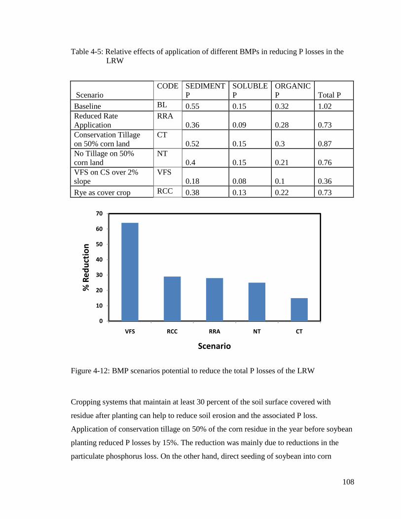
108

Table 4-5: Relative effects of application of different BMPs in reducing P losses in the LRW

Scenario CODE SEDIMENT

P SOLUBLE P

ORGANIC P Total P

Baseline BL 0.55 0.15 0.32 1.02 Reduced Rate Application

RRA 0.36 0.09 0.28 0.73

Conservation Tillage on 50% corn land

CT 0.52 0.15 0.3 0.87

No Tillage on 50% corn land

NT 0.4 0.15 0.21 0.76

VFS on CS over 2% slope

VFS 0.18 0.08 0.1 0.36

Rye as cover crop RCC 0.38 0.13 0.22 0.73

Figure 4-12: BMP scenarios potential to reduce the total P losses of the LRW

Cropping systems that maintain at least 30 percent of the soil surface covered with

residue after planting can help to reduce soil erosion and the associated P loss.

Application of conservation tillage on 50% of the corn residue in the year before soybean

planting reduced P losses by 15%. The reduction was mainly due to reductions in the

particulate phosphorus loss. On the other hand, direct seeding of soybean into corn

0

10

20

30

40

50

60

70

VFS RCC RRA NT CT

% R

ed

uct

ion

Scenario

109

residue without tillage showed a 25% reduction in P losses. This is mainly a result of an

increase in infiltration rates and reduction in soil erosion. Application of no-till reduced

sediment adsorbed P, but increased soluble P losses. Nevertheless, no-tillage is not

recommended on most soils in the LRW because of negative effects on crop yield.

Establishment of vegetative grass strips on corn-soybean fields with slopes steeper than

2% showed the highest P loss reduction potential of 64%. Another effective management

practice was planting rye as a fall cover crop. Cover cropping reduced phosphorus losses

by 29%, mainly through reducing surface runoff from the soil.

110


The average annual phosphorus concentrations in the Minnesota River and the Le Sueur

River over the years 2000 - 2005 were 0.34 mg/L and 0.47 mg/L, respectively. The P

yield of the LRW is the highest of all the major tributaries in the Minnesota River

Basin. A modeling study that could contribute towards mitigating high P losses from the

Minnesota River Basin and severe contamination of water resources from Lake Pepin to

the Gulf of Mexico is very timely. This study was conducted in the LRW with the

objectives of investigating the level of P contamination, P source areas and best

management practices.

The SWAT model was used to simulate P dynamics in the LRW, based on pre-

calibration and validation of the model for hydrology and sediment transport processes.

The initial concentrations of soluble and particulate P in the soils of the LRW, and the P

enrichment ratio for loading with sediment were the most sensitive model input

parameters. The P calibration and validation NSE values were 0.77 and 0.67,

respectively. Since channel sources contribute about 70% of the annual sediment yield

in the LRW, neglecting channel P losses by the SWAT model was a big limitation on

model efficiency.

The LRW annual phosphorus application from fertilizer and manure was about 38

kg/ha. Applied mineral fertilizer, animal manure and P from point sources accounted for

85%, 15% and less than 0.001%, respectively. Model estimated annual total P losses

averaged 1.02 kg/ha from 1994-2006. There is a soil P accumulation of 11 kg/ha/year.

Steeply sloping lands in the northern and eastern parts of the watershed have the highest

annual P yields, exceeding 2 kg/ha/year. These areas are situated in the Upper Le Sueur

major sub-watershed. Application of vegetative filter strips on targeted areas of the

LRW reduced P losses by 64%. P losses in the LRW were reduced by 25-30% relative

to baseline conditions by reducing P application rates by 34% or implementing no

tillage on 50% of corn fields, or planting rye as a cover crop. P losses were reduced by

15% with conservation tillage on 50% of corn fields.

111


WATERSHED NITROGEN DYNAMICS

112

SYNOPSIS

Physically based deterministic models are useful tools that can be used to simulate

spatial and temporal dynamics of nitrate-N within a watershed. These models can be

used to identify relative importance of alternative best management practices that can

reduce nitrate-N water quality impacts. In this study, the SWAT model was used to

understand the sources, transport and fate of nitrate-N in the LRW.

The LRW soil organic and mineral nitrogen concentrations and rates of mineralization

were the most sensitive model parameters based on the organic matter contents of the

different soil layers. The monthly calibration and validation of nitrate-N in the Beauford

sub-watershed gave NSE values of 0.74 and 0.77, respectively. The calibrated

parameters were transferred to the LRW, a 285,000 ha watershed in South Central

Minnesota. Evaluation of the SWAT model after transfer of parameters to the LRW

showed good agreement between predicted and observed nitrate-N loads, with an NSE

value of 0.74.

The LRW has an annual riverine nitrate-N loss of 17.6 kg/ha/year. Temporal variations

in nitrate losses in the LRW were strongly related to variations in water yield and tile

flow. Nitrate-N losses peak during the period from March to May at 1.5-3.5

kg/ha/month. This period is characterized by large discharges due to snow melt and tile

flow. Overall, the calculated nitrogen mass balance showed a net gain of 0.8 kg/ha/yr.

Despite the big losses of nitrate-N from the LRW, there is no net depletion of watershed

soil nitrogen. Reduced rates of nitrogen fertilizer application and winter cover crops

were effective at reducing nitrate losses.

113

5.1. INTRODUCTION

Nitrogen (N) is the most abundantly available element in the atmosphere, hydrosphere,

and biosphere. However, it is the least readily available element to sustain life; and

living organisms require it in large amounts. Less than 1% of the global N stock is

available to more than 99% of living organisms (Galloway et al., 2003). The nitrogen in

our environment is almost entirely in the form of molecular nitrogen, which cannot be

used by most organisms. Breaking the triple bond holding together the two nitrogen

atoms requires a significant amount of energy. This strong bond can only be broken

under high-temperature processes or by a small number of specialized nitrogen fixing

microbes (Galloway et al., 2003).

There is extensive spatial and temporal variability in soil nitrate concentrations, caused

by local variations in the nitrogen cycle processes of mineralization, immobilization,

nitrification, denitrification, leaching, and plant uptake etc. These processes are difficult

to characterize at the watershed scale using measurements collected one time at a single

site (Khan et al., 2001). For this reason, application of physically based deterministic

continuous models, including the SWAT model, have been commonly used to estimate

nitrogen dynamics of a watershed (Krysanova and Arnold, 2008).

Despite the minimal availability of nitrate-N, some studies have indicated that the

nitrogen inputs to terrestrial systems have approximately doubled over the last 50 years

(Vitousek et al., 1997). This has resulted in eutrophication of water resources, severe

hypoxia, and decline in aquatic fisheries. Agricultural sources of nitrogen are the major

causes of surface and ground water contamination in USA and Europe (Kolpin et al.,

1999).

The loss of nitrogen to surface and ground water resources has been cited as one of the

major causes of water resources contamination on all continents (Vitousek et al., 1997).

The global nitrate-N fluxes and concentrations in water bodies are affected by changes

in the global nitrogen cycle. This is mainly attributed to changes in the production and

114

usage of nitrogen fertilizers, cultivation of nitrogen-fixing legumes, the increase in

human population and urbanization (Galloway, 1998). Howarth et al. (2002) showed

that there is a consistent increase in reactive nitrogen delivery from the continental US

to coastal oceans through riverine export. They estimated a 67% increase in the reactive

annul nitrogen flux in the year 1997 compared to the year 1961. According to their

forecast, there will be a 116% increase by the year 2030 (Howarth et al., 2002).

The Mississippi and Atchafalaya Rivers that drain over 41% of the conterminous United

States are the primary riverine sources of freshwater and nutrients discharged to the

Gulf of Mexico. Nitrate concentrations in the Mississippi River have increased by more

than two fold since the 1950s (Justić et al., 1995; Rabalais et al., 1996). Nitrate-N

concentrations in agricultural drainage lines of several watersheds in the Midwestern

Corn Belt often exceeded the USEPA maximum concentration limit (MCL) of 10 mg/L

for drinking water (Baker et al., 1975; Gast et al., 1978; Jaynes et al., 2001). This severe

increase in nitrate flux resulted from the increased application of N-fertilizers. McIsaac

et al. (2002) estimated that a 33% decrease in nitrogen flux could be achieved with a

12% decrease in N-fertilizer use in the Mississippi River basin.

Local, regional and global scale contamination of water resources as caused by nitrogen

loadings needs to be investigated so as to develop appropriate remedies. Identifying best

management practices that can reduce nitrate-N contamination of water resources based

on targeted source areas is important to mitigate the problem.


The mean annual nitrate concentration of 122 samples taken from the Minnesota River

Basin during 1980-1996 was 4.19 mg/l. This is a 13 fold increase over the

concentrations typical of the early 1900’s (Goolsby et al., 2000). According to Magner

et al. (2004), the high nitrate flux in the Upper Mississippi River in general, and the

Minnesota River basin in particular, is due not only to the effect of increases in fertilizer

use, but also due to the expansion of sub-surface drainage technology. Skaggs et al.

115

(2003) showed similar results, and further indicated that nitrogen losses increase with

deeper installation of tiles drains. They recommended installing drains at shallow depths

with close spacing.

Subsurface tile drainage is a common agricultural practice in the flat landscapes and

poorly drained soils of the LRW. Subsurface tile drainage lowers the water table and

soil saturation, thereby avoiding subsequent crop damage (Magner et al., 2004).

According to Randall et al. (1995) the annual nitrate-N loss through subsurface drainage

ranges from 1.4 to 139 kg/ha at Waseca in the LRW. This variability depends on

variations in climate and cropping system (Randall and Iragavarapu, 1995). The high

nitrogen losses in tile drainage from upland agricultural areas of the LRW detrimentally

affect downstream water quality.

Intensive monitoring and sample analysis of LRW streams for nitrate-N have been

conducted for the last several years. Monitoring all water resources in watersheds can

be time consuming, very expensive and labor intensive. However, monitored data over

a limited time span can be used as a basis for the application of watershed models.

Models can be useful tools for simulating spatial and temporal variability of nitrate-N

contaminants in the LRW, and more importantly, identifying relative importance of

different management practices. The SWAT modeling approach was selected for this

study to understand the sources, transport and fate of nitrogen from the LRW.

5.1.2. Objectives

The specific objectives of the study are:

• Evaluate the ability of SWAT to simulate nitrogen in the LRW

• Understand major processes triggering nitrogen loss

• Quantify the spatial and temporal dynamics of nitrogen transport and loss

• Evaluate the impact of selected BMPs on nitrate-N losses

116

5.1.3. Models of Nitrogen Dynamics

In order to mitigate nitrogen contamination, better understanding of spatial and

temporal processes of watershed scale nitrogen dynamics and the effects of specific

nitrogen source areas are needed. Thus, several models of nitrogen dynamics have been

developed to understand the processes of nitrogen transport and fate. Models can be

used to identify nitrogen source areas, predict the extent of contamination of water

resources and to give decisions on how to manage nitrogen related pollution problems.

Nitrogen simulation is a very complex task, because nitrogen dynamics processes

represented in models require significant input data which are often not available.

Most recent nitrogen models, including HSPF (Bicknell et al., 1997), SWAT

(Srinivasan et al., 1998), AGNPS (Young et al., 1989) and ADAPT (Chung et al.,

2001), are mechanistic, comprehensive and include most processes of the nitrogen

cycle. The HSPF and SWAT models are complex deterministic models that can

describe nitrogen availability, transport, and attenuation processes in detail (Alexander

et al., 2002). They have algorithms that can describe the spatial and temporal variations

of watershed nitrogen sources and sinks. The SWAT model was developed from models

such as GLEAMS (Leonard et al., 1987), CREAMS (Knisel, 1980), SWRRB (Williams

et al., 1985), QUAL2E (Brown and Barnwell, 1987), EPIC (Williams et al., 1984),

LEACHM (USDA-ARS, 1992), RZWQM (USDA-ARS, 1992), and DRAINMOD-N

(Breve et al., 1997) etc.

Several water quality modeling studies were conducted in the Minnesota River Basin

and the LRW. These studies were made either at field or watershed scale, some of them

focused on nitrogen loading estimations, identification of source areas and evaluation of

best management practices. Mulla et al. (2003) used the ADAPT model in the Beauford

sub-watershed of the LRW. They concluded that changes in application rate of nitrogen

fertilizer from 120 kg/ha to 160 kg/ha would increase nitrate-N losses by 5 to 6

kg/ha/year. Gowda et al. (2007) used the ADAPT model in Bevens and Sand Creek

watersheds, where they found that a 30% reduction in nitrate losses could be attained by

117

shifting the application time from fall to spring . A soil-plant-atmosphere model called

RyeGro model has been used in southwestern Minnesota to investigate the effects of

cereal rye ( Secale cereale L.) as a cover crop on nitrate-N losses from artificial

subsurface drainage systems. Feyereisen et al. (2005) and Deliman et al. (2001) have

tested the functionality of HSPF-WMS in the LRW. Chung et al. (2001) have used the

EPIC model to study the relative impacts of three cropping systems (continuous corn

(CC), corn–soybean (CS), and continuous alfalfa (CA)) on nitrogen losses.

5.1.4. Nitrogen Simulation Processes in SWAT Model

The dynamic processes of nitrogen cycle in the soils, water and atmosphere are

challenging to model. The SWAT model simulation of nitrogen can account for

transport and transformation processes in the soil profile and the shallow aquifer,

roughly up to a depth of 20 m. Two inorganic (NH4+ and NO3

−) and three organic (fresh

organic nitrogen from crop residue and microbial biomass, active and stable organic

nitrogen from the soil humus) pools of nitrogen are simulated by the SWAT model

(Neitsch et al., 2002; Neitsch et al., 2005).

The different processes modeled by SWAT in the HRUs and the various pools of nitrogen

in the soil are depicted in Figure 5-1. Plant use of nitrogen is estimated using the supply

and demand approach described in the section on plant growth.

The soil nitrogen content, both organic nitrogen and nitrate-N, in all soil layers needs to

be defined by the user or estimated by the SWAT model for simulation of nitrogen.

Nitrogen in the soil humus is divided into active and stable pools.

SWAT describes nitrogen transport and loss processes by simulating nitrogen

availability, transport, and attenuation processes using mechanistic functions. The

model describes the spatial and temporal variations of sources and sinks within a

watershed on a continuous time frame.

118

Figure 5-1: SWAT soil nitrogen processes (Source: (Neitsch et al., 2005)


5.2.1. Study Area

The LRW is part of the Minnesota River basin which was formed at the end of the last

glacial period some twelve thousand years ago. During the last glaciations, the southern

end of Glacial Lake Agassiz flowed southeast as Glacial River Warren, and formed the

current Minnesota River (Waters, 1980).

The LRW is a predominantly agricultural watershed that produces corn-soybean in two

year rotations. Nitrogen fertilizer is applied to corn crops in greater quantity than any

other fertilizer and contributes greatly to the agricultural economy of South-Central

Minnesota crop producers. The sources of nitrogen include application from animal

manure and/or mineral fertilizer. Soils in this region also have high organic matter

content and poor drainage, which requires intensive tile drainage. Consequently, there is

high nitrate-N flux from the watershed.


The nitrogen model development was made after calibration and validation of SWAT’s

hydrology and sediment components. Organization of input data specific to nitrogen

119

including the time, rate and sources of fertilizer applied, application methods and tillage

operations. The management operations file was organized based on knowledge about

the watershed and a farm survey made by the Minnesota Department of Agriculture.

Monitoring results for nitrogen collected by the Met Council and the Minnesota

Department of Agriculture for the period from 1994 to 2006 were used to calibrate and

validate the model. Monthly calibration was made on the Beauford sub-watershed for

the year 2000, and validation was made over the years 2001-2006 in the Beauford sub-

watershed, and from 1994 -2006 in the LRW. Procedures similar to those used in

hydrology and sediment predictions were applied for sensitivity analysis, and

calibration and validation of nitrogen.

5.2.3.1. Data Analysis

The nitrate-nitrogen and organic nitrogen contents of all soil layers were estimated

based on the organic matter content and bulk density of each layer following the

procedures of Dinnes et al. (2002). It was assumed that the soil organic matter (SOM) in

the top 30 cm of soil had a C/N ratio of 10:1 and a mass of 4.5 x 106 kg / ha. Therefore

every 1% SOM had 4500 kg N /ha or 1,000 mg of nitrogen per one kg of soil mass on

average. O'Leary et al. (1990) estimated the amount of nitrate-nitrogen mineralized

from soil in southern Minnesota to be 22.5kg/ha/year. These studies were used as the

basis to estimate the SOM content of each layer of soils in the LRW, adopted from the

SSURGO data base. The estimation for nitrate nitrogen and organic nitrogen content

was made using the following two equations:

Organic-N = 100,000*SOM (5.1)

Nitrate-N = 500*SOM (5.2)

Where: SOM is the soil organic matter content in %, organic-N is the organic nitrogen

content of a soil layer (mg/kg), and nitrate-N is the nitrate-nitrogen content of a

soil layer (mg/kg).

120

Decomposition, Mineralization and Immobilization

The nitrogen mineralization algorithms in SWAT are net mineralization algorithms

which incorporate immobilization into the equations. The algorithms were adapted from

the PAPRAN mineralization model (Seligman and Keulen, 1981). Once the soil organic

and mineral nitrogen contents are defined, SWAT estimates the mineralization and

immobilization based on the C:N ratio relationship. The kinetics of decomposition of

crop residues and mineralization of nitrogen it contains are largely influenced by the

quality of the plant materials, mainly the C:N ratio (Constantinides and Fownes, 1994),

and the content of lignin and polyphenols ((Oglesby and Fownes, 1992).

When the C:N ratio is less than 20 there will be mineralization, and a net gain in soil

NH4+ and NO3

-. For ratios between 20 and 30, mineralization and immobilization rates

are in equilibrium, and there is no net gain or loss of N. when the C:N ratio is greater

than 30, N is limited and net immobilization occurs with uptake and loss of N from the

active pool.

Decomposition from the residue fresh organic N pool which will add to the humus

active organic pool in the layer is calculated by:

>?.�.@A � 0.2 " CDEF.@A " orgNKL'M.(N (5.3)

Where >?.�.@A is the nitrogen decomposed from fresh organic N pool (kg N/ha), CDEF.@A,

is the residue decay rate constant, and orgNKL'M.(N is the nitrogen in the fresh organic

pool (kg N/ha).

Mineralization from the humus active organic N pool which will be added to the nitrate

pool in the layer is calculated as:

>OPDQ.@A � ROPD;SEOT.@A " SUV.@A<W/X " orgNYZ[.(N (5.4)

Where >OPDQ.@A the nitrogen mineralized from the humus active organic N pool

(kg N/ha), ROPD, is the rate coefficient for mineralization of the humus active

121

organic nutrients, SEOT.@A is, the nutrient cycling temperature factor for layer, SUV.@Ais

the nutrient cycling water factor for layer and org NYZ[.(N ,is the amount of nitrogen

in the active organic pool (kg N/ha).

Mineralization from the residue fresh organic N pool which will add to the nitrate pool

in the layer is calculated with the equation:

>OPD/.@A � 0.8 " CDEF.@A " orgNKL'M.(N (5.5)

Where >OPD/.@A is the nitrogen mineralized from fresh organic N pool (kg N/ha),

CDEF.@A, is the residue decay rate constant, and orgNKL'M.(N is the nitrogen in the fresh

organic pool (kg N/ha).

Nitrification, Volatilization, Denitrification and Leaching

The microbial (Nitrosomonas) conversion of ammonium to nitrite (NO2_) and then to

nitrate (NO3_) by the Nitrobacter is commonly known as nitrification. Nitrification is a

biological process that slows when soil temperatures drop below 10oC. This is why

ammonium-forming fertilizers should not be fall applied until soil temperatures are

below 10oC. The losses of ammonia to the atmosphere, mainly from some surface-

applied nitrogen sources can occur through the process of volatilization. Ammonia is an

intermediate form of nitrogen during the process in which applied fertilizer is

transformed to NH4+. Soil pH values higher than 7.3 and high air temperatures increase

volatilization losses. The total amount of ammonium lost to nitrification and

volatilization is calculated in SWAT using a first-order kinetic rate equation developed

by Reddy et al. (1979) and Godwin et al. (1984):

>DPE/]^@.@A � >_`@A " �1 � expd�eDPE.@A � e]^@.@Af� (5.6)

Where Nnit/vol.ly is the amount of ammonium converted via nitrification and

volatilization in layer (kg N/ha), NH4ly is the amount of ammonium in layer

(kg N/ha), enit.ly is the nitrification regulator, and evol.ly is the volatilization regulator.

122

Denitrification is the process by which bacteria convert nitrate (NO3_ ) to nitrogen gas

(N2), which is lost to the atmosphere. Denitrifying bacteria use NO3_ instead of oxygen

in their metabolic processes when the soil atmosphere lacks oxygen. Denitrification

occurs in waterlogged soil with ample organic matter to provide energy for bacteria. For

these reasons, denitrification generally is limited to topsoil. Denitrification can proceed

rapidly when soils are warm and saturated for two or three days.

SWAT determines the amount of nitrate lost to denitrification with the equation:

>?.DPE.@A � >gh@A " �1 � expd�R?.DPE " γ[j).(N " orgC@Af� (5.7)

Where Ndenit,ly is the amount of nitrogen lost to denitrification (kg N/ha), N03ly is

the amount of nitrate in layer (kg N/ha), βdenit is the rate coefficient for denitrification,

γtmp.ly is the nutrient cycling temperature factor for layer, γsw.ly is the nutrient cycling

water factor for layer, orgCly is the amount of organic carbon in the layer (%), and γsw,thr

is the threshold value of nutrient cycling water factor for denitrification to occur.

The risk of nitrate leaching down the soil profile is calculated in SWAT model as a

function of the water discharge and residual soil nitrate in the profile. Nitrate is a

soluble anion that does not adsorb to soil particles. Nitrate that moves below the root

zone has the potential to enter either groundwater or surface water through tile drainage

systems. The federal standard for the amount of nitrate allowed in drinking water is 10

ppm.

Nitrogen Deposition and Fixation

Deposition of atmospheric nitrogen can occur in rainfall. SWAT calculates the amount

of nitrogen deposition in rainfall based on a user defined coefficient of nitrogen

concentration in rain. SWAT also simulates nitrogen fixation by legumes when the soil

does not supply the plant with the amount of nitrogen needed for growth. The nitrogen

obtained by fixation is incorporated directly into the plant biomass and never enters the

soil, unless plant biomass is added to the soil as residue after the plant is killed.

123

Nitrate in the Shallow Aquifer, In-Stream and Tile Drainage

SWAT accounts for nitrate transformation and loss processes in the shallow aquifer

based on the amount of nitrate that reaches the aquifer and a user defined half life of

nitrate in the aquifer. The SWAT nitrogen simulation is accomplished for each HRU

and then aggregated to the sub-basin, and finally routed to the watershed outlet passing

through in stream transformation processes. SWAT uses kinetic routines from the

QUAL2E model to simulate in-stream nitrogen dynamics (Brown and Barnwell, 1987).

Nitrate losses from the LRW occur largely in tile drainage. Nitrate removed through the

tile drainage is calculated using:

N03tile = ConcNO3,mobile*Qtile (5.8) Where N03tile is the nitrate removed in tile flow from a layer (kg N/ha), ConcNO3 mobile is

the concentration of nitrate in the mobile water through tiles (kg N/mm H20), and Qtile

the water discharged from the layer by tile drainage (mm H20).

The amount of water removed from a layer in the tile drain on a given day is calculated using:

tileo[L � �pqrst�uvwxy�pqrs

" �� z{�|1 � exp �� X`Euvwxy�

�} (5.9)

where tilewtr is the amount of water removed from the layer on a given day by tile

drainage (mm H20), hwtbl is the height of the water table above the impervious zone

(mm), hdrain is the height of the tile drain above the impervious zone (mm), SW is the

water content of the profile on a given day (mm H20), FC is the field capacity water

content of the profile (mm H20), and tdrain is the time required to drain the soil to field

capacity (hrs).

Analysis of Nitrogen Budget

Although SWAT model estimates of the LRW N fluxes are somewhat uncertain, the N

budget has been calculated based on a complete mass balance of inputs and outputs.

Ninputs-Noutputs = Change in Soil N Storage (∆NSoil) (5.10)

124

The LRW simulation outputs for the period from 1994-2006 as summarized in the

SWAT model standard output file (.std) were used to derive the N inputs and outputs.

Applied mineral and manure fertilizers, mineralization of organic matter, residue and

microbial biomass, nitrogen deposition and fixation were the pools on the input side.

Crop uptake, immobilization, volatilization of ammonia, denitrification, and losses

through seepage, subsurface and surface flows were accounted for on the output side.

5.2.3.2. Selection of Nitrogen BMPs

The selection of nitrogen BMPs was based on field research conducted mainly in the

LRW (Randall and Schmitt, 1993). Accordingly, the following five BMPs have been

evaluated:

E. Reduced rate fall/spring nitrogen application so as to meet the University of

Minnesota nitrogen fertilization rate guidelines (Rehm et al., 2000).

The baseline application rate of nitrogen fertilizer from both animal manure (33

kg/ha) and applied anhydrous ammonia was 167 kg/ha. In order to meet the

University of Minnesota recommendation of 134 kg/ha of nitrogen, fall applied

anhydrous and spring applied urea rates were reduced by 20%.

F. Conservation tillage

A tillage system that leaves at least 30 percent residue after planting corn was applied to

50% of the corn fields in the LRW. Conservation tillage can greatly reduce soil erosion,

with minimal effect on crop yields.

G. Vegetative filter strips (VFS)

VFS was applied on crop land steeper than 2%.

H. No-tillage

Similar to the conservation tillage no-tillage was applied on 50% corn fields.

I. Cover Crops: Rye was planted after the October corn harvest to increase uptake

of nitrogen from the soil, which otherwise would have been lost in tile drainage.

125


Nitrogen was applied to corn fields of the LRW at a rate of about 134 to 167 kg

N/hectare from commercial fertilizer (anhydrous ammonia) and animal manure.

Applied nitrogen from animal manure ranges from 20-25% of the total. The application

was made following the previous year’s soybean crop (Table 5-1).

Table 5-1: Baseline Scheduled Management Operations for Corn-Soybean Rotation

Year Crop type Management operation Date Year 1 Corn - Secondary tillage Cultivation (Field

Cultivator) 28-Apr

- Planting corn 1-May - 18-46-00 @ 163 lb/ac 1-May - Metolachlor application (2.21 lb/ac) 3-May - Acetochlor application (1.6 lb/ac) 29-Apr - Atrazine application (0.59 lb/ac) 29-Apr - Harvest/kill 20-Oct - Primary Tillage (Chisel Plow) 25-Oct

Year 2 Soybean - Secondary tillage Cultivation (Field Cultivator)

May 12

- Planting soybean 15-May - Metolachlor (0.89 lb/ac) 14-May - Harvest/kill 7-Oct - Primary Tillage (Chisel Plow) 12-Oct - Swine fresh manure application 30-Oct - Broiler Fresh Manure 24-Apr - Dairy fresh manure 30-Oct - Anhydrous ammonia @ 120 lb/ac (injected) 1-Nov

5.3.1. Sensitivity Analysis of Nitrogen Parameters

There are over 24 input parameters specific to nitrogen simulation in the SWAT model

(Table 5-2). Other parameters like the curve number and USLE factors were calibrated

for hydrology and sediment modeling as described in Chapters 2 and 3.

The soil organic and mineral nitrogen concentration and rate of mineralization were the

most sensitive parameters. The uncertainty in spatial representation of soil organic

Table 5-2: Input parameters associated with nitrogen

Variable Description File Default Calibrated RCN Concentration of nitrogen in rainfall, mg/L bsn 1 1.03 CMN Rate factor for Humus mineralization of active organic nitrogen bsn 0.0003 0.5 CDN Denitrification exponential rate coefficient bsn 0 0.032 SDNCO Denitrification threshold water content bsn 0 0.7 N_UPDIS Nitrogen uptake distribution parameter bsn 20 35 NPERCO Nitrogen percolation coefficient bsn 0.2 0.97 RSDCO Residue decomposition coefficient bsn 0.05 0.05 ANION_EXCL Fraction of porosity from which anions are excluded .sol 0.5 0.5 SHALLST_N Ground water nitrate concentration .gw 0 0.001 SOL_NO3 Soil nitrate concentration .chm 0 variable SOL ORGN Soil organic nitrogen concentration .chm 0 variable SOL CBN Organic carbon content .sol 0 variable ERORGN Organic nitrogen enrichment ratio .hru 0 0.85 FERT_ID Fertilizer application .mgt variable variable FMINN Fraction of mineral N in fertilizer (nitrate and ammonia) fert.dat variable variable FORGN Fraction of organic N in fertilizer fert.dat variable variable FNH3N Fraction of mineral N in fertilizer as ammonia fert.dat variable variable TILL_ID Tillage operation .mgt variable variable EFFMIX Mixing efficiency till.dat variable variable DEPTIL Depth of mixing caused by tillage operation till.dat variable variable CNYLD Fraction of nitrogen in harvested biomass crop.dat variable variable BN1 Fraction of nitrogen in plant at emergence crop.dat variable variable BN2 Fraction of nitrogen in plant at 0.5 maturity crop.dat variable variable BN3 Fraction of nitrogen in plant at maturity crop.dat variable variable

12699

127

nitrogen is very challenging. Organic nitrogen in soil humus stores over 90% of the

nitrogen (Krug and Winstanley, 2002). Nitrate losses were also very sensitive to the

humus mineralization rate (CMN). Very slight changes in CMN can result in large

errors in the amount of nitrate available for plant and microbial uptake, leaching,

denitrification, and ammonia/ammonium available for biological microbial uptake and

volatilization. The most sensitive seven parameters were Rate coefficient for

mineralization of the residue fresh organic nutrients (RSDCO), Nitrate percolation

coefficient (NPERCO), Organic nitrogen enrichment ratio (ERORGN), amount of

organic carbon in the soil layer (SOL-CBN), (SOL-NO3), humus mineralization rate

(CMN) and Initial NO3 concentration in soil layer (SOL-ORGN) Figure 5-2.

Figure 5-2: Relative sensitivity of nitrogen related parameters

5.3.2. Calibration and Validation of Nitrogen

Due to the complexity of the SWAT model nitrogen component and its intensive input

data requirements, calibration and validation of the model are very important. The

LRW SWAT model calibration and validation was made on a monthly basis using

graphical comparisons and Nash–Sutcliffe simulation efficiency (NSE) values.

The SWAT model under-predicted denitrifiction and organic nitrogen mineralization

with default settings for the exponential rate coefficient of denitrification (CDN) and the

rate factor for humus mineralization of active organic nitrogen (CMN). Therefore the

0 1 2 3 4 5 6 7

SOL-ORGN

CMN

SOL-NO3

SOL-CBN

ERORGN

NPERCO

RSDCO

Rank

128

CDN and CMN were increased to 0.032 and 0.5 respectively. Changes were also made

to the organic nitrogen enrichment ratio and some other default parameters as listed in

Table 5-2.

The total monthly calibration of nitrogen in the Beauford sub-watershed gave an NSE

value at the outlet of the watershed of 0.74 (Figure 5-3). The ratio of predicted to

measured annual N loads was about 89%.

Figure 5-3: Nitrate-Nitrogen calibration in the Beauford Sub-watershed.

The model validation of nitrate-N loads was evaluated in both the Beauford sub-watershed

and the entire LRW. The monthly validation NSE values for nitrate-nitrogen loading

were 0.77 and 0.74 in the Beauford sub-watershed and LRW, respectively. The ratio of

predicted to measured nitrate-N loads were 0.81 and 0.76 in the Beauford sub-

watershed and LRW, respectively (Figure 5-4 and Figure 5-5).

0

10000

20000

30000

40000

NO

3-N

, k

g

Measured Predicted

129

Figure 5-4: Average Monthly Nitrogen Loss Validation in the Beauford Sub-watershed

Figure 5-5: Monthly Nitrogen Loss Validations in the LRW

5.3.3. Impacts of Hydrology on Nitrate-N Flux

The total monthly and annual precipitation in the LRW were poorly correlated to the

nitrate-N losses. Peak rainfall amounts after June did not cause much nitrate-N loss. At

this time of year the land is covered by corn and soybeans, and the soil nitrate

concentration is low. Snow melt and tile flow peak during the period from March to

May, leading to large nitrate-N losses of 1.5-3.5 kg/ha/month (Figure 5-6). Water yield

and tile flow in the LRW explained 79% and 89% of the temporal variation in nitrate

losses, respectively.

0

5000

10000

15000

20000

25000

30000

35000

40000

45000

NO

3-N

O2

, k

g/m

on

th Mesured Predicted

0

1000000

2000000

3000000

4000000

5000000

6000000

Nit

rate

-N l

oa

d,

kg

Measured Predicted

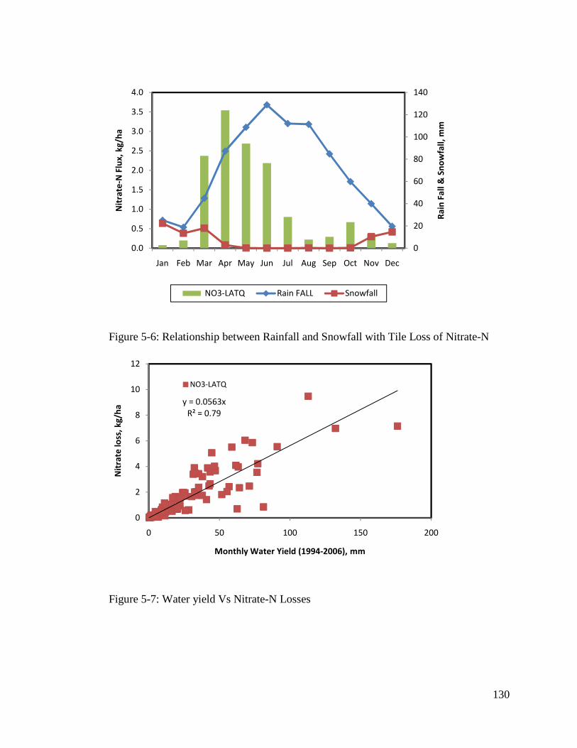
130

Figure 5-6: Relationship between Rainfall and Snowfall with Tile Loss of Nitrate-N

Figure 5-7: Water yield Vs Nitrate-N Losses

0

20

40

60

80

100

120

140

0.0

0.5

1.0

1.5

2.0

2.5

3.0

3.5

4.0


Ra

in F

all

& S

no

wfa

ll,

mm

Nit

rate

-N F

lux

, k

g/h

a

NO3-LATQ Rain FALL Snowfall

y = 0.0563x

R² = 0.79

0

2

4

6

8

10

12

0 50 100 150 200

Nit

rate

lo

ss,

kg

/ha

Monthly Water Yield (1994-2006), mm

NO3-LATQ

131

Figure 5-8: Tile flow Vs Nitrate-N losses

Figure 5-9: Relationships between water yield and tile flow with Nitrate-N losses

5.3.4. Nitrogen Budget

N losses through tile drains, groundwater discharge and interflow averaged 16.2 kg/ha,

which is 8.1% of applied fertilizer and manure. The annual average crop N-uptake of

corn and soybeans in the LRW was 55.5 kg/ha more than the applied N-fertilizer.

Mineralization of fresh and active organic matter adds 116.1 kg/ha N, and an additional

42.1 kg/ha N was supplied from fixation and deposition. N losses by volatilization and

denitrification totaled 22.3 kg/ha/year (Table 5-3 & Table 5-4). Snow fall and rainfall

conditions in the LRW induced saturation of soils and consequently denitrification. The

annual rate of denitrification rate was 15.9 kg/ha. This is in close agreement to the

findings of David et al. (1997, 2009). Overall, the calculated mass balance revealed a

y = 0.1143x

R² = 0.89

0

1

2

3

4

5

6

7

8

9

10

0 20 40 60 80 100

Nit

rate

lo

ss,

kg

/ha

Monthly Tile Flow (1994-2006), mm

NO3-LATQ

0

10

20

30

40

50

60

0.0

1.0

2.0

3.0

4.0

Jan Feb Mar Apr May Jun Jul Aug Sep Oct Nov DecW

ate

r y

ield

& T

ile

Flo

w,

mm

Nit

rta

e l

oss

, k

g/h

a

NO3-LATQ

WATERYIELD

Tile Flow

132

net gain of 0.8 kg/ha N. Thus, with the current production system of the LRW there is

no net depletion of soil nitrogen.

Table 5-3: Nitrogen inputs to the LRW

INPUTS (Kg/Ha) % N-FERTILIZER APPLIED 139.4 46.9 MIN OF FRESH ORG N 33.8 11.4 MIN OF ACTIVE ORG N 82.3 27.7 NO3 IN RAINFALL 8.0 2.7 N FIXATION 34.1 11.5 TOTAL 297.5 100

Table 5-4: Nitrogen outputs from the LRW

OUTPUTS (Kg/Ha) % ACTIVE TO STABLE ORG N 61.4 20.7 N-UPTAKE 194.9 65.5 AMMONIA VOLATILIZATION 6.4 2.2 DENITRIFICATION 15.9 5.4 NO3 YIELD (Interflow) 2.1 0.7 NO3 YIELD (Tile Drains) 13.5 4.6 NO3 YIELD (Groundwater) 0.6 0.2 ORGN_OUT 1.8 0.6 TOTAL 296.7 100.0

Ninputs-Noutputs = Change in Soil N Storage (∆NSoil)

297.5-296.7 = 0.8 kg/ha

5.3.5. Spatial and Temporal Distribution of Nitrate-N Losses

The average annual total riverine nitrogen load from the LRW was 17.6 kg/ha (Table

5-6). Tile drainage accounts for 76% of the total loss. The organic and mineral nitrogen

losses accounted for 9% and 91% of the total loss, respectively. Croplands contributed

99% of the predicted total nitrogen loading to surface waters in the LRW. About 30%

of the watershed area contributes half of the losses.

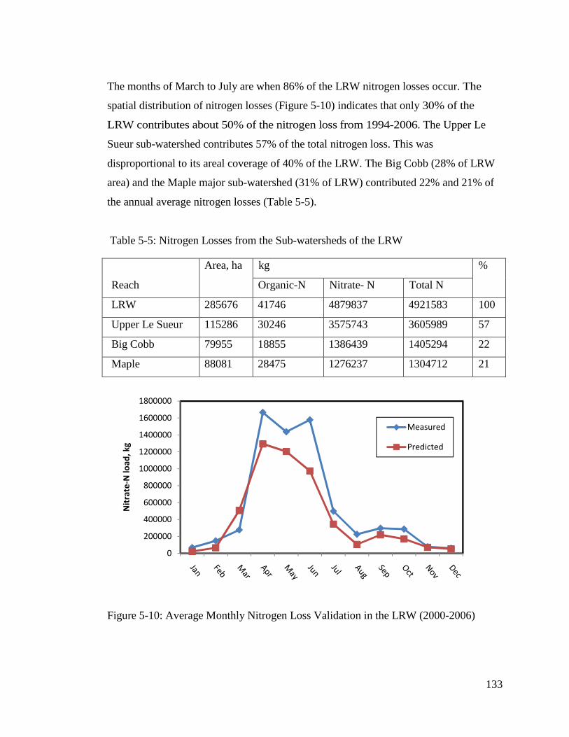
133

The months of March to July are when 86% of the LRW nitrogen losses occur. The

spatial distribution of nitrogen losses (Figure 5-10) indicates that only 30% of the

LRW contributes about 50% of the nitrogen loss from 1994-2006. The Upper Le

Sueur sub-watershed contributes 57% of the total nitrogen loss. This was

disproportional to its areal coverage of 40% of the LRW. The Big Cobb (28% of LRW

area) and the Maple major sub-watershed (31% of LRW) contributed 22% and 21% of

the annual average nitrogen losses (Table 5-5).

Table 5-5: Nitrogen Losses from the Sub-watersheds of the LRW

Figure 5-10: Average Monthly Nitrogen Loss Validation in the LRW (2000-2006)

0

200000

400000

600000

800000

1000000

1200000

1400000

1600000

1800000

Nit

rate

-N l

oa

d,

kg

Measured

Predicted

Reach

Area, ha kg %

Organic-N Nitrate- N Total N

LRW 285676 41746 4879837 4921583 100

Upper Le Sueur 115286 30246 3575743 3605989 57

Big Cobb 79955 18855 1386439 1405294 22

Maple 88081 28475 1276237 1304712 21

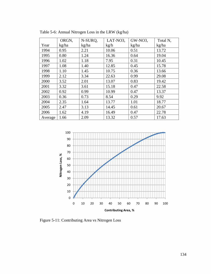
134

Table 5-6: Annual Nitrogen Loss in the LRW (kg/ha)

Year ORGN, kg/ha

N-SURQ, kg/ha

LAT-NO3, kg/h

GW-NO3, kg/ha

Total N, kg/ha

1994 0.95 2.21 10.06 0.51 13.72 1995 0.80 1.24 16.36 0.64 19.04 1996 1.02 1.18 7.95 0.31 10.45 1997 1.08 1.40 12.85 0.45 15.78 1998 1.10 1.45 10.75 0.36 13.66 1999 2.12 3.34 22.63 0.99 29.08 2000 3.52 2.01 13.07 0.83 19.42 2001 3.32 3.61 15.18 0.47 22.58 2002 0.92 0.99 10.99 0.47 13.37 2003 0.36 0.73 8.54 0.29 9.92 2004 2.35 1.64 13.77 1.01 18.77 2005 2.47 3.13 14.45 0.61 20.67 2006 1.62 4.19 16.49 0.47 22.78 Average 1.66 2.09 13.32 0.57 17.63

Figure 5-11: Contributing Area vs Nitrogen Loss

0

10

20

30

40

50

60

70

80

90

100

0 10 20 30 40 50 60 70 80 90 100

Nit

rog

en

Lo

ss,

%

Contributing Area, %

135

Figure 5-12: Nitrogen Contributing Areas in the LRW

5.3.6. Nitrate-N BMPs

A. Reduced rate fall/spring nitrogen application

The baseline application rate of nitrogen fertilizer from both animal manure and applied

anhydrous ammonia was 167 kg/ha. Fall application of 134 kg/ha of nitrogen (a

reduction of 20%) reduced total N losses by about 22%. In contrast to this, spring

application of reduced rates of urea only reduced 7% of the nitrogen loss (Table 5-7).

This result does not agree with the findings of Randall et al., (1993) for the same study

area. According to them, planted corn recovered 13% more nitrogen when urea is

applied in spring than anhydrous ammonia applied in fall (Randall and Schmitt, 1993).

136

B. Conservation tillage

SWAT simulation of conservation tillage on 50% of corn land did not show any

reductions in nitrogen loss. An increase in surface residue cover reduced soil erosion

and increased infiltration. Consequently, organic N losses decreased and tile drainage

losses increased.

Table 5-7: Relative effects of application of different BMPs in reducing N loss in the LRW

C. Vegetative filter strips (VFS)

Application of VFS on corn-soy land steeper than 2% slope showed an 8% reduction in

total N loss. This was mainly due to a decrease in total organic nitrogen and surface

runoff losses.

Scenario

kg/ha

% Reduction

Organic-N

Surface-N

Tile-N

Groundwater-N

Total N

Baseline 1.7 2.1 13.3 0.6 17.6 Reduced rate fall nitrogen application (AA) 1.4 1.9 10.0 0.5 13.8 21.6 Reduced rate spring nitrogen application (Urea) 1.4 2.0 12.4 0.5 16.35 7.1

Conservation Tillage on 50% corn residue 1.5 2.2 13.4 0.6 17.6 0 No Tillage on 50% corn residue 1.4 2.1 13.3 0.6 17.3 1.7

VFS on CS over 2% slope 1.2 1.3 14.1 0.5 17.1 2.8

Rye as cover crop 1.2 2.3 10.4 0.5 14.3 18.8

137

D. No-tillage

There is no substantial reduction in total nitrogen loss from the application of no-tillage

on 50% corn fields. There was only a 2% reduction in the total loss.

E. Cover Crops Planting rye after corn harvest covered the soil during the winter season and reduced the

total nitrogen loss by 16%. Rye was planted after the October corn harvest and

produced high above-ground biomass until the 3rd week of April. The high rye biomass

production resulted in increased uptake of nitrogen from the soil, which otherwise

would have been lost in tile drainage. Consequently, rye reduced the amount lost in tile

drainage by 2.9 kg/ha/year.

138


The increase in application of commercial fertilizers and the expansion of sub-surface

drainage technology have caused high nitrate flux in the upper Mississippi River in

general, and the Minnesota River basin and the LRW in particular (Magner et al., 2004).

The LRW in the Minnesota River basin is an agricultural watershed covering 285,000

ha, from which about 18 kg/ha of nitrate-N is discharged every year.

The LRW SWAT model nitrate-N simulation built upon good calibration and validation

results of the SWAT hydrology and sediment simulation modeling. Monthly calibration

and validation of nitrate-N in the Beauford sub-watershed gave NSE values of 0.74 and

0.77, respectively. The calibrated nitrate-N parameters were transferred to the LRW,

where good agreement between predicted and observed nitrate-N values was obtained,

with an NSE value of 0.74.

The nitrate-N losses were well correlated to the water yield and tile flow in the LRW

with R2 values of 0.79 and 0.89, respectively. The compounded effects of snow melt

and tile flow in the months of March to May have caused the climax nitrate-N losses of

1.5-3.5 kg/ha/month. The calculated nitrogen mass balance has shown a net gain of 0.8

kg/ha. Despite the big losses of nitrate-N from the LRW, there is no net depletion of the

watershed soil nitrogen. Reduced rate nitrogen fertilizer applications and winter cover

cropping are proven to be the best management practices that can reduce the losses.

Further research is needed to improve the LRW SWAT modeling of nitrate-N

dynamics:

• A routine that accounts for variations in drain spacing and depth of tile drains

• Routing of flow and pollutants between HRUs

• Targeted placement of BMPs like filter strips, grassed water ways, riparian

buffer zones, wetlands, grassland or other land use within a given sub-

watershed

• A routines for concentrated animal feeding operations.

139

Chapter 6 : SWAT MODELING OF LRW PESTICIDE DYNAMICS

140

SYNOPSIS

Pesticides from diffuse and point sources can enter water resources and cause surface

and ground water pollution. In this study the movement and fate of the pesticides

acetochlor, metolachlor, and atrazine were studied using the SWAT model in the Le

Sueur River watershed (LRW) of South Central Minnesota. Monitoring results have

shown frequent detections of these herbicides in surface waters of the LRW. The

objective of this study was to investigate management options for reducing pesticide

contamination. The SWAT model was calibrated in the Beauford sub-watershed and

applied to the entire LRW.

SWAT model setup and configuration was made for a baseline acetochlor application

rate of 1.79 kg/ha applied to 35% of the fields planted to corn. Predicted monthly

average losses of acetochlor, atrazine and metolachlor were very accurate, with NSE

values of 0.96, 0.91 and 0.71, respectively. Losses of all three pesticides were for the

most part in solution form. The estimated average annual losses of acetochlor, atrazine,

and metolachlor from the LRW were 0.47%, 0.02% and 0.0034% of the total annual

application.

Reducing the acetochlor application rate to 1.47 kg/ha and the application area to 20%

of the corn fields reduced losses by 17% and 56%, respectively, from baseline

conditions. In contrast, increasing the application rate to 2.45 kg/ha and the application

area to 50% increased losses by 37% and 117% of the baseline scenario, respectively.

The combination of reduced application rate (1.47 kg/ha) and incorporation of

acetochlor can reduce losses by over 95%. Vegetated filter strips reduced acetochlor

losses by over 60%.

141

6.1. Introduction

Roughly 500,000 metric tons of pesticide active ingredients are used in the United

States annually. Herbicides are widely used for the control of grassy and broad leaf

weeds, accounting for 43% of the total pesticides, of which more than 77% is applied

for agricultural production purposes (Aspelin, 2003; Rebich et al., 2004). The Upper

Mississippi River Basin receives a large portion of the applied herbicides (Rebich et al.,

2004). Cropland in the Midwest receives about two thirds of the herbicides used for

agriculture in the United States (Barbash and Resek, 1996).

Despite all the advantages of pesticides, high pesticide usage can have unintended

effects on the environment and human health through its effects on surface and ground

water quality (Aspelin, 2003). Banning pesticide usage may cause the losses of food

and fiber crops, expansion of infectious diseases and damage of native habitats by

invasive species (Rice et al., 2007). Thus, proper pesticide use and management to

balance its economic benefit with the possible environmental impacts is the challenge

not yet completely resolved.

According to the National Water-Quality Assessment (NAWQA) of streams draining

agricultural watersheds from 1992-2001, pesticides or pesticide degradates were

detected 90 percent of the time. Pesticide concentrations exceeded human-health risk

limits more than once in about 10 percent of agricultural streams. Most of those streams

are in the corn-soybean producing areas, including Minnesota (Gilliom et al., 2006).

High herbicide loadings to the Gulf of Mexico were reported by Clark et al. (1999) in

the spring following post application of herbicides. Rebich et al., (2002) analyzed water

samples taken from March 1999 to May 2001from the Mississippi River Basin, and

atrazine was the most frequently detected (present in 97% of the samples). The

chloroacetanilide herbicides metolachlor and acetochlor were detected in 60% and 31%

of the samples, respectively. The extent of tile drainage throughout the Mississippi

River Basin appeared to be related to the occurrence and distribution of

chloroacetanilide degradates in water samples.

142

Studies by Battaglin and Goolsby (1999) showed large amounts of herbicide losses to

streams and major rivers of the Midwest during periods of late spring and early summer

rainfall (Battaglin and Goolsby, 1999). Several studies in the Midwestern US showed

herbicides in streams, reservoirs, ground water, and precipitation (Gilliom et al., 2006;

Gilliom, 1984; Kalkhoff et al., 2003; Kolpin et al., 1995; Larson et al., 1997; Scribner et

al., 1998; Thurman et al., 1992).


Three herbicides that are typically applied to corn and soybean (acetochlor, atrazine and

metolachlor) were frequently detected in the Minnesota River Basin (Minnesota River

Basin Data Center MRBDC., 2004). Detections were observed from 2000-2002 at the

Le Sueur River at Highway 66, the Blue Earth River below the Rapidan Dam, and the

Minnesota River at Judson.

Acetochlor, atrazine and metolachlor are the three most commonly used herbicides in

Minnesota (Minnesota Department of Agriculture (MDA), 2009; USDA, 1998). The Le

Sueur River is impaired for acetochlor (based on the proposed chronic standard of 1.7

µg/L) from the Maple River to Blue Earth River and the Beauford Ditch (MPCA, 2007).

The Minnesota Department of Agriculture is actively studying the use and management

of acetochlor in the LRW (Minnesota Department of Agriculture (MDA), 2009).

Atrazine is a family of the triazine pesticides. It is a weak base that inhibits protein

synthesis of broad leaf weeds. It is widely used for corn production as a pre-plant, pre-

emerge or post emergence treatment. The relatively low affinity for soil sorption makes

atrazine very mobile. It has a large potential to leach down the soil profile and to move

in solution with surface runoff and subsurface drainage. It is one of the most frequently

detected herbicides in surface water and groundwater of the Midwest (Goolsby et al.,

1991; Clay and Koskinen, 1990; Goss, 1992).

143

Acetochlor and metolachlor are non ionic herbicides of the acetamide family. They are

used as pre-emergent herbicide to control grasses and some broadleaf weeds in corn.

Metolachlor is also used to control weeds in soybeans. The two herbicides have high

water solubility and are moderately adsorbed to soils. Their sorption is mainly related to

clay and organic matter content of soils. These herbicides are primarily degraded by

microorganisms (Kolpin et al., 1996; Weber and Peter, 1982).

Analysis of herbicide concentrations in soil and water samples is expensive (Wauchope,

1992). Simulation models can be used to characterize the temporal and spatial

magnitude of pesticide concentrations and fluxes at the watershed scale, reducing the

need for extensive spatial and temporal water sampling and analysis. Accurate

simulation of pesticide fate and transport requires good representation of the transport

mechanisms that occur in the field and calibration and validation of model predictions

against measured pesticide concentration data.

6.1.2. Objectives The SWAT pesticide model was used to quantify pesticide fate and transport processes

in the LRW as controlled by surface and subsurface settings, hydrologic conditions, and

agricultural practices. The specific objectives of the study are to:

• Quantify the spatial and temporal distributions of pesticide losses

• Evaluate potential adverse impacts on water resources

• Identify feasible management practices using modeling techniques.

6.1.3. Models of Pesticide Dynamics Several watershed scale pesticide fate and transport models were developed over the

last three decades. The complexity of these models ranges from screening to research

models. Simple screening models usually have minimal input data, are relatively easy to

use, and produce fast results. The primary function of these models is the preliminary

assessment of specific geographic environments, or pesticide behavior and fate

processes for future study. Complex research models are meant to simulate the actual

144

physical, chemical, or biological processes accurately using a large amount of input data

and require large amounts of computer time. Their output describes pesticide

concentrations as a function of time and space (Larson et al., 1997).

Relatively complex pesticide models are listed in Table 6-1. Among the recently

developed more complex pesticide simulation models are the event based models of

AGNPS (Merritt et al., 2003; Young, 1987) and DWSM (Borah et al., 2002),

continuous simulation models of AnnAGNPS (Bingner and Theurer, 2001), HSPF

(Bicknell et al., 1995), SWAT (Neitsch, et al., 2002), and MIKE SHE (Refsgaard et al.,

1995) which works using either a single-event or long-term continuous simulations,

mainly for small watersheds (Borah and Bera, 2003). The major difference among these

models include, land phase and in-stream pesticide transport and transformations

processes, spatial and temporal variability in their input parameters.

6.1.4. Pesticide Simulation Processes in SWAT Model

SWAT pesticide simulation starts by defining the type, amount and dates of application

of pesticides to an HRU with further details describing the initial pesticide residue in the

soil. The simulation modeling routines were made based on the interactions among the

pesticide properties, soils, climate, and management effects on pesticide losses.

However, the model does not simulate the stress on the growth of a plant due to the

presence of weeds.

SWAT simulates pesticide movement into the stream network via surface runoff in

solution and adsorbed to sediment, and into the soil profile by leaching. The movement

of the pesticide is controlled by its solubility, degradation half-life, and soil organic

carbon adsorption coefficient. The equations in SWAT used to model pesticide

movement and fate are adapted from GLEAMS (Leonard et al., 1987).

SWAT is largely used for prediction of pesticide fluxes to rivers (Holvoet et al., 2005;

Holvoet et al., 2007; Kannan et al., 2007; Kannan et al., 2006). Borah and Bera (2003)

have reviewed eleven watershed scale hydrologic and nonpoint -source pollution

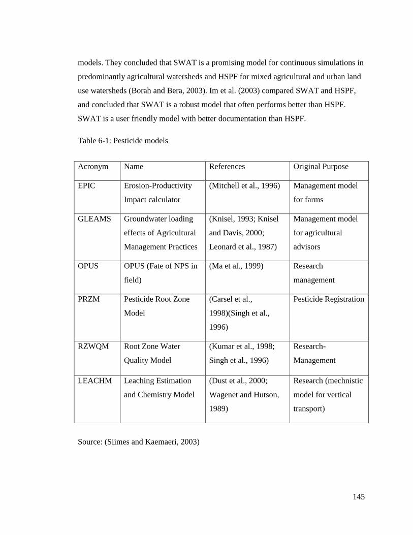
145

models. They concluded that SWAT is a promising model for continuous simulations in

predominantly agricultural watersheds and HSPF for mixed agricultural and urban land

use watersheds (Borah and Bera, 2003). Im et al. (2003) compared SWAT and HSPF,

and concluded that SWAT is a robust model that often performs better than HSPF.

SWAT is a user friendly model with better documentation than HSPF.

Table 6-1: Pesticide models

Acronym Name References Original Purpose

EPIC Erosion-Productivity

Impact calculator

(Mitchell et al., 1996) Management model

for farms

GLEAMS Groundwater loading

effects of Agricultural

Management Practices

(Knisel, 1993; Knisel

and Davis, 2000;

Leonard et al., 1987)

Management model

for agricultural

advisors

OPUS OPUS (Fate of NPS in

field)

(Ma et al., 1999) Research

management

PRZM Pesticide Root Zone

Model

(Carsel et al.,

1998)(Singh et al.,

1996)

Pesticide Registration

RZWQM Root Zone Water

Quality Model

(Kumar et al., 1998;

Singh et al., 1996)

Research-

Management

LEACHM Leaching Estimation

and Chemistry Model

(Dust et al., 2000;

Wagenet and Hutson,

1989)

Research (mechnistic

model for vertical

transport)

Source: (Siimes and Kaemaeri, 2003)

146

6.2. Materials and Methods

6.2.1. Study Area This study was conducted in the LRW, a region of extensive corn-soybean production

in South Central Minnesota. Acetochlor, atrazine and metolachlor are the three most

commonly used herbicides for corn and soybean production in the watershed. The draft

2008 303(d) impaired waters list for acetochlor includes the Le Sueur River from the

Maple River to the Blue Earth River and the Beauford Ditch (MPCA, 2007).

6.2.2. Data Collection and Analysis Application area, rate and date for the three selected pesticides (acetochlor, atrazine and

metolachlor) as surveyed by MDA were organized in the SWAT operation management

database. Application of herbicides was made to randomly selected fields in the LRW in

conformity with the MDA survey areas receiving herbicide application. The year 2005

was used for calibration of pesticide input parameters. The Beauford sub-watershed was

selected as a representative area for calibration. The calibrated model parameters were

transferred to the entire LRW. No model validation was possible, given the short

duration of water quality monitoring data in the LRW.

SWAT model pesticide potential pathways and processes were adapted from the

GLEAMS model (Leonard, 1987). These processes govern the fate and transport of

pesticides on plant foliage and in the soil. Pesticide wash-off from the plant foliage

occurs when the rainfall on a given day exceeds 2.54 mm, using the equation:

PK,o'M � fro'M " PK �6.1�

where Pf,wsh (kg/ha) is the amount of pesticide that is washed-off from the plant foliage,

frwsh is the fraction of total pesticide that is washed off, and Pf (kg/ha) is the total

amount of pesticide that is present on the plant foliage.

The three simulated pesticides are organic compounds that contain carbon. Therefore,

they can be degraded by microorganisms following first order kinetics:

�E � �U,^ " expd��TU " �f �6.2�

�/ � �/,^ " expd��T/ " �f �6.3�

147

where Pt and Pf are pesticide concentration at time t in the soil and foliar , (kg/ha), Ps,o

and Pf,o are the initial concentration of pesticide in soil layer and foliar (mg/L), and Kps

and Kpf are the rate constant for pesticide degradation in soil and foliar (1/time) and t is

time elapsed since initial pesticide amount was determined. days.

The relation of rate constant to half life is given by:

�W/X � 0.693�T

�6.4�

Where t1/2 is the half life of the pesticide.

SWAT model pesticide transport algorithms were taken from EPIC model (Williams et

al., 1984). Surface runoff is the major process of pesticide movement from the land

surface to the stream network. This occurs in solution or adsorbed forms as partitioned

by the adsorption coefficient of pesticides to soils, as normalized for soil organic carbon

content.

�T � {U^@P?{U^@�

� �� g��{100 �6.5�

where Kp is the adsorption coefficient (mg/kg)/(mg/L), Csolid is the concentration of

pesticide in solid phase (mg/kg), and Csolu is the concentration in the solution phase

(mg/L), Koc is the soil adsorption coefficient normalized for soil organic carbon content

(mg/kg)/(mg/L), and OrgC is the organic carbon content of the soil.

Soluble Phase Pesticide Transport

The amount of pesticide removed in surface runoff is given by:

P��LK � β� " Conc).�(�o " Q'�LK �6.6�

Where pstsurf is the amount of pesticide removed in surface runoff (kg/ha), βP is the

pesticide percolation coefficient, Concp.flow is the pesticide concentration in mobile

water for the top 10 mm of soil (kg/mm H2O), and Qsurf is the surface runoff generated

on a given day (mm H2O).

148

Adsorbed Pesticide Transport

The sediment loading from an HRU affects the loading of adsorbed pesticides. This is

calculated using the equation:

P�� 0.001 " C'�(�� " sedHRUYL�Y

" ε).'��

�6.7�

where Psed is the amount of sorbed pesticide transported to the main channel in

surface runoff (kg/ha), Csolid is the concentration of pesticide on sediment

in the top 10 mm (g pest/metric ton soil), sed is the sediment yield on a given day

(metric tons), HRUarea is the HRU area (ha), and εp:sed is the pesticide enrichment

ratio.

Pesticide Percolation

The amount of pesticide percolated to lower soil layers is given by:

P)�LZ � Conc�.�(�o " w)�LZ �6.8�

Where pperc is the pesticide moved to the underlying layer by percolation (kg/ha),

concp,flow is the concentration of pesticide in the mobile water for the layer (kg/mm

H2O), and wperc is the amount of water percolating to the underlying soil layer on a

given day (mm H2O).

Pesticide Lateral Flow

�@QE.U�F/ � RT{��./@^V " �@QE.U�F/ �6.9�

�@QE � {��./@^V " �@QE �6.10�

where Plat is the pesticide removed in lateral flow from a layer (kg/ha), βp is the

pesticide percolation coefficient, concp,flow is the concentration of pesticide in the

mobile water for the layer (kg/mm H2O), and Qlat is the water discharged from the layer

by lateral flow (mm H2O).

149

6.3. Results and Discussion

The pesticide calibration and validation process was conducted after calibrating and

validating the model for hydrology and sediment yield. Model simulation was initiated

by setting the physico-chemical properties of the three pesticides (Table 6-2) and the

baseline application management as defined in the management input file (Table 6-3).

Table 6-2: Physico-Chemical Properties of Selected Pesticides

Table 6-3: Baseline Scheduled Herbicide Applications

Year Crop type Management operation Date Year 1 Corn - Metolachlor application (2.48 kg/ha) May 3

- Acetochlor application (1.79 kg/ha) Apr 29 - Atrazine application (0.66 kg/ha) Apr 29

Year 2 Soybean - Metolachlor (1.0 kg/ha) May 14

Note

• Acetochlor was applied to 35% of the corn acreage

• Atrazine was applied to 15% of the corn acreage

• Metolachlor was applied to 4% of corn and 1% of soybean acreage

6.3.1. Calibration and Validation

The predicted and observed monthly average losses of acetochlor, atrazine and

metolachlor (Figure 6-1) have NSE values of 0.96, 0.91 and 0.71, respectively. This

indicates the SWAT model can predict the monthly losses of these pesticides with great

accuracy. The loss of all three pesticides is for the most part in solution form.

Comparing the three pesticides, acetochlor has the largest (93%) loss in solution form,

and metolachor has the largest sorbed loss of 18% (Table 6-4). Of the total amount

applied in 2005, about 4.1% of the applied acetochlor and 0.01% of atrazine and

metolachlor reached the mouth of the Beauford sub-watershed.

PESTICIDE Atrazine Metolachlor Acetochlor SOIL-KOC ( mg/kg)/(mg/L) 100 190 150 HALF LIFE FOLIAR (days) 5 5 5 HALF-LIFE SOIL (days) 60 100 12 WATER-SOLUBLITY (mg/L) 33 530 223

150

A) Acetochlor

B) Atrazine

C) Metolacholr

Figure 6-1: Pesticide Calibration Results in the Beauford Sub-Watershed

0

2000000

4000000

6000000

8000000

10000000

12000000

Ace

toch

lor

Loa

d,

mg

Measured

Predicted

0

4000

8000

12000

16000

Atr

azi

ne

Lo

ad

, m

g

Measured

Predicted

0

4000

8000

12000

16000

20000

Me

tola

chlo

r Lo

ad

, m

g

Measured

Predicted

151

Table 6-4: Predicted pesticide losses in solution and adsorbed forms

Pesticide Solution, % Sorbed, %

Acetochlor 93 7 Atrazine 86 14 Metolachlor 82 18

6.3.2. LRW Estimated Pesticide Losses

6.3.2.1. Acetochlor

About 35% of LRW corn fields received acetochlor applications. The average

application rate was 1.79 kg/ha active ingredient. The estimated average annual loss of

acetochlor from the LRW was 0.47% of the total applied amount. Maximum losses

occurred in the years 2000, 2005 and 2006, with percent losses of 1.56%, 1.59% and

1.75%, respectively (Figure 6-2). Acetochlor has a solubility of 223 mg/L and a short

half life of 12 days, so it is largely lost in solution form. Ninety four percent of

acetochlor loss in the LRW was in solution form. The three months from April to June

are critical periods in which 99% of the acetochlor loss occurs (Figure 6-2 & Figure

6-3).

Figure 6-2: Annual loss of Acetochlor in the LRW

0

200

400

600

800

1000

1200

1400

1600

Ace

toch

lor

Loss

, k

g

152

Figure 6-3: Average monthly cumulative losses of acetochlor in the LRW

6.3.2.2. Atrazine

Atrazine was applied to 15% of the corn fields in the LRW. The average application

rate was 0.66 kg/ha of active ingredient. SWAT simulation results showed that 85% of

the atrazine loss in the LRW occurs in the four months from April to July (Figure 6-4).

About 82% of this loss occurs in solution form, and the remaining 18% is adsorbed to

soil particles. Considering the high water solubility and low sorption coefficient of

atrazine this result looks reasonable. Studies made by Wauchope (1978), Baker et al.

(1978), Baker and Johnson (1979), and Arora et al. (1996) estimated 75 to 100% loss in

solution and about 25% or less to be removed through sediment losses.

Figure 6-4: Average Monthly Loss of Atrazine in the LRW

0

50

100

150

200

250

300


Cu

mu

lati

ve

Lo

ss,

kg

0

100

200

300

400

500

600

700


Atr

azi

ne

Lo

ss,

gm

153

The variability in timing of precipitation after application of atrazine is one of the most

important factors that affects the loss in different years. The LRW has an average

annual atrazine loss of about 3.2 kg or 0.02% of the total applied over the years 1994-

2006. The maximum loss was 4.8% in the years 2000 and 2005 (Figure 6-5).

Figure 6-5: Annual Loss of Atrazine in the LRW

6.3.2.3. Metolachlor

SWAT simulation of metolachlor was made assuming that 4% of the corn fields and 1%

of soybean fields in the LRW receivied this pesticide. The average application rate was

2.48 kg/ha for corn and 1 kg/ha for soybean. The simulated average annual loss of

metolachlor was 5.54 kg or 0.034% of the amount applied. The maximum loss occurred

in the year 2000, and was about 33 kg of the amount applied (Figure 6-6). The months

of April to July are critical periods in which 91% of the loss occurs (Figure 6-7).

Figure 6-6: Annual Loss of Metolachlor in the LRW

0

1

2

3

4

5

6

Atr

azi

ne

Lo

ss.

kg

0

5

10

15

20

25

30

35

Me

tola

chlo

r lo

ss,

kg

154

Figure 6-7: Average Monthly Loss of Metolachlor in the LRW

6.3.3. Acetochlor Best Management Practices (BMPs)

Evaluation of five alternative BMP scenarios for acetochlor were made in the Beauford

sub-watershed, including 1) rate of application, 2) watershed area of application, 3)

timing of application, 4) incorporation of acetochlor and 5) effects of buffer strips.

The first alternative scenario involved rate of acetochlor application. Rate of acetochlor

was either the low or high label rate of 1.47 or 2.45 kg/ha in comparison with the

baseline rate of 1.79 kg/ha. The second scenario involved area receiving acetochlor

applications. Watershed area receiving acetochlor applications was studied in two ways.

The first was to apply acetochlor at a rate of 1.47 kg/ha on all Critical Contributing

Areas (CCAs) and 1.79 kg/ha on all non-CCAs or to apply a rate of 1.47 kg/ha on all

CCAs and 2.45 kg/ha on all non-CCAs. The second was to apply 1.79 kg/ha on 20% of

the corn fields or 1.79 kg/ha on 50% of all corn fields. The third scenario involved date

of application. Application date was varied from April 29 to May 3. The fourth scenario

involved incorporation of acetochlor. The fifth scenario involved field buffer strips.

Buffer strips were investigated with different rates of acetochlor on all land receiving

acetochlor, or only on CCAs.

A. Acetochlor BMP Scenarios in the Beauford Sub-Watershed

Application rate had a significant effect on acetochlor losses (Figure 6-8a). In

comparison with the baseline simulation, applying 1.47 kg/ha reduced acetochlor losses

0.0

0.5

1.0

1.5

2.0

2.5


Me

tola

chlo

r Lo

ss,

kg

155

by 17%. Applying 2.45 kg/ha increased acetochlor losses by 37%. Concentrations of

acetochlor at the watershed scale were also affected by rate of application (Figure 6-8-

8). Maximum concentrations were reached in the month of May. With an application

rate of 1.47 kg/ha, the maximum concentration of acetochlor was 4.39 ug/L, with a rate

of 2.45 kg/ha the maximum concentration was 7.23 ug/L.

Figure 6-8: Effect of Changing Application Rate of Acetochlor in the Beauford

Watershed.

Application of acetochlor at low label rates on CCAs reduced acetochlor losses

considerably (Figure 6-9). Applying 1.47 kg/ha to CCAs and 1.79 kg/ha to non-CCAs

resulted in an 11% reduction of acetochlor losses relative to the baseline scenario.

Applying 1.47 kg/ha to CCAs and 2.45 kg/ha to non-CCAs (NCCA) resulted in a 3%

reduction of acetochlor losses relative to the baseline scenario. Application of

acetochlor at a rate of 1.79 kg/ha to 20% of the land planted to corn reduced acetochlor

0

5

10

15

Dec-04 Feb-05 Apr-05 May-05 Jul-05 Sep-05 Oct-05 Dec-05

Ace

toch

lor

Loa

d,

kg

Measured, kg

1.79 April 29

2.45 April 29

1.47 April 29

a

0

2

4

6

8

Dec-04 Feb-05 Apr-05 May-05 Jul-05 Sep-05 Oct-05

Ace

toch

lor

Co

nc.

, p

pb

Measured, ug/L

1.79 April 29

2.45 April 29

1.47 April 29

b

losses by 56% relative to the default application on 35% of the corn

the area receiving acetochlor to 50% of the corn increased acetochlor losses by 117%

relative to the baseline scenario.

Figure 6-9: Effect of Watershed Application Area on Acetochlor

Application date had a considerable

application date of April 29 (

increased the losses by 31% with an application rate of 1.79 kg/ha

by 8% with an application rate of 1.47 kg/ha.

storms shortly after May 3.

to avoid large losses.

ative to the default application on 35% of the corn fields


relative to the baseline scenario.

: Effect of Watershed Application Area on Acetochlor Losses.

considerable effect on acetochlor losses, relative to the baseline

application date of April 29 (Figure 6-10). Delaying acetochlor applications until May 3

increased the losses by 31% with an application rate of 1.79 kg/ha and increased losses

by 8% with an application rate of 1.47 kg/ha. This increase is due to the occurrence of

storms shortly after May 3. Acetochlor should not be applied shortly before rainstorms

156

fields. Increasing


Losses.

effect on acetochlor losses, relative to the baseline

Delaying acetochlor applications until May 3

and increased losses

This increase is due to the occurrence of

Acetochlor should not be applied shortly before rainstorms

Figure 6-10: Acetochlor Losses i

Incorporation of acetochlor produced

relative to the baseline scenario with no incorporation (

of acetochlor application (1.47 kg/ha), in

relative to the baseline scenario with an application rate of 1.79 kg/ha.

Field buffer strips had a

the buffer was somewhat important.

the watershed, acetochlor losses were reduced by 68% relative to the situation without

buffers. With a 22 m (66 ft

Buffers were more effective at lower rates of acetochlor application.

strips only in CCAs reduced acetochlor losses by roughly 50%, relative to the baseline

scenario.

Acetochlor Losses in Response to Application Date and Rate.

Incorporation of acetochlor produced considerable reductions in acetochlor losses

relative to the baseline scenario with no incorporation (Figure 6-11). At the lowest rate

of acetochlor application (1.47 kg/ha), incorporation reduced acetochlor losses by 95%

relative to the baseline scenario with an application rate of 1.79 kg/ha.

Field buffer strips had a considerable effect on acetochlor losses (Figure

the buffer was somewhat important. With an 11m (33 ft) wide buffer applied throughout


66 ft) wide buffer everywhere, losses were reduced by 89%.

Buffers were more effective at lower rates of acetochlor application. Installing buffer


157

n Response to Application Date and Rate.

reductions in acetochlor losses

At the lowest rate

corporation reduced acetochlor losses by 95%

Figure 6-12). Width of

wide buffer applied throughout


wide buffer everywhere, losses were reduced by 89%.

Installing buffer


Figure 6-11: Effect of Acetochlor Incorporation on Acetochlor Lo

Figure 6-12: Effect of Buffer Strips on Acetochlor Losses.

: Effect of Acetochlor Incorporation on Acetochlor Losses.

Effect of Buffer Strips on Acetochlor Losses.

158

159

B. Acetochlor BMP Scenarios for the LRW

Based on model simulation results in the Beauford sub-watershed, six acetochlor best

management practices were selected and applied to the LRW. The BMPs were:

1. Reduced rate of application, 1.47 kg/ha

2. Reducing application area from 35% of the watershed to 20%

3. Change in application time, post emergence on May 3rd

4. Incorporation of acetochlor

5. 11 m (33ft) wide buffer strips on all corn and soybean fields

6. 11 m (33ft) wide buffer strips on CCAs.

Incorporation of acetochlor reduced acetochlor losses in the LRW by over 95% (Fig. 6-

13). This practice may not be feasible for adoption by farmers, as it requires significant

changes in tillage and manure management. Reducing application rate to 1.47 kg/ha and

application area to 20% of the corn fields, and establishing buffer strips reduces the loss

by 18%, 62% and 73%, respectively. Buffer strip establishment targeted to CCAs

reduced the loss by 14%. A change in application time to post emergence on May 3

reduces losses by only 9% (Figure 6-12).

Figure 6-13: Relative Importance of Acetochlor Management Practices in the LRW

0

50

100

150

200

250

300

350

400

Baseline (1.79

kg/ha on april

29)

Application

Time (May 3)

33ft Buffer

strip on CCAs

Rate of

Application

(1.47 kg/ha)

Reduced

Application

Area (20%

area)

33ft Buffer

strip on all

corn-soy land

Incorporation

of acetochlor

Av

era

ge

Ace

toch

lor

Loss

, k

g/y

ea

r

160


Despite all the advantages of pesticides, high pesticide usage can have unintended

effects on surface and ground water quality. In this study the movement and fate of the

pesticides acetochlor, metolachlor, and atrazine were studied using the SWAT model in

the LRW of South Central Minnesota. Monitoring results showed frequent detections of

these herbicides in surface waters of the LRW. This study was intended to investigate

management options that can mitigate the prevailing contamination and maintain the

future sustainability of water quality in the LRW and the Minnesota River Basin. The

model was calibrated in the Beauford sub-watershed and applied to the entire LRW.

SWAT predictions of monthly average losses of acetochlor, atrazine and metolachlor

were very accurate with NSE values of 0.96, 0.91 and 0.71, respectively. The loss of all

the three pesticides was primarily in solution form. Acetochlor had the largest (93%)

loss in solution form, and metolachor has the largest sorbed loss of 18%. About 4.1% of

the acetochlor applied in 2005 and 0.01% of atrazine and metolachlor reached the

mouth of the Beauford sub-watershed. The estimated average annual loss of acetochlor,

atrazine, and metolachlor from the LRW were 0.47%, 0.02% and 0.0034% of the total

annual application.

Reducing the baseline application rate to 1.47 kg/ha and application area to 20% of the

corn fields minimized losses by 17% and 56%, respectively. Increasing application rate

to 2.45 kg/ha and application area to 50% increased losses by 37% and 117% of the

baseline scenario. Combining reduced rate application (1.47 kg/ha) and incorporation of

acetochlor can reduce losses by over 95%. A change in application time to post

emergence on May 3 reduces the loss by only 9%. Although vegetative filter strips were

predicted to reduce acetochlor losses by over 60%, the mechanism for these reductions

is unclear given that acetochlor losses occur primarily in solution form.

161

Chapter 7 : SWAT MODELING OF SURFACE WATER QUALITY

IMPACTS OF ALTERNATIVE BIOFUEL CROPS

AND CROP RESIDUE REMOVAL

162

SYNOPSIS

Corn ethanol production in Minnesota has increased to nearly 3.2 billion liters per year,

requiring corn grain from roughly 25% of Minnesota’s corn acreage. Minnesota corn

acreage increased 14% between 2006 and 2007. Most of this increase was due to loss of

soybean acreage and the shift from a corn-soybean to a corn-corn-soybean rotation. As

a result of this shift, Minnesota producers applied more nitrogen and phosphorus

fertilizer.

The objective of this section of the research was to quantify the impacts on water

quality of increases in corn acreage, and removal of crop residue or switchgrass

plantings for cellulosic ethanol production. The Soil Water Assessment Tool (SWAT)

model was used to evaluate the overall impacts of increased corn acreage on water

quality due to sediment, nutrient and pesticide losses. The study was conducted in the

Le Sueur River Watershed (LRW) of South Central Minnesota, where a corn-soybean

rotation is the dominant cropping system. The SWAT model was calibrated over two

years and validated over four years for monthly and annual water yield, sediment yield,

total nitrogen and total phosphorus outflows. Water quality impacts were studied with a

baseline corn-soybean rotation in comparison with a corn-corn-soybean rotation and a

biofuel production alternative involving extensive plantings of switchgrass on

environmentally sensitive landscapes. Impacts of various crop residue removal rates

were also studied.

Model simulation results indicated that increased corn acreage had no significant impact

on the annual water yield (98.7%), but increased sediment yield and total phosphorus

losses by 14%, and total nitrate-N losses by 53%. Compared to the baseline scenario,

phosphorus and sediment losses were increased by up to 51% and 71%, respectively,

for 60% residue removal under a corn-corn-soy rotation. Switchgrass established on

land steeper than 2% slope reduced sediment yield, phosphorus and nitrate-N losses by

73%, 39 % and 9%, respectively.

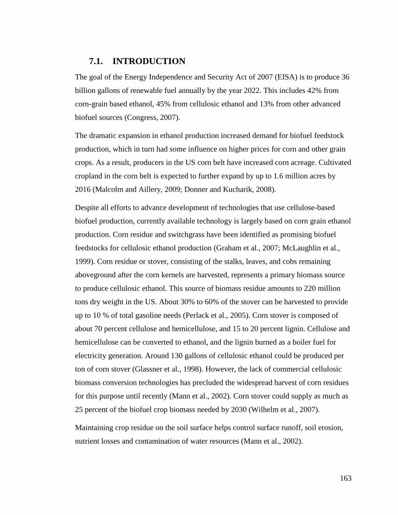
163

7.1. INTRODUCTION

The goal of the Energy Independence and Security Act of 2007 (EISA) is to produce 36

billion gallons of renewable fuel annually by the year 2022. This includes 42% from

corn-grain based ethanol, 45% from cellulosic ethanol and 13% from other advanced

biofuel sources (Congress, 2007).

The dramatic expansion in ethanol production increased demand for biofuel feedstock

production, which in turn had some influence on higher prices for corn and other grain

crops. As a result, producers in the US corn belt have increased corn acreage. Cultivated

cropland in the corn belt is expected to further expand by up to 1.6 million acres by

2016 (Malcolm and Aillery, 2009; Donner and Kucharik, 2008).

Despite all efforts to advance development of technologies that use cellulose-based

biofuel production, currently available technology is largely based on corn grain ethanol

production. Corn residue and switchgrass have been identified as promising biofuel

feedstocks for cellulosic ethanol production (Graham et al., 2007; McLaughlin et al.,

1999). Corn residue or stover, consisting of the stalks, leaves, and cobs remaining

aboveground after the corn kernels are harvested, represents a primary biomass source

to produce cellulosic ethanol. This source of biomass residue amounts to 220 million

tons dry weight in the US. About 30% to 60% of the stover can be harvested to provide

up to 10 % of total gasoline needs (Perlack et al., 2005). Corn stover is composed of

about 70 percent cellulose and hemicellulose, and 15 to 20 percent lignin. Cellulose and

hemicellulose can be converted to ethanol, and the lignin burned as a boiler fuel for

electricity generation. Around 130 gallons of cellulosic ethanol could be produced per

ton of corn stover (Glassner et al., 1998). However, the lack of commercial cellulosic

biomass conversion technologies has precluded the widespread harvest of corn residues

for this purpose until recently (Mann et al., 2002). Corn stover could supply as much as

25 percent of the biofuel crop biomass needed by 2030 (Wilhelm et al., 2007).

Maintaining crop residue on the soil surface helps control surface runoff, soil erosion,

nutrient losses and contamination of water resources (Mann et al., 2002).

164

Removing corn stover can reduce evapotranspiration by cooling the soil surface and

plant roots (Wagger and Denton, 1992). Linden et al. (2000) in their study in east

central Minnesota, reported that residue removal can minimize soil moisture and

increase soil temperatures, which in turn increases decomposition rates and could

increase water stress Holt (1979) reported that residue harvest removes more nutrients

than grain harvest alone, the greatest loss was predicted for the U.S. Midwest.

The amount of residue required to protect the loss of sediment and nutrients from

surface soils varies depending on soil type, slope, crop rotation, tillage system and

existing conservation practices (Wilhelm et al., 2007; Cruse and Herndl, 2009)

According to Charles (2009), no-till practices on slopes less than 2% leaving 1 ton/acre

residue are generally sufficient to reduce water erosion to less than 5 tons/acre/ per year.

Under tilled conditions with a slope of more than 5%, more than 5 tons/acre residue

may be required. Leaving more than 4 tons/ acre will be required on tilled row crop

rotations (Charles, 2009).

With the limited available land resources, the production of food crops and crop

residues may not be the only option for biofuel production. Producing environmentally

and economically competitive bioenergy crops depends on the availability of low-cost

and high biomass feedstocks (Graham et al., 1995). In this regard, switchgrass has been

identified as an energy crop that can successfully grow across a wide range of climatic

conditions (Vogel, 1996). Switchgrass has promising biofuel attributes, including its

high biomass production, and low chloride and ash contents (Lemus et al., 2002). It

provides year-round soil cover that reduces soil erosion and potential water

contamination of water resources from sediment and nutrient runoff losses. These

benefits can be credited to the density of switchgrass stems and roots, which promote

soil stability, increase infiltration, and slow runoff (Redfearn et al., 1997; Woolsey,

1992).

165


The State of Minnesota produces about one billion gallons of ethanol annually, which is

8.4% of the total U.S. production (RFA, 2009). Corn ethanol production in Minnesota

has increased to nearly 3.2 billion liters per year, requiring corn grain from roughly 25%

of Minnesota’s corn acreage. Consequently, Minnesota corn acreage increased by 14%

between 2006 and 2007 (USDA NASS, 2009). Most of this increase was due to loss of

soybean acreage, and shift from a corn-soybean to a corn-corn-soybean rotation. Some

of the additional acreage planted to corn came from Conservation Reserve Program

(CRP) land (Lakes, 2007). As a result, Minnesota producers applied more nitrogen and

phosphorus fertilizers. The increase in applied chemical inputs associated with increases

in corn acreage are a threat to water quality (Thomas et al., 2009; Vaché et al., 2002).

It is important to understand the environmental implications of shifts in cropping

systems and crop management associated with biofuel production. A SWAT modeling

approach was used to analyze the water quality impacts of changes in the cropping

systems and crop management to produce biofuel crops in the Le Sueur River

Watershed (LRW). The water quality impacts of alternative scenarios were quantified

for a baseline corn-soybean rotation, and compared to results involving a shift from a

corn-soy to a corn-corn-soy rotation, removal of crop residue for cellulosic biofuel

production and extensive plantings of switchgrass.

7.1.2. Objectives

The specific objectives of the LRW SWAT biofuel crop modeling project are:

• To evaluate water quality impacts of biofuel crop production alternatives,

including:

o A shift from a corn-soy to a corn-corn-soy rotation

o Removal of crop residue for cellulosic biofuel production

o Planting switchgrass

166

7.1.3. Models of Crop Growth

Crop growth models are important tools for evaluating agricultural management

strategies that optimize crop production while improving water quality and reducing

environmental degradation (Jame and Cutforth, 1996). Several crop growth models

have been developed in the last three decades. These models can be categorized in to

two broad categories, empirical regression models and mechanistic models. Regression

models describe the crop growth with empirical functions and little attention to

mechanisms involved. Mechanistic models, on the other hand, consider growth

processes such as daily dry matter accumulation as a function of crop growth stage

(Spitters, 1989;Jame and Cutforth, 1996). The selection and application of mechanistic

crop growth models depends on the type of problem to be studied, the details of climate,

crop type, cropping patterns/rotations, soil quality indicators, and potential management

interventions to be studied. Appropriate mathematical representation of major crop

physiological processes and reliability of input parameters determine the prediction

accuracy of process-based crop growth models. Crop growth models must accurately

predict mean grain yields and describe much of the year to year variability in yields

over a range of conditions (Kiniry et al., 1997; Zhai et al., 2001).

Commonly used mechanistic crop growth models include the Agricultural Land

Management Alternatives with Numerical Assessment Criteria (ALMANAC) (Kiniry et

al., 1992), CropSyst (Stöckle et al., 2003), Crop-Environment Resource Synthesis

(CERES) (Jones et al., 1986)), and Erosion Productivity Impact Calculator (EPIC)

(Williams et al., 1984). The ALMANAC and CropSyst models are process-oriented

models that can simulate crop growth and its interaction with management and the

surrounding environment. These models were designed based on the concepts of EPIC

and have additional detail for plant growth. The CERES and EPIC models are

comprehensive crop–soil system simulation models that utilize a daily time step to

model crop phenology as a function of accumulated heat units or degree days. The

CERES model consists of six cereal models: wheat, maize, barley, sorghum, millet and

167

rice (Hasegawa et al., 1999). Hodges et al. (1987) have used the CERES-Maize model

to estimate annual fluctuations in corn production for the U.S. Corn-belt.

7.2. MATERILAS AND METHODS

7.2.1. Study Area The LRW is located in the US corn-belt region, specifically in south-central Minnesota.

Land use in the watershed is dominated by two year rotations of corn-soybean

production. Compared to corn-soybean rotations, continuous-corn rotations demand a

higher level of nitrogen and phosphorus fertilizers. An increase in corn acreage in the

LRW is associated with increases in the application of fertilizer and pesticides,

potentially leading to degradation of surface water quality. According to Donner et al.

(2008), an increase in corn production to meet the 2022 goal of 15-billion-gallon

ethanol production would increase the area of hypoxia in the Gulf of Mexico by 10-18%

(Donner and Kucharik, 2008).

7.2.2. Data Collection and Analysis The SWAT model was used to evaluate biofuel feedstock production in the LRW and

the resulting impacts on sediment and chemical pollutants. Plant growth and production

simulations were made after the model was calibrated and validated for hydrology,

sediment and nutrients (chapters 2-5). Simulation of LRW alternative biofuel crop

growth and yield was made based on spatial and temporal variability of weather

(temperature, precipitation, solar radiation, and humidity conditions), soil and

management conditions for the years from 1990 to 2006.

Four different scenarios were simulated. The baseline scenario was the commonly used

corn-soybean rotation system. Management operations for the baseline condition were

described in previous chapters. The second scenario involved expansion of corn acreage

by about 17%/year due to increased acreage of the corn-corn-soybean rotation. The

third scenario involved extensive switchgrass plantings on CRP lands, critical

contributing areas (CCAs), on 15% low corn yielding land and on all fields with slopes

168

steeper than 2%. The fourth scenario was the removal of crop residue for cellulosic

ethanol production. This involves 10%, 30% and 60% residue removal rates.

The total heat units required for growing corn and soybeans in the Le Sueur watershed

was calculated using potential heat units based on a long-term climatic record (1990-

2006) from the North Mankato station. The crop growth parameters (such as maximum

leaf area index, canopy height, root depth) were set to the SWAT model default values.

Management operations in the CS rotation differed from those in the CCS rotation by

virtue of changes in tillage from chisel plow to moldboard plow and 43 kg/ha additional

N-fertilizer during the second year of corn. For the corn residue removal scenario, every

1% of corn residue removed required an additional 0.6 kg of N fertilizer, assuming there

is 60 kg/ha N in the corn residue. This assumption was based on Burgess et al., (2002)

in which they reported corn residues can contain 40-80 kg N/ha depending on yield and

N concentrations.

The water quality effects of switchgrass planted in the LRW was evaluated. Switchgrass

was established in the watershed without tillage, however, atrazine (1.68 kg/ha) was

applied during the establishment year, and 51 kg/ha of nitrogen fertilizer was applied

annually. Assuming there will soon be a switchgrass cultivar producing more than the

current 4 ton/ha biomass yield, the SWAT model was set to achieve a targeted biomass

yield of 11 ton/ha.

The calibration of corn and soybean Leaf Area Index (LAI) was made using measured

data from two sites (G19 and G21) at Rosemount, MN from 2004-2006. The two sites

were under a corn soybean rotation with conventional management. Crop yield was

calibrated in the Beauford sub-watershed and validated for the entire LRW based on the

NASS crop area and harvest for the years 1994-2006. Crop growth was modeled using

management operation timing inputs and estimated plant heat units following the

approach presented in the SWAT theoretical documentation (Neitsch et al., 2005).

169

7.2.2.1. Crop Growth Simulation Processes in SWAT Model

The SWAT model crop growth routines are adapted from EPIC. SWAT computes

potential plant growth under optimal conditions with adequate water and nutrient supply

and a favorable climate, and then computes actual growth under stresses of temperature,

water and nutrients. The crop growth attributes summarized in the crop growth database

and in the management operations timing file control the crop growth cycle in the

SWAT model. Leaf area development, fraction of nutrients in the total plant biomass at

different stages of crop growth, radiation use efficiency and its conversion to biomass

are the major components used for crop growth simulation.

Temperature is one of the most important and limiting factors governing plant growth.

SWAT uses the potential heat unit (PHU) theory to regulate the growth cycle of plants.

According to the heat unit theory, each plant has specific heat/temperature requirements

that makes it grow to maturity. The minimum, optimum, and maximum temperature

ranges required for plant growth vary from plant to plant. The accumulation of daily

mean air temperatures above the plant's base temperature is recorded over the period of

the plant's growth and expressed in terms of heat units. Each degree of the daily mean

temperature above the base temperature is one heat unit. The heat unit accumulation for

a given day is calculated with the equation:

baseTTHU −= When baseTT ≥ (7.1)

The total number of heat units required for a plant to reach maturity is calculated using:

�_� � ∑ _�O?�W (7.2) Where PHU is the total heat units required for plant maturity (heat units), HU is the

number of heat units accumulated on day d where d = 1 on the day of planting and m is

the number of days required for a plant to reach maturity. PHU is also referred to as

potential heat units.

170

The biomass production component of SWAT model uses plant species-specific

radiation-use efficiency calculated using the procedures of Monteith and Moss (1977).

∆�� " _T�^UAD �7.3�

Where ∆bio is the potential increase in total plant biomass on a given day (kg/ha), RUE

is the radiation-use efficiency of the plant kg/ha/(MJ/rn2), and Hphosyn is the amount of

intercepted photosynthetically active radiation on a given day (MJ /m2).

The total biomass on a given day, d, is calculated as:

�� ∑ ∆��P?P�W (7.4)

Where bio is the total plant biomass on a given day (kg/ha), and ∆bioi is the increase in

total plant biomass on day i (kg/ha).

The daily solar radiation intercepted by the leaf area of the plant is calculated based on

Beer's Law (Monsi and Saeki, 1953).

_T�^UAD � 0.5 " _?QA " �1 � exp��E " �� 7.5�

Where Hphosyn is the amount of intercepted photosynthetically active radiation (400-700

nm wavelength) on a given day (MJ m-2), Hday is the incident total solar (MJ m-2), 0.5.

Hday is the incident photosynthetically active radiation (MJ m-2), Kt is the light

extinction coefficient, and LAI is the leaf area index.

The total LAI is calculated from the leaf area added over each day of the crop growth.

�� P � �� PtW ∆�� P �7.6�

∆�� P � ��¡¢£O¤,P � ��¡¢£O¤,PtW� " �� O¤ " �1 � �¥-�5 " �� PtW � �� O¤��

(7.7)

Where ∆LAI i is the leaf area added on day i, LAIi and LAIi-l are the leaf area

indices for day i and i-1 respectively, frLAImx,i and frLAImx,i-1 are the fraction of the

plant's maximum leaf area index, and LAImx is the maximum leaf area index for the

crop.

171

The maximum LAI is calculated using:

fr¦�§j¨ � ©ª«¬©ª«¬®¯°±�²*³²$"©ª«¬�

(7.8)

where frLAImX is the fraction of the plant's maximum leaf area index corresponding

to a given fraction of potential heat units for the plant, frPHU is the fraction of

potential heat units accumulated for the plant on a given day in the growing

season, and L1and L2 are shape coefficients.

The fraction of potential heat units, frPHU accumulated by a given date, d is calculated as:

��´µ � ∑ ´µxux¶*�´µ (7.9)

Where HU is the heat units accumulated on day i and PHU is the total potential heat

units for the plant.

172

7.3. RESULTS AND DISCUSION Sustainable biofuel crop production provides net environmental benefits that can

maintain air, water and soil quality. Conventional production of crops and crop residue

feedstocks for bioenergy, however, typically involves activities that adversely impact

water quality (Donner and Kucharik, 2008 ). Farm management practices that often

degrade water quality include moldboard tillage, artificial drainage, and over-

application of fertilizer and pesticides.

7.3.1. Baseline Crop Production Scenario The baseline crop production scenario involved a two-year corn-soybean rotation

practiced by the majority of growers in South Central Minnesota and the LRW. The

planting dates of corn and soybean were set at May 1 and May 15, respectively, for all

simulation years. Fall chisel plowing and spring field cultivation was used for corn-

soybean production on flat, poorly drained soils of the LRW. Management operation

input data specific to the corn and soybean planting years are shown in Table 7-1.

Table 7-1: Scheduled Management Operations for Baseline Corn-Soybean Rotation

Year Crop type Management operation Date

Year 1 Corn - Secondary tillage Cultivation (Field Cultivator) 28-Apr - Planting corn 1-May - 18-46-00 @ 163 lb/ac 1-May - Metolachlor application (2.21 lb/ac) 3-May - Acetochlor application (1.6 lb/ac) 29-Apr - Atrazine application (0.59 lb/ac) 29-Apr - Harvest/kill 20-Oct - Primary Tillage (Chisel Plow) 25-Oct

Year 2 Soybean - Secondary tillage Cultivation (Field Cultivator) May 12 - Planting soybean 15-May - Metolachlor (0.89 lb/ac) 14-May - Harvest/kill 7-Oct - Primary Tillage (Chisel Plow) 12-Oct - Swine fresh manure application 30-Oct - Broiler Fresh Manure 24-Apr - Dairy fresh manure 30-Oct - Anhydrous ammonia @ 120 lb/ac (injected) 1-Nov

173

Note: Acetochlor was applied to 35% of the corn acreage; Atrazine to 15% of the corn

acreage; Metolachlor to 4% of corn and 1% of soy acreage

7.3.1.1. Plant Heat Units (PHUs)

The base temperature required to initiate growth of corn, soybean and switchgrass in the

Le Sueur watershed was set at 10 OC. The optimum temperature was set at 25 OC for

corn and soybean, and 30 OC for switchgrass. When optimum temperature is exceeded,

the growth rate will slow down until a maximum temperature is reached, at which time

growth ceases.

The average annual PHU for the period from 1990-2006 in the Beauford sub-watershed

was about 1714 (Figure 7-1 to Figure 7-3). Since the total heat units required for

growing corn, soybean and switchgrass in the LRW are 1490 HU, 1256 HU and 1350

HU, respectively (Table 7-2), there is no temperature stress to grow these crops.

Table 7-2: PHU for crops in the LRW

NAME Days to maturity

Total heat units required (PHU)

Alfalfa 90 1132 Barley 105 1435 Corn 120 1490 Oats 105 1435 Potato 100 1296 Rye 90 1210 Soybeans 120 1256 Switchgrass 150 1350

174

Figure 7-1: Optimum temperature to grow corn-soybean and switchgass in the LRW

Figure 7-2: PHU in the LRW 1990-2006

0

200

400

600

800

1000

1200

1400

1600

1800

2000

PH

U

PHU Corn PHU Soy PHU

175

Figure 7-3 : Cumulative average annual PHU in the LRW

7.3.1.2. Calibration of Leaf Area Index (LAI)

LAI is the ratio of leaf area to the projected area of the crop canopy. It is the component

of crop growth analysis that accounts for the ability of the crop to capture light energy

and is critical to understanding the function of many crop management practices. LAI

increases from planting to flowering, and decreases from flowering to maturity.

The calibration of LAI was made using measured data at Rosemount, MN from 2004-

2006. The LAI of corn and soybean were measured at two sites (G19 and G21) under a

corn soybean rotation with conventional management. The calibrated maximum LAI of

corn and soybeans in the crop data base were set at 7 and 6 m2/m2, respectively (Figure

7-4 and Figure 7-5).

0

200

400

600

800

1000

1200

1400

1600

1800

PH

U

176

Figure 7-4 : Corn LAI calibration

Figure 7-5: Soybean LAI calibration

7.3.1.3. Calibration of Crop Yield and Biomass Production

The crop input data file for biomass and grain production was calibrated in the Beauford

sub-watershed, and applied to the entire LRW. Crop nutrient uptake and growth

parameters needed to estimate biomass yield are shown in the plant growth database..

The simulated and observed average production data corresponded fairly well to each

other in the Beauford sub-watershed as presented in Table 7-3 and Table 7-4. Corn

yield predicted prior to 2001 was higher than the measured yield. This may be due to

the fact that the model does not consider genetic improvement in the corn cultivars or

0

1

2

3

4

5

6

7

8-Apr 28-May 17-Jul 5-Sep 25-Oct 14-Dec 2-Feb

LAI

SWAT LAI

Measured at site

G19

Measured at site

G21

0

1

2

3

4

5

6

7

8

8-Apr 28-May 17-Jul 5-Sep 25-Oct 14-Dec 2-Feb

LAI

SWAT Predicted

Measured at site G19

Measured at site G21

177

stress from high rainfall during the growing season. The model estimated yield was

satisfactory.

Table 7-3: Measured and predicted corn grain yield at Beauford sub-watershed

Year Measured, ton/ha

Predicted, ton/ha

1994 9.89 12.91 1995 8.68 11.04 1996 9.42 12.91 1997 9.68 10.68 1998 11.10 11.51 1999 10.56 11.87 2000 9.95 12.36 2001 8.81 11.26 2002 10.96 11.18 2003 11.03 11.44 2004 12.11 12.40 2005 12.37 11.63 2006 11.77 12.01 Average 10.49 11.78

Figure 7-6: Calibration of corn grain yield

0

2

4

6

8

10

12

14

2001 2002 2003 2004 2005 2006

Yie

ld,

kg

/ha

Year

NASS

Measured

178

Table 7-4: Measured and predicted soybean grain yield in the Beauford sub-watershed

Year Measured, ton/ha Predicted, ton/ha

1999 3.03 2.88

2000 3.03 3.11

2001 2.56 2.71

2002 3.36 2.81

2003 2.35 2.91

2004 2.89 2.66

2005 3.50 2.86

2006 3.70 3.01

Average 3.02 2.90

Figure 7-7: Calibration of soybean grain yield in the Beauford sub-watershed

7.3.1.4. LRW Crop Yield and Biomass Estimates

The SWAT model average annual corn and soybean grain production estimates for the

LRW were 1.29 and 0.32 million tons, respectively. Compared to the total corn-soy

production of LRW counties, adjusted for the production area proportion, the SWAT

0.0

1.0

2.0

3.0

4.0

2001 2002 2003 2004 2005 2006

Yie

ld,

kg

/ha

Year

NASS Predicted

SWAT Predicted

179

estimated grain yield was about 89% of the actual production. There was a 31%

increase in corn biomass and residue production as a result of the shift from a corn-

soybean to a corn-corn-soybean rotation (Table 7-5) .

Table 7-5: Corn and Soybean grain and biomass yield under different rotations in the LRW

Rotation Crop Area,

ha Biomass,

t/ha Yield, t/ha

Biomass, ton

Yield, ton

Residue Produced,

ton C-S Corn 116746 21.65 11.06 2524696 1290091 1234605 C-S Soybean 116746 5.30 2.71 617683 315802 301882 C-C-S Corn 155661 21.21 10.8 3316837 1695209 1621628 C-C-S Soybean 77831 5.69 2.73 443481 212950 230531

7.3.2. Water Quality Impacts of Shifting from a Corn-Soybean to a

Corn-Corn-Soybean Rotation

The LRW is located in the US corn-belt. Land use in the watershed is dominated by two

year rotations of corn-soybean production. NASS recently showed an increase in corn

acreage and a decrease in soybean acreage for the Blue Earth, Faribault, Freeborn,

Steele and Waseca counties in the LRW (USDA NASS, 2009). An increase in corn

prices associated with high biofuel demand is the major cause for the increase in corn

acreage. Corn acreage in the LRW increased by 11% from 2006 to 2007. Soybean

acreage for the same time period decreased by 10%, indicating the shift from soybean to

corn (Figure 7-8 and Figure 7-9).

180

Figure 7-8: Corn acreage and production in LRW

Figure 7-9: Soybean acreage and production in LRW

Compared to a corn-soybean rotation, a continuous-corn rotation demands higher levels

of nitrogen and phosphorus fertilizers. Thus, if the increase in ethanol leads to planting

more corn acres, the applied additional fertilizers and pesticides would become a big

threat for the water quality. According to Donner et al (2008), an increase in corn

181

production to meet the 2022 goal of 15-billion-gallon ethanol production would

increase the size of the Golf hypoxic zone by 10-18% (Donner and Kucharik, 2008).

Primary tillage in the corn-soy rotation involves chisel plowing, while it involves

moldboard plowing after the first year of corn in the corn-corn-soy rotation. The shift

from a corn-soy to a corn-corn-soy rotation also involves application of an additional 43

kg/ha of N-fertilizer during the second year of corn.

SWAT predictions show that the shift from a corn-soy to a corn-corn-soy rotation has

no pronounced effect on the hydrology of the LRW (Table 7-6). However, this shift

would increase the sediment yield and total phosphorus losses by 14%. In addition,

there would be a 53% increase in the total nitrate-N losses (Table 7-6). This large

increase is associated with application of extra N fertilizer in the CCS rotation.

Table 7-6: Water quality impacts of shifting from a C-S to a C-C-S rotation

Component C-S C-C-S % Change I. Hydrology, mm

Precipitation 840.8 840.8 0.0 Surface runoff 88.2 89.02 0.9 Lateral flow 9.7 9.6 -1.0 Groundwater flow 24.8 24.7 -0.4 Tile flow 108.7 105.1 -3.3 Evapotranspiration 599.7 602.8 0.5 Water yield 230.2 227.2 -1.3

II. Sediment Yield, ton/ha 1.83 2.08 13.7 III. Phosphorus Loss, kg/ha 0.70 0.80 14.3

Organic P 0.21 0.24 14.3 Soluble P 0.15 0.15 0.0 Sediment P 0.35 0.41 17.1

IV. Nitrate-N, kg/ha 18.01 27.50 52.7 Organic N 1.76 2.03 15.3 Surface Runoff NO3 2.13 2.63 23.5 Tile Drainage NO3 13.53 22.03 62.8 Ground Water NO3 0.59 0.81 37.3

182

7.3.3. Water Quality Impacts of Planting Switchgrass The water quality impacts of planting switchgrass were estimated using four different

strategies for planting switchgrass (Table 7-7). For each of the four scenarios, the

SWAT model was set to achieve a biomass yield of 11 ton/ha in anticipation of genetic

improvements obtained by new research. Switchgrass biomass production varies from

13,541 tons if it is planted only on existing CRP parcels to over 637,000 tons if planted

on all corn-soybean critical contributing areas (CCAs) (Table 7-7). The other two

scenarios produce roughly 400,000 tons of switchgrass biomass and involve planting

switchgrass on the lowest 15% of corn production land or planting switchgrass on all

fields with slopes steeper than 2%.

Table 7-7: Switchgrass production potential in the LRW

Switchgrass production tended to increase the evapotranspiration relative to the baseline

CS rotation (Table 7-8). As a result, there was a 7 mm or 0.8% decrease in the surface

runoff and total water yield. Water quality benefits of switchgrass plantings were

significant for some planting strategies. Planting switchgrass on land steeper than 2%

slope reduced sediment yield, phosphorus and nitrate-N losses by 73%, 39 % and 9%

respectively, relative to the CS rotation (Table 7-8) . Planting switchgrass on steep lands

produces much greater water quality benefits than planting switchgrass on all CCAs or

on the lowest yielding (marginal) corn-soybean land. However, the water quality

benefits of planting switchgrass on marginal lands are still significant. Planting

switchgrass on small acreage of CRP lands did not show significant water quality

benefits relative to the CS rotation with existing CRP parcels (Table 7-8).

Scenario Planted Area, ha Biomass, tons

SG on 15% Low Yielding CS land 40,463 445,093

SG on all CS CCAs 57,911 637,021

SG on CS land > 2% slope 30,699 337,689

SG on all CRP lands 1,231 13,541

183

Table 7-8: Water quality effects of planting switchgrass in the LRW

Component C-S

SG on 15% Low Yielding CS land

SG on all CCAs

SG on CS land > 2% Slope

SG on all CRP lands

I. Hydrology, mm

Precipitation 840.8 840.8 840.8 840.8 840.8

Surface runoff 88.2 82.5 81.6 83.7 88.3

Lateral flow 9.7 9.9 10.1 11.5 9.4

Groundwater flow 24.8 24.1 21.2 24.9 24.5

Tile flow 108.7 111.2 111.5 109.2 108.1

Evapotranspiration, 599.7 603.4 606.4 601.6 601.0

Water yield 230.2 226.6 223.3 228.1 228.9

II. Sediment Yield, ton/ha 1.83 1.37 1.30 0.49 1.85

III. Phosphorus Loss, kg/ha 0.70 0.54 0.51 0.43 0.68

Organic P 0.21 0.16 0.14 0.06 0.20

Soluble P 0.15 0.13 0.12 0.11 0.14

Sediment P 0.35 0.26 0.25 0.26 0.33

IV. Nitrate-N, kg/ha 18.01 16.73 16.52 16.45 18.20

Organic N 1.76 1.30 1.29 1.26 1.58

Surface Runoff NO3 2.13 1.92 1.83 1.76 2.22

Tile Drainage NO3 13.53 12.97 13.00 13.02 13.90

Ground Water NO3 0.59 0.54 0.40 0.41 0.50

7.3.4. Water Quality Impacts of Corn Residue Removal for Cellulosic Ethanol Production

Residue removal does not change water yield in the LRW under a CS rotation.

However, shifting to a corn-corn-soybean rotation reduces water yield by 3-7 mm,

depending on the extent of residue removal. As residue is removed, surface roughness

decreases, this explains the reduction in water yield.

184

Removing crop residue causes a linear increase in sediment yield for both the C-S and C-C-S

rotations (Figure 7-10). For each of the three rates of residue removal (10%, 30% and 60%), the

CCS rotation lost roughly 0.5 ton/ha more sediment than the corresponding CS rotation (Figure

7-100). Given that the LRW is already impaired for sediment pollution, increased removal of

crop residue for cellulosic ethanol production would worsen the impairment under the CS

rotation. Shifting to a CCS rotation would also worsen the sediment impairment, and removing

crop residue under the CCS rotation would make the situation even worse. The adverse impacts

on sediment of either crop residue removal or shifting to a CCS rotation could potentially be

partially alleviated by agricultural BMPs such as riparian buffer strips or cover crops.

Figure 7-10: Sediment yield response to residue removal and changes in crop rotation

y = 0.308x + 1.415

R² = 0.93

y = 0.365x + 1.69

R² = 0.98

0.0

0.5

1.0

1.5

2.0

2.5

3.0

3.5

0 10 30 60

Se

dim

en

t Y

ield

, to

n/h

a

Residue Removal, %

C-S

C-C-S

185

Table 7-9: Water quality impacts of residue removal under C-S rotation

Component C-S

Baseline 10 % 30 % 60 %

I. Hydrology, mm

Precipitation 840.8 840.8 840.8 840.8

Surface runoff 88.2 94.8 94.8 94.8

Lateral flow 9.7 9.5 9.5 9.5

Groundwater flow 24.8 24.7 24.7 24.7

Tile flow 108.7 102.9 102.9 102.9

Evapotranspiration, 599.7 599.4 599.4 599.4

Water yield 230.2 230.5 230.5 230.5

II. Sediment Yield, ton/ha 1.83 1.89 2.30 2.72

III. Phosphorus Loss, kg/ha 0.70 0.71 0.87 0.94

Organic P 0.21 0.21 0.26 0.31

Soluble P 0.15 0.15 0.15 0.15

Sediment P 0.35 0.35 0.46 0.48

IV. Nitrate-N, kg/ha 18.01 17.81 18.25 18.74

Organic N 1.76 1.89 2.35 2.83

Surface Runoff NO3 2.13 2.25 2.25 2.25

Tile Drainage NO3 13.53 13.09 13.08 13.08

Ground Water NO3 0.59 0.58 0.58 0.58

186

Table 7-10: Water quality impacts of residue removal under C-C-S rotation

Compared to the baseline scenario, phosphorus losses were increased by up to 34% and

51% for the highest rates of residue removal (60%) under C-S and C-C-S rotations,

respectively. This increase was attributed mainly to increased sediment losses as

described above.

Residue removal under the CS rotation did not have much impact on nitrate-N losses.

In contrast, nitrate-N losses increased by about 60% in the shift from a C-S to a C-C-S

rotation with no residue removal. Removing residue produced an additional 8% increase

in nitrate-N losses for the CCS rotation at any specific residue removal rate. The main

pathway for nitrate-N losses was through tile drainage (Table 7-9).

Component Baseline C-S

C-C-S 0% RR 10 %

RR 30 % RR

60 % RR

I. Hydrology, mm Precipitation 840.8 840.8 840.8 840.8 840.8 Surface runoff 88.2 89.02 88.9 89.7 88.5 Lateral flow 9.7 9.6 9.6 9.5 9.5 Groundwater flow 24.8 24.7 24.7 24.6 24.5 Tile flow 108.7 105.1 104.8 102.8 102.7 Evapotranspiration, 599.7 602.8 603.4 604.8 606.2 Water yield 230.2 227.2 226.6 225.3 223.8

II. Sediment Yield, ton/ha 1.83 2.08 2.35 2.85 3.13 III. Phosphorus Loss, kg/ha 0.70 0.80 0.87 1.00 1.06

Organic P 0.21 0.24 0.26 0.31 0.33 Soluble P 0.15 0.15 0.15 0.15 0.15 Sediment P 0.35 0.41 0.46 0.54 0.58

IV. Nitrate-N, kg/ha 18.01 27.50 27.73 29.86 31.74 Organic N 1.76 2.03 2.32 2.88 3.17 Surface Runoff NO3 2.13 2.63 2.63 2.80 2.79 Tile Drainage NO3 13.53 22.03 21.98 23.33 24.88 Ground Water NO3 0.59 0.81 0.81 0.85 0.90

187


Policies to promote more corn ethanol production have resulted in increased corn

acreage and the associated chemical fertilizer inputs in Minnesota and the LRW. NASS

showed up to an 11% increase in corn acreage and a 10% decrease in soybean acreage

for the LRW counties Blue Earth, Faribault, Freeborn, Steele and Waseca. This study

investigated the risk to water quality associated with these changes.

The SWAT model was used to investigate the water quality impacts of increased corn

acreage, switchgrass cultivation on marginal and CRP lands , and removal of crop

residue for cellulosic ethanol production. Model predictions showed that increased corn

acreage has no significant impact on the annual water yield, but caused sediment yield

and total phosphorus losses to increase by 14%, and total nitrate-N losses to increase by

53%. Compared to the baseline scenario, phosphorus and sediment losses were

increased by up to 51% and 71%, respectively, for 60% residue removal under a corn-

corn-soy rotation. Switchgrass established on land steeper than 2% slope reduced

sediment yield, phosphorus and nitrate-N losses by 73%, 39 % and 9%, respectively, in

comparison with the baseline scenario.

The results of this research in one of the most polluted watersheds in the Minnesota

River Basin, the Le Sueur River Watershed, improve our understanding of the water

quality effects of various biofuel crop production alternatives in the basin. Further study

that considers the economic costs and benefits, as well as the impacts of biofuel crop

production at the scale of the Minnesota River Basin on soil and water quality are

recommended.

188

Chapter 8 : General Conclusions

The Le Sueur River watershed (LRW), in the Minnesota River Basin was studied using

the SWAT modeling approach. SWAT is physically based distributed model developed

at the USDA-ARS to predict the impact of land management practices on water,

sediment and agricultural chemical yields in large, complex watersheds with varying

soils, land use and management conditions. The major objective of the research was to

test applicability of the SWAT model to identify factors that influence the process of

mobilization and transport of surface and sub-surface runoff, sediment and agricultural

chemicals. Investigation was made to identify alternative management options that can

mitigate the loss of contaminant from the watershed to the surrounding water resources.

The model was satisfactory for simulation of losses of upland sediment , nutrients

(nitrate-nitrogen, phosphorus) and pesticides (atrazine, acetochlor and metolachlor).

The spatial and temporal patterns of pollutants in the LRW were estimated and critical

source areas identified. The model was used to evaluate the effectiveness of alternative

best management practices (BMPs) at reducing pollutant loads. The LRW had an

estimated annual loading of 1.02 kg TP/ha, 18 kg NO3-N/ha and 302,000 t/yr of

sediment that contribute to water quality impairments in Lake Pepin and the Mississippi

River. Alternative management practices were predicted to reduce upland sediment

yield by up to 54%, nitrate-N losses by 22%, and phosphorus loadings by 64%.

Overall, the SWAT model was able to accurately simulate the hydrology and transport

of chemical pollutants under the land use systems, climate, hydrologic and

physiographic settings of South-Central Minnesota. The calibrated and validated model

parameters can be applied to watersheds in the Minnesota River basin and other areas

with similar land use, topography and climate. The model simulation results are

expected to contribute to the future development of TMDLs in the LRW.

Further research is recommended in the following directions:

• Routing of flow and pollutants between HRUs and improvements in the

stream channel degradation and sediment deposition routines

189

• In watersheds like the LRW, non-field sources of sediment such as erosion

of stream banks, ravines and/or bluffs are more important than field sources.

More research is required to include these aspects in the SWAT model.

• Targeted placement of BMPs like filter strips, grassed water ways, riparian

buffer zones, wetlands, grassland or other land use within a given sub-

watershed is not adequately treated by the model.

• The model need to have better routines for concentrated animal feeding

operations

• The tile drainage routines in SWAT are based on empirical parameters

related to timing of field drainage and do not explicitly account for the

spacing and depth of tile drains

• Linking the model with socio-economic information would improve its

application and importance as a management tool.

190

BIBLIOGRAPHY

Ahmadi, S.H., S. Amin, A. Reza Keshavarzi and N. Mirzamostafa. 2006. Simulating

watershed outlet sediment concentration using the ANSWERS model by applying

two sediment transport capacity equations. Biosystems Engineering 94:615-626.

Alexander, R.B., P.J. Johnes, E.W. Boyer and R.A. Smith. 2002. A comparison of

models for estimating the riverine export of nitrogen from large watersheds.

Biogeochemistry 57:295-339.

Arnold, J., J. Williams and D. Maidment. 1995. Continuous-time water and sediment-

routing model for large basins. J. Hydraul. Eng. 121:171.

Arnold, J., P. Allen, R. Muttiah and G. Bernhardt. 1995. Automated base flow

separation and recession analysis techniques. Ground Water 33:1010-1018.

Arnold, J., R. Srinivasan, R. Muttiah and J. Williams. 1998. Large area hydrologic

modeling and assessment Part I: Model Development. J. Am. Water Resour.

Assoc. 34:73-89.

Arnold, J., R. Srinivasan, R. Muttiah and P. Allen. 1999. Continental scle simulation of

the hydrologic balance. J. Am. Water Resour. Assoc. 35:1037-1051.

Arnold, J., Williams, J.. Srinivasan R . and King K.1996. SWAT: Soil and water

assessment tool. USDA-ARS, grassland. Soil and Water Research Laboratory,

Temple, TX.

Arora, K., S.K. Mickelson, J.L. Baker, D.P. Tierney and C.J. Peters. 1996. Herbicide

retention by vegetative buffer strips from runoff under natural rainfall. Trans.

ASAE 39:2155-2162.

Aspelin, A. 2003. Pesticide usage in the United States: Trends during the 20th century.

CIPM Technical Bulletin, 105. Center for Integrated Pest Management, North

Carolina State University, Raleigh, North Carolina, USA.

Bagnold, R. 1977. Bed load transport by natural rivers. Water Resour. Res. 13:303-312.

191

Baker, J., K. Campbell, H. Johnson and J. Hanway. 1975. Nitrate, phosphorus, and

sulfate in subsurface drainage water. J. Environ. Qual. 4:406-412.

Baker, J.L. and H.P. Johnson. 1979. The effect of tillage systems on pesticides in runoff

from small watersheds. Trans. ASAE 23:554-559.

Baker, J.L., J.M. Laflen and H.P. Johnson. 1978. Effect of tillage systems on runoff

losses of pesticides, a rainfall simulation study. Trans. ASAE 21:886-892.

Barbash, J. and E. Resek. 1996. Pesticides in ground water. Ann Arbor PressS, Chelsea,

MI 48118.

Battaglin, W.A. and D.A. Goolsby. 1999. Are shifts in herbicide use reflected in

concentration changes in Midwestern rivers? Environ. Sci. Technol. 33:2917-2925.

Beasley, D., L. Huggins and E. Monke. 1980. ANSWERS: A model for watershed

planning. Trans. ASAE 23:938-944.

Betson, R.P. 1964. What is watershed runoff. Journal of Geophysical Research

69:1541-1552.

Bicknell, B., J. Imhoff, J. Kittle, A. Donigan and R. Johanson. 1997. Hydrologic

simulation program: Fortran user's manual for version 11. athens, GA, US

environmental protection agency, ecosystems research division. Environmental

Research Laboratory Report no EPA/600/R-97/080.

Bicknell, B.R., J.C. Imhoff, J.L. Kittle Jr, A.S. Donigian Jr and R. Johanson. 1995.

Hydrological simulation program-FORTRAN. user's manual for release 11.

Environmental Research Laboratory, Office of Research and Development, US

Environmental Protection Agency, Athens, Georgia.

Bingner, R. and F. Theurer. 2001. AnnAGNPS: Estimating sediment yield by particle

size for sheet & rill erosion. p. 1-7. In AnnAGNPS: Estimating sediment yield by

particle size for sheet & rill erosion. Proceedings of the seventh interagency

sedimentation conference, Reno, NV.

192

Bingner, R., Garbrect, J., Arnold J. and Srinivasan R. 1997. Effect of watershed

subdivision on simulation runoff and fine sediment yield. Trans. ASAE 40:1329-

1335.

Birr, A. and D. Mulla. 2001. Evaluation of the phosphorus index in watersheds at the

regional scale. J. Environ. Qual. 30:2018-2015.

Borah, D. and M. Bera. 2003. Watershed-scale hydrologic and nonpoint-source

pollution models: Review of mathematical bases. Trans. ASAE 46:1553-1566.

Borah, D. and M. Bera. 2003. Watershed-scale hydrologic and nonpoint-source

pollution models: Review of mathematical bases. Trans. ASAE 46:1553-1566.

Borah, D., G. Yagow, A. Saleh, P. Barnes, W. Rosenthal, E. Krug and L. Hauck. 2006.

Sediment and nutrient modeling for TMDL development and implementation.

Trans. ASAE 49:967-986.

Borah, D., M. Bera and R. Xia. 2004. Storm event flow and sediment simulations in

agricultural watersheds using DWSM. Trans. ASAE 47:1539-1559.

Borah, D., R. Xia and M. Bera. 2002. DWSM–A dynamic watershed simulation model.

Mathematical Model for Small Watershed Hydrology, WRP Edition, 2002.

Bouraoui, F., G. Vachaud, R. Haverkamp and B. Normand. 1997. A distributed physical

approach for surface-subsurface water transport modeling in agricultural

watersheds. Journal of Hydrology 203:79-92.

Breve, M., R. Skaggs, J. Gilliam, J. Parsons, A. Mohammad, G. Chescheir and R.

Evans. 1997. Field testing of DRAINMOD-N. Trans. ASAE 40:1077-1085.

Broberg, O. and G. Persson. 1988. Particulate and dissolved phosphorus forms in

freshwater: Composition and analysis. Hydrobiologia 170:61-90.

Brown, L.C. and T.O. Barnwell. 1987. Enhanced stream water quality models QUAL2E

and QUAL2E-UNCAS: Documentation and user model. EPA/600/3-87/007.

193

Burgess, M.S., G.R. Mehuys, and C.A. Madramootoo. 2002. Nitrogen dynamics of

decomposing corn residue components under three tillage systems. Soil Sci. Soc.

Am. J. 66:1350–1358.

Carpenter, S., N. Caraco, D. Correll, R. Howarth, A. Sharpley and V. Smith. 1998.

Nonpoint pollution of surface waters with phosphorus and nitrogen. Ecol. Appl.

8:559-568.

Carsel, R., J. Imhoff, P. Hummel, J. Cheplick and A. Donigian Jr. 1998. PRZM-3, a

model for predicting pesticide and nitrogen fate in the crop root and unsaturated

soil zones: Users manual for release 3.0. National Exposure Research Laboratory,

Office of Research and Development, US Environmental Protection Agency.

Athens, GA, USA (1998).

Charles W. 2009. Harvesting crop residue: What's it worth? USDA. NRCS. Iowa.

Available at.

http://www.ia.nrcs.usda.gov/news/brochures/HarvestingResidue.html.

Chow VT, Maidment DR, Mays LW. 1988. Applied hydrology. McGraw-Hill, New

York. pp 572.

Chung, S., P. Gassman, D. Huggins, G. Randall and A. USDA. 2001. EPIC tile flow

and nitrate loss predictions for three Minnesota cropping systems. J. Environ.

Qual. 30:822-30..

Clark, G., D. Goolsby and W. Battaglin. 1999. Seasonal and annual load of herbicides

from the Mississippi River basin to the Gulf of Mexico. Environ. Sci. Technol.

33:981-986.

Clay, S.A. and W.C. Koskinen. 1990. Adsorption and desorption of atrazine,

hydroxyatrazine, and s-glutathione atrazine on two soils. Weed Sci. 38:262-266.

Colo. Constantinides, M. and J. Fownes. 1994. Nitrogen mineralization from leaves and litter

of tropical plants: Relationship to nitrogen, lignin and soluble polyphenol

concentrations. Soil Biology and Biochemistry. 26: 49–55.

194

David, M.B., L.E. Gentry, D.A. Kovacic and K.M. Smith. 1997. Nitrogen balance in

and export from an agricultural watershed. J. Environ. Qual. 26:1038-1048.

David, M.B., S.J. Del Grosso, X. Hu, E.P. Marshall, G.F. McIsaac, W.J. Parton, C.

Tonitto and M.A. Youssef. 2009. Modeling denitrification in a tile-drained, corn

and soybean agroecosystem of illinois, USA. Biogeochemistry 93:7-30.

Dawdy, D.R. and T. O’Donnell. 1965. Mathematical models of catchment behavior.

American Society of Civil Engineers. Proceedings. 91:123-137.

De Roo, A.P.J. and V. Jetten. 1999. Calibrating and validating the LISEM model for

two data sets from the netherlands and south africa. Catena 37:477-493.

DeBarry, P.A. and R.G. Quimpo. 1999. GIS modules and distributed models of the

watershed: Report, Amer Society of Civil Engineers, Reston VA.

Deliman, P., C.E. Ruiz, A.S. Donigian, T.H. Jobes, E.J. Nelson and C.T. Manwaring.

2001. Application of HSPF-AGCHEM module within the WMS for the Le Sueur

basin. Water Quality Technical Notes Collection.

Di Luzio, M., R. Srinivasan and J.G. Arnold. 2002. Integration of watershed tools and

SWAT model into BASINS. J. Am. Water Resour. Assoc. 38:1127-1142.

Dickinson, W. and H. Whiteley. 1970. Watershed areas contributing to runoff. IASH-

UNESCO Publ. Paris, France. No 96:12-26.

Dillaha, T., R. Reneau, S. Mostaghimi and D. Lee. 1989. Vegetative filter strips for

agricultural nonpoint source pollution control. Trans. of the ASAE 32(2) 513-519..

Dinnes, D.L., D.L. Karlen, D.B. Jaynes, T.C. Kaspar, J.L. Hatfield, T.S. Colvin and

C.A. Cambardella. 2002. Nitrogen management strategies to reduce nitrate

leaching in tile-drained midwestern soils. Agron. J. 94:153-171.

Donigian, A. and H. Davis. 1978. User's manual for agricultural runoff

management(ARM) model. Available from the National Technical Information

Service, Springfield VA 22161 as PB-286 366, Price Codes: A 08 in Paper Copy,

A 01 in Microfiche. Report.

195

Donner, S.D. and C.J. Kucharik. 2008. Corn-based ethanol production compromises

goal of reducing nitrogen export by the Mississippi river. Proceedings of the

National Academy of Sciences 105:4513-4518.

Dust, M., N. Baran, G. Errera, J. Hutson, C. Mouvet, H. Schäfer, H. Vereecken and A.

Walker. 2000. Simulation of water and solute transport in field soils with the

LEACHP model. Agric. Water Manage. 44:225-245.

Elliot, W.J., Foster, G.R. and Elliot, A.V. 1994. 1994. Soil erosion: Processes, impacts

and prediction, in R. lal and F.J. pierce (eds), soil management for sustainablity,

soil and water conservation society, iowa, pp 25-34. p. 25-34.

Engstrom, D.R., J.E. Almendinger and J.A. Wolin. 2009. Historical changes in

sediment and phosphorus loading to the upper mississippi river: Mass-balance

reconstructions from the sediments of lake pepin. J. Paleolimnol. 41:563-588.

Ewen, J., G. Parkin and P.E. O'Connell. 2000. SHETRAN: Distributed river basin flow

and transport modeling system. J. Hydrol. Eng. 5:250-258.

Feyereisen, G.W., G.R. Sands, B.N. Wilson, J.S. Strock and P.M. Porter. 2005. A

simple model to estimate artificial subsurface drainage losses. In A simple model

to estimate artificial subsurface drainage losses. Proceedings of the American

Society of Agricultural and Biological Engineers International (ASABE), 2005.

Galloway, J.N. 1998. The global nitrogen cycle: Changes and consequences.

Environmental Pollution 102:15-24.

Galloway, J.N., J.D. Aber, J.W. Erisman, S.P. Seitzinger, R.W. Howarth, E.B. Cowling

and B.J. Cosby. 2003. The nitrogen cascade. Bioscience 53:341-356.

Gassman, P.W., M.R. Reyes, C.H. Green and J.G. Arnold. 2007. The soil and water

assessment tool: Historical development, applications, and future research

directions. Trans.ASABE 50:1211-1250.

Gast, R., W. Nelson and G. Randall. 1978. Nitrate accumulation in soils and loss in tile

drainage following nitrogen applications to continuous corn. J. Environ. Qual.

7:258.

196

Gburek, W., C. Drungil, M. Srinivasan, B. Needelman and D. Woodward. 2002.

Variable-source-area controls on phosphorus transport: Bridging the gap between

research and design. J. Soil Water Conserv. 57:534-543.

Gessler, P., I. Moore, N. McKenzie and P. Ryan. 1995. Soil-landscape modelling and

spatial prediction of soil attributes. Int. J. Geogr. Inf. Sci. 9:421-432.

Gilliom, R.J. 1984. Pesticides in rivers of the United States. In: National Water

Summary 1984 – Hydrologic Events Selected Water-Quality Trends and Ground-

Water Resources. U.S. Geol. Surv. Water-Supply Paper 2275, p. 85–92.

Gilliom, R.J., J.E. Barbash, C.G. Crawford, P.A. Hamilton, J.D. Martin, N. Nakagaki,

L.H. Nowell, J.C. Scott, P.E. Stackelberg and G.P. Thelin. 2006. Pesticides in the

nation’s streams and ground water, 1992-2001. Sacramento (CA): US Geological

Survey Circular 1291.172.p.

Gitau, M., T. Veith, W. Gburek and A. USDA. 2004. Farm-level optimization of BMP

placement for cost-effective pollution reduction. Trans. ASAE 47:1923-1931.

Glassner, D., J. Hettenhaus and T. Schechinger. 1998. Corn stover collection project.

BioEnergy’98—Expanding bioenergy partnerships: Proceedings. p. 1100-1110.

Goolsby, D., E. Thurman and D. Kolpin. 1991. Geographic and temporal distribution of

herbicides in surface waters of the upper midwestern United States, 1989–90. p.

15. In Geographic and temporal distribution of herbicides in surface waters of the

upper midwestern United States, 1989–90. US Geological Survey toxic substances

hydrology Program—Proceedings of the technical meeting, Monterey, California.

Goolsby, D.A., W.A. Battaglin, B.T. Aulenbach and R.P. Hooper. 2000. Nitrogen flux

and sources in the mississippi river basin. Science of the Total Environment, the

248:75-86.

Goolsby, D.A., W.A. Battaglin, G.B. Lawrence, R.S. Artz, B.T. Aulenbach, R.P.

Hooper, D.R. Keeney and G.J. Stensland. 1999. Flux and sources of nutrients in

the Mississippi-Atchafalaya river basin. Task Group 3 Report, Gulf of Mexico

197

Hypoxia Assessment. National Oceanic and Atmospheric Administration

(NOAA). Silver Spring, Maryland.

Goss, D.W. 1992. Screening procedure for soils and pesticides for potential water

quality impacts. Weed Technol. 6:701-708.

Gowda, P., Dalzell, B.J., Mulla, D.J. 2007. Model based nitrate TMDLs for two

agricultural watersheds of Southeastern Minnesota. Journal of the American Water

Resources Association. 43::254-263.

Graham, R., R. Nelson, J. Sheehan, R. Perlack and L. Wright. 2007. Current and

potential US corn stover supplies. Agron. J. 99:1-11.

Graham, R.L., E. Lichtenberg, V.O. Roningen, H. Shapouri and M.E. Walsh. 1995. The

economics of biomass production in the united states. In The economics of

biomass production in the united states. Proceedings of the second biomass

conference of the americas: Energy, environment, agriculture, and industry, 1995.

Green, W.H. and G. Ampt. 1911. Studies on soil physics: 1. The flow of air and water

through soils. J. Agric. Sci. 4:1-24.

Grismer, M., M. Orang, R. Snyder and R. Matyac. 2002. Pan evaporation to reference

evapotranspiration conversion methods. J. Irrig. Drain. Eng. 128:180-184.

Gutteridge Haskins and Davey (1991). CSIRO TOPOG home page,

http://www.clw.csiro.au/topog/intro/intro.html. .

Haith, D.A. and L.L. Shoemaker. 1987. Generalized watershed loading functions for

stream flow nutrients. Water Resour Bull 23:471-478.

Hanley, N., R. Faichney, A. Munro and J.S. Shortle. 1998. Economic and

environmental modelling for pollution control in an estuary. J. Environ. Manage.

52:211-225.

Harmon, R.S. and W.W. Doe. 2001. Landscape erosion and evolution modeling.

Plenum Pub Corp New York, USA.

198

Hasegawa, H., J.M. Labavitch, A.M. McGuire, D.C. Bryant and R.F. Denison. 1999.

Testing CERES model predictions of N release from legume cover crop residue.

Field Crops Res. 63:255-267.

Hassan, Q.K., P.A.B. Charles, F.R. Meng and R.M. Cox. 2007. A wetness index using

terrain-corrected surface temperature and normalized difference vegetation index

derived from standard MODIS products: An evaluation of its use in a humid

forest-dominated region of eastern canada. Sensors 7:2028-2048.

Holt, R. 1979. Crop residue, soil erosion, and plant nutrient relationships. J. Soil Water

Conserv. 34:96-98.

Holvoet, K., A. van Griensven, P. Seuntjens and P. Vanrolleghem. 2005. Sensitivity

analysis for hydrology and pesticide supply towards the river in SWAT. Phys.

Chem. Earth 30:518-526.

Holvoet, K.M.A., P. Seuntjens and P.A. Vanrolleghem. 2007. Monitoring and modeling

pesticide fate in surface waters at the catchment scale. Ecol. Model. 209:53-64.

Howarth, R.W., E.W. Boyer, W.J. Pabich and J.N. Galloway. 2002. Nitrogen use in the

united states from 1961–2000 and potential future trends. AMBIO: A Journal of

the Human Environment 31:88-96.

Im, S., K. Brannan, S. Mostaghimi and J. Cho. 2003. A comparison of SWAT and

HSPF models for simulating hydrologic and water quality responses from an

urbanizing watershed. In A comparison of SWAT and HSPF models for simulating

hydrologic and water quality responses from an urbanizing watershed. 2003 ASAE

annual international meeting, American Society of Agricultural Engineers, Las

Vegas, Nevada.

Irmak, S., T. Howell, R. Allen, J. Payero, D. Martin and A. USDA. 2005. Standardized

ASCE Penman-Monteith: impact of sum-of-hourly vs. 24-hour time step

computations at reference weather station sites. Trans. ASAE 48(3):1063-1077.

Jain, M.K. and U.C. Kothyari. 2000. Estimation of soil erosion and sediment yield using

GIS. Hydrol Sci J 45:771-786.

199

Jakeman, A.J., T.R. Green, S.G. Beavis, L. Zhang, C.R. Dietrich and P.F. Crapper.

1999. Modelling upland and instream erosion, sediment and phosphorus transport

in a large catchment. Hydrol. Process. 13:745-752.

Jame, Y. and H. Cutforth. 1996. Crop growth models for decision support systems.

Canadian Journal of Plant Science 76:9-20.

James, W.F. and C.E. Larson. 2008. Phosphorus dynamics and loading in the turbid

Minnesota river (USA): Controls and recycling potential. Biogeochemistry

90:75-92.

Jaynes, D., T. Colvin, D. Karlen, C. Cambardella and D. Meek. 2001. Nitrate loss in

subsurface drainage as affected by nitrogen fertilizer rate. Journal of

Environmental Quality 30:1305-1314 (2001)

Jha, M., P.W. Gassman, S. Secchi, R. Gu and J. Arnold. 2004. Effect of watershed

subdivision on SWAT flow, sediment, and nutrient predictions. J. Am. Water

Resour. Assoc. 40:811-825.

Johanson, R., J. Imhoff and H. Davis. 1980. Users Manual for the Hydrologic

Simulation Program—Fortran (HSPF) Version no.5.0.

Johanson, R.C., J.C. Imhoff, J.L. Kittle Jr and A. Donigian Jr. 1984. Hydrologic

simulation program-FORTRAN (HSPF) User’s manual for release 8.

Environmental Research Laboratory, Athens, Georgia 3-84.

Jones, C., A. Sharpley, J. Williams and A. USDA. 1984. A simplified soil and plant

phosphorus model. III. testing. Soil Sci Soc Am J 48:810-813.

Jones, C.A., J. Kiniry and P. Dyke. 1986. CERES-maize: A simulation model of maize

growth and development. Texas A&M University Press, College Station, Texas.

Julien, P.Y. 1998. Erosion and sedimentation. Cambridge Univ Pr, New York..

Justić, D., N.N. Rabalais, R.E. Turner and Q. Dortch. 1995. Changes in nutrient

structure of river-dominated coastal waters: Stoichiometric nutrient balance and its

consequences. Estuar. Coast. Shelf Sci. 40:339-356.

200

Kalkhoff, S.J., K.E. Lee, S.D. Porter, P.J. Terrio and E.M. Thurman. 2003. Herbicides

and herbicide degradation products in upper midwest agricultural streams during

August base-flow conditions. J. Environ. Qual. 32:1025-1035.

Kannan, N., S. White and M. Whelan. 2007. Predicting diffuse-source transfers of

surfactants to surface waters using SWAT. Chemosphere 66:1336-1345.

Kannan, N., S.M. White, F. Worrall and M.J. Whelan. 2006. Pesticide modelling for a

small catchment using SWAT-2000. J. Environ. Sci. Health B. 41:1049-1070.

Khan, S., R. Mulvaney and R. Hoeft. 2001. A simple soil test for detecting sites that are

nonresponsive to nitrogen fertilization. Soil Sci. Soc. Am. J. 65:1751-1760.

Kiniry, J., J. Williams, P. Gassmann and P. Debaeke. 1992. General, process-oriented

model for two competing plant species. Trans. ASAE 35:801-810.

Kiniry, J.R., J.R. Williams, R.L. Vanderlip, J.D. Atwood, D.C. Reicosky, J. Mulliken,

W.J. Cox, H.J. Mascagni Jr, S.E. Hollinger and W.J. Wiebold. 1997. Evaluation of

two maize models for nine US locations. Agron. J. 89:421-426.

Kinnell, P. I. A. (2005) Why the universal soil loss equation and the revised version of

it do not predict event erosion well. Hydrol. Processes, 19, 851–854.

Kirsch, K., A. Kirsch and J. Arnold. 2002. Predicting sediment and phosphorus loads in

the rock river basin using SWAT. ASAE. 45: 1757–1769

Knisel, W. 1993. GLEAMS, groundwater loading effects of agricultural management

systems, version 2.1. User’s Manual. UGA-CPES-BAED Pub. No. 5. Washington,

D.C.

Knisel, W. and F. Davis. 2000. GLEAMS version 3.0 user manual. US Department of

Agriculture, Agricultural Research Service, Southeast Watershed Research

Laboratory, Tifton, GA.202 pp.

Knisel, W.G. 1980. CREAMS: A field scale model for chemicals, runoff, and erosion

from agricultural management systems [USA]. United States.Dept.of

Agriculture.Conservation Research Report (USA).

201

Knisel, W.G. 1980. CREAMS: a field scale model for Chemicals, Runoff and Erosion

from Agricultural Management Systems, Conservation Research Report No. 26,

USDA, Washington, DC.

Kolpin, D., M. Burkart and D. Goolsby. 1999. Nitrate in groundwater of the

Midwestern United States: A regional investigation on relations to land use and

soil properties. IAHS Publication111-116.

Kolpin, D.W., B.K. Nations, D.A. Goolsby and E.M. Thurman. 1996. Acetochlor in the

hydrologic system in the midwestern United States, 1994. Environ. Sci. Technol.

30:1459-1464.

Kolpin, D.W., E.M. Thurman and D.A. Goolsby. 1995. Occurrence of selected

pesticides and their metabolites in near-surface aquifers of the midwestern United

States. Environ. Sci. Technol. 30:335-340.

Kronvang, B., M. Bechmann, M.L. Pedersen and N. Flynn. 2003. Phosphorus dynamics

and export in streams draining micro-catchments: Development of empirical

models. Journal of Plant Nutrition and Soil Science 166:469-474.

Krug, E. and D. Winstanley. 2002. The need for comprehensive and consistent

treatment of the nitrogen cycle in nitrogen cycling and mass balance studies: I.

terrestrial nitrogen cycle. Science of the Total Environment, the 293:1-29.

Krysanova, V. and J.G. Arnold. 2008. Advances in ecohydrological modelling with

SWAT-a review. Hydrol. Sci. J. /J. Sci. Hydrol. 53:939-947.

Krysanova, V., Wechsung, F., Arnold, J., Srinivasan, R., and Williams, J.: SWIM, User

manual, PIK-Report, H. 69, Potsdam Institut f¨ur Klimafolgenforschung, 2000.

Kumar, A., R. Kanwar and L. Ahuja. 1998. Evaluation of preferential flow component

of RZWQM in simulating water and atrazine transport to subsurface drains. Trans.

ASAE 41:627-637.

Laflen, J. and T. Colvin. 1981. Effect of crop residue on soil loss from continuous row

cropping. Trans. ASAE 24:605-609..

202

Laflen, J., L. Lane, G. Foster and A. USDA. 1991. WEPP: A new generation of erosion

prediction technology. J. Soil and Water Conserv. 46:30-34.

Lakes, G. 2007. The potential impacts of increased corn production for ethanol in the

Great Lakes-St. Lawrence River Region. Great Lakes Commission for the U.S.

Army Corps of Engineers Great Lakes & Ohio River Division: Cincinnati, OH,

2007; Available at

http://www.glc.org/tributary/pubs/documents/EthanolPaper121807FINAL.pdf.

Larson, S.J., P.D. Capel and M.S. Majewski. 1997. Pesticides in surface waters:

Distribution, trends, and governing factors. Ann Arbor Press, Inc., Chelsea,

Michigan, 373 pp.

Leavesley, G., R. Lichty, B. Troutman and L. Saindon. 1983. Precipitation-runoff

modeling system: User's manual. Available from Books and Open File Report

Section, USGS Box 25425, Denver, Co 80225.USGS Water Resources

Investigations Report 83-4238, 1983.207 p, 54 Fig, 15 Tab, 51 Ref, 8 Attach.

Lemunyon, J. and T.C. Daniel. 1998. Phosphorus management for water quality

protection: A national effort.In: JT Sims (ed), Soil Testing for Phosphorus:

Environmental Uses and Implications. S Coop Ext Series Bull No 389. pp 1–4.

Lemus, R., E.C. Brummer, K.J. Moore, N.E. Molstad, C.L. Burras and M.F. Barker.

2002. Biomass yield and quality of 20 switchgrass populations in southern iowa,

USA. Biomass Bioenergy 23:433-442.

Leonard, R., W. Knisel and D. Still. 1987. GLEAMS: Groundwater loading effects of

agricultural management systems. Transactions of the ASAS, 30:1403-1418.

Lim, K.J. and B.A. Engel,. 2004. WHAT: Web-based hydrograph analysis tool.

available at http://pasture.ecn.purdue.edu/~what.

Lim, K.J., B.A. Engel, Z. Tang, J. Choi, K.S. Kim, S. Muthukrishnan and D. Tripathy.

2005a. Automated Web GIS Based Hydrograph Analysis Tool, WHAT . J. Am.

Water Resour. Assoc. 41:1407-1416.

203

Linden, D., C. Clapp and R. Dowdy. 2000. Long-term corn grain and stover yields as a

function of tillage and residue removal in East Central Minnesota. Soil & Tillage

Research 56:167-174.

Littleboy, M., D. Silburn, D. Freebairn, D. Woodruff, G. Hammer and J. Leslie. 1992.

Impact of soil erosion on production in cropping systems. I. development and

validation of a simulation model. Aust. J. Soil Res. 30:757-757.

Luzio, M., R. Srinivasab and J. Arnold. 2001. ArcView interface for SWAT 2000,

user's guide. Blackland Research Center Texas Agricultural Experiment Station.

USDA. Temple, TX.

L'vovich, M. 1979. World water resources and their future. American Geophysical

Union. Washington, D.C , (33921), pp. 415.

Ma, Q., A. Smith, J. Hook, R. Smith and D. Bridges. 1999. Water runoff and pesticide

transport from a golf course fairway: Observations vs. opus model simulations. J.

Environ. Qual. 28:1463-1473.

Magner, J., G. Payne and L. Steffen. 2004. Drainage effects on stream nitrate-N and

hydrology in south-central minnesota (USA). Environ. Monit. Assess. 91:183-198.

Malcolm, S. and M. Aillery. 2009. Growing crops for biofuels has spillover effects.

Amber Waves 7:10-15.

Mallarino, A., B. Stewart, J. Baker, J. Downing and J. Sawyer. 2002. Phosphorus

indexing for cropland: Overview and basic concepts of the Iowa phosphorus

index. J. Soil Water Conserv. 57:440-447.

Mann, L., V. Tolbert and J. Cushman. 2002. Potential environmental effects of corn

(zea mays L.) stover removal with emphasis on soil organic matter and erosion.

Agriculture, Ecosystems and Environment 89:149-166.

McIsaac, G.F., M.B. David, G.Z. Gertner and D.A. Goolsby. 2001. Eutrophication:

Nitrate flux in the Mississippi river. Nature 414:166-167.

204

McLaughlin, S., J. Bouton, D. Bransby, B. Conger, W. Ocumpaugh, D. Parrish, C.

Taliaferro, K. Vogel and S. Wullschleger. 1999. Developing switchgrass as a

bioenergy crop. In: J.J. Janick, Editor, Proceedings of the fourth national new

crops symposium, ASHS Press, Alexandria, VA (1999), pp. 282–299.

Mehta, V.K., A.M. Marrone, J. Boll, P. Gérard-Marchant and T.S. Steenhuis. 2003.

Simple estimation of prevalence of Hortonian flow in New York City watersheds.

J. Hydrol. Eng. 8:214-218.

Mehta, V.K., M.T. Walter, E.S. Brooks, T.S. Steenhuis, M.F. Walter, M. Johnson, J.

Boll and D. Thongs. 2004. Application of SMR to modeling watersheds in the

Catskill mountains. Environmental Modeling and Assessment 9:77-89.

Merritt, W., R. Letcher and A. Jakeman. 2003. A review of erosion and sediment

transport models. Environmental Modelling & Software 18:761-799.

Merritt, W., R. Letcher and A. Jakeman. 2003. A review of erosion and sediment

transport models. Environmental Modelling & Software 18:761-799.

Migliaccio, K.W. and I. Chaubey. 2008. Spatial distributions and stochastic parameter

influences on SWAT flow and sediment predictions. J. Hydrol. Eng. 13:258.

Minnesota Department of Agriculture (MDA). 2009. 2007 pesticide usage on four

major crops in Minnesota. USDA: NASS, Minnesota & North Dakota field offices.

St. Paul, MN.

Minnesota River Basin Data Center MRBDC. 2004. Pesticides. online.

http://mrbdc.mnsu.edu/mnbasin/wq/pesticides.html. Water Resources Center,

Minnesota State University, Mankato.

Minnesota State University. October, 2000. Le Sueur river major watershed diagnostic

report. Rep. 951-1-194-07. Minnesota State University, Mankato, Mankato, MN.

Mitchell, G., R. Griggs, V. Benson and J. Williams. 1996. The EPIC model:

Environmental policy integrated climate. User’s guide. (Formerly Erosion

Productivity Impact Calculator).” Texas Agricultural Experiment Station,

Blackland Research Center, Temple, TX.

205

Moldenhauer, W., W. Burrows and D. Swartzendruber. 1961. Influence of rainstorm

characteristics on infiltration measurements. In International Congress of Soil

Science, Madison, Wisconsin; 426-432.

Monsi, M. and T. Saeki. 1953. Über den lichtfactor in den pflanzengesellschaften und

seine bedeutung für die stoffproduktion. Jpn.J.Bot. 14:22-52.

Monteith, J. and C. Moss. 1977. Climate and the efficiency of crop production in britain

[and discussion]. Philosophical Transactions of the Royal Society of

London.Series B, Biological Sciences 281:277-294.

Moody, D. 1990. Groundwater contamination in the United States. Journal of Soil and

Water Conservation 45(2):170-179.

Moore, I., P. Gessler, G. Nielsen and G. Peterson. 1993. Soil attribute prediction using

terrain analysis. Soil Sci. Soc. Am. J. 57:443-443.

Morgan, R., J. Quinton, R. Smith, G. Govers, J. Poesen, K. Auerswald, G. Chisci, D.

Torri and M. Styczen. 1998. The european soil erosion model (EUROSEM): A

dynamic approach for predicting sediment transport from fields and small

catchments. Earth Surf. Process. Landforms 23:527-544.

MPCA, 2. 2009. Minnesota's impaired waters and TMDLs: Maps of impaired

waters.http://www.pca.state.mn.us/water/tmdl/index.html.

MPCA. 2007. Impaired waters assessments for pesticides and draft 2008 303(d) list:

Update. wq-iw1-14. St. Paul, MN.

Muleta, M.K. and J.W. Nicklow. 2005. Sensitivity and uncertainty analysis coupled

with automatic calibration for a distributed watershed model. Journal of Hydrology

306:127-145.

Mulla, D. 1998. Phosphorus in surface waters: The Minnesota river case study. Potash

& Phosphate Institute, Better Crops with Plant Food 1:8-11.

206

Mulla, D.J. and A.C. Sekely. 2009. Historical trends affecting accumulation of sediment

and phosphorus in Lake Pepin, upper Mississippi river, USA. J. Paleolimnol.

41:589-602.

Mulla, D.J., P.H. Gowda, A.S. Birr, and B.J. Dalzell. 2003. In: Pachepsky, Y.;

Radcliffe, D.E.; Selim, H.M.E. Scaling Methods in Soil Physics. p 295-307. CRC

Press, Boca Raton, FL.

Munoz-Carpena, R., J.E. Parsons and J.W. Gilliam. 1999. Modeling hydrology and

sediment transport in vegetative filter strips. Journal of Hydrology 214:111-129.

Muttiah, R.S. and R.A. Wurbs. 2002. Scale-dependent soil and climate variability

effects on watershed water balance of the SWAT model. Journal of Hydrology

256:264-285.

Nash, J.E. and Sutcliffe, J.V. 1970. River flow forecasting through conceptual models;

part 1–A discussion of principles. J. Hydrol. 10 (3): 282–290.

Nearing, M. and Lane L.J. and Lopes V.L. (1994). 1994. Modeling soil erosion. p. 127-

156. In Soil erosion research methods. second ed. Soil and Water Conservation

Society. pp. 127-156..

Nearing, M., G. Foster, L. Lane, S. Finkner and A. USDA. 1989. A process-based soil

erosion model for USDA-water erosion prediction project technology. Trans.

ASAE, 32:1587–1593. Needelman, B.A., Gburek, W.J., Petersen, G.W., Sharpley, A.N., Kleinman, P.J.A.,

2004. Surface runoff along two agricultural hillslopes with contrasting soils. Soil

Sci. Soc. Am. J. 68, 914 – 923.

Neitsch, S., J. Arnold, J. Kiniry and J. Williams. 2005. Soil and water assessment tool

theoretical documentation, version 2005. Temple, TX.USDA Agricultural

Research Service and Texas A&M Blackland Research Center. College Station,

TX.

207

Neitsch, S., J. Arnold, J. Kiniry and J. Williams. 2005a. Soil and water assessment tool

theoretical documentation, version 2005. Temple, TX.USDA Agricultural

Research Service and Texas A&M Blackland Research Center.

Neitsch, S., J. Arnold, J. Kiniry and J. Williams. 2005b. Soil and water assessment tool

theoretical documentation, version 2005. Agricultural Research Service,

Grassland, Soil and Water Research Laboratory and Texas Agricultural

Experiment Station, Blackland Research Center, Temple, TX.

Neitsch, S.L., Arnold, J.G. and Srinivasan, R. 2002 Pesticide fate and transport

predicted by the soil and water assessment tool (SWAT). Atrazine, Metolachlor

and Trifluralin in the Sugar Creek Watershed: BRC Report 2002-03; Blackland

Research and Extension Center: Temple, TX..

Neitsch, S.L., Arnold, J.G. Kiniry, J.R., Srinivasan, R. and Williams J.R. 2002. Soil and

water assessment tool User’s manual version 2000. Rep. GSWRL Report 02-02,

BRC Report 02- 06. Texas Water Resources Institute TR-192, College Station,

TX.

Neitsch, S.L., J.G. Arnold, J.R. Kiniry, R. Srinivasan, and J.R. Williams. 2002. Soil and



TX.

Neitsch, S.L., J.G. Arnold, J.R. Kiniry, R. Srinivasan, and J.R. Williams. 2002. Soil and



TX.

Nichols, M., K. Renard and A. USDA. 2003. Sediment yield from semiarid watersheds.

p. 27-30. In Sediment yield from semiarid watersheds. First interagency

conference on research in the waterscheds, october, 2003.

208

Oglesby, K.A. and J.H. Fownes. 1992. Effects of chemical composition on nitrogen

mineralization from green manures of seven tropical leguminous trees. Plant Soil

143:127-132.

O'Leary, M., G. Rehm and M. Schmitt. 1990. Understanding nitrogen in soils. AG-FO-

3770. University of Minnesota Ext. Serv., St Paul, MN

Ouyang, D. and J. Bartholic. 1997. Predicting sediment delivery ratio in saginaw bay

watershed. In Predicting sediment delivery ratio in saginaw bay watershed. The

22nd national association of environmental professionals conference proceedings,

orlando, USA, 1997.

Payne, G. 1994. Sources and transport of sediment, nutrients, and oxygen-demanding

substances in the minnesota river basin, 1989-92. Water-Resources Investigations

Report (USA).

Perlack, R.D., L.L. Wright, A.F. Turhollow, R.L. Graham, B.J. Stokes and D.C. Erbach.

2005. Biomass as feedstock for a bioenergy and bioproducts industry: The

technical feasibility of a billion-ton annual supply. (Tech. Rep. ORNL/TM-

2006/66, Oak Ridge National Laboratory, Oak Ridge, TN, 2005). Also available at

http://feedstockreview.ornl.gov/pdf/billion_ton_vision.pdf.

Pierson, S., M. Cabrera, G. Evanylo, P. Schroeder, D. Radcliffe, H. Kuykendall, V.

Benson, J. Williams, C. Hoveland and M. McCann. 2001. Phosphorus losses

from grasslands fertilized with broiler litter: EPIC simulations. J. Environ. Qual.

30:1790-1795.

Price, N.C. 2006. The State of food and agriculture. FAO. Rome. Italy.

Prosser, I., B. Young, P. Rustomji, A. Hughes and C. Moran. 2001. A model of river

sediment budgets as an element of river health assessment. p. 10–13. In A model

of river sediment budgets as an element of river health assessment. Proceedings of

the international congress on modelling and simulation (MODSIM’2001),

december, 2001.

209

Pye, V. and R. Patrick. 1983. Ground water contamination in the United States. Science

221:713-718.

Rabalais, N.N., R.E. Turner, D. JustiĆ, Q. Dortch, W.J. Wiseman and B.K. Sen Gupta.

1996. Nutrient changes in the Mississippi river and system responses on the

adjacent continental shelf. Estuaries and Coasts 19:386-407.

Radcliffe, D., J. Freer and O. Schoumans. 2009. Diffuse phosphorus models in the

United States and Europe: Their usages, scales, and uncertainties. J. Environ.

Qual. 38:1956-1967.

Radcliffe, D.E. and M.L. Cabrera. 2006. Modeling phosphorus in the environment.

CRC, New York.

Randall, G. and M. Schmitt. 1993. Best management practices for nitrogen use in

South-Central Minnesota. AG-FO-6127. Univ. of Minnesota Ext. Serv., St Paul,

MN

Randall, G. and T. Iragavarapu. 1995. Impact of long-term tillage systems for

continuous corn on nitrate leaching to tile drainage. J. Environ. Qual. 24:360-366.

Randall, G., D. Mulla, G. Rehm, L. Busman, J. Lamb and M. Schmitt. 1997.

Phosphorus transport and availability in surface waters. Saint Paul MN:

University of Minnesota, Minnesota Extension Service FO-6796-B.

Rebich, R., R. Coupe and E. Thurman. 2004. Herbicide concentrations in the

Mississippi River Basin—The importance of chloroacetanilide herbicide

degradates. Science of the Total Environment, 321:189-199.

Redfearn, D., K. Moore, K. Vogel, S. Waller, R. Mitchell and A. USDA. 1997. Canopy

architecture and morphology of switchgrass populations differing in forage yield.

Agron. J. 89:262–269.

Reed-Andersen, T., S.R. Carpenter and R.C. Lathrop. 2000. Phosphorus flow in a

watershed-lake ecosystem. Ecosystems 3:561-573.

210

Refsgaard, J., B. Storm and V. Singh. 1995. MIKE SHE. Computer Models of

Watershed Hydrology 1:809-846.

Refsgaard, J.C. 1997. Parameterisation, calibration and validation of distributed

hydrological models. Journal of Hydrology 198:69-97.

Rehm, G., M. Schmitt, G. Randall, J. Lamb and R. Eliason. 2000. Fertilizing corn in

Minnesota. FO-3790.Univ.of Minnesota Ext.Serv., St. Paul, MN.

Renard, K.G., G. Foster, G. Weesies, D. McCool and D. Yoder. 1997. Predicting soil

erosion by water: A guide to conservation planning with the revised universal soil

loss equation (RUSLE). United States Department of Agriculture (USDA).

Washington, DC, USA.

Renewable Fuels Association (RFA). 2009. Biorefinery locations. Available at

http://www.ethanolrfa.org/industry/locations/

Rice, P.J., P.J. Rice, E.L. Arthur and A.C. Barefoot. 2007. Advances in pesticide

environmental fate and exposure assessments. J. Agric. Food Chem. 55:5367-5376.

Rose, C., K. Coughlan, L. Ciesiolka and B. Fentie. 1997. Program GUEST (Griffith

University Erosion System Template), a New Soil Conservation Methodology and

Application to Cropping Systems in Tropical Steeplands.

Santhi, C., J. Arnold, J. Williams, W. Dugas, R. Srinivasan and L. Hauck. 2001.

Validation of the SWAT MODEL on large river water basin with point and non

point sources. J. Am. Water Resour. Assoc. 37:1169-1188.

Santhi, C., J. Arnold, J. Williams, W. Dugas, R. Srinivasan and L. Hauck. 2001.

validation of the SWAT model on a large river basin with point and nonpoint

sources. J. Am. Water Resour. Assoc. 37:1169-1188.

Schmitt, M., J. Schmidt, G. Randall, J. Lamb, J. Orf and H. Gollany. 2001. Effect of

manure on accumulation of dry matter, nitrogen, and phosphorus by soybean.

Commun. Soil Sci. Plant Anal. 32:1931-1941.

211

Scribner, E., D. Goolsby, E. Thurman and W. Battaglin. 1998. A reconnaissance for

selected herbicides, metabolites, and nutrients in streams of nine midwestern

states, 1994–95. US Geological Survey Open-File Report 98:181, 44 p.

Sekely, A., D. Mulla and D. Bauer. 2002. Streambank slumping and its contribution to

the phosphorus and suspended sediment loads of the blue earth river, Minnesota.

J. Soil Water Conserv. 57:243-249.

Seligman, N. and H. Keulen. 1981. PAPRAN: A simulation model of annual pasture

production limited by rainfall and nitrogen. Simulation.

Senjem, N. 1997. Minnesota river basin information document. Minnesota Pollution

Control Agency, St.Paul 261 p.

Senjem, N., J. Moncrief, G. Randall and S. Evans. 1996. Sediment problems and

solutions for the minnesota river. Minnesota Extension Service FO–6671–

C.St.Paul, MN.

Sharpley, A., B. Foy, P. Withers and A. USDA. 2000. Practical and innovative

measures for the control of agricultural phosphorus losses to water: An overview.

J Environ Qual 29:1-9

Sharpley, A., C. Jones, C. Gray, C. Cole and A. USDA. 1984. A simplified soil and

plant phosphorus model. II. prediction of labile, organic, and sorbed phosphorus.

Soil Sci Soc Am J 48:805-809.

Sharpley, A., P. Kleinman, R. McDowell, M. Gitau, R. Bryant and A. USDA. 2002.

Modeling phosphorus transport in agricultural watersheds: Processes and

possibilities. J. Environ. Qual. 57:425-439.

Sharpley, A., S. Chapra, R. Wedepohl, J. Sims, T. Daniel, K. Reddy and A. USDA.

1994. Managing agricultural phosphorus for protection of surface waters: Issues

and options. J. Environ. Qual. 23:437-451.

212

Sharpley, A.N. and A. USDA. 2003. Agricultural phosphorus and eutrophication.

USDA–ARS, Pasture Systems & Watershed Management Research Unit, Curtin

Road, University Park, PA.

Sherman, L.K. 1932. Streamflow from rainfall by unit-graph method. Engineering

News-Record 108(14):501-506.

Shigaki, F., A. Sharpley and L.I. Prochnow. 2006. Animal-based agriculture,

phosphorus management and water quality in Brazil: Options for the future.

Scientia Agricola 63:194-209.

Shirmohammadi, A., I. Chaubey, R. Harmel, D. Bosch, R. Muñoz-Carpena, C.

Dharmasri, A. Sexton, M. Arabi, M. Wolfe and J. Frankenberger. 2006.

Uncertainty in TMDL models. Trans. ASAE 49:1033-1049.

Shoemaker, L., T. Dai, J. Koenig and M. Hantush. 2005. TMDL model evaluation and

research needs. EPA 600-R-05-149. Cincinnati, Ohio: U.S. Environmental

Protection Agency, National Risk Management Research Laboratory.

Siimes, K. and J. Kaemaeri. 2003. A review of available pesticide leaching models:

Selection of models for simulation of herbicide fate in Finnish sugar beet

cultivation. Boreal Environ. Res. 8:31-51.

Simon, A. and M. Rinaldi. 2006. Disturbance, stream incision, and channel evolution:

The roles of excess transport capacity and boundary materials in controlling

channel response. Geomorphology 79:361-383.

Sims, J., R. Simard and B. Joern. 1998. Phosphorus loss in agricultural drainage:

Historical perspective and current research. J. Environ. Qual. 27:277-293.

Singh, P., R. Kanwar, K. Johnsen and L. Ahuja. 1996. Calibration and evaluation of

subsurface drainage component of RZWQM V. 2.5. J. Environ. Qual. 25:56-63.

Singh, V. 1995a. Computer models of watershed hydrology. Water Resources

Publications. Highlands Ranch, Colo.

213

Singh, V. P., and D. K. Frevert (2002), Mathematical Models of Large Watershed

Hydrology, Water Resour. Publ., 891 pp., Highlands Ranch,

Singh, V.P. and D.A. Woolhiser. 2002. Mathematical modeling of watershed

hydrology. J. Hydrol. Eng. 7:270-292.

Skaggs, R. and G. Chescheir. 2003. Effects of subsurface drain depth on nitrogen losses

from drained lands. Trans. ASAE 46:237-244.

Slaymaker, O. 2003. The sediment budget as conceptual framework and management

tool. Hydrobiologia 494:71-82.

Sloan, P.G. and I.D. Moore. 1984. Modeling subsurface stormflow on steeply sloping

forested watersheds. Water Resour. Res. 20:1815-1822.

Smakhtin, V. 2001. Low flow hydrology: A review. Journal of Hydrology 240:147-186.

Spitters, C. 1989. Crop growth models: Their usefulness and limitations. Acta Hortic.

267:349-368.

Srinivasan, M.S., Gerard-Marchant, P., Veith, T.L., Gburek, W.J., Steenhuis, T.S.,

2005. Watershed scale modeling of critical source areas of runoff generation and

phosphorus transport. J. Am. Water Resour. Assoc. 41, 361–375.

Srinivasan, R., T. Ramanarayanan, J. Arnold and S. Bednarz. 1998. Large area

hydrologic modeling and assessment PART II: Model Application. J. Am. Water

Resour. Assoc. 34:91-101.

Stöckle, C.O., M. Donatelli and R. Nelson. 2003. CropSyst, a cropping systems

simulation model. Eur. J. Agron. 18:289-307.

Summer, W., E. Klaghofer and W. Zhang. 1998. Modelling soil erosion, sediment

transport and closely related hydrological processes. IAHS Press, Publication no.

249, Institute of Hydrology, Wallingford, Oxfordshire OX10 8BB, UK

Takken, I., L. Beuselinck, J. Nachtergaele, G. Govers, J. Poesen and G. Degraer. 1999.

Spatial evaluation of a physically-based distributed erosion model(LISEM). Catena

37:431-447.

214

Tallaksen, L. 1995. A review of baseflow recession analysis. Journal of Hydrology

165:349-370.

Tarboton, D. 2002. Terrain Analysis using Digital Elevation Models (TauDEM).Utah

State University, Logan, UT.

Thomas, M.A., B.A. Engel and I. Chaubey. 2009. Water quality impacts of corn

production to meet biofuel demands. J. Environ. Eng. 135:1123-1135.

Thurman, E.M., D.A. Goolsby, M.T. Meyer, M.S. Mills, M.L. Pomes and D.W. Kolpin.

1992. A reconnaissance study of herbicides and their metabolites in surface water

of the Midwestern United States using immunoassay and gas

chromatography/mass spectrometry. Environ. Sci. Technol. 26:2440-2447.

Trimble, S.W. 1999. Decreased rates of alluvial sediment storage in the coon creek

basin, wisconsin, 1975-93. Science 285:1244.

U.S. Congress. 2007. “Energy Independence and Security Act of 2007.” Washington,

DC: Public Law 110-140, 110th Cong., 1st sess., December 19, Title II, Sec. 202.

Available at http://www.govtrack.us/congress/bill.xpd?tab=summary&bill=h110-6.

U.S. Environmental Protection Agency (USEPA). 2000. The total maximum daily load

(TMDL) program. EPA 841-F-00-009. USEPA, office of water (4503F).

Washington, D.C.: U.S. Government Printing Office.

US EPA. 1994. SWRRBWQ Window’s interface users guide. US Environmental

Protection Agency. Washing ton, D. C.

USDA NASS. 2009. USDA national agricultural statistics service: Minnesota county

data - crops. Available at

http://www.nass.usda.gov/Statistics_by_State/Minnesota/index.asp.

USDA, N.M. 2008. Rapid watershed assessment resource profile Le Sueur (MN) HUC .

7020011. USDA, NRCS MN, Minnesota. Available at

www.mn.nrcs.usda.gov/technical/rwa/Assessments/reports/le_sueur.pdf.

215

USDA. 1998. Agricultural chemical usage-1997. Field crops summary. Agricultural

statistics, Washington, D. C.

USDA-ARS. 1992. Root zone water quality model technical documentation version 1.0.

USDA-NRCS. 2006. Geospatial Data Gateway, URL:

http://datagateway.nrcs.usda.gov.html. Accessed 1 November 2007.

USEPA, Office of Water, Washington, DC. 1996a. Environmental indicators of water

quality in the United States. EPA 841-R-96-002. Office of water, Washington,

DC.; USEPA.

USEPA. 2006. Overview of current total maximum daily load - TMDL - program and

regulations. Available at: Www.epa.gov/owow/tmdl/overviewfs.html.

Vachaud, G. and T. Chen. 2002. Sensitivity of a large-scale hydrologic model to quality

of input data obtained at different scales; distributed versus stochastic non-

distributed modelling. Journal of Hydrology 264:101-112.

Vaché, K.B., J.M. Eilers and M.V. Santelmann. 2002. Water quality modeling of

alternative agricultural scenarios in the U. S. corn belt. J. Am. Water Resour.

Assoc. 38:773-788.

Van Rompaey, A., J. Krasa, T. Dostal and G. Govers. 2003. Modelling sediment supply

to rivers and reservoirs in eastern europe during and after the collectivisation

period. Hydrobiologia 494:169-176.

Vanoni, V. 1975. Sedimentation engineering, ASCE manuals and reports on

engineering practice—No. 54. American Society of Civil Engineers, New York.

Vertessy, R.A., F.G.R. Watson, J.M. Rahman, S.M. Cuddy, S.P. Seaton, F. Chiew, P.J.

Scanlon, F.M. Marston, L. Lymburner and S. Jeannelle. 2001. New software to aid

water quality management in the catchments and waterways of the south-east

queensland region. p. 611-616.

Viney, N.R. and M. Sivapalan. 1999. A conceptual model of sediment transport:

Application to the avon river basin in western australia. Hydrol. Proc. 13: 727-743.

216

Vitousek, P.M., J.D. Aber, R.W. Howarth, G.E. Likens, P.A. Matson, D.W. Schindler,

W.H. Schlesinger and D.G. Tilman. 1997. Human alteration of the global nitrogen

cycle: Sources and consequences. Ecol. Appl. 7:737-750.

Vogel, K.P. 1996. Energy production from forages (or American agriculture-back to the

future). Journal of Soil and Water Conservation-USA- 51:137-139.

Wagenet, R. and J. Hutson. 1989. LEACHM, a process-based model of water and solute

movement, transformations, plant uptake and chemical reactions in the unsaturated

zone. Centre for Environ.Res., Cornell Universtity, Ithaca, NY.

Wagger, M. and H. Denton. 1992. Crop and tillage rotations: Grain yield, residue cover,

and soil water. Soil Sci. Soc. Am. J. 56:1233-1237.

Wang, X., and A.M. Melesse. 2005. Evaluation of the SWAT model’s snowmelt

hydrology in a northwestern Minnesota watershed. Trans. ASAE 48(4): 1359-

1376.

Wang, X., A. Melesse and W. Yang. 2006. Influences of potential evapotranspiration

estimation methods on SWAT's hydrologic simulation in a northwestern minnesota

watershed. Transactions of the ASAE. 49(6): 1755-1771.

Water Resources Center. 2007. State of the Minnesota River: Summary of surface water

quality, monitoring 2000-2005. Water Resources Center, Minnesota State

University, Mankato, MN.

Waters, T.F. 1980. The streams and rivers of Minnesota. Univ. of Minnesota Pr,

Watson, F., J. Rahman and S. Seaton. 2001. Deploying environmental software using

the tarsier modelling framework. p. 631-637.

Wauchope, R. 1978. The pesticide content of surface water draining from agricultural

fields a review. J. Environ. Qual. 7:459-472.

Wauchope, R.D. 1992. Environmental risk assessment of pesticides: Improving

simulation model credibility. Weed Technol. 6:753-759.

217

Weber, J.B. and C.J. Peter. 1982. Adsorption, bioactivity, and evaluation of soil tests for

alachlor, acetochlor, and metolachlor. Weed Sci. 30:14-20.

Western, A.W., R.B. Grayson, G. Bloschl, G.R. Willgoose and T.A. McMahon. 1999.

Observed spatial organization of soil moisture and its relation to terrain indices.

Water Resour. Res. 35:797-810.

White, K.L. and I. Chaubey. 2005. Sensitivity analysis, calibration, and validations for a

multisite and multivariable SWAT model. J. Am. Water Re. Assoc. 41:1077-1089.

White, M.J., D.E. Storm, P.R. Busteed, S.H. Stoodley and S.J. Phillips. 2009.

Evaluating nonpoint source critical source area contributions at the watershed

scale. J. Environ. Qual. 38:1654-1663.

Wilhelm, W., J.M.F. Johnson, D.L. Karlen and D.T. Lightle. 2007. Corn stover to

sustain soil organic carbon further constrains biomass supply. Agron. J. 99:1665-

1667.

Williams, J. 1969. Flood routing with variable travel time or variable storage

coefficients. Trans. ASAE 12:100-103.

Williams, J. 1975. Sediment routing for agricultural watersheds. J. Am. Water Resour.

Assoc. 11:965-974.

Williams, J. 1980. SPNM, A model for predicting sediment, phosporus, and nitrogen

yields from agricultural basins. J. Am. Water Resour. Assoc. 16:843-848.

Williams, J., A. Nicks and J. Arnold. 1985. Simulator for water resources in rural

basins. J. Hydraul. Eng. 111:970-986.

Williams, J., C. Jones and P. Dyke. 1984. Modeling approach to determining the

relationship between erosion and soil productivity. Transactions of the American

Society of Agricultural Engineers 27:.

Williams, J., C. Jones and P. Dyke. 1984. The EPIC model and its application. p. 11-

121. In The EPIC model and its application. Proc. ICRISAT-IBSNAT-SYSS

symp. on minimum data sets for agrotechnology transfer, 1984.

218

Williams, J., C. Jones and P. Dyke. 1984. The EPIC model and its application. In The

EPIC model and its application. Proc. of ICRISAT-IBSNAT-SYSS symp. On

minimum data sets for agrotechnology transfer, 1984. Hyderabad, India, pp, 111-

121.

Williams, J., J. Arnold, J. Kiniry, P. Gassman and C. Green. 2008. History of model

development at Temple, Texas. Hydrological Sciences Journal 53(5): 948-960..

Williams, J.R. 1975. Sediment-yield prediction with universal equation using runoff

energy factor. Present and Prospective Technology for Predicting Sediment Yields

and Sources. 244-252.

Winter, T.C. 1998. Ground water and surface water: A single resource. USGS Circular

1139.

Wischmeier, W. and D. Smith. 1965. Predicting rainfall erosion losses from cropland

east of the rocky mountains. agricultural handbook, no. 282. US Department of

Agriculture, Washington, DC.

Withers, P.J.A., I.A. Davidson and R.H. Foy. 2000. Prospects for controlling nonpoint

phosphorus loss to water: A UK perspective. J. Environ. Qual. 29:167-175.

Woolsey, E. 1992. Switchgrass-back to the future. In Switchgrass-back to the future.

Energy crops forum, Oak Ridge National Laboratory, Spring, 1992.

Wurbs, R.A. 1998. Dissemination of generalized water resources models in the United

States. Water Int. 23:190-198.

Wurbs, R.A., US Army Engineer Institute for Water Resources and A. Texas. 1994.

Computer models for water resources planning and management. Army Engineer

Inst for Water Resources. Fort Belvoir, VA.

Young, R.A. 1987. AGNPS, agricultural non-point-source pollution model: A

watershed analysis tool. Rep. 35. US Dept. of Agriculture, Agricultural Research

Service, Conservation Research Report 35.

219


watershed analysis tool. Rep. 35. US Dept. of Agriculture, Agricultural Research

Service, Conservation Research Report 35.


watershed analysis tool. USDA-ARS Report 35.

Young, R.A., C. Onstad, D. Bosch and W. Anderson. 1989. AGNPS: A nonpoint-source

pollution model for evaluating agricultural watersheds. J. Soil Water Conserv.

44:168-173.

Young, R.A., C. Onstad, D. Bosch and W. Anderson. 1989. AGNPS: A nonpoint-source

pollution model for evaluating agricultural watersheds. J. Soil Water Conserv.

44:168-173.

Zhai, T., R.H. Mohtar and B.A. Engel. 2001. Estimating crop growth parameters for

process based models. ASAE Annual International Meeting. Sacramento,

California.

SWAT MODELING OF SEDIMENT, NUTRIENTS AND ...

Documents

Transcript of SWAT MODELING OF SEDIMENT, NUTRIENTS AND ...