arX

iv:1

202.

4175

v4 [

cs.L

O]

19 N

ov 2

014

Average Case Analysis of the Classical Algorithm forMarkov Decision Processes with Buchi Objectives

Krishnendu ChatterjeeIST Austria

krish.chat@gmail.com

Manas JoglekarStanford University

manasrj@stanford.edu

Nisarg ShahCarnegie Mellon University

nkshah@cs.cmu.edu

Abstract

We consider Markov decision processes (MDPs) with specifications given as Buchi (live-ness) objectives, and examine the problem of computing the set of almost-surewinning ver-tices such that the objective can be ensured with probability 1 from these vertices. We studyfor the first time the average case complexity of the classical algorithm for computing the setof almost-sure winning vertices for MDPs with Buchi objectives. Our contributions are as fol-lows: First, we show that for MDPs with constant out-degree the expected number of iterationsis at most logarithmic and the average case running time is linear (as compared to the worstcase linear number of iterations and quadratic time complexity). Second, for the average caseanalysis over all MDPs we show that the expected number of iterations is constant and the aver-age case running time is linear (again as compared to the worst case linear number of iterationsand quadratic time complexity). Finally we also show that when all MDPs are equally likely,the probability that the classical algorithm requires morethan a constant number of iterationsis exponentially small.

1 Introduction

In this work, we consider the qualitative analysis of Markovdecision processes with Buchi (live-ness) objectives, and establish optimal bounds for the average case complexity. We start by brieflydescribing the model and the objectives, then the significance of qualitative analysis, followed bythe previous results, and finally our contributions.

A preliminary version appeared in the proceedings of 32nd IARCS Annual Conference on Foundations of Soft-ware Technology and Theoretical Computer Science (FSTTCS), 2012.

The research was supported by FWF Grant No P 23499-N23, FWF NFN Grant No S11407-N23 (RiSE), ERC Startgrant (279307: Graph Games), and Microsoft faculty fellowsaward. Nisarg Shah is also supported by NSF grantCCF-1215883.

1

Markov decision processes.Markov decision processes (MDPs)are standard models for proba-bilistic systems that exhibit both probabilistic and nondeterministic behavior [19], and widely usedin verification of probabilistic systems [1, 26]. MDPs have been used to model and solve controlproblems for stochastic systems [18]: there, nondeterminism represents the freedom of the con-troller to choose a control action, while the probabilisticcomponent of the behavior describes thesystem response to control actions. MDPs have also been adopted as models for concurrent prob-abilistic systems [14], probabilistic systems operating in open environments [23], under-specifiedprobabilistic systems [2], and applied in diverse domains [26]. A specificationdescribes the setof desired behaviors of the system, which in the verificationand control of stochastic systemsis typically anω-regular set of paths. The class ofω-regular languages extends classical regularlanguages to infinite strings, and provides a robust specification language to express all commonlyused specifications, such as safety, liveness, fairness, etc [25]. Parity objectives are a canonical wayto define suchω-regular specifications. Thus MDPs with parity objectives provide the theoreticalframework to study problems such as the verification and control of stochastic systems.

Qualitative and quantitative analysis.The analysis of MDPs with parity objectives can be classi-fied into qualitative and quantitative analysis. Given an MDP with parity objective, thequalitativeanalysisasks for the computation of the set of vertices from where theparity objective can beensured with probability 1 (almost-sure winning). The moregeneralquantitative analysisasks forthe computation of the maximal (or minimal) probability at each state with which the controllercan satisfy the parity objective.

Importance of qualitative analysis. The qualitative analysis of MDPs is an important problemin verification that is of interest independent of the quantitative analysis problem. There are manyapplications where we need to know whether the correct behavior arises with probability 1. Forinstance, when analyzing a randomized embedded scheduler,we are interested in whether everythread progresses with probability 1 [5]. Even in settings where it suffices to satisfy certain spec-ifications with probabilityp < 1, the correct choice ofp is a challenging problem, due to the sim-plifications introduced during modeling. For example, in the analysis of randomized distributedalgorithms it is quite common to require correctness with probability 1 (see, e.g., [21, 20, 24]).Furthermore, in contrast to quantitative analysis, qualitative analysis is robust to numerical per-turbations and modeling errors in the transition probabilities, and consequently the algorithms forqualitative analysis are combinatorial. Finally, for MDPswith parity objectives, the best known al-gorithms and all algorithms used in practice first perform the qualitative analysis, and then performa quantitative analysis on the result of the qualitative analysis [14, 15, 3, 4, 6, 12]. Thus qualitativeanalysis for MDPs with parity objectives is one of the most fundamental and core problems inverification of probabilistic systems.

Previous results. The qualitative analysis for MDPs with parity objectives isachieved by itera-tively applying solutions of the qualitative analysis of MDPs with Buchi objectives [14, 15, 12].The qualitative analysis of an MDP with a parity objective with d priorities can be achieved byO(d) calls to an algorithm for qualitative analysis of MDPs with Buchi objectives, and hence wefocus on MDPs with Buchi objectives. The qualitative analysis problem for MDPs with Buchiobjectives has been widely studied. The classical algorithm for the problem was given in [14, 15],and the worst case running time of the classical algorithm isO(n · m) time, wheren is the num-

2

ber of vertices, andm is the number of edges of the MDP. Many improved algorithms have alsobeen given in the literature, such as [11, 7, 8, 9, 10], and several special cases have also been stud-ied [13], and the current best known worst case complexity ofthe problem isO(minn2, m·√m).Moreover, there exists a family of MDPs where the running time of the improved algorithms matchthe above bound. While the worst case complexity of the problem has been studied, to the bestof our knowledge the average case complexity of none of the algorithms has been studied in theliterature.

Our contribution. In this work we study for the first time the average case complexity of thequalitative analysis of MDPs with Buchi objectives. Specifically we study the average case com-plexity of the classical algorithm for the following two reasons: First, the classical algorithm isvery simple and appealing as it iteratively uses solutions of the standard graph reachability andalternating graph reachability algorithms, and can be implemented efficiently by symbolic algo-rithms. Second, while more involved algorithms that improve the worst case complexity have beenproposed [11, 7, 8, 9, 10], it has also been established in [8,10] that there are simple variants ofthe involved algorithms that require at most a linear running time in addition to the time of theclassical algorithm, and hence the average case complexityof these variants is no more than theaverage case complexity of the classical algorithm. We study the average case complexity of theclassical algorithm and establish that compared to the quadratic worst case complexity, the averagecase complexity is linear. Our main contributions are summarized below:

1. MDPs with constant out-degree.We first consider MDPs with constant out-degree. In prac-tice, MDPs often have constant out-degree: for example, see[16] for MDPs with large statespace but constant number of actions, or [18, 22] for examples from inventory managementwhere MDPs have constant number of actions (the number of actions correspond to the out-degree of MDPs). We consider MDPs where the out-degree of every vertex is fixed andgiven. The out-degree of a vertexv is dv and there are constantsdmin anddmax such that foreveryv we havedmin ≤ dv ≤ dmax. Moreover, every subset of the set of vertices of sizedv is equally likely to be the neighbour set ofv, independent of the neighbour sets of othervertices. We show that the expected number of iterations of the classical algorithm is at mostlogarithmic (O(log n)), and the average case running time is linear (O(n)) (as compared tothe worst case linear number of iterations and quadraticO(n2) time complexity of the clas-sical algorithm, and the current best knownO(n · √

n) worst case complexity). The averagecase complexity of this model implies the same average case complexity for several relatedmodels of MDPs with constant out-degree. For further discussion on this, see Remark 2.

2. MDPs in the Erdos-Renyi model.To consider the average case complexity over all MDPs,we consider MDPs where the underlying graph is a random directed graph according to theclassical Erdos-Renyi random graph model [17]. We consider random graphsGn,p, overnvertices where each edge exists with probabilityp (independently of other edges). To ana-lyze the average case complexity over all MDPs with all graphs equally likely, we need toconsider theGn,p model withp = 1

2(i.e., each edge is present or absent with equal prob-

ability, and thus all graphs are considered equally likely). We show a stronger result (thanonly p = 1

2) that if p ≥ c·log(n)

n, for some constantc > 2, then the expected number of

iterations of the classical algorithm is constant (O(1)), and the average case running time is

3

linear (again as compared to the worst case linear number of iterations and quadratic timecomplexity). Note that we obtain that the average case (whenp = 1

2) running time for the

classical algorithm is linear over all MDPs (with all graphsequally likely) as a special caseof our results forp ≥ c·log(n)

n, for any constantc > 2, since1

2≥ 3·log(n)

nfor n ≥ 17. Moreover

we show that whenp = 12

(i.e., all graphs are equally likely), the probability thatthe classicalalgorithm will require more than constantly many iterations is exponentially small inn (lessthan

(34

)n).

Implications of our results.We now discuss several implications of our results. First, since weshow that the classical algorithm has average case linear time complexity, it follows that the averagecase complexity of qualitative analysis of MDPs with Buchiobjectives is linear time. Second, sincequalitative analysis of MDPs with Buchi objectives is a more general problem than reachability ingraphs (graphs are a special case of MDPs and reachability objectives are a special case of Buchiobjectives), the best average case complexity that can be achieved is linear. Hence our results forthe average case complexity are tight. Finally, since for the improved algorithms there are simplevariants that never require more than linear time as compared to the classical algorithm it followsthat the improved algorithms also have average case linear time complexity. Thus we complete theaverage case analysis of the algorithms for the qualitativeanalysis of MDPs with Buchi objectives.In summary our results show that the classical algorithm (the most simple and appealing algorithm)has excellent and optimal (linear-time) average case complexity as compared to the quadratic worstcase complexity.

Technical contributions.The two key technical difficulties to establish our results are as follows:(1) Though there are many results for random undirected graphs, for the average case analysis ofthe classical algorithm we need to analyze random directed graphs; and (2) in contrast to otherresults related to random undirected graphs that prove results for almost all vertices, the classicalalgorithm stops only when all vertices satisfy a certain reachability property; and hence we needto prove results for all vertices (as compared to almost all vertices). In this work we set up novelrecurrence relations to estimate the expected number of iterations, and the average case runningtime of the classical algorithm. Our key technical results prove many interesting inequalities relatedto the recurrence relation for reachability properties of random directed graphs to establish thedesired result. We believe the new interesting results related to reachability properties we establishfor random directed graphs will find future applications in average case analysis of other algorithmsrelated to verification.

2 Definitions

Markov decision processes (MDPs). A Markov decision process (MDP)G =((V, E), (V1, VP ), δ) consists of a directed graph(V, E), a partition(V1,VP ) of the finite set Vof vertices, and a probabilistic transition functionδ: VP → D(V ), whereD(V ) denotes the set ofprobability distributions over the vertex setV . The vertices inV1 are theplayer-1 vertices, whereplayer1 decides the successor vertex, and the vertices inVP are theprobabilistic (or random)ver-tices, where the successor vertex is chosen according to theprobabilistic transition functionδ. We

4

assume that foru ∈ VP andv ∈ V , we have(u, v) ∈ E iff δ(u)(v) > 0, and we often writeδ(u, v)for δ(u)(v). For a vertexv ∈ V , we writeE(v) to denote the set u ∈ V | (v, u) ∈ E of possibleout-neighbours, and|E(v)| is the out-degree ofv. For technical convenience we assume that everyvertex in the graph(V, E) has at least one outgoing edge, i.e.,E(v) 6= ∅ for all v ∈ V .

Plays, strategies and probability measure.An infinite path, or aplay, of the graphG is an infinitesequenceω = 〈v0, v1, v2, . . .〉 of vertices such that(vk, vk+1) ∈ E for all k ∈ N. We writeΩ forthe set of all plays, and for a vertexv ∈ V , we writeΩv ⊆ Ω for the set of plays that start fromthe vertexv. A strategyfor player1 is a functionσ: V ∗ · V1 → D(V ) that chooses the probabilitydistribution over the successor vertices for all finite sequences~w ∈ V ∗ · V1 of vertices ending ina player-1 vertex (the sequence represents a prefix of a play). A strategy must respect the edgerelation: for all~w ∈ V ∗ andu ∈ V1, if σ(~w · u)(v) > 0, thenv ∈ E(u). Let Σ denote the set of allstrategies. Once a starting vertexv ∈ V and a strategyσ ∈ Σ is fixed, the outcome of the MDP is arandom walkωσ

v for which the probabilities of events are uniquely defined, where aneventA ⊆ Ωis a measurable set of plays. For a vertexv ∈ V and an eventA ⊆ Ω, we writePσ

v (A) for theprobability that a play belongs toA if the game starts from the vertexv and player 1 follows thestrategyσ.

Objectives. We specifyobjectivesfor the player 1 by providing a set ofwinning playsΦ ⊆ Ω.We say that a playω satisfiesthe objectiveΦ if ω ∈ Φ. We considerω-regular objectives[25],specified as parity conditions. We also consider the specialcase of Buchi objectives.

• Buchi objectives.Let B ⊆ V be a set of Buchi vertices. For a playω = 〈v0, v1, . . .〉 ∈ Ω, wedefineInf(ω) = v ∈ V | vk = v for infinitely manyk to be the set of vertices that occurinfinitely often inω. The Buchi objectives require that some vertex ofB be visited infinitelyoften, and defines the set of winning plays Buchi(B) = ω ∈ Ω | Inf(ω) ∩ B 6= ∅ .

• Parity objectives.For c, d ∈ N, we write [c..d] = c, c + 1, . . . , d . Let p: V → [0..d]be a function that assigns apriority p(v) to every vertexv ∈ V , whered ∈ N. Theparityobjectiveis defined asParity(p) = ω ∈ Ω | min

(

p(Inf(ω)))

is even . In other words,the parity objective requires that the minimum priority visited infinitely often is even. In thesequel we will useΦ to denote parity objectives.

Qualitative analysis: almost-sure winning.Given a player-1 objectiveΦ, a strategyσ ∈ Σ isalmost-sure winningfor player 1 from the vertexv if P

σv (Φ) = 1. Thealmost-sure winning set

〈〈1〉〉almost(Φ) for player 1 is the set of vertices from which player 1 has an almost-sure winningstrategy. The qualitative analysis of MDPs corresponds to the computation of the almost-surewinning set for a given objectiveΦ.

Remark 1 (Implication for parity objectives). The almost-sure winning set for MDPs with parityobjectives can be computed usingO(d) calls to compute the almost-sure winning set of MDPs withBuchi objectives [12, 14, 15, 3, 4, 6]. Hence we focus on the qualitative analysis of MDPs withBuchi objectives. We will establish that the average case complexity is linear for Buchi objectiveswhich implies anO(m ·d) upper bound on the average case complexity for the qualitative analysisof MDPs with parity objectives, wherem is the number of edges.

Algorithm for qualitative analysis. The algorithms for qualitative analysis for MDPs do notdepend on the transition function, but only on the graphG = ((V, E), (V1, VP )). We now describe

5

the classical algorithm for the qualitative analysis of MDPs with Buchi objectives. The algorithmrequires the notion of random attractors.

Random attractor. Given an MDPG, let U ⊆ V be a subset of vertices. Therandom attractorAttrP (U) is defined as follows:X0 = U , and fori ≥ 0, let Xi+1 = Xi ∪ v ∈ VP | E(v) ∩ Xi 6=∅ ∪ v ∈ V1 | E(v) ⊆ Xi . In other words,Xi+1 consists of (a) vertices inXi, (b) probabilisticvertices that have at least one edge toXi, and (c) player-1 vertices, whose every successor is inXi. ThenAttrP (U) =

⋃

i≥0 Xi. Observe that the random attractor is equivalent to the alternatingreachability problem (reachability in AND-OR graphs).

Classical algorithm. The classical algorithm for MDPs with Buchi objectives is asimple iterativealgorithm, and every iteration uses graph reachability andalternating graph reachability (randomattractors). Let us denote the MDP in iterationi by Gi with vertex setV i. Then in iterationithe algorithm executes the following steps: (i) computes the setZ i of vertices that can reach theset of Buchi verticesB ∩ V i in Gi; (ii) let U i = V i \ Z i be the set of remaining vertices; ifU i is empty, then the algorithm stops and outputsZ i as the set of almost-sure winning vertices,and otherwise removesAttrP (U i) from the graph, and continues to iterationi + 1. The classicalalgorithm requiresO(n) iterations, wheren = |V |, and each iteration requiresO(m) time, wherem = |E|. Moreover the above analysis is tight, i.e., there exists a family of MDPs where theclassical algorithm requiresΩ(n) iterations, and total timeΩ(n · m). HenceΘ(n · m) is the tightworst case complexity of the classical algorithm for MDPs with Buchi objectives. In this work weconsider the average case analysis of the classical algorithm.

3 Average Case Analysis for MDPs with Constant Out-degree

In this section we consider the average case analysis of the number of iterations and the runningtime of the classical algorithm for computing the almost-sure winning set for MDPs with Buchiobjectives on the families of graphs with constant out-degree (out-degree of every vertex fixed andbounded by two constantsdmin anddmax).

Family of graphs and results.We consider families of graphs where the vertex setV (|V | = n),the target set of Buchi verticesB (|B| = t), and the out-degreedv of each vertexv is fixed acrossthe whole family. The only varying component is the edges of the graph; for each vertexv, everyset of vertices of sizedv is equally likely to be the neighbour set ofv, independent of neighboursof other vertices. Finally, there exist constantsdmin anddmax such thatdmin ≤ dv ≤ dmax for allverticesv. We will show the following for this family of graphs: (a) if the target setB has sizemore than30 · x · log(n), wherex is the number of distinct degrees, (i.e.,t ≥ 30 · x · log(n)),then the expected number of iterations isO(1) and the average running time isO(n); and (b) if thetarget vertex setB has size at most30 · x · log(n), then the expected number of iterations requiredis O(log(n)) and average running time isO(n).

Notation.We usen andt for the total number of vertices and the size of the target set, respectively.We will denote byx the number of distinct out-degrees. Letdi, for 1 ≤ i ≤ x, be the distinctout-degrees. Since for all verticesv we havedmin ≤ dv ≤ dmax, it follows that we havex ≤dmax − dmin + 1. Let ai be the number of vertices with degreedi andti be the number of target

6

(Buchi) vertices with degreedi.

The eventR(k1, k2, ..., kx). The reverse reachable setof the target setB is the set of verticesusuch that there is a path in the graph fromu to a vertexv ∈ B. Let S be any set comprising ofki

vertices of degreedi, for 1 ≤ i ≤ x. We defineR(k1, k2, ..., kx) as the probability of the event thatall vertices ofS can reachB via a path that lies entirely inS. Due to symmetry between vertices,this probability only depends onki, for 1 ≤ i ≤ x and is independent ofS itself.1 For ease ofnotation, we will sometimes denote the event itself byR(k1, k2, ..., kx). We will investigate thereverse reachable set ofB, which containsB itself. Recall thatti vertices inB have degreedi, andhence we are interested in the case whenki ≥ ti for all 1 ≤ i ≤ x.

Consider a setS of vertices that is the reverse reachable set, and letS be composed ofki

vertices of degreedi and of sizek, i.e., k = |S| =∑x

i=1 ki. SinceS is the reverse reachableset, it follows that for all verticesv in V \ S, there is no edge fromv to a vertex inS (otherwisethere would be a path fromv to a target vertex and thenv would belong toS). Thus there are noincoming edges fromV \ S to S. Thus for each vertexv of V \ S, all its neighbours must lie

in V \ S itself. This happens with probability∏

i∈[1,x],ai 6=ki

(

(n−kdi

)(n

di)

)ai−ki

, since inV \ S there are

ai −ki vertices with degreedi and the size ofV \S is n−k (recall that[1, x] = 1, 2, . . . , x). Notethat whenai 6= ki, there is at least one vertex of degreedi in V \ S that has all its neighbours inV \ S and hencen − k ≥ di. For simplicity of notation, we skip mentioningai 6= ki and substitutethe term by1 whereai = ki. The probability that each vertex inS can reach a target vertex isR(k1, k2, ..., kx). Hence the probability ofS being the reverse reachable set is given by:

x∏

i=1

(n−kdi

)

(ndi

)

ai−ki

· R(k1, k2, ..., kx)

There are∏x

i=1

(ai−ti

ki−ti

)

possible ways of choosingki ≥ ti vertices (since the target set is contained)out ofai. Notice that the terms are1 whereai = ki. The valuek can range fromt to n and exactlyone of these subsets ofV will be the reverse reachable set. So the sum of probabilities of thishappening is1. Hence we have:

1 =n∑

k=t

∑

∑ki=k,ti≤ki≤ai

x∏

i=1

(

ai − ti

ki − ti

)

·

(n−kdi

)

(ndi

)

ai−ki

· R(k1, k2, ..., kx) (1)

Let

ak1,k2,...,kx =

x∏

i=1

(

ai − ti

ki − ti

)

·

(n−kdi

)

(ndi

)

ai−ki

· R(k1, k2, ..., kx);

αk =∑

∑ki=k,ti≤ki≤ai

ak1,k2,...,kx.

Thus,ak1,k2,...,kx is the probability that the reverse reachable set has exactly ki vertices of degreedi for 1 ≤ i ≤ x, andαk is the probability that the reverse reachable set has exactly k vertices.

1This holds because the outdegrees of vertices inS are fixed, but their neighbors are chosen randomly.

7

Our goal is to show that for30 · x · log(n) ≤ k ≤ n − 1, the value ofαk is very small; i.e.,

we want to get an upper bound onαk. Note that two important terms inαk are((

n−kdi

)

/(

ndi

))ai−ki

andR(k1, k2, . . . , kx). Below we get an upper bound for both of them. Firstly note that whenkis small, for any setS comprising ofki vertices of degreedi for 1 ≤ i ≤ x and |S| = k, theeventR(k1, k2, . . . , kx) requires each non-target vertex ofS to have an edge insideS. Sincekis small and all vertices have constant out-degree spread randomly over the entire graph, this ishighly improbable. We formalize this intuitive argument inthe following lemma.

Lemma 1 (Upper bound onR(k1, k2, . . . , kx)). For k ≤ n − dmax

R(k1, k2, . . . , kx) ≤x∏

i=1

1 −(

1 − k

n − di

)di

ki−ti

≤x∏

i=1

(

di · k

n − dmax

)ki−ti

.

Proof. Let S be the given set comprising ofki vertices of degreedi, for 1 ≤ i ≤ x. Then for everynon-target vertex ofS, for it to be reachable to a target vertex via a path inS, it must have at leastone edge insideS. This gives the following upper bound onR(k1, k2, ..., kx).

R(k1, k2, ..., kx) ≤x∏

i=1

1 −(

n−kdi

)

(ndi

)

ki−ti

We have the following inequality for alldi, 1 ≤ i ≤ x:(

n−kdi

)

(ndi

) =di−1∏

j=0

(

1 − k

n − j

)

≥(

1 − k

n − di

)di

≥ 1 − di · k

n − di

The first inequality follows by replacingj with di ≥ j, and the second inequality follows fromstandard binomial expansion. Using the above inequality inthe bound forR(k1, k2, . . . , kx) weobtain

R(k1, k2, ..., kx) ≤x∏

i=1

1 −(

1 − k

n − di

)di

ki−ti

≤x∏

i=1

(

di · k

n − di

)ki−ti

≤x∏

i=1

(

di · k

n − dmax

)ki−ti

The result follows.

Now for((

n−kdi

)

/(

ndi

))ai−ki

, we give an upper bound. First notice that whenai 6= ki, there isat least one vertex of degreedi outside the reverse reachable set and it has all its edges outside thereverse reachable set. Hence, the size of the reverse reachable set (i.e.n − k) is at leastdi. Thus,(

n−kdi

)

is well defined.

Lemma 2. For any1 ≤ i ≤ x such thatai 6= ki, we have

(

(n−kdi

)(n

di)

)ai−ki

≤(

1 − kn

)di·(ai−ki).

8

Proof. We have

(n−kdi

)

(ndi

)

ai−ki

=

di−1∏

j=0

(

1 − k

n − j

)

ai−ki

≤(

1 − k

n

)di·(ai−ki)

The inequality follows sincej ≥ 0 and we replacej by 0 in the denominator. The result follows.

Next we simplify the expression ofαk by taking care of the summation.

Lemma 3. The probability that the reverse reachable set is of size exactly k is αk, and

αk ≤ nx · max∑ki=k,ti≤ki≤ai

ak1,k2,...,kx.

Proof. The probability that the reverse reachable set is of size exactly k is given by

αk =∑

∑ki=k,ti≤ki≤ai

x∏

i=1

(

ai − ti

ki − ti

)

·

(n−kdi

)

(ndi

)

ai−ki

· R(k1, k2, ..., kx),

(refer to Equation 1). Sinceαk =

∑

∑ki=k,ti≤ki≤ai

ak1,k2,...,kx,

and there arex distinct degree’s andn vertices, the number of different terms in the summation isat mostnx. Hence

αk ≤ nx · max∑ki=k,ti≤ki≤ai

ak1,k2,...,kx.

The desired result follows.

Now we proceed to achieve an upper bound onak1,k2,...,kx. First of all, intuitively if k is small,thenR(k1, k2, . . . , kx) is very small (this can be derived easily from Lemma 1). On theother hand,consider the case whenk is very large. In this case there are very few vertices that cannot reach thetarget set. Hence they must have all their edges within them,which again has very low probability.Note that different factors that bindαk depend on whetherk is small or large. This suggests weshould consider these cases separately. Our proof will consist of the following case analysis of thesizek of the reverse reachable set: (1) Smallk: 30 · x · log(n) ≤ k ≤ c1 · n for some constantc1 > 0, (2) Largek: c1 · n ≤ k ≤ c2 · n for all constantsc2 ≥ c1 > 0, and (3) Very largek:c2 · n ≤ k ≤ n − dmin − 1 for some constantc2 > 0. The analysis of the constants will followfrom the proofs. Note that since the target setB (with |B| = t) is a subset of its reverse reachableset, the casek < t is infeasible. Hence in all the three cases, we will only considerk ≥ t. We firstconsider the case whenk is small.

9

3.1 Smallk: 30 · x · log(n) ≤ k ≤ c1n

In this section we will consider the case when30 ·x · log(n) ≤ k ≤ c1 ·n for some constantc1 > 0.Note that this case only occurs whent ≤ c1 · n (sincek ≥ t). We will assume this throughout thissection. We will prove that there exists a constantc1 > 0 such that for all30 ·x · log(n) ≤ k ≤ c1 ·nthe probability (αk) that the size of the reverse reachable set isk is bounded by1

n2 . Note that wealready have a bound onαk in terms ofak1,k2,...,kx (Lemma 3). We use continuous upper bounds ofthe discrete functions inak1,k2,...,kx to convert it into a form that is easy to analyze. Let

bk1,k2,...,kx =x∏

i=1

(

e · (ai − ti)

ki − ti

)ki−ti

· e− kn

·di·(ai−ki) ·(

di · k

n − dmax

)ki−ti

,

wheree is Euler’s number (the base of the natural logarithm).

Lemma 4. We haveak1,k2,...,kx ≤ bk1,k2,...,kx.

Proof. We have

ak1,k2,...,kx =

x∏

i=1

(

ai − ti

ki − ti

)

·

(n−kdi

)

(ndi

)

ai−ki

· R(k1, k2, ..., kx)

≤x∏

i=1

(

ai − ti

ki − ti

)

·(

1 − k

n

)di·(ai−ki)

·(

di · k

n − dmax

)ki−ti

≤x∏

i=1

(

e · (ai − ti)

ki − ti

)ki−ti

· e− kn

di(ai−ki) ·(

di · k

n − dmax

)ki−ti

The first inequality follows from Lemma 1 and Lemma 2. The second inequality follows from thefirst inequality of Proposition 1 (in technical appendix) and the fact that1 − x ≤ e−x.

Maximum ofbk1,k2,...,kx. Next we show thatbk1,k2,...,kx drops exponentially as a function ofk.Note that this is the reason for the logarithmic lower bound on k in this section. To achieve this weconsider the maximum possible value achievable bybk1,k2,...,kx. Let∂ki

bk1,k2,...,kx denote the changein bk1,k2,...,kx due to change inki. For fixed

∑xi=1 ki = k, it is known thatbk1,k2,...,kx is maximized

when for alli andj we have∂kibk1,k2,...,kx = ∂kj

bk1,k2,...,kx. We have

∂kibk1,k2,...,kx = bk1,k2,...,kx ·

(

di · k

n+ log

(

di · k

n − dmax

)

+ log(

ai − ti

ki − ti

))

Thus, for maximizingbk1,k2,...,kx, for all i andj we must have

di · k

n+ log

(

di · k

n − dmax

)

+ log(

ai − ti

ki − ti

)

=dj · k

n+ log

(

dj · k

n − dmax

)

+ log

(

aj − tj

kj − tj

)

⇒ ki − ti

(ai − ti) · di·kn−dmax

· edi·k/n=

kj − tj

(aj − tj) · dj ·k

n−dmax· edj ·k/n

⇒ ki − ti

(ai − ti) · di · edi·k/n=

kj − tj

(aj − tj) · dj · edj ·k/n

10

This implies that for alli we have

ki − ti

(ai − ti) · di · edi·k/n=

k − t∑x

i=1(ai − ti) · di · edi·k/n

⇒ ki − ti =(ai − ti) · di · edi·k/n

∑xi=1(ai − ti) · di · edi·k/n

· (k − t)

Lemma 5. Let L =∑x

i=1(ai − ti) · di · edi·k/n. We have

bk1,k2,...,kx ≤(

L

n − dmax

)−t

·(

L

n − dmax

· e1−

∑x

i=1di·(ai−ti)

n

)k

Proof. The argument above shows that the maximum ofbk1,k2,...,kx is achieved when for all1 ≤i ≤ x we haveki − ti = (ai−ti)·di·edi·k/n

L· (k − t). Now, plugging the values inbk1,k2,...,kx, we get

bk1,k2,...,kx =x∏

i=1

(

e · (ai − ti)

ki − ti

)ki−ti

· e− kn

·di·(ai−ki) ·(

di · k

n − dmax

)ki−ti

≤x∏

i=1

(

e · L

di · edi·k/n · (k − t)

)ki−ti

· e− kn

·di·(ai−ki) ·(

di · k

n − dmax

)ki−ti

=x∏

i=1

(L

n − dmax

)ki−ti

·(

e(ki−ti) · e−di·(k/n)·(ki−ti) · e− kn

·di·(ai−ki))

·(

di · k

di · (k − t)

)ki−ti

(Rearranging denominators of first and third term, gathering powers ofe together)

=(

L

n − dmax

)∑x

i=1(ki−ti)

·(

e∑x

i=1(ki−ti) · e−

∑x

i=1di·(k/n)·(ai−ti)

)

·(

k

(k − t)

)∑x

i=1(ki−ti)

(Product is transformed to sum in exponent)

=(

L

n − dmax

)(k−t)

·(

e(k−t) · e−(k/n)·∑x

i=1di·(ai−ti)

)

·(

1 +t

(k − t)

)(k−t)

(Asx∑

i=1

ki − ti = k − t)

≤(

L

n − dmax

)k−t

· ek−t · e−k/n·∑x

i=1di·(ai−ti) · et

(Since1 + x ≤ ex we have(

1 +t

k − t

)

≤ et

k−t )

=(

L

n − dmax

)−t

·(

L

n − dmax· e1−

∑x

i=1di·(ai−ti)

n

)k

(Arranging in powers byt andk).

11

The desired result follows.

We now establish an upper bound on each term in the bound of Lemma 5. First, we consider

the term Ln−dmax

· e1−

∑x

i=1di·(ai−ti)

n .

Lemma 6. Let n be sufficiently large and letc1 ≤ 0.04dmax

. Then for all k ≤ c1 · n we have(

Ln−dmax

· e1−

∑x

i=1di·(ai−ti)

n

)

≤ 910

.

Proof. We have the following inequality:(

L

n − dmax· e1−

∑x

i=1di·(ai−ti)

n

)

=

∑xi=1 di · (ai − ti) · edi·k/n

n − dmax· e1−

∑x

i=1di·(ai−ti)

n

≤ edmax·c1

n − dmax·(

x∑

i=1

di · (ai − ti)

)

· e1−

∑x

i=1di·(ai−ti)

n

(di ≤ dmax andk ≤ c1 · n)

≤ edmax·c1 · n

n − dmax·∑x

i=1 di · (ai − ti)

n· e1−

∑x

i=1di·(ai−ti)

n

(multiplying numerator and denominator withn)

= edmax·c1 · n

n − dmax

· d

ed−1

Here,

d =1

n·

x∑

i=1

di · (ai − ti) ≥ dmin · n − t

n≥ dmin · (1 − c1) ≥ 1

The last inequality follows becausec1 ≤ 0.5 anddmin ≥ 2. Sincef(d) = d/ed−1 is a decreasingfunction ford ≥ 1, we havef(d) ≤ f(dmin · (1 − c1)). Thus,

edmax·c1 · n

n − dmax

· d

ed−1≤ edmax·c1 · n

n − dmax

· dmin · (1 − c1)

edmin·(1−c1)−1

= e(dmin+dmax)·c1 · n

n − dmax· dmin · (1 − c1)

edmin−1

≤ e2·dmax·c1 · n

n − dmax

· 2

e(1 − c1 ≤ 1 andf(dmin) ≤ f(2) = 2/e)

≤ 2 · e−0.92 · 1

0.9

(n

n − dmax≤ 1

0.9for sufficiently large n andc1 ≤ 0.04

dmax

)

≤ 0.9

The desired result follows.

12

Finally, we provide an upper bound on the remaining termLn−dmax

in the bound of Lemma 5.

Lemma 7. For sufficiently largen andc1 ≤ 0.2 we have Ln−dmax

≥ 1.

Proof. We have the following inequality:

L =∑x

i=1(ai − ti) · di · edi·k/n

≥ 2 ·∑xi=1(ai − ti)

= 2 · (n − t)

≥ 2 · n · (1 − c1)

≥ 1.6 · n,

where the second transition holds becauseedi·k/n ≥ 1 anddi ≥ dmin ≥ 2, the fourth transitionholds becauset ≤ c1 · n, and the last transition holds becausec1 ≤ 0.2. Finally,n − dmax < 1.6 · nfor largen. Hence, the desired result follows.

Now we prove a bound onbk1,k2,...,kx.

Lemma 8 (Upper bound onbk1,k2,...,kx). There exists a constantc1 > 0 such that for sufficiently

largen andt ≤ k ≤ c1 · n, we havebk1,k2,...,kx ≤(

910

)k.

Proof. Let 0 < c1 ≤ 0.04dmax

≤ 0.2 as in Lemma 6. By Lemma 5 we have

bk1,k2,...,kx ≤(

L

n − dmax

)−t

·(

L

n − dmax· e1−

∑x

i=1di·(ai−ti)

n

)k

By Lemma 7 we have(

Ln−dmax

)

≥ 1, and hence(

Ln−dmax

)−t ≤ 1. By Lemma 6 we have

L

n − dmax· e1−

∑x

i=1di·(ai−ti)

n ≤ 9

10

The desired result follows trivially.

Taking appropriate bounds on the value ofk, we get an upper bound onak1,k2,...,kx. Recall thatx is the number of distinct degrees and hencex ≤ dmax − dmin + 1.

Lemma 9 (Upper bound onak1,k2,...,kx). There exists a constantc1 > 0 such that for sufficientlylargen with t ≤ c1 · n and for all30 · x · log(n) ≤ k ≤ c1 · n, we haveak1,k2,...,kx < 1

n3·x .

Proof. By Lemma 4 we haveak1,k2,...,kx ≤ bk1,k2,...,kx and by Lemma 8 we havebk1,k2,...,kx ≤(

910

)k.

Thus fork ≥ 30 · x · log(n),

ak1,k2,...,kx ≤(

9

10

)30·x·log(n)

= n30·x·log(9/10) ≤ 1

n3·x

The desired result follows.

13

Lemma 10 (Main lemma for smallk). There exists a constantc1 > 0 such that for sufficientlylarge n with t ≤ c1 · n and for all 30 · x · log(n) ≤ k ≤ c1 · n, the probability that the size of thereverse reachable setS is k is at most 1

n2 .

Proof. The probability that the reverse reachable set is of sizek is given byαk. By Lemma 3 andLemma 9 it follows that the probability is at mostnx · n−3·x = n−2·x ≤ 1

n2 . The desired resultfollows.

3.2 Largek: c1 · n ≤ k ≤ c2 · n

In this section we will show that for all constantsc1 andc2, with 0 < c1 ≤ c2, whent ≤ c2 · n theprobabilityαk is at most 1

n2 for all c1 · n ≤ k ≤ c2 · n. We start with some notation that we will usein the proofs. Letai = pi · n, ti = yi · n, ki = si · n for 1 ≤ i ≤ x andk = s · n for c1 ≤ s < c2.We first present a bound onak1,k2,...,kx.

Lemma 11. For all constantsc1 andc2 with 0 < c1 ≤ c2 and for all c1 · n ≤ k ≤ c2 · n, we have

ak1,k2,...,kx ≤ (n + 1)x · Term1 · Term2,

where

Term1 =

x∏

i=1

(

pi − yi

si − yi

)si−yi(

pi − yi

pi − si

)pi−si

(1 − s)di(pi−si)(1 − (1 − s)di)si−yi

n

and

Term2 =x∏

i=1

1 −(

1 − s1−di/n

)di

1 − (1 − s)di

n(si−yi)

.

Proof. We have

ak1,k2,...,kx =

x∏

i=1

(

ai − ti

ki − ti

)

·

(n−kdi

)

(ndi

)

ai−ki

· R(k1, k2, ..., kx)

≤

x∏

i=1

(ai − ti + 1) ·(

ai − ti

ki − ti

)ki−ti

·(

ai − ti

ai − ki

)ai−ki

(n−kdi

)

(ndi

)

ai−ki

· R(k1, k2, ..., kx)

(Applying second inequality of Proposition 1 withℓ = ai − ti andj = ki − ti)

≤ (n + 1)x ·

x∏

i=1

(ai − ti

ki − ti

)ki−ti

·(

ai − ti

ai − ki

)ai−ki

(n−kdi

)

(ndi

)

ai−ki

· R(k1, k2, ..., kx).

Proposition 1 is presented in the technical appendix. The last inequality above is obtained asfollows: (ai − ti + 1) ≤ n + 1 asai ≤ n. Our goal is now to show that

Y =

x∏

i=1

(ai − ti

ki − ti

)ki−ti

·(

ai − ti

ai − ki

)ai−ki

(n−kdi

)

(ndi

)

ai−ki

· R(k1, k2, . . . , kx) ≤ Term1 · Term2.

14

We have (i)ai − ti = n(pi − yi); (ii) ki − ti = n(si − yi); and (iii) ai − ki = n(pi − si). Hence wehave

x∏

i=1

(ai − ti

ki − ti

)ki−ti

·(

ai − ti

ai − ki

)ai−ki

=x∏

i=1

(

pi − yi

si − yi

)n(si−yi) (pi − yi

pi − si

)n(pi−si)

.

By Lemma 2 we havex∏

i=1

(n−kdi

)

(ndi

)

ai−ki

≤x∏

i=1

(

1 − k

n

)di·n·(pi−si)

By Lemma 1 we have

R(k1, k2, . . . , kx) ≤x∏

i=1

1 −(

1 − k

n − di

)di

n(si−yi)

Hence we have

Y ≤x∏

i=1

(

pi − yi

si − yi

)n(si−yi) (pi − yi

pi − si

)n(pi−si) (

1 − k

n

)din(pi−si)

1 −(

1 − k

n − di

)di

n(si−yi)

=x∏

i=1

(

pi − yi

si − yi

)n(si−yi) (pi − yi

pi − si

)n(pi−si)

(1 − s)din(pi−si)

1 −(

1 − s

1 − di/n

)di

n(si−yi)

=

x∏

i=1

(

pi − yi

si − yi

)si−yi(

pi − yi

pi − si

)pi−si

(1 − s)di(pi−si)

n

︸ ︷︷ ︸

X1

·x∏

i=1

1 −(

1 − s

1 − di/n

)di

n(si−yi)

︸ ︷︷ ︸

X2

=

x∏

i=1

(

pi − yi

si − yi

)si−yi(

pi − yi

pi − si

)pi−si

(1 − s)di(pi−si)(1 − (1 − s)di)si−yi

n

·x∏

i=1

1 −(

1 − s1−di/n

)di

1 − (1 − s)di

n(si−yi)

The last equality is obtained by multiplying(1 − (1 − s)di)n(si−yi) to X1 and dividing it fromX2.Thus we obtainY ≤ Term1 · Term2, and the result follows.

Given the bound in Lemma 11, we now present upper bounds onTerm2 andTerm1.

Lemma 12. Term2 of Lemma 11, i.e.,x∏

i=1

1 −(

1 − s1−di/n

)di

1 − (1 − s)di

n(si−yi)

is bounded from above by

a constant.

15

Proof. We have

1 −(

1 − s1−di/n

)di

1 − (1 − s)di

n(si−yi)

≤

1 −(

1 − s(1 + 2di

n))di

1 − (1 − s)di

n(si−yi)

(for sufficiently largen)

≤

1 − (1 − s)di +

(di

1

)

· 2sdi

n· (1 − s)di−1

1 − (1 − s)di

n(si−yi)

(taking first two terms of bionomial expansion)

=

1 +

(1−s)di−1

1−(1−s)di· 2sdi

2

n

n(si−yi)

≤ e(1−s)di−1

1−(1−s)di·2sdi

2·(si−yi)((1 + x) ≤ ex).

Sincec1 ≤ s ≤ c2 we haves is constant, and similarlydmin ≤ di ≤ dmax and hencedi is constant.Hence it follows that the above expression is constant and hence the product of those terms for1 ≤ i ≤ x is also bounded by a constant (sincex is constant). The result follows.

Lemma 13. There exists a constant0 < η < 1 such thatTerm1 of Lemma 11 is at mostηn

(exponentially small), i.e.,

x∏

i=1

(

pi − yi

si − yi

)si−yi(

pi − yi

pi − si

)pi−si

(1 − s)di(pi−si)(1 − (1 − s)di)si−yi

n

≤ ηn

Proof. Let

f(di) =

(

pi − yi

si − yi

)si−yi(

pi − yi

pi − si

)pi−si

(1 − s)di(pi−si)(1 − (1 − s)di)si−yi

Note thatf(di) is maximum when

∂dif(di) = 0 ⇔ d∗

i =log

(pi−si

pi−yi

)

log(1 − s)

Moreover, it can easily be checked that this maximum value isf(d∗i ) = 1. Hence, in general

we havef(di) ≤ 1. We wish to prove that there exists somei such thatdi 6= d∗i . Suppose for

contradicton thatdi = d∗i for all i. Then, we have

d∗i ≥ 2 ⇒ (1 − s)2 ≥ pi − si

pi − yi

for all i. For fractionsαi/βi, we have(∑

i αi)/(∑

i βi) ≤ maxi αi/βi. Hence, we have

(1 − s)2 ≥∑

i(pi − si)∑

i(pi − yi)=

1 − s

1 − y⇒ (1 − s)(1 − y) ≥ 1

16

The last inequality is a contradiction, because0 < s < 1. Hence, not alldi can be equal tod∗i .

Hence,∏

i f(di) cannot achieve its maximum value1. Since eachdi∗ ∈ [dmin, dmax] has a compactdomain andf is a continuous function, there exists a constantη < 1 such that

∏xi=1 f(di) ≤ η.

The result thus follows.

Lemma 14 (Main lemma for largek). For all constantsc1 and c2 with 0 < c1 ≤ c2, whenn issufficiently large andt ≤ c2 ·n, for all c1 ·n ≤ k ≤ c2 ·n, the probability that the size of the reversereachable setS is k is at most 1

n2 .

Proof. By Lemma 11, we haveak1,k2,...,kx ≤ (n + 1)x · Term1 · Term2, and by Lemma 12 andLemma 13,Term2 is a constant andTerm1 is exponentially small inn, wherex ≤ (dmax−dmin+1).The exponentially smallTerm1 overrides the polynomial factor(n + 1)x and the constantTerm2,and ensures thatak1,k2,...,kx ≤ n−3x. By Lemma 3 it follows thatαk ≤ n−2x ≤ 1

n2 .

3.3 Very largek: (1 − 1/e2)n to n − dmin − 1

In this subsection we consider the case when the sizek of the reverse reachable set is between(1 − 1

e2 ) · n andn − dmin − 1. Note that if the reverse reachable set has size at leastn − dmin,then the reverse reachable set must be the set of all vertices, as otherwise the remaining verticescannot have enough edges among themselves. Takeℓ = n − k. Hencedmin + 1 ≤ ℓ ≤ n/e2. Asstated earlier, in this caseak1,k2,...,kx becomes small since we require that theℓ vertices outside thereverse reachable set must have all their edges within themselves; this corresponds to the factor of((

n−kdi

)

/(

ndi

))ai−ki

. Sinceℓ is very small, this has a very low probability. With this intuition, weproceed to show the following bound onak1,k2,...,kx.

Lemma 15. We haveak1,k2,...,kx ≤(

x · e · ℓn

)ℓ.

17

Proof. We have

ak1,k2,...,kx =

x∏

i=1

(

ai − ti

ki − ti

)

(n−kdi

)

(ndi

)

ai−ki

· R(k1, k2, ..., kx)

≤x∏

i=1

(

ai − ti

ki − ti

)

(n−kdi

)

(ndi

)

ai−ki

(Ignoring probability valueR(k1, k2, . . . , kx) ≤ 1)

=x∏

i=1

(

ai − ti

ai − ki

)

(n−kdi

)

(ndi

)

ai−ki

(Since

(

x

y

)

=

(

x

x − y

)

)

≤x∏

i=1

(

ai − ti

ai − ki

)(

1 − k

n

)di(ai−ki)

(By Lemma 2)

≤x∏

i=1

(

e · (ai − ti)

ai − ki

)ai−ki(

n − k

n

)di(ai−ki)

(Inequality 1 of Proposition 1)

≤ eℓ ·(

ℓ

n

)2ℓ

·x∏

i=1

(ai − ti

ai − ki

)ai−ki

(Sincedi ≥ 2 andx∑

i=1

(ai − ki) = ℓ)

Recall that in the product appearing in the last expression,we take the value of the term to be1 whereai = ki. Proposition 1 is presented in the technical appendix. Since for all i we have(ai − ti) ≤ n − t, it follows that

∏xi=1(ai − ti)

ai−ki ≤ ∏xi=1(n − t)ai−ki = (n − t)ℓ.

We also want a lower bound for∏x

i=1(ai − ki)ai−ki. Note that

∑xi=1(ai − ki) = ℓ is fixed.

Hence, this is a problem of minimizing∏x

i=1 yiyi given that

∑xi=1 yi = ℓ is fixed. As before, this

reduces to∂ya

∏xi=1 yi

yi = ∂yb

∏xi=1 yi

yi, for all a, b. Hence, the minimum is attained atyi = ℓ/x,

for all i. Hence,∏x

i=1(ai − ki)ai−ki ≥

(ℓx

)ℓ. Combining these,

ak1,k2,...,kx ≤ eℓ ·(

ℓ

n

)2ℓ

·x∏

i=1

(ai − ti

ai − ki

)ai−ki

≤ eℓ ·(

ℓ

n

)2ℓ

·

n − t(

ℓx

)

ℓ

≤(

x · e · ℓ

n

)ℓ

Hence we have the desired inequality.

We see that(

x · e · ℓn

)ℓis a convex function inℓ and its maximum is attained at one of the

endpoints. Forℓ = n/e2, the bound is exponentially decreasing withn whereas for constantℓ,the bound is polynomially decreasing inn. Hence, the maximum is attained at left endpoint ofthe interval (constant value ofℓ). However, the bound we get is not sufficient to apply Lemma 3directly. We break this case into two sub-cases;dmax +1 < ℓ ≤ n/e2 anddmin +1 ≤ ℓ ≤ dmax +1.

18

Lemma 16. For dmax + 1 < ℓ ≤ n/e2, we haveak1,k2,...,kx < n−(2+x) andαk ≤ 1/n2.

Proof. As we have seen, we only need to prove this for the value ofℓ whereak1,k2,...,kx attains itsmaximum i.e.ℓ = dmax + 2. Note thatdmax + 1 = x + dmin ≥ x + 2. Hence,

ak1,k2,...,kx ≤(

x · e · ℓ

n

)ℓ

(By Lemma 15)

≤(

x · e · dmax + 2

n

)dmax+2

= (x · e · (dmax + 2))dmax+2 · n−(dmax+2)

< n−(dmax+1) (Since first term is a constant)

≤ n−(2+x)

Hence we obtain the first inequality of the lemma. By Lemma 3 and the first inequality of thelemma we haveαk ≤ 1

n2 .

Lemma 17. There exists a constanth > 0 such that fordmin + 1 ≤ ℓ ≤ dmax + 1, we haveak1,k2,...,kx < h · n−ℓ andαk ≤ h

n2 .

Proof. By Lemma 15 we have

ak1,k2,...,kx ≤(

x · e · ℓ

n

)ℓ

≤ (x · e · (dmax + 1))dmax+1 · n−ℓ

Let h = (x · e · (dmax + 1))dmax+1. Hence, first part is proved.Now, for the second part, we note that since there areℓ vertices outside the reverse reachable

set, and all their edges must be within theseℓ vertices, they must have degree at mostℓ−1. Hence,there are nown vertices with at mostℓ − dmin distinct degrees. Hence, in the summation

αk =∑

k1,...,kx s.t.∑ki=k,ti≤ki≤ai

ak1,k2,...,kx,

there are at mostnℓ−dmin terms. Thus we have

αk ≤ nℓ−dmin · h · n−ℓ = h · n−dmin ≤ h

n2.

The desired result follows.

Lemma 18(Main lemma for very largek). For all t, for all (1− 1e2 )·n ≤ k ≤ n−1, the probability

that the size of the reverse reachable setS is k is at mostO( 1n2 ).

Proof. By Lemma 16 and Lemma 17 we obtain the result for all(1 − 1e2 ) · n ≤ k ≤ n − dmin − 1.

Since the reverse reachable set must contain all vertices ifit has size at leastn − dmin, the resultfollows.

19

3.4 Expected Number of Iterations and Running Time

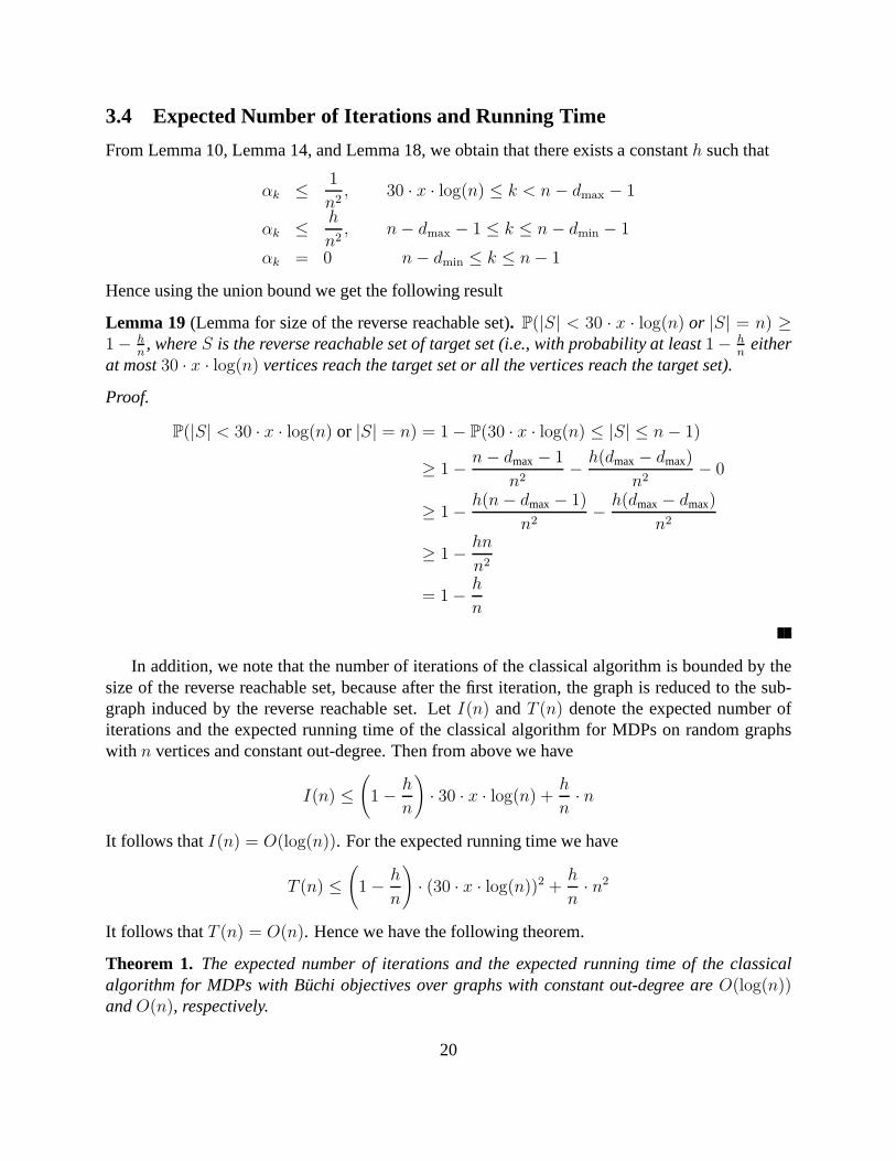
From Lemma 10, Lemma 14, and Lemma 18, we obtain that there exists a constanth such that

αk ≤ 1

n2, 30 · x · log(n) ≤ k < n − dmax − 1

αk ≤ h

n2, n − dmax − 1 ≤ k ≤ n − dmin − 1

αk = 0 n − dmin ≤ k ≤ n − 1

Hence using the union bound we get the following result

Lemma 19 (Lemma for size of the reverse reachable set). P(|S| < 30 · x · log(n) or |S| = n) ≥1 − h

n, whereS is the reverse reachable set of target set (i.e., with probability at least1 − h

neither

at most30 · x · log(n) vertices reach the target set or all the vertices reach the target set).

Proof.

P(|S| < 30 · x · log(n) or |S| = n) = 1 − P(30 · x · log(n) ≤ |S| ≤ n − 1)

≥ 1 − n − dmax − 1

n2− h(dmax − dmax)

n2− 0

≥ 1 − h(n − dmax − 1)

n2− h(dmax − dmax)

n2

≥ 1 − hn

n2

= 1 − h

n

In addition, we note that the number of iterations of the classical algorithm is bounded by thesize of the reverse reachable set, because after the first iteration, the graph is reduced to the sub-graph induced by the reverse reachable set. LetI(n) andT (n) denote the expected number ofiterations and the expected running time of the classical algorithm for MDPs on random graphswith n vertices and constant out-degree. Then from above we have

I(n) ≤(

1 − h

n

)

· 30 · x · log(n) +h

n· n

It follows thatI(n) = O(log(n)). For the expected running time we have

T (n) ≤(

1 − h

n

)

· (30 · x · log(n))2 +h

n· n2

It follows thatT (n) = O(n). Hence we have the following theorem.

Theorem 1. The expected number of iterations and the expected running time of the classicalalgorithm for MDPs with Buchi objectives over graphs with constant out-degree areO(log(n))andO(n), respectively.

20

Remark 2. For Theorem 1, we considered the model where the out-degree of each vertexv isfixed asdv and there exist constantsdmin anddmax such thatdmin ≤ dv ≤ dmax for every vertexv. We discuss the implication of Theorem 1 for related models.First, when the out-degrees ofall vertices are same and constant (sayd∗), Theorem 1 can be applied with the special case ofdmin = dmax = d∗. A second possible alternative model is when the outdegree of every vertexis a distribution over the range[dmin, dmax]. Since we proved that the average case is linear forevery possible value of the outdegreedv in [dmin, dmax] for every vertexv (i.e., for all possiblecombinations), it implies that the average case is also linear when the outdegree is a distributionover [dmin, dmax].

4 Average Case Analysis in Erdos-Renyi Model

In this section we consider the classical Erdos-Renyi model of random graphsGn,p, with n vertices,where each edge is chosen to be in the graph independently with probabilityp [17] (we considerdirected graphs and thenGn,p is also referred asDn,p in the literature). First, in Section 4.1 weconsider the case whenp is Ω

(log(n)

n

)

, and then we consider the case whenp = 12

(that generates

the uniform distribution over all graphs). We will show two results: (1) ifp ≥ c·log(n)n

, for someconstantc > 2, then the expected number of iterations is constant and the expected running timeis linear; and (2) ifp = 1

2(with p = 1

2we consider all graphs to be equally likely), then the

probability that the number of iterations is more than one falls exponentially inn (in other words,graphs where the running time is more than linear are exponentially rare).

4.1 Gn,p with p = Ω(

log(n)n

)

In this subsection we will show that givenp ≥ c·log(n)n

, for some constantc > 2, the probability thatnot all vertices can reach the given target set isO(1/n). Hence the expected number of iterations ofthe classical algorithm for MDPs with Buchi objectives is constant and hence the algorithm worksin average time linear in the size of the graph. Observe that to show the result the worst possiblecase is when the size of the target set is 1, as otherwise the chance that all vertices reach the targetset is higher. Thus from here onwards, we assume that the target set has exactly 1 vertex.

The probabilityR(n, p). For a random graph inGn,p and a given target vertex, we denote byR(n, p)the probability that each vertex in the graph has a path alongthe directed edges to the target vertex.Our goal is to obtain a lower bound onR(n, p).

The key recurrence.Consider a random graphG with n vertices, with a given target vertex, andedge probabilityp. For a setK of vertices with sizek (i.e., |K| = k), which contains the targetvertex,R(k, p) is the probability that each vertex in the setK, has a path to the target vertex, thatlies within the setK (i.e., the path only visits vertices inK). The probabilityR(k, p) depends onlyon k andp, due to the symmetry among vertices.

Consider the subsetS of all vertices inV , which have a path to the target vertex. In that case,for all verticesv in V \ S, there is no edge going fromv to a vertex inS (otherwise there wouldhave been a path fromv to the target vertex). Thus there are no incoming edges fromV \ S to S.

21

Let |S| = i. Then thei · (n − i) edges fromV \ S to S should be absent, and each edge is absentwith probability(1 − p). The probability that each vertex inS can reach the target isR(i, p). Sothe probability ofS being the reverse reachable set is given by:

(1 − p)i·(n−i) · R(i, p). (2)

There are(

n−1i−1

)

possible subsets ofi vertices that include the given target vertex, andi can rangefrom 1 to n. Exactly one subsetS of V will be the reverse reachable set. So the sum of probabilitiesof the events thatS is reverse reachable set is1. Hence we have:

1 =n∑

i=1

(

n − 1

i − 1

)

· (1 − p)i·(n−i) · R(i, p) (3)

Moving all but the last term (withi = n) to the other side, we get the following recurrence relation:

R(n, p) = 1 −n−1∑

i=1

(

n − 1

i − 1

)

· (1 − p)i·(n−i) · R(i, p). (4)

Bound onp for lower bound onR(n, p). We will prove a lower bound onp in terms ofn suchthat the probability that not alln vertices can reach the target vertex is less thanO(1/n). In otherwords, we require

R(n, p) ≥ 1 − O(

1

n

)

(5)

SinceR(i, p) is a probability value, it is at most 1. Hence from Equation 4 it follows that it sufficesto show that

n−1∑

i=1

(

n − 1

i − 1

)

· (1 − p)i·(n−i) · R(i, p) ≤n−1∑

i=1

(

n − 1

i − 1

)

· (1 − p)i·(n−i) ≤ O(

1

n

)

(6)

to show thatR(n, p) ≥ 1 − O(

1n

)

. We will prove a lower bound onp for achieving Equation 6.

Let us denote byti =(

n−1i−1

)

· (1 − p)i·(n−i), for 1 ≤ i ≤ n − 1. The following lemma establishes arelation ofti andtn−i.

Lemma 20. For 1 ≤ i ≤ n − 1, we havetn−i = n−ii

· ti.

Proof. We have

tn−i =

(

n − 1

n − i − 1

)

(1 − p)i·(n−i)

=

(

n − 1

i

)

· (1 − p)i·(n−i)

=n − i

i·(

n − 1

i − 1

)

(1 − p)i·(n−i)

=n − i

i· ti

The desired result follows.

22

Definegi = ti + tn−i, for 1 ≤ i ≤ ⌊n/2⌋. From the previous lemma we have

gi = tn−i + ti =n

i· ti =

n

i·(

n − 1

i − 1

)

· (1 − p)i·(n−i) =

(

n

i

)

· (1 − p)i·(n−i).

We now establish a bound ongi in terms oft1. In the subsequent lemma we establish a bound ont1.

Lemma 21. For sufficiently largen, if p ≥ c·log(n)n

with c > 2, thengi ≤ t1 for all 2 ≤ i ≤ ⌊n2⌋.

Proof. Let p ≥ c·log(n)n

with c > 2. Now

t1

gi=

(1 − p)n−1

(ni

)

· (1 − p)i·(n−i)≥ 1

ni · (1 − p)(i−1)·(n−i−1)(Rearranging powers of(1 − p) and

(

n

i

)

≤ ni)

≥ 1

ni · e−c·log(n)

n·(i−1)·(n−i−1)

(1 − x ≤ e−x)

= ncn

·(i−1)·(n−i−1)−i

To show thatt1 ≥ gi, it is sufficient to show that for2 ≤ i ≤ ⌊n/2⌋,

c

n· (i − 1) · (n − i − 1) − i ≥ 0 ⇔ i · n

(i − 1) · (n − i − 1)≤ c

Note thatf(i) = i·n(i−1)·(n−i−1)

is convex for2 ≤ i ≤ ⌊n/2⌋. Hence, its maximum value is attainedat either of the endpoints. We can see that

f(2) =2 · n

n − 3≤ c (for sufficiently largen andc > 2)

and

f(⌊n/2⌋) =⌊n/2⌋ · n

(⌊n/2⌋ − 1) · (⌈n/2⌉ − 1)

Note thatlimn→∞ f(⌊n/2⌋) = 2, and hence for any constantc > 2, f(⌊n/2⌋) ≤ c for sufficientlylargen. The result follows.

Lemma 22. For sufficiently largen, if p ≥ c·log(n)n

with c > 2, thent1 ≤ 1n2 .

Proof. We havet1 = (1 − p)n−1. Forp ≥ c·log(n)n

we have

t1 ≤(

1 − c·log(n)n

)n−1 ≤ e−c·log(n)·(n−1)

n ( Since1 − x ≤ e−x)

≤ e−2·log(n) = 1n2 (for sufficiently large n,c > 2)

Hence, the desired result follows.

We are now ready to establish the main lemma that proves the upper bound onR(n, p) and thenthe main result of the section.

23

Lemma 23. For sufficiently largen, for all p ≥ c·log(n)n

with c > 2, we haveR(n, p) ≥ 1 − 1.5n

.

Proof. We first show that∑n−1

i=1 ti ≤ 1.5n

. We have

n−1∑

i=1

ti = t1 + tn−1 +n−2∑

i=2

ti

≤ t1 + tn−1 +⌊n/2⌋∑

i=2

gi (t⌊n/2⌋ is repeated ifn is even)

≤ n · t1 +⌊n/2⌋∑

i=2

gi (We applyti + tn−i =n

i· ti with i = 1)

≤ n · t1 +⌊n/2⌋∑

i=2

t1 (By Lemma 21 we havegi ≤ t1 for 2 ≤ i ≤ ⌊n/2⌋)

≤ 3 · n

2· t1

≤ 3 · n

2 · n2(By Lemma 22 we havet1 ≤ 1

n2)

By Equation 6 we have thatR(n, p) ≥ 1 −∑n−1i=1 ti. It follows thatR(n, p) ≥ 1 − 1.5

n.

Theorem 2. The expected number of iterations of the classical algorithm for MDPs with Buchiobjectives for random graphsGn,p, with p ≥ c·log(n)

n, wherec > 2, is O(1), and the average case

running time is linear.

Proof. By Lemma 23 it follows thatR(n, p) ≥ 1 − 1.5n

, and if all vertices reach the target set,then the classical algorithm ends in one iteration. In the worst case the number of iterations of theclassical algorithm isn. Hence the expected number of iterations is bounded by

1 ·(

1 − 1.5

n

)

+ n · 1.5

n= O(1).

Since the expected number of iterations isO(1) and every iteration takes linear time, it follows thatthe average case running time is linear.

4.2 Average-case analysis over all graphs

In this section, we consider uniform distribution over all graphs, i.e., all possible different graphsare equally likely. This is equivalent to considering the Erdos-Renyi model such that each edge hasprobability 1

2. Using 1

2≥ 3 · log(n)/n (for n ≥ 17) and the results from Section 4.1, we already

know that the average case running time forGn,1/2 is linear. In this section we show that inGn, 12,

the probability that not all vertices reach the target is in fact exponentially small inn. It will followthat MDPs where the classical algorithm takes more than constant iterations are exponentially rare.We consider the same recurrenceR(n, p) as in the previous subsection and considertk andgk asdefined before. The following theorem shows the desired result.

24

Theorem 3. In Gn, 12

with sufficiently largen the probability that the classical algorithm takes more

than one iteration is less than(

34

)n.

Proof. We first observe that Equation 4 and Equation 6 holds for all probabilities. Next we observethat Lemma 21 holds forp ≥ c·log(n)

nwith any constantc > 2, and hence also forp = 1

2for

sufficiently largen. Hence by applying the inequalities of the proof of Lemma 23 we obtain that

n−1∑

i=1

ti ≤ 3 · n

2· t1.

Forp = 12

we havet1 =(

n−10

)

·(

1 − 12

)n−1= 1

2n−1 . Hence we have

R(n, p) ≥ 1 − 3 · n

2 · 2n−1> 1 − 1.5n

2n= 1 −

(3

4

)n

.

The second inequality holds for sufficiently largen. It follows that the probability that the classicalalgorithm takes more than one iteration is less than(3

4)n. The desired result follows.

References

References

[1] C. Baier and J-P. Katoen.Principles of Model Checking. MIT Press, 2008.

[2] A. Bianco and L. de Alfaro. Model checking of probabilistic and nondeterministic systems.In FSTTCS, volume 1026 ofLNCS, pages 499–513, Springer, 1995.

[3] K. Chatterjee.Stochasticω-Regular Games. PhD thesis, UC Berkeley, 2007.

[4] K. Chatterjee. The complexity of stochastic Muller games. Inf. Comput., 211:29–48, 2012.

[5] K. Chatterjee, L. de Alfaro, M. Faella, R. Majumdar, and V. Raman. Code-aware resourcemanagement.Formal Methods in System Design, 42(2):146–174, 2013.

[6] K. Chatterjee, L. de Alfaro, and T. A. Henzinger. The complexity of stochastic Rabin andStreett games. InICALP, volume 3580 ofLNCS, pages 878–890, Springer, 2005.

[7] K. Chatterjee and M. Henzinger. Faster and dynamic algorithms for maximal end-componentdecomposition and related graph problems in probabilisticverification. In SODA, pages1318–1336, ACM-SIAM, 2011.

[8] K. Chatterjee and M. Henzinger. An O(n2) algorithm for alternating Buchi games. InSODA,pages 1386–1399, ACM-SIAM, 2012.

[9] K. Chatterjee and M. Henzinger. Efficient and dynamic algorithms for alternating Buchigames and maximal end-component decomposition. InJACM, 61(3), 2014.

25

[10] K. Chatterjee, M. Henzinger, M. Joglekar, and N. Shah. Symbolic algorithms for qualitativeanalysis of Markov decision processes with Buchi objectives. Formal Methods in SystemDesign, 42(3):301–327, 2013.

[11] K. Chatterjee, M. Jurdzinski, and T.A. Henzinger. Simple stochastic parity games. InCSL,volume 2803 ofLNCS, pages 100–113, Springer, 2003.

[12] K. Chatterjee, M. Jurdzinski, and T.A. Henzinger. Quantitative stochastic parity games. InSODA, pages 121–130, SIAM, 2004.

[13] K. Chatterjee and J. Lacki. Faster algorithms for Markov decision processes with lowtreewidth. InCAV, volume 8044 ofLNCS, pages 543–558, Springer, 2013.

[14] C. Courcoubetis and M. Yannakakis. The complexity of probabilistic verification.Journal ofthe ACM, 42(4):857–907, 1995.

[15] L. de Alfaro. Formal Verification of Probabilistic Systems. PhD thesis, Stanford University,1997.

[16] L. de Alfaro and P. Roy. Magnifying-lens abstraction for Markov decision processes. InCAV,volume 4590 ofLNCS, pages 325–338, Springer, 2007.

[17] P. Erdos and A. Renyi. On the evolution of random graphs. Math. Inst. of the HungarianAcad. of Sciences, pages 17–61, 1960.

[18] J. Filar and K. Vrieze.Competitive Markov Decision Processes. Springer-Verlag, 1997.

[19] H. Howard.Dynamic Programming and Markov Processes. MIT Press, 1960.

[20] M. Kwiatkowska, G. Norman, and D. Parker. Verifying randomized distributed algorithmswith PRISM. InWorkshop on Advances in Verification (WAVe), 2000.

[21] A. Pogosyants, R. Segala, and N. Lynch. Verification of the randomized consensus algorithmof Aspnes and Herlihy: a case study.Distributed Computing, 13(3):155–186, 2000.

[22] M. L. Puterman.Markov Decision Processes. J. Wiley and Sons, 1994.

[23] R. Segala.Modeling and Verification of Randomized Distributed Real-Time Systems. PhDthesis, MIT, 1995. Technical Report MIT/LCS/TR-676.

[24] M.I.A. Stoelinga. Fun with FireWire: Experiments withverifying the IEEE1394 root con-tention protocol. InFormal Aspects of Computing, 14(3):328–337, 2002.

[25] W. Thomas. Languages, automata, and logic. In G. Rozenberg and A. Salomaa, edi-tors,Handbook of Formal Languages, volume 3, Beyond Words, chapter 7, pages 389–455.Springer, 1997.

[26] M. Kwiatkowska, G. Norman, and D. Parker, PRISM: Probabilistic Symbolic ModelChecker. In TOOLS, volume 2324 ofLNCS, pages 200–204, Springer, 2002.

26

A Technical Appendix

Proposition 1 (Useful inequalities from Stirling inequalities). For natural numbersℓ and j withj ≤ ℓ we have the following inequalities:

1.(

ℓj

)

≤(

e·ℓj

)j

.

2.(

ℓj

)

≤ (ℓ + 1) ·(

ℓj

)j ·(

ℓℓ−j

)ℓ−j.

Proof. The proof of the results is based on the following Stirling inequality for factorial:

e ·(

j

e

)j

≤ j! ≤ e ·(

j + 1

e

)j+1

.

We now use the inequality to show the desired inequalities:

1. We have(

ℓj

)

≤ ℓj

j!≤ ℓj · ej

e · jj(using Stirling inequality)

≤ 1

e·(

e · ℓ

j

)j

≤(

e · ℓ

j

)j

2. We have(

ℓj

)

=ℓ!

j! · (n − j)!

≤

e ·(

ℓ + 1

e

)ℓ+1

·

1

e ·(

je

)j · e ·(

ℓ−je

)ℓ−j

=1

e2· (ℓ + 1) ·

(

ℓ + 1

j

)j

·(

ℓ + 1

ℓ − j

)ℓ−j

≤ 1

e2· (ℓ + 1) ·

(

ℓ + 1

ℓ

)ℓ (ℓ

j

)j

·(

ℓ

ℓ − j

)ℓ−j

≤ 1

e2· (ℓ + 1) · e ·

(

ℓ

j

)j

·(

ℓ

ℓ − j

)ℓ−j (

Since(

1 +1

ℓ

)ℓ

≤ e

)

≤ (ℓ + 1) ·(

ℓ

j

)j

·(

ℓ

ℓ − j

)ℓ−j

The first inequality is obtained by applying the Stirling inequality to the numerator (in thefirst term), and applying the Stirling inequality twice to the denominator (in the second term).

27