2 IEEE TRANSACTIONS ON AUTOMATIC CONTROL, VOL. 40, NO. I , JANUARY 1995

Percentile Performance Criteria For Limiting Markov Decision Average Processes

Jerzy A. Filar, Dmitry Krass, and Keith W. Ross, Senior Member, IEEE

Abstract- In this paper we address the following basic fea- sibility problem for infinite-horizon Markov decision processes (MDP’s): can a policy be found that achieves a specified value (target) of the long-run limiting average reward at a specified probability level (percentile)? Related optimization problems of maximizing the target for a specified percentile and vice versa are also considered. We present a complete (and discrete) clas- sification of both the maximal achievable target levels and of their corresponding percentiles. We also provide an algorithm for computing a deterministic policy corresponding to any feasible target-percentile pair.

Next we consider similar problems for an MDP with multiple rewards and/or constraints. This case presents some difficulties and leads to several open problems. An LP-based formulation provides constructive solutions for most cases.

I. INTRODUCTION AND DEFINITIONS

NFINITE horizon Markov decision processes (MDP’s, for I short) have been extensively studied since the 1950’s. One of the most commonly considered versions is the so-called “limiting average reward” model. In this model the decision- maker aims to maximize the expected value of the limit- average (“long-run average”) of an infinite stream of single- stage rewards. There are now a number of good algorithms for computing optimal deterministic policies in the limiting average MDP’s (e.g., see [41, [6], [ill).

It should be noted, however, that an optimal policy in the above “classical” sense is insensitive to the probability distribution function of the long-run average reward. That is, it is possible that an optimal policy, while yielding an acceptably high expected long-run average reward, carries with it unacceptably high probability of low values of that same random variable. This “risk insensitivity” is inherent in the formulation of the classical objective criterion as that of maximizing the expected value of a random variable, and it is not necessarily undesirable. Nonetheless, in this paper we adopt the point of view that there are many natural situations where the decision-maker is interested in finding a policy that will achieve a sufficiently high long-run average reward, that is, a target level with a sufficiently high probability, that is, a percentile. The key conceptual difference between this paper

Manuscript received January 22, 1992; revised April 12, 1993. This work was supported in part by the AFOSR and the NSF Grants ECS-8704954 and NCR-8707620.

J. A. Filar is with the Department of Mathematics and Statistics, University of Maryland Baltimore County, Baltimore, MD 21228 USA.

D. Krass is with the Faculty of Management, University of Toronto, Toronto, Ontario, M5SlV4.

K. W. Ross is with the Department of Systems, University of Pennsylvania, Philadelphia, PA 19104 USA.

IEEE Log Number 9406094.

and the classical problem is that our controller is not searching for an optimal policy but rather for a policy that is “good enough,” knowing that such a policy will typically fail to exist if the target level and the percentile are set too high. Conceptually, our approach is somewhat analogous to that often adopted by statisticians in testing of hypotheses where it is desirable (but usually not possible!) to simultaneously minimize both the “type 1” and the “type 2” errors. See Bouakiz [5] for a review of similar approaches in economics and operations research literature and White [ 161 for a review of various approaches to risk-sensitivity in MDP’s.

We start out by considering a problem with a single objec- tive. It will be seen (Section IV below) that for our target level- percentile problem it is possible to present a complete (and discrete) classification of both the maximal achievable target levels and of their corresponding percentiles (see Theorem 4.3 and its corollaries). The case of a communicating MDP is particularly interesting as here every target level can be achieved with only two possible values: zero or one (see Theorem 4.1 and its corollary). In all cases our approach is constructive in the sense that we can supply an algorithm for computing a deterministic policy for any feasible target level and percentile pair.

In Section V we turn our attention to problems with multiple objectives and/or constraints. The connection of this to the problem with sample path constraint of [13] and [14] is dis- cussed. In Section VI, we show how the techniques developed in Section IV extend directly to these problems, provided that the problems can be solved for a communicating MDP (see Theorem 6.3). The multiobjective/constrained problems are considered in detail for communicating MDP’s, with construc- tive solutions obtained for most cases (see Theorems 6.1 and 6.2). Conclusions and some open problems are presented in Section VII.

Our analysis is made possible by the recently developed de- composition and sample path theory due to Ross and Varadara- jan [14]. The logical development of the results is along the lines of Filar [SI. The latter paper, to the best of our knowledge, introduced the percentile objective criterion in the context of a limiting average Markov control problem, but substituted the long-run expected frequencies in place of actual percentile probabilities since the decomposition and sample path theory of [14] was not known at that time (the unusual way of evaluating risk in [8] was also pointed out in [16]). Some earlier related work appeared in Mitten [12], Sobel [15], and Henig [lo]. In the remainder of this section we shall introduce the notation of the limiting average Markov decision process.

0018-9286/95$04.00 0 1995 IEEE

m P

Archived at Flinders University: dspace.flinders.edu.au

P,,(R 2 7 I X1 = S I ) 2 a? (2.1)

If (2.1) holds for some policy U , then we shall say that U

achieves the target level 7 at percentile a, and r will be called a-achievable.

Problem 2: Given a E [0, I] find

re: = sup {r I r is N - achievable}. (2.2)

FILAR er al: LIMITING AVERAGE MARKOV DECISION PROCESSES

A finite MDP, I?, is observed at discrete-time points n = 1, 2, .. . . The state space is denoted by S = (1, 2, ... , IS/}. With each state i E S we associate a finite action set A( i ) . At any time point n, the system is in one of the states, and an action has to be chosen by the decision-maker. If the system is in state i and the action a E A( i ) is chosen, then an immediate reward ~ ( i , a ) is earned and the process moves to a state j E S with transition probability p i a j , where pi,j 2 0 and

A decision rule U , at time n is a function which assigns a probability to the event that action a is taken at time n. In general U , may depend on all realized states up to and including time n. A policy (or a control) U is a sequence of decision rules: U = (ul, U’, . . . ,U,, ...). A policy is stationary if each U , depends only on the current state at

. A pure (or deterministic) policy is a stationary policy with nonrandomized decision rules. A stationary policy f induces a Markov chain

CjEs P i a j = 1.

time n, and u1 = u2 = ... = U” = ...

P ( f ) with the transitions > ( f j t J = CaEA(i p i a j f i a for i, j E S, where f i a is the probability (under )) that action a is chosen whenever state i is visited. If P ( f ) consists of a single recurrent class of states, then f is called an irreducible policy. If P ( f ) contains some transient states in addition to a single recurrent class, then f is called a unichain policy. MDP F is called unichain if every stationary policy in r is unichain.

Let X , and A , be the random variables that denote the state at time n and the action chosen at time n, and define the limiting average reward as the random variable

n=l

It should now be clear that once a policy U and an initial state X 1 = s1 are fixed, the expectation 4(u, SI): = E,[R I X 1 = SI] of R is well defined and will, from now on, be referred to as the expected average reward due to a policy U .

The classical limiting average reward problem is to find an optimal policy U* such that for all policies U

4(u*, SI) 2 4(u, s1) for all s1 E S. (1.1)

It is well known (e.g., see [4]) that there always exists a pure optimal policy U*.

11. PROBLEMS RELATING TO PERCENTILE OBJECTIVE CRITERIA

We shall say that any pair (7, a ) such that 7 E R and a E [0, 11 constitutes a target level-pqcentile pair. We shall address the following problems.

Problem 1: Fix s1 E S. Given (7, a ) E R x [0, 11 does there exist a policy U such that

3

Problem3: Given r E R find

aT: = sup { a E [0, 11 I 3 a policy U s.t. (2.1) holds}. (2.3)

Remark 2.1: It should be clear that in many situations the natural goal of maximizing the target level will be in direct conflict with the goal of maximizing the’percentile value. This is because r, is a nonincreasing function of a, while a, is a nonincreasing function of r.

111. PRELIMINARIES

We shall develop our results within the framework of the decomposition and sample path theory due to Ross and Varadarajan [14] (for a related decomposition, see [2]). This decomposition approach has also proved instrumental in solv- ing other limiting average MDP problems with nonstandard criteria (see [14] and [3]). In this section we collect some results from [14] that will be needed for the proofs in the subsequent sections.

In 1141 it is shown that the state space S has a unique par- tition C1, C,, . . . , C K , T , whose properties are summarized below.

Theorem 3.1 (Proposition 2 of [14]): For any policy U , we have

K

k = l

where

@ k : = { X , E c k almost always)

(where “almost always” means that X , q! c k finitely often). The sets CI, . . . , CK and T are referred to as strongly com-

municating classes and the set of transient states, respectively. For a given strongly communicating class c k , denote by q k ) the MDP restricted to c k . Thus, the state space of r ( k ) is c k

and the action space & ( i ) , i E c k , is given by

A k ( i ) = { U E A(2): Piaj = 0 v’j q! c k } .

From [14] we know that A k ( i ) is nonempty for all E c k and that r ( k ) is a communicating MDP. Recall that a communicating MDP is such that for any pair of states ‘L, j E S, there is a pure policy under which j is accessible from i . Now consider the following linear program L P ( k )

k t ‘uk denote the optimal objective function value of LP(k ) . We can now state the following result.

Archived at Flinders University: dspace.flinders.edu.au

4 IEEE TRANSACTIONS ON AUTOMATIC CONTROL, VOL. 40, NO. I , JANUARY 1995

Theorem 3.2 (Lemma 4 [14]): For all policies U , all initial states s1 E S , and all k = 1,. . . , K , we have

Pu(R 5 ‘Uk I @ k , x1 = 31) = 1

whenever P u ( @ k , XI = SI) > 0.

Iv. BASIC RESULTS FOR THE SINGLE REWARD CASE

We shall first solve Problems 1-3 for the case of r being a communicating MDP. In this case, there is one strongly communicating class C1, and T is empty; thus, S = C 1 .

Consider then LP( 1) and to simplify notation denote v: = VI. Also let {x,’,} be an optimal basic feasible solution of LP( 1) and g* be a stationary optimal policy constructed from {x&} (e.g., see [l l] , [9], or [13]). Then g* satisfies

4(g* , s1) = v, s1 E s (4.1)

where v is the maximal objective function value in LP(1). Moreover, the Markov chain P(g*) associated with the policy g* has at most one recurrent class plus (a perhaps empty) set of transient states.

Theorem 4.1: In a communicating MDP r there exists a policy that achieves the target level T with percentile Q if and only if r 5 v. If T 5 v, then the pure policy g* achieves the target level T with percentile a, for any Q E [0, 11

Note: This result (at least for the unichain case) seems to be well known in the “folklore” of MDP’s. A proof for the communicating case can be found in Asriev and Rotar’ [ l] (who establish this result for a much more general stochastic dynamic control model). Since our proof is quite simple, we present it here for completeness.

Proofi Since g* gives rise to a Markov chain with one recurrent class, we have

Pg* ( R = (b(g*, SI) 1 x1 = SI) = 1

(e.g., see 113, Proposition 1 (iii)]). Combining this with (4.1) gives

Pg*(R = v 1 XI = SI) = 1. (4.2)

From Theorem 3.2, we have

P,(R I v I x1 = s1) = 1. (4.3)

The result then follows from (4.2) and (4.3).

following corollary.

a E(0, 11, moreover

As a direct consequence of Theorem 4.1 we have the

Corollary 4.1: In a communicating MDP r, T~ = v for all

1 i f . r I v 0 if r > v. a, = {

Problems 1-3 have now been solved for the communicating MDP’s. We retum to the general case, where we have strongly communicating classes C1, . . . , CK and the set T of transient states. Denote by g; the pure policy of Theorem 4.1 associated with q k ) , the MDP restricted to c k .

Corollary 4.2: For a fixed k E { 1, . . . , K}, let g be a pure policy that coincides with g; on c k and is defined arbitrarily elsewhere. Then

if P g ( @ k , X1 = SI) > -0. Proof.’ Note that, the definition of @ k implies that c k

must be reached in finite time (Pg - as.). Thus, the result follows easily from the proof of Theorem 4.1.

Next, we shall consider a fixed target level T and associate with it an index set I , = {k: 1 5 k 5 K , V k 2 T } , and an auxiliary “0-1 MDP’ I?,, whose states, actions, and transition probabilities are the saMe as I?, but with rewards defined by

1 T T ( i , a) : = 0 6thenvise.

if i E c k and k E I ,

It is easy to see that for an arbitrary policy U, the expected average reward in r, is given by

(4.4)

where 1(.) is the indicator function. Note that the last equality above follows from Theorem 3.1 and the definition of @ k ,

since P,-a.s. after some finite time t we must have X, E c k

for all n 2 t and some k E { l , . . . , K } . Theorem 4.2: Let g* be an optimal pure policy in r, which

coincides with g; on c k for k E I,‘ There exists a policy U

satisfying

Pu(R 2 7 1 xi = Si) 2 Q (4.5)

where Q is the percentile, if and only if 4T(g* , S I ) 2 a. Further, if the target T can be achieved at percentile a, then it can be achieved by the pure policy g*.

Proof: From Theorem 3.1 we have that for any policy U

K

Pu(R 2 T 1 x1 S I ) = c P , ( R 2 T I @ k , x1 = 31) k = l

P,(@k I X i = si ) . (4.6)

From Theorem 3.2 we have

From Corollary 4.2

I I I T

I Note that there is no loss of generality here, because g; ensures that once the process enters Ch it remains there forever. Thus it yields the maximal reward of one for every state i E Ck, 1. E I,.

Archived at Flinders University: dspace.flinders.edu.au

FILAR et 01: LIMITING AVERAGE MARKOV DECISION PROCESSES 5

where the inequality follows from the optimality of g; for r(k). Combining (4.6)-(4.8) gives

P,(R 2 7 I x1 = SI ) 5 Pg*(R 2 7 1 x1 = SI)

= C P g * ( @ k I x1 = 31) k € I T

= 4T(9*, s1)

from which the result follows. It is important to note that Theorem 4.2 provides a con-

structive answer to Problem 1 of Section I1 concerning a- achievability of the target level T . We shall now address the problem of determining .r,-the maximal achievable per- centile for the fixed level r. Towards this goal we assume without loss of generality that the strongly communicating classes C1, . . . , CK are ordered so that

U1 2 U 2 2 ” ‘ 2 OK. (4.9)

Recall the definition of the MDT rUk (here Vk is the target level). To simplify the notation, we will refer to I’Uk as rk and to the corresponding expected average reward as 4k instead

Theorem 4.3: Let g; be an optimal pure policy for MDP

r, = r*: = max {vk I @(Si, SI) 2 a,

of p.

r k chosen as in Theorem 4.2. We have for a ~ ( 0 , 11 that

k = 1 , . . . , K}. (4.10)

Proofi Let 1 be the largest index that achieves the maxi- mum in (4.10), 1 is well defined since $ K ( g ; ( , SI) = 1. Since r* = vl, we have 1,. = (1, 2 , . . . , I } . Thus, from Theorem 4.2, we know that

Pg;(R 2 T* x1 = SI) 2 a. (4.1 1)

Hence, r* is a-achievable, implying that T, 2 T*. If strict inequality were possible in the preceding statement, then there would exist a r’ > r* and a policy U such that

P,(R 2 7’ I x1 = SI) 2 a. (4.12)

Now let

m: = max { k : v k 2 T ’ }

noting that if 01, < T’ for all k = 1, . . . , K , then the left side of (4.12) equals zero contradicting the hypothesis a > 0. By the definition of m we have

U , 2 7’ > r*

Applying Theorem 3.1, Theorem 4.1 (4.12) yields

K

a 5 C P , ( R 2 7’ I @k, Xi = s1 k = l m

= C P , ( R 2 7‘ I cpk , x1 = s1

5 C P U ( @ k I x1 = s1)

k = l m

k = l

= 4 m ( U , s1) I $,(&, 31).

(4.13)

and optimality gk to

(4.14)

But, by the definition of T * , (4.14) implies r* >_ vm, which contradicts (4.13).

Corollary 4.3: The maximal a-achievable target level, T,,

is a monotone nonincreasing step-function of a, defined on the interval (0, 11.

Proof: Choose g; as in Theorem 4.3. Let ak:= qhk(g;, SI) for k = l , . . . , K , so that 0 5 a1 5 a2 5 ... 5 CXK = 1. If we define TO: = VI, then by Theorem 4.3, r, = TO

for all a ~ ( 0 , all. Similarly, r, = Tk, a constant for all a €(arc, a k + 1 ] , where Tk 2 T ~ + I for each k = 1 , . . . , K - 1.

Corollary4.4: Choose g; as in Theorem 4.3. The maxi- mum percentile aT for a given target level r , is a mono- tone nonincreasing step function of r defined in the interval [VK, VI]. In particular for T ~ ( v k + l , vk] we have

for each k = l , . - . , K - 1. Proof: This follows easily from the monotonicity of

@(g;, SI) in the index k . Remark 4.1: Corollaries 4.3 and 4.4 demonstrate the

strength of the percentile objective criteria. Namely, the decomposition of states into Cl , . . . , CK and T, and the subsequent computation of policies g; together with “breakpoints” ~ k , and v k for T, and aT, respectively, allows for a flexible and practical evaluation of gain-risk trade-offs in an average reward MDP.

In view of Corollaries 4.3 and 4.4 the only “reasonable” choices of a and r are of the special form (7, a) with T = T~

and a = a,; these correspond to Pareto-optimal solutions. The preceding results are summarized in the following

algorithm, which (for a fixed initial state SI) finds all target- level-percentile pairs of the indicated “special form”

Step I : Apply the algorithm of [14] to find the decompo- sition C~,,..,CK, T.

Step2: Foreachk E { l , . . . , K } ,findthevaluevk o f r (k ) . Order the strongly communicating classes so that

Step 3: For each k E { 1, . . . , K}, form the MDP r,+ and find the optimal policy 9;. Let = 4k(g;, SI).

Srep4: Let J = {(wk, a k ) I k = l , . . . ,K} . If (rl, a ) , ( T ~ , a) E J and T~ > 7-2, then elimi- nate (72, a ) from J. Continue until no further eliminations are possible.

Step.5: We have constructed the set J = ((7, a ) =

Note that Step 2 is not hard computationally, since very efficient algorithms are known for communicating MDP’s. In Step 3 one should use the aggregated MDP method of [ 141, where each strongly communicating class is replaced by one state. In addition to computational efficiency, this method will automatically yield a deterministic optimal policy satisfying the conditions of Theorem 4.2. Also, since when k is incremented by one, only one immediate reward changes in the aggregated problem (the rest of the data stay the same), perhaps a parametric solution method can be used (e.g. by using LP algorithms for solving the aggregated problem). Further computational efficiency can be gained by quitting

U1 >_ . . . 2 O K .

(T,, a,) I 7 E R, a E (0, 111.

7 I l l

Archived at Flinders University: dspace.flinders.edu.au

6 IEEE TRANSACTIONS ON AUTOMATIC CONTROL, VOL. 40, NO. 1, JANUARY 1995

Step 3 as soon as a k = 1 for some k (since all subsequent CYk’s are automatically equal to one). Note also that steps 1 and 2 need not be repeated for different starting states. Finally, we note that before starting the algorithm, one should check whether MDP r‘ is communicating (easily verifiable conditions can be found in [9]). If so, the complete characterization is immediately available from Corollary 4.1.

V. PROBLEMS WITH MULTIPLE REWARDS AND CONSTRAINTS-FORMULATIONS

A natural extension of the percentile objective criteria is to the case where each action carries multiple immediate rewards, i.e., each immediate reward is actually a vector of some fixed length L

r( i , a ) E RL for i E S , a E A ( i ) .

The definition of the limiting average reward in Section I leads to a vector R of random variables.

At this point two approaches can be taken. Under the first approach, a separate target level-percentile pair would be specified for each of the L components of R = (RI , . . . , RL). This leads to the following multi-objective version of Problem 1 (of Section 11).

ProbZem4: Fix s1 E S. Given a pair of vectors (r, a) E RL x [0, 1IL, does there exist a policy U such that

P,(R1 2 71 1 X1 = SI) 2 (YL for 1 = 1,. . . , L?

This problem appears to present serious difficulties and is presently unsolved. Below we present an example showing that stationary policies do not suffice for this case, thus indicating that it is unlikely that a simple extension of the results and methods developed in Section IV will work in this case.

Example 5.1: Consider the following MDP with L = 2

Thus action 1 is absorbing in both states, and action 2 in state 1 results in immediate rewards of (0, 0) and transition to state 2 with probability one.

Suppose the initial state is one and that the target level- percentile pairs are (;, ;) for each component of the reward vector. Note that for any stationary policy f

and

Therefore, no stationary policy suffices. Let g be the deterministic policy that takes action 1 in each

state, and let u1 be the decision rule that takes actions 1 and 2 with probabilities 1/2 each in state 1. Define the nonstationary

policy U to be U = (ul, g) (i.e., U uses the decision rule u1 at time 1 and follows g thereafter). It is easy to see that

and thus U achieves both the specified target-levels at the corresponding percentiles. In fact the same conclusions apply for any 71, 72 E (0, 1).

Under the second approach to a problem with multiple rewards, a separate target level is specified for each compo- nent of R, and all target levels are required to be achieved simultaneously at a single percentile level (I.

Problem5: Fix SI E S. Given a vector r E RL and (I E [0, 11, does there exist a policy U such that

Intuitively, the difference between the two approaches is that in Problem 4, the requirements are placed on the marginal distributions of the components of R, while in Problem 5 the requirement is placed on the joint distribution of R. Henceforth, we will refer to these two approaches as the “marginal-probability” and the “joint-probability” formula- tions, respectively. While the marginal-probability formulation provides for more modeling flexibility, the advantage of the joint-probability formulation is that it leads to more tractable problems: most of the results obtained for Problem 1 will be extended to Problem 5.

We note that an extension to multiple rewards is especially important, since some of the components of r(i, a ) can be re- garded as negatives of the costs. In this case, the corresponding components of R and r can be regarded as constraints which must be satisfied at the specified percentile level (either singly in Problem 4 or jointly in Problem 5). This can be seen as a generalization of the “sample path constraint” of Ross and Varadarajan [13] and [I41 (which in our notation corresponds to (Y = 1 and L = 1).

VI. BASIC RESULTS FOR THE MULTIPLE REWARDS CASE

In this section we consider Problem 5 for the case of com- municating MDP’s. We employ the linear-programming-based techniques developed in [6], [ 1 I], and [ 131 and introduced in Section I11 above. It should be noted that the problem considered in this section is related to the problem of finding optimal policies in average-reward communicating MDP’s with state-action frequency constraints. It is well known (see e.g., [7, example 9.31) that stationary policies may not be optimal in this case. For a problem with one inequality constraint, [13] shows that an €-optimal stationary policy can always be found (the policy is generally not deterministic). This result is related to Theorem 6.2.

In the sequel, all vector inequalities and equalities are defined componentwise, that is R 2 r means R1 2 71,

1 = l , . . . , L .

Archived at Flinders University: dspace.flinders.edu.au

FILAR et al: LIMITING AVERAGE MARKOV DECISION PROCESSES 7

We first state some preliminary definitions and results. Consider the following polyhedral set

(this is simply the feasible region of LP(k) of Section 111). For z = (xia) E A, define a stationary policy

if i E S,

a E A ( i )

a E A(i ) xia > 0,

f ( z ) i a =

if i E S, CaEA(i) xia = 0. (6.2)

Define the following random variable (whenever it exists), representing long-term average state-action frequencies

1 3 ' Zi, = lim - x l [ X t = i , At = a]. (6.3)

T+oo T t=l

We will need the following well-known results, the proofs

Lemma 6.1: Let I' be an arbitrary MDP. of which can be found in [ 1 11 and [ 131.

i) If f is a stationary policy then Pf-almost surely, 2 is well-defined, Z E A, and

ii) If f is a stationary policy and f is unichain, then

where r(f) is the unique stationary probability vector of P(f).

iii) If z E A and f(z) is unichain, then

iv) If I? is a communicating MDP and z E A, z > 0, then f(z) is an irreducible stationary policy.

Let r be a given target vector and Q a given percentile level. We now define the following linear program LP

max b Subiect to

Note that the feasible region of LP is contained in A x R. Theorem 6.1 : Let r be a communicating MDP. i) If LP is infeasible, then for any policy U

ii) Suppose LP is feasible. Let (z*, b*) be an optimal solution and f* = f(z*). If b* > 0, or f* is unichain, then

Proof: i) The proof is analogous to the proof of Proposition 2 in

ii) If b* > 0 then f* is irreducible by Lemma 6 . 1 4 ~ ) and thus, by Lemma 6.1-iii), z* = 2 P p - a s . It now follows by Lemma 6.1-i) and the feasibility of z* that

~ 4 1 .

This result is a counterpart of Theorem 4.1 for the single- objective case. When conditions in part it) of Theorem 6.1 hold, it provides a solution to Problem 5 for any a E [0, 11, and if the condition in part i) holds then Problem 5 has no solutions for any a. Unlike Theorem 4.1, however, the current result does not provide a complete characterization of solutions. If the optimal value b* of LP is equal to zero and f(z*) is not unichain, then it is not currently known whether Problem 5 has any solutions or any solutions in stationary policies. The following example shows that it is possible to have a situation where no feasible stationary policies exist when b* = 0.

Example 6.1: Consider the following MDP I' with L = 2

where s1 = 1, r = (1/2, 1/2) and Q > 0. Then LP is feasible with b* = 0 and

Thus f(z*) is not unichain, and in fact it is easy to see that for any stationary policy f, Pf(R 2 r ) = 0. It is not known whether there exists some nonstationary policy U such that P,(R 2 r) > 0.

It might be reasonable to suppose that when b* = 0, the presence of feasible stationary policies might be detected by checking whether f(z*) is unichain for any optimal basic feasible solution x* of LP (this would cover Example 6.1 where there is only one optimal basic feasible solution). The following example, however, shows that it is possible that b* = 0, f(z*) is not unichain for any optimal basic feasible solution, and yet, feasible stationary policies exist for any Q > 0.

Example 6.2: Consider the following MDP I? with L = 3

and let s1 = 1. Take some a > 0 and r = (1/4,1/4, 1/4). It is not hard to verify that the resulting LP has the optimal value b* = 0 with only two optimal basic feasible solutions

2' = (zll, 2 1 2 , 2 1 3 , 2 2 1 , 5 2 2 , 5 3 1 , 5 3 2 ) T

= (1/4, 1/4, 0, 1/4, 0, 1/4, O ) T

m

Archived at Flinders University: dspace.flinders.edu.au

8 IEEE TRANSACTIONS ON AUTOMATIC CONTROL, VOL. 40, NO. 1 . JANUARY 1995

and

z2 = (1/4, 0, 0, 0, 1/4, 1/4, 1/4)T.

Neither f(zl) nor f(z2) is unichain and, in fact, the proba- bility of achieving T is zero for both of these policies. If we take the feasible point

1 2 2

z* = -zl + Az2 = (1/4, 1/8, 0, 1/8, 1/8, 1/4, 1/8)T

then f ( z*) is unichain and Pf(z*)(R 2 T 1 X 1 = S I ) = 1 We will call a target vector r for which LP is feasible and

has optimal value b* = 0 an indeterminate target vector. We note that this case does not arise in the case of unichain

MDP’s (since one of the two conditions of Theorem 6.1 must be met), and we have the following corollary.

Corollary 6.1: Suppose r is a unichain MDP. Then either LP is infeasible, in which case Problem 5 has no solutions for any a > 0, or LP is feasible with an optimal solution (b*, z*), in which case for f = f ( z*) , P f ( R 2 T I XI = SI) = 1.

In the remainder of this section we show that the difficulties associated with indeterminate target vectors can always be avoided by a slight relaxation of the target vector and that indeterminate target vectors are sufficiently “rare” in the set of all possible target vectors. We will need the following result.

Lemma6.2: Suppose I? is a communicating MDP. Take z E A. Then for any t > 0 and SI E S, there exists an irreducible stationary policy f such that

(where 1 1 . I( is an arbitrary vector norm). > 0, then f = f ( z ) is irreducible by Lemma

6.1-iv), and it follows by Lemma 6.1-iii) that 2 = z Pj-a.s. Now suppose that xia = 0 for some i E S , a E A(i).

Let g be a completely randomized (stationary) policy (i.e., gia = for any i E S, a E A(i)). Since I‘ is a communicating MDP, g must be irreducible. By Lemma 6.1- ii), 2 = z(g) P,-almost surely, where z(g)ia = r ( g ) i g i , for i E S , a E A(i ) . By Lemma 6.1-i), z(g) > 0 and z(g) E A. Let

Proof: If

z(X) = X z + (1 - X)z(g) for X E (0, I).

Clearly, z ( X ) E A and %(A) > 0 for any X < 1. It follows by continuity of z (X) with respect to X that we can choose A* E (0, 1) so that

an irreducible stationary policy f such that

Pf ( R 2 T - Eb 1 x 1 = S I ) = 1.

Proofi Let (b*, z*) be an optimal solution of LP with target vector T. By assumption, b* = 0. By Lemma 6.2, for any y > 0, there exists an irreducible stationary policy f such that ((z’ - z*I( I y, where z’ = 2 is a constant Pf-almost surely. Choose y small enough so that

xi , r ( i , a ) 2 T - tS Pj - as . (6.5) i ES a€ A ( i )

(this can always be done since the left-hand side of (6.5) is a continuous function of z’ and CaEA(i) x b r ( i , a ) 2 S.

Since f is irreducible, by Lemma 6.1-ii), Pf-almost surely z’ > 0, i.e., z’ 2 b’ > 0 for some b’ E R. It follows from (6.5) that (b’, z’) is feasible in LP with the target vector T - €15 and consequently, the optimal value for this LP is positive. The result now follows from Theorem 6.1 -ii).

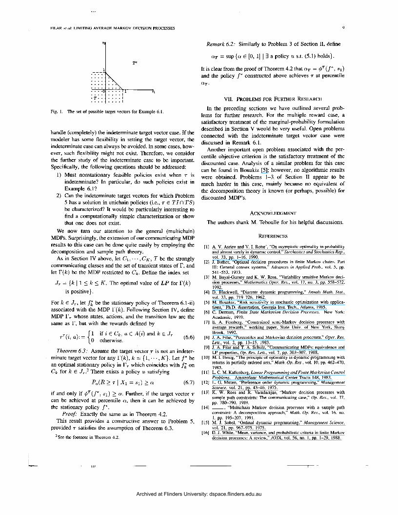
Thus, any strict relaxation of an indeterminate target vector produces a target vector for which Problem 5 can be solved by an irreducible policy for any percentile level a. Geometrically, the situation is as follows: let T = {T I LP is feasible]. T must be a closed set. Let

TS = {T I Problem 5 has a solution in unichain policies for any percentile o E [O, 111, . TF = {T I LP has optimal value b* > O}, . TI = {T 1 T is an indeterminate target vector}.

Then TSUTI = T, TF c TS, and TI c boundary{T}. Note also that the intersection of TS and T I need not be empty, as shown by Example 6.2. We illustrate the relationships between these sets in the context of Example 6.1, where

(represented by the shaded region on Fig. 1)

(the boundary of T), and

TF = T \ T I .

Let f = f(z(X*)). By Lemma 6.1-iv), f must be irreducible. It follows by Lemma 6.1-iii) that 2 = z(X*) Pf-as. The result now follows immediately from (6.4).

We are now ready to prove the following result. Theorem 6.2: Suppose r is a communicating MDP and T

is an indeterminate target vector. Let S be an arbitrary vector with positive components and choose E > 0. Then there exists

Remark 6.1: In summary, our results for the communicat- ing case with multiple rewards closely parallel the correspond- ing results for the single reward: for “most” target vectors, either Problem 5 has no solution or else it is solvable by irreducible policies for any percentile level. The differences from the single reward case lie in the fact that the feasible stationary policies might have to be randomized (for single reward deterministic policies sufficed), and in our inability to

Archived at Flinders University: dspace.flinders.edu.au

FILAR et a1 LIMITING AVERAGE MARKOV DECISION PROCESSES 9

T=

Remark 6.2: Similarly to Problem 3 of Section 11, define

a7 = sup {a E [0, 11 1 3 a policy U s.t. (5.1) holds}.

It is clear from the proof of Theorem 4.2 that aT = q5T(f*, SI) and the policy f * constructed above achieves T at percentile QT.

Fig. 1. The set of possible target vectors for Example 6.1.

handle (completely) the indeterminate target vector case. If the modeler has some flexibility in setting the target vector, the indeterminate case can always be avoided. In some cases, how- ever, such flexibility might not exist. Therefore, we consider the further study of the indeterminate case to be important. Specifically, the following questions should be addressed:

1 ) Must nonstationary feasible policies exist when 7 is indeterminate? In particular, do such policies exist in Example 6.1?

2) Can the indeterminate target vectors for which Problem 5 has a solution in unichain policies (i.e., T E TI n TS) be characterized? It would be particularly interesting to find a computationally simple characterization or show that one does not exist.

We now turn our attention to the general (multichain) MDPs. Surprisingly, the extension of our communicating MDP results to this case can be done quite easily by employing the decomposition and sample path theory.

As in Section IV above, let CI, . . . , C K , T be the strongly communicating classes and the set of transient states of r, and let r ( k ) be the MDP restricted to C k . Define the index set

J , = { k I 1 5 k 5 K, The optimal value of LP for r ( k ) is positive}.

For k E J,, let f i be the stationary policy of Theorem 6.1-ii) associated with the MDP r ( k ) . Following Section IV, define MDP I?, whose states, actions, and the transition law are the same as I?, but with the rewards defined by

(6.6) 1 0 otherwise.

if i E ck, a E A ( i ) and k E J , T T ( i , a ) : =

Theorem 6.3: Assume the target vector ,T is not an indeter- minate target vector for any I?(k), k = { 1,. . . , K}. Let f * be an optimal stationary policy in r, which coincides with f ; on ck for k E J,.* There exists a policy U satisfying

P,(R 2 T I x1 = SI) 2 a (6.7)

if and only if 4T(f* , SI) 2 a. Further, if the target vector T

can be achieved at percentile a, then it can be achieved by the stationary policy f*.

Proof: Exactly the same as in Theorem 4.2. This result provides a constructive answer to Problem 5,

provided T satisfies the assumption of Theorem 6.3.

See the footnote in Theorem 4.2.

VII. PROBLEMS FOR FURTHER RESEARCH

In the preceding sections we have outlined several prob- lems for further research. For the multiple reward case, a satisfactory treatment of the marginal-probability formulation described in Section V would be very useful. Open problems connected with the indeterminate target vector case were discussed in Remark 6.1.

Another important open problem associated with the per- centile objective criterion is the satisfactory treatment of the discounted case. Analysis of a similar problem for this case can be found in Bouakiz [5 ] ; however, no algorithmic results were obtained. Problems 1-3 of Section I1 appear to be much harder in this case, mainly because no equivalent of the decomposition theory is known (or perhaps, possible) for discounted MDP’s.

ACKNOWLEDGMENT

The authors thank M. Teboulle for his helpful discussions.

REFERENCES

[ l ] A. V. Asriev and V. I. Rotar’, “On asymptotic optimality in probability and almost surely in dynamic control,” Srochasrics and Stochustics Rep.,

[2] J. Bather, “Optimal decision procedures in finite Markov chains. Part 111: General convex systems,” Advances in Applied frob., vol. 5, pp. 541-553, 1973.

[3] M. Bayal-Gursoy and K. W. Ross, “Variability sensitive Markov deci- sion processes,” Mathematics Oper. Res., vol. 17, no. 3, pp. 558-572, 1992.

[4] D. Blackwell, “Discrete dynamic programming,” Annals Math. Star., vol. 33, pp. 719-726, 1962.

[5] M. Bouakiz, “Risk sensitivity in stochastic optimization with applica- tions,’’ Ph.D. dissertation, Georgia Inst. Tech., Atlanta, 1985.

[6] C. Der”, Finite Stare Markovian Decision Processes. New York: Academic, 1970.

[7] E. A. Feinberg, ‘Constrained semi-Markov decision processes with average rewards,” working paper, State Univ. of New York, Stony Brook, 1992.

[8] J. A. Filar, “Percentiles and Markovian decision processes,” Oper. Res. Lerr., vol. 2, pp. 13-15, 1983.

[9] J. A. Filar and T. A. Schulz, “Communicating MDPs: equivalence and LP properties, Op. Res. Lerr., vol. 7, pp. 303-307, 1988.

[lo] M. I. Henig, “The principle of optimality in dynamic programming with retums in partially ordered sets,” Marh. Up . Res., vol. 10, pp. 462-470, 1985.

[ 1 11 L. C. M. Kallenberg, Linear Programming and Finite Markovian Control Problems. Amsterdam: Mathematical Center Tracts 148, 1983.

[ 121 L. G. Mitten, “Preference order dynamic programming,” Managemenr Science, vol. 21, pp. 43-46, 1975.

[I31 K. W. Ross and R. Varadarajan, “Markov decision processes with sample path constraints: The communicating case,” Op. Res., vol. 37, pp. 780-790, 1989.

[14] -, “Multichain Markov decision processes with a sample path constraint: A decomposition approach,” Marh. Op. Res., vol. 16, no.

[ 151 M. J. Sobel, “Ordinal dynamic programming,” Management Science, vol. 21, pp. 967-975, 1975.

[I61 D. J. White, “Mean, variance, and probabilistic criteria in finite Markov decision processes: A review,” JOTA, vol. 56, no. I , pp. 1-29, 1988.

vol. 33, pp. 1-16, 1990.

I , pp. 195-207, 1991.

I l l 1

Archived at Flinders University: dspace.flinders.edu.au

10 IEEE TRANSACTIONS ON AUTOMATIC CONTROL, VOL. 40, NO. I , JANUARY 1995

Jerzy A. Filar was bom in Warsaw in 1949. He studied Mathematics and Statistics at the University of Melbourne, Australia and at Monash University. He received the Ph.D. degree at the University of Illinois, Chicago, in 1980.

Dr. Filar is currently Professor of Mathematics and Statistics at the University of South Australia and is Director of its Centre for Mathematical Applications. He has also held academic positions at the University of Minnesota, the Johns Hopkins University, and the University of Maryland, Bal-

timore County. His current research interests include operations research, control theory, and environmental modeling.

Keith W. Ross (S’82-M’85-SM’90) received the B.S. degree from Tufts Uni- versity, Medford, MA, in 1979, the M.S. degree from Columbia University, New York, in 1981, and the Ph.D. degree from the University of Michigan, Ann Arbor, in 1985.

He is an Associate Professor in the Department of Systems Engineering, University of Pennsylvania, Philadelphia. He also holds secondary appoint- ments in the Computer Information Science and in the Operations and Informations Management (Wharton) Departments. In 1980 he designed satellite radar systems as an employee of AVCO. He has been a visiting scholar at several research and academic institutions in France. His current research interests include protocols and traffic management in high-speed telecommunication networks, including local area networks, wide area data networks, voice networks, and broadband integrated services digital networks.

Dr. Ross is the Program Chairman of the 1995 ORSA Telecommunications Conference and is an Associate Editor for Probability in the Engineering and the Information Sciences and for Telecommunication Systems. He has published over 30 papers in leading joumals and is completing a book on multiservice loss models for broadband telecommunication networks. He is the recipient of numerous grants from AT&T and NSF.

Dmitry Krass received the B.Sc. in mathematics from the University of Chicago in 1984 and the M.S.E. and the Ph.D. in operations research from Johns Hopkins University in 1986 and 1989, re- spectively.

Since 1989, Dr. Krass has been as Associate Pro- fessor of Operations Management and Statistics at the Faculty of Management, University of Toronto. His current research interests include optimization and stochastic dynamic programming, and in de- veloping advanced tools for managerial decision

- support in stochastic environments.

Archived at Flinders University: dspace.flinders.edu.au