AUTOMATIC VISION BASED FAULT DETECTION

ON ELECTRICITY TRANSMISSION

COMPONENTS USING VERY HIGH-

RESOLUTION IMAGERY AND DEEP LEARNING

MODEL

Chukwuemeka Fortune Igwe

ii

Automatic Vision-Based Fault Detection on Electricity

Transmission Components Using Very High-Resolution

Imagery and Deep Learning Model

Dissertation supervised by Joel Dinis Baptista Ferreira da Silva, PhD

NOVA Information Management School ()

Universidade Nova de Lisboa (UNL)

Lisbon, Portugal

and co-supervised by

Prof. Edzer Pebesma, PhD

Institute for Geoinformatics (IFG)

University of Münster

Heisenbergstr. 2, D-48149 Münster.

Ditsuhi Iskandaryan

GEOTEC

Universitat Jaume I

Castelló, Spain.

February 2021

iii

Declaration of Originality

I declare that the work described in this document is my own and not from someone else. All the

assistance I have received from other people is duly acknowledged, and all the sources (published

or not published) are referenced.

This work has not been previously evaluated or submitted to NOVA Information Management

School or elsewhere.

Lisbon, February 16, 2021.

Chukwuemeka Fortune Igwe

[the signed original has been archived by the NOVA IMS services]

iv

Acknowledgments

The acknowledgment of this project is split seven ways:

To the Triune, who gave light during my darkest days and made me whole during the times when

all things were against me; for their continuous reproof, guidance, sustenance, and coordinated

directions.

To my well-disposed supervisor, Dr. Joel Silva, for taking the time to go over this thesis for

correction meticulously and his valuable suggestions. His blitheness knows no bounds as that at

every unceasing demand made by me; he offered conscientious criticism and invaluable guidance

to the thesis progress even with a busy schedule.

To my co-supervisors, Prof. Dr. Edzer Pebesma and Ditsuhi Iskandaryan (Ph.D. in view), for their

guidance, technical and constructive criticism on the thesis dissertation. Also, to my Course

Coordinator, Prof Marco Painho, for sharing his experience and giving his time and effort in giving

moral support throughout; for his patience during times, we commit failure and gross errors, and

big thanks for motivating me to work harder.

To my mentor, Prof. F. I. Okeke and Dr. Iyke Maduako helped me acquire the necessary data and

trusted enough to accomplish this thesis. Also, I am grateful to the Sterblue team and Geogeek

group, who served as a guide to becoming knowledgeable with deep learning concepts and

power industry Jargons.

To my parents, Mr. & Mrs. A. C. Igwe, and my siblings, Zainab, Stanley, Aminu, Kasie, for their

understanding, support, unfailing advice, words of encouragement, and prayers during this

period. I indebted to them for their undying love and support; for always being there for me; for

making me feel how much they are proud of me; for their teachings and guidance, which made

me become what I am now. Without them, I would never have gotten a strong formation and had

the sense to soar higher. You all remain my inspiration, strength, and motivation to fulfill my

dreams and accomplish this phase.

To my newfound family, my colleague and course mate “Geotech class of ‘21”, for their

enchanting company, challenge, friendship, and encouragement in hard times and during this

thesis dissertation. I want to thank Erasmus Mundus for supplying me with the resources required

to achieve this astounding master’s degree.

v

To my relatives, the Isiofias, most especially Mr. Chukwuemeka Isiofia, for their support during

this journey towards achieving my Masters. Finally, to you, who contributed in diverse ways

towards completing my study, and if you have stuck with me until this very end.

vi

Automatic Vision-Based Fault Detection on Electricity

Transmission Network Components Using Very High-

Resolution Imagery and Deep Learning Model

Abstract

Electricity is indispensable to modern-day governments and citizenry’s day-to-day operations.

Fault identification is one of the most significant bottlenecks faced by Electricity transmission and

distribution utilities in developing countries to deliver credible services to customers and ensure

proper asset audit and management for network optimization and load forecasting. This is due to

data scarcity, asset inaccessibility and insecurity, ground-surveys complexity, untimeliness, and

general human cost. In this context, we exploit the use of oblique drone imagery with a high spatial

resolution to monitor four major Electric power transmission network (EPTN) components

condition through a fine-tuned deep learning approach, i.e., Convolutional Neural Networks

(CNNs). This study explored the capability of the Single Shot Multibox Detector (SSD), a one-

stage object detection model on the electric transmission power line imagery to localize, classify

and inspect faults present. The components fault considered include the broken insulator plate,

missing insulator plate, missing knob, and rusty clamp. The adopted network used a CNN based

on a multiscale layer feature pyramid network (FPN) using aerial image patches and ground truth

to localise and detect faults via a one-phase procedure. The SSD Rest50 architecture variation

performed the best with a mean Average Precision of 89.61%. All the developed SSD based

models achieve a high precision rate and low recall rate in detecting the faulty components, thus

achieving acceptable balance levels F1-score and representation. Finally, comparable to other

works of literature within this same domain, deep-learning will boost timeliness of EPTN inspection

and their component fault mapping in the long - run if these deep learning architectures are widely

understood, adequate training samples exist to represent multiple fault characteristics; and the

effects of augmenting available datasets, balancing intra-class heterogeneity, and small-scale

datasets are clearly understood.

vii

Keywords

Single Shot Multibox Detector (SSD)

Convolutional Neural Network

Deep Learning

Unmanned Arial Vehicle Imagery

Electric Power Transmission Network Components

viii

List of Acronyms and Abbreviations

CNN - Convolution Neural Network

DCNN - Deep Convolution Neural Network

DDN - Defect Detector Network

DEM - Digital Elevation Model

DL - Deep Learning

ELU - Exponential Linear Unit

EPTN - Electric Power Transmission Network

ESA - European Space Agency

ETL - Electric Transmission Lines

FPISA - Faster Pixel-wise Image Saliency Aggregating

Faster RCNN - Faster Region-based Convolution Neural Network

GSS - Graphical Shed Spacing

GSO - Graphical Shed Overhang

HSV - Hue Saturation Value

ILN - Insulator Localizer Network

LIDAR - Light Detection and Ranging

MLP - Multilayer Perceptron

NMS - Non-Maximum Suppression

R-FCN - Region-based Fully Convolution Network

RADAR - Radio Detection and Ranging

ReLU - Rectified Linear Unit

ResNet - Residual Network

RGB - Red Green Blue

RoI - Region of Interest

RUE - RoI Union Extraction

S-AM - Saliency and Adaptive Morphology

SAR - Synthetic Aperture RADAR

SSD - Single Shot Multibox Detector

SVM - Support Vector Machine

TCN - Transmission Company of Nigeria

UAV - Unmanned Aerial Vehicle

VGG - Visual Geometry

VHRI - Very-High Resolution Imagery

ix

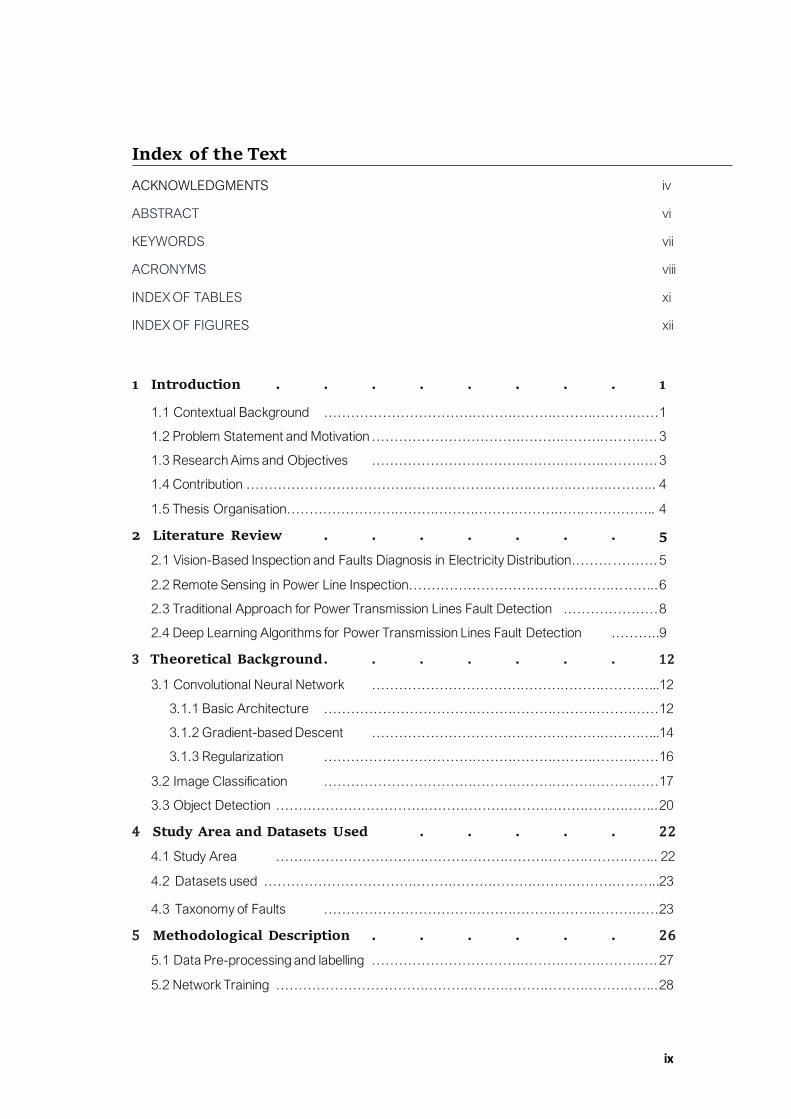
Index of the Text

ACKNOWLEDGMENTS iv

ABSTRACT vi

KEYWORDS vii

ACRONYMS viii

INDEX OF TABLES xi

INDEX OF FIGURES xii

1 Introduction . . . . . . . . 1

1.1 Contextual Background …………………………………………………………………1

1.2 Problem Statement and Motivation ………………………………………………………. 3

1.3 Research Aims and Objectives ………………………………………………………. 3

1.4 Contribution ……………………………………………………………………………….. 4

1.5 Thesis Organisation……………………………………………………………………….. 4

2 Literature Review . . . . . . . 5

2.1 Vision-Based Inspection and Faults Diagnosis in Electricity Distribution………………. 5

2.2 Remote Sensing in Power Line Inspection……………………………………………….. 6

2.3 Traditional Approach for Power Transmission Lines Fault Detection ………………… 8

2.4 Deep Learning Algorithms for Power Transmission Lines Fault Detection ………..9

3 Theoretical Background . . . . . . . 12

3.1 Convolutional Neural Network ………………………………………………………..12

3.1.1 Basic Architecture …………………………………………………………………12

3.1.2 Gradient-based Descent ………………………………………………………..14

3.1.3 Regularization …………………………………………………………………16

3.2 Image Classification …………………………………………………………………17

3.3 Object Detection ………………………………………………………………………….. 20

4 Study Area and Datasets Used . . . . . 22

4.1 Study Area ………………………………………………………………………….. 22

4.2 Datasets used ……………………………………………………………………………..23

4.3 Taxonomy of Faults …………………………………………………………………23

5 Methodological Description . . . . . . 26

5.1 Data Pre-processing and labelling ………………………………………………………. 27

5.2 Network Training ………………………………………………………………………….. 28

x

5.3 Experimental Settings …………………………………………………………………30

5.4 Sensitivity to Hyperparameter .……………………………………………………… 31

5.5 Performance Evaluation …………………………………………………………………32

6 Result and Discussion . . . . . . . 35

6.1 Analysis of Experimenting DCNN Hyperparameter …………………………………….35

6.2 Performance of EPTN Faults Detection network …………………………………….37

6.3 Further Investigation .……………………………………….………………….........41

6.4 Qualitative Experimental Evaluations ……………………………………............. 41

7 Conclusion . . . . . . . . 43

7.1 Findings ……………..…………………………………………………………………….. 43

7.2 Limitations ………………………………………………………………………….. 44

7.3 Future Works ………………………………………………………………………….. 45

Bibliographic References. . . . . . . . 47

xi

Index of Tables

Table 3.1: Detail layer for MobileNet Architecture (adapted from Wang et al., [71]). ……….. 18

Table 3.2: Detail architecture of Resnet 50 and Resnet 101 [72]. ………………………….. 19

Table 5.1: Data partition. ………………………………………………………………………….. 27

Table 5.2: Training hyperparameters settings for CNN models. ………………………….. 31

Table 5.3: List of DCNN experiments on hyperparameters tuned using

hold-out validation. The bold font shows the final chosen

values from the hyperparameter settings. ……………………………………. 31

Table 6.1: Influence of using varying optimizers. ……………………………………………… 36

Table 6.2: Effect of anchor aspect ratio ……………………………………………………….. 37

Table 6.3: Assessment of SSD Rest101, SSD Rest50, and SSD MobNet on the test dataset.

……………………………………………………………………………………………… 38

xii

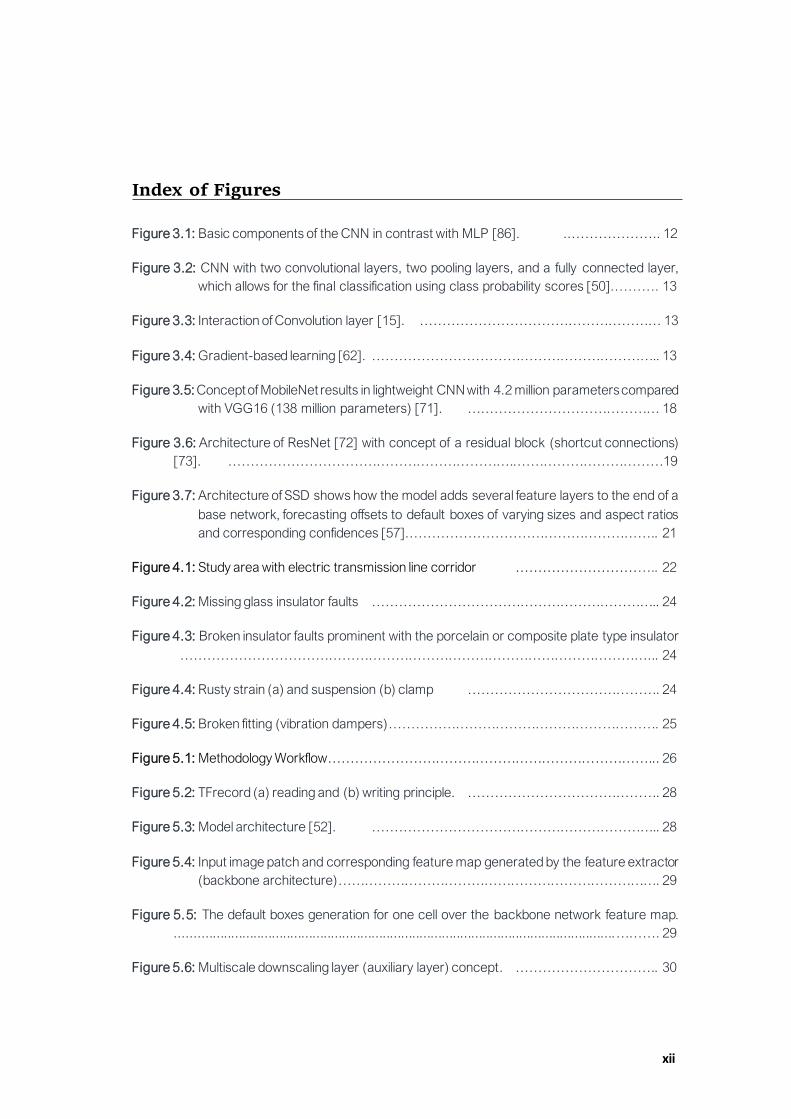
Index of Figures

Figure 3.1: Basic components of the CNN in contrast with MLP [86]. ..……………….. 12

Figure 3.2: CNN with two convolutional layers, two pooling layers, and a fully connected layer,

which allows for the final classification using class probability scores [50].………. 13

Figure 3.3: Interaction of Convolution layer [15]. ……………………………………………… 13

Figure 3.4: Gradient-based learning [62]. ……………………………………………………….. 13

Figure 3.5: Concept of MobileNet results in lightweight CNN with 4.2 million parameters compared

with VGG16 (138 million parameters) [71]. ….………………………………… 18

Figure 3.6: Architecture of ResNet [72] with concept of a residual block (shortcut connections)

[73]. ………………………………………………………..……………………………19

Figure 3.7: Architecture of SSD shows how the model adds several feature layers to the end of a

base network, forecasting offsets to default boxes of varying sizes and aspect ratios

and corresponding confidences [57].……………………………………………….. 21

Figure 4.1: Study area with electric transmission line corridor ………………………….. 22

Figure 4.2: Missing glass insulator faults ……………………………………………………….. 24

Figure 4.3: Broken insulator faults prominent with the porcelain or composite plate type insulator

……………………………………………………………………………………………... 24

Figure 4.4: Rusty strain (a) and suspension (b) clamp ……………………………………. 24

Figure 4.5: Broken fitting (vibration dampers)……………………………………………………. 25

Figure 5.1: Methodology Workflow………………………………………………………………... 26

Figure 5.2: TFrecord (a) reading and (b) writing principle. ……………………………………. 28

Figure 5.3: Model architecture [52]. ……………………………………………………….. 28

Figure 5.4: Input image patch and corresponding feature map generated by the feature extractor

(backbone architecture)………………………………………………………………. 29

Figure 5.5: The default boxes generation for one cell over the backbone network feature map.

.......................................................................................................................………. 29

Figure 5.6: Multiscale downscaling layer (auxiliary layer) concept. ………………………….. 30

xiii

Figure 5.7: IoU concept (Jaccard Index). ……………………………………………………….. 33

Figure 6.1: Effect of varying optimizers ……………………………………………………….. 35

Figure 6.2: The accuracy achieved using varying learning rate ………………………….. 36

Figure 6.3: Epoch vs. Loss Graphs……………………………………………………………….. 39

Figure 6.4: Experimental results of the four components faults. The first column to the third column

depicts the proposed method’s performance in each row, SSD MobNet, SSD Rest50,

and SSD Rest101. ……………………………………………………………………. 42

1

1 Introduction

1.1 Contextual Background

Growing population and a shortage of energy availability have placed problems for

economies concerning the development of effective manufacturing industry, citizens’

expectations, and livelihood sustainability. According to the United Nations (UN),

electricity, among others, is a necessity for life [1]. The UN Sustainable Development

Goals 7 for 2030 has specifically established one of their key priorities: improving

equitable access to cost-effective, secured, and optimum energy (electricity) resources

[2]. This can be done by expanding infrastructure and updating technologies to deliver

sufficient energy facilities via consistent energy efficiency monitoring, particularly for

developed countries. Accordingly, remote sensing techniques have proven to be an

efficient tool in which defects such as corrosion and mechanical loss can be managed

and identified, power component damage detected, and energy supply conditions

monitored, especially with UAV surveillance [3]. As a result, various public-private

partnerships (PPP) are being established to tackle and upgrade existing systems. One

of the challenges for these PPPs is the current dilapidated state of most power

transmission assets and infrastructure [4], [5]. Other challenges they face include

meeting customer demands; forecast and distribution of customer’s load; excessive cost;

customer service delivery; capturing of accurate, up-to-date information of network

infrastructures and asset; network optimization; cybersecurity; fault resolution and

outage; and technical and commercial losses [4]–[7].

In terms of faults in electrical transmission and control systems, defects such as

breakage and corrosion are a significant source of in-service system deterioration and

disruption [8]. Once faults are not handled at their early stages, it may soon affect system

reliability, resulting in the drop in voltage, network diminishment, grid destruction, along

with increasing outages, with ultimately impact threatening repercussions to the

ecosystem [9]. This ultimately has unintended consequences in the form of cost and

sanctions. This was further emphasized by an annual report released in the US, which

evaluates the corrosion cost at about $276 billion in maintenance [10]. In other climes

like Brazil, the 2010 large-scale blackout that impacted 11 of the 27 states containing 6

million people was attributed to corrosion and wear of transmission lines [10].

Before integrating the IT system in early 2010 [4], [6], manual methods were

conventionally employed by the electricity distribution company. Electrical linesmen were

sent to the site to inspect, track, and maintain distribution and overhead power lines with

mechanical devices. This procedure generally included pole climbing, foot patrols, and

vehicle inspection, involving just human subjectivity [3]. These manual methods are time-

consuming, labour-intensive, imprecise, and risky. Providentially, the current availability

of fast computers, digital data acquisition technology, digital data processing technique,

information technology, and geographic Information system brought a revolution into

electricity distribution [4]–[7]. For example, in fault analysis, network optimization, asset

2

audit, load forecasting, customer indexing, and listing [4]–[7], GIS and GPS have been

used to provide database management capabilities and pinpoint the location of electrical

assets. However, this process is cumbersome and exposes utility staff directly to unsafe

conditions during inspection [3].

As a result of these, other geospatial technique has been adopted. Most notable is the

use of very high-resolution imagery (VHRI) via Unmanned Aerial Vehicle (UAV)

surveillance using red-green-blue (RGB), light detection and ranging (LIDAR), radio

detection and ranging (RADAR) [12], or a modular combination of any of these sensors

[3], [11]. UAV monitoring offers high-spatial multispectral images that deal with the

limitation of other techniques with the benefit that they can capture accurate images of

transmissions components at closer proximity [13], which are very useful for the

detection of small-scale defects such as broken fittings and missing knobs and can be

incorporated with other modes of remote sensing.

Most research only considers the transmission lines’ delineation after the data has been

captured using different mathematical models. However, to create an automated vision-

based fault detection system for power transmission networks utilizing high-quality

remote sensing imagery [13], a high-level vision task is needed to adopt a high-level

vision task capable of advanced learning characteristics and generalization. Currently,

improved algorithms and multilayer neuron systems such as CNN, DNN, and RNN have

demonstrated more outstanding performance than standard approaches, particularly in

power line identification, transmission components detection, and vegetation

encroachment prevention [14]. The traditional approach for pattern recognition depends

on the parameters that are well built by humans. Hence, this manual extraction process

is inefficient, unfavourable, and inadequate for generalization necessities.

Also, most machine learning approaches using primary neural networks need vast

quantities of standardized hand-made structured training data in the form of rows of

records, which can be cumbersome. With deep learning algorithms, visual perception to

extract feature hierarchies and generalization ability is enhanced on several levels [15].

These algorithms have demonstrated that conventional learning methods are sluggish

and unreliable; they require substantial post-processing attempts to differentiate

between transmission infrastructure [16]. Succinctly, power transmission network

mapping and defect inspection require a more advanced adequate hybrid classifier that

is way beyond task-based approaches, promoting the improved performance of visual

recognition tasks and successfully adapts from multimodal data sensors for object

detection.

Therefore, by leveraging VHRI and robust classifiers with deep learning models, the PPPs

can ensure comprehensive and accurate track of the conditions, especially corrosion of

their transmission line assets wherever they are, both as part of service provision,

network expansion, and routine maintenance. Additionally, for many electricity

companies, especially private electricity distribution Companies: a critical step in

ensuring smooth service delivery lies in monitoring the electricity distribution assets [4],

[7]. Hence, they must know what assets they have, where they are, their state, and how

they are working.

3

1.2 Problem Statement and Motivation

In traditional operations, utilities must power off entire distribution grid sections to identify

damaged outgoing lines. Many power grids are linked across the network. A domino

effect in one field can also lead to supra-regional blackouts [11]. After finding the

damaged line, technicians will power the faulty line part by part until they ultimately locate

the ground fault. This process often takes several hours or even days, further made

strenuous by unfavourable weather conditions and mountainous terrain. Usually, field

and airborne surveys that are quite challenging are standard methodologies used for

decades for inspecting power networks [3], [11]. However, this traditional approach is

limited in terms of accuracy and ability to extract features at multiscale as well as portrays

a low-level generalization ability. In recent years, several studies have been undertaken

to automate the inspection of defects using remote sensing satellite and aerial images,

including LIDAR, SAR, and optical images; however, very little public analysis and

implementation have been adopted and published. They focus mainly on mapping and

monitoring the power line components and vegetation invasion encroachment adjoining

transmission lines. These studies are generally carried out majorly in developed countries

like China, where adequate data with high quality are easily acquired by qualified

technical know-how propelled by the right motivation and adequate funds. Alternatively,

developing countries such as Nigeria are limited to such very high multispectral data

needed for a complete overhaul of transmission assets.

Nigeria’s development agenda is anchored in a vision that identifies energy as one of the

vital infrastructural enablers for development. For a country to successively make a

significant positive transition in development, it must have efficient, reliable, vast, and

environment-friendly energy source transmission. This power should also be availed at

the points of demands consistently and effectively. This means that majority of the burden

of energy demand is on power companies to provide and transmit quali ty energy services

to consumers. Against this backdrop, the recent images available inspire research and

development in maintenance and asset inventory to overcome such difficulty and look

for effective and sustainable solutions. Based on that, deep learning has demonstrated

potential promising advances in power line component inspection and other study fields.

Thus, the potential solution of developing an automatic vision-based fault detection

system that uses multispectral images and deep learning (DL) framework also adds

motivation to conduct this study.

1.3 Research Aims and Objectives

This research seeks to detect and inspect vision-based components’ faults on the

electricity transmission line using very high-resolution UAV imageries (VHRI) and deep

learning techniques (DLT). To achieve these main research aims, the following sub-

questions are addressed:

a) Which different hyperparameters finetuning yields the best results in the

implemented deep learning model?

b) To what extent will the deep convolution neural network perform based on

the predicted component fault classes’ performance metrics analysis?

4

1.4 Contribution

Most current studies focus separately on either identifying transmission assets or

detecting a single fault on transmission components individually using either traditional

methods or DL. However, this research focuses on the following contributions:

→ Explore the feasibility of using a single-phase deep learning model and affordable

drone surveillance to develop a power line component fault detection and

classification pipeline for a series of faults (multi-class) that typically exists on

power transmission components. Based on my understanding, very little

research has been carried out here as most implemented or underway

are proprietary and have provided little benefit to the research communities and

electric utilities.

→ Empirically, evaluate via comparative analysis different backbone architectures

to classify and localize multi-class electric power transmission component fault.

1.5 Thesis Organization

This thesis is divided into seven chapters. The remainder of this thesis is organized as

follows. Chapter 2 reviews vision-based inspection in the electric power transmission

network (EPTN). It further evaluates the related works on the existing approach and

technique utilized for electric transmission components fault detection. Chapter 3

provides a theoretical background needed to understand the basic concept approaches

applied to the thesis methodology. Deeper explanations are given on the convolution

neural networks (CNNs) basic building blocks concept and image classification that

serves as backbone architecture for feature extraction. In addition, a brief exposition of

the SSD as the meta-architecture of choice is presented. Chapter 4 outlines the research

location and describes the dataset used in the potential deep learning models. It further

describes the research problem, i.e., how each components’ faults appear. Chapter 5

describes extensively the method adopted in this work. It provides details about the data

pre-processing, network training of the deep learning framework, and the

hyperparameter augmentation and validation approach.

Furthermore, the evaluation and performance metrics utilized are established. In Chapter

6, the evaluation and comparison of hyperparameter configurations and results over the

three implemented SSD-based models were discussed via outline, graphs, and

overview. It aims to show fusing deep learning and high-resolution RGB oblique imagery;

it is feasible to build a model that better identifies component fault of interest in cluttered

backgrounds. The thesis concludes by summarizing the findings and possible directions

of the analysis for future works in Chapter 7.

5

2 Literature Review

2.1 Vision-Based Inspection and Faults Diagnosis in Electricity Distribution

The inspection of electric transmission lines (ETL) has become an essential concern

because virtually all human communities, processes, and mechanisms rely on electricity.

External forces, especially meteorological influences, have been identified as the primary

cause of the collapse of electric power transmission networks (EPTN) [18], [20]. Hence,

frequent monitoring and assessment of the transmission line are necessary to strengthen

and sustain the transmission network and provide reliable and quality service delivery to

customers [5].

According to Chen et al. [21], faults associated with electrical power grids are described

as accidental short circuits, or a prolonged short circuit, between power-conductors or

an energy-efficient conductor and the ground due to wear, corrosions, and interruptions

by adjoining ecosystem, causing irregular electrical current. Generally, ETL faults are

classified into symmetrical (balanced) and unsymmetrical (unbalanced). In engineering,

a fault is symmetric if it impacts all phases equally (three lines), while it is unsymmetric

when it does not affect each of the phases equally [18], [23]. Nonetheless, many power

system failures are fundamentally unsymmetrical. This is because the current induces

unevenness. This implies an unequal difference in the frequency of fault currents along

the usual three-phase conductor (wires) present in the ETL [18].

The electricity line inspection aims to verify these faults on a power line, the output of

which is used as a reference to determine which components to retain or replace. A

precise and straightforward inspection will make sustaining decisions more effective and

reduce the risk that the transmission network will fail, facilitating secure and stable power

distribution [3], [19]. Overhead power line inspection by a human observer and airborne

surveys is the most utilized means for regular inspection and power line maintenance.

With the increased advancement of technologies, geo-referenced remote sensing

techniques such as the Unmanned Aerial Vehicle (UAV) mounted with different sensors

have become a great alternative providing rich data sources for data analysis.

The UAV is operated manually or automatically along the power lines corridors. Multiple

sensors are used on the aircraft to track and gather data during this operation. A variety

of benefits of the UAV make it a preferred inspection method: 1) Proximity to problematic

areas, which allows data collection incredibly versatile, 2) Ability to load multiple

inspections sensing instruments, 3) Fix low-efficiency issues and line harm, 4) saves time

and human resources and is associated with a high rate of safety. With this technology,

data processing is distinguished from data acquisition using digital data captured

via remote sensing sensors and laser scanners. This is especially relevant as data

acquisition practices now concentrate solely on cost-reduction; hence, allowing precise

assessment, repeated study, and persistent data storage enabling multi-temporal

analysis and evaluation [3].

6

The UAV images serve as an inexhaustible source of information for utilities to know

where assets are located, their functional status, and to determine their net worth. This

falls into a broader system that assists with a well-organized inventory of distribution

facilities for optimum electric lines, pole support infrastructures, transformers, and all

network assets fault diagnosis [3]. Combining these data with scientific and technological

developments like artificial intelligence enables an ever-increasing volume of data to be

processed and has increased growing research on the use of UAV survey imageries to

allow the conditions on power lines to be distinguished automatically [24]. In the

classification of the insulator status, Zhao et al. [25] have proposed object detectors and

insulator fault detection processes utilizing multi-patch in-depth features learnt from the

aerial images to classify the insulator into normal, damaged, dusty, and missing caps.

2.2 Remote Sensing in Power Line Inspection

To investigate the electric power transmission network (EPTN) usually located in remote

areas, various data sources ranging from coarse-resolution satellite images to detailed

ground images and point clouds obtained via ground vehicles are utilized. These data

sources primarily result from optical, microwave, and LIDAR (LASER) remote sensing

techniques. These approaches provide multispectral imagery with varying temporal

resolution access based on operational capabilities and technical limitations [11].

Studies presented using microwave sensing imageries, majorly employ synthetic

aperture radar (SAR), have noted the advantage of being acquired in all weather

conditions, making them particularly interesting to inspect powerlines, most especially

during disaster monitoring [27].

For example, Xue et al. [27] utilized SAR image-based systems for landslide detection to

measure electricity towers’ damage. Based on pixel resolution, morphology algorithm,

and location of the damage caused by landslides, the authors detected and geotagged

power lines damaged by landslides directly. The use of TerraSAR-X imagery of high-

resolution in spotlight mode with 300 MHZ range bandwidth to track power line towers

in natural disaster situations was discussed by Yan et al. [28]. SAR imagery was

preferred to optical imagery as the author points out that SAR geometry makes it suitable

to detect vertical, human-made objects, such as power towers. The critical theory was

that towers were finally derived from single imagery, and the estimated tower height

information was used to detect fallen or deformed towers.

Sentinel-1 SAR satellite from the European Space Agency, ESA, and other very high-

resolution (VHR) SAR images (TerraSAR, RADARSAR) that are higher than five metres

have recently opened a wide range of surveillance, tracking, and monitoring of power

transmission systems [29]. However, VHR SAR for EPTN seems impacted by distortions

connected to imagery, the particularly pseudo-random variation of the different

components imprints, making it semantically challenging to interpret [30]. They are also

limited by coarse resolution to detect small defects in electricity transmission

components, geometric deformations, strong noise-like effect creating false

representations, and multi-path scattering [11], [27]. In light of this, various studies of

transmission line inspections utilize multispectral images acquired from optical satellite

7

remote sensing, as it allows for straightforward interpretation. However, these data are

still restricted by resolution in power line inspections.

Optical remote sensing has focused on fault diagnosis for the different EPTN components

themselves because the ground sample distance (GSD) is usually greater than the

individual components’ size, especially for those caused by the adjoining environment.

As a result, most power line inspection research is fixated on vegetation encroachment

and minimum height and clearance distance [14], [31]. Additionally, a stereo pair of

optical satellite images have been utilized to extract the canopy height model to monitor

damages to EPTN caused by vegetation [32]. This has allowed the identification of

individual overgrown trees affecting power lines with high accuracy. The studies on

vegetation encroachment faults affecting transmission lines from satellite and aerial

images have habitually utilized the classification of trees, extraction, vegetation indices,

and segmentation approach. Vegetation invasion on transmission lines was studied by

Ahmad et al. [31]. The paper explored the use of multispectral satellite stereo imagery to

simulate transmission lines using a 3D digital elevation model (DEM) to detect dangerous

vegetation branches that could affect power lines and cause blackouts.

Apart from vegetation encroachment, a variety of papers addressed automatic

inspection of insulators’ condition. These techniques aimed to take images of the

insulators periodically and use automated classification methods to identify damaged

insulators. Reddy et al. [33], for example, used fixed cameras on poles. Jiang et al. [34],

using a photogrammetric method, addressed flashover faults - pollution-related flashes

affecting insulators. In the experiment, a sensing camera placed on a tripod was used.

However, most remote optical sensing techniques are primarily restricted by the

atmosphere. Consequently, using the Lidar method through airborne laser scanning or

mobile laser scanning has also been used to improve the shortcomings of multispectral

optical images to detect and identify tall trees that may collapse through the conductor

and exceed the required vegetation clearance. In responsive inspections and audits for

transmission lines, such as catenary modelling for thermal upgrade and vegetation

encroachment research, Ussyshkin et al. [35] explored using LIDAR data.

Other remote sensing techniques have further involved integrated sensors, which majorly

involves integrating ultraviolet images over both an infrared and multispectral visible

colour image. For instance, a UAV surveillance incorporated with optical and thermal

Infrared sensors was identified by Luque Vega et al. [36] for the power transmission

network. The corona impact can be located by utilizing the different layers’ stack, and

the ultraviolet/infrared image can be analysed for damage and phenomenon magnitude

[11]. The most exciting uses for satellite data concerning power lines have been

automatic extraction of power transmission components [11], power lines affected by

vegetation encroachment [17], damaged transmission tower [27], and damaged

conductor faults at a coarse level over large areas [26]. It is possible to apply optical and

SAR images. Airborne and terrestrial scanning systems have more reliable information

than satellite imagery, but it is impossible to regularly cover vast regions. Optical images

captured by UAVs are proposed as a data source since (i) they are easily accessible and

available, and (ii) they can be analysed very quickly, while (iii) ample information is given

for the identification of a wide variety of common small defects in both power components

8

and power lines. Most literature has yet to address more than one fault affecting the

power line and detect small faults.

2.3 Traditional Approach for Power Transmission Lines Fault Detection

Optical imagery, particularly multispectral RGB images, has proven to be effective means

for automatic inspection and identification of power transmission lines components

compared to traditional ground-based surveys, which consume a lot of money, time, and

human resources [37]. Hence, making it a better choice of detecting and classifying

faults critically across electricity networks. In terms of fault detection approaches, they

can be grouped into two types in general: supervised and unsupervised classification

[38], [39]. Many methods for the automated identification and monitoring of the electric

power transmission network (EPTN) faults have been implemented in recent years using

supervised classification.

The typical detection process can be divided into two stages: extraction of feature and

feature (fault) classification [24]. Features are extracted from images and subsequently

inserted into the classifier to identify the components’ faults. Significant parameters for

these features (ETPN components) classifications, which are primarily used, include

colour, form, texture, and fusion. A widely used approach applied to check faults of power

line components primarily involves clustering, mathematical-based techniques such as

Hough transform, Gabon filters, and low-level filters. In detecting broken transmission

line spacers, a Canny edge detector combined with Hough transform [40] by Song et al.

extracts the conductors. First, a scan window was formed in the path of the conductor.

During the convolution process, if there are a candidate’s spacers, they are recognized

in all sliding windows. Finally, the shape configuration parameter was structured to

decide whether the sensed spacer was broken based on the measurement of linked

parts. However, several factors can make it challenging to extract power line

components’ faults automatically. These include complex background, camera viewing

angle at the moment of capture, background light and spectral resonance, weather, and

seasonal changes in the background [3], [11].

The icing status of insulators was measured by Hao et al. [41] on the basis of the iced

insulator geometric framework. The knowledge-based rules were designed to define the

glaciation state by the distance between two neighbouring insulator caps using Graphical

Shed Spacing (GSS) and Graphical Shed Overhang (GSO). Similarly, an improved

uniform LBP (IULBP) was proposed for feature extraction of thaw insulator using the

texture variable difference between predefined ice template type and the feature

extracted from IULBP Yang et al. [42]. Zhai et al. [43] exploited Saliency Aggregating

Faster Pixel-wise Image (FPISA) for insulator extraction. Based on the colour channel in

Lab colour space, the observed insulator’s flashover region was extracted. The system

was tested using 100 flashover fault insulating images and obtained a detection rate of

92.7%. Zhai et al. [44] and Han et al. [45] detected the faults associated with missing-

cap of insulators based on saliency and adaptive morphology (S-AM).

One of the most challenging fault diagnosis tasks is faults with a tiny aspect ratio on the

EPTN components, for instance, power line fitting such as missing pin, nut, bolts, and a

9

small degree of fault severity on some large components. To detect such kinds of faults,

aerial images are captured close to the exact components containing the faults or the

components (or faults) cropped from the original image manually [46], automatically, or

via segmentation [47]. Fu et al. [48] implemented a dynamic model for the missing pin

type of faults. The fitting is usually a combination of multiple sections, such as pin and

nut, for example. The haar-like attribute and Adaboost classifier was used to detect each

part of the fitting. The methodology involved first extracting the segmented region and

circles with LSD. and Hough transform, respectively, to identify the missing pin. The

missing pin fault was finally obtained and then observed based on the distance limit

between the centre of the circle and the pin section. This procedure was validated using

42 images. Out of the five images with pin fitting identified, only one of them was classified

correctly.

In terms of conventional classification, machine learning-based algorithms have also

been used as the feature classifier, primarily Adaboost [48], SVM [49], which have been

applied successfully to detect foreign bodies on conductor faults. Most literature has

dealt with majorly components detection over the years compared with fault detection

associated with these components. Essentially, a fault has different types and affects

different components, requiring robust architecture to tackle the problem. Overall, most

faults detected focused on the missing insulator head, while other EPTN fault types

are limited. Study on the other components continues to dwindle because of variations

of components, inadequate data, and inappropriate scale. Furthermore, in most cases,

each research study is centred only on one fault of a particular component. Hence, the

deep learning concept is proposed to handle some of these limitations that have been

stated above.

2.4 Deep Learning Algorithms for Power Transmission Lines Fault Detection

Prior studies have employed the deep learning approach to multispectral images (RGB

channel) for fault detection. Most of them have achieved better performance than the

study using knowledge-based or physical parameters as described above. The articles

[46], [47], [50], [51] contain comparative studies for a single type of fault. The most

notable deep learning models have been developed for EPTN faults with several essential

considerations in mind due to the need for robustness and generalization capability.

These considerations include data augmentation, data resizing to deal with small aspect

ratio, and high-resolution images collected from UAV. Data augmentation

is usually adopted to overcome data insufficiency, add variability, and increase the

robustness in research [47], [50], [52], [53]. DL is a deep convolution neural network

(DCNN), which offers a hierarchical representation of knowledge that facilitates a greater

understanding of problems’ complexities [16]. Promising DL approaches used to detect

faults through EPTN components are addressed in this section.

Deep learning-based object detection consists of two components: a DCNN for the

feature extraction model (also referred to as a backbone) and the object classification

and localization scheme (meta-architecture) for the project [54]. According to the

detection system, the DL-based detection process is classified into two categories: the

two-stage and the one-stage detection approach [54]. The former consists of an

10

additional stage for region proposal network formation and abstracting the region of

interest (object) such as Faster RCNN [55] and R-FCN [56]. The latter stage does not

require proposals network generation. The one-stage detection approach, for instance,

SSD [57], eliminates the protocol for proposal generation and reduces processing

operations, storage requirement, time, and computing capacities.

One of the earliest works on fault detection was detecting surface discoloration due to

flashover on insulator using CNN classifier with pre-trained AlexNet published by Zhao

et al. [25]. The experiments were performed with a score of 98.71% mAP on 1000

samples. Faster R-CNN was applied by Liu et al. [53] to identify insulators with missing

caps. The system was tested for three different voltage transmission line levels with 1,000

training samples and 500 research samples prepared for each level. About 120

photographs (80 for training) were used to test the diagnosis of missing cap fault. The

entire experiment was carried out by resizing all images to 500 x 500 pixels and flipping

and cropping to expand the dataset. Similarly, Jiang et al. [58] developed a novel

approach using SSD as the meta-architecture for multi-level perception (low, mid, and

high perception) based on ensemble learning to extract the missing insulator fault from

the image resolution of 1920 × 1080-pixel. The middle and high-level perception images

are made via the ROIs Union Extraction (RUE) image pre-processing. The proposed

approach’s absolute precision and recall rates were 93.69% and 91.23% on the test

image dataset with various perception levels containing missing cap insulator problems.

However, these papers considered the contextual characteristics of one type of fault that

affect the insulator component.

One particular issue in power line fault detection using deep learning CNN is data

insufficiency. This is because the DL model is required to generalize the solution at the

end of the training. To achieve this, a robust and large amount of dataset is usually

required. In the previous papers to tackle this challenge, attempts were made, such

as synthesized images (e.g. [59]) and data augmentation (e.g., [52], [53]). Other

researchers have examined the use of transfer learning and few-shot learning to identify

fault types. The model was first developed using the ImageNet data kit, which included a

1.2 million samples dataset. This same model was then trained, i.e., fine-tuned by the

limited data set obtained containing the surface fault of insulators by Bai et al. [60] based

on the SPP networks (SPP-Net) with transfer learning approaches. This allowed the

weight optimization to begin at top layers (where there is a different feature complexity

from the original training data utilized) in the 3D CNN of the SPP-Net adopted rather than

for the whole model.

In recent years, there have been few efforts to develop the deep learning approach,

which has made it ideally suited for identifying power lines faults. Typically, a two-step

object detection technique is commonly utilized: first, to identify the component and

second, to detect the fault in those components. In this light, Tao et al. [59] developed

two separate backbone models, D.D.N. and I.L.N. (V.G.G. and ResNet, respectively),

based on domain knowledge of EPTN components structure. In order to find a missing

cap fault, a cascading architecture combining a custom-developed Insulator localizer

Network (ILN) and a Defect Detector Network (DDN) models were utilized. The ILN

identifies all the insulators in the aerial image and then cuts the detected areas and feeds

them into the DDN. A total of 900 regular images were collected from UAV for this

11

experiment and 60 defective images. Data insufficiency was tackled by segmenting the

image using the U-net algorithm to divide the output of the ILN into insulator and

background. The segmented insulator was then combined with distinct images of

different backgrounds to mimic real-life background situations concerning insulator

position. The result of this was then merged as input for the DDN development. Finally,

about 1956 pictures for ILN (1186 for training) and 1056 images with missing caps (782

for training) were prepared. The DDN detection precision and recall are 0.91and 0.96.

12

3 Theoretical Background

3.1 Convolutional Neural Network

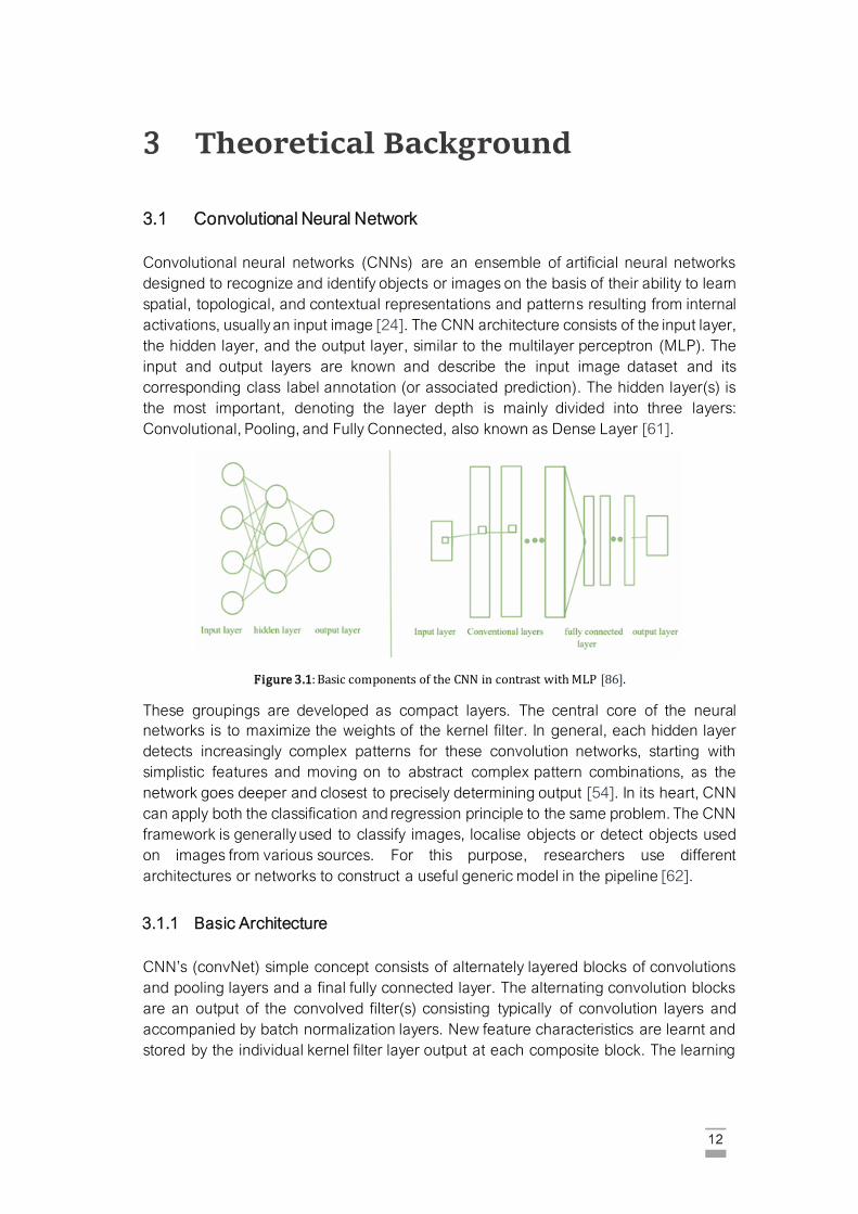
Convolutional neural networks (CNNs) are an ensemble of artificial neural networks

designed to recognize and identify objects or images on the basis of their ability to learn

spatial, topological, and contextual representations and patterns resulting from internal

activations, usually an input image [24]. The CNN architecture consists of the input layer,

the hidden layer, and the output layer, similar to the multilayer perceptron (MLP). The

input and output layers are known and describe the input image dataset and its

corresponding class label annotation (or associated prediction). The hidden layer(s) is

the most important, denoting the layer depth is mainly divided into three layers:

Convolutional, Pooling, and Fully Connected, also known as Dense Layer [61].

Figure 3.1: Basic components of the CNN in contrast with MLP [86].

These groupings are developed as compact layers. The central core of the neural

networks is to maximize the weights of the kernel filter. In general, each hidden layer

detects increasingly complex patterns for these convolution networks, starting with

simplistic features and moving on to abstract complex pattern combinations, as the

network goes deeper and closest to precisely determining output [54]. In its heart, CNN

can apply both the classification and regression principle to the same problem. The CNN

framework is generally used to classify images, localise objects or detect objects used

on images from various sources. For this purpose, researchers use different

architectures or networks to construct a useful generic model in the pipeline [62].

3.1.1 Basic Architecture

CNN’s (convNet) simple concept consists of alternately layered blocks of convolutions

and pooling layers and a final fully connected layer. The alternating convolution blocks

are an output of the convolved filter(s) consisting typically of convolution layers and

accompanied by batch normalization layers. New feature characteristics are learnt and

stored by the individual kernel filter layer output at each composite block. The learning

13

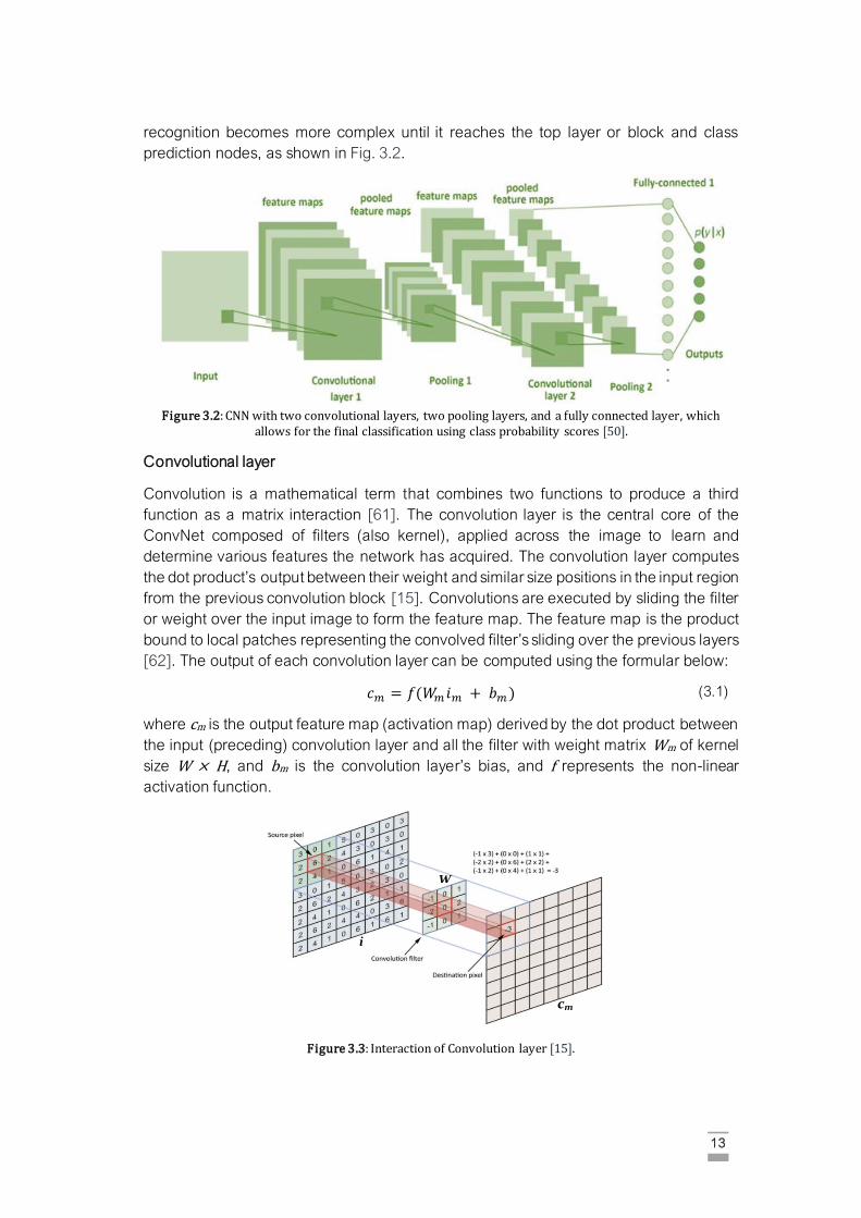
recognition becomes more complex until it reaches the top layer or block and class

prediction nodes, as shown in Fig. 3.2.

Figure 3.2: CNN with two convolutional layers, two pooling layers, and a fully connected layer, which

allows for the final classification using class probability scores [50].

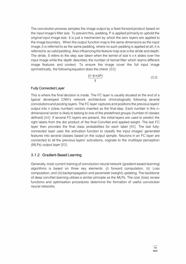
Convolutional layer

Convolution is a mathematical term that combines two functions to produce a third

function as a matrix interaction [61]. The convolution layer is the central core of the

ConvNet composed of filters (also kernel), applied across the image to learn and

determine various features the network has acquired. The convolution layer computes

the dot product’s output between their weight and similar size positions in the input region

from the previous convolution block [15]. Convolutions are executed by sliding the filter

or weight over the input image to form the feature map. The feature map is the product

bound to local patches representing the convolved filter’s sliding over the previous layers

[62]. The output of each convolution layer can be computed using the formular below:

𝑐𝑚 = 𝑓(𝑊𝑚 𝑖𝑚 + 𝑏𝑚 )

where cm is the output feature map (activation map) derived by the dot product between

the input (preceding) convolution layer and all the filter with weight matrix Wm of kernel

size W × H, and bm is the convolution layer’s bias, and f represents the non-linear

activation function.

Figure 3.3: Interaction of Convolution layer [15].

cm

W

i

(3.1)

14

The convolution process samples the image output by a feed-forward product based on

the input image’s filter size. To prevent this, padding, P is applied primarily to uphold the

original input image size. It is just a mechanism by which the zero layers are applied to

the image boundary. When the output function map is the same dimensions as the input

image, it is referred to as the same padding, where no such padding is applied at all; it is

referred to as valid padding. Also influencing the feature map size is the stride and depth.

The stride, S refers to the step size taken when the kernel of size k x k slides over the

input image while the depth describes the number of kernel filter which learns different

image features and context. To ensure the image cover the full input image

symmetrically, the following equation does the check [63]:

(𝐼−𝑘+2𝑃)

𝑆

Fully Connected Layer

This is where the final decision is made. The FC layer is usually situated at the end of a

typical developed CNN’s network architecture chronologically following several

convolutions and pooling layers. The FC layer captures and positions the previous layers’

output into n (class number) vectors inserted as the final step. Each number in this n-

dimensional vector is likely to belong to one of the predefined groups (number of classes

defined) [64]. If several FC layers are present, the initial layers are used to predict the

right labels from the dot product of the final ConvNet and applied weight. The last FC

layer then provides the final class probabilities for each label [65]. The last fully-

connected layer uses the activation function to classify the input images’ generated

features into several classes based on the output sample. Neurons in an FC layer are

connected to all the previous layers’ activations, cognate to the multilayer perceptron

(MLPs) output layer [63].

3.1.2 Gradient-Based Learning

Generally, most current training of convolution neural network (gradient-based learning)

algorithms is based on three key elements: (i) forward computation, (ii) Loss

computation, and (iii) backpropagation and parameter (weight) updating. The backbone

of deep convNet learning utilizes a similar principle as the MLPs. The cost (loss) review

functions and optimisation procedures determine the formation of useful convolution

neural networks.

(3.2)

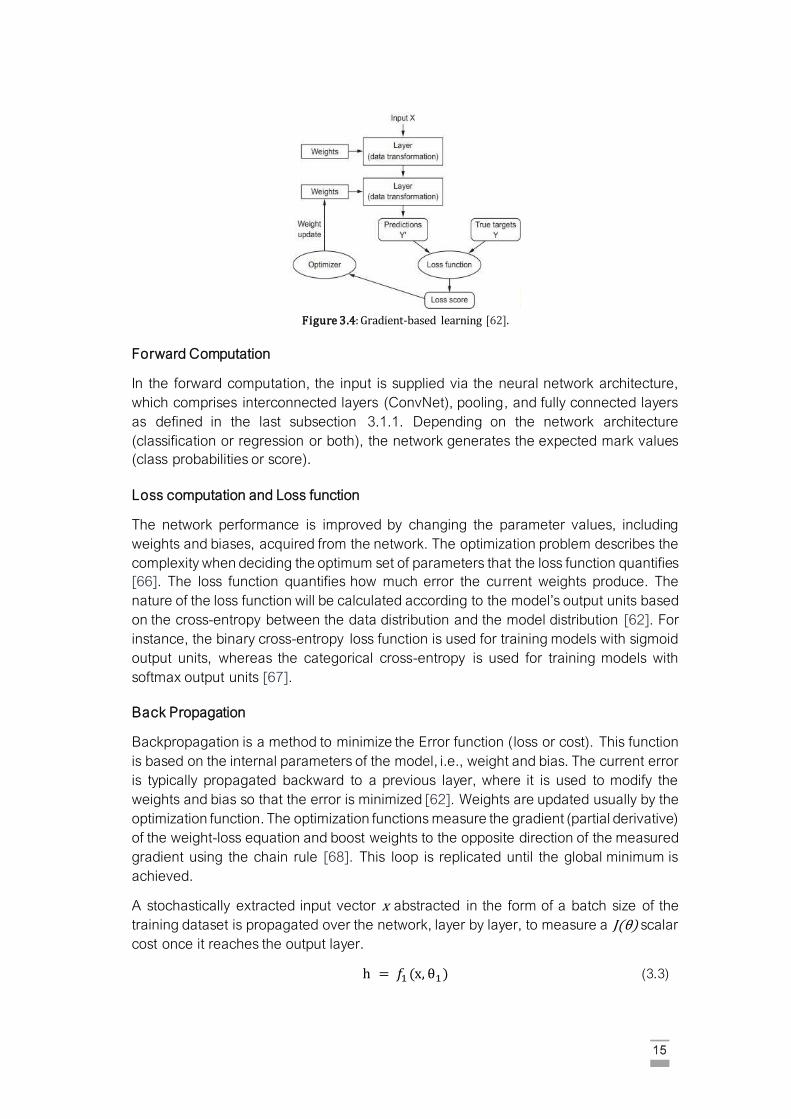
15

Figure 3.4: Gradient-based learning [62].

Forward Computation

In the forward computation, the input is supplied via the neural network architecture,

which comprises interconnected layers (ConvNet), pooling, and fully connected layers

as defined in the last subsection 3.1.1. Depending on the network architecture

(classification or regression or both), the network generates the expected mark values

(class probabilities or score).

Loss computation and Loss function

The network performance is improved by changing the parameter values, including

weights and biases, acquired from the network. The optimization problem describes the

complexity when deciding the optimum set of parameters that the loss function quantifies

[66]. The loss function quantifies how much error the current weights produce. The

nature of the loss function will be calculated according to the model’s output units based

on the cross-entropy between the data distribution and the model distribution [62]. For

instance, the binary cross-entropy loss function is used for training models with sigmoid

output units, whereas the categorical cross-entropy is used for training models with

softmax output units [67].

Back Propagation

Backpropagation is a method to minimize the Error function (loss or cost). This function

is based on the internal parameters of the model, i.e., weight and bias. The current error

is typically propagated backward to a previous layer, where it is used to modify the

weights and bias so that the error is minimized [62]. Weights are updated usually by the

optimization function. The optimization functions measure the gradient (partial derivative)

of the weight-loss equation and boost weights to the opposite direction of the measured

gradient using the chain rule [68]. This loop is replicated until the global minimum is

achieved.

A stochastically extracted input vector x abstracted in the form of a batch size of the

training dataset is propagated over the network, layer by layer, to measure a J(θ) scalar

cost once it reaches the output layer.

h = 𝑓1 (x, θ1) (3.3)

16

y = 𝑓2 (h, 𝜃2)

J(𝜃) = 1

2(y − 𝑦)2

The vector x represents the input (image batch), which is then utilized by the hidden layer

to output a vector, h = f1 (x, θ1), where θ1 is the kernel filter weight of the hidden layer.

The output layer receives the hidden input vector, h, and generates the output value y =

f2 (x, θ2), and which θ2 represents the weight of the output layer. f1 and f2 represent the

activation function or classifier utilized to generate the output at the hidden and the final

output layers. The scalar cost J(θ) is then backwardly distributed over the network, layer

by layer until the first hidden layer is reached, to quantify the gradient of the network

∇θJ(θ):

∂𝐽(𝜃)

𝜕 y= (y − 𝑦)2

∂𝐽(𝜃)

𝜕θ2

=∂𝐽(𝜃)

𝜕y

𝜕y

𝜕𝜃2

∂𝐽(𝜃)

𝜕𝜃1

=∂𝐽(𝜃)

𝜕y 𝜕y

𝜕ℎ

𝜕h

𝜕𝜃1

∇𝜃 𝐽(𝜃) = ⟦∂𝐽(𝜃)

𝜕𝜃1

,∂𝐽(𝜃)

𝜕θ2

⟧

The network’s weights θ are updated based on the computed gradient as follows:

𝜃1 = 𝜃1 − 𝜂∂𝐽(𝜃)

𝜕𝜃1

𝜃2 = 𝜃2 − 𝜂∂𝐽(𝜃)

𝜕𝜃2

Some of the challenges of gradient-based learning include (i) Overfitting - where the

model is good at understanding the training set but poorly interprets the test set, i.e.,

comparing the train loss/accuracy with the validation loss/accuracy. (ii) Vanishing and

exploding gradients - The problem of the vanishing gradient describes the

model learning is either very slow or ceases operating. In contrast, gradient exploding

describes when the gradient signal increases exponentially, allowing learning to be

unstable [69]. (iii) Hyperparameter tuning and model interpretability. Several optimization

algorithms exist to make the training process faster, like Stochastic Gradient Descending

(SGD) with momentum), Adaptive Gradient (AdaGrad), Root Mean Square Propagation

(RMSProp), and Adaptive Moment Estimation (Adam).

3.1.3 Generalization of a model

A learning algorithm’s strength is associated with its ability to generalize, i.e., handle

unknown data. In addition to the generalization theory, there are two circumstances for

model training: under-fitting and over-fitting [62]. Underfitting happens where the model

trained is too straightforward to learn the data’s underlying structure and fails to capture

(3.4)

(3.5)

(3.6)

(3.7)

(3.8)

(3.9)

(3.10)

(3.11)

17

significant variables representing the reality of the situation being modelled [15]. In

contrast, overfitting typically occurs in the case of complex models. Here the model

learns unimportant information and makes noise more meaningful [64]. This may also be

attributed to too many distinct classes (labels) at the output layer. Both conditions tend

to make generalizations crappy. In under-fitting, a variety of approaches can be applied

to fix it, such as using a more effective model with more parameters, having better

functionality for learning algorithms, or reducing model limitations by reducing the

hyperparameter for regularization [69]. In the case of over-fitting, certain approaches

can be applied, such as simplifying the algorithm, minimizing the number of parameters

(the use of additional parameters tends to contribute to a model that is vulnerable to

over-fitting), gathering more training data (e.g., using data optimization techniques), and

others. One or more loss functions are used to calculate this, which may vary based on

the type of problem being faced. During the planning phase, the main goal is to reduce

this shortfall.

Regularization

During training, models can sometimes find features or interpret noise to be important in

a dataset due to their ability to memorize features concurrently. Consequently, there is a

need to reach convergence, i.e., a level where the model optimally detects new tests or

unseen data. Hence, regularization provides such a solution [15]. The aim is to minimize

the amount of unpenalized costs considered a penalty term, consisting of other bias, and

prefer a simplified model to minimize the variance and penalize larger weights. The

penalized model involves trade-offs as it decreases uncertainty and therefore avoids

overfitting. Several methods are suggested to regularize the model to avoid overfitting

during training, utilized in this research. They include L1 and L2 regularization, drop out,

the max norm regularizer, and data augmentation.

3.2 Image Classification

One of CNN’s most popular applications is possibly an image classification that attempts

to identify the prevalent object type in an image dataset. Deep convNet utilized for image

classification is based on the performance of convolution layers as its studies edges,

patterns, context, and shapes resulting in a convolution feature map having

spatial dimensions smaller and deeper than the original [64]. The progenitor of the image

classification architecture referred to as feature extractor in object detection solutions is

AlexNet with an 8-layer CNN, i.e., 5 convolutional layers + 3 fully connected layers

developed by Krizhevsky et al. [70] in Imagenet challenge of 2012.

MobileNet

Mobile networks are lightweight deep neural networks. MobileNets and its derivatives

were implemented to substitute a much deeper network constrained by the speed in

achieving satisfactory output and real-time applications. This design’s idea is that the

regular neural network convolution layer is broken down into two filters, depth-wise

convolution and pointwise convolution [71]. The convolutional filter is more

computationally complicated than depth-wise and pointwise convolutions. To achieve

18

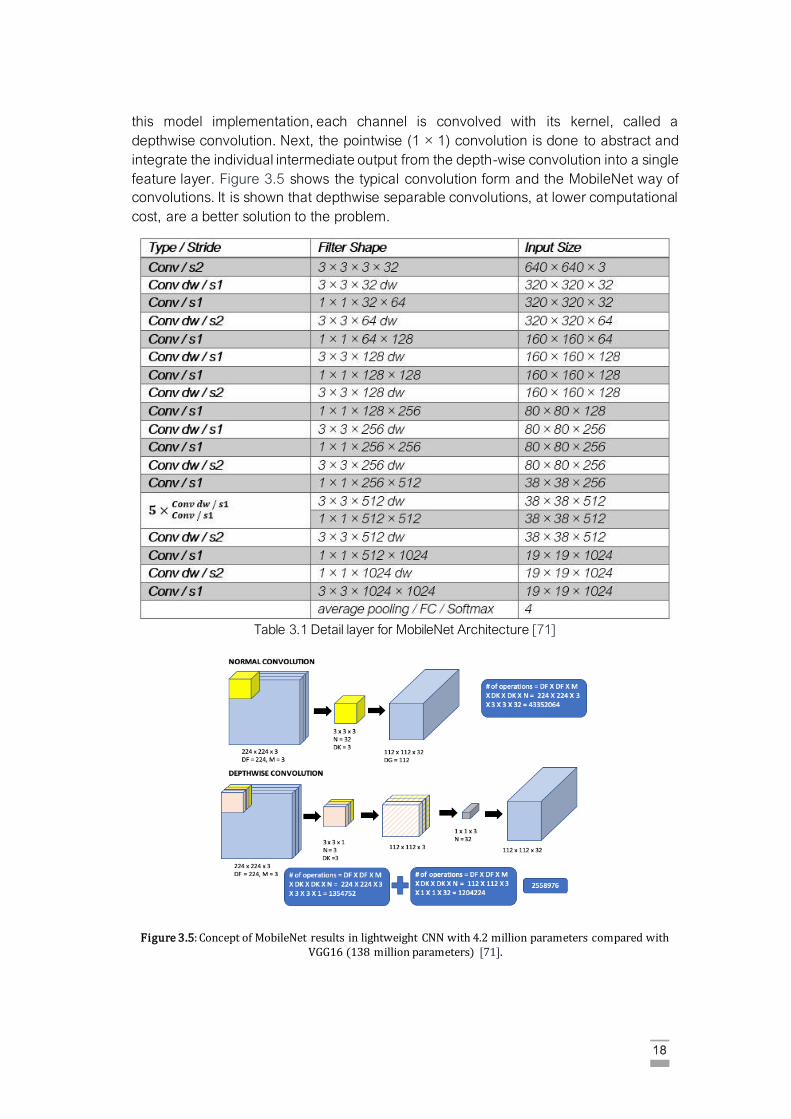
this model implementation, each channel is convolved with its kernel, called a

depthwise convolution. Next, the pointwise (1 × 1) convolution is done to abstract and

integrate the individual intermediate output from the depth-wise convolution into a single

feature layer. Figure 3.5 shows the typical convolution form and the MobileNet way of

convolutions. It is shown that depthwise separable convolutions, at lower computational

cost, are a better solution to the problem.

Table 3.1 Detail layer for MobileNet Architecture [71]

Figure 3.5: Concept of MobileNet results in lightweight CNN with 4.2 million parameters compared with VGG16 (138 million parameters) [71].

19

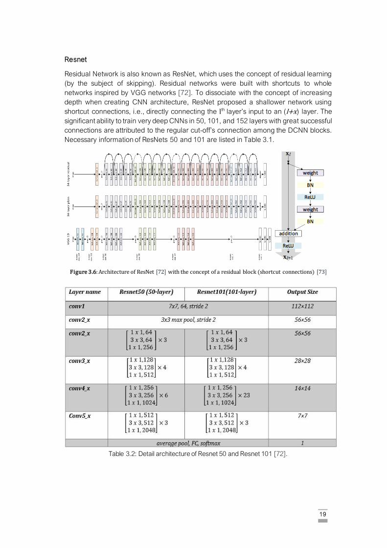
Resnet

Residual Network is also known as ResNet, which uses the concept of residual learning

(by the subject of skipping). Residual networks were built with shortcuts to whole

networks inspired by VGG networks [72]. To dissociate with the concept of increasing

depth when creating CNN architecture, ResNet proposed a shallower network using

shortcut connections, i.e., directly connecting the lth layer’s input to an (l+x) layer. The

significant ability to train very deep CNNs in 50, 101, and 152 layers with great successful

connections are attributed to the regular cut-off’s connection among the DCNN blocks.

Necessary information of ResNets 50 and 101 are listed in Table 3.1.

Figure 3.6: Architecture of ResNet [72] with the concept of a residual block (shortcut connections) [73]

Table 3.2: Detail architecture of Resnet 50 and Resnet 101 [72].

20

3.3 Object Detection

Object detection follows the deep learning concept based on incorporating additional

layers to neural networks to solve complex problems. Object recognition goes deeper

and incorporates the idea of the image positioning of the object. It is a mixture of two

tasks: object localization where bounding boxes are defined, which are made up of four

variables (x-y-coordinate, width, and height) describing the rectangle that defines

the object extent and the classification of the object within the selected bounding boxes

to be uniquely defined [24].

The object detection follows the concept of the basic architecture of the CNN as

discussed in section 3.1.1 and described by Equation 3.1 with multiple sliding windows

capable of providing solutions to both the classification and regression problem.

Multiclass object detection is enforced by thresholding the output feature maps, defined

by several hyperparameters, to achieve the stated hypothesis to form a concrete

response, i.e., an object class and a bounding box. However, this simultaneous

localisation and classification process results in several instances labelled as objects,

resulting in duplicate detections. Hence, the application of the non-maximum

suppression (NMS) module to eliminate duplicate detection. In a nutshell, the resulting

bounding box score with high-class score prediction was picked using a greedy strategy,

and consequently, the remaining boxes with less than 50% overlap are deleted.

Various architecture has been developed for object detection, however choosing the

best fit for any dataset is usually a herculean task because of the numerous base features

used in extractors, different image resolutions, and various processing and computation

trade-offs [74]. However, most custom-developed models are differentiated and chosen

in terms of the trade-off between speed and accuracy. Several deep learning models

implement object detection; however, based on these trade-offs discussed, the SSD [57]

model is utilized in this study.

Single Shot Multibox Detector (SSD)

The SSD approach is focused on a feed-forward-based convolution network generating

a fixed-size bounding box set and scores of object instances present in these boxes and

a final detection process based on a non-maximum suppression criterion [57]. The early

network layers are constructed on a standard image-classification architecture known as

the base network (i.e., the classification layer without the flattened fully connected layer).

SSD supersedes its counterpart, YOLO, by introducing several modifications: (i) multi-

feature maps from subsequent networking stage are predicted to allow multiscale

detection; (ii) object classes and offsets at bounding box locations are predicted using

regular sized small convolutional filter; and (iii) after deriving final feature map, different

predictors (classifiers) are used to identify objects at varying aspect ratios in the form of

feature pyramids [75]. SSD’s comprises two main parts: A feature map extractor (VGG

16 was used in the published paper, but ResNet or DenseNet can also be utilized to

provide better results) and the convolution filter for object detection.

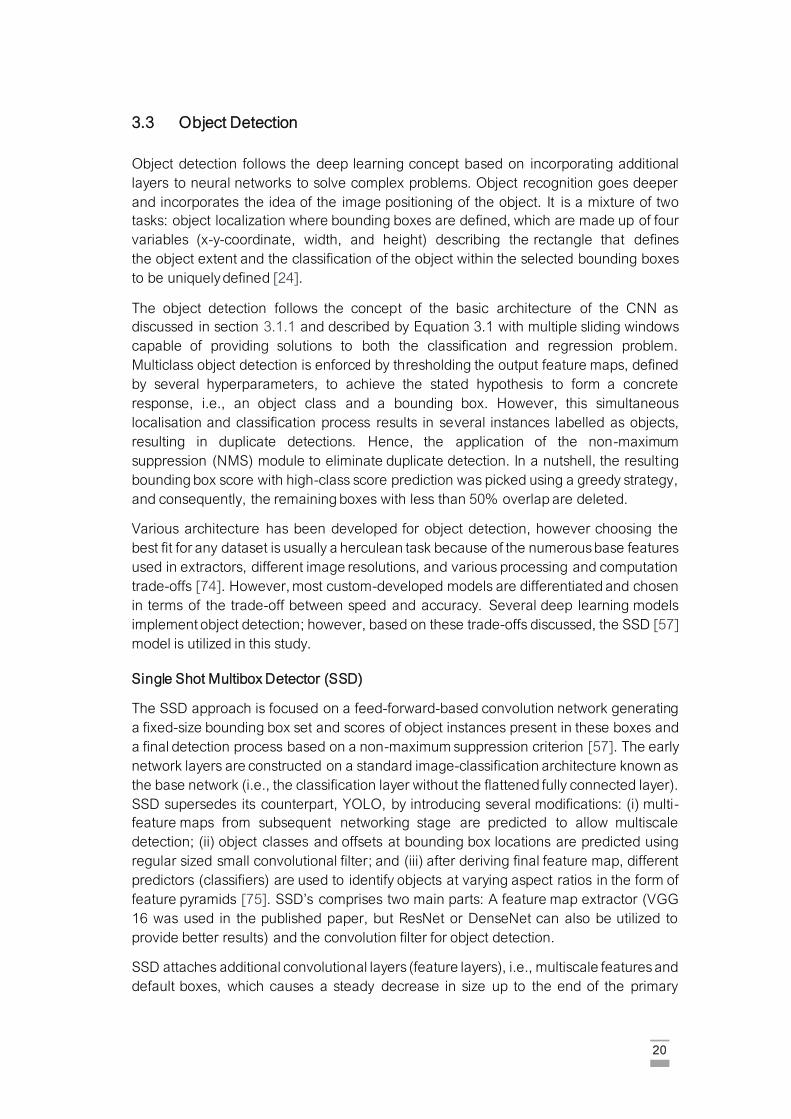
SSD attaches additional convolutional layers (feature layers), i.e., multiscale features and

default boxes, which causes a steady decrease in size up to the end of the primary

21

network. Hence, the predictions of detected objects are produced at multiple levels.

Unlike YOLO, which uses a fully connected layer to make predictions, the SSD adds a

series of small convolutional filters to each added feature layer (or an existing one in the

base network optionally) and uses them in boundary box positions to predict classes and

offsets of objects. SSD adds default boxes to various feature maps of various resolutions

[57].

Figure 3.7: Architecture of SSD showing how the model adds several feature layers to the end of a base

network, forecasting offsets to default boxes of varying sizes and aspect ratios and their corresponding confidences [57] [76]

22

4 Study Area and Datasets Used

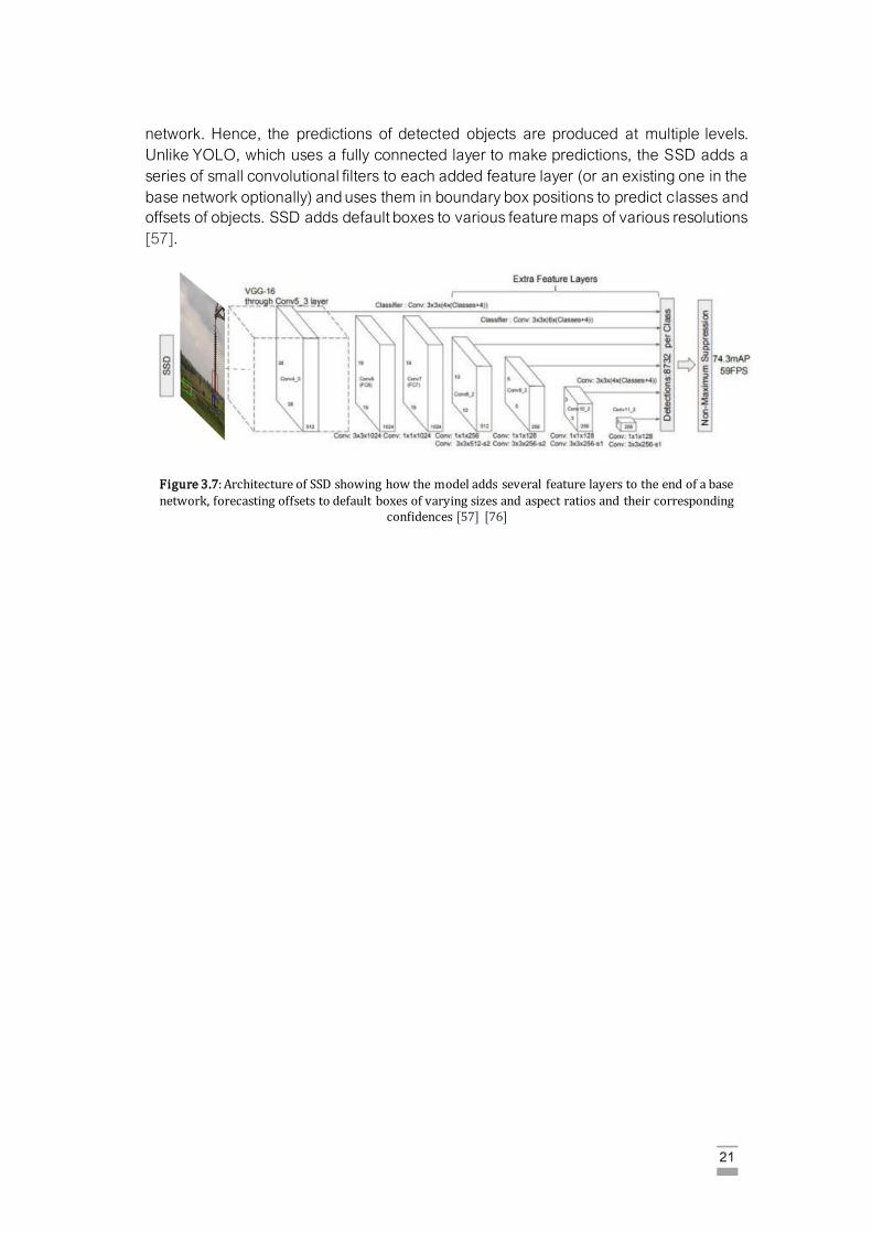
4.1 Study Area

Figure 4.1: Study area with electric transmission line corridor

The study is based on the Shiroro - Kaduna Transmission Line corridor. The Shiroro-

Kaduna corridor connects about seven states in northwest Nigeria. Nigeria lies between

latitudes 4° and 14°N, and longitudes 2° and 15°E. The Nigerian Transmission Network,

called the transmission company of Nigeria (TCN), deals with the transport of voltage in

two phases, the 330kV - 132 kV and the 132kV-33kV along transmission lines (otherwise

referred to as conductors). In general, all transmission corridor shares similar structure,

their infrastructure is radial and thus causes inherent problems without redundancies.

Even though several sources of power are abundantly available, on average, around

7.4%, network-wide propagation losses are high relative to the 2 - 6% benchmarks

proposed for the developing countries and are majorly associated with asset

maintenance [78], [79]. All of these represent vital infrastructure and market issues in

the industry’s subsector of transmission. In 2018, the industry struggled to distribute

about 12.5% (5,000 megawatts) out of the amount estimated to support the population’s

basic needs [80]. This shortfall is also compounded by unannounced load shedding,

partial and complete grid breakdown, and power failure mostly linked to the transmission

company. Consequently, Nigeria’s energy sector generates, transmits, and distributes

megawatts of electric power substantially less than what is required to satisfy basic

23

household and industrial needs, indicating the need for substantial investment to improve

distribution efficiency.

4.2 Datasets used

The DJI Phantom (DJI FC330) fitted with high-resolution cameras was flown across the

Shiroro-Kaduna T.C.N. network of 111-132 kV overhead transmission lines (7km) for the

capture of pylons, conductors, elements of power line/pylon accessories (e.g., insulators,

fittings, cross arms) and the objects surrounding (e.g., vegetation) from a range of angles

of images. The sensor provided three spectral bands with a high spatial resolution

comprising of the visible RGB. The products had been acquired by an aerial survey

conducted from October 12, 2020, to October 22, 2020. In the event of lost or

compromised images of transmission towers, the images were discarded. A total of 140

images covered the study area and can be characterised as high-resolution oblique RGB

images of dimension 4000 x 3000 pixels (72dpi). The mean pixel sensor resolution is

0.00124m. Generally, within the images’ most prominent objects are located and

systematically distributed transmission conductor and pylons with dirt roads, small

patches of natural forest, and grasslands.

4.3 Taxonomy of faults

Inspection of power line components is a primary activity for utilities and one of the most

common research needs in power line inspection. The purpose of this task is to

detect and classify the faults found in the transmission components. Many components

are connected like pylons, conductors, and pylon accessories or fittings (e.g., insulators,

dampers, and fixtures), and each type of component has different faults.

Pylons are pillars used for the extension of conductors over large areas, support lightning

safety cables and other transmission elements, ensure proper electrical transmission

process of the other components by preserving the original design positioning, and

provide sufficient grounding against adjoining objects. Insulators are critical elements in

a transmission system as they protect conductors by allowing lines to retain their

expected electrical insulation strength [18]. As seen in Figure 4.3, the insulator has a

repetitive, stacked cap structure. The colour, size, and string numbers of the insulators

vary based on the transmission capacity and manufacturing design (e.g., single string

and double strings). The pylon accessories, also called fittings, are the connectors of

major components or elements seen in the electricity transmission lines. They mainly

serve as support, inhibitors, connectors to the other transmission components. These

include conductor clamps, dampers, splicing fitting, protective fittings, and guy wire

fittings.

Consequently, most of these individual components have many different types of

faults. For this research, the defects were divided taxonomically into four categories:

missing insulator, broken insulator, rusty clamp, and broken dampers according to the

contents of the captured aerial photographs. The detailed fault taxonomy discussed in

this study is as follow:

24

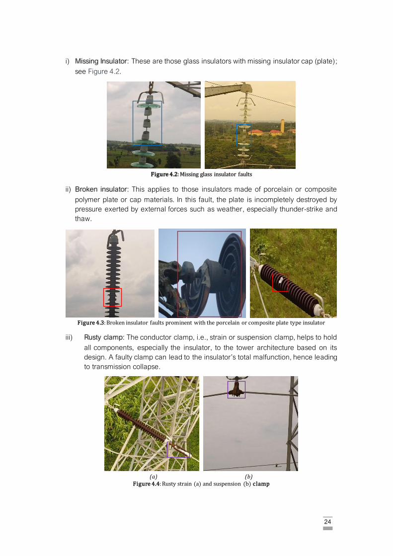
i) Missing Insulator: These are those glass insulators with missing insulator cap (plate);

see Figure 4.2.

Figure 4.2: Missing glass insulator faults

ii) Broken insulator: This applies to those insulators made of porcelain or composite

polymer plate or cap materials. In this fault, the plate is incompletely destroyed by

pressure exerted by external forces such as weather, especially thunder-strike and

thaw.

Figure 4.3: Broken insulator faults prominent with the porcelain or composite plate type insulator

iii) Rusty clamp: The conductor clamp, i.e., strain or suspension clamp, helps to hold

all components, especially the insulator, to the tower architecture based on its

design. A faulty clamp can lead to the insulator’s total malfunction, hence leading

to transmission collapse.

(a) (b)

Figure 4.4: Rusty strain (a) and suspension (b) clamp

25

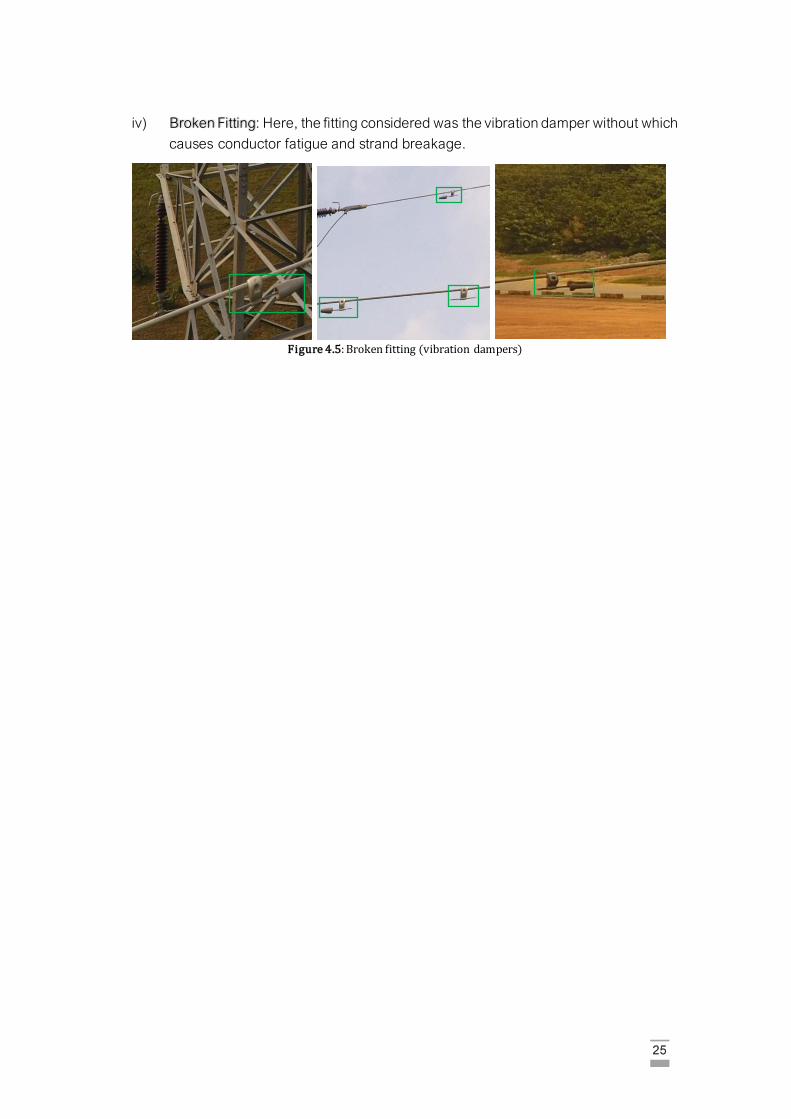
iv) Broken Fitting: Here, the fitting considered was the vibration damper without which

causes conductor fatigue and strand breakage.

Figure 4.5: Broken fitting (vibration dampers)

26

5 Methodological Description

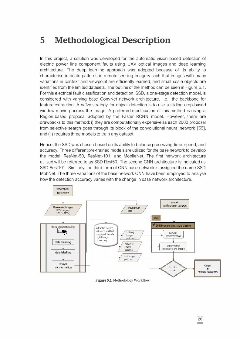
In this project, a solution was developed for the automatic vision-based detection of

electric power line component faults using UAV optical images and deep learning

architecture. The deep learning approach was adopted because of its ability to

characterise intricate patterns in remote sensing imagery such that images with many

variations in context and viewpoint are efficiently learned, and small-scale objects are

identified from the limited datasets. The outline of the method can be seen in Figure 5.1.

For this electrical fault classification and detection, SSD, a one-stage detection model, is

considered with varying base ConvNet network architecture, i.e., the backbone for

feature extraction. A naïve strategy for object detection is to use a sliding crop-based

window moving across the image. A preferred modification of this method is using a

Region-based proposal adopted by the Faster RCNN model. However, there are

drawbacks to this method: i) they are computationally expensive as each 2000 proposal

from selective search goes through its block of the convolutional neural network [55],

and (ii) requires three models to train any dataset.

Hence, the SSD was chosen based on its ability to balance processing time, speed, and

accuracy. Three different pre-trained models are utilized for the base network to develop

the model: ResNet-50, ResNet-101, and MobileNet. The first network architecture

utilized will be referred to as SSD Rest50. The second CNN architecture is indicated as

SSD Rest101. Similarly, the third form of CNN base network is assigned the name SSD

MobNet. The three variations of the base network CNN have been employed to analyse

how the detection accuracy varies with the change in base network architecture.

Figure 5.1: Methodology Workflow.

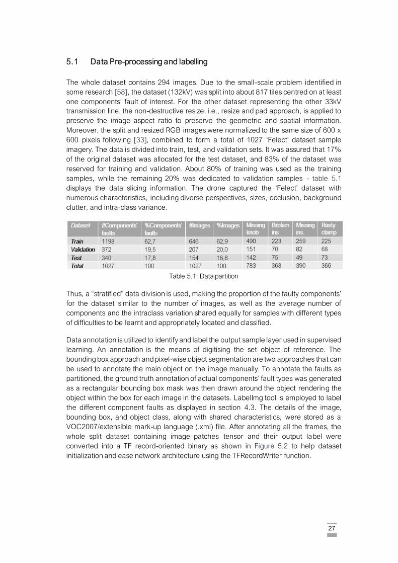
27

5.1 Data Pre-processing and labelling

The whole dataset contains 294 images. Due to the small-scale problem identified in

some research [58], the dataset (132kV) was split into about 817 tiles centred on at least

one components’ fault of interest. For the other dataset representing the other 33kV

transmission line, the non-destructive resize, i.e., resize and pad approach, is applied to

preserve the image aspect ratio to preserve the geometric and spatial information.

Moreover, the split and resized RGB images were normalized to the same size of 600 x

600 pixels following [33], combined to form a total of 1027 ‘Felect’ dataset sample

imagery. The data is divided into train, test, and validation sets. It was assured that 17%

of the original dataset was allocated for the test dataset, and 83% of the dataset was

reserved for training and validation. About 80% of training was used as the training

samples, while the remaining 20% was dedicated to validation samples - table 5.1

displays the data slicing information. The drone captured the ‘Felect’ dataset with

numerous characteristics, including diverse perspectives, sizes, occlusion, background

clutter, and intra-class variance.

Table 5.1: Data partition

Thus, a “stratified” data division is used, making the proportion of the faulty components’

for the dataset similar to the number of images, as well as the average number of

components and the intraclass variation shared equally for samples with different types

of difficulties to be learnt and appropriately located and classified.

Data annotation is utilized to identify and label the output sample layer used in supervised

learning. An annotation is the means of digitising the set object of reference. The

bounding box approach and pixel-wise object segmentation are two approaches that can

be used to annotate the main object on the image manually. To annotate the faults as

partitioned, the ground truth annotation of actual components’ fault types was generated

as a rectangular bounding box mask was then drawn around the object rendering the

object within the box for each image in the datasets. LabelImg tool is employed to label

the different component faults as displayed in section 4.3. The details of the image,

bounding box, and object class, along with shared characteristics, were stored as a

VOC2007/extensible mark-up language (.xml) file. After annotating all the frames, the

whole split dataset containing image patches tensor and their output label were

converted into a TF record-oriented binary as shown in Figure 5.2 to help dataset

initialization and ease network architecture using the TFRecordWriter function.

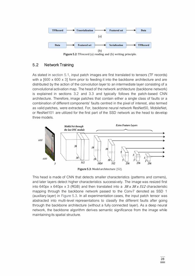
28

(a)

(b)

Figure 5.2: TFrecord (a) reading and (b) writing principle.

5.2 Network Training

As stated in section 5.1, input patch images are first translated to tensors (TF records)

with a [600 x 600 x 3] form prior to feeding it into the backbone architecture and are

distributed by the action of the convolution layer to an intermediate layer consisting of a

convolutional activation map. The head of the network architecture (backbone network)

is explained in sections 3.2 and 3.3 and typically follows the patch-based CNN

architecture. Therefore, image patches that contain either a single class of faults or a

combination of different components’ faults centred in the pixel of interest, also termed

as valid patches, were extracted. For, backbone neural network ResNet50, MobileNet,

or ResNet101 are utilized for the first part of the SSD network as the head to develop

three models.

Figure 5.3: Model architecture [52].

This head is made of CNN that detects smaller characteristics (patterns and corners),

and later layers detect higher characteristics successively. The image was resized first

into 640px x 640px x 3 (RGB) and then translated into a 38 x 38 x 512 characteristic

mapping through the backbone network passed to the Conv7 denoted as SSD 1

(auxiliary layer) in Figure 5.3. In all experimentation cases, the input patch tensor was

abstracted into multi-level representations to classify the different faults after going

through the backbone architecture (without a fully connected layer). As a deep neural

network, the backbone algorithm derives semantic significance from the image while

maintaining its spatial structure.

600

600

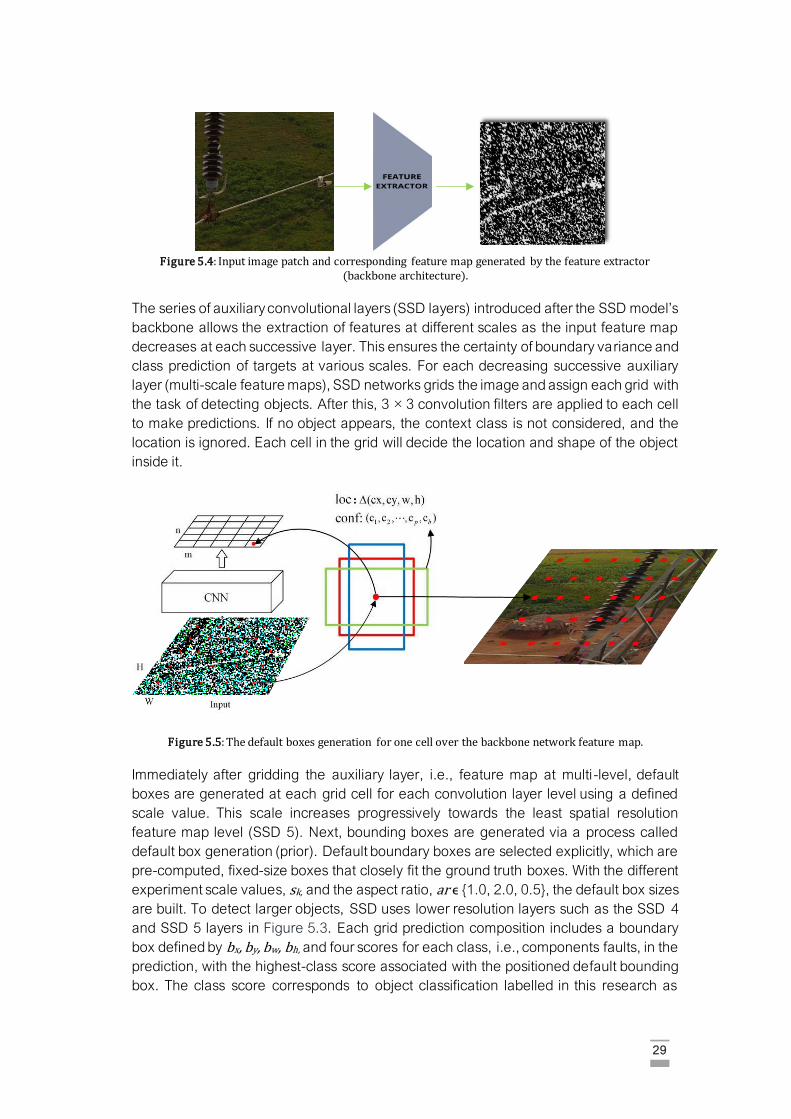
29

Figure 5.4: Input image patch and corresponding feature map generated by the feature extractor

(backbone architecture).

The series of auxiliary convolutional layers (SSD layers) introduced after the SSD model’s

backbone allows the extraction of features at different scales as the input feature map

decreases at each successive layer. This ensures the certainty of boundary variance and

class prediction of targets at various scales. For each decreasing successive auxiliary

layer (multi-scale feature maps), SSD networks grids the image and assign each grid with

the task of detecting objects. After this, 3 × 3 convolution filters are applied to each cell

to make predictions. If no object appears, the context class is not considered, and the

location is ignored. Each cell in the grid will decide the location and shape of the object

inside it.

Figure 5.5: The default boxes generation for one cell over the backbone network feature map.

Immediately after gridding the auxiliary layer, i.e., feature map at multi -level, default

boxes are generated at each grid cell for each convolution layer level using a defined

scale value. This scale increases progressively towards the least spatial resolution

feature map level (SSD 5). Next, bounding boxes are generated via a process called

default box generation (prior). Default boundary boxes are selected explicitly, which are

pre-computed, fixed-size boxes that closely fit the ground truth boxes. With the different

experiment scale values, sk, and the aspect ratio, ar ϵ {1.0, 2.0, 0.5}, the default box sizes

are built. To detect larger objects, SSD uses lower resolution layers such as the SSD 4

and SSD 5 layers in Figure 5.3. Each grid prediction composition includes a boundary

box defined by bx, by, bw, bh, and four scores for each class, i.e., components faults, in the

prediction, with the highest-class score associated with the positioned default bounding

box. The class score corresponds to object classification labelled in this research as

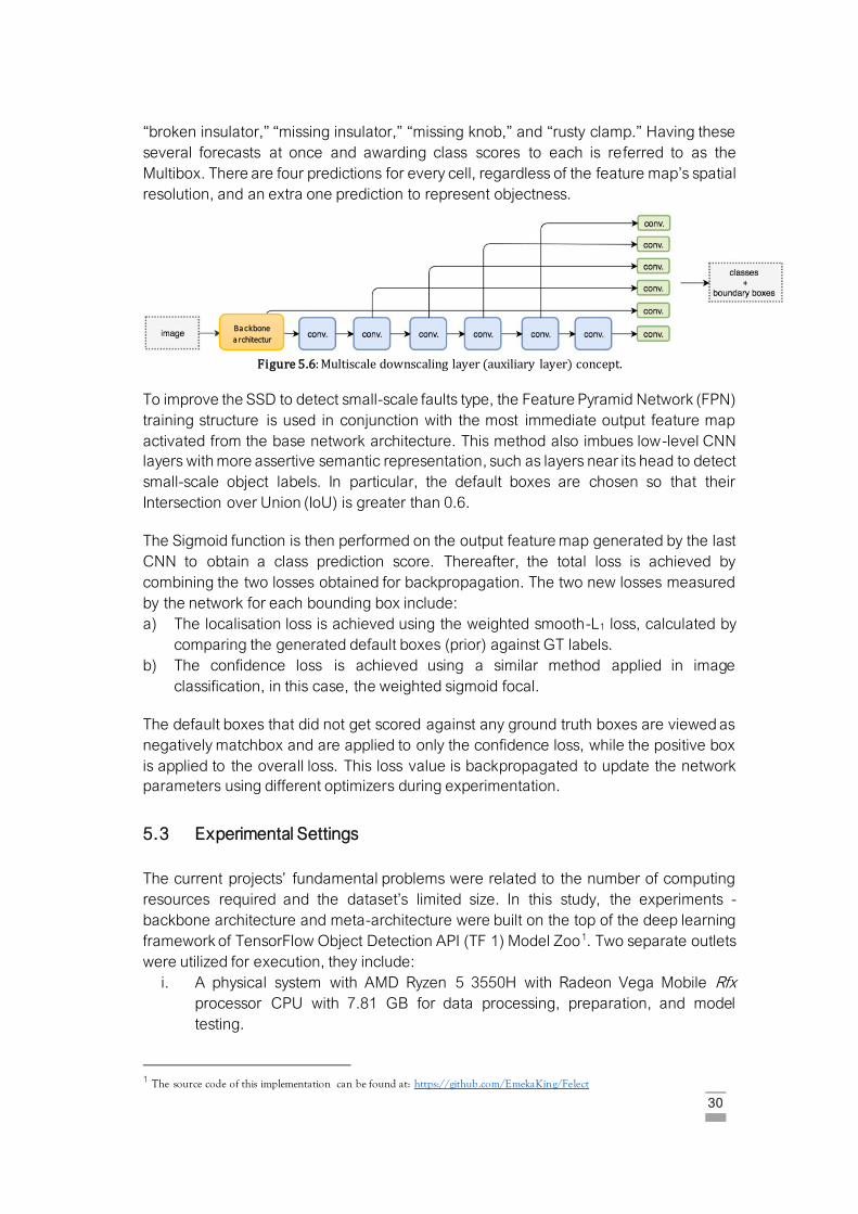
30

“broken insulator,” “missing insulator,” “missing knob,” and “rusty clamp.” Having these

several forecasts at once and awarding class scores to each is referred to as the

Multibox. There are four predictions for every cell, regardless of the feature map’s spatial

resolution, and an extra one prediction to represent objectness.

Figure 5.6: Multiscale downscaling layer (auxiliary layer) concept.

To improve the SSD to detect small-scale faults type, the Feature Pyramid Network (FPN)

training structure is used in conjunction with the most immediate output feature map

activated from the base network architecture. This method also imbues low-level CNN

layers with more assertive semantic representation, such as layers near its head to detect

small-scale object labels. In particular, the default boxes are chosen so that their

Intersection over Union (IoU) is greater than 0.6.

The Sigmoid function is then performed on the output feature map generated by the last

CNN to obtain a class prediction score. Thereafter, the total loss is achieved by

combining the two losses obtained for backpropagation. The two new losses measured

by the network for each bounding box include:

a) The localisation loss is achieved using the weighted smooth-L1 loss, calculated by

comparing the generated default boxes (prior) against GT labels.

b) The confidence loss is achieved using a similar method applied in image

classification, in this case, the weighted sigmoid focal.

The default boxes that did not get scored against any ground truth boxes are viewed as

negatively matchbox and are applied to only the confidence loss, while the positive box

is applied to the overall loss. This loss value is backpropagated to update the network

parameters using different optimizers during experimentation.

5.3 Experimental Settings

The current projects’ fundamental problems were related to the number of computing

resources required and the dataset’s limited size. In this study, the experiments -

backbone architecture and meta-architecture were built on the top of the deep learning

framework of TensorFlow Object Detection API (TF 1) Model Zoo1. Two separate outlets

were utilized for execution, they include:

i. A physical system with AMD Ryzen 5 3550H with Radeon Vega Mobile Rfx

processor CPU with 7.81 GB for data processing, preparation, and model

testing.

1 The source code of this implementation can be found at: https://github.com/EmekaKing/Felect

Ba ckbone

a rchitectur

e

31

ii. Google Colab on the Google cloud server with 2 Intel(R) Xeon(R) @ 2.20GHz

processor CPU with 13GB RAM (200 GB free space disk) and 1 GPU (Tesla K80)

with 12.6 GB RAM for parallel processing for experimentation.

To ensure optimal experimentation with the data available, the validation dataset

covering the research assets was utilized for evaluating the trained network. Due to

computation cost and speed, the k fold cross-validation was not implemented. Hence, a

hold-out validation with shuffling was used to generate an average detection result for all

the models.

The training set was used during network training, while the validation dataset was used

to modify hyperparameters. In the NMS process, 100 detections and an IoU threshold of

0.6 were maintained for each class. The momentum and the batch size were set as .9

and 8. The regularization value was set to 0.0004. The warm-up learning rate of

0.0001333 was used to assist in the weight optimization after 5,000 training steps and

at the end of the training period decay to zero. Batch normalization (BN) is used after the

convolution layer and before nonlinearity layers [81] to avoid overfitting and to save time

during hyperparameter tuning. During training, the data augmentation technique

increases samples’ diversity because of insufficient training data. Six methods were

employed for this data augmentation in the training phase: jitter boxes, horizontal flip,

vertical flip, crop, pixel value, and rotation. To ensure guaranteed detection, the IOU

confidence level is set at 0.6. Five measurements, including recall, precision, f 1 score,

and mAP, are applied to evaluate the components’ faults model performance.

Hyperparameters Values

Momentum .9

L2 regularization 0.0004

Batch size 8

IoU -Threshold 0.6

Min and max scale 3 - 7 Table 5.2: Training hyperparameters settings for CNN models

5.4 Sensitivity to Hyperparameters

In this study, the hyperparameters examined were learning rate optimizers and the

aspect ratio (Table 5.3). During the experiments, when the value of one hyperparameter

is modified, other hyperparameters are retained continuously to achieve the optimum

value of the hyperparameter.

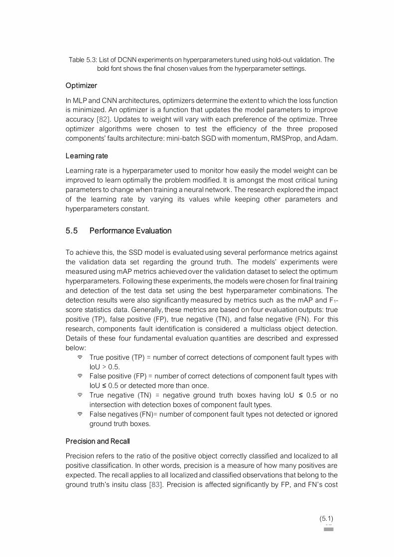
32

Table 5.3: List of DCNN experiments on hyperparameters tuned using hold-out validation. The

bold font shows the final chosen values from the hyperparameter settings.

Optimizer

In MLP and CNN architectures, optimizers determine the extent to which the loss function

is minimized. An optimizer is a function that updates the model parameters to improve

accuracy [82]. Updates to weight will vary with each preference of the optimize. Three

optimizer algorithms were chosen to test the efficiency of the three proposed

components’ faults architecture: mini-batch SGD with momentum, RMSProp, and Adam.

Learning rate

Learning rate is a hyperparameter used to monitor how easily the model weight can be

improved to learn optimally the problem modified. It is amongst the most critical tuning

parameters to change when training a neural network. The research explored the impact

of the learning rate by varying its values while keeping other parameters and

hyperparameters constant.

5.5 Performance Evaluation

To achieve this, the SSD model is evaluated using several performance metrics against

the validation data set regarding the ground truth. The models’ experiments were

measured using mAP metrics achieved over the validation dataset to select the optimum

hyperparameters. Following these experiments, the models were chosen for final training

and detection of the test data set using the best hyperparameter combinations. The

detection results were also significantly measured by metrics such as the mAP and F1-

score statistics data. Generally, these metrics are based on four evaluation outputs: true

positive (TP), false positive (FP), true negative (TN), and false negative (FN). For this

research, components fault identification is considered a multiclass object detection.

Details of these four fundamental evaluation quantities are described and expressed

below:

True positive (TP) = number of correct detections of component fault types with

IoU > 0.5.

False positive (FP) = number of correct detections of component fault types with

IoU ≤ 0.5 or detected more than once.

True negative (TN) = negative ground truth boxes having IoU ≤ 0.5 or no

intersection with detection boxes of component fault types.

False negatives (FN)= number of component fault types not detected or ignored

ground truth boxes.

Precision and Recall

Precision refers to the ratio of the positive object correctly classified and localized to all

positive classification. In other words, precision is a measure of how many positives are

expected. The recall applies to all localized and classified observations that belong to the

ground truth’s insitu class [83]. Precision is affected significantly by FP, and FN’s cost

(5.1)

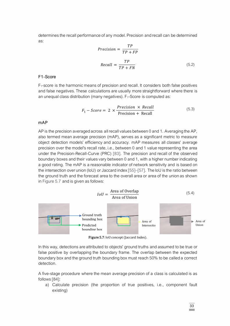
33

determines the recall performance of any model. Precision and recall can be determined

as:

𝑃𝑟𝑒𝑐𝑖𝑠𝑖𝑜𝑛 = 𝑇𝑃

𝑇𝑃 + 𝐹𝑃

𝑅𝑒𝑐𝑎𝑙𝑙 = 𝑇𝑃

𝑇𝑃 + 𝐹𝑁

F1-Score

F1-score is the harmonic means of precision and recall. It considers both false positives

and false negatives. These calculations are usually more straightforward where there is

an unequal class distribution (many negatives). F1-Score is computed as:

𝐹1 − 𝑆𝑐𝑜𝑟𝑒 = 2 × 𝑃𝑟𝑒𝑐𝑖𝑠𝑖𝑜𝑛 × 𝑅𝑒𝑐𝑎𝑙𝑙

Precision + Recall

mAP

AP is the precision averaged across all recall values between 0 and 1. Averaging the AP,

also termed mean average precision (mAP), serves as a significant metric to measure

object detection models’ efficiency and accuracy. mAP measures all classes' average

precision over the model's recall rate, i.e., between 0 and 1 value representing the area

under the Precision-Recall-Curve (PRC) [83]. The precision and recall of the observed

boundary boxes and their values vary between 0 and 1, with a higher number indicating

a good rating. The mAP is a reasonable indicator of network sensitivity and is based on

the intersection over union (IoU) or Jaccard index [55]–[57]. The IoU is the ratio between

the ground truth and the forecast area to the overall area or area of the union as shown

in Figure 5.7 and is given as follows:

𝐼𝑜𝑈 = Area of Overlap

Area of Union

Figure 5.7: IoU concept (Jaccard Index).

In this way, detections are attributed to objects' ground truths and assumed to be true or

false positive by overlapping the boundary frame. The overlap between the expected

boundary box and the ground truth bounding box must reach 50% to be called a correct

detection.

A five-stage procedure where the mean average precision of a class is calculated is as

follows [84]:

a) Calculate precision (the proportion of true positives, i.e., component fault

existing)

Ground truth bounding box

Predicted bounding box

Area of

Intersectio

n

Area of Union

(5.2)

(5.3)

(5.4)

34

b) Calculate recall (the proportion of good positive out of all events)

c) Compute the Precision x Recall curve for the various thresholds. For this, we

must first order the detections by their confidences, then determine the precision

and recall for each cumulative detection.

d) Average the overall precision value for all recall stages. By Interpolating over all

data points or an 11-point interpolation, i.e., by calculating the precision of the

eleven recall stages evenly spaced [0, 0.1, 0.2, ..., 1.], the average precision

score for each class is:

𝐴𝑃 = 1

11∑ 𝑃𝑟𝑒𝑐𝑖𝑠𝑖𝑜𝑛(𝑅𝑒𝑐𝑎𝑙𝑙𝑖)

𝑅𝑒𝑐𝑎𝑙𝑙𝑖∈{0,0.1,…,1.}

e) Finally, the mAP is determined by taking the average AP for all classes and/or

IoU thresholds. The mAP is approximated AUC of the Precision x Recall curve.

In the current project, only one IoU threshold (mAP@0.5) is considered.

(5.5)

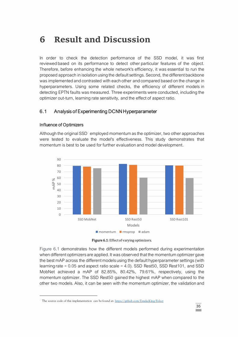
35

6 Result and Discussion

In order to check the detection performance of the SSD model, it was first

reviewed based on its performance to detect other particular features of the object.

Therefore, before enhancing the whole network's efficiency, it was essential to run the

proposed approach in isolation using the default settings. Second, the different backbone

was implemented and contrasted with each other and compared based on the change in

hyperparameters. Using some related checks, the efficiency of different models in

detecting EPTN faults was measured. Three experiments were conducted, including the

optimizer out-turn, learning rate sensitivity, and the effect of aspect ratio.

6.1 Analysis of Experimenting DCNN Hyperparameter

Influence of Optimizers

Although the original SSD2 employed momentum as the optimizer, two other approaches

were tested to evaluate the model's effectiveness. This study demonstrates that

momentum is best to be used for further evaluation and model development.

Figure 6.1: Effect of varying optimizers.

Figure 6.1 demonstrates how the different models performed during experimentation

when different optimizers are applied. It was observed that the momentum optimizer gave

the best mAP across the different models using the default hyperparameter settings (with

learning rate = 0.05 and aspect ratio scale = 4.0). SSD Rest50, SSD Rest101, and SSD

MobNet achieved a mAP of 82.85%, 80.42%, 79.61%, respectively, using the

momentum optimizer. The SSD Rest50 gained the highest mAP when compared to the

other two models. Also, it can be seen with the momentum optimizer, the validation and

2 The source code of this implementation can be found at: https://github.com/EmekaKing/Felect

0

10

20

30

40

50

60

70

80

90

SSD MobNet SSD Rest50 SSD Rest101

mA

P %

Models

momentum rmsprop adam

36

total loss converge optimally. Furthermore, it has been expressively proven that the

model's convergence is affected by the optimizer utilized, as seen in Table 6.1.

Table 6.1: Influence of using varying optimizers.

We can also observe based on Table 6.1 that all the optimizers attain acceptable rates

of mAP, but one of the most glaring differences in the value of training loss and validation

loss as well as the model convergence, i.e., the degree of loss range from zero. It can be

inferred that the optimizer momentum with cosine learning rate is the one that provides

the best results and the quickest to converge.

Learning rate effect

Using Momentum as the ideal learning algorithm, numerous learning rate settings were

checked to improve the model performance. After several preliminary evaluations, it was

confirmed that the best initial Learning rate (Lr) was 0.09.

Figure 6.2: The accuracy achieved using varying learning rates.

The learning rate detection results are presented in Figure 6.2, with the aspect ratio scale

is set to 4. The first model, SSD MobNet, reached a mAP of 73.94%, 71.56%, 79.61%,

and 82.52%, with the learning rate was 0.001, 0.01, 0.05, and 0.09 respectively, better

performance of the model with increasing learning rate value. Similarly, the remaining

0

10

20

30

40

50

60

70

80

90

100

SSD MobNet SSD Rest50 SSD Rest101

mA

P %

Models

0.001 0.01 0.05 0.09

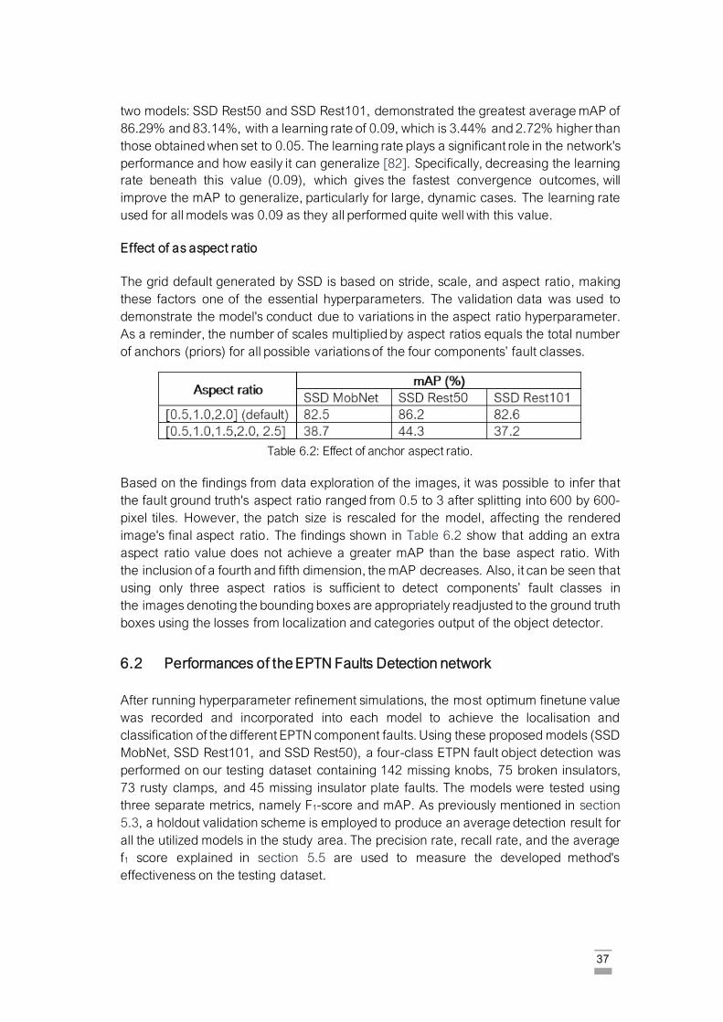
37

two models: SSD Rest50 and SSD Rest101, demonstrated the greatest average mAP of

86.29% and 83.14%, with a learning rate of 0.09, which is 3.44% and 2.72% higher than

those obtained when set to 0.05. The learning rate plays a significant role in the network's

performance and how easily it can generalize [82]. Specifically, decreasing the learning

rate beneath this value (0.09), which gives the fastest convergence outcomes, will

improve the mAP to generalize, particularly for large, dynamic cases. The learning rate

used for all models was 0.09 as they all performed quite well with this value.

Effect of as aspect ratio

The grid default generated by SSD is based on stride, scale, and aspect ratio, making

these factors one of the essential hyperparameters. The validation data was used to

demonstrate the model's conduct due to variations in the aspect ratio hyperparameter.

As a reminder, the number of scales multiplied by aspect ratios equals the total number

of anchors (priors) for all possible variations of the four components’ fault classes.

Table 6.2: Effect of anchor aspect ratio.

Based on the findings from data exploration of the images, it was possible to infer that

the fault ground truth's aspect ratio ranged from 0.5 to 3 after splitting into 600 by 600-

pixel tiles. However, the patch size is rescaled for the model, affecting the rendered

image's final aspect ratio. The findings shown in Table 6.2 show that adding an extra

aspect ratio value does not achieve a greater mAP than the base aspect ratio. With

the inclusion of a fourth and fifth dimension, the mAP decreases. Also, it can be seen that

using only three aspect ratios is sufficient to detect components’ fault classes in

the images denoting the bounding boxes are appropriately readjusted to the ground truth

boxes using the losses from localization and categories output of the object detector.

6.2 Performances of the EPTN Faults Detection network

After running hyperparameter refinement simulations, the most optimum finetune value

was recorded and incorporated into each model to achieve the localisation and

classification of the different EPTN component faults. Using these proposed models (SSD

MobNet, SSD Rest101, and SSD Rest50), a four-class ETPN fault object detection was

performed on our testing dataset containing 142 missing knobs, 75 broken insulators,

73 rusty clamps, and 45 missing insulator plate faults. The models were tested using

three separate metrics, namely F1-score and mAP. As previously mentioned in section

5.3, a holdout validation scheme is employed to produce an average detection result for

all the utilized models in the study area. The precision rate, recall rate, and the average

f1 score explained in section 5.5 are used to measure the developed method's

effectiveness on the testing dataset.

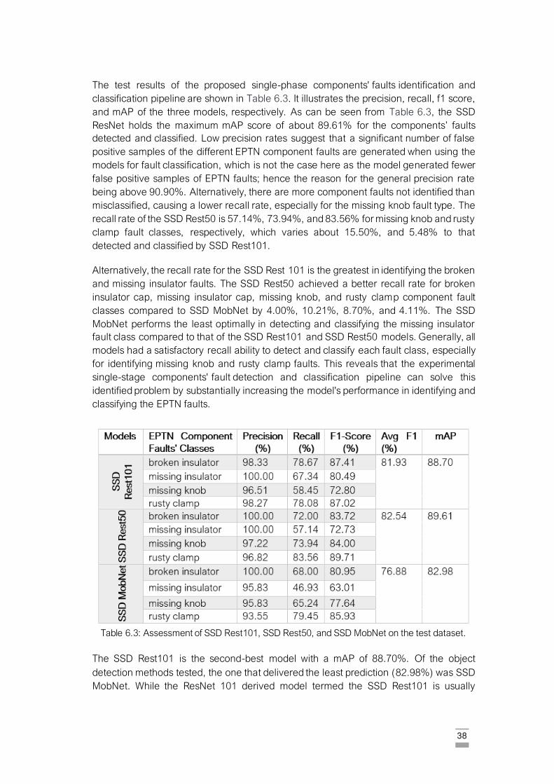
38

The test results of the proposed single-phase components' faults identification and

classification pipeline are shown in Table 6.3. It illustrates the precision, recall, f1 score,

and mAP of the three models, respectively. As can be seen from Table 6.3, the SSD

ResNet holds the maximum mAP score of about 89.61% for the components’ faults

detected and classified. Low precision rates suggest that a significant number of false

positive samples of the different EPTN component faults are generated when using the

models for fault classification, which is not the case here as the model generated fewer

false positive samples of EPTN faults; hence the reason for the general precision rate

being above 90.90%. Alternatively, there are more component faults not identified than

misclassified, causing a lower recall rate, especially for the missing knob fault type. The

recall rate of the SSD Rest50 is 57.14%, 73.94%, and 83.56% for missing knob and rusty

clamp fault classes, respectively, which varies about 15.50%, and 5.48% to that

detected and classified by SSD Rest101.

Alternatively, the recall rate for the SSD Rest 101 is the greatest in identifying the broken

and missing insulator faults. The SSD Rest50 achieved a better recall rate for broken

insulator cap, missing insulator cap, missing knob, and rusty clamp component fault

classes compared to SSD MobNet by 4.00%, 10.21%, 8.70%, and 4.11%. The SSD

MobNet performs the least optimally in detecting and classifying the missing insulator

fault class compared to that of the SSD Rest101 and SSD Rest50 models. Generally, all

models had a satisfactory recall ability to detect and classify each fault class, especially

for identifying missing knob and rusty clamp faults. This reveals that the experimental

single-stage components' fault detection and classification pipeline can solve this

identified problem by substantially increasing the model's performance in identifying and

classifying the EPTN faults.

Table 6.3: Assessment of SSD Rest101, SSD Rest50, and SSD MobNet on the test dataset.

The SSD Rest101 is the second-best model with a mAP of 88.70%. Of the object

detection methods tested, the one that delivered the least prediction (82.98%) was SSD

MobNet. While the ResNet 101 derived model termed the SSD Rest101 is usually

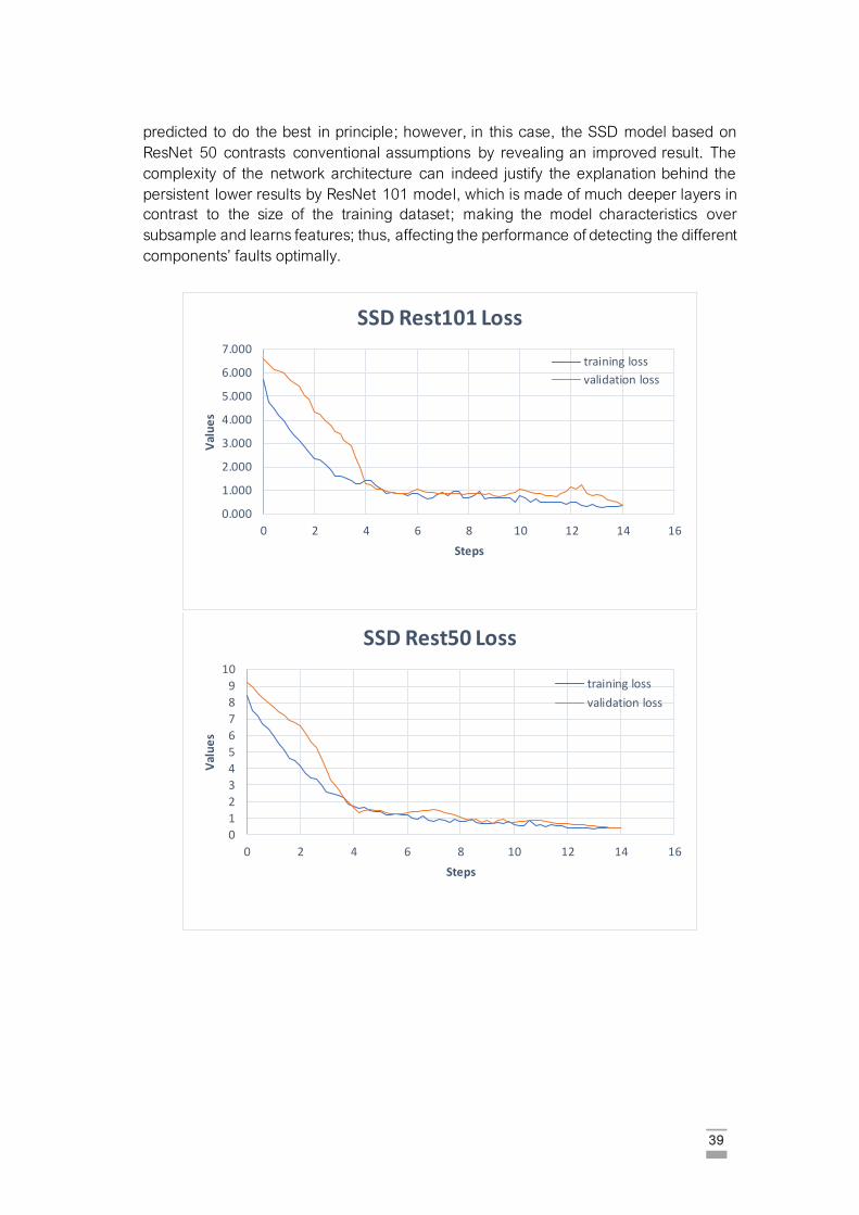
39

predicted to do the best in principle; however, in this case, the SSD model based on

ResNet 50 contrasts conventional assumptions by revealing an improved result. The

complexity of the network architecture can indeed justify the explanation behind the

persistent lower results by ResNet 101 model, which is made of much deeper layers in

contrast to the size of the training dataset; making the model characteristics over

subsample and learns features; thus, affecting the performance of detecting the different

components’ faults optimally.

0.000

1.000

2.000

3.000

4.000

5.000

6.000

7.000

0 2 4 6 8 10 12 14 16

Val

ue

s

Steps

SSD Rest101 Loss

training loss

validation loss

0

1

2

3

4

5

6

7

8

9

10

0 2 4 6 8 10 12 14 16

Val

ue

s

Steps

SSD Rest50 Loss

training loss

validation loss

40

Figure 6.3: Epoch vs. Loss Graphs.

Furthermore, to intuitively reflect the proposed model's detection performance, the loss

value graph was evaluated to understand, rationalize, and justify the proposed models'

generalization ability. In general, we can assess the proposed model's performance using

the loss graphs and the summary information of the validation loss and examine the

group of classification, localisation, and regularization loss [57]. Figure 6.3 gives

snapshots of the loss values sensitivity over the training and validation phase over the

network trajectory. A good performance is established by a total and validation loss that

reduces until it becomes stable and the difference between both loss values reaches a

minimum [82]. If the prediction errors are unbiased, the validation error should be near

zero, and the validation loss decrease with a decrease in training loss. This can be seen

distinctively by the loss graph of SSD Rest50, SSD Rest101, and SSD MobNet model.

The Rest50 model represents a Deep network; the SSD Rest 101 can be seen as a super

Deep Network, while the SSD MobNet is a shallow network.

It can be seen that the various weight optimizations associated with the training and

validation of the dataset based on the model architecture show that the loss value

remained relatively stable. In the experiments, the base and top CNN layer used the

Rectified Linear Units (ReLUs) [31] as activation functions over shuffled mini-batch

gradient descent (batch size of 8) with the Adam optimization algorithm. The final output

uses a sigmoid classifier for each decision node. Using the sigmoid activation, the final

achieved pair total losses, i.e., [validation loss, training loss] for the SSD MobNet, SSD

Rest50, and SSD Rest101, were approximately equal to [0.281, 0.309], [0.378, 0.385]

and [0.356, 0.342] respectively.

In contrast to the SSD MobNet, SSD Rest50 and SSD Rest101 have higher orders of

magnitude as they have more parameters because they have more layers and more

filters per layer. This allowed the model to adapt to more convoluted representations

(features) than the shallow network can provide. In the SSD Rest101, it is observable

that the dataset was not sufficient to train the deeper network. The ResNet 50 backbone

architecture, which represents the Deep Network, performs much better in minimizing

0

0.5

1

1.5

2

2.5

3

3.5

4

0 2 4 6 8 10 12 14 16

Val

ue

s

Steps

SSD MobNet Loss

training loss

validation loss

41

the loss values than the other two networks, accomplishing train and validation losses of

0.378 and 0.385, respectively, after 15 epochs. Finally, there is a strong link between

training loss and validation loss. They both decrease and then become stable at a

constant value. This suggests that the model is correctly trained and has a high

probability of working well over testing data within this domain.

6.3 Further Investigation

It should be noted that the proposed method and the SSMD [85] method achieve a high

precision rate but have a lesser recall rate, especially for the missing insulator cap faults.

This can be attributed to the inability to identify small-scale missing cap insulator location

due to minuscule pixel area (about 20 x 20 pixel) indistinguishable from each other in the

600 × 600-pixel input patch image. After the downsampling of pooled CNN outputs,

much of the semantic information about missing insulator cap fault would be overwritten

by the contextual background. This will lead to difficulty in identifying faults, such as the

missing insulator caps. Also, the lack of sufficient missing insulator samples in the test

dataset could be responsible. However, this study's proposed method incorporates other

component fault types all at once, which cannot be seen in the other developed model

and could be somewhat said to be responsible for the low satisfactory recall rate. As far

as these fault detection methods' overall efficiency is concerned, the proposed method

has demonstrated that the algorithms' continued developments could be improved.

The proposed system performs object detection using a series of weights extracted from

a set of representative random seeds, where each weight corresponds to a specific

perspective of the problem being considered (four-component faults) and is developed

using an iterative method in which alternative refining and integration of compatible

training examples are performed. SSD has shown the capacity to detect multiclass faults

from the UAV imagery; however, improvements such as image tiling to tackle small -scale

problems and sufficient datasets are required. While experimenting with the model,

overfit and exploding gradient sometimes manifest, which can be resolved by different

techniques, requiring training the model over long periods. Finally, our findings show

much greater precision using well-calibrated UAV images and a reasonably good recall

rate. In summary, the comparison with detection results from the literature review with

the analysis in this current work indicates the suitability of deep learning to monitor and

detect components fault on electric power transmission networks to help the decision-

making process required for asset management in developing countries like Nigeria.

6.4 Qualitative Experimental Evaluations

Figure 6.4 provides an example of all the output images produced by all the

models implemented. The sky-blue box denotes the missing insulator; the green box

denotes the broken insulator, the turquoise box denotes the missing knob faults, while

the white box bounds the rusty clamp defects. Each box is marked by the components'

faults and its confidence score. In contrast, the red ellipse show faults undetected by the

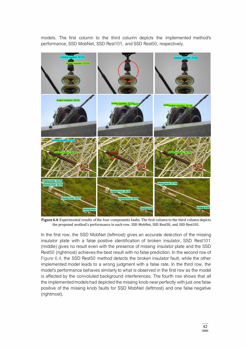
42

models. The first column to the third column depicts the implemented method's

performance, SSD MobNet, SSD Rest101, and SSD Rest50, respectively.

Figure 6.4: Experimental results of the four components faults. The first column to the third column depicts

the proposed method's performance in each row, SSD MobNet, SSD Rest50, and SSD Rest101.

In the first row, the SSD MobNet (leftmost) gives an accurate detection of the missing

insulator plate with a false positive identification of broken insulator, SSD Rest101

(middle) gives no result even with the presence of missing insulator plate and the SSD

Rest50 (rightmost) achieves the best result with no false prediction. In the second row of

Figure 6.4, the SSD Rest50 method detects the broken insulator fault, while the other

implemented model leads to a wrong judgment with a false rate. In the third row, the

model's performance behaves similarly to what is observed in the first row as the model

is affected by the convoluted background interferences. The fourth row shows that all

the implemented models had depicted the missing knob near perfectly with just one false

positive of the missing knob faults for SSD MobNet (leftmost) and one false negative

(rightmost).

43

7 Conclusion

7.1 Findings

This thesis explores the use of high-resolution multispectral UAV-based imagery for

electric power transmission line component fault detection using the deep learning

approach without any physical participation by the site inspection by engineers. This

research's feasibility test was conducted using the Shiroro-Kaduna transmission network

in Niger State as a case study, one of the substations for the Transmission Company of

Nigeria. The results demonstrate the feasibility of using high-resolution multispectral

UAV-based imagery to identify and classify transmission component faults, particularly

for emerging and formative transmission companies in developing countries confronted

by data scarcity, asset seclusion, and insecurity ground-surveys complexity,

untimeliness, and general human cost. The final models utilizing SSD object detection

pipeline were developed in this study as an approach for power transmission network

components fault identification. After analysing the results of the revealed studies, some

important conclusions can be reached, such as:

a) Which are different hyperparameters finetuning yields the best results in the

implemented deep learning model?

To help address this research query, all the chosen object detection models using

various backbone architecture were implemented in Chapter 53. The models'

efficiency was analysed in an exhaustive hyperparameter configuration setting to

choose the best hyperparameter values. In addition to this, some retrospective

studies were run to assess the usefulness of the DCNN. The following conclusions

were observed:

Transfer learning is a better strategy to follow to produce short-term outcomes.

Since the issue being discussed requires data that is not identical to current

datasets (weights trained on images with little or no geocentric interests),

processing just the weights of the pre-trained model resulted in a more robust

outcome than freezing the layers, with the repercussion of a slower training

method. This helps scopes out the model weight so that the model weight

optimization is not starting from scratch, i.e., net-zero but from an existing optimal

value for each convolution layer;

The adaptive optimizer, momentum with mini-batch SGD, allowed for the faster

convergence of the proposed model and to automatically predict the optimum

learning rate;

It was observed that higher learning rate achieved better mAP values across all

the models implemented;

3 The source code of this implementation can be found at: https://github.com/EmekaKing/Felect

44

During preparation, the objects' measurements in the images were precisely

calculated to determine the best values for the anchor parameters accurately.

The model achieved better mAP by using the default three aspect ratio value.

Furthermore, data augmentation was a vital technique allowing the model to

manage invariance among the component fault classes and improve the size of

a training dataset.

b) To what extent will the deep convolution neural network perform based on the

predicted component fault classes' performance metrics analysis?

The assessment of object detection models showed that the implemented SSD

selected based on speed and computing capabilities models achieve excellent

results both in localising and classifying components faults utilizes high-resolution

RGB images with complex background context. The deep learning object detection

models implemented offered high mAP, with SSD Rest50 achieving the best, followed

by SSD Rest101 and SSD MobNet regarding mAP and F1-score. Given the findings,

we can deduce that in the case of related network architectures, SSD Rest50

performs better than SSD Rest101, demonstrating that spatial and semantic

knowledge and representations with the right proportion of deep layers like SSD

Rest50 obtains a better detection accuracy. Second, the improved performance of

ConvNet SSD MobNet indicates that the least-complex network architecture with the

lesser number of filters does not lead to increased accuracy of the model and that

any smaller native model with fewer blocks could require a much deeper or broader

design. In the final step, the applied models' competence was checked by the final

achieved error based on the loss values deducted by the difference between the

training error and validation error. The final model shows that our EPTN fault

detection accuracy is feasible and achievable with remarkable performance.

With this, the thesis's aim was achieved, which is “to propagate the possibility of detecting and inspecting EPTN assets of Electric Utilities in Nigeria utilizing UAV imagery and deep learning approach.” In summary, the findings are positive and optimistic. It can be seen

that object detection strategies could help monitor faults on transmission lines, monitor

assets, and optimize EPTN for Transmission companies using deep learning. Further

research on applying other deep neural networks, i.e., instance segmentation model to

different transmission line components fault identification, is encouraged.

7.2 Limitation

While the study produced promising research findings, there are several limi tations and

opportunities for further research, mainly dataset sampling, and standardized evaluation

metrics. A majority of EPTN corridors use a wide variety of power line components.

Consequently, the grids are exposed to a tremendous range of problems. Additionally,

other small defects in power line components such as missing knobs and rust can occur

in various forms and simultaneously; and are described differently based on the expertise

and technical framework of electric utilities. This, combined with the lack of uniform

training/validation data, presents a significant challenge for the inspection of vision-based

45

faults using a combination of RGB imagery and DL due to the lack of templates for

classifying unknown groups.

Regarding the evaluation baseline, the assessment of object detection projects is

subjective. There is little standard exposition in studies concerning analysis metrics and

computation, especially against the dataset, and the degree to which the analysis

methods generalize are still limited. The final output containing a bounding box should

undergo digital photogrammetry workflow to form a 3D electrical transmission model

network and further analyzed to identify severity level to assist site inspectors and

engineers in planning and implementing fault repairs across multiple remote and

unsecured locations. Due to image acquisition technical specifications limitations and

some deficient computer science skills, concrete cartographic products (maps) are not

provided. Hence, the result contained a CSV file containing the bounding box’s

coordinates, fault type, and confidence sore, and the detected tiled images with

bounding box overlaid and linked to the original geolocated imagery. Consequently,

investigating spatial patterns existing among the fault detected fell outside this thesis’s

scope.

7.3 Future Works

The findings discussed in Chapter 6 have several aspects that require further analysis.

To enhance this analysis, several possible steps are posited:

First, the single-stage component identification and classification pipeline should be

expanded to account for faults in different components' shapes and severity levels. Two

phases are used simultaneously in the developed frameworks: first, location of

components faults; second, determination and classification of the component faults. The

pipeline can detect four different types of defects from inspection images; however, it

cannot measure the magnitude of the detected defects' scale. One alternative solution

is to determine the limits of the observed faults directly at the precise pixel level by

applying instance segmentation and uses this knowledge to measure the scale and

magnitude of the faults by, for example, estimating the defect/component pixel ratio.

Second, this study concentrates on only high-resolution multispectral RGB

(visible) bands of the electric transmission network corridor right-of-way (ROW). Hence

there is a need to incorporate other various data sources that adopt the other

electromagnetic channel such as thermal images, ultraviolet images, aerial and mobile

laser scanning images. This will allow creating a model pipeline inclusive to others not

detectable by the human eye, such as wire failure and corona discharges.

Third, power transmission networks have various components, and issues arise in

different positions concerning these components. These components have several

different instances and manifestations, and those instances can have different

characteristics such as colour, form, texture, scale, and content. Furthermore, the

change in imaging state will result in the object's presence being affected consistently.

The dynamic context involves the photo's direction and distance, occlusion, context, and

lighting conditions. Two methods can be explored to solve the issue of component fault

46

imbalance and intra-component variation. They include foreground and background

overlay using segmentation network and image processing technique; and Generative

Adversarial Networks (GANs) to create synthetic images.

Fourth, the model can be extended to cover for real-time autonomous vision detection in

the field incorporated with GPS-INS navigation, i.e., motion pictures. This can be

consolidated into synchronized database logging camera GPS position and time logs and

linked to a multiple object monitoring algorithm to allow fully automated asset

management during data acquisition.

47

Bibliographic References

[1] S. Alkire, A. Conconi, G. Robles, and A. V. June, “Who and where are the poorest

of the poor?” 2015.

[2] R. B. Johnston, “Arsenic and the 2030 Agenda for sustainable development,”

Arsen. Res. Glob. Sustain. - Proc. 6th Int. Congr. Arsen. Environ. AS 2016, pp.

12–14, 2016, doi: 10.1201/b20466-7.

[3] L. Matikainen et al., “Remote sensing methods for power line corridor surveys,”

ISPRS J. Photogramm. Remote Sens., vol. 119, pp. 10–31, 2016, doi:

10.1016/j.isprsjprs.2016.04.011.

[4] D. Mentis et al., “Energy for Sustainable Development A GIS-based approach for

electrification planning — A case study on Nigeria,” Energy Sustain. Dev., vol. 29,

pp. 142–150, 2015, doi: 10.1016/j.esd.2015.09.007.

[5] P. Bertheau, C. Cader, and P. Blechinger, “Electrification modelling for Nigeria,”

Energy Procedia, vol. 93, no. March, pp. 108–112, 2016, doi:

10.1016/j.egypro.2016.07.157.

[6] B. Meehan, Modelling Electricity Distribution with GIS, 1st Editio. ESRI Press,

2013.

[7] Ikeja Electric (IE), “Sustainability Report,” Lagos, 2016.

[8] P. Mayer and P. Mayer, “Corrosion evaluation methods for power transmission

lines.”

[9] Matergenics, “Corrosion Inspection of Power Transmission Structures,” 2020.

http://www.matergenics.com/drone-inspection-services/corrosion-inspection-of-

power-transmission-structures (accessed May 15, 2020).

[10] H. Baorong, The Cost of Corrosion in China, 1st Ed. Netherlands: Beijing: Science

Press/ Springer, 2019.

[11] Y. Hu and K. Liu, Remote sensing and remote measurement technology of transmission lines. 2017.

[12] H. Guan, Y. Yu, J. Li, Z. Ji, and Q. Zhang, “Extraction of power-transmission lines

from vehicle-borne lidar data,” Int. J. Remote Sens., vol. 37, no. 1, pp. 229–247,

2016, doi: 10.1080/01431161.2015.1125549.

[13] A. Zormpas, K. Moirogiorgou, K. Kalaitzakis, G. A. Plokamakis, and P.

Partsinevelos, “Power Transmission Lines Inspection using Properly Equipped

Unmanned Aerial Vehicle ( UAV ),” 2018 IEEE Int. Conf. Imaging Syst. Tech., pp.

1–5, 2018.

[14] J. Ahmad, A. S. Malik, M. F. Abdullah, N. Kamel, and L. Xia, “A novel method for

48

vegetation encroachment monitoring of transmission lines using a single 2D

camera,” Pattern Anal. Appl., vol. 18, no. 2, pp. 419–440, 2015, doi:

10.1007/s10044-014-0391-9.

[15] X. Yu, X. Wu, C. Luo, and P. Ren, “Deep learning in remote sensing scene

classification: a data augmentation enhanced convolutional neural network

framework,” GIScience Remote Sens., vol. 54, no. 5, pp. 741–758, 2017, doi:

10.1080/15481603.2017.1323377.

[16] Y. Baştanlar and M. Özuysal, “Introduction to machine learning,” Methods Mol. Biol., vol. 1107, pp. 105–128, 2014, doi: 10.1007/978-1-62703-748-8_7.

[17] R. A. McLaughlin, “Extracting transmission lines from airborne LIDAR data,” IEEE Geosci. Remote Sens. Lett., vol. 3, no. 2, pp. 222–226, 2006, doi:

10.1109/LGRS.2005.863390.

[18] Y. Hu and K. Liu, Parameters and characteristics of transmission lines. 2017.

[19] G. E. Braga and R. M. R. Junqueira, “Methodology for Planning Tower Leg

Foundations Corrosion Maintenance of Overhead Transmission Lines Based on

GIS,” IEEE Trans. Power Deliv., vol. 31, no. 4, pp. 1601–1608, 2016, doi:

10.1109/TPWRD.2016.2524003.

[20] Z. Lin, Z. Xu, and I. Engineering, “A METEOROLOGICAL RISK ASSESSMENT

METHOD FOR POWER LINES BASED,” vol. III, no. July, pp. 12–19, 2016, doi:

10.5194/isprsannals-III-8-19-2016.

[21] K. Chen, C. Huang, and J. He, “Fault detection, classification and location for

transmission lines and distribution systems: A review on the methods,” High Volt.,

vol. 1, no. 1, pp. 25–33, 2016, doi: 10.1049/hve.2016.0005.

[22] V. C. Ogboh and T. C. Madueme, “Investigation of Faults on the Nigerian Power

System Transmission Line Using Artificial Neural Network,” Int. J. Res. Manag. Sci. Technol. (E, vol. 3, no. 4, pp. 87–95, 2015, [Online]. Available:

www.ijrmst.org.

[23] F. Miralles, N. Pouliot, and S. Montambault, “State-of-the-art review of computer

vision for the management of power transmission lines,” Proc. 3rd Int. Conf. Appl. Robot. Power Ind. CARPI 2014, 2015, doi: 10.1109/CARPI.2014.7030068.

[24] Z. A. Siddiqui and U. Park, “A Drone Based Transmission Line Components

Inspection System with Deep Learning Technique,” Energies, vol. 13, no. 13, pp.

1–24, 2020, doi: 10.3390/en13133348.

[25] Z. Zhao, G. Xu, Y. Qi, N. Liu, and T. Zhang, “Multi-patch deep features for power

line insulator status classification from aerial images,” Proc. Int. Jt. Conf. Neural Networks, vol. 2016-October, pp. 3187–3194, 2016, doi:

10.1109/IJCNN.2016.7727606.

[26] Y. Wang and B. Yan, “Vision-based detection and location for cracked insulator,”

Comput. Eng. Des., vol. 35, no. 2, pp. 583–587, 2014, [Online]. Available:

49

https://pay.cnki.net/zscsdoc/download?flag=cnkispace&plat=cnkispace&filenam

e=SJSJ201402043&dbtype=CJFD&year=2014&dtype=pdf.

[27] Z. Xue, S. Luo, Y. Chen, and L. Tong, “The application of the landslides detection

method based on SAR images to transmission line corridor area,” 2016 13th Int. Comput. Conf. Wavelet Act. Media Technol. Inf. Process. ICCWAMTIP 2017, pp.

163–166, 2017, doi: 10.1109/ICCWAMTIP.2016.8079829.

[28] L. Yan, W. Wu, and T. Li, “Power transmission tower monitoring technology based

on TerraSAR-X products,” Int. Symp. Lidar Radar Mapp. 2011 Technol. Appl., vol.

8286, p. 82861E, 2011, doi: 10.1117/12.912336.

[29] S. Li et al., “Study on extra-high voltage power line scatterers in time series SAR,”

3rd Int. Work. Earth Obs. Remote Sens. Appl. EORSA 2014 - Proc., no. May 2016,

pp. 47–51, 2014, doi: 10.1109/EORSA.2014.6927847.

[30] Y. Liu, K. Xu, S. Shi, and T. Li, “Effects of Span Length and Radar Polarimetry on

the Backscattering Characteristics of Ultra-High Voltage Power Transmission Line

in TerraSAR-X Images,” 5th Int. Work. Earth Obs. Remote Sens. Appl. EORSA 2018 - Proc., pp. 5–9, 2018, doi: 10.1109/EORSA.2018.8598570.

[31] J. Ahmad, A. S. Malik, L. Xia, and N. Ashikin, “Vegetation encroachment

monitoring for transmission lines right-of-ways: A survey,” Electr. Power Syst. Res., vol. 95, pp. 339–352, 2013, doi: 10.1016/j.epsr.2012.07.015.

[32] X. Yu et al., “Comparison of laser and stereo optical, SAR and InSAR point clouds

from the air- and space-borne sources in the retrieval of forest inventory

attributes,” Remote Sens., vol. 7, no. 12, pp. 15933–15954, 2015, doi:

10.3390/rs71215809.

[33] M. Jaya Bharata Reddy, B. Karthik Chandra, and D. K. Mohanta, “Condition

monitoring of 11 kV distribution system insulators incorporating complex imagery

using combined DOST-SVM approach,” IEEE Trans. Dielectr. Electr. Insul., vol.

20, no. 2, pp. 664–674, 2013, doi: 10.1109/TDEI.2013.6508770.

[34] J. Jiang, L. Zhao, J. Wang, Y. Liu, M. Tang, and Z. Ji, “The electrified insulator

parameter measurement for flashover based on photogrammetric method,”

MIPPR 2011 Multispectral Image Acquis. Process. Anal., vol. 8002, no. 86, p.

80021I, 2011, doi: 10.1117/12.902054.

[35] R. V. Ussyshkin, L. Theriault, M. Sitar, and T. Kou, “Advantages of airborne lidar

technology in power line asset management,” 2011 Int. Work. Multi-Platform/Multi-Sensor Remote Sens. Mapping, M2RSM 2011, pp. 1–5, 2011, doi:

10.1109/M2RSM.2011.5697427.

[36] L. F. Luque-Vega, B. Castillo-Toledo, A. Loukianov, and L. E. Gonzalez-Jimenez,

“Power line inspection via an unmanned aerial system based on the quadrotor

helicopter,” Proc. Mediterr. Electrotech. Conf. - MELECON, no. April, pp. 393–

397, 2014, doi: 10.1109/MELCON.2014.6820566.

[37] M. Wang, W. Tong, and S. Liu, “Fault detection for power line based on

50

convolution neural network,” ACM Int. Conf. Proceeding Ser., vol. Part F128535,

pp. 95–101, 2017, doi: 10.1145/3094243.3094254.

[38] Y. Tiantian, Y. Guodong, and Y. Junzhi, “Feature fusion-based insulator detection

for aerial inspection,” Chinese Control Conf. CCC, pp. 10972–10977, 2017, doi:

10.23919/ChiCC.2017.8029108.

[39] K. Chen, J. Hu, and J. He, “Detection and Classification of Transmission Line

Faults Based on Unsupervised Feature Learning and Convolutional Sparse

Autoencoder,” IEEE Trans. Smart Grid, vol. 9, no. 3, pp. 1748–1758, 2018, doi:

10.1109/TSG.2016.2598881.

[40] Y. Song et al., “A vision-based method for the broken spacer detection,” 2015 IEEE Int. Conf. Cyber Technol. Autom. Control Intell. Syst. IEEE-CYBER 2015, pp.

715–719, 2015, doi: 10.1109/CYBER.2015.7288029.

[41] Y. Hao et al., “Icing condition assessment of in-service glass insulators based on

graphical shed spacing and graphical shed overhang,” Energies, vol. 11, no. 2,

2018, doi: 10.3390/en11020318.

[42] L. Yang et al., “Recognition of natural ice types on in-service glass insulators

based on texture feature descriptor,” IEEE Trans. Dielectr. Electr. Insul., vol. 24,

no. 1, pp. 535–542, 2017, doi: 10.1109/TDEI.2016.006049.

[43] Y. Zhai, H. Cheng, R. Chen, Q. Yang, and X. Li, “Multi-saliency aggregation-based

approach for insulator flashover fault detection using aerial images,” Energies, vol.

11, no. 2, pp. 1–12, 2018, doi: 10.3390/en11020340.

[44] Y. Zhai, D. Wang, M. Zhang, J. Wang, and F. Guo, “Fault detection of insulator

based on saliency and adaptive morphology,” Multimed. Tools Appl., vol. 76, no.

9, pp. 12051–12064, 2017, doi: 10.1007/s11042-016-3981-2.

[45] J. Han et al., “A method of insulator faults detection in aerial images for high-

voltage transmission lines inspection,” Appl. Sci., vol. 9, no. 10, pp. 1–22, 2019,

doi: 10.3390/app9102009.

[46] J. Han et al., “Search like an eagle: A cascaded model for insulator missing faults

detection in aerial images,” Energies, vol. 13, no. 3, pp. 1–20, 2020, doi:

10.3390/en13030713.

[47] X. Li, N. Kwok, J. E. Guivant, K. Narula, R. Li, and H. Wu, “Detection of imaged

objects with estimated scales,” VISIGRAPP 2019 - Proc. 14th Int. Jt. Conf. Comput. Vision, Imaging Comput. Graph. Theory Appl., vol. 5, no. October, pp.

39–47, 2019, doi: 10.5220/0007353600390047.

[48] J. Fu, G. Shao, L. Wu, L. Liu, and Z. Ji, “Defect detection of line facility using a

hierarchical model with a learning algorithm,” High Volt. Eng. Dep. CEPRI, vol. 43,

no. 1, pp. 266–275, 2017, doi: 10.13336/j.1003-6520.hve.20161227035.

[49] T. Mao et al., “Defect recognition method based on HOG and SVM for drone

inspection images of the power transmission line,” 2019 Int. Conf. High Perform.

51

Big Data Intell. Syst. HPBD IS 2019, no. 61701404, pp. 254–257, 2019, doi:

10.1109/HPBDIS.2019.8735466.

[50] Y. Liu et al., “2016 4th International Conference on Applied Robotics for the Power

Industry, CARPI 2016,” 2016 4th Int. Conf. Appl. Robot. Power Ind. CARPI 2016,

pp. 1–5, 2016.

[51] X. Hui, J. Bian, X. Zhao, and M. Tan, “Vision-based autonomous navigation

approach for unmanned aerial vehicle transmission-line inspection,” Int. J. Adv. Robot. Syst., vol. 15, no. 1, pp. 1–15, 2018, doi: 10.1177/1729881417752821.

[52] L. Ma, C. Xu, G. Zuo, B. Bo, and F. Tao, “Detection Method of Insulator Based on

Faster R-CNN,” 2017 IEEE 7th Annu. Int. Conf. CYBER Technol. Autom. Control. Intell. Syst. CYBER 2017, pp. 1410–1414, 2018, doi:

10.1109/CYBER.2017.8446155.

[53] X. Liu, H. Jiang, J. Chen, J. Chen, S. Zhuang, and X. Miao, “Insulator Detection

in Aerial Images Based on Faster Regions with Convolutional Neural Network,”

IEEE Int. Conf. Control Autom. ICCA, vol. 2018-June, pp. 1082–1086, 2018, doi:

10.1109/ICCA.2018.8444172.

[54] P. Soviany and R. T. Ionescu, “Optimizing the trade-off between single-stage and

two-stage deep object detectors using image difficulty prediction,” Proc. - 2018 20th Int. Symp. Symb. Numer. Algorithms Sci. Comput. SYNASC 2018, pp. 209–

214, 2018, doi: 10.1109/SYNASC.2018.00041.

[55] E. Hanna and M. Cardillo, “Faster R-CNN2015,” Biol. Conserv., vol. 158, pp. 196–

204, 2013.

[56] R. F. C. Networks and J. Dai, “Aron cap II - A crítica filosófica.pdf.”

[57] W. Liu et al., “SSD Net,” Lect. Notes Comput. Sci. (including Subser. Lect. Notes Artif. Intell. Lect. Notes Bioinformatics), vol. 9905 LNCS, pp. 21–37, 2015.

[58] Y. Yang, L. Wang, Y. Wang, and X. Mei, “Insulator self-shattering detection: a

deep convolutional neural network approach,” Multimed. Tools Appl., vol. 78, no.

8, pp. 10097–10112, 2019, doi: 10.1007/s11042-018-6610-4.

[59] X. Tao, D. Zhang, Z. Wang, X. Liu, H. Zhang, and D. Xu, “Detection of power line

insulator defects using aerial images analyzed with convolutional neural

networks,” IEEE Trans. Syst. Man, Cybern. Syst., vol. 50, no. 4, pp. 1486–1498,

2020, doi: 10.1109/TSMC.2018.2871750.

[60] R. Bai, H. Cao, Y. Yu, F. Wang, W. Dang, and Z. Chu, “Insulator Fault Recognition

Based on Spatial Pyramid Pooling Networks with Transfer Learning (Match

2018),” ICARM 2018 - 2018 3rd Int. Conf. Adv. Robot. Mechatronics, pp. 824–

828, 2019, doi: 10.1109/ICARM.2018.8610720.

[61] J. Brownlee, “Crash Course in Convolutional Neural Networks for Machine

Learning,” Machine Learning Mastery, 2019.

https://machinelearningmastery.com/crash-course-convolutional-neural-

52

networks/ (accessed Oct. 23, 2020).

[62] C. Francois, Deep Learning with Python, vol. 53, no. 9. 2019.

[63] K. O’Shea and R. Nash, “An Introduction to Convolutional Neural Networks,” pp.

1–11, 2015, [Online]. Available: http://arxiv.org/abs/1511.08458.

[64] D. of C. S. U. Stanford, “CS231n: Convolutional Neural Networks for Visual

Recognition,” STANFORD VISION AND LEARNING LAB.

https://cs231n.github.io/convolutional-networks/ (accessed Nov. 21, 2020).

[65] R. Shanmugamani, A. G. A. Rahman, S. M. Moore, and N. Koganti, Deep Learning for Computer Vision: Expert techniques to train advanced neural networks using Tensorflow and Keras., 1st ed. Birmingham, UK: Packt Publishing Ltd, 2018.

[66] H. Li, Z. Xu, G. Taylor, C. Studer, and T. Goldstein, “Visualizing the loss landscape

of neural nets,” arXiv, vol. 1, no. NeurIPS 2018, pp. 1–11, 2017.

[67] S. Saha, “A Comprehensive Guide to Convolutional Neural Networks — the ELI5

way,” Medium, 2018. https://towardsdatascience.com/a-comprehensive-guide-

to-convolutional-neural-networks-the-eli5-way-3bd2b1164a53 (accessed Nov.

15, 2020).

[68] L. Pasteur and R. Koch, “Gradient-Based Learning Methods,” vol. 74, no. 1934,

pp. 535–546, 1941.

[69] A. Géron, Hands-on machine learning with Scikit-Learn and TensorFlow: concepts, tools, and techniques to build intelligent systems., 2nd Editio. California,

United States of America: O’Reilly Media, Inc., 2019.

[70] Y. Zhang, J. Gao, and H. Zhou, “Breeds Classification with Deep Convolutional

Neural Network,” ACM Int. Conf. Proceeding Ser., pp. 145–151, 2020, DOI:

10.1145/3383972.3383975.

[71] A. G. Howard and W. Wang, “MobileNets: Efficient Convolutional Neural Networks

for Mobile Vision Applications,” 2012. arXiv:1704.04861v1.

[72] J. W. Yun, “Deep Residual Learning for Image Recognition arXiv:1512.03385v1,”

Enzyme Microb. Technol., vol. 19, no. 2, pp. 107–117, 2015, [Online]. Available:

https://arxiv.org/pdf/1512.03385.pdf.

[73] A. Rosebrock, “ImageNet: VGGNet, ResNet, Inception, and Xception with Keras,”

pyimagesearch, 2017. https://www.pyimagesearch.com/2017/03/20/imagenet-

vggnet-resnet-inception-xception-keras/ (accessed Nov. 25, 2020).

[74] J. Huang et al., “Speed/accuracy trade-offs for modern convolutional object

detectors,” Proc. - 30th IEEE Conf. Comput. Vis. Pattern Recognition, CVPR

2017, vol. 2017-January, pp. 3296–3305, 2017, doi: 10.1109/CVPR.2017.351.

[75] Y. Konishi, Y. Hanzawa, M. Kawade, and M. Hashimoto, “Fast 6D Pose Estimation

Using Hierarchical Pose Trees,” Eccv, vol. 1, pp. 398–413, 2016, DOI:

53

10.1007/978-3-319-46448-0.

[76] W. Shi, S. Bao, and D. Tan, “FFESSD: An accurate and efficient single-shot

detector for target detection,” Appl. Sci., vol. 9, no. 20, 2019, doi:

10.3390/app9204276.

[77] T. Olawale and S. A. Ad, “REPORT ON Student Industrial Work Experience

Scheme ( SIWES ) AT Transmission Company of Nigeria ( TCN ) for the Student

Industrial Work Experience Scheme ( SIWES ),” no. August 2018, 2018, doi:

10.13140/RG.2.2.35067.05929.

[78] JICA Study Team & TCN, “CHAPTER 7 Transmission Network Development

Plan,” 2020.

[79] O. M. Komolafe and K. M. Udofia, “Review of electrical energy losses in Nigeria,”

Niger. J. Technol., vol. 39, no. 1, pp. 246–254, 2020, doi: 10.4314/njt.v39i1.28.

[80] M. P. Blimpo and M. Cosgrove-Davies, Electricity Access in Sub-Saharan Africa: Uptake, Reliability, and Complementary Factors for Economic Impact. 2019.

[81] S. Ioffe and C. Szegedy, “Batch normalization: Accelerating deep network training

by reducing internal covariate shift,” 32nd Int. Conf. Mach. Learn. ICML 2015, vol.

1, pp. 448–456, 2015.

[82] G. Perin and S. Picek, “On the Influence of Optimizers in Deep Learning-based

Side-channel Analysis,” Cryptol. ePrint Arch., no. Report 2020/977, pp. 1–22,

2020, [Online]. Available: https://eprint.iacr.org/2020/977.

[83] G. Cheng, J. Han, P. Zhou, and L. Guo, “Multi-class geospatial object detection

and geographic image classification based on the collection of part detectors,”

ISPRS J. Photogramm. Remote Sens., vol. 98, pp. 119–132, 2014, doi:

10.1016/j.isprsjprs.2014.10.002.

[84] R. Padilla, “Object Detection Metrics.” 2018, [Online]. Available:

https://github.com/rafaelpadilla/Object-Detection-Metrics.

[85] Z. Ling et al., “An Accurate and Real-time Self-blast Glass Insulator Location

Method Based On Faster R-CNN and U-net with Aerial Images,” IEEE Geosci.

Remote Sens. Lett., Jan. 2018, [Online]. Available:

http://arxiv.org/abs/1801.05143.

[86] H. Alaskar, “Convolutional Neural Network Application in Biomedical Signals,” J.

Comput. Sci. Inf. Technol., vol. 6, no. 2, pp. 45–59, 2018, doi:

10.15640/jcsit.v6n2a5.

54

Automatic Vision-Based Fault Detection on Electricity Transmission Network

Components Using Very High-Resolution Imagery and Deep Learning Model

2021 Chukwuemeka Fortune Igwe

55