Automatic reconfiguration and control of theMARES AUV in the presence of a thruster fault

Bruno Ferreira, Anıbal Matos, Nuno CruzINESC Porto, University of Porto

Rua Dr. Roberto Frias, 3784200-465 Porto, Portugal

bm.ferreira, anibal, nacruz@fe.up.pt

Abstract—In this paper, we address the control of a small-sized autonomous underwater vehicle (AUV), the MARES. Wefocus on the vertical motion of the vehicle while contemplatingan alternative actuator configuration which may operate in thepresence of a possible fault. We present a method to detectthe occurence of a fault and to identify the faulty thruster. Innormal operation, the MARES AUV makes use of two through-hull thrusters for accurate vertical positioning. Nevertheless, thevehicle depth is still controllable with only one of these but anadequate operation requires the redefinition of the control law.Two modes of operation are made possible by deriving a newfeedback control law for the configuration with only one verticalthruster. Based on the Lyapunov theory and on the backsteppingmethod, we determine a control law that makes the vehicletend to the reference with null error. As a demonstration of theperformances of our approach, we present some results obtainedfrom field experiments.

I. INTRODUCTION

This paper addresses the problem of controlling an au-tonomous underwater vehicle (AUV). Autonomy is a subjectthat has been tackled by several authors and different ap-proaches or even concepts are used in the various autonomoussystems that have been developed. From a broad point ofview, the autonomy is induced by several methods that endowthe system with the capability to take decisions without theintervention of thirds, allowing to accomplish the on-goingmission. Such decisions have to be based on monitoring andcan imply the reconfiguration or the adoption of differentmethods during operation.

By taking advantage of the configuration of the thrusters onthe MARES (Modular Autonomous Robot for EnvironmentSampling) AUV (Fig.1), it is possible to navigate even inthe presence of a thruster failure. The MARES AUV [1],[2] has four degrees of freedom (DOF): surge, heave, yawand pitch. The heave and pitch DOFs are ensured by theactuation of two through-hull thrusters. In normal operation,the pitch angle and the depth can be controlled in a decoupledway. Nevertheless, if one of these fails, the pitch DOF isstill accessible and the vehicle’s depth remains controllableas long as the surge speed is greater than a positive constant.The control under such configuration is addressed here. Basedon nonlinear control theory, and on the dynamic model ofthe vehicle, we present a control law that allows MARES to

retrieve from a faulty scenario. Moreover, we expose a real-time method for detection and identification of the actuationfault based on estimation tools.

Actuation faults can easily be detected by the differencebetween the expected and the actual forces. However, asthrust in underwater vehicles is hard to measure, forces areusually estimated through closed loop models that make useof fedback variables, such as current and voltage, or evencomputed through open loop models. Several methods basedon the observation of residuals have been developed to detectfaults in systems [3]. In [4] and [5], an approach is exposedfor fault detection of actuators in linear systems. Inspired bytheir work, we propose a similar method to detect and identifya possible fault in one of the vertical thrusters of MARES,while expanding the approach to nonlinear systems subject topractical disturbances. Our approach implements an extendedKalman filter whose state estimate includes loss of controleffectiveness factors (see [4]), rooting the prediction on thedynamic and kinematic models.

Based on the vehicle dynamic model, a control law isdetermined. The backstepping method, that comes from Lya-punov theory (see [6], for example), is here used to derive afeedback control law that guarantees stability of the verticalmotion under the configuration with only one vertical thruster.

Fig. 1. The MARES autonomous underwater vehicle

Making use of the pitch angle controllability, we derive twocontrol laws to drive the vehicle to a depth reference, possiblytime variant. Nevertheless, as it is well known in practicalapplications, the presence of biases in steady state shiftsthe equilibrium point of the error away from zero. Thosebiases are commonly induced by unmodeled, neglected effectsor external disturbances whose values are hard to observeor to estimate. The introduction of an integral term, undersome assumptions, would solve the problem allowing theerror to converge to zero as time goes to infinity. Basedon the conditional integrators, extended beyond sliding modecontrol [7] by Singh and Khalil in [8] to more general controlframework, we present a control law that makes it possibleto achieve asymptotic regulation of the vehicle depth errorwhen operating with only one vertical thruster. The methodconsiders an integral component in the control law derived inthe first step of the backstepping method.

Finally, the methods developed in the following sectionsare implemented and tested in MARES. In order to verifyand to validate our approach, we voluntarily induce faults onthe thrusters and make the vehicle switch from the normaloperation controller to one of the degraded mode controllers.

The organization of the paper is as follows. In section II, webriefly presents the AUV under consideration as well as thekinematic and dynamic models. Section III exposes the mainconcepts and the mathematical formulation of the observer forfault detection and identification. In section IV, we derive thecontrol laws for depth tracking with only one vertical thrusterand end in section V with some results of real tests performedin the water.

II. MOTION OF MARES

The MARES autonomous underwater vehicle was devel-oped in 2006 at the Faculty of Engineering of the Universityof Porto (FEUP). Typical operations have been performed inthe ocean and fresh water, collecting relevant data for surveysand environment monitoring during several tens of missions todate. Its configuration was specially designed to dive verticallyin the water column while its horizontal motion is controlledindependently, resulting in truly decoupled vertical and hori-zontal motions. Such particularity is appreciated in missionswhere the operation area is restricted or precise positioning isrequired.

Parallel to the missions, the MARES AUV is also used asa testbed for intensive research being performed in severalproblems related to robotics, such as localization and control.Thus, besides the typical applications, several missions havebeen conducted to test and to verify implemented algorithms.

Before presenting our approaches to detect a possible faultand to control the vehicle under such faulty situation, letus first introduce the kinematics and dynamics concepts andequations. We assume an inertial earth-fixed frame I =xI , yI , zI, where xI , yI , zI ∈ R3 are orthonormal vectors(in the marine literature, they are often made coincident withnorth, east and down directions, respectively), and a body-fixed frame B = xB , yB , zB, where xB , yB , zB ∈ R3

are orthonormal vectors frequently refered to as surge, swayand heave directions, respectively. The absolute position andorientation of the vehicle is expressed in the inertial frame Ithrough the vector ηc = [η1, η2]T = [x, y, z, φ, θ, ψ]T , whereη2 = [φ, θ, ψ]T is the vector of euler angles with respect toxI , yI and zI , and [x, y, z] are the coordinate of the frame Bexpressed in I. The vehicle’s velocity, expressed in the bodyframe B, is given by νc = [u, v, w, p, q, r]T , where p, q andr are the angular velocities along xB , yB and zB , respectively.

The velocities in both referentials are related through thekinematic equation [9]

ηc = J(η2)νc, (1)

where ηc denotes the time derivative of ηc and J(η2) =block diag[J1, J2] is the rotation matrix, with J1, J2 ∈ R3×3.Although this transformation is common in the literature tomap vectors from a referential frame to another, it is not theonly one. An alternative can be found in quaternions (see [10],for an introduction and useful results), avoiding the singularityproblems of the matrix J2. However, in this paper, we willassume that the values of the angles that make the matrixJ2 singular (and J , consequently) are not reached. Moreover,since the water currents present in the ocean and in the riversdo not influence the development of the present work, theywill not be considered for simplicity.

As it is well known, rigid bodies moving in the threedimensional space are governed by nonlinear equations. Forthe particular case of underwater vehicles, such equationsinclude the effects of the added mass, viscous damping,restoring and actuation forces and moments. Using the samenotation as in [9], the nonlinear second order, six dimensionsequation can be written as:

Mcνc = −Cc(νc)νc −Dc(νc)νc − gc(ηc) + τc (2)

where Mc ∈ R6×6 is the sum of the body inertia and addedmass matrices, Cc ∈ R6×6 results from the sum of the Coriolisand centrifugal terms from body inertia and added mass, Dc ∈R6×6 is the viscous damping matrix, gc ∈ R6 is the vectorof restoring forces and moments and τc ∈ R6 is the vectorof actuation forces and moments. The reader can find furtherinformation about the dynamics of underwater vehicles in [9],[11]–[13].

Such system is complex and the task of deriving controllaws that ensure stability is not trivial, having led to orderreduction in several works (see [14], [15], for example).By taking advantage of the body shape symmetries and ofthe configuration of the actuators on the body, it is usualto decouple the complex motion in more elementary ones.However, this has consequences since some cross-couplingterms must be eliminated. Nonetheless, their influence is oftensmall and can be neglected or considered as disturbances. Suchapproach has been implemented in the MARES AUV andthe corresponding performances were already demonstrated in[16]. The current thruster configuration on the MARES makesit possible to decouple the motion into the vertical and thehorizontal plane. Since the roll angle is stable (and φ ≈ 0)

two reduced order models are extracted. For further details,the reader is directed to [16].

III. FAULT DETECTION AND IDENTIFICATION

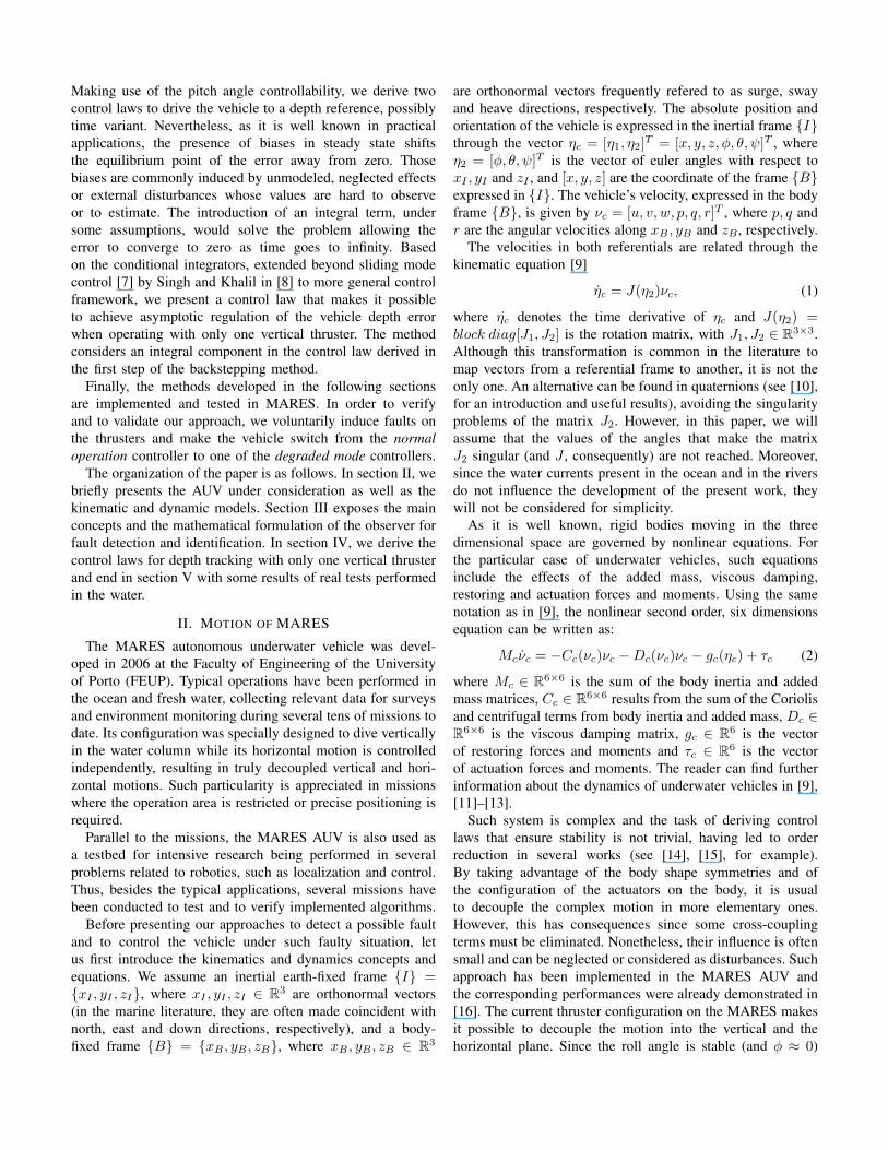
Under normal operation, we are able to control both pitchand heave degrees of freedom (DOF) in MARES, by actuatingthrough the two vertical thrusters. However, if one of thesefails, the heave DOF is no longer controllable making thevehicle operate in a degraded mode. In such situation, thecontrol law has to change as one of the commands would befailing, possibly leading to instability. On the other hand, thedecision of switching from a control law to another must bebased on an appropriate information about the status of eachvertical thrusters.

Our approach consists in implementing an extended Kalmanfilter to estimate the state of the vehicle along operation. Byintroducing two new variables in the state, referred to as loss ofcontrol effectiveness factors in [4], the cyclic estimation of thestate by the augmented state extended Kalman filter providesuseful information about the force effectively applied by thevertical thrusters.

First, let us introduce the reduced order model, derived from(2), as:

Mν = −C(ν)ν −D(ν)ν − g(η2) + Pf ft(t) (3)

where ν = [u,w, q]T and M,C(·), D(·) ∈ R3×3, g(·) ∈R3, Pf ∈ R3×4 result directly from (2) by neglecting the crossterms due to sway, roll and yaw motions.

The choice of the variables that compose the state to beestimated has a strong relation with the measurements we areable to obtain. Hence, we propose the following state model,while assuming that it can take the following representation:

x =

[x1

x2

]=

z

θwq

= Al(x)x + fu(x, u) + f(x, u, fv)

+wx(t) (4)

y =

zθq

= Chx + vn(t),

where Al(·) ∈ R4×4, fu(·), f(·) ∈ R4, Ch ∈ R3×4 andwx ∈ R4 and vn ∈ R3 are the process and the measurementnoises, respectively, assumed to be zero mean, Gaussian anduncorrelated.

Note that the model (4) ideally assumes that there is nobiases on the actuation fv. In order to include the effect ofthese deviation, we define γ = [γs, γb]

T as the vector of loss ofcontrol effectiveness factors, adopting the same notation as in[4]. The variable γs stands for the loss of control effectivenessof the stern thruster, while γb stands for the bow one. Hence,we redefine the state model as

x = Al(x)x + fu(x, u) + f(x, u, fv) + E(fv)γ + wx(t)

γ = wγ(t) (5)y = Chx + vn(t),

where wγ ∈ R2 is a zero-mean, Gaussian noise vector,uncorrelated with wx, and E(fv) is given such that E(fv)γ =f(0, 0, diag(γ)fv) is the contribution corresponding to the lossof control effectiveness. Note that γ is driven only by thenoise, since we can not predict by a model how the loss ofcontrol will occur. A practical consideration has to be takeninto account at this stage: The covariance of the noise wγ

must be maintained sufficiently large to quickly respond to anabrupt change in control effectiveness, but, on the other hand,it cannot be excessive in order to avoid impetuous corrections.The range in which it must keeped depends on the applicationand it can be handled along the operation to satisfy some givencriteria (see [4]).

Defining s = [xT , γT ]T and adopting the notation β for thenominal (estimated) vector, or matrix, of the generic functionβ, the discretized extended Kalman filter follows directly from[17]:

sk+1|k = Ask(sk)sk + fusk(sk, uk) + fsk(sk, uk, fvk) (6)

+Esk(fvk)sk (7)Pk+1|k = FkPkF

Tk +Qk, (8)

where Qk is the covariance matrix of the state noise, Fk standsfor the Jacobian of s evaluated at sk:

Fk =∂s

∂s |s=sk,

Ask, fusk, fsk, Esk are the discrete time equivalent functionsfor the augmented state s = [xT , γT ]T in (5) and P is thestate covariance matrix.

The so-called Kalman gain, the updates of the estimate andof the covariance matrix are respectively given by

Kk+1 = Pk+1|kCTs (CsPk+1|kC

Ts +Rk)−1 (9)

sk+1|k+1 = sk+1|k +Kk+1(yk+1 − Cssk+1|k) (10)Pk+1|k+1 = (I −Kk+1Cs)Pk+1|k., (11)

where Rk is the covariance matrix of the observation noise.The loss of control effectiveness factors provides an estimate

of the performances of the actuators. Ideally, a fault wouldbe identified whenever the absolute value of one of thefactors would rise above a preset threshold. However, modeluncertainties will be directly reflected in these factors and theirvalues can translate the effects of a damping forces greaterthan the modeled, for example. As these errors are frequentlycommited on the overall model, their effects are verified on allactuators either by increasing or decreasing the loss of controleffectiveness factors. Hence, for the present case, a reasonablemeasure of the malfunction of one of the thrusters is given bythe difference of the corresponding estimates of loss of controleffectiveness factor. On the other hand, taking a decision aboutthe malfunction of a given thruster should also be based on theconfidence of the factor estimate, which can be indirectly takenfrom the eigenvalues λγ of P γk , where P γk is the submatrixof P corresponding to γs and γb, avoiding taking decisionson transient state, where considerable corrections on the state

Fig. 2. Depth control by actuating either fb or fs

could be occuring. Thus, we propose the following (estimated)measure for fault detection:

δ =|γs − γb|

fλ(λγ1 + λγ2). (12)

where fλ is an increasing function of its argument.Whenever δ is greater than a preset threshold, a fault is

detected and the identification is made according to the greater|λ|, i.e., if |γs| > |γb| then the stern thruster is faulty and vice-versa.

IV. CONTROL OF MARES

In the presence of a faulty vertical thruster, the recon-figuration of the actuation is required. Otherwise, keepingthe same actuation will likely lead to instability or to otherpratical problems such as thruster dammage or large batteryconsumption, for example. Therefore, the control law fornormal operation could be inadequate and another control lawmust take over. In this section, we first start by deriving suchcontroller and present the main concepts behind the derivationof the control law for normal operation to cover the results inthe ensuing section.

A. Control under fault

We consider now the scenario in which only one of thevertical thrusters is available to control the motion of thevehicle. Under such situation, the heave DOF is no longercontrollable but the depth is still controllable by manipulatingpitch. Based on the Lyapunov theory we will derive a con-troller that makes it possible to control the vehicle’s depth.The derivation of the controller also employs the well knownbackstepping method as well as a conditional integrator toachieve asymptotic regulation.

As the final goal in this section is to control the vehicledepth, we will assume that roll angle is null (φ = 0), resulting:

z = −u sin θ + w cos θ. (13)

Let us introduce the error variable ez = z − zd, which wewant to drive to zero, and the quadratic Lyapunov function

V1 =1

2e2z, (14)

whose time derivative results

V1 = ez ez = ez(−u sin θ + w cos θ − zd). (15)

Although u, θ and z are either measured by sensors or es-timated, it is hard to accurately compute w due to modeluncertainties and measurement noise. Thus we will assumethat it constitutes a disturbance acting on the system, shiftingthe equilibrium point ez = 0 to an uncertain value. Throughoutthe following developments, we will consider that the surge ve-locity is maintained constant in order to simplify our approach.Indeed, in most missions the surge velocity is intended to beconstant along the trajectory. Moreover, the limited actuationon the vertical thruster makes the pitch angular velocity tolie in a bounded interval. Hence, from the vertical dynamics,we can assume an upper bound on the absolute value ofw ∈ [−wmax, wmax].

Inspired in [8], let us suppose we are able to handle θdirectly through the virtual control law

θ = θd(ez) = arcsin[− 1

u

(zd − α(ez)ϕ(

ezµ

))], (16)

where ϕ(·) : R→ R is the continuous infinitely differentiablesigmoid function

ϕ(x) =2

1 + e−ςx− 1, (17)

which verifies xϕ(x) > 0, x 6= 0, and α(·) > 0 is acontinuous function left to be determined later. Of course,handling θ directly and instantaneously is not realistic andsuch assumption will be lifted next. In opposition to [8], wehave selected a sigmoid function ϕ instead of a saturated linearfunction due to the differentiability characteristic. Let us taketake ς = 2, which will make ϕ(·) equal to the hyperbolictangent function.

Assuming zd sufficiently smooth, u > 0 and imposing

− 1

u

(zd − α(ez)ϕ(

ezµ

))≤ 1, (18)

the time derivative of the Lyapunov function in (15) results

V1 = ez

(− α(ez)ϕ(

ezµ

) + w cos θ)

≤ −ezα(ez)ϕ(ezµ

) + |ez|wmax, (19)

where we used the fact that | cos θ| ≤ 1 and w be bounded. Bychoosing appropriately α(·) and ϕ(·), the system can now bemade pratically stable (see [8]). Hence, let us define ε ∈ (0, 1)and take µ = 1

tanh−1(ε), then choosing α(ez) = Kz, Kz ∈

(wmax

ε , u+zd], such that it satisfies (18). Then, one can verify:

V1 < 0, ||ez|| > 1

V1 ≤ −ezα(ez)ϕ(ezµ

) + |ez|wmax, ||ez|| ≤ 1.

Thus, the system is pratically stable and the invariant setfor which the error tends to can be made arbitrarily smallby handling µ. However, a too small µ induces chatteringphenomena which are intended to be minimal.

Taking into account that V1 is a strictly increasing functionof ez , from the last inequalities we can state that the errorenters a positively invariant set Ω = ||ez|| ≤ 1. However,due to non null disturbances considered above, asymptoticstability can not be achieved. Therefore, following the sameidea as in [8], the conditional integrator is now introduced toobtain asymptotic convergence to the origin ez = 0. Modifiyngthe control law in (16) to include an integral component, itresults

θd(ez) = arcsin[− 1

u

(zd − α(ez)ϕ(

ez + σ

µ))], (20)

where

σ = −γσ + µϕ(ez + σ

µ), γ > 0, σ(t0) = 0.

Since |φ(x)| < 1, ∀x ∈ R, it is easy to check that σ ≤ µγ .

In order to guarantee convergence to zero, one has to set γand µ such that the maximum absolute value of the integralsatisfies|σ| > µ|ϕ−1

(wmax

Kz

)|. Although conservative, this will

allow the integral component to compensate the disturbanceeffect. By applying theorem 1 in [8], convergence to ez = 0as t→∞ is ensured.

So far, we have considered that we are able to handle θdirectly, which is not true, as it was stated before. Thus, basedon the backstepping method [6], let us introduce the newerror variable eθ = θ − θd and the new augmented Lyapunovfunction as follows

V2 = V1 +1

2e2θ (21)

whose time derivative results

V2 = V1 + eθ(θ − θd) (22)

with

θd = −zd −Kz

∂∂tϕ( ez+σµ )(

u2 −(zd −Kzϕ( ez+σµ )

)2)1/2 .Then, by imposing

θ = qd = θd −Kθeθ, Kθ > 0, (23)

the time derivative of the augmented Lyapunov function satis-fies V2 ≤ V1 −Kθe

2θ. Taking into account the previous result

about the convergence of ez to zero and the fact that V1 is aclass K∞ function, we can deduce that V2 → 0 as t→∞.

Nevertheless, we are not able to handle θ directly and, as itcan be seen from (1) and (2), a last step is required. Hence,we define eq = q − qd = Sqν − qd, with Sq = [0, 0, 1], asthe pitch rate error variable as well as the new augmentedLyapunov function:

V3 = V2 +1

2e2q. (24)

Considering (3), the time derivative results

V3 = V2 + eq(Sq ν − qd)= V2 + eq(SqM

−1(−C(ν)ν −D(ν)ν − g(η2)

+Pifpi)− qd). (25)

where Pi and fpi, i = s, b, are given as functions of theactuator configuration. When the vehicle is operating with onlyone thruster, either stern or bow thruster, Pi is respectivelygiven by

Ps =

1 1 00 0 00 0 xts

, Pb =

1 1 00 0 00 0 xtb

,fps =

fpfrfs

, fpb =

fpfrfb

.Note that Pi takes the form P = [Ph|Pvi], where Ph ∈

R3×2 is the submatrix composed by the first two columns ofPi and Pvi ∈ R3×1 is the last column of Pi. Further, let usdecouple the input vector into fpi = [fTh , f

Ti ]T , where fh ∈

R2 is composed by the first two entries of fpi and fi is thelast entry, which we can manipulate directly. By consideringthe decoupled form of Pi, we can rewrite (25) as

V3 = V2 + eq(SqM−1(−C(ν)ν −D(ν)ν − g(η2) + Phfh

+Pvifi)− qd).

Clearly SqM−1Phfh = 0, which means that the horizontal

thrusters have no direct influence on the pitch dynamics (seethe entries of Ps and Pb).

Finally, defining the proportional gain Kq > 0 and choosingthe control law

fi = (SqM−1Pvi)

−1(SqM−1(C(ν)ν +D(ν)ν + g(η)) + qd

−Kqeq), i = s, b (26)

the time derivative of the Lyapunov function (25) becomes

V3 = V2 −Kqe2q. (27)

Therefore, the convergence of the error ez to zero is thenguaranteed by setting the input fi according to the controllaw (26). Note that (26) gives the two control laws for eitheractuating with only stern or bow thruster, being different onlyon the entries of Pvi.

B. Control without fault

Under normal operation, the two through-hull thrustersprovide controllability on the heave and the pitch DOFs. Wewill not give emphasis to the derivation of this controller sinceit was previously derived in [16]. Thus, we aim at exposingthe main concepts that led to the control law, in order to betterunderstand the results of the next section for fault detection.The controller was derived using common backstepping withno integral terms.

In opposition to the previous subsection, the errors consid-ered for the control with the two thrusters are bidimensionalvectors. Naturally, the error vector for vertical position comes

e′p =

[z − zdθ − θd

],

assuming that θ, θd 6= π/2. Following the same method aspreviously, a first Lyapunov function is defined as a quadratic

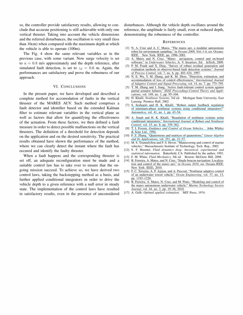
(a) Loss of control effectiveness factors

(b) Fault detection measure

Fig. 3. Fault detection

function of the error ep and its time derivative is made negativedefinite by adequately choosing z and θ as virtual controlvariables to achieve asymptotic stability.

A new augmented Lyapunov function is then introduced byadding a quadratic term of the error

e′ν =

[w − wdq − qd

],

and, from the reduced dynamics model (3), the control lawfor the two vertical thrusters fpv = χ(e′p, e

′ν , u, η2) ∈ R2

is determined such that the time derivative of the augmentedLyapunov function is negative definite.

V. RESULTS

The methods described in this paper were implemented andtested in MARES. In this section, we will present some of themain results produced by the fault detection and identificationalgorithm, as well as the performances of the controllers underreal conditions.

A. Fault detection and identification

In order to verify the behavior of our approach, we haveestablished a procedure that comprises disturbing the actuationunder normal operation. Although several tests were carriedout, we will only expose the most typical. The procedureincluded the following steps: under normal operation, thevehicle dives and stabilize at a given depth reference then,at time t ≈ 60s the bow thruster is counteracted with a forcein the opposite direction.

The Fig. 3 shows the results obtained for the loss of controleffectiveness factor and for the fault measure. Uncertaintiesand model errors were not corrected in order to analyze thesensitivity to such effects. One can verify that γs and γb aredifferent from zero, even before the disturbance on the bowthruster (t < 60). As stated before, the unmodeled effects,model errors and uncertainties are directly reflected in γ asbiases on the actuation. Nevertheless, they are not critical andthe graph 3(b) shows that we able to set a sufficiently largethreshold δthr to avoid erroneous fault detection. Practicalmethods such as integrating δ − δthr when the result isgreater than zero, together with a forgetting factor would be agood alternative, while making the algorithm more robust toerroneous detections.

Once the fault detection is made, the identification is per-formed based on the absolute value of γb and γs. The Fig. 3(a)shows clearly that a fault have occured on the bow thruster,being |γb| approximately four times greater than |γs|.

B. Control under fault

The control laws derived in section IV were implementedin MARES and tested in real conditions. The results of theoperations are shown in this section, being the analysis of theperformances of the controllers the main topic. The vehiclemissions were programed such that it navigates at a constantdepth with a given constant orientation. We must highlight thatseveral unconsidered disturbances have acted on the vehicleduring operations, namely more bouyancy than the assumedin the mathematical model, the fedback depth measurement isactually performed in the nose of MARES instead of beingmeasured on its center of gravity. Such disturbances induceundesired effects on the controllers. However, the followingfigures show the robustness of our approach.

Fig. 5 shows the results obtained during the operation ofthe controllers. The mission was set such that the vehiclestarts diving with the two vertical thrusters simultaneouslycontrolling pitch and depth, with surge velocity u = 0. Attime t = 20s, a fault is simulated and one of the degradedmode controllers starts operating.

The Fig. 5 shows the variables directly measured from thesensors for a mission with a depth reference zd = 0.7m, onlywith bow thruster. One can verify that the depth (Fig.5(a)) isreasonably close the reference and the small oscillation is dueto natural disturbances that the vehicle founds in real opera-tions. Moreover, while operating near the surface, the vehicleis more affected by the waves than if it would be deeper. Even

(a) Depth

(b) Pitch angle

(c) Surge velocity

Fig. 4. MARES controlling depth with bow and horizontal thrusters only(zd = 0.6 m)

(a) Depth

(b) Pitch angle

(c) Surge velocity

Fig. 5. MARES controlling depth with bow and horizontal thrusters only(zd = 0.7 m)

so, the controller provide satisfactory results, allowing to con-clude that accurate positioning is still achievable with only onevertical thruster. Taking into account the vehicle dimensionsand the referred disturbances, the oscillation is very small (lessthan 10cm) when compared with the maximum depth at whichthe vehicle is able to operate (100m).

The Fig. 4 show the same relevant variables as in theprevious case, with some variant. Now surge velocity is setto u = 0.8 m/s approximately and the depth reference, aftersimulated fault detection, is set to zd = 0.6 m. Again, theperformances are satisfactory and prove the robustness of ourapproach.

VI. CONCLUSIONS

In the present paper, we have developed and described acomplete method for accomodation of faults in the verticalthruster of the MARES AUV. Such method comprises afault detector and identifier based on the extended Kalmanfilter to estimate relevant variables in the vertical plane aswell as factors that allow for quantifying the effectivenessof the actuation. From these factors, we then defined a faultmeasure in order to detect possible malfunctions on the verticalthrusters. The definition of a threshold for detection dependson the application and on the desired sensitivity. The practicalresults obtained have shown the performance of the method,where we can clearly detect the instant where the fault hasoccured and identify the faulty thruster.

When a fault happens and the corresponding thruster isset off, an adequate reconfiguration must be made and asuitable control law has to take over to ensure that the on-going mission succeed. To achieve so, we have derived twocontrol laws, taking the backstepping method as a basis, andfurther applied conditional integrators in order to drive thevehicle depth to a given reference with a null error in steadystate. The implementation of the control laws have resultedin satisfactory results, even in the presence of unconsidered

disturbances. Although the vehicle depth oscillates around thereference, the amplitude is fairly small, even at reduced depth,demonstrating the robustness of the controller.

REFERENCES

[1] N. A. Cruz and A. C. Matos, “The mares auv, a modular autonomousrobot for environment sampling,” in Oceans 2008, Vols 1-4, ser. Oceans-IEEE. New York: IEEE, pp. 1996–2001.

[2] A. Matos and N. Cruz, “Mares navigation, control and on-boardsoftware,” in Underwater Vehicles, A. V. Inzartsev, Ed. InTech, 2009.

[3] P. M. Frank and X. Ding, “Survey of robust residual generation andevaluation methods in observer-based fault detection systems,” Journalof Process Control, vol. 7, no. 6, pp. 403–424, 1997.

[4] N. E. Wu, Y. M. Zhang, and K. M. Zhou, “Detection, estimation, andaccommodation of loss of control effectiveness,” International Journalof Adaptive Control and Signal Processing, vol. 14, no. 7, pp. 775–795.

[5] Y. M. Zhang and J. Jiang, “Active fault-tolerant control system againstpartial actuator failures,” IEEE Proceedings-Control Theory and Appli-cations, vol. 149, no. 1, pp. 95–104.

[6] H. Khalil, Nonlinear Systems, 3rd ed. Michigan State University, EastLansing: Prentice Hall, 2002.

[7] S. Seshagiri and H. K. Khalil, “Robust output feedback regulationof minimum-phase nonlinear systems using conditional integrators?”Automatica, vol. 41, no. 1, pp. 43–54.

[8] A. Singh and H. K. Khalil, “Regulation of nonlinear systems usingconditional integrators,” International Journal of Robust and NonlinearControl, vol. 15, no. 8, pp. 339–362.

[9] T. I. Fossen, Guidance and Control of Ocean Vehicles. John Whiley& Sons Ltd., 1994.

[10] F. Z. Zhang, “Quaternions and matrices of quaternions,” Linear Algebraand Its Applications, vol. 251, pp. 21–57.

[11] M. S. Triantafyllou and F. S. Hover, “Maneuvering and control of marinevehicles,” Massachussets Institute of Technology, Tech. Rep., 2002.

[12] S. F. Hoerner, Fluid dynamics drag: theoretical, experimental andstatistical information. Bakerfield, CA: Published by the author, 1993.

[13] F. M. White, Fluid Mechanics, 5th ed. Boston: McGraw Hill, 2008.[14] B. Ferreira, A. Matos, and N. Cruz, “Single beacon navigation: Localiza-

tion and control of the mares auv,” in Oceans 2010, ser. Oceans-IEEE.New York: IEEE, 2010.

[15] F. C. Teixeira, A. P. Aguiar, and A. Pascoal, “Nonlinear adaptive controlof an underwater towed vehicle,” Ocean Engineering, vol. 37, no. 13,pp. 1193–1220.

[16] B. Ferreira, A. Matos, N. Cruz, and M. Pinto, “Modeling and control ofthe mares autonomous underwater vehicle,” Marine Technology SocietyJournal, vol. 44, no. 2, pp. 19–36, 2010.

[17] A. Gelb, Optimal applied estimation. MIT Press, 1974.