Automatic and robust noise suppression in EEG and MEG

This is an electronic reprint of the original article.This reprint may differ from the original in pagination and typographic detail.

Powered by TCPDF (www.tcpdf.org)

This material is protected by copyright and other intellectual property rights, and duplication or sale of all or part of any of the repository collections is not permitted, except that material may be duplicated by you for your research use or educational purposes in electronic or print form. You must obtain permission for any other use. Electronic or print copies may not be offered, whether for sale or otherwise to anyone who is not an authorised user.

Mutanen, Tuomas P.; Metsomaa, Johanna; Liljander, Sara; Ilmoniemi, Risto J.Automatic and robust noise suppression in EEG and MEG

Published in:NeuroImage

DOI:10.1016/j.neuroimage.2017.10.021

Published: 01/02/2018

Document VersionPublisher's PDF, also known as Version of record

Please cite the original version:Mutanen, T. P., Metsomaa, J., Liljander, S., & Ilmoniemi, R. J. (2018). Automatic and robust noise suppressionin EEG and MEG: The SOUND algorithm. NeuroImage, 166, 135-151.https://doi.org/10.1016/j.neuroimage.2017.10.021

https://doi.org/10.1016/j.neuroimage.2017.10.021


NeuroImage 166 (2018) 135–151

Contents lists available at ScienceDirect

NeuroImage

journal homepage: www.elsevier .com/locate/neuroimage

Automatic and robust noise suppression in EEG and MEG: TheSOUND algorithm

Tuomas P. Mutanen a,b,*,1, Johanna Metsomaa a,b,1, Sara Liljander a,c, Risto J. Ilmoniemi a,b

a Department of Neuroscience and Biomedical Engineering, Aalto University School of Science, P.O. Box 12200, FI-00076, AALTO, Finlandb BioMag Laboratory, HUS Medical Imaging Center, Helsinki University Hospital, P.O. Box 340, FI-00029, HUS, Finlandc Department of Clinical Neurophysiology, Jorvi Hospital, HUS Medical Imaging Center, Helsinki University Central Hospital, P.O. Box 800, FI-00029, HUS, Finland

A R T I C L E I N F O

Keywords:ElectroencephalographyMagnetoencephalographyArtifactsNoiseWiener estimationCross-validationMinimum-norm estimation

* Corresponding author. Aalto University School of SciE-mail address: [email protected] (T.P. Mutan

1 These authors have contributed equally to this work.

https://doi.org/10.1016/j.neuroimage.2017.10.021Received 6 June 2017; Accepted 10 October 2017Available online 20 October 20171053-8119/© 2017 Elsevier Inc. All rights reserved.

A B S T R A C T

Electroencephalography (EEG) and magnetoencephalography (MEG) often suffer from noise- and artifact-contaminated channels and trials. Conventionally, EEG and MEG data are inspected visually and cleanedaccordingly, e.g., by identifying and rejecting the so-called ”bad” channels. This approach has several short-comings: data inspection is laborious, the rejection criteria are subjective, and the process does not fully utilize allthe information in the collected data.

Here, we present noise-cleaning methods based on modeling the multi-sensor and multi-trial data. These ap-proaches offer objective, automatic, and robust removal of noise and disturbances by taking into account thesensor- or trial-specific signal-to-noise ratios.

We introduce a method called the source-estimate-utilizing noise-discarding algorithm (the SOUND algorithm).SOUND employs anatomical information of the head to cross-validate the data between the sensors. As a result,we are able to identify and suppress noise and artifacts in EEG and MEG. Furthermore, we discuss the theoreticalbackground of SOUND and show that it is a special case of the well-known Wiener estimators. We explain how acompletely data-driven Wiener estimator (DDWiener) can be used when no anatomical information is available.DDWiener is easily applicable to any linear multivariate problem; as a demonstrative example, we show howDDWiener can be utilized when estimating event-related EEG/MEG responses.

We validated the performance of SOUND with simulations and by applying SOUND to multiple EEG and MEGdatasets. SOUND considerably improved the data quality, exceeding the performance of the widely used channel-rejection and interpolation scheme. SOUND also helped in localizing the underlying neural activity by preventingnoise from contaminating the source estimates. SOUND can be used to detect and reject noise in functional braindata, enabling improved identification of active brain areas.

Introduction

Electroencephalography (EEG) and magnetoencephalography (MEG)are non-invasive functional imaging methods that are able to record post-synaptic neural activity with excellent temporal resolution. Because MEGand EEG sensors are very sensitive, they are highly susceptible to noisecontamination (Ferree et al., 2001; Vrba and Robinson, 2001), whichmay lead to erroneous interpretations of the cortical activity. We presentan effective way to clean noisy EEG/MEG signals by optimally utilizingthe multi-sensor data with the help of Wiener estimation. The suggestedtechnique makes use of the bioelectromagnetic model of the head todistinguish noise from neural signals.

ence, Department of Neuroscience anen).

Common approaches to deal with noisy data are frequency-domainfiltering and the visual identification and rejection of poor-quality sen-sors or data segments (e.g., Styliadis et al., 2014; Van der Meer et al.,2013; Tewarie et al., 2014; Dominguez et al., 2014). However, the fre-quency range of the noise may not have well-specified limits, or the noisespectra and the neural spectra of interest may overlap (Herrmann andDemiralp, 2005; Jensen and Colgin, 2007; Monto et al., 2008). Second,visual inspection of the data is laborious, and making rejection decisionsis highly subjective. Finally, rejecting sensors always reduces the datadimensionality (amount of information), which cannot be regained evenif interpolation is used to reconstruct the data.

We present an objective and robust methodology to quantify noise

d Biomedical Engineering, Espoo, P.O. Box 12200, FI-00076, AALTO, Finland.

mailto:[email protected]

http://crossmark.crossref.org/dialog/?doi=10.1016/j.neuroimage.2017.10.021&domain=pdf

www.sciencedirect.com/science/journal/10538119

http://www.elsevier.com/locate/neuroimage




T.P. Mutanen et al. NeuroImage 166 (2018) 135–151

levels in different parts of the data and to correct the measured signals ina way that optimally utilizes the gathered multidimensional information.We call this approach the source-estimate-utilizing noise-discarding algo-rithm (the SOUND algorithm, hereafter referred to as SOUND). SOUNDdetects noise automatically by assessing, with the help of a forwardmodel, howwell the signal in each channel can be predicted from the restof the signals. Each sensor is then corrected based on the signal-to-noise-ratio (SNR) values of all the recording sensors.

We show that SOUND is a special case of a more general class ofWiener estimators, whichminimize the mean-squared error in estimatingthe noiseless signal. In addition to SOUND, an alternative Wiener-estimation approach, which can be computed based only on the recor-ded data samples, is discussed. In this paper, we refer to this generaltechnique as data-drivenWiener (DDWiener). By applying the DDWienerapproach to event-related responses, we illustrate how the noise in in-dividual trials can be automatically detected and taken into account sothat the SNR of the estimated evoked response is maximized. The pre-sented data-correction methods work automatically and withoutcompletely rejecting any dimension in the data.

For MEG analysis, powerful noise-cleaning techniques that utilizephysical principles to separate noise from the multi-sensor signals, e.g.,signal-space separation (SSS) (Taulu et al., 2004; Taulu and Kajola, 2005)and the generalized side lobe canceller (Mosher et al., 2009), have beentaken into use. Another common approach in MEG is to measure theenvironmental noise signals from an empty MEG room prior to subjectentering the recording space. The noisy signal-space directions can thenbe rejected from the actual data, e.g., by using signal-space projection(SSP) (Uusitalo and Ilmoniemi, 1997).

SSP can be used to clean certain EEG artifacts (M€aki and Ilmoniemi,2011; Mutanen et al., 2016), but it is often difficult to determine thepoor-quality signal directions as the empty-room measurement is notpossible. In practice, the most common approach to tackle the sensor-specific noise is to identify and reject the noisy channels and to inter-polate the data in the rejected channels using, e.g., the spherical-splinebasis functions (Perrin et al., 1989) or source modeling (Mutanenet al., 2016; Nieminen et al., 2016). One may also build a surrogatemodel that describes the brain-derived and the artifactual EEG simulta-neously to clean the data (Litvak et al., 2007; Berg and Scherg, 1994); forthis purpose, the artifact topographies need to be defined, e.g., with thehelp of principal component analysis.

If the data contain artifacts that can be characterized by few topog-raphies and the corresponding time-domain samples arise from non-Gaussian distributions, independent components analysis (ICA) mayalso be useful in cleaning the data (Vig�ario, 1997; Korhonen et al., 2011).Artifactual ICA components are often identified and rejected manuallybut also some automatic methods have been suggested, e.g., FASTER(Nolan et al., 2010), which uses a set of predefined artifactual features tocategorize the obtained ICA components into brain and noise compo-nents. However, it is not always true that the noise sources follow theassumptions of ICA.

All the above-mentioned EEG-correction techniques require that thecontaminated data are confined to only a few channels or signal-spacedirections, which are identifiable based on the amplitudes or the distri-butions of the data samples. It should be noted that these techniquesdecrease the dimensionality of the data and they may require a notableamount of heuristic knowledge.

Possibly, the algorithm closest to SOUND is Sensor Noise Suppression(SNS) (De Cheveign�e and Simon, 2008), which corresponds to DDWienerin the sensor space. As SOUND, SNS detects noise in MEG and EEGchannels by comparing the signal in each sensor to the rest of the sensortraces. In SNS, each sensor signal is replaced by that part of the originalsignal belonging to the signal subspace spanned by the other sensorsignals. SNS works well with noise that is completely uncorrelated acrossdifferent sensors as well as uncorrelated with the brain signal, but it is

136

very sensitive to violations of these assumptions.As EEG noise cannot be estimated from an empty-roommeasurement,

we here concentrate on studying the performance of SOUND and generalWiener estimation with EEG. We illustrate through sample datasets howSOUND improves EEG signal quality. With simulations, we demonstratethat SOUND improves SNR, is robust against modeling errors, and canimprove source localization. We compare the performance of SOUND tothe most commonly applied method, the channel rejection and interpo-lation, as well as to SNS. As a proof of concept, we show that SOUND canalso be used to clean evoked MEG data.

Methods

In this section, we explain the theoretical basis for the methods anddescribe how we measured, simulated, and analyzed the data.

We use the following notation: an upper-case bold character denotes amatrix, a lower-case bold character denotes a vector, and a non-bolded,italic character refers to a scalar. An element in the ith row and jth col-umn of matrix X is denoted by xi;j. We use the subscript notation x⋅;j toindicate that we take the jth column vector of matrix X. To simplify thenotation, instead of xi;⋅, we use xi to indicate the ith row vector of ma-trix X.

The subscript ≠i means inclusion of all the rows or columns of amatrix/vector except the ith one. Hence, x≠i;j is the jth column vector ofmatrix X from which the element xi;j has been excluded, X≠i refers to asubmatrix of X, where the ith row has been excluded, and X≠i;≠j refers to asubmatrix of X, where the ith row and the jth column havebeen excluded.

The SOUND algorithm

Here, we introduce the SOUND algorithm, which makes use of themultidimensional nature of the data; we estimate the reliability of eachsensor, given measurements in all the other sensors, and clean themeasured data accordingly.

Both EEG and MEG quantify brain activity by measuring electro-magnetic fields created by post-synaptic currents, which form the sourcecurrents of the signal. The signals measured by S sensors at T time in-stants (samples) can be written as

Y ¼ Yþ N ¼ LJþ N ; (1)

where Y and Y are S� T matrices containing the noisy and the noise-freesignals, respectively, and N is an S� T noise matrix. Y can be expressedas a matrix product between the S� J lead-field matrix L and the J � Tsource-current matrix J, J being the number of all the sources. Theelement ls;j in L describes the sensitivity of sensor s to source j, while jj,the jth row of J, contains the waveform of source j.

Our goal is to estimate Y from Y. To achieve this, we first attempt toconstruct the minimally noisy source estimates, bJ, and then use bJ inreconstructing the cleaned versions of the sensor signals, bY. Note that Jmay also include uninteresting brain activity, which generates so-calledneural-noise signals. However, our goal here is not to separate theneural-noise component from the data. We wish to minimize the amountof noise and artifacts (of extracranial origin), N, leaking into the sourceestimate bJ.

If we knew how the noise is distributed in the sensor space, i.e., thenoise covariance matrix Σ, we should emphasize the most reliable signaldirections in the estimation of source currents J. We achieve this bymultiplying Eq. (1) from left with Σ�1=2, which corresponds to whiteningthe data with respect to the noise:�Σ�1=2

�Y ¼ �

Σ�1=2�LJþ �

Σ�1=2�N ¼ ~Y ¼ ~LJþ ~N ; (2)


where ~Y, ~L, and ~N are the whitened versions of the signal, lead-field, andnoise matrix, respectively. From Eq. (2), J can be estimated as theTikhonov-regularized minimum-norm estimate (MNE)2:

bJ ¼ ~LT�~L~LT þ λI

��1~Y: (3)

The regularization parameter λ can be selected, e.g.,

λ ¼ λ0trace

�~L~L

T�S

; (4)

where S is the number of sensors and λ0 is a tuning scalar that can beheuristically chosen, e.g., based on the SNR, λ0 ¼ 1=SNR (Linet al., 2006).

To use Eq. (3), we obviously need to know Σ. If we assume that thenoise is uncorrelated across the sensors, the noise covariance matrixbecomes diagonal, Σ ¼ diagðσ21;…; σ2SÞ, and it is sufficient to estimatethe noise level σs in each sensor s. The diagonality assumption simplifiesthe interpretation of Eqs. (2) and (3); when estimating J, we give moreweight to those sensors that have better SNR.

If we knew ys;t , the noiseless measurement in sensor s at time t, thenthe noise level in s could be computed simply as

σs ¼ffiffiffiffiffiffiffiffiffiffiffiffiffiffiffiffiffiffiffiffiffiffiffiffiffiffiffiffiffiffiffiffiffiPT

t¼1

�ys;t � ys;t

�2T

s: (5)

Provided that we are able to estimate the source currents reliably, wecan estimate the noise-free sensor signal ys;t by

bys;t ¼ lsbj⋅;t: (6)

Substituting bys;t to Eq. (5) results in the noise estimate bσ s.Next, we discuss how Eqs. (2)–(6) can be used to cross-validate the

signals measured by different sensors. Let us evaluate the noise level ofsensor s0 using Eq. (5). We look for the most likely value for ys0 ;t , given the

measurements of all the other sensors y≠s0 ;t . Thus, we first find bj⋅;t bysubstituting ~Y ¼ ~Y≠s0 and ~L ¼ ~L≠s0 into Eq. (3). We can then estimate thenoiseless signal in s0 by using Eq. (6) and, subsequently, the noise level inthe same sensor by using Eq. (5).

We may next continue evaluating the noise level in any other sensors00 in an identical way. As we now have quantified the noise level insensor s0, we can take this into account by updating bΣ and whitening the

original data again to improve bj⋅;t (Eq. (2) and (3)). From the improved

version of bj⋅;t , we now estimate the noise in sensor s00.The obvious problem is that in order to estimate the noise in sensor s0,

we need to know the noise levels in all the other sensors. We solve thisissue by evaluating each sensor several times in an iterative fashion, al-ways updating bΣ based on the latest noise estimates. Step by step, thenoise covariance matrix estimates, and thus, the sensor-signal estimatesbecome more accurate. In the next section, we show a suitable initialguess for bΣ that can be used to launch the iteration.

To ensure that the suggested cross-validation scheme works properly,EEG data should be referenced to a good-quality channel prior to theiteration. Otherwise, the noise of the chosen reference channel leaks toall the channels, violating the assumption of non-correlated noise. Wepresent an automatic way to choose a suitable reference channel in thenext section.

All in all, the noise levels can now be determined by using thefollowing iterative scheme (See also Fig. 1 for a visual illustration ofthe iteration):

2 When the noise covariance is not known, the MNE operator in Eq. (3) is often usedwithout pre-whitening.

137

1. Re-reference the data to a selected good-quality sensor. Make aninitial guess for bΣ in the chosen reference system.

2. Iterate the estimations of the values bσ s; s 2 1;2;…; S, using Eqs. (2),(3), (5), and (6); at each step a new value for bσ s is obtained accordingto

bσ s ¼

ffiffiffiffiffiffiffiffiffiffiffiffiffiffiffiffiffiffiffiffiffiffiffiffiffiffiffiffiffiffiffiffiffiffiffiffiffiffiXT

t¼1

�ys;t � lsbj⋅;t�2T

s; where

bj ⋅;t ¼ ~LT≠s

�~L≠s~L

T≠s þ λI

��1~y≠s;t :

Update bΣ ¼ diagðbσ21 ;…; bσ2

SÞ after each iteration and re-whiten theoriginal data.

3. Repeat step 2 until bΣ has converged.

To monitor the convergence of bΣ, we can compute the relativechanges in the sensor-specific noise levels between two consecutive fulliteration rounds. When the relative change in all the channels is less thana desired threshold, e.g., 1%, the iteration can be terminated.

We can take the final estimate for the noise covariance matrix and useit to whiten the original data (as in Eq. (2)). As the final step, we use thenoise-suppressed source estimates to construct the cleaned versions ofthe sensor-space signals (Eq. (6)). Thus, the final cleaned version of thedata can be written as

bY ¼ L�bΣ�1=2

L�T�bΣ�1=2

LLTbΣ�1=2 þ λI��1bΣ�1=2

Y;

λ ¼ λ0trace�bΣ�1=2

LLTbΣ�1=2��S:

(7)

Relation between SOUND and Wiener estimation

In the previous section, we showed how SOUND can be used to es-timate noise levels in EEG/MEG channels and to suppress the noiseaccordingly. SOUND is closely related to Wiener estimation (or Wienerfiltering). In this framework, the Wiener filter estimates a single-sensorsignal as a linear combination of all the recorded EEG/MEG traces tominimize the mean-squared error (MSE). Assuming in Eq. (1) that thenoise has a diagonal covariance matrix and that the sources are inde-pendent and identically distributed (i.i.d.), SOUND can be shown tocorrespond to the Wiener estimator for the noiseless signals, thusproviding an optimal solution in the MSE sense (see Appendix Afor details).

The Wiener estimator can also be computed based on the measureddata samples only, when no information on the underlying head model(lead fields) is available. For this alternative implementation, the noise isagain assumed uncorrelated across the sensors, and the sample Wiener

estimate, bysamples , becomes (See Appendix A for the derivation)

bysamples ¼ ysðY≠sÞT

�Y≠sðY≠sÞT

��1Y≠s: (8)

To make Eq. (8) more stable, Tikhonov regularization is often usedaccording to (Foster, 1961) as

bysamples ðγÞ ¼ ysðY≠sÞT

�Y≠sðY≠sÞT þ γI

��1Y≠s ; (9)

where γ needs to be tuned to a sufficient level to guarantee that thematrix is invertible. In particular, γ should be appropriately adjustedwhen the number of channels approaches or even exceeds the number ofsamples. Otherwise, the rest of the sensor signals might also explain thenoise in sensor s. The signals over all the sensors can be corrected byapplying Eq. (9) once to each sensor s separately. We here refer to thisapproach, in general, as the data-driven Wiener estimationmethod (DDWiener).

In the previous section, we saw that an initial guess for the noisecovariance matrix is needed to start SOUND. A natural way is to use

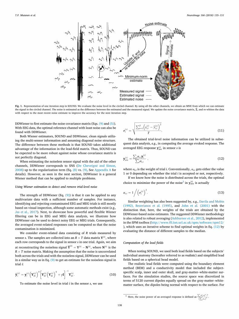
Fig. 1. Representation of one iteration step in SOUND. We evaluate the noise level in the circled channel. By using all the other channels, we obtain an MNE from which we can estimatethe signal in the circled channel. The noise is estimated as the difference between the estimated and the measured signal. We update the noise covariance matrix, bΣ, and re-whiten the datawith respect to the most recent noise estimate to improve the accuracy for the next iteration step.


DDWiener to first estimate the noise covariance matrix (Eqs. (9) and (5)).With EEG data, the optimal reference channel with least noise can also befound with DDWiener.

Both Wiener estimators, SOUND and DDWiener, clean signals utiliz-ing the multi-sensor information and assuming diagonal noise structure.The difference between these methods is that SOUND takes additionaladvantage of the information in the lead-field matrix. Thus, SOUND canbe expected to be more robust against noise whose covariance matrix isnot perfectly diagonal.

When estimating the noiseless sensor signal with the aid of the otherchannels, DDWiener corresponds to SNS (De Cheveign�e and Simon,2008) up to the regularization term (Eq. (8) vs. (9), See Appendix A fordetails). However, as seen in the next section, DDWiener is a generalWiener method that can be applied to multiple problems.

Using Wiener estimation to detect and remove trial-level noise

The strength of DDWiener (Eq. (9)) is that it can be applied to anymultivariate data with a sufficient number of samples. For instance,identifying and rejecting contaminated EEG and MEG trials is still mostlybased on visual inspection, although some automatic methods exist (e.g.,Jas et al., 2017). Next, to showcase how powerful and flexible Wienerfiltering can be in EEG and MEG data analysis, we illustrate howDDWiener can be used to detect noisy EEG or MEG trials. Consequently,the averaged event-related responses can be computed so that the noisecontamination is minimized.

We consider event-related data consisting of R trials measured bysensor s. The samples are collected into an R� T data matrix YðsÞ, whereeach row corresponds to the signal in sensor s in one trial. Again, we aim

at reconstructing the noiseless signal YðsÞ ¼ YðsÞ �NðsÞ, where NðsÞ is theR� T noise matrix. Making the assumption that the noise is uncorrelatedboth across the trials and with the noiseless signal, DDWiener can be usedin a similar way as in Eq. (9) to get an estimate for the noiseless signal intrial i:

byðsÞi ¼ yðsÞ

i

�YðsÞ

≠i

TYðsÞ

≠i

�YðsÞ

≠i

Tþ γI

��1

YðsÞ≠i : (10)

To estimate the noise level in trial i in the sensor s, we use

138

ffiffiffiffiffiffiffiffiffiffiffiffiffiffiffiffiffiffiffiffiffiffiffiffiffiffiffiffiffiffiffiffiffiffiffiffiffiPTt¼1

�yðsÞi;t � byðsÞi;t

2vuut

σðsÞi ¼T

: (11)

The obtained trial-level noise information can be utilized in subse-quent data analysis, e.g., in computing the average evoked response. Theaveraged EEG response yðsÞ

ave in sensor s is

yðsÞave ¼

Piαs;iy

ðsÞiP

iαs;i; (12)

where αs;i is the weight of trial i. Conventionally, αs;i gets either the value1 or 0 depending on whether the trial i is accepted or not, respectively.

If we know how the noise is distributed across the trials, the optimal

choice to minimize the power of the noise3 in yðsÞave is actually

αs;i ¼ 1��

σðsÞi

2: (13)

Similar weighting has also been suggested by, e.g., Davila and Mobin(1992), Bezerianos et al. (1995), and John et al. (2001) with thedistinction that, here, the weights of the trials are obtained by theDDWiener-based noise estimates. The suggested DDWiener methodologyis also related to robust averaging (Ashburner et al., 2012), implementedin the SPM toolbox (http://www.fil.ion.ucl.ac.uk/spm/software/spm12/), which uses an iterative scheme to find optimal weights in Eq. (12) byevaluating the distance of different samples to the median.

Computation of the lead fields

When testing SOUND, we used both lead fields based on the subjects’individual anatomy (hereafter referred to as realistic) and simplified leadfields based on a spherical head model.

The realistic lead fields were computed using the boundary elementmethod (BEM) and a conductivity model that included the subject-specific scalp, inner and outer skull, and gray-matter–white-matter sur-faces. For the simulation studies, the source space was discretized interms of 5120 current dipoles equally spread on the gray-matter–white-matter surface, the dipoles being normal with respect to the surface. For

3 Here, the noise power of an averaged response is defined asP

iα2s;iðσ

ðsÞi Þ2

ðPiαs;iÞ2 .

http://www.fil.ion.ucl.ac.uk/spm/software/spm12/


cleaning the real-life MEG data with SOUND, the source space consistedof 1640 freely oriented dipoles, while for MEG localization we used an8200-dipole model. For the TMS–EEG source localization we used amodel consisting of 5120 freely oriented dipoles. The relative conduc-tivities of the brain, skull, and skin were 1, 1/50, and 1, respectively. Inthe simulations, we also tested the sensitivity of SOUND to head-modelinaccuracies: we changed the relative skull conductivity to either lower(1/100) or higher (1/25) than the skull conductivity of the model thatwas used to simulate the neural signals. The surfaces were based on T1-weighted magnetic resonance images of the subject. We used Freesurfer(Fischl, 2012) to segment the gray-matter–white-matter surface andBrainSuite (Shattuck and Leahy, 2002) to segment the scalp and skullsurfaces. The lead fields were computed with the combination of theMNE software (Gramfort et al., 2014) and the BEM MATLAB toolbox(Stenroos and Sarvas, 2012). For more details of our segmentationpipeline, see Mutanen et al. (2016).

The concentric spherical head model consisted of the brain, skull, andscalp volume, which had outer radii of 81, 85, and 88 mm, respectively.The relative conductivities were 1, 1/50, and 1, respectively. The leadfields for the spherical head model were computed as explained inMutanen et al. (2016).

Simulation analysis

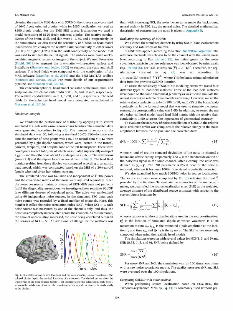
We validated the performance of SOUND by applying it to severalsimulated EEG sets with various noise characteristics. The simulated datawere generated according to Eq. (1). The number of sensors in thesimulated data was 60, following a standard 10–20 EEG-electrode sys-tem; the number of time points was 146. The neural data Y ¼ LJ weregenerated by eight dipolar sources, which were located in the frontal,parietal, temporal, and occipital lobe of the left hemisphere. There weretwo dipoles in each lobe, one of which was situated superficially on top ofa gyrus and the other one about 1 cm deeper in a sulcus. The waveforms(rows of J) and the dipole locations are shown in Fig. 2. The lead fieldmatrix resulting from these dipoles was computed according to a realistichead model, which was constructed based on the MRI of a 26-year-oldfemale who had given her written consent.

The simulated noise was Gaussian and independent of Y. The powerand the covariance matrix of the noise were adjusted separately. Sincethe noise covariance matrix of measured EEG/MEG may not perfectlyfulfill the diagonality assumption, we investigated how sensitive SOUNDis to different degrees of correlated noise. The noise was randomizedusing 60 independent noise sources. In the simulated EEG data, eachnoise source was recorded by a fixed number of channels. Here, thisnumber is called the noise correlation index (NCI). When NCI ¼ 1, eachnoise source was measured by one of the channels only, and thus, thenoise was completely uncorrelated across the channels. As NCI increased,the amount of correlation increased, the noise being correlated across allthe sensors at NCI ¼ 60. An additional challenge for the methods was

Fig. 2. Simulated neural source locations and the corresponding source waveforms. Thecolored circles depict the cortical locations of the sources. The dashed curves show thewaveforms of the deep sources (about 1 cm inwards along the sulcus from each circle),whereas the solid curves illustrate the waveforms of the superficial sources located exactlyat the circles.

139

that, with increasing NCI, the noise began to resemble the backgroundneural activity in EEG, i.e., the neural noise. The detailed mathematicaldescription of constructing the noise is given in Appendix B.

Evaluating the accuracy of SOUNDWe cleaned the simulated datasets by using SOUND and evaluated its

accuracy and robustness as follows.SOUND was applied according to Section The SOUND algorithm. The

reference electrode was chosen to be the channel with the lowest noiselevel according to Eqs. (9) and (5). An initial guess for the noisecovariance matrix in the new reference was then obtained by using againEqs. (9) and (5). For i.i.d. sources cov

�Y� ¼ λ�1LLT. Therefore, the reg-

ularization constant in Eq. (3) was set according to

λ ¼ traceðLLTÞ=traceðT�1 bYbYTÞ, where bY is the latest estimated noiselessdata from the previous SOUND iteration.

To assess the sensitivity of SOUND to modeling errors, we tested fourdifferent types of lead-field matrices. Three of the lead-field matriceswere based on the same anatomical geometry as was used to simulate theneural sources (we refer to these models as realistic). However, we set therelative skull conductivity to be 1/100, 1/50, and 1/25 of the brain/scalpconductivity. In the forward model that was used to simulate the neuralsources, the corresponding value was 1/50. In addition, we tested the useof a spherical-head-model-based lead-field matrix with the relative skullconductivity 1/50 to assess the importance of geometrical accuracy.

To evaluate the accuracy of noise cancellation of SOUND, the relativenoise reduction (rNR) was computed as the relative change in the noiseamplitudes between the original and the corrected data:

rNR ¼ 100%�Xs

σs � σcsνs

,Xs

σsνs

; (14)

where σs and σcs are the standard deviations of the noise in channel sbefore and after cleaning, respectively, and νs is the standard deviation ofthe noiseless signal in the same channel. After cleaning, the noise wasdefined as bys � ys. The rNR parameter is 0% if none of the noise isremoved, whereas it becomes 100% if the signal is perfectly corrected.

We also quantified how much SOUND helps in source localization.The source estimates were computed by Eq. (3) utilizing the final bΣprovided by the iteration. To evaluate the accuracies of the source esti-mates, we quantified the source localization error (SLE) as the weightedaverage distance of the distributed source estimates with respect to thecorrect dipole locations by

SLE ¼ 18

X8

m¼1

"1P

n

bjn;tm Xn

bjn;tm ��rn � rdm

��2

#; (15)

where n runs over all the cortical locations used in the source estimation,rdm is the location of simulated dipole m whose waveform is at its

maximum at time tm, bjn;tm is the estimated dipole amplitude at the loca-tion rn and time tm, and ||�||2 is the L2 norm. The SLE values were onlycomputed when using the realistic head models.

The simulations were run with several values for NCI (1, 3, and 9) andSNR (0.33, 1, 3, and 9), SNR being defined by

SNR ¼trace

�YYT

traceðNNTÞ : (16)

For every SNR and NCI, the simulation was run 100 times, each timewith a new noise covariance matrix. The quality measures rNR and SLEwere averaged over the 100 simulations.

Comparing SOUND with other methodsWhen performing source localization based on EEG/MEG, the

Tikhonov-regularized MNE by Eq. (3) is commonly used without pre-


whitening (e.g., Hauk, 2004; Komssi et al., 2004; Hauk and Pulvermüller,2004; Moratti and Keil, 2005). Therefore, we compared the SLE values(Eq. (15)) obtained when using SOUND to those obtained with the non-whitened version of the Tikhonov-regularized estimation. We refer tothis approach as the L2-regularized MNE. Contrary to SOUND, in L2regularization, the noise levels are assumed to be equal across all thesensors. Because we know the SNR of the simulated data, we can directlyuse this knowledge to set the regularization parameter in Eqs. (3) and (4)using λ0 ¼ 1=SNR, as suggested by Lin et al. (2006). The lead-field matrixused in the L2-regularized estimation was the same as the one used tosimulate the neural EEG signals. This ”inverse crime”4 was permitted inorder to get the best possible L2-regularized estimate for the comparison.

When analyzing EEG/MEG data, it is common practice to reject ’bad’channels and replace the original signal with some form of interpolation.We evaluated how SOUND performs as compared to the popular spher-ical spline interpolation (Perrin et al., 1989), which is generally recom-mended in the literature (Picton et al., 2000; Michel et al., 2004). Theimplementation of the interpolation was used as given in Bio-electromagnetism MATLAB Toolbox [http://eeg.sourceforge.net/bioelectromagnetism.html, 15 September 2017]. In real life, channelscan be rejected based on visual inspection or some heuristic, quantitativecriteria, see, e.g., the PREP pipeline (Bigdely-Shamlo et al., 2015) or therecently published Autoreject (Jas et al., 2017). As the simulated noiselevels were known, here, we rejected a channel if its noise level (standarddeviation) was three times larger than the average noise level over all thechannels. The signals in the rejected channels were then reconstructedwith the spherical spline interpolation using all the remaining chan-nel traces.

Each simulated dataset was corrected by two different approaches:SOUNDwith the spherical head model, which yields more approximativesolutions than the realistic head geometry, and the spherical splineinterpolation. The rNR values (Eq. (14)) were computed for bothmethods and averaged over the interpolated channels.

SOUND was also compared to SNS, which corresponds to DDWienerin the sensor space, up to the regularization term. DDWiener was used asexplained in Section Relation between SOUND and Wiener estimation andSNS as described in the original work by De Cheveign�e and Simon(2008). As SOUND, SNS and DDWiener were tested with different SNRlevels and degrees of correlated noise. After the simulation runs, theperformance of SNS and DDWiener were quantified with rNR (Eq. (14)).

Demonstrating the presented methods with measured EEG and MEG data

We verified the functioning of the DDWiener-based bad-quality-trialdetection and SOUND with three different real-life datasets. All themeasurements followed the declaration of Helsinki. The EEG measure-ments were approved by the Coordinating Ethics Committee of theHospital District of Helsinki and Uusimaa, whereas the MEG measure-ment was approved by the Research Ethics Committee of Aalto Univer-sity. For detailed information about the specific instruments, stimulussetup, and recording parameters used in different measurements, pleaserefer to Supplementary material I.

TMS–EEG dataThe first sample dataset consists of transcranial-magnetic-stimulation

(TMS)-evoked EEG measured from a male subject (age 25). TMS canactivate a region of interest in the cortex by applying a rapidly changingmagnetic field to the subject's head. The magnetic pulse induces anelectric field strong enough to launch action potentials in the superficialcortex. Because of the strong magnetic pulse, concurrently measured EEG

4 The term inverse crime refers to simulation analysis that does not try to addressproperly the ill-posed nature of the problem. As a consequence, the obtained results canlead to overly optimistic interpretations. (Kaipio and Somersalo, 2006). For instance, inreality, there are always modeling errors in constructing the lead-field matrix.

140

is prone to suffer from large noise and artifact signals (Ilmoniemi andKi�ci�c, 2010; Ilmoniemi et al., 2015). Here, single-pulse TMS was targetedto the right primary motor cortex, to the representation area of the leftabductor pollicis brevis muscle. In total, 100 epochs of single-TMS-pulse-evoked EEG were recorded, with a 60-electrode TMS-compatible EEGsystem (Nexstim Plc., Finland), the bandwidth and sampling frequencybeing 0–350 Hz and 1450 Hz, respectively.

AD–ERP dataThe second sample dataset comes from an event-related potential

(ERP) study where an Alzheimer's disease (AD) patient (female, age 73years) received auditory stimuli via headphones. The data werecontaminated by muscle and movement artifacts caused by the patient'sinability to stay still, resulting in a significant amount of correlated noise.The AD–ERP data consisted of auditory ERP responses evoked by a beepsound (the first beep of a 4-beep train; 40 trains in total). The ERPs wererecorded by using a Cognitrace EEG system (eemagine Medical ImagingSolutions GmbH, Germany) with a 64-electrode EEG cap (WaveGuard,eemagine Medical Imaging Solutions GmbH, Germany). The bandwidthof the amplifier (Refa8-64 amplifier, TMS International, TheNetherlands) was limited to 0–138 Hz and the sampling frequencywas 512 Hz.

Visual evoked MEG dataThe third sample dataset contains 160 epochs of visual evoked MEG

responses. The subject (male, age 29) observed flashes of a checkerboardpattern shown to the right visual field. The studied MEG data containsome gradiometer signals that have rather high noise power if sufficientfiltering is not applied to the data. The data were measured with a 306-sensor MEG system with 204 planar gradiometers and 102 magnetome-ters (Elekta Neuromag, Elekta Oy, Finland). The bandwidth of theamplifier was 0.03–330 Hz and the sampling frequency was 1000 Hz.

Data analysisFrom each of the datasets, we extracted the epochs of interest (100 for

TMS–EEG, 40 for AD–ERP data, and 160 for MEG) including the timepoints between �500 and 500 ms with respect to the stimulus onset. Allepochs were high-pass-filtered from 1 Hz with a fourth-order Butter-worth filter and then baseline-corrected with respect to the time interval�500…0 ms . Next, we applied DDWiener to find the trial-specific noiselevels for all the sensors (Eq. (10) and (11)). The trial-specific noise levelswere used to find the estimate for the average evoked response in eachsensor (Eqs. (12) and (13)).

We further analyzed the interval �50…300 ms and used SOUND toclean the obtained evoked responses. With the EEG data, we used Eqs. (5)and (8) to find the least noisy sensor and referenced both the data and thelead fields to this sensor. When cleaning the EEG data, we decided tovalidate the performance of SOUND with the spherical-head-model-based lead-field matrix to assess whether a fairly simple head modelwould be sufficient for SOUND to clean EEG. With MEG, it is well knownthat a single spherical head model is not sufficient to explain neuronalactivity from all cortical locations (Crouzeix et al., 1999). Thus, whencleaning MEG signals we used the realistic head model based on thesubject's magnetic-resonance images. Before running SOUND, the initialguess for the noise covariance matrix was obtained with Eqs. (5) and (8).When running SOUND, we let the noise-estimation iteration to continueuntil the relative change in all the channels was less than 1%. To find asuitable regularization parameter (Eqs. (3) and (4)) for SOUND, we testedthe values of λ0 from 10�4 to 103 in ten-fold steps.

To evaluate quantitatively how SOUND affected the measured data,we computed the relative change in the SNR due to SOUND ineach sensor:

http://eeg.sourceforge.net/bioelectromagnetism.html

http://eeg.sourceforge.net/bioelectromagnetism.html


kby l

sk2

kby k� kylsk2

kysk2
ΔSNRs ¼ 100%� s 2
kylsk2kysk2

; (17)

where ys and bys are the signals of sensor s before and after SOUND,respectively, and the superscript l indicates that the signal has been low-pass-filtered from 60 Hz. Because we know that in EEG and MEG neuralactivity manifests itself mostly at low frequencies (Buzsaki and Draguhn,2004; H€am€al€ainen et al., 1993), whereas the non-neural noise has a muchbroader effective frequency range, we use

��y1s ��2=kysk2 as an approxi-mation for the SNR.

In addition to ΔSNR, we also quantified the amount of overcorrectionof SOUND in each sensor (OCs) as the absolute value of the correlationcoefficient between the cleaned signal and the estimated noise:

OCs ¼ bysðys � bysÞT

kbysk2kys � bysk2

; (18)

where ys and bys are the original and cleaned signals measured by sensors, respectively. The more SOUND overcorrects the data (removes alsosignals of interest), the more the cleaned signal will correlate with theestimated noise, i.e., the difference between the original and cleanedsignal ðys � bysÞ.

After the quantitative analysis, the data were low-pass-filtered from100 Hz with a fourth-order Butterworth filter for visualization.

Finally, we studied whether source localization could benefit fromSOUND. For this analysis, we used the MEG and TMS–EEG data since thecorrespondingmagnetic-resonance images of the subjects were available.For both data, we tested whether focal cortical activity could explainsome aspects of the measured data by fitting a current dipole to the earlyEEG/MEG deflections. With the TMS–EEG data, we restricted the analysisto the time interval of 2–20 ms after the TMS onset, as the first 2 ms areblocked by the TMS-compatible amplifier and it is well known that theTMS-evoked activity can spread from M1 to other brain regions after20 ms (Ilmoniemi et al., 1997; Komssi et al., 2002). The fitted dipoleswere freely oriented and laid on the gray-matter–white-matter surfaceformed by 5120 equally spread grid points. The localization was doneseparately at each studied time point; each dipole was fitted to the databy using the method of least squares with no prior knowledge of thenoise. The dipole producing the best goodness of fit (GOF) (Kaukorantaet al., 1986) was considered to be the best representation for the neuronalcurrent. The dipole fit was considered reliable if GOF exceeded 0.90. Thesame source localization was done both to the noisy and cleanedTMS-evoked data. The dipole search was applied to the

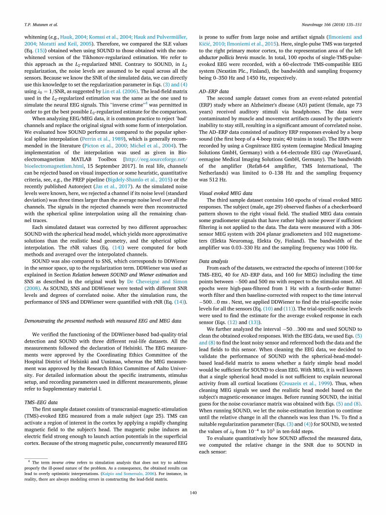
Fig. 3. Example case of SOUND estimation (SNR ¼ 1, and the signals from the noise sources aresignals are shown in the sensor layout as seen from above, with the nose pointing upwards. B: Testimated noise levels in all the channels.

141

low-pass-filtered data.When studying the MEG data, we restricted the localization analyses

to the time interval of 0–100 ms after the visual stimulus, as it has beenshown that during this interval the primary visual MEG deflections canbe modeled as focal dipolar sources (Portin et al., 1999). Now, the set offitted dipoles consisted of 8196 freely oriented dipoles, located on thegray-matter–white-matter surface. The source-localization procedurewas identical with the TMS–EEG data.

MATLAB demo package

We have prepared a MATLAB demo package that demonstrates howSOUND and DDWiener can be used in practice together with the open-access EEG analysis toolbox EEGLAB (Delorme and Makeig, 2004). Thedemo package was implemented so that it works with open-access dataavailable in the HeadIT EEG repository (Delorme et al., 2011), moreprecisely with the data measured in the ”Auditory Two-Choice ResponseTask with an Ignored Feature Difference” study [http://headit.ucsd.edu/studies/9d557882-a236-11e2-9420-0050563f2612, 15 September2017]. To use the data, one has to accept the HeadIT Data Use Agreementand the applied Terms of Use. The description of the demo package aswell as the corresponding download link can be found in Supplementarymaterial II.

Validating SOUND with 12 open-access auditory evoked EEG datasets

In addition to the three sample datasets presented in this work, wevalidated the functioning of SOUNDwith the 12 auditory evoked datasetsfreely accessible in the HeadIT EEG repository (Delorme et al., 2011).The studied datasets came from the ”Auditory Two-Choice Response Taskwith an Ignored Feature Difference” study [http://headit.ucsd.edu/studies/9d557882-a236-11e2-9420-0050563f2612, 15 September2017]. The data analysis of the 12 open-access datasets was based on theMATLAB demo package, provided in Supplementary material II. Wecompared the performance of SOUND to the spatial DDWiener, as well asto SNS. Because it is impossible to know the ground truth of the truenoiseless EEG of the studied datasets, we used four different measures,adapted from (Nolan et al., 2010), to quantify the signal quality beforeand after the different cleaning methods. For more details about theanalysis, see Supplementary material III.

Results

Results with the simulated data

Among the tested methods (SOUND, SNS, and spherical spline

correlated across three channels). A: The noisy (red curves) and the cleaned (black curves)he topographies and the scatter plot illustrate the correspondence of the simulated and the

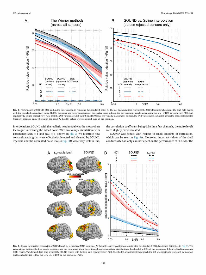
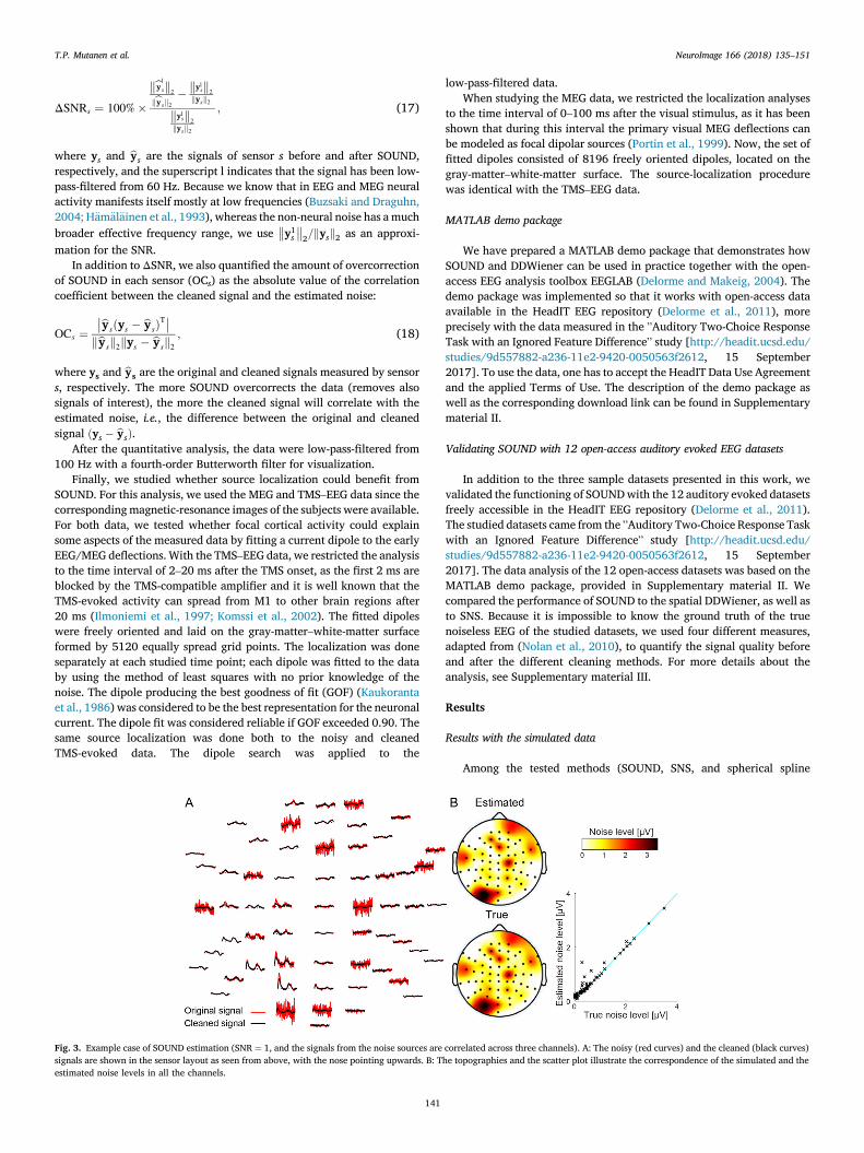
http://headit.ucsd.edu/studies/9d557882-a236-11e2-9420-0050563f2612




Fig. 4. Performance of SOUND, SNS, and spline-interpolation in removing the simulated noise. A: The dot-and-dash lines represent the SOUND results when using the lead-field matrixwith the true skull conductivity value (1/50); the upper and lower boundaries of the shaded areas indicate the corresponding results when using too low (1/100) or too high (1/25) skullconductivity values, respectively. Note that the rNR values provided by SNS and DDWiener are visually inseparable. B: Here, the rNR values were computed across the spline-interpolated(noisiest) channels only, whereas in the panel A, the rNR values were computed over all the channels.


interpolation), SOUNDwith the realistic head model was the most robusttechnique in cleaning the added noise. With an example simulation (withparameters SNR ¼ 1 and NCI ¼ 3) shown in Fig. 3, we illustrate howcontaminated signals were effectively detected and cleaned by SOUND.The true and the estimated noise levels (Fig. 3B) were very well in line,

Fig. 5. Source-localization accuracies of SOUND and L2-regularized MNE solutions. A: Examplgreen circles indicate the true source locations, and the color maps show the estimated source(SLE) results. The dot-and-dash lines present the SOUND results with the true skull conductivityskull conductivities (either too low, i.e., 1/100, or too high, i.e., 1/25).

142

the correlation coefficient being 0.98. In a few channels, the noise levelswere slightly overestimated.

SOUND was robust with respect to small amounts of correlation,which can be seen in Fig. 4A. Moreover, incorrect values of the skullconductivity had only a minor effect on the performance of SOUND. The

e source localization results with the simulated EEG data (same dataset as in Fig. 3). Theamplitude distributions, thresholded at 30% of the maximum. B: Source-localization error(1/50). The shaded areas indicate how much the SLE was maximally worsened by incorrect

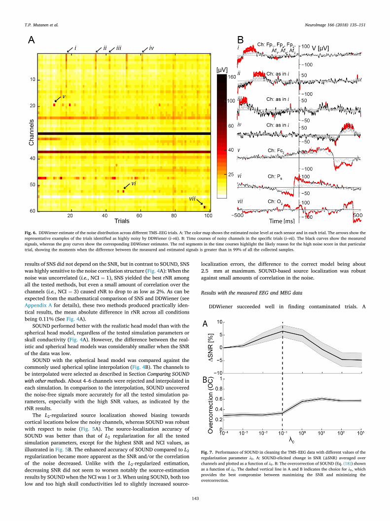
Fig. 6. DDWiener estimate of the noise distribution across different TMS–EEG trials. A: The color map shows the estimated noise level at each sensor and in each trial. The arrows show therepresentative examples of the trials identified as highly noisy by DDWiener (i–vii). B: Time courses of noisy channels in the specific trials (i–vii). The black curves show the measuredsignals, whereas the gray curves show the corresponding DDWiener estimates. The red segments in the time courses highlight the likely reason for the high noise score in that particulartrial, showing the moments when the difference between the measured and estimated signals is greater than in 99% of all the collected samples.

Fig. 7. Performance of SOUND in cleaning the TMS–EEG data with different values of theregularization parameter λ0. A: SOUND-elicited change in SNR (ΔSNR) averaged overchannels and plotted as a function of λ0. B: The overcorrection of SOUND (Eq. (18)) shownas a function of λ0. The dashed vertical line in A and B indicates the choice for λ0, whichprovides the best compromise between maximizing the SNR and minimizing theovercorrection.


results of SNS did not depend on the SNR, but in contrast to SOUND, SNSwas highly sensitive to the noise correlation structure (Fig. 4A): When thenoise was uncorrelated (i.e., NCI ¼ 1), SNS yielded the best rNR amongall the tested methods, but even a small amount of correlation over thechannels (i.e., NCI ¼ 3) caused rNR to drop to as low as 2%. As can beexpected from the mathematical comparison of SNS and DDWiener (seeAppendix A for details), these two methods produced practically iden-tical results, the mean absolute difference in rNR across all conditionsbeing 0.11% (See Fig. 4A).

SOUND performed better with the realistic head model than with thespherical head model, regardless of the tested simulation parameters orskull conductivity (Fig. 4A). However, the difference between the real-istic and spherical head models was considerably smaller when the SNRof the data was low.

SOUND with the spherical head model was compared against thecommonly used spherical spline interpolation (Fig. 4B). The channels tobe interpolated were selected as described in Section Comparing SOUNDwith other methods. About 4–6 channels were rejected and interpolated ineach simulation. In comparison to the interpolation, SOUND uncoveredthe noise-free signals more accurately for all the tested simulation pa-rameters, especially with the high SNR values, as indicated by therNR results.

The L2-regularized source localization showed biasing towardscortical locations below the noisy channels, whereas SOUND was robustwith respect to noise (Fig. 5A). The source-localization accuracy ofSOUND was better than that of L2 regularization for all the testedsimulation parameters, except for the highest SNR and NCI values, asillustrated in Fig. 5B. The enhanced accuracy of SOUND compared to L2regularization became more apparent as the SNR and/or the correlationof the noise decreased. Unlike with the L2-regularized estimation,decreasing SNR did not seem to worsen notably the source-estimationresults by SOUNDwhen the NCI was 1 or 3. When using SOUND, both toolow and too high skull conductivities led to slightly increased source-

143

localization errors, the difference to the correct model being about2.5 mm at maximum. SOUND-based source localization was robustagainst small amounts of correlation in the noise.

Results with the measured EEG and MEG data

DDWiener succeeded well in finding contaminated trials. A

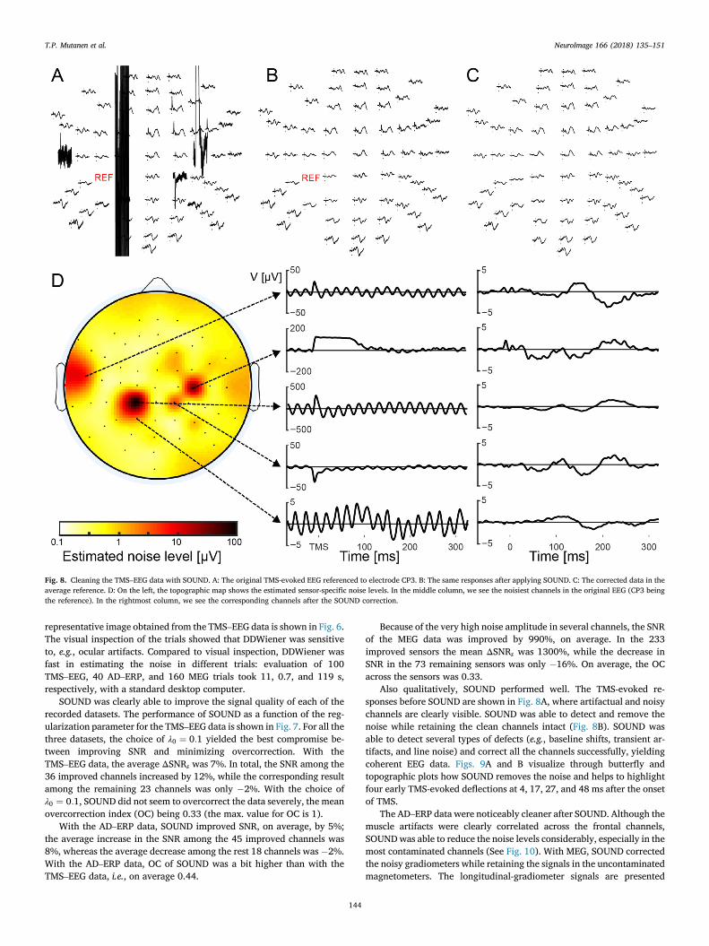
Fig. 8. Cleaning the TMS–EEG data with SOUND. A: The original TMS-evoked EEG referenced to electrode CP3. B: The same responses after applying SOUND. C: The corrected data in theaverage reference. D: On the left, the topographic map shows the estimated sensor-specific noise levels. In the middle column, we see the noisiest channels in the original EEG (CP3 beingthe reference). In the rightmost column, we see the corresponding channels after the SOUND correction.


representative image obtained from the TMS–EEG data is shown in Fig. 6.The visual inspection of the trials showed that DDWiener was sensitiveto, e.g., ocular artifacts. Compared to visual inspection, DDWiener wasfast in estimating the noise in different trials: evaluation of 100TMS–EEG, 40 AD–ERP, and 160 MEG trials took 11, 0.7, and 119 s,respectively, with a standard desktop computer.

SOUND was clearly able to improve the signal quality of each of therecorded datasets. The performance of SOUND as a function of the reg-ularization parameter for the TMS–EEG data is shown in Fig. 7. For all thethree datasets, the choice of λ0 ¼ 0:1 yielded the best compromise be-tween improving SNR and minimizing overcorrection. With theTMS–EEG data, the average ΔSNRs was 7%. In total, the SNR among the36 improved channels increased by 12%, while the corresponding resultamong the remaining 23 channels was only �2%. With the choice ofλ0 ¼ 0:1, SOUND did not seem to overcorrect the data severely, the meanovercorrection index (OC) being 0.33 (the max. value for OC is 1).

With the AD–ERP data, SOUND improved SNR, on average, by 5%;the average increase in the SNR among the 45 improved channels was8%, whereas the average decrease among the rest 18 channels was �2%.With the AD–ERP data, OC of SOUND was a bit higher than with theTMS–EEG data, i.e., on average 0.44.

144

Because of the very high noise amplitude in several channels, the SNRof the MEG data was improved by 990%, on average. In the 233improved sensors the mean ΔSNRs was 1300%, while the decrease inSNR in the 73 remaining sensors was only �16%. On average, the OCacross the sensors was 0.33.

Also qualitatively, SOUND performed well. The TMS-evoked re-sponses before SOUND are shown in Fig. 8A, where artifactual and noisychannels are clearly visible. SOUND was able to detect and remove thenoise while retaining the clean channels intact (Fig. 8B). SOUND wasable to detect several types of defects (e.g., baseline shifts, transient ar-tifacts, and line noise) and correct all the channels successfully, yieldingcoherent EEG data. Figs. 9A and B visualize through butterfly andtopographic plots how SOUND removes the noise and helps to highlightfour early TMS-evoked deflections at 4, 17, 27, and 48 ms after the onsetof TMS.

The AD–ERP data were noticeably cleaner after SOUND. Although themuscle artifacts were clearly correlated across the frontal channels,SOUNDwas able to reduce the noise levels considerably, especially in themost contaminated channels (See Fig. 10). With MEG, SOUND correctedthe noisy gradiometers while retaining the signals in the uncontaminatedmagnetometers. The longitudinal-gradiometer signals are presented

Fig. 9. Effects of SOUND to the TMS–EEG data quality. A: Original data. B: The same dataafter SOUND. The top panels of (A) and (B) show the butterfly plot of the data before andafter cleaning. The vertical red dashed lines in the top panels of (A) and (B) indicate thelatencies of the early deflections that were identified from the cleaned data. The topog-raphies illustrate the EEG voltage maps at the identified deflection latencies. C: Thelocation of the best-fitting dipole (GOF > 0.9) at 18 ms after TMS.


in Fig. 11.With the assumption that the early TMS-evoked EEG deflections

mainly reflect focal cortical activity close to the stimulation target, itseems that SOUND was able to improve the source localization consid-erably (Fig. 9C). When the dipole search was done with the originalTMS–EEG data, no reliable dipole fits were found as the GOF alwaysremained under 0.7. After SOUND, the best-matching dipole was foundin the stimulated hemisphere, at 17–20 ms after the TMS pulse, 2 cmaway from the TMS target (GOF> 0:9).

As with the TMS–EEG data, no reliable dipole fits were found for theMEG data before the SOUND correction (throughout the studied timeinterval, GOF< 0:78). After SOUND, two dipoles were found in the leftvisual cortex, at 53–75 ms and 79–83 ms after the stimulus presented tothe right visual field (GOF>0:9 for both dipoles). This is in line withprevious findings in the literature (Portin et al., 1999). The dipole fit at�65 ms is illustrated in Fig. 11.

145

When cleaning the EEG sample datasets, five full iteration roundswere enough for SOUND to converge to the requested level. With MEG,11 iterations were required. With the TMS–EEG, AD–ERP, andMEG data,SOUND fully converged in �20, �30, and �50 iterations, respectively,after which the noise-estimate changes were merely numeric(� 10�14%). The changes in the noise-estimates as a function of theiteration step are illustrated in Fig. 12. The resulting cleaned data werepractically identical regardless of whether iteration was continued untiltrue convergence or stopped at the suggested 1%-criterion. For the 60-and 64-sensor EEG data, it took less than 5 s for a standard desktopcomputer to perform SOUND, whereas with the 306-sensor MEG data thecorresponding time was 105 s.

Results with the open-access EEG data

According to the visual and quantitative analysis, SOUND performedrobustly with the open-access datasets. Overall, SOUND was sensitive todifferent outlier EEG activities, correcting the signals in the contaminatedEEG channels to a level that could be expected from neuronal activity.Compared to DDWiener, SOUND was much more efficient in detectingand correcting the outlier activity. Neither DDWiener nor SOUND,seemed to overcorrect the channel signals that more likely reflectedintracranial post-synaptic-currents. With these specific datasets, bothSOUND and DDWiener clearly outperformed SNS. See Supplementarymaterial II for the detailed description of the quantitative analysis, aswell as the corresponding results.

Discussion

In this work, we introduced methods, most importantly SOUND, toclean EEG/MEG data. SOUND takes a novel approach to identify andseparate the neural and noisy data based on their spatiotemporal char-acteristics. We have provided a theoretical basis for SOUND and tested itsfunctioning under several conditions using both simulated and measureddata. Here, we discuss some implications of the obtained results.

Practical considerations on cleaning EEG/MEG signals by Wienerestimation

Inspecting data visually can be laborious. Since the presented noise-cleaning approaches work automatically and require only seconds tofew minutes of computational time, they can considerably save the data-processing time. Therefore, projects with large populations, e.g., someclinical studies (Bresnahan and Barry, 2002), can significantly benefitfrom the Wiener estimation methods. In less-cooperative subject groups,such as children or neurological patients, rejecting trials and/or channelscompletely may lead to an unrepresentative amount of data. UsingWiener estimation would enable the utilization of most of the collecteddata and prevent valuable recordings from being wasted.

SOUND requires very little user input: once the conductivity modelfor the head is chosen, SOUND has only one degree of freedom; theregularization parameter may need to be fine-tuned for the measureddata. In this work, we showed an example of how a proper value can befound in a data-driven fashion.

When cleaning the visual evoked MEG data with SOUND, we did nottake possible head movements into account. If the subject is prone tomove inside the MEG helmet, the head movement can be corrected withSOUND using the magnetic-field realignment approach suggested byNumminen et al. (1995) and Uutela et al. (2001).

In this work, SOUND was applied to evoked responses. If the noise isexpected to be non-stationary across the trials, SOUND can also be usedto clean each trial separately. The cost of this approach is the lengthenedcomputing time. On the other hand, if the noise can be assumed sta-tionary across the trials, but the user wishes to retain the trial-level de-tails, a much faster approach exists; one can estimate the noise

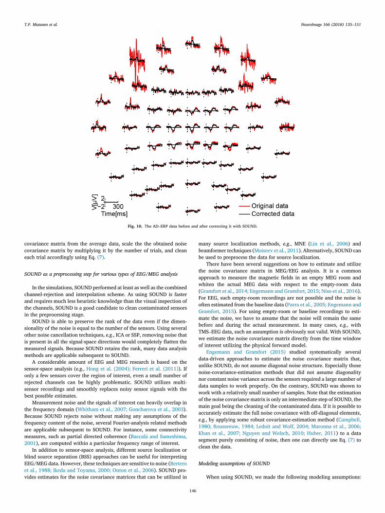
Fig. 10. The AD–ERP data before and after correcting it with SOUND.


covariance matrix from the average data, scale the the obtained noisecovariance matrix by multiplying it by the number of trials, and cleaneach trial accordingly using Eq. (7).

SOUND as a preprocessing step for various types of EEG/MEG analysis

In the simulations, SOUND performed at least as well as the combinedchannel-rejection and interpolation scheme. As using SOUND is fasterand requires much less heuristic knowledge than the visual inspection ofthe channels, SOUND is a good candidate to clean contaminated sensorsin the preprocessing stage.

SOUND is able to preserve the rank of the data even if the dimen-sionality of the noise is equal to the number of the sensors. Using severalother noise cancellation techniques, e.g., ICA or SSP, removing noise thatis present in all the signal-space directions would completely flatten themeasured signals. Because SOUND retains the rank, many data analysismethods are applicable subsequent to SOUND.

A considerable amount of EEG and MEG research is based on thesensor-space analysis (e.g., Hong et al. (2004); Ferreri et al. (2011)). Ifonly a few sensors cover the region of interest, even a small number ofrejected channels can be highly problematic. SOUND utilizes multi-sensor recordings and smoothly replaces noisy sensor signals with thebest possible estimates.

Measurement noise and the signals of interest can heavily overlap inthe frequency domain (Whitham et al., 2007; Goncharova et al., 2003).Because SOUND rejects noise without making any assumptions of thefrequency content of the noise, several Fourier-analysis related methodsare applicable subsequent to SOUND. For instance, some connectivitymeasures, such as partial directed coherence (Baccal�a and Sameshima,2001), are computed within a particular frequency range of interest.

In addition to sensor-space analysis, different source localization orblind source separation (BSS) approaches can be useful for interpretingEEG/MEG data. However, these techniques are sensitive to noise (Berteroet al., 1988; Ikeda and Toyama, 2000; Onton et al., 2006). SOUND pro-vides estimates for the noise covariance matrices that can be utilized in

146

many source localization methods, e.g., MNE (Lin et al., 2006) andbeamformer techniques (Moiseev et al., 2011). Alternatively, SOUND canbe used to preprocess the data for source localization.

There have been several suggestions on how to estimate and utilizethe noise covariance matrix in MEG/EEG analysis. It is a commonapproach to measure the magnetic fields in an empty MEG room andwhiten the actual MEG data with respect to the empty-room data(Gramfort et al., 2014; Engemann and Gramfort, 2015; Niso et al., 2016).For EEG, such empty-room recordings are not possible and the noise isoften estimated from the baseline data (Parra et al., 2005; Engemann andGramfort, 2015). For using empty-room or baseline recordings to esti-mate the noise, we have to assume that the noise will remain the samebefore and during the actual measurement. In many cases, e.g., withTMS–EEG data, such an assumption is obviously not valid. With SOUND,we estimate the noise covariance matrix directly from the time windowof interest utilizing the physical forward model.

Engemann and Gramfort (2015) studied systematically severaldata-driven approaches to estimate the noise covariance matrix that,unlike SOUND, do not assume diagonal noise structure. Especially thosenoise-covariance-estimation methods that did not assume diagonalitynor constant noise variance across the sensors required a large number ofdata samples to work properly. On the contrary, SOUND was shown towork with a relatively small number of samples. Note that the estimationof the noise covariance matrix is only an intermediate step of SOUND, themain goal being the cleaning of the contaminated data. If it is possible toaccurately estimate the full noise covariance with off-diagonal elements,e.g., by applying some robust covariance-estimation method (Campbell,1980; Rousseeuw, 1984; Ledoit and Wolf, 2004; Maronna et al., 2006;Khan et al., 2007; Nguyen and Welsch, 2010; Huber, 2011) to a datasegment purely consisting of noise, then one can directly use Eq. (7) toclean the data.

Modeling assumptions of SOUND

When using SOUND, we made the following modeling assumptions:

Fig. 11. Effects of SOUND on the MEG data quality. A: The signals in the longitudinal gradiometers before (red curves) and after (black curves) SOUND. B: Magnified figures of a set ofgradiometers over visual cortex. C: Topographic maps showing the original signal values in the longitudinal gradiometers at 65 ms after the stimulus (the latency indicated by the verticaldashed lines in B). D: The corresponding topographies after SOUND. E: The dipole matching best the cleaned signals at 65 ms after the visual stimulus.

Fig. 12. Convergence of the noise-estimation iteration in the three measured datasets. The black curves show the changes in the sensor-specific noise estimates relative to the estimates inthe previous step. The plots show that after few dozens of iterations the changes in the noise estimates are only numeric.


(1) the noise correlation matrix is diagonal, (2) the head conductivitymodel is known, and (3) the neural sources are i.i.d. The third assump-tion is not mandatory. If there is prior information on the underlyingsource distribution, it can be easily included in Eq. (3) in the form of thesource covariance matrix (Lin et al., 2006), leading to more accurate datacorrection. Furthermore, the assumptions (1) and (2) do not need to befully correct to achieve a good outcome in the noise cancellation.

Unlike with SNS, the noise does not have to be perfectly diagonal for

147

SOUND to work. This is due to the fact that SOUND also utilizes the in-formation of the neural sources in the form of the lead-field matrix. Thesimulations also suggest that the conductivity values in the head need tobe known only approximately to obtain good data-correction accuracy.The use of realistic geometry was more advantageous compared to thespherical head model. However, also the spherical-head-model-basedSOUND proved to work clearly better than the spherical spline interpo-lation. When using SOUND to clean data with poor SNR, the effects of the


head-model inaccuracies were less pronounced.The simulations showed that SOUND may overestimate noise am-

plitudes in some channels possibly leading to overcorrection. Thisovercorrection most likely takes place in channels that are not sur-rounded by a sufficient number of neighboring sensors, or in channelsthat measure mostly signals from very superficial sources. Indeed, su-perficial sources generate high-spatial-frequency components in thesensor space, which might be incorrectly identified as noise during theSOUND iteration. In addition, if the used sensor array is much sparserthan the arrays studied in this work, it is possible that SOUND attenuatesthe signals of interest more as the information gathered by differentsensors becomes less correlated. The overcorrection might be managedby tuning the amount of regularization. In terms of source localizationaccuracy, SOUND was beneficial, also with the superficial sources, sug-gesting that overestimation of noise is not crucial if the focus is mainly onlocalizing the neural sources.

Comparison of SOUND to existing methods

In this work, we concentrated in comparing SOUNDwith the channel-rejection and interpolation approach, which is a commonly used methodto clean noisy channels (e.g., Julkunen et al. (2011); Casarotto et al.(2013); Atluri et al. (2016)). The channel-rejection-and-interpolationscheme is also used in many signal-processing pipelines and algo-rithms, such as PREP and Autoreject (Jas et al., 2017). In addition, wecompared SOUND to a previously presented method, SNS, which sharesseveral conceptual and theoretical similarities with SOUND.

In the literature, there are suggestions for full EEG and MEG signal-processing pipelines (Nolan et al., 2010; Gramfort et al., 2014; Bigdely-Shamlo et al., 2015). Comparing SOUND directly to these pipelines isdifficult because SOUND is designed for a specific noise-rejection step,the bad-channel detection and rejection. In the future, one should verifyhow SOUND could be optimally integrated to some already establishedEEG/MEG analysis pipelines and/or analysis toolboxes, such as EEGLAB.

In addition to SOUND, we discussed the DDWiener-based approachesto tackle EEG and MEG noise. As a proof of concept, we showed howDDWiener can be utilized in finding the trial-specific noise levels. Ac-cording to visual inspection, DDWiener performed well. We did not,however, compare the performance of this approach to a related method,

148

robust averaging, implemented in the SPM toolbox.

Conclusion

We introduced a method called SOUND that robustly identifies andsuppresses noise and artifacts in EEG. We showed mathematically that,when assuming diagonal noise structure, SOUND provides an optimalestimate for the noiseless EEG/MEG signals, with minimum MSE.Furthermore, through simulations, we showed that SOUND is to someextent robust against the violation of this assumption.

SOUND is completely automatic up to defining the regularizationparameter. We showed a strategy to define this parameter from the data.In addition to SOUND, we showed how general Wiener estimators can beused in a data-driven fashion to clean the measured multi-sensor andmulti-trial data. The suggested methods provide quantitative, objective,and efficient ways to preprocess and clean the gathered data. We vali-dated the performance of the presented methods in practice by analyzingseveral real-life datasets.

Along with this publication, we provide a MATLAB demo packagethat demonstrates how the presented methods can be applied in practice.The description of the package and the download link can be found in theSupplementary material II. In the future, we are willing to help to includethese techniques to some freeware MATLAB toolbox, such as EEGLAB.

Acknowledgments

We thank Prof. Jukka Sarvas, Prof. Lauri Parkkonen, Dr. Matti Sten-roos, and Dr. Jaakko Nieminen for valuable suggestions regarding themanuscript. In addition, we would like to thank Prof. Sarvas forproviding tools for the MATLAB demo package. This study was supportedby the Academy of Finland (Grant No. 283105), the Finnish CulturalFoundation (Grant No. 00150064, 00161149, 00140634, and00160630), the Foundation for Aalto University Science and Technology,the Kymenlaakso Regional fund of the Finnish Cultural Foundation(35162142), and the Finnish Brain Foundation.

Some datasets used for this study were downloaded from the HeadITData Repository (http://www.headit.org), supported by grants to theHeadIT (R01-MH084819) and EEGLAB (5-R01-NS047293-08) funded bythe National Institutes of Health, U.S.A.

Appendices.

A. Wiener estimation for cleaning noise in multi-sensor data

Here, we show that SOUND corresponds to Wiener estimation of the noiseless EEG/MEG signals. We also explain how the data-driven version of theWiener estimator (Eq. (8)) is obtained, and that this approximation corresponds to Sensor Noise Suppression (SNS) (De Cheveign�e and Simon, 2008).

We aim at estimating Y from the noisy data, expressed in Eq. (1), assuming that N is uncorrelated with Y and that the correlation matrix of N isdiagonal. Again, we wish to find an estimate for the signal in sensor s using the data recorded by all the other sensors. If we know the correlation matrixof the data, C ¼ corrðYÞ, and the cross-correlation vector r≠s;s between Y≠s and ys, we can use Wiener estimation (or filtering) (Hayes, 2009) to find anestimate for the noiseless data in the sensor s by

Wiener T
bys ¼ ð bwsÞ Y≠sbws ¼ ðC≠s;≠sÞ�1r≠s;s;(A.1)
where the optimal weight vector bws is found so that the corresponding mean-squared error, T�1PTt¼1

�ys;t � ð bwsÞTy≠s;t

2, has been minimized. Wiener

estimation is a robust method against small errors in bws since the mean-square-error increases only in proportion to the square of the deviants from theoptimal weights.

For the measured data described in Eq. (1), the data correlation matrix is found to be C � T�1ðLJþ NÞðLJþNÞT � LΓLT þ Σ, Γ and Σ being thesource and noise correlation matrices, respectively. The corresponding cross-correlation vector between Y and ys can be written asr⋅;s � T�1ðLJþNÞðlsJÞT � LΓlTs . Since the expectation values of the noise and the recorded data are assumed zero, their correlation matrices areidentical with the corresponding covariance matrices. In practice, the source correlation matrix is commonly not known, and hence, the sources are

http://www.headit.org


assumed independent and identically distributed (i.i.d.), leading to Γ ¼ λ�2I, where λ�2 is the source variance. Thus,

�2 T
C≠s;≠s ¼ λ L≠sL≠s þ Σ≠s;≠s
r≠s;s ¼ λ�2L≠slTs :

(A.2)

Substituting these identities into Eq. (A.1) yields the estimate

i:i:d: � ��1
bys ¼ lsLT≠s L≠sLT
≠s þ λ2Σ≠s;≠s Y≠s

¼ ls~LT≠s

�~L≠s~L

T≠s þ λ2I

�1~Y≠s;

(A.3)

where the latter form is written in terms of whitened data (Eq. (2)).We see that Eq. (A.3) actually corresponds to combining Eqs. (3) and (6) in the same way as used by SOUND in the iterative estimation of the noise

covariance matrix. After the iterations, SOUND takes into account all the measured data and the final estimated noise covariance matrix to reconstructcleaned EEG using Eq. (7). Thus, the final step of SOUND corresponds to building the Wiener estimator for Y using all the sensor signals as the esti-mator input.

An alternative approach for implementing the Wiener estimator is to use the collected data samples for computing the sample correlation matrix ofthe data C≃T�1 YYT. Since the noise correlation matrix is diagonal, r≠s;s ¼ c≠s;s. This can be used to simplify the expression for the weight vector inEq. (A.1):

�1
bws ¼ ðC≠s;≠sÞ c≠s;s: (A.4)
Note that this simplification would not be possible if the sth sensor was included in the input of the estimator. Substituting this approximation for bws

in Eq. (A.1) yields

sample T� T��1
bys ¼ ysðY≠sÞ Y≠sðY≠sÞ Y≠s: (A.5)
This approach can be seen to be data-driven since it uses only the recorded data to estimate the noiseless signals.It is straightforward to show that Eq. (A.5) corresponds to SNS algorithm (De Cheveign�e and Simon, 2008), which replaces each noisy channel by its

regression on the subspace formed by the other channels. We express the ≠s rows of the data in terms of singular-value decomposition (SVD),Y≠s ¼ USVT, where the columns ofU and V contain the left and right singular vectors, respectively, and S holds the singular values on its K first diagonalentries. The column vectors of V form a complete orthonormal basis for all the possible signals in the rows of Y, whereas the K first columns span onlythe subspace needed for explaining the measured signals in sensors ≠s.

With the help of SVD, Eq. (A.5) can be written as:
h i�1 bysamples ¼ ysðUSVTÞT USVTðUSVTÞT USVT
¼ ysVSTðSSTÞ�1SVT:

(A.6)

If SST is not invertible, one may use its generalized inverse. In either case, the estimate becomes:

K
bysamples ¼
Xk¼1

ðysv⋅;kÞðv⋅;kÞT; (A.7)

which is the mathematical expression for SNS.

B. Generating the noise for the simulated data

Here, we describe how the correlation structure of the simulated noise, with T samples and S sensors, was controlled. We first randomized T samplesof an S-variate Gaussian random noise vector with zero mean and identity covariance matrix and collected them in an S� T noise matrix ε, where eachrow represents the activity (waveform) of one noise source. In the sensor space, the noise sources were mixed by matrix A, yielding the noise signalsN ¼ Aε. If the ith column of A has m non-zero elements, the noise signals become correlated across the corresponding m channels.

Based on this reasoning, the noise was generated by

ðmÞ
N ¼ Aε ¼ ðB ∘L Þ ε ; (B.1)
where ∘ denotes the entry-wise matrix product and BðmÞ is a binary matrix with m elements in each column equal to 1 (the remaining elements beingzero). Thus, the signals from each noise source were correlated across m channels. We call m the noise correlation index (NCI). When NCI ¼ 1, theresulting noise covariance matrix is diagonal, whereas, when NCI approaches S, the noise becomes correlated across an increasing number of sensorsand starts to resemble neural noise with covariance matrix Σ ¼ LLT. Thus, as NCI increases, the data correction becomes increasingly difficult forSOUND. For a fixed NCI (m), the non-zero elements in the columns of BðmÞ were randomly chosen for each simulation.

Appendix C. Supplementary data

Supplementary data related to this article can be found at https://doi.org/10.1016/j.neuroimage.2017.10.021.

149



References

Ashburner, J., Barnes, G., Chen, C.-C., Daunizeau, J., Flandin, G., Friston, K., Kiebel, S.,Kilner, J., Litvak, V., Moran, R., Penny, W., Razi, A., Stephan, K., Tak, S., Zeidman, P.,Gitelman, D., Henson, R., Hutton, C., Glauche, V., Mattout, J., Phillips, C., 2012.SPM12 Manual. Functional Imaging Laboratory, Wellcome Trust Centre forNeuroimaging, Institute of Neurology, UCL.

Atluri, S., Frehlich, M., Mei, Y., Dominguez, L.G., Rogasch, N.C., Wong, W.,Daskalakis, Z.J., Farzan, F., 2016. TMSEEG: a MATLAB-based graphical user interfacefor processing electrophysiological signals during transcranial magnetic stimulation.Front. Neural Circuits 10.

Baccal�a, L.A., Sameshima, K., 2001. Partial directed coherence: a new concept in neuralstructure determination. Biol. Cybern. 84, 463–474.

Berg, P., Scherg, M., 1994. A multiple source approach to the correction of eye artifacts.Electroencephalogr. Clin. Neurophysiology 90, 229–241.

Bertero, M., De Mol, C., Pike, E.R., 1988. Linear inverse problems with discrete data: II.Stability and regularisation. Inverse Probl. 4, 573–594.

Bezerianos, A., Laskaris, N., Fotopoulos, S., Papathanasopoulos, P., 1995. Data dependentweighted averages for recording of evoked potential signals. Electroencephalogr.Clin. Neurophysiology/Evoked Potentials Sect. 96, 468–471.

Bigdely-Shamlo, N., Mullen, T., Kothe, C., Su, K.-M., Robbins, K.A., 2015. The PREPpipeline: standardized preprocessing for large-scale EEG analysis. Front.Neuroinformatics 9, 16.

Bresnahan, S.M., Barry, R.J., 2002. Specificity of quantitative EEG analysis in adults withattention deficit hyperactivity disorder. Psychiatry Res. 112, 133–144.

Buzsaki, G., Draguhn, A., 2004. Neuronal oscillations in cortical networks. Science 304,1926–1929.

Campbell, N.A., 1980. Robust procedures in multivariate analysis I: robust covarianceestimation. Appl. Stat. 231–237.

Casarotto, S., Canali, P., Rosanova, M., Pigorini, A., Fecchio, M., Mariotti, M., Lucca, A.,Colombo, C., Benedetti, F., Massimini, M., 2013. Assessing the effects ofelectroconvulsive therapy on cortical excitability by means of transcranial magneticstimulation and electroencephalography. Brain Topogr. 26, 326–337.

Crouzeix, A., Yvert, B., Bertrand, O., Pernier, J., 1999. An evaluation of dipolereconstruction accuracy with spherical and realistic head models in MEG. Clin.Neurophysiol. 110, 2176–2188.

Davila, C.E., Mobin, M.S., 1992. Weighted averaging of evoked potentials. IEEE Trans.Biomed. Eng. 39, 338–345.

De Cheveign�e, A., Simon, J.Z., 2008. Sensor noise suppression. J. Neurosci. Methods 168,195–202.

Delorme, A., Makeig, S., 2004. EEGLAB: an open source toolbox for analysis of single-trialEEG dynamics including independent component analysis. J. Neurosci. Methods 134,9–21.

Delorme, A., Mullen, T., Kothe, C., Acar, Z.A., Bigdely-Shamlo, N., Vankov, A., Makeig, S.,2011. EEGLAB, SIFT, NFT, BCILAB, and ERICA: new tools for advanced EEGprocessing. Comput. Intell. Neurosci. 2011, 10.

Dominguez, L.G., Radhu, N., Farzan, F., Daskalakis, Z.J., 2014. Characterizing longinterval cortical inhibition over the time-frequency domain. PloS One 9, e92354.

Engemann, D.A., Gramfort, A., 2015. Automated model selection in covariance estimationand spatial whitening of MEG and EEG signals. NeuroImage 108, 328–342.

Ferree, T.C., Luu, P., Russell, G.S., Tucker, D.M., 2001. Scalp electrode impedance,infection risk, and EEG data quality. Clin. Neurophysiol. 112, 536–544.

Ferreri, F., Pasqualetti, P., M€a€att€a, S., Ponzo, D., Ferrarelli, F., Tononi, G., Mervaala, E.,Miniussi, C., Rossini, P.M., 2011. Human brain connectivity during single and pairedpulse transcranial magnetic stimulation. NeuroImage 54, 90–102.

Fischl, B., 2012. FreeSurfer. NeuroImage 62, 774–781.Foster, M., 1961. An application of the Wiener-Kolmogorov smoothing theory to matrix

inversion. J. Soc. Industrial Appl. Math. 9, 387–392.Goncharova, I.I., McFarland, D.J., Vaughan, T.M., Wolpaw, J.R., 2003. EMG

contamination of EEG: spectral and topographical characteristics. Clin. Neurophysiol.114, 1580–1593.

Gramfort, A., Luessi, M., Larson, E., Engemann, D.A., Strohmeier, D., Brodbeck, C.,Parkkonen, L., H€am€al€ainen, M.S., 2014. MNE software for processing MEG and EEGdata. NeuroImage 86, 446–460.

H€am€al€ainen, M., Hari, R., Ilmoniemi, R.J., Knuutila, J., Lounasmaa, O.V., 1993.Magnetoencephalography—theory, instrumentation, and applications to noninvasivestudies of the working human brain. Rev. Mod. Phys. 65, 413.

Hauk, O., 2004. Keep it simple: a case for using classical minimum norm estimation in theanalysis of EEG and MEG data. NeuroImage 21, 1612–1621.

Hauk, O., Pulvermüller, F., 2004. Neurophysiological distinction of action words in thefronto-central cortex. Hum. Brain Mapp. 21, 191–201.

Hayes, M.H., 2009. Statistical Digital Signal Processing and Modeling. John Wiley & Sons.Herrmann, C.S., Demiralp, T., 2005. Human EEG gamma oscillations in neuropsychiatric

disorders. Clin. Neurophysiol. 116, 2719–2733.Hong, L.E., Summerfelt, A., McMahon, R., Adami, H., Francis, G., Elliott, A.,

Buchanan, R.W., Thaker, G.K., 2004. Evoked gamma band synchronization and theliability for schizophrenia. Schizophrenia Res. 70, 293–302.

Huber, P.J., 2011. Robust statistics. In: International Encyclopedia of Statistical Science.Springer, pp. 1248–1251.

Ikeda, S., Toyama, K., 2000. Independent component analysis for noisy data—MEG dataanalysis. Neural Netw. 13, 1063–1074.

Ilmoniemi, R.J., Hernandez-Pavon, J.C., M€akel€a, N.N., Metsomaa, J., Mutanen, T.P.,Stenroos, M., Sarvas, J., 2015. Dealing with artifacts in TMS-evoked EEG. In:Engineering in Medicine and Biology Society (EMBC), 2015 37th AnnualInternational Conference of the IEEE. IEEE, pp. 230–233.

150

Ilmoniemi, R.J., Ki�ci�c, D., 2010. Methodology for combined TMS and EEG. Brain Topogr.22, 233–248.

Ilmoniemi, R.J., Virtanen, J., Ruohonen, J., Karhu, J., Aronen, H.J., Katila, T., 1997.Neuronal responses to magnetic stimulation reveal cortical reactivity andconnectivity. NeuroReport 8, 3537–3540.

Jas, M., Engemann, D.A., Bekhti, Y., Raimondo, F., Gramfort, A., 2017. Autoreject:automated artifact rejection for MEG and EEG data. NeuroImage 159, 417–429.

Jensen, O., Colgin, L.L., 2007. Cross-frequency coupling between neuronal oscillations.Trends Cognitive Sci. 11, 267–269.

John, M.S., Dimitrijevic, A., Picton, T.W., 2001. Weighted averaging of steady-stateresponses. Clin. Neurophysiol. 112, 555–562.

Julkunen, P., Jauhiainen, A.M., K€on€onen, M., P€a€akk€onen, A., Karhu, J., Soininen, H.,2011. Combining transcranial magnetic stimulation and electroencephalography maycontribute to assess the severity of Alzheimer's disease. Int. J. Alzheimer’s Dis. 2011.

Kaipio, J., Somersalo, E., 2006. Statistical and Computational Inverse Problems. SpringerScience & Business Media.

Kaukoranta, E., H€am€al€ainen, M., Sarvas, J., Hari, R., 1986. Mixed and sensory nervestimulations activate different cytoarchitectonic areas in the human primarysomatosensory cortex SI. Exp. Brain Res. 63, 60–66.

Khan, J.A., Van Aelst, S., Zamar, R.H., 2007. Robust linear model selection based on leastangle regression. J. Am. Stat. Assoc. 102, 1289–1299.

Komssi, S., Aronen, H.J., Huttunen, J., Kes€aniemi, M., Soinne, L., Nikouline, V.V.,Ollikainen, M., Roine, R.O., Karhu, J., Savolainen, S., Ilmoniemi, R.J., 2002. Ipsi- andcontralateral EEG reactions to transcranial magnetic stimulation. Clin. Neurophysiol.113, 175–184.

Komssi, S., Huttunen, J., Aronen, H.J., Ilmoniemi, R.J., 2004. EEG minimum-normestimation compared with MEG dipole fitting in the localization of somatosensorysources at S1. Clin. Neurophysiol. 115, 534–542.

Korhonen, R.J., Hernandez-Pavon, J.C., Metsomaa, J., M€aki, H., Ilmoniemi, R.J.,Sarvas, J., 2011. Removal of large muscle artifacts from transcranial magneticstimulation-evoked EEG by independent component analysis. Med. Biol. Eng.Comput. 49, 397–407.

Ledoit, O., Wolf, M., 2004. A well-conditioned estimator for large-dimensional covariancematrices. J. Multivar. Analysis 88, 365–411.

Lin, F.-H., Belliveau, J.W., Dale, A.M., H€am€al€ainen, M.S., 2006. Distributed currentestimates using cortical orientation constraints. Hum. Brain Mapp. 27, 1–13.

Litvak, V., Komssi, S., Scherg, M., Hoechstetter, K., Classen, J., Zaaroor, M., Pratt, H.,Kahkonen, S., 2007. Artifact correction and source analysis of earlyelectroencephalographic responses evoked by transcranial magnetic stimulation overprimary motor cortex. NeuroImage 37, 56–70.

M€aki, H., Ilmoniemi, R.J., 2011. Projecting out muscle artifacts from TMS-evoked EEG.NeuroImage 54, 2706–2710.

Maronna, R.A., Martin, R.D., Yohai, V.J., 2006. Robust Statistics. John Wiley & Sons.Michel, C.M., Murray, M.M., Lantz, G., Gonzalez, S., Spinelli, L., de Peralta, R.G., 2004.

EEG source imaging. Clin. Neurophysiol. 115, 2195–2222.Moiseev, A., Gaspar, J.M., Schneider, J.A., Herdman, A.T., 2011. Application of multi-

source minimum variance beamformers for reconstruction of correlated neuralactivity. NeuroImage 58, 481–496.

Monto, S., Palva, S., Voipio, J., Palva, J.M., 2008. Very slow EEG fluctuations predict thedynamics of stimulus detection and oscillation amplitudes in humans. J. Neurosci. 28,8268–8272.

Moratti, S., Keil, A., 2005. Cortical activation during Pavlovian fear conditioning dependson heart rate response patterns: an MEG study. Cognitive Brain Res. 25, 459–471.

Mosher, J.C., Hamalainen, M.S., Pantazis, D., Hui, H.B., Burgess, R.C., Leahy, R.M., 2009.Generalized sidelobe canceller for magnetoencephalography arrays. In: BiomedicalImaging: from Nano to Macro, 2009. ISBI’09. IEEE, pp. 149–152. IEEE InternationalSymposium on.

Mutanen, T.P., Kukkonen, M., Nieminen, J.O., Stenroos, M., Sarvas, J., Ilmoniemi, R.J.,2016. Recovering TMS-evoked EEG responses masked by muscle artifacts.NeuroImage 139, 157–166.

Nguyen, T.-D., Welsch, R.E., 2010. Outlier detection and robust covariance estimationusing mathematical programming. Adv. Data Analysis Classif. 4, 301–334.

Nieminen, J.O., Gosseries, O., Massimini, M., Saad, E., Sheldon, A.D., Boly, M., Siclari, F.,Postle, B.R., Tononi, G., 2016. Consciousness and cortical responsiveness: a within-state study during non-rapid eye movement sleep. Sci. Rep. 6, 30932.

Niso, G., Rogers, C., Moreau, J.T., Chen, L.-Y., Madjar, C., Das, S., Bock, E., Tadel, F.,Evans, A.C., Jolicoeur, P., et al., 2016. OMEGA: the open MEG archive. NeuroImage124, 1182–1187.

Nolan, H., Whelan, R., Reilly, R., 2010. FASTER: fully automated statistical thresholdingfor EEG artifact rejection. J. Neurosci. Methods 192, 152–162.

Numminen, J., Ahlfors, S., Ilmoniemi, R., Montonen, J., Nenonen, J., 1995.Transformation of multichannel magnetocardiographic signals to standard grid form.IEEE Trans. Biomed. Eng. 42, 72–78.

Onton, J., Westerfield, M., Townsend, J., Makeig, S., 2006. Imaging human EEG dynamicsusing independent component analysis. Neurosci. Biobehav. Rev. 30, 808–822.

Parra, L.C., Spence, C.D., Gerson, A.D., Sajda, P., 2005. Recipes for the linear analysis ofEEG. NeuroImage 28, 326–341.

Perrin, F., Pernier, J., Bertrand, O., Echallier, J.F., 1989. Spherical splines for scalppotential and current density mapping. Electroencephalogr. Clin. Neurophysiology72, 184–187.

Picton, T.W., Bentin, S., Berg, P., Donchin, E., Hillyard, S.A., Johnson, R., Miller, G.A.,Ritter, W., Ruchkin, D.S., Rugg, M.D., Taylor, M.J., 2000. Guidelines for using humanevent-related potentials to study cognition: recording standards and publicationcriteria. Psychophysiology 37, 127–152.

http://refhub.elsevier.com/S1053-8119(17)30848-0/sref1






























































































































































































































































Portin, K., Vanni, S., Virsu, V., Hari, R., 1999. Stronger occipital cortical activation tolower than upper visual field stimuli Neuromagnetic recordings. Exp. Brain Res. 124,287–294.

Rousseeuw, P.J., 1984. Least median of squares regression. J. Am. Stat. Assoc. 79,871–880.

Shattuck, D.W., Leahy, R.M., 2002. BrainSuite: an automated cortical surfaceidentification tool. Med. Image Anal. 6, 129–142.

Stenroos, M., Sarvas, J., 2012. Bioelectromagnetic forward problem: isolated sourceapproach revis(it)ed. Phys. Med. Biol. 57, 3517–3535.

Styliadis, C., Ioannides, A.A., Bamidis, P.D., Papadelis, C., 2014. Amygdala responses tovalence and its interaction by arousal revealed by MEG. Int. J. Psychophysiol. 93,121–133.

Taulu, S., Kajola, M., 2005. Presentation of electromagnetic multichannel data: the signalspace separation method. J. Appl. Phys. 97, 124905.

Taulu, S., Kajola, M., Simola, J., 2004. Suppression of interference and artifacts by thesignal space separation method. Brain Topogr. 16, 269–275.

Tewarie, P., Hillebrand, A., Schoonheim, M., Van Dijk, B.W., Geurts, J.J.G., Barkhof, F.,Polman, C.H., Stam, C.J., 2014. Functional brain network analysis using minimum

151

spanning trees in Multiple Sclerosis: an MEG source-space study. NeuroImage 88,308–318.

Uusitalo, M.A., Ilmoniemi, R.J., 1997. Signal-space projection method for separating MEGor EEG into components. Med. Biol. Eng. Comput. 35, 135–140.

Uutela, K., Taulu, S., H€am€al€ainen, M., 2001. Detecting and correcting for headmovements in neuromagnetic measurements. NeuroImage 14, 1424–1431.

Van der Meer, M.L., Tewarie, P., Schoonheim, M.M., Douw, L., Barkhof, F., Polman, C.H.,Stam, C.J., Hillebrand, A., 2013. Cognition in MS correlates with resting-stateoscillatory brain activity: an explorative MEG source-space study. NeuroImage Clin.2, 727–734.

Vig�ario, R.N., 1997. Extraction of ocular artefacts from EEG using independentcomponent analysis. Electroencephalogr. Clin. Neurophysiology 103, 395–404.

Vrba, J., Robinson, S.E., 2001. Signal processing in magnetoencephalography. Methods25, 249–271.

Whitham, E.M., Pope, K.J., Fitzgibbon, S.P., Lewis, T., Clark, C.R., Loveless, S.,Broberg, M., Wallace, A., DeLosAngeles, D., Lillie, P., Hardy, A., Fronsko, R.,Pulbrook, A., Willoughby, J.O., 2007. Scalp electrical recording during paralysis:quantitative evidence that EEG frequencies above 20 Hz are contaminated by EMG.Clin. Neurophysiol. 118, 1877–1888.























































Automatic and robust noise suppression in EEG and MEG

Documents

Transcript of Automatic and robust noise suppression in EEG and MEG