M/EEG source reconstruction based on Gabor

thresholding in the source space

Daniel Strohmeier, Alexandre Gramfort, Jens Haueisen, Matti Hamalainen,

Matthieu Kowalski

To cite this version:

Daniel Strohmeier, Alexandre Gramfort, Jens Haueisen, Matti Hamalainen, Matthieu Kowalski.M/EEG source reconstruction based on Gabor thresholding in the source space. NFSI 2011,May 2011, Banff, Canada. 2011. <hal-00621044>

HAL Id: hal-00621044

https://hal.archives-ouvertes.fr/hal-00621044

Submitted on 9 Sep 2011

HAL is a multi-disciplinary open accessarchive for the deposit and dissemination of sci-entific research documents, whether they are pub-lished or not. The documents may come fromteaching and research institutions in France orabroad, or from public or private research centers.

L’archive ouverte pluridisciplinaire HAL, estdestinee au depot et a la diffusion de documentsscientifiques de niveau recherche, publies ou non,emanant des etablissements d’enseignement et derecherche francais ou etrangers, des laboratoirespublics ou prives.

MEG/EEG source reconstruction based on Gaborthresholding in the source space

Daniel Strohmeier1, Alexandre Gramfort234, Jens Haueisen156, Matti Hamalainen2 and Matthieu Kowalski71Institute of Biomedical Engineering and Informatics, Ilmenau University of Technology, Ilmenau, Germany

2Martinos Center for Biomedical Imaging, Department of Radiology, MGH, Harvard Medical School, Boston, MA3INRIA Parietal Project Team, Saclay, France

4LNAO/NeuroSpin, CEA Saclay, Bat. 145, Gif-sur-Yvette, France5Biomagnetic Center, Department of Neurology, University Hospital Jena, Jena, Germany6Department of Applied Medical Sciences, King Saud University, Riyadh, Saudi Arabia

7Laboratoire des Signaux et Systemes (L2S), Universite Paris-Sud, Orsay, FranceEmail: daniel.strohmeier@tu-ilmenau.de, gramfort@nmr.mgh.harvard.edu, jens.haueisen@tu-ilmenau.de,

msh@nmr.mgh.harvard.edu, matthieu.kowalski@lss.supelec.fr

Abstract—Thanks to their high temporal resolution, sourcereconstruction based on Magnetoencephalography (MEG) and/orElectroencephalography (EEG) is an important tool for nonin-vasive functional brain imaging. Since the MEG/EEG inverseproblem is ill-posed, inverse solvers employ priors on the sources.While priors are generally applied in the time domain, thetime-frequency (TF) characteristics of brain signals are rarelyemployed as a spatio-temporal prior. In this work, we present aninverse solver which employs a structured sparse prior formedby the sum of `21 and `1 norms on the coefficients of the GaborTF decomposition of the source activations. The resulting convexoptimization problem is solved using a first-order scheme basedon proximal operators. We provide empirical evidence based onEEG simulations that the proposed method is able to recoverneural activations that are spatially sparse, temporally smoothand non-stationary. We compare our approach to alternativesolvers based also on convex sparse priors, and demonstratethe benefit of promoting sparse Gabor decompositions via amathematically principled iterative thresholding procedure.

I. INTRODUCTION

For both neuroscience research and clinical diagnosis, non-invasive measurements of the brain function are of majorimportance. Solving the bioelectromagnetic inverse problem ofMagnetoencephalography (MEG) and/or Electroencephalogra-phy (EEG) (collectively M/EEG) is a way to achieve this.Due to the ill-posed nature of the M/EEG inverse problem, itis mandatory to impose suitable constraints on the solution.These constraints, also called priors, should reflect neuro-physiologically motivated assumptions on the sources. Priorsare typically related to the number of active sources, theiramplitudes or their spatio-temporal characteristics.

During the past few years, several source reconstructionmethods based on spatially sparse priors have been introduced,sparsity-inducing Bayesian formulations [1]–[3], and convexmixed norms [4]–[6]. These approaches assume that only a

This work was supported by a research grant offered by the GermanResearch Foundation (Ha 2899/8-1).

limited number of focal sources is involved in a specific cog-nitive task. To do so, these imaging methods rely on sparsityinducing priors in the time domain. In contrast, the inversesolvers presented in [7], [8] impose structured sparsity onthe time-frequency (TF) decomposition of the source signals.As will be illustrated in this work, this allows to performsource reconstruction and TF analysis in the source spacesimultaneously. While the TF decomposition in the sensorspace is commonly applied as a preprocessing step to identifyTF components, which can then be localized is a second step[9]–[11], the TF characteristics of the source signals are rarelyemployed directly as a prior to regularize the inverse problem.The relevant TF components are typically identified by lookingat high coefficients in Wavelet or Gabor decompositions anddenoising is then naturally done by thresholding [1]. Thisresults in smooth time series which can also be obtainedwith an `1 regularization [12]. In order to obtain spatiallysparse source estimates, Ou et al. [5] apply a `21 mixed normprior, which promotes a dense block row structure on thematrix of the source estimates. The reconstructed sources arespatially sparse, but their activation time series are likely to benoisy since they are not regularized. In order to have spatiallysparse and temporally smooth source estimates, we present acomposite prior combining `21 mixed norm and `1 norm priorsthat is applied on the TF coefficients of the source signals.Such a prior promotes a block row structure with intra-rowsparsity, see Fig. 1.

In a previous work [13], we described the mathematicalframework which applies structured sparsity of the TF de-composition coefficients to recover the spatial sparsity, tem-poral smoothness and non-stationarity of neural activations.In this contribution, we start by presenting some aspects ofthe convex optimization procedure detailed in [13] and thenextend this work by providing empirical evidence based onEEG simulations using isolated current dipoles and dipolepatches that our method is able to recover the location as wellas the TF characteristics of neuronal sources simultaneously.

TF coefficients

so

urc

e

(a) `2 norm

TF coefficients

so

urc

e

(b) `1 norm

TF coefficients

so

urc

e

(c) `21 mixed norm

TF coefficients

so

urc

e

(d) `21 mixed norm + `1 norm

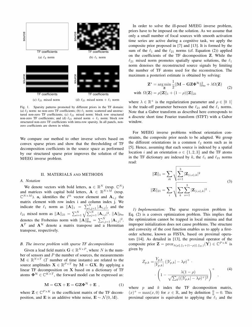
Fig. 1. Sparsity patterns promoted by different priors in the TF domain:(a) `2 norm: no non-zero TF coefficients; (b) `1 norm: scattered and unstruc-tured non-zero TF coefficients; (c) `21 mixed norm: block row structurednon-zero TF coefficients; and (d) `21 mixed norm + `1 norm: block rowstructured non-zero TF coefficients with intra-row sparsity. In all panels, non-zero coefficients are shown in white.

We compare our method to other inverse solvers based onconvex sparse priors and show that the thresholding of TFdecomposition coefficients in the source space as performedby our structured sparse prior improves the solution of theM/EEG inverse problem.

II. MATERIALS AND METHODS

A. Notation

We denote vectors with bold letters, a ∈ RN (resp. CN )and matrices with capital bold letters, A ∈ RN×M (resp.CN×M ). ai identifies the ith vector element and Ai,j thematrix element with row index i and column index j. Weindicate the `1 norm as ‖A‖1 =

∑Ni,j=1 |Ai,j |, and the

`21 mixed norm as ‖A‖21 =∑Ni=1

√∑Nj=1 |Ai,j |2. ‖A‖Fro

denotes the Frobenius norm with ‖A‖2Fro =∑Ni,j=1 |Ai,j |2.

AT and AH denote a matrix transpose and a Hermitiantranspose, respectively.

B. The inverse problem with sparse TF decompositions

Given a lead field matrix G ∈ RN×P , where N is the num-ber of sensors and P the number of sources, the measurementsM ∈ RN×T (T number of time instants) are related to thesource amplitudes X ∈ RP×T by M = GX. By applying alinear TF decomposition on X based on a dictionary of TFatoms ΦH ∈ CK×T , the forward model can be expressed as:

M = GX + E = GZΦH + E , (1)

where Z ∈ CP×K is the coefficient matrix of the TF decom-position, and E is an additive white noise, E ∼ N (0, λI).

In order to solve the ill-posed M/EEG inverse problem,priors have to be imposed on the solution. As we assume thatonly a small number of focal sources with smooth activationtime series are active during a cognitive task, we apply thecomposite prior proposed in [7] and [13]. It is formed by thesum of the `1 and the `21 norms (cf. Equation (2)) appliedon the coefficients of the TF decomposition Z. While the`21 mixed norm promotes spatially sparse solutions, the `1norm denoises the reconstructed source signals by limitingthe number of TF atoms used for the reconstruction. Themaximum a posteriori estimate is obtained by solving:

Z? = arg minZ

1

2‖M−GZΦH‖2Fro + λΩ(Z)

with Ω(Z) = ρ‖Z‖1 + (1− ρ)‖Z‖21

(2)

where λ ∈ R+ is the regularization parameter and ρ ∈ [0 1]is the trade-off parameter between the `21 and the `1 norms.Note that a Gabor transform as described here corresponds toa discrete short time Fourier transform (STFT) with a Gaborwindow.

For M/EEG inverse problems without orientation con-straints, the composite prior needs to be adapted. We groupthe different orientations in a common `2 norm such as in[5]. Hence, assuming that each source is indexed by a spatiallocation i and an orientation o ∈ 1, 2, 3 and the TF atomsin the TF dictionary are indexed by k, the `1 and `21 normsread:

‖Z‖1 =∑ik

√√√√ 3∑o=1

|Z(i,o),k|2

‖Z‖21 =∑i

√√√√∑k

3∑o=1

|Z(i,o),k|2 ,

(3)

1) Implementation: The sparse regression problem inEq. (2) is a convex optimization problem. This implies thatthe optimization cannot be trapped in local minima and thatimproper initialization does not cause problems. The structureand convexity of the cost function enables us to apply a first-order scheme, known as FISTA, based on proximal opera-tors [14]. As detailed in [13], the proximal operator of thecomposite prior Z = proxλ(ρ‖.‖1+(1−ρ)‖.‖21)(Y) ∈ CP×K isgiven by

Zp,k =Yp,k|Yp,k|

(|Yp,k| − λρ)+ ·

·

(1− λ(1− ρ)√∑

k((|Yp,k| − λρ)+)2

)+

,

(4)

where p and k index the TF decomposition matrix,(x)+ = max(x, 0) for x ∈ R, and by definition 0

0 = 0. Thisproximal operator is equivalent to applying the `1 and the

`21 proximal operators successively [15], [16]. The pseudo-code for the optimization process is given in Algorithm 1.Note that contrary to previous contributions like [7] that usea truncated Newton method, which should be only applied todifferentiable problems, this contribution provides a principledmethod to minimize the cost function in Equation (2).

Algorithm 1 FISTA with TF dictionariesRequire: Measurements M, lead field matrix G, regulariza-

tion parameter λ > 0 and I the number of iterations.Ensure: Z?

1: Aux. variables: Y and Zo ∈ RP×K , and τ and τo ∈ R.2: Estimate the Lipschitz constant L with the power iteration

method.3: Y = Z? = Z, τ = 1, 0 < µ < L−1

4: for i = 1 to I do5: Zo = Z?

6: Z? = proxµλΩ

(Y + µGT (M−GYΦH)Φ

)7: τo = τ8: τ = 1+

√1+4τ2

29: Y = Z? + τo−1

τ (Z? − Zo)10: end for

We apply a Gabor transform with a Gabor frame basedon the LTFAT toolbox [17] to compute the TF decompo-sition. This allows to recover stationary as well as non-stationary source signals x ∈ RT from their Gabor coefficients(〈x,φk,f 〉) = ΦHx. To reduce the computation time, wecompute the Gabor transform only for active sources, i.e.,sources with non-zero TF decomposition coefficients.

C. Simulation setup

In order to evaluate the performance of the sparse TF inversealgorithm, we performed simulations with isolated currentdipoles and dipole patches as sources. The simulation setupconsisted of a three shell boundary element model (BEM)which was computed with OpenMEEG [18] using skin, skull,and CSF surfaces segmented from a MRI scan using MNE1.The conductivities were chosen according to [19]. The sourcespace was built from 5000 triplets of orthogonal currentdipoles placed on the boundary between white and gray matter,which was segmented using FreeSurfer [20]. We used 128EEG channels for spatially sampling of the simulated data.Finally, a common-average reference transform was appliedto the leadfield matrix.

D. Simulation

1) Isolated current dipoles : We modeled 2 current dipoleslocated in Brodmann areas 3b and 1. The orientations areset perpendicular to the white matter surface. The geodesic

1http://www.nmr.mgh.harvard.edu/martinos/userInfo/data/sofMNE.php

distance between the simulated dipoles was 15.7 mm, andthe angle between dipole moment vectors 101.4. The acti-vation curves were modeled using synthetic, non-stationarychirp signals with an exponential decay (cf. Fig. 2). Toevaluate the performance with different signal to noise ra-tios (SNR) (-6db, 0dB, and 6dB), which we define hereas 20 log10(‖M‖Fro/‖E‖Fro), white noise was added to theforward simulation. By adding white noise, we assume thatthe data were spatially whitened based on a noise covariancematrix estimated during baseline.

We applied the sparse TF inverse approach with orientationconstraint and a tight Gabor frame with time shift k =4 samples and frequency shift f = 4 samples. In order tocompensate the depth bias, the columns of the lead fieldmatrix were normalized before solving the inverse problem.We compare our solution to inverse solvers based on `21 mixednorm priors [5] and a `1 norm priors, respectively. We imposedthe `1 norm prior both on the source activations in the timedomain and on the coefficients of the TF decomposition. Incontrast, as the `21 mixed norm prior in the time and TFdomain are mathematically equivalent when using tight Gaborframes, we chose to apply it in the time domain.

Although solving the inverse problem based on the com-posite prior is tractable for high dimensional data sets (see[13] for a real MEG data set), we reduced the source spacewith regard to the complexity of the simulations in order todecrease the computation time. Faster optimization relies onan active set approach [21] and is further discussed in [13].As the application and evaluation of this method is beyond thescope of this contribution, we simulated the result of the activeset approach by restricting the source space to patches withgeodesic radii of 50 mm, which include the simulated sources.The restricted source space was applied for all inverse solversmaking results comparable.

2) Patches: The presented inverse solver is based on theassumption that the neural activity can be modeled by spatiallysparse isolated current-dipole sources. In order to analyze theperformance of the proposed method in the case that thismodel assumption is violated, we performed a simulationstudy with spatially extended sources. It is based on threesource patches with geodesic radii of 10 mm located in theleft and right auditory cortices and the left motor cortex.A similar simulation is described in [22]. The sources wereperpendicular to the white matter surface. The source activa-tions are simulated as non-stationary, synthetic chirp signalswith an exponential decay. The simulated patches as wellas their activation curves are displayed in Fig. 4. DifferentSNRs (−6 dB, 0 dB, and 6 dB) are generated by adding whitenoise. The inverse problem was solved without orientationconstraints. The regularization parameter λ and the trade-offparameter ρ were set to λ = 6 · 10−5 and ρ = 0.1 respectively.

III. RESULTS

A. Isolated current dipoles

To compare the different priors, we calculate the rootmean square error (RMSE) in the source space defined asRMSE = ‖Xsim −Xest‖2Fro. For each prior and SNR, we ana-lyze the RMSE as a function of the regularization parameterλ and determined the minimum. λ was chosen from 10−6 to10−3 and ρ fixed to 0.1 for the composite prior. The results arepresented in Table I. All values are normalized to the RMSEof the composite prior.

TABLE INORMALIZED RMSE IN THE SOURCE SPACE FOR DIFFERENT SPARSITY

INDUCING PRIORS. THE BEST RMSE IS MARKED IN BOLD

prior normalized RMSE in the source space

SNR = −6 dB SNR = 0 dB SNR = 6 dB

`21 + `1 norm 1 1 1(TF domain)

`21 norm 1.66 1.32 1.22(time domain)

`1 norm 2.10 1.71 1.77(time domain)

`1 norm 2.12 1.86 2.26(TF domain)

The `1 norm based approaches led to the highest RMSEfollowed by the `21 mixed norm based method. The minimalRMSE was achieved by the composite prior based technique.Fig. 2 shows the simulated as well as the estimated sourcesignals for SNR = 0 dB. Compared to the solutions obtainedwith the alternative priors, the composite prior led to thesmoothest and spatially sparsest solution (cf. Fig. 2). This isparticularly obvious in periods dominated by noise where thecomposite prior based approach benefits from the denoisingbased on Gabor TF thresholding. Besides the two simulateddipoles, at least two erroneous sources, located close to thesimulated ones, are reconstructed with all priors which arelocated close to the simulated sources. Their amplitude issignificantly smaller than the true sources and the time coursescorrelate primarily with the deep tangential source. This canbe attributed to the applied depth compensation and the lowersensitivity of EEG to tangential sources.

Due to the TF resolution of the applied Gabor frame andthe shape of the covered Gabor atoms, the composite priorbased inverse solver was not able to reconstruct perfectly theabrupt changes at the signals onsets. This resulted in a transientoscillation at the signals onsets (cf. Fig. 2(b)). By decreasingthe length of the Gabor atoms and increasing the TF resolution,the reconstruction of abrupt changes can be improved.

Besides the source location and activation time series,the proposed inverse solver also provides the time-frequencydistribution (TFD) of the source signals. This is illustrated

0 0.1 0.2 0.3 0.4

−0.5

0

0.5

time in s

am

plit

ud

e

(a) simulation

0 0.1 0.2 0.3 0.4

−0.5

0

0.5

time in s

am

plit

ud

e

(b) `21 + `1 in the TF domain

0 0.1 0.2 0.3 0.4

−0.5

0

0.5

time in s

am

plit

ud

e

(c) `21 in the time domain

0 0.1 0.2 0.3 0.4

−0.5

0

0.5

time in s

am

plit

ud

e

(d) `1 in the time domain

0 0.1 0.2 0.3 0.4

−0.5

0

0.5

time in s

am

plit

ud

e

(e) `1 in the TF domain

Fig. 2. Simulated and estimated source signals based on sparse priors. Thesimulated dipoles, which are reconstucted in Brodmann area 3b and 1, aremarked in green and blue, the erroneous dipoles in black. The erroneousdipole with the highest amplitude is colored in red. Note the different numberof erroneous dipoles for the different priors.

in Fig. 3. Thanks to the structured sparsity imposed by thecomposite prior, small TFD coefficients are discarded andthe TF structure is well identified. The non-stationarity andthe chirp appear clearly. Vertical components in the TFDs,at 100 ms and 200 ms respectively, reflect the steep slope atthe onset of the chirps. In contrast, due to the unstructuredsparsity pattern, the TFDs based on the `1 norm prior do notallow to identify correctly the TF characteristics. Note that theGabor dictionary does not contain any chirp like atom, whichsuggests that the solver does not rely on a very accurate apriori knowledge of the temporal dynamics of the sources.

frequency in H

z

time in s

0 0.1 0.2 0.3 0.40

20

40

60

frequency in H

z

time in s

0 0.1 0.2 0.3 0.40

20

40

60

(a) simulation

frequency in H

z

time in s

0 0.1 0.2 0.3 0.40

20

40

60

frequency in H

ztime in s

0 0.1 0.2 0.3 0.40

20

40

60

(b) `21 + `1 in the TF domain

frequency in H

z

time in s

0 0.1 0.2 0.3 0.40

20

40

60

frequency in H

z

time in s

0 0.1 0.2 0.3 0.40

20

40

60

(c) `1 in the time domain

Fig. 3. Simulated and estimated source signals in Brodmann 3b (leftcolumn) and 1 (right column) in the TF domain for SNR = 0 dB. The TFDsof the simulated signals and the `1 norm prior solutions are computed usinga Gabor transform. The TFDs of the composite prior solution are obtainedfrom the inverse solution in the TF domain.

B. Patches

Fig. 4 shows the simulated and the reconstructed sourceactivations for SNR = 0 dB. The final active set contains 45active dipoles. For visualization purposes, the dipoles wereclustered into three groups based on the correlation of thesimulated and reconstructed source activations. In order tocompare the contribution of each group to the source estimates,source amplitudes within each group were normalized tohave a unit Frobenius norm. Both the smoothness and non-stationarity of the simulated source signals is recovered. Thesites of the estimated sources agree with the simulation.

IV. DISCUSSION AND CONCLUSION

In this work, we presented an M/EEG inverse solverbased on a composite prior, formed by the sum of a`21 and a `1 norm priors, which is imposed on the TFdecomposition of the source activations. We briefly describedthe mathematical framework, which is applied to formulatethe convex optimization problem (for details see [13]), andprovided further information on the implementation. Weobtained empirical evidence by using isolated current dipolesand patches in EEG simulations that our approach is able toreconstruct the spatial sparsity, temporal smoothness, and non-stationarity of neural activations. We showed that the solverprovides in one step, the locations and TF characteristicsof the sources. The simulations indicated that the presentedmethod is more robust to noise than alternative sparse inversesolvers due to the Gabor thresholding in the source space.

(a) simulated extended sources

0 0.1 0.2 0.3 0.4 0.5−0.5

0

0.5

1

time in s

am

plit

ud

e

(b) simulated source activations

(c) reconstructed dipolar sources

0 0.1 0.2 0.3 0.4 0.5−0.1

0

0.1

0.2

time in s

no

rma

lize

d a

mp

litu

de

(d) reconstructed source activations

Fig. 4. Results of the patch simulation study for SNR = 0 dB. Thereconstructed source activations were clustered in three groups based onthe correlation of the simulated and reconstructed source activations. Theactivations within each group were normalized to have a unit Frobenius norm.

The results evidenced that the proposed inverse solver is apromising approach for M/EEG source analysis.

Further investigations are needed to study the impact ofthe choice of the time-frequency dictionary. To improve thesignal reconstruction, a union of different Gabor dictionariescan be used to allow for different time-frequency resolutions.In addition, the application of TF decomposition algorithms,which are robust to outliers such as artifacts, is of interest.

ACKNOWLEDGMENTS

The authors would like to thank Alexander Hunold forproviding the segmented MRI data.

REFERENCES

[1] N. J. Trujillo-Barreto, E. Aubert-Vazquez, and W. D. Penny, “BayesianM/EEG source reconstruction with spatio-temporal priors,” Neuroimage,vol. 39, no. 1, pp. 318–35, jan 2008.

[2] K. Friston, L. Harrison, J. Daunizeau, S. Kiebel, C. Phillips, N. Trujillo-Barreto, R. Henson, G. Flandin, and J. Mattout, “Multiple sparse priorsfor the M/EEG inverse problem,” Neuroimage, vol. 39, no. 3, pp. 1104–20, feb 2008.

[3] D. Wipf and S. Nagarajan, “A unified Bayesian framework forMEG/EEG source imaging,” Neuroimage, vol. 44, no. 3, pp. 947–966,feb 2009.

[4] S. Haufe, V. V. Nikulin, A. Ziehe, K.-R. Muller, and G. Nolte,“Combining sparsity and rotational invariance in EEG/MEG sourcereconstruction,” NeuroImage, vol. 42, no. 2, pp. 726–38, aug 2008.

[5] W. Ou, M. Hamalainen, and P. Golland, “A distributed spatio-temporalEEG/MEG inverse solver,” NeuroImage, vol. 44, no. 3, pp. 932–946,feb 2009.

[6] A. Gramfort, “Multi-condition M/EEG Inverse Modeling with SparsityAssumptions: How to Estimate What Is Common and What Is Specificin Multiple Experimental Conditions,” in Proc. of the 17th InternationalConference on Biomagnetism Advances in Biomagnetism (Biomag2010),Dubrovnik, , Croatia, apr 2010, pp. 124–127.

[7] A. Polonsky and M. Zibulevsky, “MEG/EEG source localization usingspatio-temporal sparse representations,” in Proc. of the 5th Intern.Conference on Independent Component Analysis and Blind SignalSeparation (ICA 2004), vol. 3195, Granada, Spain, sep 2004, pp. 1001–1008.

[8] D. Model and M. Zibulevsky, “Signal reconstruction in sensor arraysusing sparse representations,” Signal Processing, vol. 86, no. 3, pp. 624– 638, mar 2006.

[9] A. B. Geva, “Spatio-temporal matching pursuit (SToMP) for multiplesource estimation of evoked potentials,” in Proc. of the 19th Conventionof Electrical and Electronics Engineers in Israel, Jerusalem, Israel, apr1996, pp. 113 –116.

[10] P. J. Durka, A. Matysiak, E. M. Montes, P. Valdes-Sosa, and K. J.Blinowska, “Multichannel matching pursuit and EEG inverse solutions,”Journal of Neuroscience Methods, vol. 148, no. 1, pp. 49 – 59, oct 2005.

[11] D. Lelic, M. Gratkowski, M. Valeriani, L. Arendt-Nielsen, and A. M.Drewes, “Inverse modeling on decomposed electroencephalographicdata: A way forward?” Journal of Clinical Neurophysiology, vol. 26,no. 4, pp. 227–235, aug 2009.

[12] D. L. Donoho, “De-noising by soft-thresholding,” IEEE Transactions onInformation Theory, vol. 41, no. 3, pp. 613–627, may 1995.

[13] A. Gramfort, D. Strohmeier, J. Haueisen, M. Hamalainen, andM. Kowalski, “Functional brain imaging with m/eeg using structuredsparsity in time-frequency dictionaries,” in Information Processing inMedical Imaging (to appear), Monastery Irsee, Germany, jul 2011.

[14] A. Beck and M. Teboulle, “A fast iterative shrinkage-thresholding algo-rithm for linear inverse problems,” SIAM Journal on Imaging Sciences,vol. 2, no. 1, pp. 183–202, mar 2009.

[15] R. Jenatton, J. Mairal, G. Obozinski, and F. Bach, “Proximal methodsfor sparse hierarchical dictionary learning,” in Proc. of the 27th Intern.Conference on Machine Learning (ICML ’10), Haifa, Israel, jun 2010.

[16] M. Kowalski, “Sparse regression using mixed norms,” Appl. Comput.Harmon. Anal., vol. 27, no. 3, pp. 303–324, nov 2009.

[17] P. Soendergard, B. Torresani, and P. Balazs, “The linear time frequencytoolbox,” Technical University of Denmark, Tech. Rep., 2009.

[18] A. Gramfort, T. Papadopoulo, E. Olivi, and M. Clerc, “OpenMEEG:opensource software for quasistatic bioelectromagnetics,” BioMedicalEngineering OnLine, vol. 9, no. 1, p. 45, sep 2010.

[19] L. Geddes and L. Baker, “The specific resistance of biological material- a compendium of data for the biomedical engineer and physiologist,”Medical and Biological Engineering and Computing, vol. 5, pp. 271–293, may 1967.

[20] A. Dale, B. Fischl, and M. I. Sereno, “Cortical surface-based analysis:I. segmentation and surface reconstruction,” NeuroImage, vol. 9, no. 2,pp. 179 – 194, feb 1999.

[21] V. Roth and B. Fischer, “The group-lasso for generalized linear models:uniqueness of solutions and efficient algorithms,” in Proc. of the 25thInternational Conference on Machine learning (ICML ’08), Helsinki,Finland, jul 2008, pp. 848–855.

[22] A. Bolstad, B. V. Veen, and R. Nowak, “Space-time event sparse pe-nalization for magneto-/electroencephalography,” NeuroImage, vol. 46,no. 4, pp. 1066–81, jul 2009.