1

Automated Instrumentation for High-Temperature Seebeck

Coefficient Measurements

Ashutosh Patel1 and Sudhir K. Pandey1

1School of Engineering, Indian Institute of Technology Mandi, Kamand 175005, Himachal

Pradesh, India

Corresponding author: Ashutosh Patel, E-mail: ashutosh_patel@students.iitmandi.ac.in

Abstract

In this work, we report the fabrication of fully automated experimental setup for high

temperature Seebeck coefficient (𝛼) measurement. The K-type thermocouples are used to

measure the average temperature of the sample and Seebeck voltage across it. The temperature

dependence of the Seebeck coefficients of the thermocouple and its negative leg is taken care

by using the integration method. Steady state based differential technique is used for 𝛼

measurement. Use of limited component and thin heater simplify the sample holder design and

minimize the heat loss. The power supplied to the heater decides the temperature difference

across the sample and the measurement is carried out by achieving the steady state. The

LabVIEW based program is built to automize the whole measurement process. The complete

setup is fabricated by using commonly available materials in the market. This instrument is

standardized for materials with a wide range of 𝛼 and for the wide range of Δ𝑇 across the

specimen. For this purpose, high temperature measurement of 𝛼 of iron, constantan, bismuth,

and 𝐵𝑖0.36𝑆𝑏1.45𝑇𝑒3 samples are carried out and data obtained from these samples are found

to be in good agreement with the reported data.

KEYWORDS: Seebeck coefficient measurement, thin heater, high temperature measurement,

bismuth, 𝐵𝑖0.36𝑆𝑏1.45𝑇𝑒3.

2

INTRODUCTION

In the present century, it is a major challenge to fulfill the demand of electricity for everyone.

Currently maximum part of electricity is generated by using various types of heat engines like

subcritical coal fired power station (maximum efficiency = 42 % [1]), supercritical coal fired

power station (maximum efficiency = 49 %), etc. So more than half of suppling energy is

released directly to the environment as waste heat. This waste heat can be converted into

electricity by using themoelectric generators. The conversion efficiency of themoelectric

materials depends on the Figure-of-merit (ZT). The larger value of ZT, higher will be the

efficiency of material.[2] ZT of any themoelectric material is calculated by using the following

formula,

𝑍𝑇 = 𝛼2𝑇/𝜌𝜅 (1)

Where 𝛼, 𝜌, 𝜅, and T are Seebeck coefficient, electrical resistivity, thermal conductivity, and

absolute temperature, respectively. From above equation, it is clear that the ZT is proportional

to square of 𝛼 and hence it plays an important role in calculating the value of ZT. The Seebeck

coefficient depends on transport properties of charge carriers and thus affected by impurity,

defects, and phase transformation in materials.[3] So, we need an instrument which should be

capable of measuring the 𝛼 in a wide temperature range with fairly good accuracy at low cost

and capable to characterize a wide variety of samples with various dimensions.

The Seebeck coefficient is determined in two ways: integral and differential methods. In

integral method, one end of the sample is kept at a fixed temperature (𝑇1) and temperature of

the other end (𝑇2) is tuned to the desired range. The Seebeck voltage generated in the sample

is recorded as a function of temperature 𝑇2. The Seebeck coefficient of the sample relative to

the connecting wire at any temperature can be obtained from the slope of the Seebeck voltage

versus temperature curve at that temperature. A large Seebeck voltage is generated due to the

3

large temperature difference across the sample (Δ𝑇). This large Seebeck voltage minimizes the

error due to the presence of small spurious voltage generated in the measurement circuit.[4] The

requirement of additional cooling system to keep one end of sample at fixed temperature

increases the complexity of the instrument along with the cost. Integration method is not

applicable for nondegenerate semiconductors and insulators.[5, 6]

In differential method, Seebeck coefficient is calculated by the given equation,

𝛼𝑠 = −𝛥𝑉

𝛥𝑇+ 𝛼𝑤 (2)

Where 𝛼𝑠, Δ𝑉, and 𝛼𝑤 are absolute Seebeck coefficient of the sample, measured Seebeck

voltage, and Seebeck coefficient of connecting wire, respectively. This is the conventional

method of Seebeck coefficient measurement. There is no need of any additional cooling system

in this method. Differential method is suitable for any type of materials. Due to the reason

described above, the differential method is used in the most of the instruments for 𝛼𝑠

measurement.[7-11] Low Seebeck coefficient materials (copper, niobium, and platinum) are used

as connecting wire to measure Seebeck voltage and thermocouples are used to measure

temperatures. Inherent accuracy of thermocouple may also lead to inaccuracy in temperature

measurement.[12] Inaccurate measurement of temperatures may also cause inaccuracy in Δ𝑇

measurement, which can change the 𝛼𝑠 largely in the case of low Δ𝑇 . To measure the

temperature and Seebeck voltage, connecting wire and thermocouple should be fixed at the

exactly same point of the sample, which is a major difficulty.[6]

To overcome these limitations, Boor et al. suggested a different equation given below, which

can be derived by using the conventional equation.

𝛼𝑠 = −𝑈𝑛𝑒𝑔

𝑈𝑝𝑜𝑠 − 𝑈𝑛𝑒𝑔𝛼𝑇𝐶 + 𝛼𝑛𝑒𝑔 (3)

Where 𝑈𝑝𝑜𝑠 and 𝑈𝑛𝑒𝑔 are Seebeck voltages measured by using positive legs and negative legs

of thermocouple wires, respectively. 𝛼𝑇𝐶, and 𝛼𝑛𝑒𝑔 are Seebeck coefficient of thermocouple

4

and its negative leg, respectively. In thisequation, Seebeck voltage is measured using

thermocouple legs only and no additional wires are required. This resolve the difficulty in the

measurement of temperature and Seebeck voltage at exactly the same point of sample. The use

of thermocouple as connecting wire also simplified the design of the instrument. Employing

Eqn. 3 over Eqn. 2 is highly advantageous for several reasons. Firstly, spurious thermal offset

voltages from the system are cancelled. Secondly, the equation requires no direct temperature

measurements, which tend to be less accurate than voltage measurements.[13] Temperature

measurements are required only to find the value of 𝑇 (mean temperature), 𝛼𝑇𝐶, and 𝛼𝑛𝑒𝑔,

where accuracy is less important. Extra effort is required to find the value of 𝛼𝑇𝐶, and 𝛼𝑛𝑒𝑔.

Eqn. 3 is used in very few papers for 𝛼𝑠 measurement.[13-16] Out of them Kolb et al.[15] and

Boor et al.[13, 16] found the value of 𝛼𝑇𝐶 and 𝛼𝑛𝑒𝑔 using the equations, given below

𝛼𝑇𝐶(𝑇𝐶 , 𝑇𝐻) ≈ 𝛼𝑇𝐶(𝑇) (4)

𝛼𝑛𝑒𝑔(𝑇𝐶 , 𝑇𝐻) ≈ 𝛼𝑛𝑒𝑔(𝑇) (5)

Above approximation is valid in two cases (i) Δ𝑇 should be small[13,15,16] and (ii) Seebeck

coefficient of the positive and negative legs should have linear temperature dependence. For

wide temperature range, case (ii) is difficult to satisfy so, Eqn. 3 is limited to the small Δ𝑇

with above approximation. Maintaining a constant Δ𝑇 throughout the experiment requires an

additional heater at cold side and temperature controller. This also makes the measurement

process complex and increases the cost of setup.

In the present work, we have addressed above issues and developed a low cost fully automated

instrument to measure 𝛼𝑠. The Seebeck coefficient of thermocouple and its negative leg has

been calculated by integrating the temperature dependent values of 𝛼𝑇𝐶 and 𝛼𝑛𝑒𝑔. A single

thin heater is used to heat the sample and Δ𝑇 across the sample is generated due to its thermal

conductivity. This heater provides high temperature at low power supply compared to bulk

5

heater. Italso simplifies the sample holder design due to its small size. The sample holder is

lightweight and small in size, in which limited components are used. Each component of the

sample holder is fabricated separately, which provides us liberty to replace any part if it gets

damaged. Its simple design makes loading and unloading of the sample easier and is capable

of holding samples of various dimensions. The LabVIEW based program is built to automize

the measurement process. Iron, constantan, bismuth and 𝐵𝑖0.36𝑆𝑏1.45𝑇𝑒3 samples are used to

validate the instrument. The data collected on these samples are found to be in good agreement

with the reported data.

PRINCIPLE OF MEASUREMENT

Theoretically, the Seebeck voltage across a sample (𝑉𝑠) can be written as,

𝑉𝑠(𝑇𝐶 , 𝑇𝐻) = −∫ 𝛼𝑠

𝑇𝐻

𝑇𝐶

(𝑇)𝑑𝑇 (6)

Where 𝑇𝐻 , 𝑇𝐶 and 𝛼𝑠(𝑇) are hot side temperature, cold side temperature, and Seebeck

coefficient as a function of temperature.

Connecting wires are required to measure Seebeck voltage across the sample. The temperature

difference is also generated across both connecting wires, which adds its own Seebeck voltage

in the measured voltage. The free ends of both connecting wires are at temperature 𝑇𝑅.

The expression for measured voltage (𝑉𝑚) in-terms of sample voltage (𝑉𝑠), cold side wire

voltage (𝑉𝑤𝑐), and hot side wire voltage (𝑉𝑤ℎ) can be written as,

𝑉𝑚(𝑇𝐶 , 𝑇𝐻) = 𝑉𝑤𝑐 + 𝑉𝑠 + 𝑉𝑤ℎ (7)

By using Eqn. 6, we can write the expression for 𝑉𝑤𝑐 and 𝑉𝑤ℎ as,

𝑉𝑤𝑐(𝑇𝑅 , 𝑇𝐶) = −∫ 𝛼𝑤

𝑇𝐶

𝑇𝑅

(𝑇)𝑑𝑇 (8)

𝑉𝑤ℎ(𝑇𝐻, 𝑇𝑅) = −∫ 𝛼𝑤

𝑇𝑅

𝑇𝐻

(𝑇)𝑑𝑇 (9)

6

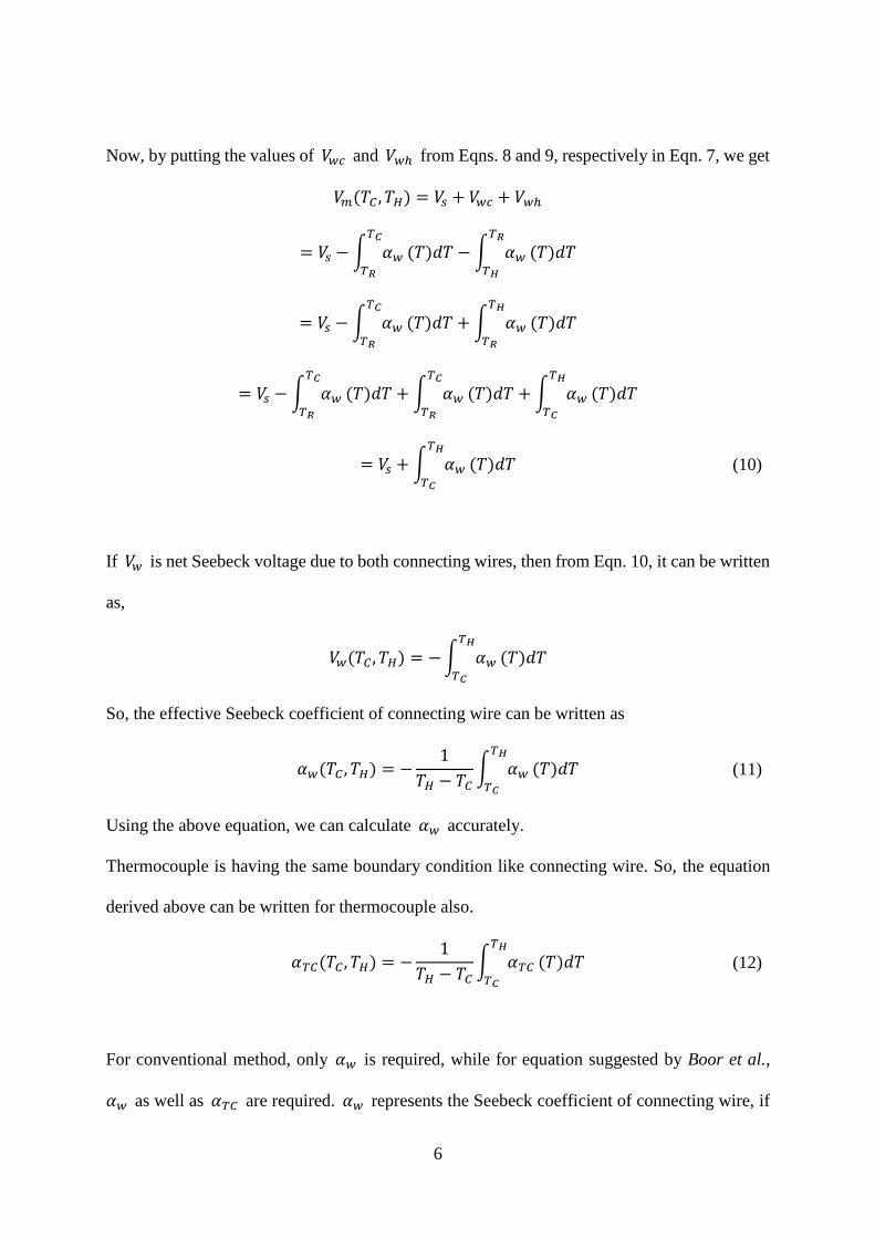
Now, by putting the values of 𝑉𝑤𝑐 and 𝑉𝑤ℎ from Eqns. 8 and 9, respectively in Eqn. 7, we get

𝑉𝑚(𝑇𝐶 , 𝑇𝐻) = 𝑉𝑠 + 𝑉𝑤𝑐 + 𝑉𝑤ℎ

= 𝑉𝑠 −∫ 𝛼𝑤

𝑇𝐶

𝑇𝑅

(𝑇)𝑑𝑇 − ∫ 𝛼𝑤

𝑇𝑅

𝑇𝐻

(𝑇)𝑑𝑇

= 𝑉𝑠 −∫ 𝛼𝑤

𝑇𝐶

𝑇𝑅

(𝑇)𝑑𝑇 + ∫ 𝛼𝑤

𝑇𝐻

𝑇𝑅

(𝑇)𝑑𝑇

= 𝑉𝑠 −∫ 𝛼𝑤

𝑇𝐶

𝑇𝑅

(𝑇)𝑑𝑇 + ∫ 𝛼𝑤

𝑇𝐶

𝑇𝑅

(𝑇)𝑑𝑇 + ∫ 𝛼𝑤

𝑇𝐻

𝑇𝐶

(𝑇)𝑑𝑇

= 𝑉𝑠 +∫ 𝛼𝑤

𝑇𝐻

𝑇𝐶

(𝑇)𝑑𝑇 (10)

If 𝑉𝑤 is net Seebeck voltage due to both connecting wires, then from Eqn. 10, it can be written

as,

𝑉𝑤(𝑇𝐶 , 𝑇𝐻) = −∫ 𝛼𝑤

𝑇𝐻

𝑇𝐶

(𝑇)𝑑𝑇

So, the effective Seebeck coefficient of connecting wire can be written as

𝛼𝑤(𝑇𝐶 , 𝑇𝐻) = −1

𝑇𝐻 − 𝑇𝐶∫ 𝛼𝑤

𝑇𝐻

𝑇𝐶

(𝑇)𝑑𝑇 (11)

Using the above equation, we can calculate 𝛼𝑤 accurately.

Thermocouple is having the same boundary condition like connecting wire. So, the equation

derived above can be written for thermocouple also.

𝛼𝑇𝐶(𝑇𝐶 , 𝑇𝐻) = −1

𝑇𝐻 − 𝑇𝐶∫ 𝛼𝑇𝐶

𝑇𝐻

𝑇𝐶

(𝑇)𝑑𝑇 (12)

For conventional method, only 𝛼𝑤 is required, while for equation suggested by Boor et al.,

𝛼𝑤 as well as 𝛼𝑇𝐶 are required. 𝛼𝑤 represents the Seebeck coefficient of connecting wire, if

7

negative leg of thermocouples used, it will be written as 𝛼𝑛𝑒𝑔. In this work, from now onward

Seebeck coefficient of connecting wire is indicated as 𝛼𝑛𝑒𝑔 . It is clear from the above

discussion that the method proposed in the present work is expected to be better than that of

Boor et al. for the general type of thermocouples and for a large value of Δ𝑇.

MEASUREMENT SETUP

A schematic view of measurement setup is shown in Fig. 1. The digital multimeter with the

multichannel scanner card is used to measure various signals. Sourcemeter is used to supply

power to the heater. GPIB ports of the digital multimeter and Sourcemeter connected by using

inline IEEE-488 GPIB bus interface cable. GPIB-USB converter is used to connect GPIB with

a computer. Digital multimeter measures 𝑈𝑝𝑜𝑠, 𝑈𝑛𝑒𝑔, 𝑇𝐻 , 𝑇𝐶 , and connector’s temperature

(𝑇𝑟𝑒𝑓). 𝑇𝑟𝑒𝑓 is considered as cold junction compensation temperature for thermocouples and

measured by using PT-100 RTD. Shielded cable is used to avoid electrical noise due to

inductive coupling in signal transmission from connector to scanner card.

The detailed overview of sample holder assembly is shown in Fig. 2, where different

components are represented by numbers. The sample (1) is sandwiched in between two copper

blocks (2) of 10mm×10mm cross section and 2 mm thickness. The two K-type

polytetrafluoroethylene coated thermocouples (3) of 36 swg are embedded in the copper

blocks. In order to make a good thermal and electrical contact between copper block and

thermocouple GaSn liquid metal is used. Fine thermocouple wire minimizes the heat flow

through thermocouple, which helps to measure more accurate temperature. Thin heater (4) is

used to heat the sample and it is made by winding 40 swg kanthal wire over the mica sheet and

wrapped by using another mica sheet then by copper sheet. The cross section of this heater is

10mm×10mm and thickness is 1 mm. Thick insulator block (5) is placed in between the

heater and brass plate (6) to minimize heat loss. The cross section and thickness of insulator

8

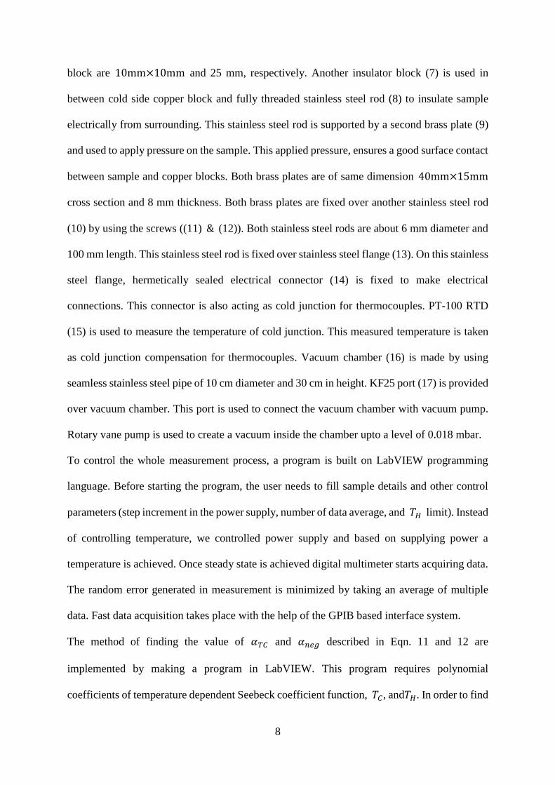
block are 10mm×10mm and 25 mm, respectively. Another insulator block (7) is used in

between cold side copper block and fully threaded stainless steel rod (8) to insulate sample

electrically from surrounding. This stainless steel rod is supported by a second brass plate (9)

and used to apply pressure on the sample. This applied pressure, ensures a good surface contact

between sample and copper blocks. Both brass plates are of same dimension 40mm×15mm

cross section and 8 mm thickness. Both brass plates are fixed over another stainless steel rod

(10) by using the screws ((11) & (12)). Both stainless steel rods are about 6 mm diameter and

100 mm length. This stainless steel rod is fixed over stainless steel flange (13). On this stainless

steel flange, hermetically sealed electrical connector (14) is fixed to make electrical

connections. This connector is also acting as cold junction for thermocouples. PT-100 RTD

(15) is used to measure the temperature of cold junction. This measured temperature is taken

as cold junction compensation for thermocouples. Vacuum chamber (16) is made by using

seamless stainless steel pipe of 10 cm diameter and 30 cm in height. KF25 port (17) is provided

over vacuum chamber. This port is used to connect the vacuum chamber with vacuum pump.

Rotary vane pump is used to create a vacuum inside the chamber upto a level of 0.018 mbar.

To control the whole measurement process, a program is built on LabVIEW programming

language. Before starting the program, the user needs to fill sample details and other control

parameters (step increment in the power supply, number of data average, and 𝑇𝐻 limit). Instead

of controlling temperature, we controlled power supply and based on supplying power a

temperature is achieved. Once steady state is achieved digital multimeter starts acquiring data.

The random error generated in measurement is minimized by taking an average of multiple

data. Fast data acquisition takes place with the help of the GPIB based interface system.

The method of finding the value of 𝛼𝑇𝐶 and 𝛼𝑛𝑒𝑔 described in Eqn. 11 and 12 are

implemented by making a program in LabVIEW. This program requires polynomial

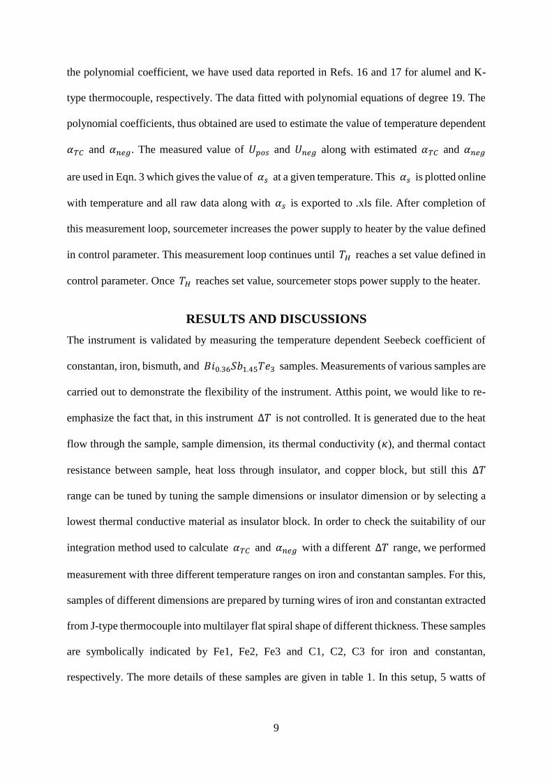
coefficients of temperature dependent Seebeck coefficient function, 𝑇𝐶, and𝑇𝐻. In order to find

9

the polynomial coefficient, we have used data reported in Refs. 16 and 17 for alumel and K-

type thermocouple, respectively. The data fitted with polynomial equations of degree 19. The

polynomial coefficients, thus obtained are used to estimate the value of temperature dependent

𝛼𝑇𝐶 and 𝛼𝑛𝑒𝑔. The measured value of 𝑈𝑝𝑜𝑠 and 𝑈𝑛𝑒𝑔 along with estimated 𝛼𝑇𝐶 and 𝛼𝑛𝑒𝑔

are used in Eqn. 3 which gives the value of 𝛼𝑠 at a given temperature. This 𝛼𝑠 is plotted online

with temperature and all raw data along with 𝛼𝑠 is exported to .xls file. After completion of

this measurement loop, sourcemeter increases the power supply to heater by the value defined

in control parameter. This measurement loop continues until 𝑇𝐻 reaches a set value defined in

control parameter. Once 𝑇𝐻 reaches set value, sourcemeter stops power supply to the heater.

RESULTS AND DISCUSSIONS

The instrument is validated by measuring the temperature dependent Seebeck coefficient of

constantan, iron, bismuth, and 𝐵𝑖0.36𝑆𝑏1.45𝑇𝑒3 samples. Measurements of various samples are

carried out to demonstrate the flexibility of the instrument. Atthis point, we would like to re-

emphasize the fact that, in this instrument Δ𝑇 is not controlled. It is generated due to the heat

flow through the sample, sample dimension, its thermal conductivity (𝜅), and thermal contact

resistance between sample, heat loss through insulator, and copper block, but still this Δ𝑇

range can be tuned by tuning the sample dimensions or insulator dimension or by selecting a

lowest thermal conductive material as insulator block. In order to check the suitability of our

integration method used to calculate 𝛼𝑇𝐶 and 𝛼𝑛𝑒𝑔 with a different Δ𝑇 range, we performed

measurement with three different temperature ranges on iron and constantan samples. For this,

samples of different dimensions are prepared by turning wires of iron and constantan extracted

from J-type thermocouple into multilayer flat spiral shape of different thickness. These samples

are symbolically indicated by Fe1, Fe2, Fe3 and C1, C2, C3 for iron and constantan,

respectively. The more details of these samples are given in table 1. In this setup, 5 watts of

10

power supply is sufficient to get the hot side temperature of 650 K.

The variation in Δ𝑇 with 𝑇 for Fe1, Fe2, and Fe3 samples are shown in Fig. 3. At 312 K, Δ𝑇

is nearly 0.25 K, 1.6 K, and 9 K for Fe1, Fe2, and Fe3, respectively. The value of Δ𝑇 are

increasing with temperature and reachto 16 K at 𝑇=625 K for Fe1, 56 K at 𝑇=585 K for Fe2,

and 160 K at 𝑇=540 K for Fe3 samples. The rate of change of Δ𝑇 is very high for Fe3

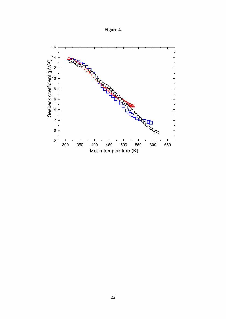
compared to Fe1 and Fe2 samples. The vlues of 𝛼 for Fe1, Fe2, and Fe3 samples with respect

to 𝑇 are shown in Fig. 4. The values of 𝛼 for all the three samples are decreasing almost

linearly throughout the temperature range, which is as per the reported data[17]. Below 400 K,

small difference (maximum ∼0.5 𝜇𝑉/𝐾) is observed among the measured values of 𝛼 for

Fe1, Fe2 and Fe3 samples. At 400 K, the values of 𝛼 for Fe1, Fe2 and Fe3 samples match

closely with each other. At this temperature, Δ𝑇 for Fe1, Fe2, and Fe3 are 2.5 K, 17 K, and 54

K, respectively. After this temperature, again the difference in the values of 𝛼 for all the three

samples increases. Upto 500 K, maximum deviation of 1 𝜇𝑉/𝐾 is observed among the

measured values of 𝛼 for Fe1, Fe2 and Fe3 samples. Due to large Δ𝑇 at high temperature, the

value of 𝛼 for Fe3 sample shows more deviation compared to Fe1 and Fe2 samples. At 𝑇=525

K, the value of 𝛼 for Fe3 sample shows difference of 0.9𝜇𝑉/𝐾 and 1.8 𝜇𝑉/𝐾 with respect to

Fe1 and Fe2 samples, respectively. The values of 𝛼 for Fe1 and Fe2 samples show a maximum

difference of 1.2 𝜇𝑉/𝐾 with each other till the end of the measurement. We also compared

our data with the reported data available in Ref. 17. In the absence of clear information provided

about the measurement method and Δ𝑇 range in Ref. 17, we compared our values of 𝛼 for

lowest Δ𝑇 range (Fe1 sample) with the reported data, which is shown in the Fig. 5. The values

of 𝛼 throughout the temperature range are almost parallel to the reported data and both

decreases with a rate of ∼0.045 𝜇𝑉/𝐾. The deviation in our data is ∼1 𝜇𝑉/𝐾 at 315 K. This

deviation increases upto ∼1.9 𝜇𝑉/𝐾 at 480 K and again decreases to ∼1.2 𝜇𝑉/𝐾 at the end

11

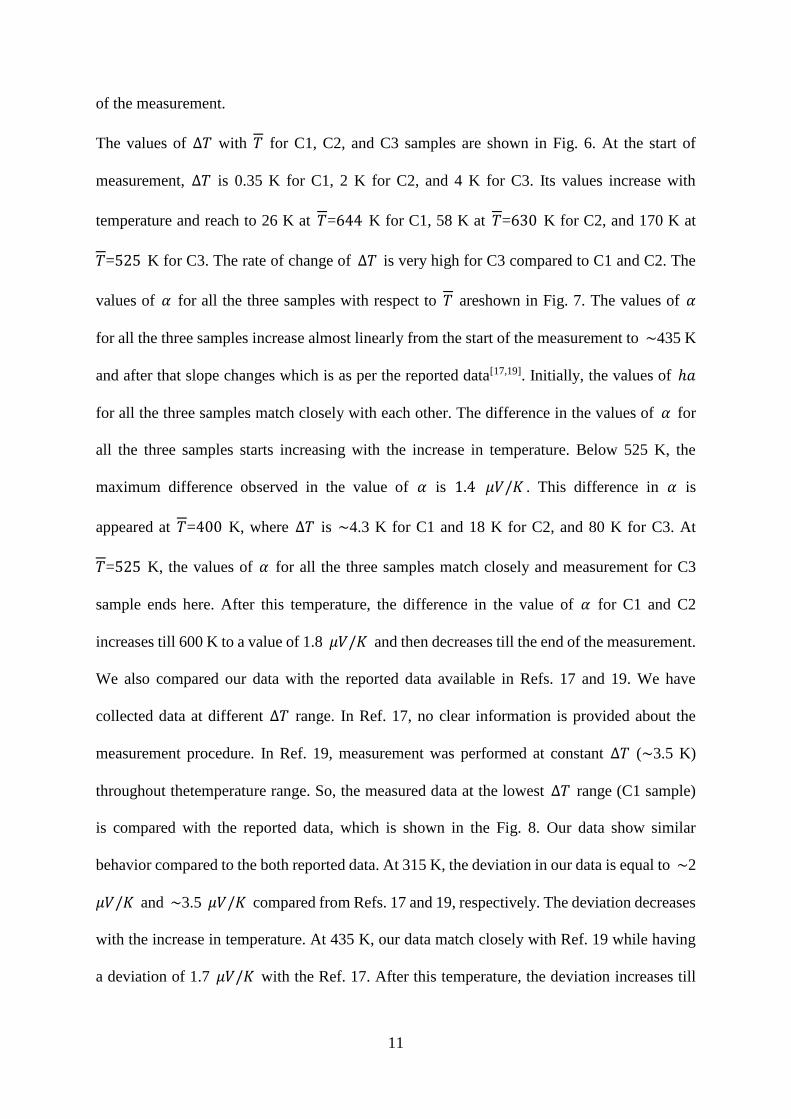
of the measurement.

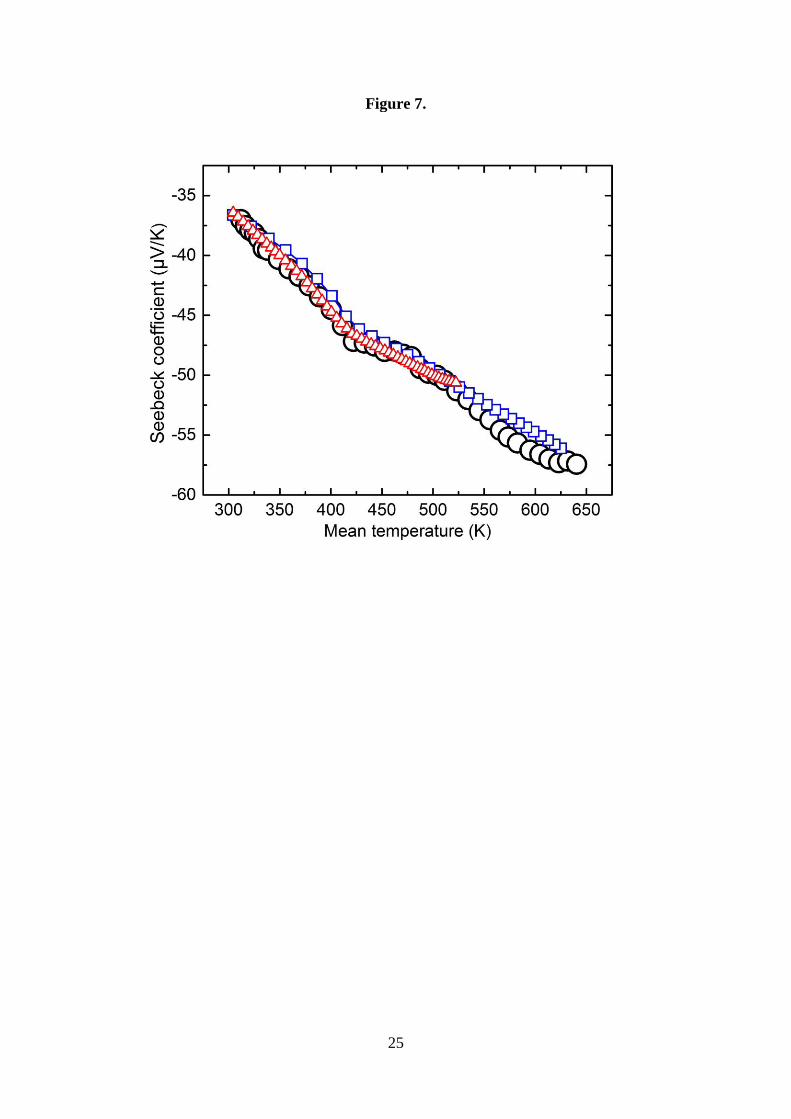
The values of Δ𝑇 with 𝑇 for C1, C2, and C3 samples are shown in Fig. 6. At the start of

measurement, Δ𝑇 is 0.35 K for C1, 2 K for C2, and 4 K for C3. Its values increase with

temperature and reach to 26 K at 𝑇=644 K for C1, 58 K at 𝑇=630 K for C2, and 170 K at

𝑇=525 K for C3. The rate of change of Δ𝑇 is very high for C3 compared to C1 and C2. The

values of 𝛼 for all the three samples with respect to 𝑇 areshown in Fig. 7. The values of 𝛼

for all the three samples increase almost linearly from the start of the measurement to ∼435 K

and after that slope changes which is as per the reported data[17,19]. Initially, the values of ℎ𝑎

for all the three samples match closely with each other. The difference in the values of 𝛼 for

all the three samples starts increasing with the increase in temperature. Below 525 K, the

maximum difference observed in the value of 𝛼 is 1.4 𝜇𝑉/𝐾 . This difference in 𝛼 is

appeared at 𝑇=400 K, where Δ𝑇 is ∼4.3 K for C1 and 18 K for C2, and 80 K for C3. At

𝑇=525 K, the values of 𝛼 for all the three samples match closely and measurement for C3

sample ends here. After this temperature, the difference in the value of 𝛼 for C1 and C2

increases till 600 K to a value of 1.8 𝜇𝑉/𝐾 and then decreases till the end of the measurement.

We also compared our data with the reported data available in Refs. 17 and 19. We have

collected data at different Δ𝑇 range. In Ref. 17, no clear information is provided about the

measurement procedure. In Ref. 19, measurement was performed at constant Δ𝑇 (∼3.5 K)

throughout thetemperature range. So, the measured data at the lowest Δ𝑇 range (C1 sample)

is compared with the reported data, which is shown in the Fig. 8. Our data show similar

behavior compared to the both reported data. At 315 K, the deviation in our data is equal to ∼2

𝜇𝑉/𝐾 and ∼3.5 𝜇𝑉/𝐾 compared from Refs. 17 and 19, respectively. The deviation decreases

with the increase in temperature. At 435 K, our data match closely with Ref. 19 while having

a deviation of 1.7 𝜇𝑉/𝐾 with the Ref. 17. After this temperature, the deviation increases till

12

480 K and at this temperature deviation is 1.4 𝜇𝑉/𝐾 and 3 𝜇𝑉/𝐾 compared from Ref. 17 and

19, respectively. Decreasing behavior in deviation is observed after this temperature. Our data

match closely with both the reported data from 550 K.

It is important to note that, we used commercially available mica sheet in heater fabrication

which is not advisable to go beyond 700 K. As there is some temperature gradient between the

mica sheet and hot side temperature, we restrict hot side temperature to a maximum value of

650 K. Due to large Δ𝑇 for Fe3 and C3 samples, even 𝑇𝐻 ≈625 K, 𝑇 value appears below

550 K.

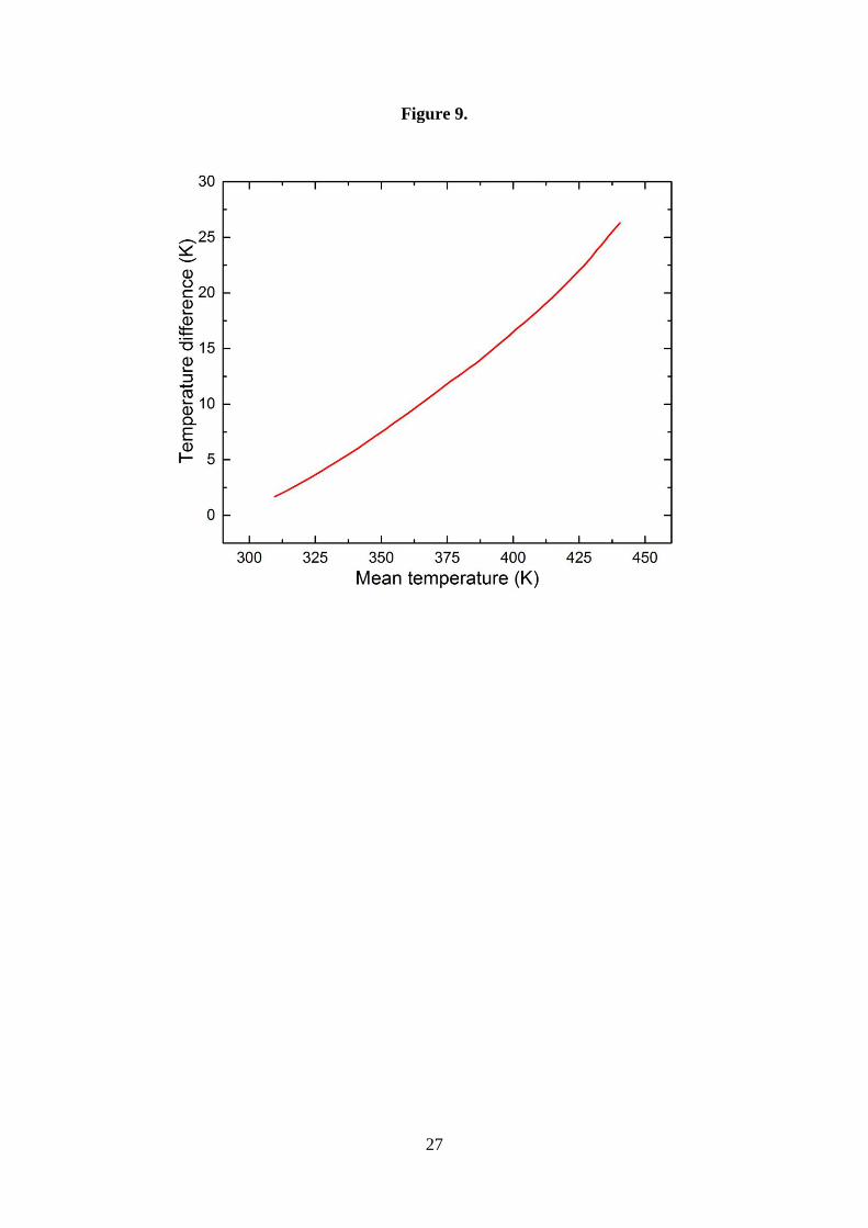
Now we take bismuth sample, as it has relatively higher Seebeck coefficient. This sample is

taken from commercial ingot. The sample is cut into dimension of 9𝑚𝑚×7𝑚𝑚 cross section

and 12 mm thickness. The variation in Δ𝑇 along with 𝑖𝑛𝑒𝑇 is shown in the Fig. 9. At 𝑇 =315

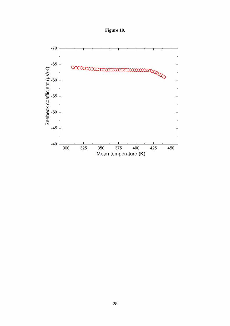
K, Δ𝑇 is ∼2.5 K. Δ𝑇 increases almost linearly and reaches to 27 K at 𝑇=440 K. The values

of 𝛼 of the bismuth sample with respect to 𝑇 are shown in Fig. 10. At the start of the

measurement, value of 𝛼 is ∼-64 𝜇𝑉/𝐾 . Value of 𝛼 decreases almost linearly to ∼-63

𝜇𝑉/𝐾 at 𝑇=415 K. After this temperature, slope changes and decreases to ∼-61 𝜇𝑉/𝐾 at

𝑇=440 K. Due to the low melting temperature of bismuth, measurement was performed till

𝑇𝐻=455 K. We also compared our 𝛼 with the reported data[20]. In Ref. 20, measurement was

performed upto a temperature of 350 K only. We found similar behavior of our data, but the

deviation is ∼11 𝜇𝑉/𝐾 with the reported data till 350 K. This deviation of our data may be

due to the highly anisotropic nature of the electronic transport.[21] Since this sample is cheaper,

we cannot expect that its purity will be upto a level of standard samples, and this may be an

another aspect behind the deviation.

Finally, we consider 𝐵𝑖0.36𝑆𝑏1.45𝑇𝑒3 sample, which has a very high Seebeck coefficient

(>200 𝜇𝑉/𝐾) at room temperature. This sample is extracted from commercially available

13

thermoelectric generator (TEC1-12706). The composition of the sample is obtained by

performing Energy-dispersive X-ray spectroscopy. The sample is about 1.4𝑚𝑚×1.4𝑚𝑚

cross section and 1.6 mm thickness. The variation in Δ𝑇 along with 𝑇 is shown in the Fig. 11.

At a temperature of 𝑇=315 K, Δ𝑇 is ∼11 K. Δ𝑇 increases almost linearly and reach to 105 K

at 𝑇=490 K. The values of 𝛼 for 𝐵𝑖0.36𝑆𝑏1.45𝑇𝑒3 sample with respect to 𝑇 are shown in Fig.

12. At the start of the measurement, the value of 𝛼 is ∼212 𝜇𝑉/𝐾 and it increases to ∼221

𝜇𝑉/𝐾 at 𝑇=375 K. After this temperature, the value of 𝛼 decreases and reaches to ∼160

𝜇𝑉/𝐾 at 𝑇=490 K. We also compared our data with the reported data[22]. In Ref. 22, sample

was taken from commercially available 𝐵𝑖𝑆𝑏𝑇𝑒 ingot. Our data show similar behavior

compared to the reported data. We observed a deviation of ∼10 𝜇𝑉/𝐾 at 𝑇=315 K. This

deviation increases with the increase in Δ𝑇 and reaches to 20 𝜇𝑉/𝐾 at 𝑇=490 K where Δ𝑇

is ∼105 K. This small difference in the magnitude of our data may be attributed to the presence

of large Δ𝑇, as seen abovefor other samples.

CONCLUSION

In this work, we have developed simple, low cost and fully automated experimental setup for

Seebeck coefficient measurement. Average temperature of the sample and the Seebeck voltage

across it were measured using K-type thermocouples. The temperature dependence of the

Seebeck coefficients of the thermocouple and its negative leg used in Seebeck coefficient

calculations was taken care by using the integration method. Thin heater, simple design and

limited components make small size and lightweight sample holder. Temperature difference

across the sample was decided based on the power supply to the heater. The LabVIEW based

program makes the whole measurement process fully automated. Commonly available

materials in the market were used in the fabrication of the complete setup. This setup is

validated by using iron, constantan, bismuth and 𝐵𝑖0.36𝑆𝑏1.45𝑇𝑒3 samples with a wide range

14

of Seebeck coefficient and wide range of temperature difference across it. The measured data

were found in good agreementwith the reported data, which indicate that this instrument is

capable to measure Seebeck coefficient with fairly good accuracy.

ACKNOWLEDGEMENTS

The authors acknowledge R. S. Raghav and other workshop staffs for their support in the

fabrication process of vacuum chamber and sample holder assembly.

REFERENCES

1. Beer, J. M. High efficiency electric power generation: The environmental role. Progress in

Energy and Combustion Science 2007, 33, 107-134.

2. Goldsmid, H. J. CRC handbook of thermoelectrics (ed. by Rowe, D. M.); CRC Press: 1995,

19-25.

3. Iwanaga, S.; Toberer, E. S.; LaLonde, A.; Snyder, G. J. A high temperature apparatus for

measurement of the Seebeck coefficient. Rev. Sci. Instrum. 2011, 82, 063905-1-063905-6.

4. Martin, J.; Tritt, T.; Uher, C. High temperature Seebeck coefficient metrology. J. Appl. Phys.

2010 108, 121101-1-121101-12.

5. Kumar, S. R. S.; Kasiviswanathan, S. A hot probe setup for the measurement of Seebeck

coefficient of thin wires and thin films using integral method. Rev. Sci. Instrum. 2008 79,

024302-1-024302-4.

6. Wood, C.; Chmielewski, A.; Zoltan, D. Measurement of Seebeck coefficient using a large

thermal gradient. Rev. Sci. Instrum. 1988 59, 951-954.

7. Ponnambalam, V.; Lindsey, S.; Hickman, N. S.; Tritt, T. M. Sample probe to measure

resistivity and thermopower in the temperature range of 300-1000K. Rev. Sci. Instrum. 2006,

77, 073904-1-073904-5.

8. Zhou, Z.; Uher, C. Apparatus for Seebeck coefficient and electrical resistivity measurements

15

of bulk thermoelectric materials at high temperature. Rev. Sci. Instrum. 2005, 76, 023901-1-

023901-5.

9. Dasgupta, T.; Umarji, A. M. Apparatus to measure high-temperature thermal conductivity

and thermoelectric power of small specimens. Rev. Sci. Instrum. 2005, 76, 094901-1-094901-

5.

10. Muto, A.; Kraemer, D.; Hao, Q.; Ren, Z. F.; Chen, G. Thermoelectric properties and

efficiency measurements under large temperature differences. Rev. Sci. Instrum. 2009, 80,

093901-1-093901-7.

11. Amatya, R.; Mayer, P. M.; Ram, R. J. High temperature Z-meter setup for characterizing

thermoelectric material under large temperature gradient. Rev. Sci. Instrum. 2012, 83, 075117-

1-075117-10.

12. Swanson, C. Optimal temperature sensor selection, accessed 15 January 2016,

[http://www.asminternational.org/documents/10192/1912096/htp00603p047.pdf/8695e0a2-

edc3-4ef7-946f-94966fa847cd]

13. Boor, J. D.; Stiewe, C.; Ziolkowski, P.; Dasgupta, T.; Karpinski, G.; Lenz, E.; Edler, F.;

Mueller, E. High-temperature measurement of seebeck coefficient and electrical conductivity.

J. Electron. Mater. 2013, 42, 1711-1718.

14. Singh, S.; Pandey, S. K.; arXiv:1508.04739, 1-15

15. Kolb, H.; Dasgupta, T.; Zabrocki, K.; Muller, E.; Boor, J. D. Simultaneous measurement

of all thermoelectric properties of bulk materials in the temperature range 300-600 K. Rev. Sci.

Instrum. 2015, 86, 073901-1-073901-8.

16. Boor, J. D.; Muller, E. Data analysis for Seebeck coefficient measurements. Rev. Sci.

Instrum. 2013, 84, 065102-1-065102-9.

17. Bentley, R. E. Handbook of temperature measurement Vol. 3: The theory and practice of

thermoelectric thermometry; Springer:1998; 31 pp.

16

18. Thermoelectric materials for thermocouples, University of Cambridge, accessed 10 January

2016,

http://www.msm.cam.ac.uk/utc/thermocouple/pages/ThermocouplesOperatingPrinciples.html

19. Guan, A.; Wang, H.; Jin, H.; Chu, W.; Guo, Y. An experimental apparatus for

simultaneously measuring Seebeck coefficient and electrical resistivity from 100 K to 600 K.

Rev. Sci. Instrum. 2013, 84, 043903-1-043903-5.

20. Mulla, R.; Rabinal, M. K. A Simple and Portable Setup for Thermopower Measurements.

ACS Comb. Sci. 2016, 18, 177-181.

21. Das, V. D.; Soundararajan, N. Size and temperature effects on the Seebeck coefficient of

thin bismuth films. Phys. Rev. B 1987, 35, 5990-5996.

22. Poudel, B.; Hao, Q.; Ma, Y.; Lan, Y. C.; Minnich, A.; Yu, B.; Yan, X.; Wang, D. Z.; Muto,

A.; Vashaee, D.; Chen, X. Y.; Liu, J. M.; Dresselhaus, M. S.; Chen, G.; Ren, Z. High-

Thermoelectric Performance of Nanostructured Bismuth Antimony Telluride Bulk Alloys.

Science. 2008, 320, 634-638.

Tables

Table 1. The relevant properties of Fe1, Fe2, Fe3, C1, C2, and C3 samples.

17

Table 1.

Symbol Sample material Shape Thickness (t) order

Fe1 36 swg iron wire

extracted from J-type

thermoocuple

Multilayer spiral coil tFe1<tFe2<tFe3

Fe2

Fe3

C1 36 swg constantan

wire extracted from J-

type thermoocuple

Multilayer spiral coil tC1<tC2<tC3

C2

C3

18

Figure Captions

Figure 1. Schematic diagram of high temperature Seebeck coefficient measurement setup

along with computer interface system.

Figure 2. Schematic diagram of sample holder assembly: (1) sample, (2) copper blocks, (3) K-

type 36 swg polytetrafluoroethylene coated thermocouples, (4) thin heater, (5) thick insulator

block, (6) brass plate, (7) another insulator block, (8) fully threaded stainless steel rod, (9)

second brass plate, (10) another stainless steel rod, (11) & (12) screws, (13) stainless steel

flange, (14) hermetically sealed electrical connector, (15) PT-100 RTD, (16) vacuum chamber,

and (17) KF25 port.

Figure 3. Variation in temperature gradient with mean temperature of iron samples (Fe1, Fe2,

and Fe3), where data corresponding to Fe1, Fe2, and Fe3 are shown by black circle, blue box,

red triangle, respectively.

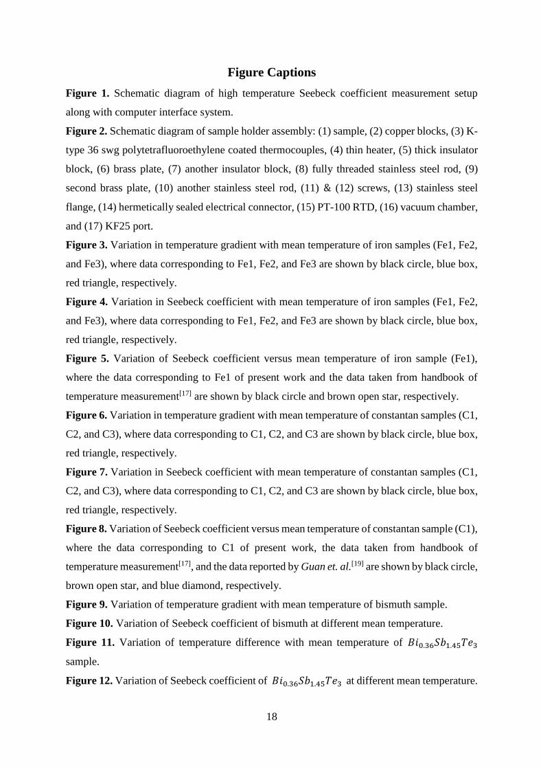
Figure 4. Variation in Seebeck coefficient with mean temperature of iron samples (Fe1, Fe2,

and Fe3), where data corresponding to Fe1, Fe2, and Fe3 are shown by black circle, blue box,

red triangle, respectively.

Figure 5. Variation of Seebeck coefficient versus mean temperature of iron sample (Fe1),

where the data corresponding to Fe1 of present work and the data taken from handbook of

temperature measurement[17] are shown by black circle and brown open star, respectively.

Figure 6. Variation in temperature gradient with mean temperature of constantan samples (C1,

C2, and C3), where data corresponding to C1, C2, and C3 are shown by black circle, blue box,

red triangle, respectively.

Figure 7. Variation in Seebeck coefficient with mean temperature of constantan samples (C1,

C2, and C3), where data corresponding to C1, C2, and C3 are shown by black circle, blue box,

red triangle, respectively.

Figure 8. Variation of Seebeck coefficient versus mean temperature of constantan sample (C1),

where the data corresponding to C1 of present work, the data taken from handbook of

temperature measurement[17], and the data reported by Guan et. al.[19] are shown by black circle,

brown open star, and blue diamond, respectively.

Figure 9. Variation of temperature gradient with mean temperature of bismuth sample.

Figure 10. Variation of Seebeck coefficient of bismuth at different mean temperature.

Figure 11. Variation of temperature difference with mean temperature of 𝐵𝑖0.36𝑆𝑏1.45𝑇𝑒3

sample.

Figure 12. Variation of Seebeck coefficient of 𝐵𝑖0.36𝑆𝑏1.45𝑇𝑒3 at different mean temperature.

19

Figure 1.

20

Figure 2.

21

Figure 3.

22

Figure 4.

23

Figure 5.

24

Figure 6.

25

Figure 7.

26

Figure 8.

27

Figure 9.

28

Figure 10.

29

Figure 11.

30

Figure 12.