
The Skipheia Wind Measurement Station. Instrumentation ...
202
-
Upload
khangminh22 -
Category
Documents
-
view
0 -
download
0
Transcript of The Skipheia Wind Measurement Station. Instrumentation ...


1
Ii
II
I
I
I
i
I
II
ljI >

ffofio&si
The Skipheia Wind Measurement Station.
Instrumentation, Wind Speed Profiles and Turbulence Spectra
Svein Erik Aasen
Thesis submitted in partial fulfilment for the degree DOCTOR SCIENTARIUM
UNIVERSITY OF TRONDHEIM
Department of Physics, AVH
Trondheim - Norway
October 1995
OF THIS MCOtpff

II

DISCLAIMER
Portions of this document may be illegible in electronic image products. Images are produced from the best available original document.


Preface
This thesis, submitted to the University of Trondheim, AVH in partial fulfilment for the degree Doctor Scientarium, discusses the design of a measurement station for turbulent wind and the analysis of the collected data.
The thesis consists of 9 chapters. Chapter 1 is a introduction to the thesis and discusses some of the general motivations for wind measurements. The station, including geographic location, local topography, masts, sensor mountings and more are described in Chapter 2. During the years the station has been in operation, several types of wind sensors (wind-speed and -direction) have been used. The operational experiences from for these sensors, together with a discussion of sensor principles are given in Chapter 3. Chapter 4 discusses a calibration of wind speed sensors; both the static and the dynamic performance are tested. Chapter 5 gives a detailed description of the data acquisition system constructed for the Station. An overview of the collected data and statistical distributions of the data are given in Chapter 6. Prior to the data analysis the data were checked for errors using several methods, these methods are briefly described in Chapter 7. The error free data are analysed and compared to models from the literature in Chapter 7 and 8. Chapter 7 discusses the wind speed profile, whereas Chapter 8 discusses one point turbulence spectra and turbulence intensity.
Much of the practical work on the station has been a team effort, where Tore Heggem, J0rgen L0vseth (my supervisor), Knut Mollestad and several others have contributed. Tore Heggem is also preparing a thesis on data from the Skipheia station. This work will be referred to as Heggem (personal communication) whenever a reference is needed in this thesis. The nature of the work described in Chapter 2 and 3 makes these chapters a joined effort between
Tore Heggem and myself.

IV

Acknowledgements
This work has been carried out at the Department of Physics, AVH, University of Trondheim. I would like to express my gratitude to my supervisor, Ass. Professor J0rgen Lpvseth, for his enthusiasm, ideas and support through the years we have spent together.
I would also like to thank the members in my group, especially Tore Heggem and Knut Mollestad for many discussions and their part in the team work which the construction of the Skipheia station was.
I am also grateful to other members of the staff at Department of Physics, particularly to the technical staff, Lars Einarsen, Oddbj0m Grandum and Dagfinn Johnsen for their contributions during the construction of the Station, and to Professor Razi Naqvi for proof-reading the manuscript.
Last and most important I want to thank my wife Aud Hilde and my children Ingrid and Martin for their never-ending support and patience during this work.
Trondheim, October 1995 JtzCv,— %ysj* fir i—
Svein Erik Aasen

VI

Contents
1 Introduction 11.1 Overview of the thesis 11.2 Motivations for wind measurements 2
1.2.1 Wind load on exposed structures 21.2.2 Wind energy 3
2 The Skipheia Station 52.1 Background 52.2 Site 62.3 Masts and Sensor Locations 72.4 Instrumentation House 72.5 Historical Review of the Station 8
3 Wind Sensors 193.1 Introduction 193.2 Principles of sensor operation 20
3.2.1 Cup anemometer 213.2.2 Propeller 223.2.3 Vortex counting 223.2.4 Vane 223.2.5 Sonic 23
3.3 Tested Wind Speed Sensors 233.3.1 J-TEC Wind Speed Sensor VA-320-2-1 243.3.2 Met-One 010b anemometer 243.3.3 Vaisala WAA12, WAA15 and WAA15A Anemometers 263.3.4 Gill UVW Anemometer, Model 27005 263.3.5 Aanderaa Wind Speed Sensor 2740 27
3.4 Tested Wind Direction Sensors 273.4.1 J-TEC Wind Direction Sensor VA-320-2-1 283.4.2 Met-One 022 Bivane 293.4.3 Gill Microvane, Model 12305 293.4.4 Gill UVW Anemometer, Model 27005 293.4.5 Teledyne Geotech Bivane, Model 1585 293.4.6 Vaisala WAA12 modified for resolver measurements 303.4.7 ED wind direction sensor 2K/352 DEG. and COS/SIN 4kHz. 30

3.4.8 Aanderaa wind direction sensor 2053 313.5 Discussion 31
4 Sensor Calibration 334.1 Steady-state calibration of cup anemometers. 33
4.1.1 Wind tunnel setup. 334.1.2 Cup anemometers. 344.1.3 Results for VAIS ALA WAA15A 354.1.4 Results for AANDERAA 2740 374.1.5 Measurement errors 394.1.6 Discussion. 40
4.2 Frequency response of cup anemometers. 414.2.1 Instrumentation. 424.2.2 Results. 42
4.3 Step response of cup anemometers. 434.3.1 Instrumentation 444.3.2 Results 45
4.4 Conclusions on the cup anemometer calibrations 47
5 Data Acquisition System 495.1 Introduction 495.2 Review of earlier systems 50
5.2.1 ABC80 system 505.2.2 Falcon system 525.2.3 Aanderaa system 53
5.3 Overview of present data acquisition system 545.3.1 Lightning protection 55
5.4 Computer - sensor connection 575.4.1 Frequency inputs 575.4.2 Resolver inputs 585.4.3 Analog inputs 59
5.5 Real-time operating system 60 •5.6 Logging Programs 625.7 Operating experiences 66
6 DataBase 716.1 Historical overview 716.2 Time series 726.3 Distributions for selected sensors 726.4 Data file format 77
6.4.1 Configuration files. 776.4.2 Error files. 786.4.3 Direction files. 786.4.4 Data files. 79
viii
7 Data Quality Control7.1 Data inspection7.2 Elimination of spikes
878788

ix
8 The Wind Speed Profile 978.1 Background 978.2 Presentation of the experimental data. . 101
8.2.1 Variation in terrain roughness 1028.2.2 Chamock effect. 1058.2.3 Influence from masts and other obstacles. 1068.2.4 Speed-up effect 1068.2.5 Stability dependence of the wind speed profile 110
8.3 Parametrisation of the experimental data. 114
9 Turbulence 1199.1 Introduction 1199.2 Turbulence intensity 1199.3 Turbulence spectra 129
9.3.1 Presentation of the experimental data 1299.3.2 Aliasing 1329.3.3 Trend 1339.3.4 Spectral models 133
9.4 Discussion 137
References 153
Appendix A Configuration File A1
Appendix B FiIesub.for B1
Appendix C Routines for Reading of Datafiles from MATLAB Cl
Appendix D Average.m Dl

X

Chapter 1
Introduction
This introductory chapter will give an overview of the thesis and discuss some of the motivations for wind measurements.
1.1 Overview of the thesis
The present thesis discusses the design of a measurement station for turbulent wind and presents results from an analysis of the collected data. The station is located at Skipheia, near the southwest end of Fr0ya, an island outside the coast of Mid-Norway. The site is presented in Chapter 2, together with maps showing the detailed location of the station and the surrounding topography. The Skipheia station was built in 1980. In 1991 the instrumentation house was damaged by a fire. Chapter 5 describes the design of a new data acquisition system for the station, both hardware and software. Through the years, the station has been equipped with various wind sensors; the operating experiences with these sensors and a discussion of various sensor principles are given in Chapter 3. The static and dynamic calibration of the present cup anemometers are discussed in Chapter 4. The Skipheia data base contains data for more than 14 years, the last 7 years with a logging frequency of 0.85 Hz. The large number of sensors located in heights from 10 m to 100 m in three masts, a sampling rate of 0.85 Hz and storage of the complete time series makes the station unique for studies of turbulent wind. Statistical descriptions of some of the data are given in Chapter 6. All measurements are checked for errors using the methods given in Chapter 7". Finally, the 1 hour mean wind speed profile is discussed and modelled in Chapter 8, and the 1 hour one point turbulence spectrum in Chapter 9.
A major part of the thesis deals with data-analysis and modelling. This does not reflect the amount of work put into the building of the station and data acquisition system. The frequency of lightning and atmospheric discharges to the masts are quite high, particularly during storms

2 Introduction
in the winter time. Much effort has therefore been put into minimization of the damages caused by lightning activity. This work has to a great extent been built on previous experiences and because this type of information is not easily collected, these experiences are very valuable. Even though the sensors and the individual components of the data acquisition system are relatively simple, the system as a whole is more complicated and valuable than can be judged at first sight.
1.2 Motivations for wind measurements
We can list at least four applications of results and data from wind measurements:
• weather forecasting
• mapping of energy production potential
• estimation of extreme wind speeds and calculations of the load on wind exposed structures (bridges, oil-rigs etc.)
• micro meteorology
This work will concentrate on the general scientific mapping and micro meteorological applications. Data gathered over more than 14 years of measurements at Skipheia form a genuine database for maritime costal wind conditions. These measurements have been utilized in several projects, both for load calculations and energy potential calculations. We will therefore give a brief discussion of these applications and the importance of long term wind measurements.
1.2.1 Wind load on exposed structures
For calculation of wind loads on exposed constructions, detailed information about the wind is necessary. Construction costs can be greatly reduced if information about the mean wind speed, direction and turbulence spectrum is available. The force F operating on a wind exposed object is proportional to
(u)
where p is the air density and V the wind speed. As we can see from Eq. (1.1), accurate wind speed measurements are important in calculations of wind load. In Norway, interest for wind measurements for load purposes has in the later years been concentrated on bridge construction and the oil production facilities on the Norwegian Continental Shelf.

Motivations for wind measurements 3
An important element in the wind load discussion is of course the estimation of the maximum wind speed at a given site, or the extreme wind. The wind is, however, generated in a nonlinear and stocastic process, making estimates of extreme wind speeds difficult from short time measurements. In fact, one of the most valuable properties of the Skipheia data base is the
large amount and the continuity of the data.
Extreme wind is a problem in many parts of the world; perhaps the most famous incidents
are the tropical hurricanes generated in the Mexico gulf, causing severe damage in the area around the Mexican gulf. The hurricane Gilbert striking Jamaica in Sept. 1988 was described as the “hurricane of the century”. The losses were over USD 2.2 billion (Davenport 1995). Although all anemometers were damaged, sustained wind speeds at 10-m height above ground near the coast were estimated to about 40 m/s with gusts up to about 60 m/s (Davenport 1995).
A storm of similar intensity was the hurricane Andrew, striking South Florida on August 24, 1992. A major problem is that most of the instruments available today tend to breakdown when the wind speed reaches 50 - 60 m/s, which makes measurements of extreme wind difficult.
Also in Norway extreme wind can cause heavy damage. The last serious incident was a hurricane striking the coast of Mid-Norway on January 1, 1992. The total insurance claims were approximately NOK 1.2 billion (USD 200 million). During this hurricane the maximum wind speed recorded by our measuring stations was 57.5 m/s at 30 m height, and this was not in the area where the hurricane was strongest. The maximum mean wind speed at 11 m height was41.8 m/s and the maximum gust in 11 m height was 54.9 m/s (Mollestad, 1995).
Accurate estimates of average wind speed at a given site, using measurements from a nearby site can be difficult using the models available today. Even worse is the prediction of gusts and turbulent wind. Particularly at the coast of Norway, where the landscape is complex with islets, fjords, mountains and frequent precipices, numerical methods can give considerable errors. Today, measurements of the wind at the site of interest are often necessary prior to construction of wind exposed structures. The efforts for improving the available models should therefore continue.
1.2.2 Wind energy
Production of electrical power from the wind is a neglected area in Norway. The wind power potential is very large in Norway, IFE (1FE 1990) has estimated 32 TWh/year as a high estimate and 12 TWh/year as a moderate estimate. The present inland consumption in Norway, where almost all electrical energy is generated by hydro power, is approximately 110 TWh/year. L0v- seth et al. (1994) have shown advantages of combining hydro and wind power. Lpvseth et al. folded a time series of ten minute mean wind speeds for 12 years from Skipheia with the power

4 Introduction
curve for a Vestas V39 500 kW wind turbine and found a mean production of 34% of the rated power. The generation of wind power is in phase with the consumption of electrical power, which is largest during the winter time. The calculations showed that 62% of the production from the wind turbine will fall in the period when the water level of the reservoirs is decreasing. Development of wind power in Norway would therefore reduce the needed capacity of the hydro reservoirs, making Norway a net exporter of electrical power. Lpvseth et al. estimate this export potential to be in the order of 80 TWh/year, including biomass and an improved energy efficiency.
Estimation of wind energy potential requires detailed knowledge to the mean wind speed and distribution. The energy potential E in the wind is proportional to
E=|V3, (1.2)
where p is the air density and V the wind speed, which means a 10% error in the mean wind speed estimate will give a 30% error in the energy estimate. Often, wind measurements are not available at the site of interest, but at a nearby site. Models for these types of problems exists, for example the WA^P computer program developed by Risp National Laboratory, Denmark
(European Wind Atlas 1989). Work done by Skaslien (1991) and Nygaard (1992), both using WA^P, showed the limitations in the traditional models. When they compared estimates from WA^P and actual measurements at the site of interest, the accuracy in the estimates was not
found satisfactory. Improvement of the traditional models with respect to the terrain at the coast of Norway, is desirable.

Chapter 2
The Skipheia Station
Since 1980, the Department of Physics has been operating an automated wind measurement
station at Skipheia, near the west end ofFr0ya, an island outside the coast of Mid-Norway. Most of the time wind speed and direction have been recorded for different heights up to hundred metres in three masts. Air temperature profiles have been measured since 1988, and since
1993 also radiation and sea temperature. This section will give a general description of the station, and a brief historical review. Maps, photographs and drawings are found at the end of
the section.
2.1 Background
As part of the Norwegian Wind Energy Program, it was decided in 1979 to establish a wind
measurement station at the west coast of Norway. The project was financed by the Royal Nor
wegian Council for Scientific and Industrial Research (NTNF) and run by Institutt for energite-
knikk (IFE), with the Department of Physics as a co-operator. The station was later handed
over to the Department of Physics. The station was built in order to study in detail the wind
structure, particularly, a data base for high wind speed conditions was desired. Data were orig
inally intended for estimation of load on wind energy systems in the region. The station at
Skipheia was built in 1980 and continuous measurements started late in 1981. Skipheia is in
many ways well suited for location of Wind Energy Converter Systems (WECSs), and is repre
sentative for many sites on the west coast of Norway. The site is exposed to maritime or near
maritime winds from a wide angle. The landscape is relatively uniform and disturbances from
nearby houses negligible. The purpose of the data collection has later changed to a more gen
eral scientific mapping of the turbulent wind field.

6 The Skipheia Station
Measurements from Skipheia have been utilized for calculations of energy production potential for S0r-Tr0ndelag Kraftselskap (STK), the local power company (Mollestad 1995). STK is operating a Wincon M55 55 kW WECS and a Vestas V34 400 kW WECS at Skipheia. IFE (1992) used Skipheia as a reference station and short term measurements from other sites for estimation of wind energy potential at the coast of Mid-Norway. Through the years a number of more short term measurement projects have been carried out at the coast of Mid-Norway, using Skipheia as a reference station. A review of the data from these satellite stations is given by Mollestad (1995).
For calculations of the dynamic load on a WECS the turbulence spectrum of the wind is necessary. Paulsen (1994) made measurements of simultaneous values for the power production of the Vestas V34 and wind speed at Skipheia (measurement frequency 14 Hz). This work revealed large problems in the WECS’s regulation mechanism for periods of the order of 5 s. It also demonstrated the typical 3P pattern, P being the rotational frequency, due to turbulence within the area swept by the turbine.
Measurements carried out at Skipheia and in a 45 metre mast at Sletringen, a flat small islet 4 kilometres west of Skipheia, were used in the project: “The maritime wind field, measurements and models”, for 8 oil companies. The purpose was to collect wind data to estimate the load on offshore constructions. This project has funded most of the measurements at Skipheia in later years. Four reports, still confidential, totalling 532 pages have been made for the oil companies. This has given rise to a new description for wind load in the guidelines issued by the Norwegian Petroleum Directorate for the petroleum activity on the Norwegian continental shelf.
2.2 Site
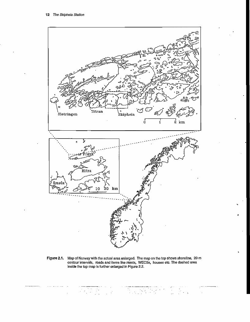
The Skipheia station is located near the village of Titran at the west end of Fr0ya. Maps showing the location of the station are shown in Figure 2.1. The distance to the shoreline varies from 300 meters to a few kilometres depending on the direction. This location of the station causes some disturbances in the wind field compared to pure maritime wind off the coast.
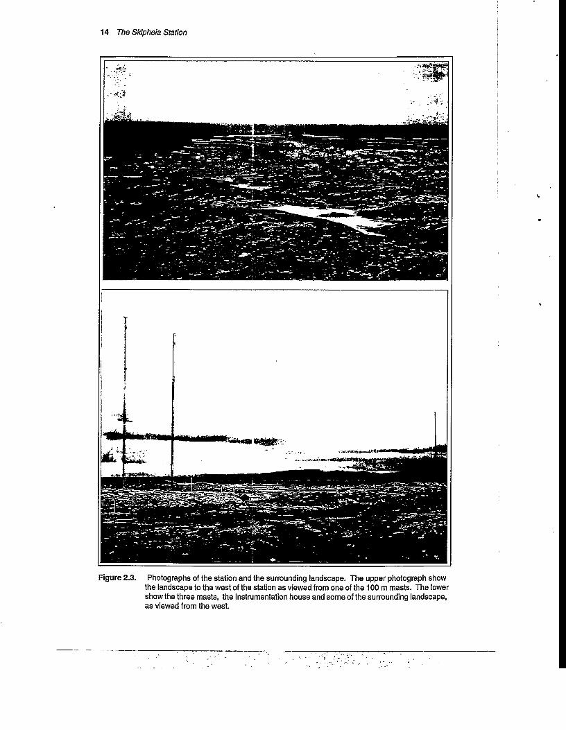
The landscape at the west end of Fr0ya is rather fiat seen on a large scale, with no trees, and the vegetation consists of moss and heather. Near the sea, there are large rocky areas, without vegetation. Photographs of the landscape west of the station and of the station are shown in Figure 2.3. The map in Figure 2.2 shows that the typical formations are small hills with a horizontal spacing of 100 to 500 meters. As we will see, the landscape and particularly the distance to the sea varies, making a division into direction sectors necessary for the data analysis. The relatively complex landscape complicates the data analysis, but as the site is typ-

Masts and Sensor Locations 7
ical for the West-Coast of Norway, a description of the wind field in this type of landscape is very valuable.
The coastline of Western Norway is exposed to maritime wind from the North-Atlantic Ocean. The dominating wind systems at the west coast of Middle Norway are anticyclones moving eastward. The most frequent wind directions are west and southwest, and the average wind speed is highest in the zone from 210° to 270°. As seen from the map in Figure 2.1 the west end of Fr0ya is exposed to nearly undisturbed maritime wind in the directions limited by the coastline from 235° via north to 50°. In the winter, north-westerly winds bring cold air from Arctic areas. When the air masses pass the warmer Gulf stream belt outside the coast, thermally generated turbulence appears, even during strong wind periods. The temperature gra
dient may also deviate from the adiabatic value during strong winds.
2.3 Masts and Sensor Locations
At Skipheia, three guyed masts are placed about 100 m apart. The exact distances and location of the masts and sensors are shown in Figure 2.4. Two of the masts have a height of 100 m while the third is 45 m. The two 100 metres masts (Mast 2 and Mast 4) are located 79 metres apart on a low, flat hill 400 metres from the sea. This distance between the masts corresponds roughly to the diameter of the rotor area for a large WECS. The 100 m masts are made of steel profiles with a square base, side length 1 metre. The 45 m mast (Mast 3), is located between the other masts and the sea on a small hill with the base level about 2 metres higher than the hundred metres masts. Mast 3 has a triangular base, 0.5 m side length.
Figure 2.5 through Figure 2.8 show drawings of the masts with sensors. The numbers in the figures refer to unique sensor identification numbers, which are listed in Table 2.1 together with the exact height and direction of the sensor relative to the mast. The sensors are located on booms, reaching 2.6 m from the mast edge in Mast 2 and Mast 4, 2.8 m in Mast 3. The wind speed sensors in Mast 2 and 4 are mounted in opposite directions. By always selecting the sensor upwind of the mast during the analysis, the mast influence on the measurements is minimized. A small effect, which will be treated by Heggem (personal communication), will persist.
2.4 Instrumentation House
The Instrumentation house provides housing for the Data Acquisition System, workshop facili
ties and overnight accommodation for service personnel. The hut is fully equipped for a team of up to 4 persons. During the planning of the station the high lightning frequency at the station

8 The Skipheia Station
was taken into account. All instruments and all cable inlets were located in one room, the
instrumentation room. The walls, ceiling and floor in the Instrumentation room are made of
concrete while the rest of the hut is built of wood. The previous hut, damaged by a fire in 1992,
was all wooden! Chicken fence-wire, connected to ground, is buried in the concrete to shield
against external electrical fields.
The telephone inlet is equipped with isolation transformers inside the Instrumentation
room and in a switch box a few hundred metres away from the station. Special signal converters
are mounted in the Instrumentation room and in the telephone central. These transform the tele
phone signal to make it transmittable through the isolation transformers.
The power inlet is extensively protected against atmospheric discharges. A heavy duty
lightning arrester and a second lightning arrester are located prior to the main fuses. All instru
mentation equipment is powered separately from the rest of the house, and is further protected
by an Uninterruptible Power Supply (UPS) and a number of isolation transformers. The protec
tion of the telephone and power inlets is further discussed in Sec. 5.3.1.
All electrical equipment, the chicken fence-wire in the walls and the masts are connected
to a grounding network surrounding the station, a sketch which appears shown in Figure 2.4.
The network consists of copper wire, welded in the joints, connected to a large copper plate
buried in the sea. A large number of earth rods are connected to the network, positioned where
the ground allows it. This grounding network is very important, as the ground consists of rock
with only local spots of bog, making proper grounding very difficult.
2.5 Historical Review of the Station
Great effort has been made to keep the station in continuous operation. The weather conditions
at the west coast of Norway can be severe, with frequent hurricanes and heavy lightning. The
main problems are enumerated below:
• Frequent failures in the local power supply. As the the station was the only load on the
local transformer, it could take some time before the failure was repaired.
• A very high lightning frequency; two or three incidents with heavy damage every year. In
spite of the comprehensive work with shielding and guarding of the equipment, heavy
lightning strikes will interrupt operation.
• Strong winds, sea spray aerosols, high humidity and salinity of the air, and over voltage
from atmospheric discharges will destroy the sensors.

Historical Review of the Station 9
A brief historical summary of the wind research activity at Skipheia will be given below. Only the most important milestones and efforts to improve the quality of the measurements will, however, be included
1978: An extensive wind measurement programme at the coast of Trpndelag was initiated. Small stations were established at different sites to estimate wind energy resources.A main station at Skipheia was planned for fast measurements of wind and temperature. The station should also act as a reference station for the wind energy resource programme.
1980: Two masts of 100 metres and one of 45 metres were raised at Skipheia. A portable hut was moved in by helicopter for use as measurement building.
1981: A measurement system was designed and tested. The data acquisition system had twenty-four input channels for frequency signals. Sixteen channels were used for wind speed sensors, four for horizontal wind direction and four for vertical direction. The system is further described in Sec. 5.2.1. The signals were read every 2- 3 seconds, 10 minutes mean values and maximum values were recorded. In January, all installed J-TEC sensors were destroyed by lightning soon after the installation.As replacement and supplementation, three-cup anemometers and bivanes from MET-ONE were obtained. Please refer to Chapter 3 for further information on the sensors. Continuous measurements of wind speed and direction started in September.
1982: In March, the top sensors were moved to a vertical bar one metre above the top of the masts to reduce the disturbance from the mast construction. Lightning conductors were installed at the same time to protect the sensors.
1983: Atmospheric discharges (lightning) were a serious problem. Most of the year, only the Met-One sensors in Mast 2 were working. For long periods no data were recorded.
1984: The station was improved with a new earthing system to reduce the damage from lightning, and the data acquisition system was improved to give a better protection from over-voltages. From May, the data retrieval was dramatically improved. To get information about the stability of the atmosphere, air temperature measurements started. Temperatures were measured in Mast 4 at four heights, near the ground and in the ground. Temperature data were acquired with a separate computer and voltmeter (Nyrud, 1985). The building was also enlarged to give more working area.
1985: At the end of the year, horizontal bars of 2.6 m were installed to move the sensorsaway from the mast body. The disturbance from the mast shadow had been regarded as a serious problem which particularly would affect the high frequency turbulence measurements. To evaluate the shading effect from the mast, doubled sensors were mounted at supports in opposite directions at one height.
1988: In March, a new station to measure pure maritime wind conditions was built atSletringen. From December, a new logging system was installed at Skipheia. High frequency time series (0.85 Hz) were logged and stored. The system is further described in Sec. 5.2.2. All wind speed sensors below 100 m in Mast 2 and 4 were doubled, mounted on supports extending from the mast in opposite directions.

10 The Skipheia Station
1991: On February 14, the building and all the equipment was destroyed by a fire. To continue the logging, a battery supported recording system from Aanderaa was installed in Mast 2. A brief description of the system is given in Sec. 5.2.3. Ten minutes mean wind speed and direction, mean and gust values from two speed sensors and one horizontal direction sensor in one mast were recorded from March.
1992: A new station was built, and an extended measurement programme started in March. Supports for doubled sensors at 100 m in Mast 2 and 4 and new supports for sensors in Mast 3 was mounted. The sensors were moved to the new locations in August.Sea temperature measurements started in October.
1993: Additional meteorological measurements (radiation, air humidity, rainfall and pressure) were incorporated in the data acquisition system.
Table 2.1. Sensor data for all sensor locations at Skipheia. All sensor locations used through the years are listed; not all of these are in use today. The table is a part of the information contained in the Configuration files, which will be described further in Sec. 6.4.1.
Id.a Typeb Height(m)c
Direct.(Deg)'
Description® Id. Type Height(m)
Direct.(Deg)
Description
1 1 101.0 301.0 'S M2T100m' 21 2 101.0 210.0 'Dh M2 100m'2 1 72.0 301.0 'S M2W 70m' 22 4 100.0 210.0 'Dv M2 100m'3 1 41.0 301.0 'S M2W 40m' 23 2 38.0 210.0 'Dh M2S 45m'4 1 20.5 301.0 'S M2W 20m ’ 24 4 45.0 210.0 'Dv M2S 45m'5 1 11.0 301.0 'S M2W 10m' 25 2 38.0 31.0 'Dh M2N 45m'6 1 72.0 121.0 'S M2E 70m' 26 4 45.0 31.0 'Dv M2N 45m'7 1 41.0 121.0 'S M2E 40m1 27 2 101.0 317.0 'Dh M4 100m'8 1 20.5 121.0 'S M2E 20m' 28 4 100.0 317.0 Dv M4 100m'9 1 11.0 121.0 'S M2E 10m' 29 2 46.0 60.0 'DhM3 45m'10 1 101.0 227.0 'SM4T100m' 30 4 45.0 60.0 'Dv M3 45m',11 1 41.0 227.0 'S M4W 40m' 100 4 22.0 301.0 'Dv UVW 20m'12 1 20.5 227.0 'S M4W 20m' 101 2 22.0 301.0 'Dh UVW 20m'13 1 11.0 227.0 'S M4W 10m1 102 4 22.0 231.0 'Dv M2S 20m'14 1 41.0 47.0 'S M4E 40m' 103 2 22.0 231.0 'Dh M2S 20m'15 1 20.5 47.0 'S M4E 20m' 105 2 38.0 317.0 'Dh M4N 40m'16 1 11.0 47.0 'S M4E 10m' 31 6 'Ref. Volt’17 1 45.0 266.0 'S M3T 45m' 32 3 99.0 ’TempM2al00’18 1 20.5 266.0 'S M3 20m' 33 3 69.0 ’TempM2a 70'19 1 11.0 266.0 'S M3 10m' 34 3 39.0 TempM2a40'70 1 101.0 301.0 'S M2W100m' 35 3 9.0 'TempM2a 10'71 1 101.0 121.0 'S M2E100m' 36 3 2.0 'Temp 2 m'72 1 101.0 227.0 'S M4W100m' 37 3 0.2 Temp 0.2 m'73 1 101.0 47.0 'S M4E100m' 38 3 0.0 'Temp bakke'74 1 45.0 231.0 'S M3W 45m' 39 3 0.0 'Diagnostic'75 1 20.5 231.0 'S M3W 20m ’ 40 3 99.0 'TempM2bl00'

Historical Review of the Station 11
Table 2.1. Sensor data for all sensor locations at Skipheia. All sensor locations used through the years are listed; not all of these are in use today. The table is a part of the information contained in the Configuration files, which will be described further in Sec. 6.4.1.
Id.a Type" ■ Height(m)c
Direct1(Deg)"
Description® Id. Type Height(m)
Direct(Deg)
Description
76 1 11.0 231.0 'SM3W 10m' 41 3 69.0 TempM2b 70'
77 1 22.0 301.0 'U_UVW 20m' 42 3 39.0 TempM2b 40'
78 1 22.0 301.0 ’V_UVW 20m' 43 3 9.0 TempM2b 10'
79 1 22.0 301.0 rW_UVW 20m' 44 3 -2.0 Temp SEA a'
80 1 22.0 301.0 'S UVW 20m' 45 3 -2.0 Temp SEA b"
81 1 99.0 311.0 'S M2 100m' 46 3 35 TempMka3.5'
82 1 72.0 311.0 'S M2 70m * 47 3 1.0 TempMkal.O'
83 1 41.0 311.0 'S M2 40m' 48 3 0.0 TempA rock'84 1 20.5 311.0 'S M2 20m' 49 3 0.0 TempAmarsh'85 1 11.0 311.0 'S M2 10m' 50 3 35 TempMkb3.5'86 1 99.0 237.0 'S M4 100m ’ 51 3 1.0 TempMkbl.O'87 1 72.0 237.0 'S M4 70m ’ 130 6 3.0 'Rainfall '88 1 41.0 237.0 'S M4 40m' 131 6 0.0 'RefAA Volt'89 1 20.5 237.0 'SM4 20m' 132 5 4.0 'E Sun up ’90 1 11.0 237.0 'SM4 10m' 133 5 4.0 'E Sun down'91 1 44.0 266.0 'SM3 45m' 134 5 4.0 'E Tot up '92 1 72.0 311.0 'S M2J 70m' 135 5 4.0 "E Tot down'93 1 20.5 311.0 'S M2J 20m' 136 6 35 'Rel.humid.'94 1 11.0 311.0 'S M2J 10m' 137 6 2.0 'Pressure '20 6 ' UPS'
a. Sensor Identification number. Must be unique for the sensor location, used in the analysis programs to identify the sensor.
b. Sensor Type. 1=Wind Speed, 2=Horizontal direction, 4=Vertical direction, 3=Temperature, 5=Radiation, 6=other.c. Sensor height above the ground.d. Sensor direction relative to the mast, as viewed from the mast.e. Usually these strings are built up from: Sensor Type+Mast+Direction+Height
12 The Skipheia Station
TitranSletringen Skipheia
2 km
Hitra
10 20 km
Figure 2.1. Map of Norway with the actual area enlarged. The map on the top shows shoreline, 20 m contour intervals, roads and items like masts, WECSs, houses etc. The dashed area inside the top map is further enlarged in Figure 2.2.

Historical Review of the Station 13
Figure 2.2. The station at Skipheia. Contour interval 5 m
14 The Skipheia Station
Figure 2.3. Photographs of the station and the surrounding landscape. The upper photograph show the landscape to the west of the station as viewed from one of the 100 m masts. The lower show the three masts, the Instrumentation house and some of the surrounding landscape, as viewed from the west.

Historical Review of the Station 15
MarshMast 4
Mast 2
-«-Earth spear ^Copper plate o Guy base
Mast 3
Figure 2.4. The three masts at Skipheia. On the left, the orientation of the masts, the distancesbetween the masts and the directions relative to north. On the right, the grounding system.

16 The Skiphela Station
tI
Lightning bar
Cup anemometer (Vaisala,Met-One)
Vortex counter (J-TEC)
GILL UVW anemometer
(Young)
r Direction sensor
(Met-One, Young, Teledyne, ED)
t Air temperature sensor
Sensor id. no.
Figure 2.5. Mast 2 with the different sensors used from the start in 1980 up to 1994. The first sensors were placed on triangular shaped structure one metre from the mast body. From 1984, the sensors have been located at end of horizontal bars at a distance of two and a half metres from the mast. Temperature sensors were installed in Mast 2 in 1992. )

Historical Review of the Station 17
ir
s.
Figure 2.6. Mast 4 with sensors. From 1984 to 1991, temperature sensors were placed in Mast 4, but are not shown in the drawing. They were located at the same heights as the sensors in Mast 2 in Figure 2.5.

18 The Skipheia Station
29/30
Figure 2.7. Mast 3 with sensors.
jjj Rain detector
5 Radiation sensor 0 Temperature sensor o Humidity sensor
Figure 2.8. The meteorological mast installed in 1993

Chapter 3
Wind Sensors
In this chapter we will try to summarize some of the experience gained with the wind speed and direction sensors at the Skipheia station during the years it has been in operation. The environmental conditions at this site are extreme (with respect to lightning frequency, salt spray from the sea and wind gusts), which make large demands on the sensors. We will also discuss some of the advantages and disadvantages of the operational principles of the various sensors.
3.1 Introduction
The sensors are vital components of the station. For continuous measurements the sensors must have a rugged construction and still be able to give adequate resolution for frequencies up to 1
Hz. The sensors must fulfil the following requirements:
• Measure the meteorological quantities with sufficient resolution and accuracy.
• Survive extreme wind conditions.
• Resist corrosion from salt and moist air.
• Resist damage from magnetic induction and over voltage caused by lightning and atmos
pheric discharges to the masts.
The quality of the sensors has been determined by long time testing at the station. The sensors
not meeting the above demands have been phased out, as the repairs were too expensive. Some of the sensors have been modified to give higher resolution and better overvoltage protection.
The only kind of wind speed sensors tested that has satisfied the requirements are cup anemometers. Only one type of the wind direction sensors used has satisfied the requirements
for long term reliability. Bivanes are particularly vulnerable to the severe weather conditions at

20 Wind Sensors
the coast. The sensors are evaluated with respect to the mechanical quality of housing, cup, propeller, bearing, contact etc., the reliability of electronic parts, resolution, accuracy and stability.
3.2 Principles of sensor operation
Three fundamentally different types of wind speed sensor and one type of direction sensor have been used at the station. We will give a short description of the principles and some of the advantages and disadvantages of each type.
Figure 3.1. Aanderaa wind speed sensor, model 2740 from AANDERAA INSTRUMENTS, Norway.The drawing is a copy from the instrument’s datasheet. The figure illustrates the principles and typical size of a cup anemometer construction. The transducer used for detecting rotational speed varies from one manufacturer to another, the principle with a reed contact and a rotating magnet as on this sensor is rather unusual.

Principles of sensor operation 21
3.2.1 Cup anemometer
This is the traditional meteorological wind speed sensor. A drawing of the Aanderaa model
2740 anemometer is shown in Figure 3.1. The figure illustrates the typical appearance of a 3-
cup anemometer. The cup anemometers measure horizontal wind speed using three conical
cups mounted on a cross fastened to the top of a shaft. The difference in the drag coefficient for
the two sides of the cup makes the cup assembly rotate. Cup anemometers can in principle have
any number of cups and of other shapes, but today the most common configuration is that hav
ing three conical cups. Optical detection of rotational speed by means of some kind of a slotted
disc and an optocoupler is often used to generate an electric output signal. Other principles such
as a tachometer generator or rotation of a magnet are also used.
Cup anemometers are often regarded as reliable and mechanically robust and are the only
type that have survived the conditions at Skipheia. The disadvantage of these sensors are their
slow dynamic response and the tendency to over-speed. At our sampling rate (0.85 Hz) the time
response is not a problem when a light cup assembly is used. Due to the relatively low distance
constant of these sensors, over-speeding is also a minor problem. The step response of the
VAIS ALA sensors was tested by Aasen (1989), the results are reproduced in Sec. 4.3. The dis
tance constant was found to be the same for increase in wind speed as for decrease. Due to the
definition of the distance constant this will, however, not eliminate a small speed-up effect.
Figure 3.2. Gill model 27005 UVW anemometer from R.M Young, USA. The drawing is a copy from the instrument’s manual. The total height of the instrument is 110 cm and the diameter of the propellers 20 cm.

22 Wind Sensors
3.2.2 Propeller
These sensors utilize an ordinary propeller shaped turbine as the active element. The rotational speed of the propeller is measured by the same methods as for cup anemometers. The way of operation for propeller anemometers is in principle better than for cup anemometers. The rotational speed of the propeller is proportional to a sort of average wind speed over the area covered by the propeller, as opposed to the cup anemometer which depends on the difference in drag force on the two sides. This makes the propeller anemometer more suitable for turbulence measurements, however, the mechanical strength of the propellers we have tried, makes them unsuitable for our purpose. Propeller anemometers are produced both as one propeller mounted on a vane or bivane and as three turbines mounted orthogonally, measuring the U, V and W components of the wind. Figure 3.2 show a drawing of the Gill model 27005 UVW anemometer. The propellers response to off-axis winds closely approximates a true cosine curve, and for additional accuracy, calibration data are available. The shading of the horizontal propellers on a UVW sensor by the sensors body is expected to influence the turbulence measurements in a way which cannot by corrected for. Due to the angle of the W propeller to the wind, the accuracy of the vertical wind speed is also questionable.
3.2.3 Vortex counting
Wind passing a stationary rod forms vortices which can be detected by ultrasonic sensing. The relation between wind speed and frequency of vortices is approximately linear, individual calibration is however needed.
The electronics in the sensors we tested did not withstand the atmospheric discharges in the masts. Due to the need of calibration, the tested sensors were not suitable for the purpose. The measuring principle seems to work well, but as we will discuss further below, other methods involving ultrasound are preferable.
3.2.4 Vane
All the wind direction sensors except the UVW propellers use the principle of a vane rotating in the horizontal plane (for bivanes also movement in the vertical plane). Some kind of transducer converts the angular position into an electrical signal. Being mechanical, the sensor’s response to wind gusts is limited. Their response functions can be approximated by a second order linear response function.
Most of the sensors uses a potentiometer transducer. For horizontal direction this means the direction sector in the potentiometer gap cannot be measured, unless special precautions are

Tested Wind Speed Sensors 23
taken. Some of our data acquisition systems used voltage-to-frequency (V/F) converters for conversion of the potentiometer signal to a series of pulses, giving additional problems when the potentiometer gap is passed during the measuring period. Another problem of potentiometers is the mechanical contact, making the operational time limited.
The resolver sensing element has no gap, is contact free and robust, and has a good linearity. The electronics required for interfacing to a computer is however more complex than for
a potentiometer.
For detection of vertical direction, both potentiometers and inductors are used. Use of potentiometers is complicated as some kind of sliding mechanism is needed. The inductor principle, making the inductance in a coil vary approximately linearly with vertical direction, is preferable. The varying inductance is transformed to an output signal with varying frequency by utilizing a L-R oscillator. Such a sensor can be operated without mechanical contact of any sort and is relatively simple both electrically and mechanically.
3.2.5 Sonic
The most promising sensor technology for this type of measurements seem to be sonic anemometers. At the present time no sonic sensor has been tested at the station because of their high price, but a project has been proposed to develop such a sensor in collaboration with Prof. Dels- ing, University of Lulea, Sweden. The sensors operate by sending a sound pulse over a known distance. By measuring the transition time in both directions, the wind speed and the speed of sound can be calculated. These sensors do not have moving parts and hence have a very low distance constant, limited in principle by the length of the sound path. The sonic/ultrasonic elements can be positioned in an arrangement to give the wind speed component in x-, y- and indirection. Only experience can tell if such a sensor will survive the saline and lightning-prone environment at the station. A sonic anemometer will need a lot of electronics which must be carefully protected to avoid damage by lightning. The electronics in such an anemometer can however be replaced, without need to recalibrate the sensor in a wind tunnel.
3.3 Tested Wind Speed Sensors
When the measurements started at Skipheia in 1981, the J-TEC sensor was selected, as it combined the roles of speed and direction sensor. Shortly after the first installation in January 1981, all sensors were seriously damaged by lightning. Repair was expensive and time-consuming, as individual calibration was required. As a consequence of the damage some of the J-TEC sensors were replaced by Met-One three-cup anemometers and bidirectional sensors in 1982. In

24 Wind Sensors
1984, three-cup anemometers were obtained from Vaisala. An UVW propeller anemometer was tested in 1992-93 but did not have sufficient mechanical strength for use in continuous
measurements. A battery powered Aanderaa system was installed as a backup system in March 1991. Specifications from the manufacturer of the wind speed sensors are given in Table 3.1
Table 3.1. Specifications of the wind speed sensors as given by the manufacturer.
Model Sensortype
Distance const, [m]
Resolution[m]
Output Threshold[m/s]
Operatingrange[m/s]
Accuracy
Met-One 010 cup >1.5 0.035 Pulses 0.2 0-60 ±1%J-TEC VA-320 0.006 0.01 Pulses 1 1-60 ±2%Vaisala WAA12 cup 1.5 0.1/0.05“ Pulses 0.23 0-75 b
Vaisala WAA15/ WAA15A
cup 1.5 0.1 Pulses 0.23 0-75 b
Gill 27005 UVW 1.5 " Analoguevoltage
0.4 0-50 ±1%
Aanderaa 2740 cup 1.5 0.597 SR10 0.3-0.5 0.5-60 c
a. Modified as described in text for the sensor.b. ±0.1 m/s u<10 m/s, ±2% u>=10 m/sc. max of ±2% and, ±0.2 m/s
3.3.1 J-TEC Wind Speed Sensor VA-320-2-1
The wind speed sensor from J-TEC, USA, uses the principle of vortex counting. The sensor is shaped as a wind vane and direction is determined from a potentiometer attached to the sensor body. The sensor gave a pulse out per vortex. The pulses were counted directly by counters in the acquisition system. The distance constant was extremely small (6 mm), the speed range wide (0 - 60 m/s), and the mechanical construction robust.
Fifteen sensors were bought in 1981 and mounted in the three masts. Unfortunately the sensor has a lot of sensitive electronic parts which are vulnerable to lightning and discharges.
The distance constant for direction measurement was also rather large (10 m), and the sensor had a tendency to rotational oscillation in the wind. The need for individual calibration of the sensors after damage by lightning made the sensors unsuitable for continuous measurements.
3.3.2 Met-One 010b anemometer
The model 010b from Met-One, USA, is a three-cup anemometer with an optical detection of
rotation. The sensing element consists of a slotted disc mounted to the anemometers shaft, rotating in the gap of an optocoupler. The number of slots is 40. The signal from the optocou- pler is amplified and shaped to form a series of pulses of fixed length.

Tested Wind Speed Sensors 25
This model has a very robust electronic part which can survive lightning strikes in the mast. However, the housing is too weak mechanically, and is damaged by vibrations in the masts. The rotor is also too weak, and we have had a lot of cup breaks during high wind periods. The rotor is of course the essential part of the sensor, and it is necessary that the rotor can withstand the extreme wind periods. Typically one of the cups fell off when the mean wind speed exceeded 30 m/s. Plots of time series with cup breakage are shown in Figure 3.3. The distance constant given by the manufacturer is 1.5 metres, verified to 1.8 metres by Aasen (Aasen 1989), please refer to Chapter 4 for a more detailed discussion on the dynamic perform
ance of a cup anemometer.
Sep. 25 1983 —S M2100m •••SM2 70m ■-SM2 20m — S M2 10m
Oct. 23 1983 —S M2100m - S M2 40m
—SM2 20m - S M2 10m
Nov. 241983 Dec. 7 1983—S M2 100m ■••SM2 70m —S M2 20m - S M2 10m
—S M2 100m - S M2 70m
■ -S M2 40m — S M2 10m
Time (hours)Time (hours)
Figure 3.3. Time series for 4 days in 1983 showing the cup breakage of the MET-ONE 010B sensor.Four of five breakdowns for the top sensor in Mast 2 in a four-week period late 1983 are shown. Ten minutes average values are used, and 30 m/s seems to be the maximum wind speed the sensor can survive. On Dec. 7, the anemometer was replaced earlier the same day.

26 Wind Sensors
3.3.3 Vaisala WAA12, WAA15 and WAA15A Anemometers
In May 1984, cup anemometers from Vaisala, Finland, were mounted in the masts. The first model used at the wind station was WAA12, a three cup anemometer with optical speed sensing. A light emitting diode sends a beam trough a transparent plastic disc with black sectors. A photo diode detects the pulses and a simple electronic circuit shapes and drives the output signal. The resolution was originally fourteen pulses per revolution, corresponding to 10 cm wind distance. The sensor was later (one to two years) modified to give twenty-eight pulses per revolution, by using another part of the plastic disc. The output is a square wave with frequency proportional to the wind speed. The distance constant given by the manufacturer is 1.5 m, which is verified in Chapter 4. Chapter 4 also discusses the steady state calibration of the sensor.
The body of the anemometer is rather large and ragged, and has a very good surface coating which is as good as new after 10 years of usage. The cups are strong, and can withstand extreme wind gusts. During the hurricane on January 1, 1992 the maximum 2-second wind gust is measured to 57.6 m/s. The electronic parts of the model WAA12 were however too weak, and were frequently damaged by lightning.
The next version from Vaisala was the model WAA15, which has the same rotor as its predecessor. The shape and the coating of the housing is changed. The body is smaller and the trank more slender. The surface coating has a poor quality, and the paint begins to peel after a few months. The top bearing is badly protected against salt spray, so the lifetime of the bearings is shorter than for the former model. The electronic parts, on the other hand, are more reliable; the pair of printed boards with light emitting diodes and photo diodes are replaced by a single optocoupler.
A new version, WAA15A used from 1992 has better protection for the top bearings, and seems to be a reliable sensor. However, the surface coating is still not good enough for the weather conditions on the coast.
3.3.4 Gill UVW Anemometer, Model 27005
The model 27005 Gill UVW anemometer, from R.M. Young, USA, measures the x-, y-andz- components of the wind. A sketch of the anemometer is shown in Figure 3.2. Three independent and identical four blade propeller anemometers form an axis cross. Tachometer generators produces DC voltage output proportional to the axial wind speed component. Carbon fibre ther
moplastic propellers are claimed to survive wind speeds up to 50 m/sec. This applies to the heavy duty model; an alternative model using propellers of expanded polystyrene is also available.

Tested Wind Direction Sensors 27
A computer algorithm is used to compensate for deviations from the cosine curve. Itera
tion is performed until the difference between the two last iterations is less than a chosen limit. Rather than using the manufacturer calibration data we used data from Connell and Morris
(1991).
The UVW anemometer was installed on Mast 2 on September 1,1992, and the first breakdown was registered on December 25, after 115 days. When the anemometer was dismounted in February 1993, two of the propellers had missing blades, the third propeller was missing due to a broken plastic shaft and one of the anemometer mountings was damaged.
3.3.5 Aanderaa Wind Speed Sensor 2740
Aanderaa 2740 (and its predecessor 2593) sensors from Aanderaa Instruments, Norway, have been used by our group since 1979 at various stations. A sketch of the anemometer is shown in Figure 3.1. The sensor is a three-cup anemometer, and the sensing element consists of a magnet mounted in the skirt of the rotor and a reed contact inside the housing. A micro controller reads the pulses from the reed contact and calculates average and maximum (2 sec.) wind speed.
The cup assembly of this sensor is not as robust as the Vaisala cups and we have experienced several cases of cup breakage. In a hurricane on January 1, 1992 the maximum gust value recorded was 57.6 m/s, and many sensors were damaged in this hurricane; so this appears to be near the sensors survival speed limit. According to Aanderaa Instruments the cup assembly has been reinforced after this incident, but there has been no any opportunity to verify the claim.
A wind tunnel calibration of this sensor, using a pitot-static tube as a reference, was performed. The results are discussed in Chapter 4.
3.4 Tested Wind Direction Sensors
As mentioned in Sec. 3.3, the first direction sensor used was the J-TEC wind vane. Due to serious damage from atmospheric discharges, the sensor was replaced by a Met-One 022 bivane. The bivane also had the advantage of vertical component measurements. However the vertical sensing mechanisms was quickly broken. In 1991 a Gill 27005 microvane was installed but showed very early severe corrosion damages. At the start-up of the new data acquisition system rebuilt Vaisala direction sensors was mounted, but the mechanical resistance in the sensors was too large. The search for a good direction sensor continued by the mounting of a Teledyne bivane and a Gill UVW propeller anemometer. None of these showed the required mechanical strength. At the present time the direction sensors consists of vanes from ED Service-Center,

28 Wind Sensors
one type utilizing potentiometer as the sensing element and one type utilizing resolver. Sensors with resolvers as signal converters have been used since 1992. Specifications from the manufacturers of wind direction sensors are given in Table 3.2.
Table 3.2. Specifications from the manufacturers of direction sensors. Empty cells mean that no information is available. The Vaisala WAA12 is modified and performance data are not available.
Model Sensortype
Distance const [m]
Dampingratio
Resolution
Output Threshold[m/s]
Operatrange[m]
Accuracy
J-TECVA-320
Vane/potmeter
10 cont Analoguevoltage
1 2-100 ±4° @2 m/s±2°>5m/
Met-One022
Bivane/potmeters
0.9 0.4-0.6 cont. Analoguevoltage
0.2 0-60 ±3%
VaisalaWAA12
Van el resolver
cont Resolver 0.4 0-75
TeledyneAzimuth
Bivane/resolver
1 0.4 cont. Resolver / pulses
0.4 0.4-75 ±2°
TeledyneVertical
Bivane/inductance
1 0.4 12Hz/degree.
Pulses 0.4 0.4-75 ±2°
ED, 2K/ 352DEG.
Vane/potmeter
1 0.4 cont. Resistance
<0.3 ±0.2%
ED,COS/SIN4kHz
Vane/resolver
1 0.4 cont Resolver <0.3 ±10 minutes
Gill12305
Vane/potmeter
1 0.44 cont. Resistance
0.4 0.25%
Gill27005UVW
propeller/tachogen.
2.1 cont. Analoguevoltage
0.4 0-50 ±1%
Aanderaa2053
Vane/compass
cont Resistance
<0.3 ±5%
3.4.1 J-TEC Wind Direction Sensor VA-320-2-1
The Wind Speed and Direction Sensor from J-TEC, USA, was used as direction sensor in the early beginning of the project. Since the speed part of the sensors was damaged by lightning, no long term experience is recorded about the quality of the VA-320 Direction Sensor. Note however the large distance constant (10 m).

Tested Wind Direction Sensors 29
3.4.2 Met-One 022 Bivane
The model 022 from Met-One, USA, was used from 1982 up to 1991. A rod with a bivane of polystyrene and a counterweight was the sensing parf, and potentiometers of 360° and ±60° con
verted the position to a voltage output signal. The sensing range of the horizontal potentiometer was only about 350°, which gave a gap around North of approximately 10°. The analogue output from the sensor was converted to frequency signal and logged by the same counting procedure as for the speed sensors. Pulses were counted during one logging period of 1.17 seconds, which gave arbitrary erroneous values when the potentiometer gap was crossed.
The polystyrene vane was damaged by hail or by birds pecking at it. Losing weight, the vane was no longer in horizontal balance and measurements of vertical direction became incorrect. Vertical potentiometer signals were connected via slide wires to the drive tube. The potentiometer and slide wires were vulnerable in lightning weather, and were out of duty for long periods. The sensor body had a weak mechanical construction, and broke after some use. The construction was reinforced in later models. The electrical circuits, which included an amplifier for output voltage proportional to vane position, had the same reliable construction as for the Met-One wind speed sensors.
3.4.3 Gill Microvane, Model 12305
The model 12305 from R.M. Young, USA, is a vane equipped with a rather large aluminium fin, utilizing a potentiometer as sensing element. The sensor body is made of aluminium, and the outside is painted. This surface coating is totally insufficient in this salty environment and the sensor is very seriously damaged within a few months. Furthermore the fin of the sensor is exhausted by vibrations and has, on several occasions during periods with high wind speeds, broken.
3.4.4 Gill UVW Anemometer, Model 27005
The components of the wind speed determine the wind direction. This sensor was discussed in Sec. 3.3.4.
3.4.5 Teledyne Geotech Bivane, Model 1585
The model 1585 from Teledyne Geotech, USA, is a bivane sensor with a resolver converting system for horizontal direction and an inductor system for vertical direction; it has no moving electrical contacts. The manufacturer has equipped the sensor with circuits for signal conver

30 Wind Sensors
sion to give output signals suitable for measurement systems. The resolver circuit generates two output signals with a phase lag proportional to the rotor shaft angle. This circuit has been disconnected in our sensors. To provide compatible signals from all resolver sensors, reference signal generators and signal processing circuits of same kind are used for all resolver channels.
The vertical position of the vane is detected by an inductor sensor. The induction varies with vertically vane rotation, and the frequency output from the L-R oscillator changes proportional to the vane elevation.
The sensor was installed at 22 metres on Mast 2 on October 20 1992 and dismounted on February 1993 when the inductor circuit and the resolver was destroyed by lightning activity in the masts. Even more serious was the wear on the bearings of the vertical shaft. These bearings were not adequately protected against salt and moist air.
3.4.6 Vaisala WAA12 modified for resolver measurements
The wind direction sensors models WAV12 and WAV 15 produced by Vaisala, Finland, correspond to the wind speed sensors reported in Sec. 3.3.3 The housing and the shaft/bearings of the speed and direction sensors are the same, the differences are the vane and the electrical circuit. The WAV sensors have optical sensing and a 6-bit Gray-code output. The resolution of the disc encoder is then 5.63 degrees, which is too large for our purpose. Experience with the WAA12 wind speed sensor show good mechanical reliability. It was decided to modify four WAA12 speed sensors to wind direction sensors. Cups were replaced by vanes, and resolvers (Tama- gawa) were installed as converter elements.
Unfortunately a silicone paste containing acetic acid was used, which destroyed the ball bearings of the resolver in few days. This was however detected and fixed, but the mechanical friction (resistance in bearings) still appeared to be too large. The response of the sensor was too slow. Furthermore, the resolver to angle decoding system had serious malfunctions. In spite of the problems, the modified Vaisala sensors were used as principal direction sensors from March, 1992 to January, 1993. Problems with the resolver decoding system led to a modification of the system where multiplexing of signals was replaced by separate decoding circuits for each sensor. The decoding system is further discussed in Sec. 5.4.2.
3.4.7 ED wind direction sensor 2K/352 DEG. and COS/SIN 4kHz.
The vane from ED Service-Center, Denmark, has a body made of brass and all other parts of stainless steel. The vane is made of laminated polystyrene. The sensor is available with both resolver (COS/SIN 4kHz) and potentiometer (2K/352 DEG.) as sensing element. The linearity

Discussion 31
of both rotational transducers has been verified. According to our experience both sensor types are very reliable, no particular problems were noted. The oldest sensor has been in operation for almost 2 years without any need of maintenance.
3.4.8 Aanderaa wind direction sensor 2053
The sensor, manufactured by Aanderaa Instruments, Norway, consists of a light wind vane, mounted on top of a housing made of ABS plastic, and is furnished with a built-in compass that is magnetically coupled to the vane. When direction is to be read, the compass is clamped by applying a current to a clamping coil inside the compass. In this way the direction is given as a potentiometer setting. The vane movements is damped by silicone oil between the pivot and the surrounding PVC skirt (rotating). Apart from some incidents with oil-leakage, no particular problems were experienced with the sensor.
3.5 Discussion
The Vaisala cup anemometers and the ED wind vane turned out to be the most reliable and the best overall sensors we have used; however, these sensors provide no information about the vertical wind speed. The bivanes and the UVW sensors do not have the required mechanical strength and are not suitable for continuous use.
As we will discuss in Chapter 4, we have reasons to believe that the steady state calibration of either the Aanderaa or the Vaisala cup anemometer is not within the manufacturers specifications. A calibration of these sensors was therefore made and the results are given in Chapter 4.

32 Wind Sensors

Chapter 4
Sensor Calibration
Measurements of turbulence using cup anemometers are limited by the time-response of the anemometers. To check the factory performance data it was decided to determine the step response by using a wind tunnel and a motor coupled to the cup anemometer rotor, and the frequency response by simultaneous measurements using a hot-wire anemometer. Since measurements from the VAISALA WAA15A and the AANDERAA 2740, located at the same heights in Mast 2 at Skipheia, indicated that average wind speed measured by the VAISALA sensors was approximately 4-6% larger than measured by the AANDERAA sensors, the steady-state performance was also examined.
4.1 Steady-state calibration of cup anemometers.
The most practical method for calibrating anemometers is to do measurements in a wind tunnel, using a pitot-static tube and a manometer to measure the wind speed in the tunnel. We will start by describing the measurement setup, then present the results together with the factory data and data from Berg and Dahl (1980). Berg and Dahl carried out a calibration of a GILL UVW anemometer and cup anemometers from VAISALA, AANDERAA, SMHI/FFI and RIS0.Finally, the error sources are discussed and the calibration is evaluated.
4.1.1 Wind tunnel setup.
The sensors were calibrated in the wind tunnel at the Norwegian Institute of Technology. Aschematic drawing of the tunnel setup is shown in Figure 4.1. The wind speed in the tunnel wasmeasured using a pitot-static tube connected to a Lambrecht 655 M16 manometer. The air temperature T in the tunnel was measured using a mercury thermometer. A mercury barometer was

34 Sensor Calibration
•2.70 m.
— Pilot tube
•0.87 m.
0.025 m
•0.86 m.
Figure 4.1. Sketch of the wind tunnel setup, showing the location of the cup anemometers and the pitot-static tube.
used to measure the static air pressure P. From Bernoulli’s equation we have the expression for the wind speed in the tunnel Vpil0„ given the height Halcohol, of the alcohol column:
Vpitot—.^“SP alcohol^alcohol
(4.1)
where
MP RT ’ (4.2)
and M is the average molecular mass of air.
4.1.2 Cup anemometers.
Due to reliability and cost the VAIS ALA WAA15A and the AANDERAA 2740 have been the preferred sensors at our measurement sites. Please refer to Chapter 3 for a review of various wind sensors. These sensors were therefore chosen for calibration. For practical purposes the

Steady-state calibration of cup anemometers. 35
cup anemometer can be regarded as a linear instrument. A useful form of the relation between
the measured value X from the anemometer and the wind speed V is:
(4.3)V=a-Cr-X+Cs,
where a is a constant depending on the anemometers signal generator, Cr is the distance the
wind has to travel to make the anemometer rotate 360° and C, is the starting wind speed of the
anemometer.
The WAAlSAs speed of rotation is measured using a toothed disc attached to the ane
mometer's rotor shaft. The disc has 14 teeths and rotates between a LED and a phototransistor.
This generates an output signal which is a pulse train where the frequency/is proportional to
the rotation speed. The frequency was measured using a HP-34401 multimeter. The calibration
equation for this anemometer can be written as:
(4.4)
The 2740s speed of rotation is measured using a magnet located at the lower end of the rotating
axis. The magnets rotation is sensed by a reed contact located inside the housing. This is con
nected to a counter inside the sensor and generates 2 counts per revolution. The 2740 was con
nected to an AANDERAA Sensor Scanning Unit 3010. The measurement N displayed on the
3010 represents average number of counts multiplied by 8. The logging interval was set to 30
seconds, making the readings 30 second average values. The calibration equation for this ane
mometer can be written as:
(4.5)
4.1.3 Results for VAISALA WAA15A
The measurements are plotted in Figure 4.2 and given in Table 4.1. As we can see, the meas
urements indicates a lower value for the Cr constant than the factory value. Table 4.2 show the
calibration constants, calculated by linear regression between the tunnel wind speed measured
by the pitot-static tube and the output frequency from the WAA15A. The factory constants and
constants from Berg and Dahl (1980) are also shown in the table. The manufacturer's accuracy
specifications are ±0.1 m/s for wind speeds < lOm/s, and ±2% for wind speeds > lOm/s. Com-

36 Sensor Calibration
Frequency [Hz]
Figure 4.2. Wind speed in tunnel as measured by the pitot-static tube plotted against output frequency from the VAISALA WAA15A. The line show the wind speed calculated from the frequency measurements using the manufacturer’s data.
pared to the manufacturers value for C„ our value will give 3.9% lower values for the wind speed. This is significantly outside the manufacturers accuracy specifications.
Table 4.1. Measurements made in wind tunnel for VAISALA WAA15A.
^alcohol(mm)
Temp.(°C)
Vpitot(m/s)
Frequency(Hz)
vour(m/s)
V manufacturer(m/s)
197.0 26.0 23.1497 238 23.1430 24.0660
164.0 26.5 21.1396 219 21.3122 22.1633
141.0 27.0 19.6176 200 19.4814 20.2606
120.0 27.5 18.1129 187 18.2288 18.9587
100.5 28.0 16.5898 170 16.5907 17.2563
85.5 28.0 15.3018 156 15.2417 15.8543
69.5 28.0 13.7960 140 13.7000 14.2520
57.5 28.0 12.5485 128 12.5437 13.0503
45.0 27.5 11.0919 113 11.0984 11.5481
33.5 27.0 . 9.5622 96 9.4603 9.8457
25.0 27.0 8.2605 83 8.2076 8.5439

Steady-state calibration of cup anemometers. 37
Table 4.1. Measurements made in wind tunnel for VAISALA WAA15A.
Halcohol Temp. Vpitot Frequency vour ^manufacturer
(mm) TO (m/s) ' (Hz) (m/s) (m/s)
17.5 26.5 6.9055 70 6.9550 7.2420
11.0 26.0 5.4703 55 5.5096 5.7399
6.0 25.5 4.0367 41 4.1606 4.3379
2.8 25.0 2.7553 26 2.7153 2.8357Static air pressure, P = 742 mm Hg.
Table 4.2. Calibration constants for VAISALA WAA15A
Source Cr(m) C, (m/s)This experiment
VAISALABerg and Dahl
1.349+ 0.005
1.4021.364
0.21± 0.05
0.2320.10
4.1.4 Results for AANDERAA 2740
+ Pitot — Aanderaa
150 2(Reading N
Figure 4.3. Wind speed in tunnel as measured by the pitot-static tube plotted against output reading N, as displayed on Sensor Scanning Unit 3010, for the AANDERAA 2740. The line show the wind speed calculated from the N values using the manufacturer’s data.
The measurements are given in Table 4.3 and plotted in Figure 4.3. The figure indicates a slightly lower starting wind speed for the anemometer than the factory value. A linear regres-

38 Sensor Calibration
Table 4.3. Measurements made in wind tunnel for AANDERAA 2740.
^alcohol(mm)
Temp.TO
Vpitot(m/s)
Reading N (from 3010)
Vou,(m/s)
"V manufacturer(m/s)
196.0 27.0 23.1294 308 23.2407 22.9768177.0 28.0 22.0164 292 22.0469 21.7832157.5 29.0 20.8027 274 20.7038 20.4404136.0 29.5 19.3468 255 19.2860 19.0230117.0 30.0 17.9593 237 17.9430 17.680298.0 28.0 16.3822 217 16.4506 16.188283.5 27.0 15.0966 199 15.1075 14.845469.5 26.5 13.7615 181 13.7644 13.502657.0 26.0 12.4523 162 12.3467 12.085245.5 26.0 11.1254 145 11.0783 10.817034.5 26.0 9.6877 127 9.7352 9.474225.5 26.0 8.3288 108 8.3175 8.056817.5 26.0 6.8997 89 6.8998 6.639410.5 26.0 5.3445 69 5.4074 5.14746.0 26.5 4.0434 51 4.0643 3.80462.9 26.5 2.8111 34 2.7959 2.5364
Static air pressure, P = 742 mm Hg.
sion of Ml 6 on Vpil01 gave the results given in Table 4.4. The table also shows the manufactur-
Table 4.4. Calibration constants for AANDERAA 2740
Source Cr(m) Cs (m/s)This experiment 1.194± 0.003 0.26± 0.03AANDERAA (data sheet) 1.194 0 or 0.3-0.5"AANDERAA (T.N. 210) 1.197 0.53Berg and Dahl 1.152 0.28
a. The data sheet is somewhat unclear at this point. In the conversion formula the constant is 0, but the threshold wind speed is equal to 0.3 - 0.5 m/s.
ers data and data from Berg and Dahl (1980). As we can see, the measurements indicate a higher value for the Cs constant than the factory constant. The manufacturer's accuracy specifications are ± 2% or + 0.2 m/s whichever is the greatest. This means the deviation is outside the manufacturers specifications only for low wind speeds; however, the deviation seem systematic.
Three 2740 sensors were calibrated by AANDERAA INSTRUMENTS in the wind tunnel at Forsvarets Forskningsinstitutt for Aerodynamik (FFA), Stockholm, Sweden in 1979. Some

Steady-state calibration of cup anemometers. 39
of the results are published in Technical Note No. 210 from AANDERAA INSTRUMENTS. These results are interpreted by AANDERAA to give the constants in the 2740s data sheet.
4.1.5 Measurement errors
leraa
Figure 4.4. Plot of the deviations Vpilot - Vourfor cup anemometers VAISALA WAA15A and AANDERAA 2740. Vpitotand Vour are printed in Table 4.1 and Table 4.3
Figure 4.4 shows the deviations between the pitot measurements and the AANDERAA and the VAISALA measurements. These residuals represents the random errors in the calibration. In addition to these errors there can be systematic errors. We will list some of the error sources and the magnitude of these errors to get an impression of the total error in the measurements.
Resolution of pitot-static tube/manometer measurements.
To maximise the manometers resolution without changing inclination during the experiment, the manometer was used at inclination 1:5. The manometers scale is in mm. This gives the resulting resolution for some values of wind speed as shown in Table 4.5. The read-out errors are dominantly random in nature and are a main source of the residuals in Figure 4.4.
Table 4.5. Pitot measurements resolution
Tunnel wind speed (m/s) 2 5 10 15 20 25Resolution (m/s) 0.58 0.26 0.13 0.09 0.07 0.05

40 Sensor Calibration
Manometer offset.
Any manometer offset error will directly affect the C, constant. Since the pressures we are measuring are on the order of 101 Pa, this is a particularly sensitive parameter. Due to this
sensitivity the manometers zero was carefully adjusted and checked during the experiment. Any errors due to erroneous adjustment are estimated to be on the order of 0.05 m/s. We also checked the manometer against other manometers of the same type, and found no differences. The calibration data, from calibration at WELH. LAMBRECT KG 30.09.83., seem to be valid.
Turbulence.Turbulence in the tunnel made the readings fluctuate. This applies both to the pitot measurements and to the frequency measurements (VAISALA). The AANDERAA readings was 30 second average values, and was unaffected. For VAISALA the effect was compensated by several readings and using an estimated mid value. This effect is estimated to be in the order of 0.2%.
Resolution of the cup anemometers measurements.
The resolution of the AANDERAA readings is 1.194/16 = 0.07 m/s. This will give a contribution to the residuals. Due to the voltmeter’s frequency measurement technique (reciprocal counting), the resolution of the VAISALA measurements is very good (6.5 digits)).
Non-uniformity of flow.
The mean wind speed in the location of the cup anemometer was measured and found equal to the wind speed at the location of the pitot tube.
4.1.6 Discussion.
The steady state calibration of the anemometers confirmed the observed difference in the measurements at Skipheia from the AANDERAA sensor and the VAISALA sensor. The measurements on the AANDERAA sensor seem to fit very well to the calibration done at the FFA laboratory in Stockholm. According to Ingolf Hilland at AANDERAA (personal communication), the sensor has been changed since the calibration took place. The diameter of the rotor skirt was enlarged, and the bearings replaced with lower friction bearings. Hilland estimated C, = 0.3 m/s. The calibration of Berg and Dahl (1980) can be interpreted to support our assertion on the C, value.
Berg and Dahl did not include any information on the tunnel setup or how the pitot data were obtained. Their report was mainly aimed at the calculation of the distance constant for the

Frequency response of cup anemometers. 41
anemometers. Steady-state calibration data were included as a minor point. In their speed range
(2 - 38 m/s) only 5 speeds were measured. This makes the quality of their calibration somewhat
questionable.
Our calibrations of the VAISALA sensor, however, differ significantly from the factory
values. We contacted VAISALA OY and their calibration representative VTT MANUFAC
TURING TECHNOLOGY, but could not find any explanation for the deviations. One possible
explanation could be differences in the turbulence intensity levels in the tunnels. Our calibra
tion is however supported by the good agreement for the AANDERAA sensor.
4.2 Frequency response of cup anemometers.
If we assume that the cup anemometer is a linear instrument, as shown in the calibration experiment in the previous section, the relation between the power spectrum of the input signal Sx(f)
and the power spectrum of the output signal Sy(f) can be written as:
(4.6)
H(J) is the frequency response function, which is the Fourier transform of the impulse response
function h(t). See e.g. Newland (1987) for a detailed discussion of these relations. If the input
and output spectra are known for all frequencies Eq. (4.6) can be used to find the magnitude of
the frequency response function.
From the calibration data we saw that the cup anemometer can be regarded as a first order
instrument. This means the frequency response function is on the form:
1(4.7)
For cup anemometers it is not the time constant t, but the distance constant DC which is the
natural property for describing the instruments dynamic performance. The distance constant is
related to % by:
DC = r-U, (4.8)
where U is the mean wind speed. On a step change in wind speed, the anemometer reaches
63% (1-e-1) of the increase after the wind has travelled DC metres.

42 Sensor Calibration
4.2.1 Instrumentation.
Measurement of S^jCf) was done using a hot wire anemometer, which has a unity frequency
response up to the kHz area. We will use these measurements as an estimate of the true wind speed. The hot wire anemometer was connected to a PC via a special bridge circuit, an ampli
fier/anti aliasing filter and a 12 bit AD interface, DAS-8 from Metrabyte Corp. The cutoff fre
quency of the anti aliasing filter was set to 33 Hz. Calibration of the hot-wire anemometer was
done using a pitot-static tube and a manometer as a reference.
Measurement of the output frequency signal from the VAISALA WAA15 cup anemometer was done using a 16 bit counter interface, UCCTM-05 from Metrabyte Corp. To get the
best possible resolution of the frequency measurements, a reciprocal counting technique was
used. The counter source input was connected to a 1 MHz crystal oscillator and the anemometer
signal connected to the counter gate input. The counter was configured to automatically store
number of counts from the crystal oscillator on every rising edge on the anemometer signal.
The anemometer signal was also connected to one of the interrupt inputs of the PC, giving one interrupt per pulse.
To approach simultaneous measurement of the hot wire- and the cup-anemometer, the AD converter and the counter was read for every pulse from the cup anemometer. At the given log
ging interval (5, 10 or 20 Hz) the measurements were averaged to form a time series with equal
spacing in time. This was repeated until the length of the time series was equal to 2048.
The instruments were placed atop the wind tunnel, just outside the return air stream. (The
wind tunnel was of an open return-circuit type.) This positioning of the anemometers was
selected to ensure that turbulence of a broad frequency range was present. The relative position
of the hot wire anemometer was 11 cm below, 0 cm to the side and 15 cm upstream of the centre of the cup assembly. Other setups were also tried, but studies of the coherence data showed
much smaller values which mean the wind at the cup anemometer is less correlated with the wind at the hot-wire anemometer.
The hot-wire- and cup-anemometer time series were Fourier transformed using a FFT routine and the power spectra was calculated.
4.2.2 Results.
Equation (4.6) with H(f) inserted from Eq. (4.7) was fitted to the experimental frequency
response data using the least squares method and % as the free variable. An example of the
experimental response, together with the fitted response function and the factory response function is shown in Figure 4.5.

Step response of cup anemometers. 43
MeasuredFitted(DC=1.44)
Frequency (Hz)
Figure 4.5. Plot of measured, fitted and factory transfer function for series 4. Fitted and factory distance constants are shown on the plot.
The fitted distance constants are listed in Table 4.6, and as we can see the average value is practically identical to the factory value.
Table 4.6. Distance Constants found from the transfer function measurements
Series no. 3 4 5 6 7 8 9 10 Mean ± Std.dev. 'DC 1.59 1.44 1.41 1.35 1.57 1.53 1.49 1.75 1.51+0.13
4.3 Step response of cup anemometers.The step response of the VAIS ALA WAA15 anemometer was also tested in the wind tunnel.To measure the step response of a system, a sharp increase/decrease of the input signal is needed. This is difficult to obtain in a wind tunnel. An investigation by Hagander (1980) used a moving trapdoor in a wind tunnel to generate the wind speed change, but with limited success.

44 Sensor Calibration
4.3.1 Instrumentation
ReleaseMechanism2.5x5
0=2.5
Motor
0=2.5
2.5x5
Figure 4.6. Cup anemometer speed up/down setup. All measures are in cm. Modified from Aasen (1989)
To generate the step input to the cup anemometer we used a DC motor coupled to the cup assembly by three pins for increasing/decreasing the anemometer speed relative to the wind speed. A sketch of the setup is shown in Figure 4.6. The motor is kept in position by a removable pin; when this pin is pulled out, the motor is pulled away from the anemometer by a spring and the anemometer slows down/speeds up. The setup is identical to the one used by Aasen (1989).
For measurements of the anemometer rotational speed we used a PC equipped with a 16 bit counter interface, UCCTM-05 from Metrabyte Corp. Analogous to the frequency response measurements we used a reciprocal counting technique for measuring the time between every pulse from the anemometer. The wind speed corresponding to this time was stored by the PC. This gives 14 wind speed measurements for every turn of the anemometer.

Step response of cup anemometers. 45
4.3.2 Results
Time [sec.]
Figure 4.7. A part of a time series measured by the VA1SALA WAA15A anemometer. Circles represents measurements, which have been joined by straight lines.
Examining the measurements revealed two characteristics in the measurements. First an effect from the shading by the individual cups, generating variations of frequency three times the revolution frequency of the anemometer. A part of a typical time series is shown in Figure 4.7, and the power spectrum of the same time series is shown in Figure 4.8. The revolution frequency is 8.23 Hz, and in Figure 4.8 we can observe a peak for 8.23x3 = 24.7 Hz. Due to irregularities in the chopper disc Aasen (1989) also found the anemometers rotational frequency in the power spectrum. For the sensor investigated here this was not found. The implications of these effects are if a reciprocal frequency counting technique is to be used, care must be taken so that measurements for an integral number of cycles of the anemometer are averaged.
Secondly we can observe a low frequency variation in the wind tunnel speed. The turbulence intensity in the tunnel was found to be in the order of 2.5%. These fluctuations generated large variations in the response curves, and the resulting standard deviation of the calculated DC’s was 0.6 m. An example of a typical experiment together with the fitted curve are shown in
Figure 4.9.

Spec
tral d
ensi
ty
46 Sensor Calibration
30Frequency [Hz]
Figure 4.8. Power spectrum of the time series in Figure 4.7.
+ Measured -----Fitted
Time [sec.]
Figure 4.9. Sample time series and fitted step response function for speed down, VAISALA WAA15.
The measurements by Aasen (1989) was made in another wind tunnel at Norwegian Institute of Technology. In that tunnel the fluctuations were much smaller, the turbulence intensity

Conclusions on the cup anemometer calibrations 47
was roughly 1.3%. The distance constants from the 1989 investigation are reproduced in
Table 4.6 and Table 4.7.
Table 4.7. Distance Constants, wind speed in the tunnel Uwind and starting speed Ustart for the VAISALA WAA15 anemometer during speed down experiments. From Aasen (1989).
Uwind [m/s] 4.58 4.42 4.49 10.17 10.19
Uslart [m/s] 9.85 14.95 20.31 15.01 10.19
DC[m] 1.730 1.539 1.492 1.849 1.686
Table 4.8. Distance Constants, wind speed in the tunnel U^nd and starting speed Ustait for the VAISALA WAA15 anemometer during speed up experiments. From Aasen (1989).
Uwind [m/s] 4.53 10.09 15.40 20.98 10.13 15.45 20.90
Ustart [m/s] 0 0 0 0 4.77 5.20 13.85
DC [m] 1.644 1.677 1.593 1.573 1.729 1.735 1.443
The 1989 investigation did not find any significant difference between the DC’s for speed up and speed down experiments. The average and standard deviation value of the DC for this anemometer was found to be:
DC = 1.64 ± 0.12 m.
In the 1989 experiment measurements were done on a MET-ONE 01 OB cup anemometer in the same way as for the VAISALA anemometer. The result for this anemometer was for both speed up and slow down:
DC= 1.81 ± 0.18 m.
4.4 Conclusions on the cup anemometer calibrations
The steady-state calibration of the VAISALA WAA15A and the AANDERAA 2740 indicated a 3.9% deviation from the factory values for the VAISALA sensor. The results for the AANDERAA sensor indicated a slightly smaller value for the starting wind speed of the anemometer, 0.26 m/s versus 0.3 - 0.5 m/s. The deviation for the AANDERAA sensor was explained by the
manufacturer as changes in the sensor design since the last calibration. VAISALA did not have
any suggestion as to the reason for the deviation.
Due to a relative high turbulence intensity in the wind tunnel, the measurements of the distance constant by the step response method gave very large variations. Results from Aasen (1989), which used an identical setup in a different wind tunnel were presented instead. Calculation of the distance constant from the power spectra of the VAISALA and a hot wire anemom
eter seemed to work well. Both the frequency response measurements and the step response

48 Sensor Calibration
measurements performed by Aasen (1989) confirmed a distance constant for the VAISALA WAA15 anemometer in close agreement to the factory value of 1.5 m.

Chapter 5
Data Acquisition System
In this chapter we will describe a data acquisition system for measuring wind speed, wind direction, temperature and other parameters of the physical environment. The term data acquisition system is defined in this context to be the computer, including the necessary software and the equipment needed for interfacing various sensors to the computer. The detailed properties of the sensors are treated in Chapter 3 and by Heggem (personal communication).
5.1 Introduction
The first data acquisition system, based on a METRIC ABC80 computer, was put into operation in 1981; the second version utilized optical fibres for electrical insulation of the sensor signals from the computer. The use of optical fibres has remained practically unchanged in later systems. In December 1989 a system based on a DEC FALCON single board computer as the logging computer and a DEC MICROVAXII for data storage were put into operation. This system stored the complete time series, not only 10 minute statistical data as the ABC80 system. The Falcon system was running till the station was damaged by fire in February 1991. A battery powered system from AANDERAA INSTRUMENTS, installed after the fire, provided 10 minutes mean and gust values for wind speed and direction. A new system was set up in March 1992, built from the bottom with many of the technical solutions based on the experiences with earlier systems. The AANDERAA system was kept as a backup system, providing
data during malfunctions of the main system. We will start by a brief description of the previous systems, both to show the decision basis and for documentation purposes. Then we will describe the current data acquisition system in more detail.

50 Data Acquisition System
5.2 Review of earlier systems
5.2.1 ABC80 system
mast mounted sensors
Figure 5.1. Schematic view of the ABC80 Data acquisition system.
This was a system for measuring ten minute average-, maximum- and standard deviation-values
of wind speed and direction. A schematic drawing of the system is shown in Figure 5.1. The
system was built around a Metric ABC80 computer, equipped with a tape recorder for program
storage, two serial interfaces, a real time clock and specially designed counter boards. All
these were connected to the ABC80 via the systems parallel bus. For data storage the system
was equipped with a Tandberg TDC-3000 tape recorder, connected via serial link, providing
40 days of data storage per tape. One counter input, connected to a temperature stabilised crys
tal oscillator provided an accurate reference frequency.
To supply power during power failures, which are very frequent during storms at this
location, the system was equipped with an Uninterruptable Power Supply (UPS). Also fuse
burning and destruction due to lightning discharges to the power lines presented severe prob
lems. A schematic sketch of the UPS and the lightning protection system is shown in

Review of earlier systems 51
(AC-DC) (DC-AC)
local powercompanytransformer
M fuses(slow)
] Measuring-equippment
BatteriesSymbols
m Gas filled surge arrestor% Zener diode
B Varistor
% Isolation transformer
Figure 5.2. Power supply for the ABC-80 system. The figure show the various lightning protective units and the battery backup system.
Figure 5.2. Completely charged, the UPS would power all measuring equipment for a period of about 12 hours.
The cup anemometers used gave a square wave output signal with the frequency proportional to wind speed. These signals were sent via optical fibres to the 16 bits Am 9513 counters. Transmitting the sensor signals via optical fibres for complete electrical isolation from sensors and masts was very important for the systems reliability, and has been practically unchanged in later systems. The optical fibre system will be further discussed in Sec. 5.4.1. The direction sensors had a voltage signal proportional to wind direction as output. This was transformed by Voltage to Frequency (V/F) converters before transmitted via the optical fibres to the counters.
The ABC80 is a 8 bit computer, based on the Zilog Z80A processor, running interpreted BASIC. The system made 256 measurements per ten minutes, which means a logging frequency of roughly 0.43 Hz. The logging frequency varied because the ABC80 computer had no interrupt abilities, and timing was performed by a program loop reading the clock and comparing actual time to a scheduled reading time. Average-, maximum-, and variance-values was calculated every ten minutes and written to the tape recorder, the local screen and to a modem, making local and remote monitoring possible.
Due to an error in the data acquisition program used until January 1987, the first reading interval in each ten minutes period was only about 13.5 milliseconds, which gave a very coarse resolution. When this first reading due to round off errors gave a value above any other reading (with full resolution) during the ten minutes period, the first logging was erroneously recorded as the ten minutes maximum value. In periods with high wind speed this problem was less noticeable.
Another problem in this system was an error which vitiated the variance calculations.

52 Data Acquisition System
5.2.2 Falcon system
mast mounted sensors
Figure 5.3. Falcon data acquisition system.
This system was built to measure wind speed, wind direction and air temperature. A schematic
drawing of the system is shown in Figure 5.3. It was based on a DEC Falcon as the logging
computer. The Falcon is a 16 bit single board computer with the program in EPROM, equipped
with a Q-bus interface, two RS-232 serial interfaces and three eight bit parallel interfaces. The
serial interfaces were connected to a Tandberg tape recorder and to a DEC MicroVAX II
(MVAX) computer.. The measurements were continuously transferred to the MV AX where
they were stored on disk. Once every day the data stored on disk were moved to a streamer tape
mounted in the MVAX. Average-, maximum-, minimum- and standard deviation-values for
the last ten minutes were stored both by the MVAX and by the Tandberg tape recorder. All log
ging equipment, including the Falcon and the Tandberg tape recorder (not the MVAX), was

Review of earlier systems 53
powered from the same UPS as the ABC80 system used, providing several hours of backup in case of power failure. This ensured recording of ten minutes average data (by the Tandberg tape recorder) during power failures. A watchdog system monitored the system and restarted the
Falcon in case of a “hang-up”.
The interface to the wind speed and direction sensors was similar to the ABC80 system, with counters mounted on specially designed boards and the boards connected via a parallel bus to a Q-bus parallel interface. Due to the limited resolution in the counter system, the temperature sensors were logged with a semiconductor multiplexer and a high quality voltmeter. The voltmeter was connected to the Q-bus via an IEEE-488 (GPIB) link.
To make measurements of turbulence in the 0.1 Hz region possible, a logging frequency of 512 per 10 minutes (0.85 Hz), was chosen. The particular number 512=29 was chosen to facilitate FFT-analysis. The Falcon program was developed in a special DEC system called Micro-Power Pascal and was a true real time system providing very accurate timing of the measurements. Timing was obtained by interrupt from an external temperature stabilized crystal oscillator. Initial time was at start-up set from the battery backed clock in the MVAX.
The MVAX was running DECNET over a dialled-up X-25 connection. This gave very easy access from the central VAX computers at the University in Trondheim. The connection was too slow and expensive to transfer the full set of data and was mostly used for monitoring purposes. The data were transferred to Trondheim by a local person exchanging tapes and sending the full tapes by mail.
5.2.3 Aanderaa system
The system is a battery powered measurement station, produced by AANDERAA INSTRUMENTS, Bergen, Norway. The system consists of a Sensor Scanning Unit 3010, a Data Storing Unit 2990E, a Battery Unit 3172 and the necessary cables connecting the units and connecting to the sensors which are described in Chapter 3. In its present configuration the system battery must be replaced every 6 months and the memory emptied every 6 months.In the configuration used by us, this system stores every 10 minutes the average wind speed, the 2 sec. maximum wind speed and the wind direction to EEPROM memory. The wind direction value is one measurement, but due to the mechanical damping of the sensor (see Sec. 3.4.8) it is effectively a sort of average value.

54 Data Acquisition System
5.3 Overview of present data acquisition systemThe old system was completely damaged by a fire in February 1991. For the present system the following design criteria were established:
• Provision of continuous time series for calculation of spectra up to the 1 Hz region. This involves treating and storing large amounts of data, 106 measurements per day.
• Provision of data for extreme wind conditions, Apart from robust sensors this means the system must be designed to minimise damage caused by lightning.
• Provision of full remote control and monitoring of the system via telephone line.• Ease of adding and removing sensors of different types and manufactures.• Assembly from off-the-shelf components.• Low price.
During the planning of the new station several commonly available meteorological measuring systems was evaluated, but none of these satisfied all the criteria listed above. The system was therefore built from scratch, with many of the technical solutions based on experiences with earlier systems.
To meet the main design criteria stated above at a reasonable price, it was decided to build a system based on a 32 bit IBM compatible personal computer. The system was designed to measure wind speed, wind direction, air and sea temperature, radiation, precipitation, humidity and pressure every 600/512 sec., but other intervals can be selected. The measurements are continuously stored on disk in the computer. Every night the data for the previous day, about 5 Mb for a configuration of 50 sensors and 0.85 Hz logging frequency, are moved to tape. A schematic drawing of the system is shown in Figure 5.4.
The sensors with digital output signals, are connected to interfaces in the PC/AT system bus via optical fibres. These interfaces (ACPC I/O) contains 16 bit counters and digital input/ output ports. Sensors with analog output signals are connected via an analog multiplexer to a digital voltmeter. The voltmeter communicates with the PC via an IEEE-488 interface.
The system is powered from an UPS providing approximately 3 hours of backup. Sensors and sensor interfaces are powered from a large number of AC/DC power supplies. The power supply and the protection against lightning will be further discussed in Sec. 5.3.1.
The system software consists of the real time operating system OS-9000 from Microware Inc. and several programs developed in “C”. The software will be further discussed in Sec. 5.5.

Overview of present data acquisition system 55
mast mounted sensors
analog sensors:temperaturespeeddirectionradiationhumiditypressure
freq. sensors: speed direction precipitation
resolver sensors: direction
bridgecircuit
phase detectors outer side
optical fibers optical fibers'
voltmeter
2400 baud Tl-1- modem
mains
i- x
AT BUS
Figure 5.4. OS-9000 Data acquisition system
5.3.1 Lightning protection
Much work has been done to minimize damage to the system caused by lightning. The light
ning protection is mainly a result of experience from several years of running the station and
several strikes by lightning. General protection arrangements are:
• Well defined system ground point, connected to the grounding network described in
Sec. 2.4.
• In the room where all logging equipment are located, walls, ceiling and floor are made
of concrete to reduce the fire hazard. Chicken fence-wire connected to ground is buried in
the concrete to shield against external electrical fields during lightning.
• Careful protection of all outdoor connections against lightning.

56 Data Acquisition System
In addition to residual direct fields, the lightning can reach the system via three paths, by the
signal wires, by the power wires or by the telephone wires.
The telephone lines are protected by isolation transformers in a box 200 m from the station and at the inlet inside the house. From the box to the house the cable lies on the ground, protected by two plastic tubes. Electronics to convert the DC telephone signal to an AC signal, which can be transmitted through the transformers, are placed inside the house and at the tele
phone exchange. For extra protection of the modem, a varistor based surge suppressor unit is mounted between the modem and the telephone AC/DC converter. The modem is connected to the PC via optical fibres for complete electrical isolation.
power ' supply'-nri overload
protectionfuses(slow) [: ■ UPS
PC• voltmeter
inner partition of optical links
voltmeter multiplexer outer partition of:
optical links resolver circuits
m%
s
SymbolsGas filled surge arrestor Zener diode VaristorIsolation transformer
] [ 1 sensor power supplies
] [ telephone AC/DC conversion
modemouter side of optical link RS232
Figure 5.5. Power supply. Schematic sketch of the power supply for the data acquisition system at Skipheia, including the UPS (Uninterruptable Power Supply) and the various lightning protective units.
An overview of the power supply is shown in Figure 5.5. The power inlet is protected by
two units of lightning arresters, fuses, an isolation transformer and the UPS. All sensors and lightning-exposed equipment are powered from separate power supplies which are connected
via additional isolation transformers. This protects against lightning entering the power supply
from the equipment side. To reduce the damages to the sensors due to lightning spreading via
the sensor power supply from one sensor to another, a large number of separate power supplies
are used. The sensors are divided into groups of sensor type, position in the mast and mast,
each group having a separate power supply. The PC and the electronics directly interfaced to
the PC are in addition protected by varistors.
T

Computer - sensor connection 57
All signal cables are of a shielded type, and the shield is connected to ground in the mast base. To prevent sparkovers from the cable shield, the shield is terminated inside the house at some distance to any metal, like the rack or the copper ground rail. Sparkovers from the shield to the wires are prevented by letting the insulation between the wires and the shield cover the
wires some distance from the shield end. Sensors at the top of the masts are especially exposed to lightning. To prevent lightning from entering the ground cable all wires to these sensors have gas filled lightning arresters mounted in the mast base. Further measures to protect against lightning entering the system via the sensor signals are discussed in Sec. 5.4.
5.4 Computer - sensor connection
Lightning protection and accuracy are the two most important qualities of the interface between the computer and the sensors. At the same time, it should be relatively simple and inexpensive.
As mentioned earlier three types of output signals can be directly measured with the system, frequency (speed and direction sensors), resolver (direction sensors) and analog sensors (speed, direction, temperature, radiation, precipitation and humidity sensors).
The preferred way of interfacing sensors to the system is via the frequency and the resolver inputs. This is due to the large electrical isolation between the sensors and the data acquisition system. The isolation between individual inputs of these types is also very good.
5.4.1 Frequency inputs
ACPC I/O board in
16-bit counter
Figure 5.6. Frequency inputs. Only sensors at the top of the masts are equipped with lightning arresters at the mast base.
A schematic drawing of the frequency inputs are shown in Figure 5.6. The frequency inputs are protected by zener"diodes, the resistor both limits the current through the LED and acts as a fuse preventing total damage to wires and print during lightning. The LEDs are powered from the
signal. This means that sensors powered from separate supplies are not connected at any point in the system. The signals are transmitted through approximately 30cm of optical fibre to the light sensitive transistors mounted in another box. The light sensitive transistors are connected

58 Data Acquisition System
via discriminators to the counter inputs. The optical fibres ensure a very good lightning protection without sacrificing any accuracy. The counter boards are Analog Connection PC Digital 1/ O from Strawberry Tree Inc., USA, these consist of eight Z8536 counter units per board making a total of 24 counters per board.
5.4.2 Resolver inputs
The resolver inputs described here is the second generation used with this system. The first inputs were based on proprietary reed-relay multiplexers and a R/D converter from Analog Microdevices. This system always generated spurious measurements. The fault rate was -10"4 making debugging difficult. Several unsuccessful attempts were done to find the error sources. The system was also rather complicated and difficult to protect against lightning. It was decided to rebuild the resolver inputs using a phase measurement principle. See Figure 5.7 for a sketch of the inputs. Adding the sine and cosine signals in a RC circuit as in the figure, given coRC = 1, makes the resulting signal phase shifted 0 - 360° compared to the reference signal. This phase shift is linearly dependent on the resolver direction. The reference signal and the sine/ cosine signal is digitised by zero voltage switches and transmitted via optical fibre to a circuit which generates a pulse with a pulse length equal to the phase difference of the two signals. This circuit is controlled from the PC to transmit one pulse to the gate input of a counter on the ACPC I/O board on signal from the PC.
sensor in mast
Figure 5.7. Resolver inputs

Computer - sensor connection 59
The advantage of using this measuring principle is the very good electrical isolation between sensors using separate power supplies. The electronics is also relatively simple and very few components are outside the optical link.
The disadvantage is low resolution, using a frequency of 3 kHz on the reference signal and given a 2 MHz frequency on the ACPC board, gives a resolution of 360° / (2Mhz/300khz) = 0.5°. This can be compensated for by taking several measurements and averaging. The circuits linearity is sensitive to aRC # 1. A small potentiometer is placed in the RC circuit to make sure coRC = 1 in installation. Any drift is minimized by stable resistors and capacitors and a crystal oscillator used as signal generator.
5.4.3 Analog inputs
The outputs of analog sensors are measured using a HP3478A multimeter. The input circuit is sketched in Figure 5.8. The advantages compared to using an A/D converter are high accuracy and robustness against lightning. Even if the rest of the measuring system has been severely damaged by lightning we have never experienced any damages to the voltmeter. To measure all analog sensors the voltmeter is used in 3V range, AVz digits mode, giving a resolution of 100 mV. In this configuration with a logging frequency of 0.85 Hz, the maximum number of sensors is 22. The signals are multiplexed into the voltmeter using several proprietary reed-relay multiplexers. The reed-relays have very low resistance, ~200m£2, and are more robust than a semiconductor multiplexer.
sensor in mast
ACPC I/O
Voltmeter IEEE-488
Figure 5.8. Analog inputs. The figure show one sensor and one relay, up to 24 can be connected in the full system.

60 Data Acquisition System
5.5 Real-time operating systemA vital part of the data acquisition system is the real time operating system. Using a real time multi-user operating system (RT-OS) simplifies the measuring programs and improves the sys
tems reliability. In fact this system with this hardware would be impossible to implement using
MS-DOS. The most important property of a RT-OS is the guaranteed maximum response time
from an external event to the program handling the event starts. This is often referred as the
interrupt latency time. MS-DOS and even worse MS-WINDOWS frequently turn off the CPU's
hardware interrupts, making it impossible to estimate any interrupt latency times. This is usual for all common operating systems, UNIX (in various flavours), OS/2, FINDER and others..
Most modem operating systems use virtual memory which is not consistent for a RT-OS, at least it must be controllable to avoid that time critical processes are swapped to the disk.
A multitasking operating system makes it possible to divide the logging procedure into several processes. One of the ways to do this is to divide the operation into tasks. As an exam
ple; one process to collect the measurements, one to do calculations and one to store the data
on disk. This means processes must communicate and exchange data. Most modem operating
systems have bulwarks between processes to protect the system from destructive programs.
This is also in some extent built into the CPU itself. A RT-OS must have mechanisms to enable data exchange and communication between processes.
A multiuser OS is useful for a data acquisition system located at a remote unmanned station. Support for operation via serial interface and modem is built into the OS, removing the
need for this to be built into the logging programs. We have experience with a similar data
acquisition system running MS-DOS, with the user communication built into the logging pro
gram. In case of a fault in the system, the logging program will stop, making user communication and fault finding impossible.
The chosen RT-OS for our system is OS-9000 from Microware Inc. OS-9000 is a real
time multiuser/multiprocess operating system designed for Intel 80386 and Motorola 68030
based computers. It is a portable version of the well known OS-9 which runs on Motorola based
VME computers. Cost and availability were decisive factors for choosing OS-9000 and the
Intel platform. Since OS-9000 runs directly on the PC hardware, bypassing the computer
BIOS, only PC's following the original IBM AT specifications (except for the CPU which must
be 80386 or higher)-are supported. 08-9000 has many features in common with UNIX and the
user interface is very similar to UNIX. TCP/IP and X-WINDOWS modules are also available.
In contrast to UNIX, OS-9000 is small, has no virtual memory, is pre-emptive and does not
require very powerful computers. To compensate for the lack of virtual memory all program
code is reentrant and shareable. For example if two users are editing a file, only one copy of the

Real-time operating system 61
editor code is loaded in memory. In a typical configuration the operating system (the complete development system) only occupies about 8 Mb of disk space and 1.3 Mb of memory.
For program development 08-9000 has an ANSI C compiler, a debugger and a Make program. The compiler has extensions for real time programming. It also offers some compatibility to UNIX and OS-9 for porting of source code. Compiling and debugging the programs on the target computer reduces development time and makes it possible to make changes in programs after the system is put in operation.
A RT-OS has some additional features compared to an ordinary OS. We will list the main
OS-9000 features used in our system:
Data modules. The data module is a memory area, managed by the OS to facilitate data sharing between separate programs. The OS offers functions to let programs create and link to data modules, either in read access, write access or both. When a program makes a call to the operating system for linking or creating a data module, the operating system returns an address to the start of the data module. If the data module is organized as one data structure (Struct in C) this address can be used as a pointer to this structure, making use of the data module very easy.
Events. This is the OS-9000 term for semaphores and can be used for mutual exclusion and synchronisation between processes. When a process waits for an event, the process is suspended from execution and will wait inactive until the specified event value is reached. When a process sets/signals an event, the event queue is searched and if there is a waiting process with sufficient priority this process will be scheduled.
Signals. Signals are interrupts generated in software and can be used to synchronize or interrupt processes. Signals are also generated by key-press <CTRL>E and <CTRL>C, the kill com-, mand and alarms. The handling of signals follows the ANSI specification with some extensions.
Alarms. This is a software timer, enabling the operating system to send a signal to the program when alarm time is due. In a multitasking system this mechanism is preferable compared to polling the systems clock. Due to the 0.01 sec. resolution in system time the signal will arrive 0
- 0.01 sec. later than specified.
Priority. OS-9000 uses a time slicing strategy for scheduling programs, each time slice is 0.01 sec. and a program is normally allowed to run in two time slices before rescheduling. The operating system is pre-emptive, which means that interrupts, events and signals can cause resched

62 Data Acquisition System
uling before the time slices is used. The priority of a process is determined by adding its age, which is the number of task switches since last scheduled, and the process initial priority. This means a process will always get some CPU time, even if all other programs have a higher priority. The maximum age of the processes can be adjusted to disable this behaviour.
Interrupts. OS-9000 offers a method for establishing interrupt service routines which are called when the specified hardware interrupt occurs.
5.6 Logging Programs
The task of logging the sensors and scaling to S.I. units are shared between three programs, one for each signal type; counter, resolver and voltmeter. During the reading of sensors, the logging programs have a higher CPU priority ensuring predictable and repeatable timing of measurements. During calculations the priority is lowered to a level below reading but above all other programs. This is ensured by setting the MAX AGE system variable to a value below the calculating priority. There are separate programs to store the data to file and display the data in real time to terminal. All programs are synchronised using alarms and exchange data via a data- module. The datamodule also contains all variable parameters; like number of sensors, sensor calibration constants, which sensors to be stored, hardware addresses, logfiles and other information. This information is read from a text file, the configuration file. When changes are made to the sensor set-up or other variable parameters, the only necessary action is to edit the configuration file and restart the programs. The program which store the data to file will make minor pauses when opening and closing files, this is compensated for by having the measuring programs store the data to a circular buffer in the datamodule. This is also utilized in the display program which will make pauses when run via a slow modem link. Further program details will be given in next section. Refer to Figure 5.9 for a schematic overview of the programs.
Ski.c
Ski.c is the main program and starts Timer.c, Counter.c, Resolver.c, Voltm.c and Store.c as indicated in Figure 5.9. See Figure 5.10 for a flowchart of Ski.c. After all programs are started, Ski.c will wait inactive for any of them to terminate, in that case the terminated program will be restarted and an errtir message written to the log file. To make it possible to add or remove sen
sors and make other changes to the systems hardware without changing the programs and recompiling, Ski.c reads all variable parameters from a text file, the configuration file. This information is made available for the other programs via the data module. The configuration file is a text file created by the operator and is vital for operating the system, details of the file

Logging Programs 63
S=CFG :
SKI.C• Reads configuration file.• Creates datamodule.• Creates alarms (semaphores)• Starts all logging programs and waits for them to terminate,
restarts any terminated program. During normal operation this program will sleep Infinitely after starting all programs.
COUNTER.C On alarm from timer.c:• Reads counters.- Scales and stores data in
circular buffer.
RESOLVER.C VOLTM.COn alarm from tirnetc On alarm from timer.c;- For a number of times: - Set multiplexer, trigger
Triggers phase detector voltmeter, wait for datacircuit, waits for 0.02 s ready alarm and readand reads length of voltmeter, scales andpulses from counters. stores the data In circular
Scales and stores the buffer for each analogdata In circular buffer for each resolver sensor.
sensor.
t.:,;;...-...& HII 1
TIMER.C- initializes system time
from the PC clock at startup.
» Maintains system time on interrups from real time clock.
»On every timer Interrupt, saves all counters to their hold registers, signals ail other programs via alarms
' On voltmeter data ready interrupt, signals voltm.c to read the measurement
STORE.C On alarm from timer.c:
- While data left in circular buffer read data from buffer, scales the data to 2-byte Integer values and store to file.
• Every ten minutes calculates and stores ten minute mean-, max- , min-and sd.dev- values.
- Every night the files are copied to tape.
Figure 5.9. Schematic overview of the programs.

64 Data Acquisition System
structure is available in Appendix A,. From the 08-9000 command prompt, Ski.c is started by
entering the command:
ski configurationfile &
Ski.c will then start the rest of the programs. The ampersand (&) at the end of the command
makes the program start as a background process. The program output is directed to file for
debugging purposes.
Timer.c. This program maintains system time via interrupts from the external real time clock.
A schematic flow diagram is shown in Figure 5.9. The frequency of the real time clock is 32768
Hz and the number of pulses to generate one timer interrupt is set in the configuration file to
38400, generating a logging frequency of 512/600 Hz. Initial time is set from the internal bat
tery backed PC clock on start-up. To compensate for drift in the PC clock, the PC clock is cor
rected every ten minutes. On every timer interrupt events are set to start the logging processes,
store and display data. All counters in the counter interface are saved by this program to ensure
an accurate timing. To be able to directly manipulate hardware interrupts the program runs in
system state. This means the program has access to the full capabilities of the processor and is
allowed (by the OS) to do potential hazardous operations, like manipulating interrupts. The
program also manages the data ready interrupt from the voltmeter, signalling Voltm.c via an
event, avoiding running Voltm.c in system state. To avoid problems due to partially updated
time variables in the datamodule and delay of events, this program has the highest priority of all
programs.
Counter.c. Counter.c reads all sensors interfaced via the counter subsystem. A schematic flow
diagram is shown in Figure 5.12. It has the highest priority after Timer.c, making this program
run first after a timer interrupt. The counter values are read from the counter hold registers
(saved to the hold register by Timer.c). The number of counts since last reading is calculated.
All counters are saved to their hold registers in a very short period of time, making all fre
quency measurements simultaneous for practical purposes. Having done this for all sensors the
priority is lowered to a value above ordinary programs, but below other measuring programs.
This enables next measuring program in its time critical loop. The measurements are scaled to
S.I. units using information from the configuration file and stored to a circular buffer in the data
module.

Logging Programs 65
Resolver.c. Resolver.c reads all resolver based sensors. A schematic flow diagram is shown in Figure 5.11. The priority is second to Timer.c, making this program start after Counter.c is finished in its time critical loop. The program will signal all external phase detection circuits to send one pulse (on the counter gate inputs), wait 0.02 s and then read the counters. This will be repeated a number of times, determined in the configuration file to increase the measurements resolution and accuracy. The measurements are scaled to S.I. units using information from the configuration file, averaged and stored to a circular buffer in the datamodule.
VoItm.c. Voltm.c reads all analog sensors interfaced via the voltmeter. A schematic flow diagram is shown in Figure 5.12. The priority is third to Timer.c, making this program start after Resolver.c is finished in its time critical loop. The program sets the multiplexer, sends the trigger command to the voltmeter, and waits for the measurement to be finished. The voltmeter is set up to send a Service Request (SRQ) signal to the computer when a measurement is finished; this makes an interrupt service routine in Timer.c run, signalling Voltm.c via an event. When the event arrives, the measurement is read from the voltmeter. This is repeated for all sensors. To be able to read as many sensors as possible, the program uses the time between the trigg command and the SRQ event to scale and save the reading from the previous sensor to the datamodule. With the current set-up, the maximum number of sensors are 22.
Store.c. Store.c continuously reads data from the circular buffers in the data module and stores the data to binary files. A schematic flow diagram is shown in Figure 5.10. When the data are saved successfully, Store.c signals the hardware watchdog to prevent restart of the PC. Every ten minutes mean-, maximum-, minimum- and std.dev.-values from all measuring programs are calculated and written to text files. The binary files contain 40 minutes time series, 2048 periods; this can be altered in the configuration file. The text files contain data for one day,144 ten minute periods. The data are multiplied with a constant (from the configuration file) and rounded to a 16 bit signed integer before being stored to the files. This is done to save disk and tape space. The text file filenames contains a string of year (2 digits), day no. (3 digits) and ten minute no. (3 digits) and the binary filenames a string of year (2 digits), day no. (3 digits) and file no. (2 digits). The name of the configuration file is saved in the start of every binary file, and every ten minutes in the text file. This makes it possible to identify the data in the files, so long as the operator uses unique names for the configuration files.

66 Data Acquisition System
5.7 Operating experiencesThough the system as a whole has proven to be reliable, some problems have been encountered,
a few are discussed below:
Lightning protection. The computer and much of the electronics have once been damaged by
lightning. Apparently the lightning entered the system mainly from the telephone side and from
the power supply side. The telephone cable at the inlet was totally burnt, and the inlet box exploded. There were also tracks of sparkovers from the shields of the signal cables from the
mast and to the grounding rail and the signal wires. This lightning strike was extremely power
ful, and led to minor changes in the lightning protection of the system. More surge arresters were added at the power inlets of the vital components. In addition the shield of the signal
cables were terminated at larger distance to any metal and the inner isolation was not cut until
10 cm outside the shield end. The telephone company also improved the protection of the tele
phone line. After this incidence the lightning protection has been very effective.
Mice. The signal cables are led into the room via pipes in the floor. The outer end of the pipes is covered by coarse gravel. Due to insufficient coverage, mice got into the room and lived in
the computer, on top of its main board! This made the computer very unstable in a period
before the problem was located and the computer replaced.
Low cost computer. When the station had been in operation for about a year the computer
started to malfunction randomly. One of the problems was traced to the hard disk which evi
dently was worn out, but other parts of the computer also generated sporadic errors. After the
computer was replaced by a more expensive, “quality” computer these problems disappeared.
Modem. Modem modems have very many configuration options. Finding a reliable and stable
setup proved to be more difficult than anticipated.
Our experiences from using OS-9000 as operating system are very good. The system has
proven to be very stable. The throughput of the serial driver of OS-9000 could probably be
improved, but due to the construction of the serial interface in PC's, high speed connections are
difficult. At 2400 baud however, everything works well.
During testing and modification of the sensor setup, the configuration file has proved to
be very useful. The concept of several small separate logging programs has made modifications
of the programs easy.

Operating experiences 67
A data acquisition system of this type is complex and consists of many parts. This increases the probability of malfunctioning and makes fault finding difficult. This was a problem during the construction of the system. Also, the PC and the large number of separate power supplies give a rather high power consumption. The system runs approximately 2 hours on the
electricity stored in the UPS.
The Aanderaa system is very reliable. We have used 4 of these systems for a period of several years, and we have only once experienced problems with the Data Storing Unit. Apart from the sensors there are no moving parts, and the system is very compact and well suited for outdoor use.
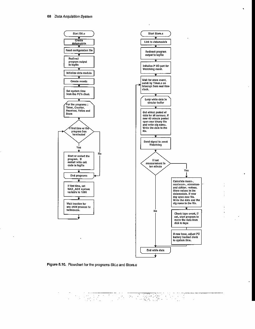
68 Data Acquisition System
Start Ski.c
End programs
if first time or the" program has
. terminated .
Initialize data module
datamoduleCreate
Create events
Read configuration file
Redirect program output to logfile
Set system time from the PC's clock
If first time, set MAX_AGE system variable to 1000
Wait inactive for any child process to termlonate.
Tor the programs: Timer, Counter, Resolver, Voitm and Store
Start or restart the program. If restart write exit code to logfile
Start Store.c
^ If last N measurement in . ten minute .
Link to datamodule
End while data
Loop while data In circular buffer
initialize P I/O port for Watchdog reset.
Send signal to reset Watchdog
Redirect program output to logfile
If new hour, adjust PC battery backed clock to system time.
Wait for store event, send! by Timer.c on Interrupt from real time clock.
Check tape event, if set, start program to move the data from disk to tape
Get oldest period of data for all sensors. If new 40 minute period open new binary file and write cfg name. Write the data to the file.
Calculate mean-, maximum-, minimlum- and stddev. -values. Store values in the datamodule. If new day open new file. Write the data and the cfg name to the file.
Figure 5.10. Flowchart for the programs Ski.c and Store.c

Operating experiences 69
Start Resolver.c
Trigg phase detector
Sleep for 2 periods
Set priority to 3000
Read UPS status
Set priority to 1000
Reset phase del. trigg
Loop for # to average
Link to datamodule
End loop S to average
Redirect program output to logfile
Save and read counters
Initialize counters and P I/O ports.
Wait for resolver event, sendt by Timer.c on interrupt from real time clock.
Convert from counts to S.l. units. Store the scaled data in a circular buffer In the datamodule.
Timer.c
Sleep forever
Set priority to 5000
datamodule
Initialize ACPC boards and timer counter
Redirect program output to logfile
Link to events. Install ISR's for timer Interrupt and SRQ Interrupt.
Unlink to events. Remove ISR's for timer Interrupt and SRQ Interrupt.
SRQ ISR.(run by OS-9000) Set voltmeter data ready event.
Timer ISR.(run by OS-9000) Update time variables. Set Counter, Voltm, Resolver, Store and Display events.
Figure 5.11. Flowchart for the programs Resolver.c and Timer.c. The Timer ISR and the SRQ ISR can be considered as separate programs, activated by the external interrupts.

70 Data Acquisition System
Voltm.c
Link to dalamodule
Set priority to 2000
Loop for all sensors
Set priority to 1000
End loop all sensors
Initialize IEEE-488 interface and voltmeter
Trigger voltmeter measurement
Redirect program output to loglile
Read measurement from voltmeter.
Wail for data ready interrupt from voltmeter
Set analogmultiplekser to current sensor
Wait for voltmeter event, send! by Timer.c on interrupt from real time clock.
Scale data for last sensor to S.l. unit. Store the scaled data to a circular buffer in the dalamodule.
Start Counter.c
Set priority to 4000
Link to dalamodule
Initialize counters
Set priority to 1000
Redirect program output to loglile
Wait for counter event, send! by Timer.c on interrupt from real time clock.
Convert from counts to S.l. units. Save the scaled data to a circular buffer in the dalamodule.
Read all counter hold registers (counters are saved into hold registers by Timer.c) and calculate number of counts since last period
Figure 5.12. Flowchart for the programs Counter.c and Voltm.c

Chapter 6
Data Base
The Skipheia data base contains measurements collected over more than 14 years. From 1981 to 1988 the data consist often minute mean values of wind speed and direction. Later data include temperature measurements and complete time series with a frequency of 0.85 Hz. In this section we will try to give an overview of the data base and statistical distributions on some of the data.
6.1 Historical overview
The station was built in 1980-1981, and reliable data exist from September 1981. During the period up to December 1988, data logging was accomplished by the computer ABC80, as discussed in Sec. 5.2.1, where also details of the data acquisition system are given. The data stored consist of ten minute average, maximum and standard deviation values of wind speed and direction. As mentioned in Sec. 5.2.1 errors in the program made the standard deviation values unusable and for low wind speeds the maximum values were unreliable.
In December 1988 the ABC80 computer was replaced by a DEC Falcon computer as logging computer and a DEC Micro-VAX computer for storage of complete time series, refer to Sec. 5.2.2 for details. The number of wind sensors was increased and temperature data included. In addition to the complete time series (sampling rate 0.85 Hz), the ten minute average, maximum, minimum and standard deviation were calculated and stored, both on the Micro-VAX and oh a tape recorder. The station was damaged by fire in February 1991.
When the measurements restarted in March 1992, the data acquisition system was based on a Personal Computer running the real time operating system OS-9000, refer to Chapter 5 for details. The sampling rate and data stored were the same as for the Falcon system. An addi
tional feature of this system was storage of complete time series during power failures.

72 Data Base
From March 1990, a battery based data acquisition system from Aanderaa Instruments has been in operation as a backup system. Data stored by this system are the ten minute average wind speed, the 2 sec. maximum wind speed during ten minutes and the wind direction.
6.2 Time series
Figure 6.7 (page 81) to Figure 6.11 (page 85) show plots of 1 hour mean wind speed at 10 m for the years 1988 - 1993, each plot contains data for one year. The data were corrected according to the procedure in Sec. 7.2. Data collected by the Aanderaa backup system are not included in the figures, and the figures give hence an approximate overview of the periods when complete time series are available.
The data for the period from 1981 to 1988 will not be used in this work and thus not presented here. Plots of wind direction, lapse rate and other variables are not shown due to the large fluctuations is these series, making plots of data for one month useless.
6.3 Distributions for selected sensors
---- 100m..... 70m---- 40m— 20m— 10m---- Weib. 100m
—//
o-O.OS
Wind speed (m/s)
Figure 6.1. Relative frequency distribution of 1 hour mean values of wind speed at 100 m, 70 m, 40 m, 20 m and 10 m heights in Mast 2. Bin width 1 m/s

Distributions for selected sensors 73
The distributions are based on 1 hour average values, calculated from the error corrected direct measurements where these are available, else from ten minute average values. All available data from the period 28.11.88. - 31.12.93. are used. The relative frequency distribution of wind
speed at heights 10, 20, 40, 70 and 100 m in Mast 2 is shown in Figure 6.1.
The wind speed is usually considered to be a Weibull distributed variable. The probability distribution function F(u) and the probability density function/(i<) of a Weibull distributed var
iable u is defined as:
F(u) = l-ejw.aa.if-r/sr
du c\cj
(6.1)
where c and k are constants. Taking the logarithm of the distribution function twice gives:
ln(- ln(l - F)) = -k ln^—j . (6.2)
In a Weibull plot this is the relation plotted. This means that data for a Weibull distributed variable will appear along a straight line in a Weibull plot. Figure 6.2 shows a Weibull plot of the same data as in Figure 6.1. Linear regression, using (6.2) and the cumulative distributions from the measurements gave the values listed in Table 6.1 for c and k. The distribution function fitted to the 100 m data is plotted in Figure 6.1 and Figure 6.2. As we can see from Figure 6.1, the correspondence for high wind speeds is relatively good due to the method used for fitting of the parameters. This makes the distribution function useful for extrapolating to higher wind speeds.
Table 6.1. Fitted Coefficients c and k in (6.2) by a fit to data from 5 heights in Mast 2.
parameter 100 m 70 m 40 m 20 m 10 mc 1.69 1.72 1.77 1.81 1.76k 9.06 8.58 8.35 7.79 7.38
From the figures we can see the wind speed distributions deviate from the Weibull distri
bution. One explanation here is the change from maritime wind to wind over land. As we can see in Figure 6.2, the fit seem to improve with height, strengthening the assumption of non uniform ground influence. Figure 6.3 show a Weibull plot of the 10 m wind speed distribution for

74 Data Base
0.999990.999900.999000.99000
yearmonth— 100m
70m— 40m— 20m— 10m— Weib. 100m0.90000
= 0.50000
0.30000
O 0.10000
0.01000
Wind speed (m/s)
Figure 6.2. Weibull plot of the cumulative frequency distribution of 1 hour mean values of wind speed at 100 m, 70 m, 40 m, 20 m and 10 m heights. Bin width 1 m/s. The labels on the right axis show the corresponding return periods. The upper vertical end of the curves means there are no data for higher wind speed.
selected direction sectors. The sectors are defined from the map in Figure 2.1, where 0 - 70° is
a land sector where the wind is influenced by the two WECSs, 70 - 130° is a mixed sea/land
sector, 130 - 200° a sector where the wind comes over the sea via Hitra, 200 - 240° a pure mar
itime sector and 240 - 360° a sector where the wind passes over the land at the west tip of Fr0ya.
This figure indicates that the distribution of the data for all directions consists of a sum of sev
eral distributions, each satisfying a Weibull distribution and where the parameters depend on
the wind direction.
Figure 6.4 show the distribution of 1 hour mean wind direction. The sensor and the loca
tion of the sensor varies during the period, depending on which sensors are operative. As we
can see from the figure the prevailing wind directions are from east and south-west. In
Figure 6.5 the distribution of wind speed at 10 m is plotted as a function of wind speed and

Distributions for selected sensors 75
yearmonth
70-130■ 130-200-200-240
0.90000 240-360
W 0.70000
:: 0.50000
0.30000
=3 0.10000
0.01000
Wind speed (m/s)
Figure 6.3. Weibull plot of the cumulative frequency distribution of 1 hour mean wind speed at 10 m level in Mast 2 for different direction sectors. The limits for the direction intervals are explained in the text.
direction. The figure show that most high wind speed data are from the south-west and east directions.
The distribution of lapse rate for the heights 100/10, 70/10 and 40/10 m and periods 1988- 1990 and 1992-1994 are plotted in Figure 6.6. The 10/40 m lapse rate show larger variations due to surface cooling/heating. Notice also the difference between the two periods. Closer comparisons of data from the same month, different years and the fact that data from the doubled sensors in the 92-94 was very similar, lead to the conclusion of a systematic error in the 88-90 temperature data. The temperature data will be further discussed by Heggem (personal communication).

Rel
ativ
e fre
quen
cy
76 Data Base
id-20
) 200 Direction
Figure 6.4. Relative frequency distribution of 1 hour mean values of wind direction. Bin width 10°.
c 150
Wind speed (m/s)
Figure 6.5. Relative frequency distribution of 1 hour mean values of wind speed at 10 m height as a function of wind speed and direction. Speed bin width 1 m/s, direction 10°.

Data file format 77
• 100/10-(92-94- 70/10 (92-94) **• 40/10-(92—94)- 70/10 (88-90
40/10 (88-90)
Lapse rate (K/km)
Figure 6.6. Frequency distribution of 1 hour mean values of lapse rate at 70/10 m and 40/10 m heights in the years 1988-1990 and 100/10 m, 70/10 m and 40/10 m heights in the years 1992- 1994. Bin width 1 K/km. Only data for wind speed at 10 m above 5 m/s is included.
6.4 Data file formatThe Skipheia data base contains data collected using 4 different data acquisition systems, all using different formats on the data files. To facilitate the data analysis it was decided to reformat the data files to a new common format. The sensor configuration at Skipheia have varied through the years. The new format must be able to keep track of these changes. A key concept in the new file format is the configuration files. These files links the data to the sensor configuration at the given time.
6.4.1 Configuration files.
A configuration (cfg) file is a text file, used for description of the station at the given time. Every data file contains the name of the corresponding cfg file. The cfg files must be located in the same directory as the data files. The cfg file names are on the form:
STATTTOl.CFG

78 Data Base
STA is a 3 character abbreviation for the site (station), TTT is the file type, 01 is a sequence number of the set-up and .CFG indicates a cfg file. The cfg file with sequence number 00 is reserved and used as a cumulative cfg file, all sensors at the station is listed in this file. The format of the cfg files are:
(in'max. 20 characters)(= 1 in TTT files), > tin RRR files)(= 1 in RRR files, 1 = mean, 2 = mean + max.3 = mean + max. + min., 4 = mean + max. + min. + sd)
<'Station name'>
<Number of measurements per ten minutes>
<Numberofdata types>
<Number of sensors (N)>
<sensor id 1> <sensor type> <scaling constant <height> <direction> <‘description' > a
<sensor id N> <sensor type> <scaling constant <height> <direction> ^description' ><Number of speed sensors which is “doubled” (M)> <id1 pair 1> <id2 pair 1> ...<id1 pairMxid2 pairM>
a. Sensor id, must be unique for the sensor location.Sensor type: 1 = speed, 2 = horizontal direction, 3 = temperature, 4 = vertical directionScaling constant: the data is stored as a 16 bit integer. Data mult, by this constant gives correct scaled data (S.l. unit)Direction: Direction of sensor, as viewed from the mast.Height: Height of sensor.Description: Max. 20 character abbreviation for sensor type and location.
6.4.2 Error files.
Prior to the data analysis, the data were checked for erroneous measurements (as described in Chapter 7). To exclude the erroneous measurements without rewriting the data files, a method involving an error file was developed. The error file is a text file containing lines of:
<sensor id> <start year> <start dayno> <start ten no> <end year> <end dayno> <end ten noxtype> <c1xc2xc3>'
This identifies the faulty sensor and period. <type> = 0 means the sensor is faulty, any other value indicates the type of error and <C;_g> are constants to correct the erroneous measurements. The error file names are on the form:
ERR_S7A.DAT
6.4.3 Direction files.
For stations with several wind direction sensors (only Skipheia up to now) a method to always get valid direction data is developed, even if the data is from different sensor id's. The direction file is a text file containing lines of:
<sensor id> <start year> <start dayno <slart ten no> <end yeat> <end dayno> <end ten no>
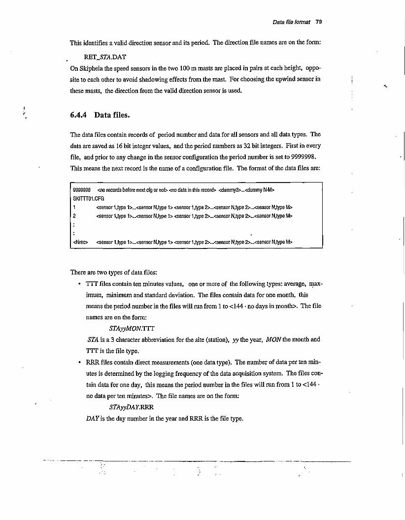
Data file format 79
This identifies a valid direction sensor and its period. The direction file names are on the form:
RET_S7A.DAT
On Skipheia the speed sensors in the two 100 m masts are placed in pairs at each height, oppo
site to each other to avoid shadowing effects from the mast. For choosing the upwind sensor in
these masts, the direction from the valid direction sensor is used.
6.4.4 Data files.
The data files contain records of period number and data for all sensors and all data types. The
data are saved as 16 bit integer values, and the period numbers as 32 bit integers. First in every
file, and prior to any change in the sensor configuration the period number is set to 9999998.
This means the next record is the name of a configuration file. The format of the data files are:
9999998 <no records before next cfg or eof> <no data in this record> <dummy3>...<dummy N-M> SKITTT01.CFG1 <sensor1,type 1>...<sensor N.type 1> <sensor1,type 2>...<sensor N.type 2>...<sensor N.type M>2 <sensor 1,type 1>...<sensor N.type 1> <sensor 1,type 2>...<sensor N.type 2>...<sensor N.type M>
<Nrec> <sensor1,type 1>...<sensor N.type 1> <sensor1,type 2>...<sensor N.type 2>...<sensor N.type M>
There are two types of data files:
• TTT files contain ten minutes values, one or more of the following types: average, max
imum, minimum and standard deviation. The files contain data for one month, this
means the period number in the files will run from 1 to <144 • no days in month>. The file
names are on the form:
STAyyMON.TTT
STA is a 3 character abbreviation for the site (station), yy the year, MON the month and
TTT is the file type.
• RRR files contain direct measurements (one data type). The number of data per ten min
utes is determined by the logging frequency of the data acquisition system. The files con
tain data for one day, this means the period number in the files will run from 1 to <144 •
no data per ten minutesx The file names are on the form:
STAyyDAY.RRR
DAY is the day number in the year and RRR is the file type.

80 Data Base
The data files are read by calling a FORTRAN subroutine, a listing is given in Appendix B. This subroutine hides all details about the internals of the data files, cfg files, error files and direction files. Input to the routine are the wanted sensor id’s, time, if the data should be checked against the error file and if an upwind sensor should be selected. Output is the data scaled to SI units and the information from the current cfg file. A similar function is programmed in MATLAB, a listing is given in Appendix C.
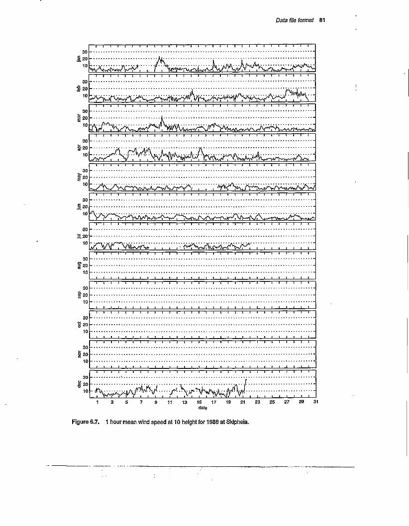
dec
nov
oct
sep
aug
Jul
]un
may
ap
r m
ar
Data file format 81
1 3 5 7 9 11 13 15 17 19 21 23 25 27 29 31date
Figure 6,7. 1 hour mean wind speed at 10 height for 1988 at Skipheia.

dec
nov
oct
sep
aug
jul
Jun
may
ap
r m
ar
82 Data Base
n—i—i—i—i—i—i—i—i—i—i—i—i—i—i—i—i—i—i—i—i—i i i i i i i i r
301.20
10
30 m 20
10
30 20 10
30 20 10
30 20 10
30 20 10
30 20 10
30 20 10
30 20 10
30 20 10
30 20 10
30 20 10
I'lln—i—i—i—i—i—i—i—i—i—i—i—i—i—i—i—i—i—i—i—i—i—i i i i i i i r
“i i i i i i i i i i i i i i i i i i i i i i i i i i i i i r
1 i i i i i i i i i i i i i i i i i i i i i i i i i i i i r~
n i i i i i i i i i i—i—i—i—i—i—i—i—i—i—i—i—i—i i i i i i r~
I'll“I i i i i i i i i i i i i—i—i—i—i—i—i—i—i i i i i i i i i r
^; ini *”i i i i i i i i i i i i i—i—i—i—i—i—i—i—i—i—i i i i i i i r*~
“i i i i i i i i i i i i i i i i i i i i i i i i i i i i i—r
~l I I I I I I I I I I I I I I 1 I I 1 I I I I I I I I I I p
i i i i i i i i i i i i—i—i—i—i—i—i—i—i—i—i—i—i—i i i i i r~
Y"a
“i i i i i i i i i i i i i—i—f—i—i—i—i—i—i i i i i i i i i r
y,viW-. ; v^; A, J-’s/Vyf:
ill'll1 3 5 7 9 11 13 15 17 19 21 23 25 27 29 31
date
Figure 6.8. 1 hour mean wind speed at 10 height for 1989 at Skipheia.

nov
oct
sep
aug
jul
jun
may
ap
r m
ar
Data file format 83
■
1 3 5 7 9 11 13 15 17 19 21 23 25 27 29 31date
Figure 6.9. 1 hour mean wind speed at 10 height for 1990 at Skipheia.

nov
oct
sep
aug
jul
jun
may
ap
r m
ar
84 Data Base
o 20 -
date
Figure 6.10. 1 hour mean wind speed at 10 height for 1991 at Skipheia.

nov
oct
sep
aug
]ul
]un
may
ap
r m
ar
Data file format 85
") I-----1-----1-----1-----1-----1 I-----1---- 1 I I---- 1-----1 I I 1 I I I I I I I I-----1 I I I I
titttiiiti i i t t t * t i i r i t i i » t * i - t i
30 hi 20
10
1—i—i i—i—i i i—i—i i i—i I i i i i i i i i ' i I I I l—l l P
I I -I- I I I l I I I I i I I 1 » I I 1 --L r I I 1 » I * I I L
30 - & 20 -
10
1 I I I I I I I I I I I I I I 1 I I I I I I I I 1 I I I I”
302010
302010
302010
302010
I I I I I I I I I I I I I I I I L ......................~i i i i—i i i i—i i i i—i i i i—i i i i i i i i i i i i i r
~l I-----1-----1 I 1 I I I I I I-----1 I I I-----1 I I F I I I I I I I I I I-
n i i i—i i i i—i—i—i i—i—i—i i—i—i—i i—i—i i i i i i i i p
1 I I I I I I 1 1 I I I----- 1 1 I |----- 1 I I I I I I I I I I I I P
302010
302010
302010
302010
302010
30
i i i i i i i i i i i i i i i i i i i i i i i i i i i i i r
“I I I I I I I I-----1—I—1 1—1------1—I—I—I—I—I----- 1—1—I-----1 I I—I—I 1 1 P
~1 I I I I I I I 1 I I I----- 1----- 1 I I----- 1----- 1 I I-----1 I I I I I I P
t t i i i i i I i - I r*ni ^AY ‘ V ‘ V ~ V1 I I I I 1 1 I I I I I----- 1 I P 1----- 1----- 1----- 1----- 1----- 1----- 1----- 1----- 1----- 1----- 1----- 1-----P
1 I 1 I I I I 1----- 1 1 I 1----- 1 I I I I I I 1 1 1 I I I 1 I I 1 P
Figure 6.11. 1 hour mean wind speed at 10 height for 1992 at Skipheia.
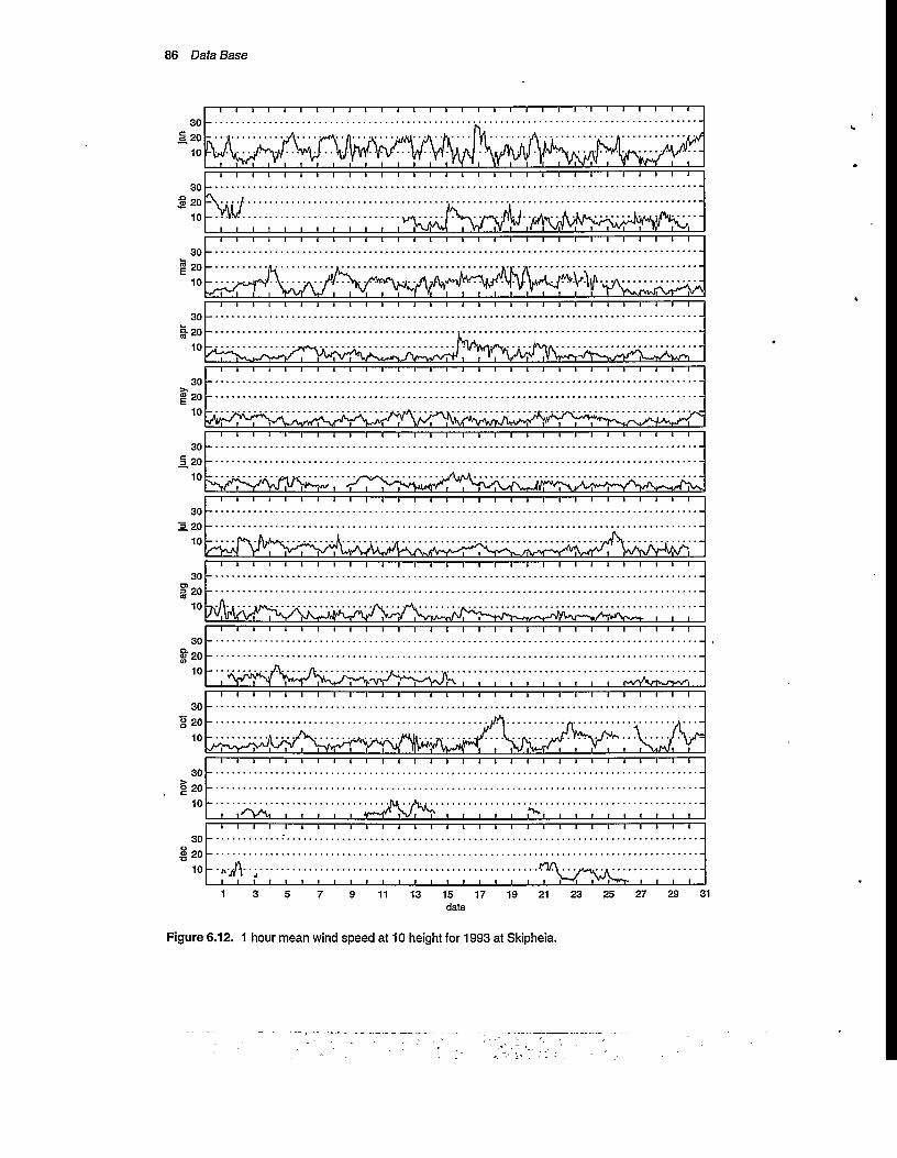
nov
oct
sep
aug
jul
jun
may
ap
r m
ar
86 Data Base
Figure 6.12. 1 hour mean wind speed at 10 height for 1993 at Skipheia.

Chapter 7
Data Quality Control
In this chapter we will describe the methods used for finding erroneous measurements in the data base. By erroneous measurements we mean measurements which, considering the actual atmospherical conditions and the sensors transfer function, are clearly unphysical. The errors may be rooted in the sensor or in the electronic interface between sensor and computer. The nature of the errors can be both consistent and sporadic. Essential in the data quality control is a visual inspection of the measurements. Most of the discusson will however deal with a computer based method for detection and elimination of spikes in the data.
7.1 Data inspection
As described in Sec. 5.3 it is possible to connect a terminal to the data acquisition system via a modem connection. A program will display the measurements in real time, showing the current measurements together with the 10 minutes mean, max., min., and std. dev. in the previous 10
minute period. This monitoring was done every working-day. Particularly the 10 minute statistical values were useful for detecting malfunction in sensors or other parts of the system. The minimum values were useful for detecting worn bearings and std. dev. for detecting more general failures in terms of unnatural fluctuations. Mean data were compared for sensors which were of comparable type and height. This monitoring was vital to avoid gaps in the time series. When problems were detected a service trip was made as quickly as possible.
The data were stored on tape in the acquisition system, and a local contact mailed the tapes to our department. When a tape was received the data files were converted to the final format, as described in Sec. 6.4.4, and the time series were plotted. The plots contained 10 minute average data for periods of one day for all sensors. Such plots exist for every day in the period
20 Mar. 1992 to 31 Jan. 1993.

88 Data Quality Control
In the analysis phase the data were controlled once more. Special routines were developed (in MATLAB) for easy moving and zooming within a time series. Periods of erroneous data could be graphically marked and the periods were returned to the user in the correct format. This was used to study time series of comparable sensors. Histograms of the data were also very useful. Studies of histograms of lapse rate for the same time of the year revealed a systematic deviation in the temperature data from the period 1988 - 1991 and the 1992 -1994 data, this is discussed further in Sec. 6.3.
A concept involving a text file containing all faulty sensors and the start and end time of the faulty periods was developed to allow removal of the erroneous measurements. This file, the Error file, is checked by all analysis programs and the erroneous data excluded. The format of the file is described in Sec. 6.4.2.
7.2 Elimination of spikes
A preliminary examination of the data showed that most erroneous measurements occurred as single measurements. Spikes occurring singly can be eliminated by comparing a measurement with its neighbours. The following variables are calculated:
For wind speed sensors :
x.—s3,=- 82,= *,-1 +x, ’
2
(7.1)
and all other sensors :
£3, =V (7.2)
where x, is the time series for the current sensor. Prior to removing erroneous data, cumulative distributions of g2 and g3 for all sensors were calculated. The distributions were calculated for intervals of wind speed and direction. Data collected when the wind speed at 10 m level was lower than 5 m/s were not included. This was done to avoid start-up effects for speed and direction sensors. In addition these data will most probably not be included in any analyses. Data from doubled wind speed sensors was only included when the sensor was upwind from the mast. The distributions was examined to find the “normal” values for g2 and g3 (g2/3)- This was

Elimination of spikes 89
in turn used to identify and remove the erroneous measurements. In addition to the phenomenon itself (speed, direction etc.), the distributions depends on the erroneous measurements, the sensor's transfer function and on the influence from the mast.
The variables represents a turbulence quantity and will have a natural variation dependent on the mechanical turbulence level. The distributions contain data for all conditions, the remaining variable is the sensors height above the ground. Some typical distributions illustrating the height variation are shown in Figure 7.1 and Figure 7.2. As we can see, the distributions broaden with decreasing height. This means, as expected, that the turbulent variations
increase for decreasing height.
Figure 7.1. Distribution of gz values for selected wind speed sensors (Vaisala WAA15). Notice the height dependence.
Two examples of the influence of obstructions in front of the sensor are shown in Figure 7.3. The sensors in this figure are all located upwind from the mast. “S M2W 40m” is influenced by an adjacent guy in direction 170° (viewed from the sensor). “S M2 100m” is mounted on a rod at the top of the mast and is more influenced by the mast than the two other 100 m sensors mounted on booms outside the mast. Due to its principle of operation a cup anemometer will normally detect an increase in the turbulence behind an obstruction.

90 Data Quality Control
----SM4W100m..... S M4W 40m—• S M4W 20m — S M4W 10m
Figure 7.2. Distribution of go values for selected wind speed sensors (Vaisala WAA15). Notice the height dependence.
----S M2 100m..... S M2W100m— S M2W 40m ----S M2E40m
g3
Figure 7.3. Distribution of gj values for selected sensors. The “M2E 40m” sensor is influenced by a adjacent guy. The “M2T 100m” sensor (sensor id 1) is mounted on top of the mast and is influenced by the mast and a lightning rod. “M2W 100m” is mounted on a boom and only upwind data are used.

Elimination of spikes 91
— Dh UVW 20nrDh M2W 20nr
— Dh M2E 45m- Dh M3 45m
g3 (degrees)
Figure 7.4. Distribution of g3 values for selected direction sensors, which illustrate the differences between direction sensors of different types.
The g3 distributions for wind direction sensors of different types are shown in Figure 7.4. Direction sensors using a potentiometer as recording element will give erroneous measurements from the direction sector corresponding to the gap in the potentiometer. These measurements will be random and have a flat distribution, see sensor “Dh M2E 45m” in Figure 7.4. “Dh M2E 45m” is a GILL 12302 microvane from R.M. YOUNG CO. It is a relatively large and heavy vane. “Dh M2W 20m” is a light bivane, type 1585 from TELEDYNE GEOTECH. The vane area is much smaller than on the Young vane. Notice the similarity between the distributions from “Dh UVW 10m”, a GILL 27005 UVW anemometer and “Dh M3 45m”, a rebuilt Vaisala WAV12 sensor.
The relatively long and flat tails of the distributions (only first part of the tails are shown in the figures) are a result of erroneous measurements. In view of the sensor transfer function, the outer part of these distributions are unphysical.
Distributions for intervals of direction and speed were examined, without finding any indication of speed or direction dependence of the spike frequency (apart from the potentiome
ter problems mentioned above).

92 Data Quality Control
The g2/3 distributions will give an overestimate for the number of spikes. A spike will give two large g2 values, one positive and one negative. For g3 the spike will give one large value and two values about half the size on each side of the large value.
Apart from the tails, and for small values of g%3, the distributions show an exponential behaviour. The exponential part of the distributions was fitted by the function :
Log(f(gV3)) was fitted to the logarithm of the distributions. In addition to a simple fitting procedure, this implied a weighting of the fit For small values of Eq. (7.3) will not give a good representation of the distribution, but for this purpose this is not important. Examples of typical fits are given in Figure 7.5.
x S M3W 40m+ S M3W 20mx S M3W 10m
0 0.1 0.2 0.3 0.4 0.5abs(g3)
Figure 7.5. Distribution of g3 and fits by Eq (7.3). The endpoints of the curves is at g0i3. The values for the fitted parameters are:S M3W 40m: a = 43.06, 6 = 50.56 S M3W 20m: a = 35.69, 6=41.21 S M3W 10m: a = 83.85, 6=40.39
The probability for a gV3 value greater than a limit gom is:
Prob(|g2/3| > £0,2/3) = 2[l ~ -^(£0.2/3)] = 2 J f{Sm)dg = ^e~b's°-™ .
so.M(7.4)

Elimination of spikes 93
The return period R for a value larger or equal to g0f2/3 is defined as
(7.5)
where t is the time between measurements, 1.17 seconds for our data. This gives the limit go,m-
So,2/3 ~ (7.6)
Values for g02/3 are listed in Table 7.1 for a return period R of one month. The values for com
parable sensors are averaged to a common value. As expected due to the decrease in the turbu
lence level for increasing height, the values are decreasing with heigth.
Table 7.1. Limits used to identify spikes in the data. The limits correspond to a return period of one month.
Sensor descriptor SensorId
80,2 80,3 Sensor descriptor
SensorId
80,2 80,3
S M2 100m 1 0.39 0.30 TempM2b 40 42 0.16 0.15S M2W 75m 2 0.34 0.23 TempM2b 10 43 0.16 0.15S M2W 40m 3 0.38 0.26 Temp SEA a 44 0.04 0.03S M2W 20m 4 0.45 0.30 Temp SEA b 45 0.04 0.03S M2W 10m 5 0.50 0.34 TempMka3.5 46 0.16 0.15S M2B 75m 6 0.34 0.23 TempMkal.O 47 0.16 0.15S M2E 40m 7 0.57 0.32 TempA rock 48 0.08 0.07S M2E 20m 8 0.45 0.30 TempAmarsh 49 0.08 0.07S M2E 10m 9 0.50 0.34 TempMkb3.5 50 0.16 0.15S M4 100m 10 0.39 0.30 TempMkbl.O 51 0.16 0.15S M4W 40m 11 0.38 0.26 S M2W100m 70 0.30 0.20S M4W 20m 12 0.45 0.30 S M2E100m 71 0.30 0.20S M4W 10m 13 0.50 0.34 S M4W100m 72 0.30 0.20S M4E 40m 14 0.57 0.32 S M4E100m 73 0.30 0.20S M4E 20m 15 0.45 0.30 S M3W 40m 74 0.38 0.28S M4E 10m 16 0.50 0.34 S M3W 20m 75 0.45 0.34S M3T 45 m 17 0.45 0.31 S M3W 10m 76 0.52 0.37SM3 20m 18 0.87 0.65 S UVW 20m 80 0.68 0.54SMS 10m 19 0.93 0.71 Dv UVW 20m 100 25.2 21.5Dh M2 100m 21 26.0 21.5 Dh UVW 20m 101 30.7 24.4Dh M2W 45m 23 46.0 31.0 Dv M2W 20m 102 36.8 33.0Dh M2E 45m 25 26.0 21.5 Dh M2W 20m 103 43.3 36.1Dh M4 100m 27 26.0 21.5 Dh M4W 40m 105 36.7 31.0

94 Data Quality Control
Table 7.1. Limits used to identify spikes in the data. The limits correspond to a return period of one month.
Sensor descriptor SensorId
So,2 So,3 Sensor descriptor
SensorId
So,2 So,3
DhM3 45m 29 26.0 21.5 E Sun up 132 80.0 30.0TempM2al00 32 0.16 0.15 E Sun down 133 30.0 20.0TempM2a 70 33 0.16 0.15 E Tot up 134 40.0 30.0TempM2a 40 34 0.16 0.15 E Tot down 135 40.0 30.0TempM2a 10 35 0.16 0.15 Rel.humid. 136 0.9 0.8TempM2blOO 40 0.16 0.15 Pressure 137 13.6 6.6TempM2b 70 41 0.16 0.15
To remove the erroneous measurements, the quantities g2 and g3 was calculated for every data point. If the absolute value of gs or g2 was larger than g0 2/j, the measurement was considered erroneous and removed. The main problem was to identify which of the three measurements was erroneous, and only excluding it if it was the mid point. The algorithm for spike removal is quite complex and is shown schematic in Figure 7.6. The algorithm can also handle several successive spikes. If a spike was found, sensor id, xhl, x„ xt+1, g2 or g3, wind speed at 10 m, wind direction and the time was written to a text file for control purposes. If a period with many errors was detected for a sensor, the sensor was declared faulty and the corresponding period was included in the Error File, which is described in section Sec. 6.4.2.

Elimination of spikes 95
If X,., and X,and X,,, is defined defined
If speed or direction
(compare to ref. speed or direction!
write to log file. write to log file.
write to log file.
End do for all sensors and all measurements
Do for all sensors and all measurements
Mark xt as spike andwrite to log file. Set
write to log file. Set
Figure 7.6. Flow diagram of the spike detection algorithm. The algorithm is implemented in the program RM_WILD.FOR. The paths not shown in the diagram implicitly mean the measurement is considered OK, and the execution continues at the top of the loop.

96 Data Quality Control

Chapter 8
The Wind Speed Profile
By the wind speed profile one understands the variation of the horizontal mean wind speed with height. We will discuss the standard description and present plots of observed profiles at heights from 10 to 100 m. A model for the profile is developed and its parameters are fitted to the observed data.
8.1 Background
To describe the wind speed profile, the two models most frequently used in the literature are the logarithmic law and the power law. The power law is an empirical relation and is often used in engineering practice. The logarithmic law is based on the fundamental fluid mechanical relations in the surface layer (Prandtl layer). The surface layer is defined as the layer in which the Reynolds stress can be regarded as constant, equal to the value at the surface. If the static stability of the surface layer is neutral, the wind profile in the surface layer can be written as (Dobbins, 1979)
which implies
(8.2)

98 The Wind Speed Profile
Here k is the von Karman constant, usually set equal to 0.4. The aerodynamical roughness length Zq is a parameter depending on the surface roughness and structure. Tables of z0 for various terrain types can be found many places in the literature (e.g. Panofsky and Dutton, 1986). Typical values of z# are 10"4 to 10'3 for calm to stormy sea, 10'2 for low grass and 10"1 for land areas with trees. For accurate determination of Zo measurements of wind speed at several heights must be used, u* is the friction velocity and is defined by u*= Jx/p, x is the surface stress and p the air density. From Eq. (8.1) and (8.2) it follows that the wind speed ratio between two heights can be written as
u(z2)= l+ctln£l
z%(8.3)
The relation between a, m„ and z0 is
cr =
u,fm(z2)'
(8.4)
For a constant “reference” heigth z% and if Zq is constant, a will be a constant. As can be shown, a is nearly equal to the exponent in the power law. For the purpose of presenting the experimental data we will use a rather than n* and z0. The parametrisation of the wind profile against a is however completely analogous to the more standard way in Equation (8.2). When the stability of the surface layer is non neutral, the logarithmic law can be generalized to (Businger et al. 1971, Dyer 1974 or Hogstrom 1987).
du&
(8.5)
which implies
«(z)=y in--yeK \ Zo
(8.6)
<|>m is an empirical relation between the wind speed gradient and the ratio zZL, L being the Monin-Obukov length, defined as (Panofsky and Dutton, 1986)

Background 99
KgH(1+0.07/B) 2500(q2-qi) 'u.3c„pT D T2-Tt+0mAz
(8.7)
Direct measurement of L involves measurements of the heat flux H, the friction velocity u, and the temperature T and humidity q at two levels. B is referred to as the Bowen ratio. For unstable air the most common expression for *¥m is given by the following equations (Businger et al.
1971, Dyer 1974)
(8.8)
An alternative expression for unstable air which is easier to evaluate, and gives, for practical purposes the same value as the above expression, is (European Wind Atlas 1989)
(8.9)
For stable air tF,„ is given by (Panofsky and Dutton, 1986)
(8.10)
In a review by Hogstrom (1987), the best values for y and P are found to respectively 15.2 and 4.8. When sufficient data to calculate L are available, the wind speed profile can be calculated from the equations above. In our dataset measurements of heat flux and friction velocity are not present, and measurements of relative humidity are only given at one height in a relatively short period. This means L has to be estimated from the measurements of horizontal wind speed at 5 heights and temperature at 4 heights. Panofsky and Dutton (1986) refer to a method for calculating L from the Richardson number, the Businger Dyer-Pandulfo empirical relations, which for unstable air are
(8.11)

100 The Wind Speed Profile
and in stable air
z _ Ri L ~ l—5Ri
(8.12)
The Richardson number Ri is defined as (Panofsky and Dutton, 1986)
8 (r„-r)2 (8.13)
where yd is the dry adiabatic lapse rate (9.8 K/km). The Richardson number can be estimated by replacing the differentials with the corresponding finite difference quotients. This gives a bulk or average value for Ri in the height interval of interest. Using wind speed and temperature at two heights this means an estimate for Ri can be written as
(8.14)
The problem using a method based on the Richardson number as described above is that the estimates contains information on the wind profile directly. In general we would prefer to parameterize the profile using variables not directly dependent on the profile.
The final parametrisation is based on the equations (8.5), (8.7), (8.8) and (8.10). In these equations Zo, and L are unknown parameters and will be fitted using procedures explained later.
An alternative parametrisation scheme was also tried. This was based on a more direct approach using functions of lapse rate, wind speed and height, constructed on an empirical basis by plotting the data against one variable for classes of the other variables. The problem using this approach was the relatively complex functions needed, especially for describing the z dependence. The lapse rate dependence was modelled by a sigmoid function, and was rather difficult to fit.

Presentation of the experimental data. 101
8.2 Presentation of the experimental data.In principle the profile is dependent on the wind speed, the roughness of the upwind terrain and on the atmospheric stability. The terrain dependence will in our case make the profile direction-
dependent. The landscape at the western part of Fr0ya is relatively rocky with small pieces of
marsh between. Typical dimensions in this landscape are 10-100 m. Typical is also the scatter
of small islets and inlets along the coastline.
All data presented are one hour averages. In the figures presented in this section values for
a are ensemble averaged, and bars for standard deviation are shown on the plots. The standard
deviation bars are tilted to increase the readability; note that the standard deviation is given by
the vertical distance from the marker to the tip of the bar, not the length of the bar.
As an indicator of atmospheric stability we have chosen the lapse rate calculated by a least
squares fit to all temperature sensors at heights 10, 40, 70 and 100 m. The classification of atmospheric stability is difficult and the local lapse rate is not necessarily a good quantity for
determining stability; see for instance Stull (1988) p. 171 for a discussion of this. The local
lapse rate is, however, the only stability parameter which can be measured easily at a station
like Skipheia. It is possible to calculate an estimate for the Richardson number or the Monin-
Obukov length by using the lapse rate divided by wind speed in a power. In this preliminary analysis where the main objective is to describe the wind speed profile by plots, we will rather
use lapse rate and divide the data into intervals of wind speed. Another complicating factor is
that the air for all wind directions at Skipheia has passed a mix of sea and land. This generates
very complex temperature and wind speed profiles.
In Figure 8.2 the logarithmic height coefficient a is plotted as a function of direction for
the 20/10 and 40/20 m heights in Mast 3, neutral stability and intervals of wind speed at 10 m.
Around 50° we can see the influence from the mast which is upwind for the sensors. Similar
plots for Mast 2 and Mast 4 are shown in Figure 8.2 and Figure 8.3. To select data for neutral
stability, the lapse rate interval 8-12 K/km is used. As explained previously, even this rather
narrow interval does not ensure a truly neutral atmosphere. We will later see from plots of a
against lapse rate that there is no identifiable plateau value for neutral stability, only a continu
ous shift from the stable value to the unstable value. Probably, this is part of the explanation for
the large standard deviations in the figures and some of the scatter.
From the figures we can see a significant variation of a against direction and height.
There are two mechanisms responsible for the main part of these variations; the development of
Internal Boundary Layers (IBL) due to variations in the terrain roughness upwind for the masts
and the speed-up effect due to the hills on which the masts are located. Figures 8.1 to 8.3 will
form the basis for the discussion in the rest of Sec. 8.2.

102 The Wind Speed Profile
0.21—
0.21—X 10-15+ 15-200.15 — * 20-25
Direction
Figure 8.1. Plot of logarithmic height coefficient a between successive heights in Mast 3 as a function of wind direction. The data consists of neutral data (Ir: 8-12 K/km) averaged in intervals of wind speed at 10 m as given by the legend. Notice the increase of a against speed in the south sector due to the Chamock effect. The negative values for a40/2o indicates a speed-up effect.
8.2.1 Variation in terrain roughness
The logarithmic wind profile applies only if the upwind terrain is reasonably homogenous. The average surface stress and surface wind speed depend on the surface conditions up to a certain upstream distance. Distant changes of roughness are “forgotten” by the tendency of the boundary layer to approach any equilibrium between the pressure gradient force and friction. The European Wind Atlas (Troen and Petersen, 1989) (EWA) states that the distance scale involved is proportional to the Rossby radius and is in the order of 10 - 100 km. The slope of the height h of the internal boundary layer at distance x downwind from a roughness change can be written as (Miyake 1965, Businger 1972, Panofsky 1973, Jensen 1978 and Larsen et al 1982)
dh _ Bu*dx u
(8.15)
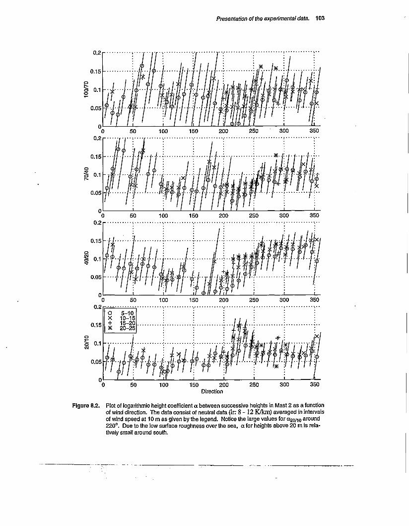
20/1
0 40
/20
70/4
0 10
0/70
Presentation of the experimental data. 103
0.15 -
X 10-15+ 15-20X 20-25
wrrmrr
0 50 100 150 200 250 300 350Direction
Figure 8.2. Plot of logarithmic height coefficient a between successive heights in Mast 2 as a function of wind direction. The data consist of neutral data (lr: 8-12 K/km) averaged in intervals of wind speed at 10 m as given by the legend. Notice the large values for 020/10 around 220°. Due to the low surface roughness over the sea, a for heights above 20 m is relatively small around south.

104 The Wind Speed Profile
0.2 r
0.15 -
o 0.1
0.2 r
X 10-1515-20
X 20-25
Direction
Figure 8.3. Plot of logarithmic height coefficient a between successive heights in Mast 4 as a function of wind direction. The data consists of neutral data (lr: 8-12 K/km) averaged in intervals of wind speed at 10 m as given by the legend.
where B is a constant approximately equal to 1.3. The methods used in the EWA are also based on the same expression. Inserting the relation between m, and a from (8.4) gives
— = Bk« = 0.5 a dx
(8.16)

Presentation of the experimental data. 105
IBL generated by the local sea-land transition.
The shoreline will define the onset of a land based IBL due to the shift in surface roughness from the relative low value for the sea to a larger value for the land. The height of this IBL will depend on the surface roughness on land and the distance to the sea. From the figures we can estimate an approximate value for a =0.1 in the west and north direction sectors where the distance to the sea is larger than 3 km. In the south sector where the distance to the sea from Mast 2 and 4 is approximately 350 m, this gives the IBL a height of 17.5 m. This height will increase proportionally to the distance from the masts to the sea. For directions from approximately 270° to 90° (west through north to east) the height is larger than 100 m. Due to turbulence generated by the rather rough terrain, particularly near the sea where precipices of around 2 m height are quite common, the height of the IBL is probably larger than these estimates.
In Figure 8.1 to Figure 8.3 this IBL is reflected as a relative small a around south for heights above 20 m. The value for (fyo/io in Mast 2 and 4 is approximately constant for all directions because the height of the land based IBL is always larger than 20 m. In Mast 3 the height of the IBL is lower than 20 m for directions around 180°.
IBL generated by the land at the other side of the Fr0y fjord.
In Figure 8.2 a10o/7o varies from the south east sector to the south west sector. The terrain in these two sectors from the shoreline and up to the masts is very similar. It is unlikely that this variation is generated by local terrain variations. The shift from a relatively large value for a is around 180°, which corresponds to the direction of the west coast of Hitra and the nearby Bis- pdyan (map in Figure 2.1). This means the wind speed profile between 70 and 100 m is influenced by the land at the other side of the fjord, at approximately 8 km distance. If we use a = 0.01 as the value over sea during light wind in Eq. (8.16), the height of the sea generated IBL is only 40 m. This height will however increase for increasing wind speed, due to the Chamock effect discussed below. Due to the low surface friction over the sea it seems probable that the profile at 100 m and to a smaller extent 70 m during low wind speed at directions from south east will be influenced by the land at Hitra and Bispdyan.
8.2.2 Charnock effect.
In Figure 8.1 to Figure 8.3 we can see an increase in a for increasing wind speed in the south direction. This can be due to the Chamock effect (Chamock, 1955):
g(8.17)

106 The Wind Speed Profile
where the Chamock constant ach varies considerably between various investigations. Chamock (1955) found ach=0.0123, Nordeng (1988) ach=0.032 and Kitaigorodskii (1970) acA=0.013, please refer to Kitaigorodskii (1970) for a further review of the value on the Chamock constant. Today, the most common value for ach seem to be around 0.015. Using Eq. (8.4) and (8.17), the Chamock constant can be estimated from the figures to be in the same order as traditionally assumed in the literature (above references or Andersen (1991) for a review).
8.2.3 Influence from masts and other obstacles.
In Figure 8.2 (X20/10 is relatively large around 240° compared (X20/10 f°r the other masts. This is probably caused by the disturbance in the profile introduced by the instrumentation house, or the steep 2 m high escarpment right behind the house extending some 10 m in each direction, orthogonal to the wind direction. A similar effect can be seen in Figure 8.1 for Mast 3, as the slope for the direction sector 120° - 270° is rather steep around the 5 m contour line on the map in Figure 2.2. In Figure 8.1 we can see the shadow from the mast around 90°. For all masts the profiles are disturbed in the direction sector 20 - 90° due to the two WECSs located as shown on the map in Figure 2.2.
8.2.4 Speed-up effect
From the map in Figure 2.2 we can see that the masts are located on small hills. According to Jackson and Hunt (1975) the speed-up effect on a hill top with height h is in the order of
„p_ Mx,Ay)u0(y=Ay)
h In 2{L/z0)L In(Ay/z0)ln(Z/z0) (8.18)
where u0 is the wind speed upwind of the hill, L is the horizontal upstream distance from the hilltop to the point where the height above initial terrain is A/2, z0 is the roughness length and l the height of the inner layer. / is approximately given by (Jackson and Hunt, 1975)
l=iz0(L/z0)°9, (8.19)

Presentation of the experimental data. 107
More complicated 3 dimensional versions of this model are frequently used, as in the EWA. This family of models is called MS3DJH. For our purpose the original model from Jackson and Hunt (1975) is adequate. A plot of AS as a function of height above the hilltop for Mast 3, using L = 75 m and h = 22 m for three different values for Zq are given in Figure 8.4. According to the figure the fractional speed-up ratio should be around 0.5 to 0.6 for the sensors in Mast 3.
---- 0.010.005
-----0.001
■a 0.7
<5 0.6
101Height (m)
Figure 8.4. Plot of fractional speed-up ratio AS (Eq. (8.18)) as a function of height above the ground for three different values of the surface roughness Zq.
In Figure 8.1 to Figure 8.3 the speed-up effect is visible as a relatively small value for o^q/ io compared to a40/20 for directions other than around south. In the south direction the situation is complicated by the land generated IBL. The land generated IBL will increase 020/10, while the speed-up effect will decrease 020/10- The speed-up effect is particularly large at Mast 3 which is located on the steepest hill. For Mast 3 in the south sector we can see the speed-up stretches up to a40/2o> while the effect from the land based IBL only affects 020/10-
Figure 8.5 show an experimental speed-up factor as a function of direction for all heights in Mast 3 relative to Mast 2, Mast 4 and a 45 m mast located at the islet Sletringen west of Fr0ya. Also shown are the experimental speed-up factor of Mast 4 relative to Mast 2. Only data for wind speed above 5 m/s and lapse rate in the interval 8-12 K/km are included. Data from Sletringen were collected in 1988 and 1989 and are compared to Skipheia data from the same period. In this period the sensor at 40 m in Mast 3 was mounted on the top of the mast and is

Spee
d-up
fact
or (1
00 m
) Sp
eed-
up fa
ctor
(40 m
) Sp
eed-
up fa
ctor
(20
m)
Spee
d-up
fact
or (1
0 m
)
108 The Wind Speed Profile
0.15 r
-0.05
0.15 r
0.1 — •,
-0.05
0.15 r
0.1 -
0.05
0 -Ail--0.05
-0.05 O M3-M2/M2 X M3-M4/M4 + M4-M2/M2X M3-SLE/SLE
Direction
Figure 8.5. Experimental fractional speed-up factor between the sensors in Mast 3 and the sensors in Mast 2, 4 and Sletringen. Only data for neutral stability (Ir: 8-12 K/km) and wind speed at 10m above 5 m/s are included. Notice the shadow from the masts (Mast 3 and Sletringen) direction around 50° and 90° and the shadow from a lightning rod in Mast 3, direction around 180°.

Presentation of the experimental data. 109
influenced by the mast and a lightning rod mounted at 50 cm distance, direction 180°. All other
Skipheia data were collected during 1992 and 1993.
The problem in this comparison is that all these sensors are influenced both by the speedup effect and the effect from the land based IBL. The land based IBL will decrease the wind speed, this decrease will increase for increasing distance to the sea. The influence from the IBL will however be most noticeable near the ground, while the speed-up effect will be felt at larger heights.
The speed-up factor for Mast 3, at 10 m height, relative to Mast 2 or 4 is close to 0.15 for wind directions around south-east to south. This is probably more a result of damping at Mast 2
and 4 than speed-up effect in Mast 3.
The speed-up factor for 100 m in Mast 4 relative to Mast 2 is within 0.02 and is caused by the influence from the mast on the sensors. This effect is present at all heights, despite the doubled sensor mountings; the maximum of this effect is approximately 5% for the heights below 100 m. The influence from the mast on the measurements will be treated in detail by Heggem (personal communication).
Mast 3 relative to Sletringen shows a 5% speed-up for directions in the interval 200° - 250°. Sletringen is a small and flat islet, the highest point of which is approximately 4 m above MSL. The speed-up effect at Sletringen should therefore be negligible compared to Skipheia. The wind in 5 and 10 m height at Sletringen, will be damped at all directions due to the approximate 200 m distance from the shoreline to the mast. At 20 and 40 m the influence from the ground based IBL should be negligible. At Skipheia the wind is damped due to the land based IBL, compared to Sletringen the maximum of this damping is 10% for wind directions around north-west.
In the sectors where measurements from Sletringen and Mast 3 are directly comparable, Figure 8.5 indicates a fractional speed-up factor around 5 - 10%, considerably smaller than predicted by the model of Jackson and Hunt. One of the basic assumptions made by Jackson and Hunt (1975) is that h«L, which means that there is no problem due to separation on the downwind or upwind side of the hill. This assumption is not fulfilled in our case. Bouwmeester et al. (1978) state that flow separation occurs for h/L > 0.3, which means separation is present, both upwind and downwind for Mast 3. Another problem is the rough terrain at the foot of the hill, with precipices and escarpments around 2 m height. According to Bouwmeester et al. (1978) this will cause separation in front of the hill. The presence of separation will make the speed-up
effect smaller than for a similar case without separation. Due to the complex landscape around the masts and the lack of undisturbed measurements of the wind upwind from the masts it seems difficult to give more accurate estimates of the speed-up effect, the comparison with Sletringen data indicates however a considerable smaller speed-up effect than predicted by Eq. (8.18).

110 The Wind Speed Profile
8.2.5 Stability dependence of the wind speed profile
As mentioned previously we will at this point of the analysis use wind speed and lapse rate as
variables to explain the stability dependence rather than a Richardson number or a Monin-Obu-
kov length calculated from a combination of lapse rate and wind speed.
From the maps in Figure 2.1 to Figure 2.2 and the plots of a against direction we can
define a “sea sector” in the interval 200 - 240° where the distance to the sea varies from 150 m
to 500 m, and a “land sector” in the interval 270 - 360°. Due to two WECSs placed 250 m from
the masts in the 20 - 70° sector, we will exclude the sector 0 - 70°. The sectors around 90° and 240° are excluded due to the transition between a land based boundary layer and a sea based boundary layer with a land generated IBL near the ground. Influence from Hitra and Bispdyan
complicates the situation in the sector 120 - 200° and in this discussion this sector is also excluded.
The logarithmic height coefficient is plotted against wind speed at 10 min Figure 8.6. The
data are divided in two direction sectors and stable, neutral and unstable atmospheric stability. In the figure a’s from Mast 2 and Mast 4 are averaged for comparable heights. For the neutral
data we can see an increase in a for increasing wind speed up to a certain level for the sea sec
tor. This could be due to the Chamock effect. In the land sector this effect is not observed. Not
surprisingly, the unstable profiles and stable profiles seem to approach the neutral profile for high wind speeds.
In Figure 8.7 a100/70, a70/40, a40/20 and a2o/io for Mast 2 is plotted as a function of 7 calcu
lated between the corresponding heights. (y;00/70, 770/40, 740/10 andy4o/io)- Use of the air-sea temperature difference as stability indicator in the sea sector were also investigated, but resulted in
larger standard deviations. In the land sector there was little correlation between the value of a
and the air-sea temperature difference. As expected, we can see an increase in a with decreasing lapse rate. The shift from a low value for a to a high value is different for the two sectors.
The data in the land sector are more homogeneous than the sea sector data; this is probably due
to the generation of a land based IBL at the ground, making the wind speed and temperature
profiles more complicated for the sea sector. Notice also the small values of O-mrn and ol70/40 in
the land sector during stable atmosphere; this indicates a very low height of the surface layer during these conditions.
In Figure 8.8 ci100/70, Oi70/40, oc40/20 and a20/io for Mast 2 are plotted as a function of 7 calcu
lated by linear regression to all temperature sensors. The general trends in the data are similar to
Figure 8.7, except at stable atmosphere, where the atmosphere is divided into more or less sep
arate layers. This makes the fitted lapse rate less good as stability indicator during stable atmosphere.

Stab
le -e-1
0-5
Neu
tral 9-1
1 U
nsta
ble
14-3
0
Presentation of the experimental data. 111
■ 0.2
■ 0.15
• 0.1
■ 0.05
100/7070/4040/20:20/10
I"X
10 15 20 25 30
0.25 ■0.25 •
0.15 •
0.25 r ■ 0.25 h
' 0.2 H
0.15 Kf-. • 0.15
• 0.05
5 10 15 20 25 30Wind speed (m/s) land sector
5 ' 10 15 20 25 30Wind speed (m/s) sea sector
•v
Figure 8.6. Plot of logarithmic height coefficient a between successive heights as a function of wind speed at 10 m. The data are divided into sea direction sector (200 - 240°), land direction sector (270 - 360°) and stability intervals.

20/1
0 40
/20
70/4
0 10
0/70
112 The Wind Speed Profile
O 5-10X 10-15+ 15-
-0.05 -10.0520 -20
-0.0520 -20
-0.05 -i0.0520 -20
-0.05-10 0 10
Lapse rate (K/km) sea sector20 -20 -10 0 10
Lapse rate (K/km) land sector
Figure 8.7. Plot of logarithmic height coefficient a between successive heights as a function of lapse rate calculated between the corresponding upper height and 10 m. The data are divided into sea direction sector (200 - 240°), land direction sector (270 - 360°) and three intervals of wind speed at 10 m, represented by different markers.

20/1
0 40
/20
70/4
0 •
100/
70
Presentation of the experimental data. 113
O 5-10X 10-150.25 •0.25 ■ + 15-
J-0.05-0.0520 -20
0.1 .....
-0.05 J-0.0520 -20
-0.05 J-0.0520 -20
-0.05 J-0.05-10 0 10
Lapse rate (K/km) sea sector20 -20
Lapse rate (K/km) land sector
Figure 8.8. Plot of logarithmic height coefficient a between successive heights as a function of lapse rate calculated by linear regression to all temperature sensors. The data are divided into sea direction sector (200 - 240°), land direction sector (270 - 360°) and three intervals of wind speed at 10 m, represented by different markers.

114 The Wind Speed Profile
8.3 Parametrisation of the experimental data.The parametrisation is in principle similar to the parametrisation used by Andersen and L0vseth (1992) in the analyses of profiles from the Sletringen station. A preliminary investigation on the current database showed that averaging a into groups by sea-air difference gave larger standard deviations than if the lapse rate is used for selection. This is probably caused by the greater distance to the sea at Skipheia. Owing to this we will use the local lapse rate as a stability indicator, rather than the air-sea temperature difference as Andersen and L0vseth did.
As mentioned previously, the final parametrisation was based on the equations (8.5), . .(8.7) and (8.8). Humidity measurements are only available for a relatively short period and only at one height. For that reason the Bowen ratio in the expression for the Monin-Obukov length (Equation (8.7)) is not used. The remaining unknown parameters which have to be modelled are
Zo, and H.The friction velocity u* is roughly proportional to wind speed, and depends on the surface
roughness Zo and the atmospheric stability, u* increases for increasing z0 and decreasing stability. The data were averaged in groups according to lapse rate and to wind speed. In each of these groups u, was considered as a free parameter. To handle the variation of z0 the data were divided into the same direction classes as mentioned previously.
In Figure 8.6 we saw that a increased for increasing wind speed for neutral stability in the sea sector. This effect is explained by the Chamock relation (Eq. (8.17)). As a model for z0 in the sea sector we will thus use the Chamock relation with ach as a free parameter in the fit. In the land sector a appears to be constant and z0 will thus be used as a free parameter in the fit
The remaining unknown parameter is the surface heat flux H. This is estimated using K- theory which states:
H = Kpcp(y-yd). (8.20)
As explained by Panofsky and Dutton (1986), K-theory has severe limitations. The most serious problem in our case is that K will depend on the turbulence structure. A simple improvement is based on the vertical speed fluctuations being proportional to the horizontal speed fluctuations which again is proportional to the friction velocity. To generalize the model further, the friction velocity was raised to a power, determined during the fitting process.
K = K'u,p. (8.21)
Models for L containing the absolute temperature T were tried, but did not improve the fit. In the final parametrisation of L the following expression was used

Parametrisation of the expenmentai data. 115
***Kg{7-rd)K' ’
(8.22)
where p and K 'are the free parameters. The lapse rate was calculated using linear regression to
all temperature sensors between 10 and 100 m.
Looking at Equations (8.6) to (8.10) we observe that the Zq and *Fm dependence make the fitting very difficult. This was solved by using the wind speed at zr = 10 m as a reference to
determine w. and then use this value of u* for the other heights. The transcendental equation - from which u* can be determined is
(8.23)
This equation cannot be inverted analytically to find m, and a least squares method was used.
The quantity which was fitted was the wind speed ratio relative to the reference level:
u(z) _ ln(z/z0-'Fm(z/L))(8.24)
ur ln(zr/z0-'Fm{zr/L)) '
As mentioned above, the data were averaged for classes in wind speed and lapse rate. In each lapse rate interval, u* was assumed to be a linear function of ur only. Minimization of the model is difficult due to the ability of w.to compensate for any changes in the parameters introduced by the minimization algorithm. A Fortran program tailored for these type of minimization problems was therefore used.
The fitted parameters for the sea sector are: ach = 0.016 K'= 0.003 p = 2.54
and for the land sector:Zo = 0.001 K'= 0.040 p = 0.77
The value for the Chamock constant is rather difficult to fit, and a two step method is used. The first fit was done for wind speed above 10 m/s. This value for the Chamock constant was then
fixed in a fit for wind speed above 5 m/s. Effectively this determines the value for the Chamock constant from near neutral data. In Figure 8.9 wind speed ratios between all heights and 10 m

116 The Wind Speed Profile
and the fitted models are plotted for the sea sector. A corresponding plot for the land sector is shown in Figure 8.10. We can notice the difference in the stability dependence in the two sectors. In the sea sector the dependence is very strong and persists even for high wind speeds as opposed to the land sector where there is no stability dependence except for low wind speeds and extremely stable atmosphere. The reason for this must be the relatively rough terrain making mechanical turbulence dominating for nearly all conditions. The value for z0 seems small, but considering that much of the surface consists of bare rock, it is not unrealistic. The value for the Chamock constant is very close to what is found in the literature. It is also probable that the larger terrain variations, hills with a typical dimension 10 m and the rugged coastline, will contribute significantly to the turbulence picture and cause the effective mixing seen in Figure 8.6.
The chosen parametrisation can probably be improved in several aspects, and brought more into line with the presentation of the experimental data. From the discussion in Sec. 8.2 it is clear that the atmosphere in the sea sector is divided into a land influenced H3L near the ground, the height of which is roughly estimated to be between 10 and 20 m, and a sea influenced layer above. At the present stage of the analysis the atmosphere was treated as one layer, but the two layer approach will be investigated later in analysing the Skipheia data. The methods for this are well known, and can for instance be found in the EWA. Another weakness of the selected parametrisation is the choice of 10 m as a reference level. Alternative parametrisation, using local a’s and stability indicator’s based on the corresponding upper height and 10 m should also be tried.

20/1
0 40
/10
70/1
0 10
0/10
Parametrisation of the experimental data. 117
1.5 rr
O Exp 4-10-2 X Exp 2-10 + Exp 10-18 X Exp 18-30----- Fit 4-10-2.......Fit 2-10----- Fit 10—18-----Fit 18-30
.......X
Wind speed (m/s)
Figure 8.9. Wind speed ratios for experimental data and model for data in the sea direction sector.The plots represents different sensor heights wile the curve/marker types represent different lapse rate intervals.

20/1
0 40
/10
70/1
0 10
0/10
118 The Wind Speed Profile
X----
X Exp 2-10+ Exp 10-18X Exp 18-30----- Fit *10-2
Fit 2-10•Fit 10-18
Fit 18-30
1.2 -V
Wind speed (m/s)
Figure 8.10. Wind speed ratios for experimental data and model for data in the land direction sector.The plots represents different sensor heights wile the curve/marker types represent different lapse rate intervals.

Chapter 9
Turbulence
The wind is often regarded as composed of a slowly varying component and a superimposed
fluctuating component. The former, the synoptic wind, is connected to the high- and low-pressure systems. The fluctuating component, the turbulent wind, is defined as the variations around the synoptic wind, and is associated with wind shear, terrain roughness, convective
motion etc. In this chapter we will study the turbulence spectrum which is the representation of
the energy in the turbulence as a function of frequency. The integral of the turbulence spectrum
is the total turbulent energy and is equivalent to the variance of the time series.
9.1 Introduction
The data will be divided into the same direction sectors as in Chapter 8 and as we will see, the
turbulence description is strongly dependent on the wind direction, or more precisely on terrain
roughness. It is also clear, that the actual dependence on wind direction is more complicated
than the simple division into two sectors indicates. This is however difficult to demonstrate as a
true neutral atmosphere is very rare and non-neutral stability strongly influences the results.
9.2 Turbulence intensity
The turbulence intensity is defined as the standard deviation of the wind speed normalized by
the mean wind speed:
^ '
(9.1)

120 Turbulence
The standard deviations were calculated for periods of 1 hour. The linear trend was removed from the time series by the least squares method prior to the calculation.
In Figure 9.1 turbulence intensity for neutral stability is plotted as a function of direction. The criterion for neutral stability is lapse rate in the interval 8-12 K/km and wind speed at 10 m level above 5 m/s. As we can see there is a significant variation in the turbulence intensity, depending on wind direction, or rather the surface roughness of the upwind terrain. The turbulence intensity for neutral stability was also examined for intervals in wind speed, the speed dependence is in this context small and can be ignored. From the Figure we can see the turbulence intensity is decreasing for decreasing distance to the sea. This is most noticeable for Mast 3 which is closest to the sea. The peak around 140° is probably caused by a land based fish farming facility, located by the sea in this direction. Notice also the effect from the two WECSs for directions around 20° - 40° (dependent on mast).
0.2 i—i
100 m
0.2 nr
0.2 —r
Direction
Figure 9.1. Turbulence intensity for neutral stability as a function of direction. The criterion for neutral stability is lapse rate in the interval 8-12 K/km and wind speed at 10 m above 5 m/s.

Turbulence intensity 121
In Figure 9.2 turbulence intensity for data in the land sector is plotted as a function of lapse
rate for different wind speed intervals and sensors. The lapse rate is calculated by linear regres
sion to the temperature measurements at heights 100, 70, 40 and 10 m. From the figure we
observe that there are very few data points for stable lapse rate. There seems to be a minimum
in the turbulence intensity for neutral stability. The increase in turbulence intensity for increas
ing instability is caused by thermally generated convections, which again are caused by the heating of the air at the ground. The increase for increasing stability is caused by low frequency
variations in the atmosphere during low wind speeds, causing non-linear trend in the time
series. This will be further discussed in Sec. 9.3. A similar plot for the sea sector is shown in
Figure 9.3. The turbulence intensity is in general much smaller in this sector, probably due to
the lower surface roughness. As expected the turbulence intensity in the sea sector is decreasing
for increasingly stable atmosphere.
Turbulence intensity as a function of wind speed at 10 m in the land direction sector is
shown in Figure 9.4 for the sensors in Mast 2 and for different lapse rate intervals. The plot
shows a small decrease of I for increasing wind speed,' caused probably by the shift of stability
towards neutral the increase in wind speed means. Please refer to Sec. 8.1 to see how increasing
wind speed influences on the Richardson number Ri and the Monin-Obukov length L, which
are two common parameters for determination of stability. A similar plot for the sea sector is
shown in Figure 9.5. There seems to be a small increase in I for increasing wind speed, proba
bly due to the increasing surface roughness for the sea as given by the Chamock effect.
According to Monin-Obukov similarity theory the standard deviation of the wind velocity
Gu normalised by the friction velocity u, is a function of z/L only in the surface layer;
L being the Monin-Obukov length. The quantity g„/h, will in neutral stability be proportional
to I, since w, will be a fraction of the wind speed. During stable or unstable atmosphere this
quantity should however be easier to model.A plot of g„/m, against L~l for the five heights in Mast 2 is shown in Figure 9.6 for the
land sector and in Figure 9.7 for the sea sector. The Monin-Obukov length L and the friction
velocity n* are calculated from the wind speed profile, please refer to Sec. 8.3 for details and
parameters. The data are divided into different intervals of trend. As expected, an upper limit
on the trend also reduces the turbulence intensity. However, the trend limits does not affect the general trends in the figures. In the land sector the span in L-1 is relatively small compared to

the sea sector. Panofsky and Dutton (1985) suggests the following empirical equation for aui u, for unstable atmosphere
122 Turbulence
(93)
where z,- is the height of the turbulent layer, or the height to the lowest temperature inversion. In all our plots we can however see a significant height dependence in oui n,. Attempts were done to model the data by z/L or 1/L but no significant dependence was found (for unstable atmosphere). In Figure 9.6 we can see an increase in a„i n,.for decreasing 1/L, but there are too few data points to make it significant. For our data the best parameterization seems to be:
(9.4)
The fitted parameters for the sea sector are:I0 = 4.36 p = -0.091
and for the land sector:Io = 4.34 p = -0.072.
The model is plotted as solid lines in Figure 9.6 and Figure 9.7. Due to the problems from the low frequency fluctuations in the time series and the division of the atmosphere into separate layers during stable conditions it is difficult to model the stable data.

10 m
20
m
40 m
70
m
100
m
Turbulence intensity 123
0.25 r5-10
X 10-15+ 15-20X 20-25
0.25 r
0.25 r
0.25 r
Lapse rate (K/km)
Figure 9.2. Turbulence intensity as a function of lapse rate for data in the land sector for the sensors inMast 2. The markers indicate the wind speed interval.

10 m
20
m
40 m
70
m
100
m
124 Turbulence
0.25 r5-10
15-2020-25
0.15 -
0.25 r
0.15 -
0.25 r
0.25 r
0.15 -•
Lapse rate (K/km)
Figure 9.3. Turbulence intensity as a function of lapse rate for data in the sea sector for the sensors inMast 2. The markers indicate the wind speed interval.

10 m
20
m
40 m
70
m
100
m
Turbulence Intensity 125
15-25
0.25 r
0.2- -
0.25 r-
0.2 “/■ •
u at 10m (m/s)
Figure 9.4. Turbulence intensity as a function of wind speed at 10 m for data in the land sector.The different axis represents sensor heights in Mast 2 and the markers differentlapse rate intervals (K/km).

10 m
20
m
40 m
70
m
100
m
126 Turbulence
0.25 r
15-25
0.25 r
0.15 - •,
0.25 r
0.15 -
0.25 r
0.2 -■
0.25 r
u at 10m (m/s)
Figure 9.5. Turbulence intensity as a function of wind speed at 10 m for data in the sea sector.The different axis represents sensor heights in Mast 2 and the markers differentlapse rate intervals (K/km).

, 10
m
i 20
m
, 40
m
, 70
m
, 10
0 m
Pro 0D
4^oi
cn pr
o co * oi
o> Pr
o to 4*
in cn pr
o co 4̂
oi o> Pr
o w 4̂
Turbulence intensity 127
0.015-0.005 0.005
-0.005 0.0150.005
-0.005 0.0150.005
0.015-0.005 0.0051/L
Figure 9.6. Ou/u,.as a function of Monin-Obukov length L for data in the land sector. The differentaxis represents sensor heights in Mast 2 and the markers different upper limits for trend inthe original time series.

, 10
m
, 20
m
, 40
m
, 70
m
, 10
0 m
pro to
4̂ m o
) pro
w a oi o>
pro to
oi o> pro
w
or o> pro
to 4-
128 Turbulence
O Trend <0.005 x Trend <0.01 + Trend <0.02 X All data
0.015-0.005 0.005
0.015-0.005 0.005
-0.005 0.0150.005
-0.005 0.0150.005
-0.005 0.0150.0051/L
Figure 9.7. a„/u, as a function of Monin-Obukov length L for data in the sea sector. The different axisrepresents sensor heights in Mast 2 and the markers different upper limits for trend in theoriginal time series.

Turbulence spectra 129
9.3 Turbulence spectraThe turbulence spectrum represents the turbulence energy as a function of frequency. The turbulence spectrum is analogous to the power spectrum and is calculated from the wind speed
time series using the FFT method. The resulting spectrum is strongly influenced in the high frequency end by aliasing and in the low frequency area by the non stationary character of the data (trend) or frequencies lower than 1 IT, where T is the length of the time series, in this work cho
sen to be 1 hour.
9.3.1 Presentation of the experimental data
Linear trend was removed from the wind speed measurements using the least squares method. The detrended time series was then Fourier transformed using an FFT routine. An estimate of the turbulence spectrum was calculated from the Fourier coefficients A„ and Bn, averaged in intervals of frequency, as
~ f ^ X(An2 + B»2) >z jVy »=l,
f -Li + Uifj~ 2 T
y = l... 30
(9.5)
where T is equal to 1 hour, corresponding to 3072 measurements for a sampling rate of 0.85 Hz. The frequency intervals had constant length on a logarithmic scale with 3 intervals corresponding to a doubling of the frequency. For 1 hour time series this gave a total of 27 frequency intervals. The lower limit Ljt upper limit Up number of frequencies Nj and average frequency/ are given in Table 9.1 and were calculated as:
A=iLj = Uh i + l, j> 1Uj = Trunc.(2'l3)Lj (9‘6)
Nj = Uj — Lj+1
Ensemble averaged turbulence spectra for the 5 heights in Mast 2 are presented for the sea sector in Figure 9.9 and for the land sector in Figure 9.10. The spectra are averaged in intervals of wind speed at 10 m and mean lapse rate. As usual for turbulence spectra, the quantity plotted is
/ • 5(/) against/. To reduce the speed dependence the spectra are divided by the mean wind

130 Turbulence
Table 9.1. Lower limit L}, upper limit Uj, number of frequencies Nj and average frequency^ for averaging the turbulence spectra as defined in Eq. (9.5) and (9.6).
j h UJ Nj fj1 1 1 1 0.000282 2 2 1 0.000563 3 3 1 0.000834 4 5 2 0.001255 6 7 2 0.001816 8 10 3 0.002507 11 13 3 0.003338 14 17 4 0.004319 18 22 5 0.00556
10 23 28 6 0.0070811 29 36 8 0.0090312 37 46 10 0.0115313 47 59 13 0.0147214 60 75 16 0.0187515 76 95 20 0.0237516 96 120 25 0.0300017 121 152 32 0.0379218 153 192 40 0.0479219 193 243 51 0.0605620 244 307 64 0.0765321 308 388 81 0.0966722 389 490 102 0.1220823 491 618 128 0.1540324 619 779 161 0.1941725 780 982 203 0.2447226 983 1238 256 0.3084727 1239 1536 298 0.38542
speed (at the actual height) squared. The different markers in the plot indicate stability as defined by the lapse rate which was calculated using linear regression on the temperature data from all heights. The number of spectra in each interval is printed on the plots. Larger and more readable plots containing the same data are given in Figure 9.11 to Figure 9.15. As can be seen from the figures, the speed dependence is stronger than u2. Alternatively, when the friction velocity is available, the turbulence spectra are normalized by u2 instead. Spectra for 5 heights in Mast 2, normalized by ut2 and divided into intervals of L"1 are presented in Figure 9.16 for the sea sector and in Figure 9.17 for the land sector. Larger plots of the same

Turbulence spectra 131
data are given in Figure 9.18 to Figure 9.21. The friction velocity «, and the Monin-Obukov length L are calculated from the profiles in section Sec. 8.3. The following observations can be made from the spectra:
• fS(f) seem to increase for decreasing frequency in the low frequency end during low wind speed and stable atmosphere. The phenomenon is only present for stable atmosphere, and seem to depend very strongly on wind speed.
• The spectral density is in general higher in the land sector than in the sea sector. (This is due to the larger surface roughness in the land sector).
• The spectra have a very clear height dependence. In general the spectral density decreases for increasing sensor height.
• The two part behaviour of the spectra is quite distinct. In the figures we can see a peak in the 10"1 Hz frequency area, particularly during stable atmosphere, this corresponds to the mechanical turbulence. During unstable atmosphere the spectra show a peak in the 10"2
Hz area, corresponding to the convective turbulence.
• For stable atmosphere all parts of the spectrum are reduced at 70 and 100 m height. Atmospheric stability seem to influence the spectra at all frequencies, but the strongest effect is in the 10"2 Hz area.
• The unstable spectra are very similar to the neutral spectra for heights below 70 m.
• The spectral density estimate for the high frequency end of the spectra, is as expected, influenced by aliasing effects.
• The high frequency part of the 10 m spectra in the sea sector during stable atmosphere have a very distinct peak.
• The spectra seems to be well normalised by u,2.
One of the most noticeable features of the spectra is large values for,fS(f) in the low frequency end of the spectrum, in general increasing for increasing stability and decreasing wind speed. Examination of single spectra and time series often revealed a strong stratification of the atmosphere during stable conditions. This is likely caused by the relative low surface roughness over the sea, which confines the mechanical turbulence to a relative low height. From our measurements it is rather difficult to explain exactly what the source of these low frequency variations is, but a possible explanation is gravity waves. According to Panofsky and Dutton (1985) this behaviour is not unusual during light winds and stable air. The effect can not be estimated in terms of Zg, L or z,-.
Another interesting property is the distinctive peak in in the 10"1 Hz frequency range for 10 m height, sea sector during stable atmosphere. The reason for this is probably the rough terrain in this sector, with a typical length scale in the order of 10 - 100 m, generating turbu

132 Turbulence
lence in this frequency range. With stable atmosphere the convection is absent, giving this
peak.
9.3.2 Aliasing
The wind speed measurements uk in our time series are average values for the wind speed in the logging interval A (1.17 sec.), see Sec. 5.3, and can be written as:
(9.7)
An estimate for the power spectrum S(f) of the continuous time series «(/) is defined as:
(9.8)
the A/s and S/s are the Fourier coefficients which are calculated by the EFT method. The ( X,!/z.,z operator indicate that an ensemble average is calculated in intervals of u, l/L, z and/,
u being the wind speed at 10 m, L the Monin-Obukov length, z the height and/ the frequency. The frequency averaging procedure is as described in Eq. (9.5) and (9.6).
The apparent spectrum is related to the true spectrum S(f) of u(t) defined by eq. (9.8) as
(9.9)
where// is the logging frequency (twice the Nyquist frequency). The sin Yj/Yj term is due to the averaging implied in Eq. (9.7), whereas the S(fL-fj) term constitute the so called aliasing effect. See Andersen and L0vseth (1992) for a more detailed discussion of this expression. Thus near the upper end of the spectrum S(f) is not directly observable. However, if we have a model for the spectrum, the r.h.s. of eq. (9.9) may be evaluated, and S(f) can be compared to the measured values for determination of the parameters.

Turbulence spectra 133
9.3.3 Trend
The choice of one hour periods was made to minimize problems caused by frequencies lower than T'1. In the literature many investigations have found a minimum in the spectral density for periods about one hour. Mechanical turbulence is supposed to give a peak in the (min.)"1 region, and the synoptic variations typically have a lower frequency. The contribution from convective
turbulence are also considered to be small in the h"1 region.
Investigations of 10 hr. 40 min. time series from the Sletringen station have been done by Gjerstad et al. (1995) and Wittje (1994). These investigations verified the existence of a one hour spectral gap in stable atmospheres, but for an even slightly unstable atmosphere no spec
tral gap was found. In this work we will concentrate on getting a description of all data, without selecting individual time series. Ensemble averaging the spectra from time series longer than 1 hour is not advisable due to the synoptic variations. The synoptic variations are of varying frequencies from one time series to another; thus the average of spectra for long periods can show properties not present in any of the individual spectra. We will therefore stick to 1 hour time series, even if this will give some effects from low frequency fluctuations.
Prior to calculating spectra, linear trend was removed from the time series using the least squares method. As we saw from the experimental spectra this did not remove low frequency variations from the time series but no alternative method was found to work better. Low pass filtering of the data using a moving average filter of 1 hour length instead of removing linear trend did not give significantly different results. An additional advantage with the l.s.q. method is easier comparison with other investigations, as this is the standard method for trend removal.
9.3.4 Spectral models
Here we will try to parameterize spectral energy density as a function of frequency, wind speed, stability and height above the ground. A classic paper by Kaimal et al. (1972) states a model for the turbulence spectrum which can be written on the form:
fS(f) an fz (9.10)
Kaimal et al. (1972) used a=105, 6=33 and m= 1. The form of this model, with various values for a, b and m is the basis for many models developed later. Figure 9.8 show Kaimal spectra plotted together with experimental spectra for neutral stability, 5 heights and sea/land sector. As we can see from the figure, the sea spectra seem to be well represented by Kaimal spectra for n above approximately 0.05. For low n the experimental spectra decreases much slower

fS(f)
/(u*A
2), Se
a se
ctor
fS
(f)/(u
*A2)
, Land
sect
or
134 Turbulence
O Exp. 100 m X Exp. 70 m+ Exp. 40 mX Exp. 20 mO Exp. 10 m----- Kaimal
Figure 9.8. Kaimal (solid lines) and experimental turbulence spectra for 5 heights in Mast 2. The top axis show spectra for the land sector and the bottom axis for the sea sector. Only neutral spectra are included in the averaged experimental spectra (|zr‘| < 5-10"5 and wind speed at 10m above 5m/s). The number of averaged spectra for each height is in the order of 30.

Turbulence spectra 135
with n than the Kaimal spectra. This means the low frequency spectral density for the lower heights are significantly larger than the corresponding Kaimal spectral density. The land sector spectra show the same behaviour for low n, and in addition the experimental spectra are larger
than the Kaimal spectra for large n.
For unstable stability Panofsky and Dutton (1985) propose that the spectra consists of a low frequency portion that scales with z,-, the height of the turbulent layer, and a high frequency portion that scales with z. H0jstrap (1981, 1982) proposed a two term model consisting of a
mechanical and a convective part that may be written as
fS(f) 0.5Clni(zi/L)2f3 , 105C2w
n,2 6,+2.2n,.5/3 (S2 + 33/i):5/3
n = JzU (z) k(z)
C, = C2 = Bl — B2 = 1
(9.11)
where C;, C2, Bh and B2 are auxiliary parameters introduced for least squares fitting. This model consists of the sum of a Kaimal term and a rather peaked stability dependent low frequency term. In our data z,- is not measured, and to evaluate it the Deaves and Harris expression was used (Deaves and Harris, 1978);
(9.12)
Using h, and L calculated from the profiles in Sec. 8.3, it was not possible get a satisfactory fit of this model to our data. In addition the C2 parameter turned out to be negative, which means the convective part of the spectrum is negative! This is clearly unphysical and considering the argumentation of Hdjstrap this model is not used for our data. Andersen and L0vseth (1992) got similar results for the Hdjstrap model and data from the Sletringen station. They suggested the following two term model based on the air-sea temperature difference (included in the X’ parameter) and the wind speed ur at zr=10 m.
fS(f)_ C,(z/zjV CJ
f -"W f «(z) (9-13)
1x1 Q,z 1x2 Q2e~Q,p
n = n0+ nleQ,p p = X (ur/10) c

136 Turbulence
This model was also tried, using lapse rate as a stability indicator, it could not represent our data very well.
Based on the models above and the properties of the experimental spectra, we have developed a model which can be written as
W) “A"!c„-A/i|/ c/Y
«.= <»+/=" («;’\ca-yn+rf' ( 1
where the friction velocity and the Monin-Obukov length are calculated from the profiles in section Sec. 8.3. Plots of the model together with the experimental spectra, are shown in Figure 9.16 to Figure 9.22.
A constrained nonlinear optimization, constr (Optimization Toolbox for use with Matlab 1992), was used to minimize the quantity
X NjNkjmuj,k,l,m
\
____ v"S(fj,Zk,Ul,Lm
(9.15)
where Nj andfj are given by Table 9.1. Sj,k,i,m are the experimental spectra ensemble averaged in intervals of frequency (as described previously), wind speed and LA for each height. NUm are number of spectra averaged in each subinterval. S(fj,zk,ui,Lm is given by Eq. (9.14). As we can see from the Nj values given in Table 9.1, this implies that the high frequency part of the spectrum will be given large weight during the fitting. A constrained optimization routine was therefore used to make sure the two terms were separated in frequency. Still, for satisfactory fit of the low frequency part of the spectrum, a good fit of the high frequency part was essential. Due to problems caused by trend in the time series, the three lowest frequencies are not included in the fit. The fitted parameters are listed in Table 9.2 for the sea and land sector.
Table 9.2. Parameters for the model in (9.14) fitted by the least squares method for data in the sea and land sector.
c, CL1 h a1 b1 C2 C[2 k 32 b2 n
Sea 0.02 2.05 291 0.71 -1.59 0.17 0.003 2.71 0.25 -0.12 1.87
Land 0.11 0.03 5.79 1.87 -1.01 0.65 0.006 0.30 0.04 -0.41 0.77
As opposed to the Hpjstrup model, our model consists of a peaked high frequency term and a blunt low frequency term. It is not correct to call the low frequency term convective and

Discussion 137
the high frequency term mechanical, as mechanical and convective turbulence influences both
parts. The low frequency part will of course be most affected by convective turbulence. The
high frequency part of the experimental spectra at low heights showed an increase for increas
ingly stable atmosphere; thus the high frequency term is given a stability dependence. The al and bl parameters are introduced to get a best possible fit in the high frequency area. The sec
ond term of the model is assembled on a trial and error basis. The basis for this term was a sta
bility dependent Kaimal type of function. This term should be scaled by z-t, but as this variable
is not measured (difficult on a station like Skipheia) we used L instead. At least for stable -
atmosphere this should make sense. Finally, concerning the actual form of the model, this can
be discussed. As we can see from the figures, there are still systematic deviations, particularly
for the sea sector and in the low frequency area. At the present time we will however stop at this
model.
9.4 Discussion
In this chapter we have looked at ensemble averaged 1 hour turbulence spectra. This is one way
to analyse the data base. As we have seen, the chosen method is not free of problems. One of
the most fundamental problems encountered is the description of stability. The standard devia
tions of the averaged spectra are not as small as preferable.
One of the most notable properties of the spectra are the relatively large values in the low frequency area during low wind speed and neutral to stable stratification. At the present time
this property of the spectra has to be further investigated. This property strongly influences the
turbulence intensity calculations and is the reason for the large standard deviations in those
results.
The presentation of the spectra normalized by m.2 and averaged in intervals of L*1 seem to
give a reasonably good description of the spectra. Most of the land spectra seem to show
approximately neutral behaviour. The present parameterization seems to give a good overall
description of the data, even if systematic deviations are discernible.
An alternative method for analysing the data is to reverse the procedure. Calculate single
spectra for 1 hour periods or longer and group these spectra by their shape and try to determine
the conditions on wind speed, direction and lapse rate which are descriptive of the situations.
This task is beyond the scope of the present work.
Further studies of both turbulence intensity and spectra are motivated. We recognize the
limitations in the present analysis, but choose not to extend the analysis at this point.

138 Turbulence
6-S
Figure 9.9. Turbulence spectra {/S(/)/u2} as a function of frequency for the sea sector. The plots arefor 5 sensors and 5 classes in wind speed at 10 m. The different markers represent intervals in lapse rate, n is the number of spectra averaged (in the order of the legend).
M21
00m

Discussion 139
i i i
=v.
= * t
6-S
Figure 9.10. Turbulence spectra {fSfflt/2} as a function of frequency for the land sector. The plots arefor 5 sensors and 5 classes in wind speed at 10 m. The different markers represent intervals in lapse rate, n is the number of spectra averaged (in the order of the legend).
M2 1
00m

10-1
5 15
-20
20-2
5
140 Turbulence
O 4-25-4-15 x 4-15-4-5 + 4-5-5 x 5- 15 • 15- 25
1CT'---------------------------- :------------------------ 10^'----------------------------- ■—10"4 10"2 10"4 10"2
o.9. .Q,
M2 10m, Sea
P. ::q
M2 10m, Land
Figure 9.11. Turbulence spectra {ZS(/)/u2} as a function of frequency for 10 m height and the sea sector.The plots are for 5 classes of wind speed at 10 m, the different markers indicate lapse rateintervals, n is number of spectra averaged, ordered as the legend.

10-1
5 15
-20
20-2
5
Discussion 141
tz
■ >••••■ • • • ft ti* •QA" y* ........................................................• ••*«•• *rif Ua'vi* ‘l'f'O&i «•••>•••••••O 4-25-4-15 X 4-15— 4-5 + 4-5-5
IQ-
10"
-------i'll 0,-0f 22,-127,-0-- -----------
:::10-
-10"
::::::: :n| p,:0j 33,;32#)::
+ if****#*#*-
10“ IQ- 10" 10"10"
10-
::::::: :fi: 0,:2; 137,: gls,: 2::::::::::::::: .................. ..................................................
■” *■■**»
IQ-10" 10"
10"
10-
10"
::::::: ;ni 8/30; :t 19; 247; 6::::::::::::::■ ■ • X - ^.................. !■ ■—9k- * *.................. -*""0
10" 10M2 20m, Sea M2 20m, Land
•v
Figure 9.12. Turbulence spectra {fS{f)U?-} as a function of frequency for 20 m height and the sea sector.The plots are for 5 classes of wind speed at 10 m, the different markers indicate lapse rateintervals, n is number of spectra averaged, ordered as the legend.

10-1
5 15
-20
20-2
5
142 Turbulence
10"
10"
10“
8.:30;:t19; 27i;6;
• i"" I.................. •........
* * - .o>»«»o. a pku> i........... y . .QiY.........................."------ O 'XX- A
b! Were
10“ 10"=
M2 40m, Sea
Figure 9.13. Turbulence spectra {fS[f)U?} as a function of frequency for 40 m height and the sea sector.The plots are for 5 classes of wind speed at 10 m, the different markers indicate lapse rateintervals, n is number of spectra averaged, ordered as the legend.

10-1
5 15
-20
20-2
5
Discussion 143
+ * 5-55- 15
• 15- 25
::+::*i;:i:,:o;88,:542,:6:::::
•* »,♦*,
M2 70m, Sea M2 70m, Land
Figure 9.14. Turbulence spectra {fS(f)li?} as a function of frequency for 70 m height and the sea sector.The plots are for 5 classes of wind speed at 10 m, the different markers indicate lapse rateintervals, n is number of spectra averaged, ordered as the legend.

10-1
5 15
-20
20-2
5
144 Turbulence
10"
10"
10"
....... • • • ipr ia • u» iaai ^........pj. u,-Ut- T) y • • • •».............
*****
o 4-25-+15 X *r15— +5 + 4-5-5* 5- 15• 15- 25
: :::::::::
•10"
10 10" 10" 10"
10"
10"
10"
: 10"
::::::::0;S,;3o;:-fi9;27i;5
10“
x *' r ”::: :t:'::: 8 Q |****^|fc^» ::::::::::: 10'
..............KOOX^ XXXxX^
.9... .0 ioo -ccCooaao o
-------- :---------------- OCQ.10"4
::::::: g,:: 107,: 619.: 27 j
rP O o n.10"=
M2100m, Sea10" 10
M2100m, Land
Figure 9.15. Turbulence spectra {fS(f)h£} as a function of frequency for 100 m height and sea sector.The plots are for 5 classes of wind speed at 10 m, the different markers indicate lapse rateintervals, n is number of spectra averaged, ordered as the legend.

Discussion 145
iv
Figure 9.16. Turbulence spectra {fS[f)lut2} as a function of frequency for the sea sector. The plots are for 5 sensors and 5 classes of stability ML, the different markers are experimental data for intervals in wind speed at 10 m, as described by the legend. The curves are model data from (9.14) for the same classes of speed. The order of the curves are solid, dot, dash- dot and dash.
M2 1
00m

146 Turbulence
i t
s\.o>
n: 2
70,1
42,4
0,2
: ° °o
1 %* *"
O X ' K O X ' • •
B /
■
*• X o 'x+n:
261
,139
,40,
2
n:42
4,18
5,17
,1
o x88
o*
o
CD XgL +
O X '
y: /-
5 «.*5 X.
XE°° »*”\
O X
n: 2
70,1
42,4
0, 2
° °8Xx
8g*
I ■£■ ■
".A.-
OX -K ^
o J&y
I" Jv\f *\*
OX
,
n: 2
53,1
04,2
6,1
0 °o
OX -HC ^
CM x ogXSc
O X ^4
„ yf
kO jjjf*: #
°O X + ^
§
o x + ^
I jf'
O X + X ^
o
Eo
Es
E§
ER
Eoo
To
8KT0 :|BJ)naN ZLO 0 :|BJ)naN 900'0 :|BJinaN 0 :|BJinaN 1o o i900‘0-:|BJinaN
Figure 9.17. Turbulence spectra {/S(/)/u,2} as a function of frequency for the land sector. The plots arefor 5 sensors and 5 classes of stability 1/L, the different markers are experimental data forintervals in wind speed at 10 m, as described by the legend. The curves are model datafrom (9.14) for the same classes of speed. The order of the curves are solid, dot, dash-dot and dash.

Discussion 147
::: i::: i: i::: H ::::::: i i:::: i
o • o
:::::::::::::::::: ::::::::
I:::::::::::::::::::*::::::::::::::::::::
:::::::::::r:::::::::::::::::::: :::::::::::::::::::r:::: d: b ": PE::::::::::::::
x) '+ •+•
10'
. ......................................
............... ^m=374,:i%,:3S....... W622:333,;6i::3i
:::::::::::::::::::r::::::::::::::::::::W?3,:0c0,:0 °::::rt<2S,:0jO,:0;.....................
10M2 10m, Sea
M2 10m, Land
Figure 9.18. Turbulence spectra {fS(f)/ut2} as a function of frequency for 10 m height. The plots aredivided into 5 classes of 1/L. The different markers are data for intervals in wind speed, nis number of spectra averaged, ordered as the legend.
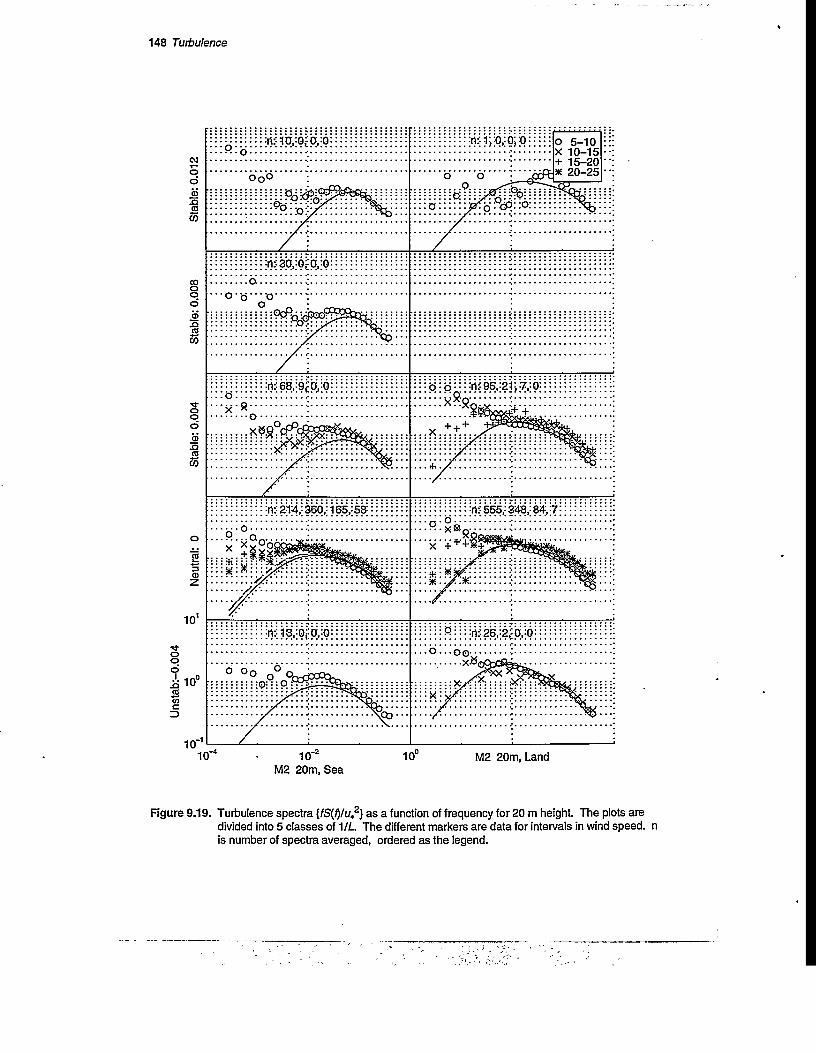
148 Turbulence
::::::::::::::::::: :::::::::::::::::::
• • * a ****** *^3** ^**^**%***^****************** . * • H * o............... ...............................
:::::::::::::::::::r::::::::::::::::::::
:::::::::::::::::::::::::::::::::::.................5-10
x 10-15 + 15-20
20-25
::::::::::::::::::::
101
• ‘ • o • y “ * *o o
:::::::::::: I:::-:::::::::::::::::::: :•
....................rti* 68i'9r 0,0...........................* * * *_* ••*•••*•••■ ••••s**** ••••*••••«••••••••... o........................* * * ** • ^ * * * *••••<••*,•• *
.......... O--”-:::::::: ?
i:^2i4,;3Bd,:ira:s8:::!!!!!o.
:::::::::::r:::::::::::::::::::: ::::::u:::::::::::r:::::::::::::::::::5::::n?26,:2c0,:0:
10M2 20m, Sea
M2 20m, Land
Figure 9.19. Turbulence spectra {fS(f)/u2} as a function of frequency for 20 m height. The plots aredivided into 5 classes of 1/L The different markers are data for intervals in wind speed,is number of spectra averaged, ordered as the legend.

Uns
tab:
-0.0
04
Discussion 149
x 10-15+ 15-20* 20-25
X + +
o'd
Figure 9.20. Turbulence spectra {fS[f)lut2} as a function of frequency for 40 m height. The plots aredivided into 5 classes of ML. The different markers are data for intervals in wind speed, n is number of spectra averaged, ordered as the legend.
4

Uns
tab:
-0.0
04
150 Turbulence
o 5-10x 10-15+ 15-20* 20-25
... X . o ■ -Xq
X o :
• • • O •
X
Figure 9.21. Turbulence spectra {fS(f)/ut2} as a function of frequency for 70 m height. The plots aredivided into 5 classes of 1/L The different markers are data for intervals in wind speed,is number of spectra averaged, ordered as the legend.

Uns
tab:
-0.0
04
Discussion 151
X 10-15+ 15-20* 20-25Oo o o o
lO-O- ■oo r, ft
...0.0
10M2100m, Sea
M2100m, Land
Figure 9.22. Turbulence spectra {fS(/)/u,2} as a function of frequency for 100 m height. The plots aredivided into 5 classes of 1/L. The different markers are data for intervals in wind speed, nis number of spectra averaged, ordered as the legend.

152 Turbulence

References
Andersen, O. (1991). The Maritime Wind Field. A literature review. Statoil report no. IGT KOB 91007, Norway.
Andersen, OJ. andL0vseth, J. (1992). The Maritime Wind Field. Measurements and Models. Phase 2 -Extension 1 - Task 4. Extended analysis of the Fr0ya data base. Allforsk, Dragvoll, Norway.
Berg, T.C. and Dahl, V. (1980). Maling pa vindhastighetsmalere i vindtunnelen NTH Trondheim. Teknisk notat nr. 7/80. NILU, Lillestrpm, Norway.
Bouwmeester, R.J.B., Meroney, R.N., Sandbom, V.A. (1978). Sites for Wind-Power Installations: Wind Characteristics Over Ridges. Colorado State University, USA.
Businger, J.A., Wyngaard, J.C, Izumi, Y., Bradley, E.F. (1971). “Flux-profile relationships in the atmospheric surface layer”. J. Atnos. Sci. 28, 181-189.
Businger, J.A. (1972). “The atmospheric boundary layer”. In Derr, V.E. (ed.). Remote sensing of the troposphere. 6/1 - 6/5. US Govt. Printing Office, Washington D.C., USA. COM/72/51061.
Charnock, H. (1955). “Wind stress on a water surface”. Quart.J.Roy.Met.Soc., 81.
Connell, J.R. and Morris, V.R. (1991). “Calibration data for improved correction of UVW propeller anemometers”. Pacific Northwest Laboratory, Richland, Washington, USA.
Davenport, A.G. (1995). “The role of wind engineering in the reduction of natural disasters”. Ninth international conference on wind engineering, New Delhi, India.
Deaves and Harris, R.I. (1978). A mathematical model of the structure of strong winds. CIRIARep. 76.
Dobbins, R.A. (1979). Atmospheric motion and air pollution: an introduction for students of engineering and science. Wiley, New York, USA. ISBN 0-471-21675-5.
Dyer, A.J. (1974). “A review of flux profile relationships”. Bound. L. Met., 22.

154 References
Gjerstad, J., Aasen S.E., Andersson, H.I., Brevik, I. and L0vseth, J. (1995). “An Analysis of Low-Frequency Maritime Atmospheric Turbulence”. J. Atmos. Sc., Vol. 52, No. 15, 2663-2669.
Hagander, A. (1980). Kontroll av anemometre i vindtunnel. Tecnical report No. 54. DetNor- ske Meteorologiske Institutt, Oslo, Norway.
Hogstrom, U. (1987). “Non-dimensional wind and temperature profiles in the atmospheric surface layer”. Bound. L. Met., 42.
Hpjstrup, J. (1981). “A simple model for the adjustment of velocity spectra in unstable conditions to an abrupt change in roughness and heat flux”. Bound. L. Met., 21.
Hpjstrup, J. (1982). “Velocity spectra in the unstable boundary layer”. J. Atmos. Sc., 39, 2239-2248.
IFE (1990). Oppdatering av vindkraftpotensialet i Norge. Report IFE/KR/F-90/131. IKE, Kjeller, Norway.
IFE (1992). Pilotprosjekt i S0r-Tr0ndelag. Report 1EE/KR/F-92/072. IFE, Kjeller, Norway.
Jackson P.S. and Hunt, J.C.R. (1975). “Turbulent wind flow over a low hill”. Quart. J. Roy. Meteorol. Soc. 101, 929-955.
Jensen, N.O. (1978). “Change of surface roughness and the planetary boundary layer”. Quart. J. Roy. Meteorol. Soc. 104, 351-356.
Kailmal, J.C., Wyngaard, J.C., Izumi, Y., Cote, O.R. (1972). ’’Spectral characteristics of surface-layer turbulence”. Quart. J. Roy. Meteorol. Soc. 98, 563-589.
Kitaigorodskii, S.A. (1970). “Physics of air-sea interactions”. Israel Prog.Sci.Trans.
Larsen, S.E., Hedegaard, K. and Troen, 1.(1982). “The change of terrain roughness problem extended to mesoscale fetches”. The first international conference on meteorology and air/ sea interaction Conference Proceedings, 8-13. Amer.Met.Soc. Boston, USA and KNMI Netherlands.
Lpvseth, J., Aasen, S.E. and Heggem, T. (1994). “Measurements and modelling of the profile and turbulence of coastal wind”. EWEC ‘94, 5th European Wind Energy Association Conference Proceedings, Vol. 2, 207-213.
Mollestad, K. and Lpvseth, J. (1995). Data fra vindmalestasjonene til UNIT-AVH / ALL- FORSK. Perioden 1981-1994. Report for S0r-Tr0ndelag kraftselskap. ALLFORSK, Norway.
NAG (1990). NAG FORTRAN LIBRARY Introductionary Guide, Mark 14. Software manual. NAG Ltd., Oxford, U.K.
Newland, D.E. (1987). An introduction to random vibrations and spectral analysis. Second edition. Longman Scientific & Technical, U.K. ISBN 0-582-30530-6.

References 155
Nordeng, T.E. (1988). An optimum use of atmospheric data in wind wave modelling - numerical experiments. Technical Report No. 68, DNMI, Norway,
Nygaard, T.A. (1992). “Estimating expected energy capture at potential wind turbine sites in Norway". Journal of wind engineering and industrial aeordynamics, 39, pp. 385-393.
Nyrud, B. (1985). Eksperimentell bestemmelse av temperatuiprofilen i bakke og luft. Master thesis at the University of Trondheim, Norway.
Optimization Toolbox for use with Matlab (1992). Software manual. The Mathworks Inc.MA. USA.
Panofsky, H.A. (1973). “Tower climatology”. In Haugen, D.A. (ed.), Workshop on micrometeorology, Amer.Meteor.Soc., Boston, USA, pp. 177-216.
Paulsen, J.I. (1994). Registering av vind og responsm0nster for et 400 kW vindkraftverk. Master thesis at the University of Trondheim, Norway.
Skaslien, T.H. (1991). Utprpving av en modell for regionale variasjoner av vind. Master thesis at the University of Trondheim, Norway.
Stull, R.B. (1989). An introduction to boundary layer meteorology. Kluwer Academic Publishers, Dordrecht, The Netherlands. ISBN 90-277-2768-6.
Tro'en, I. and Petersen, E.L. (1989). European Wind Atlas. Ris0 National Laboratory, Roskilde, Denmark. ISBN 87-550-1482-8.
UNIRAS (1992). UNIRAS Reference Guide. Software manual. UNIRAS A/S, Spborg, Denmark.
Wittje, R. (1994). Analysis of the Spectrum of Turbulence Kinetic Energy in Coastal Wind in the 0.5 -0.12 mHz Region. Semester Project at Department of Physics, College of Arts and Science, University of Trondheim, Norway.
Aasen, S.E. (1989). Maling av turbulens med koppanemometer. Master thesis at the University of Trondheim, Norway.

156 References


Appendix A
Configuration File
This appendix will explain the format of the configuration file. The configuration file is a text file containing all variable parameters for the acquisition programs at Skipheia. The file is read by the programs on startup of the acquisition system. The concept of this file has proven very valuable during the operation of the station.
! section for main program1<log file for main program^
! section for timer program<name of timer program>
<number formed by dip switch 2, 3 and 4 on ACPC board> <number of ACPC boards>
<interrupt line used by timer interrupt><counter number used as timer (0. ,47)> <number of counts in timer counter to generate an interrupt>
<number of measurements per 10 minutes, depends on number of counts>
<log file for timer program** >
! section for counter program<name of timer program>
<number of counters>
<sensor id> <counter no> <sensor type> <C1> <C2> <C3> <CS> <sensor height> <sensor description>"*
I the line above repeated for each counter sensor
<log file for counter program**>
! section for voltmeter program<najne of voltmeter program><number of analog sensors>
<sensor id> <mux ch> <sensor type> <C1> <C2> <C3> <C4> <CS> <sensor height> <sensor description
! the line above repeated for each analog sensor

A2
<voltmeter initialisation string>
< number of periods between each logging (1,2,4,8.... )>
<interrupt line used by the NX-488 IEEE-488 interface>
<address of the NI-488 IEEE-488 interface (hex)>
<IEEE-488 address of voltmeter>
<number of characters in data from vol tmeter>
<port a number in acpc pio, used for mux> <mask for bits used (hex)>
<log file for voltmeter prograitP>
! section for resolver program<name of resolver program><number of resolver sensors>
<sensor id for XJPS> <mux ch (not used)> <6>
<sensor id> <counter no> <sensor typo <C1>
! the line above repeated for each resolver
<C1> <C2> <CS> <sensor height> <sensor description
<C2> <CS> <sensor height> <sensor description4
sensor
<port a number in acpc pio, used for ups> <mask for bits used (hex)> <port a number in acpc pio, used for trigger> <mask for bits used (hex)>
<resolver reference frequency>
<log file for resolver program^>
! section for store program<name of store program><number of sensors to store>
<sensor id>
l the line above repeated for each sensor to store
<full path for directory to store data>
<name of ten minute files^>
<number of measuring periods in binary files>
<name of binary files<port a number in acpc pio, used for watchdog> <mask for bits used (hex)> <name of tape backup program>
<name of program to delete the binary files backed up>
<ten minute number for start of backup>
<log file for store program^>
Note 1All lines starting with ! are comments, blank lines are not allowed in the actual file
Note 2Sensor types for Counter.c are:
0: wind speed : speed = #counts-Cl + C21,2: wind horizontal and vertical direction : dir. = #counts-Cl + C2
10: precipitation : mm = #counts = Cl
UVW sensors : requires six channels, u-, v-, w-speed, speed, hor.dir, vert.dir. Speed, hor.dir and vert.dir. do not have input from counters but from u-, v-, w-speed channels, this is fixed by using 99 as counter input and Cl = u-speed sensor id, C2 = v-speed sensor

A3•v.
id and C3 = w-speed sensor id. Apart from between the u-, v- and w-channels the order of the channels must be as above.The CS constants are used by Store.c to scale the data to an integer value.
Note 3Sensor types for Voltmeter.c are:
1,2: Wind horizontal and vertical direction : dir. = volts Cl + C2 3: Temperature, termistor:
T = C2\n[ci(V/Ub-V)\
(A.l)
where Cl = R/A, C2 = B, C3=l/C and Ub is the bridge voltage. R is the series resist
ance in the bridge circuit, A, B and C are found by individually calibration the termis- tors and fitting to the formula:
Rj. = Ae^jC • (A.2)
5: Bridge voltage for temp, sensors :U=C1• volts, Cl = (Rr + K)/R„ Rr is a reference resistor.
7: Bridge voltage for Aanderaa sensors : U = Cl • volts, Cl = (Rr + R)/Rr, Rr is a reference resistor.
8: Aanderaa half bridge sensors : C1=D, C2=C, C3=B, C4=AwhereA, B, CandD are calibration values given by Aanderaa. The formula for calculation of total radiation, humidity and pressure is
, V 21d~u'u (A.3)
ET,Rh,P = Cl-d3 +C2-d2 +C3-d+C4
9: Thermopile : G = volts Cl
UVW sensors : requires six channels, u-, v-, w-speed, speed, hor.dir, vert.dir.Speed, hor.djr and vert.dir. do not have input from voltmeter but from u-, v-, w-speedchannels, this is fixed by using 99 as mux ch and Cl = u-speed sensor id, C2 = v-speedsensor id and C3 = w-speed sensor id. Apart from between the u-, v- and w-channels theorder of the channels must be as above.The CS constants are used by Store.c to scale the data to an integer value.
Note 4

A4
Sensor types for Resolver.c are :
1,2: wind horizontal and vertical direction : dir. = #counts-Cl + Cl
The CS constants are used by Store.c to scale the data to an integer value.
Note 5The log file names can contain the string '*****', this will be replaced with year and day number on start-up.
Note 6The filename must contain the string '********' which is replaced with year, dayno and ten min. no.
Note?The filename must contain the string '*******' which is replaced with year, dayno and fileno.

Appendix B
Filesub.for
This appendix is a partial program listing of the FORTRAN file filesub.f. The listing contains all the necessary routines for reading of the Skipheia datafiles. Check of data against the Error File and selection of upwind sensor is included in the routines. The routines included in this listing are essentialfor use of data from the Skipheia data base (or from other'stations). During the analysis several FORTRAN programs have been developed, totaling several thousand lines of FORTRAN code. These programs make use of the NAG FORTRAN LIBRARY (NAG, 1990) for numerical calculations and the UNIRAS LIBRARY (UNIRAS, 1992) for graphical presentations. Listing of these programs are not included in the thesis.
cC Subroutines for use on files (files with new format)CC File name: filesub.fCc***************************************************************************C SUBROUTINE Read_fileC Reads n_in_ten periods from files .RRR and .TTTC The routine can handle Nstax stations in paralellC Parameters :C data - out : 2 dim. array of scaled dataC data_ok - out : .TRUE, if data is read (data can still be BAD)C nsta - in : number of stations to readC nsens - in : number of sensors to readC sensid - in : sensor id's to readC type - in : datatype's to read: 10-min data: l=mean,2=max,3=min,4=sdC -1 or -2 etc. if up-wind sensor should be chosen.C Use type = +1 or -1 for raw-data (10 min time series)C sta - in : station numbers (relative) for each sensor to readC iyear,idayno,iper - in : year,dayno.,terrain. period for startC stacode - in : 3 char abbreviation for station (upper case)C filetype - in : 3 char abbreviation for filetype (TTT or RRR)

B2
Ccccccc
dir - in : the directory where the data and config. file is err_check - in : .TRUE, if data are to be checked against error file cfg - out : data read from cfgfile cfg_ok - out : .TRUE, if cfg data is defined
11-7-1991 S.E.
C***************************************************************************SUBROUTINE Read_file(data,data_ok,nsta,nsens,sensid,type,sta,iyear,
& idayno,iper,stacode,filetype,dir,err_check,cfg,cfg_ok)IMPLICIT NONE
INCLUDE 'filstruc.f'
RECORD /cfg_data/ cfg(nXsta)
INTEGER iyear,idayno,iper,nsta,nsens,sensid(nXsens)INTEGER type(nXsens),sta(nXsens)CHARACTER*3 stacode(nXsta),filetype CHARACTER*(*) dir(nXsta)REAL data(nXm,nXsens)LOGICAL cfg_ok(nXsta),err_check(nXsta),data_ok(nXsens)
LOGICAL dir_ok(nXsta)INTEGER i,sens,rsens,err_typeINTEGER*2 idata(nXsens,nXm,nXtype,nXsta)INTEGER ista,im,dirsensid(nXsta),dir_im,per80,period_since80 LOGICAL dir_dep(nXsta),ok(nXsta)REAL dir_val(nXsta),err_const(3)RECORD /cfg_data/ cfgOO(nXsta)CHARACTER*3 last_stacode(nXsta),last_filetype
IF (filetype.EQ.1rrr') THENCALL Read_file_rrr(idata,nsta,iyear,idayno,iper,stacode,dir,cfg,
& cfg_ok,ok)ELSECALL Read_file_ttt(idata,nsta,iyear,idayno,iper,stacode,dir,cfg,
& cfg_ok,ok)ENDIFDO ista=l,nsta
dir_dep(ista) = .FALSE. dir_ok(ista) = .FALSE.IF ((stacode(ista).NE.last_stacode(ista)).OR.
& (filetype.NE.last_filetype)) THENlast_stacode(ista)=stacode(ista) last_filetype=filetypeWRITE (cfgOO(ista).cfgname(l:12),'(A3,A3,A6)') stacode(ista),
& filetype,'00.cfg'CALL read_cfgfile(dir(ista),cfgOO(ista))
ENDIFENDDOperSO = period_since80(1,iyear,idayno,iper,1)DO sens = 1,nsens
IF (type(sens).LT.O) dir_dep(sta(sens)) = .TRUE.IF ((cfg(sta(sens)).ch_no(sensid(sens)).EQ.nXsens).OR.
& (.NOT.ok(sta(sens)))) THENdata_ok(sens) = .FALSE.
ELSE!sensor does not exist

B3
data_ok(sens) = .TRUE. !sensor existsENDIF
ENDDODO ista=l,nsta! find direction
IF (dir_dep(ista).AND.cfg_ok(ista).AND.ok(ista)) THEN CALL
SelectDirSens(dir,ista,stacode(ista),dirsensid(ista),dir_ok(ista),& perSO)
IF (dir_ok(ista)) THENdir_im = NINT(FLOAT(cfg(ista),n_in_ten)/2.0)
C use mid datapoint C or first datapoint okrsens = cfg(ista),ch_no(dirsensid(ista))I=idata(rsens,dir_im,1,ista)IF (ABS(I).GE.29999) THEN DO dir_im=l,cfg(ista).n_in_ten
I=idata(rsens,dir_im,1,ista)IF (ABS(I).LT.29999) GOTO 100
ENDDOdir_ok(ista) = .FALSE.
ENDIF100 IF (dir_ok(ista)) THEN
dir_val(ista) = idata(rsens,dir_im,1,ista) *& cfg(ista),sensscale(dirsensid(ista))
ENDIFDO WHILE (dir_val(ista)-GT.360.0) dir_val(ista) = dir_val(ista) - 360.0
ENDDODO WHILE (dir_val(ista).LT.0.0)
dir_val(ista) = dir_val(ista) + 360.0 ENDDO
ENDIF ENDIF
ENDDODO sens=l,nsens
IF (data_ok(sens)) THEN IF (type(sens).LT.0) THEN
IF (dir_ok(sta(sens))) THENrsens = cfg(sta(sens)).ch_no(sensid(sens))IF (cfg(sta(sens)).double_sensptr(sensid(sens)).NE.0) THEN CALL dirdepsens(dir_val(sta(sens)),sta(sens),rsens,
& cfg(sta(sens)),double_sensptr(sensid(sens)),& stacode(sta(sens)),cfg(sta(sens)))
ENDIFELSEdata_ok(sens) = .FALSE.ENDIF
ELSErsens = cfg(sta(sens)).ch_no(sensid(sens))
ENDIFENDIFIF ((.type(sens) .LT.0) .AND.
& (cfgOO(sta(sens)).senstype(sensid(sens)).EQ.2)) THENIF (dir_ok(sta(sens))) THEN ! set to selected direction
rsens = cfg(sta(sens)),ch_no(dirsensid(sta(sens))) data_ok(sens) = .TRUE.
ELSEdata_ok(sens) =
ENDIF•FALSE.

B4
ENDIFIF (data_ok(sens)) THEN ! if ok so far, check error file
IF (err_check(sta(sens))) THEN CALL Checkdatase(dir,stacode(sta(sens)),sta(sens),
& cfgtsta(sens)).sensid(rsens),& perSO,err_type,err_const)
IF (err_type.EQ.0) data_ok(sens) = .FALSE.ENDIF
ENDIFIF (data_ok(sens)) THENDO im=l,cfg(sta(sens)).n_in_ten
I=idata(rsens,im,ABS(type(sens)),sta(sens))IF (ABS(I).LT.29999) THENdata(im,sens) = idata(rsens,im,ABS(type(sens)),sta(sens)) *
& cfg(sta(sens)).sensscale(cfg(sta(sens)).sensid(rsens))IF (err_type.EQ.1) data(im,sens) = data(im,sens) *
& err_const(1)+err_const(2)ELSEdata(im,sens) = BAD ENDIF
ENDDO! im ELSEDO im=l,cfg(sta(sens)).n_in_ten
data(im,sens) = BAD ENDDO
ENDIF! data_ok ENDDO ! sens RETURN END
Q***************************************************************************C Local subroutines called from subroutines aboveQ************************************ ***************************************
**************************************************************************** C SUBROUTINE Read_cfgfileC Reads configuration file, called by Read_file_ttt an Read_file_rrrC Parameters :C dir - in : the directory where the config. file isC cfg - in/out : cfgname is input, rest of structure is outputC 11-7-1991 S.E.Q******************************************************** *******************
SUBROUTINE Read_cfgfile(dir,cfg) IMPLICIT NONE
INCLUDE 'filstruc.f'
RECORD /cfg_data/ cfg CHARACTER*(*) dir
INTEGER cfgfile/11/,line,i,j,id,ch,lnblnk CHARACTER*100 full_cfgname

B5
LOGICAL op
1 FORMAT (A,A)
DO j = l,nXsensidcfg.ch_no(j) = nXsens!always point to last datarecord, i.e. BAD cfg.double_sensptr(j) = 0
ENDDO£ull_cfgname = dir j = lnblnk(full_c£gname)+1
full_cfgname(j:(j+11)) = cfg.cfgname 60 INQUIRE(UNIT=cfgfile,OPENED=op)
IF (op) THENcfgfile = cfgfile + 1 GOTO 60
ENDIFOPEN(UNIT=cfgfile,FILE=full_cfgname,STATUS='OLD',ERR=100,
& READONLY,SHARED)GOTO 110
100 TYPE 1,' FATAL ERROR opening configuration file ',full_cfgname RETURN
110 line = 1READ(c£gfile,*,ERR=120) cfg.staname line = line + 1READ(cfgfile,*,ERR=120) cfg.nsens line = line + 1READ(cfgfile,*,ERR=120) cfg.ntype line = line + 1READ(cfgfile,*,ERR=120) cfg.n_in_ten DO ch = 1 , cfg.nsens
line = line + 1READ(cfgfile,*,ERR=120) id,cfg.senstype(id),cfg.sensscale(id), cfg.sensheight(id),cfg.sensdir(id),cfg.sensdesc(id) cfg.sensid(ch) = id cfg.ch_no(id) = ch
ENDDOREAD(cfgfile,*,ERR=120) cfg.ndouble,((cfg.double_sensid(i,j),i=l,2),
& j=l,(cfg.ndouble/2))DO j=l,cfg.ndouble/2
DO i=l,2cfg.double_sensptr(cfg.double_sensid(i,j)) = j
ENDDO ENDDOCLOSE(cfgfile)GOTO 130
120 TYPE *,' Error reading configuration file, line 1, & full_cfgname,line
STOP130 RETURN
END

onnn
onoo
nonn
B6
*************************************************************************** SUBROUTINE Read_file_rrr Reads n_in_ten periods from file.The routine can handle Nstax stations in paralell Parameters :
data - out : max 4 dim. array of data read from file nsta - in : number of stations to readiyear,idayno,iper - in : year,dayno.,tenmin. period for start stacode - in : 3 char abbreviation for station (upper case) dir - in : the directory where the data and config. file is cfg - out : data read from cfgfile cfg_ok - out : .TRUE, if cfg data is defined
C ok - out : .TRUE, if any data at all existsC 11-7-1991 S.E.q***************************************************************************
SUBROUTINE Read_file_rrr(data,nsta,iyear,idayno,iper,& stacode,dir,cfg,cfg_ok,ok)
IMPLICIT NONE
INCLUDE 'filstruc.f'
RECORD /cfg_data/ cfg(nXsta)
INTEGER nsta,iyear,idayno,iper CHARACTER*3 stacode(nXsta)CHARACTER*(*) dir(nXsta)INTEGER*2 data(nXsens,nXm,nXtype,nXsta)LOGICAL cfg_ok(nXsta),ok(nXsta)
CHARACTER*12 last_cfgname(nXsta)LOGICAL file_open(nXsta)/nXsta*.FALSE./LOGICAL cfg_read(nXsta)/nXsta*.FALSE./,op CHARACTER*100 filename,full_cfgname INTEGER sign/9999998/INTEGER p,maxrec,month_.no,date_no,leap_year,iday,i,sens,type INTEGER ufile(nXsta)/13,14/,swrec,ewrec,Irec(nXsta)INTEGER*2 rbuff(nXsens,nXsta)INTEGER last_idayno(nXsta)/nXsta*0/,ista,imINTEGER last_per80(nXsta)/nXsta*0/,lnblnk,per80,Period_since80 CHARACTER*3 last_stacode(nXsta)
1 FORMAT (12,A3)
DO ista=l,nstaper80=Period_since80(1,iyear,idayno,iper,1)IF ((stacode(ista).NE.last_stacode(ista)).OR.
& (per80.NE.last_per80(ista)+l)) THEN cfg_read(ista)=.FALSE. last_cfgname(ista)=' 'last_idayno(ista)=0 irec(ista)=0
ENDIFlast_stacode(ista)=stacode(ista)
ENDDODO ista=l,nsta
swrec = cfg(ista).n_in_ten * (iper-1) + 1 ewrec = cfg(ista).n_in_ten * iper ok(ista) = .FALSE.

B7
IF (cfg_read(ista)) THEN DO im=l,cfg(ista).n_in_ten
DO sens=l,cfg(ista).nsens data(sens,im,I,ista) = BAD
ENDDO ENDDO
ELSEDO im=l,nXmDO sens=l,nXsensdata(sens,im,1,ista) = BAD
ENDDO ENDDO
ENDIFIF ((idayno.NE.last_idayno(ista)).OR,
& (per80.NE.last_per80(ista)+l)) THEN last_idayno(ista) = idayno IF (file_open(ista)) THEN CLOSE(ufile(ista))£ile_open(ista) = .FALSE.
ENDIFfilename = dir(ista) i = lnblnk(filename)+1filename(i:(i+13)) = stacode(ista)//'*****.'//'rrr' i = Index(filename,'* 1)write (filename (i: (i+4)), ' (15) '.) (1000*iyear+idayno)
C CALL Modfilse(filename,filename,(1000*iyear+idayno))60 INQUIRE(UNIT=ufile(ista),OPENED=op)
IF (op) THENufile(ista) = ufile(ista) + 1 GOTO 60
ENDIFOPEN(UNIT=ufile(ista),STATUS='OLD',FORM='UNFORMATTED',
& NAME=filenarne,READONLY,SHARED,ERR=120,RECORDTYPE='SEGMENTED')file_open(ista) = .TRUE.READ(ufile(ista)) irec(ista)TYPE *,1 File open : 1//filename GOTO 140
120 TYPE *,1 Error opening file 1//filenameGOTO 170
ENDIF
140 CONTINUEIF (file_open(ista)) THEN DO WHILE ((irec(ista).LE.ewrec).OR.
& ((irec(ista)-GE.sign).AND.(.NOT.(ok(ista)))))IF (irec(ista).GE.sign) THEN
C Read .cfg fileREAD(ufile(ista)) cfg(ista).cfgname CALL lowcase(cfg(ista).cfgname,12).IF (cfg(ista).cfgname.NE.last_cfgname(ista)) THEN
last_cfgname(ista) = cfg(ista).cfgname CALL Read_cfgfile(dir(ista),cfg(ista)) swrec = cfg(ista).n_in_ten * (iper-1) + 1 ewrec = cfg(ista).n_in_ten * iper cfg_read(ista) = .TRUE.
ENDIFREAD(ufile(ista),END=160,ERR=150) irec(ista),

B8
& (rbuff(sens,ista),sens=l,cfg(ista).nsens)ELSE IF (Irec(ista).LT.swrec) THEN ! read more READ(ufile(ista),END=160,ERR=150) irec(ista),
& (rbuff(sens,ista),sens=l,cfg(ista).nsens)ELSE IF ((Irec(ista)-GE.swrec)-AND.(Irec(ista)-LE.ewrec)) THEN
! period foundDO sens = l,cfg(ista).nsensdata(sens,(irec(ista)-swrec+1),1,ista) = rbuff(sens,ista)
ENDDOok(ista) = .TRUE.READ(ufile(ista),END=160,ERR=150) irec(ista),
& (rbuff(sens,ista),sens=l,cfg(ista).nsens)ENDIF! irec.EQ.wrec
150 CONTINUEENDDO! irec.LT.ewrec
ENDIF ! file_openGOTO 170
160 CLOSE(ufile(ista))file_open(ista) = .FALSE.
170 CONTINUEcfg_ok(ista) = cfg_read(ista) last_per80(ista)=per80
ENDDO ! ista
RETURNEND
Q***************************************************************************C SUBROUTINE Read_file_tttC Reads n_in_ten (1) periods from file.C The routine can handle Nstax stations in paralellC Parameters :C data - out : max 4 dim. array of scaled dataC nsta - in : number of stations to readC iyear,idayno,iper - in : year,dayno.,tenmin. period for startC stacode - in : 3 char abbreviation for station (upper case)C dir - in : the directory where the data and config. file isC cfg - out : data read from cfgfileC cfg_ok - out : .TRUE, if cfg data is definedC ok - out : .TRUE, if any data at all existsC 11-7-1991 S.E.****************************************************************************
SUBROUTINE Read_file_ttt(data,nsta,iyear,idayno,iper,& stacode,dir,cfg,cfg_ok,ok)
IMPLICIT NONE
INCLUDE 'filstruc.f1
RECORD /c£g_data/ cfg(nXsta)
INTEGER nsta,iyear,idayno,iper CHARACTER*3 stacode(nXsta)CHARACTER*(*) dir(nXsta)INTEGER*2 data(nxsens,nXm,nxtype,nXsta)LOGICAL cfg_ok(nXsta),ok(nXsta)

B9
INTEGER n_in_ten(nXs ta)CHARACTER*12 last_cfgname(nXsta)CHARACTER*3 monthcode(12)/'jan','feb','mar','apr','may','jun',
& 'jul','aug','sep','oct','nov','dec'/INTEGER DAYS_A_MONTH(12)/31,28,31,30,31,30,31,31,30,31,30,31/LOGICAL £ile_open(nXsta)/nXsta*.FALSE./,dir_ok,op LOGICAL c£g_read(nXsta)/nXsta*.FALSE./CHARACTER*100 filename,full_cfgname INTEGER sign/9999998/INTEGER p,maxrec,month_no,date_no,iday,i,sens,type INTEGER ufile(nXsta)/13,14/,wrec,Irec(nXsta),osens INTEGER*2 rbuff(nxsens.nxtype,nXsta)INTEGER month,last_month(nXsta)/nXsta*0/zistaINTEGER last_per80(nXsta)/nXsta*0/,lnblnk,Period_since80,per80 CHARACTER*3 last_stacode(nXsta)
1 FORMAT (12,A3)
DO ista=l,nstaper80=Period_since80(1,iyear,idayno,iper,1)IF ((stacode(ista).NE.last_stacode(ista)).OR.
& (per80.NE.last_per80(ista)+l)) THEN c£g_read(ista)=.FALSE. last_c£gname(ista)=' 'las t_month(ista)=0 irec(ista)=0
ENDIFlast_stacode(ista)=stacode(ista)
ENDDODO ista=l,nstawrec = (Date_no(iyear,idayno) - 1) * 144*c£g(ista),n_in_ten + iper ok(ista) = .FALSE.IF (cfg_read(ista)) THEN DO sens=l,c£g(ista).nsens
DO type=l,nxtypedata(sens,1,type,ista) = BAD
ENDDO ENDDO
ELSEDO sens=l,nxsens DO type=l,nxtype
data(sens,1,type,ista) = BAD.ENDDO
ENDDOENDIFmonth = month_no(iyear,idayno)IF (month.NE.last_month(ista).OR.(per80.NE.Iast_per80(ista)+1)) THEN
last_month(ista) = month IF (£ile_open(ista)) THEN CLOSE(ufile(ista))£ile_open(ista) = .FALSE.
ENDIFfilename = dir(ista) i = Inblnk(filename)+1filename(i:(i+13)) = stacode(ista)//'*****.'//1ttt' i = Index(filename,'*')write(filename(i:(i+4)),1) iyear,monthcode(month)INQUIRE(UNIT=ufile(ista),OPENED=op)60

B10
120
140
&
C Read
&
&&
&
&
&
&
150
160
170
IF (op) THENufile(ista) = ufile(ista) + 1 GOTO 60
ENDIFOPEN(UNIT=ufile(ista),STATUS='OLD',FORM=■UNFORMATTED',NAME=filename,READONLY,SHARED,ERR=120,RECORDTYPE='SEGMENTED') £ile_open(ista) = .TRUE.TYPE *, ' File open '//filename READ(ufile(ista)) irec(ista)GOTO 140
TYPE *,' Error opening file 1//filename GOTO 170
ENDIF
CONTINUEIF (file_open(ista)) THEN DO WHILE ((irec(ista).LE.wrec).OR.((irec(ista)-GE.sign).AND.(.NOT.(ok(ista)))))IF (irec(ista).GE.sign) THEN
.cfg fileREAD(ufile(ista)) cfg(ista).cfgname CALL lowcase(cfg(ista).cfgname,12)IF (cfg(ista).cfgname.NE.last_cfgname(ista)) THEN
last_cfgname(ista) = cfg(ista).cfgname CALL Read_cfgfile(dir(ista),cfg(ista))
wrec = (Date_no(iyear,idayno) - 1) * 144*cfg(ista).n_in_ten + iper
cfg_read(ista) = .TRUE.ENDIFREAD(ufile(ista),END=160,ERR=150) irec(ista),((rbuff(sens,type,ista),sens=l,cfg(ista).nsens), type=l,cfg(ista).ntype)
ELSE IF (Irec(ista).LT.wrec) THEN ! read more READ(ufile(ista),END=160,ERR=150) irec(ista),((rbuff(sens,type,ista),sens=l,cfg(ista).nsens), type=l,cfg(ista).ntype)
ELSE IF (Irec(ista).EQ.wrec) THEN ! period found DO sens = 1,cfg(ista).nsens
DO type = 1,cfg(ista).ntype data(sens,1,type,ista) = rbuff(sens,type,ista)
ENDDO! type ENDDO! sens ok(ista) = .TRUE.READ(ufile(ista),END=160,ERR=150) irec(ista),((rbuff(sens,type,ista),sens=l,cfg(ista).nsens), type=l,cfg(ista).ntype)
ENDIF! irec.EQ.wrec CONTINUE
ENDDO! irec.LT.wrec ENDIF . ! file_openGOTO 170CLOSE(ufile(ista)) file_open(ista) = .FALSE.CONTINUEcfg_ok(ista) = cfg_read(ista) last_per80(ista) = perSO
ENDDO ! ista

B11
RETURNEND
SUBROUTINE CHECKDATAse(path,stacode,Ista,sensid,per_since80,err_type,& err_const)
Q***************************************************************************C Check data for sensors sensid against error file. Stacode is a 3 char, code C for station, sensid will then mean sensor no in error file, periods for each C sensor must be def. timeordered, incl. error periods for station (sensid=0), C but they may overlap excisting periods C OK = TRUE means sensor is ok C per_since80 is tenmin period since 1-1-1980Q***************************************************************************
IMPLICIT NONE
INCLUDE 1filstruc.f'
INTEGER Ista,sensid, I,J,Js, NerrX, Y1,D1,T1,Y2,D2,T2,Ti,Tf, Eo INTEGER SensI, SensF,err_type CHARACTER*(*) path REAL err_const(3)PARAMETER(NerrX=400)CHARACTER*3 stacodeINTEGER Ierr(nXsta.NxSensid), Nerr(nXsta,NxSensid),
& Liml(nXsta,NxSensid,NerrX),ErrType(nXsta,NxSensid,NerrX),& Lim2(nXsta,NxSensid,NerrX),per_since80,Period_since80,t
REAL ErrConst(3,nXsta,NxSensid,NerrX),c(3)LOGICAL No_Overlap,op CHARACTER*100 ErrFilLOGICAL file_read(nXsta) /nXsta*.FALSE./INTEGER last_per80(nXsta,nXsensid),lnblnk,errunit/11/CHARACTER*3 last_stacode(nXsta)
IF (.NOT.file_read(ista)) GOTO 50!err file is not yet read IF (stacode.NE.last_stacode(ista)) THEN CLOSE (errunit)GOTO 50!new station
ENDIFIF (per_since80,NE.last_per80(ista,sensid)+1) THEN ! reset buffer
Ierr(ista,sensid)=1 ENDIF
10 last_per80(ista,sensid)=per_since80IF (Ierr(ista,sensid).LE.Nerr(ista,sensid)) THEN !checked all?
IF (Liml(ista,sensid,Ierr(ista,sensid)),LE.per_since80) THEN IF (Lim2(ista,sensid,Ierr(ista,sensid)),GE.per_since80) THEN
err_type = ErrType(ista,sensid,Ierr(ista,sensid))DO i=l,3
■err_const(i) = ErrConst(i,ista,sensid,Ierr(ista,sensid))ENDDORETURN
ELSEIerr(ista,sensid) = Ierr(ista,sensid) + 1!this was ok GOTO 10
ENDIF ENDIF

ENDIFerr_type = -1 RETURN
last_stacode(ista)=stacode DO 1=1,nxsensid
Nerr(ista,I) = 0 Ierr(ista,I) = 1
ENDDOerrfil = path i = lnblnk(errfil)+lWRITE(errfil(i:i+10),'(A4,A3,A4)1) 1err_',stacode,1.dat'INQUIRE(UNIT=errunit,OPENED=op)IF (op) THENerrunit = errunit + 1 GOTO 60
ENDIFOPEN (UNIT=errunit, FILE=errfil, STATUS='OLD1,
& READONLY, SHARED, FORM='FORMATTED',ERR=8 0)GOTO 90TYPE *,1 FATAL ERROR: The error file does not exist '//errfil RETURNfile_read(ista) = .TRUE.DO 1=1,99999READ (errunit,*,END=100) Js, Y1,D1,T1, Y2,D2,T2,t,(c(j),j=l,3) ti = Period_since8 0(1,Y1,D1,T1,1) tf = Period_since80(1,Y2,D2,T2,1)IF (Ti.GT.Tf) THENTYPE *, 'Nonsens data in errfile, last line1,
& Js, Y1,D1,T1, Y2,D2,T2 STOP 1Err_file error'
ENDIF
IF (Js.EQ.O) THEN!all sensors Sensl=lSensF=nxsensid
ELSESensI=JsSensF=Js
ENDIF
DO Js=SensI,SensFIF (NErr(ista,Js).GT.O) THEN ! Check if previous intervals
IF ((Tf.GE.Liml(ista,Js,Nerr(ista,Js))).AND.& (Ti.LE.Lim2(ista,Js,Nerr(ista,Js)))) THEN ! Overlap
to existing range. New regions out of order will be detected below IF (Ti.LT.Liml(ista,Js,Nerr(ista,Js)))
& Liml(ista,Js,Nerr(ista,Js)) = Ti ! Lower lim. adjustedIF (Tf,GT.Lim2(ista,Js,Nerr(ista,Js)))
& , Lim2(ista,Js,Nerr(ista,Js)) = Tf ! Upper lim. adjustedThis test provides no overlapping intervals, and no succeding subintervals . However, there might be preceding subintervals, and succeding intervals laying befor in time(=wrong order).This will be checked later
ELSE ! No overlap to existing rangeNerr(ista,Js) = Nerr(ista,Js) + 1 Liml (ista,Js,Nerr(ista,Js)) = Ti

B13
Lim2(ista,Js.Nerr(ista,Js)) = Tf ErrType(ista,Js.Nerr(ista,Js)) = t DO j=l,3
ErrConst(j,ista,Js.Nerr(ista,Js)) = c(j)ENDDO
ENDIFELSE ! No previous intervalsNerr(ista,Js) = Nerr(ista,Js) + 1 Liml(ista,Js,Nerr(ista,Js)) = Ti Lim2(ista,Js,Nerr(ista,Js)) = Tf ErrType(ista,Js.Nerr(ista,Js)) = t "DO j=l,3ErrConst(j,ista,Js.Nerr(ista,Js)) = c(j)
ENDDOENDIF ! Previous intervals
ENDDO ! Sensor loopENDDO ! Reading intervals from file
100 CLOSE(errunit)Q***************************************************************************C Counting no. of error intervals, and checking order C Subintervalls should never occourQ***************************************************************************
Js=0Eo=0DO I=l,nxsensid
Js=Js+Nerr(ista,I)IF (Nerr(ista,I).GE.2) THEN DO J=2,Nerr(ista,I)
IF(Liml(ista,I,J).LT.Liml(ista,I,J-l)) THEN Eo=Eo+lTYPE *, ' Unorder in errfile lolim for ',stacode,
& 1 sensor',I,' entry1,JENDIFIF((Lim2(ista,I,J),LT.Lim2(ista,I,J-l)).AND.
& (Liml(ista,I,J).LT.Liml(ista,I,J-l))) THEN ! Allow subintervalEo=Eo+l ! to be doubly disabledTYPE *,1 Unorder in errfile HiLim for ',stacode,
& 1 sensor', I,' entry1,JENDIF
ENDDO ENDIF
ENDDOIF (Eo.GT.O) THENTYPE *, Eo, ' cases of wrong order in ',errfil STOP 'Unorder in errfile'
ENDIFTYPE *, Js, ' data error intervals read for '//stacode GOTO 10!the datafile is read, now do the checking END
SUBROUTINE DirDepSens(dir,Ista,ch_no,idouble,stacode,cfg)Q***************************************************************************C Calculate direction from direction sensor selected by calling SelectDirSens. C For speed sensors, ch_no is given correct value dependent on direction.Q***************************************************************************

B14
IMPLICIT NONE
INCLUDE 'filstruc.f'
RECORD /cfg_data/ cfg
INTEGER ista,ch_no CHARACTER*3 stacodeINTEGER timina,last_timina(nXsta),idouble,i,ich_no,ndir REAL hilim,lowlim,dir,sensdir
ich_no = ch_no
sensdir = cfg.sensdir(cfg.double_sensid(l,idouble)) lowlim = sensdir-90.0 hilim = sensdir+90.0IF ((dir.GT.lowlim).AND.(dir.LE.hilim)) THENch_no = cfg.ch_no(cfg.double_sensid(l,idouble))
ELSEIF (((dir+360.0).GT.lowlim).AND.((dir+360.0).LE.hilim)) THEN ch_no = cfg.ch_no(cfg.double_sensid(l,idouble))
ELSEIF (((dir-360.0).GT.lowlim).AND.((dir-360.0).LE.hilim)) THEN ch_no = cfg.ch_no(cfg.double_sensid(1,idouble))
ELSEch_no = cfg.ch_no(cfg.double_sensid(2,idouble))
ENDIFRETURNEND
SUBROUTINE SelectDirSens(path,Ista,stacode,sensid,OK,timina)q***************************************************************************C Select direction sensor defined by RET_***.DAT C The selected sens. no. is returned as sensidC***************************************************************************
IMPLICIT NONE INCLUDE 'filstruc.f1
INTEGER I,J,Js, NTimLimX, Yl,D1,Tl,Y2,D2,T2,Ti,Tf, Eo,Ista PARAMETER(NTimLimX=100)CHARACTER*(*) pathINTEGER ITimLim(nXsta), NTimLim(nXsta), TimLiml(NTimLimX,nXsta) INTEGER TimLim2(NTimLimX,nXsta),DirSens(NTimLimX,nXsta),lnblnk INTEGER sensid,period_since80,timina,last_per80(nXsta),dirunit/112/ LOGICAL OK,file_read(nXsta)/nXsta*.FALSE./,op CHARACTER*100 dirfilCHARACTER*3 stacode,last_stacode(nXsta)
IF ((.NOT..file_read(ista)).OR.(stacode.NE.last_stacode(ista))) THEN last_stacode(ista)=stacode NTimLim(ista) = 0 ITimLim(ista)= 1 dirfil = path i = lnblnk(dirfil)+1WRITE(dirfil(i:i+10),'(A4,A3,A4)') 'ret_',stacode,'-dat'INQUIRE(UNIT=dirunit,OPENED=op)60

IF (op) THENdirunit = dirunit + 1 GOTO 60
ENDIFOPEN (UNIT=dirunit, FILE=dir£il, STATUS='OLD',
& READONLY, SHARED, FORM=‘FORMATTED1,ERR=80)GOTO 90
80 TYPE *,' FATAL ERROR The direction file does not exist '//dirfilRETURN
90 DO 1=1,99999READ (112,*,END=100) Js, Y1,D1,T1, Y2,D2,T2 Ti = period_since80(1,Y1,D1,T1,1)Tf = period_since80(1,Y2,D2,T2,1)IF (Ti.GT.Tf) THENTYPE *, 'Nonsens data in TimLimFile, last line',
& Js, Y1,D1,T1, Y2,D2,T2STOP 1Err_file error1
ENDIFNTimLim(ista) = NTimLim(ista) + 1 DirSens(NtimLim(ista),ista) = Js TimLiml(NTimLim(ista),ista) = Ti TimLim2(NTimLim(ista),ista) = Tf
ENDDO100 CONTINUE
CLOSE(112)Q************************ ************************************************C Counting no. of error intervals, and checking orderQ*********************************** *************************************
Eo=0Js=NTimLim(ista)IF (NTimLim(ista).GE.2) THEN DO J=2,NTimLim(ista)
IF(TimLiml(J,ista).LT.TimLiml(J-l,ista)) THEN Eo=Eo+lTYPE *,* Unorder in TimLimFile LoLim for sensor1,
& I,' entry',J,dirfilENDIFIF(TimLim2(J,ista),LT.TimLim2(J-l,ista) ) THEN Eo=Eo+lTYPE *,' Unorder in TimLimFile HiLim for sensor',
& I,' entry',J,dirfilENDIF
ENDDO ENDIFIF (Eo.GT.0) THENTYPE *, Eo, ' cases of wrong order in ',dirFil STOP 'Unorder in TimLimFile'
ENDIFTYPE *, Js, ' data direction intervals read from file '//dirfil £ile_read(ista) = .TRUE.
ENDIF !. file not read
IF (timina.NE.Iast_per80(ista)+1) Itimlim(ista)=1!reset index last_per80(ista)=timina OK = .FALSE.DO WHILE ((.NOT.OK).AND.(ITimLim(ista).LE.NTimLim(ista)))
IF (TimLiml(ITimLim(ista),ista).LE.TiMinA) THEN IF (TimLim2(ITimLim(ista),ista).GE.TiMinA) THEN

sensid = DirSens(ItimLim(ista),ista)OK = .TRUE.
ELSEITimLim(ista) = ITimLim(ista) + 1
ENDIF ELSE
RETURN ENDIF
ENDDOTYPE*,' From SelectDirSens - sensid,OK:1,sensid,OKRETURNEND

Appendix C
Routines for Reading of Datafiles from MATLAB
This appendix contains program listings of the FORTRAN files readdataf and readdatag.F. These routines enables reading of the binary FORTRAN data files directly from MATLAB. The routines take care of the interface between MATLAB and FORTRAN, the actual reading of the datafiles is handled by the routines in Appendix B.
readdata.fC Main subroutine for reading of Fortran datafiles (.RRR and .TTT) from C matlab. Calls subroutines in Filesub.f.C Jun 95 S.E.
SUBROUTINEREADDATA(data,cfgdata,cfgdesc,path,station,err_check,
& n_in_ten,sta,sensid,type,timespec,nper,nsta,nsensid)IMPLICIT NONEINCLUDE ’/usr/users/fys/v_titran/felles/filstrue.f'
INTEGER nsensid,nper,nsta,n_in_tenINTEGER sensid(nsensid),sta(nsensid),timespec(3),type(nsensid) INTEGER errcheck,upwind,err_check(nsta),lriblnkREAL*8 data(nper*n_in_ten,nsensid),cfgdata(5,nsensid),mexgetnan CHARACTER*2 0 cfgdesc(nsensid)CHARACTER*(*) path(nXsta)CHARACTER*3 station(nXsta),filetype
INTEGER i,j,im,iper,ista,isens,period_since80,per80,m/1/REAL perdata(nXm,nXsens)LOGICAL data_ok(nXsens),check_err(nXsta),cfg_ok(nXsta)RECORD /cfg_data/ cfg(nXsta)CHARACTER*3 last_stacode(nXsta),last_filetype
DO ista=l,nsta

C2
check_err(ista)=(err_check(ista).NE.0) i=lnblnk(path(ista))IF (path(ista)(i:i).NE.'/') path(ista)(i+l:i+l)='/'
ENDDOIF (n_in_ten.EQ.1) THEN
filetype='ttt'ELSE
filetype='rrr'ENDIFDO ista=l,nsta
IF .((station(ista).NE.last_stacode(ista)).OR.& (filetype.NE.last_filetype)) THEN
last_stacode(ista)=station(ista) last_£iletype=filetypeWRITE (cfg(ista),cfgname(l:12),'(A3,A3,A6)') station(ista),
& filetype,'OO.cfg'CALL read_c£g£ile(path(ista),cfg(ista))
ENDIFENDDODO isens=l,nsensidIF (n_in_ten.NE.cfg(sta(isens)).n_in_ten) THEN TYPE *,n_in_ten,cfg(sta(isens)),n_in_tenCALL mexErrMsgTxt('Number of data per 10 minutes is not consistent
& with user input')ENDIFi=cfg(sta(isens)).ch_no(sensid(isens)) j=cfg(sta(isens)).sensid(i) cfgdesc(isens)=cfg(sta(isens)).
& sensdesc(j)cfgdata(1,isens)=jcfgdata(2,isens)=cfg(sta(isens)).senstype(j) cfgdata(3,isens)=cfg(sta(isens)).sensscale(j) cfgdata(4,isens)=cfg(sta(isens)).sensheight(j) cfgdata(5,isens)=cfg(sta(isens)).sensdir(j)
ENDDO
im=lper80=period_since80(1,timespec(1),timespec(2),timespec(3),1)-1 DO iper=l,nper per80=per80+lCALL time_since80(per80,1,timespec(1),timespec(2).timespec(3),m) CALLRead_file(perdata,data_ok,nsta.nsensid,sensid,type,sta,
& timespec(1),timespec(2).timespec(3),station,filetype,path,check_err,& cfg,cfg_ok)
DO i=l,n_in_ten DO isens=l,nsensid
IF (perdata(i,isens)-EQ.BAD) THEN data(im,isens) = mexgetnan()
ELSEdata(im,isens) = perdata(i,isens)
ENDIFENDDOim=im+l
ENDDOENDDORETURNEND

C3

o o
04
C readdatag.F - Gateway function for readdata.f CSinclude <fintrf.h>C fintrf.h- MATLAB/FORTRAN interface header file. This file C contains the declaration of the pointer type neededC by the MATLAB/FORTRAN interface.C Copyright (c) 1993 by The MathWorks, Inc.C $Revision: 1.2 $ $Date: 1994/01/03 11:07:27 $C-------------------------------------------------------------------------------------------------------------------------------c
This subroutine is the main gateway to MATLAB. When a MEX function C is executed MATLAB calls the USRFCN subroutine in the corresponding C MEX file.C
SUBROUTINE MEXFUNCTION(NLHS, PLHS, NRHS, PRHS)IMPLICIT NONE POINTER PLHS(*), PRHS(*)INTEGER NLHS, NRHS
CPOINTER MXCREATEFULL, MXGETPR, MXCALLOC, MXCREATESTRING INTEGER MXGETM, MXGETN, MxGetString REAL*8 mxGetScalar
CC KEEP THE ABOVE SUBROUTINE, ARGUMENT, AND FUNCTION DECLARATIONS FOR USE C IN ALL YOUR FORTRAN MEX FILES.C-----------------------------------------------------------------------C
INCLUDE ' /usr/users/ fys/v_titran/ felles/ fils true. f'
POINTER dataP,cfgdataP,cfgdescP,& pathP,s tationP,err_checkP,& sensidP,timespecP,staP,senstypeP,n_in_tenP
REAL*8 temp(nXsens)POINTER IdataPCHARACTER*20 cfgdesc(nXsens)CHARACTER*(20*nXsens) desetmp CHARACTER*200 path CHARACTER*3 station(nXsta)CHARACTER*(3*nXsta) tempsta INTEGER nper,Nsensid,Nsta,i,j,k INTEGER timespec(3),sensid(nXsens),senstype(nXsens)INTEGER err_check(nXsta),n_in_ten,sta(nXsens),m,n,lnblnk
CC CHECK FOR PROPER NUMBER OF ARGUMENTS C
IF (NRHS ,NE. 9) THENCALL MEXERRMSGTXT('READDATA requires 9 input arguments')
ELSEIF (NLHS .NE. 3) THENCALL MEXERRMSGTXT('READDATA requires 3 output arguments')
ENDIFCc
Nsensid = MXGETN(PRHS(6))Nsta = MXGETM(PRHS(2)) nper=Nint(MxGetScalar(PRHS(9)))
CC ASSIGN POINTERS TO THE VARIOUS PARAMETERS C

non
non
C5
i = MXGetString(PRHS(l),path,MXGETN(PRHS(1))) m=mxGetM(PRHS(2)) n=mxGetN(PRHS(2))i = MXGetString(PRHS(2),tempsta,n*m)IF ((m.NE.3).AND.(n.EQ.3)) THEN DO j=l,m
DO k=l,3station(j)(k:k)=tempsta((k-1)*m+j:(k-1)*m+j) ,
ENDDO ENDDO
ENDIFerrJcheckP = MXGETPR(PRHS(3)) n_in_tenP=MXGETPR(PRHS(4)) staP = MXGETPR(PRHS(5)) sensidP = MXGETPR(PRHS(6)) senstypeP = MXGETPR(PRHS(7)) timespecP = MXGETPR(PRHS(8))
COPY RIGHT HAND ARGUMENTS TO LOCAL ARRAYS OR VARIABLES CALL MXCOPYPTRTORealS(err_checkP, temp, Nsta)DO i=l,Nstaerr_check(i)=Nint(temp(i))
ENDDOCALL MXCOPYPTRTORealS(n_in_tenP, temp, 1) n_in_ten=temp{1)CALL MXCOPYPTRTORealS(staP, temp, Nsensid)DO i=l,Nsensid
sta(i)=Nint(temp(i))ENDDOCALL MXCOPYPTRTORealS(sensidP, temp, Nsensid)DO i=l,Nsensid sensid(i)=Nint(temp(i))
ENDDOCALL MXCOPYPTRTORealS(senstypeP, temp, Nsensid)DO i=l,Nsensid senstype{i)=Nint(temp(i))
ENDDO <CALL MXCOPYPTRTORealS(timespecP, temp, 3)DO i=l,3timespec(i)=Nint(temp(i))
ENDDO
CREATE A MATRIX FOR RETURN ARGUMENT
PLHS(l) = MXCREATEFULL(nper*n_in_ten,Nsensid,0)PLHS(2) = MXCREATEFULL(5,Nsensid,0)
C IF (NLHS .GE. 3) PLHS(3) = MXCREATEFULL(20,Nsensid,0)dataP = MXGETPR(PLHS(1)) cfgdata.P = MXGETPR (PLHS (2) )
CC DO THE ACTUAL COMPUTATIONS IN A SUBROUTINE CREATED ARRAYS.C
CALL READDATA(%VAL(dataP),%VAL(cfgdataP),cfgdesc.path,station, & err_check,n_in_ten,sta,sensid,senstype,timespec,nper,ns ta,& nsensid)

n n
C6
COPY OUTPUT WHICH IS STORED IN LOCAL ARRAY TO MATRIX OUTPUT C CALL MXCOPYREAL8TOPTR(Idata, dataP, 100)
n=0DO i=l,nsensid
j=lnblnk(cfgdesc(i)) n=max(n,j)
ENDDOk=lDO 1=1,nDO jFl,nsensid
desctmp(k:k)=cfgdesc(j)(1:1) k=k+l
ENDDO ENDDODO i=l,nsensiddesctmp(k:k+n)=cfgdesc(1)(l:n) k=k+n
ENDDOPLHS(3) = MXCREATEString(desctmp)CALL mxSetN(PLHS(3),n)CALL mxSetM(PLHS(3),nsensid)RETURNEND

Appendix D
Average.m
This is a listing of a matlab function for averaging of a vector or matrix in intervals of one or two other vectors. The function is used in almost all analysis of the data, one example used to average turbulence intensity in intervals of wind speed and lapse rate or average tubulence spectra in intervals of lapse rate and wind speed. During the the data analysis, a great number of MATLAB routines were developed, these are not listed in the thesis. Average.m is included because it is a general routine which can be used in all problems involving ensemble averaging, also it is not trivial to program such a routine efficiently in MATLAB.
function [ave,sd,n,xl,x2]=average(X,condil,liral,condi2,lim2,avemode)% [ave,sd,n,xl,x2]=average(X,condil,liml,condi2,lim2,avemode)% Average calculates the mean- and sd-values using is the % condi variables for bin specification.%
% X - vector or matrix of data to average% condil - conditional variabel 1% liml - [start inc stop] ; start < condil <= stop % condi2 - conditional variabel 2% lim2 - [start inc stop] for selection of data in condi2 % avemode- if avemode=0 or avemode is omitted xl and x2 returns midpoints in each bin,% else the actual average value is returned.% ave - averaged data% sd - sd of averaged data% n - # data averaged in each bin% xl - midpoint or average value in each bin as specified in liml% x2 - midpoint or average value in each bin as specified in lim2% condi2, lim2 and avemode can be omitted %% For vectors :% ave(condil(n),(condi2(n)})=X(n)% For matrices (Ncol colums):% one condi variable :

D2
% ave(condil(n),:)=X(n,:)% two condi variables :% The matrix ave(condil(n),condi2(n))=X(n,:) is repeated Ncol times % (r3d(ave,[Nbinl,Nbin2,Ncol],1,1,) gives first averaged data% for first bins.)%
% Version pr. 29.11.94 S.E.AA.%
[i,M] = size(X); if i == 1
M = 1;x=x‘;
endif (nargin == 3 | nargin == 5) avemode=0;
elseif (nargin == 4) avemode=condi2;
endif (nargin == 3 | nargin == 4)N=(liml(3)-liml(1))./liml(2);N=round(N.*lel5),/lel5; if (avemode)condil_t=condil;
elsexl=liml(1)+liml(2)/2:liml(2):liml(3)-liml(2)/2;
end;if rem(N,l)~=0
if -(avemode) xl=[xl liml(3)-rem(N,1)*liml(2)/2]; end; disp('Warning, bins are not equally sized');N=ceil(N);
endsum=zeros(N,M); qsum= zeros(N,M); ave=ones (N,M) . *NaN; sd=ones(N,M),*NaN; n=zeros(N,1); condil=condil/liml(2);fil=find(condil>liml(1)/liml(2) & condil<=liml(3)/liml(2));[fiil,j]=find(isnan(X(fil,:)) | isinf(X(fil,:))); if -isempty(fiil)
fil(fiil)=[]; endcondil(1:length(fil))=ceil(condil(fil)-liml(1)/liml(2)); for i=l:length(fil)sum(condil(i),:)=sum(condil(i),:)+X(fil(i),:); gsum(condil(i),:)=qsum(condil(i),:)+(X(fil(i),:)-A2); n(condil(i))=n(condil(i))+1;
endj=find(n);for i=l:length(j)
ave(j (i) , :) =sum(j (i) , :) ./n(j (i)) ; endj=find(n>l); for i=l:length(j)sd(j(i),:)=sqrt((qsum(j(i),:)-((sum(j(i),:).A2)./n(j(i))))./(n(j(i))-1));
endif avemodesum=zeros(N);

D3
nxl=zeros(N,l); xl=ones(N,1).*NaN; condil=condil_t/liml(2) ;£il=£ind(condil>liml(1)/liml(2) & condil<=liml(3)/liml(2)); condil(1:length(fil))=ceil(condil(fil)-liml(1)/liml(2)); for i=l:length(fil)sum(condil(i))=sum(condil(i))+condil_t(fil(i)); nxl(condil(i))=nxl(condil(i))+l;
endj=find(nxl); for i=l:length(j)xl(j (i) )=sum(j (i)) ./nxl(j (i));
end end
elseif (nargin == 5 | nargin == 6)N=[(lim2(3)-lim2(l)) ./lim2(2) ; (liml (3)-liml(1)) ./liml (2) ] ;N=round(N.*lel5),/lel5; if (avemode)condil_t=condil; condi2_t=condi2;
elsexl=liml(1)+liml(2)/2:liml(2):liml(3)-liml(2)/2; x2=lim2(1)+lim2(2)/2:lim2(2):lim2(3)-lim2(2)/2;
end;
if rem(N(l),1)~=0if -(avemode) x2=[x2 lim2(3)-rem(N(l),1)*lim2(2)/2]; end; disp('Warning, bins for condi2 are not equally sized');
endif rem(N(2),1)~=0
if -(avemode) xl=[xl liml(3)-rem(N(2),1)*liml(2)/2]; end; disp('Warning, bins for condil are not equally sized');
endN=ceil(N); ave=[]; sd=[];
condil=condil/liml(2); condi2=condi2/lim2(2);fil=find(condil>liml(1)/liml(2) & condil<=liml(3)/liml(2)); fi2=fil(find(condi2(fil)>lim2(1)/lim2(2) & condi2(fil)<=lim2(3)/lim2(2))); [fii2 i]=£ind(isnan(X(fi2,:)) | isinf(X(fi2,:)));if -isempty(fii2)
fi2(fii2)=[]; endcondil(1:length(fi2))=ceil(condil(fi2)-liml(1)/liml(2)); condi2(1:length(fi2))=ceil(condi2(fi2)-lim2(1)/lim2(2)); n=zeros(N); for i=l:length((£i2))n(condi2(i),condil(i))=n(condi2(i),condil(i))+1;
endk=find(n==0);n(k)=ones(size(k)).*NaN;nsd=n;k=find(n==l);nsd(k)=ones(size(k)).*NaN; for j=l:Msum=zeros(N);

D4
qsum=zeros(N); for i=l: length (fi2)sum(condi2(i),condil(i))=sum(condi2(i),condil(i))+X(fi2(i), j); qsum(condi2(i),condil(i))=qsum(condi2(i),condil(i))+X(fi2(i),j)*2;
endave=[ave sum. /n];sd=[sd sqrt( (qsum- ((sum.^2),/nsd)) ./(nsd-1) ■ )3;
end
if avemodenxl=zeros(N);for i=l:length((fi2))nxl(condi2(i),condil(i))=nxl(condi2(i).condil(i))+l;
endk=find(nxl==0);nxl(k)=ones(size(k)).*NaN;sum=zeros(N);for i=l:length(fi2)sum(condi2(i),condil(i))=sum(condi2(i),condil(i))+condil_t(fi2(i))
endxl=sum./nxl; sum=zeros (N) ; for i=l:length(fi2)sum(condi2{i),condil(i))=sum(condi2(i),condil(i))+condi2_t(fi2(i))
endx2=sum./nxl;
end elsedisp('number of input arguments must be 3, 4, 5 or 6');
end end