Optimization of hybrid PV/wind power system for remote telecom station
129
Universidade de Aveiro 2011 Departamento de Engenharia Mecânica SUBODH PAUDEL OPTIMIZATION OF HYBRID PV/WIND POWER SYSTEM FOR REMOTE TELECOM STATION
Transcript of Optimization of hybrid PV/wind power system for remote telecom station

Universidade de Aveiro 2011
Departamento de Engenharia Mecânica
SUBODH PAUDEL OPTIMIZATION OF HYBRID PV/WIND POWER SYSTEM FOR REMOTE TELECOM STATION

Universidade de Aveiro 2011
Departamento de Engenharia Mecânica
SUBODH PAUDEL
OPTIMIZATION OF HYBRID PV/WIND POWER SYSTEM FOR REMOTE TELECOM STATION
Integrated MSc Dissertation submitted to the University of Aveiro, under the program
Erasmus held under scientific guidance of Doutor Fernando José Neto da Silva,
Professor Auxiliar and Doutor Jorge Augusto Fernandes Ferreira, Professor Auxiliar,
Department of Mechanical Engineering, University of Aveiro.

o júri
Presidente Doutor Francisco José Malheiro Queirós de Melo
Professor Associado do Departamento de Engenharia Mecânica da Universidade de
Aveiro
Arguente Doutor Joaquim José Borges Gouveia
Professor Catedrático do Departamento de Economia, Gestão e Engenharia Industrial
da Universidade de Aveiro
Orientadores Doutor Fernando José Neto da Silva
Professor Auxiliar do Departamento de Engenharia Mecânica da Universidade de
Aveiro
Doutor Jorge Augusto Fernandes Ferreira
Professor Auxiliar do Departamento de Engenharia Mecânica da Universidade de
Aveiro

Agradecimento s
This Master Dissertation concludes my degree in Renewable Energy Engineering at the
Tribhuvan University, Institute of Engineering, Pulchowk Campus, Nepal. The study
was carried out in the University of Averio, Portugal within the framework of Erasmus
Mundus Mobility for Life Project coordinated by Center for TeleInfraStruktur, Aalborg
University, Denmark. This work is a result of my supervisor Doutor Fernando José Neto
da Silva, Professor Auxiliar and Doutor Jorge Augusto Fernandes Ferreira, Professor
Auxiliar at the University of Aveiro and Prof. Dr. Jagannath Shrestha at the Institute of
Engineering, Pulchowk Campus. I would like to express my sincere gratitude to them
for the help and support all the time during this research and dissertation work. Their
insights and directions are priceless.
I would also like to express my appreciate to Prof. Dr. Bhakta Bhadhur Ale, Project
Coordinator of Erasmus Mundus Mobility for Life Project, Dr. Tri Ratna Bajarcharya,
Director of Center for Energy Studies, Ram Chandra Sapkota, Program Coordinator of
Mechanical Engineering Department and Dr. Rajendra Shrestha, Head of Mechanical
Engineering Department, Tribhuvan University for their encouragement and support
in conducting the dissertation. I would, moreover, like to acknowledge Nepal Telecom
for the assistance in providing study leave and some data for this dissertation.
Finally, I would like to thank my friends and whole family for their ongoing
encouragement and support, especially to my wife, Muna, for the patience and
understanding. I would like to take upon this opportunity to present this dissertation
as a gift to my beloved daughter Sumi.
Subodh Paudel
Aveiro, February 2011

Palavras -chave
Sistemas híbridos solar/eólico; geração de perfis artificiais de radiação solar,
velocidade de vento e temperatura; viabilidade, modelação, optimização
Resumo
O rápido esgotamento dos recursos fósseis e as preocupações ambientais tem gerado
uma consciencialização acrescida sobre as possibilidades de aproveitamento de
recursos energéticos renováveis. De entre os vários recursos renováveis, os sistemas
híbridos solar/eólicos aparentam resultados promissores no que se refere ao
fornecimento fiável de energia, com melhoria da eficiência e redução dos requisitos de
armazenagem em sistemas isolados. A presente dissertação apresenta uma nova
metodologia para realização da análise de viabilidade de sistemas isolados, a qual
inclui a geração artificial de disponibilidade horária de recursos renováveis e a
optimização das dimensões da matriz fotovoltaica, da turbina eólica e do painel de
baterias para um sistema autónomo híbrido fotovoltaico/eólico (HSWPS). Em qualquer
sistema baseado em recursos renováveis, o estudo de viabilidade é considerado como
a primeira etapa de análise. Neste trabalho, o estudo de viabilidade é realizado
através do modelo híbrido de optimização para as energias renováveis HOMER. A
segunda etapa consiste no desenvolvimento de modelos matemáticos para geração de
perfis artificiais horários de velocidade do vento, radiação solar e temperatura a partir
das médias mensais conhecidas ao longo de um ano. A terceira etapa engloba o
desenvolvimento de modelos matemáticos para caracterização do desempenho dos
módulos fotovoltaicos, turbina eólica e baterias. Finalmente, a metodologia
desenvolvida permite encontrar as configurações ideais para uma determinada carga
e para um determinado factor de probabilidade de perda de alimentação (LPSP) a
partir de um conjunto de componentes de sistemas com o menor valor da função de
custo que é definir, em termos de fiabilidade e de custo de eletricidade nivelado
unidade (LUEC).
A viabilidade de aplicação desta metodologia foi ensaiada num caso de estudo,
composto por um terminal de telecomunicações de pequena abertura (VSAT), por uma
estação repetidora e por uma estação transceptora de acesso múltiplo (BTS CDMA
2C10) localizada numa zona remota do Nepal. Os modelos matemáticos foram
implementados em ambiente MATLAB e os resultados da simulação foram obtidos
quer para a configuração actual quer para a configuração optimizada. Os resultados
da simulação mostram que a arquitectura existente, composta por módulos
fotovoltaicos KC85T de 6,12 kW, uma turbina eólica H3.1 de 1kW e um banco de
baterias de 1600 Ah GFM-800 proporciona cerca de 36,6% de carga não satisfeita
durante um ano caracterizando-se esta por potências de 655 W a plena carga e 405 W
a meia-carga. Por outro lado, o sistema proposto de configuração optimizada inclui 2
turbinas eólicas de 1 kW H3.1, módulos fotovoltaicos TSM-175DA01 com 8,05 kW e um
banco de baterias T-105 de 1125 Ah. Esta configuração apresenta uma fiabilidade de
99,99%, com uma redução significativa dos custos e uma produção energética estável.

Keywords Abstract
Hybrid PV/Wind energy system; Synthetic solar, wind and temperature generation;
Feasibility study; Modeling; Optimization
The rapid depletion of fossil fuel resources and environmental concerns has given
awareness on generation of renewable energy resources. Among the various
renewable resources, hybrid solar and wind energy seems to be promising solutions to
provide reliable power supply with improved system efficiency and reduced storage
requirements for stand-alone applications. This dissertation presents a methodology
for carrying the feasibility analysis, for generation of hourly synthetic availability of
renewable resources sources (RES) and optimum size of PV array, Wind Power and
battery bank for a standalone hybrid Solar/Wind Power system (HSWPS). In any RES
based system, the feasibility assessment is considered as the first step analysis. In this
work, feasibility analysis is carried through hybrid optimization model for electric
renewables (HOMER). Mathematical models to generate hourly synthetic solar, wind
and temperature from the monthly average RES of a year were developed. In addition,
mathematical models to characterize PV modules, Wind power and battery were
created. And finally, the optimal configurations for a given load and a desired loss of
power supply probability (LPSP) from a set of systems components with the lowest
value of cost function defined in terms of reliability and levelized unit electricity cost
(LUCE) was performed.
Applying this methodology, a telecommunication load consisting Very Small Aperture
Terminal (VSAT), Repeater station and Code Division Multiple Access Base Transceiver
Station(CDMA 2C10 BTS) of a remote station of Nepal is used as a case study for load
demand of the hybrid system. The mathematical models were implemented in the
MATLAB environment and the simulation results for the existing and the proposed
models are compared. The simulation results shows that existing architecture
consisting of 6.12 kW KC85T photovoltaic modules, 1kW H3.1 wind turbine and 1600
Ah GFM-800 battery bank have a 36.6% of unmet load during a year with a full and
half load demand of 655 W and 405 W. On the other hand, the proposed system
includes 1kW *2 H3.1 Wind turbine, 8.05 kW TSM-175DA01 photovoltaic modules and
1125 Ah T-105 battery bank with system reliability of 99.99% with a significant cost
reduction as well as reliable energy production.

i
Table of Contents
List of Figures iii
List of Tables v
Notations vi
Subscripts ix
Abbreviations x
1.0 Introduction 1
1.1 Background . . . . . . . . . . . . . . . . . . . . . . . . . . . . . . . . . . . . . . . . . . . . . . . . . . . . . . . . . . . . . . . 1
1.2 Research Motivation and Objectives . . . . . . . . . . . . . . . . . . . . . . . . . . . . . . . . . . . . . . . . . . . 2
1.3 Outline of the dissertation . . . . . . . . . . . . . . . . . . . . . . . . . . . . . . . . . . . . . . . . . . . . . . . . . . . 3
2.0 Background and Literature Reviews 5
2.1 Introduction . . . . . . . . . . . . . . . . . . . . . . . . . . . . . . . . . . . . . . . . . . . . . . . . . . . . . . . . . . . . . 5
2.2 Standalone Hybrid Solar Wind Power Systems . . . . . . . . . . . . . . . . . . . . . . . . . . . . . . . . . . 6
2.3 Assessment of Renewable Energy Sources . . . . . . . . . . . . . . . . . . . . . . . . . . . . . . . . . . . . . 8
2.4 Solar Energy Modeling . . . . . . . . . . . . . . . . . . . . . . . . . . . . . . . . . . . . . . . . . . . . . . . . . . . . . 10
2.4.1 Synthetic Generation of Solar Radiation . . . . . . . . . . . . . . . . . . . . . . . . . . . . . . . . . . . 10
2.4.2 Inclined Plane Models . . . . . . . . . . . . . . . . . . . . . . . . . . . . . . . . . . . . . . . . . . . . . . . . . . 12
2.4.3 PV Array Models . . . . . . . . . . . . . . . . . . . . . . . . . . . . . . . . . . . . . . . . . . . . . . . . . . . . . . 14
2.5 Wind Energy Modeling. . . . . . . . . . . . . . . . . . . . . . . . . . . . . . . . . . . . . . . . . . . . . . . . . . . . . . 15
2.5.1 Synthetic Generation of Wind Speed . . . . . . . . . . . . . . . . . . . . . . . . . . . . . . . . . . . . . . 15
2.5.2 Wind Turbine Models . . . . . . . . . . . . . . . . . . . . . . . . . . . . . . . . . . . . . . . . . . . . . . . . . . 16
2.6 Temperature Modeling . . . . . . . . . . . . . . . . . . . . . . . . . . . . . . . . . . . . . . . . . . . . . . . . . . . . 19
2.7 Storage Modeling . . . . . . . . . . . . . . . . . . . . . . . . . . . . . . . . . . . . . . . . . . . . . . . . . . . . . . . . . 20
2.8 Power Reliability Modeling . . . . . . . . . . . . . . . . . . . . . . . . . . . . . . . . . . . . . . . . . . . . . . . . . . 21
2.9 System Cost Modeling . . . . . . . . . . . . . . . . . . . . . . . . . . . . . . . . . . . . . . . . . . . . . . . . . . . . . . 23
2.10 Optimization Techniques . . . . . . . . . . . . . . . . . . . . . . . . . . . . . . . . . . . . . . . . . . . . . . . . . . . 24
3.0 Methodology 27
3.1 Assumptions . . . . . . . . . . . . . . . . . . . . . . . . . . . . . . . . . . . . . . . . . . . . . . . . . . . . . . . . . . . . . . 29
3.2 Algorithm and Flowchart . . . . . . . . . . . . . . . . . . . . . . . . . . . . . . . . . . . . . . . . . . . . . . . . . . . . 29
3.3 Research Tools . . . . . . . . . . . . . . . . . . . . . . . . . . . . . . . . . . . . . . . . . . . . . . . . . . . . . . . . . . . 45

ii
3.3.1 HOMER Software . . . . . . . . . . . . . . . . . . . . . . . . . . . . . . . . . . . . . . . . . . . . . . . . . . . . 45
3.3.2 Solar Energy Model . . . . . . . . . . . . . . . . . . . . . . . . . . . . . . . . . . . . . . . . . . . . . . . . . . . . 50
3.3.2.1 Geometrical Parameter Estimation . . . . . . . . . . . . . . . . . . . . . . . . . . . . . . . . . . 50
3.3.2.2 Knight Hourly Irradiance Model . . . . . . . . . . . . . . . . . . . . . . . . . . . . . . . . . . . . . 52
3.3.2.3 Extraterrestrial Radiation . . . . . . . . . . . . . . . . . . . . . . . . . . . . . . . . . . . . . . . . . . 55
3.3.2.4 Beam and Diffuse Components . . . . . . . . . . . . . . . . . . . . . . . . . . . . . . . . . . . . . 56
3.3.2.5 HDKR Model . . . . . . . . . . . . . . . . . . . . . . . . . . . . . . . . . . . . . . . . . . . . . . . . . . . . . 57
3.3.2.6 PV Array Model . . . . . . . . . . . . . . . . . . . . . . . . . . . . . . . . . . . . . . . . . . . . . . . . . . . 58
3.3.3 Wind Energy Model . . . . . . . . . . . . . . . . . . . . . . . . . . . . . . . . . . . . . . . . . . . . . . . . . . . . . 60
3.3.3.1 Synthetic Wind Speed Generation Model . . . . . . . . . . . . . . . . . . . . . . . . . . . . . 60
3.3.3.2 Wind Turbine System Models . . . . . . . . . . . . . . . . . . . . . . . . . . . . . . . . . . . . . . . 62
3.3.4 Temperature Model . . . . . . . . . . . . . . . . . . . . . . . . . . . . . . . . . . . . . . . . . . . . . . . . . . . . 64
3.3.5 Battery Model . . . . . . . . . . . . . . . . . . . . . . . . . . . . . . . . . . . . . . . . . . . . . . . . . . . . . . . . . 66
3.3.6 Reliability Model . . . . . . . . . . . . . . . . . . . . . . . . . . . . . . . . . . . . . . . . . . . . . . . . . . . . . . . 68
3.3.7 System Cost Model . . . . . . . . . . . . . . . . . . . . . . . . . . . . . . . . . . . . . . . . . . . . . . . . . . . . . 70
3.3.8 Optimization Model . . . . . . . . . . . . . . . . . . . . . . . . . . . . . . . . . . . . . . . . . . . . . . . . . . . . 71
4.0 Case Study 73
4.1 Location of the Site . . . . . . . . . . . . . . . . . . . . . . . . . . . . . . . . . . . . . . . . . . . . . . . . . . . . . . . . . 73
4.2 Data Collection . . . . . . . . . . . . . . . . . . . . . . . . . . . . . . . . . . . . . . . . . . . . . . . . . . . . . . . . . . . . 72
4.3 Assumption . . . . . . . . . . . . . . . . . . . . . . . . . . . . . . . . . . . . . . . . . . . . . . . . . . . . . . . . . . . . . . . 78
4.4 Existing System . . . . . . . . . . . . . . . . . . . . . . . . . . . . . . . . . . . . . . . . . . . . . . . . . . . . . . . . . . . . 79
4.5 Proposed System . . . . . . . . . . . . . . . . . . . . . . . . . . . . . . . . . . . . . . . . . . . . . . . . . . . . . . . . . . . 81
5.0 Results and Discussion 83
6.0 Conclusion and Future Works 103
6.1 Conclusion . . . . . . . . . . . . . . . . . . . . . . . . . . . . . . . . . . . . . . . . . . . . . . . . . . . . . . . . . . . . . . . . 103
6.2 Future Works . . . . . . . . . . . . . . . . . . . . . . . . . . . . . . . . . . . . . . . . . . . . . . . . . . . . . . . . . . . . . . 104
References 107

iii
List of Figures
2-1 Block diagram of hybrid solar and wind power generation system . . . . . . . . . . . . . . . . . . . . . 5
3-1 Flowchart for synthetic generation of hourly solar radiation on inclined surface . . . . . . . . . . 34
3-2 Flowchart for synthetic generation of hourly wind speed . . . . . . . . . . . . . . . . . . . . . . . . . . . . . 37
3-3 Flowchart for synthetic generation of hourly temperature . . . . . . . . . . . . . . . . . . . . . . . . . . . . 38
3-4 Flowchart for power generation of PV array . . . . . . . . . . . . . . . . . . . . . . . . . . . . . . . . . . . . . . . . 40
3-5 Flowchart for power generation from wind turbine . . . . . . . . . . . . . . . . . . . . . . . . . . . . . . . . 41
3-6 Flowchart for simulation operation and optimization of HSWPS . . . . . . . . . . . . . . . . . . . . . . 42
3-7 Characteristic shape of daily temperature profile [21] . . . . . . . . . . . . . . . . . . . . . . . . . . . . . . . . 64
4-1 Nepal map [Google Maps 2011] . . . . . . . . . . . . . . . . . . . . . . . . . . . . . . . . . . . . . . . . . . . . . . . . . . 74
4-2 Site location [Google Earth 2011] . . . . . . . . . . . . . . . . . . . . . . . . . . . . . . . . . . . . . . . . . . . . . . . . . 74
4-3 Latitude, longitude and boundary of site [Wikipedia 2011] . . . . . . . . . . . . . . . . . . . . . . . . . . . 74
4-4 Existing system consisting PV array, wind turbine and telecommunication load [70] . . . . . . . 80
4-5 Architecture of existing system . . . . . . . . . . . . . . . . . . . . . . . . . . . . . . . . . . . . . . . . . . . . . . . . . . 80
5-1 Schematic diagram of hybrid system of the site . . . . . . . . . . . . . . . . . . . . . . . . . . . . . . . . . . . . . 83
5-2 Average daily solar radiation in a year . . . . . . . . . . . . . . . . . . . . . . . . . . . . . . . . . . . . . . . . . . . . . 84
5-3 Hourly solar radiation in a year . . . . . . . . . . . . . . . . . . . . . . . . . . . . . . . . . . . . . . . . . . . . . . . . . . 84
5-4 Average wind speed in a year . . . . . . . . . . . . . . . . . . . . . . . . . . . . . . . . . . . . . . . . . . . . . . . . . . . . 84
5-5 Hourly wind speed . . . . . . . . . . . . . . . . . . . . . . . . . . . . . . . . . . . . . . . . . . . . . . . . . . . . . . . . . . . . . 84
5-6 Probability of solar radiation distribution . . . . . . . . . . . . . . . . . . . . . . . . . . . . . . . . . . . . . . . . . . 85
5-7 Probability of wind speed distribution . . . . . . . . . . . . . . . . . . . . . . . . . . . . . . . . . . . . . . . . . . . . . 85
5-8 Daily load profiles . . . . . . . . . . . . . . . . . . . . . . . . . . . . . . . . . . . . . . . . . . . . . . . . . . . . . . . . . . . . . . 85
5-9 Monthly load profiles during a year . . . . . . . . . . . . . . . . . .. . . . . . . . . . . . . . . . . . . . . . . . . . . . . . 85
5-10 D-map showing the power generated from 6.12kW KC85T PV array . . . . . . . . . . . . . . . . . . . . . 86
5-11 D-map showing power generated from 1kW H3.1 wind turbine . . . . . . . . . . . . . . . . . . . . . . . . 87
5-12 Monthly average electricity production from KC85T PV array and H3.1 wind turbine system 87
5-13 Monthly SOC of the battery . . . . . . . . . . . . . . . . . . . . . . . . . . . . . . . . . . . . . . . . . . . . . . . . . . . . . 87
5-14 Frequency histogram of the battery . . . . . . . . . . . . . . . . . . . . . . . . . . . . . . . . . . . . . . . . . . . . . . 87
5-15 D-map showing 1600Ah GFM-800 battery bank state of charge . . . . . . . . . . . . . . . . . . . . . . . . 88
5-16 Optimization results of different configuration systems . . . . . . . . . . . . . . . . . . . . . . . . . . . . . . 89
5-17 Synthetic generation of temperature, solar radiation, wind speed and telecom load . . . . . . 90
5-18 Synthetic monthly solar radiation generated during a year . . . . . . . . . . . . . . . . . . . . . . . . . . . . 90
5-19 Synthetic wind speed generation during a year . . . . . . . . . . . . . . . . . . . . . . . . . . . . . . . . . . . . . . 91
5-20 Synthetic temperature generation during a year . . . . . . . . . . . . . . . . . . . . . . . . . . . . . . . . . . . . 91
5-21 Power generation from different PV manufacturer during a year . . . . . . . . . . . . . . . . . . . . . 93
5-22 Power generation from different wind turbine manufacturer during a year . . . . . . . . . . . . 93

iv
5-23 Reliability and excess energy as a function of PV power for different wind turbine . . . . . . . . 96
5-24 Reliability and excess energy as a function of PV power for different capacity of battery . . . 96
5-25 Reliability and excess energy as a function of PV power for different capacity of T-105 battery 97
5-26 Hourly variation of state of charge (SOC) of battery bank . . . . . . . . . . . . . . . . . . . . . . . . . . . . 98
5-27 Hourly variation of waste energy for the optimal configuration system . . . . . . . . . . . . . . . . . 99
5-28 Levelized unit cost of electricity as a function of excess energy for optimal configurations . 100
5-29 Comparison of existing and new system in terms of reliability and excess energy . . . . . . . . 100
5-30 NPC of proposed HSWPS . . . . . . . . . . . . . . . . . . . . . . . . . . . . . . . . . . . . . . . . . . . . . . . . . . . . . . 101
5-31 NPC of existing HSWPS . . . . . . . . . . . . . . . . . . . . . . . . . . . . . . . . . . . . . . . . . . . . . . . . . . . . . . . . 101

v
List of Tables
3-1 Recommended average days for months and declination angle [22] . . . . . . . . . . . . . . . . . . . . 51
3-2 �� ordering sequences [16] . . . . . . . . . . . . . . . . . . . . . . . . . . . . . . . . . . . . . . . . . . . . . . . . . . . . . 53
4-1 Weather data for the site [66] . . . . . . . . . . . . . . . . . . . . . . . . . . . . . . . . . . . . . . . . . . . . . . . . . . . 75
4-2 Technical and economic specifications of PV products . . . . . . . . . . . . . . . . . . . . . . . . . . . . . . . 76
4-3 Technical and economic specifications of wind turbine products . . . . . . . . . . . . . . . . . . . . . . 77
4-4 Technical and economic specifications of battery products . . . . . . . . . . . . . . . . . . . . . . . . . . . 77
4-5 Typical power consumption of ZTE BTS for 1xEVDO [73] . . . . . . . . . . . . . . . . . . . . . . . . . . . . . . 78
5-1 Configurations of simulation results . . . . . . . . . . . . . . . . . . . . . . . . . . . . . . . . . . . . . . . . . . . . . . 95
vi
Notations
� autoregressive parameters �� anisotropy index � scale factor ���� total net present cost of battery � capacity of battery �� total net present cost of PV system ��� total net present cost of wind turbine system �� cost function � day length day of the year ���(�) excess energy � horizon brightening �′ annual inflation rate
f(t) gaussian white noise �(�) probability density function �(�) cumulative distribution function Ḡ , �� global horizontal radiation
Ḡ� beam radiation
Ḡ diffuse radiation �� extraterrestrial irradiance over horizontal surface
Ḡ� average extraterrestrial irradiance over horizontal surface �� , �� extraterrestrial horizontal solar radiation ��� solar constant
Ḡ� global solar radiation incident on PV array ℎ height of measurement ℎ� reference height � annual real interest rate �’ nominal interest rate �!�" maximum current �� PV panel current at maximum power point
�� change in current ��� short circuit current # shape factor #1 lag #� hourly clearness index

vii
�� daily clearness index Ќ� monthly clearness index &'((�) loss of power supply
)*�� number of battery )+�� nocturnal operating cell temperature )� number of PV panels )� number of wind turbine ∆'(�) differences between total renewable energy power generated and total load power '&(�) total load power '� PV panel power at maximum power point '�(�) total power generated by PV array '� rated power of wind turbine '�-(�) total renewable energy power generated '�(�) total power generated by wind turbine � distance between sun and earth �1 sunrise time �2 sunset time /� geometric factor /�(�) renewable energy contribution ��1 autocorrelation factor �� mean distance between sun and earth � wind speed at projected height �� wind speed at reference height (+� state of charge �� ambient temperature �� PV panel operating cell temperature ��-� PV panel reference operating temperature 0*1� bus voltage 0� overall heat coefficients 0� voltage of PV panels � wind velocity ���2 average wind speed ��� cut-in wind speed ��� cut-out wind speed �� mean wind speed �!�" maximum voltage ��! nominal voltage ��� open circuit voltage �� PV panel voltage at maximum power point
�� change in voltage

viii
�� rated wind speed 3�(�) waste energy 3 power rating of PV panels 4� autocorrelated values 5 inclination angle 56� solar zenith angle
ɸ latitude 7� hour of peak wind speed 8 slope of the surface 9 normally distributed stochastic variable :, ��� temperature coefficients for short circuit current :, ��� temperature coefficients for open circuit voltage < transmittance coefficients of PV cells = absorptance coefficients of PV cells ∝ power law coefficient ?��� efficiency of battery @ declination angle @� diurnal pattern strength A standard deviation B normally distributed random disturbance B� eccentricity correction factor C� solar azimuth D� solar altitude E1 sunrise hour angle E2, E� sunset hour angle E hour angle

ix
Subscripts
��2 average !� minimum !�" maximum ! monthly daily ℎ hourly -� new �! nominal � series

x
Abbreviations
ANN Artificial Neural Network
ARMA Autoregressive Moving Average
BTS Base Transreceiver Station
CDMA Code Division Multiple Access
CRF Capital Recovery Factor
DC Direct Current
DOD Depth of Discharge
EENS Energy Expected Not Supplied
EIR Energy Index Reliability
EVDO Evolution Data Optimized
GHG Greenhouse gases
GPRS General Packet Radio Service
GSM Global System for Mobile Communications
HAWT Horizontal Axis Wind Turbine
HSWPS Hybrid Solar/Wind Power System
HOMER Hybrid Optimization Model for Electric Renewables
IESRES Isolated Electrical System based on renewable energy sources
LCC Life Cycle Cost
LOLP Loss of Load Probability
LPS Loss of Power Supply
LPSP Loss of Power Supply Probability
LUEC Levelized Unit Electricity Cost
MPPT Maximum Power Point Tracker
MTM Markov Transition Matrix
NASA National Aeronautics and Space Administration
NPN Net Present Cost
NREL National Renewable Energy Laboratory
NT Nepal Telecom
O&M Operation and Maintenance
PV Photovoltaic
RES Renewable Energy Sources
RLC Radio Link Control
RSM Response Surface Methodology
SPL System Performance Level
SWERA Solar and Wind Energy Resource Assessment

xi
TCH Traffic Channel
TMY Typical Meteorological Year
VAWT Vertical Axis Wind Turbine
VSAT Very Small Aperture Terminal
WT Wind Turbine

xii

1
Chapter 1
Introduction
1.1 Background
Telecommunication Networks have changed the way people live, work and play. Since many people
around the world are connected by telecommunication networks, the challenge to provide reliable and
cost effective power solutions to these expanding networks is indispensable for telecom operators. In
remote areas, grid electricity is not available or is available in limited quantities. In the past, diesel
generators with backup battery were used for powering these sites. These systems, usually located in
areas with difficult accessibilities require regular maintenance and are characterized by their high fuel
consumption and high transportation cost. Also, due to the rapid depletion of fossil fuel reserves and
increasing demand of clean energy technologies to reduce the greenhouse gas emission (CO2, NOX, and
SOX) urgent search for alternative solutions for powering these sites is needed. Thus, stand alone
renewable sources can be a feasible solution for powering these sites.
The various RES such as solar energy, wind energy, fuel cells, biodiesel and so on are used for
telecommunications applications in the developing countries. The fuel cell, an electrochemical device
which produces electricity through the combination of hydrogen and oxygen gases into water, is not an
economically viable technology for powering telecommunication sites to the least developing countries
especially in Nepal. In addition, proton exchange membrane and maintenance costs of such
membranes are higher in fuel cells and storage of hydrogen is difficult as well. The other technology,
biodiesel, which is used in diesel generators, is also not economically feasible. Thus, solar and wind
energy which are available freely appears a promising technology to provide reliable power supply in the
remote areas of Nepal.
Due to the development of new convergent broadband technologies which comprise voice, video and
data in a single platform system, the telecom operator has grown an interest in reliable power services
to provide a guarantee of quality of service for the remote BTS operation hours and traffic management.

2
The standalone system comprising only PV and battery and only Wind and battery could not provide a
reliable power supply at these remote stations due to high traffic demand by these enhanced features.
For instance, the power generated by wind turbine and PV array is high and low in the winter seasons
since the wind speed and solar radiation is generally high and low respectively at this season. Moreover
during nights, the solar energy cannot be utilized while the wind energy can be utilized. With these
ideas, both renewable sources should be integrated to form a hybrid solar and wind energy system to
meet the load demand. The combination of solar and wind energy, moreover, will results a substantial
reduction in the number of solar panels and the size of the battery and therefore the total cost of the
system. In present days, the cost of wind energy installation is much lower than that of a solar panel
installation and the adaptation of hybrid energy system results in a reduction of the battery capital and
maintenance cost.
The intermittent nature of the solar and wind energy under varying climatic conditions requires a
feasibility assessment and optimal sizing of hybrid solar and wind energy system. Without proper
technical and financial feasibility study, the hybrid alternative energy systems previously installed in the
remote areas showed a poor efficient design. Since the hourly renewable resources data is necessary for
the effective simulation of HSWPS and the hourly meteorological data of many years does not exist for
all the location especially the remote areas, it is indispensable to carry the feasibility assessment and
design the optimal sizing of the hybrid renewable energy systems with limited RES site information.
Various authors have produced the feasibility assessment and designed the optimal sizing of hybrid solar
and wind energy system which takes into account the hourly meteorological data. However, it is hard to
find papers in the literature which takes a limited scope of meteorological data to simulate analyze and
design the optimal sizing of hybrid solar and wind energy system for the telecommunication
applications.
1.2 Research Motivation and Objectives
The intent behind this dissertation is to recognize a suitable methodology to design and analyze the
hybrid solar wind energy system with limited meteorological data such as the monthly average of solar
energy, wind energy and temperature so that it provides adequate answers to the installation and
operation of a remote telecom station. These renewable energy produces electricity with a sporadic
behavior that has made them untrustworthy in terms of power reliability. The inclusion of energy
storage is a solution to this problem. However, the amount of energy storage required is typically
enormous resulting in a huge implementation cost. Thus, the dissertation outlines the relevant storage

3
technology for designing the hybrid solar and wind energy system. In addition, it provides the selection
of appropriate manufacturers to meet the load in terms of technical and economical viability.
The main objective of the dissertation is to design, optimize and analyze an effective hybrid PV-wind
power system for a remote telecom station. The specific objectives of the dissertation are:
1. To conduct the feasibility assessment of HSWPS
2. To simulate, design and model the optimal HSWPS
3. To implement generalized models for any HSWPS
4. To select the appropriate manufacturers for sizing HSWPS
5. To compare the existing system with the proposed system as a case study
1.3 Outline of the Dissertation
The remainder of the dissertation is organized as follows:
Chapter 2 presents the literature survey of various feasibility assessment techniques, modeling, criteria
and optimization methods for standalone HSWPS with battery storage. The first part of the section is the
general introduction to HSWPS. The second part of the survey describes the standalone hybrid power
systems used for telecommunication application. The third part of the survey includes several simulation
software used by authors to carry the feasibility assessment. The fourth part of the section delineates
the literature reviews to synthetically generate hourly solar radiation, wind speed and temperature. It
also reviews the appropriate PV array, wind turbines and storage models. The fifth part of the section
outlines the literature survey on the technical reliability and system cost model for the criteria of HSWPS
optimization. Finally, the last section describes the optimization procedure used to find the optimal
solutions of HSWPS.
Chapter 3 proposes a methodology to carry feasibility assessment and to design an optimal sizing of any
HSWPS. Initially, this chapter presents an overview of methodology used for the purposes of this study.
In addition, the assumptions, algorithm and flowchart used in the methodology are briefly outlined.
Finally, the research tools used for the methodology are described. The research tool includes
simulation software and mathematical models. The introduction, input and output variables, advantages
and disadvantages of the simulation software to carry the feasibility assessment is briefly described. The
various mathematical models as solar energy model, wind energy model, temperature model, battery

4
model, reliability model, system cost model and optimization model implemented in this dissertation
work are represented.
Chapter 4 presents a case study to implement the model for the remote telecom station of Nepal. It
summarizes the existing and proposed system architecture. The technical and economic data
requirement with some assumptions for the case study is briefly reviewed.
Chapter 5 presents the graphical and simulated results of the case study for the feasibility assessment
and the optimal sizing of HSWPS. It delineates the various implemented methodologies to obtain the
objectives of dissertation in a graphical way and compares the existing and proposed system in terms of
technical and economic viability.
Chapter 6 presents the conclusion and future direction of dissertation works.

5
Chapter 2
Background and Literature Reviews
2.1 Introduction
The solar and wind energy are omnipresent, freely available, inexhaustible, environmental friendly and
are considered as promising technologies to deliver power supply to remote telecommunication
applications. The combination of solar and wind energy technology results in hybrid systems which
consists of PV array, wind turbine, inverter, storage system and other accessories. There are various
researches carried out on HSWPS with respect to performance and optimization and other several
parameters needed. For the purposes of this study, HSWPS components like inverter is not used since
the methodology assumes the wind turbine to be direct current (DC) as stated in section 3.1. The
storage system used for the purposes of this study is a battery bank and is used as justifiable solution to
the hybrid system as discussed in the literature reviews of section 2.7.
The hybrid wind turbine and PV array work together to provide power supply to the load. The simple
block diagram of the hybrid system is given below in figure (2-1). The hybrid system is designed in such
a way that when the power generated from wind and solar energy is higher than the power demanded
by the load, the surplus power is stored in the battery. On the contrary, when the power generated from
these resources is less than the power demanded by the load, unmet power will be supplied through the
battery storage system.
Fi system []
Figure 2-1: Block diagram of hybrid solar and wind power generation system
PV Array
Controls and Integration Wind Turbines
Battery
Load

6
The individual components of HSWPS should be modeled and analyzed to meet the reliability for the
effective performance of the hybrid system since HSWPS design depends on the performance of the
individual components. The individual system performance and other losses will affect the overall
performance of the system, which normally results in the over sizing of HSWPS. However, HSWPS should
delivered optimum power at the minimum cost if the energy generation predicted from these individual
components is accurate.
2.2 Standalone Hybrid Solar Wind Power Systems
A standalone power system is defined as an autonomous system that provides electricity without
connections to the electricity grid lines. It is also called remote areas power system because they are
mostly located in the remote and inaccessible areas. Thus, standalone HSWPS is a system that consists
of PV array and wind turbines to supply electricity to the load without access to the grid electricity. Due
to the intermittent nature of the solar and wind energy, it is difficult to regulate the output power
generated from these sources to meet the load.
There are various factors that affect the standalone systems as time and location, energy resources,
climate, environment, physical laws and so on. Various authors consider these several factors in the
design and analysis of standalone hybrid solar wind power system for powering remote telecom
stations. This section reviews the literature of standalone HSWPS for telecommunication applications.
Marian and Irina [1] described a standalone hybrid wind/photovoltaic system for a remote
telecommunication system located on the Black Sea Coast. They used the monthly average data for
sizing of the hybrid system and stated that hybrid PV and wind power systems proven to be a good
alternative for continuous power supply to the telecom applications. They analyzed the sizing procedure
from the monthly average data. However, this methodology does not explain how the hourly status of
power generation was obtained.
Pragya et al. [2] proposed a standalone PV/wind hybrid energy system with diesel generator as a backup
for a cellular mobile telephony station site located in isolated areas of Central India. They used HOMER
simulation for carrying the feasibility of standalone system and stated that the fuel consumption is also
reduced to approximate 80% and this standalone system payback period is 2-4 years in a good sunny
and windy location. However, this system used diesel generator as a backup system. In some cases
transportation and refueling of this diesel generator is not feasibly and economically viable at the
remote telecom station.

7
Yang et al. [3] proposed the optimal sizing method for standalone hybrid solar wind system and
analyzed this architecture for a telecommunication relay station on a remote island along the south-east
coast of China. For the modeling part, they considered the hourly weather data of solar radiation and
wind speed for the site. The result shows that with some bad resource year, the system will suffer from
much higher probability of losing power than the desired value. Although this paper sized the optimal
solution using genetic algorithm, this model considered the hourly weather data, which might not be
available for the remote telecom station in general.
Kazuhiro et al. [4] described a large 250kW hybrid system consisting of wind turbine, PV modules,
inverter and battery storage to supply power to the telecommunication equipment at the radio relay
station at a small island in the south-west of Japan. They used large hybrid system to provide power to
telecommunication relay station and power grid by reversing power flow method. If the power grid is
available, the method of generation of renewable resources is not economically justifiable in the remote
areas.
Banu and Orhan [5] proposed the sizing of a PV/wind hybrid energy system with battery storage using
response surface methodology for the mobile communications (GSM) base station at Urla, Turkey. They
used an hourly mean solar radiation and wind speed data for 2 year period to simulate the hybrid
energy systems. However, this method does not consider the sizing procedure using limited resources
and selection of appropriate manufactures.
The mentioned above authors [1-5] simulated, designed and analyzed the HSWPS for a remote
telecommunication station using various methodologies to find the optimal solution based on hourly
meteorological data which was given. The purpose of the dissertation is to design and optimize the
optimal solution of the HSWPS with few meteorological data and select the appropriate manufacturers
with lowest value of cost function definition in terms of reliability and system cost.
2.3 Assessment of Renewable Energy Sources
The planning of any standalone renewable energy sources consists feasibility analysis and system
design. Feasibility analysis deals with the selection of RES technology at the particular site and system
design gives the overall specifications of the components based on the technical and economic viability.
Feasibility assessment, moreover, includes both technical and economic potential at the given sites.

8
The assessment of appropriate RES technology should be justified by considering the precise data and
information of all possible RES (e.g., through meteorological, wind, solar radiation, and other RES
measurements). This, however, can be a rather cumbersome and time consuming task for long term
data and information. For instance, the duration of the process of collecting relevant data and
information of wind-based RES is one year [6]. Thus, the feasibility analysis should give the idea of
selection of RES technology of the particular site.
After selecting the most appropriate RES technology (taking into account economic factors like initial
cost and investment, cost of maintenance, expected lifetime and other electrical and non-electrical
factors), the next step is the assessment of the appropriate size, i.e. dimensioning of the isolated
electrical system based on renewable energy sources (IESRES). Selection of the appropriate topology is
another fundamental task which includes a margin for the expected future increase in load [7]. The
sizing of appropriate technology, moreover, depends on cost functions as reliability and Investment.
Reliability is the most important technical factor to evaluate the different systems to guarantee within
its limit to meet the load demand according to the available generated and stored electrical energy.
Harder and Gibson [8] studied the feasibility assessment of large photovoltaic power plant in Abu Dhabi.
The energy production, financial feasibility and greenhouse gases (GHG) emission reductions was
analyzed through RETScreem modeling software and the results showed that high initial costs and low
expected price for electricity generation are the driving reasons for not implementing the PV systems.
Himri et al. [9] described the economic feasibility study of wind farms at three stations (Adrar, Timimoun
and Tindouf in Algeria) through RETScreen software. The study showed that the energy production
potential saved tons of GHG over the lifetime of wind power plant at these sites.
Dalton et al. [10] carried a feasibility analysis of stand-alone renewable power systems for a large tourist
hotel over 100 beds located in a subtropical coastal area of Queensland, Australia. HOMER and HYBRIDS
software were used as assessment tools in terms of net present cost, renewable factor and payback
time. The results shown by both modeling software provided the different configurations of similar
standalone power system for replacement of conventional thermal energy supply considering
renewable resources potential and cost factors. However with HYBRIDS, the average production had a
higher NPC than that of HOMER.

9
Khan and Iqbal [11] carried a pre-feasibility study of stand-alone hybrid energy system with hydrogen as
an energy carrier in Newfoundland, Canada using HOMER software. The result showed that the area
contained good potential of wind resources compared with solar resources and cost of energy
production from hybrid solar and wind energy is cheaper than the other configuration of hybrid system.
Haidar et al. [12] studied the energy generation from wind, solar and diesel for the different regions of
Malaysia. They used HOMER software to know the potential and cost of production from these
resources. Their result was compared with the total energy production and cost of energy from the
diesel generator. It was found that the cost of energy production from these resources is cheaper than
diesel generator.
Rehman and Hadhrami [13] studied the PV-diesel hybrid power system with battery backup in Saudi
Arabia to displace part of existing diesel generated electricity using HOMER simulation software. Their
results showed that the hybrid schemes are more sustainable in terms of supplying electricity compared
to only PV system due to the prolong cloudy and dense haze periods.
Bekele and Palm [14] investigated the possibility of supplying electricity from solar-wind hybrid system
to a remotely located community of 200 families with approximately 1000 people detached from the
grid in Ethiopia through HOMER software. The results were compared from the list of feasible
renewable power sources based on net present cost and found that hybrid solar and wind system is only
the promising technology for power generation to these communities.
Mills and Hallaj [15] used Hybrid2 simulation software for the configuration of renewable resources
available in Chicago, IL. The results showed that simulated hydrogen-based hybrid system met the
average load with a very small battery bank and without the use of fossil fuel.
From the above literature reviews, it is well known that RETScreen does not support and is not
appropriate for hybrid system consisting of more than one renewable energy technology (e.g. PV and
wind energy) used by [8, 9] although it is dedicated to feasibility analysis. In addition, analysis using
Hybrid2 [15] emphasized system design with little focus on the pre-feasibility analysis of RES. HOMER
gives more detailed information than the statistical models such as RETScreen and provides the
optimization and sensitivity analysis with limited input [10-14]. Moreover, HOMER is widely used for
most of the RES based systems. Thus, based on the above literature reviews, HOMER software is taken
for the purposes of this study to carry the feasibility assessment. The detailed description of HOMER is
given in section 3.3.1 HOMER Software.
10
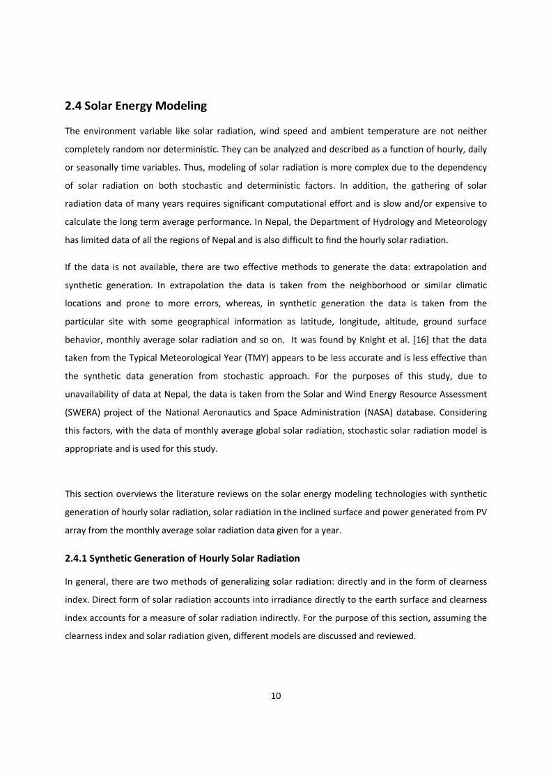
2.4 Solar Energy Modeling
The environment variable like solar radiation, wind speed and ambient temperature are not neither
completely random nor deterministic. They can be analyzed and described as a function of hourly, daily
or seasonally time variables. Thus, modeling of solar radiation is more complex due to the dependency
of solar radiation on both stochastic and deterministic factors. In addition, the gathering of solar
radiation data of many years requires significant computational effort and is slow and/or expensive to
calculate the long term average performance. In Nepal, the Department of Hydrology and Meteorology
has limited data of all the regions of Nepal and is also difficult to find the hourly solar radiation.
If the data is not available, there are two effective methods to generate the data: extrapolation and
synthetic generation. In extrapolation the data is taken from the neighborhood or similar climatic
locations and prone to more errors, whereas, in synthetic generation the data is taken from the
particular site with some geographical information as latitude, longitude, altitude, ground surface
behavior, monthly average solar radiation and so on. It was found by Knight et al. [16] that the data
taken from the Typical Meteorological Year (TMY) appears to be less accurate and is less effective than
the synthetic data generation from stochastic approach. For the purposes of this study, due to
unavailability of data at Nepal, the data is taken from the Solar and Wind Energy Resource Assessment
(SWERA) project of the National Aeronautics and Space Administration (NASA) database. Considering
this factors, with the data of monthly average global solar radiation, stochastic solar radiation model is
appropriate and is used for this study.
This section overviews the literature reviews on the solar energy modeling technologies with synthetic
generation of hourly solar radiation, solar radiation in the inclined surface and power generated from PV
array from the monthly average solar radiation data given for a year.
2.4.1 Synthetic Generation of Hourly Solar Radiation
In general, there are two methods of generalizing solar radiation: directly and in the form of clearness
index. Direct form of solar radiation accounts into irradiance directly to the earth surface and clearness
index accounts for a measure of solar radiation indirectly. For the purpose of this section, assuming the
clearness index and solar radiation given, different models are discussed and reviewed.

11
There are different varieties of stochastic models for predicting solar radiation sequences. Depending
upon the application of models, these models often require many input parameters and produce a large
number of possible outputs. For instance, Aguiar et al. [17] developed a simple method to generate daily
series of global solar radiation from the monthly mean values of clearness index. However, we are
interested in hourly average global radiation on the tilted surface, so only global horizontal radiation
that gives hourly averages were considered.
There are different models developed to estimate global solar radiation data: simple statistics, Fourier
series, Markov Transition Matrix (MTM), Auto Regressive Moving Average (ARMA), Artificial Neural
Network (ANN) and so on. Many of these models are developed for specific geographical locations and
daily global solar radiation instead of hourly radiation sequences due to the complexity in
transformation of hourly sequences.
To expand these models to hourly sequences, Olseth and Skartveit [18] used a clear sky irradiance
model to estimate irradiance from the cloud and sunshine observations, developed an empirical
relationship to find hourly clearness index and used this clearness index to calculate the hourly global
irradiance. Although this model generates hourly global irradiance, it is not appropriate since it requires
atmospheric cloud data and needs stochastic cloud modeling.
Auguiar et al. [17] developed a simple method to generate daily series of global irradiation from the first
order Markov matrices. The only parameter required for this model is monthly mean value of clearness
index. Although this method is proven to be universal to generate new series, it is not suitable since it
generates daily global radiation instead of hourly irradiation.
Lopez and Cardona [19] developed a methodology based on ARMA model to analyze each monthly
series of hourly values and generate new hourly series with similar behavior. This model uses first order
autoregressive model ARMA (1, 0) and first order moving average model (0, 1) for the regular part and
seasonal part. This model is not appropriate as a standard model since it does not give the information
about changing from one location to another.
M. Benghanem et al. [20] developed a hybrid model consisting of artificial neural network and a library
of Markov transition matrices to generate sequences of global solar radiation for Algeria. Although this

12
model requires geographical coordinates of the site with input data latitude, longitude and altitude to
generate solar radiations, these models is not a universal model for changing geographical locations and
is valid only for Algeria.
Dagelman Larry [21] developed hourly weather simulation to model energy in buildings and synthesize a
hourly event using atmospheric transmittance variables. Using the probability distribution curves, he
generated daily events and estimated hourly values. However, his research does not evaluate the
statistical and stochastic features.
Knight et al. [16] developed a stochastic model to generate hourly solar radiation. They calculated the
daily clearness index from a monthly clearness index and arranged this daily clearness index to
predetermined sequences. From the daily clearness index, they calculated the hourly clearness index
using first order autoregressive model. The result showed that distribution of hourly clearness index is
similar to the original clearness index and is validated for changing the geographical location. This model
takes all the parameters into consideration for modeling solar radiation sequences and was chosen as
the model for purposes of this study. The detail of this model is given in section 3.3.2.2.
2.4.2 Inclined Plane Models
It should be noted that the incoming solar radiation has a significant effect on the available energy at
the inclined surface of PV modules. It is necessary to choose the appropriate model to calculate the
radiation on tilted surface.
A number of papers present the approach of global solar radiation on inclined plane model considering
several parameters as direct radiation, diffuse radiation, reflected radiation from the ground surface and
so on. Direct radiation is the radiation received from the sun without having been scattered by the
atmosphere and diffuse radiation is the radiation resulting from clouds, water vapour and other
elements in the area and is a function of cloudiness and atmospheric clarity. Thus, there are many
complex models developed to calculate the global radiation on tilted surface, which are used to
differentiate the diffuse components.
For instance, J.A. Duffie [22] stated in his book that Hottel and Woertz used the combination of diffuse
and ground reflected radiation which is isotropic. In this model, it is assumed that the sum of the diffuse

13
components from the sky and ground-reflected radiation on the inclined surface is the same regardless
of orientation. However, in this assumption it is assumed that all the radiations are considered to be
beam. In addition, the author stated that Liu and Jordan developed an isotropic diffuse model, in which
they considered three components (beam, isotropic diffuse and solar radiation reflected from the
ground). Although this model is the simplest, it gives poor estimates of radiation on an inclined surface.
The author stated that Hay and Mkcay had developed the model for the calculation of the sky
hemisphere. This model is based on the assumptions that diffuse components are split into two
components as isotropic and anisotropic.
Reindl et al. [23] described and compared several models, one isotropic and three anisotropic. They
found that performance of isotropic model was poor and anisotropic models have comparable
performances each other.
Olmo et al. [24] described a model which only requires the global irradiance, and not the direct
irradiance value to calculate the global irradiance on an inclined plane. Although they developed the
model for Granada, Spain, their validation is valid for a variety of conditions.
J.A. Duffie [22] in his book stated that Hay and Davies proposed HDKR model in which Reindl et al. add
horizontal brightening term to the Hay and Davies model. In this model, Isotropic defines the radiation
received uniformly from the entire sky, circumsolar diffuse defines the radiation due to forward
scattering i.e. diffuse radiation emanates from the direction of the sun and horizon brightening defines
the component which emanates from the horizon and more pronounced in clear skies. This model takes
into consideration of timely behavior of radiation and is regarded as a universal model.
Although more models discussed the solar radiation in titled surface, most of the model was not tested
for changing geographical locations. Since HDKR model is simple and is integrated from different models
and produces the results closer to the measured values, it is used for the purposes of this study. The
detailed description of this model is given in section 3.3.2.5.

14
2.4.3 PV Array Models
There are various PV array models found in the literature based on the current voltage characteristics of
photovoltaic modules. Some authors modeled the system considering the dynamic and static electrical
characteristics of the system and some on one or two diode models.
Borowy and Salameh [25] modeled the PV module for average power output with detailed technical
characteristics like module series resistance, number of cells, open circuit voltage, maximum voltage,
short circuit current, maximum current etc... All the precise data of each manufacturer is difficult to find
to use this model.
Markvard [26] modeled the output power from the PV generator in terms of area of a single module,
instantaneous PV generator efficiency, global irradiance incidence on the tilted plane and number of
modules. This model does not consider other technical factors like open circuit voltage, short circuit
current, maximum current and maximum voltage of PV panels and assumes all the losses to be zero.
Yang et al. [27] proposed the PV array model consisting of five parameters as series resistance, non
linear temperature voltage effects, nonlinear effects of the photocurrent, PV module dimensionless
coefficient and maximum power point tracking efficiency. In order to calculate the output power from
PV modules, the dynamic behavior of the systems has to be calculated and this data is not available in all
the technical datasheets of manufacturers.
Bajpai et al. [28] used one diode equivalent circuit model which considers series and parallel resistance,
reverse saturation current of diode, peak voltage and current of PV panels. This type of model is used
for cell base analysis and since this model needs to calculate the parallel resistance, it is extremely
complex to use.
Lasnier and Ang [29] defined the current voltage relationships based on the electrical characteristics of
the PV panel as short circuit current, maximum current, maximum voltage, open circuit voltage.
Although this is the simplest model based on maximum power point tracker (MPPT), it is not widely
used and not tested for validity.

15
Nikraz et al. [30] used four parameters to model the electrical characteristics of the PV panel in a similar
to that used by Lasnier and Ang [29]. The result showed that this model is validated for analysis of PV
characteristic and best for single crystal and polycrystalline PV arrays.
For the purposes of this study, four parameters model based on Nikraz et al. [30] is used since this
model takes static characteristics which is validated and widely used by various simulation software.
Although this model is appropriate, it does not consider the effect of nocturnal operating cell
temperature. So, in this study, PV cell operating cell temperature is calculated from method proposed
by the J. A. Duffie [22]. The detailed description of this model is given in section 3.3.2.6.
2.5 Wind Energy Modeling
The behavior of wind speed during a year is indispensable for the simulation and modeling of hybrid
Solar/Wind energy systems. Since, the hourly wind speed data is difficult to find, it needs to be
synthetically generated in a manner that resembles the pattern of the original location.
This section describes the models available for synthetic generation of hourly wind speed and accurate
wind turbine power from the monthly average wind speed data given for a year.
2.5.1 Synthetic Generation of Hourly Wind Speed
There are various stochastic, probabilistic and deterministic methods found in the literature to generate
hourly mean wind speed data with the same characteristics of wind resources, namely autocorrelation
over time. Most of the papers present Auto Regressive Moving Average (ARMA), Markov transition
matrices, artificial neural network, deterministic and stochastic models and so on. This section reviews
several literatures to generate synthetic hourly wind speed.
Degelman Larry [21] used a Monte Carlo method to generate hourly wind speed data which includes
stochastic models. The simulating results were applied for performance of building thermal loads and
annual energy consumption. He stated that wind speed plays a minor role in the energy of the buildings,
so, only stochastic model is useful for synthetic generation of hourly wind speed. Since, in the hybrid
system, wind plays a major role, this method of using stochastic model is not favorable.
Bellington et al. [31] used both a simple autoregressive model and a combined ARMA model for wind
speed and presented the useful and reasonable results. However, this model is based on normally
distributed sequences, since wind is not a normally distributed sequence.

16
Shamshad et al. [32] used a transition matrix approach of the Markov chain process to generate hourly
wind speed from time series data of two meteorological stations of Malaysia. Their result showed that
observed wind speed and synthetically generated ones shows the same statistical characteristics.
However, they do not assess the adequacy of general model for varying geographical locations.
Hafzullah et al. [33] used a different methodology to generate the hourly wind speed sequences. This
methodology was based on a wavelet transformation approach and used four years of meteorological
data from Diyarbakir station in Turkey and was compared with first order Markov chain. Although their
model produces similar results to Markov chain model of particular station, they do not generalize the
model for changing geographical location.
Hans et al. [34] proposed a Shinozuka method for synthetic hourly annual time series wind speed data
from the monthly average of mean wind speed based on spectral power density of wind speed data. The
result showed the similar hourly pattern of the original wind speed generation. However, they do not
validate the model for changing the geographical locations.
HOMER [35] uses stochastic modeling and deterministic models to generate the hourly wind speed
sequences. It uses diurnal cosine wave pattern and first order autocorrelation as a deterministic model.
It uses its own algorithm for the probability transformation of the diurnal pattern to the stochastic
patterns and methodology of probability transformation is more complex.
Based on the literature review it is well known that the stochastic model used by Degelman Larry [21]
takes no consideration of diurnal pattern and autocorrelation of hourly wind speed and the HOMER [6]
probability transformation of the diurnal pattern to the stochastic pattern is more complex. Considering
the above factors and since the stochastic model used by Degelman Larry [21] and the deterministic
model developed by HOMER [35] are simple and widely used, these models are taken for the purposes
of this study. The details of this are described in section 3.3.3.1.
2.5.2 Wind Turbine Models
Basically there are two types of wind turbines as Horizontal axis wind turbine (HAWT) and Vertical axis
wind turbine (VAWT). Today, most of the system uses horizontal axis systems since in this type of
configuration the total swept area by the blades is greater than the actual blade area and can be
mounted on tower to achieve higher wind resources. So, only HAWT technology is considered in this
section. There are several factors that determine the output power from the wind turbine: the power

17
output curve as a function of aerodynamic power efficiency, mechanical transmission and electrical
energy conversion efficiency, wind speed distribution of the selected sites and the hub height of the
wind tower.
This section describes different literature reviews on these factors: power output curve, wind speed
distribution and wind height adjustment.
Power Output Curve
The power output curve plays a significant role in the extraction of energy from the wind turbine. There
are several existing models to estimate the wind turbine power such as- linear, cubic, quadratic, Weibull
parameters and so on.
Borowy and Salameh [25] used the Weibull parameters to calculate the output power from the wind
turbine. Since the information about Weibull parameters is required for specific site, it is not widely
used.
Bueno and Carta [36] used a linear approximate model to determine the power generated by the wind
turbine in which the output power from wind turbine is expressed in terms of reliability factor and a
wake factor, which increases complexity to determine the variables.
Lin Lu et al. [37] used the quadratic equations and Weibull shape parameters # to calculate the average
power from the wind turbine. Since this model also requires the site specific information of Weibull
shape parameters, it is not widely used.
Hocaoglu et al. [38] defined the output of wind turbines in terms of interpolation of values of the data
provided by the manufacturer. This model approximated the power cube law using cubic spline
interpolation in which the wind turbine characteristics is separated into four sub-functions and modeled
using a piece-wise cubic polynomial fit. This model is complex to find the polynomial coefficients and is
not widely used because of its complexity.
Chou and Corotis [39] used a quadratic model which is generalized for any system without site specific
information and is widely used. This model approximates the output power generated from wind
turbine for any wind speed distributions.
18
For the purposes of this study, Chou and Corotis model [39] is used since it is simple and widely used
and does not required more specific information about the power characteristics curve and Weibull
shape parameters. The detail of this model is described in section 3.3.3.2.
Wind Height Adjustment
The variation of height effects the assessment of the wind resources and in the design of wind turbines.
There are generally two mathematical models used to model the wind turbine over the homogeneous
regions and flat terrain. First approach is the log law which considers boundary layer characteristics for
wind height adjustment. The second approach is the power law which is the simplest model for vertical
wind speed and is widely found in the literature. For the purposes of this study, the power law is
applied. The detail of this model is described in section 3.3.3.2.
Wind Speed Distributions
The wind energy potential at the site depends on the characteristics of wind resources. The wind
resources characteristics are defined by the several probabilistic functions as Weibull distribution,
Rayleigh distribution, exponential distribution, gamma distribution, logistic distribution and so on by
fitting field data with the standard mathematical functions. However, Weibull and Rayleigh distribution
is widely used and is thus discussed in this section. Both Weibull and Rayleigh distributions are used to
characterize the wind resources in terms of its probability distribution and cumulative distributions.
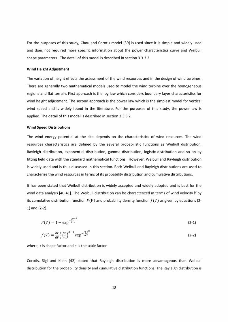
It has been stated that Weibull distribution is widely accepted and widely adopted and is best for the
wind data analysis [40-41]. The Weibull distribution can be characterized in terms of wind velocity � by
its cumulative distribution function �(�) and probability density function �(�) as given by equations (2-
1) and (2-2).
�(�) = 1 − expKLMNOP (2-1)
�(�) = QRQS TU LSUOTKV expKLMNOP (2-2)
where, k is shape factor and � is the scale factor
Corotis, Sigl and Klein [42] stated that Rayleigh distribution is more advantageous than Weibull
distribution for the probability density and cumulative distribution functions. The Rayleigh distribution is

19
validated for long term wind data from many sites and provides considerable fit with observed wind
velocity and power histogram.
Rayleigh distribution is the simplest version of the Weibull distribution in which the shape parameter is
equal to 2. It is widely used since it requires only the average data and does not require shape
parameters information. The American Wind Energy Association has also recommended Rayleigh
distribution for assessment of wind energy potential. Hence, for the purpose of this study, Rayleigh
distribution is used to characterize the wind resources. The detail is described in section 3.3.3.2.
2.6 Temperature Modeling
This section describes the synthetic generation of hourly temperature from the given monthly average
temperature of a year. Since the effect of temperature affects the output power of PV cells in very small
amount, the temperature modeling is briefly discussed with few literature reviews.
There are various literature reviews on predicting hourly generation of temperature data from the
collection of large number of data from weather stations and uses several methodology as Auto
Regressive Moving Average (ARMA), Markov transitions matrices, Artificial Neural Network (ANN) etc..
However, these methodologies require collection of large number of data of several years and hourly
transformation is also complex. There are few literatures on generation of hourly temperature from the
monthly average temperature and some of them are reviewed.
Imran et al. [43] proposed artificial neural networks for the prediction of hourly mean values of ambient
temperature for the coastal location of Jeddah, Saudi Arabia. It required only one temperature value as
input to predict the temperature for the following day for the same hour. Although the result showed
the similar behavior of the original profiles, this model is not validated for changing geographical
locations.
Knight et al. [16] used stochastic and diurnal models to generate hourly temperature from the monthly
average temperature of a year. The author first generated daily stochastic temperature and again by a
Gaussian random variable and transformed it into a temperature value through the cumulative
distribution function. The author then used diurnal variation for the mean value distribution of
temperature for each hour of the day. The result showed that the stochastic method described by the

20
author does not replicate the original characteristics from the monthly average daily temperature values
for all the places.
Degelman Larry [21] used a Monte Carlo method to generate hourly weather data which includes both
deterministic and stochastic models and applied the simulating results for performance of building
thermal loads and annual energy consumption. His model is validated for the changing geographical
locations according to diurnal pattern and is used widely for the simulation of energy in buildings.
Degelman Larry [21] takes all the parameters into consideration and his method is suitable for the
purposes of this study to generate synthetic temperature profiles from the monthly average
temperature of a year. The detail of the models is described in section 3.3.4.
2.7 Storage Modeling
For any hybrid renewable energy systems, there is excess and deficit of energy at any instant of time. If
the renewable resources system produces excess energy than the power demanded by the load, the
extra energy should be stored. Also, if the renewable resources system produces less energy than the
power demanded by the load, then storage system should satisfy the load. So, storage system is
indispensable for any renewable energy stand-alone systems.
There are various storage technologies to store the energy from renewable sources such as batteries,
compressed air, hydrogen combined with fuel cells and electrolysers as well as flywheels. This section
reviews the literature on these storage technologies and identifies the reliable and justified storage
model for the hybrid solar and wind energy standalone systems.
Lu Aye et al. [44] used a hydrogen storage technology for the technical feasibility and financial analysis
of hybrid solar wind system for Cooma, Australia. Although the results were technically viable, it shows
that fifty two percent of the total project cost was due to the electrolyser, which is quite expensive.
Nelson, Nehrir and Wang [45] used combination of fuel cell stack, an electrolyser and hydrogen storage
tanks as an energy storage system for the hybrid PV and wind standalone systems. They presented the
comparison with battery, fuel cell and electrolyser. The results showed that battery system is still
superior than fuel and electrolyser system even though fuel and electrolyser has zero capital cost.

21
Kamaruzzaman et al. [46] studied the performance of a PV-wind hybrid system for hydrogen production.
Although the results demonstrated feasible and reliable solution through hydrogen storage, the
improvements on the fuel cell stacks assemble still remain to avoid hydrogen leak.
Vanhanen and Lund [47] used a hydrogen storage system model to improve the performance of the
overall energy system. This model requires 25 parameters to evaluate more than the 50 equations and is
complex to analyze.
Wei, Hongxing and Zhaohong [48] modeled the battery of the system considering several characteristics
as current rate, charging efficiency, self-discharge rate, state of charge, floating charge voltage and
battery life time. Although this model provides reliable output, it requires detail technical characteristics
of the battery which results complexities. Moreover, the methodology for finding floating voltage is
complex since it computes the different coefficients of the battery during charging and discharging
mode using second degree polynomial equations.
Belfkira, Zhang and Barakat [49] modeled the hybrid solar/wind energy systems with battery storage.
This model uses state of charge condition of the battery and does not require details technical
characteristics to calculate the coefficients of battery as open circuit voltage, internal resistance and so
on as Zhou et al. The result showed that this model is technically and economically viable.
Based on the above literature review, fuel cell and electrolyser are not economically justified technology
for the design of hybrid solar wind energy technology. Furthermore, proton exchange membrane and
maintenance cost of such membranes are higher in fuel cells and storage of hydrogen is difficult as well.
It justifies that battery storage should be used for less economical hybrid system and for the purposes of
this study, Belfkira, Zhang and Barakat [49] model is used since it is both technically and financially
justified and does not require complex calculations. The detail is given in section 3.3.5.
2.8 Power Reliability Modeling
The optimal sizing of hybrid system which meets the load demand is evaluated based on the power
system reliability and system life cycle cost. The optimal solution of hybrid system can be best
compromise with power reliability and system cost. The higher the power reliability, the higher will be
the system cost and vice versa. There are various methods to calculate the reliability of the hybrid
systems such as loss of load probability (LOLP), loss of power supply probability (LPSP), system
performance level (SPL), loss of load hours and so on. This section gives an overview of literature

22
reviews on technical reliability and identifies the best model for the optimal sizing of hybrid solar wind
energy in standalone system.
Gomaa, Seoud and Kheiralla [50] used the least-square method for the design and analysis of hybrid
solar and wind energy systems in Alexandria, Egypt. The method used to meet the power reliability i.e.
excess power and the power deficiency of the systems is based on statistical analysis. Although the
result provided significant output, these methods are more prone to error while calculating one hour
time step during a year since it requires calculating the mean square deviation of the output.
Bagul, Salameh and Borowy [51] used new techniques of three event probability density for the optimal
sizing of the hybrid solar wind energy systems and based on loss of load probability. The result showed
that three event approximation increases the accuracy of the system sizing without any significant
increase in the effort and time consumed for computation is lower. However, the result showed the
daily surplus energy distribution instead of hourly distributions which is the concern of this study.
Deshmukh et al. [52] modeled the hybrid renewable energy system based on loss of load probability
(LOLP). The result showed that if LOLP is low then it results in high cost of the system and vice versa.
Although the result is significant in analyzing the power reliability, the computation of statistical
parameter as coefficient of variance, confidence level etc… results errors in the hybrid energy system.
Tina and Gagliano [53] performed the reliability analysis of hybrid solar/wind power system using the
energy index reliability (EIR), which is related to the energy expected not supplied (EENS). The result
showed the good measurement of reliability index for hybrid system in grid connected system, however,
this method does not explain about the application in standalone system. The computation of EENS
parameters, moreover, is complex.
Diaf et al. [54] used the LPSP concept to find the optimal configuration of the hybrid solar/wind energy
systems. This result showed the feasible choices in the cost reduction as well as energy production with
simple computation.
Since both solar and wind energy is intermittent in nature under the varying atmospheric conditions and
the telecommunication load for the purposes of this study is constant for two different intervals i.e. half
load and full load, the reliable power supply design is best suitable analysis for the purposes of this
study. Considering this factor, Diaf et al. [54] LPSP model is used for the purposes of this study since it is
simple to compute. The detail of the method is explained in Chapter 3 of section 3.3.6.

23
2.9 System Cost Modeling
The economic analysis of hybrid energy system is essential to know whether the system is affordable to
produce unit price of power and to find the optimal configuration based on minimum cost. There are
several economic measurements to know the system to be feasible or not: Return on Investment,
Payback Period, Cost Benefit Analysis, Net Present Cost, Levelized Cost of Energy and so on. This section
outlines the literature reviews by different authors and identifies the suitable economic model for the
optimum design and analysis of hybrid solar wind energy in standalone system.
Ekren et al. [55] used the net present value method for the economic analysis of autonomous hybrid
energy system to supply power for a global system for mobile communication base station (GSM) at
Turkey. Although the results produced proper sizing of systems, it does not consider inflation rate and
time value of money which is one of the important criteria of economic analysis.
Yang et al. [3] proposed the hybrid solar wind energy system to supply power for a telecommunication
relay station using annualized cost of the system at remote Dalajia Island in China. The result showed
that the economic approach of annualized cost of system provides good analysis in system cost in the
hybrid solar wind energy systems. However, the used method does not include the time value of money
for the whole project span.
HOMER [35] uses life cycle cost method using net present value for the economic analysis of any
renewable energy system and assumes that all the cost to be real. This method moreover takes the real
(inflation-adjusted) interest rate instead of nominal interest rate and assumes the prices to be constant
during the project span which may not be realistic.
Bakos and Tsagas [56] presented the economic analysis of hybrid solar/wind grid connected system
based on life cycle savings method for a typical residence in the Greece. This method is based on
increasing mortgage payments and decreasing fuel costs thus resulting in savings in cost of energy.
Although this method considers time value of money and allows detailed consideration of complete
cost, it is difficult to analyze the saving of energy which considers only the renewable energy sources.
Reichling and Kulachki [57] performed the analysis of a hybrid wind-solar power plant in Minnesota. The
result provided the unit cost of energy generation from the hybrid solar-wind system and proved that
levelized cost of energy is a useful tool in the economic analysis for the electrical generation of the
hybrid energy systems.

24
Kaabeche, Bellamel and Ibtiouen [58] used levelised unit electricity cost for the economic analysis of
hybrid photovoltaic wind power generation system using a battery bank in Bouzareah, Algeria. They
mentioned that the levelised unit electricity cost is the best indicator of economic profitability of system
cost analysis and is used widely for commercial projects.
The levelized cost of energy is used to test whether the unit electricity cost production is appropriate or
not. Based on the above conclusion, levelized cost of energy used by [58] is the most suitable model for
the economic analysis of hybrid solar wind energy system and is considered as the economic model for
purposes of this study. Section 3.3.7 provides the details concerning this method.
2.10 Optimization Techniques
With the increase in number of optimization variables, the number of simulations also increases
exponentially which takes more time and effort for the computation. Thus, it is necessary to find the
optimal system configuration quickly and accurately using feasible optimization techniques. There are
various optimization techniques used by the different authors for the design of HSWPS such as graphical
construction methods, linear programming, probabilistic approach, iterative approach, genetic
algorithm, artificial neural network methods and so on. Whichever the optimization method, the
objective of each designer is to find the best optimal value for a given configuration. This section
reviews the literature on the optimization techniques and identifies the suitable and simpler techniques
to find the optimal solution of HSWPS.
Borowy and Salameh [25] proposed the graphical construction techniques for the optimal sizing of
hybrid wind/PV system for a load demand in house of Massachusetts. The objective function of the
system is to minimize the system cost for a desired LPSP and it is assumed that total cost of the system
is linearly related to both the number of PV array and batteries. The optimum configuration is achieved
for a minimum cost function which is the point of tangency of the curve drawn from the relationship
between the number of PV array and the batteries. The proposed model considers only two parameters
(PV and battery) and does not take into number of wind turbine as an optimization variables. Also, there
is tendency of errors in the optimal solution due to graphical construction techniques.
Chedid and Rehman [59] designed and sized the hybrid solar wind energy system with batteries storage
using linear programming. The objective function of the system is to minimize the system total cost
function which comprises initial and operation & maintenance cost.

25
Yang, Lu and Zhou [60] proposed the sizing methodology of hybrid PV wind power system using iterative
optimization techniques. The used method is based on LPSP concept for the selection of PV array, wind
size and battery to meet the load demand and uses iterative process to minimize the system costs.
Yang et al. [3] proposed the hybrid solar wind energy system to power a telecommunication relay
station using genetic algorithm. They mentioned that that genetic algorithm is the best suitable method
of optimization in finding global optimal solutions, particularly in multi-modal and multi-objective
optimization problems.
Belfkira et al. [61] proposed the optimal sizing of hybrid renewable energy system using deterministic
algorithm. The method proposed was based on dynamic evaluation of the wind and solar energetic
potential. The objective function of the system is to minimize the life cycle costs of the hybrid systems.
Banu and Orhan [5] proposed the optimal sizing of hybrid solar and wind energy system with battery
storage using response surface methodology (RSM) optimization techniques for mobile communications
(GSM) base station at Urla, Turkey. They mentioned that RSM is the statistical and mathematical
method used to characterize the system cost for a given time-varying hourly energy load in which the
optimum parameter sizes leading to the minimum life cycle cost can be obtained graphically. The sizing
method obtained for wind and PV energy in terms of wind turbine rotor swept area and PV area
respectively is not the most appropriate sizing optimization technique since it does not consider the
power rating of the system.
For the purposes of this study, Iterative Approach is used as an optimization technique which is simple
to model and the output result produced by it is similar to the new evolved optimization techniques as
artificial neural network methods and genetic algorithm. Although this technique takes more time to
compute and simulate the results in comparison to the new evolved optimization techniques, it is also
widely used. The detailed description is given in section 3.3.8.

26

27
Chapter 3
Methodology
This chapter outlines the methodology applied to carry the feasibility assessment and the optimal design
of HSPWS for the remote telecommunication station. In the remote areas, the meteorological data is
hardly available, so, this dissertation gives an overview of methodology for the optimal design of HSWPS
with limited meteorological information.
The first step of the methodology is the feasibility assessment and HOMER is chosen as the appropriate
software for the feasibility analysis. Input and sensitivity variables are provided as an input to the
HOMER.
The second step of the methodology is to generate the synthetic hourly solar radiation, wind speed and
temperature profile from the monthly average meteorological data so that it produces a realistic output
for the simulation and analysis of HSWPS. For the synthetic generation of solar radiation, Knight Hourly
Irradiance Model is taken which synthesizes the monthly average clearness index into hourly clearness
index. Degelman Stochastic and HOMER Deterministic Model are used to generate the synthetic hourly
wind speed from the monthly average wind speed, diurnal pattern strength and hour of peak wind
speed from the meteorological data. The synthetic generation of hourly temperature profiles, moreover,
uses Degelman Stochastic and Deterministic model.
The third step of the methodology is to produce the power generated from the solar and wind energy
system. The appropriate PV array model and Wind Turbine model is chosen to produce the power
generated from these renewable sources. For the effective conversion of horizontal solar radiation into
the inclined surface of PV panels, HDKR Model is chosen. The tilted solar radiation is converted into
electrical power using PV Array Model which takes technical data to produce the results. The power
generated from the wind turbine depends on several characteristics such as wind speed distribution,
wind measurement height, geographical boundary of the site, turbine model and so on. Chou and
Corotis wind turbine model is used to represent the turbine model. The wind height adjustment is

28
characterized by the power law and the wind speed distribution is represented by the Rayleigh
distribution.
The fourth step of the methodology is to model the load. Although this dissertation work represent the
general model for solar and wind energy system, the load model is not characterized as a general model
since the load in telecommunication networks depends on several technical factors. The dissertation
assumes that the load on the remote telecommunication station encompasses the several remote relay
stations, VSAT and BTS. The power consumption by this equipment depends on the bandwidth of
transmitting and receiving signals and the overall traffic. It is complex to model power consumption
considering detail technical factors since the traffic used by these station depends on radio switch rate,
TCH traffic rate, call drop rate, RLC packet channel uplink and downlink rate, GPRS uplink and downlink
rate and so on. The load is modeled based on the traffic scenario of telecommunication services and for
the purposes of this work, load is modeled on the basis of case study remote station power
consumption.
The fifth step of the methodology is to model the battery. At each hourly time step, sometimes, the
power generated by the renewable resources is higher and lower than the power demanded by the
load. If the power generated by the renewable sources is higher than the power demanded by the load,
then surplus power is to be stored in the battery. Sometimes while charging the battery, the battery
capacity may be full, in this case, the waste energy should be transferred to a dummy load. If the power
generated by the renewable sources is lower than the power demanded by the load, deficient power is
to be supplied from the battery. While discharging energy from the battery, the battery may be drop to
the minimum capacity. Since minimum capacity cannot be reached, these steps need to be considered
while modeling the battery as illustrated in section 3.3.5.
The sixth step of methodology is to analyze the HSWPS based on reliability and economics. The higher
the reliability, the higher the system costs. The reliability is measured in terms of whether the power
generated by the renewable energy system meets the load or not and is best described in terms of LPSP.
The system cost model considers the unit cost of the energy generated by this renewable energy to
measure whether the desired unit production of electricity is economically viable or not.
Finally an iterative optimization technique is used to find the optimal solution of sizing the appropriate
technologies from different manufacturers which meet the desired reliability with minimum cost
function.
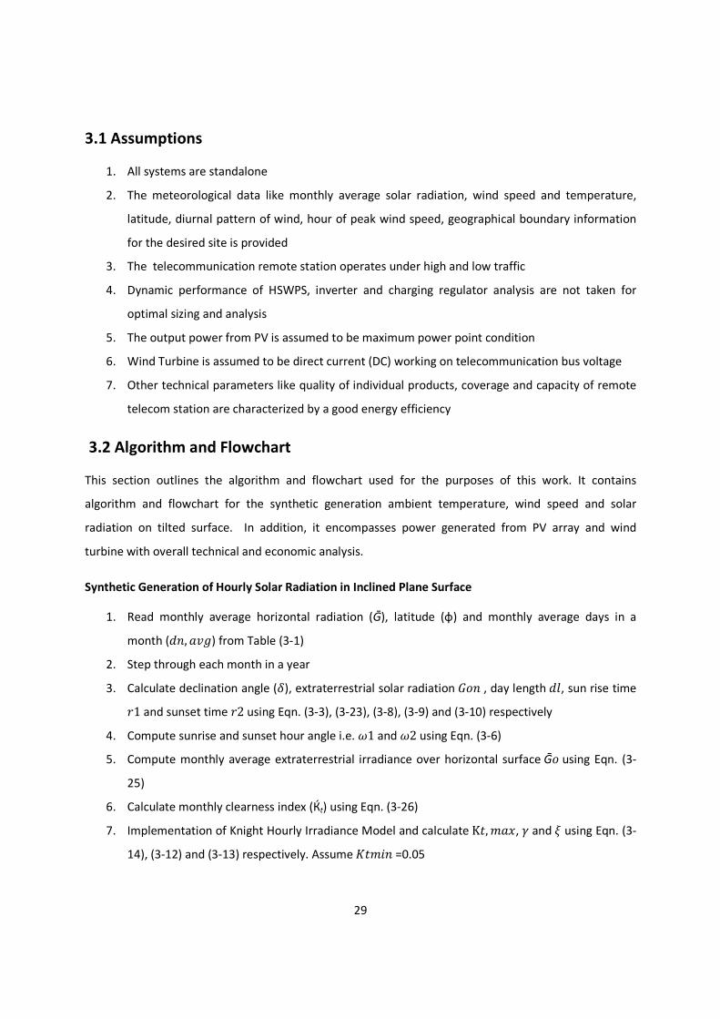
29
3.1 Assumptions
1. All systems are standalone
2. The meteorological data like monthly average solar radiation, wind speed and temperature,
latitude, diurnal pattern of wind, hour of peak wind speed, geographical boundary information
for the desired site is provided
3. The telecommunication remote station operates under high and low traffic
4. Dynamic performance of HSWPS, inverter and charging regulator analysis are not taken for
optimal sizing and analysis
5. The output power from PV is assumed to be maximum power point condition
6. Wind Turbine is assumed to be direct current (DC) working on telecommunication bus voltage
7. Other technical parameters like quality of individual products, coverage and capacity of remote
telecom station are characterized by a good energy efficiency
3.2 Algorithm and Flowchart
This section outlines the algorithm and flowchart used for the purposes of this work. It contains
algorithm and flowchart for the synthetic generation ambient temperature, wind speed and solar
radiation on tilted surface. In addition, it encompasses power generated from PV array and wind
turbine with overall technical and economic analysis.
Synthetic Generation of Hourly Solar Radiation in Inclined Plane Surface
1. Read monthly average horizontal radiation (Ḡ), latitude (ɸ) and monthly average days in a
month ( , ��2) from Table (3-1)
2. Step through each month in a year
3. Calculate declination angle (@), extraterrestrial solar radiation �� , day length �, sun rise time �1 and sunset time �2 using Eqn. (3-3), (3-23), (3-8), (3-9) and (3-10) respectively
4. Compute sunrise and sunset hour angle i.e. E1 and E2 using Eqn. (3-6)
5. Compute monthly average extraterrestrial irradiance over horizontal surface Ḡ� using Eqn. (3-
25)
6. Calculate monthly clearness index (Ќt) using Eqn. (3-26)
7. Implementation of Knight Hourly Irradiance Model and calculate K�, !�", D and X using Eqn. (3-
14), (3-12) and (3-13) respectively. Assume ��!� =0.05
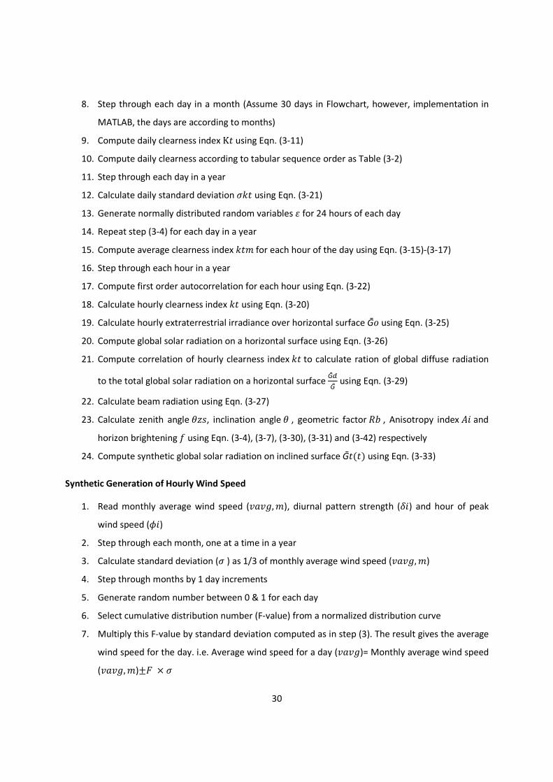
30
8. Step through each day in a month (Assume 30 days in Flowchart, however, implementation in
MATLAB, the days are according to months)
9. Compute daily clearness index K� using Eqn. (3-11)
10. Compute daily clearness according to tabular sequence order as Table (3-2)
11. Step through each day in a year
12. Calculate daily standard deviation A#� using Eqn. (3-21)
13. Generate normally distributed random variables B for 24 hours of each day
14. Repeat step (3-4) for each day in a year
15. Compute average clearness index #�! for each hour of the day using Eqn. (3-15)-(3-17)
16. Step through each hour in a year
17. Compute first order autocorrelation for each hour using Eqn. (3-22)
18. Calculate hourly clearness index #� using Eqn. (3-20)
19. Calculate hourly extraterrestrial irradiance over horizontal surface Ḡ� using Eqn. (3-25)
20. Compute global solar radiation on a horizontal surface using Eqn. (3-26)
21. Compute correlation of hourly clearness index #� to calculate ration of global diffuse radiation
to the total global solar radiation on a horizontal surface ḠQḠ
using Eqn. (3-29)
22. Calculate beam radiation using Eqn. (3-27)
23. Calculate zenith angle 56�, inclination angle 5 , geometric factor /� , Anisotropy index �� and
horizon brightening � using Eqn. (3-4), (3-7), (3-30), (3-31) and (3-42) respectively
24. Compute synthetic global solar radiation on inclined surface Ḡ�(�) using Eqn. (3-33)
Synthetic Generation of Hourly Wind Speed
1. Read monthly average wind speed (���2, !), diurnal pattern strength (@�) and hour of peak
wind speed (7�)
2. Step through each month, one at a time in a year
3. Calculate standard deviation (A ) as 1/3 of monthly average wind speed (���2, !)
4. Step through months by 1 day increments
5. Generate random number between 0 & 1 for each day
6. Select cumulative distribution number (F-value) from a normalized distribution curve
7. Multiply this F-value by standard deviation computed as in step (3). The result gives the average
wind speed for the day. i.e. Average wind speed for a day (���2)= Monthly average wind speed
(���2, !)±� × A

31
8. Compute hourly average wind speed (��) using Eqn. (3-48)
9. Calculate autocorrelation factor during a year using Eqn. (3-50)
10. Compute autocorrelation numbers for a year using Eqn. (3-49)
11. Generate hourly synthetic wind speed (���2, ℎ) using adding results from step 8 and 10
Synthetic Generation of Hourly Temperature
1. Read monthly average temperature (���2, !), diurnal hour of maximum temperature (3pm as
case study)
2. Step through each month one at a time in a year
3. Calculate standard deviation (A ) as 1/3 of monthly average temperature (���2, !)
4. Step through months by 1 day increments
5. Generate random number between 0 & 1 for each day
6. Select cumulative distribution number (F-value) from a normalized distribution curve
7. Multiply this F-value by standard deviation computed as in step (3). The result gives the average
temperature for the day. i.e. Average temperature for a day (���2, )= Monthly average
temperature(���2, !)±� × A
8. Step through each day in a year
9. Compute declination angle (δ) using Eqn. (3-3), day length ( �) using Eqn. (3-8), sunrise time (�1)
using Eqn. (3-9)
10. Calculate standard deviation (A ) for that day as 1/3 of daily average temperature (���2, )
11. Step through 24 hours day in 1 hour steps
12. For each hour, step exactly the same procedure from steps (5-7) for each hour except
multiplying F-value by daily average temperature (���2, ) from step 7. i.e. result will be
average temperature for each hour (���2, ℎ)
13. Compute minimum temperature (�!�) at each sunrise time and maximum temperature
(�!�") at given diurnal temperature (3pm) for each day
14. Compute hourly average temperature (�(�) using Eqns. (3-64) – (3-66) at different time intervals
Power Generation from PV Array
1. Read synthetic solar radiation on inclined surface Ḡ�(�) and synthetic temperature �(�)
2. Read technical database of the components as nominal voltage (��!), maximum Current
(�!�"), maximum voltage (�!�"), short circuit current (���), open circuit voltage (���),

32
Nocturnal operating cell temperature ()+��), temperature coefficient for short circuit current :, ��� and temperature coefficient for open circuit voltage :, ��� from different manufacturer
3. Step through each time step for a year
4. Step through each n number of technical configurations
5. Calculate PV panel operating temperature using Eqns. (3-42)-(3-43)
6. Compute power generated by PV array ('�(�)) using four parameter model applying Eqns. (3-
35)-(3-46)
Power Generation from Wind Turbine
1. Read synthetic wind speed (���2, ℎ), height of projected wind speed (ℎ), and reference height
of wind speed measured (ℎ�) in meters.
2. Read technical database of the components as cut-in wind speed (���), cut-out wind speed
(���), rated wind speed (��) and rated power (�) from different manfuaactuer
3. Step through each time step for a year
4. Step through each technical configurations
5. Compute hourly average wind speed at reference height (�) using Eqn. (3-56)
6. Compute hourly average power generated by wind turbine ('�(�)) using Eqn. (3-63)
Operation Simulation and Optimization
1. Read power generated by PV array '�(�), wind turbine '�(�) and load '&(�)
2. Initialize the minimum and maximum number of battery, PV array and wind turbine
3. Read technical database of components from different manufacturer
4. Step through each number of technical configurations
5. Step through the minimum number of wind turbine and battery
6. Calculate number of batteries in series )*��, � ; ��!�; ��!�"
7. Step through minimum number of PV array
8. Step through each time steps
9. Check if the power generated by renewable sources is greater or equal to load demand. If it is
greater, calculate the state of charge of the battery storage using Eqn. (3-68) and check if it is
greater than maximum state of charge ((+�!�"). If energy content in the battery is greater
than (+�!�", calculate the waste energy using Eqn. (3-75), else loss of power supply (&'() is
zero. Else, calculate the state of charge during discharging using Eqn. (3-69). Check during the

33
discharging process, if the minimum state of charge ((+�!�) is reached or not. If the minimum
state of charge ((+�!�) of the battery is greater than energy during discharging, calculate LPS
using Eqn. (3-76), else LPS=0
10. Check if the time step of simulation is completed or not, if not repeat the process from step 8
else calculate the loss of power supply probability (LPSP) using Eqn. (3-77)
11. Calculate renewable energy contribution /�(�) and excess energy percentage ���(�) using
Eqn. (3-78) and (3-79) respectively
12. Calculate the net present cost of the individual configurations and levelized unit electricity cost
(&0��) using Eqns. (3-80)-(3-83)
13. Store the configurations
14. Check the desired &'(' for analysis from store configurations. Neglect the configurations that
does not meet desired &'('
15. Define the cost function consisting reliability and &0�� (e.g �� = 0.6 /-��������^ + 0.4 &0��)
16. Check the configurations that meets &'(' requirement with minimum cost function
17. The minimum cost function gives the optimal configuration of HSWPS

34
, ��2
Read Ḡ, ɸ
Ḡ� = 12a × �� b���7 ���@ ((�E2 − (�E1) + a (E2 − E1)180 (�7 (�@d
#� = Ḡ
Ḡ�
@ = 23.45 �� b360( + 284)365 d
�� = ��� B� = ��� g1 + 0.33 ��� 360 365 h
� = iVj × ��� -1(−��@ ��∅) ; �1 = (12 − Qli ); �2 = (12 + Qli )
E = (�� − 12 ℎ�) × 150 /ℎ� ;E1; E2
l=1
D = −1.498 + 1.184ξ − 27.182exp(−1.5ξ)K�, !�" − K�, !�
X = K�, !�" − K�, !�K�, !�" − Ќ�
K�, !�" = 0.6313 + 0.267Ќ� − 11.9 (Ќ� − 0.75)o ; ��!� = 0.05
d==
30? � = exp(γK�, !�) − exp(γK�)exp(γK�, !�) − exp(γK�, !�")
d=1
d=d+1 D
No
E
Fig. 3-1: Flowchart for synthetic generation of hourly solar radiation on inclined surface

35
Generate random variable B
Calculate@, ��, �, �1, �2, E2, E1
m=1
A#� = 0.1557 �� g aK�0.933h
Compute K� using table (3-2)
� = 0.409 + 0.5016 sin(E� − 60)
� = 0.6609 + 0.4767 sin(E� − 60)
#�! ≈ �� �� tuvu ; �� = (wxyUuz{)vutu
Ḡ = Ḡ + Ḡ�
9� = 71 9� − 1 + B
#� = #�! − A#�1.58 � | 10.5 }1 + erf g χ√2h� − 1�
t=1
Compute Ḡ�, #�
D
F
G
H

36
Compute ḠQḠ
correlation
���56� = (�@ (�∅ + ���@ ���∅
���5 = (�@ (�7 ���8 − (�@ ���7 (� 8 ���C� + ���@ ���7 ���8 ���E + ���@ (�7 (�8 ���C� ���E + ���@ (�8 (�C� (�E
/� = �uz��uz��z; �� = ḠyḠu; � = √Ḡy
Ḡ
Ḡ� = �Ḡ� + Ḡ ��� /� + Ḡ �1 − ��� �1 + ���8�2 }1 + �(�� g82h� + Ḡ �2 g1 − ���82 h t=24?
m=365?
l=12?
t=t+1
m=m+1
l=l+1
F
G
H
E
Synthetic solar radiation generation in titled surface (Ḡ����)
No
No
No
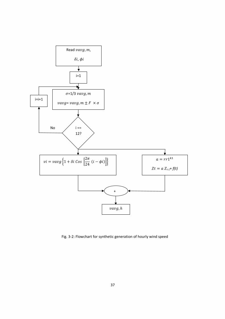
37
i=i+1
Read ���2, !,
@�, 7�
i=1
� = ��1TV
4� = � 4t-1+ f(t)
i ==
12?
+
A=1/3 ���2, !
���2= ���2, ! ± � × A
�� = ���2 �1 + @� ��� }2a24 �� − 7����
���2, ℎ
No
Fig. 3-2: Flowchart for synthetic generation of hourly wind speed

38
i=i+1
Read ���2, !,
i=1
i ==
12?
A=1/3 ���2, !
���2, = ���2, ! ± � × A
No
j=1
�1 = �12 − �2 �
� = iVj × ��� -1�−��@ ��∅�
k=1
j=j+1
�!�"
�!�
���2, ℎ= ���2, ! ± � × A
No
k=k+1
k
==
24?
No
A
j=365?
B
k=�1?
A
Yes
Fig. 3-3: Flowchart for synthetic generation of hourly temperature
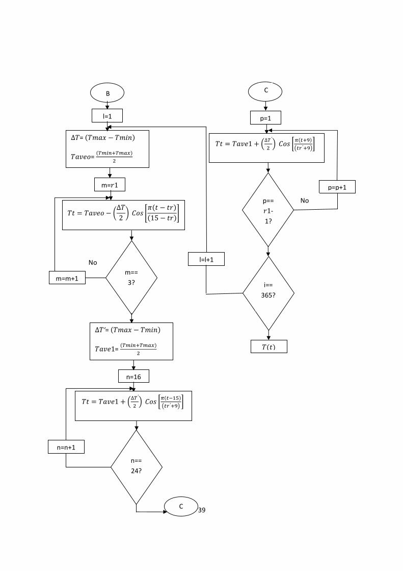
39
B
l=1
m=m+1
m=�1
m==
3?
�� = ���-� − g∆�2 h ��� ba�� − ����15 − ���d
∆�′= ��!�" − �!��
���-1= �����x��w��i
∆�= ��!�" − �!��
���-�= �����x��w��i
n=16
No
�� = ���-1 + L∆�′i O ��� }���KVj����′x�� �
n==
24?
n=n+1
C
p=1
C
�� = ���-1 + L∆�′i O ��� }���x�����′x���
p== �1-
1?
p=p+1
l=l+1
No
i==
365?
?
����
40
Read Ḡ���� , ����
��!, �!�", �!�", ���, ���, )+��; :, ���; :, ��� Read technical database containing n configurations
Configurations
j=1
j=j+1
t=8760?
j==n?
t=1
t=t+1
�� = �� + Ḡ� L���lO; �<=/0�� = ����Ki�o��
�1 = 0.01175 ; �4 = � �1 + �VTV� ; �2 = � SuU¡
�3 = � �vzU�Vx�V�Kv�w��V vzU � ; ! = l��¢£¢¤�l��M¡¥¦M§N �
�� = ��� ¨1 − �1©exp �2 ��� − 1ª«
∆�� = ��� L Ḡ�¬�®O + :, ��� ��� − ��-�� ; Δ�� = :, ������ − ��-��
��, -� = �� + Δ�� ; ��, -� = �!�" + Δ�� ; '�, -� = ��, -� × ��, -�
'����
No
No
Fig. 3-4: Flowchart for power generation from PV array

41
j=j+1
ℎ, ℎ� Read (���2, ℎ=��)
'�, ��2 = ¯ 2�� �� + �� + ��i� expK°±² � + '� ¯ 2�� expK�S² �³Uu³� ³�
³U�
� = �� L ´́�O�; � = �
Read technical database containing n
configurations
��� ��� �� �Configurations
j=1
t=1
t=t+1
'����
t=8760
?
j==n?
No
No
� = Pr L�!�� O� ���i − ���i� − ��!i − ���i���� − ������� − �!���! − ����
�! = ��� + ��2
� = ¶�Ky�³�K³U��³�²K³U�² ; � = −� ��� − � ���i
Fig. 3-5: Flowchart for power generation from wind turbine

42
Read '���� ; '���� ; '&���
Initialize: )���!�, )���!�",)�!�, )�!�", )�� !�, )�� !�" Technical database components
l no. of wind , m no. of PV and n no.
of battery configurations
)� = )�!�
)�� = )�� !�
)��� = )���!�
Configurations of PV
j=1
Configurations of wind
k=1
Configurations of wind
i=1
p=1
��!� = �1 − ·+·���!�"
)*��, � = �y¸z�y¸z,�u� ; ��!�" = 0�1� �¹w��¹w�,z ��
q=1
K
O
N
M
L
Q
P
Fig. 3-6: Flowchart for simulation operation and optimization of HSWPS
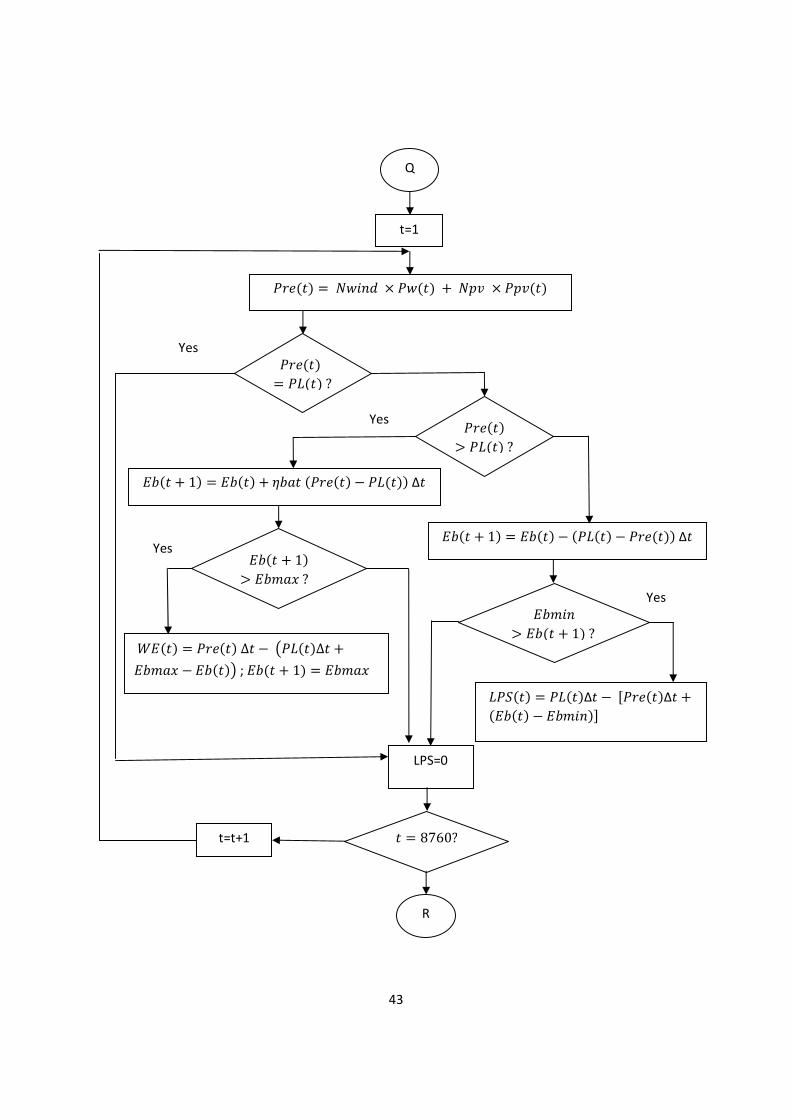
43
t=1
'�-��� = )�� × '���� + )� × '���� '�-��� = '&��� ?
'�-���> '&��� ? ���� + 1� = ����� + ?��� �'�-��� − '&���� Δ�
���� + 1�> ��!�" ? 3���� = '�-��� ∆� − �'&���∆� +��!�" − ������ ; ���� + 1� = ��!�"
LPS=0
���� + 1� = ����� − �'&��� − '�-���� Δ�
� = 8760?
&'(��� = '&���Δ� − ©'�-���Δ� + ������ − ��!��ª
Q
��!�> ���� + 1� ?
R
t=t+1
Yes
Yes
Yes
Yes
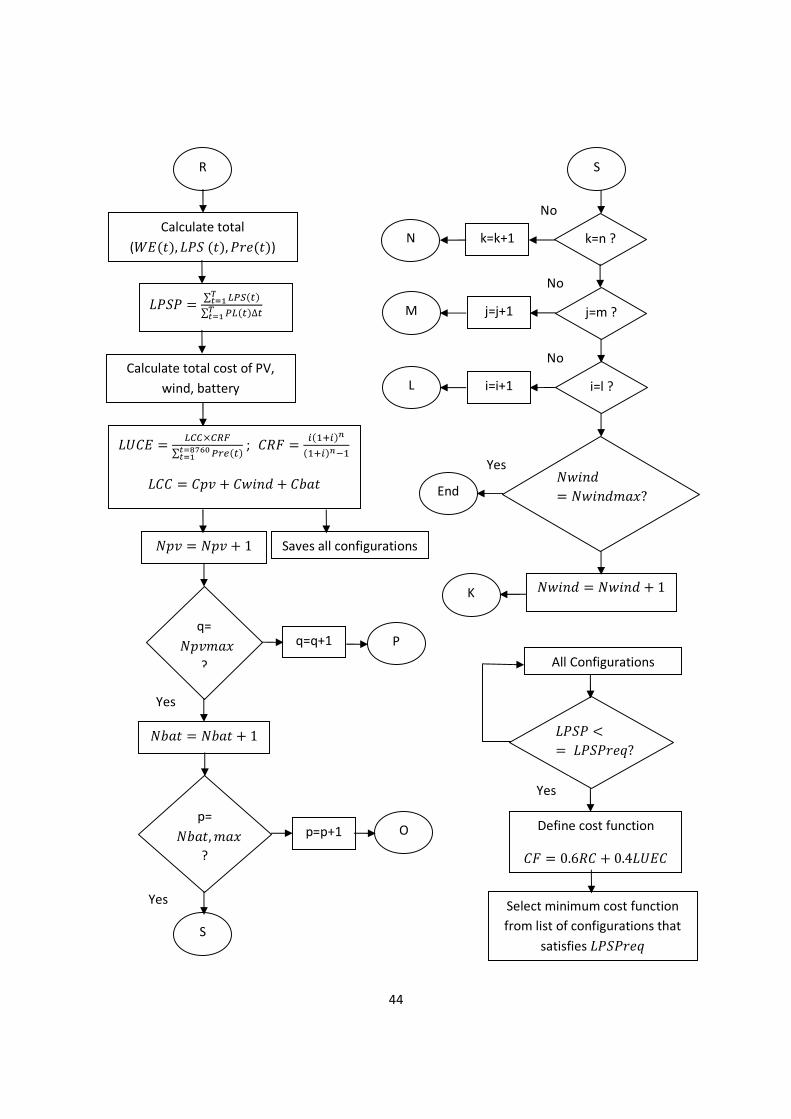
44
Calculate total
(3����, &'( ���, '�-���)
Calculate total cost of PV,
wind, battery
&'(' = ∑ ½¶¾���¿ÀÁÂ∑ ¶½���∆�¿ÀÁÂ
&�� = �� + ��� + ����
&0�� = ½��×�ÃR∑ ¶����ÀÁÄÅÆÇÀÁ ; �/� = ��Vx��È�Vx��ÈKV
Saves all configurations
&'(' <= &'('�-Ê?
�� = 0.6/� + 0.4&0�� Define cost function
Select minimum cost function
from list of configurations that
satisfies &'('�-Ê
)� = )� + 1
)��� = )��� + 1
q=)�!�"
?
k=n ?
R
p=)���, !�"
?
j=m ?
i=l ?
)�� = )�� !�"?
All Configurations
q=q+1 P
p=p+1 O
S
S
k=k+1
j=j+1
i=i+1
M
L
N
)�� = )�� + 1
End
K
Yes
Yes
Yes
Yes
No
No
No

45
3.3 Research Tools
For the simulation and analysis of the problem, two kinds of research tools as software and
mathematical models are performed. The feasibility assessment is conducted through HOMER software
and synthetic generation of weather variables and modeling of PV array and wind turbine with battery
storage for the optimum sizing components are performed through mathematical models. This section
focuses on methodology implementation of the different mathematical models (solar energy, wind
energy, temperature, reliability, system cost and optimization) with a brief introduction to HOMER
software.
3.3.1 HOMER Software
Introduction
HOMER is a computer model developed by the U.S. National Renewable Energy Laboratory (NREL) to
assist in the design of micropower systems and to facilitate the comparison of power generation
technologies across a wide range of applications. HOMER models power system’ s physical behavior and
its life-cycle cost, which is the total cost of installing and operating system over its life span. HOMER
allows the modeler to compare many different design options based on their technical and economic
merits. It also assists in understanding and quantifying the effects of uncertainty or changes in the inputs
[62]. It can be reiterated that HOMER is hybrid optimization renewable energy model software for both
standalone and grid connected micropower systems with the combination of PV modules, wind
turbines, biomass, hydro, reciprocating engine generators, microturbines, fuel cells, batteries and
hydrogen storage for thermal and electric load.
Inputs
The HOMER inputs can be broken down into the following categories:
1. Resources:
It uses four renewable resources as solar, wind, hydro and biomass and fuel.
2. Loads:
It uses three types of loads as primary, deferrable and thermal loads. The primary load
is the electrical load which must be served all the time while the deferrable load is also
the electrical load that must be served within some time period for which exact timing
is not important. Thermal load is the load for thermal heat energy.

46
3. Components:
It uses ten components as PV, wind turbine, hydro, battery, converter, electrolyzer,
generator, grid, boiler and converter.
4. Economics:
It uses different economic parameters as- system fixed capital cost, system fixed
operation and maintenance (O&M) cost, annual real interest, project life time, carbon
tax and cost of penalty for economic analysis.
5. Generator Control:
It uses additional operation for the system including battery bank and generator which
determines how the generator charges the battery.
6. Constraints:
It consists of operating reserve, maximum annual capacity shortage and minimum
renewable fraction.
7. Decision Variables:
It contains the values of each decision variables for the set of possible system
configurations.
For many inputs, HOMER provides default values so that computation of simulation operation can be
quicker.
Outputs
The outputs of results from HOMER are displayed in the form of simulation, optimization and sensitivity
analysis. These are briefly described below.
Simulation
HOMER uses energy balance calculation for hourly time-step simulation of its operation for one year
duration. It calculates the available renewable energy and compare with the required electrical/thermal
loads for each hour. It, moreover, decides each hour to charge or discharge the batteries. If the system
meets the load for the entire year, it estimates the life cycle costs of the systems. The life-cycle cost is a
convenient to compare the economics of the various system configurations. The outputs of the
simulation are split into the following categories as:
47
1. Cost
Its output results are the total net present cost and levelized cost of energy for the
entire project duration. In addition, it breaks down the cost into initial capital,
annualized capital, annualized replacement, annual operation and maintenance for each
component of the system.
2. Electrical
Its output provides total annual energy production of each component with excess and
shortage of energy.
3. Thermal
Its output provides total annual energy production of each thermal component and
total amount of thermal energy that went towards serving the thermal load during the
year.
4. Generator
It provides details of generators electrical output, life span, hours of operation, thermal
output, annual fuel usage and specific fuel usage.
5. Battery
It gives the overall status of the battery bank with minimum state of charge and
maximum state of charge for the whole one year duration.
Optimization
HOMER displays the list of possible feasible configurations based on the lifecycle cost of the systems.
The least life cycle cost is arranged according to top down approach for all the feasible configurations,
which provides the optimized results. Thus, optimization modules in HOMER provides possible decision
variables as size of PV array, number of wind turbines, number of batteries, size of generator, size of
electrolyzer, size of hydrogen storage tank, dispatch strategy etc..
Sensitivity
HOMER can perform sensitivity analysis to see how the results vary with changes in inputs. For example,
the values of certain parameters (e.g. PV cell cost) can be changed to determine the impact of cost of
energy for the systems. For any input, sensitivity analysis can be performed by assigning more than one
values of interest. HOMER repeats the optimization process for all the input values of interest so that
the effect of changes can be analyzed in the results.

48
Mathematical Modeling
HOMER uses the mathematical model based on physical and econometric model. These two types of
model are described below.
Physical Modeling
HOMER physical modeling is flexible so that the system can be modeled in two ways:
1. Basic inputs
• Annual averages for resources and loads
• Cost per kW or unit for equipment
2. Detailed information
• Hourly measured renewable resources data
• Technical components
• Cost of individual components
HOMER models the loads based on the components of the system and their respective resources. It uses
24 hours variation of load of ac or dc types to model load profiles. Similarly, to model a PV array system,
users must provide monthly average global horizontal solar radiation (kWh/m2/day) or hourly average
global solar radiation on the horizontal surface (kW/m2) or monthly average clearness index. For
instance, HOMER generates synthetic hourly global solar radiation data using the algorithm developed
by Graham and Hollands [63]. The input to this algorithm is the monthly average solar radiation values
or monthly average clearness index and the latitude. For each hour of the year, HOMER calculates the
global solar radiation incident on the PV array using the HDKR model [22]. The output of the results is
8760 hours of synthetic generation of solar radiation.
To model a system comprising one or more wind turbines, the HOMER user must provide wind resource
data indicating the wind velocity in a typical year. The user can provide measured hourly wind speed
data if available. Otherwise, HOMER can generate synthetic hourly data from 12 monthly average wind
speeds and four additional statistical parameters: Weibull shape factor, the autocorrelation factor, the
diurnal pattern strength, the hour of peak wind speed [62].
HOMER models a single battery as a device capable of storing a certain amount of dc electricity at fixed
round-trip energy efficiency, with limits as to how quickly it can be charged or discharged, how deeply it

49
can be discharged without causing damage, and how much energy can cycle through it before it needs
replacement. HOMER assumes that the properties of the batteries remain constant throughout its
lifetime and are not affected by external factors such as temperature [62]. For keeping the durability of
the battery, battery should not go below minimum state of discharge and should not exceed maximum
amount of charge. HOMER uses the kinetic battery model [64] to calculate the battery’s maximum
allowable rate of charge or discharge.
HOMER determines the optimal battery charging strategy based on load following and cycle charging
dispatch strategy. Under the load following strategy, a generator produces only enough power to serve
the load, and does not charge the battery bank. Under the cycle charging strategy, whenever a
generator operates, it runs at its maximum rated capacity (or as close as possible without incurring
excess electricity) and charges the battery bank with the excess.
Economic Modeling
For economic analysis, HOMER uses the lowest total NPC and life cycle cost within the life span of the
system for the set of all the feasible configurations. Conventional and non-conventional energy have
different cost characteristics in which non-conventional energy sources have high initial capital cost but
low operational cost whereas conventional energy sources have low initial capital cost but high
operational cost. A HOMER optimization module compares the economics of wide range of system
configurations for varying amounts of conventional and non-conventional energy sources. It uses a real
interest rate as an input parameters, which is the discount rate used to convert between one-time costs
and annualized costs. It also assumes all the prices to be escalated at a constant rate over the project life
span. Thus, HOMER ranks the system according to least life cycle cost within the project duration.
Advantages and Disadvantages
The main advantages of HOMER are:
1. It is very flexible and friendly for the users with limited resources of data to model, analyze and
optimize any RES system.
2. Its sensitivity analysis assists the user to analyze the optimum results with the input changing
parameters.
3. Its optimization module helps to find the optimal conditions based on the least life cycle cost of
the systems.

50
The disadvantages of HOMER are:
1. It doesn’t support some renewable technologies like biogas and geothermal or solar thermal.
2. It only emphasizes the feasibility assessment of renewable resources. It does not give a clear
idea about sizing the systems.
3.3.2 Solar Energy Models
3.3.2.1 Geometrical Parameters Estimation
The solar beam radiation on the earth surface is affected by various geometrical parameters such as
latitude, inclination angle, declination angle and zenith angle. It is well known that the Earth goes
around the sun in an elliptic orbit with the sun at one of the foci. The plane containing this orbit is called
ecliptic plane and the time that the earth takes to complete this orbit is the year. The distance between
the sun and the earth, � is given by the equations (3-1) [65].
� = �� ©1 + 0.017 �� L�Ë��Q�K����Ëj O (3-1)
where, = day of the year [ a number between 1 and 365] �� = mean distance between sun and earth 1.496 × 10o�!
For most of the engineering applications, eccentricity correction factor, B�, is used and is given by the
equation (3-2) [65].
B� = L�u� Oi = 1 + 0.033 ��� L360 Q��ËjO (3-2)
It is also known that the angle between the equatorial plane and a straight line drawn between the
centre of the Earth and centre of the sun is constantly changing over the year, which is known as solar
declination angle δ. If the angles north to the equator are considered as a positive, the solar declination
angle is given by the equation (3-3) [65].
@ = 23.45 �� ��Ë��Q�xio ��Ëj � (3-3)
In order to calculate the declination angle for the average month in a year, it is necessary to know the
average value so that the global solar radiation can give a precise value. The average recommended days
for months is given by [22] and is shown in the table (3-2). Moreover, it is well known that the solar

51
zenith angle 56� is the angle between vertical and the incident solar beam i.e. angle of incidence of
beam radiation on the horizontal surface; solar azimuth C� is the angle of displacement from south of
the projection of beam radiation on the horizontal plane. The component of the zenith angle is called
the solar altitude, D�, and represents the angle between the horizon and the solar beam in a plane
determined by the zenith and the sun. It is assumed that in the northern (southern) hemisphere, the
solar azimuth is referenced to south (north) and is defined as positive towards the west i.e. in the
evening and negative towards east i.e. in the morning.
Month for ith
Day of the month
For the Average Day of the Month
Date , Day of Year δ, Declination
January I 17 17 -20.9
February 31+i 16 47 -13
March 59+i 16 75 -2.4
April 90+i 15 105 9.4
May 120+i 15 135 18.8
June 151+i 11 162 23.1
July 181+i 17 198 21.2
August 212+i 16 228 13.5
September 243+i 15 258 2.2
October 273+i 15 288 -9.6
November 304+i 14 318 -18.9
December 334+i 10 344 -23
Table 3-1: Recommended average days for months and declination angle [22] The angular coordinates of the sun with respect to latitude ɸ is calculated in terms of solar zenith angle 56� , solar azimuth C� and solar altitude D� is given by the equations (3-4) and (3-5) [65]. It is assumed
that ɸ is positive towards north and negative towards south.
���56� = (�@ (�∅ + ���@ ���∅ ��� E = (�D� (3-4)
���C� = ¾��Ìz ¾��ÍK¾��Î�uzÌz �uzÍ ©��2�7�ª (3-5)
where, E = hour anlge [0]
The hour angle E can be described by the time of day, which also affects the location of the sun in the
sky. It is assumed that E is zero at solar noon (the time of day at which the sun is at its highest point in

52
the sky), negative before solar noon and positive after solar noon. Thus, hour angle varies according to
sun rise and sun set time. The hour angle E is given by the equation (3-6) [22].
E = ��� − 12 ℎ�� × 150 /ℎ� (3-6) The value of �� is 12 hr at solar noon, and 13.5 hr ninety minutes later. The above equation shows that
the sun moves across the sky at 15 degrees per hour.
The angle of incidence of beam radiation 5 plays a major role in the energy available at the earth surface
and depends on solar declination angle @ , latitude∅, slope of the surface 8, hour angle E and azimuth
of the surface C� and is given by the equation (3-7) [22].
���5 = (�@ (�7 ���8 − (�@ ���7 (� 8 ���C� + ���@ ���7 ���8 ���E + ���@ (�7 (�8 ���C� ���E + ���@ (�8 (�C� (�E �3 − 7� Since sunrise and sunset time depends on the length of the day during a year, the day length �
measured in hours can be calculated from the equation (3-8) [22].
� = iVj × ��� -1�−��@ ��∅� (3-8)
Accordingly, it is easier to calculate the rise time �1 and sun set time �2 during a particular day in a year
measured in hours and these values are given by equations (3-9) and (3-10) [22].
�1 = �12 − Qli � (3-9)
�2 = �12 + Qli � (3-10)
3.3.2.2 Knight Hourly Irradiance Model
Knight et al. hourly solar radiation model [16] was chosen as the best model for the purpose of this
study since this model synthesize the monthly average clearness index into hourly clearness index
stochastically. This model uses a stochastic sequence of clearness index �� for each day of each month
and generates hourly clearness index #�. Knight et al. explains the various statistical distributions
presented in the literature, but found that, although these distributions are applicable to the location
studied, their universality is questionable. The correlation used by Knight et al. which is verified for

53
different locations of New York is described by the following equation (3-11) with γ found from
equations (3-12). ��, !� was taken 0.05 and ��, !�" was given by the equations (3-14) [16].
� = ÏÐÑ�γ°�,����KÏÐÑ�γ°��ÏÐÑ�γ°�,����KÏÐÑ�γ°�,�w�� (3-11)
D = −1.498 + V.Vo ξKiÒ.VoiÏÐÑ�KV.jξ�°�,�w�K°�,��� (3-12)
X = °�,�w�K°�,���°�,�w�KЌ� (3-13)
K�, !�" = 0.6313 + 0.267Ќ� − 11.9 �Ќ� − 0.75�o (3-14) Thus, �� values are calculated from the daily �� cumulative distribution function in which cumulative
distribution function relates to the cumulative fraction of occurrence, F, to ��. The procedure to select
the �� value is to take the average of this F value V�V and previous one (0) and results F =
VËi. Thus, from
the cumulative distribution function, the corresponding F value can be found. Thus this method is
applied same for 28 and 30 months. After the sequences are generated, Knight et al. sequences are
chosen so that it maintains the statistical correlation of data. Table (3-2) shows the sequences
developed by Knight et al. for the average clearness index Ќ� to determine the order of sequences to
apply. The same sequences are applied for each month of the year with the starting point in the
sequence randomly selected for each month using a random seed.
Ќ� Sequence Order Ќ�<0.45 24, 28, 11, 19, 18, 3, 2, 4, 9, 20, 14, 23, 8, 16, 21, 26,
15, 10, 22, 17, 5, 1, 6, 29, 12, 7, 31, 30, 27, 13, 25
0.45<Ќ�<0.55 24, 27, 11, 19, 18, 3, 2, 4, 9, 20, 14, 23, 8, 16, 21, 7,
22, 10, 28, 6, 5, 1, 26, 29, 12, 17, 31, 30, 15, 13, 25
0.55<Ќ� 24, 27, 11, 4, 18, 3, 2, 19, 9, 25, 14, 23, 8, 16, 21, 26,
22, 10, 15, 17, 5, 1, 6, 29, 12, 7, 31, 20, 28, 13, 30
Table 3-2: �� Ordering Sequences [16]
The next step is to find the average clearness index, #�!, which gives the long term average value of #�
for that hour of the day, month and daily clearness index value. #�! can be found from the equations
(3-15) - (3-18) or equations (3-19)[16].
#�! ≈ �� �� tuvu (3-15)
�� = �wxyUuz{�vutu (3-16)
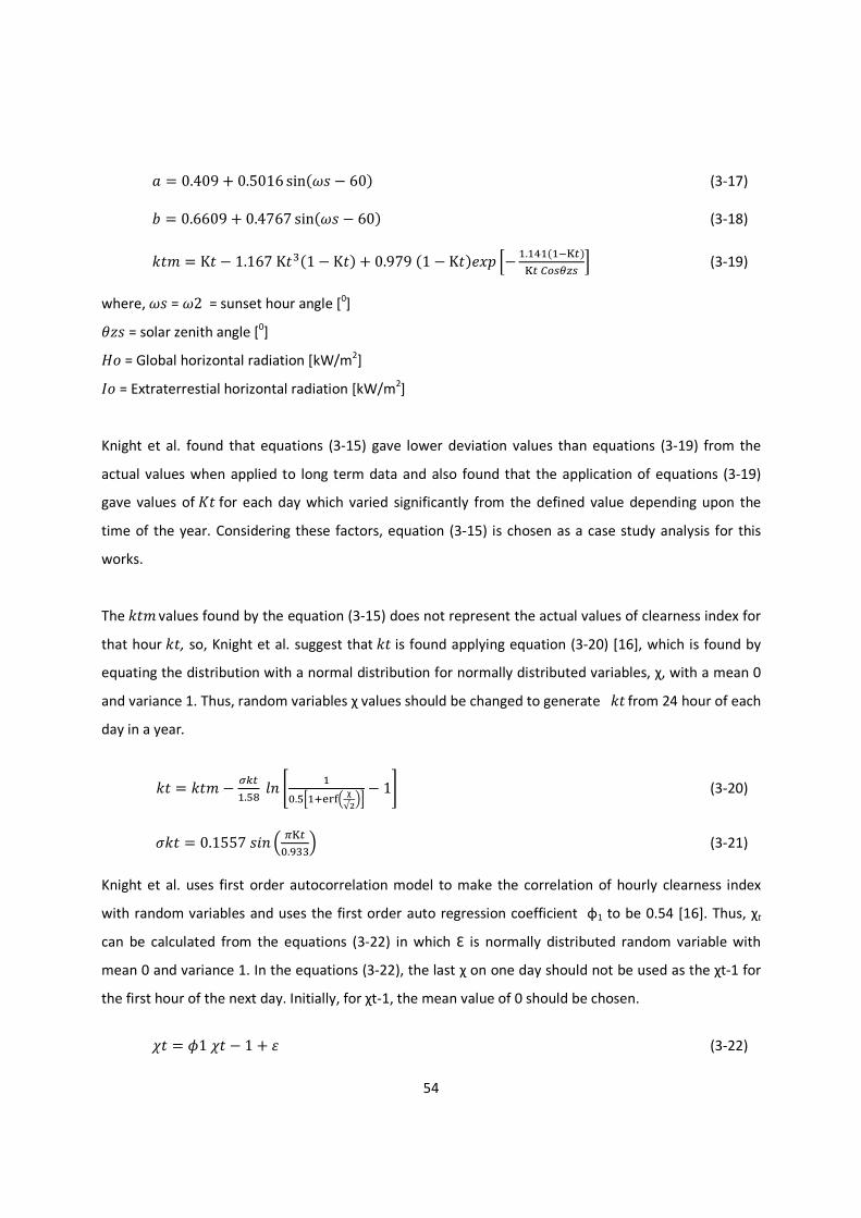
54
� = 0.409 + 0.5016 sin�E� − 60� (3-17) � = 0.6609 + 0.4767 sin�E� − 60� (3-18)
#�! = K� − 1.167 K���1 − K�� + 0.979 �1 − K��-" �− V.V V�VK°��°� �uz��z � (3-19)
where, E� = E2 = sunset hour angle [0] 56� = solar zenith angle [0] �� = Global horizontal radiation [kW/m2] �� = Extraterrestial horizontal radiation [kW/m2]
Knight et al. found that equations (3-15) gave lower deviation values than equations (3-19) from the
actual values when applied to long term data and also found that the application of equations (3-19)
gave values of �� for each day which varied significantly from the defined value depending upon the
time of the year. Considering these factors, equation (3-15) is chosen as a case study analysis for this
works.
The #�! values found by the equation (3-15) does not represent the actual values of clearness index for
that hour #�, so, Knight et al. suggest that #� is found applying equation (3-20) [16], which is found by
equating the distribution with a normal distribution for normally distributed variables, χ, with a mean 0
and variance 1. Thus, random variables χ values should be changed to generate #� from 24 hour of each
day in a year.
#� = #�! − ÓT�V.jo � b V�.j�VxÏÔÕL χ√²O� − 1d (3-20)
A#� = 0.1557 �� L �°��.���O (3-21)
Knight et al. uses first order autocorrelation model to make the correlation of hourly clearness index
with random variables and uses the first order auto regression coefficient ɸ1 to be 0.54 [16]. Thus, χt
can be calculated from the equations (3-22) in which Ɛ is normally distributed random variable with
mean 0 and variance 1. In the equations (3-22), the last χ on one day should not be used as the χt-1 for
the first hour of the next day. Initially, for χt-1, the mean value of 0 should be chosen.
9� = 71 9� − 1 + B (3-22)

55
Thus, after finding the hourly clearness index, the HDKR model was implemented for inclined plane
surface to generate hourly solar radiation values in inclined PV surface.
3.3.2.3 Extraterrestrial Radiation
Solar Radiation outside the atmosphere is referred to as extraterrestrial radiation. The average amount
of radiant energy received outside the atmosphere from the sun is known as the solar constant. The
amount of sunlight striking the top of the earth’s atmosphere varies over the year because the distance
between the sun and the earth varies due to the eccentricity of the earth’s orbit. The dependence of
extraterrestrial normal radiation on time of the year, defined as the amount of solar radiation striking a
surface normal to the sun’s rays at the top of the atmosphere is given by the equation (3-23) [22].
�� = ��� B� = ��� L1 + 0.33 ��� �Ë�Q��Ëj O (3-23)
where, �� = extraterrestrial horizontal radiation [kW/m2] ��� = solar constant [1367 W/m2]
The amount of global radiation that reaches the earth surface at the collector is extremely variable. The
extraterrestrial radiation also experiences daily and yearly variation due to the apparent motion of the
sun. These variations are predictable and can be theoretically determined by geometrical
considerations. For instance, the extraterrestrial irradiance over a horizontal surface �� measured in
kW/m2 is given by the equation (3-24) [22].
�� = �� ���56� (3-24) Also, the average extraterrestrial irradiance over a horizontal surface is found by integrating equation
(3-24) over one time step and is given by equation (3-25) [22].
Ḡ� = Vi� × �� ����7 ���@ �(�E2 − (�E1� + a �{iK{V�Vo� (�7 (�@� (3-25)
where, Ḡ� = extraterrestrial horizontal radiation averaged over the time step [kW/m2] E1 = hour angle at the beginning of time step [0] E2 = hour angle at the end of the time step [0]
56
For the given hourly clearness index #� calculated from the Knight et al., the global horizontal radiation
on the earth’s surfaced averaged over the time step Ḡ measured in [kW/m2] is calculated from the
equation (3-26) [22].
#� = Ḡ
Ḡu (3-26)
3.3.2.4 Beam and Diffuse Components
As discussed above global horizontal radiation on the earth’s surface consists of beam radiation Ḡ� and
diffuse radiation Ḡ measured in [kW/m2] and is given by equation (3-27) [22].
Ḡ = Ḡ + Ḡ� (3-27)
It is indispensable to split total global horizontal solar radiation into diffuse and beam components. The
estimation of long-time performance of concentrating collector depends on the availability of beam
radiation. There are different approaches to correlate Ḡ /Ḡ from hourly clearness index #�.
Orgil and Hollands [22] used the data of this type from Canadian station and his correlation is given by
the equation (3-28).
ḠQḠ
= Ö 1.0 − 0.249#�1.557 − 1.84#�0.177 × #� < 00.35 < #� < 0.75#� > 0.75 Ø (3-28)
Erbs et al. [22] have used the data from four US and one Australian station and used the correlation of
Ḡ /Ḡ as a function of hourly clearness index #� as described by the equation (3-29).
ḠQḠ
= Ö 1.0 − 0.09#�0.9511 − 0.1604#� + 4.388#�i − 16.638#�i + 12.336#� 0.165 × #� ≤ 0.220.22 < #� ≤ 0.80#� > 0.80 Ø (3-29)
For values of #� greater than 0.8, there is very few data. Some of the data that is available shows
increasing diffuse fraction as #� increases above 0.8. This apparent rise in the diffuse fraction is probably
due to the reflection of radiation from the sun to the observer. The use of a diffuse fraction of 0.165 is
recommended in this region [22].
Thus, for each time step from the hourly clearness index #� obtained from Knight et al., the diffuse
radiation is calculated after the correlation and then the beam radiation is determined by subtracting
diffuse radiation from global horizontal radiation.

57
Although these correlation methods are derived from different data base, they essentially show
identical results. For the purposes of this study, Erbs et. al is used because this correlation produces
practical results and is even used by the National Renewable Energy Laboratory of USA .
3.3.2.5 HDKR Model
As discussed in the previous section the HDKR model is implemented in this work. The HDKR model
calculates the global radiation on the tilted surface. Before the model is implemented, there are
different factors that need to be taken into consideration.
The geometric factor /�, the ratio of beam radiation on the tilted surface to the beam radiation on the
horizontal surface is given by equation (3-30) [22].
/� = �uz��uz��z (3-30)
The anisotropy index ��, is a measure of the atmospheric transmittance of beam radiation. It is used to
calculate the forward scattered radiation, the amount of circumsolar diffuse radiation and is given by
equation (3-31) [22].
�� = ḠyḠu (3-31)
Under clear conditions, it is assumed that �� will be high and most of the diffuse components will results
from forward scatter. When there is no beam �� will be zero and diffuse components result in isotropic
components only.
Other parameters to define HDKR model is horizon brightening �. It is related to the cloudiness and
assumes that more diffuse radiation comes from the horizon than from the rest of the sky and is given
by equation (3-32) [22].
� = √ḠyḠ
(3-32)
Thus, HDKR model calculates the global solar radiation incident on the PV array Ḡ� by equation (3-33)
[22], where �2 is the ground reflectance measured in percentage.
Ḡ� = �Ḡ� + Ḡ ��� /� + Ḡ �1 − ��� �Vx�uzÚ�i �1 + �(�� LÚiO� + Ḡ �2 L1 − �uzÚi O (3-33)

58
3.3.2.6 PV Array Model
The PV generator is a non-linear device and is described by the I-V characteristics and by the equivalent
circuit. There are many mathematical models developed to describe the behavior of PV. In the present
work, the “Four Parameter Model”, which is widely used by the large software, is utilized [30]. For the
calculation of PV power output, we assume that maximum power point tracker is used. To model the
system, we assume that various characteristics of manufacturer like short circuit current, maximum
current, maximum voltage, open circuit voltage, nominal voltage, temperature coefficients for short
circuit current and open circuit voltage of PV panels are known.
The PV Array equivalent circuit current �� can be expressed as a function of the PV array voltage ��
and is given by equation (3-34) [30], where the coefficients �1, �2 and ! are defined by equations (3-
34) –(3-39).
�� = ��� ¨1 − �1©exp �2 ��� − 1ª« (3-34)
�1 = 0.01175 (3-35)
�2 = � SuU¡ (3-36)
! = l��¢£¢¤�l��M¡¥¦M§N � (3-37)
�3 = � �vzU�Vx�V�Kv�w��V vzU � (3-38)
�4 = � �1 + �VTV� (3-39)
where, ��� =PV panel short circuit current at hour t [Ampere, A] �!�" = PV panel current at the maximum power point at hour t [Ampere, A] �� = �!�"= PV panel maximum voltage at the maximum power point at hour t [Volt, V] ��� = PV panel open circuit voltage at hour t [Volt, V]
Due to the change in temperature under the operating conditions, the PV cell temperature changes and
results in the change in current and voltage. This effect is given by equations (3-40) and (3-41) [30],
where PV panel operating cell temperature can be calculated from equation (3-42) which is based on
the energy balance proposed by J. A. Duffie et al. [22].

59
∆�� = ��� L Ḡ�¬�®O + :, ��� ��� − ��-�� (3-40)
Δ�� = :, ������ − ��-�� (3-41)
�� = �� + Ḡ� L���lO (3-42)
�<=/0�� = ����Ki�o�� (3-43)
where,�� = Change in current due to the operating temperature [Ampere, A]
�� = Change in the voltage due to the operating temperature [Volt, V]
Ḡ� = Hourly irradiance on a tilted surface [Watt/m2] �� = PV panel operating at temperature (0C) at hour t [0C] ��-� = PV Panel temperature of 250C at reference operating conditions [0C] :, ��� = Temperature coefficients for short circuit current [A/0C] :, ��� = Temperature coefficients for open circuit voltage [V/0C] �� = Ambient temperature of the site under hour t [0C] 0�= Overall heat coefficients (W/m2 per 0C) <= Transmittance coefficients of PV cells = = Absorptance coefficients of PV cells )+�� = Nocturnal operating cell temperature [0C]
)+�� is defined as the cell temperature when PV panel operates under 800 W/m2 of solar irradiation
and 200C of ambient temperature.
The new values of the PV current, voltage and power are given by equations (3-44)-(3-46) [30].
��, -� = �� + �� (3-44)
��, -� = �!�" + �� (3-45)
'�, -� = ��, -� × ��, -� (3-46) where, ��, -� = PV panel voltage at the maximum power point at hour t [Volt, V] ��, -� = PV panel current at the maximum power point at hour t [Ampere, A] '�, -� = PV panel power at the maximum power point at hour t [Watt, W]

60
The number of PV panels that is connected in the series )�, � is given by equation (3-47), where 0*1�
is the bus voltage of the architecture and 0�, �! is the nominal PV panel voltage.
)�, � = �¹¸z�Û³,�u� (3-47)
The number of PV panels in series )�, � is fixed where as the number of PV panels in parallel needs to
be optimized for the optimal number of PV panels.
3.3.3 Wind Energy Model
3.3.3.1 Synthetic Hourly Wind Speed Generation Model
The synthetic generation of wind speed used for the purposes of this study is based on stochastic and
deterministic models. The first step of the algorithm is using the stochastic model to generate daily wind
speed profiles and uses the diurnal pattern and autocorrelation for each hour of the day to get the
synthetic wind generation profiles.
Stochastic Model
Degelman Larry [21] states that weather distribution pattern can be described by the normal
distribution curves. He described that the higher frequencies will occur at the mean value while a few
are extremely high and a few are extremely low. Thus the standard deviation of daily average wind
speed was to be 1/3 of the monthly average wind speed.
Accordingly, if the average monthly wind speed is known, then the standard deviation of each month is
1/3 of the monthly average wind speed. For each month a random number is generated between 0 to 1
and for each day of a month, the cumulative distribution number (F-value) is obtained from a normal
distribution curves. When this F-value is multiplied by the standard deviation of each month and add
(plus or minus) to the monthly average wind speed results the average wind speed for each day.
Deterministic Model
As stated above the stochastic model generates the daily wind profiles during a year and since the wind
speed varies according to geographic location, the behavior of wind speed is indispensable for the
analysis of wind speed sequences and is explained by diurnal pattern.

61
Diurnal Pattern
The diurnal pattern plays a significant role to know how strongly wind speed depends on the time of the
day. The pattern of wind speed is cosinusoidal and is given by equation (3-48) [35].
�� = ���2 Ü1 + @� ��� �i�i �� − 7���Ý ��� � = 1,2, … 24 (3-48)
where, �� = Mean wind speed in hour
���2= Average wind speed during a day
@�= Diurnal pattern strength, a number between 0 and 1
7� = Hour of peak wind speed, an integer between 1 and 24
The hour of peak wind speed 7� is the hour of the day that tends to be the windiest and it depends on
the geographical locations.
Autocorrelation
Timely behavior of wind speed is described by the autocorrelation factor. It defines that wind speed in
one time step depends on the wind speed in the previous time steps. The geographical location affects
the autocorrelation factor. High autocorrelation factor signifies that the wind speed in one instant is
strongly dependent of the previous instant whereas a low autocorrelation signifies that the wind speed
in one instant is less dependent and is of fluctuating nature in a random fashion from one time step to
the next. For a complex topography, its value is lower (0.70-0.80) and for more uniform topography, its
value is higher (0.90-0.97) [35].
The first order autocorrelation [35] is given by equation (3-49) which generates a sequence of
autocorrelated numbers one for each time step i.e. 8760 hours of the year.
4� = � 4t-1+ f(t) (3-49)
where, 4� = Autocorrelated values in time step i
4t-1 = Autocorrelated values in time step i-1
� = Autoregressive parameters
f(t) = White noise which passes through a normal distribution with mean 0 and a standard deviation 1
62
For each hour of time i.e. 8760 hour during a year, an autocorrelation factor � is calculated from each
hour autocorrelation factor ��1 for a lag of #1 time steps in a year and is given by equation (3-50) [35].
� = ��1TV (3-50)
Thus, the synthetic generation of wind profiles is obtained by adding the hourly wind speed obtained
from equation (3-48) and equation (3-49).
3.3.3.2 Wind Generator System Models
Chou and Corotis Wind Turbine Model
Chou and Corotis [39] model is used to calculate the output power from a wind turbine '��� and is
given by equation (3-51). Variables �, � and � are given by equations (3-52)-(3-54), where ��� is the cut-
in wind sped of the wind turbine, �� is the rated wind speed of the wind turbine, ��� is the cut-out wind
speed of the turbine and '� is the rated power of the wind turbine. In order to obtain these equations,
a boundary condition is imposed at the median wind speed vm and is given by equation (3-55). At this
wind speed, the output power from a wind turbine is Pr L³�³� O�.
'��� = á 0� + �� + ��i'�0 â � ≤ ������ < � ≤ ���� ≤ � ≤ ���0 ã (3-51)
� = Pr Lä¡äå O£�³�²K³U�²�K�³�²K³U�²��³�K³U���³�K³���³�K³U�� (3-52)
� = ¶�Ky�³�K³U��³�²K³U�² (3-53)
� = −� ��� − � ���i (3-54)
�! = ³U�x³�i (3-55)
Power Law
The installation height of wind turbine has a large effect on the energy available from the system, so, a
height adjustment is necessary for wind resources. The wind speed at the specific hub height for the
63
location can be estimated from the wind speed measured from a reference height and is given by
equation (3-56) [61].
� = �� L ´́�O� (3-56)
where, � = wind speed projected at height h
��= wind sped at reference height hr
∝ is the power law coefficient which varies with time of the day, season, elevation, temperature, wind
speed, nature of terrain and various thermal and mechanical mixing parameters. The value of ∝ plays a
major role and is usually taken as 1/7 [61].
Rayleigh Distribution Model
The simplified version of wind speed distribution is described by the Rayleigh distribution which takes
the average wind speed and shape factor # to be 2 [42].
The Rayleigh distribution modified from Weibull distribution with average wind speed �!, cumulative
distribution function ���� and probability density function ���� as given by equations (3-57) and (3-58)
[42].
���� = 1 −expK}æ¤ L MM¡O²� (3-57)
���� = �i SS�² exp gK}æ¤ L MM¡O²�h (3-58)
The wind power available at the site for each hour can be given by equation (3-59) [42].
', ��2 = ç ' ���� �∞� (3-59)
Assume,
� = � S�² (3-60)
Using equations (3-58) and (3-60), the probability density function ���� can be expressed as:
���� = 2�� expK�S² (3-61)
According to Chou and Corotis [39], the energy available from the wind turbine is characterized by the
Cut-in wind speed, Cut-out wind speed and rated wind speed. The rated wind speed is able to produce

64
constant power corresponding to the rated power of wind generator. If the wind velocity is greater than
the cut-out wind speed, the wind generator stops to prevent damage to the system resulting from highly
intensive thrust forces.
Thus, the total average power available from the wind generator according to Chou and Corotis and
Rayleigh Distribution can be reduced to equation (3-62).
'�, ��2 = ç '������� � + Pr ç ���� �³Uu³�³�³U� (3-62)
Substituting the value from equation (3-51) into equation (3-62), the equation (3-62) is modified to
equation (3-63), which is the total average power generated from wind generator at continuous hourly
instant of time.
'�, ��2 = ç 2�� �� + �� + ��i� expK°±² � + '� ç 2�� expK�S² �³Uu³� ³�³U� (3-63)
3.3.4 Temperature Model Degelman Synthetic Temperature Generation Algorithm
The first step of Degelman Larry algorithm is used to generate the ambient temperature values by
selecting the daily average and maximum temperatures from a normal distribution and orders them
according to predetermined day sequences in a month. The second step of algorithm is to apply the
deterministic model to generate hourly temperature by fitting a cosine curve between maximum and
minimum points. The minimum temperature is obtained from the sunrise time of each day obtained
from Eqns. (3-9) and maximum temperature of each day is obtained from the stochastic models.
Stochastic Model
Degelman Larry [21] states that temperature distribution pattern fits a bell-shaped curve and can be
described by the normal distribution curve. He explains this is similar to the measuring heights of
people, areas covered by numerous gallons of paint or fuel efficiencies attained by a sample of
automobiles. With this idea, he discovered that highest frequencies will occur at the mean value while a
few are extremely high and a few are extremely low.
Thus, according to Degelman Larry, the average daily temperature and daily maximum temperatures
can behave in the similar fashion and are distributed in a normal distribution pattern defined by a mean
and a standard deviation. He found that the standard deviation of daily average temperature was 1/3 of

65
the monthly average temperature and that the standard deviation of hourly temperature was 1/3 of the
daily temperature.
As the average monthly temperature is known, the standard deviation of each month is calculated
which is 1/3 of the monthly average temperature. For each month a random number is generated
between 0 to 1 and cumulative distribution number (F-value) for each day of each month is obtained
from a normal distribution curves. When this F-value is multiplied by the standard deviation of each
month and added (plus or minus) to the monthly average temperature, the average temperature for
each day is obtained. In a similar fashion, the hourly temperature can be obtained for each day.
Deterministic Model
After obtaining the stochastic generation of hourly temperature, the deterministic model is
implemented. For the deterministic model, the temperature of the sun rise time and the maximum
temperature during a day at the diurnal time of day act as input parameters.
The deterministic approach gives the shape of the diurnal pattern, is fairly consistent from day to day
and its daily diurnal pattern is shown in figure (3-7). The known variable sunrise time and time at which
temperature will be maximum for each day gives the diurnal pattern of the temperature during a day. If
the temperature of sunrise time is known and is assumed to be minimum (�!�) and if the maximum
temperature (Tmax) is known, then hourly values can be estimated by fitting a sinusoidal curve between
the two ends points. Similarly, if low temperature (Tmin1) is known of next morning’s, a second curve
can be fitted between these two points. The derivation of hourly values is given by equations (3-64)-(3-
66) [21].
Fig. 3-7: Characteristic shape of daily temperature profile [21]
The temperature during sunrise time to 3 pm is given by equation (3-64).
�� = ���-� − L∆�i O ��� ����K����VjK���� (3-64)

66
where, �� = Temperature at time t [0C]
���-� = Average morning temperature = �����x��w��i
∆� = Diurnal temperature = ��!�" − �!��
�� = Time of Sunrise
15 = Hour of maximum temperature occurrence (used as 3 pm)
The temperature from 3 pm to midnight is given by equation (3-65).
�� = ���-1 + L∆�′i O ��� }���KVj����′x�� � (3-65)
where, �� = Temperature at time �
���-1= Average evening/night temperature = ���w�x����V�i
∆�′ = Evening temperature drop = ��!�" − �!�1�
��′= Time of sunrise on next day
The temperature from midnight to sunrise the next day is given by equation (3-66).
�� = ���-1 + L∆�′i O ��� }���x�����′x��� (3-66)
It is assumed that time 0 stands for 1 am in the morning while synthetic generation of temperature
through MATLAB programming. Since the diurnal pattern starts from the sunrise time, the last
temperature value of December from midnight to sunrise next day is taken as the beginning of time in
the January for sequential generation of hourly temperature pattern in MATLAB.
3.3.5 Battery Model
Most of the batteries used in hybrid systems are of deep-cycle lead acid type. There are several other
appropriate types (nickel-cadmium, nickel-iron, iron-air and sodium-sulphur) but these are generally
either too expensive or too unreliable for practical application as most of them are still in the
experimental stage. The lead acid battery is widely used and, although complex, is well known [49].
The commonly used battery lead-acid type is used to store the surplus energy so that it can provide
continuous power supply to the load in case of low wind and low solar radiation. The Lead-acid
batteries used in hybrid solar and wind energy system operate at different conditions and is difficult to

67
predict during the energy consumption and production. In general, the battery can be modeled into
three characteristics i.e. the state of charge of the battery�(+��, the floating charge voltage (or the
terminal voltage) and the life span of the battery. However, Belfkira, Zhang and Barakat [49] modeled
the battery in terms of state of charge�(+��.
It is known that the power generated by the hybrid system and the energy stored in the battery are time
dependent. So, the power input to the battery bank is governed by equation (3-67).
∆'��� = '�-��� − '&��� (3-67)
where, Pre�t�= Total power produced by the renewable resources (Solar and Wind Energy) '&���= Total load power demanded
For any hour the state of the battery is related to the previous state of charge and to the energy
production from the renewable resources and consumption by the battery during the time from t to t+1.
During the charging process, the total power generated by the renewable resources is greater than the
power demanded by the load i.e. ∆'��� > 0, and during discharging process, the total power generated
by the renewable resources is less than the power demanded by the load i.e. ∆'��� < 0 .
During the charging and discharging process, the state of charge �(+�� can be calculated from
equations (3-68) and (3-69) respectively, where ?��� is equal to round-trip efficiency in the charging
process and is equal to 100% in the discharging process [49]. 0�1�, �! is the nominal DC voltage of
individual battery and Δ� is the hourly time step and is set equal to 1 hour interval.
(+��� + 1� = (+���� + ?��� L¶����K¶½����y¸z,�u� O Δ� (3-68)
(+��� + 1� = (+���� − L¶½���K¶�����y¸z,�u� O Δ� (3-69)
In order to increase the life span of the battery, the maximum state of charge of the battery is given and
is set to upper limit (+�!�" such that battery does not overcharge and is equal to the total nominal
capacity of the battery bank,�, which is related to the total number of batteries, )���, the number of
batteries connected in series, )*��, � and the nominal capacity of each battery, ��(Ah) and is given by
equation (3-70)[49].
� = �¹w��¹w�,z �� (3-70)

68
The minimum state of charge of the battery is set to lower limit (+�!� such that battery does not
discharge below the minimum state of charge and is expressed in equation (3-71) [49], where ·+· is
the Depth of Discharge of the battery.
(+�!� = �1 − ·+·�(+�!�" (3-71)
For any hour, the state of the charge of the battery should be subject to the constraints given by
equation (3-72) [49].
(+�!� ≤ (+���� ≤ (+�!�" (3-72)
The batteries are connected in the series such that they provide the nominal DC bus voltage to the load
and are connected in parallel so that they provide the desired Ah system storage capacity. Thus, the
number of the batteries connected in series is related to the nominal DC voltage of the individual
battery 0�1�, �! and the DC voltage of the bus system 0�1� and is given by the equation (3-73).
)*��, � = �y¸z�y¸z,�u� (3-73)
The number of batteries connected in series is the fixed part whereas the batteries connected in the
parallel is a design variable which needs optimization.
3.3.6 Reliability Model
The intermittent nature of both solar and wind energy makes it necessary to use the reliable power
supply design. There are two different approaches for utilizing the LPSP concept. The first approach is
based on chronological simulation which is computationally burdensome and requires the availability of
data for a certain period of time. The second approach is the probabilistic technique which requires
varying conditions of loads and renewable resources, thus eliminating the need for time-series data [3].
This section describes the second approach as the loss of power supply probability (LPSP). The system is
said to be reliable if the power generated by the renewable energy sources meets the load demand
during a certain period of time or with a minimum loss of power supply probability.
Loss of power supply probability can be defined as the long-term average fraction of the total load that
is not supplied by a stand-alone system. A LPSP of 0 means that the load will be always be satisfied, and
the LPSP of 1 means that the load will be never be satisfied [3]. Also, it is the probability that an
insufficient power supply results when the hybrid PV and wind energy system is not able to satisfy the
load demand.

69
The total power '��� ���, generated by the renewable resources as PV array and wind turbine at hour t
can be expressed by equation (3-74).
'�-��� = '���� + '���� (3-74)
In the hybrid solar/wind energy systems, there are two different scenarios occurs since the total power
generated by the renewable resources is greater or less than the power demanded by the load. When
the total power generated by the renewable resources such as solar and wind energy is greater than the
power demanded by the load, the load is always satisfied, the extra energy is stored in the batteries and
the new state of charge of the battery is calculated using Eqns. (3-68) until the battery reaches to the
maximum state of charge. If the battery state of charge reaches the value greater than (+�!�", then,
the control system stops the charging process and the waste energy not used by the system for hour t is
calculated using equation (3-75) [54].
3���� = '�-��� ∆� − L'&���∆� + ¾���w�K¾������y¸z éyw� O (3-75)
However, when the total power generated by the renewable resources is less than the power
demanded by the load, then the energy deficit is supplied through battery i.e. the load is not satisfied
and the new state of charge of the battery is calculated using Eqns. (3-69) until the battery state of
charge drops to minimum state of charge (+�!�. If the battery state of charge drops below the
minimum state of charge (+�!�, then the control system disconnects the load and the energy deficit
i.e. loss of power supply for hour t, &'(��� is calculated using equation (3-76) [54].
&'(��� = '&���Δ� − ©'�-���Δ� + �(+���� − (+�!�� × 0�1�ª (3-76)
For a period T (8760 hours i.e. 1 year in this study), LPSP is the ratio of total power deficit to the total
power demand by the load during interval T and is expressed by equation (3-77) [54].
&'(' = ∑ ½¶¾���¿ÀÁÂ∑ ¶½���∆�¿ÀÁ (3-77)
Thus technical reliability can be further analyzed in terms of renewable energy contribution /���� and
energy excess percentage ������. The renewable energy contribution /���� can be defined as the
ratio of the total load supplied by the hybrid energy system during a given time period over the total
load during the same period and thus, can be calculated using equation (3-78) [54].
/���� = 1 − &'(' (3-78)

70
The second technical reliability analysis is the excess energy percentage and is defined as the waste
energy to the total energy produced by the renewable resources during time T and is calculated using
equation (3-79) [54].
������ = êë���¶���� (3-79)
Accordingly, there are various configurations which meet the technical criteria in terms of given LPSP
and reliability and the best optimal configuration is achieved using the lowest cost function measured in
terms of reliability and LUEC.
3.3.7 System Cost Model
For the optimal configuration of the hybrid solar wind energy systems, the lowest unit electricity cost
production is taken as the input to the cost function for the optimal solution.
The levelised unit electricity cost (&0��) is defined as the total cost of the whole hybrid system divided
by the energy supplied from the hybrid systems. There are three parts considered in it as: PV array, wind
turbine and battery bank. &0�� is thus defined as given below [58].
&0�� = ½��×�ÃR∑ ¶����ÀÁÄÅÆÇÀÁ (3-80)
where, '�-��� = Hourly total energy generated by both wind and PV system
&��= Life cycle cost of the hybrid systems
�/�= Capital Recovery Factor
The Capital Recovery factor �/� is a ratio that calculates the present value of an annuity (a series of
equal annual cash flows) and can be expressed as [58]
�/� = ��Vx��È�Vx��ÈKV (3-81)
&�� = �� + ��� + ���� (3-82)
Where, � = annual real interest rate
= system life period in years
��= Total present value of the capital, installation and maintenance cost of the PV system during its
life span

71
��� = Total present value of the capital, installation and maintenance cost of the wind turbine and
tower during its life span
���� = Total present value of the capital, installation, maintenance and replacement cost of the battery
bank during its life span
The annual real interest rate is � related to the nominal interest rate �’ (the rate at which you could get a
loan) and the annual inflation rate �′ and is given by the equation below [58].
� = � ′K®′Vx®′ (3-83)
3.3.8 Optimization Model
The optimization techniques used to analyze and design the HSWPS is the Iterative approach. This is the
simplest method and uses iterative steps to optimize the results in terms of LPSP and LUEC concept. The
flowchart of the optimization process is shown in figure (3-6).
The decision variables to find the optimal sizing are number of PV modules, number of wind turbines
and number of batteries. The synthetic hourly solar radiation, wind speed and temperature data are
generated from monthly average values. The assumption used for the system configurations are subject
to the following constraints as:
1 ≤ )*�� ≤ )���!�" (3-84)
1 ≤ )� ≤ )�!�" (3-85)
1 ≤ )� ≤ )�!�" (3-86)
(+�!� ≤ (+���� ≤ (+�!�" (3-87)
The power output from the PV array is calculated from the PV array model using the technical
specifications of different manufacturer. The power output from the wind turbine is calculated by
considering the wind turbine system characteristics as wind distribution, wind height adjustment and
suitable turbine model using the technical specifications from manufacturer. Similarly, the battery
capacity and its state of charge is calculated at every instant to know the status of the battery.
There are many configurations obtained for the HSWPS with the constraints defined. For each system
configurations, the system’s LPSP will be examined in order to know whether the load requirement is
satisfied or not. The configurations that does not meet LPSP requirement are neglected for further
analysis. The overall objective of the system is to achieve the minimum cost function (CF) which is

72
defined in terms of reliability and levelized unit cost of electricity generation as shown in equation (3-
88). Further, Reliability is calculated from LPSP and is given by equation (3-89). The configurations that
meets LPSP requirement are analyzed from objective function to find the optimal sizing configurations.
�� = '���������^ �� �-��������^ �-Ê1��-!-� × /-��������^ + '���������^ �� &0�� �-Ê1��-!-� × &0�� �3 − 88� /-��������^ = 1 − &'(' (3-89)
Thus, the optimal configurations can be identified from the set of configurations that meets the LPSP
requirement by achieving the lowest cost function in terms of technical and financial aspects.

73
Chapter 4
Case Study
This methodology is applied as a case study for Nepal Telecom (Nepal Doorsanchar Company Limited) to
illustrate feasibility assessment and design and selection of appropriate technology of HSWPS. Nepal
Telecom (NT) is the largest telecom operator in Nepal which provides telecommunication network at the
remote locations through VSAT, BTS, and Repeater Station. It installs the HSPWS at few remote
locations, in which wind power seems to be the new technology. Dadakharka site which is located in
Solukhumbu district of Nepal is taken as a case study for the purposes of this work where NT has
installed HSWPS to provide power supply to the load. This chapter gives a brief overview of the existing
and purposed system. In addition, it encompasses assumptions and data requirement in the analysis of
the HSWPS for the case study site.
4.1 Location of the site
Nepal is a small landlocked country located in southern Asia between China (Tibet) in the north and
India in the east, south and west. The country is coasted through high mountains of the Himalayas, with
several peaks over 6000 meters high, among which Mount Everest is the highest peak on the Earth. The
country is divided into 14 states and 75 districts. Among 75 districts, Solukhmbu district is one of them
which is a part of Sagarmatha Zone. To provide voice, video and data services in the remote station of
Solukhmbu, NT installed a hybrid solar and wind energy system in Dadakharka at Latitude (270 23’ 50’’)
and Longitude(860 44’ 23’’). Figure (4-1) represents the overall map of Nepal where point A indicates
the position of site. Figure (4-2) shows the Dadakharka site which is located at high altitude where there
is a snowfall near its boundary. Dadakharka latitude, longitude and its boundary region is shown in the
figure (4-3).
4.2 Data Collection
The data such as meteorological, technical, economical and so on are one of the important parts to
analyze, select and design any system. It is hard to find the meteorological data at the particular site of

74
Nepal, so, the meteorological data is taken from Solar and Wind Energy Resource Assessment (SWERA)
database and NT. The data are broadly classified into two categories as meteorological data and
technical and economical data.
Fig. 4-1: Nepal map [Google Maps 2011] Fig. 4-2: Site location [Google Earth 2011]
Fig. 4-3: Latitude, longitude and boundary of site [Wikipedia, 2011]
Meteorological data
The monthly average global solar radiation, wind speed and temperature of latitude (270 23’ 50’’) and
longitude (860 44’ 23’’) are taken from SWERA project and is shown in table (4-1). The diurnal pattern
strength (wind speed variation over day) and hour of peak wind speed meteorological information is
Dadakharka

75
taken consulting NT employee. The diurnal pattern strength according to the geographical boundary is
taken to be 0.25 and the hour of peak wind speed taken is 3pm [NT, Wind Velocity Log Book].
Month Insolation
(kWh/m2/day) Wind Velocity
(m/s) Site Temperature
(degree-centigrade)
January 5.75 5.4 3.85
February 6.21 5.87 5.53
March 6.47 6.1 9.65
April 6.32 5.93 12.59
May 5.92 5.23 14.22
June 5.29 4.31 16.27
July 4.85 3.58 16.81 August 4.89 3.48 16.68
September 4.9 3.52 15.16
October 5.98 4.6 11.7
November 6.1 5.35 8.22
December 5.83 5.23 5.52
Table 4-1: Weather data for the site [66]
Technical and Economic Data
For the effective design, selection and analysis of HSWPS, technical and financial data plays an important
role. In order to select the appropriate technology from different manufacturer, the higher the
manufacturer products database, better is the choice of selection of appropriate manufacturer
products. As the different manufacturer datasheets are not available from NT, only the existing HSWPS
data is taken from NT and rest of it is taken from several authors’ literature and internet.
The table (4-2) shows the PV products manufacturer’s technical specification where KC and KD stands
for Kyocera, BP, NE, ES and TSM stands for BP Solar, Sharp, Evergreen Spruce and Trina Solar
manufacturer respectively. The technical characteristics like ��!, �!�", �!�", ���, ���, )+��, :, ���, :, ��� and 3 in table (4-2) represent the nominal voltage, maximum current, maximum
voltage, open circuit voltage, short circuit current, nocturnal operating cell temperature, temperature
coefficient for short circuit current, temperature coefficient for open circuit voltage and power rating of
PV panels from different manufacturers respectively. Similarly, table (4-3) shows the wind turbine
products manufacturer’s technical specification where H, Wh, BWC and WT stands for Hummer,
Whisper, Bergey and Phenix wind turbine manufacturer respectively. The wind turbine characteristics
like ��, ��1�, �� and � represent the cut-in wind speed, cut-out wind speed, rated wind speed and
rated power.
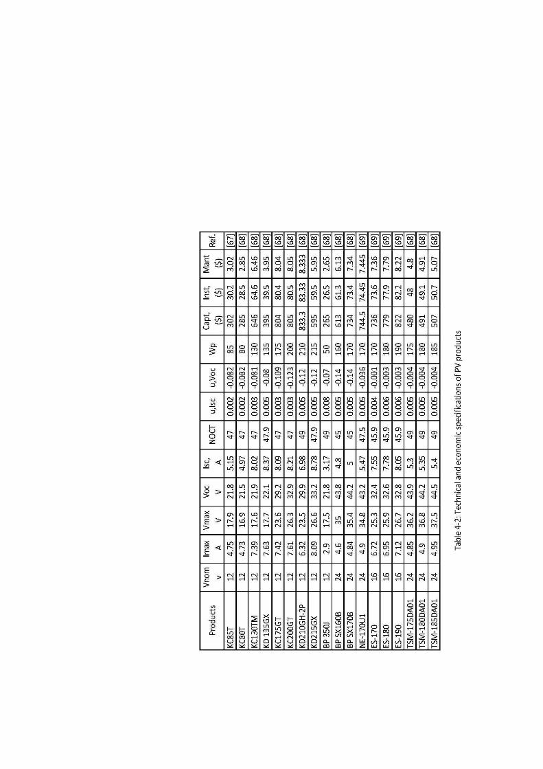
76

77

78
Finally, table (4-4) shows the battery products database where Con, S, DEKA and STECO stands for
Concorde, Surrette, East Penn and Spruter battery manufacturer respectively. In table (4-4), Nom,
Capacity, Eff, DOD and Life represent nominal voltage, nominal capacity, efficiency, depth of discharge
and life span of the battery products respectively. In table (4-2)-(4-4), Capt, Inst, Mant, Tcapt, Tinst and
Tmant represent the capital cost, installation cost, maintenance cost, tower capital cost, tower
installation cost and tower maintenance cost of HSWPS respectively. Ref. represents the references of
the data taken.
Load Data
It is reiterated that the chosen site consists of a CDMA 2C10 BTS, VSAT and Repeater Station with power
requirement of 530Watt, 75Watt and 50 Watt respectively. The specifications of power consumption by
the CDMA BTS are given in the table (4-5). BTS is operated at full load and half load condition under
maximum and minimum traffic, so, power consumption of BTS can be categorized according to the time
intervals carried by the traffic. According to NT, traffic of the telecommunication network at Nepal is
very low at 1:00 am -6 am and 11:00 pm – 12:00 pm, so for this case study, CDMA 2C10 BTS power
consumption is varied under different intervals of time. Under full load and half load condition, the
power consumption of CDMA 2C10 BTS is 530Watt and 480Watt respectively [73].
Typical Configuration
Output Power
Full Load Power
Half Load Power
1C1S 20 W 340W 310W
2C10 20 W 530W 480W
2C1S 20 W 590W 540W
3C1S 20 W 860W 780W
1C2S 20 W 590W 540W
1C3S 20 W 860W 780W
Table 4-5: Typical power consumption of ZTE BTS for 1xEVDO [73]
4.3 Assumptions
1. Life span of the project is taken to be 20 years
2. The life span of PV array and wind turbine is equal to the project duration
3. The installation cost of each components is 10% of Capital cost per year
4. The maintenance cost of each components is 1% of Capital Cost per year

79
5. The nominal interest and Inflation rate are 12% and 6% respectively
6. The minimum number of battery, PV modules and wind turbine are one for each simulation
7. The maximum number of parallel batteries bank, PV modules and wind turbine are 5, 24 and 2
respectively for each simulation based on the site area
8. LPSP requirement is 0.2 with reliability and LUEC probability of 0.6 and 0.4 respectively
9. The transportation cost to reach each components as wind turbine, PV module, and battery to
Nepal is $25, $5 and $8 respectively based on the existing system database
10. The cost of charging regulator of the existing system is not taken for the economic analysis
11. Except NT Capital cost of Tower, the other tower cost is same for each products
4.4 Existing System
The existing system consists two 3.06 kW Kyocera KC85T PV array connected in parallel and the output
of PV array is fed to voltage regulator. Since, the bus voltage of telecommunication is 48V, for each array
4 panels are connected in series to provide fixed bus voltage and 18 panels are connected in parallel to
meet the telecommunication load. The charge regulator TRISTAR TS-60 of 60A current is used in the
system so that it provides reliable solar battery charging, load control or diverse regulation. Its main
function of it is to fully charge a battery without permitting overcharge while preventing reverse current
flow at night. The output of the charge regulator is connected to the battery so that it provides constant
charging process. Instead of providing renewable power direct to load, all the energy generated from
renewable resources is charged to the battery. The battery used is Narada GFM-800 of 800AH capacity
with 2 battery bank where 24 batteries each of 2V are connected in series to meet bus voltage resulting
in 48 batteries. Similarly, the power generated from the 1kW Hummer H3.1 DC wind turbine operating
at 48V is fed to the hybrid solar/wind controller and the output of hybrid solar/wind controller is fed to
the battery.
Again, the output voltage from the battery is fed to the charge controller so that it provides constant
power to the load. The charge controller used is PROSTAR PS-15M-48V PG of 48V/15A. Thus, the existing
system with 6.12kW PV Array, 1 kW wind turbine and 1600AH battery bank provides the power supply
to the remote station telecommunication load. The site station consisting of PV array, wind turbine and
remote load for case study is shown in figure (4-4) and its architecture is shown in figure (4-5).

80
Fig. 4-4: Existing system consisting of PV array, wind turbine and telecommunication load [70]
Fig. 4-5: Architecture of existing system

81
4.5 Proposed System
The proposed system includes PV array, wind turbine, battery, telecom load and dummy load as the
components of HSWPS. The algorithm of power supply to the telecom load is different from the existing
system. If the power generation from the RES is greater than the telecom load, then HSWPS directly
supplies power to the load and the surplus energy is stored in the battery and new storage is calculated
at every instant until the full capacity is obtained. Similarly, if the power generation from RES is lesser
than the telecom load, then deficient power is supplied from the battery to the load. The proposed
system, moreover, emphasizes the reduction of the size of the battery bank for the HSWPS.
Furthermore, in order to save the life span of the battery from over charging and over discharging, the
state of charge of the battery is calculated for each instant of time. The details are illustrated in the
flowchart for simulation operation and optimization of HSWPS in figure (3-6).

82

83
Chapter 5
Results and Discussion
The results can be analyzed and discussed in terms of the feasibility assessment of the site and sizing of
the existing and proposed system. The feasibility assessment of the site is carried through HOMER
software which comprises HSWPS components as PV array, wind turbine and battery of the existing
system to provide dc bus voltage (48V) to the telecommunication load shown in figure (5-1). The
developed methodology has been applied to design and sizing standalone hybrid PV/wind system in
MATLAB environment.
Fig. 5-1: Schematic diagram of hybrid system of the site
The monthly average horizontal solar radiation, wind speed and telecom load with several optimization
variables is given as the input of HOMER software and it generates time series simulations of battery
state of charge and power generation from PV array and wind turbine for a year. Figure (5-2) shows the
monthly average daily solar radiation and clearness index in year and figure (5-3) represents the
synthetic hourly solar radiation generated by the HOMER. Figure (5-4) shows the monthly average wind
speed profiles and figure (5-5) represent hourly generation wind speed.

84
Fig. 5-2: Average daily solar radiation in a year Fig. 5-3: Hourly solar radiation in a year
Fig. 5-4: Average wind speed in a year Fig. 5-5: Hourly wind speed
It is clear from figures (5-2) and (5-4) that Dadakharka site which is located in the mountainous belt and
has a different climatic variation than other places. During the months of February, March and April, it
has a higher wind speed and solar radiation, whereas, during the months of July, August and September,
it has a low wind speed and solar radiation. However, figures (5-3) and (5-5) representing timely
simulations shows that during summer seasons i.e. July, August and September, the solar radiation and
wind speed reaches the maximum and minimum limit respectively. In addition, during winter seasons
i.e. October, November and December, figures (5-5) and (5-3) shows that wind speed is higher and the
solar radiation is lower. Figure (5-2) illustrates that the clearness index goes on decreasing from the
month January and reaches the minimum value for the month July and again it increases till December.
The frequency distribution of renewable resources during a month, season or year is best described by
the probability distribution function (PDF) and HOMER calculates the PDF of wind and solar radiation for
the optimization results. The PDF for solar radiation and wind speed is shown in figures (5-6) and (5-7)
respectively.

85
Fig. 5-6: Probability of solar radiation distribution
Fig. 5-7: Probability of wind speed distribution
From figure (5-6), it is clear that the case study site has 52% probability of solar radiation to be 0 kW/m2.
It means that it has a chance of 48% available solar radiation to produce solar energy in which the
average solar radiation is 4 kW/m2. Similarly, figure (5-7) shows the wind resource distribution
characterized by the Weibull distribution with average wind speed of 4.07 m/s and scale factor (k) of 2.0
during a year. The probability of having wind speed to be 4.07m/s is about 93% during a year and the
site can provide reasonable wind power.
The daily and monthly telecommunication load profiles for the chosen site is shown in figures (5-8) and
(5-9). The 2C1S and 3C1S configuration of 1xEVDO CDMA power consumption are also considered in the
sensitivity analysis to identify the best system with increase in telecommunication load.
Fig. 5-8: Daily load profiles Fig. 5-9: Monthly load profiles during a year

86
The power produced by the 6.12 kW Kyocera KC85T PV array is shown in figure (5-10). The figure is a D-
map (data map) which shows the time series data of one year. In this figure, the x-axis represents each
time step of the year and y-axis represent the time of the day.
Fig. 5-10: D-map showing the power generated from the 6.12 kW KC85T PV array
From figure (5-10) it is clear that during January to September, the power generated by the KC85T PV
array reaches the maximum value of about 2kW and up to 1.4kW during October to December. It also
illustrates that minimum and maximum power available from KC85T PV array is 0kW and 2kW.
Furthermore, the figure shows that sunrise and sunset time during March to September is between 6:00
am - 6:00 pm and 5:00 am - 5:00 pm during September to December. From the HOMER results, the
KC85T PV array produces a mean output of 0.41kW i.e. 9.75kWh/day with a total power available 3,557
kWh/year. The PV is operated for 4,382 hour/year with its penetration of about 71.1%.
The output power from 1kW Hummer H3.1 wind turbine is shown in figure (5-11). From the figure it is
clear that power generated by the wind turbine is low and high in the summer and winter season
respectively. It also shows that during midnight and in the afternoon i.e. 3pm (which is taken as peak
hour of the sun in the case study), the power generated from H3.1 wind turbine is about 0.24kW. The
HOMER results, moreover, shows that maximum power generated from the H3.1 wind turbine reaches
up to 0.6 kW with a mean output of 0.09 kW. The wind turbine is operated for 7,115 hour/year with its
penetration of about 9.32% and a total power of 816kWh/year.
Figure (5-12) summarizes the monthly average electricity production from the 6.12 kW KC85T PV array
and 1kW H3.1 wind turbine system. It shows that PV array and wind turbine produces 4,374 kWh during
a year. It clearly delineates that the power generated from KC85T PV array system is higher than that of
H3.1 wind turbine system where the renewable power generation contribution from PV array and wind
turbine is 81% and 19% respectively.

87
Fig. 5-11: D-map showing power generated from 1kW H3.1 wind turbine
Fig. 5-12: Monthly average electricity production from KC85T PV array and H3.1 wind turbine system
The RES stored in the battery is distinguished by the battery SOC. Figure (5-13) represents the monthly
SOC of the 1600 Ah Narada GFM-800 battery and figures (5-14) represent its probability of frequency
distribution during a year. Figure (5-15) shows the D-map of battery SOC illustrating seasonal and
monthly profile.
Fig. 5-13: Monthly SOC of the battery Fig. 5-14: Frequency histogram of the battery

88
Fig 5-15: D-map showing 1600Ah GFM-800 battery bank state of charge
From figure (5-14), it is clear that the probability of battery SOC to be 30% is 0.55 and the probability of
battery to reach the maximum value i.e. greater than 80% is around 0.05. Also, from figure (5-13), it is
distinct that the battery SOC reaches the maximum value during January to April whereas after April till
December the SOC of the battery decreases. The average SOC during January to April is about 65%
whereas from May to December, SOC is about the minimum value i.e. 30%. From the D-map in figure
(5-15), it can be pictured out that the battery reaches the maximum value during January and SOC of the
battery reach up to 86% from March to April. It is known from HOMER results that the energy input and
energy output from the GFM-800 battery is 1,732kWh and 1,549kWh respectively during a year. In
addition, results shows that the annual throughput of the battery is 1,670kWh/year with losses of
135kWh/year.
The economic analysis is also indispensable for the assessment of the RES. HOMER financial results
shows that 6.12 kW KC85T PV system has five times higher net present value (NPV) than that of 1kW
H3.1 wind turbine system and 1600 Ah GFM-800 battery has five times higher NPV than that of 1kW
H3.1 wind turbine system for the project duration.
Figure (5-16) shows the optimization results of different configuration systems for varying wind speed
and telecommunication load. From the figure it is clear that only 6.12 kW KC85T PV system cannot meet
the telecommunication load demand. The figure delineates that if the wind speed is below 4.5 m/s, only
PV system is applicable to the telecom load of 750Watt. Similarly, if the wind speed is above 7 m/s, only
wind system is feasible for the all the load demand. However, most feasible configuration of the system
is categorized by hybrid system consisting wind turbine and the PV array. It is moreover, vivid that the
probability of only PV system to meet the telecom load is about 15% for wind speed below 4.5 m/s,
whereas the probability of only wind turbine system to meet the telecom load is about 25% for the wind
speed above 7 m/s. It means that there is 60% probability of HSWPS to meet the telecom load
technically and financially. It can also be concluded that hybrid system consisting Wind/PV/Battery is
suitable for the 2C1S and 3C1S 1xEVDO CDMA technology as well.

89
Fig. 5-16: Optimization results of different configuration systems
Overall, HOMER shows that levelized cost of energy generation from 6.12 kW KC85T PV system is
$0.647/kWh and that of 1kW H3.1 wind turbine system is $0.533. Thus, from the HOMER feasibility
assessment, we can conclude that the most feasible configurations for the existing and converged
telecommunication network system is the hybrid PV and wind system at the remote station.
The various methodology of dissertation is implemented to find the optimal sizing of HSWPS using
MATLAB. Before sizing the system, it is imperative to generate the synthetic solar and wind generation
profiles from the monthly average data and the output power from each individual system. Figure (5-
17) shows the synthetic ambient temperature, solar radiation and wind speed generation for a year by
applying the methodology in MATLAB environment. The load pattern of a year is also shown in figure (5-
17). In figure (5-17), initially, temperature is low and it goes on increasing till 4000 hours. From 4000-
6000 hours, the temperature reaches the maximum value and it decreases till 8760 hours from 6000
hours. In contrast to it, the wind speed and solar radiation values is low for time interval 4000-6000
hours and its value is high for time interval 1-4000 hours and 6000-8000 hours. Figures (5-18)-(5-20)
shows the hourly synthetic generation of solar radiation, wind speed and ambient temperature
respectively using the methodology. The figures delineate the each month hourly pattern.
Figures (5-18)-(5-20) also delineates the sporadic nature of solar radiation, wind speed and temperature.
The result shows that during January till July, the solar radiation goes on increasing with some random
variations and decreases its value from August till December.

90
Fig. 5-17: Synthetic generation of temperature, solar radiation, wind speed and telecom load
Fig. 5-18: Synthetic monthly solar radiation generated during a year
0 1000 2000 3000 4000 5000 6000 7000 8000 9000-10
0
10
20
30
40
50
60
Time(hours)
Am
bien
t T
empe
ratu
re (
deg/
cent
)
0 1000 2000 3000 4000 5000 6000 7000 8000 90000
100
200
300
400
500
600
700
800
Time(hours)
Sol
ar R
adia
tion
(Wh/
m2 )
0 1000 2000 3000 4000 5000 6000 7000 8000 90000
2
4
6
8
10
12
14
Time(hours)
Win
d sp
eed
(m/s
)
0 1000 2000 3000 4000 5000 6000 7000 8000 9000400
450
500
550
600
650
700
Time(hours)
Tel
ecom
Loa
d (W
att)
0 200 400 600 8000
200
400
600
Time(hours)
Sol
ar R
adia
tion
Wh/
m2 January
600 800 1000 1200 1400 16000
200
400
600
Time(hours)
Sol
ar R
adia
tion
Wh/
m2 February
1400 1600 1800 2000 22000
500
1000
Time(hours)
Sol
ar R
adia
tion
Wh/
m2 March
2000 2200 2400 2600 2800 30000
500
1000
Time(hours)
Sol
ar R
adia
tion
Wh/
m2 April
2800 3000 3200 3400 3600 38000
200
400
600
Time(hours)
Sol
ar R
adia
tion
Wh/
m2 May
3600 3800 4000 4200 44000
200
400
600
Time(hours)
Sol
ar R
adia
tion
Wh/
m2 June
4200 4400 4600 4800 5000 52000
200
400
600
Time(hours)
Sol
ar R
adia
tion
Wh/
m2 July
5000 5200 5400 5600 5800 60000
200
400
600
Time(hours)
Sol
ar R
adia
tion
Wh/
m2 August
5800 6000 6200 6400 66000
200
400
600
Time(hours)
Sol
ar R
adia
tion
Wh/
m2 September
6400 6600 6800 7000 7200 74000
200
400
600
Time(hours)
Sol
ar R
adia
tion
Wh/
m2 October
7200 7400 7600 7800 80000
200
400
600
Time(hours)
Sol
ar R
adia
tion
Wh/
m2 November
8000 8200 8400 8600 88000
200
400
Time(hours)
Sol
ar R
adia
tion
Wh/
m2 December
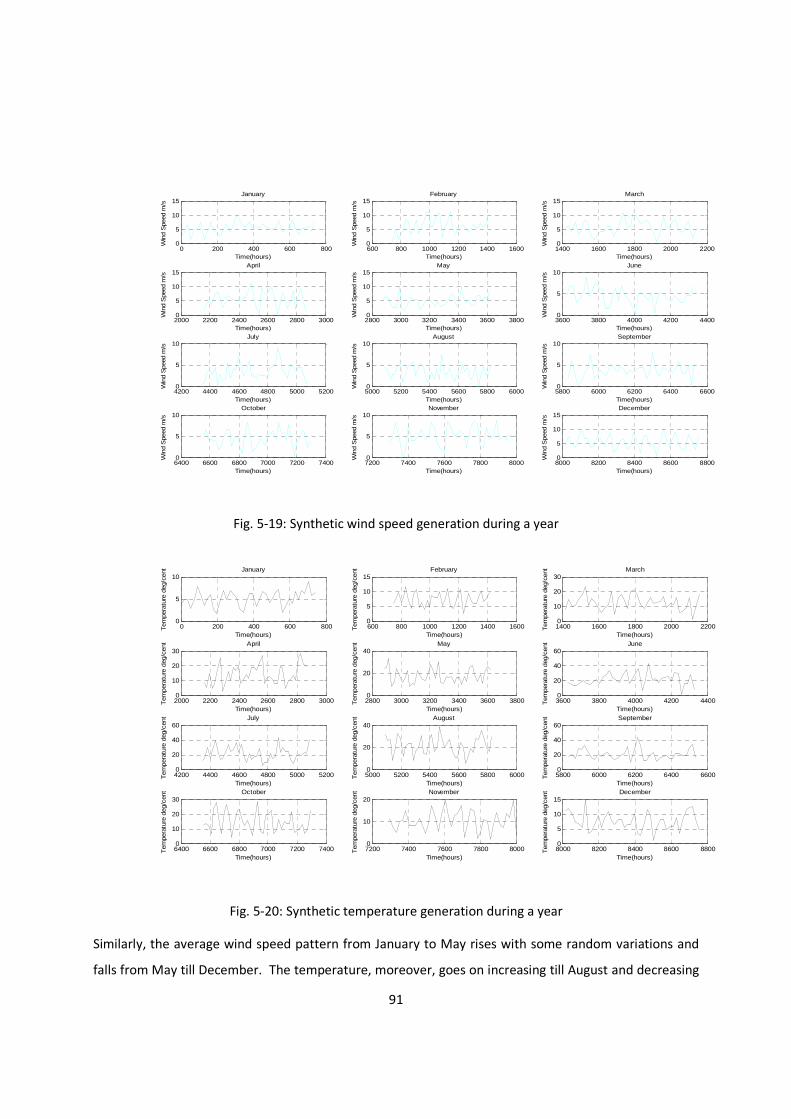
91
Fig. 5-19: Synthetic wind speed generation during a year
Fig. 5-20: Synthetic temperature generation during a year
Similarly, the average wind speed pattern from January to May rises with some random variations and
falls from May till December. The temperature, moreover, goes on increasing till August and decreasing
0 200 400 600 8000
5
10
15
Time(hours)
Win
d S
peed
m/s
January
600 800 1000 1200 1400 16000
5
10
15
Time(hours)
Win
d S
peed
m/s
February
1400 1600 1800 2000 22000
5
10
15
Time(hours)
Win
d S
peed
m/s
March
2000 2200 2400 2600 2800 30000
5
10
15
Time(hours)
Win
d S
peed
m/s
April
2800 3000 3200 3400 3600 38000
5
10
15
Time(hours)
Win
d S
peed
m/s
May
3600 3800 4000 4200 44000
5
10
Time(hours)
Win
d S
peed
m/s
June
4200 4400 4600 4800 5000 52000
5
10
Time(hours)
Win
d S
peed
m/s
July
5000 5200 5400 5600 5800 60000
5
10
Time(hours)
Win
d S
peed
m/s
August
5800 6000 6200 6400 66000
5
10
Time(hours)
Win
d S
peed
m/s
September
6400 6600 6800 7000 7200 74000
5
10
Time(hours)
Win
d S
peed
m/s
October
7200 7400 7600 7800 80000
5
10
Time(hours)
Win
d S
peed
m/s
November
8000 8200 8400 8600 88000
5
10
15
Time(hours)
Win
d S
peed
m/s
December
0 200 400 600 8000
5
10
Time(hours)
Tem
pera
ture
deg
/cen
t January
600 800 1000 1200 1400 16000
5
10
15
Time(hours)
Tem
pera
ture
deg
/cen
t February
1400 1600 1800 2000 22000
10
20
30
Time(hours)
Tem
pera
ture
deg
/cen
t March
2000 2200 2400 2600 2800 30000
10
20
30
Time(hours)
Tem
pera
ture
deg
/cen
t April
2800 3000 3200 3400 3600 38000
20
40
Time(hours)
Tem
pera
ture
deg
/cen
t May
3600 3800 4000 4200 44000
20
40
60
Time(hours)
Tem
pera
ture
deg
/cen
t June
4200 4400 4600 4800 5000 52000
20
40
60
Time(hours)
Tem
pera
ture
deg
/cen
t July
5000 5200 5400 5600 5800 60000
20
40
Time(hours)
Tem
pera
ture
deg
/cen
t August
5800 6000 6200 6400 66000
20
40
60
Time(hours)
Tem
pera
ture
deg
/cen
t September
6400 6600 6800 7000 7200 74000
10
20
30
Time(hours)
Tem
pera
ture
deg
/cen
t October
7200 7400 7600 7800 80000
10
20
Time(hours)
Tem
pera
ture
deg
/cen
t November
8000 8200 8400 8600 88000
5
10
15
Time(hours)
Tem
pera
ture
deg
/cen
t December

92
from August till December. It can be observed from the figure that during January, the average solar
radiation, wind speed and temperature is about 400 Wh/m2, 5 m/s and 50C respectively. Solar radiation
is almost constant in January whereas the wind speed and temperature reaches to maximum values of
10 m/s and 80C respectively and minimum values of 3 m/sand 30C respectively. In addition, during
February, the average solar radiation is 420Wh/m2 and is constant during entire month. During this
month, the wind speed reaches to peak value 12 m/s with base value of 1 m/s and average value of 8
m/s. The pattern of temperature is fluctuating with the uttermost value 120C and bottom value 40C
having mean value of 7.50C. Furthermore, during March and April, the solar radiation value is almost
constant and is about 500 Wh/m2, whereas, the wind speed and temperature ultimate value is about 12
m/s and (22-28) 0C. The minimum value of wind speed is 2 m/s in March and there is no wind available
at some days in April. During summer i.e June, July and August, the solar radiation increases with
maximum value of 520 Wh/m2 to 600 Wh/m2 with some stochastic fluctuations in second and third
week of each month. During these months, temperature reaches the maximum value of 420C with
minimum value of 100C. Similarly, the average wind speed falls during these months with some random
variations of peak and bottom value of 8m/s and 0 m/s. Consequently during winter seasons, the solar
radiation falls to about 400 Wh/m2 with some random variations, whereas the wind speed increases in
these seasons. The topmost value of wind speed during these seasons is about 10 m/s with bottom
value of 2 m/s. However, the average temperature value is decreasing in these seasons with the average
of 120C.
Figures (5-21) and (5-22) show the power generation from PV array and wind turbine of different
manufacturer during a year. It is clear from the figure (5-21) that Kyocera KC85T produces maximum
and minimum power of about 55 Watt and 5 Watt during a year. Similarly, BP Solar SX170B with 170
Watt of panel capacity produces maximum and minimum power of 118 Watt and 5 Watt. On the other
hand, Evergreen Spruce ES-170 with same panel capacity as BP Solar SX170B produces more power than
BP solar. It can be observed from the figure that maximum and minimum power generation from ES-170
is about 120 Watt and 5 Watt. Consequently, Trina Solar TSM-175 DA01 with panel capacity of 175Watt
generated the peak and bottom power of 130 Watt and 10 Watt. In comparing the power generation
capacity of these 4 different manufacturers from figure (5-21), TSM-175 DA01 seems more superior in
terms of average power generation.

93
Fig.5-21: Power generation from different PV manufacturer during a year
Fig. 5-22: Power generation from different wind turbine manufacturer during a year
It can be observed from figure (5-22) that the three wind turbine as Hummer H3.1, Kestrel 1000 and
Bergey BWCXL100 has a power rating of each 1kW whereas Bornay 1500 has 1.5kW. Bornay 1500
generates the maximum power of about 800 Watt during entire year. Hummer H3.1, Kestrel 1000 and
0 1000 2000 3000 4000 5000 6000 7000 8000 90000
10
20
30
40
50
60
time(hours)
PV
Pow
er o
/p
Kyocera KC85T
0 1000 2000 3000 4000 5000 6000 7000 8000 90000
20
40
60
80
100
120
time(hours)
PV
Pow
er o
/p
BP Solar SX170B
0 1000 2000 3000 4000 5000 6000 7000 8000 90000
20
40
60
80
100
120
140
time(hours)
PV
Pow
er o
/p
Trina Solar TSM-175DA01
0 1000 2000 3000 4000 5000 6000 7000 8000 90000
20
40
60
80
100
120
140
time(hours)
PV
Pow
er o
/p
Evergreen Spruce ES-170
0 1000 2000 3000 4000 5000 6000 7000 8000 90000
100
200
300
400
500
600
700
time(hours)
Win
d P
ower
o/p
Hummer H3.1
0 1000 2000 3000 4000 5000 6000 7000 8000 90000
100
200
300
400
500
600
700
800
time(hours)
Win
d P
ower
o/p
Bornay 1500
0 1000 2000 3000 4000 5000 6000 7000 8000 90000
100
200
300
400
500
600
time(hours)
Win
d P
ower
o/p
Kestrel 1000
0 1000 2000 3000 4000 5000 6000 7000 8000 90000
100
200
300
400
500
600
time(hours)
Win
d P
ower
o/p
BWCXL100

94
Bergey BWCXL100 generates a maximum power of 650 Watt, 580 Watt and 590 Watt respectively. Also,
from the figure it is clear that power distribution during a entire year in the Hummer is far better than
the three turbines as Kestrel 1000, Bergey BWCXL100 and Bornay 1500. Thus, we can conclude that
Hummer H3.1 wind turbine is superior to rest of the turbine in power generation capacity.
Large configurations of the system can be achieved with the constraints of battery, PV modules and
wind turbines in the simulation work. Table (5-1) shows a sample of configuration results obtained from
MATLAB simulation. The table represents the summary of simulation operations from which optimum
sizing results can be obtained in terms of reliability and LUEC. In the table, Wty, Pty and Bty represent
the wind turbine, PV and battery different manufacturer system. The values 1, 2, 3 etc... in each type
system shows the manufacturer configuration. Similarly, Pwt, Nwt and Tpwt represent the power
rating of wind turbine (WT), number of WT and total power rating of WT. Ppv, Npv and Tppv, moreover,
stand for power rating of each panel, number of PV panels and total power rating of PV array. In
addition, CB and Nbat represent the capacity of each battery and number of battery. Finally, PL, Pre,
WE% represent the total load power, total renewable energy generation, excess energy percentage for a
year and Tcost represents the total cost of the system for the entire project duration. The detail of the
list of the configurations of the system is included in the separate CD.
The optimal configuration of the system is achieved by defining the cost function in terms of reliability
and LUEC that meets the desired LPSP. The simulation result shows that Hummer H3.1 (1kWx2) wind
turbine, Trina Solar TSM-175DA01 (8.05kW) PV array and Trojan T-105 (1125Ah) justified the remote
telecom load requirement of Dadakhara with reliability of 99.99% with a significant cost reduction as
well as reliable energy production. On the contrary, the existing system containing Hummer H3.1 (1kW)
wind turbine, Kyocera KC85T (6.12kW) PV array and Narada GFM-800 (1600Ah) have a unmet load of
36.6% during a year. The results can be analyzed in terms of excess energy, reliability and LUEC from
different manufacturer specifications. Figure (5-23) delineates the reliability and excess energy as a
function of Trina Solar TSM-175DA01 power with Trojan T-195 (1125Ah) battery capacity for a different
wind turbine.
It can be observed from figure (5-23) that Hummer H3.1 has a better reliability than BWCXL 100 and
Kestrel 1000 each of 1 kW capacity. From the figure it is clear that Kestrel 1000 (two 1kW capacity) has a
less excess energy than rest of the system, however, the reliability of it is similar to the 1kW Hummer
H3.1 wind turbine. The figure shows that Hummer H3.1 two 1kW wind turbine has a higher reliability
than rest of the system with excess energy higher than rest.

95

96
Fig. 5-23: Reliability and excess energy as a function of PV power for different wind turbine
Thus, we can conclude from figure (5-23) that with increase of PV array, reliability and excess energy
also increases. There is a tradeoff between reliability and excess energy. However, when the PV power
is 8.05 kW, the reliability of Hummer H3.1 (1kW x2) is superior to other system.
Fig. 5-24: Reliability and excess Energy as a function of PV power for different capacity of battery
0 1 2 3 4 5 6 7 8 90
0.1
0.2
0.3
0.4
0.5
0.6
0.7
0.8
0.9
1
PV- TSM-175DA01 power (kW)
Rel
iabi
lity/
Exc
ess
Ene
rgy
Hummer H3.1(1kWx1)
Hummer H3.1(1kWx2)
BWCXL 100(1kWx1)BWCXL100(1kWx2)
Kestrel 1000(1kWx1)
Kestrel 1000(1kWx2)
Excess Energy
Reliability
0 1 2 3 4 5 6 7 8 90
0.1
0.2
0.3
0.4
0.5
0.6
0.7
0.8
0.9
1
PV- TSM-175DA01 power (kW)
Rel
iabi
lity/
Exc
ess
Ene
rgy
Narada GFM-800 (800Ah)
Trojan T-105 (675Ah)Surrette S-460 (1050Ah)
Concorde PVX890T (510Ah)
Excess Energy
Reliability
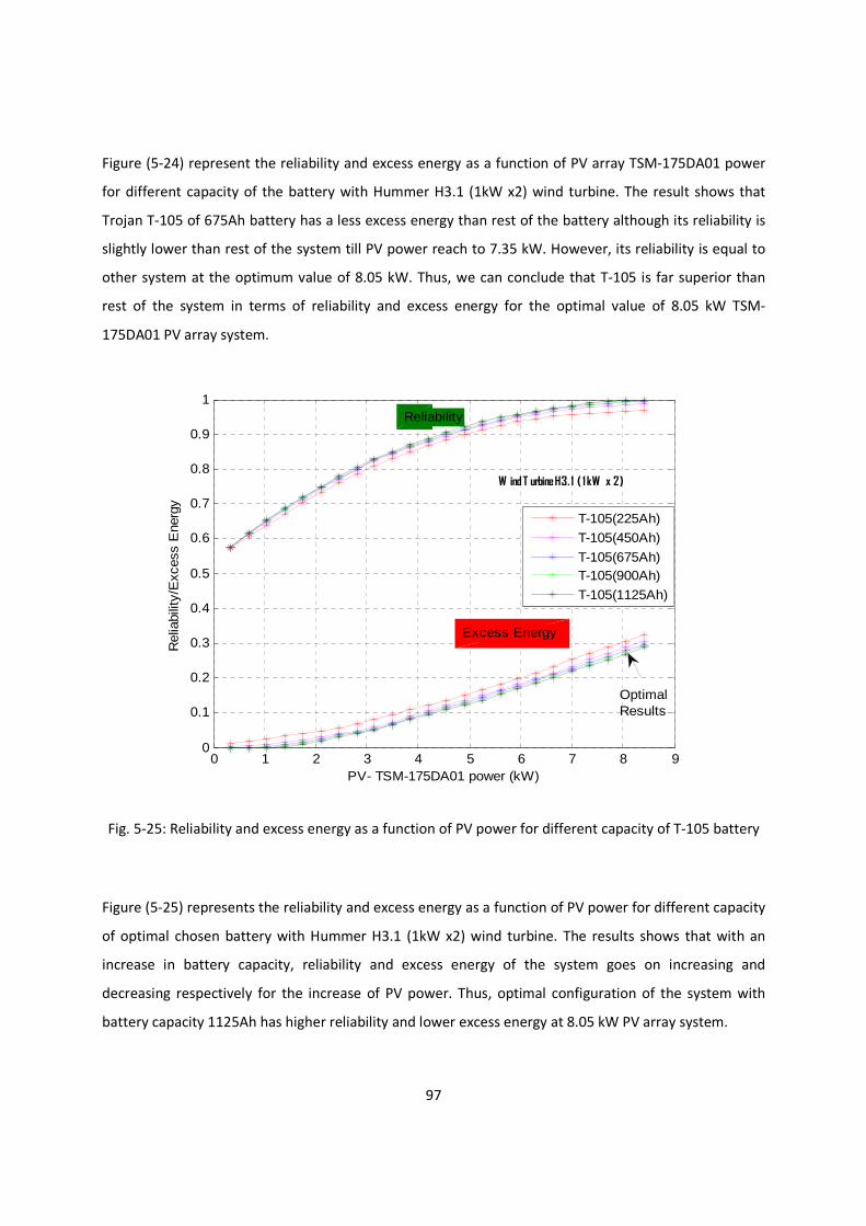
97
Figure (5-24) represent the reliability and excess energy as a function of PV array TSM-175DA01 power
for different capacity of the battery with Hummer H3.1 (1kW x2) wind turbine. The result shows that
Trojan T-105 of 675Ah battery has a less excess energy than rest of the battery although its reliability is
slightly lower than rest of the system till PV power reach to 7.35 kW. However, its reliability is equal to
other system at the optimum value of 8.05 kW. Thus, we can conclude that T-105 is far superior than
rest of the system in terms of reliability and excess energy for the optimal value of 8.05 kW TSM-
175DA01 PV array system.
Fig. 5-25: Reliability and excess energy as a function of PV power for different capacity of T-105 battery
Figure (5-25) represents the reliability and excess energy as a function of PV power for different capacity
of optimal chosen battery with Hummer H3.1 (1kW x2) wind turbine. The results shows that with an
increase in battery capacity, reliability and excess energy of the system goes on increasing and
decreasing respectively for the increase of PV power. Thus, optimal configuration of the system with
battery capacity 1125Ah has higher reliability and lower excess energy at 8.05 kW PV array system.
0 1 2 3 4 5 6 7 8 90
0.1
0.2
0.3
0.4
0.5
0.6
0.7
0.8
0.9
1
PV- TSM-175DA01 power (kW)
Rel
iabi
lity/
Exc
ess
Ene
rgy
T-105(225Ah)
T-105(450Ah)
T-105(675Ah)T-105(900Ah)
T-105(1125Ah)
W ind T urbine H3.1 ( 1 kW x 2)
Excess Energy
Reliability
OptimalResults

98
Figure (5-26) represents the hourly variation of state of charge of the battery T-105. The optimal
configuration of the system consists of 40 batteries each of 225Ah with 5 battery bank in parallel
resulting in a maximum capacity of 1125Ah. From the figure it is clear that from February to June and
October to December, the battery is fully charged. It means that power generated by renewable
resources always fulfills the load. However, during July to September, the power generated by
renewable resources is weak. In this duration also, the battery state of charge does not drop below
minimum state of charge ((+�!�) which is 168.75 Ah. So, the remote telecom station load is always
satisfied by the proposed configurations.
Fig. 5-26: Hourly variation of state of charge (SOC) of battery bank
Figure (5-27) represents the hourly variation of waste energy for the optimal configuration system with
6.12kW TSM-175DA01 PV Array, 1kW X2 Hummer H3.1 wind turbine and 1125Ah Trojan T-105 battery.
The results show that waste energy reaches up to maximum of 2.8kW during April, however, the waste
energy is 0 from the July to September. It means that proposed system guarantee the reliability of
99.99% during these months.
0 1000 2000 3000 4000 5000 6000 7000 8000 90000
200
400
600
800
1000
1200
Number of hours
Cap
acity
of
batt
ery
(Ah)
1125 Ah T-105
SOCmin
SOCmax

99
Fig. 5-27: Hourly variation of waste energy for the optimal configuration system
Figure (5-28) represent the LUEC as a function of excess energy for the optimal configuration system
with TSM-175DA01 PV Array and battery T-105 of 1125Ah capacity. It can be observed from the figure
that unit electricity cost generation from Hummer wind turbine is very cheap than rest of the turbines.
The result shows that power generation from Kestrel is higher than rest of the system and the LUEC of
optimal HSWPS configuration is found to be 0.86.
Figure (5-29) represents the comparison of the existing NT system and the proposed system. It
illustrates that existing system has deficient energy to fulfill the remote telecom load. The reliability is
also poor than the newly proposed system which has reliability of 99.99 % with excess energy of 26.9%
in a year.
0 1000 2000 3000 4000 5000 6000 7000 8000 90000
0.5
1
1.5
2
2.5
3
Number of hours
Was
te E
nerg
y kW
h

100
Fig. 5-28: Levelized unit cost of electricity as a function of excess energy for optimal configuration
Fig. 5-29: Comparison of existing and new system in terms of reliability and excess energy
Figures (5-30) – (5-31) represent the net present cost (NPC) of the proposed and existing HSWPS for the
project duration of 20 years. In the proposed system, wind turbine, PV array and battery net present
system cost are `15%, 40% and 46 % respectively for total net present system cost of $72,378. Similarly,
0 0.05 0.1 0.15 0.2 0.25 0.3 0.350.45
0.5
0.55
0.6
0.65
0.7
0.75
0.8
0.85
0.9
0.95
Excess Energy (%)
Leve
lized
Uni
t C
ost of
Ele
ctric
ity ($/
kWh)
Hummer H3.1(1kWx1)
Kestrel 1000(1kWx1)
BWCXL 100(1kWx1)Hummer H3.1(1kWx2)
Kestrel 1000(1kWx2)
BWCXL100(1kWx2)
T SM-175DA 01
T -105 ( 1 1 25 A h)
Optimal Results
0 1 2 3 4 5 6 7 8 90
0.1
0.2
0.3
0.4
0.5
0.6
0.7
0.8
0.9
1
PV power (kW)
Rel
iabi
lity/
Exc
ess
Ene
rgy
Existing System
New System
Reliability
Excess Energy
Existing sizing
New sizing

101
for the existing system, net present cost of wind turbine, PV array and battery are 14%, 34% and 51%
respectively for the total net present cost of $101,550. The result shows that existing system has 1.4
times higher net present value of system cost than the proposed system and the battery cost in the
existing system is also higher. Also, it is known from the simulation result that LUEC from existing and
proposed system is $1.22 and $0.87 respectively.
Fig. 5.30: NPC of proposed HSWPS Fig. 5.31: NPC of existing HSWPS
15%
40%
46%
H3.1 (1kWx2)
TSM-175DA 01 (8.05 kW)T-105 (1125Ah)
14%
34%
51%
H3.1 (1kW)
KC85T (6.12kW)
GFM-800 (1600Ah)

102

103
Chapter 6
Conclusion and Future Works
6.1 Conclusion
The development of wind and solar energy for satisfying the telecommunication load at the remote
station has received considerable attention in the recent years due to the unavailability of the grid
electricity supply, rapid depletion of fossil fuel reserves and increasing demand of clean energy
technologies to reduce greenhouse gas emissions. However, due to the sporadic nature of solar and
wind energy, it is imperative to carry the feasibility assessment and evaluate the reliability of these
power. In this work, a methodology has been developed for carrying the feasibility assessment and
optimal sizing of standalone hybrid PV/wind system with battery storage using an optimization model.
The proposed methodology has been applied to analyze HSWPS for a remote telecom station on
Dadakharka of Nepal. The algorithm is based on the monthly average data of solar radiation, wind speed
and temperature for the site under consideration.
The feasibility assessment result is analyzed by varying the wind speed as a function of remote telecom
load for three configurations as only PV, only wind and hybrid PV/wind system with battery storage. It
can be recapitulated that for the existing system, if the wind speed is below 4 m/s, only PV system with
battery storage is suitable for the remote load and if the wind speed is above 7 m/s, only wind system
with battery storage is appropriate for the entire telecom load. However, most feasible configurations
of the system is categorized by hybrid system consisting wind turbine and PV array with battery storage.
It is also concluded that hybrid PV/wind system is viable for the 2C1S and 3C1S 1xEVDO CDMA
technology as well.
In addition, the synthetic hourly solar radiation, wind speed and temperature profile have been
generated. Based on these data, the performance of various technology of PV module and wind turbine
is analyzed in terms of power generation. The simulation result shows that Trina Solar TSM-175 DA01 PV
module seems superior in terms of average power generation for a year in compare to Evergreen Spruce

104
ES-170 and BP Solar SX170B PV module. Similarly, it also found that Hummer H3.1 1kW wind turbine is
superior to Kestrel 1000 and Bergey BWCXL100 each 1kW wind turbine in terms of power distribution
during a year. The result, moreover, obtained from simulation is broadly analyzed in terms of excess
energy and reliability of the HSWPS. While analyzing the same capacity of wind turbine, it is found that
the Hummer H3.1 1kW has a better reliability than BWCXL 100 and Kestrel 1000. Similarly, it is found
that Trojan T-105 battery is reasonable to GFM-800, Surrette S-460 and Concorde PVX890T in terms of
reliability and excess energy. Furthermore, the result shows that with an increase in battery capacity,
the reliability of the system increases and excess energy of the system decreases for the increase of PV
power. Consequently, it is found that optimal configuration of the system with battery capacity 1125Ah
of T-105 has higher reliability and lower excess energy at 8.05kW TSM-175DA01 PV array and Hummer
H3.1 (1kW x2) wind turbine system.
Finally, the optimal configuration of the system is achieved by defining the cost function in terms of
reliability and LUCE that fulfill the desired LPSP. The simulation result shows that Hummer H3.1 (1kWx2)
wind turbine, Trina Solar TSM-175DA01 (8.05kW) PV array and Trojan T-105 (1125Ah) justified the
remote telecom load requirement of Dadakhara with reliability of 99.99% with a significant cost
reduction as well as reliable energy production. On the contrary, the existing system containing Hummer
H3.1 (1kW) wind turbine, Kyocera KC85T (6.12kW) PV array and Narada GFM-800 (1600Ah) has an
unmet load of 36.6% during a year with large investment in battery storage. The result eventually shows
that existing system has 1.4 times higher net present value of system cost than the proposed system and
LUCE of the existing system is 16 % higher than proposed system.
At length, we can conclude that existing system is not technically and financially viable. The optimal
configurations of the proposed system guarantee the reliability of 99.99% with a significant reduction in
cost.
6.2 Future Works
Many interesting question remain that can possibly yield additional insightful analysis. It is well known
that solar and wind resources are intermittent in nature and their prediction is complex due to its
dependency in geographical location. The methodology implemented in this work for the synthetic wind
speed, solar radiation and temperature generation is not validated in context to specific site of Nepal
and can be improved in few ways namely by developing a new model for both solar and wind resources

105
using advanced models as ARMA, Markov Transition, Artificial Intelligence and so on. However, the
improvement of methodology requires time series data of specific site for model development.
In addition, the proposed methodology can be used for the residential application in the remote areas
and further economic analysis in terms of reduction of greenhouse gases with the conventional energy
sources can be evaluated. Moreover, the optimization technique in finding the suitable configurations of
HSWPS in the proposed model is based on Iterative techniques. Although this technique provides
significant results, it takes time to compute the simulation. The time computation in the optimization
process can be reduced using several newly evolved optimization techniques as artificial neural network
and genetic algorithm in the future.
Finally, due to the rapid development of converged broadband telecommunication network and new
renewable energy technologies, the cost of these technologies can be cheaper in the remote areas. The
broadband communication, however, requires high power consumption which can not only fulfill by the
solar and wind energy technologies in the future. So, the other renewable resources with various
storage technologies can be integrated to the existing system for the optimum broadband
communication at the remote site.

106

107
References
[1] Marian Vilsan, Irina Nita, “A hybrid wind-photovoltaic power supply for a telecommunication system”, IEEE, 1997. [2] Pragya Nema, Dr. Saroj Rangnekar, Dr. R.K. Nema, “Pre-feasibility study of PV-solar/wind hybrid energy system for GSM type mobile telephony base station in central India”, IEEE, 2010. [3] Hongxing Yang, Wei Zhou, Lin Lu, Zhaohong Fang, “Optimal sizing method for stand-alone hybrid solar-wind system with LPSP technology by using genetic algorithm”, Solar Energy, vol.82, pp.354-367, 2008. [4] Kazuhiro Kurozumi, Takeru Tawara, Toshikazu Tanaka, Yuji Kawagoe, Takashi Yamanaka, Hiroaki Ikebe, Kazuhiko Shindou, Tetsuo Miyazato, “A hybrid system composed of wind power and photovoltaic system at NTT Kume-jima radio relay station ”, IEEE, 1998. [5] Orhan Ekren, Banu Yetkin Ekren, “Size optimization of a PV/wind hybrid energy conversion system with battery storage using response surface methodology”, Applied Energy, vol.85, pp.1086-1101, 2008. [6] IEC 62257, Series of Standards/Technical Specifications, “Recommendations for small renewable energy and hybrid systems for rural electrification- Part 2: from requirements to a range of electrification system”, International Electro technical Commission, 2004. [7] Report D1.8 for RISE Project, The University of Manchester, “Technical requirements for isolated electrical systems based on renewable energy sources”, European Union, Sixth Framework Programme, June 2005. [8] Elizabeth Harder, Jacqueline MacDonald Gibson, “The costs and benefits of large-scale solar photovoltaic power production in Abu Dhabi, United Arab Emirates”, Renewable Energy, vol. 36, pp. 789-796, 2011. [9] Y. Himri, A. Boudghene Stambouli, B. Draoui, “Prospects of wind farm development in Algeria”, Desalination, vol. 239, pp. 130-138, 2009. [10] G.J. Dalton, D.A. Lockington, T.E. Baldock, “Feasibility analysis of stand-alone renewable energy supply options for a large hotel”, Renewable Energy, vol. 33, pp. 1475-1490, 2008. [11] M.J.Khan, M.T. Iqbal, “Pre-feasibility study of stand-alone hybrid energy systems for applications in Newfoundland”, Renewable Energy, vol. 30, pp. 835-854, 2005.

108
[12] Ahmed M.A. Haidar, Priscilla N. John, Mohd Shawal, “Optimal configuration assessment of renewable energy in Malaysia”, Renewable Energy, vol. 36, pp.881-888, 2011. [13] Shafiqur Rehman, Luai M. Al-Hadhrami, “Study of a solar PV-diesel-battery hybrid power system for a remotely located population near Rafha, Saudi Arabia”, Energy, vol. 35, pp. 4986-4995, 2010. [14] Getachew Bekele, Bjorn Palm, “Feasibility study for a standalone solar-wind-based hybrid energy system for application in Ethiopia”, Applied Energy, vol.87, pp.487-495, 2010. [15] Andrew Mills, Said Al-Hallaj, “Simulation of hydrogen-based hybrid systems using Hybrid2”, International Journal of Hydrogen Energy, vol. 29, pp. 991-999, 2004. [16] K.M. Night, S.A. Klein, J.A. Duffie, “A methodology for the syndissertation of hourly weather data”, Solar Energy, vol.46, no.2, pp. 109-120, 1991. [17] R.J. Aguiar, R. Collares-Perreira, J.P. Conde, “Simple procedure for generating sequences of daily radiation values using a library of markov transition matrices”, Solar Energy, vol. 40, no. 3, pp. 269-279, 1998. [18] Olseth. J.A., A.Skartveit, “Characteristics of hourly global irradiance modeled from cloud data”, Solar Energy, vol.51, pp. 197-204, 1993. [19] LL.Mora-Lopez, M.Sidrach-de-Cardona, “Multiplicative ARMA models to generate hourly series of global irradiation”, Solar Energy, vol. 63, no. 5, pp. 283-291, 1998. [20] A.Mellit, M. Benghanem, A. Hadj Arab, A. Guessoum, “A simplified model for generating sequences of global radiation data for isolated sites: Using artificial neural network and a library of Markov transition matrices approach”, Solar Energy, vol. 79, pp. 469-482, 2005. [21] Degelman Larry, “Simulation and uncertainty: weather predictions”, Advanced Bldg. Simulation, (Malkawi and Augenbroe, Ed.), Spon Press, New York and London, chap.3, pp. 60-86, 2004. [22] John A. Duffie, William A. Beckman, “Solar Engineering of Thermal Process”, John Wiley & Sons, Inc., 1991. [23] Reindl, D.T., W.A .Beckman, J.A. Duffie, “Evaluation of hourly titled surface radiation models”, Solar Energy, 1990, vol. 45, pp. 9-17, 1990. [24] Olmo, F.J., J.Vida, I.Foyo, Y.Castro-Diez, L.Alados-Arboledas, “Prediction of global irradiance on inclined surfaces from horizontal global irradiance”, Energy (Oxford), vol. 24, pp. 689-704, 1999. [25] B.S. Borowy, Ziyad M. Salameh, “Methodology for Optimally Sizing the Combination of a Battery Bank and Pv Array in a Wind/PV Hybrid System”, IEEE Transactions on Energy Conversions, vol.11, no.2, pp. 367-375, Jun. 1996. [26] Markvard T., “Solar Electricity”, 2nd ed. Wiley, USA, 2000.

109
[27] Zhou W., Yang H.X., Fang Z.H., “A Novel model for photovoltaic array performance prediction”, Applied Energy, vol. 84, no. 12, pp. 1187-1198, 2007. [28] P. Bajpai, Prakshan N.P., N.K. Kishore, “Renewable Hybrid Stand-Alone Telecom Power System Modeling and Analysis”, IEEE, TENCON, 2009. [29] F. Lasnier, T.G. Ang, “Photovoltaic Engineering Handbook”, Bristol, England, 1990. [30] M. Nikraz, H. Dehbonei, C.V. Nayar, “A DSP Controlled PV System with MPPT”, Australian Power Engineering Conference, Christchurch, pp. 1-6, 2003. [31] R. Billinton, C. Hua, R. Ghajar, “Time-series models for reliability evaluation of power systems including wind energy”, Microelectronics and Reliability, vol. 36, pp.1253-1261, 1996. [32] A.Shamshad, M.A. Bawadi, W.M.A. Wan Hussin, T.A. Majid, S.A.M. Sanusi, “ First and second order Markov chain models for synthetic generation of wind speed time series”, Energy, vol.30, pp. 693-708, 2005. [33] Hafzullah Aksoy, Z.Fuat Toprak, Ali Aytek, N. Erdem Unal, “Stochastic generation of hourly mean wind speed data”, Renewable Energy, vol.29, pp. 2111-2131, 2004 [34] Hans Georg Beyer, Klaus Nottebaum, “Syndissertation of long-term hourly wind speed time series on the basis of European wind atlas data”, Solar Energy, vol.54, pp. 351-355, 1995. [35] HOMER Software Help Toolboxes. [36] C.Bueno, J.A. Carta, “Technical-economic analysis of wind-powered pumped hydrostorage systems. Part I: model development”, Solar Energy, vol.78, pp.382-395, 2005. [37] Lin Lu, Hongxing Yang and John Burnett, “Investigation on wind power potential on Hong Kong islands-an analysis of wind power and wind turbine characteristics”, Renewable Energy, vol.27, pp.1-12, 2002. [38] Faith O. Hocaoglu, Omer N. Gerek, Mehmet Kurban, “A novel hybrid (wind-photovoltaic) system sizing procedure”, Solar Energy, vol.83, pp.2019-2028, 2009. [39] Chou K.C., R.B. Corotis, “Simulation of Hourly Wind Speed and Array Wind Power”, Solar Energy, vol. 26, pp. 199-212, 1981. [40] Justus CG, Hargraves WR, Mikhail A, Graber D., “Methods of estimating wind speed frequency distribution”, Journal of Applied Meteorology, vol.17, pp.350-353, 1978. [41] Stevens MJM, Smulders PT, “The estimation of parameters of the Weibull wind speed distribution for wind energy utilization purposes”, Wind Engineering, vol. 3, no.2, pp.132-145, 1979. [42] Corotis RB, Sigl AB, Klein J, “Probability models for wind velocity magnitude and persistence”, Solar Energy, vol.20, pp.483-493, 1978.

110
[43] Imran Tasadduq, shafiqur Rehman, Khaled Bubshait, “Application of neural networks for the
prediction of hourly mean surface temperatures in Saudi Arabia”, Renewable Energy, vol.25, pp. 545-
554, 2002.
[44] B.D. Shakya, Lu Aye, P. Musgrave, “Technical feasibility and financial analysis of hybrid wind-
photovoltaic system with hydrogen storage for Cooma”, International Journal of Hydrogen Energy,
vol.30, pp.9-20, 2005.
[45] D.B. Nelson, M.H. Nehrir, C. Wang, “Unit sizing and cost analysis of stand-alone hybrid wind/PV/fuel
cell power generation systems”, Renewable Energy, vol.31, pp.1641-1656, 2006.
[46] Kamaruzzaman Sopian, Mohd Zamri Ibrahim, Wan Ramli Wan Daud, Mohd Yusof Othman,
Baharuddin Yatim, Nowshad Amin, “Performance of a PV-wind hybrid system for hydrogen production”,
Renewable Energy, vol.34, pp.1973-1978, 2009.
[47] Vanhanen J.P., P.D. Lund, “Computational approaches for improving seasonal storage systems
based on hydrogen technologies”, International Journal of hydrogen energy, vol.20, pp. 575, 1995.
[48] Wei Zhou, Hongxing Yang, Zhaohong Fang, “Battery behavior prediction and battery working state
analysis of a hybrid solar-wind power generation system”, Renewable Energy, vol.33, pp.1413-1423,
2008.
[49] Rachid Belfkira, Lu Zhang, Georges Barakat, “Optimal sizing study of hybrid wind/PV/diesel power
generation unit”, Solar Energy, vol.85, pp.100-110, 2011.
[50] S.Gomaa, A.K. Aboul Seoud, H.N. Kheiralla, “Design and Analysis of Photovoltaic and Wind Energy
Hybrid Systems in Alexandria, Egypt”, Renewable Energy, vol.6, no.5-6, pp.643-647, 1995.
[51] A.D. Bagul, Z.M. Salameh, B. Borowy, “Sizing of a stand-alone hybrid wind-photovoltaic system
using a three-even probability density approximation”, Solar Energy, vol.56, no.4, pp.323-335,1996.
[52] M.K. Deshmukh, S.S. Deshmukh, “Modeling of hybrid renewable energy systems”, Renewable and
Sustainable Energy Reviews, vol.12, pp.235-249, 2008.
[53] Giuseppe Marco Tina, Salvina Gagliano, “Probabilistic modeling of hybrid solar/wind power system
with solar tracking system”, Renewable Energy, vol.36, pp.1719-1727, 2011.
[54] S. Diaf, D. Diaf, M. Belhamel, M. Haddadi, A. Louche, “A methodology for optimal sizing of
autonomous hybrid PV/wind system”, Energy Policy, vol.35, pp.5708-5718, 2007.
[55] Orhan Ekren, Banu Y. Ekren, Baris Ozerdem, “Break-even analysis and size optimization of a
PV/wind hybrid energy conversion system with battery storage- A case study”, Applied Energy, vol.86,
pp.1043-1054, 2009.
[56] G.C. Bakos, N.F. Tsagas, “Technoeconomic assessment of a hybrid solar/wind installation for
electrical energy saving”, Energy and Buildings, vol.35, pp.139-145, 2008.

111
[57] J.P. Reichling, F.A. Kulachki, “Utility scale hybrid wind-solar thermal electrical generation: A case
study of Minnesota”, Energy, vol.33, pp.626-638, 2008.
[58] A.Kaabeche, M. Belhamel, R. Ibtiouen, “Sizing optimization of grid-independent hybrid
photovoltaic/wind power generation system”, Energy, pp. 1-9, 2010.
[59] R. Chedid, S. Rehman, “Unit sizing and control for hybrid wind-solar power systems”, IEEE
Transactions on Energy Conversion, vol.12, no.1. pp.79-85, 1997.
[60] Hongxing Yang, Lin Lu, Wei Zhou, “A novel optimization sizing model for hybrid solar-wind energy
power generation systems”, Solar Energy, vol.81, no.1, pp.76-84, 2007.
[61] Rachid Belfkira, Cristian Nichita, Pascal Reghem, Georges Barakat, “Modeling and Optimal Sizing of Hybrid Renewable Energy System”, International Power Electronics and Motion Control Conference (EPE-PEMC), IEEE, 2008. [62] Lambert T., Gilman P., Lilienthal P., “Micropower system modeling with HOMER, Integration of Alternatives Sources of Energy”, Farret, F.A. and Simoes, M.G., John Wiley & Sons, pp. 379-418, 2006. [63] Graham V.A., Hollands K.G.T., “A method to generate synthetic hourly solar radiation globally”, Solar Energy, vol.44, pp. 333-341, 1990. [64] Manwell J.F., McGowan J.G., “Lead acid battery storage model for hybrid energy systems”, Solar
Energy, vol. 50, pp.399-405, 1993.
[65] Eduardo Lorenzo, “Energy collected and delivered by PV Modules”, Handbook of Photovoltaic
Science and Engineering, John Wiley & Sons, chap.20, pp.905-970, 2003.
[66] Solar and Wind Energy Resource Assessment (SWERA) Web Service API, www.swera.unep.net ,
online access at Nov. 2010.
[67] Materials Management Department, Nepal Telecom, Kathmandu, Nepal.
[68] Wholesale Solar, www.wholesalesolar.com , online access at Nov. 2010.
[69] Miguel Rios Rivera, MSc Dissertation, “Small wind/photovoltaic hybrid renewable energy system
optimization”, University of Ruerto Rico, Mayaguez Campus, 2008.
[70] Power Department, Nepal Telecom, Chhauni, Kathmandu, Nepal.
[71]Qingdao Phenix International Ltd., www.phenixtyre.en.alibaba.com, online access at Nov. 2010.
[72]BatteryPlex, www.batteryplex.com, online access at Nov. 2010.
[73] ZXCBTS CDMA MicroBase Transceiver Station (EVDO) General Description, ZTE Corporation, 2006.