Asymptotic normality of additive functions on polynomial sequences in canonical number systems

FoSPFoSPAlgorithmen &

mathematischeModellierung Forschungsschwerpunkt

Algorithmen und mathematische Modellierung

ASYMPTOTIC NORMALITY OF b-ADDITIVE

FUNCTIONS ON POLYNOMIAL SEQUENCES IN

CANONICAL NUMBER SYSTEMS

Manfred Madritsch

Institut fur Statistik

Report 2008-35, September 2008

ASYMPTOTIC NORMALITY OF b-ADDITIVE FUNCTIONS ONPOLYNOMIAL SEQUENCES IN CANONICAL NUMBER SYSTEMS

MANFRED G. MADRITSCH

Abstract. We consider b-additive functions f where b is the base of a canonical number system

in an algebraic number field. In particular, we show that the asymptotic distribution of f(p(z))

with p a polynomial running through the integers of the algebraic number field is the normal law.This is a generalization of results of Bassily and Katai (for the integer case) and of Gittenberger

and Thuswaldner (for the Gaussian integers).

1. Introduction

The objective of this paper is the consideration of additive functions in number systems. Westart with a simple example of a q-additive function: Let sq denote the sum-of-digits function inbase q, where q is a positive integer. This function has been studied by several authors and wewant to mention Delange [4]. He computed the average of the sum-of-digits function, i.e.,

1N

∑n≤N

sq(n) =q − 1

2logq(N) + γ1(logq(N)),

where logq denotes the logarithm in base q and γ1 is a continuous function of period 1.A canonical question is the distribution into residue classes of the sum-of-digits functions. Thus

we consider sets of the form

Sr,m(N) = {n ≤ N : sq(n) ≡ r mod m} .Then Mauduit and Sarkozy [23] where able to show the following.

Theorem. Let A,B ⊂ {1, . . . , N} with N ∈ N. Then the estimate∣∣∣∣# {(a, b) ∈ A× B : a+ b ∈ Sr,m(2N)} − |A| |B|m

∣∣∣∣ = O(Nθ(|A| |B|) 12 )

holds, where θ < 1 and the implied O-constant is absolute.

An extension of the results above to general q-additive functions was given by Bassily andKatai [2]. Recall that a function f is said to be q-additive if it acts only on the q-adic digits, i.e.,f(0) = 0 and

f(n) =∑k≥0

f(ak(n)qk) for n =∑k≥0

ak(n)qk,

where ak(n) ∈ N := {0, . . . , q−1} are the digits of the q-adic expansion. Obviously, sq is a specialq-additive function.

The above mentioned distributional result by Bassily and Katai [2] reads as follows.

Theorem. Let f be a q-additive function such that f(aqk) = O(1) as k → ∞ and a ∈ N .Furthermore let

mk,q :=1q

∑a∈N

f(aqk), σ2k,q :=

1q

∑a∈N

f2(aqk)−m2k,q,

Date: October 27, 2008.

2000 Mathematics Subject Classification. 11K16 (11A63,60F05).Key words and phrases. additive functions, canonical number systems, exponential sums.Supported by the Austrian Research Foundation (FWF), Project S9603, that is part of the Austrian Research

Network “Analytic Combinatorics and Probabilistic Number Theory”.

1

2 M. G. MADRITSCH

and

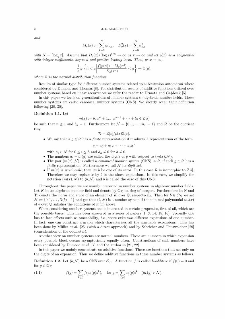
Mq(x) :=N∑k=0

mk,q, D2q(x) =

N∑k=0

σ2k,q

with N = [logq x]. Assume that Dq(x)/(log x)1/3 → ∞ as x → ∞ and let p(x) be a polynomialwith integer coefficients, degree d and positive leading term. Then, as x→∞,

1x

#{n < x

∣∣∣∣f(p(n))−Mq(xd)Dq(xd)

< y

}→ Φ(y),

where Φ is the normal distribution function.

Results of similar type for different number systems related to substitution automaton whereconsidered by Dumont and Thomas [8]. For distribution results of additive functions defined overnumber systems based on linear recurrences we refer the reader to Drmota and Gajdosik [5].

In this paper we focus on generalizations of number systems to algebraic number fields. Thesenumber systems are called canonical number systems (CNS). We shortly recall their definitionfollowing [26, 30].

Definition 1.1. Letm(x) := bnx

n + bn−1xn−1 + · · ·+ b0 ∈ Z[x]

be such that n ≥ 1 and bn = 1. Furthermore let N = {0, 1, . . . , |b0| − 1} and R be the quotientring

R = Z[x]/p(x)Z[x].• We say that a g ∈ R has a finite representation if it admits a representation of the form

g = a0 + a1x+ · · ·+ ahxh

with ai ∈ N for 0 ≤ i ≤ h and dh 6= 0 for h 6= 0.• The numbers ai = ai(g) are called the digits of g with respect to (m(x),N ).• The pair (m(x),N ) is called a canonical number system (CNS) in R, if each g ∈ R has a

finite representation. Furthermore we call N its digit set.• If m(x) is irreducible, then let b be one of its zeros. In this case R is isomorphic to Z[b].

Therefore we may replace x by b in the above expansions. In this case, we simplify thenotation (m(x),N ) to (b,N ) and b is called the base of this CNS.

Throughout this paper we are mainly interested in number systems in algebraic number fields.Let K be an algebraic number field and denote by OK its ring of integers. Furthermore let N andTr denote the norm and trace of an element of K over Q, respectively. Then for b ∈ OK we setN := {0, 1, . . . ,N(b)−1} and get that (b,N ) is a number system if the minimal polynomial mb(x)of b over Q satisfies the conditions of m(x) above.

When considering number systems one is interested in certain properties, first of all, which arethe possible bases. This has been answered in a series of papers [1, 3, 14, 15, 16]. Secondly onehas to face effects such as amenability, i.e., there exist two different expansions of one number.In fact, one can construct a graph which characterizes all the amenable expansions. This hasbeen done by Muller et al. [25] (with a direct approach) and by Scheicher and Thuswaldner [29](consideration of the odometer).

Another view on number systems are normal numbers. These are numbers in which expansionevery possible block occurs asymptotically equally often. Constructions of such numbers havebeen considered by Dumont et al. [7] and the author in [21, 22]

In this paper we mainly concentrate on additive functions. These are functions that act only onthe digits of an expansion. Thus we define additive functions in these number systems as follows.

Definition 1.2. Let (b,N ) be a CNS over OK . A function f is called b-additive if f(0) = 0 andfor g ∈ OK

f(g) =∑k≥0

f(ak(g)bk), for g =∑k≥0

ak(g)bk (ak(g) ∈ N ).(1.1)

ASYMPTOTIC NORMALITY OF b-ADDITIVE FUNCTIONS 3

As indicated above the simplest version of an additive function is the sum-of-digits function sbdefined by

sb(g) :=∑k≥0

ak(g).

A first step towards CNS is the consideration of b-additive function in the field of Gaussianrationals. First a generalization of the result by Delange was given by Grabner et al. in [12].

Theorem. Let b = −n± i be a base of a CNS in Z[i]. Then we have∑N(z)≤Nz∈Z[i]

sb(z) =N(b)− 1

2πN logN(b)N +Nγ2

(logN(b)N

)+O

(√N logN(b)N

)where γ2 is a continuous function of period 1.

Also the result by Bassily and Katai was generalized to number systems over the Gaussianrationals. Gittenberger and Thuswaldner [11] gained the following distribution result.

Theorem. Let (b,N ) be a canonical number system over Z[i]. Let f be a b-additive function suchthat f(cbk) = O(1) as k →∞ and c ∈ N . Furthermore let

mk,b :=1

N(b)

∑c∈N

f(cbk), σ2k,b :=

1N(b)

∑c∈N

f2(cbk)−m2k,b,

and

Mb(x) :=L∑k=0

mk,q, D2b (x) =

L∑k=0

σ2k,q

with L = [logN(b) x]. Assume that Db(x)/(log x)1/3 → ∞ as x → ∞ and let p(x) be a polynomialof degree d with coefficients in Z[i]. Then, as N →∞,

1# {z ∈ Z[i]|N(z) < N}

#{

N(z) < N

∣∣∣∣f(p(z))−Mb(Nd)Db(Nd)

< y

}→ Φ(y),

where Φ is the normal distribution function and z runs over the Gaussian integers.

This build the base for further considerations of b-additive functions over CNS in general. Firstthe result of Delange was further generalized to arbitrary number fields by Thuswaldner [32].Furthermore the moments of the sum-of-digits function in algebraic number fields were consideredby Gittenberger and Thuswaldner [10].

Theorem. Let K be a number field of degree n and OK its ring of integers. Furthermore, let bbe a base of a CNS. Then∑

z∈P (N)

(sb(z))d = cb

(|N(b)| − 1

2

)dN logd|N(b)|N +N

d−1∑j=0

logj|N(b)|Nγj(log|N(b)|N)

+O(N

n−1n logd|N(b)|N

),

where cb is a constant depending on K and b and the γjs are continuous functions of period 1.

In the same vain the above mentioned result by Mauduit and Sarkozy was generalized toarbitrary number fields by Thuswaldner [33]. Therefore we write

Ur,m(M(T )) = {z ∈M(T ) : sb(z) ≡ r mod m} ,where M(T ) is the set described below in (2.2). Then his result reads as follows.

Theorem. Let K be a number field of degree n with ring of integers OK . Let b be the base of acanonical number system in OK and mb(x) = xn + · · ·+ b1x+ b0 the minimal polynomial of b. If(mb(1),m) = 1, then∣∣∣∣# {(a, b) ∈ A× B : a+ b ∈ Sr,m(M(2T ))} − |A| |B|

m

∣∣∣∣ = O(|M(T )|θ (|A| |B|) 12 )

4 M. G. MADRITSCH

holds for any two sets A,B ⊂M(T ). Furthermore θ < 1 and the implied O-constant is absolute.

Despite of these considerations of the sum-of-digits function and other b-additive functions,we also want to mention Katai and Liardet [17], who could show a Delange type result forb-multiplicative functions. Finally there has also been work on the generalization of Waring’sProblem restricted to sets of the form Sr,m defined above. Here we want to mention Petho andTichy [27] (counting the number of solutions for a S-unit equation) and Thuswaldner and Tichy [34](counting the number of solutions of Waring’s Problem with digital restrictions).

In the present paper our aim is to extend the result of Bassily and Katai and Gittenbergerand Thuswaldner to arbitrary algebraic number fields. The main problem we have to face is thedifferent setting for number systems. Especially the fact that the conjugates of a number need notto have equal absolute value will play a role. This difference occurs essentially in the estimationof the involved Weyl sums. Know estimates deal with Waring’s problem and its generalization.Since in these generalizations the leading coefficients of the involved polynomial go through thewhole unit interval and its approximations therefore only targets the splitting into major andminor arcs, we need a different approach. In Section 3 we will develop a more general estimationof these sums.

2. Definitions and Results

In the following paragraphs we will define the tools we need in order to properly estimate thedistribution. These definitions are standard in the area and the reader may refer to Ribenboim [28]or Wang [35].

Throughout the rest of the paper we fix an algebraic number field K and denote by OK itsring of integers. Then let K(`) (1 ≤ ` ≤ r1) be the real conjugates of K, while K(m) and K(m+r2)

(r1 < m ≤ r1 + r2) are the complex conjugates of K, where r1 + 2r2 = n. Throughout this paperthe indices ` and m are always over the sets of integers cited here. Furthermore we set r = r1 + r2and call the pair (r1, r2) the signature of K.

If not stated otherwise an upper case letter will always denote a real number, a lower case letteran element of OK and a Greek letter an element of K, the completition of K. Furthermore sumsare always extended over rational or algebraic integers, respectively.

For γ ∈ K we denote by γ(i) (1 ≤ i ≤ n) the conjugates of γ. In order to extend the termof conjugation to the completition K of K we define for γj ∈ K and xj ∈ R (1 ≤ j ≤ n)λ =

∑1≤j≤n xjγj and λ(i) :=

∑1≤j≤n xjγ

(i)j . We recall that for λ ∈ K

N(λ) =∏

1≤i≤n

λ(i), Tr(λ) =∑

1≤i≤n

λ(i), |λ |= max1≤i≤n

∣∣∣λ(i)∣∣∣

are the norm, trace and house of an element of K over Q, respectively. Furthermore for λ ∈ K let

e(x) := exp(2πi x) and E(λ) = e(Tr(λ)).(2.1)

Let δ be the different and D the absolute value of the discriminant of K. We need somegeometry of numbers and therefore let ω1, . . . , ωn be an integral basis of OK and let ρ1, . . . , ρn bethe corresponding basis of δ−1 such that

Tr (ρiωj) =

{1 i = j,

0 i 6= j.

Let Λ be the lattice constructed by the n linear forms

Li =n∑j=1

ρ(i)j xj .

Then we denote by λ1 the first successive minimum of the convex body B := {z ∈ Rn : |z| ≤ 1}with respect to the lattice Λ.


We call a number totally non-negative if λ(i) ≥ 0 for 1 ≤ i ≤ n. As we will successively extendthe maximum length of the expansions we define M(T1, . . . , Tr) to be the set

M(T1, . . . , Tr) :={η ∈ OK :

∣∣∣η(i)∣∣∣ ≤ Ti, 1 ≤ i ≤ r} .(2.2)

Furthermore we will write for short M(T ) := M(T, . . . , T ).Now we can state our main result.

Theorem 2.1. Let (b,N ) be a CNS and f be a b-additive function such that f(abk) = O(1) ask →∞ and a ∈ N . Furthermore let

mk,b :=1

N(b)

∑a∈N

f(abk), σ2k,b :=

1N(b)

∑a∈N

f2(abk)−m2k,b,

and

Mb(x) :=L∑k=0

mk,q, D2b (x) =

L∑k=0

σ2k,q

with L = [logN(b) x]. Assume that there exists an ε > 0 such that Db(x)/(log x)ε →∞ as x→∞and let p ∈ OK [X] be a polynomial of degree d. Then, as T →∞,

1#M(T )

#{z ∈M(T )

∣∣∣∣f(p(z))−Mb(T d)Db(T d)

< y

}→ Φ(y),

where Φ is the normal distribution function.

We will show this theorem in five steps.(1) In Section 3 we start with the estimation of the Weyl sums which will occur in the proof.

Therefore we use tools which come from generalizations of Waring’s Problem to algebraicnumber fields together with Hua’s method of estimating Weyl sums. The main differencewill be the approximation of the coefficients we use.

(2) For counting the number of occurrences of a certain digit in the expansion of the integervalues of the polynomial p we need an Urysohn function. This function is developed inSection 4 were we consider the fundamental domain of the CNS.

(3) The error term when counting the number of occurrences of a digit comes from those nearthe border of the fundamental domain. Therefore we estimate the number of elementswhich are in a small tube around the border in Section 5.

(4) In Section 6 we have to count the number of elements within the fundamental domainitself, which gives the proof of the central proposition.

(5) Finally we show Theorem 2.1 by truncation and two applications of the Frechet-ShohatTheorem.

3. Weyl sums

In this section we want to consider and estimate the exponential sums which will occur in thefollowing sections. We will begin by giving some background on how exponential sums are definedin number fields.

Throughout this section letg(x) = αdx

d + · · ·+ α1x

be a polynomial of degree d. Let a boldface letter always denote a vector. Then for T = (T1, . . . , Tr)we set M(T) = M(T1, . . . , Tr). The sum

S(g,T) =∑

x∈M(T)

E(g(x)),

where E is as in (2.1), is called a Weyl sum.The main tool in order to estimate these sums is Weyl’s differentiation method. Therefore we

need a generalization of Dirichlet’s theorem on rational approximation, which is provided by Siegel(cf. [31]). Since in our case the Ti are not all equal (see Lemma 6.1) we have to slightly modifySiegel’s original theorem in order to cope with this new situation.

6 M. G. MADRITSCH

Lemma 3.1. Let N1, . . . , Nr be real numbers and let N = n√N1 · · ·Nr1(Nr1+1 · · ·Nr1+r2)2 be their

geometric mean. Suppose that N > D1n , then, corresponding to any ξ ∈ K, there exist q ∈ OK

and a ∈ δ−1 such that∣∣∣q(i)ξ(i) − a(i)∣∣∣ < N−1

i , 0 <∣∣∣q(i)∣∣∣ ≤ Ni, 1 ≤ i ≤ r,

max(Ni

∣∣∣q(i)ξ(i) − a(i)∣∣∣ , ∣∣∣q(i)∣∣∣) ≥ D− 1

2 , 1 ≤ i ≤ r,

and

N((q, aδ)) ≤ D 12 .

Proof. This easily follows from the appropriate modifications in the proof of Theorem 3.1 of [35].�

Now we can state the main estimate of the exponential sum above.

Proposition 3.2. LetT = n

√T1 · · ·Tr1(Tr1+1 · · ·Tr1+r2)2

be the geometric mean of the Ti (1 ≤ i ≤ r). Suppose that αk satisfies the hypotheses from Lemma3.1 with Ni = T di (log T )−σ1 and

(log T )σ1 ≤ α(i)k ≤ T

di (log T )−σ1 1 ≤ i ≤ r,

thenS(g,T)� Tn(log T )−σ0

with σ1 ≥ 2d−1(σ0 + r22d

).

The proof consists of modifications of the proof of Theorem 3.2 of Wang [35], since in ourconsiderations the Ti need not all be equal and we essentially need the (log T )−σ0 term. We startwith the main tools needed for the proof of Proposition 3.2.

Lemma 3.3 ([35, Lemma 3.2]). Let Ti (1 ≤ i ≤ r) be positive integers and set Tr1+r2+i = Tr1+i

for (1 ≤ i ≤ r2). Then

M(T ) =2rπr2√D

T1 · · ·Tn +O(Tn−1

0

),

where T0 = max(

1, (T1 · · ·Tn)1/n)

.

Since in the classical case the Ti are all equal we have to rewrite the proof of Wang’s Lemma 3.6.Therefore we need the following adoption of Lemma 3.5 of Wang [35].

Lemma 3.4. Let Ti and Ni ≥ 0 for 1 ≤ i ≤ s be integers. Then denote by M the set of all points(t1, . . . , ts) ∈ Zs such that

Ti ≤ ti < Ti +Ni 1 ≤ i ≤ s.Let M0 be a subset of M and define

S =∑t∈M0

min(N1

t1, · · · , Ns

ts

).

ThenS � N(#M0)1−

1s (log(N + 2)),

where N is the geometric mean of the Ni.

Proof. This proof mainly follows that of Lemma 3.5 of Wang [35]. In the same way we start bysetting Mν to be the subset of M0 such that tν

Nν≥ ti

Nifor 1 ≤ i ≤ s. Furthermore we denote by

Aν = #Mν its number of elements and by

Sν =∑

t∈Mν

min(N1

t1, · · · , Ns

ts

)


the restriction of the sum S to elements of Mν .Then it suffices to show that

Sν � NA1− 1

sν log(Nν + 2),

which together with S ≤ S1 + · · ·+ Ss proves the lemma.Without loss of generality we show this for ν = 1. For t > 0 let D(t) be the subset of u ∈ Rs

such thatt ≥ u1 > 0,

u1

N1≥ uiNi≥ 0, 2 ≤ i ≤ s.

Let M(t) := D(t)∩Zs be the integer points in D(t) and denote by n(t) their number. In the samemanner let M0(t) := {t ∈M0 : t ≥ t1} and denote by n0(t) = #M0(t) its cardinality.

Now let t0 be an integer such that

n(t0) ≤ A1 = n0(N1) < n(t0 + 1).

Then

S1 ≤∑

t∈M(t0+1)

N1

t1≤ N1

s∏i=2

NiN1

(t0 + 2)∑

t1≤t0+1

1t1≤ Ns(t0 + 2)s−1

Ns−11

log(t0 + 2)

and

A1 ≥ n(t0) ≥t0∑t=1

s∏i=2

NiN1

t =Ns

Ns1

t0∑t=1

ts−1 ≥ c(s)Ns

Ns1

ts0.

Putting these together proves the lemma. �

Now we state our modified version of Lemma 3.6 of Wang [35]. In its original version thislemma essentially goes back to Mitsui [24].

Lemma 3.5. Let A,Bi (1 ≤ i ≤ r),N be positive numbers satisfying A ≥ 1 and N � 1. Further-more let B be the geometric mean of the Bi and let Ni (1 ≤ i ≤ r) be in the same ration to N asthe Bi are to B, i.e.,

B := n√B1 · · ·Br1(Br1+1 · · ·Br)2 and Ni := N

BiB

1 ≤ i ≤ r.

Suppose that 1 ≤ B � N , then, for any ξ,∑m∈M(B)

min1≤i≤n

(A, |1− E(ξmωi)|−1

)� ABn

(1

|N(q)|+

1B

+N logNAB

+logNA

),

where q denotes an integer satisfying the conditions in Lemma 3.1 with ξ and Ni.

Proof. Since this is a modification of the proof of Lemma 3.6 in Wang [35] we only sketch theproof and mainly follow the lines there.

First let X be the Minkowski embedding, i.e., for ξ ∈ K

X(ξ) = (X1(ξ), . . . , Xn(ξ)) := (ξ(1), . . . , ξ(r1),<(ξ(r1+1)), . . . ,=(ξ(r1+r2))).

Then we write with rational integers ei and − 12 ≤ di ≤

12

Tr(ξmωi) = ei + di (1 ≤ i ≤ n) and set ζ =n∑i=1

diρi.

One easily checks that

S =∑

m∈M(B)

min1≤i≤n

(A, |1− E(ξmωi)|−1

)�

∑m∈M(B)

min1≤i≤n

(A, |Xi(ζ)|−1

)= S∗.

Now we assign to every m in M(B) its corresponding ζ and a vector y(m) defined by

y(m) = (R1X1(ζ), . . . , RnXn(ζ)) with Ri = 2D1n

∣∣∣q(i)∣∣∣ .

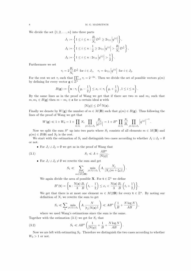
8 M. G. MADRITSCH

We divide the set {1, 2, . . . , n} into three parts

J1 :={

1 ≤ i ≤ n :BiNiD

1n ≥ 2c11

∣∣∣q(i)∣∣∣} ,J2 :=

{1 ≤ i ≤ n :

12≥ 2c11

∣∣∣q(i)∣∣∣ > BiNiD

1n

},

J3 :={

1 ≤ i ≤ n : 2c11∣∣∣q(i)∣∣∣ > 1

2

}.

Furthermore we set

τi = 2BiNiD

1n for i ∈ J1, τi = 4c11

∣∣∣q(i)∣∣∣ for i ∈ J2.

For the rest we set τi such that∏ni=1 τi = 2−2n. Then we divide the set of possible vectors y(m)

by defining for every vector g ∈ Zn

B(g) :={

x : τi

(gi −

12

)≤ xi < τi

(gi +

12

), 1 ≤ i ≤ n

}.

By the same lines as in the proof of Wang we get that if there are two m and m1 such thatm,m1 ∈ B(g) then m−m1 ∈ a for a certain ideal a with

|N(q)| ≤ D 1nN(a).

Finally we denote by W (g) the number of m ∈M(B) such that y(m) ∈ B(g). Thus following thelines of the proof of Wang we get that

W (g)� 1 +W0 = 1 +∏i∈J1

Ni∏

j∈J2∪J3

Bj∣∣q(j)∣∣ = 1 +Bn∏i∈J1

NiBi

∏j∈J2∪J3

∣∣∣q(j)∣∣∣−1

.

Now we split the sum S∗ up into two parts where S1 consists of all elements m ∈ M(B) andy(m) ∈ B(0) and S2 is the rest.

We start with the estimation of S1 and distinguish two cases according to whether J1 ∪ J2 = ∅or not.

• For J1 ∪ J2 = ∅ we get as in the proof of Wang that

S1 � A+ABn

|N(q)|.(3.1)

• For J1 ∪ J2 6= ∅ we rewrite the sum and get

S1 �∑m∈a

m∈M(2B)

minj∈J1∪J2

(A,

Nj|Xj(m+ ξ0)|

).

We again divide the area of possible X. For t ∈ Zn we define

B∗(t) ={

x :N(a)

3BiB

(ti −

12

)≤ xi <

N(a)3

BiB

(ti +

12

)}.

We get that there is at most one element m ∈ M(2B) for every t ∈ Zn. By noting ourdefinition of Ni we rewrite the sum to get

S1 �∑t

minj∈J1∪J2

(A,

N

|tj |N(a)1n

)� ABn

(1B

+N logNAB

),

where we used Wang’s estimations since the sum is the same.Together with the estimation (3.1) we get for S1 that

S1 � ABn(

1|N(q)|

+1B

+N logNAB

).(3.2)

Now we are left with estimating S2. Therefore we distinguish the two cases according to whetherW0 > 1 or not.


• For the first case (W0 > 1) we get by following the lines of the proof of Wang that

S2 � Bn logN.(3.3)

• In the case of W0 ≤ 1 we reach the estimate

S2 �∑

gi∈G0

mini∈J3

(Ni∣∣q(i)∣∣

),

where G0 is the set of all gi, i ∈ J3 such that

W (g) 6= 0, {gi} 6= 0.

In the same manner as in Wang’s proof we get that the value |gi| in G0 does not exceedNi. Thus by an application of Lemma 3.4 we get that

S2 � NBn−1 logN

Together with the estimation (3.3) this yields

S2 � ABn(

logNA

+N logNAB

).(3.4)

Putting the estimates of S1 and S2 in (3.2) and (3.4) together proves the lemma. �

Lemma 3.6 ([35, Lemma 3.8]). Let m ∈ OK and T be the geometric mean of the Ti, i.e.,

T = n√T1 · · ·Tr1(Tr1+1 · · ·Tr1+r2)2

Then ∑h∈M(T)

E(ξmh)� Tn−1 min1≤i≤n

(T, |1− E(ξmωi)|−1),

where ωi (1 ≤ i ≤ n) is an integral basis.

Lemma 3.7 ([35, Lemma 3.9]). Suppose that 1 ≤ t ≤ d − 1 and T is the geometric mean of theTi, then we have

|S(g,T)|2t

� T (2t−t−1)n∑

h1,...,ht∈M(2T )

∑h∈M(T)

E(h1 · · ·htg(h, h1, . . . , ht)ξ),

whereg(h, h1, . . . , ht) = d(d− 1) · · · (d− t+ 1)αdhd−t + · · ·

is a polynomial of degree d− t in h, h1, . . . , ht.

Now we consider the divisor function in more detail. This idea essentially goes back to Hua [13].

Lemma 3.8 ([35, Lemma 3.7]). For a ∈ Ok and T ≥ 0 let dk(a, T ) be the number of solutions ofthe equation

u1 · · ·uk = a, where u1, . . . , uk ∈M(T ) for i = 1, . . . , k.

Thendk(a, T )� |N(a)|ε (log T )(r−1)(k−1).

We write for short d(a, T ) := d2(a, T ). Now we have collected all our tools in order to estimatesums involving divisor function, which will occur in our proof of Proposition 3.2.

Lemma 3.9. Let t be a non-negative integer. Furthermore let T = (T1, . . . , Tr) and suppose thatTi � T0 for 1 ≤ i ≤ r, then ∑

m∈M(T)

(d(m,T0))t

N(m)� (n(log T0)r)2

t

.

10 M. G. MADRITSCH

Proof. For simplicity we set Tr1+r2+i = Tr1+i for 1 ≤ i ≤ r2 and continue by induction on t. Fort = 0 we get that m ∈M(T) implies that |N(m)| ≤

∏ni=1 Ti � Tn0 . Thus by Lemma 3.8∑

m∈M(T)

1|N(m)|

�∑N≤Tn0

(log T0)r−1

N� n(log T0)r.

Now we assume that the lemma holds for t− 1. Then∑m∈M(T)

(d(m,T0))t

|N(m)|=

∑m∈M(T)

(d(m,T0))t−1

|N(m)|∑uv=m

u,v∈M(T0)

1 ≤∑

u∈M(T0)

∑uv=m

m∈M(T)

(d(m,T0))t−1

|N(m)|

=∑

u∈M(T)

∑v∈M

“T1|u(1)|−1

,...,Tr|u(r)|−1”

(d(uv, T0))t−1

|N(u · v)|

� (n · (log T0)r)2t−1

(n · (log T0)r)2t−1

= (n · (log T0)r)2t

.

�

By the last lemma we can estimate a divisor sum which occurs in the estimation of our Weylsum.

Lemma 3.10. Let t be a non-negative integer and let T = (T1, . . . , Tr). Furthermore set Tr1+r2+i =Tr1+i for 1 ≤ i ≤ r2 and suppose that Ti � T0 for 1 ≤ i ≤ n. Then∑

m∈M(T)

(d(m,T0))t � T1 · · ·Tn(n(log T0)r)2t−1.

Proof. We show this by induction on t. For t = 0 this essentially is Lemma 3.3. Now we assumethat the lemma holds for t− 1, then by an application of Lemma 3.9∑

m∈M(T)

(d(m,T0))t =∑

m∈M(T)

(d(m,T0))t−1∑uv=m

u,v∈M(T0)

1 =∑

u∈M(T)

∑uv=mu∈M(T)

(d(m,T0))t−1

=∑

u∈M(T)

∑v∈M

“T1|u(1)|−1

,...,Tr|u(r)|−1”(uv, T0))t−1

�∑

u∈M(T)

(d(u, T0))t−1T1 · · ·Tn|N(u)|

(n(log T0)r)2t−1−1

� T1 · · ·Tn(n(log T0)r)2t−1.

�

Finally we need a Lemma whose idea essentially goes back to Hua (c.f. Hilfssatz 6.1 of [13]) inorder to get a better estimation of the Weyl sum.

Lemma 3.11. Let t be a non-negative integer and let T = (T1, . . . , Tr). Suppose that Ti � T0 for1 ≤ i ≤ n. Then, for any σ2 ≥ 23t−1 we get∑′

m∈M(T)

(d(m,T0))t � Tn0 (n(log T0)r)−σ2

where∑′

stands for the sum over all m such that

(n(log T0)r)σ2 � (d(m,T0))t.

Proof.

(n(log T0)r)2σ2∑′

m∈M(T)

(d(m,T0))t �∑

m∈M(T)

(d(m,T0))3t

� Tn0 (n(log T0)r)23t−1 � Tn0 (n(log T0)r)σ2 .

�


Proof of Proposition 3.2. We set G = 2d−1 and get by an application of Lemma 3.7

|S(f,T)|G � T (G−d)n∑

h1,...,hd−1∈M(2T )

∣∣∣∣∣∣∑

h∈M(T)

E(αdmh)

∣∣∣∣∣∣ ,where

m = d!h1 · · ·hd−1.(3.5)

Now we denote by A(m) the number of solutions of (3.5). Noting that dk(m,T ) ≤ d(m,T )k weget that

A(m)�

{T (d−2)n if m = 0,d(m,T )d−1 if m 6= 0.

Putting everything together yields

|S(f,T)|G � T (G−2)n + T (G−d)n∑

m∈M(d!2qTd−1)

d(m,T )d−1

∣∣∣∣∣∣∑

h∈M(T)

E(αdmh)

∣∣∣∣∣∣ .Now we distinguish two cases for m according to the hypotheses of Lemma 3.11, i.e., whether

(n(log T )r)σ2 � d(m,T ) or not. Thus by an application of Lemma 3.5 and Lemma 3.6

|S(f,T)|G � T (G−2)n + T (G−d)n

(Tn(n(log T )r)σ +

∑′

m

(n(log T )r)σ∣∣∣∣∣∑h

E(αdmh)

∣∣∣∣∣)

� T (G−2)n + T (G−d+1)n(log T )rσ

+ T (G−d)n(log T )rσ∑′

m

Tn−1 mini

(T, |1− E(αdmh)|−1

)� T (G−2)n + T (G−d+1)n(log T )rσ + TGn(log T )rσ

(1

N(αd)+

1T

+ (log T )−σ1

)� T (G−2)n + T (G−d+1)n(log T )rσ + TGn(log T )rσ−σ1 .

�

4. Fundamental domain

In this section we want to construct the Urysohn function for indicating the elements startingwith a certain digit. The following definitions are standard in that area and we mainly followGittenberger and Thuswaldner [11]. We need the fundamental domain, which is defined as the setof all numbers whose integer part is zero, i.e.,

F ′ :=

z ∈ C

∣∣∣∣∣∣z =∑k≥1

akb−k, ak ∈ N

.

It is more convenient to consider the embedding of the fundamental domain in Rn. This idea isbased on a result by Kovacs (cf. Lemma 1 of [18]), that if (b,N ) is a CNS then {1, b, b2, . . . , bn−1}is an integral basis for K. Thus we define the embedding φ by

φ :{

K → Rn,α0 + α1b+ · · ·+ αn−1b

n−1 7→ (α0, . . . , αn−1).,

where K is the completition of K.

12 M. G. MADRITSCH

Now let mb(x) = a0 + a1x+ · · ·+ an−1xn−1 be the minimal polynomial of b, then we define the

corresponding matrix B by

B =

0 0 · · · · · · · · · −a0

1 0 · · · · · · 0...

0 1. . .

......

.... . . . . . . . .

......

.... . . 1 0

...0 0 · · · 0 1 −an−1

.

One easily checks thatφ(b · z) = B · φ(z).

By this we define the embedding of the fundamental domain by

F = φ(F ′) =

z ∈ Rn∣∣∣∣∣∣z =

∑k≥1

B−kak, ak ∈ φ(N )

.

The rest of this section follows the ideas of Gittenberger and Thuswaldner [11] and thereforewe only show the results and left the proofs to the reader. For the construction of the Urysohnfunction the border of the fundamental domain is of special interest. We can approximate F withhelp of the sets

Q0 :={z ∈ R2

∣∣‖z‖∞ ≤ 12

},

Qk :=⋃a∈N

B−1(Qk−1 + φ(a)).

This approximation satisfies d(∂Qk, ∂F) � |b|−k, where d(·, ·) denotes the Hausdorff metric. Byconsulting [25, 29], we get that the Qk consists of |N |k parallelograms. Furthermore there existsa µ with 1 < µ < |N(b)| such that O(µk) of theses parallelograms intersect the boundary of Qk.

Now we define the fundamental domain consisting of all numbers whose first digit equals a ∈ N ,i.e.,

Fa = B−1(F + φ(a)).Imitating the proof of Lemma 3.1 of [11] we get the following.

Lemma 4.1. For all a ∈ N and all k ∈ N there exists an axe-parallel tube Pk,a with the followingproperties:

• ∂Fa ⊂ Pk,a for all k ∈ N,

• the Lebesgue measure of Pk,a is a O(

µk

|N(b)|k

),

• Pk,a consists of O(µk) axe-parallel rectangles, each of which has Lebesgue measure O(|N(b)|k),where λ denotes the Lebesgue measure.

As in the proof of Lemma 3.1 of [11] we can construct for each pair (k, a) an axe-parallel polygonΠk,a and the corresponding tube

Pk,a :={z ∈ Rn

∣∣∣‖z −Πk,a‖∞ ≤ 2cp |b|−k}.

Furthermore we denote by Ik,a the set of all points inside Πk,a. Now we define our Urysohnfunction ua by

ua(x1, . . . , xn) =1

∆n

∫ ∆2

−∆2

· · ·∫ ∆

2

−∆2

ψa(x1 + y1, . . . , xn + yn) dy1 · · · dyn,(4.1)

where

∆ := 2cu |b|−k(4.2)


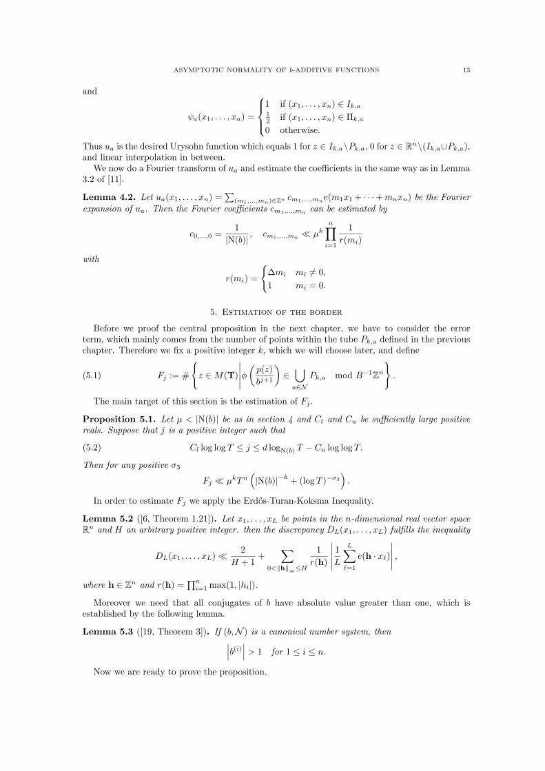
and

ψa(x1, . . . , xn) =

1 if (x1, . . . , xn) ∈ Ik,a12 if (x1, . . . , xn) ∈ Πk,a

0 otherwise.

Thus ua is the desired Urysohn function which equals 1 for z ∈ Ik,a\Pk,a, 0 for z ∈ Rn\(Ik,a∪Pk,a),and linear interpolation in between.

We now do a Fourier transform of ua and estimate the coefficients in the same way as in Lemma3.2 of [11].

Lemma 4.2. Let ua(x1, . . . , xn) =∑

(m1,...,mn)∈Zn cm1,...,mne(m1x1 + · · ·+mnxn) be the Fourierexpansion of ua. Then the Fourier coefficients cm1,...,mn can be estimated by

c0,...,0 =1

|N(b)|, cm1,...,mn � µk

n∏i=1

1r(mi)

with

r(mi) =

{∆mi mi 6= 0,1 mi = 0.

5. Estimation of the border

Before we proof the central proposition in the next chapter, we have to consider the errorterm, which mainly comes from the number of points within the tube Pk,a defined in the previouschapter. Therefore we fix a positive integer k, which we will choose later, and define

Fj := #

{z ∈M(T)

∣∣∣∣∣φ(p(z)bj+1

)∈⋃a∈N

Pk,a mod B−1Zn}.(5.1)

The main target of this section is the estimation of Fj .

Proposition 5.1. Let µ < |N(b)| be as in section 4 and Cl and Cu be sufficiently large positivereals. Suppose that j is a positive integer such that

Cl log log T ≤ j ≤ d logN(b) T − Cu log log T.(5.2)

Then for any positive σ3

Fj � µkTn(|N(b)|−k + (log T )−σ3

).

In order to estimate Fj we apply the Erdos-Turan-Koksma Inequality.

Lemma 5.2 ([6, Theorem 1.21]). Let x1, . . . , xL be points in the n-dimensional real vector spaceRn and H an arbitrary positive integer. then the discrepancy DL(x1, . . . , xL) fulfills the inequality

DL(x1, . . . , xL)� 2H + 1

+∑

0<‖h‖∞≤H

1r(h)

∣∣∣∣∣ 1LL∑`=1

e(h · x`)

∣∣∣∣∣ ,where h ∈ Zn and r(h) =

∏ni=1 max(1, |hi|).

Moreover we need that all conjugates of b have absolute value greater than one, which isestablished by the following lemma.

Lemma 5.3 ([19, Theorem 3]). If (b,N ) is a canonical number system, then∣∣∣b(i)∣∣∣ > 1 for 1 ≤ i ≤ n.

Now we are ready to prove the proposition.

14 M. G. MADRITSCH

Proof of Proposition 5.1. In order to apply the Erdos-Turan-Koksma Inequality we have to con-sider rectangles. Recall that the tube Pk,a consists of rectangles as mentioned in Lemma 4.1. Wesplit the tube Pk,a into this family of rectangles and let Ra be one of them. Then our goal is toestimate

Fj(Ra) :={z ∈M(T)

∣∣∣∣φ( p(z)bj+1

)∈ Ra mod B−1Zn

}.

We set xz := φ(p(z)/bj+1) and get by the definition of the discrepancy (cf. [6, Definition 1.5])that

Fj(Ra)� Tn (λ(Ra) +DL({xz})) ,(5.3)

where L is the number of elements in M(T) and T is the geometric mean of the Ti. Thus we getby Lemma 3.3 that

L =2rπr2√D

Tn +O(Tn−1

).(5.4)

In order to estimate the discrepancy we use Lemma 5.2 to get

DL({xz})�2

H + 1+

∑0<‖h‖∞≤H

1r(h)

∣∣∣∣∣∣ 1L∑

z∈M(T)

e(h · xz)

∣∣∣∣∣∣ .(5.5)

Our aim is the application of Proposition 3.2. Since E is defined in (2.1) as E = e ◦Tr we have torewrite the exponential sum with scalar multiplication into one involving the trace. It is easy tosee that the following function suffices our purpose.

τ(z) := (Tr(z),Tr(bz), . . . ,Tr(bn−1z)) = Ξφ(z),(5.6)

where Ξ = V V T and V is the Vandermonde matrix

V =

1 1 · · · 1b b(2) · · · b(n)

......

...bn−1 (b(2))n−1 · · · (b(n))n−1

.

Thus we get

h · xz = h · φ(p(z)bj−1

)= hΞ−1τ

(p(z)bj−1

)= Tr

(n∑i=1

hibi−1 p(z)

bj−1

),(5.7)

where we have set (h1, h2, . . . , hn) := hΞ−1.Plugging (5.4), (5.5) and (5.7) into (5.3) and applying Lemma 4.1 yields

Fj(Ra)� λ (Ra)Tn +Tn

H + 1+

∑0<‖h‖∞≤H

1r(h)

∑z∈M(T)

E

(n∑i=1

hibi−1 p(z)

bj−1

),(5.8)

where

H = (log T )σ4 .(5.9)

Now we want to apply Proposition 3.2 for the last sum. Since∑ni=1 hib

i−1p(z) is a polynomialof degree d we write ξ for its leading coefficient for short. Then we apply Lemma 3.1 to get a ∈ δ−1

and q ∈ OK such that∣∣∣∣ ξ(i)

(b(i))j+1q(i) − a(i)

∣∣∣∣ ≤ T−di (log T )σ1 and 0 < q(i) ≤ T di (log T )−σ1 for 1 ≤ i ≤ r.

Now we distinguish three cases according to the size of | q |.• Case 1, | q |≥ (log T )σ1 : By Proposition 3.2 we get∑

z∈M(T)

E

(n∑i=1

hibi−1 p(z)

bj+1

)� Tn(log T )−σ0 .


• Case 2, 2 ≤ | q | < (log T )σ1 : Let 1 ≤ i ≤ n be such that∣∣q(i)∣∣ ≥ 2. Then by noting∣∣q(i)∣∣ ≤| q |we get ∣∣∣∣ ξ(i)

(b(i))j+1q(i) − a(i)

∣∣∣∣ < (log T )σ1

T di≤ 1∣∣q(i)∣∣

and thus (using our first successive minimum λ1)∣∣∣∣ ξ(i)

(b(i))j+1

∣∣∣∣ ≥ ∣∣∣∣a(i)

q(i)

∣∣∣∣− 1∣∣q(i)∣∣2 ≥ λ1

(1∣∣q(i)∣∣ − 1∣∣q(i)∣∣2

)≥ λ1

12∣∣q(i)∣∣ � (log T )−σ1 .(5.10)

Therefore by noting Lemma 5.3 and our definition of H in (5.9) we have∣∣∣b(i)∣∣∣j+1

�∣∣∣ξ(i)∣∣∣ (log T )σ1 � nH(log T )σ1 � (log T )σ1+σ4 ,

which yields

j � (σ1 + σ2)log |b|

log log T

contradicting the lower bound for j in (5.2) for sufficiently large Cl.• Case 3, 0 < | q |< 2: We have to consider two further cases according to whether a 6= 0

or a = 0.– Case 3.1,

∣∣∣ ξbj+1 q

∣∣∣≥ λ12 : Let 1 ≤ i ≤ n be such that

∣∣∣ ξ(i)

(b(i))j+1 q(i)∣∣∣ ≥ λ1

2 . Then we getwith H as in (5.9) ∣∣∣b(i)∣∣∣j+1

� H = (log T )σ4

which again contradicts the lower bound of j in (5.2).

– Case 3.2,∣∣∣ ξbj+1 q

∣∣∣< λ12 : Since λ1 is the first successive minima for the sphere with

respect to the lattice of δ−1 we get that a = 0. Thus for 1 ≤ i ≤ n∣∣∣∣ ξ(i)

(b(i))j+1q(i)∣∣∣∣ < (log T )σ1

T di.

Talking the norm we get

N(

ξ

bj+1q

)=

N(ξ)N(bj+1)

N(q) <(log T )nσ1

Tnd.

This implies

j + 1 ≥ nd log|N(b)| T −nσ

log |N(b)|log log T + C

contradicting the upper bound of j in (5.2) for sufficiently large Cu.Thus we get for all j satisfying (5.2), that∑

z∈M(T)

E

(n∑i=1

hibi−1 f(z)

bj+1

)� Tn(log T )−σ0 .

Plugging this into (5.8) together with (5.9) yields

Fj(Ra)� Tnλ(Ra) +Tn

(log T )σ4+ Tn(log T )−σ0

∑0<‖h‖∞≤H

1r(h)

� Tnλ(Ra) +Tn

(log T )σ4+ Tn(log T )−σ0(log log T )n.

Finally setting σ4 := σ0/2 and summing over all rectangles Ra yields

Fj � µkTn(|N(b)|−k + (log T )−σ0/2

).

By setting σ3 = σ0/2 the proposition is proven. �

16 M. G. MADRITSCH

6. The central proposition

Before we can state the central proposition we need a lemma estimating the length of theexpansion of every integer. This will provide us with an upper bound for the scope of interest(namely for the Ti in M(T)) and further establish us with the tools needed in order to prove theTheorem 2.1.

Lemma 6.1 ([20, Theorem]). Let `(γ) be the length of the expansion of γ to the base b. Then∣∣∣∣∣`(γ)− max1≤i≤n

log∣∣γ(i)

∣∣log∣∣b(i)∣∣

∣∣∣∣∣ ≤ C.We fix a T and set Ti for 1 ≤ i ≤ n such that

log Ti = log Tlog∣∣b(i)∣∣n

log |N(b)|.(6.1)

Thus we get in view of Lemma 6.1 that the expansions of the elements of M(T) have the samemaximum length. Now we are in the position to state the central proposition in the proof ofTheorem 2.1.

Proposition 6.2. Let T ≥ 0 and Ti for 1 ≤ i ≤ n be defined as in (6.1). Let L be the maximumlength of the b-adic expansion of z ∈M(T) and let Cl and Cu be sufficiently large. Then for

Cl logL ≤ l1 < l2 < · · · < lh ≤ dL− Cu logL(6.2)

we have,

Θ := #{z ∈M(T)

∣∣alj (f(z)) = bj , j = 1, . . . , h}

=2rπr2

√D |N(b)|h

Tn +O(Tn(log T )−σ0

)uniformly for T →∞, where bj ∈ N are given and σ0 is an arbitrary positive constant.

Proof. We recall our Urysohn function ua (defined in (4.1)) and set for ν ∈ Rn

t(ν) = ub1(B−l1−1ν) · · ·ubh(B−lh−1ν).

Now we want to apply the Fourier transformation, which we developed in Lemma 4.2. Thereforewe set

M := {M = (µ1, . . . , µh)|µj = (mj1, . . . ,mjn) ∈ Zn, for j = 1, . . . , h} .An application of Lemma 4.2 yields

t(ν) =∑M∈M

TMe

h∑j=1

µjB−lj−1ν

,

where TM =∏hj=1 cmj1,...,mjn . Combining these results we get∣∣∣∣∣∣Θ−

∑z∈M(T)

t(φ(p(z)))

∣∣∣∣∣∣ ≤ Fl1 + · · ·+ Flh .(6.3)

Using the function τ defined in (5.6) we get

∑z∈M(T)

t(φ(p(z))) =∑M∈M

TM∑

z∈M(T)

e

h∑j=1

µjB−lj−1Ξ−1τ(p(z))

.

Settingµj = (mj1, . . . , mjn) := µjB

−lj−1Ξ−1 (j = 1, . . . , h)yields ∑

z∈M(T)

t(φ(p(z))) =∑M∈M

TM∑

z∈M(T)

E

h∑j=1

n∑i=1

mjip(z))blj+1

.


We want to apply the same ideas as in the proof of Proposition 5.1. For 1 ≤ j ≤ h we set ξjto be the leading coefficient of

∑ni=1 mjip(z). Then we apply Lemma 3.1 with Ni = T di (log T )−σ1

for 1 ≤ i ≤ r in order to get that there exist a ∈ δ−1 and q ∈ OK such that∣∣∣∣∣∣h∑j=1

ξ(i)j

(b(i))lj+1q(i) − a(i)

∣∣∣∣∣∣ < (log T )σ1

T diand 0 <

∣∣∣q(i)∣∣∣ < T di(log T )σ1

for 1 ≤ i ≤ n.

Now we again distinguish several cases.• Case 1, | q |≥ (log T )σ1 : We apply Proposition 3.2 and get

∑z∈M(T)

E

h∑j=1

n∑i=1

mjip(z))blj+1

� Tn(log T )−σ0 .

• Case 2, 2 ≤| q |< (log T )σ1 : In the same manner as in (5.10) we get

(log T )σ1 ≤

∣∣∣∣∣∣h∑j=1

ξ(i)j

(b(i))lj+1

∣∣∣∣∣∣ ≤∑hj=1

∣∣∣ξ(i)j ∣∣∣∣∣b(i)∣∣l1+1,

l1 + 1� log log T.

Together with the definition of L this contradicts the lower bound of l1 for sufficientlylarge Cl in (6.2).

• Case 3, 0 < | q |< 2: We have to consider two sub cases

– Case 3.1,∣∣∣∑h

j=1ξj

blj+1 q∣∣∣≥ λ1

2 : Let 1 ≤ i ≤ n be such that

λ1

2≤

∣∣∣∣∣∣h∑j=1

ξ(i)j

(b(i))lj+1q(i)

∣∣∣∣∣∣ ≤∑hj=1

∣∣∣ξ(i)j ∣∣∣∣∣b(i)∣∣l1+1

∣∣∣q(i)∣∣∣ ,then

l1 + 1� log log T

again contradicts the lower bound of l1 for sufficiently large Cl in (6.2).

– Case 3.2,∣∣∣∑h

j=1ξj

blj+1 q∣∣∣< λ1

2 : By Minkowski’s theorem we get that a = 0. Thus for1 ≤ i ≤ n∣∣∣∣∣∣

h∑j=1

ξ(i)j

(b(i))lj+1q(i)

∣∣∣∣∣∣ =

∣∣∣∣∣∣ 1(b(i))lh+1

h∑j=1

ξ(i)j (b(i))lh−ljq(i)

∣∣∣∣∣∣ ≤ (log T )σ1

T di

which implies (taking the norm of the left side)

lh + 1 ≥ nd log|N(b)| T − c(log log|N(b)| T )

contradicting the upper bound for sufficiently large Cu.After these considerations it is clear, that Case 1 is the only possible case which suffices the

hypotheses in (6.2). Plugging this into (6.3) and applying Lemma 4.2 and Lemma 3.3 for thecoefficient c0,...,0 yields

Θ =2rπr2

√D |N(b)|h

Tn +O

Tn(log T )−σ0∑

0 6=M∈M

TM

+O

h∑j=1

Fj

.

An application of Proposition 5.1 with k � log log T and the observation that∑M∈M

|TM | � ∆−2h � |b|2hk � (log T )σ0/2,

where we used the definition of ∆ in (4.2), proves the proposition. �

18 M. G. MADRITSCH

7. Proof of Theorem 2.1

At this point we will need the Frechet-Shohat Theorem which we state for completeness.

Lemma 7.1 ([9, Lemma 1.43]). Let (Fn(z))n≥1 be a sequence of distribution functions. For eachnon-negative integer k let

αk = limn→∞

∫ ∞−∞

zkdFn(z)

exist.Then there is a subsequence of Fnj (z) (n1 < n2 < · · · ), which converges weakly to a limiting

distribution F (z) for which

αk =∫ ∞−∞

zkdF (z) (k = 0, 1, . . .).

Moreover, if the set of moments αk determine F (z) uniquely, then as n → ∞ the distributionFn(z) converge weakly to F (z).

For the proof of Theorem 2.1 we mainly follow the proof of Theorem 1.2 of Gittenberger andThuswaldner [11]. In the same manner as in their proof we set C := max(Cl, Cu), A := [C logL]and B := L−A, where L, Cl and Cu are defined in the statement of Proposition 6.2. Furthermorewe define the truncated function f ′ to be

f ′(p(z)) =B∑j=A

f(aj(p(z))bj).

By the definition of A and f(abj)� 1 with a ∈ N we get that f ′(p(z)) = f(p(z)) +O(logL). Inthe same manner we define the truncated mean and standard deviation

M ′b(T ) :=B∑j=A

mj and D′2b (T ) :=B∑j=A

σ2j .

Since Mb(T ) −M ′b(T ) = O(logL) and D2b (T ) − D′2b (T ) = O(logL) we get that it suffices to

show that1

#M(T )#{z ∈M(T )

∣∣∣∣f ′(p(z))−M ′b(T d)D′b(T d)< y

}−→ Φ(y).

By Lemma 7.1 this holds true if and only if the moments

ξk(T ) :=1

#M(T )

∑z∈M(T )

(f ′(p(z))−M ′b(T d)

D′b(T d)

)kconverge to the moments of the normal law for T → ∞. We will show the last statement bycomparing the moments ξk with

ηk(T ) :=1

#M(T d)

∑z∈M(Td)

(f ′(z)−M ′b(T d)

D′b(T d)

)k.

An application of Proposition 6.2 gives that

ξk(T )− ηk(T )→ 0 for T →∞.

Furthermore we get by Lemma 6.1 that these sums consist of independently identically dis-tributed random variables (with possible 2C exceptions). By the central limit theorem we getthat their distribution converges to the normal law. Thus the ηk(T ) converge to the moments ofthe normal law. This yields

limT→∞

ξk(T ) = limT→∞

ηk(T ) =∫xkdΦ.

We apply the Frechet-Shohat Theorem again to prove the theorem.


Acknowledgement

Parts of the work were written when the author was at “laboratoire GREYC” of University ofCaen.

References

[1] Shigeki Akiyama, Horst Brunotte, and Attila Petho, Cubic CNS polynomials, notes on a conjecture of W. J.

Gilbert, J. Math. Anal. Appl. 281 (2003), no. 1, 402–415.

[2] N. L. Bassily and I. Katai, Distribution of the values of q-additive functions on polynomial sequences, ActaMath. Hungar. 68 (1995), no. 4, 353–361.

[3] Horst Brunotte, Andrea Huszti, and Attila Petho, Bases of canonical number systems in quartic algebraic

number fields, J. Theor. Nombres Bordeaux 18 (2006), no. 3, 537–557.[4] H. Delange, Sur la fonction sommatoire de la fonction“somme des chiffres”, Enseignement Math. (2) 21

(1975), no. 1, 31–47.

[5] M. Drmota and J. Gajdosik, The distribution of the sum-of-digits function, J. Theor. Nombres Bordeaux 10(1998), no. 1, 17–32.

[6] M. Drmota and R. F. Tichy, Sequences, discrepancies and applications, Lecture Notes in Mathematics, vol.1651, Springer-Verlag, Berlin, 1997.

[7] J. M. Dumont, P. J. Grabner, and A. Thomas, Distribution of the digits in the expansions of rational integers

in algebraic bases, Acta Sci. Math. (Szeged) 65 (1999), no. 3-4, 469–492.[8] J. M. Dumont and A. Thomas, Gaussian asymptotic properties of the sum-of-digits function, J. Number

Theory 62 (1997), no. 1, 19–38.

[9] P. D. T. A. Elliott, Probabilistic number theory. I, Grundlehren der Mathematischen Wissenschaften [Funda-mental Principles of Mathematical Science], vol. 239, Springer-Verlag, New York, 1979, Mean-value theorems.

[10] B. Gittenberger and J. M. Thuswaldner, The moments of the sum-of-digits function in number fields, Canad.

Math. Bull. 42 (1999), no. 1, 68–77.[11] , Asymptotic normality of b-additive functions on polynomial sequences in the Gaussian number field,

J. Number Theory 84 (2000), no. 2, 317–341.[12] P. J. Grabner, P. Kirschenhofer, and H. Prodinger, The sum-of-digits function for complex bases, J. London

Math. Soc. (2) 57 (1998), no. 1, 20–40.

[13] L.-K. Hua, Additive Primzahltheorie, B. G. Teubner Verlagsgesellschaft, Leipzig, 1959.[14] I. Katai and I. Kornyei, On number systems in algebraic number fields, Publ. Math. Debrecen 41 (1992),

no. 3-4, 289–294.

[15] I. Katai and B. Kovacs, Kanonische Zahlensysteme in der Theorie der quadratischen algebraischen Zahlen,Acta Sci. Math. (Szeged) 42 (1980), no. 1-2, 99–107.

[16] , Canonical number systems in imaginary quadratic fields, Acta Math. Acad. Sci. Hungar. 37 (1981),

no. 1-3, 159–164.[17] I. Katai and P. Liardet, Additive functions with respect to expansions over the set of Gaussian integers, Acta

Arith. 99 (2001), no. 2, 173–182.[18] B. Kovacs, Canonical number systems in algebraic number fields, Acta Math. Acad. Sci. Hungar. 37 (1981),

no. 4, 405–407.

[19] B. Kovacs and A. Petho, Number systems in integral domains, especially in orders of algebraic number fields,Acta Sci. Math. (Szeged) 55 (1991), no. 3-4, 287–299.

[20] , On a representation of algebraic integers, Studia Sci. Math. Hungar. 27 (1992), no. 1-2, 169–172.

[21] M. G. Madritsch, Generating normal numbers over gaussian integers, Acta Arith., to appear.[22] , A note on normal numbers in matrix number systems, Math. Pannon. 18 (2007), no. 2, 219–227.[23] C. Mauduit and A. Sarkozy, On the arithmetic structure of the integers whose sum of digits is fixed, Acta

Arith. 81 (1997), no. 2, 145–173.[24] T. Mitsui, On the Goldbach problem in an algebraic number field. I, II, J. Math. Soc. Japan 12 (1960), 290–324,

325–372.

[25] W. Muller, J. M. Thuswaldner, and R. F. Tichy, Fractal properties of number systems, Period. Math. Hungar.42 (2001), no. 1-2, 51–68.

[26] A. Petho, On a polynomial transformation and its application to the construction of a public key cryptosystem,

Computational number theory (Debrecen, 1989), de Gruyter, Berlin, 1991, pp. 31–43.[27] A. Petho and R. F. Tichy, S-unit equations, linear recurrences and digit expansions, Publ. Math. Debrecen

42 (1993), no. 1-2, 145–154.[28] P. Ribenboim, Classical theory of algebraic numbers, Universitext, Springer-Verlag, New York, 2001.

[29] K. Scheicher and J. M. Thuswaldner, Canonical number systems, counting automata and fractals, Math. Proc.Cambridge Philos. Soc. 133 (2002), no. 1, 163–182.

[30] , On the characterization of canonical number systems, Osaka J. Math. 41 (2004), no. 2, 327–351.[31] Carl Ludwig Siegel, Generalization of Waring’s problem to algebraic number fields, Amer. J. Math. 66 (1944),

122–136.

20 M. G. MADRITSCH

[32] J. M. Thuswaldner, The sum of digits function in number fields, Bull. London Math. Soc. 30 (1998), no. 1,37–45.

[33] , The sum of digits function in number fields: distribution in residue classes, J. Number Theory 74

(1999), no. 1, 111–125.[34] J. M. Thuswaldner and R. F. Tichy, Waring’s problem with digital restrictions, Israel J. Math. 149 (2005),

317–344, Probability in mathematics.

[35] Y. Wang, Diophantine equations and inequalities in algebraic number fields, Springer-Verlag, Berlin, 1991.

(M. G. Madritsch) Institute of Statistics, Graz University of Technology, A-8010 Graz, Austria

E-mail address: [email protected]

Asymptotic normality of additive functions on polynomial sequences in canonical number systems

Documents

Transcript of Asymptotic normality of additive functions on polynomial sequences in canonical number systems