Best Signal Quality in Cellular Networks: Asymptotic ... - arXiv

arX

iv:1

502.

0079

4v1

[cs.

IT]

3 F

eb 2

015

EURASIP JOURNAL ON WIRELESS COMMUNICATIONS AND NETWORKING, SPECIAL ISSUE ON FEMTOCELL NETWORKS, 2010 1

Best Signal Quality in Cellular Networks:Asymptotic Properties and Applications to Mobility

Management in Small Cell NetworksVan Minh Nguyen, Francois Baccelli, Laurent Thomas, and Chung Shue Chen

Abstract—The quickly increasing data traffic and the userdemand for a full coverage of mobile services anywhere andanytime are leading mobile networking into a future of smallcell networks. However, due to the high-density and randomnessof small cell networks, there are several technical challenges.In this paper, we investigate two critical issues: best signalquality and mobility management. Under the assumptions thatbase stations are uniformly distributed in a ring shaped regionand that shadowings are lognormal, independent and identicallydistributed, we prove that when the number of sites in thering tends to infinity, then (i) the maximum signal strengthreceived at the center of the ring tends in distribution to aGumbel distribution when properly renormalized, and (ii) i tis asymptotically independent of the interference. Using theseproperties, we derive the distribution of the best signal quality.Furthermore, an optimized random cell scanning scheme isproposed, based on the evaluation of the optimal number ofsites to be scanned for maximizing the user data throughput.

Index Terms—Small cell networks, maximum SINR, handover,random cell scanning, extreme value theory.

I. I NTRODUCTION

Mobile cellular networks were initially designed for voiceservice. Nowadays, broadband multimedia services (e.g., videostreaming) and data communications have been introduced intomobile wireless networks. These new applications have led toincreasing traffic demand. To enhance network capacity andsatisfy user demand of broadband services, it is known thatreducing the cell size is one of the most effective approaches[1]–[4] to improve the spatial reuse of radio resources.

Besides, from the viewpoint of end users, full coverageis particularly desirable. Although today’s macro and microcellular systems have provided high service coverage, 100%-coverage is not yet reached because operators often have manyconstraints when installing large base stations and antennas.This generally results in potential coverage holes and deadzones.

A promising architecture to cope with this problem is thatof small cell networks [4], [5]. A small cell only needslightweight antennas. It helps to replace bulky roof top basestations by small boxes set on building facade, on publicfurniture or indoor. Small cells can even be installed by end

Van Minh Nguyen and Laurent Thomas are with Networks and Network-ing Domain, Bell Labs Research, Alcatel-Lucent, Nozay, France. Email:van [email protected], [email protected].

Francois Baccelli and Chung Shue Chen are with TREC, INRIA-ENS,Paris, France. Email: [email protected], [email protected].

This work was done within the framework of the Alcatel-Lucent Bell LabsFrance - INRIA joint laboratory.

users (e.g., femtocells). All these greatly enhance networkcapacity and facilitate network deployment. Pervasive smallcell networks have a great potential. For example, Willcomhas deployed small cell systems in Japan [6], and Vodafonehas recently launched home 3G femtocell networks in the UK[7].

In principle, high-density and randomness are the two basiccharacteristics of small cell networks. First, reducing cell sizeto increase the spatial reuse for supporting dense traffic willinduce a large number of cells in the same geographicalarea. Secondly, end users can set up small cells by theirown means [2]. This makes small cell locations and coverageareas more random and unpredictable than traditional mobilecellular networks. The above characteristics have introducedtechnical challenges that require new studies beyond thosefor macro and micro cellular networks. The main issuesconcern spectrum sharing and interference mitigation, mobilitymanagement, capacity analysis, and network self-organization[3], [4]. Among these, thesignal quality, e.g., in terms ofsignal-to-interference-plus-noise ratio (SINR), andmobilitymanagement are two critical issues.

In this paper, we first conduct a detailed study on theproperties ofbest signal quality in mobile cellular networks.Here, the best signal quality refers to the maximum SINRreceived from a number of sites. Connecting the mobile tothe best base station is one of the key problems. The bestbase station here means the base station from which themobile receives the maximum SINR. As the radio propagationexperiences random phenomena such as fading and shadowing,the best signal quality is a random quantity. Investigatingits stochastic properties is of primary importance for manystudies such as capacity analysis, outage analysis, neighborcell scanning, and base station association. However, to thebest of our knowledge, there is no prior art in this area.

In exploring the properties of best signal quality, we focuson cellular networks in which the propagation attenuationof the radio signal is due to the combination of a distance-dependent path-loss and of lognormal shadowing. Consider aring B of radiiRmin andRB such that0 < Rmin < RB < ∞.The randomness of site locations is modeled by a uniformdistribution of homogeneous density inB. Using extremevalue theory (c.f., [8], [9]), we prove that the maximumsignal strength received at the center ofB from n sites inB converges in distribution to a Gumbel distribution whenproperly renormalized and it is asymptotically independent ofthe total interference, asn → ∞. The distribution of the best

http://arxiv.org/abs/1502.00794v1


signal quality can thus be derived.The second part of this paper focuses on applying the

above results to mobility support in dense small cell networks.Mobility support allows one to maintain service continuityeven when users are moving around while keeping efficientuse of radio resources. Today’s cellular network standardshighlight mobile-assisted handover in which the mobile mea-sures the pilot signal quality of neighbor cells and reportsthemeasurement result to the network. If the signal quality froma neighbor cell is better than that of the serving cell by ahandover margin, the network will initiate a handover to thatcell. The neighbor measurement by mobiles is calledneighborcell scanning. Following mobile cellular technologies, it isknown that small cell networking will also use mobile-assistedhandover for mobility management.

To conduct cell scanning [10]–[12], today’s cellular net-works use aneighbor cell list. This list contains informationabout the pilot signal of selected handover candidates andis sent to mobiles. The mobiles then only need to measurethe pilot signal quality of sites included in the neighbor celllist of its serving cell. It is known that the neighbor celllist has a significant impact on the performance of mobilitymanagement, and this has been a concern for many years inpractical operations [13], [14] as well as in scientific research[15]–[18]. Using neighbor cell list is not effective for thescanning in small cell networks due to the aforementionedcharacteristics of high-density and randomness.

The present paper proposes an optimizedrandom cellscanning for small cell networks. This random cell scanningwill simplify the network configuration and operation byavoiding maintaining the conventional neighbor cell list whileimproving user’s quality-of-service (QoS). It will also beimplementable in wideband technologies such as WiMAX andLTE.

In the following, Section II describes the system model. Sec-tion III derives the asymptotic properties and the distributionof the best signal quality. Section IV presents the optimizedrandom cell scanning and numerical results. Finally, Section Vcontains some concluding remarks.

II. SYSTEM MODEL

The underlying network is composed of cells covered bybase stations with omni-directional antennas. Each base stationis also called asite. The set of sites is denoted byΩ ⊂ N.We now construct a model for studying the maximum signalstrength, interference, and the best signal quality, afterspec-ifying essential parameters of the radio propagation and thespatial distribution of sites in the network.

As mentioned in the introduction, the location of a smallcell site is often not exactly known even to the operator. Thespatial distribution of sites seen by a mobile station will hencebe treated as completely random [19] and will be modeled byan homogeneous Poisson point process [20] with intensityλ.

In the following, it is assumed that the downlink pilot signalis sent at constant power at all sites. LetRmin be some strictlypositive real value. For any mobile user, it is assumed that thedistance to his closest site is at leastRmin and hence the path

loss is the far-field. So, the signal strength of a sitei receivedby a mobile at a positiony ∈ R

2 is given by

Pi(y) = A(|y − xi|)−βXi, for |y − xi| ≥ Rmin, (1)

where xi ∈ R2 is the location of sitei, A represents the

base station’s transmission power and the characteristicsofpropagation,β is the path loss exponent (here, we consider2 < β ≤ 4), and the random variablesXi = 10X

dBi /10,

which represent the lognormal shadowing, are defined fromXdB

i , i = 1, 2, . . ., an independent and identically dis-tributed (i.i.d.) sequence of Gaussian random variables withzero mean and standard deviationσdB. Typically, σdB isapproximately 8 dB [21], [22]. Here, we consider that fastfading is averaged out as it varies much faster than thehandover decision process.

Cells sharing a common frequency band interfere. Each cellis assumed allocated no more than one frequency band. Denotethe set of all the cells sharing frequency bandk-th by Ωk,where k = 1, . . . ,K. So Ωk ∩ Ωk′ = ∅ for k 6= k′, and⋃K

k=1 Ωk = Ω. The SINR received aty ∈ R2 from sitei ∈ Ωk

is expressible as

ζi(y) =Pi(y)

N0 +∑

j 6=i,j∈ΩkPj(y)

, for i ∈ Ωk, (2)

whereN0 is the thermal noise average power which is assumedconstant. For notational simplicity. LetA := A/N0. Thenζi(y) is given by

ζi(y) =Pi(y)

1 +∑

j 6=i,j∈ΩkPj(y)

, for i ∈ Ωk. (3)

In the following, we will use (3) instead of (2).

III. B EST SIGNAL QUALITY

In this section, we derive the distribution of the best signalquality. Given a set of sitesS ⊂ Ω, the best signal qualityreceived fromS at a positiony ∈ R

2, denoted byYS(y), isdefined as:

YS(y) = maxi∈S

ζi(y). (4)

Let us first consider a single-frequency network (i.e.,K =1).

Lemma 1: In the cell set S of single-frequency network,the site which provides a mobile the maximum signal strengthwill also provide this mobile the best signal quality, namely

YS(y) =MS(y)

1 + I(y) −MS(y), ∀y ∈ R

2, (5)

whereMS(y) = max

i∈SPi(y)

is the maximum signal strength received at y from the cell setS, and

I(y) =∑

i∈Ω

Pi(y)

is the total interference received at y.Proof: Since ζi(y) = Pi(y)/1 + I(y) − Pi(y) and

Pi(y) < I(y), (5) follows from the fact that no matter whichcell i ∈ Ω is considered,I(y) is the same and from the fact


that x/(c − x) with c constant is an increasing function ofx < c.

Let us now consider the case of multiple-frequency net-works. Under the assumption that adjacent-channel interfer-ence is negligible compared to co-channel interference, cellsof different frequency bands do not interfere one another. Thus,for a given network topologyT , the SINRs received from cellsof different frequency bands are independent. In the contextof a random distribution of sites, the SINRs received fromcells of different frequency bands are therefore conditionallyindependent givenT . Write cell setS as

S =

K⋃

k=1

Sk : Sk ⊂ Ωk,

with Sk the subset ofS allocated to frequencyk. Let

YSk(y) = max

i∈Sk

ζi(y)

be the best signal quality received aty from sites whichbelong toSk. The random variablesYSk

(y), k = 1, ...,Kare conditionally independent givenT . As a result,

PYS(y) ≤ γ | T =

K∏

k=1

PYSk(y) ≤ γ | T .

Remark. For the coming discussions, we define

IS(y) =∑

i∈S

Pi(y)

which is the interference from cells in setS. In the following,for notational simplicity, the location variabley appearing inYS(y), MS(y), IS(y) andI(y) will be omitted in case of noambiguity. We will simply writeYS , MS, IS , andI. Note thatIS ≤ I sinceS ⊂ Ω.

Following Lemma 1, the distribution ofYS can be deter-mined by the joint distribution ofMS and I, which is givenbelow.

Corollary 1: The tail distribution of the best signal qualityreceived from cell set S is given by

FYS(γ) =

∫ ∞

u=0

∫1+γγ

u−1

v=u

f(I,MS)(v, u)dvdu (6)

where f(I,MS) is the joint probability density of I and MS .Proof: By Lemma 1, we have

PYS ≥ γ = P

MS/(1 + I −MS) ≥ γ

= P

I ≤ 1 + γ

γMS − 1

=

∫ ∞

u=0

∫1+γγ

u−1

v=u

f(I,MS)(v, u)dvdu.

In view of Corollary 1, we need to study the propertiesof the maximum signal strengthMS as well as the jointdistribution of MS and I. As described in the introduction,in dense small cell networks, there could be a large numberof neighbor cells and a mobile may thus receive from manysites with strong enough signal strength. This justifies theuseof extreme value theory within this context.

For someRmin andRB such that0 < Rmin < RB < ∞, letB ⊂ R

2 be a ring with inner and outer radiiRmin andRB,respectively. In this section, we will establish the followingresults:

(i) The signal strengthPi received at the center ofBbelongs to themaximum domain of attraction (MDA)of the Gumbel distribution (c.f., Theorem 1 in Sec-tion III-A).

(ii) The maximum signal strength and the interference re-ceived at the center ofB from n sites therein areasymptotically independent asn → ∞ (c.f., Corollary 3in Section III-A).

(iii) The distribution of the best signal quality is derived(c.f.,Theorem 2 in Section III-C).

A. Asymptotic Properties

To begin with, some technical details need to be specified.Given a ringB as previously defined, we will study metrics(such as e.g., signal strength, interference, etc.) as seenat thecenter ofB for a setS ⊂ Ω of n sites located inB. We willuse the notationMn, Yn, andIn instead ofMS, YS , andIS ,respectively, with

Mn =n

maxi=1,i∈S

Pi, In =

n∑

i=1,i∈S

Pi, Yn =n

maxi=1,i∈S

ζi.

Lemma 2: Assume that 0 < Rmin < RB < ∞, that sitesare uniformly distributed in B, and that the shadowing Xi

follows a lognormal distribution of parameters (0, σX). Thenthe cdf of the signal strength Pi received at the center of Bfrom a site located in B is given by:

FP (x) = c

a−2β G1(x)− b−

2β G2(x)

− eνx− 2β G3(x) + eνx− 2

β G4(x)

(7)

where a = AR−βB , b = AR−β

min, c = A2β (R2

B − R2min)

−1,ν = 2σ2

X/β2, and Gj , j = 1, . . . , 4, refers to the cdf of alognormal distribution of parameters (µj , σX), in which

µ1 = log a, µ3 = µ1 + 2σ2X/β,

µ2 = log b, µ4 = µ2 + 2σ2X/β.

Proof: See Appendix A.Under the studied system model,Pi, i = 1, 2, ... are

independent and identically distributed (i.i.d.), and so the cdfFMn

and probability density function (pdf)fMnof Mn are

directly obtained as follows:Corollary 2: Under the conditions of Lemma 2, the cdf and

the pdf of Mn are given respectively by:

FMn(x) = Fn

P (x), (8)

fMn(x) = nfP (x)F

n−1P (x), (9)

where FP (x) is given by (7), and fP is the pdf of Pi, fP (x) =dFP (x)/dx.

SinceMn is the maximum of i.i.d. random variables, we canalso study its asymptotic properties by extreme value theory.Fisher and Tippett [9, Thm. 3.2.3] proved that under appropri-ate normalization, if the normalized maximum of i.i.d. random


variables tends in distribution to a non-degenerate distributionH , thenH must have one of the three known forms: Frechet,Weibull, or Gumbel distribution. In the following, we provethatPi belongs to the MDA of a Gumbel distribution. First ofall, we establish the following result that is required to identifythe limiting distribution ofMn.

Lemma 3: Under the conditions of Lemma 2, the signalstrength received at the center of B from a site located in Bhas the following tail equivalent distribution:

FP (x) ∼ κexp

(

− (log x− µ2)2/(2σ2

X))

(log x− µ2)2/(2σ2X)

(10a)

∼ κ2√2πσXG2(x)

log x− µ2, as x → ∞, (10b)

where G2(x) = 1−G2(x), and κ = σX√2πβ

R2min

R2B−R2

min.

Proof: See Appendix B.Equation (10b) shows that the tail distribution of the signal

strengthPi is close to that ofG2, although it decreases morerapidly. The fact thatG2 determines the tail behavior ofFP

is in fact reasonable, sinceG2 is the distribution of the signalstrength received from the closest possible neighboring site(with b = AR−β

min andσX ). The main result is given below.Theorem 1: Assume that 0 < Rmin < RB < ∞, that sites

are uniformly distributed in B, and that shadowings are i.i.d.and follow a lognormal distribution of parameters (0, σX)with 0 < σX < ∞. Then there exists constants cn > 0 anddn ∈ R such that:

c−1n (Mn − dn)

d→ Λ as n → ∞, (11)

where Λ is the standard Gumbel distribution:

Λ(x) = exp−e−x, x ∈ R,

andd→ represents the convergence in distribution. A possible

choice of cn and dn is:

cn = σX(2 logn)−12 dn,

dn = exp

µ2 + σX

(√

2 logn+− log logn+ log κ√

2 logn

)

,

(12)

with κ given by Lemma 3.Proof: See Appendix C.

By Theorem 1, the signal strength belongs to the MDAof the Gumbel distribution, denoted by MDA(Λ). From [23],[24], we have the following corollary of Theorem 1.

Corollary 3: Let σ2P be the variance and µP be the mean

of signal strength Pi. Let In = (In − nµP )/(√nσP ). Let

Mn = (Mn − dn)/cn, where cn and dn are given by (12).Under the conditions of Theorem 1,

(

Mn, In) d→

(

Λ,Φ)

as n → ∞, (13)

where Λ is the Gumbel distribution and Φ the standard Gaus-sian distribution, and where the coordinates are independent.

Proof: Conditions0 < Rmin andσX < ∞ provideσ2P ≤

varAR−βminXi < ∞. Then the result follows by Theorem 1

and [23], [24].

Note that the total interferenceI can be written asI =In + Ic

n whereIcn denotes the complement ofIn in I. Under

the assumptions that the locations of sites are independentand that shadowings are also independent,In and Ic

n areindependent. The asymptotic independence betweenMn andIn thus induces the asymptotic independence betweenMn andI. This observation is stated in the following corollary.

Corollary 4: Under the conditions of Theorem 1, Mn andI are asymptotically independent as n → ∞.

This asymptotic independence facilitates a wide range ofstudies involving the total interference and the maximumsignal strength. This result will be used in the coming sub-section to derive the distribution of the best signal quality.

Remark: The asymptotic properties given by Theorem 1and Corollaries 3 and 4 hold when the number of sites inabounded area tends to infinity. This corresponds to a networkdensification process in which more sites are deployed ina given geographical area in order to satisfy the need forcapacity, which is precisely the small cell setting.

B. Convergence Speed of Asymptotic Limits

Theorem 1 and Corollaries 3 and 4 provide asymptoticproperties whenn → ∞. In practice,n is the number of cellsto be scanned, and so it can only take moderate values. Thus,it is important to evaluate the speed of convergence speedsof (11) and (13). We will do this based on simulations andwill measure the discrepancy using a symmetrized version ofthe Kullback-Leibler divergence (the so called Jensen-Shannondivergence (JSdiv)).

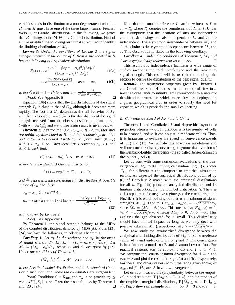
Let us start with some numerical evaluations of the con-vergence ofMn to its limiting distribution. Fig. 1(a) showsFMn

for different n and compares to empirical simulationresults. As expected the analytical distributions obtained by(8) of Corollary 2 match with the empirical distributionsfor all n. Fig. 1(b) plots the analytical distribution and itslimiting distribution, i.e. the Gumbel distributionΛ. There isa discrepancy in the negative regime (see the circled regioninFig.1(b)). It is worth pointing out that as a maximum of signalstrengths,Mn ≥ 0 and thusMn ≥ −dn/cn = −√

2 logn/σX

sinceMn = (Mn − dn)/cn. This means thatFMn(x) = 0,

∀x ≤ −√2 logn/σX , whereasΛ(x) > 0, ∀x > −∞. This

explains the gap observed forn small. This dissimilarityshould have limited impact as long as we only deal withpositive values ofMn (respectively,Mn ≥ −√

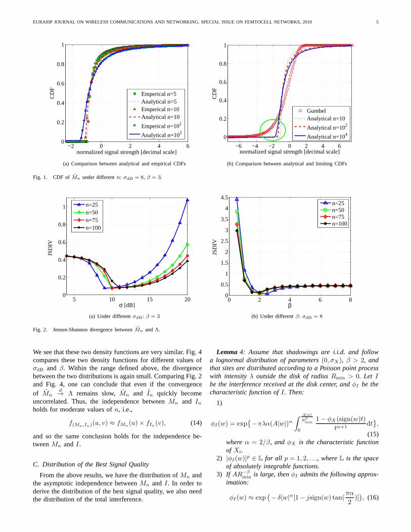
2 logn/σX ).We now study the symmetrized divergence between the

analytical and limiting distributions ofMn for some moderatevalues ofn and under differentσdB andβ. The convergenceis best forσdB around 10 dB andβ around two to four. Forpractical systems,σdB is approx. 8 dB and2 < β ≤ 4.We compute the Jensen-Shannon divergence forβ = 3 andσdB = 8 and plot the results in Fig. 2(a) and (b), respectively.For these (and other) values (within the range given above) ofσdB andβ, Mn andΛ have low divergence.

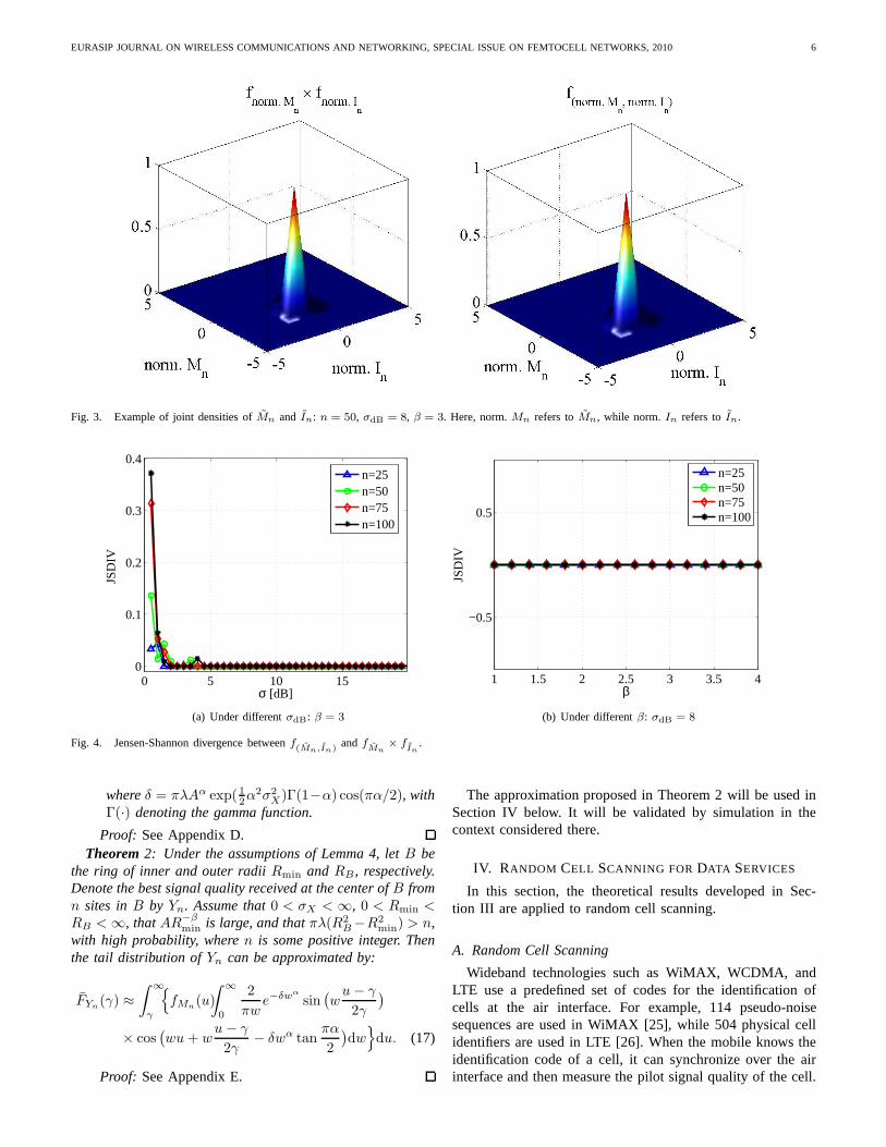
Let us now measure the (dis)similarity between the empiri-cal joint distribution,PMn ≤ u, In ≤ v, and the product ofthe empirical marginal distributions,PMn ≤ u × PIn ≤v. Fig. 3 shows an example withn = 50, β = 3 andσdB = 8.


−2 0 2 4 60

0.2

0.4

0.6

0.8

1

normalized signal strength [decimal scale]

CD

F

Emperical n=5Analytical n=5Emperical n=10Analytical n=10

Emperical n=102

Analytical n=102

(a) Comparison between analytical and empirical CDFs

−6 −4 −2 0 2 4 6

0

0.2

0.4

0.6

0.8

1

normalized signal strength [decimal scale]

CD

F

GumbelAnalytical n=10

Analytical n=102

Analytical n=104

(b) Comparison between analytical and limiting CDFs

Fig. 1. CDF ofMn under differentn: σdB = 8, β = 3.

5 10 15 200

0.2

0.4

0.6

0.8

1

σ [dB]

JSD

IV

n=25n=50n=75n=100

(a) Under differentσdB: β = 3

0 2 4 6 80

0.5

1

1.5

2

2.5

3

3.5

4

4.5

β

JSD

IV

n=25n=50n=75n=100

(b) Under differentβ: σdB = 8

Fig. 2. Jensen-Shannon divergence betweenMn andΛ.

We see that these two density functions are very similar. Fig. 4compares these two density functions for different values ofσdB and β. Within the range defined above, the divergencebetween the two distributions is again small. Comparing Fig. 2and Fig. 4, one can conclude that even if the convergenceof Mn

d→ Λ remains slow,Mn and In quickly becomeuncorrelated. Thus, the independence betweenMn and Inholds for moderate values ofn, i.e.,

f(Mn,In)(u, v) ≈ fMn(u)× fIn(v), (14)

and so the same conclusion holds for the independence be-tweenMn andI.

C. Distribution of the Best Signal Quality

From the above results, we have the distribution ofMn andthe asymptotic independence betweenMn and I. In order toderive the distribution of the best signal quality, we also needthe distribution of the total interference.

Lemma 4: Assume that shadowings are i.i.d. and followa lognormal distribution of parameters (0, σX), β > 2, andthat sites are distributed according to a Poisson point processwith intensity λ outside the disk of radius Rmin > 0. Let Ibe the interference received at the disk center, and φI be thecharacteristic function of I . Then:

1)

φI(w) = exp

−πλα(A|w|)α∫

A|w|

Rβmin

0

1− φX(sign(w)t)

tα+1dt

,

(15)where α = 2/β, and φX is the characteristic functionof Xi.

2) |φI(w)|p ∈ L for all p = 1, 2, . . ., where L is the spaceof absolutely integrable functions.

3) If AR−βmin is large, then φI admits the following approx-

imation:

φI(w) ≈ exp(

− δ|w|α[1− jsign(w) tan(πα

2)])

, (16)


Fig. 3. Example of joint densities ofMn and In: n = 50, σdB = 8, β = 3. Here, norm.Mn refers toMn, while norm.In refers toIn.

0 5 10 150

0.1

0.2

0.3

0.4

σ [dB]

JSD

IV

n=25n=50n=75n=100

(a) Under differentσdB: β = 3

1 1.5 2 2.5 3 3.5 4

−0.5

0.5

β

JSD

IV

n=25n=50n=75n=100

(b) Under differentβ: σdB = 8

Fig. 4. Jensen-Shannon divergence betweenf(Mn,In) andfMn

× fIn

.

where δ = πλAα exp(12α2σ2

X)Γ(1−α) cos(πα/2), withΓ(·) denoting the gamma function.

Proof: See Appendix D.Theorem 2: Under the assumptions of Lemma 4, let B be

the ring of inner and outer radii Rmin and RB , respectively.Denote the best signal quality received at the center of B fromn sites in B by Yn. Assume that 0 < σX < ∞, 0 < Rmin <RB < ∞, that AR−β

min is large, and that πλ(R2B−R2

min) > n,with high probability, where n is some positive integer. Thenthe tail distribution of Yn can be approximated by:

FYn(γ) ≈

∫ ∞

γ

fMn(u)

∫ ∞

0

2

πwe−δwα

sin(

wu − γ

2γ

)

× cos(

wu + wu − γ

2γ− δwα tan

πα

2

)

dw

du. (17)

Proof: See Appendix E.

The approximation proposed in Theorem 2 will be used inSection IV below. It will be validated by simulation in thecontext considered there.

IV. RANDOM CELL SCANNING FOR DATA SERVICES

In this section, the theoretical results developed in Sec-tion III are applied to random cell scanning.

A. Random Cell Scanning

Wideband technologies such as WiMAX, WCDMA, andLTE use a predefined set of codes for the identification ofcells at the air interface. For example, 114 pseudo-noisesequences are used in WiMAX [25], while 504 physical cellidentifiers are used in LTE [26]. When the mobile knows theidentification code of a cell, it can synchronize over the airinterface and then measure the pilot signal quality of the cell.


Therefore, by using a predefined set of codes, these widebandtechnologies can have more autonomous cell measurementconducted by the mobile. In this paper, this identification codeis referred to as cell synchronization identifier (CSID).

In a dense small cell network where a large number of cellsare deployed in the same geographical area, the mobile canscan any cell as long as the set of CSIDs used in the networkis provided. This capability motivates us to proposerandomcell scanning which is easy to implement and has only veryfew operation requirements. The scheme is detailed below:

(1) When a mobile gets admitted to the network, its (first)serving cell provides him the whole set of CSIDs usedin the network. The mobile then keeps this informationin its memory.

(2) To find a handover target, the mobile randomly selects aset ofn CSIDs from its memory and conducts the stan-dardized scanning procedure of the underlying cellulartechnology, e.g., scanning specified in IEEE 802.16 [25],or neighbor measurement procedure specified in 3G [27]and LTE [12].

(3) The mobile finally selects the cell with the best receivedsignal quality as the handover target.

In the following, we determine the number of cells to bescanned which maximizes the data throughput.

B. Problem Formulation

The optimization problem has to take into account the twocontrary effects due to the number of cells to be scanned.On one hand, the larger the set of scanned cells, the betterthe signal quality of the chosen site, and hence the larger thedata throughput obtained by the mobile. On the other hand,scanning can have a linear cost in the number of scanned cells,which is detrimental to the throughput obtained by the mobile.

Let us quantify this using the tools of the previous sections.Let W be the average cell bandwidth available per mobile

and assume that it is a constant. Under the assumption ofadditive white Gaussian noise, the maximum capacityξn thatthe mobile can have by selecting the best amongn randomlyscanned cells is

ξn = W log(1 + Yn). (18)

Hence

Eξn = WElog(1 + Yn)

= W

∫ ∞

γ=0

log(1 + γ)fYn(γ)dγ,

where fYnis the pdf of Yn. By an integration by parts of

log(1 + γ) andfYn(γ)dγ = −dFYn

(γ), this becomes:

Eξn = W

∫ ∞

γ=0

FYn(γ)

1 + γdγ. (19)

Note thatEξn is the expected throughput from the bestcell. SinceYn is the maximum signal quality of then cells,Yn increases withn and so doesξn. Hence, the mobile shouldscan as many cells as possible. However, on the other hand,if scanning many cells, the mobile will consume much timein scanning and thus have less time for data transmission

with the serving cell. A typical situation is that where thescanning time increases proportionally with the number ofcells scanned and where the data transmission is suspended.This for instance happens if the underlying cellular technologyuses acompressed mode scanning1, like e.g., in IEEE 802.16[25] and also inter-frequency cell measurements defined by3GPP [12], [27].

Another scenario is that ofparallel scanning-transmission:here scanning can be performed in parallel to data transmissionso that no transmission gap occurs; this is the case in e.g.,intra-frequency cell measurements in WCDMA [27] and LTE[12].

Let T be the average time during which the mobile staysin the tagged cell and receives data from it. Lets be the timeneeded to scan one cell (e.g., in WCDMA, the mobile needss = 25 ms if the cell is in the neighbor cell list ands = 800 msif not [28], whereas in WiMAX,s = 10 ms, i.e., two 5-msframes). LetL(n) be the duration of the suspension of datatransmission due to the scanning of then cells:

L(n) =

s× n if compressed mode is used,

0 if parallel scan.-trans. is enabled.(20)

Finally, letEξ0 be the average throughput received from theserving cell when no scanning at all is performed (this wouldbe the case if the mobile would pick as serving site one of thesites of setS at random).

The gain of scanningn cells can be quantified by thefollowing metric, that we will call theacceleration:

ρn ,T · Eξn

T · Eξ0+ L(n) ·Eξ0

=T

T + L(n)× Eξn

Eξ0. (21)

In this definition,T ·Eξn (resp.T ·Eξ0+L(n) ·Eξ0))is the expected amount of data transmitted when scanningncells (resp. doing no scanning at all). We aim at finding thevalue ofn that maximizes the accelerationρn.

It is clear thatT/(T + L(n)) = 1 when (i) T → ∞, i.e.,the mobile stays in and receives data from the tagged cellforever, or (ii)L(n) = 0, i.e., parallel scanning-transmissionis enabled. In these cases,ρn increases withn and the mobile“should” scan as many cells as possible. However,ρn isoften concave and the reward of scanning then decreases. Tocharacterize this, we introduce agrowth factor g defined asfollows:

gn ,ρn

ρn−1=

T + L(n− 1)

T + L(n)× Eξn

Eξn−1. (22)

Special cases as those considered above can be cast withina general framework which consists in finding the value ofn that maximizesρn under the constraint thatgn ≥ 1 + ∆g,where∆g > 0 is a threshold.

1In this mode, scanning intervals, where the mobile temporarily suspendsdata transmission for scanning neighbor cells, are interleaved with intervalswhere data transmission with the serving cell is resumed.


0 50 100 150 200 250

10−1

100

n [number cells scanned]

Eξ

n / E

ξ25

0

NumericalSimulation

(a) Plot of Eξnmaxk Eξk

100

101

102

0

0.2

0.4

0.6

0.8

1


ρ n / ρ 25

0

NumericalSimulationn

numerical = 43

nsimulation

= 42

(b) Plot of ρnmaxk ρk

, T = 0.5 second

0 20 40 60 80 1000

20

40

60

80

100

T/s

Opt

imal

n

(c) Optimal number of cells to be scanned

100

101

102

1

1.2

1.4

1.6

1.8

2


g n

Limiting caseT = 5.0 secondT = 0.5 secondT = 0.2 second

(d) Growth factorgn under differentT

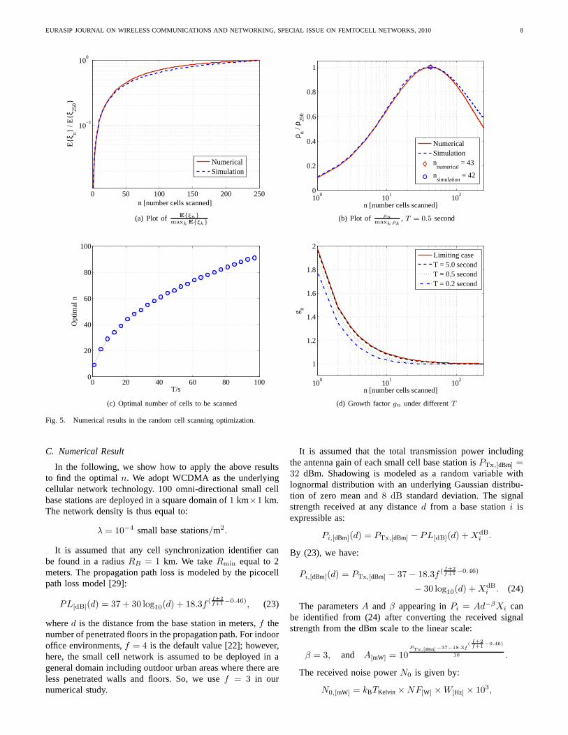
Fig. 5. Numerical results in the random cell scanning optimization.

C. Numerical Result

In the following, we show how to apply the above resultsto find the optimaln. We adopt WCDMA as the underlyingcellular network technology. 100 omni-directional small cellbase stations are deployed in a square domain of1 km×1 km.The network density is thus equal to:

λ = 10−4 small base stations/m2.

It is assumed that any cell synchronization identifier canbe found in a radiusRB = 1 km. We takeRmin equal to 2meters. The propagation path loss is modeled by the picocellpath loss model [29]:

PL[dB](d) = 37 + 30 log10(d) + 18.3f (f+2f+1−0.46), (23)

whered is the distance from the base station in meters,f thenumber of penetrated floors in the propagation path. For indooroffice environments,f = 4 is the default value [22]; however,here, the small cell network is assumed to be deployed in ageneral domain including outdoor urban areas where there areless penetrated walls and floors. So, we usef = 3 in ournumerical study.

It is assumed that the total transmission power includingthe antenna gain of each small cell base station isPTx,[dBm] =32 dBm. Shadowing is modeled as a random variable withlognormal distribution with an underlying Gaussian distribu-tion of zero mean and8 dB standard deviation. The signalstrength received at any distanced from a base stationi isexpressible as:

Pi,[dBm](d) = PTx,[dBm] − PL[dB](d) +XdBi .

By (23), we have:

Pi,[dBm](d) = PTx,[dBm] − 37− 18.3f (f+2f+1−0.46)

− 30 log10(d) +XdBi . (24)

The parametersA andβ appearing inPi = Ad−βXi canbe identified from (24) after converting the received signalstrength from the dBm scale to the linear scale:

β = 3, and A[mW] = 10PTx,[dBm]−37−18.3f

(f+2f+1

−0.46)

10 .

The received noise powerN0 is given by:

N0,[mW] = kBTKelvin ×NF[W] ×W[Hz] × 103,


where the effective bandwidthW[Hz] = 3.84 × 106 Hz, kB

is the Boltzmann constant, andTKelvin is the temperature inKelvin, kBTKelvin = 1.3804× 10−23 × 290 W/Hz andNF[dB]

is equal to 7 dB.It is assumed that the mobile is capable of scanning eight

identified cells within 200 ms [28]. So, the average timeneeded to scan one cell is given bys = 25 ms.

In order to check the accuracy of the approximations used inthe analysis, a simulation was built with the above parametersetting. The interference field was generated according to aPoisson point process of intensityλ in a region betweenRmin

andR∞ = 100 km. For a numbern, the maximum of SINRreceived fromn base stations which are randomly selectedfrom the diskB between radiiRmin andRB was computed.After that the expectation of the maximal capacityEξnreceived from then selected BSs was evaluated.

In Fig. 5(a), the expectation of the maximal throughputEξn for differentn is plotted, as obtained through the an-alytical model and simulation. The agreement between modeland simulation is quite evident. As shown in Fig. 5(a),Eξnincreases withn, though the increasing rate is slow down asn increases. Note that in Fig. 5(a),Eξn is plotted afternormalization byEξ250.

Fig. 5(b) gives an example of accelerationρn for T = 0.5second andL(n) = n× 25 ms. In the plot,ρn is normalizedby its maximum. Here, an agreement between model andsimulation is also obtained. We see thatρn first increasesrapidly with n, attains its maximum atn = 42 by simulationandn = 43 by model, and then decays.

Next, using the model we compute the optimal number ofcells to be scanned and the growth factorgn for differentT .Note that in (21), the factorT/(T + L(n)) can be re-writtenas:

T

T + L(n)=

1

1 + n× s/Tfor

T < ∞,

L(n) = n× s.

It is clear that this factor also depends on the ratioT/s.Fig. 5(c) plots the optimaln for different values ofT/s. LargerT/s will drive the optimaln towards larger values. SinceTcan be roughly estimated as the mobile residence time in acell, which is proportional to the cell diameter divided by theuser speed, this can be rephrased by stating that the fasterthe mobile, the smallerT and thus the fewer cells the mobileshould scan.

Finally, Fig. 5(d) plots the growth factorgn with differentT . In Fig. 5(d), the “limiting case” corresponds to the casewhen T → ∞ or L(n) = 0. We see thatgn is quite stablew.r.t. the variation ofT . Besides,gn flattens out at about 30cells for a wide range ofT . Therefore, in practice this valuecan be taken as a recommended number of cells to be scannedin the system.

V. CONCLUDING REMARKS

In this paper, we firstly develop asymptotic properties of thesignal strength in cellular networks. We have shown that thesignal strength received at the center of a ring shaped domainB from a base station located inB belongs to the maximum

domain of attraction of a Gumbel distribution. Moreover, themaximum signal strength and the interference received fromn cells in B are asymptotically independent asn → ∞. Theabove properties are proved under the assumption that sitesareuniformly distributed inB and that shadowing is lognormal.Secondly, the distribution of the best signal quality is derived.These results are then used to optimize scanning in small cellnetworks. We determine the number of cells to be scanned formaximizing the mean user throughput within this setting.

REFERENCES

[1] W. C. Y. Lee, “Smaller cells for greater performance,”IEEE Communi-cations Magazine, vol. 29, no. 11, pp. 19–23, Nov. 1991.

[2] H. Claussen, L. T. W. Ho, and L. G. Samuel, “Financial analysisof a pico-cellular home network deployment,” inIEEE InternationalConference on Communications, Jun. 2007, pp. 5604–5609.

[3] V. Chandrasekhar, J. Andrews, and A. Gatherer, “Femtocell networks:a survey,”IEEE Communications Magazine, vol. 46, no. 9, pp. 59–67,Sep. 2008.

[4] S. Saunders, S. Carlaw, A. Giustina, R. R. Bhat, V. S. Rao,andR. Siegberg,Femtocells: Opportunities and Challenges for Business andTechnology. Wiley, Jun. 2009.

[5] A. Urie, “Keynote: The future of mobile networking will be smallcells,” in IEEE International Workshop on Indoor and Outdoor FemtoCells, Sep. 2009. [Online]. Available: http://iosc-workshop.homeip.net

[6] Y. Chika, “Keynote: True BWA - eXtended Global Platform,” in IEEEInternational Workshop on Indoor and Outdoor Femto Cells, Sep.2009. [Online]. Available: http://iosc-workshop.homeip.net

[7] P. Judge, “Vodafone launches home 3G Femtocell in the UK,” eWeekEu-rope, June 2009.

[8] M. R. Leadbetter, G. Lindgren, and H. Rootzen,Extremes and RelatedProperties of Random Sequences and Processes. Springer Verlag, 1983.

[9] P. Embrechts, C. Kluppelberg, and T. Mikosch,Modelling ExtremalEvents for Insurance and Finance. Springer, Feb. 1997.

[10] M. Nawrocki, H. Aghvami, and M. Dohler,Understanding UMTS RadioNetwork Modelling, Planning and Automated Optimisation: Theory andPractice. John Wiley & Sons, 2006.

[11] WiMAX Forum, “Mobile System Profile,” Approved Spec. Release 1.0,Revision 1.4.0, May 2007.

[12] 3GPP TS 36.331, “Evolved Universal Terrestrial Radio Access (E-UTRA) Radio Resource Control (RRC): Protocol Specification(Release8),” Tech. Spec. v8.8.0, Dec. 2009.

[13] NGMN Alliance, “Next Generation Mobile Networks Use cases relatedto self-organising network, Overall description,” Tech. Rep. v2.02, Dec.2008.

[14] ——, “Next Generation Mobile Networks Recommendation on SONand O&M requirements,” Req. Spec. v1.23, Dec. 2008.

[15] S. Magnusson and H. Olofsson, “Dynamic neighbor cell list planningin a microcellular network,” inIEEE International Conference onUniversal Personal Communications Record, Oct. 1997, pp. 223–227.

[16] R. Guerzoni, I. Ore, K. Valkealahti, and D. Soldani, “Automatic neighborcell list optimization for UTRA FDD networks: theoretical approach andexperimental validation,”WPMC, Aalborg, Denmark, 2005.

[17] D. Soldani and I. Ore, “Self-optimizing neighbor cell list for UTRAFDD networks using detected set reporting,” inIEEE 65th VehicularTechnology Conference, 2007, pp. 694–698.

[18] M. Amirijoo, P. Frenger, F. Gunnarsson, H. Kallin, J. Moe, and K. Zetter-berg, “Neighbor cell relation list and measured cell identity managementin LTE,” in IEEE Network Operations and Management Symposium,Apr. 2008, pp. 152–159.

[19] M. Z. Win, P. C. Pinto, and L. A. Shepp, “A mathematical theory ofnetwork interference and its applications,”Proceedings of the IEEE,vol. 97, no. 2, pp. 205–230, Feb. 2009.

[20] F. Baccelli and B. Błaszczyszyn,Stochastic Geometry and WirelessNetworks, Volume I - Theory, 2009, vol. 1. [Online]. Available:http://hal.inria.fr/inria-00403039/en/

[21] 3GPP TR 36.942, “Evolved Universal Terrestrial Radio Access (E-UTRA): Radio Frequency (RF) system scenarios (Release 8),”Tech.Rep. v8.2.0, May 2009.

[22] WiMAX Forum, “WiMAX systems evaluation methodology,”Spec.v2.1, Jul. 2008.

http://iosc-workshop.homeip.net

http://iosc-workshop.homeip.net

http://hal.inria.fr/inria-00403039/en/


[23] T. Chow and J. Teugels, “The sum and the maximum of i.i.d.randomvariables,” inProc. Second Prague Symp. Asymptotic Statistics, 1978,pp. 81–92.

[24] C. W. Anderson and K. F. Turkman, “The joint limiting distributionof sums and maxima of stationary sequences,”Journal of AppliedProbability, vol. 28, no. 1, pp. 33–44, 1991.

[25] IEEE 802.16, “Air Interface for Broadband Wireless Access Systems,”IEEE, Standard Std 802.16-2009, May 2009.

[26] 3GPP TS 36.300, “Evolved Universal Terrestrial Radio Access (E-UTRA) and Evolved Universal Terrestrial Radio Access Network (E-UTRAN) - Overall description: Stage 2 (Release 8),” Tech. Spec.v8.11.0, Dec. 2009.

[27] 3GPP TS 25.331, “Radio Resource Control (RRC): Protocol Specifica-tion (Release 8),” Tech. Spec. v8.6.0, Mar. 2009.

[28] 3GPP TS 25.133, “Requirements for support of Radio Resource Man-agement FDD (Release 8),” Tech. Spec. v8.9.0, Dec. 2009.

[29] ETSI TR 101.112, “Selection procedures for the choice of radio trans-mission technologies of the UMTS,” Tech. Rep. v3.2.0, Apr. 1998.

[30] M. Abramowitz and I. A. Stegun,Handbook of Mathematical Functions.Dover Publications, 1965.

[31] R. Takahashi, “Normalizing constants of a distribution which belongsto the domain of attraction of the Gumbel distribution,”Statistics &Probability Letters, vol. 5, no. 3, pp. 197–200, 1987.

[32] W. Feller, An Introduction to Probability Theory and Its Applications,2nd ed. John Wiley & Sons, 1971, vol. 2.

APPENDIX APROOF OFLEMMA 2

Let di = |y − xi| be the distance from a site located atxi ∈ R

2 to a positiony ∈ R2. Under the assumption that site

locations are uniformly distributed inB, the distancedi froma site located inB, i.e., xi ∈ B, to the center ofB has thefollowing distribution:

FD(d) = P[di ≤ d] =πd2 − πR2

min

πR2B − πR2

min

=d2 −R2

min

R2B −R2

min

.

Let Ui = Ad−βi , for β > 0, its distribution is equal to:

FU (u) = −c(

u− 2β − a−

2β

)

, for u ∈ [a, b],

wherec = A2β (R2

B − R2min)

−1, a = AR−βB , andb = AR−β

min.The density ofUi is given byfU (u) = (2c/β)u−1−2/β .

Thus, the distributionFP of the powerPi is equal to:

FP (x) =

∫ b

u=a

FX(x

u)fU (u)du. (25)

SubstitutingFX with lognormal distribution of parameters(0, σX) and fU given above into (25), after changing thevariable such thatt = log(xu ), we have:

FP (x) =c

βx− 2

β

(

∫ log ( xa)

log ( xb)

e2tβ dt

+

∫ log ( xa)

log ( xb)

e2tβ erf

( t√2σX

)

dt)

where the first integral is straightforward. By doing an integra-tion by parts oferf

(

t√2σX

)

ande2tβ dt for the second integral,

we get:

FP (x) =c

βx− 2

ββ

2

[

e2tβ + e

2tβ erf

( t√2σX

)

− e2σ2

Xβ2 erf

( t√2σX

−√2σX

β

)

]∣

∣

∣

log ( xa)

t=log ( xb).

After some elementary simplifications, we can obtain:

FP (x) = c

a−2β

(1

2+

1

2erf(

log x− µ1√2σX

))

−b−2β

(1

2+1

2erf(

log x− µ2√2σX

))

+eνx− 2β

[

−1

2−1

2erf(

log x− µ3√2σX

)

+1

2+

1

2erf(

log x− µ4√2σX

)]

whereν =2σ2

X

β2 , µ1 = log a, µ3 = µ1 + 2σ2X/β, µ2 = log b,

andµ4 = µ2+2σ2X/β. Let Gj , j = 1, ..., 4, be the lognormal

distribution of parameters(µj , σX), j = 1, ..., 4, FP can berewritten as (7).

APPENDIX BPROOF OFLEMMA 3

Let Gj(x) = 1−Gj(x) and note thatc(a−2β − b−

2β ) = 1,

we have from (7):

FP (x) = 1− c

a−2β G1(x)− b−

2β G2(x)

− eνx− 2β G3(x) + eνx− 2

β G4(x)

.

This yields the tail distributionFp = 1− FP :

Fp(x) = c

a−2β G1(x)− b−

2β G2(x)

− eνx− 2β G3(x) + eνx− 2

β G4(x)

. (26)

For (26), we haveGj(x) =12 erfc(log x− µj)/(

√2σX).

An asymptotic expansion oferfc(x) for large x [30, 7.1.23]gives us:

G3(x) ∼∞

σX√2π(log x− µ3)

exp

− (log x− µ3)2

2σ2X

=σX√

2π(log x− µ1 − 2σ2X

β )exp

−(log x− µ1 − 2σ2

X

β )2

2σ2X

=σXa−

2β e−νx

2β

√2π(log x− µ1)

exp

− (log x− µ1)2

2σ2X

1

1− 2σ2X

β(log x−µ1)

in which after a Taylor expansion of the last term on the right-hand side, we can have:

eνx− 2β G3(x) ∼∞

a−2β

[

G1(x)+

√

2

π

σ3X

β

exp(

− (log x−µ1)2

2σ2X

)

(log x− µ1)2

]

.

This implies that

a−2β G1(x) − eνx− 2

β G3(x)

∼∞

−√

2

π

a−2β σ3

X

β

exp(

− (log x−µ1)2

2σ2X

)

(log x− µ1)2. (27)

In the same manner, we have

b−2β G2(x)− eνx− 2

β G4(x)

∼∞

−√

2

π

b−2β σ3

X

β

exp(

− (log x−µ2)2

2σ2X

)

(log x− µ2)2. (28)


A substitution of (27) and (28) into (26) results in

Fp(x) ∼∞

√

2

π

cσ3X

β

b−2βexp

(

− (log x− µ2)2/(2σ2

X))

(log x− µ2)2

− a−2βexp

(

− (log x− µ1)2/(2σ2

X))

(log x− µ1)2

. (29)

Moreover,b > a yieldsµ2 − µ1 = log(b/a) > 0. Then, wehave the following result for largex:

exp(

− (log x−µ1)2

2σ2X

)

/(log x− µ1)2

exp(

− (log x−µ2)2

2σ2X

)

/(log x− µ2)2

=( log x− µ2

log x− µ1

)2

exp(µ2

2 − µ21

2σ2X

)

x−µ2−µ1

σ2X →

x→∞0.

Taking this into account in (29), finally we have:

Fp(x) ∼∞κexp

(

− (log x− µ2)2/(2σ2

X))

(

(log x− µ2)/(√2σX)

)2

∼∞

2√2πσXκ

G2(x)

log x− µ2, κ =

σX√2πβ

R2min

R2B −R2

min

.

APPENDIX CPROOF OFTHEOREM 1

We will use Lemma 3 and the following two lemmas toprove Theorem 1.

Lemma 5 (Embrechts et al. [9]): Let Zi be i.i.d. randomvariables having distribution F , and Ψn = maxni=1 Zi. Letg be an increasing real function, denote Zi = g(Zi), andΨn = maxni=1 Zi. If F ∈ MDA(Λ) with normalizing constantcn and dn, then

limn→∞

P(

Ψn ≤ g(cnz + dn))

= Λ(z), z ∈ R.

Lemma 6 (Takahashi [31]): Let F be a distribution func-tion. Suppose that there exists constants ω > 0, l > 0, η > 0and r ∈ R such that

limx→∞

(

1− F (x))

/(

lxre−ηxω)

= 1. (31)

For µ ∈ R and σ > 0, let F∗ = F ((x − µ)/σ). Then, F∗ ∈MDA(Λ) with normalizing constants c∗n = σcn and d∗n =σdn + µ, where

cn =(log n/η)

1ω−1

ωη, and

dn =( logn

η

)1/ω+

η1/ω

ω2

r(log logn− log η) + ω log l

(logn)1−1ω

.

Let g(t) = e√2σX t+µ2 be a real function defined onR, g

is increasing witht. Let Qi be the random variable such thatPi = g(Qi). By (10a) of Lemma 3, the tail distributionFQ isgiven by:

FQ(x) = FP

(

e√2σXx+µ2

)

∼ κx−2e−x2

, asx → ∞. (32)

By (32), FQ satisfies Lemma 6 with constantsl = κ, r =−2, η = 1, andω = 2. So,FQ ∈ MDA(Λ) with the followingnormalizing constants:

c∗n =(logn/η)

1ω−1

ωη=

1

2(logn)−

12 , and

d∗n =( logn

η

)1/ω+

η1/ω

ω2

r(log logn− log η) + ω log l

(logn)1−1ω

=(logn)12 +

1

2

(− log logn+ log κ)

(logn)12

.

(33)

Then, by Lemma 5, we have

limn→∞

P

(

Mn ≤ g(c∗nx+ d∗n))

= Λ(x), x ∈ R.

By a Taylor expansion ofexp(√2σXc∗nx), we have:

limn→∞

P

e−(√2σXd∗

n+µ2)Mn ≤ 1 +√2σXc∗nx+ o(c∗n)

= Λ(x).

Sincec∗n → 0 whenn → ∞, we have

Mn − e√2σXd∗

n+µ2

√2σXc∗ne

√2σXd∗

n+µ2

d→ Λ, asn → ∞. (34)

Substitutingc∗n andd∗n from (33) into (34), we obtaincn anddn for (12). The conditionsRmax < ∞, Rmin > 0 andσX >0 provide κ > 0. This leads todn > 0, and consequently,cn > 0.

APPENDIX DPROOF OFLEMMA 4

Under the assumptions of the lemma, the interference fieldcan be modeled as a shot noise defined onR

2 excluding theinner disk of radiusRmin. Hence, using Proposition 2.2.4 in[20], the Laplace transform ofI is given by:

LI(s) = exp

− 2πλ

∫ ∞

Rmin

(

1−Ee−sAXi

rβ )

rdr

. (35)

Noting that

φI(w) = LI(−jw), w ∈ R,

we have from (35) that:

φI(w) = exp

− 2πλ

∫ ∞

Rmin

(1 − EejwAXi

rβ )rdr

. (36)

Using the change of variablet = |w|Ar−β , we obtain

∫ +∞

Rmin

(1−EejwAXi

rβ )rdr

=(A|w|)2/β

β

∫A|w|

Rβmin

0

1−Eejsign(w)tXit2/β+1

dt, (37)

whereEejsign(w)tXi = φX(sign(w)t). So, substituting thisinto (36), we get the first part of the Lemma 4.


From (15), for allp = 1, 2, . . ., we have:

|φI(w)|p = exp(

− pπλα(A|w|)αE

∫

A|w|

Rβmin

0

1− cos(tXi)

tα+1dt

)

. (38)

Since1− cos(tXi) ≥ 0, ∀t ∈ R, we have

E

∫A|w|

Rβmin

0

1− cos(tXi)

tα+1dt

≥ 0. (39)

Therefore

|φI(w)|p ≤ exp(−c|w|α), (40)

wherec is some positive constant, and hence the right hand-side of this is an absolutely integrable function. This provesthe second assertion of Lemma 4.

Under the assumption thatAR−βmin ≈ ∞, φI can be

approximated by:

φI(w) ≈ exp(

− πλα(A|w|)α∫ ∞

0

1− φX(sign(w)t)

tα+1dt)

.

(41)For 0 < α < 1, we have

∫ ∞

0

1− ejsign(w)tXi

tα+1dt

= −Γ(−α)|sign(w)Xi|αe−jsign(w)πα2 (42)

SinceXi ≥ 0, we can write|sign(w)Xi|α = Xαi . Taking

expectations on both sides, we get∫ +∞

0

1−Eejsign(w)tXitα+1

dt

= −EXαi Γ(−α)e−jsign(w)πα

2

= EXαi

Γ(1− α)

αcos(

πα

2)[1− jsign(w) tan(

πα

2)].

Substituting this into (41) and noting that

EXαi = exp(

1

2α2σ2

X), (43)

for Xi lognormally distributed, we obtain (16).

APPENDIX EPROOF OFTHEOREM 2

Under the assumption that sites are distributed as a homoge-neous Poisson point process of intensityλ in B, the expectednumber of cells inB is πλ(R2

B − R2min). We assume that

πλ(R2B − R2

min) is much larger thann, which ensures thatthere aren cells inB with high probability, so thatYn is welldefined.

Under the conditions of Theorem 2,Mn andI are asymp-totically independent according to Corollary 4. So, by substi-tuting (14) into (6), we have:

PYn ≥ γ ≈∫ ∞

0

fMn(u)

∫ ∞

0

h(v, u)fI(v)dvdu (44)

where

h(v, u) = 1(v≤ (1+γ)u

γ−1)

1(v≥u)

=

1 if v ∈ [u, 1+γγ u− 1] andu > γ

0 otherwise. (45)

It is easily seen thath(v, u) is square-integrable with respectto v, and its Fourier transform w.r.t.v is given by:

h(w

2π, u) =

0 if u ≤ γ∫

1+γγ

u−1

u e−jwvdv if u > γ(46)

which yields:

h(w

2π, u) =

0 if u ≤ γ

1jw

(

e−jwu − ejw(

1−1+γγ

u)

)

if u > γ. (47)

Besides, according to Lemma 4 we have thatφI ∈ L andφI ∈ L

2, whereL2 is the space of square integrable functions.And so, by Theorem 3 in [32, p.509],fI is bounded continuousand square integrable. Hence, by applying the Plancherel-Parseval theorem to the inner integral of (44), we have

∫ ∞

0

h(v, u)fI(v)dv =

∫ ∞

−∞h(−w, u)fI(w)dw, (48)

wherefI(w) is the Fourier transform offI(v). Take (47) intoaccount for (48) and (44), we have:

FYn(γ) =

∫ ∞

γ

fMn(u)

∫ ∞

−∞h(−w, u)fI(w)dw

du, (49)

where we further have∫ ∞

−∞h(−w, u)fI(w)dw

=1

2π

∫ +∞

−∞h(− w

2π, u)fI(

w

2π)dw

=1

2π

∫ +∞

0

(

h(w

2π, u)fI(

−w

2π) + h(

−w

2π, u)fI(

w

2π))

dw.(50)

Note that

fI(w

2π) = φI(−w). (51)

And under the assumption thatAR−βmin ≈ ∞, φI is ap-

proximated by (16). Thus, by (16) and (47), we have forw ∈ [0,+∞):

h(w

2π, u)fI(−

w

2π) ≈ e−δwα

jw

ej(−wu+δwα tan πα2 )

− e−j(−w+w 1+γγ

u−δwα tan πα2 )

(52)

and

h(− w

2π, u)fI(

w

2π) ≈ e−δwα

jw

− e−j(−wu+δwα tan πα2 )

+ ej(−w+w 1+γγ

u−δwα tan πα2 )

. (53)


By (52) and (53), we get

1

2π

[

h(w

2π, u)fI(

−w

2π) + h(

−w

2π, u)fI(

w

2π)]

≈ e−δwα

πw

[

sin(−wu+ δwα tanπα

2)

+ sin(−w + w1 + γ

γu− δwα tan

πα

2)]

=2e−δwα

πwsin

(

wu− γ

2γ

)

× cos(

wu + wu− γ

2γ− δwα tan

πα

2

)

.

Substitute the above into (50) and then into (49), we have(17).

Best Signal Quality in Cellular Networks: Asymptotic ... - arXiv

Documents

Transcript of Best Signal Quality in Cellular Networks: Asymptotic ... - arXiv