Research Article

Published online 15 July 2010 in Wiley Online Library(wileyonlinelibrary.com) DOI: 10.1002/qre.1125

Effect of Non-normality on the Monitoringof Simple Linear ProfilesR. Noorossana,a A. Vaghefib and M. Dorria∗†

In some statistical process control (SPC) applications, it is assumed that a quality characteristic or a vector of qualitycharacteristics of interest follows a univariate or multivariate normal distribution, respectively. However, in certainapplications this assumption may fail to hold and could lead to misleading results. In this paper, we study the effect ofnon-normality when the quality of a process or product is characterized by a linear profile. Skewed and heavy-tailedsymmetric non-normal distributions are used to evaluate the non-normality effect numerically. The results reveal thatthe method proposed by Kim et al. (J. Qual. Technol. 2003; 35:317–328) can be designed to be robust to non-normalityfor both highly skewed and heavy-tailed distributions. Copyright © 2010 John Wiley & Sons, Ltd.

Keywords: average run length (ARL); linear profiles; non-normality; T2 control chart; exponentially weighted moving averagecontrol chart

1. Introduction

Control charts have been used in practice extensively since their introduction by Dr Walter A. Shewhart of Bell TelephoneLaboratories in 1924 for the purpose of monitoring product or process quality characteristics in various situations. Informationrelated to a univariate quality characteristic or a vector of multivariate quality characteristics is usually plotted on a control

chart as a single point in order to evaluate the process performance. However, in certain applications the quality of a process orproduct can be monitored effectively using the relationship between a response variable and one or more explanatory variables.This relationship is usually referred to as profile. Many authors including Mestek et al.1, Stover and Brill2, Lawless et al.3, Kangand Albin4, Mahmoud and Woodall5, Wang and Tsung6, Gupta et al.7, Jensen et al.8, and Noorossana et al.9 discussed real-worldapplications in which a linear profile could be used to represent the status of a process or product effectively.

According to Kang and Albin4, a profile data consists of a set of measurements with a response variable y and one or moreexplanatory variables xj, j=1, 2,. . ., which are used to assess the quality of a manufactured product. They proposed Phase I and

Phase II control chart methods to monitor the performance of a process characterized by a linear profile. Kim et al.10 alsorecommended three independent univariate exponentially weighted moving average (EWMA) control charts to monitor shifts inthe parameters of a profile. They showed that their proposed method is superior to those recommended by Kang and Albin4.Mestek et al.1 and Mahmoud and Woodall5 focused on Phase I analysis of linear profiles with calibration applications and evaluatedthe performance of their proposed procedures. Noorossana et al.11 proposed a multivariate cumulative sum (MCUSUM) chart andR chart for monitoring a linear profile. They showed that their proposed scheme is superior to the methods proposed by Kangand Albin4 and Kim et al.10. Zou et al.12 and Mahmoud et al.13 proposed change-point methods for monitoring linear profiles inboth Phase I and Phase II. Zou et al.14 proposed a multivariate exponentially weighted moving average (MEWMA) control chart formonitoring general linear profiles in Phase II. In addition, Zou et al.15 used a combination of two EWMA control charts to proposea self-starting Phase II control chart based on recursive residuals for monitoring regression coefficients and standard deviationof a linear profile when they are unknown before the control scheme begins. Zhang et al.16 proposed a control chart based onlikelihood ratio to detect shifts in either the intercept, slope or standard deviation. Saghaei et al.17 proposed a cumulative sumstatistic to enhance monitoring linear profiles in Phase II. Zhu and Lin18 proposed a Shewhart-type control chart for monitoringslope parameter of linear profiles in both Phase I and Phase II. Kazemzadeh et al.19 considered polynomial profiles and developedthree Phase I methods for monitoring such profiles. Further studies on linear profile monitoring can also be found in Croarkinand Varner20, Gupta et al.7, Jensen et al.21 and Saghaei et al.22. Several authors including Jin and Shi23, Walker and Wright24,Ding et al.25, Moguerza et al.26, Williams et al.27, and Vaghefi et al.28 proposed methods for monitoring nonlinear profiles.

aIndustrial Engineering Department, Islamic Azad University, South-Tehran Branch, Tehran, IranbIndustrial and System Engineering Department, Rutgers, The State University of New Jersey, Piscataway, NJ 08854, U.S.A.∗Correspondence to: M. Dorri, Industrial Engineering Department, Islamic Azad University, South-Tehran Branch, Tehran, Iran.†E-mail: me.dorri@gmail.com

Copyright © 2010 John Wiley & Sons, Ltd. Qual. Reliab. Engng. Int. 2011, 27 425--436

42

5

R. NOOROSSANA, A. VAGHEFI AND M. DORRI

In this study, we assume that paired observations (xi , yij) for i=1, 2,. . . , n and j=1, 2,. . . are collected over time and therelationship between paired observations can be best represented by the following linear profile:

yij =A0 +A1xi +�ij . (1)

In most cases, it is assumed that �ij ’s are independent and identically distributed (i.i.d) normal random variables with mean

zero and variance �2. However, in some practical cases, these standard assumptions may fail to hold. According to Williamset al.29, engineering applications that give rise to profile data may lead to autocorrelated error terms especially when the processperformance is characterized by nonlinear profiles. They also discussed that a common source of autocorrelated errors is thespatial or serial manner in which data are collected. Noorossana et al.9 and Kazemzadeh et al.30 extended a method for monitoringlinear profiles where there is an inter-correlation between profiles over time. Soleimani et al.31 considered a simple linear profileand assumed that a first-order autoregressive model can be used to model autocorrelation structure among observations. Theyproposed four methods to monitor profiles in the presence of within profile autocorrelation in Phase II.

Non-normality is often studied for individual observations because it is not a significant concern with large subgroups. Schillingand Nelson32 showed that Shewhart control charts are typically robust to the normality assumption for n>4 (see also Yourstoneand Zimmer33 and Amin et al.34). DeVor et al.35 recommended checking the assumption of non-normality when individualobservations are used. Several authors, including Borror et al.36 and Stoumbos and Reynolds37, reported that non-normality couldseriously degrade the performance of X and X control charts; however, EWMA and CUSUM control charts can be designed tobe robust to the non-normality assumption. The effect of non-normality on the statistical performance of MEWMA control chartwas also investigated by Stoumbos and Sullivan38. They found that smaller choices of the smoothing parameter � are needed toyield average run length (ARL) values close to those under normality assumption. A few studies have also addressed the effectof non-normality on the monitoring of linear or nonlinear profiles. According to Mahmoud and Woodall5, normality is a criticalassumption in Phase I and should be checked prior to conducting profile analysis. Noorossana et al.39 studied the non-normalityeffect of error terms on the performance of EWMA/R methods proposed by Kang and Albin4. Williams et al.29 and Vaghefi et al.28

discussed that non-normality should be a problem of concern in Phase II monitoring of nonlinear profiles. They mentioned thatsince the parameter vector estimate in a nonlinear model is an asymptotically normal random variable, then for small samplesizes the non-normality issue could be a problem of concern.

In this paper, we study the effect of non-normality on the statistical performance of linear profile monitoring. The ARL isconsidered as a vehicle to evaluate the performance of linear profile when observations fail to follow a normal distribution.Section 2 discusses some methods proposed for Phase II monitoring of linear profiles. Section 3 covers some non-normality issuesrelated to linear profiles. Numerical results for evaluating the non-normality effect are presented in Section 4. Our concludingremarks are provided in the final section.

2. Phase II methods

As most of the studies on profile monitoring are related to the simple linear model, we investigate the effect of non-normalityon the performance of three common control charts developed by Kang and Albin4 and Kim et al.10. Kang and Albin4 proposedtwo strategies to monitor a process when the parameters of a linear profile represented by a regression line are all known. Theirfirst strategy is to use a bivariate T2 control chart to monitor the regression coefficients. This chart is based on the fact that theleast squares estimators of A0 and A1 have a bivariate normal distribution. The least squares estimators of A0 and A1 for samplej are given by the following formulas:

a0j = yj −a1j x and a1j =Sxy(j) / Sxx, (2)

where yj =n−1 ∑ni=1 yij , x =n−1 ∑n

i=1 xi , Sxy(j) =∑n

i=1 (xi − x)yij , and Sxx =∑ni=1 (xi − x)2. If the error terms are independent and

identically distributed normal random variable, the least squares estimators a0j and a1j have a bivariate normal distribution withmean vector �= (A0, A1) and the following variance–covariance matrix:

�=⎛⎝ �2

0 �201

�201 �2

1

⎞⎠ , (3)

where �20 =�2(n−1 + x2 / Sxx) and �2

1 =�2 / Sxx are the variance of a0j and a1j , respectively, and �201 =−�2x / Sxx is the covariance

between a0j and a1j .

In their first monitoring strategy, the vector of sample estimators zj = (a0j , a1j)T for sample j, where a0j and a1j are the sample

intercept and the sample slope defined in Equation (2) is computed and then, the following T2 statistic is calculated:

T2j = (zj −�)T�−1(zj −�), (4)

where � is given by �= (A0, A1) and � is defined by Equation (3). It can be shown that T2j follows a central chi-square distribution

with 2 degrees of freedom when process is under statistical control. Therefore, the recommended upper control limit (UCL) for

42

6

Copyright © 2010 John Wiley & Sons, Ltd. Qual. Reliab. Engng. Int. 2011, 27 425--436

R. NOOROSSANA, A. VAGHEFI AND M. DORRI

the chart is UCL=�2� , where �2

� is the 100(1−�) percentile of the chi-square distribution with 2 degrees of freedom. Their secondstrategy is to apply some standard control chart schemes to the regression residuals obtained at sample j using

eij =yij −A0 −A1xi, i=1, 2,. . . , n. (5)

They applied a EWMA control chart to monitor the average values of these deviations and recommended the use of an R controlchart in combination with the EWMA control chart. They refer to this method as the EWMA/R approach. The average of theresiduals for the jth sample denoted by ej is calculated using

ej =n−1n∑

i=1eij. (6)

The EWMA control chart statistic, denoted by zj , for j=1, 2,. . . is given by

zj =�ej +(1−�)zj−1, (7)

where �(0<�≤1) is a smoothing constant and z0 =0. An out-of-control signal is given when zj is less than the lower control limit(LCL) or zj is greater than the UCL, where

LCL=−L�

√�

(2−�)nand UCL=L�

√�

(2−�)n, (8)

and L>0 is a threshold selected to obtain a specified in-control ARL value. Kang and Albin4 proposed the range control chart inconjunction with the EWMA control chart for two reasons. The first reason is to detect shifts in the process variance �2 since theEWMA control chart is not sensitive to shifts in the process variation. The second reason is that the EWMA control chart basedon the average residual is not sensitive to some shifts in A0 and A1 for which the magnitudes of the residuals tend to be largebut the average residuals tend to be very small. This can occur, for example, when the slope of the line changes but the averagevalue of Y does not.

For the R-chart, Kang and Albin4 recommended plotting the sample ranges Rj =max(eij)−min(eij), where i=1, 2,. . . , n andj=1, 2,. . . The LCL and UCL for the R-chart are

LCL=�(d2 −Ld3) and UCL=�(d2 +Ld3), (9)

respectively, where L(>0) is a threshold chosen to obtain a specified in-control ARL value. The values of d2 and d3 are constantsthat depend on the sample size n. Kim et al.10 proposed alternative control charts for monitoring the process performancein Phase II. In their proposed method, X-values are coded and the resulted alternative form of the underlying model givenas yij =B0 +B1X ′

i +�ij , i=1, 2,. . . , n, where B0 =A0 +A1X, B1 =A1 and X ′i = (Xi − X) is considered for monitoring purposes. According

to Myers40, the least squares estimator for B0 is b0j = yj and, the least squares estimator for B1 denoted by b1j is similar

to A1. The estimators b0j and b1j are independent normal random variables with means B0 and B1 and variances n−1�2 and

�2 / Sxx , respectively. The covariance between b0j and b1j is zero. By transforming the X-values, Kim et al.10 applied three

EWMA control charts to monitor B0, B1, and �2, respectively, without the problems that would result if the estimators werecorrelated. For the EWMA control chart used for monitoring the Y-intercept or B0, the statistic b0j is used to compute the chartstatistics zj,b0

=�b0j +(1−�)zj−1,b0, j=1, 2,. . ., where �(0<�≤1) is the smoothing parameter, and z0,b0

is assumed equal to B0.An out-of-control signal is generated when zj,b0

<LCL or zj,b0>UCL, where

LCL=B0 −Lb0�

√�

(2−�)nand UCL=B0 +Lb0

�

√�

(2−�)n, (10)

and Lb0is a multiple that can be adjusted to obtain a specified in-control ARL. B1 can also be monitored by using EWMA chart

statistic computed as zj,b1=�b1j +(1−�)zj−1,b1

, j=1, 2,. . ., where �(0<�≤1) is the smoothing parameter and z0,b1is assumed

equal to B1. The LCL and UCL for the chart are given by

LCL=B1 −Lb1�

√�

(2−�)Sxxand UCL=B1 +Lb1

�

√�

(2−�)Sxx, (11)

where Lb1is a multiple adjusted to obtain a specified in-control ARL.

In order to monitor process variability, Kim et al.10 considered EWMA control chart for monitoring the error variance �2

based on the method proposed by Crowder and Hamilton41. As MSE is an unbiased estimator of �2, Kim et al.10 usedzj,MSE =max{� ln(MSEj)+(1−�)zj−1,MSE, ln(�2

0)}, j=1, 2,. . . with z0,MSE = ln(�2) as the chart statistic. Crowder and Hamilton41 give

asymptotic variance of ln(MSEj) as var[ln(MSEj)]∼=2(n−2)−1 +2(n−2)−2 +(4 / 3)(n−2)−3 +(16 / 15)(n−2)−5. Hence, the UCL for thechart is given as

UCL=LMSE�

√�

(2−�)Sxxvar[ln(MSEj)]. (12)

Copyright © 2010 John Wiley & Sons, Ltd. Qual. Reliab. Engng. Int. 2011, 27 425--436

42

7

R. NOOROSSANA, A. VAGHEFI AND M. DORRI

Again, LMSE is a multiple chosen to obtain a specified in-control ARL. Kim et al.10 point out that a two-sided control limit couldbe used if a decrease in the variance is also considered to be important.

3. Non-normality

As mentioned before, non-normality is often investigated for individual observations. Based on central limit theorem, samplemeans are approximately normally distributed for all reasonable distributions and as a result non-normality is not a major concernwith large subgroups. However, for small sample sizes which are quite common in statistical process control (SPC) practices,distribution of a quality characteristic may be far from normal.

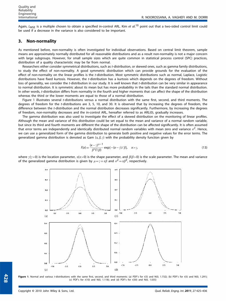
Researchers either consider symmetrical distributions, such as t-distribution, or skewed ones, such as gamma family distributions,to study the effect of non-normality. A good symmetric distribution which can provide grounds for the evaluation of theeffect of non-normality on the linear profiles is the t-distribution. Most symmetric distributions such as normal, Laplace, Logisticdistributions have fixed kurtosis. However, the t-distribution has a kurtosis which depends on the degrees of freedom. Withoutloss of generality, we consider the t-distribution in our study. It is well known that t-distribution can be very similar in appearanceto normal distribution. It is symmetric about its mean but has more probability in the tails than the standard normal distribution.In other words, t-distribution differs from normality in the fourth and higher moments that can affect the shape of the distributionwhereas the third or the lower moments are equal to those of a normal distribution.

Figure 1 illustrates several t-distributions versus a normal distribution with the same first, second, and third moments. Thedegrees of freedom for the t-distributions are 3, 5, 10, and 30. It is observed that by increasing the degrees of freedom, thedifference between the t-distribution and the normal distribution decreases significantly. Furthermore, by increasing the degreesof freedom, non-normality decreases and the in-control ARL, hereafter referred to as ARL(0), gradually increases.

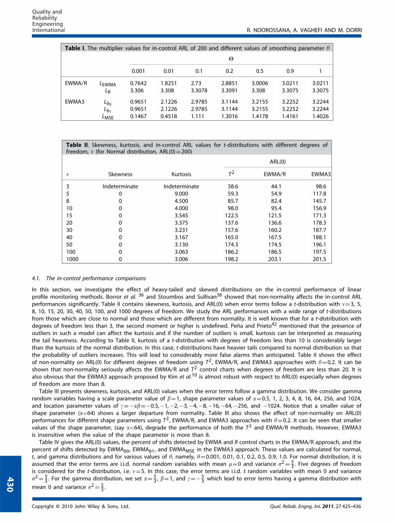
The gamma distribution was also used to investigate the effect of a skewed distribution on the monitoring of linear profiles.Although the mean and variance of this distribution could be set equal to the mean and variance of a normal random variable,but since its third and fourth moments are different the shape of the distribution can be affected significantly. It is often assumedthat error terms are independently and identically distributed normal random variables with mean zero and variance �2. Hence,we can use a generalized form of the gamma distribution to generate both positive and negative values for the error terms. Thegeneralized gamma distribution is denoted as Gam (�,�,) with the probability density function given by

f (x)= (x−)�−1

���(�)exp{−(x−) / �}, x>, (13)

where (>0) is the location parameter, �(�>0) is the shape parameter, and �(�>0) is the scale parameter. The mean and varianceof the generalized gamma distribution is given by �=+�� and �2 =��2, respectively.

Figure 1. Normal and various t-distributions with the same first, second, and third moments: (a) PDF’s for t(3) and N(0, 1.732); (b) PDF’s for t(5) and N(0, 1.291);(c) PDF’s for t(10) and N(0, 1.118); and (d) PDF’s for t(30) and N(0, 1.035)

42

8

Copyright © 2010 John Wiley & Sons, Ltd. Qual. Reliab. Engng. Int. 2011, 27 425--436

R. NOOROSSANA, A. VAGHEFI AND M. DORRI

Figure 2. Comparison of normal distribution to various generalized gamma distributions with the same first, second, and third moments: (a) PDF’s for Gam(0.5, 1,−0.5) and N(0, 0.707); (b) PDF’s for Gam(1, 1, −1) and N(0, 1); (c) PDF’s for Gam(2, 1, −2) and N(0, 1.414); and (d) PDF’s for Gam(4, 1, −4) and N(0, 2)

Figure 2 presents several generalized gamma distributions along with a normal distribution with the same first and secondmoments. The shape parameter � is set equal to 0.5, 1, 2, and 4 whereas the scale parameter � is held constant at the value ofone. It is observed through these figures that as the � value increases the gamma distribution approaches a normal distribution.

4. The performance comparisons of the control chart schemes

In this section, the in-control and out-of-control ARL values denoted by ARL(0) and ARL(1), respectively, are compared to a normaldistribution, a t-distribution, and a gamma distribution. An ideal control chart should maintain a desirable in-control ARL valueand simultaneously provide a reasonable out-of-control ARL value when a shift in the parameters of a profile appears. However,if a control chart is designed to be insensitive or less sensitive to changes in the functional form of the distribution, then thechart is said to be robust with respect to the changes in the functional form of the distribution. In order to investigate theeffect of smoothing parameter � on the performance of the control charts in terms of robustness, we used various values of�, namely, �=0.001, 0.01, 0.1, 0.2, 0.5, 0.9, 1. A total of 10 000 replications were used in our simulation study to estimate theout-of-control ARL values. The underlying in-control model is similar to that proposed by Kang and Albin4, which can be writtenas yij =3+2xi +�ij , where x-values are 2, 4, 6, and 8. By coding the x-values, the alternative model yij =13+2x′

i +�ij is obtained,where the x′-values are −3,−1, 1, and 3.

For T2 control chart, the UCL is given by UCL=�22,0.005 =10.59653 yielding an in-control ARL of roughly 200. Kim et al.10

stated that if the error terms are i.i.d normal random variables, then the exact out-of-control ARL of T2 control chart could beanalytically found. However, we use simulation to find the ARL performance because the error terms in our study can be a t orgamma random variables.

The EWMA/R approach uses a combination of the smoothing parameter � and the multipliers, LEWMA and LR yielding anoverall in-control ARL value approximately equal to 200. Table I provides LEWMA values corresponding to different values of thesmoothing parameter � yielding an in-control ARL of 400. Notice that for the R-chart, a value of 3.308 is considered for themultiplier yielding an in-control ARL of approximately 400. Therefore, the combination of the two charts has an overall in-controlARL value of approximately 200.

For EWMA3 approach, the smoothing parameter � and multipliers Lb0, Lb1

, and LMSE are designed to yield an overall in-controlARL of roughly 200. For monitoring the Y-intercept, Lb0

and for monitoring the slopes, Lb1are both chosen such that an in-control

ARL of 800 is achieved. A combination of these two EWMA control charts leads to an overall in-control ARL of approximately 400.Besides, the multiplier LMSE is chosen such that an in-control ARL of roughly 400 is obtained. As a result, the overall in-controlARL for the EWMA3 approach is approximately equal to 200. Different values of multipliers Lb0

, Lb1, and LMSE corresponding to

different values of the smoothing parameter � are shown in Table I.

Copyright © 2010 John Wiley & Sons, Ltd. Qual. Reliab. Engng. Int. 2011, 27 425--436

42

9

R. NOOROSSANA, A. VAGHEFI AND M. DORRI

Table I. The multiplier values for in-control ARL of 200 and different values of smoothing parameter �

�

0.001 0.01 0.1 0.2 0.5 0.9 1

EWMA/R LEWMA 0.7642 1.8251 2.73 2.8851 3.0006 3.0211 3.0211LR 3.306 3.308 3.3078 3.3091 3.308 3.3075 3.3075

EWMA3 Lb00.9651 2.1226 2.9785 3.1144 3.2155 3.2252 3.2244

Lb10.9651 2.1226 2.9785 3.1144 3.2155 3.2252 3.2244

LMSE 0.1467 0.4518 1.111 1.3016 1.4178 1.4161 1.4026

Table II. Skewness, kurtosis, and in-control ARL values for t-distributions with different degrees offreedom, (for Normal distribution, ARL(0)=200)

ARL(0)

Skewness Kurtosis T2 EWMA/R EWMA3

3 Indeterminate Indeterminate 38.6 44.1 98.65 0 9.000 59.3 54.9 117.88 0 4.500 85.7 82.4 145.710 0 4.000 98.0 95.4 156.915 0 3.545 122.5 121.5 171.320 0 3.375 137.6 136.6 178.330 0 3.231 157.6 160.2 187.740 0 3.167 165.0 167.5 188.150 0 3.130 174.3 174.5 196.1100 0 3.063 186.2 186.5 197.51000 0 3.006 198.2 203.1 201.5

4.1. The in-control performance comparisons

In this section, we investigate the effect of heavy-tailed and skewed distributions on the in-control performance of linearprofile monitoring methods. Borror et al. 36 and Stoumbos and Sullivan38 showed that non-normality affects the in-control ARLperformances significantly. Table II contains skewness, kurtosis, and ARL(0) when error terms follow a t-distribution with =3, 5,8, 10, 15, 20, 30, 40, 50, 100, and 1000 degrees of freedom. We study the ARL performances with a wide range of t-distributionsfrom those which are close to normal and those which are different from normality. It is well known that for a t-distribution withdegrees of freedom less than 3, the second moment or higher is undefined. Peña and Prieto42 mentioned that the presence ofoutliers in such a model can affect the kurtosis and if the number of outliers is small, kurtosis can be interpreted as measuringthe tail heaviness. According to Table II, kurtosis of a t-distribution with degrees of freedom less than 10 is considerably largerthan the kurtosis of the normal distribution. In this case, t-distributions have heavier tails compared to normal distribution so thatthe probability of outliers increases. This will lead to considerably more false alarms than anticipated. Table II shows the effectof non-normality on ARL(0) for different degrees of freedom using T2, EWMA/R, and EWMA3 approaches with �=0.2. It can beshown that non-normality seriously affects the EWMA/R and T2 control charts when degrees of freedom are less than 20. It isalso obvious that the EWMA3 approach proposed by Kim et al.10 is almost robust with respect to ARL(0) especially when degreesof freedom are more than 8.

Table III presents skewness, kurtosis, and ARL(0) values when the error terms follow a gamma distribution. We consider gammarandom variables having a scale parameter value of �=1, shape parameter values of �=0.5, 1, 2, 3, 4, 8, 16, 64, 256, and 1024,and location parameter values of =−��=−0.5,−1,−2,−3,−4,−8,−16,−64,−256, and −1024. Notice that a smaller value ofshape parameter (�<64) shows a larger departure from normality. Table III also shows the effect of non-normality on ARL(0)performances for different shape parameters using T2, EWMA/R, and EWMA3 approaches with �=0.2. It can be seen that smallervalues of the shape parameter, (say �<64), degrade the performance of both the T2 and EWMA/R methods. However, EWMA3is insensitive when the value of the shape parameter is more than 8.

Table IV gives the ARL(0) values, the percent of shifts detected by EWMA and R control charts in the EWMA/R approach, and thepercent of shifts detected by EWMAb0, EWMAb1, and EWMAMSE in the EWMA3 approach. These values are calculated for normal,t, and gamma distributions and for various values of �, namely, �=0.001, 0.01, 0.1, 0.2, 0.5, 0.9, 1.0. For normal distribution, it isassumed that the error terms are i.i.d. normal random variables with mean �=0 and variance �2 = 5

3 . Five degrees of freedomis considered for the t-distribution, i.e. =5. In this case, the error terms are i.i.d. t random variables with mean 0 and variance�2 = 5

3 . For the gamma distribution, we set �= 53 , �=1, and =− 5

3 which lead to error terms having a gamma distribution with

mean 0 and variance �2 = 53 .

43

0

Copyright © 2010 John Wiley & Sons, Ltd. Qual. Reliab. Engng. Int. 2011, 27 425--436

R. NOOROSSANA, A. VAGHEFI AND M. DORRI

Table III. Skewness, kurtosis and, ARL(0) values for gamma distributions with different shape parameter(for Normal distribution, ARL(0)=200)

ARL0

� � Skewness Kurtosis T2 EWMA/R EWMA3

0.5 1 2.828 15.000 30.7 33.6 73.71 1 2.000 9.000 39.0 45.3 93.12 1 1.414 6.000 52.6 63.7 119.93 1 1.155 5.000 64.9 77.6 134.34 1 1.000 4.500 73.7 90.4 145.78 1 0.707 3.750 99.8 123.7 166.116 1 0.500 3.375 128.9 150.2 180.464 1 0.250 3.094 177.2 186.9 196.7256 1 0.125 3.023 190.0 197.1 200.91024 1 0.063 3.006 199.3 200.3 199.1

Table IV. ARL(0) values and percent of shift detected by EWMA and R control charts in EWMA/R approach for Normal, t, andgamma distributions

EWMA/R

N(0, 53 ) t(5) Gam ( 5

3 , 1,− 53 )

� ARL EWMA (%) R (%) ARL EWMA (%) R (%) ARL EWMA (%) R (%)

0.001 201.5 50.0 50.2 58.5 7.3 93.2 126.3 26.8 73.60.01 200.8 49.6 50.4 58.1 8.6 92.2 59.0 9.6 90.90.1 200.8 49.3 50.9 56.3 13.0 89.6 59.4 11.4 90.80.2 199.4 49.4 50.7 55.9 16.3 88.5 57.9 15.3 88.90.5 200.9 50.3 49.8 52.7 27.3 84.0 55.2 28.8 81.70.9 200.7 50.4 49.6 50.7 34.5 80.3 49.8 37.7 76.61 196.7 50.2 49.8 50.4 34.7 80.7 49.7 39.5 75.3

EWMA3

N(0, 53 ) t(5) Gam ( 5

3 , 1,− 53 )

EWMAI EWMAS EWMAE EWMAI EWMAS EWMAE EWMAI EWMAS EWMAE� ARL (%) (%) (%) ARL (%) (%) (%) ARL (%) (%) (%)

0.001 200.0 25.0 25.3 49.8 199.4 23.6 23.7 53.3 190.6 21.8 22.0 56.60.01 201.0 24.7 25.1 50.4 198.9 23.6 24.1 53.0 188.3 21.8 22.4 56.60.1 200.6 24.9 24.5 50.7 154.7 20.8 23.5 59.6 147.5 18.0 23.0 62.50.2 199.7 25.1 25.0 50.0 119.2 22.2 25.6 59.9 111.4 18.2 24.9 62.40.5 200.4 24.7 24.6 50.5 69.4 22.6 29.4 63.2 60.1 21.3 26.3 63.30.9 200.1 25.3 25.3 49.6 53.0 25.6 31.5 63.0 44.3 24.0 28.5 62.61 200.4 25.0 25.4 49.6 51.2 24.6 30.6 64.6 43.9 24.1 28.4 62.6

Borror et al.36 and Stoumbos and Sullivan38 illustrated that as the value of the smoothing parameter � decreases, ARL(0)increases and concluded that even with highly non-normal distribution, smaller values of � (say �<0.05) lead to an in-control ARLvalue very close to the nominal ARL. However, for the EWMA/R approach, based on the results in Table IV, as the value of thesmoothing parameter � decreases no significant improvement is achieved. For example, for the t-distribution, as the smoothingparameter � decreases from 1 to 0.001, the ARL(0) values change from 50.4 to 58.5, which is not a significant improvement. Forthe gamma distribution, a small value of � such as 0.001 gives an ARL(0) value of approximately 126.3. Again, this is not closeto the nominal ARL(0) of 200.

The main reason for the inefficient performance of the EWMA/R approach is the high signal rate of the R control chart. Theheavy-tailed symmetrical t-distribution and the skewed gamma distribution generate many outliers which are detected by the Rcontrol chart and this forces the approach to have low in-control ARL value. For example, assume that the in-control ARL forboth R and EWMA control charts are set equal to 400 which yields an overall in-control ARL of 200. In doing so, it is expectedthat the number of false alarms detected by R and EWMA control charts are statistically identical. However, according to Table IV,

Copyright © 2010 John Wiley & Sons, Ltd. Qual. Reliab. Engng. Int. 2011, 27 425--436

43

1

R. NOOROSSANA, A. VAGHEFI AND M. DORRI

Table V. Comparison of ARL(1) with normal, t, and gamma distributions for �=0.2 and �= 53 under

Y-intercept shift from A0 to A0 +��

Shift magnitude �

Distribution Method 0.20 0.40 0.60 0.80 1.00 1.20 1.40 1.60 1.80 2.00

Normal T2 138.4 63.0 28.3 13.2 6.9 4.0 2.6 1.8 1.4 1.2EWMA/R 51.5 14.5 7.3 4.8 3.6 2.9 2.5 2.2 2.0 1.8EWMA3 66.93 17.95 8.43 5.38 3.97 3.17 2.68 2.34 2.11 1.9

t(v =5) T2 53.3 37.4 24.0 13.5 7.6 4.4 2.7 1.9 1.4 1.2EWMA/R 33.7 13.1 7.0 4.7 3.5 2.9 2.4 2.2 2.0 1.8EWMA3 58.2 17.3 8.4 5.3 4.0 3.2 2.7 2.3 2.1 1.9

Gam( 53 , 1,− 5

3 ) T2 33.0 22.7 14.8 9.8 6.4 4.3 2.9 2.1 1.6 1.3EWMA/R 33.7 14.2 7.4 4.9 3.6 2.9 2.5 2.2 2.0 1.8EWMA3 52.5 18.3 8.8 5.6 4.0 3.2 2.7 2.3 2.1 1.9

Table VI. Comparison of ARL(1) with normal, t, and gamma distributions for �=0.2 and �= 53 under

slope shift from A1 to A1 +��

Shift magnitude �

Distribution Method 0.00 0.025 0.050 0.075 0.100 0.125 0.150 0.175 0.200 0.225 0.250

Normal T2 200.1 166.2 106.4 60.8 34.8 19.8 12.0 7.8 5.3 3.7 2.8EWMA/R 200.4 97.4 34.2 16.2 9.8 6.8 5.2 4.2 3.6 3.1 2.8EWMA3 199.7 111.9 41.8 18.8 11.0 7.6 5.8 4.6 3.9 3.4 3.0

t(v =5) T2 59.4 55.2 48.8 38.1 27.0 18.8 12.8 8.6 5.8 4.1 2.9EWMA/R 55.9 45.6 25.7 14.4 9.2 6.5 5.0 4.1 3.5 3.0 2.7EWMA3 119.2 84.6 38.8 18.7 11.1 7.6 5.7 4.6 3.9 3.4 3.0

Gam( 53 , 1,− 5

3 ) T2 49.2 38.6 29.6 23.0 17.0 12.5 9.7 6.9 5.4 4.1 3.1EWMA/R 57.9 43.9 26.6 15.3 9.8 7.0 5.3 4.3 3.6 3.1 2.8EWMA3 111.4 73.4 37.5 19.2 11.5 8.1 6.0 4.8 4.0 3.5 3.1

when the error terms have t distribution and �=0.01, the signal rate for EWMA and R control charts is equal to 8.6% and 92.2%,respectively. This illustrates that the rate of false signal for the R control chart is considerably high.

On the other hand, Table IV shows that for the EWMA3 approach, as the value of the smoothing parameter � increases,the ARL(0) value increases to the nominal ARL(0) of 200. For a smoothing parameter less than 0.1, the value for ARL(0) is veryclose to 200 and for a smoothing parameter less than 0.01 the ARL(0) value is nearly the same as the normal distributioncase. In the EWMA3 approach, since the EWMA statistic used for monitoring process variability is not as sensitive as the Rcontrol chart, then the value of the false signal rates are not large. For example, the percent of shift detected by the EWMAMSEcontrol chart when the error terms are independent t random variables and �=0.01 is 53% which is close to the nominalvalue of 50%. Hence, the EWMA3 approach is robust with respect to both t and gamma distributions and normality assumptionviolation does not significantly degrade the in-control performance of the approach particularly when the smoothing parameteris small.

4.2. The out-of-control performance comparisons

We also investigated the effect of non-normality on the out-of-control performance of the control schemes considered in ourstudy. Tables V and VI present the ARL(1) values for normal, t, and gamma distributions when there is a shift of size � in theY-intercept and slope, respectively. For EWMA/R and EWMA3 approaches, the smoothing parameter � is equal to 0.2. Althoughnon-normality affects the in-control ARL performances significantly, this impact is not relatively as big for the out-of-controlsituations. In other words, all the approaches are almost robust with respect to the out-of-control shifts in the Y-intercept and/orslope of a linear profile.

According to the results in Tables V and VI, the EWMA3 is considerably more robust than other methods. For example, if thereis a shift of size 0.05 in the slope then ARL(1) values corresponding to normal, t, and gamma distributions are 41.8, 38.8, and 37.5,

43

2

Copyright © 2010 John Wiley & Sons, Ltd. Qual. Reliab. Engng. Int. 2011, 27 425--436

R. NOOROSSANA, A. VAGHEFI AND M. DORRI

Table VII. Comparison of ARL(1) with normal, t, and gamma distributions for �=0.2 and �= 53 under slope shift from

� to �

Shift magnitude

Distribution Method 1.20 1.40 1.60 1.80 2.00 2.20 2.40 2.60 2.80 3.00

Normal T2 39.9 14.8 7.9 5.1 3.8 3.0 2.5 2.2 1.9 1.8EWMA/R 38.0 13.2 6.7 4.3 3.0 2.4 2.0 1.8 1.6 1.5EWMA3 31.6 12.0 7.0 4.9 3.9 3.3 2.8 2.5 2.2 2.0

t(=5) T2 24.2 16.6 13.3 11.7 10.6 9.9 9.5 9.3 9.2 8.9EWMA/R 21.9 14.7 12.0 10.3 9.4 8.9 8.6 8.3 7.9 7.8EWMA3 37.9 23.3 18.0 15.5 14.0 13.1 12.2 12.0 11.6 11.5

Gam( 53 , 1,− 5

3 ) T2 25.6 14.9 8.9 5.7 4.0 3.1 2.6 2.3 2.0 1.8EWMA/R 24.3 11.9 6.7 4.4 3.2 2.5 2.0 1.8 1.6 1.5EWMA3 32.5 13.4 7.6 5.3 4.0 3.3 2.8 2.5 2.2 2.0

respectively. Therefore, the percentage deviation in ARL values associated with t and gamma distributions from those associatedwith the normal distribution are −7.2 and −10.3%, respectively. For the EWMA/R approach, ARL(1) values corresponding to thenormal, t, and gamma distributions are 34.2, 25.7, and 26.6, respectively, which results in the ARL percentage deviations of −24.9and −22.2% for the t and gamma distributions, respectively.

On the other hand, T2 control chart is seriously affected by non-normality. For example, if there is a shift of size 0.05 in theslope then the ARL(1) value corresponding to normal, t, and gamma distributions are 106.4, 48.8, and, 29.6, respectively. Hence,the percentage deviation in ARL values associated with t and gamma distributions from those associated with normal distributionare −54.1 and −72.1%.

Although non-normality affects the control charts’ performances, the amount of impact is almost similar for both t and gammadistributions. As a result, deviations from normality in the third or higher moments and in the fourth or higher moments yieldthe same performances in terms of ARL. Table VII presents values ARL(1) values for normal, t, and gamma distributions whenthere is a shift of size in the standard deviation of the error terms. It is shown that if the error terms are gamma randomvariables and there is a shift in the standard deviation, then the methods considered in this study are superior to the case ofnormal distribution. On the other hand, for the case that the error terms are t random variables, the out-of-control performancesdegrade significantly. For example, assume that there is a shift of size 1.8 in the standard deviation of the error terms. In thiscase, the ARL(1) values for T2, EWMA/R, and EWMA3 corresponding to the normal distribution are 5.1, 4.3, and 4.9, respectively.The ARL(1) values associated with T2, EWMA/R, and EWMA3 corresponding to the gamma distribution are 5.7, 4.4, and, 5.3,respectively. However, the corresponding ARL(1) values for t-distribution are 11.7, 10.3, and 15.5, respectively. As a result, deviationfrom the fourth or higher moments can seriously degrade the out-of-control performances for the linear profile monitoringmethods.

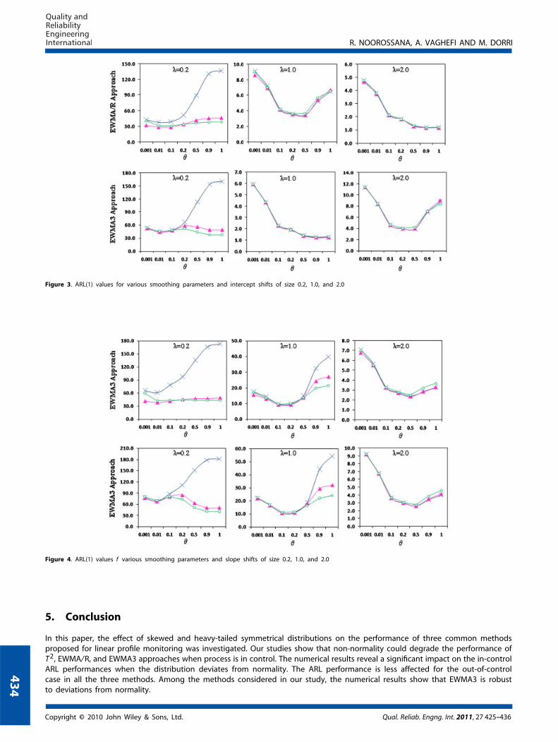
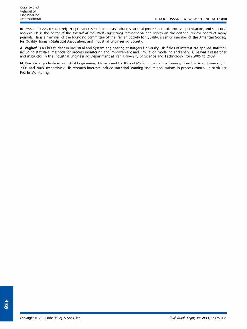
Effect of smoothing parameter on the out-of-control performance is also evaluated. Figures 3 and 4 present the ARL(1) valuesfor different values of smoothing parameters and magnitudes of shift in the intercept and slope, respectively.

Figure 3 indicates that for a small value of �, say �=0.2, the impact of non-normality is more obvious particularly for largervalues of smoothing parameter (�>0.2). For example, if there is a shift of size 0.2 in the intercept, then by increasing thesmoothing parameter value from 0.001 to 1, the ARL(1) values for the EWMA/R approach changes from 40.2 to 39.8 for the gammadistribution and from 31.6 to 45.8 for the t-distribution. However, in the normal distribution case, the ARL(1) value changes from42.1 to 137.4. For moderate and large shifts in the intercept, the impact of non-normality is insignificant and can be ignored. Forexample, if there is a shift of size 1 in the intercept, the ARL(1) for the EWMA/R approach and value of �=0.001, 0.01, 0.1, 0.2,0.5, 0.9, and 1 are 8.6, 6.9, 4.1, 3.5, 3.4, 5.4, and 6.7 for t-distribution and 9.0, 7.0, 4.2, 3.6, 3.7, 5.7, and 6.5 for gamma distribution.In this situation, the ARL(1) values for normal distribution are 9.1, 7.2, 4.2, 3.6, 3.5, 5.2, and 6.45. It is obvious that non-normalitydoes not seriously affect the out-of-control performance.

Similar results could be obtained when there is a shift of size � in the slope. Based on these figures, one can recommend avalue of � between 0.1and 0.2 to improve the out-of-control performance of the approach regardless of the � value.

Although, the out-of-control performances of different linear profile monitoring methods are relatively robust, based on theanalyses provided in Section 4, the performance of the EWMA3 approach can be less affected when the error terms are non-normalrandom variables. As mentioned before, the R control chart proposed for monitoring process variability is mainly responsiblefor the poor in-control performance of the EWMA/R method. In EWMA3 approach, the EWMA control chart based on the meansquare error is insensitive to deviation from normality. As a result, violation of the normality assumption does not significantlydegrade its in-control and out-of-control performances when the value of smoothing parameter is small or moderate. Therefore,when error term distributions are different from normality in the third or higher moments, the EWMA3 approach is recommendedfor monitoring linear profiles.

Copyright © 2010 John Wiley & Sons, Ltd. Qual. Reliab. Engng. Int. 2011, 27 425--436

43

3

R. NOOROSSANA, A. VAGHEFI AND M. DORRI

Figure 3. ARL(1) values for various smoothing parameters and intercept shifts of size 0.2, 1.0, and 2.0

Figure 4. ARL(1) values f various smoothing parameters and slope shifts of size 0.2, 1.0, and 2.0

5. Conclusion

In this paper, the effect of skewed and heavy-tailed symmetrical distributions on the performance of three common methodsproposed for linear profile monitoring was investigated. Our studies show that non-normality could degrade the performance ofT2, EWMA/R, and EWMA3 approaches when process is in control. The numerical results reveal a significant impact on the in-controlARL performances when the distribution deviates from normality. The ARL performance is less affected for the out-of-controlcase in all the three methods. Among the methods considered in our study, the numerical results show that EWMA3 is robustto deviations from normality.

43

4

Copyright © 2010 John Wiley & Sons, Ltd. Qual. Reliab. Engng. Int. 2011, 27 425--436

R. NOOROSSANA, A. VAGHEFI AND M. DORRI

References1. Mestek O, Pavlik J, Suchánek M. Multivariate control charts: Control charts for calibration curves. Fresenius’ Journal of Analytical Chemistry

1994; 350:344--351.2. Stover FS, Brill RV. Statistical quality control applied to ion chromatography calibrations. Journal of Chromatography A 1998; 804:37--43.3. Lawless JF, MacKay RJ, Robinson JA. Analysis of variation transmission in manufacturing processes—Part I. Journal of Quality Technology

1999; 31:131--142.4. Kang L, Albin SL. On-line monitoring when the process yields a linear profile. Journal of Quality Technology 2000; 32:418--426.5. Mahmoud MA, Woodall WH. Phase I analysis of linear profiles with calibration applications. Technometrics 2004; 46:380--391.6. Wang K, Tsung F. Using profile monitoring techniques for a data-rich environment with huge sample size. Quality and Reliability Engineering

International 2005; 21:677--688.7. Gupta S, Montgomery DC, Woodall WH. Performance evaluation of two methods for online monitoring of linear calibration profiles.

International Journal of Production Research 2006; 44:1927--1942.8. Jensen WA, Birch JB. Profile monitoring via nonlinear mixed model. Journal of Quality Technology 2009; 41:18--34.9. Noorossana R, Amiri A, Soleimani P. On the monitoring of autocorrelated linear profiles. Communications in Statistics—Theory and Methods

2008; 37:425--442.10. Kim K, Mahmoud MA, Woodall WH. On the monitoring of linear profiles. Journal of Quality Technology 2003; 35:317--328.11. Noorossana R, Amiri A, Vaghefi A, Roghanian E. Monitoring quality characteristics using linear profile. Proceedings of the Third Conference

International Industrial Engineering, Tehran, Iran, 2004.12. Zou C, Zhang Y, Wang Z. Control chart based on change-point model for monitoring linear profiles. IIE Transactions 2006; 38:1093--1103.13. Mahmoud MA, Parker PA, Woodall WH, Hawkins DM. A change point method for linear profile data. Quality and Reliability Engineering

International 2007; 23:247--268.14. Zou C, Tsung F, Wang Z. Monitoring general linear profiles using multivariate exponentially weighted moving average schemes. Technometrics

2007; 49:395--408.15. Zou C, Zhou C, Wang Z, Tsung F. A self-starting control chart for linear profiles. Journal of Quality Technology 2007; 39:364--375.16. Zhang J, Li Z, Wang Z. Control chart based on likelihood ratio for monitoring linear profiles. Computational Statistics and Data Analysis 2009;

53:1440--1448.17. Saghaei A, Mehrjoo M, Amiri A. A CUSUM-based method for monitoring simple linear profile. The International Journal of Advanced

Manufacturing Technology 2009; DOI: 10.1007/s00170-009-2063-2.18. Zhu J, Lin DKJ. Monitoring the slopes of linear profiles. Quality Engineering 2010; 22:1--12.19. Kazemzadeh RB, Noorossana R, Amiri A. Phase I monitoring of polynomial profiles. Communications in Statistics—Theory and Methods 2008;

37:1671--1686.20. Croarkin C, Varner R. Measurement assurance for dimensional measurements on integrated-circuit photomasks. NBS Technical Note 1164, U.S.

Department of Commerce, Washington, DC, U.S.A., 1982.21. Jensen WA, Birch JB, Woodall WH. Monitoring correlation within linear profiles using mixed models. Journal of Quality Technology 2008;

40:167--183.22. Saghaei A, Amiri A, Mehrjoo M. Performance evaluation of control schemes under drift in simple linear profiles. Proceedings of the International

Conference of Manufacturing Engineering and Engineering Management, London, England, 2009.23. Jin J, Shi J. Feature-preserving data compression of stamping tonnage information using wavelets. Technometrics 1999; 41:327--339.24. Walker E, Wright S. Comparing curves using additive models. Journal of Quality Technology 2002; 34:118--129.25. Ding Y, Zeng L, Zhou S. Phase I analysis for monitoring nonlinear profiles in manufacturing processes. Journal of Quality Technology 2006;

38:199--216.26. Moguerza JM, Muñoz A, Psarakis S. Monitoring nonlinear profiles using support vector machines. Lecture Notes in Computer Science 2007;

4789:574--583.27. Williams JD, Woodall WH, Birch JB. Statistical monitoring of nonlinear product and process quality profiles. Quality and Reliability Engineering

International 2007; 23:925--941.28. Vaghefi A, Tajbakhsh SD, Noorossana R. Phase II monitoring of nonlinear profiles. Communications in Statistics: Theory and Methods 2009;

18:1834--1851.29. Williams JD, Birch JB, Woodall WH, Ferry NM. Statistical monitoring of heteroscedastic dose-response profiles from high-throughput screening.

Journal of Agricultural, Biological and Environmental Statistics 2007; 12:216--235.30. Kazemzadeh RB, Noorossana R, Amiri A. Phase II monitoring of autocorrelated polynomial profiles in AR(1) processes. Scientia Iranica,

Transaction E: Industrial Engineering 2010; 17:12--24.31. Soleimani P, Noorossana R, Amiri A. Simple linear profiles monitoring in the presence of within profile autocorrelation. Computers and

Industrial Engineering 2009; 57:1015--1021.32. Schilling EG, Nelson PR. The effect of non-normality on the control limits of x charts. Journal of Quality Technology 1976; 8:183--188.33. Yourstone SA, Zimmer WJ. Non-normality and the design of control charts for averages. Decision Science Journal 1992; 23:1099--1113.34. Amin RW, Reynolds MR, Bakir ST. Nonparametric quality control charts based on the sign statistic. Communications in Statistics—Theory and

Methods 1995; 24:1597--1623.35. DeVor RE, Chang T, Sutherland JW. Statistical Quality Design and Control Contemporary Concepts and Methods. Prentice-Hall, Inc., Simon and

Schuster: NJ, U.S.A., 1992.36. Borror CM, Montgomery DC, Runger GC. Robustness of the EWMA control chart to non-normality. Journal of Quality Technology 1999;

31:309--316.37. Stoumbos ZG, Reynolds MR. Robustness to non-normality and autocorrelation of individuals control charts. Journal of Statistical Computation

and Simulation 2000; 66:145--187.38. Stoumbos ZG, Sullivan JH. Robustness to non-normality of the multivariate EWMA control chart. Journal of Quality Technology 2002;

34:260--276.39. Noorossana R, Vaghefi SA, Amiri A. The effect of non-normality on monitoring linear profiles. Proceedings of the Second International Industrial

Engineering Conference, Riyadh, Saudi Arabia, 2004.40. Myers RH. Classical and Modern Regression with Applications (2nd edn). PWS-Kent Publishing Company: Boston, MA, 1990; 11--15.41. Crowder SV, Hamilton MD. An EWMA for monitoring a process standard deviation. Journal of Quality Technology 1992; 24:12--21.42. Peña D, Prieto FJ. Multivariate outlier detection and robust covariance matrix estimation. Technometrics 2001; 43:286--310.

Authors’ biographies

R. Noorossana is Professor of Statistics at Iran University of Science and Technology. He received his BS in Engineering fromLouisiana State University in 1983 and his MS and PhD in Engineering Management and Statistics from the University of Louisiana

Copyright © 2010 John Wiley & Sons, Ltd. Qual. Reliab. Engng. Int. 2011, 27 425--436

43

5

R. NOOROSSANA, A. VAGHEFI AND M. DORRI

in 1986 and 1990, respectively. His primary research interests include statistical process control, process optimization, and statisticalanalysis. He is the editor of the Journal of Industrial Engineering International and serves on the editorial review board of manyjournals. He is a member of the founding committee of the Iranian Society for Quality, a senior member of the American Societyfor Quality, Iranian Statistical Association, and Industrial Engineering Society.

A. Vaghefi is a PhD student in industrial and System engineering at Rutgers University. His fields of interest are applied statistics,including statistical methods for process monitoring and improvement and simulation modeling and analysis. He was a researcherand instructor in the Industrial Engineering Department at Iran University of Science and Technology from 2005 to 2009.

M. Dorri is a graduate in Industrial Engineering. He received his BS and MS in Industrial Engineering from the Azad University in2006 and 2008, respectively. His research interests include statistical learning and its applications in process control, in particularProfile Monitoring.

43

6

Copyright © 2010 John Wiley & Sons, Ltd. Qual. Reliab. Engng. Int. 2011, 27 425--436