Asteroseismology with the WIRE satellite. I. Combining Ground and Space-based Photometry of the...

arX

iv:a

stro

-ph/

0610

539v

1 1

8 O

ct 2

006

Astronomy & Astrophysicsmanuscript no. bruntt˙AA5766 c© ESO 2008February 5, 2008

Asteroseismology with the satellite

I. Combining Ground- and Space-based Photometry of the δ Scuti Starǫ Cephei

H. Bruntt1,2, J.C. Suarez3,4 ⋆, T.R. Bedding2, D.L. Buzasi5, A. Moya4, P.J. Amado6,3, S. Martın-Ruiz3, R. Garrido3,P. Lopez de Coca3, A. Rolland3, V. Costa3, I. Olivares3, and J.M. Garcıa-Pelayo3

1 Niels Bohr Institute, Juliane Maries Vej 30, University of Copenhagen, Denmark e-mail:[email protected] School of Physics A28, University of Sydney, 2006 NSW, Australia e-mail:[email protected] Instituto de Astrofısica de Andalucıa, CSIC, CP3004, Granada, Spain e-mail:[email protected] Observatoire de Paris, LESIA, UMR 8109, Meudon, France e-mail: [email protected] US Air Force Academy, Department of Physics, CO, USA, e-mail: [email protected] Universidad de Granada, Departamento Fısica Teorica y del Cosmos, Campus Fuentenueva, Granada, Spain

Received xxx; accepted yyy

ABSTRACT

Aims. We have analysed ground-based multi-colour Stromgren photometry and single-filter photometry from the star tracker on thesatellite of theδ Scuti starǫ Cephei.Methods. The ground-based data set consists of 16 nights of data collected over 164 days, while the satellite data are nearly continuous coverageof the star during 14 days. The spectral window and noise level of the satellite data are superior to the ground-based dataand this data set isused to locate the frequencies. However, we can use the ground-based data to improve the accuracy of the frequencies due to the much longertime baseline.Results. We detect 26 oscillation frequencies in the data set, but only some of these can be seen clearly in the ground-based data. We haveused the multi-colour ground-based photometry to determine amplitude and phase differences in the Stromgrenb− y colour and they filter inan attempt to identify the radial degree of the oscillation frequencies. We conclude that the accuracies of the amplitudes and phases are notsufficient to constrain theoretical models ofǫ Cep. We find no evidence for rotational splitting or the largeseparation among the frequenciesdetected in the data set.Conclusions. To be able to identify oscillation frequencies inδ Scuti stars with the method we have applied, it is crucial to obtain morecomplete coverage from multi-site campaigns with a long time baseline and in multiple filters. This is important when planning photometricand spectroscopic ground-based support for future satellite missions like and.

Key words. Stars: oscillations; Stars: variable:δ Sct; Stars: individual:ǫ Cephei (HD 211336; HR 8494)

1. Introduction

δ Scuti stars are main sequence population I A- and F-typestars. They are found in the classical Cepheid instability stripon the main sequence, have masses around twice solar, andtemperatures around 7 500 K. They have only very shallowouter convection zones but their cores are fully convective.Most stars found in the instability strip are variable and mostare multi-periodic, with periods around 1–2 hours and ampli-tudes typically at the mmag level, although some have ampli-tudes above 0.1 mag (Rodrıguez et al., 2000).

To get a better understanding ofδ Scuti stars, several multi-site ground-based campaigns have carried out extensive moni-

Send offprint requests to: H. Bruntt⋆ Associate researcher at l’Observatoire de Paris.

toring of selected targets. For example, the Delta Scuti Network(Zima, 1997; Zima et al., 2002) has monitored FG Virginisduring several seasons and 79 frequencies have been detected(Breger et al., 2005). In that case, data from several ground-based observatories collected over 13 years were combined,which allowed the detection of frequencies down to amplitudesof just 0.2 mmag in Stromgreny. It is important to note thatabout 50 of the reported frequencies have amplitudes below 0.5mmag. Breger et al. (2005) stated that typical multi-site cam-paigns with a duration of 200 to 300 h detect only 5–10 fre-quencies. Since so few frequencies are detected, while theorypredicts a much higher number of excited modes, Breger et al.(2005) concluded that either longer ground-based photometriccampaigns or high-precision space-based campaigns are neces-sary.

http://arXiv.org/abs/astro-ph/0610539v1

2 H. Bruntt et al.: Asteroseismology with the satellite

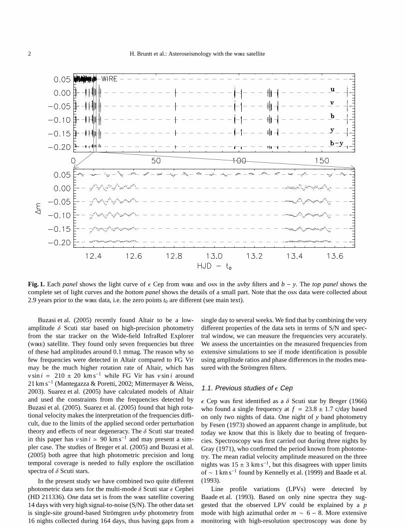
Fig. 1. Eachpanelshows the light curve ofǫ Cep from and in the uvbyfilters andb − y. The top panelshows thecomplete set of light curves and thebottom panelshows the details of a small part. Note that the data were collected about2.9 years prior to the data, i.e. the zero pointst0 are different (see main text).

Buzasi et al. (2005) recently found Altair to be a low-amplitudeδ Scuti star based on high-precision photometryfrom the star tracker on the Wide-field InfraRed Explorer() satellite. They found only seven frequencies but threeof these had amplitudes around 0.1 mmag. The reason why sofew frequencies were detected in Altair compared to FG Virmay be the much higher rotation rate of Altair, which hasvsini = 210 ± 20 km s−1 while FG Vir hasvsini around21 km s−1 (Mantegazza & Poretti, 2002; Mittermayer & Weiss,2003). Suarez et al. (2005) have calculated models of Altairand used the constraints from the frequencies detected byBuzasi et al. (2005). Suarez et al. (2005) found that high rota-tional velocity makes the interpretation of the frequencies diffi-cult, due to the limits of the applied second order perturbationtheory and effects of near degeneracy. Theδ Scuti star treatedin this paper hasvsini ≃ 90 km s−1 and may present a sim-pler case. The studies of Breger et al. (2005) and Buzasi et al.(2005) both agree that high photometric precision and longtemporal coverage is needed to fully explore the oscillationspectra ofδ Scuti stars.

In the present study we have combined two quite differentphotometric data sets for the multi-modeδ Scuti starǫ Cephei(HD 211336). One data set is from the satellite covering14 days with very high signal-to-noise (S/N). The other data setis single-site ground-based Stromgrenuvbyphotometry from16 nights collected during 164 days, thus having gaps from a

single day to several weeks. We find that by combining the verydifferent properties of the data sets in terms of S/N and spec-tral window, we can measure the frequencies very accurately.We assess the uncertainties on the measured frequencies fromextensive simulations to see if mode identification is possibleusing amplitude ratios and phase differences in the modes mea-sured with the Stromgren filters.

1.1. Previous studies of ǫ Cep

ǫ Cep was first identified as aδ Scuti star by Breger (1966)who found a single frequency atf = 23.8 ± 1.7 c/day basedon only two nights of data. One night ofy band photometryby Fesen (1973) showed an apparent change in amplitude, buttoday we know that this is likely due to beating of frequen-cies. Spectroscopy was first carried out during three nightsbyGray (1971), who confirmed the period known from photome-try. The mean radial velocity amplitude measured on the threenights was 15± 3 km s−1, but this disagrees with upper limitsof ∼ 1 km s−1 found by Kennelly et al. (1999) and Baade et al.(1993).

Line profile variations (LPVs) were detected byBaade et al. (1993). Based on only nine spectra they sug-gested that the observed LPV could be explained by apmode with high azimuthal orderm ∼ 6 − 8. More extensivemonitoring with high-resolution spectroscopy was done by

H. Bruntt et al.: Asteroseismology with the satellite 3

Kennelly et al. (1999). They monitoredǫ Cep in a multi-sitecampaign during eight nights. They detected a rich set offrequencies in the range 17–40 c/day with radial degreesl = 5 − 15 using two-dimensional Fourier analysis, but theirresults were preliminary.

Costa et al. (2003) monitoredǫ Cep with Stromgren filtersbut they concluded that the rich amplitude spectrum could notbe adequately resolved based on their single-site data set.Wewill use this data set in the present study.

2. Observations

2.1. Observations from the ground

ǫ Cephei (HD 211336) was monitored with simultaneousuvbymeasurements from Observatorio de Sierra Nevada () in2001–2 on 16 nights during a period of 164 days (Costa et al.,2003). Eight nights of data were collected from 2001 August9–25. There is data from October 8 and two nights on 2001November 13 and 17. Four nights were obtained from 2001December 3 to 9. Finally, data from a single night was obtainedon 2002 January 20.

In total ǫ Cep was observed for 16 nights from withtypically 6–8 hours of observations each night. A total of 2250data points were collected. After removal of the oscillationsthermsnoise is 3.3 mmag inu and 1.8 mmag inv, b andy. Thecomplete light curve is shown in thetop panelin Fig. 1 whiledetails of the stellar oscillations are seen in thebottom panel.The zero point in time ist0 = 2 452 130.

2.2. Observations from space

The Wide-field InfraRed Explorer () satellite missionwas designed to study star-burst galaxies in the infrared(Hacking et al., 1999). Unfortunately, the hydrogen which wasto be used for cooling the main camera was lost soon afterlaunch. Since 1999 the 52 mm star tracker on has beenused to monitor bright stars continuously for one to six weeks(see Bruntt & Buzasi, 2006).ǫ Cep was observed with from 2004 June 20 to July

4. The raw data set consists of around 600 000 8x8 pixel CCDwindows centered on the star with a time-sampling of 0.5 s.The data were reduced as described by Bruntt et al. (2005) andpoints taken within 15 s were binned. The resulting light curvehas 25 293 data points collected during 13.6 days with threeshort gaps with durations of 0.2, 0.2, and 0.5 days. The com-plete light curve is shown in Fig. 1 where the zero point intime ist0 = 2 453 175.5. Note that the observations startedabout 2.9 years after the run.

The rms noise level in the data set after removal ofthe oscillations is 1.7 mmag. To estimate the white noise com-ponent we calculated the noise in the amplitude spectrum athigh frequencies (10± 0.5 mHz; the Nyquist frequency is 33.3mHz). From this we found the noise level to be 12.3 ppm or1.2 mmag per 15 s bin. Each observation collects aboutestar = 105 electrons, and after binning every 30 data points(15 s sampling), the theoretical Poissonian noise is 0.6 mmagor more than a factor two lower than the actual observed noise

Table 1. Basic photometric indices forǫ Cephei.

V B− V b− y m1 c1 Hβ4.19 0.28 0.171(2) 0.192(4) 0.784(4) 2.761

level. The higher noise level is due to the relatively high skylevel during theǫ Cep run. We estimate the noise contribu-tion from the background to beσ2

AP = npix ∗ (esky + σ2ro)/e2

starfollowing eq. 31 in Kjeldsen & Frandsen (1992); herenpix isthe number of pixels in the aperture,σro is the readout noise,while estar andesky are the number of electrons from the starand sky background, respectively. We usenpix = 12, a gainof 15 e−1/ADU, esky = 420± 220 ADU, and aσro = 10e−1

to obtainσAP = 2.7 ± 0.7 mmag which is comparable to thePoissionian noiseσcount= 1/

√estar= 3.2 mmag. This explains

the relatively high noise level.

3. Fundamental parameters of ǫ Cep

The basic photometric indices forǫ Cep are summarized inTable 1. TheV magnitude andB − V colour are based on 12measurements and are taken from Mermilliod’s compilation ofEggen’sUBV data (available through). The Stromgrenindices are from Hauck & Mermilliod (1998) and are basedon a combination of 60 measurements, while Hβ is based on47 measurements. The projected rotational velocity (vsini)of ǫ Cep is 105 km s−1 according to 10 measurements fromBernacca & Perniotto (1970), while Royer et al. (2002) found91 km s−1. The typical uncertainty onvsini is 5% (Royer et al.,2002), i.e.σ(vsini)= 5 km s−1.

We used (Rogers, 1995) to determine the funda-mental atmospheric parameters ofǫ Cep and the results areTeff= 7340± 50 , logg= 3.9 ± 0.1, [Fe/H]= 0.12 ± 0.04.This is consistent with the spectral type F0 IV. We stress thatthe quoted uncertainties are based solely on the uncertainty onthe photometric indices. Realistic uncertainties onTeff, logg,and [Fe/H] are 150 K, 0.2 dex, and 0.2 dex (Rogers, 1995;Kupka & Bruntt, 2001). Based on the Stromgrenb− y and Hβindices there is no significant interstellar reddening.

Erspamer & North (2002, 2003) used an automated proce-dure to determine individual abundances of 140 A– and F–type stars andǫ Cep was included in their data set. They usedGeneva photometry to fixTeff = 7244± 150 K and the- parallax and evolution models to find logg = 4.02± 0.2,which both agree with our Stromgren photometry when us-ing . The abundance analysis ofǫ Cep yielded [Fe/H]= +0.08± 0.10, which is also in good agreement with-. The error estimate on [Fe/H] given here is based on thevarious contributions to the error budget, as discussed in detailby Erspamer & North (2002).

The location ofǫ Cep in the Hertzsprung-Russell (HR) di-agram is shown in Fig. 2. We show evolutionary tracks fromLejeune & Schaerer (2001) for solar metallicity (Z = 0.02).The dashed track is for a metallicity of twice the solar valuefora massM/M⊙ = 2.0. To estimate the luminosity, we used thevisual magnitudeV = 4.19±0.03 and the parallax of38.9± 0.5 mas (ESA, 1997). We found the bolometric correc-


Fig. 2. HR diagram with evolution tracks fromLejeune & Schaerer (2001) forZ = 0.02 (solar) andZ = 0.04.The 1σ error box forǫ Cep is indicated and is consistent witha slightly evolved star with massM/M⊙ = 1.75± 0.20 for ametallicity of [Fe/H] = 0.1.

tion (BC) by interpolation in the tables by Bessell et al. (1998),i.e. BC= 0.04± 0.02. For the solar bolometric magnitude weused 4.75± 0.04. Thus, we findL/L⊙ = 10.7± 0.6 and adoptTeff = 7340± 150 K. The 1σ error box is indicated in Fig. 2.

From the location ofǫ Cep in the HR diagram relative tothe evolutionary tracks from Lejeune & Schaerer (2001), andadopting a metallicity [Fe/H] = 0.1± 0.1, we estimate the massto beM/M⊙ = 1.75± 0.20.

From the estimated mass, temperature, and parallax wecan calculate the surface gravity using loggπ = 4[Teff] +[M] + 2 logπ + 0.4(V + BCV + 0.26)+ 4.44, where [Teff] =log(Teff/Teff ⊙) and [M] = log(M/M⊙). For ǫ Cep we findloggπ = 4.0±0.1 which agrees with Erspamer & North (2003)and the photometric calibration from.

4. Time Series Analysis

4.1. Spectral windows

To illustrate the difference between the and data setsin the frequency domain we have calculated the spectral win-dows. To do this we used the same observation times as inthe real data sets and inserted an artificial sinusoidal signal atf = 20 c/day. The resulting spectral windows for the and data sets are shown in Fig. 3 in thetop andbottom panels,respectively.

The complexity of the spectral window is apparent,with several alias peaks at 1.0, 0.5, and 0.01 c/d. The latteris seen in the inset in Fig. 3 and arises from the large gaps inthe time series, i.e.f ≃ 1/Tobs≃ 0.01 c/day, since the totalobserving time isTobs= 122 days. Note that we decided not touse the last night from in the analysis since it degrades thespectral window. The reason is the long gap of 42 nights fromnight 15 to night 16.

Fig. 3. Spectral windows for the (top panel) and data sets (bottom panel) computed for a single frequency atf = 20 c/day. The insets show the details of the main peak.

As a result of the long gaps in the time series, the peaksin the amplitude spectrum atf ± n × 1/Tobs – wheren is aninteger – are almost equally good solutions. However, if onecan be sure about selecting the “right peak,” the accuracy ofthefrequency is significantly better than in the data set. Thismay prove difficult since in the real data set the spectrum isaffected by closely spaced frequencies and noise sources suchas photon shot noise and non-white instrumental drift noise.

The spectral window has a much more well-definedpeak. During each orbit the satellite switches between twotargets in order to minimize the effect of scattered light fromthe illuminated face of the Earth. Thus,ǫ Cep was observedwith a duty cycle of≃ 40% (cf. bottom panelin Fig. 1). Asa consequence, significant alias peaks are seen at frequenciesthat are combinations of the frequency of the oscillation signaland the orbital frequency of, fi = | f ± n fW|, where f isthe genuine frequency,n is an integer, andfW is the orbitalfrequency: fW = 15.348± 0.001 c/day. The first set of sidelobes have amplitudes relative to the main peak of 76%.

4.2. Observed amplitude spectra

The observed amplitude spectra are shown in Fig. 4. In the twotop panelswe have used the data set: the firstpanel isan overview and the secondpanelshows the details of the re-gion 12–28 c/day where the oscillations intrinsic to the star arefound. In the twobottom panelswe used 15 nights from inthey filter andb− y colour, respectively. The different proper-ties of the time series are reflected in the amplitude spectra.

There are many frequencies present inǫ Cep and their loca-tion can be identified in the spectrum. The periods rangefrom 0.7–1.9 hours and the amplitudes of highest peaks are inthe range 1–3 ppt1, which is typical for low amplitudeδ Scutistars. The amplitude spectra are more complicated to in-terpret, with two main regions of excess power around 12–17and 24–28 c/day. This makes the extraction of closely spaced

1 We note that 1 ppt≃ 1.086 mmag


frequencies difficult and is a well-known problem for single-site observations ofδ Scuti stars (Costa et al., 2003). For ex-ample, as a result of the combination of the frequenciesf2 tof4, the highest peak in the amplitude spectra is found at≃ 14 c/day. Also, above 20 c/day the highest peak in they amplitude spectrum is found around 25.2 c/day due to thecombinations off1 and the close pair of frequenciesf5 and f9.

In the following Section we describe how we have extractedthe individual frequencies from the light curves.

5. Analysis of the ǫ Cep light curves

5.1. Using the superior spectral window

Since the spectral window of the data set is less compli-cated than for the data, we used the data to detectthe significant frequencies. Also, the S/N level is much higherin the data: in the cleaned amplitude spectrum the noiselevel is about 85 and 460 ppm in the range 10–30 c/day for the andy data, respectively. In the v filter the noiselevel is 645 ppm but the amplitudes are about 50% higher thanin y. The data set is useful for avoiding the 1 c/day aliasingproblem that hamper our single-site ground-based data set andwe can also detect additional frequencies with low amplitude.

We used the software package04 by Lenz & Breger(2005) for the extraction of the frequencies. After the extrac-tion of the first frequency, the detection of additional frequen-cies is based on prewhitening or “cleaning” of the already de-tected frequencies. However, the solution is improved by aleast-squares fit to the observations by a function of the formΣN

i=1Ai sin(2π[ fi t+φi] ), thus each of theN terms is determinedby frequency (fi), phase (φi) and amplitude (Ai). We note thatthe data set is very homogeneous and we therefore did notapply point weights.

The satellite observedǫ Cep during 40% of its orbit,but the last part of each orbit is affected by scattered light whichsystematically offsets the measured flux. To minimize the effectof this we only used the part of the light curve which was unaf-fected by scattered light, i.e. this data set had a 30% duty cycle.From this data set we extracted 25 frequencies with S/N above4. After subtracting these terms from the light curve we per-formed a decorrelation of the light curve with the backgroundlevel and orbital phase. This allowed us to use the completedata set and increase the duty cycle from 30% to 40%. Thisgreatly improves the spectral window and the first set of sidelobes decrease from 88% to 76% while the second set of sidelobes decrease from 58% to 25% (cf.top panelin Fig. 3).

Using the data set with 40% duty cycle we extracted26 frequencies. The frequencies are marked in Fig. 4 and inTable 2 we list the frequency, amplitude, and phase of each fre-quency. Phases in Table 2 are given relative to the zero pointin time, t0 = 2 453 175.5. In the last column we give the S/Nwhich is the ratio of the amplitude and the noise level estimatedin the cleaned amplitude spectrum. We will estimate the uncer-tainties on the frequency, phase, and amplitude based on sim-ulations in Sect. 6.3. The first 24 frequencies in Table 2 haveS/N above 6, and are numbered according to their S/N. Theremaining two frequencies are less certain are labeleda andb.

Table 2. Frequencies, amplitudes, phases, and S/N for 26 indi-vidual frequencies extracted from the data set.

ID fi [c/day] ai [ppt] φi S/Nf1 27.053 3.12 0.994 41.2f2 12.734 2.13 0.329 27.6f3 14.976 1.80 0.524 23.4f4 13.568 1.36 0.617 17.7f5 25.262 1.25 0.096 16.1f6 17.674 1.18 0.238 15.4f7 19.689 1.13 0.858 14.6f8 21.041 1.03 0.068 13.3f9 25.409 0.99 0.541 12.8

f10 19.842 0.95 0.756 12.3f11 15.157 0.90 0.939 11.8f12 27.298 0.86 0.618 11.3f13 14.050 0.86 0.573 11.2f14 20.980 0.84 0.771 10.9f15 20.255 0.70 0.781 9.1f16 22.415 0.64 0.711 8.1f17 15.392 0.55 0.489 7.2f18 27.416 0.52 0.872 6.9f19 25.663 0.53 0.013 6.8

f2 + f3 = f20 27.702 0.49 0.538 6.5f21 13.118 0.48 0.131 6.3

f10 + f13 = f22 33.957 0.44 0.793 6.3f23 22.277 0.48 0.101 6.1f24 26.119 0.47 0.202 6.1f 1a 13.697 0.39 0.486 5.0fb 24.102 0.35 0.865 4.5

1 Note thatfa = f12 − f4 = f20 − f13 = f22 − f15

We have searched for frequencies that are given as linearcombinations of other terms within the frequency resolution,and for the data set this isδ f = 3/2Tobs = 0.11 c/day(Loumos & Deeming, 1978). The three frequenciesf20, f22,and fa are found to have low amplitude and found near theselinear combinations:f20 = f2 + f3, f22 = f10 + f13, andfa = f12 − f4 = f20 − f13 = f22 − f15. The many combina-tions for fa indicate that it is probably not intrinsic to the star.In addition, we findf9 = 2 · f2 and f18 = 2 · fa, which may bechance alignments.

5.2. Analysis of the light curves

The data set was collected 2.9 years prior to thedata set. While someδ Scuti stars are known to have vari-able amplitudes we expect that the frequencies remain constantover such a short time scale. However, Breger & Pamyatnykh(2006) found that the amplitude variation seen in FG Vir duringseveral observing seasons can be explained by closely spacedfrequencies. With this in mind we searched for frequencies us-ing 04 while using the frequencies extracted fromas a guide. We recovered the frequenciesf1 to f9, but in somecases we had to apply an offset of the apparently highest peakby exactly±1 c/day. We found evidence forf11, f12, and f19 butthese frequencies have low amplitude and the systematic offsetsdue to close neighbours and their aliases become significant.


Fig. 4. The twotop panelsare the amplitude spectra ofǫ Cep based on the data set. The frequencies extracted from andthe orbital frequency atfW = 15.348 c/day (dashed line) have been marked. The peaks below 12 c/day and above 28 c/day arealias peaks due to the orbit of the satellite. The twobottom panelsare the amplitude spectra of the y andb− y data sets.[astro-ph: quality of figure reduced.]

Due to the long gaps in the data sets there are aliasesin the spectral window separated byfobs ≃ 1/Tobs = 0.009c/day. These aliases have almost equal amplitude but we canpick the right peak in the amplitude spectrum using the approx-imate frequency from the data set as we will demonstratein Sec. 6.4. From the simulations in Sec. 6.3 we find the uncer-tainty on the frequencies to be 0.001− 0.003 c/day for thefrequenciesf1 to f6 and up to 0.004 c/day for the frequenciesf7 to f9. This means that the shift from one alias to the next inthe amplitude spectrum is at least at the 3-sigma level forf1 to f6 and about 2-sigma forf7 to f9.

Another method of cleaning the data set is to assumethat all frequencies with S/N above 6 found in can be fit-ted to the data set. In Fig. 5 we compare the frequenciesand amplitudes found in the and y data sets. Thetoppanel in Fig. 5 shows the ratio of amplitudesaWIRE/ay. Thebottom panelshows the difference between the frequencies vs.the amplitude. The individual error bars are found fromsimulations. We find that the uncertainties are very large forthe frequencies with low amplitude, but all frequencies agreewithin the uncertainties. That fact that several frequencies arefound to have amplitudes that are different by more than 50%


Fig. 5. We fitted all 26 frequencies found from the data setto the y data set. Thepanelsshow the ratio of the input andoutput amplitudes (top) and the difference between input andoutput frequencies.

(marked by horizontal dashed lines in thetop panelin Fig. 5)indicates that it is not sensible to fit all these frequenciesto the data, although they are present in the data set. Thefact that we cannot extract all the frequencies found in thedata set will systematically affect the parameters of the frequen-cies we extract from the data sets. We have assessed this bydoing simulations (see Sect. 6.3).

In Table 3 we summarize the frequency, amplitude, andphase off1 to f8, which are clearly identified in the data set.The frequencies are the weighted mean values of the individualfits to uvby. The quoted error is the weighted mean error andis based on simulations done in Sect. 6.3. We give amplitudesin each of the four Stromgren filters and the colour light curveb − y. The phases ofy andb − y are given relative to the zeropoint in time,t0 = 2 452 130.0. Three of the frequencies,f5, f7,and f8 have some closely spaced frequencies seen in the

data set, namelyf9, f10, and f14. It is very likely that the param-eters listed for these frequencies in Table 3 are systematicallyaffected by this. We also note thatf7 ≃ f6 + 2.0 c/day and thiswill also affect the amplitude and phase.

6. Accuracy of the extracted frequencies

6.1. Theoretical estimates

The formal uncertainty on the frequency determined from alight curve is determined by the duration of the observing

Fig. 6. Part of the light curves from (top panel) andy including the fitted light curves in grey colour. The residualsare also shown but offset by−0.02 mag. As in Fig. 1 the zero-pointst0 are different.

run, the number of data points, and S/N ratio, i.e. the ratioof the amplitude to the noise in the light curve. The standardestimate of the uncertainty of the frequency is based on theleast-squares covariance matrix or the Rayleigh resolution cri-terion. However, Schwarzenberg-Czerny (1991) demonstratedthat both estimates are statistically incorrect. On one hand theleast-squares covariance matrix does not account for correla-tion of residuals in the fit. Neglecting this may cause a largeunder-estimation of the uncertainty. On the other hand theRayleigh resolution criterion is insensitive to the S/N and there-fore does not reflect the quality of the observations.

For an ideal light curve with only white noiseMontgomery & O’Donoghue (1999) derived the uncer-tainty on the frequency, amplitude and phase (in radians)as

σ( fi) =

√6π·

1N1/2

·1

Tobs·σ

ai, (1)

σ(ai) =

√

2N· σ and (2)

σ(φi) =

√

2N· σ

ai, (3)

whereσ is the rms uncertainty per data point,ai is the am-plitude,N is the number of data points, andTobs is the obser-vational time baseline. These uncertainties are strictly lowerlimits in the case of uncorrelated white noise. Using simpleassumptions for correlated noise, Montgomery & O’Donoghue(1999) found that the error estimates using the above equationsare too optimistic by up to a factor of five. Following the sug-gestion by Montgomery & O’Donoghue (1999) we calculatedthecorrelation length Dfrom the autocorrelation of the cleanedamplitude spectra (after subtracting the mean) and locatedtheintersection with zero. From the and data sets we find


Fig. 7. Smoothed power density spectrum of the y data setbefore and after cleaning (solid lines). The dashed line is fora simulation after cleaning. The location of the oscillations ismarked by the hatched region.

DWIRE ≃ 10.5, DOSN;y = 9.0, andDOSN;b−y = 10.5, respec-tively, and we multiplied the error estimates from Eq. 1–3 bythe square root of the corresponding correlation length,D.

6.2. Power density spectra

For the simulations done in Sect. 6.3 we have found that it isimportant that the noise sources in the simulations mimic theobserved data as closely as possible and we will investigatethem in detail here.

In Fig. 6 we show part of the light curve ofǫ Cep from yand. The grey curves show the fit to each of the completelight curves. The residuals are also shown, offset by−0.02 mag.It is seen that there are significant systematic trends in theresid-uals which may be due to a combination of unresolved frequen-cies and instrumental drift.

The significance of this is seen more clearly in the fre-quency domain, and in Fig. 7 we show a smoothed versionof the power density (PD) spectra of the y data set beforeand after the cleaning process. The region of excess power dueto the oscillations is indicated by the hatched region (12–35c/day). The PD is seen to increase by about an order of mag-nitude from the theoretical white noise level (> 80 c/day). Theslight increase in noise level above 200 c/day (marked by thearrow) is because the telescope at switched between theǫ Cep and the comparison stars every 2–4 minutes.

A virtue of the PD spectrum is that we can compare thefrequency dependence of the noise in different data sets eventhough the temporal coverage, time sampling, and number ofdata points are quite different. In Fig. 8 we compare the PDspectra of the cleaned y (grey) and spectra (blacksolid line). The curves are similar in shape but there are fun-damental differences. At the high frequency end the noise in y is higher by an order of magnitude and this is becausethe data set has∼ 10 times more data points thanand slightly lower uncertainty on each data point. At low fre-quencies (f < 40 c/day) the PD is still smaller for at allfrequencies which means that there are additional noise sourcespresent in the data set. If the noise were intrinsic to the star

Fig. 8. Smoothed power density spectra of the cleaned and data sets. The dashed line indicates the increase in noisetowards low frequencies.

the PD in and would be identical at low frequencies.However, a large number of frequencies is present inǫ Cep anda perfect cleaning of the data set is not possible. This prob-ably explains the higher PD atf < 40 c/day compared toby a factor of≃ 3.

The increase towards lower frequencies in the data setis likely due to a combination of instrumental drift and a num-ber of undetected frequencies. This possibility was also dis-cussed by Breger et al. (2005) in their analysis of the residualsafter cleaning about 80 frequencies in theδ Scuti star FG Vir.We motioned in Sect. 1.1 that Kennelly et al. (1999) found sev-eral frequencies of high degree based on LPV studies. Thesefrequencies will have negligible amplitude in photometry dueto geometrical cancellation effects, but they may produce partof the increase in the noise that we observe.

6.3. Simulations of the and time series

To confirm the theoretical error estimates in Sect. 6.1 and tobetter understand the different properties of the anddata sets we computed a large set of simulations. Thedata set has long gaps of up to a month and thus the frequencyanalysis is hampered by a complicated spectral window. Theinteraction between frequencies can only be estimated by do-ing a large number of realistic simulations.

To mimic the large increase towards low frequencies dis-cussed in Sect. 6.2, we added a number of frequencies withlow amplitude in a wide frequency range. The simulations ofthe y filter andb− y data set were done by including the 26frequencies detected in but using the frequencies, ampli-tudes, and phases fitted to the observed data. We then added110 frequencies with random (low) amplitudes from 0.0 to0.4 ppt and frequencies in the range 1–35 c/day for they fil-ter. For theb − y light curve we added 350 frequencies withamplitudes 0.0–0.1ppt in the same frequency range. Finally,we added a white noise component withrms of 1.85 and1.60 mmag fory andb − y, respectively. In the simulations ofthe data set we add 75 frequencies with random frequen-cies in the range 10–35c/day, random amplitudes in the range0.0–0.3 ppt, random phases, and a white noise component with


Table 3. Frequencies and amplitudes in the Stromgren filters for frequencies extracted from the data set. The frequencies arethe weighted mean of the fit to each of theuvby light curves. Amplitudes are given for each filter in parts per thousand (ppt).Phases fitted toy andb − y are also given and indicated in units of the period. The threefrequencies labeledcl have a closeneighbouring frequency with similar amplitude and the parameters are likely to be affected by this.

ID fcomb [c/d] aW au av ab ay ab−y φy φb−y

f1 27.0522± 0.0003 3.12 2.76 3.12 2.61 2.13 0.4960.570 0.584f2 12.7357± 0.0002 2.13 4.15 5.15 3.78 3.19 0.7130.046 0.130f3 14.9766± 0.0002 1.80 3.78 4.61 3.79 2.82 1.0850.447 0.470f4 13.5688± 0.0009 1.36 1.80 2.12 1.64 1.17 0.4590.373 0.462f cl5 25.2635± 0.0004 1.25 2.88 3.33 2.72 2.13 0.6540.139 0.159

f6 17.6745± 0.0004 1.18 1.46 2.19 2.11 1.81 0.5140.955 0.705f cl7 19.6904± 0.0004 1.13 1.27 2.00 1.89 1.34 0.6390.315 0.106

f cl8 21.0380± 0.0004 1.03 1.99 1.92 1.43 1.04 0.3870.028 0.889

Fig. 9. Uncertainties on frequency, amplitude, and phase as found from simulations of (black) and (grey) data sets. The results are shown in bothpanelsand the results fory andb−y are shown in theleft andright panels, respectively. Whenfixing the frequencies in the data set the uncertainties on the amplitudes and phases decrease as indicated by arrows. Thesolid lines are the theoretical predictions for the uncertainty from Eqs. 1–3.

rms 1.7 mmag. An example of the cleaned PD spectrum of asimulation of an y time series is shown with a dashed linein the left panelin Fig. 7.

Thesead hocsimulations roughly reproduce the increasein noise towards low frequencies while still no significant fre-quencies are present above the noise. We made 800 simulationsof the y, b−y, and light curves. We extracted frequen-cies from all simulations using an automated cleaning programusing the procedure described in Sect. 5.1. For the data setwe also fitted the light curves when assuming the known fre-quencies and only fitting amplitudes and phases. We found the

uncertainty by calculating thermsscatter in frequency, ampli-tude, and phase extracted from the 800 simulations.

In Fig. 9 we compare the uncertainties on frequency, am-plitude, and phases as found from Eq. 1–3 (solid lines) andthe simulations (points). Theleft panelshows the uncertaintieson the frequency, amplitude, and phase for y and therightpanelis for b− y, while the results for are shown withblack points in bothpanels. The uncertainties of the simula-tions of the data sets are shown when both frequency, am-plitude and phase are fitted (grey× symbols) and the system-atically lower uncertainties when only amplitude and phaseare


Fig. 10. Histogram of frequencies recovered in simulations of the (black) and (grey) data sets forf1 to f12. In thepanelfor f2 two groups of solutions in separated by 1/Tobs= 0.009c/day are marked. It is seen that the data set can be usedto pick the right group, and that within this group the data set has significantly lower uncertainty.

fitted (grey circle symbols). The improvement is indicated bya vertical arrow for each frequency. It can be seen that the fre-quencies are more accurately determined when using the ydata set. This is in agreement with Eq. 1 where the time base-line enters linearly while the number of data points enters asthe square root; for the two data sets we approximately havethe ratiosNWIRE/NOSN ≃ TOSN/TWIRE ≃ 10, while the point-to-point noise,σ, is very similar. For the frequenciesf1 to f8 theerrors on frequency are about 0.001− 0.003 c/day in and0.0005− 0.0010c/day in. We should note that the re-sults rely on the important fact that we can select the right aliaspeak in the data by using theapproximatefrequency foundwith; this is discussed in detail in Sect. 6.4. The uncertain-ties on amplitude and phase are independent of the time base-line and therefore they are more accurately determined fromthe data set sinceNWIRE/NOSN ≃ 10.

6.4. Resolving the ambiguity of alias peaks

Due to long gaps in the data set the spectral window hasaliases of similar amplitude separated by∆ f ≃ 0.009 c/day.If we only had the data set, each frequency found in theobserved data set can be offset by n × 0.009 c/day for anyn = ±1,±2. However, using the frequencies found fromwe may choose the right aliassub-peakin the amplitudespectrum.

The results from our simulations in Fig. 10 illustrate thatthis is indeed possible. Eachpanelshows two histograms ofthe difference between the input frequency and theextractedfrequency forf1 to f12: the grey histogram is for the simulations

of the data and black is used for y. Several ”groups”of frequencies separated by 0.009 c/day are seen for thesimulations while a single but broader peak is seen for the dis-tribution of extracted frequencies.

It can be seen that the uncertainty in the data set issufficiently small that we can select the right peak in thedata set, at least for the dominant frequencies. We note thattheuncertainties in the simulations shown in Fig. 9 are basedon the internalrmsscatter within one ”group” of extracted fre-quencies.

7. Comparison of observations and models

7.1. Amplitude ratios and phase differences

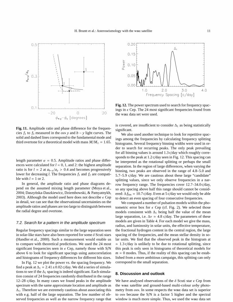
By measuring the parameters of frequencies in different filterswe can infer the spherical degree,l, of the associated spheri-cal harmonic. Each frequency can in principle be identified bymeasuring the phase difference and amplitude ratio in two fil-ters as shown by Garrido et al. (1990) and Moya et al. (2004).In Fig. 11 we show the the amplitude ratio vs. the phase differ-ences in they filter andb− y colour for the three frequenciesf1to f3. The uncertainties are based on the simulations describedin Sect. 6.3. The solid and dashed lines are results for a modelwith massM/M⊙ = 1.65 andTeff = 7720 K. We used an over-shooting parameter ofdov = 0.2 but did not include the effectsof rotation. We note that in Sec. 3 we inferred a slightly coolertemperature, i.e.Teff = 7340±150 and an evolutionary mass ofM/M⊙ = 1.75± 0.20. In the model shown in Fig. 11 the solidline is for Q = 0.033 (fundamental radial mode,n = 1) and thedashed line forQ = 0.017 (third overtone,n = 4) for a mixing


Fig. 11. Amplitude ratio and phase difference for the frequen-cies f1 to f3 measured in the y andb− y light curves. Thesolid and dashed lines correspond to the fundamental mode andthird overtone for a theoretical model with massM/M⊙ = 1.65.

length parameterα = 0.5. Amplitude ratios and phase differ-ences were calculated forl = 0, 1, and 2: the highest amplituderatio is for l = 2 at ab−y/ay > 0.4 and becomes progressivelylower for decreasingl. The frequenciesf1 and f2 are compati-ble with l = 1 or 2.

In general, the amplitude ratio and phase diagrams de-pend on the assumed mixing length parameter (Moya et al.,2004; Daszynska-Daszkiewicz, Dziembowski, & Pamyatnykh,2003). Although the model used here does not describeǫ Cepin detail, we can see that the observational uncertainties on theamplitude ratios and phases are too large to distinguish betweenthe radial degree and overtone.

7.2. Search for a pattern in the amplitude spectrum

Regular frequency spacings similar to the large separationseenin solar-like stars have also been reported for someδ Scuti stars(Handler et al., 2000). Such a measurement would enable usto compare with theoretical predictions. We used the 24 mostsignificant frequencies seen inǫ Cep, namely those with S/Nabove 6 to look for significant spacings using autocorrelationand histograms of frequency differences for different bin sizes.

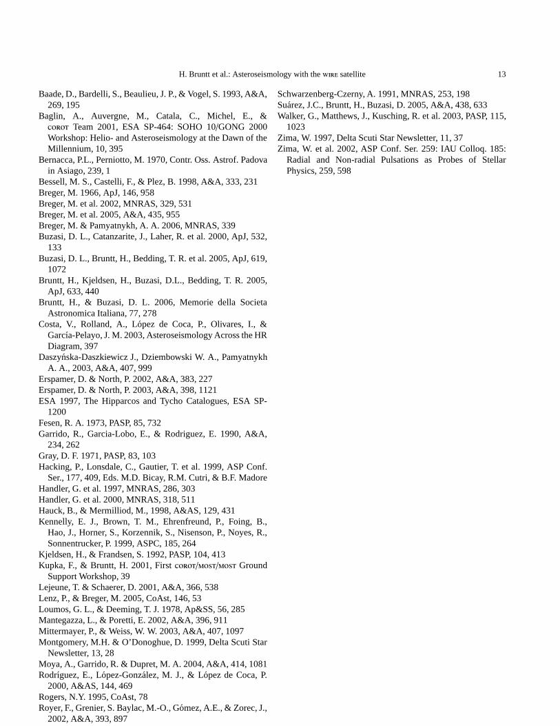
In Fig. 12 we plot the power vs. the spacing frequency. Wefind a peak at∆1 = 2.41±0.02 c/day. We did a series of simula-tions to see if the∆1 spacing is indeed significant. Each simula-tion consist of 24 frequencies randomly distributed in the range12–28 c/day. In many cases we found peaks in the amplitudespectrum with the same approximate location and amplitude as∆1. Therefore we are extremely cautious about associating thiswith e.g. half of the large separation. The low number of ob-served frequencies as well as the narrow frequency range that

Fig. 12. The power spectrum used to search for frequency spac-ings inǫ Cep. The 24 most significant frequencies found fromthe data set were used.

is covered, are insufficient to consider∆1 as being statisticallysignificant.

We also used another technique to look for repetitive spac-ings among the frequencies by calculating frequency splittinghistograms. Several frequency binning widths were used in or-der to search for recurring peaks. The only peak prevailingfor all binning values is around 1.3 c/day which roughly corre-sponds to the peak at 1.2 c/day seen in Fig. 12. This spacing canbe interpreted as the rotational splitting or perhaps the smallseparation. In the region of large differences, when varying thebinning, two peaks are observed in the range of 4.8–5.0 and5.7–5.9 c/day. We are cautious about these large “candidate”splitting values, since we only observe frequencies in a nar-row frequency range. The frequencies cover 12.7–34.0c/day,so any spacing above half this range should cannot be consid-ered:∆ flim = 10.7 c/day. Even at 5 c/day we would only be ableto detect an even spacing of four consecutive frequencies.

We computed a number of pulsation models within the pho-tometric error box forǫ Cep (cf. Fig. 2). We selected thosemodels consistent with∆1 being half the value of the meanlarge separation, i.e.∆ν ≃ 4.8 c/day. The parameters of thesemodels are given in Table 4. For each model we give the mass,radius, and luminosity in solar units, the effective temperature,the fractional hydrogen content in the central region, the largespacing of the frequencies, and the mean stellar density in so-lar units. We find that the observed peak in the histogram at≃ 1.3 c/day is unlikely to be due to rotational splitting, sincethis peak is only seen in histograms of theoretical models form = 0 modes. Thus, if the reality of this spacing can be estab-lished from a more ambitious campaign, this splitting can onlycorrespond to the small separation.

8. Discussion and outlook

We have analysed observations of theδ Scuti starǫ Cep fromthe satellite and ground-based multi-colouruvbyphoto-metry from. In some respects the data set is superiorto because the S/N is a factor 5 higher and the spectralwindow is much more simple. Thus, we used the data set


Table 4. Parameters of selected theoretical models forǫ Cep.The mass, radius, and luminosity are given in solar units,Teff

is the surface temperature,Xc is the central hydrogen fraction,∆ν is the large separation, andρ is the stellar mean density insolar units.

M/M⊙ R/R⊙ L/L⊙ Teff [K] Xc ∆νl=0 [c d−1] ρ/ρ⊙1.55 1.76 6.70 7000 0.48 4.99 0.2831.60 1.77 7.50 7190 0.50 4.94 0.2871.65 1.79 8.46 7370 0.51 4.95 0.2881.70 1.82 9.57 7530 0.51 4.89 0.2811.75 1.83 10.70 7720 0.52 4.90 0.2841.80 1.84 11.89 7910 0.53 4.92 0.288

to extract the location of the oscillation frequencies. Duetothe long gaps in the light curve, the resulting spectral win-dow is complicated. In addition to aliases at 1.0 and 0.5 c/day,there are also “fine structure” sub-peaks with a spacing of 0.009c/day (roughly 1/Tobs). We performed a large set of realisticsimulations to demonstrate that we can select the right sub-peak in the amplitude spectrum, and in turn determine thefrequencies of the dominant frequencies with accuracies ofjust≃ 0.0005c/day. The frequencies found with each of the fourStromgren filters agree and we have computed the weightedmean frequency, thus improving in accuracy to≃ 0.0003 c/dayfor the main frequencies (cf. Tab. 3).

Accurate frequencies are only of interest if they can becompared with theoretical models, and this requires that thedegree of the mode can be determined. This can be done fromthe amplitude ratio and phase difference in different filters. Weused the amplitudes and phases from the y filter andb− ycolour light curve, but our comparison with a theoretical modelclearly indicates that the observed accuracies of phases and am-plitude ratios are insufficient to perform a mode identification.While accurate frequencies can be obtained very effectivelyby extending the time baseline of the observations, accuratephases and amplitudes require higher S/N. The uncertaintieswe estimate from simulations tell us that around 25 000 datapoints with≃ 2 mmag point-to-point uncertainty are required,but we only have 10% of this available from.

In order to use the method of the amplitude ratio vs. phasedifference diagram we need a more complete monitoring ofǫ Cep. This would require a multi-site campaign with moni-toring in two or more filters. This has been done for a num-ber ofδ Scuti stars where extensive multi-site campaigns withlong temporal coverage were carried out. Examples are XX Pyx(Handler et al., 2000) and BI CMi (Breger et al., 2002). Wepropose to use high-resolution time-series spectroscopy tostudy line-profile variations, which will make it possible toidentify the modes. In addition, information on mode splitting(and azimuthal orderm) can be achieved. When this is com-bined with additional photometric observations from ground(or space) we may hope to improve on the present work.

Perhaps the most interesting result from the current studyis that we have detected several significant (S/N=4.5–6.5) fre-quencies with very low amplitude: seven frequencies have am-plitudes below 0.5 ppt. For many years is has been a puzzle

why only some of the frequencies predicted from models ofδ Scuti stars were in fact detected. Breger et al. (2005) discusstheir results for FG Vir and point out that the “missing modes”are indeed there but that the detection level in previous studieswas too poor. About two thirds of the frequencies detected inFG Vir have amplitudes iny below 0.5 ppt. From the dataof ǫ Cep we also find that several frequencies have amplitudesbelow 0.5 ppt (≃ y filter). The reason why we do not find evenmore frequencies with low amplitude is most likely that thefrequency resolution in the data is too low. Even so, our resultsgive support to the suggestion by Breger et al. (2005) that themodes predicted by models ofδ Scuti stars are indeed presentin the stars but one must have long temporal coverage with highphotometric precision to be able to detect them.

The Canadian satellite (Walker et al., 2003) can moni-tor stars for up to 60 days with a duty cycle close to 100% withhigh photometric precision. Preliminary results for aδ Scutistar observed as a secondary target by show about 80 fre-quencies to be present with amplitudes as low as 0.1 mmag(J. M. Matthews, private communication). In the coming yearstwo more dedicated photometry missions will be launched: and. The mission (Baglin et al., 2001) willmonitor several relatively bright stars for up to 150 days toob-tain photometry with very high precision and with a duty cycleclose to 100%. However, observations are done in one filteronly for all the missions mentioned here:, , ,and . Hence, ground-based support observations withmultiple filters and/or spectroscopic measurements are neededin order to be able to identify the modes.

The present analysis ofǫ Cep has shown that much morecomplete and carefully planned ground-based observationsareneeded to avoid problems resulting from a complex spectralwindow. Also, it is necessary to collect enough multi-colourphotometry to be able to measure phases and amplitudes withthe required accuracy to be able to identify the modes. Multi-site campaigns that overlap in time with the space-based obser-vations should be arranged for the future missions. For exam-ple, most primary targets are quite bright (V ≃ 6) and solong-term (i.e. months) monitoring with small 20–80 cm classtelescopes with Stromgren filters and a stable photometer willbe adequate to collect the necessary data. The missions haveseveral secondary targets which are monitored at the same timeas the primary target. Thus it will be a difficult but potentiallyvaluable task to coordinate and collect all the necessary data.

Acknowledgements.HB is supported by the Danish Research Agency(Forskningsrådet for Natur og Univers), the Instrument center forDanish Astrophysics (IDA), and the Australian Research Council. HBis grateful to Torben Arentoft and Gerald Handler for usefuldiscus-sions. JCS acknowledges support from the Instituto de Astrofısica deAndalucıa through an I3P contract financed by the European SocialFund and from the Spanish Plan Nacional del Espacio under projectESP2004-03855-C03-01.

References

Aerts, C., Handler, G., Arentoft, T., Vandenbussche, B.,Medupe, R., & Sterken, C. 2002, MNRAS, 333, L35


Baade, D., Bardelli, S., Beaulieu, J. P., & Vogel, S. 1993, A&A,269, 195

Baglin, A., Auvergne, M., Catala, C., Michel, E., & Team 2001, ESA SP-464: SOHO 10/GONG 2000Workshop: Helio- and Asteroseismology at the Dawn of theMillennium, 10, 395

Bernacca, P.L., Perniotto, M. 1970, Contr. Oss. Astrof. Padovain Asiago, 239, 1

Bessell, M. S., Castelli, F., & Plez, B. 1998, A&A, 333, 231Breger, M. 1966, ApJ, 146, 958Breger, M. et al. 2002, MNRAS, 329, 531Breger, M. et al. 2005, A&A, 435, 955Breger, M. & Pamyatnykh, A. A. 2006, MNRAS, 339Buzasi, D. L., Catanzarite, J., Laher, R. et al. 2000, ApJ, 532,

133Buzasi, D. L., Bruntt, H., Bedding, T. R. et al. 2005, ApJ, 619,

1072Bruntt, H., Kjeldsen, H., Buzasi, D.L., Bedding, T. R. 2005,

ApJ, 633, 440Bruntt, H., & Buzasi, D. L. 2006, Memorie della Societa

Astronomica Italiana, 77, 278Costa, V., Rolland, A., Lopez de Coca, P., Olivares, I., &

Garcıa-Pelayo, J. M. 2003, Asteroseismology Across the HRDiagram, 397

Daszynska-Daszkiewicz J., Dziembowski W. A., PamyatnykhA. A., 2003, A&A, 407, 999

Erspamer, D. & North, P. 2002, A&A, 383, 227Erspamer, D. & North, P. 2003, A&A, 398, 1121ESA 1997, The Hipparcos and Tycho Catalogues, ESA SP-

1200Fesen, R. A. 1973, PASP, 85, 732Garrido, R., Garcia-Lobo, E., & Rodriguez, E. 1990, A&A,

234, 262Gray, D. F. 1971, PASP, 83, 103Hacking, P., Lonsdale, C., Gautier, T. et al. 1999, ASP Conf.

Ser., 177, 409, Eds. M.D. Bicay, R.M. Cutri, & B.F. MadoreHandler, G. et al. 1997, MNRAS, 286, 303Handler, G. et al. 2000, MNRAS, 318, 511Hauck, B., & Mermilliod, M., 1998, A&AS, 129, 431Kennelly, E. J., Brown, T. M., Ehrenfreund, P., Foing, B.,

Hao, J., Horner, S., Korzennik, S., Nisenson, P., Noyes, R.,Sonnentrucker, P. 1999, ASPC, 185, 264

Kjeldsen, H., & Frandsen, S. 1992, PASP, 104, 413Kupka, F., & Bruntt, H. 2001, First// Ground

Support Workshop, 39Lejeune, T. & Schaerer, D. 2001, A&A, 366, 538Lenz, P., & Breger, M. 2005, CoAst, 146, 53Loumos, G. L., & Deeming, T. J. 1978, Ap&SS, 56, 285Mantegazza, L., & Poretti, E. 2002, A&A, 396, 911Mittermayer, P., & Weiss, W. W. 2003, A&A, 407, 1097Montgomery, M.H. & O’Donoghue, D. 1999, Delta Scuti Star

Newsletter, 13, 28Moya, A., Garrido, R. & Dupret, M. A. 2004, A&A, 414, 1081Rodrıguez, E., Lopez-Gonzalez, M. J., & Lopez de Coca, P.

2000, A&AS, 144, 469Rogers, N.Y. 1995, CoAst, 78Royer, F., Grenier, S. Baylac, M.-O., Gomez, A.E., & Zorec,J.,

2002, A&A, 393, 897

Schwarzenberg-Czerny, A. 1991, MNRAS, 253, 198Suarez, J.C., Bruntt, H., Buzasi, D. 2005, A&A, 438, 633Walker, G., Matthews, J., Kusching, R. et al. 2003, PASP, 115,

1023Zima, W. 1997, Delta Scuti Star Newsletter, 11, 37Zima, W. et al. 2002, ASP Conf. Ser. 259: IAU Colloq. 185:

Radial and Non-radial Pulsations as Probes of StellarPhysics, 259, 598

Asteroseismology with the WIRE satellite. I. Combining Ground and Space-based Photometry of the...

Documents

Transcript of Asteroseismology with the WIRE satellite. I. Combining Ground and Space-based Photometry of the...