A note on the numerical treatment of the k-epsilon turbulence model�

Adrian J. Lew�, Gustavo C. Buscaglia�and Pablo M. CarricaCentro Atomico Bariloche and Instituto Balseiro, 8400 Bariloche, Argentina.

To appear in International Journal of Computational Fluid Dynamics

Abstract

Numerical solution of the equations arising from the� � � turbulence model has difficulties inherent to nonlinearconvection-reaction-diffusion equations with strong reaction terms, resulting in that numerical schemes easily becomeunstable. We present a formulation that stresses on the robustness of the solution method, tackling common problems thatproduce instability. The main contribution concerns the loss of positivity of� and�, which is addressed by acting on thecoefficients of the reaction and diffusion terms rather than on the turbulent variables themselves. In addition, a linearizedimplicit, non-iterative, treatment of the wall law is proposed.

Keywords: turbulence, numerical methods, k-epsilon model, finite elements

1 Introduction

The numerical simulation of turbulent flows modeled by the� � � model has been the subject of much research in the lastyears. This article is mainly focused on the stability of numerical approximations for this model. Though mathematicalresults exist ensuring the well-posedness of the equations [7], the strong nonlinearities may interact with discretization errorsin such a way as to instabilize computations. This indeed happens if, as frequently occurs, no physically meaningful initialcondition is at hand.

A typical behavior of unstable computations involves the loss of positivity of� or �. This changes the sign of several terms inthe equations, with disastrous effects. To avoid such loss of positivity is not an easy task. One may limit� and� from below(e.g., [5]) but the solution strongly depends on the limitation strategy and numerical results are frequently unacceptable.The failure of this simple approach motivates the use of numerical techniques that preserve positivity [3, 7], but in mostunstructured meshes obtuse angles exist that preclude these algorithms from guaranteing positive results. Though elaborateiterative techniques provide further improvement [3], the difficulty is not removed. Another alternative is to solve for thelogarithms of� and� [4], but one then deals with a modified set of equations involving exponentials of the unknowns.

The numerical trick we propose here is very simple and can be implemented in most� � � solvers. The idea is to lookat the linearized equations for� and� as convection-diffusion-reaction equations, and to notice that their coefficients arealways positive for the exact solution. Since a negative coefficient must be due to discretization errors, it can be put tozeroremorselessly. One never touches the values of� or �, just the coefficients of the linearized equations. This trick, together withan improved treatment of the wall-law, results in a very robust scheme. It was combined with a recent equal-order methodintroduced by Codina and Blasco [2], using linear interpolation for all the unknowns. The following sections describe theproposed method, with numerical tests assessing both its stability and accuracy.

2 Problem Formulation

Let �� , �, � , � and�� be the Reynolds-averaged velocity, pressure, volumetric force, density and viscosity of the fluid,respectively, and also let� � ���. We start from the Reynolds Averaged Navier-Stokes (RANS) equations for

�Dedicated to F. Basombr´ıo on his 60th birthday�Present address: Mail Code 105-50, Graduate Aeronautical Laboratories, California Institute of Technology, Pasadena, CA 91125, USA�Corresponding author,gustavo@cab.cnea.gov.ar

1

incompressible flow

�� ��

��� ��� � ��� ���� ����� � �� � � � (1)

� � �� � � (2)

Here is theReynolds Stress Tensorfor which the�� � turbulence model proposes

� ��

���� �

���� �����

�� � � ��

��

�(3)

where�� � ����, � is the turbulent kinetic energy and� is the dissipation of�. Replacing from (3) in the RANS equationswe obtain equations identical to the laminar case but with an effective viscosity ��� � � � � and an effective pressure� � �� �

��.

The equations for� and� are of the convection-diffusion-reaction type, with non-linear coefficients, as given below in a formsuitable for later use [7]:

��

��� �� � ���� � ������ � ��� � �� (4)

��

��� �� � ���� � ������ � ��� � �� (5)

where the diffusion coefficients are given by

�� ����

� �� �� ����

� � (6)

the reaction coefficients by

�� ��

�� �� � ��

�

�(7)

and the source terms by

�� ���� ��� ����� ��� �� �

���

�� ��� ����� �� (8)

with �� � ��� , �� � ��� , �� � �� and�� � ��. Notice that the diffusion and reaction coefficients, and the sourceterms, are non-negative for physically admissible solutions (non-negative� and�).

The previous equations are defined on a domain�, that we assume bounded by�� . The portion of�� corresponding tosolid walls is denoted by��, along which a layer of thicknessÆ has been removed and replaced by a wall law. This amountsto the imposition of the no-penetration condition�� � � � � (� is the normal), of a tangential stress�� (opposite to localvelocity) obeying

� �� ������ ����

� �

��Æ

�

�������������

� � (9)

and of Dirichlet-type values for� and�

� �������

� ����

�Æ(10)

In (9)-(10),� � � for smooth walls,� � ���, �� ����� ��, and defining� � ���, the inequalities�� � � � ��

must hold.

It is customary to specify the value forÆ over��, so that in order to find�� one must solve the nonlinear equation (9). Asecond possibility has been successfully applied in this work: To specify the value ofÆ � over the boundary with wall lawcondition. The main advantage of this choice is that givenÆ� we can calculate�� in a direct fashion (no iterations that couldfail to converge). As a balancing drawback, nowÆ depends on the solution, and can take different values at different pointson the boundary. This is however not an issue whenÆ is negligible compared to the dimensions of the domain.

2

3 Numerical Scheme

The implemented numerical scheme consists of four fractional steps: (1) Calculate the projection of the pressure gradient,(2) Solve continuity and momentum equations, (3) Solve equation for�, and (4) Solve equation for�. The first two willnot be discussed here (see [2]), except for the treatment of the wall law that is deferred to paragraph 3.2. Let� � and��

be the interpolation spaces for� and�, respectively, consisting of continuous, piecewise linear functions. The implementedvariational formulations are:

Fractional step 3: Let�� � �������

��� ����� � ����� � ���

��� � ��, find���� �� such that

���� ��� ������������

�� ���

���� �������� � � ��� ��� (11)

Fractional step 4: Let�� ��������

��� ����� � ����� � ���

��� � ��, find���� �� such that

���� ��� ������������

�� ���

���� �������� � � ��� ��� (12)

where��� �� ���� � �� and spaces with a dot above indicate homogeneous Dirichlet data. The first two terms in Eq.

(11) (and analogously for Eq. (12)) come from the Galerkin formulation. The third one is a stabilization term, involvingan algorithmic parameter�� and a perturbation function�, which introduces upwinding. Specific designs for this term areprovided by the SUPG or SGS methods [1].

3.1 Positivity of the coefficients

The numerical scheme as explained so far performs poorly due to its inability to guarantee that� and� remain positive.Undershoots develop in boundary and internal layers, and negative values of either� or � result in the immediateinstabilization of the scheme. However, by inspection of the formulation it is realized thatit is not the negative values of� and� that really matter, but instead the appearance of negative reaction or diffusion coefficients that cause the exponentialgrowth of the solution. We propose to limit� , ��, �� and�� from belowwithout touching the nodal values of� or �. Therationale for this is that we can accept local regions with negative values of these fields as long as these “problematic” regionsremain localized and do not lead to global instability. The modifications introduced in the numerical scheme are:

� � is limited from below to a small fraction of�, and evaluated at the previous time step.

� � ��� �� �����

�� ����� (13)

� The rest of the coefficients are limited from below by zero,

�� � ��� ����

�� �� (14)

�� � ��� ����

����� �� (15)

�� � ��� ������

�

������ ��������� � �� (16)

3.2 Implementation of the wall law

From (9),�� can be written as

�� � ���� �� �

� ��

� �� � (17)

where the function� simply equals� �� � �� � ��� Æ����� when Æ� is specified, but is an implicit expression (iterationsneeded) ifÆ is specified. All of the following can be done in either case, the latter requiring differentiation of implicitfunctions.

3

Evaluating�� at the previous time step leads to instability. We use instead a linearized implicit scheme, i.e.,

���

������

� �� ���

������

�������

����������

������ � ���

�

�(18)

where summation over repeated indices holds. Using (17) and some algebra we get

���

������

�� ��

������

����� � ����

�

������ ��

� ��� �

����

������

����������

�������

���� �

�� �

����

������� ��

�

�(19)

This formulation turns out to be stable. Furthermore, the terms multiplying����� in (19) lead to a positive contribution to thesystem matrix.

4 Numerical results for two test problems

4.1 Fully developed flow in a channel

This test consists of the flow between parallel plates due to a constant pressure gradient. The following flow conditions wereused:��� � ������ � � ���� ! � , resulting in a Reynolds number "� � ��� ���, based on! , the channelheight, and��, the maximum velocity. Wall-law boundary conditions were imposed, fixingÆ � ����! .

Several numerical tests were performed, those chosen as representative are listed in Table 1. Initial condition A correspondsto U,� and� set to zero at� � �. This initial condition is physically meaningfull. Conversely, initial condition B correspondsto U=100,�=0, �=0, which is non-physical and generates a strong initial transient. Case 1 addresses the accuracy of themethod, while cases 2 to 4 were used to test its robustness.

In cases 1, 2 and 4 a steady state was reached, and case 3 oscillates. The solutions obtained for the steady state, not shownhere for brevity, agree with the experimental results by Laufer and the numerical results by Utnes [9]. Also, the solutionsobtained with different grids and time steps (cases 1, 2 and 4) practically coincide.

The usefulness of the proposed tricks is realized looking at Figs. 1 and 2, where the maxima and minima of� and� duringthe transient are shown. Wild oscillations appear (locally!) in cases 2, 3 and 4. However, in cases 2 and 4 the steady stateis reached without problem. Moreover, persistant oscillations such as those in case 3 can be avoided byrefiningeither thetemporal or spatial discretizations (leading to cases 2 and 4, respectively).

4.2 Backward facing step (BFS)

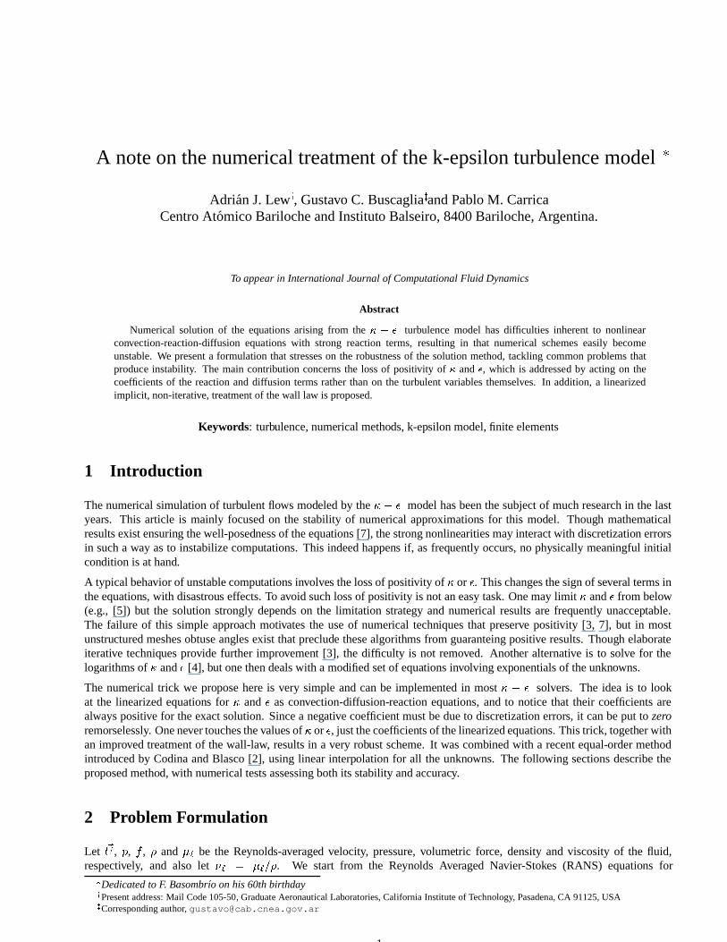
The geometry of this problem (2D) is shown in Fig.3. The dimensions are! � ,! � � �,#� � � and#� � ��. Wall laws(imposing� � ��) hold along top and bottom boundaries. Inflow conditions correspond to fully-developed flow. The casediscussed here corresponds to " � ����� (based on step height! and maximum inlet velocity� �), with � � ��������

and� � ��, which lead to�� � ���. The initial condition is uniform over�, � � ��, � � ���, � � ���, � � ���.Notice that this does not respect mass conservation and is far away from the steady state solution. The grid consists of 6823nodes and 13280 linear triangles (see Fig. 4). With a quite large time step (�� � �����) a quasi-steady state was obtainedwithout difficulty in ��� steps. Nevertheless, at a few nodes near cornera the turbulent dissipation� kept oscillating. Thislocal phenomenon did not pollute the solution away from this corner, and could be damped by further reduction of the timestep (�� additional steps with�� � ����� proved sufficient).

Though not presented here, comparison of velocity and Reynolds stress profiles with previous experimental and numericalresults [10] is satisfactory (see [6] for details). The obtained reattachment length, frequently used for comparison, was#� � ���, in good agreement with both an experimental value# � � � and several works reporting that the� � � modelunderestimates#� by 10% to 25% [8].

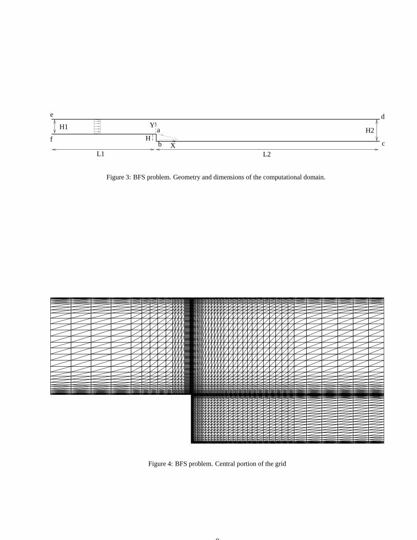
Coming back to the central topics of this article, there are regions of the flow in which� or � are negative, even at steady state.It must be recalled that our method allows for the appearance of such regions, and that our speculation is that in physicallymeaningfull transients or at the steady state they will be sharply localized and will not affect the overall solution. For thepresent example at steady state (things are much worse during the initial transient) such regions are shown in Fig. 5. It isclear that� or � are negative at just a few nodes. Furthermore, this happens where crossflow gradients are steep, and could beavoided by refining the grid or by introducing a discontinuity-capturing operator in the formulation. The minimum values of� and� (see Table 2) are indeed small (in modulus) as compared to the maximum values.

4

5 Concluding remarks

A robust algorithm to solve the�� � equations has been presented. Its design is based on the manipulation of the differentterms so as to add as many positive terms as possible to the system matrix and to keep source terms also positive. Then,as discretization errors may induce non-physical negative values of diffusion or reaction coefficients, these are limited frombelow by zero. This approach works much better than the frequently used limiters on the turbulent variables. Along the samedesign line is the proposed treatment of the wall boundary condition by semi-implicit linearization, an additional trick beingthe imposition ofÆ� instead ofÆ, avoiding iterations in the wall-law algorithm that may fail to converge. Remarkably, theproposed algorithm can easily be implemented in most flow solvers, not just finite element ones. Also worth mentioning isthe good behavior of the recent stabilized method of Codina and Blasco [2], for which few reported experiments (none ofthem turbulent) exist.

ACKNOWLEDGMENTS: Financial support from Agencia Nacional de Promoci´on Cient´ıfica y Tecnologica through grantPICT 12-982 is acknowledged. GCB also belongs to Consejo Nacional de Investigaciones Cient´ıficas y Tecnicas.

References

[1] R. Codina, “Comparison of some finite element methods for solving the diffusion-convection-reaction equation”,Comp.Meth. Appl. Mech. Eng., 156, 185-210 (1998).

[2] R. Codina and J. Blasco, “Stabilized finite element method for the transient Navier-Stokes equations based on a pressuregradient projection”,Comp. Meth. Appl. Mech. Eng., 182, 277-300 (2000).

[3] R. Codina and O. Soto, “Finite element implementation of two-equation and algebraic stress turbulence models forsteady incompressible flows”,Int. J. Numer. Meth. in Fluids, 30, 309-334 (1999).

[4] F. Ilinca and D. Pelletier, “Positivity preservation and adaptive solution for the�� � model of turbulence”,AIAAPaperNo. 97-0205,35th Aerospace Sciences Meeting & Exhibit, January 1997, Reno, USA.

[5] F. Ilinca, D. Pelletier and F. Arnoux-Guisse, “An adaptive finite element scheme for turbulent free shear flows”,Int. J.Comput. Fluid Dyn., 8, 171-188 (1997).

[6] A. Lew, The Finite Element Method in High Performance Computing Environments, Master’s Thesis in NuclearEngineering, Instituto Balseiro, Argentina. In Spanish.

[7] B. Mohammadi and O. Pironneau,Analysis of the�� � turbulence model, J. Wiley & Sons (1994).

[8] S. Tangham and C. Speziale, “Turbulent separated flow past a backward-facing step: A critical evaluation of two-equation turbulence model”, Rep. 91-23, Inst. for Computer Appl. in Sci. and Eng., NASA Langley Res. Ctr. (1991).

[9] T. Utnes, “Two equations (�,�) turbulence computations by the use of a finite element model”,Int. J. Numer. Meth. inFluids, 8, 965-975 (1988).

[10] V. Yakhot, S. Tangham, T. Gatski, S. Orszag and C. Speziale, “Development of turbulence models for shear flows by adouble expansion technique”, Rep. 91-65, Inst. for Computer Appl. in Sci. and Eng., NASA Langley Res. Ctr. (1991).

5

Case Number of nodes (N) �� initial condition1 260 0.01 A2 31 0.01 B3 31 0.1 B4 260 0.1 B

Table 1: Details of the numerical tests for the channel flow problem. The grids are nonuniform, refined near the walls.

max� 6.5305min � -0.0708max� 922.924min � -20.4855

Table 2: Maximum and minimum values of� and� at the steady state of the BFS test problem.

6

0.01

0.1

1

10

100

0 20 40 60 80 100

K

time

Case 1

Case 2

Case 4

Case 3

Max(K)

a)

-10

-8

-6

-4

-2

0

2

4

0 20 40 60 80 100

K

time

Case 1

Case 2

Case 4

Case 3

Min(K)

b)

Figure 1: Channel flow problem. Evolution of the maximum (a) and minimum (b) of� in the initial transient for each of thecases.

7

0.01

0.1

1

10

100

1000

10000

100000

1e+06

0 20 40 60 80 100

E

time

Case 1

Case 2

Case 4

Case 3

Max(E)

a)

-100

-80

-60

-40

-20

0

0 20 40 60 80 100

E

time

Case 1Case 2 Case 4

Case 3

Min(E)

b)

Figure 2: Channel flow problem. Evolution of the maximum (a) and minimum (b) of� in the initial transient for each of thecases.

8

L1 L2

H1

HH2

b c

de

f

Y

X

a

Figure 3: BFS problem. Geometry and dimensions of the computational domain.

Figure 4: BFS problem. Central portion of the grid

9

K< 0

a)

e < 0

b)

Figure 5: BFS problem. Regions with negative values of� (a) and� (b).

10