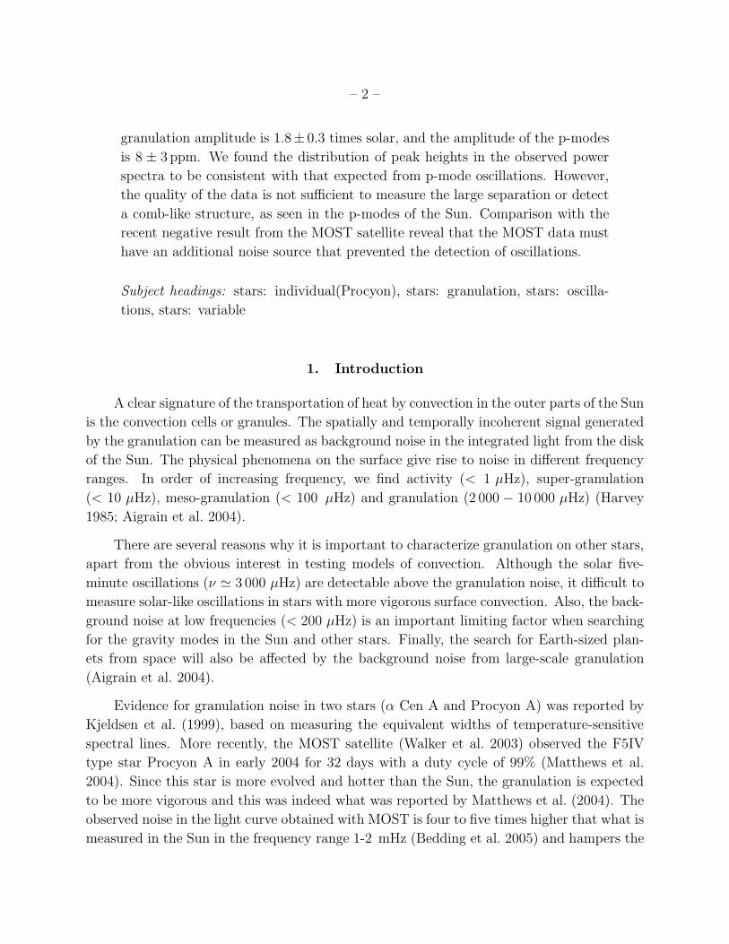
arX

iv:a

stro

-ph/

0504

469v

2 2

5 A

pr 2

005

To appear in ApJ., XXX

Evidence for Granulation and Oscillations in Procyon from

Photometry with the WIRE satellite

H. Bruntt

Niels Bohr Institute, University of Copenhagen, Juliane Maries Vej 30, DK-2100

Copenhagen Ø, Denmark

bruntt@phys.au.dk

H. Kjeldsen

Department of Physics and Astronomy, University of Aarhus, Ny Munkegade, Bygn. 520,

DK-8000 Aarhus C., Denmark

hans@phys.au.dk

D. L. Buzasi

US Air Force Academy, Department of Physics, CO, USA

Derek.Buzasi@usafa.af.mil

T. R. Bedding

School of Physics, University of Sydney, Australia

T.Bedding@physics.usyd.edu.au

ABSTRACT

We report evidence for the granulation signal in the star Procyon A, based

on two photometric time series from the star tracker on the WIRE satellite.

The power spectra show evidence of excess power around 1mHz, consistent with

the detection of p-modes reported from radial velocity measurements. We see a

significant increase in the noise level below 3mHz, which we interpret as the gran-

ulation signal. We have made a large set of numerical simulations to constrain

the amplitude and timescale of the granulation signal and the amplitude of the

oscillations. We find that the timescale for granulation is Γgran = 750±200 s, the

– 2 –

granulation amplitude is 1.8± 0.3 times solar, and the amplitude of the p-modes

is 8 ± 3 ppm. We found the distribution of peak heights in the observed power

spectra to be consistent with that expected from p-mode oscillations. However,

the quality of the data is not sufficient to measure the large separation or detect

a comb-like structure, as seen in the p-modes of the Sun. Comparison with the

recent negative result from the MOST satellite reveal that the MOST data must

have an additional noise source that prevented the detection of oscillations.

Subject headings: stars: individual(Procyon), stars: granulation, stars: oscilla-

tions, stars: variable

1. Introduction

A clear signature of the transportation of heat by convection in the outer parts of the Sun

is the convection cells or granules. The spatially and temporally incoherent signal generated

by the granulation can be measured as background noise in the integrated light from the disk

of the Sun. The physical phenomena on the surface give rise to noise in different frequency

ranges. In order of increasing frequency, we find activity (< 1 µHz), super-granulation

(< 10 µHz), meso-granulation (< 100 µHz) and granulation (2 000 − 10 000 µHz) (Harvey

1985; Aigrain et al. 2004).

There are several reasons why it is important to characterize granulation on other stars,

apart from the obvious interest in testing models of convection. Although the solar five-

minute oscillations (ν ≃ 3 000 µHz) are detectable above the granulation noise, it difficult to

measure solar-like oscillations in stars with more vigorous surface convection. Also, the back-

ground noise at low frequencies (< 200 µHz) is an important limiting factor when searching

for the gravity modes in the Sun and other stars. Finally, the search for Earth-sized plan-

ets from space will also be affected by the background noise from large-scale granulation

(Aigrain et al. 2004).

Evidence for granulation noise in two stars (α Cen A and Procyon A) was reported by

Kjeldsen et al. (1999), based on measuring the equivalent widths of temperature-sensitive

spectral lines. More recently, the MOST satellite (Walker et al. 2003) observed the F5IV

type star Procyon A in early 2004 for 32 days with a duty cycle of 99% (Matthews et al.

2004). Since this star is more evolved and hotter than the Sun, the granulation is expected

to be more vigorous and this was indeed what was reported by Matthews et al. (2004). The

observed noise in the light curve obtained with MOST is four to five times higher that what is

measured in the Sun in the frequency range 1-2 mHz (Bedding et al. 2005) and hampers the

– 3 –

detection of the p modes (Matthews et al. 2004). However, Bedding et al. (2005) have made

simulations of the MOST time series and suggested that the noise signal seen by Matthews

et al. (2004) is a combination of granulation and instrumental effects (e.g. scattered light).

In this study we have used two photometric time-series of Procyon A from the star

tracker on the Wide-field Infrared Explorer satellite (WIRE). In Section 2 we describe the

observations and data reduction procedure. In Section 3 we analyze the resulting power den-

sity spectra. In Section 4 we compare the observed power spectra with a grid of simulations

in order to estimate the amplitude and timescale of the granulation and to constrain the

amplitude of the p mode signal. In Section 5 we discuss our results.

2. Observations and Data Reduction

The star tracker on WIRE has a 52mm aperture with a 512×512 CCD. A window of

8×8 pixels centered on the star image is integrated for 0.5 seconds and read out. The FWHM

of the stellar image is around 1.8 pixels and thus is well sampled. The CCD image is not

flat-fielded, so variations of sensitivity with position are expected. Fortunately, the pointing

of the satellite is stable to about one hundredth of a pixel over periods of several days. Note

that one pixel corresponds to about one arc minute.

WIRE observed Procyon in September/October 1999 and September 2000 for 9.5 and

7.9 days, respectively. Each of the two data sets consists of a few hundred thousand CCD

images. Each WIRE observation consist of five 0.1 second integrations which are summed

on-orbit by the firmware. Since the onboard electronics is 16-bit, when these five frames are

summed for a bright target such as Procyon, saturation occurs, but this is only saturation in

the sense that the data registers overflow and wrap when reaching 216 = 65536 ADU. Procyon

is so bright that three of the central pixels reach the digital 16-bit maximum. Above this

level the pixel value will start counting from zero. Thus we added 216 to the central three

pixels to account for this.

We have developed a new pipeline for the data reduction which differs significantly from

our previous work on WIRE data (Buzasi et al. 2000; Schou & Buzasi 2001; Retter et al.

2003) and so we will describe it in some detail. For the background estimate we used 12 pixels

(3 pixels in each corner of the CCD window). We fitted a Gaussian to each image to find the

approximate position and FWHM of the image. For robustness, the background, position

and FWHM used for each image were the means of 20 images taken before and after that

image (while requiring that no image was separated in time by more than 30 seconds). Thus,

we typically averaged these parameters over 41 × 0.5 = 20.5 seconds. We then performed

– 4 –

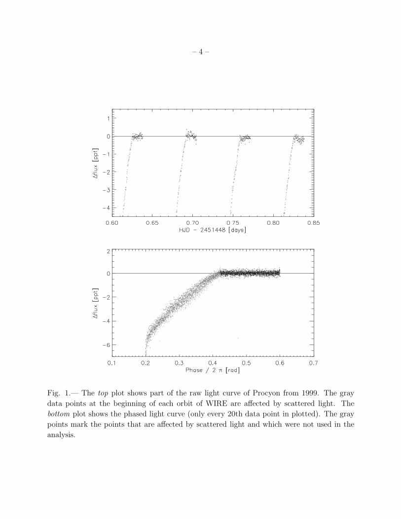
Fig. 1.— The top plot shows part of the raw light curve of Procyon from 1999. The gray

data points at the beginning of each orbit of WIRE are affected by scattered light. The

bottom plot shows the phased light curve (only every 20th data point in plotted). The gray

points mark the points that are affected by scattered light and which were not used in the

analysis.

– 5 –

Fig. 2.— The top plot shows the change in the measured FWHM of the stellar profile versus

time for the WIRE 1999 light curve. Only data points not affected by scattered light are

plotted and only every 20th data point is plotted. In the bottom plot the flux change is

plotted versus FWHM when using the same data points as in the top plot. There is a

significant correlation which was taken out by a spline fit to the data points.

– 6 –

aperture photometry with nine increasing sizes, allowing us to select the one with the lowest

intrinsic noise. The aperture sizes were scaled to the measured FWHM to include the same

amount of light, independent of FWHM. However, the changes in FWHM for the Procyon

observations were below 2% and so the actual number of pixels being summed did not vary.

For the reduction of the Procyon data we summed 22 pixels.

For faster processing of the light curves, we binned data within every 15.5 seconds (i.e.

31 data points) which resulted in light curves from WIRE 1999 and 2000 series with 22 013

and 14 179 data points. In Fig. 1 we show the light curve from 1999 for four orbits. In

the top panel the data are plotted versus time and in the bottom panel they are phased

with the orbital frequency of 15.003 ± 0.001 c/day. The gray points are data affected by

scattered Earth light. This is due to the fact that we underestimated the contribution of the

background light and thus overestimated the brightness of the star. We have tried to remove

the scattered light by fitting a spline to the phased light curve in Fig. 1 but the overall noise

level is worse than if we just discard these data. Thus, the data affected by scattered light

have been removed and the number of data points was then reduced to 10 610 and 8 397 for

the WIRE 1999 and 2000 light curves.

In the case of the WIRE 1999 light curve we found that a group of data points taken

around heliocentric Julian date 2451051.3± 0.4 days were offset by a significant amount, i.e.

+3 ppt. We have found no correlation with any of our reduction parameters, e.g. FWHM,

background level or orbital phase. This group of points contains 13% of the total data set

and so, instead of rejecting them, we artificially offset these points to have the same median

level as the rest of the dataset. We presume that this effect could be caused by one of the

bits “sticking” in the ADC.

In Fig. 2 we show how the 1999 photometry correlates with the measured FWHM of

the stellar profile. The top panel shows the FWHM changing slowly with time and the

bottom panel shows flux versus FWHM. There is a significant correlation in the bottom

panel, which we removed using a spline fit. A similar decorrelation procedure was carried

out for the WIRE 2000 data.

2.1. Comparison of the WIRE and MOST time series

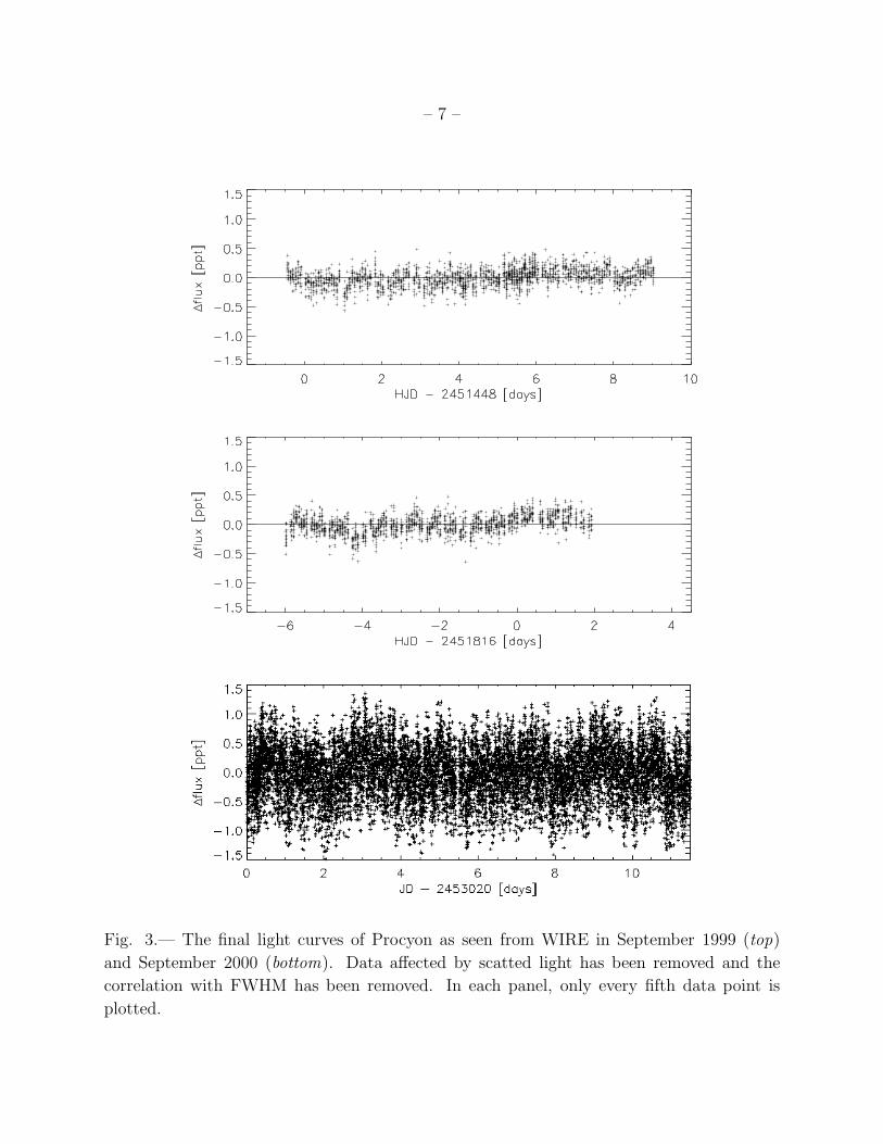
In Fig. 3 we show the final WIRE light curves of Procyon as observed in 1999 (top panel)

and 2000 (middle panel). For comparison we also show part of the light curve observed by

– 7 –

Fig. 3.— The final light curves of Procyon as seen from WIRE in September 1999 (top)

and September 2000 (bottom). Data affected by scatted light has been removed and the

correlation with FWHM has been removed. In each panel, only every fifth data point is

plotted.

– 8 –

MOST in 20041. A slowly varying trend seen in the MOST light curve was subtracted. The

same trend was also seen in a comparison star as shown by Matthews et al. (2004). During

the first 20 days the MOST time series has a data point every 14.7 seconds which is part of

the data shown in Fig. 3. This is very close to the cadence for the binned WIRE light curves

which has one data point each 15.5 seconds. Note, however that the duty cycle is 18% in

the WIRE datasets compared to 99% for the MOST dataset. In Fig. 3 only every fifth data

point is plotted.

The values of rms noise in the 1999 and 2000 WIRE light curves are 135 and 129 ppm,

and the point-to-point scatters (which measure high-frequency noise) are 105 and 101 ppm.

The photon-noise limit for WIRE is 88 ppm, which is about 15–20% lower than the observed

point-to-point scatter. The extra noise could be due to intrinsic variations in Procyon or

instrumental effects. For MOST, the point-to-point scatter is 370 ppm and the photon-noise

limit is 111 ppm, based on the mean flux level of 1.34 × 107 ADU (Matthews et al. 2004)

and a gain of 6.1 e−/ADU (Walker et al. 2003). Thus, the photon noise in the MOST data

is a factor of 3.3 lower than the observed noise level. Note that the results of Matthews et

al. (2004) were based on a preliminary data reduction and a more refined reduction gives

slightly better results (J. Matthews & R. Kuschnig, private communication). We conclude

that the MOST time series is affected by a noise source other than pure photon statistics,

which was also suggested by Bedding et al. (2005) based on the distribution of peak heights

in the amplitude spectrum.

We measured the white noise levels in the 1999 and 2000 WIRE amplitude spectra at

frequencies between 8 and 10mHz and found 1.8 and 1.9 ppm. Thanks to the much higher

number of data points, the MOST amplitude spectrum has a noise level of 1.6 ppm in the

same frequency range.

3. Power density analysis

To measure noise levels as a function of frequency in the different time series, we cal-

culated power density spectra (PDS). Power density measures the power per frequency res-

olution element, which automatically makes it independent of the length (and sampling

function) of the time series. We calculated the frequency resolution by measuring the area

under the spectral window, which is the power spectrum of a single sinusoidal oscillation with

an amplitude of 1 ppm that is sampled using the same times and weights as the observed

series. These areas, which we used to convert from power to power density, were 7.29 and

1The light curve was obtained at CADC through the MOST website: http://www.astro.ubc.ca/MOST/

– 9 –

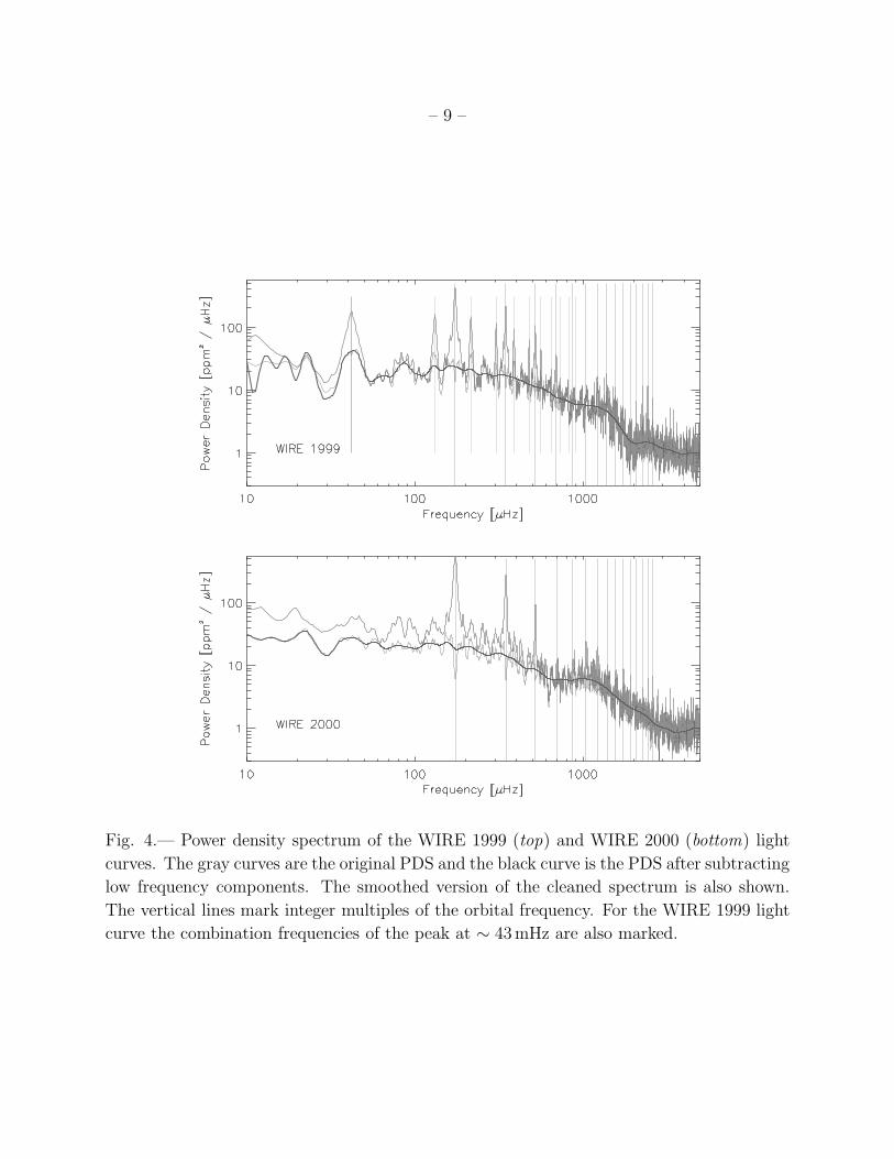
Fig. 4.— Power density spectrum of the WIRE 1999 (top) and WIRE 2000 (bottom) light

curves. The gray curves are the original PDS and the black curve is the PDS after subtracting

low frequency components. The smoothed version of the cleaned spectrum is also shown.

The vertical lines mark integer multiples of the orbital frequency. For the WIRE 1999 light

curve the combination frequencies of the peak at ∼ 43mHz are also marked.

– 10 –

7.02 µHz for the WIRE 1999 and 2000 light curves, respectively.

The WIRE light curves contain a number of significant outliers and to suppress their

influence on the amplitude spectra we have computed weights for all points. Each point

was a weight based on the scatter relative to the neighboring four data points (with the

additional constraint that those data points must be within the same WIRE orbit). We then

smoothed these weights using a running mean of width 150 data points.

The gray curve in each panel of Fig. 4 shows the PDS from WIRE for 1999 and 2000.

There are a few peaks below 15 µHz (corresponding to periods longer than one day) which

we do not attribute to the star. This low-frequency power generates aliases close to the

harmonics of the orbital frequency of the WIRE satellite, around n × 174 µHz, which are

marked by vertical lines. In the case of the WIRE 1999 spectrum, we also see a power excess

around 43 µHz that is not seen in the WIRE 2000 data. This excess also appears as aliases

on either side of each orbital harmonic, as marked by additional vertical lines in the upper

panel of Fig. 4.

We removed the low-frequency components from each light curve by the standard

method of repeatedly subtracting the sinusoid corresponding to the strongest peak in the

power spectrum. We removed three and four components from the WIRE 1999 and 2000

light curves, respectively, and so obtained the high-pass filtered PDS shown in black in Fig. 4.

We can see that the excess power at the harmonics of the orbital frequency is greatly re-

duced. In each panel we have also over-plotted a smoothed version of the high-pass filtered

PDS, and these are also shown in Fig. 5.

It can be seen in Fig. 4 that the high-pass filtered WIRE 1999 PDS still has some excess

power at the orbital harmonic frequencies that is not seen in the WIRE 2000 PDS. This may

explain the slightly higher level seen in the PDS of WIRE 1999 compared to WIRE 2000 in

the 300–800µHz range in Fig. 5.

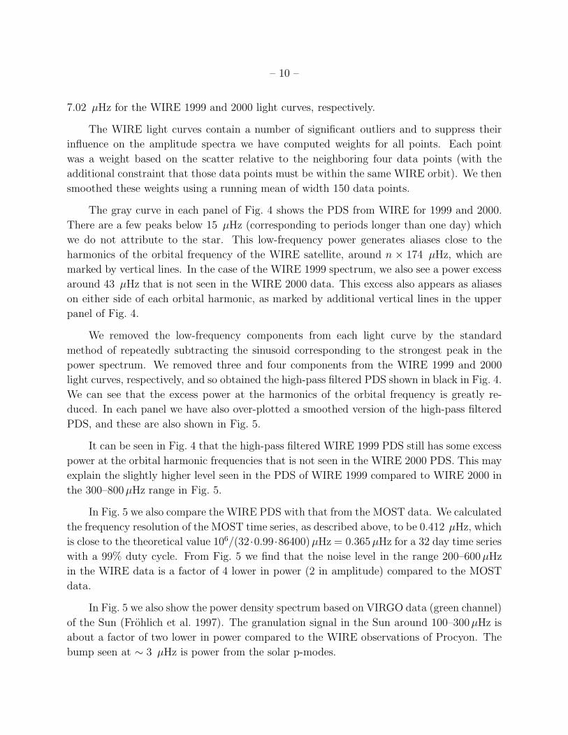
In Fig. 5 we also compare the WIRE PDS with that from the MOST data. We calculated

the frequency resolution of the MOST time series, as described above, to be 0.412 µHz, which

is close to the theoretical value 106/(32·0.99·86400)µHz = 0.365µHz for a 32 day time series

with a 99% duty cycle. From Fig. 5 we find that the noise level in the range 200–600µHz

in the WIRE data is a factor of 4 lower in power (2 in amplitude) compared to the MOST

data.

In Fig. 5 we also show the power density spectrum based on VIRGO data (green channel)

of the Sun (Frohlich et al. 1997). The granulation signal in the Sun around 100–300µHz is

about a factor of two lower in power compared to the WIRE observations of Procyon. The

bump seen at ∼ 3 µHz is power from the solar p-modes.

– 11 –

When comparing observations, we must keep in mind that they were taken over different

wavelength ranges. The MOST satellite has a broadband filter covering 350–700 nm, while

the VIRGO green channel has a narrow band at 500 nm. The filter response of the WIRE

star tracker is not known, but calibrations of the count levels observed in about 50 stars of

different spectral type indicate that the filter response is more sensitive in the blue than in

the red. We find the observed count levels observed with WIRE agree for both early and

late type stars if the filter is Johnson B. Thus, the passbands of the MOST, VIRGO and

WIRE spacecraft are roughly comparable.

4. Simulations of Procyon

We have made simulations of the granulation and p-modes in Procyon based on a

software package developed to provide time-series simulations for the Danish MONS/Rømer

satellite mission as well as for the ESA Eddington mission. We refer to Stello et al. (2004)

for details of the simulations.

The simulation software has several parameters that can be modified. Firstly, we can

set the white noise level in the simulations, which is determined by the noise level at high

frequencies (above 8mHz). For the granulation noise, we can change the timescale and

granulation amplitude, while the p-modes are described by peak amplitude, lifetime and

frequencies. The granulation signal seen in the PDS will depend on the input amplitude

but also the time scale of the granulation. Thus, we use the measured granulation power

density at low frequencies (20–120µHz) from this point on. To include the p-modes in the

simulation, we adopted a large separation of 55.5µHz and a small separation of 4.9µHz (e.g.

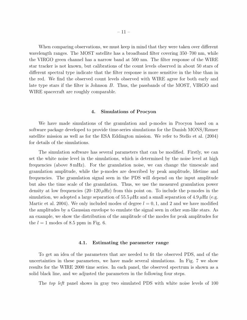
Martic et al. 2004). We only included modes of degree l = 0, 1, and 2 and we have modified

the amplitudes by a Gaussian envelope to emulate the signal seen in other sun-like stars. As

an example, we show the distribution of the amplitude of the modes for peak amplitudes for

the l = 1 modes of 8.5 ppm in Fig. 6.

4.1. Estimating the parameter range

To get an idea of the parameters that are needed to fit the observed PDS, and of the

uncertainties in these parameters, we have made several simulations. In Fig. 7 we show

results for the WIRE 2000 time series. In each panel, the observed spectrum is shown as a

solid black line, and we adjusted the parameters in the following four steps.

The top left panel shows in gray two simulated PDS with white noise levels of 100

– 12 –

Fig. 5.— Smoothed PDS based on the MOST 2004, WIRE 1999 and 2000 data sets. The

PDS based on VIRGO solar data from the green channel is shown for comparison.

Fig. 6.— Input frequencies and amplitudes for the simulation of p-modes in Procyon.

– 13 –

Fig. 7.— The four panels show the power density spectrum of the WIRE 2000 along with

different simulations. Each simulation is the mean of five simulations with different seed

numbers. The hatched regions show the 1-σ variation for selected simulations. In the top

left panel simulations for two different white noise levels are shown. In the top right panel

the simulations have timescales of the granulation of 250, 750, and 1250 s. In the bottom

left panel the timescale of the granulation is 750 s but the granulation power densities (PDs)

are 10, 18, and 64 ppm2/µHz. In the bottom right panel the granulation timescale and

granulation PDs are 750 s and 18 ppm2/µHz, while the amplitude of the p-modes are 5, 10,

15 ppm.

– 14 –

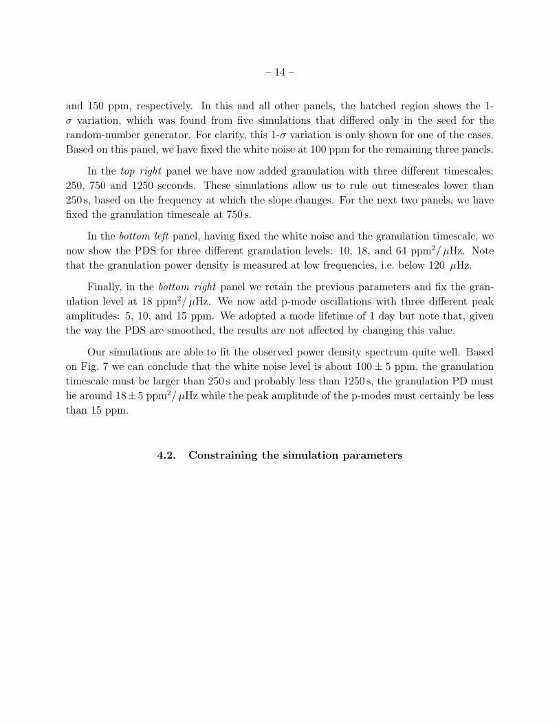
and 150 ppm, respectively. In this and all other panels, the hatched region shows the 1-

σ variation, which was found from five simulations that differed only in the seed for the

random-number generator. For clarity, this 1-σ variation is only shown for one of the cases.

Based on this panel, we have fixed the white noise at 100 ppm for the remaining three panels.

In the top right panel we have now added granulation with three different timescales:

250, 750 and 1250 seconds. These simulations allow us to rule out timescales lower than

250 s, based on the frequency at which the slope changes. For the next two panels, we have

fixed the granulation timescale at 750 s.

In the bottom left panel, having fixed the white noise and the granulation timescale, we

now show the PDS for three different granulation levels: 10, 18, and 64 ppm2/µHz. Note

that the granulation power density is measured at low frequencies, i.e. below 120 µHz.

Finally, in the bottom right panel we retain the previous parameters and fix the gran-

ulation level at 18 ppm2/µHz. We now add p-mode oscillations with three different peak

amplitudes: 5, 10, and 15 ppm. We adopted a mode lifetime of 1 day but note that, given

the way the PDS are smoothed, the results are not affected by changing this value.

Our simulations are able to fit the observed power density spectrum quite well. Based

on Fig. 7 we can conclude that the white noise level is about 100 ± 5 ppm, the granulation

timescale must be larger than 250 s and probably less than 1250 s, the granulation PD must

lie around 18±5 ppm2/µHz while the peak amplitude of the p-modes must certainly be less

than 15 ppm.

4.2. Constraining the simulation parameters

– 15 –

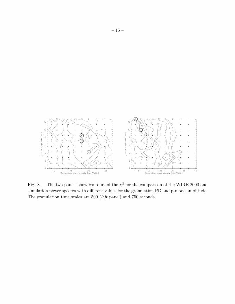
Fig. 8.— The two panels show contours of the χ2 for the comparison of the WIRE 2000 and

simulation power spectra with different values for the granulation PD and p-mode amplitude.

The granulation time scales are 500 (left panel) and 750 seconds.

– 16 –

Fig. 9.— The power density spectra of the WIRE 2000 light curve compared to models with

granulation timescales of 500 (upper panel) and 750 seconds. The WIRE 2000 spectrum is

marked by open box symbols. The different shades of gray correspond to the filled circles on

the contour plot in Fig. 8. The parameters of the models are given in the upper right corner

of each panel.

– 17 –

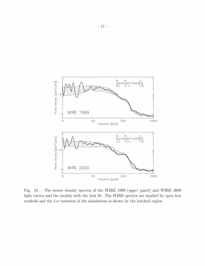
Fig. 10.— The power density spectra of the WIRE 1999 (upper panel) and WIRE 2000

light curves and the models with the best fit. The WIRE spectra are marked by open box

symbols and the 1-σ variation of the simulations is shown by the hatched region.

– 18 –

To put further constraints on the granulation PD and oscillation amplitudes, we have

computed a large grid of simulations that include the ranges of parameters indicated above.

We made time series with granulation timescales of 500, 750, 1000, and 1250 s; granulation

PD in the range 12–41 ppm2/µHz in average step size of 3 ppm2/µHz; and oscillation

amplitudes between 0 and 13 ppm in steps of 1.5 ppm. The white noise was fixed at

100 and 105 ppm for the WIRE 1999 and 2000 time series, respectively. Each time series

was calculated for five different random number seeds to estimate the scatter. In total we

calculated 5 × 440 = 2200 time series for both the WIRE 1999 and 2000 datasets.

For each time series we calculated the power density spectrum. In order to select the

best models we computed the χ2 in the frequency range between 50 and 5000µHz. We used

logarithmic frequency bins in order to avoid giving too much weight to the high-frequency

part of the spectrum.

In Fig. 8 we show results for the simulations of the WIRE 2000 time series. The

two contour plots correspond to granulation timescales of 500 and 750 s, respectively. The

contours show the χ2 value for each set of granulation PD and oscillation amplitudes. The

crosses mark the locations of the computed simulations. We have marked three models with

circles of different color that have the smallest values of χ2, and the corresponding power

density spectra are shown in Fig. 9, where the simulation parameters are given in each panel.

We find that the region 400–800 µHz is better fitted for the granulation timescale of 750 s.

This region is located just below the excess power seen around 1mHz.

In Fig. 10 we show examples of simulations that provide good fits to the WIRE 1999 and

2000 power density spectra. The hatched regions correspond to the 1-σ uncertainty, based

on the scatter of the five simulations with different random number seeds. The agreement

between 1999 and 2000 for the best-fitting parameters is not surprising given the similarity

of the power density curves (cf. Fig. 5). The main difference between the two WIRE PDS

is the region 400–800 µHz. As noted in Sec. 2, we found a group of data points that were

offset from the rest in the WIRE 1999 light curve that may be the source of additional noise.

We thus conclude that the parameters that best fit the observed power density curves

lie in the range 750± 200, 18± 4 ppm2/µHz, and 8.5± 2 ppm for the granulation timescale,

granulation PD and p-mode amplitude, respectively.

The granulation time scale in Procyon is about twice that of the Sun (VIRGO data; cf.

Fig. 5), the granulation PD is three times higher, and the peak p-mode amplitude is twice

solar.

– 19 –

4.3. Peak height distribution

Following Bedding et al. (2005), we have investigated whether the distribution of peak

heights in the power density spectrum of the WIRE light curves (cf. Fig. 4) agrees with

the simulations. We consider the frequency range 700–1 800 µHz, which contains the excess

power that may be due to oscillations. Since the power increases rapidly when going to lower

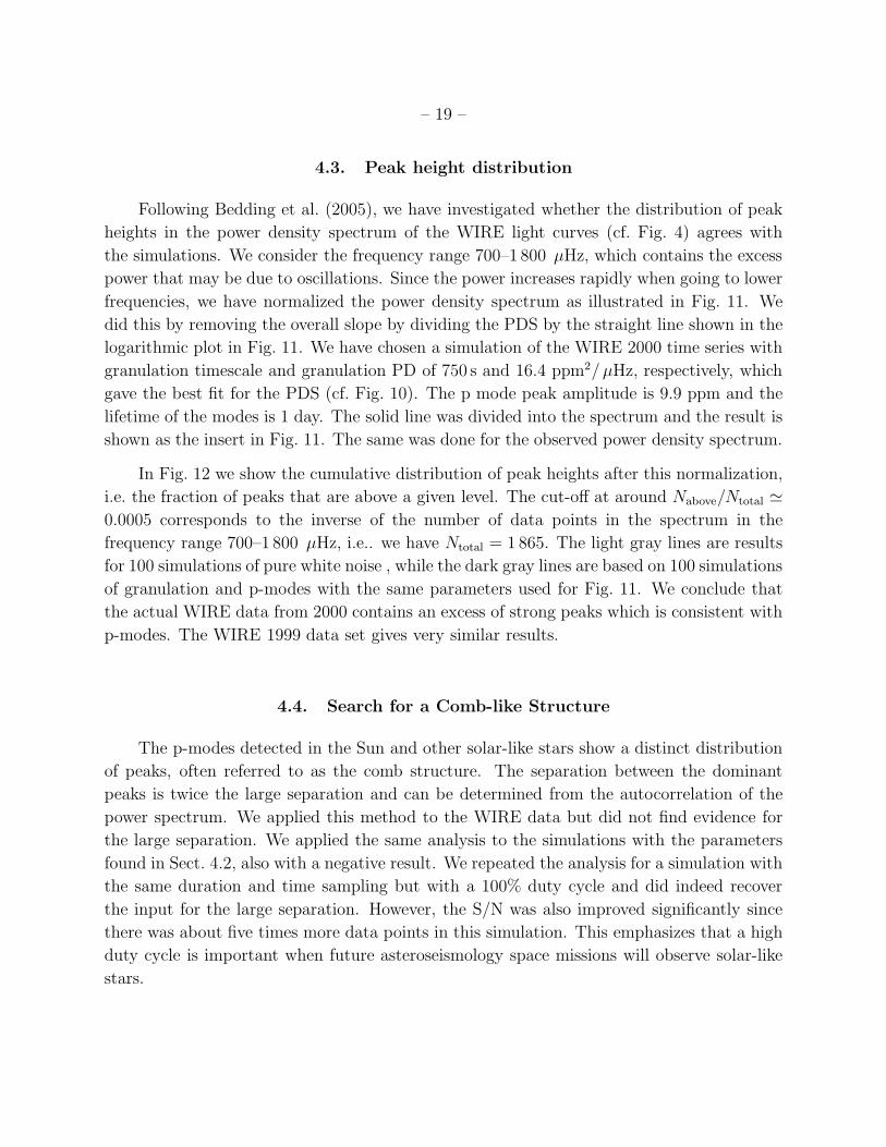
frequencies, we have normalized the power density spectrum as illustrated in Fig. 11. We

did this by removing the overall slope by dividing the PDS by the straight line shown in the

logarithmic plot in Fig. 11. We have chosen a simulation of the WIRE 2000 time series with

granulation timescale and granulation PD of 750 s and 16.4 ppm2/µHz, respectively, which

gave the best fit for the PDS (cf. Fig. 10). The p mode peak amplitude is 9.9 ppm and the

lifetime of the modes is 1 day. The solid line was divided into the spectrum and the result is

shown as the insert in Fig. 11. The same was done for the observed power density spectrum.

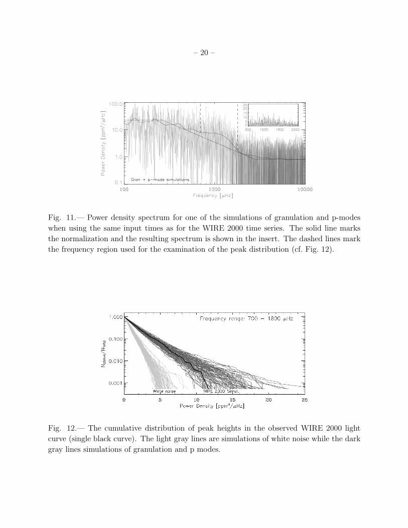
In Fig. 12 we show the cumulative distribution of peak heights after this normalization,

i.e. the fraction of peaks that are above a given level. The cut-off at around Nabove/Ntotal ≃

0.0005 corresponds to the inverse of the number of data points in the spectrum in the

frequency range 700–1 800 µHz, i.e.. we have Ntotal = 1 865. The light gray lines are results

for 100 simulations of pure white noise , while the dark gray lines are based on 100 simulations

of granulation and p-modes with the same parameters used for Fig. 11. We conclude that

the actual WIRE data from 2000 contains an excess of strong peaks which is consistent with

p-modes. The WIRE 1999 data set gives very similar results.

4.4. Search for a Comb-like Structure

The p-modes detected in the Sun and other solar-like stars show a distinct distribution

of peaks, often referred to as the comb structure. The separation between the dominant

peaks is twice the large separation and can be determined from the autocorrelation of the

power spectrum. We applied this method to the WIRE data but did not find evidence for

the large separation. We applied the same analysis to the simulations with the parameters

found in Sect. 4.2, also with a negative result. We repeated the analysis for a simulation with

the same duration and time sampling but with a 100% duty cycle and did indeed recover

the input for the large separation. However, the S/N was also improved significantly since

there was about five times more data points in this simulation. This emphasizes that a high

duty cycle is important when future asteroseismology space missions will observe solar-like

stars.

– 20 –

Fig. 11.— Power density spectrum for one of the simulations of granulation and p-modes

when using the same input times as for the WIRE 2000 time series. The solid line marks

the normalization and the resulting spectrum is shown in the insert. The dashed lines mark

the frequency region used for the examination of the peak distribution (cf. Fig. 12).

Fig. 12.— The cumulative distribution of peak heights in the observed WIRE 2000 light

curve (single black curve). The light gray lines are simulations of white noise while the dark

gray lines simulations of granulation and p modes.

– 21 –

5. Conclusion

We have analyzed light curves of Procyon from the WIRE satellite from two epochs in

1999 and 2000. When comparing the power density spectrum (PDS) of Procyon and the Sun

we find a higher noise level by a factor of 1.8± 0.3 at frequencies in the range 100–300 µHz,

which is expected since Procyon is hotter and more luminous than the Sun.

We find evidence for excess power around 1µHz which is consistent with the p-modes

reported from spectroscopic campaigns (Brown et al. 1991; Martic et al. 2004; Eggenberger

et al. 2004; Claudi et al. 2005). We have compared the observed PDS of the observations

with a grid of simulations with different input granulation timescale, granulation PD and

p-mode amplitude. We have thus constrained the granulation timescale, granulation PD

and p-mode amplitude to be 750 ± 200, 18 ± 4 ppm2/µHz, and 8.5 ± 2 ppm, respectively.

The upper limit we put on the p-mode peak amplitude is consistent with measured radial

velocity amplitudes which lie in the range 50–70 cm/s (Martic et al. 2004). We note that the

determined peak amplitude of the p-modes does not depend on the assumed life time (1 day)

but will depend slightly on our assumed distribution of peaks (cf. Fig. 6). In particular this

is true for the assumed width of the the Gaussian envelope used for modifying the input

peak heights.

We have compared the distribution of peak heights in the PDS of the observations and

in several simulations of granulation and p-modes. We find a good agreement for the peak

distribution which supports our interpretation of the excess power around 1µHz as being due

to p-modes. However, we find no evidence for the comb-like structure expected for solar-like

oscillations.

Our results do not agree with the much higher noise level (a factor two in amplitude)

found from observations with the MOST satellite (Matthews et al. 2004). The analysis by

Bedding et al. (2005) of the MOST power spectrum showed that the the distribution of peak

heights was not consistent with a pure noise source and Bedding et al. (2005) concluded that

an additional error source could be present. This is confirmed by the present comparison

with observations from the WIRE satellite.

HB and DLB acknowledge support from NASA (NAG5-9318) and from the US Air Force

Academy. HB and HK are grateful for the support from the Danish Research Council

(Forskningsrad for Natur og Univers) and TRB thanks the Australian Research Council.

We are grateful to the MOST team for making the Procyon data available through the

Canadian Astronomy Data Centre (operated by the Herzberg Institute of Astrophysics,

National Research Council of Canada). We also thank Dennis Stello for useful discussions

– 22 –

and, in particular, his ideas for the investigation of the peak-height distribution in power

spectra.

REFERENCES

Aigrain, S., Favata, F. & Gilmore, G., 2004, Proc. 2nd Eddington workshop, ESA SP-538,

eds. F. Favata & S. Aigrain, p. 215

Bedding, T. R., Kjeldsen, H., Butler, P. R., McCarthy, C., Marcy, G.W., 2004, ApJ, 614,

380

Bedding, T. R., Kjeldsen, H., Bouchy, F. et al., 2005, A&A, 432, 43L

Brown, T. M., Gilliland, R. L., Noyes, R. W. & Ramset, L. W., 1991, ApJ, 368, 599

Buzasi, D. L., Catanzarite, J., Laher, R. et al., 2000, ApJ, 532, 133

Buzasi, D. L., Bruntt, H., Bedding, T. R., et al., 2004, ApJ, 619, 1072

Claudi, R. U., Bonanno, A., Ventura, R. et al., 2005, A&A, 429, L17

Eggenberger, P., Carrier, F., Bouchy, F. & Blecha, A., 2004, A&A, 422, 247

Frohlich, C., Andersen, B.N., Appourchaux, T., Berthomieu, G., 1997, Sol. Phys., 170, 1

Harvey J.W., 1985, In: Noyes R.W., Rhodes E.J. Jr. (eds.) Probing the depths of a Star:

the study of solar oscillations from space. JPL 400-327

Kjeldsen, H., Bedding, T. R., Frandsen, S., & Dall, T. H., 1999, MNRAS, 303, 579.

Martic, M., Lebrun, J.-C., Appourchaux, T. & Korzennik, S.G., 2004, A&A, 418, 295

Matthews, J. M., Kusching, R., Guenter, D. B. et al., 2004, Nature, 430, 51, Erratum: 430,

921

Palle, P.L., Roca Cortes, T. & Jimenez, A., 1999, ASP Conf. Ser., 173, 297

Retter, A., Bedding, T.R., Buzasi, D.L. et al., 2003, ApJ, 591, 151

Rucinski, S. M., 2004, Walker, G. A. H., Matthews, J. M., et al., 2004, PASP, 116, 1093

Schou, J. & Buzasi, D.L., 2001, Proc. SOHO 10/GONG 2000 Workshop, ESA SP-464, p.

391

– 23 –

Stello, D., Kjeldsen, H., Bedding, T.R., et al., 2004, Sol. Phys., 220, 207

Stetson, P. B, 1990, PASP, 102, 932

Walker, G., Matthews, J., Kusching, R. et al., 2003, PASP, 115, 1023

This preprint was prepared with the AAS LATEX macros v5.2.