General rights Copyright and moral rights for the publications made accessible in the public portal are retained by the authors and/or other copyright owners and it is a condition of accessing publications that users recognise and abide by the legal requirements associated with these rights.

• Users may download and print one copy of any publication from the public portal for the purpose of private study or research. • You may not further distribute the material or use it for any profit-making activity or commercial gain • You may freely distribute the URL identifying the publication in the public portal

If you believe that this document breaches copyright please contact us providing details, and we will remove access to the work immediately and investigate your claim.

Downloaded from orbit.dtu.dk on: Dec 20, 2017

Assessing Miniaturized Sensor Performance using Supervised Learning, withApplication to Drug and Explosive Detection

Alstrøm, Tommy Sonne; Larsen, Jan

Publication date:2013

Document VersionPublisher's PDF, also known as Version of record

Link back to DTU Orbit

Citation (APA):Alstrøm, T. S., & Larsen, J. (2013). Assessing Miniaturized Sensor Performance using Supervised Learning,with Application to Drug and Explosive Detection. Kgs. Lyngby: Technical University of Denmark (DTU). (IMM-PHD-2012; No. 292).

Assessing Miniaturized SensorPerformance using Supervised

Learning, with Application to Drugand Explosive Detection

Tommy Sonne Alstrøm

Kongens Lyngby 2012IMM-PhD-2012-292

Technical University of DenmarkInformatics and Mathematical ModellingBuilding 321, DK-2800 Kongens Lyngby, DenmarkPhone +45 45253351, Fax +45 45882673reception@imm.dtu.dkwww.imm.dtu.dk IMM-PhD-2012-292

Summary (English)

This Ph.D. thesis titled “Assessing Miniaturized Sensor Performance using Su-pervised Learning, with Application to Drug and Explosive Detection” is a partof the strategic research project “Miniaturized sensors for explosives detectionin air” funded by the Danish Agency for Science and Technology’s, ProgramCommission on Nanoscience Biotechnology and IT (NABIIT), case number:2106-07-0031. The project, baptized “Xsense” was led by professor Anja Boisen,DTU Nanotech. DTU Informatics participate in the project as data analysispartner.

This thesis presents advances in the area of detection of vapor emanated by ex-plosives and drugs, similar to an electronic nose. To evaluate sensor responses adata processing and evaluation pipeline is required. The work presented hereinfocuses on the feature extraction, feature representation and sensor accuracy.Thus the primary aim of this thesis is twofold; firstly, present methods suit-able for assessing sensor accuracy, and secondly improve sensor performance byenhancing the preprocessing and feature extraction.

Five different miniaturized sensors are presented. Naturally, each sensor requireits own special preprocessing and feature extraction techniques before the sensorresponses can be applied to supervised learning algorithms. The technologiesused for sensing consist of Calorimetry, Cantilevers, Chemoselective compounds,Quartz Crystal Microbalance and Surface Enhanced Raman Scattering. Eachof the sensors have their own strength and weaknesses. The reasoning for usingmultiple sensors was the desire to investigate the feasibility for an integratedmultisensor solution. A unique setup of multiple independent detectors is ableto vastly enhance accuracy compared to what a single sensor can deliver.

ii

As we are detecting hazardous compounds this enables the need for sensors todeliver not only decisions but also certainty about decisions. This requirement ishandled by introducing classifiers that offer posterior probabilities and not onlydecisions. The three probabilistic classification models utilized are ArtificialNeural Networks, Logistic Regression and Gaussian Processes. Often, thereis no tradition for using these methods in the communities of the prescribedsensors. Here, a method of too much complexity is often undesired so it is abalance when to utilize more sophisticated methods. For this reason, an arrayof methods that only discriminate between samples are used as baseline. Themethods used vary from sensor to sensor, as these methods serve as baselineperformance when introducing new methods.

The most widely used baseline method in this thesis is the k-nearest-neighboralgorithm. This method is of particular interest in the application of sensors,as the sensors are designed to provide robust and reliable measurements. Thatmeans, the sensors are designed to have repeated measurement clusters.

Sensor fusion is presented for the sensor based on chemoselective compounds.An array of color changing compounds are handled and in unity they makeup an colorimetric sensor array. In this setting it is valuable to qualify whichcompounds in the colorimetric sensor array are important. That knowledge en-ables the ability to either reduce the size of the sensor or replace less sensitiveand unimportant compounds with more selective and responsive compounds. Aframework based on forward selection Gaussian Process classification is demon-strated to successfully identify a set of important compounds.

Summary (Danish)

Ph.D.-projektet “Assessing Miniaturized Sensor Performance using SupervisedLearning, with Application to Drug and Explosive Detection” er et led i det stra-tegiske forskningsprojekt “Miniaturized sensors for explosives detection in air”,som er af Det Strategiske Forskningsrads Programkomite for Nanovidenskab og-teknologi, Bioteknologi og IT (NABIIT), bevilling 2106-07-0031. Projektet erblevet døbt ”Xsense” og blev ledet af professor Anja Boisen, DTU Nanotech.DTU Informatik deltager i projektet som data analyse partner.

Formalet med projektet har været at udvikle nano-sensorer med henblik pa atskabe grundlaget for en elektronisk næse, som kan detektere farlige stoffer f.eks.sprængstoffer. En sadan næse ville kunne bruges i lufthavne, hos anti-terrorkorps, i afsøgningen af vejsidebomber, m.v. og dermed kraftigt reducere denmenneskelige risiko.

Forskningsarbejdet har haft to primære mal. For det første at præsentere me-toder, som var i stand til at vurdere sensorernes nøjagtighed. For det andet atforbedre sensorernes ydeevne gennem optimeret signalbehandling og datamodel-lering. Ved identifikation af farlige stoffer, er der behov for en sensor som kan de-tektere med høj nøjagtighed, men ogsa behov for vurdering af hvor palideligheddenne er.

Arbejdet har involveret fem forskellige kemiske nano-sensorer og fokuseret paudvikling, optimering og evaluering af metoder og modeller til databehand-ling. Sensorne viser sig i stand til at detektere sprængstoffer som ofte bliverbenyttet af terrorister savel som stoffer i forbindelse narkotika bekæmpelse.Nøjagtigheden kan forbedres hvis systemet indeholder flere sensorer. Fordele

iv

ved en integreret enhed er undersøgt og de er indikationer at nøjagtigheden kanforbedres i et multisensor system.

Preface

This thesis was prepared at the Department of Informatics and MathematicalModeling, Technical University of Denmark, in partial fulfillment of the require-ments for acquiring the Ph.D. degree in engineering. The Ph.D. project was apart of the strategic research project named “Xsense - Miniaturized sensors forexplosives detection in air”, led by Professor Anja Boisen, DTU Nanotech, andfunded by the Danish Agency for Science and Technology’s, Program Commis-sion on Nanoscience Biotechnology and IT (NABIIT).

The Xsense project worked towards the development of four individual sensortechnologies for detection of explosives. All of the sensor technologies can po-tentially be incorporated into a single miniaturized device. The main hypothesisof the project is that sufficient reliability can only be ensured by merging severalindependent measuring principles.

The main idea behind this Ph.D. project was to develop the signal processingpipeline for each sensor and then perform sensor fusion. This objective howeverturned out to be a little too optimistic. A complete device was never built andthe work herein is exclusively about the processing of data obtained using theindividual sensors and the application of machine learning methods to assessthe performance of the sensors. Fortunately the work conducted in Xsense hasspurred a new project named MUSE, which in many ways is a continuation ofXsense. The application area is different, but the sensor technologies are similarand there is a greater focus on sensor integration. There is also a continuity ofpersonnel. Several of the researchers in MUSE participated in Xsense, and nowthese people have more experience and know-how.

In Xsense, each sensor technology was developed and refined by people at DTU

vi Preface

Nanotech and Department of Chemistry, Syddansk University respectively. Alldata was collected by researchers at DTU Nanotech though. Due to the dataflow in Xsense, my project turned out to be provider of data analysis knowledgefor the researchers developing the sensors. My research has therefore been verymuch about handling the data produced by these sensors, assessing the sensorperformance and then handing the results to the scientists at DTU Nanotech.Thus, whenever data has been handled, the overall goal was always to assessand possibly improve the sensor performance.

The starting point was to use existing techniques, and if the sensor was able todeliver flawless performance using these techniques, no refinement in the signalprocessing was made. For this very reason, the research conducted has not atall been equally balanced among the sensors. Some of the sensing principleswere mature and there was already a lot of work published on those, whereasothers were rather new and here there was often more room for improvement.

Also a lot of traditional statistical hypothesis testing and design of experimentshave been carried out. Not all experiments used an experimental design as itturned out that most “sensor people” are not aware of the issues solved by theapplication of a proper experimental design. So this Ph.D. project has beeneducational not just for me but also for the people at DTU Nanotech. Twodifferent worlds have meet and we have all come out richer.

In the early days of the project, no data was produced as the sensors wereunder development. Fortunately I was able to get hold of data similar to thedata that would be produced within Xsense, but with the application of ecstacydetection. The thesis contains a chapter about detection of ecstasy using quartzmicrobalance sensors. This sensor was also developed at DTU Nanotech inanother project called Nanonose.

The thesis consists of a summary report and a collection of six research paperswritten during the period 2008–2012. Four of the papers have been publishedelsewhere whereas the remaining two still have to be published. One is stillin draft (paper F) while the other has been submitted. A total of 15 researchpapers have been co–authored in the period, but only the papers that containedcontributions in the signal processing of sensor data have been included in thethesis.

The introductory chapter will explain chemical sensing and the need for newdevices for explosives detection. Knowledge about chemical detection is notassumed. Readers knowledgeable in the area on explosives detection can godirectly to the end of the chapter. There, an outline of the thesis is given aswell as a list of the main contributions contained herein. The list of contributionsis best read in order to know where the thesis advances current methods.

vii

Chapter 2 will then explain how machine learning in the context of sensors can beemployed. Readers with knowledge in machine learning can skim this chapter,however attention should be given to section 2.3. Here I explain specificallyhow the models were applied for the sensors, as well as which performancemeasures were used. Further, the implementation details for each model aregiven although not explained. If the implementation of the model was not doneby either me or my collaborators, I will give references to the software that wasused. Interested readers can find in-depth explanations in the referred material.Likewise it is also my aim to publish the majority of the code used to create theresults presented throughout this thesis so others can reproduce the results.

Chapter 3 and 4 extract and present the main advances in the area of signalprocessing and how specifically the models explained in chapter 2 were applied.Advances have been made mostly on the sensors based on quartz microbalancecrystals and chemoselective colorimetric compounds and the two chapters arebased on the papers B-F. These papers are provided mostly as supportinginformation to chapter 3 and 4.

The material covered in paper A is only covered briefly in the main part ofthe thesis (chapter 1 and 5). The paper shows proof-of-concept measurementsmade on the four sensors in the Xsense project and justify the application of amultisensor approach. The paper can be read as stand-alone. With these words,I wish you happy reading and I hope you will have an informative ride.

Lyngby, 31-December-2012

Tommy Sonne Alstrøm

viii

List of Publications madeduring the PhD

Submitted Journal Papers

[A] Tommy S. Alstrøm, Natalie V. Kostesha, Filippo G. Bosco, Michael S.Schmidt, Jesper K. Olsen, Michael Bache, Jan Larsen, Mogens H. Jakob-sen, and Anja Boisen. Miniaturized multisensory approach for the highlysensitive and selective detection of explosives. Submitted to Journal ofMaterials Chemistry, 2013.

� Sanjukta Bose, Stephan S. Keller, Tommy S. Alstrøm, Anja Boisen, andKristoffer Almdal. Design of Experiments for Process Optimization ofSpray Coated Polymer Films. Submitted to Langmuir, 2013.

Published Conference Papers

[B] Tommy S. Alstrøm, Jan Larsen, Claus H. Nielsen, and Niels B. Larsen.Data-driven modeling of nano-nose gas sensor arrays. In Ivan Kadar, ed-itor, Proceedings of SPIE, volume 7697, pages 76970U–76970U–12. SPIE,2010. doi: 10.1117/12.850314.

� Michael S. Schmidt, Natalie Kostesha, Filippo Bosco, Jesper K. Olsen,Carsten Johnsen, Kent a. Nielsen, Jan O. Jeppesen, Tommy S. Alstrøm,Jan Larsen, Mogens H. Jakobsen, Thomas Thundat, and Anja Boisen.

x List of Publications made during the PhD

Xsense: using nanotechnology to combine detection methods for high sen-sitivity handheld explosives detectors. In Proceedings of SPIE, volume7664, pages 76641H–76641H–6, 2010. doi: 10.1117/12.850219.

� Natalie V. Kostesha, Tommy S. Alstrøm, Carsten Johnsen, Kent A. Niel-sen, Jan O. Jeppesen, Jan Larsen, Mogens H. Jakobsen, and Anja Boisen.Development of the colorimetric sensor array for detection of explosivesand volatile organic compounds in air. In Proceedings of SPIE, volume7673, pages 76730I–76730I–9, April 2010. doi: 10.1117/12.850310.

� Natalie V. Kostesha, Michael S. Schmidt, Filippo G. Bosco, Jesper K.Olsen, Carsten Johnsen, Kent A. Nielsen, Jan O. Jeppesen, Tommy S.Alstrøm, Jan Larsen, Thomas Thundat, Mogens H. Jakobsen, and AnjaBoisen. The Xsense project: The application of an intelligent sensor arrayfor high sensitivity handheld explosives detectors. In Sensors ApplicationsSymposium (SAS), 2011 IEEE, pages 7–11, 2011. doi: 10.1109/SAS.

2011.5739782.

� Michael S. Schmidt, Natalie V. Kostesha, Filippo G. Bosco, Jesper K.Olsen, Carsten Johnsen, Kent A. Nielsen, Jan O. Jeppesen, Tommy S.Alstrøm, Jan Larsen, Thomas Thundat, Mogens H. Jacobsen, and AnjaBoisen. Xsense - a miniaturised multi-sensor platform for explosives de-tection. In Proceedings of SPIE, volume 8031, pages 803123–803123–7,2011. doi: 10.1117/12.884050.

� Natalie V. Kostesha, Tommy S. Alstrøm, Carsten Johnsen, Kent A. Niel-sen, Jan O. Jeppesen, Jan Larsen, Anja Boisen, and Mogens H. Jakobsen.Multi-colorimetric sensor array for detection of explosives in gas and liquidphase. In Proceedings of SPIE, volume 8018, pages 80181H–80181H–12,2011a. doi: 10.1117/12.883895.

[C] Tommy S. Alstrøm, Jan Larsen, Natalie V. Kostesha, Mogens H. Jakob-sen, and Anja Boisen. Data representation and feature selection for colori-metric sensor arrays used as explosives detectors. In IEEE InternationalWorkshop on Machine Learning for Signal Processing (MLSP), pages 1–6,2011. doi: 10.1109/MLSP.2011.6064615.

[D] Tommy S. Alstrøm, Raviv Raich, Natalie V. Kostesha, and Jan Larsen.Feature extraction using distribution representation for colorimetric sensorarrays used as explosives detectors. In IEEE International Conferenceon Acoustics, Speech, and Signal Processing (ICASSP), pages 2125–2128,2012. doi: 10.1109/ICASSP.2012.6288331.

[E] Tommy S. Alstrøm, Bjørn S. Jensen, Mikkel N. Schmidt, Natalie V. Koste-sha, and Jan Larsen. Hausdorff and Hellinger for Colorimetric Sensor Ar-ray Classification. In IEEE International Workshop on Machine Learning

xi

for Signal Processing (MLSP), pages 1–6, 2012. doi: 10.1109/MLSP.

2012.6349724.

� Natalie V. Kostesha, Tommy S. Alstrøm, Jan Larsen, Anja Boisen, andMogens H. Jakobsen. Multi-Colorimetric Sensor Array for Detection ofIllegal Materials. In IEEE Sensors, number 09, 2012.

Under preparation

� Colorimetric sensor array data processing toolbox. 2013. URL http://

www.imm.dtu.dk/pubdb/p.php?6498.

� Tommy S. Alstrøm and Jan Larsen. Feature Extraction and Signal Rep-resentation for Colorimetric Sensor Arrays. Technical report, DTU Infor-matics, 2010-2012. URL http://www.imm.dtu.dk/pubdb/p.php?5845.

[F] Natalie V. Kostesha, Tommy S. Alstrøm, Olga V. Mednova, CarstenJohnsen, Kent A. Nielsen, Jan O. Jeppesen, Mogens H. Jakobsen, JanLarsen, and Anja Boisen. Advanced detection of explosives using multi-colorimetric sensor array. Will be submitted to Journal of American Chem-ical Society (JACS), 2013.

� Tommy S. Alstrøm, Ryota Tomioka, Bjørn S. Jensen, Mikkel N. Schmidt,Natalie V. Kostesha, and Jan Larsen. Robust Feature Extraction forColorimetric Sensor Arrays. Will be submitted to IEEE Transactions onSignal Processing, 2013.

� Jaeyoung Yang, Mirko Palla, Filippo G. Bosco, Michael S. Schmidt, TomasRindzevicius, Tommy S. Alstrøm, Milan N. Stojanovic, Anja Boisen, JingyueJu, and Qiao Lin Utilizing large area mapping of uniform SERS substratesfor ultra sensitive and specific detection of biomolecules. To be submittedto ACS Nano, 2013.

xii

Acknowledgements

In the writing of this thesis I also had the chance to look back on the past fouryears of my life. It turned out that quite a lot of people have contributed inmaking this thesis possible.

First, I’d like to thank my supervisor, associate professor Jan Larsen for choosingme to be the person that could carry out this work, to inspire discussions andto teach me the style and etiquette of academia.

Anja Boisen, professor at DTU Nanotech has also been an inspiration and Iwould like to thank her for the support and encouragement she has given methroughout the project, and for taking time to help me improve my work andunderstanding in nanotechnology. The same gratitude is extended to Mogens H.Jakobsen whom offered financial support and invited me to his group for threemonths to improve the work on the colorimetric sensor array.

I would like to thank all the people of the cognitive systems section and inparticular professor Lars K. Hansen and associate professor Ole Winther whomhave been of great help and inspiration. Your insight in machine learning runsdeep and thank you for taking the time to explain theories to me. Both of youhave always been helpful when I came knocking on your door. I would like toextend the same gratitude to associate professor Morten Mørup who has alwaysbeen helpful when I had questions to ask.

I also wish to thank Dr. Morten Angren for helping me to understand the L1and L2 regularization and the connection to Gaussian/Laplacian priors. Theunderstanding had eluded me many times before you took the time to explain

xiv Acknowledgements

it to me.

This thesis has been made a lot more readable due to the help from severalproofreaders. I am sure that readers are also happy that the language has beenimproved and is more smooth on the eye now than earlier editions. Proofreadersof this theses are (in alphabetic order): Carsten Stahlhut, Dylan O’Donnell,Gitte S. Alstrøm, Mikkel N. Schmidt, Natalie V. Kostesha, and Scott Mileham.Thanks to you all.

The work presented in this thesis would never have be possible without the helpfrom my close collaborator. Their contributions have in so many ways improvedmy research for which I am very grateful. Their contributions are written here,in alphabetic order:

Collaborator ContributionsBjørn S. Jensen Implemented the distance kernel specified in (4.32) and

the multiple kernel covariance function specified in (4.33).Without these implementations, it is unlikely that thesensor fusion for colorimetric arrays would be carried outwithin this project. I’m very grateful that Bjørn tooktime to do this even though he didn’t really had time todo it. Having a keen understanding of Gaussian Processclassification, he also assisted me in writing section 2.5.4,and should be considered a main contributor to thissection.

Claus H. Nielsen Conducted all experiments with the quartz crystalmicrobalance sensors. Claus also spend time to help meunderstand the ideas behind of polymer-based sensors.

Filippo Bosco Conducted all experiments with the cantilever sensor andhas participated in many fruitful discussions in Xsense.

Gabriela Blagoi Was involved in the early stages of the colorimetric sensorarray and help me understand the technology.

Jesper K. Olsen Conducted all experiments on the calorimetric sensor.Even after Jesper got a full-time job in the industry hetook time to answer questions by email.

xv

Michael S.Schmidt

Conducted all experiments with the surface enhancedRaman scattering sensor. Michael has on numerousoccasions patiently explained the idea behind Ramanscattering, and when I think I finally understood I alwayshad to ask for more clarifications.

Mikkel N.Schmidt

Suggested the idea of using Hausdorff for colorimetricsensor arrays. Mikkel has also taken time to explain agreat deal of machine learning methods to me in my timehere.

Natalie V.Kosteha

Carried out experiments with the colorimetric sensorarray. Assisted in categorize the chemicals and describedtheir possible application areas. As such, Natalie shouldbe considered as the main author of appendix G. Nataliealso managed to proof read the entire thesis and correctmy chemistry mistakes where it was needed.

Raviv Raich Brought the idea of histogram methods for colorimetricsensor arrays to the table. This idea has been crucial ingoing forward with the work with colorimetric sensorarrays.

Ryota Tomioka Has patiently helped me to understand multiple kernellearning and inspired the idea to utilize the method forcolorimetric sensor arrays.

I want to express my gratitude to my parents and my parents in law. Conductinga Ph.D. study with small kids is never easy but thankfully you have all extendeda helping hand in the time of need.

Finally, I want to express my deepest gratitude to my loving wife, Gitte S.Alstrøm. Her support and encouragement has been crucial for me during thepast four years and without her support I would never have been where I amtoday and finish my Ph.D study. I am forever thankful.

xvi

Nomenclature

Terms

Term MeaningAnalyte A chemical constituent or substance that is exposed to a

sensor and undergo analysis.Antipersonnelmine

Landmine is specifically designed to harm humans.

Chemoselective Selective compound that reacts with just one functionalgroup in the presence of others.

Deflagrate A substance that is suddenly and violently ignited, i.e. anexplosive.

Densityestimation

Estimation of the concentration of a detected vapor.

Difference map A graphical representation of the response of acolorimetric sensor array.

Dot Refers to a circular dot on a colorimetric sensor array.The dot consist of a dye that has been spotted on a pieceof silica gel and then dried.

Dye Refers to a given chemo-selective compound employed ina colorimetric sensor array. One dye corresponds to onesensor.

False alarm A positive detection that turned out to be false.Precursor A substance that participates in the chemical reaction

that produces another substance.Solvent Substance that are used to dissolve compounds.Trace detection Detection of small amount of analyte vapor in air.

xviii Nomenclature

Treatment In terms of classical analysis of experiments, thetreatment is the act of exposing the object of interest tothe factors that is under investigation. In the context ofsensors, a treatment refers to the act if exposing thesensor to a control or a target compound.

Abbreviations

Term Meaningi.i.d. Independent and identically distributed1-NN 1-nearest-neighborANN Artificial Neural NetworkAXO Abandoned explosive ordnanceCDF Cumulative distribution functionDPI Dots per inchDTA Differential Thermal AnalysisDTA Differential Thermal AnalysisEP Expectation PropagationERW Explosive Remnants of WarGP Gaussian ProcessGPR Gaussian Process RegressionGTD Global Terrorism DatabaseGTI Global Terrorism IndexHCA Hierarchical Cluster AnalysisHCL Hierarchical Cluster AnalysisICBL International Campaign to Band LandminesIED Improvised Explosives Devicek-NN k-nearest-neighborLHS Left hand sideLOOCV Leave-One-Out Cross ValidationLR Linear regressionMAE Mean Absolute ErrorNMF Non-negative Matrix FactorizationPC Principal ComponentsPCA Principal Component AnalysisPCR Principal Component Regressionppm parts-per-millionQCM Quartz Crystal Microbalance

xix

RCBD Randomized Complete Block DesignRGB Red-green-blue color modelRHS Right hand sideRMAE Relative Mean Absolute ErrorRT Room TemperatureRT Room TemperatureSERS Surface Enhanced Raman ScatteringSLR Sparse Logistic RegressionSotA State of the ArtSVD Singular Value DecompositionUXO Unexploded ordnance

Notation

Symbol MeaningD The dimensionality of the data being treated.D Denotes the dataset D = {xi, yi}Ni=1

E[f ] Expectation of f .ε A normal distributed random variable used to add noise to

models.E(·) The error function.ED(·) The data dependent part of the error function.Ew(·) The data independent part of the error function.Eh[f ] The expectation with respect to the distribution measure h,

Eh[f ] =∫f(x)h(x)dx

h(·) Denotes the activation function used in a neural network.Ik(i,j) An image matrix for channel k where the channels are RGB.

Ibef The image of a colorimetric sensor array before exposure.Iaft The image of a colorimetric sensor array that has been

exposed.Idif The difference image of a colorimetric sensor array.k − CV k fold cross validation, k can be a number.k(x,x′) A kernel function or the covariance function.K The number of classes in a data set.m(x) The mean function prior of a Gaussian Process.M The dimensionality of a reduced subspace based on X.Nerr The total number of missclassified points in a classification

problem.Nk The total number of measurements in a given dataset with

class label k.N The total number of measurements in a given dataset.

xx Nomenclature

Nktr The number of training points for class k.

R The set of real numbers.R0+ The set of non-negative real numbers, R0+ = {x | 0 ≤ x < ∞}x A vector of dimensionality D that contains a measurement.xm,n Corresponds to element X(m,n).X A D ×N data matrix.X(m,n) The element on the mth row and nth column in the matrix

X.yi The label that is associated with measurement xi.θ Vector that contains hyperparameters.

xxi

xxii Contents

Contents

Summary (English) i

Summary (Danish) iii

Preface v

List of Publications made during the PhD ix

Acknowledgements xiii

Nomenclature xvii

1 Introduction 11.1 Chemical sensing . . . . . . . . . . . . . . . . . . . . . . . . . . . 41.2 Antiterrorism . . . . . . . . . . . . . . . . . . . . . . . . . . . . . 41.3 Demining . . . . . . . . . . . . . . . . . . . . . . . . . . . . . . . 71.4 Explosive detection using a multisensor approach . . . . . . . . . 101.5 Sensor evaluation framework . . . . . . . . . . . . . . . . . . . . 121.6 Outline . . . . . . . . . . . . . . . . . . . . . . . . . . . . . . . . 14

2 Learning Theory in the context of sensors 172.1 A brief history of machine learning . . . . . . . . . . . . . . . . . 182.2 Unsupervised learning . . . . . . . . . . . . . . . . . . . . . . . . 22

2.2.1 Principal component analysis . . . . . . . . . . . . . . . . 222.2.2 Non-negative matrix factorization . . . . . . . . . . . . . 24

2.3 Supervised learning . . . . . . . . . . . . . . . . . . . . . . . . . . 252.3.1 Model evaluation . . . . . . . . . . . . . . . . . . . . . . . 262.3.2 Model selection . . . . . . . . . . . . . . . . . . . . . . . . 272.3.3 Performance measures . . . . . . . . . . . . . . . . . . . . 28

xxiv CONTENTS

2.4 Regression . . . . . . . . . . . . . . . . . . . . . . . . . . . . . . . 292.4.1 Linear regression . . . . . . . . . . . . . . . . . . . . . . . 302.4.2 Principal component regression . . . . . . . . . . . . . . . 31

2.4.3 Artificial neural network regression . . . . . . . . . . . . . 312.4.4 Gaussian process regression . . . . . . . . . . . . . . . . . 33

2.5 Classification . . . . . . . . . . . . . . . . . . . . . . . . . . . . . 342.5.1 k -nearest-neighbor . . . . . . . . . . . . . . . . . . . . . . 352.5.2 Vector-space classification . . . . . . . . . . . . . . . . . . 35

2.5.3 Sparse logistic regression . . . . . . . . . . . . . . . . . . . 362.5.4 Gaussian process classification . . . . . . . . . . . . . . . 362.5.5 Artificial neural network classification . . . . . . . . . . . 37

3 Quartz crystal microbalance sensors 393.1 Detection of Ecstasy . . . . . . . . . . . . . . . . . . . . . . . . . 40

3.1.1 Data partitioning . . . . . . . . . . . . . . . . . . . . . . . 413.1.2 Model evaluation . . . . . . . . . . . . . . . . . . . . . . . 41

3.1.3 Analyte classification . . . . . . . . . . . . . . . . . . . . . 423.1.4 Concentration estimation . . . . . . . . . . . . . . . . . . 45

3.2 Related work . . . . . . . . . . . . . . . . . . . . . . . . . . . . . 47

3.3 Summary . . . . . . . . . . . . . . . . . . . . . . . . . . . . . . . 49

4 Colorimetric sensors 51

4.1 Preproccesing of images . . . . . . . . . . . . . . . . . . . . . . . 534.1.1 Dye localization . . . . . . . . . . . . . . . . . . . . . . . 534.1.2 Aligning images . . . . . . . . . . . . . . . . . . . . . . . . 57

4.1.3 Feature extraction . . . . . . . . . . . . . . . . . . . . . . 594.2 Datasets . . . . . . . . . . . . . . . . . . . . . . . . . . . . . . . . 614.3 Visualization of colorimetric data . . . . . . . . . . . . . . . . . . 65

4.4 Detection using single value statistics on difference colors . . . . 684.4.1 Comparing the statistics . . . . . . . . . . . . . . . . . . . 70

4.4.2 Detection of explosives . . . . . . . . . . . . . . . . . . . . 714.4.3 Detection of drugs . . . . . . . . . . . . . . . . . . . . . . 72

4.5 Improving detection accuracy by calibrating colors . . . . . . . . 73

4.5.1 Evaluation using k-nearest-neighbor . . . . . . . . . . . . 754.6 Using histogram and manifold methods . . . . . . . . . . . . . . 77

4.6.1 Hellinger Distance . . . . . . . . . . . . . . . . . . . . . . 78

4.6.2 The Hausdorff Distance . . . . . . . . . . . . . . . . . . . 804.6.3 Evaluation using k-nearest-neighbor . . . . . . . . . . . . 814.6.4 Evaluation using Gaussian process classification . . . . . . 83

4.7 Related work . . . . . . . . . . . . . . . . . . . . . . . . . . . . . 864.8 Summary . . . . . . . . . . . . . . . . . . . . . . . . . . . . . . . 87

5 Multisensor approach for dection of explosives 89

CONTENTS xxv

6 Conclusion and future work 93

A Miniaturized multisensory approach for the highly sensitive andselective detection of explosives 97

B Data-driven modeling of nano-nose gas sensor arrays 139

C Data representation and feature selection for colorimetric sen-sor arrays used as explosives detectors 159

D Feature extraction using distribution representation for colori-metric sensor arrays used as explosives detectors 175

E Hausdorff and Hellinger for Colorimetric Sensor Array Classi-fication 191

F Advanced detection of explosives using colorimetric sensor ar-ray 205

G Analytes 241

Bibliography 247

xxvi CONTENTS

Chapter 1

Introduction

This Ph.D. project concerns the detection of explosives and drugs in air and isa part of “Xsense”. The Xsense project has worked towards the developmentof four individual sensor technologies for detection of explosives. The sensordevelopment has primarily been driven by two aims; to provide new tools forthe fight against terrorism and to provide cost efficient yet reliable sensors thatcan be applied in the area of demining.

To meet either of these goals, a sensor platform that can detect explosives isrequired. Detection of explosives is complicated due to the existence of a vast ar-ray of explosive substances. The list of explosives employed by terrorists is longand the detection is further complicated by terrorists often producing their ownexplosives, usually referred to as an improvised explosives device (IED) [Wernickand Von Glinow, 2012, Rollings and Wyler, 2012].

The situation of landmines is likewise complex as there exist an estimated 650different types of antipersonnel mines around the world [Habib, 2007]. Antiper-sonnel landmines are specifically designed to harm humans and is typically duginto soil. Landmines are mostly an issue in developing countries where the localinhabitants are often forced to cultivate minefields or they will starve [LandmineMonitor, 2012].

2 Introduction

The detection of drugs is closely related to the fight against terrorism1. Thefunding of terror cells is often (in part) achieved by the manufacturing anddistribution of illicit drugs [Costa et al., 2010]. Hence, it is a natural step toinvestigate how well sensors can detect drugs.

Nevertheless, the primarily objective of the Xsense project was to develop aminiaturized sensor platform for the detection of explosives so we will start there.Due to the complexity of the detection of explosives, the playing field had to benarrowed down and the sensors were tested on a few selected compounds whichwill be detailed later. Furthermore, the sensors has been deployed exclusively ina laboratory setting where numerous proof-of-concept measurements has beenmade. The issue of mixed compounds (IEDs) is not handled explicitly in theproject, but instead several substances that is used to manufacture explosivesare measured standalone.

Measurements have also been performed on an array of non-explosive substancesthat served as control. A list that details all of the applied substances and theirpossible application can be found in appendix G. Finally, the task of getting theexplosives to the sensor in a real world setting is not handled within the Xsenseproject. It is basically assumed that this is handled by an external device calleda preconcentrator that will collect samples in sufficient amounts.

Today vapors emanating from explosives are mainly detected by canines, elec-tronic nose and sniffing probes [Furton and Lawrence, 2001, Singh, 2007, Yinon,2003]. The electronic nose is the device that combines chemical-sensing andpattern-recognition systems; in nature it could be the sensing organ of an ani-mal like the nose of a bomb-sniffing dog or rat as illustrated on figure 1.1. Thesensor can recognize specific molecules and can be applied in many areas ofresearch, such as food quality analysis, medical diagnostics, explosives, toxinsdetection, and environmental. Further, the sensor has shown high capability fordetecting substances, such as ammonium nitrate and mineral explosives (salts)in low concentrations [Gui et al., 2009]. Nevertheless, the traditionally appliedelectronic nose technique has limitations due to the detection problems at lowanalyte concentrations, as well as at high or low temperature and humidity.

The minimization of false alarms is identified as a priority in sensing devices [Yi-non, 2003, Gui et al., 2009]. Currently, the screening and identification of suspi-cious substances is often done by canine units or specialized teams which employsophisticated methods e.g. terahertz pulsed spectroscopic imaging [Fitch et al.,2007, Barber et al., 2005], gas chromatography, mass spectroscopy [Barshickand Griest, 1998] or long-range Raman spectrometry [Carter et al., 2005]. The

1In this work we are only concerned with the detection of illicit drugs and explosives. Legalsubstances such as medicine or fireworks are not what is in focus here.

3

Figure 1.1: The two state of the art explosives detection units at work. Imageof the dog is courtesy of [Danminar, 2012] and the rat is courtesy of [APOPO,2012].

screening is characterized by a high assignment of personnel and high costs [Sheaand Morgan, 2007]. Furthermore, in relation to the requested volume the meth-ods are often slow. Airport screening requires systems to handle up to 10 pas-sengers per minute [Shea and Morgan, 2007]. Canine units work swiftly butrequire breaks, have significant upkeep cost and can only be applied by experthandlers [Shea and Morgan, 2007].

Todays market shows a demand for portable multisensor instruments [Air, 2012,Rki, 2012, Ins, 2012]. These instruments are sensitive enough to detect low con-centrations of analytes and can within a few seconds identify common volatilecompounds. For example, in the product “GDA 2” by AirSense Analytics, acombination of different sensors is applied. The product comprises an ion mo-bility spectrometer, a photo ionization detector, two semiconductor gas sensorsand an electrochemical cell. Other detecting combinations like an array of chem-ical sensors [Stetter et al., 2000, Suslick et al., 2004a, Kostesha et al., 2010] ora surface modified with different sensing layers can also be called a multisensorapproach.

The use of detection systems based on multisensor approaches could tremen-dously help in the fast identification of explosives, reduce false alarms and pro-vide new opportunities for the real-time analysis of explosives [Xsense, 2012].A simultaneous application of a variety of sensor techniques, which are basedon different physical principles, will enhance the collection of data where erro-neous detections are statistically independent. This improves the possibility toreliably detect presence of explosives molecules with a high confidence [Stetteret al., 2000, Raman et al., 2009].

The application of multisensor detection technologies has a great perspective inthe identification of different analytes. In the cases of demining, a minimum

4 Introduction

acceptable clearance rate of 99.6% has been set by United Nations [Kimberg,1996]. Obtaining this rate is almost impossible using a single detection tech-nique. Trained dogs are by many considered the best known explosives detector,but they require excessive training and are greatly obstructed by the environ-ment. In severe cases their accuracy may be as low as 50% [Habib, 2007].

The sensors within this thesis measure responses based on chemical reduction-oxidation reactions, molecular interactions, etc. so there is a need for someintroductory remarks about the nomenclature of trace detection.

1.1 Chemical sensing

All of the sensors presented in this theses are chemical sensors that is usedfor vapor detection emanating by explosives (or drugs), also denoted as tracedetection. Trace detection is the detection of a small amount of molecules inair. While the sensor manufacturing is very different all of them still rely onthe evaporation of the chemical target denoted analyte. An analyte is the sub-stance or chemical constituent that is undergoing analysis, either classificationor density estimation. Classification is the act of identifying which compoundis reacting with the sensor whereas density estimation is the task of estimatinghow much of the compound is present.

Often, the target analyte is dissolved into some kind of carrier liquid or carriergas. This carrier is denoted a solvent. Solvents are widely used in the productionof chemical constituents, whether these are cosmetics, explosives or somethingelse. Whenever one of our sensors is utilized it is always designed with thedetection of a specific compound in mind. An experiment is then conductedwith the target analyte and some alternative analytes could for example besolvents that are used to create explosives as well as other compounds. As such,solvents serve as potential false alarms for the compound that we really wantto detect. If solvents were not included in the experiment, the experimenterreally does not know if the sensor is detecting the solvent or the target molecule,unless of course it can be argued by other means that the sensor made a positivedetection.

1.2 Antiterrorism

Over the past decade, explosives have been a preferred tool for terrorists [Wer-nick and Von Glinow, 2012, Rollings and Wyler, 2012]. The organization of

1.2 Antiterrorism 5

0

500

1000

1500

2000

2500

3000

OthersIncendiary

Unknown

Firearms

Explosives

201120072002

Figure 1.2: Types of weapons used in terrorist attacks in the period 2002-2011.The most common choice is explosives followed by firearms. Figure courtesyof [Global Terrorism Index, 2012].

Compound Incidents Fatalities Injuries

Ammonium Nitrate (AN) 94 139 328Royal Demolition Explosive (RDX) 22 121 437Triacetone Triperoxide (TATP) 3 17 26

Trinitrotoluene (TNT) 1272 1695 6177

Table 1.1: Confirmed instances where the listed compounds were used toperform an attack [Global Terrorism Database, Dec, 2012].

Global Terrorism Index (GTI) has compiled figures of all recorded attacks in2002-2011 and here explosives clearly shows to be the weapon of choice, whichis shown on figure 1.2.

The issue of terrorism is a global concern and almost every country in the worldis affected by the threat posed by terrorism. GTI has computed the threatposed by terrorism according to a heuristic on the scale 0-10 for 158 countries,and inspection of the results geographically shown in figure 1.3 reveals thatterrorism is indeed a worldwide concern. The figure also shows that the densityof terrorist attacks is highest in Columbia, the Middle-east, India, Pakistan andthe Philippines.

In the scope of Xsense we have measured four compounds commonly appliedby terrorists. These are the three explosives RDX, TATP and TNT and thesalt ammonium nitrate (widely found in fertilizers). The compounds and therecorded number of incidents are listed in table 1.1. RDX and TNT are militaryclass compounds whereas TATP is a recently applied compound utilized in IEDsthat is easily manufactured using ordinary house-hold chemicals.

6 Introduction

LOWEST IMPACT OF TERRORISM

HIGHEST IMPACT OF TERRORISM

0.01 - 2

2.01 - 4

4.01 - 6

6.01 - 8

8.01 - 10

0

NOT INCLUDED

IMPACT OF TERRORISM 2011GLOBALTERRORISM

INDEX

Figure 1.3: The top map illustrates the worldwide threat calculated accordingto the global terrorism index. The red dots on the bottom map marks geo-graphical locations of attacks. Figures courtesy of [Global Terrorism Index,2012].

It should be noted that table 1.1 only enumerates the number of confirmedinstances. Often the compound cannot be identified precisely, e.g. in the well-known Oklahoma bombing where 168 fatalities and 650 injured were listed,the explosive type is listed as unknown, even though it is the general notionthat ammonium nitrate was used it cannot be established beyond reasonabledoubt [Hoffman, 1998]. The perhaps most well-known recent example happenedin Norway, 2011, where a terrorist attacked the prime minister’s office buildinglocated in Oslo using a lethal bomb based on ammonium nitrate [Pol, 2011a].

1.3 Demining 7

The explosive TATP is not widely used but is well known in Denmark. Here,we had two recent incidents (2007 and 2010) of failed terrorist attacks wherethe police made arrests before the attacks were completed [Pol, 2011b, 2008].

Two more compounds where measured and although not often utilized (norecords where found in the GTD) by terrorists they are still highly relevant.The first one is HMX (Octogen) which is closely related to RDX as the twocompounds are chemically close and in the production of RDX up to 10% ofthe produced RDX turns out to be HMX (see appendix F). HMX is also oftenmixed with TNT and thus it is possible that HMX has already been applied byterrorists but merely it could not be detected post-blast.

The other compound measured was 2,4-dinitrotoluene (DNT). DNT is a byprod-uct of TNT as TNT decomposed into DNT in time so an indirect method ofdetecting TNT is to detect DNT. DNT has higher vapor pressure than TNTand is therefore easier to collect and detect compared to TNT.

As a final note, the fatalities/injuries in table 1.1 is the minimum as only con-firmed numbers are included. A total of of 50,098 incidents that included explo-sives are recorded. If the incidents2 that resulted in more that 100 victims areextracted, a total of 396 incidents are recorded with a total of 19,353 fatalitiesand 59,106 injuries [STA].

1.3 Demining

Antipersonnel mines were first applied on a wide scale in World War II andhas been widely used since then [ICBL, 2012]. Originally a military weapon,landmines has evolved to become an issue for civilian life as well. This is dueto mine fields remaining intact in former battle areas after ended conflicts. Inthe year 2011 the portion of civilian casualties was at 72% out of all recordedcasualties.

In the mission of demining the International Campaign to Band Landmines(ICBL) is a significant organization on the goal of worldwide demining andmost of the information contained in this section is based on the reports madeby the Landmine and Cluster Munition Monitor research by ICBL3.

2excluding incidents within legitimate warfare.3Landmine and Cluster Munition Monitor is the research and monitoring initiative of the

International Campaign to Ban Landmines (ICBL) and the Cluster Munition Coalition (CMC)and has provided civil-society reporting on landmines, cluster munitions and other explosiveremnants of war since 1999. The ICBL is the author of the reports. Human Rights Watch isthe publisher of reports from 1999-2004 and Mines Action Canada is the publisher of reports

8 Introduction

Demining took place in 1997 with the creation of the “Ottawa treaty”. TheOttawa treaty is a framework for putting a total ban of landmines into place.Countries that have signed the treaty also commits to clearance of minefieldsand assisting affected communities. ICBL calls for a total ban on usage ofantipersonnel mines, as well as clearance of emplaced landmines and explosiveremnants of war (ERW). ERW refers to ordnance left behind after an endedconflict such as explosive devices that failed to detonate (UXO) or equipmentthat has been abandoned (AXO). Both UXO and AXO pose a significant threatto local communities. Removal of ERW is also related to antiterrorism, sincemilitary groups recover ERW and use them to manufacture their own explosivesdevices (IEDs). Landmines are almost a worldwide problem, with presence ofminefields in Asia, Africa, South America and Europe (see figure 1.4). Fortu-nately the creation of new minefields has almost come to a stop. In 2011–2012only two governments applied new antipersonnel mines, Myanmar and Syria.The list of countries containing new minefields is a bit wider though, as non-state armed groups also deploy antipersonnel mines. This has been recorded tohappen in Afghanistan, Colombia, Myanmar, Pakistan, Thailand, and Yemen.

It is mostly in developing countries that minefields are a problem. The listof countries that have most casualties due to landmines are dominated by de-veloping countries located in Africa and the Middle-east. The number of ca-sualties in 2011 on countries with over 100 casualties, with the number of ca-sualties in parentheses was: Afghanistan(812), Pakistan(569), Colombia(538),Myanmar(381), Cambodia(211), South Sudan(206), Libya(184), Somalia(146),Iraq(141), and Sudan(122).

In recent years the number of casualties is declining. The number of registeredcasualties since the year 2000 is displayed in figure 1.5. The numbers are antic-ipated to be more precise in the latter years as more countries have developedregistration procedures as the years went by, e.g. in year 2000 it was estimatedthat the total number of casualties was about 20,000 even though the recordednumber is just 8,000. A total of 4,286 casualties by ERW was registered in theyear of 2011, a significant decrease since the year 2000. The amount of casualtiesin year 2011 among children was 42% and in some countries the percentage wasas high as 61%, so ERW are mostly hurting children. According to [LandmineMonitor, 2012] the appearance of minefields is decreasing and “Worldwide, anarea covering some 3, 000km2 remains to be cleared of antipersonnel mines”.

Current demining techniques are expensive compared to laying new mines. In2007, [Habib, 2007] reported that the production cost of an antipersonnel minewas about 3-30US� whereas the cost of clearing one mine was ranging between300-1,000US�. One of the major reasons is that minefields must be cleared using

from 2004 onward.

1.3 Demining 9

SudanSouth

Burundi

IsraelLebanon

Armenia

Azerbaijan

CroatiaBosnia andHerzegovina

Montenegro

Moldova

Djibouti

CambodiaVietnam

Sudan

J ordanKuwaitAlgeria

Iraq

Zimbabwe

Ethiopia

Western Sahara

Somaliland

Palestine

Kosovo

Nagorno-Karabakh

Afghanistan

TaiwanMauritania

ColombiaVenezuela

Hungary

Nepal

Falkland Islands/Malvinas *

MaliChadNiger

Turkey

Peru

Chile

Angola

DRCongo

Namibia

Germany

Yemen

Mozambique

Thailand

Serbia

Republic of CongoUganda

Ecuador

Senegal

TajikistanGreece

Eritrea

Philippines

Bhutan

Cyprus

Palau

Russia

China

India

Iran

Libya

Mongolia

Egypt Pakista

n

Myanmar

Uzbekistan

Morocco

Oman

Somalia

Syria

Lao PDR

Kyrgyzstan

Cuba

North Korea

Georgia

SouthKorea

Sri Lanka

Mine Contamination as of October 2012

©ICBL-CMC 2012

Very heavycontamination (>100 km²)Heavy contamination (10-100 km²)Mediumcontamination (1-10 km²)Lowcontamination (<1 km²)Residual or suspected contaminationNo evidence ofmined areas Note: Other areas are indicated by italics.

*Argentina and the United Kingdomhave both declared that they are affectedbyvirtue of their claimof sovereignty over the Falkland Islands/Malvinas.

Americas

South

Middle East andNorth Africa

Africa

Europe,Caucasus, and

Central Asia

Asia

Russia

Libya

SudanChad

Angola

Iraq

EthiopiaColombia

Syria Afghanistan

DRCongo

Mozambique

Laos

Sudan

Vietnam

Uganda

Tajikistan

Serbia

Western Sahara

EritreaCambodia

CroatiaGeorgia

Albania

Sierra Leone

Israel

Bosnia and Herzegovina

Kuwait

Guinea Bissau

Lebanon

Nagorno-Karabakh

KosovoMontenegro

Cluster Munition Casualties

©ICBL-CMC 2012

Casualties by region

Recorded clustermunition casualtiesNo recorded cluster munition casualties

Note: Other areas are indicated by italics.Countries whose names appear larger have larger numbers of clustermunition casualties.

10010

1,000

Figure 1.4: Figures courtesy of [Landmine Monitor, 2012].

10 IntroductionNumber

ofcasualties

Year

2000 2001 2002 2003 2004 2005 2006 2007 2008 2009 2010 20110

2000

4000

6000

8000

10000

12000

Figure 1.5: The number of casualties per year from explosive remnants of war.Although the number of casualties rise on a few instances the number of casu-alties is generally decreasing. The graph is based on numbers from [LandmineMonitor, 2012].

multiple techniques, otherwise the required minimum acceptable clearance rateof 99.6% cannot be achieved. This situation calls for the development of efficientmethods.

Despite the need for new reliable detection devices there is yet to be developed asatisfactory mobile and portable solution. Sensors must not only easily detect avariety of hidden explosives but they must also be able to detect illegal chemicalsand products of the explosives industry. A further requirement is that thesensing device should be portable, rapid, highly sensitive, specific (minimizefalse alarms), and inexpensive [Schmidt et al., 2011a].

1.4 Explosive detection using a multisensor ap-proach

The main hypothesis in the Xsense project is that sufficient reliability can onlybe ensured by merging several independent and sensitive measuring principles.The basic scientific goal of the Xsense project was on the development andrefinement of miniaturized sensors in order to achieve a detection limit towardsexplosives in the parts-per-billion range. DNT and TNT were the major testmolecules as TNT is commonly found in landmines, and DNT is a byproduct of

1.4 Explosive detection using a multisensor approach 11

D.

C.

B.

A.

Analyte causes bending

Chemical coating

Color changing compounds

Deflagration

Heating bridge

Substrate

Reflected laserLaser beam

Figure 1.6: Illustration of the four sensing techniques used in Xsense: A.Surface enhanced Raman scattering sensor; sensor; B. Calorimetric sensor; C.Cantilever sensor; D. Colorimetric sensor.

TNT. DNT that leaks to the surrounding soil is generally easier to detect thanTNT thus TNT is located by detecting DNT.

The proposed multisensor system is based on four miniaturized sensors: calori-meter, cantilever, colorimetric array, and surface enhanced Raman scattering(SERS). The four utilized sensors are shown on figure 1.6.

SERS is increasingly used as a versatile analytical tool for both chemical andbiochemical sensors in liquid and gas phase. In fact, single molecule detectionwith SERS has been demonstrated [Kneipp et al., 1997]. SERS-based sensorsrely on increasing the number of inelastically scattered photons from an ana-lyte adsorbed on a so-called SERS substrate. A new class of SERS substrateshas been developed at DTU Nanotech using standard clean-room silicon pro-cessing techniques [Talian et al., 2009]. This class of substrates demonstratesa signal enhancement factor of up to 7.8 · 106 due to plasmonic effects from ananostructured and silver coated surface.

Calorimetry is widely applied to investigate thermal properties of various sampleanalytes. The micro-calorimetric sensing device used in Xsense is based ondifferential thermal analysis (DTA) where the temperature difference betweentwo highly sensitive temperature sensors is measured [Yi et al., 2008a, b, Senesacet al., 2009, Greve et al., 2010]. One sensor is loaded with a sample analyte andthe other is left blank. Using integrated heating elements both sensors are heatedat a constant rate while the differential temperature is continuously measured.At certain temperatures the sample will sublimate, melt, evaporate or deflagrate

12 Introduction

which results in a change in differential temperature.

The cantilever based sensor is an established micro- and nano-mechanical sens-ing tool for trace detection of biochemical compounds [Raiteri et al., 2001, Fritz,2008, Boisen et al., 2011]. The response of cantilever-based sensors can bemeasured by monitoring change in resonance frequency of the cantilevers. Anegative frequency shift is generated through mass added to the surface of thecantilevers [Fritz et al., 2000, Sushko et al., 2008]. Generally, the larger the res-onance frequency change, the higher the amount of a given analyte is present inthe sample. The change in resonance frequency of each cantilever is measured.The surface of the cantilever is functionalized with receptor molecules designedto specifically bind target analytes [Gimzewski et al., 1994].

Colorimetric sensing is a technique which can be useful in both detection andidentification of volatile organic compounds in air and liquids [Kostesha et al.,2011, Zhang and Suslick, 2005, Nielsen et al., 2008]. Chemoselective compoundsare capable of changing colors when exposed to analytes or analyte mixtures.The colorimetric sensor array technique showed great potential for real-time4

monitoring of analytes such as DNT, acids, alcohols and arenas with sensitivitybelow the parts-per-million (ppm) range [Kostesha et al., 2010]. Chemoselectivecompounds are capable of recognizing specific analytes; this recognition is afunction of intermolecular interactions, basically weak, non-covalent interactionsor donor-acceptor interactions.

As mentioned in the introduction, multisensor devices are emerging such as theGDA 2. But, while the “GDA 2” is a handheld device it has a weight of 4.2 kg.The methods proposed in Xsense enables use of micro- and nano sized sensorsand these sensors can facilitate a even lighter handheld device that can containa multitude of sensors. This is a great strength in the goal of developing highaccuracy sensors. Suppose that the sensor measuring techniques in Xsense arecompletely independent and that each sensor have an accuracy of just 75%. Amultisensor approach would under these assumptions have an accuracy of 99.6%.The main hypothesis of the Xsense project is exactly that; to investigate to whatextent the sensors are independent, and what accuracy can be obtained by acombined solution as opposed to each of the sensor individually.

1.5 Sensor evaluation framework

The development of a multisensor system begins with the development of theindividual sensor technologies. Some of the technologies in Xsense are rather

42 minutes of analyte exposure is needed for the current sensor.

1.5 Sensor evaluation framework 13

Raw data

Desicion

EstimateRegressor

Classifier

Data processing pipeline

processing extractionPre- Feature

Figure 1.7: Data processing pipeline used throughout this thesis.

new and here we hypothesize that the accuracy of these sensors can be improvedif more specifically designed methods are developed. The work carried outherein is about handling data produced by these sensors and how the sensorperformance can be assessed.

The generic framework that is repeated throughout the thesis is, 1) collection ofsensor data, 2) preprocessing and feature extraction, 3) assessment of the sensorperformance using machine learning. The procedure is illustrated in figure 1.7.

Some requirements were put on the machine learning methods. The currentstate of the art (SotA) machine learning method for the given sensor field isincluded as baseline. But as we are detecting hazardous compounds we requirethat the classifier offers posterior probabilities and not only classifications.

When working with sensors the quality and accuracy of the sensor have to beassessed. In our measurement setup we often work both in the two-class settingand themulticlass setting. In the two-class setting, we are looking to identify theanalyte as either an explosives or non–explosives. In the multiclass setting we areworking in a more precise setting where either the exact name of the analyte isused (e.g. DNT) or the chemical family of the analyte (e.g. DNT is an explosivesubstance). When working in the multiclass setting, the goal is to understandthe strength of the sensor better and often the results are illustrated using aconfusion matrix. A confusion matrix illustrates the amount measurements thatwas not classified correctly and where the sensor has weaknesses.

When comparing classifiers, often they are compared using the McNemar sig-nificance test [McNemar, 1947]. The McNemar is a paired test which uses thenumber of cases where two classifiers disagree about a decision. One p–value iscalculated for each comparison. In the cases of multiple hypothesis testing, theframework proposed by Storey [Storey, 2002] is applied. Based on the p–valuesan expected positive false discovery rate (E[pFDR]) is calculated. This rate is

14 Introduction

used to calculate the expected quantity of wrongly significant results relative toall significant results.

1.6 Outline

The remainder of the thesis is structured as follows; Chapter 2 gives a briefreview of the origins of machine learning and describes the machine learningmethods that is applied in subsequent chapters. The focus of the chapter is onthe models and how they are applied and not so much how exactly the trainingis handled. Often the training involves the minimization of a cost function.Where appropriate the cost function will be described as well, but concerningthe numerical optimizations that is carried out, readers are referred to referencematerial.

Chapter 3 shows some advanced made to quartz microbalance crystal (QCM)sensor detection and estimation of concentration levels. QCM based sensors arehighly linear, yet sophisticated non-linear methods have often been applied andin particular artificial neural networks. A data set is presented and analyzed us-ing both linear and non–linear methods, and a recommendation on the handlingof data based on QCM sensors is summarized.

Chapter 4 includes several advances made to the colorimetric sensor array dataprocessing. First, the preprocessing of images is described and then the traditionfeature extraction process is detailed. Next follows some advances made onvisualization of colorimetric sensor arrays and the issues with current featureselection methods are highlighted. Then follows advanced in the handling andmodeling of colorimetric sensor array data. Finally a generic framework basedon Gaussian process classification is introduced and used to identify importantchemoselective compounds.

Chapter 5 introduces the multisensor approach that formed the backbone of theXsense project. The chapter extracts the main results that is more elaboratelypresented in appendix A. A dataset inspired by a post-blast5 car bomb scenariowas created. The analytes are measured on all four sensors under identicalconditions. Based on the findings it is rendered probably that a multisensorapproach comprising the aforementioned sensors will improve the overall pre-diction accuracy.

Chapter 6 summarizes the thesis, highlights the innovations and put them into

5The situation after a detonation have occurred and forensics collect samples in order toidentify the explosives that was used

1.6 Outline 15

perspective.

Papers B-F are in most part covered in chapter 3 and 4 and serve as supportinginformation. Finally, appendix G enumerates the analytes that has been appliedin the work presented in this thesis.

Contributions

Here follows a condensed list of scientific contributions contained in this thesis:

� Improved performance of density estimation on quartz microbalance crys-tal based sensors by applying Gaussian process regression [chapter 3, pa-per B].

� Improved the visualization and interpretation of data collected from col-orimetric sensor arrays by application of the cumulative density function[chapter 4].

� Developed a unified approach to perform both sensor selection and analyteclassification for colorimetric sensor arrays. This is achieved by use ofsparse logistic regression [paper C].

� Improved accuracy in prediction performance for colorimetric sensor ar-rays by improving the feature extraction. The color representation is car-ried out using distribution methods and the Hausdorff distance [chapter 4,paper D, E].

� Developed a sensor selection and sensor fusion scheme that based on Gaus-sian process classification for colorimetric sensor arrays. The sensor selec-tion effectively identifies sensors that will improve prediction performancewhen sensor fusion is performed [chapter 4, paper E].

� Improved classification accuracy by applying 1-nearest-neighbor majorityvoting for SERS-based sensors [paper A].

� Improved signal visualization of responses from calorimetric sensors byconducting noise reduction using Gaussian process regression [paper A].

16 Introduction

Chapter 2

Learning Theory in thecontext of sensors

Modern day machine learning concerns the processing and handling of data.Data is typically divided into two groups: labeled or unlabeled, and whichmachine learning method should be applied depends on the data. Labeled datais for example data gathered for prediction tasks, e.g. prediction of explosives orprediction of the amount of explosives. Here, the experimenter will collect datasimultaneously with labeling each measurement appropriately. On the contraryunlabeled data is data gathered without labels, but where the experimenter hascollected data without labels and e.g. would like to discover structures in thedata in order to gain insight. Discovering these structures can be used to labelthe data and thus create a labeled dataset. To reflect the distinction betweenlabeled and unlabeled data, machine learning methods are traditionally dividedinto three categories:

� Unsupervised learning concerns unlabeled data. Typical usage is todiscover structure in data in an objective manner, i.e. the algorithm hasno knowledge of labels. In the context of sensors, unsupervised learningis often applied to visualize the data.

� Supervised learning concerns the handing of labeled data. The goal isto construct an algorithm that is able to predict labels. When handing

18 Learning Theory in the context of sensors

sensor data, the algorithm is used to determine what the sensor measuredand possibly also quantify how much is measured.

� Reinforcement learning which is closely related to supervised learningalthough here the data labels are not explicit. In reinforcement learningthe computer algorithm has the ability to learn from a delayed reward,e.g. in a game of checkers.

Handling of sensor data is mostly in the supervised learning domain. As suchthe majority of this chapter is about supervised learning.

Before delving into the world of machine learning some opening remarks on no-tation are in order. When measuring the sensor responses are digitalized usinga sensor dependent system. The response is either a scalar response or a mul-tivariate response. A multivariate response is a readout that consists of morethan one scalar, e.g. a spectrum or multiple quantities measured simultane-ously. In case of a scalar response, the response is denoted x. If the response ismultivariate the scalars are stacked into a vector x = (x1, . . . , xD). The variableD denotes the number of scalars that are measured each time a sensor readoutis performed. This number D is referred to as the dimensionality of the datawhich naturally emerges when data is represented using the vector space model.In this model each observation corresponds to a column in the data matrixX = [x1 x2 · · · xN ] where N denotes the total number of measurements (ordata points). Throughout this thesis we assume that X ∈ R

D×N .

The remainder of this chapter will first give a brief overview of the history ofmachine learning and formally define machine learning. This is followed by aoverview of the methods that is applied in later chapters. No attempt to explainthe models exhaustively and derive how algorithms learn the models has beenmade. Such derivations is found in referred material listed for each method asthey are explained.

2.1 A brief history of machine learning

The concept of learning was put in a machine learning context in the late 1940’s.One of the pioneers of machine learning was Claude E. Shannon. AlthoughShannon is often proclaimed as the “father of the information age” he also madesignificant contributions which helped spur the development of machine learning.In 1949 he wrote a paper6 discussing how a computer could be programmed

6To my best knowledge this is the oldest reference to the concept of a learning machine.Alan M. Turing published a famous paper in 1936 describing the “Turing Machine”. While the

2.1 A brief history of machine learning 19

to play chess [Shannon, 1950a]. Although Shannon did not specifically use theterm “machine learning” or “artificial intelligence” he did discuss possible futureevolvements from the theoretical framework presented in the paper. Consideringthe importance of modern machine learning, it is quite humorous that Shannon,in his introduction, tones down the importance of such application by writing“Although perhaps of no practical importance, the question is of theoreticalinterest” [Shannon, 1950a]. The items he enumerated include numerous areasthat have been solved successfully since then:

“(1)Machines for designing filters, equalizers, etc.(2)Machines for designing relay and switching circuits.(3)Machines which will handle routing of telephone calls based onthe individual circumstances rather than by fixed patterns.(4)Machines for performing symbolic (non-numerical) mathematicaloperations.(5)Machines capable of translating from one language to another.(6)Machines for making strategic decisions in simplified military op-erations.(7)Machines capable of orchestrating a melody.(8)Machines capable of logical deduction.”

Shannon (1950a)

In the following year Shannon managed to build a machine which was possi-bly the very first example of machine learning. The example is manifested inan electrically controlled mouse named Theseus [Shannon, 1950b]. Figure 2.1displays the machine built by Shannon and Theseus at work. The mouse is setloose in a 5�5 maze and expected to locate a predefined tile. By exploring, themouse learns the layout of the maze remembering the position of walls. Oncethe maze has been fully explored the mouse is able to navigate through themaze flawlessly. The maze can be altered on the fly and the mouse will adaptand relearn the new layout. AT&T Inc. has put a video online where Shannonis presenting the machine [Shannon, 1950b]. The video is an example of thebrilliance of one of the great pioneers of information theory.

Other important developments happened in the year of 1950. In this year AlanM. Turing published the famous paper titled “Computing Machinery and Intel-ligence” where he considers the question “Can machines think?” [Turing, 1950].Turing even refers to the concept of a “learning machine” – a mechanical ma-chine with the ability to learn from experience. However it was not until a few

Turing Machine is a learning machine as such, his paper described more on how an algorithmcould be implemented in machinery and not so much on the topic of how a machine could beprogramed to learn from experience.

20 Learning Theory in the context of sensors

Figure 2.1: Image of Theseus at work (left) and the controlling electronicsunder the hood (right). Courtesy of [MIT Museum].

years later John McCarthy coined the term “artificial intelligence”. In 1955 Mc-Carthy wrote a proposal for support for the “Dartmouth Artificial IntelligenceConference” held in 1956 where he defined the term. In an interview given byMcCarthy he explained:

Interviewer: “You’re credited with coining the term ”artificial intel-ligence” just in time for the 1956 conference. Were you just puttinga name to existing ideas, or was it something new that was in theair at that time?”

McCarthy: “Well, I came up with the name when I had to writethe proposal to get research support for the conference from theRockefeller Foundation. And to tell you the truth, the reason forthe name is, I was thinking about the participants rather than thefunder.”

“Claude Shannon and I had done this book called ”Automata Stud-ies,” and I had felt that not enough of the papers that were submittedto it were about artificial intelligence, so I thought I would try tothink of some name that would nail the flag to the mast. ”

Skillings (2006)

A few years later, in 1959, the term “machine learning” was used by ArthurL. Samuel – perhaps for the first time. In his paper “Some Studies in MachineLearning Using the Game of Checkers” Samuel discussed how he had created acomputer program that was able to learn how to play a better game of checkersthan himself. Samuel, Shannon and others often described machine learningas a computer algorithm with the ability to learn from experience. McCarthyproposed a more concise definition in a publication from 2007:

2.1 A brief history of machine learning 21

“It [AI] is the science and engineering of making intelligent machines,especially intelligent computer programs. It is related to the similartask of using computers to understand human intelligence, but AIdoes not have to confine itself to methods that are biologically ob-servable.”

McCarthy (2007)

Machine learning is often thought of as a branch of artificial intelligence as thetwo disciplines have very similar goals. How the two fields are different can belearned by looking at a definition given by Tom M. Mitchell:

“The field of machine learning is concerned with the question ofhow to construct computer programs that automatically improvewith experience.”

Mitchell (1997)

That is, machine learning concerns construction of computer programs whereasartificial intelligence is broader. Further Mitchell formally defines what a ma-chine learning program exactly is:

“A computer program is said to learn from experience E with re-spect to some class of tasks T and performance measure P , if itsperformance at tasks in T , as measured by P , improves with expe-rience E.“

Mitchell (1997)

To achieve the above mentioned goals, modern machine learning relies heavilyon statistics. In fact, modern machine learning and statistics are so closelyknit together that often one cannot tell when a practitioner is doing machinelearning or statistics. The distinction is discussed by Neil D. Lawrence in arecent lecture titled “What is machine learning?” [Lawrence, 2010]. Lawrencerefers to a conversation in particular between Zoubin Ghahramani and TonyO’Hagan. They discussed whether machine learning is indeed just statisticsor not. Based on the discussion Lawrence states that statistics and machinelearning is not the same, because the two fields have ultimately different goals.Lawrence explains

“Statistics and machine learning are fundamentally different. Statis-tics aims to provide a human with the tools to analyze data. Machinelearning wants to replace the human in the processing of data.”

Lawrence (2010)

22 Learning Theory in the context of sensors

To summarize, both disciplines are engaged about the handling of data, theyuse similar tools, often the same tools, but the end goal for machine learningresearch is ultimately different than statistical research.

2.2 Unsupervised learning

Visualizing the data in X can sometimes be challenging especially if D is higherthan three or four. In this thesis unsupervised learning is used both for vi-sualizing the data matrix X and for performing dimensionality reduction. Themain idea behind the methods presented in this section is that there exists somelatent structure in the data that is more suitable for representing the data. Ifsuch a structure exists then the potential for dimensionality reduction of datais there. Further, possibilities for making meaningful visualizations using just afew dimensions also exists.

2.2.1 Principal component analysis

Principal Component Analysis (PCA) was originally proposed by Karl Pearsonin 1901 [Pearson, 1901]. The concept of the procedure is to transform thedata stored in X to a new coordinate system that is more suitable to representthe data (to reiterate, X is a representation of the data in Euclidean spaceof dimension D). This is achieved by a linear transformation of X. ThenPCA will identify a new set of basis vectors, principal components (PCs). Thefirst PC identified is the direction which contains the most variance, hence themain assumption of PCA is that this is the direction that will best capturethe structure of the data.The second direction is now identified as the directionof second-most variance with the constraint that it has to be orthogonal tothe previous basis vector(s) and so forth. The idea is illustrated in figure 2.2in the two dimensional case. The two variables in question are quite stronglycorrelated. The line of worst fit which is orthogonal to the line of best fitis mostly projecting noise and is thus not needed. PCA works very well forhigh dimensional data provided that the signal-to-noise ratio is sufficiently high.Otherwise the identified basis vectors will mostly display noise.

Various algorithms exist to compute PCA [Elden, 2007, Shlens, 2009], butthe most commonly used is singular value decomposition7 (SVD). SVD is the

7SVD is used due to computational advantages. When SVD is used to perform PCA, thematrix X is centered by subtracting the mean off each measurement type (i.e. each row)before calculating the factorization.

2.2 Unsupervised learning 23

Figure 2.2: PCA as illustrated by the inventor Karl Pearson [Pearson, 1901].In the example there is just one variable which is a latent structure that is alinear combination of the two variables x and y. In modern day machine learningthe y-axis is denoted as x2 as this is the second observed variable. The letter yis usually used for labels in supervised learning. Permission granted by Taylor& Francis group, copyright 1901.

following matrix factorization

X = SΣV� (2.1)

where S ∈ RD×M and V ∈ R

M×N are orthogonal, that is S�S = I andV�V = I. The matrix Σ ∈ R

M×M0+ is a diagonal matrix with elements

Σ = diag(σ1, σ2, · · · , σM ) and is ordered such that σ1 ≥ σ2 ≥ · · · ≥ σM ≥ 0.The value of M will be the minimum of M = min(D,N). The parameter M canalso be chosen to be smaller in which case the above equation no longer holdsand the factorization becomes an approximation using the first M principalcomponents. This corresponds to dimensionality reduction.

24 Learning Theory in the context of sensors

NMF

=×

PCA

=×

Original

Figure 2.3: Non–negative matrix factorization as introduced by Lee and Seung.The matrices to the left graphically illustrate the identified basis vectors. Colorson gray scale represent positive values, white corresponds to zero and colorscontaining red represent negative values. The middle matrices are the loadingsmatrices. Adapted by permission from Macmillan Publishers Ltd: Nature [Leeand Seung, 1999], copyright 1999.

Of final note the amount of variance explained by the mth PC is often calculatedand displayed when making PCA plots or conducting dimensionality reduction.The amount of variance explained by the mth PC is calculated as

Var(PCm) =σm∑i σi

(2.2)

A strategy for dimensionality reduction is to choose M such that the new sub-space explains 95% or 99% of the variance in the data.

2.2.2 Non-negative matrix factorization

Non–negative Matrix Factorization (NMF) is a linear vector–space projectionmethod much like PCA, but with different considerations and assumptions. The

2.3 Supervised learning 25

method is applicable provided that the data contains no negative values8, thatis X ∈ R

D×N0+ . In this case NMF will identify basis vectors and loadings that

have no negative values as well. This should increase the interpretability of boththe basis vectors and the loadings. The NMF model is

X ≈ AS (2.3)

whereA ∈ RD×M0+ and S ∈ R

M×N0+ . The method is also known as Positive Matrix

Factorization [Paatero and Tapper, 1994] but is largely credited to Daniel D.Lee and H. Sebastian Seung [Lee and Seung, 1999] due to their proposal of acomputationally simple procedure to estimate A and S.

NMF will often identify more sparse basis vectors which are easier to interpret,see figure 2.3. The NMF basis vectors identified comprise various recognizablefacial features and then the loading matrix displays how much of each feature isneeded to construct a face. PCA identifies a drastically different solution wheremost basis vectors are hard to interpret. Interestingly, even though the PCAidentifies a much more complex basis and loadings matrix, the face constructedusing PCA is of similar quality to the naked eye.

2.3 Supervised learning

In supervised learning the data is accompanied with a label so data is measuredas a pair (x, y). The label y is either a univariate continuous variable or adiscrete variable. Handling of continuous data is regression. Handling of discretevariable is classification. There exists a few variations of classification problemsdepending on the nature of the discrete variable. Suppose that observationshave to be identified to belong to one of K distinct classes. In this case the datais called nominal. If K = 2 the classification problem is called binary, and forK > 2 the classification problem is multinomial (or multiclass). The last typeof data, which is not handled is this thesis, is ordinal data. Here the K distinctclasses can be ordered according to some scale.

As in the unsupervised case the data is stored in a design matrix X and thelabels in a vector y. Typically supervised learning problems are formulated asthe problem of learning a function f(·) that maps observations to labels

yi = f(xi) (2.4)

where xi is the ith measurement and yi is the corresponding label. The functionf(·) is manifested in the form of a mathematical model. Supervised learning

8Or all negative values are set to zero.

26 Learning Theory in the context of sensors

x1 x2 xN

Run 1

Run 2

Run N

Figure 2.4: Leave-one-out cross validation illustrated. In each run exactly onetest point is used (the colored) and N − 1 points are used to train the classifier.Each point is used as test point exactly once

concerns how one identifies the model that “best” maps the observations tolabels. The handling of labeled data leaves open questions such as how shouldthe outcome of f(·) be handled, how do we choose between multiple inferredmodels and how is the quality of a model assessed. These issues will be discussedin this section as well as how supervised learning is employed in the frameworkof sensors.

The subject of model evaluation, model selection and decision theory is ratherlarge thus in this section only the theory applied in this thesis is explained.Further information can be found in the books [Berger, 1985, Bishop, 2006,Hastie et al., 2008, Chen et al., 2010].

2.3.1 Model evaluation

In supervised learning, the data stored in X is divided into two separate matri-ces: the training set matrix, Xtr and the test set matrix, X∗. The model usedto approximate the function f(·) is decided based on the data in Xtr. Furtherthe model is also inferred based on Xtr. This stage is often called the inferencestage. The performance of the model is now evaluated on the test set X∗ in thedecision stage.

The purpose of dividing the data into two portions is to be able to estimate thegeneralization error. The generalization error is a measure of how well a sensorperforms on unknown data. This corresponds to real world scenarios wherea sensor is always measuring unknown data. Obviously the true generalizationerror can never be known and must be estimated from data. A realistic estimatethus requires a very rich data set that encompass a broad range of classes. Inthe case of having limited number of measurements, the generalization errorcan be estimated using the method of leave-one-out cross validation (LOO-CV) [Hansen and Larsen, 1996]. The leave-one-out cross validation scheme isillustrated in figure 2.4. A rather significant disadvantage of LOO-CV, is that

2.3 Supervised learning 27

LOO-CV requires the training of N models which quickly becomes infeasibledue to computational cost. In this case, precision on the generalization errorestimate can be sacrificed by dividing the data into equally sized portions thusreducing the amount of needed models. This concept is called K-fold crossvalidation (K-CV).

2.3.2 Model selection

The supervised methods explained throughout this chapter all have tuneableparameters that will have influence on the performance. The topic of modelselection handles how the parameters are chosen to best represent the observeddata. However, the caveat is that we want the model that performs best onunknown test data and not on the training data. In order to meet this goalthe parameterization of f(x) is changed to include the model parameters. Thefunction then is f(x,w) where w denotes model parameters. Two methods areemployed depending on the type of parameters. The first method is again crossvalidation. Here, the cross validation is performed over the training set, andthen the model that performs with the best generalization error is being used.This model is trained anew on the entire training set, before prediction on thetest set is performed.

The second method that is employed to estimate the model parameters is themethod of maximum likelihood. Here, the model parameters are formulated inthe context of a prior probability function p(w). The effect of the observed data,D = {xi, yi}Ni=1, is likewise expressed through a probability function p(D|w).Now, given Bayes’ rule [Bishop, 2006, Laplace, 1812, MacKay, 1992a] the pos-terior p(w|D) takes the form

p(w|D) =p(D|w)p(w)

p(D)(2.5)

The equation is often put in words:

posterior =likelihood× prior

evidence(2.6)

In the case where we have no knowledge about the prior p(w), i.e. all modelparameters are equally likely before observing data such that p(w) is a uniformdistribution, the posterior is proportional to the likelihood

p(w|D) ∝ p(D|w) (2.7)

In maximum likelihood, one looks at the probability p(D|w) as a function of wand then maximizes this function in respect to w. As equation (2.7) shows, this

28 Learning Theory in the context of sensors

corresponds to choosing the value of w that maximizes the posterior probabilityof w.

In some models, the prior p(w) is not chosen to be uniform but is governed bysome other distribution. In this case, the prior for w is written as p(w|θ) whereθ is a vector that contains the hyperparameters. Hyperparameters are quantitiesthat control the distribution of the model parameters. Given hyperparameters,the posterior now takes the form

p(w|D, θ) =p(D|w, θ)p(w|θ)

p(D|θ) (2.8)

Hence, the likelihood function must now be optimized both in terms of w andθ. However, the hyperparameters are optimized in the evidence function (again,the evidence distribution is interpreted as a function of θ)

p(D|θ) =∫

p(D|w)p(w|θ)dw (2.9)

that is, all model parameters w are considered by integrating over w. Thisapproach is called marginalization over w, and for this reason equation (2.9) isoften referred to as marginal likelihood.

2.3.3 Performance measures

Performance measures are different depending on the type of data being handled.We begin with classification, where each measurement is mapped to one of Kclasses. Generally the number of classes in a data set is denoted K, and hasnothing to do with the K in “K-fold cross validation”.

First we consider a discriminant function which is a model that directly mapsan observation to a label. The way the performance of classifiers is measured inthis thesis is by the accuracy, defined as

Accuracy =Number of correctly classified measurements

Total number of measurements(2.10)

From the Accuracy measure follows another measure that is also often reported,which is the “classification error rate” defined as 1 - Accuracy.

When measuring highly dangerous chemicals such as explosives, classifiers mustnot only be able to classify explosives, they must also be able to measure thecertainty of the classifier regarding the decision. One way to achieve this is tomodel the posterior probability

p(Ck|x) = f(x) (2.11)

2.4 Regression 29

Models that model the posterior probability directly are called discriminativemodels. Prediction is carried out by mapping x to the label that has the highestposterior probability. This approach obtains the highest accuracy which alsoseem rather intuitive [Bishop, 2006].

For continuous data the performance measure must reflect the ability to predicta scalar. The most simple measure one might think of is the mean absoluteerror defined as

MAE =1

N

N∑n=1

|yn − yn| (2.12)

In essence the MAE measures how much a prediction is off the mark on average.This measure is often inappropriate in the context of sensors, because sensorsoften operate over a large range of values, and prediction accuracy is importantfor values in both the lower and higher range. This issue is fixed by the meanrelative absolute error

RMAE =1

N

N∑n=1

∣∣∣∣yn − ynyn

∣∣∣∣ (2.13)

This measure calculates how much an error is off the mark on average in per-centage! Thus prediction errors in the entire range are equally important.

2.4 Regression

Handling continuous data is done using a regression model however there arenumerous ways to model continuous data. Overall we distinguish between linearand non-linear models. Linear models are suited for data that can be modeledlinearly, either by directly applying the data to the model or by introducingnon-linear features based on the original data.

Four different models are discussed, first the classic linear regression model.This model has issues in the case where the dimensionality of the data is greaterthan the number of measurements D > N . This deficiency can be handled ina number of ways. Two strategies are introduced, one being the concept ofregularization and the other being that of dimensionality reduction. Finallytwo non-linear methods are introduced, one being artificial neural network re-gression which is a classic well-known model. The other Gaussian process re-gression (GPR) which has advantages compared to the other models but alsodis-advantages. The main advantage of GPR when working with sensors is that

30 Learning Theory in the context of sensors

Gaussian process models (GP) also inherently model prediction uncertainty9.The regression models introduced in this section are almost the same that areused for classification, only the models are changed to handle nominal data.

2.4.1 Linear regression

Linear regression was most likely proposed by Gauss [Stigler, 1981] and uses themodel

y = w0 +w�x (2.14)

where w is usually called the weight vector or the loadings vector. From theequation it is seen that w is of length D, and in this thesis we further requireall numbers to be real numbers i.e. w ∈ R

D. Inspection of the equation revealsthat one would require D + 1 equations to uniquely solve the set of equations.Having more equations (observations) will results in an overdetermined system10

where there are too many equalities to be met. In this case one can estimatethe vector w using the method of least squares.

The idea is to find the solution that comes as close as possible to solving theequations by solving the minimization problem

X0 = [x0 x1 · · · xn] (2.15)

where x0 is a vector of length D containing ones. Using the above design matrixthe least squares estimate of w is

w = (X0X�0 )

−1X�0 y (2.16)

The set of equations generated by the above expressions is usually referred toas the normal equations. It can be shown that given the measurements followa linear model and are contaminated by Gaussian distributed noise this is theoptimal estimate of w [Bishop, 2006]. The model described here forms the basisof both prediction models applied later.

Applying least square regression corresponds to minimizing the function

ED(w) =1

2

n∑i=1

(yi − yi)2 (2.17)

9Although one has to remember that the uncertainty predicted is under the assumptionthat the model is correct, as the uncertainty is modeled within the model.

10Unless some observations are linearly determined by others.

2.4 Regression 31

That is, least square minimizes the sum of the squared error. The concept ofan error function is important in supervised learning. In linear regression thesolution is found in closed form, but in other instances the model is learned bysome minimization of an error function, often derived by maximum likelihood.

The case arises if one has an under-determined system. In this scenario there aretoo few equations to estimate w uniquely, i.e. an ill-posed problem11. Furtherconstraints must be put onw in order to make the solution unique and tractable.We use the approach of regularization. The basic idea behind regularization isimposing penalties for large values in w. The system will now have a uniquesolution and often be converted to a well-posed problem thus avoiding over-fitting. The error function is separated into a data dependent part ED(w) anda data independent part Ew(w,λ)

E(w) = ED(w) + Ew(w,λ) (2.18)

There are various choices of Ew(w,λ) which will be introduced as they areapplied.

2.4.2 Principal component regression

Principal component regression (PCR) is an alternative strategy to handle theissue of under-determined systems. Principal component regression is a linearregression method that is related to regularized least squares regression andpartial least squares regression [Elden, 2007, Bishop, 2006]. It is essentially acombination of linear regression and PCA. The parameters to be chosen whenusing principal component regression are which principal components to includein the regression. We include principal components in the model ordered by theirvariance choosing the highest variance component. The new set of variablesgenerated is used as input to a linear regression model.

2.4.3 Artificial neural network regression

The artificial neural network model is originally inspired by a mathematicalformulation on the processes happening in the brain, introduced by [McCullochand Pitts, 1943]. However, much credit is given to Rosenblatt [Rosenblatt,1962] for his perceptron model which is illustrated on figure 2.5. The network isa feed-forward network where data flows through the network in order to reach

11The problem might have been ill-posed anyway as well-posed problems also require sta-bility in the solution of w.

32 Learning Theory in the context of sensors

x0

x1

xD

z0

z1

zM

y1

yK

w(1)MD w

(2)KM

w(2)10

hidden units

inputs outputs

Figure 2.5: Figure by courtesy of Christopher M. Bishop [Bishop, 2006]

a prediction. For each dimension in x a corresponding input node is given andfor each output an output node is given. What makes the network special is thehidden layer consisting of M nodes zj. Essentially each hidden node has its ownlinear model associated. Following the principle of neurons, the hidden nodescan be either active or inactive. This is formally achieved by wrapping eachlinear model with an activation function h(·). In this work we use the tangenthyperbolic sigmoidal function zj = tanh(aj), h : R → [−1; 1]. The output nodethus becomes a linear combination of M activation functions. Formally themodel for node yk can be written as

yk(x,w) =M∑j=0

w(2)kj h

(D∑i=0

w(1)ji xj

)(2.19)

The equation specified corresponds to the network displayed in figure 2.5.

Training neural networks is generally a non-convex problem however the rewardsfor such a complex model is the gain of a very general approximation possibil-ity. Therefore neural networks with one hidden layer are said to be universalapproximators. This knowledge is largely due to [Hornik et al., 1989, Hornik,1991, 1993] who published a series of papers investigating which type of func-tions could be approximated. Using the tangent hyperbolic sigmoidal functionas activation function, almost any function can be approximated, provided thenetwork has a sufficiently large number of hidden units.

Unfortunately, introduction of each hidden node results in D + K additionalparameters that must be estimated. Thus the big issue when using ANN is not

2.4 Regression 33

the flexibility in approximation capability, but to find the best solution. A greatdeal of research has gone into how to estimate the weights.

The training used throughout this thesis is based on an implementation by [Sig-urdsson et al., 2004]. This is a two-layer feed-forward network with tangenthyperbolic sigmoidal function as activation function. When used for regressionthere is only one output unit, thus the k subscript vanishes.

Here the number of hidden units is assumed to be found by other means, e.g.by CV whereas the model parameters w are governed by a zero mean Gaussianprior (see section 2.3.2). Stacking all weights into one vector w the prior is

p(w|α) = N (w|0, α−1I) (2.20)

and the corresponding error function becomes

E(w) = ED(w) +α

2‖w‖22 (2.21)

The value α is optimized by marginal likelihood as described in section 2.3.2.The network training is performed by iteratively optimizing the error functionfor a given α and then performing evidence optimization on α. The initial valuefor α is always α = 1/D.

2.4.4 Gaussian process regression

The theory behind Gaussian process regression goes back as far as 1880 [Lau-ritzen, 1981], but was put into a machine learning context by [Williams andRasmussen, 1996]. A Gaussian process (GP) is completely specified by its meanfunction and covariance function. Gaussian process is defined as [Rasmussenand Williams, 2006a], “A Gaussian process is a collection of random variables,any finite number of which have a joint Gaussian distribution.”

Suppose that the function f(·), that maps observations to labels, is taken to bea real random process. Two new functions are defined, the mean function m(x)and the covariance function k(x,x′) of the process:

m(x) = E [f(x)] (2.22)

k(x,x′) = E [(f(x)−m(x)) (f(x′)−m(x′))] (2.23)

The formal Gaussian process is written as

f(x) ∼ GP (m(x), k(x,x′)) (2.24)

34 Learning Theory in the context of sensors

where m(x) is the mean function of the real process k(x,x′)

Sensor measurements are (almost) always noisy, however when we build a modelof a sensor response, what we would really like to model is the sensor and notthe noise. As such, a natural model to assume is

y = f(x) + ε (2.25)

Prediction is in this case

f(x∗) =N∑i=1

αik(xi,x∗) (2.26)

To summarize, the covariance function is the heart of prediction using GP, andit is paramount to choose a suitable covariance function. Of popular choice isthe squared exponential kernel

k(x,x′) = exp

(−‖x− x′‖22

2�2

)(2.27)

The specific choice of covariance function is introduced as the GPR frameworkis applied. Generally we use the implementation made by [Rasmussen andNickisch, 2010].

2.5 Classification

Classification is closely related to the regression models, as classification is aspecial case of regression where the prediction variable is constrained to bediscrete. There are essentially three families of classification methods: clusterbased classifiers, linear classifiers and nonlinear classifiers. They have differentassumptions, e.g. cluster based classifiers assume that the data points measuredare clustered. In turn, that means cluster based methods might extrapolatepoorly depending on the type of sensor response, e.g. if theoretical insight aboutthe sensor reveals a linear dependence between the measured variables and theresponses linear classifiers are better suited. Non-linear methods assume that anon-linear effect may exist. All three types of classifiers have been used and willbe explained in this section. The explanations are typically shorter comparedto the regression section, and only the differences when moving from regressionto classification are highlighted.

2.5 Classification 35

x1

x2

(a)x1

x2

(b)

Figure 2.6: A. Black diamond refers to a new test point that is going to beclassified. The k-nn classifier in this case identifies the three closest points. B.The green line represents the decision place in case only the closest point (1-nn)is being used to classify unknown points. Figures courtesy of [Bishop, 2006].

2.5.1 k-nearest-neighbor

The k-nearest-neighbor (k-NN) is an effective classification technique that hasthe general assumption that points belonging to the same class should clus-ter together. As such it can be characterized as a cluster based classificationalgorithm. The basic idea is illustrated in figure 2.6.

When testing an unknown data point, the Euclidean distances for all knownpoints are calculated. The classes of the closest k points are then identified andthe unknown point is classified using majority voting of these known points.In the event of a tie, the algorithm uses the nearest neighbor among the tiedclasses to break the tie selecting the closest point as the class.

2.5.2 Vector-space classification

In vector-space classification, the data is represented in a subspace of lowerdimensionality than the original space. Training consists of finding a suitablesubspace as representative for each class. When classifying an unknown datapoint, the data point is projected into each subspace. The subspace that rep-resents the data point best (calculated as residuals) is chosen as the correctclass.

36 Learning Theory in the context of sensors

This is done as follows; the training points stored in X is factorized using eitherNMF or PCA. Using CV the optimal dimensionality of the subspaces are foundwhere the subspaces are required to be of the same dimensionality. After trainingwe have one matrix per class. When classifying test points, the data points areprojected into each of the subspaces. Classification is made by identifying theunknown class as the subspace that represents the data point best.

2.5.3 Sparse logistic regression

The logistic regression model is an extension of the linear regression model.Although the name implies regression the logistic regression model is a classi-fication model. The idea is to use the output of a linear regression model andthen “squash” it using the logistic sigmoid function

σ(y) =1

1 + exp(−y)(2.28)

The sigmoid function has a domain y ∈ R and a range of σ(y) = [0, 1], thusit maps the real space into a number that can be interpreted as a probability.Binary logistic regression is now defined by the model

p(C1|x) = σ(w�x) (2.29)

with p(C2|x) = 1 − p(C1|x). The model is extended to a multiclass model byusing the normalized exponential (also called softmax)

p(Ck|x) = exp(w�k x)∑

j exp(w�j x)

(2.30)

For the logistic regression model a closed form solution of w no longer existsand one must be estimated using iterative techniques.

To promote a sparse solution and to handle over-fit, we use L1 regularization.This is achieved by adding the term to the error function where λ is the modelselection parameter.

Ew(w) = λ‖w‖1 (2.31)

The error function is minimized using the Projection L1 method described bySchmidt et al. [Schmidt et al., 2007].

2.5.4 Gaussian process classification

Gaussian process classification comes naturally now that Gaussian Process re-gression has been explained. As in the case with GPR the framework is imple-

2.5 Classification 37

mented using [Rasmussen and Nickisch, 2010]. The model choice of covariancefunction is still the same, as is the choice of a mean function, but having discretevariables the modeling changes.

Here we consider the binary case so the labels are now y = +1 for the targetclass and y = −1 for all other classes. The cumulative Gaussian12 is considered

p (yi|f (xi)) =

yi·f(xi)∫−∞

N (t|0, 1) dt = Φ(yi · f (xi)) (2.32)

which is parameterized by a given function value, f(xi). Hence, the model, orfree parameter is the function value, f(xi), and by taking a Bayesian approach,we can directly consider the posterior over the function defined by the finite setof random variables, f = [f(x1), f(x2), ..., f(xN )]

�, i.e.,

p (f |y,X) =p (y|f ) p (f |X)∫p (y|f ) p (f |X) df

=p (y|f ) p (f |X)

p (y|X)(2.33)

The prior for f(x) is then a Gaussian process as specified in (2.24).

Given the probit likelihood model, the posterior over p (f |y,X) needs to be ap-proximated and here the Expectation Propagation (EP) which provides a Gaus-sian approximation to the posterior is used [Rasmussen and Williams, 2006a].

The prediction for a new input x∗ is obtained by first computing the predictivedistribution, p(f∗|y,X,x∗), which is Gaussian due to the EP approximation(f∗ = f(x∗)). The probability of a given class C1 is computed by

p (C1|y,X,x∗) =∫

p (y = +1|f∗) p(f∗|y,X,x∗)df∗ (2.34)

and p (C2|y,X,x∗) = 1− p (C1|y,X,x∗).

2.5.5 Artificial neural network classification

The neural network framework used for classification is largely identical to theframework presented in the regression case with two differences which are high-lighted in this section. Again the implementation provided by [Sigurdsson et al.,2004] is used.

12Also known as the probit model

38 Learning Theory in the context of sensors

First, number of output nodes is increased to K − 1, i.e. the number of classesin the dataset minus one, and then the outputs are converted to probabilitiesby using a modified softmax

p(Ck|x) = exp(yk(x))

1 +∑K−1

k′=1 exp(yk′(x))(2.35)

where the output from each node yk is defined in (2.19). The probability forclass K is then

p(CK |x) = 1−K−1∑k=1

p(Ck|x) (2.36)

The other difference is the addition of outlier detection. Outlier detection aimsto locate random label noise which could lead to wrong decisions. Having out-lier detection should improve the networks ability to predict accurately. Theoutlier probability is introduced in the data dependent part of the model as thehyperparameter β, leading to the error function

E(w) = ED(w, β) + αEw(w) (2.37)

β is a scaled outlier probability as detailed in [Sigurdsson et al., 2004] with therange β = [0; 1/(K − 1)].

Chapter 3

Quartz crystal microbalancesensors

Quartz crystal microbalance (QCM) devices, originally proposed by GunterSauerbrey [Sauerbrey, 1959], are often used as gas sensors. The working princi-ple of a QCM sensor resemble a tuning fork. The resonance frequency responseof QCM sensors is close to linear with respect to mass change. The crystalitself is not selective and will change mass whenever some molecule is presenton the crystal. To make the sensor selective the crystal is coated with somekind of chemical. The coating is specifically chosen or designed to detect apredetermined type of analyte. Some coatings are chosen as responders to rele-vant background molecules as well. This is done to strengthen the sensor in anenvironment which contains a rich amount of molecules.

In this chapter we examine a QCM sensor consisting of eight different coatings.A picture of one of the crystals is shown on figure 3.1. The sensor is used todetect both the type of gas (classification) and the gas density (regression). Weinvestigate current QCM state-of-the-art classification and density estimationtechniques. Classification methods previously applied to QCM sensors are prin-cipal component analysis [Lu et al., 2009, Rosengren et al., 2009, Si et al., 2007],hierarchical cluster analysis [Ying et al., 2008, Sepcic et al., 2004] and artificialneural networks [Gulbag et al., 2008]. However NMF has never been tried de-spite the fact that QCM sensor responses are almost always positive. In thischapter we conduct classification using ANN, SVD and NMF.

40 Quartz crystal microbalance sensors

Figure 3.1: Picture of an uncoated QCM device.

For density estimation three different methods are evaluated; Principal compo-nent regression, artificial neural network and Gaussian process regression. PCRis a linear method that performs well with a limited amount of training pointsalthough it handles non–linearity in data poorly. To overcome this problem,neural networks have usually been applied as the non–linear model [Gulbaget al., 2008, Saraoglu and Kocan, 2010, Mumyakmaz et al., 2008, Ozmen et al.,2006]. However, GPR is so far an untried method for QCM data. GPR, a non–linear method like ANN, should be able to perform well with a limited amountof data points.

3.1 Detection of Ecstasy

The dataset is focused on the detection of Ecstasy. The analyte “benzodioxol”is an important precursor for Ecstasy. The other analytes in the dataset arecompounds used in the production of Ecstasy but can also be found elsewhere.Hence they serve as a natural background.

The data is measured using eight different coatings thus the dimensionalityof the data is D = 8. Six different analytes were measured, K = 6, whichare: acetone, benzodioxol, ethanol, heptane, pentanol and water. Each analytewas measured at six different concentration levels, listed in table 3.1. Eachexperiment is repeated three times, thus the dataset contains a total of N = 108measurements. Details on the measurement system is found in appendix B.

PCA is used to visualize the entire dataset more effectively, see figure 3.2. Thesensor response for each analyte is almost on a linear manifold of its own, hence

3.1 Detection of Ecstasy 41

Level Acetone Benzodioxol Ethanol Heptane Pentanol Water1 2125 820 900 628 103 2882 4250 1640 1800 1526 192 5753 8500 3280 3600 2512 300 11504 18200 6575 7200 5025 416 23005 32400 13150 14400 10050 600 46006 72800 26300 28800 20100 1400 9200

Table 3.1: List of concentration levels for each of the analytes. All concentra-tion levels are in ppm.

the usage of linear methods is justified and reasonable. Also, it seems that PC1and PC2 is sufficient to classify benzodioxol and pentanol whereas the otheranalytes are very close, especially at low concentration levels.

3.1.1 Data partitioning

The data is partitioned into a training set and a test set. Learning curvesare produced for each algorithms so the size of the training set will vary. Thenumber of training points per analyte, denoted Nk

tr, will have a lower bound atNk

tr = 3 and an upper bound of Nktr = 12. The upper bound corresponds to an

experimental setup where all concentration levels for each analyte are includedtwice.

The training set size is increased in roughly the same manner as an experimenterwould include more and more experiments. The training set is expanded asfollows: each analyte must be represented evenly in the training set - thusthe training set size Ntr is a multiple of K. Furthermore, each concentrationlevel within each analyte is represented as evenly as possible, e.g. for Nk

tr = 6each concentration level is represented exactly once. The data partitioning isgraphically illustrated in figure 3.3.

3.1.2 Model evaluation

The two–tiered model described in section 1.5 is adopted where classification andconcentration level estimation is carried out separately. Output from the sensoris applied to a classifier. Based on the decision made by the classifier, a givenregression model is selected with one regression model per analyte. Altogether,the output from the framework is both an analyte name and a concentration

42 Quartz crystal microbalance sensors

WaterPentanolHeptaneEthanolBenzodioxolAcetone

Principalcomponent2

Principal component 1

−100 0 100 200 300 400 500 600−200

−100

0

100

200

300

Figure 3.2: The data visualized using PCA. The symbol size represents theconcentration level: the higher the concentration the bigger the symbol.

level.

Each data partitioning and subsequent model training and evaluation is per-formed 100 times. This is done to ensure that we are not comparing the algo-rithms on a training/test set that turned out to be an exception rather than thenorm. The models are evaluated using LOO-CV, hence all numbers reportedare the generalization estimate.

3.1.3 Analyte classification

As mentioned in the introduction, the performance of three methods is assessed.Of particular interest is the performance of NMF compared to the two SotAmethods in detection using QCM sensors, SVD and ANN. Before the results aredisplayed some notes on how model selection and model training were performedis given.

3.1 Detection of Ecstasy 43

A. B. C.

Figure 3.3: Illustration of three different data partitioning scenarios. Eachsquare corresponds to a data point. The collection of blank squares constitutethe test set and the collection of colored squares constitute the training set.The cki denotes concentration level i for analyte k. Here acetone corresponds tok = 1 and water is k = 6. A. Nk

tr = 3. B. Nktr = 6. C. Nk

tr = 8.

Model training

The model parameters are in all cases selected based on cross validation. ForSVD and NMF will use leave–one–out cross validation (LOO-CV). However,due to computational limitations, model selection for ANN classification is 6–fold cross validation. The each fold will contain one data point per analyte.The performance of the classifiers are evaluated based on the classification errorrate, already defined in section 2.3.1, but stated for completeness

Eerr =Nerr

N(3.1)

Training of NMF

NMF assumes that all values in X is non–negative so all negative values in thedataset are set to zero. Effectively it means pentanol will be classified withoutusing the contribution from HDFD (see appendix B, figure B.3).

To reiterate classification using NMF, the data matrix X is factorized accordingto

X ≈ AS (3.2)

where A ∈ RD×M0+ and S ∈ R

M×N0+ . One subspace, Ak, is found as a represen-

tation for each analyte. The subspaces are required to be of equal size. Thesize of the subspaces M is estimated by LOO-CV on the training set. Allowable

44 Quartz crystal microbalance sensors

subspace size is in the interval M ∈ {2, . . . ,min(Nktr − 1, 10)}. Note that M

must be less than the amount of training points – so if Nktr = 3, the subspace

size is automatically chosen to be M = 2.

Training of NMF consists of estimating A and A. Each element of matrices Aand S is initialized to a value drawn from a uniform distribution in the interval]0; 1[. The stopping criterion for the algorithm is either 30 iterations or 10−4 asrelative error, whatever comes first.

Training of SVD

Classification using SVD is identical to the NMF classification method except forthe matrix factorization. The matrix factorization is carried out using SVD in-stead and basis vectors are included based on their eigenvalues, always choosingthe basis vector with the highest eigenvalue. As with NMF the model selec-tion parameter is the subspace size M , which is found using LOO-CV, againconstrained to the subspace size for each analyte being identical. For modelselection the allowable subspace size is M ∈ {1, . . . ,min(Nk

tr − 1, 7)}.

Training of ANN

The neural network has an input layer, a hidden layer and an output layer. Thenetwork has eight inputs – one per crystal, and six outputs – one per analyte.The number of hidden units in the network is found using 6-CV. The numberof hidden units tested was two to six.

Prior to training the entire dataset is whitened (made zero mean and scaled tounit variance). The error function E(w) has two hyper–parameters α and β.

E(w) = ED(w, β) + αEW (w) (3.3)

where ED(w, β) is the cross-entropy error function and EW (w) is a regulariza-tion term as explained in section 2.4.3. The hyperparameters are initialized toα = 8 and β = 0 and the network weights are initialized using a zero mean Gaus-sian with variance equal to α. The stopping criterion for the network training iseither 100 iterations or if the hyperparameters are updated with a margin lowerthat 10−5. Each network training cycle is repeated 10 times and the networkwith the lowest training error ED(w, β) is selected.

3.1 Detection of Ecstasy 45

SVDNMFANN

log(E

err)

Training points Nktr

4 6 8 10 12−10

−5

0

Figure 3.4: Learning curves for the classification algorithms on a test set. Theshaded area is the standard error on the mean.

Results

Figure 3.4 shows learning curves for the three algorithms. The SVD classifieris the preferred method regardless of the amount of training points. The per-formance of SVD classification is superior to both ANN and NMF. Using only3 training points per analyte we gain remarkable accuracy – only misclassifying3% of the test points. ANN is quite poor initially but as the amount of trainingpoint increases ANN classification catches up. But clearly, given the almostlinear responses of QCM sensors, a method such as ANN is hardly justified –at least for this data. A numerical representation of figure 3.4 can be found inappendix B, table B.1.

3.1.4 Concentration estimation

Concentration estimation is conducted using PCR, ANN and GPR. Linear re-gression could have been, but since we mostly have under-determined systemsit would overfit. Instead PCR is included as this is the most typical approachto handle overfitting in QCM sensing. Of special interest is the performance ofGPR since no previous work has been done in QCM sensing with this method.

Model training

The model parameters for ANN and PCR are selected based on cross validation.For GPR three different covariance functions are tested. One could argue that

46 Quartz crystal microbalance sensors

the choice of covariance function is a model parameter, however, we take theview that it’s a separate model type. Using this notion, there are no modelparameters in GPR.

When performing concentration estimation, only points measured on the sameanalyte are used. The performance measure used is the mean relative absoluteerror, already defined in section 2.3.1, but stated for completeness

MRAE =1

Nktr

Nktr∑

i=1

∣∣∣∣yi − yiyi

∣∣∣∣ (3.4)

where yi is the true concentration, yi is the predicted concentration.

Training of PCR

The parameters to be chosen when using principal component regression arewhich principal components to include in the regression. We include principalcomponents in the model ordered by their variance choosing the highest variancecomponent. The number of allowable components is M ∈ {1, . . . ,min(Nk

tr, 8)}.

Training of ANN

Training of neural networks for regression uses the same configuration as forclassification. For each analyte, one neural network containing one output neu-ron is trained, where the output neuron is the concentration level estimate.Alternatively, one could have trained one network with one output neuron peranalyte, however, comparing ANN with the other models becomes unjust as themodels are no longer trained on the same data. This is the only reason for thechoice of one ANN per analyte.

Training of GPR

A Gaussian process is completely specified by its mean function and covariancefunction, therefore these are the two functions that must be defined when usingGPR. A zero mean Gaussian is used, hence to make this prior plausible theempirical mean is subtracted from the data. The empirical mean and empiricalvariance are calculated using the training set alone and as such the test data isnot guaranteed to have either zero mean or unit variance.

3.2 Related work 47

Three different covariance functions are used, all based on the squared expo-nential covariance function

k(x,x′) = σ2f exp

(−1

2(x− x′)�M(x− x′)

)+ σ2

nδpq (3.5)

where σ2f , σ

2n and M are the hyper–parameters. Choosing Miso = �−2I yields

the isotropic squared exponential function where � is the length–scale. Choos-ing Mard = diag(�)−2I yields automatic relevance determination. The twoapproaches are combined by adding the covariance functions together thus cre-ating the third covariance function. The hyperparameters are found using themarginal likelihood approach as discussed by [Rasmussen and Williams, 2006a].During optimization up to 1000 function evaluations are allowed. The initialvalues for hyper–parameters are drawn from a zero–mean Gaussian distributionwith unit variance. In order to avoid bad local minima, 10 optimizations arerun, and then the hyperparameters that yield the best marginal likelihood arechosen.

Results

Learning curves for concentration level estimation are shown in figure 3.5. ANNis generally worst, probably because there are too few training points to trainan adequate neural network solution, or because it is too hard to find a goodsolution, just as was the case for classification. For a small amount of points,Nk

tr = 3, the best regressor is PCR. Only for benzodioxol concentration esti-mation is PCR surpassed, where the GP ARD+ISO combination is the best.At Nk

tr = 4, GPR generally performs similar to PCR and for Nktr ≥ 5 GPR is

either the superior method or on par for all choices of analyte. At Ntrain = 12the GPR method offers superior accuracy. There is no significant indicationof which of the three covariance functions is the best although the combinedcovariance function seems slightly better.

3.2 Related work

QCM sensors have been applied in many different scenarios, and also beenstudied using supervised learning, both to identify analytes and to conductdensity/concentration level estimation.

Among the most used classification schemes are principal component analysis,hierarchical cluster analysis (HCL) and artificial neural networks. Both PCA

48 Quartz crystal microbalance sensors

ANNGP ARD+ISOGP ARDGP ISOPCR

WaterPentanol

HeptaneEthanol

BenzodioxolAcetone

4 6 8 10 124 6 8 10 12

4 6 8 10 124 6 8 10 12

4 6 8 10 124 6 8 10 12

−2.5−2

−1.5−1

−0.5

−3

−2

−1

−2

−1

0

−3

−2

−1

−3

−2

−1

−3

−2

−1

0

Figure 3.5: Learning curves for the regression algorithms. On the x-axis is thenumber of training points per analyte, Nk

tr. On the y-axis is the log of the meanrelative absolute error log(MRAE). The shaded area is 2 times the standarderror on the mean. The standard error is multiplied to enhance visibility.

and HCA have been commonly applied to visualize QCM data and to arguethat a classifier could easily be built [Lu et al., 2009, Rosengren et al., 2009,Si et al., 2007, Ying et al., 2008, Sepcic et al., 2004]. ANN has been appliedas well, recently by Gulbag et al., where an approach using probabilistic neuralnetworks coupled with radial basis functions is applied [Gulbag et al., 2008].

For concentration level estimation, partial least squares (PLS) has been usedon QCM sensors with success by Si et al. [Si et al., 2007] to estimate the con-centration level of ethanol and toluene. Wang and Shih [Wang and Shih, 2006]used multivariate linear regression to compute the concentrations of methanoland carbon disulfide. Artificial neural networks have been applied as densityestimators in a vast range of applications. Saraoglu and Kocan used ANN toestimate the blood glucose value by breath from patients [Saraoglu and Ko-can, 2010]. Mumyakmaz et al. applied a model based on two networks whereone ANN classifies analytes and the other ANN quantifies the concentration

3.3 Summary 49

ratios [Mumyakmaz et al., 2008]. The quantifying ANN handles three differentanalytes (acetone, chloroform and methanol) simultaneously by having one out-put neuron per analyte. Ozmen et al. applied ANN to estimate concentrationlevels in mixtures of analytes. They conducted experiments of three analytes(acetone, ethanol and trichloroethylene) but in their mixtures consisted of twoanalytes at various concentration levels [Ozmen et al., 2006].

3.3 Summary

A two–tiered data analysis framework has successfully classified responses froman eight–dimensional polymer coated QCM sensor. By using linear methodssuch as SVD and NMF, remarkable high accuracy (> 96%) is obtained, evenwith as low as 3 training points per analyte. Having one training point peranalyte per concentration level (Nk

tr = 6, SVD has a classification accuracy of99.8%. NMF does not perform to the level of SVD, but for a limited amount oftraining points NMF is still better than ANN. This study clearly shows that oneshould think twice before applying ANN to QCM sensors. The theory behindQCM states that the responses should be linear, and as such there is little reasonto introduce a highly non-linear method such as ANN. Furthermore, ANN arenotoriously hard to train and requires a lot of computational effort, especiallycompared to SVD which can be computed in seconds on modern computers.

For concentration level estimation, the Gaussian process regression quickly be-came better than the linear method, and both methods are significantly betterthan ANN. The issue with ANN regression being most likely that it is too hardto identify the proper solution.

The best case scenario for GPR is a mean relative error of 3%. However the GPRmethod does have difficulties when having just three training points per analyte.Likely this is due to the zero mean Gaussian prior and the way data partitioningis performed. For training sets where the lowest and/or highest concentrationlevels are omitted the GPR will perform poorly. In general the GPR will predictzero concentrations outside the training interval. The performance outside thetraining interval could probably be improved by adding a growing term to theprior or using a thin–plate spline kernel as covariance function [Wahba, 1990].

Arguably the GPR performs close to the level of an ideal concentration levelestimator. The expected error of an ideal estimator is related to the varianceof the measurement points [Bishop, 2006]. As the PCA plots show, there isnotable variance between measurements of the same concentration level, so it isnot possible to create an estimator with zero estimation error.

50 Quartz crystal microbalance sensors

To sum up, one should use GPR to perform concentration level estimation forQCM instead of PCR or ANN. If there are issues with too many data points,sparse approaches exist [Smola and Bartlett, 2000].

Chapter 4

Colorimetric sensors

A colorimetric sensor array is an ensemble of chemoselective13 compounds, typ-ically called dyes that will undergo a color change when exposed to molecules inair or a target substance (analyte). Each dye can also be considered as a singlesensor so we will also refer to a dye as a “sensor”. Hence, a colorimetric sensorarray is in essence a multisensor approach where each sensor is based on thesame technology.

Measuring with a colorimetric sensor array is considered to be a two-step pro-cedure. Prior exposure to an analyte, each dye is digitally recorded typicallyusing a flatbed scanner or a digital camera. The sensor array is then exposed tothe target and the colors are recorded again. Figure 4.1 shows an example of acolorimetric sensor array where RDX have been measured. Each dye is realizedas a dot on the material that makes up the sensor array.

This chapter gives an overview of the advances made in the signal processingof colorimetric sensor array. The results presented are largely based on resultsfrom the papers in appendix C, D, E and F. Section 4.1 describes how thecolorimetric sensor arrays are digitalized and how the dyes are located on thesensor array. The positioning of the dyes is an issue that must be handled dueto two factors; First, the arrays are manufactored and digitalized by hand so

13Chemoselectivity is when a compound have a preferential reaction over a set of otherpossible reactions.

52 Colorimetric sensors

A. B.

Figure 4.1: Example of a colorimetric sensor array. A. The sensor array beforeexposed to the target analyte. B. The sensor array exposed to RDX at 100�.Some sensors change color, some evaporate and finally some remains unchanged.

the exact dye localization changes from array to array. Secondly, some analytesmay change the size and geometry of a dye.

In section 4.2 the sensor arrays that have been utilized is described as well asthe analytes that was measured.

Section 4.3 gives an overview of the traditional methods of visualizing colori-metric data. The traditional approaches like utilization of difference imageshave some weaknesses that are often ignored, such as the lack of uniqueness andthe inability to visualize repeated measurements in a condensed manner. Analternative visualization technique based on the cummulative density functionthat copes with these weaknesses is introduced. However, the introduced vi-sualization method have other weaknesses, so the technique should be used ascomplementary to existing techniques.

The next section, section 4.4 handles the presented datasets and give some

4.1 Preproccesing of images 53

results on the sensor accuracies. Traditional feature extraction techniques areemployed and we argue that these can be improved. Further, we show thesparse logistic regression model works well in analyzing sensor performance.The method is benchmarked against k-nearest-neighbor classification which isthe de-facto standard classier for colorimetric sensor arrays.

In section 4.5 a traditional statistic analysis is performed and is used to improvethe colorimetric sensor accuracy. Traditionally, the color change of the sensorsis used as the sensor response, but in this section we show that the original coloralso have an effect on the sensor response.

Finally, in section 4.6 new dye color representation techniques are introduced.These techniques are based on distance measures between the sensor responsesand as such they do not fit well into the traditional classifiers that assumes avector-space representation. To handle this issue while also performing sensorselection, we introduce a forward selection paradigm based on Gaussian processclassification.

4.1 Preproccesing of images

Before the colorimetric sensor array are analyzed using computers the sensorresponse digitalized using an ordinary flatbed scanner (Epson V750-M Pro Per-fection scanner). The images are captured immediately14 after immobilizationof dyes and after exposure of analytes. Pictures were obtained at 600 DPI ina lossless format using the red-green-blue (RGB) color scheme with 8 bits percolor. An image captured in the RGB color scheme produces a matrix for eachof the RGB color channels. Formally the image is written as Ik(i,j) which cor-responds to the value of pixels at row i, column j for color channel k wherek = {1, 2, 3}. The range for i and j varies from image to image as the imagesare captured by manual labor.

4.1.1 Dye localization

After digitalization the next step is to locate the dyes. All the sensor arraysare fabricated by hand and therefore the exact dye location varies. The algo-rithm for locating dyes have changed during the research project and different

14Due to the manual fabrication process, the dyes that where spotted in the initial part ofthe process was exposed to the surrounding environment for up to 15 minutes whereas thedyes that were spotted in the latter part was only contaminated for a few seconds.

54 Colorimetric sensors

algorithms have been used in different papers [Alstrøm and Larsen, 2011]. Thealgorithms has largely been inspired by the approach used in DNA micro-arrayspot localization explained by [Bemis, 2004]. In this section, the most recentversion of the algorithm will be described. This algorithm is based purely onthe images before exposure to target analyte. This is because exposing the sen-sor array to certain analytes will cause the dyes to completely vanish (to theperception of the scanner). Figure 4.1 show examples of dyes that completelyvanish when exposed to target analyte. The gray dyes in the lower left cornerhas become the same color as the background.

Initially the sensor array before exposure, denoted Ibef is smoothed using asymmetric Gaussian filter. Each weight in Gaussian filter is calculated as

hg(n1, n2, σ) = exp

(−n2

1 + n22

2σ2

)(4.1)

where the parameters have been chosen as n1 and n2 is in the set {−2,−1, 0, 1, 2}and σ = 3. The width and standard deviation has been experimentally chosenwith the aim to of remove undesired artifacts from the sensors while at the sametime maintaining the size of the dot and keeping the primary color unaffected.The filter is normalized such that the filter sums to one:

h(n1, n2, σ) =hg(n1, n2, σ)∑

n1,n2hg(n1, n2, σ)

(4.2)

A circular averaging filter has also been considered and was used in earlierversions of the algorithm. This filter has a similar structure as a Gaussian filterin the sense that it computes an weighted average over an area with largerweights in the center. Realizations of the filters are shown on figure 4.2.

The filter is linearly applied to Ibef where the corresponding filtered image isdenoted as I. An example of the noise reduction properties of the filters is foundin figure 4.3. The artifact in the lower left corner of figure 4.3A is particularlytroublesome when identifying dots, so it’s exactly defects like this we seek toremove. While the circular averaging filter almost manages to completely removethe artifact the Gaussian filter is superior in this regard.

The next step of the algorithm is to separate colors from dyes from the back-ground color. To do this we assume that the majority of the image consistsof clean silica gel. Figure 4.4 shows the histograms of the image displayed infigure 4.1A where it is clearly seen that the majority of pixel values are lightgray. Having this assumption in mind, the background is removed by first

4.1 Preproccesing of images 55

A.

0.0320.0380.0400.0380.032

0.0380.0440.0470.0440.038

0.0400.0470.0500.0470.040

0.0380.0440.0470.0440.038

0.0320.0380.0400.0380.032B.

0.0000.0170.0380.0170.000

0.0170.0780.0800.0780.017

0.0380.0800.0800.0800.038

0.0170.0780.0800.0780.017

0.0000.0170.0380.0170.000

Figure 4.2: A. Gaussian filter will smooth pixels more drastically which in turnwill smear out defects that consist of only a few pixels. B. Circular averagingfilter that was used in earlier version of the algorithm.

finding the most frequent pixel value for each color channel excluding zeros15

bk = argmaxx �=0

∣∣∣{n | Ik(i,j) = x}∣∣∣ ∀i, j (4.3)

where {b ∈ Z3 | bk > 0 ∧ bk < 256}. A new matrix is now calculated by

subtracting b from each pixel of the image

B(i,j) =∥∥∥b− I(i,j)

∥∥∥22

∀i, j (4.4)

The matrix B can be visualized as a gray scaled image by coloring elementsequal to zero as black and then gradually coloring increasing values increasinglywhite. Based on the matrix B a new black–white image is constructed andstored in the matrix B such that {B ∈ R

m×n : B(i,j) = B2(i,j)}. The matrix B

is constructed by choosing the pth quantile as a threshold (initially set to 0.80)for when a value should be set to one. All values below the threshold is set tozero and all values above the threshold is set to one. The matrix is a binarymask for pixels that is considered as a potential dye location. Finally, since thedyes are realized as circular dots all holes are filled. The process is illustratedin figure 4.5.

The next step is to identify possible locations to search for the circular dots thatmakes up a dye. The mean value of the binary image matrix is calculated for

15Zeros may exist in the image due to a rare need to manually rotate the image before thealgorithm processes the image. Some of the captured images had the sensor placed askewinside the scanner.

56 Colorimetric sensors

A. B. C.

Figure 4.3: A. Raw image of a dot taken from figure 4.1A. B. The dot issmoothed using the circular averaging filter. Some remains of the artifacts inthe lower left corner remains. C. The dot is smoothed using the Gaussian filter.The artifacts has almost been completely removed.

A.

Pixel value [a.u.]

Counts

[104]

0 100 2000

1

2B.

Pixel value [a.u.]

Counts

[104]

0 100 2000

1

2C.

Pixel value [a.u.]

Counts

[104]

0 100 2000

1

2

Figure 4.4: A. Histogram of red channel. B. Histogram of green channel. C.Histogram of blue channel.

each row and column producing two vectors mrow and mcolumn

mrow,i =1

n

∑j

B(i,j) ∀i (4.5)

mcolumn,j =1

m

∑i

B(i,j) ∀j (4.6)

If these vectors are considered as a graph, the graph will have peaks in the areaswhere there is much mass of ones (i.e. potential dye pixels). Before identifyingpeaks the the vectors are smoothed using a 3rd order Savitzky–Golay [Savitzkyand Golay, 1964]. The process is illustrated in figure 4.6.

The algorithm requires some manual tuning. The user is required to define thenumber of dyes that must be localized. Looking and the lower right corner ofthe images in figure 4.5 there are some remnants of the letters “RDX” that is

4.1 Preproccesing of images 57

A. B. C.

Figure 4.5: A. The enhanced gray scaled image that created based on thebackground matrix B calculated for the measurement displayed on figure 4.1.B. The corresponding black-white image when using the 0.8 quantile. C. Theblack-white when holes has been filled.

marked as potential dye. The labeling is always made in the lower right corner,so the algorithm starts searching from the upper left corner and then searchesrow-wise. But once the algorithm has found the prescribed number of dyes thesearch is terminated. The user is then asked to confirm the dye locations. Ifthe dye locations were not correct, the algorithm restarts lowering the thresholdwith 0.01 and then the process is repeated.

The user can also manually mark areas with zeros such that these areas willnot be searched. This is required for sensor arrays that e.g. have defects onthe surface as these defects often have colors different that the background.There exist a number of features of more pragmatic nature which make thedye localization process smoother for the investigator. These are described ina MATLAB toolkit of the dye localization algorithm, found in the publishedtoolkit for colorimetric sensor arrays listed on page xi.

4.1.2 Aligning images

Dye localization on the image after exposure to analyte is carried out differently.This is mainly due to the fact that some dyes completely vanish. Instead, theimage pairs that comprise a measurement are aligned. The image Ibef is usedas a reference image and then the image captured of the sensor after exposure,

58 Colorimetric sensors

Mean color value of a row in the image matrix

Meanvalue

Column index

Row

index

intheim

age

D.C.

B.A.

0.35 0.4 0.45 100 200

0 0.1 0.2 0.3 0.4

20

30

0

0.2

0.4

100

200

300

400

Figure 4.6: Example of how the potential search areas are located. A. Visu-alization of the row-wide average. B. The binary image. C. Illustration of thesmoothing effect of the Savitzky–Golay filter D. Visualization of the column-wide average.

denoted Iaft is translated and rotated to align with the reference image. Thealigning of images are considered as an optimization problem formally put onthe form

mint,θ

‖Ibef − g(Iaft, t, θ)‖1/(mn) (4.7)

where t is an (x, y) translation, θ is a rotation and g(·) is the function thatimplements the transformation: first rotating the images using nearest neighborinterpolation, then translating (x, y)–pixels according to t. The parameters(t, θ) are initialized to zero.

The value of the expression that is minimized can be interpreted as the amountof color per pixel where a fully black pixel is fixed at a value of zero. At perfectimage alignment, all the background pixels will be black16 and all dye pixels

16Of course this statement is subject to scanner precision and that no defects have occurred

4.1 Preproccesing of images 59

will have the weakest possible color, hence, blackness per pixel should be max-imized. The optimization problem is solved using a UCMINF implementationby [Nielsen, 2001], which can be found in a public available toolbox [Nielsen,2010].

Once the optimization problem has been solved a difference matrix is calculated

Idif = Ibef − g(Iaft, t, θ) (4.8)

The values in Idif can be both positive and negative, so the difference matrixdoes not represent a real image. On figure 4.8 a subset of the difference matrix isvisualized. By taking the absolute value of all the elements in Idif, visualizationis possible as all values now fall into the range of RGB images.

4.1.3 Feature extraction

The final step of colorimetric preprocessing before the data is suitable to ma-chine learning methods is feature extraction. As mentioned in chapter 1, one ofthe major research topics covered in this thesis is the pursuit of optimal featureextraction/dye representation for colorimetric sensors. In this section, the mosttypical single feature approach is covered as well as other single feature ap-proaches. A single feature approach is a feature extraction method that reducesthe sensor response to a single number, i.e. the mean statistic.

The typical feature extraction methodology of colorimetric sensor arrays consistsof extracting the mean color change of each dye for each color channel (RGB).A digitalized dye consist of up to several hundred pixels, therefore summarizinga color change with just one color is quite convenient. However, in order for themean to be a robust and informative measure of color change, the pixels of adye have to be normally distributed (or at least have a symmetric distributionwith one mode). One of the more extreme examples of a response from acolorimetric sensor is visualized in figure 4.7. The dye color distribution is abimodal distribution and the color that is calculated as the mean color is rarelyfound in the color distribution. Clearly, in this case the mean color fails tocapture the essential properties of the sensor response.

Other possible single feature approaches could be to use either the median ormode. Just as the case with the mean, the median requires a symmetric dis-tribution with one mode. On the other hand the mode does not require thedistribution to be symmetric and could potentially be more robust. However, all

to the background while exposing the sensor array to the target analyte. For the measurementsetup used this assumption turned out to be reasonable.

60 Colorimetric sensors

A. B.

Counts

Color code [a.u.]

multi-mode

median

mean

mode

C.

−5 0 5 10 15 20 25 30 350

5

10

15

20

Figure 4.7: An example of a specific dye of colorimetric sensor array exposedto the explosive analyte HMX. A. The sensor before exposure. B: The enhanced(more light is added) difference image. C: Histogram of the difference color ofthe blue channel.

the aforementioned statistics have the weakness that they consider each channelin the RGB color scheme as independent of each other. A multi-mode statistic

4.2 Datasets 61

A. B. C.

Figure 4.8: Illustration of the coffee stain effect. The images are a magni-fication of dot 27 from figure 4.1. A. Control image. B. Exposed image. C.Difference image.

does not have this weakness and will find the most occurring color in the dye.These four feature extraction methods will be compared in section 4.4.

There is an additional significant concern that can affect the accuracy of thefeature extraction. This is the coffee stain effect which is a consequence of thedrying of the dye. During spotting17 the dye is liquid and once the dye is ontothe silica gel the dye begin to dry, leaving a dark rim as illustrated on figure 4.8.The color of the outer rim is unreliable as the effect is not reliably reproducible.To accommodate for the coffee stain effect, a smaller area of a dye is used forfeature extraction, corresponding to 2/3 of the dye radius, the figure that istraditionally used (see appendix E).

4.2 Datasets

The sensor arrays have been employed on a wide range of compounds. Thesecompounds can basically be divided into five different categories; 2) Target:the target substances which in this chapter is either explosives or drugs. 2)Control: a blank measurement that is used to make sure the sensor did measure“something” (e.g. room temperature on the table). 3) Real world disturber:substances which are commonly found in real world scenarios that may disturband possible ruin measurements (e.g. aldehydes). 4) Precursor: compound thatis used to manufacture target chemical and may also be a part of the targetchemical (e.g. ammonium nitrate). 5) Positive false alarm: A compound thatis part of the target chemical but also widely used elsewhere (e.g. acetone). Itcan also be a compound that is known to have affinity with some of the sensors

17The process of spotting the dyes onto the silica gel.

62 Colorimetric sensors

Category Nk Treatment Nk

Acid 32Acetic acid (AA) 10Formic acid (FA) 11

Hydrogen chloride (HCl) 11

Alcohol 20Ethanol (EtOH) 7Methanol (MeOH) 6Propanol (PrOH) 7

Aldehyde 12Nonanal (NA) 6Octonal (OA) 6

Arene 10 Toluene (Tol) 10

Environment 12100� 6

Room temperature (RT) 6

Explosive 20Dinitrotoluene (DNT) 16Trinitrotoluene (TNT) 4

Ketone 7 Acetone (Ac) 7

Salt 16Potassium chloride (KCl) 5

Ammonium chloride (NH4Cl) 6Sodium chloride (NaCL) 5

Table 4.1: The first proof-of-concept dataset collected, named dataset “A”. Itconsists of N = 129 measurements in total. The numbers specified by Nk arethe number of measurements made per class, depending on the class label beingthe category or the treatment.

in the array.

Three datasets have been collected with three different sensor arrays. The firstsensor array utilized comprised 15 sensors [Kostesha et al., 2010]. The sensorarray was employed on 15 different analytes that was divided into 7 class labelsbased on chemical families. The dataset also contains control measurementsconducted at both room temperature and 100�. This is required as the ex-plosives are heated to 100� when measuring,18 whereas analytes belonging tothe other chemical families are measured at room temperature. The dataset isdetailed in table 4.1. A detailed explanation follows: most of the chemistry onthe sensor array was known to be sensitive to acids hence acids are included as

18The explosives have low vapor pressure so at room temperature there is almost no vaporpresent. The explosives are then heated in order to decrease the time required to performmeasurements.

4.2 Datasets 63

Category Nk Treatment Nk

Drug 6Isosafrole (IA) 2

Lysergic acid diethylamide (LSD) 2Phenylacetone (PhA) 2

Environment 8100� 4

Room temperature (RT) 4

Explosive 8

Dinitrotoluene (DNT) 2Octogen (HMX) 2

Cyclotrimethylenetrinitramine (RDX) 2Triacetone Triperoxide (TATP) 2

Table 4.2: The second dataset collected, named dataset “B” consists of N =22 measurements in total. The numbers specified by Nk are the number ofmeasurements made per class, depending on the class label being the categoryor the treatment.

possible false alarm [Nielsen, 2012]. The alcohols are also possible false alarmsince alcohols are commonly used as solvents when manufacturing explosives.The aldehydes included are real world disturber as aldehydes are secrete fromcommonly found bugs. Arenes, and in particular Toluene is used to produceTNT and is included as a precursor. Acetone is a widely used solvent that is apossible disturber. The salts included are chosen based on two different condi-tions; KCl and NH4CL are present in air in maritime climate (e.g. Denmark)as these evaporate from the ocean. And finally, NaCl is widely found but canalso be used to produce explosives.

The second dataset collected was measured using the same sensors as in theprevious sensor array with one added sensor [Kostesha et al., 2011]. The scopehere was to measure illicit drugs and other types of explosives. The chemicalscategorized as drugs were: Isosafrole, a precursor for an array of drugs suchas Ecstacy and Metamphetamine; LSD, a commonly known hallucination drug;Phenylacetone, a precursor for an array of drugs such as Ampethamine andMetamphetamine. The drugs have sufficiently high vapor pressure to be mea-sured at room temperature. The new explosives included were HMX, RDX andTATP, which have already been described in chapter 1. These explosive aremeasured at 100�.

The final dataset consists of 31 sensors, 16 old and 15 new. The dataset iscollected using a randomized complete block design (RCBD) which is detailedin appendix F, page 222. The list of analytes and measurements are shown

64 Colorimetric sensors

Category Nk Treatment Nk

Acid 45Acetic acid (AA) 15Formic acid (FA) 15

Hydrogen chloride (HCl) 15

Alcohol 27Ethanol (EtOH) 13Methanol (MeOH) 14

Amine 42Ethylendiamine (EDA) 14

Propylamine (PA) 14Triethanolamine (TEA) 14

Arene 14 Toluene (Tol) 14

Environment 28100� 14

Room temperature (RT) 14

Explosive 56

Dinitrotoluene (DNT) 14Octogen (HMX) 14

Cyclotrimethylenetrinitramine (RDX) 14Triacetone Triperoxide (TATP) 14

Ketone 13 Acetone (Ac) 13

Salt 14 Potassium nitrate (KNO3) 14

Thiol 14 Mercaptoethanol (ME) 14

Table 4.3: The last dataset collected, named dataset “C”. It consists of N =253 measurements in total. The numbers specified by Nk are the number ofmeasurements made per class, depending on the class label being the categoryor the treatment.

in table 4.3. Amines were included in this dataset as they are also widelyused solvents. The salt included are the kind that can be used to producehomemade explosives, but is also widely used in fertilizers. The sulfur analogueof alcohols, thiols are used to measure food freshness and was mostly includedin the experiment in order to investigate new areas of application, but thiolscan also be considered common real-world disturbers.

4.3 Visualization of colorimetric data 65

TATPRDXHMXDNT100CPC

2

PC 1

PC

2

PC 1

B.A.

Figure 4.9: Visualization using principal component analysis of the data pre-sented in section 4.5. A. PCA using 100� and DNT. B. More explosives addedto the plot; HMX, RDX and TATP. Note, PC 1 and PC 2 changes as new dataare added.

4.3 Visualization of colorimetric data

Data from colorimetric sensors is often visualized using principal componentanalysis. If the sensor signal is strong as is often the case with colorimetric sensorarray experiments, PCA will successfully display class dispersion. Visualizationexamples are shown in figure 4.9. Here the data is nicely visualized in thecase of two classes, however when three more explosives are added, the classdispersion lessens and it is no longer clear to what extend the sensor is ableto distinguish between classes. Furthermore, added new data will change theprincipal component which will also change the plots in figure 4.9. So, onedisadvantage of plots made using PCA is that adding new points will changethe plot as whole.

Another major trend in colorimetric sensing is visualization using differencemaps (or analogously, difference images). A difference map is calculated asfollows; 1) extract the mean color difference for each sensor array, 2) for eachanalyte, calculate the mean response, 3) convert the mean values to integers byrounding off, then take the absolute value 4) enhance the final results by linearlyexpanding a predefined color range to span the entire RGB range. Figure 4.10shows two difference maps calculated using the prescribed procedure. The pro-cedure can be modified in a number of ways e.g. by using another statistic thanthe mean or by taking the absolute values of Idif and displaying the result as anRGB image.

66 Colorimetric sensors

A. B.

Figure 4.10: Difference maps based on the data presented in section 4.5. Dye#24 is highlighted - this is a very good detector of DNT although it is noteasily shown using difference maps. A. Mean difference map of 100�. B. Meandifference map of DNT.

The above procedure has some clear disadvantages; due the the need of takingabsolute values, the corresponding difference map is not unique, i.e. for a givencolor channel the color change can be in both a negative or positive directionon the RGB color scale, which is two different colors on the exposed image. Butin the difference map the color will be the same. Further, a difference map isarbitrary due to the color expanding. So why is difference maps so heavily used?Most likely due to difference maps being easy to interpret but also because theresponse is visualized in the same domain as the original sensor.

An alternative visualization that complement the difference map well is plot ofthe empirical cumulative density function (CDF) as shown on figure 4.11. Theplot is the empirical CDF function plotted using colors. The CDF plot showsclear and significant differences in the response, even though it may be hardto spot these color differences in the difference map. For dye 24 – red, thesituation described earlier is occurring, the control measurement changes colorin one direction whereas the explosives change color in another direction. Onthe CDF plot (figure 4.11), a clear signal separation is visualized whereas onthe difference map (figure 4.10) only a vague signal separation is displayed.

4.3 Visualization of colorimetric data 67

TATP

RDX

HMX

DNT

100C

TATP

RDX

HMX

DNT

100C

TATP

RDX

HMX

DNT

100C

TATP

RDX

HMX

DNT

100C

TATP

RDX

HMX

DNT

100C

Dye 24 -Blue

Dye 24 -Green

Dye 24 -Red

Dye 19 -Red

Dye 12 -Red

0

1

−100

−80

−60

−40

−20

0

20

40

60

Figure 4.11: CDF plot of selected dyes using the data presented in section 4.5.Dye 12 is a very good DNT detector. Dye 12 is discriminative for DNT whereasdye 19 and 24 are not discriminative for DNT but for explosives in general.

Another advantage of CDF is the ability to visualize signal spread and evenraw measurements. If the resolution of the CDF function is chosen to be thesame as the number of measurements, the color changes will happen where themeasurement are located. The notable disadvantage of CDF plots are that theyare harder to interpret and understand for untrained users. Further, displayingthe entire dataset will clutter the plot and often a few selected dyes/color com-binations must be chosen. However these dyes can easily be identified using e.g.a statistical test such as the Mann–Whitney–Wilcoxon test [Wilcoxon, 1945,Mann and Whitney, 1947]. The dyes presentation here are found using exactlythis method, see appendix F for further details.

68 Colorimetric sensors

4.4 Detection using single value statistics on dif-ference colors

In section 4.1.3 the traditional feature extracting for colorimetric sensors wasexplained. In this section we investigate how well the single value statisticsperform. The goal is the establish if one statistic is universally better than theother. It could be that the best statistic depends on both the dataset and theclassifier employed. To mitigate this effect the the feature extraction methodsare investigated on three different datasets using four different classifiers. Thegoal is to identify if one of the single feature extraction methods are optimal.The optimal feature extracting method could easily depend on both the classifierand the dataset. By using multiple datasets and multiple classifiers we are inposition to make more generic conclusions.

The classifiers used to evaluate the features are: 1–nearest-neighbor (1-NN), k–nearest-neighbor (k–NN), sparse logistic regression (SLR) and artificial neuralnetworks (ANN). The reason for choosing these classifiers are as follows; 1–NN and k–NN are basically the de-facto method when analyzing colorimetricsensor responses (see section 4.7), and these are included to establish a baselineperformance. The reason for choosing SLR, is because this is the “simplest”of classifiers that offers two important properties; 1) SLR is a probabilisticclassier19. 2) We seek to qualify which dyes in the sensor are important. Thisknowledge enables the ability to either reduce the size of the sensor or replaceless sensitive dyes. ANN is mainly included in order to investigate if the usageof a non–linear model improves prediction performance.

Model training

In order to estimate the generalization error the data is partitioned using 10–foldstratified cross validation (CV). The methods perform model selection withineach fold, again using 10–fold stratified CV. The performance of the classi-fiers are evaluated based on the classification error rate, already defined in sec-tion 2.3.1, but stated here for completeness

Eerr =Nerr

N(4.9)

where Nerr is the number if misclassified measurements and N is the totalnumber of measurements.

19It is a probabilistic classier in the sense that it models the posterior class probabilitydirectly, i.e. a discriminative model.

4.4 Detection using single value statistics on difference colors 69

k–nearest neighbor

For k–NN, the model selection parameter is the number of neighbor that isused to perform classification. All possible values of k is probed during modelselection.

Sparse logistic regression

Sparse logistic regression uses L1 regularization in the error function. The errorfunction was specified in equation (2.18), but written for completeness

E(w) = ED(w) + λ‖w‖1 (4.10)

where ED(w) is the data dependent error function for ordinary logistic regres-sion. During training, the weights w are initialized to zero. Possible regulariza-tion values are λ = [0, 10].

Training of artificial neural networks

The neural network applied is the usual two-layered feed-forward network witherror function specified in equation (2.37), but stated for completeness

E(w) = ED(w, β) + αEw(w) (4.11)

The hyper-parameter are initialized to α = D and β = 0. Each network trainingcycle is repeated ten times and the network with the lowest error rate on the ontraining set is selected.

The number of hidden units is the model parameter. To estimate the numberof hidden units, we assume that the misclassification error is roughly convex interms of number of hidden units, that is, we minimize Eerr(Nhu). The trainingbegins with two hidden units. Hidden units are iteratively added until Eerr(Nhu)stop decreasing. At that point, the “optimal” Nhu is identified. Of course,given the noise in the data and the fact that ANN training is a non-convexoptimization problem, the above scheme will likely identify different values foroptimal Nhu for each run. Nevertheless this scheme should provide a goodestimation for a suitable number of hidden units.

70 Colorimetric sensors

Method Median Mode Multi-mode Mean Combined

A-1-NN 5.40 5.83 5.27 5.33 5.40A-K-NN 5.77 6.20 5.40 5.15 5.52A-SLR 5.71 5.52 6.08 5.71 5.71A-ANN 5.52 5.40 5.52 5.71 5.64

B-1-NN 1.77 1.77 2.18 1.91 1.77B-K-NN 1.64 1.50 1.91 1.64 1.64B-SLR 1.36 1.36 1.91 1.36 1.36B-ANN 1.36 1.09 1.50 1.36 1.36

C-1-NN 6.05 6.12 6.15 6.05 6.05C-K-NN 5.91 6.05 5.94 6.12 6.05C-SLR 6.79 6.69 6.65 6.72 6.79C-ANN 6.40 6.37 6.19 6.47 NaN

Total 1 2 6 3 1

Table 4.4: Summary of how well the features and classifiers perform comparedto random guessing i.e. how many times better the classifier is compared torandom guessing. The best performers are highlighted. The figures that cor-respond to flawless prediction are; 8 for dataset A, 3 for dataset B, and 9 fordataset C. A figure of 1 would correspond to random guessing.

4.4.1 Comparing the statistics

Since the sensors have a different amount of classes, we find it better to assessthe quality of the classifiers by using the classification rate relative to randomguessing as the classification rate alone can be misleading. For example a clas-sification rate of 0.33% for sensor B would only be as good as random guessingwhile for sensor A and C it would be better than random guessing. The ratiois calculated as (Ncorrect ·NC)/N , where NC is the number of points correctlyclassified, N is the total number of points and NC is the number of classes.

Table 4.4 shows the best statistic is the multivariate mode which is the bestperformer in six out of twelve cases20. However, all the other features are alsorepresented at least once as the top performer, so the results indicate that inorder to build the most accurate classifier one must extract all of the proposedfeatures from the colorimetric sensor and then let the feature selection be partof the model selection process.

20This table is based on the results one presented in table C.2, page 168. During the writingof this thesis, it was discovered that Octonal was wrongly categorized as alcohol so all thenumbers for dataset A has been recomputed.

4.4 Detection using single value statistics on difference colors 71

The considered classification methods all perform similarly. As expected thesimplest method, 1-NN is the best performer on the smallest dataset B. Fordataset A, the k-NN method is the best performer and on dataset C the SLRmethod is the best performer. The non-linear ANN is performing well. As isthe case with ANN, there is a high number of parameters to estimate and thefact that SLR is better than ANN except in one instance where they are equal,implies that linear methods such as SLR is better suited to model data fromcolorimetric sensor arrays.

Interestingly 1-NN performs better than k-NN on dataset C, indicating thatthere is high variance in the data, as k-NN should perform at least as good as1-NN. The situation likely arises because of noise in the dataset and it seemsthat to obtain a good estimate of model parameters require a finer partitioningthan 10–fold cross validation.

The logistic regression method demonstrated equal classification ability com-pared to k-NN and due to the added perks in terms of sparsity and probabilisticdecisions, SLR is preferable to k-NN. The results do not merit the use of a non–linear method such ANN. This is likely because there is not enough training dataand since the experimental process of colorimetric sensors is time consuming,methods that work with fewer points are more appealing.

The results about which statistic to are more ambitious. The multi-mode statis-tic is the overall best choice, but any of the feature extraction statistics are thebest choice at least once. What can be concluded though is that it is not givenbeforehand that the traditional approach of using the mean is the best choice.

4.4.2 Detection of explosives

Two datasets have been collected with the purpose of detection of explosives,dataset A (table 4.1)and dataset C (table 4.3). The first dataset was collectedusing the 1st generation sensor array which consisted of just 15 sensors. It turnedout that the sensor array was not very good at detecting the exact analyte inquestion, but was able to identify the group of the analyte with greater precision.The sensors in the array consisted exclusively of chemoselective dyes specificallydesigned to react with explosives. Therefore, it was no surprise to see the arraycould detect explosives accurately but struggled with other compounds.

72 Colorimetric sensors

Salt

Ketone

Explosive

Environment

Arene

Aldehyde

Alcohol

Acid

130001101

05000020

002000000

20160201

00009001

00020130

330102161

000001130Acid

Alcohol

Aldehyde

Arene

Environment

Explosive

Ketone

Salt

Figure 4.12: Confusion matrix for dataset A computed using the highestperforming configuration as indicated in table 4.4.

4.4.3 Detection of drugs

This dataset is the smallest only consisting of N = 14 data point. The purposeof the dataset was to establish if the sensor array could be used to detect illicitdrugs as well as military class explosives. The confusion matrix computed usingthe multi-mode 1-NN configuration is shown in figure 4.14. Due to the lownumber of measurements collected per class, any conclusions drawn from thisdataset should be taken with moderation. The sensor is able to distinguishdrugs from explosives as all except one of the misclassification are due to falsenegatives (drugs/explosives classified as environment). However, a PCA plot ofthe data strongly suggests that the low classification accuracy is mostly due tothe limited amount of measurements, and of more measurements were collecteda linear classier with higher accuracy could be computed [Kostesha et al., 2011].

4.5 Improving detection accuracy by calibrating colors 73

Thiol

Salt

Ketone

Explosive

Environment

Arene

Amine

Alcohol

Acid

1300000100

020053310

005010070

0005600000

0212140540

051015110

0500313300

0020411190

0001000044Acid

Alcohol

Amine

Arene

Environment

Explosive

Ketone

Salt

Thiol

Figure 4.13: Confusion matrix for dataset C computed using the highestperforming configuration as indicated in table 4.4.

4.5 Improving detection accuracy by calibratingcolors

In section 4.4, the only information used by the classification methods are theclass labels. Put in terms of traditional Design and Analysis of experiments(DoE) [Montgomery, 2009], the model used is

yijkl = μikl + εijkl (4.12)

where yijkl is the sensor response, μikl is the treatment effect and εijkl is thenoise induced at each measurement assumed to be independent and identicallydistributed (i.i.d.). For the analysis in this section, the mean color difference isused as sensor response as this is the response traditionally used. The treatmenteffect μikl is effect of exposing the sensor to a given analyte (i.e. the class label).The i index refers to different treatments, i = {1, 2, . . . , Na}. The j index refersto repeated measurements, j = {1, 2, . . . , N}. The index k and l are the sensorresponse index, i.e. we operate with Ns sensors with L = 3 channels for each

74 Colorimetric sensors

Explosive

Environment

Drug

530

170

024Drug

Environment

Explosive

Figure 4.14: Confusion matrix for dataset B computed using the highest per-forming configuration as indicated in table 4.4.

sensor (RGB); k = {1, 2, . . . , Ns}, l = {1, 2, 3}. Thus we have NsL systemsof equations that must be analyzed as each sensor array yields a total of NsLreadouts per measurement.

The data presented in table 4.3 was collected using the randomized completeblocked design approach (RCBD). In this design, the measurements are groupedinto B = 15 blocks, and within each block each analyte is exposed to the sensorarray exactly once. The exact experimental details can be found in appendix F.The purpose of the design is to enable more precise estimation of effects sincethe variation from block to block can be removed; hence the RCBD is oftenreferred to as a noise reducing design. Adding the block effect to the modelyields

yijkl = μikl + βjkl + εijkl (4.13)

where βjkl is the effect of the j’th block. As the experiment was designedaccording to the scheme where each repetition was in a distinct block, j can bereplaced as the block index instead of the repetition index j (βjkl instead of i).For each of our NsL systems there will be B block effect variables. All of thesevariables must be zero; otherwise there is an effect from the blocking. Thus thenull hypothesis that can be applied is

H0 : β1kl = β2kl = · · · = βBkl = 0

H1 : βjkl �= 0 for at least one j(4.14)

The equation is augmented further by considering if the difference color con-tains all the information about color change, i.e. the color of a sensor beforeexposure might have influence on the color after exposure. This correspondsto conducting analysis of covariance (ANCOVA) originally proposed by [Fisher,

4.5 Improving detection accuracy by calibrating colors 75

1938]. Formally, the color before exposure to analyte is a possible covariate (orconcomitant variable) of the sensor response:

yijkl = μikl + βjkl + αikl(xijkl − xi·kl) + εijkl (4.15)

whereαikl is a linear regression coefficient. If αikl is different than zero, thenthe color response before exposure has influence on sensor response (k, l) fortreatment i. The null hypothesis when testing for significant covariates is

H0 : αikl = 0

H1 : αikl �= 0(4.16)

The model specified in equation (4.15) is considered the complete model and isapplied to the data. Using that model, adjusted responses that averages out theeffects from blocks and covariates is calculated.

The hypothesis tests (4.14) and (4.16) reveals that both blocking effects andthe covariate effects are significant. 25 out of the 31 sensors are subject toblocking effects. Significance of the covariate effects depend on the treatment(analyte) and on the sensor as well, but in the case of explosives approximately2/3 of the responses showed to have a covariate effect. The p-values are shownin appendix F, page 234–239.

4.5.1 Evaluation using k-nearest-neighbor

The impact of the noise reduction model (4.15) is investigated by use of k-nearest-neighbor. The classifier was trained used the double LOOCV scheme,where the inner loop estimates a value for k and the outer loop estimates thegeneralization error, just as described earlier.

Initially the data is converted to a binary classification in the explosives versusrest problem. Here it turned out that the sensor was very accurate even forthe unadjusted values, making three false alarms (non-explosives identified asexplosives) and zero false negatives (explosives identified as non-explosives). Forthe adjusted values however, no errors was made.

To elaborate further, the data is handled as a multiclass problem using theanalyte names as class labels. For the unadjusted values a total of 114 measure-ments are correctly classified corresponding to an accuracy of 45.1%, as shownin figure 4.15. For the adjusted values, a total of 159 measurements are cor-rectly classified corresponding to an improved classification accuracy of 62.8%,as shown in figure 4.16.

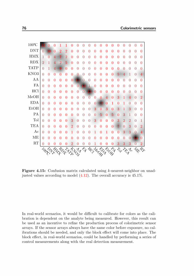
76 Colorimetric sensors

RTME

Ac

TEA

Tol

PAEtOH

EDA

MeOH

HCl

FAAA

KNO3

TATP

RDX

HMX

DNT

100�

203330001000200000

0140000000000000000

403300101000100000

203070000000200000

102230003000300000

001305050000000000

003130303000000000

0001010120000000000

204130400000000000

0000000001500000000

0000000001140000000

0000000000015000000

401450000000000000

000000000000009410

000000000000052412

000000000000027401

0000000000000220100

0000000000000110012100�

DNT

HMX

RDX

TATP

KNO3

AA

FA

HCl

MeOH

EDA

EtOH

PA

Tol

TEA

Ac

ME

RT

Figure 4.15: Confusion matrix calculated using k-nearest-neighbor on unad-justed values according to model (4.12). The overall accuracy is 45.1%.

In real-world scenarios, it would be difficult to calibrate for colors as the cali-bration is dependent on the analyte being measured. However, this result canbe used as an incentive to refine the production process of colorimetric sensorarrays. If the sensor arrays always have the same color before exposure, no cal-ibrations should be needed, and only the block effect will come into place. Theblock effect, in real-world scenarios, could be handled by performing a series ofcontrol measurements along with the real detection measurement.

4.6 Using histogram and manifold methods 77

RTME

Ac

TEA

Tol

PAEtOH

EDA

MeOH

HCl

FAAA

KNO3

TATP

RDX

HMX

DNT

100�

1001020000000100000

0140000000000000000

107320000000000000

201830000000000000

002280000000200000

000206060000000000

003020204000200000

0000010130000000000

205120400000000000

0000000001500000000

0000000000150000000

0000000000015000000

200800000000400000

000000000000057200

000000000000068000

0000000000000311000

0000000000000000140

0000000000000000014100�

DNT

HMX

RDX

TATP

KNO3

AA

FA

HCl

MeOH

EDA

EtOH

PA

Tol

TEA

Ac

ME

RT

Figure 4.16: Confusion matrix calculated using k-nearest-neighbor on adjustedvalues according to model (4.15). The overall accuracy is 62.8%.

4.6 Using histogram and manifold methods

In the lack of conclusive results based on single feature methods, a natural stepis to use other measures to represent the color from the sensor response. Oneidea is to make better use of the pixels that constitutes a measurement. Onemeasurement can consist of up to 1000 pixels so reducing a measurement to justone number is a drastic compression and it is likely that valuable informationis lost due to this compression. Two family of methods as applied; distancemeasures based on the Hellinger distance and distance measures based on theHausdorff distance. Each of these distance measures come in different flavors,which will be explained in depth in this section.

78 Colorimetric sensors

The i’th example (dye) is represented by Xi = {xi1, . . . , xini}, where xij is thej’th three–dimensional difference RGB pixel value between control and exposed,and ni is the number of pixels considered for the representation of the i’thexample. For several classifiers a notion of distance between examples is a keycomponent. To construct a distance between two examples in the bag-of-wordsrepresentation, we propose to represent each multi-instance example with adistribution and use the Hellinger distance as a metric between two examples.The motivation behind this approach is that differences between distributions,which are not directly measurable through the mean (or other moments), canstill be detected. This approach was demonstrated to be effective in severalapplication areas, e.g., disease classification using flow cytometry [Carter et al.,2009a] and document classification [Carter et al., 2009b].

4.6.1 Hellinger Distance

The Hellinger distance measures similarity between two probability measuresfi(x) and fk(x) and is given by

dHe(fi, fk)2 =

∫ (√fi(x) −

√fk(x)

)2dx (4.17)

i.e., the Euclidean distance between the square-root of the PDFs.By completingthe square of the integrand, the Hellinger distance can be rewritten to thefollowing equivalent alternative:

dHe(fi, fk)2 = 2− 2

∫ √fi(x)fk(x)dx (4.18)

If the probability measures are equal the Hellinger distance is dHe(fi, fj)2 = 0.

On the contrary, if the probability measures fi(x) and fk(x) are completelynon-overlapping, then dHe(fi, fj)

2 = 2.

Parzen window Kernel density estimator

The Hellinger distance requires a choice of model to construct the probabil-ity measure. The first one to consider is the Parzen window Kernel densityestimator. Assuming an underlying probability density function fi such thatxij ∼ fi for j = 1, 2, . . . , ni, one can associate Xi with the following kerneldensity estimate

fi(x) =1

ni

ni∑k=1

K(x− xik) (4.19)

4.6 Using histogram and manifold methods 79

where the kernel used is the isotropic squared exponential kernel

K(x) = 1/(2πσ2)D/2 exp(−‖x‖22/2σ2) (4.20)

As the sensor responses are RGB values the dimensionality is D = 3. The kernelparameter is chosen to be σ2 = 1 which seems like a reasonable smoothing.

To utilize the KDE a revision of the Hellinger distance expression is required.Looking at the integral term in (4.18), we inject a new term∫ √

fi(x)fk(x)dx =

∫fi(x) + fk(x)

fi(x) + fk(x)

√fi(x)fk(x)dx (4.21)

which enables us to split the integral in two:∫ √fi(x)fk(x)dx =∫

fi(x)

fi(x) + fk(x)

√fi(x)fk(x)dx+

∫fk(x)

fi(x) + fk(x)

√fi(x)fk(x)dx (4.22)

Rearranging by moving the denominator into the square root yields∫ √fi(x)fk(x)dx =∫

fi(x)

√fi(x)fk(x)

(fi(x) + fk(x))2 dx+

∫fk(x)

√fi(x)fk(x)

(fi(x) + fk(x))2 dx (4.23)

Defining a new function T (x) enables further simplification

T (x) =fi(x)

fi(x) + fk(x)(4.24)

Also notice that the two terms on the RHS in equation (4.23) are on the formof expectation. Combining T (x) and expectation yields∫ √

fi(x)fk(x)dx = Efi

[√T (x)(1 − T (x))

]+ Efk

[√T (x)(1 − T (x))

](4.25)

Substituting the result from (4.25) into (4.18) finally yields the Hellinger dis-tance on the alternative form

dHe(fi, fk)2 = 2− 2

(Efi

[√T (x)(1− T (x))

]+ Efk

[√T (x)(1 − T (x))

])(4.26)

80 Colorimetric sensors

where Eh[f ] =∫f(x)h(x)dx. A sample-based version of this expression is

computed by replacing the expectations with their sample averages and thedistributions with their kernel estimates,

Efi [√T (x)(1− T (x))] ≈ 1

ni

ni∑j=1

√T (xij)(1− T (xij))

Naturally, the distance calculation can be directly applied to a K-NN classifier.This approach can be considered an alternative to a set distance between twocollections instances.

Gaussian distribution

The second approach applied to the Hellinger distance is the multivariate normaldistribution using a full covariance matrix

fi(x) =1

(2π)d/2|Σi|d/2

exp

(−1

2(μi − x)

�Σi

−1 (μi − x)

)(4.27)

where μi is the mean and Σi the covariance matrix. Both parameters are esti-mated by maximum likelihood. Once the parameters are estimated the Hellingerdistance can be calculated in closed form. The result is derived by [Jebara et al.,2004] for the general case of a product probability kernel. Such a kernel is onthe form

Kp(fi, fj) =

∫RD

fi(x)pfk(x)

pdx (4.28)

Setting p = 1/2, we get the integral on the RHS of equation (4.18). Using theresult derived by [Jebara et al., 2004] when fi and fj are Gaussian distributionswith D = 3 yields

dHe(fi, fk)2 =

2− 4√2|Σ†|1/2|Σi||Σk| exp

(−1

4

(μ�

i Σ−1i μi + μ�

k Σ−1k μk + μ†�Σ†μ†

))(4.29)

where Σ† = (Σ−1i +Σ−1

k )−1 and μ† = Σ−1i μi +Σ−1

k μk.

4.6.2 The Hausdorff Distance

The Hausdorff distance measures distance between two point sets, and it issmall if all points in each set are close to some point in the other set. It is a

4.6 Using histogram and manifold methods 81

Chemical M P IM MH G E[pFD] #Significant

Acids 1 2 2 6 0 0.89 11Alcohols 0 0 0 0 3 0.15 3Amines 1 0 1 0 0 1.02 2Explosives 0 3 0 7 1 0.98 11

Table 4.5: Number of instances the best performing method is significantlybetter than another method. The methods are Mean, Parzen, Inner Mean, Mod.Hausdorff and Gaussian. E[pFD] is the expected positive false discoveries and nis the number of significant results. The inner mean is explained in appendix E.

fundamentally different measure than the Hellinger distance, e.i. the Hausdorffdistance becomes larger as the two point sets becomes further apart. On thecontrary, having to completely separating point sets the Hellinger distance willat most be two, no matter how far apart the point sets are. This property couldbe useful for comparing sensor color, as the amount of color change could beimportant.

First define the distance between two points xi and xk as the Euclidean distanced(xi,xk) = ‖xi − xk‖2. The distance between a point xi and a set Xk is thend(xi,Xk) = min

xk∈Xk

d(xi,xk). The Hausdorff distance is defined as

dHa(Xi,Xk) = max

{maxxi∈Xi

d(xi,Xk), maxxk∈Xk

d(xk,Xi)

}(4.30)

As an alternative approach one can use the modified Hausdorff distance whichis more robust in the presence of noise and outliers

dMH(Xi,Xk) = max

{1

NXi

∑xi∈Xi

d(xi,Xk),1

NXk

∑xk∈Xk

d(xk,Xi)

}(4.31)

It should be noted that this distance is not a metric as the triangle inequalityis not fulfilled [Dubuisson and Jain, 1994].

4.6.3 Evaluation using k-nearest-neighbor

The k-nearest-neighbor classifier is applied to each sensor for each representationtechnique. The dataset presented in table 4.3 is used to investigate the proposedmethods. The dataset is reduced to a five-class dataset as we only want toinvestigate the performance on the chemical families that the sensor has proven

82 Colorimetric sensors

Acids

Error[%

]

Sensor number

16 30 29 17 25 28 22 21 27 14 15 19 20 8 24 5 18 6 10 13

0

5

10

15

Alcohols

Error[%

]

Sensor number

19 27 23 12 16 17 18 22 30 21 29 20 5 8 28 6 11 13 14 3

5

10

15

Amines

Error[%

]

Sensor number

17 30 19 22 16 18 20 28 23 27 26 21 29 13 8 1 24 10 7 12

5

10

15

20

Explosives

Error[%

]

Sensor number

19 30 28 16 24 7 17 22 27 12 14 1 4 20 25 29 13 18 5 23

0

5

10

15

ParzenMod. HausdorffMeanGaussian

Figure 4.17: Individual error for the sensors. The dotted line corresponds torandom guessing. For acids and explosives it is 17.8% and 22.1% respectively.

4.6 Using histogram and manifold methods 83

able to detect. Based on the results shown in figure 4.13 the chemical familiesare: acids, alcohols, amines and explosives. For each of the labels, the accuracyfor each sensor is calculated using 1-vs-all. In this setting, the chosen chemicalfamily that is to be detected is kept as the class label and all other measurementsare labeled as ’other’.

To judge the differences in classification performance the McNemar significancetest [McNemar, 1947] is employed. The McNemar significance is a paired testwhich uses the the number of instances where two classifiers disagree about adecision. From this test p–values for each comparison is calculated21 and usethe multiple hypothesis framework proposed by Storey [Storey, 2002]. Based onthe p–values the expected positive false discoveries (E[pFD]) for our significantdifferences is calculated, that is, the expected quantity of wrongly significantresults among all identified significant results. These finding are summarizedin table 4.5 and the performance of the individual sensors are displayed in fig-ure 4.17.

The overall best performing distance measure is the modified Hausdorff methodalthough it is notable that this method is not best even once for alcohols whereasit is best on numerous occasions for acids and explosives. Looking into theindividual sensors reveal that the top sensor for acids largely overlap with thetop sensors for explosives (also see appendix F).

4.6.4 Evaluation using Gaussian process classification

It is clear that the distance measures are capturing “something” that the meancannot and that the distance measures generally performs on par or better thanthe mean. However, using distance measures it is no longer applicable to fusethe sensors simply by stacking the responses in a vector-space model. One so-lution is to use a classifier that is designed to work on distances, i.e. a kernelclassifier. Having distance measure d(X i,Xj) we can apply a distance substi-tution approach [Haasdonk and Bahlmann, 2004] using the squared exponentialkernel

k (Xi,Xj) = exp

(−1

�d(Xi,Xj)

)(4.32)

where � is the length scale. If the distance measure is a metric the correspondingGram matrix produced using the above expression is guaranteed to be a positivesemi-definite matrix [Haasdonk and Bahlmann, 2004].

21The null hypothesis is that the two classifiers have equal classification accuracy againstthe alternative that one classifier is better than the other.

84 Colorimetric sensors

We note that a valid covariance function may be constructed directly for theHellinger distance by considering the inner product given by the integral whichis known as the Probability Product Kernel [Jebara et al., 2004]; however, tomake a fair comparisons we treat the Hellinger distance like the other distancemeasure and employ (4.32) when converting any distance measure to a Grammatrix Also note that since the modified Hellinger distance is not a metric,the distance substitution kernel may not be positive definite [Haasdonk andBahlmann, 2004]. The same may apply to the Hellinger distances based onParzen windows as these distances are calculated using approximations.

The use of kernels provides a convenient way of integrating information from dif-ferent sensors by combining different kernels as a weighted sum. Thus, differentsensors can be combined by constructing the following kernel

k (Xi,Xj) = σ2I+M∑

m=1

αmk(Xm

i ,Xmj

)(4.33)

where each kernel function is the distance substitution kernel with one of therespective metrics.

Initially we want to establish the performance of GP in the same setting ask-NN. The results from this approach are shown in figure 4.18. In the case ofexplosives, the modified Hausdorff is again the top performer for the first twodyes, which is again dye 19 and 30. However for dye 28 and 24 the modifiedHausdorff coupled with GP yields an error of 21% and 30% respectively. Thismight very well be an effect of the modified Hausdorff not being a valid metricand as such the corresponding kernel might not be psd [Dubuisson and Jain,1994]. But as the case of k-NN, the figure does not show a clear indication ofwhich method is superior although it seems that modified Hausdorff is able tocapture more information about dye 19 and 30 than the the methods.

To fuse the different sensors a forward selection method using the following stepsis applied. 1) For a given sensor, perform a grid search of hyperparameters σ2,αm and �. 2) Find the hyper parameters by optimizing the evidence in GP usingthe optimal point found in the grid as initial guess. 3) Perform leave-one-outcross validation to get classification error. 4) Choose the sensor that yields thelowest classification error.

When fusing the dyes one by one using forward selection we find no significantresults between the methods (figure 4.19). To get a significant result (accordingto McNemar testing) the performance must at least differ 2.4 percent points butalready with one dye we are below that margin.

The modified Hausdorff method is however the overall best performing method.

4.6 Using histogram and manifold methods 85

Acids

Error[%

]

Sensor number

16 17 30 28 29 25 22 20 5 19 21 14 6 13 15 24 27 10 18 23

0

5

10

15

Alcohols

Error[%

]

Sensor number

27 19 30 16 29 22 13 17 18 23 12 21 20 6 8 28 1 2 3 4

5

10

15

Amines

Error[%

]

Sensor number

17 19 22 30 16 28 18 23 20 27 26 29 21 13 10 25 1 8 2 3

5

10

15

20

Explosives

Error[%

]

Sensor number

19 30 28 24 17 16 29 7 14 25 1 12 13 22 5 20 18 10 4 27

0

5

10

15

ParzenMod. HausdorffMeanGaussian

Figure 4.18: Confusion matrix calculated using k-nearest-neighbor on unad-justed values according to model (4.12). The overall accuracy is 45.1%.

86 Colorimetric sensors

Acids

Error[%

]

Number of sensors

1 2 3 4 50

1

2Alcohols

Error[%

]

Number of sensors

1 2 3 4 50

5

10

Amines

Error[%

]

Number of sensors

1 2 3 4 50

5

10Explosives

Error[%

]

Number of sensors

1 2 3 4 50

1

2

ParzenMod. HausdorffMeanGaussian

Figure 4.19: Confusion matrix calculated using k-nearest-neighbor on unad-justed values according to model (4.12). The overall accuracy is 45.1%.

It is particularly strong for classifying explosives. In the fusing scheme themodified Hausdorff method also works well and is the overall best performer.

4.7 Related work

Over the past years colorimetric sensor arrays has been developed and success-fully applied in various areas. In 2000 a paper co-authored by Kenneth S. Suslickwas published in Nature [Rakow and Suslick, 2000]. Since then, Suslick has pi-oneered work in applying the colorimetric sensor arrays in various areas, suchas the application of the colorimetric sensor array for detecting volatile organiccompounds in the gas phase [Suslick et al., 2004b, Rakow et al., 2005] as wellas for identifying different organic compounds in the liquid phase [Zhang andSuslick, 2005, Zhang et al., 2006].

The colorimetric sensor is a fascinating technique for detecting different chemicalcompounds belonging to various classes, like amines, cyanides, alcohols, arenes,

4.8 Summary 87

ketones, aldehydes and acids in the parts-per-million (ppm) and parts-per-billion(ppb) ranges [Rakow et al., 2005, Lim et al., 2009, Zhang and Suslick, 2007]. Amore elaborate description on the state-of-the-art for chemical sensing is givenin paper found in appendix F.

The feature extraction and sensor evaluation has not been improved since thepaper published by Suslick in 2004 [Suslick et al., 2004b]. All papers subsequentto this paper follows the same line of data processing. First, the data is extractedusing dye localization, the dot size is reduced to accommodate for the coffeestain effect and the mean difference color response is extracted and representedin a vector-space model. The data is then visualized suing principal componentanalysis and hierarchical cluster analysis [Janzen et al., 2006, Suslick et al.,2010, Luo et al., 2010]. The hierarchical cluster analysis is carried out usingthe Euclidean distance between measurements so in essence this corresponds toperforming 1-nearest-neighbor.

4.8 Summary

This chapter highlighted the major developments made for colorimetric sensorarrays. The entire processing pipeline was described, from the preprocessing ofimages to the classification of analytes and identification of important chemos-elective compounds.

There are numerous ideas on how to further explore the results put forwardin this chapter, especially the results presented in section 4.6. Obviously theissues for dye number 14, 24 and 28 (figure 4.18) when combining the modifiedHausdorff with Gaussian process classification is an issue that must be put un-der scrutiny. The issue could be that the Modified Hausdorff distance is nota real metric which is required in order to guarantee that the resulting kernelis positive semi-definite. Another issue is that the Modified Hausdorff is quiteprone to outliers. This is an issue only a few bad pixels are required to ruina measurements. An easy way to solve this could be to remove the outliersby doing image smoothing as specified in section 4.1. Expanding the Hellingerdistance measure by using Gaussian mixture models is also worthwhile to con-sider. Finally, in the lack of one distance measure clearly outperforming theothers, it could be of interest to combine all the features extracting methods byeither using multiple kernel learning or further developing the MKL-equivalentcovariance function presented in equation (4.33)

Other ideas are to explore is based on the results in section 4.5. Measuring thedye color before exposing the sensor to analyte enhances the signal substan-

88 Colorimetric sensors

tially. These finding could possibly be build into the framework of Manifoldand Histogram methods. The ideas presented here are currently being inves-tigated in collaboration with Ryota Tomioka22 and a paper is currently underdevelopment. This paper compiles the major research findings presented in thischapter as well as the possible enhancements listed.

22Assistant Professor at Department of Mathematical Informatics, The University of Tokyo

Chapter 5

Multisensor approach fordection of explosives

The other three sensors within the Xsense project were only briefly described.This is because all the work that has been carried on these sensors is containedwithin a recently submitted paper (appendix A), and it would make little senseto spend too much time on writing a chapter repeating everything in the sameformat. The main innovation of the paper is the multisensor approach, wheremeasurements were collected under identical conditions utilizing all the sensorsin the Xsense project. The highlights of the paper found in appendix A is brieflypresented here.

By using the technologies shown in figure 5.1 it is possible to simultaneouslydetect explosives in trace concentrations. These are the sensors that were de-scribed in the introduction (section 1.4) and the working principles will not berepeated here. Instead readers are refered to appendix A.

A dataset consisting of the four analytes were collected; ammonium nitrate(AN), 2,4-diaminotoluene (DAT), 2,4-dinitrotoluene (DNT), and diesel. Thedataset is inspired by a post-blast scenario of e.g. a car bomb. The numberof measurements as well as the classification results (obtained using 1-nearest-neighbor) is shown in table 5.1.

90 Multisensor approach for dection of explosives

A.

400 μm

100 μm

Heater elements

B.

300 μm

C.

Before After

4 cm

D.

300 nm

Measurementresistor

Figure 5.1: Illustration of the four sensing techniques: (A). Calorimetric sen-sor; (B). Cantilever sensor; (C). Colorimetric sensor; (D). SERS sensor.

Analyte Calorimetric Cantilever Colorimetric SERS

AN 2/3 N.D 2/2 8/8DAT 3/3 N.D 6/7 5/5DNT 3/3 3/3 5/5 6/6Diesel N.D N.D 4/4 N.D

Table 5.1: Detection rates of the four sensors. False positives are not includedin the table although it should be emphasized that there are neither false pos-itives nor false negatives for DNT. Some scenarios are marked as no detection(N.D.) as by inspecting the sensor response it was deemed that the sensor wasnot able to detect the analyte in question, but only show that the analyte wasnot causing false alarms for DNT.

As described in the introduction, all of the Xsense sensors were designed todetect TNT so it is no surprise that all the DNT measurements were identifiedcorrectly for all the sensors. More interestingly it seems that the colorimetricsensor is the most versatile in the current setup. However, comparing e.g. the

91

cantilever and the colorimetric sensors on the grounds on these results is unfair.The cantilever is functionlized using just one chemoselective compound whereasthe colorimetric sensor utilized 41 compounds. The situation more confirms twoideas: one) sensor fusion improves detection (as has been described in chapter 4,a colorimetric sensor array is sensor fusion, it is just that they are build on thesame technology), and two) The sensors seems to compliment each other well,although it is questionable whether their detection patterns are independent.

92 Multisensor approach for dection of explosives

Chapter 6

Conclusion and future work

This thesis has shown advanced on the data analysis of data collected usingfive different sensors. The first one was based on quartz crystal microbalancecrystals (QCM). The inclusion of the QCM sensor was mostly an opportunitythat presented itself back when the sensors within the Xsense project was stillbeing developed. Handling the QCM data was a very good experience and giventhat QCM resembles cantilever sensing closely it also allowed me to be setupnicely for future data. The cantilever sensor is a sensor that is chemically coatedjust like QCM, so QCM and cantilevers can be considered very much alike, onlythe medium is different.

The task for the QCM sensor was the detection of benzodioxol, an importantprecursor for ecstasy. Despite the fact that QCM produces close to linear re-sponses it has been a growing trend to apply artificial neural networks to bothclassify analytes and to perform density estimation. One of the hypothesis whenthe QCM data was analyzed (from a signal processing point of view), was thatadequate performance would be obtained using linear methods to both classifyand estimate concentration levels.

In chapter 3 [paper B] we showed that the linear method SVD greatly out-performs ANN in classification and given that SVD is much faster than ANN,based on the dataset, it makes little sense to apply ANN. In regression a similarpicture showed. ANN was again outperformed by the linear PCR method but

94 Conclusion and future work

also the GPR, and it actually turned out that GPR was overall the best method.Likely because GPR can adapt to the minor non-linearities that sneak into anydataset that is measured from real-world. To summarize, linear methods suchas SVD and PCR are preferable over ANN. GPR might provide an extra edgewhen estimated concentrations but with the application of GPR some modelcomplexity follows.

The majority of the work presented has mostly concerned colorimetric data han-dling and here a number innovations was proposed. The main hypothesis thatwe wanted to investigate was the possibility to improve the feature extractionfor colorimetric sensors. In chapter 4 we showed that the traditional approachcan be improved in two ways. First, ff the colors are calibrated, or the colors be-fore exposure is included in the analysis the classification accuracy is improved.Secondly, by using more advanced methods to represent the sensor response,such as the modified Hausdorff, the overall system accuracy is improved.

In the same chapter, we also proposed satisfactory solutions to the importantproblem of sensor fusion for colorimetric sensor arrays. This was solved by aGaussian Process approach, where the algorithm successfully identified sensorsthat improved the accuracy.

With the combination of Gaussian Process classification and the modified Haus-dorff some issues arose. The modified Hausdorff is not a real metric and as suchthe Gram matrix that is calculated based on the modified Hausdorff might vi-olate the requirements of positive semidefinite matrices. These issues will belooked upon in the near future and if we can solve them the results will beincluded in the upcoming paper. With this paper, a toolbox that contains allthe code that I have written during the project will also be released. When webegun to use colorimetric sensors, we found that there was quite a lot of workrequired to even begin to handle the data. This toolbox should help makingcolorimetric sensor arrays more accessible to other research groups. Also, theresults (and the accompanying software) on feature selection presented shouldenable researchers to analyze their sensors better and enable them to iterativelydesign better colorimetric sensor arrays.

The remaining three sensors within the Xsense project where briefly describedin chapter 5. The main innovation of the work was the multisensor approach,where measurements were collected under identical conditions utilizing all thesensors in the Xsense project. The results should be considered as a proof ofconcept and they imply that the sensors within the Xsense project are suitableto be combined and that the overall accuracy would be improved in all foursensors were integrated.

The work within the Xsense group has spurred the project, “Multisensor DVD-

95

platform - MUSE”, Danish Council for Strategic Research grant 11-115314 andled by Anja Boisen, DTU Nanotech. Within this project, future work will in-clude system integration of sensors which will enable the possibility for collect-ing simultaneous measurements from all sensors. The system integration willfacilitate automatic data collection that will provide sufficient data to enablethe possibility of using data fusing. Only then can a full multisensor systemutilizing sensors based on different physical properties be proclaimed.

The sensors included initially are SERS and cantilevers, as these are the tech-nologies that fits into the designed integrated system. The application is dif-ferent too, here the goal is to measure sepsis in blood and hormones in wastewater. However, a lot of the work that was presented in thesis, and especiallythe work with sensor fusion developed for the colorimetric sensor array serve asa platform. Kernel methods are very suitable for data fusion as kernels naturallyallow sensors with widely different signals to be merged. In this framework, onehas to design kernels that fit the data well and then they can be merged. I ampersonally very excited and grateful that I can be apart of this new researchproject.

96 Conclusion and future work

Appendix A

Miniaturized multisensoryapproach for the highlysensitive and selectivedetection of explosives

Tommy S. Alstrøm, Natalie V. Kostesha, Filippo G. Bosco, Michael S. Schmidt,Jesper K. Olsen, Michael Bache, Jan Larsen, Mogens H. Jakobsen, and AnjaBoisen. Miniaturized multisensory approach for the highly sensitive and se-lective detection of explosives. Submitted to Journal of Materials Chemistry,2013.

The paper was submitted to the Journal of American Chemical Society (JACS)and was rejected with the editor suggesting that we submit the paper to a morespecialized journal. JACS being one of the most important journals in the fieldof chemisty with an impact factor of 9.91 (2011), we were happy they took thepaper under consideration and gave reviews that have improved this work. Thepaper is now submitted to Journal of Materials Chemistry.

The layout of the paper has been revised.

98

Miniaturized multisensory approach for the highlysensitive and selective detection of explosives

Tommy S. Alstrøm,† Natalie V. Kostesha,‡ Filippo G. Bosco,‡

Michael S. Schmidt,‡ Jesper K. Olsen,‡ Michael Bache,‡

Jan Larsen,† Mogens H. Jakobsen,‡ and Anja Boisen∗,‡

†Department of Applied Mathematics and Computer Science,Building 305, DK-2800 Kgs. Lyngby, Denmark, and

‡Department of Micro- and Nanotechnology,Ørsteds Plads, Building 345east, DK-2800 Kgs. Lyngby,

Technical University of Denmark

E-mail: Anja.Boisen@nanotech.dtu.dk

ABSTRACT

Substances like explosives, explosives derivatives, and energetic materials areextremely dangerous, even in small quantities. To this date no single measure-ment technology has demonstrated the desired detection performance. In theattempt to improve the overall detection accuracy, we propose a miniaturizedmultisensory approach for sensing explosives, in real-time with the perspectiveof integrating them into a handheld device. This makes our approach relevantfor defense, clearance, and security applications. The sensing system, which issimilar to an electronic nose, is based on the application of a unique setup offour sensors based on calorimetric, cantilever, colorimetric, and surface enhancedRaman spectroscopy. Although the sensors are yet to be integrated, we haveconducted an experiment where the measurements are collected simultaneouslyutilizing all sensors. Hence, it is garanteed that the sensors worked under iden-tical conditions. The identification of 2,4–dinitrotoluene as well as backgroundmolecules such as ammonium nitrate, 2,4–diaminotoluene, and diesel is demon-strated. To improve the responses from the sensors, the data is preprocessedand enhanced using methods such as least squares regression and Gaussian pro-cess regression. The preprocessed sensor responses are then identified as one

∗To whom correspondence should be adressed

99

of the target analytes using a 1–nearest neighbor approach. Finally the perfor-mance of each the sensors are compared. All of the sensors were able to detect2,4–dinitrotoluene without error, even though the chemically closely related 2,4–diaminotoluene was in the dataset. Further, it turned out at the sensors were noable to detect the other analytes without error. The individual error patternsfor the sensors are not identical either, which indicates that a single integrateddevice containing all sensors would enhance detection performance.

A.1 Introduction

Preventing the development, production, stockpiling, transport and use of illegalexplosives, is one of the most significant challenges for law enforcement agencies.The detection techniques and equipment (sensors) must not only detect a varietyof hidden explosives, but must also be able to detect components that can beused for fabrication of such explosives.

For most explosives the equilibrium vapor concentration is in the range fromparts-per-million (ppm) to parts-per-billion (ppb) range, making detection achallenging task. Ideally, explosive identification systems have to be quick,precise and deliver a high level of confidence. This requires reliable, selectiveand sensitive detection techniques that provide identification of trace amountsof explosives within a few minutes.

The minimization of false alarms1,2 is identified as a priority in chemical sens-ing devices. Currently, the screening and identification of suspicious substancesis often done by canine units or specialized teams which employ sophisticatedmethods e.g. terahertz pulsed spectroscopic imaging3,4, gas chromatography,mass spectroscopy5 or long-range Raman spectrometry6. The screening is char-acterized by a high assignment of personnel and high costs7. Furthermore, inrelation to the requested volume the methods are often slow. Airport screeningrequires systems to handle up to 10 passengers per minute7. Canine units workswiftly but require breaks, have significant upkeep cost and can only be appliedby expert handlers7

The use of detection systems based on multisensory approaches could tremen-dously help in the fast identification of explosives, reduce false alarms and pro-vide new opportunities for the real-time analysis of explosives8. A simultane-ous application of a variety of sensor techniques, which are based on differentmeasurement principles, will enhance the collection of data where erroneous de-tections are statistically independent. This improves the possibility to reliablydetect presence of explosives molecules with a high confidence9,10.

100

The application of multisensory detection technologies has a great perspective inthe identification of different analytes and today’s market also show a demandfor portable multisensory instruments11–13. These instruments are sensitiveenough to detect low concentrations of analytes and can within few secondsidentify common volatile compounds, such as ammonia, methane, phosphine,chlorine, carbon monoxide, hydrogen sulfide and other dangerous gases in air.For example, in the product “GDA 2” by AirSense Analytics, a combination ofdifferent sensors is applied. The product comprises an ion mobility spectrometer,a photo ionization detector, two semiconductor gas sensors and an electrochemi-cal cell. Other detecting combinations like an array of chemical sensors9,14,15 ora surface modified with different sensing layers can also be called a multisensoryapproach. While the “GDA 2” is a handheld device with a weight of 4.2 kg, wepropose the use of micro- and nano sized sensors which can facilitate a handhelddevice that is even lighter and which can contain a multitude of sensors. Thesesensors also facilitate the realization of miniaturized sensor systems to be usedin for example security and surveillance, potentially allowing the sensor unit tohave a footprint of only a few mm2.

The four measurement techniques that are being investigated are : calori-meter, cantilever, colorimetric array, and surface enhanced Raman spectroscopy(SERS). The utilized sensors are shown on Figure A.1.

Calorimetry is widely applied to investigate thermal properties of various sam-ples analytes. In this work we present a micro-calorimetric sensing device (Fig-ure A.1A) that is based on differential thermal analysis (DTA) where the tem-perature difference between two highly sensitive temperature sensors is mea-sured16–19. One sensor is loaded with a sample analyte and the other is leftblank. Using integrated heating elements both sensors are heated at a constantrate while the differential temperature is continuously measured. At certaintemperatures the sample will sublimate, melt, evaporate or deflagrate whichresults in a change in differential temperature. Using the calorimetric sensor,we have previously demonstrated successful detection of TNT, PETN and RDXmolecules20,21.

The cantilever based sensor is an established micro- and nano-mechanical sens-ing tool for trace detection of bio-chemical compounds22–24. The response ofcantilever-based sensors can be measured by monitoring change in resonance fre-quency of the cantilevers. A negative frequency shift is generated through massadded to the surface of the cantilevers25,26. Generally, the larger the resonancefrequency change, the higher the amount of a given analyte is present in thesample. We measure the change in resonance frequency on chips each contain-ing eight cantilevers (Figure A.1B)27. The cantilever’s surface is functionalizedwith receptor molecules designed to specifically bind target analytes28. In thiswork cantilevers are employed in the detection of DNT molecules. For this

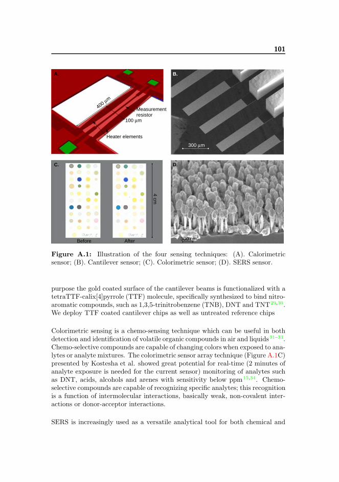
101

A.

400 μm

100 μm

Heater elements

B.

300 μm

C.

Before After

4 cm

D.

300 nm

Measurementresistor

Figure A.1: Illustration of the four sensing techniques: (A). Calorimetricsensor; (B). Cantilever sensor; (C). Colorimetric sensor; (D). SERS sensor.

purpose the gold coated surface of the cantilever beams is functionalized with atetraTTF-calix[4]pyrrole (TTF) molecule, specifically synthesized to bind nitro-aromatic compounds, such as 1,3,5-trinitrobenzene (TNB), DNT and TNT29,30.We deploy TTF coated cantilever chips as well as untreated reference chips

Colorimetric sensing is a chemo-sensing technique which can be useful in bothdetection and identification of volatile organic compounds in air and liquids31–33.Chemo-selective compounds are capable of changing colors when exposed to ana-lytes or analyte mixtures. The colorimetric sensor array technique (Figure A.1C)presented by Kostesha et al. showed great potential for real-time (2 minutes ofanalyte exposure is needed for the current sensor) monitoring of analytes suchas DNT, acids, alcohols and arenes with sensitivity below ppm15,34. Chemo-selective compounds are capable of recognizing specific analytes; this recognitionis a function of intermolecular interactions, basically weak, non-covalent inter-actions or donor-acceptor interactions.

SERS is increasingly used as a versatile analytical tool for both chemical and

102

biochemical sensors in liquid and gas phase. In fact, single molecule detectionwith SERS has been demonstrated35. SERS-based sensors rely on increasingthe number of inelastically scattered photons from an analyte adsorbed on aso-called SERS substrate. A new class of SERS substrates have been devel-oped at DTU Nanotech using standard cleanroom silicon processing techniques(Figure A.1D)36. This class of substrates demonstrates a signal enhancementfactor of up to 7.8 · 106 due to plasmonic effects from a nanostructured andsilver coated surface. In this paper we demonstrate how this new class of sub-strates can be used to greatly improve the Raman enhancement thus enablingexplosives detection which is approximately a factor of 100 more sensitive thancommercially available SERS substrates36,37.

In the strategic research project Xsense funded by the Danish Agency for Scienceand Technology we work towards the development and implementation of fourindividual miniaturized sensor technologies for detection of military and impro-vised explosives 8,38. By using the technologies described above (Figure A.1)it is possible to simultaneously detect explosives in trace concentrations. Ourhypothesis is that sufficient reliability can be ensured by merging several in-dependent and sensitive measuring principles. The basic scientific goal of theXsense project is to focus on the development and refinement of the miniatur-ized sensors in order to achieve a detection limit towards explosives of 1 ppb(DNT and TNT being the major test molecules). A summary of the sensorscharacteristics and sensing principles are given in Table A.1.

A.2 Results and discussion

To confirm that our sensors work independently we conducted experimentswhere the sensors were sequentially exposed to the analytes: ammonium ni-trate (AN), 2,4-diaminotoluene (DAT), 2,4-dinitrotoluene (DNT), and diesel.All sensors have previously been individually used for DNT detection – herewe for the first time present combined measurements and data analysis on fourcommon analytes, including potentially highly disturbing backgroundmolecules.We chose DNT as the explosive molecule as DNT is a decomposition product ofTNT, the explosive most commonly deployed in landmines in the ground today.Ammonium nitrate is widely used as a fertilizer and is thus a common back-ground molecule. Also, ammonium nitrate is a main compound in production ofimprovised homemade-fertilizer based bombs. DAT has been chosen since thismolecule is chemically closely related to DNT; DNT carries two nitro-groupsin the structure, DAT carries two amino-groups in the same positions.. Thus,DAT could cause concern about sensor selectivity and heighten false alarm rate.Diesel is chosen as an environmental disturbance that would often be present ina mine field and in post-blast scenarios, e.g. a detonated car bomb. Diesel is

103

Table A.1: Comparison of sensor characteristics.

Sensor char-acteristics

Calorimetric Cantilever Colorimetric SERS

Sensingprinciple:

Thermalanalysis ofsamplemolecules.

Determinationof mass andsurface stresschange

Chemicalinteractions:donor-acceptor,non-covalent,covalent, van derWaals,host-guest

Identification ofvibrationalscattering profilethroughRaman-basedspectroscopy

Lowerdetectionlimit:

ppt18 ppb39 ppm40 ppm41

Measurementtime:

1 minute 2 min forindication, 10min forequilibriumresponse

2 min 5-10 min

Robustness: Very robust Sensitive toabrupt changesin humidity andtemperature

Sensitive to lightand oxygen.Robust tomechanicalstress

Mechanicallyfragile

WorkingConditions:

Gas phase Gas and liquidphase

Gas and liquidphase

Gas and liquidphase

Sensorshelf-life42:

Years Several months Several months Several months

Recyclingtime:

Chip cleaningafter ∼1000measurements

Sensorregenerationafter positivedetection

Single time use Single time use

Feasibility: Compatible withsilicon-basedmass production

Compatible withsilicon-basedmass production

Compatible withchemicalmicro-arraymass production

Compatible withsilicon-basedmass production

Scalability: Extendable tosome othertarget analytes

Applicable tovirtually anyreceptor-analyteassay

Applicable toalmost all classesof chemicalcompounds

Applicable todetection ofvirtually anyRaman-activecompound

also the most widely employed fuel in heavy truck and automotive engines usedby military forces and mine clearance agencies. The signal processing of thesensors responses was tailored to each sensor as the responses are very differentin nature. Elaborate details on the signal processing can be found in the Sup-porting Information. In this section we discuss the individual response of eachsensor to the four chemical compounds and show examples of sensor responses.

104

0 0.5 1 1.5 2 2.5

0

10

20

30

40

50

60

70

80

Time [ms]

Δ T

empe

ratu

re [C

]

NH4NO

3

DAT

DNT

Diesel

Figure A.2: Example calorimetric responses of the four target analytes af-ter trimming and smoothing. A distinct response is obtained for each analytedue to the different thermal properties. Additional responses are found in theSupporting Information.

A.2.1 Calorimetric responses

A sample will at certain temperatures change phases and either sublimate, melt,evaporate or deflagrate which results in a change in the differential temperaturein a differential thermal analysis. Figure A.2 shows the calorimetric responsefrom the calorimetric sensor, of ammonium nitrate, DAT, DNT and diesel.

Significant and distinct responses are obtained for ammonium nitrate, DAT andDNT. A very limited response is observed for diesel. A positive ΔT means thatthe sample sensor is cooler than the reference sensor. The initial increase in ΔTis due to a higher thermal mass of the sensor containing the sample. Sublimationwill start cooling the sample sensor further. The first peak observed for DATand ammonium nitrate and the change in slope observed for DNT (at ∼0.5 ms)is due to melting of the sample. The last peak is due to sample depletion. From

105

an analysis of the responses after the last peaks the signal decay is observedto be fastest for DNT21. This is interpreted as due to deflagration whereasDAT and ammonium nitrate decay at a rate determined by the characteristictime constant of the integrated temperature sensor. The different calorimetricsignatures are a result of different analytes having different vapor pressures,phase change temperatures, phase change enthalpies and thermal mass for thedifferent phases.

The responses of the calorimetric sensor can be handled using various ap-proaches, e.g., as described by Olsen43. The peak value of the sensor responsegives an indication of the amount of analyte on the sensor as well as the type.Studies have shown that for explosives the shape of the sensor response is highlydiscriminative43.

A.2.2 Cantilever responses

For analyte detection eight silicon-gold-coated cantilevers were functionalizedusing TTF molecules. As a control we used eight blank silicon-gold-coatedcantilevers without immobilized TTF on the surface. The measuring principlehas been described elsewhere44.

The results show how TTF-coated cantilevers shift their resonance frequenciesup to one order of magnitude more when exposed to DNT than when exposed tothe other vapor samples. This behavior indicates a higher selectivity for DNTwith respect to a control. As has been shown before, TTF molecules can inter-act with electron-deficient molecules30, and have demonstrated high specificityto nitro-aromatic explosives such as 2,4,6-trinitrotoluene, trinitrobenzene andpicric acid, respectively45

To evaluate signals obtained from the cantilever-based sensor a statistical anal-ysis was performed. Figure A.3 presents the response of 64 independent can-tilevers with and without TTF as a cumulative distribution function (CDF). Forsmall sample sizes (in our case each chip provide up to N=8 measurements), theCDF will more accurately display the nature of the data compared to a plotwith mean and variance. Using the CDF we can graphically display whether weexpect the detection to fail or succeed.

From Figure A.3 we can see that TTF–coated cantilevers also react to DATwhere a slight positive frequency shift is observed. This positive change is likelycaused by both mass addition and surface properties modifications, generatedfrom unspecific binding of molecules on both cantilever surfaces46. The blankcantilevers partially respond when exposed to ammonium nitrate (negative shift)

106

−800

−600

−400

−200

0

200

Δ S

hift

[Hz]

NH4 NO

3

DATDiesel

DNTNH

4 NO3

DATDiesel

DNT

TTF coating Control(blank coating)

n=1

n=2

n=3

n=4

n=5

n=6

n=7

Figure A.3: Data analysis obtained from the cantiliver-based sensor on thepresence of the target analytes. Data was collected from 64 independent can-tilevers (eight chips), exposed to the four selected analytes. The destribution ofresponses are presented as a cumulative distribution function (CDF). The valueof CDF is initially 0 (below the bars) and once n cantilevers have been mea-sured, the CDF function will be n/N, where N is to total amount of measuredcantilevers. Above the bars the CDF has the value 1. Due to sporadic mal-function of cantilevers, N=6 for DNT-TTF and AN-Control, N=7 for AN-TTFand DNT-Control, N=8 for remaining bars. The number of event is marked bycolor. Additional cantilever responses are found in the Supporting Information.

and diesel (positive shift), while they don’t present significant frequency changefor DAT and DNT. The blank cantilevers’ response is used as reference foreliminating measurement artifacts on the TTF functionalized sensors.

The negative frequency shift generated by diesel is attributed to sticking ofhydrocarbons on the cantilever surfaces. The TTF layer which covers the spe-cific cantilevers probably acts as an oleophobic protective coating that preventsunspecific sticking of diesel on the treated surface.

107

A.2.3 Colorimetric responses

In the colorimetric sensor 41 chemo-selected compounds (dyes) which are ableto change color in the presence of different molecules were chosen. The detectingprinciple of the colorimetric sensor array and the data analysis using a differencemap (DM) have been described previously15,40.

Results demonstrate that the colorimetric sensor is able to detect vapor ema-nating by DAT, DNT, ammonium nitrate and diesel. From the data analysisit seems that almost each chosen dye in the array reacts with the analytes ofinterest. Ammonium nitrate was detected by 8 dyes out of 41; where only 3dyes in the array were particularly specific to ammonium nitrate. Diesel wasdetected by 5 dyes; where only 1 dye was particularly specific to diesel. DATwas detected by 6 dyes where 1 dye was specific to DAT. Finally, DNT wasdetected by 9 dyes where 4 of the dyes were particularly specific to DNT.

Using DM analysis it is observe that a combination of chemo-selective dyescompose a unique fingerprint for each analyte. Also, with DM analysis it ispossible to study the unspecific cross-reactivity for our applied dyes. In total10 of the dyes show similar color-change response to the analytes. Specificcross-reactivity is observed during detection of DAT and DNT, where 2 dyesdemonstrated similar color change. For ammonium nitrate and DAT 3 dyes showcross-reactivity. Cross-reactivity is also observed between ammonium nitrate,DAT and diesel, as well as between DNT and diesel. However, there is nocross-reactivity observed between ammonium nitrate and DNT. DM is widelyused in colorimetry. However, the color representations in DM is weak andfurthermore negative color change values are eliminated (a color difference isbasically calculated by taking the absolute value of a pixel value before andafter exposure to an analyte). Also, for most dyes scaling is needed in order tomake color differences visible. As an alternative to DM we suggest to use barplots where each bar represents the CDF of the color change for a given dyecolor (RGB) when exposed to a given analyte.

Data analysis is here generated after the mathematical analysis of color changes.Mathematical algorithms were applied in order to analyze positive and negativevalues during color changes with statistical methods; the sensory output was putinto a numerical form. As an example, Figure A.4 shows exposure responsesfrom dye 4, dye 22 and dye 28., Those dyes were identified as significant inthe array. The CDF plotting offers some advantages over the traditional DManalysis as no scaling is needed and negative values can be plotted directly onthe graph.

From Figure A.4 dye number 4 shows a cross-reactive signal to ammonium

108

−100

−50

0

50

100

Δ C

olor

val

ue [a

.u.]

NH4 NO

3

DATDiesel

DNTNH

4 NO3

DATDiesel

DNTNH

4 NO3

DATDiesel

DNT

n=1

n=2

n=3

n=4

n=5

n=6Dye 4 − Red Dye 22 − Blue Dye 28 − Blue

Figure A.4: Representation of response as cumulative densities function anal-ysis for chemo-selective compounds of 4, 22 and 28 in the colorimetric sensorarray when target analytes were present. Up to seven repetitions (color bar)were performed to evaluate color changes of the dyes (left axis). Bars on thescheme represent color changes after calculation of the median and probabilityvalues of the signal. N=2 for AN, N=7 for DNT, N=4 for Diesel and N=5 forDNT. Additional responses are found in the Supporting Information.

nitrate, DAT and diesel; however the specific signal is demonstrated for DNTonly. Dyes number 22 and 28 show unique responses to all analytes. In thepresence of DAT the dye number 22 turned from green to pink. However, in thepresence of other analytes the same dye exhibited color change from green totransparent or light green in different intensity. For dye number 28 a positivevalue for color changes was observed for ammonium nitrate. In the presence ofammonium nitrate the light green color of the dye turned to dark green, while inthe presence of other analytes the dye changed color from light green to yellow.

109

200 400 600 800 1000 1200 14000

2000

4000

6000

8000

10000

Raman shift [cm−1]

Inte

nsity

[a.u

.]

DNT

DAT

NH4NO

3

Diesel

Figure A.5: Example responses of Raman signals from SERS substrates whenexposed to target. It is seen that the peaks defining DNT are not found in thespectra from the other substances thus enabling DNT to be distinguished fromthe potential background substances. The horizontal bars mark the frequencyintervals where notable peaks should occur for the given analyte. Additionaldetails on responses are found in the Supporting Information.

A.2.4 SERS responses

The exposure results of the SERS surface to DAT, DNT, ammonium nitrateand diesel show a specific spectrum for each compound. Figure A.5 shows thevarious spectra with the peak areas of interest highlighted.

For the recorded DNT spectrum the areas of interest are around 650 cm−1 and1150 cm−1. These peaks are shifted compared to the bulk Raman values of pureDNT crystals found in literature where the nitro groups give origin to a distinctpeak at around 1350 cm−1 and 1530 cm−1. The origin of the measured peaksis thus difficult to identify47. Ammonium nitrate has a single distinct peak at850 cm−1 and 650 cm−1, again this is ∼200 cm−1 lower when comparing with

110

bulk measurements in literature, where the nitrate symmetric stretch at 1040cm−1 and the nitrate in-plane bending mode at 712 cm−1 are the recognizablepeaks48.

When comparing the DNT spectrum with the DAT spectrum a clear distinc-tion to DNT can be seen as DAT has a large peak at 1300-1400 cm−1 and anadditional peak at 500 cm−1.

The spectrum of diesel shows a comparable flat profile. This is expected as dieselis usually composed by a complex mixture of saturated and aromatic carboncompounds of a 8-22 chain length and often diesel includes other additives toimprove the engines combustion performance. The fouling properties of dieseland large variety of composition can thus coat a sensor surface and potentiallyovershadow a signal from DNT49,50.

A.2.5 Classification and combined responses

A careful mathematical analysis was performed to statistically analyze responsesobtained from calorimetric, cantilever, colorimetric and SERS-based sensors. Inthis paper we used new methods for extracting features from all sensors and tocategorize and evaluate signals in order to understand the efficiency of sensingtechnologies for detecting military and improvised explosives. By using machinelearning classifiers the quality and robustness of these features were determined.

Applied sensors must not only be able to classify explosives, explosive deriva-tives and volatile organic compounds. They must also be able to measure thecertainty of the classifier. This means there is a need for classifiers that not onlygive a decision, but also give a posterior probability about the decision. Thepre-calibration of the system or the application of libraries (classifiers) allowswith high precision to identify a broad range of target compounds.

All the sensors were able to give positive responses to DNT, but in order toassess the recognition performance of each sensor we have created an artificialclassification system. Prior to the classification system each sensor output isprocessed using a custom made signal processing system. As the sensor re-sponses are of very different nature each sensor has a unique signal processingsystem which is described in the supporting information. The classification sys-tem consists of the 1-Nearest Neighbor classification method51 as this methodis easy to apply when few examples of measurements exist. The method classi-fies each measurement in turn and treats this measurement as unknown. Themeasurement is compared to all the other measurements which are treated asknown and then selecting the measurement that most resembles the unknown

111

measurement. The unknown measurement is classified as the same analyte asthe known measurement. The classification results are illustrated as confusionmatrices shown in Figure A.6.

The array of sensors demonstrated a high classification rate for explosives, likeDNT with zero false negatives. The calorimetric sensor (Figure A.6A) made onemisclassification which is an ammonium nitrate sample which was detected asDAT. The cantilever sensor (Figure A.6B) was very unreliable for ammoniumnitrate, DAT and diesel; DNT was detected with high precision. This was ex-pected as the cantilever-based sensor only operated with a TTF-coating thatis specifically designed to detect DNT and similar analytes. The colorimetricsensor is a more specific sensor compared to calorimetric and cantilever sen-sors. The colorimetric sensor comprises 41 unique chemo-selective compounds,including 25 TTFs (Figure A.1C). The results (Figure A.6C) show that thissensor is able to detect all analytes; the sensor was able to detect DNT withboth zero false negatives and zero false positives (all 5 measurements were clas-sified correctly), also ammonium nitrate and diesel gave zero false negatives.DAT showed one false positive and control measurements (environment) gavetwo false positives responses (one for DAT and one for diesel).

The SERS sensor is a more specific sensor compared to the colorimetric sensoras our SERS sensor scans 2000 frequencies. SERS makes a perfect classification(Figure A.6D) although it should be remarked (as described in section 2.4) thatdiesel is not actually detected as it consists of a mixture of different lengthcarbon chains that read out as a broad Raman signature overlapping with thatof many carbon based analytes. The confusion matrix shows that diesel doesnot give rise to false alarms. In general, the sensors have a high detectionrate and it is quite possible that the false alarms could be lowered significantlyor even extinguished entirely if more measurements are made as this wouldnot only give more knowledge of the sensor but also make more sophisticatedclassification systems applicable.

To summarize how the sensors complement each other we draft up all detectionrates in Table A.2. The table shows that DNT is detected in all cases for allfour sensors. The higher dimensional sensors (colorimetric and SERS) are themost specific making very few detection mistakes.

A.3 Conclusions

From our experiments we can conclude that the most versatile sensor seems to bethe colorimetric sensor as this sensor was able to positively detect all the testedanalytes only making one misclassification to DAT. However, the sensor also had

112

Predicted Analyte

Act

ual A

naly

te

3 0 0 0

0 3 0 0

0 0 3 0

1 0 0 2NH4NO

3

NH4NO

3

A.

DAT DNT Diesel

DAT

DNT

Diesel

Predicted Analyte

Act

ual A

naly

te

0 0 1 2

0 3 0 0

1 0 2 0

3 0 0 0NH4NO

3

NH4NO

3

B.

DAT DNT Diesel

DAT

DNT

Diesel

Predicted Analyte

Act

ual A

naly

te

6 0 0 0

0 5 0 0

0 0 4 0

0 0 0 2NH4NO

3

NH4NO

3

C.

DAT DNT Diesel

DAT

DNT

Diesel

Predicted Analyte

Act

ual A

naly

te

5 0 0 0

0 6 0 0

0 0 8 0

0 0 0 8NH4NO

3

NH4NO

3

D.

DAT DNT Diesel

DAT

DNT

Diesel

Figure A.6: Confusion matrix presenting the responses of the sensors on thepresence of ammonium nitrate, DAT, DNT and diesel calculated using 1-NN.A. Calorimetry – classification rate of 11/12; B. Cantilever – classification rateof 5/12; C. Colorimetric – classification rate of 17/1752; D. SERS – classifi-cation rate of 27/27. Herein, rows indicate the true class; columns indicatethe predicted class and the number indicate the counts; e.g. for A. two of theammonium nitrate measurements was correctly identified as ammonium nitratewhile one measurement was incorrectly identified as DAT. Each element in thematrix is colored based on the number of measurements classified according tothe given matrix element relative to the total number of measurements. Themore measurements in the element the darker the element is.

113

Table A.2: Detection rates of the four sensors. False positives are not includedin the table although it should be emphasized that there are neither false pos-itives nor false negatives for DNT. Some scenarios are marked as no detection(N.D.) as by inspecting the sensor response it was deemed that the sensor wasnot able to detect the analyte in question, but only show that the analyte wasnot causing false alarms for DNT.

Analyte Calorimetric Cantilever Colorimetric SERSDAT 3/3 N.D 6/7 5/5DNT 3/3 3/3 5/5 6/6Diesel N.D N.D 4/4 N.DNH4NO3 2/3 N.D 2/2 8/8

two false alarms, one for DAT and one for diesel which indicates that the sensorat times may be too sensitive. Based on Table A.2 the calorimetric and SERSsensors have in this experimental setup very similar properties. The advantageof the calorimetric sensor (Table A.1) is that the sensor can conduct hundredsof repeated measurements without requiring cleaning or manual operation, andtherefore this sensor is ideal to use as a screener before applying samples to theother sensors. The cantilever requires cleaning between each measurement whilecolorimetric and SERS are single disposable sensors, thus it is desirable to applythese sensors only if a sample has a suspicious content. These results encouragethe fabrication of a sensor network of the sensors and conduct a larger scaleexperiment where sensor fusion is applied.

In this paper we have shown that by establishing a network of four miniatur-ized independent sensors the reliability in explosives detection can potentiallybe improved significantly. Proof of the concept has been confirmed for all foursensor technologies hence the ongoing effort is thus in optimizing sensitivity andintegrating all the sensors into one device. The inherent design qualities of thecompleted device should enable its use by personnel with minimal training thusmaking explosives detection capabilities accessible beyond trained dog teams.The proposed system has potential to be highly suitable for the use in anti-terrorefforts, border control, monitoring of environment and mine clearance. Futurework will include system integration of sensors which would enable the possi-bility for collecting simultaneous measurements from all sensors. The systemintegration would facilitate automatic data collection that will provide sufficientdata to enable the possibility of using a data fusing classification algorithm.

114

A.4 Experimental

Analytes that has been exposed to sensors: 2,4-diaminotoluene (DAT), 2,4-dinitrotoluene (DNT), ammonium nitrate were all from Sigma (St. Louise,MO, USA). Diesel was used as received from a Shell petrol station.

A.4.1 Sensor preparations

The colorimetric sensor array consists of 41 different chemo-selective compoundsselected from a set of compounds described by Kostesha et al53. SERS sub-strates were developed as described by Schmidt et al54. The cantilevers fab-rication and modification was reported by Bosco et al44. Calorimetric chipswere fabricated following the protocol developed by Olsen et al16–19. Tetrathia-fulvalene–Calix[4]pyrroles are used in the fabrication of the colorimetric sensorarray as well as coating for the cantilevers30.

A.4.2 Experimental setup

All the measurements were conducted using a vapor generator which was builtand tested at Technical University of Denmark, Department of Micro- and Nan-otechnology. The generator used the principle where a nitrogen gas is passedthrough a heated reservoir containing the analyte of interest. An illustration ofthe vapor generator system can be seen in Figure A.7. Deposition is done byplacing a sensor close to the exhaust of the system making the analyte condenseon the sensor surface.

It consists of an explosive reservoir, an oven, a mass flow controller and variousfittings. The explosive reservoir is a copper tube containing glass wool. The an-alytes DAT, DNT and ammonium nitrate was first dissolved and then injectedin the glass wool using a syringe whereas diesel was injected without treatment.Ethanol was used for DAT and DNT and water for ammonium nitrate. Beforethe reservoir was ready for use solvent was first evaporated at low temperature.The copper tube was inserted into the heating oven and connected to a nitro-gen flow connector, controlled by a mass flow controller. When the nitrogenflowed through the heated reservoir it became saturated with the analyte. Byreducing the nozzle diameter to 2 mm the velocity of the hot saturated vaporwas increased. The cantilever, calorimetry and SERS surface sensors were keptat approximately 1 mm distance from the nozzle opening for 2 minutes, thus apart of the analyte condensated on the sensor surface. The colorimetric sensor

115

Heaters

Heaters

Analyte reservoir

Sensors

Analyte in vapor phase

Nitrogen flow

Figure A.7: Illustration of the vapor generator used for deposition of analytesonto the sensors.

was only exposed to the analyte vapors at a greater distance from the nozzleopening.

Pictures from the colorimetric sensor were scanned through an ordinary flatbedscanner (Epson V750-M Pro Perfection scanner) immediately after immobiliza-tion of dyes and after exposure of analytes. Pictures were obtained at 600 dotsper inch in RGB color format. Data analysis obtained from the colorimetricsensor was analyzed as described in earlier work31,34. Raman measurementswere performed using 780 nm wavelength excitation at a power of 0.5 mW for 2seconds. The laser spot diameter was 3.1 μm. Raman measurements were made

116

on SERS substrates where silver coated nanopillars were in the pre-leaned, post-leaned and non-leaning configurations54. The nanopillars were brought to leanby 1 μL water.

A.4.3 Signal Processsing

The calorimetry sensor response is contaminated by white measurement noise.We smooth the response by using Gaussian Process regression55 as this methodeffectively removes the noise and at the same time we do not need to concernabout choosing model parameters. The smoothed responses are directly appliedto the 1-NN classifier.

Our cantilever measurement system collects readout of the entire cantilever sur-face for each cantilever on the chip, thus one measurement consist of 8 cantileversurface readouts, where one surface contains multiple readouts. These readoutsare reduced to a single value by taking the mean bending of the entire surface44.All measurements are manually inspected as cantilevers on occasion malfunc-tions. In these cases the measurement is regarded as not available. The finalmeasurement that is applied to the 1-NN classifier is the mean value of the TTFcoated cantilevers subtracted with the mean value of the blank cantilevers.

The colorimetric sensor response is a pair of images; an image of the clean sensorand an image of the exposed sensor. The colorimetric sensor response undergoesseveral steps before the response is applied to the 1-NN classifier56. The finalresult is one RGB value from each dye is selected and concatenated into onevector for each measurement. These vectors are applied to the classifier.

The SERS responses are baseline corrected using a 5th order polynomial cal-culated using least squares regression. The functional values of the polynomialis then subtracted from the original response and then normalized. The spec-trum in the interval [100,1000] is then applied to the 1-NN classifier. To makethe classification we train one 1-NN classifier per reading mode (pre-bending,post-bending, no bending) and then make the final prediction using majorityvoting.

Acknowledgement

We acknowledge the financial support from the Danish Agency for Scienceand Technology’s, Program Commission on Nanoscience Biotechnology and IT(NABIIT). Case number: 2106-07-0031 – Xsense - Miniaturized sensors for ex-

117

plosives detection in air. We acknowledge Kent A. Nielsen, Carsten Johnsen andJan O. Jeppesen, Department of Physics and Chemistry, University of South-ern Denmark for providing TTF molecules for the cantilever and colorimetricsensors. Finally we thank Mads S. Jensen from Danish Emergency Manage-ment Agency for providing insight regarding current challenges on explosivesdetection for intelligence agencies.

Supporting Information Available

The full data set will be described in the Supporting Information document. Thedata set is not showed in this text in completeness; however the full collectionof data accompanied with supporting MATLABTM scripts that was used toproduce all figures in this paper as well as the signal processing modules can bedownloaded at http://www.imm.dtu.dk/pubdb/p.php?6401

A.5 REFERENCES

[1] Yanghai Gui, Changsheng Xie, Jiaqiang Xu, and Guoqing Wang. Detectionand discrimination of low concentration explosives using MOS nanoparticlesensors. Journal of hazardous materials, 164(2-3):1030–5, May 2009. ISSN1873-3336. doi: 10.1016/j.jhazmat.2008.09.011.

[2] Jehuda Yinon. Detection of Explosives by Electronic Noses. AnalyticalChemistry, 75(5):98 A–105 A, March 2003. ISSN 0003-2700. doi: 10.

1021/ac0312460.

[3] Michael J. Fitch, Megan R. Leahy-Hoppa, Edward W. Ott, and RobertOsiander. Molecular absorption cross-section and absolute absorptivityin the THz frequency range for the explosives TNT, RDX, HMX, andPETN. Chemical Physics Letters, 443(4–6):284–288, August 2007. ISSN0009-2614. URL http://www.sciencedirect.com/science/article/

pii/S0009261407008676.

[4] Jeffrey Barber, Daniel E. Hooks, David J. Funk, Richard D. Averitt, An-toinette J. Taylor, and Dmitri Babikov. Temperature-Dependent Far-Infrared Spectra of Single Crystals of High Explosives Using TerahertzTime-Domain Spectroscopy. The Journal of Physical Chemistry A, 109(15):3501–3505, March 2005. ISSN 1089-5639. doi: 10.1021/jp044384h.URL http://dx.doi.org/10.1021/jp044384h.

[5] Stacy-Ann Barshick and Wayne H. Griest. Trace Analysis of Explosives inSeawater Using Solid-Phase Microextraction and Gas Chromatography/Ion

118

Trap Mass Spectrometry. Analytical Chemistry, 70(14):3015–3020, May1998. ISSN 0003-2700. doi: 10.1021/ac980060b. URL http://dx.doi.

org/10.1021/ac980060b.

[6] J. Chance Carter, S. Michael Angel, Marion Lawrence-Snyder, Jon Scaffidi,Richard E. Whipple, and John G. Reynolds. Standoff Detection of HighExplosive Materials at 50 Meters in Ambient Light Conditions Using aSmall Raman Instrument. Applied spectroscopy, 59(6):769–775, June 2005.URL http://as.osa.org/abstract.cfm?URI=as-59-6-769.

[7] Dana A. Shea and Daniel Morgan. Detection of explosiveson airline passengers: Recommendation of the 9/11 Commissionand related issues. CRS Report for Congress, April(RS21920):1–6, 2007. URL http://oai.dtic.mil/oai/oai?verb=getRecord&amp;

metadataPrefix=html&amp;identifier=ADA453711.

[8] Xsense. Xsense - Miniaturized Sensors for Explosives Detection in Air,2012. URL http://www.xsense.dk.

[9] Joseph R. Stetter, S. Strathmann, Carol McEntegart, Maylin Decastro,and William R. Penrose. New sensor arrays and sampling systems for amodular electronic nose. Sensors and Actuators B: Chemical, 69(3):410–419, October 2000. ISSN 0925-4005. URL http://www.sciencedirect.

com/science/article/pii/S0925400500005037.

[10] Baranidharan Raman, Douglas C. Meier, Jon K. Evju, and Steve Semancik.Designing and optimizing microsensor arrays for recognizing chemical haz-ards in complex environments. Sensors and Actuators B: Chemical, 137(2):617–629, April 2009. ISSN 0925-4005. URL http://www.sciencedirect.

com/science/article/pii/S0925400508008125.

[11] AIRSENSE Analytics, 2012. URL http://www.airsense.com/en.

[12] RKI Instruments, Inc., 2012. URL http://www.rkiinstruments.com.

[13] Industrial Scientific, 2012. URL http://www.indsci.com.

[14] Kenneth S. Suslick, Keren I. Hulkower, Avijit Sen, Mitchell A. Sroka, andWilliam B. McNamara III. Method and apparatus for detecting ammoniafrom exhaled breath, August 2004.

[15] Natalie V. Kostesha, Tommy S. Alstrøm, Carsten Johnsen, Kent A. Nielsen,Jan O. Jeppesen, Jan Larsen, Mogens H. Jakobsen, and Anja Boisen. De-velopment of the colorimetric sensor array for detection of explosives andvolatile organic compounds in air. In Proceedings of SPIE, volume 7673,pages 76730I–76730I–9, 2010. doi: 10.1117/12.850310.

119

[16] Dechang Yi, Anders Greve, Jan H. Hales, Larry R. Senesac, Zachary J.Davis, Don M. Nicholson, Anja Boisen, and Thomas Thundat. De-tection of adsorbed explosive molecules using thermal response ofsuspended microfabricated bridges. Applied Physics Letters, 93(15):154102, October 2008. ISSN 00036951. doi: DOI:10.1063/1.

3002285. URL http://dx.doi.org/doi/10.1063/1.3002285http://

link.aip.org/link/?APPLAB/93/154102/1.

[17] Dechang Yi, Larry Senesac, and Thomas Thundat. Speciation of En-ergetic Materials on a Microcantilever Using Surface Reduction. Scan-ning, 30(2):208–212, 2008. ISSN 1932-8745. doi: 10.1002/sca.

20096. URL http://dx.doi.org/10.1002/sca.20096http://www.ncbi.

nlm.nih.gov/pubmed/18288710.

[18] Larry R. Senesac, Dechang Yi, Anders Greve, Jan H. Hales, Zachary J.Davis, Don M. Nicholson, Anja Boisen, and Thomas Thundat. Micro-differential thermal analysis detection of adsorbed explosive moleculesusing microfabricated bridges. Review of Scientific Instruments, 80(3):35102, March 2009. ISSN 1089-7623. doi: 10.1063/1.3090881.URL http://link.aip.org/link/?RSI/80/035102/1http://link.aip.

org/link/?RSINAK/80/035102/1.

[19] Anders Greve, Jesper K. Olsen, Natalya L. Privorotskaya, Larry R.Senesac, Thomas Thundat, William P. King, and Anja Boisen.Micro-calorimetric sensor for vapor phase explosive detection withoptimized heat profile. Microelectronic Engineering, 87(5-8):696–698, May 2010. ISSN 0167-9317. doi: 10.1016/j.mee.2009.

12.069. URL http://www.sciencedirect.com/science/article/pii/

S0167931709009125http://dx.doi.org/10.1016/j.mee.2009.12.069.

[20] Jesper K. Olsen, Anders Greve, Larry R. Senesac, Thomas Thundat, andAnja Boisen. Differential thermal analysis microsystem for explosive de-tection. In Thomas George, M Saif Islam, and Achyut K Dutta, editors,Micro- and Nanotechnology Sensors, Systems, and Applications III, volume8031, page 80312P. SPIE, 2011. doi: 10.1117/12.883960. URL http://

link.aip.org/link/?PSI/8031/80312P/1.

[21] Jesper K. Olsen, Larry R. Senesac, Thomas Thundat, and Anja Boisen.Trace explosives detection by micro differential thermal analysis. In Mi-cro Electro Mechanical Systems (MEMS), 2011 IEEE 24th InternationalConference on, pages 984–987, 2011. ISBN 1084-6999 VO -.

[22] Roberto Raiteri, Massimo Grattarola, Hans-Jurgen Butt, and Petr Skladal.Micromechanical cantilever-based biosensors. Sensors and Actuators B:Chemical, 79(2–3):115–126, October 2001. ISSN 0925-4005. URL http://

www.sciencedirect.com/science/article/pii/S0925400501008565.

120

[23] Jurgen Fritz. Cantilever biosensors. Analyst, 133(7):855–863, 2008. ISSN0003-2654. URL http://dx.doi.org/10.1039/B718174D.

[24] Anja Boisen, Søren Dohn, Stephan S. Keller, Silvan Schmid, and MariaTenje. Cantilever-like micromechanical sensors. Reports on Progress inPhysics, 74(3):36101, 2011. ISSN 0034-4885. URL http://stacks.iop.

org/0034-4885/74/i=3/a=036101.

[25] Jurgen Fritz, Marko K. Baller, Hans P. Lang, Hugo E. Rothuizen, PeterVettiger, Ernst Meyer, Hans-Joachim Guntherodt, Christoph Gerber, andJames K. Gimzewski. Translating Biomolecular Recognition into Nanome-chanics. Science, 288(5464):316–318, 2000. doi: 10.1126/science.288.

5464.316. URL http://www.sciencemag.org/content/288/5464/316.

abstract.

[26] Maria L. Sushko, John H. Harding, Alexander L. Shluger, Rachel A. McK-endry, and Moyu Watari. Physics of Nanomechanical Biosensing on Can-tilever Arrays. Advanced Materials, 20(20):3848–3853, 2008. ISSN 1521-4095. doi: 10.1002/adma.200801344. URL http://dx.doi.org/10.

1002/adma.200801344.

[27] Filippo G. Bosco, En-Te Hwu, and Anja Boisen. High-throughput readoutsystem for cantilever-based sensing of explosive compounds. In ThomasGeorge, M Saif Islam, and Achyut K Dutta, editors, Micro- and Nanotech-nology Sensors, Systems, and Applications II, volume 7679, page 767925.SPIE, 2010. doi: 10.1117/12.850008. URL http://link.aip.org/

link/?PSI/7679/767925/1.

[28] James K. Gimzewski, Christoph Gerber, Ernst Meyer, and Reto R.Schlittler. Observation of a chemical reaction using a micromechani-cal sensor. Chemical Physics Letters, 217(5–6):589–594, 1994. ISSN0009-2614. doi: 10.1016/0009-2614(93)E1419-H. URL http://www.

sciencedirect.com/science/article/pii/0009261493E1419H.

[29] Kent A. Nielsen, Won-Seob Cho, Jan O. Jeppesen, Vincent M. Lynch, JanBecher, and Jonathan L. Sessler. Tetra-TTF Calix[4]pyrrole: A RationallyDesigned Receptor for Electron-Deficient Neutral Guests. Journal of theAmerican Chemical Society, 126(50):16296–16297, November 2004. ISSN0002-7863. doi: 10.1021/ja044664a.

[30] Jung S. Park, Franck Le Derf, Christopher M. Bejger, Vincent M. Lynch,Jonathan L. Sessler, Kent A. Nielsen, Carsten Johnsen, and Jan O. Jeppe-sen. Positive Homotropic Allosteric Receptors for Neutral Guests: Annu-lated Tetrathiafulvalene–Calix[4]pyrroles as Colorimetric Chemosensors forNitroaromatic Explosives. Chemistry - A European Journal, 16(3):848–54,January 2010. ISSN 1521-3765. doi: 10.1002/chem.200902924.

121

[31] Natalie V. Kostesha, Tommy S. Alstrøm, Carsten Johnsen, Kent A. Nielsen,Jan O. Jeppesen, Jan Larsen, Anja Boisen, and Mogens H. Jakobsen. Multi-colorimetric sensor array for detection of explosives in gas and liquid phase.In Proceedings of SPIE, volume 8018, pages 80181H–80181H–12, 2011. doi:10.1117/12.883895.

[32] Chen Zhang and Kenneth S. Suslick. A colorimetric sensor array for organ-ics in water. Journal of the American Chemical Society, 127(33):11548–9,August 2005. ISSN 0002-7863. doi: 10.1021/ja052606z.

[33] Kent A. Nielsen, Luis Martın-Gomis, Ginka H. Sarova, Lionel Sanguinet,Dustin E. Gross, Fernando Fernandez-Lazaro, Paul C. Stein, Eric Lev-illain, Jonathan L. Sessler, Dirk M. Guldi, Angela Sastre-Santos, andJan O. Jeppesen. Binding studies of tetrathiafulvalene-calix[4]pyrroleswith electron-deficient guests. Tetrahedron, 64(36):8449–8463, September2008. ISSN 0040-4020. URL http://www.sciencedirect.com/science/

article/pii/S0040402008010740.

[34] Tommy S. Alstrøm, Jan Larsen, Natalie V. Kostesha, Mogens H. Jakobsen,and Anja Boisen. Data representation and feature selection for colorimetricsensor arrays used as explosives detectors. In IEEE International Workshopon Machine Learning for Signal Processing (MLSP), pages 1–6, 2011. doi:10.1109/MLSP.2011.6064615.

[35] Kneipp Kneipp, Yang Wang, Harald Kneipp, Lev T. Perelman, IrvingItzkan, Ramachandra R. Dasari, and Michael S. Feld. Single moleculedetection using surface-enhanced Raman scattering (SERS). Physical Re-view Letters, pages 1667–1670, 1997. URL http://link.aps.org/doi/

10.1103/PhysRevLett.78.1667.

[36] Ivan Talian, Klaus B. Mogensen, Andrej Orinak, Dusan Kaniansky, andJorg Hubner. Surface-enhanced Raman spectroscopy on novel black silicon-based nanostructured surfaces. Journal of Raman Spectroscopy, 40(8):982–986, 2009. ISSN 1097-4555. URL http://dx.doi.org/10.1002/jrs.2213.

[37] Klarite. Klarite, 2012. URL http://www.d3technologies.co.uk.

[38] Michael S. Schmidt, Natalie V. Kostesha, Filippo G. Bosco, Jesper K.Olsen, Carsten Johnsen, Kent A. Nielsen, Jan O. Jeppesen, Tommy S.Alstrøm, Jan Larsen, Thomas Thundat, Mogens H. Jacobsen, and AnjaBoisen. Xsense - a miniaturised multi-sensor platform for explosives detec-tion. In Proceedings of SPIE, volume 8031, pages 803123–803123–7, 2011.doi: 10.1117/12.884050.

[39] Jessica L. Arlett, Edward B. Myers, and Michael L. Roukes. Comparativeadvantages of mechanical biosensors. Nature Nanotechnology, 6(4):203–215,

122

April 2011. ISSN 1748-3387. URL http://dx.doi.org/10.1038/nnano.

2011.44.

[40] Kenneth S. Suslick, Neal A. Rakow, and Avijit Sen. Colorimetric sensorarrays for molecular recognition. Tetrahedron, 60(49):11133–11138, Novem-ber 2004. ISSN 00404020. doi: 10.1016/j.tet.2004.09.007.

[41] Desiree S. Grubisha, Robert J. Lipert, Hye-Young Park, Jeremy Driskell,and Marc D. Porter. Femtomolar Detection of Prostate-Specific Anti-gen: An Immunoassay Based on Surface-Enhanced Raman Scattering andImmunogold Labels. Analytical Chemistry, 75(21):5936–5943, September2003. ISSN 0003-2700. doi: 10.1021/ac034356f. URL http://dx.doi.

org/10.1021/ac034356f.

[42] The sensors should be carefully sealed as they will react with the environ-ment swiftly

[43] Jesper Kenneth Olsen. Micro Calorimetric Sensors for Explosives Detec-tion. PhD thesis, Technical University of Denmark (DTU), 2011.

[44] Filippo G. Bosco, En-Te Hwu, Ching-Hsiu Chen, Stephan Keller, MichaelBache, Mogens H. Jakobsen, Ing-Shouh Hwang, and Anja Boisen. Highthroughput label-free platform for statistical bio-molecular sensing. LabChip, 11(14):2411–2416, 2011. doi: 10.1039/C1LC20116F. URL http://

dx.doi.org/10.1039/C1LC20116F.

[45] Dae-Sik Kim, Vincent M. Lynch, Kent A. Nielsen, Carsten Johnsen, Jan O.Jeppesen, and Jonathan L. Sessler. A chloride-anion insensitive colorimetricchemosensor for trinitrobenzene and picric acid. Analytical and bioanalyti-cal chemistry, 395(2):393–400, 2009. doi: 10.1007/s00216-009-2819-4.

[46] Javier Tamayo, Daniel Ramos, Johan Mertens, and Montserrat Calleja. Ef-fect of the adsorbate stiffness on the resonance response of microcantileversensors. Applied Physics Letters, 89(22):224104, 2006. doi: 10.1063/1.

2388925. URL http://link.aip.org/link/?APL/89/224104/1.

[47] Alejandro Blanco, Nairmen Mina, Miguel E. Castro, Jairo Castillo-Chara,and Samuel P. Hernandez-Rivera. Spectroscopic investigation of the spec-troscopic signatures of 2,4-DNT and 2,6-DNT: their interactions with sandparticles. In Russell S Harmon, J Thomas Broach, John H Holloway, andJr., editors, Detection and Remediation Technologies for Mines and Mine-like Targets IX, volume 5415, pages 1357–1366. SPIE, 2004. doi: 10.1117/12.542870. URL http://link.aip.org/link/?PSI/5415/1357/1.

[48] Esam M. A. Ali, Howell G. M. Edwards, and Ian J. Scowen. In-situ detection of single particles of explosive on clothing with confo-cal Raman microscopy. Talanta, 78(3):1201–1203, May 2009. ISSN

123

0039-9140. URL http://www.sciencedirect.com/science/article/

pii/S0039914008009211.

[49] Michael J. Kleeman, James J. Schauer, and Glen R. Cass. Size and Com-position Distribution of Fine Particulate Matter Emitted from Motor Ve-hicles. Environmental Science & Technology, 34(7):1132–1142, February2000. ISSN 0013-936X. doi: 10.1021/es981276y. URL http://dx.doi.

org/10.1021/es981276y.

[50] John W. Haas III, James M. Sylvia, Kevin M. Spencer, Thomas M. John-ston, and Susan L. Clauson. Surface-enhanced Raman sensor for nitroexplo-sive vapors. In Abinash C Dubey, James F Harvey, and J Thomas Broach,editors, Detection and Remediation Technologies for Mines and MinelikeTargets III, volume 3392, pages 469–476. SPIE, 1998. doi: 10.1117/12.

324179. URL http://link.aip.org/link/?PSI/3392/469/1.

[51] Christopher M. Bishop. Pattern Recognition and Machine Learning.Springer, Secaucus, NJ, USA, 2006. ISBN 0387310738.

[52] The colorimetric sensor contained 5 additional control measurements wherethree of them resulted in false alarms; hence the classification rate is 19/22.See Supporting Information for details.

[53] Jan O. Jeppesen, Natalie V. Kostesha, Carsten Johnsen, Kent A. Nielsen,Anja Boisen, and Mogens H. Jakobsen. Multisensor array useful for de-tection and/or identification of an analyte (e.g. amines, alcohols, ketonesand thiols) in the gas phase or in the liquid phase, comprises at least twodifferent chemo-selective heteroaryl compounds, 2011.

[54] Michael S. Schmidt, Jorg Hubner, and Anja Boisen. Large Area Fabri-cation of Leaning Silicon Nanopillars for Surface Enhanced Raman Spec-troscopy. Advanced Materials, pages OP11–OP18, November 2011. ISSN09359648. doi: 10.1002/adma.201103496. URL http://www.ncbi.nlm.

nih.gov/pubmed/22105972.

[55] Carl E. Rasmussen and Christopher K. I. Williams. Gaussian Processesfor Machine Learning. MIT Press, April 2006. URL http://www.

gaussianprocess.org/gpmlhttp://www.ncbi.nlm.nih.gov/pubmed/

15112367.

[56] Tommy S. Alstrøm and Jan Larsen. Feature Extraction and Signal Rep-resentation for Colorimetric Sensor Arrays. Technical report, DTU Infor-matics, 2011. URL http://www.imm.dtu.dk/pubdb/p.php?5845.

124

A.6 Supporting Information for “Miniaturized multisen-sory approach for the highly sensitive and selective detec-tion of explosives”

A.6.1 Sensor responses and signal processing

Herein the full data set will be described. The data set is not showed in this textin completeness; however the full collection of data accompanied with supportingMATLABTM scripts that was used to produce all figures in this paper as wellas the signal processing modules can be downloaded at http://www.imm.dtu.dk/pubdb/p.php?6401.

The measurements are done in four consecutive days where each analyte istested in one day. The reason for doing it on different days is that the vaporgenerator needs thorough cleaning when changing the analyte to avoid possiblecross contaminations. The change takes some time and makes it impossible withour current experimental setup to measure on different analytes in the same day.

For all the sensors except SERS, DNT, DAT and diesel are all evaporated at70� with a 2 mm distance to a to a 2 mm nozzle opening for 2 minutes (DATwas handled differently for the calorimetric sensor, see 1.1 in this supportinginformation). Due to the much lower vapor pressure of ammonium nitrate thetemperature was increased to 250� to get comparable amounts of added massfor a 2 minute evaporation time. SERS chips are evaporated using the samesettings except for evaporation time. Only a 1 minute evaporation time is usedas 2 minute evaporation time causes crystallizations of analyte on the surface.

A.6.1.1. The calorimetric sensor

Figure A.8 shows a clean bridge of the calorimetric sensor. Figure A.9-A.12

Figure A.8: An image of the bridge that is located on the calorimetric sensorin clean state.

shows the responses (after smoothing) for the calorimetric sensor when exposed

125

to the analytes. The condensation of DAT turned to be troublesome (Fig-ure A.10). To force the DAT to condensate a droplet of nitrogen was put onthe opposite side of the sensor thus cooling the sensor while depositing DAT.First the sensor was evaporated for 2 minutes, but this turned out to saturatethe sensor (Figure A.10, top panel), so the evaporation time was reduced to oneminute (middle and bottom panel).

When measuring, both reference and measurement sensor is calibrated in orderto be heated with the same linear heating rate by applying a calibrated voltagewaveform. Calibration ensures constant heating rate, and that reference andmeasurement chip signal is kept close together when no sample is present. Asbaseline correction, each time a sensor reading is performed, we also measure10 times with no sample present. The median of these 10 samples is used tobaseline correct the signal.

The baseline corrected signal is contaminated with noise. This noise is removedusing Gaussian Process Regression (GPR). As fitting the hyper parameters whenusing GPR is not a convex optimization problem, we use 10 restarts and thenselect the model that has the maximum evidence. Readers interested in furtherdetails are referred to the downloadable package.

Figure A.9: The three runs for the calorimetric sensor when exposed to DNT.The shape is reproducible and distinct from the other responses. The left imagesare images of the bridge just before the heating pulse is applied to the sensor.Clearly the bridge is loaded with DNT molecules. The right hand images arethe corresponding profiles obtained when the heating pulse is applied.

126

Figure A.10: The three runs for the calorimetric sensor when exposed to DAT.

Figure A.11: The three runs for the calorimetric sensor when exposed toammonium nitrate.

A.6.1.2. The cantilever sensor

A priori we know that cantilever measurements are prone to high variabilityso in order to improve robustness 16 cantilevers are used per measurement, 8cantilevers with TTF coating and 8 cantilevers with no coating. If the sensoris able to make a detection there should be a significant difference betweenthe changes of resonance frequency for TTF coating cantilevers vs. non-coatedcantilevers.

127

Figure A.12: The three runs for the calorimetric sensor when exposed toDiesel. No surface images of the calorimetric sensor are shown as it turned outthat we were not able to condensate Diesel on the sensor.

Analysis of the data shows that the data is in general normally distributed butthere are expectations. For this reason we employ the nonparametric methodKruskal-Wallis for significance test. Kruskal-Wallis assumes that the distribu-tions to be tested are identically shaped. Since our data have few samples withhigh variance we don’t have enough data to verify this claim hence we shoulduse the conclusions with caution for p-values close to the significance level whichwe choose to 0.05. For all three cases the test show that there are significantdifferences when the target analyte is Diesel and DNT with p¡0.01. For DATand ammonium nitrate the results are more ambiguous. For experiment 1 therewas found a significant difference for DAT and ammonium nitrate however, forexperiment 2 and 3 no significant differences was found.

In order to apply 1-NN the measurements for each experiment are reduced toa single number by using the median response of an experience subtracting themedian response for the blank cantilever.

Figure A.13-A.16 contains the complete data gathered from the cantilever sen-sor. The entries with “n.a.” represent a cantilever that could not be read withthe optical system, i.e., some kind of malfunction with the cantilever in question.

A.6.1.3. The colorimetric sensor

The colorimetric sensor responses is a series of images pairs (before exposure to

128

DAY 1 DAT TTF Blank

Before After Shift Before After Shift EXP Cantilever exposure exposure exposure exposure

# (Hz) (Hz) (Hz) (Hz) (Hz) (Hz) 1 4964.6 4957.6 -7 4929.7 4935.8 6.1 2 4991.1 5001.3 10.2 4942.3 4943.4 1.1 3 5032.6 5042.2 9.6 4944.5 4947.8 3.3 1 4 5133.4 5153.3 19.9 4947 4943.7 -3.3 5 5258.7 5285.9 27.2 4949.1 4951.1 2 6 5454.6 5520.8 66.2 4952.7 4951.3 -1.4 7 5731 5846.1 115.1 4968 4973.3 5.3 8 5543.2 5655.2 112 4976.1 4976 -0.1 1 n.a. n.a. n.a. 4988.7 4917.7 -71 2 5165.5 4999.1 -166.4 4934.3 4914.4 -19.9 3 4886.1 4979.4 93.3 4985.5 4939.2 -46.3 2 4 4955.6 5023 67.4 4754.4 4922.9 168.5 5 5214.4 5139.1 -75.3 4877.58 4936.8 59.22 6 5011.7 5280.7 269 4972.8 4957.8 -15 7 5234.6 5321.8 87.2 5011 4962.5 -48.5 8 5144.56 5182.9 38.34 4971.5 4972.25 0.75 1 4934.5 4946 11.5 4829.7 4917.1 87.4 2 4897.9 4981.3 83.4 4778.2 4870.3 92.1 3 5033.9 5021.9 -12 4922.9 4928.9 6 3 4 5229.2 5137.2 -92 4717.3 4923 205.7 5 5198.2 5283.1 84.9 4881.2 4930.9 49.7 6 5298.4 5529.5 231.1 4959.1 4956 -3.1 7 5633.1 5728.7 95.6 4958.2 4958.9 0.7 8 n.a. n.a. n.a. 5001.1 4877.5 -123.6

AVERAGES 5179.403 5228.005 48.60182 4923.037 4937.856 14.81958 Differential averaged shift 33.7822 Hz

Figure A.13: Cantilever measurements for DAT.

analyte, after exposure to analyte and difference maps). Examples are shownfigure s10 but otherwise the raw images can be found in the data set download.

129

DAY 2 DNT TTF Blank

Before After Shift Before After Shift EXP Cantilever exposure exposure exposure exposure

# (Hz) (Hz) (Hz) (Hz) (Hz) (Hz) 1 4573.7 4098 -475.7 4697.2 4702.9 5.7 2 4581.6 4280.7 -300.9 4711.5 4673.8 -37.7 3 n.a. n.a. n.a. 4692.7 4656.8 -35.9 1 4 n.a. n.a. n.a. 4721.6 4713.9 -7.7 5 4552 3850 -702 4716.2 4714.8 -1.4 6 4564.9 3891.4 -673.5 4651.6 4689.3 37.7 7 4582.1 3991.4 -590.7 4674.7 4717.3 42.6 8 4350.1 3923.8 -426.3 n.a n.a. n.a. 1 n.a. n.a. n.a. 4903.4 4896.9 -6.5 2 3714 3611.7 -102.3 4899.1 4907.9 8.8 3 4293.6 4007.8 -285.8 4912.5 4803.8 -108.7 2 4 4621.1 4226.3 -394.8 4907.3 4903 -4.3 5 4763.6 4542.4 -221.2 4915.5 4912.3 -3.2 6 4921.2 4799.3 -121.9 4932.8 4901.7 -31.1 7 5091 4852.3 -238.7 4947.6 4939.7 -7.9 8 4572.7 4269.5 -303.2 n.a. n.a. n.a. 1 3733 3597.5 -135.5 4899.1 4835.2 -63.9 2 4288.7 4156.3 -132.4 4704.2 4762.4 58.2 3 4711.1 4482.4 -228.7 4918.2 4872.5 -45.7 3 4 4788.6 4619.7 -168.9 4972.3 4977.8 5.5 5 4986.1 4792 -194.1 4921.4 4899.8 -21.6 6 5109.4 4985 -124.4 4908.9 4915 6.1 7 4674.1 4511.2 -162.9 4829.1 4930.4 101.3 8 n.a. n.a. n.a. 4912.6 4909.4 -3.2

AVERAGES 4573.63 4274.435 -

299.195 4834.068 4828.936 -

5.13182 Differential averaged shift -294.06 Hz

Figure A.14: Cantilever measurements for DNT.

Images of the sensor were scanned using an ordinary flatbed scanner immediately

130

DAY 3

Ammonium Nitrate

TTF Blank

Before After Shift Before After Shift EXP Cantilever exposure exposure exposure exposure

# (Hz) (Hz) (Hz) (Hz) (Hz) (Hz) 1 5684.5 5646.6 -37.9 n.a n.a. n.a. 2 5547.1 5574.8 27.7 4802.6 4730.6 -72 3 5688.4 5643.5 -44.9 4779.3 4714.2 -65.1 1 4 5584.3 5599.3 15 4834 4702.7 -131.3 5 5702.9 5693.8 -9.1 4785.5 4720.2 -65.3 6 5701.8 5680.9 -20.9 4767.6 4746.2 -21.4 7 5599.7 5673.1 73.4 4792.1 4715.1 -77 8 n.a n.a. n.a. n.a n.a. n.a. 1 5994 6017.9 23.9 4986.9 4969.6 -17.3 2 6109.4 6104.5 -4.9 4955 4940.4 -14.6 3 6144.5 6112 -32.5 4945.7 4923.9 -21.8 2 4 6168.8 6164.4 -4.4 4936 4902.5 -33.5 5 6202.2 6203.2 1 4914.2 4891.5 -22.7 6 6201.5 5881.9 -319.6 4912.7 4877.4 -35.3 7 6260.4 6139.1 -121.3 4897.1 4846.5 -50.6 8 6293.9 6327.2 33.3 4849.1 4335 -514.1 1 6105.4 6035.8 -69.6 n.a n.a. n.a. 2 6122.3 6099 -23.3 5002.1 4952.5 -49.6 3 6198.5 6109.5 -89 5025.6 4994.4 -31.2 3 4 6215 6101.4 -113.6 5147.8 5092.3 -55.5 5 6203.1 6214.5 11.4 5244.9 5232.7 -12.2 6 6274.9 6210.8 -64.1 5598.7 5452.3 -146.4 7 n.a n.a. n.a. 5841.6 5767.4 -74.2 8 n.a n.a. n.a. n.a n.a. n.a.

AVERAGES 6000.124 5963.486 -

36.6381 5000.925 4925.37 -75.555

Differential averaged shift 38.9169 Hz

Figure A.15: Cantilever measurements for ammonium nitrate.

after immobilization of dyes and then again after exposure of target analytes.The images were encoded in a lossless format using the red-green-blue (RGB)color scheme with 8 bits per color. The images were used to generate color

131

DAY 4 DIESEL TTF Blank

Before After Shift Before After Shift EXP Cantilever exposure exposure exposure exposure

# (Hz) (Hz) (Hz) (Hz) (Hz) (Hz) 1 5867.6 5864 -3.6 4863.6 4769.9 -93.7 2 5947.7 5956 8.3 4868 4847.5 -20.5 3 6071 6074.8 3.8 4805.9 4501.2 -304.7 1 4 6079.4 6062.3 -17.1 4583 4325.1 -257.9 5 6156.8 6150.9 -5.9 4808 4652.7 -155.3 6 6154.5 6153 -1.5 4868.1 4682.4 -185.7 7 6225.5 6213.2 -12.3 4923.9 4768.5 -155.4 8 6288.4 6265.8 -22.6 4933.3 4868.9 -64.4 1 n.a n.a. n.a. n.a n.a. n.a. 2 6118 6115.8 -2.2 4719.1 4408.1 -311 3 6149.4 6123.1 -26.3 4706.3 4524 -182.3 2 4 6239 6221.5 -17.5 4712.5 4544.2 -168.3 5 6281.7 6205.9 -75.8 4672.8 4588.8 -84 6 6144.9 6138.7 -6.2 4877.6 4689.5 -188.1 7 6197.3 6157.8 -39.5 4709.6 4597.2 -112.4 8 6087.1 6077.5 -9.6 4801.2 4621.7 -179.5 1 n.a n.a. n.a. 4788.6 4598.5 -190.1 2 6219.1 6182.5 -36.6 4871.6 4602.7 -268.9 3 6084.5 6022.8 -61.7 4821.1 4716.9 -104.2 3 4 6138.8 6122.9 -15.9 4863.6 4703.2 -160.4 5 n.a n.a. n.a. 4796.5 4688.4 -108.1 6 6212.3 6189.7 -22.6 4768.1 4695.2 -72.9 7 6109.6 6087.4 -22.2 4824.2 4711.6 -112.6 8 n.a n.a. n.a. 4799.3 4710.2 -89.1

AVERAGES 6138.63 6119.28 -19.35 4799.387 4644.191 -

155.196 Differential averaged shift 135.846 Hz

Figure A.16: Cantilever measurements for diesel.

132

difference images by pixel subtraction (Figure A.17).

To align the two images a cost function that measures the L1 norm error perpixel is minimized The L1 norm error can be interpreted as the amount of colorper pixel where a fully black pixel is fixed at a value of zero. At perfect imagealignment, all the background pixels will be black and all dye pixels will havethe weakest possible color, hence, blackness per pixel should be maximized.

Once the images are digitalized feature extraction is employed using the meanpixel value. Chemically we know that a dye should only have one color, as thedye is homogeneous and exposed to a homogeneous vapor. However, noise isinduced from: the scanner, the drying process of the dye, external light, androughness of surface. Some of these effects can be handled easily. The drying ofthe dyes often results in a ring near the perimeter (the coffee stain effect) andthis area of the dye is unreliable. To accommodate for this effect, a smaller areaof a dye is used for feature extraction, corresponding to 2/3 of the dye radius.

The full list of chemoselective compounds used to manufacture the colorimetricsensor arrays are also included, see Table A.3.

A.6.1.4. SERS Sensor Responses

Examples of the SERS signals have been shown in the main paper, and the datais too large to print in this document. Interested readers are referred to thedownloadable package.

133

Figure A.17: Examples of the colorimetric sensor. B is the sensor beforeexposure; C is the sensor after exposure; and D is the difference map.

134

A.6.2 Confusion matrices and 1-Nearest Neighbor

The confusion matrices on Figure 6 are calculated using 1-Nearest Neighbor(1-NN). The 1-NN technique which works as follows: a given sensor responseis considered to be a single point in a high dimensional vector space. E.g. forthe colorimetric sensor, the dimensionality of the space becomes the numberof dyes multiplied by three, as each dye is represented using one RGB color,which again is a three dimensional number. When testing an unknown datapoint, the Euclidean distances for all known points are calculated. The analyteof the closest point is then identified and the unknown point is classified as theidentified analyte.

A.6.2.1. Colorimetric confusion matrix

Since the colorimetric sensor is a chemical sensor that immediately reacts withthe environment, control measurements for the surrounding environment wereincluded. The control measurements resulted in misclassification on three occa-sions as can be seen shown on Figure A.18.

Figure A.18: The three runs for the calorimetric sensor when exposed toDiesel. No surface images of the calorimetric sensor are shown as it turned outthat we were not able to condensate Diesel on the sensor.

135

Table A.3: List of the 41 chemoselective compounds tested and applied further in the colorimetric sensor array for detection of ammonium nitrate, DAT, DNT, and diesel.

CAS- Formula Mw Structure and Name Availability

1 NA C13H25N3O6S7 760.00S

SN

S

S

S

STs

NO2

NO2

R1,R4 : N-Tosyl-[c]pyrroloR2,R3 : 2-(4-Nitrophenyl)ethylthio

Synthetic procedure described in 1

2 NA C38H30N4O8S12 1055.45

N

N

S

SS

S S

S

COOMe

COOMe

S

SS

S S

S

COOMe

COOMeNC

NC

R1 : (4’-{[7-(2-Cyanoethylthio)-2,3-Dimethoxy-carbonyl-6-thiomethylene]tetrathiafulvalene}-4-bipyridine)methylethioR2,R3 : Methoxycarbonyl R4 : 2-Cyanoethylthio

Synthetic procedure described in 1

3 NA C28H28N4O6S8 773.07

S

SS

S S

S

S

S

NO2

NO2

H2N

H2N

O

O

R1,R4 : 2-(Carboxamide)ethylthioR2,R3 : 2-(4-Nitrophenyl)ethylthio

Synthetic procedure described in 1

4 26314-39-6

C14H12O8S8 436.50S

SMeOOC

MeOOC S

S

COOMe

COOMe

R1,R2,R3,R4 : Methoxycarbonyl

2

5 300766-19-2

C25H31NO2S7

601.97

S

SN

S

S

S

STs

R1,R4 : N-Tos yl-[c]pyrroloR2,R3 : Pentylthio

3

6 NA C25H35NO2S7 606.01 S

SN

S

S

S

STs

HH

HH

R1,R4 : N-Tosyl-2,5-Dihydro-[c]pyrrolo

Synthetic procedure described in 1

136

R2,R3 : Pentylthio

7 NA C19H15NO6S5 516.65

S

SN

S

S

COOMe

COOMeTs

R1,R4 : N-Tosyl-[c]pyrroloR2,R3: Methoxycarbonyl

Synthetic procedure described in 1

8 NA C25H31N3S6 565.92

S

SN

S

S

S

S

H2N

HN

R1,R4 : N-(p-amidinophenyl)-[c]pyrroloR2,R3 : Pentylthio

Synthetic procedure described in 1

9 NA C23H35NO6S6 613.92S

SN

S

S

S

S O O O

O O O

R1,R4 : N-Methyl-[c]pyrroloR2,R3 :2-(2-(2-Methoxyethoxy)ethoxy)ethylthio

Synthetic procedure described in 1

10 132765-36-7

C18H16N4S8 544.87 S

SS

S S

S

S

S

CN

CNNC

NC

R1,R2,R3,R4 : 2-Cyanoethylthio

Synthetic procedure described in 4

11 NA C14H14Br2S12 566.52S

SS

S

S

S

SBr

Br

R1,R4 : 2,5-Dibromo-[c]thienoR2,R3 : Propylthio

Synthetic procedure described in 5

12 31366-25-3

C6H4S4 204.36S

S

S

S Sigma-Aldrich.Co.LLC.

13 55259-49-9

C10H12Se4 448.04Se

Se

Se

Se

R1,R2,R3,R4 : Methyl

Sigma-Aldrich.Co.LLC.

14 NA C100H148N4O24S242559.82

HNNH

NH HN

SS

SSS

S

SS

SSS

S

SS S

SS

S

S

S

S

S

S

S

O O

O

O

O

O

O

O

O

OO

OO

O

O

O

O

O

O

O

O

OO

O

6

137

15 NA C68H84N4S241727,01

NH HN

HNNH

SS

SSS

S

SS

SS

SS

SS

SS

PrS

PrS SPr

SPr

SPr

SPrPrS

PrS

7

16 61940-34-9 C16H20S4 340.59

S

S

S

S

R1, R4: TetramethylelethioR2, R3: Tetramethylelethio

Sigma-Aldrich.Co.LLC.

17 S926035 C38H52O4S4 701.09 Sigma-Aldrich.Co.LLC.

18 75258-46-7 C22H20O2S4 444.56

Sigma-Aldrich.Co.LLC.

19 83362-96-3 C20H14Cl2S4 453.49 S

S

S

S

Cl Cl

R1, R2 : p-ChlorophenylR3, R4 : Methyl

Sigma-Aldrich.Co.LLC.

20 56851-13-9 C20H16S4 384.60 S

S

S

S

Z

R1, R2 : PhenylR3, R4 : Methyl

Sigma-Aldrich.Co.LLC.

21 61485-52-7 C18H10Br2S4 514.35

Sigma-Aldrich.Co.LLC.

22 40210-84-2 C6H4S4× C12H4N4 408.54 Sigma-

Aldrich.Co.LLC.

23 100760-57-4 C20H16S4 384.60

S

S

S

S

E

R1, R3 : PhenylR2, R4 : Methyl

Sigma-Aldrich.Co.LLC.

24 71938-96-0 C22H16S4 408.62

S

S

S

S

R1, R3 : 4,5-DihydronaphtoR2, R4 : 4,5-Dihydronaphto

Sigma-Aldrich.Co.LLC.

25 24648-13-3 C14H8S4 304.47

S

S

S

S

R1, R3 : BenzoR2, R4 : Benzo

Sigma-Aldrich.Co.LLC.

26 72-48-0 C14H8O4 240.21 Alizarin Sigma-Aldrich.Co.LLC.

27 76-60-8 C21H14Br4O5S 698.01 Bromocresol Green Sigma-Aldrich.Co.LLC.

28 115-40-2C21H16Br2O5S

540.22 Bromocresol Purple Sigma-Aldrich.Co.LLC.

29 34722-90-2 C27H27Br2NaO5S 646.36 Bromothymol Blue sodium salt Sigma-

Aldrich.Co.LLC.

138

30 115-39-9C19H10Br4O5S

669.96 Bromphenol Blue Sigma-Aldrich.Co.LLC.

31 125-31-5 C23H22O5S 410.48 Xylenol Blue Sigma-Aldrich.Co.LLC.

32 4430-20-0C19H12Cl2O5S

423.27 Chlorphenol Red Sigma-Aldrich.Co.LLC.

33 1733-12-6C21H18O5S

382.43 Cresol Red Sigma-Aldrich.Co.LLC.

34 1552-42-7C26H29N3O2 415.53 Crystal Violet Lactone Sigma-

Aldrich.Co.LLC.

35 121792-58-3 C29H19Cl2NO 468.37

2,6-Dichloro-4-(2,4,6-triphenyl-1-pyridinio)phenolate

Sigma-Aldrich.Co.LLC.

36 10081-39-7 C41H29NO 551.68 Reichardt’s dye Sigma-

Aldrich.Co.LLC.

37 143-74-8 C19H14O5S 354.38 Phenol Red Sigma-Aldrich.Co.LLC.

38 603-45-2 C19H14O3 290.31 Rosolic acid Sigma-Aldrich.Co.LLC.

39 493-52-7 (CH3)2NC6H4N=NC6H4CO2H

269.30 Methyl Red Sigma-Aldrich.Co.LLC.

40 5423-07-4 C16H8N4Na2O11S2 542.36 Nitrazine yellow Sigma-Aldrich.Co.LLC.

41 2374-05-2 BrC6H2(CH3)2OH 201.06 4-Bromo-2,6-Dimethylphenol Sigma-Aldrich.Co.LLC.

(1) Jeppesen, J. O.; Kostesha, N. V.; Johnsen, C.; Nielsen, K. A.; Boisen, A.; Jakobsen, M. H. Multisensor array useful for detection and/or identification of an analyte (e.g. amines, alcohols, ketones and thiols) in the gas phase or in the liquid phase, comprises at least two different chemo-selective heteroaryl compounds 2011, 73.

(2) Le Coustumer, G.; Mollier, Y. J. Chem. Soc., Chem. Commun. 1980, 38–39.

(3) Rice, J. E.; Okamoto, Y. J. Org. Chem. 1981, 42, 446–447.

(4) Svenstrup, N.; Rasmussen, K. M.; Hansen, T. K.; Becher, J. Synthesis 1994, 809–812.

(5) Kim, D.-S.; Lynch, V. M.; Nielsen, K. a; Johnsen, C.; Jeppesen, J. O.; Sessler, J. L. Analytical and bioanalytical chemistry 2009, 395, 393–400.

(6) Larsen, J.; Lenoir, C. Synthesis 1989, 134.

(7) Nielsen, K. A.; Cho, W. S.; Lyskawa, J.; Levillain, E.; Lynch, V. M.; Sessler, J. L.; Jeppesen, J. O. Journal of the American Chemical Society 2006, 128, 2444–2451.

Appendix B

Data-driven modeling ofnano-nose gas sensor arrays

Copyright 2010 Society of Photo Optical Instrumentation Engineers. One printor electronic copy may be made for personal use only. Systematic reproductionand distribution, duplication of any material in this paper for a fee or for com-mercial purposes, or modification of the content of the paper are prohibited.

Tommy S. Alstrøm, Jan Larsen, Claus H. Nielsen, and Niels B. Larsen. Data-driven modeling of nano-nose gas sensor arrays. In Ivan Kadar, editor, Proceed-ings of SPIE, volume 7697, pages 76970U–76970U–12. SPIE, 2010. doi: 10.

1117/12.850314.

The layout of the paper has been revised.

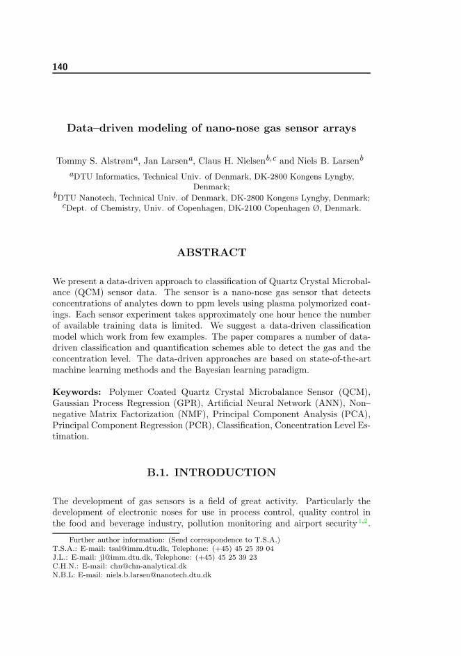
140

Data–driven modeling of nano-nose gas sensor arrays

Tommy S. Alstrøma, Jan Larsena, Claus H. Nielsenb,c and Niels B. Larsenb

aDTU Informatics, Technical Univ. of Denmark, DK-2800 Kongens Lyngby,Denmark;

bDTU Nanotech, Technical Univ. of Denmark, DK-2800 Kongens Lyngby, Denmark;cDept. of Chemistry, Univ. of Copenhagen, DK-2100 Copenhagen Ø, Denmark.

ABSTRACT

We present a data-driven approach to classification of Quartz Crystal Microbal-ance (QCM) sensor data. The sensor is a nano-nose gas sensor that detectsconcentrations of analytes down to ppm levels using plasma polymorized coat-ings. Each sensor experiment takes approximately one hour hence the numberof available training data is limited. We suggest a data-driven classificationmodel which work from few examples. The paper compares a number of data-driven classification and quantification schemes able to detect the gas and theconcentration level. The data-driven approaches are based on state-of-the-artmachine learning methods and the Bayesian learning paradigm.

Keywords: Polymer Coated Quartz Crystal Microbalance Sensor (QCM),Gaussian Process Regression (GPR), Artificial Neural Network (ANN), Non–negative Matrix Factorization (NMF), Principal Component Analysis (PCA),Principal Component Regression (PCR), Classification, Concentration Level Es-timation.

B.1. INTRODUCTION

The development of gas sensors is a field of great activity. Particularly thedevelopment of electronic noses for use in process control, quality control inthe food and beverage industry, pollution monitoring and airport security1,2.

Further author information: (Send correspondence to T.S.A.)T.S.A.: E-mail: tsal@imm.dtu.dk, Telephone: (+45) 45 25 39 04J.L.: E-mail: jl@imm.dtu.dk, Telephone: (+45) 45 25 39 23C.H.N.: E-mail: chn@chn-analytical.dkN.B.L: E-mail: niels.b.larsen@nanotech.dtu.dk

141

Ideally such an electronic nose should be portable, provide both a qualitativeand quantitative determination of analytes as well as offer stable performanceover extended periods of time. This means that the sensor element(s) mustoperate in a reversible manner and show an affinity towards target analytes.

Many different strategies have been pursued to develop selective gas sensors.One approach is to functionalize the physical sensor device with chemical coat-ings. Molecularly imprinted polymers (MIPs) seek to mimic biological antibod-ies. The selectivity of these “plastic antibodies” has been shown to be somewhatrandom and not easily controlled3. Several macromolecules have been evaluatedas potential gas sensors. One of the more popular choices are cyclodextrins,which are cage-like molecules with hydrophobic cavities and hydrophilic edges4.These molecules offer both chemical and steric selectivity and serve as a plat-form for a vast group of derivatives that tune the specificity towards certaincompounds or classes of compounds. However, the selective modification of cy-clodextrins is not a simple process and requires elaborate synthesis and isolationsteps5. Another drawback is the fact that these substances must be dissolvedin a solvent from which a film can be cast by for example spin or spray coatingin order to functionalize a sensor surface.

In this work an alternative methodology known as plasma polymerization isused for sensor functionalization. This method allows for solvent free depositionof a wide range of thin polymer films on the surface of most sensors includ-ing cantilever and quartz crystal microbalance (QCM) based sensors6. Plasmapolymerization also offers excellent control over film thickness since it is di-rectly proportional to polymerization time as confirmed by Kurosawa et al.7. Awide selection of monomers with many different functional groups can be usedfor plasma polymerization making it a very versatile technique. The choice ofmonomer naturally depends on the target analytes to be detected. As describedby Grate and Abraham the choice of coatings can advantageously be based onthe main interaction parameters that are responsible for the sorption of gasesinto solids8. According to the linear solvation energy relationship (LSER) modelthese parameters are: dispersion interactions, polarizability, dipolarity and hy-drogen bonding. Ideally one would develop a selection of coatings where eachcoating is representing only one of the above interaction parameters. This ishowever not easily done in practice, but Grate and Abraham suggest severalgood candidates that can be assumed to primarily interact via one parameteronly. The coatings are deposited on a QCM based sensor. The working princi-ple of QCM sensors resemble tuning forks. The resonance frequency response ofQCM sensors is close to linear with respect to mass change6. Coating the quartzcrystals make them selective towards various analytes making them suitable asgas sensors. In order to verify the selectivity of the coatings the sensor is testedusing six different analytes. The response data is subject to data analysis meth-ods. A number of methods have been applied to polymer coated QCM sensors.

142

Often QCM sensors selectivity has been analyzed by using principal compo-nent analysis (PCA)9–11 or hierarchical cluster analysis (HCA)12,13. Recentlythe application of artificial neural networks (ANN) evolved as the dominantmethod14.

As described earlier the response of QCM sensors is sensitive to mass changesmaking them viable for detecting concentration levels of analytes. Various meth-ods have been used to construct QCM based concentration level estimators suchas partial least squares (PLS)11 and multivariate linear regression15. Artificialneural networks have been applied as concentration level estimators in a broadrange of applications14,16–18.

In this paper we compare classification using ANN and PCA with a Non–negative Matrix Factorization (NMF) classification scheme. NMF was intro-duced by Lee and Seung19 as an alternative to PCA for feature extractionapplied to identifying facial features but have found use in a vast range of areas.Further we propose a QCM sensor consisting of 8 crystals with different coatings.The sensor is able to classify the test analytes with high accuracy even thoughthe available training data is limited. In order to perform concentration levelestimation the analytes are measured at various concentrations. Three differentmethods for concentration level estimation are evaluated; Principal componentregression (PCR), ANN and Gaussian process regression (GPR). PCR is a linearmethod that performs well with a limited amount of training points although ithandles non–linearity in data poorly. To overcome this problem neural networkshas usually been applied as ANN can model non–linearities. GPR is so far anuntried method for QCM data. GPR is a non–linear method as ANN but GPRshould be able to perform well with a limited amount of data points.

B.2. SENSORS AND MEASUREMENT SYSTEM

A selection of eight monomers were chosen based on the single interactionparameter. All monomers used, dodecane (DOD), heptadecafluoro-1-decene(HDFD), maleic anhydride (MAH), methylene dioxobenzene (MDOB), methylmethacrylate (MMA), styrene (STY) and vinyl pyrrolidone (VP), were of atleast ≥ 99% purity except di(ethylene glycol) vinyl ether (DEGVE), which wasof 98% purity, and all of them were used without further purification. Themonomers were polymerized at a total pressure of 10-13 Pa and at a power of0.5W

l in a 50 Hz (i.e. low frequency) plasma chamber20. Argon was used as acarrier gas. Surfaces were activated for 2 min in argon plasma followed by ad-dition of monomer to initiate polymerization. After polymerization power wasturned off, but the monomer was allowed to flow for another 2 min. This “af-terglow polymerization” is believed to reduce the amount of free radicals on the

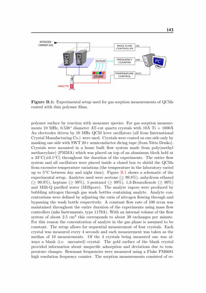
143

MFC1

MFC2

QCM ARRAY

MASS FLOWCONTROLLER

FREQUENCY COUNTER

TEMPERATURE CONTROL

MULTIPLEXER

USB

GPIB

RS232

PC

NITROGENCARRIER GAS

ANALYTE

Figure B.1: Experimental setup used for gas sorption measurements of QCMscoated with thin polymer films.

polymer surface by reaction with monomer species. For gas sorption measure-ments 10 MHz, 0.538“ diameter AT-cut quartz crystals with 10A Ti + 1000AAu electrodes driven by 10 MHz QCM lever oscillators (all from InternationalCrystal Manufacturing Co.) were used. Crystals were coated on one side only bymasking one side with SWT 20+ semiconductor dicing tape (from Nitto Denko).Crystals were mounted in a home built flow system made from poly(methylmethacrylate) (PMMA) which was placed on top of an aluminum block held ata 33◦C(±0.1◦C) throughout the duration of the experiments. The entire flowsystem and all oscillators were placed inside a closed box to shield the QCMsfrom excessive temperature variations (the temperature in the laboratory variedup to 5◦C between day and night time). Figure B.1 shows a schematic of theexperimental setup. Analytes used were acetone (≥ 99.8%), anhydrous ethanol(≥ 99.9%), heptane (≥ 99%), 1-pentanol (≥ 99%), 1,3-Benzodioxole (≥ 99%)and Milli-Q purified water (Millipore). The analyte vapors were produced bybubbling nitrogen through gas wash bottles containing analyte. Analyte con-centrations were defined by adjusting the ratio of nitrogen flowing through andbypassing the wash bottle respectively. A constant flow rate of 100 sccm wasmaintained throughout the entire duration of the experiments using mass flowcontrollers (mks Instruments, type 1179A). With an internal volume of the flowsystem of about 2.5 cm3 this corresponds to about 39 exchanges per minute.For this reason the concentration of analyte in the gas phase is assumed to beconstant. The setup allows for sequential measurement of four crystals. Eachcrystal was measured every 4 seconds and each measurement was taken as themedian of 10 measurements. Of the 4 crystals being measured one was al-ways a blank (i.e. uncoated) crystal. The gold surface of the blank crystalprovided information about unspecific adsorption and deviations due to tem-perature changes. Resonant frequencies were measured using a Fluke PM6681high resolution frequency counter. The sorption measurements consisted of re-

144

0 200 400 600 800 1000−120

−100

−80

−60

−40

−20

0

20

Time [min]

Δfre

quency [

Hz]

Water

BLANK

MAH

MDOB

MMA

Figure B.2: Δfrequency responses for MAH, MDOB, MMA and a blank quartzcrystal for nine measurement cycles. The first three measurement cycles iswater at 9200 parts per million (ppm), the next three cycles the concentrationis at 4600 ppm and the last three cycles has a concentration level at 2300ppm. The sign reversed peak value during a measurement cycle is recordedas representative for the cycle.

peated cycles of 100 min pure nitrogen flow followed by 40 min of analyte-spikedflow. The response was measured at six different concentrations, three times ateach concentration, for each analyte. Figure B.2 shows the response for MAH,MDOB and MMA using water as analyte. A measurement cycle consist offilling the chamber with pure nitrogen for 100 minutes allowing the coatingsto get a known steady state response. After the 100 minutes have passed ananalyte at a given concentration level is added to the flow maintained for 40minutes. The peak response is recorded as representative for the measurementcycle. Figure B.3 shows the measured (peak sign reversed) frequency responsesfor all analytes. The frequency readings show a near linear response with re-spect to mass for most coatings. Other coatings such as STY for heptane showa non-linear response. All responses but one are of the same sign. HDFD showsa negative response towards pentanol. This is because HDFD is a teflon-likecoating onto which condensation of pentanol is less likely to occur compared tothe uncoated reference quartz crystal.

B.3. ALGORITHM TRAINING AND EVALUATION

B.3.1 Data partitioning

As described in section B.2 we have conducted experiments on six differentanalytes. Each analyte is measured at 6 different concentration levels and eachexperiment is repeated 3 times. Therefore the dataset has 108 data points intotal, 18 data points per analyte. The data is partitioned into a training set

145

MAH MDOB MMA HDFD PVP DEGVE DODE STY0

50

100

150

200

250

Coating

ΔRes

ponz

e (H

z)

Sensory data for acetone

728003640018200850042502125

MAH MDOB MMA HDFD PVP DEGVE DODE STY0

50

100

150

200

250

300

350

400

450

Coating

ΔRes

ponz

e (H

z)

Sensory data for benzodioxol

2630013150657532801640820

MAH MDOB MMA HDFD PVP DEGVE DODE STY0

50

100

150

Coating

ΔRes

ponz

e (H

z)

Sensory data for ethanol

2880014400720036001800900

MAH MDOB MMA HDFD PVP DEGVE DODE STY0

20

40

60

80

100

120

Coating

ΔRes

ponz

e (H

z)

Sensory data for heptane

2010010050502525121526628

MAH MDOB MMA HDFD PVP DEGVE DODE STY−10

0

10

20

30

40

50

60

70

Coating

ΔRes

ponz

e (H

z)

Sensory data for pentanol

1400600416300192103

MAH MDOB MMA HDFD PVP DEGVE DODE STY0

10

20

30

40

50

60

70

80

90

100

Coating

ΔRes

ponz

e (H

z)

Sensory data for water

9200460023001150575288

Figure B.3: The bars are averages of the measured responses. Inspection of thedata shows that only on one occasion does a crystal give a negative Δfrequencyresponse, namely HDFD for pentanol. Note both the concentration levels andthe y–axis scaling varies between analytes. The concentration levels is in partsper million (ppm).

146

Figure B.4: The figure illustrate three different data partitioning scenarios.Left has Ntrain = 3, center has Ntrain = 6 and right has Ntrain = 8. Eachsquare corresponds to one data point. The test set comprise the blank squaresand the training set comprise the colored squares. cai denoted that concentrationlevel i for analyte a. Here acetone corresponds to a = 1 and water is a = 6.

and a test set. We want to produce learning curves for the different algorithmsso the size of the training set will vary. Our minimum training set size willbe three training points per analyte – the minimum number of points that canreveal non–linearities in the sensor response. The maximum trained set size ischosen to be twelve training points per analyte, denoted as Ntrain = 12. Thiscorresponds to an experimental setup where all concentration levels per analyteis included twice. We want to increase the training set size in roughly thesame manner as an experimenter would include more and more experiments.To achieve this we impose constraints on how the data is partitioned. Eachanalyte must be represented evenly in training set - thus the training set sizemust be a multiple of six. Further each concentration level within each analyte,should be represented as evenly as possible. Choosing Ntrain = 6 we have eachconcentration represented exactly once. Figure B.4 shows examples of datapartitioning for Ntrain = 3, Ntrain = 6 and Ntrain = 8. Each data partitioningand subsequent model training and evaluation is performed 100 times. This isdone to ensure that we are not comparing the algorithms on a training/test setthat turned out to be an exception rather than the norm.

B.3.2 Model training and evaluation

The proposed methods have several parameters that can have a huge impact ofperformance. These parameters are often set using model selection. In orderto select the model that has the lowest generalization error21 model selectionmethodology must be applied. We will work with both cross validation21 (CV)and marginal likelihood22 (ML) depending on the method in question. Modelselection for classification using SVD and NMF will use leave–one–out cross val-

147

idation (LOO-CV). Due to computational limitations model selection for ANNclassification will use a 6–fold cross validation scheme (6F-CV) instead of LOO-CV . The 6F-CV set will contain one data point per analyte. Model selectionfor PCR and ANN regression will use LOO-CV. Model selection for GPR willuse ML as described by Rasmussen and Williams22. The performance of theclassifiers are evaluated based on the misclassification rate defined as

Emis =Nerror

N(B.1)

where Nerror is the amount of misclassified points and N is the total amount ofpoints that was classified. Evaluating performance on quantifiers must be donedifferently than for the classifiers. The performance criterion used is the meanrelative absolute error as has been used by others14,17. It is defined as

E(RAE) =1

N

N∑n=1

∣∣∣∣yn − ynyn

∣∣∣∣ (B.2)

where yn is the true concentration, yn is the predicted concentration andN is theamount of data points estimated. The advantage of this performance criterionis that errors at both high and low concentrations are penalized equally.

B.3.3 Data analysis framework

We adopt a two–tiered model where classification and concentration level es-timation (quantification) is handled separately14. Figure B.5 shows how dataand decisions are made throughout the data processing pipeline. Output fromthe QCM sensor is applied to a classifier. Based on the decision made by theclassifier a given quantifier is selected. There is one quantifier trained per an-alyte. The output from the model is a class given as an analyte name and aconcentration level given in ppm.

We will use past implementations in MATLAB� of most of the algorithms.The neural network algorithms has been developed during the past years atDTU Informatics and is freely available for download at DTU ISP toolbox23.The NMF algorithm is implemented by Lin24 and is freely available from Lin’swebsite but can be found in the DTU ISP Toolbox as well. The Gaussian processregression implementation used is published by Rasmussen and Williams25. TheSVD and PCR algorithms are implemented by the authors.

148

Figure B.5: The schematic setup of the classification/quantification frame-work.

B.3.4 Gaussian Process regression

Gaussian process regression is an extension of the linear Bayesian regressionframework. A recent textbook on Gaussian processes in a machine learningcontext is written by Rasmussen and Williams22. A Gaussian process is com-pletely specified by its mean function and covariance function. Using Gaussianprocesses for regression requires two choices: a prior and a covariance function.We choose a zero mean Gaussian prior with unit variance. To make this priorplausible we subtract the empirical mean from the data and scale the data tounit variance. The empirical mean and empirical variance is calculated usingthe training set alone and as such the test data is not guaranteed to neither zeromean nor unit variance. We try three different covariance functions all basedon the squared exponential covariance function22

k(xp,xq) = σ2f exp

(−1

2(xp − xq)

�M (xp − xq)

)+ σ2

nδpq (B.3)

where σ2f , σ

2n and M are called the hyper–parameters. Typically σ2

f is called

the signal variance and σ2n the noise variance. Choosing M iso = �−2I yields

the isotropic squared exponential function where � is called the length–scale.Choosing Mard = diag(�)−2I yields a covariance function that implementsautomatic relevance determination22,26. The two approaches can be combinedby adding the covariance functions together thus creating the third covariancefunction. Model selection consists of choosing suitable values for the hyper-parameters. This is done using the marginal likelihood approach as discussed

149

by Rasmussen and Williams22 allowing 1000 function evaluations during theoptimization. The initial values for hyper–parameters are drawn from a zero–mean Gaussian distribution with unit variance. In order to avoid bad localminima 10 restarts is tried picking the hyper–parameters that yields the bestmarginal likelihood.

B.3.5 Artificial Neural Networks

The neural network classifier is a two–layered feed forward network (one hiddenlayer). Neural networks with one hidden layer are general approximators21 so itis sufficient to use just one hidden layer. The network has eight inputs – one perpolymer, and six outputs – one per analyte. Prior to training the entire dataset whitened (made zero mean and scaled to unit variance). The hidden unitsuse tangent hyperbolic sigmoidal function as transfer function. The networkis trained using the BFGS optimization algorithm as described by Nielsen27.The cost function (that is used by the optimizer) is a quadratic cost functionaugmented with outliers detection and weight decay. The cost function S(w)has two hyper–parameters α and β.

S(w) = ED(w, β) + αEW (w) (B.4)

where ED(w, β) is the cross-entropy error function and EW (w) is a regular-ization term28. Both hyper–parameters are updated after each iteration usingMacKays Bayesian maximum likelihood II (MLII) scheme29,30. The hyper-parameters are initialized to α = 8 and β = 1 and the network weights areinitialized using a zero mean Gaussian with variance equal to α. The stop-ping criterion for the network training is either 100 iterations or if the hyper-parameters are updated with a margin lower that 10−5. Each network train-ing cycle is repeated 10 times and the network with the lowest training errorED(w, β) is selected for concentration level estimation. The network trainingand cost function is described in details by Sigurdsson et. al.28. The neuralnetwork regressor is almost identical to the neural network classifier. The costfunction does not have outliers detection and the regressor uses just one outputneuron which hold the estimated concentration level.

The tunable parameters subject to cross validation is the number of hiddenunits. For the model selection part two to six hidden units were tested. The mostoften number of hidden units chosen was three which was chosen in 52.3% of theruns. The number of hidden units chosen for the regressor turned out to dependheavily on the analyte and the amount of training points available. Makinga histogram on all runs put together showed an almost uniform histogram.However if the histogram is calculated for each value of Ntrain the most commonchoice for hidden units was 2 (for Ntrain in range 6–9)

150

B.3.6 Non–negative Matrix Factorization

Classification using NMF is a linear vector–space method. The data is repre-sented in a 8–dimensional vector space and training consist of finding a suitablesubspace as representative for each analyte. When classifying an unknown datapoint, the date point is projected into each subspace. The subspace that rep-resents the data point best (calculated as residuals) is chosen as the correctanalyte. This is done as follows; the training points for each analyte is storedas columns in a data matrix Xanalyte ∈ R

8×Ntrain . NMF factorizes X into twonew matrices

WH ≈ X, W ∈ R8×b0+ , H ∈ R

b×Ntrain0+ , X ∈ R

8×Ntrain0+ (B.5)

NMF assumes that all values in X is non–negative so all negative values inthe data set are set to zero. Effectively it means pentanol will be classifiedwithout using the contribution from HDFD, see figure B.3. The matrix W isthe basis and the columns of matrix H is the data points represented in thebasis W . After training we have one W matrix per analyte (it is enforcedthat all subspaces are of the same size). When classifying data points the NMFfactorization is run with W held fixed. This procedure is carried out for all sixW matrices resulting in six different H matrices. The H matrix that representthe data point best is chosen as the correct analyte.

The factorization is calculated using the approach by Lin24. Each element ofmatrices W and H are initialized to a value drawn from a uniform distributionin the interval ]0; 1[. The stopping criterion for the algorithm is either 30 itera-tions or 10−4 as relative error. The amount of basis vectors to use per subspaceb is a model parameter that is allocated by LOO-CV. Allowable subspace sizeis in the interval b ∈ {2, . . . ,min(Ntrain − 1, 10)}. The most often value chosenwas b = 2. Note that b must be less that the amount of training points – so ifNtrain = 3 the subspace size is automatically chosen to b = 2. If we look at thecase where Ntrain = 12 the subspace size was mostly chosen to b = 2 but onlyfor 20% of the runs.

B.3.7 Principal component regression

Principal component regression is a linear regression method that is related toregularized least squares regression and partial least squared regression (PLS)21,31.The parameters to be chosen when using principal component regression iswhich principal components to include in the regression. We include prin-cipal components in the model ordered by their variance choosing the high-est variance component. To determine the amount of components k to in-clude in the model we use LOO-CV. The number of allowable components is

151

−100 0 100 200 300 400 500 600−200

−150

−100

−50

0

50

100

150

200

250

Principal component 1

Prin

cipa

l com

pone

nt 2

−100 0 100 200 300 400 500 600−100

−80

−60

−40

−20

0

20

40

60

80

Principal component 1

Prin

cipa

l com

pone

nt 3

−60 −50 −40 −30 −20 −10 0 10−20

−15

−10

−5

0

5

10

15

20

Principal component 1

Prin

cipa

l com

pone

nt 3

acetonebenzodioxolethanolheptanepentanolwater

Figure B.6: QCM data visualized using PCA. The size of the squares representthe concentration. Panel 3 is a zoomed in version of panel 2.

k ∈ {1, . . . ,min(Ntrain, 8)}. For Ntrain = 12 the most commonly chosen valuewas k = 6, but only in 22.3% of the runs.

B.3.8 Singular Value Decomposition

Classification using SVD is identical to the NMF classification method exceptfor the matrix factorization. The matrix factorization is carried out using SVDinstead and basis vectors are included based on their eigenvalues, always choos-ing the basis vector with the highest eigenvalue. The SVD classification methodused is described in details by Elden31. As with NMF the model selection pa-rameter is the subspace size. For model selection the allowable subspace size ofis b ∈ {1, . . . ,min(Ntrain − 1, 7)}. For Ntrain = 12 the most commonly chosensubspace size was b = 2 which was chosen in 90% of the runs.

B.4. RESULTS

Principal component analysis is used to visualize the entire data set more effec-tively, see figure B.6. The plots illustrate that the analytes lying on their ownalmost linear manifold thus motivating the use of linear methods. The plotsimply (but do not verify) that clustering methods such as K–nearest neigh-bor21 would not perform well given a small amount of training points. If allconcentrations are not represented by a cluster a substantial amount of datapoints would likely be misclassified. Table B.1 lists the classification accuracyfor the tested classification algorithms. The performance of SVD classificationis superior to both ANN and NMF. Using only 3 training points per analytewe gain remarkable accuracy – only misclassifying 3% of the test points. ANNis quite poor initially but as the amount of training point increases ANN clas-sification catches up. NMF performance is similar to SVD although not quite

152

Algorithm Ntrain

3 4 5 6 12ANN 0.611 ± 0.027 0.200 ± 0.024 0.076 ± 0.003 0.023 ± 0.002 0.003 ± 0.001NMF 0.039 ± 0.004 0.028 ± 0.004 0.025 ± 0.003 0.017 ± 0.003 0.009 ± 0.002SVD 0.032 ± 0.004 0.012 ± 0.002 0.006 ± 0.001 0.002 ± 0.001 0.001 ± 0.000

Table B.1: Classification error on test sets calculated as the mean over a100 runs ± the standard deviation of the mean. Note Ntrain is the amountof training points per analyte – the total amount of training points is Ntrain

multiplied with six.

3 4 5 6 7 8 9 10 11 1210

−4

10−3

10−2

10−1

100

Ntrain

Cla

ssifi

catio

n er

ror

ANNNMFSVD

Figure B.7: Learning curves for the classification algorithms on a test set.Note Ntrain refers to the amount of training points per analyte. The totalamount of training points is 6Ntrain.

as good. Figure B.7 shows learning curves for the three algorithms. The SVDclassifier is the preferred method regardless of the amount of training points.Concentration level estimation results are listed in table B.2. There is no clearindication of which algorithm should be the preferred choice although it showsthat ANN is consistently the poorest performer. As with classification there aretoo few training points to train an adequate neural network solution. The bestregressor for Ntrain = 3 is PCR regardless of analyte except for Benzodioxolwhere the GPAI approach is the best. At Ntrain = 4 the GPR method performssimilar to PCR and for Ntrain ≥ 5 GPR is either the superior method or onpar for all choices of analyte. At Ntrain = 12 the GPR method offers superioraccuracy. There is no significant indication of which of the three covariancefunctions is the best although the combined covariance function (GPAI) seemsslightly better. Figure B.8 shows learning curves for the concentration levelestimators. The learning curves clearly illustrates the troubles of ANN using alimited amount of training points. Another interesting observation is that PCRdoes not seem to improve significantly once Ntrain reaches 6.

153

Analyte Algorithm Ntrain3 4 5 6 12

Acetone

PCR 0.14 ± 0.009 0.09 ± 0.004 0.07 ± 0.003 0.08 ± 0.003 0.07 ± 0.003GPI 0.56 ± 0.094 0.12 ± 0.010 0.06 ± 0.004 0.04 ± 0.001 0.04 ± 0.001GPA 0.52 ± 0.088 0.09 ± 0.020 0.06 ± 0.006 0.04 ± 0.001 0.03 ± 0.002GPAI 0.30 ± 0.047 0.09 ± 0.008 0.05 ± 0.003 0.04 ± 0.001 0.04 ± 0.002ANN 1.05 ± 0.060 0.58 ± 0.021 0.56 ± 0.026 0.48 ± 0.015 0.40 ± 0.024

Benzodioxol

PCR 0.22 ± 0.008 0.17 ± 0.008 0.13 ± 0.005 0.12 ± 0.003 0.14 ± 0.011GPI 0.24 ± 0.024 0.07 ± 0.004 0.05 ± 0.001 0.05 ± 0.001 0.04 ± 0.001GPA 0.22 ± 0.027 0.12 ± 0.005 0.08 ± 0.003 0.06 ± 0.002 0.04 ± 0.002GPAI 0.16 ± 0.011 0.12 ± 0.006 0.08 ± 0.004 0.06 ± 0.003 0.04 ± 0.001ANN 0.87 ± 0.057 0.68 ± 0.043 0.63 ± 0.036 0.46 ± 0.018 0.49 ± 0.034

Ethanol

PCR 0.10 ± 0.005 0.09 ± 0.003 0.07 ± 0.002 0.05 ± 0.002 0.04 ± 0.001GPI 0.36 ± 0.053 0.10 ± 0.006 0.05 ± 0.002 0.03 ± 0.000 0.03 ± 0.001GPA 0.61 ± 0.108 0.15 ± 0.021 0.07 ± 0.004 0.05 ± 0.001 0.04 ± 0.001GPAI 0.29 ± 0.049 0.14 ± 0.019 0.07 ± 0.003 0.05 ± 0.001 0.03 ± 0.001ANN 0.81 ± 0.047 0.55 ± 0.015 0.56 ± 0.041 0.47 ± 0.021 0.41 ± 0.023

Heptane

PCR 0.31 ± 0.014 0.26 ± 0.009 0.22 ± 0.007 0.17 ± 0.004 0.16 ± 0.008GPI 1.21 ± 0.161 0.41 ± 0.034 0.28 ± 0.015 0.17 ± 0.004 0.13 ± 0.002GPA 0.68 ± 0.098 0.23 ± 0.012 0.16 ± 0.006 0.12 ± 0.002 0.13 ± 0.003GPAI 0.44 ± 0.059 0.26 ± 0.019 0.17 ± 0.008 0.12 ± 0.003 0.12 ± 0.003ANN NaN ± NaN 0.83 ± 0.043 0.57 ± 0.016 0.56 ± 0.022 0.54 ± 0.032

Pentanol

PCR 0.35 ± 0.007 0.25 ± 0.010 0.13 ± 0.004 0.12 ± 0.002 0.12 ± 0.003GPI 0.60 ± 0.058 0.24 ± 0.019 0.12 ± 0.004 0.10 ± 0.002 0.06 ± 0.002GPA 0.38 ± 0.026 0.19 ± 0.008 0.14 ± 0.005 0.12 ± 0.003 0.04 ± 0.005GPAI 0.37 ± 0.024 0.19 ± 0.008 0.14 ± 0.004 0.12 ± 0.003 0.04 ± 0.004ANN NaN ± NaN 0.81 ± 0.024 0.73 ± 0.026 0.58 ± 0.002 0.37 ± 0.003

Water

PCR 0.18 ± 0.002 0.17 ± 0.002 0.17 ± 0.003 0.17 ± 0.003 0.17 ± 0.007GPI 0.44 ± 0.038 0.18 ± 0.012 0.13 ± 0.007 0.10 ± 0.003 0.07 ± 0.003GPA 0.30 ± 0.037 0.16 ± 0.013 0.12 ± 0.009 0.10 ± 0.005 0.07 ± 0.003GPAI 0.31 ± 0.037 0.19 ± 0.018 0.12 ± 0.011 0.11 ± 0.010 0.07 ± 0.003ANN NaN ± NaN 0.89 ± 0.032 0.70 ± 0.021 0.64 ± 0.012 0.50 ± 0.026

Table B.2: Estimation error on test sets calculated as the mean over a 100 runs± the standard deviation of the mean. The three instances where ANN is listedas NaN means that there was occurrences where the network failed to train dueto an unlucky choice of training set. GP* refers to Gaussian process regressionusing the different covariance functions. GPI is the isotropic covariance function,GPA is the ARD covariance function and GPAI is the combined covariancefunction.

B.5. CONCLUSSION

Eight different polymer coatings have been evaluated for their suitability as gassensors by exposing polymer coated QCMs to volatile organic compounds. Thehigh classification accuracy implies that the coatings do indeed represent therange of interactions described by the LSER model very well. Each polymer filmseems to contribute with unique data. According to our analysis the coatingsare useful as gas sensing elements and can thus advantageously be used tofunctionalize many other types of sensors. Deposition of multiple types of sensorcoatings by plasma polymerization is compatible with practically any sensingdevice, and circumvents the use of solvents and subsequent drying processesduring deposition which can often damage fragile device components.

We presented a two–tiered data analysis framework that successfully classifiedresponses from an eight–dimensional polymer coated QCM sensor. By usinglinear methods such as SVD and NMF we get remarkable high accuracy (> 96%)

154

3 4 5 6 7 8 9 10 11 1210

−2

10−1

100

101

acetone

Xtrain

Mea

n re

lativ

e er

ror

3 4 5 6 7 8 9 10 11 1210

−2

10−1

100

benzodioxol

Xtrain

Mea

n re

lativ

e er

ror

3 4 5 6 7 8 9 10 11 1210

−2

10−1

100

ethanol

Xtrain

Mea

n re

lativ

e er

ror

3 4 5 6 7 8 9 10 11 1210

−0.9

100

heptane

Xtrain

Mea

n re

lativ

e er

ror

3 4 5 6 7 8 9 10 11 1210

−2

10−1

100

pentanol

Xtrain

Mea

n re

lativ

e er

ror

3 4 5 6 7 8 9 10 11 1210

−2

10−1

100

water

Xtrain

Mea

n re

lativ

e er

ror

PCRGPIGPAGPAIANN

Figure B.8: Learning curves for the concentration level estimation.

with only 3 training points per analyte. Having one training point per analyteper concentration level SVD have an classification accuracy of 99.8%. NMFdoes not perform to the level of SVD, but is still better than ANN for a limitedamount of training points. The NMF classification algorithm is fairly simple andmore sophisticated approaches could be developed. One could perform NMF onthe entire data set instead of per analyte and then map the basis vectors toclasses using a probabilistic approach32. The model selection for NMF andSVD can be improved further as well. If there is more than one choice of b tiedfor the best model, b is assigned randomly to a value among the best choices.One could construct a cost function that takes the residual values into accountand then select the value of b based on the cost function.

For concentration level estimation the Gaussian process regression is better thanthe linear method PCR (when Ntrain ≥ 5). Both of these methods are markedlybetter than the ANN. The issue with ANN regression being that the system isunderspecified. For the smallest possible neural network with two hidden units,the number of parameters in the model is 18 (16 weights in the first layer, 2weights in the second layer), but the network only have up to 12 training points.One could possibly improve ANN performance by reducing the dimension of thedata before applying the data to the neural network (for example using PCA)thus reducing the number of input neurons.

The best case scenario for GPR is a mean relative error of 3%. However theGPR method does have difficulties when having just three training points per

155

analyte. This can be explained by the zero mean Gaussian prior and the waydata partitioning is performed. For training sets where the lowest and/or high-est concentrations levels are omitted the GPR will perform poorly. In generalthe GPR will return to zero when estimating points outside the training inter-val. The performance outside the training interval could probably be improvedby adding a growing term to the prior or using a thin–plate spline kernel ascovariance function33.

B.6. ACKNOWLEDGMENTS

We acknowledge the support from the Danish Agency for Science and Technol-ogy’s, Program Commission on Nanoscience Biotechnology and IT (NABIIT),grant: 2106-07-0031 and 2106-05-0039.

REFERENCES

[1] Hamdi M. Saraoglu and Burcak Edin. E-Nose System for AnestheticDose Level Detection using Artificial Neural Network. Journal of Medi-cal Systems, 31(6):475–482, August 2007. ISSN 0148-5598. doi: 10.1007/s10916-007-9087-7.

[2] J. Yinon. Detection of Explosives by Electronic Noses. Analytical Chem-istry, 75(5):98 A–105 A, March 2003. ISSN 0003-2700. doi: 10.1021/

ac0312460.

[3] J.O. O. Mahony, K. Nolan, M.R. R. Smyth, and B. Mizaikoff. Molecularlyimprinted polymers—potential and challenges in analytical chemistry. An-alytica Chimica Acta, 534(1):31–39, April 2005. ISSN 00032670. doi: 10.1016/j.aca.2004.07.043.

[4] Jozsef Szejtli. Introduction and General Overview of Cyclodextrin Chem-istry. Chemical Reviews, 98(5):1743–1754, July 1998. ISSN 0009-2665. doi:10.1021/cr970022c.

[5] Abdul R. Khan, Peter Forgo, Keith J. Stine, and Valerian T. D’Souza.Methods for Selective Modifications of Cyclodextrins. Chemical Reviews,98(5):1977–1996, July 1998. ISSN 0009-2665. doi: 10.1021/cr970012b.

[6] Gunter Sauerbrey. Verwendung von Schwingquarzen zur Wagung dunnerSchichten und zur Mikrowagung. Zeitschrift fur Physik, 155(2):206–222,April 1959. ISSN 1434-6001. doi: 10.1007/BF01337937.

156

[7] Shigeru Kurosawa, Tomoya Hirokawa, Kazuya Kashima, Hidenobu Aizawa,Dae-Sang Han, Yasuo Yoshimi, Yuji Okada, Kiyoshi Yase, Jun Miyake,Minoru Yoshimoto, and Jons Hilborn. Detection of deposition rate ofplasma-polymerized films by quartz crystal microbalance. Thin SolidFilms, 374(2):262–267, October 2000. ISSN 00406090. doi: 10.1016/

S0040-6090(00)01161-5.

[8] Jay W. Grate and Michael H. Abraham. Solubility interactions and thedesign of chemically selective sorbent coatings for chemical sensors andarrays. Sensors and Actuators B: Chemical, 3(2):85–111, February 1991.ISSN 09254005. doi: 10.1016/0925-4005(91)80202-U.

[9] Hsin-Hsien Lu, Yerra Koteswara Rao, Tzong-Zeng Wu, and Yew-MinTzeng. Direct characterization and quantification of volatile organic com-pounds by piezoelectric module chips sensor. Sensors and Actuators B:Chemical, 137(2):741–746, April 2009. ISSN 09254005. doi: 10.1016/j.

snb.2009.01.060.

[10] Annika M. Rosengren, Kerstin Golker, Jesper G. Karlsson, and Ian A.Nicholls. Dielectric constants are not enough: principal component analysisof the influence of solvent properties on molecularly imprinted polymer-ligand rebinding. Biosensors & bioelectronics, 25(3):553–7, November 2009.ISSN 1873-4235. doi: 10.1016/j.bios.2009.06.042.

[11] Pengchao Si, John Mortensen, Alexei Komolov, Jens Denborg, andPreben J. Mø ller. Polymer coated quartz crystal microbalance sensors fordetection of volatile organic compounds in gas mixtures. Analytica chimicaacta, 597(2):223–30, August 2007. ISSN 1873-4324. doi: 10.1016/j.aca.2007.06.050. URL http://www.ncbi.nlm.nih.gov/pubmed/17683733.

[12] Kelly Sepcic, Mira Josowicz, Jiri Janata, and Ted Selby. Diagnosis of usedengine oil based on gas phase analysis. The Analyst, 129(11):1070, 2004.ISSN 0003-2654. doi: 10.1039/b406619g.

[13] Zhihua Ying, Yadong Jiang, Xiaosong Du, Guangzhong Xie, Junsheng Yu,and Huiling Tai. Polymer coated sensor array based on quartz crystalmicrobalance for chemical agent analysis. European Polymer Journal, 44(4):1157–1164, April 2008. ISSN 00143057. doi: 10.1016/j.eurpolymj.

2008.01.015.

[14] Ali Gulbag, Feyzullah Temurtas, and Ismihan Yusubov. Quantitative dis-crimination of the binary gas mixtures using a combinational structure ofthe probabilistic and multilayer neural networks. Sensors and Actuators B:Chemical, 131(1):196–204, April 2008. doi: 10.1016/j.snb.2007.11.008.

[15] Ya-Ling Wang and Jeng-Shong Shih. Multi-channel piezoelectric crystalgas sensor with principal component analysis for organic solvent pollutants

157

from polymer plants. Journal of the Chinese Chemical Society, 53(6):1427–1437, December 2006. ISSN 0009-4536.

[16] Hamdi M. Saraoglu and Mehmet Kocan. Determination of Blood GlucoseLevel-Based Breath Analysis by a Quartz Crystal Microbalance Sensor Ar-ray. IEEE Sensors Journal, 10(1):104–109, January 2010. ISSN 1530-437X.doi: 10.1109/JSEN.2009.2035769. URL http://ieeexplore.ieee.org/

lpdocs/epic03/wrapper.htm?arnumber=5352205.

[17] Bekir Mumyakmaz, Ahmet Ozmen, Mehmet A. Ebeoglu, and CihatTasaltın. Predicting gas concentrations of ternary gas mixtures for a prede-fined 3D sample space. Sensors and Actuators B: Chemical, 128(2):594–602,January 2008. ISSN 09254005. doi: 10.1016/j.snb.2007.07.062.

[18] Ahmet Ozmen, F. Tekce, Mehmet A. Ebeoglu, Cihat Tasaltın, and Zafer Z.Ozturk. Finding the composition of gas mixtures by a phthalocyanine-coated QCM sensor array and an artificial neural network. Sensors andActuators B: Chemical, 115(1):450–454, May 2006. ISSN 09254005. doi:10.1016/j.snb.2005.10.007.

[19] Daniel D. Lee and H. Sebastian Seung. Learning the parts of objects by non-negative matrix factorization. Nature, 401(6755):788–791, October 1999.doi: 10.1038/44565.

[20] Bjø rn Winther-Jensen and Kristian Glejbø l. Method and apparatus forthe excitation of a plasma, 2003.

[21] Christopher M. Bishop. Pattern Recognition and Machine Learning.Springer, Secaucus, NJ, USA, 2006. ISBN 0387310738.

[22] Carl E. Rasmussen and Christopher K. I. Williams. Gaussian Processesfor Machine Learning. MIT Press, April 2006. URL http://www.

gaussianprocess.org/gpmlhttp://www.ncbi.nlm.nih.gov/pubmed/

15112367.

[23] DTUInformatics. DTU:Toolbox. URL http://cogsys.imm.dtu.dk/

toolbox/.

[24] Chih-Jen Lin. Projected gradient methods for nonnegative matrix factoriza-tion. Neural computation, 19(10):2756–79, October 2007. ISSN 0899-7667.doi: 10.1162/neco.2007.19.10.2756.

[25] Carl E. Rasmussen and Christopher K. I. Williams. GPML code, 2006.URL http://www.gaussianprocess.org/gpml.

[26] Radford M. Neal. Bayesian Learning for Neural Networks. Springer-VerlagNew York, lecture no edition, 1996. ISBN 0-387-94724-8.

158

[27] Hans B. Nielsen. UCMINF - an Algorithm for Unconstrained, NonlinearOptimization. Technical Report IMM-TEC-0019, IMM, Technical Univer-sity of Denmark, 2001.

[28] Sigurdur Sigurdsson, Jan Larsen, Lars K. Hansen, Peter A. Philipsen, andHans C. Wulf. Outlier estimation and detection application to skin lesionclassification. In IEEE International Conference on Acoustics Speech andSignal Processing, volume 1, pages I–1049–I–1052. IEEE, May 2002. ISBN0-7803-7402-9. doi: 10.1109/ICASSP.2002.5743975.

[29] David J. C. MacKay. A Practical Bayesian Framework for BackpropagationNetworks. Neural Computation, 4(3):448–472, May 1992. ISSN 0899-7667.doi: 10.1162/neco.1992.4.3.448.

[30] David J. C. MacKay. The Evidence Framework Applied to ClassificationNetworks. Neural Computation, 4(5):720–736, September 1992. ISSN 0899-7667. doi: 10.1162/neco.1992.4.5.720.

[31] Lars Elden. Matrix Methods in Data Mining and Pattern Recognition. Soci-ety for Industrial and Applied Mathematics, Philadelphia, PA, USA, 2007.ISBN 9780898716269.

[32] Thomas Kolenda, Lars K. Hansen, Jan Larsen, and Ole Winther. Inde-pendent component analysis for understanding multimedia content. InH Bourlard, T Adali, S Bengio, J Larsen, and S Douglas, editors, Proceed-ings of the 12th IEEE Workshop on Neural Networks for Signal Processing,pages 757–766, Piscataway, New Jersey, 2002. IEEE. ISBN 0-7803-7616-1.doi: 10.1109/NNSP.2002.1030096.

[33] Grace Wahba. Spline Models for Observational Data. Society for Industrialand Applied Mathematics, January 1990. ISBN 978-0-89871-244-5. doi:10.1137/1.9781611970128.

Appendix C

Data representation andfeature selection for

colorimetric sensor arraysused as explosives detectors

� 2011 IEEE. Personal use of this material is permitted. Permission from IEEEmust be obtained for all other uses, in any current or future media, includingreprinting/republishing this material for advertising or promotional purposes,creating new collective works, for resale or redistribution to servers or lists, orreuse of any copyrighted component of this work in other works.

Tommy S. Alstrøm, Jan Larsen, Natalie V. Kostesha, Mogens H. Jakobsen,and Anja Boisen. Data representation and feature selection for colorimetricsensor arrays used as explosives detectors. In IEEE International Workshopon Machine Learning for Signal Processing (MLSP), pages 1–6, 2011. URLhttp://dx.doi.org/10.1109/MLSP.2011.6064615.

The layout of the paper has been revised.

160

DATA REPRESENTATION AND FEATURESELECTION FOR COLORIMETRIC SENSOR ARRAYS

USED AS EXPLOSIVES DETECTORS

Tommy S. Alstrøma, Jan Larsena, Natalie V. Kosteshab,Mogens H. Jakobsenb and Anja Boisenb

aDept. of Informatics and Mathematical Modeling,Technical University of Denmark

Richard Petersens Plads 321, 2800 Kgs. Lyngby, Denmark{tsal,jl}@imm.dtu.dk

bDept. of Micro- and Nanotechnology,Technical University of Denmark

Ørsteds Plads 345 East, DK-2800, Kgs. Lyngby, Denmark{natalie.kostesha,mogens.jakobsen,anja.boisen}@nanotech.dtu.dk

ABSTRACT

Within the framework of the strategic research project Xsense at the TechnicalUniversity of Denmark, we are developing a colorimetric sensor array which canbe useful for detection of explosives like DNT, TNT, HMX, RDX and TATP andidentification of volatile organic compounds in the presence of water vapor inair. In order to analyze colorimetric sensors with statistical methods, the sensoryoutput must be put into numerical form suitable for analysis. We present newways of extracting features from a colorimetric sensor and determine the qualityand robustness of these features using machine learning classifiers. Sensors, andin particular explosive sensors, must not only be able to classify explosives,they must also be able to measure the certainty of the classifier regarding thedecision it has made. This means there is a need for classifiers that not onlygive a decision, but also give a posterior probability about the decision. Wewill compare K–nearest neighbor, artificial neural networks and sparse logistic

We acknowledge the support from the Danish Agency for Science and Technology’s, Pro-gram Commission on Nanoscience Biotechnology and IT (NABIIT). Case number: 2106-07-0031 - Miniaturized sensors for explosives detection in air.

161

regression for colorimetric sensor data analysis. Using the sparse solutions weperform feature selection and feature ranking and compare to Gram–Schmidtorthogonalization.

Index Terms— artificial neural networks (ANN), chemo–selective com-pounds, classification, colorimetric sensor array, DNT, explosives detection,feature ranking, Gram–Schmidt orthogonalization, K–nearest neighbor (KNN),sparse logistic regression (SLR), TNT

C.1 Introduction

Over the past decade, explosives have been a preferred tool for terrorists, yetthere is no satisfactory mobile and portable solution to detect explosives. Todetect a variety of military and industrial explosives easily, new technologiesmust be developed. There are several application areas for explosives sensors,such as anti-terrorism (screening luggage and mail packages, checking suspectsand mass transit systems), demining and environmental monitoring of hazardouscompounds.

Sensors must not only easily detect a variety of hidden explosives but they mustalso be able to detect illegal chemicals and products of the explosives industry. Afurther requirement is that the sensing device should be portable, rapid, highlysensitive, specific (minimize false alarms), and inexpensive [1].

Over the past years a number of detecting methods have been developed andsuccessfully applied in explosives detectors. These include, but are not limitedto, gas chromatography, Raman spectrometry, mass spectrometry, ion mobilityspectrometry and colorimetric sensors. Suslick et al. described the applicationof the colorimetric sensor array for detecting volatile organic compounds in thegas phase [2, 3] as well as for identifying different organic compounds in theliquid phase [4, 5]. In our project we develop a colorimetric sensor array thatcan be useful in detecting and identifying explosives like TNT, DNT, HMX,RDX and TATP [6, 7]. The colorimetric sensor is a fascinating technique fordetecting different chemical compounds belonging to various classes, like amines,cyanides, alcohols, arenes, ketones, aldehydes and acids in the parts-per-million(ppm) and parts-per-billion (ppb) ranges [3, 8, 9]. In our research we use acompletely different class of chemo–selective compound which has already shownexcellent results for detecting TNT. This type of colorimetric sensor could besuccessfully applied in homeland security and defense [10, 11].

A colorimetric sensor array consists of a number of chemo–selective compoundsof various colors that will undergo a color change when subjected to an environ-

162

ment or a target substance, hereafter denoted an analyte. These chemo–selectivecompounds, which are typically called dyes are digitalized using a flatbed scan-ner. One dye consists of several hundred pixels, but a dye is considered to haveonly one color which is typically found by calculating the mean pixel value.We investigate how feature extraction using the mean pixel value compares toalternatives.

Having acquired the sensor response digitally enables the application of signalprocessing and statistic methods such as principal component analysis (PCA)and hierarchical cluster analysis (HCA) [12–14]. In the domains where colori-metric sensors have been investigated, HCA shows high accuracy and low falsealarm rate. The closely related K-Nearest Neighbor (KNN) classifier [15] withK = 1 set to one has evolved as the de–facto method.

Our requirements for a classifier go beyond what KNN offers. As we are detect-ing hazardous compounds, we require the classifier to offer posterior probabilitiesand not only decisions. Further we seek to qualify which compounds in the col-orimetric sensor are important, and which are less important. This knowledgeenables the ability to either reduce the size of the sensor or replace less sensitiveand unimportant compounds with more selective and responsive compounds.Various feature selection strategies can be employed to select the dyes but sofar none have been applied to colorimetric sensor arrays. Our preference wouldbe to use a sparse classifier thus making the feature selection an inherent partof the classification. Our main goal is not to find the classifier that has thebest classification rate but to identify a classifier with these attributes and atthe same time delivers comparable or better performance compared to KNN.We will consider two classifiers: sparse logistic regression (SLR) [16] which is alinear classifier that is extended to model posterior probabilities and implementsparsity, and artificial neural networks (ANN) [17] which is a proven non–linearclassifier. Our primary motivation to include a non–linear classifier is to inves-tigate if non–linear models are better suited for colorimetric sensor arrays.

C.2 Colorimetric sensors

We have operated with three different sensors: sensor A comprised 15 dyes [6];sensor B equal to sensor A with one added dye [7]; sensor C which is a furtherextension adding 15 dyes to sensor B (unpublished results). Fig. C.1A showssensor B when exposed to the explosive analyte RDX. The sensors have beenexposed to analytes belonging to the various chemical families (Table C.1). Fora more elaborate description of sensor fabrication, dyes and target analytes werefer to our earlier published work [6, 7].

163

Figure C.1: An example of a colorimetric sensor exposed to the explosiveanalyte RDX. A: sensor before exposure. B: enhanced difference image.

Chemical family A B CAcids 32 45

Alcohols 26 27Aldehydes 6Amines 42Arenes 10 13Drugs 6

Environment 12 8 28Explosives 20 8 56

Inorganic Explosives 14Ketones 7 13Thiols 14

Total measurements: 129 22 253

Table C.1: The different chemical families and how many measurements wereapplied to the sensors, i.e. sensor B has been measured 22 times in total, where6 of the measurements were drugs. Each family comprises several compounds.

C.2.1 Data acquisition

Images of the sensor were scanned using an ordinary flatbed scanner immediatelyafter immobilization of dyes and then again after exposure of target analytes.The images were encoded in a lossless format using the red-green-blue (RGB)color scheme with 8 bits per color. The images were used to generate colordifference images by pixel subtraction (Fig. C.1). To align the two images acost function that measures the L1 norm error per pixel is minimized:

mint,θ

‖Ibefore − g(Iafter, t, θ)‖1/Npixels (C.1)

164

where I is an image matrix, t is an (x, y) translation, θ is a rotation and g(·)is the function that implements the transformation: first rotating the imagesusing nearest neighbor interpolation, then translating (x, y)–pixels according tot. The parameters (t, θ) are initialized to zero.

The L1 norm error can be interpreted as the amount of color per pixel where afully black pixel is fixed at a value of zero. At perfect image alignment, all thebackground pixels will be black and all dye pixels will have the weakest possiblecolor, hence, blackness per pixel should be maximized. Dye localization andgeneration of colorimetric difference maps are described in detail in [18].

C.2.2 Data extraction

Once the images are digitalized feature extraction is employed typically usingthe mean pixel value. In order for the mean to be a robust measure of colorchange, the pixels of a dye have to be normally distributed (or at least havea symmetric distribution with one mode) and relatively free from outliers. Ascan be seen in Fig. C.2 this is may not always be the case. Chemically weknow that a dye should only have one color, as the dye is homogeneous andexposed to a homogeneous vapor. However, noise is induced from: the scanner,the drying process of the dye, external light, and roughness of surface. Someof these effects can be handled easily. The drying of the dyes often resultsin a ring near the perimeter (the coffee stain effect) and this area of the dyeis unreliable. To accommodate for this effect, a smaller area of a dye is usedfor feature extraction, corresponding to 2/3 of the dye radius. To handle theother noise effects that cause pixel outliers, the median or mode can be usedas both statistics are more robust to outliers. Just as the case with the mean,the median requires a symmetric distribution with one mode. On the otherhand the mode does not require the distribution to be symmetric and couldpotentially be more robust. However, these three statistics have the weaknessthat they consider the RGB colors as independent since an RGB color value isa 3 dimension vector. The multinomial mode does not have this weakness andwill find the most occurring color in the dye hence we expect the multinomialmode to be the best representation. The entire data acquisition and extractionpipeline is described in detail in [18].

C.2.3 Data visualization

Data from colorimetric sensors can be visualized using principal componentanalysis (PCA) with a certain degree of success. However, once the sensor has

165

−20 −15 −10 −5 0 5 100

5

10

15

20

25

30

35m

ode

mea

nm

edia

ngm

ode

Pixel value

Figure C.2: An example of colorimetric sensor B exposed to the explosiveanalyte RDX. A: the sensor before exposure. B: the enhanced difference image.C: histogram of the green value and the value of the statistics.

been applied to many different classes, this kind of data visualization is of limitedvalue. Fig. C.3 shows how PCA can be used to plot data for the sensor B case.However for sensors A and C the data collected is too high dimensional for a PCAplot to show the entire structure of the data [6]. Fig. C.4 shows how the variancein the data is distributed among the different dimensions. While the figureimplies that sensor C is a higher dimensional sensor, the plot does not meritconclusions about the true dimensionality of the sensor. The dyes are highlycorrelated, especially the red-green-blue dimensions within each dye, but evenmore so there may be a lot of uncorrelated noise. PCA requires one dimensionper uncorrelated signal channel and if the noise channels are sufficiently strongmore dimensions will be needed to represent the data accurately. Observe thatfor three dimensions the sensors are almost equal, even though sensor C has

166

−100 0 100−50

0

50

PC 1

PC

2

DrugsEnvironmentExplosives

Figure C.3: PCA plot from sensor B. The PCA plot implies that the sensorshould be able to separate well although there is an explosive outlier.

1 2 3 4 5 6 7 8 9 10 11 12 13 14 150.4

0.5

0.6

0.7

0.8

0.9

1

Number of Principal Components

Rep

rese

ntab

le v

aria

nce

Figure C.4: The colorimetric sensor is a high dimensional sensor. For sensorA (blue) it requires 9 dimensions to represent 95% of the variance, whereas forsensor C (red) it requires 15 dimensions.

twice as many dyes as sensor A.

C.3 Methods

Each classification method is evaluated using 10–fold double cross validation(CV) partitioning used is a stratified approach. The partitioning of the outerfold that is used to estimate the test error remains fixed, while the partitions

167

that are used for model selection are regenerated in each run.

C.3.1 K–nearest neighbor

Despite its simplicity the K–nearest neighbor is an effective classification tech-nique [15] which works as follows: when testing an unknown data point, theEuclidean distances for all known points are calculated. The classes of theclosest K points are then identified and the unknown point is classified usingmajority voting of these known points. In the event of a tie, the algorithm usesthe nearest neighbor among the tied classes to break the tie selecting the closestpoint as the class. All possible values of K are probed during model selection.

C.3.2 Sparse multinomial logistic regression

The multinomial logistic regression model offers a posterior probability of a classgiven a measurement. The model is written as

p(Ck|x) = exp(wTkx)∑

j exp(wTj x)

(C.2)

where p(Ck|x) is the probability of class Ck given a data point x. To promote asparse solution and to handle over-fit, we use L1 regularization. This is achievedby adding the term λ‖w‖1 to the cost function where λ is the model selectionparameter. The cost function is minimized using the Projection L1 method de-scribed by Schmidt et al. [16]. To further promote sparse solutions, the weightsare initialized to zero. The optimal λ is searched for in the interval [0; 10].

C.3.3 Artificial neural networks

The artificial neural network classifier used is a two–layered feed-forward withthe hidden units using tangent hyperbolic sigmoidal function as the transferfunction. A quadratic cost function augmented with outlier detection and weightdecay is used. S(w) has two hyper–parameters; the regularization parameter αand outlier probability β:

S(w) = ED(w, β) + αEW (w) (C.3)

where ED(w, β) is the cross-entropy error function and EW (w) is a regulariza-tion term. The hyper-parameter α is initialized to the number of inputs, i.e.,

168

Method Median Mode MMode Mean Comb.A-1NN 5.40 5.83 5.27 5.33 5.40A-KNN 5.77 6.20 5.40 5.15 5.52A-SLR 5.71 5.52 6.08 5.71 5.71A-ANN 5.52 5.40 5.52 5.71 5.64B-1NN 1.77 1.77 2.18 1.91 1.77B-KNN 1.64 1.50 1.91 1.64 1.64B-SLR 1.36 1.36 1.91 1.36 1.36B-ANN 1.36 1.09 1.50 1.36 1.36C-1NN 6.05 6.12 6.15 6.05 6.05C-KNN 5.91 6.05 5.94 6.12 6.05C-SLR 6.79 6.69 6.65 6.72 6.79C-ANN 6.40 6.37 6.19 6.47 NaNTotal 1 2 6 3 1

Table C.2: Summary of how well the features and classifiers perform comparedto random guessing, with the best performers highlighted.

the more inputs, the stronger regularization needed. The hyper-parameter β isinitialized to zero as a priori there are no known outliers. The network weightsare initialized using a zero mean Gaussian with variance equal to 1/α. Eachnetwork training cycle is repeated ten times and the network with the lowesttraining error ED(w, β) is selected for classification. The outputs are convertedto probabilities using the soft–max function. The network training and costfunction are described in detail by Sigurdsson et al. [17].

C.4 Results and discussion

Since the sensors have a different amount of classes, we find it better to assessthe quality of the classifiers by using the classification rate relative to randomguessing as the classification rate alone can be misleading. For example a clas-sification rate of 0.33% for sensor B would only be as good as random guessingwhile for sensor A and C it would be better than random guessing. The ratiois calculated as (Ncorrect ·NC)/N , where NC is the number of points correctlyclassified, N is the total number of points and NC is the number of classes.

Table C.2 shows the best statistic is the multivariate mode which is the bestperformer in six out of twelve cases. However, all the other features are alsorepresented at least once as the top performer, so the results indicate that inorder to build the most accurate classifier one must extract all of the proposed

169

Thiol

Ketone

Inorganic Expl.

Explosives

Environment

Arenes

Amines

Alcohols

Acids 44 0 0 0 0 1 0 0 0

0 19 1 1 4 0 0 2 0

0 0 33 1 3 0 5 0 0

0 1 1 5 1 0 5 1 0

0 4 5 0 14 2 2 1 0

0 0 0 0 0 56 0 0 0

0 1 3 3 5 0 2 0 0

0 7 0 0 1 0 0 5 0

0 0 1 0 0 0 0 0 13

Figure C.5: Confusion matrix for C-SLR-Median where rows indicate thetrue class, columns indicate the predicted class and the number indicate thecounts [19]. The sensor has a high classification rate for explosives with zerofalse negatives (all 56 measurements are classified correctly) but three falsepositives.

features from the colorimetric sensor and then let the feature selection be partof the model selection process.

The considered classification methods all perform similarly. As expected thesimplest method, 1NN, is the best performer on the smallest dataset B. Forsensor A, the KNN method is the best performer and on C the SLR is the bestperformer.

Sensor C is the richest sensor, with respect to data points, dyes and classes,and we will now discuss the results from this sensor in more detail. The bestperforming classifier for sensor C is SLR using median as feature extractionstatistic. Fig. C.5 shows the confusion matrix for this situation and clearlyshows that the sensor is very good for detecting especially acids and explosives,although some chemicals, such as arenes, pose a greater challenge. Havingestablished that SLR is the classifier with the highest accuracy, we will nowinvestigate how well SLR detects informative dyes by scrutinizing the sparsesolutions.

A colorimetric sensor array is likely to have redundant features, as some dyes will

170

0

5

10

15

20

25

30

28 29 24 23 12 10 30 20 26 9Dye

Ran

k

Figure C.6: Dyes ranked according to their mean rank for sensor C. The dyesignificance is listed from left to right where the more significant dye is the left.

react similarly, and it is not clear for the experimenter which dyes should be usedin the next iteration of the sensor. We want to explore how well SLR identifiesimportant dyes compared to the simple forward selection method based on theGram–Schmidt orthogonalization [20].

For the feature selection process we convert the classification problem into abinary problem; explosives versus non-explosives (inorganic explosives will bepart of the non-explosives group, as these explosives are not part of our detectionfocus). For each of the four feature extraction statistics, we will train ten modelsusing the same data partitioning that was used in the multinomial classificationcase, hence forty models are trained in total. The sparsity parameter λ willstart from zero and be incremented slowly, removing one feature at a time fromthe model. Each dye consist of three values (the RGB values) so in order toremove a dye all three features belonging to a dye have to be eliminated fromthe model. A dye is considered as completely removed once the weights for allthe values are below a threshold which we set to 10−3. Fig. C.6 shows how thedyes for sensor C rank according to their mean ranking. The top ten rankeddyes using the median as the feature extraction statistic are used to detectexplosives. Fig. C.7 shows how well suited the dyes are for classification. Usingthree dyes the classification error is below 0.01% and after this adding moredyes only decreases the error marginally. Comparing the dyes identified by SLRto GS, the SLR dyes are clearly more suited, however if whitening is used GSshow similar performance as SLR.

171

1 2 3 4 5 6 7 8 9 100

0.02

0.04

0.06

0.08

0.1

0.12

Number of dyes used

Cla

ssifi

catio

n er

ror

2

4

6

8

10

12

Ave

rage

ran

k

SLR−LR

SLR−1NN

SLR−Rank

GS−LR

GS−1NN

GS−Rank

Figure C.7: Classification error with respect to number of dyes used, based onsensor C–Median. The classification error decreases to a certain point as dyesare added. SLR-LR is logistic regression classifier applied on the dyes identifiedby SLR. SLR-1NN used 1NN as classifier instead. SLR-Rank indicates the meanfeature rank of dye i as shown on Fig. C.6. Similarly GS-X uses the featuresfound by the GS based feature selection method.

C.5 Conclusion

We have tried five different feature sets of four different classifiers on three dif-ferent colorimetric sensor arrays. The logistic regression method demonstratedequal classification ability compared to KNN and due to the added perks interms of sparsity and probabilistic decisions, SLR is preferable to KNN. Theresults do not merit the use of a non–linear method such ANN. This is likelybecause there is not enough training data and since the experimental processof colorimetric sensors is time consuming, methods that work with fewer pointsare more appealing.

The classification results allow us to make a recommendation about which statis-tic to use for feature extraction. The de–facto approach is to use the mean butas the results show, this statistic only gives the best results on three instances,and never when combined with SLR. When using SLR the multivariate modeproved to be the best statistic. For sensor A and B the multivariate mode scoreshighest although for sensor C the median scored 2% higher than the multivariatemode.

SLR showed remarkable ability to identify a subset of dyes that could accurately

172

identify explosives from non–explosives. SLR did not reliably estimate the samefeatures as important, but using the average rankings proved to be an adequatesolution. Using the top 5 identified compounds we were are able to train aclassifier that identified explosives without any false negatives (Fig. C.7).

Other popular classification methods such as linear discriminant analysis (LDA)and support vector machines (SVM) was not considered since they do not bothmodel posterior probabilities and implement sparsity although one could con-sider using sparse relevance vector machines. Further, the dyes contribute withthree features each (the RGB values) so one could also consider using grouplasso instead of traditional regularization. This will be subject for future study.

References

[1] Michael S. Schmidt, Natalie V. Kostesha, Filippo G. Bosco, Jesper K.Olsen, Carsten Johnsen, Kent A. Nielsen, Jan O. Jeppesen, Tommy S.Alstrøm, Jan Larsen, Thomas Thundat, Mogens H. Jacobsen, and AnjaBoisen. Xsense - a miniaturised multi-sensor platform for explosives detec-tion. In Proceedings of SPIE, volume 8031, pages 803123–803123–7, 2011.doi: 10.1117/12.884050.

[2] Kenneth S. Suslick, Neal A. Rakow, and Avijit Sen. Colorimetric sensorarrays for molecular recognition. Tetrahedron, 60(49):11133–11138, Novem-ber 2004. ISSN 00404020. doi: 10.1016/j.tet.2004.09.007.

[3] Neal A. Rakow, Avijit Sen, Michael C. Janzen, Jennifer B. Ponder, andKenneth S. Suslick. Molecular recognition and discrimination of amineswith a colorimetric array. Angewandte Chemie (International ed. in En-glish), 44(29):4528–32, July 2005. ISSN 1433-7851. doi: 10.1002/anie.

200500939.

[4] Chen Zhang and Kenneth S. Suslick. A colorimetric sensor array for organ-ics in water. Journal of the American Chemical Society, 127(33):11548–9,August 2005. ISSN 0002-7863. doi: 10.1021/ja052606z.

[5] Chen Zhang, Daniel P. Bailey, and Kenneth S. Suslick. Colorimetric sensorarrays for the analysis of beers: a feasibility study. Journal of agriculturaland food chemistry, 54(14):4925–31, July 2006. ISSN 0021-8561. doi: 10.1021/jf060110a.

[6] Natalie V. Kostesha, Tommy S. Alstrøm, Carsten Johnsen, Kent A. Nielsen,Jan O. Jeppesen, Jan Larsen, Mogens H. Jakobsen, and Anja Boisen. De-velopment of the colorimetric sensor array for detection of explosives andvolatile organic compounds in air. In Proceedings of SPIE, volume 7673,pages 76730I–76730I–9, 2010. doi: 10.1117/12.850310.

173

[7] Natalie V. Kostesha, Tommy S. Alstrøm, Carsten Johnsen, Kent A. Nielsen,Jan O. Jeppesen, Jan Larsen, Anja Boisen, and Mogens H. Jakobsen. Multi-colorimetric sensor array for detection of explosives in gas and liquid phase.In Proceedings of SPIE, volume 8018, pages 80181H–80181H–12, 2011. doi:10.1117/12.883895.

[8] Sung H. Lim, Liang Feng, Jonathan W. Kemling, Christopher J. Musto,and Kenneth S. Suslick. An Optoelectronic Nose for Detection of ToxicGases. Nature chemistry, 1:562–567, September 2009. ISSN 1755-4349.doi: 10.1038/nchem.360.

[9] Chen Zhang and Kenneth S. Suslick. Colorimetric sensor array for softdrink analysis. Journal of agricultural and food chemistry, 55(2):237–42,January 2007. ISSN 0021-8561. doi: 10.1021/jf0624695.

[10] Dae-Sik Kim, Vincent M. Lynch, Kent A. Nielsen, Carsten Johnsen, Jan O.Jeppesen, and Jonathan L. Sessler. A chloride-anion insensitive colorimetricchemosensor for trinitrobenzene and picric acid. Analytical and bioanalyti-cal chemistry, 395(2):393–400, 2009. doi: 10.1007/s00216-009-2819-4.

[11] Jung S. Park, Franck Le Derf, Christopher M. Bejger, Vincent M. Lynch,Jonathan L. Sessler, Kent A. Nielsen, Carsten Johnsen, and Jan O. Jeppe-sen. Positive Homotropic Allosteric Receptors for Neutral Guests: Annu-lated Tetrathiafulvalene–Calix[4]pyrroles as Colorimetric Chemosensors forNitroaromatic Explosives. Chemistry - A European Journal, 16(3):848–54,January 2010. ISSN 1521-3765. doi: 10.1002/chem.200902924.

[12] Michael C. Janzen, Jennifer B. Ponder, Daniel P. Bailey, Crystal K. Ingison,and Kenneth S. Suslick. Colorimetric sensor arrays for volatile organiccompounds. Analytical chemistry, 78(11):3591–600, June 2006. ISSN 0003-2700. doi: 10.1021/ac052111s.

[13] Benjamin A. Suslick, Liang Feng, and Kenneth S. Suslick. Discrimination ofcomplex mixtures by a colorimetric sensor array: coffee aromas. Analyticalchemistry, 82(5):2067–73, March 2010. ISSN 1520-6882. doi: 10.1021/

ac902823w.

[14] Xiao-gang Luo, Ping Liu, Chang-jun Hou, Dan-qun Huo, Jia-le Dong,Huan-bao Fa, and Mei Yang. A novel chemical detector using colorimetricsensor array and pattern recognition methods for the concentration analy-sis of NH3. The Review of scientific instruments, 81(10):105113, October2010. ISSN 1089-7623. doi: 10.1063/1.3501965.

[15] Christopher M. Bishop. Pattern Recognition and Machine Learning.Springer, Secaucus, NJ, USA, 2006. ISBN 0387310738.

174

[16] Mark Schmidt, Glenn Fung, and Romer Rosales. Fast Optimization Meth-ods for L1 Regularization: A Comparative Study and Two New Ap-proaches. In Joost Kok, Jacek Koronacki, Raomon Mantaras, Stan Matwin,Dunja Mladenic, and Andrzej Skowron, editors, Machine Learning: ECML2007, volume 4701 of Lecture Notes in Computer Science, pages 286–297.Springer Berlin / Heidelberg, 2007. doi: 10.1007/978-3-540-74958-5_

28.

[17] Sigurdur Sigurdsson, Jan Larsen, Lars K. Hansen, Peter A. Philipsen, andHans C. Wulf. Outlier estimation and detection application to skin lesionclassification. In IEEE International Conference on Acoustics Speech andSignal Processing, volume 1, pages I–1049–I–1052. IEEE, May 2002. ISBN0-7803-7402-9. doi: 10.1109/ICASSP.2002.5743975.

[18] Tommy S. Alstrøm and Jan Larsen. Feature Extraction and Signal Rep-resentation for Colorimetric Sensor Arrays. Technical report, DTU Infor-matics, 2011. URL http://www.imm.dtu.dk/pubdb/p.php?5845.

[19] Ian T. Nabney. Netlab 3.3: Algorithms for Pattern Recognition,2004. URL http://www1.aston.ac.uk/eas/research/groups/ncrg/

resources/netlab/.

[20] Isabelle Guyon and Andre Elisseeff. An introduction to variable and featureselection. The Journal of Machine Learning Research, 3:1157–1182, March2003. ISSN 1532-4435. URL http://jmlr.csail.mit.edu/papers/v3/

guyon03a.html.

Appendix D

Feature extraction usingdistribution representation for

colorimetric sensor arraysused as explosives detectors

� 2012 IEEE. Personal use of this material is permitted. Permission from IEEEmust be obtained for all other uses, in any current or future media, includingreprinting/republishing this material for advertising or promotional purposes,creating new collective works, for resale or redistribution to servers or lists, orreuse of any copyrighted component of this work in other works.

Tommy S. Alstrøm, Raviv Raich, Natalie V. Kostesha, and Jan Larsen. Fea-ture extraction using distribution representation for colorimetric sensor arraysused as explosives detectors. In IEEE International Conference on Acoustics,Speech, and Signal Processing (ICASSP), pages 2125–2128, 2012. doi: 10.

1109/ICASSP.2012.6288331.

The layout of the paper has been revised.

176 Appendix D

FEATURE EXTRACTION USING DISTRIBUTION REPRESENTATION FOR

COLORIMETRIC SENSOR ARRAYS USED AS EXPLOSIVES DETECTORS

Tommy S. Alstrøma, Raviv Raichb, Natalie V. Kosteshac, Jan Larsena

aDept. of Informatics and Mathematical Modeling, Technical University of DenmarkRichard Petersens Plads 321, 2800 Kgs. Lyngby, Denmark

{tsal,jl}@imm.dtu.dk

bSchool of Electrical Engineering and Computer ScienceOregon State University, Corvallis, OR 97331-5501

raich@eecs.oregonstate.edu

cDept. of Micro- and Nanotechnology, Technical University of Denmarkørsteds Plads 345 East, DK-2800, Kgs. Lyngby, Denmark

natalie.kostesha@nanotech.dtu.dk

ABSTRACT

We present a colorimetric sensor array which is able to de-tect explosives such as DNT, TNT, HMX, RDX and TATPand identifying volatile organic compounds in the presence ofwater vapor in air. To analyze colorimetric sensors with sta-tistical methods, a suitable representation of sensory readingsis required. We present a new approach of extracting featuresfrom a colorimetric sensor array based on a color distribu-tion representation. For each sensor in the array, we constructa K–nearest neighbor classifier based on the Hellinger dis-tances between color distribution of a test compound and thecolor distribution of all the training compounds. The perfor-mance of this set of classifiers are benchmarked against a setof K–nearest neighbor classifiers that is based on traditionalfeature representation (e.g., mean or global mode). The sug-gested approach of using the entire distribution outperformsthe traditional approaches which use a single feature.

Index Terms— Hellinger distance, chemo–selectivecompounds, explosives detection, feature extraction, K–nearest neighbor classification

We acknowledge the support from the Danish Agency for Science andTechnology’s, Program Commission on Nanoscience Biotechnology and IT(NABIIT). Case number: 2106-07-0031 - Miniaturized sensors for explo-sives detection in air. Further we acknowledge Mikkel Schmidt, Dept. ofInformatics and Mathematical Modeling, Technical University of Denmarkand Ryota Tomioka, Dept. of Mathematical Informatics, University of Tokyofor invaluable and insightfull discussions.

1. INTRODUCTION

Over the past decade, explosives have been a preferred toolfor terrorists, yet there is no satisfactory mobile and portablesolution to detect explosives. To detect a variety of militaryand industrial explosives easily, new technologies must be de-veloped. There are several application areas for explosivessensors, such as anti-terrorism (screening luggage and mailpackages, checking suspects and mass transit systems), demi-ning and environmental monitoring of hazardous compounds.

Sensors must not only easily detect a variety of hidden ex-plosives, they must also be able to detect illegal chemicals andproducts of the explosives industry. Further requirements arethat the sensing device should be portable, rapid, highly sen-sitive, specific (minimize false alarms), and inexpensive [1].

Over the past years a number of detection methods havebeen developed and successfully applied in explosives detec-tors. These include, but are not limited to, gas chromatog-raphy, Raman spectrometry, mass spectrometry, ion mobil-ity spectrometry and colorimetric sensors. Suslick et al. de-scribed the application of the colorimetric sensor array fordetecting volatile organic compounds in the gas phase [2, 3]as well as for identifying different organic compounds in theliquid phase [4, 5]. In our project we develop a colorimetricsensor array that can be useful in detecting and identifyingexplosives such as TNT, DNT, HMX, RDX and TATP [6, 7].The colorimetric sensor is a fascinating technique for distin-guishing different chemical compounds belonging to variousclasses, like amines, cyanides, alcohols, arenes, ketones, alde-hydes and acids in the parts-per-million (ppm) and parts-per-billion (ppb) ranges [3, 8, 9]. In our research we use a com-

Feature extraction using distribution representation for colorimetric sensorarrays used as explosives detectors 177

pletely different class of chemo–selective compound, whichhas already shown excellent results for detecting TNT. Thistype of colorimetric sensor could be successfully applied innational security and defense [10, 11].

A colorimetric sensor array consists of a number ofchemo–selective compounds of various colors that will un-dergo a color change when subjected to an environment or atarget substance, hereafter denoted an analyte. These chemo–selective compounds, which are typically called dyes aredigitalized. Currently we use a flatbed scanner. One dyeconsists of several hundred pixels, but classically a dye isconsidered to have only one color, which is commonly foundby calculating the mean or global mode pixel value [12]. Wehypothesize that the complete distribution of color pixel valuemay contain additional information that can improve classi-fication accuracy relative the information associated with asingle pixel value such as the mean.

In this paper, we present a new method for representationand analyzing of the output of a colorimetric sensor array us-ing the complete color distribution. To classify a given ana-lyte, we propose a K-NN approach which uses the Hellingerdistance between color distributions as a metric. By compar-ing this with a K-NN that use of a single feature such as themean or global mode we are able to demonstrate significantimprovement in accuracy.

2. COLORIMETRIC SENSORS

The colorimetric sensor array consists of a number of chemo–selective compounds immobilized onto silica gel resulting incircular spots (Fig. 1A). Each individual spot was approxi-mately 3 mm in diameter with the total size of the sensor arrayof approximately 2.5 cm × 4.0 cm.

The dataset used in this paper has been discussed in detailin earlier work [12] but is summarized here for completeness.The sensor array has been exposed to analytes belonging tothe various chemical families – 9 families in total, making ita multi-class dataset. The chemical families are: acids (45),alcohols (27), amines (42), arenes (14), environment (28), ex-plosives (56), inorganic explosives (14), ketones (13) and thi-ols (14). The number in the parenthesis denotes the numberof examples measured for the class in question, bringing tototal number of examples to 253.

Data acquisition

Once the images of the sensor arrays have been digitalized,feature extraction is employed, typically using the mean pixelvalue. In order for the mean to be a robust measure of colorchange, the pixels of a dye have to be normally distributed(or at least have a symmetric distribution with one mode) andrelatively free from outliers. As can be seen in Fig. 1 this maynot always be the case. From a chemical point of view we

Fig. 1. An example of a specific dye of colorimetric sensorarray exposed to the explosive analyte RDX. A: the sensorbefore exposure. B: the enhanced difference image.

know that a dye should only have one color, as the dye is ho-mogeneous and exposed to a homogeneous vapor. However,noise is induced from: the scanner, the enhanced temperaturefor explosive detection, external light, and roughness of thesurface. Some of these effects can be handled easily. Thehigh temperature often results in a ring near the perimeterof the dyes (the coffee stain effect) and this area of the dyesis unreliable. In order to accommodate this effect, a smallerarea of a dye is used for feature extraction, corresponding to2/3 of the dye radius. To handle the other noise effects thatcause pixel outliers, we have in earlier work suggested thatthe global mode is the most robust single value statistic com-pared to the mean, mode or median [12]. The global modefinds the most frequent pixel value occurring in a dye and assuch is guaranteed to calculate a pixel value that exist in thegiven dye.

Histogram features

In addition to the mean and global mode features used tocharacterize the color change response, we consider in thiscontext the bag-of-words representation for multiple instanceexamples. The i’th example (dye) is represented by X i ={xi1, . . . , xini}, where xij is the j’th three–dimensional dif-ference RGB pixel value between control and exposed, andni is the number of pixels considered for the representationof the i’th example. For several classifiers a notion of dis-tance between examples is a key component. To construct adistance between two examples in the bag-of-words represen-tation, we propose to represent each multi-instance examplewith a distribution and use the Hellinger distance as a metricbetween two examples. The motivation behind this approachis that differences between distributions, which are not di-rectly measurable through the mean (or other moments), canstill be detected. This approach was demonstrated to be ef-fective in several application areas, e.g., disease classificationusing flow cytometry [13] and document classification [14].

Assuming an underlying probability density function f i

178 Appendix D

such that xij ∼ fi for j = 1, 2, . . . , ni, one can associate Xi

with the following kernel density estimate

fi(x) =1

ni

ni∑j=1

K(x− xij)

where K(x) = 1/(2πσ2)d/2 exp(−||x||2/2σ2), d = 3 inour case. Recall that given two PDFs fi and fk, the squaredHellinger distance between the two distributions is given by

dH(fi, fk)2 =

∫ (√fi(x) −

√fk(x)

)2dx

i.e., the Euclidean distance between the square-root of thePDFs. Note that the squared Hellinger distance can be com-puted using the following equivalent formula: dH(fi, fk)

2 =2 − 2

∫ √fi(x)fk(x)dx. For computational simplicity, we

consider the following equivalent alternative:

dH(fi, fk)2 = 2− 2(Efi [

√T (x)(1− T (x))]

+ Efk [√T (x)(1− T (x))])

where T (x) = fi(x)fi(x)+fk(x)

and Eh[·] =∫ ·h(x)dx. A

sample-based version of this expression can be computed byreplacing the expectations with their sample averages and thedistributions with their kernel estimates,

Efi [√T (x)(1 − T (x))] ≈ 1

ni

ni∑j=1

√T (xij)(1 − T (xij))

Naturally, the distance calculation can be directly applied to aK-NN classifier. This approach can be considered an alterna-tive to a set distance between two collections instances.

Moreover, this approach allows for a feature vector con-struction. Consider a new example X associated with PDFf . The feature vector for this example can be constructed asφ(X) = [dH(f, f1), dH(f, f2), . . . , dH(f, fN )]T where N isthe number of training examples. Note that this feature vec-tor has a fixed size, independent of the number of instances(pixels) in its bag-of-words representations. This representa-tion can be applied to a variety of classifiers. For example,in SVM [15] the classifier can be of the form sgn〈w, φ(X)〉.In many cases, the SVM solution results in a sparse vectorw for which the non-zero entries correspond to support vec-tors. In our setup, the Hellinger distance to key multi-instanceexamples will determine the output of the classifier.

3. METHODS AND RESULTS

Despite its simplicity, K-NN is an effective classificationtechnique [15] which works as follows. When testing anunknown data point, the Euclidean distances for all knownpoints are calculated. The classes of the closest K pointsare then identified and the unknown point is classified usingmajority voting of these known points.

Dye rankClass Method 1st 2nd 3rdAcids Mean 1.2 2.4 4.3Acids GMode 2.4 2.4 3.6Acids Hellinger 1.6 2.4 2.8

Alcohols Mean 7.5 8.3 8.3

Alcohols GMode 8.3 8.7 8.7Alcohols Hellinger 7.9 8.3 8.7Amines Mean 7.1 7.1 7.1Amines GMode 7.1 7.1 7.5Amines Hellinger 6.3 6.7 6.7

Explosives Mean 2.8 3.2 4.3Explosives GMode 3.2 4.7 5.9Explosives Hellinger 1.2 2.0 2.8

Thiol Mean 0.8 5.1 5.1Thiol GMode 0.8 3.6 4.7Thiol Hellinger 0.4 3.2 4.0

Table 1. The error rate of the 3 best performing dyes for eachfeature extraction method. The numbers are reported as %leave–one–out classification error.

We apply a K-NN classifier to each dye for each fea-ture extraction technique in a 1 vs all setting. From earlierwork [12] it was shown that the sensor is proficient in de-tecting acids, alcohols, amines, explosives and thiols so theseare the classes for which we train classifiers. In order tocarry out both model selection and estimation of the gener-alization error, double-cross validation using leave–one–outis performed. Our scheme result in a total of 155 classifiersper feature extraction method (31 dyes × 5 classes).

To establish if the Hellinger method produces greater orsmaller classification error rate relative to the mean and globalmode we examine wins, ties, and losses. To determine tieswe use significance testing following McNemar significancetest [16] using α = 0.01 due to the amount of hypotheses wetest. For Hellinger vs mean we find that Hellinger has eightwins, 146 ties and one loss. For Hellinger vs global mode wefind Hellinger better nine times and global mode two timesand 144 ties. Of out the twenty significant results we havea positive false discovery rate (pFDR) of 0.10, that is, weexpect that two of the significant results where erroneouslydeclared significant [17]. Table 1 shows how the feature ex-traction methods compare against each other when we choosethe three best dyes for each combination of chemical/feature.

We also apply K-NN classifiers in a multi-class settingresulting in a total of 31 classifiers per feature extractionmethod, one classifier per dye. Fig. 2 shows the classificationerror for each of the method ordered by classification errorusing the Hellinger method. Performing the same hypothesistest idiom as before, we find that the Hellinger method wassignificantly better in 14 cases out of 62 (better than the meanand global mode in seven cases respectively, not always for

179

HellingerGModeMean

Leav

e–on

e–ou

tcla

ssifi

catio

ner

ror

Dyes ordered by error0 5 10 15 20 25 30

0.2

0.25

0.3

0.35

0.4

0.45

0.5

0.55

0.6

0.65

0.7

Fig. 2. Classification error for the feature extraction methodswhen k-NN is used to quantify the errors.

the same dyes) and worse in zero cases. The pFDR is 0.02 inthe multi-class setting.

4. CONCLUSION

Despite the variability in the color reading of a given com-pound using one sensor, traditional methods consider repre-senting the entire reading using a single value. To account forthis variability, we proposed a complete distribution represen-tation. To classify using the distribution representation, weadopted the Hellinger distance-based K-NN algorithm. Toevaluate the potential benefit of using the complete distribu-tion as opposed to the mean only for example, we comparedsingle feature vector representation with the full distributionrepresentation. We showed that the distribution representa-tion with a Hellinger K-NN approach is either equal or betterthan the single vector representation with a Euclidean K-NNapproach. The evidence for Hellinger being the better methodis especially strong in the multi-class setting where it was sig-nificantly better in 23% of the cases.

References

[1] M. S. Schmidt, N. Kostesha, F. Bosco, J. K. Olsen,C. Johnsen, K. A. Nielsen, J. O. Jeppesen, T. S. Alstrøm,J. Larsen, T. Thundat, M. H. Jakobsen, and A. Boisen,“Xsense - a miniaturised multi-sensor platform for ex-plosives detection,” in Proceedings of SPIE, 2011.

[2] K. S. Suslick, N. A. Rakow, and A. Sen, “Colorimetricsensor arrays for molecular recognition,” Tetrahedron,vol. 60, no. 49, pp. 11133–38, Nov. 2004.

[3] N. Rakow, A. Sen, M. C. Janzen, J. B. Ponder, and K. S.Suslick, “Molecular recognition and discrimination ofamines with a colorimetric array.,” Angewandte Chemie

(International ed. in English), vol. 44, no. 29, pp. 4528–32, July 2005.

[4] C. Zhang and K. S. Suslick, “A colorimetric sensorarray for organics in water.,” Journal of the AmericanChemical Society, vol. 127, no. 33, pp. 11548–9, Aug.2005.

[5] C. Zhang, D. P. Bailey, and K. S. Suslick, “Colorimet-ric sensor arrays for the analysis of beers: a feasibilitystudy.,” Journal of agricultural and food chemistry, vol.54, no. 14, pp. 4925–31, July 2006.

[6] N. V. Kostesha, T. S. Alstrøm, C. Johnsen, K. A. Nile-sen, J. O. Jeppesen, J. Larsen, M. H. Jakobsen, andA. Boisen, “Development of the colorimetric sensor ar-ray for detection of explosives and volatile organic com-pounds in air,” in Proceedings of SPIE, Apr. 2010, vol.7673, pp. 76730I–76730I–9.

[7] N. V. Kostesha, T. S. Alstrøm, C. Johnsen, K. A.Nielsen, J. O. Jeppesen, J. Larsen, A. Boisen, and M. H.Jakobsen, “Multi-colorimetric sensor array for detectionof explosives in gas and liquid phase,” in Proceedingsof SPIE, 2011.

[8] S. H. Lim, L. Feng, J. W. Kemling, C. J. Musto, andK. S. Suslick, “An Optoelectronic Nose for Detectionof Toxic Gases.,” Nature chemistry, vol. 1, pp. 562–567,Sept. 2009.

[9] C. Zhang and K. S. Suslick, “Colorimetric sensor arrayfor soft drink analysis.,” Journal of agricultural andfood chemistry, vol. 55, no. 2, pp. 237–42, Jan. 2007.

[10] D. Kim, V. M. Lynch, K. Nielsen, C. Johnsen, J. O.Jeppesen, and J. L. Sessler, “A chloride-anion insen-sitive colorimetric chemosensor for trinitrobenzene andpicric acid,” Analytical and bioanalytical chemistry, vol.395, no. 2, pp. 393–400, Sept. 2009.

[11] J. S. Park, F. Le Derf, C. M. Bejger, V. M. Lynch, J. L.Sessler, K. Nielsen, C. Johnsen, and J. O. Jeppesen,“Positive Homotropic Allosteric Receptors for NeutralGuests,” A European Journal, vol. 16, no. 3, pp. 848–54, Jan. 2010.

[12] T. S. Alstrøm, J. Larsen, N. V. Kostesha, M. H. Jakob-sen, and A. Boisen, “Data representation and feature se-lection for colorimetric sensor arrays used as explosivesdetectors,” in IEEE International Workshop on MachineLearning for Signal Processing, Sept. 2011.

[13] K. M. Carter, R. Raich, W. G. Finn, and A. O. Hero,“Information preserving component analysis: Data pro-jections for flow cytometry analysis,” Selected Topicsin Signal Processing, IEEE Journal of, vol. 3, no. 1, pp.148–158, 2009.

[14] K. M. Carter, R. Raich, W. G. Finn, and A. O. Hero,“Fine: Fisher information nonparametric embedding,”IEEE transactions on pattern analysis and machine in-telligence, pp. 2093–2098, 2009.

[15] C. M. Bishop, Pattern Recognition and Machine Learn-ing, Springer, 2006.

[16] Quinn McNemar, “Note on the sampling error of the dif-ference between correlated proportions or percentages,”Psychometrika, vol. 12, pp. 153–157, 1947.

[17] John D. Storey, “A direct approach to false discoveryrates,” Journal of the Royal Statistical Society: SeriesB, vol. 64, no. 3, pp. 479–498, 2002.

We acknowledge the support from the Danish Agency for Science and Technology’s, Pro-gram Commission on Nanoscience Biotechnology and IT (NABIIT). Case number: 2106-07-0031 - Miniaturized sensors for explosives detection in air. Further we acknowledge MikkelSchmidt, Dept. of Informatics and Mathematical Modeling, Technical University of Denmarkand Ryota Tomioka, Dept. of Mathematical Informatics, University of Tokyo for invaluableand insightfull discussions.

180

FEATURE EXTRACTION USING DISTRIBUTIONREPRESENTATION FOR COLORIMETRIC SENSOR

ARRAYS USED AS EXPLOSIVES DETECTORS

Tommy S. Alstrøma, Raviv Raichb, Natalie V. Kosteshac,Jan Larsena

aDept. of Informatics and Mathematical Modeling,Technical University of Denmark

Richard Petersens Plads 321, 2800 Kgs. Lyngby, Denmark{tsal,jl}@imm.dtu.dk

bSchool of Electrical Engineering and Computer ScienceOregon State University, Corvallis, OR 97331-5501

raich@eecs.oregonstate.edu

cDept. of Micro- and Nanotechnology,Technical University of Denmark

ørsteds Plads 345 East, DK-2800, Kgs. Lyngby, Denmarknatalie.kostesha@nanotech.dtu.dk

ABSTRACT

We present a colorimetric sensor array which is able to detect explosives such asDNT, TNT, HMX, RDX and TATP and identifying volatile organic compoundsin the presence of water vapor in air. To analyze colorimetric sensors with sta-tistical methods, a suitable representation of sensory readings is required. Wepresent a new approach of extracting features from a colorimetric sensor arraybased on a color distribution representation. For each sensor in the array, weconstruct a K–nearest neighbor classifier based on the Hellinger distances be-tween color distribution of a test compound and the color distribution of all thetraining compounds. The performance of this set of classifiers are benchmarkedagainst a set of K–nearest neighbor classifiers that is based on traditional fea-ture representation (e.g., mean or global mode). The suggested approach ofusing the entire distribution outperforms the traditional approaches which usea single feature.

181

Index Terms— Hellinger distance, chemo–selective compounds, explosivesdetection, feature extraction, K–nearest neighbor classification

D.1 INTRODUCTION

Over the past decade, explosives have been a preferred tool for terrorists, yetthere is no satisfactory mobile and portable solution to detect explosives. Todetect a variety of military and industrial explosives easily, new technologiesmust be developed. There are several application areas for explosives sensors,such as anti-terrorism (screening luggage and mail packages, checking suspectsand mass transit systems), demining and environmental monitoring of hazardouscompounds.

Sensors must not only easily detect a variety of hidden explosives, they mustalso be able to detect illegal chemicals and products of the explosives industry.Further requirements are that the sensing device should be portable, rapid,highly sensitive, specific (minimize false alarms), and inexpensive [1].

Over the past years a number of detection methods have been developed andsuccessfully applied in explosives detectors. These include, but are not limitedto, gas chromatography, Raman spectrometry, mass spectrometry, ion mobilityspectrometry and colorimetric sensors. Suslick et al. described the applicationof the colorimetric sensor array for detecting volatile organic compounds in thegas phase [2, 3] as well as for identifying different organic compounds in theliquid phase [4, 5]. In our project we develop a colorimetric sensor array thatcan be useful in detecting and identifying explosives such as TNT, DNT, HMX,RDX and TATP [6, 7]. The colorimetric sensor is a fascinating technique fordistinguishing different chemical compounds belonging to various classes, likeamines, cyanides, alcohols, arenes, ketones, aldehydes and acids in the parts-per-million (ppm) and parts-per-billion (ppb) ranges [3, 8, 9]. In our researchwe use a completely different class of chemo–selective compound, which hasalready shown excellent results for detecting TNT. This type of colorimetricsensor could be successfully applied in national security and defense [10, 11].

A colorimetric sensor array consists of a number of chemo–selective compoundsof various colors that will undergo a color change when subjected to an environ-ment or a target substance, hereafter denoted an analyte. These chemo–selectivecompounds, which are typically called dyes are digitalized. Currently we use aflatbed scanner. One dye consists of several hundred pixels, but classically a dyeis considered to have only one color, which is commonly found by calculatingthe mean or global mode pixel value [12]. We hypothesize that the completedistribution of color pixel value may contain additional information that can

182

Figure D.1: An example of a specific dye of colorimetric sensor array exposedto the explosive analyte RDX. A: the sensor before exposure. B: the enhanceddifference image.

improve classification accuracy relative the information associated with a singlepixel value such as the mean.

In this paper, we present a new method for representation and analyzing of theoutput of a colorimetric sensor array using the complete color distribution. Toclassify a given analyte, we propose a K-NN approach which uses the Hellingerdistance between color distributions as a metric. By comparing this with a K-NN that use of a single feature such as the mean or global mode we are able todemonstrate significant improvement in accuracy.

D.2 COLORIMETRIC SENSORS

The colorimetric sensor array consists of a number of chemo–selective com-pounds immobilized onto silica gel resulting in circular spots (Fig. D.1A). Eachindividual spot was approximately 3 mm in diameter with the total size of thesensor array of approximately 2.5 cm × 4.0 cm.

The dataset used in this paper has been discussed in detail in earlier work [12]but is summarized here for completeness. The sensor array has been exposed toanalytes belonging to the various chemical families – 9 families in total, makingit a multi-class dataset. The chemical families are: acids (45), alcohols (27),amines (42), arenes (14), environment (28), explosives (56), inorganic explosives(14), ketones (13) and thiols (14). The number in the parenthesis denotes thenumber of examples measured for the class in question, bringing to total numberof examples to 253.

183

Data acquisition

Once the images of the sensor arrays have been digitalized, feature extractionis employed, typically using the mean pixel value. In order for the mean tobe a robust measure of color change, the pixels of a dye have to be normallydistributed (or at least have a symmetric distribution with one mode) and rel-atively free from outliers. As can be seen in Fig. D.1 this may not always bethe case. From a chemical point of view we know that a dye should only haveone color, as the dye is homogeneous and exposed to a homogeneous vapor.However, noise is induced from: the scanner, the enhanced temperature for ex-plosive detection, external light, and roughness of the surface. Some of theseeffects can be handled easily. The high temperature often results in a ring nearthe perimeter of the dyes (the coffee stain effect) and this area of the dyes isunreliable. In order to accommodate this effect, a smaller area of a dye is usedfor feature extraction, corresponding to 2/3 of the dye radius. To handle theother noise effects that cause pixel outliers, we have in earlier work suggestedthat the global mode is the most robust single value statistic compared to themean, mode or median [12]. The global mode finds the most frequent pixelvalue occurring in a dye and as such is guaranteed to calculate a pixel valuethat exist in the given dye.

Histogram features

In addition to the mean and global mode features used to characterize the colorchange response, we consider in this context the bag-of-words representationfor multiple instance examples. The i’th example (dye) is represented by Xi ={xi1, . . . , xini}, where xij is the j’th three–dimensional difference RGB pixelvalue between control and exposed, and ni is the number of pixels considered forthe representation of the i’th example. For several classifiers a notion of distancebetween examples is a key component. To construct a distance between twoexamples in the bag-of-words representation, we propose to represent each multi-instance example with a distribution and use the Hellinger distance as a metricbetween two examples. The motivation behind this approach is that differencesbetween distributions, which are not directly measurable through the mean (orother moments), can still be detected. This approach was demonstrated tobe effective in several application areas, e.g., disease classification using flowcytometry [13] and document classification [14].

Assuming an underlying probability density function fi such that xij ∼ fi for

184

j = 1, 2, . . . , ni, one can associate Xi with the following kernel density estimate

fi(x) =1

ni

ni∑j=1

K(x− xij)

where K(x) = 1/(2πσ2)d/2 exp(−||x||2/2σ2), d = 3 in our case. Recall thatgiven two PDFs fi and fk, the squared Hellinger distance between the twodistributions is given by

dH(fi, fk)2 =

∫ (√fi(x)−

√fk(x)

)2dx

i.e., the Euclidean distance between the square-root of the PDFs. Note thatthe squared Hellinger distance can be computed using the following equivalentformula: dH(fi, fk)

2 = 2 − 2∫ √

fi(x)fk(x)dx. For computational simplicity,we consider the following equivalent alternative:

dH(fi, fk)2 = 2− 2(Efi [

√T (x)(1 − T (x))] + Efk [

√T (x)(1− T (x))])

where T (x) = fi(x)fi(x)+fk(x)

and Eh[·] =∫ ·h(x)dx. A sample-based version of this

expression can be computed by replacing the expectations with their sampleaverages and the distributions with their kernel estimates,

Efi [√T (x)(1− T (x))] ≈ 1

ni

ni∑j=1

√T (xij)(1− T (xij))

Naturally, the distance calculation can be directly applied to a K-NN classifier.This approach can be considered an alternative to a set distance between twocollections instances.

Moreover, this approach allows for a feature vector construction. Consider anew example X associated with PDF f . The feature vector for this examplecan be constructed as φ(X) = [dH(f, f1), dH(f, f2), . . . , dH(f, fN )]T where Nis the number of training examples. Note that this feature vector has a fixedsize, independent of the number of instances (pixels) in its bag-of-words repre-sentations. This representation can be applied to a variety of classifiers. Forexample, in SVM [15] the classifier can be of the form sgn〈w, φ(X)〉. In manycases, the SVM solution results in a sparse vector w for which the non-zeroentries correspond to support vectors. In our setup, the Hellinger distance tokey multi-instance examples will determine the output of the classifier.

D.3 METHODS AND RESULTS

Despite its simplicity, K-NN is an effective classification technique [15] whichworks as follows. When testing an unknown data point, the Euclidean distances

185

Dye rankClass Method 1st 2nd 3rdAcids Mean 1.2 2.4 4.3Acids GMode 2.4 2.4 3.6Acids Hellinger 1.6 2.4 2.8Alcohols Mean 7.5 8.3 8.3Alcohols GMode 8.3 8.7 8.7Alcohols Hellinger 7.9 8.3 8.7Amines Mean 7.1 7.1 7.1Amines GMode 7.1 7.1 7.5Amines Hellinger 6.3 6.7 6.7Explosives Mean 2.8 3.2 4.3Explosives GMode 3.2 4.7 5.9Explosives Hellinger 1.2 2.0 2.8Thiol Mean 0.8 5.1 5.1Thiol GMode 0.8 3.6 4.7Thiol Hellinger 0.4 3.2 4.0

Table D.1: The error rate of the 3 best performing dyes for each featureextraction method. The numbers are reported as % leave–one–out classificationerror.

for all known points are calculated. The classes of the closest K points are thenidentified and the unknown point is classified using majority voting of theseknown points.

We apply aK-NN classifier to each dye for each feature extraction technique in a1 vs all setting. From earlier work [12] it was shown that the sensor is proficientin detecting acids, alcohols, amines, explosives and thiols so these are the classesfor which we train classifiers. In order to carry out both model selection andestimation of the generalization error, double-cross validation using leave–one–out is performed. Our scheme result in a total of 155 classifiers per featureextraction method (31 dyes × 5 classes).

To establish if the Hellinger method produces greater or smaller classificationerror rate relative to the mean and global mode we examine wins, ties, and losses.To determine ties we use significance testing following McNemar significancetest [16] using α = 0.01 due to the amount of hypotheses we test.

For Hellinger vs mean we find that Hellinger has eight wins, 146 ties and oneloss. For Hellinger vs global mode we find Hellinger better nine times and globalmode two times and 144 ties. Of out the twenty significant results we have a

186

HellingerGModeMean

Leave–one–outclassificationerror

Dyes ordered by error0 5 10 15 20 25 30

0.2

0.25

0.3

0.35

0.4

0.45

0.5

0.55

0.6

0.65

0.7

Figure D.2: Classification error for the feature extraction methods when k-NNis used to quantify the errors.

positive false discovery rate (pFDR) of 0.10, that is, we expect that two of thesignificant results where erroneously declared significant [17]. Table D.1 showshow the feature extraction methods compare against each other when we choosethe three best dyes for each combination of chemical/feature.

We also apply K-NN classifiers in a multi-class setting resulting in a total of31 classifiers per feature extraction method, one classifier per dye. Fig. D.2shows the classification error for each of the method ordered by classificationerror using the Hellinger method. Performing the same hypothesis test idiomas before, we find that the Hellinger method was significantly better in 14 casesout of 62 (better than the mean and global mode in seven cases respectively,not always for the same dyes) and worse in zero cases. The pFDR is 0.02 in themulti-class setting.

D.4 CONCLUSION

Despite the variability in the color reading of a given compound using one sen-sor, traditional methods consider representing the entire reading using a singlevalue. To account for this variability, we proposed a complete distribution rep-resentation. To classify using the distribution representation, we adopted theHellinger distance-based K-NN algorithm. To evaluate the potential benefit

187

of using the complete distribution as opposed to the mean only for example,we compared single feature vector representation with the full distribution rep-resentation. We showed that the distribution representation with a HellingerK-NN approach is either equal or better than the single vector representationwith a Euclidean K-NN approach. The evidence for Hellinger being the bettermethod is especially strong in the multi-class setting where it was significantlybetter in 23% of the cases.

References

[1] Michael S. Schmidt, Natalie V. Kostesha, Filippo G. Bosco, Jesper K.Olsen, Carsten Johnsen, Kent A. Nielsen, Jan O. Jeppesen, Tommy S.Alstrøm, Jan Larsen, Thomas Thundat, Mogens H. Jacobsen, and AnjaBoisen. Xsense - a miniaturised multi-sensor platform for explosives detec-tion. In Proceedings of SPIE, volume 8031, pages 803123–803123–7, 2011.doi: 10.1117/12.884050.

[2] Kenneth S. Suslick, Neal A. Rakow, and Avijit Sen. Colorimetric sensorarrays for molecular recognition. Tetrahedron, 60(49):11133–11138, Novem-ber 2004. ISSN 00404020. doi: 10.1016/j.tet.2004.09.007.

[3] Neal A. Rakow, Avijit Sen, Michael C. Janzen, Jennifer B. Ponder, andKenneth S. Suslick. Molecular recognition and discrimination of amineswith a colorimetric array. Angewandte Chemie (International ed. in En-glish), 44(29):4528–32, July 2005. ISSN 1433-7851. doi: 10.1002/anie.

200500939.

[4] Chen Zhang and Kenneth S. Suslick. A colorimetric sensor array for organ-ics in water. Journal of the American Chemical Society, 127(33):11548–9,August 2005. ISSN 0002-7863. doi: 10.1021/ja052606z.

[5] Chen Zhang, Daniel P. Bailey, and Kenneth S. Suslick. Colorimetric sensorarrays for the analysis of beers: a feasibility study. Journal of agriculturaland food chemistry, 54(14):4925–31, July 2006. ISSN 0021-8561. doi: 10.1021/jf060110a.

[6] Natalie V. Kostesha, Tommy S. Alstrøm, Carsten Johnsen, Kent A. Nielsen,Jan O. Jeppesen, Jan Larsen, Mogens H. Jakobsen, and Anja Boisen. De-velopment of the colorimetric sensor array for detection of explosives andvolatile organic compounds in air. In Proceedings of SPIE, volume 7673,pages 76730I–76730I–9, 2010. doi: 10.1117/12.850310.

[7] Natalie V. Kostesha, Tommy S. Alstrøm, Carsten Johnsen, Kent A. Nielsen,Jan O. Jeppesen, Jan Larsen, Anja Boisen, and Mogens H. Jakobsen. Multi-colorimetric sensor array for detection of explosives in gas and liquid phase.

188

In Proceedings of SPIE, volume 8018, pages 80181H–80181H–12, 2011. doi:10.1117/12.883895.

[8] Sung H. Lim, Liang Feng, Jonathan W. Kemling, Christopher J. Musto,and Kenneth S. Suslick. An Optoelectronic Nose for Detection of ToxicGases. Nature chemistry, 1:562–567, September 2009. ISSN 1755-4349.doi: 10.1038/nchem.360.

[9] Chen Zhang and Kenneth S. Suslick. Colorimetric sensor array for softdrink analysis. Journal of agricultural and food chemistry, 55(2):237–42,January 2007. ISSN 0021-8561. doi: 10.1021/jf0624695.

[10] Dae-Sik Kim, Vincent M. Lynch, Kent A. Nielsen, Carsten Johnsen, Jan O.Jeppesen, and Jonathan L. Sessler. A chloride-anion insensitive colorimetricchemosensor for trinitrobenzene and picric acid. Analytical and bioanalyti-cal chemistry, 395(2):393–400, 2009. doi: 10.1007/s00216-009-2819-4.

[11] Jung S. Park, Franck Le Derf, Christopher M. Bejger, Vincent M. Lynch,Jonathan L. Sessler, Kent A. Nielsen, Carsten Johnsen, and Jan O. Jeppe-sen. Positive Homotropic Allosteric Receptors for Neutral Guests: Annu-lated Tetrathiafulvalene–Calix[4]pyrroles as Colorimetric Chemosensors forNitroaromatic Explosives. Chemistry - A European Journal, 16(3):848–54,January 2010. ISSN 1521-3765. doi: 10.1002/chem.200902924.

[12] Tommy S. Alstrøm, Jan Larsen, Natalie V. Kostesha, Mogens H. Jakobsen,and Anja Boisen. Data representation and feature selection for colorimetricsensor arrays used as explosives detectors. In IEEE International Workshopon Machine Learning for Signal Processing (MLSP), pages 1–6, 2011. doi:10.1109/MLSP.2011.6064615.

[13] Kevin M. Carter, Raviv Raich, William G. Finn, and Alfred O. Hero. In-formation Preserving Component Analysis: Data Projections for Flow Cy-tometry Analysis. IEEE Journal of Selected Topics in Signal Processing, 3(1):148–158, February 2009. ISSN 1932-4553. doi: 10.1109/JSTSP.2008.2011112.

[14] Kevin M. Carter, Raviv Raich, William G. Finn, and Alfred O. Hero. FINE:fisher information nonparametric embedding. IEEE transactions on patternanalysis and machine intelligence, 31(11):2093–8, November 2009. ISSN1939-3539. doi: 10.1109/TPAMI.2009.67.

[15] Christopher M. Bishop. Pattern Recognition and Machine Learning.Springer, Secaucus, NJ, USA, 2006. ISBN 0387310738.

[16] Quinn McNemar. Note on the sampling error of the difference betweencorrelated proportions or percentages. Psychometrika, 12(2):153–157, June1947. ISSN 0033-3123. doi: 10.1007/BF02295996.

189

[17] John D. Storey. A direct approach to false discovery rates. Journal of theRoyal Statistical Society: Series B (Statistical Methodology), 64(3):479–498, August 2002. ISSN 13697412. doi: 10.1111/1467-9868.00346. URLhttp://doi.wiley.com/10.1111/1467-9868.00346.

190

Appendix E

Hausdorff and Hellinger forColorimetric Sensor Array

Classification

� 2012 IEEE. Personal use of this material is permitted. Permission from IEEEmust be obtained for all other uses, in any current or future media, includingreprinting/republishing this material for advertising or promotional purposes,creating new collective works, for resale or redistribution to servers or lists, orreuse of any copyrighted component of this work in other works.

Tommy S. Alstrøm, Bjørn S. Jensen, Mikkel N. Schmidt, Natalie V. Kostesha,and Jan Larsen. Hausdorff and Hellinger for Colorimetric Sensor Array Clas-sification. In IEEE International Workshop on Machine Learning for SignalProcessing (MLSP), pages 1–6, 2012. doi: 10.1109/MLSP.2012.6349724.

The layout of the paper has been revised.

192

HAUSDORFF AND HELLINGER FORCOLORIMETRIC SENSOR ARRAY CLASSIFICATION

Tommy S. Alstrøma, Bjørn S. Jensena, Mikkel N. Schmidta,Natalie V. Kosteshab, Jan Larsena

aDept. of Informatics and Mathematical Modeling,Technical University of Denmark

Asmussens Alle 321, 2800 Kgs. Lyngby, Denmark{tsal,bjje,mns,jl}@imm.dtu.dk

bDept. of Micro- and Nanotechnology,Technical University of Denmark

Ørsteds Plads 345 East, DK-2800, Kgs. Lyngby, Denmarknatalie.kostesha@nanotech.dtu.dk

ABSTRACT

Development of sensors and systems for detection of chemical compounds is animportant challenge with applications in areas such as anti-terrorism, demining,and environmental monitoring. A newly developed colorimetric sensor array isable to detect explosives and volatile organic compounds; however, each sen-sor reading consists of hundreds of pixel values, and methods for combiningthese readings from multiple sensors must be developed to make a classificationsystem. In this work we examine two distance based classification methods, K-Nearest Neighbor (KNN) and Gaussian process (GP) classification, which bothrely on a suitable distance metric. We evaluate a range of different distancemeasures and propose a method for sensor fusion in the GP classifier. Our re-sults indicate that the best choice of distance measure depends on the sensorand the chemical of interest.

We acknowledge the support from the Danish Agency for Science and Technology’s, Pro-gram Commission on Nanoscience Biotechnology and IT (NABIIT). Case number: 2106-07-0031 - Miniaturized sensors for explosives detection in air. Further we acknowledge assistantprofessor Raviv Raich, Oregon State University, for lending his code for distance calculationbased on Hellinger distances using Parzen windows [1, 2].

193

Index Terms— Hausdorff distance, Hellinger distance, chemo–selectivecompounds, feature extraction,K–nearest neighbor classification, Gaussian Pro-cess Classification

E.1. INTRODUCTION

The development of rapid, reliable, and portable solutions for detection of chem-ical compounds is an important challenge with many possible applications in-cluding screening luggage and packages for explosives, detecting land mines,and monitoring the environment for hazardous compounds. In recent years anumber of methods has been developed based on different technologies suchas gas chromatography, Raman spectrometry, mass spectrometry, ion mobilityspectrometry and colorimetric sensors.

Colorimetric sensors can be used to detect a wide range of organic compoundsin gas as well liquid phase [3–8]. In previous work a novel colorimetric sensorarray developed by Kostesha et al. has been described [9, 10]. The sensorarray proved useful for identifying a wide range of explosives as well as othercompounds such as amines, cyanides, alcohols, arenes, ketones, aldehydes andacids. A colorimetric sensor contains a chemo-selective compound: A so-calleddye which changes color when exposed to a target chemical compound denotedas analyte. The sensor is read by capturing a digital image of the dye beforeand after exposure to an analyte. Typically, the mean color change is usedfor detection; however, in earlier work it has been shown that accuracy can beimproved by considering the complete distribution of color change for differentimage pixels [11]. An example of a colorimetric sensor is shown on Fig. E.1.In this example the mean value is a particular bad choice as the mean colorvalue is scarcely present in the sensor as shown on Fig. E.1C. Furthermore, thesensor array comprises several colorimetric sensors, and detection could likelybe improved further by combining information from multiple sensors.

In this paper, we present new methods for analyzing the output of a colorimetricsensor array using the complete distribution of color changes. We hypothesizethat using the entire distribution of a sensor one will get an equal or betterclassification accuracy compared to a single feature representation such as themean value. To classify a given analyte, we compare the de-facto method K-Nearest Neighbor (KNN) with a Gaussian process (GP) classifier. Both of theseapproaches rely on a measure of similarity between sensor readings—the KNNthrough a suitable distance measure and the GP through a covariance function.We motivate and compare several measures of similarity, demonstrating thata proper choice of similarity measure can significantly improve classificationaccuracy using a single dye. Finally, we propose a multi kernel method using

194

GP for fusing information from several sensors leading to superior performancecompared to using a single sensor.

E.2. MATERIALS AND METHODS

In this section we describe the colorimetric sensor data and the proposed clas-sification approach.

E.2.1. Notation

N = 253 Number of observationsL = 3 Number of channels (RGB)M = 31 Number of dyes/sensorsNpix = [49; 1009] Pixels per dye/sensorxl,n 1×Npix vector of pixel valuesXn = [x�

1,nx�2,nx

�3,n]

� 3×Npix matrix with RGB pixel valuesX = {xn‖n = 1 : N} a set of inputsY = {yn;xn|n = 1 : N} a set of labels for the given inputs

E.2.2. Colorimetric sensor data

The colorimetric sensor array consists of a number of chemo–selective com-pounds immobilized onto silica gel resulting in circular spots (Fig. E.1A). Eachindividual sensor was approximately 3 mm in diameter with the total size of thesensor array of approximately 2.5 cm × 4.0 cm.

The dataset used in this paper has been discussed in detail in earlier work [12]but is summarized here for completeness. The sensor array has been exposed toanalytes belonging to various chemical families; acids (45), alcohols (27), amines(42), explosives (56) and other (83). The number in the parenthesis denotes thenumber of examples measured for the class in question. The group denotedother is not one chemical family but comprises various molecules that is usedas reference measurements.

E.2.2.1. Data acquisition

The sensors were scanned using an ordinary flatbed scanner immediately afterimmobilization of dyes and then again after exposure of target analytes. Theimages are then pixel aligned, the dye locations are identified and finally pixel

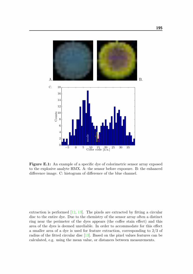
195

A. B.

Counts

Color code [a.u.]

med

ian

mean

mode

−5 0 5 10 15 20 25 30 350

2

4

6

8

10

12

14

16

C. 18

Figure E.1: An example of a specific dye of colorimetric sensor array exposedto the explosive analyte HMX. A: the sensor before exposure. B: the enhanceddifference image. C: histogram of difference of the blue channel.

extraction is performed [12, 13]. The pixels are extracted by fitting a circulardisc to the entire dye. Due to the chemistry of the sensor array often a distinctring near the perimeter of the dyes appears (the coffee stain effect) and thisarea of the dyes is deemed unreliable. In order to accommodate for this effecta smaller area of a dye is used for feature extraction, corresponding to 2/3 ofradius of the fitted circular disc [13]. Based on the pixel values features can becalculated, e.g. using the mean value, or distances between measurements.

196

E.2.3. Classification Methods

E.2.3.1. K-Nearest Neighbor

The KNN is a simple yet effective classification technique [14] which worksas follows. When testing a data point belonging to an unknown class, thedistances to all points with known class labels are calculated. The classes of theclosest K points are then identified and the unknown point is classified usingmajority voting. In order to carry out both model selection and estimation of thegeneralization error, double-cross validation using leave-one-out is performed.The inner loop is used to determine the value of K and the outer loop is usedto estimate the generalization error.

E.2.3.2. Gaussian Process Classification

We now turn to a different but equally powerful classification framework basedon a non-parametric Bayesian approach. The core of any probabilistic classifi-cation methods is a likelihood function modeling the likelihood of observing aspecific outcome. Here we consider the cumulative Gaussian (known as a probitmodel) defined as

p (yn|f (Xn)) =

yn·f(Xn)∫−∞

N (t|0, 1) dt = Φ(yn · f (Xn)) (E.1)

parameterized by a given a functional value, f(Xn). Hence, the model or freeparameter is the functional value, f(Xn), and by taking a Bayesian approach,we can directly consider the posterior over the function defined by the finite setof random variables, f = [f(X1), f(X2), ..., f(XN )]

�, i.e.,

p (f |Y,X ) =p (Y|f ) p (f |X )∫p (Y|f ) p (f |X ) df

=p (Y|f) p (f |X )

p (Y|X )(E.2)

The natural prior for, f(·), is a Gaussian Process (GP) and we denote a functiondrawn from a GP as f (X) ∼ GP (0, k(·, ·)θc

)with a zero mean function, and

k(·, ·)θcreferring to the covariance function with hyper-parameters θc, defining

the covariance between the random variables f . The GP can thus be considereda distribution over functions, i.e., p (f |X , θc).

Given the probit likelihood model, the posterior over f needs to be approximatedand we resort to Expectation Propagation (EP) which provides a Gaussianapproximation to the posterior [15]. The hyper parameters are approximatedby point-estimates found by considering the marginal likelihood/evidence whichcan be optimized in regards to the hyper parameters by gradient methods. Thispossibility is a clear advantage over non-Bayesian methods.

197

The prediction for a new input X∗ is obtained by first computing the predic-tive distribution, p(f∗|Y,X ,X∗), which is Gaussian due to the EP approxima-tion. The probability of a given outcome y∗ is computed by P (y|Y,X ,X∗) =∫p (y|f∗) p(f∗|Y,X ,X∗)df∗.

E.2.4. Distances and Covariance Functions

The two classification methods outlined above both require some notion of simi-larity either in the form of a distance function/metric or in the form of a covari-ance function. In the following we present and motivate a number of distancemeasures that can be used for measuring similarities between dyes.

E.2.4.1. Mean and “inner mean”

The traditional approach when using colorimetric sensors is to calculate themean value of the response by averaging the color change over all pixels.

Since we have observed that pixel values in the outer edge of the dyes areless reliable, we propose to estimate an optimal radius instead of a fixed radius(typically r=2/3) and compute the mean in the central region within this radius.Assuming that each dye should have a unique color change and such that anyvariation is due to noise, a reasonable assumption is to choose the radius thatestimates the mean most accurately. This is done by choosing

r = arg minr

1√Npix(r)

σ(r), (E.3)

where Npix(r) and σ(r) denote the number of pixels and the standard deviationof pixel values within the central region with radius r. We denote this method“Inner Mean”.

E.2.4.2. Hellinger Distance

As an alternative to computing the average color change, we can consider thedistribution of color change over the dye. The Hellinger distance measuressimilarity between two probability measures fi(x) and fj(x) and is given by

dHe(fi, fj)2 =

∫ (√fi(x)−

√fj(x)

)2

dx (E.4)

Using the Hellinger distance require us to choose how to represent the probabilitymeasures. We consider a nonparametric and a parametric approach: The first isa Parzen window Kernel density estimator which have been discussed in earlier

198

work [11]:

fi(x) =1

ni

ni∑k=1

K(x− xik) (E.5)

whereK(x) = 1/(2πσ2)d/2 exp(−||x||2/2σ2) and the kernel width is set to σ = 1.The second approach is a multivariate normal distribution using a full covariancematrix

fi(x) =1

(2π)d/2|Σi|d/2exp

(−1

2(μi − x)

�Σi

−1 (μi − x)

)(E.6)

where μi is the mean and Σi the covariance matrix which is estimated bymaximum likelihood.

E.2.4.3. The Hausdorff Distance

The Hausdorff distance measures distance between two point sets, and it is smallif all points in each set are close to some point in the other set. This could beuseful for comparing dye color changes that are not uniform over the dye. Firstdefine the distance between two points xi and xj as the Euclidean distanced(xi,xj) = ‖xi − xj‖2. The distance between a point xi and a set Xj is thend(xi,Xj) = min

xj∈Xj

d(xi,xj). The Hausdorff distance is defined as

dHa(Xi,Xj) = max

{maxxi∈Xi

d(xi,Xj), maxxj∈Xj

d(xj ,Xi)

}(E.7)

As an alternative approach one can use the modified Hausdorff distance whichis more robust in the presence of noise and outliers

dMH(Xi,Xj) =

max

⎧⎨⎩ 1

NXi

∑xi∈Xi

d(xi,Xj),1

NXj

∑xj∈Xj

d(xj ,Xi)

⎫⎬⎭ (E.8)

It should be noted that this distance is not a metric as the triangle inequalityis not fulfilled [16].

E.2.4.4. From Distances to Covariance Functions

Given a distance metric d(X i,Xj) we use the distance substitution approach [17]

based on a squared exponential kernel, k (Xi,Xj) = exp(− 1

σld(X i,Xj)

).

We note that a valid covariance function may be constructed directly for theHellinger distance by considering the inner product given by the integral which

199

is known as the Probability Product Kernel [18]; however, to make a fair com-parisons we treat the Hellinger distance like the other distance measures. Notealso, that since the modified Hellinger distance is not a metric, the distancesubstitution kernel is not positive definite [17].

The use of kernels provides a convenient way of integrating information from dif-ferent sensors by combining different kernels in a weighted sum. Thus, differentdyes can be combined by constructing the following kernel

k (Xi,Xj) = σ2I+M∑

m=1

αmk(Xm

i ,Xmj

)(E.9)

where each kernel function is the distance substitution kernel with one of therespective metrics.

To fuse the difference dyes we employ a forward selection method using thefollowing steps. 1) For a given dye, perform a grid search of hyper parametersσ2, αm and σl. 2) Find the hyper parameters by optimizing the evidence in GPusing the optimal point found in the grid as initial guess. 3) Perform leave-one-out cross validation to get classification error. 4) Choose the dye that yields thelowest classification error.

E.2.5. Evaluation

We apply nearest neighbor classifiers to each dye for each feature extractiontechnique in a one vs all setting. From earlier work [12] it was shown thatthe sensor is proficient in detecting among others acids, alcohols, amines andexplosives so these are the classes we evaluate. The generalization error isestimated using LOOCV [19]. This scheme result in a total of 124 classifiers ofeach type per feature extraction method (31 dyes × 4 classes).

To judge the differences in classification performance we use the McNemar sig-nificance test [20]. The McNemar is a paired test which uses the the numberof cases where two classifiers disagree about a decision. From this test we cal-culate p–values for each comparison and use the multiple hypothesis frameworkproposed by Storey [21]. Based on the p–values we can calculate the expectedpositive false discoveries (E[pFD]) for our significant differences, that is, theexpected quantity of wrongly significant results amount all found significantresults.

200

Dye number

Leave–one–outclassifi

cation

error[%

]

Explosives – KNN

19 30 28 16 24 7 17 22 27 10

2

4

6

8

10

12

14

Dye number

Leave–one–outclassifi

cation

error[%

]

Alcohols – KNN

19 27 23 12 16 17 18 22 30 216

7

8

9

10

11

12

13

14

15

16

Dye number

Leave–one–outclassifi

cation

error[%

]

Explosives – GP

19 30 28 24 17 25 16 29 7 140

2

4

6

8

10

12

14

Dye number

Leave–one–outclassifi

cation

error[%

]

Alcohols – GP

27 16 19 30 29 22 13 17 18 216

7

8

9

10

11

12

13

14

15

16

GaussianMod. HausdorffInner MeanParzenMean

Number of dyes

Leave–one–outclassifi

cation

error[%

]

1 2 3 4 50

0.2

0.4

0.6

0.8

1

1.2

1.4

1.6

1.8

2

GaussianMod. HausdorffInner MeanParzenMean

Number of dyes

Leave–one–outclassifi

cation

error[%

]

1 2 3 4 50

1

2

3

4

5

6

7

8

9

Figure E.2: Classification error for the different measures of similarity for GPand KNN. The top panels show the best performing dyes for explosives andalcohols using KNN. The middle panels show the best performing dyes usingGP. The bottom panels shows the result of fusing the dyes together using GP.Bottom left is explosives and bottom right is alcohols.

201

Chemical M P IM MH G E[pFD] n

Acids 1 2 2 6 0 0.89 11Alcohols 0 0 0 0 3 0.15 3Amines 1 0 1 0 0 1.02 2Explosives 0 3 0 7 1 0.98 11

Table E.1: Number of instances the best performing method is significantlybetter than another method. The methods are Mean, Parzen, Inner Mean, Mod.Hausdorff and Gaussian. E[pFD] is the expected positive false discoveries andn is the number of significant results.

E.3. RESULTS AND DISCUSSION

Initially we employ KNN and rank the dyes according to their best performance.Fig. E.2 top panels show the dye ranking for KNN. The modified Hausdorff isthe best performer for dyes 19 and 30 where it is significantly better than thesingle feature methods. Further the distribution methods are generally betteror on par compared to the single feature methods.

Table E.1 shows a summery of the McNemar significance tests. The overallbest distance is the modified Hausdorff method although it is noteworthy thatthis method is not best even once for alcohols whereas is is best for numerousoccasions for acids and explosives. Looking into the dyes reveal that the top dyesfor acids largely overlap with the top dyes for explosives whereas for alcoholsone of the top dyes is dye number 5. For this dye the Inner Mean is significantlybetter than any of the other methods. It should be noted that the majorityof the differences is between one of the distribution methods and the singlefeature method, i.e. of the 52 significant results, only on 3 instances was theParzen window worst and only 4 times where the Mod. Hausdorff method worst.Considering we have a total of 6 false discoveries we can only conclude that thedistribution methods are significantly better than the single feature methods.To explore the effect of the methods deeper we fuse the dyes using GP.

Initially we want to establish the performance of GP in the same setting as KNN.Fig. E.2 show the classification performance for GP when classifying explosives.Again the modified Hausdorff is the top performer for the first two dyes, whichis again dye 19 and 30. However for dye 28 and 24 the modified Hausdorffcoupled with GP yields an error of 21% and 30% respectively. This might verywell be an effect of the fact that the modified Hausdorff is not a valid metricand as such the corresponding kernel might not be psd [16, 17]. But as the caseof KNN, the figure does not show a clear indication of which method is superior

202

although it seems that modified Hausdorff is able to capture more informationabout dye 19 and 30 than the the methods.

When fusing the dyes one by one using forward selection we find no significantresults between the methods (Fig. E.2). To get a significant result the perfor-mance must at least differ 2.4 percent points but already with one dye we arebelow that margin.

E.4. CONCLUSIONS

We have proposed three new methods for representation of sensory data incolorimetric sensor arrays, namely the Inner Mean, Hellinger distance usinga Gaussian distribution and the Modified Hausdorff. Each method have it’smerits. The Inner Mean seem to be particularly proficient for dye number 5and 22 whereas the modified Hausdorff is especially strong for dye number 19and 30. This suggests that none of the methods are capable of representingall the dye measurements optimally, although the methods that use the entirehistogram are more often superior.

The modified Hausdorff method is the overall best performing method. It isparticularly strong for classifying explosives, and since the distance calculationis based on sets of pixels and is parameter-free it can potentially work a lotbetter for high dimensional data where the Hellinger distance method might beinappropriate.

Finally, we have demonstrated that fusing the sensors can improve the classifica-tion error. GP classification effectively identifies which dyes should be includedand generally including more dyes reduces the LOOCV error rate. In the fusingscheme the modified Hausdorff method also works well and is the overall bestperformer. Future work could be to combine all distance methods and learn thecombination using Multiple Kernel Learning or evidence optimization insteadof minimizing the classification error.

E.5. REFERENCES

[1] Kevin M. Carter, Raviv Raich, William G. Finn, and Alfred O. Hero. In-formation Preserving Component Analysis: Data Projections for Flow Cy-tometry Analysis. IEEE Journal of Selected Topics in Signal Processing, 3(1):148–158, February 2009. ISSN 1932-4553. doi: 10.1109/JSTSP.2008.2011112.

203

[2] Kevin M. Carter, Raviv Raich, William G. Finn, and Alfred O. Hero. FINE:fisher information nonparametric embedding. IEEE transactions on patternanalysis and machine intelligence, 31(11):2093–8, November 2009. ISSN1939-3539. doi: 10.1109/TPAMI.2009.67.

[3] Chen Zhang and Kenneth S. Suslick. A colorimetric sensor array for organ-ics in water. Journal of the American Chemical Society, 127(33):11548–9,August 2005. ISSN 0002-7863. doi: 10.1021/ja052606z.

[4] Kenneth S. Suslick, Neal A. Rakow, and Avijit Sen. Colorimetric sensorarrays for molecular recognition. Tetrahedron, 60(49):11133–11138, Novem-ber 2004. ISSN 00404020. doi: 10.1016/j.tet.2004.09.007.

[5] Neal A. Rakow, Avijit Sen, Michael C. Janzen, Jennifer B. Ponder, andKenneth S. Suslick. Molecular recognition and discrimination of amineswith a colorimetric array. Angewandte Chemie (International ed. in En-glish), 44(29):4528–32, July 2005. ISSN 1433-7851. doi: 10.1002/anie.

200500939.

[6] Chen Zhang, Daniel P. Bailey, and Kenneth S. Suslick. Colorimetric sensorarrays for the analysis of beers: a feasibility study. Journal of agriculturaland food chemistry, 54(14):4925–31, July 2006. ISSN 0021-8561. doi: 10.1021/jf060110a.

[7] Sung H. Lim, Liang Feng, Jonathan W. Kemling, Christopher J. Musto,and Kenneth S. Suslick. An Optoelectronic Nose for Detection of ToxicGases. Nature chemistry, 1:562–567, September 2009. ISSN 1755-4349.doi: 10.1038/nchem.360.

[8] Chen Zhang and Kenneth S. Suslick. Colorimetric sensor array for softdrink analysis. Journal of agricultural and food chemistry, 55(2):237–42,January 2007. ISSN 0021-8561. doi: 10.1021/jf0624695.

[9] Natalie V. Kostesha, Tommy S. Alstrøm, Carsten Johnsen, Kent A. Nielsen,Jan O. Jeppesen, Jan Larsen, Mogens H. Jakobsen, and Anja Boisen. De-velopment of the colorimetric sensor array for detection of explosives andvolatile organic compounds in air. In Proceedings of SPIE, volume 7673,pages 76730I–76730I–9, 2010. doi: 10.1117/12.850310.

[10] Natalie V. Kostesha, Tommy S. Alstrøm, Carsten Johnsen, Kent A. Nielsen,Jan O. Jeppesen, Jan Larsen, Anja Boisen, and Mogens H. Jakobsen. Multi-colorimetric sensor array for detection of explosives in gas and liquid phase.In Proceedings of SPIE, volume 8018, pages 80181H–80181H–12, 2011. doi:10.1117/12.883895.

[11] Tommy S. Alstrøm, Raviv Raich, Natalie V. Kostesha, and Jan Larsen.Feature extraction using distribution representation for colorimetric sensor

204

arrays used as explosives detectors. In IEEE International Conference onAcoustics, Speech, and Signal Processing (ICASSP), pages 2125–2128, 2012.doi: 10.1109/ICASSP.2012.6288331.

[12] Tommy S. Alstrøm, Jan Larsen, Natalie V. Kostesha, Mogens H. Jakobsen,and Anja Boisen. Data representation and feature selection for colorimetricsensor arrays used as explosives detectors. In IEEE International Workshopon Machine Learning for Signal Processing (MLSP), pages 1–6, 2011. doi:10.1109/MLSP.2011.6064615.

[13] Tommy S. Alstrøm and Jan Larsen. Feature Extraction and Signal Rep-resentation for Colorimetric Sensor Arrays. Technical report, DTU Infor-matics, 2011. URL http://www.imm.dtu.dk/pubdb/p.php?5845.

[14] Christopher M. Bishop. Pattern Recognition and Machine Learning.Springer, Secaucus, NJ, USA, 2006. ISBN 0387310738.

[15] Carl E. Rasmussen and Christopher K. I. Williams. Gaussian Processesfor Machine Learning. MIT Press, April 2006. URL http://www.

gaussianprocess.org/gpmlhttp://www.ncbi.nlm.nih.gov/pubmed/

15112367.

[16] Marie-Pierre Dubuisson and Anil K. Jain. A modified Hausdorff distancefor object matching. In Proceedings of 12th International Conference onPattern Recognition, pages 566–568, 1994. ISBN 0-8186-6265-4. doi: 10.

1109/ICPR.1994.576361.

[17] Bernard Haasdonk and Claus Bahlmann. Learning with Distance Substi-tution Kernels. Pattern Recognition, 3175:220–227, 2004. doi: 10.1007/

978-3-540-28649-3_27.

[18] Tony Jebara, Risi Kondor, and Andrew Howard. Probability ProductKernels. Journal of Machine Learning Research, 5:819–844, 2004. URLhttp://jmlr.csail.mit.edu/papers/v5/jebara04a.html.

[19] Lars K. Hansen and Jan Larsen. Linear unlearning for cross-validation.Advances in Computational Mathematics, 5(1):269–280, 1996. doi: 10.

1007/BF02124747.

[20] Quinn McNemar. Note on the sampling error of the difference betweencorrelated proportions or percentages. Psychometrika, 12(2):153–157, June1947. ISSN 0033-3123. doi: 10.1007/BF02295996.

[21] John D. Storey. A direct approach to false discovery rates. Journal of theRoyal Statistical Society: Series B (Statistical Methodology), 64(3):479–498, August 2002. ISSN 13697412. doi: 10.1111/1467-9868.00346. URLhttp://doi.wiley.com/10.1111/1467-9868.00346.

Appendix F

Advanced detection ofexplosives using colorimetric

sensor array

Natalie V. Kostesha, Tommy S. Alstrøm, Olga V. Mednova, Carsten Johnsen,Kent A. Nielsen, Jan O. Jeppesen, Mogens H. Jakobsen, Jan Larsen, and AnjaBoisen. Advanced detection of explosives using multi-colorimetric sensor array.Will be submitted to Journal of American Chemical Society (JACS), 2013.

This manuscript is yet to be submitted as should be considered work in progress.Some details still needs to be ironed out, but the manuscript is included as itexplains a lot of details about colorimetric sensor arrays.

206 Appendix F

Advanced detection of explosives using colorimetric sensor array

Natalie V. Kosteshaa, Tommy S. Alstrømb, Olga V. Mednovaa, Carsten Johnsenc, Kent A. Nielsenc, Jan O. Jeppesenc,

Mogens H. Jakobsena, Jan Larsenb, and Anja Boisena

aDepartment of Micro and Nanotechnology, Technical University of Denmark, Ørsteds Plads 345 East, DK-2800, Kgs. Lyngby, Denmark

bDepartment of Applied Mathematics and Computer Science, Technical University of Denmark, Richard Petersens Plads 305, 2800 Kgs. Lyngby, Denmark

cDepartment of Physics, Chemistry and Pharmacy, University of Southern Denmark, Campusvej 55, DK-5230, Odense M, Denmark

Abstract

Through the combination of chemically selective compounds with colour changing properties we developed a

colorimetric sensor array for the detection of explosives like DNT, HMX, RDX and TATP. The colorimetric sensing

technology was based on an array of chemo-selective compounds belonging to different chemical families immobilized

on a solid support. Upon exposure to an analyte in suspicion the colorimetric array changes colour. Almost each chosen

compound reacted chemo-selectively with the analyte of interest. Colour changes indicated the presence of unknown

explosives and volatile organic compounds. The colorimetric sensor was sensitive to DNT in the concentration from

1 ppm and higher. Such sensing technology can be used to screen for relevant explosives in a complex background as

well as to distinguish mixtures of volatile organic compounds distributed in gas phase.

Keywords: colorimetric sensor array, DNT, HMX, RDX, TATP, chemo-selective compounds, tetrathiafulvalene, RGB,principal component analysis, the K–nearest neighbor analysis.

* Corresponding Author: Natalie Kostesha, natalie.kostesha@nanotech.dtu.dk; Tel: + 45 45 258142;Fax: + 45 45 88 77 62; www.dtu.dk; http://www.xsense.dk/

Introduction

The production and utilization of explosives and explosive-related compounds have a great concern on public security

and environment. New technology must be developed to detect easily a variety of explosives, illegal chemicals and

drugs, drug precursors carried by suspects as well as hidden in mails, luggage and conveyance. Colorimetric sensing

technique is a promising analytical method which can be used for detection and identification of explosives with high

probability. This method is an easy-to-use on-site method similar to the well-known pH paper stick which shows a

prominent response based on colour changes in the presence of explosives. The colorimetric sensor array (31 dyes) is

based on the application of four successive dye classes: Tetrathiafulvalene derivatives (TTF), Lewis acid/base dyes (i.e.

metal ion containing dyes), Brønsted acidic or basic dyes (i.e. pH indicators), and dyes with large permanent dipoles

(i.e. zwitterionic solvatochromic dyes).

Advanced detection of explosives using colorimetric sensor array 207

Suslick et al. demonstrated the capability of the colorimetric sensor array to sense different analytes, even a mixture of

analytes by applying three classes of chemo-selective compounds: 1). Lewis acid or base dyes, 2). Brønsted acidic or

basic dyes and 3). Dyes with large permanent dipoles. The colorimetric response is based on specific interactions

between molecules e.g. dipolar and multipolar interactions, acid-based interaction, van der Waals interaction and

physical adsorption.1,2 The colorimetric array was able to change the colour upon exposure to an analyte of interest.

Digital imaging of the colorimetric array before and after exposure to analytes, like for example amine molecules, gave

the possibility to create a colour difference map which was presented as a unique fingerprint for each molecule of

interest.3 The colorimetric sensing technology has already been successfully applied for the visualization of the

presence of relevant molecules in a complex background4,5 as well as for the distinction of volatile organic compound

mixtures distributed in a liquid phase.6

The colorimetric sensor has shown promising results in the detection of molecules at low concentration rates, e.g. in

detection of formaldehyde with detection limit of 20 ppm,7 mercury in aqueous environments demonstrating a detection

limit of 2 ppm,8 in selective detection of closely related amines with a detection limit of 600 ppb,3 even in detection of

an explosive, like triacetone triperoxide – TATP.9 The sensor has been exposed to the liquids testing an ethanol rate and

organic compounds in the beer10 and a CO2 content in soft drink samples.11

For the first time a new colorimetric sensor array containing 31 chemo-selective compounds was applied and examined

in the prospect of detecting explosive molecules e.g. 2,4-dinitrotoluene (DNT); 1,3,5-trinitroperhydro-1,3,5-triazine

(RDX); 1,3,5,7-tetranitro-1,3,5,7-tetraazacyclooctane (HMX); 3,3,6,6,9,9-hexamethyl-1,2,4,5,7,8-hexaoxacyclononane

(TATP). The colorimetric sensor array presented in this paper was designed by using derivatives of tetrathiafulvalene

(TTF) molecules (1-15 dye) with their ability to change colour combined with additional three classes of chemo-

selective compounds described above (16-31 dye).1

In general, the TTF molecular unit presented in Figure 1A was the core unit for synthesis of 13 TTF molecules. TTF

molecules containing various incorporated electron withdrawing and accepting groups represented in Figure 1B; TTF

molecules were synthesized at the University of Southern Denmark (More information on synthesis presented in

Supplementary Material). The conductive properties of TTF molecules12 first are based on oxidation-reduction

behaviour of the TTF molecular unit where the neutral non- -system turns to aromatic 6-

converting from the radical-cation (TTF•+) to dication (TTF2+) and vise-versa (Fig. 1A).13,14 Also, the conductivity can

be enhanced by modifying the TTF unit with electron withdrawing and accepting groups (Fig. 1B). Conductive

properties and chemical stability of TTF have enabled TTF molecules to play a fundamental role in material science,

macrocyclic and supramolecular chemistry; during the past two decades and being a key candidates for the construction

of sensors,15,16 switches,17 for synthesis of conducting and semiconducting polymers and materials.18 Tetrathiafulvalene

and TTF derivatives are known as molecules which provide non-covalent interactions between molecules, where

- -dipole etc. which also occurred and provide the formation

of supramolecular complexes between molecules. 19 The formation of supramolecular complexes in TTF chemistry is a

common effect; a TTF molecular originates as a host molecular, binding another molecular which occurred to be a guest

molecular, thereby producing the supramolecular complex. A host is usually larger than a guest molecular containing

groups to perform hydrogen bonding, whereas a guest molecular fitting a binding site, providing groups to complete the

interaction. Supramolecular host-guest complexes exhibit good stability in both solutions and solid phases. The chemo-

selective properties of TTF molecules have attracted considerable attention due to the electron donor-acceptor

208 Appendix F

properties, their capability of recognizing specific analytes and potential selective colour change after exposure to a

specific analyte.16 TetraTTF-calix[4]pyrrole is one of the promising molecules for the detection of explosives. A

tetraTTF-calix[4]pyrrole-based sensor has been tested already in the identification of 3,5-dinitrobenzoate,20

trinitrobenzene, picric acid,21 towards anions such as Cl¯, Br¯ , F¯.15 TTF molecules can be used in detection of other

chemical compounds belonging to various classes: amines, alcohols, arenes, ketones, aldehydes, and acids.22 In this

research the application of tetrathiafulvalene and TTF derivatives was expanded for sensing and identification of the

most widely used military high-energetic explosives.

The main effort in efficient detection of explosives is based on the development of a method which will be successful in

the detection of molecules in low concentrations in gas or vapour phase. Explosives in both solid and liquid form

release some vapour denoted as a vapour pressure which depends exponentially on a temperature range. By knowing

the heat of sublimation it is possible to perform a rough theoretical calculation of the vapour pressure of explosives

based on the Antoine equation as a simplified from of the Clausius-Clapeyron equation.23,24 Due to the low vapour

pressure of explosives under the ambient conditions the detection of such materials as DNT or RDX usually fails.

However, the temperature rise effects on the vapour pressure parameters thereby enhance the concentration of

explosives from particles per billion (ppb) to particles per million (ppm), respectively and therefore increase a chance

for explosives tracking. Terrorists and distributors of illegal materials always work towards the development of new

compositions and substances with low vapour pressures which are not easy to detect.

New methods have been developed for sensing vapours emanating from explosives; these technologies are mainly

based on the application of electrochemical approaches,25 calorimetric 26–28 and optical9 methods and etc. In this paper

we present a simple chemical sensor, like an artificial nose, based on the application of a colorimetric sensor array for

detecting explosives like DNT, RDX, HMX and TATP. The chemo-selective compounds in the array have been chosen

due to their potential selectively change colour after exposure of the specific explosives.

To increase the colorimetric sensor probability we applied different statistical methods. To evaluate the colorimetric

sensor features four independent classifiers were applied in this work: 1). 1–Nearest-neighbor (1-NN); 2). k– Nearest-

neighbor (k–NN); 3). Sparse logistic regression (SLR) and 4). Artificial neural networks (ANN). We have found that

the best statistic depends on both the experimental setup and the classifier employed. The goal of this work was to

identify the optimal mathematical approach which can be applied in detection of explosives. By using multiple

classifiers we were able to improve the detection accuracy of the sensor of 62.8%.

Materials and Methods

Reagents:

Analytes that have been exposed to the sensor: 1-methyl-2,4-dinitrobenzene (DNT), dimethyl sulfoxide (DMSO), 1,4-

dichlorobenzene (DB) and 1-nitro-2-octyloxybenzene (NPOE) were acquired from Sigma-Aldrich (St. Louise, MO,

USA); 1,3,5-trinitroperhydro-1,3,5-triazine (RDX), 1,3,5,7-tetranitro-1,3,5,7-tetraazacyclooctane (HMX), 3,3,6,6,9,9-

hexamethyl-1,2,4,5,7,8-hexaoxacyclononane (TATP) were supplied from the Danish Emergency Management Agency

(Beredskabstyrelsen).

For the colorimetric sensor array 31 dyes were applied. TTF compounds – dyes 1 to 15 in the array were synthesized at

the department of Physics, Chemistry and Pharmacy, University of Southern Denmark. The information on TTF

Advanced detection of explosives using colorimetric sensor array 209

compounds presented in the Supplementary Material part. Other dyes: Alizarin (16), bromocresol green (17),

bromocresol purple (18), bromothymol blue sodium salt (19), bromphenol blue (20), xylenol blue (21), chlorphenol red

(22), cresol red (23), crystal violet lactone (24), 2,6-dichloro-4-(2,4,6-triphenyl-1-pyridinio)-phenolate (25), Reichardt’s

dye (26), phenol red (27), rosolic acid (28), methyl red (29), nitrazine yellow (30), 4-brom-2,6-dimethylphenol (31)

were provided from Sigma-Aldrich (St. Louise, MO, USA). Stock solutions of chemo-selective compounds (1% in

NPOE, DMSO and DB) were freshly prepared and stored in a lightproof flask before use.

Colorimetric sensor array:

A colorimetric sensor array was designed by using 31 selected dyes. Dyes were immobilized onto silica gel Kieselgel

60F254 plates (Merck KGaA, Germany) in the working volume of 1 µL per spot. Since explosives have very low vapor

pressure at room temperature and consequently low concentration, tested analytes were heated up. Explosives were

detected at 25º C and the elevated temperature of 35°C, 50°C, 70°C and 100°. Samples of explosives in tightly closed

vessels were heated up at defined temperature during 3 hours and removed from a heating system before the

measurements.

Pictures of the colorimetric sensor array before and after the exposure of an analyte were scanned through an ordinary

flatbed scanner (Epson V750-M Pro Perfection scanner). Pictures were obtained immediately after immobilization of

dyes and after exposure of analytes. The colorimetric sensor was dipped into a vessel containing an analyte and

remained there during 2 minutes. Images from the Epson scanner were obtained at 600 dots per inch in RGB color and

saved in tiff format. Pictures were analyzed using the MatLab software.

Data extraction:

In order to extract the color code from each dye the position of each dye on the image was located. The exact procedure

that was used is described in. Each dye was represented using the red, green, and blue color scheme. In this model every

color is provided as red, green, and blue color (RGB); RGB values are given in the 0-255 integer range. The minimum

intensity of the color gives black (0;0;0) and maximum white color (255;255;255). After the dye was located and

converted to RGB values, we calculated the median value of each. We used the median instead of the mean in order to

be more robust to noise and outliers.

A traditional difference map was obtained from the values of red, green or blue colors after exposure minus the value of

red, green or blue color before the exposure. Since the RGB color scheme does not allow negative values the absolute

difference was taken. In the detection of DNT part we used the real value obtained from the colorimetric sensor. In the

detection of other explosives part in order to enhance the visibility of the colors difference maps the RGB values were

first scaled with a factor 5 and then shifted by 10. The instances where the difference map (before scaling) resulted in a

color value lower than 3 the pixel was rounded down to a color value of 0.

However, the elimination of negative values and the need for scaling in order to make the differences visible imply that

color the difference map does not produce unique representations and further that sign-information is list. As an

alternative we suggest to use bar plots where each bar represents the cumulative density function (CDF) of difference

values.

Statistical visualization

210 Appendix F

Data obtained with the colorimetric sensor array has been evaluated by using the principal component analysis (PCA)

method. PCA is a simple, non-parametric method which is often used to visualize high dimensional data. The original

data obtained from the colorimetric sensor is of 93 dimensions (31 dyes, 3 colors per dye) which is not visualized in an

informative figure unless data processing has been done22,29. PCA will transform the data matrix and identify the linear

projections which have maximum variability often denoted principal components. Each successive linear projection is

orthogonal to all previous projections. Assuming that the sensor has a high signal to noise ratio the first principal

components will visually analyte dispersion nicely.

Data evaluation:

To assess the ability of the colorimetric sensor array to classify explosives we build a multi-nominal classifier which is

called K-nearest-neighbor30,31. The K–nearest neighbor has been as an effective classification technique provided that

measurements made on identical analytes make up clusters in the data space. The method works as follows; Data is

separated into two sets, a training set and a test set. The test set corresponds of just a single measurement; however each

measurement in the data set will become a test set exactly once. Thus N data sets are created. This procedure in called

leave-one-out crosses validation (LOO-CV). When identifying the analyte in the test set the Euclidian distance between

the point (one measurement corresponds to one point in 93 dimensional space) in the test set and every point in the

training set is calculated. The K closest points and the corresponding analyte are then identified. The unknown

measurement is now classified using majority voting among the identified analytes. In case of a tie the algorithm uses

the nearest neighbor among the tied classes to break the tie selecting the closest point as the analyte. Possible values of

K is set to [1;20]. To choose the value of K the training set is evaluated using LOO-CV and the value that maximizes

classification accuracy is chosen. In case of more than one optimal K the smallest value is favored.

Results:

Detection of DNT

The colorimetric sensor array first was exposed to vapour emanating from the explosive 2,4-dinitrotoluene (DNT).

Samples of DNT were heated up to 100° C to achieve the saturated condition. The response of the colorimetric sensor

before and after exposure of DNT is presented in Figure 2. Experiments here were performed when CSCs were in the

random order applied on the solid support.

The idea of the randomization of CSC in the array was based on the understanding of cross-reactivity effects if such

exists between chemo-selective compounds after the immobilization. The cross-reactivity effect was analyzed before

and after exposure of DNT.

From the obtained results we could conclude that chemo-selective compounds do not react with each other after the

immobilization on the solid support, the randomization of CSC didn’t effect on the colorimetric sensor response. The

stability of CSC on the solid support were also evaluated; we couldn’t observed dyes colour changes after the

application on the solid support. Only, bromocresol purple (18) initiated the color changes from green to brown before

the assay due to the reaction with molecules present in air. We recommend applying bromocresol purple in the end of

the array to avoid the spontaneous reaction with molecules present in the air. In our previous work we have investigated

the “the coffee stain effect” of dyes applied on the solid support32.

Advanced detection of explosives using colorimetric sensor array 211

Results on the detection of DNT were evaluated after 16 independent measurements which were performed during 8

days. The Figure 2 presents one of 16 experiments where the random immobilization of chemo-selective compounds on

a solid support was applied. The position of CSCs was assessed and adjusted according to the positions of dyes

presented in the Material and Methods part and Tab. 1S in the Supplementary Material.

After the exposure of DNT the chemo-selective compounds changed colour. Almost each chosen dye reacted chemo-

selectively with the analyte of the interest. (Fig.2B, C). Chemo-selective compounds under the number of 8, 10, 12, 13,

14, 15 – TTF family and 16, 17, 18, 19, 20, 21, 22, 23, 24, 27, 28, 29 and 30 shown the response on presence of DNT.

Chemo-selective compounds under the number of 2, 3, 4, 7, 8, 9, 13 – TTF family and 16, 17, 18, 19, 20, 21, 22, 23, 24,

25, 26, 27, 28, 29 and 30 shown the response on the elevated temperature - 100° C. An unspecific response on both

DNT and 100° C has been shown by 19 dyes out of 31 dyes applied in the assay. Probability of the experiment is

presented in the Supplementary Material part. It has been describe earlier in22 that the elevated temperature was

effected on the sensor response.

Data presented in this experiment was not enhanced by a mathematical method which allows increasing the visibility of

the colours difference maps after the modification of RGB values, the unmodified signal was presented on Figure 2.

Chemo-selective compounds under the number of 8, 10, 12, 14, 15, 19 and 24 demonstrated the specific response on the

presence of DNT. By using difference map analysis was possible to distinguish the color difference after the RGB

extraction (Fig. 2C). Moreover by a naked eye it was possible to observe the different between the analyte and the

control: compound 3 became dark yellow in presence of DNT and at 100° C turned to yellow (Fig. 2B); compound 9

became light-yellow in presence of DNT and at 100° C turned to light brown, compound 10 became grey in presence of

DNT, the same color appeared for the compound 12 in presence of DNT, compounds 14 and 15 turned brown in

presence of DNT, compound 19 became yellow in presence of DNT and at 100° C turned to grey-yellow, compound 24

became light yellow in the presence of DNT and turned to blue at 100° C. Moreover, compound 25 became more

brownish and compound 26 became dark grey at 100° C (Fig. 2A, B).

The different map analysis is a very common method in colorimetry for RGB values extraction2. A difference map is

able to compose a unique fingerprint for each analyte and this can be a possibility to make a sensor response visible,

therefore simplifies the interpretation of results if fast answer is needed. In our research we developed the sensor for

detecting analytes with low vapor pressure like explosives and we can conclude that the different map analysis is

relatively weak method for this purpose. Furthermore, sometime negative color change values were obtained during

data analysis especially if a color of CSC became less intensive or disappeared from the solid support after the analyte

exposure; during the different map analysis such values are usually eliminated, basically the calculation is taking the

absolute value of a pixel value before and after exposure to an analyte.

Our goal was to evaluate the response of the colorimetric sensor from the statistical point of view. We employed the

principal component analysis (PCA) and cumulative density function (CDF) analysis. The applied algorithm for data

estimation was described in the supplementary material and in22. To evaluate the difference between DNT and 100° C

statistically 16 independent measurements were preformed. Experiments were conducted during 8 days, 2 accomplished

measurements were completed per day, and 2 measurements were failed due to the data lost. Figure 3 shows the PCA

plot for DNT and 100° C for 1st to the 2th principal components (PC). According to the PCA plot the overlap in the

response between DNT and 100° C is insignificant (Fig.3A). We could observe that 100 °C and DNT grouped into

212 Appendix F

clusters. The PCA plot supports the difference map analysis where we could observe specific responses on DNT

and100° C.

Another alternative to difference map we suggest to use bar plots where each bar represents cumulative density function

(CDF) of the color change for a given dye color (RGB) when exposed to a given analyte. The CDF plot presenting the

sensor response on the presence of DNT displayed in Figure 3B. The analysis was performed after the mathematical

evaluation of color changes similar to the difference map. Mathematical algorithms were applied in order to analyze

both positive and negative values simultaneously during color changes with statistical methods; the sensory output was

put into a numerical form. Bars on the graph represent colour changes in the numerical form similar to RGB after

calculation of the median and probability values of the signal. Different colours of bars illustrate the statistics; 14

measurements were evaluated. Compete mathematical algorithms of data extraction from the colorimetric sensor is

presented in the Supplementary Material part. The cumulative densities function analysis represents the response of 4

chemo-selective compounds which were defined as significant in detection of DNT and were different from a control:

compound 12 in the blue and green spectra, compound 14 in the green spectra, compound 15 in the green spectra and

compound 24 in the blue spectra.

Sensor kinetics

In this work we were trying to investigate the sensor response when different concentration of DNT were applied and

understand the sensor sensitivity in relation to color changes. It is well know that DNT has low vapor pressure at room

temperature; at 25° C corresponds to 0.34 ppm23.

DNT samples were heated up to 25° C, 35° C, 50° C and 70° C to achieve DNT concentration of 0.33; 1.09; 6.05 and

47.4 ppm, respectively. The vapor pressure was calculated from the Antoine equation reported as the relation between

vapor pressure of a pure compound and temperature. Our results correspond to the literature data23.

All experiments were performed at room temperature, however to obtained different concentration of the explosive,

DNT samples were heated up during 3 hours at the elevated temperature as described above. The colorimetric sensor

was immersed into a vessel where the relevant concentration of DNT was achieved and remained there for 2 min; the

“naked eye” response was observed as a color change of CSC already at the concentration of DNT of 6.05ppm, sample

was heated up to 50° C.

To evaluate the sensor response four measurements on each concentration of DNT were performed. Data analysis has

shown that compounds with number 8, 12 and 13 were able to detect DTN when samples were heated up from 25° C to

70° C (Fig. 4A), thereby the sensor response increased with the increscent of DNT concentrations. However,

compound 13 has shown stable color response on different concentrations of DNT. Compounds have shown the color

shift in the blue and green spectra, similar spectra for DNT as described above when DNT samples were heated up to

100° C.

It is evident that the color intensity of the sensor increased with concentration and slop of the colorimetric curve rose up

(Fig. 4B); the response of the colorimetric sensor became more prominent because the concentration of DNT increased.

Figure 4B shows a concentration-response curve obtained from the colorimetric sensor when DNT samples were

heated up to certain temperature.

Detection of other explosives

Advanced detection of explosives using colorimetric sensor array 213

Simultaneously, with the detection of DNT we have applied the colorimetric sensor for detection of other explosives:

HMX, RDX and TATP. HMX and RDX are chemically related explosives belonging to the nitramines; HMX has four

carbon and four nitrogen atoms placed in the variable order in the eight-membered ring where one nitro-group attached

to each nitrogen atom; RDX has similar structure to HMX with the difference in one carbon and nitrogen and one nitro-

group group, respectively. TATP is a peroxide based explosive, which can be obtained by a reaction between acetone

and hydrogen peroxide forming the cyclic trimer of acetone peroxide. DNT, HMX, RDX and TATP are belonging to

different chemical classes.

The detection of explosives was performed under the same conditions as has been described in the detection of DNT

section. Experiments were carried out under the saturated condition of analyte vapours; analytes were heated up to 100°

C. The resulting colorimetric sensor was applied for 2 minutes for analysis of vapour emanating by HMX, RDX and

TATP. Digital imaging of the colorimetric array before and after exposure to analytes was used for creating of

difference map for each explosive of interest (Fig.6). In this experiment in order to enhance the visibility of the colours

difference maps the RGB values were first scaled with a factor 5 and then shifted by 10. The instances where the

difference map (before scaling) resulted in a colour value lower than 3 the pixel was rounded down to a colour value of

0. The analysis has shown that almost each chosen dye reacted chemo-selectively with the analyte of interest. A change

in a colour signature indicates the presence of explosive molecules. By using the digital imaging analysis we could

observe that obtained responses on all four analytes were unspecific, but different from a control. Only, compound 12 -

TTF and compound 24 - Crystal violet lactone have shown the specific response on the present of DNT (Fig. 6).

To analyse acquired data statistically signal processing methods were applied such as CDF, PCA and confusion matrix

(CM) analysis (Supplementary Material). Measurements have been taken during eight days performing sixteen

measurements in total (N=8; n=2), two measurement were failed due to the data lost.

The colour distributions in the numeric form are presented in Figure 7 as a CDF plot after the data processing. CSCs

under the number of 12 (TTF), Bromothymol blue sodium salt (19) and Crystal violet lactone (24) demonstrated the

signal to DNT, HMX, RDX, TATP and Control-100º C. Compound 19 and 24 demonstrated the specific signal to 100º

C. Compounds 12 and 24 demonstrated the specific signal to DNT. The response to HMX, RDX and TATP was

unspecific.

Since the sensor application in the future will be adapted to the detection of explosives under the complex environment,

like detection of dangerous materials in airports, marine ports and train stations. Additional analytes which are not

related to explosive materials, but could be present in the air were tested by the colorimetric sensor. Our goal was to

evaluate the colorimetric sensor on the presence of other molecules and estimate false positive and negative alarms. In

this paper we didn’t describe in details the sensor response non-explosive materials; the previous results were published

in22. Non-explosive materials were described in the Supplementary Material part and here we combine tested analytes

in one group and describe it as Other.

To establish the difference in detection of explosives in relation to other analytes the PCA analysis was applied (Fig.8).

In the domains where colorimetric sensors have been investigated, PCA showed high precision and low false alarm rate.

The closely related K-Nearest Neighbor (KNN) classifier which uses the Hellinger distance between colour

distributions as a metric was able to demonstrate significant improvement in accuracy. Figure 8 shows the PCA plot for

the 2nd to the 4th principal components (PC) for explosive and control - DNT, HMX, RDX, TATP and 100° C as selected

analytes and Other as selected non-explosive analytes. PCA has shown the overlap in the response for DNT, HMX,

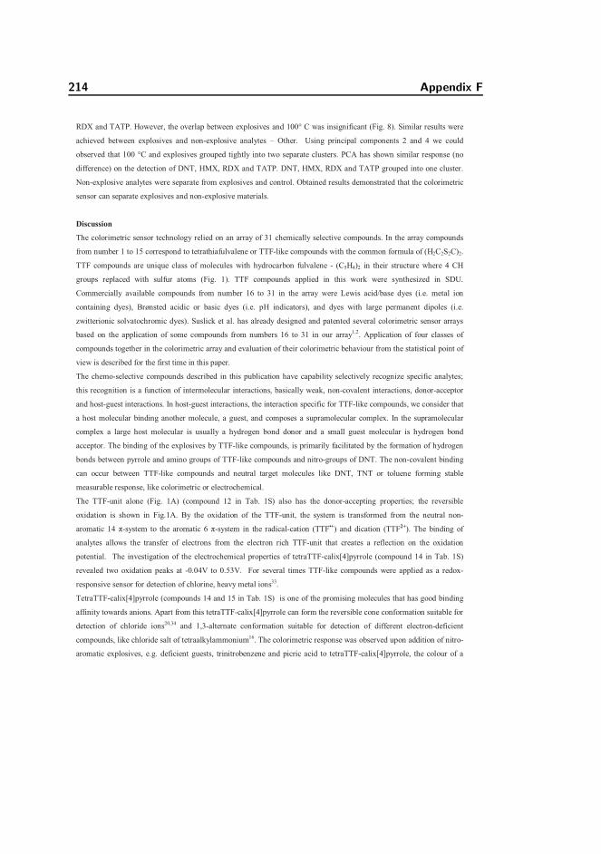
214 Appendix F

RDX and TATP. However, the overlap between explosives and 100° C was insignificant (Fig. 8). Similar results were

achieved between explosives and non-explosive analytes – Other. Using principal components 2 and 4 we could

observed that 100 °C and explosives grouped tightly into two separate clusters. PCA has shown similar response (no

difference) on the detection of DNT, HMX, RDX and TATP. DNT, HMX, RDX and TATP grouped into one cluster.

Non-explosive analytes were separate from explosives and control. Obtained results demonstrated that the colorimetric

sensor can separate explosives and non-explosive materials.

Discussion

The colorimetric sensor technology relied on an array of 31 chemically selective compounds. In the array compounds

from number 1 to 15 correspond to tetrathiafulvalene or TTF-like compounds with the common formula of (H2C2S2C)2.

TTF compounds are unique class of molecules with hydrocarbon fulvalene - (C5H4)2 in their structure where 4 CH

groups replaced with sulfur atoms (Fig. 1). TTF compounds applied in this work were synthesized in SDU.

Commercially available compounds from number 16 to 31 in the array were Lewis acid/base dyes (i.e. metal ion

containing dyes), Brønsted acidic or basic dyes (i.e. pH indicators), and dyes with large permanent dipoles (i.e.

zwitterionic solvatochromic dyes). Suslick et al. has already designed and patented several colorimetric sensor arrays

based on the application of some compounds from numbers 16 to 31 in our array1,2. Application of four classes of

compounds together in the colorimetric array and evaluation of their colorimetric behaviour from the statistical point of

view is described for the first time in this paper.

The chemo-selective compounds described in this publication have capability selectively recognize specific analytes;

this recognition is a function of intermolecular interactions, basically weak, non-covalent interactions, donor-acceptor

and host-guest interactions. In host-guest interactions, the interaction specific for TTF-like compounds, we consider that

a host molecular binding another molecule, a guest, and composes a supramolecular complex. In the supramolecular

complex a large host molecular is usually a hydrogen bond donor and a small guest molecular is hydrogen bond

acceptor. The binding of the explosives by TTF-like compounds, is primarily facilitated by the formation of hydrogen

bonds between pyrrole and amino groups of TTF-like compounds and nitro-groups of DNT. The non-covalent binding

can occur between TTF-like compounds and neutral target molecules like DNT, TNT or toluene forming stable

measurable response, like colorimetric or electrochemical.

The TTF-unit alone (Fig. 1A) (compound 12 in Tab. 1S) also has the donor-accepting properties; the reversible

oxidation is shown in Fig.1A. By the oxidation of the TTF-unit, the system is transformed from the neutral non-

- -system in the radical-cation (TTF•+) and dication (TTF2+). The binding of

analytes allows the transfer of electrons from the electron rich TTF-unit that creates a reflection on the oxidation

potential. The investigation of the electrochemical properties of tetraTTF-calix[4]pyrrole (compound 14 in Tab. 1S)

revealed two oxidation peaks at -0.04V to 0.53V. For several times TTF-like compounds were applied as a redox-

responsive sensor for detection of chlorine, heavy metal ions33.

TetraTTF-calix[4]pyrrole (compounds 14 and 15 in Tab. 1S) is one of the promising molecules that has good binding

affinity towards anions. Apart from this tetraTTF-calix[4]pyrrole can form the reversible cone conformation suitable for

detection of chloride ions20,34 and 1,3-alternate conformation suitable for detection of different electron-deficient

compounds, like chloride salt of tetraalkylammonium16. The colorimetric response was observed upon addition of nitro-

aromatic explosives, e.g. deficient guests, trinitrobenzene and picric acid to tetraTTF-calix[4]pyrrole, the colour of a

Advanced detection of explosives using colorimetric sensor array 215

solution turned from yellow to green21. The optically active tetraTTF-calix[4]pyrrole-based sensor has already been

applied for the detection of 1,3,5-trinitrobenzene, tetrafluoro- p-benzoquinone, tetrachloro-p-benzoquinone, p-

benzoquinone, and 1,3,5-trinitrophenole35.

In this work the focus on tetraTTF-calix[4]pyrroles (number 14 and 15 in Tab. 1S) was due to their ability to form

strong complex with pyrrole units forming the cone conformation of the molecular. Binding with the pyrrole group is

the essential part in the detection of explosives, moreover the 1,3-alternate conformation is also suitable for this purpose

while the interaction with electron-deficient guests. In order to increase sensing properties of TTF-like compounds,

different functional groups (Fig. 1B) either electron withdrawing group (EWG) e.g. NO2- (compound: 1, 3); COOMe-

(compound: 2, 4, 7); CN- (compound: 2, 10); CH3C6H4SO2- (compound: 1, 5, 6, 7, 9); Br- (compound: 11) or electron

donating group (EDG) e.g. NH2- (compound: 3, 8); NH- (compound: 8, 14, 15) can be incorporated to the TTF-unit.

The specific colorimetric response was observed when the charge transfer from the electron rich TTF unit (compound:

12), tetraselenofulvalene (TSeF) (compound: 13), the selenium analogue of TTF and TTF-modified with EDGs e.g.

compounds 8, 14 and 15 were binding of electron-deficient compounds, like DNT containing 2 electron deficient nitro-

groups.

The presence of DNT in the gas phase was also detected by other applied CSCs, from 16 to 31 in Table 1S e.g.

Bromothymol blue sodium salt (number 19) and Crystal violet lactone (number 24). Where, the most significant and

applicable compound in detection of DNT and other explosives was crystal violet lactone (number 24) (Fig 3A and 7).

In the colorimetric array the original – transparent colour of the dye turned into yellow in the presence of DNT and

remained transparent in the presence of HMX, RDX and TATP. At elevated temperature this dye turned to the blue

colour.

According to the analyzed data, CSCs were not only being able to detect specific analytes, also they were able to

change the colour pattern specifically at the high temperature. This effect has been described in previous publications

we were able to observe the colour change of CSCs when the temperature was elevated22. CSCs under the number of 3,

9, 17, 24, 25 and 26 changed their colour at 100° C. The thermo-stability phenomenon of CSCs was investigated in this

research; however the dipper analysis of this effect can be applied for the development of the thermo-sensor that can be

used together with the chemo-selective sensor.

The sensor response was investigated under the presence of DNT at different concentrations. We could observe the dose

response effect where the colour difference related to the concentration of the analyte.

The colorimetric sensor array demonstrated a high classification rate to explosives, especially to DNT. The colorimetric

sensor can be tested and evaluated as a thermo-sensor due to the specific colour changes at 100° C. From the obtained

results the presence of DNT could be determinate by the colorimetric sensor with high precision, with zero false

negatives (See also confusion matrix in the Supplementary Material part). However, the colorimetric sensor was very

unreliable for HMX, RDX and TATP; molecules were detected with a low precision rate: HMX was detected by sensor

4 times out of 14 measurements; RDX was detected 8 times out of 14 measurements; TATP only 3 times out of 14

measurements was classified correctly(See also confusion matrix in the Supplementary Material part).

HMX and RDX have very similar chemical structure. When RDX is manufactured in the large-scale over than 6% of

HMX is available in the explosive mixture, and also various impurities and intermediate products are present. Also,

RDX and HMX on the market are present as a mixture with other explosives like TNT, PETN and other.

216 Appendix F

It was observed that TATP is difficult to detect by using colorimetric molecules with donor-acceptor properties9. This is

probably, why the colorimetric sensor was not able to detect the difference between RDX, HMX and TATP

The resulting colorimetric sensor was used for the analysis vapour of acetone, acetic acid, ethanol, formic acid,

hydrochloric acid, methanol, propanol, and toluene22. To evaluate and expand the potential of the colorimetric sensor

advanced signal processing and statistic methods such as principal component analysis and hierarchical cluster analysis

will be applied to enhanced the sensor accuracy and reduce false alarm rate.

Conclusions:

The colorimetric sensor is a unique proprietary colour change-based sensor technology developed at DTU Nanotech and

SDU with enormous potential to form the basis of a practical technological platform for the detection of traces of

explosives like DNT, HMX, RDX and TATP. Using colorimetric sensors it is possible to observe colour changes due to

particular molecules of interest that are indicative of explosives; be they amines, alcohols, phenols, ketones, aldehydes,

or acids in the ppm and ppb range.

We are working towards the detection possibilities by the selection of new colorimetric molecules that undergo colour

changes in the presence of explosives and illegal molecules, as well as improving immobilisation methods for anchoring

dye molecules on the solid support.

This colorimetric sensor array is a rapid detection method. During of this work we could decrease the sensing time, it is

possible to achieve accurate results within 2 minutes. The colorimetric sensing technology can be used as a platform

for the rapid detection and analysis of potential illegal substances through detection of their vapour with high specificity

and sensitivity. Prior and this research showed a low limit in detection, improvement in sensitivity, specificity,

enhanced simplicity, advanced data processing and validation may be obtainable with the multi-colorimetric sensor as

compared to currently used technologies.

Another advantage of this technique is that colorimetric sensor array is an inexpensive approach, and can potentially be

produced as single use disposable units.

Advanced detection of explosives using colorimetric sensor array 217

References:

(1) Suslick, K. S.; Rakow, N. A.; Sen, A. Tetrahedron 2004, 60, 11133–11138.

(2) Janzen, M. C.; Ponder, J. B.; Bailey, D. P.; Ingison, C. K.; Suslick, K. S. Analytical Chemistry 2006, 78, 3591–3600.

(3) Rakow, N. A.; Sen, A.; Janzen, M. C.; Ponder, J. B.; Suslick, K. S. Angewandte Chemie-International Edition2005, 44, 4528–4532.

(4) Huang, X.; Xin, J.; Zhao, J. Journal of Food Engineering 2011, 105, 632–637.

(5) Suslick, B. a; Feng, L.; Suslick, K. S. Analytical chemistry 2010, 82, 2067–73.

(6) Zhang, C.; Suslick, K. S. Journal of the American Chemical Society 2005, 127, 11548–9.

(7) Feng, L.; Musto, C. J.; Suslick, K. S. Journal of the American Chemical Society 2010, 132, 4046–7.

(8) Shunmugam, R.; Gabriel, G. J.; Smith, C. E.; Aamer, K. a; Tew, G. N. Chemistry (Weinheim an der Bergstrasse, Germany) 2008, 14, 3904–7.

(9) Lin, H.; Suslick, K. S. Journal of the American Chemical Society 2010, 132, 15519–21.

(10) Zhang, C.; Bailey, D. P.; Suslick, K. S. Journal of Agricultural and Food Chemistry 2006, 54, 4925–4931.

(11) Zhang, C.; Suslick, K. S. Journal of Agricultural and Food Chemistry 2007, 55, 237–242.

(12) Demiralp, E.; Goddard, W. A. 1997, 5639, 8128–8131.

(13) Bendikov, M.; Wudl, F.; Perepichka, D. F. Tetrathiafulvalenes, oligoacenenes, and their buckminsterfullerene derivatives: the brick and mortar of organic electronics.; 2004; Vol. 104, pp. 4891–946.

(14) Nielsen, M. B.; Lomholt, C.; Becher, J. Chemical Society Reviews 2000, 29, 153–164.

(15) Nielsen, K. A.; Jeppesen, J. O.; Levillain, E.; Becher, J. 2003, 3824, 187–191.

(16) Nielsen, K. A.; Martin-Gomis, L.; Sarovac, G. H.; Sanguinet, L.; Gross, D. E.; Fernandez-Lazaro, F.; Stein, P. C.; Levillain, E.; Sessler, J. L.; Guldi, D. M.; Sastre-Santos, A.; Jeppesen, J. O. Tetrahedron 2008, 64, 8449–8463.

(17) Pease, a R.; Jeppesen, J. O.; Stoddart, J. F.; Luo, Y.; Collier, C. P.; Heath, J. R. Accounts of chemical research2001, 34, 433–44.

(18) Kaminska, I.; Das, M. R.; Coffinier, Y.; Niedziolka-Jonsson, J.; Woisel, P.; Opallo, M.; Szunerits, S.; Boukherroub, R. Chemical communications (Cambridge, England) 2012, 48, 1221–3.

(19) Steed, J.W., Atwood, J. L. Supramolecular Chemistry; Sons, J. W. &, Ed.; 2 nd.; 2009; p. 990.

(20) Nielsen, K. a. Tetrahedron Letters 2012, 53, 5616–5618.

(21) Kim, D.-S.; Lynch, V. M.; Nielsen, K. a; Johnsen, C.; Jeppesen, J. O.; Sessler, J. L. Analytical and bioanalytical chemistry 2009, 395, 393–400.

218 Appendix F

(22) Kostesha, N. V.; Alstrøm, T. S.; Johnsen, C.; Nilesen, K. a.; Jeppesen, J. O.; Larsen, J.; Jakobsen, M. H.; Boisen, A. SPIE Proc. 2010, 7673, 76730I–76730I–9.

(23) Östmark, H.; Wallin, S.; Ang, H. G. Propellants, Explosives, Pyrotechnics 2012, 37, 12–23.

(24) Oxley, J. C.; Smith, J. L.; Luo, W.; Brady, J. Propellants, Explosives, Pyrotechnics 2009, 34, 539–543.

(25) Forzani, E. S.; Lu, D.; Leright, M. J.; Aguilar, A. D.; Tsow, F.; Iglesias, R. a; Zhang, Q.; Lu, J.; Li, J.; Tao, N. Journal of the American Chemical Society 2009, 131, 1390–1.

(26) Greve, a.; Olsen, J.; Privorotskaya, N.; Senesac, L.; Thundat, T.; King, W. P.; Boisen, a. Microelectronic Engineering 2010, 87, 696–698.

(27) Yi, D. C.; Greve, A.; Hales, J. H.; Senesac, L. R.; Davis, Z. J.; Nicholson, D. M.; Boisen, A.; Thundat, T. Applied Physics Letters 2008, 93, 3.

(28) Senesac, L. R.; Yi, D.; Greve, A.; Hales, J. H.; Davis, Z. J.; Nicholson, D. M.; Boisen, A.; Thundat, T. Review of Scientific Instruments 2009, 80, 9.

(29) Carey, J. R.; Suslick, K. S.; Hulkower, K. I.; Imlay, J. a; Imlay, K. R. C.; Ingison, C. K.; Ponder, J. B.; Sen, A.; Wittrig, A. E. Journal of the American Chemical Society 2011, 133, 7571–6.

(30) Alstrøm, T. S.; Larsen, J.; Kostesha, N. V; Jakobsen, M. H.; Boisen, A.; Plads, R. P.; Lyngby, K.; East, Ø. P. 2011.

(31) Alstrøm, T. S.; Raich, R.; Kostesha, N. V; Larsen, J.; Plads, R. P.; Lyngby, K.; East, P. .

(32) Alstrøm, T. S.; Jensen, B. S.; Schmidt, M. N.; Kostesha, N. V; Larsen, J.; Allé, A.; Lyngby, K.; East, Ø. P. 2012.

(33) Nielsen, K. a.; Martín-Gomis, L.; Sarova, G. H.; Sanguinet, L.; Gross, D. E.; Fernández-Lázaro, F.; Stein, P. C.; Levillain, E.; Sessler, J. L.; Guldi, D. M.; Sastre-Santos, Á.; Jeppesen, J. O. Tetrahedron 2008, 64, 8449–8463.

(34) Nielsen, K. A.; Cho, W. S.; Jeppesen, J. O.; Lynch, V. M.; Becher, J.; Sessler, J. L. Journal of the American Chemical Society 2004, 126, 16296–16297.

(35) JEPPESEN J.O.; NIELSEN K.A New porphyrinogen derivative useful for detection of explosive chemicals such as 2,4,6-trinitrotoluene, 1,3,5-trinitrobenzene or 1,3,5-trinitrophenole 2008, 46.

Advanced detection of explosives using colorimetric sensor array 219

Figures:

Fig.1. Simplified schematics of reversible two electron reduction-oxidation mechanism (A.) and schematic structure of

the diversity of TTF molecules applied for the colorimetric sensor (B.). Common radicals: 1. R- Cyanoethylthio; 2. R-

Pentylthio; 3. R-(4-Nitrophenyl)ethylthio; 4. R-Methoxycarbonyl; 5. 2,5-Dibromo-[c]thieno; 6. R-

2-(2-(2-Methoxyethoxy)ethoxy)ethylthio; 7. R-2-(Carboxamide)ethylthio; 8. R- ????; 9. R-[c]pyrrolo; 10. R-N-Tos yl-

[c]pyrrolo; 11. R- N-Tosyl-2,5-Dihydro-[c]pyrrolo. Molecules with different radicals in TTF structure were synthesized

in SDU. Complete structure and synthesis of the molecules described in the Supplementary Material and [Patent ,Ref].

Fig. 2. Representation of the colorimetric sensor array before and after the exposure of DNT. Results were obtained in

the presence of DNT in the gas phase at 100° C. The control experiment - 100° C. The images of the difference map

was generated after the mathematical calculations of the colour changes; and presented as the difference map obtained

from the absolute values of RGB values of each dye spot before and after the exposure of the target.

220 Appendix F

Fig 3.The PCA results (A.) and CDF plot (B.) of the colorimetric sensor array obtained from the response results of DNT (N=7; n=2). The DNT signal was compared with the signal obtained at the elevated temperature 100° C. A. The PCA plot demonstrates the position of DNT and 100° C replicates demonstrating the significant variables in relation to principal components (PC) to axis 1 and 2. B. The cumulative densities function analysis represents the response of chemo-selective compounds of 12, 12, 14, 15, and 24; molecules were defined as significant in detection of DNT. Up to 14 independent measurements (coloured right side of the plot B.) were performed to evaluate colour changes of in the array (the left side of the plot B. demonstrates the delimitation of RGB values). Bars on the scheme represent colourchanges after calculation of the median and probability values of the signal.

Advanced detection of explosives using colorimetric sensor array 221

Fig 4. Representation of the sensor response at different concentrations of DNT obtained at temperatures – 25, 35, 50 and 70° C (N=1; n=4). A. The cumulative densities function analysis represents the response of chemo-selective compounds on DNT at different temperatures; 8, 12, 13 molecules were defined as significant in detection of DNT.Four independent measurements (coloured right side of the plot A.) were performed to evaluate colour changes of in the array (the left side of the plot A. demonstrates the delimitation of RGB values). Bars on the scheme represent colour changes after calculation of the median and probability values of the signal.

(B.) Calculation of the sensor correlations elevated temperatures – 25, 35, 50, 70 and 100° C (actual temperature) and predicted temperature (o-y) in relation to different concentration of DNT molecules.

Fig. 5 Mathematical representation of the signal-noise ratio of the colorimetric sensor during DNT detection.

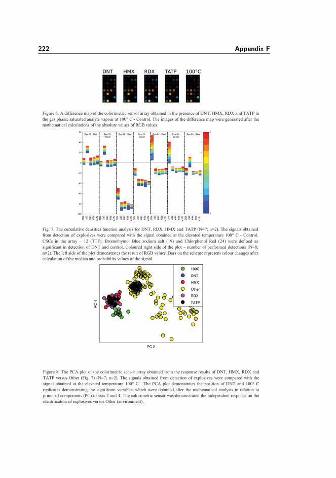
222 Appendix F

Figure 6. A difference map of the colorimetric sensor array obtained in the presence of DNT, HMX, RDX and TATP in the gas phase; saturated analyte vapour at 100° C - Control. The images of the difference map were generated after the mathematical calculations of the absolute values of RGB values.

Fig. 7. The cumulative densities function analysis for DNT, RDX, HMX and TATP (N=7; n=2). The signals obtained from detection of explosives were compared with the signal obtained at the elevated temperature 100° C - Control. CSCs in the array – 12 (TTF), Bromothymol Blue sodium salt (19) and Chlorphenol Red (24) were defined as significant in detection of DNT and control. Coloured right side of the plot – number of performed detections (N=8;n=2). The left side of the plot demonstrates the result of RGB values. Bars on the scheme represent colour changes after calculation of the median and probability values of the signal.

Figure 8. The PCA plot of the colorimetric sensor array obtained from the response results of DNT, HMX, RDX and TATP versus Other (Fig. 7) (N=7; n=2). The signals obtained from detection of explosives were compared with the signal obtained at the elevated temperature 100° C. The PCA plot demonstrates the position of DNT and 100° C replicates demonstrating the significant variables which were obtained after the mathematical analysis in relation to principal components (PC) to axis 2 and 4. The colorimetric sensor was demonstrated the independent response on the identification of explosives versus Other (environment).

Advanced detection of explosives using colorimetric sensor array 223

Supplementary material

Advanced detection of explosives using colorimetric sensor array

Natalie V. Kosteshaa, Tommy S. Alstrømb, Olga V. Mednovaa, C. Johnsenc, Kent A. Nielsenc, Jan

O. Jeppesenc, Mogens H. Jakobsena, Jan Larsenb and Anja Boisena

aDepartment of Micro and Nanotechnology, Technical University of Denmark, Ørsteds Plads 345 East, DK-2800, Kgs. Lyngby, Denmark

bDepartment of Informatics and Mathematical Modelling, Technical University of Denmark, Richard Petersens Plads 321, 2800 Kgs. Lyngby, Denmark

cDepartment of Physics and Chemistry, University of Southern Denmark, Campusvej 55, DK-5230, Odense M, Denmark

Our research is based on the selection of chemo-selective compounds (dyes) that undergo color changes in the presence of explosives and volatile organic compounds (VOCs). The list tested VOCs presented below (Table s2). The colorimetric sensor presented in this paper contains of 31 chemically selective dyes immobilized on a silica gel membrane (Table s1).

Table s1. List of chemo-selective compound tested and applied further in the colorimetric sensor array for detection of explosives and volatile organic compounds.

CAS- Formula Mw Structure and Name Availability

1 NA C13H25N3O6S7 760.00S

SN

S

S

S

STs

NO2

NO2

R1,R4 : N-Tosyl-[c]pyrroloR2,R3 : 2-(4-Nitrophenyl)ethylthio

Synthetic procedure described in 1

2 NA C38H30N4O8S12 1055.45

N

N

S

SS

S S

S

COOMe

COOMe

S

SS

S S

S

COOMe

COOMeNC

NC

R1 : (4’-{[7-(2-Cyanoethylthio)-2,3-Dimethoxy-carbonyl-6-thiomethylene]tetrathiafulvalene}-4-

Synthetic procedure described in 1

224 Appendix F

bipyridine)methylethioR2,R3 : Methoxycarbonyl R4 : 2-Cyanoethylthio

3 NA C28H28N4O6S8 773.07

S

SS

S S

S

S

S

NO2

NO2

H2N

H2N

O

O

R1,R4 : 2-(Carboxamide)ethylthioR2,R3 : 2-(4-Nitrophenyl)ethylthio

Synthetic procedure described in 1

4 26314-39-6

C14H12O8S8 436.50S

SMeOOC

MeOOC S

S

COOMe

COOMe

R1,R2,R3,R4 : Methoxycarbonyl

2

5 300766-19-2

C25H31NO2S7

601.97

S

SN

S

S

S

STs

R1,R4 : N-Tos yl-[c]pyrroloR2,R3 : Pentylthio

3

6 NA C25H35NO2S7 606.01S

SN

S

S

S

STs

HH

HH

R1,R4 : N-Tosyl-2,5-Dihydro-[c]pyrroloR2,R3 : Pentylthio

Synthetic procedure described in 1

7 NA C19H15NO6S5 516.65

S

SN

S

S

COOMe

COOMeTs

R1,R4 : N-Tosyl-[c]pyrroloR2,R3: Methoxycarbonyl

Synthetic procedure described in 1

8 NA C25H31N3S6 565.92

S

SN

S

S

S

S

H2N

HN

R1,R4 : N-(p-amidinophenyl)-[c]pyrroloR2,R3 : Pentylthio

Synthetic procedure described in 1

9 NA C23H35NO6S6 613.92S

SN

S

S

S

S O O O

O O O

R1,R4 : N-Methyl-[c]pyrroloR2,R3 :2-(2-(2-Methoxyethoxy)ethoxy)ethylthio

Synthetic procedure described in 1

10 132765-36-7

C18H16N4S8 544.87S

SS

S S

S

S

S

CN

CNNC

NC

R1,R2,R3,R4 : 2-Cyanoethylthio

Synthetic procedure described in 4

Advanced detection of explosives using colorimetric sensor array 225

11 NA C14H14Br2S12 566.52S

SS

S

S

S

SBr

Br

R1,R4 : 2,5-Dibromo-[c]thienoR2,R3 : Propylthio

Synthetic procedure described in 5

12 31366-25-3

C6H4S4 204.36S

S

S

S Sigma-Aldrich.Co.LLC.

13 55259-49-9

C10H12Se4 448.04Se

Se

Se

Se

R1,R2,R3,R4 : Methyl

Sigma-Aldrich.Co.LLC.

14 NA C100H148N4O24S242559.82

HNNH

NH HN

SS

SSS

S

SS

SSS

S

SS S

SS

S

S

S

S

S

S

S

O O

O

O

O

O

O

O

O

OO

OO

O

O

O

O

O

O

O

O

OO

O

6

15 NA C68H84N4S241727,01

NH HN

HNNH

SS

SSS

S

SS

SS

SS

SS

SS

PrS

PrS SPr

SPr

SPr

SPrPrS

PrS

7

16 72-48-0 C14H8O4 240.21 Alizarin Sigma-Aldrich.Co.LLC.

17 76-60-8 C21H14Br4O5S 698.01 Bromocresol Green Sigma-Aldrich.Co.LLC.

18 115-40-2C21H16Br2O5S

540.22 Bromocresol Purple Sigma-Aldrich.Co.LLC.

19 34722-90-2 C27H27Br2NaO5S 646.36 Bromothymol Blue sodium salt Sigma-

Aldrich.Co.LLC.

20 115-39-9C19H10Br4O5S

669.96 Bromphenol Blue Sigma-Aldrich.Co.LLC.

21 125-31-5 C23H22O5S 410.48 Xylenol Blue Sigma-Aldrich.Co.LLC.

226 Appendix F

22 4430-20-0C19H12Cl2O5S

423.27 Chlorphenol Red Sigma-Aldrich.Co.LLC.

23 1733-12-6C21H18O5S

382.43 Cresol Red Sigma-Aldrich.Co.LLC.

24 1552-42-7C26H29N3O2 415.53 Crystal Violet Lactone Sigma-

Aldrich.Co.LLC.

25 121792-58-3 C29H19Cl2NO 468.37

2,6-Dichloro-4-(2,4,6-triphenyl-1-pyridinio)phenolate

Sigma-Aldrich.Co.LLC.

26 10081-39-7 C41H29NO 551.68 Reichardt’s dye Sigma-

Aldrich.Co.LLC.

27 143-74-8 C19H14O5S 354.38 Phenol Red Sigma-Aldrich.Co.LLC.

28 603-45-2 C19H14O3 290.31 Rosolic acid Sigma-Aldrich.Co.LLC.

29 493-52-7 (CH3)2NC6H4N=NC6H4CO2H

269.30 Methyl Red Sigma-Aldrich.Co.LLC.

30 5423-07-4 C16H8N4Na2O11S2 542.36 Nitrazine yellow Sigma-Aldrich.Co.LLC.

31 2374-05-2 BrC6H2(CH3)2OH 201.06 4-Bromo-2,6-Dimethylphenol Sigma-Aldrich.Co.LLC.

Experimental design

Notation for experimental design section

Number of blocks; = 15.Number of sensors; = 31. One dye / chemo-selective compound corresponds to one sensor.

L Number of sensor responses; L= 3.Number of analytes; = 18.Number of measurements; = missing arrays = 253.

To conduct experiments correctly, we employ the randomized complete blocked design approach(RCBD). In this design the measurements are grouped into blocks, and within each block each analyte is exposed to the sensor array exactly once. The purpose of the design is to enable more precise estimation of effects since the variation from block to block can be removed; hence the RCBD is often referred to as a noise reducing design. Moreover, the order of the chemo-selective compounds (CSC) on the silica gel was randomized between 15 blocks. This is due to the fact that some of chemo-selective compounds used in this array were very reactive, the order those compounds on the silica gel support was randomized. We analyzed the sensor sensitivity to the

Advanced detection of explosives using colorimetric sensor array 227

environment first since some CSCs were exposed to the environment before the sensor array was exposed to the target analyte. This behavior of CSCs was predictable due to a strong reactive environment of a chemical laboratory. However, the response of CSCs on the environment was neglected; pictures of the colorimetric sensor have been taken immediately after the immobilization of dyes and directly after the exposure of analytes and this response were evaluated.

The application of CSCs on the silica gel support was around of 20 minutes (6 applications were performed per 1 assay) thus the maximum time a compound was exposed to the surrounding environment was around 20 minutes.

The total experimental design is listed in Table s2. The experiment lasted for 8 days, with two days break between day 4 and 5. Every day one block was executed in the morning and another block in the afternoon; although on the 8th day only the morning block was executed. The room temperature (RT) was measured each day and was always in the range 21-25° C.

During performed measurements it was observed that CSCs could change colors due to their stability; a new batch of CSCs was prepared every 3rd day.

The design contained in total of = 15, where each analyte was measured exactly once excluding mishaps. During the experiments some random mishaps occurred resulting in sensor array loss. The lost sensor arrays are listed in Table s3. Alternatively, we could have chosen to disregard incomplete blocks as whole, but we choose to use the entire collected data.

Table s2. The list of analytes tested by the colorimetric sensor array.

Tested analyte

Acid Alcohol Amine Arene Environ

ment

Explosive Inorganic

Explosive

Ketone Thiol

Acetic acid

Ethanol Ethylendiamine

Toluene 100° C DNT KNO3 Acetone Mercaptoethanol

Formic acid

Methanol

Propylamine RT HMX

Hydrochloric acid

Triethanolamine

RDX

TATP

Table s3. List of excluded sensor arrays.

Day 1 block1 Day 1 block 2 Day 8 block 1

Acetone Acetone RTDNT Ethylendiamine 100° C

228 Appendix F

Ethanol Ethanol KNO3HMX Mercaptoethanol

Methanol PropylamineRDX TriethanolamineTATP Toluene

The careful experimental design allowed us to control nuisance factors that could influence the experiment performance and conclusions. Two factors were investigated, the first factor was a block effect (which coincides with the day effect) and the second factor we were taking in account was a spotting effect (which corresponds with dyes distribution on the solid support).

The spotting effect characterizes the different variability of the spotting procedure; factors such asthe origin of the solid support, mechanical damage of the solid support, pH, solvents and humidity can effect on the spotting procedure. Moreover, the immobilization of compounds on the silica gel is likely to induce noise as this is manual labor.

Digital imaging of the dye’s array before and after exposure to the analyte (Tab. s2) creates a color difference map which composes a unique fingerprint for each analyte.

Silica gel slides carrying colorimetric arrays were scanned before exposing dyes to an analyte, if the color of a dye before exposure affected the sensor response then that was estimated as a nuisance effect. That factor was undesired and can be minimized by refining and perfecting the sensor manufacturing procedure, thus the effect was not relevant for determining of the sensor performance.

Traditionally, the model that is implicitly assumed when working with colorimetric sensor arrays is

= + (1)

where, is the color difference sensor response. The index refers to different treatments,= {1,2, … , }. A treatment consists of exposing the array to an analyte in 2 minutes using a fixed

temperature of 100°C for organic explosives and room temperature for other analytes. The index refers to repeated measurements, = {1,2, … , }. The index and are the sensor response index, i.e. we operate with = 31 dyes with = 3 channels for each dye (RGB); = {1,2, … , },

= {1,2,3}. Thus we have = 93 systems that must be analysed as each sensor array yields a total of 93 readouts per measurement. The noise term is assumed to be independent and normally distributed. The significant term in the equation is the treatment term which is the mean sensor response ( , ) of the th treatment. The colorimetric sensor was measured against controls (100°C and RT), so to verify statistically the sensor measurement is significant to the target analyte and we have the null hypothesis ( and ):

: = :

(2)

Advanced detection of explosives using colorimetric sensor array 229

where, refers to the mean of the control treatment. Since our experimental design was a blocked noise reducing design we can augment the Equation 1 and test for a block effect in the Equation 3:

= + + (3)

where is the effect of the th block. As the experiment was designed according to the scheme where each repetition was in a distinct block, can be replaced as the block index instead of the repetition index ( instead of ). For each of our system there will be block effect variables. All of these variables must be zero; otherwise there is an effect from the blocking. Thus the null hypothesis that can be applied is

: = = = = 0 : 0 for at least one

(4)

We can choose to augment the equation further by considering if the difference color contains all possible information, i.e. the color of a dye before exposure to analyte might influence on a response in general. This corresponds to conducting analysis of covariance (ancova) originallyproposed by Fisher8. Formally, the color before exposure to analyte is a possible covariate (or concomitant variable) of the sensor response:

= + + + (5)

where is a linear regression coefficient. If is different than zero, then the color response before exposure has influence on sensor response ( , ) for treatment . The null hypothesis whentesting for significant covariates is

: = 0

: 0(6)

The model specified in eq. (5) is considered the complete model and is applied to the data. Using that model, adjusted responses that averages out the effects from blocks and covariates have been calculated. This is done by using the estimated means and then adding the residuals. The adjusted values were used to create the PCA and CDF plots as well as calculate confusion matrices in the main paper.

Hypothesis testing

Since we are performing multiple hypothesis tests we applied a low significance acceptance levelof = 0.01 during the analysis.

The hypotheses are tested using two different tests. The treatment effects specified in eq. (2) are most likely not normally distributed with constant variance. In order to make the results as convincing as possible we choose a test that only put mild assumptions on the distribution of the treatment effects. Hence we test using the Mann–Whitney–Wilcoxon (MWW) test9,10. The MWWtest is a nonparametric test with the only assumptions that treated data is ordinal and independently(randomly) collected. The null hypothesis of the MWW test is that two variables (in this case, the

230 Appendix F

treatment versus the control) are stochastically equal. The alternative hypothesis is that one of the variables is stochastically greater than the other.

To perform the hypothesis tests specified in eq. (4) and (6), we use the traditional student1 -test11.The -test tests if the mean of a normally distributed variable is significantly different than zero. For testing the block effects it is reasonable assumptions, since each block is containing (almost) identical treatments. Hence, the variation for the blocks should be only due to measurement noise and a block offset. The same can be said for the regression coefficients . Here, it is the same treatment that is always applied, since the regression coefficients are estimated for each treatment.Further, given the amount of samples the -test should be approximately correct.

To summarize the outcomes of the hypothesis tests requires more work. The -value from a hypothesis test is the probability of rejecting a true . Hence, when performing many hypothesis tests it is likely that some of these are wrongfully found significant. E.g. from an average point of few, given 20 tests with =0.05 one of them is wrong even though all of them is found significant.

Table s4 summarizes the gathered variables when multiple hypothesis tests are performed.

Table s4. Possible outcomes of multiple hypothesis tests. and are results from the significance tests, is the number of times was not rejected and is the number of times was rejected.

is the number of times was true and also found true by the test. is the number of times the test found true even though it was false. Likewise is the number of times was true but was found false by the test. So + is the total amount of false findings and + is the total amount of true findings.

Not Significant SignificantNull trueAlternative trueTotals

The issue here is that we are only able to observe and as these are totals from the significant test. The other variables , , , are unobserved variables and unknown. To handle this issue the framework of controlling the false discovery rate is applied12. In this framework the ratio of falsely significant results is estimated:

FDR = [ / ] (7)

The FDR is used to inform about the strength of the findings, e.g. if FDR = 0.5 it means that half of the significant results are expected to be wrongfully found significant. The FDR controlled such that FDR < 0.01, that is at most 1% of the significant results are wrongfully found significant.

For each dye/coefficient we report the number of significant results and the highest significant -value. Table(s5-s9 in other document).

1 Student was an alias used by William Sealy Gosset.

Advanced detection of explosives using colorimetric sensor array 231

To further summarize the results we can estimate the -value, which is the expected FDR given that significant results was found, often written as positive false discovery rate13

= [ | > 0] (8)

The -value is estimated according to the framework proposed by Storey14 with the accompanying software QVALUE. The approach allows for weak block dependences in -values which is likely the case for colorimetric sensor arrays.

Kinetics plot

To evaluate how able the sensor is to estimate the temperature / analyte density an experiment is conduction. Four repetitions was made each temperature was measured each day.

A linear regression is performed selecting dye 8,12,13,18,29 (REF: MLSP2012 paper) as these are dyes that are particular proficient at detecting explosives. Since we are an ill-posed problem we employ forward selection using Bayesian Information Criterion to select which dyes should be used as regressors. The model is build using LOO-CV. (This needs updating, discuss at meeting at the 5th)

Supporting Information

All hypothesis testing, linear regression and PCA was made using MATLAB R2012b ModelLinear class. The -nearest neighbor classification was made using custom MATLAB script. All code and data can be downloaded at http://www.imm.dtu.dk/pubdb/p.php?6504

Confusion matrix here

As additional evidence that the model specified in eq. (5) is reducing the noise of the experiment, a -nn classifier was applied to the data, i.e. we are comparing the results if we are using the model

specified in eq. (1) versus the model in eq. (5). A significant improvement is observed and it must be said that if the model in eq. (5) is used when analyzing data from colorimetric array, a significant increase in accuracy may be obtained.

232 Appendix F

Figure s1: The confusion matrix when using the model in eq. (1)

Advanced detection of explosives using colorimetric sensor array 233

Figure s2: The confusion matrix when using the model in eq. (5).

References

(1) Jeppesen, J. O.; Kostesha, N. V.; Johnsen, C.; Nielsen, K. A.; Boisen, A.; Jakobsen, M. H. Multisensor array useful for detection and/or identification of an analyte (e.g. amines, alcohols, ketones and thiols) in the gas phase or in the liquid phase, comprises at least two different chemo-selective heteroaryl compounds 2011.

(2) Le Coustumer, G.; Mollier, Y. Journal of the Chemical Society, Chemical Communications1980, 38.

(3) Rice, J. E.; Okamoto, Y. The Journal of Organic Chemistry 1981, 46, 446–447.

234 Appendix F

(4) Svenstrup, N.; Rasmussen, K. M.; Hansen, T. K.; Becher, J. Synthesis 1994, 809–812.

(5) Kim, D.-S.; Lynch, V. M.; Nielsen, K. A.; Johnsen, C.; Jeppesen, J. O.; Sessler, J. L. Analytical and bioanalytical chemistry 2009, 395, 393–400.

(6) Larsen, J.; Lenoir, C. Synthesis 1989, 134–134.

(7) Nielsen, K. A.; Cho, W.-S.; Lyskawa, J.; Levillain, E.; Lynch, V. M.; Sessler, J. L.; Jeppesen, J. O. Journal of the American Chemical Society 2006, 128, 2444–51.

(8) Fisher, R. A. Annals of Human Genetics 1938, 8, 376–386.

(9) Wilcoxon, F. Biometrics Bulletin 1945, 1, 80–83.

(10) Mann, H. B.; Whitney, D. R. The annals of mathematical statistics 1947, 18, 50–60.

(11) Student Biometrika 1908, 6, 1–25.

(12) Benjamini, Y.; Hochberg, Y. Journal of the Royal Statistical Society. Series B … 1995, 57,289–300.

(13) Storey, J. D. Journal of the Royal Statistical Society: Series B (Statistical Methodology)2002, 64, 479–498.

(14) Storey, J. D.; Taylor, J. E.; Siegmund, D. Journal of the Royal Statistical Society. Series B (Statistical Methodology) 2004, 66, 187–205.

Advanced detection of explosives using colorimetric sensor array 235

Table 5: Summary of the hypothesis test H0 : aikl 1= 0 for TTF dyes when organic and inorganic

explosives were measured. R is the number of rejected H0 for a given dye. The listed p-value is

the highest value of the significant results.

Dye 100° C DNT HMX KNO3 RDX TATP

1 R = 3p < 0.001

R = 2p = 0.001

R = 3p < 0.001 R = 0 R = 3

p < 0.001R = 3

p < 0.001

2 R = 3p < 0.001

R = 3p < 0.001

R = 3p < 0.001 R = 0 R = 3

p < 0.001R = 3

p < 0.001

3 R = 3p < 0.001

R = 3p < 0.001

R = 3p < 0.001

R = 2p < 0.001

R = 3p < 0.001

R = 3p < 0.001

4 R = 3p < 0.001

R = 3p < 0.001

R = 3p < 0.001 R = 0 R = 3

p < 0.001R = 3

p < 0.001

5 R = 3p < 0.001

R = 3p < 0.001

R = 2p = 0.002 R = 0 R = 3

p < 0.001R = 3

p < 0.001

6 R = 2p < 0.001

R = 2p < 0.001

R = 2p < 0.001

R = 1p = 0.001

R = 2p < 0.001

R = 2p < 0.001

7 R = 3p < 0.001

R = 3p < 0.001

R = 3p < 0.001 R = 0 R = 3

p < 0.001R = 3

p < 0.001

8 R = 2p < 0.001

R = 3p < 0.001

R = 3p = 0.001

R = 1p < 0.001

R = 2p < 0.001

R = 2p < 0.001

9 R = 3p < 0.001

R = 3p < 0.001

R = 3p < 0.001 R = 0 R = 3

p < 0.001R = 3

p < 0.001

10 R = 2p < 0.001

R = 2p = 0.003

R = 3p = 0.001 R = 0 R = 3

p = 0.002R = 2

p < 0.001

11 R = 2p < 0.001

R = 3p = 0.005

R = 3p < 0.001

R = 3p < 0.001

R = 3p < 0.001

R = 3p = 0.005

12 R = 3p < 0.001

R = 3p < 0.001

R = 2p = 0.001 R = 0 R = 1

p < 0.001R = 3

p < 0.001

13 R = 3p < 0.001

R = 3p = 0.006

R = 3p = 0.002

R = 2p = 0.003

R = 2p = 0.003

R = 3p = 0.002

14 R = 3p < 0.001

R = 3p < 0.001

R = 3p < 0.001 R = 0 R = 3

p < 0.001R = 3

p < 0.001

15 R = 3p = 0.002

R = 3p < 0.001

R = 3p = 0.002 R = 0 R = 3

p < 0.001R = 3

p < 0.001

236 Appendix F

Table 6: Summary of the hypothesis test H0 : aikl 1= 0 for non-TTF dyes when organic and

inorganic explosives were measured. R is the number ofrejected H0 for a given dye. The listed p-value is the highest value of the significant results.

Dye 100° C DNT HMX KNO3 RDX TATP

16 R = 0 R = 3p = 0.003

R = 2p = 0.004 R = 0 R = 3

p < 0.001R = 3

p < 0.001

17 R = 1p < 0.001

R = 2p = 0.002

R = 2p < 0.001 R = 0 R = 2

p < 0.001R = 2

p = 0.001

18 R = 2p < 0.001

R = 2p < 0.001

R = 2p < 0.001 R = 0 R = 2

p < 0.001R = 2

p < 0.001

19 R = 2p < 0.001

R = 2p < 0.001

R = 3p = 0.004 R = 0 R = 3

p = 0.004R = 2

p < 0.001

20 R = 1p < 0.001

R = 1p < 0.001

R = 2p = 0.001 R = 0 R = 2

p = 0.004R = 2

p = 0.005

21 R = 0 R = 0 R = 2p = 0.007 R = 0 R = 0 R = 0

22 R = 2p < 0.001

R = 2p < 0.001

R = 2p < 0.001 R = 0 R = 2

p < 0.001R = 2

p < 0.001

23 R = 0 R = 0 R = 1p < 0.001 R = 0 R = 1

p = 0.001R = 1

p < 0.001

24 R = 1p < 0.001

R = 1p < 0.001

R = 1p < 0.001

R = 1p = 0.002

R = 1p < 0.001

R = 1p < 0.001

25 R = 3p < 0.001

R = 3p < 0.001

R = 3p < 0.001 R = 0 R = 3

p < 0.001R = 3

p < 0.001

26 R = 2p = 0.006 R = 0 R = 0 R = 0 R = 0 R = 0

27 R = 0 R = 1p = 0.003 R = 0 R = 0 R = 0 R = 1

p < 0.001

28 R = 2p = 0.003

R = 3p < 0.001

R = 2p = 0.001 R = 0 R = 3

p = 0.002R = 3

p = 0.001

29 R = 3p < 0.001

R = 2p = 0.002

R = 1p < 0.001

R = 1p < 0.001

R = 2p = 0.005

R = 2p = 0.006

30 R = 1p = 0.001 R = 0 R = 1

p < 0.001 R = 0 R = 3p = 0.006 R = 0

31 R = 3p < 0.001

R = 3p < 0.001

R = 3p < 0.001 R = 0 R = 3

p < 0.001R = 3

p < 0.001

Advanced detection of explosives using colorimetric sensor array 237

Table 7: Treatment effect different from control H0 : i jk = c jk , TTF dyes. R is the number of rejected H0 for a given dye. The listed p-value is the highest value of the significant results

Dye DNT HMX KNO3 RDX TATP

1 R = 1p = 0.002 R = 0 R = 3

p < 0.001R = 3

p = 0.009 R = 0

2 R = 2p = 0.003 R = 0 R = 3

p < 0.001 R = 0 R = 0

3 R = 2p < 0.001 R = 0 R = 3

p = 0.004 R = 0 R = 0

4 R = 1p = 0.002

R = 2p = 0.006

R = 2p < 0.001

R = 1p = 0.002

R = 2p < 0.001

5 R = 0 R = 0 R = 2p = 0.001

R = 3p = 0.004

R = 1p = 0.001

6 R = 3p < 0.001 R = 0 R = 3

p = 0.002 R = 0 R = 0

7 R = 0 R = 2p < 0.001

R = 2p < 0.001

R = 3p < 0.001

R = 2p = 0.003

8 R = 2p < 0.001

R = 2p < 0.001 R = 0 R = 2

p < 0.001R = 2

p < 0.001

9 R = 3p = 0.005

R = 3p < 0.001

R = 3p = 0.005 R = 0 R = 0

10 R = 2p < 0.001

R = 3p = 0.002

R = 3p < 0.001 R = 0 R = 0

11 R = 3p = 0.006 R = 0 R = 2

p < 0.001R = 1

p = 0.001 R = 0

12 R = 3p < 0.001 R = 0 R = 3

p < 0.001R = 1

p < 0.001 R = 0

13 R = 2p < 0.001

R = 1p < 0.001

R = 1p < 0.001

R = 2p = 0.005

R = 3p = 0.003

14 R = 2p < 0.001

R = 3p = 0.002

R = 3p < 0.001

R = 3p < 0.001

R = 3p < 0.001

15 R = 3p < 0.001 R = 0 R = 3

p < 0.001R = 3

p = 0.009R = 1

p = 0.002

238 Appendix F

Table 8. Treatment effect different from control H0 : i jk = c jk , Non-TTF dyes. R is thenumber of rejected H0 for a given dye. The listed p-value is the highest value of the significantresults

Dye DNT HMX KNO3 RDX TATP

16 R = 3p = 0.002 R = 0 R = 3

p = 0.007R = 1

p = 0.002R = 1

p < 0.001

17 R = 2p < 0.001

R = 2p < 0.001

R = 3p = 0.001

R = 1p < 0.001

R = 2p < 0.001

18 R = 1p < 0.001

R = 1p < 0.001

R = 3p < 0.001

R = 1p < 0.001

R = 1p < 0.001

19 R = 3p < 0.001

R = 3p < 0.001

R = 2p < 0.001

R = 3p < 0.001

R = 3p < 0.001

20 R = 2p = 0.001

R = 2p < 0.001

R = 3p = 0.004

R = 1p < 0.001

R = 2p < 0.001

21 R = 2p < 0.001

R = 2p < 0.001

R = 2p < 0.001

R = 2p < 0.001

R = 2p < 0.001

22 R = 3p = 0.006

R = 3p < 0.001

R = 3p < 0.001

R = 3p = 0.001

R = 3p < 0.001

23 R = 3p < 0.001

R = 3p < 0.001

R = 2p < 0.001

R = 3p < 0.001

R = 3p < 0.001

24 R = 3p < 0.001

R = 2p < 0.001

R = 3p < 0.001

R = 2p < 0.001

R = 2p < 0.001

25 R = 1p < 0.001

R = 1p < 0.001

R = 1p < 0.001

R = 3p = 0.003

R = 3p = 0.007

26 R = 3p < 0.001

R = 3p = 0.002

R = 3p < 0.001

R = 3p < 0.001

R = 3p < 0.001

27 R = 2p < 0.001

R = 2p < 0.001

R = 2p < 0.001

R = 2p < 0.001

R = 2p < 0.001

28 R = 2p < 0.001

R = 3p < 0.001

R = 3p = 0.001

R = 2p < 0.001

R = 2p < 0.001

29 R = 0 R = 2p < 0.001

R = 3p = 0.001

R = 2p < 0.001

R = 2p < 0.001

30 R = 2p < 0.001

R = 2p < 0.001

R = 3p < 0.001

R = 2p < 0.001

R = 2p < 0.001

31 R = 0 R = 0 R = 3p < 0.001

R = 3p = 0.004 R = 0

R = 65q = 0.000

R = 51q = 0.004

R = 79q = 0.000

R = 58q = 0.004

R = 53q = 0.002

Advanced detection of explosives using colorimetric sensor array 239

Dye Block

11 Rp

12 Rp

13 Rp

14 Rp

15 R 0

16 Rp

17 Rp

18 Rp

19 R 0

20 Rp

Dye Block

21 Rp

22 Rp

23 Rp

24 R 0

25 Rp

26 Rp

27 R 0

28 Rp

29 Rp

30 Rp

Dye Block

31 R 0

Table 9: Summary of the hypothesis test H0 : ikl =0, i = {1,2, . . . ,B} . R is the number of rejectedH0 for a given dye. The listed p-value is the highest value of the significant results.

Dye Block

1 R = 2p = 0.004

2 R = 3p < 0.001

3 R = 3p < 0.001

4 R = 3p < 0.001

5 R = 0

6 R = 1p < 0.001

7 R = 3p < 0.001

8 R = 2p < 0.001

9 R = 3p < 0.001

10 R = 3p < 0.001

240 Appendix F

Appendix G

Analytes

In this appendix the compounds that has been handled during this ph.d. isdescribed in detail. There is also a table that shows which chemical family thevarious compounds belong to.

Compound Possible applicationAcetic acid A raw material in production of acetic anhydride,

acetates, dyes (salts of acetic acid (Fe, Al, Cr, etc.).Acetic acid is used as a solvent in production of varnish,latex coagulant, acetylating agent in the organicsynthesis. In medicine for production of aspirin. In themanufacture of condiments, pickles, canned foods in theform of vinegar - 3-15% aqueous solution and vinegar -80% aqueous solution food acetic acid.

Acetone Commonly used solvent of many organic chemicals:nitrocellulose and cellulose acetate (synthetic fiber). Dueto the relatively low toxicity it is used in chemical andpharmaceutical industry for the synthesis of aceticanhydride, diacetone alcohol, methyl methacrylate,diphenylolpropane, isophorone and many othercompounds.

242 Analytes

Compound Possible applicationAmmoniumNitrate

Nitrogen fertilizer. It is also used in the production ofexplosives (e.g. ammonites – amatol), in the reprocessingof irradiated nuclear fuel.

Benzodioxol A precursor for perfumes, insecticide andpharmaceuticals. In production of safrole and ecstacy.

Diesel Diesel fuel

2,4-Dinitrotoluene manufacture of explosives, dyes, in organic synthesis, as aplasticizer. Precursor in the production of trinitrotoluene(TNT)

Ethanol A solvent of many organic chemicals: diethylether,chloroform, acetaldehyde, acetic acid, ethylacetate,ethylamine, ethylacrylate, ethylsilicates, etc. Ethanol iscomponent of antifreeze, jet fuel, can be used as a biofuel.Used in electronics, as household chemical, in productionof explosives.

Ethylendiamine Used as a plasticizers for phenol-formaldehyde resins,polyurethane fibers, used to stabilize the lubricants andrubber latex in the production of polyurethanes andthermoplastic adhesives, in production of fungicides andadditives to motor oils, in pharmaceutical industry.

Formic acid Used in dyeing of textiles and paper, leather processing,and as a preservative in silage of green mass, fruit juices,as well as for disinfection of barrels of beer and wine. Inproduction of pesticides, solvents (e.g.dimethylformamide - DMF), salts and esters. Used as asolvent - nitrates and cellulose acetate; as a perfume -soap, used in he production of vitamins B1, A, E.

Heptane Added to motor fuels to increase high-octanecomponents, n-heptane is used as a solvent.

HMX Octahydro-1,3,5,7-tetranitro-1,3,5,7-tetrazocine - is amilitary class explosives. HMX is the highest-energy solidexplosive.

243

Compound Possible applicationHydrochloric acid Used in production in organic synthesis – production of

vinyl chloride and rubber; production of chlorides (Mn,Fe, Zn), sodium glutamate, as a catalyst (e.g. alkylationof benzene).

Isosafrole Synthesis of illegal drugs.

Mercaptoethanol Research: electrophoresis, biological antioxidant.

Methanol In production of formaldehyde, methyl methacrylate,methylamines, dimethyl, methylformate, acetic acid,methyl alcohol, acetic anhydride, vinyl acetate, ethanol,acetaldehyde, ethylene glycol. As an additive to gasoline(methyl alcohol has a high octane number) and as a partof biofuel. In pharmaceutical industry.

Pentanol

Potassium nitrate Used as a basic fertilizer containing 44% K2O and 13%Nitrogen); production of explosives

Propanol Used as a solvent for waxes, polyamide containing inks,synthetic resins, polyacrylonitrile, co-solvent of PVCadhesives, gelling and plasticizing agent. It is also usedfor the synthesis of propionic acid, propionaldehyde,propylamine, detergents, pesticides, drugs.

Propylamine Used as cellulose modifiers, corrosion inhibitors andstabilizers. In pharmaceutical industry, in production oflubricates, dyes, resins, for the treatment of textile andleather products, crude oil emulsion breakers, etc. Ascleaning, flotation agents, emulsion floor wax,antioxidants and rubber accelerators.

RDX Hexahydro-1,3,5-trinitro-1,3,5-triazine - cyclonite orhexogen is currently the most important military highexplosive.

TATP Triacetone triperoxide is peroxide based type explosive.

Toluene Used in production of TNT.

244 Analytes

Compound Possible applicationTriethanolamine Used in the cement industry as a binder between

synthetic and natural ingredients of cement, in theproduction of corrosion inhibitors, synthetic fibers. Usedas an absorbent of ”acid” gases (H2S, CO2, SO2, etc.)during purification of process gases at oil refineries, gasproduction and chemical industries. In pharmaceuticalindustry and cosmetics as a emulsifying, dispersing,stabilizing foams agent, detergents, shampoos, detergents.

TNT Trinitrotoluene, used the manufacturing of dyes,explosives; used as a solvent in production of polymers,printing inks, in rubber and pharmaceutical industry.

Water Purified water, commonly used solvent.

245

Categorization of analytes

Chemical family Analyte Abbreviation

AcidAcetic acid AAFormic acid FA

Hydrogen chloride HCl

Alcohol

Ethanol EtOHMethanol MeOHPentanol PeOHPropanol PrOH

AldehydeNonanal NAOctonal OA

AmineEthylendiamine EDAPropylamine PA

Triethanolamine TEA

AreneDiaminotoluene DAT

Toluene Tol

Drug

Benzodioxole BDOIsosafrole IA

Lysergic acid diethylamide LSDPhenylacetone PhA

Explosive

Dinitrotoluene DNTOctogen HMX

Cyclotrimethylenetrinitramine RDXTriacetone Triperoxide TATP

Trinitrotoluene TNT

Ketone Acetone Ac

OtherDiesel Diesel

Heptane Hep

Salt

Potassium chloride KClPotassium nitrate KNO3

Ammonium chloride NH4ClAmmonium nitrate ANSodium chloride NaCL

Thiol Mercaptoethanol ME

246 Analytes

Bibliography

David A. Wernick and Mary Ann Von Glinow. Reflections on the EvolvingTerrorist Threat to Luxury Hotels: A Case Study on Marriott International.Thunderbird International Business Review, 54(5):729–746, September 2012.ISSN 10964762. doi: 10.1002/tie.21496.

John Rollings and Liana S. Wyler. Terrorism and Transnational Crime: ForeignPolicy Issues for Congress. Report for Congress, R41004, 2012.

Maki K. Habib. Humanitarian Demining: Reality and the Challenge of Tech-nology - The State of the Arts. International Journal of Advanced RoboticSystems, page 1, 2007. ISSN 1729-8806. doi: 10.5772/5699.

International Campaign to Ban Landmines, Landmine Monitor 2012 (Ottawa:Mines Action Canada: December 2012). Landmine and Cluster MunitionMonitor, 2012. ISBN 978-2-8399-1102-3. URL www.the-monitor.org.

Antonio Maria Costa, Fabio Valencia Cossio, and Franco Frattini, editors. Digestof Terrorist Cases. United Nations Office on Drugs and Crime, v.09-86635edition, 2010.

Kenneth G. Furton and Myers J. Lawrence. The scientific foundation and ef-ficacy of the use of canines as chemical detectors for explosives. Talanta, 54(3):487–500, May 2001. ISSN 00399140.

Suman Singh. Sensors–an effective approach for the detection of explosives.Journal of hazardous materials, 144(1-2):15–28, June 2007. ISSN 0304-3894.doi: 10.1016/j.jhazmat.2007.02.018.

Jehuda Yinon. Detection of Explosives by Electronic Noses. Analytical Chem-istry, 75(5):98 A–105 A, March 2003. ISSN 0003-2700. doi: 10.1021/

ac0312460.

248 Bibliography

Yanghai Gui, Changsheng Xie, Jiaqiang Xu, and Guoqing Wang. Detectionand discrimination of low concentration explosives using MOS nanoparticlesensors. Journal of hazardous materials, 164(2-3):1030–5, May 2009. ISSN1873-3336. doi: 10.1016/j.jhazmat.2008.09.011.

Michael J. Fitch, Megan R. Leahy-Hoppa, Edward W. Ott, and RobertOsiander. Molecular absorption cross-section and absolute absorptivityin the THz frequency range for the explosives TNT, RDX, HMX, andPETN. Chemical Physics Letters, 443(4–6):284–288, August 2007. ISSN0009-2614. URL http://www.sciencedirect.com/science/article/pii/

S0009261407008676.

Jeffrey Barber, Daniel E. Hooks, David J. Funk, Richard D. Averitt, An-toinette J. Taylor, and Dmitri Babikov. Temperature-Dependent Far-InfraredSpectra of Single Crystals of High Explosives Using Terahertz Time-DomainSpectroscopy. The Journal of Physical Chemistry A, 109(15):3501–3505,March 2005. ISSN 1089-5639. doi: 10.1021/jp044384h. URL http://dx.

doi.org/10.1021/jp044384h.

Stacy-Ann Barshick and Wayne H. Griest. Trace Analysis of Explosives inSeawater Using Solid-Phase Microextraction and Gas Chromatography/IonTrap Mass Spectrometry. Analytical Chemistry, 70(14):3015–3020, May 1998.ISSN 0003-2700. doi: 10.1021/ac980060b. URL http://dx.doi.org/10.

1021/ac980060b.

J. Chance Carter, S. Michael Angel, Marion Lawrence-Snyder, Jon Scaffidi,Richard E. Whipple, and John G. Reynolds. Standoff Detection of HighExplosive Materials at 50 Meters in Ambient Light Conditions Using a SmallRaman Instrument. Applied spectroscopy, 59(6):769–775, June 2005. URLhttp://as.osa.org/abstract.cfm?URI=as-59-6-769.

Dana A. Shea and Daniel Morgan. Detection of explosives on airline passengers:Recommendation of the 9/11 Commission and related issues. CRS Report forCongress, April(RS21920):1–6, 2007. URL http://oai.dtic.mil/oai/oai?

verb=getRecord&amp;metadataPrefix=html&amp;identifier=ADA453711.

Danminar, 2012. URL http://www.danminar.dk.

APOCO, 2012. URL http://www.apopo.org.

AIRSENSE Analytics, 2012. URL http://www.airsense.com/en.

RKI Instruments, Inc., 2012. URL http://www.rkiinstruments.com.

Industrial Scientific, 2012. URL http://www.indsci.com.

Bibliography 249

Joseph R. Stetter, S. Strathmann, Carol McEntegart, Maylin Decastro, andWilliam R. Penrose. New sensor arrays and sampling systems for a modularelectronic nose. Sensors and Actuators B: Chemical, 69(3):410–419, October2000. ISSN 0925-4005. URL http://www.sciencedirect.com/science/

article/pii/S0925400500005037.

Kenneth S. Suslick, Keren I. Hulkower, Avijit Sen, Mitchell A. Sroka, andWilliam B. McNamara III. Method and apparatus for detecting ammoniafrom exhaled breath, August 2004a.

Natalie V. Kostesha, Tommy S. Alstrøm, Carsten Johnsen, Kent A. Nielsen,Jan O. Jeppesen, Jan Larsen, Mogens H. Jakobsen, and Anja Boisen. De-velopment of the colorimetric sensor array for detection of explosives andvolatile organic compounds in air. In Proceedings of SPIE, volume 7673,pages 76730I–76730I–9, 2010. doi: 10.1117/12.850310.

Xsense. Xsense - Miniaturized Sensors for Explosives Detection in Air, 2012.URL http://www.xsense.dk.

Baranidharan Raman, Douglas C. Meier, Jon K. Evju, and Steve Semancik.Designing and optimizing microsensor arrays for recognizing chemical hazardsin complex environments. Sensors and Actuators B: Chemical, 137(2):617–629, April 2009. ISSN 0925-4005. URL http://www.sciencedirect.com/

science/article/pii/S0925400508008125.

Benny Kimberg, editor. Report of the The International Conference on MineClearance Technology. United Nations, 1996.

Global Terrorism Index, Capturing the Impact of Terrorism from 2002 - 2011.Institute for Economics & Peace, 2012.

National Consortium for the Study of Terrorism and Responses to Terror-ism (START). (2012). Global Terrorism Database [Data file]. Retrieved fromhttp://www.start.umd.edu/gtd.

David Hoffman. The Oklahoma City Bombing and the Politics of Terror. 1998.ISBN 0922915490. URL http://www.constitution.org/ocbpt/ocbpt.htm.

Danske regler tjekkes efter Oslo-bombe. Politiken, 25:1, July 2011a.

Etbenet bombemand skal forklare sig i byretten. Politiken, 16:3, May 2011b.

Udvist terrordømt fra Gasvejsag anker sin dom. Politiken, 23:4, October 2008.

International campaign to ban landmines, 2012. URL http://www.icbl.org.

250 Bibliography

Michael S. Schmidt, Natalie V. Kostesha, Filippo G. Bosco, Jesper K. Olsen,Carsten Johnsen, Kent A. Nielsen, Jan O. Jeppesen, Tommy S. Alstrøm, JanLarsen, Thomas Thundat, Mogens H. Jacobsen, and Anja Boisen. Xsense -a miniaturised multi-sensor platform for explosives detection. In Proceedingsof SPIE, volume 8031, pages 803123–803123–7, 2011a. doi: 10.1117/12.

884050.

Kneipp Kneipp, Yang Wang, Harald Kneipp, Lev T. Perelman, Irving Itzkan,Ramachandra R. Dasari, and Michael S. Feld. Single molecule detection usingsurface-enhanced Raman scattering (SERS). Physical Review Letters, pages1667–1670, 1997. URL http://link.aps.org/doi/10.1103/PhysRevLett.

78.1667.

Ivan Talian, Klaus B. Mogensen, Andrej Orinak, Dusan Kaniansky, and JorgHubner. Surface-enhanced Raman spectroscopy on novel black silicon-basednanostructured surfaces. Journal of Raman Spectroscopy, 40(8):982–986,2009. ISSN 1097-4555. URL http://dx.doi.org/10.1002/jrs.2213.

Dechang Yi, Anders Greve, Jan H. Hales, Larry R. Senesac, Zachary J. Davis,Don M. Nicholson, Anja Boisen, and Thomas Thundat. Detection of ad-sorbed explosive molecules using thermal response of suspended microfabri-cated bridges. Applied Physics Letters, 93(15):154102, October 2008a. ISSN00036951. doi: DOI:10.1063/1.3002285. URL http://dx.doi.org/doi/

10.1063/1.3002285http://link.aip.org/link/?APPLAB/93/154102/1.

Dechang Yi, Larry Senesac, and Thomas Thundat. Speciation of Ener-getic Materials on a Microcantilever Using Surface Reduction. Scan-ning, 30(2):208–212, 2008b. ISSN 1932-8745. doi: 10.1002/sca.20096.URL http://dx.doi.org/10.1002/sca.20096http://www.ncbi.nlm.nih.

gov/pubmed/18288710.

Larry R. Senesac, Dechang Yi, Anders Greve, Jan H. Hales, Zachary J.Davis, Don M. Nicholson, Anja Boisen, and Thomas Thundat. Micro-differential thermal analysis detection of adsorbed explosive moleculesusing microfabricated bridges. Review of Scientific Instruments, 80(3):35102, March 2009. ISSN 1089-7623. doi: 10.1063/1.

3090881. URL http://link.aip.org/link/?RSI/80/035102/1http://

link.aip.org/link/?RSINAK/80/035102/1.

Anders Greve, Jesper K. Olsen, Natalya L. Privorotskaya, Larry R.Senesac, Thomas Thundat, William P. King, and Anja Boisen.Micro-calorimetric sensor for vapor phase explosive detection withoptimized heat profile. Microelectronic Engineering, 87(5-8):696–698, May 2010. ISSN 0167-9317. doi: 10.1016/j.mee.2009.

12.069. URL http://www.sciencedirect.com/science/article/pii/

S0167931709009125http://dx.doi.org/10.1016/j.mee.2009.12.069.

Bibliography 251

Roberto Raiteri, Massimo Grattarola, Hans-Jurgen Butt, and Petr Skladal. Mi-cromechanical cantilever-based biosensors. Sensors and Actuators B: Chem-ical, 79(2–3):115–126, October 2001. ISSN 0925-4005. URL http://www.

sciencedirect.com/science/article/pii/S0925400501008565.

Jurgen Fritz. Cantilever biosensors. Analyst, 133(7):855–863, 2008. ISSN 0003-2654. URL http://dx.doi.org/10.1039/B718174D.

Anja Boisen, Søren Dohn, Stephan S. Keller, Silvan Schmid, and MariaTenje. Cantilever-like micromechanical sensors. Reports on Progress inPhysics, 74(3):36101, 2011. ISSN 0034-4885. URL http://stacks.iop.org/

0034-4885/74/i=3/a=036101.

Jurgen Fritz, Marko K. Baller, Hans P. Lang, Hugo E. Rothuizen, Peter Vettiger,Ernst Meyer, Hans-Joachim Guntherodt, Christoph Gerber, and James K.Gimzewski. Translating Biomolecular Recognition into Nanomechanics. Sci-ence, 288(5464):316–318, 2000. doi: 10.1126/science.288.5464.316. URLhttp://www.sciencemag.org/content/288/5464/316.abstract.

Maria L. Sushko, John H. Harding, Alexander L. Shluger, Rachel A. McK-endry, and Moyu Watari. Physics of Nanomechanical Biosensing on Can-tilever Arrays. Advanced Materials, 20(20):3848–3853, 2008. ISSN 1521-4095.doi: 10.1002/adma.200801344. URL http://dx.doi.org/10.1002/adma.

200801344.

James K. Gimzewski, Christoph Gerber, Ernst Meyer, and Reto R. Schlittler.Observation of a chemical reaction using a micromechanical sensor. ChemicalPhysics Letters, 217(5–6):589–594, 1994. ISSN 0009-2614. doi: 10.1016/

0009-2614(93)E1419-H. URL http://www.sciencedirect.com/science/

article/pii/0009261493E1419H.

Natalie V. Kostesha, Tommy S. Alstrøm, Carsten Johnsen, Kent A. Nielsen,Jan O. Jeppesen, Jan Larsen, Anja Boisen, and Mogens H. Jakobsen. Multi-colorimetric sensor array for detection of explosives in gas and liquid phase.In Proceedings of SPIE, volume 8018, pages 80181H–80181H–12, 2011. doi:10.1117/12.883895.

Chen Zhang and Kenneth S. Suslick. A colorimetric sensor array for organics inwater. Journal of the American Chemical Society, 127(33):11548–9, August2005. ISSN 0002-7863. doi: 10.1021/ja052606z.

Kent A. Nielsen, Luis Martın-Gomis, Ginka H. Sarova, Lionel Sanguinet,Dustin E. Gross, Fernando Fernandez-Lazaro, Paul C. Stein, Eric Levil-lain, Jonathan L. Sessler, Dirk M. Guldi, Angela Sastre-Santos, and Jan O.Jeppesen. Binding studies of tetrathiafulvalene-calix[4]pyrroles with electron-deficient guests. Tetrahedron, 64(36):8449–8463, September 2008. ISSN

252 Bibliography

0040-4020. URL http://www.sciencedirect.com/science/article/pii/

S0040402008010740.

Quinn McNemar. Note on the sampling error of the difference between correlatedproportions or percentages. Psychometrika, 12(2):153–157, June 1947. ISSN0033-3123. doi: 10.1007/BF02295996.

John D. Storey. A direct approach to false discovery rates. Journal of the RoyalStatistical Society: Series B (Statistical Methodology), 64(3):479–498, August2002. ISSN 13697412. doi: 10.1111/1467-9868.00346. URL http://doi.

wiley.com/10.1111/1467-9868.00346.

Claude E. Shannon. Programming a computer for playing chess. PhilosophicalMagazine Series 7, 41(314):256–275, 1950a.

Claude E. Shannon. Theseus, an electrically controlled mouse, 1950b.URL http://techchannel.att.com/play-video.cfm/2010/3/16/

In-Their-Own-Words-Claude-Shannon-Demonstrates-Machine-Learning.

MIT Museum Collections. Theseus, 2007. URL http://webmuseum.mit.edu/

detail.php?type=related&kv=76066&t=objects.

Alan M. Turing. Computing Machinery and Intelligene. Mind Association, 59(236):433–460, 1950.

Jonathan Skillings. Getting machines to think like us, 2006. URL http://

news.cnet.com/Getting-machines-to-think-like-us/2008-11394_

3-6090207.html.

John McCarthy. What is artificial intelligence. Technical report, Stanford Uni-versity, 2007. URL http://www-formal.stanford.edu/jmc/whatisai.pdf.

Tom M. Mitchell. Machine Learning. McGraw Hull, 1997. ISBN 0070428077.

Neal D. Lawrence. Machine learning for cognitive science 1: What is ma-chine learning? In Cognitive Science and Machine Learning SummerSchool (MLSS), Sardinia. PASCAL - Pattern Analysis, Statistical Mod-elling and Computational Learning, 2010. URL http://videolectures.

net/mlss2010_lawrence_mlfcs.

Karl Pearson. On Lines and Planes of Closest Fit to Systems of Pointsin Space. Philosophical Magazine, 2(6):559–572, 1901. doi: 10.1080/

14786440109462720.

Lars Elden. Matrix Methods in Data Mining and Pattern Recognition. Societyfor Industrial and Applied Mathematics, Philadelphia, PA, USA, 2007. ISBN9780898716269.

Bibliography 253

Jonathon Shlens. A Tutorial on Principal Component Analysis. Technical re-port, Center for Neural Science, New York University, 2009. URL http://

www.snl.salk.edu/~shlens/pca.pdf.

Daniel D. Lee and H. Sebastian Seung. Learning the parts of objects by non-negative matrix factorization. Nature, 401(6755):788–791, October 1999. doi:10.1038/44565.

Pentti Paatero and Unto Tapper. Positive matrix factorization: A non-negativefactor model with optimal utilization of error estimates of data values. Envi-ronmetrics, 5(2):111–126, 1994. doi: 10.1002/env.3170050203.

James O. Berger. Statistical Decision Theory and Bayesian Analysis. SpringerVerlag New York, Inc., 2nd edition, 1985. ISBN 0387960988.

Christopher M. Bishop. Pattern Recognition and Machine Learning. Springer,Secaucus, NJ, USA, 2006. ISBN 0387310738.

Trevor Hastie, Robert Tibshirani, and Jerome Friedman. The Elements of Sta-tistical Learning: Data Mining, Inference, and Prediction. Springer, 2nd edi-tio edition, June 2008. doi: 10.1198/jasa.2004.s339. URL http://pubs.

amstat.org/doi/abs/10.1198/jasa.2004.s339.

Ming-Hui Chen, Peter Muller, Dongchu Sun, Keying Ye, and Dipak K. Dey,editors. Frontiers of Statistical Decision Making and Bayesian Analysis.Springer, 1st edition, 2010. ISBN 978-1-4419-6943-9.

Lars K. Hansen and Jan Larsen. Linear unlearning for cross-validation. Ad-vances in Computational Mathematics, 5(1):269–280, 1996. doi: 10.1007/

BF02124747.

Pierre-Simon Laplace. Theorie analytique des probabilites. Paris, Ve. Courcier,1812.

David J. C. MacKay. Bayesian Interpolation. Neural Computation, 4(3):415–447, May 1992a. ISSN 0899-7667. doi: 10.1162/neco.1992.4.3.415.

Stephen M. Stigler. Gauss and the Invention of Least Squares. The An-nals of Statistics, 9(3):465–474, 1981. ISSN 0090-5364. doi: 10.1214/aos/

1176345451.

Warren S. McCulloch and Walter Pitts. A logical calculus of the ideas immanentin nervous activity. The Bulletin of Mathematical Biophysics, 5(4):115–133,December 1943. ISSN 0007-4985. doi: 10.1007/BF02478259.

F Rosenblatt. Principles of Neurodynamics. Spartan Book, 1962.

254 Bibliography

Kurt Hornik, Maxwell Stinchcombe, and Halbert White. Multilayer feedfor-ward networks are universal approximators. Neural Networks, 2(5):359–366,January 1989. ISSN 08936080. doi: 10.1016/0893-6080(89)90020-8.

Kurt Hornik. Approximation capabilities of multilayer feedforward networks.Neural Networks, 4(2):251–257, January 1991. ISSN 08936080. doi: 10.

1016/0893-6080(91)90009-T.

Kurt Hornik. Some new results on neural network approximation. NeuralNetworks, 6(8):1069–1072, January 1993. ISSN 08936080. doi: 10.1016/

S0893-6080(09)80018-X.

Sigurdur Sigurdsson, Peter A. Philipsen, Lars K. Hansen, Jan Larsen, MonikaGniadecka, and Hans C. Wulf. Detection of skin cancer by classification ofRaman spectra. IEEE transactions on bio-medical engineering, 51(10):1784–93, October 2004. ISSN 0018-9294. doi: 10.1109/TBME.2004.831538.

Steffen L. Lauritzen. Time Series Analysis in 1880: A Discussion of Contribu-tions Made by T.N. Thiele. International Statistical Review, 49(3):319–331,1981. doi: 10.1093/acprof:oso/9780198509721.003.0003.

Christopher K. I. Williams and Carl E. Rasmussen. Gaussian Processes forRegression. In Advances in Neural Information Processing Systems, volume 8,1996.

Carl E. Rasmussen and Christopher K. I. Williams. Gaussian Processesfor Machine Learning. MIT Press, April 2006a. URL http://www.

gaussianprocess.org/gpmlhttp://www.ncbi.nlm.nih.gov/pubmed/

15112367.

Carl E. Rasmussen and Hannes Nickisch. Gaussian Processes for Machine Learn-ing (GPML) Toolbox. Journal of Machine Learning Research, 11:3011–3015,2010. URL http://jmlr.csail.mit.edu/papers/v11/rasmussen10a.html.

Mark Schmidt, Glenn Fung, and Romer Rosales. Fast Optimization Methods forL1 Regularization: A Comparative Study and Two New Approaches. In JoostKok, Jacek Koronacki, RaomonMantaras, Stan Matwin, Dunja Mladenic, andAndrzej Skowron, editors, Machine Learning: ECML 2007, volume 4701 ofLecture Notes in Computer Science, pages 286–297. Springer Berlin / Heidel-berg, 2007. doi: 10.1007/978-3-540-74958-5_28.

Gunter Sauerbrey. Verwendung von Schwingquarzen zur Wagung dunnerSchichten und zur Mikrowagung. Zeitschrift fur Physik, 155(2):206–222, April1959. ISSN 1434-6001. doi: 10.1007/BF01337937.

Hsin-Hsien Lu, Yerra Koteswara Rao, Tzong-Zeng Wu, and Yew-Min Tzeng.Direct characterization and quantification of volatile organic compounds by

Bibliography 255

piezoelectric module chips sensor. Sensors and Actuators B: Chemical, 137(2):741–746, April 2009. ISSN 09254005. doi: 10.1016/j.snb.2009.01.060.

Annika M. Rosengren, Kerstin Golker, Jesper G. Karlsson, and Ian A. Nicholls.Dielectric constants are not enough: principal component analysis of the influ-ence of solvent properties on molecularly imprinted polymer-ligand rebinding.Biosensors & bioelectronics, 25(3):553–7, November 2009. ISSN 1873-4235.doi: 10.1016/j.bios.2009.06.042.

Pengchao Si, John Mortensen, Alexei Komolov, Jens Denborg, and Preben J.Møller. Polymer coated quartz crystal microbalance sensors for detection ofvolatile organic compounds in gas mixtures. Analytica chimica acta, 597(2):223–30, August 2007. ISSN 1873-4324. doi: 10.1016/j.aca.2007.06.050.URL http://www.ncbi.nlm.nih.gov/pubmed/17683733.

Zhihua Ying, Yadong Jiang, Xiaosong Du, Guangzhong Xie, Junsheng Yu, andHuiling Tai. Polymer coated sensor array based on quartz crystal microbal-ance for chemical agent analysis. European Polymer Journal, 44(4):1157–1164,April 2008. ISSN 00143057. doi: 10.1016/j.eurpolymj.2008.01.015.

Kelly Sepcic, Mira Josowicz, Jiri Janata, and Ted Selby. Diagnosis of usedengine oil based on gas phase analysis. The Analyst, 129(11):1070, 2004.ISSN 0003-2654. doi: 10.1039/b406619g.

Ali Gulbag, Feyzullah Temurtas, and Ismihan Yusubov. Quantitative discrimi-nation of the binary gas mixtures using a combinational structure of the prob-abilistic and multilayer neural networks. Sensors and Actuators B: Chemical,131(1):196–204, April 2008. doi: 10.1016/j.snb.2007.11.008.

Hamdi M. Saraoglu and Mehmet Kocan. Determination of Blood GlucoseLevel-Based Breath Analysis by a Quartz Crystal Microbalance Sensor Ar-ray. IEEE Sensors Journal, 10(1):104–109, January 2010. ISSN 1530-437X.doi: 10.1109/JSEN.2009.2035769. URL http://ieeexplore.ieee.org/

lpdocs/epic03/wrapper.htm?arnumber=5352205.

Bekir Mumyakmaz, Ahmet Ozmen, Mehmet A. Ebeoglu, and Cihat Tasaltın.Predicting gas concentrations of ternary gas mixtures for a predefined 3Dsample space. Sensors and Actuators B: Chemical, 128(2):594–602, January2008. ISSN 09254005. doi: 10.1016/j.snb.2007.07.062.

Ahmet Ozmen, F. Tekce, Mehmet A. Ebeoglu, Cihat Tasaltın, and Zafer Z.Ozturk. Finding the composition of gas mixtures by a phthalocyanine-coatedQCM sensor array and an artificial neural network. Sensors and ActuatorsB: Chemical, 115(1):450–454, May 2006. ISSN 09254005. doi: 10.1016/j.

snb.2005.10.007.

256 Bibliography

Ya-Ling Wang and Jeng-Shong Shih. Multi-channel piezoelectric crystal gassensor with principal component analysis for organic solvent pollutants frompolymer plants. Journal of the Chinese Chemical Society, 53(6):1427–1437,December 2006. ISSN 0009-4536.

Grace Wahba. Spline Models for Observational Data. Society for Industrial andApplied Mathematics, January 1990. ISBN 978-0-89871-244-5. doi: 10.1137/1.9781611970128.

Alex J. Smola and Peter Bartlett. Sparse Greedy Gaussian Process Regression.In Advances in Neural Information Processing Systems, 2000.

Tommy S. Alstrøm and Jan Larsen. Feature Extraction and Signal Represen-tation for Colorimetric Sensor Arrays. Technical report, DTU Informatics,2011. URL http://www.imm.dtu.dk/pubdb/p.php?5845.

Robert Bemis. DNA MicroArray Image Processing Case Study, 2004. URLhttp://www.mathworks.com/matlabcentral/fileexchange/2573.

Abraham Savitzky and Marcel E. J. Golay. Smoothing and Differentiation ofData by Simplified Least Squares Procedures. Analytical Chemistry, 36(8):1627–1639, July 1964. ISSN 0003-2700. doi: 10.1021/ac60214a047. URLhttp://dx.doi.org/10.1021/ac60214a047.

Hans B. Nielsen. UCMINF - an Algorithm for Unconstrained, Nonlinear Op-timization. Technical Report IMM-TEC-0019, IMM, Technical University ofDenmark, 2001.

Hans B. Nielsen. A MATLAB toolbox for optimization and data fitting 2.2,2010. URL http://www2.imm.dtu.dk/~hbni/immoptibox/.

Kent A. Nielsen. A colorimetric tetrathiafulvalene-calix[4]pyrrole anion sensor.Tetrahedron Letters, 53(42):5616–5618, October 2012. ISSN 00404039. doi:10.1016/j.tetlet.2012.08.011.

Frank Wilcoxon. Individual Comparison by Ranking Methods. Biometrics Bul-letin, 1(6):80–83, 1945.

Henry B. Mann and Donald R. Whitney. On a test of whether one of two randomvariables is stochastically larger than the other. The annals of mathemati-cal statistics, 18(1):50–60, 1947. URL http://projecteuclid.org/euclid.

aoms/1177730491.

Douglas C. Montgomery. Design and Analysis of Experiments. John Wiley &Sons Inc., 7th edition, 2009. ISBN 978-0-470-39882-1.

Ronald A. Fisher. The statistical utilization of multiple measurements. An-nals of Human Genetics, 8(4):376–386, 1938. URL http://onlinelibrary.

wiley.com/doi/10.1111/j.1469-1809.1938.tb02189.x/abstract.

Bibliography 257

Kevin M. Carter, Raviv Raich, William G. Finn, and Alfred O. Hero. Informa-tion Preserving Component Analysis: Data Projections for Flow CytometryAnalysis. IEEE Journal of Selected Topics in Signal Processing, 3(1):148–158,February 2009a. ISSN 1932-4553. doi: 10.1109/JSTSP.2008.2011112.

Kevin M. Carter, Raviv Raich, William G. Finn, and Alfred O. Hero. FINE:fisher information nonparametric embedding. IEEE transactions on patternanalysis and machine intelligence, 31(11):2093–8, November 2009b. ISSN1939-3539. doi: 10.1109/TPAMI.2009.67.

Tony Jebara, Risi Kondor, and Andrew Howard. Probability Product Kernels.Journal of Machine Learning Research, 5:819–844, 2004. URL http://jmlr.

csail.mit.edu/papers/v5/jebara04a.html.

Marie-Pierre Dubuisson and Anil K. Jain. A modified Hausdorff distance forobject matching. In Proceedings of 12th International Conference on PatternRecognition, pages 566–568, 1994. ISBN 0-8186-6265-4. doi: 10.1109/ICPR.1994.576361.

Bernard Haasdonk and Claus Bahlmann. Learning with Distance Substitu-tion Kernels. Pattern Recognition, 3175:220–227, 2004. doi: 10.1007/

978-3-540-28649-3_27.

Neal A. Rakow and Kenneth S. Suslick. A colorimetric sensor array for odourvisualization. Nature, 406(6797):710–3, August 2000. ISSN 0028-0836. doi:10.1038/35021028.

Kenneth S. Suslick, Neal A. Rakow, and Avijit Sen. Colorimetric sensor arraysfor molecular recognition. Tetrahedron, 60(49):11133–11138, November 2004b.ISSN 00404020. doi: 10.1016/j.tet.2004.09.007.

Neal A. Rakow, Avijit Sen, Michael C. Janzen, Jennifer B. Ponder, and Ken-neth S. Suslick. Molecular recognition and discrimination of amines with acolorimetric array. Angewandte Chemie (International ed. in English), 44(29):4528–32, July 2005. ISSN 1433-7851. doi: 10.1002/anie.200500939.

Chen Zhang, Daniel P. Bailey, and Kenneth S. Suslick. Colorimetric sensorarrays for the analysis of beers: a feasibility study. Journal of agriculturaland food chemistry, 54(14):4925–31, July 2006. ISSN 0021-8561. doi: 10.

1021/jf060110a.

Sung H. Lim, Liang Feng, Jonathan W. Kemling, Christopher J. Musto, andKenneth S. Suslick. An Optoelectronic Nose for Detection of Toxic Gases.Nature chemistry, 1:562–567, September 2009. ISSN 1755-4349. doi: 10.

1038/nchem.360.

258 Bibliography

Chen Zhang and Kenneth S. Suslick. Colorimetric sensor array for soft drinkanalysis. Journal of agricultural and food chemistry, 55(2):237–42, January2007. ISSN 0021-8561. doi: 10.1021/jf0624695.

Michael C. Janzen, Jennifer B. Ponder, Daniel P. Bailey, Crystal K. Ingison, andKenneth S. Suslick. Colorimetric sensor arrays for volatile organic compounds.Analytical chemistry, 78(11):3591–600, June 2006. ISSN 0003-2700. doi: 10.1021/ac052111s.

Benjamin A. Suslick, Liang Feng, and Kenneth S. Suslick. Discrimination ofcomplex mixtures by a colorimetric sensor array: coffee aromas. Analyti-cal chemistry, 82(5):2067–73, March 2010. ISSN 1520-6882. doi: 10.1021/

ac902823w.

Xiao-gang Luo, Ping Liu, Chang-jun Hou, Dan-qun Huo, Jia-le Dong, Huan-bao Fa, and Mei Yang. A novel chemical detector using colorimetric sensorarray and pattern recognition methods for the concentration analysis of NH3.The Review of scientific instruments, 81(10):105113, October 2010. ISSN1089-7623. doi: 10.1063/1.3501965.

Jesper K. Olsen, Anders Greve, Larry R. Senesac, Thomas Thundat, and AnjaBoisen. Differential thermal analysis microsystem for explosive detection. InThomas George, M Saif Islam, and Achyut K Dutta, editors, Micro- andNanotechnology Sensors, Systems, and Applications III, volume 8031, page80312P. SPIE, 2011a. doi: 10.1117/12.883960. URL http://link.aip.

org/link/?PSI/8031/80312P/1.

Jesper K. Olsen, Larry R. Senesac, Thomas Thundat, and Anja Boisen. Traceexplosives detection by micro differential thermal analysis. In Micro ElectroMechanical Systems (MEMS), 2011 IEEE 24th International Conference on,pages 984–987, 2011b. ISBN 1084-6999 VO -.

Filippo G. Bosco, En-Te Hwu, and Anja Boisen. High-throughput readout sys-tem for cantilever-based sensing of explosive compounds. In Thomas George,M Saif Islam, and Achyut K Dutta, editors, Micro- and Nanotechnology Sen-sors, Systems, and Applications II, volume 7679, page 767925. SPIE, 2010.doi: 10.1117/12.850008. URL http://link.aip.org/link/?PSI/7679/

767925/1.

Kent A. Nielsen, Won-Seob Cho, Jan O. Jeppesen, Vincent M. Lynch, JanBecher, and Jonathan L. Sessler. Tetra-TTF Calix[4]pyrrole: A RationallyDesigned Receptor for Electron-Deficient Neutral Guests. Journal of theAmerican Chemical Society, 126(50):16296–16297, November 2004. ISSN0002-7863. doi: 10.1021/ja044664a.

Bibliography 259

Jung S. Park, Franck Le Derf, Christopher M. Bejger, Vincent M. Lynch,Jonathan L. Sessler, Kent A. Nielsen, Carsten Johnsen, and Jan O. Jeppe-sen. Positive Homotropic Allosteric Receptors for Neutral Guests: Annu-lated Tetrathiafulvalene–Calix[4]pyrroles as Colorimetric Chemosensors forNitroaromatic Explosives. Chemistry - A European Journal, 16(3):848–54,January 2010. ISSN 1521-3765. doi: 10.1002/chem.200902924.

Tommy S. Alstrøm, Jan Larsen, Natalie V. Kostesha, Mogens H. Jakobsen,and Anja Boisen. Data representation and feature selection for colorimetricsensor arrays used as explosives detectors. In IEEE International Workshopon Machine Learning for Signal Processing (MLSP), pages 1–6, 2011. doi:10.1109/MLSP.2011.6064615.

Klarite. Klarite, 2012. URL http://www.d3technologies.co.uk.

Jessica L. Arlett, Edward B. Myers, and Michael L. Roukes. Comparativeadvantages of mechanical biosensors. Nature Nanotechnology, 6(4):203–215,April 2011. ISSN 1748-3387. URL http://dx.doi.org/10.1038/nnano.

2011.44.

Desiree S. Grubisha, Robert J. Lipert, Hye-Young Park, Jeremy Driskell, andMarc D. Porter. Femtomolar Detection of Prostate-Specific Antigen: AnImmunoassay Based on Surface-Enhanced Raman Scattering and Immuno-gold Labels. Analytical Chemistry, 75(21):5936–5943, September 2003. ISSN0003-2700. doi: 10.1021/ac034356f. URL http://dx.doi.org/10.1021/

ac034356f.

Jesper Kenneth Olsen. Micro Calorimetric Sensors for Explosives Detection.PhD thesis, Technical University of Denmark (DTU), 2011.

Filippo G. Bosco, En-Te Hwu, Ching-Hsiu Chen, Stephan Keller, Michael Bache,Mogens H. Jakobsen, Ing-Shouh Hwang, and Anja Boisen. High throughputlabel-free platform for statistical bio-molecular sensing. Lab Chip, 11(14):2411–2416, 2011. doi: 10.1039/C1LC20116F. URL http://dx.doi.org/10.

1039/C1LC20116F.

Dae-Sik Kim, Vincent M. Lynch, Kent A. Nielsen, Carsten Johnsen, Jan O.Jeppesen, and Jonathan L. Sessler. A chloride-anion insensitive colorimetricchemosensor for trinitrobenzene and picric acid. Analytical and bioanalyticalchemistry, 395(2):393–400, 2009. doi: 10.1007/s00216-009-2819-4.

Javier Tamayo, Daniel Ramos, Johan Mertens, and Montserrat Calleja. Effectof the adsorbate stiffness on the resonance response of microcantilever sensors.Applied Physics Letters, 89(22):224104, 2006. doi: 10.1063/1.2388925. URLhttp://link.aip.org/link/?APL/89/224104/1.

260 Bibliography

Alejandro Blanco, Nairmen Mina, Miguel E. Castro, Jairo Castillo-Chara, andSamuel P. Hernandez-Rivera. Spectroscopic investigation of the spectroscopicsignatures of 2,4-DNT and 2,6-DNT: their interactions with sand particles.In Russell S Harmon, J Thomas Broach, John H Holloway, and Jr., editors,Detection and Remediation Technologies for Mines and Minelike Targets IX,volume 5415, pages 1357–1366. SPIE, 2004. doi: 10.1117/12.542870. URLhttp://link.aip.org/link/?PSI/5415/1357/1.

Esam M. A. Ali, Howell G. M. Edwards, and Ian J. Scowen. In-situ detectionof single particles of explosive on clothing with confocal Raman microscopy.Talanta, 78(3):1201–1203, May 2009. ISSN 0039-9140. URL http://www.

sciencedirect.com/science/article/pii/S0039914008009211.

Michael J. Kleeman, James J. Schauer, and Glen R. Cass. Size and Compo-sition Distribution of Fine Particulate Matter Emitted from Motor Vehicles.Environmental Science & Technology, 34(7):1132–1142, February 2000. ISSN0013-936X. doi: 10.1021/es981276y. URL http://dx.doi.org/10.1021/

es981276y.

John W. Haas III, James M. Sylvia, Kevin M. Spencer, Thomas M. Johnston,and Susan L. Clauson. Surface-enhanced Raman sensor for nitroexplosivevapors. In Abinash C Dubey, James F Harvey, and J Thomas Broach, editors,Detection and Remediation Technologies for Mines and Minelike Targets III,volume 3392, pages 469–476. SPIE, 1998. doi: 10.1117/12.324179. URLhttp://link.aip.org/link/?PSI/3392/469/1.

Jan O. Jeppesen, Natalie V. Kostesha, Carsten Johnsen, Kent A. Nielsen, AnjaBoisen, and Mogens H. Jakobsen. Multisensor array useful for detectionand/or identification of an analyte (e.g. amines, alcohols, ketones and thi-ols) in the gas phase or in the liquid phase, comprises at least two differentchemo-selective heteroaryl compounds, 2011.

Michael S. Schmidt, Jorg Hubner, and Anja Boisen. Large Area Fabrication ofLeaning Silicon Nanopillars for Surface Enhanced Raman Spectroscopy. Ad-vanced Materials, pages OP11–OP18, November 2011b. ISSN 09359648. doi:10.1002/adma.201103496. URL http://www.ncbi.nlm.nih.gov/pubmed/

22105972.

Hamdi M. Saraoglu and Burcak Edin. E-Nose System for Anesthetic Dose LevelDetection using Artificial Neural Network. Journal of Medical Systems, 31(6):475–482, August 2007. ISSN 0148-5598. doi: 10.1007/s10916-007-9087-7.

J.O. O. Mahony, K. Nolan, M.R. R. Smyth, and B. Mizaikoff. Molecularly im-printed polymers—potential and challenges in analytical chemistry. AnalyticaChimica Acta, 534(1):31–39, April 2005. ISSN 00032670. doi: 10.1016/j.

aca.2004.07.043.

Bibliography 261

Jozsef Szejtli. Introduction and General Overview of Cyclodextrin Chemistry.Chemical Reviews, 98(5):1743–1754, July 1998. ISSN 0009-2665. doi: 10.

1021/cr970022c.

Abdul R. Khan, Peter Forgo, Keith J. Stine, and Valerian T. D’Souza. Methodsfor Selective Modifications of Cyclodextrins. Chemical Reviews, 98(5):1977–1996, July 1998. ISSN 0009-2665. doi: 10.1021/cr970012b.

Shigeru Kurosawa, Tomoya Hirokawa, Kazuya Kashima, Hidenobu Aizawa,Dae-Sang Han, Yasuo Yoshimi, Yuji Okada, Kiyoshi Yase, Jun Miyake,Minoru Yoshimoto, and Jons Hilborn. Detection of deposition rate ofplasma-polymerized films by quartz crystal microbalance. Thin SolidFilms, 374(2):262–267, October 2000. ISSN 00406090. doi: 10.1016/

S0040-6090(00)01161-5.

Jay W. Grate and Michael H. Abraham. Solubility interactions and the design ofchemically selective sorbent coatings for chemical sensors and arrays. Sensorsand Actuators B: Chemical, 3(2):85–111, February 1991. ISSN 09254005. doi:10.1016/0925-4005(91)80202-U.

Bjørn Winther-Jensen and Kristian Glejbøl. Method and apparatus for theexcitation of a plasma, 2003.

DTUInformatics. DTU:Toolbox. URL http://cogsys.imm.dtu.dk/toolbox/.

Chih-Jen Lin. Projected gradient methods for nonnegative matrix factorization.Neural computation, 19(10):2756–79, October 2007. ISSN 0899-7667. doi: 10.1162/neco.2007.19.10.2756.

Carl E. Rasmussen and Christopher K. I. Williams. GPML code, 2006b. URLhttp://www.gaussianprocess.org/gpml.

Radford M. Neal. Bayesian Learning for Neural Networks. Springer-Verlag NewYork, lecture no edition, 1996. ISBN 0-387-94724-8.

Sigurdur Sigurdsson, Jan Larsen, Lars K. Hansen, Peter A. Philipsen, andHans C. Wulf. Outlier estimation and detection application to skin lesionclassification. In IEEE International Conference on Acoustics Speech andSignal Processing, volume 1, pages I–1049–I–1052. IEEE, May 2002. ISBN0-7803-7402-9. doi: 10.1109/ICASSP.2002.5743975.

David J. C. MacKay. A Practical Bayesian Framework for BackpropagationNetworks. Neural Computation, 4(3):448–472, May 1992b. ISSN 0899-7667.doi: 10.1162/neco.1992.4.3.448.

David J. C. MacKay. The Evidence Framework Applied to Classification Net-works. Neural Computation, 4(5):720–736, September 1992c. ISSN 0899-7667.doi: 10.1162/neco.1992.4.5.720.

262 Bibliography

Thomas Kolenda, Lars K. Hansen, Jan Larsen, and Ole Winther. Independentcomponent analysis for understanding multimedia content. In H Bourlard,T Adali, S Bengio, J Larsen, and S Douglas, editors, Proceedings of the 12thIEEE Workshop on Neural Networks for Signal Processing, pages 757–766,Piscataway, New Jersey, 2002. IEEE. ISBN 0-7803-7616-1. doi: 10.1109/

NNSP.2002.1030096.

Ian T. Nabney. Netlab 3.3: Algorithms for Pattern Recognition, 2004.URL http://www1.aston.ac.uk/eas/research/groups/ncrg/resources/

netlab/.

Isabelle Guyon and Andre Elisseeff. An introduction to variable and feature se-lection. The Journal of Machine Learning Research, 3:1157–1182,March 2003.ISSN 1532-4435. URL http://jmlr.csail.mit.edu/papers/v3/guyon03a.

html.

Tommy S. Alstrøm, Raviv Raich, Natalie V. Kostesha, and Jan Larsen. Fea-ture extraction using distribution representation for colorimetric sensor arraysused as explosives detectors. In IEEE International Conference on Acoustics,Speech, and Signal Processing (ICASSP), pages 2125–2128, 2012. doi: 10.

1109/ICASSP.2012.6288331.