arX

iv:h

ep-l

at/9

8060

21v1

22

Jun

1998

Universidad de Zaragoza

Facultad de Ciencias

Departamento de Fısica Teorica

ESTUDIO EN EL RETICULO DE

TRANSICIONES DEBILES

DE PRIMER ORDEN

EN DIMENSION 4.

Memoria de tesis doctoral

presentada por

Isabel M. Campos Plasencia

Zaragoza, Junio 1998.

2

ALFONSO TARANCON LAFITA, Profesor titular de Fısica Teorica de laUniversidad de Zaragoza,

CERTIFICA

que la presente memoria, “Estudio en el retıculo de transiciones debiles deprimer orden en dimension 4”, ha sido realizada en el Departamento deFısica Teorica de la Universidad de Zaragoza bajo su direccion, y autorizasu presentacion para que sea calificada como Tesis Doctoral.

Zaragoza, JUNIO 1998.

Fdo: Alfonso Tarancon Lafita.

4

Agradecimientos

Llego la hora de los agradecimientos, y realmente no sabe una por dondeempezar. A lo largo de estos anos muchas personas me han prestado suayuda a nivel cientıfico y su apoyo a nivel personal, a todos ellos quierodejar patente mi mas profundo reconocimiento.

En primer lugar, gracias a Alfonso Tarancon, por querer asumir la res-ponsabilidad de dirigir mi trabajo durante estos anos, por todo lo que meha ensenado, por las largas horas de explicaciones, y en especial por suesfuerzo en inculcarnos a todos una forma de trabajo en concordancia conel espıritu cientıfico.

Gracias en general al resto de miembros de la colaboracion RTN: Jose,Carlos, David, Hector, Vıctor, Juan Jesus, Antonio, Luis Antonio, Andresy Jose Luis. Se espera del doctorando que destaque a las personas y no alas entidades pero realmente es muy difıcil.

Sin embargo no serıa justa si no menciono especialmente a Luis AntonioFernandez para darle las gracias por su generosidad a la hora de transmitirlo mucho que sabe, por su paciencia a la hora de contestar a mis muchaspreguntas, y por sus valiosos consejos.

Gracias tambien a Jose Luis Alonso por tratar de contagiarnos a todossu interes y dinamismo a la hora de dedicarnos a la investigacion cientıfica,y por los animos que me ha dado siempre.

A Andres Cruz, por la colaboracion mantenida durante este tiempo,durante la cual me ha hecho llegar grandes dosis de sensatez.

Por supuesto el ambiente de trabajo creado por los miembros del depar-tamento de Fısica Teorica ha ayudado a la feliz consecucion de esta tesis.Quiero destacar especialmente a Isabel y a Pedro, sin los cuales, esto se nosvendrıa encima sin duda, y a mis sucesivos companeros de despacho PeppeBimonte, Arjan Van der Sijs y Jesus Salas.

Vamos ahora de paseo por Europa:No tengo palabras para agradecer a Richard Kenway su hospitalidad,

su encanto, su ayuda durante y despues de mi estancia en Edimburgo.Como ya no tengo mas palabras, no se como decirle a Christian Lang que

le estoy muy agradecida por su amabilidad extrema, su simpatıa, sus clasesde Ingles, (y de Austrıaco) y en general por la acogida en su departamentodurante mi estancia en Graz, tan importante para mi formacion tanto enel plano cientıfico como en el humano, en resumen, gracias Christian.

Los comentarios (de todo tipo, remarco) de Jiri Jersak significaron mu-cho para mi en un momento difıcil, y vinieron a despejar muy negros nuba-rrones. Gracias por esos dıas en Aachen y por las utiles discusiones quehemos mantenido desde entonces. Es una pena que no nos pongamos deacuerdo, pero todo llegara.

Por supuesto hay siempre que mirar hacia el futuro, y ası he agradecera Istvan Montvay la magnıfica oportunidad que me brinda para continuarmi formacion a nivel post-doctoral.

Ya en el plano personal, no puedo olvidarme de los amigos que hanestado siempre al otro lado de la pantalla, todos ellos por esos mundos deDios: Marıa Pilar y Juan Pablo, vaya mails hijos mıos; Belen, Nuria ysolo falta Silvia, siempre en el otro lado del mundo, pero afortunadamentesiempre tan cercana.

Y a Paula, y a Ana, por los buenos ratos que hemos pasado, y los quenos quedan por pasar, of course.

A esa panda que montamos en Edimburgo aquel glorioso verano del95, y que siguen en mi vida desde entonces: Juan, Marıa, Dora, graciaspor ser tan majos; Maria Grazia, gracias por ser tan sensata siempre; porsupuesto al inefable Tim, que no tiene arreglo (al menos que yo sepa) peroque tambien merece estar aquı.

Mis companeros de piso han sido los que me han aguantado dıa a dıa, locual algunos dıas no era trivial. Estos pobres han soportado pacientementetodas mis veleidades, todas: Jano, Javier, Juan, Oscar, Alfonso y last butnot least, moquito, el cocker mas guapo del mundo.

Ya para el final el agradecimiento a quien mas se lo merece, a mi familia,por proporcionarme la mejor educacion posible, y por todo su apoyo. A mimadre, a mi hermano, y especialmente a mi padre, a cuya memoria estadedicado el trabajo de todos estos anos.

Isabel, Junio 1998

6

Presentacion

Desde que Feynman en 1948 introdujera la integral de camino en TeorıaCuantica de Campos (TCC), una gran parte de los fısicos teoricos departıculas han trabajado usando este formalismo.

Las predicciones obtenidas estuvieron practicamente limitadas al regi-men perturbativo (pequenas fluctuaciones en torno al campo libre) en losprimeros anos, puesto que en este lımite las integrales son Gaussianas y portanto se pueden resolver por metodos analıticos.

No perturbativamente, una posible regularizacion se obtiene reemplazandoel espacio-tiempo continuo por una red discreta (Wilson, 1974). Por supuestola pregunta a responder es si las observaciones fısicas que tenemos en el con-tinuo se corresponden de alguna manera con la formulacion de la teorıa enla red. Si se puede probar que el lımite continuo de una teorıa de camposen la red existe, uno podrıa usar la definicion de la teorıa en la red comodefinicion de la teorıa en el continuo.

El trabajo pionero de Wilson desencadeno interes por atacar la solucionde las integrales funcionales numericamente. El impresionante auge de lainformatica en la ultima decada, con el consiguiente aumento de los recursosaccesibles de potencia de calculo, ha favorecido sin duda el avance de estetipo de estudios, gracias a los cuales se ha obtenido conocimiento sobre losaspectos no pertubativos de TCC.

A lo largo de esta memoria se van a estudiar las propiedades de distintosmodelos relevantes para la Fısica de Partıculas mediante su formulacionen una red espacio-temporal. Los analisis estaran basados en resultadosque se obtienen con la ayuda de ordenadores. Para ello se van a usarideas provenientes de la Mecanica Estadıstica Clasica. Ası utilizaremos elconcepto de transicion de fase y de parametro de orden, aplicandolos endiferentes contextos.

Cualquiera que este interesado en el estudio numerico de fenomenoscrıticos debe considerar como fundamental el hecho de que las transicionesde fase ocurren solo en el lımite termodinamico. Cuando se hacen si-mulaciones numericas se esta forzado a trabajar con un numero finito de

grados de libertad, por tanto no hay transiciones de fase. Sin embargolos efectos que se observan en redes de tamano finito son precursores delverdadero comportamiento lımite. La teorıa de Finite Size Scaling dicta laforma concreta en que esto ocurre y por lo tanto, mediante el estudio de laevolucion de los observables de interes con el tamano de la red se puedenobtener predicciones sobre el comportamiento en el lımite termodinamico.Las tecnicas de tamano finito son por lo tanto una herramienta fundamentalen los analisis que se realizan a lo largo de esta memoria.

La estructura de la memoria es la siguiente. Se ha querido, por mo-tivos de completitud, hacer una breve introduccion al estudio de fenomenoscrıticos en la red en un capıtulo preliminar. Tras este preliminar, en primerlugar se describe el modelo O(4) Anti-Ferromagnetico. La motivacion ini-cial de este trabajo fue la busqueda de puntos fijos no triviales en cuatrodimensiones en el sector Anti-Ferromagnetico del Modelo Estandar.

El segundo capıtulo corresponde al estudio de una transicion que podrıamosdecir clasica en el marco de las simulaciones en la red de TCC, la transicionde fase en el modelo SU(2)-Higgs a temperatura cero.

En el tercer capıtulo se ha abordado un problema que durante losultimos anos esta sometido a una vigorosa discusion: la influencia de lascondiciones de contorno en el orden de la transicion de fase de la teorıaU(1) compacta pura gauge.

Debido a la conexion existente entre Mecanica Estadıstica y TCC es -natural realizar incursiones en problemas puramente de Mecanica Estadıstica,dentro de la interaccion con otros grupos de investigacion. En mi caso estaincursion se hizo estudiando un problema podrıamos decir que de modacomo es la formulacion de modelos adaptados a la descripcion de proce-sos que envuelven un flujo de informacion. Este trabajo se describe en elcapıtulo final de esta memoria.

La estructura de cada capıtulo consta de una introduccion para motivary presentar el trabajo realizado, seguida de una exposicion del metodoutilizado y de los resultados obtenidos.

Finalmente se comentan las conclusiones obtenidas y se detalla la listade publicaciones.

8

Chapter 1

Preliminares

10

1.1 Regularizacion no perturbativa en TeorıaCuantica de Campos

La Teorıa Cuantica de Campos es el marco mas adecuado para describirlas interacciones fuerte y electrodebil. En el Modelo Estandar (SM) [1] lateorıa unificada que describe estas interacciones esta basada en el grupogauge SU(3)⊗ SU(2)⊗ U(1)Y.

Uno de los posibles formalismos que permiten estudiar las propiedadesde una TCC es el de la integral de camino. A esta formulacion se llega atraves de la generalizacion del concepto de integral de camino introducidopor Feynmann para la Mecanica Cuantica, y su extension a tiempos imagi-narios (integral de camino Euclıdea). En este contexto las funciones deGreen Euclıdeas o funciones de Schwinger a partir de las cuales se construyela TCC [2], se pueden escribir como los momentos de una determinadamedida de probabilidad:

Sn(x1, . . . , xn) =

∫

[dΦ]Φ(x1) · · ·Φ(xn)e−S[Φ] , (1.1)

donde S[Φ] es la accion Euclıdea [3]:

S[Φ] =

∫

dtL(Φ, ∂µΦ) (1.2)

La formulacion de la integral de camino no solo proporciona una visionfısica llamativa de la evolucion de un sistema cuantico como una sumasobre caminos clasicos, sino que abre el camino a calculos tanto analıticoscomo numericos. Ademas ayuda a comprender la relacion entre TCC yfenomenos crıticos en Mecanica Estadıstica (ME) clasica. Para ver estarelacion consideremos la funcion de correlacion a n puntos de una TCCescalar en el espacio Euclıdeo:

〈0|T (Φ(x1) · · ·Φ(xn))|0〉 =1

Z

∫

[dΦ]Φ(x1) · · ·Φ(xn)e−S[Φ] , (1.3)

donde hemos incluido la normalizacion Z de manera que el valor medio dela identidad sea uno:

Z =

∫

[dΦ]e−S[Φ] . (1.4)

Estas ecuaciones se pueden interpretar como la funcion de correlacion yla funcion de particion respectivamente de un sistema de ME clasica. LaTCC en ds dimensiones espaciales se puede hacer equivalente a un sistemade ME clasica en equilibrio en d = ds+1 dimensiones Euclıdeas. La accion

11

Euclıdea juega el papel de E/kbT , donde con E se denota la energıa clasicade la configuracion 1.

Una primera aproximacion a la solucion de este tipo de integrales fun-cionales es considerar pequenas fluctuaciones en torno al campo libre (in-tegral gausiana), este es el contexto de la Teorıa de Perturbaciones. Laresolucion perturbativa pasa por hacer un desarrollo en serie de la parteno gausiana de (1.3). Sin embargo al calcular la contribucion de los distin-tos terminos de la serie perturbativa aparecen divergencias asociadas a losgrandes momentos como consecuencia de trabajar con un numero infinito degrados de libertad (la variable x es continua). En los calculos perturbativosestas divergencias ultravioletas (UV) han de ser compensadas mediante laintroduccion de contraterminos en el lagrangiano de partida, lagrangianodesnudo, expresado en funcion de parametros desnudos, acoplamientos ymasas.

Para hacer calculos hay que dar sentido a estas integrales divergentes,mediante un cut-off en momentos, trabajando en dimension menor que 4,etc. Este procedimiento se denomina regularizacion. Una vez que se hanhecho los calculos se suprime la regularizacion, para ello se fijan un ciertonumero de parametros (acoplamientos y masas) a sus valores renorma-lizados y se hace tender el cut-off a infinito o la dimension a 4. En esteproceso, los infinitos que aparecen al calcular los terminos de la serie per-turbativa son absorbidos en los parametros desnudos y las constantes derenormalizacion que aparecen en los contraterminos. Una teorıa se dicerenormalizable cuando bastan un numero finito de contraterminos parahacer la teorıa finita a todos los ordenes de teorıa de perturbaciones. Endimension 4 las teorıas gauge, como el SM, son renormalizables [4], y portanto no hay ningun problema en dar sentido perturbativo a la definicion(1.1).

Resumiendo, las integrales funcionales del tipo (1.1) no estan definidasapropiadamente, su expresion es puramente formal y para darle sentido hayque regularizar la teorıa de manera que no aparezcan infinitos en el UV.En teorıa de perturbaciones son posibles varias regularizaciones que nospermiten dar sentido a las integrales.

Sin embargo, si se quiere dar cuenta de fenomenos no accesibles alcalculo perturbativo, como son por ejemplo la rotura espontanea de lasimetrıa quiral, o la generacion de masas para los hadrones, necesitamosuna regularizacion que permita dar sentido al formalismo de la integralde camino en el regimen no perturbativo. Se obtiene una regularizacionno perturbativa introduciendo una longitud elemental “a” en el espacio-tiempo [5]. En este esquema las coordenadas del espacio-tiempo xµ estan

1 Se ha usado el convenio kb = 1 a lo largo de esta memoria

12

discretizadas:xµ = anµ, nµ ∈ Z . (1.5)

Debido a la discretizacion, la transformada de Fourier de una funcion G(x)

G(k) = a4∑

nµ

eiakµnµG(x) , (1.6)

es periodica, es decir invariante bajo

kµ → kµ + 2π/a . (1.7)

Por lo tanto se puede restringir kµ a todo intervalo de longitud 2π/a, porejemplo −π/a < kµ ≤ π/a, que recibe el nombre de primera zona deBrillouin. Es decir, la consecuencia de haber introducido una longitudelemental “a”, es que hemos regularizado la teorıa en el UV puesto queahora los momentos estan restringidos a los valores del interior de una cajade arista 2π/a. Esta regularizacion es mas potente que las regularizacionesperturbativas, puesto que se espera que sirva como definicion de la teorıacompleta, no solo de su aspecto perturbativo.

1.2 Formulacion en la red de la TCC

Para una teorıa escalar hemos visto que si colocamos las variables dinamicasen los nodos de la red, el sistema es equivalente a un modelo de ME dondelas variables son los valores de los campos.

En general en los nodos de la red se colocan los campos escalares y losfermionicos, las derivadas se sustituyen por diferencias finitas y los camposvectoriales se colocan en los segmentos que unen nodos vecinos (links).En cuanto a estos ultimos, parecerıa que la eleccion natural es colocar loscampos vectoriales (potenciales gauge) en las links. Sin embargo hacerlo asırompe la invariancia gauge poniendo en peligro la renormalizabilidad. Laforma de poner los campos gauge en la red es poner en las links no el mismocampo gauge, sino los elementos del grupo gauge. La link que conecta elsite n con el site de coordenadas n + µ se denota por Uµ(n),

Uµ(n) = eiagAbn,µTb , (1.8)

donde µ es el vector unitario en la direcion espacio-temporal µ, y Tb son losgeneradores del grupo gauge que estemos considerando.

En la red es conveniente trabajar con magnitudes adimensionales demanera que los operadores definidos en el continuo se redefinen en la redde la siguiente forma:

Qcont → Qlat = asQcont , (1.9)

13

donde s es la dimension de Qcont en unidades de energıa.La formulacion de la integral de camino en TCC y su regularizacion

en la red, permite la evaluacion numerica de las integrales funcionales.En particular estaremos interesados en calcular el promedio de operadoresinvariantes gauge:

〈O(Φ, A)〉 = 1

Z

∫

[dΦ][dA]O(Φ, A)e−S[Φ,A] , (1.10)

en una red finita cuadridimensional de lado Lmediante integracion numerica.Para obtener informacion sobre (1.10) numericamente definimos

O ≡ limΘ→∞

∫ Θ

0

dtO(Φ(t), A(t))/Θ , (1.11)

donde t es un tiempo de ordenador, definido mediante la dinamica quenosotros hayamos elegido.

En estas condiciones, se evalua el operador O y se suma sobre las dife-rentes configuraciones de los campos [Φ(τ), A(τ)] generadas en el curso dela dinamica, que en general es discreta, es decir, se generan configuracionesnumeradas 1,2,3 etc..., con lo cual la integral (1.11) sera en realidad unasuma del operador O evaluado sobre las diferentes configuraciones.

La dinamica se suele elegir definiendo una matriz de probabilidad detransicion de una configuracion a otra, que sea ergodica (para que el sistemano quede atrapado en un subconjunto del espacio fase), y que deje invariantela distribucion de probabilidad de Boltzmann. Una tal dinamica se llamaproceso de Markov y la secuencia de configuraciones generadas se llamacadena de Markov. Es posible demostrar que una dinamica que cumpleestas condiciones converge a la distribucion de equilibrio de Boltzmanndefinida en (1.10), y por tanto se tiene que:

O = 〈O〉 (1.12)

En la practica hay dos problemas a tener en cuenta. El primero es que no sepuede generar un numero infinito de configuraciones. Cuando se consideraun numero finito de configuraciones N , la expresion (1.12) es cierta con unerror que es del orden de 1/

√N (teorema del lımite central). El segundo

problema es que la dinamica que usamos genera configuraciones que estancorrelacionadas. El tiempo que tarda el sistema en perder la memoria de laconfiguracion de la que viene se denomina tiempo de autocorrelacion y sedenota por τ . Hablando cualitativamente, si se generan N configuracionesel numero de configuraciones independientes es N/τ . Para una exposiciondetallada sobre los errores intrınsecos a una simulacion de Monte Carlovease [6].

14

Del mismo modo que se hace en teorıa de perturbaciones, una vez quehemos dado sentido a las integrales hay que eliminar la regularizacion. Elproceso de eliminar la regularizacion impuesta por la formulacion en lared se denomina tomar el lımite continuo. La forma precisa en que hay quetomar este lımite la dicta el Grupo de Renormalizacion (RG). En particularcuando se esta suficientemente proximo al lımite continuo las magnitudesfısicas no deben depender de los acoplamientos desnudos ni de ”a”. Es decir,la renormalizabilidad de la teorıa implica la existencia de trayectorias defısica constante en el espacio de acoplamientos desnudos.

En este contexto el proceso a seguir serıa el siguiente. Se evalua en la redel operardor Q(g) correspondiente al observable Q para distintos valores delos acoplamientos g. Despues se restauran las dimensiones multiplicandoQ(g) por la potencia adecuada de “a”, obtenemos ası Q(g, a). La formaen que depende g de “a” la sabemos perturbativamente, de manera que almenos en la region perturbativa sabemos por donde pasan las trayectoriasde fısica constante. Usando pues la prediccion perturbativa podemos cono-cer Q(g(a), a). Si el observable Q no depende de “a” podremos decir queestamos estudiando correctamente la fısica del continuo mediante nuestraformulacion en la red. Esto es lo que se conoce como scaling asintotico. Unacondicion mas suave que la anterior es lo que se conoce como scaling. Aquıse exige que cocientes adimensionales de cantidades con dimensiones (porejemplo m0++/m2++) permanezcan constantes al variar los parametros yacercarnos al lımite contınuo. Por supuesto scaling asintotico implica scal-ing pero no a la inversa.

Supongamos que queremos calcular el espectro de masas de la teorıa,calculando para ello el decaimiento en la red de las funciones de correlacionapropiadas para largos tiempos Euclıdeos. La masa mas pequena de lateorıa esta determinada por la longitud de correlacion ξ mas larga, que sedefine como la escala de longitud sobre la cual la partıcula se puede propagarcon una amplitud significativa. La renormalizabilidad de la teorıa exige quela masa fısica sea finita, por lo tanto la masa en unidades de la red, m = am,tiene que ser cero. Esto implica que la longitud de correlacion medida enunidades de la red ξ debe diverger.

Resumiendo, el lımite continuo de una teorıa de campos en la red puedetener lugar solo en un punto crıtico del sistema de ME al cual es equivalentela TCC, y que esta definido mediante la funcion de particion (1.4). Estacondicion es por otra parte logica, puesto que solo cuando ξ → ∞ el sistemapierde memoria de la red subyacente.

15

1.3 Transiciones de fase en el retıculo

Los mecanismos de transicion de fase aparecen frecuentemente en fısica departıculas para dar cuenta de las propiedades observadas en la naturaleza.Ası por ejemplo, la generacion de masa para los bosones vectoriales seentiende a traves del mecanismo de Higgs, que se origina en una transicionde fase producida por la ruptura espontanea de la simetrıa del campo deHiggs.

La ausencia de una transicion de fase en SU(2) y SU(3) entre la regionde acoplamiento fuerte y acoplamiento debil, sugerida por los trabajos pi-oneros de Creutz [7], se toma como criterio para pensar que la propiedadde confinamiento que puede ser demostrada en el regimen de acoplamientofuerte [8], se mantiene en el regimen de acoplamiento debil, y por tantodan fundamento a la creencia de que la QCD es una teorıa razonable paraestudiar la interaccion fuerte.

Como se ha apuntado anteriormente la construccion de una teorıa en elcontınuo, implica la existencia de un punto crıtico en el sentido de la teorıade transiciones de fase en ME.

Por lo tanto es fundamental el estudio del diagrama de fases de las TCCen el retıculo, tanto desde el punto de vista de la caracterizacion de las fasesen que se manifiesta la teorıa, como para encontrar puntos crıticos en loscuales la teorıa es susceptible de definir una TCC en el continuo.

Las propiedades de un sistema fısico dependen de parametros como latemperatura, la presion, el campo magnetico aplicado, etc... Sin embargoun cambio en las condiciones a que esta sometido puede hacer que laspropiedades del sistema varıen bruscamente. Este cambio brusco se denomi-na transicion de fase. Un cambio brusco, en el lenguaje de las matematicases una discontinuidad, la cual se manifestara en las medidas de las funcionestermodinamicas.

Vamos a centrarnos en las transiciones inducidas por la competicionorden-desorden. Para tener un soporte concreto la discusion se hara para elmodelo de Ising. A pesar de su simplicidad las conclusiones que se obtenganseran aplicables con gran generalidad. La accion del modelo de Ising enpresencia de un campo magnetico externo es:

S = −β∑

〈i,j〉σiσj − h

∑

i

σi , (1.13)

donde β = J/T y h = H/T , siendo J la intensidad del acoplamientoentre espines y H el campo magnetico externo aplicado. El espın σ tomalos valores +1 o -1. La notacion 〈i, j〉 indica que la suma se extiende a lasparejas de primeros vecinos.

16

La funcion de particion del sistema esta dada por:

ZN =∑

conf

e−S(conf) , (1.14)

donde el sumatorio en configuraciones significa:

∑

conf

=∑

σ1=±1

∑

σ2=±1

· · ·∑

σN=±1

, (1.15)

siendo N el numero total de espines. Por tanto el numero de terminosen la funcion de particion es 2N .

La densidad de energıa libre esta dada por:

F (β, h) = − 1

NlogZN , (1.16)

cuyas derivadas con respecto a β y/o a h nos daran las magnitudes ter-modinamicas.

Definimos el valor medio del espın σi como:

〈σi〉 =1

Z

∑

conf

σie−S(conf) . (1.17)

Debido a la invarianza traslacional de la accion, y trabajando en una redcon condiciones de contorno periodicas, este promedio no depende del espıni particular para el que se calcula.

La magnetizacion del sistema estara dada por el valor medio de la sumade los espines individuales:

M(T, h) = N−1〈∑

i

σi〉 , (1.18)

Denotando por w(E) el numero de configuraciones con energıa internaE, podemos reagrupar la funcion de particion, y expresarla como una sumasobre energıas en lugar de como una suma sobre configuraciones:

Z =∑

E

w(E)e−E =∑

E

e−[E−TΩ(E)] , (1.19)

donde hemos usado la definicion de entropıa, Ω = logw(E). La probabili-dad de aparicion de una configuracion con energıa interna E es proporcionala su factor de Boltzman multiplicado por la degeneracion w(E). Si el estadofundamental tiene una degeneracion finita, la configuracion correspondientea T = 0 sera aquella que corresponda al estado de mınima energıa (todos losespines alineados) pues es infinitamente mas probable que cualquier otra.

17

El modelo de Ising presenta una lınea de transiciones de fase a campomagnetico cero: h = 0, 0 ≤ T ≤ Tc. Que las transiciones de fase tienenque ocurrir a campo magnetico nulo es una consecuencia de la simetrıa dela accion [9]:

σi → −σi, h→ −h . (1.20)

Por encima de Tc las fluctuaciones termicas desordenan por completo alsistema y ya no hay transiciones de fase.

El parametro conveniente para estudiar la aparicion de la transicion defase es la magnetizacion, en particular lamagnetizacion espontanea definidacomo:

M0(T ) = limh→0

M(T, h) . (1.21)

Por encima de Tc la magnetizacion espontanea se anula, mientras quees distinta de cero para T < Tc.

Las transiciones de fase se clasifican de acuerdo con el comportamientocualitativo de M0 en el punto de la transicion. En el modelo de Ising M0

es continua en T = Tc, y acorde a ello la transicion se dice que es continuaen el punto h = 0, T = Tc.

Sin embargo, en el resto de puntos de transicion de fase de la lınea, esdecir h = 0, 0 ≤ T < Tc, M0 se comporta de forma discontinua:

limh→0−

M(T, h) = −M0(T )

limh→0+

M(T, h) = +M0(T ) . (1.22)

Correspondientemente se dice que las transiciones de fase son de primerorden o discontinuas.

Por ser la magnetizacion espontanea la magnitud que indica en quefase se encuentra el sistema, recibe el nombre de parametro de orden de latransicion.

Hablando con generalidad, se dice que una transicion de fase es deprimer orden cuando hay una discontinuidad en la primera derivada delpotencial termodinamico, en el caso que estamos considerando, de la en-ergıa libre:

Energıa interna: U = ∂F/∂β

Magnetizacion: M = −(∂F/∂h)(1.23)

Si las primeras derivadas son continuas, pero aparecen discontinuidadesen las derivadas segundas (al menos una de ellas es discontinua) la transicionse dice de segundo orden. En general se habla de transiciones de fasecontinuas cuando la discontinuidad aparece en una derivada de orden igualo superior a dos, siendo todas las primeras derivadas contınuas.

18

En el caso Ising en el punto (h = 0, T = Tc) la transicion es de se-gundo orden por lo que aparecen divergencias en el calor especıfico y en lasusceptibilidad magnetica:

Calor Especıfico: Cv = ∂U/∂β = (∂2F/∂β2)

Susceptibilidad: χ = ∂M/∂h = −(∂2F/∂h2)(1.24)

La diferencia fundamental entre ambos tipos de transiciones es que las tran-siciones continuas presentan ordenamientos de largo alcance en el punto dela transicion. Las divergencias que aparecen estan ligadas a la divergenciade la longitud de correlacion. Sin embargo en las transiciones de primerorden el sistema no anticipa la transicion y la longitud de correlacion per-manece finita cuando nos aproximamos al punto de la discontinuidad.

Desde el punto de vista de la TCC las transiciones interesantes son portanto las de segundo orden pues solo en estos puntos se puede obtener unateorıa estrictamente renormalizable. Puesto que en esta memoria estaremosespecialmente interesados en la diferenciacion de transiciones de fase deprimer y segundo orden, veamos mas detalladamente las caracterısticas deambas.

1.3.1 Transiciones de fase continuas

Para una descripcion cualitativa de los fenomenos que ocurren en estastransiciones de fase tomemos como ejemplo el modelo de Ising (1.13) enausencia de campo magnetico externo (h = 0).

A temperatura elevada se observan espines hacia arriba y espines haciaabajo formando islotes cuyo tamano promedio es la longitud de correlacionentre espines. La correlacion entre dos espines situados a una distancia rijtiende a cero exponencialmente con la separacion:

〈σiσj〉 ∼ e−rij/ξ(T ) , (1.25)

con una longitud de correlacion caracterıstica de la temperatura, ξ(T ). Enestas condiciones la magnetizacion M es nula.

A medida que disminuye T , el tamano de los islotes aumenta pues la cor-relacion entre espines aumenta al disminuir la agitacion termica. Cuando sealcanza la temperatura crıtica, T = Tc los islotes tienen todos los tamanosposibles. Es decir, a Tc las fluctuaciones del sistema son de todas las lon-gitudes, ya no hay una escala tıpica para el sistema, por eso se dice quela fısica es invariante de escala en el punto de la transicion, que recibe elnombre de punto crıtico.

19

Ası mismo por debajo de Tc la funcion de correlacion entre espinessituados a distancia rij es el parametro de orden al cuadrado:

limrij→∞

〈σiσj〉 = 〈σi〉〈σj〉 =M2 . (1.26)

Se define la funcion de correlacion entre dos espines de la siguienteforma:

Γ(ǫ, rij) = 〈σiσj〉 − 〈σi〉〈σj〉 , (1.27)

donde ǫ = (T − Tc)/Tc recibe el nombre de temperatura reducida.

Con esta definicion para T > Tc y T < Tc , Γ(ǫ, rij) decrece exponen-cialmente con la distancia: Γ(ǫ, rij) ∼ exp(−rij/ξ), siendo ξ la longitudde correlacion asociada a la funcion de correlacion entre dos espines. Ladefinicion precisa viene dada por:

ξ ≡ lim|rij|→∞

−|rij |log Γ(ǫ, r0i)

. (1.28)

Que exista una magnetizacion espontanea a campo exterior nulo, es depor si un hecho remarcable puesto que uno no esperarıa en estas condicionesque el sistema elija una direccion privilegiada hacia la que apuntar. Sinembargo la mas pequena inhomegeneidad en los islotes, o un campo residualno nulo pueden hacer que una direccion resulte privilegiada frente a lasdemas, o dicho de otra forma el vacıo con M = 0 no es estable. Estefenomeno se llama ruptura espontanea de la simetrıa.

El hecho de que la transicion se produzca como un fenomeno coopera-tivo a gran escala induce a pensar que ciertas de sus caracterısticas solodependen de las propiedades del sistema a gran escala, esto es, de suspropiedades generales, tales como la dimension d del espacio, la dimensiondel parametro de orden o las simetrıas de los acoplamientos, y no de los de-talles de la interaccion. Esta es la idea sobre la que descansa el concepto deUniversalidad, que nos llevara a definir magnitudes para describir el com-portamiento crıtico de los sistemas dependiendo solo de estas caracterısticasgenerales, por ejemplo los exponentes crıticos.

Los exponentes crıticos caracterizan el comportamiento de los parame-tros de orden, susceptibilidades, etc, en el entorno del punto crıtico. Lahipotesis que se hace es que el comportamiento de los observables en elentorno del punto crıtico se puede describir como una potencia de la tem-peratura reducida, ǫ. Esta potencia se llama exponente crıtico y cada ob-servable fısico dependiente de la temperatura tiene asociado uno. De estamanera dado un observable f(ǫ), se hace la hipotesis de que f(ǫ) es contınuoy positivo para valores pequenos y positivos del parametro ǫ. Se supone

20

ademas que el lımite

λ = limǫ→0

log f(ǫ)

log ǫ, (1.29)

existe y esta bien definido. A λ se le llama exponente crıtico asociado af(ǫ).

Para sistemas magneticos como el modelo de Ising, los exponentes sedefinen de la siguiente forma:

Cv(T ) ∼ ǫ−α ;

M(T ) ∼ (−ǫ)β ;

χ(T ) ∼ ǫ−γ ;

ξ(T ) ∼ ǫ−ν .

(1.30)

Por ultimo se definen tambien exponentes para el comportamiento enel punto crıtico (ǫ=0) de la funcion de correlacion de dos espines situadosa distancia r:

Γ(0, r) ∼ r−(d−2+η) , (1.31)

En general la funcion de correlacion se puede expresar como:

Γ(ǫ, r) =g(r, ξ)

rd−2+η. (1.32)

Para T 6= Tc, g(r, ξ) ∼ exp(−r/ξ) mientras que en el entorno del puntocrıtico (ξ = ∞) la funcion de correlacion se comporta como una potenciade r.

Se introduce tambien un exponente crıtico asociado al comportamientodel parametro de orden en el punto crıtico a campo externo distinto de cero:

M(Tc, h) ∼ |h|1/δ . (1.33)

En la dimension crıtica superior estas predicciones estan modificadaspor la existencia de correcciones logarıtmicas [10].

Hay dos motivos esencialmente por los cuales estamos interesados enestas cantidades a pesar de que posean menos informacion que la funcioncompleta f(ǫ):

1. Cerca del punto crıtico (T ≈ Tc) domina el termino con ǫ elevado a lapotencia mas baja. Esto se confirma experimentalmente en graficaslog-log puesto que se obtienen rectas en torno al punto crıtico cuyapendiente es el exponente crıtico. Por otra parte los fenomenos fısicosen los que estamos interesados, tales como las existencia de largascorrelaciones, ocurren en el entorno del punto crıtico.

21

2. Existen relaciones entre los exponentes que trascienden a cualquiersistema particular pues dependen de caracterısticas muy generales,en la lınea del concepto de Universalidad mencionado anteriormente.Estas relaciones no han sido probada con la mayor generalidad sinosolo en el marco de ciertas hipotesis que conciernen a la forma de lospotenciales termodinamicos.

En particular se supone que el potencial de Gibbs es una funcion homo-genea generalizada (hipotesis de escala) es decir:

G(λaǫǫ, λaHH) = λG(ǫ,H) . (1.34)

Esta hipotesis permite establecer relaciones entre los exponentes crıticos:

γ = ν(2 − η) ;

α+ 2β + γ = 2 ;

γ = β(δ − 1) ;

γ = 2βδ + α− 2 .

(1.35)

Si ademas se asume la hipotesis de hiperescala que consiste en suponerque las fluctuaciones que contribuyen a la parte singular de la densidad deenergıa libre van como:

Fsing(ǫ) ∼1

ξ(ǫ)d∼ ǫνd , (1.36)

teniendo en cuenta que el calor especıfico es la segunda derivada de laenergıa libre, podemos escribir su ley de escalado como:

Cv ∼ ǫνd−2 . (1.37)

Como consecuencia se obtiene la relacion de Josephson:

α = 2− νd . (1.38)

Si bien la hipotesis de escala no ha sido demostrada con rigurosidad, estasurge de un modo natural en el marco de las hipotesis de trabajo del grupode renormalizacion. En este contexto vamos a describir la lınea argumentalde Kadanoff que lleva a la plausibilidad de la hipotesis de escala.

Supongamos un Hamiltoniano tipo Ising como el descrito por la accion(1.13), es decir un sistema de N espines en una red de dimension d. Con-sideremos la red dividida en celdas de lado aL, tenemos por tanto n = N/Ld

celdas cada una con Ld espines. Los argumentos de Kadanoff se aplican

22

solo a la situacion en que ξ ≫ aL, es decir, en un entorno suficientementepequeno del punto crıtico. En estas condiciones dentro de un mismo islotede espines correlacionados hay un gran numero de celdas.

Vamos a asociar a cada celda α (α = 1, 2, . . . , n) un espın σα de acuerdocon la regla de la mayorıa. Puesto que cada celda esta enteramente dentrode un islote de espines correlacionados, es razonable asumir que los σα secomportaran como los espines individuales σi en el sentido de que actuarancomo si tomasen los valores ±1.

Podemos pensar que la accion escrita en terminos de estos momentosσα, tenga la misma forma que la accion original, excepto que los parametrosβ y h seran en general distintos. Asociamos pues unos nuevos β y h a laaccion construida con las σα. Puesto que la temperatura crıtica es unamedida de la intensidad de la interaccion J , no haremos la discusion enfuncion de β sino de la temperatura reducida ǫ.

Ahora bien, si la accion tiene la misma forma funcional, es razonablepensar que lo mismo ocurrira con los potenciales termodinamicos. Ası porejemplo el potencial de Gibbs de cada celda, G(ǫ, h), sera la misma funcionde h y ǫ que el potencial de Gibbs correspondiente a cada site. Por ser esteuna magnitud extensiva se tiene:

G(ǫ, h) = LdG(ǫ, h) . (1.39)

La dependencia de h con h y ǫ con ǫ se puede pensar que sera en generaluna funcion de L:

h = H(L)hǫ = T (L)ǫ .

(1.40)

En estas condiciones ya se puede argumentar el cumplimiento de lahipotesis de escala, sin embargo siguiendo con el argumento de Kadanoff,se asume que H(L) y T (L) se pueden expresar como una potencia de L:H(L) = Lx y T (L) = Ly, con x e y arbitrarios. Esto nos permite reescribir(1.39) como:

G(Lyǫ, Lxh) = LdG(ǫ, h)

⇒ G(Ly/dǫ, Lx/dh) = LG(ǫ, h) ,(1.41)

que tiene la misma forma funcional que (1.34) excepto que L no es unparametro libre como lo es λ en (1.34). En efecto L esta sujeto a la condicion1 ≪ Lξ/a, sin embargo, puesto que ξ diverge en el punto de la transicionsiempre podemos ponernos tan proximos al punto crıtico como queramospara lograr que L este en ese intervalo. Es decir que (1.41) significa que elpotencial de Gibbs es una funcion homogenea generalizada.

Una lınea de argumentacion analoga aplicada a la funcion de correlaciona dos puntos, Γ(ǫ, r), muestra que esta es tambien una funcion homogenea

23

generalizada. Teniendo en cuenta que la longitud de correlacon es funcionsolo de la temperatura reducida, podemos escribir Γ(ǫ, r) sustituyendo ladependencia en ǫ por la dependencia en ξ: Γ(ξ, r). Puesto que es unafuncion homogenea tenemos:

Γ(λξ, λr) = λuΓ(ξ, r) . (1.42)

Tomando λ = 1/ξ:

Γ(1, r/ξ) = ξ−uΓ(ξ, r) . (1.43)

Puesto que uno de los dos parametros esta fijo podemos escribir lafuncion de correlacion como dependiente de un solo parametro, es decirΓ(1, r/ξ) ≡ F (ξ, r). Es decir que podemos escribir:

Γ(ξ, r) = ξpΓ(1, r/ξ) . (1.44)

Esta igualdad significa que la correlacion entre dos espines situados adistancia r, depende de r solo a traves del cociente r/ξ. Dicho de otraforma, que solo existe una longitud caracterıstica en el problema y que estaes la longitud de correlacion.

Sin embargo a la hora de extraer informacion mediante metodos numericoshay que tener en cuenta que las divergencias que marcan la existencia deuna transicion de fase ocurren solo cuando el numero de grados de libertadtiende a infinito. En un volumen finito, es decir dentro de los ordenadores,todas las cantidades se obtienen mediante sumas finitas siendo por tantofunciones analıticas en todo el espacio de acoplamientos. Como conse-cuencia aparecen dos fenomenos fundamentalmente: las divergencias sonsustituidas por picos de altura finita, creciente con el tamano de la red; lalocalizacion de estos picos se mueve en el espacio de acoplamientos conformeel tamano de la red cambia.

La teorıa de Finite Size Scaling (FSS) [11] esta basada en que estosefectos que aparecen al aumentar el tamano de la red son precursores delcomportamiento del sistema en el lımite termodinamico, y que pueden serexplotados para extraer las propiedades de la transicion de fase. Considere-mos un retıculo de lado L. La teorıa de FSS descansa sobre la hipotesis deque en el entorno del punto crıtico el comportamiento del sistema se puededescribir enteramente en funcion de la variable reescalada:

y = L/ξ(T ) . (1.45)

En una transicion de fase continua ξ(T ) crece conforme nos acercamos aTc. Es razonable suponer que los efectos de tamano finito se haran palpablescuando esta alcance el tamano de la red L. Definimos la temperatura crıtica

24

aparente T ∗c (L) como aquella en la que ξ(T ∗

c (L)) ∼ L. En estas condicionespodemos estimar como depende de L la temperatura aparente puesto que:

ξ(T ∗c (L)) ∝ L ∼ |T ∗

c (L)− Tc|ν

⇒ |T ∗c (L)− Tc| ∼ L−1/ν . (1.46)

En general si QL(T ) es un observable fısico en el sistema finito, cuyocomportamiento en el lımite termodinamico es:

Q∞(T ) ∼ C∞ǫ−ρ ǫ→ 0 . (1.47)

En un volumen finito el comportamiento sera del tipo:

QL(T ) ∼ CLǫ−ρ , (1.48)

con ǫ = |T − T ∗c (L)| ∼ L−1/ν .

Si introducimos ahora la hipotesis de FSS se tiene:

QL(T ) ∼ Lωf(y) . (1.49)

Para determinar ω basta imponer que (1.49) reproduzca (1.47) en ellımite de L→ ∞:

f(y) ∼ C∞ǫ−ρ L→ ∞ , (1.50)

para ello ω = ρ/ν.Por otra parte puesto que en el sistema finito no hay transicion de fase:

f(y) → f0 ǫ→ 0 , (1.51)

es decir f(y) debe aproximar una constante finita en el punto crıtico.Para resumir, el resultado significativo de este analisis, desde el punto

de vista de extraer informacion numerica, es que la forma en que varıanlas magnitudes termodinamicas con el tamano de la red esta determinadapor los exponentes crıticos del sistema en el lımite termodinamico: dado unobservable Q(ǫ) que en L = ∞ diverge en el punto de la transicion comoQ(ǫ) ∼ ǫ−ρ, en L finito su comportamiento sera de la forma:

QL(T∗c (L)) ∼ f0L

ρ/ν . (1.52)

1.3.2 Transiciones de fase de primer orden.

Como ya se ha senalado anteriormente, segun el criterio basico de clasifi-cacion termodinamica las transiciones de fase de primer orden son aquellas

25

en las que la primera derivada de la energıa libre presenta una discon-tinuidad.

Cuando un sistema realiza una transicion de fase de primer orden deuna fase de alta temperatura a otra de baja temperatura, este desprendeuna cantidad no nula de calor (el calor latente Cl) a medida que se enfrıaen un intervalo infinitesimal de temperaturas alrededor de la temperaturade la transicion. El valor de Cl se relaciona con el salto en la entropıa quese produce en las transiciones de primer orden de la siguiente forma:

Ω = −(∂F/∂T ) ⇒ Cl = Tc∆Ω . (1.53)

Se tiene mucho menor conocimiento teorico sobre el comportamientode las transiciones de fase de primer orden que sobre los fenomenos aso-ciados a las transiciones continuas. Esto es debido a que al no haber unalongitud de correlacion divergente, no podemos restringir el estudio a losfenomenos asociados a largas longitudes de onda, por lo tanto el conceptode Universalidad no es aplicable. Las singularidades que aparecen en lastransiciones de primer orden se deben exclusivamente a la coexistencia defases, no hay region crıtica, ni exponentes crıticos. No podemos usar portanto la teorıa de FSS para estudiar el comportamiento de estas transicionesen un volumen finito.

Debido a la existencia de calor latente, el calor especıfico es una funcionδ(ǫ). Analogamente a lo que ocurre con las transiciones continuas, en unared finita de lado L, las singularidades de las funciones en el punto de latransicion, en este caso las δ′s, seran suavizadas y sustituidas por picosde altura finita. De la misma forma esperamos un desplazamiento de latemperatura a la cual aparecen estos picos con el tamano de la red, T ∗

c (L).Para discutir cuantitativamente los efectos de tamano finito asocia-

dos a una transicion de primer orden vamos a utilizar la aproximacionfenomenologica introducida por Binder [12]. Se asumira que el tamano dela red es mayor que la longitud de correlacion de cada fase, de tal maneraque los observables toman los valores asintoticos de la transicion.

En una red de lado L y a una cierta temperatura T , la distribucion deprobabilidad de la energıa, PL(E), es gausiana:

PL(E) =A√C

exp− (E − E0)2Ld

2T 2C , (1.54)

donde E0 es la energıa del sistema en el lımite de volumen infinito, yes caracterıstica de la temperatura T . La anchura de la distribucion esproporcional al calor especıfico en este lımite, denotado por C.

En el punto de la transicion de fase la caracterıstica fundamental de lastransiciones de primer orden es la coexistencia entre fases. Supongamos

26

que ocurre una transicion en T = Tc de un estado desordenado a un estadoordenado con degeneracion q. Denotemos por E+ (E−) la energıa internade la fase desordenada (ordenada) a T = Tc, de manera que el calor latentees E+ − E−.

La generalizacion de (1.54) al caso en que hay coexistencia de fases esconsiderar que la distribucion de probabilidad a Tc es una doble gaussiana.En el intervalo ∆T = T − Tc las gaussianas estaran centradas respectiva-mente en E+ + C+∆T y E− + C−∆T :

PL(E) ∝ a+√

C+

exp− (E − E+ − C+∆T )2Ld

2T 2C+ (1.55)

+a−

√

C−exp− (E − E− − C−∆T )2Ld

2T 2C− , (1.56)

siendo C+ y C− el calor especıfico de las fases desordenada y ordenadarespectivamente:

limT→T−

c

Cv(T ) = C− (1.57)

limT→T+

c

Cv(T ) = C+ , (1.58)

Puesto que se esta considerando el comportamiento del sistema cercade Tc se puede considerar que C+ y C− son constantes a lo largo de estaregion. Los dos picos estan pesados de acuerdo con la diferencia de energıalibre entre las dos fases ∆F (T ) = F+ − F−, de manera que lejos de Tcsolo uno de los picos sobrevive, mientras que en el punto de la transicion∆F (Tc) = 0 y ambos terminos contribuyen con el mismo peso:

a+ =√

C+ex (1.59)

a− = q√

C−e−x , (1.60)

donde

x =−∆FLd

2T. (1.61)

Se puede aproximar x expandiendo en serie F+ y F− entorno a Tc hastaorden ∆T (orden mayor significarıa considerar la variacion de C+ y C−).Teniendo en cuenta que F± = U± − TS± y que dF± = −S±dT se obtiene:

∆F =−(E+ − E−)∆T

Tc(1.62)

27

El valor medio de la energıa vendra dado por el primer momento de ladistribucion de probabilidad (1.56):

〈E〉 = a+E+ + a−E−a+ + a−

+∆Ta+C+ + a−C−

a+ + a−, (1.63)

y por lo tanto el calor especıfico:

Cv(T, L) =∂〈E〉L∂T

=a+C+ + a−C−

a+ + a−(1.64)

+a+a−Ld

T 2

[(E+ − E−) + (C+ − C−)∆T ]2

(a+ + a−)2, (1.65)

cuyo maximo ocurre para:

T ∗c (L)− Tc

Tc=

Tc log q

E+ − E−

1

Ld, (1.66)

con una altura de:

Cv(L)max =

(E+ − E−)2

4T 2c

Ld +C+ + C−

2. (1.67)

Cuando se esta interesado en simulaciones de Monte Carlo hay erroresasociados a la simulacion que pueden hacer mas aceptable una descripcionde los efectos de tamano finito en funcion de exponentes efectivos:

T ∗c (L)− Tc(∞) ∝ L−λ (1.68)

Cmaxv (L) ∝ Lαm , (1.69)

donde hemos introducido los ındices λ y αm para estudiar esta depen-dencia con L. Es decir, el resultado que se encuentra es que los exponentesλ y αm son igual a la dimension del espacio, d, asintoticamente, es decirpara L suficientemente grande (L≫ ξ).

Sin embargo la definicion de estos exponentes es puramente formal, y notienen nada que ver con las definiciones que hemos visto En una transicionde primer orden L aparece solo porque el volumen es Ld en d dimensiones:los maximos de las susceptibilidades y del calor especıfico crecen como Ld

y la funcion δ se obtiene en el lımite de volumen infinito porque la anchurade estas funciones decrece como L−d.

Desde el punto de vista del estudio numerico, en las transiciones deprimer orden, en general, cualquier observable termodinamico muestra enla evolucion de MC saltos entre las dos fases (flip-flops) generando unadistribucion de doble pico.

28

Las transiciones fuertes (pequena ξ) son faciles de detectar. Las discon-tinuidades se observan ya a nivel de los ciclos de histeresis que muestran ra-mas metaestables. Las discontinuidades en la magnitudes termodinamicasson relativamente faciles de detectar, y tanto el calor especıfico como lassusceptibilidades en transiciones magneticas divergen como Ld para redesde tamano no muy grande.

La situacion numerica es menos clara en las llamadas transiciones deprimer orden debiles. La longitud de correlacion es muy grande, y por tantolos efectos transitorios se prolongan hasta redes de tamano respetable paranuestro actuales ordenadores. En estos casos uno debe simular redes deL creciente y tratar de ver si el comportamiento de primer orden anteri-ormente descrito se alcanza en el lımite de volumenes muy grandes. Enparticular se pueden usar las tecnicas desarrolladas de FSS para estudiarlos exponentes crıticos efectivos y ver como evolucionan con L las magni-tudes termodinamicas. Dentro de este contexto se dice que en la regionasintotica las transiciones de primer orden tienen asociado un exponentecrıtico “ν”= 1/d o que “α/ν” = d, pero entendiendo bien que no son expo-nentes crıticos definibles en sentido extricto.

29

30

Bibliography

[1] S.L. Glashow, Nuc. Phys.22 (1961) p 579S. Weinberg, Phys. Rev. Lett. 19 (1967) p 1264

[2] K. Osterwalder and R. Schrader,Commun. Math. Phys. 31 (1973) p 83Commun. Math. Phys. 42 (1975) p 281

[3] K. Symanzik, J. Math. Phys. 7 (1966) p 510

[4] G. t’Hooft and M. Veltman, Nuc. Phys. B44 (1972) p 189

[5] K.G. Wilson, Phys. Rev. D10 (1974) p 2445

[6] A. Sokal,

“Bosonic Algorithms” en

Quantum Fields on the Computer

Ed. M. Creutz (World Scientific) (1992)

[7] M. Creutz, Phys. Rev. Lett. 43 (1979) p 553

[8] K. Osterwalder and E. Seiler, Ann. Phys. 110 (1978) p 440

[9] T.D. Lee and C.N. Yang, Phys. Rev. 87 (1952) p 410

[10] E. Brezin, J.C. Le Guillou and J. Zinn-Justin,

“Field Theoretical approach to critical phenomena” en

Phase Transition and Critical phenomena Vol 6

Ed. C. Domb and M.S. Green (Academic Press) (1976)

[11] M.N. Barber,

“Finite-size Scaling” en

Phase Transition and Critical phenomena Vol 8

Ed. C. Domb and J.L. Lebowitz (Academic Press) (1983)

[12] K. Binder, Rep. Prog. Phys. 50 (1987) 783

31

32

Chapter 2

El Modelo O(4)Anti-Ferromagnetico

34

2.1 Introduccion

En el Lagrangiano del Modelo Estandar el campo de Higgs esta descrito porun campo escalar de cuatro componentes, el cual, aparte de interaccionarcon los campos gauge y con los fermiones, interacciona consigo mismo atraves de un autoacoplo cuartico. Si consideramos el lımite en el que losacoplos gauge y los de Yukawa tienden a cero, los campos gauge y losfermionicos se desacoplan. La accion correspondiente a este lımite es elmodelo λΦ4:

Scont =

∫

Ω

1

2

∑

µ

(∂µΦB(r))2 +

1

2m2

BΦB(r)2 +

gB4!

ΦB(r)4 . (2.1)

Una forma conveniente de escribir la accion cuando estamos interesadosen simulaciones de MC o expansiones de alta T es:

Slat =∑

r

(−κ∑

µ

ΦrΦr+µ +Φ2r + λ[Φ2

r − 1]2) , (2.2)

donde κ recibe el nombre de hopping parameter.La correspondencia entre los parametros en la red y en el contınuo es la

siguiente:

ΦB(r)a =√2κΦr ;

m2Ba

2 = (1− 2λ)/κ− 8 ;

gB = 6λ/κ2 .

(2.3)

El diagrama de fases del modelo (2.2) presenta una linea de transicionesde segundo orden κc(λ) separando la fase simetrica de la fase en que lasimetrıa O(4) esta rota a O(3)⊗O(3). El lımite contınuo hay que tomarloaproximandose a esta lınea crıtica.

En λ = 0 se tiene el punto fijo Gaussiano infrarojo puesto que la teorıaen este lımite se reduce al campo escalar libre. El lımite contınuo en elentorno de este punto fijo es trivial en el sentido de que la constante deacoplamiento renormalizada gR se hace cero.

Para poder definir un lımite contınuo no trivial (gR 6= 0) es necesarioencontrar un punto fijo ultravioleta.

En dimension d > 4 esta probado rigurosamente [1, 2] que λΦ4 no tieneningun punto fijo ultravioleta, la teorıa es por tanto trivial para todo valorde λ.

En dimension d = 4 las evidencias analıticas [3, 4] y numericas [5, 6, 7]acumuladas soportan la conjetura de Wilson [3] apuntando a la trivialidadde las teorıas λΦ4. Sin embargo una prueba rigurosa como la obtenida en

35

d > 4 no ha sido obtenida, a pesar de los serios intentos llevados a cabo(ver por ejemplo [8]).

Los teoremas existentes cubren solo ciertos casos especiales, que por ar-gumentos de plausibilidad, se supone que las QFT deben cumplir [9]. Enparticular se asume generalmente que la autointeraccion del campo escalarse puede tratar perturbativamente. Sin embargo las teorıas con acoplosnegativos generan fuertes oscilaciones en los campos, que podrıan dar lugara que se generen no perturbativamente nuevos puntos fijos, donde even-tualmente se podrıan definir lımites contınuos no triviales [10]. Desde estepunto de vista el estudio de teorıas Anti-ferromagneticas (AF) es intere-sante puesto que nada impide formular una una QFT, “honesta” en el sen-tido de que cumple los axiomas de Osterwalder-Schrader, usando modelosantiferromagneticos (AF) [11].

El antiferromagnetismo ha sido considerado en una amplia variedad demodelos con el objetivo de encontrar propiedades no presentes en teorıaspuramente ferromagneticos. En el contexto de la superconductividad dealta temperatura el AF parece jugar un papel esencial [12]. En dimensiond = 4, interacciones competitivas como posibles agentes de nuevas clasesde universalidad han sido investigadas para estudiar el punto multicrıticode modelos tipo Yukawa. Este punto multicrıtico es el punto de encuentrode cuatro fases distintas (FM, AF, Ferrimagnetica y Paramagnetica (PM)).La cuestion de si es posible o no definir un lımite contınuo no trivial en estepunto permanece como un problema abierto [13, 14, 15, 16].

Ası pues el estudio de modelos AF se presenta como una posibilidadinteresante de estudiar en detalle. Estos modelos suelen presentar diagra-mas de fases muy ricos, y presumiblemente nuevas clases de universalidadpodrıan ser encontradas [17]. La existencia de acoplamientos de signo o-puesto influencia el vacıo de la teorıa, en concreto en el estado fundamentalse pueden observar fenomenos de frustracion (la energıa no puede ser mi-nimizada simultaneamente para todos los acoplamientos) o de desorden (laentropıa del vacıo es distinta de cero).

En el trabajo que se presenta a continuacion se considera la teorıa λΦ4

en el lımite en que λ → ∞, lo cual equivale a fijar el modulo del campode Higgs. Para introducir Antiferromagnetismo se ha anadido un acoplonegativo a segundos vecinos. El objetivo es la busqueda y caracterizacionde puntos de transicion de fase de segundo orden en el diagrama de fases.

36

Abstract

We study the phase diagram of the four dimensional O(4) model withfirst (β1) and second (β2) neighbor couplings, specially in the β2 < 0 region,where we find a line of transitions which is compatible with second order.We also compute the critical exponents on this line at the point β1 = 0 (F4

lattice) by Finite Size Scaling techniques up to a lattice size L = 24, beingthese exponents different from the Mean Field ones.

2.2 Description of the model

Our starting point is the non-linear σ model, with action:

Sσ = −β∑

r,µ

ΦrΦr+µ . (2.4)

Where Φ is a 4-component vector with fixed modulus Φr ·Φr = 1.The naive way to introduce AF in the non-linear σ model is to consider

a negative coupling. In this case the state with minimal energy for large β isa staggered vacuum. On a hypercubic lattice, if we denote the coordinatesof site r as (rx, ry, rz , rt), making the transformation

Φr → (−1)rx+ry+rz+rtΦr , (2.5)

the system with negative β is mapped onto the positive β one, both regionsbeing exactly equivalent.

Therefore to consider true AF we must take into account either differentgeometries or more couplings, in order to break the symmetry under thetransformation (2.5). In four dimensions the simplest option is to add morecouplings, we have chosen to add a coupling between points at a distanceof

√2 lattice units.Following this we will consider a system of spins Φr taking values in

the hyper-sphere S3 ⊂ R4 and placed in the nodes of a cubic lattice. Theinteraction is defined by the action

S = −β1∑

r,µ

ΦrΦr+µ − β2∑

r,µ<ν

ΦrΦr+µ+ν , (2.6)

The transformation (2.5) maps the semi-plane β1 > 0 onto the β1 < 0,and therefore only the region with β1 ≥ 0 will be considered. On the lineβ1 = 0 the system decouples in two F4 independent sublattices.

When β2 = 0 the model is known to present a continuous transitionbetween a disordered phase, where O(4) symmetry is exact, to an ordered

37

phase where the O(4) symmetry is spontaneously broken to O(3). Thistransition is second order, being the critical exponents those of MFT: α = 0,ν = 0.5, β = 0.5, η = 0 and γ = 1 up to logarithmic corrections. The criticalcoupling for this case can be studied analytically by an expansion in powersof the coordination number (q = 2d), being βc = 0.6055 +O(q−2d) [18].

From a Mean Field analysis, we observe that for β2 > 0 the behaviorof the system will not change qualitatively from the β2 = 0 case but withhigher coordination number. In fact, taking into account that the energy(for non-frustrated systems) is approximately proportional to the coordi-nation number, there will be a transition phase line whose approximateequation is

βc1 +Qβc

2 = βc , (2.7)

where Q is the quotient between the number of second and first neighbors,2d(d− 1) and 2d, respectively. This line can be thought as a prolongationof the critical point at β2 = 0 so the transitions on this line are expectedto be second order with MFT exponents. This is also the behavior of thetwo couplings Ising model in this region [19].

When β2 < 0, the presence of two couplings with opposite sign makesfrustration to appear, and very different vacua are possible.

2.3 Observables and order parameters

We define the energy associated to each coupling:

E1 ≡ ∂ logZ

∂β1=

∑

r,µ

Φr ·Φr+µ , (2.8)

E2 ≡ ∂ logZ

∂β2=

∑

r,µ<ν

Φr ·Φr+µ+ν . (2.9)

In terms of these energies, the action reads

S = −β1E1 − β2E2 . (2.10)

It is useful to define the energies per bound as

e1 =1

4VE1, e2 =

1

12VE2 , (2.11)

where V = L4 is the lattice volume. With this normalization e1 , e2 belongto the interval [−1, 1].

38

We have computed the configurations which minimize the energy forseveral asymptotic values of the parameters. We have only considered con-figurations with periodicity two. More complex structures have not beenobserved in our simulations.

Considering only the β1 ≥ 0 case, we have found the following regions:

1. Paramagnetic (PM) phase or disordered phase, for small absolutevalues of β1, β2.

2. Ferromagnetic (FM) phase. It appears when β1 + 6β2 is large andpositive.

When the fluctuations go to zero, the vacuum takes the form Φr = v,where v is an arbitrary element of the hyper-sphere.

Concerning the definition of the order parameter let us remark thatbecause of tunneling phenomena in finite lattice we are forced to usepseudo-order parameters for practical purposes. Such quantities be-have as true order parameters only in the thermodynamical limit. Inthe FM phase, we define the standard (normalized) magnetization as

MF =1

V

∑

r

Φr , (2.12)

and we use as pseudo-order parameter the square root of the norm ofthe magnetization vector

MF = 〈√

M2F 〉 . (2.13)

This quantity has the drawback of being non-zero in the symmetricphase but it presents corrections to the bulk behavior order 1/

√V .

3. Hyper-Plane Antiferromagnetic phase (HPAF). It corresponds to largeβ1, with β2 in a narrow interval ([−β1/2,−β1/6] in the Mean Field ap-proximation). In this region the vacuum correspond to spins alignedin three directions but anti-aligned in the fourth (µ).

In absence of fluctuations the associated vacuum would be Φr =(−1)rµv, where µ can be any direction, and v any vector on S4.

We define an ad hoc order parameter for this phase as

MHPAF,µ =1

V

∑

r

(−1)rµΦr . (2.14)

MHPAF,µ will be different from zero only in the HPAF phase, wherethe system becomes antiferromagnetic on the µ direction. From the

39

four order parameters (one for every possible value of µ) only one ofthem will be different from zero in the HPAF phase. So, we define asthe pseudo order parameter:

MHPAF =

√

∑

µ

M2HPAF,µ . (2.15)

4. Plane Anti-Ferromagnetic (PAF) phase for β2 large and negative. Inthis region the ground state is a configuration with spins aligned intwo directions and anti-aligned in the remaining two. It is character-ized with by one of the six combinations of two different directions(µ, ν), and an arbitrary spin v: Φr = (−1)rµ+rνv. For the PAFregion we first define

MPAF,µ,ν =1

V

∑

r

(−1)rµ+rνΦr , (2.16)

and the quantity we measure is

MPAF =

√

∑

µ<ν

M2PAF,(µ,ν) (2.17)

In order to avoid undesirable (frustrating) boundary effects for orderedphases, we work with even lattice side L as periodic boundary conditionsare imposed.

From this data we can compute the derivatives of any observable withrespect to the couplings as the connected correlation function with theenergies

∂O

∂βj= 〈OEj〉 − 〈O〉〈Ej〉 (2.18)

An efficient method to determine βc for a second order transition is tomeasure the Binder cumulant [20] for various lattice size and to locate thecross point in the space of β.

For O(N) models UL(β) takes the form [21]:

UL(β) = 1 + 2/N − 〈(m2)2〉〈m2〉2

(2.19)

where m is an order parameter for the transition.It can be shown [20, 21] that UL(0) → O(1/V ) and UL(∞) → 2/N .

The slope of UL(β) at βc increases with L.

40

The value of the Binder cumulant is closely related with the trivialityof the theory since the renormalized coupling (in the massless thermody-namical limit) at zero momentum can be written as:

gR = limL→∞

gR(L) = limL→∞

(L/ξL)dUL(βc) (2.20)

where ξL is the correlation length in the size L lattice.From this point of view triviality is equivalent to have a vanishing gR

in the thermodynamical limit. In this context it is clear that we can usethe value of gR to classify the universality class. Out of the upper criticaldimension, L/ξL is a constant at βc since ξ ∼ L, and we could use theBinder cumulant for the same purpose [22]. At the upper critical dimension,ξL presents logarithmic corrections and L/ξL is no longer a constant atβc. For the FM O(4) model in d = 4 (upper critical dimension) we haveperturbatively L/ξL ∼ (lnL)−1/4 [23]. In order to have a non trivial theory,the Binder cumulant should behave as a positive power of lnL, but from itsdefinition [20] we see that UL(β) ≤ 1. This is just another way of statingthe perturbative triviality of the FM O(4) model.

2.3.1 Symmetries on the F4 lattice

In the β1 = 0 case the system decouples in two independent lattices, eachone constituted by the first neighbors of the other. So we consider twolattices with F4 geometry. There are several reasons to choose the pointβ1 = 0 for a careful study of the PM-PAF transition. The region withβ1 > 1.5 evolve painfully with our local algorithms; For small β1 we expectvery large correlation in MC time because the interaction between bothsublattices is very small, and the response of one lattice to changes inthe other is very slow. We also remark that the presence of two almostdecoupled lattices is rather unphysical.

We also have the experience from a previous work for the Ising model[19] that the correlation length at its first order transition is smaller in theF4 lattice, that means, we can find asymptotic critical behavior in smallerlattices.

However we should point out that the results in the F4 lattice cannotbe easily extrapolated to a neighborhood of the β1 axis. Certainly, thegeometry of the model is very modified when β1 6= 0, and perhaps continuityarguments present problems. Nevertheless, we have run also the case β1 ∼0, and as occurs in the Ising model we have not found qualitative differences.

In the following when we refer to the size of the lattice L on the F4

lattice we mean a lattice with L4/2 sites.We have to find the configurations that maximize E2 in order to define

appropriate order parameters for the phase transition.

41

The system has a very complex structure. As starting point we havestudied numerically the vacuum with β2 ≪ 0. For this values we have foundin the simulation:

1. The vacuum has periodicity two. To check this, we have defined:

Vi =1

Ld/2d

∑

I

ΦIi , (2.21)

where i = 0, . . . , 7 stands for the ith vertex of each 24 hypercubebelonging to the F4 lattice, and with I we denote the 24 hypercubesthemselves.

From these vectors we can define the 8 magnetizations associated tothe elementary cell,

Vi = 〈√

V2i 〉 , (2.22)

We have checked that all Vi tends to 1 for the ordered phase in thethermodynamical limit, so we conclude that the ordered vacua haveperiodicity two.

Let us remark for the sake of completeness that all order parameterswe have defined can be written as an appropriate linear combinationof the Vi.

2. In the elementary cell, Φr+µ+ν = Φr ∀µ, ν with µ < ν. So, in thissection we will restrict the study of the vacuum structure to the foursites (i = 0, 1, 2, 3) belonging to the cube in the hyper-plane rt = 0.

3. We have measured the energy per bound associated to the secondneighbors coupling. We check that in the thermodynamical limite2 = −1/3.

4. If we choose the symmetry breaking direction by keeping fix one vec-tor, (eg. Φ0) we find:

3∑

i=1

((Φ0 ·Φi)Φ0 −Φi) = 0 , (2.23)

The vacuum structure is not completely fixed by these three conditionssince different symmetry breaking patterns are possible. For instance, a

configuration Φ0 = (1, 0, 0, 0), Φ1 = (−1/3, 2√2

3 v1), Φ0 = (−1/3, 2√2

3 v2),

Φ0 = (−1/3, 2√2

3 v3), with vi a 3-component unitary vector with the con-straint

∑

i6=j vivj = 0, breaks O(4), but an O(2) symmetry remains (forthe different vi).

42

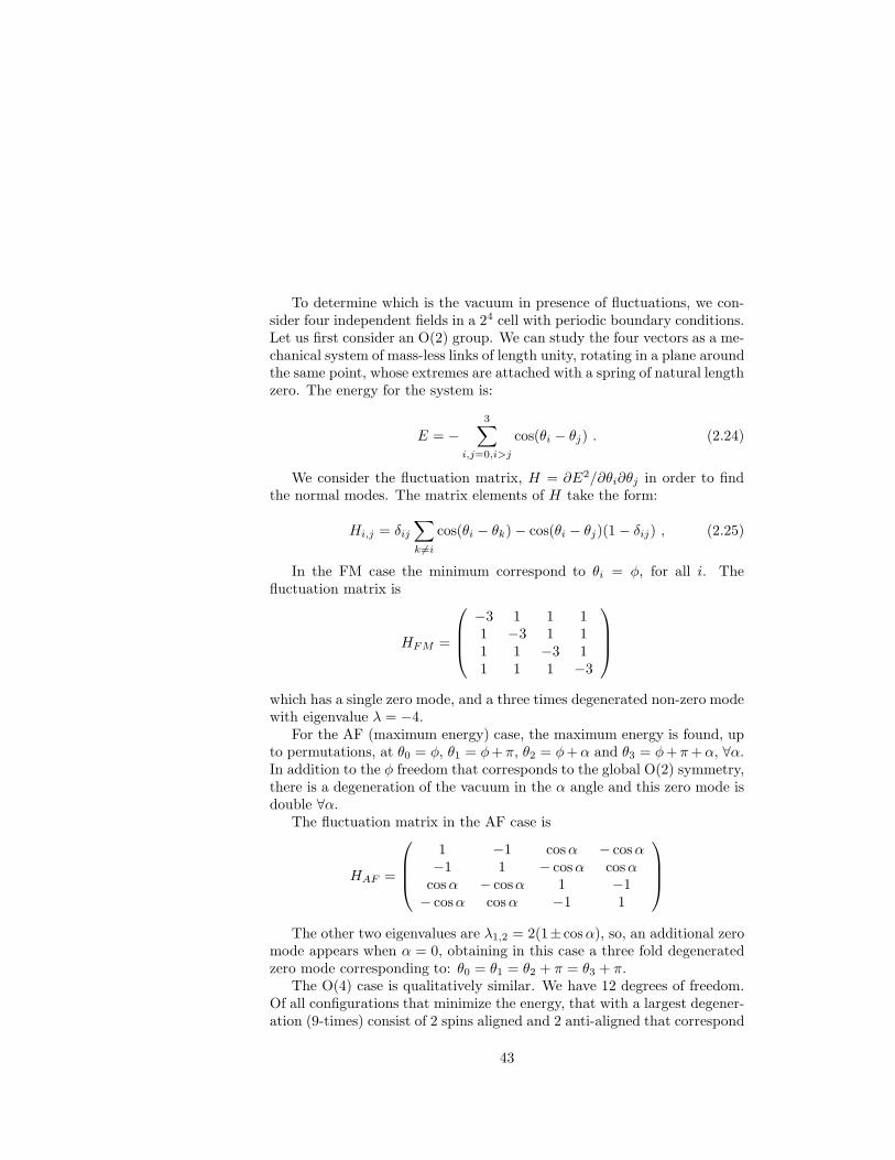
To determine which is the vacuum in presence of fluctuations, we con-sider four independent fields in a 24 cell with periodic boundary conditions.Let us first consider an O(2) group. We can study the four vectors as a me-chanical system of mass-less links of length unity, rotating in a plane aroundthe same point, whose extremes are attached with a spring of natural lengthzero. The energy for the system is:

E = −3

∑

i,j=0,i>j

cos(θi − θj) . (2.24)

We consider the fluctuation matrix, H = ∂E2/∂θi∂θj in order to findthe normal modes. The matrix elements of H take the form:

Hi,j = δij∑

k 6=i

cos(θi − θk)− cos(θi − θj)(1 − δij) , (2.25)

In the FM case the minimum correspond to θi = φ, for all i. Thefluctuation matrix is

HFM =

−3 1 1 11 −3 1 11 1 −3 11 1 1 −3

which has a single zero mode, and a three times degenerated non-zero modewith eigenvalue λ = −4.

For the AF (maximum energy) case, the maximum energy is found, upto permutations, at θ0 = φ, θ1 = φ+ π, θ2 = φ+α and θ3 = φ+ π+α, ∀α.In addition to the φ freedom that corresponds to the global O(2) symmetry,there is a degeneration of the vacuum in the α angle and this zero mode isdouble ∀α.

The fluctuation matrix in the AF case is

HAF =

1 −1 cosα − cosα−1 1 − cosα cosαcosα − cosα 1 −1− cosα cosα −1 1

The other two eigenvalues are λ1,2 = 2(1± cosα), so, an additional zeromode appears when α = 0, obtaining in this case a three fold degeneratedzero mode corresponding to: θ0 = θ1 = θ2 + π = θ3 + π.

The O(4) case is qualitatively similar. We have 12 degrees of freedom.Of all configurations that minimize the energy, that with a largest degener-ation (9-times) consist of 2 spins aligned and 2 anti-aligned that correspond

43

to a PAF vacuum. We consider this degeneration as the main differencewith the FM sector, and could be relevant to obtain different critical expo-nents.

In presence of fluctuations the configurations with largest degenerationare favored by phase space considerations, so we expect that the real vac-uum is a PAF one. This statement will be checked below with Monte Carlodata in the critical region.

2.4 Finite Size Scaling analysis

Our measures of critical exponents are based on the FSS ansatz [24, 26].Let be 〈O(L, β)〉 the mean value of an observable measured on a size Llattice at a coupling β. If O(∞, β) ∼ |β − βc|xO , from the FSS ansatz onereadily obtains [26]

〈O(L, β)〉 = LxO/νFO(L/ξ(∞, β)) + . . . , (2.26)

where FO is a smooth function and the dots stand for corrections to scalingterms.

To obtain ν we apply equation (2.26) to the operator d logMPAF/dβwhose related x exponent is 1. As this operator is almost constant in thecritical region, we just measure at the extrapolated critical point or anydefinition of the apparent critical point in a finite lattice, the differencebeing small corrections-to-scaling terms.

For the magnetic critical exponents the situation is more involved as theslope of the magnetization or the unconnected susceptibility is very largeat the critical point.

We proceed as follows (see refs. [25] for other applications of thismethod). Let be Θ any operator with scaling law xΘ = 1 (for instancethe Binder parameter or a correlation length defined in a finite lattice di-vided by L). Applying eq. (2.26) to an arbitrary operator, O, and to Θ wecan write

〈O(L, β)〉 = LxO/νfO,Θ(〈Θ(L, β)〉) + . . . . (2.27)

Measuring the operatorO in a pair of lattices of sizes L and sL at a couplingwhere the mean value of Θ is the same, one readily obtains

〈O(sL, β)〉〈O(L, β)〉

∣

∣

∣

∣

Θ(L,β)=Θ(sL,β)

= sxO/ν + . . . . (2.28)

The use of the spectral density method (SDM) [27] avoids an exact a prioriknowledge of the coupling where the mean values of Θ cross. We remark

44

that usually the main source of statistical error in the measures of magneticexponents is the error in the determination of the coupling where to mea-sure. However, using eq. (2.28) we can take into account the correlationbetween the measures of the observable and the measure of the couplingwhere the cross occurs. This allows to reduce the statistical error in anorder of magnitude.

2.4.1 FSS at the upper critical dimension: logarithmiccorrections

Being d = 4 the upper critical dimension of the FM O(4) model, logarith-mic corrections to the Mean Field predictions are expected to set in. Inparticular, FSS in its standard formulation breaks at d = 4 because theessential assumption, namely ξL(βc) ∼ L is no longer true. In fact, in fourdimensions [29]:

ξ(∞, t) ∼ |t|−1/2| ln |t|| 14 . (2.29)

The FSS formula for the correlation length was calculated by Brezin[23]. At the critical point one gets:

ξ(L, βc) ∼ L(lnL)1/4 . (2.30)

It has been suggested [28] that the usual FSS statement should be re-placed by the more general one:

O(L, βc)

O(∞, β)= FO

(

ξ(L, βc)

ξ(∞, β)

)

. (2.31)

When applying the quotient method described above to systems in fourdimensions one has to take into account the logarithmic corrections, so thatthe modified formula reads:

〈O(sL, β)〉〈O(L, β)〉

∣

∣

∣

∣

Θ(L,β)=Θ(sL,β)

= sxO/ν

(

1 +ln s

lnL

)1/4

. (2.32)

This point is particularly important when measuring the magnetic crit-ical exponents because as we have already mentioned, the slope of themagnetization and susceptibility are very large, and special care has to betaken when locating the coupling where to measure.

2.5 Numerical Method

We have simulated the model in a L4 lattice with periodic boundary con-ditions. The biggest lattice size has been L = 24. For the update we have

45

employed a combination of Heat-Bath and Over-relaxation algorithms (10Overrelax sweeps followed by a Heat-Bath sweep).

The dynamic exponent z we obtain is near 1. Cluster type algorithmsare not expected to improve this z value. In systems with competing in-teractions the cluster size average is a great fraction of the whole system,loosing the efficacy they show for ferromagnetic spin systems.

We have used for the simulations ALPHA processor based machines.The total computer time employed has been the equivalent of two years ofALPHA AXP3000. We measure every 10 sweeps and store the individualmeasures to extrapolate in a neighborhood of the simulation coupling byusing the SDM.

In the F4 case, we have run about 2 × 105τ for each lattice size, beingτ the largest integrated autocorrelation time measured, that correspondsto MPAF, and ranges from 2.3 measures for L = 6 to 8.9 for L = 24. Wehave discarded more than 102τ for thermalization. The errors have beenestimated with the jack-knife method.

2.6 Results and Measures

2.6.1 Phase Diagram

We have studied the phase diagram of the model using a L = 8 lattice.We have done a sweep along the parameter space of several thousandsof iterations, finding the transition lines shown in Figure 1. The symbolsrepresent the coupling values where a peak in the order parameter derivativeappears.

The line FM-PM has a clear second order behavior. It contains thecritical point for the O(4) model with first neighbor couplings (β1 ≈ 0.6,β2 = 0) with classical exponents (ν = 0.5, η = 0). In the β1 = 0 axis, wehave computed the critical coupling (βc

2 ≈ 0.18) and the critical exponentsas a test for the method in the F4 lattice. We have also considered theinfluence of the logarithmic corrections when computing the exponents.

The lines FM-HPAF, HPAF-PAF and PM-HPAF show clear metasta-bility, indicating a first order transition.

The regions between the lower dotted line and the PAF transition line,and between the upper dotted line and the FM transition line, are disor-dered up to our numerical precision. We could expect always a PM regionseparating the different ordered phases, however, from a MC simulation it isnot possible to give a conclusive answer since the width of the hypotheticalPM region decreases when increasing β1, and for a fixed lattice size thereis a practical limit in the precision of the measures of critical values.

46

Figure 2.1: Phase diagram obtained from the MC simulation on a L = 8 lattice

The line PM-PAF has a very interesting behavior. To get ride of theinfluence of the HPAF region we have started the study at β1 = 1.5. Theenergy distributions encountered at β1 = 1.5 and β1 = 1.0 are displayed infigure 2.2. We do not obeserve latent heat anymore in lattices up to L=16in β1 = 0. Two scenarios are suggested by this fact:

1. There exist a value of β1 in which the order of the phase transitionchanges from being first order, to be continuous.

2. The phase transition line is first order everywhere, though increasilyweak as the limit β1 = 0 is approached.

The possibility of a second order behavior of the PM-PAF transition linecontrast with the first order one found in the Ising model with two couplingsin the analogous region [19]. This would not be that surprising becausewe are dealing now with a global continuous symmetry. The spontaneoussymmetry breaking of such symmetries manifest in the appearance of softmodes or low energy excitations (long wavelength), the Goldstone bosonsin QFT terminology [29]. In general, these low energy modes will perturbthe mechanism of long distance ordering, softening in this way the phasetransitions.

47

Figure 2.2: Energy distribution for L=8,12,16 measured at the peak of thespecific heat at β1 = 1.5 (upper window) and at β1 = 1.0 (lower window).

Regarding the differences with the FM case, the most remarkable fea-ture is the different vacuum structures appearing, specially the very largedegeneration in the PAF transition, in contrast with the single degenerationof the FM O(4) mode.

For the reasons mentioned in section 1.3.1, the simpler point for studyingthe properties of the transition, namely the critical exponents is the F4

limit. Most of the MC work has been done for this case.

2.6.2 Results on the F4 lattice

Results on the FM region

Firstly, we have checked our method on the FM region of the F4 lattice.In Figure 3 the crossing points of the Binder cumulant for various latticesizes are displayed. The prediction for the critical coupling βc ∼ 0.1831(1)agrees with an earlier study by Bhanot [30].

Concerning the measures of critical exponents, we have applied the quo-tient method, described in section 1.4 . In table 2.1 we quote the resultswhen logarithmic corrections are included (formula (2.32)), and also for

48

sake of comparison, when they are neglected (formula (2.28)). We see howin fact the agreement of the critical exponents with the MFT predictionsis better when the logarithmic corrections are taken into account.

L values 8/16 12/16 10/12(without logarithmic corrections)α/ν 0.08(5) 0.02(2) 0.13(12)β/ν 0.92(3) 0.94(3) 0.87(4)γ/ν 2.16(2) 2.12(2) 2.24(4)(with logarithmic corrections)

α/ν 0.0 0.0 0.03(8)β/ν 1.04(3) 1.06(3) 1.04(2)γ/ν 1.94(3) 1.90(4) 1.93(3)

Table 2.1: Critical exponents for the FM-PM phase transition in the F4

lattice.

Figure 2.3: Energy distribution for L=16,20 and 24 at the peak of the specificheat on the F4 lattice.

49

Figure 2.4: Crossing points of the Binder Cumulant for various lattice sizes onthe FM-PM phase transition

From now on we will focus on the transition between the PM phase andthe PAF phase on the F4 lattice.

Vacuum symmetries on the PAF region

We will check using MC data that the ordered vacuum in the critical regionis of type PAF.

Let us define

Aij = Vi ·Vj . (2.33)

The leading ordering corresponds to the eigenvector associated to the max-imum eigenvalue of the matrix A, that should scale as L−2β/ν at the criticalpoint. The scaling law of the biggest eigenvalue agrees with the β/ν valuereported in Table 2.3, and the associated eigenvector is, within errors, (1,1,-1,-1).

We also have found that the other eigenvalues scale as L−4. This is theexpected behavior if just the O(4) symmetry is broken, and it remains anO(3) symmetry in the subspace orthogonal to the O(4) breaking direction.

50

Figure 2.5: Crossing points of the Binder cumulant for various lattice sizes.

Critical Coupling

To obtain a precise determination of the critical point, βc, we have usedthe data for the Binder parameter (2.19).

In Figure 4 we plot the crossing points of the Binder cumulants for thesimulated lattices sizes. Extrapolations have been done using SDM fromsimulations at β2 = −0.7090 for L = 6, 8, 10, 12 and 16; β2 = −0.7078 forL = 20, and β2 = −0.7070 for L = 24.

The shift of the crossing point of the curves can be explained throughthe finite-size confluent corrections. The dependence in the deviation of thecrossing point for L and sL size lattices was estimated by Binder [20]

βc(L, sL)− βc ∼1− s−ω

s1/ν − 1L−ω−1/ν , (2.34)

where ω is the universal exponent for the corrections-to-scaling.The infinite volume critical point the value

βc = −0.7065(5)[+2][−2] , (2.35)

where the errors in brackets correspond to the variations in the extrapola-tion when we use the values ω = 0.5 and ω = 2 respectively. In Figure 5

51

0 0.00025 0.00050 0.00075 0.00100 0.00125 0.00150

(1 - s-1/s2 - 1)L1-3

-0.712

-0.710

-0.708

-0.706

β c(L2,L

1)

Figure 2.6: Extrapolation to βc(∞) for L1 = 6, 8, 10, 12 (circles, crosses, trianglesand squares symbol respectively)

we plot eq. (2.34) for ω = 1.Using the previous value of βc we can compute the Binder cumulant at

this point. In table 2.2 we quote the obtained values. The result points tothat the Binder cumulant stays constant in the critical region. This resultwould be compatible with a non zero value of the renormalized couplingwhen L increases.

Concerning the possibility of having logarithmic corrections in the de-termination of the critical coupling, from the numerical point of view, it isnot possible to discern between the ω effect, and a logarithmic correction.

Thermal Critical exponents: α, ν

The critical exponent associated to correlation length can be obtained fromthe scaling of:

κ =∂ logM

∂β, (2.36)

where M is an order parameter for the transition, MPAF for our purposes.In the critical region κ ∼ L1/ν . As κ is a flat function of β, is not crucial the

52

Lattice sizes UL(βc(ω = 0.5)) UL(βc(ω = 1)) UL(βc(ω = 2))6 0.4435(15) 0.4437(12) 0.4438(12)8 0.4406(15) 0.4409(12) 0.4413(12)10 0.4407(14) 0.4411(16) 0.4414(14)12 0.436(4) 0.437(3) 0.438(3)16 0.435(3) 0.436(3) 0.437(3)20 0.429(5) 0.431(5) 0.433(5)24 0.428(6) 0.430(7) 0.433(7)

Table 2.2: Binder cumulant for various lattices sizes at the extrapolatedcritical point for ω = 0.5, 1, 2.

point where we actually measure. The results displayed in table 2.3 havebeen obtained measuring at the crossing point of the Binder parameters forlattice sizes L and 2L using (2.28).

For measuring α/ν we study the scaling of the specific heat

C =∂〈E2〉∂β2

, (2.37)

We expect that C scales as A+ BLα/ν , where A is usually non-negligible.In Figure 6 we plot the specific heat measuring at (2.35), as well as at thepeak of the specific heat, as a function of L. We observe a linear behaviorfor intermediate lattices. For the largest lattice the slope decreases. Theweak first order behavior [31] (α/ν = 1 for small lattices that becomes dfor large enough sizes) seem hardly compatible with our data. If we neglectthe A term (what is asymptotically correct), and compute the exponentusing eq. (2.28) we obtain α/ν ≈ 0.3 for intermediate lattices that reducesto α/ν = 0.15(2) for the (20,24) pair.

However, to give a conclusive answer for the value of α statistics onlarger lattices are mandatory.

Magnetic Critical exponents: γ, β

The exponents γ and β can be obtained respectively from the scaling ofsusceptibility and magnetization:

χ ≡ V 〈M2〉 ∼ Lγ/ν (2.38)

M ∼ L−β/ν (2.39)

53

Figure 2.7: Specific heat at the peak (triangle symbols) and at β = −0.7068(cross symbols) as a function of the lattice size.

Where M is an order parameter for the phase transition. In Figure 7upper part, we plot the quotient between MPAF for lattices L and 2L asa function of the quotient between the Binder cumulants for both latticesizes.

For large L in the critical region we should obtain a single curve, thedeviations corresponding to corrections to scaling. In the lower part ofFigure 7 we plot the same function for susceptibility.

The values for γ and β are summarized in Table 2.3.

2.6.3 Logarithmic corrections

We now address the question of the possibility of logarithmic correctionsin the AF O(4) model. For the thermal critical exponents, the situationseems clear, they are compatible with the classical exponent ν = 0.5. Forthe magnetic exponents, the situation is more involved. In principle, onecan think that they disagree from MFT due to logarithmic corrections. Wehave no perturbative predictions about the form in which these correctionswould affect ξL for the AF case. However, one expects that such corrections

54

Figure 2.8: Quotients to obtain β/ν and γ/ν

slightly modify the critical exponents, as occurs in the FM case. It couldbe possible that logarithmic corrections modify largely the previous criticalexponents and drift them to the FM ones. To sort this out, we have consid-ered the possibility of a behavior FM like, so that ξL ∼ L(lnL)1/4. In thelower part of Table 2.3 we quote the values of the critical exponents for thePAF phase transition when logarithmic corrections are included (formula(2.32)). We see how in effect the magnetic critical exponents are too farfrom the classical ones for being the result of a logarithmic correction to theMFT predictions. It is interesting to compare this situation with that inthe RP2 model in d = 4 [32] where small deviations from MFT exponentscan be explained as logarithmic corrections.

2.7 Conclusions and open problems

We have studied the phase diagram of the four dimensional O(4) modelwith first and second neighbors couplings. We have found that the pres-ence of couplings with opposite signs makes frustration to manifest in formof antiferromagnetism in different dimensionalities. Whether or not these

55

Lattice sizes γ/ν β/ν ν(without logarithmic corrections)

6/12 2.417(3) 0.791(4) 0.474(10)8/16 2.403(3) 0.792(6) 0.483(8)10/20 2.410(2) 0.790(4) 0.471(6)12/24 2.403(5) 0.797(5) 0.483(7)20/24 2.398(5) 0.802(4) 0.487(6)

(with logarithmic corrections)6/12 2.301(3) 0.849(4) 0.484(9)8/16 2.300(3) 0.850(5) 0.489(7)10/20 2.315(2) 0.843(3) 0.488(5)12/24 2.314(2) 0.842(5) 0.487(5)20/24 2.317(5) 0.839(4) 0.498(5)

Table 2.3: Critical Exponents for the PM-PAF phase transition in the F4

lattice

vacua have interest from the point of view of Quantum Field Theory is anopen question. The transition between the paramagnetic phase, and theAF plane ordered one is compatible with very weak first order and withhigher order. To shed some light on this question we have studied the evo-lution of the effective critical exponents in the limit β1 = 0. We found thatup to L = 24 the exponents are in disagreement with the Mean Field pre-dictions. Specifically, from our γ/ν estimation (or β/ν using hyper-scalingrelation) the exponent η asociated with the anomalous dimension of thefield is η ≈ −0.4. This fact itself would imply the non-triviality of thetheory because Green functions would not factorize anymore. We have alsomeasured the Binder cumulant at the critical point, finding that it staysalmost constant when increasing the lattice size.

However, before claiming about the important issue of a non-trivialphase transition in four dimensions we have tried to acomodate the data intwo possible scenarios: 1) logarithmic triviality; 2) weak first order scenario.

The mere observation of critical exponents different from the Mean Fieldones is in principle still compatible with a logarithmic trivial theory. Wehave contrasted our data with the perturbative predictions derived in theFM case, which do not fit the results. It would be possible to obtaintriviality also with a logarithmic exponent in equation (2.32) different from1/4. We can fix the critical exponents to its mean field value and computethis parameter from the numerical data. The results obtained shown a non-

56

Figure 2.9: Effective γ/ν exponents in O(N) with N=2,3,4.

asymptotic behavior with values ranging from 0.8 to 1.2 for the latticesused. In short, this model encounters the typical problems observed byother triviality studies, which make the numerical approach to this issueso difficult: one would need much stronger analytic insight to rule outlogarithmic triviality.

In the other hand, the possibility of being behind a very weak firstorder phase transition is a possibility that cannot be discarded a priori.Our data do not evidence any two state signature. Moreover, the stabilityof our measure of γ/ν for lattices ranging from L = 6 to L = 24, whichare more than a hundred standard deviations apart the MF value, makesthis hypothesis rather unlikely. However the question is wether or not thishypothesis can be ruled out beyond any doubt. The phase transition inthis region for the Ising case, O(1), has been shown to be first order [19].Lately, the models O(2) and O(3) have been considered with the purposeof checking wether or not the order of the phase transition changes with N[33] in lattice sizes as larger as L = 48. Evidence is given for a first ordercharacter of the transition in O(2). In O(3) the transition is weaker, anddespite no double peak structure is observed, the behavior of the effectiveexponents leaves little doubts about the first order character of O(3) as well

57

(see Figure 2.9). In the O(4) case we cannot observe any particular trendin the effective γ/ν . Indeed, since the transition seems to be continuousin the limit N → ∞, N = 4 might be a sort of critical N value from whichon the transition is second order.

However, from the observations in O(2) and O(3) we would be prone toconsider the weak first order scenario as the most plausible. If the transitionturns out to be first order, it would be weaker than the observed in O(3),and hence lattices larger than L = 48 would be needed to observe suchasymptotic behavior in the critical exponents.

58

Bibliography

[1] M. Aizenman Phys. Rev. Lett. 47 (1981) p 1

[2] J. Frolich, Nuc. Phys. B200 [FS4] (1982) p 281

[3] K.G. Wilson and J. Kogut, Phys. Rep. 12 (1974) p 75

[4] G.A. Baker and J.M. Kincaid, J. Stat. Phys. 24 (1981) p 469

[5] M. Luscher and P. Weisz Nuc. Phys. B290 [FS4] (1987) p 25

[6] M. Luscher and P. Weisz Nuc. Phys. B318 [FS4] (1989) p 705

[7] C.B. Lang,“Advances in lattice gauge theory”Tallahasee conference 1985Eds. D.W. Duke and J.F. Owens, World Scientific, Singapore, (1985)

[8] M. Aizenmann and R. Graham, Nuc. Phys. B225 (1983) p 261

[9] R. Fernandez, J. Frohlich and A. Sokal “Random Walks, Critical Phe-nomena and Triviality in Quantum Field Theory” Texts and Mono-graph in Physics Springer-Verlag (1992).

[10] G. Gallavotti and V. Rivasseau, Ann. Inst. Henri Poincare 40, 2 (1984)p 185

[11] G. Gallavotti and V. Rivasseau, Phys. Lett. B122 (1983) p 268

[12] J.L. Alonso, Ph. Boucaud, V. Martin-Mayor and A.J. Van der Sijshep-lat:/9706022

[13] W. Bock, A.K. De, K. Jansen, J. Jersak, T. Neuhaus and J. Smit Nuc.Phys. B344 (1990) p 207

[14] W. Bock, A.K. De, C. Frick, J. Jersak and T. Trapenberg Nuc. Phys.B378 (1992) p 652

59

[15] T. Ebihara and K. Kondo Prog. Theor. Phys. vol 87 (1992) p 4

[16] J.L. Alonso, Ph. Boucaud, F. Lesmes and E. Rivas. Phys. Lett. B329(1994) p 75

[17] J. Fingberg and J. Polonyi Nuc. Phys. B486 (1997) p 315

[18] P.R.Gerber and M.E. Fisher, Phys. Rev. B10 (1974) p 4697

[19] J.L. Alonso, J.M. Carmona, J. Clemente, L.A. Fernandez, D. Iniguez,A. Tarancon and C.L. Ullod, Phys. Lett. B376 (1996) p 148

[20] K. Binder, Z. Phys. B43 (1981) p 119

[21] E. Brezin and J. Zinn-Justin Nuc. Phys. B257 [FS14] (1985) p 867

[22] Giorgio Parisi, Statistical Field Theory, Ed. Addison Wesley (1992).

[23] E. Brezin J. Phys. 43 (1982) p 15

[24] C. Itzykson and J.M.Drouffe, Statistical Field Theory, Vol. 1, Cam-bridge University Press (1989)

[25] H. G. Ballesteros, L.A. Fernandez, V. Martın-Mayor and A. Munoz-Sudupe, Nuc. Phys. B483 (1997) p 707

[26] Finite size scaling, Current Physics - Sources and comments, vol. 2,Ed. J.L. Cardy, Elsever Science Publishers B. V. (1988)

[27] A.M. Ferrenberg and R.H. Swendsen, Phys. Rev. Lett. B61 (1988) p2635

[28] R. Kenna and C.B. Lang Nuc. Phys. B393 (1993) p 461

[29] Michel Le Bellac Des phenomenes critiques aux champs de jauge Inter-Editions / Editions du CNRS, Paris (1988)

[30] G. Bhanot Nuc. Phys. B17 (Proc. Suppl.) (1990) 653

[31] L.A. Fernandez, M.P. Lombardo, J.J Ruiz-Lorenzo and A. Tarancon,Phys. Lett. B277(1992) p 485

[32] H. G. Ballesteros, J.M. Carmona, L.A. Fernandez, V. Martın-Mayor,A. Munoz-Sudupe and A. Tarancon Phys. Rev. D55 (1997) p 5067

[33] H.G. Ballesteros, J.M. Carmona, L.A. Fernandez, A. Tarancon Phys.Lett. B419 (1998) p 303

60

Chapter 3

La transicion de fase en elmodelo SU(2)-Higgs

62

3.1 Introduccion

Los modelos Higgs describen la autointeraccion del campo de Higgs y suacoplamiento con los campos gauge SU(2)L y U(1)Y .

En la aproximacion en la que se desprecian los acoplos de Yukawa entreel campo Higgs y los fermiones, estos modelos estan considerados comouna razonable descripcion del sector electrodebil del Modelo Estandar. Enparticular se persigue mediante su formulacion en la red dar cuenta de losaspectos no perturbativos de la teorıa electrodebil, como por ejemplo lageneracion de masa mediante el mecanismo de ruptura espontanea de lasimetrıa.

Los acoplamientos gauge de U(1)Y y SU(2)L se denotan respectivamentepor g′/2 y g. La relacion entre ellos es a traves del angulo de Weinberg,concretamente la relacion es g′/g = tan θW, puesto que este angulo espequeno (sin2 θW ≈ 0.23), podemos despreciar en un primer paso el gradode libertad U(1)Y . En este sentido SU(2)-Higgs puede considerarse comoel modelo Higgs mas simple.

El interes del estudio de estos modelos no es tanto la necesidad dedeterminar parametros medibles en la naturaleza, sino mas bien profundizaren el entendimiento teorico de la formulacion de la teorıa electrodebil. Adiferencia de la QCD, esta teorıa no es asintoticamente libre, el punto fijogaussiano a acoplamiento cero es inestable ultravioleta, y la existencia deun punto fijo no trivial se hace necesaria para la formulacion de la teorıaen el continuo.

La accion del modelo SU(2)-Higgs consiste en una parte pura gauge masun termino de interaccion escalar-gauge:

S[U,Φ]λ = Sg[U ] + SΦ[U,Φ] . (3.1)

La interaccion entre la parte escalar y la gauge esta controlada por elhopping parameter, κ. Una normalizacion adecuada cuando se esta intere-sado en trabajar en el lımite de autoacoplamiento cuartico infinito (regimenno perturbativo) es la siguiente:

SΦ[U,Φ]λ =∑

x

Φ†(x)Φ(x) − 1

2κ∑

x,µ

trΦ†(x)Uµ(x)Φ(x + µ)

+ λ∑

x[Φ†(x)Φ(x) − 1]2 ,

(3.2)

con esta normalizacion el lımite λ → ∞ equivale a fijar el modulo delcampo Higgs a la unidad.

La parte pura gauge, Sg[U ], se expresa como la suma sobre las plaquetasorientadas positivamente:

63

Sg = β∑

P

(1− 1

2trUP) , (3.3)

donde β = 4/g2. En el lımite β → ∞ el campo gauge se desacopla yse recupera el modelo Φ4, el cual presenta una transicion de fase entre unaregion simetrica (pequeno κ) y una region en la que la simetrıa se ha rotoespontaneamente (κ grande) [1].

Cuando β es finita (g 6= 0) esta transicion de fase se prolonga en unalınea de transiciones de fase en el interior del espacio de acoplos [3, 4, 5],como se muestra en la figura 3.1.

La continuacion de la fase simetrica de Φ4 cuando el acoplo gauge esdistinto de cero es una region confinante en el sentido de que los camposgauge SU(2) confinan las partıculas escalares de materia. En este sentidola fase simetrica de SU(2)-Higgs es analoga a QCD.

La continuacion de la fase de simetrıa rota cuando el coupling gaugees distinto de cero es la fase Higgs. En esta fase, mediante el mecanismode ruptura espontanea de la simetrıa, el campo de Higgs adquiere un valoresperado en el vacıo distinto de cero. Los bosones vectoriales adquieren sumasa a traves de su acoplamiento con el campo escalar. Los tres bosonesde Goldstone del modelo Φ4 se hacen masivos al mezclarse con los bosonesgauge vectoriales. El resultado es un isovector con spin 1, el boson W .

Esta lınea de transiciones de fase termina en un valor finito del espaciode acoplamientos, estando las fases Higgs y confinante conectadas analiti-camente.

En cuanto al orden de la transicion de fase, para pequenos acoplamientosexisten argumentos perturbativos debidos a Coleman y Weinberg [2] apun-tando que la transicion deberıa ser de primer orden. El estudio numericode la transicion de fase para pequenos e intermedios valores de λ parececonfirmar esta conjetura [6, 7, 8].

Sin embargo se observa que la transicion se debilita (las discontinuidadesson mas pequenas) conforme λ aumenta. En el lımite λ = ∞ la opiniongeneralizada es que la transicion sigue siendo de primer orden aunque ex-tremadamente debil, si bien no existen evidencias que justifiquen esta creen-cia. Los ultimos resultados numericos fueron obtenidos por Montvay en1985, en redes no demasiado grandes y a pesar de observar metaestabili-dades en los ciclos de histeresis no se pudieron obtener resultados con-cluyentes [11].

Tratando de arrojar algo de luz sobre este punto hemos enfocado elproblema desde un punto de vista distinto, formulando el modelo SU(2)-Higgs en un espacio de parametros extendido. Sin embargo la motivacionno es solo hacer un estudio con alta estadıstica del modelo, sino tratar de

64

β

κ

Confined Phase

Higgs Phase

β=∞0

Figure 3.1: Grafico esquematico del diagrama de fases del modelo SU(2)-Higgscon modulo fijo (λ = ∞).

extraer las propiedades generales que presentan las transiciones de primerorden debiles en la red en modelos gauge acoplados a campos escalares.Con este proposito se ha anadido a la accion estandard un acoplo extraentre el campo gauge y el campo escalar conectando segundos vecinos enla red. Este acoplamiento nuevo sera usado como un parametro para re-forzar o debilitar la transicion, permitiendo ası estudiar su mecanismo dedebilitamiento cuando este acoplamiento se hace tender a cero.

65

Abstract

The properties of the Confinement-Higgs phase transition in the SU(2)-Higgs model with fixed modulus are investigated. We show that the systemexhibits a transient behavior up to L=24 along which, the order of the phasetransition cannot be discerned. To get stronger conclusions about thispoint, without going to prohibitive large lattice sizes, we have introduceda second (next-to-nearest neighbors) gauge-Higgs coupling (κ2). On thisextended parameter space we find a line of phase transitions which becomeincreasely weaker as κ2 → 0. The results point to a first order characterfor the transition with the standard action (κ2 = 0).

3.2 The Model

The SU(2) lattice gauge model coupled to an scalar field, in the fundamentalrepresentation of the gauge field can be described by the action

Sλ = β∑

p

[1− 1

2trUp]−

1

2κ1

∑

x,µ

trΦ†(x)Uµ(x)Φ(x + µ) +

+λ∑

x

[Φ†(x)Φ(x) − 1]2 +∑

x

Φ†(x)Φ(x) . (3.4)

Where Uµ(x) represents the link variables, and Up are their productsalong all the positive oriented plaquettes of a four-dimensional lattice ofside L.

The scalar field at the site x is denoted by Φ(x), being λ the parametercontrolling its radial mode. In the limit (λ = ∞, β = ∞) the modelbecomes a pure O(4)-symmetric scalar model.

As we pointed out in the previous section, the PT line ends at somefinite value of the parameters (β, κ1) The endpoint moves towards larger βvalues as λ increases. For λ ≥ 0.1 the endpoint crosses to the β > 0 region,and in the limit λ = ∞ the phase transition ends at (κ1 ≈ 0.6, β ≈ 1.6) [6].It is commonly believed that the transition at this point is second order withclassical critical exponents [9], however a careful numerical study would benecessary.

In the scaling region, and for finite λ, the phase transition turns out tobe first order. Also, the transition becomes weaker as β or λ increases. Inparticular in the limit β = ∞ (spin model) the transition is second orderwith classical critical exponents [1].

In the limit λ = ∞ the situation is less transparent, and it is not clearwhether the transition is weak first order or higher order.

66

The study of the model with the parameter λ = ∞ is equivalent to fixingthe modulus of the Higgs field, Φ† ·Φ = 1. In the pioneer work, [10], the PTwas considered first order for finite λ and second order for λ = ∞. Later,larger statistics, and the hypothesis of a universal behavior of the PT for allvalues of λ, seem to point to a first order character of the PT in the scalingregion. Nowadays, though it is generally believed that the transition is stillfirst order in this limit, the numerical proofs [11, 7] on which rely thesestatements are not conclusive, as the authors safely conclude, because thestatistic and lattice sizes are not enough for excluding the possibility of ahigher order phase transition in the edge λ = ∞.

The model with fixed modulus is described by the action

S∞ = β∑

p

[1− 1

2trUp]−

1

2κ1

∑

x,µ

trΦ†(x)Uµ(x)Φ(x + µ) . (3.5)

As we shall show below, we have simulated this model up to latticesL=24, and the result is still compatible with a second or higher order PT,however, we have no indications of asymptoticity in the behavior of theobservables, and the results are compatible with a very weak first order PTtoo. This means that larger lattices are needed to overcome these transienteffects, but the added difficulty here is that such lattices would suffer of ter-malization problems, and severe autocorrelation times. Altogether makesthis approach too CPU expensive for nowadays computers.

In order to get a more conclusive answer without going to prohibitivelarge lattice sizes, we have studied the model in an extended parameterspace. For this purpose we have introduced a second coupling betweenthe gauge and the scalar field connecting next-to-nearest neighbors on thelattice, in such a way that the new action reads

S = S∞− 1

4κ2

∑

x,µ<ν

TrΦ†(x)[Uµ(x)Uν(x+µ)+Uν(x)Uµ(x+ν)]Φ(x+µ+ν)

(3.6)Within this parameter space we expect to get a global vision on what the

properties of the PT are, and also, to give a stronger conclusion about theorder. In the region of κ2 positive, (competing interaction effects appear ifκ2 < 0) this extended model is expected to belong to the same universalityclass than the standard one (κ2 = 0) since both models posses the samesymmetries. The effect of the new coupling κ2 > 0 is to reinforce thetransition but should not change the order if the system has not tricriticalpoints. An example of such behavior appears in the O(4)-symmetric σmodel with second neighbors coupling. This model presents a (κc1, κ

c2) line

of phase transitions which is second order, since the model with κ2 = 0shows a second order PT too [12].

67

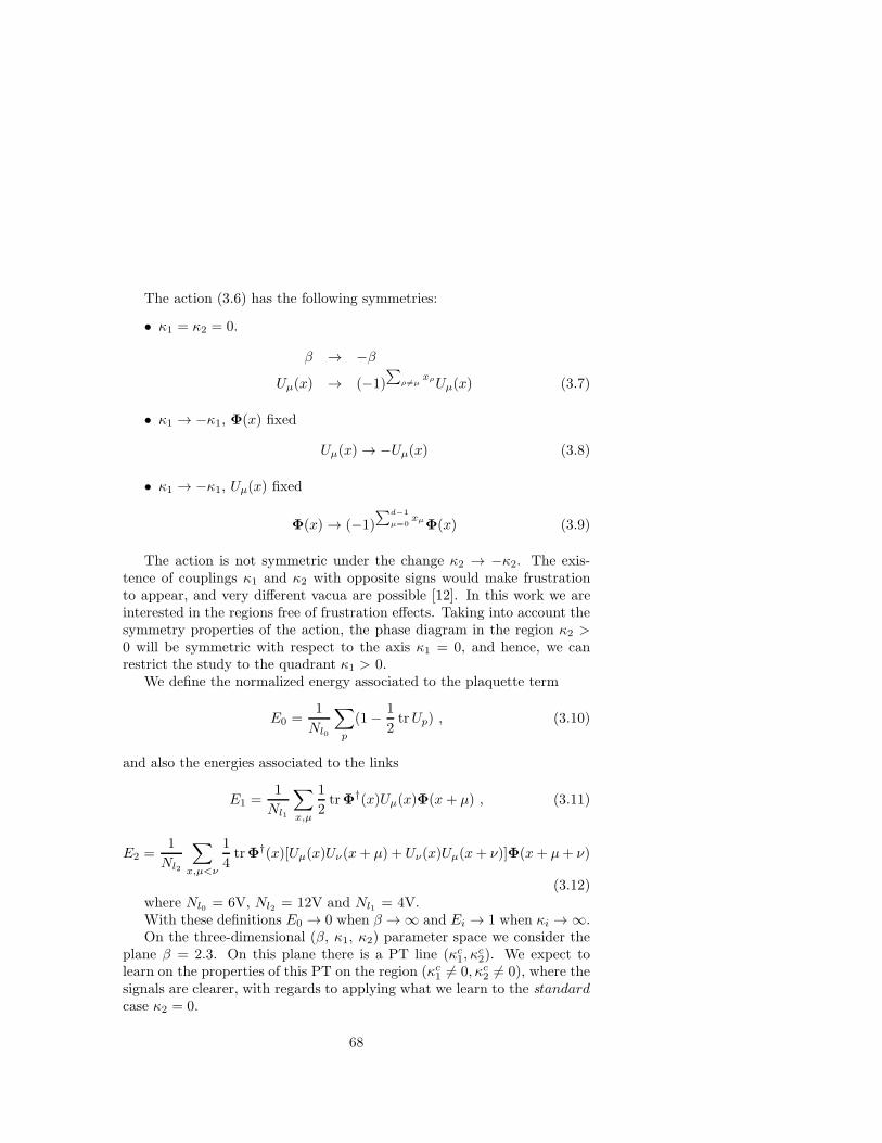
The action (3.6) has the following symmetries:

• κ1 = κ2 = 0.

β → −βUµ(x) → (−1)

∑

ρ6=µxρUµ(x) (3.7)

• κ1 → −κ1, Φ(x) fixed

Uµ(x) → −Uµ(x) (3.8)

• κ1 → −κ1, Uµ(x) fixed

Φ(x) → (−1)

∑

d−1

µ=0xµΦ(x) (3.9)

The action is not symmetric under the change κ2 → −κ2. The exis-tence of couplings κ1 and κ2 with opposite signs would make frustrationto appear, and very different vacua are possible [12]. In this work we areinterested in the regions free of frustration effects. Taking into account thesymmetry properties of the action, the phase diagram in the region κ2 >0 will be symmetric with respect to the axis κ1 = 0, and hence, we canrestrict the study to the quadrant κ1 > 0.

We define the normalized energy associated to the plaquette term

E0 =1

Nl0

∑

p

(1− 1

2trUp) , (3.10)

and also the energies associated to the links

E1 =1

Nl1

∑

x,µ

1

2trΦ†(x)Uµ(x)Φ(x + µ) , (3.11)

E2 =1

Nl2

∑

x,µ<ν

1

4trΦ†(x)[Uµ(x)Uν(x+ µ) + Uν(x)Uµ(x+ ν)]Φ(x+ µ+ ν)

(3.12)where Nl0 = 6V, Nl2 = 12V and Nl1 = 4V.With these definitions E0 → 0 when β → ∞ and Ei → 1 when κi → ∞.On the three-dimensional (β, κ1, κ2) parameter space we consider the

plane β = 2.3. On this plane there is a PT line (κc1, κc2). We expect to

learn on the properties of this PT on the region (κc1 6= 0, κc2 6= 0), where thesignals are clearer, with regards to applying what we learn to the standardcase κ2 = 0.

68

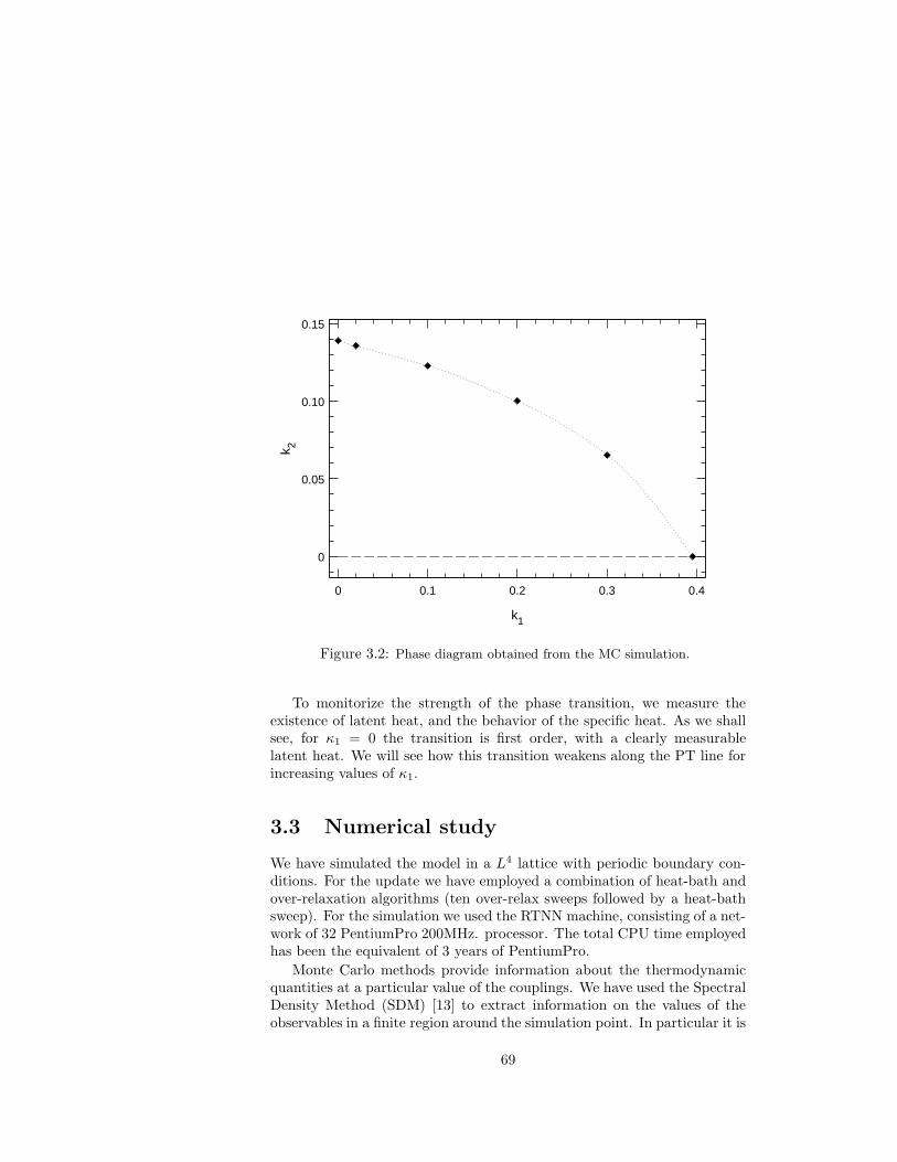
0 0.1 0.2 0.3 0.4

k1

0

0.05

0.10

0.15

k 2

Figure 3.2: Phase diagram obtained from the MC simulation.

To monitorize the strength of the phase transition, we measure theexistence of latent heat, and the behavior of the specific heat. As we shallsee, for κ1 = 0 the transition is first order, with a clearly measurablelatent heat. We will see how this transition weakens along the PT line forincreasing values of κ1.

3.3 Numerical study

We have simulated the model in a L4 lattice with periodic boundary con-ditions. For the update we have employed a combination of heat-bath andover-relaxation algorithms (ten over-relax sweeps followed by a heat-bathsweep). For the simulation we used the RTNN machine, consisting of a net-work of 32 PentiumPro 200MHz. processor. The total CPU time employedhas been the equivalent of 3 years of PentiumPro.

Monte Carlo methods provide information about the thermodynamicquantities at a particular value of the couplings. We have used the SpectralDensity Method (SDM) [13] to extract information on the values of theobservables in a finite region around the simulation point. In particular it is

69

0.380 0.385 0.390 0.395

E0

0

50

100

150

200

N(E

0)

Figure 3.3: Normalized energy distribution for L=12, λ = ∞, κ1=0.395, β=2.3from [11] (dotted line), compared with the distribution we obtain at the samecouplings (solid line) in L=12 too, when statistics is increased by one order ofmagnitude.

useful to have a precise location of the coupling where some observables havea maximum, as well as an accurate measure of the value of that maximum.

From the Monte Carlo simulation at some coupling κ, we got the his-togram H(E) which is an approximation to the density of states. Using theSDM approximation the probability of finding the system with an energyE at a different coupling κ′ can be written as:

Pκ′(E) ∝ H(E)e(κ′−κ)V E . (3.13)

The region of validity of the SDM approximation is ∆κ ∼ 1/(V σ), beingσ the width of the distribution H(E). Although σ gets the maximum valuesin the critical region, the approximation has been very useful, specially fortuning the couplings where to measure.

Concerning the lattice sizes, we have used lattices ranging from L=6to L=24. For the small lattices (L=6, 8 and 12) we have done 4×105τiterations, being τ the largest autocorrelation time for the energy, whichranges from τ ≈ 10 in L=8 to τ ≈ 35 in L=24. For the largest lattices,

70

L=20 and 24, we run up to 105τ MC iterations.The statistical errors are computed with the jackknife method.

3.4 Results

We shall make the discussion with the first-neighbors link energy, E1, butas far as the critical behavior is concerned, we could carry out the analysiswith any of the energies. We remark that an appropriate linear combinationof E1, E2 and E0 could give slightly more accurate results [14].

We have considered fixed values of κ1 (0, 0.02, 0.1, 0.2 and 0.3) andsought the κ2 critical for every line, κc2(κ1). We have also studied the caseκ2= 0 varying κ1 which corresponds to the usual SU(2)-Higgs model.

The SDM has been used to locate the apparent critical point, definedthrough the specific heat behavior. From the specific heat matrix:

Ci,jv (L) =

∂Ei

∂κj, (3.14)

we obtain the best signal for C1,2v (L), which can be calculated as (we shall

omit the superscript from now on)

Cv(L) = 4Ld(〈E1E2〉 − 〈E1〉〈E2〉) . (3.15)

In a first order phase transition, Cmaxv (L) behaves, asymptotically, pro-

portional to the volume, Ld. If the PT is second order, the dominantbehavior for Cv(L)

max is Lα/ν which diverges too provided that α > 0. Atthe upper critical dimension α = 0, and one has to go further the leadingorder, appearing logarithmic divergences [15].

As a consequence of this divergent behavior, in a finite lattice Cv(L)shows a peak at some value of the coupling which will be taken as apparentcritical point, κ∗2(L).

In Figure 3.2 we plot the critical line (κc1, κc2). This line is obtained by

extrapolation to the thermodynamic limit according to κc2(∞) = κ∗2(L) −AL−d. We point out that this extrapolation is valid only in first orderphase transitions. If the PT is second order the power in L is (−1/ν).

In continuous PT scale invariance holds, and the thermodynamic mag-nitudes, such as the specific heat, or susceptibilities do scale. However ifthe transition is first order the correlation length remains finite and hencethere is not scaling properties, and no critical exponents can be defined.

Nevertheless in a first order PT we can ask how large is the latticewe need in order to observe the asymptotic behavior of Cv. In particular,with abuse of language one can measure a pseudo α/ν exponent to get

71

-0.05 0 0.050

200

400

600

N(E

1)

E1

Figure 3.4: E1 distribution on the axis κ1 = 0 on a L=8 lattice at (κ2 = 0.15, β =2.3). The cosine fit is very accurate in spite of the finite β value, in this region ofparameters the pure gauge term couples slightly both sub-lattices.

insight on the nature of the PT: the larger is the lattice we need to measureν = 1/d, the weaker the PT is. Following this, first order PT can beclassified according to their degree of weakness.

However, the so called weak first-order PT appear often in literature (see[16, 17] and references there in) as PT characterized by a transient behaviorwith a non-measurable latent heat. Let be ξc the correlation length of thesystem at the critical point in the thermodynamic limit. In a finite lattice ofsize L, the first order behavior will be evidenced if L ≥ ξc. For lattice sizesmuch smaller than ξc the system will behave like in a second-order PT, sincethe correlation length is effectively infinite. As an example, in Figure 3.3we plot the energy distribution in a L=12 lattice at (β = 2.3, κ1 = 0.395)obtained in [11], compared with the one we obtain at the same couplingsand in the same L, when the statistics increases by one order of magnitude.We observe that the order of the PT can not be discerned at this volume,even when the statistics is enough. Termalization effects can also contributeto mistake the histogram structure.

The entire line (κc1, κc2) is first order, but the weak character increases

72

0.14 0.15 0.16 0.17 0.180

20

40

60

N(E

1)

E1

Figure 3.5: Normalized distribution of E1 at (κ1 = 0.2, κ2 = 0.10036) in a L=16lattice. The cubic fit at the maxima to get ∆E is superimposed.

as κ2 → 0. We will make a quantitative description of the weakeningphenomenon by studying the specific heat, and the latent heat.

But before going on, we shall make a remark concerning the behavioron κ1 = 0. As we pointed out, the system is symmetric under the changeκ1 → −κ1. The transformation (3.9) maps the positive κ1 semi-plane withenergy E1, onto the negative κ1 semi-plane with energy -E1. The transitionacross this axis is first order because the energy is discontinuous. In thelimit β → ∞, and in κ1 = 0, the system decouples in two independentsublattices, each one constituted by the first neighbors of the other. Thefirst neighbors energy for this system is proportional to cos θ, being θ theangle between the symmetry breaking direction of the scalar field in bothsub-lattices. In Figure 3.4 we plot the E1 distribution for L=8 at (κ1 =0, κ2 = 0.15) and β = 2.3. We see that the agreement with a cosinedistribution is quite good in spite of the finite β value.

73

0 1000 2000 3000 4000 5000

MC iterations

0.12

0.14

0.16

0.18

0.20

E1

0.14

0.15

0.16

0.17

0.18

E1

0.14

0.15

0.16

0.17

E1

Figure 3.6: MC evolution of E1 at (κ1 = 0.2, κ∗

2(L)) for L=8 (lower part), L=12(middle) and L=16 (upper part).

3.4.1 Latent Heat

Along the apparent critical line we have done simulations for different latticesizes and stored the plaquette and links energies to construct the histogramsfor the energy distributions. In a first-order phase transition the energy hasa discontinuity which manifest in the appearance of latent heat, ∆E. Thisquantity is not well defined in a finite lattice, so we measure the distancebetween the two maximum of the energy distribution, and extrapolate tothe thermodynamic limit. The drawback of this approximation is that themaxima of the energy distribution are difficult to discern, since this functionat the apparent critical point is very noisy We have used a cubic spline atthe maxima in order to get a more reliable estimation (Figure 5).

In Figure 3.6 we show the MC evolution of E1 for L=8, 12 and 16 atκ1 = 0.2. In L=8 the latent heat is not clearly measurable. We observe inthe MC evolution how the two-state signal becomes cleaner as the latticesize increases (see Figure 3.7).

In Figure 3.7 we plot the distribution of E1 at κ1 = 0.2 at the apparentcritical point κ∗2(L) for L=6, 8, 12 and 16. A remarkable stability of ∆E1

74

0.12 0.14 0.16 0.18 0.20 0.22

0

5

10

15

20N

(E1)

L = 6

0

10

20

30

0.12 0.14 0.16 0.18 0.20 0.22

L = 8

0.12 0.14 0.16 0.18 0.20 0.22

E1

0

10

20

30

40

50

N(E

1)

L = 12

0.12 0.14 0.16 0.18 0.20 0.22

E1

0

20

40

60

80

L = 16

Figure 3.7: Normalized distribution of E1 at (κ1 = 0.2, κ∗

2(L)) for L=6, 8, 12and 16.

with the volume is observed. This is a common feature for all values of κ1.

As we have already pointed out, the transition weakens when increasingκ1 and larger lattices are needed in order to observe a measurable latentheat. We give a quantitative description of this fact in Figure 3.8, wherethe distribution of E1 for several values of (κ1, κ

∗2(12)) is displayed. The

two-state signal is no longer measurable in L=12 at κ1 = 0.3. The firstevidences of two-states appear in L=20 (see Figure 3.9). but from its energydistribution we can only give an approximate value for ∆E1(L = 20) sincethe two-peaks appear too close to each other.

In Figure 3.10 we plot ∆E1(L) and ∆E2(L) as a function of 1/L4, inorder to get ∆Ei in the thermodynamic limit with a linear fit. Finally wequote these values in Table 3.1, together with the change in the action (3.6)between the two phases.

From the energy distributions at κ2 = 0, see Figure 3.11 we have nodirect evidences of the existence of latent heat. However, on the largerlattices one can observe non-gaussianities in the energy distributions. Suchasymmetries could precede the onset of clear two-peak structures in largerlattices, however this is just a guess. We conclude that no information con-

75

0.01 0.02 0.03 0.04

0

20

40

60

80

100

N(E

1)

k1 = 0.02

0

20

40

60

0.06 0.07 0.08 0.09 0.10

k1 = 0.1

0.14 0.16 0.18

E1

0

10

20

30

40

50

N(E

1)

k1 = 0.2

0.20 0.21 0.22 0.23 0.24 0.25

E1

0

10

20

30

40

50

k1 = 0.3

Figure 3.8: Normalized distributions of E1 for κ1 = 0.02, 0.1, 0.2 and 0.3 atκ∗

2(12).

cerning the order of the PT can be obtained from the energy distributionsup to L=24.

3.4.2 Specific Heat

We have done MC simulations at the points predicted by SDM, (κ1, κ∗2(L)),

in order to measure accurately the peak of Cv(L).

As an example we show in Figure 3.12 the value of Cv(L) around itsmaximum for various lattice sizes at κ1 = 0.2 (upper plane) and at κ1 =0.3 (lower plane). We observe that the maximum of the specific heat growsslower when increasing κ1, indicating a weakening in the PT.

In Figure 3.13 we draw Cmaxv (L) relative to Cmax

v (6) as a function ofthe lattice size. The values have been normalized to Cmax

v (8)/Cmaxv (6) in

order to compare distinctly the behaviors for different κ1. The slope of thesegment joining the values of Cmax

v in consecutive lattices gives the pseudoα/ν exponent. We observe that such slope is approximately 4 at κ1 =0.02, 0.1 and 0.2 for all the volumes we compare. However the transitionat κ1 = 0.3 evidences much more weakness. We do not have evidences

76

Figure 3.9: Normalized distribution of E1 at κ1 = 0.3 for L=12,16 and 20

of asymptoticity in Cmaxv till L=20, as could be expected from the energy

distributions (Figure 3.9). The slope of the segment joining Cmaxv (16) with

Cmaxv (20) is 3.05(12) which is almost the asymptotic value expected for a

first order PT.

As expected, only if the two-peak structure is observed in the energydistributions and ∆E is stable, the maximum of the specific heat will growup like the volume, Ld.

At κ2 = 0 we are within the transient region even for L=24. We remarkthat in this case Cv is defined by the element C1,1 of the specific heatmatrix (3.14) since this is the most natural choice at this point, and alsois the best signal we measure. As we observe in Figure 3.13, at κ2 = 0Cmax

v (L) seems to tend to a constant value as V→ ∞ up to L=20. From ourprevious discussions we should conclude that either the correlation lengthat the transition point ξc is much larger than the lattice size up to L=20,or the transition is second order with α = 0 in the thermodynamic limit.However, in L = 24 things are changing, Cmax

v (L = 24) starts to run awayof this quasi-plateau, and the pseudo α/ν exponent grows again. As canbe observed in Figure 3.13, at κ1 = 0.3 the pseudo α/ν exponent decreasesfor the segment L = 12-16, with respect to the value in the segment L =

77

coupling ∆E1(∞) ∆E2(∞) ∆Sκ1 = 0 - 0.0366(8) 0.0134(12)κ1 = 0.02 0.0162(6) 0.0347(5) 0.0137(13)κ1 = 0.1 0.0162(7) 0.0345(9) 0.0094(10)κ1 = 0.2 0.0179(7) 0.0201(8) 0.0078(12)κ1 = 0.3 ≈0.006 ≈ 0.012 ≈ 0.0026

Table 3.1: ∆E(∞) for E1 and E2, and variation of the action.

0.0100

0.0125

0.0150

0.0175

0.0200

0.0225

∆E1(L

)

κ1=0.02

κ1=0.1

κ1=0.2

0 0.01 0.02 0.03

1/L4

0.01

0.02

0.03

0.04

∆E2(L

)

κ1=0κ1=0.02

κ1=0.1

κ1=0.2

Figure 3.10: ∆E1 (upper plane) and ∆E2 (lower plane) as a function of 1/L4.The two-peak structure is not clearly observed in L=6 at any κ1 value. Thevalues quoted for this lattice size are upper bounds.

8-12. The lattice L = 20 is enough to overcome the transient region, butthe behavior is qualitatively the same that in κ2 = 0, though the transitionis stronger.

We believe that this behavior is general for weak first order transitionsin four dimensions. There exists a transient region in which the correlationlength is effectively infinite compared with the lattice size, and the systembehaves like suffering a second order PT with thermal index α ≈ 0 in the

78

Figure 3.11: Normalized distribution of E1 at κ2=0, in L=16, 20 and 24 at thepeak of the specific heat

thermodynamic limit.

3.4.3 Binder Cumulant

In order to check the consistency of our results we have also considered thebehavior of the Binder cumulant

VL = 1− 〈E41 〉L

3〈E21 〉2L

. (3.16)

This quantity behaves differently depending on the order of the PT. Ifthe transition is second order the minimum of the cumulant, V min

L approach2/3 in the thermodynamic limit. However if the transition is first order,V minL tends a value smaller than 2/3 reflecting the non-gaussianity of the

energy distribution at the transition point.In Figure 3.14 we plot V min

L for several κ1 values.For those values of κ1 in which the PT is distinctly first order, the

minimum of the Binder cumulant stays safely away from 2/3, as we observeV minL extrapolated to L→ ∞ is 0.65401(4) at κ1 = 0.1. However, this value

79

0.0998 0.1000 0.1002 0.1004 0.1006 0.1008

κ2

0

50

100

150

200

250

Cv(L

)

L=6L=8

L=12

L=16

κ1=0.2

0.0650 0.0652 0.0654 0.0656

20

40

60

80

100

Cv(L

)

L=20

L=16

L=12

L=8

κ1=0.3

0.3956 0.3957 0.3958 0.3959

κ1

8

9

10

Cv(L

)

L=12

κ2=0

L=16

L=24

Figure 3.12: Cmaxv (L) at κ1 = 0.2 (lower plane), at κ1 = 0.3 (middle) and at

κ2 = 0 (upper plane). The dotted line is the SDM extrapolation.

reachs 0.66637(5) at κ1 = 0.3, and 0.66657(8) at κ2 = 0. Again we find atight difference between a very weak first order PT and a continuous one.

For the sake of discussing quantitatively the order of magnitude of thelatent heat in the limit κ2 = 0, from the energy distributions we find thatat κ2 = 0 one can approximately locate one the peaks of the energy at Ea ≈0.273. The other should be at certain Eb = Ea − ∆, being ∆ the latentheat.

In the thermodynamic limit the energy distributions are two delta func-tions situated at Ea and Eb, then

Vmin∞ = 1− 2(E4

a + E4b )

3(E2a + E2

b )2. (3.17)

If we use Vmin∞ = 0.66657 and Ea in (3.17) the value we got for the latent

heat is ∆ ≈ 0.006 which is of the same order as the one expected from thehistograms.

80

0.25 0.50 0.75 1.00 1.25 1.50

ln (L/6)

1

2

3

4

ln C

v(L)

norm

3.05(12)

2.92(10)

3.09(8)

1.37(11)0.89(7)

1.44(8)

2.41(5)

κ1=0.02κ1=0.1κ1=0.2κ1=0.3κ2=0

Figure 3.13: Cmaxv for the various κ1 values and κ2 = 0. We have normalized the

values with respect to Cmaxv (8)/Cmax

v (6). The slope of the segments is indicatedwhen smaller than 4.

3.5 Conclusions

The order of the Confinement-Higgs phase transition in the SU(2)-Higgsmodel with fixed modulus is a highly non trivial issue. We have used anextended parameter space, in order to get a global vision on the problem.On this extended parameter space we have found a line of first order phasetransitions which get weaker as κ2 → 0. We have also observed that,because of the computer resources needed, it is too ambitious trying tomeasure two-peak energy distributions in the limit κ2 = 0. However, onthis point, we can extract conclusions from the behavior of the specific heat.

As we have discussed along the paper, a fake second order PT seemsto exists for a range of L in very weak first order phase transitions. Wehave applied Finite Size Scaling properties along this transient region tocompute a pseudo α/ν critical index. We want to be extremely careful atthis point, this computation is completely meaningless when the transitionis first order, since Scaling does not hold, but it can be used as a technicaltool to catalogue the PT when there is no direct evidences, as in this case.

81

0 0.0002 0.0004 0.0006 0.0008

1/L4

0.60

0.62

0.64

0.66

Vm

in κ1 = 0.1

κ1 = 0.2

κ1 = 0.3κ2 = 0

0 0.000005 0.000010 0.000015

0.6656

0.6658

0.6660

0.6662

0.6664

0.6666

Figure 3.14: V minL for κ1 = 0.1, 0.2,0.3 and κ2 = 0, as a function of 1/L4. The

dashed line represents the value 2/3.

Using the relation α = 2− νd, we got ν varying in the interval (0.36, 0.41)in the range L = 8, . . . , 20. Calculated from L=20 and L=24, ν ≈ 0.35. Weexpect this behavior to be transitory, and when going to larger lattices sizes,if the transition is second order, ν should reach its mean field value ν = 1/2.If the transition is first order this value should go to 1/d, indicating that thespecific heat maximum grows like the volume Ld. We believe that this isthe case, since the pseudo ν exponent in L=24, instead of approaching 1/2,starts to decrease. An example of weak first order PT showing a similarbehavior is described in [19].

In what concerning the motivation of introducing a second coupling, wepointed out that κ2 should not change the order of the PT because do notchange the symmetry properties. This argument is heuristic, but the phasediagram we found supports this assertion. As far as the order of the PT isconcerned, we think that this approach can be useful when dealing with PTof questionable order in the sense that it is not clear whether the transitionis weakly first order or higher order. The hope is that it could be appliedto other more controversial models.

82

Bibliography

[1] C. Itzykson and J.M.Drouffe, Statistical Field Theory, Vol. 1, Cam-bridge University Press (1989)

[2] S. Coleman and S. Weinberg Phys. Rev. D7 (1973) 1888

[3] J. M. Drouffe and J. B. Zuber. Phys. Rep. 102, p 1 (1983)

[4] E. Fradkind and E. Shenker. Phys. Rev. D19, p 3682 (1979)

[5] M. Creutz, L. Jacobs and C. Rebbi. Phys. Rep. 95, p 201 (1983)

[6] J. Jersak, C.B. Lang, T. Neuhaus and G. Vones. Phys. Rev. D32, p2761(1985)

[7] W. Langguth, I. Montvay and P. Weisz. Nuc. Phys. B277, p 11(1986)

[8] W. Bock, H. G. Evertz, J. Jersak, D.P. Landau, T. Neuhaus and J. L.Xu. Phys. Rev. D41, p 2573(1990)

[9] D.J.E. Callaway and R. Petronzio Nuc. Phys. B267, p 253 (1986)

[10] C.B. Lang, C. Rebbi and M.A. Virasoro. Phys. Lett. B104, p294(1981)

[11] W. Langguth and I. Montvay Phys. Lett. B165, p 135(1985)

[12] I. Campos, A. Tarancon and L.A. Fernandez. Phys. Rev. D55, p 2965(1997)

[13] A.M. Ferrenberg and R.H. Swendsen, Phys. Rev. Lett. B61 (1988)2635

[14] RTN collaboration (J.L. Alonso et al.) Nuc. Phys.B405, p 574 (1993)

83

[15] E. Brezin, J.C. Le Guillou and J. Zinn-Justin. “Field Theoreticalapproach to critical phenomena” in Phase Transitions and CriticalPhenomena ed. C. Domb and M.S. Green (Academic Press, London)(1976).

[16] J.J. Ruiz-Lorenzo Ph.D. Thesis U. Complutense de Madrid (1993)

[17] L.A. Fernandez, M.P. Lombardo, J.J Ruiz-Lorenzo and A. Tarancon,Phys. Lett. B277(1992) 485

[18] M.S.S. Challa, D.P. Landau and K. Binder. Phys. Rev. B34, p 1841(1986)

[19] J.L. Alonso, J.M. Carmona, J. Clemente, L.A. Fernandez, D. Iniguez,A. Tarancon and C.L. Ullod, Phys. Lett. B376 (1996) 148

84

Chapter 4

El modelo U(1) gauge enD=4 con topologıastoroidal y esferica

86

4.1 Introduccion

La transicion de la teorıa libre de Dirac a la electrodinamica cuantica (QED)implica reemplazar una simetrıa global por una local es decir, hacer gaugela teorıa. Concretamente de la accion correspondiente a la teorıa libre deDirac:

S(0)F =

∫

dx4ψ(x)(iγµ∂µ −M)ψ(x) , (4.1)

invariante bajo transformaciones globales de U(1), es decir del tipo G = eiΛ,se pasa a la electrodinamica cuantica (QED) haciendo que la invarianzaglobal sea tambien local, esto es, invariante bajo cambios locales de fasepertenecientes a U(1), es decir G(x) = eiΛ(x). Esta transformacion implicaintroducir un potencial gauge Aµ(x) y reemplazar las derivadas ordinariaspor derivadas covariantes: Dµ = ∂µ + ieAµ(x).

Sin embargo para que el campo gauge juegue un papel en la dinamicahay que anadir a la accion original un termino cinetico que permita supropagacion. Para ello se introduce el tensor Fµν :

Fµν(x) = − i

e[Dµ, Dν] = ∂µAν(x) − ∂νAµ(x) , (4.2)

de manera que la accion que describe la QED en el espacio euclıdeoqueda:

ScontQED = SG + SF

=1

4

∫

dx4Fµν(x)Fµν(x) +

∫

dx4ψ(x)(iγµDµ +M)ψ(x) .(4.3)

En lo que sigue estaremos interesados en el estudio de la parte puragauge en la red, donde una posible formulacion de la teorıa del continuoesta dada por la accion de Wilson [1]:

SW = β∑

n

∑

µ<ν

[1− 1

2(Uµν(n) + U †

µν(n))] , (4.4)

donde Uµν(n) es el usual producto ordenado de las links que formancada plaqueta

Uµν(n) = Uµ(n)Uν(n+ µ)U †µ(n+ ν)U †

ν (n) . (4.5)

En el lımite en el que el espaciado de la red se hace tender a cero serecupera la accion del continuo, SG, con la siguiente correspondencia:

87

Uµ(n) = eieaAµ(n) , (4.6)

β =1

e2. (4.7)

En efecto, usando la version discretizada de Fµν :

Fµν(n) =1

a[(Aν(n+ µ)−Aν(n))− (Aµ(n+ ν)−Aµ(n))] , (4.8)

se tiene que la variable plaqueta se puede escribir como:

Uµν(n) ≈ eiea2Fµν(n) , (4.9)

y por tanto la accion en el lımite a→ 0 queda:

SW ≈ 1

4

∑

n

∑

µ,ν

a4FµνFµν . (4.10)

El modelo U(1) compacto en d = 4 posee dos fases. Una es la regionde acoplamiento fuerte en la cual los fotones estan confinados, y la otraes la region de acoplamiento debil en la que los fotones son portadoresde un potencial tipo culombiano. La transicion de fase que separa ambasregiones tiene lugar en β ∼ 1 y ha sido ampliamente estudiada debido ala relevancia del modelo U(1) para estudiar QED. Sin embargo el estudiode esta transicion de fase ha resultado ser mas complicado de lo que sepodıa esperar en un principio, de su al menos aparente simplicidad. En laactualidad, las cuestiones relacionadas con el orden de la transicion de fase,y con los mecanismos que la provocan, siguen siendo temas controvertidos.

La mayorıa de los estudios numericos han sido realizados en redes cubicasen 4D con condiciones de contorno periodicas, es decir en un hipertoro(HT ). Los estudios iniciales de este modelo apuntaban a que la tran-sicion era continua, puesto que las simulaciones numericas no evidenciaronninguna senal de metaestabilidad [2, 3, 4]. Las redes mas grandes utilizadasen aquellos trabajos fueron L = 4, 5. Sin embargo, cuando los recursos delos ordenadores permitieron simular en redes mas grandes, se empezaron aobservar metaestabilidades e histogramas con doble pico de L = 6 en ade-lante, revelando que la transicion tenıa calor latente y por lo tanto serıa deprimer orden [6, 7, 8]. Esta idea fue corroborada por trabajos que aproxi-maron el problema desde el punto de vista del Grupo de Renormalizacion[10, 11].

Actualmente, quedan un cierto numero de problemas abiertos.

88

1. Las simulaciones desde L = 6 hasta L = 12 revelan calor latente, perosu valor decrece con L.

2. El exponente crıtico efectivo ν esta en el intervalo (0.29,0.32) que esdistinto de lo que se espera en primer orden, ν = 0.25, y tambien delvalor correspondiente al segundo orden trivial, ν = 0.5.

Estos hechos llevaron a considerar la posibilidad de que el calor latentefuese a cero en el lımite termodinamico. Es decir, la transicion de fase enU(1) podrıa a pesar de todo ser continua si los dos picos que aparecen enlas simulaciones fuesen un efecto de tamano finito [13].

Aparte de la accion de Wilson, se consideraron acciones extendidas paratratar de clarificar el problema mediante su formulacion en un espacio defases extendido. En este contexto, una accion que incluye un terminoproporcional a las plaquetas al cuadrado fue propuesta por G. Bhanot acomienzos de los ’80 [12]:

SEW = β∑

n

∑

µ<ν

[1− 1

2(Uµν +U

†µν)]+γ

∑

n

∑

µ<ν

[1− 1

2(U2

µν +U†2µν)] . (4.11)

Esta accion posee el mismo lımite continuo que la accion de Wilson conla identificacion β + 4γ = 1/g2.

En este trabajo se estudio el espacio de parametros extendido (β, γ)en L = 4, 5. Se encontro que la linea transicion de fase desconfinante seextiende para todo γ. En estas redes solo se observaron metaestabilidadesen γ ≥ +0.2, sugiriendo que la linea de transiciones de fase βc(γ) se hacede primer orden para γ ≥ +0.2, mientras que en γ < +0.2 la transicionaparecıa como de segundo orden.

Simulaciones posteriores, siempre en redes HT , han mostrado la exis-tencia de calor latente para todo valor de γ, tanto positivo como negativo,para retıculos suficientemente grandes. Por tanto, el trabajo de Bhanot noes exacto cuantitativamente, pero cualitativamente sus conclusiones si soncorrectas: los valores de γ positivos refuerzan la transicion en el sentido queel calor latente crece cuanto mas positivo es este parametro, mientras quelos valores negativos de γ debilitan la transicion y calor latente decrece.

Actualmente se acepta con generalidad que la transicion es de primerorden para valores positivos de γ. Sin embargo para γ ≤ 0 son posibles dosescenarios: 1) la linea de transiciones βc(γ) es de primer orden para todo γfinito, positivo o negativo; 2) Existe un γTCP ≤ 0 punto tricrıtico a partirdel cual la transicion es de segundo orden [13].

Este problema fue estudiado desde el punto de vista del Grupo de Renor-malizacion [14]. Los resultados dan soporte al primer escenario descrito, en

89

concreto se encuentra un debilitamiento de la transicion al hacer γ mas ne-gativo, pero ello sin cambiar el caracter de primer orden, sino simplementedebilitandola.

Hasta aquı se han descrito los resultados existentes en la topologıa HT .Sin embargo a lo largo del estudio de esta transicion de fase se han

usado otras topologıas aparte de la toroidal. El motivo para ello es laidea debatida hace algunos anos sobre la influencia de los monopolos enla transicion de fase de U(1). Concretamente se argumento que debido alas condiciones de contorno periodicas existen monopolos no triviales, enel sentido de que no son contraıbles a un punto [15]. Al ser los monopolosconfiguraciones asociadas a mınimos locales de la accion, su existencia hacecrecer la energıa, y se sugirio que el salto en la energıa observado en latransicion de fase se debe a la desaparicion de estos monopolos, que en laregion desconfinada no existen.

Estas hipotesis indujeron a trabajar en redes con condiciones de con-torno esfericas, puesto que en la esfera todos los monopolos son contraıblesa un punto [16, 17]. En concreto ha sido sugerido que los dos estadosmetaestables desaparecen cuando se trabaja en una red construıda con-siderando la superficie de un cubo en 5D [16, 18], que tiene la mismatopologıa que la esfera. La ausencia de doble pico, junto la estimaciondel exponente crıtico ν ∼ 0.37 medido en γ = 0,−0.2,−0.5 ha inducido alos autores en [18] a decir que los dos picos observados en el toro son unefecto de tamano finito, y que trabajando en la esfera se ve que la lineaβc(γ) es crıtica para γ ≤ 0 y esta caracterizada por un exponente crıticoν ∼ 1/3.

El papel de los monopolos no triviales mencionados anteriormente pareceestar descartado en cuanto a su influencia en el orden de la transicion defase [19]. Por lo tanto a primera vista la situacion es bastante extrana.Puesto que que los monopolos no triviales no parecen jugar ningun papel,uno esperarıa obtener antes el comportamiento asintotico en una red ho-mogenea e invariante por traslaciones, es decir la toroidal, que en una redmanifiestamente no homogenea, como la superficie de un cubo en 5D, y enla cual la invariancia traslacional se recupera solo en el lımite de volumeninfinito.

Como se ha venido exponiendo a lo largo de esta memoria, la ausenciade doble pico no prueba que una transicion sea de segundo orden. Ademasla aparicion de un exponente ν ∼ 0.37, intermedio entre el valor de primerorden y el de segundo orden trivial, ha sido encontrado en otros modeloscomo caracterizador del regimen transitorio de las transiciones de primerorden debiles [20, 21].

Para tratar de arrojar algo de luz sobre este problema se ha hecho unestudio sistematico de la linea de transiciones de fase βc(γ) en el toro y en

90

la red con topologıa esferica empleada en [16, 18] y que denotaremos porHS. Para esta red hemos empleado tamanos mas grandes de los medidosanteriormente para ver si la senal de doble pico aparece. En la red HThemos mejorado la estadıstica que habıa hasta la fecha, midiendo en redeshasta L = 24 para algunos valores de γ.

91

Abstract

We have performed a systematic study of the phase transition in thepure compact U(1) lattice gauge theory in the extended coupling parameterspace (β, γ) on toroidal and spherical lattices. The observation of a non-zerolatent heat in both topologies for all investigated γ ∈ [+0.2,−0.4], togetherwith an exponent νeff ∼ 1/d when large enough lattices are considered,lead us to conclude that the phase transition is first order. For negative γ,our results point to an increasingly weak first order transition as γ is mademore negative.

4.2 Description of the model and observables

We shall consider the parameter space described by the extended Wilsonaction, which can be expressed in terms of the plaquette angle in the fol-lowing way:

S = −β∑

p

cos θp − γ∑

p

cos 2θp . (4.12)

We use for the simulations the conventional 4D hypercube with toroidalboundary conditions (hypertorus), and, for comparison we also considerthe surface of a 5D cube which is topologically equivalent to a 4D sphere.Contrarily to the hypertorus, the surface of a 5D cube is not homogeneous.There are a number of sites which do not have the maximum connectivity,namely 8 neighbors. Due to this fact, uncontrolled finite size effects areexpected to turn up. Their influence can be somehow alleviated by theintroduction of appropriate weight factors in those inhomogeneous sites[18]. Since the topology remains unchanged and we do not expect theorder of the phase transition to be affected by the rounding, we do not useweight factors.

As a notational remark, we label with L and N the side length for theHT topology and for the HS topology respectively.

Next we define the energies associated to each term in the action

Ep =1

Np〈∑

p

cos θp〉 , (4.13)

E2p =1

Np〈∑

p

cos 2θp〉 , (4.14)

where Np stands for the number of plaquettes. On the hyper-torusthis number is simply proportional to the volume, namely the forward

92

plaquettes are Np = 6L4. On the sphere the number of plaquettes hasa less simple expression, and can be computed as a function of N asNp = 60(N − 1)4 + 20(N − 1)2. In this case, the system is not homo-geneous and Np is not proportional to the number of points on the fourdimensional surface, which is N5 − (N − 2)5, some points having a numberof surrounding plaquettes less than the possible maximum 12, as opposedto what happens on the torus . In order to allow comparison, we defineLeff = (

Np

6 )1/4, in such a way that a hypertorus of L = Leff has the samenumber of plaquettes as the corresponding hypersphere.

The specific heat and the Binder cumulant are useful quantities to mon-itorize the properties of a phase transition. At the critical point, they areknown to posses different thermodynamical limits depending on whetherthe transition is first order or higher order, and hence, their behavior withincreasing lattice size can give some clues as to the order of the phase tran-sition. We have studied the Finite Size Scaling (FSS) of these two energycumulants.

The specific heat is defined for both energies as:

Cv =∂

∂βEp = Np(〈E2

p〉 − 〈Ep〉2) , (4.15)

C2v =∂

∂γE2p = Np(〈E2

2p〉 − 〈E2p〉2) . (4.16)

As we have observed a high correlation between both energies, the re-sults being qualitatively the same, we shall only report on the observabledefined for the plaquette energy Ep.

In a second order phase transition, scaling theory predicts the specificheat maximum to diverge as Lα/ν . If the transition is first order it isexpected to diverge like the volume Ld (or strictly like the number of pla-quettes Np) reflecting that the maximum of the energy fluctuation has thesize of the volume. This is expected to hold in the asymptotic region of thetransition L≫ ξc. In the transient region, namely L < ξc, the specific heatis expected to grow more slowly than the volume.

We shall use the number of plaquettes Np to study the specific heatbehavior in order to have a single parameter for both the HT and the HStopologies. This is of course equivalent to doing the discussion as a functionof L on the HT and Leff on the HS. We have in this case Cv ∼ (Np)

α/dν .

We have also studied the behavior of the fourth cumulant of the energy

VL = 1−〈E4

p〉L〈E2

p〉2L. (4.17)

93

When the energy distribution describing the system is gaussian VL →2/3 in the thermodynamic limit. This is the case for a second order phasetransition. If the transition is first order, far from the critical coupling βc,VL also tends to 2/3, reflecting the gaussianity of the energy distribution.However, at βc the distribution can be described by two gaussians cen-tered about the energy of each metastable state E1 and E2, and hence thisquantity has the non-trivial thermodynamic limit:

VL→∞ → 1− 2(E41 + E4

2 )

3(E21 + E2

2)2< 2/3 . (4.18)

Another interesting quantity measurable from the density of states is thedistribution of the partition function zeroes, or Lee-Yang zeroes [24]. Toclarify the role of the partition function zeroes let us first stress a well knownfact: there are no phase transitions on a finite volume, phase transitionsarise in the thermodynamical limit and are signaled by non-analyticity inthe free energy:

F (β, V ) = − 1

βVlogZ(β) . (4.19)

Z(β) is a linear combination of exponentials, and hence an analyticalfunction. This implies that the free energy can be singular only whereZ(β) = 0. However if the coupling β is real, and the volume is finite, thatlinear combination is a sum of positive terms and hence, the zeroes of Z(β)are located in the complex plane of the coupling β. The onset of the phasetransition in the limit of infinite volume is signaled by a clustering of thezeroes on the real axis at βc.

Here follows the description of our procedure, for a general descriptionof the method see [25].

As mentioned previously we work only with Ep, and then we consideronly the spectral density method [26] for this variable. Since we work atfixed γ we consider only the β coupling derivatives.

From the MC simulation at β we obtain an approximation to the densityof states which allows us to compute the normalized energy distributionPβ(E). The energy distribution can be expressed as

Pβ(E) =1

ZW (E)e−βE . (4.20)

We use the standard reweighting technique to obtain from the distribu-tion measured at β the distribution at another coupling ω, which is complexin the more general case ω = η + iξ. The standard reweighting formula is:

94

Pω(E) =Pβ(E)e−(ω−β)E

∑

E Pβ(E)e−(ω−β)E, (4.21)

using (4.20) and the normalization condition∑

E Pβ(E) = 1 one obtains

Z(ω)

Z(β)=

∑

E

Pβ(E)e−(ω−β)E . (4.22)

We can factorize the contributions from the real and imaginary part:

Z(ω)

Z(β)=

∑

E

Pβ(E)(cos(Eξ) + i sin(Eξ))e−(η−β)E . (4.23)

This is the standard reweighting formula extended to the complex pa-rameter space of couplings. As a first observation we have a pure oscillatingfactor due to Im(ω) 6= 0. Since E is O(V ) this is a rapidly oscillating func-tion which makes it impossible to locate zeroes with large imaginary part.

The real part of the coupling contributes to the well known exponentialdamping, e−(η−β)E, which is telling us that we can trust the extrapolationonly in a small neighborhood β ± η.

Since Z(Reω) has no zeroes in a finite volume, an easy way to locatethe zeroes numerically is looking at the minima of the function |G(ω)|2,where:

G(ω) =Z(ω)

Z(Reω)=

∑

E Pβ(E)(cos(Eξ) + i sin(Eξ))e−(η−β)E

∑

E Pβ(E)e−(η−β)E. (4.24)

The function to minimize is:

|G(ω)|2 =(∑

E Pβ(E)e−(η−β)E cos(Eξ))2 + (∑

E Pβ(E)e−(η−β)E sin(Eξ))2

(∑

E Pβ(E)e−(η−β)E)2

(4.25)One interesting property of the partition function zeroes concerns the

estimation of critical exponents. Denoting by ω0 the coupling where thefirst zero is located, the distance to the real axis scales with the ν exponent:

Im(ω0) ∼ L−1/ν . (4.26)

We shall use this property to compute the effective ν exponent.From PE(β)L, we can measure the free energy gap, ∆F (L), which is

the difference between the minima and the local maximum of the free en-ergy [22]. We use the spectral density method to get, from the measured

95

Figure 4.1: Phase diagram of U(1) in the extended (β, γ) parameter space. Thedotted lines have been taken from [12]. The symbols correspond to our simulationson the torus. The crosses correspond to the peak of Cv(L = 16), the errors arenot visible in this scale. The diamonds have been obtained with hysteresis cyclesin L = 8.

histograms, a new histogram where both peaks have equal height. We takethe logarithm of those histograms and measure the energy gap. A growing∆F (L) in the asymptotic region of the transition implies a first order phasetransition. An increase proportional to Ld−1 is expected [22]. For the tran-sition to be second order, ∆F (L) must stay constant with increasing latticesizes.

4.2.1 Schwinger-Dyson Equations

As a further check we have implemented the Schwinger-Dyson equations(SDE) [26] which allow one to recover the simulated couplings from theMontecarlo data.

Let A(θ) be an operator with null expectation value:

〈A(θ)〉 = Z−1

∫

[dθ]A(θ)e−S[θ] ≡ 0 . (4.27)

Derivating with respect to θ this equation trivially yields

96

〈∂A(θ)∂θ

〉 = 〈A(θ)∂S[θ]∂θ

〉 , (4.28)

which is the equation of movement of the operator A(θ) or Schwinger-Dyson equation. When the action depends on several couplings the equa-tion (4.28) can be expressed as:

〈∂A(θ)∂θ

〉 =∑

i

βi〈A(θ)∂Si[θ]

∂θ〉 . (4.29)

This equation relates the values of the couplings with the expectationvalues we measure from the MC simulation. We need as many independentequations as couplings we have to determine in the action. In our case, inorder to measure both β and γ, we need two operators with null expectationvalue in order to have two independent tests. At each lattice site n and forevery direction µ we consider the operators:

A(θ) = sin θp = sin(θn,µ − θstap) , (4.30)

B(θ) = sin 2θp = sin 2(θn,µ − θstap) , (4.31)

where θstap is the staple of the link labeled by (n,µ).Applying equation (4.29) to those operators we get:

〈∑

p

cos(θn,µ − θstap)〉 = β〈∑

p

sin(θn,µ − θstap)∑

p

sin(θn,µ − θstap)〉+

+2γ〈∑

p

sin(θn,µ − θstap)∑

p

sin 2(θn,µ − θstap)〉 (4.32)

〈∑

p

2 cos 2(θn,µ − θstap)〉 = β〈∑

p

sin 2(θn,µ − θstap)∑

p

sin(θn,µ − θstap)〉+

+2γ〈∑

p

sin 2(θn,µ − θstap)∑

p

sin 2(θn,µ − θstap)〉(4.33)

On the hypertorus∑

p means the sum over the plaquettes in positive andnegative directions (±µ) bordering the link (12 plaquettes). On the sphereone has to be careful, since not all the links have 12 surrounding plaquettes,and the sum has to be understood as extended to the existing plaquettes.

These equations hold for all n in such a way that we can sum up theequations for every single link and average over the number of links. Wequote in Table 4.1 for the tests done at γ = −0.2 using both topologies.They show a perfect agreement between the simulated couplings and theones recovered from the MC expectation values.

97

HT topology HS topology

L βsim (β, γ)SD N βsim (β, γ)SD6 1.1460 1.1466(44),-0.2009(26) 6 1.1587 1.1592(14),-0.1998(12)

8 1.1535 1.1527(22) -0.1997(15) 8 1.1600 1.1599(12) -0.1999(8)

12 1.1582 1.1581(12),-0.1999(8) 10 1.1602 1.1602(7),-0.2001(9)

Table 4.1: Couplings obtained from the MC simulations at γ=-0.2 using theSchwinger-Dyson equations.

4.3 Numerical Simulation

γ = +0.2

N Leff βsim τ Nτ β∗(L) Im(ω0)

4 5.383 0.8910 70 29142 0.8906(2) 0.0169(1)

5 7.150 0.8855 210 8000 0.8855(2) 0.00604(6)

6 8.921 0.8834 520 3800 0.88330(5) 0.00244(6)

7 10.694 0.8818 790 2300 0.88182(3) 0.00090(3)

8 12.469 0.88095 930 1930 0.88097(3) 0.00040(2)

γ = 0

N Leff βsim τ Nτ β∗(L) Im(ω0)

6 8.921 1.0128 240 8300 1.01340(5) 0.00616(8)

8 12.469 1.0125 400 2300 1.0127(2) 0.00196(4)

10 16.021 1.0120 780 1200 1.01212(3) 0.00075(3)

12 19.574 1.0119 850 1150 1.01194(2) 0.00031(2)

14 23.123 1.0117 920 1900 1.01168(2) 0.00013(1)

γ = −0.2

N Leff βsim τ Nτ β∗(L) Im(ω0)

6 8.921 1.1587 160 2000 1.1587(4) 0.0107(3)

7 10.694 1.1600 320 2800 1.1597(1) 0.00550(7)

8 12.469 1.1597 510 1000 1.1603(2) 0.00321(4)

10 16.021 1.1602 680 1500 1.1604(2) 0.00171(2)

12 19.574 1.1604 820 1200 1.1602(1) 0.00083(1)

14 23.123 1.1605 900 1100 1.16048(5) 0.00044(1)

16 26.684 1.1604 1150 1200 1.16038(2) 0.00023(1)

Table 4.2: Statistics of the data obtained for the HS topology

Most of the work has been done by simulating the subgroup Z(1024) ⊂

98

γ = −0.1

L βsim τ Nτ β∗(L) Im(ω0)

6 1.0720 350 1900 1.0716(2) 0.0097(1)

8 1.0784 640 1400 1.0786(2) 1.1539(2)

12 1.0820 820 750 1.0818(1) 0.00114(2)

16 1.08278 930 900 1.0827(1) 0.00040(2)

20 1.0833 1150 1100 1.0833(1) 0.00020(1)

γ = −0.2

L βsim τ Nτ β∗(L) Im(ω0)

6 1.1460 380 2000 1.1452(2) 0.0115(1)

8 1.1535 620 1900 1.1539(2) 0.00506(6)

12 1.1582 840 1200 1.1582(2) 0.00152(3)

16 1.15935 920 900 1.1593(1) 0.00060(2)

20 1.1599 1150 900 1.1599(1) 0.00028(1)

γ = −0.3

L βsim τ Nτ β∗(L) Im(ω0)

6 1.2255 340 2000 1.2237(4) 0.0138(1)

8 1.2344 560 1800 1.2340(1) 0.00623(4)

12 1.2395 770 1000 1.2395(2) 0.00190(3)

16 1.2410 900 900 1.2410(1) 0.00084(2)

20 1.2416 1100 1200 1.24156(5) 0.00041(2)

24 1.2417 1200 1100 1.24162(5) 0.00022(1)

γ = −0.4

L βsim τ Nτ β∗(L) Im(ω0)

6 1.3090 400 1800 1.3082(4) 0.0152(1)

8 1.3192 600 1600 1.3194(3) 0.00704(5)

12 1.3258 710 1400 1.3259(1) 0.00238(3)

16 1.32775 840 900 1.3278(1) 0.00108(2)

20 1.3285 930 1600 1.3284(1) 0.00054(2)

24 1.3286 1150 1500 1.3286(1) 0.00029(1)

Table 4.3: Statistics of the data obtained in the HT topology.

U(1), since the phase transition associated to the discrete group lies safelyfar away. The overrelax algorithm can be applied only in the simulationswith γ = 0 so that the gain in statistical quality due to the overrelax effectis limited to the Wilson action, where we have simulated both, the fullgroup U(1) and the discrete one for the sake of comparison. For γ 6= 0 wehave simulated the discrete group since so the simulation is considerably

99

speeded up.For every lattice size we consider, we perform trial runs to locate the

coupling β∗(L) where the specific heat shows a peak. We use the standardreweighting techniques to extrapolate in a neighborhood of the simulatedcoupling. Once the peak is located within an error in the fourth digit of thecoupling, we perform an intensive simulation there to get PE(β

∗)L. Thestatistics performed at these pseudo-critical couplings are reported in Table4.2 and Table 4.3 for the HS and the HT topology respectively.

Typically we measure the energies every 10 MC sweeps in order toconstruct the energy histogram (4.20) From this energy distribution weobtain the cumulants of the energy we are interested in, and the criticalexponents using Finite Size Scaling techniques. We remark that one of themain sources of systematic error when measuring critical exponents, is theindetermination in the coupling β∗(L) where to measure.

The simulations have been done in the RTNN machine consisting of 32Pentium Pro 200MHz processors. The total CPU time used is the equivalentof 6 Pentium Pro years.

We have updated using a standard Metropolis algorithm with 2 hits.The acceptance has always been between 65% and 75%.

In order to consider the statistical quality of the simulation, following[27] we define the unnormalized autocorrelation function for the energy

C(t) =1

N − t

N−t∑

i=1

EiEi+t − 〈E〉2 , (4.34)

as well as the normalized one

ρ(t) =C(t)

C(0). (4.35)

The integrated autocorrelation time for the energy, τ int, can be mea-sured using the window method

τ int(t) =1

2+

t∑

t′=1

ρ(t′) , (4.36)

for large enough t, which is in practice selected self-consistently. We uset in the range 5τ int, 10τ int, and we check that the obtained τ int remainsstable as the window in t is increased.

We have always started from hot and cold configurations in order tomake sure that the system does not remain in a long living metastablestate, which could be interpreted as a Dirac sheet. The results comingfrom both types of starts have always been indistinguishable.

100

4.4 The phase transition line βc(γ)

We have studied the deconfinement-confinement phase transition line atseveral values of γ (Figure 4.1).

In the region of negative γ, apart from the deconfinement transitionline, there is another transition line provoked by the competing interactionbetween the couplings (β, γ). In the limit γ = −∞ the model is not dy-namical since for all finite β, cos θp = 0. So we expect this line to end atthe corner (γ = −∞, β = +∞). We have not performed a deep study ofthis transition line, however the simulations at L = 8 revealed double-peakstructures pointing to a first order character. The limit γ = +∞ is equiv-alent to a Z(2) theory and the critical point can be calculated exactly byself-duality.

We have studied carefully the region between lines A and B finding nosignatures of the existence of additional lines.

We have focused on the transition line A, at several values of γ, on thehyper-torus and on the hyper-sphere.

The structure of this section is the following:

First, we describe the results at γ = +0.2 on the spherical topology.Our purpose is to observe how does the HS topology behave in a non con-troversial region, and comparing with the known results on the hypertorus.

Second, we study the point γ = 0 (Wilson action) on the sphericallattice. This coupling has been recently claimed to be the starting point ofa critical line (infinite correlation length at the critical point) which extendsin the range γ ≤ 0, with an associated critical exponent ν ∼ 0.37 [18]. Sincethis assertion relies on the absence of two-state signals on spherical latticesup to N = 10, we shall check whether or not double peak structures set inwhen larger spheres are considered.

Third, we go to the region of negative γ values. We are aware of noprevious systematic study on the hypertorus in this region, so we run sim-ulations up to L = 24 at γ = −0.1,−0.2,−0.3,−0.4. Motivated by theresults on the hyper-torus we have just run a single γ negative value on thehyper-sphere. For the sake of comparison with [18] we choose this value tobe γ = −0.2.

Finally, we discuss the Finite Size Scaling behavior exhibited by bothtopologies.

4.4.1 Results at γ = +0.2 on the spherical topology

As we have pointed out, there is a general agreement on considering thephase transition first order in the region of positive γ.

101

Figure 4.2: MC evolution of Ep at γ = +0.2 on the HS topology for N = 6(lower window),N = 7 (middle) and N = 8 (top).

Figure 4.3: Ep distribution at γ = +0.2 on the HS topology. The small windowis the distribution we obtained on the HT topology in L = 4 at β = 0.8595

102

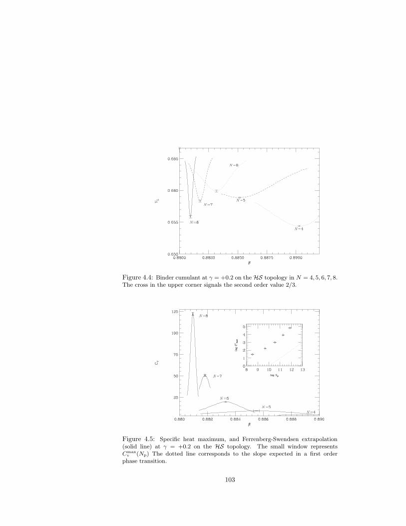
Figure 4.4: Binder cumulant at γ = +0.2 on the HS topology in N = 4, 5, 6, 7, 8.The cross in the upper corner signals the second order value 2/3.

Figure 4.5: Specific heat maximum, and Ferrenberg-Swendsen extrapolation(solid line) at γ = +0.2 on the HS topology. The small window representsCmax

v (Np) The dotted line corresponds to the slope expected in a first orderphase transition.

103

Figure 4.6: Ep distribution at γ = +0.1 on the HS topology.

The lattice sizes used range from N = 4 to N = 8, which correspond toLeff ∼ 5 and Leff ∼ 12 respectively see (Table 4.2).

In Figure 4.2, the MC evolution for N = 6, 7, 8 is shown. We remarkthat no multicanonical update is needed to obtain a very high rate of flip-flops up to N = 8. However, on the torus, for L > 6 the probabilityof tunneling between both metastable states is so tiny that a reasonablerate of flip-flops is not accessible to ordinary algorithms. Probably theinhomogeneity of the sphere is increasing the number of configurations withenergies which correspond neither to the confined nor to the deconfinedphase, but in between. These configurations make the free energy gap todecrease and hence the tunneling is easier on the HS topology. In short,the sites without maximum connectivity act as catalysts of the tunneling.

In Figure 4.3 the energy distributions are plotted. The distributionat N = 6 is distinctly non-gaussian, but a blatant two-peak structure isobserved only from N = 7 (Leff ∼ 11) on. So, when comparing with theresult at L = 4 on the torus, (see small window in Figure 4.3) a firstobservation is that the onset of a two-state signal is particularly spoiled bythe HS topology, at least in 4D pure compact U(1) gauge theory.

Concerning the latent heat, we remark its stability already at N = 7,or, if anything, its increase from N = 7 to N = 8. One would even saythat the same happens between the positions of the would-be two states in

104

N = 6 and the position observed in N = 7. The behavior of the Bindercumulant reflects this fact (see Figure 4.4). We observe a rapid growth ofV minL for small lattices sizes, apparently towards 2/3 (second order value).

This growth stops when the splitting of the two peaks is observed. Thesplitting of the two peaks is reflected by smaller values in V min

L . We remarkthat the errors quoted for V min

L are calculated taking into account the in-determination in the value of the minimum, but not the displacement inthe position of the coupling where the minimum appears.

In our opinion, mainly two reasons can give account of this behavior.The first one comes from general grounds: at the very asymptotic regionof a first order phase transition, the energy jump gets sharper and sharper,and a slightly increase of the latent heat could be expected. The secondone would be the increasing restoration of homogeneity in the hyperspherewhen increasing the lattice size. The latent heat observed in small N mightbe affected by the inhomogeneity of the hyper-sphere.

At this point we cannot give a single reason for this to happen. Wepostpone a stronger conclusion to the section devoted to the Finite SizeScaling discussion.

The value of the latent heat when obtained with a cubic spline fit to thepeaks in N = 8 is Clat = 0.064(2). Results obtained with mixed hot-coldstarts in N = 9 seems to give an energy jump around 0.067. However thereliability of this method is very limited and we do not dare to extractstrong conclusions from it. Taking into account that he cubic spline atN = 7 gives 0.053(2) a possible scenario would be a slowly increasing latentheat towards its asymptotic value Clat(∞).

The peak of the specific heat for the different lattice sizes is displayed inFigure 4.5. The continuous line represents the FS extrapolation. The plotof the peak value, Cmax

v (Np) as a function of the plaquette number revealsa linear relationship, and hence a first order character.

We have also run simulations at γ = +0.1 in order to get an estima-tion for the latent heat. The results, being qualitatively similar to thoseencountered at γ = +0.2 are not reported in detail. We plot the energydistribution in Figure 4.6.

4.4.2 Results at γ = 0 on the spherical topology

Let us first situate the status of the studies using the toroidal topologywith the Wilson action. As we have pointed out in the introduction, thetransition was believed to be continuous till the simulation of a L = 6lattice revealed the first signs of the existence of two metastable states [5].Numerical simulations up to L = 10 showed a rapid decrease of the latentheat when increasing the lattice size, suggesting that the two metastable

105

states might superimpose in the limit L → ∞ [6]. However, in [7], Azcoitiet al. suggest that the latent heat starts to stabilize at L ∼ 12, 14.

When one tries to simulate large lattices the tunneling becomes scarceand the use of multicanonical simulations for those lattice sizes seems tobe in order. However, in spite of its usefulness in spin models, as far as weknow, there are no multicanonical simulation showing a substancial flip-floprate improvement for this model.

Lattice sizes up to L = 16 have also been studied using multihistogram-ming techniques [8] and RG approaches [10, 11]. The results support theidea of a quasi stable latent heat for L > 12.

Topological considerations stressed already in the introduction led someauthors to use lattices homotopic to the sphere. In the case of the Wilsonaction (γ = 0) the two-state signal is absent up to N = 10 [18]. Followingthis, we have simulated on the spherical topology in lattices ranging fromN = 6 to N = 14, finding that the two-state signal sets in from N = 12 on.

The MC evolution for N = 10, 12, 14 is plotted in Figure 4.7. For theN = 14 lattice we have four independent runs, signaled by the dashed linesin the figure, all of them giving the same predictions.

In Figure 4.8 the distribution of Ep is plotted in lattices ranging fromN = 6 to N = 14. We observe that a two-peak structure is revealed firsttime by the histogram in N = 12, which has a Leff ∼ 19. On the toroidaltopology the equivalent signal is observed already at L = 6 (see smallwindow in Figure 4.8).

Having in mind the results of the previous section at γ = +0.2, it seemsthat the minimum Leff required to observe a two-peak structure in thespherical topology is around three times the minimum lattice size L neededin the torus to observe two peaks.

The lattice sizes used in [18] at γ = 0 ranged from N = 4 to N =10, so it is not surprising that they did not see any two-peak structure.Our results are in that sense compatible with theirs, though ours show afaster divergence for Cmax

v (N) with increasing N than the one observed in[18] in the lattice sizes we share (N=6,8,10). However we are particularlyconfident on this point because our simulation has been performed closerto the peak of the specific heat β∗(L), and so we expect the Ferrenberg-Swendsen extrapolation to be more precise.

For the sake of comparison with the full group U(1), simulations withthe Wilson action have been performed at γ = 0. At this coupling animplementation of overrelax is possible, and the global decorrelating effectshould manifest itself in a better statistical quality.

In Figure 4.9 we show the histograms of Ep from N = 6 to N = 12 sim-ulating the full group. The results are fully compatible with those obtainedfrom simulations with Z(1024).

106

Figure 4.7: MC evolution of Ep at γ = 0 on the HS topology for N = 10 (lowerwindow), N = 12 (middle) and N = 14 (top). The vertical dashed lines separatedifferent runs

This test being performed, we go back to the description of the resultsobtained for the discrete group.

In Figure 4.10 we plot Cv(N) for differentN ′s, together with the Ferrenberg-Swendsen extrapolation. The small window is a log− log plot of Cmax

v (N)as a function of Np. A linear behavior is observed from N = 10 on, whichis even faster than linear when N = 14 is taken into account. This factby itself implies the first order character of the transition since it meansthat the maximum in the energy fluctuation has the size of the volume. Asa further check we have measured the ν exponent from the scaling of theFisher zeroes (see Table 4.2).

In Figure 4.11 we plot |G(ω)|2 for several lattice sizes on the spheri-cal topology at γ = 0. The different curves stand for the different ω weextrapolate. For small lattice sizes Im(ω0) is larger, and the damping ismore severe than for the larger lattices since in the later the imaginary partcontributes with a faster oscillating function. Actually, we observe that forN = 14 even a second minimum could be measured before the signal isdamped, while for N = 10 one can measure accurately only the first one.

The results for the effective ν are plotted in Figure 4.12 lower win-dow. As could be expected from the behavior of the specific heat, for smalllattices the effective exponent is somewhat larger than 0.25. It gets com-

107

Figure 4.8: Ep distribution at γ = 0 on the HS topology. The small windowcorresponds to our simulation in the HT topology in L=6 at β = 1.0020.

Figure 4.9: Ep distribution at γ = 0 on the HS topology simulating the fullgroup U(1).

108

Figure 4.10: Specific heat maximum, and Ferrenberg-Swendsen extrapolation(solid line) at γ = 0 on the HS topology. The small window represents Cmax

v (Np)The dotted line corresponds to the slope expected in a first order phase transition.

patible with the first order value from N = 10 on. In the largest latticesthe distance between the two peaks slightly increases, and we measure aνeff slightly smaller than the first order value. As a ν < 0.25 is strictlyimpossible we expect this to be a transient effect due to finite size effectsassociated to the observed splitting up of the two peaks.

Concerning the latent heat, we observe a behavior completely analogousto the one observed at γ = +0.2. We do observe a two peak structure quitestable when comparing N = 12 and N = 14, but it slightly increases inN = 14. The plot of the Binder cumulant reflects again this fact (seeFigure 4.13). The fast growth of V min

L towards 2/3 is preempted by theonset of double peaked histograms from N = 12 on, and it even decreasesin N = 14.

The cubic spline fit in N = 14 at the peaks gives a latent heat Clat ≈0.018(2). which is compatible with the results suggested by extrapolatingto infinite volume the values obtained on the torus up to L = 14. Ourresults are hence supporting the conjecture stressed in [7] about a quasistabilization of the latent heat on the torus from L = 12 on.

109

Figure 4.11: Plot of (4.25) for N = 10 (lower window), N = 12 (middle) andN = 14 (top) at γ = 0 in the HS topology.

Figure 4.12: Effective exponent ν at γ = 0 (lower window), and at γ = −0.2(upper window) on the spherical topology. In the smaller lattices an νeff ∼ 1/3is observed which becomes 1/d when large enough lattices are considered.

110

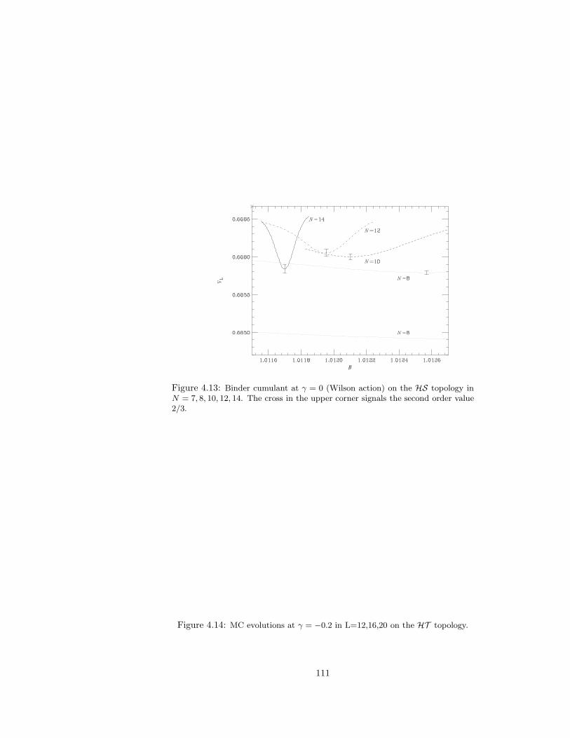
Figure 4.13: Binder cumulant at γ = 0 (Wilson action) on the HS topology inN = 7, 8, 10, 12, 14. The cross in the upper corner signals the second order value2/3.

Figure 4.14: MC evolutions at γ = −0.2 in L=12,16,20 on the HT topology.

111

Figure 4.15: Ep distributions at the different negative γ on the HT topology.We have run up to L = 20 at γ = −0.1,−0.2 and up to L = 24 at γ = −0.3,−0.4.

0 0.00001 0.00002 0.00003 0.00004 0.00005

0

0.005

0.010

0.015

0.020

0.025

0.030

Cla

t

1/V

0 0.05 0.10 0.150

1

2

3

∆F

1/L

γ=-0.1γ=-0.2γ=-0.3γ=-0.4

Figure 4.16: Free energy gap ∆F (L) (lower window) and latent heat (upperwindow) for the different negative γ in the HT topology.

112

Figure 4.17: Effective ν exponent for the different negative γ in theHT topology.

Figure 4.18: Cmaxv (L) as a function of Np for the different negative γ values on

the HT topology. We have used log− log scale for the clarity of the graphic sake.The dotted line corresponds to the first order slope.

113

4.4.3 Results for γ < 0

Toroidal topology

We have performed a systematic study of the transition at several negativevalues of γ on the toroidal topology.

We find that the two-state signal persists for all γ values we consider.

The MC evolution at γ = −0.2 is plotted for several lattices sizes infigure 4.14. As a general observation the more negative is γ, the flip ratebecomes scarce for increasing lattice size. As an example, at γ = −0.4 theflip rate in L = 20 is comparable to the one observed in L = 16 at γ = −0.2.

The energy histograms reveal an increasing weakness of the transitionwhen going to more negative γ values (see Figure 4.15). A double peakstructure is clearly visible at γ = −0.1 in L = 8, while at γ = −0.4 one hasto go to L = 12 to observe an equivalent signal.

In what concerns the behavior of the free energy gap ∆F (L), it growsfor all investigated lattice sizes at all negative γ values (see Figure 4.16lower window) signaling the first order character of the transition. Thevalue of L at which ∆F (L) starts growing is certainly larger as the value ofγ is more negative. This is another test of the increasing weakness of thetransition as γ gets more negative.

The statistics performed on the torus are reported in Table 4.3. We alsoquote for the different negative γ, the value of β∗(L) and the position ofpartition function zero closest to the real axis. We have computed from theimaginary part of the zeroes the effective ν exponent between consecutivelattice sizes following (4.26).

In Figure 4.17 we plot for the different γ values the νeff we measure. Inall cases a νeff ∼ 1/3 is observed for small lattice sizes, which gets closerto 0.25 when the lattice is large enough. From this figure the trend of νeffseems rather clear towards the first order value.

From the energy distributions we measure the latent heat through acubic spline at the peaks. Taking into account the value νeff = 0.25 wemeasure, we plotted it as a function of the inverse of the volume L−4,which is also the expected behavior of the latent heat when the transitionis first order. The latent heat can be extrapolated to a value which is safelyfar from zero (see Figure 4.16 upper window).

In Figure 4.18 we plot Cmaxv (L) as a function of Np. As could be ex-

pected from the behavior of the effective exponent ν, the maximum ofthe specific heat for small lattices diverges slower than the volume. Forthe smaller lattices the effective exponent is α/ν ∼ 1.4. This value in-creases monotonically with the lattice size. In the largest ones we observeα/ν ∼ 3.5.

114

Figure 4.19: MC evolution of Ep in N = 12 (lower window), N = 14 (middlewindow) and N = 16 (upper window) at γ = −0.2 on the HS topology. The twodifferent runs in N = 16 are separated by a vertical dashed line.

Spherical topology

On the toroidal topology we have found that the minimum lattice sizerequired to observe a two state signal is obtained through an apropriatecombination (γ, Lmin), with increasing Lmin for increasingly negative γ, thebehavior being qualitatively similar for all the γ values we have investigated.In view of this, we have studied a single γ < 0 value on the spherical latticeto check if the two state signal is absent on this topology. For the sake ofcomparison with [16, 18] we choose this value to be γ = −0.2.

We have run simulations on spheres ranging from N = 6 (Leff ∼ 8) toN = 16 (Leff ∼ 26). The MC evolution is plotted in Figure 4.19.

The distribution in N = 14 is distinctly non gaussian and the splittingof the peaks occurs in N = 16 (see Figure 4.20). We remark that thesimulations inN = 16 are extremely expensive in CPU. In order to alleviatethermalization we have parallelized the code using shared memory in twoPPro processors. In this lattice we have run two independent simulationsstarting from different configurations the results being fully compatible.

The behavior of the maximum of the specific heat is shown in Figure4.21. We observe the same trend than in the previous values of γ in thesphere, i.e., an increasingly fast divergence of the specific heat with the

115

Figure 4.20: Ep distributions at γ = −0.2 on the HS topology.

Figure 4.21: Specific heat maximum, and Ferrenberg-Swendsen extrapolation(solid line) at γ = −0.2. The small window represents Cmax

v (Np) The dotted linecorrespond to the slope expected in a first order phase transition.

116

Figure 4.22: Binder cumulant at γ = −0.2 on the HS topology inN = 10, 12, 14, 16. The cross in the upper corner signals the second order value2/3.

lattice size, showing an effective α/ν ∼ 4 already when the histogram widthbecomes constant with increasing lattice size.

At this value of γ we have a worse estimation for the latent heat to be,as the two peaks have not split enough to allow an accurate measurement.

Again the behavior of the Binder cumulant is very significant (see Fig-ure 4.22. The value V min

L shows a very fast trend towards 2/3 in the smalllattices. When increasing the lattice size the rate gets slower, and finallythe value in N = 16 is compatible with the value in N = 14 preempting theextrapolation to 2/3. Unfortunately lattices larger than N = 16 are unac-cessible to our computers nowadays, and we cannot observe a decreasingV minL as we did for the other γ values. However from the behavior betweenN = 14 and N = 16 an increasing V min

L for larger spheres seems to be veryunlikely.

Concerning the effective critical exponent ν we have measured the po-sition of the first Fisher zero (see Table 4.2) and compute νeff (see Figure4.12). Again the first order value 1/d is reached in the largest lattices.

117

4.4.4 Toroidal versus Spherical topology

Due to the fact that on the sphere there are a number of points with lessthan the maximum connectivity, violations to standard FSS in the form ofuncontrolled finite size effects are expected to appear on this topology.

We have observed all along this work that working on the sphericaltopology retards the onset of two-state signals. In terms of Leff , somequalitative prediction arising from our results would be that at fixed γ, theminimum lattice size required to observe a double peak structure, Lmin, isaround three times larger on the sphere than on the torus. This one beingthe showier difference, is not certainly the only one.

When comparing Cmaxv (Leff) on both topologies one finds always smaller

values on the spherical topology (see small window in Figure 4.23). We didrun on L = 12 on the torus and N = 8 on the sphere, which has anLeff ∼ 12, sweeping an interval of β values including the phase transition.In Figure 4.23 we have plotted Ep in both topologies. In the region of lowβ the system is disordered, the entropy is higher and the system is not sosensitive to inhomogeneities of the lattice. However, in the region of high βthe energy is in general smaller than for the homogeneous lattice since thesystem tends to be ordered, and the influence of the sites with less than

Figure 4.23: Ep at γ = −0.2 in Leff ∼ 12. The dotted line corresponds to thetoroidal topology, the dashed one to the sphere N = 8. The small window showsthe difference in the specific heat between both cases.

118

maximum connectivity is more evident. This difference gets smaller whenthe lattice size is increased on the sphere, and hence the energy jump islarger. This feature explains the observed splitting of the two states on thespherical lattices when increasing lattice size.

Altogether, it is not recommended to work on spherical lattices to checkthe existence or not of two-state signals. However, there are a number offacts that make this topology not so dissapointing in spite of those uncon-trolled finite size effects. The first one concerns the behavior of β∗(L) andthe second one the measure of the latent heat.

In Figure 4.24 we compare β∗(L) on the torus and on the sphere. A firstobservation is that despite they not having the same values in finite lattices,both curves get closer when increasing the lattice size. This supports theidea of a common thermodynamic limit for both topologies. On the otherhand, the shift in the apparent critical coupling with L is much less dramaticon the sphere than on the torus. It seems that finite size corrections to βcare smaller in the case of the spherical topology. This behavior has alsobeen observed in the Ising model on spherical lattices [28].

The behavior of the latent heat is very significant. In Figure 4.25 wecompare the latent heat in finite volumes for both topologies. On the

Figure 4.24: β∗(L) for the different lattice sizes on the torus (dotted lines) andon the sphere (dashed lines) at γ = 0 (lower window) and at γ = −0.2 (upperwindow). The couplings for γ = 0 on the torus have been taken from [11].

119

Figure 4.25: Latent heat for the different lattice sizes on the torus and on thesphere at γ = 0 (lower window) and at γ = −0.2 (upper window). The dottedline corresponds to Clat(∞) obtained by extrapolating the values on the torusthrough a linear fit as function of 1/V . The values for γ = 0 on the torus havebeen taken from [11].

Wilson line, at γ = 0 the asymptotic value of the latent heat is obtained inthe spherical topology. The inhomogeneity of the sphere has, paradoxically,helped us to run lattices with Leff ∼ 24 without having to worry about thetunneling rate. From this graph we quote Clat(∞) = 0.018(1). In the upperwindow the same is plotted for γ = −0.2. Unfortunately we have just asingle lattice size on the sphere to measure the latent heat, however, fromthe behavior exhibited by this topology, an increase of the latent heat onspheres larger than N = 16 seems rather likely. Altogether, at γ = −0.2 aClat(∞) ∼ 0.009 is plausible.

In what concerns the latent heat, the spherical topology seems to affordan useful complement to the results obtained for the the toroidal lattice. Infact, on the Wilson line lattices larger than L = 16 cannot be studied dueto the technical problem associated to the scarce tunneling. The sphericallattice alleviates this technical problem, and the results are supporting thevalue of the extrapolated latent heat as a function of the inverse of thevolume, from the data on toroidal lattices up to L = 16. One could considerthe possibility of simulating on spherical lattices at negative γ to solve thetunneling problem, but in our opinion, the price to pay is too high.

120

4.5 Conclusions

The first order character of the deconfinement transition in pure U(1) hasbeen proved, up to the limits of a rather reasonable numerical evidence, inthe interval γ ∈ [+0.2,−0.4].

In γ = +0.2 we have been able to stabilize the latent heat. We are awareof no simulation on the torus showing a stable latent heat due to the scarcetunneling in lattices larger than L = 6. The spherical topology has helpedto solve this problem. However, probably any lattice with inhomogeneitieswould produce the same catalysing effects.

In γ = 0 we have obeserved an increasing energy gap on the sphericallattice, and also, we have been able to measure the asymptotic value ofthe latent heat. We have proved the suggestions of several authors about aquasi stabilization on lattices larger than L ∼ 12. The data on the sphericaltopology have been crucial to discard the possibility of a slowly vanishinglatent heat. It follows that the discretization of pure compact U(1) LGTon the lattice using the Wilson action exhibits a first order phase transitionwith a latent heat in the thermodynamical limit Clat ∼ 0.018.

On the toroidal topology things happen qualitatively in the same waythan in γ = 0 up to γ = −0.4. We have run on spherical lattices inγ = −0.2 looking for an argument similar to the one found in the Wilsoncase concerning the stabilization of the latent heat. The simulation inN = 16 gives an estimation for the latent heat though rather imprecisebecause the splitting of the peaks is not good enough for the measurementto be accurate. However, in view of the behavior exhibited by the sphericaltopology concerning the trend of the two peaks on spherical lattices toseparate, we are prone to consider the value measured in N = 16 as alower bound for the latent heat in γ = −0.2. On the other hand, wewould at present say that the latent heat extrapolated from the data onthe torus up to L = 20 is rather accurate, in view of the behavior forthe Wilson case. The possibility of running larger spheres surpasses ourcomputer resources. A highly parallelized version of the code should beused to alleviate thermalization, which is a possibility we do not discardcompletely at medium term.

As for the evolution of the latent heat along the transition line as afunction of γ. the scenario that follows from our results is plotted in Figure4.26.

Either proving or discarding the possibility of a TCP at some finitenegative |γTCP| > 0.4 will be a very difficult task from the numerical pointof view. An analytical argument would be welcome. A very tiny two-statesignal, comparable with the one observed in L = 8 at γ = −0.4, is observedon the torus in L = 16 at γ = −0.8, which is the most negative value we

121

Figure 4.26: Extrapolated value for the latent heat as a function of γ. Thevalues quoted for γ < 0 come from data on toroidal lattices, the ones for γ ≥ 0from data on spherical lattices.

have run on the torus. Taking into account the factor 3 in Leff one wouldneed a N ∼ 30 sphere to observe a tiny double peak structure. Simulationwith spherical lattices in this range of γ have no sense, and nothing canbe concluded from the absence of two state signals from such negative γvalues.

In view of these difficulties to stabilize the latent heat for very negativeγ values, the only chance to discern the order of the phase transition isthe study of effective critical exponents. Cumulants of the energy, such asthe Binder cumulant, have been shown to behave like expected in the firstorder case only when the stable two-peak structure is almost setting in, andthere, we do not need further evidences any longer. We could not expectadditional information since by definition the Binder cumulant relies on theexistence of stable latent heat in order to extrapolate to V min

L=∞ < 2/3.The advantage of studying the effective exponents (which is nothing

but studying the evolution of the histograms width) is that we do not needa direct observation of latent heat to conclude that a transition is firstorder [33, 30]. We have observed a νeff which evolves monotonically until itreaches the first order value, namely 0.25, in all cases. The statistics neededto observe a monotonous behavior, are order 1000τ at the coupling β∗(L),which has to be located with high precision (four digits in our experience)

122

in order to accurately measure effective exponents. However, one has tomake every effort to observe the trend of the effective exponents, since it isthe only chance to discern the order of such tricky transitions.

In pure U(1), for the Wilson case, an exponent ν ∼ 1/3 was widelypredicted [3, 4, 12] at the beginning of the eighties when the lattice sizeswhere too small to reveal two peaks. That ν was shown to become ν ∼ 0.29when simulating L = 14 [7]. We have measured ν = 0.25 on sphericallattices and stated its first order character. Within the approximation ofeffective potentials it can be shown that along the transient region of a weakfirst order phase transition, everything goes like in a second order one witha thermal exponent α = 0.5 [20]. Together with Josephson law (α = 2−νd)it implies ν ∼ 0.37. This statement has been checked in 2D Potts [20], 3Dand 4D O(N) models [29, 30, 31, 32] and in the 4D SU(2)-Higgs at T=0with fixed Higgs modulus [33]. Our results prove that pure compact U(1)theory behaves in the same way.

123

124

Bibliography

[1] K.G. Wilson Phys. Rev. D10 2445

[2] M. Creutz, L. Jacobs and C. Rebbi. Phys. Rev. D20 (1979) 1915

[3] B. Lautrup and M. Nauenberg Phys. Lett. B95 (1980) 63

[4] G. Bhanot Phys. Rev. D24 (1981) 461

[5] J. Jersak, T. Neuhaus and P.M. Zerwas Phys. Lett. B133 (1983) 103

[6] V. Azcoiti, G. di Carlo and A. Grillo Phys. Lett. B238 (1990) 355

[7] V. Azcoiti, G. di Carlo and A. Grillo Phys. Lett. B268 (1991) 101

[8] G. Bhanot, T. Lippert, K. Schilling and P. Ueberholz Nuc. Phys.B378(1992) 633

[9] D.J. Callaway and R. Petronzio Nuc. Phys. B280 (1987) 481

[10] P. Hasenfratz and A. Hasenfratz Nuc. Phys. B295 (1988) 1

[11] L.A. Fernandez, A. Munoz-Sudupe, R. Petronzio and A. Tarancon.Phys. Lett. B267 (1991) 100

[12] G. Bhanot Nuc. Phys. B205 (1982) 168

[13] H.G. Evertz, J. Jersak, T. Neuhaus and P.M. Zerwas Nuc. Phys. B251(1985) 279

[14] A. Hasenfratz Phys. Lett. B201 (1988) 492

[15] R. Gupta, M.A. Novotny and R. Cordery Phys. Lett. B172 (1986) 86

[16] C.B. Lang and T. Neuhaus Nuc. Phys. B431 (1994) 119

[17] M. Baig and H. Fort Phys. Lett. B332 (1994) 428

125

[18] J. Jersak, C.B. Lang and T. Neuhaus Phys. Rev. Lett. 77 (1996) 1933

[19] W. Kerler, C. Rebbi and A. Werber Phys. Lett. B348 (1995) 565

[20] L.A. Fernandez, M.P. Lombardo, J.J. Ruiz-Lorenzo and A. Tarancon.Phys. Lett. B277 (1992) 485

[21] The APE collaboration Nuc. Phys. B318 (1989) 553

[22] J. Lee and J.M. Kosterlitz Phys. Rev. Lett. 65 (1990) 137

[23] M.S. Challa, D.P. Landau, K. Binder Phys. Rev. D34 (1986) 1841

[24] C. N. Yang and T. D. Lee. Phys. Rev. 87 (1952) 404

[25] E. Marinari in 1996 Budapest Summer School on Monte Carlo methodse-print: cond-mat//9612010

[26] M. Falcioni, G. Martinelli, M.L. Paciello, G. Parisi and B. TaglientiNuc. Phys. B265 (1986) 187.

[27] A.D. Sokal Bosonic Algorithms in Quantum Fields on the Computer.Advanced Series on Direction in High Energy Physics Vol. 11, M.Creutz Editor. World Scientific, Singapore 1992.

[28] O. Diego, J. Gonzalez, J. Salas J. Phys. A27 (1994) 2965.

[29] J.L. Alonso, J.M. Carmona, J. Clemente, L.A. Fernandez, D. Iniguez,A. Tarancon and C.L. Ullod. Phys. Lett. B376 (1996) 148

[30] H.G. Ballesteros, J.M. Carmona, L.A. Fernandez and A. TaranconPhys. Lett. B419 (1998) 303

[31] I. Campos, L.A. Fernandez, A. Tarancon Phys. Rev. D55 (1997) 2965

[32] J.L. Alonso, H.G. Ballesteros, L.A. Fernandez, V. Martın-Mayor, A.Munoz Sudupe and A. Tarancon Phys. Rev. B53 (1996) 2537

[33] I. Campos, Nuc. Phys. B514 (1998) 336

126

Chapter 5

Modelos bidimensionalesde flujo de partıculas

128

5.1 Introduccion

En los ultimos anos esta recibiendo una especial atencion la formulacion demodelos para describir por ejemplo el paso de mensajes a traves de redes deordenadores [1], el trafico en grandes ciudades [2], la adsorcion de moleculasen un cristal [3], conductores de iones rapidos [4].

Todos estos problemas tienen en comun que pueden ser estudiados desdeel punto de vista de la teorıa de Random Walks. Sin embargo, el ele-vado numero de grados de libertad hace imposble extraer informacion rele-vante mediante calculos analıticos. La alternativa es el uso de simulacionesnumericas.

Desde este punto de vista uno podrıa pensar en formular modelos tanproximos a la realidad como sea posible, incluyendo todos los grados delibertad que se sea capaz de manejar. Sin embargo los modelos que resultanaplicando esta filosofıa son demasiado complicados de estudiar, no solo enlo que concierne a la descripcion de fenomenos relevantes, sino tambienporque carecen de poder predictivo en general.

Una aproximacion alternativa es formular modelos mas simples, menosrealistas pero manteniendo los rasgos fundamentales del sistema fısico.Tales modelos estan descritos por unos pocos parametros, siendo por ellomas faciles de tratar y haciendo posible un estudio global del espacio deparametros sin perder intuicion fısica.

Mediante la formulacion de estos modelos se pretende obtener resulta-dos relevantes sobre sistemas complejos, estudiando aproximaciones relati-vamente simples, como se suele hacer en Mecanica Estadıstica (ME) dondesistemas tan complicados como redes ferromagneticas comparten muchaspropiedades con modelos tan simples como el de Ising. En ME la relacionentre ambos sistemas se entiende a traves del Grupo de Renormalizacion.Desgraciadamente estamos lejos de poder probar una relacion de este tipopara modelos de flujo de partıculas, debido fundamentalmente a que notienen un lımite termodinamico bien definido. Sin embargo la modelizacionde estos sistemas es necesaria.

Los problemas que se encuentran cuando se estudian sistemas que en-vuelven flujo de partıculas estan relacionados con procesos de congestion.Los sistemas realizan una transicion de una situacion de trafico fluido aotra caracterizada por el atasco.

Podrıamos utilizar las herramientas de la ME para estudiar estos prob-lemas si asimilamos este cambio a una transicion de fase. Un primer pasoes buscar las variables que gobiernan la transicion.

El flujo en la red esta condicionado por el numero maximo de partıculasque un nodo es capaz de contener, por la interaccion entre las partıculas ypor la geometrıa de la red (por ejemplo el numero de coordinacion).

129

En nuestro modelo hay una inyeccion continua de partıculas en la red,para cada una de ellas se elije al azar un nodo que sera su destino final.El movimiento de las partıculas se implementa permitiendoles moverse enla red de acuerdo con determinadas reglas que definiremos mas tarde. Enel trafico real las partıculas encuentran a menudo obstaculos en su camino.Estos obstaculos se simulan limitando el numero de partıculas que un nodode la red puede almacenar simultaneamente.

Volviendo a la discusion desde el punto de vista de la ME, vamos a enfo-car la situacion en la que la densidad de partıculas es alta. Intuitivamentees claro que una partıcula podrıa evitar zonas de atasco si le permitimosrodear el obstaculo. El sistema estara globalmente mas descongestionado yesperamos una mejora en el numero de partıculas que alcanzan finalmentesu destino. En terminos de ME, la discusion previa significa que calentandoel sistema (T 6= 0) se obtendran mejores resultados [5]

En lo que concierne a la interaccion entre las partıculas, hemos intro-ducido un termino de contacto, la existencia de obstaculos en forma denodos completamente ocupados. Las consecuencias de esta interaccion sepueden ver como si existiera un potencial infinito que actua en los nodossaturados.

Un termino de interaccion apropiado se obtiene asignando carga electricaa cada partıcula. La repulsion alejara a las partıculas de las regiones densa-mente cargadas. Consideraremos este tipo de repulsion actuando solo sobreprimeros vecinos en la red.

Este tipo de fuerzas repulsivas se consideran a menudo en problemas depolımeros [6].

Hemos introducido un modelo en el cual hay un termino que controlala magnitud de las fluctuaciones termicas y otro que simula una fuerzarepulsiva. Los parametros que controlan estos terminos son respectivamentela temperatura y la carga. Veremos como ajustando ambos parametros esposible mejorar el flujo de partıculas.

130

Abstract

We study a particle flow model which may be used to get insight intovarious real traffic problems. The model is implemented using a discretelattice, in which particles move towards their destination, fluctuating aboutthe minimal distance path. A repulsive interaction between particles isintroduced so as to avoid the appearance of a traffic jam. We have studiedthe parameter space finding regions of fluid traffic, and saturated ones, bothregions being separated by abrupt changes. The improvement of the systemperformance is also explored by introducing a non-constant potential actingon the particles. Finally, we deal with the behaviour of the system whentemporary failures in transmission occur.

5.2 The Model

We consider a two-dimensional lattice with coordination number 4, andperiodic boundary conditions. The particles live in the lattice sites, la-beled by n ≡ (n0, n1) and can move from its site to one of its four nearestneighbors at every time step. The maximum number of particles that asite can contain will be denoted by B, and will be kept fixed for all thesimulation at a value B = 5. We denote the occupation number of the siten by σ(n). In this notation, the particles are prevented from moving tosites with σ(n) = B. In addition we consider an input queue at each sitefor the particles waiting to be injected on the lattice.

By analogy with statistical mechanics systems, we work with the inverseof the temperature, β. We denote the charge of the particles by κ and theprobability of particle injection to the lattice by p.

The dynamic of the system is as follows:

1. A lattice site is chosen at random.

2. A particle is added, with fixed probability p, to the queue of the site,waiting to be introduced to the lattice 1

3. If the queue of the site is not empty, and σ(n) < B, a new particle isintroduced in the lattice, and an endpoint assigned to it at random.

4. All particles at the considered site, try to move towards one of itsfour neighbors. For a given particle located at the position n we

1The size of the queue is as big as necessary, so that it contains all particles waitingto be fed at that lattice site

131

must assign a probability of it jumping to each of its neighbouringlocations. This probability is given by:

P (±µ) = N exp(±βsign(nfµ − nµ)− κσ(nµ)) , (5.1)

where nµ here signifies the µ coordinate of site n, nf is the endpointof the particle being considered, and N is the normalization constant.To choose between possible destinations we use a Heat Bath [7] al-gorithm.

The factor multiplying β, is a potential term. It implies a constantforce acting on the particle driving it to its endpoint. The κ term pro-duces a repulsion between particles sitting in nearer neighbors sites.Obviously there is a wide range of potentials that could be considered,in order to produce more effective forces, and partial improvementswill be expected.

5. Movement is allowed if the chosen site has σ(n) < B, otherwise theparticle remains at its original site until a new movement is attemptedin the next iteration.

6. A particle is removed from the lattice when it reaches its endpoint.

The smaller p is, the weaker is the effect of the interaction betweenthe particles. For fixed (β, κ) the fluid flow of particles on the lattice onlytakes place for those values of p being less than a certain threshold which is(β, κ) dependent. Above this threshold, the density becomes too high andthe transmission process is prevented. We say the system is saturated. Thesaturation mechanism begins with the appearance of saturated domains,which grows in size making the movement of the particles more and moredifficult.

Our purpose is to quantify this threshold density, as well as to describethe flow properties along the parameter space (β, κ, p).

From the point of view of Telecommunication Networks, the lattice sitescan be thought of as nodes of such networks, and particles here can be in-terpreted as messages/packets. Within this approach, B can be identifiedwith the available buffer space at the considered node. In this way, ourmodel can be considered as a first step towards an abstract modeling ofpacket/message Telecommunication Networks. In such networks, packetsare routed by each node according to routing tables dynamically maintainedby the network so as to minimize some cost function along the trajectory ofthe packets [8]. In the present model, this cost function is simply the trav-eled distance, and, as the network state does not change during simulations,routing tables need not be dynamically calculated. A natural extension of

132

this model would be to allow variable link lengths between the nodes andto compute routing tables according to the path lengths. The role of thetemperature parameter is to quantify how firmly the network will try tostick to its policy of minimizing the cost along a trajectory: as will beshown below, implementing the routing according to the cost minimizationprocedure in a rigid way (zero temperature), although this is the best naivechoice from an individual user point of view, can be detrimental to theglobal behavior of the network and thus to its collective utility (the totalthroughput offered by the network).

Congestion is an unavoidable phenomenon in uncontrolled packet net-works, since packets introduced at one node have no guarantee of findingthe necessary resources (available buffer space) in the transit nodes. Ifuncontrolled, congestion result in packet losses which, in the case of datatransmission, are detected by upper layer protocols (the Transport ControlProtocol, TCP , for instance in the case of the Internet) and are corrected byretransmision request. Hence these packet losses will trigger more packetsto be introduced into the network, thus further amplifying the congestionTwo approaches are possible to avoid this vicious circle: reducing the sourceemission rate when a congestion is detected (this is the TCP approach) ortrying to control the congestion inside the network by preventing pack-ets from accessing overloaded areas (this approach does not rely on anysource behavior: in the extreme congestion case the source is simply deniedany access to the network). This last option, congestion control inside thenetwork, is presently a very active area of research in the networking com-munity [9]. To implement such a control, the overload information shouldbe transmitted by a node to its neighbors at least. This is precisely whatis modeled by the repulsive charge term in the present model: access toa loaded node is discouraged, and access to an overloaded node is simplyforbidden. It should be noted that in the model as it stands, a node isinstantaneously aware of the load state of its neighbors. A more complexmodel should take into account the latency introduced by the node-to-nodetransit time, leading to a description of the congestion control by some kindof retarded potential. It will be particularly important to take this latencyaspect into account for modeling high speed networks [10], but this is leftfor future work.

The system we are considering here is also related to a lattice gas withfixed number of particles in a constant electric field ~E [11]. The electric cur-rent is related to the traffic speed. Also in this model a transition appears,between a disordered phase and another one were particles move collec-tively in the ~E direction. In our case the electric field is no longer constant,it depends dynamically on the particle environment: the surrounding elec-trical charge and the end point associated with the particle. As is usual for

133

traffic models, the number of particles is not constant; as a consequence,the transition mechanism is different.

5.3 Numerical Simulation

We have performed Monte Carlo (MC) simulations in order to study theparameter space. Here we present results obtained using a L × L latticewith L = 32 and periodic boundary conditions. The computations havebeen carried out on workstations.

The starting configuration is obtained by generating a particle withprobability p at each site of the lattice, therefore, the total number of sitesoccupied initially is about p× L2. The random number generator is basedon one described in [12]. The time step is identified with a MC iteration,that is the update of L2 lattice sites in the way described in section 2.

The temporal evolution of the system exhibits a transient regime, char-acterized by the instability in the observables (see next section). After this,the system falls into an extremely long-living metastable state, where theflow properties do not change significantly with the temporal evolution. Wesay the system has reached the asymptotic regime.

The time the system spends in the transient regime depends on theparameter space point (β, κ, p). In this regime, in the non-saturated region,the particle density is initially low and grows with the particle injection.

This transit time also grows near the parameter space points wherean abrupt change in the properties is observed (e.g. near the thresholddensity), reaching in this case up to 2× 104.

For each value of the parameters, we have performed typically 8 × 104

MC iterations. For β and κ ∈ (0, 0.4) the transient regime takes around5000 iterations, while above 0.5 for both parameters, this time falls to400− 600 iterations. We have also performed the simulations starting fromdifferent configurations, allowing the system to evolve for up to 2×105 iter-ations. We have computed the errors by calculating the dispersion betweenthe results obtained from starting from these different configurations.

5.4 Observables

A correct description of the system is obtained from the measurement of therelevant observables. From their temporal evolution we are able to evaluatewhen the asymptotic regime is reached, or even whether this regime willor will not be saturated. From the averaged value of these magnitudes weobtain a quantitative description of the flow process.

134

0 2000 4000 6000 8000 10000

MC iterations

0

0.5

1.0

1.5

2.0

2.5M

p=0.0073β=0.2 κ=1.0

Figure 5.1: Temporal evolution of M bellow the critical injection pc.

For a given configuration, we define the occupation M as:

M = (1/V )V∑

i=1

σ(i) . (5.2)

Where V is L× L.The statistical average over the configurations (labeled by j) is:

〈M〉 = limN→∞

(1/N)

N∑

j=1

Mj . (5.3)

N being the number of averaged configurations.During the time interval tj − ti ≡ t, ne particles will reach their

endpoint. We define the Band Width (BW ) as the number of particles thatarrive at the endpoint per time unit.

BW (t) = ne

t . (5.4)

The statistical average for BW is obtained from its mean value over a num-ber of time intervals NT :

〈BW 〉 = limNT→∞

(1/NT )

NT∑

j=1

BW (j) . (5.5)

135

0

1

2

3

4

5

M β=0.2 κ=1p=0.0087

0 5000 10000 15000 20000 25000 300000

1

2

3

4

5

M

MC iterations

β=4.0 κ=1p=0.0890

Figure 5.2: Temporal evolution of M above pc.

We can obtain a good measure of the system performance from the meantime taken by the particles to reache their endpoint, TM . We compute TMin the time interval t by adding the individual time spent by each particle(delay time), divided by nf :

TM (t) =∑nf

i=1 Tinf

(5.6)

In the same way we define the statistical average as over NT intervals as:

〈TM 〉 = limNT→∞

(1/NT )

NT∑

j=1

TM (j) (5.7)

The occupation frequency of a certain occupation number, σ(n), is de-fined as the number of times that the occupation σ(n) appears at any latticesite.

5.5 Phase Diagram

We examine the parameter space (β, κ, p) searching for regions where sharpchanges in the temporal evolution arise. At each (β, κ) value there is a p

136

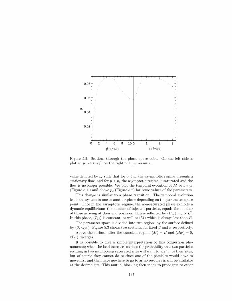
0 2 4 6 8 10

β (κ=1.0)

0.02

0.04

0.06

0.08p c

0 1 2 3

κ (β=4.0)

Figure 5.3: Sections through the phase space cube. On the left side isplotted pc versus β, on the right one, pc versus κ.

value denoted by pc such that for p < pc the asymptotic regime presents astationary flow, and for p > pc the asymptotic regime is saturated and theflow is no longer possible. We plot the temporal evolution of M below pc(Figure 5.1 ) and above pc (Figure 5.2) for some values of the parameters.

This change is similar to a phase transition. The temporal evolutionleads the system to one or another phase depending on the parameter spacepoint. Once in the asymptotic regime, the non-saturated phase exhibits adynamic equilibrium: the number of injected particles, equals the numberof those arriving at their end position. This is reflected by 〈BW 〉 = p×L2.In this phase, 〈TM 〉 is constant, as well as 〈M〉 which is always less than B.

The parameter space is divided into two regions by the surface definedby (β, κ, pc). Figure 5.3 shows two sections, for fixed β and κ respectively.

Above the surface, after the transient regime 〈M〉 = B and 〈BW 〉 = 0,〈TM 〉 diverges.

It is possible to give a simple interpretation of this congestion phe-nomenon; when the load increases so does the probability that two particlesresiding in two neighboring saturated sites will want to exchange their sites,but of course they cannot do so since one of the particles would have tomove first and then have nowhere to go to as no resource is will be availableat the desired site. This mutual blocking then tends to propagate to other

137

neighboring sites and once above a given load a complete congestion willdevelop at the scale of the network.

Such mutual blocking is well-known in most no loss routing schemessuch as wormhole routing and is called deadlock [13]. Deadlock avoidanceis a very active research area, specially for massively parallel system inter-connections [14].

β dependence

The thermal fluctuations move particles away from their minimal distancepath. The higher β is, the less the importance of these fluctuations.

As shown in Figure 5.3 (left side), there is an interval of β values wherethe reduction of fluctuations have a positive influence on the throughput:pc rises, as well as 〈BW 〉, while 〈TM 〉 decreases, as shown in Figure 5.4.

When going to higher β values, the situation does not persist. The ab-sence of thermal fluctuations damages the throughput because particles arenot able of going round obstacles. As a consequence pc and 〈BW 〉 decrease.〈TM 〉 does not appreciably change from its minimal value, correspondingto the infinite directionality one.

Figure 5.2 shows how the thermal fluctuations influence the saturationmechanism. If they are important, M grows slowly until it reaches B. Ifthey are not significant a sharp jump appears in the temporal evolution ofM , between its value in the transient regime and B. We conclude from thisthat the saturated domains grow faster in the absence of fluctuations, aswould be expected from the earlier discussions.

In particular, it is intuitive that a mutual deadlock will last longer ifthermal fluctuations are disallowed (particles in mutual deadlock will re-peatedly attempt to exchange their sites) hence creating a larger local con-gestion area which can eventually evolve towards a global congestion. Thiswas clearly observed in [5] where only one buffer was available per siteand this behavior is also exhibited in this model, hence illustrating thewell-known fact [15] that deadlock is a consequence of our no loss routingscheme 2 and not a consequence of insufficient resources.

κ dependence

The dependence of pc on κ presents two different regions (see Figure 5.3).

In the first one, pc rises with increasing κ. For these κ values, theinclusion of the repulsion term helps the system to avoid congested regions.We denote by κopt the value at which pc reaches its maximal value.

2movement is granted if and only if the available resource is available at the low end

138

0 2 4 6 8 100

100

200

300T

M

β (κ=1.0)

Figure 5.4: 〈TM 〉 dependence on β for p ≈ pc.

0 2 4 6 8

β

0

0.5

1.0

1.5

2.0

2.5

3.0

κ opt

Figure 5.5: (β, κopt) line. The errors are of the size of the κ step measured,(κ = 0.5.)

139

In the second region, κ > κopt, pc decreases with κ. Above κopt on, therepulsion is too strong and the particles move far away from their minimalpaths. As a result, the collapse appears for smaller injection densities.

In Figure 5.5 we give the values of κopt for some β values. The more aparticle is restricted to its minimal path, the stronger the repulsion neededto avoid obstacles in the lattice.

Therefore, there is a maximal value for the particle injection supportedby each β value, which is reached for κ in a neighborhood of κopt.

5.6 General Behavior and Optimization

Let us focus on the behaviour of the other significant observables for thetraffic flow, when β and κ have been tuned to obtain a maximal pc.

Behavior of BW

As we have already pointed out, BW in the asymptotic regime is propor-tional to p by a factor L2, as it may be checked in figure 6. Hence,at each(β, κ) value the maximum for 〈BW 〉 is reached when p = pc.

Above pc, 〈BW 〉 remains constant during the transient regime, andsharply falls to zero after it. BW is a good measure to determine when

0

20

40

60

80

100

<B

w>

β=4.0 κ=1.0

0.02 0.04 0.06 0.08 0.1015

16

17

18

19

20

TM

p

Figure 5.6: 〈BW 〉 (upper part) and 〈TM 〉 (lower part) versus p.

140

0 1 2 315

20

25

30

<T

M>

κ (β=4.0)

Figure 5.7: 〈TM 〉 dependence on κ.

0 2 4 6

σ(n)

0

5.0 x 105

1.0 x 106

1.5 x 106

2.0 x 106

2.5 x 106

σ(n)

freq

[σ(n

)]

β=0.2 κ=0.1p=0.006

0 2 4 6

σ(n)

β=4.0 κ=1.0p=0.06

Figure 5.8: Distribution of the occupation number σ(n) times the frequencyof this state versus σ(n) after 5 × 105 MC iterations. Transient regimecontributions has been discarded.

141

0 2 4 6 8 10

β (κ=1)

0.02

0.04

0.06

0.08

0.10

p c

Figure 5.9: β dependence of pc for the distance dependent force (dashedline). Dotted line represents the values obtained for the constant force.

the system has reached the asymptotic regime.

Behavior of TM

The greater p the stronger the effect of the interaction over the particles:they move further and further away from their minimal path with increasing〈TM 〉 (Figure 5.6). In Figure 5.7, we observe how 〈TM 〉 slightly increaseswith κ until κopt is reached From κopt on, 〈TM 〉 increases with a high slope.

We conclude that better performances are obtained for the maximalinjection supported and for the bandwidth on the line (β, κopt). The re-pulsion term damages TM : the greater κ, the larger the time the particlestake to reach their destination. However, it is only for κ > κopt that 〈TM 〉increases in a dramatic fashion.

Figure 5.8 shows the particle distribution in the simulation for β = 0.2and β = 4.0. The plot of σ(n)freq[σ(n)] exhibits a maximum around 〈M〉,and also reveals a wider distribution of particles for small β values.

142

0 2 4 6 8 10

β (κ=1)

0

50

100

150

200

250

300T

M

Figure 5.10: < TM > versus β for fixed κ = 1 in p ≈ pc for the distancedependent force (dashed line) and constant force (dotted line).

5.7 Improving the throughput: distance de-

pendent force.

Although our implementation of the physical system has been inspired bythe search for the simplest model accomplishing the desired features, par-tial improvements are to be expected by taking into account details notincluded up to this point. As an example, we develop a possible improve-ment: quenching thermal fluctuations when they are no longer useful, thatis, at the neighborhood of the endpoints.

In the primary implementation, we have used a constant force and there-fore the particles support thermal fluctuations of the same strength no mat-ter what the remaining distance to the endpoint is. We can expect a globallyless congested lattice if particles which are only a few sites away from theirdestination are prevented from fluctuating. We will see how the inclusionof this feature does not spoil the good properties of the throughput, andalso that the general behaviour of the system is not altered.

A possible implementation to take this fact into account is obtainedby introducing a distance dependence in the probability distribution, suchthat contributions of the fluctuations decrease with decreasing distance tothe endpoint.

143

0 200 400 600 800

0

500

1000

1500

2000

Num

ber

of p

artic

les

Constant force

dispersion=390(20)

0

500

1000

1500

20000 200 400 600 800

Distance dependent force

dispersion=95.5(5)

0 20 40 60

Delay Time (in MC steps)

0

20000

40000

60000

80000

Distance dependent force

dispersion=24.5(5)

0 20 40 60

Delay time (in MC steps)

0

20000

40000

60000

80000

Num

ber

of p

artic

les

Constant force

dispersion=24.7(5)

Figure 5.11: Delay distribution for the whole particles after 4 × 104 MCiterations. Graphics on the left (constant force) must be compared withthe right side ones (distance dependent force). The distributions in the topare calculated in (β = 0.2, κ = 1, p = 0.08) in the bottom they correspondto (β = 4, κ = 1, p = 0.008).

144

A straightforward way of doing this is to include a dependence on therelative distance to the endpoint: the probability distribution now reads:

P (±µ) = N exp(±βsign(nfµ − nµ)− κσ(nµ))

(

rnrn+µ

)

. (5.8)

Where rn is defined by:

r(n0,n1) =√

(nf0 − n0)2 + (nf

1 − n1)2 , (5.9)

In Figure 5.9 the evolution of pc with β is shown. A global throughputimprovement is reflected by higher pc values. This effect is more remarkablewhen the size of the thermal fluctuations is important (small β values),corroborating our first intuition on the effect of fluctuations in the stepspreceding the endpoint.

In Figure 5.10 we plot the β dependence of TM . We observe a globaldecrease in this time for all β values.

The improvements concerning the delay time, are not restricted to asmaller 〈TM 〉. Figure 5.11 shows the delay distribution for all particles,compared with the delay distribution obtained with the constant potential.We see at β = 0.2 how the dispersion of the distribution strongly decreaseswhen using a distance dependent force. So, the particles arrive in moresimilar times, increasing the uniformity and the reliability of the trafficflow.

Shift n = 10 n = 100 n = 200β = 4.0 κ = 1.0

rpc 0.09 0.40 0.58r〈TM 〉(≈ pc) -0.05 -0.38 -0.89r〈M〉(≈ pc) 0.00 0.37 0.55

β = 0.2 κ = 1.0rpc 0.04 0.24 0.41

r〈TM 〉(≈ pc) -0.00 -0.08 -0.37r〈M〉(≈ pc) 0.00 0.43 0.50

Table 5.1: Shifted values of relevant observables for some values of thenumber of failures n.

145

0.02 0.04 0.06 0.08 0.10

0

1

2

3

4

5

<M

> n=10

1

2

3

4

5

0.02 0.04 0.06 0.08 0.10

n=100

0.002 0.004 0.006 0.008 0.010

p

0

1

2

3

4

5

n=100

0 0.002 0.004 0.006 0.008 0.010

p

0

1

2

3

4

5

<M

>

n=10

Figure 5.12: 〈M〉 versus p for values of the fault percentage. Dotted linesrepresent 〈M〉 values obtained for an ideal lattice. On the top diagram theparameter space point is (β = 4, κ = 1), and on the bottom frames theplotted point is (β = 0.2, κ = 1).

5.8 Fault tolerance

As we have pointed out, the lattice sites may simulate the control nodes ofan information flow system. Needless to say the sites here are idealizationsof nodes in real system because the possibility of communication failures isnot allowed. Real nodes are subject to external factors, such as technicalconstraints or outside influences, that often damage the communicationability between some nodes. These nodes are then temporarily out of order,and cannot communicate or receive information from other nodes. It istherefore of interest to have an estimate of how robust a system is whentemporary problems in the transmission occur.

To implement the ocurrence of communication problems, informationexchange is prevented at n randomly chosen sites during an interval oft ≡ 10 MC iterations in the simulation. After this time interval these nsites are again allowed to communicate and another n sites are broken atrandom 3.

In general, the measured values for observables will be shifted by an

3In this section the probability distribution (5.1) is used

146

amount depending on n and in the parameter region. For each p value, wedefine the shift in the observable O as its value relative to the one obtainedin the ideal system:

r O(p) =O(p, n = 0)−O(p, n)

O(p, n = 0). (5.10)

We have studied the influence on the relevant parameters of communi-cation failures for n = 10, 100 and 200 with β = 0.2 and β = 4.0.

Figure 5.12 shows the comparative evolution of 〈M〉 for n = 10 andn = 100.

The first consequence of a bad transmission is that the system mustsupport globally higher occupation numbers. We measure smaller rpcvalues for lower β, because, as has been already demonstrated, the latticesupports higher occupation numbers when the fluctuations are important.

r〈M〉 is almost zero for both β values with n = 10 (around 1% ofnodes out of order), while with n = 100 and 200 r〈M〉 is always large.

In Table 5.1 we give the results obtained. As would be expected 〈TM 〉increases for all n values even though it is almost zero for n = 10.

5.9 Summary and Outlook

We have studied a model useful for describing the relevant processes occur-ring in traffic flow systems with immediate applications to network messagepassing and traffic problems in general.

The introduction of the parameters β and κ as controllers of the systembehavior allows us to go a step further from purely descriptive models,because we are able to give prescriptions to improve the performance of theflow process.

Deeper studies are also possible. Concretely an accurate study of thescaling with L of the relevant magnitudes as well as a detailed descriptionof how the saturation time behaves, could lead us to the definition of quan-tities analogous to critical exponents. Also non-equilibrium states couldbe studied in order to monitor the parameters controlling the saturationprocess.

The introduction of the κ parameter has implied that the particles areable to avoid congested regions. The study has been limited to short-rangedinteractions, because the particles at a site only see the occupation of itsnearest neighbors. By informing the particles about the occupation of widersurrounding regions improvements in the throughput are expected.

147

148

Bibliography

[1] A. G. Greembergand, B. Hajek, IEEE Transactions on Communication40, 1070, (1992).

[2] J. A. Cuesta, F. C. Martınez, J. M. Molera and A. Sanchez, Phys. Rev.E Vol. 48, R4175 (1993).

[3] When-Shyan Sheu and Katja Lindenberg, Phys. Lett. A 147, 437(1991).

[4] S. Katz, J.L. Lebowitz and H. Spohn, Phys. Rev. B 28, 1655 (1983).

[5] I. Campos and A. Tarancon, Phys. Rev. E 50,91 (1994).

[6] S. Mukherji and S. M. Bhattacharjee, Phys. Rev. E 48, 3427 (1993).

[7] A. Sokal in Quantum Fields on the Computer, World Scientific, Singa-pore, (1992).

[8] D. Berteskas and R. Gallagher, Data Networks, Prentice Hall, Engle-wood Cliffs, (1987).

[9] F. Bonomi and K. W. Fendick, IEEE Network 9, 25 (1995); H. T. Kungand R. Morris, IEEE Network 9, 40 (1995); K. K. Ramakrishnan andP. Newman, IEEE Network 9, 49, (1995).

[10] L. Kleinrock, IEEE Communications Magazine 30, 36, (1992).

[11] S. Katz, J.L. Lebowitz and H. Spohn, Phys. Rev. B 28, 1655 (1983).

[12] G. Parisi and F. Rapuano, Phys. Lett. B 157, 301, (1985).

[13] L. M. Li and P. K. McKinley, Computer, February, 62, (1993).

[14] D. J. Pritchard and D. A. Nicole, IEEE Trans. Parallel and DistributedSystems 4 111 (1993).

149

[15] A. Tanenbaum, Modern Operating Systems, Prentice Hall, EnglewoodCliffs, (1992).

150

Conclusiones

Las conclusiones de esta memoria se han expuesto individualmente a lolargo de cada capıtulo. A continuacion pasamos a resumir y comentar losresultados mas importantes que se han obtenido.

• El Modelo O(4) Anti-ferromagnetico

La introduccion de un acoplo negativo a segundos vecinos en el modeloσ no lineal hace que aparezca frustracion en los vacıos encontrados enel diagrama de fases. La consecuencia de la frustracion en este modeloes la aparicion de antiferromagnetismo en distintas dimensionalidades.La forma que hemos encontrado mas simple para introducir antiferro-magnetismo en 4d es trabajar en una red F4 con acoplos negativos. Latransicion del vacıo desordenado paramagnetico al vacıo AF a planoses la mas interesante puesto que los datos numericos son compati-bles con segundo orden y los exponentes crıticos no son los de campomedio.

Se han expuesto las explicaciones alternativas, razonables dentro de laevidencia numerica, que pueden dar cuenta de los resultados numericos.Probablemente la explicacion menos plausible es la posibilidad detener trivialidad logarıtmica puesto que la dimension anomala delcampo que hemos encontrado es demasiado distinta de cero, y estetipo de correcciones dan cuenta de pequenas desviaciones a las predic-ciones de campo medio.

Como se ha senalado, a la vista de los resultados obtenidos en O(2)y O(3) es muy difıcil mantener esperanzas de que la transicion enO(4) pueda ser de segundo orden. El escenario de primer orden debilparece ser el mas plausible.

• La transicion de fase en el modelo SU(2)-Higgs

Esta transicion de fase de nuevo es un ejemplo del problema que seencuentra en d = 4 a la hora de discernir entre transiciones de primerorden muy debiles y transiciones continuas.

Hemos visto que en SU(2)-Higgs la prueba mas directa que demuestrael caracter de primer orden de la transicion, a saber la medicion delcalor latente, no es accesible a un tiempo de calculo razonable. Se haestudiado el problema en un espacio de parametros extendido, lo cualha ayudado a tener una vision global del mecanismo de debilitamientode la transicion de fase. La observacion de la tendencia de los expo-nentes crıticos efectivos hacia los valores de primer orden constituyeuna evidencia del caracter de primer orden de la transicion.

• U(1) compacto con topologıas toroidal y esferica

Este es un problema podrıamos decir que clasico en el estudio de TCCen la red. Las cuestiones abiertas son dos: el orden de la transicion defase y los mecanismos que la producen. En concreto se ha venido con-jeturando sobre una posible influencia de las condiciones de contornoen el orden de la transicion de fase.

En esta memoria se ha expuesto el estudio de la transicion de fasedesconfinante en U(1) puro gauge en redes con topologıa toroidal yesferica (homotopica a S4). Se han estudiado los efectos de tamanofinito asociados a ambas topologıas encontrando que en la red esfericahay mas efectos de tamano finito incontrolados que en la toroidaldebido a las inhomogeneidades.

En cuanto al orden de la transicion de fase, se ha chequeado la exis-tencia de gap de energıa para redes suficientemente grandes en ambastopologıas, lo cual caracteriza a la transicion como de primer orden.Ası mismo se ha dado una estimacion del calor latente en el lımite devolumen infinito.

• Modelos bidimensionales de flujo de partıculas

Se ha formulado un modelo para describir, en general, sistemas queenvuelven un flujo de informacion.

Se ha encontrado que se pueden obtener mejoras en el flujo permi-tiendo a las partıculas fluctuar alrededor de la trayectoria de mınimadistancia. La introduccion del parametro κ permite al sistema evitarregiones altamente congestionadas.

La combinacion apropiada de flexibilidad en la direccionalidad delmovimiento de las partıculas hacia su destino, es decir fluctuacionestermicas, y posibilidad de evitar zonas congestionadas, es decir elparmetro κ, es lo que permite un flujo optimo de partıculas en la red.

152

Relacion de publicaciones

1. “The Confining Higgs phase transition in U(1)-Higgs LatticeGauge Theory ”Colaboracion RTN (J.L. Alonso et al.)Phys. Lett. B296 (1992) p 154

2. “The U(1)-Higgs model:critical behavior in the confiningHiggs region ”Colaboracion RTN (J.L. Alonso et al.)Nuc. Phys. B405 (1993) p 574

3. “The U(1)-Higgs model: study of the confining Higgs tran-sition ”Colaboracion RTN (J.L. Alonso et al.)Nuc. Phys. B30 (Proc. Suppl.) (1993) p 701

4. “Instanton like contribution to the dynamics of the Yang-Mills fields on the twisted torus ”Colaboracion RTN (J.L. Alonso et al.)Phys. Lett. B305 (1993) p 366

5. “Critical behavior of Random Walks”I. Campos y A. Tarancon,Phys. Rev. E50 (1994) p 91

6. “Thermal and repulsive traffic flow”I. Campos, F. Clerot, L.A. Fernandez y A. Tarancon,Phys. Rev. E52 (1995) p 5946

7. “Anti-ferromagnetic 4D O(4) model”I. Campos, L.A. Fernandez y A. TaranconPhys. Rev. D55 (1997) p 2965

8. “Anti-ferromagnetism in four dimensions: the search fornon triviality”J.L. Alonso et al.Nuc. Phys. B53 (Proc. Suppl.) (1997) p 680

9. “On the SU(2)-Higgs phase transition”I. CamposNuc. Phys. B514 (1998) p 336

10. “The order of the SU(2)-Higgs phase transition”I. CamposNuc. Phys. B63 (Proc. Suppl.) (1998) p 676

11. “First order signatures in the 4D pure compact U(1) gaugetheory with toroidal and spherical topologies”I. Campos, A. Cruz y A. TaranconPhys. Lett. B424 (1998) p 328

12. “A study of the phase transition in 4D pure compact U(1)LGT on toroidal and spherical lattices”I. Campos, A. Cruz y A. TaranconAceptado en Nuc. Phys. B

154

EPILOGO

En efecto, rematado ya su juicio, vino a dar en el masextrano pensamiento que jamas dio loco en el mundo,

y fue que le parecio convenible y necesario, ası parael aumento de su honra como para el servicio de su

republica, hacerse caballero andante e irse por todoel mundo con sus armas y su caballo a buscar aven-

turas y a ejercitarse en todo el aquello que el habıaleıdo que los caballeros andantes se ejercitaban, des-

faciendo todo genero de agravio, y poniendose en oca-siones y peligros, donde, acabandolos, cobrase eternonombre y fama.

Capıtulo primero: Que trata de la condicion y ejercicio del famoso hidalgoDon Quijote de la Mancha

“El Ingenioso hidalgo Don Quijote de la Mancha”(Miguel de Cervantes Saavedra)

155