arX

iv:h

ep-p

h/98

0623

4v1

2 J

un 1

998

Factorization is not violated

John C. Collins

Department of Physics, Penn State University 104 Davey Lab.

University Park, PA 16802, U.S.A.

Davison E. Soper

Institute of Theoretical Science, University of Oregon

Eugene, OR 97403, U.S.A.

George StermanInstitute for Theoretical Physics, State University of New York

Stony Brook, NY 11794-3840, U.S.A.

2 June 1998

Abstract

We show that existing proofs of factorization imply the cancellation of certain multi-

ladder contributions that Gotsman, Levin, and Maor had suggested would invalidate

the basic factorization theorem in QCD. No modifications of the original argument are

necessary, although the details of the example offer useful insight into the mechanisms

of factorization.

1 Introduction

Factorization theorems are at the heart of the theory of high-energy inclusive processesinvolving a large momentum transfer. Examples include the inclusive production in hadron-hadron collisions of new, heavy particles, such as the Higgs boson or the supersymmetricpartners of the currently known particles. These theorems apply to inclusive cross sectionsfor the production of a set F of heavy particles or of a system of jets with a total mass Q,

A+B → F (Q) +X . (1)

The theorem assumes that F is defined in such a way that all final states that differ by theemission of soft hadrons and by the collinear rearrangement of momenta between outgoinglight hadrons are summed over. It is important here that Q be large. One usually assumesthat Q is of the order of the AB invariant mass

√s. For 1 GeV ≪ Q ≪ √

s, one shouldsum logarithms of

√s/Q to improve the usefulness of the perturbative expansion used in the

calculations.

1

According to the factorization theorem, the cross section for (1) may be written as aconvolution of parton distributions and perturbative hard scattering functions,

σAB =∑

ab

∫

dxadxb φa/A(xa, µ2)φb/B(xb, µ

2) σ̂ab

(

Q2

xaxbs,Q

µ, αs(µ)

) (

1 +O(

1

QP

))

. (2)

Here, the nonperturbative functions φc/C(xc, µ2) give the distribution of parton c in hadron

C as a function of the longitudinal momentum fraction xc, evolved to factorization scale µ.The hard-scattering function σ̂ab is computed in perturbation theory up to some order, αN

s ,leaving corrections of order αN+1

s . As indicated, corrections to the factorization formula aresuppressed by a positive power, P , of the large mass.

Despite their central role, the foundations of the factorization theorems have receivedrather little theoretical attention in recent years beyond the arguments given in Ref. [1, 2]and reviewed in Ref. [3]. An exception is a recent paper by Gotsman, Levin, and Maor [4],which discusses the possibility of corrections to the right-hand side of Eq. (2) that are notpower-suppressed at all. These conjectured corrections are associated with the exchange ofladders of the reggeon type. It is our aim in this paper to show that such exchanges donot require a revision of Eq. (2), and that, indeed, in an inclusive cross section of the typedescribed above, contributions from the regions of momentum space identified in [4] cancel.We shall rely heavily on the discussion of Ref. [2], and will not find it necessary to modifythe reasoning presented there. Indeed, the discussion of that paper already includes thetreatment of the effect identified in Ref. [4], to all orders in perturbation theory. Nevertheless,since Ref. [2] does not include low-order examples, the treatment of a rapidity-ordered ladderwill, we hope, illustrate and perhaps clarify the proof.

2 Ladder Diagrams in Inclusive Cross Sections

We consider the cross section dσ/dy for the production of a Higgs boson with rapidity yin the collision of two hadrons with c.m. energy

√s. Our hadrons each consist of a simple

quark-antiquark pair with a pointlike coupling to the hadron field. The hard scale in theproblem is the Higgs boson mass, which we denote by Q. We may have s ∼ Q2 or s ≫ Q2.Our analysis works in either case.

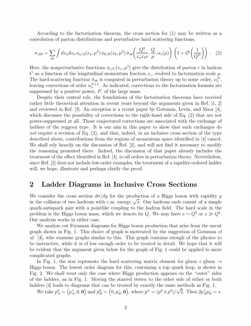
We analyze cut Feynman diagrams for Higgs boson production that arise from the uncutgraph shown in Fig. 1. This choice of graph is motivated by the suggestion of Gotsman et

al. [4], who examine graphs similar to this. This graph contains enough of the physics tobe instructive, while it is of low enough order to be treated in detail. We hope that it willbe evident that the argument given below for the graph of Fig. 1 could be applied to morecomplicated graphs.

In Fig. 1, the star represents the hard scattering matrix element for gluon + gluon →Higgs boson. The lowest order diagram for this, containing a top quark loop, is shown inFig. 2. We shall treat only the case where Higgs production appears on the “outer” sidesof the ladders, as in Fig. 1. Moving the starred vertex to the other side of either or bothladders [4] leads to diagrams that can be treated by exactly the same methods as Fig. 1.

We take pµA =(

p+A, 0, 0)

and pµB =(

0, p−B, 0)

, where p± = (p0±p3)/√2. Then 2p+Ap

−

B = s.

2

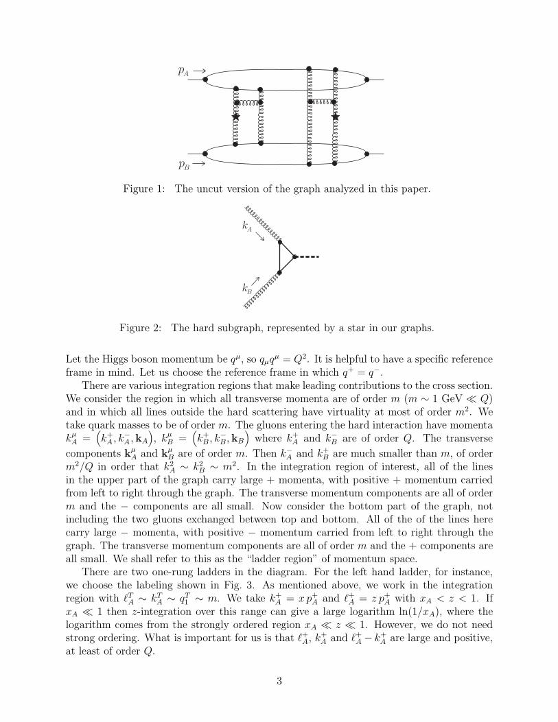
Figure 1: The uncut version of the graph analyzed in this paper.

Figure 2: The hard subgraph, represented by a star in our graphs.

Let the Higgs boson momentum be qµ, so qµqµ = Q2. It is helpful to have a specific reference

frame in mind. Let us choose the reference frame in which q+ = q−.There are various integration regions that make leading contributions to the cross section.

We consider the region in which all transverse momenta are of order m (m ∼ 1 GeV ≪ Q)and in which all lines outside the hard scattering have virtuality at most of order m2. Wetake quark masses to be of order m. The gluons entering the hard interaction have momentakµA =

(

k+

A , k−

A ,kA

)

, kµB =

(

k+

B , k−

B,kB

)

where k+

A and k−

B are of order Q. The transverse

components kµA and k

µB are of order m. Then k−

A and k+

B are much smaller than m, of orderm2/Q in order that k2

A ∼ k2B ∼ m2. In the integration region of interest, all of the lines

in the upper part of the graph carry large + momenta, with positive + momentum carriedfrom left to right through the graph. The transverse momentum components are all of orderm and the − components are all small. Now consider the bottom part of the graph, notincluding the two gluons exchanged between top and bottom. All of the of the lines herecarry large − momenta, with positive − momentum carried from left to right through thegraph. The transverse momentum components are all of order m and the + components areall small. We shall refer to this as the “ladder region” of momentum space.

There are two one-rung ladders in the diagram. For the left hand ladder, for instance,we choose the labeling shown in Fig. 3. As mentioned above, we work in the integrationregion with ℓTA ∼ kT

A ∼ qT1 ∼ m. We take k+

A = x p+A and ℓ+A = z p+A with xA < z < 1. IfxA ≪ 1 then z-integration over this range can give a large logarithm ln(1/xA), where thelogarithm comes from the strongly ordered region xA ≪ z ≪ 1. However, we do not needstrong ordering. What is important for us is that ℓ+A, k

+

A and ℓ+A − k+

A are large and positive,at least of order Q.

3

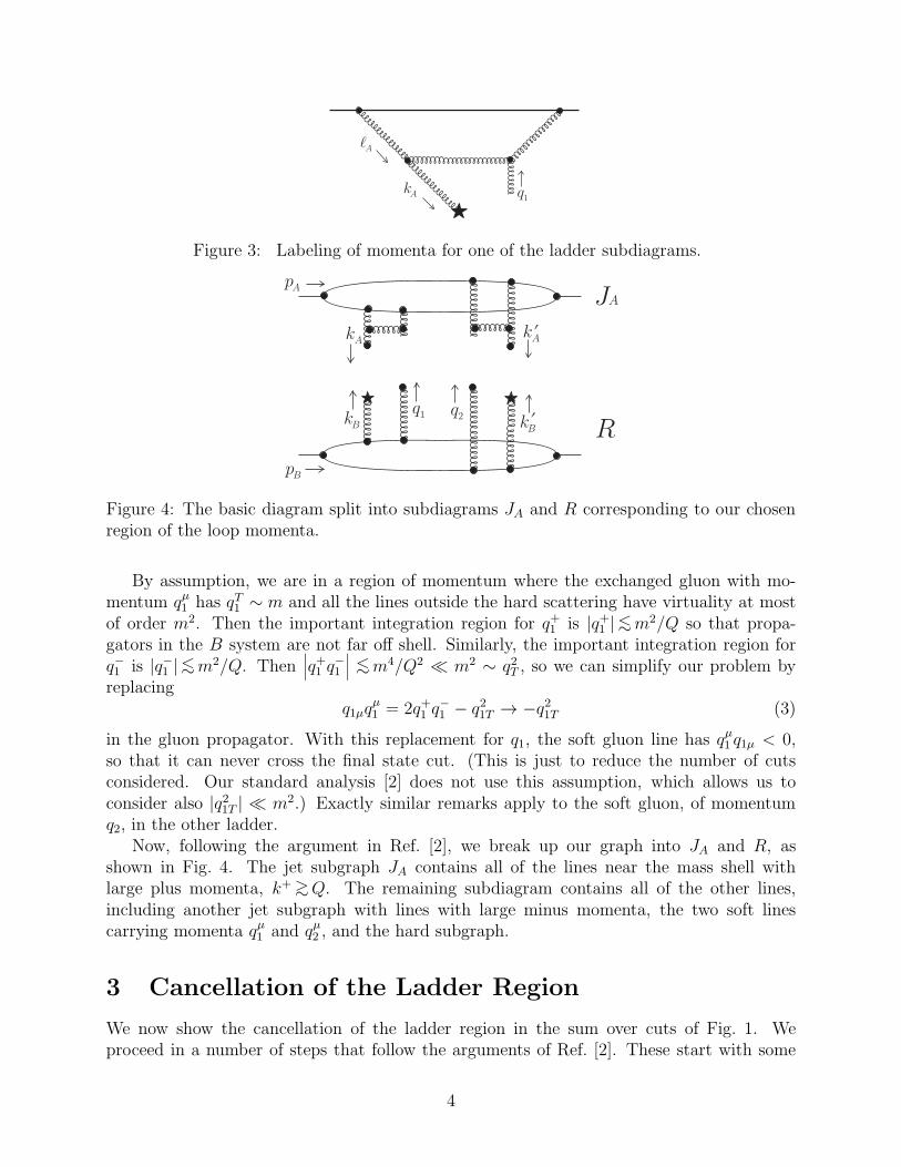
Figure 3: Labeling of momenta for one of the ladder subdiagrams.

Figure 4: The basic diagram split into subdiagrams JA and R corresponding to our chosenregion of the loop momenta.

By assumption, we are in a region of momentum where the exchanged gluon with mo-mentum qµ1 has qT1 ∼ m and all the lines outside the hard scattering have virtuality at mostof order m2. Then the important integration region for q+1 is |q+1 |<∼m2/Q so that propa-gators in the B system are not far off shell. Similarly, the important integration region forq−1 is |q−1 |<∼m2/Q. Then

∣

∣

∣q+1 q−

1

∣

∣

∣

<∼m4/Q2 ≪ m2 ∼ q2T , so we can simplify our problem byreplacing

q1µqµ1 = 2q+1 q

−

1 − q21T → −q21T (3)

in the gluon propagator. With this replacement for q1, the soft gluon line has qµ1 q1µ < 0,so that it can never cross the final state cut. (This is just to reduce the number of cutsconsidered. Our standard analysis [2] does not use this assumption, which allows us toconsider also |q21T | ≪ m2.) Exactly similar remarks apply to the soft gluon, of momentumq2, in the other ladder.

Now, following the argument in Ref. [2], we break up our graph into JA and R, asshown in Fig. 4. The jet subgraph JA contains all of the lines near the mass shell withlarge plus momenta, k+ >∼Q. The remaining subdiagram contains all of the other lines,including another jet subgraph with lines with large minus momenta, the two soft linescarrying momenta qµ1 and qµ2 , and the hard subgraph.

3 Cancellation of the Ladder Region

We now show the cancellation of the ladder region in the sum over cuts of Fig. 1. Weproceed in a number of steps that follow the arguments of Ref. [2]. These start with some

4

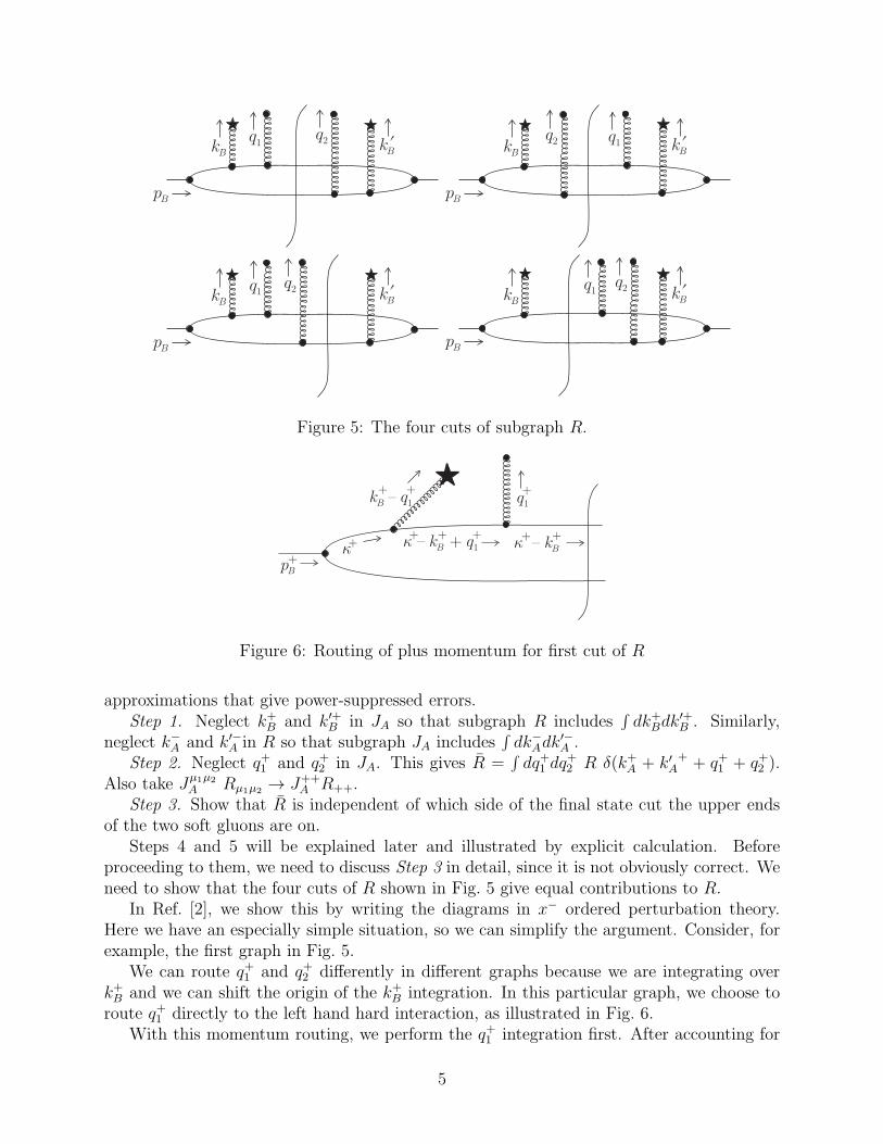
Figure 5: The four cuts of subgraph R.

Figure 6: Routing of plus momentum for first cut of R

approximations that give power-suppressed errors.Step 1. Neglect k+

B and k′+

B in JA so that subgraph R includes∫

dk+

Bdk′+

B . Similarly,neglect k−

A and k′−

A in R so that subgraph JA includes∫

dk−

Adk′−

A .Step 2. Neglect q+1 and q+2 in JA. This gives R̄ =

∫

dq+1 dq+2 R δ(k+

A + k′

A+ + q+1 + q+2 ).

Also take Jµ1µ2

A Rµ1µ2→ J++

A R++.Step 3. Show that R̄ is independent of which side of the final state cut the upper ends

of the two soft gluons are on.Steps 4 and 5 will be explained later and illustrated by explicit calculation. Before

proceeding to them, we need to discuss Step 3 in detail, since it is not obviously correct. Weneed to show that the four cuts of R shown in Fig. 5 give equal contributions to R.

In Ref. [2], we show this by writing the diagrams in x− ordered perturbation theory.Here we have an especially simple situation, so we can simplify the argument. Consider, forexample, the first graph in Fig. 5.

We can route q+1 and q+2 differently in different graphs because we are integrating overk+

B and we can shift the origin of the k+

B integration. In this particular graph, we choose toroute q+1 directly to the left hand hard interaction, as illustrated in Fig. 6.

With this momentum routing, we perform the q+1 integration first. After accounting for

5

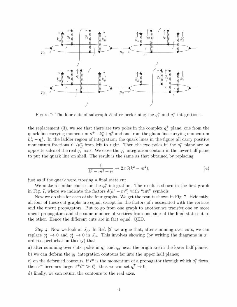
Figure 7: The four cuts of subgraph R after performing the q+1 and q+2 integrations.

the replacement (3), we see that there are two poles in the complex q+1 plane, one from thequark line carrying momentum κ+−k+

B+q+1 and one from the gluon line carrying momentumk+

B − q+1 . In the ladder region of integration, the quark lines in the figure all carry positivemomentum fractions ℓ−/p−B from left to right. Then the two poles in the q+1 plane are onopposite sides of the real q+1 axis. We close the q+1 integration contour in the lower half planeto put the quark line on shell. The result is the same as that obtained by replacing

i

k2 −m2 + iǫ→ 2π δ(k2 −m2), (4)

just as if the quark were crossing a final state cut.We make a similar choice for the q+2 integration. The result is shown in the first graph

in Fig. 7, where we indicate the factors δ(k2 −m2) with “cut” symbols.Now we do this for each of the four graphs. We get the results shown in Fig. 7. Evidently,

all four of these cut graphs are equal, except for the factors of i associated with the verticesand the uncut propagators. But to go from one graph to another we transfer one or moreuncut propagators and the same number of vertices from one side of the final-state cut tothe other. Hence the different cuts are in fact equal. QED.

Step 4. Now we look at JA. In Ref. [2] we argue that, after summing over cuts, we canreplace qT1 → 0 and qT2 → 0 in JA. This involves showing (by writing the diagrams in x−

ordered perturbation theory) that

a) after summing over cuts, poles in q−1 and q−2 near the origin are in the lower half planes;

b) we can deform the q−i integration contours far into the upper half planes;

c) on the deformed contours, if ℓµ is the momentum of a propagator through which qµi flows,then ℓ− becomes large: ℓ+ℓ− ≫ ℓ2T ; thus we can set qTi → 0;

d) finally, we can return the contours to the real axes.

6

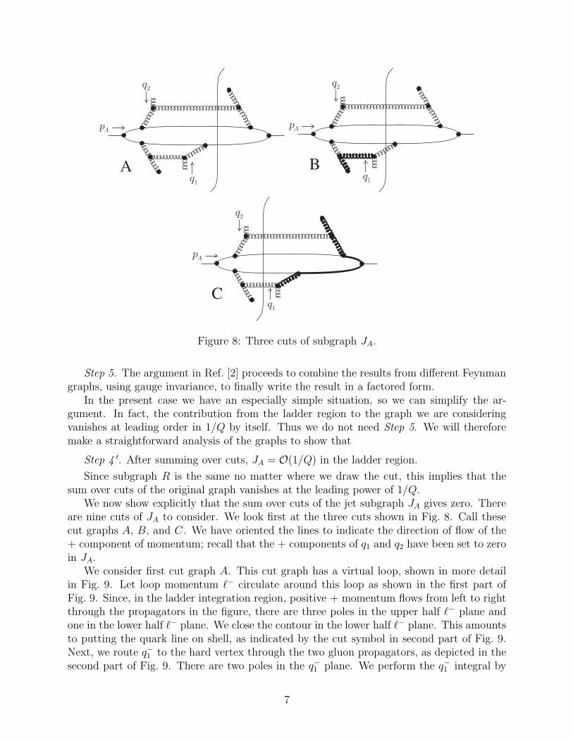
Figure 8: Three cuts of subgraph JA.

Step 5. The argument in Ref. [2] proceeds to combine the results from different Feynmangraphs, using gauge invariance, to finally write the result in a factored form.

In the present case we have an especially simple situation, so we can simplify the ar-gument. In fact, the contribution from the ladder region to the graph we are consideringvanishes at leading order in 1/Q by itself. Thus we do not need Step 5. We will thereforemake a straightforward analysis of the graphs to show that

Step 4 ′. After summing over cuts, JA = O(1/Q) in the ladder region.

Since subgraph R is the same no matter where we draw the cut, this implies that thesum over cuts of the original graph vanishes at the leading power of 1/Q.

We now show explicitly that the sum over cuts of the jet subgraph JA gives zero. Thereare nine cuts of JA to consider. We look first at the three cuts shown in Fig. 8. Call thesecut graphs A, B, and C. We have oriented the lines to indicate the direction of flow of the+ component of momentum; recall that the + components of q1 and q2 have been set to zeroin JA.

We consider first cut graph A. This cut graph has a virtual loop, shown in more detailin Fig. 9. Let loop momentum ℓ− circulate around this loop as shown in the first part ofFig. 9. Since, in the ladder integration region, positive + momentum flows from left to rightthrough the propagators in the figure, there are three poles in the upper half ℓ− plane andone in the lower half ℓ− plane. We close the contour in the lower half ℓ− plane. This amountsto putting the quark line on shell, as indicated by the cut symbol in second part of Fig. 9.Next, we route q−1 to the hard vertex through the two gluon propagators, as depicted in thesecond part of Fig. 9. There are two poles in the q−1 plane. We perform the q−1 integral by

7

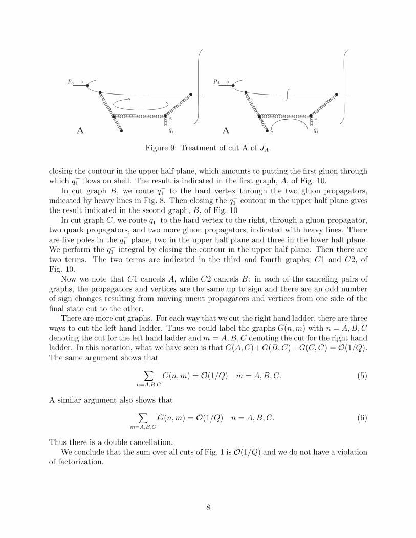
Figure 9: Treatment of cut A of JA.

closing the contour in the upper half plane, which amounts to putting the first gluon throughwhich q−1 flows on shell. The result is indicated in the first graph, A, of Fig. 10.

In cut graph B, we route q−1 to the hard vertex through the two gluon propagators,indicated by heavy lines in Fig. 8. Then closing the q−1 contour in the upper half plane givesthe result indicated in the second graph, B, of Fig. 10

In cut graph C, we route q−1 to the hard vertex to the right, through a gluon propagator,two quark propagators, and two more gluon propagators, indicated with heavy lines. Thereare five poles in the q−1 plane, two in the upper half plane and three in the lower half plane.We perform the q−1 integral by closing the contour in the upper half plane. Then there aretwo terms. The two terms are indicated in the third and fourth graphs, C1 and C2, ofFig. 10.

Now we note that C1 cancels A, while C2 cancels B: in each of the canceling pairs ofgraphs, the propagators and vertices are the same up to sign and there are an odd numberof sign changes resulting from moving uncut propagators and vertices from one side of thefinal state cut to the other.

There are more cut graphs. For each way that we cut the right hand ladder, there are threeways to cut the left hand ladder. Thus we could label the graphs G(n,m) with n = A,B,Cdenoting the cut for the left hand ladder andm = A,B,C denoting the cut for the right handladder. In this notation, what we have seen is that G(A,C)+G(B,C)+G(C,C) = O(1/Q).The same argument shows that

∑

n=A,B,C

G(n,m) = O(1/Q) m = A,B,C. (5)

A similar argument also shows that

∑

m=A,B,C

G(n,m) = O(1/Q) n = A,B,C. (6)

Thus there is a double cancellation.We conclude that the sum over all cuts of Fig. 1 is O(1/Q) and we do not have a violation

of factorization.

8

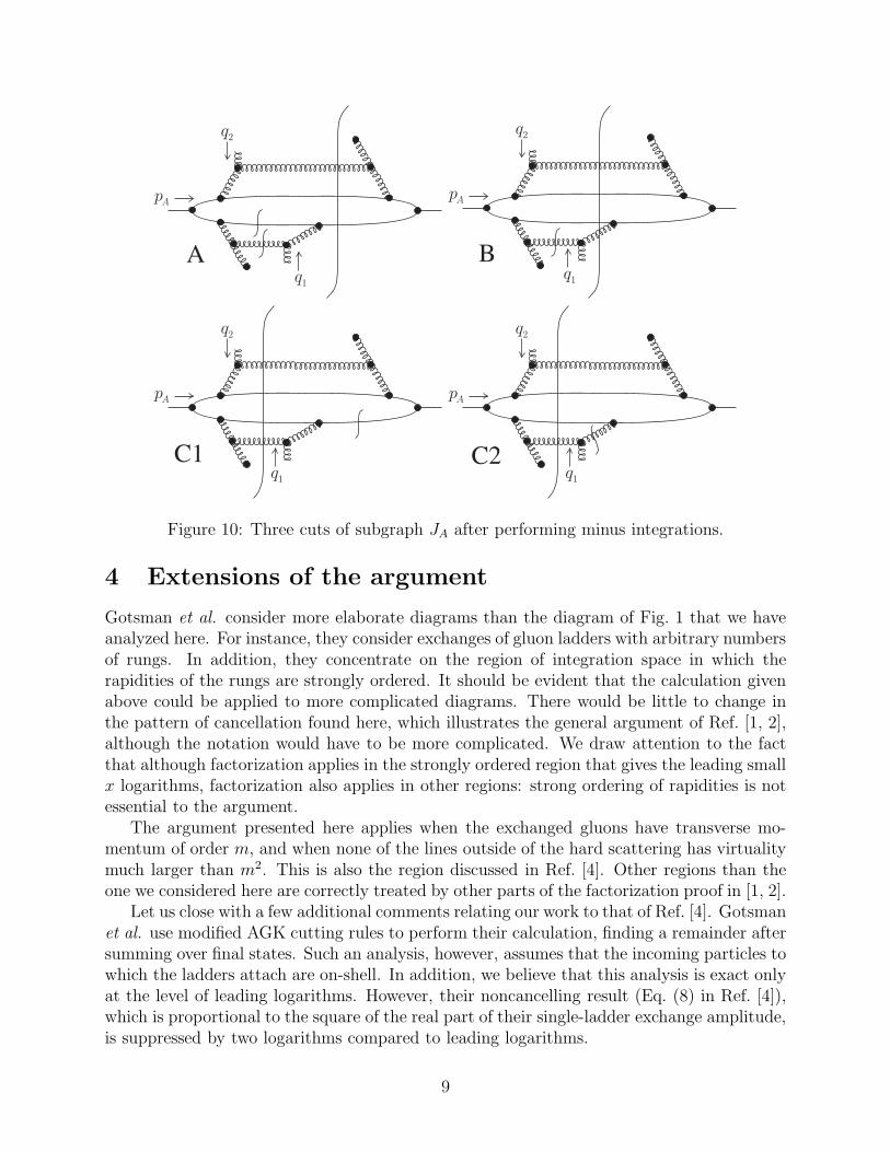
Figure 10: Three cuts of subgraph JA after performing minus integrations.

4 Extensions of the argument

Gotsman et al. consider more elaborate diagrams than the diagram of Fig. 1 that we haveanalyzed here. For instance, they consider exchanges of gluon ladders with arbitrary numbersof rungs. In addition, they concentrate on the region of integration space in which therapidities of the rungs are strongly ordered. It should be evident that the calculation givenabove could be applied to more complicated diagrams. There would be little to change inthe pattern of cancellation found here, which illustrates the general argument of Ref. [1, 2],although the notation would have to be more complicated. We draw attention to the factthat although factorization applies in the strongly ordered region that gives the leading smallx logarithms, factorization also applies in other regions: strong ordering of rapidities is notessential to the argument.

The argument presented here applies when the exchanged gluons have transverse mo-mentum of order m, and when none of the lines outside of the hard scattering has virtualitymuch larger than m2. This is also the region discussed in Ref. [4]. Other regions than theone we considered here are correctly treated by other parts of the factorization proof in [1, 2].

Let us close with a few additional comments relating our work to that of Ref. [4]. Gotsmanet al. use modified AGK cutting rules to perform their calculation, finding a remainder aftersumming over final states. Such an analysis, however, assumes that the incoming particles towhich the ladders attach are on-shell. In addition, we believe that this analysis is exact onlyat the level of leading logarithms. However, their noncancelling result (Eq. (8) in Ref. [4]),which is proportional to the square of the real part of their single-ladder exchange amplitude,is suppressed by two logarithms compared to leading logarithms.

9

We may note two specific differences between our analysis and that of Gotsman et al.,both of which are important beyond the leading logarithmic approximation. First, theyignore certain final-state cuts, for example cut B in Fig. 8. This cut crosses the side of aladder. Such a cut is not allowed in the leading logarithm approximation, but it is presentwhen one goes beyond leading logarithms. Observe that the cut in question would not bekinematically allowed if the gluon ladder coupled to on-shell quark lines instead of internaloff-shell lines. Second, Gotsman et al. appear to have ignored the loop integral that welabel k+

B , which we use to prove that the subgraph R is independent of the final state cutof JA (Step 3). Both the extra cuts and the integral over k+

B are necessary to evaluate theladder region fully. The proof of factorization that we gave in Ref. [1, 2] applies to thefull leading-power contribution and not just to leading logarithms. It is this more generalmethod that we have explained in the context of particular Feynman graphs.

Although we believe that factorization works, we should emphasize our concern thatimprovements are needed in the rigor of existing proofs of factorization [2, 3]. Conspicuouslylacking are iterative algorithms for demonstrating (2) along the lines of those available forproofs of renormalization. Our presentation here is not a step in this direction, rather itis an illustration of already-existing arguments. We believe, however, that it is possible toconstruct such an algorithm (Cf. Ref. [5]). Improvements in the proof would help both toincrease confidence in factorization and to clarify its variant applications, for instance totransverse momentum distributions [6] in the range of QT ≪ M . We therefore welcome themotivation provided by [4] to reopen the discussion of these important issues.

Acknowledgments

We thank the Aspen Center for Physics for its hospitality during the formative stages of thisanalysis. This work was supported by the U. S. Department of Energy grants DE-FG02-90ER-40577 and DE-FG03-96ER40969 and the U. S. National Science Foundation, grantPHY9722101.

References

[1] J.C. Collins, D.E. Soper and G. Sterman, Nucl. Phys. B 261 (1985) 104; G.T. Bodwin,Phys. Rev. D 31 (1985) 2616, E. D 34 (1986) 3932.

[2] J.C. Collins, D.E. Soper and G. Sterman, Nucl. Phys. B 308 (1988) 833.

[3] J.C. Collins, D.E. Soper and G. Sterman, in Perturbative QCD, edited by A. H. Mueller(World Scientific, Singapore, 1989).

[4] E. Gotsman, E. Levin, and U. Maor, Phys. Lett. B 406 (1997) 89, e-Print Archive: hep-ph/9705205; E. Levin, in DIS 97, Proceedings of the 5th International Workshop on

Deep Inelastic Scattering and QCD, edited by J. Repond and D. Krakauer, AIP Conf.Proc. 407, (AIP, New York, 1997), p. 970, e-Print Archive: hep-ph/9705375.

10

[5] J.C. Collins and D.E. Soper, Nucl. Phys. B 193 (1981) 381; F.V. Tkachov, e-PrintArchive: hep-ph/9703432

[6] J.C. Collins, D.E. Soper and G. Sterman, Nucl. Phys. B 250 (1985) 199; G. Altarelli,R.K. Ellis, M. Greco and G. Martinelli, Nucl. Phys. B 246 (1984) 12; C.T.H. Daviesand W.J. Stirling, Nucl. Phys. B 244 (1984) 337 ; C.T.H. Davies, B.R. Webber andW.J. Stirling, Nucl. Phys. B 256 (1985) 413; P.B. Arnold and R.P. Kauffman, Nucl.Phys. B 349 (1991) 381; G.A. Ladinsky and C.P. Yuan, Phys. Rev. D 50 (1994) R4239,e-Print Archive: hep-ph/9311341.

11