Applying Value at Risk (VaR) analysis to Brent Blend Oil prices

Applying Value at Risk (VaR) analysis to Brent

Blend Oil prices

Ali Khadar

2011

Publikationstyp, magisternivå, 15 hp

Företagsekonomi

Examensarbete

Friståendekurs

Handledare: Markku Penttinen

Examinator: Stig Sörling

i

ACKNOWLEDGEMENT

I would like to express my gratitude to all who have contributed with their professional and

personal support to the success of my Master Thesis

I would like to express my gratitude and appreciation to my supervisor Markku Penttinen for

his valuable suggestions improving the quality of the study and encouragement throughout the

thesis writing.

Sincerely,

ii

ABSTRACT

TITLE: Applying Value at Risk (VaR) analysis to Brent Blend Oil

prices

LEVEL: Master Degree in Business Administration 15 hp

AUTHOR: Khadar Ali (840320-6330)

SUPERVISOR: Markku Penttinen

BACKGROUND: Risk management has during the years experienced innovative

development for financial institutions. The concept of Value at Risk (VaR) was derived from

the financial crisis during the period of 1990s. VaR is a risk management system used for

managing market risk. VaR is widely implement by the financial institutions such as banks,

asset managers, nonfinancial corporations and regulators and has become very important as

risk management tool.

AIM: The aim with this paper is to study Brent Blend Oil prices using four models to VaR.

The studied VaR models are Historical Simulation (HS), Simple Moving Average (SMA) and

Exponentially Weighted Moving Average (EWMA) and Exponentially Weighted Historical

Simulation (EWHS). In order to study the accuracy with the models they are applied to one

underlying asset, which is the Brent Blend Oil. The estimations of the VaR models are based

on two important assumptions namely student t-distribution and normal distribution.

Specifically, the models are studied in terms of accuracy which is determined by the

frequency of exceptions concerning a given window size and corresponding confidence level.

METHOD: The quantitative method is conducted for this study. Specifically, the daily prices

of Brent Blend Oil are gathered for period 2002 – 2009. The data is collected from Energy

Information Administration (EIA) and is used for estimation of the selected VaR models.

RESULTS & ANALYSIS: The results of this study show that the EWHS model is most

accurate based on the two distributions. The EWHS produces good results in window size of

250 and 750 and is accepted by Kupiec Test at all confidence levels. The HS seem to be

indifferent whether the returns of the underlying asset are normal distributed or student t-

distributed. Even if the EWHS and HS models produce good results under the two

distributions the SMA model is most accurate under student t-distribution but only at larger

window sizes (750 and 1000-days). Both SMA and EWMA represent the variance covariance

models and perform better under student t-distribution compared with the assumption of

normality. The main conclusions made from this study are that the accuracy of the HS seems

not be effected by the two distributions. The accuracy of SMA and EWMA according to this

iii

study is depending on how well the underlying assets return fits the distribution of normality.

We can see that the characteristics of the underlying asset have great impact on both SMA

and EWMA. In this case, the Brent Blend Oils return seems to deviate from normality and

that is probably why the SMA and EWMA are less accurate under the assumption of normal

distribution compare to the assumption of student t-distribution. Following recommendations

should be considered; before selection of distribution function is made the characteristics of

the underlying asset should be studied, which will further simplify the choice of VaR models.

SUGGESTIONS FOR FUTURE STUDIES: For further studies following suggestions

should be considered, other advance models should be applied such as GARCH (Generalized

Autoregressive Conditional Heteroskedasticity), Monte Carlo Simulation, and ARCH

(Autoregressive Conditional Heteroskedasticity). Additionally, other financial assets should

be used, other distribution functions (mixed distribution or chi-square distribution) should be

applied and other validation models (Christoffersen Test and Mixed Kupiec Test) should be

implemented.

KEYWORDS: Value at Risk, Historical Simulation, Simple Moving Average, Exponentially

Weighted Moving Average, Exponentially Weighted Historical Simulation, Normal

distribution, Student t-distribution, returns characteristics, Basel Committee Penalty Zones.

iv

GLOSSARY OF MAIN TERMS

Value at Risk (VaR): Is the maximum expected loss over a given horizon period at a given level of

confidence.

Normal distribution: The Gaussian probability distribution.

Student t-distribution: A probability distribution that has a fatter tails than normal distribution.

Confidence level: The confidence level is used to indicate the reliability of an estimate.

Kupiec Test: Is a statistical test for model validation based on failure rates.

Kurtosis: Describes the degree of flatness of a distribution.

Skewness: Describes departures from symmetry.

Risk: The dispersion of unexpected outcomes owing to movements in financial variables.

Basel Committee: Is an international organ for banking supervision by providing standards,

guidelines and recommendations to financial institution around the world

(http://www.bis.org/publ/bcbs17.htm).

v

TABLE OF CONTENTS

Applying Value at Risk (VaR) analysis to Brent Blend Oil prices .........................................................1

ABSTRACT ..........................................................................................................................................ii

GLOSSARY OF MAIN TERMS .............................................................................................................. iv

1. INTRODUCTION ..............................................................................................................................1

1.1 CHOICE OF SUBJECT ..................................................................................................................1

1.2 PROBLEM BACKGROUND ...........................................................................................................1

1.3 PURPOSE ...................................................................................................................................5

1.4 DELIMITATIONS .........................................................................................................................6

1.5 DISPOSITION .............................................................................................................................7

2. THEORETICAL FRAMEWORK ...........................................................................................................8

2.1 RISK AND RISK MANAGEMENT ..................................................................................................8

2.2 VALUE AT RISK...........................................................................................................................9

2.2.1 VARIANCE COVARIANCE - VaR .............................................................................................. 10

2.2.2 HISTORICAL BASED - VaR ...................................................................................................... 11

2.2.3 EXPONENTIALLY BASED -VaR ................................................................................................ 13

2.2.4 DRAWBACKS - VaR ............................................................................................................... 13

2.2.5 CHOICE OF CONFIDENCE LEVEL ............................................................................................ 14

2.2.6 NORMAL DISTRIBUTION - VaR .............................................................................................. 15

2.2.7 STUDENT t-DISTRIBUTION – VaR ........................................................................................... 17

2.3 VaR MODELS ........................................................................................................................... 18

2.3.1 HISTORICAL SIMULATION ..................................................................................................... 19

2.3.2 SIMPLE MOVING AVERAGE ................................................................................................... 20

2.3.3 EXPONENTIALLY WEIGHTED MOVING AVERAGE ................................................................... 21

2.3.4 EXPONENTIALLY WEIGHTED HISTORICAL SIMULATION ......................................................... 22

2.4 DESCRIPTION OF SELECTED UNDERLYING ASSET ...................................................................... 23

file:///K:/Introduction%201.8.13.2.doc%23_Toc303969303

vi

2.5 PREVIOUS RESEARCH............................................................................................................... 24

2.6 MODEL VALIDATION ................................................................................................................ 25

2.6.1 KUPIEC BACKTEST ................................................................................................................. 26

2.6.2 THE BASEL COMMITTEE ........................................................................................................ 28

3. METHOD ....................................................................................................................................... 30

3.1 PRECONCEPTIONS ................................................................................................................... 30

3.1.1 SCIENTIFIC APPROACH .......................................................................................................... 30

3.1.2 PERSPECTIVE ........................................................................................................................ 31

3.1.3 LITERATURE SEARCH............................................................................................................. 31

3.1.4 QUANTITATIVE APPROACH ................................................................................................... 32

3.1.5 DEDUCTIVE APPROACH ........................................................................................................ 32

3.2 HOW TO COMPUTE/VaR ......................................................................................................... 33

3.2.1 HISTORICAL SIMULATION ..................................................................................................... 33

3.2.2 SIMPLE MOVING AVERAGE ................................................................................................... 35

3.2.3 EXPONENTIALLY WEIGHTED MOVING AVERAGE ................................................................... 36

3.2.4 EXPONENTIALLY WEIGHTED HISTORICAL SIMULATION ......................................................... 36

3.3 DESCRIPTIVE DATA .................................................................................................................. 37

3.3.1 AVERAGE RETURN ................................................................................................................ 37

3.3.2 VOLATILITY ........................................................................................................................... 38

3.3.3 SKEWNESS ............................................................................................................................ 38

3.3.4 KURTOSIS ............................................................................................................................. 39

3.4 KUPIEC BACKTEST .................................................................................................................... 39

3.5 BASEL VALIDATION .................................................................................................................. 40

4. RESULTS & ANALYSIS .................................................................................................................... 42

4.1 NORMAL DISTRIBUTION - VaR ................................................................................................. 42

4.2 STUDENT t-DISTRIBUTION - VaR .............................................................................................. 47

5. CONCLUSIONS .............................................................................................................................. 55

vii

6. RELIABILITY & VALIDITY ................................................................................................................ 58

7. RECOMMENDATION ..................................................................................................................... 59

REFERENCES ..................................................................................................................................... 60

LITERARY SOURCES ....................................................................................................................... 60

INTERNET SOURCES .......................................................................................................................... 62

viii

LIST OF FIGURES & TABLES

Page nr

Figure 1: Sweden´s oil import 2004-2009 4

Figure 2: VaR for normal distribution estimated with 95 % confidence level 16

Figure 3: Oil price movements from 1960-2006 24

Figure 4: The volatility rate during the period: 2002-2009 38

Figure 5: A distribution with both positive and negative skewness 39

Figure 6: Illustration of normal distribution curve using histogram 40

Table 1: The relationship between standard deviation, probability and confidence level 15

Table 2: Decision errors (Jorion, 2007, p. 146) 28

Table 3: Forecasting HS by using Brent Blend Oil´s daily prices 34

Table 4: Valuation of observations based on decay factor ( ) 37

Table 5: Summary statistics for the Brent Blend Oil: 2002-2009 38

Table 6: Non rejection region according to Kupiec Test 41

Table 7: The Basel Penalty Zones (Jorion, 2007, p. 150) 42

Table 8: Result from HS, SMA, EWMA and EWHS under normal distribution 46-48

Table 9: Result from HS, SMA, EWMA and EWHS under student t- distribution 50-52

Table 10: Results from Basel Committee Penalty Zones and Kupiec Test (normal) 53

Table 11: Results from Basel Committee Penalty Zones and Kupiec Test (student t-

distribution) 54

CHAPTER 1: INTRODUCTION

1

1. INTRODUCTION

The aim of this chapter is to clarify the choice of subject. Afterwards the reader will be leaded

to the problem background and the purpose with the study. In this chapter, a presentation is

given about the study’s delimitation and disposition.

1.1 CHOICE OF SUBJECT

In these days the concept of risk seems to be something impossible to manage when the

financial markets around world fluctuates. On the other hand, everyone recognizes the

significance of managing risk in order to avoid financial losses. Especially, the financial

institutions that are trading with Crude Oil contract using futures or other derivatives

instruments as underlying variable. From the recent financial crisis many successful financial

institutions has collapsed such as Lehman Brothers, Bernard L. Madoff Investment Securities

and American Home Mortgage. Therefore, the significance of risk management has grown

specially the concept of Value at Risk (VaR) and the way risk measures particularly the

market risk which further simplified the choice of subject. Risk management comprises

various qualified models which are designed to minimize particular risk exposure. The most

advanced risk management system has to be VaR because of its versatility and of its

simplicity which attracts many financial institutions to implement in their risk management

system.

1.2 PROBLEM BACKGROUND

Risk management has during the last years experienced revolutionary development for

financial institutions and for the academic world of finance. The amount of theory shows

indication of the broadness and the significance of the subject where in many places is

regarded as an own field in the theory of finance. Though the year’s new models or new ways

of measuring risk has been developed regarding to condition of the financial markets in order

to reduce risk exposure. Many times, old models were refined and transformed into more

simplified practical estimations. The Black- Scholes option pricing model is good example.

The Black-Scholes model was difficult to grasp when one wants to use for pricing options,

therefore simplification of the model was required. The model has developed in to the extent

that professionals use in their daily business. During 1970s and 1980s the world was facing

instability in financial markets concerning some significant background factors such as

exchange rate, interest rate and stock market volatility (Dowd, 1998, p. 4-6).


2

The collapse of the exchange rate system during 1971 (Bretton Woods system) results in that

many countries went from fixed exchange rate to floating exchange rate with the intention of

saving the value of the currency. Nevertheless, the transformation influenced flexibility on the

exchange rate market since supply and demand determined the exchange rate movements.

Since that, the floating exchange market was characterized with high volatility. Additionally,

the interest rate has been high during 1970s and 1990s largely as a result of monetary inflation

caused by implemented policies. The losses from interest fluctuations are valued to more than

1.5 trillion dollar invested specially in bonds and different fixed-income securities. The stock

market was not exceptional concerning the high volatility caused by partly inflation and partly

uncertainty in the market (Dowd, 1998, p.4-6).

Furthermore, we can mention “The Black Monday” during 1987 where many of the world´s

stock exchanges fell dramatically and in accordance to Jorion (2007) the losses were

evaluated to enormous figures ($ 1 trillion) (Jorion, 2007, p. 4). Another contributing factor

behind further development of risk management can be explained with the oil crisis during

1973. The oil prices around the world rose extremely causing high inflation and increased

interest rate as a consequence. Jorion (2007) emphasizes the significance of having access to

effective risk management system in order to reduce the exposure to above described risks

(Jorion, 2007, p. 4-5). In the beginning of 1990s a new financial market called derivatives

started rapidly to grow offering new opportunities of derivative contracts. There are different

definitions of what derivatives is but Dowd (1998) describe as “Derivatives are contracts

whose or pay –offs depend on those of other assets” (Dowd, 1998, p.7). The traded assets in

the derivatives market are swaps (different types of interest rate swap, currency swap, and

equity swap); different types of futures (interest rate futures, commodity future) various types

of options (Asian options, credit options, American and European currency options and

others). The derivatives contracts could be traded globally which also increases the risk

exposure for these financial institutions (Dowd, 1998, p.7-8).

In a broad sense, the concept of Value at Risk (VaR) is derived from the financial crisis in

early 1990s for measurement of market risk. VaR as a risk management system is widely used

and has become more significant as a risk management tool. To minimize risk exposure the

financial institutions have to implement VaR in their systems and they have to report VaR at

daily basis (Jorion, 2007). Being the most adopted risk management model many authors and

researcher give their definitions of VaR. Jorion (2007) define VaR as “VaR is the worst loss

over a target horizon such that there is a low, prespecified probability that the actual loss will

be larger” (Jorion, 2007, p. 106). Additionally, Dowd (1998) explain VaR as “the value at

risk (VaR) is the maximum expected loss over a given horizon period at a given level of

confidence” (Dowd, 1998, p. 39). Both definitions are similar concerning two important

variables such as time horizon and the level of confidence. Notice, VaR is implemented as

volatility forecast and nothing more. Using VaR, the forecasts are summarized in a single

number which facilitates the interpreting of VaR figures. Corresponding to selected

confidence level VaR estimates losses due to movements in the market. The probability that

estimated VaR exceeds is very small and only happens with a specified probability which


3

depends on the assumption used in the computation. Once one understands the statistical

thinking behind VaR, the model become forthright and easy to implement (Dowd, 1998, p.

20).

On the other hand, VaR is umbrella term for a group risk management models. Every VaR

model has its own attractions and limitations which confirms the various numbers of ways to

compute VaR. Generally, VaR as risk management tool can be applied to any asset that has a

measurable return. Furthermore, different financial institutions use different VaR models

which mean different values of VaR. A high value of VaR infers the idea of having enough

capital to manage potential losses. The riskier the assets are, the higher the VaR and greater

the capital requirement (Dowd, 1998, p.21).

Selecting the right model is not easy. Most institutions use more than one model in their daily

business reporting institutions daily VaRs. How well the VaR-models perform has to do with

the underlying assets characteristics and the assumption that the models are applied to.

Different assets have different characteristics such as volatility (standard deviation), kurtosis

and skewness. The computed VaR depends on the values of these factors. The volatility factor

shows the risk of an asset measured as standard deviation of the return (Hull, 2009, p.282).

“The higher the risk of an investment, the higher the expected return demanded by an

investor” (Hull, 2009, p.119). The application of VaR gives the firms a great advantage to

determine which market is characterized with higher returns at lowest rate of risk (Beder,

1995, p.12). Both kurtosis and skewness are factors which only show how the return of an

asset deviates from a known distribution function. Before computing VaR one must make

some assumptions of the assets return. It could be that the assets return follows a known

distribution which can be the normal distribution, student t-distribution or other known

distribution functions. In general, all VaR-models are categorized into three main blocks,

Variance Covariance based models, and Historical based models and Monte Carlo simulating

based model (Butler, 1999, p.50). Additionally, this leads us to the problem that this study is

trying to solve, the connection between the accuracy of the VaR-models under a given

assumption, window size and level of confidence and the characteristics of the underlying

assets return and how they affect computed VaR.

In this paper, four different models to VaR are studied which represent Variance covariance

based and historically based and exponentially based. The models will be applied to two

important distributions such as the student t- distribution and normal distribution. The biggest

disparity between the two distributions is the shape of the tails. According to Dowd (1998) the

student t-distribution has fatter tails compared with the normal distribution (Dowd, 1998,

p.44). The selected models are Historical Simulation (historical based), Simple Moving

Average (variance covariance based), Exponentially Weighted Moving Average

(exponentially based) and Exponentially Weighted Historical Simulation (exponentially

based). The motives for selecting these models are that they have different attractions and

limitations.


4

To compare the precision of these models they have to be applied to an underlying asset. In

this study, Brent Blend Oil (crude oil) is used as the empirical evidence. In 2005 Sweden

exported 11.0 million m3 petroleum, for that approximately 12.1 million m

3 crude oil were

required. The export of petroleum products are priced higher than the import of crude oil

therefore a boost to the balance of trade (in Sweden) is gained. In 2006, the export of

petroleum products was estimated to 64.4 billion SEK compared to 2005 were the import of

crude oil was valued to 56.4 billion SEK1. Sweden´s import of oil from 2004 to 2009 is

shown in figure 1:

Figure 1: Sweden´s oil import 2004 - 2009

Svenska Petroleum Institutet (SPI)

Using the mentioned distribution functions (student t-distribution and normal distribution)

concerning the return of the underlying asset three levels of confidence will be applied. The

selected confidence levels are 95 %, 99 % and 99, 9 %. Mostly, the financial institutions

implement different levels of confidence but in accordance with Hendricks (1996) the 95 % to

99 % are the most commonly used.

To validate the models applied on a given distribution function, confidence level and window

size the Kupiec Test and The Basel Committee Penalty zones are used to ensure whether the

models predict market risk reasonably well.

The failure rates are measured in terms of the amount of exceptions or the number of VaR

breaks the models produce. Or corresponding to selected confidence level, how many times

exceeds the computed VaR.

1http://www.konj.se/download/18.70c52033121865b13988000119456/Petroleumprodukter+%E2%80%93+en

+viktig+exportvara+med+mindre+betydelse+den+svenska+ekonomin19.pdf


5

Which of the VaR models are most accurate under a given assumption, confidence

level and window size?

The majority of the VaR-models are based on variance covariance techniques assuming

normality of the return. Despite that, it’s widely believed that financial time series is

characterized by fatter tails. The shape of the tails is determined mainly by the number of

extreme values observed in the past. Inferring that, many times the VaR-models applied on

normality assumption underestimate the mass in the tails of the distribution. Therefore, the

selected VaR-models are studied under two different distribution functions namely student t-

distribution and normal distribution.

How do the two assumptions about the assets returns affect the accuracy of the VaR-

models?

1.3 PURPOSE

The purpose with this study is to compare four different models to VaR in terms of accuracy,

namely Historical Simulation (HS), Simple Moving Average (SMA), Exponentially Weighted

Moving Average (EWMA) and Exponentially Weighted Historical Simulation (EWHS).

These VaR models will be applied to one underlying asset which is the Brent Blend Oil using

these confidence levels 95 %, 99 % and 99, 9 %. Concerning the return of the asset the

models under two different assumptions namely student t-distribution and normal distribution

will be studied.

The selected VaR models will be applied in different window sizes namely 250, 500, 750 and

1000 days.

Lastly, the accuracy of the models will be evaluated by Kuipec Test and Basel Committee

penalty zones.


6

1.4 DELIMITATIONS

VaR is used by the majority of financial institutions for managing market risk. Here,

Historical Simulation (HS), Exponentially Weighted Moving Average (EWMA), Simple

Moving Average (SMA) and Exponentially Weighted Historical Simulation (EWHS) are

investigated.

Selecting these models infers excluding other VaR models such as GARCH (Generalized

Autoregressive Conditional Heteroskedasticity) model, Monte Carlo Simulation model and

ARCH (Autoregressive Conditional Heteroskedasticity) model. VaR as a risk management

tool can be applied to any asset that has a measurable return.

In this study, the VaR models will be concerned only Brent Blend Oil. Other distribution

functions are excluded besides the selected distributions, normal distribution and student t-

distribution. Kupiec Test and Basel Committee penalty zones are used for evaluation of the

VaR models, therefore other back testing models are not concerned such as Christoffersen

Backtest, Mixed Kupiec test, Backtesting Based on Loss Function and Backtests on Multiple

VaR Levels.


7

1.5 DISPOSITION

Chapter 1: Turns to give the reader an introduction to the chosen subject. The chapter

describes the problem background and the purpose of the study. Afterwards a presentation is

given about the study´s delimitations.

Chapter 2: Turns to give a presentation of the theories that this study is based on. It´s shown

how VaR can be estimated using a variance covariance based model, historical based model

and exponentially based model. A presentation is given about the chosen VaR models and the

assumptions they are based on. In this chapter, the underlying asset is presented and

discussed what previous studies have said about subject. This chapter turns to give the

verification of VaR models using Kupiec Test and Basel Committee penalty zones. The

chapter describes briefly risk and risk management.

Chapter 3: The methods used in the study are presented in this chapter. First, description

about the nature of the study is given; second the computations of the VaR models are

explained.

Chapter 4: Turns to present the results and analysis from the VaR models. The VaR models

will be analyzed separately concerning the assumptions they are based on.

Chapter 5: The conclusions from the VaR models are presented in this chapter. Here, the

questions stated in the problem background are discussed.

Chapter 6: The truth criteria of the study are described in this chapter, reliability and validity.

Chapter 7: Turns to give a suggestion to further studies.

CHAPTER 2: THEORETICAL FRAMEWORK

8

2. THEORETICAL FRAMEWORK

In this chapter, some theories that are relevant for the implementation of this study are

presented. The beginning of this chapter provides a general description of risk and risk

management. It follows by a broader introduction to the concept of VaR. Further, VaR will

be illustrated numerically by showing how it can be computed. A presentation of the VaR

models and what previous studies have said about the subject is also given in this chapter.

Lastly, the validation models are introduced which are Kupiec Test and Basel Committee

Penalty Zones.

2.1 RISK AND RISK MANAGEMENT

Both measuring and defining risk constitute a central role in the world of finance. Some risks

we accept and the others we choose to avoid. By monitoring risk exposure the financial

institutions can create a better position concerning competitive with other companies (Jorion,

2007, p. 3). Jorion (2007) define risk as “the dispersion of unexpected outcomes owing to

movements in financial variables” (Jorion, 2007, p. 75).

According to Jorion (2007) the financial-market risk contains four different types of risks,

interest-rate risk, exchange-rate risk, equity risk and commodity risk. These risks are

depending on some underlying risk factors such as interest rate, stock price, equity price and

commodity price (Jorion, 2007, p. 76). Jorion (2007) emphasize the reason why risk

management becomes more fundamental for the financial institutions is mostly driven by the

desire of monitoring these underlying risk factors (Jorion, 2007, p. 76).

In the early 1990s the financial world was experiencing new growing financial market such as

the derivative market. The derivative market was traded widely and intensification in the

number of contract led many times that the market was exposed to risks. Dubofsky & Miller

(2003, p. 3)) define derivative as “A derivative is a financial contract whose value is derived

from or depends on, the price of some underlying asset”. The contracts traded in derivative

are divided in four classes; forwards, futures, swaps and options. On the face of it, there are

two types of derivatives contracts namely options and forwards, this because forwards, futures

and swaps are very similar types of contract. Under that time, older risk management models

were not enough and the needs for new risk management models became more vital. It

became more obvious that the older risk management models were associated with problems

concerning the way they capturing market risk. Therefore, different group’s published

different reports regarding managing the market risk on derivative market. According to

Dowd (1998) some of the groups behind a report published in July 1993 “Group of Thirty,

New York – based consultative group of leading bankers, financiers and academics. This


9

report was followed by a report by US General Accounting Office in May 1994, a joint report

issued by the Bank for the International Settlement, International Organization of Securities in

July 1994 and many other reports by the Derivatives Policy Group, International Swaps and

Derivatives Association, Moody´s, Standard and Poor´s and other interested parties” (Dowd.

1998, p. 16). These reports recommended one thing, the need to better understand the risks

that the financial markets are exposed to and the way these risks should be managed. Another

dimension to the issue is the expansion of the financial markets globally which provides the

financial institutions enormous possibilities to invest, produce and to sell their products in

other countries than their native country.

2.2 VALUE AT RISK

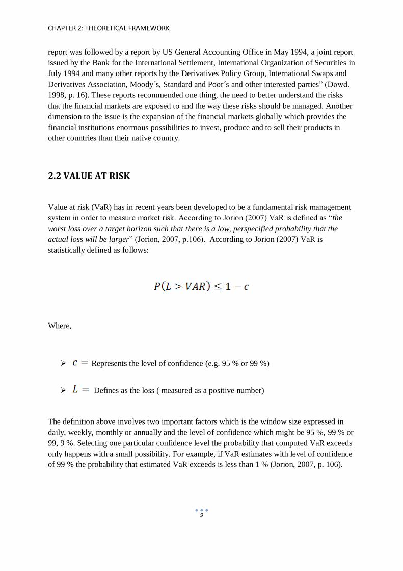
Value at risk (VaR) has in recent years been developed to be a fundamental risk management

system in order to measure market risk. According to Jorion (2007) VaR is defined as “the

worst loss over a target horizon such that there is a low, perspecified probability that the

actual loss will be larger” (Jorion, 2007, p.106). According to Jorion (2007) VaR is

statistically defined as follows:

Where,

Represents the level of confidence (e.g. 95 % or 99 %)

Defines as the loss ( measured as a positive number)

The definition above involves two important factors which is the window size expressed in

daily, weekly, monthly or annually and the level of confidence which might be 95 %, 99 % or

99, 9 %. Selecting one particular confidence level the probability that computed VaR exceeds

only happens with a small possibility. For example, if VaR estimates with level of confidence

of 99 % the probability that estimated VaR exceeds is less than 1 % (Jorion, 2007, p. 106).


10

2.2.1 VARIANCE COVARIANCE - VaR

The estimation of VaR can be simplified considerably if some assumptions are made about

how the underlying assets returns are distributed. The underlying assets returns can either fit

the distribution of normality which has a smaller tails or the student t-distributed categorize

with fatter tails. Assuming that the distribution belongs to variance covariance based models,

such as the normal distribution one assumes automatically the studied assets return follows

these assumptions. Practically, you might find out that the return deviates from these

assumptions. The VaR computation can be determined directly from the underlying assets

returns. The parameters one needs to estimate VaR is the standard deviation using a

multiplicative factor that depends on the selected confidence level. The variance covariance

based models are depending on above described parameters. In contrast, other historical or

exponentially based models estimate VaR by selecting a quintile from the distribution

function of the return (Jorion, 2007, p. 109).

The estimations of VaR are a process which includes three pillars. First, one has to make

some assumption about the density function f(R), it can be that the density function f(R) is

normal distributed, student t- distributed or follows other probability distribution. The

distribution function will simplify for us finding the cut off return to estimate VaR. In

general, the underlying assets return is assumed to have a density function f(R) which fits

normal distribution. According to Dowd (1998) the assumption of normality makes the

estimation of VaR less complicated (Dowd, 1998, p. 42).

A normal distributed variable has parameters with mean μ and standard deviation σ. The

confidence level c of a normal distributed variable is described with alpha α. Alpha defines

where the cut of values of the distribution are relative to the mean μ. Suppose we select a

confidence level of 95 %, finding the cut off value so that the probability of a return less than

is given by the probability density function (Dowd, 1998, p. 42):

(2.2.1.2)

In order to find the cut value we can transform the distribution function R into a standard

normal distribution. A standard normal distributed variable has a mean of 0 and standard

deviation of 1 therefore the density function becomes (Dowd, 1998, p.42):

(2.2.1.3)


11

The idea behind this transformation is to simplify for us the determination of cut off value of

( from the standard normal tables. From the standard normal tables we can read

that 95 % confidence level is equal to – 1.645. Consequently ( equals -1.645

(Dowd, 1998, p. 43).

(2.2.1.4)

Concerning equation (2.2.1.4) the R* stands for the cut off value, μ for mean return, (-1.645)

defines alpha (α) corresponding to level of confidence (e.g. – 1.645 for a 95 % confidence

level) and W represents the initial investment (Dowd, 1998, p. 43). We can transform these

equations to implied VaR:

(2.2.1.5)

(2.2.1.6)

Having these equations we can observe that the absolute VaR depends on the parameters

mean μ, standard deviation σ and the parameter α. In contrast, the relative VaR only depends

on standard deviation σ of the return and the parameter α. Absolute VaR and relative VaR

represent two different ways to estimate VaR. According to Dowd (1998) the relative VaR is

easier to estimate using variance covariance model to VaR, because estimating of the

parameter μ is not necessary. Using the relative VaR the variables needed are the standard

deviation of the return and the confidence level (Dowd, 1998, p.43). Dowd (1998) further

argue by emphasizing the fairly small differences between absolute and relative VaR

especially when dealing with shorter window sizes (Dowd, 1998, p. 43).

2.2.2 HISTORICAL BASED - VaR

The historical based VaR is a method which makes no assumption about the probability

distribution of returns. Computing VaR based on the value of portfolio which is defined as

and the level of return as R. The computation of VaR depends on selected window size often

assumed as fixed. Reaching the end of the window size the final value of the portfolio is


12

expressed as . The portfolios volatility measured as standard deviation and

the mean return are also defined as μ and σ. In addition, VaR quantifies the potential worst

loss at a specified confidence level and window size. As mentioned above (see variance

covariance based VaR) the two existing types of VaR are relative and absolute. Jorion (2007)

define the relative VaR as “as dollar loss relative to the mean on the horizon” and absolute

VaR as “the dollar loss relative to zero or without reference to the expected value” (Jorion,

2007, p. 108).

(2.2.2.1)

(2.2.2.2)

Both Jorion (2007) and Dowd (1998) emphasize when the window size is short the difference

between the relative and absolute VaR will be fairly small anyway. This because the average

returns are small and mostly assumes to be zero. According to Jorion (2007) the relative VaR

prefers more theoretically defining risk as deviation from the mean. The definition of relative

VAR seems to be more straightforward concerning how risk is viewed compared to absolute

VaR (Jorion, 2007, p. 108). In general, the estimates of VaR can be extracted from a known

distribution representing the underlying assets future value f (w) defining when value is

exceeded corresponding to a given confidence level c and window size (Jorion, 2007, p.109).

(2.2.2.3)

Extracting values smaller than , is equal to 1-c which give us following

equation,

(2.2.2.4)

According to equation (2.2.2.4) the integral from to is equal to .

represents the quantile of the probability distribution, or in other words the critical value in


13

tails of the distribution. Any values greater than are viewed as extreme inferring VaR

breaks. Using historical based VaR model the computation of standard deviation is not

necessary since the percentile of the distribution is used. Notice, the historical based VaR can

be applied to any distribution, discrete or continuous, fat or thin tailed. For instance, ignoring

how the underlying assets return is shaped, normal or not, and assume that we have a

distribution consists of 100 observation with purpose of finding daily VaR applying a

confidence level of 95 %. The computed VaR estimate is locate 5 worst loss of the

distribution (Jorion, 2007, p. 108-110).

2.2.3 EXPONENTIALLY BASED -VaR

The exponentially based VaR compared to both variance covariance and historical based

models and goes one step further concerning how observations are viewed. The exponentially

based VaR is built on an assumption which says that the recent observation or recent

occurrence affects most the forecast of future volatility (Butler, 1999, p. 199). Therefore, it’s

significant to value the observations according to their occurrence. To solve the problem the

exponentially based VaR uses a decay factor (λ) which is constant between 0 and 1 (Hull,

2009, p. 479).

2.2.4 DRAWBACKS - VaR

As highlighted before, VaR is adopted by many financial institutions to minimize the

exposure of financial market risk. VaR is not problem free even though the model is broadly

implemented and used by various institutions. By knowing its limitations the implementers

must have taken that into consideration when monitoring VaR. According to Dowd (1998) the

implementers must have the right knowledge when computing VaR in order to avoid

underestimation or overestimation of market risk (Dowd, 1998, p. 22). In general, three

typical limitations stand out. First, the majority of all VaR models are historical based

focusing on backward in time. VaR uses available historical data to forecast future outcome.

Notice, VaR estimates are only forecasts and can deviate from reality outcomes. However, it

is of great significant not to reject VaR as a model but it’s important to have awareness about

the limitations with the model (Dowd, 1998, p. 22).

Second, all (also HS)VaR models are based on some type of assumptions about how a

specific reality is designed. The assumptions may not reflect that specific reality in any given

circumstances which can affect the results. Some assumptions are often made of how the

underlying assets return is distributed (Dowd, 1998, p. 22). Third, VaR models are only

statistical tools which are not reliable in all circumstances. Importantly, the people who are


14

responsible for computing VaR should have the knowledge of how to use, how to interpret the

results and surely how to implement the models. VaR contains various models, therefore in

hand of experienced implementers even a weak VaR models can still be useful. In contrary, in

the hand of inexperienced implementers a relatively strong VaR model can produce poor

results which lead to serious problems. It’s essential that knowledgeable people work with the

computation of VaR (Dowd, 1998, p. 23).

2.2.5 CHOICE OF CONFIDENCE LEVEL

To compute VaR one has to select a confidence level. Different institutions use different

confidence levels. There is no reason to favor one confidence level to another. According to

Dowd (1998)” the choice of confidence level depends on the purpose at hand”. As

highlighted by Dowd, the motive for selecting a particular confidence level could be to

determine internal capital requirement, validate VaR systems, to report VaR or to further

study and compare among different financial institutions. Institutions should not select a high

confidence level concerning validation systems. Because, with higher confidence levels the

amount of exceptions are very rare and requires larger window sizes and a lot of historical

data in order to excess losses to give reliable results. Institutions should therefore use a low

confidence level for internal model validation (Dowd, 1998, p. 52).

The relationship between the level of capital requirement and selected confidence level

depends on how risk averse institutions are. The more risk averse, the more important they

have access to enough capital to cover risk. To determine the level of capital requirement

financial institutions should use a high confidence level to obtain high capital level when

adopting VaR (Dowd, 1998, p. 52).

As far as comparison is concerned, different confidence levels are used by various institutions

for computing their daily VaRs. For instance, one institution may use 99 percent confidence

level reporting their daily VaRs; another may select 95 percent confidence level, another 99.9

percent and so on. The question is whether we can compare these institutions VaRs? Surely, a

comparison between the institutions VaRs are possible but under specified condition. In order

to translate across different VaRs we have to assume e.g. normality concerning the

distribution of the underlying assets returns. Thereafter, we can compare the institutions daily

VaRs by translating one particular confidence level to another. Notice, without the

assumption of normality, or something similar the translating of VaRs is not possible and

gives us very little information about institutions VaRs (Dowd, 1988, p.52-53). Assuming

normality the relationship between selected confidence level, probability and standard

deviation is as follows:


15

Table 1: The relationship between standard deviation, probability and confidence level

Number of standard deviations -1.645 -2.326 -3.030

Confidence Level 95.00 % 99.00 % 99.90 %

Probabilities 5 % 1 % 0.01 %

Assuming normality we are interested in to identify the number of standard deviations and

observation is below the mean. In accordance with Table 1 selecting a confidence level of 5

percent, observing an observation at this probability is -1.645 standard deviations below the

mean (Butler, 1999, p. 11).

2.2.6 NORMAL DISTRIBUTION - VaR

All most every VaR-model is based on some assumptions that affect estimation of VaR. The

assumption concerns the underlying assets return, either the return is assumed to be normal or

not. The assumption of normality simplifies computation of VaR because normality as a

distribution has a lot of informative parameters. The normal distribution in statistics plays a

central role and is one of the important distributions (Anderson, et al., 2002, p. 218).

Assuming the normality of the assets return, VaR is illustrated graphically in Figure 2.

Figure 2: VaR for normal distribution estimated with 95 % confidence level


16

Figure 2 illustrates VaR for 95 % confidence level when assuming independence of normally

distributed returns and a mean return of zero it can easily be shown that: (Van den Goorbegh

& Vlaar, 1999, p. 10-11):

The distributional return of the underlying asset is assumed to be independent identically

distributed:

Furthermore, this leads us to the complete formula of VaR:

(2.2.6.1)

where,

Initial investment of the portfolio

The cumulative distribution function of the standard normal distribution

Represents the mean return

Standard deviation of the assets return

The normal distribution is described by its two first moments, the mean (μ) and variance

(variability), that is N (μ, ). The first parameter tells us the place where the average return is

found and the variance represents the variation of the return around the mean. According to


17

Jorion (2007) the normal distribution has the probability density function (Jorion, 2007, p.

85):

(2.2.6.2)

where,

= Represents the exponential of y

= The mean return

= Represents the variance (shows the variation of the risk factor)

The normal distribution is characterized also by two other moments, skewness and kurtosis.

The first parameter describes deviation from symmetry. A normal distributed population

should have a skewness of zero which indicates a perfect symmetry. There are two types of

skewness, negative and positive skewness (see Figure 5). Negative skewness describes when

the distribution has a long left tail compared to positive skewness where the majority of

observations are on the right tail. The other higher moment is kurtoses which describes the

shape of the tails in a distribution. A perfect normal distribution should have a value of

kurtosis of three. Larger values than 3 indicate a deviation from normality and a concentration

of observations mostly extremes values in the tails (Jorion, 2007, p. 84-87).

2.2.7 STUDENT t-DISTRIBUTION – VaR

An alternative distribution function to normal distribution is the student t- distribution.

Student t-distribution is useful when the distribution of the sample deviates from normality.

The student t- distribution is characterized by fatter tails concerning the distribution of the

sample inferring that more extreme observations can be captured and included in the

estimations (Dowd, 1998, p. 44). According to Van den Goorbergh & Vlaar (1999) the

mentioned phenomenon is called leptokurtosis and the student t-distribution can manage that

(Van den Goorbergh & Vlaar, 1999, p.12). Characterized by fatter tails (see Figure 6), the

confidence level of t- VaR is higher compare to normal VaR. The student t- distribution

provides an easy way of capturing the variations of an assets return. Further, the student t-


18

distribution is easy to understand and to apply for estimation of VaR. Same as normal VaR

the t-VaRs properties are well defined and its value can easily be found in standard tables.

The student t- distribution is described by some known parameters such as μ (location), the

scale γ > 0 and v > 0 is the degrees of freedom. When the value of degrees of freedom (v)

increases the student t-distribution becomes closer to the normal distribution (Jorion, 2007, p.

87-88). However, when the value of n is small the student t-distribution indicates fatter tails.

In order to estimate VaR based on t-distribution one has to determine the degrees of freedom.

The selected degrees of freedom are based on empirically observed kurtosis. Knowing the

value of degrees of freedom and the value of alpha based on t-distribution , we can

then compute VaR under probability function of t-distribution (Van den Goorbergh & Vlaar,

1999, p. 13):

(2.2.7.1)

where,

= The cumulative distribution function of a standardized t distributed random variable

= The initial value of the portfolio

On the face of it, the student t- distribution seems to be problem free but some issue should be

considered. One clear disadvantage with student t-distribution is for its inability to consider

the significance of asymmetry of the underlying assets return (Chu-Hsiung & Shan-Shan,

2006). The VaR estimates are often higher with student t-distribution which increases the

level of capital requirements. The higher the confidence level, the higher the VaR estimates

and the higher is the capital requirements (Dowd, 1998, p.52).

2.3 VaR MODELS

The implemented VaR models will be presented below. The models have their own

attractions and limitations which affects the result in this study. Furthermore, the models are

based on two different assumptions which deal with the characteristics of the underlying

assets return in various ways namely student t- distribution and normal distribution.


19

2.3.1 HISTORICAL SIMULATION

The Historical Simulation (HS) is historical based model that does not depend whether the

underlying assets return is distributed after some specific distribution. HS is widely used

because of its simplicity and its ability to produce relatively good results. HS needs enormous

historical data in order to simulate assets VaR. The idea behind HS is to use historical data to

forecast what might happen in the future ( Hull, 2009, p. 454).

To Estimate VaR based on HS one has to first gather the underlying asset returns over the

observed period. The gathered return is then used to simulate the assets VaR. The gathered

return should be good proxy for future return. Before estimating VaR based on HS the assets

returns must be computed. As soon as computations are completed HS is estimates by

selecting a quantile from the historical distribution of the returns. “The relevant percentile

from the distribution of historical returns then leads us to the expected VaR for our current

portfolio “(Dowd, 1998, p. 99). According to Van den Goorbergh & Vlaar (1999, p. 20) HS is

estimated as follows:

(2.3.1.1)

where,

= VaR at time t + 1

= Initial value of the asset

= Represents the return at time t; p represents the percentile2 of historical return.

The attractions with this model are according to Dowd (1998) and Jorion (2007) its simplicity.

It’s of great significant for those who are responsible for the risk management since the data

that are needed easily is available from public sources. Furthermore, HS is not depending on

2 The percentile (also called quantile) is defined as cutoff values p such as that the area to their right (or left)

represents a given probability (Jorion, 2007, p. 89).


20

any assumption concerning distribution on return, whether the return follows a known

distribution or not such as the normal distribution or the student t-distribution or any other

particular distribution. HS deals with another major issue which is the independences of the

risk factor over time. The variance covariance models have issue with distributions

characterized with fatter tails. HS seems to perform better when a lot of observations are

further out in the distribution. Both theory and previous studies confirm that HS perform well

on higher confidence levels. HS has a tendency to catch more extreme returns and produces

unbiased VaR estimates with higher confidence levels (Dowd, 1998, p.101).

Jorion (2007) mean that the limitation with HS is that the model needs enormous data to

perform well at higher confidence levels (Jorion, 2007, p. 264-265). And the fact that

historical data seems to be representative for future price development. Van den Goorbergh &

Vlaar (1999) emphasize the impossibilities of simulating VaR with a number of historical

values that’s less than correspondent confidence level. This mean if one wants to estimate HS

with 99, 9 percent confidence level the number observations needed is 1(1-0,999) = 1000

(Van den Goorbergh & Vlaar, 1999, p. 22).

2.3.2 SIMPLE MOVING AVERAGE

Simple Moving Average (SMA) is a variance covariance based model which infers that

assumption of normality is made about the assets return. The standard deviation from the

underlying assets return represents the risk which needs in order to estimate VaR and further

to study the probability that certain outcomes occur in the future.

SMA is widely implemented at technical analysis of time series and is built on the idea of

measuring the moving average standard deviation of the asset. According to Jorion (2007, p.

222) a typical moving average window is 20 and 60 trading days. Here, are measured SMA,

EWMA, HS, and EWHS with 250, 500, 750 and 1000 moving average window to estimate

VaR and to compare the four selected VaR-models under same conditions.

Observing the underlying assets return over M days, the moving average volatility is

modeled with following formula:

(2.3.2.1)


21

where,

= The variance of the assets return at the time t (shows the variation of the risk factor)

= Represent the number of observations

= Represent the assets return in square at time t-i

To estimate the volatility with SMA the return of the underlying asset is used. Each day, the

estimation is moving one day forward by adding new information simultaneously as old

information is dropping out. SMA are widely used and this because of its simplicity.

The model is simple to implement and to estimate. A major drawback with SMA is that the

model gives all the observations same weights according to theirs occurrence. Old

observations get same relevance or value as recent observations. The length of window size

has even an effect on the performance of the model. According to Jorion (2007) shorter period

of window size has higher volatility than longer period of window size, this because SMA is

measuring moving- average of volatility (Jorion, 2007, p. 223).

2.3.3 EXPONENTIALLY WEIGHTED MOVING AVERAGE

The Exponentially Weighted Moving Average (EWMA) is a VaR model that takes pragmatic

model to estimating market risk. The variances estimated with Exponentially Weighted

Moving Average (EWMA) are used in order to estimate the assets VaR. However, the recent

modeled variance is a weighted average of the past variances. In order to value the

observations EWMA is using a weight parameter called decay factor for recent variance

and (1- for the variance of the previous observation (Jorion, 2007, p. 230). The variances

are modeled with following formula (Dowd, 1998, p. 95):

(2.3.3.1)

This volatility formula (approximately) is only valid when the number of observations is

large.


22

where,

= Defines the variance for time t

= A parameter called decay factor

= Represent the assets return in square at time t

One of the main attractions with EWMA is the dynamic ordering of the observations. The

decay factor (λ) is between 0 and 1. The model gives the recent observations the highest

weight ( = 0. 94 or = 0.97) and the past information less weight ( = 0. 06 or = 0.03)

(Jorion, 2007, p. 230).

2.3.4 EXPONENTIALLY WEIGHTED HISTORICAL SIMULATION

The Exponentially Weighted Historical Simulation (EWHS) is built on same assumptions as

HS. The only disparity between the two models is how the observations are valued. HS values

the observations equally whether they are old or not, but the EWHS consider observations

after their own occurrence. Inferring that the recent observations attributes most value when

estimating VaR. EWHS deals with another issue namely the distributional returns further in

the tails which have great impact on the performance of VaR model (Boudoukh, et al., 1998,

p. 10). EWHS is first estimated with following equation (Van den Goorbergh & Vlaar, 1999,

p. 22):

(2.3.4.1)

where,

= VaR at time t + 1

= Initial value of the asset


23

= Represents the return at time t; p represents the percentile3 of historical returns

Moreover, the EWHS attributes a decay factor for valuing observations same as EWMA. The

decay factor is a constant between 0 and 1.

2.4 DESCRIPTION OF SELECTED UNDERLYING ASSET

To assess the performance of the VaR models they have to be applied on an underlying asset.

The underlying asset the estimations are based on is Brent Blend Oil. Being the most used and

widely traded commodities the Brent Blend Oil is characterized by higher volatility

specifically in recent years. More than 60 percent of the world oil is using Crude oil as

reference for pricing their commodity (Eydeland & Wolyniec, 2003, p.2). The majority of oil

export countries are political instable which affects the oil price markets. Furthermore, price

movements are determined by two significant economic concepts, demand and supply.

Globally, the most oil is produced by OPEC (Organization of the Petroleum Exporting

Countries) countries and by controlling the production OPEC countries can truly affect the

world price (Cabedo & Moya, 2003, p. 240). Mostly, VaR is applied on other financial assets

such as stocks and financial instruments inferring the lack of application of VaR for Crude

Oil. Some of these studies are done by following authors (Cabedo & Moya, 2003 and Giot &

Laurent 2003). Comparing to other financial assets the Crude Oil has more explaining factors

concerning the characteristics of the asset. The supply and demand is not the only significant

factor when analyzing the VaR estimates. Factors such as government policies, wars, and

natural disasters are important to consider for deeper understanding. In this study, the above

highlighted factors are ignored. Implementations of VaR models are desirable for financial

institutions point of view in order to manage commodity risk (Jorion, 2007, p. 8). The

development of Oil prices through the years are shown in Figure 3.

3 The percentile (also called quantile) is defined as cutoff values p such as that the area to their right (or left)

represents a given probability (Jorion, 2007, p. 89).


24

Figure 3: Oil price movements from 1960-2006 (Jorion, 2007, p.8)

2.5 PREVIOUS RESEARCH

It exists several earlier studies on the subject. Most of them aim to develop new ways to

estimate VaR in order to facilitate the understanding behind the estimations of VaR. Due to

the fact that there are different ways to estimate VaR, the obvious question is, which model

estimates VaR best? The choice of the model should fulfill the purpose at hand and further

emphasize the disparity between the models in terms of the way they capture market risk and

the way they are implemented (Linsmeier & Pearson, 1996, p. 16).

Giot &Laurent (2002) applied four VaR models to Brent crude oil to assess the performance

of the models. The models were categorized into two blocks namely symmetric models (Risk

metrics and student APARCH (Asymmetric Power Autoregressive Conditional

Heteroskedasticity ) and asymmetric models (Skew student APARCH and skew student

ARCH ( Autoregressive Conditional Heteroskedasticity). The conclusions made by Giot &

Laurent (2002) ensure that the skew student APARCH was most accurate under applied

conditions. Additionally, the skew student ARCH seems to produce good results compared to

symmetric models.

Cabedo & Moya (2003) assessed in their study three VaR models such as the Historical

Simulation standard approach, Historical Simulation with ARMA (Autoregressive Moving

Average) and Variance Covariance model based on Autoregressive Conditional

Heteroskedasticity (ARCH) models forecasts. The models were applied on Brent oil prices

from period 1992- 1999. The results show that the Historical Simulation with ARMA is better

than the other studied VaR models. As highlighted by Cabedo & Moya (2003) the Historical


25

Simulation with ARMA shows a more flexible VaR quantification, which better fits the

continuous price movements.

The majority of the VaR models are based on some assumptions concerning the returns of the

underlying asset. Hendricks (1996) studied three models to VaR namely Simple Moving

Average model, Exponentially Weighted Moving Average model and Historical Simulation

model. He could not find a conclusive answer to which of the models performs best. Instead,

Hendricks state as he writes in his conclusions “Almost all cases the models cover the risk

that they are intended to cover” (Hendricks, 1996, p. 55). Another conclusion made by him

(1996) is that conducted models perform best at lower confidence levels (Hendricks, 1996, p.

56).

Van den Goorbergh & Vlaar (1999) studied three models to VaR namely Variance models,

Historical Simulation model and GARCH (Generalized Autoregressive Conditional

Heteroskedastic) model under assumptions of normal distribution, student t-distribution and

mixed distribution. The models were then applied on Amsterdam Stock Exchange (AEX)

which consists of a 25 Dutch stocks in different weights. The GARCH model and the

assumption of mixed distribution are not concerned in this study. Van den Goorbergh &

Vlaar (1999) affirm that the performances of the variance models based on normal

distribution are poor at higher confidence levels. The variance models based on normal

distribution produces too many failure rates (Van den Goorbergh & Vlaar, 1999, p. 11).

This infers simply that the variance based models underestimate the mass in the tails of the

distribution. The Variance based models show indication of to perform best at lower

confidence levels. The Variance based models applied on student t-distribution seems to

outperform the normal fit. The student t-distribution captures the mass far out in the tails and

includes more extreme observations in the estimations. Van den Goorbergh & Vlaar (1999)

studied the HS model under different window sizes 250, 500, 1000 and 3038 days. In their

study, the HS model seems to be more accurate for higher confidence levels but only for a

window size of 250 days and the maximum window size 3038 (Van den Goorbergh & Vlaar,

1999, p. 22). The accuracy of HS depends on the choice of the window size. The VaR

estimations based on HS is sustained constant longer for larger window sizes, while more

observations is rejected relatively fast under smaller window sizes ( Van den Goorbergh &

Vlaar, 1999, p. 24). Boudoukh et al. (1998) has in their study combined the traditional HS and

exponentially EWHS approach which the combined hybrid approach was applied on different

underlying assets. The underlying assets characteristic such as skewness, kurtosis and

volatility seem to have a great impact of traditional HS.

2.6 MODEL VALIDATION

Various VaR models were discussed in the previous chapter. The drawbacks and

shortcomings of these VaR models were highlighted and the concept of VaR in general. The


26

question is if selected VaR models forecast market risk accurately well. For that reason, VaR

models are only applicable when they seem to capture market risk. Therefore, to evaluate the

models some back testing models are used. Apparently, back testing models reveal possible

incorrectness of the VaR models (Haas, 2001, p.1). The applied models are Kupiec Test and

Basel Committee Penalty Zones. Kupiec Test compares the asset actual returns with historical

forecast return. For instance, if VaR is estimated with confidence level of 95 percent, an

exception of 5 percent is accepted to occur (5 percent * the number of observations =

expected failure rate). The Basel Committee evaluates the models with green, yellow and red

zones concerning how accurate the models are based on a specified distribution, window size

and confidence level.

2.6.1 KUPIEC BACKTEST

”Back testing is a formal statistical framework that consists of verifying that actual losses are

in line with projected losses“(Jorion, 2007, p. 139).

Corresponding to selected confidence level the Kupiec Test examines whether the frequency

of exceptions is within fixed interval over some specified time. According to Jorion (2007)

this type of model validation is called for unconditional coverage. The unconditional coverage

ignores when exceptions occur focusing only on the frequency of the exceptions (Jorion,

2007, p. 151).

The unconditional coverage represents the type of back test that strongly evaluate the number

of occurrences when the underlying assets daily losses exceeds VaR forecast. On the other

hand, if the numbers of occurrences are less than corresponding confidence levels it indicates

that VaR models overestimates risk. However, too many occurrences also indicate

underestimation of market risk. The probability that a particular VaR- model produces exact

number of occurrences corresponding to chosen confidence level is very rare. The statistical

procedure so called unconditional coverage will evaluate the accuracy of the VaR models and

if the number of occurrences is reasonable or not (accepted or rejected). Defining the total

number of observations as T and the number of occurrences as x, then the total number of

failure rate is defined as x/T. In theory, the failure rate would reflect the corresponding

confidence level. For example, selecting a confidence level of 95 percent, the frequency of tail

losses is equal according to theory to p = (1- c) = 1- 0.95 = 5 percent. According to Jorion

(2007) the distribution of occurrences follows a binomial probability distribution and

estimated with this formula (Jorion, 2007, p. 143):

(2.6.1.1)


27

With larger window sizes, the binomial distribution function are difficult to use therefore

following normal distribution formula is preferred as an approximation:

(2.6.1.2)

where,

= The expected number of exceptions

= The variance of exceptions

Concerning the frequency of the exceptions they should be spread over time corresponding to

selected intervals both in confidence level c and window size. This infers that recent

exceptions are not directly related with previous exceptions; otherwise the exceptions seem to

be auto correlated. In order to avoid volatility clustering” the right” window size has to be

selected “It must be large enough, in order to make statistical inference significant, and it

must not be too large, to avoid the risk of taking observations outside of the current volatility

cluster” (Manganelli & Engle, 2001, p. 10). The conditional coverage covers observations

occurrences due to fact that it takes account of conditioning or variation over time (Jorion,

2007, p. 151). Specifically, one validation model used for testing conditional coverage is the

Christoffersen Test. The Christoffersen Test divides the test in three steps, test for

unconditional coverage, test for independence and test of coverage and independence

(Christoffersen, 1998, pp. 844- 847). The Christoffersen Test is not concerned and is excluded

from this study. By using this back-testing model one can examine the accuracy of the VaR-

models. An alternative validation technique is use historical profit and loss which can be

compared to the daily changes of the assets return (Kupiec, 1995, p. 81). The VaR-models

will either be accepted or rejected. There are two types of errors one can make while back-

testing the models (see Table 2).


28

Table 2: Decision errors (Jorion, 2007, p. 146)

Model

Decision Correct Incorrect

Accept Ok Type 2 error

Reject Type 1 error Ok

Type 1error: Represents the possibility of rejecting a correct model

Type 2 error: The possibility of accepting an incorrect model.

To minimize both types of errors one would use powerful statistical test (Jorion, 2007, p.144-

147).

2.6.2 THE BASEL COMMITTEE

The Basel Committee is responsible for supervision of the financial institutions concerning

requirement of capital4. Financial institutions implement their own risk management tool for

minimization of risk expose. The Basel Committee found it necessary to require the financial

institutions to use similar risk management system in order to identify the particular risk

expose and to transform the computed risk value between the institutions. In addition, the

financial institutions seem to be responsible for potential damages corresponding to

irresponsibility of managing risk (Butler, 1999, p.28).

Generally, financial institutions apply more than one VaR model for managing market risk.

The models are used to analyze a particular risk exposure using some confidence levels c

under specified time horizon (Basel Committee on Banking Supervision, 1995, p. 9).

Therefore, the requirement from these institutions are to report the institutions daily VaRs.

According to Butler (1999, p. 31) VaR helps the Basel Committee to develop a risk

management system reducing the financial institutions to collapse. The Basel Committee

regulations are described by two accords, Basel I and Basel II accord. The Basel I ensure the

risk of minimum of capital that’s required from the institutions globally. According to Basel I

4 http://www.bis.org/publ/bcbs17.htm


29

the financial institution should have enough capital to cover only credit risk (Jorion, 2007, p.

53-60).

The Basel II takes one step further by implementing these three following pillars, minimum

regulatory requirements (requirement of capital not only covering credit risk but also market

risk and operational risk), supervisory review (define the expanding role for institutions

concerning implementing the second pillar) and market discipline (concerns the need for

sharing information about the particular institutions risk exposure) (Jorion, 2007, p. 58).

CHAPTER 3: METHOD

30

3. METHOD

The methods used in this study are presented here. First, description about the nature of the

study is given; second the computations of the VaR models are described.

3.1 PRECONCEPTIONS

Mostly, in process of writing it’s significant to highlight the author’s way of thinking

concerning the motive behind his or hers choice. Since, the credibility and reliability of the

thesis can be questioned reflecting whether the researcher is not value free or objective.

Unavoidably, the one who is writing the thesis has his or hers own values and experiences and

is not value free as science researcher. However, according to Bryman (2008, p. 24) we would

expect the researchers to be objective by not letting his or hers values to affect the way the

researcher interpret his or her findings.

Being the author of this thesis I have received the fundamental knowledge of financial

theories during the period that I studied Finance at the Master´s as well as Bachelor level.

The study is conducted in a way that the models used are relying heavily on value free,

objective and hard evidence. This study is based on the quantitative method which refers to

systematic empirical research on the particular case studied.

3.1.1 SCIENTIFIC APPROACH

There is strong relationship between the choice of scientific methods and particular problem

studied. The choice of methods depends strongly on the assumptions made about the nature of

society and the nature of science. This study applies positivistic methods which advocate that

the accuracy of the VaR models must be tested empirically.

In this study positivism show clear evidence of how some selected variable from a population

is related to one another. Bryman (2008) describes positivism as “positivism is an

epistemological position that advocates the application of the methods of the nature sciences

to the study of social reality and beyond” (Bryman, A. 2008, p. 13). The gathered data will be

quantified and therefore the analysis and conclusions made by the results is depending on the

used theoretical knowledge and methods.

An alternative scientific approach to positivism is interpretivism. Interpretivism as an

epistemological position assumes to find deeper understanding and subjective way of thinking

about social action. According to Bryman (2008) interpretivism “It is predicated upon the

CHAPTER 3: METHOD

31

view that a strategy is required that respects the differences between people and the objects of

the natural sciences and therefore requires the social scientist to grasp the subjective

meaning of social action”. On the face of it, this will determine the type of data that needs to

be gathered. In this study, public sources such as market prices are used. These facts are not

based on individual and subjective interpretations (Bryman, A. 2008, p. 15-17).

3.1.2 PERSPECTIVE

As a reader it’s important to understand in which perspective this particular problem has been

studied, because the same problem can be studied from different perspectives. The purpose of

this study is to examine four models to VaR and the way they capture the market risk based

on two different assumptions which are normal distribution and student t – distribution.

Therefore, the models are applied on one underlying asset which is Brent Blend Oil. VaR is

daily used by various institutions such as regulators, nonfinancial corporations and asset

managers dealing with larger trading portfolios. Even if these institutions have the same

purpose of why applying VaR as risk management in their daily businesses, they have still

different perspective of applying it. Therefore, the VaR models are studied from the financial

institutions perspective managing the commodity risk in order to minimize financial losses.

3.1.3 LITERATURE SEARCH

In order to search relevant literature for this study databases are mainly found at the Umea

University library. These databases include Business Source Premier, Emerald Full text,

Blackwell Synergy, JSTOR and Elsevier Science Direct. Moreover, Google Scholar has been

used in order to find relevant scientific articles. These databases provide articles which are

peer reviewed. Searching in these databases keywords and key phrases such as Value at Risk

(VaR), Risk management, Historical Simulation (HS), Simple Moving Average (SMA),

Exponentially Weighted Moving Average (EWMA) and Exponentially Weighted Historical

Simulation (EWHS), normal Distribution, student t- distribution have been applied.

Additionally, when a relevant article is found the index is used for searching after other

relevant articles.

CHAPTER 3: METHOD

32

3.1.4 QUANTITATIVE APPROACH

How a researcher collects, uses and analyzes empirical data can be defined with two different

models, the quantitative and the qualitative approach. In general, the both models have the

same purpose, which is to provide a better understanding on the particular cases studied.

Many authors give their explanation of the differences between the models. Walliman (2005)

explain the differences by “they differ not only in the nature of the data sought and the

subsequent methods of data analysis, but also in their psychological rationale” (Walliman,

2005, p. 246).

The quantitative approach is widely used in social sciences and refers to the systematic

empirical research of social entities and their relationship. The quantitative approach focuses

on to quantify numerical data (Bryman, A. 2008, p. 140). The qualitative approach according

to Bryman (2008) is concerned with words rather than numbers and aim to provide a deeper

understanding on the particular subject studied (Bryman, A. 2008, p. 366).

In order to be able to answer the problem statement and the purpose with study, which is to

examine whether VaR models measures the risk exposure correctly, I as researcher must

manage the empirical material in objective way so that the study become more valid. The

estimations of the models are based upon a lot of historical data. Daily price changes for Brent

Blend Oil are studied in order to examine the accuracy of the models. It simplifies the choice

of applying a quantitative approach. In accordance with Arbnor & Bjekner (1994) a

researcher can study more variables and cover a larger number of observations with a

quantitative approach compared to a qualitative approach. Even if the quantitative approach is

widely used, the approach is associated with some limitations. The approach sees often

numbers as the only truth and has a tendency to easily misjudge the results (Holme &

Solvang, 1991, p. 150).

3.1.5 DEDUCTIVE APPROACH

In order to ensure the accuracy of selected four VaR models based on some specific

assumptions, a researcher can go in two different ways. One is deductive approach, where in

accordance with Bryman (2008) the researcher on the basis of what is known about in

particular domain and of theoretical considerations in relation to that domain deduces a

hypothesis that must then be subjected to empirical scrutiny (Bryman, A. 2008, p. 9). An

alternative method is the inductive approach, where the researcher starts with empirical study

and from the outcome makes theoretical conclusions (Bryman, A. 2008, p. 11).

The aim with this study is not to develop new models to VaR or new ways to estimate VaR.

But the purpose is to determine which of the chosen models to VaR are most accurate. Based

on these discussions the approach that fits this research most is the deductive approach.

CHAPTER 3: METHOD

33

3.2 HOW TO COMPUTE/VaR

The purpose with this study is to compare four different models to VaR in terms of accuracy

based on two important assumptions namely student t- distribution and normal distribution.

The models are Historical Simulation model (HS), Simple Moving model (SMA),

Exponentially Weighted Moving Average model (EWMA) and Exponentially Weighted

Historical Simulation (EWHS).

These models are used for estimation of market risk. As theory claims all VaR models have

their own attractions and limitations which will affect their performances. Therefore, it´s

crucial to select the right VaR model for the right purpose. For instance, selecting wrong

model can lead to overestimation or underestimation of market risk. According to Basel

Committee regulations the financial institutions must evaluate the applied VaR models in

order to avoid misjudgments of market risk (Jorion, 2007, p. 148-150). VaR models covers

variance covariance based historical based and exponentially based ones and will be applied

to one underlying asset which is the Brent Blend Oil. To test if the distribution of the

underlying asset fits the assumption of normality the SPSS is used. The SPSS (statistical

product and service solutions) is powerful statistical tool used for calculations of important

variables. Besides SPSS, Microsoft Excel has been used for estimations of the models. All the

estimations are done with Excel. Excel is selected because of its simplicity and powerfulness

it can be used almost for different purposes but only if anyone knows how to use it right.

3.2.1 HISTORICAL SIMULATION

To estimate HS one has to select a time period which reflects the forecast period. Therefore, a

lot of historical data is required for the estimations corresponding to selected confidence level.

Using higher confidence levels (99 % and 99.9 %) the more historical data that are added to

the estimations the more observations are studied in the tails of the applied distribution. Yet,

there is always risk that unusual events are incorporated to the estimations which leads to

higher VaR estimates (Dowd, 1998, p. 102). Here the estimations of the four VaR models are

based on historical data from (2002-2005) which is used as forecast for (2006-2009). A time

horizon of 2000 observations was selected in order to study the models at higher confidence

levels. According to Van den Goorbergh & Vlaar (1999) it needs at least 1000 observations to

be able to get any exceptions at highest confidence levels.

Before VaR estimates with HS the daily returns for the 2000 trading days were computed.

The daily returns can be defined as arithmetic or geometric form. In accordance with Dowd

(1998) the arithmetic return is the most common and should be used for its

straightforwardness (Dowd, 1998, p. 41). The computations of the daily returns are based on

the arithmetic form and are defined as follows:

CHAPTER 3: METHOD

34

(3.2.1.1)

where,

= Return at time t

= Price at time t

= Price at time

Table 3: Forecasting HS by using Brent Blend Oil´s daily prices

Day Brent Blend Oil Forecast Scenario

Historical Data Estimated for Tomorrow (Day 1001)

0 20.97 1 57.76

1 20.76 2 56.54

2 20.12 3 58.18

3 20.18

. .

. .

998 56.91 998 58.83

999 57.72 999 58.97

1000 58.34

The estimations of HS are illustrated in Table 3. Table 3 shows how today’s close of trading

price is used for estimation of tomorrow´s trading prices. This is defined in following

formula (Hull, 2009, p. 454- 455):

CHAPTER 3: METHOD

35

where,

= The value of day m

= The value of day i

= The value of previous day

In our case, today’s price is 58.34, the price of day i is 20.76 and previous day´s price is

20.97. The first day´s scenario is as following:

When the daily returns for the 2000 observations is computed, one can easily simulate the

VaR with HS by taking a percentile that corresponds with selected confidence level. For

instance, selecting a confidence level of 95 percent and window size of 1000 days, we find

our VaR estimates in the worst fifty losses ( 95 % * 1000 = 50). These estimates are then

compared with the actual returns (losses) for that period. If the actual return in that particular

day is smaller than the VaR estimate it was defined as an exception. Since all the estimations

were done in Excel the following formula is used for the estimation of HS5 (see equation

2.3.1.1).

3.2.2 SIMPLE MOVING AVERAGE

Before Simple Moving Average (SMA) is estimated the underlying assets variances

(volatility) are computed. The computed risk factor represents the moving average on the

asset volatility over a given time horizon. In order to get the VaR estimates the daily returns

are computed which is based on the arithmetic form of returns. SMA represents the variance

covariance models and is built on the assumption of normality. Clearly, The SMA needs the

value of both volatility and daily returns which are two important factors for quantification of

the risk exposure. Once the value of these factors is measured one can then estimate VaR with

SMA by multiplying the variances with corresponding confidence level. In this study,

different window sizes such as 250, 500, 750 and 1000 trading days which infers that 1000

historical observations are used. As the window size moves along the risk factor (standard

5 = [Percentile (A1: A1000; 5 %), or = Percentile (A1:A1000; 1%), or = Percentile

(A1:A1000; 0, 1 %))], [Tdistr (5 %; 7; 2)* Percentile (A1:1000; 5 %), or Tdistr (1 %; 7; 2)*

Percentile (A1:1000; 1 %), or Tdistr (0, 1 %; 7; 2)* Percentile (A1:1000; 0, 1%))]

CHAPTER 3: METHOD

36

deviation) changes. The following Excel formula is needed if one wants to estimate VaR with

SMA6 (see equation 2.3.2.1).

3.2.3 EXPONENTIALLY WEIGHTED MOVING AVERAGE

The Exponentially Weighted Moving Average (EWMA) is exponentially based model, which

weights observations similar to EWHS. We need the values of the risk factor (standard

deviation) in order to estimate VaR with EWMA (see equation 2.3.3.1). Once the values of

these factors are available one can easily multiply it with the corresponding confidence level.

The great advantage with EWMA is the dynamic ordering of the observations. This means

that the recent observations are valued most and previous observations are valued less. This is

illustrated with Table 4:

Table 4: Valuation of observations based on decay factor ( = 0.97)

Date Daily Price Decay Factor

Dec 17. 2009 71.28 0.97

Dec 16. 2009 73.34 0.0291

Dec 15. 2009 71.33 0.0283

The observations are valued by a decay factor ( ) and the recent observations obtains highest

weight and relevance and the older observations less weight. VaR estimates with EWMA are

computed by multiplying the risk factor (standard deviation) with the corresponding

confidence level plus the decay factor at time t.

3.2.4 EXPONENTIALLY WEIGHTED HISTORICAL SIMULATION

Estimating VaR with EWHS is not that difficult. Once the daily returns are collected for

observed time horizon VaR can be obtained by taking percentiles corresponding to selected

confidence level same as HS. For instance, estimating VaR with confidence level of 95

percent and window size of 1000 days my VaR estimates is found in between the 50th worst

6 = [Rot (1/1000)* SUM (A1:A1000)* Selected confidence level (-1.645 (95 %), -2.33 (99

%), -3.03 (99.9 %))], Tdistr (conf.lev; 7; 2) * Rot (1/1000)* SUM (A1:A1000)* Selected

confidence level (-1.895 (95 %), -2.998 (99 %), -4.785 (99.9 %))]

CHAPTER 3: METHOD

37

losses. Addition to that the observations are valued with a decay factor (λ) inferring that the

distant observations (losses) are not of great importance while the recent losses are valued

most. Therefore, VaR estimate (a given percentile of the returns added to corresponding

weights, are compared with daily actual daily return. The times when the actual return is less

than the VaR estimate is defined as VaR exception.

3.3 DESCRIPTIVE DATA

The VaR-models are applied to financial time series concerning the fluctuations of prices for

the selected asset. The gathered financial data consists of 2000 historical prices and stretches

from (2002-02-14 to 2009-12-17).The estimations will be based on only one underlying asset

therefore data has been collected from one source. Daily prices for the 2000 historical prices

are gathered from Energy Information Administration (EIA). EIA provides information and

data from different energy production, stocks, import, export and daily prices (U.S Energy

Information Administration, 2009).

Some of the key statistical variables about the assets return have been computed with SPSS

(statistical product and service solutions). The following statistical variables characterize the

underlying assets behavior and are called kurtosis, volatility, skewness and average return.

The summary of the asset´s characteristics during the period 2002- 2009 is shown in Table 5.

Table 5: Summary statistics for the Brent Blend Oil: 2002-2009

Number of Daily Observations 2000

Average Return 0.0009 %

Standard Deviation 1.77 %

Skewness 0.23

Kurtosis 4.818

3.3.1 AVERAGE RETURN

In accordance with Table 5 the Brent Blend Oils average return is almost close to zero, or at

least very small comparing to the assets standard deviation under this period. For that reason,

the assets average return is set to zero when the models are estimated. The average return for

the studied period is computed with Excel as follows: (average return =Average (A1:A1000)).

CHAPTER 3: METHOD

38

3.3.2 VOLATILITY

Figure 4: The volatility rate during the period: 2002-2009

As we can see from Table 5 the Brent Blend Oils volatility is not relatively high under

estimated period with an average standard deviation of 1.77 percent. As Figure 4 shows the

asset has experienced more extreme fluctuation in middle of 2008 up to the beginning of

2009. These fluctuations are derived probabily from the global financial crisis which will

affect the volatility of the asset.

3.3.3 SKEWNESS

Figure 5: A distribution with both positive and negative skewness

The skewness of a distribution tells us how the observations are distributed as we can see in

Figure 5. As mentioned before a perfectly symmetric distribution has a zero value of

skewness. In our case, the distribution curve is not perfectly symmetric. The distribution has a

CHAPTER 3: METHOD

39

small positive skewness with 0, 23. With a positive value of skewness (0, 23) the distribution

of the returns are skewed to right side which further indicates that under this particular period

the profits are more than the losses.

3.3.4 KURTOSIS

Figure 6: Illustration of normal distribution curve using histogram

Figure 6 shows the distribution of the returns for the Brent Blend Oil. As we can see in Figure

6 there are observations outside of the distribution curve which shows indications of kurtosis.

The value of observed kurtosis is 4.818 which further indicate the tails deviate less quickly

from the normal distribution.

3.4 KUPIEC BACKTEST

“VaR models are only useful insofar as they can be demonstrated to be reasonably accurate

(Jorion, 2007, p. 140)”.

To validate the models they have been backtested to see if they are statistically correct.

Implemented validation models are as described before Kupiec Test and Basel Committee

Penalty Zones (further description see 3.5). VaR estimates each day are compared against the

actual return each day and the times when the VaR estimates exceeds (the actual losses are

CHAPTER 3: METHOD

40

greater than the VaR estimates) is interpret as exception. The exception indicator factor

defines as:

The estimations, zero is set when the actual return is less than the VaR estimate which

indicates as mentioned before an exception. On the other hand, one is set when the actual

return is greater than estimated VaR and there is no exception. The expected failure rates is

one minus the corresponding confidence level times the number of observations. The ideal

number of failure rates is compiled in Table 6.

Table 6: Non rejection region according to (Van den Goorbergh & Vlaar, 1999, p.7)

Left tail Evaluation sample size

Probability 250 500 750 1000

5, 00 % 7 ≤ N ≤ 19 17 ≤ N ≤ 35 27 ≤ N ≤ 49 38 ≤ N ≤ 64

1, 00 % 1 ≤ N ≤ 6 2 ≤ N ≤ 9 3 ≤ N ≤ 13 5 ≤ N ≤ 16

0, 10 % 0 ≤ N ≤ 1 0 ≤ N ≤ 2 0 ≤ N ≤ 3 0 ≤ N ≤ 3

The models will produce different amount of failure rates depending on selected confidence

level and window size. It’s with small probability that expected failure rates are produced by

selected VaR models. However, the nearer the models are to ideal failure rates the better are

the results. The number of failure rates must be within the Kupiec Test intervals otherwise the

models will be rejected.

3.5 BASEL VALIDATION

Due to the fact of non-rejection regions the number of exceptions is valued by financial

regulators such as Basel Committee. The Basel Committee regulates the capital requirement

for financial institutions against unexpected market fluctuations. In accordance with Basel

Committee rules the financial institutions must have enough capital to manage potential losses

otherwise they are not valuing the risk exposure correctly (Joirion, 2007, p.49). The Basel

Committee rules consist of the need of useful risk management tool such as VaR. Therefore,

in order to manage the market risk the institutions according to Basel Committee must use one

or more models to VaR. Additionally, the institutions must even continuously validate

CHAPTER 3: METHOD

41

implemented VaR models to see if they capture market risk properly. Accepting the Kupiec

Test rejection regions the Basel Committee has developed an evaluation test called “The

Basel Committee Penalty Zones”. The penalty zones consists of three zones; green, yellow

and red. For instance, if one is estimating VaR with confidence level of 95 percent and

window size of 250 days, the expected failure rates are 12,5 (13). According to Kupiec Test

the model is useful up to 19 exceptions. The Basel Committee is valuing 0 to 4 exceptions as

“green zone”, when the amount of exceptions increases 5 to 9 the model is valued as “yellow

zone” and as the exceptions rises (10 or more) the model falls into “red zone”. The green zone

is preferred more than both the yellow and red zones. However, the yellow zone is still

acceptable and does not result in penalty but the red zone comes with progressive penalty

which increases with scaling factor (see Table 7) (Van den Goorbergh & Vlaar, 1999, p. 5).

As highlighted in Table 2, it ensures the significance of balancing the two types of errors

when VaR models are evaluated. The cumulative probability allocates a number of future

possibilities to either accept incorrect model or reject correct model. As the level of

occurrences increases the probability of accepting incorrect model also accelerates.

Table 7: The Basel Penalty Zones (Van den Goorbergh & Vlaar, 1999, p. 5)

Zone Number of exceptions Scaling Factor

Green 0 3.00

1 3.00

2 3.00

3 3.00

4 3.00

Yellow 5 3.40

6 3.50

7 3.65

8 3.75

9 3.85

Red 10+ 4.00

CHAPTER 4: RESULTS & ANALYSIS

42

4. RESULTS & ANALYSIS

In this chapter, the results from the models will be presented. Thereafter, the results will be

analyzed in relation to the purpose with the study. The models will be analyzed separately

concerning the assumptions they are based on. The aim is to get a better overview of the

models and their performance.

The purpose with this study is to compare four different models to VaR namely Historical

Simulation model (HS), Simple Moving Average model (SMA), Exponentially Weighted

Moving Average model (EWMA) and Exponentially Weighted Historical Simulation

(EWHS) based on under two different assumptions which are normal distribution and student

t- distribution. The models are then applied on one underlying asset which is Brent Blend Oil

using the confidence levels (95 %, 99 % and 99, 9 %). In the end, the accuracy of the models

is evaluated by Kupiec Test and Basel Committee Penalty Zones.

The results from the models based on normal and student t- distribution are presented in Table

8 and 9. The results are then compared to Kupiec Tests non rejection intervals (see Table 6)

and places in Table 8 and 9 we see this dagger †7 means that the models under this given

confidence level and window size is rejected by Kupiec Test. This means simply that the

models produce too many exceptions.

The numbers of expected exceptions in Table 8 and 9 has been rounded to the nearest integer.

4.1 NORMAL DISTRIBUTION - VaR

Table 8 shows the performance of HS, SMA, EWMA and EWHS under the assumption of

normal distribution. In Table 8 we see that the failure rates of the models are not always close

to their corresponding left tail probabilities, and exceed most of the times. We can see that the

HS model seems to predict the VaR accurately for a window size of 250 days. The HS model

based on 250 days window size is accepted by Kupiec Test at all confidence levels.

Apparently, the HS model produces more failure rates as the window size increases.

We can see in Table 8 that the HS model only rejects in 99 % confidence level in window size

of 500 days. The window size of 750 and 1000 days the HS model performs poorly and

rejects both in 95 % and 99 % confidence levels. One reason is according to Van den

Goorbergh & Vlaar (1999) that in preceding period the market risk must have been smaller

7 † is a dagger which indicates the failure rate differs significantly from corresponding left

tail probability according to Kupiec´s back-test (Van den Goorbergh & Vlaar, 1999, p. 12).


43

than the period that is studied. According to Dowd (1998) the HS model should perform well

on higher confidence levels because HS has a tendency to catch more extreme returns at

higher confidence levels. In this study, we can see that the HS model performs well on 99, 9

% confidence level and is accepted by Kupiec Test in all window sizes. In addition, the

standard HS seem to be less accurate according to previous studies (Cabedo & Moya, 2003),

especially when the underlying asset is crude oil. This study cannot confirm that, the two

studied HS (standard and exponential) performs equally based on Brent Blend Oil. The

disparity between this study and studies done by (Cabedo & Moya 2003 and Giot & Laurent

2002) could reflect choice of windows size and confidence level which the models are applied

to.

The result from SMA shows that the model performs well on the window size of 250. The

window size of 250 days the model is accepted by Kupiec Test in all confidence levels

besides the highest confidence level (99, 9 %). The windows size of 500 days the model same

as HS rejects on 99 % confidence level. The window sizes of 750 and 1000 days the SMA

model perform poorly and leads to the Kupiec Test reject the model at 95 %, 99, 9 % (750

days) and 99 %, 99, 9 % (1000 days).

The SMA model is a variance covariance model which assumes normality of the underlying

assets return. This means that SMA model should perform well as long as the assets return fits

the assumption of normality. As discussed in the method chapter, the returns of Brent Blend

Oils give an indication of deviation from normal distribution especially in the tails (see Figure

5). The distribution of the Brent Blend Oils return is not that skewed with only a skewness of

0.23. Other factors that affect the accuracy of the variance covariance models besides

skewness are kurtosis and volatility. According to Table 2 the asset has a kurtosis of 4.818

and an average volatility of 1.77 %.

The length of window size is even of great importance when we analyzing the variance

covariance models. The shorter period of window size has higher volatility than longer period

of window size, this because SMA is measuring moving- average of volatility (Jorion, 2007,

p. 222). It cannot be confirmed that because in this study the SMA model performs better in

shorter window sizes than longer window sizes. The reason why SMA performs poorly at

longer window sizes could be explained by that fact it includes periods with high volatility in

the estimation.

We can explain that by looking at the plot of the Brent Blend Oils returns (see Figure 4).

Figure 4 shows that the asset experienced more extreme fluctuation in middle of 2008 up to

the beginning of 2009. These fluctuations are derived almost certainly from the global

financial crisis and affects the volatility of the asset. This infers that under these time peroid

the VaR is underestimated which leads to the fact that the SMA model fails to capture the

market risk correctly. The SMA model produced good result at lower confidence levels

besides, window size of 750 days where the model rejects at 95 % confidence level.

Performing well at lower confidence level has been confirmed by Hendricks (1996) who


44

points out that in general the variance covariance appoaches including SMA has a tendency to

perform better at lower confidence levels.

Under the assumption of normality the model that performs poorly compared with HS, SMA

and EWHS is EWMA. The EWMA model rejects by Kupiec Test on lower confidence level

(e.g. 95 %) in all window sizes.Window sizes of 750 and 1000 days the EWMA model

performs poorly and this results in that the Kupiec Test reject the model at all confidence

levels. The few times where EWMA performs well is relativly on short window sizes of 250

and 500 days but at higher confidence levels. In accordance with theory the EWMA model is

based on the assumption by given the recent observation much more weight than earlier

observation in order to capture conditional volatility clustering. It seems that the model does

not capture the conditional volatiltiy clustering with the decay factor under the assumption of

normality. According to Hendricks (1996) the model should perform better at lower

confidence levels. but I can not confirm that in my study. One clear factor that affects the

performance of EWMA is the higher volatility period under middle of 2008 and in the

beginning of 2009. I can clearly confirm that by interpreting the results from the model which

can be seen in window sizes of 250 and 500 days the model produce three acceptance but only

at higher confidence levels (e.g 99 %, 99,9 %).

The result from EWHS shows that the model performs poorly at lower confidence level (5 %)

under window size of 250 and 500 days. But under window size of 750 and 1000 days the

model seems to produce good results and leads to acceptance of Kupiec Test but only at lower

confidence level. As mentioned in theory the EWHS is based on same distribution function as

HS concerning the estimation of the appraoch. The great advantege with EWHS is the

valuation of the observation where the newest observation attributes most value and older

observation less value. According to theory the EWHS deals with the distributional returns

further in the tails which have great impact on the accuracy of the models ( Boudoukh et al.

1998). That can be confirm by the results from the appraoch where the appraoch seems to

perform best at higher confidence level but only at window size of 750 and 1000 days.

Furthermore, the appraoch deals with the characteristic of the underlying asset such as

skewness, kurtosis and volatility in accordance with (Boudoukh et al. 1998). The mentioned

characteristics seems to have impact on the model under the assumption of normality. The

normal distribution has smaller tails which results in underestimations of risk and rejection by

Kupiec Test.


45

Table 8: Result from HS, SMA, EWMA and EWHS under normal distribution

HS Window size 250 500

Left tail Expected exceptions8 Failure rate

9 Failure rate

Probability (%) (pT) (Times No.) (pT) (Times No.)

5, 00 % 13 14 25 21

1, 00 % 3 4 5 1†

0, 10 % 0 1 1 0

Window size 750 1000

Left tail Expected exceptions Failure rate Failure rate


5, 00 % 38 51† 50 67†

1, 00 % 8 16† 10 19†

0, 10 % 1 3 1 3

SMA Window size 250 500



5, 00 % 13 15 25 22

1, 00 % 3 1 5 1†

0, 10 % 0 9† 1 0



8 Expected exceptions measure the frequency of deviations corresponding to selected

confidence level. 9 Failure rate represent the proportion of times VaR is exceeded in a given sample.


46


5, 00 % 38 5† 50 58

1, 00 % 8 13 10 17†

0, 10 % 1 5† 1 9†

EWMA Window size 250 500



5, 00 % 13 28† 25 40†

1, 00 % 3 9† 5 7

0, 10 % 0 1 1 1




5, 00 % 38 76† 50 83†

1, 00 % 8 31† 10 28†

0, 10 % 1 11† 1 13†

EWHS Window size 250 500



5, 00 % 13 6† 25 11†

1, 00 % 3 0 5 0


47

0, 10 % 0 1 1 1




5, 00 % 38 31 50 57

1, 00 % 8 6† 10 14

0, 10 % 1 2 1 4†

4.2 STUDENT t-DISTRIBUTION - VaR

Now when we have studied the models under the assumption of normality it seems natural to

apply the models on a distribution that has fatter tails. The distribution will be applied on my

chosen models is the student t-distribution. The expectation on this distribution is the

possibility to capture more extreme observations further in the left tail in order to include

them in the estimations. The phenomenon that the student t-distribution quantifies is called

leptokurtosis which seems to have a great impact of models based on normal distribution.

The results from the four models are presented in Table 9. We can see that the HS model

under this distribution performs same as under the assumption of normality. The HS produces

a good result in both window sizes of 250 and 500 days with only one rejection at 99 %

confidence level. The accuracy of the HS model reduces as the window sizes increases. We

can further see that the HS model produces very poor results on window sizes of 750 and

1000 days in confidence levels of 95 % and 99 %.

Hence, the HS model shows indication to perform much better at higher confidence level. The

model is accepted by Kupiec Test on confidence level of 99, 9 % in window sizes of 750 and

1000 days. The HS model is historical based model which makes no assumption about the

assets return. According to Dowd (1998) the model should perform well at higher confidence

levels because one of the biggest attractions with HS is the possibility to capture more

observation in the left tail of the distribution which is included the estimations, especially

when higher level of confidence is implemented.

The results confirm as seen in Table 9 that the model performs well in higher confidence

levels in all window sizes. Even when we have a high volatility under 2008 and 2009 which

should probably affect the accuracy of the model, the HS shows to perform well even under


48

this extreme period of time but only at higher confidence level. This is the reason why the

model is widely used and preferred by the financial institutions. The results of the HS model

under both assumptions show that the accuracy of model does not depend on whether the

assets return follows the normal distribution or student t-distribution. And as the window size

increases the accuracy of the model become less reliable and is affected by both kurtosis and

skewness, it’s highlighted by Boudoukh et al. (1998) and is confirmed in my study.

In consensus with existing theory the accuracy of the model should not be good at lower

confidence levels, but in this study the results show that the HS model performs well at lower

confidence levels in both assumptions in shorter window sizes of 250 and 500 days.

Additionally, it’s further confirmed by Van den Goorbergh & Vlaar (1999) who points out

that HS seems to accurately predict the VaR for window size of 250 days.

The results from the SMA model based on the student t-distribution show that the model is

accepted by Kupiec Test on both 95 % and 99, 9 % confidence level in window size of 250

days. Further, the model performs poorly on window size of 500 days under 95 % and 99 %

confidence levels. The SMA model accepts by Kupiec Test at confidence level of 99, 9 %.

For longer window sizes of 750 and 1000 days the model seems to produce very strong result

and is accepted by Kupiec Test at all confidence levels.

Comparing this with the results from SMA 750 and 1000 days under the assumption of

normality it seems that SMA based on student t-distribution is more accurate and reliable.

The reason why the SMA model performs well under assumption of student t-distribution is

probably that more observations can be studied than under assumption of normality. In

general, the SMA model based on normality underestimates observations further out in the

tails of the distribution because due to the fact of kurtosis. According to theory the student t-

distribution can deal with this so called leptokurtosis which indicates that many of the

observations gathers further in the tails of the distribution. In this study the student t-

distribution shows evidence to work when we want to include more observations in the

estimations. The performance of SMA under student t-distribution seems to outperform SMA

based on normality as it’s highlighted by Van den Goorbergh & Vlaar (1999).

The EWMA model under student t-distribution performs exceptionally well. In window size

of 250 days the model is accepted by Kupiec Test under higher confidence levels (e.g. 99 %

and 99, 9 %). The EWMA model seems to accurately predict the market risk under window

size of 500 days but only for a confidence level of 95 % and 99, 9 %. For a window size of

750 days the EWMA model seems to perform well at higher confidence levels (e.g. 99 % and

99, 9 %). In contrary, window size of 1000 days the results from the model is very good but

only on confidence levels of 95 % and 99 %.

EWMA seems to perform better under this assumption compare with the assumption of

normal distribution. It seems that the characteristics of the underlying asset have an effect on

EWMA under the normal distribution. Under the assumption of student t-distribution the


49

assets characteristics such as volatility, skewness and kurtosis have less affect on the

performance of the model. Broadly speaking, in this study, the EWMA model based on

student t- distribution performs much better than EWMA based on normal distribution.

Additionally, the greatest advantage with exponentially based VaR models is as described

before valuation of observations according to their occurrences. Specifically, that advantage

couldn’t be observed under the assumption of normality, however the reason behind the better

performance under the assumption of student t-distribution is partly determined by the

ordering of observations. Hendricks (1996) couldn’t find a definitive conclusion which my

study disagree. My conclusions about the performance of EWMA under student t-distribution

are similar to conclusions made of Giot & Laurent (2003) which indicates in general VaR

models based on asymmetric assumption is more reliable than symmetric based ones.

The results from EWHS show under this assumption to perform much better than the

traditional HS. The model produces good results in all confidence levels under window sizes

of 250 and 1000 days which further leads to acceptance of Kupiec Test. Under window size of

500 days the model produces poor results and is rejected by Kupiec Test in confidence of 95

% and 99 %. The window size of 1000 days the model performs best at lower confidence

level and is rejected by Kupiec Test only at 99 % confidence level. The model according to

theory should produce good results under assumption of student t-distribution because the

characteristics of the underlying asset have less affect on the model under this distribution.

Therefore, similarity with EWMA the EWHS performs much better than EWHS based on

normal distribution.

Table 9: Result from HS, SMA, EWMA and EWHS under student t- distribution

HS Window size 250 500



5, 00 % 13 15 25 27

1, 00 % 3 5 5 1†

0, 10 % 0 1 1 0




5, 00 % 38 58† 50 78†


50

1, 00 % 8 17† 10 20†

0, 10 % 1 3 1 2

SMA Window size 250 500



5, 00 % 13 11 25 13†

1, 00 % 3 0† 5 0†

0, 10 % 0 0 1 0




5, 00 % 38 37 50 44

1, 00 % 8 5 10 11

0, 10 % 1 1 1 1

EWMA Window size 250 500



5, 00 % 13 25† 25 32

1, 00 % 3 3 5 0†

0, 10 % 0 0 1 0




51


5, 00 % 38 57† 50 59

1, 00 % 8 12 10 13

0, 10 % 1 3 1 13†

EWHS Window size 250 500



5, 00 % 13 7 25 13†

1, 00 % 3 1 5 0†

0, 10 % 0 1 1 1




5, 00 % 38 37 50 61

1, 00 % 8 6 10 15

0, 10 % 1 2 1 4†


52

Table 10 and 11 compares the results from Basel Committee Penalty Zones (colours) and

Kupiec Test (accept/reject) based on the two distribution functions (student and normality).

Table 10: Results from Basel Committee Penalty Zones and Kupiec Test

VaR – models based on Normal Distribution Window Size (days)

Confidence Level 95 %, 99 % & 99.9 % 95 %, 99 5 % & 99.9 %

Kupiec Test

250 500

HS Accept, Accept, Accept Accept, Reject, Accept

SMA Accept, Accept, Reject Accept, Reject, Accept

EWMA Reject, Reject, Accept Reject, Accept, Accept

EWHS Reject, Reject, Accept Reject, Reject, Accept

750 1000

HS Reject, Reject, Accept Reject, Reject, Accept

SMA Reject, Accept, Reject Accept, Reject, Reject

EWMA Reject, Reject, Reject Reject, Reject, Reject

EWHS Accept, Accept, Accept Accept, Accept, Accept


53

Table 11: Results from Basel Committee Penalty Zones and Kupiec Test

VaR – models based on Student t- distribution Window Size (days)

Confidence Level 95 %, 99 % & 99.9 % 95 %, 99 % & 99.9 %

Kupiec Test

250 500

HS Accept, Accept, Accept Accept, Reject, Accept

SMA Accept, Reject, Accept Reject, Reject, Accept

EWMA Reject, Accept, Accept Accept, Reject, Accept

EWHS Accept, Accept, Accept Reject, Reject, Accept

750 1000

HS Reject, Reject, Accept Reject, Reject, Accept

SMA Accept, Accept, Accept Accept, Accept, Accept

EWMA Reject, Accept, Accept Accept, Accept, Reject

EWHS Accept, Accept, Accept Accept, Accept, Reject

In Table 10 and Table 11 we can see the relationship between Basel Committee penalty zones

and the amount of exceptions produced by the studied VaR models. . Having the knowledge

about the concept of VaR the Basel Committee found it necessary to evaluate the frequency of

exceptions in particular VaR model studied. In general, the Basel committee valuation zones

and Kupiec Test rejection region seem to work together in the places where Kupiec Test reject

a specific VaR model corresponding to confidence level and window size.

In a broad sense, there are few places where a VaR model rejects by Kupiec Test and still

evaluates with green light by the Basel Committee such as HS (500-days), SMA (500-days)

and EWHS (250-days) under assumption of normality (see Table 10). Under the assumption

of student t- distribution the Kupiec Test rejects EWHS (1000-days), HS (500-days) and SMA

(250-days) still the models are valued with green light by the Basel Committee (see Table 11).

According to Basel Committee these models are still useful even though they are rejected by

Kupiec Test. Additionally, if these VaR models under described conditions are correct the

probability of accepting incorrect model is quite low (see Table 7).

The Basel Committee penalty begins when the amount of exceptions is more than five or

when the models fall into the yellow and red zones. In this study, there are few places where

the models fall into yellow zone such as SMA, EWMA and EWHS (250-days), EWHS (500-


54

days), HS, SMA and EWHS (750 and 1000-days) under normal distribution. Under student t-

distribution the models fall into yellow zone EWHS (250-days), SMA, EWMA and EWHS

(500-days), HS (750-days) and SMA, EWMA and EWHS (1000-days). The yellow zone

results in penalty which is up to the supervisor concerning the reason behind the exceptions.

The reason for the exception could be from “bad luck, model accuracy could be improved,

basic integrity of the model and intraday trading” (Jorion, 2007, p. 149). Within the red zone

the penalty increases with multiplicative factor k which indicates the existence of serious

errors with the model (Jorion, 2007, p. 148). In Table 10 and 15 we can see that almost in the

places where the Kupiec Test rejects a particular VaR model also the Basel Committee

defines a “red zone” unless one acceptance by Kupiec Test where the Basel Committee

defines with red light. Specifically, when a model is rejected by Kupiec Test and defines

“red” by Basel Committee the probability that this particular model is correct is very rare. It

simply demonstrates the serious issue combined with the model.

CHAPTER 5: CONCLUSIONS

55

5. CONCLUSIONS

“ In short, we ought to be able to identify most bad VaR- models, but the worrying issue is

whether we can find any good ones” (Dowd, 2006, p. 37).

The concept of VaR has been examined in this study. As highlighted by earlier studies VaR as

risk management system has in recent years became more significant for the financial

institutions. In this study, VaR has been concerned with analysis of Brent Blend Oil. Different

VaR model has been presented and empirically evaluated by applying them on one underlying

asset. Subsequently, the models have been applied to two different assumptions concerning

the return of the underlying asset namely normal distribution and student t-distribution.

Lastly, the models are evaluated by Kupiec Test and Basel Committee Penalty Zones.

The main conclusions are:

1) Interpreting the results from Table 10 we can see that the model which performs best

under the assumption of normality is the EWHS model specifically under larger

window sizes. The EWMA performs worst under this assumption which results in

rejections of Kupiec Test under larger window sizes (750 and 1000 days) at all

confidence levels. The exponentially based VaR models are less accurate under

smaller sizes (250 and 500 days) under normal distribution compared with both

variance covariance based model and historical based model. As we can see in Table

11 the EWHS is the only model which is accepted by Kupiec Test in all confidence

levels at window sizes of 250 and 750 days. Window sizes of 500 and 1000 days the

EWHS model only produce good results under higher confidence level.

2) Comparing the results from HS based on the two assumptions we can see that the

accuracy of the model is indifferent whether the returns are normal distributed or

student t-distributed. Under the assumption of normality the variance covariance

models are not successful, due to the fact that they do not cope with the fatter tails

phenomenon. From Table 10 we see that the SMA model performs poorly compared

with HS. This because the return of Brent Blend Oil does not seem not perfectly fit the

assumption of normality (see Figure 6).

3) For left tail probability of 95 % the SMA model indicate to produce good results as

expected. The SMA model based on normal distribution is accepted by Kupiec Test at

confidence levels of 95 % three of four window sizes (250, 500 and 1000 days). For

the left tail probabilities of 99 % or higher, the variance covariance models based on

normal distribution are in general less reliable. Using the fatter tailed distribution, the

SMA model seems to capture market risk better and seems even to include more


56

extreme observations into estimations. Additionally, window sizes of 750 and 1000

days the SMA model produces good results and is accepted by Kupiec Test in all

confidence level (e.g. 95 %, 99 % and 99, 9 %). The EWMA model does not perform

as well as it would be expected in relation to its usefulness. Based on the assumption

of normality the EWMA seems in this study to be accepted only at higher confidence

levels (e.g. 99 % and 99, 9 %) in window sizes of 250 and 500 days. Window sizes of

750 and 1000 days the model is rejected by Kupiec Test in all confidence levels (e.g.

95 %, 99 % and 99, 9 %). The assumption of normal distribution seems to affect the

model negatively and leads to rejection of the model in those window sizes.

Comparing the results from the EWMA under the two assumptions, we can see that

the EWMA performs better under student t-distribution. The EWMA model produces

fewer exceptions and has more acceptances in all window sizes.

4) As validation is concern, the Basel Committee ensures to have relatively good

evaluation system to identify useful VaR models based on the number of occurrences.

The Basel Committee Penalty Zones shows evidence of being applicable when

evaluating the models. As highlighted in Table 10 and 15 the evaluation zones and

Kupiec Test seem to work together. Mostly, in places where Kupiec Test rejects a

particular VaR model the Basel Committee define as “red”.

The questions stated in the problem background were:

Which of the VaR models are most accurate under a given assumption, confidence

level and window size?

A conclusive answer is found using the results in this study. According to the results, the

model which is most accurate under the both assumptions is EWHS. Both HS and EWHS are

more accurate than SMA and EWMA under the assumption of normality. On the contrary, the

HS method seems to be indifferent on the distribution of the underlying assets return and that

is probably the reason why the models produces goods results in both assumptions. Under the

student t-distribution the SMA method is most accurate but only at larger window sizes. The

characteristics of the underlying asset such as (skewness, volatility and kurtosis) seems to

have a great impact when we estimating VaR with SMA and EWMA under the normal

distribution. This simply determines which VaR model is more accurate at different level of

confidence and window size. The EWMA is the only model which is less accurate under both

assumptions.


57

How do the two assumptions about the assets return affect the accuracy of the VaR-

models?

Whether we assume normal distribution or student t-distribution it does not affect the

accuracy of the historical based model such as HS. However, the accuracy of the SMA and

EWMA based on normal distribution seems to rely on how the return of the underlying asset

fits the assumption of normality. As highlighted earlier, the distribution of the Brent Blend

Oils return is characterized by fatter tails (kurtosis) and seems to affect the SMA and EWMA

negatively under the assumption of normality. On the other hand, the assumption of student t-

distribution affects the SMA and EWMA positively which leads to more acceptances of the

models.

58

6. RELIABILITY & VALIDITY

Lastly, completing the process of writing one question is left to answer which is whether the

study is fulfilling the criteria of reliability and validity. The reliability and validity are two

important criteria concerning determination the quality of the study.

The term reliability explains whether the results from a study are reliable or not. According to

Bryman (2008) the term concern with the question of whether the results of a study are

repeatable (Bryman, A. 2008, p. 31). Other researchers should be able to recreate the research

and achieve the same results. Estimations of the VaR models are based on historical data

which is taking from a reliable public source such as U.S Energy Information Administration

(EIA). Significantly, this makes the study reproducible. I have during the method chapter

clearly described the procedure one needs to do the estimations of the VaR models. This is of

great significance for the replication of the study. To estimate the VaR models SPSS and

Microsoft Excel have been used. These programs are reliable when one wants to do an

empirical data analysis

The term validity is important factor in the social science when judging whether the results

are reasonable or not. Bryman (2008) explain the term by validity is concerned with the

integrity of the conclusions that are generated from a piece of research (Bryman, A. 2008, p.

32). This means, if the results from a study do not reflect a true picture of reality, the results

can easily become insignificant. On the contrary, the more the results reflect the true situation,

given particular definition, the higher the validity. There are two types of validity, internal and

external validity. In order to get the highest validity same words and definitions as in

literature are used to avoid misunderstanding. These words are daily used in the academic

world of finance. VaR as a concept is umbrella term for a group risk management models.

This study concerns Historical Simulation, Simple Moving Average, Exponentially Weighted

Moving Average and Exponentially Weighted Historical Simulation. As described in previous

studies which indicates strongly that the accuracy of the VaR models are depending on the

underlying assets characteristics such as kurtosis, skewness and volatility. As confirmed in

this study the window size which the research is conducted has a great impact on the

performance of the models. The conclusions from my study only concerns the applied

assumption, window size and confidence level. The historical data is gathered from US

Energy Information Administration (EIA) which is considered to be very reliable public

source. The provided data is objective which reduces the risk for unsystematic errors. The

possibility of computed VaR not being correct is very small and should not affect the results.

59

7. SUGGESTIONS FOR FUTURE STUDIES

In this thesis, four models to VaR are studied. The applied VaR models are Historical

Simulation (HS), Simple Moving Average (SMA), Exponentially Weighted Moving Average

(EWMA) and Exponentially Weighted Moving Average (EWHS) using three different

confidence levels (95 %, 99 % and 99, 9 %) and two different assumptions (normal

distribution and student t-distribution). Studying the accuracy of the models they are applied

on one underlying asset, which is the Brent Blend Oil. Lastly, the results from the models are

evaluated by Kupiec Test and Basel Committee Penalty Zones. As described earlier different

asset has different characteristics that affect the performance of the models. It would be

interesting to apply these models on other underlying assets to see if the accuracy of the

models changes and if same conclusions can be drawn. It would be interesting if one could

find an asset with normal distributed returns and apply that on different models to VaR.

Besides the applied VaR models it would be interesting to study more advanced models such

as GARCH model, Monte Carlo Simulation model and ARCH model. Additionally, it would

be interesting to apply the models on other distribution functions (mixed distribution or chi-

square distribution), other window sizes. In this thesis, the results from models are evaluated

by Kupiec Test and Basel Committee Penalty Zones. Therefore, other back testing models

such as (Christoffersen Test and Mixed Kupiec Test) should be selected in order to study if

the acceptance of the models increases or not.

60

REFERENCES

LITERARY SOURCES

Anderson, D.R., Sweeney, D.J., & Williams, T.A. (2002). Statistics for Business and

Economics. 8th ed. South-Western.

Arbnor, I., Bjerkner, B., (1994). Företagsekonomiska metodlära. 2nd

ed. Studentlitteratur.

Basel Committee on Banking Supervision (1995). An internal model-based approach to

market risk capital requirements. Available at: http://www.bis.org/publ/bcbsc224.pdf

(2011-09-04).

Beder, T. (1995) VAR: Seductive but Dangerous, Financial Analysts Journal.Vol. 51, No. 5

pp.12-24

Boudoukh, J., M. Richardson, and R. Whitelaw. (May 1998). “The best of both worlds: a

hybrid approach to calculating value at risk”, Risks, Stern School of Business

http://pages.stern.nyu.edu/~rwhitela/papers/hybrid%20risk98.pdf (2011-09-04).

Bryman, A. (2008). Social Research Methods. 3th ed. Oxford University Press.

Butler, C. (1999). Mastering Value at Risk: A step-by step Guide to Understanding and

Applying VaR. Pearson Education Limited.

Cabedo, J. D., Moya, I., (2003). Estimating Oil Price: Value at Risk, Using the Historical

Simulation Approach”, Energy Economics 25, Vol. 39, No. 4, pp. 239- 253.

Christoffersen, Peter F. (1998). Evaluating Interval Forecasts, International Economic Review, Vol.39., No.4.pp.841-862.

Chu- Hsiung, L., Shan- Shan. (2006). Can the student- t distribution provide accurate value

at risk. The Journal of Risk Finance,Vol. 7. No.3. pp.292-300.

Dowd, K. (2006). Beyond Value at Risk: The New Science Of Risk Management John. Wiley

& Sons Ltd.

http://www.bis.org/publ/bcbsc224.pdf

http://pages.stern.nyu.edu/~rwhitela/papers/hybrid%20risk98.pdf

61

Dowd, K. (1998). Beyond Value at Risk: The New Science Of Risk Management. Chichester

England: John, Wiley & Sons Ltd.

Dubofsky, D., Miller, T., (2003). Derivatives: Valuations and Risk Management. Oxford

University Press, Inc.

Eydeland, A., Wolyniec, K., (2003). Energy and Power Risk Management, New

Developments in modeling, pricing and hedging. John Wiley & Sons, Inc.

Giot, P., Laurent, S., (2003).Market Risk in Commodity Markets: A VaR Approach, Energy Economics, Vol. 25. No.5. pp. 435-457.

Haas, M. (2001). New Methods in Backtesting, Financial Engineering Research Center

Caesar. Fredensplatz, Bonn, Germany. Available at:

http://www.each.usp.br/rvicente/risco/haas.pdf (2011-09-04).

Hendricks, D. (1996). Evaluation of Value - at- Risk Models Using Historical Data, Economic

Policy Review. Vol. 2. No.1. pp. 39-69.

Holme, I. M., Solvang, B.K., (1991). Forskningsmetodik- Om kvalitativa och kvantintativa

metoder. Lund: Studentlitteratur.

Hull, J.J. (2009). Option, Futures, and other Derivatives. 7th ed. Pearson Education Ltd.,

London.

Jorion, P. (2007). Value At Risk. The New Benchmark for Managing Financial Risk. 3th ed.

The McGraw-Hill Companies.

Kupiec, P.H. (1995). Techniques for Verifying the Accuracy of Risk Measurement Model. The

Journal of Derivatives, Vol. 3. No. 2. pp. 73-84.

Linsmeier, T., & Pearson, N. (July 1996). Risk measurement: An Introduction to Value at

Risk, University of Illinois at Urbana Champaign, 45 pp. Available at:

http://www.exinfm.com/training/pdfiles/valueatrisk.pdf (2011-09-05).

Manganelli, S., Engle, R. F. (2001). Value at Risk Models in Finance. European Central Bank,

Working Paper Series, No. 75. Available at:

http://www.ecb.eu/pub/pdf/scpwps/ecbwp075.pdf (2011-09-05).

http://www.each.usp.br/rvicente/risco/haas.pdf

http://www.exinfm.com/training/pdfiles/valueatrisk.pdf

http://www.ecb.eu/pub/pdf/scpwps/ecbwp075.pdf

62

Van den Goorbergh, R., & Vlaar, P. (March 1999). Value at Risk Analysis of Stock Returns,

Historical Simulation, Variance Techniques or Tail Index Estimation.Research Memorandum

Wo & E nr 579, Economtric Research and Special Studies Department, De Nederlandsche

Bank, 42 pp. Available at: http://www.dnb.nl/binaries/sr040_tcm46-146818.pdf (2011-09-

05).

Walliman, N., (2005). You Research Project: A Step-by-step Guide for the first-time

Reseacher. 2nd

ed. London: Sage.

INTERNET SOURCES

U. S Energy Information Administration (EIA): http://www.eia.doe.gov/. (2010-04-16).

Thomson DataStream. ´

Bank For International Settlements (BIS): http://www.bis.org/publ/bcbs17.htm/. (2011-09-

04).

Konjunkturinstitutet (KI): http://www.konj.se/. (2011-09-06).

Svenska Petroleum Institutet (SPI): http://spi.se/. (2011-09-07).

http://www.dnb.nl/binaries/sr040_tcm46-146818.pdf

http://www.eia.doe.gov/

http://www.bis.org/publ/bcbs17.htm/

http://www.konj.se/

http://spi.se/

Applying Value at Risk (VaR) analysis to Brent Blend Oil prices

Documents

Transcript of Applying Value at Risk (VaR) analysis to Brent Blend Oil prices