For Peer Review O

nly

Applying an integrated logistics network design and

optimisation model: the Pirelli Tyre Case

Journal: International Journal of Production Research

Manuscript ID: TPRS-2010-IJPR-0553.R2

Manuscript Type: Original Manuscript

Date Submitted by the Author:

06-Apr-2011

Complete List of Authors: Creazza, Alessandro; Università Carlo Cattaneo LIUC, Logistics Research Centre Dallari, Fabrizio; Università Carlo Cattaneo LIUC, Logistics Research Centre Rossi, Tommaso; Università Carlo Cattaneo LIUC, Logistics Research Centre

Keywords: LOGISTICS, SUPPLY CHAIN MANAGEMENT, MIXED INTEGER LINEAR PROGRAMMING, OPTIMIZATION

Keywords (user): SUPPLY CHAIN DESIGN, CASE STUDY

http://mc.manuscriptcentral.com/tprs Email: ijpr@lboro.ac.uk

International Journal of Production Researchpe

er-0

0723

192,

ver

sion

1 -

8 Au

g 20

12Author manuscript, published in "International Journal of Production Research (2011) 1"

DOI : 10.1080/00207543.2011.588614

For Peer Review O

nly

Applying an integrated logistics network design and optimisation model: the

Pirelli Tyre Case

Alessandro Creazza

Logistics Research Centre, Università Carlo Cattaneo LIUC, Castellanza (VA), Italy

Corso Matteotti 22, 21053, Castellanza, Varese, Italy

Fabrizio Dallari

Logistics Research Centre, Università Carlo Cattaneo LIUC, Castellanza (VA), Italy

Corso Matteotti 22, 21053, Castellanza, Varese, Italy

Tommaso Rossi

Logistics Research Centre, Università Carlo Cattaneo LIUC, Castellanza (VA), Italy

Corso Matteotti 22, 21053, Castellanza, Varese, Italy

The aim of the present paper is to provide an application to a real life supply chain context (i.e. the Pirelli Tyre

European logistics network) of an integrated logistics network design and optimisation model. Starting from the

analysis of supply chain under study and of the configuration problem to be solved, we identified the most suitable

approach: a mixed integer linear programming optimisation model endowed with a series of guidelines for gathering

and processing all the data necessary to set-up and run the model. The application of the selected integrated design and

optimisation model to the Pirelli Tyre case allowed obtaining significant cost savings related to three different service

level scenarios. Thus, the applied model could be profitably implemented by supply chain and logistics managers for

optimising various operating contexts. Moreover, the exemplified data mapping section represents a useful guideline,

which can be applied by practitioners to gather and handle the high volume of data necessary for running the model in a

real-life context. In conclusion, being the current state of the art particularly wanting of exhaustive supply chain design

models, the implemented integrated approach represents a significant contribution to the existing body of knowledge on

supply chain configuration.

Keywords: supply chain design, spreadsheet programs, linear programming, data mapping

Page 1 of 40

http://mc.manuscriptcentral.com/tprs Email: ijpr@lboro.ac.uk

International Journal of Production Research

123456789101112131415161718192021222324252627282930313233343536373839404142434445464748495051525354555657585960

peer

-007

2319

2, v

ersi

on 1

- 8

Aug

2012

For Peer Review O

nly

Applying an integrated logistics network design and optimisation

model: the Pirelli Tyre Case

The aim of the present paper is to provide an application to a real life supply chain

context (i.e. the Pirelli Tyre European logistics network) of an integrated logistics

network design and optimisation model. Starting from the analysis of supply chain under

study and of the configuration problem to be solved, we identified the most suitable

approach: a mixed integer linear programming optimisation model endowed with a series

of guidelines for gathering and processing all the data necessary to set-up and run the

model. The application of the selected integrated design and optimisation model to the

Pirelli Tyre case allowed obtaining significant cost savings related to three different

service level scenarios. Thus, the applied model could be profitably implemented by

supply chain and logistics managers for optimising various operating contexts.

Moreover, the exemplified data mapping section represents a useful guideline, which can

be applied by practitioners to gather and handle the high volume of data necessary for

running the model in a real-life context. In conclusion, being the current state of the art

particularly wanting of exhaustive supply chain design models, the implemented

integrated approach represents a significant contribution to the existing body of

knowledge on supply chain configuration.

Keywords: supply chain design, spreadsheet programs, linear programming, data mapping

1. Introduction and background

In recent years supply chains have witnessed a restless evolution, due to impressive

changes of the world economy and of the competitive environment. In particular, an

ever-growing pressure on service level (Gunaserakan et al., 2008) concurrently with a

global competition, which causes reduction of the price of goods and services

(Jammernegg and Reiner, 2007; Christopher, 2007; Jahene et al., 2009), drive

companies in seeking the optimal topological configuration of their supply chain,

especially those ones characterised by a global supply chain with numerous

subsidiaries in different worldwide locations. In fact, nowadays the supply chain

design issue, i.e. the definition of the number, size and location of the supply chain

nodes (Canel and Khumawala, 2001; Teo and Shu, 2004; Simchi-Levi et al., 2005;

Zhang et al., 2008), is proving itself to have great importance for companies to gain

cost effectiveness and competitiveness (Ballou, 2005). In order to address this issue,

these days supply chain managers need decision support tools which allow to easily,

Page 2 of 40

http://mc.manuscriptcentral.com/tprs Email: ijpr@lboro.ac.uk

International Journal of Production Research

123456789101112131415161718192021222324252627282930313233343536373839404142434445464748495051525354555657585960

peer

-007

2319

2, v

ersi

on 1

- 8

Aug

2012

For Peer Review O

nly

more accurately and more frequently configure/re-design logistics networks

(Melachrinoudis and Min, 2007; Melo et al., 2009).

For responding to this requirement, the logistics network configuration

problem has been widely addressed by means of a number of different methodological

approaches, including genetic or heuristic methods, simulation methods and, as

foremost approach, linear programming (Gargeya and Meixell, 2005; Truong and

Azadivar, 2005; Chopra and Meindl, 2007). Generally speaking, linear programming

is characterised by some limitations (Sharma, 2006): first of all, it is necessary that

both the objective function and the constraints are linear. Then, linear programming is

not the most suitable technique for considering the effect of time and uncertainty and

the model parameters are usually considered as constant in the optimisation horizon.

Moreover, linear programming is not suitably applicable when in a multi-objective

problem the objective function includes different measures for the diverse objectives.

With linear programming, any model which tends to be as more realistic as possible

entails the solution of an impressive amount of calculations, hence requiring powerful

computer systems, and not always such complex models have a possible solution.

Notwithstanding its limitations, its wide adoption and use are due to the fact that it

allows for easily developing solvers, which enable solutions for the network

configuration problems to be obtained, taking into account a series of objectives and

constraints (Sharma, 2006). Moreover, this kind of solvers can be easily implemented

by means of spreadsheet software packages, so as they can be used in a very effective

way for analysing logistics and supply chain issues and creating different scenarios

for deriving the optimal values of variables such as, for instance, facility number and

size (Smith, 2003).

Page 3 of 40

http://mc.manuscriptcentral.com/tprs Email: ijpr@lboro.ac.uk

International Journal of Production Research

123456789101112131415161718192021222324252627282930313233343536373839404142434445464748495051525354555657585960

peer

-007

2319

2, v

ersi

on 1

- 8

Aug

2012

For Peer Review O

nly

For these reasons, in the present case study, which concerns with the re-

configuration of the European Pirelli Tyre supply chain, we decided to apply linear

programming and, in particular, the mixed integer linear programming model we

proposed in a previous work (Creazza et al., 2011). We decided to choose our model

since, on the one hand, it is able to deal with multi-commodity and multi-layer supply

chains as well to consider service level constraints and, on the other hand, it is

provided with data gathering and processing guidelines. According to us, such

characteristics make our model actually suitable for addressing the supply chain

configuration problem in real-life cases.

The present paper is organised as follows: an introduction of Pirelli Tyre and

of its operating context is provided in paragraph 2.1, along with a description of the

as-is configuration of its European logistics network (paragraph 2.2). Afterwards, we

describe the implementation of the optimisation model and of the data mapping

procedure to the Pirelli Tyre case (paragraph 2.3). The model is validated in

paragraph 3, while the results of the entire implementation process are illustrated in

paragraph 4. A series of concluding remarks and managerial implications deriving

from the present study are discussed in paragraph 5.

2. The Pirelli Tyre Case

The objective of a logistics network configuration problem is to find a minimal-cost

configuration of the logistics network able to satisfy product demands at specified

customer service levels. The integrated logistics network configuration model

proposed by the authors (Creazza et al., 2011) encompasses all these issues and it is

accompanied by data gathering and processing guidelines, which allow it to be

practically implemented. As a consequence, we applied our model to re-configure the

Pirelli European logistics network.

Page 4 of 40

http://mc.manuscriptcentral.com/tprs Email: ijpr@lboro.ac.uk

International Journal of Production Research

123456789101112131415161718192021222324252627282930313233343536373839404142434445464748495051525354555657585960

peer

-007

2319

2, v

ersi

on 1

- 8

Aug

2012

For Peer Review O

nly

2.1 Pirelli Tyre: the company

Pirelli Tyre is a multinational automotive tyre manufacturer, headquartered in Italy,

member of the Pirelli & C. Group. Its product range includes a wide variety of tyres,

from commodity products to motorsport special tyres, and it can be subdivided in

three main categories: car, motorcycle and truck tyres. Each of them is characterised

by different features, basically regarding quality and product density (volume/weight

ratio). Pirelli’s customers can be subdivided in two main groups: original equipment

manufacturers (OEM customers, represented by automotive manufacturers) and

replacement customers (technical assistance centres for automobiles, garages, fast

fitters, tyre wholesalers, retail shops). OEM customers basically receive direct

shipments from plants, following a make-to-order policy. Replacement customers,

which approximately demand 65% of the overall annual Pirelli’s production volume,

require a high service level in terms of short delivery times. Consequently, in order to

replenish these customers (more than 40,000 delivery points located on the entire

European area) with small size and frequent orders, Pirelli has built a logistics

network composed by a series of Regional Distribution Warehouses, where a stock to

serve a specific market area is held.

With respect to the European market, Pirelli Tyre is challenged in increasing

the cost-efficiency of its supply chain, with the aim to gain competitive advantage in a

business environment characterised by a growing pressure on cost control and ever

stricter service level requirements. The Pirelli Tyre European logistics network is a 2-

echelon network composed by a series of production plants, a set of regional

distribution warehouses and a number of delivery points. In particular, in the

configuration problem the company needs to optimise the set of regional distribution

Page 5 of 40

http://mc.manuscriptcentral.com/tprs Email: ijpr@lboro.ac.uk

International Journal of Production Research

123456789101112131415161718192021222324252627282930313233343536373839404142434445464748495051525354555657585960

peer

-007

2319

2, v

ersi

on 1

- 8

Aug

2012

For Peer Review O

nly

warehouses (in terms of number, size and location) and the network linkages (i.e. the

linkages between plants and warehouses, and warehouses and delivery points), but

without modifying the production network, which the company considers as given in

the medium term horizon.

Before presenting the details of the Pirelli Tyre case, we would like to inform

the reader that all the numerical data shown in the paper have been entirely disguised

for strict confidentiality reasons.

2.2 The current Pirelli Tyre European logistics network

In the current Pirelli Tyre European logistics network six product-focused production

plants, 15 regional distribution warehouses and approximately 40,000 delivery points

are present (for a scheme of the European Pirelli Tyre logistics network see Figure 1).

Figure 1. Current configuration of the European Pirelli logistics network

The products of the different plants basically differ for quality and product density,

the regional distribution warehouses are served by plants through full truck loads

(FTL) and, finally, the delivery points are supplied by the regional distribution

warehouses according to a single sourcing policy. In details, the regional distribution

warehouses are owned and run by third-party logistics service providers (3PL) and

Pirelli has signed with them three-year logistics outsourcing contracts. The physical

distribution process from the regional distribution warehouses to the each single

delivery point is generally performed by means of less than truck load deliveries

(LTL), often through the network of transit points run by the 3PLs. It is worth to

remind that this last section of the physical distribution process is out of the scope of

the present work, not being under Pirelli’s direct responsibility.

Page 6 of 40

http://mc.manuscriptcentral.com/tprs Email: ijpr@lboro.ac.uk

International Journal of Production Research

123456789101112131415161718192021222324252627282930313233343536373839404142434445464748495051525354555657585960

peer

-007

2319

2, v

ersi

on 1

- 8

Aug

2012

For Peer Review O

nly

As far as the objectives given by Pirelli Tyre to the re-design activity, they are

represented by:

• defining the regional distribution warehouses (named as RDWh) to be included

into the new logistics network configuration (such RDWh must be selected among

the 15 current ones and 9 other further potential locations. The choice of the

potential locations has been driven by the geographical distribution of Pirelli’s

customer demand concurrently with the analysis of the best locations in the

European logistics real estate market);

• defining which of the activated RDWh must serve which delivery points;

so as to minimize the overall logistics and distribution cost connected to the

network, i.e. the sum of the primary and secondary distribution costs as well as of the

warehousing cost (given, in turn, by the sum of housing and handling costs).

2.3 The implementation of the optimisation model and of the data mapping section In this paragraph we aim at recalling the main specifications and characteristics of the

adopted mixed integer linear programming model, with particular reference to the

Pirelli operating context, and we aim at describing how, for the Pirelli Tyre case, we

applied the data mapping procedure.

The input data of the optimisation model selected for the application are the

following:

• 6 production plant (Pp) originating the logistics flows, with their geographical

location (i.e. latitude and longitude) all over the European continent, and

manufactured type of product;

• a set of 15 current regional distribution warehouses (RDWh) and 9 further

potential RDWh, with their geographical location all over the European continent,

maximum floor space size, inventory turnover ratio and throughput capacity;

• 42,455 delivery points (to be aggregated in a set of Aggregated Delivery Points -

ADPj) to be served, with their geographical location, service level requirements;

• the demand characteristics (annual amount of required products) of each delivery

point (to be aggregated in the ADPj).

The model is aimed at minimising the overall logistics cost (primary and

secondary distribution costs and warehousing costs), fulfilling a required service

level, by setting the values of the following decision variables:

Page 7 of 40

http://mc.manuscriptcentral.com/tprs Email: ijpr@lboro.ac.uk

International Journal of Production Research

123456789101112131415161718192021222324252627282930313233343536373839404142434445464748495051525354555657585960

peer

-007

2319

2, v

ersi

on 1

- 8

Aug

2012

For Peer Review O

nly

• a Boolean decision variable (kh) for selecting which RDWh out of the potential

locations must be activated;

• a Boolean decision variable (kh,j) for determining which RDWh, if activated, must

serve which ADPj.

In designing our model, we considered the following model variables and

parameters:

• csh,j is the unit secondary distribution cost for shipping one unit of product along

one unit of distance (i.e. according to the commonly adopted transportation rates,

this is the cost for shipping one kilogram of product for one kilometre) from

RDWh to ADPj [€/kg·km];

• dh,j is the distance between RDWh and ADPj [km];

• Dj is the annual demand of ADPj [kg/year];

• cwh is the unit housing cost [€/m2·year];

• Sj is the average space utilisation index connected to the products requested by

ADPj [kg/m2];

• ITRh is the average yearly inventory turnover ratio characterising the products

requested by ADPj [1/year];

• chh is the unit handling cost for RDWh [€/kg];

• cpp,h is the primary distribution cost for a full truck load shipment from Pp to

RDWh [€/FTL shipment];

• mp,j is the percentage of Dj fulfilled by means of products supplied by Pp;

• LCp represents the average full truck load capacity for a FTL shipment from Pp

[kg/FTL shipment].

It is particularly opportune to mention that the unit secondary distribution cost

is a unit transportation rate calculated on the basis of a series of fixed costs (e.g. truck

depreciation, road taxes) and variable costs (e.g. fuel and lubricants, tyres,

maintenance costs, road tolls), which are allocated to each unit of product to be

delivered, according to the distance to be covered in a shipment and to the amount of

products transported in that shipment. In order to practically derive the value of csh,j,

please refer to section 2.3.4. Obviously, the definition of this variable is based on the

assumption that the secondary distribution cost is directly dependent on the distance

to be travelled and on the quantity to be shipped. This is a realistic assumption for the

considered context but also from a general perspective, since it is a very common

Page 8 of 40

http://mc.manuscriptcentral.com/tprs Email: ijpr@lboro.ac.uk

International Journal of Production Research

123456789101112131415161718192021222324252627282930313233343536373839404142434445464748495051525354555657585960

peer

-007

2319

2, v

ersi

on 1

- 8

Aug

2012

For Peer Review O

nly

practice that the distribution rate defined by the majority of transport service providers

is based on the abovementioned factors (i.e. distance and loaded quantities).

Other assumptions in the definition of the model variables concern Sj and the

product mix. With respect to Sj, we assumed that its value is almost exclusively

depending on the required products’ space utilisation index (essentially deriving from

the product density and from its physical configuration) and not on the features of the

warehouse. We deem this is a valid assumption since we are studying a context where

the tyres are stored in specific metal cages and the stock piling is limited to 5 levels

due to safety and stability requirements.

As regards the product mix, we considered the percentage of product volumes

manufactured by the various plants and required by the delivery points (and thus by

the ADPj) equal to the one of the previous years. This is a strong assumption since it

considers that the demand is not going to significantly vary in the considered time

horizon and that there is no production relocation on different plants by Pirelli Tyre

(here it is important to recall that the different plants are product focused).

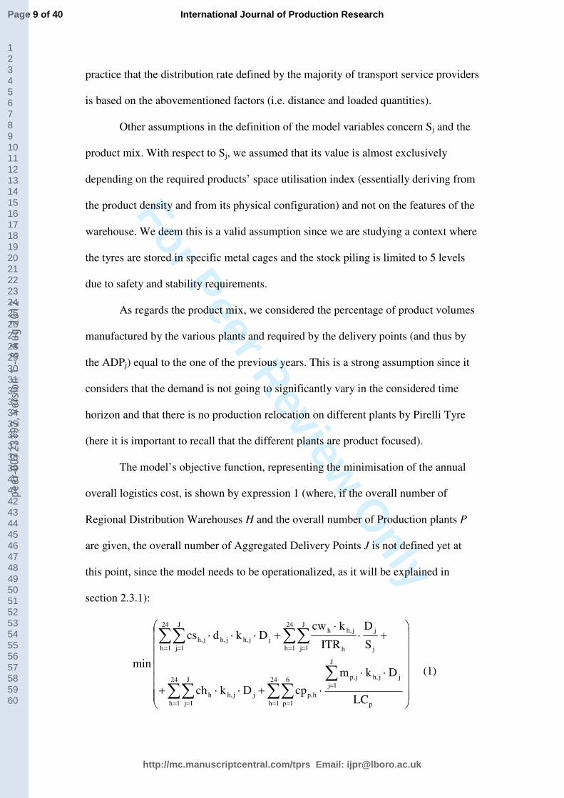
The model’s objective function, representing the minimisation of the annual

overall logistics cost, is shown by expression 1 (where, if the overall number of

Regional Distribution Warehouses H and the overall number of Production plants P

are given, the overall number of Aggregated Delivery Points J is not defined yet at

this point, since the model needs to be operationalized, as it will be explained in

section 2.3.1):

⋅⋅

⋅+⋅⋅+

+⋅⋅

+⋅⋅⋅

∑∑∑

∑∑

∑∑∑∑

= =

=

= =

= == =

24

1h

6

1p p

J

1j

jjh,jp,

hp,

24

1h

J

1j

jjh,h

24

1h

J

1j j

j

h

jh,h24

1h

J

1j

jjh,jh,jh,

LC

Dkm

cpDkch

S

D

ITR

kcwDkdcs

min

(1)

Page 9 of 40

http://mc.manuscriptcentral.com/tprs Email: ijpr@lboro.ac.uk

International Journal of Production Research

123456789101112131415161718192021222324252627282930313233343536373839404142434445464748495051525354555657585960

peer

-007

2319

2, v

ersi

on 1

- 8

Aug

2012

For Peer Review O

nly

The constraints of the mixed integer linear programming model are given by

the following expressions:

jh,kIk hjh,jh, ∀⋅≤ (3)

jh,bink jh, ∀= (4)

hbink1

h ∀=∑ (5)

h 4,000ITRS

Dk

J

1j hj

jjh, ∀>

⋅⋅∑

=

(6)

Expression 2 represents the single sourcing policy constraint (each ADPj can

be served by a single RDWh only). Expression 3 represents the service level

requirement constraint: the linkage between a RDWh and an ADPj exists only if that

activated RDWh allows goods to be delivered to that ADPj within a given time (the

Boolean variable Ih,j allows modelling this condition). Expressions 4 and 5 constrains

the decision variables kh,j and kh respectively to be Boolean variables and expression 6

constraints the minimum size of a RDWh to be activated (the minimum size is set

equal to 4,000 square metres since this represents the typical minimum plot size

offered by logistics service providers, on whom Pirelli relies for its warehousing

activities).

After having described the optimisation model adopted in the Pirelli Tyre case,

in the following pages we present the numerical implementation of the data mapping

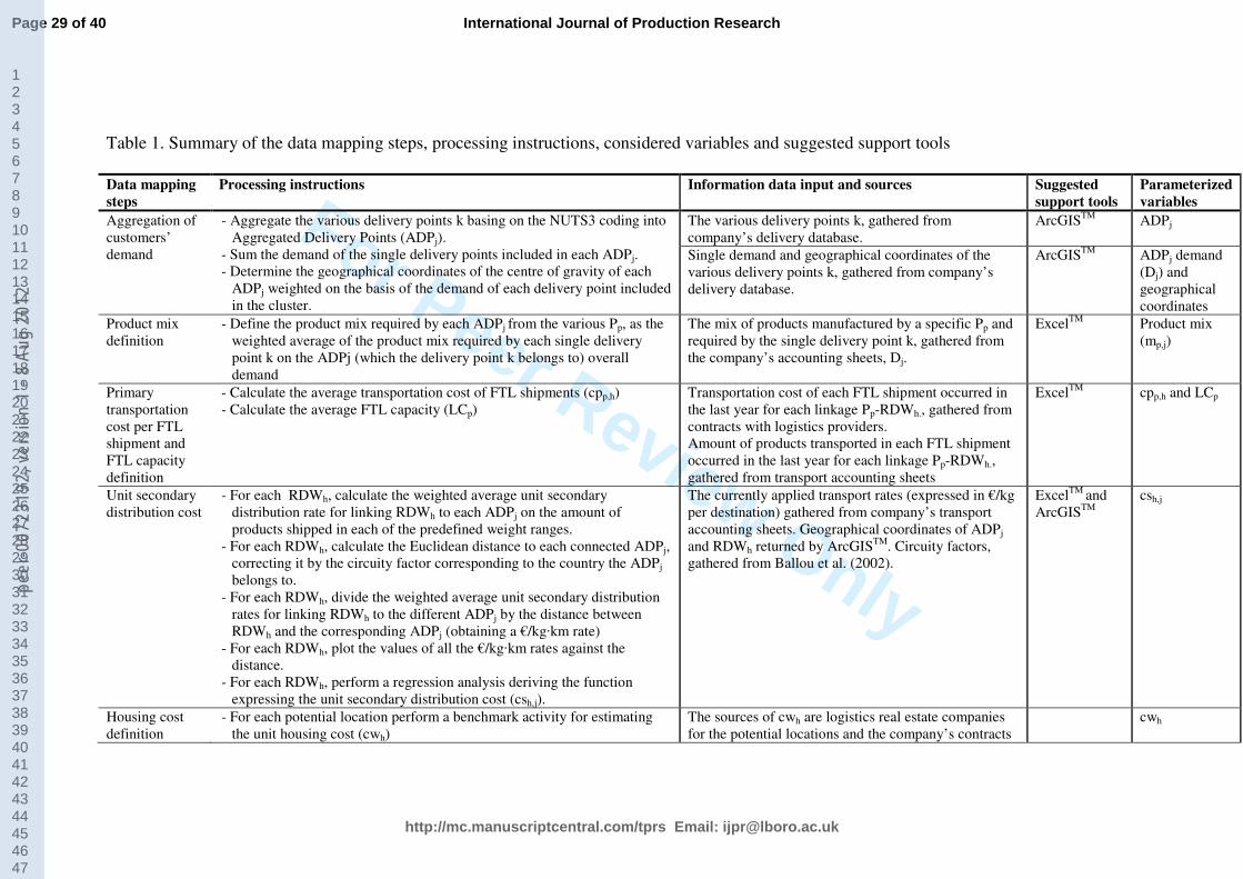
procedure, whose guidelines are summarized in Table 1 (including the steps, the

processing instructions, the sources of information along with the suggested support

j1k24

1h

jh, ∀=∑=

(2)

Page 10 of 40

http://mc.manuscriptcentral.com/tprs Email: ijpr@lboro.ac.uk

International Journal of Production Research

123456789101112131415161718192021222324252627282930313233343536373839404142434445464748495051525354555657585960

peer

-007

2319

2, v

ersi

on 1

- 8

Aug

2012

For Peer Review O

nly

tools necessary for completing the model operationalisation and finally the

parameterized variables).

Table 1. Summary of the data mapping steps, processing instructions, suggested

support tools and parameterised variables

2.3.1 Definition of the ADPj and the aggregation of customer’s demand

With reference to the ADPj to be used in the model, they are obtained by clustering,

according to a geographical basis, the destination points characterising the Pirelli Tyre

European logistics network. Hereinafter, due to simplicity reasons (being Austria the

first market area represented in Figure 1) the definition of the Austrian ADPj

geographical aggregation is described (see Table 2, where the characteristics of the

nine Austrian ADPj in terms of NUTS3 clusters they refer to, demand and location are

depicted).

Table 2. The Austrian ADPj

The Austrian 1,972 delivery points are firstly grouped according to the NUTS coding

(Nomenclature des Unités Territoriales Statistiques, Nomenclature of Territorial

Units for Statistics, proposed by Eurostat in 1988). Three different levels of

aggregation are present in the NUTS codes, based on the number of inhabitants per

aggregated cluster. As suggested in Creazza et al., (2011), we chose the most

disaggregated codes (NUTS3), and we obtained 35 NUTS3 areas characterising the

Austrian territory, i.e. from AT111 to AT342. For instance, all the delivery points

located in Graz belong to the cluster corresponding to the NUTS3 code AT221. For

each of the abovementioned clusters, the demand is calculated as the sum of the

demands (in kilograms of products) of all the delivery points which belong to that

specific cluster, i.e. to the corresponding NUTS3 area. In the Austrian case, nine

Page 11 of 40

http://mc.manuscriptcentral.com/tprs Email: ijpr@lboro.ac.uk

International Journal of Production Research

123456789101112131415161718192021222324252627282930313233343536373839404142434445464748495051525354555657585960

peer

-007

2319

2, v

ersi

on 1

- 8

Aug

2012

For Peer Review O

nly

clusters only (i.e. AT112, AT123, AT126, AT130, AT211, AT221, AT312, AT323

and AT332) are characterised by a not null demand. They correspond to the ADPj

used in the mixed integer linear programming model for representing the Pirelli

Austrian market. The location of each of the nine ADPj is obtained by geographically

referencing on the ArcGISTM

software package the demand data of the delivery points

belonging to the corresponding cluster. Moving from this data, ArcGISTM

is able to

calculate the geographical coordinates of the cluster’s centre of gravity, which are

assigned to the corresponding ADPj.

Applying this procedure to the entire European Pirelli Tyre network

(composed by 42,455 delivery points), we obtained 976 NUTS3 areas, which

represent the clustered demand of the aggregated delivery points (ADPj).

2.3.2 Definition of the product mix

As far as the product mix is concerned, it is necessary to define the various mp,j

percentages, which can be calculated according to expression 7:

where:

• mp,k is the percentage of the delivery point demand (dk) represented by the product

manufactured by Pp and

• Dj is the ADPj demand.

However, it should be remarked that in the Pirelli Tyre case the products mix

requested by each delivery point, i.e. the percentages according to which the delivery

points’ demands are split among the different product-focused plants (mp,k), is not

known. For this reason, we consider the following assumption: if the RDWh’s demand

pjD

dmm

K~

'Kk j

kkp,jp, ∀∀

⋅= ∑

=

(7)

Page 12 of 40

http://mc.manuscriptcentral.com/tprs Email: ijpr@lboro.ac.uk

International Journal of Production Research

123456789101112131415161718192021222324252627282930313233343536373839404142434445464748495051525354555657585960

peer

-007

2319

2, v

ersi

on 1

- 8

Aug

2012

For Peer Review O

nly

is satisfied by the different plants Pp according to the percentages Mp,h and the k-th

delivery point in the as-is configuration of the Pirelli European logistics network is

served by the h-th RDW, then the demand of that delivery point inherits from that

specific RDWh the product mix percentages according to which its demand is fulfilled

from the different plants Pp. Hence, we calculate the percentages mp,j according to

equation 8:

jp,D

IdM

mj

K~

'Kk

24

1h

hk,khp,

jp, ∀∀

⋅⋅

=∑∑= =

(8)

where Ik,h is a Boolean variable whose value is 1 if in the as-is configuration of

the logistics network the k-th delivery point receives products from that specific

considered RDWh, 0 otherwise and K’ and K~

are the indexes of the generic delivery

point within a generic ADPj.

With reference to the Austrian territory, Table 3 shows, for each ADPj

representing the Pirelli Tyre Austrian market, the number of delivery points served (in

round brackets) and the kilograms of products supplied (in square brackets) by each

RDWh.

Table 3. Sourcing features of the Austrian territory

As shown in Table 3, all the delivery points included into each Austrian ADPj

are served by RDW1 only, i.e. by the RDWj located in Gumtransdorf – AT (see Figure

1). As a consequence, by applying equation 8 the equality shown by expression 9 for

ADP2 can be obtained.

Page 13 of 40

http://mc.manuscriptcentral.com/tprs Email: ijpr@lboro.ac.uk

International Journal of Production Research

123456789101112131415161718192021222324252627282930313233343536373839404142434445464748495051525354555657585960

peer

-007

2319

2, v

ersi

on 1

- 8

Aug

2012

For Peer Review O

nlypM

D

DM

D

1dM

D

0dM1dM

D

IdM

m

p,1

2

2p,1

2

107

28k

kp,1

2

107

28k

15

2h

khp,

107

28k

kp,1

2

107

28k

15

1h

hk,khp,

p,2

∀=⋅

=

⋅⋅

=

=

⋅⋅+⋅⋅

=

⋅⋅

=

∑

∑∑∑∑∑

=

= === =

(9)

An expression similar to expression 9 can be written for all the Austrian ADPj.

In particular, it is possible to surmise that each of them is characterized by

percentages mp,j exactly equal to the percentages Mp,h characterizing RDW1, i.e. to the

percentages according to which the generic production plant Pp serves the

Gumstrandorf RDW. Due to the data provided by Pirelli Tyre for the quantities of

products that RDW1 yearly receives from each plant, the mp,j percentages

characterizing the Austrian DPj can be calculated and they are depicted in Table 4.

Table 4. mp,j percentages characterizing the Austrian ADPj

2.3.3 Definition of the primary transportation cost

The other elements necessary for running the model and concurring in determining

the primary transportation costs are represented by the unit cost per FTL shipment

(cpp,h) from a Pp to RDWh and the average FTL transport capacity (LCp, expressed in

kg/FTL shipment). We obtained the various rates per delivery (from each plant to

each Pirelli existing RDWh) from the contracts signed by the company with its

providers for the considered cases and by means of a benchmarking activity involving

the best-in-class transport service providers for the other potential locations not

included in the current Pirelli Tyre logistics network. LCp was derived considering the

quantity (expressed in kilograms) that can be loaded on a trailer according to an

average product mix, as indicated in the transport accounting sheets provided by the

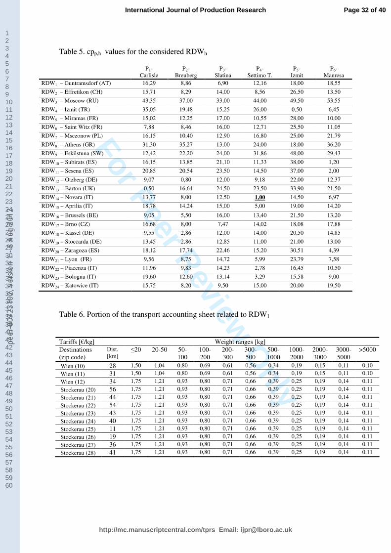
company itself. In Table 5 we report the values of cpp,h for each considered RDWh.

Page 14 of 40

http://mc.manuscriptcentral.com/tprs Email: ijpr@lboro.ac.uk

International Journal of Production Research

123456789101112131415161718192021222324252627282930313233343536373839404142434445464748495051525354555657585960

peer

-007

2319

2, v

ersi

on 1

- 8

Aug

2012

For Peer Review O

nly

Table 5. cpp,h values for the considered RDWh

As abovementioned, all values in the analysis have been disguised for confidentiality

reasons. In particular, in this case we set as a fictitious measure the value “1” for the

cost for connecting P4 (Settimo Torinese) to RDW14 (Novara): the other values are

multiples of this baseline value.

In Figure 2 we include the values of LCp for the Pirelli Tyre case (with

reference to the 15 existing RDWh). As further information, it is worth to specify that

LCp values are influenced by the loaded product type (being Pirelli Tyre products

characterised by different product density values) and by the particular load weight

restrictions applied by the various countries hosting Pirelli’s warehouses and plants.

Figure 2. LCp values (in tons) for the Pirelli Tyre case

2.3.4 Definition of the secondary distribution cost

With reference to the secondary distribution cost, it is necessary to first derive the unit

cost to ship a kilogram of tyres from a certain RDWh to a certain ADPj. It can

obtained from the secondary distribution cost function of each single RDWh, which,

in turn, is derived from the RDWh transport accounting sheet and from the quantities

of product (in kilograms) yearly shipped. Hereinafter, the definition of the secondary

distribution cost for RDW1, located in Gumstrandorf – AT (see Figure 1), and the

calculation of the unit secondary distribution costs to connect RDW1 to each ADPj are

shown. Tables 6 and 7 respectively represent a portion of the transport accounting

sheet and a sample of the quantities shipped from RDW1 during the year 2008.

Table 6. Portion of the transport accounting sheet related to RDW1

Page 15 of 40

http://mc.manuscriptcentral.com/tprs Email: ijpr@lboro.ac.uk

International Journal of Production Research

123456789101112131415161718192021222324252627282930313233343536373839404142434445464748495051525354555657585960

peer

-007

2319

2, v

ersi

on 1

- 8

Aug

2012

For Peer Review O

nly

Table 7. Shipped quantities from RDW1to Wien and Stockerau

It is possible to see from such tables that, in the Pirelli Tyre case, the transport

accounting sheet reports the transport rates (€/kg) for different weight ranges and

destinations. In this case as well, the values have been disguised for confidentiality

reasons.

In particular, for each destination indicated in Table 6, the average €/kg rate

weighted on the actual shipped quantities per weight range (Table 7) can be

calculated. Then, by dividing each rate by the distance between the corresponding

destination and RDW1, the related €/kg·km rate is obtained (see Table 8).

Table 8. €/kg·km rates from RDW1to Wien and Stockerau

Finally, by plotting the values of all the €/kg·km rates (i.e. not only the ones

reported in Table 8) against the distance and performing a regression analysis on such

points, the cost function is derived. It is important to underline that this cost function

is valid for distance ranges comprised between 50 and 700 km. In Figure 3 the cost

function for RDW1 is depicted (such a cost function is the one obtained by using not

disguised values of tariffs and shipped quantities).

Figure 3. Secondary distribution cost function for RDW1

Moving from the function depicted in Figure 3, it is possible to derive the

secondary distribution costs for connecting each ADPj to RDW1. To do this, it is

necessary to calculate the Euclidean distance between RDW1 and each ADPj moving

from their geographical coordinates and to multiply such a distance by the circuity

factor corresponding to the country the ADPj belongs to. The circuity factor is a

Page 16 of 40

http://mc.manuscriptcentral.com/tprs Email: ijpr@lboro.ac.uk

International Journal of Production Research

123456789101112131415161718192021222324252627282930313233343536373839404142434445464748495051525354555657585960

peer

-007

2319

2, v

ersi

on 1

- 8

Aug

2012

For Peer Review O

nly

multiplier used to convert and correct estimated distances into approximate actual

travel distances (Ballou et al., 2002). Circuity factors are expressed by means of an

average and a standard deviation values and for instance for the Austrian country the

average circuity factor is equal to 1.34, with a standard deviation equal to 0.18.

Entering in the cost function depicted by Figure 3 with the adjusted distances allows

the €/kg·km rates referring to the couples given by RDW1 and each ADPj to be

obtained. Finally, the unit secondary distribution cost (in Euros) for moving one

kilogram of products from RDW1 to each ADPj is obtained by multiplying such rates

by the adjusted distances between RDW1 and each ADPj. Table 9 shows this

calculation with reference to the nine Austrian ADPj.

Table 9. Calculation of the secondary distribution costs for connecting RDW1 to the

Austrian ADPj

2.3.5 Definition of the housing and handling costs

For deriving the housing cost we needed the value of Sj and ITRh in order to transform

the annual flow of goods (kg/year) into required warehouse floor space, along with

the unit warehousing cost (cwh), expressed in €/m2·year.

Sj and ITRh values were provided by Pirelli Tyre for each ADPj and RDWh. In

particular, Sj values are almost exclusively depending on the required products’ space

utilisation index (essentially deriving from the product density and from the physical

configuration of each stock keeping unit), since we are considering in the present

study a set of similar and equivalent warehouses (potential and activated), while ITRh

can be considered as a standard average value for the new potential RDWh while for

the existing RDWh the current values apply.

With respect to the cwh values, they were found in the contracts signed by

Pirelli Tyre with warehousing companies, for each of the RDWh currently present in

Page 17 of 40

http://mc.manuscriptcentral.com/tprs Email: ijpr@lboro.ac.uk

International Journal of Production Research

123456789101112131415161718192021222324252627282930313233343536373839404142434445464748495051525354555657585960

peer

-007

2319

2, v

ersi

on 1

- 8

Aug

2012

For Peer Review O

nly

the Pirelli logistics network. As for the other locations, it was necessary to contact

primary logistics real estate companies (e.g. Cushman&Wakefield, Jones Lang

LaSalle and CB Richard Ellis) which provided a series of documents including the

values of the annual rent per square metre for the potential sites we considered in the

study. With reference to Gumstrandorf, i.e. to the current Austrian RDW, the annual

rent is equal to 60 €/m2·year. For Brno and Katowice, i.e. for two potential RDWh,

such cost is equal respectively to 48 €/m2·year and 36 €/m

2·year.

With regards to the handling cost, we needed the handling unit cost chh,

which, similarly to the housing cost, was derived from the contracts signed by Pirelli

Tyre with service providers for the already preset RDWh and from a survey of the

handling rates applied by logistics service providers for the potential considered

locations. With reference to Gumstrandorf, the current applied handling rate is equal

to 0,059 €/kg; with reference to Brno and Katowice the handling rate is equal

respectively to 0,050 €/kg and 0,056 €/kg.

2.3.6 Definition of the service level

As far as the service level is concerned, in the Pirelli Tyre case we considered three

different scenarios: the first (S1) where all the ADPj must be served within 24 hours,

the second (S2) where all the ADPj must be served within 36 hours and the third (S3)

where all the ADPj must be served within 48 hours. In particular, to fill in the row of

Table 9 corresponding to RDW1, i.e. to the Gumstrandorf RDWh, in the scenario S1 it

is necessary to derive, by means of Microsoft MapPoint 6.0TM

, the area reachable

within 24 hours from RDW1 (i.e. the RDW1 24-hour isochronal zone), considering an

average driving speed of 60 km/hours and 4 hours driving stops every 8 hours. Once

such an isochronal zone has been drawn, it is possible to verify which NUTS3 areas

are completely included in there and which lie outside this zone (see Figure 4). Then,

Page 18 of 40

http://mc.manuscriptcentral.com/tprs Email: ijpr@lboro.ac.uk

International Journal of Production Research

123456789101112131415161718192021222324252627282930313233343536373839404142434445464748495051525354555657585960

peer

-007

2319

2, v

ersi

on 1

- 8

Aug

2012

For Peer Review O

nly

in the possible origin-destination matrix the cells corresponding to the ADPj that refer

to the former NUTS3 areas should be set to 1, to 0 the others (see Table 10 for an

example focused on the Austrian RDW and including the Austrian, Hungarian, Czech

and Slovakian ADPj).

Figure 4. NUTS3 areas covered within 24 hours from RDW1

Table 10. Example of a service level origin-destination matrix

3. Model validation

After having completed the data mapping section implementation, it was then possible

to solve the configuration problem for the Pirelli Tyre European logistics network.

First of all, we decided to test the adherence of the model as well as of the

input data by deriving the overall logistics costs of the current configuration of the

Pirelli Tyre European logistics network (i.e. the sum of transportation costs and of the

warehousing costs). To this aim we set the decision variables kh and kh,j so as to

replicate the logistics network structure depicted in Figure 1. The model provides an

overall logistics cost very similar to actual figures for year 2008, with a difference

equal to only -0,9%. Such a result allows for proving the adherence of the model

objective function and of the input data to the Pirelli logistics cost function and

context respectively. On the other side, in more general terms, it demonstrates the

effectiveness of the proposed data mapping section.

With regard to the development of the model, we had to confront some critical

points in order to match the real dynamics of the considered operating environment.

In fact, some choices regarding the model variables were immediately induced by the

modelisation process (e.g. primary transportation cost and the handling cost). On the

other hand, other choices such the unit secondary distribution cost required a series of

iterations in order to derive a meaningful approximation: we initially started by

Page 19 of 40

http://mc.manuscriptcentral.com/tprs Email: ijpr@lboro.ac.uk

International Journal of Production Research

123456789101112131415161718192021222324252627282930313233343536373839404142434445464748495051525354555657585960

peer

-007

2319

2, v

ersi

on 1

- 8

Aug

2012

For Peer Review O

nly

considering an average distribution rate based on weight ranges for the shipments

from RDWh to ADPj from the transport accounting reports. However, by deeply

analysing the reports, we understood that the rates we previously obtained were

strongly depending on the shipped quantities along the various linkages between

RDWh and ADPj, since they were closely referred to those specific transport linkages.

Then, since in our modelisation it is evident that the transport leg set changes from a

configuration to another, it is generally unfeasible to directly apply the cost values

present in the transport accounting reports for assessing the overall secondary

distribution cost. For these reasons, we had to derive for each RDWh a function of the

travelled distance expressing the secondary distribution unit cost. Such a function is

derived by means of a regression analysis which allows for obtaining the best fitting

curve interpolating the €/kg rate per each single destination, weighted on the basis of

the shipped volume for each weight range, divided by the distances between the

corresponding destinations and the considered RDWh.

4. Outcomes of the optimisation process

In the present section we report the results of the optimisation process applied

to the Pirelli Tyre case and we then propose a sensitivity analysis aimed at evaluating

the robustness of the solution obtained for Scenario 2, as it will be explained.

4.1. Numerical results

We exploited the mixed integer linear programming model to solve the

configuration problem. In particular, by using Lindo What’s Best? 9.0TM

software, the

values of kh and kh,j which minimise the overall logistics cost function in the three

different service level scenarios (S1, S2 and S3) are found. Table 11 synthesises the

results obtained for the configuration problem in each scenario and compares them

Page 20 of 40

http://mc.manuscriptcentral.com/tprs Email: ijpr@lboro.ac.uk

International Journal of Production Research

123456789101112131415161718192021222324252627282930313233343536373839404142434445464748495051525354555657585960

peer

-007

2319

2, v

ersi

on 1

- 8

Aug

2012

For Peer Review O

nly

with the as-is configuration of the Pirelli Tyre European logistics network (the base

case), in terms of number of activated RDWh and of percentage reduction of each cost

item of the overall logistics cost. For the three considered optimisation processes, the

average computational time was about 2,400 seconds (on a 1.3 GHz chipset machine

with 512 RAM DDR).

Table 11. The outcomes of the implementation of the optimisation model (consider as

100% the overall logistics cost of the base case)

In particular, it is possible to observe how the service level constraint

influences the total logistics cost. It is interesting to notice how for a very high service

level (S1, i.e. delivery time within 24 hours) the number of warehouses resulting from

the optimisation is the same as for the base case, even though 3 warehouses out of 15

change (i.e. they are not the same warehouses as before). The saving (equal to 4%)

arises from the selection of an optimised set of RDWh and of linkages between the

logistics network nodes so as to reduce each single item of the overall logistics cost.

In S2 (i.e. delivery time within 36 hours), which allows broader reachable

geographical zones within a wider time window due to a less strict service level

constraint, 14 RDWh are activated. In this case the optimisation allows for a higher

saving (equal to 7%). Of course, the saving concerning the warehousing cost is to be

ascribed to the fact that a wider time window allows selecting a more efficient set of

RDWh, in terms of unit warehousing costs, compared to current ones. In scenario S3

(i.e. delivery time within 48 hours) the model returns a configuration for the Pirelli

Tyre European logistics network equal to the one returned in the case of scenario S2.

This is probably due to the fact that the savings in the warehousing costs obtainable

by the selection of a more efficient set of RDWh (due to the fact that, with an even

wider allowed time window, a lower number of warehouses could be potentially

Page 21 of 40

http://mc.manuscriptcentral.com/tprs Email: ijpr@lboro.ac.uk

International Journal of Production Research

123456789101112131415161718192021222324252627282930313233343536373839404142434445464748495051525354555657585960

peer

-007

2319

2, v

ersi

on 1

- 8

Aug

2012

For Peer Review O

nly

activated) are more than compensated by the consequent increases in the primary and

secondary distribution costs to connect RDWh with more distant Pp and ADPj, due to

the lower number of activated RDWh and to the deriving increased distance between

the nodes of the network.

It is important to underline that the overall warehouse floor space does not

change in the considered scenarios, even if the number of activated RDWh varies in

the different analysed cases: in fact, the overall required warehouse floor space

depends on the flows of products through the logistics network and on the values of Sj

and ITRj, which are connected to the ADPj overall demand product mix, which does

not vary as well in the different considered scenarios.

4.2. Sensitivity analysis

In order to discuss the robustness of the obtained solution, we used the developed

model to perform a sensitivity analysis. We took as a reference the network

configuration obtained from the optimisation of Scenario 2. As a matter of fact, the

resulting logistics network configuration is the lowest one and the service level

characterising Scenario 2 is the one Pirelli Tyre has to assure in its real-life context. In

particular, we used as benchmark variable the overall logistics cost and we modified

the values of significant model variables and parameters (selected by discussing their

relevance with Pirelli Tyre). We ran the model and we derived the new optimal

logistics network configuration (named as “new solution”) connected to the changed

input variables (and the corresponding value of the overall logistics cost). Then, we

calculated the overall logistics cost connected to the original logistics network

configuration in Scenario 2 (named as “original solution”) due to the changes in the

values of the input variables. We measured the robustness of “original solution” by

calculating the percentage difference between the overall logistics costs connected to

Page 22 of 40

http://mc.manuscriptcentral.com/tprs Email: ijpr@lboro.ac.uk

International Journal of Production Research

123456789101112131415161718192021222324252627282930313233343536373839404142434445464748495051525354555657585960

peer

-007

2319

2, v

ersi

on 1

- 8

Aug

2012

For Peer Review O

nly

“original solution” and to “new solution”. The relevant model variables and

parameters we considered in the sensitivity analysis were:

• cwh and chh values referred to a potential RDWh located in Kassel (Germany). As

a matter of fact Pirelli Tyre was awaiting for receiving an offer from a logistics

service provider whose warehouse is placed in Kassel. Since in “original solution”

Kassel was not activated, in the sensitivity analysis we considered only a

reduction of its cwh and chh values. Pirelli Tyre suggested that the reduction of

these value could range from 5% to 10%;

• product mix: Pirelli Tyre wanted to know the impacts of the relocation of the

production of certain products from one or more production plants to another. In

particular, the relocations of a 10% and a 15% of product volumes were tested.

For confidentiality reasons, in this paper we do not report the details of the plants

potentially involved in the production relocation.

The results of the sensitivity analysis are depicted in Table 12, as a % value of

the base case configuration overall logistics cost (which is considered equal to 100%).

Table 12. The outcomes of the performed sensitivity analysis

As it is possible to see from Table 12, the maximum percentage difference

between the overall logistics costs connected to “original solution” and to “new

solution” (taking as a reference the optimal cost, i.e. the one related to “new

solution”) is equal to 0.35% (corresponding to Variation “-10% cwh & chh (RDWh

Kassel)”). Consequently, we are able to affirm that the logistics network configuration

obtained for Scenario 2, besides being the most realistic one in terms of considered

service level constraints and the most cost-efficient one, it is also remarkably robust.

5. Concluding remarks

The present paper addresses a topical and current supply chain issue, i.e. supply chain

configuration and optimisation, by means of a case study. In particular, a design and

Page 23 of 40

http://mc.manuscriptcentral.com/tprs Email: ijpr@lboro.ac.uk

International Journal of Production Research

123456789101112131415161718192021222324252627282930313233343536373839404142434445464748495051525354555657585960

peer

-007

2319

2, v

ersi

on 1

- 8

Aug

2012

For Peer Review O

nly

optimisation model for logistics and distribution networks, based on mixed integer

linear programming (see Creazza et al., 2011), was applied to a real-life supply chain

(the Pirelli Tyre European logistics network).

In detail, we exhaustively implemented the integrated approach we proposed

in our previous work, starting from the gathering of the input data necessary for

running the optimisation model. To accomplish this task, we relied on the data

mapping procedure, composed of different sub-sections, which allowed obtaining the

values of all the required parameters, substantially reducing the complexity of the data

mapping and processing activity, which is considered as a relevant, difficult and time-

consuming operation in real-life contexts (Carlsson and Ronnqvist, 2005).

Then, after having implemented the model (parameterized with the data

previously obtained) on a spreadsheet software package, we succeeded in applying it

to the Pirelli Tyre European logistics network, which is characterised by a high

complexity level (being a multi-product and multi-stage supply chain with more than

40,000 nodes) and by service level as a pre-eminent critical success factor. In

particular, based on the comparison of the outcomes of the model with budgetary

data, the model proved to be accurate and adherent to the actual figures. Then, we

solved the configuration problem for Pirelli Tyre, obtaining significant results in

terms of saving, compared to the as-is configuration, with different scenarios of

service level constraints. In fact, in any of the considered cases, the savings resulting

from the implementation of the proposed method (i.e. the developed mapping section

and integer linear programming model) are significant (see Table 10). Such a result

allows for proving the usefulness of the proposed method in the Pirelli context and in

addition it demonstrates, in more general terms, the effectiveness of the proposed

method for configuring multi-item, multi-layer logistics networks.

Page 24 of 40

http://mc.manuscriptcentral.com/tprs Email: ijpr@lboro.ac.uk

International Journal of Production Research

123456789101112131415161718192021222324252627282930313233343536373839404142434445464748495051525354555657585960

peer

-007

2319

2, v

ersi

on 1

- 8

Aug

2012

For Peer Review O

nly

We believe that the model we implemented in the present case study could be

profitably applied by supply chain and logistics managers for optimising operating

contexts characterised by similar features compared to the considered one. Moreover,

the exemplified data mapping section could represent a useful guideline, which can be

successfully applied by practitioners to gather and handle the high volume of data

necessary for running the model in a real-life context. In more general terms, being

the current state of the art particularly wanting of exhaustive configuration models,

i.e. models dealing with real-life complexity and practically implemented in realistic

contexts and including the data mapping section as well (see for examples the

scientific contributions analysed by Melo et al., 2009), we believe that the

implemented integrated approach could represent a significant contribution to the

existing body of knowledge on supply chain configuration.

Furthermore, our proposed approach, besides being an optimisation tool for

configuring/redesigning supply chains, represents also a useful instrument for

performing scenario and what-if analysis.

In fact, the proposed model can be exploited by supply chain managers for

analysing the variations of the supply chain performance (i.e. the overall logistics

cost) with reference to the changes of the key parameters of the model. For instance,

they could assess the overall logistics cost in function of the unit cost value

modifications. In this way, they could build a sort of managerial cockpit where

monitoring the supply chain performance in function of the variation of the key

parameters of the model, by running the optimisation model in a changed

environment.

On the other hand, supply chain managers, by modifying themselves the

values of the Boolean decision variables (without running the model), can easily

Page 25 of 40

http://mc.manuscriptcentral.com/tprs Email: ijpr@lboro.ac.uk

International Journal of Production Research

123456789101112131415161718192021222324252627282930313233343536373839404142434445464748495051525354555657585960

peer

-007

2319

2, v

ersi

on 1

- 8

Aug

2012

For Peer Review O

nly

evaluate the impact of their decisions concerning the activation of different RDWh

and/or the sourcing policy (i.e. the allocation of the logistics flows from the various

RDWh to the ADPj) on the supply chain performance. In this way, for instance, supply

chain managers could consider the outcomes of the what-if analysis as a basis for

negotiating the service level the sales & marketing wants to ensure to their customers.

Moving from this statement, supply chain managers could similarly assess the

risk connected to disruptions of a certain production plant or of a RDW. In fact, they

could simulate the shut down of a production plant/RDW or else the reduction of the

production capacity of a production plant. By running the model excluding a Pp or a

RDWh, or else modifying their specific features, the model is able to provide a

simulation on how the logistics flows get redistributed in the network according to the

changed context conditions, deriving the resulting overall logistics cost. In this case,

supply chain managers modify by themselves such values and then they should run

the optimisation model and assess the impact of such variations on the supply chain

configuration and on the supply chain performance. This what-if scenario analysis of

the behaviour of the supply chain allows to quantify the effect on the overall logistics

cost, i.e. the variation of the supply chain performance from its as-is optimised

network configuration value in each considered scenario.

Still, the proposed integrated approach presents some limitations which should

be critically discussed. In fact, even if the provided data mapping guidelines allow for

an easier and more structured operationalisation of the model, our model necessitates

a considerable amount of reliable and sound data to be elaborated (e.g. the data

necessary for determining the secondary distribution cost). Then, our proposed

approach can be used in those contexts where production plants are product focused

and where it is possible to clearly identify and define an unambiguous equivalent

Page 26 of 40

http://mc.manuscriptcentral.com/tprs Email: ijpr@lboro.ac.uk

International Journal of Production Research

123456789101112131415161718192021222324252627282930313233343536373839404142434445464748495051525354555657585960

peer

-007

2319

2, v

ersi

on 1

- 8

Aug

2012

For Peer Review O

nly

product unit (e.g. tons or pallets or kilos), since the LCp values and the required

warehouse floor space depend on this equivalent product unit. Finally, with respect to

the modelling features, our approach is not time-dependent, even if, by allowing the

possibility to handle a definitely higher computational complexity and longer

computational times, it could be made time-dependent: this represents one of our aims

as a further research on this theme, along with the development of a multi-location

layer mixed integer linear programming model for considering the redesign and the

optimisation of production-distribution networks.

Acknowledgments We would like to express our gratitude to the reviewers for their valuable contribution in enhancing the

quality of the present paper and to our native-English-speaking proof reader for supporting us in

refining the writing style of the paper.

References

Ballou, R.H., 2005. Business Logistics Management. Prentice-Hall.

Ballou, R.H., 2002. Selected country circuity factors for road travel distance

estimation. Transportation Research Part A: Policy and Practice, 36 (9). 843-

848.

Canel, C. and Khumawala, B.M., 2001. International facilities location: A heuristic

procedure for the dynamic uncapacitated problem. International Journal of

Production Research, 39 (30), 3975–4000.

Carlsson, D. and Ronnqvist, M., 2005. Supply chain management in forestry - case

studies at Sodra cell AB. European Journal of Operational Research, 163 (3),

589–616.

Chopra, S. and Meindl, P., 2007. Supply chain management: Strategy, planning and

operations. Prentice Hall.

Christopher, M., 2007. New Directions in Logistics. In: Waters, D., eds. Global

Logistics: new directions in supply chain management, Kogan Page.

Creazza, A., Dallari, F., Rossi, T., 2011, An integrated model for designing and

optimising an international logistics network. International Journal of

Production Research, forthcoming.

Gargeya, V., Meixell, M. (2005), “Global supply chain design: a literature review and

critique”, Transportation Research part E, Vol. 41, No. 6, pp. 531-550.

Gunaserkaran, A., Lai, K. and Cheng, T.C.E., 2008. Responsive supply chain: A

competitive strategy in a networked economy. Omega, 36 (4), 549-564.

Jahene, D.M., Riedel, R. and Mueller, E., 2009. Configuring and operating global

production networks. International Journal of Production Research, 47 (8),

2013-2030.

Page 27 of 40

http://mc.manuscriptcentral.com/tprs Email: ijpr@lboro.ac.uk

International Journal of Production Research

123456789101112131415161718192021222324252627282930313233343536373839404142434445464748495051525354555657585960

peer

-007

2319

2, v

ersi

on 1

- 8

Aug

2012

For Peer Review O

nly

Jammernegg, W. and Reiner, G., 2007. Performance improvement of supply chain

processes by coordinated inventory and capacity management. International

Journal of Production Economics, 108 (1-2), 183-190.

Melachrinoudis, E. and Min, H., 2000. The dynamic relocation and phase-out of a

hybrid, two echelon plant/warehousing facility: A multiple objective approach.

European Journal of Operational Research, 123 (1), 1–15.

Melo, M.T., Nickel, S. and Saldanha-da-Gama, F., 2009. Facility location and supply

chain management – A review, European Journal of Operational Research,

196 (2), 401-412.

Sharma, J.K., 2006. Linear programming: theory and applications, MacMillan.

Simchi-Levi D., Kaminski P. and Simchi-Levi E., 2005. Designing and managing the

supply chain: concepts, strategies and case studies - 2nd edition. McGraw

Hill.

Smith, G.A., 2003. Using integrated spreadsheet modelling for supply chain analysis”.

Supply Chain Management: An International Journal, 8 (4), 285-290.

Teo, C.P. and Shu., J., 2004. Warehouse-retailer network design problem. Operations

Research, 52 (3), 396–408.

Truong, T.H. and Azadivar, F., 2005. Optimal design methodologies for configuration

of supply chains. International Journal of Production Research, 43 (11),

2217-2236.

Zhang, X., Huang, G.Q. and Rungtusanatham, M.J., 2008. Simultaneous

configuration of platform products and manufacturing supply chains.

International Journal of Production Research, 46 (21), 6137-6162.

Page 28 of 40

http://mc.manuscriptcentral.com/tprs Email: ijpr@lboro.ac.uk

International Journal of Production Research

123456789101112131415161718192021222324252627282930313233343536373839404142434445464748495051525354555657585960

peer

-007

2319

2, v

ersi

on 1

- 8

Aug

2012

For Peer Review Only

Table 1. Summary of the data mapping steps, processing instructions, considered variables and suggested support tools

Data mapping

steps

Processing instructions

Information data input and sources Suggested

support tools

Parameterized

variables

The various delivery points k, gathered from

company’s delivery database.

ArcGISTM

ADPj Aggregation of

customers’

demand

- Aggregate the various delivery points k basing on the NUTS3 coding into

Aggregated Delivery Points (ADPj).

- Sum the demand of the single delivery points included in each ADPj.

- Determine the geographical coordinates of the centre of gravity of each

ADPj weighted on the basis of the demand of each delivery point included

in the cluster.

Single demand and geographical coordinates of the

various delivery points k, gathered from company’s

delivery database.

ArcGISTM

ADPj demand

(Dj) and

geographical

coordinates

Product mix

definition

- Define the product mix required by each ADPj from the various Pp, as the

weighted average of the product mix required by each single delivery

point k on the ADPj (which the delivery point k belongs to) overall

demand

The mix of products manufactured by a specific Pp and

required by the single delivery point k, gathered from

the company’s accounting sheets, Dj.

ExcelTM

Product mix

(mp,j)

Primary

transportation

cost per FTL

shipment and

FTL capacity

definition

- Calculate the average transportation cost of FTL shipments (cpp,h)

- Calculate the average FTL capacity (LCp)

Transportation cost of each FTL shipment occurred in

the last year for each linkage Pp-RDWh., gathered from

contracts with logistics providers.

Amount of products transported in each FTL shipment

occurred in the last year for each linkage Pp-RDWh.,

gathered from transport accounting sheets

ExcelTM

cpp,h and LCp

Unit secondary

distribution cost

- For each RDWh, calculate the weighted average unit secondary

distribution rate for linking RDWh to each ADPj on the amount of

products shipped in each of the predefined weight ranges.

- For each RDWh, calculate the Euclidean distance to each connected ADPj,

correcting it by the circuity factor corresponding to the country the ADPj

belongs to.

- For each RDWh, divide the weighted average unit secondary distribution

rates for linking RDWh to the different ADPj by the distance between

RDWh and the corresponding ADPj (obtaining a €/kg·km rate)

- For each RDWh, plot the values of all the €/kg·km rates against the

distance.

- For each RDWh, perform a regression analysis deriving the function

expressing the unit secondary distribution cost (csh,j).

The currently applied transport rates (expressed in €/kg

per destination) gathered from company’s transport

accounting sheets. Geographical coordinates of ADPj

and RDWh returned by ArcGISTM

. Circuity factors,

gathered from Ballou et al. (2002).

ExcelTM

and

ArcGISTM

csh,j

Housing cost

definition

- For each potential location perform a benchmark activity for estimating

the unit housing cost (cwh)

The sources of cwh are logistics real estate companies

for the potential locations and the company’s contracts

cwh

Page 29 of 40

http://mc.manuscriptcentral.com/tprs Email: ijpr@lboro.ac.uk

International Journal of Production Research

123456789101112131415161718192021222324252627282930313233343536373839404142434445464748495051525354555657585960

peer

-007

2319

2, v

ersi

on 1

- 8

Aug

2012

For Peer Review Only

for the existing locations.

Handling cost

definition

- For each potential location perform a benchmark activity for estimating

the unit handling cost (chh)

The sources of cwh are handling service providers for

the potential locations and the company’s contracts for

the existing locations.

chh

Service level

requirement

definition

- Define a required delivery time for each ADPj.

- From each RDWh draw the isochronal zone for the various required

delivery times, considering the average driving speeds and other factors

such as the driving stops imposed by regulations.

- Verify which ADPj completely lie within the isochronal zone for each

RDWh.

- Fill in each cell (Ih,j) of the origin-destination matrix with 1 if the

correspondence between each RDWh and each ADPj is verified, with 0

otherwise.

RDWh and ADPj geographical coordinates returned by

ArcGISTM

, driving speeds and number and frequency of

driving stops, gathered from local and international

regulations. Delivery times gathered by service level

specifications.

ExcelTM

,

MapPointTM

and ArcGISTM

Ih,j

Page 30 of 40

http://mc.manuscriptcentral.com/tprs Email: ijpr@lboro.ac.uk

International Journal of Production Research

123456789101112131415161718192021222324252627282930313233343536373839404142434445464748495051525354555657585960

peer

-007

2319

2, v

ersi

on 1

- 8

Aug

2012

For Peer Review O

nly

Table 2. The Austrian ADPj

ADPj NUTS3 cluster ADPj demand [kg] ADPj geographical coordinates X coordinate Y coordinate

ADP1 AT112 95,009 131,116 -237,154 ADP2 AT123 465,655 48,041 -204,049

ADP3 AT126 297,091 100,847 -183,598 ADP4 AT130 503,437 102,108 -198,224

ADP5 AT211 403,415 -75,938 -375,822

ADP6 AT221 764,405 29,379 -319,175 ADP7 AT312 1,201,131 -63,222 -194,536

ADP8 AT323 450,261 -133,736 -248,635

ADP9 AT332 503,743 -276,214 -304,616

Table 3. Sourcing features of the Austrian territory

ADP1 ADP2 ADP3 ADP4 ADP5 ADP6 ADP7 ADP8 ADP9

RDW1 (27)

[95,00

9]

RDW1 (107)

[465,65

5]

RDW1 (65)

[297,09

1]

RDW1 (119)

[503,43

7]

RDW1 (102)

[403,41

5]

RDW1 (189)

[764,40

5]

RDW1 (275)

[1,201,13

1]

RDW1 (121)

[450,26

1]

RDW1 (167)

[503,74

3] RDW2 to RDW15

(0) [0]

Table 4. mp,j percentages characterizing the Austrian ADPj

p=1 (UK)

p=2 (DE)

p=3 (RO)

p=4 (IT)

p=5 (TR)

p=6 (ES)

j∀ ( 1 ≤ j ≤ 9 )

14% 18% 8% 31% 20% 9%

Page 31 of 40

http://mc.manuscriptcentral.com/tprs Email: ijpr@lboro.ac.uk

International Journal of Production Research

123456789101112131415161718192021222324252627282930313233343536373839404142434445464748495051525354555657585960

peer

-007

2319

2, v

ersi

on 1

- 8

Aug

2012

For Peer Review O

nly

Table 5. cpp,h values for the considered RDWh

P1-

Carlisle

P2-

Breuberg

P3-

Slatina

P4-

Settimo T.

P5-

Izmit

P6-

Manresa

RDW1 – Guntramsdorf (AT) 16,29 8,86 6,90 12,16 18,00 18,55

RDW2 – Effretikon (CH) 15,71 8,29 14,00 8,56 26,50 13,50

RDW3 – Moscow (RU) 43,35 37,00 33,00 44,00 49,50 53,55

RDW4 – Izmit (TR) 35,05 19,48 15,25 26,00 0,50 6,45

RDW5 – Miramas (FR) 15,02 12,25 17,00 10,55 28,00 10,00

RDW6 – Saint Witz (FR) 7,88 8,46 16,00 12,71 25,50 11,05

RDW7 – Msczonow (PL) 16,15 10,40 12,90 16,80 25,00 21,79

RDW8 – Athens (GR) 31,30 35,27 13,00 24,00 18,00 36,20

RDW9 – Eskilstuna (SW) 12,42 22,20 24,00 31,86 48,00 29,43

RDW10 – Subirats (ES) 16,15 13,85 21,10 11,33 38,00 1,20

RDW11 – Sesena (ES) 20,85 20,54 23,50 14,50 37,00 2,00

RDW12 – Otzberg (DE) 9,07 0,80 12,00 9,18 22,00 12,37

RDW13 – Barton (UK) 0,50 16,64 24,50 23,50 33,90 21,50

RDW14 – Novara (IT) 13,77 8,00 12,50 1,00 14,50 6,97

RDW15 – Aprilia (IT) 18,78 14,24 15,00 5,00 19,00 14,20

RDW16 – Brussels (BE) 9,05 5,50 16,00 13,40 21,50 13,20

RDW17 – Brno (CZ) 16,68 8,00 7,47 14,02 18,08 17,88

RDW18 – Kassel (DE) 9,55 2,86 12,00 14,00 20,50 14,85

RDW19 – Stoccarda (DE) 13,45 2,86 12,85 11,00 21,00 13,00

RDW20 – Zaragoza (ES) 18,12 17,74 22,46 15,20 30,51 4,39

RDW21 – Lyon (FR) 9,56 8,75 14,72 5,99 23,79 7,58

RDW22 – Piacenza (IT) 11,96 9,83 14,23 2,78 16,45 10,50

RDW23 – Bologna (IT) 19,60 12,60 13,14 3,29 15,58 9,00

RDW24 – Katowice (IT) 15,75 8,20 9,50 15,00 20,00 19,50

Table 6. Portion of the transport accounting sheet related to RDW1

Tariffs [€/kg] Weight ranges [kg]

Destinations

(zip code)

Dist.

[km] ≤20 20-50 50-

100

100-

200

200-

300

300-

500

500-

1000

1000-

2000

2000-

3000

3000-

5000

>5000

Wien (10) 28 1,50 1,04 0,80 0,69 0,61 0,56 0,34 0,19 0,15 0,11 0,10

Wien (11) 31 1,50 1,04 0,80 0,69 0,61 0,56 0,34 0,19 0,15 0,11 0,10

Wien (12) 34 1,75 1,21 0,93 0,80 0,71 0,66 0,39 0,25 0,19 0,14 0,11

Stockerau (20) 56 1,75 1,21 0,93 0,80 0,71 0,66 0,39 0,25 0,19 0,14 0,11

Stockerau (21) 44 1,75 1,21 0,93 0,80 0,71 0,66 0,39 0,25 0,19 0,14 0,11

Stockerau (22) 54 1,75 1,21 0,93 0,80 0,71 0,66 0,39 0,25 0,19 0,14 0,11

Stockerau (23) 43 1,75 1,21 0,93 0,80 0,71 0,66 0,39 0,25 0,19 0,14 0,11

Stockerau (24) 40 1,75 1,21 0,93 0,80 0,71 0,66 0,39 0,25 0,19 0,14 0,11

Stockerau (25) 11 1,75 1,21 0,93 0,80 0,71 0,66 0,39 0,25 0,19 0,14 0,11

Stockerau (26) 19 1,75 1,21 0,93 0,80 0,71 0,66 0,39 0,25 0,19 0,14 0,11

Stockerau (27) 36 1,75 1,21 0,93 0,80 0,71 0,66 0,39 0,25 0,19 0,14 0,11

Stockerau (28) 41 1,75 1,21 0,93 0,80 0,71 0,66 0,39 0,25 0,19 0,14 0,11

Page 32 of 40

http://mc.manuscriptcentral.com/tprs Email: ijpr@lboro.ac.uk

International Journal of Production Research

123456789101112131415161718192021222324252627282930313233343536373839404142434445464748495051525354555657585960

peer

-007

2319

2, v

ersi

on 1

- 8

Aug

2012

For Peer Review O

nly

Table 7. Shipped quantities from RDW1to Wien and Stockerau

Shipped

quantities [kg]

Weight ranges [kg]

Destinations

(zip code)

≤20 20-50 50-

100

100-

200

200-

300

300-

500

500-

1000

1000-

2000

2000-

3000

3000-

5000

>5000

Wien (10) 1,128 4,781 5,929 5,681 3,719 5,607 8,739 7,398 1,162 1,707

Wien (11) 1,864 7,047 7,237 4,998 4,148 6,281 2,962 5,149 3,660

Wien (12) 2,788 11,331 16,775 17,274 11,975 15,971 22,180 21,943 22,596 6,751 13,256

Stockerau (20) 389 1,149 1,904 1,737 1,156 1,284 1,558 4,815 1,076 3,758

Stockerau (21) 200 1,185 1,826 1,607 2,177 565 1,866 735 1,163

Stockerau (22) 189 1,043 1,403 1,363 1,439 1,319 983 3,528 1,902

Stockerau (23) 705 3,204 4,453 4,706 2,290 1,730 3,017 2,975 1,529

Stockerau (24) 346 1,402 2,892 3,136 845 1,255 1,270 2,051 1,476

Stockerau (25) 660 2,562 2,754 1,859 1,155 878 1,801 1,538 12,704

Stockerau (26) 234 1,104 1,690 2,301 728 1,547 873 5,725

Stockerau (27) 570 1,904 2,314 2,804 2,388 1,395 1,613 1,558 1,063

Stockerau (28) 50 335 729 597 938 324 3,173 3,756 2,449 2,155

Table 8. €/kg·km rates from RDW1to Wien and Stockerau

Delivery

point code

10 11 12 20 21 22 23 24 25 26 27 28

Weighted

€/kg rate

0.5547 0.6446 0.5402 0.5020 0.6903 0.5630 0.7274 0.6826 0.4721 0.5514 0.7386 0.3783

Distance

[km]

28 31 34 56 44 54 43 40 11 19 36 41

€/kg·km

rate

0.0198 0.0208 0.0159 0.0090 0.0157 0.0104 0.0169 0.0171 0.0429 0.0290 0.0205 0.0092

Table 9. Calculation of the secondary distribution costs for connecting RDW1 to the

Austrian ADPj

Geographical coordinates

X coordinate

(A) Y coordinate

(B)

Distance [km] from

RDW1

(C=(1.34*((XcoordRD

W-A)2+(YcoordRDW-

B)2)

1/2))

€/kg·km rate

(D=0.1139*C-0.843

) Secondary

distribution cost –

cshj [€/kg]

(E=D*C)

ADP1 131,116 -237,154 41.72018462 0.004898755 0.20437698 ADP2 48,041 -204,049 82.11961096 0.002767392 0.227257147 ADP3 100,847 -183,598 44.72164489 0.004620001 0.206614054 ADP4 102,108 -198,224 25.36079057 0.007454066 0.189041012 ADP5 -75,938 -375,822 326.4862257 0.000864135 0.282128103 ADP6 29,379 -319,175 173.7299387 0.001471084 0.255571301 ADP7 -63,222 -194,536 231.4147293 0.001155135 0.267315286 ADP8 -133,736 -248,635 326.9859552 0.000863021 0.282195727 ADP9 -276,214 -304,616 528.4611897 0.000575714 0.304242497

Page 33 of 40

http://mc.manuscriptcentral.com/tprs Email: ijpr@lboro.ac.uk

International Journal of Production Research

123456789101112131415161718192021222324252627282930313233343536373839404142434445464748495051525354555657585960

peer

-007

2319

2, v

ersi

on 1

- 8

Aug

2012

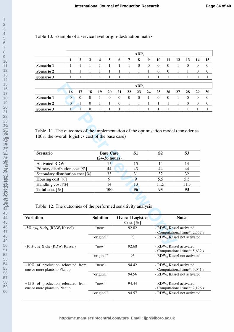
For Peer Review O

nly

Table 10. Example of a service level origin-destination matrix

ADPj

1 2 3 4 5 6 7 8 9 10 11 12 13 14 15

Scenario 1 1 1 1 1 1 1 1 0 0 0 0 1 0 0 0

Scenario 2 1 1 1 1 1 1 1 1 1 0 0 1 1 0 0

Scenario 3 1 1 1 1 1 1 1 1 1 1 1 1 1 0 1

ADPj

16 17 18 19 20 21 22 23 24 25 26 27 28 29 30

Scenario 1 0 0 0 1 0 0 0 0 1 0 0 1 0 0 0

Scenario 2 0 1 0 1 1 0 1 1 1 1 1 1 0 0 0

Scenario 3 1 1 0 1 1 1 1 1 1 1 1 1 1 1 1

Table 11. The outcomes of the implementation of the optimisation model (consider as

100% the overall logistics cost of the base case)

Scenario Base Case

(24-36 hours)

S1 S2 S3

Activated RDW 15 15 14 14

Primary distribution cost [%] 44 43 44 44

Secondary distribution cost [%] 33 31 32 32

Housing cost [%] 9 9 5.5 5.5

Handling cost [%] 14 13 11.5 11.5

Total cost [%] 100 96 93 93

Table 12. The outcomes of the performed sensitivity analysis

Variation Solution Overall Logistics

Cost [%]

Notes

“new” 92.82 - RDWh Kassel activated

- Computational time*: 2,557 s

-5% cwh & chh (RDWh Kassel)

“original” 93 - RDWh Kassel not activated

“new” 92.68 - RDWh Kassel activated

- Computational time*: 5,632 s

-10% cwh & chh (RDWh Kassel)

“original” 93 - RDWh Kassel not activated

“new” 94.42 - RDWh Kassel activated

- Computational time*: 3,041 s

+10% of production relocated from

one or more plants to Plant p

“original” 94.56 - RDWh Kassel not activated

“new” 94.44 - RDWh Kassel activated

- Computational time*: 2,126 s

+15% of production relocated from

one or more plants to Plant p

“original” 94.57 - RDWh Kassel not activated

Page 34 of 40

http://mc.manuscriptcentral.com/tprs Email: ijpr@lboro.ac.uk

International Journal of Production Research

123456789101112131415161718192021222324252627282930313233343536373839404142434445464748495051525354555657585960

peer

-007

2319

2, v

ersi

on 1

- 8

Aug

2012

For Peer Review O

nly

* The model was run on a 1.3 GHz chipset with 512 Mb DDR RAM

Page 35 of 40

http://mc.manuscriptcentral.com/tprs Email: ijpr@lboro.ac.uk

International Journal of Production Research

123456789101112131415161718192021222324252627282930313233343536373839404142434445464748495051525354555657585960

peer

-007

2319

2, v

ersi

on 1

- 8

Aug

2012

For Peer Review O

nly

Figure 1. Current configuration of the European Pirelli logistics network

Figure 2. LCp values (in tons) for the Pirelli Tyre case

Figure 3. Secondary distribution cost function for RDW1

Figure 4. NUTS3 areas covered within 24 hours from RDW1

Page 36 of 40

http://mc.manuscriptcentral.com/tprs Email: ijpr@lboro.ac.uk

International Journal of Production Research

123456789101112131415161718192021222324252627282930313233343536373839404142434445464748495051525354555657585960

peer

-007

2319

2, v

ersi

on 1

- 8

Aug

2012

For Peer Review O

nly

272x175mm (72 x 72 DPI)

Page 37 of 40

http://mc.manuscriptcentral.com/tprs Email: ijpr@lboro.ac.uk

International Journal of Production Research

123456789101112131415161718192021222324252627282930313233343536373839404142434445464748495051525354555657585960

peer

-007

2319

2, v

ersi

on 1

- 8

Aug

2012

For Peer Review O

nly

252x147mm (72 x 72 DPI)

Page 38 of 40

http://mc.manuscriptcentral.com/tprs Email: ijpr@lboro.ac.uk

International Journal of Production Research

123456789101112131415161718192021222324252627282930313233343536373839404142434445464748495051525354555657585960

peer

-007

2319

2, v

ersi

on 1

- 8

Aug

2012

For Peer Review O

nly

245x126mm (72 x 72 DPI)

Page 39 of 40

http://mc.manuscriptcentral.com/tprs Email: ijpr@lboro.ac.uk

International Journal of Production Research

123456789101112131415161718192021222324252627282930313233343536373839404142434445464748495051525354555657585960

peer

-007

2319

2, v

ersi

on 1

- 8

Aug

2012

For Peer Review O

nly

215x146mm (72 x 72 DPI)

Page 40 of 40

http://mc.manuscriptcentral.com/tprs Email: ijpr@lboro.ac.uk

International Journal of Production Research

123456789101112131415161718192021222324252627282930313233343536373839404142434445464748495051525354555657585960

peer

-007

2319

2, v

ersi

on 1

- 8

Aug

2012