#.

ANGULAR MOMENTUM EXCHANGE AMONG THE SOLID EARTH,ATMOSPHERE AND OCEANS:

A CASE STUDY OF THE 1982-83 EL NIliO EVENT

by

J. 0, Dickeyl, S. L, Marcusl, R, Hidezjl, T. M. Eubanksq and D. H. Boggsl

1Space Geodetic Science and Applications GroupJet Propulsion Laboratory

California Institute of TechnologyPasadena, California 91109-8099 USA

zOceanography Group, Clarendon LaboratoryThe Observatory, Parks Road

Oxford OX1 3PU, England, U.K.

%J.S. Naval ObservatoryWashington, D. C. 20392-5420

.7.Geophy.s.Res. (submitted)

January 3, 1994

1

Outline

Abstract

1. Introduction

2. Data Considered

2.1 Length-of-day

2.2 Atmospheric Angular Momentum

2.3 Southern Oscillation Index

3. Atmospheric Excitation of Interannual Variations

3.1 Background

3.2 Stratospheric Contribution

3.3 Bimodality Analysis

3.4 Error Estimates

4. Role of the Oceans

5. summary

Acknowledgments

Appendix

References

Tables

Figure Captions

Figures

2

ABSTRACT

The 1982-83 El Niiio/Southern Oscillation (ENSO) event was accompanied by the

largest ‘interannual variation in the Earth’s rotation rate on record. In this study we

demonstrate that #mospheric forcing was the dominant cause for this f@ational anomaly,

with at~ospheric”angular momentum (AAM) integrated from 1000 to 1 mb (troposphere

plus atmosphere) accounting for up to 92% of the interannual variance in the length-of-day

(LOD). Winds between 100 and 1 mb contributed nearly 20% of the variance explained,

indicating that the stratosphere can play a significant role in the Earth’s angular momentum

budget on interannual time scales. Examination of LOD, AAM, and Southern Oscillation

Index (S01) data for a 15-year span surrounding the 1982-83 event suggests that the strong

rotational response resulted from constructive interference between the low-frequency (- 4-

6 year) and quasi-biennial (- 2-3 year) components of the ENSO phenomenon, as well as

the stratospheric QBO. Sources of the remaining LOD discrepancy (- 55 ~s) are explored;

data noise and systematic errors are estimated to contribute 18 and 33 Ls, respectively,

leaving a residual of 40 ys unaccounted for. Oceanic angular momentum contributions

(both moment of inertia changes associated with baroclinic waves and motion terms) are

shown to be candidates in closing the interannual axial angular momentum budget.

1. Introduction “

The rotation rate of the solid Earth exhibits minute but complicated changes of up to

several parts in 10s in speed [corresponding to a variation of several milliseconds in the

length of day (LOD)] and even larger variations in the direction of the rotation axis (polar

motion). These changes occur over a broad spectrum of time scales, ranging from days to

centuries and longer, reflecting the fact that they are produced by a wide variety .of

geophysical and astronomical phenomena. The extent to which fluctuations in the angular

momentum of the atmosphere Hi(t) give rise to compensating changes in the angular

3

momentum of the”solid Earth, thereby exciting contributions to LOD [ = A(t)] , has been

the subject of many studies. Advances have been made possible by the availability for the

past decade of routine daily or twice-daily determinations of all three components of Hi(t)

by several meteorological agencies [see for example, Hide and Dickey, 1991 and references

therein]. These studies are facilitated by the use of dimensionless functions xi, i = 1, 2, 3

introduced by Barnes et aL [1983] related to the equatorial components HI and Hz, and the

axial component H3.

The axial component %3satisfies

where (@,A) denote latitude and longitude respectively,p.(@At) is the surface Pressure

and u(@Zp,t) the eastward (westerly) component of the wind velocity at the Pressure level

p. The calculations presented here follow Barnes et al. [1983] and take R = 6.37 x 106 m

for the mean radius of the solid Earth, andg=9.81 ins-z for the mean acceleration due to

gravity. The coefficient 0.70 incorporates the so-called “Love number” correction which

allows for small concomitant changes in the inertia tensor of the imperfectly-rigid solid

Earth. The dominant contribution to fluctuations in ~(t) comes from the “wind” term given

by the first integral of the right-hand side of equation (1.1), which depends on the strength

of the zonally averaged eastward wind speed u and also on its distribution with latitude.

given by the second integral are generally smaller, btitFluctuations in the “matter” term

make a significant contribution.

The seasonal and intraseasonal LOD components are well accounted for in terms of

the exchange of angular momentum between the atmosphere and the solid Earth [see for

example Lambeck, 1988; Hide and Dickey, 1991 and references therein]. Meteorological’

effects cannot be the dominant cause of the larger decadal variations, but it is a matter for

investigation as to whether meteorological excitation is the main cause of the interannual

4

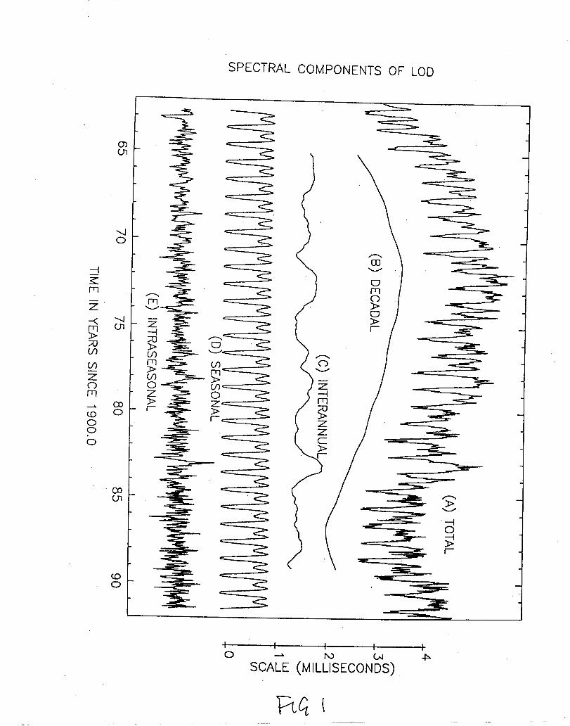
variations on time scales ranging from 1 to 5 years. The amplitude of this component of the

spectrum, up to 0.5 ms, is comparable with that of the seasonal cycle (see Fig. 1),

implying that the atmosphere could play a significant role in its generation.

Fig. 1 near here

In this paper we adduce evidence that atmospheric motions are largely responsible

for generating Earth rotation fluctuations on these interannual time scales, focusing on the

1982-83 ENSO event. These results are obtained from comparisons of the interannual LOD

fluctuations with operational atmospheric angular momentum (AAM) estimates, combined

with geostrophic wind estimates derived from satellite temperature soundings of the

stratosphere. A description of the data sets is presented in Section 2. Sections 3 and 4 deal

with the atmospheric and oceanic excitation of interannual LOD variations, respectively.

Results are summarized in the final section. The reader is also referred to several more

general accounts of the excitation of Earth orientation changes. References to early work

can be found in the classical monograph on the subject by Munk and MacDonald, [1960]

and to more recent work in various monographs and other publications [e.g., Cazenave,

1986; Dickey, 1993; Dickey and Eubanks, 1986; Eubanks, 1993; Hide, 1977, 1984, 1986;

Hide and Di,ckey, 1991; Larnbeck, 1980 and 1988; Moritz and Mueller, 1987; Rosen,

1993; and W’ahr, 1988].

2. Data Considered ‘

2.1 Zzngth-of-Day

The LOD series utilized (Fig. 1) is the Jet Propulsion Laboratory (JPL) Kalman-

filtered series, which combines Earth rotation results from optimal astrometry, Very Long

Baseline Interferometry (VLBI) and Lunar Laser Ranging (LLR) to form a high-quality

series, in which the issues of reference frame commonality and the unevenness of data

quality and quantity have been addressed [Gross, 1992; Morabito et al., 1988]. The LOD

data improves in quality with time, especially after 1985. In 1976 the uncertainty is about

5

0.09 ms, decreasing almost linearly to about 0.03 ms in 1985 and thereafter. During the

1982-83 ENSO, the uncertainty is 0.05-0.06 ms. Since the average spacing of data points

used as input to the Kalman filter at this time is about five days, we estimate that annual

mean LOD values during the 1982-83 ENSO contain -73 degree of freedom, so that the

error associated with interannual variations is -7 ps [see Dickey et al., 1992a for a further

discussion of the spectral characteristics of LOD errors].

2.2 Atmospheric Angular Momentum

For the AAM data, we use two series that are available during the 1982-83 ENSO

event, from the National Meteorological Center (NMC) and the European Centre for

Medium Range Weather Forecasts [ECMWF—see Salstein et al., 1993 for a review of

existing data]. Analyses incorporating winds up to the 100 and 50 mb levels, respectively,

as well as the full pressure term are available from both centers; in addition, the pressure

term incorporating the inverted barometer correction is provided by the NMC. We also

consider zonal wind variations from 100 mb to the 1 mb level, computed by Hirota [1983]

from temperature soundings using the geostrophic assumptions [see Rosen et al,, 1985 for

further details of this series]. These data were combined with the 100 mb values to obtain

AAM variations incorporating almost the full atmosphere (1000 to 1 rob). Formal errors are

not provided with the AAM values; estimates of the uncertainty in the AAM data are

considered in Section. 3.4

2.3 Southern Oscillation Index

We use here a modified version of the index based on the Tahiti and Darwin surface”

pressure data, provided by the NMC Climate Analysis Center [Rasmussen, private

communication]. Our “Modified Southern Oscillation Index” (MSOI) is given as the

difference between the Darwin and Tahiti surface pressures in millibars, and is positively

correlated with the LOD.

6

3. Atmospheric

3.1 Background

Excitation of Interannual LOD Variation

Several earlier studies attempted to link interannual LOD variations (defined here to

be A*P, following notation of Hide and Dickey, 199l—see Fig. 1) to the Quasi-Biennial

Oscillation (QBO) exhibited by zonal winds in the equatorial stratosphere [for a review, see

L.ambeck, Chapter 7, 1980]. Lumbeck and Cazenave [1973], for example, associated A*P

changes during the 1955-71 period with the QBO. Subsequent work by Stephanie [1982]

indicated a connection between A* p and the “Southern Oscillation” by establishing

coherence between A*P and fluctuations in ‘equatorial Pacific air temperature, which is

related to the intensity of the Southern Oscillation, Further investigations were stimulated

by the occurrence of an unusually strong and well observed El Nifio in 1982-83 [see e.g.

Philander, 1983 and 1990; Rasmussen and Wallace, 1983]. The largest changes ever

recorded in A*P and AAM occurred during January and February 1983 [Rosen et al., 1984

and Eubanks et al,, 1985a].

The El Nifio/Southern Oscillation (ENSO) phenomenon is associated with

persistent but irregular variations of atmospheric pressure over the South Pacific on

interannual time scales. This gives rise to pronounced year-to-year variations in the climate

of the South Pacific basin [Rasmussen and Wallace, 1983] associated with extensive

fluctuations in the atmospheric and oceanic circulation and in sea surface temperatures

[Philander, 1983 and 1990]. The dynamical processes involved include nonlinear air-sea

interactions, with changes in the sea surface temperature causing changes in the surface

winds which, in turn, modify ocean surface waters, providing a feedback loop. The

persistence of the oscillation is probably a consequence of the thermal inertia of the oceans,

which provides a means of storing heat from one year to the next. According to a model by

Wyrtki [1985], the ENSO cycle is driven by the steady accumulation of warm water in the

western part of the equatorial Pacific caused by the prevailing surface easterly winds. An El

7

Niiio event is triggered by a relaxation of the easterlies, which causes a surge of warm

water to move from the West to the East Pacific until it encounters the coasts of North and

South America, where it is deflected to higher latitudes in both hemispheres. The El Nifio

events thus serve to remove the excess warm equatorial water, setting the stage for the

oscillation to begin again. The associated “Southern Oscillation” in surface air pressure has

the structure of a standing wave, with antinodes near the eastern and western boundaries of

the South Pacific, - 90° longitude apart [lJorel and Wallace, 1981]. This has led to the

development of various Southern Oscillation Indices (S01) based on the difference between

sea level surface pressure in the East and West Pacific. The most commonly used index is

based on the normalized seasonally adjusted pressure difference between Tahiti, in the east,

and Darwin, Australia, in the west [Chen, 1982].

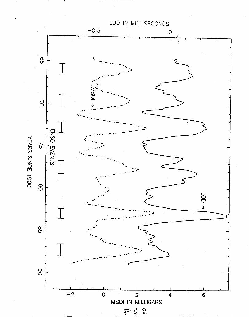
Figure 2 presents a comparison between interannual variations in the Earth’s

rotation, measured as changes in A~(t), and the strength of the ENSO cycle, represented by

the Modified Southern Oscillation Index (MS OI—see Section 2.3) series. Here the

interannual fluctuations are taken to be the difference between one-year and five-year

running means of each data type. The agreement between the two series is striking, with

high interannual values of LOD generally coinciding with ENSO events, represented as

periods for which the MSOI has a continuous positive anomaly of more than one-half its

standard deviation. During an ENSO event, the MSOI (S01) reaches a maximum

(minimum), leading to an increase in XS(t) associated with the collapse of the tropical

easterlies. Further increases in Z-j(t) may result from a strengthening of westerly flow in

the sub-tropical jet streams [Rosen et al,, 1984], Conservation of total angular momentum

then requires the Earth’s rate of rotation to slow down, thus increasing A. The largest

variations seen in A&t) are evidently associated with the 1982-83 ENSO event.

Fig. 2 near here

A one-month time-lag in A$t) relative to the MSOI is found to give the maximum

cross-correlation (0.67). For shorter record lengths, higher correlations are obtained (e.g.,

8

a correlation ‘of 0.79 with A~(t) lagging the MSOI by two months for the period 1972-

1986), although the level of statistical significance is about the same [Dickey et al., 1993].

Other studies have indicated significant correlation between interannual LOD variations and

indices of the Southern Oscillation; Chao [1984] reported a correlation coefficient of 0.56

for the period 1957-1983, while Eubanks et al. [1986] computed a correlation coefficient of

-0.5 for the period 1962-1984, and Chao [1988] found a correlation of 0.68 for the period

1962-1984, Chao [1989] also obtained a correlation coefficient of 0.75 for the period

1964-1984 by using multiple regression on the SOI and a stratospheric AAM series,

derived from monthly data from three stations using an idealized model of the QBO.

3.2 Stratospheric Contribution

Routine determinations of the atmospheric ~ functions are available since 1976,

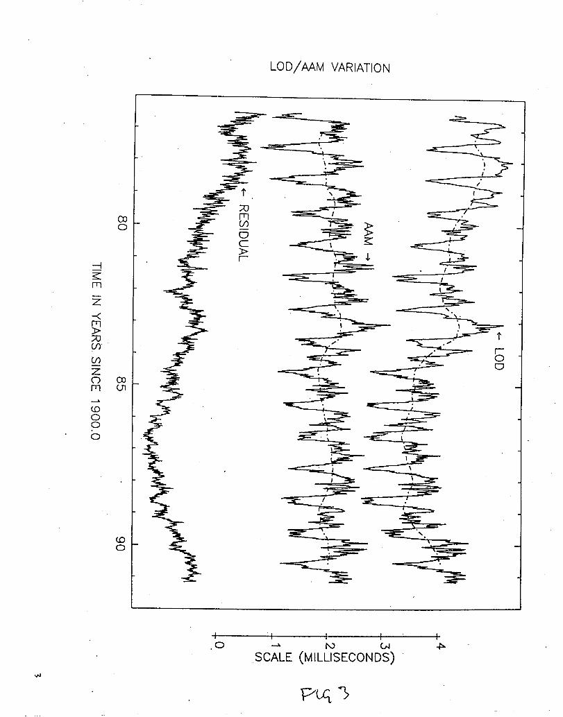
using data compiled from the NMC. Figure 3 shows a comparison between LOD and

AAM, calculated from zonal winds integrated up to the 100 mb level, for the 15-year period

extending from June, 1976, to May, 1991. Since the LOD is given as a residual from the

standard length-of-day (86400 S1 seconds), the vertical offset between the LOD and AAM

curves has no physical significance. Note that the quality and quantity of the space-geodetic

data improved substantially in 1985, resulting in a higher time-resolution LOD series after

this time. Excellent agreement is seen between the two series over the entire span when

variations with periods of two years or less are considered, Considerable discrepancy is

found on longer time scales, however, as indicated by the divergence of the annual running

means for the two data types (dot-dash lines in Fig. 3),

Fig. 3 near here

Previous studies [Dickey et al., 1990 and Rosen et al., 1990] found the residual

between the overlapping LOD and AAM series to be dominated by a long-term linear drift

with some indication of a second-order term being significant. Examination of the residual

with the longer data sets now available shows the clear presence of a second-order term

9

(bottom curve in Fig. 3), which is due to decadal effects present in the LOD series.

Interannual changes are also seen in the slope of the residual, and have been associated

with the ENSO phenomenon [Dickey et al., 1990]; Rosen et al. [1990] concluded that

either core-mantle coupling is a nonsteady phenomenon or that unmodeled oceanic

processes are responsible for the intermittence of the slope. The residual also shows a

strong semi-annual signature, indicative of a missing stratospheric component on seasonal

time scales [Rosen and Salstein, 1985].

In order to form a more quantitative estimate of atmospheric forcing during the

1982-83 ENSO, we combined the operational atmospheric analyses available from the

NMC and ECMWF with the satellite-derived stratospheric data to form daily AAM series

that integrate the angular momentum of the atmosphere up to 1 mb for the period 1980

through 1986. While the span of this atmospheric data is too short to allow for a spectral

study, its temporal coverage is ideally suited for a case study of the intense 1982-83 El

Nifio, which was associated with the largest interannual variations of LOD and AAM on

record (cf. Fig. 1). In order to focus on interannual variations, all series were subject to a

365-day moving average; a cosine taper was applied to the first and last 10% of the

average, in order to reduce ripple effects [Bloomjield, 1976]. Decadal effects were

removed by detrending each of the smoothed series.

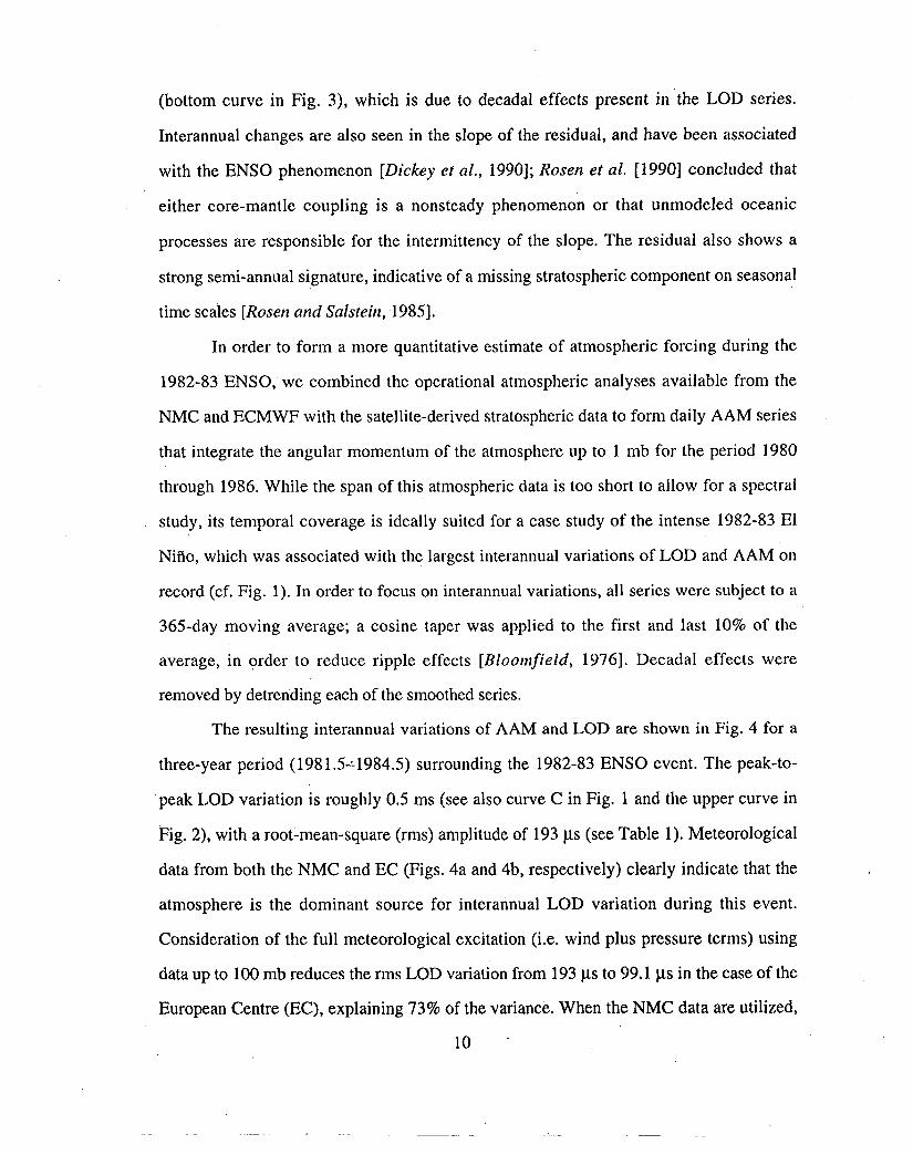
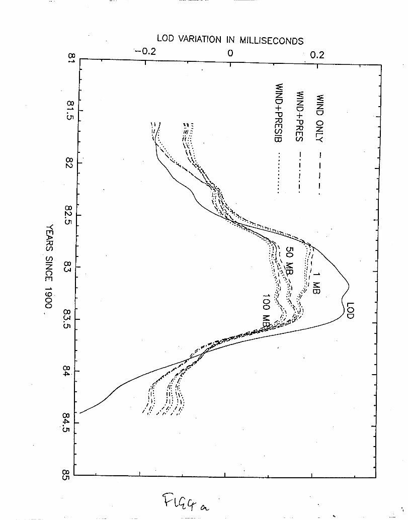
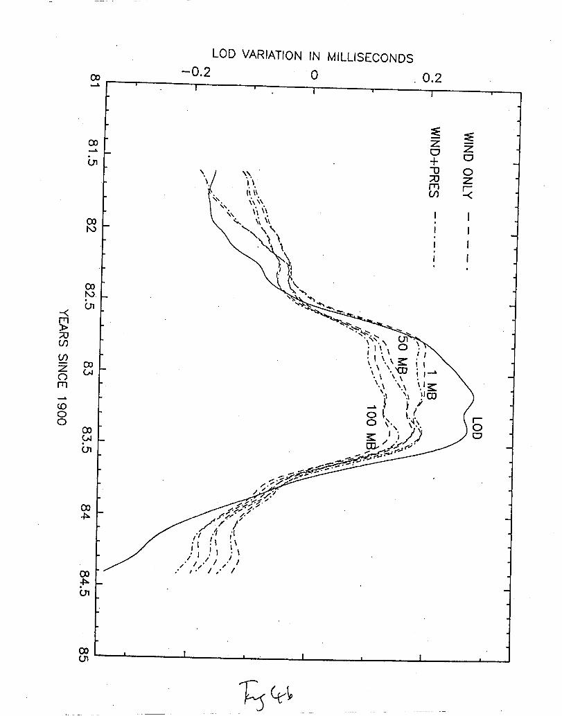
The resulting interannual variations of AAM and LOD are shown in Fig. 4 for a

three-year period (198 1.5=1984.5) surrounding the 1982-83 ENSO event. The peak-to-

peak LOD variation is roughly 0.5 ms (see also curve C in Fig. 1 and the upper curve in

Fig. 2), with a root-mean-square (rms) amplitude of 193 ps (see Table 1). Meteorological

data from both the NMC and EC (Figs. 4a and 4b, respectively) clearly indicate that the

atmosphere is the dominant source for interannual LOD variation during this event.

Consideration of the full meteorological excitation (i.e. wind plus pressure terms) using

data up to 100 mb reduces therms LOD variation from 193 ws to 99.1 us in the case of the

European Centre (EC), explaining 73% of the variance. When the NMC data are utilized,

10

.—

the residual is decreased to 104.7 LS with 70,6V0 of the variance accounted for. The

utilization of atmospheric data integrated to 50 mb further increases the variance explained.

For the EC case, the LOD-AAM residual becomes 75.8 p,s (84.6% variance explained),

while for the NMC data, the residual is 89.6 ps (78.4% variance explained).

Fig. 4 near here

The utilization of the atmospheric data up to the 1 mb level decreases the residual,

further. The EC wind plus pressure terms now accounts for 91.9% of the variance, leaving

a residual of 55 ps. The corresponding NMC data set explains 89.0% of the variance with

64 ps remaining. Thus the stratosphere does make a significant contribution to interannual

AAM variation during this event, with atmospheric data integrated from 100 to 1 mb

explaining nearly an additional 20’ZOof the LOD variance. This is not surprising for

stratospheric winds are typically twice as strong as tropospheric winds on average. We also

note that the application of EC data consistently gives lower unexplained residuals, and that

the pressure term had only a small (~ 1?o) effect on the amount of variance explained in all

cases considered. The inclusion of the pressure term with the inverted barometer correction

(available from the NMC analysis only) reduces the explained variance at all three levels

studied, indicating some difficulty either with the inverted barometer model, or with the

quality of the pressure term estimates, on interannual time scales.

Chao [1989] noted an apparent lead of the idealized stratospheric AAM with respect

to LOD of about 1 month, which is the resolving interval of the data he analyzed. A similar

effect can be seen in the daily data plotted in Fig. 4, where the 100mb and 50mb AAM

curves show their maximum departures during the mature phase of the 1982-83 event,

while the full AAM (integrated up to lmb) has its peak near the end of the onset phase (late

1982). This implies that the strongest variations in the stratosphere preceded both the

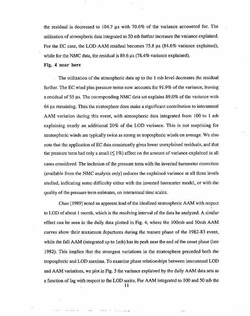
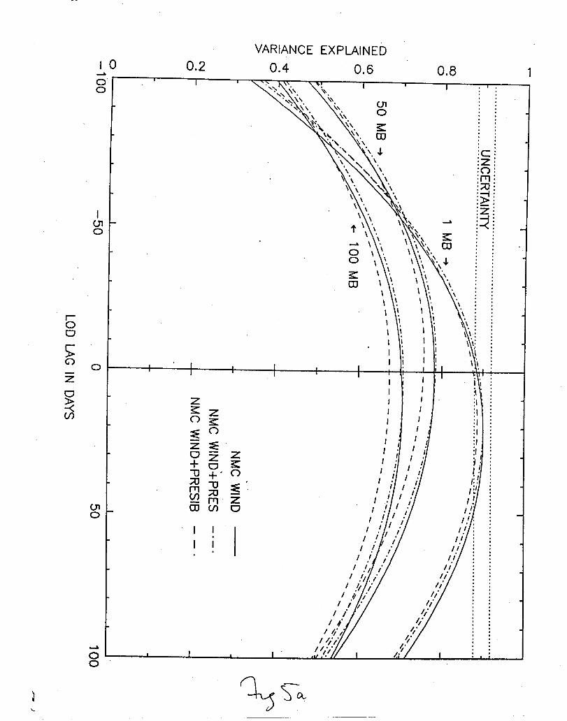
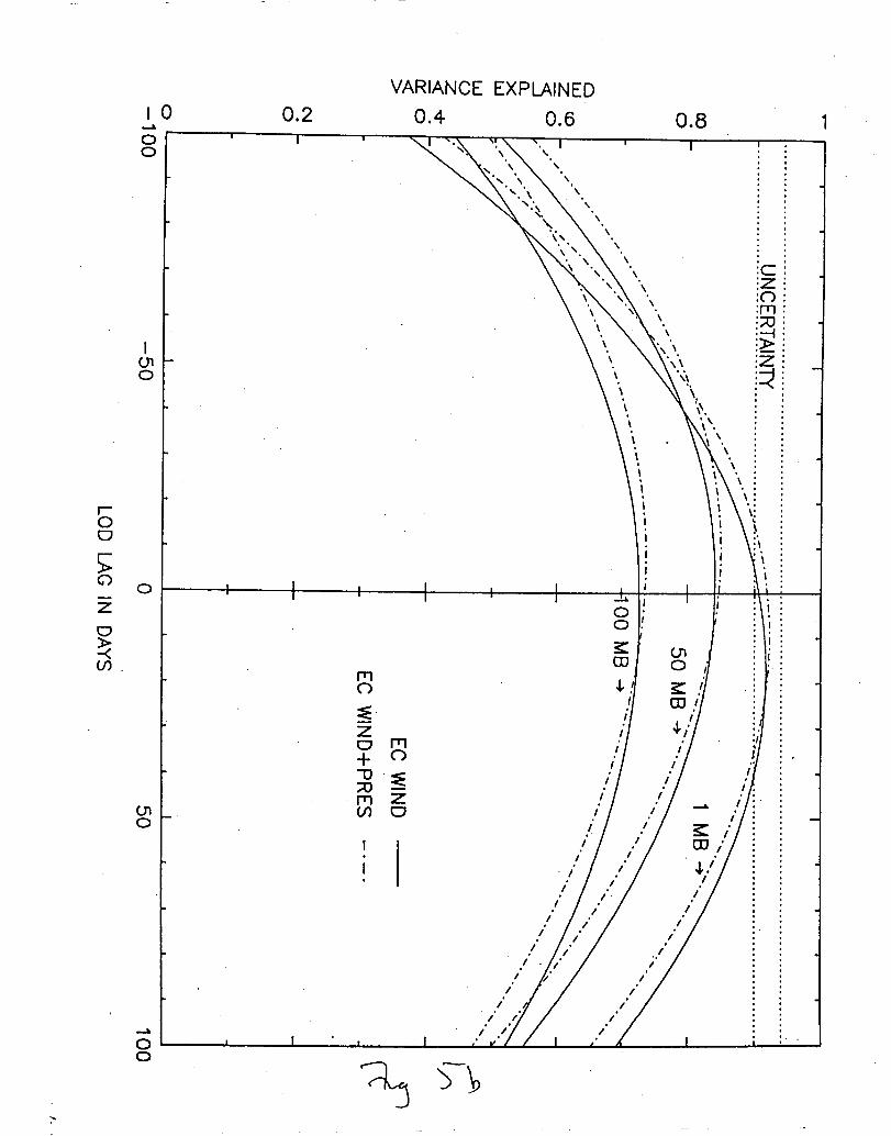
tropospheric and LOD maxima. To examine phase relationships between interannual LOD

and AAM variations, we plot in Fig. 5 the variance explained by the daily AAM data sets as

a function of lag with respect to the LOD series. For AAM integrated to 100 and 50 mb the11

explained variance is approximately symmetric with respect to zero, with no discernible lag

or lead between the two data types. When the stratospheric data are considered with NMC

analysis, however, the LOD appears to lag by about 20 days, with the AAM explaining a

maximum of 90% of the interannual LOD variations. A similar analysis using EC data

indicates a smaller lag for the LOD (10 days with wind plus pressure and 16 days with

wind only), with the AAM explaining a maximum of 92% of the variance. If we consider

the difference of 2% to be a lower bound on the uncertainty in the explained variance, these

results are consistent with a null hypothesis of zero lag between the two data types and the

apparent lead is not statistically significant.

Fig. 5 near here

3.3 Bimodality Analysis

Several studies have shown that the ENSO phenomenon is bimodal in nature, with

a quasi-biennial (QB) component having periods in the 2-3 year range and a low-frequency

(LF) component with periods in the 4-6 year range [Rasmussen et al., 1990; Barnett, 1991;

Keppenne and Ghil, 1992]. For a 15-year span surrounding the 1982-83 event, in

particular, spectral analysis of both LOD and SOI data further indicates bimodality with

clear peaks at periods centered at 4.2 and 2.4 years [Dickey et al., 1992]. Here, we use the

recursive filter of Murakami [1979] to study variations of LOD, SOI, and AAM data for the

same 15-year span in the QB (18-35 month) and LF (32-88 month) bands defined by

Barnett [1991]. In addition, the currently available six-year record of stratospheric AAM

(spanning 1980-86) is considered.

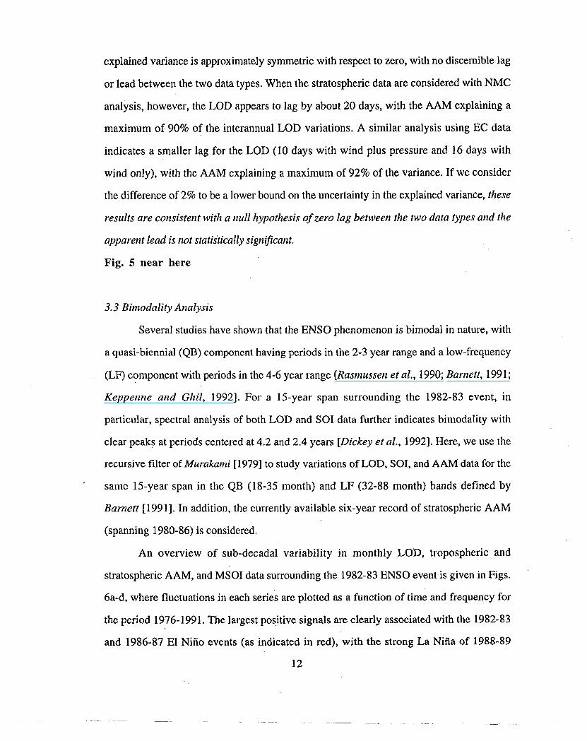
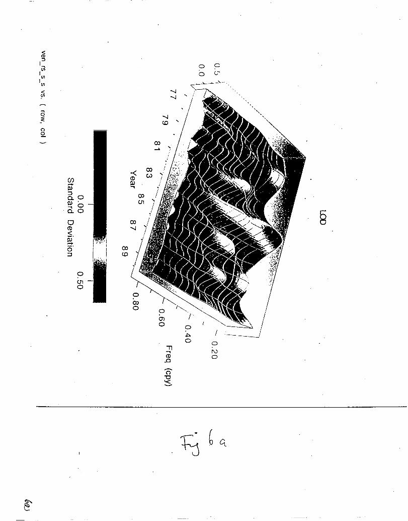
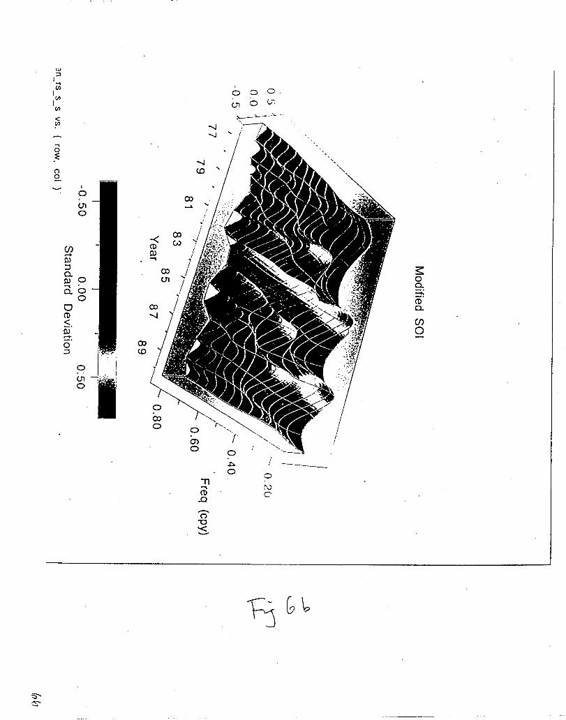
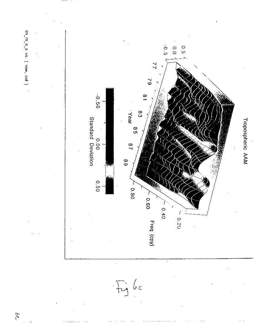
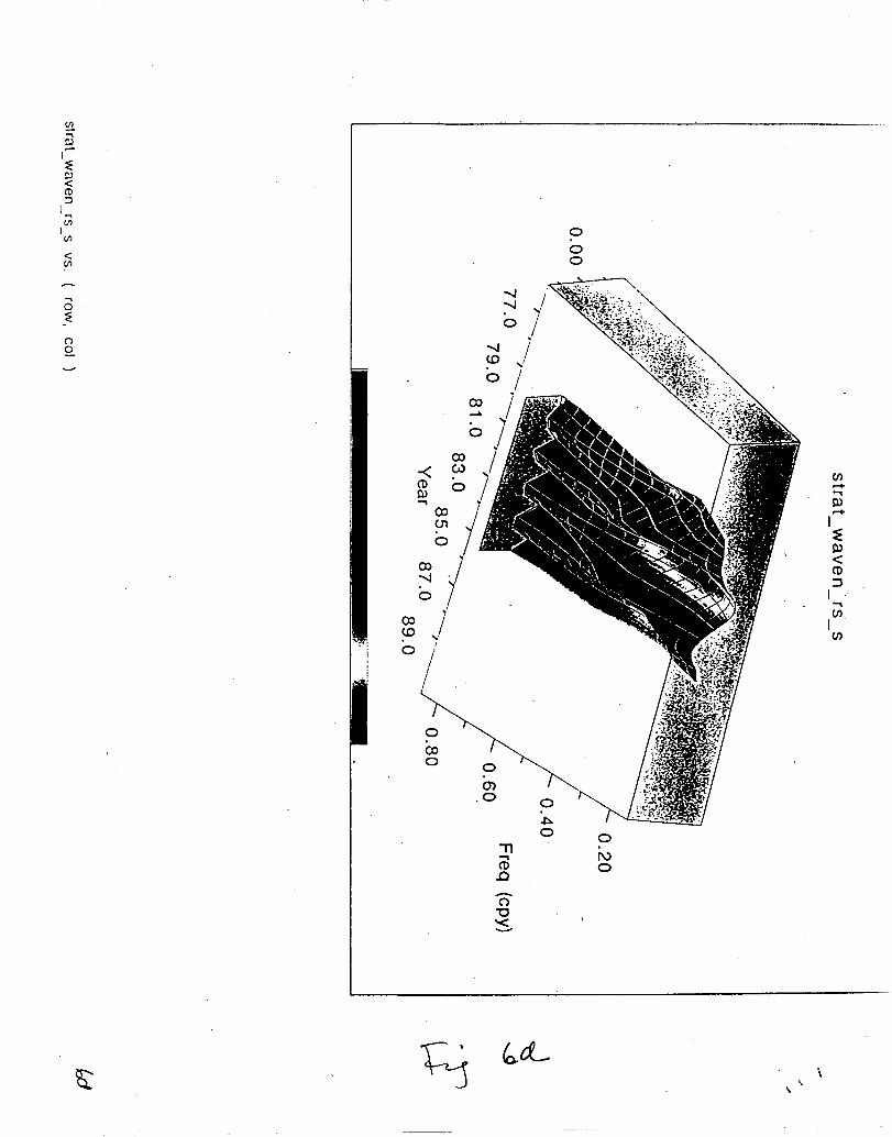
An overview of sub-decadal variability in monthly LOD, tropospheric and

stratospheric AAM, and MSOI data surrounding the 1982-83 ENSO event is given in Figs.

6a-d, where fluctuations in each series are plotted as a function of time and frequency for

the period 1976-1991. The largest positive signals are clearly associated with the 1982-83

and 1986-87 El Nifio events (as indicated in red), with the strong La Niiia of 1988-89

12

appearing as a negative signal in all three data types. Bimodality on interannual time scales

is evident, with enhanced variability appearing at relatively low (4-6 year) and quasi-

biennial (2-3 year) frequencies. ENSO and La Nifia events result when variations in both

bands add constructively to produce a significant index; for example, in 1977-78, 1982-83,

and 1986-87, positive signals from both bands produce significant ENSO events, while in

1988-89, negative signals from both bands result in a La Niiia event. In contrast, positive

QB components interfere destructively with the LF components in 1980-81 and 1984-85

with no resultant events.

Fig 6 near here, please

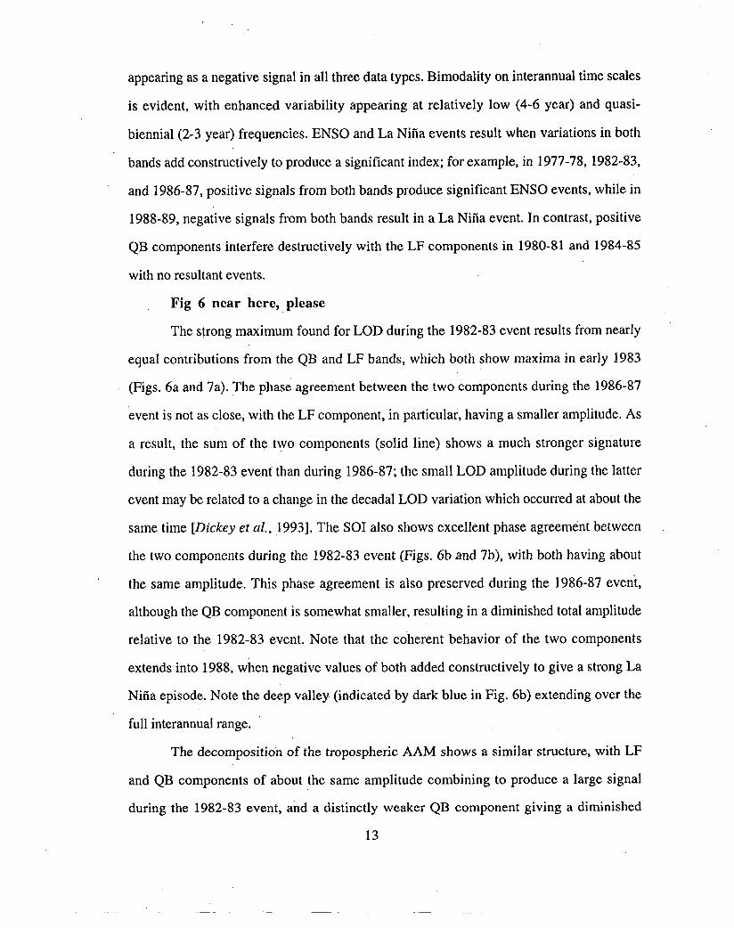
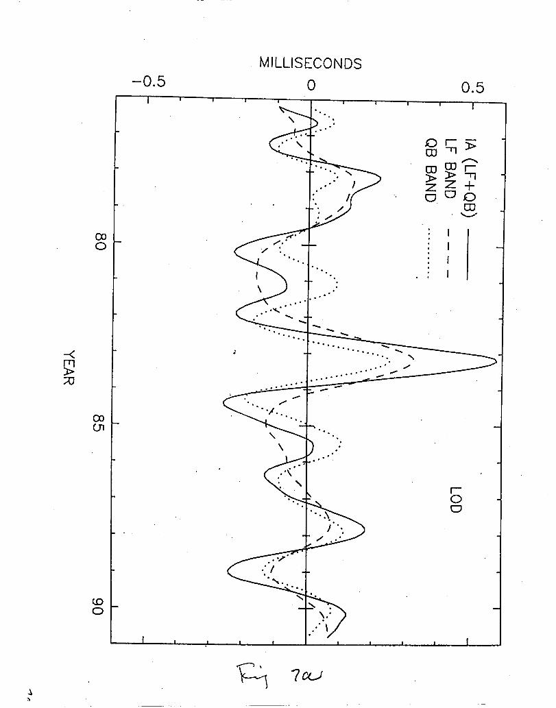
The strong maximum found for LOD during the 1982-83 event results from nearly

equal contributions from the QB and LF bands, which both show maxima in early 1983

(Figs. 6a and 7a). The phase agreement between the two components during the 1986-87

event is not as close, with the LF component, in particular, having a smaller amplitude. As

a result, the sum of the two components (solid line) shows a much stronger signature

during the 1982-83 event than during 1986-87; the small LOD amplitude during the latter

event may be related to a change in the decadal LOD variation which occurred at about the

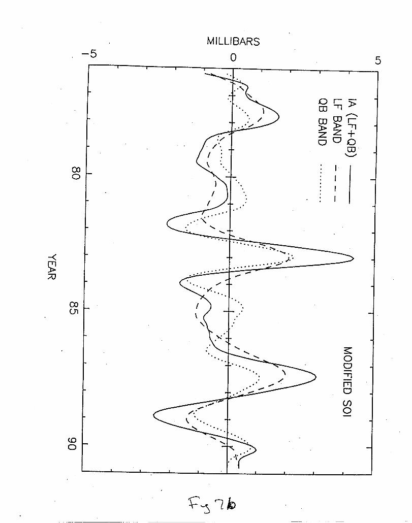
same time [Dickey et al., 1993]. The SOI also shows excellent phase agreement between

the two components during the 1982-83 event (Figs. 6b and 7b), with both having about

the same amplitude. This phase agreement is also preserved during the 1986-87 event,

although the QB component is somewhat smaller, resulting in a diminished total amplitude

relative to the 1982-83 event. Note that the coherent behavior of the two components

extends into 1988, when negative values of both added constructively to give a strong La

Niiia episode. Note the deep valley (indicated by dark blue in Fig. 6b) extending over the

full interannual range.

The decomposition of the tropospheric AAM shows a similar structure, with LF

and QB components of about the same amplitude combining to produce a large signal

during the 1982-83 event, and a distinctly weaker QB component giving a diminished

13

amplitude for the 1986-87 event (Fig. 7c). Interannual fluctuations in tropospheric AAM

are closely related to the ENSO cycle, as evidenced by the similarity of their signatures in

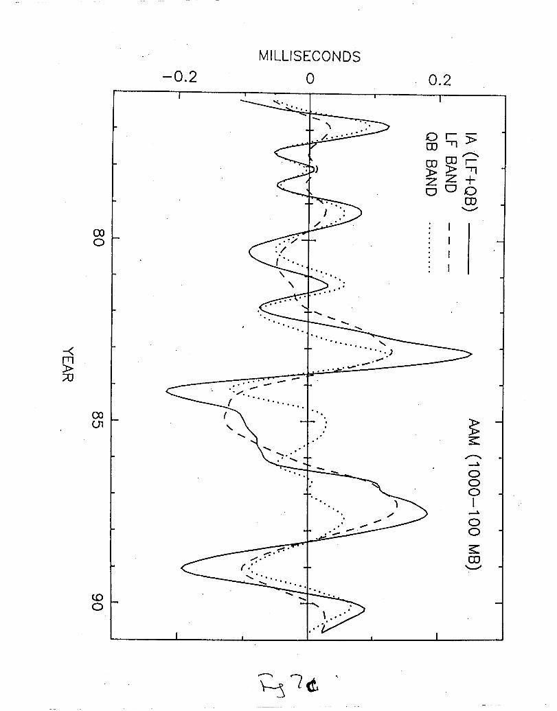
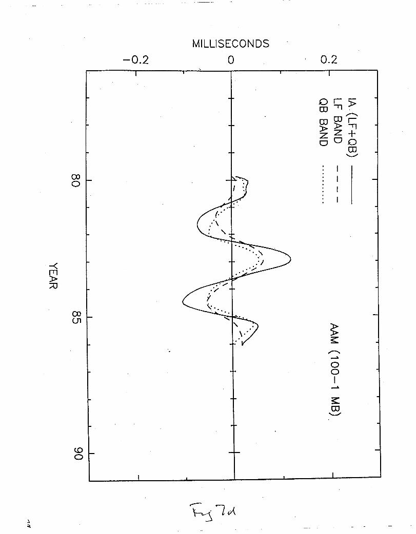
Figs. 6b and 6c. The shorter record of stratospheric AAM (Fig. 7d) also shows phase

agreement between the QB and LF components during the 1982-83 event, although this

decomposition is less meaningful given the limited span of data available.

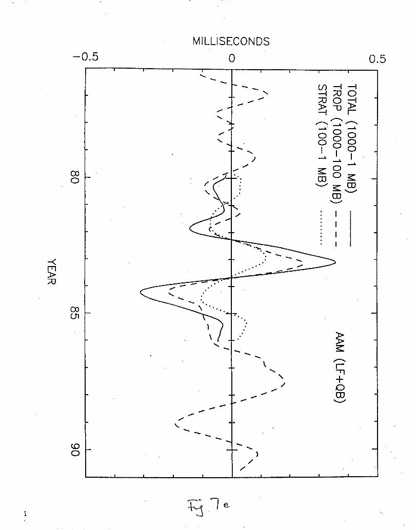
The total interannual variation (sum of the QB and LF bands) for AAM in the

troposphere, stratosphere, and the full atmosphere (1000- 1 mb) is shown in Fig. 7e. Note

that while the stratosphere as defined in this study contains only 10% of the mass of the

atmosphere, its contribution to the 1982-83 rotational anomaly is roughly half that of the

troposphere. This is consistent with the results of Chao [1989], who used multiple

regression to show that an index of stratospheric AAM, derived using monthly data from

three stations with an idealized model of the QBO, accounted for about half the LOD

variation associated with the SOI. While they have similar time scales, dynamical

connections between QB variations in the troposphere and stratosphere remain elusive (e.g.

XU, 1992; Barnett, 1991; see, however, Yasunari 1989); thus, it is possible that the

fortuitous coincidence in phase between these two oscillations, as shown by their AAM

signatures (dotted lines in Figs. SCand 5d), may have contributed to the unusually large

amplitude of the 1982-83 ENSO.

3.4 Error Estimates

The results of the case study demonstrate that atmospheric forcing was the

dominant source of interannual LOD variations during the 1982-83 ENSO event, the largest

for which detailed records exist. The atmosphere integrated to the l-rob level accounted for

up to 92$Z0of the variance, leaving an unexplained rms residual of -60 ps (55 ps and 64

ps in the EC and NMC case, respectively) in the interannual LOD. In order to investigate

the source of this discrepancy, we assume that both the LOD and AAM data sets are

14

.

composed of a common geophysical signal, S, and noise components,

respectively, assumed to be uncorrelated with the signal and with each other:

LOD = L(t) = S + NL

NL and NA

AAM = X(t) = S + NA.

The expected power of the residual between the two series is then

<(L-X)2> = <NLZ>-t <NAS>.

As indicated in Sect. 2.1, the estimated error pertaining to interannual LOD determinations

during the period of the case study is -7 ps; for a residual with rms value -60 p,

therefore, the effect of the LOD error is essentially negligible (c 1 ys). Similarly, since the

contribution of the atmosphere above 1 mb is estimated to be -4 ps (see Sect. 2.2), its

effect on the size of the rms residual can also be neglected. We hypothesize, therefore, that

the observed residual arises from noise in the AAM signal considered (1000 – 1 rob).

In order to estimate the noise associated with the AAM signal, we initially assume

that AAM errors from different centers are independent. Hence, the expected power of the

intercenter difference (i,j) is

<(Xi-Xj)2> = <Niz> + <Njz> = 2 E

where E denotes the”average squared error for the centers considered.

The rms residual between the EC and NMC (wind plus pressure) data sets at 100 mb and

50 mb is 13.1 ~s and 18.2 ps, respectively; hence

E1O(X)-IOO = (13.1)2/2 = 85.5

and

E10W-50= (18.2)2/2 = 165.5

ps2

ps2

where the subscript on the left-hand side indicates the pressure levels considered. If the

errors from different levels are uncorrelated, then

E] 00-50= EIC)Oo-50– EloO&100-80 ~S2,

so that the error variance of the 50-mb layer lying directly above the 100-mb level is

approximately equal to that of the entire atmosphere beneath it. Since independent

15

determinations of stratospheric AAM were not available for the period of this study, the

error for the 50-1 -mb layer cannot be estimated directly. Particularly in view of the fact that

winds in this layer were estimated solely from satellite temperature soundings in contrast to

the operational analyses available up to the 50 mb level, it is reasonable to expect that the

error variance contributed by this layer is also comparable to that of the atmosphere below

it. We assume, therefore, that

E50_1- E1000-50,

so that

Elooo-1 = E5&1 + E1000_5CI-2 E10(Io_50= 331 @,

and we estimate for the AAM noise an rms value of

NA -18.2 PS.

Note that because of the assumptions made above, this is the same value as found for the

inter-center difference between the two series at 50 mb.

All numerical weather prediction centers have access to the same suite of

meteorological data. If these observations contain errors due to missing or inaccurate data

(e.g. in the tropics or the Southern Hemisphere), a systematic AAM error may arise which

cannot be detected by inter-center comparisons. The total AANi error is then taken to be

NA=Ns+Ni

where Ns denotes the systematic component, common to all centers, and Ni is the inter-

center error estimated above. Under the assumption that the

errors are uncorrelated, the expected error variance becomes

<(L–X)2> = <Niz> + <Nsz>,

where the interannual LOD error NL has been neglected.

systematic and inter-center

In a study of sub-seasonal variations in the Earth’s angular momentum budget,

Dickey et al. [1992b] found that systematic AAM error behaved as flicker noise, with a

power spectral density of the form

P(f) = E~(f~f),

16

where f. is a standard frequency ( = 0.1 cycles/day) , and EA -0.009 ms2 (cycles/day)-l.

If we assume that this behavior extends to interannual frequencies, the power of the

systematic error may be estimated as

N:= E*f~ Jfz

‘2 $ = E*f~ In (G) = 0.001 ms2,f,

where the frequency interval is bounded by the averaging time (1 year) and the length of the

record considered (3 years). The resulting estimate for the systematic noise is NS= 31.6

ps. However, the interannual AAM fluctuations may be more heavily influenced by data-

poor regions (such as the stratosphere as shown by this study) than the sub-seasonal

variations, which would increase the systematic noise.

Combining this value with the uncorrelated inter-center error estimated above gives

a likely lower bound of about 37 ps for the interannual rms residual arising from noise in

the AAM data. Residuals of 55 and 64 ps were found using the l-rob wind-plus-pressure

series for the EC and NMC, respectively, during the case study (cf. Table 1), implying the

possible existence of an additional (uncorrelated) source of excitation with rms variation on

the order of 40 to 50 us when the EC or NMC data are considered. Possible oceanic

contributions to this discrepancy are discussed in the following section.

4. Role of the Oceans

The analysis of the preceding section has shown that the dominant portion of the

interannual LOD variation observed during the 1982-83 ENSO event can be explained by

variations in globally-integrated atmospheric angular momentum (AAM), Furthermore, the

lack of a significant delay between the AAM and LOD series examined in this study implies

a relatively rapid exchange of angular momentum between “thesolid Earth and atmosphere.

A significant

torque at the

W@-, 1988].

portion of this exchange may occur directly over land, through frictional

surface or pressure gradients acting across orography [Swinbank, 1985;

WoZf and Smith [1988], in particular, presented evidence that rapid AAM

17

variations observed at the peak of the 1982-83 ENSO were produced by mountain torques

acting over the Rockies. Furthermore, in a study of the AAM budget from a 20-year climate

simulation using the Canadian Climate Centre general circulation model, Boer [1990] found

that the dominant portion of angular momentum exchange on sub-annual time scales (in the

model) occurred over land.

On the longest time scale resolved in Boer’s analysis (1 year), however, the AAM

variance explained by surface stress over the ocean was twice that associated with the

combined friction and mountain torque over the land, indicating that ocean torques may

predominate on interannual time scales. The ENSO cycle, in particular, is associated with

pronounced fluctuations in the strength of the surface winds over the tropical oceans [e.g.

Lukas et al., 1983; Wyrtki, 1985; Philander, 1990], with the largest AAM anomalies

occurring in the sub-tropics [Rosen et al., 1984; Dickey et al., 1992]. If the bulk of the

interannual AAM changes are associated with ENSO, as inferred in this and previous

studies [e.g. Chao, 1984, 1988; Eubanks’ et al., 1986], therefore, it is likely that a large

fraction of the angular momentum exchanged with the solid Earth on these timescales is

transmitted through the oceans,

Ponte [1990] has shown that the vertically-integrated torque on the ocean can be

expressed in terms of external (barotropic) and internal (baroclinic) modes, and concluded

that the bamtropic modes dominate the oceanic angular momentum balance. The arguments

of Ponte [1990] against the importance of baroclinic modes in the zonal angular momentum

balance are not really applicable, however, both because Ponte ignores the mathematical

question of convergence of his wind stress torque expansion, and because Ponte ignores

the frequency dependent dynamical response of the various ocean modes to this forcing.

Even if barotropic modes do dominate the long period ocean torque budget, quickly

transmitting most of the total interannual wind stress torque to the solid Earth, at the same

time significant amounts of angular momentum can still be accumulated by the slower

interannual baroclinic waves. Large baroclinic modes are definitely excited as part of the

18

ENSO cycle, and (as will be shown below) these modes can certainly be significant in the

angular momentum budget. In addition, therefore, to its role as an intermediary in the

transmission of atmospheric stresses to the solid Earth, interannual changes in ocean

circulation and mass distribution can also give rise to a separate dynamical contribution to

the global angular momentum budget.

For the ENSO event of 1982-83, in particular, an imbalance of - 25% between the

torques at the top and bottom of the oceans would be all that would be required to account

for the 40-50 VSresidual between the interannual LOD and AAM variations, assuming that

the bulk of the total atmospheric stress on the solid Earth is actually transmitted through the

oceans. Large changes in oceanic circulation were associated with the 1982-83 ENSO

[Philander, 1990, and references therein]; in a study of sea-level variations during this

event, Wyrtki [1985] used a two-layer approximation to the thermal structure of the tropical

ocean to infer the presence of a zonal, 40-SV current, flowing between the west- and east-

tropical Pacific. Much of this water appeared to escape polewards, implying that

recirculation may have occurred in basin-scale gyres rather than locally. For a return flow at

latitude 45°, for example, such a current system would generate anomalies of -20 ps in

LOD (see appendix), up to half the magnitude of the unexplained residual.

Changes in the mass distribution of the oceans may also be of sufficient magnitude

to significantly influence the global angular momentum budget. In particular, the decimeter

level variations observed in sea level during an El Nifio event, together with the much

larger simultaneous changes in thermocline depth, can be modeled as baroclinic waves [see

Kessler, 1990]. Although sea level changes from local thermal expansion would not excite

rotational variations, baroclinic changes caused by large scale redistributions of warm

upper-level ocean water can modify the total mass content of the water column, leading to

rotational effects. Baroclinic ocean modes have phase speeds of a few m/s, taking hundreds

of days to years to propagate across the Pacific; hence these waves may play an important

19

role in the interchange of angular momentum among the atmosphere, ocean, and solid Earth

on interannual time scales.

A rough estimate of the magnitude of these contributions can be made using a

simple two-layer ocean model [e.g. Gill, 1982; Eubanks, 1993]. The two-layer model can

be used to relate the integrated sea-level change in an area to the total change in the oceanic

mass loading over the area, assuming that conditions are uniform across the area. This

model supports a mode— the baroclinic mode—in which the changes in sea level and

thermocline depth always oppose each other. For the baroclinic mode in the two-layer

model, the ratio of the actual bottom pressure perturbation to the sea-level-induced pressure

change is a constant, e, which is always less that zero (i.e., the bottom pressure change is

always dominated by t“hechanges in thermocline depth). Eubaiiks [1993] applied this

model to the equatorial Pacific and estimated that e there is - –0.06. During the 1983-83

event; a pulse of warm water similar to a barocline Kelvin wave propagated across the

Pacific [Wyrtki, 1984; Lukas et al., 1984], increasing the tropical sea level by 20 cm or

more. Thus, in the two-layer model, this sea-level increase would be associated with a

bottom pressure decrease of - 1.2 millibar, sufficient to significantly change the LOD,

provided the perturbed area is large enough.

In his study of the 1982-83 ENSO event, Wyrtki [1985] found that the integrated

tropical Pacific sea level decreased by -5 x 1012ms between t 15° latitude from late 1982

to mid-1983. Applying the calculated value of e = –0.06 indicates that the resulting

equatorial mass load increased by -3 x 1014,kg during this time, equivalent to an LOD

increase of 6.2 ps if the excess water comes from a globally uniform layer polewards of&

15° latitude (see appendix). Luther [personal communication] estimated &--0.25 at 124”W

at the equator; application of this value to the entire tropical Pacific gives an LOD increase

of --26 ps, comparable to the estimated current contribution. Since the LOD increased

substantially from late 1982 to mid-1983 while the total AAM signal remained essentially

20

flat (see Fig. 4), sucha contribution has the correct sign and timing to favorably impact the

interannual LOD-AAM discrepancy.

Thus, the oceanic angular momentum contribution (including both moment-of-

inertia changes transferred via baroclinic waves, and motion terms) must be considered a

viable option to close the interannual axial angular momentum budget. The real ocean is

considerably more complex than the simplified two-layer model considered here, having

both continuous stratification and variations across the ocean basin [Philander, 1990], with

a number of baroclinic modes to be considered [Carzwrigh? et al., 1987]. While a more

quantitative evaluation of OAM changes during the 1982-83 ENSO event is beyond the

scope of this study, it is clear that oceanic effects, though small, cannot be ignored in

detailed determinations of the Earth’s angular momentum budget on interannual time scales.

5. Summary

Interannual variations in the Earth’s rate of rotation, and hence in the length-of-day

(LOD), have previously been related to the El Nifio/Southern Oscillation (ENSO)

phenomenon through studies of the Southern Oscillation Index (S01) [e.g. Chao, 1984,

1988; Eubanks et al., 1986; Salstein and Rosen, 1986; Dickey et al., 1993], and to the

stratospheric Quasi-Biennial Oscillation (QBO) through an idealized model based on

monthly wind data from three stations [Chao, 1989]. In this study we use time series of

atmospheric angular momentum (AAM) up to 100 mb and 50 mb from the NMC and

ECMWF operational tmalyses, combined with A.4M estimates from 100 mb to 1 mb

derived from satellite temperature soundings, to perform a case study of the Earth’s

interannual angular momentum budget during the unusually strong and well-observed

1982-83 ENSO.

A time-frequency analysis of LOD, AAM, and SOI data surrounding the 1982-83

event confirms the bimodal nature of the ENSO cycle found in previous studies

[Rasmussen et al., 1990; Burnett, 1991; Keppenne and Ghil, 1992; Dickey et al., 1992a],

21

and indicates that the large amplitude of the 1982-83 event resulted from constructive

interference between variations in a low-frequency (4-6 year) and a quasi-biennial (2-3

year) band. Atmospheric forcing was found to be the dominant cause of the associated

rotational anomaly, with the AAM integrated up to 1 mb accounting for up to 92% of the

interannual LOD variance from mid-1981 to mid-1984. The stratosphere was found to play

an important role in the Earth’s angular momentum budget on interannual time scales,

accounting for - 20% of the LOD variance relative to the atmosphere below 100 mb; by

contrast, variations in the atmospheric moment of inertia (the “pressure” term) played only

a minor role, accounting for - 1% of the LOD variance. A small lag (10-20 days) in the

LOD response to the full (1000 to 1 mb) AAM variation was found, but does not appear to

be statistically significant.

The remaining 8-10% of the LOD variance (- 55-64 us) cannot be accounted for

with the existing atmospheric data sets, implying that exchange with another reservoir of

angular momentum may play a significant role on these time scales, or that systematic

problems exist with the current models and/or data sets. The difference between the

interannual AAM variations from the NMC and ECMWF analyses integrated up to 50 mb

(18.2 USrms) is a sizable fraction of the remaining LOD-AAM residual, implying that

noise in the AAM data accounts for a significant portion of the residual. Systematic errors

were estimated to be -33 ps by extrapolating the “flicker law” behavior of the subseasonal

AAM error found by Dickey et al., 1992b, to interannual time scales, Combining these

error sources and assuming that errors in LOD values are negligible on interannual time

scales gives a total expected LOD-AAM residual of 38 ps, implying the possible existence

of an additional uncorrelated source of excitation with an rms variation of 40 to 52 vs,

using the ECMWF and NMC data respectively, Oceanic angular momentum contributions

(both moment-of-inertia changes transferred via baroclinic waves and motion terms) were

shown to be promising candidates in closing the interannual axial angular momentum

budget.

22 “

ACKNOWLEDGMENTS

We acknowledged interesting discussions with Y. Chao, I. Fukumori, and R. S.

Gross. The authors thank D. A. Salstein for supplying the stratospheric AAM data used in

our analysis. This paper presents the results of one phase of research carried out at the Jet

Propulsion Laboratory, California Institute of Technology, sponsored by the National

Aeronautics and Space Administration.

23

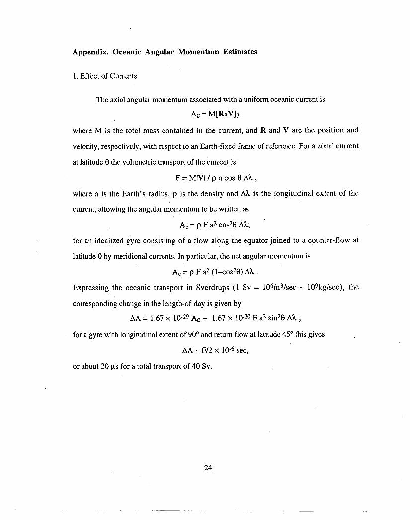
Appendix. Oceanic Angular Momentum Estimates

1. Effect of Currents

The axial angular momentum associated with a uniform oceanic current is

Ac = M[RxV]3

where M is the totai mass contained in the current, and R and V are the position and

velocity, respectively, with respect to an Earth-fixed frame of reference. For a zonal current

at latitude (l the volumetric transport of the current is

F= MIV1/pacos OAk,

where a is the Earth’s radius, p is the density and Ah is the longitudinal extent of the

current, allowing the angular momentum to be written as

A.= p F a2 cos2e Ah;

for an idealized gyre consisting of a flow along the equator joined to a counter-flow at

latitude e by meridional currents. In particular, the net angular momentum is

AC= p F az (1-eos%) Ak.

Expressing the oceanic transport in Sverdrups (1 Sv = 10bm3/sec - 10gkglsec), the

corresponding change in the length-of-day is given by

AA= 1.67 X 1O-Z9Ac - 1.67 x 10-20F a2 sin20 Ak ;

for a gyre with longitudinal extent of 90° and return flow at latitude 45° this gives

AA - F/2x 10-6see,

or about 20 ps for a total transport of 40 Sv.

24

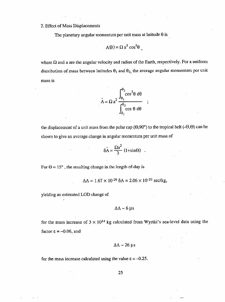
2. Effect of Mass Displacements

The planetmy angular momentum per unit mass at latitude 6 is

A(0) = !2 a2 cos20 ,

where Cland a are the angular velocity and radius of the Earth, respectively. For a uniform

distribution of mass between latitudes el and 02, the average angular momentum per unit

mass is

the displacement of a unit mass from the polar cap ((3,90°) to the tropical belt (-@,@)can be

shown to give an average change in angular momentum per unit mass of

For @= 15°, the resulting change in the length-of-day is

AA = 1.67 x 10-295A= 2.06x 10-20see/kg,

yielding an estimated LOD change of

AA-6ps

for the mass ‘increase of 3 x 1014kg calculated from Wyrtki’s sea-level data using the

factor &= –0.06, and

AA -26 ~S

for the mass increase calculated using the value &= -0.25.

25

REFERENCES

Barnes, R. T. H., R. Hide, A. A. White, and C. A. Wilson, Atmospheric AngularMomentum Fluctuations, Length of Day Changes and Polar Motion, Proc, R. Sot.London, A387, 31-73, 1983.

Barnett, T. P., The Interaction of Multiple Time Scales in the Tropical Climate System,J, Climare, 4, 269-288, 1991.

Bloomfield, P., Fourier Analysis of Time Series: An Introduction, John Wiley & Sons,New York, 1976.

Cartwright, D. E., R. Spencer, and J. M. Vassie, Pressure Variations on the AtlanticEquator, J. Geophys. Res., 92, 725-741, 1987.

Cazenave, A. (cd.), Earth Rotation: Solved and Unsolved Problems, NATO AdvancedInstitute Series C: Mathematical and Physical Sciences Vol. 187, ed. A. Cazenave, D.Reidel, Boston, 1986.

Chao, B. F., Interannual Length-of-Day Variations with Relation to the SouthernOscillation/El Nifio, Geophys. Res. Lett., 11, 541-544, 1984.

Chao, B. F., Correlation of Interannual Lengths-of-Day Variation with El Nifio/SouthernOscillation, 1972-1986, J. Geophys, Res., 93, B7, 7709-7715, 1988.

Chao, B. F., Length-of-Day Variations Caused by El Nifio/Southern Oscillation and theQuasi-Biennial Oscillation, Science, 243,923-925, 1989.

Chen, W. Y., Assessment of Southern Oscillation Sea-Level Pressure Indices,, h40n.Weather Rev., 110, 800-807, 1982.

Dickey, J. O., and T. M. Eubanks, The Application of Space Geodesy to Earth OrientationStudies, Space Geodesy and Geodynamics (eds.) by A. J, Anderson and A. Cazenave,Academic Press, New York, 221-269, 1986.

Dickey, J. O., T. M. Eubanks, and R. Hide, Interannual and Decade Fluctuations in theEarth’s Rotation, Variations in the Earth’s Rotation, Geophysical Monograph Series ofthe American Geophysical Union, Washington, D, C. McCarthy (cd.), 157-162, 1990.

Dickey, J. O., S. L, Marcus and R. Hide, Global Propagation of Interannual Fluctuationsin Atmospheric Angular Momentum, Nature, 357,482-488, 1992a.

Dickey, J. O., S. L, Marcus, J. A. Steppe, and R. Hide, The Earth’s Angular MomentumBudget on Subseasonal Time Scales, Science, 255,321-324, 1992b.

Dickey, J. O., Atmospheric Excitation of the Earth’s Rotation: Progress and Prospects viaSpace Geodesy, Space Geodesy and Geodynamics, Geophysical Monograph of theAmerican Geophysical Union, cd., D. Turcotte, Washington D. C., in press, 1993.

Dickey, J. O., S. L. Marcus, T. M, Eubanks, and R. Hide, Climate Studies Via SpaceGeodesy: Relationships Between ENSO and Interannual Length-of-Day Variations, Am.Geophys. Un. Mono. 75, IUGG Symposium Volume 15, Interactions Between GlobalClimate Subsystems: The Legacy of Harm, Eds. G. A. Bean and M. Hantell,Washington, D. C,, 141-155, 1993.

26

Eubanks, T. M., J. O. Dickey, and J. A. Steppe, The 1982-83 EINifio, the SouthernOscillation, and Changes in the Length of Day, Trop. Ocean and Atmos. Newsletter, 29,21-23, 1985a.

Eubanks, T. M., J. O. Dickey, J. A. Steppe, and P. S. Callahan, A Spectral Analysis ofthe Earth’s Angular Momentum Budget, J. Geophys. Rest, 90, B7, 5385-5404, 1985b.

Eubanks, T. M,, J. A. Steppe, and J, O. Dickey, The El Niiio, the Southern Oscillationand the Earth’s Rotation, in Earth Rotation; Solved and Unsolved Problems, NATOAdvanced Institute Series C: Mathematical and Physical Sciences, 187, ed, A. Cazenave,163-186, D. Reidel, Hingham, Mass., 1986.

Eubanks, T. M., Variations in the Orientation of the Earth, Space Geodesy andGeodynamics Geophysical Monograph of the American Geophysical Union, cd,, D.Turcotte, Washington D. C., in press, 1993.

Gross, R. S., A Combination of Earth Orientation Data: SPACE91, in IERS TechnicalNote 11: Earth Orientation Reference Frame, Atmospheric Excitation Functions,(submitted for the 1991 IERS Annual Report) (Annex to the IERS Annual Report for1991), ed. P. Chariot, in press, Observatoire de Paris, Paris, France, 1992.

Hide, R., Towards a Theory of Irregular Variations in the Length of the Day and Core-Mantle Coupling, Phil. Trans. Roy. Sot., A284, 547-554, 1977.

Hide, R., Rotation of the Atmospheres of the Earth and Planets, Phil. Trans. R. Sot.Lend. A313, 107-121, 1984.

Hide, R., Presidential Address: The Earth’s Differential Rotation, Quart. J. Roy. Astron.SOC., 278, 3-14, 1986,

Hidej R,, and J. O. Dickey, Earth’s Variable Rotation, Science, 253,629, 1991.

Hirota, I., T. Hirooka, and M. Shiotani, Upper Stratospheric Circulations in the TwoHemispheres Observed by Satellites, Q. J. R. Meteorol. Sot., 109,443-454, 1983.

Horel, J. D., and J. M. Wallace, Planetary-Scale Atmospheric Phenomena Associated withthe Southern Oscillation, Mon. Weather Rev., 109, 813-828, 1981.

Keppenne, C. L., and M. Ghil, Adaptive Filtering and Prediction of the SouthernOscillation Index, J. Geophys. Res., 97, 20,449-20,454, 1992.

Kessler, W. S., Observations of Long Rossby Waves in the Northern Tropical Pacific, J.Geophys. Res., 95, 5183-5217, 1990.

Lambeck, K., The Earth’s Variable Rotation, Cambridge Univ. Press, London and NewYork, 1980.

Lambeck, K., Geophysical Geodesy, The Slow Deformation of the Earth, ClarendonPress, Oxford, 1988.

Lambeck, K., and A. Cazenave, The Earth’s Rotation and Atmospheric Circulation, I,Seasonal Variations, Geophys. J. R. Astron. Sot., 32, 79-93, 1973.

27

Lukas, R., S. P. Hayes, and K. Wyrtki, Equatorial Sea Level Response During the 1982-1983 El Niiio, J. Geophys, Res., 89, 10425-10430, 1984.

Meehl, G. A., Air-Sea Biennial Mechanism in the Tropical Indian and Pacific Region—Role of the Ocean, J. Climate, 6, 1,31-41, 1993.

Morabito, D. D., T. M. Eubanks, and J. A. Steppe, Kalman Filtering of Earth OrientationChanges. The Earth’s Rotation and Reference Frames for Geodesy and Geodynamics, A.K. Babcock and G. A. Wilkins, Kluwer Academic Publishers, Dordrecht, 257-268,1988.

Moritz, H., and I. I. Mueller, Earth Rotation: Theory and Observation, The UngarPublishing Co., New York, 1987.

Munk, W. H., and G. J. F. MacDonald, The Rotation of the Earth, Cambridge UniversityPress, 1960.

Murakami, M., Large-scale Aspects of Deep Convective Activity Over the GATE Area,Mon. Wea. Rev., 107, 994-1013, 1979.

Philander, S. G. H., El Nifio Southern Oscillation Phenomena, Nature, 302, 295-301,1983.

Philander, S. G. H., El Niiio, Lu Nifia, and the Southern Oscillation, Academic Press,New York, 1990.

Rasmussen, E. U., and J. M. Wallace, Meteorological Aspects of the El Nifio/SouthernOscillation, Science, 222, 1195-1202, 1983.

Rasmussen, E. M., X. Wang, and C. F. Ropelewski, The Biennial Component of ENSOVariability, J. Mar. Systems, 1,71-96, 1990.

Rochester, M. G., Causes of Fluctuations in the Earth’s Rotation, Phil, Trans. R, Sot.Lond., A313, 95-105, 1984.

Rosen, R. D., D. A. Salstein, T. M. Eubanks, J. O. Dickey, and J. A. Steppe, An El NifioSignal in Atmospheric Angular Momentum and Earth Rotation, Science, 225,411-414,1984.

Rosen, R. Dl, and D. A. Salstein, Contribution of Stratospheric Winds to Annual andSemi-Annual Fluctuations in Atmospheric Angular Momentum and the Length of Day, ~Geophys. Res., 90, 8033-8041, 1985.

Rosen, R. D., D. A. Saltein, A. J. Miller, and K. Arpe, Accuracy of Atmospheric AngularMomentum Estimates from Operational Analyses, Mon. Wea. Rev., 115, 1627-1639,1987.

Rosen, R. D., D. A. Salstein; T. M. Wood, Discrepancies in the Earth-AtmosphereAngular Momentum Budget, J. Geophys. Res., 95, 265-279, 1990.

Rosen, R. D., The Axial Momentum Balance of Earth and its Fluid Envelope, SurveysGeophys., 14, 1-29, 1993.

28

Salstein, D. A., and R. D. Rosen, Earth Rotation as a Proxy for Interannual Variability inAtmospheric Circulation, 1860-Present, J. Clim. and Appl. Meteorcd., 25, 1870-1877,1986.

Salstein, D. A., D. M. Kann, A. J. Miller, and R. D. Rosen, The Sub-Bureau forAtmospheric Angular Momentum of the International Earth Rotation Service: Ameteorological data center with geodetic applications, Bull. Amer. Meteor. Sot., 74, 67-80, 1993.

Stephanie, M., Interannual Atmospheric Angular Momentum Variability 1963-1973 and theSouthern Oscillation, J. Geophys. Res., 87, 428-432, 1982

Swinbank, R., The Global Atmospheric Angular Balance Inferred from Analysis MadeDuring GFFE, Quart. J. R. Met. Sot., 111, 977-992, 1985.

Wahr, J. M., ,The Earth’s Rotation, Ann. Rev. Earth Planet Sci., 16,231-249, 1988.

Wyrtki, K., The Slope of Sea Level Along the Equator During the 1982/1983 El Nifio, .7.Geophys. Res., 89, 10419-10424, 1984.

Wyrtki, K., Water Displacements in the Pacific and the Genesis of El Nifio Cycles, J.Geophys. Res., 90, 7129-7132, 1985.

Xu, J. S., On the Relationship Between the Stratospheric Quasi-Biennial Oscillation andthe Tropospheric Southern Oscillation, J. Atmos. Sci., 49,9,725-734, 1992.

29

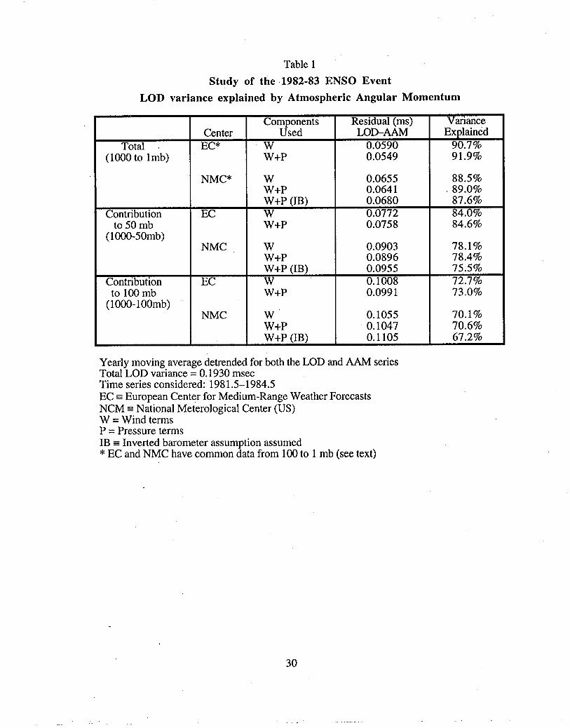
Table 1

Study of the 1982-83 ENSO Event

LOD variance explained by Atmospheric Angular Momentum

Components Residual (ins) VarianceCenter Used LOD-AAM Explained

Total . EC* w 0.0590 90.7%(1000 to lmb) W+P 0.0549 91.9%

NMC* w 0.0655 88.5%W+P 0.0641 . 89.0%W+P (IB) 0.0680 87.6%

Contribution EC w 0.0772 84.0%to 50 mb W+P 0.0758 84.6%

(1000-50mb)NMC w 0.0903 78.1%

W+P 0.0896 78.4%W+P (IB) 0.0955 75.5%

Contribution EC w“ 0.1008 72.7%to 100 mb W+P 0.0991 73.0%

(1000-100mb)NMC w 0.1055 70.1%

W+P 0.1047 70.6%W+P (IB) 0.1105 67.2%

Yearly moving average detrended for both the LOD and AAM seriesTotal LOD variance= 0.1930 msecTime series considered: 1981.5-1984.5EC= European Center for Medium-Range Weather ForecastsNCM = National MeteorologicalCenter (US)W = Wind termsP = Pressure termsIB = Inverted barometer assumption assumed* EC and NMC have common data from 100 to 1 mb (see text)

30

LEGENDS FOR FIGURES

Fig, 1, Time series of irregular fluctuations in the length-of-day A*(t) (curve (A)) and its

decadal (Au(t)), interannual (A~(t)), seasonal (Aft)), and intraseasonal (A~(t)) components

(curves (B), (C), (D) and (E) respectively) updated from Hide and Dickey [1991].

Fig. 2. The interannual LOD variation, A*B(computed as the one-year moving average minus

the five-year moving average — upper curve), compared to the negative of the interannual

variation in the Southern Oscillation Index (MSOI — lower curve).

Fig. 3. Length-of-day from the JPL Kalrnan smoothing of space geodetic measurements as

well as that inferred from atmospheric angular momentum from the National Meteorological

Center (NMC) analysis for the period 1976 through 1991, together with a 365-day moving

average which allows comparison on interannual time scales. Variation in the residual is shown

by the lower curve.

Fig. 4. (a) Variations in a daily time series of LOD (solid line), smoothed with a tapered 365-

day running average to remove seasonal variability, and detrended to remove decadal

variability. Also shown are similarly smoothed variations in daily AAM from the EC

operational analysis extending to 100 mb and to 50 mb (dashed lines — wind term only; dash-

dot lines — wind plus pressure), and variations up to 1 mb formed by adding the stratospheric

series to the 100-mb values. (b) as in (a), for the NMC operational analysis (dotted line —

wind-plus-pressure calculated with the inverted barometer (IB) assumption).

Fig. 5. Fractional variance of the LOD series in Fig. 4 explained by the AAM series based on

(a) NMC and (b) EC operational analyses to the 100-mb and 50-mb levels, and by variations

up to 1 mb formed by adding the stratospheric series to the 100-mb values. A lower bound on

31

the unce~ainty (dotted lines) is computed as the difference in the maximum variance explained

by the 1-mb series incorporating NMC and EC data. Since the difference between the

maximum explained variance and the explained variance at zero-lag for each center falls within

this band, the LOD lag with respect to the 1-mb series considered here is not significant.

Fig. 6. (a) Interannual variations in a monthly time series of normalized LOD values for the

period 1976-1991, filtered recursively [Murakami, 1979] in 8 equal-frequency bands ranging

from 0.1 to 0.9 cycles per year. (b) as in (a), for the modified Southern Oscillation Index. (c)

as in (a), for the tropospheric (1000-100 mb) ,AAM from the operational NMC analysis. (d) as

in (a), for the stratosphere (100-1 rob),

Fig. 7. (a) Variations in a monthly time series of LOD, filtered recursively [Murakami, 1979]

in the LF (32-88 month — dashed line) and QB (18-35 month — dotted line) bands defined by

Barnett [1991]. The full interannual variation (sum of the LF and QB components) is shown by

the solid line. (b) as in (a), for the modified Southern Oscillation Index. (c) as in (a), for the

tropospheric (1000-100 mb) AAM from the operational NMC analysis. (d) as in (a), for the

stratospheric ( 100–1 mb) AAM inferred from satellite temperature soundings. (e) The full

interannual variation (sum of the LF and QB components) for tropospheric ( 1000–100 mb)

AAM (dashed line), stratospheric (100-1 mb) AAM, and the total (1000–1 mb) AAM (solid

line).

32

SPECTRAL COMPONENTS OF LOD

03U-1

I .

L-

/

0 h &scAUE (MILIY!sECONDs)

1

LOD IN MILLISECONDS

m

-0.5 0r I I I I 1 I , 1 ,

.

I

I

I

$.2

.4-----

/.-.-”

<“.-,+“-. +.-

-------. -.+

~.-”

.- .-”-”._ ----.+/

‘\. -----

“-.+,%

“-. .-. .-.-

----./----

. “\..)

1 ‘------u.-”

0/“.- .-.

-----

c..

.>. -‘.>

> .-.-----

“-.’3

—.- <

I * I * 1 , I 1 1 1

-2 0 2 4 6MSOI IN MILLIBARS

1.

LOD/MM VARIATION

mo

03u-l

u)o00

coo

=%

=&

<

“ <

.0 4

SCALE

(0o0

LOO

‘-0.2

VARIATION

o

I

.

.

.

MILLISECONDS

0.2I 7i ,

I

I

II

I

.

, 1 I , I 1

‘t

m

m

LOD

-0.2I

, I

VARIATION IN MILLISECONDS

o .0.2

coul

1

1-1 I

I I

I , 1 1 I , 1 1

d..—

VARIANCE EXPIJYNED10

Fc

I

o

0.2 0.4 0.6 0.8 1i I 1 ., \\“Xy <, *J 1\\ I , I ::

i%

Ii

I I,

I I,

I

N’. ‘J ‘i

\

\\

\ ii1,

1’1’1II

1

IIIIIIIl“

IIi’/ 1“

i]! 1I /.1it! . .I , yI it!

I jl!I 1/!

t ;1.’. . .

,!

f!

1,1

/!II

//’//”

//”//”

//”/,”

~’

4“4

0 1/ /,$” 5“

1 , I I/. . I /!i 10

VARIANCE

~

(Lo

0

ulo

10 0.2I

o0

EXPIAINED

0.6 0.8 10.4I , \l .. xl\ \ I , I 1

P-1c-l

! 1 1,

I 1 1 I I1 ,

I I

z ! io !

mj

I

i.

/

I

ii

i

I

. .,,.,. .

.:,,,,!,,.

:.

L

I

i;

ii

i

/“

_

o00

5 II

Opo ~-

~--J”- ..-.J k---n. ‘.

p..”-,. ;

I+1

o’~—0

t?

ino

n-12

z0Q-.+-.a)CL

‘Y

(n0

-----13

0

-.

b 07r)

\

&ino

u)G

00~o—.CLJ-.03

a)co

I

I

I

I

000

(n

I

z(n

MILLISECONDS

–0.5 o 0.5I I 1 I I I 1 8 1 I

. . .

..” ).“.s

I\

. . . . . .,.

. ...”,

. . ...”.. . . .. ,,. /

+

-

\. . .

\

“. 5.“ . u

“./ ““,

.“ “\I

.1 t 1 t I # 1 1 I

u

.

III

I

F’+ 7U

ac

mUT

coo

–5MILLIBARS

oI 1 I I I [-. . I 1 1

w

.

. . .

. ...>.. . . . ...” /

/ “

/

\

...“.

“.. .

..4

“. }.. /

.“

“.O\

\T .

i I I t I 1 1

5

alo

MILLISECONDS

–0.2 o 0.2I 1 I I 1

~L... I

) “:

\\

“..

I

c1UJ

.

.

.

I

III

●✎✎✎““. . .

(. . .

\x z

nA

. ... 0

0“.

“. ) I“,“,

. /. # 0

0.

zmw

\

.’I 1 I 1

cmc1

CQcm

C(3o

–0.2

MILL SECONDS

o “ 0.2

nA

o0I

A

–0.5

alo

alU-I

MILLISEC

oONDS

0.5

I \I

000I

0/

\UJ

.“..

“,N

..”/

. . ...”

..O.

1...

:W

I

s

--

-k 7 e