IOP PUBLISHING JOURNAL OF PHYSICS A: MATHEMATICAL AND THEORETICAL

J. Phys. A: Math. Theor. 40 (2007) 13075–13089 doi:10.1088/1751-8113/40/43/015

Fractional monodromy in systems with coupledangular momenta

M S Hansen1, F Faure2 and B I Zhilinskiı3

1 Institute of Mathematics, Technical University of Denmark, 2800 Kgs Lyngby, Denmark2 Institut Fourier, Universite Joseph Fourier, BP 74, 38402 Saint-Martin d’Heres, Cedex, France3 Universite du Littoral, UMR du CNRS 8101, 59140 Dunkerque, France

E-mail: M.S.Hansen@mat.dtu.dk, frederic.faure@ujf-grenoble.fr and zhilin@univ-littoral.fr

Received 27 February 2007, in final form 12 September 2007Published 9 October 2007Online at stacks.iop.org/JPhysA/40/13075

AbstractWe present a one-parameter family of systems with fractional monodromy,which arises from a 1:2 diagonal action of a dynamical symmetry SO(2). In aregime of adiabatic separation of slow and fast motions, we relate the presenceof fractional monodromy to a redistribution of states both in the quantum andin the semi-quantum spectra.

PACS numbers: 03.65.Sq, 02.40.Yy

(Some figures in this article are in colour only in the electronic version)

1. Introduction

In this paper we consider a simple one-parameter family of Hamiltonian which is a slightgeneralization of the well-known example of spin–orbit coupling. This latter model has beenthe object of several studies [1, 6–8], demonstrating the presence of integer monodromy forsome interval of parameter values.

We remind here that Hamiltonian monodromy is a generic property of classical integrablesystems, intensively studied and popularized by Cushman [5] and described in detail byDuistermaat in 1980 [9]. In a classical dynamical system with two degrees of freedom,the Hamiltonian monodromy can typically appear in one-parameter families through theHamiltonian Hopf bifurcation [10]. It was shown later that there is a correspondence betweenthe appearance of monodromy within a one-parameter family of classical Hamiltonians andthe redistribution of bands in the spectrum of the associated quantum problem [6, 11]. Theappearance of Hamiltonian monodromy in the classical system also indicates the presence ofa topological bifurcation in a semi-quantum description [12].

Our model has fractional monodromy which is a recent generalization of the integermonodromy concept [13–16]. This is the first example of a system with this property on acompact phase space.

1751-8113/07/4313075+15$30.00 © 2007 IOP Publishing Ltd Printed in the UK 13075

13076 M S Hansen et al

If we suppose that one angular momentum is much larger than the other, then the firstone has a slower motion compared to the second one. One gets a slow–fast dynamic thatcan be analyzed using a semi-quantum description (the fast motion is quantum while the slowmotion is classical). This gives line bundles over the ‘slow’ classical phase space, whosetopology is characterized by Chern indices. These line bundles have a nice interpretation forthe exact quantum spectrum: the energy levels form different groups named bands. Each bandis associated with a line bundle, and the exact number of levels in each band is given from theChern index of the bundle using an index formula. These topological phenomena have alreadybeen observed and analyzed in other situations [7, 28]. Here, we show how the presence offractional monodromy is related to the locus of topological bifurcations of the bundles, whichimply a change of the Chern indices and redistributions of levels between bands.

Compared to the spin–orbit model already studied in [1, 6–8] where there is a 1:1 diagonalaction of the group SO(2), here the major change is a 1:2 diagonal action of the symmetrygroup SO(2), and this is responsible for fractional monodromy.

This paper is a part of the ongoing study of global properties of integrable systems onthe one side [14, 17–20] (especially in the context of molecular physics [2, 3, 6, 21–25]) andadiabatically coupled systems [7, 26–28] on the other side.

In sections 1–3 we present the model and discuss the fractional monodromy phenomenonin the classical model, using the generalized moment map. In section 4 we study the quantummodel and discuss the quantum manifestation of fractional monodromy in the joint spectrum.In section 5 we suppose an adiabatic regime where one angular momentum is much largerthan the other, and discuss the topological interpretation of redistributions of levels betweenbands.

2. Presentation of model

2.1. Hamiltonian with a dynamical 1:2 symmetry action of SO(2)

Very often global properties of the dynamical model under study are due to the symmetry of thephysical problem under consideration. Let N = (Nx,Ny,Nz) ∈ R3, S = (Sx, Sy, Sz) ∈ R3

with fixed |N| =√

N2x + N2

y + N2z and |S| =

√S2

x + S2y + S2

z be two (effective) angularmomenta living on S2 × S2. The model we study in this paper admits a diagonal 1:2 groupaction of SO(2) defined by

SO(2) × (S2 × S2) → S2 × S2

(φ;N+, N−, Nz, S+, S−, Sz) �→ (N+ eiφ,N− e−iφ,Nz, S+ e2iφ, S− e−2iφ, Sz),(1)

where N± = Nx ± iNy, S± = Sx ± iSy . The action defined by (1) can be considered as ana priori condition imposed by the physical model. As soon as the group action is given, ageneric Hamiltonian can be constructed as a linear combination of polynomials invariant underthe group action (1). This leads to a Hamiltonian which has a SO(2) symmetry generated by

Jz = 2Sz + Nz (2)

(i.e. such that [Hλ, Jz] = 0):

Hλ = 1 − λ

|S| Sz + λ

(1

|S‖N|SzNz +1

2|S‖N|2(N2

−S+ + N2+S−

)), 0 � λ � 1. (3)

Here λ is a coupling parameter. It can be due to an external magnetic field, for example,recall that the amplitudes |S|, |N| are held fixed and in this paper, we only consider the case|N| > 2|S|4.4 A preliminary study of the case |N| < 2|S| has been initiated in [29].

Fractional monodromy in systems with coupled angular momenta 13077

The SO(2) symmetry generated by Jz = 2Sz + Nz rotates simultaneously N and S abouttheir respective z-axes. In [6] the SO(2) action on the phase space S2 × S2 was 1:1 diagonalbut now the asymmetric appearance of N and S implies that while N is rotated by an angle φ,S is rotated by 2φ.

2.2. Quantum description and the semi-classical limit

We begin by a presentation of the quantum system and deduce after the classical one in thesemi-classical limit5.

Let N, S be the angular momentum operators [31] generating an irreducible representationof su(2) × su(2) in a Hilbert space H = HN ⊗ HS of dimension (2N + 1)(2S + 1). N, S

are the respective angular momentum quantum numbers taking integer or half-integer values.Similarly H λ, equation (3), is the Hamiltonian operator. The quantum description is given bythe Schrödinger equation (with h ≡ 1)

idψ(t)

dt= H λψ(t), (4)

where ψ(t) is a vector in H. To study the semi-classical limit of large quantum numbersN, S � 1, we introduce the normal symbol of H [34]

〈N, S|H λ|N, S〉 = Hλ + O(hN,S), (5)

which is a power series in hN = 1/(2N), hS = 1/(2S). Here |N, S〉 are SU(2) coherent statesoften used to study the semi-classical limit of angular momentum dynamics.

Keeping only the first term of (5) we have a classical Hamiltonian, Hλ, which is theprincipal symbol of H λ. The dynamics is approximately described by classical angularmomenta N, S moving according to Hamilton’s equations of motion [4]:

d

dtN = hN∂NHλ ∧ N,

d

dtS = hS∂SHλ ∧ S, (6)

on the phase space S2 ×S2. Putting hN,S → 0 illustrates how the semi-classical limit is relatedto the limit of adiabatically slow motion. Under the additional assumption N � S givinghN � hS , Hamilton’s equations (6) describe the dynamics of an adiabatically coupled systemwith the motion of N being much slower than that of S.

3. Classical description: structure of the generalized moment map

3.1. Second integral of motion

The SO(2) symmetry gives rise to a second integral of motion Jz, equation (2), which is theprojection of the total angular momentum J = 2S + N onto the z-axes. Together Hλ, Jz definea one-parameter family of integrable systems with two degrees of freedom.

3.2. Reduction of symmetry, space of orbits

The symmetry of the system can be used to reduce the number of degrees of freedom. This isdone by mapping each orbit of the SO(2) action on S2 × S2 onto the three-dimensional spaceof orbits. As the group action is not transitive, this is an example of the so-called singularreduction [5] based on the theory of invariants [5, 6, 35].

5 Several quantum systems may give rise to the same classical system. See e.g. [30] for an example.

13078 M S Hansen et al

Figure 1. Left: the space of orbits of the SO(2) action. The boundary is given by φ = 0. Thevertical plane is a section for constant Jz. Middle: a typical section for Nz = −|N|, |Sz| < |S|.This is a part of the continuous family of singular spaces. The singular orbit at the intersection ofthe boundary and the constant energy level set has a Z2 stabilizer. Right: a singular section forJz = 2|S| − |N|. The singular orbit situated at the intersection of the constant energy level set andthe boundary (critical orbit) has the stabilizer SO(2).

The idea is to see Hλ, Jz as made up of SO(2)-invariant polynomials

θ1 = Sz, θ2 = Nz, θ3 = N2−S+ + N2

+S−,

φ = N2−S+ − N2

+S−,

satisfying the algebraic relation [35]

φ2 = θ23 − 4

(S2 − θ2

1

)(N2 − θ2

2

)2. (7)

An orbit of the SO(2) action (1) can be characterized by the value of the three algebraicallyindependent invariants θi, i = 1, 2, 3, and the sign of the linearly independent, but algebraicallydependent through (7), invariant φ. The space of orbits can then be visualized in a (θ1, θ2, θ3)-coordinate system as a closed body defined by

θ23 − 4

(S2 − θ2

1

)(N2 − θ2

2

)2 � 0. (8)

The space of orbits is shown in figure 1 (left). Its interior points correspond to two orbitsdistinguished by the sign of φ while the boundary points correspond to a single orbit.

There are three equivalence classes of orbits forming different strata in the initial 4 D-phasespace, which are as follows:

• Generic circular orbits with a trivial stabilizer (4 D regular stratum).• A continuous family of orbits for Nz = ±|N| and |Sz| < |S| with the stabilizer Z2 (2 D

critical stratum). These orbits are half as long as a generic orbit.• Four isolated critical orbits for (Sz,Nz) = (±|S|,±|N|) with the stabilizer SO(2) (0 D

critical stratum).

3.3. Generalized moment map

The most natural way to characterize qualitatively the classical dynamics for an integrablemodel is to introduce the generalized moment map [4, 36, 37]

Fλ = (Hλ, Jz) : S2 × S2 → R2, (9)

Fractional monodromy in systems with coupled angular momenta 13079

Figure 2. Image Bλ of the generalized momentum map (9) for different values of the externalparameter λ. For λ ∼ 1/2, there are critical values inside B1/2 and the system has fractionalmonodromy.

which maps the compact phase space to a bounded domain Bλ ⊂ R2 which can be expressedas the union of regular and critical values of (9) Bλ = Br

λ ∪ Bcλ. Quite naturally, the shape of

Bλ depends on the parameter λ as figure 2 shows.The generalized moment map defines a fibration over Bλ: for fixed b ∈ Bλ the dynamics

takes place on the fiber F−1λ (h, j). Here and later on we use j to denote possible values of Jz.

From the Arnold–Liouville theorem, it is known that the fiber over a regular value b ∈ Brλ

is a 2-torus [4] (since S2 × S2 is compact). We denote it here as a regular fiber. The criticalstrata in the phase space are mapped via (9) to the critical values bc ∈ Bc

λ. These critical valuescan form isolated points inside the image of the generalized moment map, boundary lines orspecial points on the boundary, and even lines of critical values situated inside the image ofthe generalized moment map. Critical values which belong to the boundary of the imagecorrespond typically to tori of lower dimension (circles or points). Critical values situatedinside the image have nontrivial inverse images [19, 38, 39].

For λ = λ∗ = 1/2 some of the critical values are found in the interior Bλ∗ , and suchvalues correspond to nontrivial fibers responsible for the appearance of fractional monodromy[13–15].

It is convenient to make a coordinate transformation in the space of orbits

Jz = 2Sz + Nz = 2θ1 + θ2, Kz = Sz − 2Nz = θ1 − 2θ2, (10)

where Kz is the variable varying on Jz sections.Figure 1 shows singular Jz sections together with constant level sets of energy. It is easy

to see geometrically that in order to have critical values on the image of the energy–momentummap inside the domain of regular values, it is necessary that the energy level going through thesingular orbit intersects the boundary of the orbit space at the singular orbit. In other words,we need to compare the slope of the constant energy level at the singular orbit with the slopeof two boundary lines of the Jz-constant section at the singular point on the boundary.

It should be noted that at the critical orbit the geometrical form of the Jz section±(−2|N|+ |S|−Kz)

3/2 implies that the two boundary lines form a cusp and have the same zeroslope. Due to that, the energy section going through the critical point intersects the boundaryonly if the energy section has itself the zero slope at the critical orbit and this can happen onlyfor λ = 1/2. The typical images of the energy momentum map for λ < 1/2, λ = 1/2, λ > 1/2are shown in figure 2. We do not go into details of the evolution of the line of singular values(dashed red line in figure 2) near λ = 1/2 which are related to the possible appearance of asecond connected component in the inverse image of the generalized moment map. We notethat such complications (as compared with a more simple scenario of the appearance of integer

13080 M S Hansen et al

0

0.5

Jz/(2|S|+|N|)

Ener

gy

λ=0.5

c

Γlc b

Figure 3. The local setup in the image of the generalized moment map Bλ∗ when the system hasfractional monodromy. The line lc of critical values is the projection of the critical stratum formedby curled tori [13, 14]. The critical value bc is the projection of curled pinched torus which is thefiber with the critical point (0, 0,−|N|), (0, 0, |S|). The figure is done for the ratio J/S = 15/2.

monodromy [6] through the Hamiltonian Hopf bifurcation [16]) are only due to the presenceof the cusp singularity in the space of orbits. Moreover, it is not essential for the appearanceof the line of singular values together with the end point inside the generalized moment imageas shown in figure 2 (center) which is responsible for the presence of fractional monodromy.

3.4. Integer monodromy: holonomy of the lattice bundle

For each regular value b ∈ Brλ, the periodicity of the Arnold–Liouville tori defines a 2 D-lattice

Lb isomorphic to the regular lattice Z2 [4]. Over critical values bc ∈ Bcλ, the fiber is singular

and we no longer have a well-defined lattice. To detect the presence of singular fibers, it issufficient to consider the lattice bundle [5]

L :⋃b∈�

Lb → Brλ, (11)

restricted to a loop � : [0, 1] → Brλ in Br

λ. This loop passes only through regular values.As �(0) = �(1) lifting of � induces an automorphism on fibers, Aut(Lb=�(0)) ∈ SL(2, Z).The bundle L|� depends only on the homotopy type of � such that we only have to considerequivalence classes of loops (the fundamental group), π1

(Br

λ

). The monodromy map is now

defined as

µ : π1(Br

λ

) → SL(2, Z), (12)

which is an example of the holonomy concept [5, 32]6. Note that here L is a flat bundle, i.e.its curvature tensor vanishes.

When the system has an isolated critical value, π1(Br

λ

) = Z. The correspondingmonodromy map depends on the topology of the singular fiber and results in the transformationof basis cycles of regular tori which can be expressed as a linear combination with integercoefficients. This gives standard integer monodromy [9, 5, 38].

As opposed to numerous known examples of integer monodromy in the literature, we nolonger have isolated critical values. This is shown in figure 3 where the critical value

bc = Fλ((0, 0, |N|), (0, 0,−|S|)) (13)

6 Holonomy has become a unifying concept in physics, e.g. the Berry phase is seen as the holonomy of a U(1)-bundle[26, 40].

Fractional monodromy in systems with coupled angular momenta 13081

of the generalized moment map is connected to a line, lc, of critical values. In such a casewe have π1

(Br

λ

) = 0 for every λ as is seen from figure 2, so there is no integer monodromy.However, a suitable restriction of the monodromy map (12) allows one to use closed pathswhich cross a critical line and surround a critical value bc. Transformation of the basis cyclesof regular tori after their parallel transfer along such closed paths leads to the new notion offractional monodromy [13–16].

3.5. Fractional monodromy: restriction of basis cycles

To determine the fractional monodromy map, we have to describe how the fibers arecontinuously modified as we go along the closed path � in the base space Bλ of the integrablefibration and how the line of critical values can be crossed using only a subgroup of cyclesgenerating the fibers.

The local setup in Bλ is sketched in figure 3. In order to understand the evolution of basiscycles of tori along the contour �, we need to note that the trajectories of Jz are closed andwell defined along all �. They are due to the SO(2) symmetry of the problem and can be usedto represent γ1, the first of the two cycles generating the first homology group of the regularfibers.

The second cycle γ2 is chosen as the intersection of fibers with an auxiliary plane. Detailsof this construction are given in figure 7 of [14]. To pass continuously along � this cycle has tobe a double loop. The applicability of the previous discussion of fractional monodromy [14]to the case of the model Hamiltonian (3) studied in the present work is confirmed by reducingthe present model (Hλ, Jz) into the normal form of fractional monodromy presented in [14].This is done in appendix A.

Due to the splitting of one of the basis cycles when crossing the singular stratum, themonodromy map is only defined for an index 2 subgroup of the first homology group of regularfibers. This is the essence of fractional monodromy. The relation between the initial basiscycles γ1,2 and the final basis cycles γ ′

1,2, at the end of the cyclic evolution along �, can bewritten in the matrix form as [13](

γ ′1

2γ ′2

)=

(1 0

−1 1

)︸ ︷︷ ︸

µcl

(γ1

2γ2

). (14)

A formal extension of the monodromy map to the basis of the whole homology group ofregular fibers introduces fractional coefficients and a monodromy matrix

µcl =(

1 0

−1/2 1

)∈ SL(2, Q). (15)

This implies that the preimage F−1λ∗ (�) does not factorize as T2 × S1 and hence the

momentum map is not a principal T2-fiber bundle [5]. There is then no unique way of labelingtori in a vicinity of the pinched curled torus, and no global set of action-angle coordinates canbe introduced.

4. Quantum monodromy

The Einstein–Brillouin–Kramer (EBK) quantization introduces quantum numbers by pickingout a set of regular tori [31]∫

γk

p dq = 2πh(nk + αk/4), k = 1, 2, (16)

13082 M S Hansen et al

0 0.5 1

0

0.5

1

Jz/(2|S|+|N|)

Ene

rgy

λ=0

0 0.5 1

0

0.5

1

Jz/(2|S|+|N|)

Ene

rgy

λ=0.3

0 0.5 1

0

0.5

1

1.5

Jz/(2|S|+|N|)

Ene

rgy

λ=0.4

0 0.5 1

0

0.5

1

1.5

Jz/(2|S|+|N|)

Ene

rgy

λ=0.5

0 0.5 1

0

0.5

1

1.5

Jz/(2|S|+|N|)

Ene

rgy

λ=0.65

0 0.5 1

0

1

2

Jz/(2|S|+|N|)

Ene

rgy

λ=1

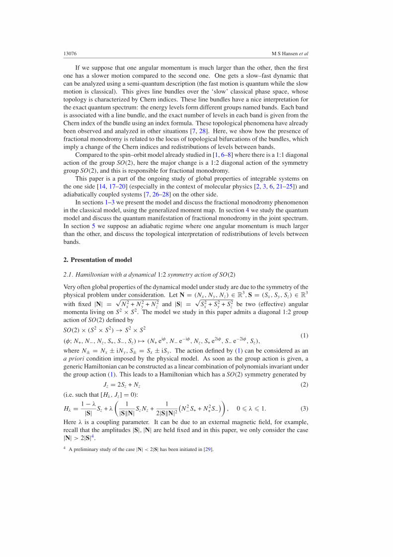
Figure 4. Modifications of the joint spectrum as λ varies, λ = 0 → 1. The bands are labeledσ = −S, . . . , S from the bottom up. Here S = 4, N = 40. For λ = 1/2 there is fractionalquantum monodromy due to the presence of the line of critical values inside of the image of themoment map. As 1/2 > λ → λ > 1/2 there is a modification of the band structure due to thedisplacement of the line of critical values from the upper side of the boundary of the moment imagetowards the lower side, passing through the interior (see figure 2). For λ = 0, there are N = 2S + 1states on each line, whereas for λ = 1, there are Nσ = (2S + 1) + 4σ states on the line σ , as isexplained below.

where γk are basis cycles, generators of the tori, and αk are Maslov indices. Given this,it is no surprise that classical monodromy manifests itself in quantum systems as quantummonodromy. The existence of this property was first demonstrated on the quantum sphericalpendulum [41] and later defined as the dual of classical monodromy [18]7.

The EBK rules lead to a 2 D-lattice of quantum states—or joint spectrum—in Bλ. From(16) the distance between consecutive quantum states decreases as h → 0. Our model isa coupling of two angular momenta S and N with effective Planck constants hS and hN ,respectively. The assumption S � N leads to hN � hS and to the existence of two scalesin the joint spectrum. This explains the local band structure easily observed in figure 4. Welabel the bands by the quantum number of Sz, σ = −S, . . . , S.

For λ = 0, the joint spectrum forms globally a regular lattice which possesses a welldefined (up to a similarity transformation with the SL(2, Z) matrix) elementary cell over thewhole lattice. This means that there exists a global labeling of states. The lattice remains tobe regular (just in a slightly deformed form) for the λ-dependent family of integrable systemsup to λ ∼ 1/2. At λ = 1/2 the presence of a one-dimensional defect is clearly seen withinthe regular part of the lattice. This defect results in a modification of the bands. For λ = 1 weagain have a globally regular lattice but now with a different band structure.

For λ ∼ 1/2, the effect of the defect on the lattice is characterized (up to conjugation) byan element µqm determined in the following way (see figure 5):

7 This is only strictly true in the semi-classical limit. In such a case, the distance between consecutive points in thespectrum goes to zero and we recover a continuous description.

Fractional monodromy in systems with coupled angular momenta 13083

Jz /(2|N|+|S|)

En

erg

y

λ=0.5

0

0.1

0.2

0.3

0.4

0.5

Jz /(2|N|+|S|)

Ene

rgy

λ=0.5

Γ

Figure 5. Joint spectrum for S = 8, N = 40 and λ = 1/2 which shows the effect of fractionalmonodromy. Left: the global view of the joint spectrum. Right: parallel transport of the doublecell along a closed path crossing once the line of critical values and surrounding the criticalvalue (Jz = 2S − N, E = 0) of the generalized moment map. For S = 8, N = 40 we haveJz/(2|S| + |N |) = −3/7 ≈ −0.4286.

• Make a choice of cell. To pass the line defect the cell should be doubled in the Jz direction.This is the quantum analogue of the restriction imposed on the choice of passable cyclesin section 3.5. Cell doubling is not necessary in the case of integer monodromy [6].

• Moving along the path � between initial and final points, the elementary cell doesnot change as long as the path remains within the class of homotopically trivial paths.However, after translation along a path � as shown in figure 5 we return with a differentcell. A rescaling as done in section 3.5 gives

µqm =(

1 1/20 1

)∈ SL(2, Q), (17)

which is the quantum monodromy matrix (after a formal rescaling of the cells)8.

The nontriviality of monodromy shows that no unique set of quantum numbers existswhich can be used to label states in the joint spectrum [42]. This is of special importance formolecular physics where effective quantum numbers are typically introduced on the basis ofexperimental spectral information using extrapolation within effective models.

4.1. Decomposition into sub-lattices

Let j label the eigenvalues of Jz, the second integral of motion, nd Nj be the dimension ofthe associated eigenspace, i.e. the number of states with Jz = const in figure 4. The numberof states function (figure 6) is a quasi-polynomial, i.e. polynomial in j with coefficients beingperiodic in j :

Nj ={

2S + 1, |j | � N − 2S12

(J − |j | + 1

2 (3 + (−1)J+|j |)), otherwise.

(18)

8 Here we observe the duality between classical and quantum monodromy explicitly as µqm = tµ−1cl [18].

13084 M S Hansen et al

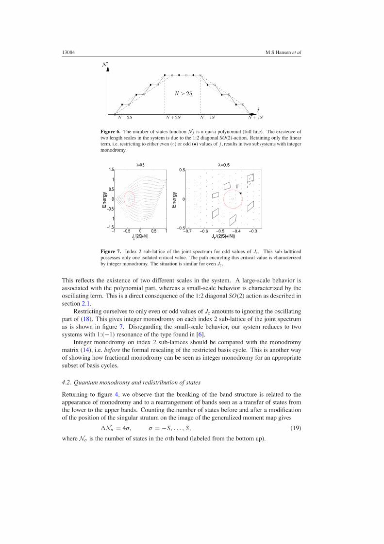
Figure 6. The number-of-states function Nj is a quasi-polynomial (full line). The existence oftwo length scales in the system is due to the 1:2 diagonal SO(2)-action. Retaining only the linearterm, i.e. restricting to either even (◦) or odd (•) values of j , results in two subsystems with integermonodromy.

0 0.5 1

0

0.5

1

1.5

Jz/(2|S|+|N|)

λ=0.5

0

0.5

Jz/(2|S|+|N|)

Ene

rgy

Ene

rgy

λ=0.5

Γ

Figure 7. Index 2 sub-lattice of the joint spectrum for odd values of Jz. This sub-ladtticedpossesses only one isolated critical value. The path encircling this critical value is characterizedby integer monodromy. The situation is similar for even Jz.

This reflects the existence of two different scales in the system. A large-scale behavior isassociated with the polynomial part, whereas a small-scale behavior is characterized by theoscillating term. This is a direct consequence of the 1:2 diagonal SO(2) action as described insection 2.1.

Restricting ourselves to only even or odd values of Jz amounts to ignoring the oscillatingpart of (18). This gives integer monodromy on each index 2 sub-lattice of the joint spectrumas is shown in figure 7. Disregarding the small-scale behavior, our system reduces to twosystems with 1:(−1) resonance of the type found in [6].

Integer monodromy on index 2 sub-lattices should be compared with the monodromymatrix (14), i.e. before the formal rescaling of the restricted basis cycle. This is another wayof showing how fractional monodromy can be seen as integer monodromy for an appropriatesubset of basis cycles.

4.2. Quantum monodromy and redistribution of states

Returning to figure 4, we observe that the breaking of the band structure is related to theappearance of monodromy and to a rearrangement of bands seen as a transfer of states fromthe lower to the upper bands. Counting the number of states before and after a modificationof the position of the singular stratum on the image of the generalized moment map gives

�Nσ = 4σ, σ = −S, . . . , S, (19)

where Nσ is the number of states in the σ th band (labeled from the bottom up).

Fractional monodromy in systems with coupled angular momenta 13085

5. Semi-quantum description: Chern index

In this section we give a different interpretation of the redistribution of states, observed infigure 4. This will be done with a topological interpretation of the number of states withineach band. For that purpose, we will derive and explain the index formula (35).

We now proceed to consider the semi-quantum description which is valid in the limitS � N , with no assumption on S. Here the slow motion of N is classical, and for any givenvalue of N the fast motion of S is quantum mechanical and depends on N: the fast motion isgenerated by the Hamiltonian H N,λ acting in HS and obtained by substituting the operators Nby the classical variable N ∈ S2.

This operator has normalized eigenstates

H λ,N|ψσ (λ, N)〉 = Eσ (λ, N)|ψσ (λ, N)〉 (20)

with σ = −S . . . + S. The eigenvalues, Eσ (λ, N) : S2 → R, seen as functions of N form2S + 1 bands calculated in the following way.

The quantum Hamiltonian is an operator-valued symbol defined by

〈N|H λ|N〉 = H λ,N + O(1/N), (21)

and explicitly given by

N ∈ S2 �→ H λ,N = Kλ(N) · S|S| ,

(22)

Kλ(N) =(

2λ

|N|2(N2

+ + N2−),−2iλ

|N|2(N2

+ − N2−), (1 − λ) +

λ

|N|Nz

),

the principal symbol with respect to N.Explicit eigenvectors are constructed from the angular momentum basis vectors by

applying the rotation taking the z-axis into Kλ

|ψσ (λ, N)〉 = eKλ(N)·S|σ 〉, σ = −S, . . . , S, (23)

and the spectrum is

Eσ (λ, N) = σ

|S| |Kλ(N)|

= σ

|S|

√(4λ

|N|2)2 (

N2x + N2

y

)2+

((1 − λ) +

λ

|N|Nz

)2

, (24)

which shows that the only degeneracy between bands occurs for

Nx = Ny = 0 ⇒ Nz = ±|N|, (25)

(1 − λ) + λNz

|N| = 0, (26)

with solution (λ∗, N∗) = (1/2, (0, 0,−|N|)). In this case, there is a collective degeneracybetween all bands in the semi-quantum spectrum due to the high degree of symmetry of themodel [1, 6]9.

9 kth-order eigenvalue degeneracies of a Hermitian operator occur in a space of dimension (dimparameters − (k2 − 1))[43]. With three independent parameters (λ, N) ∈ [0, 1] × S2 only point-wise degeneracies between pairs ofeigenvalues are generic, i.e. cannot be removed by perturbing the model. The important point is that with threeparameters we shall always have band degeneracies where the Chern index can be ‘exchanged’ [12].

13086 M S Hansen et al

5.1. Complex line bundles over S2

For each σ = −S, . . . , S there is a natural vector bundle structure associated with a parameter-dependent operator constructed as follows.

The normalized eigenvectors (23) are only defined up to a phase factor but the projector

Pσ : N ∈ S2 �→ |ψσ (λ, N)〉〈ψσ (λ, N)| (27)

onto the corresponding eigenspace is well defined and associates with each point N ∈ S2

a one-dimensional complex subspace of HS . This defines 2S + 1 complex line bundlesLs → S2 for almost all values of λ (except when the degeneracy mentioned in the previoussection is encountered). Each bundle has an isomorphism class depending on λ ∈ [0, 1] andcharacterized by a single integer Cσ ∈ Z, the so-called Chern index [12, 44].

5.2. Trivial topology

For λ = 0 eigenstates form the usual angular momentum basis set |ψσ (0, N)〉 = |σ 〉. As thesestates are parameter independent, we have 2S + 1 trivial line bundles over S2 characterized byCσ = 0. As the topology remains unchanged under continuous deformations, this remainstrue until the sphere spanned by N encounters (λ∗, N∗) at the south pole.

This happens for λ = 1/2 and the collective degeneracy can be seen as a trivial rankC 2S+1bundle over S2. In fact, since the total space HS is a trivial vector bundle

C =S∑

σ=−S

Cσ = 0, (28)

for all values of λ.

5.3. Nontrivial topology

As the only degeneracy occurs at (λ∗, N∗), it is sufficient to calculate C ′σ for λ = 1. This

is done algebraically by defining the Chern index C ′n as a sum of oriented zeros of a global

section [12]10.A choice of a reference coherent state |S0〉 defines a global section

Pσ (N)|N0〉 = |ψσ (1, N)〉〈ψσ (1, N)|S0〉, (29)

where Pσ (N) is the projector onto the σ th eigenspace in HS spanned by |ψσ (1, N)〉. Thesection has the same zeros as the Husimi distribution

Hσ (S) = |〈ψσ (1, N)|N0〉|2, (30)

of |S0〉. Here |ψσ 〉 is simply a rotation of the angular momentum eigenstates |σ 〉 with a Husimidistribution known to have (S − σ) oriented zeros at K1(N) and −(S + σ) oriented zeros at−K1(N) [33].

Introducing spherical coordinates (�, ) on the parameter sphere

K1(�, ) = (4 sin2( ) cos(2�), 4 sin2( ) sin(2�), cos( )), (31)

we see that as (�, ) cover the sphere once |ψσ 〉 cover the phase space twice. Then each setof zeros pass over all points on the sphere—including S0—twice and

C ′σ = 2(S − σ + (−(S + σ))) = −4σ. (32)

10 A section is a continuous choice of elements in each fiber. A non-vanishing section globally defines a frame andhence a global separation of the bundle. In this case the bundle is trivial: it is isomorphic to S2 × C.

Fractional monodromy in systems with coupled angular momenta 13087

The change in the Chern index for the σ th bundle is then

�Cσ = C ′σ − Cσ = −4σ, (33)

as λ = 0 → 1.

5.4. Exchange of states and indices: an index formula

In section 4.2 the change in the number of states was found to be �Nσ = 4σ such that

�Cσ = −�N , (34)

and Nσ + Cσ is conserved for all values of λ. When λ = 0 we have H 0(N) = Sz andNσ = 2S + 1 = dimHN which leads to

Nσ = dimHS − Cσ = (2S + 1) + 4σ, (35)

relating the topology of a complex line bundle in the semi-quantum description to the numberof quantum states in a band [7]. This so-called index formula on the sphere is the simplestcase of the Atiyah–Singer index formula [45].

6. Discussion

Quantum systems with a slow-fast coupled motion are very common in nature, the textbookexample being that of a rovibrational molecular system [1, 3, 6, 7, 22, 30]. We have givena model example of such a system with a specific (1:2 diagonal) action of the dynamicalsymmetry group which has the additional property of being integrable.

The raison d’être of our model is a SO(2) with 1:2 diagonal action leading to fractionalmonodromy, the essence being a restriction of the monodromy map to an index 2 subset ofbasis cycles. To our knowledge, this is currently the only example of fractional monodromyin a system with compact phase space. This gives a bounded spectrum which is importantwhen we turn to the physically relevant question of redistribution. The hydrogen atom inthe presence of electric and magnetic fields leads under certain conditions to effective modelswhich manifest the fractional monodromy effect [46].

Here we observe that the appearance of monodromy is related to a breaking of the bandstructure in the joint spectrum. Furthermore, this is associated with a rearrangement of bandsseen as a redistribution of quantum states.

In the semi-quantum description the notion of integrability is not present but theredistribution of states appears as a change in the Chern index of the associated complexline bundles. This is the result of a simple index formula expressing the redistribution of levelsin terms of Chern indices [7].

Also a recent generalization of the so-called moment polytopes of Atiyah, Guillemin–Sternberg and Delzant to problems with integer monodromy [11] makes the precise relationbetween redistribution (Chern index) and general p/q-monodromy a pertinent question. Ourmodel can easily be generalized to 1/k-monodromy [29] but for the time being the more actualquestion is to find a physical example of a system exhibiting fractional monodromy and theredistribution phenomenon.

Acknowledgments

MSH would like to thank LPMMC exquisite hospitality during his masters thesis (2003/04).This work was partly supported by the EU project Mechanics and Symmetry in Europe(MASIE), contract no HPRN-CT-2000-00113.

13088 M S Hansen et al

Appendix. Local structure of the generalized moment map: monodromy

To establish the presence of fractional monodromy H1/2, Jz is reduced to a normal form forfractional monodromy presented in [13]. This is done by linearizing around (N∗, S∗) =((0, 0, |N|), (0, 0,−|S|))

Nx = p1, Ny = q1, Nz =√

1 − (N2x + N2

y ) � 1 − 1

2

(p2

1 + q21

),

Sx = p2, Sy = q2, Sz = −√

1 − (S2x + S2

y ) � −1 +1

2

(p2

2 + q22

),

where (q1, p1, q2, p2) ∈ TN∗S2 × TS∗S2 ∼= R2 × R2 is a set of local symplectic coordinates.Then

H1/2(q, p) = Re[i(q1 − ip1)(q2 − ip2)2]︸ ︷︷ ︸

H0

+ 12

(p2

2 + q22

)︸ ︷︷ ︸Hr

− 12

(p2

1 + q21

)(p2

2 + q22

)︸ ︷︷ ︸Hc

, (A.1)

Jz(q, p) = −(p2

1 + q21

)+

1

2

(p2

2 + q22

). (A.2)

To find the position of the critical values, we solve

DH1/2(q, p) = 0, DJz(q, p) = 0, (A.3)

including terms up to third order (qi, pi � 1). There is a corank-2 critical value at(H, Jz) = (0, 0) and a line of corank-1 critical points

(H, Jz) = (0,−p2

1 − q21

), (A.4)

in accordance with figure 3. As Hr 1gonly depends on q2, p2, it has no influence on thequalitative picture and can be disregarded.

Jz is the Hamiltonian of a pair of oscillators in 1 : (−2) resonance. Together with H0,it is the system of functions in involution used to demonstrate the existence of fractionalmonodromy in [13].

This completes the reduction to the normal form [13, 14].

References

[1] Pavlov-Verevkin V B, Sadovskiı D A and Zhilinskiı B I 1988 On the dynamical meaning of diabolic pointsEurophys. Lett. 6 573–8

[2] Efstathiou K, Sadovskiı D A and Zhilinskiı B I 2004 Analysis of rotation-vibration relative equilibria on theexample of a tetrahedral four atom molecule SIAM J. Appl. Dyn. Syst. (SIADS) 3 261–351

[3] Cushman R H and Sadovskiı D A 2000 Monodromy in the hydrogen atom in crossed fields Physica D 65 166–96[4] Arnol’d V I 1989 Mathematical Methods of Classical Mechanics (Heidelberg: Springer)[5] Cushman R H and Bates L M 1997 Global Aspects of Classical Integrable Systems (Basle: Birkhauser)[6] Sadovskiı D A and Zhilinskiı B I 1999 Monodromy, diabolic points, and angular momentum coupling Phys.

Lett. A 256 235–44[7] Faure F and Zhilinskiı B I 2000 Topological Chern indices in molecular spectra Phys. Rev. Lett. 85 960–3[8] Grondin L, Sadovskiı D A and Zhilinskiı B I 2002 Monodromy in systems with coupled angular momenta and

rearrangement of bands in quantum spectra Phys. Rev. A 65 012105-1–15[9] Duistermaat J J 1980 On global action angle coordinates Commun. Pure Appl. Math. 33 687–706

[10] Duistermaat J J 1998 The monodromy of the Hamiltonian Hopf bifurcation Z. Angew. Math. Phys. 49 156–61[11] Ngo. c S Vu 2007 Moment polytopes for symplectic manifolds with monodromy Adv. Math. 208 909–34[12] Faure F and Zhilinskiı B I 2001 Topological properties of the Born–Oppenheimer approximation and

implications for the exact spectrum Lett. Math. Phys. 55 219–38[13] Nekhoroshev N N, Sadovskiı D A and Zhilinskiı B I 2002 Fractional monodromy of resonant classical and

quantum oscillators C. R. Acad. Sci., Paris I 335 985–8

Fractional monodromy in systems with coupled angular momenta 13089

[14] Nekhoroshev N N, Sadovskiı B I and Zhilinskiı B I 2006 Fractional Hamiltonian monodromy Ann. HenriPoincare 7 1099–211

[15] Efstathiou K, Cushman R H and Sadovskiı D A 2007 Fractional monodromy in the 1 : (−2) resonance Adv.Math. 209 241–73

[16] Efstathiou K 2005 Metamorphoses of Hamiltonian Systems with Symmetries (Lectures Notes in Mathematicsvol 1864) (New York: Springer-Verlag) pp 149

[17] Broer H, Cushman R H and Fasso F 2007 Geometry of KAM tori for nearly integrable Hamiltonian systemsErgod. Th Dyn. Sys. 27 725–41 (Preprint math.DS/0210043)

[18] Ngo. c S Vu 1999 Quantum monodromy in integrable systems Commun. Math. Phys. 203 465–79[19] Zung T Z 1996 Symplectic topology of integrable Hamiltonian systems: I. Arnol’d–Liouville with singularities

Comput. Math. 101 179–215[20] Zung T Z 2003 Symplectic topology of integrable Hamiltonian systems: II. topological classification Comput.

Math. 138 125–56[21] Cushman R H, Dullin H R, Giacobbe A, Joyeux M, Lynch P, Sadovskiı D A and Zhilinskiı B I 2004 CO2

molecule as a quantum realization of the 1 : 1 : 2 resonant swing-spring with monodromy Phys. Rev.Lett. 93 24302

[22] Joyeux M, Sadovskiı D A and Tennyson J 2003 Monodromy of the LiNC/NCLi molecule Chem. Phys.Lett. 382 439–42

[23] Sadovskiı D A and Zhilinskiı B I 2006 Quantum monodromy, its generalizations and molecular manifestationsMol. Phys. 104 2595–615

[24] Child M S 2007 Quantum monodromy and molecular spectroscopy Adv. Chem. Phys. at press[25] Sadovskiı D A and Zhilinskiı B I 2007 Hamiltonian systems with detuned 1 : 1 : 2 resonance. manifestations

of bidromy Ann. Phys., (NY) 232 164–200[26] Berry M V 1984 Quantal phase factors accompanying adiabatic change Proc. R. Soc. Lond. A 392 45–57[27] Panati G, Spohn H and Teufel S 2003 Space-adiabatic perturbation theory Adv. Theor. Math. Phys. 7 145–204[28] Faure F and Zhilinskiı B I 2002 Topologically coupled energy bands Phys. Lett. A 302 242–52[29] Hansen M S 2004 Adiabatically coupled systems: Redistribution, monodromy, and Chern index Master’s Thesis

Technical University of Denmark[30] Zhilinskiı B I 2001 Symmetry, invariants, and topology in molecular models Phys. Rep. 341 85–171[31] Landau L and Lifshitz E 1965 Quantum Mechanics (Theo. Phys. vol 3) (Moscow: Mir)[32] Nakahara M 1990 Geometry, Topology and Physics (Bristol: Hilger)[33] Lebœuf P 1991 Phase space approach to quantum dynamics J. Phys. A: Math. Gen. 24 4574–86[34] Zhang W, Feng D H and Gilmore G 1990 Coherent states: theory and some applications Rev. Mod.

Phys. 62 867–927[35] Michel L and Zhilinskiı B I 2001 Symmetry, invariants, topology. Basic tools Phys. Rep. 341 11–84[36] Guillemin V 1994 Moment Maps and Combinatorial Invariants of Hamiltonian T n-spaces (Boston: Birkhauser)[37] Marsden J E and Ratiu T S 1999 Introduction to Mechanics and Symmetry 2nd ed (Heidelberg: Springer)[38] Zung T Z 1997 A note on focus-focus singularities Differ. Geom. Appl. 7 123–30[39] Bolsinov A V and Fomenko A T 1997 Integrable Hamiltonian Systems. Geometry, Topology, Classification

(London/Boca Raton, FL: Chapman and Hall/CRC Press)[40] Simon B 1983 Holonomy, the quantum adiabatic theorem, and Berry’s phase Phys. Rev. Lett. 51 2167–70[41] Cushman R H and Duistermaat J J 1988 The quantum mechanical spherical pendulum Bull. Am. Soc. 19 475–9[42] Giacobbe A, Cushman R H, Sadovskiı D A and Zhilinskiı B I 2004 Monodromy of the quantum 1:1:2 resonant

swing spring J. Math. Phys. 45 5076–100[43] Avron J, Zur B and Raveh A 1988 Adiabatic transport in multiply connected systems Rev. Mod. Phys 60 873–915[44] Griffiths P and Harris J 1978 Principles of Algebraic Geometry (New York: Wiley)[45] Fedosov F 2000 The Atiyah–Bott–Patodi method in deformation quantizaton Commun. Math.

Phys. 209 691–728[46] Efstathiou K, Sadovskiı D A and Zhilinskiı B I 2007 Classification of perturbations of the hydrogen atom by

small static electric and magnetic fields Proc. R. Soc. Lond. A 463 1771–90